Turbulent Models. DNS – Direct Numerical Simulation ◦ Solve the equations exactly ◦ Possible with today’s supercomputers ◦ Upside – very accurate if.

Turbulent Models

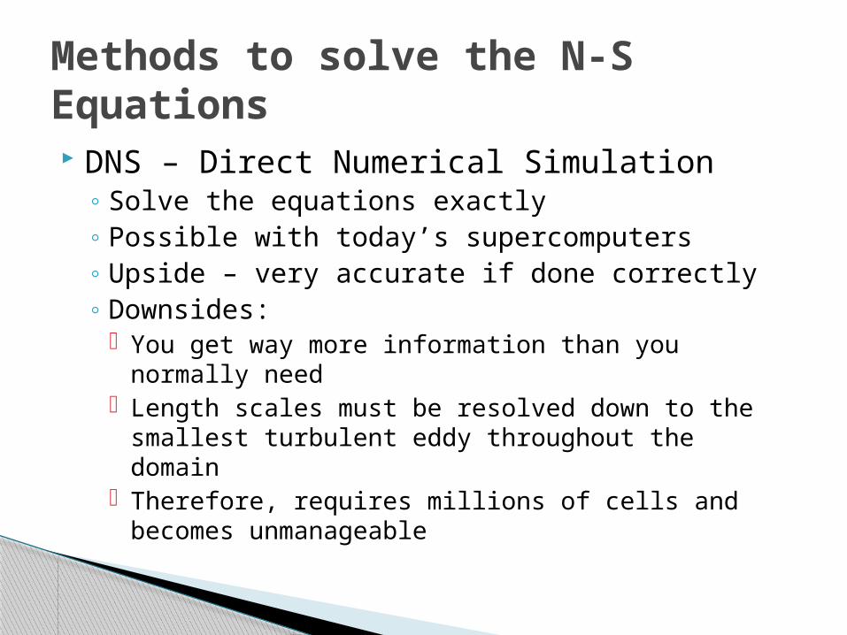
DNS – Direct Numerical Simulation◦ Solve the equations exactly◦ Possible with today’s supercomputers◦ Upside – very accurate if done correctly◦ Downsides:

You get way more information than you normally need

Length scales must be resolved down to the smallest turbulent eddy throughout the domain

Therefore, requires millions of cells and becomes unmanageable

Methods to solve the N-S Equations

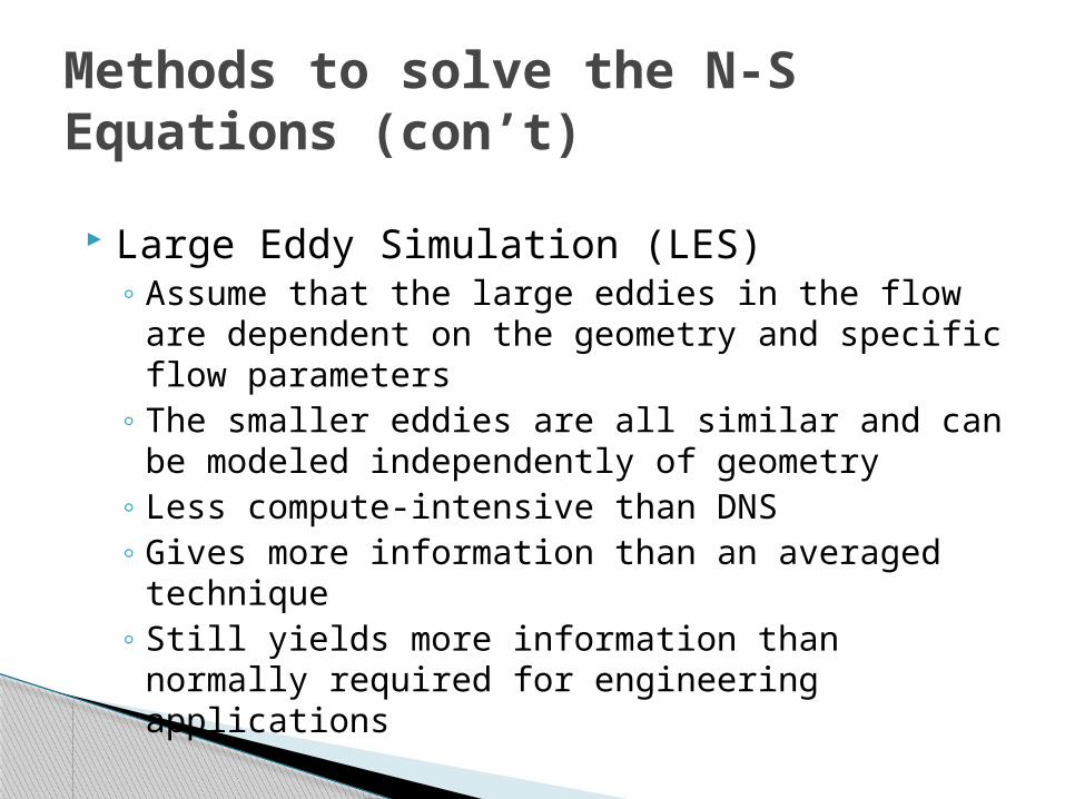
Large Eddy Simulation (LES)◦ Assume that the large eddies in the flow are

dependent on the geometry and specific flow parameters

◦ The smaller eddies are all similar and can be modeled independently of geometry

◦ Less compute-intensive than DNS◦ Gives more information than an averaged

technique◦ Still yields more information than normally

required for engineering applications

Methods to solve the N-S Equations (con’t)

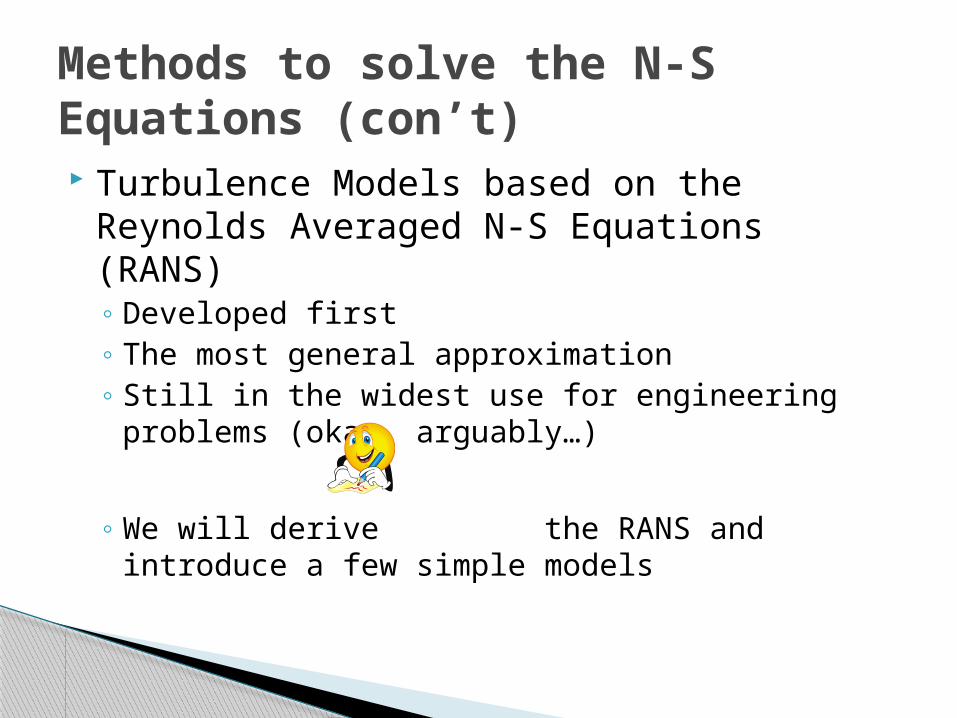
Turbulence Models based on the Reynolds Averaged N-S Equations (RANS)◦ Developed first◦ The most general approximation◦ Still in the widest use for engineering problems

(okay, arguably…)

◦ We will derive the RANS and introduce a few simple models

Methods to solve the N-S Equations (con’t)

Reynolds decomposition

Tools you will need in the Derivation of RANS

Mathematical rules for flow variables f and g, and independent variable s

Incompressible Newtonian Fluid:

Starting point… N-S Equations of motion

Incompressible: density is constantNewtonian: stress/strain rate is linear and described by:

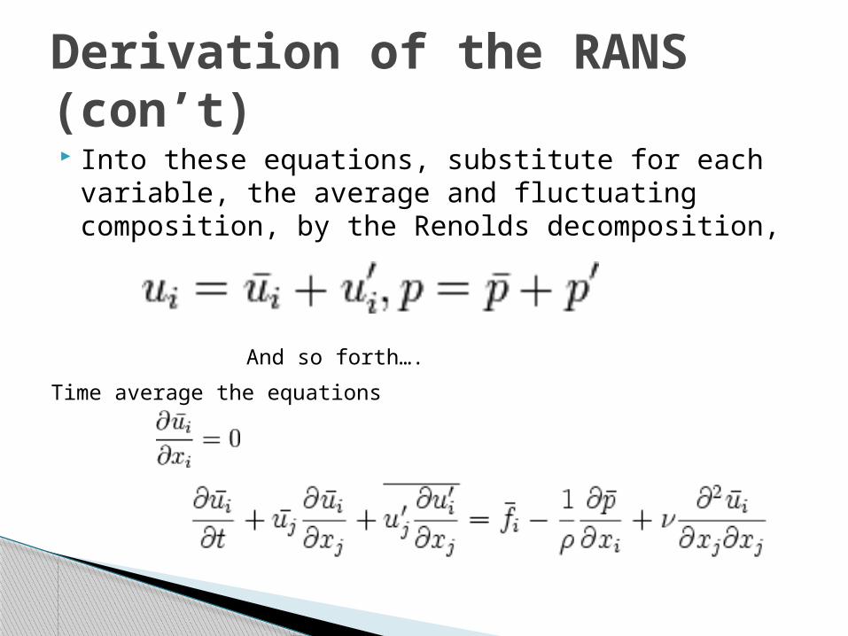
Into these equations, substitute for each variable, the average and fluctuating composition, by the Renolds decomposition,

Derivation of the RANS (con’t)

And so forth….

Time average the equations

Rearrange using the relationships presented earlier

Derivation of the RANS (con’t)

Replace the strain tensor term with the mean rate of the strain tensor:

And rearrange some more…..

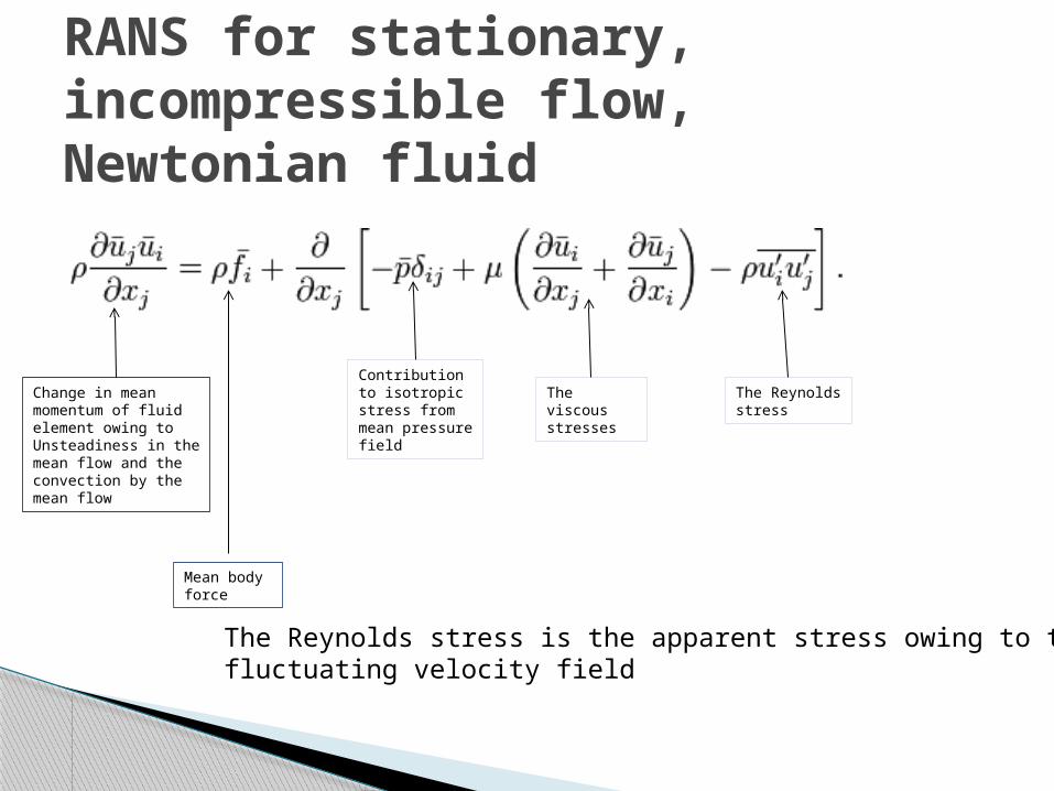
RANS for stationary, incompressible flow, Newtonian fluid

Change in meanmomentum of fluidelement owing toUnsteadiness in themean flow and the convection by the mean flow

Mean body force

Contributionto isotropic stress frommean pressurefield

The viscous stresses

The Reynoldsstress

The Reynolds stress is the apparent stress owing to thefluctuating velocity field

The Reynolds Stress term is non-linear and is the most difficult to solve – so we model it!

First, and most simple model, proposed by Joseph Boussinesq, was the Eddy Viscosity model. Simply increase the viscous stress by some proportional amount to account for the Reynolds’ stresses. Works very well for axisymmetric jets, 2-D jets, and mixing layers, but not much else.

Turbulence Models – Eddy Viscosity

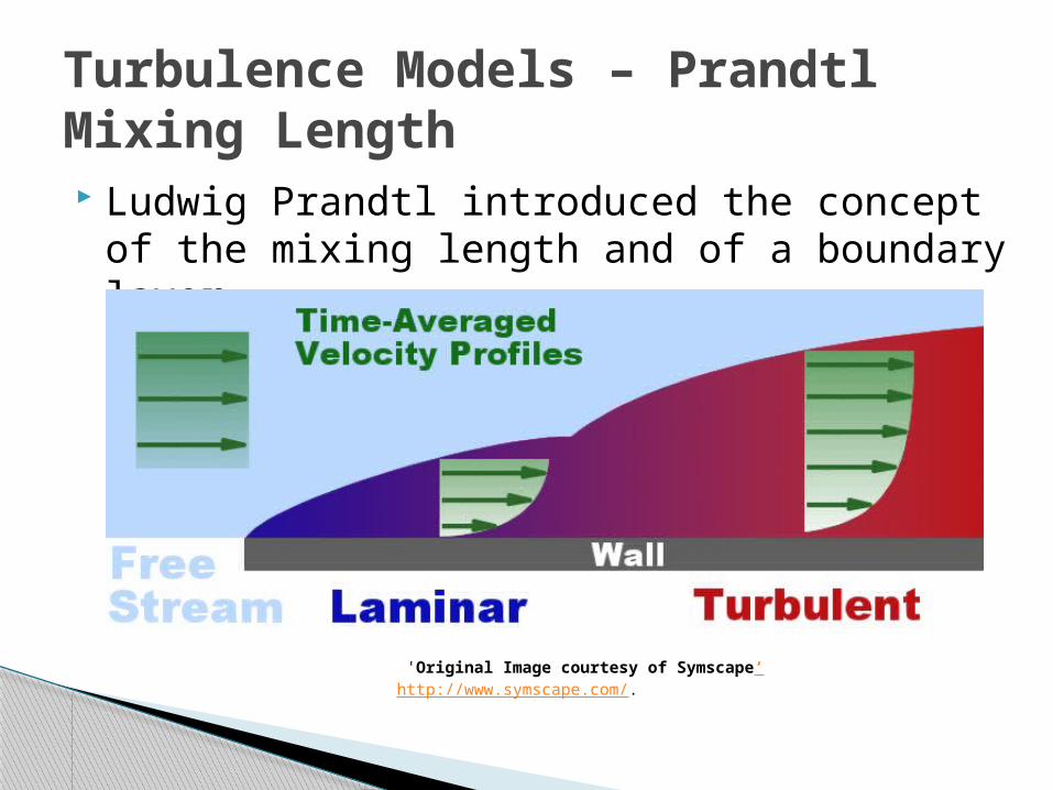
Ludwig Prandtl introduced the concept of the mixing length and of a boundary layer.

Turbulence Models – Prandtl Mixing Length

'Original Image courtesy of Symscape‘ http://www.symscape.com/.

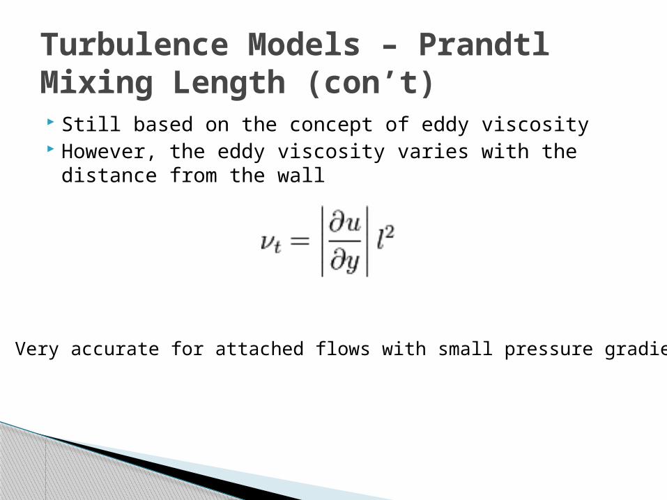
Still based on the concept of eddy viscosity However, the eddy viscosity varies with the

distance from the wall

Turbulence Models – Prandtl Mixing Length (con’t)

Very accurate for attached flows with small pressure gradients.

k-Є is one of a class of two-equation models The first two-equation models were k-l, based on k,

the kinetic energy of turbulence, and l, the length scale

More commonly in use now, however, are k-Є models, Є being turbulent diffusion

Application of the model requires additional transport equations for solution

Turbulence Models – k-Є model

Transport equations for k and Є

Turbulent viscosity:

k production term Pk

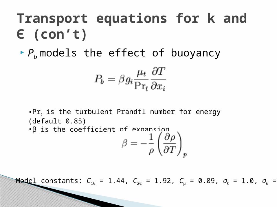
Pb models the effect of buoyancy

Transport equations for k and Є (con’t)

•Prt is the turbulent Prandtl number for energy (default 0.85)•β is the coefficient of expansion

Model constants: C1Є = 1.44, C2Є = 1.92, Cμ = 0.09, σk = 1.0, σЄ = 1.3

http://www.cfd-online.com/Wiki/CFD-Wiki:Copyrights

Launder, B.F., and Spalding, D.B., Mathematical Models of Turbulence, Academic Press, London and New York, 1972.

Symscape‘ http://www.symscape.com

Sources