Scientific computing on accelerator-based supercomputers

Scientific computing on accelerator-basedsupercomputers

Xing Cai

Simula Research Laboratory & University of Oslo

FFI, 2013.09.20

– p. 1

Outline

Motivation

Bits & piecesUsing GPUsUsing Xeon Phi coprocessors

Realistic applications

– p. 2

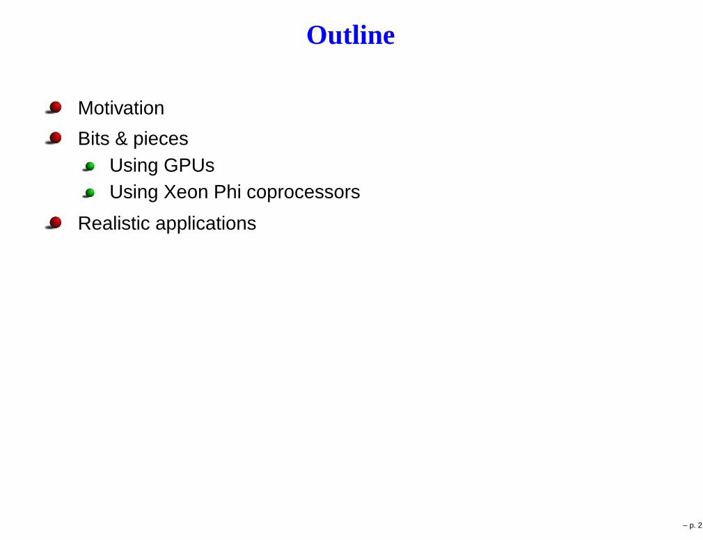
Why using accelerators?

Hardware Peak DP rate Peak memory BW

Intel Xeon E5-2650 8-core GPU 128 GFlop/s 51 GB/s

NVIDIA Kepler GK110 GPU 1170 GFlop/s 208 GB/s

Intel Xeon Phi 5110P coprocessor 1011 GFlop/s 320 GB/s

Accelerators have tremendous computing power, but requires carefulusage

– p. 3

A conceptual picture

– p. 4

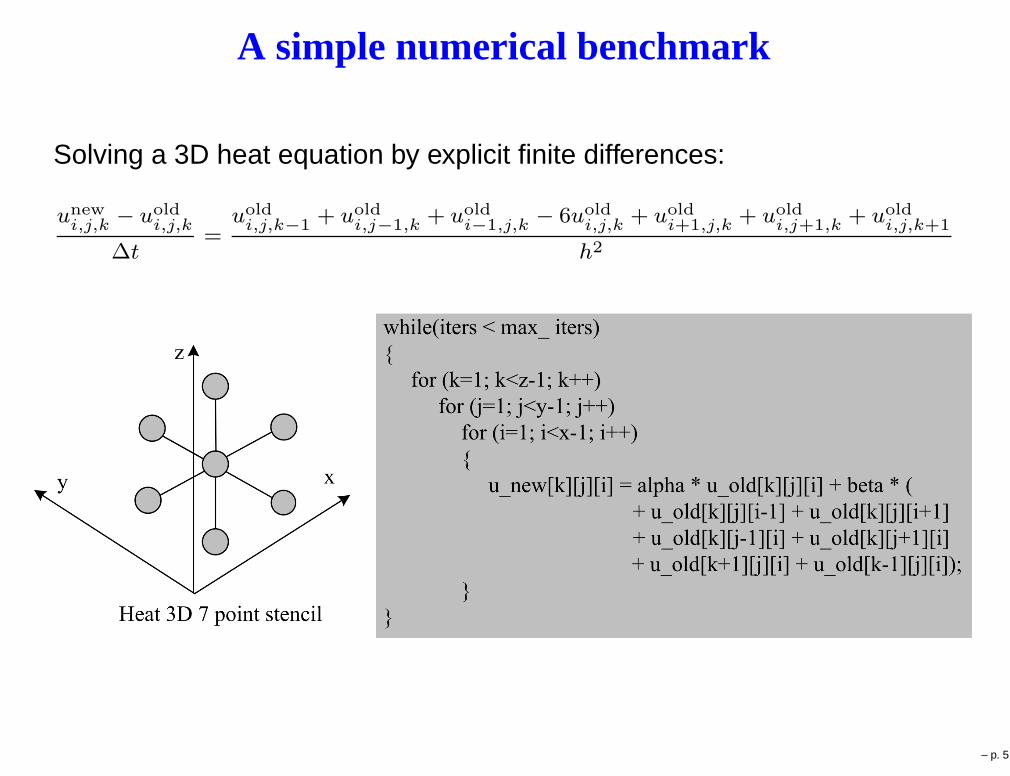
A simple numerical benchmark

Solving a 3D heat equation by explicit finite differences:

unewi,j,k

− uoldi,j,k

∆t=

uoldi,j,k−1

+ uoldi,j−1,k

+ uoldi−1,j,k

− 6uoldi,j,k

+ uoldi+1,j,k

+ uoldi,j+1,k

+ uoldi,j,k+1

h2

– p. 5

Baseline CUDA implementation__global__ void stencil (double * device_u, double * device_u_new,

double alpha, double beta, int Nx, int Ny)

{

int gid_x = blockIdx.x*blockDim.x + threadIdx.x + 1;

int gid_y = blockIdx.y*blockDim.y + threadIdx.y + 1;

int gid_z = blockIdx.z*blockDim.z + threadIdx.z + 1;

double (*in)[Ny][Nx];

double (*out)[Ny][Nx];

in = (double (*)[Ny][Nx])device_u;

out = (double (*)[Ny][Nx])device_u_new;

out[gid_z][gid_y][gid_x]=(alpha*in[gid_z][gid_y][gid_x])+

beta*(in[gid_z][gid_y][gid_x-1]

+in[gid_z][gid_y][gid_x+1]

+in[gid_z][gid_y-1][gid_x]

+in[gid_z][gid_y+1][gid_x]

+in[gid_z-1][gid_y][gid_x]

+in[gid_z+1][gid_y][gid_x]);

}

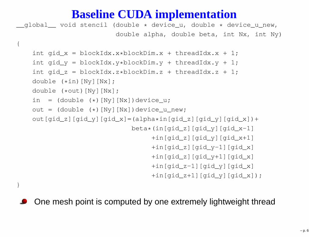
One mesh point is computed by one extremely lightweight thread

– p. 6

Improving the GPU performance

Typical performance-enhancing strategies:OPT-1: Let each thread compute a z-column of mesh pointsOPT-2: Use the on-chip shared memoryOPT-3: Chunking in the y-direction

GTX590 GPU K20 GPU

– p. 7

OpenCL programming__kernel void stencil(__global double * device_u,

__global double * device_u_new,

double alpha, double beta,

int Nx, int Ny)

{

int gid_x = get_global_id(0)+1;

int gid_y = get_global_id(1)+1;

int gid_z = get_global_id(2)+1;

__global double (*in)[Ny][Nx];

__global double (*out)[Ny][Nx];

in = (__global double (*)[Ny][Nx])device_u;

out = (__global double (*)[Ny][Nx])device_u_new;

out[gid_z][gid_y][gid_x]=(alpha*in[gid_z][gid_y][gid_x])+

beta*(in[gid_z][gid_y][gid_x-1]

+in[gid_z][gid_y][gid_x+1]

+in[gid_z][gid_y-1][gid_x]

+in[gid_z][gid_y+1][gid_x]

+in[gid_z-1][gid_y][gid_x]

+in[gid_z+1][gid_y][gid_x]);

}

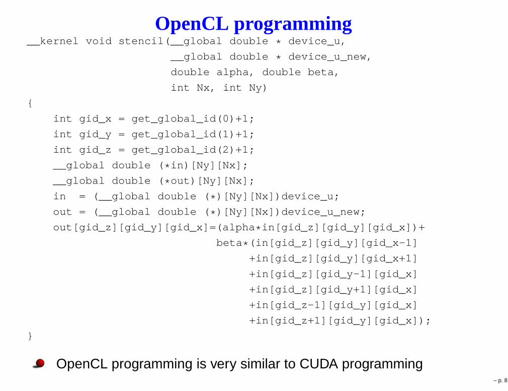
OpenCL programming is very similar to CUDA programming– p. 8

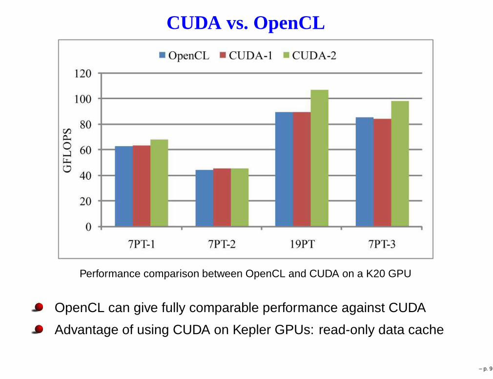
CUDA vs. OpenCL

Performance comparison between OpenCL and CUDA on a K20 GPU

OpenCL can give fully comparable performance against CUDA

Advantage of using CUDA on Kepler GPUs: read-only data cache

– p. 9

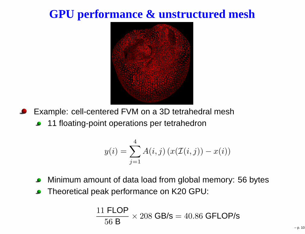
GPU performance & unstructured mesh

Example: cell-centered FVM on a 3D tetrahedral mesh11 floating-point operations per tetrahedron

y(i) =4∑

j=1

A(i, j) (x(I(i, j))− x(i))

Minimum amount of data load from global memory: 56 bytesTheoretical peak performance on K20 GPU:

11 FLOP56 B

× 208 GB/s = 40.86 GFLOP/s– p. 10

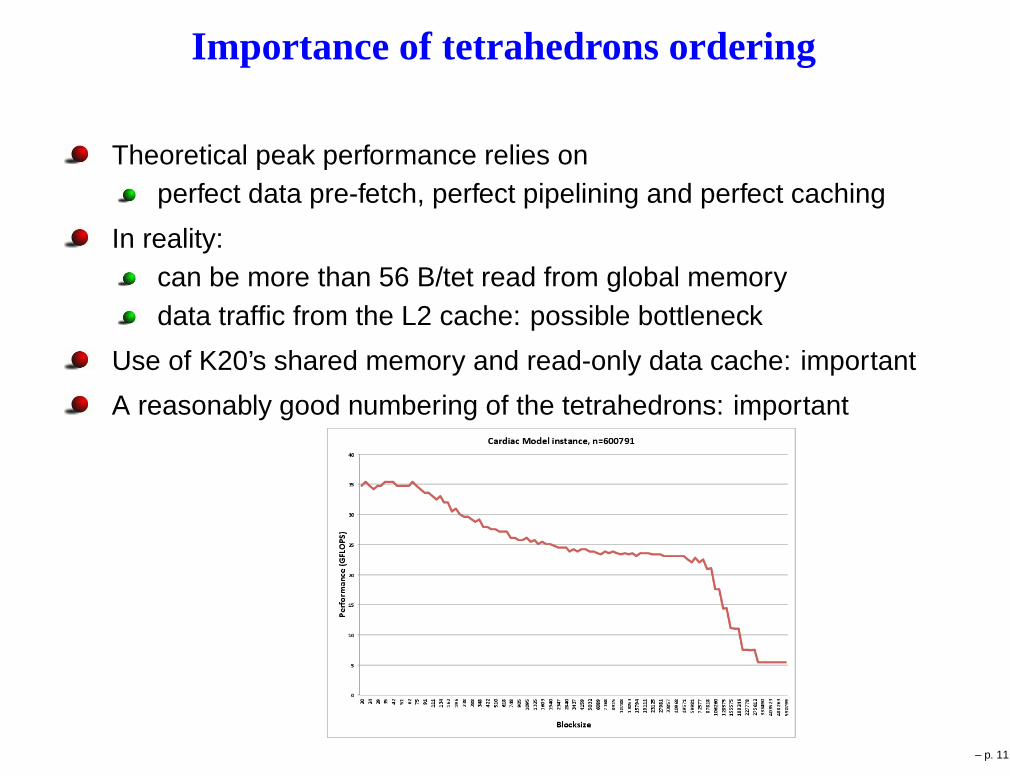
Importance of tetrahedrons ordering

Theoretical peak performance relies onperfect data pre-fetch, perfect pipelining and perfect caching

In reality:can be more than 56 B/tet read from global memorydata traffic from the L2 cache: possible bottleneck

Use of K20’s shared memory and read-only data cache: important

A reasonably good numbering of the tetrahedrons: important

– p. 11

GPU programming is cumbersome

GPU computing needs a CPU host, explicit data shuffles needed

CUDA example of copying a 3D array from host to device:

cudaError_t stat_dev_1_u_old = make_cudaExtent((n) * sizeof(double ),(n),(n));

cudaPitchedPtr dev_1_u_old = cudaMalloc3D(&dev_1_u_old,ext_dev_1_u_old);

cudaMemcpy3DParms param_1_dev_1_u_old = {0};

param_1_dev_1_u_old.srcPtr = make_cudaPitchedPtr(((void *)u_old[0][0]),(n) * sizeof(double

param_1_dev_1_u_old.dstPtr = dev_1_u_old;

param_1_dev_1_u_old.extent = ext_dev_1_u_old;

param_1_dev_1_u_old.kind = cudaMemcpyHostToDevice;

stat_dev_1_u_old = cudaMemcpy3D(&param_1_dev_1_u_old);

– p. 12

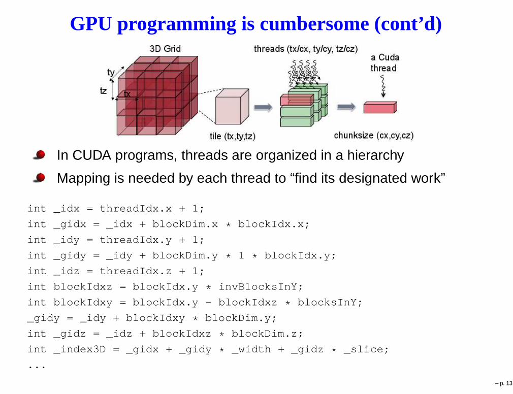
GPU programming is cumbersome (cont’d)

In CUDA programs, threads are organized in a hierarchy

Mapping is needed by each thread to “find its designated work”

int _idx = threadIdx.x + 1;

int _gidx = _idx + blockDim.x * blockIdx.x;

int _idy = threadIdx.y + 1;

int _gidy = _idy + blockDim.y * 1 * blockIdx.y;

int _idz = threadIdx.z + 1;

int blockIdxz = blockIdx.y * invBlocksInY;

int blockIdxy = blockIdx.y - blockIdxz * blocksInY;

_gidy = _idy + blockIdxy * blockDim.y;

int _gidz = _idz + blockIdxz * blockDim.z;

int _index3D = _gidx + _gidy * _width + _gidz * _slice;

...

– p. 13

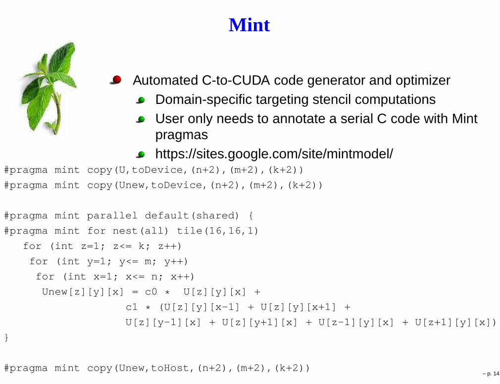
Mint

Automated C-to-CUDA code generator and optimizerDomain-specific targeting stencil computationsUser only needs to annotate a serial C code with Mintpragmashttps://sites.google.com/site/mintmodel/

#pragma mint copy(U,toDevice,(n+2),(m+2),(k+2))

#pragma mint copy(Unew,toDevice,(n+2),(m+2),(k+2))

#pragma mint parallel default(shared) {

#pragma mint for nest(all) tile(16,16,1)

for (int z=1; z<= k; z++)

for (int y=1; y<= m; y++)

for (int x=1; x<= n; x++)

Unew[z][y][x] = c0 * U[z][y][x] +

c1 * (U[z][y][x-1] + U[z][y][x+1] +

U[z][y-1][x] + U[z][y+1][x] + U[z-1][y][x] + U[z+1][y][x]);

}

#pragma mint copy(Unew,toHost,(n+2),(m+2),(k+2))– p. 14

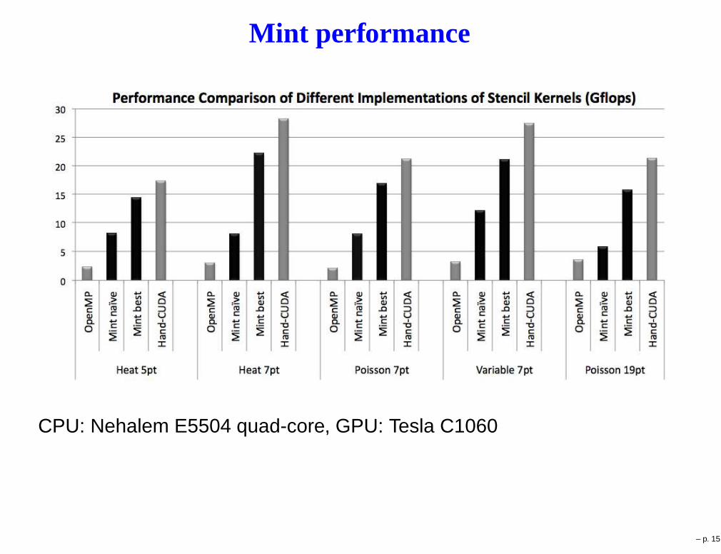
Mint performance

CPU: Nehalem E5504 quad-core, GPU: Tesla C1060

– p. 15

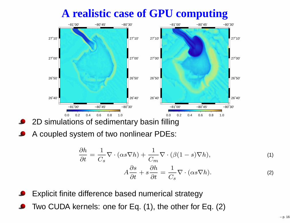
A realistic case of GPU computing

−81˚00'

−81˚00'

−80˚45'

−80˚45'

−80˚30'

−80˚30'

26˚40' 26˚40'

26˚50' 26˚50'

27˚00' 27˚00'

27˚10' 27˚10'

0.0 0.2 0.4 0.6 0.8 1.0

−81˚00'

−81˚00'

−80˚45'

−80˚45'

−80˚30'

−80˚30'

26˚40' 26˚40'

26˚50' 26˚50'

27˚00' 27˚00'

27˚10' 27˚10'

0.0 0.2 0.4 0.6 0.8 1.0

2D simulations of sedimentary basin filling

A coupled system of two nonlinear PDEs:

∂h

∂t=

1

Cs

∇ · (αs∇h) +1

Cm

∇ · (β(1− s)∇h), (1)

A∂s

∂t+ s

∂h

∂t=

1

Cs

∇ · (αs∇h). (2)

Explicit finite difference based numerical strategy

Two CUDA kernels: one for Eq. (1), the other for Eq. (2)– p. 16

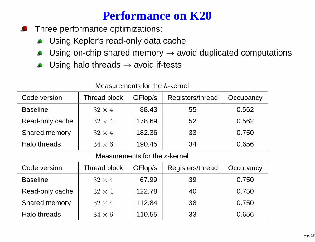
Performance on K20Three performance optimizations:

Using Kepler’s read-only data cacheUsing on-chip shared memory → avoid duplicated computationsUsing halo threads → avoid if-tests

Measurements for the h-kernel

Code version Thread block GFlop/s Registers/thread Occupancy

Baseline 32× 4 88.43 55 0.562

Read-only cache 32× 4 178.69 52 0.562

Shared memory 32× 4 182.36 33 0.750

Halo threads 34× 6 190.45 34 0.656

Measurements for the s-kernel

Code version Thread block GFlop/s Registers/thread Occupancy

Baseline 32× 4 67.99 39 0.750

Read-only cache 32× 4 122.78 40 0.750

Shared memory 32× 4 112.84 38 0.750

Halo threads 34× 6 110.55 33 0.656

– p. 17

Using more GPUs

Inter-GPU MPI communication has to go through the host CPUs

– p. 18

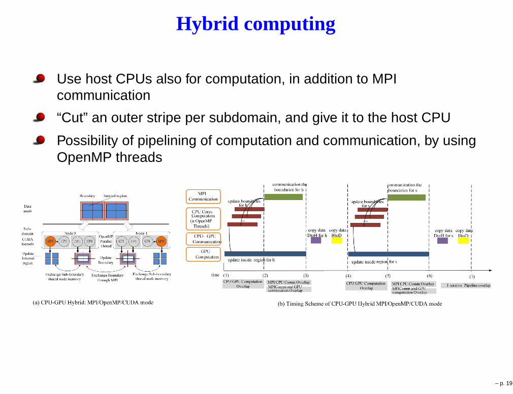
Hybrid computing

Use host CPUs also for computation, in addition to MPIcommunication

“Cut” an outer stripe per subdomain, and give it to the host CPU

Possibility of pipelining of computation and communication, by usingOpenMP threads

– p. 19

Measurements on Tianhe-1A

Tianhe-1A: the world’s largest supercomputer in June 2010

Each node: Tesla M2050 GPU + two Xeon 6-core X5670 CPUs

Global 2D mesh: 16384× 16384

– p. 20

Xeon Phi coprocessor

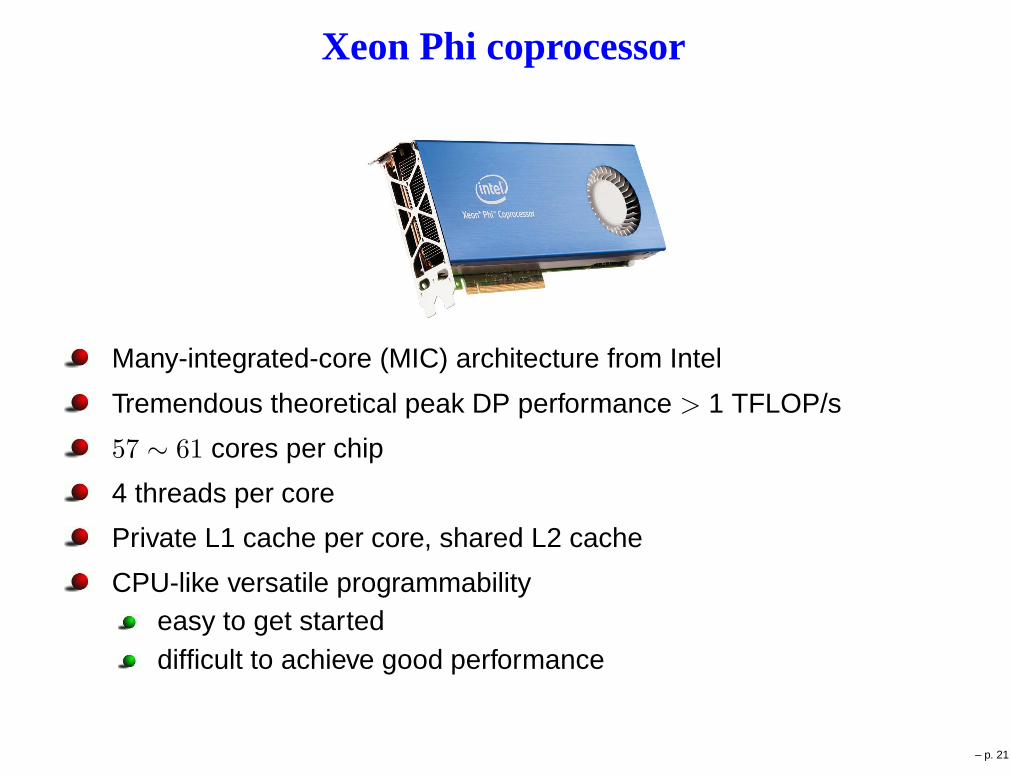
Many-integrated-core (MIC) architecture from Intel

Tremendous theoretical peak DP performance > 1 TFLOP/s

57 ∼ 61 cores per chip

4 threads per core

Private L1 cache per core, shared L2 cache

CPU-like versatile programmabilityeasy to get starteddifficult to achieve good performance

– p. 21

Realistic application 2

Subcellular calcium diffusion

A coupled system of multiple 3D reaction-diffusion equations

Towards nanometer mesh resolution

– p. 22

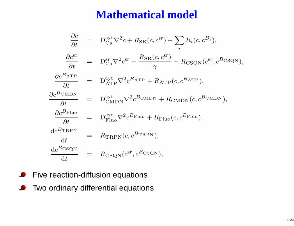
Mathematical model

∂c

∂t= Dcyt

Ca∇

2c+RSR(c, csr)−∑

i

Ri(c, cBi ),

∂csr

∂t= Dsr

Ca∇2csr −

RSR(c, csr)

γ− RCSQN(csr, cBCSQN),

∂cBATP

∂t= Dcyt

ATP∇

2cBATP + RATP(c, cBATP ),

∂cBCMDN

∂t= Dcyt

CMDN∇

2cBCMDN +RCMDN(c, cBCMDN ),

∂cBFluo

∂t= Dcyt

Fluo∇

2cBFluo +RFluo(c, cBFluo ),

dcBTRPN

dt= RTRPN(c, cBTRPN ),

dcBCSQN

dt= RCSQN(csr, cBCSQN),

Five reaction-diffusion equations

Two ordinary differential equations

– p. 23

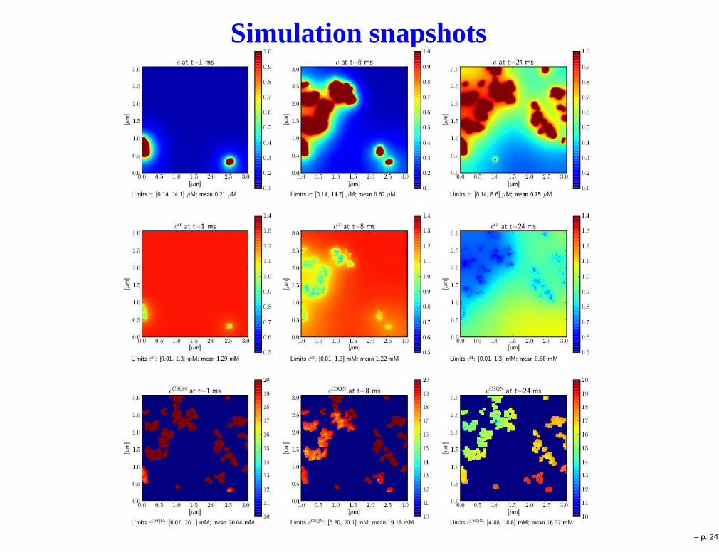
Simulation snapshots

– p. 24

Using Tianhe-2

Tianhe-2: currently No. 1 supercomputer

16,000 compute nodesEach node has three Xeon Phi coprocessors

– p. 25

Single-MIC performance

Offload programming mode (initiated by host CPU)#pragma offload target(mic)

Spawning of 4× 56 = 224 OpenMP threads on each Xeon Phi#pragma omp for collapse(2) as parallelization

Optimization techniques:First touch + thread bindingLoop fusionHierarchical loop blockingExplicit vectorizationVector registers reuse

Achieved 138 GB/s per MIC (90% of realistic memory bandwidth)

Achieved 118 GFLOP/s per MIC (11.8% of theoretical DP peak)

– p. 26

Single-node performance

Three MICs lie side-by-side (in the y-direction)

Offload programming mode

Different sub-tasks done by different threads on host CPU:invokes computation in the three MICsdoes additional computationissues host-MIC and MIC-host data exchange

# MICs Mesh points per MIC Gflop/s

1 142× 1200× 112 111

2 142× 600× 112 226

3 142× 400× 112 326

– p. 27

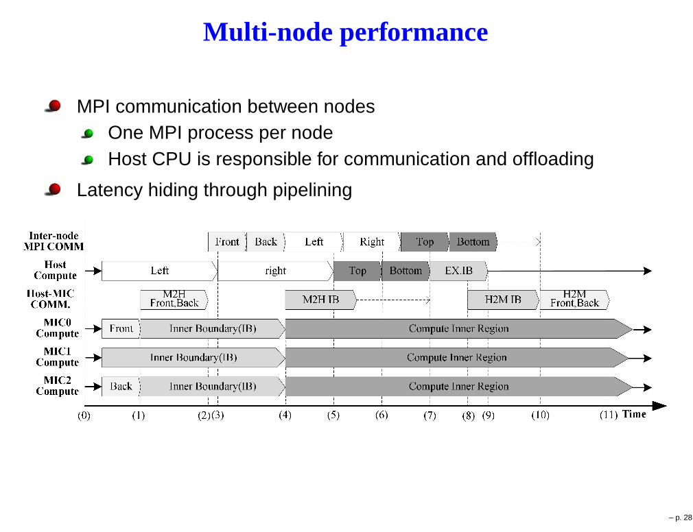
Multi-node performance

MPI communication between nodesOne MPI process per nodeHost CPU is responsible for communication and offloading

Latency hiding through pipelining

– p. 28

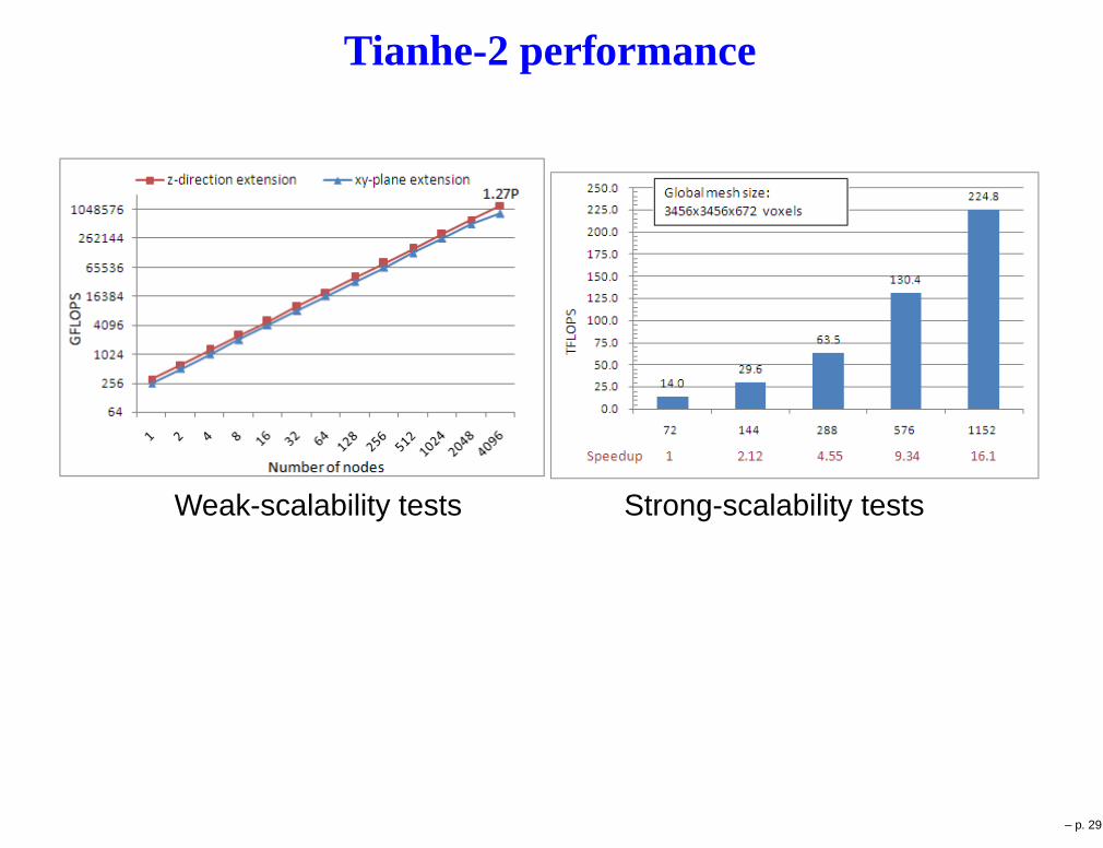
Tianhe-2 performance

Weak-scalability tests Strong-scalability tests

– p. 29

Some concluding remarks

Accelerators provide new computing capabilities... new headaches at the same time

Effective use of accelerators requires complicated programming

Hybrid computing (using both CPUs and accelerators) is even morechallenging

Some programming tasks can possibly be generalizedautomated code generation targeting specific computationdomainsongoing 4-year FriNatek project: User-friendly programming ofGPU-enhanced clusters via automated code translation and optimization

– p. 30