TRUE AND EFFICIENT SOLUTION OF UNIFIED BEM-FEM ACOUSTIC-STRUCTURAL COUPLING USING CHIEF REGULARIZATION

TRUE AND EFFICIENT SOLUTION OF UNIFIED BEM-FEM ACOUSTIC-STRUCTURAL COUPLING USING CHIEF REGULARIZATION

Harijono Djojodihardjo* Universitas Al-Azhar Indonesia Jalan Sisingamangaraja, Jakarta 121010,Indonesia [email protected]

59th

International Astronautical Congress

29 September and 3 October 2008, Glasgow,

Scotland

*Professor, Faculty of Industrial Technology, Universitas Al-Azhar Indonesia, Jakarta, Indonesia

For permission to copy or republish, contact the International Astronautical Federation

3-5 Rue Mario-Nikis, 75015 Paris, France

IAC-08-C2.3.7

2

IAC-08-C2.3.7

TRUE AND EFFICIENT SOLUTION OF UNIFIED BEM-FEM ACOUSTIC-STRUCTURAL COUPLING USING CHIEF REGULARIZATION

Harijono Djojodihardjo Professor, Universitas Al-Azhar Indonesia

[email protected]

ABSTRACT

Structural-acoustic interaction, which is a significant issue found in many applications, including modern

new and relatively lighter aircrafts operating at very high speed and altitudes, vibration problems can severely and adversely affect spacecraft structures and their payloads, and other engineering applications]. Following earlier series of work carried out by the author and colleagues addressing the vibration of structures due to sound wave, structural-acoustic interaction is modeled and analyzed using boundary and finite element coupling. The computational scheme developed for the calculation of the acoustic radiation as well as the structural dynamic response of the structure using coupled BEM/FEM has given satisfactory results for acoustic disturbance in the low frequency range, which was the range of particular interest in many practical applications. However, for larger frequency range, it is well known that while the solution to the original boundary value problem in the exterior domain to the boundary is perfectly unique for all wave numbers, this is not the case for the numerical treatment of integral equation formulation, which breaks down at certain frequencies known as irregular frequencies or fictitious frequencies. Although such phenomenon is completely nonphysical since there are no discrete eigenvalues for the exterior problems, a method known as CHIEF (Combined Helmholtz Interior integral Equation Formulation) can be utilized to overcome such problem. Test-case application of CHIEF method to spherical shell geometry has given excellent results. The work carried out is focused on further treatment in the formulation and solution of the basic problem of acoustic radiation and scattering problem, and the excitation and vibration of elastic structure in a coupled fluid-elastic-structure interaction.

1. Introduction .

Structural-acoustic interaction, which is a significant issue found in many applications, including modern new and relatively lighter aircrafts operating at very high speed and altitudes, vibration problems, which can severely and adversely affect spacecraft structures and their payloads, and other engineering applications [1-9], can be modeled using boundary and finite element coupling [10-12]. Following the author‟s and colleagues‟ work [13-18], the present work is focused on looking into the true and efficient solution of Unified BEM-FEM Acoustic-Structural coupling using CHIEF regularization [19], and considerations on the use of Multipole Expansion as introduced in [20].

2. Surface Helmholtz Integral Equation for the

Acoustic Field For an exterior problem, as depicted in Fig. 2, the problem domain V is the free space Vext outside the closed surface S. The problem domain V is the exterior region. V is considered enclosed in between

the surface S and an imaginary surface at a sufficiently large distance from the acoustic sources and the surface S such that the boundary condition on

satisfies Sommerfeld‟s acoustic radiation condition as the distance approaches infinity.

Green‟s first and second theorem provide the basis for transforming the differential equations in the problem domain V and the boundary conditions on the surface S into an integral equation over the surface S.

Fig 1. Exterior problem for homogeneous Helmholtz

equation

For time-harmonic acoustic problems in fluid domains, the corresponding boundary integral equation is the Helmholtz integral equation [21-22]

3

dSn

pRRg

n

gRpRcp

S

0

0

0ˆˆ

(1a)

or following the formulation of [18] can be written as

0

0

0

ˆ

ˆ

S

ext

gcp x p g R R v dS

n

x V

pv

n

(1b)

where 0n̂ is the surface unit normal vector, and the

value of c depends on the location of R in the fluid domain as is well known, and where g the free-space Green‟s function. Ro denotes a point located on the boundary S, as given by

0

04

0

RR

eRRg

RRik

(2)

To solve equation (1) with g given by (2), one of the two physical properties, acoustic pressure and normal velocity, must be known at every point on the boundary surface. The specific normal impedance, which describes the relationship between pressure and normal velocity, can also serve as a boundary condition. At the infinite boundary, the Sommerfeld radiation condition in three dimensions can be written as [21-22]:

0lim0

ikg

r

gr

RRas (3)

which is satisfied by the fundamental solution. Scattering pressure is also considered in the problem formulation to give the total pressure which serves as an acoustic excitation on the structure. For scattering problems, Eq. (1) only gives the solution to the scattered wave. The boundary conditions are however given in terms of the total wave, which is the sum of the incident and the scattered waves. It is necessary to modify the equations to include the incident wave. For exterior scattering problems, the modification can be easily done by adding to the scattered wave integral equations the result of applying the interior Helmholtz equations to the incident wave pinc. Adding to the integral equation for the scattering wave in the exterior problem, we have

ext

0

0

0 0

int

( ) ( ), R V

1( ) ( ), R S

ˆ ˆ 2

( ), R V

inc

inc

S

inc

p R p R

G R R p Rp R G R R dS p R p R

n n

p R

(4) For total pressure p, which is p = pinc + pscatter or on the simplified manner, we have

0

0

0 0

( ) ( )ˆ ˆ

q

inc

S

p rG R Rcp R p R p R G R R dS

n n

(5) where

ext

int

, R V1

, R S1/ 2

, R S / 4 (non smooth surface)

, R V0

c

(6)

In order to evaluate the pressure in the medium Vext by means of Eq. 1b, one must know the normal velocity and the pressure on the surface S. However, these two functions are not independent, and if the normal velocity is known at all points of the surface then the pressure can be determined. If

we allow the point x in Eq. 10 to approach a point on S, we obtain the following integral equation for the surface pressure in terms of the known velocity:

0

0ˆ

,

S S

gcp p dS g R R v dS

n

S

R R

(7) The normal derivative in Eq. 7 is taken with respect

to the dummy variable . Eq. 7 can also be solved approximately by converting it into Boundary Integral Elements to form a system of algebraic equations. 3. Interior Helmholtz Integral Formulation

The Helmholtz integral formula (Eq. 1) is valid no matter how the surface pressure is obtained. When the field point is restricted to lie in the region Vint interior to the surface S, the following integral formula is obtained in place of Eq. 1:

0

0

0 0

0

,0

ˆ

, ; ,

ˆ

S

g Xp g R R v dS

n

R R X R R X

pv

n

(8) and g is given by Eq. (2) as before.

If the normal velocity v() is known, the integral relation (Eq. 8) provides another way to determine the surface pressure. In this interior Helmholtz integral formulation, the surface pressure is obtained from Eq. 8 and then the pressure in the medium VInt is determined from Eq. 1b as in the surface Helmholtz integral formulation. These formulations closely follows the rationale of Schenck [19] in establishing the CHIEF method to be elaborated subsequently.

4. Combined Helmholtz Integral Equation

Formulation (CHIEF)

The rationale of the improved method, known as the Combined Helmholtz Integral Equation

r

4

Formulation (CHIEF) method, is as follows: If we want a method that will work for any wave- number k, we must abandon the simple source based integral formulation, since the solution cannot be represented in terms of the integral relation for all velocity distributions and wavenumbers [19]. The surface Helmholtz integral formulation (Eq. 1b) has an advantage in that solutions exist for any wavenumber, but it becomes deficient, i.e., fails to yield a unique answer, for each characteristic wavenumber k. The interior Helmholtz integral formulation (Eq. 8) can lead to similar difficulties, but the primary objection to its use alone lies in its undesirable computational characteristics. Broadly stated, the improved method consists of a practical means for finding the (unique) surface-pressure function that satisfies both Helmholtz integral equations (Eqs. 1b and 8), and using this function in the Helmholtz integral formula (Eq. 1b) to predict the pressure anywhere in VExt. This method is implemented in the discrete sense by converting the surface Helmholtz integral formula into a Boundary Element Formulation and arrive at an N-by-N system of equations, and then overdetermining the solution with additional compatible equations based on the interior Helmholtz integral formulation for strategic interior points. In order to preserve the good numerical characteristics of the surface Helmholtz integral formulation, the additional equations should not exceed those that are needed to make up for the deficiencies of the surface Helmholtz integral formulation. Specifically, we implement the method as follows: As before, we break the surface of the radiator up mathematically into N pieces each of which is small enough that it is reasonable to remove a mean value of pressure or velocity from under the integral sign. Therefore, Eq. 1b becomes

0

1 1

N N

i inc

j jS S

cp p pgdS i gvdS (9)

for S, and Eq. 8 becomes

0

1 1

0N N

j jS S

pgdS i gvdS (10)

for X VInt . Next, we require that Eq. (9) hold for the Ns surface

points = S (on the surface S) and that Eq. (10) hold

for Ni interior points XI. Vint. In matrix form, this system of equations, Eq. (9), as well as Eq. (9) and (10), as appropriately written, can be written as

0 incp i G v p H (11)

where H and G are two N x N matrices (N is the number of nodes), and p and v are N dimensional vectors, as well elaborated in [14-18]. 5. Acoustic Boundary Element Method

Validation In order to verify the validity of the computational method developed, the method is applied to some

test cases, where exact results or worked out examples are available.

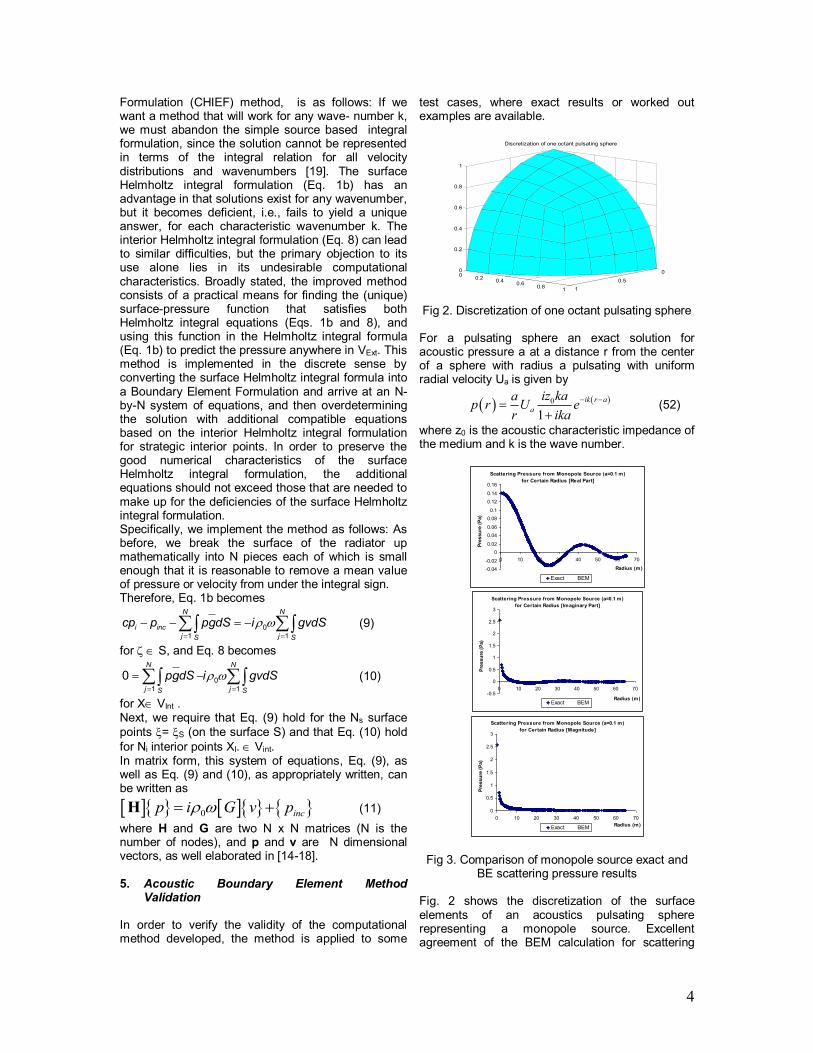
Fig 2. Discretization of one octant pulsating sphere

For a pulsating sphere an exact solution for acoustic pressure a at a distance r from the center of a sphere with radius a pulsating with uniform radial velocity Ua is given by

0

1

ik r a

a

iz kaap r U e

r ika

(52)

where z0 is the acoustic characteristic impedance of the medium and k is the wave number.

Fig 3. Comparison of monopole source exact and BE scattering pressure results

Fig. 2 shows the discretization of the surface elements of an acoustics pulsating sphere representing a monopole source. Excellent agreement of the BEM calculation for scattering

0

0.5

1

00.2

0.40.6

0.81

0

0.2

0.4

0.6

0.8

1

Discretization of one octant pulsating sphere

Scattering Pressure from Monopole Source (a=0.1 m)

for Certain Radius [Real Part]

-0.04

-0.02

0

0.02

0.04

0.06

0.08

0.1

0.12

0.14

0.16

0 10 20 30 40 50 60 70

Radius (m)

Pre

ssu

re (

Pa)

Exact BEM

Scattering Pressure from Monopole Source (a=0.1 m)

for Certain Radius [Imaginary Part]

-0.5

0

0.5

1

1.5

2

2.5

3

0 10 20 30 40 50 60 70

Radius (m)

Pre

ssu

re (

Pa)

Exact BEM

Scattering Pressure from Monopole Source (a=0.1 m)

for Certain Radius [Magnitude]

0

0.5

1

1.5

2

2.5

3

0 10 20 30 40 50 60 70

Radius (m)

Pre

ssu

re (

Pa)

Exact BEM

5

pressure from acoustic monopole source with exact results is shown in Fig. 3. The calculation was based

on the assumption of f=10 Hz, =1.225 Kg/m3, and

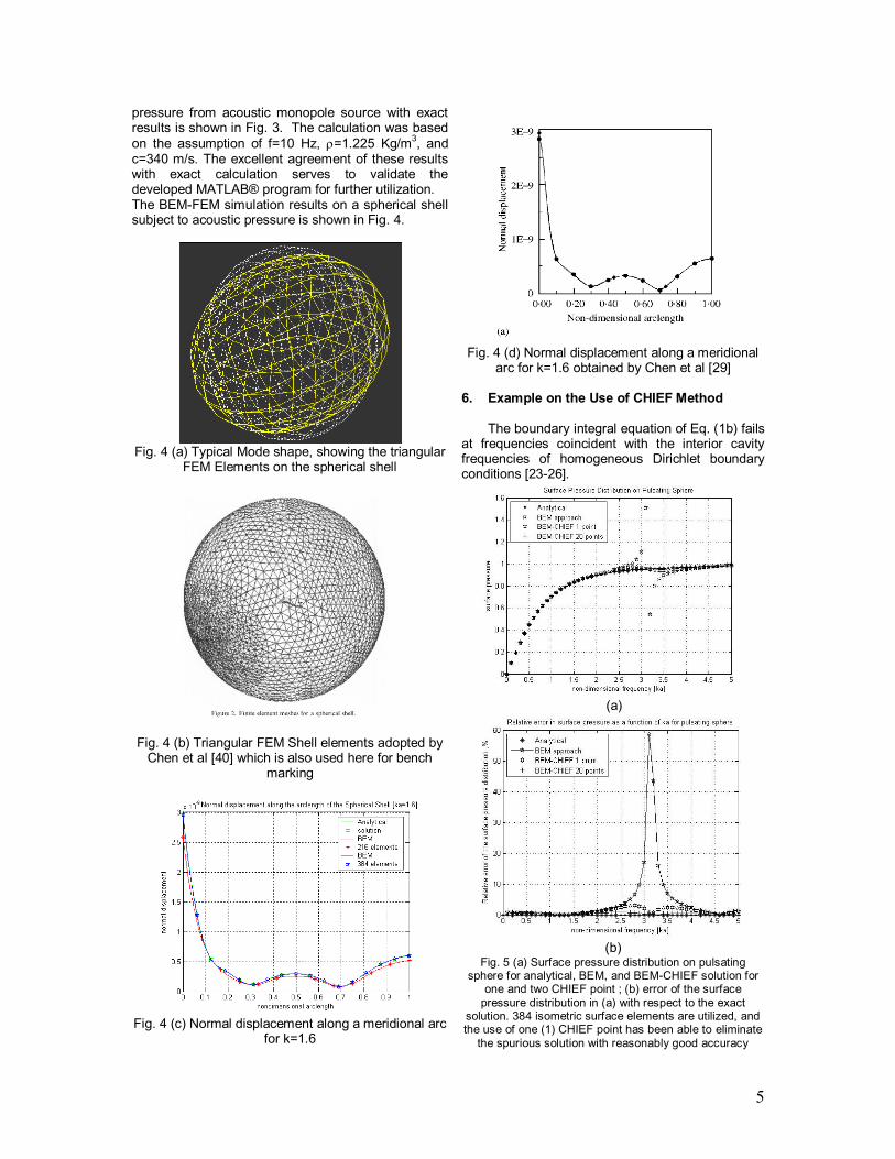
c=340 m/s. The excellent agreement of these results with exact calculation serves to validate the developed MATLAB® program for further utilization. The BEM-FEM simulation results on a spherical shell subject to acoustic pressure is shown in Fig. 4.

Fig. 4 (a) Typical Mode shape, showing the triangular

FEM Elements on the spherical shell

Fig. 4 (b) Triangular FEM Shell elements adopted by Chen et al [40] which is also used here for bench

marking

Fig. 4 (c) Normal displacement along a meridional arc

for k=1.6

Fig. 4 (d) Normal displacement along a meridional

arc for k=1.6 obtained by Chen et al [29] 6. Example on the Use of CHIEF Method

The boundary integral equation of Eq. (1b) fails at frequencies coincident with the interior cavity frequencies of homogeneous Dirichlet boundary conditions [23-26].

(a)

(b)

Fig. 5 (a) Surface pressure distribution on pulsating sphere for analytical, BEM, and BEM-CHIEF solution for

one and two CHIEF point ; (b) error of the surface

pressure distribution in (a) with respect to the exact solution. 384 isometric surface elements are utilized, and the use of one (1) CHIEF point has been able to eliminate

the spurious solution with reasonably good accuracy

6

In the formulation of the exterior problem, these frequencies correspond to the natural frequencies of acoustic resonances in the interior region. When the interior region resonates, the pressure field inside the interior region has non-trivial solution. Since the interior problem and the exterior problem shares similar integral operators, the exterior integral equation may also break down. The discretized equation of the [H] matrix in Eq. (11) becomes ill-conditioned when the exciting frequency is close to the interior frequencies, thus providing an erroneous acoustic loading matrix.

This problem is then solved using CHIEF method described above [20]. For the purpose of this study, to avoid non-uniqueness problem, special treatment is carried out to inspect whether the H matrix is ill-behaved or not by utilizing SVD updating technique [27-28]. If it is ill-behaved, the present method resorts to the utilization of CHIEF method, which has been proved to be successful, as indicated in Fig. 5. 7. Acoustic-Structure Coupling For the purpose of establishing acoustic-structure coupling formulation, both the BE-Acoustic and the FE structure domain are schematically illustrated in Fig. 6. The utilization of FE for the structural dynamic equation of motion in the structural domain leads to a system of simultaneous equations which relate the displacements at all the nodes to the nodal forces. In the BEM, on the other hand, a relationship between nodal displacements and nodal tractions should be established. Representing the elastic structure by FE model, the structural dynamic equation of motion is given by [30-32]

x x x M C K F (12)

where M, C and K are structural mass, damping and stiffness, respectively, which are expressed as matrices in a FE model, while F is the given external forcing function vector, and {x} is the structural displacement vector. The elastic structure can be represented by FE model.

Fig 6. Schematic of Fluid-Structure Interaction Domain

Let divide the BE nodes into two parts; part a, which is related to the finite elements that represents the surface of the acoustic medium in contact with the elastic structure, and part b, which is the remaining acoustic domain. Through the use of well established modal analysis, the acoustic-structure problem as the BEM/FEM coupling represented by Eq. (12) can be recast into equivalent one using generalized coordinates, and yields

aq q q p M C K L F (13)

where M, C and K are now the generalized structural mass, damping and stiffness, respectively which are expressed as matrices in a FE model, while F is the given external forcing function vector, and q the generalized coordinate vector. L is a coupling matrix of size m x n, where m is the number of FE degrees of freedom and n is the number of BE nodes on the coupled boundary representing part a of the acoustic domain. Accordingly, the node pressure values, p, from the BE model are categorized into two groups, pa and pb. The global coupling matrix L transforms the acoustic fluid pressure acting on the nodes of boundary elements on the entire fluid-structure interface surface a, to nodal forces on the finite elements of the structure. Hence L consists of n assembled local transformation matrices Le, given by

e

T

e F B

S

L N nN dS (14)

in which NF is the shape function matrix for the finite element and NB is the shape function matrix for the boundary element. It can be shown that:

1 0 0 0 0

0 1 0 0 0

0 0 1 0 0

F iN N

(15)

and where Ni„s are the shape functions defined for four-node linear elements. The rotational parts in NF are neglected since these are considered to be small in comparison with the translational ones in the BE-FE coupling, consistent with the assumptions in structural dynamics as, for example, as stipulated in [30].

In similar fashion, the normal velocities are categorized into va and vb . Hence the discretized Helmholtz Eq. (11) using BE model can be rewritten as

Acoustic Domain

Structure Domain

Acoustic

Source

Incident Pressure

Scattering

Pressure Total Pressure at

coinciding nodes

Pressure at non-coinciding nodes

Coupling Matrix L a

b

7

b

a

b

a

v

v

GG

GGi

p

p

HH

HH

2221

1211

0

2221

1211 (16)

where the subscripts 1 and 2 in H refer to the a and b domain, respectively.

The normal fluid velocities of the acoustic problem and the normal translation of the structural surface-fluid interface have to satisfy certain relationship which takes into account the velocity continuity over the coinciding nodes. For a first approximation, one may assume that it is dominated by either the fluid as acoustic medium or by the surface of the structure, without taking into account interference and reflection effects. However, realistic treatment should take into account these effects. For the normal fluid velocities and the normal translational displacements on the shell elements at the fluid-structure coupling interface, a relationship, which takes into account the velocity continuity over the coinciding nodes, should be established. This relationship is given by

av i q T (17)

Similar to L, T (n × m) is also a global coupling matrix that connects the normal velocity of a BE node with the translational displacements of FE nodes obtained by taking the transpose of the boundary surface normal vector n [5,9,15]. The local transformation

matrix has the size 1 3 and is obtained by taking the transpose of the unit normal vector to the boundary surface.

(18)

With all these considerations, Eq. (16) reduces to

bb

a

vi

qT

GG

GG

p

p

HH

HH

0

2

0

2221

1211

2221

1211

(19) Combining the modified structural FE model, Eq. (12), with the modified acoustic BE model, Eq. (19), one obtains the governing equation for the coupled FE/BE acoustic-structure model:

(20)

Flexible Structure Subject to Harmonic External Forces in Acoustic Medium

Several cases are considered to validate the program as well as to evaluate its performance. An example is carried out for a box with vibrating membrane as shown in Fig.7. The structure consists of five hard walls and one flexible membrane on the

top and has the dimension a × b x c = 304.8 × 152.4 × 152.4 mm. The flexible structure, which consists of a 0.064 mm thick undamped aluminum plate, is modeled with coupled boundary and finite elements.

Fig. 7 Generic flexible structure typical of space-structure subjected to harmonic external forces in acoustic medium

Fig. 8 Comparison between FEM-FEM and BEM-FEM

approach for acoustic pressure [dB] on plate center

a

b

T

e nT

b

b

b

a

vGi

vGi

F

p

p

q

HHTG

HHTG

LMDiK

220

120

221221

2

0

121111

2

0

2 0

8

c

Fig 9. b. Convergence trend of the sound pressure level frequency response of a vibrating top membrane of an

otherwise rigid box due to monopole source at the center of the box a studied in [12] as a function of frequency

calculated using present computational scheme for various

grid size; c. Total pressure distribution on the surfaces of the

same box. Top surface is modeled as BE-FE, others as BE. The frequency response due to the application of arbitrary harmonic excitation forces to the membrane following the present method using BEM-FEM Coupling is shown in Fig. 8, and is compared to results obtained using FEM-FEM approach [15]. Comparable agreement has been indicated and serves to validate the present method. The convergence trend of the sound pressure level frequency response of a vibrating top membrane of an otherwise rigid box due to monopole source at the center of the box as studied in [9] is exhibited in Fig.9

Flexible Structure Subject to Acoustic Excitation in a Confined Medium

Application of the method to another example is carried out for a box shown in Fig. 10 with a dimension of a × b x c = 450 × 450 × 270 mm.. Five walls of the structure are modeled as shell elements and the bottom of the box is modeled as a rigid wall. Each of the flexible walls is assumed to be made of 1 mm aluminum plate, and is modeled as coupled boundary and finite elements. This box structure is subjected to an acoustic monopole source at the center of the box and the acoustic medium is air with the following properties: density, ρ =1.21 kg/m

3 and sound velocity c =340 m/s.

The discretization of the box is also depicted in Fig.10b.

Fig. 10 Generic flexible structure typical of space-

structure subjected to monopole acoustic source in an acoustic medium

a. Normal Mode Analysis

The result of the modal analysis of the box to obtain the first three normal modes using finite element program developed in MATLAB

® is shown in Fig.

11. The first five eigen-frequencies for the shell elements obtained using the present routine are compared to those obtained using commercial package NASTRAN

®. As exhibited in Table 1, good

agreement is obtained.

Fig.11 First three normal modes for box modeled

with five flexible walls using shell elements

b. Acoustic Excitation

Acoustic excitation due to an acoustic monopole source with initial frequency, f = 10 Hz, is applied at the center of the box. No other external forces are applied. The resulting distribution of the incident acoustic pressure is shown in Fig. 12.

Table.1 First five Eigen-frequencies for box modeling with shell element

Mode Natural Frequency (Hz) MATLAB

® NASTRAN

®

1 17.644 16.190 2 36.026 35.986 3 41.072 41.520 4 44.585 44.787 5 51.231 51.689

Fig.12 Incident acoustic pressure distribution on the surface of box due to monopole acoustic excitation

a b

c

9

The total pressures on the surface of the box obtained from the computational results are shown in Fig.13. The frequency response for the incident pressure and total pressure on the center top surface of the box computed using Eq. (20) is shown in Fig. 14.

Fig. 13 Total acoustic pressure distribution on the

surface of box due to monopole acoustic excitation

Fig. 14 Incident and total acoustic pressure

distribution on the center top surface of box as a function of frequency

8. Concluding Remarks A method and computational procedure for BEM-FEM Acousto-Elasto-Mechanic Coupling has been developed. The method is founded on three generic elements; the calculation of the acoustic radiation from the vibrating structure, the finite element formulation of structural dynamic problem, and the calculation of the acousto-elasto-mechanic fluid-structure coupling using coupled BEM/FEM techniques. In particular the CHIEF method for regularization of the Boundary Element discretization for the Acoustic Problem, as well as for Acoustic-Structural Coupling as a Coupled BEM-FEM Fluid-Structure Interaction, which has been proved to be successful. The procedure developed has been validated by reference to classical examples or others available in the literature. The applicability of the method for analyzing typical problems encountered in space structure has been demonstrated. Refinement of the method for fast computation and for complex geometries are in progress. Such steps may be useful

for acoustic load qualification tests as well as structural health monitoring. References [1] Edson, J.R.,”Review of Testing and

Information on Sonic Fatigue,”Doc. No. D-17130, Boeing Co., 1957.

[2] Powell, C.A. and Parrott, T.L., “A summary of Acoustic Loads and Response Studies, “Tenth National Aero-Space Plane Technology Symposium, Paper No. 106, April, 1991.

[3] Eaton, D.C.G., An Overview of Structural Acoustics and Related High-Frequency-Vibration Activities, http://esapub.esrin.esa.it/bulletin/ bullet92/b92eaton.htm.

[4] Chuh Mei, and Carl S. Pates, III, Analysis Of Random Structure-Acoustic Interaction Problems Using Coupled Boundary Element And Finite Element Methods, NASA-CR-195931, 1994.

[5] Marquez, A., Meddahi, S., and Selgas, V., “A new BEM–FEM coupling strategy for two-dimensional fluid–solid interaction problems”, Journal of Computational Physics 199 pp. 205–220, 2004.

[6] Renshaw, A. A., D‟Angelo, C., and Mote, C. D., Jr., 1994, „„Aeroelastically Excited Vibration of a Rotating Disk,‟‟ J. Sound Vib., 177(5), pp. 577–590.

[7] Kang, Namcheol and Raman, Arvind, Aeroelastic Flutter Mechanisms of a Flexible Disk Rotating in an Enclosed Compressible Fluid, Transactions of the ASME, Vol. 71, January 2004, pp 120-130.

[8] Tandon, N. , Rao, V.V.P. and Agrawal, V.P. , Vibration and noise analysis of computer hard disk drives, Measurement 39 (2006) 16–25, www.elsevier.com/locate/measurement

[9] Holström, F., Structure-Acoustic Analysis Using BEM/FEM; Implementation In MATLAB

®, Master’s Thesis, Copyright © 2001

by Structural Mechanics & Engineering Acoustics, LTH, Sweden, Printed by KFS i Lund AB, Lund, Sweden, May 2001, Homepage: http://www.akustik.lth

[10] Forth, S.C. and Staroselsky, A. , A Hybrid FEM/BEM Approach for Designing an Aircraft Engine Structural Health Monitoring, CMES, Vol. 9, No. 3, pp. 287-298, 2005.

[11] Eller, D. and Carlsson, M., An efficient aerodynamic boundary element method for aeroelastic simulations and its experimental validation, Aerospace Science and Technology 7 (2003) pp 532–539

[12] Gennaretti, M and Iemma, U., Aeroacoustoelasticity in state-space format using CHIEF regularization, Journal of Fluids and Structures 17 (2003), pp 983–999

[13] Djojodihardjo, H and Tendean, E., A Computational Technique For The Dynamics

10

Of Structure Subject To Acoustic Excitation, ICAS 2004, Vancouver, October 2004.

[14] Djojodihardjo, H and Safari, I., Further Development of the Computational Technique for Dynamics of Structure Subjected to Acoustic Excitation, paper IAC-05-C2.2.08, presented at the 56

th International Astronautical Congress /

The World Space Congress-2005, 17-21 October 2005/Fukuoka Japan.

[15] Djojodihardjo, H and Safari, I., Unified Computational Scheme For Acoustic Aeroelastomechanic Interaction, paper IAC-06-C2.3.09, presented at the 57

th International

Astronautical Congress / The World Space Congress-2006, 1-6 October 2006/Valencia Spain.

[16] Djojodihardjo, H and Safari, I., BEM-FEM Coupling For Acoustic Effects On Aeroelastic Stability Of Structures, keynote paper, ICCES 07, paper ICCES0720060930168, Miami Beach, Florida, 3-6 January 2007

[17] Harijono Djojodihardjo, BE-FE Coupling Computational Scheme For Acoustic Effects On Aeroelastic Structures, paper IF-086, Proceedings Of The International Forum on Aeroelasticity and Structural Dynamics, held at the Royal Institute of Technology (KTH), Stockholm, Swede, 18-20 June 2007.

[18] Harijono Djojodihardjo, BEM-FEM Acoustic-Structural Coupling For Spacecraft Structure Incorporating Treatment Of Irregular Frequencies, paper IAC.07-C2.3.4, IAC Proceedings, presented at the 58

th International

Astronautical Congress, The World Space Congress-2007, 23-28 September 2007/Hyderabad, India.

[19] Schenck, H. A. , Improved integral formulation for acoustic radiation problems, J. Acoust. Soc. Am. 44(1) (1976) 41–58.

[20] Fischer, M., Gauger, U. and Gaul, H., A Multipole Galerkin Boundary Element Method For Acoustics, Engineering Analysis with Boundary Elements 28 (2004) 155–162

[21] Dowling, A.P. and Ffowcs Williams, J.E., Sound and Sources of Sound, Ellis Horwood Limited, Chichester – John Wiley & Sons, New York Brisbane Chichester Toronto, 1983, ©1983, A.P.Dowling and J.E. Ffowcs Williams.

[22] Norton, M.P., 1989, Fundamentals of Noise and Vibration Analysis for Engineers, Cambridge University Press, Cambridge, New York, Melbourne, Sydney.

[23] Wrobel, L.C., The Boundary Element Methods, Vol.1, Applications in Thermo-Fluids and Acoustics, John Wiley & Sons, Chichester, West Sussex PO19 IUD, England, 2002

[24] Beer, G. and Watson, J.O., “Introduction to Finite and Boundary Element Methods for Engineers”. John Wiley & Sons Ltd, Baffins Lane, Chichester, England, 1992.

[25] Wu T W, Boundary Element Acoustics: Fundamentals and Computer Codes,

WITPRESS, ISBN: 1-85312-570-9 2000, Southampton. 2000.

[26] Estorff O, Boundary Elements in Acoustics: Advances and Applications, WITPRESS, ISBN: 1-85312-556-3 2000, Southampton, 2000.

[27] J.T. Chen, I. L. Chen and K. H. Chen, 2006, “Treatment of Rank Deficiency in Acoustic using SVD”, J. Comp. Acoustic, Vol. 14, No.2, pp.157-183.

[28] J.T. Chen, I. L. Chen and M. T. Liang, 2001, “Analytical Study and Numerical Experiments for Radiation and Scattering Problems using the CHIEF Method”, Journal of Sound and Vibration, 248(5), pp.809-828.

[29] P.-T. Chen, S.-H. Ju and K.-C. Cha, A Symmetric Formulation Of Coupled BEM/FEM In Solving Responses Of Submerged Elastic Structures For Large Degrees Of Freedom, Journal of Sound and Vibration (2000) 233(3), pp 407-422

[30] Bisplinghoff, R. L, Ashley, H, Halfman, R., Aeroelasticity, Addison Wesley, Reading, Massachusetts, 1955.

[31] Zwaan, R,J., Aeroelasticity of Aircraft, Lecture Notes delivered at the Institute of Technology Bandung, 1992.

[32] Dowell, E.H.(Ed), Curtiss, H.C., Scanlan, R.H., and Sisto, F., A modern course in aeroelasticity, Sijthoff & Noordhoff, Alphen aan den Rijn, The Netherlands, 1980.