Triangular Decompositions of Polynomial Systems: From Theory to Practice Marc Moreno Maza Univ. of Western Ontario, Canada ISSAC tutorial, 9 July 2006 1

Welcome message from author
This document is posted to help you gain knowledge. Please leave a comment to let me know what you think about it! Share it to your friends and learn new things together.
Transcript

Triangular Decompositions of Polynomial Systems:From Theory to Practice
Marc Moreno Maza
Univ. of Western Ontario, Canada
ISSAC tutorial, 9 July 2006
1

Why a tutorial on triangular decompositions?
• The theory is mature:
- the objects are well understood,
- the interactions with other theories also,
- notions and terminologies are unifying.
• The algorithms are evolving very quickly:
- modular algorithms are available now,
- complexity estimates also,
- fast polynomial and matrix arithmetic start to be used.
• The implementation effort is growing
- triangular decompositions are available in major computer algebra systems,
- implementation techniques are a priority.
2
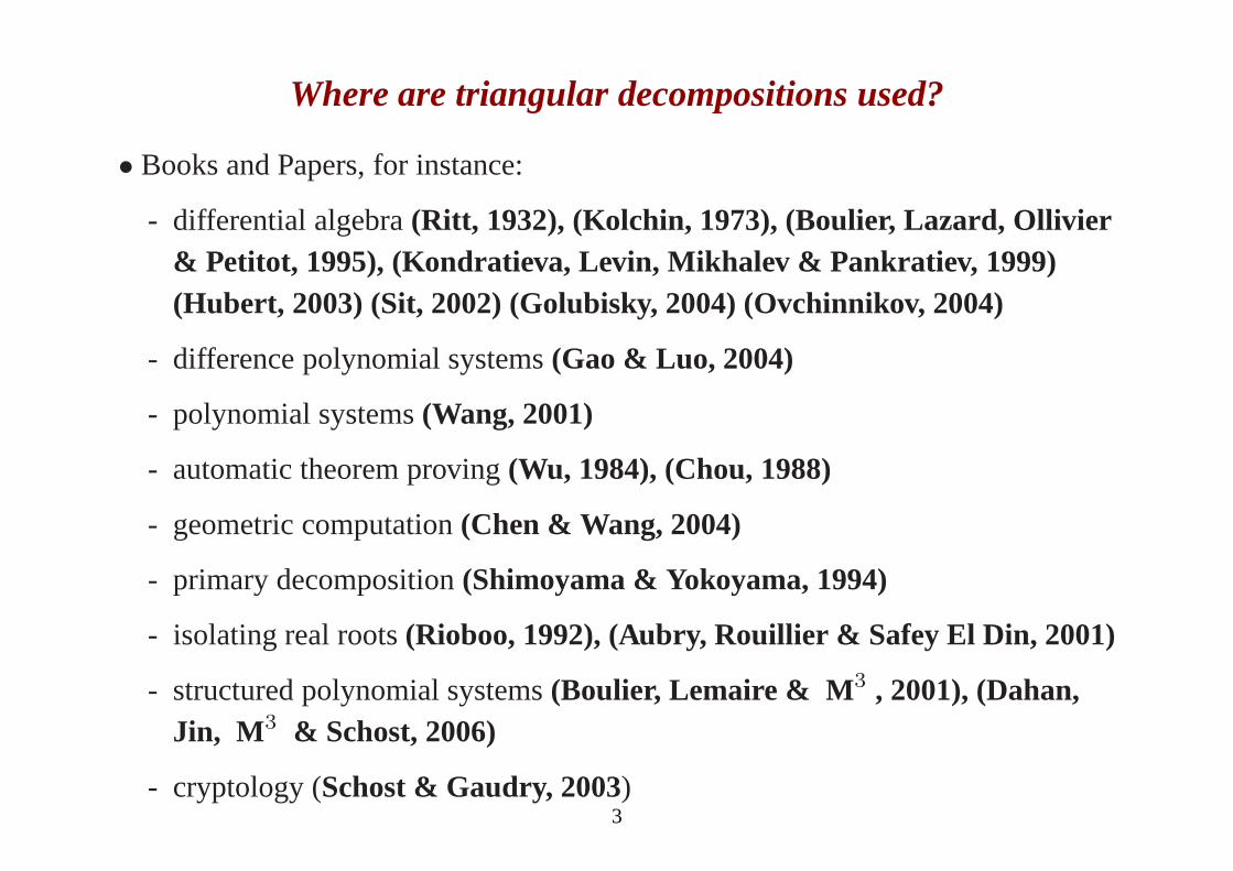
Where are triangular decompositions used?
• Books and Papers, for instance:
- differential algebra(Ritt, 1932), (Kolchin, 1973), (Boulier, Lazard, Ollivier& Petitot, 1995), (Kondratieva, Levin, Mikhalev & Pankrati ev, 1999)(Hubert, 2003) (Sit, 2002) (Golubisky, 2004) (Ovchinnikov, 2004)
- difference polynomial systems(Gao & Luo, 2004)
- polynomial systems(Wang, 2001)
- automatic theorem proving(Wu, 1984), (Chou, 1988)
- geometric computation(Chen & Wang, 2004)
- primary decomposition(Shimoyama & Yokoyama, 1994)
- isolating real roots(Rioboo, 1992), (Aubry, Rouillier & Safey El Din, 2001)
- structured polynomial systems(Boulier, Lemaire & M 3 , 2001), (Dahan,Jin, M 3 & Schost, 2006)
- cryptology (Schost & Gaudry, 2003)3
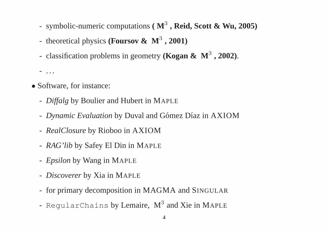
- symbolic-numeric computations( M3 , Reid, Scott & Wu, 2005)
- theoretical physics(Foursov & M 3 , 2001)
- classification problems in geometry(Kogan & M 3 , 2002).
- . . .
• Software, for instance:
- Diffalg by Boulier and Hubert in MAPLE
- Dynamic Evaluationby Duval and Gomez Dıaz in AXIOM
- RealClosureby Rioboo in AXIOM
- RAG’lib by Safey El Din in MAPLE
- Epsilonby Wang in MAPLE
- Discovererby Xia in MAPLE
- for primary decomposition in MAGMA and SINGULAR
- RegularChains by Lemaire, M3 and Xie in MAPLE
4
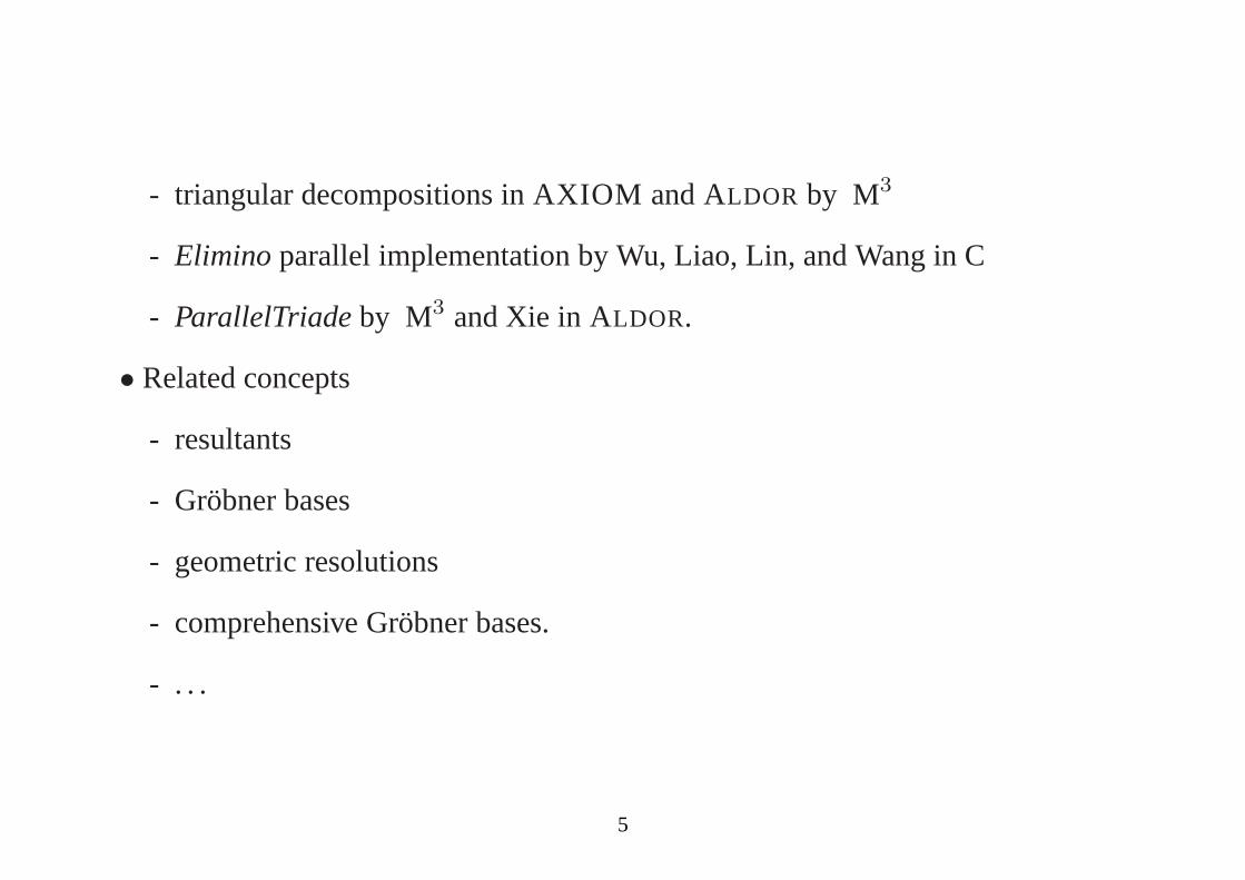
- triangular decompositions in AXIOM and ALDOR by M3
- Elimino parallel implementation by Wu, Liao, Lin, and Wang in C
- ParallelTriadeby M3 and Xie in ALDOR.
• Related concepts
- resultants
- Grobner bases
- geometric resolutions
- comprehensive Grobner bases.
- . . .
5

Acknowledgments
• The ISSAC Tutorial Chair, Stephen M. Watt, and ISSAC organizers.
• My PhD students: Yuzhen Xie and Xin Li.
• My colleagues at UWO: Robert M. Corless, David J. Jeffrey, Gregory J. Reid,
Eric Schost and Stephen M. Watt.
• My current collaborators on the subject oftriangular decompositions:
- Francois Boulier & Francois Lemaire (Univ. Lille 1, France)
- Xavier Dahan andEric Schost (Ecole Polytechnique, France)
- Jurgen Gerhard and Michael Cherkassoff (Maplesoft)
- Oleg Golubitsky (Queen’s Univ., Canada)
- Marina V. Kondratieva (Moscow State Univ., Russia)
- Alexey Ovchinnikov (North Carolina State Univ., USA)
6

An overview of this tutorial
• Main objective: an introduction for non-experts.
• Prerequisites: some familiarity with Grobner bases would be useful, but notnecessary.
• Outline:
- an informal introduction of the key ideas
- the case of polynomial systems with finitely many solutions: Lazard
triangular sets
- the general case: triangular sets, characteristic sets, Wu’s method
- regular chains, reduction to dimension zero
- theTriade algorithm, its parallel implementation
- implementation issues
- theRegularChains library in MAPLE.
7
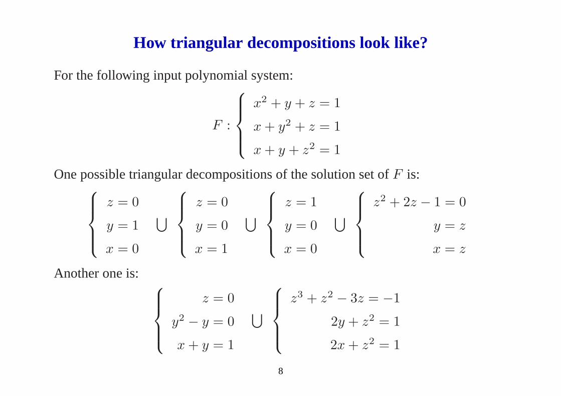
How triangular decompositions look like?
For the following input polynomial system:
F :
x2 + y + z = 1
x + y2 + z = 1
x + y + z2 = 1
One possible triangular decompositions of the solution setof F is:
z = 0
y = 1
x = 0
⋃
z = 0
y = 0
x = 1
⋃
z = 1
y = 0
x = 0
⋃
z2 + 2z − 1 = 0
y = z
x = z
Another one is:
z = 0
y2 − y = 0
x + y = 1
⋃
z3 + z2 − 3z = −1
2y + z2 = 1
2x + z2 = 1
8
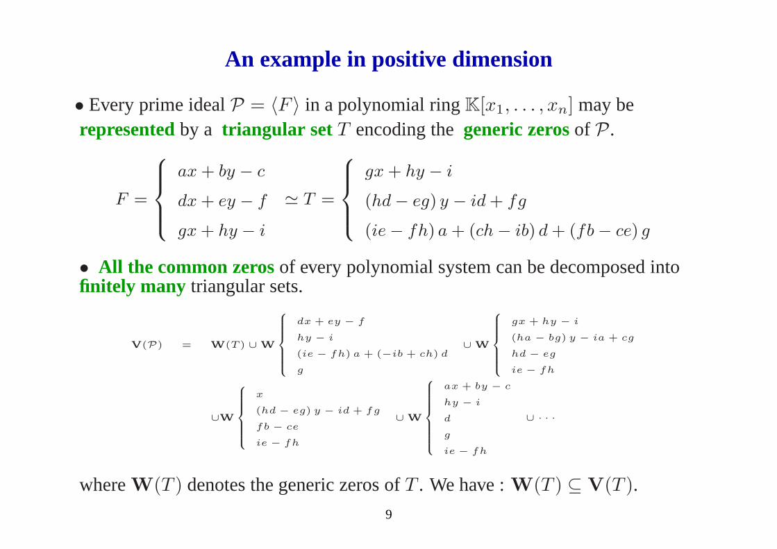
An example in positive dimension
• Every prime idealP = 〈F 〉 in a polynomial ringK[x1, . . . , xn] may berepresentedby a triangular set T encoding thegeneric zerosof P.
F =
8
>
>
<
>
>
:
ax + by − c
dx + ey − f
gx + hy − i
≃ T =
8
>
>
<
>
>
:
gx + hy − i
(hd − eg) y − id + fg
(ie − fh) a + (ch − ib) d + (fb − ce) g
• All the common zerosof every polynomial system can be decomposed intofinitely many triangular sets.
V(P) = W(T) ∪ W
8
>
>
>
>
>
<
>
>
>
>
>
:
dx + ey − f
hy − i
(ie − fh) a + (−ib + ch) d
g
∪ W
8
>
>
>
>
>
<
>
>
>
>
>
:
gx + hy − i
(ha − bg) y − ia + cg
hd − eg
ie − fh
∪W
8
>
>
>
>
>
<
>
>
>
>
>
:
x
(hd − eg) y − id + fg
fb − ce
ie − fh
∪ W
8
>
>
>
>
>
>
>
<
>
>
>
>
>
>
>
:
ax + by − c
hy − i
d
g
ie − fh
∪ · · ·
whereW(T ) denotes the generic zeros ofT . We have :W(T ) ⊆ V(T ).
9
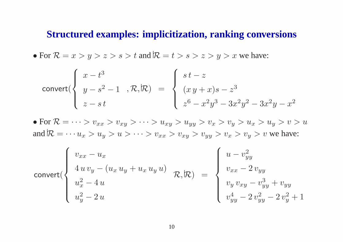
Structured examples: implicitization, ranking conversions
• ForR = x > y > z > s > t andR = t > s > z > y > x we have:
convert(
x − t3
y − s2 − 1
z − s t
,R,R) =
s t − z
(x y + x)s − z3
z6 − x2y3 − 3x2y2 − 3x2y − x2
• ForR = · · · > vxx > vxy > · · · > uxy > uyy > vx > vy > ux > uy > v > u
andR = · · ·ux > uy > u > · · · > vxx > vxy > vyy > vx > vy > v we have:
convert(
vxx − ux
4 u vy − (ux uy + ux uy u)
u2x − 4 u
u2y − 2 u
R,R) =
u − v2yy
vxx − 2 vyy
vy vxy − v3yy + vyy
v4yy − 2 v2
yy − 2 v2y + 1
10

How to compute triangular decompositions?
• Consider again solving the systemF for x > y > z:
F :
x2 + y + z = 1
x + y2 + z = 1
x + y + z2 = 1
• Eliminatingx leads to
y2 + (−1 + 2z2)y − 2z2 + z + z4 = 0
y2 + z − y − z2 = 0
• Eliminatingy2 and theny we can arrive tor(z) = 0 withr(z) = z8 − 4z6 + 4z5 − z4.
• Factorizingr(z) leads toz4(z2 + 2z − 1)(z − 1)2 = 0 and thus toz = 0, z = 1
or z2 + 2z = 1. In each case, it is easy to conclude either by substitution,or byGCD computation in(Q[z]/〈z2 + 2z − 1〉)[y].
• Alternatively, one can directly perform GCD computation in(Q[z]/〈r(z)〉)[y].But this is unusual sinceQ[z]/〈r(z)〉 is not a field! Let us see this now.
11

Computing a polynomial GCD over a ring with zero-divisors (I)
• Let us consider again the polynomials
f1 = y2 + (2z2 − 1)y − 2z2 + z + z4
f2 = y2 + z − y − z2
• Let us compute their GCD inL[y] with L = Q[z]/〈s(z)〉 where
s(z) = z(z2 + 2z − 1)(z − 1) is the squarefree part ofr(z). (Replacingr(z) with
s(z) makes the story simpler.)
• We proceedas if L were a fieldand run theEuclidean Algorithm in L[y]. Of
course, before dividing by an element ofL we check whether it is a zero-divisor.
We pretend we are not aware of the factorization ofs(z).
• Dividing f1 by f2 is no problem sincef2 is monic. We obtain:f1 f2
f3 1with
f3 = 2z2y − z2 + 2z2 − z.
12

Computing a polynomial GCD over a ring with zero-divisors (II)
• In order to dividef2 by f3, we need to check whether2z2 divides zero inL.
This is done by computinggcd(s(z), 2z2) in Q[z], which isz.
• Hences(z) writesz(z3 + z2 − 3z + 1) and we split the computations into two
cases:z = 0 andz3 + z2 − 3z = 1.
• Casez = 0. Thenf3 = 0 andf2 = y2 − y is the GCD.
• Casez3 + z2 − 3z = −1. SinceS(z) is square-free,2z2 has an inverse in this
case, namelyi(z) = −(3/2)z2 − 2z + 4.
• Thus, the polynomialf3 = i(z)f3 = y + (1/2)z2 − (1/2) is monic. So, we can
computef2 f3
0 y − (1/2)z2 − (1/2).
• Finally gcd(f1, f2, L[y]) =
y2 − y if z = 0
2y + z2 − 1 if z3 + z2 − 3z = −1
13
How those triangular sets look like? (I)
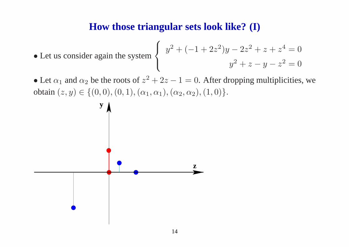
• Let us consider again the system
y2 + (−1 + 2z2)y − 2z2 + z + z4 = 0
y2 + z − y − z2 = 0
• Let α1 andα2 be the roots ofz2 + 2z − 1 = 0. After dropping multiplicities, weobtain(z, y) ∈ {(0, 0), (0, 1), (α1, α1), (α2, α2), (1, 0)}.
y
z
14
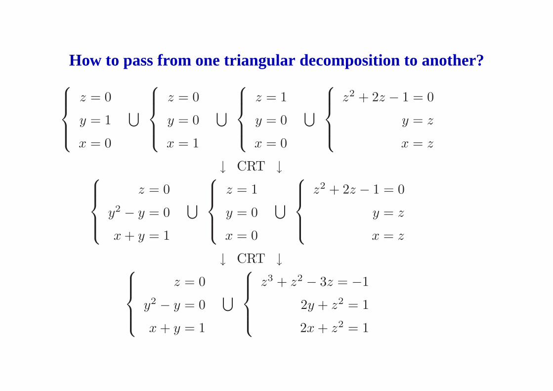
How to pass from one triangular decomposition to another?
z = 0
y = 1
x = 0
⋃
z = 0
y = 0
x = 1
⋃
z = 1
y = 0
x = 0
⋃
z2 + 2z − 1 = 0
y = z
x = z
↓ CRT ↓
z = 0
y2 − y = 0
x + y = 1
⋃
z = 1
y = 0
x = 0
⋃
z2 + 2z − 1 = 0
y = z
x = z
↓ CRT ↓
z = 0
y2 − y = 0
x + y = 1
⋃
z3 + z2 − 3z = −1
2y + z2 = 1
2x + z2 = 1

From a lexicographical Grobner basis to a triangulardecomposition (I)
• Let us consider again (last time) the polynomials
f1 = y2 + (2z2 − 1)y − 2z2 + z + z4
f2 = y2 + z − y − z2
• It is natural to ask how we could obtain a triangular decomposition from the
reduced lexicographical Grobner basis of{f1, f2} for y > z. This basis is:
g1 = z6 − 4z4 + 4z3 − z2
g2 = 2z2y + z4 − z2
g3 = y2 − y − z2 + z
• We initializeT := {g1}. We would add g2 into T provided thatlc(g2, y) is a
unit .
16
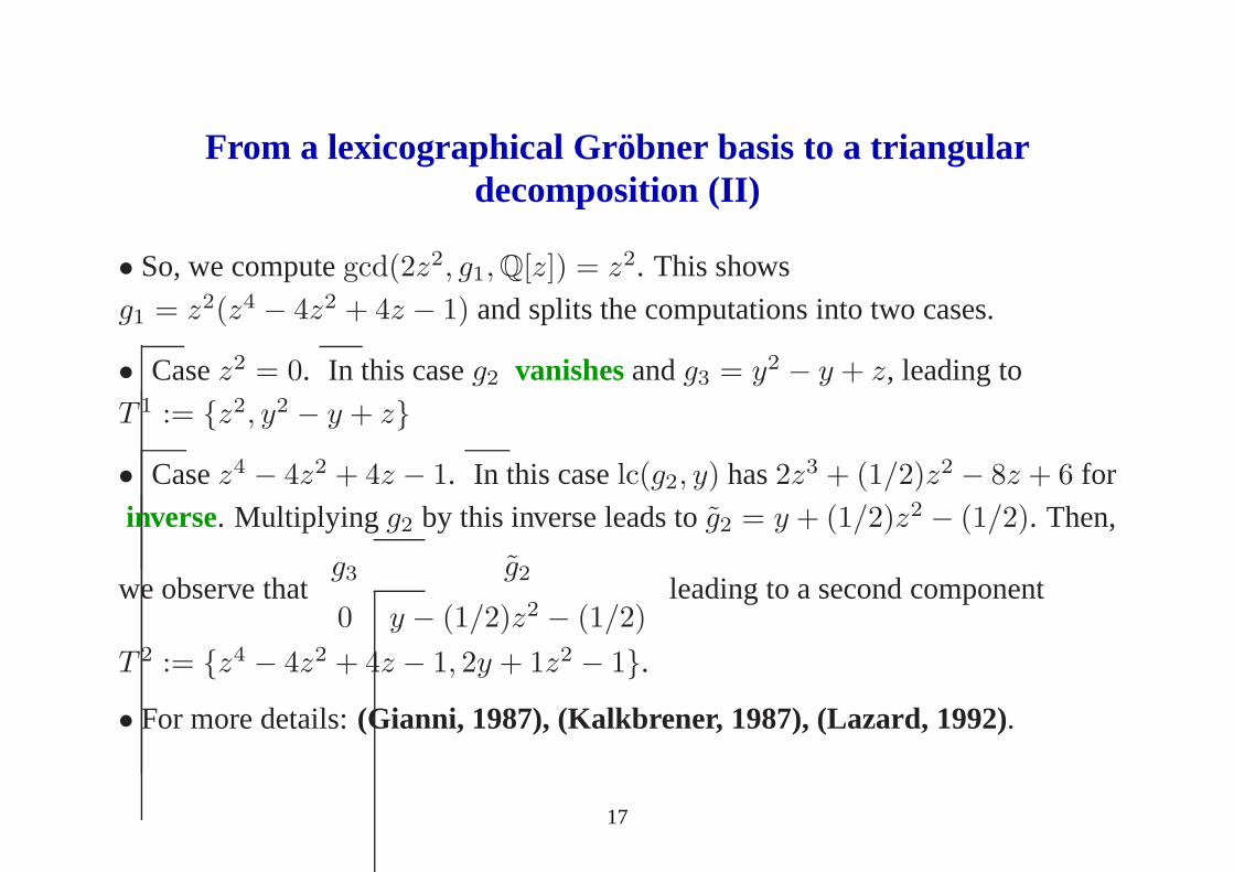
From a lexicographical Grobner basis to a triangulardecomposition (II)
• So, we computegcd(2z2, g1, Q[z]) = z2. This shows
g1 = z2(z4 − 4z2 + 4z − 1) and splits the computations into two cases.
• Casez2 = 0. In this caseg2 vanishesandg3 = y2 − y + z, leading to
T 1 := {z2, y2 − y + z}
• Casez4 − 4z2 + 4z − 1. In this caselc(g2, y) has2z3 + (1/2)z2 − 8z + 6 for
inverse. Multiplying g2 by this inverse leads tog2 = y + (1/2)z2 − (1/2). Then,
we observe thatg3 g2
0 y − (1/2)z2 − (1/2)leading to a second component
T 2 := {z4 − 4z2 + 4z − 1, 2y + 1z2 − 1}.
• For more details:(Gianni, 1987), (Kalkbrener, 1987), (Lazard, 1992).
17

Some notations before we start the theory (I)
NOTATION. Throughout the talk, we consider a fieldK and an ordered setX = x1 < · · · < xn of n variables. TypicallyK will be
- a finite field, such asZ/pZ for a primep, or
- the fieldQ of rational numbers, or
- a field of rational functions overZ/pZ or Q.
We will denote byK an algebraic closureof K.
NOTATION. We denote byK[x1, . . . , xn] the ring of the polynomials withcoefficients inK and variables inX . ForF ⊂ K[x1, . . . , xn], we write〈F 〉 and√
〈F 〉 for the ideal generated byF in K[x1, . . . , xn] and its radical, respectively.
NOTATION. ForF ⊂ K[x1, . . . , xn], we are interested in
V (F ) = {ζ ∈ Kn| (∀f ∈ F ) f(ζ) = 0},
the zero-setof F or algebraic variety of F in Kn.
REMARK . In some circumstancesKn
will be denotedAn(K), especially whenwe consider severaln at the same time.18

Some notations before we start the theory (II)
NOTATION. Let i andj be integers such that1 ≤ i ≤ j ≤ n and letV ⊆ An(K)
be a variety overK. We denote byπji the natural projection map fromAj(K) to
Ai(K), which sends(x1, . . . , xj) to (x1, . . . , xi). Moreover, we defineVi = πn
i (V ). Often, we will restrictπji from Vi to Vj .
NOTATION. The algebraic varieties inKn
defined by polynomial sets ofK[x1, . . . , xn] form the closed setsof a topology, calledZariski Topology. For asubsetW ⊂ K
n, we denote byW the closure ofW for this topology, that is, the
intersection of theV (F ) containingW , for all F ⊂ K[x1, . . . , xn].
NOTATION. ForW ⊂ Kn, we denote byI(W ) the ideal ofK[x1, . . . , xn]
generated by the polynomials vanishing at every point ofW .
REMARK . WhenK = K andW = V (F ), for someF ⊂ K[x1, . . . , xn], recallthe Hilbert Theorem of Zeros:
√
〈F 〉 = I(V (F )).
19

Lazard triangular sets
DEFINITION. (Lazard, 1992)A subset
T = {T1, . . . Tn} ⊂ K[x1 < · · · < xn]
is aLazard triangular setif for i = 1 · · ·n
Ti = 1xdi
i+ adi−1 x
di−1
i+ · · · + a1 xi + a0
with
adi−1, . . . , a1, a0 ∈ k[x1, . . . , xi−1].
reduced w.r.t〈T1, . . . , Ti−1〉 in the sense of Grobner bases.
THEOREM. A family T of n polynomials inK[x1 < · · · < xn] is a
Lazard triangular set if and only it is the
reduced lexicographical Grobner basisof a zero-dimensionalideal.
20
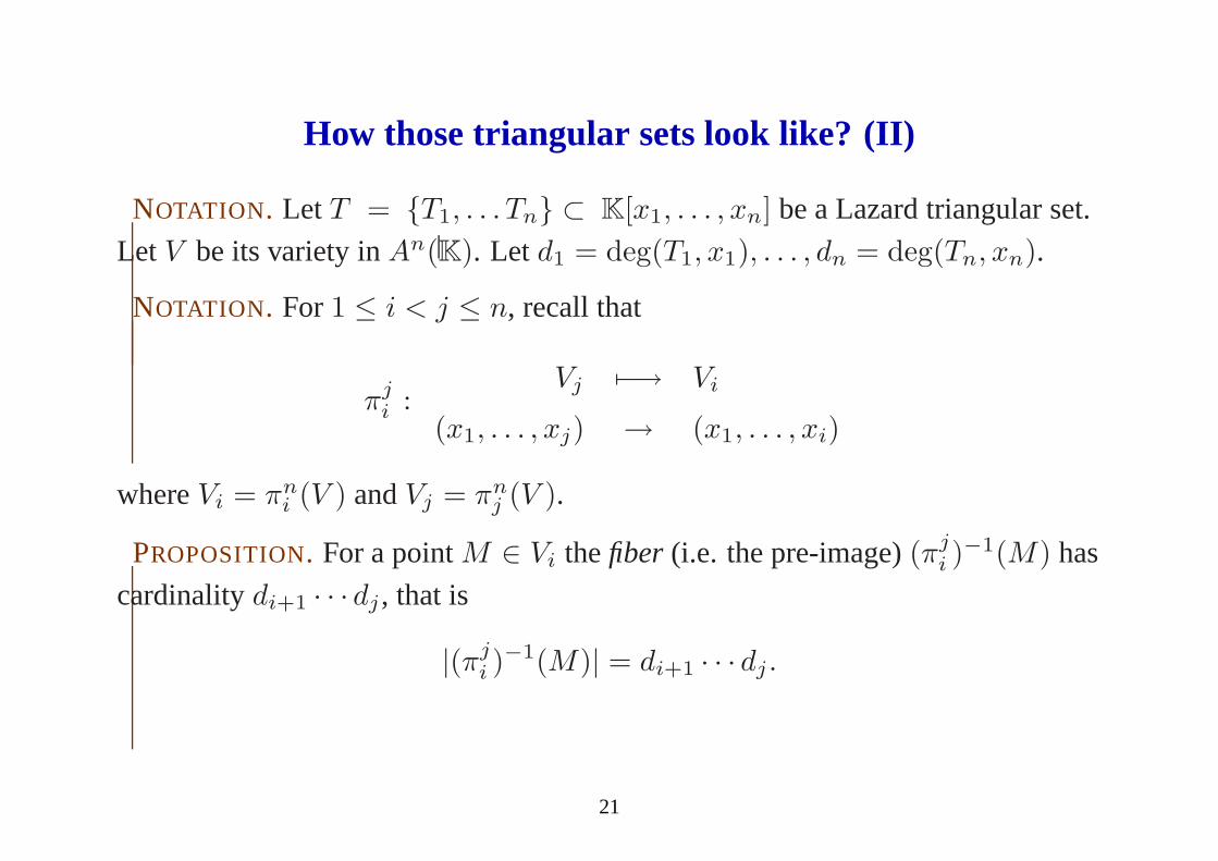
How those triangular sets look like? (II)
NOTATION. Let T = {T1, . . . Tn} ⊂ K[x1, . . . , xn] be a Lazard triangular set.
Let V be its variety inAn(K). Let d1 = deg(T1, x1), . . . , dn = deg(Tn, xn).
NOTATION. For1 ≤ i < j ≤ n, recall that
πji :
Vj 7−→ Vi
(x1, . . . , xj) → (x1, . . . , xi)
whereVi = πni (V ) andVj = πn
j (V ).
PROPOSITION. For a pointM ∈ Vi thefiber (i.e. the pre-image)(πji )
−1(M) has
cardinalitydi+1 · · · dj , that is
|(πji )
−1(M)| = di+1 · · · dj .
21
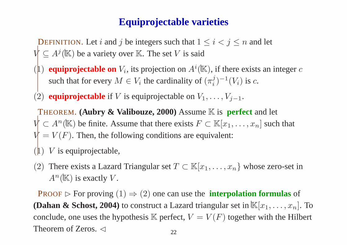
Equiprojectable varieties
DEFINITION. Let i andj be integers such that1 ≤ i < j ≤ n and letV ⊆ Aj(K) be a variety overK. The setV is said
(1) equiprojectable onVi, its projection onAi(K), if there exists an integercsuch that for everyM ∈ Vi the cardinality of(πj
i )−1(Vi) is c.
(2) equiprojectable if V is equiprojectable onV1, . . . , Vj−1.
THEOREM. (Aubry & Valibouze, 2000) AssumeK is perfect and letV ⊂ An(K) be finite. Assume that there existsF ⊂ K[x1, . . . , xn] such thatV = V (F ). Then, the following conditions are equivalent:
(1) V is equiprojectable,
(2) There exists a Lazard Triangular setT ⊂ K[x1, . . . , xn} whose zero-set inAn(K) is exactlyV .
PROOF⊲ For proving(1) ⇒ (2) one can use theinterpolation formulas of(Dahan & Schost, 2004)to construct a Lazard triangular set inK[x1, . . . , xn]. Toconclude, one uses the hypothesisK perfect,V = V (F ) together with the HilbertTheorem of Zeros.⊳ 22

The interpolation formulas: sketch (I)
• Let V ⊂ An(K) be (finite and) equiprojectable. LetK be a field, with
K ⊆ K ⊆ K such that every point ofV has its coordinates inK.
• We haveT1 =∏
α∈V1(x1 − α). Let 1 ≤ ℓ < n. We give interpolation formulas
for Tℓ+1 from the coordinates (inK) of the points ofVℓ+1, for 1 ≤ ℓ < n.
• Let α = (α1, . . . , αℓ) ∈ Vℓ. We define the varieties
V 1α = { β = (β1, . . . , βℓ, βℓ+1) ∈ Vℓ+1 | β1 6= α1}
V 2α = { β = (α1, β2, . . . , βℓ, βℓ+1) ∈ Vℓ+1 | β2 6= α2}
· · · · · · · · · · · · · · ·
V ℓα = { β = (α1, . . . , αℓ−1, βℓ, βℓ+1) ∈ Vℓ+1 | βℓ 6= αℓ}
V ℓ+1α = { β = (α1, . . . , αℓ, βℓ+1) ∈ Vℓ+1 }
The setsV 1α , V 2
α , V 3α , . . . , V ℓ
α , V ℓ+1α form a partition ofVℓ+1.
• The intermediate goal is to buildTα,ℓ+1 = Ti(α1, . . . , αℓ, xℓ+1) ∈ K[xℓ+1].
23
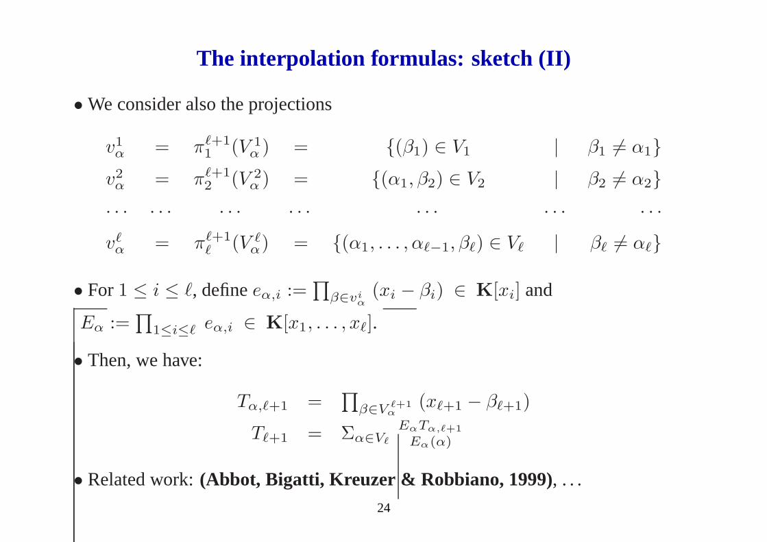
The interpolation formulas: sketch (II)
• We consider also the projections
v1α = πℓ+1
1 (V 1α ) = {(β1) ∈ V1 | β1 6= α1}
v2α = πℓ+1
2 (V 2α ) = {(α1, β2) ∈ V2 | β2 6= α2}
· · · · · · · · · · · · · · · · · · · · ·
vℓα = πℓ+1
ℓ (V ℓα) = {(α1, . . . , αℓ−1, βℓ) ∈ Vℓ | βℓ 6= αℓ}
• For1 ≤ i ≤ ℓ, defineeα,i :=∏
β∈viα
(xi − βi) ∈ K[xi] and
Eα :=∏
1≤i≤ℓ eα,i ∈ K[x1, . . . , xℓ].
• Then, we have:
Tα,ℓ+1 =∏
β∈Vℓ+1
α(xℓ+1 − βℓ+1)
Tℓ+1 = Σα∈Vℓ
EαTα,ℓ+1
Eα(α)
• Related work:(Abbot, Bigatti, Kreuzer & Robbiano, 1999), . . .
24

Direct product of fields, the D5 Principle (I)
PROPOSITION. Let f ∈ K[x] be a non-constant andsquare-freeunivariate
polynomial. ThenL = K[x]/〈f〉 is a direct product of fields (DPF).
PROOF⊲ The factors off are pairwise coprime. Then, apply the
Chinese Remaindering Theorem. (If f = f1f2 then
L ≃ K[x]/〈f1〉 × K[x]/〈f2〉. ⊳
PRINCIPLE. (Della Dora, Dicrescenzo & Duval, 1985)If L is a DPF, then one
can compute withL as if it were a field: it suffices to split the computations into
cases whenever azero-divisor is met.
PROPOSITION. Let L be a DPF andf ∈ L[x] be a non-constant monic
polynomial such thatf and its derivative generateL[x], that is,〈f, f ′〉 = L[x].
ThenL[x]/〈f〉 is another DPF.
PROOF⊲ It is convenient to establish the following more general theorem:A
Noetherian ring is isomorphic with a direct product of fieldsif and only if every
non-zero element is either a unit or a non-nilpotent zero-divisor. ⊳
25
Direct product of fields, the D5 Principle (II)
PROPOSITION. Let T ⊂ K[x1, . . . , xn] be a Lazard triangular set such that〈T 〉
is radical. Then, we have
• K[x1, . . . , xn]/〈T 〉 is a DPF,
• if K is perfect thenK[x1, . . . , xn]/〈T 〉 is a DPF.
REMARK . Recall the trap! ConsiderF = Z/pZ(t), for a primep. Consider the
polynomialf = xp − t ∈ F[x] andF an algebraic closure ofF.
Sincef is not constant, it has a rootα ∈ F and we have
f = xp − t = xp − αp = (x − α)p (1)
in F[x], which is clearly not square-free. Howeverf is irreducible, and thus
squarefree, inF[x].
26

Polynomial GCDs over DPF, quasi-inverses (I)
DEFINITION. ( M3 & Rioboo, 1995)Let L be a DPF. The polynomialh ∈ L[y]
is aGCD of the polynomialsf, g ∈ L[y] if the ideals〈f, g〉 and〈h〉 are equal.
REMARK . Another trap! Even iff, g are bothmonic, theremay not exist a monicpolynomialh in L[y] such that〈f, g〉 = 〈h〉 holds.Consider for instancef = y + a+1
2 (assuming that2 is invertible inL) andg = y + 1 wherea ∈ L satisfiesa2 = a, a 6= 0 anda 6= 1.
REMARK . In practice, polynomial GCDs over DPF are computed via the D5Principle. Moreover, only monic GCDs are useful. So, we generalize:
DEFINITION. Let L be a DPF andf, g ∈ L[y]. A GCD of f, g in L[y] is asequence of pairs((hi, Li), 1 ≤ i ≤ s) such that
• Li is a DPF, for all1 ≤ i ≤ s and the direct product ofL1, . . . , Ls isisomorphic toL,
• hi is a null or monic polynomial inLi[y], for all 1 ≤ i ≤ s,
• hi is a GCD (in the above sense) of the projections off, g to Li[y], for all1 ≤ i ≤ s.
27
Polynomial GCDs over DPF, quasi-inverses (II)
DEFINITION. Let L be a DPF and letf ∈ L. A quasi-inverseof f is a sequence
of pairs((gi, Li), 1 ≤ i ≤ s) such that
• Li is a DPF, for all1 ≤ i ≤ s and the direct product ofL1, . . . , Ls is
isomorphic toL
• gi ∈ Li, for all 1 ≤ i ≤ s,
• let fi be the projection off to Li; eitherfi = gi = 0 or figi = 1 hold, for all
1 ≤ i ≤ s.
PROPOSITION. Let T ⊂ K[x1, . . . , xn] be a Lazard triangular set such that〈T 〉
is radical. We defineL = K[x1, . . . , xn]/〈T 〉.
(1) For allf ∈ K[x1, . . . , xn] (reduced w.r.t.T ) one can compute a
quasi-inversein L of f (regarded as an element ofL).
(1) For allf, g ∈ L[y] one can compute aGCD of f andg in L[y].
28

Equiprojectable decomposition
REMARK . Not every variety is equiprojectable, for instanceV = {(0, 1), (0, 0), (1, 0)}.
DEFINITION. Let V ⊂ An(K) be finite. Consider the projection
π : V 7−→ Kn−1
which forgetsxn. To everyx ∈ V we associate
N(x) = #π−1(π(x)).
We writeV = C1 ∪ · · · ∪ Cd whereCi = {x ∈ V | N(x) = i}. This splittingprocess is applied recursively to all varietiesC1, . . . , Cd.
In the end, we obtain a family of pairwise disjoint, equiprojectable varieties,whose reunion equalsV . This is theequiprojectable decompositionof V .
PROPOSITION. Let V (F ) ⊂ An(K) be finite withF ⊂ K[x1, . . . , xn]. Thereexist Lazard triangular setsT 1, . . . , T s ⊂ K[x1, . . . , xn] such that
V (F ) = V (T 1) ∪ · · · ∪ V (T s) and i 6= j ⇒ V (T i) ∩ V (T j) = ∅.
They form a triangular decomposition of V (F ).29

Equiprojectable variety definition (1/3)
30
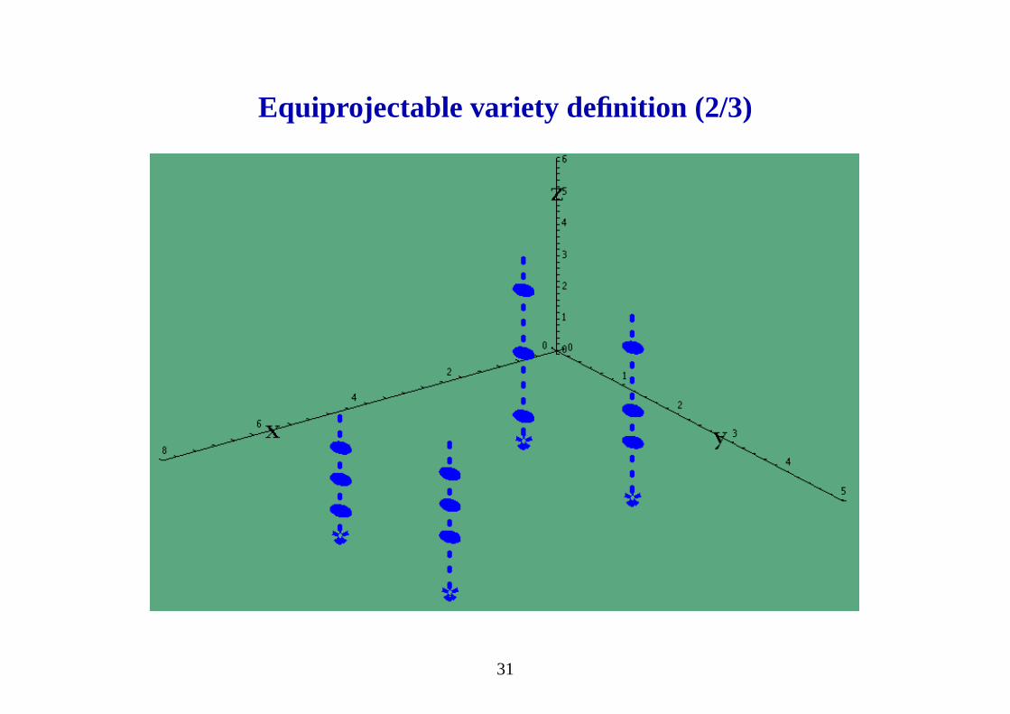
Equiprojectable variety definition (2/3)
31

Equiprojectable variety definition (3/3)
32
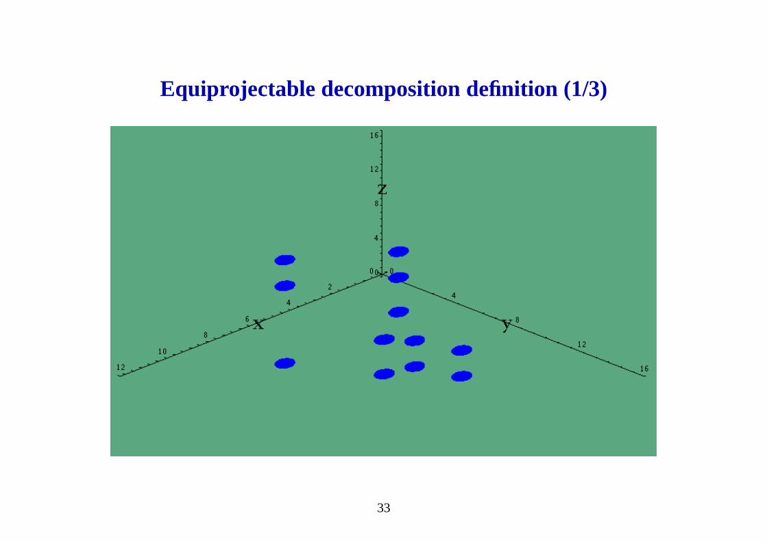
Equiprojectable decomposition definition (1/3)
33

Equiprojectable decomposition definition (2/3)
34

Equiprojectable decomposition definition (3/3)
35
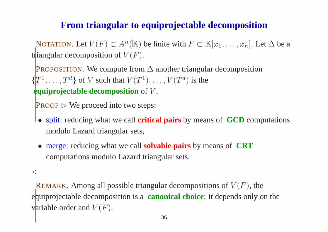
From triangular to equiprojectable decomposition
NOTATION. Let V (F ) ⊂ An(K) be finite withF ⊂ K[x1, . . . , xn]. Let ∆ be atriangular decomposition ofV (F ).
PROPOSITION. We compute from∆ another triangular decomposition{T 1, . . . , T d} of V such thatV (T 1), . . . , V (T d) is theequiprojectable decompositionof V .
PROOF⊲ We proceed into two steps:
• split: reducing what we callcritical pairs by means ofGCD computationsmodulo Lazard triangular sets,
• merge: reducing what we callsolvable pairsby means ofCRTcomputations modulo Lazard triangular sets.
⊳
REMARK . Among all possible triangular decompositions ofV (F ), theequiprojectable decomposition is acanonical choice: it depends only on thevariable order andV (F ).
36
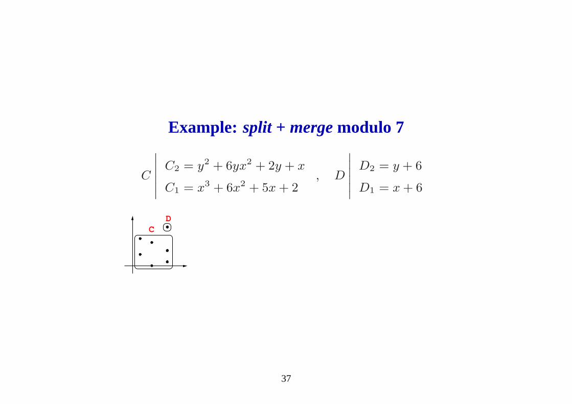
Example: split + merge modulo 7
C
˛
˛
˛
˛
˛
˛
C2 = y2 + 6yx2 + 2y + x
C1 = x3 + 6x2 + 5x + 2, D
˛
˛
˛
˛
˛
˛
D2 = y + 6
D1 = x + 6
��������
������
������
��������
��������
��������
������
������
��������
CD
37
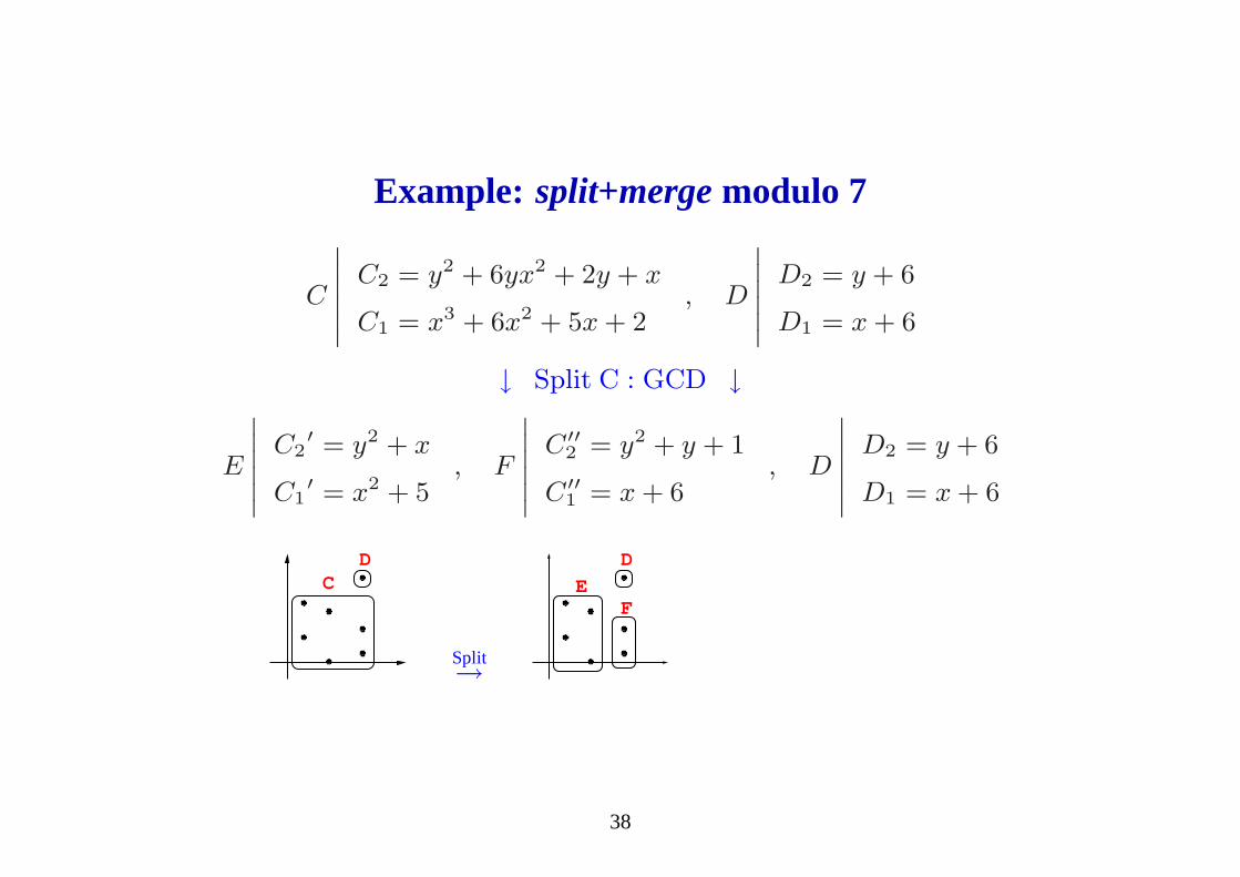
Example: split+merge modulo 7
C
˛
˛
˛
˛
˛
˛
C2 = y2 + 6yx2 + 2y + x
C1 = x3 + 6x2 + 5x + 2, D
˛
˛
˛
˛
˛
˛
D2 = y + 6
D1 = x + 6
↓ Split C : GCD ↓
E
˛
˛
˛
˛
˛
˛
C2′ = y2 + x
C1′ = x2 + 5
, F
˛
˛
˛
˛
˛
˛
C′′
2 = y2 + y + 1
C′′
1 = x + 6, D
˛
˛
˛
˛
˛
˛
D2 = y + 6
D1 = x + 6
��������
������
������
��������
��������
��������
������
������
��������
CD
Split→
��������
������
������
��������
��������
��������
������
������
��������
��������������������������������
E
D
F
38

Example: split+merge modulo 7
C
˛
˛
˛
˛
˛
˛
C2 = y2 + 6yx2 + 2y + x
C1 = x3 + 6x2 + 5x + 2, D
˛
˛
˛
˛
˛
˛
D2 = y + 6
D1 = x + 6
↓ Split C : GCD ↓
E
˛
˛
˛
˛
˛
˛
C2′ = y2 + x
C1′ = x2 + 5
, F
˛
˛
˛
˛
˛
˛
C′′
2 = y2 + y + 1
C′′
1 = x + 6, D
˛
˛
˛
˛
˛
˛
D2 = y + 6
D1 = x + 6
↓ Merge F and D : CRT ↓
E
˛
˛
˛
˛
˛
˛
C′
2 = y2 + x
C′
1 = x2 + 5, G
˛
˛
˛
˛
˛
˛
G2 = y3 + 6
G1 = x + 6
��������
������
������
��������
��������
��������
������
������
��������
CD
Split→
��������
������
������
��������
��������
��������
������
������
��������
��������������������������������
E
D
F
Merge→
������
������
��������
��������
��������
��������
������
������
��������
��������������������������������
E
G
39
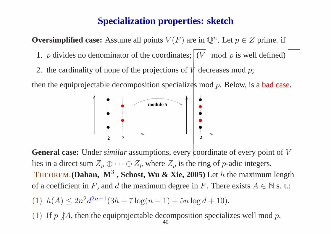
Specialization properties: sketch
Oversimplified case:Assume all pointsV (F ) are inQn. Let p ∈ Z prime. if
1. p divides no denominator of the coordinates;(V mod p is well defined)
2. the cardinality of none of the projections ofV decreases modp;
then the equiprojectable decomposition specializes modp. Below, is abad case.
����
����
����
����
����
����
2 7 2
modulo 5
General case:Undersimilar assumptions, every coordinate of every point ofV
lies in a direct sumZp ⊕ · · · ⊕ Zp whereZp is the ring ofp-adic integers.THEOREM.(Dahan, M3 , Schost, Wu & Xie, 2005)Let h the maximum lengthof a coefficient inF , andd the maximum degree inF . There existsA ∈ N s. t.:
(1) h(A) ≤ 2n2d2n+1(3h + 7 log(n + 1) + 5n log d + 10).
(1) If p 6 |A, then the equiprojectable decomposition specializes wellmodp.40
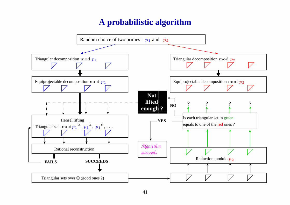
A probabilistic algorithm
��������������������
��������������������
����
��������������
Algorithmsucceeds
Hensel lifting
Rational reconstruction
Reduction modulop2
Triangular sets overQ (good ones ?)
Random choice of two primes :p1 and p2
Triangular decompositionmod p1
Equiprojectable decompositionmod p1
Triangular decompositionmod p2
Equiprojectable decompositionmod p2
equals to one of theredones ?
? ? ? ?
Is each triangular set ingreen
Triangular setsmodp12, p1
4, p1
8, . . .
NO
SUCCEEDS
YES
FAILS
Notlifted
enough ?
41
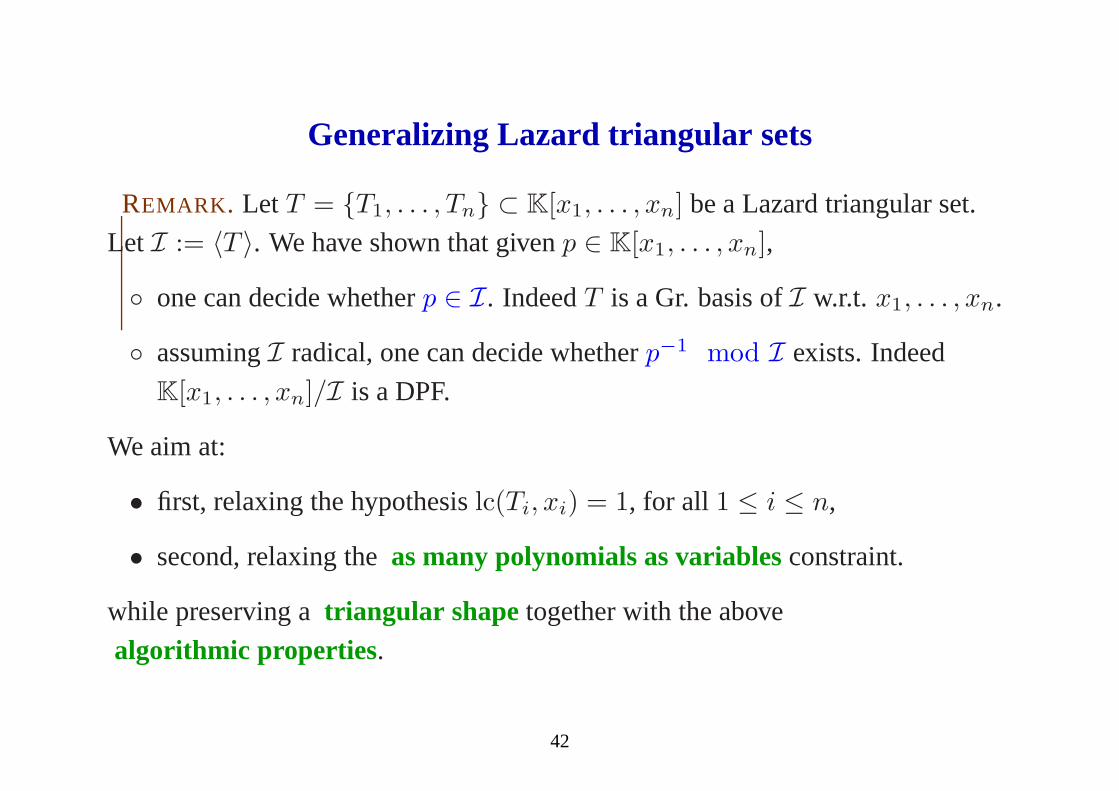
Generalizing Lazard triangular sets
REMARK . Let T = {T1, . . . , Tn} ⊂ K[x1, . . . , xn] be a Lazard triangular set.
Let I := 〈T 〉. We have shown that givenp ∈ K[x1, . . . , xn],
◦ one can decide whetherp ∈ I. IndeedT is a Gr. basis ofI w.r.t. x1, . . . , xn.
◦ assumingI radical, one can decide whetherp−1 mod I exists. Indeed
K[x1, . . . , xn]/I is a DPF.
We aim at:
• first, relaxing the hypothesislc(Ti, xi) = 1, for all 1 ≤ i ≤ n,
• second, relaxing theas many polynomials as variablesconstraint.
while preserving atriangular shape together with the above
algorithmic properties.
42
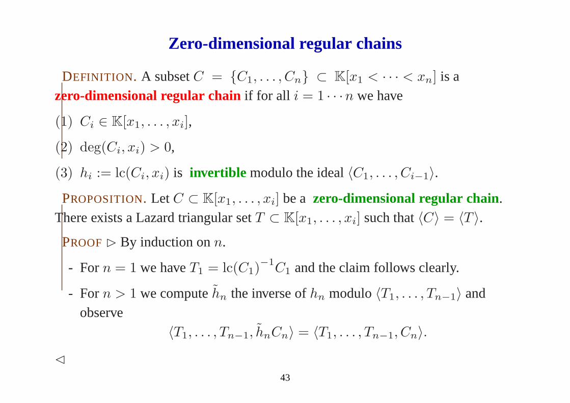
Zero-dimensional regular chains
DEFINITION. A subsetC = {C1, . . . , Cn} ⊂ K[x1 < · · · < xn] is azero-dimensional regular chainif for all i = 1 · · ·n we have
(1) Ci ∈ K[x1, . . . , xi],
(2) deg(Ci, xi) > 0,
(3) hi := lc(Ci, xi) is invertible modulo the ideal〈C1, . . . , Ci−1〉.
PROPOSITION. Let C ⊂ K[x1, . . . , xi] be a zero-dimensional regular chain.There exists a Lazard triangular setT ⊂ K[x1, . . . , xi] such that〈C〉 = 〈T 〉.
PROOF⊲ By induction onn.
- Forn = 1 we haveT1 = lc(C1)−1C1 and the claim follows clearly.
- Forn > 1 we computehn the inverse ofhn modulo〈T1, . . . , Tn−1〉 andobserve
〈T1, . . . , Tn−1, hnCn〉 = 〈T1, . . . , Tn−1, Cn〉.
⊳
43

The Dahan-Schost Transform (I)
PROPOSITION. ConsiderT = {T1, . . . , Tn} a Lazard triangular set. AssumeT
generates a radical ideal. LetD1 = 1 andN1 = T1. For2 ≤ ℓ ≤ n, define
Dℓ =∏
1≤i≤ℓ−1∂Ti
∂ximod 〈T1, . . . , Tℓ−1〉
Nℓ = DℓTℓ mod 〈T1, . . . , Tℓ−1〉
ThenN = {N1, . . . , Nn} is a zero-dimensional regular chain with〈T 〉 = 〈N〉.
REMARK . The results of(Dahan & Schost, 2004)“essentially” show that the
height (or “size”) of each coefficient inN is upper bounded by
• the height ofV(T ) if K = Q, that is the minimum size of a data set encoding
V(T ),
• the degree ofV(T ↓) if K is a fieldk(t1, . . . , tm) of rational functions andT ↓
is T regarded ink[t1, . . . , tm, x1, . . . , xn].
See the authors’ article for precise statements.
44

The Dahan-Schost Transform (II)
• Consider the systemF (Barry Trager).
−x5 + y5 − 3y − 1 = 5y4 − 3 = −20x + y − z = 0
We solve it forz < y < x.• V (F ) is equiprojectable and its Lazard triangular set is
•
114741279465692560074688619671388225994546322534047768700511994762226192690048901447618534394846710571230
177126050500820286210285405170218983414450704192140091221285435794696093319533564185839650189693585028838
699349416725564387706041955516121939729771831066168137301361047343316167529521509773976546819862973936865
469803305737200436962857230940384594351690145609608094579328266988168648539093657866617523596721342746025
362457794998087226523064237197118238681455387434685379217170814307753153223785029557758914206492139656047
182558840983144129257028601685384373297644771129092120128266359787322504095639220690574114668770499695595
151384178460667251183582226588998788962467225266512277813388396930460206274093549761989465144274545813617
443943358739034775586223820376199033996055435130191939848508110344015397674352445829758618270875644685197
239889463831973885970439654459159240773157947028995584430781544269432684180568707791767576191787113033986
273833966279899712882771296735352080757871215616119541262433845931685356908075413015471945211962286282353
152371339486589977786933953445963421265232316881028589410282951401496074779560518480664573334972022843566
485639134741063277706156095111089627563494088702934461198572429832808992812870412765974147039531428471109
182770901475269211462030828375934181004032581754339209581456763239413822566355167569080400536438012882499
309191296130950729973668595368021125635249693248658751381279239017170403224531631090451630403456902301090
683868839664164549094509086861836658249042063767397085327986947101834888709181774954667584759337690865176
748156823800707525930652056310913558181154201465607063798861710733037765053357306037655291256264679716332
154608045527569292338754337973797843824713701855230758768236174292780150592090630056630234512064066763987
124695385819578642285275287975402015668994502200477065094640515598601115130175167063705343665239193213631
661526598571882453204248880242229677381842937378916991769765942931876746884848648814238710335767650654224
573598714920124956474610718803150703376812978417179178775576117319500000077857129232958889104193427114987
239787108649287987286424755607482454864690786827841184696976286133386057573817722098997859322480446751288
45

•
573706397328462800373443098356941129972731612670238843502559973811130963450244507238092671974233552856154
177126050500820286210285405170218983414450704192140091221285435794696093319533564185839650189693585028838
699349416725564387706041955516121939729771831066168137301361047343316167529521509773976546819862973936865
469803305737200436962857230940384594351690145609608094579328266988168648539093657866617523596721342746025
362457794998087226523064237197118238681455387434685379217170814307753153223785029557758914206492139656047
182558840983144129257028601685384373297644771129092120128266359787322504095639220690574114668770499695595
151384178460667251183582226588998788962467225266512277813388396930460206274093549761989465144274545813617
443943358739034775586223820376199033996055435130191939848508110344015397674352445829758618270875644685197
239889463831973885970439654459159240773157947028995584430781544269432684180568707791767576191787113033986
273833966279899712882771296735352080757871215616119541262433845931685356908075413015471945211962286282353
152371339486589977786933953445963421265232316881028589410282951401496074779560518480664573334972022843566
485639134741063277706156095111089627563494088702934461198572429832808992812870412765974147039531428471109
182770901475269211462030828375934181004032581754339209581456763239413822566355167569080400536438012882499
309191296130950729973668595368021125635249693248658751381279239017170403224531631090451630403456902301090
683868839664164549094509086861836658249042063767397085327986947101834888709181774954667584759337690865176
748156823800707525930652056310913558181154201465607063798861710733037765053357306037655291256264679716332
154608045527569292338754337973797843824713701855230758768236174292780150592090630056630234512064066763987
124695385819578642285275287975402015668994502200477065094640515598601115130175167063705343665239193213631
661526598571882453204248880242229677381842937378916991769765942931876746884848648814238710335767650654224
107682408337843898832379553790426595918634253059664726983856491630963372387378005133782870040125741167383
239787108649287987286424755607482454864690786827841184696976286133386057573817722098997859322480446751288
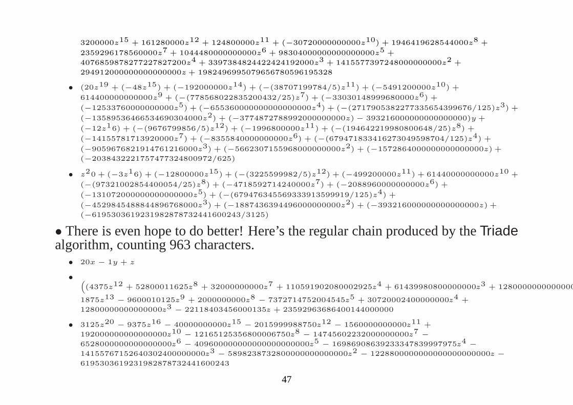
• 3125z20 − 9375z16 − 40000000000z15 − 2015999988750z12 − 1560000000000z11 +
192000000000000000z10 − 12165125356800006750z8 − 14745602232000000000z7 −
6528000000000000000z6 − 409600000000000000000000z5 − 16986908639233347839997975z4 −
14155767152640302400000000z3 − 5898238732800000000000000z2 − 1228800000000000000000000z −
6195303619231982878732441600243
• Applying the transformation of Dahan and Schost leads to 1787 characters.• (20z19 + (−48z15) + (−192000000z14) + (−(38707199784/5)z11) + (−5491200000z10) +
614400000000000z9 + (−(778568022835200432/25)z7) + (−33030148999680000z6) +
(−12533760000000000z5) + (−655360000000000000000z4) + (−(2717905382277335654399676/125)z3) +
(−13589536466534690304000z2) + (−3774872788992000000000z) − 393216000000000000000)x +
46
3200000z15 + 161280000z12 + 124800000z11 + (−30720000000000z10) + 1946419628544000z8 +
2359296178560000z7 + 1044480000000000z6 + 98304000000000000000z5 +
4076859878277227827200z4 + 3397384824422424192000z3 + 1415577397248000000000z2 +
294912000000000000000z + 1982496995079656780596195328
• (20z19 + (−48z15) + (−192000000z14) + (−(38707199784/5)z11) + (−5491200000z10) +
614400000000000z9 + (−(778568022835200432/25)z7) + (−33030148999680000z6) +
(−12533760000000000z5) + (−655360000000000000000z4) + (−(2717905382277335654399676/125)z3) +
(−13589536466534690304000z2) + (−3774872788992000000000z) − 393216000000000000000)y +
(−12z16) + (−(9676799856/5)z12) + (−1996800000z11) + (−(194642219980800648/25)z8) +
(−14155781713920000z7) + (−8355840000000000z6) + (−(679471833416273049598704/125)z4) +
(−9059676821914761216000z3) + (−5662307155968000000000z2) + (−1572864000000000000000z) +
(−2038432221757477324800972/625)
• z20 + (−3z16) + (−12800000z15) + (−(3225599982/5)z12) + (−499200000z11) + 61440000000000z10 +
(−(97321002854400054/25)z8) + (−4718592714240000z7) + (−2088960000000000z6) +
(−131072000000000000000z5) + (−(679476345569333913599919/125)z4) +
(−4529845488844896768000z3) + (−1887436394496000000000z2) + (−393216000000000000000z) +
(−6195303619231982878732441600243/3125)
• There is even hope to do better! Here’s the regular chain produced by theTriadealgorithm, counting 963 characters.
• 20x − 1y + z
•“
(4375z12 + 52800011625z8 + 32000000000z7 + 110591902080002925z4 + 61439980800000000z3 + 12800000000000000
1875z13 − 9600010125z9 + 2000000000z8 − 7372714752004545z5 + 30720002400000000z4 +
12800000000000000z3 − 22118403456000135z + 23592963686400144000000
• 3125z20 − 9375z16 − 40000000000z15 − 2015999988750z12 − 1560000000000z11 +
192000000000000000z10 − 12165125356800006750z8 − 14745602232000000000z7 −
6528000000000000000z6 − 409600000000000000000000z5 − 16986908639233347839997975z4 −
14155767152640302400000000z3 − 5898238732800000000000000z2 − 1228800000000000000000000z −
6195303619231982878732441600243
47
Grobner bases (I)
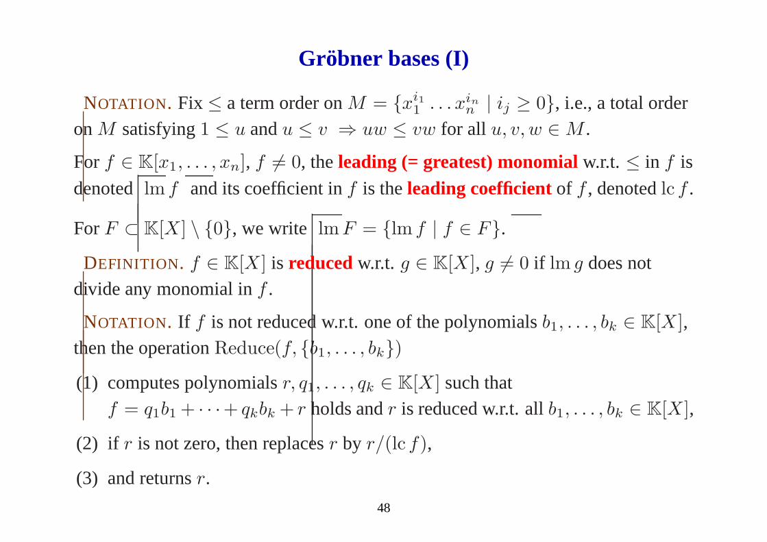
NOTATION. Fix ≤ a term order onM = {xi11 . . . xin
n | ij ≥ 0}, i.e., a total orderonM satisfying1 ≤ u andu ≤ v ⇒ uw ≤ vw for all u, v, w ∈ M .
Forf ∈ K[x1, . . . , xn], f 6= 0, theleading (= greatest) monomialw.r.t. ≤ in f is
denoted lm f and its coefficient inf is theleading coefficientof f , denotedlc f .
ForF ⊂ K[X ] \ {0}, we write lmF = {lm f | f ∈ F}.
DEFINITION. f ∈ K[X ] is reducedw.r.t. g ∈ K[X ], g 6= 0 if lm g does notdivide any monomial inf .
NOTATION. If f is not reduced w.r.t. one of the polynomialsb1, . . . , bk ∈ K[X ],then the operationReduce(f, {b1, . . . , bk})
(1) computes polynomialsr, q1, . . . , qk ∈ K[X ] such thatf = q1b1 + · · ·+ qkbk + r holds andr is reduced w.r.t. allb1, . . . , bk ∈ K[X ],
(2) if r is not zero, then replacesr by r/(lc f),
(3) and returnsr.
48

Grobner bases (II)
NOTATION. ForA, B finite subsets ofK[X ] \ {0} the collection of theReduce(a, B), for a ∈ A, is denoted byReduce(A, B).
DEFINITION. A subsetB ⊂ K[X ] \ {0} is auto-reducedif for all b ∈ B thepolynomialb is reduced w.r.t.B \ {b} andlcb = 1.
PROPOSITION. (Dickson’s Lemma) Every auto-reduced set is finite.
DEFINITION. ForA, B ⊆ F auto-reduced sets, we writeA ≤ B whenever
[lmB ⊆ lmA] or [min(lmA \ lmB) < min(lmB \ lmA)].
DEFINITION. For an idealI ⊂ K[x1, . . . , xn], a minimal auto-reduced subsetB ⊂ I is called areduced Grobner basisof I.
PROPOSITION. Every idealI ⊂ K[x1, . . . , xn] admits a reduced Grobner basis;moreover an auto-reduced subsetB ⊂ I is a reduced Grobner basis ofI iff wehave for allf ∈ K[x1, . . . , xn]
f ∈ I ⇐⇒ Reduce(f, B) = 0.
49
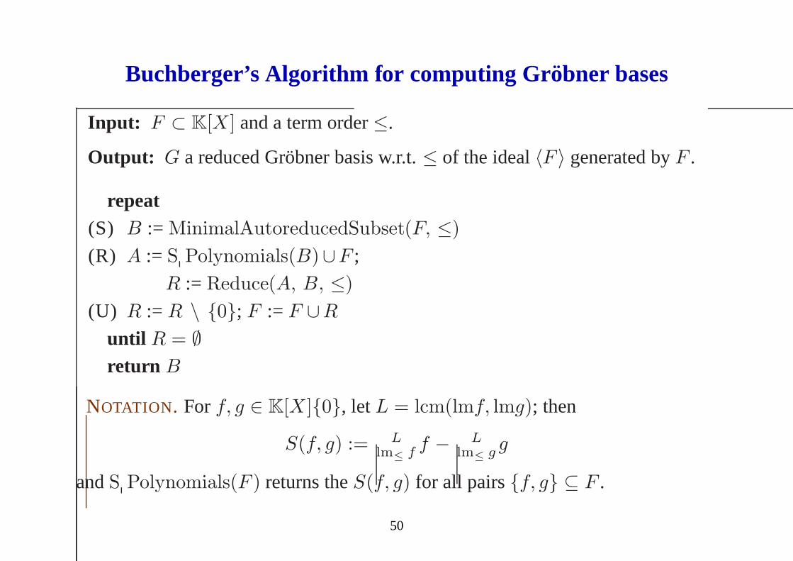
Buchberger’s Algorithm for computing Gr obner bases
Input: F ⊂ K[X ] and a term order≤.
Output: G a reduced Grobner basis w.r.t.≤ of the ideal〈F 〉 generated byF .
repeat(S) B := MinimalAutoreducedSubset(F, ≤)
(R) A := S Polynomials(B)∪F ;
R := Reduce(A, B, ≤)
(U) R := R \ {0}; F := F ∪R
until R = ∅
return B
NOTATION. Forf, g ∈ K[X ]{0}, let L = lcm(lmf, lmg); then
S(f, g) := Llm≤ f
f − Llm≤ g
g
andS Polynomials(F ) returns theS(f, g) for all pairs{f, g} ⊆ F .
50

A recursive vision of polynomials
DEFINITION. Let f, g ∈ K[X ] with g 6∈ K.
mvar(g): the greatest variable ing is theleader or main variable of g,
init(g): the leading coefficient ofg w.r.t. mvar(g) is theinitial of g,
mdeg(g): the degree ofg w.r.t. mvar(g),
rank(g) = vd wherev = mvar(g) andd = mdeg(g),
pdivide(f, g) = (q, r) with q, r ∈ K[X ], deg(r, vg) < dg andhegf = qg + r
wherehg = init(g), e = max(deg(f, v) − dg + 1, 0), vg = mvar(g) anddg = mdeg(g),
prem(f, g) = r if pdivide(f, g) = (q, r). f ∈ K[X ] is said(pseudo-)reducedw.r.t. g ∈ K[X ] 6∈ K if deg(f, mvar(g)) < mdeg(g).
EXAMPLE .
Assumen ≥ 3. If p = x1x23 − 2x2x3 + 1, then we have mvar(p) = x3,
mdeg(p) = 2, init(p) = x1 and rank(p) = x23.
51

Triangular sets and auto-reduced sets
DEFINITION. A finite subsetB ⊂ K[X ] \ K is
- a triangular set if for all f, g ∈ B we havef 6= g ⇒ mvar(f) 6= mvar(g),
- auto-(pseudo-)reduced if all b ∈ B is pseudo-reduced w.r.t.B \ {b}.
PROPOSITION. Every auto-reduced set is finite and is a triangular set.
NOTATION. Let f ∈ K[X ] andB ⊂ K[X ] \K an auto-reduced set. IfB = ∅ we
write prem(f, B) = f . Otherwise letb ∈ B with largest main variable; we write
prem(f, B) = prem(prem(f, b), B \ {b}). ForA ⊂ K[X ] write
prem(A, B) = {prem(a, B) | a ∈ A}.
EXAMPLE . For instance, withT4 = {x1(x1 − 1), x1x2 − 1} and
p = x22 + x1x2 + x2
1, we have
prem(p, T ) = prem(prem(p, Tx2), Tx1) = prem(x41 + x2
1 + 1, Tx1) = 2 x1 + 1.
where Tx1 = x1(x1 − 1) and Tx2 = x1x2 − 1.
52
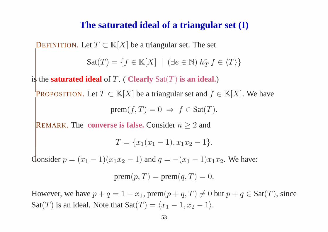
The saturated ideal of a triangular set (I)
DEFINITION. Let T ⊂ K[X ] be a triangular set. The set
Sat(T ) = {f ∈ K[X ] | (∃e ∈ N) heT f ∈ 〈T 〉}
is thesaturated idealof T . ( Clearly Sat(T ) is an ideal.)
PROPOSITION. Let T ⊂ K[X ] be a triangular set andf ∈ K[X ]. We have
prem(f, T ) = 0 ⇒ f ∈ Sat(T ).
REMARK . The converse is false.Considern ≥ 2 and
T = {x1(x1 − 1), x1x2 − 1}.
Considerp = (x1 − 1)(x1x2 − 1) andq = −(x1 − 1)x1x2. We have:
prem(p, T ) = prem(q, T ) = 0.
However, we havep + q = 1 − x1, prem(p + q, T ) 6= 0 butp + q ∈ Sat(T ), since
Sat(T ) is an ideal. Note that Sat(T ) = 〈x1 − 1, x2 − 1〉.
53

The saturated ideal of a triangular set (II)
• Consider again forx > y > a > b > c > d > e > f > g > h > i
F =
8
>
>
<
>
>
:
ax + by − c
dx + ey − f
gx + hy − i
and T =
8
>
>
<
>
>
:
gx + hy − i
(hd − eg) y − id + fg
(ie − fh) a + (ch − ib) d + (fb − ce) g
• Using Grobner basis computations, one can check the following assertions for
this example:
- Sat(T ) = 〈F 〉.
- Sat(T ) is an ideal stricly larger than〈T 〉.
- In fact 〈T 〉 ⊂ Sat(T ) ∩ 〈g, h, i〉,
- and none of Sat(T ) or 〈g, h, i〉 contains the other.
54

Relations between Grobner bases and regular chains
(P) =
8
>
>
<
>
>
:
ax + by − c
dx + ey − f
gx + hy − i
and T =
8
>
>
<
>
>
:
gx + hy − i
(hd − eg) y − id + fg
(ie − fh) a + (ch − ib) d + (fb − ce) g
V(P) = W(T) ∪ W
8
>
>
>
>
>
<
>
>
>
>
>
:
dx + ey − f
hy − i
(ie − fh) a + (−ib + ch) d
g
∪ W
8
>
>
>
>
>
<
>
>
>
>
>
:
gx + hy − i
(ha − bg) y − ia + cg
hd − eg
ie − fh
∪W
8
>
>
>
>
>
<
>
>
>
>
>
:
x
(hd − eg) y − id + fg
fb − ce
ie − fh
∪ W
8
>
>
>
>
>
>
>
<
>
>
>
>
>
>
>
:
ax + by − c
hy − i
d
g
ie − fh
∪ · · ·
Lex base (P):8
>
>
>
<
>
>
>
:
xa + yb − c xd + ye − f xg + yh − i
yae − ydb − af + dc yah − ygb − ai + gc ydh − yge − di + gf
aei − ahf − dbi + dhc + gbf − gec
• For more details see(Aubry, Lazard & M 3 , 1997).
55
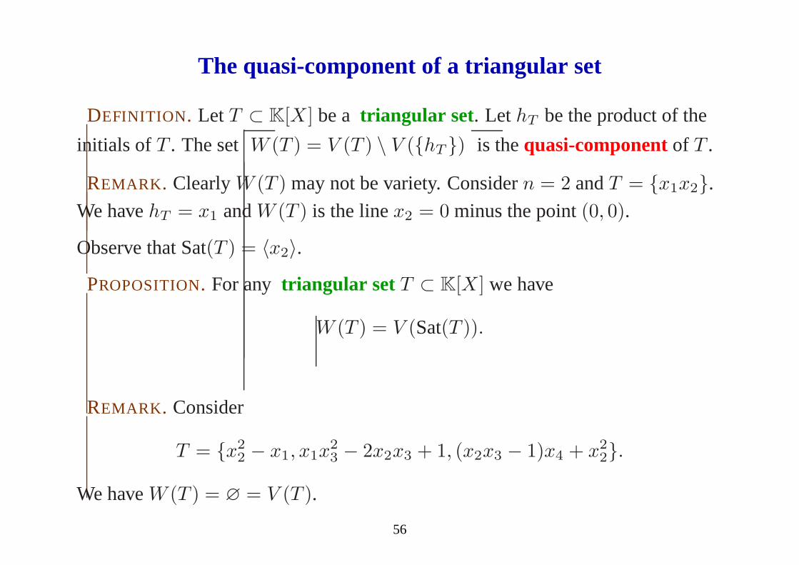
The quasi-component of a triangular set
DEFINITION. Let T ⊂ K[X ] be a triangular set. Let hT be the product of the
initials of T . The set W (T ) = V (T ) \ V ({hT }) is thequasi-componentof T .
REMARK . ClearlyW (T ) may not be variety. Considern = 2 andT = {x1x2}.
We havehT = x1 andW (T ) is the linex2 = 0 minus the point(0, 0).
Observe that Sat(T ) = 〈x2〉.
PROPOSITION. For any triangular set T ⊂ K[X ] we have
W (T ) = V (Sat(T )).
REMARK . Consider
T = {x22 − x1, x1x
23 − 2x2x3 + 1, (x2x3 − 1)x4 + x2
2}.
We haveW (T ) = ∅ = V (T ).
56

Characteristic sets (I)
NOTATION. If f, g 6∈ K, we write rank(f) < rank(g) if mvar(f) < mvar(g) or,
mvar(f) = mvar(g) and mdeg(f) < mdeg(g). ForF ⊂ K[X ] \ K, we write
rank(F ) = {rank(f) | f ∈ F}.
DEFINITION. ForA, B auto-reduced sets, we writeA ≤ B whenever
[rank(B) ⊆ rank(A)] or [min(rank(A) \ rank(B)) < min(rank(B) \ rank(A))].
DEFINITION. For an idealI ⊂ K[X ], a minimal auto-pseudo-reduced subset
B ⊂ I is called aRitt (or Kolchin) characteristic set of I.
PROPOSITION. Every idealI ⊂ K[X ] admits aRitt characteristic set; an
auto-reducedB ⊂ I is a Ritt characteristic set ofI iff prem(f, B) = 0 for all
f ∈ I.
57

Characteristic sets (II)
DEFINITION. For a setF ⊂ K[X ], an auto-pseudo-reduced subsetB ⊆ F suchthat prem(F, B) ⊂ K is called aWu characteristic setof F .
PROPOSITION. If B ⊆ F is a Wu characteristic setof F ⊂ K[X ], then
• If prem(F, B) contains a non-zero constant thenV (F ) = ∅,
• If prem(F, B) = {0} then
V (F ) = W (B) ∪⋃
b∈B
V (F ∪ {init(b)}).
PROOF⊲ Indeed, prem(f, B) = 0 implies that there exists a producth of theinitials of B such thathf ∈ 〈B〉. HenceW (B) ⊆ V (F ). Thus anyζ ∈ V (F )
either belongs toW (B) or cancels one of the initials ofB. ⊳
THEOREM. (Wu, 1987)For anyF ⊂ K[X ], one can compute finitely manytriangular setsT 1, . . . , T s such that
V (F ) = W (T 1) ∪ · · · ∪ W (T s).
58

Wu’s Method
Input: F ⊂ K[X ] and a variable ordering≤.
Output: C a Wu characteristic set ofF .
repeat(S) B := MinimalAutoreducedSubset(F, ≤)
(R) A := F \ B;
R := prem(A, B)
(U) R := R \ {0}; F := F ∪R
until R = ∅
return B
• Repeated calls to this procedure computes a decomposition of V (F ).
• Cannot detect whether a quasi-component is empty.
⇒ This leads to the theory ofregular chains. (Kalkbrener, 1991) and(Yang &Zhang, 1991).
59

Regular chains
DEFINITION. Let I be a proper ideal ofK[X ]. We say that a polynomial
p ∈ K[X ] is regular moduloI if for every prime idealP associated withI we
havep 6∈ P, equivalently, this means thatp is neither null moduloI, nor a
zero-divisor moduloI.
DEFINITION. Let T = {T1, . . . , Ts} be a triangular set where polynomials are
sorted by increasing main variables.
The triangular setT is aregular chain if for all i = 2 · · · s the initial ofTi is
regular modulo the saturated idealof T1, . . . Ti−1.
PROPOSITION. If T is a regular chain then Sat(T ) is a proper ideal ofK[X ] and,
thus,W (T ) 6= ∅.
60
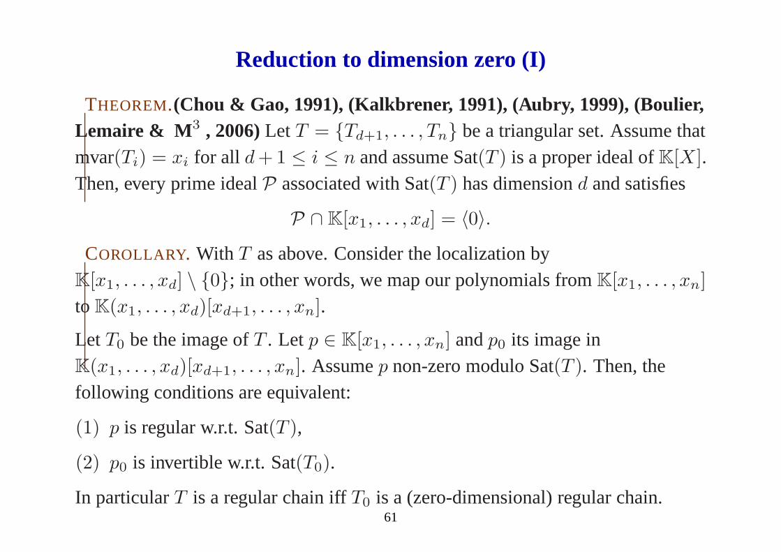
Reduction to dimension zero (I)
THEOREM.(Chou & Gao, 1991), (Kalkbrener, 1991), (Aubry, 1999), (Boulier,Lemaire & M 3 , 2006)Let T = {Td+1, . . . , Tn} be a triangular set. Assume thatmvar(Ti) = xi for all d + 1 ≤ i ≤ n and assume Sat(T ) is a proper ideal ofK[X ].Then, every prime idealP associated with Sat(T ) has dimensiond and satisfies
P ∩ K[x1, . . . , xd] = 〈0〉.
COROLLARY. With T as above. Consider the localization byK[x1, . . . , xd] \ {0}; in other words, we map our polynomials fromK[x1, . . . , xn]
to K(x1, . . . , xd)[xd+1, . . . , xn].
Let T0 be the image ofT . Let p ∈ K[x1, . . . , xn] andp0 its image inK(x1, . . . , xd)[xd+1, . . . , xn]. Assumep non-zero modulo Sat(T ). Then, thefollowing conditions are equivalent:
(1) p is regular w.r.t. Sat(T ),
(2) p0 is invertible w.r.t. Sat(T0).
In particularT is a regular chain iffT0 is a (zero-dimensional) regular chain.61

Reduction to dimension zero (II)
REMARK . Consequently, we can generalize to positive dimension our
computations ofpolynomial GCDsdefined previously over zero-dimensional
regular chains. (Indeed, It is also possible to relax the condition Sat(T0) radical.)
NOTATION. Let T is a regular chain andF ⊂ K[X ] be a polynomial set. We
denote byZ(F, T ) the intersectionV (F )∩W (T ), that is the set of the zeros ofF
that are contained in the quasi-componentW (T ). If F = {p}, we writeZ(p, T )
for Z(F, T ).
PROPOSITION. Let T be a regular chain. Ifp is regular modulo Sat(T ), then
Z(p, T ) is either empty or it is contained in a variety of dimension strictly less
than the dimension ofW (T ).
62

Regular chains and characteristic sets
THEOREM.(Aubry, Lazard & M 3 , 1997)Let C ⊂ K[X ] be an
auto-(pseudo-)reduced set. Then, we have
Sat(C) = {p | prem(p, C) = 0}
m
C regular chain
m
C characteristic set of Sat(C)
63

Incremental triangular decompositions: a geometrical approach
{
x2 + y + z = 1
x2 + y + z = 1
x + y2 + z = 1
x2 + y + z = 1
x + y2 + z = 1
x + y + z2 = 1
64
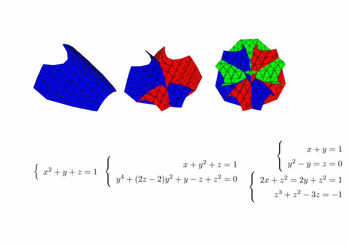
{
x2 + y + z = 1
x + y2 + z = 1
y4 + (2z − 2)y2 + y − z + z2 = 0
x + y = 1
y2 − y = z = 0
2x + z2 = 2y + z2 = 1
z3 + z2 − 3z = −1

Triade: a task manager algorithm (I)
DEFINITION. A task is any[F, T ] whereF, T ⊂ K[X ] with T regular chain. Itis solvediff F = ∅ andunsolved, otherwise.
By solvinga task, we mean computing regular chainsT1, . . . , Tℓ such that:
V (F ) ∩ W (T ) ⊆ ∪ℓi=1W (Ti) ⊆ V (F ) ∩ W (T ).
DEFINITION. The tasks[F1, T1], . . . , [Fd, Td] form adelayed splitof the task[F, T ] and we write[F, T ] 7−→D [F1, T1], . . . , [Fd, Td] if we have:
(D1) Z(Fi, Ti)≺Z(F, T ),
(D2) Z(F, T ) ⊆ Z(F1, T1) ∪ · · · ∪ Z(Fd, Td),
(D3) Sat(T ) ⊆ Sat(Ti),
(D4) Fi 6= ∅ =⇒ F ⊆ Fi,
(D5) Fi = ∅ =⇒ W (Ti) ⊆ V (F ).
66

Triade: a task manager algorithm (II)
REMARK . Property(D1) means that each “output” task[Fi, Ti] is more solvedthan the “input” one[F, T ]. Properties(D2) to (D5) imply:
V (F ) ∩ W (T ) ⊆ ∪di=1Z(Fi, Ti) ⊆ V (F ) ∩ W (T ).
Input: F ⊂ K[X ] and a variable ordering≤.
Output: T a triangular decomposition ofV (F ) by means of regular chains.
ToDo := [[F, ∅]; T := [ ]
repeatif ToDo = ∅ then break
(S) Tasks := Select(ToDo)
(R) Results := LazySolve(Tasks)
(U) (ToDo, T ) := Update(Results, ToDo, T )
return T
67
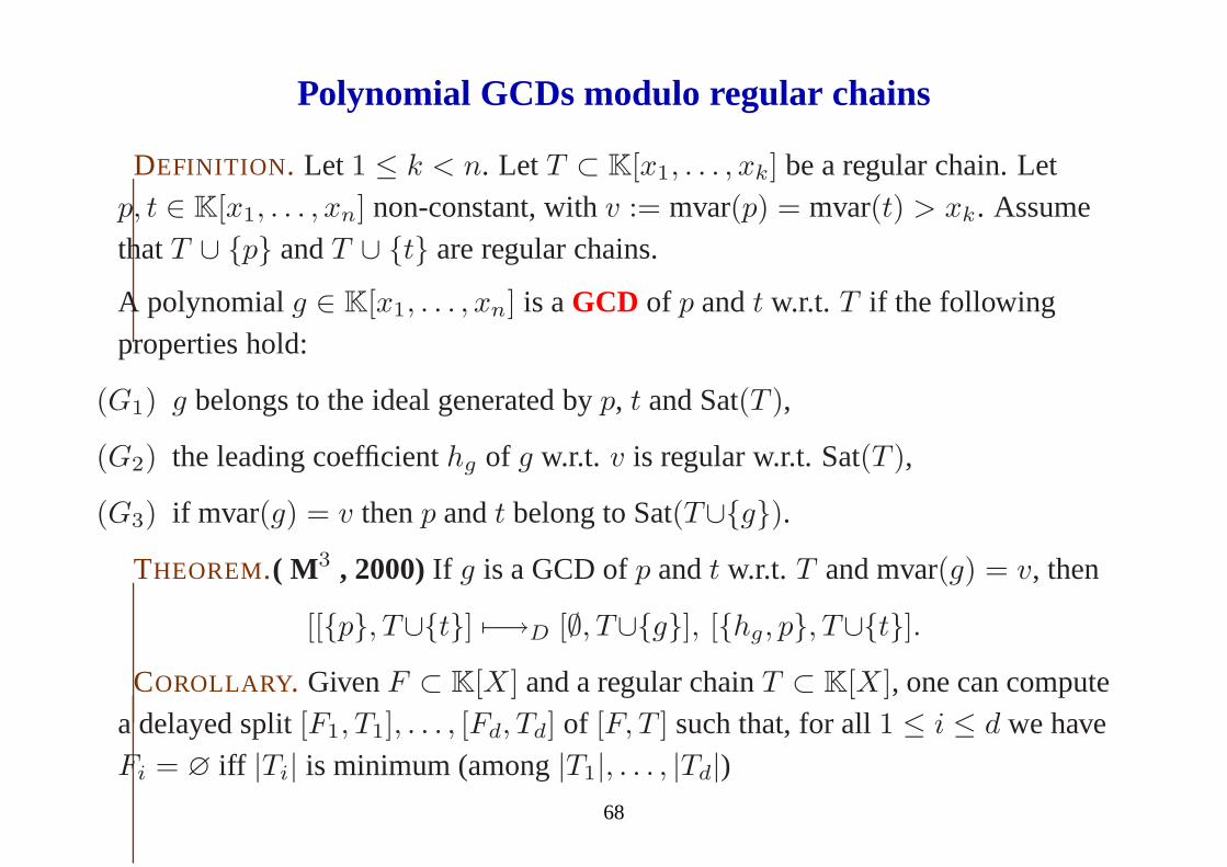
Polynomial GCDs modulo regular chains
DEFINITION. Let 1 ≤ k < n. Let T ⊂ K[x1, . . . , xk] be a regular chain. Letp, t ∈ K[x1, . . . , xn] non-constant, withv := mvar(p) = mvar(t) > xk. AssumethatT ∪ {p} andT ∪ {t} are regular chains.
A polynomialg ∈ K[x1, . . . , xn] is aGCD of p andt w.r.t. T if the followingproperties hold:
(G1) g belongs to the ideal generated byp, t and Sat(T ),
(G2) the leading coefficienthg of g w.r.t. v is regular w.r.t. Sat(T ),
(G3) if mvar(g) = v thenp andt belong to Sat(T∪{g}).
THEOREM.( M3 , 2000)If g is a GCD ofp andt w.r.t. T and mvar(g) = v, then
[[{p}, T∪{t}] 7−→D [∅, T∪{g}], [{hg, p}, T∪{t}].
COROLLARY. GivenF ⊂ K[X ] and a regular chainT ⊂ K[X ], one can computea delayed split[F1, T1], . . . , [Fd, Td] of [F, T ] such that, for all1 ≤ i ≤ d we haveFi = ∅ iff |Ti| is minimum (among|T1|, . . . , |Td|)
68
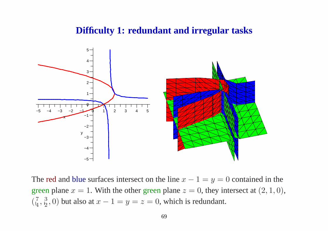
Difficulty 1: redundant and irregular tasks
x
4
4
2
2
−2−4
0
y
5
5
31
3
0−1−3
1
−5−1
−2
−3
−4
−5
Theredandbluesurfaces intersect on the linex − 1 = y = 0 contained in thegreenplanex = 1. With the othergreenplanez = 0, they intersect at(2, 1, 0),( 74 , 3
2 , 0) but also atx − 1 = y = z = 0, which is redundant.
69
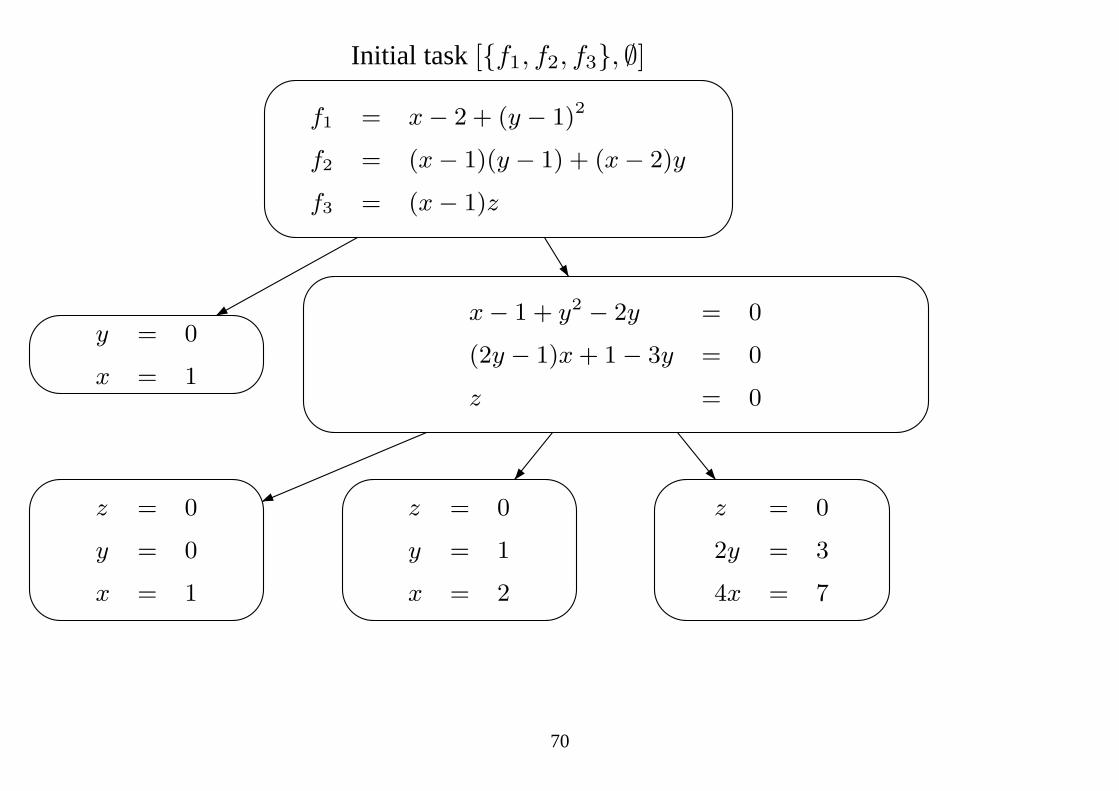
Initial task[{f1, f2, f3}, ∅]
f1 = x − 2 + (y − 1)2
f2 = (x − 1)(y − 1) + (x − 2)y
f3 = (x − 1)z
y = 0
x = 1
x − 1 + y2 − 2y = 0
(2y − 1)x + 1 − 3y = 0
z = 0
z = 0
y = 0
x = 1
z = 0
y = 1
x = 2
z = 0
2y = 3
4x = 7
70

Difficulty 2: load balancing
• How do splits occur during decompositions? Gien a polynomial idealI and
polynomialsp, a, b, there are two rules:
• I 7−→ (I + p, I : p∞).
• I + 〈a b〉 7−→ (I + 〈a〉, I + 〈b〉).
• The second one is more likely tosplit computations evenly. But geometrically,
it means that a component isreducible.
• Unfortunately, most polynomial systemsF ⊆ Q[X ] (both in theory and
practice) areequiprojectable, that is they can be represented by a single regular
chain.
• However, forF ⊆ Z/pZ[X ] wherep prime, the second rule is more likely to be
used.
71

Key solutions
• We solve completelyonly in the cases where dimension does not drop andsolve
lazily the other cases.
⇒ Computations in lower dimension are delayed toward the endof the
solving process.
• For solvingF ⊆ Q[X ] we usemodular methods(Dahan, M3 , Schost, Wu, Xie,
2005)
- Forp big enough, a triangular decomposition ofV (F ) can bereconstructed(= merged + lifted) from one ofV (F mod p).
- Thereconstructionis cheap (comparing to the decomposition phasis).
- This modular approach consumes less resources than the direct one.
72
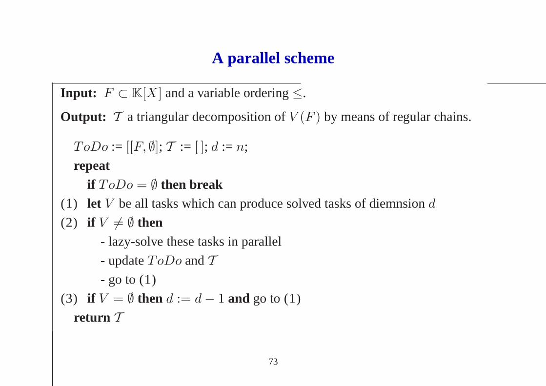
A parallel scheme
Input: F ⊂ K[X ] and a variable ordering≤.
Output: T a triangular decomposition ofV (F ) by means of regular chains.
ToDo := [[F, ∅]; T := [ ]; d := n;
repeatif ToDo = ∅ then break
(1) let V be all tasks which can produce solved tasks of diemnsiond
(2) if V 6= ∅ then- lazy-solve these tasks in parallel
- updateToDo andT
- go to (1)
(3) if V = ∅ then d := d − 1 and go to (1)
return T
73
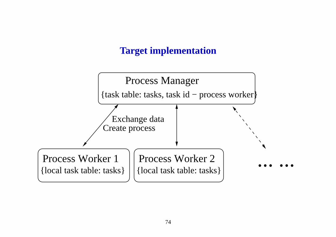
Target implementation
Process Manager{task table: tasks, task id − process worker}
Process Worker 2{local task table: tasks}
Process Worker 1{local task table: tasks}
... ...
Create processExchange data
74

Current implementation
• In ALDOR on a 4-processor machine using shared memory for
data-communication.
• Only the output components are generated by decreasing order of dimension.
(This does not hold yet for the intermediate components)
⇒ Hence, we do not implement yet the above parallel scheme, butonly an
approximation of it.
• Splitting (of the 2nd kind) relies only on theD5 Principleand univariate
polynomial factorization.
• EachLazySolverequires to activate a process worker, which terminates after
completing this computation.
⇒ Hence, we pay a severe penalty in data-communication and O/Scalls w.r.t. our
target implementation (work in progress).
75

Preliminay results
0
1
2
3
4
5
6
7
8
9
0 50 100 150 200 250
[Num
ber
of W
orke
rs]
Uteshev-Bikker: Time [s]
Number of Workers vs Time [s]Average
76

0
2
4
6
8
10
12
14
16
0 20 40 60 80 100 120 140 160 180
[Num
ber
of W
orke
rs]
gametwo5: Time [s]
Number of Workers vs Time [s]Average
77
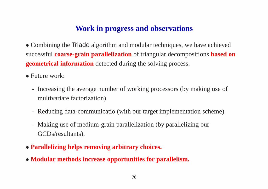
Work in progress and observations
• Combining theTriade algorithm and modular techniques, we have achieved
successfulcoarse-grain parallelizationof triangular decompositionsbased ongeometrical information detected during the solving process.
• Future work:
- Increasing the average number of working processors (by making use of
multivariate factorization)
- Reducing data-communicatio (with our target implementation scheme).
- Making use of medium-grain parallelization (by parallelizing our
GCDs/resultants).
• Parallelizing helps removing arbitrary choices.
• Modular methods increase opportunities for parallelism.
78

Implementation issues
• Fast algorithms for low-level subroutines
THEOREM. (Dahan, M3 , Schost & Xie, 2005)Let T ⊂ K[X ] be a Lazard
triangular set, with〈T 〉 radical and#|V (T )| = δ. DefineL = K[X ]/〈T 〉 There
existsG > 0, and for anyε > 0, there existsAε > 0, such that one can compute a
gcd of polynomials inL[y], with degree at mostd, usingGAnε d1+ε δ1+ε
operations inK.
See also(Pascal & Schost, 2006).
• Implementation techniques for fast polynomial arithmeticalgorithms in
high-level programming languages(Filatei, Li, M 3 , Schost, 2006).
79

Topics I did not have time to discuss
• Solving in the senses of Kalkbrener and Lazard.
• Complexity issues.( A. Szanto, 1997).
• Symbolic-numeric computations( M3 , Reid, Scott & Wu, 2005).
• and many other things.
80
Related Documents


![Tensor Decompositions and Applications · 2018-09-11 · TENSOR DECOMPOSITIONS AND APPLICATIONS 457 (CP) [38, 90] and Tucker [226] tensor decompositions can be considered to be higher-order](https://static.cupdf.com/doc/110x72/5f02faff7e708231d406f3cd/tensor-decompositions-and-applications-2018-09-11-tensor-decompositions-and-applications.jpg)

