Polynomial Matrix Decompositions Stephan Weiss Centre for Signal & Image Processing Department of Electonic & Electrical Engineering University of Strathclyde, Glasgow, Scotland, UK F¨ orderverein, Alpen-Adria Universit¨ at Klagenfurt, 25. April 2016 With many thanks to: J.G. McWhirter, I.K. Proudler, J. Corr and F.K. Coutts This work was supported by QinetiQ, the Engineering and Physical Sciences Research Council (EPSRC) Grant number EP/K014307/1 and the MOD University Defence Re- search Collaboration in Signal Processing. 1 / 74

Welcome message from author
This document is posted to help you gain knowledge. Please leave a comment to let me know what you think about it! Share it to your friends and learn new things together.
Transcript
Polynomial Matrix Decompositions
Stephan Weiss
Centre for Signal & Image ProcessingDepartment of Electonic & Electrical EngineeringUniversity of Strathclyde, Glasgow, Scotland, UK
Forderverein, Alpen-Adria Universitat Klagenfurt, 25. April 2016
With many thanks to:J.G. McWhirter, I.K. Proudler, J. Corr and F.K. Coutts
This work was supported by QinetiQ, the Engineering and Physical Sciences Research
Council (EPSRC) Grant number EP/K014307/1 and the MOD University Defence Re-
search Collaboration in Signal Processing.
1 / 74

Overview PART I Basics PEVD Iter. Toolbox PART II MIMO AoA MVDR Material
Presentation Overview1. Overview
Part I: Polynomial Matrices and Decompositions2. Polynomial matrices and basic operations
2.1 occurence: MIMO systems, filter banks, space-time covariance2.2 basic properties and operations
3. Polynomial eigenvalue decomposition (PEVD)4. Iterative PEVD algorithms
4.1 sequential best rotation (SBR2)4.2 sequential matrix diagonalisation (SMD)
5. PEVD Matlab toolbox
Part II: Beamforming & Source Separation Applications
6. Broadband MIMO decoupling7. Broadband angle of arrival estimation
7.1 broadband / polynomial subspace decomposition7.2 polynomial MUSIC
8. Broadband beamforming9. Summary and materials
2 / 74
Overview PART I Basics PEVD Iter. Toolbox PART II MIMO AoA MVDR Material
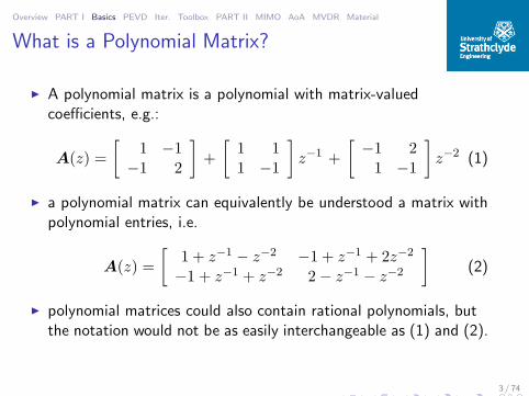
What is a Polynomial Matrix?
A polynomial matrix is a polynomial with matrix-valuedcoefficients, e.g.:
A(z) =
[1 −1
−1 2
]
+
[1 11 −1
]
z−1 +
[−1 21 −1
]
z−2 (1)
a polynomial matrix can equivalently be understood a matrix withpolynomial entries, i.e.
A(z) =
[1 + z−1 − z−2 −1 + z−1 + 2z−2
−1 + z−1 + z−2 2− z−1 − z−2
]
(2)
polynomial matrices could also contain rational polynomials, butthe notation would not be as easily interchangeable as (1) and (2).
3 / 74

Overview PART I Basics PEVD Iter. Toolbox PART II MIMO AoA MVDR Material
Where Do Polynomial Matrices Arise?
A multiple-input multiple-output (MIMO) system could be madeup of a number of finite impulse response (FIR) channels:
+h11[n]
h21[n]
h12[n]
h22[n] +
y1[n]
y2[n]
x1[n]
x2[n]
writing this as a matrix of impulse responses:
H[n] =
[h11[n] h12[n]
h21[n] h22[n]
]
(3)
4 / 74

Overview PART I Basics PEVD Iter. Toolbox PART II MIMO AoA MVDR Material
Transfer Function of a MIMO System Example for MIMO matrix H[n] of impulse responses:
0 1 2 3 4
−0.5
0
0.5
1
h11[n]
0 1 2 3 4
−0.5
0
0.5
1
h12[n]
0 1 2 3 4
−0.5
0
0.5
1
h21[n]
discrete time index n0 1 2 3 4
−0.5
0
0.5
1
h22[n]
discrete time index n
the transfer function of this MIMO system is a polynomial matrix:
H(z) =∞∑
n=−∞
H[n]z−1 or H(z) •— H[n] (4)
5 / 74

Overview PART I Basics PEVD Iter. Toolbox PART II MIMO AoA MVDR Material
Analysis Filter Bank Critically decimated K-channel analysis filter bank:
H1(z)
H2(z)
HK(z)
↓K
↓K
...
↓K
equivalent polyphase representation:
z−1
z−1
↓K
↓K
↓K
H1,1(z) . . . H1,K(z)H2,1(z) . . . H2,K(z)
......
HK,1(z) . . . HK,K(z)
H(z) =
6 / 74

Overview PART I Basics PEVD Iter. Toolbox PART II MIMO AoA MVDR Material
Polyphase Analysis Matrix
With the K-fold polyphase decomposition of the analysis filters
Hk(z) =
K∑
n=1
Hk,n(zK)z−n+1 (5)
hk[n]
n
K = 4
the polyphase analysis matrix is a polynomial matrix:
H(z) =
H1,1(z) H1,2(z) . . . H1,K(z)H2,1(z) H2,2(z) . . . H2,K(z)
......
. . ....
HK,1(z) HK,2(z) . . . HK,K(z)
(6)
7 / 74

Overview PART I Basics PEVD Iter. Toolbox PART II MIMO AoA MVDR Material
Synthesis Filter Bank
Critically decimated K-channel synthesis filter bank:
↑K
↑K
↑K
G1(z)
G2(z)
GK(z)
...
+
+
equivalent polyphase representation:
G1,1(z) . . . G1,K(z)G2,1(z) . . . G2,K(z)
......
GK,1(z) . . . GK,K(z)
G(z) =
...
+
+
z−1
z−1
↑K
↑K
↑K
8 / 74

Overview PART I Basics PEVD Iter. Toolbox PART II MIMO AoA MVDR Material
Polyphase Synthesis Matrix
Analoguous to analysis filter bank, the synthesis filters Gk(z) canbe split into K polyphase components, creating a polyphsesynthesis matrix
G(z) =
G1,1(z) G1,2(z) . . . G1,K(z)G2,1(z) G2,2(z) . . . G2,K(z)
......
. . ....
GK,1(z) GK,2(z) . . . GK,K(z)
(7)
operating analysis and synthesis back-to-back, perfectreconstruction is achieved if
G(z)H(z) = I ; (8)
i.e. for perfect reconstruction, the polyphase analysis matrix mustbe invertible: G(z) = H−1(z).
9 / 74

Overview PART I Basics PEVD Iter. Toolbox PART II MIMO AoA MVDR Material
Space-Time Covariance Matrix
Measurements obtained from M sensors are collected in avector x[n] ∈ C
M :
xT[n] = [x1[n] x2[n] . . . xM [n]] ; (9)
with the expectation operator E·, the spatial correlation iscaptured by R = E
x[n]xH[n]
;
for spatial and temporal correlation, we require a space-timecovariance matrix
R[τ ] = Ex[n]xH[n− τ ]
(10)
this space-time covariance matrix contains auto- andcross-correlation terms, e.g. for M = 2
R[τ ] =
[Ex1[n]x
∗1[n− τ ] Ex1[n]x
∗2[n− τ ]
Ex2[n]x∗1[n− τ ] Ex2[n]x
∗2[n− τ ]
]
(11)
10 / 74

Overview PART I Basics PEVD Iter. Toolbox PART II MIMO AoA MVDR Material
Cross-Spectral Density Matrix example for a space-time covariance matrix R[τ ] ∈ R
2×2:
−2 −1 0 1 2−0.5
0
0.5
1
r x1x1[τ]
−2 −1 0 1 2−0.5
0
0.5
1
r x1x2[n]
−2 −1 0 1 2−0.5
0
0.5
1
r x2x1[n]
lag τ
−2 −1 0 1 2−0.5
0
0.5
1
r x2x2[n]
lag τ
the cross-spectral density (CSD) matrix
R(z) —• R[τ ] (12)
is a polynomial matrix.11 / 74

Overview PART I Basics PEVD Iter. Toolbox PART II MIMO AoA MVDR Material
Parahermitian Operator
A parahermitian operation is indicated by ·, and compared tothe Hermitian (= complex conjugate transpose) of a matrixadditionally performs a time-reversal;
example:
A(z) =
0 1 2 3 4
−0.5
0
0.5
1
0 1 2 3 4
−0.5
0
0.5
1
0 1 2 3 4
−0.5
0
0.5
1
0 1 2 3 4
−0.5
0
0.5
1
parahermitian A(z) = AH(z−1):
A(z) =
−4 −3 −2 −1 0
−0.5
0
0.5
1
−4 −3 −2 −1 0
−0.5
0
0.5
1
−4 −3 −2 −1 0
−0.5
0
0.5
1
−4 −3 −2 −1 0
−0.5
0
0.5
1
12 / 74
Overview PART I Basics PEVD Iter. Toolbox PART II MIMO AoA MVDR Material
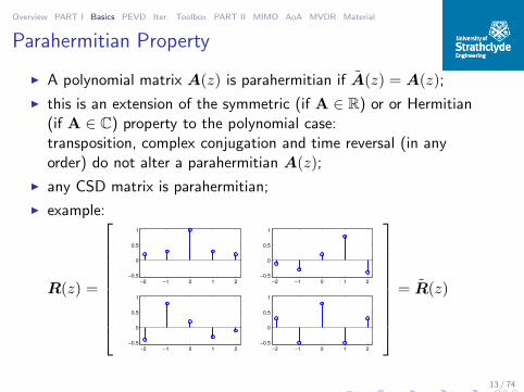
Parahermitian Property
A polynomial matrix A(z) is parahermitian if A(z) = A(z);
this is an extension of the symmetric (if A ∈ R) or or Hermitian(if A ∈ C) property to the polynomial case:transposition, complex conjugation and time reversal (in anyorder) do not alter a parahermitian A(z);
any CSD matrix is parahermitian;
example:
R(z) =
−2 −1 0 1 2−0.5
0
0.5
1
−2 −1 0 1 2−0.5
0
0.5
1
−2 −1 0 1 2−0.5
0
0.5
1
−2 −1 0 1 2−0.5
0
0.5
1
= R(z)
13 / 74

Overview PART I Basics PEVD Iter. Toolbox PART II MIMO AoA MVDR Material
Paraunitary Matrices
Recall that A ∈ C (or A ∈ R) is a unitary (or orthonormal)matrix if AAH = AHA = I;
in the polynomial case, A(z) is paraunitary if
A(z)A(z) = A(z)A(z) = I (13)
therefore, if A(z) is paraunitary, then the polynomial matrixinverse is simple:
A−1(z) = A(z) (14)
example: polyphase analysis or synthesis matrices of perfectlyreconstructing (or lossless) filter banks are usually paraunitary.
14 / 74

Overview PART I Basics PEVD Iter. Toolbox PART II MIMO AoA MVDR Material
Attempt of Gaussian Elimination
System of polynomial equations:
[A11(z) A12(z)A21(z) A22(z)
]
·
[X1(z)X2(z)
]
=
[B1(z)B2(z)
]
(15)
modification of 2nd row:[
A11(z) A12(z)
A11(z)A11(z)A21(z)
A22(z)
]
·
[X1(z)X2(z)
]
=
[
B1(z)A11(z)A21(z)
B2(z)
]
(16)
upper triangular form by subtracting 1st row from 2nd:[
A11(z) A12(z)
0 A11(z)A22(z)−A12(z)A21(z)A21(z)
]
·
[X1(z)X2(z)
]
=
[B1(z)B2(z)
]
(17)
penalty: we end up with rational polynomials.
15 / 74

Overview PART I Basics PEVD Iter. Toolbox PART II MIMO AoA MVDR Material
Polynomial Eigenvalue Decomposition[McWhirter et al., IEEE TSP 2007]
Polynomial EVD of the CSD matrix
R(z) ≈ Q(z) Λ(z) Q(z) (18)
with paraunitary Q(z), s.t. Q(z)Q(z) = I;
diagonalised and spectrally majorised Λ(z):
−10 0 100
10
20
30
40
−10 0 100
10
20
30
40
−10 0 100
10
20
30
40
−10 0 100
10
20
30
40
γij[τ]
−10 0 100
10
20
30
40
−10 0 100
10
20
30
40
−10 0 100
10
20
30
40
−10 0 100
10
20
30
40
lat τ−10 0 100
10
20
30
40
0 0.1 0.2 0.3 0.4 0.5 0.6 0.7 0.8 0.9 1−10
−5
0
5
10
15
20
normalised angular frequency Ω/(2π)
10log 1
0|Γ
i|/[dB]
i=1
i=2
i=3
approximation in (18) can be close with an FIR Q(z) ofsufficiently high order [Icart & Comon 2012].
16 / 74

Overview PART I Basics PEVD Iter. Toolbox PART II MIMO AoA MVDR Material
PEVD Ambiguity[Corr et al., EUSIPCO 2015]
We believe diagonalised and spectral majorised Λ(z) is unique; but there is ambiguity w.r.t. the paraunitary matrix Q(z); set Q(z) = Q(z)Γ(z), with a diagonal allpass Γ(z):
R(z) = Q(z)Λ(z) ˜Q(z) = Q(z)Γ(z)Λ(z)Γ(z)Q(z)
= Q(z)Λ(z)Γ(z)Γ(z)Q(z) = Q(z)Λ(z)Q(z) (19)
example for Q(z) — note different orders:
0 10 20 300
0.2
0.4
0.6
0 10 20 300
0.2
0.4
0.6
0 10 20 300
0.2
0.4
0.6
0 10 20 300
0.2
0.4
0.6
0 10 20 300
0.2
0.4
0.6
0 10 20 300
0.2
0.4
0.6
0 10 20 300
0.2
0.4
0.6
0 10 20 300
0.2
0.4
0.6
0 10 20 300
0.2
0.4
0.6
0 10 20 300
0.2
0.4
0.6
0 10 20 300
0.2
0.4
0.6
0 10 20 300
0.2
0.4
0.6
0 10 20 300
0.2
0.4
0.6
0 10 20 300
0.2
0.4
0.6
0 10 20 300
0.2
0.4
0.6
0 10 20 300
0.2
0.4
0.6
0 2 4 60
0.2
0.4
0.6
0 2 4 60
0.2
0.4
0.6
0 2 4 60
0.2
0.4
0.6
0 2 4 60
0.2
0.4
0.6
0 2 4 60
0.2
0.4
0.6
0 2 4 60
0.2
0.4
0.6
0 2 4 60
0.2
0.4
0.6
0 2 4 60
0.2
0.4
0.6
0 2 4 60
0.2
0.4
0.6
0 2 4 60
0.2
0.4
0.6
0 2 4 60
0.2
0.4
0.6
0 2 4 60
0.2
0.4
0.6
0 2 4 60
0.2
0.4
0.6
0 2 4 60
0.2
0.4
0.6
0 2 4 60
0.2
0.4
0.6
0 2 4 60
0.2
0.4
0.6
17 / 74
Overview PART I Basics PEVD Iter. Toolbox PART II MIMO AoA MVDR Material
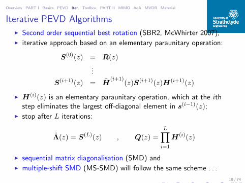
Iterative PEVD Algorithms
Second order sequential best rotation (SBR2, McWhirter 2007);
iterative approach based on an elementary paraunitary operation:
S(0)(z) = R(z)...
S(i+1)(z) = H(i+1)
(z)S(i+1)(z)H(i+1)(z)
H(i)(z) is an elementary paraunitary operation, which at the ithstep eliminates the largest off-diagonal element in s(i−1)(z);
stop after L iterations:
Λ(z) = S(L)(z) , Q(z) =
L∏
i=1
H(i)(z)
sequential matrix diagonalisation (SMD) and
multiple-shift SMD (MS-SMD) will follow the same scheme . . .
18 / 74

Overview PART I Basics PEVD Iter. Toolbox PART II MIMO AoA MVDR Material
Elementary Paraunitary Operation
An elementary paraunitary matrix [Vaidyanathan] is defined as
H(i)(z) = I− v(i)v(i),H + z−1v(i)v(i),H , ‖v(i)‖2 = 1
we utilise a different definition:
H(i)(z) = D(i)(z)Q(i)
D(i)(z) is a delay matrix:
D(i)(z) = diag1 . . . 1 z−τ 1 . . . 1
Q(i)(z) is a Givens rotation.
19 / 74

Overview PART I Basics PEVD Iter. Toolbox PART II MIMO AoA MVDR Material
Sequential Best Rotation Algorithm (McWhirter)
At iteration i, consider S(i−1)(z) —• S(i−1)[τ ]
0
−T
T
20 / 74

Overview PART I Basics PEVD Iter. Toolbox PART II MIMO AoA MVDR Material
Sequential Best Rotation Algorithm (McWhirter)
D(i)(z)S(i−1)(z)D(i)(z)
0
−T
T
·
1.
.
.
z−T
1
1.
.
.
zT
1
·
20 / 74

Overview PART I Basics PEVD Iter. Toolbox PART II MIMO AoA MVDR Material
Sequential Best Rotation Algorithm (McWhirter)
D(i)(z) advances a row-slice of S(i−1)(z) by T
0
−T
T
1.
.
.
zT
1
·
·
1.
.
.
z−T
1
20 / 74
Overview PART I Basics PEVD Iter. Toolbox PART II MIMO AoA MVDR Material
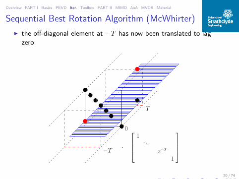
Sequential Best Rotation Algorithm (McWhirter)
the off-diagonal element at −T has now been translated to lagzero
0
·
1.
.
.
z−T
1
T
−T
20 / 74

Overview PART I Basics PEVD Iter. Toolbox PART II MIMO AoA MVDR Material
Sequential Best Rotation Algorithm (McWhirter)
D(i)(z) delays a column-slice of S(i−1)(z) by T
0
·
1.
.
.
z−T
1
T
−T
20 / 74
Overview PART I Basics PEVD Iter. Toolbox PART II MIMO AoA MVDR Material
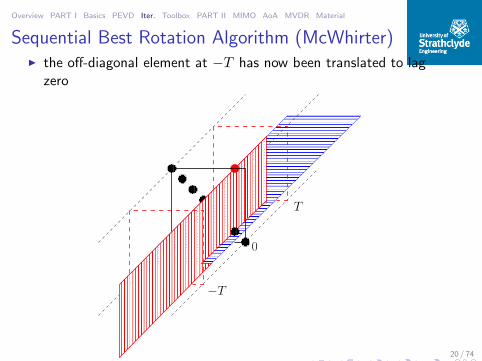
Sequential Best Rotation Algorithm (McWhirter) the off-diagonal element at −T has now been translated to lag
zero
0
T
−T
20 / 74

Overview PART I Basics PEVD Iter. Toolbox PART II MIMO AoA MVDR Material
Sequential Best Rotation Algorithm (McWhirter)
the step D(i)(z)S(i−1)(z)D(i)(z) has brought the largest
off-diagonal elements to lag 0.
0
T
−T
20 / 74

Overview PART I Basics PEVD Iter. Toolbox PART II MIMO AoA MVDR Material
Sequential Best Rotation Algorithm (McWhirter)
Jacobi step to eliminate largest off-diagonal elements by Q(i)
0
·
c −e−jϑs
I
ejϑs c
1
c e−jϑs
I
−ejϑs c
1
·
T
−T
20 / 74

Overview PART I Basics PEVD Iter. Toolbox PART II MIMO AoA MVDR Material
Sequential Best Rotation Algorithm (McWhirter)
iteration i is completed, having performed
S(i)(z) = Q(i)D(i)(z)S(i−1)(z)D(i)(z)Q(i)(z)
0
T
−T
20 / 74

Overview PART I Basics PEVD Iter. Toolbox PART II MIMO AoA MVDR Material
SBR2 Outcome
At the ith iteration, the zeroing of off-diagonal elements achievedduring previous steps may be partially undone;
however, the algorithm has been shown to converge, transferingenergy onto the main diagonal at every step (McWhirter 2007);
after L iterations, we reach an approximate diagonalisation
Λ(z) = S(L)(z) = Q(z)R(z)Q(z)
with
Q(z) =
L∏
i=1
D(i)(z)Q(i)
diagonalisation of the previous 3× 3 polynomial matrix . . .
21 / 74

Overview PART I Basics PEVD Iter. Toolbox PART II MIMO AoA MVDR Material
SBR2 Example — Diagonalisation
−10 0 100
10
20
30
40
−10 0 100
10
20
30
40
−10 0 100
10
20
30
40
−10 0 100
10
20
30
40
γij[τ]
−10 0 100
10
20
30
40
−10 0 100
10
20
30
40
−10 0 100
10
20
30
40
−10 0 100
10
20
30
40
lat τ−10 0 100
10
20
30
40
lag τ 22 / 74
Overview PART I Basics PEVD Iter. Toolbox PART II MIMO AoA MVDR Material
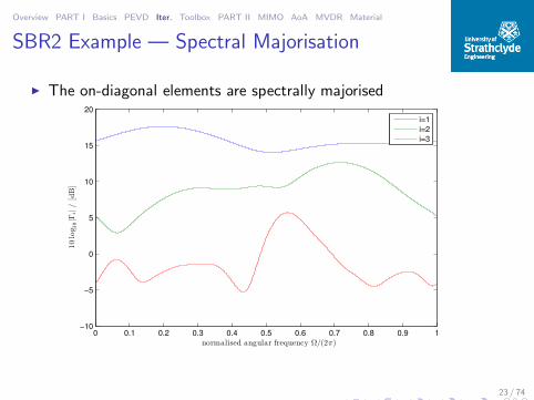
SBR2 Example — Spectral Majorisation
The on-diagonal elements are spectrally majorised
0 0.1 0.2 0.3 0.4 0.5 0.6 0.7 0.8 0.9 1−10
−5
0
5
10
15
20
normalised angular frequency Ω/(2π)
10log 1
0|Γ
i|/[dB]
i=1
i=2
i=3
23 / 74

Overview PART I Basics PEVD Iter. Toolbox PART II MIMO AoA MVDR Material
SBR2 — Givens Rotation
A Givens rotation eliminates the maximum off-diagonal elementonce brought onto the lag-zero matrix;
note I: in the lag-zero matrix, one column and one row aremodified by the shift:
note II: a Givens rotation only affects two columns and two rowsin every matrix;
Givens rotation is relatively low in computational cost!
24 / 74

Overview PART I Basics PEVD Iter. Toolbox PART II MIMO AoA MVDR Material
Sequential Matrix Diagonalisation (SMD)[Redif et al., IEEE Trans SP 2015]
Main idea — the zero-lag matrix is diagonalised in every step; initialisation: diagonalise R[0] by EVD and apply modal matrix to
all matrix coefficients −→ S(0); at the ith step as in SBR2, the maximum element (or column
with max. norm) is shifted to the lag-zero matrix:
an EVD is used to re-diagonalise the zero-lag matrix; a full modal matrix is applied at all lags — more costly than
SBR2. 25 / 74

Overview PART I Basics PEVD Iter. Toolbox PART II MIMO AoA MVDR Material
Sequential Matrix Diagonalisation (SMD)[Redif et al., IEEE Trans SP 2015]
Main idea — the zero-lag matrix is diagonalised in every step; initialisation: diagonalise R[0] by EVD and apply modal matrix to
all matrix coefficients −→ S(0); at the ith step as in SBR2, the maximum element (or column
with max. norm) is shifted to the lag-zero matrix:
−→
an EVD is used to re-diagonalise the zero-lag matrix; a full modal matrix is applied at all lags — more costly than
SBR2. 25 / 74

Overview PART I Basics PEVD Iter. Toolbox PART II MIMO AoA MVDR Material
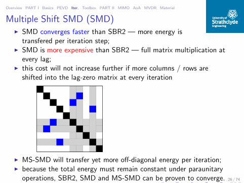
Multiple Shift SMD (SMD) SMD converges faster than SBR2 — more energy is
transfered per iteration step; SMD is more expensive than SBR2 — full matrix multiplication at
every lag; this cost will not increase further if more columns / rows are
shifted into the lag-zero matrix at every iteration
MS-SMD will transfer yet more off-diagonal energy per iteration; because the total energy must remain constant under paraunitary
operations, SBR2, SMD and MS-SMD can be proven to converge. 26 / 74

Overview PART I Basics PEVD Iter. Toolbox PART II MIMO AoA MVDR Material
Multiple Shift SMD (SMD) SMD converges faster than SBR2 — more energy is
transfered per iteration step; SMD is more expensive than SBR2 — full matrix multiplication at
every lag; this cost will not increase further if more columns / rows are
shifted into the lag-zero matrix at every iteration
MS-SMD will transfer yet more off-diagonal energy per iteration; because the total energy must remain constant under paraunitary
operations, SBR2, SMD and MS-SMD can be proven to converge. 26 / 74
Overview PART I Basics PEVD Iter. Toolbox PART II MIMO AoA MVDR Material
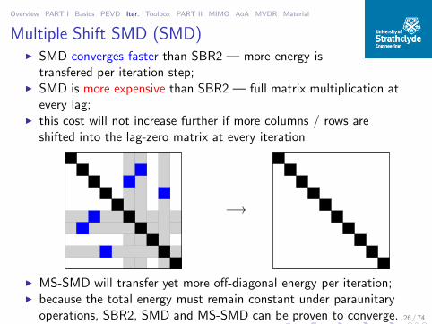
Multiple Shift SMD (SMD) SMD converges faster than SBR2 — more energy is
transfered per iteration step; SMD is more expensive than SBR2 — full matrix multiplication at
every lag; this cost will not increase further if more columns / rows are
shifted into the lag-zero matrix at every iteration
−→
MS-SMD will transfer yet more off-diagonal energy per iteration; because the total energy must remain constant under paraunitary
operations, SBR2, SMD and MS-SMD can be proven to converge. 26 / 74
Overview PART I Basics PEVD Iter. Toolbox PART II MIMO AoA MVDR Material
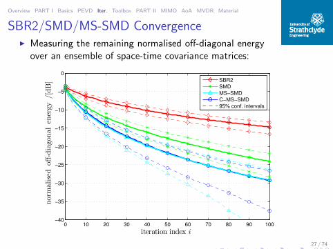
SBR2/SMD/MS-SMD Convergence Measuring the remaining normalised off-diagonal energy
over an ensemble of space-time covariance matrices:
0 10 20 30 40 50 60 70 80 90 100−40
−35
−30
−25
−20
−15
−10
−5
0
iteration index i
normalised o
ff-diago
nal energy
/[dB]
SBR2
SMD
MS−SMD
C−MS−SMD
95% conf. intervals
27 / 74

Overview PART I Basics PEVD Iter. Toolbox PART II MIMO AoA MVDR Material
SBR2/SMD/MS-SMD Application Cost 1 Ensemble average of remaining off-diagonal energy vs. order
of paraunitary filter banks to decompose 4x4x16 matrices:
0 5 10 15 20 25−30
−25
−20
−15
−10
−5
0
paraunitary filter bank order
normalised o
ff-diago
nal energy
/[dB]
SBR2
SMD
MS−SMD
C−MS−SMD
28 / 74

Overview PART I Basics PEVD Iter. Toolbox PART II MIMO AoA MVDR Material
SBR2/SMD/MS-SMD Application Cost 2
Ensemble average of remaining off-diagonal energy vs. orderof paraunitary filter banks to decompose 8x8x64 matrices:
10 15 20 25 30 35 40 45 50 55 60−30
−25
−20
−15
−10
−5
0
paraunitary filter bank order
5log 1
0M
E
(i)
norm/[dB]
SBR2
SBR2C
SMD v2
SMD
29 / 74

Overview PART I Basics PEVD Iter. Toolbox PART II MIMO AoA MVDR Material
MATLAB Polynomial EVD Toolbox The MATLAB polynomial EVD toolbox can be downloaded from
pevd-toolbox.eee.strath.ac.uk
the toolbox contains a number of iterative algorithms to calculatean approximate PEVD, related functions, and demos. 30 / 74

Overview PART I Basics PEVD Iter. Toolbox PART II MIMO AoA MVDR Material
Narrowband MIMO Communications
a narrowband channel is characterised by a matrix C containingcomplex gain factors;
problem: how to select the precoder and equaliser?
C? ?...
.
.
....
.
.
.
overall system;
31 / 74

Overview PART I Basics PEVD Iter. Toolbox PART II MIMO AoA MVDR Material
Narrowband MIMO Communications a narrowband channel is characterised by a matrix C containing
complex gain factors; problem: how to select the precoder and equaliser?
C = UΣVH
VH
Σ U? ?...
.
.
....
.
.
....
.
.
.
the singular value decomposition (SVD) factorises C into twounitary matrices U and VH and a diagonal matrix Σ;
31 / 74

Overview PART I Basics PEVD Iter. Toolbox PART II MIMO AoA MVDR Material
Narrowband MIMO Communications a narrowband channel is characterised by a matrix C containing
complex gain factors; problem: how to select the precoder and equaliser?
C = UΣVH
VH
Σ UV UH.
.
.
.
.
.
.
.
.
.
.
.
.
.
.
.
.
.
we select the precoder and the equaliser from the unitary matricesprovided by the channel’s SVD;
the overall system is diagonalised, decoupling the channel intoindependent single-input single-output systems by means ofunitary matrices. 31 / 74

Overview PART I Basics PEVD Iter. Toolbox PART II MIMO AoA MVDR Material
Broadband MIMO Channel
The channel is now a matrix of FIR filters; example for a 3× 4MIMO system C[n]:
0 1 2 30
1
2
0 1 2 30
1
2
0 1 2 30
1
2
0 1 2 30
1
2
0 1 2 30
1
2
0 1 2 30
1
2
0 1 2 30
1
2
0 1 2 30
1
2
0 1 2 30
1
2
0 1 2 30
1
2
0 1 2 30
1
2
0 1 2 30
1
2
discrete time index n
|ci,j[n]|
the transfer function C(z) •— C[n] is a polynomial matrix;
an SVD can only diagonalise C[n] for one particular lag n.
32 / 74
Overview PART I Basics PEVD Iter. Toolbox PART II MIMO AoA MVDR Material
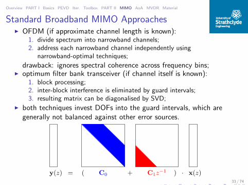
Standard Broadband MIMO Approaches OFDM (if approximate channel length is known):
1. divide spectrum into narrowband channels;2. address each narrowband channel independently using
narrowband-optimal techniques;
drawback: ignores spectral coherence across frequency bins; optimum filter bank transceiver (if channel itself is known):
1. block processing;2. inter-block interference is eliminated by guard intervals;3. resulting matrix can be diagonalised by SVD;
both techniques invest DOFs into the guard intervals, which aregenerally not balanced against other error sources.
C0 C1z−1( +y(z) = ) · x(z)
33 / 74

Overview PART I Basics PEVD Iter. Toolbox PART II MIMO AoA MVDR Material
Standard Broadband MIMO Approaches OFDM (if approximate channel length is known):
1. divide spectrum into narrowband channels;2. address each narrowband channel independently using
narrowband-optimal techniques;
drawback: ignores spectral coherence across frequency bins; optimum filter bank transceiver (if channel itself is known):
1. block processing;2. inter-block interference is eliminated by guard intervals;3. resulting matrix can be diagonalised by SVD;
both techniques invest DOFs into the guard intervals, which aregenerally not balanced against other error sources.
C0 C1z−1( +y(z) = ) · x(z)
33 / 74
Overview PART I Basics PEVD Iter. Toolbox PART II MIMO AoA MVDR Material
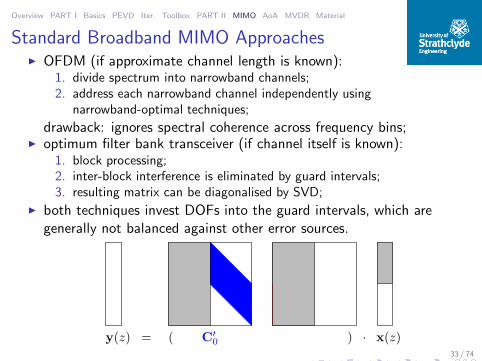
Standard Broadband MIMO Approaches OFDM (if approximate channel length is known):
1. divide spectrum into narrowband channels;2. address each narrowband channel independently using
narrowband-optimal techniques;
drawback: ignores spectral coherence across frequency bins; optimum filter bank transceiver (if channel itself is known):
1. block processing;2. inter-block interference is eliminated by guard intervals;3. resulting matrix can be diagonalised by SVD;
both techniques invest DOFs into the guard intervals, which aregenerally not balanced against other error sources.
C′
0(y(z) = ) · x(z)
33 / 74

Overview PART I Basics PEVD Iter. Toolbox PART II MIMO AoA MVDR Material
Standard Broadband MIMO Approaches OFDM (if approximate channel length is known):
1. divide spectrum into narrowband channels;2. address each narrowband channel independently using
narrowband-optimal techniques;
drawback: ignores spectral coherence across frequency bins; optimum filter bank transceiver (if channel itself is known):
1. block processing;2. inter-block interference is eliminated by guard intervals;3. resulting matrix can be diagonalised by SVD;
both techniques invest DOFs into the guard intervals, which aregenerally not balanced against other error sources.
C0 C1z−1( +y(z) = ) · x(z)
33 / 74

Overview PART I Basics PEVD Iter. Toolbox PART II MIMO AoA MVDR Material
Standard Broadband MIMO Approaches OFDM (if approximate channel length is known):
1. divide spectrum into narrowband channels;2. address each narrowband channel independently using
narrowband-optimal techniques;
drawback: ignores spectral coherence across frequency bins; optimum filter bank transceiver (if channel itself is known):
1. block processing;2. inter-block interference is eliminated by guard intervals;3. resulting matrix can be diagonalised by SVD;
both techniques invest DOFs into the guard intervals, which aregenerally not balanced against other error sources.
C′
0(y(z) = ) · x(z)
33 / 74

Overview PART I Basics PEVD Iter. Toolbox PART II MIMO AoA MVDR Material
Polynomial Singular Value Decompositions
Iterative algorithms have been developed to determine apolynomial eigenvalue decomposition (EVD) for a parahermitianmatrix R(z) = R(z) = RH(z−1):
R(z) ≈ H(z)Γ(z)H(z)
paraunitary H(z)H(z) = I, diagonal and spectrally majorisedΓ(z);
polynomial SVD of channel C(z) can be obtained via two EVDs:
C(z)C(z) = U(z)Σ+(z)Σ−(z)U (z)
C(z)C(z) = V (z)Σ−(z)Σ+(z)V (z)
finally:
C(z) = U(z)Σ+(z)V (z)
34 / 74

Overview PART I Basics PEVD Iter. Toolbox PART II MIMO AoA MVDR Material
MIMO Application Example Polynomial SVD of the previous C(z) ∈ C
3×4 channel matrix:
0 5 100
2
4
0 5 100
2
4
0 5 100
2
4
0 5 100
2
4
0 5 100
2
4
0 5 100
2
4
0 5 100
2
4
0 5 100
2
4
0 5 100
2
4
0 5 100
2
4
0 5 100
2
4
0 5 100
2
4
discrete time index n
|σi,j[n]|
the singular value spectra are majorised:
0 0.05 0.1 0.15 0.2 0.25 0.3 0.35 0.4 0.45 0.5−10
0
10
norm. angular frequency Ω/(2π)
PS
D / [dB
]
Σ+1 (e
jΩ)Σ+2 (e
jΩ)Σ+3 (e
jΩ)
35 / 74
Overview PART I Basics PEVD Iter. Toolbox PART II MIMO AoA MVDR Material
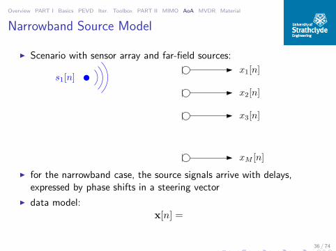
Narrowband Source Model
Scenario with sensor array and far-field sources:
x1[n]
x2[n]
x3[n]
xM [n]
s1[n]
for the narrowband case, the source signals arrive with delays,expressed by phase shifts in a steering vector
data model:x[n] =
36 / 74

Overview PART I Basics PEVD Iter. Toolbox PART II MIMO AoA MVDR Material
Narrowband Source Model
Scenario with sensor array and far-field sources:
x1[n]
x2[n]
x3[n]
xM [n]
s1[n]
for the narrowband case, the source signals arrive with delays,expressed by phase shifts in a steering vector s1
data model:x[n] = s1[n] · s1
36 / 74
Overview PART I Basics PEVD Iter. Toolbox PART II MIMO AoA MVDR Material
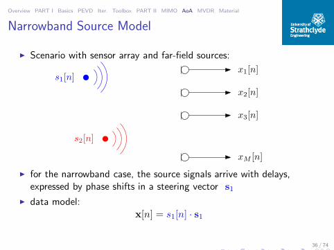
Narrowband Source Model
Scenario with sensor array and far-field sources:
x1[n]
x2[n]
x3[n]
xM [n]
s1[n]
s2[n]
for the narrowband case, the source signals arrive with delays,expressed by phase shifts in a steering vector s1
data model:x[n] = s1[n] · s1
36 / 74

Overview PART I Basics PEVD Iter. Toolbox PART II MIMO AoA MVDR Material
Narrowband Source Model
Scenario with sensor array and far-field sources:
x1[n]
x2[n]
x3[n]
xM [n]
s1[n]
s2[n]
for the narrowband case, the source signals arrive with delays,expressed by phase shifts in a steering vector s1, s2
data model:x[n] = s1[n] · s1 + s1[n] · s2
36 / 74
Overview PART I Basics PEVD Iter. Toolbox PART II MIMO AoA MVDR Material
Narrowband Source Model
Scenario with sensor array and far-field sources:
x1[n]
x2[n]
x3[n]
xM [n]
s1[n]
s2[n]
sR[n]
for the narrowband case, the source signals arrive with delays,expressed by phase shifts in a steering vector s1, s2
data model:x[n] = s1[n] · s1 + s1[n] · s2
36 / 74

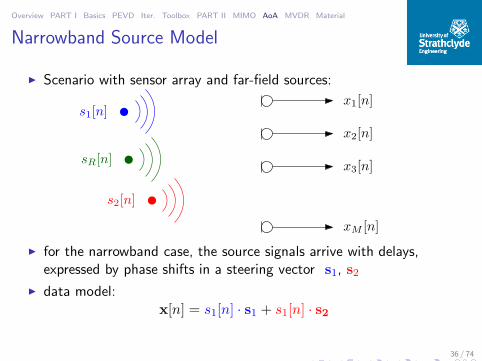
Overview PART I Basics PEVD Iter. Toolbox PART II MIMO AoA MVDR Material
Narrowband Source Model Scenario with sensor array and far-field sources:
x1[n]
x2[n]
x3[n]
xM [n]
s1[n]
s2[n]
sR[n]
for the narrowband case, the source signals arrive with delays,expressed by phase shifts in a steering vector s1, s2, . . . sR;
data model:
x[n] = s1[n] · s1 + s1[n] · s2 + · · · + sR[n] · sR =
R∑
r=1
sr[n] · sr
36 / 74

Overview PART I Basics PEVD Iter. Toolbox PART II MIMO AoA MVDR Material
Steering Vector
A signal s[n] arriving at the array can be characterised bythe delays of its wavefront (neglecting attenuation):
x0[n]x1[n]...
xM−1[n]
=
s[n− τ0]s[n− τ1]
...s[n− τM−1]
=
δ[n − τ0]δ[n − τ1]
...δ[n − τM−1]
∗s[n] —• aϑ(z)S(z)
if evaluated at a narrowband normalised angular frequency Ωi, thetime delays τm in the broadband steering vector aϑ(z) collapse tophase shifts in the narrowband steering vector aϑ,Ωi
,
aϑ,Ωi= aϑ(z)|z=ejΩi =
e−jτ0Ωi
e−jτ1Ωi
...e−jτM−1Ωi
.
37 / 74

Overview PART I Basics PEVD Iter. Toolbox PART II MIMO AoA MVDR Material
Data and Covariance Matrices
A data matrix X ∈ CM×L can be formed from L measurements:
X =[x[n] x[n + 1] . . . x[n + L− 1]
]
assuming that all xm[n], m = 1, 2, . . . M are zero mean, the(instantaneous) data covariance matrix is
R = Ex[n]xH[n]
≈
1
LXXH
where the approximation assumes ergodicity and a sufficientlylarge L;
Problem: can we tell from X or R (i) the number of sources and(ii) their orgin / time series?
w.r.t. Jonathon Chamber’s introduction, we here only consider theunderdetermined case of more sensors than sources, M ≥ K, andgenerally L ≫ M .
38 / 74

Overview PART I Basics PEVD Iter. Toolbox PART II MIMO AoA MVDR Material
SVD of Data Matrix
Singular value decomposition of X:
X U ΣV
H=
unitary matrices U = [u1 . . .uM ] and V = [v1 . . .vL];
diagonal Σ contains the real, positive semidefinite singular valuesof X in descending order:
Σ =
σ1 0 . . . 0 0 . . . 0
0 σ2. . .
......
......
. . .. . . 0
......
0 0 σM 0 . . . 0
with σ1 ≥ σ2 ≥ · · · ≥ σM ≥ 0.
39 / 74

Overview PART I Basics PEVD Iter. Toolbox PART II MIMO AoA MVDR Material
Singular Values If the array is illuminated by R ≤ M linearly independent sources,
the rank ofthe data matrix is
rankX = R
only the first R singular values of X will be non-zero; in practice, noise often will ensure that rankX = M , with
M −R trailing singular values that define the noise floor:
1 2 3 4 5 6 7 8 9 100
0.2
0.4
0.6
0.8
1
ordered index m
σm
therefore, by thresholding singular values, it is possible to estimatethe number of linearly independent sources R.
40 / 74

Overview PART I Basics PEVD Iter. Toolbox PART II MIMO AoA MVDR Material
Subspace Decomposition
If rankX = R, the SVD can be split:
X = [Us Un]
[Σs 0
0 Σn
] [VH
s
VHn
]
with Us ∈ CM×R and VH
s ∈ CR×L corresponding to the R
largest singular values;
Us and VHs define the signal-plus-noise subspace of X:
X =M∑
m=1
σmumvHm ≈
R∑
m=1
σmumvHm
the complements Un and VHn ,
UHs Un = 0 , VsV
Hn = 0
define the noise-only subspace of X.
41 / 74
Overview PART I Basics PEVD Iter. Toolbox PART II MIMO AoA MVDR Material
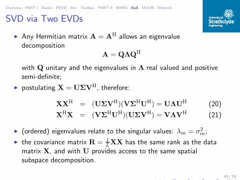
SVD via Two EVDs
Any Hermitian matrix A = AH allows an eigenvaluedecomposition
A = QΛQH
with Q unitary and the eigenvalues in Λ real valued and positivesemi-definite;
postulating X = UΣVH, therefore:
XXH = (UΣVH)(VΣHUH) = UΛUH (20)
XHX = (VΣHUH)(UΣVH) = VΛVH (21)
(ordered) eigenvalues relate to the singular values: λm = σ2m;
the covariance matrix R = 1LXX has the same rank as the data
matrix X, and with U provides access to the same spatialsubspace decomposition.
42 / 74

Overview PART I Basics PEVD Iter. Toolbox PART II MIMO AoA MVDR Material
Narrowband MUSIC Algorithm EVD of the narrowband covariance matrix identifies
signal-plus-noise and noise-only subspaces
R = [Us Un]
[Λs 0
0 Λn
] [UH
s
UHn
]
scanning the signal-plus-noise subspace could only help to retrievesources with orthogonal steering vectors;
therefore, the multiple signal classification (MUSIC) algorithmscans the noise-only subspace for minima, or maxima of itsreciprocal
SMUSIC(ϑ) =1
‖Unaϑ,Ωi‖22
−80 −60 −40 −20 0 20 40 60 80
−40
−20
0
ϑ / [o]
SMUSIC(ϑ)/[dB]
43 / 74

Overview PART I Basics PEVD Iter. Toolbox PART II MIMO AoA MVDR Material
Narrowband Source Separation
Via SVD of the data matrix X or EVD of the covariance matrixR, we can determine the number of linearly independent sourcesR;
using the subspace decompositions offered by EVD/SVD, thedirections of arrival can be estimated using e.g. MUSIC;
based on knowledge of the angle of arrival, beamforming could beapplied to X to extract specific sources;
overall: EVD (and SVD) can play a vital part in narrowbandsource separation;
what about broadband source separation?
44 / 74

Overview PART I Basics PEVD Iter. Toolbox PART II MIMO AoA MVDR Material
Broadband Array Scenario
x0[n]
x1[n]
x2[n]
xM−1[n]
s1[n]
Compared to the narrowband case, time delays rather than phaseshifts bear information on the direction of a source.
45 / 74

Overview PART I Basics PEVD Iter. Toolbox PART II MIMO AoA MVDR Material
Broadband Steering Vector
A signal s[n] arriving at the array can be characterised bythe delays of its wavefront (neglecting attenuation):
x0[n]x1[n]...
xM−1[n]
=
s[n− τ0]s[n− τ1]
...s[n− τM−1]
=
δ[n − τ0]δ[n − τ1]
...δ[n − τM−1]
∗s[n] —• aϑ(z)S(z)
if evaluated at a narrowband normalised angular frequency Ωi, thetime delays τm in the broadband steering vector aϑ(z) collapse tophase shifts in the narrowband steering vector aϑ,Ωi
,
aϑ,Ωi= aϑ(z)|z=ejΩi =
e−jτ0Ωi
e−jτ1Ωi
...e−jτM−1Ωi
.
46 / 74
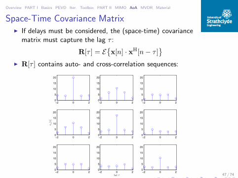
Overview PART I Basics PEVD Iter. Toolbox PART II MIMO AoA MVDR Material
Space-Time Covariance Matrix If delays must be considered, the (space-time) covariance
matrix must capture the lag τ :
R[τ ] = Ex[n] · xH[n− τ ]
R[τ ] contains auto- and cross-correlation sequences:
−2 0 20
5
10
15
20
−2 0 20
5
10
15
20
−2 0 20
5
10
15
20
−2 0 20
5
10
15
20
r ij[τ]
−2 0 20
5
10
15
20
−2 0 20
5
10
15
20
−2 0 20
5
10
15
20
−2 0 20
5
10
15
20
lat τ−2 0 20
5
10
15
20
47 / 74
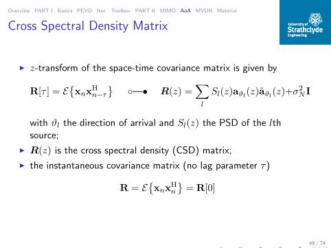
Overview PART I Basics PEVD Iter. Toolbox PART II MIMO AoA MVDR Material
Cross Spectral Density Matrix
z-transform of the space-time covariance matrix is given by
R[τ ] = Exnx
Hn−τ
—• R(z) =
∑
l
Sl(z)aϑl(z)aϑl
(z)+σ2N I
with ϑl the direction of arrival and Sl(z) the PSD of the lthsource;
R(z) is the cross spectral density (CSD) matrix;
the instantaneous covariance matrix (no lag parameter τ)
R = Exnx
Hn
= R[0]
48 / 74
Overview PART I Basics PEVD Iter. Toolbox PART II MIMO AoA MVDR Material
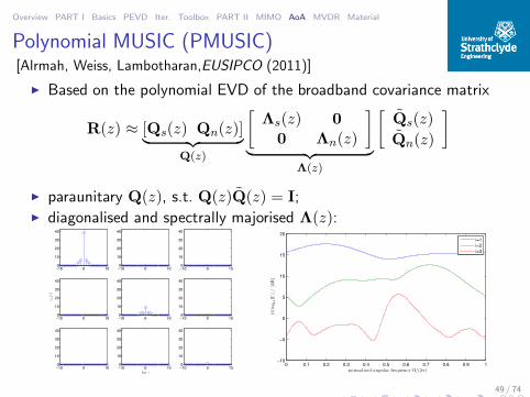
Polynomial MUSIC (PMUSIC)[Alrmah, Weiss, Lambotharan,EUSIPCO (2011)]
Based on the polynomial EVD of the broadband covariance matrix
R(z) ≈ [Qs(z) Qn(z)]︸ ︷︷ ︸
Q(z)
[Λs(z) 0
0 Λn(z)
]
︸ ︷︷ ︸
Λ(z)
[Qs(z)
Qn(z)
]
paraunitary Q(z), s.t. Q(z)Q(z) = I; diagonalised and spectrally majorised Λ(z):
−10 0 100
10
20
30
40
−10 0 100
10
20
30
40
−10 0 100
10
20
30
40
−10 0 100
10
20
30
40
γij[τ]
−10 0 100
10
20
30
40
−10 0 100
10
20
30
40
−10 0 100
10
20
30
40
−10 0 100
10
20
30
40
lat τ−10 0 100
10
20
30
40
0 0.1 0.2 0.3 0.4 0.5 0.6 0.7 0.8 0.9 1−10
−5
0
5
10
15
20
normalised angular frequency Ω/(2π)
10log 1
0|Γ
i|/[dB]
i=1
i=2
i=3
49 / 74

Overview PART I Basics PEVD Iter. Toolbox PART II MIMO AoA MVDR Material
PMUSIC cont’d
Idea —- scan the polynomial noise-only subspace Qn(z) withbroadband steering vectors
Γ(z, ϑ) = aϑ(z)Qn(z)Qn(z)aϑ(z)
looking for minima leads to a spatio-spectral PMUSIC
SPSS−MUSIC(ϑ,Ω) = (Γ(z, ϑ)|z=ejΩ)−1
and a spatial-only PMUSIC
SPS−MUSIC(ϑ) =
(
2π
∮
Γ(z, ϑ)|z=ejΩdΩ
)−1
= Γ−1ϑ [0]
with Γϑ[τ ] —• Γ(z, ϑ).
50 / 74

Overview PART I Basics PEVD Iter. Toolbox PART II MIMO AoA MVDR Material
Simulation I — Toy Problem
Linear uniform array with critical spatial and temporal sampling;
broadband steering vector for end-fire position:
aπ/2(z) = [1 z−1 · · · z−M+1]T
covariance matrix
R(z) = aπ/2(z)aπ/2(z) =
1 z1 . . . zM−1
z−1 1...
.... . .
...z−M+1 . . . . . . 1
.
PEVD (by inspection)
Q(z) = TDFTdiag1 z−1 · · · z−M+1
; Λ(z) = diag1 0 · · · 0
simulations with M = 4 . . .51 / 74

Overview PART I Basics PEVD Iter. Toolbox PART II MIMO AoA MVDR Material
Simulation I — PSS-MUSIC
−60 −40 −20 0 20 40 60 80 100 120
0
0.5
1
−50
0
Ω/πϑ/
SPSS(ϑ
,ejΩ)/[dB] (a)
−60 −40 −20 0 20 40 60 80 100 120
0
0.5
1−120−100
−80−60−40−20
Ω/πϑ/
Sdiff(ϑ
,ejΩ)/[dB] (b)
52 / 74

Overview PART I Basics PEVD Iter. Toolbox PART II MIMO AoA MVDR Material
Simulation II M = 8 element sensor array illuminated by three sources; source 1: ϑ1 = −30, active over range Ω ∈ [3π8 ; π]; source 2: ϑ2 = 20, active over range Ω ∈ [π2 ; π]; source 3: ϑ3 = 40, active over range Ω ∈ [2π8 ; 7π
8 ]; and
0 40 60 90-30-60-90
π
π
2
Ω
ϑ/[]
20
filter banks as innovation filters, and broadband steering vectorsto simulate AoA;
space-time covariance matrix is estimated from 104 samples.53 / 74
Overview PART I Basics PEVD Iter. Toolbox PART II MIMO AoA MVDR Material
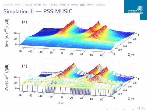
Simulation II — PSS-MUSIC
−80 −60 −40 −20 0 20 40 60 800
0.2
0.4
0.6
0.8
1
0
20
40
Ω/πϑ/
SPSS(ϑ
,ejΩ)/[dB]
(a)
−80 −60 −40 −20 0 20 40 60 800
0.2
0.4
0.6
0.8
1
0
20
40
Ω/πϑ/
SAF(ϑ
,ejΩ)/[dB]
(b)
54 / 74
Overview PART I Basics PEVD Iter. Toolbox PART II MIMO AoA MVDR Material
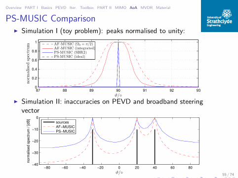
PS-MUSIC Comparison Simulation I (toy problem): peaks normalised to unity:
87 88 89 90 91 92 930
0.2
0.4
0.6
0.8
1
ϑ/
norm
alisedspectrum
AF-MUSIC (Ω0 = π/2)AF-MUSIC (integrated)PS-MUSIC (SBR2)PS-MUSIC (ideal)
Simulation II: inaccuracies on PEVD and broadband steeringvector
−80 −60 −40 −20 0 20 40 60 80−40
−30
−20
−10
0
ϑ/
norm
alis
ed s
pectr
um
/ [dB
]
sources
AF−MUSIC
PS−MUSIC
55 / 74

Overview PART I Basics PEVD Iter. Toolbox PART II MIMO AoA MVDR Material
AoA Estimation — Conclusions We have considered the importance of SVD and EVD for
narrowband source separation; narrowband matrix decomposition real the matrix rank and offer
subspace decompositions on which angle-of-arrival estimationalhorithms such as MUSIC can be based;
broadband problems lead to a space-time covariance or CSDmatrix;
such polynomial matrices cannot be decomposed by standardEVD and SVD;
a polynomial EVD has been defined; iterative algorithms such as SBR2 can be used to approximate the
PEVD; this permits a number of applications, such as broadband angle of
arrival estimation; broadband beamforming could then be used to separate
broadband sources.56 / 74

Overview PART I Basics PEVD Iter. Toolbox PART II MIMO AoA MVDR Material
Narrowband Minimum Variance DistortionlessResponse Beamformer
Scenario: an array of M sensors receives data x[n], containing adesired signal with frequency Ωs and angle of arrival ϑs, corruptedby interferers;
a narrowband beamformer applies a single coefficient to every ofthe M sensor signals:
x1[n]
x2[n]
xM [n]
w1
w2
wM
+
×
×
×
...
e[n]
57 / 74

Overview PART I Basics PEVD Iter. Toolbox PART II MIMO AoA MVDR Material
Narrowband MVDR Problem
Recall the space-time covariance matrix:
R[τ ] = Ex[n]xH[n− τ ]
the MVDR beamformer minimises the output power of thebeamformer:
minw
E|e[n]|2
= min
wwHR[0]w (22)
s.t. aH(ϑs,Ωs)w = 1 , (23)
this is subject to protecting the signal of interest by a constraintin look direction ϑs;
the steering vector aϑs,Ωsdefines the signal of interest’s
parameters.
58 / 74

Overview PART I Basics PEVD Iter. Toolbox PART II MIMO AoA MVDR Material
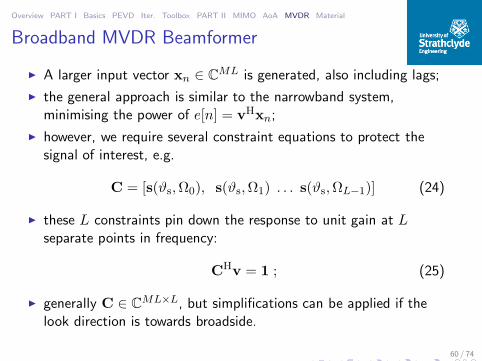
Broadband MVDR Beamformer
Each sensor is followed by a tap delay line of dimension L, givinga total of ML coefficients in a vector v ∈ C
ML
+ e[n]
z−1
z−1
z−1
× ×××
x1[n]
+ + +
w1,1 w1,2 w1,3 w1,L
x1[n− L+ 1]x1[n− 2]
z−1
z−1
z−1
× ×××
xM [n]
+ + +
wM,1 wM,2 wM,3 wM,L
xM [n− L+ 1]xM [n− 2]
......
59 / 74
Overview PART I Basics PEVD Iter. Toolbox PART II MIMO AoA MVDR Material
Broadband MVDR Beamformer
A larger input vector xn ∈ CML is generated, also including lags;
the general approach is similar to the narrowband system,minimising the power of e[n] = vHxn;
however, we require several constraint equations to protect thesignal of interest, e.g.
C = [s(ϑs,Ω0), s(ϑs,Ω1) . . . s(ϑs,ΩL−1)] (24)
these L constraints pin down the response to unit gain at Lseparate points in frequency:
CHv = 1 ; (25)
generally C ∈ CML×L, but simplifications can be applied if the
look direction is towards broadside.
60 / 74
Overview PART I Basics PEVD Iter. Toolbox PART II MIMO AoA MVDR Material
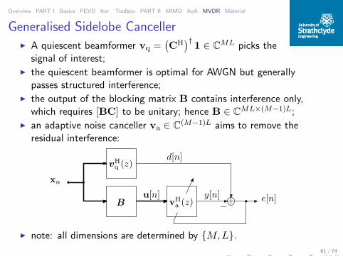
Generalised Sidelobe Canceller A quiescent beamformer vq =
(CH
)†1 ∈ C
ML picks thesignal of interest;
the quiescent beamformer is optimal for AWGN but generallypasses structured interference;
the output of the blocking matrix B contains interference only,which requires [BC] to be unitary; hence B ∈ C
ML×(M−1)L; an adaptive noise canceller va ∈ C
(M−1)L aims to remove theresidual interference:
vHq (z)
B vHa (z) +
−
d[n]
e[n]y[n]
xn
u[n]
note: all dimensions are determined by M,L.
61 / 74
Overview PART I Basics PEVD Iter. Toolbox PART II MIMO AoA MVDR Material
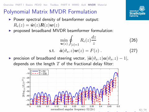
Polynomial Matrix MVDR Formulation Power spectral density of beamformer output:
Re(z) = w(z)R(z)w(z) proposed broadband MVDR beamformer formulation:
minw(z)
∮
|z|=1Re(z)
dz
z(26)
s.t. a(ϑs, z)w(z) = F (z) . (27)
precision of broadband steering vector, |a(ϑs, z)a(ϑs, z)− 1|,depends on the length T of the fractional delay filter:
0 0.05 0.1 0.15 0.2 0.25 0.3 0.35 0.4 0.45 0.5−80
−70
−60
−50
−40
−30
−20
−10
0
normalised angular frequency Ω/(2π)
20log10|E
1(e
jΩ)|
T=50T=100
62 / 74

Overview PART I Basics PEVD Iter. Toolbox PART II MIMO AoA MVDR Material
Generalised Sidelobe Canceller
Instead of performing constrained optimisation, the GSC projectsthe data and performs adaptive noise cancellation:
wq(z)
B(z) wa(z) +−
d[n]
e[n]y[n]
x[n]
u[n]
the quiescent vector wq(z) is generated from the constraints andpasses signal plus interference;
the blocking matrix B(z) has to be orthonormal to wq(z) andonly pass interference.
63 / 74

Overview PART I Basics PEVD Iter. Toolbox PART II MIMO AoA MVDR Material
Design Considerations The blocking matrix can be obtained by completing a paraunitary
matrix from wq(z); this can be achieved by calculating a PEVD of the rank one
matrix wq(z)wq(z); this leads to a block matrix of order N that is typically greater
than L; maximum leakage of the signal of interest through the blocking
matrix:
0 0.05 0.1 0.15 0.2 0.25 0.3 0.35 0.4 0.45 0.5−55
−50
−45
−40
−35
−30
−25
normalised angular frequency Ω/(2π)
20log10|E
2(e
jΩ)|
truncation 1e-4, N = 164truncation 1e-3, N = 140
64 / 74
Overview PART I Basics PEVD Iter. Toolbox PART II MIMO AoA MVDR Material
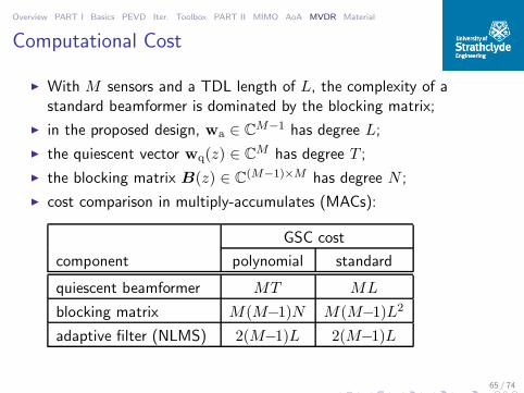
Computational Cost
With M sensors and a TDL length of L, the complexity of astandard beamformer is dominated by the blocking matrix;
in the proposed design, wa ∈ CM−1 has degree L;
the quiescent vector wq(z) ∈ CM has degree T ;
the blocking matrix B(z) ∈ C(M−1)×M has degree N ;
cost comparison in multiply-accumulates (MACs):
GSC cost
component polynomial standard
quiescent beamformer MT ML
blocking matrix M(M−1)N M(M−1)L2
adaptive filter (NLMS) 2(M−1)L 2(M−1)L
65 / 74
Overview PART I Basics PEVD Iter. Toolbox PART II MIMO AoA MVDR Material
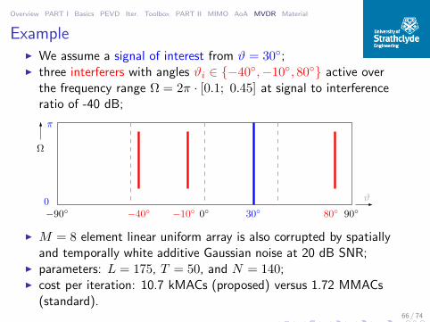
Example We assume a signal of interest from ϑ = 30; three interferers with angles ϑi ∈ −40,−10, 80 active over
the frequency range Ω = 2π · [0.1; 0.45] at signal to interferenceratio of -40 dB;
ϑ
Ω
−90 900
π
0−40 −10 30 80
M = 8 element linear uniform array is also corrupted by spatiallyand temporally white additive Gaussian noise at 20 dB SNR;
parameters: L = 175, T = 50, and N = 140; cost per iteration: 10.7 kMACs (proposed) versus 1.72 MMACs
(standard).66 / 74

Overview PART I Basics PEVD Iter. Toolbox PART II MIMO AoA MVDR Material
Quiescent Beamformer
Directivity pattern of quiescent standard broadband beamformer:
angle of arrival ϑ /[]
20log10|A
(ϑ,e
jΩ)|
/[dB]
Ω
2π
67 / 74
Overview PART I Basics PEVD Iter. Toolbox PART II MIMO AoA MVDR Material
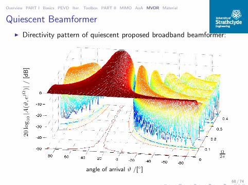
Quiescent Beamformer
Directivity pattern of quiescent proposed broadband beamformer:
angle of arrival ϑ /[]
20log10|A
(ϑ,e
jΩ)|
/[dB]
Ω
2π
68 / 74
Overview PART I Basics PEVD Iter. Toolbox PART II MIMO AoA MVDR Material
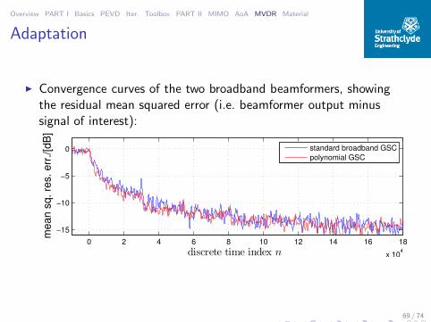
Adaptation
Convergence curves of the two broadband beamformers, showingthe residual mean squared error (i.e. beamformer output minussignal of interest):
0 2 4 6 8 10 12 14 16 18
x 104
−15
−10
−5
0
me
an
sq
. re
s.
err
./[d
B]
discrete time index n
standard broadband GSC
polynomial GSC
69 / 74

Overview PART I Basics PEVD Iter. Toolbox PART II MIMO AoA MVDR Material
Adapted Beamformer
Directivity pattern of adapted proposed broadband beamformer:
angle of arrival ϑ /[]
20log10|A
(ϑ,e
jΩ)|
/[dB]
Ω
2π
70 / 74

Overview PART I Basics PEVD Iter. Toolbox PART II MIMO AoA MVDR Material
Adapted Beamformer
Directivity pattern of adapted standard broadband beamformer:
angle of arrival ϑ /[]
20log10|A
(ϑ,e
jΩ)|
/[dB]
Ω
2π
71 / 74

Overview PART I Basics PEVD Iter. Toolbox PART II MIMO AoA MVDR Material
Gain in Look Direction Gain in look direction ϑs = 30 before and after adaptation:
0 0.05 0.1 0.15 0.2 0.25 0.3 0.35 0.4 0.45 0.5−2
−1.5
−1
−0.5
0
0.5
1
1.5
2
normalised angular frequency Ω/(2π)
20log 1
0|A
(ϑs,ej
Ω)|/[dB]
standard quiescentstandard adaptedpoint constraintspolynomial quiescentpolynomial adapted
due to signal leakage, the standard broadband beamformer afteradaptation only maintains the point constraints but deviateselsewhere.
72 / 74

Overview PART I Basics PEVD Iter. Toolbox PART II MIMO AoA MVDR Material
Broadband Beamforming Conclusions
Based on the previous AoA estimation, beamforming can help toextract source signals and thus perform “source separation”;
broadband beamformers usually assume pre-steering such that thesignal of interest lies at broadside;
this is not always given, and difficult for arbitary array geometries;
the proposed beamformer using a polynomial matrix formulationcan implement abitrary constraints;
the performance for such constraints is better in terms of theaccuracy of the directivity pattern;
because the proposed design decouples the complexities of thecoefficient vector, the quiescent vector and block matrix, and theadaptive process, the cost is significantly lower than for astandard broadband adaptive beamformer.
73 / 74

Overview PART I Basics PEVD Iter. Toolbox PART II MIMO AoA MVDR Material
Additional Material Key papers:
1 J.G. McWhirter, P.D. Baxter, T. Cooper, S. Redif, and J. Foster:“An EVD Algorithm for Para-Hermitian Polynomial Matrices,”IEEE Trans SP, 55(5): 2158-2169, May 2007.
2 S. Redif, J.G. McWhirter, and S. Weiss: “Design of FIRParaunitary Filter Banks for Subband Coding Using a PolynomialEigenvalue Decomposition,” IEEE Trans SP, 59(11): 5253-5264,Nov. 2011.
3 S. Redif, S. Weiss, and J.G. McWhirter: “Sequential matrixdiagonalisation algorithms for polynomial EVD of parahermitianmatrices,” IEEE Trans SP, 63(1): 81–89, Jan. 2015.
If interested in the discussed methods and algorithms, pleasedownload the free Matlab PEVD toolbox from
pevd-toolbox.eee.strath.ac.uk for questions, please feel free to ask:
• Stephan Weiss ([email protected]) or• Jamie Corr ([email protected])• Fraser Coutts ([email protected])
74 / 74
Related Documents