Transport optimization on complex networks

arX

iv:c

ond-

mat

/070

1184

v1 [

cond

-mat

.dis

-nn]

9 J

an 2

007

Transport optimization on complex networks

Bogdan Danila,1, ∗ Yong Yu,1 John A. Marsh,2, † and Kevin E. Bassler1, ‡

1Department of Physics, The University of Houston, Houston TX 77204-5005

2Assured Information Security, Rome NY 13440

Abstract

We present a comparative study of the application of a recently introduced heuristic algorithm

to the optimization of transport on three major types of complex networks. The algorithm bal-

ances network traffic iteratively by minimizing the maximum node betweenness with as little path

lengthening as possible. We show that by using this optimal routing, a network can sustain sig-

nificantly higher traffic without jamming than in the case of shortest path routing. A formula is

proved that allows quick computation of the average number of hops along the path and of the

average travel times once the betweennesses of the nodes are computed. Using this formula, we

show that routing optimization preserves the small-world character exhibited by networks under

shortest path routing, and that it significantly reduces the average travel time on congested net-

works with only a negligible increase in the average travel time at low loads. Finally, we study the

correlation between the weights of the links in the case of optimal routing and the betweennesses

of the nodes connected by them.

Keywords: complex networks, scaling laws, transport

∗[email protected]†[email protected]‡[email protected]

1

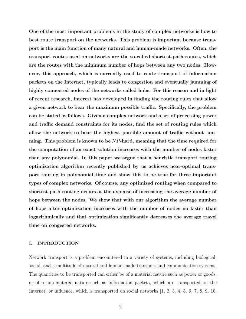
One of the most important problems in the study of complex networks is how to

best route transport on the networks. This problem is important because trans-

port is the main function of many natural and human-made networks. Often, the

transport routes used on networks are the so-called shortest-path routes, which

are the routes with the minimum number of hops between any two nodes. How-

ever, this approach, which is currently used to route transport of information

packets on the Internet, typically leads to congestion and eventually jamming of

highly connected nodes of the networks called hubs. For this reason and in light

of recent research, interest has developed in finding the routing rules that allow

a given network to bear the maximum possible traffic. Specifically, the problem

can be stated as follows. Given a complex network and a set of processing power

and traffic demand constraints for its nodes, find the set of routing rules which

allow the network to bear the highest possible amount of traffic without jam-

ming. This problem is known to be NP -hard, meaning that the time required for

the computation of an exact solution increases with the number of nodes faster

than any polynomial. In this paper we argue that a heuristic transport routing

optimization algorithm recently published by us achieves near-optimal trans-

port routing in polynomial time and show this to be true for three important

types of complex networks. Of course, any optimized routing when compared to

shortest-path routing occurs at the expense of increasing the average number of

hops between the nodes. We show that with our algorithm the average number

of hops after optimization increases with the number of nodes no faster than

logarithmically and that optimization significantly decreases the average travel

time on congested networks.

I. INTRODUCTION

Network transport is a problem encountered in a variety of systems, including biological,

social, and a multitude of natural and human-made transport and communication systems.

The quantities to be transported can either be of a material nature such as power or goods,

or of a non-material nature such as information packets, which are transported on the

Internet, or influence, which is transported on social networks [1, 2, 3, 4, 5, 6, 7, 8, 9, 10,

2

11, 12, 13, 14, 15, 16, 17, 18, 19, 20, 21, 22, 23]. Optimization of network transport is

thus an important problem for a variety of fields in science and technology. In this paper we

present a comparative study of the application of a recently published transport optimization

algorithm [8] to three major types of complex networks: Erdos-Renyi [24], Barabasi-Albert

[25], and uncorrelated scale-free networks generated using the configuration model [26].

For concreteness, we consider the transport of particles that hop from nodes to nearest-

neighbor nodes on complex networks. Traditionally, the routing of network transport is

based on the idea of using the shortest paths (usually defined as the paths containing the

smallest number of hops) between any two nodes on the network. More generally, the

length of a path can be computed as the sum of the weights assigned to the links that

form the path. In the case of the Internet for example, link weights are typically assigned

manually by operators according to simple rules based on experience [3]. Recently, a series

of algorithms have also been proposed for network traffic optimization. These algorithms

are aimed at reducing link [3, 4, 5, 6, 7] or node [8, 9, 10, 11, 12] loads by a judicious link

weight assignment. They have the effect of improving network transport capacity, which is

defined as the rate of particle insertion at which the network becomes jammed.

In a recent paper [8] we presented an algorithm that significantly improves transport ca-

pacity by a systematic adjustment of link weights to minimize the maximum betweenness on

the network. Our algorithm leads to higher transport capacity than other recently proposed

algorithms [9, 10]. In this paper, we argue that our algorithm achieves near-optimal routing

for all three types of complex networks and discuss the reasons why this is possible. Fur-

thermore, we show that routing optimization preserves the small-world character of network

routing [2] and that it significantly decreases the average travel time on congested networks

while only marginally increasing it at low loads. Finally, we study the correlation between

the optimal weights of the links and the betweenness of the nodes connected by them and

show that, as networks approach optimal routing, it becomes impossible to achieve further

improvement by relating link weights to node betweennesses.

The problem of finding the exact optimal routing is mathematically tied to the problem

of finding the minimal sparsity vertex separator [10], which has been shown to be an NP -

hard problem [27]. This means that the number of flops necessary for the computation of an

exact solution increases with the number of nodes N faster than any polynomial. Despite

this fact, our heuristic algorithm finds near-optimal solutions for the routing problem in

3

polynomial time. For networks with given average degree, the running time is O(N3 log N)

(O(N2 log N) for one iteration and requiring O(N) iterations). In its most general form, the

algorithm proceeds as follows:

1. Assign uniform or random weight to every link and compute the shortest paths between

all pairs of nodes and the betweenness of every node.

2. Find the node which has the highest betweenness Bmax and increase the weight of every

link that connects it to other nodes, or the weight of every incoming link if the network is

a directed one. This is done by adding either a constant or a random number to the weight

of each link.

3. Recompute the shortest paths and the betweennesses. Go back to step 2.

Note that the algorithm picks the “least fit” element of a set and changes its parameters.

Therefore, it is a form of extremal optimization [28, 29]. However, this algorithm may assign

parameters in a deterministic way, unlike many of the other existing extremal optimization

algorithms.

The outline of the paper is as follows. In Sec. II we give a detailed description of our

model and prove a formula that can be used to compute the average number of hops along

the path and the average travel time from the betweennesses of the nodes. In Sec. III we

present our results. Section IV summarizes our results and conclusions.

II. MODEL

We present a comparative analysis of the results obtained with our algorithm [8] in the

case of three of the most common types of complex networks. These are the random Erdos-

Renyi (ER) networks, Barabasi-Albert (BA) networks, and uncorrelated scale-free networks

generated using the configuration model (CM). All three network types are undirected.

Random ER networks are characterized by a binomial distribution of node degrees, while

BA and CM networks exhibit scale-free distributions of node degrees in the limit of a large

number of nodes. BA networks are grown by preferential attachment and are characterized

by a strong correlation between the degrees of the nodes at the ends of the links. Results

are presented for transport for the case of shortest path (SP) routing and for the case of the

optimal routing (OR) provided by our algorithm. The number of nodes N varies between

25 and 2500 in the case of SP routing and between 25 and 1600 in the case of optimal

4

routing. To facilitate comparison with previously published results [19], the average degree

of both random and BA networks was kept at a constant value of 〈k〉 = 6, regardless of the

number of nodes. Additionally, we consider only fully connected networks. Large connected

random networks of lower average degree are prohibitively unlikely to be generated. The

average degree of the uncorrelated scale-free networks cannot be strictly controlled but, for a

given value of the exponent γ that describes the power-law degree distribution of the nodes

p(k) ∝ k−γ, it varies with the number of nodes slower than logarithmically. In keeping

with Refs. [8, 10], we chose a value of the exponent γ = 2.5, but the value of the lower

cutoff parameter [26] was set to m = 4, which results in the average degree varying between

approximately 4.5 and 7.5 as the number of nodes increases from 25 to 1600.

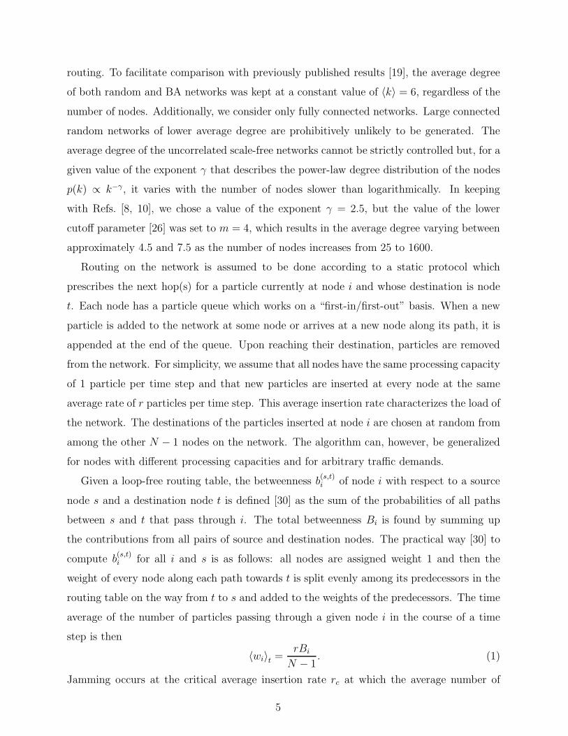
Routing on the network is assumed to be done according to a static protocol which

prescribes the next hop(s) for a particle currently at node i and whose destination is node

t. Each node has a particle queue which works on a “first-in/first-out” basis. When a new

particle is added to the network at some node or arrives at a new node along its path, it is

appended at the end of the queue. Upon reaching their destination, particles are removed

from the network. For simplicity, we assume that all nodes have the same processing capacity

of 1 particle per time step and that new particles are inserted at every node at the same

average rate of r particles per time step. This average insertion rate characterizes the load of

the network. The destinations of the particles inserted at node i are chosen at random from

among the other N − 1 nodes on the network. The algorithm can, however, be generalized

for nodes with different processing capacities and for arbitrary traffic demands.

Given a loop-free routing table, the betweenness b(s,t)i of node i with respect to a source

node s and a destination node t is defined [30] as the sum of the probabilities of all paths

between s and t that pass through i. The total betweenness Bi is found by summing up

the contributions from all pairs of source and destination nodes. The practical way [30] to

compute b(s,t)i for all i and s is as follows: all nodes are assigned weight 1 and then the

weight of every node along each path towards t is split evenly among its predecessors in the

routing table on the way from t to s and added to the weights of the predecessors. The time

average of the number of particles passing through a given node i in the course of a time

step is then

〈wi〉t =rBi

N − 1. (1)

Jamming occurs at the critical average insertion rate rc at which the average number of

5

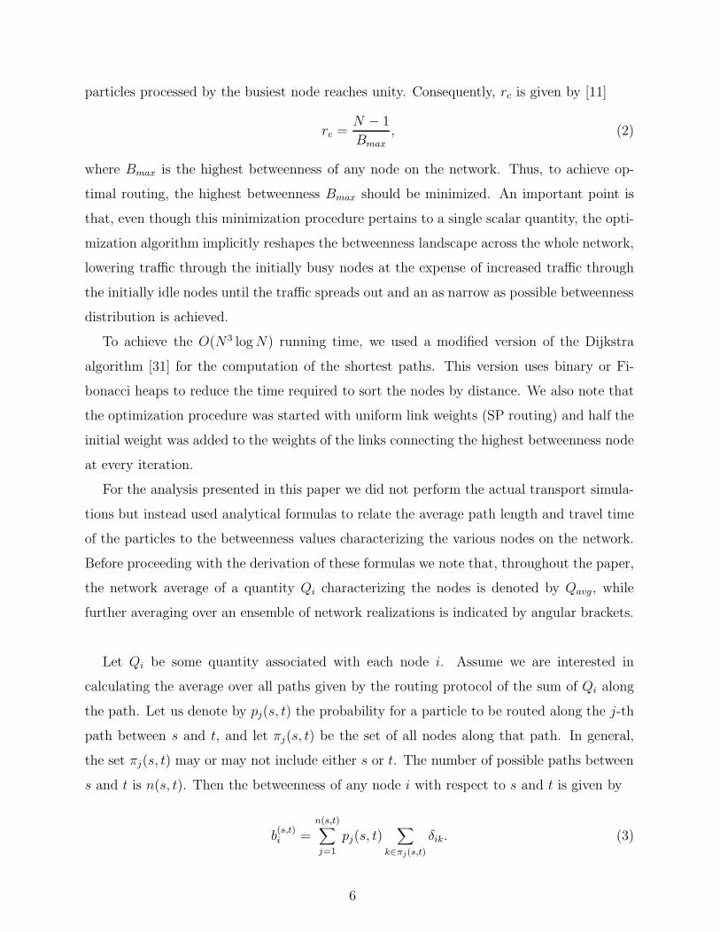
particles processed by the busiest node reaches unity. Consequently, rc is given by [11]

rc =N − 1

Bmax

, (2)

where Bmax is the highest betweenness of any node on the network. Thus, to achieve op-

timal routing, the highest betweenness Bmax should be minimized. An important point is

that, even though this minimization procedure pertains to a single scalar quantity, the opti-

mization algorithm implicitly reshapes the betweenness landscape across the whole network,

lowering traffic through the initially busy nodes at the expense of increased traffic through

the initially idle nodes until the traffic spreads out and an as narrow as possible betweenness

distribution is achieved.

To achieve the O(N3 log N) running time, we used a modified version of the Dijkstra

algorithm [31] for the computation of the shortest paths. This version uses binary or Fi-

bonacci heaps to reduce the time required to sort the nodes by distance. We also note that

the optimization procedure was started with uniform link weights (SP routing) and half the

initial weight was added to the weights of the links connecting the highest betweenness node

at every iteration.

For the analysis presented in this paper we did not perform the actual transport simula-

tions but instead used analytical formulas to relate the average path length and travel time

of the particles to the betweenness values characterizing the various nodes on the network.

Before proceeding with the derivation of these formulas we note that, throughout the paper,

the network average of a quantity Qi characterizing the nodes is denoted by Qavg , while

further averaging over an ensemble of network realizations is indicated by angular brackets.

Let Qi be some quantity associated with each node i. Assume we are interested in

calculating the average over all paths given by the routing protocol of the sum of Qi along

the path. Let us denote by pj(s, t) the probability for a particle to be routed along the j-th

path between s and t, and let πj(s, t) be the set of all nodes along that path. In general,

the set πj(s, t) may or may not include either s or t. The number of possible paths between

s and t is n(s, t). Then the betweenness of any node i with respect to s and t is given by

b(s,t)i =

n(s,t)∑

j=1

pj(s, t)∑

k∈πj(s,t)

δik. (3)

6

10 30 100 300 1000 3000

102

103

104

aver

age

betw

eenn

ess

10 30 100 300 1000 3000

102

103

104

105

106

aver

age

betw

eenn

ess

10 30 100 300 1000 3000N

102

103

104

105

aver

age

betw

eenn

ess

(a)

(b)

(c)

FIG. 1: Ensemble averages of the average and maximum betweenness as functions of network size

for (a) ER, (b) BA, and (c) CM networks. Lower (black) dots represent⟨

BSPavg

⟩

, upper (red) dots

represent⟨

BSPmax

⟩

, lower (green) crosses⟨

BORavg

⟩

, and upper (blue) crosses⟨

BORmax

⟩

.

Let us now compute the quantity (ΣQ)(s,t)avg defined by

(ΣQ)(s,t)avg =

N∑

i=1

Qib(s,t)i . (4)

By substituting Eq. (3) into (4) and changing the order of summation, we find

(ΣQ)(s,t)avg =

n(s,t)∑

j=1

pj(s, t)∑

k∈πj(s,t)

Qk. (5)

The inner sum on the right-hand side of Eq. (5) is exactly the quantity whose average we

are interested in. Thus, Eq. (4) gives the average over all possible paths between s and t of

the sum of Qi along the path. Its average over all s and t is (ΣQ)avg , defined as

(ΣQ)avg =1

N(N − 1)

N∑

s,t=1

(ΣQ)(s,t)avg . (6)

7

10 30 100 300 1000 30001

2

3

4

5

aver

age

path

leng

th

10 30 100 300 1000 30001

2

3

4

5

6

aver

age

path

leng

th

10 30 100 300 1000 3000N

1

2

3

4

5

aver

age

path

leng

th

(a)

(b)

(c)

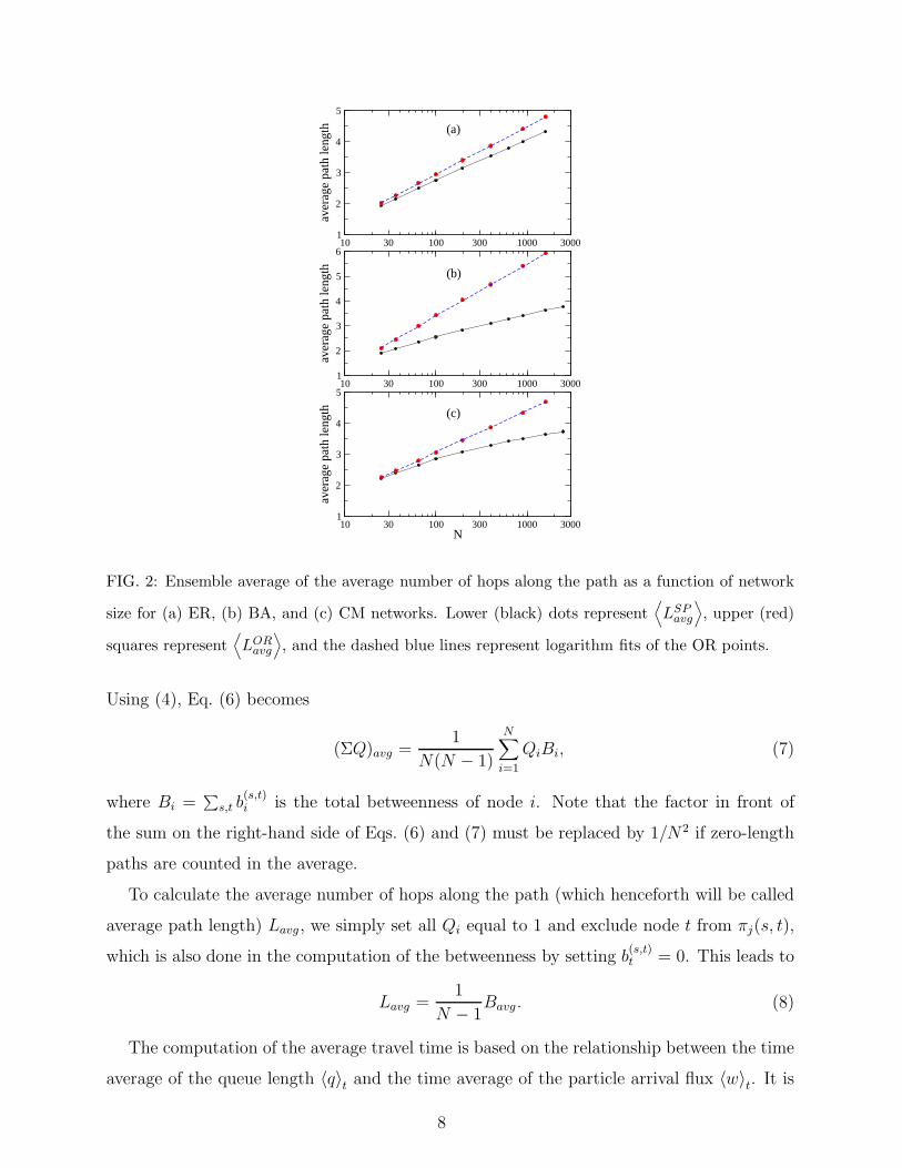
FIG. 2: Ensemble average of the average number of hops along the path as a function of network

size for (a) ER, (b) BA, and (c) CM networks. Lower (black) dots represent⟨

LSPavg

⟩

, upper (red)

squares represent⟨

LORavg

⟩

, and the dashed blue lines represent logarithm fits of the OR points.

Using (4), Eq. (6) becomes

(ΣQ)avg =1

N(N − 1)

N∑

i=1

QiBi, (7)

where Bi =∑

s,t b(s,t)i is the total betweenness of node i. Note that the factor in front of

the sum on the right-hand side of Eqs. (6) and (7) must be replaced by 1/N2 if zero-length

paths are counted in the average.

To calculate the average number of hops along the path (which henceforth will be called

average path length) Lavg , we simply set all Qi equal to 1 and exclude node t from πj(s, t),

which is also done in the computation of the betweenness by setting b(s,t)t = 0. This leads to

Lavg =1

N − 1Bavg . (8)

The computation of the average travel time is based on the relationship between the time

average of the queue length 〈q〉t and the time average of the particle arrival flux 〈w〉t. It is

8

10 30 100 300 1000 30000

5

10

15

20

25

30

aver

age

trav

el ti

me

10 30 100 300 1000 30000

5

10

15

20

25

30

aver

age

trav

el ti

me

10 30 100 300 1000 3000N

0

5

10

15

20

25

30

aver

age

trav

el ti

me

(a)

(c)

(b)

FIG. 3: Ensemble average of the average travel time computed for each network at 99% of its SP

transport capacity, as a function of network size for (a) ER, (b) BA, and (c) CM networks. Upper

(black) dots represent⟨

T SPavg

⟩

and lower (red) squares represent⟨

TORavg

⟩

.

0 0.5 1 1.5 2 2.5 3ζ

1

3

10

30

100

300

aver

age

trav

el ti

me

Tavg

SP

Tavg

OR

FIG. 4: Average SP (black dots) and OR (red squares) travel times for a CM network with 196

nodes as functions of the load fraction ζ defined with respect to SP routing.

9

known from the theory of Markovian queues [11, 32] that, assuming unity processing power,

these quantities are related by

〈q〉t =〈w〉t

1 − 〈w〉t. (9)

In our model, 〈w〉t for every node i is given by Eq. (1). The average travel times are

computed at a fraction ζ of the the critical insertion rate rSPc = (N − 1)/BSP

max at which the

network starts jamming when using shortest path routing. Thus, we have

〈wi〉t = ζBi

BSPmax

, (10)

which yields

〈qi〉t =ζBi

BSPmax − ζBi

. (11)

Unless otherwise specified, all average travel times were computed for ζ = 0.99.

The quantity associated with every node i is in this case Qi = Ti = 1+〈qi〉t. This accounts

for the average number of time steps a particle has to wait in the queue of node i plus one

time step to hop to the next node. When the resulting expression for Qi is substituted into

Eq. (7), we find

Tavg =BSP

max

N(N − 1)

N∑

i=1

Bi

BSPmax − ζBi

. (12)

III. RESULTS

Fig. 1 shows plots of the SP and OR ensemble averages of the network average and

maximum betweenness, 〈Bavg〉 and 〈Bmax〉 respectively, as functions of network size N . All

ensemble averages are computed over a set of 100 network realizations. Fig. 1(a) shows the

results for random networks, while Figs. 1(b,c) pertain to BA and CM networks, respectively.

In light of Eq. (8) and of the fact that the average path lengths of all three types of networks

are known to increase with network size no faster than log N , we expect their average SP

betweenness to increase no faster than N log N . The maximum SP betweenness is known to

scale with network size according to a power law [8, 10]. Our results show that, regardless

of network type, the same types of laws characterize the average and maximum betweenness

after optimization. Results for the exponents of the power laws characterizing 〈Bmax〉 for

the six network type and routing combinations are given in Table I, with the quoted errors

being 2σ estimates. The exponents for 〈Bmax〉 in the case of random networks were obtained

10

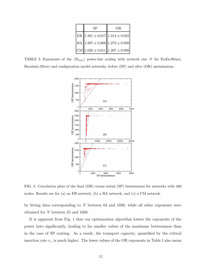
SP OR

ER 1.381 ± 0.017 1.214 ± 0.022

BA 1.897 ± 0.008 1.273 ± 0.009

CM 1.626 ± 0.011 1.207 ± 0.009

TABLE I: Exponents of the 〈Bmax〉 power-law scaling with network size N for Erdos-Renyi,

Barabasi-Albert and configuration model networks, before (SP) and after (OR) optimization.

0 1000 2000 3000 4000 50000

500

1000

1500

2000

OR

bet

wee

nnes

s

0 10000 20000 30000 400000

500

1000

1500

2000

2500

3000

OR

bet

wee

nnes

s

0 2000 4000 6000 8000SP betweenness

0

500

1000

1500

2000

OR

bet

wee

nnes

s

(a)

(b)

(c)

FIG. 5: Correlation plots of the final (OR) versus initial (SP) betweenness for networks with 400

nodes. Results are for (a) an ER network, (b) a BA network, and (c) a CM network.

by fitting data corresponding to N between 64 and 1600, while all other exponents were

obtained for N between 25 and 1600.

It is apparent from Fig. 1 that our optimization algorithm lowers the exponents of the

power laws significantly, leading to far smaller values of the maximum betweenness than

in the case of SP routing. As a result, the transport capacity, quantified by the critical

insertion rate rc, is much higher. The lower values of the OR exponents in Table I also mean

11

that transport capacity for networks with nodes of given processing power decreases much

slower with increasing network size. Moreover, even though the ensemble average of the

maximum betweenness scales with N according to a power law while the ensemble average

of the average betweenness is proportional to N log N , the difference between their OR values

remains negligible over almost two orders of magnitude of network size. This indicates the

optimality of the routing. Finally, optimization leads to only a small increase in the average

betweenness (which is explained by the need to have slightly longer paths around the hubs).

The reason for the higher values of the exponents exhibited by Barabasi-Albert networks

both before and after optimization is discussed in a later paragraph.

Plots of the ensemble average of the average path length 〈Lavg〉 as a function of network

size are shown in Fig. 2. As expected, the average SP path length is proportional to log N in

the case of ER networks and increases even slower with network size in the case of the scale-

free networks. The important finding is that after optimization, the average path length

scales with the logarithm of network size for all three types of networks. This means that

routing optimization preserves the small-world character of network routing [2].

In Fig. 3 we show the network size dependence of the ensemble average of the average

travel time 〈Tavg〉. Average travel times are computed for each network realization using

Eq. (12) at 99% of the critical insertion rate corresponding to shortest path routing. It is

apparent that, regardless of network type or size, when routing optimization is applied to a

network working close to its maximum transport capacity, it results in significant reduction

of the average travel time between source and destination. This is in addition to the fact

that optimization allows insertion rates significantly higher than the critical rate for SP

routing.

The dependence of the average travel time on network load is shown in Fig. 4, where Tavg

for a single CM network realization with 196 nodes is plotted against the load parameter

ζ = r/rSPc . For this case, the ratio between the SP and OR maximum betweennesses is

approximately 2.95, which is the maximum allowable value for ζ when this network uses op-

timal routing. Even though optimal routing results in longer travel times when the network

bears only small loads, the increase is not significant. For the overall efficiency of network

transport, this is at least as important as the decrease in travel time at higher loads.

Plots of the optimal routing (OR) betweenness versus the shortest path (SP) betweenness

for one network with N=400 nodes of each type are shown in Fig. 5. It is apparent from

12

0 1000 2000 3000 4000 50000

1000

2000

3000

4000

5000

SP b

etw

eenn

ess

0 500 1000 1500 20000

500

1000

1500

2000

OR

bet

wee

nnes

s

0 10000 20000 30000 400000

10000

20000

30000

40000

SP b

etw

eenn

ess

0 500 1000 1500 2000 2500 30000

500

1000

1500

2000

2500

3000

OR

bet

wee

nnes

s

0 2000 4000 6000 8000SP betweenness

0

2000

4000

6000

8000

SP b

etw

eenn

ess

0 500 1000 1500 2000OR betweenness

0

500

1000

1500

2000

OR

bet

wee

nnes

s

(a) (b)

(c) (d)

(e) (f)

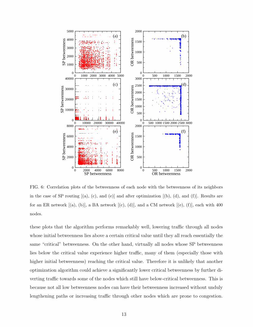
FIG. 6: Correlation plots of the betweenness of each node with the betweenness of its neighbors

in the case of SP routing [(a), (c), and (e)] and after optimization [(b), (d), and (f)]. Results are

for an ER network [(a), (b)], a BA network [(c), (d)], and a CM network [(e), (f)], each with 400

nodes.

these plots that the algorithm performs remarkably well, lowering traffic through all nodes

whose initial betweenness lies above a certain critical value until they all reach essentially the

same “critical” betweenness. On the other hand, virtually all nodes whose SP betweenness

lies below the critical value experience higher traffic, many of them (especially those with

higher initial betweenness) reaching the critical value. Therefore it is unlikely that another

optimization algorithm could achieve a significantly lower critical betweenness by further di-

verting traffic towards some of the nodes which still have below-critical betweenness. This is

because not all low betweenness nodes can have their betweenness increased without unduly

lengthening paths or increasing traffic through other nodes which are prone to congestion.

13

0 1000 2000 3000 4000 50000

50

100

150

200

250

300

OR

link

wei

ght

1000 1200 1400 1600 1800 20000

50

100

150

200

250

300

OR

link

wei

ght

0 10000 20000 30000 400000

200

400

600

800

OR

link

wei

ght

1000 1500 2000 2500 30000

200

400

600

800

OR

link

wei

ght

0 2000 4000 6000 8000link average SP betweenness

0

100

200

300

400

OR

link

wei

ght

1000 1200 1400 1600 1800 2000link average OR betweenness

0

100

200

300

400O

R li

nk w

eigh

t

(a)

(c)

(e)

(b)

(d)

(f)

FIG. 7: Correlation plots of the final (OR) link weights versus link average SP betweenness [(a),

(c), and (e)] and link average OR betweenness [(b), (d), and (f)]. Results are for an ER network

[(a), (b)], a BA network [(c), (d)], and a CM network [(e), (f)], each with 400 nodes.

The simplest examples (which are not valid in the case of BA networks) are those of a

small subnetwork connected to the rest of the network through a single link to a high SP

betweenness node, or a triangle connected to the rest of the network only by containing

such a node. There is no way of diverting traffic through the aforementioned structures, and

nodes belonging to them will have low betweenness even in the case of rigorously optimal

routing.

The case of Barabasi-Albert networks deserves special attention. As can be seen from

Table I, their power-law exponent is higher both before and after optimization. Moreover,

the initial betweenness is spread over a much wider interval, and even after optimization

there is a narrow but dense “trail” of nodes of the lowest possible SP betweenness and

14

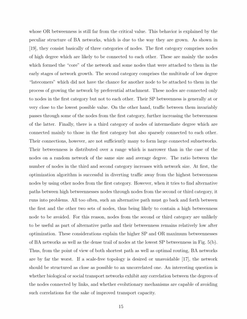
whose OR betweenness is still far from the critical value. This behavior is explained by the

peculiar structure of BA networks, which is due to the way they are grown. As shown in

[19], they consist basically of three categories of nodes. The first category comprises nodes

of high degree which are likely to be connected to each other. These are mainly the nodes

which formed the “core” of the network and some nodes that were attached to them in the

early stages of network growth. The second category comprises the multitude of low degree

“latecomers” which did not have the chance for another node to be attached to them in the

process of growing the network by preferential attachment. These nodes are connected only

to nodes in the first category but not to each other. Their SP betweenness is generally at or

very close to the lowest possible value. On the other hand, traffic between them invariably

passes through some of the nodes from the first category, further increasing the betweenness

of the latter. Finally, there is a third category of nodes of intermediate degree which are

connected mainly to those in the first category but also sparsely connected to each other.

Their connections, however, are not sufficiently many to form large connected subnetworks.

Their betweenness is distributed over a range which is narrower than in the case of the

nodes on a random network of the same size and average degree. The ratio between the

number of nodes in the third and second category increases with network size. At first, the

optimization algorithm is successful in diverting traffic away from the highest betweenness

nodes by using other nodes from the first category. However, when it tries to find alternative

paths between high betweennesses nodes through nodes from the second or third category, it

runs into problems. All too often, such an alternative path must go back and forth between

the first and the other two sets of nodes, thus being likely to contain a high betweenness

node to be avoided. For this reason, nodes from the second or third category are unlikely

to be useful as part of alternative paths and their betweenness remains relatively low after

optimization. These considerations explain the higher SP and OR maximum betweennesses

of BA networks as well as the dense trail of nodes at the lowest SP betweenness in Fig. 5(b).

Thus, from the point of view of both shortest path as well as optimal routing, BA networks

are by far the worst. If a scale-free topology is desired or unavoidable [17], the network

should be structured as close as possible to an uncorrelated one. An interesting question is

whether biological or social transport networks exhibit any correlation between the degrees of

the nodes connected by links, and whether evolutionary mechanisms are capable of avoiding

such correlations for the sake of improved transport capacity.

15

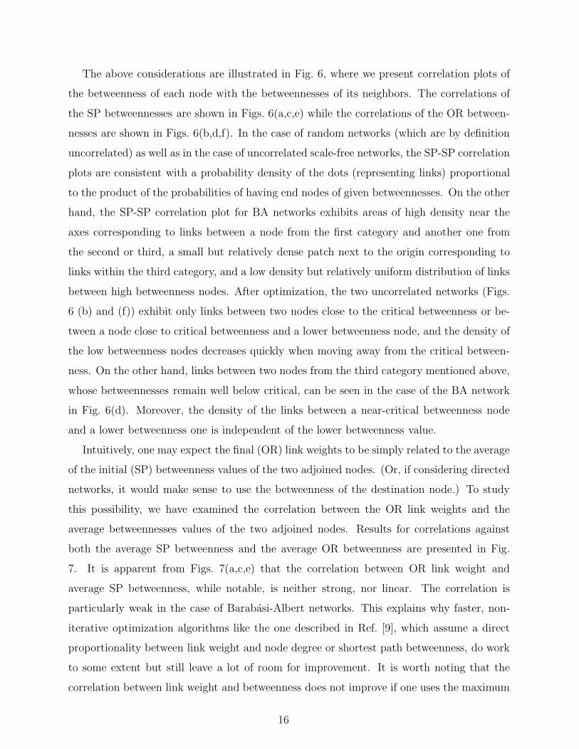
The above considerations are illustrated in Fig. 6, where we present correlation plots of

the betweenness of each node with the betweennesses of its neighbors. The correlations of

the SP betweennesses are shown in Figs. 6(a,c,e) while the correlations of the OR between-

nesses are shown in Figs. 6(b,d,f). In the case of random networks (which are by definition

uncorrelated) as well as in the case of uncorrelated scale-free networks, the SP-SP correlation

plots are consistent with a probability density of the dots (representing links) proportional

to the product of the probabilities of having end nodes of given betweennesses. On the other

hand, the SP-SP correlation plot for BA networks exhibits areas of high density near the

axes corresponding to links between a node from the first category and another one from

the second or third, a small but relatively dense patch next to the origin corresponding to

links within the third category, and a low density but relatively uniform distribution of links

between high betweenness nodes. After optimization, the two uncorrelated networks (Figs.

6 (b) and (f)) exhibit only links between two nodes close to the critical betweenness or be-

tween a node close to critical betweenness and a lower betweenness node, and the density of

the low betweenness nodes decreases quickly when moving away from the critical between-

ness. On the other hand, links between two nodes from the third category mentioned above,

whose betweennesses remain well below critical, can be seen in the case of the BA network

in Fig. 6(d). Moreover, the density of the links between a near-critical betweenness node

and a lower betweenness one is independent of the lower betweenness value.

Intuitively, one may expect the final (OR) link weights to be simply related to the average

of the initial (SP) betweenness values of the two adjoined nodes. (Or, if considering directed

networks, it would make sense to use the betweenness of the destination node.) To study

this possibility, we have examined the correlation between the OR link weights and the

average betweennesses values of the two adjoined nodes. Results for correlations against

both the average SP betweenness and the average OR betweenness are presented in Fig.

7. It is apparent from Figs. 7(a,c,e) that the correlation between OR link weight and

average SP betweenness, while notable, is neither strong, nor linear. The correlation is

particularly weak in the case of Barabasi-Albert networks. This explains why faster, non-

iterative optimization algorithms like the one described in Ref. [9], which assume a direct

proportionality between link weight and node degree or shortest path betweenness, do work

to some extent but still leave a lot of room for improvement. It is worth noting that the

correlation between link weight and betweenness does not improve if one uses the maximum

16

of the betweennesses of the two nodes connected by the link, nor when using an undirected

version of our routing algorithm, which increases only the weights of the links incoming to

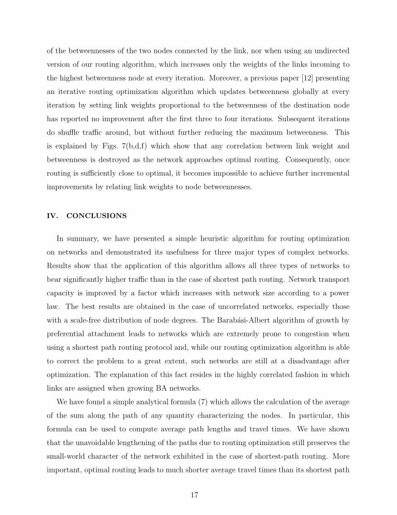
the highest betweenness node at every iteration. Moreover, a previous paper [12] presenting

an iterative routing optimization algorithm which updates betweenness globally at every

iteration by setting link weights proportional to the betweenness of the destination node

has reported no improvement after the first three to four iterations. Subsequent iterations

do shuffle traffic around, but without further reducing the maximum betweenness. This

is explained by Figs. 7(b,d,f) which show that any correlation between link weight and

betweenness is destroyed as the network approaches optimal routing. Consequently, once

routing is sufficiently close to optimal, it becomes impossible to achieve further incremental

improvements by relating link weights to node betweennesses.

IV. CONCLUSIONS

In summary, we have presented a simple heuristic algorithm for routing optimization

on networks and demonstrated its usefulness for three major types of complex networks.

Results show that the application of this algorithm allows all three types of networks to

bear significantly higher traffic than in the case of shortest path routing. Network transport

capacity is improved by a factor which increases with network size according to a power

law. The best results are obtained in the case of uncorrelated networks, especially those

with a scale-free distribution of node degrees. The Barabasi-Albert algorithm of growth by

preferential attachment leads to networks which are extremely prone to congestion when

using a shortest path routing protocol and, while our routing optimization algorithm is able

to correct the problem to a great extent, such networks are still at a disadvantage after

optimization. The explanation of this fact resides in the highly correlated fashion in which

links are assigned when growing BA networks.

We have found a simple analytical formula (7) which allows the calculation of the average

of the sum along the path of any quantity characterizing the nodes. In particular, this

formula can be used to compute average path lengths and travel times. We have shown

that the unavoidable lengthening of the paths due to routing optimization still preserves the

small-world character of the network exhibited in the case of shortest-path routing. More

important, optimal routing leads to much shorter average travel times than its shortest path

17

counterpart at load levels at which a network using SP routing becomes congested, while

the lengthening of the average travel times at low loads is negligible.

Finally, we show that there is no correlation between the optimal weight of a link and the

optimal routing betweenness of the nodes at its ends, and that the correlation is weak and

nonlinear if shortest path betweenness is used. This explains the performance limitations

of previously proposed routing optimization algorithms, which attempt to determine link

weights from node betweennesses. The only way to avoid this limitation is to update link

weights incrementally, and only for the links connecting the node which exhibits the highest

betweenness at the previous iteration.

Acknowledgments

The authors acknowledge support from the NSF through grant No. DMR-0427538 and

also from SI International through A. Williams of the Air Force Research Laboratory Infor-

mation Directorate under contract No. FA8750-04-C-0258.

[1] M. E. J. Newman, SIAM Review 45, 167 (2003).

[2] D. J. Watts and S. H. Strogatz, Nature 393, 440 (1998).

[3] M. Ericsson, M. G. C. Resende, and P. M. Pardalos, Journal of Combinatorial Optimization 6,

299-333 (2002).

[4] B. Fortz and M. Thorup, IEEE Journal on Selected Areas in Communications 20 (4), (2002).

[5] V. Gabrel, A. Knippel, and M. Minoux, Journal of Heuristics 9, 429-445 (2003).

[6] D. Allen, I. Ismail, J. Kennington, and E. Olinick, Journal of Heuristics 9, 375-399 (2003).

[7] E. Mulyana and U. Killat, European Transactions on Telecommunications 16 (3), 253-261

(2005).

[8] B. Danila, Y. Yu, J. A. Marsh, and K. E. Bassler, Phys. Rev. E 74, 046106 (2006).

[9] G. Yan, T. Zhou, B. Hu, Z.-Q. Fu, and B.-H. Wang, Phys. Rev. E 73, 046108 (2006).

[10] S. Sreenivasan, R. Cohen, E. Lopez, Z. Toroczkai, and H. E. Stanley, e-print cs.NI/0604023.

[11] R. Guimera, A. Dıaz-Guilera, F. Vega-Redondo, A. Cabrales, and A. Arenas, Phys. Rev. Lett.

89, 248701 (2002).

18

[12] W. Krause, J. Scholtz, and M. Greiner, Physica A 361 (2), 707 (2006).

[13] P. Echenique, J. Gomez-Gardenes, and Y. Moreno, Phys. Rev. E 70, 056105 (2004).

[14] P. Echenique, J. Gomez-Gardenes, and Y. Moreno, Europhys. Lett. 71, 325 (2005).

[15] L. Zhao, Y.-C. Lai, K. Park, and N. Ye, Phys. Rev. E 71, 026125 (2005).

[16] K. Park, Y.-C. Lai, L. Zhao, and N. Ye, Phys. Rev. E 71, 065105(R) (2005).

[17] Z. Toroczkai and K. E. Bassler, Nature 428, 716 (2004).

[18] Z. Toroczkai, B. Kozma, K. E. Bassler, N. W. Hengartner, and G. Korniss, e-print

cond-mat/0408262.

[19] B. Danila, Y. Yu, S. Earl, J. A. Marsh, Z. Toroczkai, and K. E. Bassler, Phys. Rev. E 74,

046114 (2006).

[20] D. J. Ashton, T. C. Jarrett, and N. F. Johnson, Phys. Rev. Lett. 94, 058701 (2005).

[21] G. Korniss, M. B. Hastings, K. E. Bassler, M. J. Berryman, B. Kozma, D. Abbott, Phys. Lett.

A 350 (5-6), 324 (2006).

[22] M. Anghel, Z. Toroczkai, K. E. Bassler, G. Korniss, Phys. Rev. Lett. 92, 058701 (2004).

[23] G. Korniss, e-print cond-mat/0609098.

[24] P. Erdos and A. Renyi, Publ. Math. (Debrecen) 6, 290 (1959); P. Erdos and A. Renyi, Bull.

Inst. Int. Stat. 38, 343 (1961).

[25] A.-L. Barabasi and R. Albert, Science 286, 509 (1999).

[26] M. Molloy and B. Reed, Random Structures and Algorithms 6, 161 (1995).

[27] T. N. Bui and C. Jones, Inf. Proc. Lett. 42, 153 (1992).

[28] P. Bak, K. Sneppen, Phys. Rev. Lett. 71 (24), 4083 (1993).

[29] S. Boettcher and A. G. Percus, Phys. Rev. Lett. 86 (23), 5211 (2001).

[30] M. E. J. Newman, Phys. Rev. E 64, 016132 (2001).

[31] T. H. Cormen, C. E. Leiserson, R. L. Rivest, and C. Stein, Introduction to Algorithms, 2nd

ed. (MIT Press and McGraw-Hill, 2001).

[32] O. Allen, Probability, Statistics and Queuing Theory with Computer Science Application, 2nd

ed. (Academic Press, New York, 1990).

19