Mathematisches Forschungsinstitut Oberwolfach Report No. 49/2005 Reactive Flow and Transport Through Complex Systems Organised by Cornelius J. van Duijn (Eindhoven) Andro Mikeli´ c (Lyon) Christoph Schwab (Z¨ urich) Oktober 30th – November 5th, 2005 Abstract. The meeting focused on mathematical aspects of reactive flow, diffusion and transport through complex systems. The research interest of the participants varied from physical modeling using PDEs, mathematical model- ing using upscaling and homogenization, numerical analysis of PDEs describ- ing reactive transport, PDEs from fluid mechanics, computational methods for random media and computational multiscale methods. Mathematics Subject Classification (2000): 35B27, 80A32, 76V05, 35R60, 65C30, 65M60. Introduction by the Organisers The workshop Reactive Flow and Transport Through Complex Systems, organized by Cornelius J. van Duijn (Eindhoven), Andro Mikeli´ c (Lyon) and Christoph Schwab (Z¨ urich) was held October 30th–November 5th, 2005. This meeting was attended by over 46 participants with broad geographic rep- resentation from all continents. The theme of the conference, modeling, analysis and numerical simulation of diffusion and transport processes in complex systems, is a response to the need for more accurate, quantitative prediction in a growing number of scientific disciplines, particularly those related to biological applications. Here, simple mathematical models have been found, in particular due to the vastly increased available experimental data from these systems, to offer only inadequate and incomplete understanding of the observed phenomena. This resulted in increased requirements for quantitative, verified predictions from sophisticated mathematical as well as computational models. The continu- ous development of complex mathematical and computational models and their

Welcome message from author
This document is posted to help you gain knowledge. Please leave a comment to let me know what you think about it! Share it to your friends and learn new things together.
Transcript
Mathematisches Forschungsinstitut Oberwolfach
Report No. 49/2005
Reactive Flow and Transport Through Complex Systems
Organised byCornelius J. van Duijn (Eindhoven)
Andro Mikelic (Lyon)
Christoph Schwab (Zurich)
Oktober 30th – November 5th, 2005
Abstract. The meeting focused on mathematical aspects of reactive flow,diffusion and transport through complex systems. The research interest of theparticipants varied from physical modeling using PDEs, mathematical model-ing using upscaling and homogenization, numerical analysis of PDEs describ-ing reactive transport, PDEs from fluid mechanics, computational methodsfor random media and computational multiscale methods.
Mathematics Subject Classification (2000): 35B27, 80A32, 76V05, 35R60, 65C30, 65M60.
Introduction by the Organisers
The workshop Reactive Flow and Transport Through Complex Systems, organizedby Cornelius J. van Duijn (Eindhoven), Andro Mikelic (Lyon) and ChristophSchwab (Zurich) was held October 30th–November 5th, 2005.
This meeting was attended by over 46 participants with broad geographic rep-resentation from all continents.
The theme of the conference,
modeling, analysis and numerical simulation of diffusion and transport processesin complex systems,
is a response to the need for more accurate, quantitative prediction in a growingnumber of scientific disciplines, particularly those related to biological applications.Here, simple mathematical models have been found, in particular due to the vastlyincreased available experimental data from these systems, to offer only inadequateand incomplete understanding of the observed phenomena.
This resulted in increased requirements for quantitative, verified predictionsfrom sophisticated mathematical as well as computational models. The continu-ous development of complex mathematical and computational models and their

2762 Oberwolfach Report 49/2005
verification and validation against available experimental data is a continuoussource of challenges for applied and computational mathematicians.
The complexity of the systems arises from several sources: highly irregulargeometries of membranes and interfaces (as, e.g. in bone marrow, cell membranes,root systems of plants, membrane structures in human organs), physical or chem-ical properties of the systems (e.g., models for spread of pollution in undergroundmedium which has uncertain material properties, where chemical reactions takeplace between constituents, and where strong transport effects on a macroscopicscale coexist with diffusion phenomena at the grain interfaces).
Quantitative mathematical and computational models of such phenomena arenot only essential for a deeper understanding of these systems but, at least equallyimportantly, are a keystone in the development of new technologies which increas-ingly mimic and adapt biological phenomena for industrial purposes (e.g., root-reactor technology for the efficient production of organic compounds, bioinspiredcatalysts for waste processing, to name but a few).
Accordingly, the rather wide scope of the topic of the conference and the blendof researchers working in several areas of applied mathematics was a necessarycondition to review modelling approaches across a number of application areas aswell as across several mathematical disciplines.
Accordingly, during the meeting, talks were presented on homogenization, a-nalysis and computation of multiscale problems, models of porous media, biologicalflow problems, to name but a few.
In addition to the regular presentations, there were three evening sessions orga-nized “on the spot” based on the discussions which started in the first half of themeeting. These were in each case opened by a presentation from a person invitedby the organizers, and were devoted to the topics:
(1) Mathematical Models in Biology – Results and challenges in the mathe-matical modelling of biological systems, (animated by W. Jager, Uni andIWR Heidelberg),
(2) Density driven flows – analytical and computational results and challenges(animated by C. van Duijn, Einhoven and F. Otto, Bonn),
(3) Numerical Models of PDEs with stochastic coefficients (animated by H.Matthies, TU Braunschweig and by C. Schwab, ETH)
The presentations of the experts present at the meeting comprised, naturally,a much wider scope of topics:
• – Flow, transport and reactions in micro-reactors and micro-channels• – Effective laws for processes on surfaces• – Effective laws for transports and reactions in membranes• – Polymer flow through porous media• – Homogenization of processes in networks (neural networks, vessels ..... )• – Overall elastic properties of fiber structures and textiles• – Flow through deformable structures with evolving process depending
geometry• – Growth of crystals, biological structures like dendrites or vessels.

Reactive Flow and Transport Through Complex Systems 2763
• – Flow and transport in bifurcating vessels with rigid and flexible walls• – Effects of walls• – Wall laws and interface laws
These talks touched on advanced mathematical methods from dynamical sys-tems, especially infinite dimensional ones arising with spatially heterogeneousproblems (PDEs), asymptotic analysis, homogenization and averaging methods,numerical multiscale methods, methods from stochastic analysis and statistics.
Apart from advancing disciplinary mathematical methods in these areas, inthe present meeting also qualitatively new mathematical developments emerged:for example, mathematical and computational modelling of PDEs with stochasticdata which are spatially inhomogeneous and do not satisfy stationarity or ergodichypotheses.
In processing experimental data (which becomes increasingly available at lowercost and, e.g. through modern scanning techniques, also at high volume and spatialand temporal resolution) new techniques of image and data processing have to bedeveloped, and the mathematical models of complex systems have to allow forincorporation of statistical data extracted from these experiments.
This has repercussions for the mathematical research and implies that novelalgorithms are needed to generate computational grids adapted to voxel data.
In the last five years mathematicians from analysis, stochastics and numericsstarted cooperation in this interdisciplinary field of research.
New journals specifically devoted to these issues such as the SIAM Journal ofMultiscale Analysis and Simulation, have been successfully launched.
The previous meeting in Oberwolfach ” Multiple Scale Systems - Modeling,Analysis and Numerics ” from July 27 to August 2, 2003, gathered 42 scientists,among them approximately 15 junior scientists, from these areas.
Since multiscale tools are crucial in many of the above themes, in the previousmeeting mainly diffusion problems were treated. Reactive flow and transport,which were central themes in the present meeting, emerged only recently as keyissues.
The meeting was, exactly because of its wide scope, successful particularly incross fertilizing different areas of applied mathematics and also raised a huge num-ber of questions and challenges to participants documenting that the applicationsof mathematics to biological, social and other “complex systems” which has beenemerging in the past years, is in the process of gaining momentum and, moreimportantly, stimulates development of new techniques and approaches in appliedand computational mathematics at an increasing rate.

2764 Oberwolfach Report 49/2005
List of all talks
• Monday, October 31, 2005:– 9h15–10h: Andrea BRAIDES: A Model for a Weak Membrane with
Defects– 10h-10h45: Gregory A. CHECHKIN: Prandtl boundary layer equa-
tions in the presence of rough boundaries– 11h30–12h30: Eduard MARUSIC-PALOKA: Rigorous Justification
of Compressible Reynolds Equation for Gas Lubrication– 16h-16h45: Maria NEUSS-RADU : Homogenization of thin porous
layers and applications to ion transport through channels of biologicalmembranes
– 16h45–17h30: Angela STEVENS: Propagation speed in inhomoge-neous media
– 17h45–18h30: Barbara NIETHAMMER: A statistical mechanics ap-proach for effective theories of domain coarsening
• Tuesday, November 1, 2005– 9h00–9h45: Hermann G. MATTHIES: Computational Approaches
for Stochastic Models in Flow Through Stochastic Porous Media– 9h45-10h30: Assyr ABDULLE: Fully Discrete Heterogeneous Multi-
scale Methods and Application to Transport Problems in Microarrays– 11h–11h45 Radu A. TODOR: Sparse Perturbation Algorithms for
Elliptic Problems with Stochastic Data– 15h30–16h15: Guy BOUCHITTE: Some asymptotic problems on op-
timal transportation.– 16h15-17h: Michel LENZINGER: Viscous fluid flow in bifurcating
channels and pipes– 17h15–18h Rene de BORST: Stability and Dispersion in Damaging
Multiphase Media• Wednesday, November 2, 2005
– 9h00–9h45: Michel KERN: Reactive Flow and Transport ThroughComplex Systems
– 9h45-10h30: Vincent GIOVANGIGLI: Gaseous flows with multicom-ponent transport and complex chemistry
– 11h–11h45 Sorin I. POP: Dissolution and Precipitation in Porous Me-dia
– 11h45 – 12h30: Giovanna GUIDOBONI: Uniqueness of weak solu-tions for a fluid-structure interaction problem

Reactive Flow and Transport Through Complex Systems 2765
• Thursday, November 3, 2005– 9h00–9h45: Bjorn ENQUIST: The Heterogeneous Multiscale Method
for Flow in Complex Systems– 9h45-10h30: Peter KNABNER: Efficient Accurate Simulation of Gen-
eral Reaction Multispecies Transport Processes in Porous Media byReduction and Selective Decoupling
– 10h45–11h30 Raul TEMPONE: Spectral Collocation for Partial Dif-ferential Equations with Random Coefficients
– 11h30-12h15: Leonid BERLYAND: Two analytical models of randomcomposites: polydispersity and correlations
– 15h15–16h: Jerome JAFFRE: Riemann solvers for flows throughrocks changing type
– 16h00–16h45: Ben SCHWEIZER: Averaging of unsaturated flow instochastic porous media
– 16h45-17h30: Rudolf HILFER: Can homogenization solve the upscal-ing problem for 2 phase flow equations in porous media?
– 17h45–18h30 Alain BOURGEAT: Some Problems in upscaling sourceterms in a waste disposal
• Friday, November 4, 2005:– 9h00–9h45: Jerome POUSIN : Order 2 in time schemes for discon-
tinuous reactive terms operator splitting for reaction diffusion with asingular reaction term.
– 9h45-10h30: Peter BASTIAN: ADG method for flow in complex do-mains
– 10h45–11h30 Eric BONNETIER: Can one detect a misplaced inclu-sion in a periodic composite by boundary measurements ?


Reactive Flow and Transport Through Complex Systems 2767
Reactive Flow and Transport Through Complex Systems
Table of Contents
Assyr AbdulleFully Discrete Heterogeneous Multiscale Methods and Application toTransport Problems in Microarrays . . . . . . . . . . . . . . . . . . . . . . . . . . . . . . . . . . 2769
Peter Bastian (joint with Christian Engwer)Solving Partial Differential Equations in Complicated Domains . . . . . . . . . 2771
Leonid BerlyandTwo analytical models of random composites: polydispersity andcorrelations . . . . . . . . . . . . . . . . . . . . . . . . . . . . . . . . . . . . . . . . . . . . . . . . . . . . . . 2775
Eric Bonnetier (joint with Fehmi Ben Hassen)Asymptotics of the potential in a perturbed periodic composite mediumcontaining misplaced inclusions . . . . . . . . . . . . . . . . . . . . . . . . . . . . . . . . . . . . . 2776
Alain Bourgeat (joint with Eduard Marusic-Paloka, Olivier Gipouloux)Some problems in scaling up the source terms in an underground wasterepository model . . . . . . . . . . . . . . . . . . . . . . . . . . . . . . . . . . . . . . . . . . . . . . . . . . 2778
Andrea Braides (joint with Andrey Piatnitski)Variational problems involving percolation . . . . . . . . . . . . . . . . . . . . . . . . . . . . 2782
Rene de Borst (joint with Marie-Angele Abellan)Dispersion and localization in a damaging multi–phase medium . . . . . . . . . 2784
Vincent GiovangigliGaseous Flows with Multicomponent Transport and Complex Chemistry . . 2787
Giovanna Guidoboni (joint with Mariarosaria Padula)Uniqueness of weak solutions for a fluid-structure interaction problem . . . . 2790
R. HilferLaboratory scale capillarity without capillary pressure . . . . . . . . . . . . . . . . . . 2791
Jerome Jaffre (joint with Adimurthi, Siddhartha, Veerappa Gowda)Riemann solvers for two-phase flow through a change in rock type . . . . . . . 2793
Michel Kern (joint with Jocelyne Erhel)Numerical Methods for Chemistry and for Coupling Transport withChemistry in Porous Media . . . . . . . . . . . . . . . . . . . . . . . . . . . . . . . . . . . . . . . . 2795
Michael LenzingerViscous fluid flow in bifurcating channels and pipes . . . . . . . . . . . . . . . . . . . . 2798
Eduard Marusic-Paloka (joint with Maja Starcevic)Rigorous Justification of the Reynolds Equations for Gas Lubrication . . . . 2799

2768 Oberwolfach Report 49/2005
Hermann G. MatthiesComputational Approaches for Flow through Stochastic Porous Media . . . . 2803
Maria Neuss-Radu (joint with Willi Jager)Homogenization of thin porous layers and applications to ion transportthrough channels of biological membranes . . . . . . . . . . . . . . . . . . . . . . . . . . . . 2809
Barbara Niethammer (joint with A. Honig, F. Otto, J. Velazquez)A non-equilibrium statistical mechanics approach to effective theories ofdomain coarsening . . . . . . . . . . . . . . . . . . . . . . . . . . . . . . . . . . . . . . . . . . . . . . . . 2812
I. S. Pop (joint with C. J. van Duijn, V. M. Devigne)Dissolution and precipitation processes in porous media: a pore scale model2814
Jerome Pousin (joint with B. Faugeras)An efficient numerical scheme for precise time integration of adissolution/precipitation chemical system . . . . . . . . . . . . . . . . . . . . . . . . . . . . . 2816
Ben SchweizerOn capillary hysteresis in porous media and the averaging of a play-typehysteresis model . . . . . . . . . . . . . . . . . . . . . . . . . . . . . . . . . . . . . . . . . . . . . . . . . . 2819
Angela Stevens (joint with Fathi Dkhil, Steffen Heinze, George Papanicolaou)Front Propagation in Heterogeneous Media . . . . . . . . . . . . . . . . . . . . . . . . . . 2822
Raul Tempone (joint with Ivo Babuska and Fabio Nobile )Spectral Collocation for Partial Differential Equations with RandomCoefficients . . . . . . . . . . . . . . . . . . . . . . . . . . . . . . . . . . . . . . . . . . . . . . . . . . . . . . 2824
Radu Alexandru TodorSparse Perturbation Algorithms for Elliptic Problems with Stochastic Data2827

Reactive Flow and Transport Through Complex Systems 2769
Abstracts
Fully Discrete Heterogeneous Multiscale Methods and Application toTransport Problems in Microarrays
Assyr Abdulle
Physical systems encompassing a variety of strongly coupled scales pose majorcomputational challenges in terms of analysis modeling and simulation. In thisreport we first discuss a multiscale modeling approach for the transport of par-ticles such as DNA in heterogeneous devices (microarrays). The model involvesa multiscale elliptic equation coupled with a multiscale advection-diffusion equa-tion. We introduce a numerical method for the solution of the coupled system ofequations. We first discuss a new multiscale finite element method for the solu-tion of the elliptic problem. We then explain how it is possible to use an explicitstabilized method (ROCK) for the numerical solution of the stiff system of ordi-nary differential equations of large dimension, originating from the method of linesdiscretization of the advection-diffusion equation.DNA separation in microarrays. We consider a (square) device with periodicasymmetric obstacles and model the transport of injected mixture with concen-tration c(t, x) as an advection-diffusion equation given by
∂cε
∂t+ ∇ · (vεcε) = D∆cε,(1)
where vε = −ρkε∇uε is the velocity field, uε is the electrical potential, kε is theelectrical conductivity and ρ is the charge density of the electrical device. Weassume for simplicity that ρ is constant and set it to one. The obstacles of themicrodevice introduce a typical self-similar structure (which will also be called a“periodic cell”), and we denote by ε the length of these cells. The equation forthe potential uε is given by
−∇ · (kε∇uε) = 0,(2)
with Neumann boundary conditions at the corner of the device and Dirichlet con-ditions at the charged sites of the boundary. The homogenization problem corre-sponding to equations (1) and (2), where the heterogeneous fine scale structure istransferred into a homogeneous large scale model, shows that the heterogeneitiesof the device have no impact on the large scale drift [6]. Thus, the large scaledrift does not depend on the diffusion constant or the molecular weight of theparticles. The heterogeneous microarrays have an impact only on the large scalediffusion. This gives a quantitative explanation of the model proposed in [11],[12]and explain the experimental results of [10]. In [9] transport problems with com-pressible flows are studied and it is shown that for such flows, the large scale driftcan depend on the small scale diffusion coefficient. In the sequel we explain howto solve numerically the coupled equations (1) and (2).Fully discrete finite element heterogeneous multiscale methods. Apply-ing a standard finite element method to the variational form of (2) requires usually

2770 Oberwolfach Report 49/2005
a meshsize h < ε for convergence, i.e., to resolve the small scale of the problem.This lead to a complexity of O(ε−d), where d is the spatial dimension, whichmakes the direct numerical simulation impossible if ε is small. When the dataof the problem are oscillatory with small period, classical two-scale approachesare well established, and the analytical treatment lead to homogenized equations.However, the fine scale behavior, i.e. the oscillations of the solution, are lost inthe homogenization process. It can be recovered through the solution of additional“corrector” problems. But these corrector problems again exhibit rapidly oscillat-ing coefficients so that their accurate numerical solution is as expensive as solvingthe original problem.
In the sequel, we present a new multiscale finite element method for the numer-ical computation of problems with multiple scales. Define a quasi-uniform macrotriangulation TH of the domain Ω, assumed to be a convex polygon. The finiteelement heterogeneous multiscale method (FE-HMM) is based on the followingideas [13],[3],[14],[4].
(1) Associated to the macro triangulation, we define a macro finite elementspace and a modified bilinear form with unknown input data.
(2) Within each macro triangle we define a sampling domain Kε of lengthscale comparable to ε, a micro finite element space and a micro bilinearform based, upon the original multiscale tensor kε, which provides inputdata for the macro problem.
The FE-HMM gives a procedure to obtain an approximation uH of the homoge-nized solution u0, without computing explicitly the homogenized equations. By apost-processing calculation, it is possible to compute an approximation uε,h of thefine scale solution uε of (2) at a much lower cost than solving the original fine scaleproblem. Indeed, we solve the fine scales only in sampling domains of size εd inthe periodic case, within a macro mesh of Ω. Furthermore, the micro problems areindependent and can be solved in parallel. In the non-periodic case, Kε should bechosen as to sample enough information of the local variation of kε. Semi-discreteanalysis of the method has been given in [3],[14]. In these works, the fine-scaleproblem involving the micro solver was assumed to be computed exactly. In [4],the first fully discrete analysis of the FE-HMM has been given. This analysis showthat the macro and the micro meshes have to be refined simultaneously. This hasbeen generalized for elasticity problems in [8].Solving an advection diffusion problem with ROCK methods. Discretiz-ing the advection-diffusion equation by the method of lines leads to a stiff systemof ordinary differential equation of large dimension. Such ODEs, originating fromthe space discretization of (1) are called stiff in the literature [15]. It is also knownthat implicit solver have better stability properties, but at the expense of solvinglinear systems of large dimension if the spatial discretization mesh is small.
Chebyshev methods are a class of explicit one step methods with extendedstability domains along the negative real axis. With such methods, large timesteps can be used. This contrasts with the severe time step restriction given bythe CFL condition for standard explicit methods.

Reactive Flow and Transport Through Complex Systems 2771
Recently, a new strategy to construct higher order Chebyshev methods with“quasi” optimal stability polynomials has been proposed [1],[2]. These methods,called ROCK, together with the FE-HMM have been combined to solve transportproblems described by equations (1) and (2) [5]. The numerical simulation of theDNA transport problem has been addressed in [7].
References
[1] A. Abdulle and A.A. Medovikov, Second order Chebyshev methods based on orthogonalpolynomials, Numer. Math. 90, pp. 1-18, 2001.
[2] A. Abdulle, Fourth order Chebyshev methods with recurrence relation, SISC, Vol.23, No. 6,pp. 2041–2054, 2002.
[3] A. Abdulle and C. Schwab, Heterogeneous Multiscale FEM for Diffusion Problem on RoughSurfaces , SIAM Multiscale Model. Simul., Vol. 3, No. 1, pp. 195–220, 2005.
[4] A. Abdulle, On a-priori error analysis of Fully Discrete Heterogeneous Multiscale FEM,SIAM Multiscale Model. Simul., Vol. 4, No. 2, pp. 447-459, 2005.
[5] A. Abdulle, Multiscale methods for advection- diffusion problems, to appear AIMS, Discreteand Continuous Dynamical Systems, 2005.
[6] A. Abdulle and S. Attinger, Homogenization methods for Transport of DNA particles inHeterogeneous Arrays, Lect. Notes in Comput. Sci. and Eng., Vol. 39, 23-34, 2004.
[7] A. Abdulle and S. Attinger, Numerical Methods for Transport Problems in Microdevices,to appear in Lect. Notes in Comput. Sci.and Eng., 2005.
[8] A. Abdulle, Heterogeneous Multiscale FEM for Problems in Elasticity, to appear in Math.Mod. Meth. in Appl. Sci. (M3AS), 2006.
[9] S. Attinger and A. Abdulle, Effective Velocity for Transport in Heterogeneous CompressibleFlows with Mean Drift, submitted for publication, preprint No. 2005-11, Department ofMathematics, University of Basel.
[10] Chou et al., Sorting biomolecules with microdevices, Electrophoresis, Vol. 21, pp. 81-90,2000.
[11] T.A. Duke and R.H. Austin, Microfabricated Sieve for the Continuous Sorting of Macro-molecules Phys. rev. Lett. Vol. 89, No. 7, 1998.
[12] D. Ertas, Lateral Separation of Macromolecules and Polyelectrolytes in MicrolithographicArrays Phys. Rev. Lett. Vol. 80, No. 7, 1998.
[13] W. E and B. Engquist, The Heterogeneous Multi-Scale Methods, Comm. Math. Sci., Vol. 1,No. 1, pp. 87-132, 2003.
[14] W. E, P. Ming and P. Zhang, Analysis of the heterogeneous multi-scale method for elliptichomogenization problems, J. Amer. Math. Soc. Vol. 18, pp. 121-156, 2004.
[15] E. Hairer and G. Wanner, Solving Ordinary Differential Equations II. Stiff and Differential-Algebraic Problems, Springer Verlag Series in Comput. Math., Vol. 14, Berlin, 1996.
Solving Partial Differential Equations in Complicated Domains
Peter Bastian
(joint work with Christian Engwer)
1. Introduction
Many practical applications require the solution of partial differential equations(PDEs) in complicated domains. We are especially interested in computing theflow around root networks of plants or in the pore space of porous media.

2772 Oberwolfach Report 49/2005
Classical numerical methods require a grid resolving the complicated geometry.Creating such grids is a highly involved process especially if coarse grids and highquality are required. Several methods have been developed that circumvent thisproblem. They are based on the use of a structured background mesh that enclosesthe domain. The Fictitious Domain method [GPP71] discretizes the PDE on thebackground mesh and adds the boundary conditions as additional constraints.This leads in general to a saddle point formulation that might be difficult to solve.The Composite Finite Element method [HS97] constructs piecewise linear basisfunctions on the fine background mesh and truncates them at the true boundary.Coarse grid basis functions for a geometric multigrid solver are constructed ascombinations of fine grid basis functions. This method has been designed withemphasis on the fast solution of the arising linear system.
Our new method is based on the observation that in discontinuous Galerkinfinite element methods the form of the element can be quite arbitrary. Thusthe elements can be taken as the intersection of the structured background meshwith the complicated geometry. Assembling the stiffness matrix then requiresintegration over the interior and boundary of those non-standard elements. Thisis accomplished by constructing a local triangulation within each element. Notethat the local triangulations of different elements are completely independent.
In the following sections we will describe the discontinuous Galerkin finite ele-ment method for an elliptic model problem, the construction of the local triangu-lation and give some numerical results.
2. Discontinuous Galerkin Scheme
Consider the following elliptic model problem in d space dimensions
(1) ∇ · j = f in Ω ⊆ Rd j = −K∇p,
subject to boundary conditions
(2) p = g on ΓD ⊆ ∂Ω, j · n = J on ΓN = ∂Ω \ ΓD.
We approximate the pressure p in the space of discontinuous finite element func-tions of order k
(3) Vk = v ∈ L2(Ω) | v|E ∈ Pk, E ∈ T (Ω)
where T (Ω) = E1, . . . , En is a partition of Ω into non-overlapping elements andPk is the set of polynomials of at most degree k. By Γint we denote the set ofinterior faces of the elements with an arbitrarily chosen normal direction n andΓext is the set of element faces intersecting with the domain boundary.
The finite element problem then reads: Find p ∈ Vk such that
(4) a(p, v) = l(v) ∀v ∈ Vk

Reactive Flow and Transport Through Complex Systems 2773
where the bilinear form is given by
a(p, v) =∑
E∈T (Ω)
∫
E
(K∇p) · ∇v dV +∑
γe∈ΓD
∫
γe
(K∇v) · n p − (K∇p) · n v ds
+∑
γef∈Γint
∫
γef
〈(K∇v) · n〉[p] − 〈(K∇p) · n〉[v] ds
and the right hand side is the linear form
l(v) =∑
E∈T (Ω)
∫
E
f v dV +∑
γe∈ΓN
∫
γe
J v ds +∑
γe∈ΓD
∫
γe
ǫ (K∇v) · n g ds.
Here 〈·〉 denotes the average at the discontinuity and [·] denotes the jump at thediscontinuity. This scheme has been introduced in [OBB98].
3. Local Triangulation Algorithm
The triangulation T (Ω) used in the finite element algorithm is generated by in-tersecting a structured background mesh with the domain Ω as is indicated in thefollowing figure:
∩ Ω............................................................................. ............. ......... ........ ........ ............
..................................................................................... ............... ................. .................. . ............ ..................................................................................................................................................................................................................
....................................................
.................. =............................................................................. ............. ......... ........ ........ ............
..................................................................................... ............... ................. .................. . ............ ..................................................................................................................................................................................................................
....................................................
..................
T (Ω)
.
..............................................................................................................................
. ......................................................................................................................
The bilinear form and right hand side now require the computation of certainintegrals over the interior and boundary of the non-standard elements. This isaccomplished by constructing a triangulation of each element. This is illustratedin the following figure:
.....
.......
.....
.......
.....
.......
........
.....
.......
.....
.......
.....
...
............................................................................
............................................................................
.....
.......
.....
.......
.....
.......
........
.....
.......
.....
.......
.....
...
. ..........................................................................
. ...................
.
............................................
.
.......................................
.....................................
..................................
...............................
.............................
..........................
........................
.....................
...............................................................................
............................................
.....................
.......................
........................
..........................
............................
.....
.......
.....
.......
.....
.......
........
.....
.......
.....
.......
.....
...............................................................................
...............................
................................ ..................
..................................................... .
............
............
.............
.
. ..................................
.
.............................................................................. ............................................................................
............................................................................
............................................................................
.....
.......
.....
.......
.....
.......
........
.....
.......
.....
.......
.....
...
. ...............................................................
.
...............................................................
. ........................................................................................................................................................................
.
........................................................................................................................................................................
. ...................... ..................... .......................................................
.......................
.....................
......................
.
.............................................................................................................................................................................................
.
.............................................................................................................................................................................................
.....
.......
.....
.......
.....
.......
........
.....
.......
.....
.......
.....
...
............................................................................
............................................................................
.....
.......
.....
.......
.....
.......
........
.....
.......
.....
.......
.....
...
. ...............................................................
. ...................................................................................................................................................
.
........................................................................................................................................................................................................
................................
.................................
..................................
..................................
...................................
.
............................................................................................................................................................................................. ............................................................................
............................................................................
............................................................................
.....
.......
.....
.......
.....
.......
........
.....
.......
.....
.......
.....
...
. ......................................................................................................... .
.......................................................................................................... ......................................................
.........................
.........................
..........................
............................
Since the we assume that the geometry of the non-standard element is not too com-plicated and the background mesh is structured we first do an adaptive bisectionand then have a lookup table that generates triangulations for certain standardsituations. Note that curved boundaries are approximated by using parametricelements of order 2. This can lead to non-standard elements having a cusp. Itturns out that the approximation properties of the DG scheme are not harmed alsofor this case. A proof of this is not available yet. In [DFS03] a convergence proof

2774 Oberwolfach Report 49/2005
for DG is given for star-shaped elements. For further details of the triangulationalgorithm we refer to [EB05].
4. Numerical Results
As an example we solve −∆u = f in Ω with u = g on ∂Ω where Ω ⊂ (0, 1)2
is shown in the figure below. The functions f, g are chosen according to a pre-scribed solution u ∈ C∞(Ω). The algorithm has been realized within the softwareframework Dune [BDE+04]. The table below shows that experimental order ofconvergence is optimal when using polynomials of degree k = 3. Note that theerror in the boundary approximation is not included.
.
............................................................................................................................................................................................................................................................................
. ............................................................................................................................................................................................................................................................................
. ............................................................................................................................................................................................................................................................................ .
............................................................................................................................................................................................................................................................................
j
hjih d d
d d
i
i
d dd d i
dd
dd
0
1
1
Mesh EOC L2 EOC H1
16×16 3.73 2.9032×32 3.94 2.9564×64 3.93 2.96
128×128 3.98 2.98
References
[BDE+04] P. Bastian, M. Droske, C. Engwer, R. Klofkorn, T. Neubauer, M. Ohlberger, andM. Rumpf. Towards a unified framework for scientific computing. In Proceedingsof the 15th Conference on Domain Decomposition Methods, LNCSE, 40:167–174.Springer-Verlag, 2004.
[DFS03] V. Dolejsı, M. Feistauer, and V. Sobotıkova. Analysis of the Discontinuous GalerkinMethod for Nonlinear Convection–Diffusion Problems. Preprint, 2003. SubmittedComput. Methods Appl. Mech. Eng.
[EB05] C. Engwer and P. Bastian. A Discontinuous Galerkin method for simulations in com-plex domains. IWR-Preprint, 2005.
[GPP71] Roland Glowinski, Tsorng-Whay Pan, and Jacques Periaux. A fictitious domainmethod for the Dirichlet problem and applications. Computer Methods in AppliedMachanics and Engineering, 8(4):722–736, 1971.
[HS97] W. Hackbusch and S. A. Sauter. Composite Finite Elements for the Approximationof PDEs on Domains with complicated Micro-Structures. Num. Math., 75:447–472,1997.
[OBB98] J. T. Oden, I. Babuska, and C. E. Baumann. A discontinuous hp-finite elementmethod for diffusion problems. Journal of Computational Physics, 146:491–519, 1998.

Reactive Flow and Transport Through Complex Systems 2775
Two analytical models of random composites: polydispersity andcorrelations
Leonid Berlyand
In this talk we discuss mathematical models of heterogeneous materials withrandom microstructure amenable to rigorous mathematical analysis when analyt-ical solution in some form can be obtained.
We distinguish two classes of such models:(A) simple (e.g., linear) PDE (constitutive law) with complex geometry (e.g.
disordered arrays of densely packed particles of various sizes and shapes)(B) complex (e.g. nonlinear) PDE or variational problem with simple geometry
We first present a problem from class (A) which models increase and decrease ofthe effective conductivity of two phase random composites due to polydispersity.Here we present a two–dimensional mathematical model of a composite materialwith conducting inclusions (fibers) randomly embedded in a matrix. Our main ob-jective is to study how polydispersity (two different sizes of particles) affects theoverall conductivity of the composite. If the conductivity of inclusions is higherthan the conductivity of the matrix, then previous studies suggest an increase ofthe effective conductivity due to polydispersity. We prove that for high volumefraction when inclusions are not well–separated and percolation effects play a sig-nificant role, polydispersity may result in either an increase or decrease of theeffective conductivity. This is a joint work with V. Mityushev [1].
Next we present a model of a laminated random polycrystal with n grains. Theorientation of each grain is given by an uncorrelated random sequence of the orien-tation angles θi, i = 1, · · · , n. Under the imposed boundary conditions each grainundergoes a stress free transformation that depends on its orientation angle andresult in transformation strains ǫT
i , i = 1, ·, n. The sequence of random variablesǫTi , i = 1, ·, n is obtain as the solution of a nonlinear optimization (variational)
problem.While the random variables θi, i = 1, · · · , n are uncorrelated, the random vari-
ables ǫTi , i = 1, ·, n may or may not be correlated – this is the central issue of
our analysis. We investigate this rise of correlations in three different scaling lim-its. Our proofs use the de Finetti’s Theorem as well as the Riesz rearrangementinequality. This is a joint work with O. Bruno and A. Novikov [2].
References
[1] Berlyand, L. V., V. Mityushev, Increase and Decrease of the Effective Conductivity ofTwo Phase Composites due to Polydispersity, Journal of Statistical Physics, 118, 3/4 pp479-507 (2005)
[2] Berlyand, L., Bruno, O., Novikov, A., Rise of correlations of transformation strains inlaminated random polycrystals, preprint.

2776 Oberwolfach Report 49/2005
Asymptotics of the potential in a perturbed periodic compositemedium containing misplaced inclusions
Eric Bonnetier
(joint work with Fehmi Ben Hassen)
We consider a conduction problem for a composite material made of identicalinclusions of conductivity 0 < k < ∞, k 6= 1, embedded in a matrix of conductivity1. In a reference configuration, the medium lies in a smooth bounded domain Ω ⊂R3 and the distribution of the inclusions is perfectly periodic. If Y = [0, 1]3 andD ⊂ Y , the associated conductivity has the form aε(x) = a(x/ε), x ∈ Ω, wherea is the Y –periodic function equal to k in D and to 1 in Y \ D.
Given Neumann boundary data g ∈ L2(∂Ω), such that
∫
∂Ω
g = 0, the potential
uε solves
(1)
div(aε(x)∇uε) = 0 in Ω,aε(x)∂nuε = g on ∂Ω∫
∂Ω uε = 0.
We compare this reference configuration to a medium where one of the inclusionshas been misplaced: Instead of ωε,1 = ε(p + D), the p–th inclusion occupies theset ωε,2 = ε(p + δ + D). We assume that |δ| = O(1), that the p–th inclusion isO(1) away from the boundary ∂Ω, and that, in its modified position, it does notintersect another inclusion. The conductivity of the perturbed configuration isdenoted by aε,d and we have
aε,d(y) =
aε(y) in Ω \ ωε,1 in ωε,1 \ ωε,2,k in ωε,2,
where ωε = ωε,1∪ωε,2. The corresponding potential, uε,d solves (1), with coefficientaε,d instead of aε.
We view the misplaced inclusion as a defect in the composite, compared to aperfectly periodic medium. We are interested in comparing the potentials uε,d
and uε, far from ωε, to study if one could detect such periodicity defect usingboundary measurements. To this end, we give an asymptotic expansion for uε,d −uε, as ε → 0. We present the result in the case of a single misplaced inclusion.However, our analysis extends to more general situations where the periodicitydefects are localized and of size comparable to the period (for instance inclusionswith conductivities different from k).
Let A∗ denote the matrix of homogenized coefficients, defined by
A =
∫
Y
a(y) (I + ∇χ(y)) dy,

Reactive Flow and Transport Through Complex Systems 2777
in terms of the solutions χ ∈ (W 1,2# (Y ))3 of the cell problems
−div(a(y)∇(χ(y) + y)) = 0 in R3∫
Yχ(y) dy = 0.
Let u∗ denote the solution to the homogenized equation
div(A∗∇u∗) = 0 in Ω,A∗∇u∗ · n = g on ∂Ω∫
∂Ωu∗ = 0,
and let Gε (resp. G∗) be the Green’s functions, vanishing on ∂Ω, of the periodic(resp. homogenized) medium.
Theorem 1. Assume that D has a smooth boundary (C 1+α for some α > 0) andthat ωε is centered at the origin. Then, for |x| >> ε, we have
uε,d(x) − uε(x) +
∫
∂Ω
∂nGε(x, y) (uε,d(y) − uε(y)) dσ(y)
= ε3 M : ∇u∗(0) ⊗∇G∗(0, x) + o(ε3).(2)
The matrix M in (2) is a polarization tensor, that accounts at first order forthe presence of a defect: for 1 ≤ i, j ≤ 3,
Mij =
∫
∂ω
(a−
a−d
− 1)(yi + χi(y))
(a+(y)
∂ϕ+j
∂νy+ a−(y)
(νj +
∂χj(y)
∂νy
))dσy ,
where ad(y) = aε,d(εy), and where the auxiliary functions ϕj are defined by
div(ad(y)∇(ϕj(y) + yj + χj(y))) = 0 in R3,lim|y|→∞ ϕj(y) = 0.
The expansion (2) has the same structure as that derived in [5] where pertur-bations of the potential are caused by small inclusions in a smooth backgroundreference medium (see also [1] and the references therein). In our case, it is theGreen’s function of the homogenized medium that appears on the right–hand side,its singularity signaling the presence of a periodicity defect. This may prove in-teresting for detection purposes, using a MUSIC type algorithm, as in the case ofa reference medium with constant coefficients [4].
The proof of (2) relies on pointwise estimates on the periodic potential and onits gradient, which are independent of ε [3]. The proof uses the ‘3 steps compact-ness method’ of M. Avellaneda and Fang Hua Lin, who gave such estimates forelliptic operators with smooth coefficients [2]. The smoothness assumption canbe loosened, as shown by L. Nirenberg and YanYan Li [6], using the fact that, ina composite medium made with C 1+α inclusions, the gradient of the potential isbounded, independently of the distance between the inclusions. These results maybe adapted to obtain the following pointwise estimates on the Green’s functions

2778 Oberwolfach Report 49/2005
Theorem 2. Let ω ⊂⊂ Ω ⊂ R3 and 0 < r < diam(ω)/4. There is a positiveconstant C, independent of ε, such that, for all B(y, r) ⊂ ω,
‖Gε(., y) − G∗(., y)‖L∞(ω\B(y,r)) ≤ Cε1/4,
‖∇xGε(., y) − (I + ∇χ(./ε))∇xG∗(., y)‖L∞(ω\B(y,r)) ≤ Cε1/4.
References
[1] H. Ammari and H. Kang, Reconstruction of Small Inhomogeneities from Boundary Mea-surements, Lecture Notes in Mathematics, vol. 1846, Springer-Verlag, Berlin (2004).
[2] M. Avellaneda and F.H. Lin, Compactness methods in the theory of homogenization, Comm.Pure Appl. Math., 40 (1987) 803–847.
[3] F. Ben Hassen and E. Bonnetier, An asymptotic formula for the voltage potential in aperturbed ε–periodic composite medium containing misplaced inclusions of size ε, Proc.Royal Soc. Edinburgh A (2005) to appear.
[4] M. Bruhl, M. Hanke and M. Vogelius, A direct impedance tomography algorithm for locatingsmall inhomogeneities, Numerische Mathematik, 93 (2003) 635–654.
[5] D.J. Fengya, S. Moskow and M. Vogelius, Identification of conductivity imperfections ofsmall diameter by boundary measurements. Continuous dependence and computational re-construction, Inverse Problems, 14 (1998) 553–595.
[6] Y. Y. Li and L. Nirenberg, Estimates for elliptic systems from composite material, Comm.Pure Appl. Math., 56 (2004), 892–925.
Some problems in scaling up the source terms in an undergroundwaste repository model
Alain Bourgeat
(joint work with Eduard Marusic-Paloka, Olivier Gipouloux)
Introduction
We are interested in ρ(x, t)the evolution in time of the density of some quantity,such as heat or chemical concentration, which is transported by diffusion andconvection from a ”sources site” made of a large number of similar ”local sources”.This type of modeling could, for instance, describe contaminants transport andmigration in aquifers from a long-lived nuclear waste underground repository.
General Equations. The process is described by a diffusion convection typeequation:
(1) Rω∂ρ
∂t−∇ · (A∇ρ) + (V · ∇)ρ + λRωρ = 0
• R the latency retardation factor,• ω the porosity,• v the Darcy’s velocity
• λ =log2
T ; T the element radioactivity half life time.

Reactive Flow and Transport Through Complex Systems 2779
There are at least three levels where there is a need for scaling up the abovemodel , from a detailed description to a global model: - from Waste Packagesto a Storage Unit model (see [1],[2]) - from Storage Units to a Zone model(see [3]) - from similar Zones to a Repository Site global model.
From the Storage Units to a Zone Global Model
The technique and the results herein after (see [1],[2])would be the same for thescaling up from “Similar Zones” to a “ Repository Site model” .
The Equations. For seek of simplicity, we will assume R = 1.
ωε ∂ϕε
∂t− div (Aε∇ϕε) + (vε · ∇ )ϕε + λωε ϕε = 0 in ΩT
ε(2)
ϕε(0, x) = ϕ0(x) x ∈ Ωε(3)
n · σ = n · (Aε∇ϕε − vε ϕε) = Φ(t) on ΓTε(4)
ϕε = 0 on S1,(5)
n · (Aε∇ϕε − vε ϕε) = 0 on S2 ;(6)
with
(7) Aε(x2) = A(x2
ε); vε(x, t) = v(x,
x2
ε, t); ωε(x2) = ω(x2/ε).
A priori Energy estimates and Homogenized equation.The following a priori estimates:
ϕε ϕ weak* in L∞(0, T ; L2(Ω))(8)
∇ϕε ∇ϕ weakly in L2(0, T ; Lβ∗(Ω))(9)
with
ϕ ∈ L2(0, T ; H1(Ω)) L∞(0, T ; L2(Ω)), and β∗ =2β
3β − 2.
And ϕ is then the solution of:
ω2 ∂ϕ
∂t− div (A2∇ϕ) + (v2 · ∇)ϕ + λω2 ϕ = 0 in ΩT(10)
ϕ(x, 0) = ϕ0(x) x ∈ Ω = Ω\Σ(11)
ϕ = 0 on S1(12)
n · (A2∇ϕ − v2 ϕ) = 0 on S2(13)
[ϕ] = 0 ,[e2 · (A2∇ϕ − v2 ϕ)
]= −|M |Φ on Σ ,(14)
where [·] denotes the jump over Σ, and |M | stands for the limit of a storage unit
area; (Mε) area = |M | + O(εβ−1)
Remark 1. We do not need exact periodicity in space, of the units; the sameproof holds whenever each unit is randomly placed in a mesh of an ε– net. Theunits do not even need to have the same shape as long as their thickness is smallenough (≪ ε).

2780 Oberwolfach Report 49/2005
The above result may be extended to a general case where the flux Φ depends alsoon the space Φ(x, t) and the units have different shapes Mε(x); then the right handside of (14) would have to be replaced by lim
ε→0|Mε(x)|Φ(x′, t).
Asymptotic expansion and Matching for the Short time.We define first the Matched Expansion:
(15) Fε =
ϕ0ε in Ω\Gε ; ( Outer Expansion)
ϕ0ε + ε
(χk
ε(x
ε)∂ϕ0
ε
∂xk+ wε(
x
ε)Φ − ϕ0
ερkε(
x
ε)v1
k
)in Gε ;
where Gε is the Inner Layer and the functions χkε , ρk
ε and wε are 1-periodic solutionsof three auxiliary stationary diffusion type problems posed in an infinite strip.
Theorem 1. For any 0 < τ < 1 there exists a constant Cτ > 0 non dependant onε, such that
(16) |ϕε − Fε|L2(0,T ;H1(Bε)) ≤ Cτ ετ ,
where Bε = Ω\∂Gε.The same estimate holds in L∞(0, T ; L2(Ωε)) norm.
Remark 2. The expansion (15) clearly points out two important terms: the zeroorder term ϕ0
ε and the first order term ε wε(xε )Φ .
On one hand the diffusion in the low permeable layer around the units is smalland on the other hand the leaking is intensive during a short time; then duringthis short time, the first order term ε wε(
xε )Φ will dominate in ϕε; and after
this short time the diffusion will become dominant, i.e. ϕ0ε will become the most
important term in the expansion.
From Waste Packages to a Storage Unit Global Model, with a
possibly damaged zone
We are now seeking a mathematical model describing the global behavior of oneStorage Unit(see [3]); assuming it is made of a high number of Waste Packages(or containers sets), lying on a hypersurface Σ and linked by parallel backfilleddrifts ; all the parallel drifts being connected at the top to a main gallery, alsobackfilled. (see [3])All the repository is embedded in a low permeability layer, called host layer . Asin the previous section, for simplicity, we assume the convection field (Hydrologyregime) is given.Denoting ε the ratio between the width of a unit and the distance between twodrifts; then in the renormalized model there are three scales: O(1) for a disposalunit scale, O(ε) for both the scale of a containers row and the drifts period, andO(εγ),γ close to three, for the Waste Packages diameter.

Reactive Flow and Transport Through Complex Systems 2781
The Model and Equations. The Darcy’s velocity is:
vε(x) =
vh(x) in the host rock Ωε\ Sε
ε−β vd(x′, x2/ε; x3/ε) in the drifts Sε;
the Diffusion/Dispersion is:
Aε(x) =
Ah(x) in the host rock Ωε\Sε
d(x) I + ε−β Ad(x2, x2/ε, x3/ε) in the drifts Sε.
And, because the convection in a storage unit goes mainly in the direction of thedrifts, we assume
Ad(x2, y2, y3) = a(x2, y2, y3) ( e1 ⊗ e1. )
With the above assumptions the ”Microscopic” model of a Storage Unit is:
ωε ∂ϕε
∂t− div (Aε∇ϕε) + (vε · ∇ )ϕε + λωε ϕε = 0 in ΩT
ε(17)
ϕε(0, x) = ϕ0(x) x ∈ Ωε(18)
n · (Aε∇ϕε − vε ϕε) = Φε(t) on ΓTε(19)
n · (Aε∇ϕε − vε ϕε) = κ (ϕε − gε) on KTε ∪ HT
ε(20)
ϕε = 0 on ZTε .(21)
with HTε the drifts Tops surface, ZT
ε the drifts (sealed) Bottoms , KTε the rest of
the exterior boundary of Ω, and ΓTε the Waste Packages boundary ×(0, T ).
Remark 3. In the above model, gε will measure the concentration entering at thedrifts tops; and ε−β the Darcy’s velocity range inside the drifts.
Results. Depending on β (the Darcy’s velocity range), with a proper rescaling ofthe source flux and of the concentration on the shafts tops, we have three differentglobal behavior :
• With 0 ≤ β < 1 ,
The shafts do not make any contribution, the repository behaves as if they werenot there. Mainly ϕε → ϕ the unique solution of a problem, similar to the Ho-mogenized equation obtained in the previous section 10- 14, i.e. of same type asthe microscopic problem.
• With β = 1
and a source term, limε→0 Φε(t) = Φ(t) uniformly in t , and some concentration,gε = ε−1 gd , entering the shafts tops Hε.This model could be seen as representing connected shafts, galleries and driftswith damaged sealings. The transport processes, inside and outside the ”damaged”shafts are comparable and there is a strong interaction between them. The solutionof the Microscopic model ϕε → ϕ weakly in L2(0, T ; W 1,γ∗
(Ω)) and ϕε−→ϕ0 =

2782 Oberwolfach Report 49/2005
ϕ(x1, x2, 0), dµε(x)2 − scale, [4], where ϕ is the unique solution of a coupledproblem:
ωh ∂ϕ
∂t− div (Ah ∇ϕ) + (vh · ∇)ϕ + λωh ϕ = 0 in ΩT ;(22)
ϕ(0, x) = ϕ0(x)in Ω;(23)
n · (Ah ∇ϕ − vh ϕ) = κ(ϕ − gh) on ST(24)
[e3 · (Ah ∇ϕ − vh ϕ)] = −MΦ− ∂
∂x1(〈a〉∂ϕ0
∂x1) + 〈vd
1〉∂ϕ0
∂x1on ΣT(25)
〈a〉∂ϕ0
∂x1(t, L, x2, 0) + 〈vd
1〉ϕ0(t, L, x2, 0) = κgd.(26)
• With 2 > β > 1
and a sufficiently strong source and some concentration entering the drifts tops
gε = ε−β+1
2 gd on Hε; then the transport process in the drifts is dominant andwe do not see anything else in the corresponding global model . We have then:ε(1−β)/2 ϕε−→φ, dµε(x)2 − scale,[4], to the global concentration ϕ0, the uniquesolution of a 1-dimensional problem for any x ∈]0, L[ :
− ∂
∂x1
(Ad
11
∂ϕ0
∂x1
)+ vd
1
∂ϕ0
∂x1= 0 in ]0, L[(27)
ϕ0(0) = 0 , Ad11
∂ϕ0
∂x1(L) + (vd
1 + κ)ϕ0(L) = κgd .
References
[1] Bourgeat A., Gipouloux O.,Marusic-Paloka E., Mathemeatical modelling of an arrayof underground waste containers, C.R..Acad.Sci.Paris , Mecanique, 330 (2002), 371-376.
[2] Bourgeat A., Gipouloux O.,Marusic-Paloka E., Modeling of an underground wastedisposal site by upscaling, Math.Meth.Appl.Sci. , 27 (2004), 381-403.
[3] Bourgeat A., Marusic-Paloka E., A homogenized model of an underground waste repos-itory including a disturbed zone, SIAM J. on Multiscale Modeling and Simulation, Vol.3,Number4 (2004) , 918 - 939.
[4] Bourgeat A., Chechkin G., Piatnitski A., Singular double porosity model, Appl.Anal., Vol82, No 2 (2003), 103-116.
Variational problems involving percolation
Andrea Braides
(joint work with Andrey Piatnitski)
In a recent paper [5] Braides and Piatnitski have studied the problem of describingthe overall properties of a discrete membrane in which a random distribution of‘defects’ is taken into account. The free energy of this two-dimensional discrete

Reactive Flow and Transport Through Complex Systems 2783
membrane with a bounded open set Ω ⊂ R2 as reference configuration is modelled
by a functional
(1) Eε(u) =1
2
∑
|i−j|=ε
φεij(ui − uj),
where u : εZ2 ∩ Ω → R. The small positive parameter ε is introduced so thataveraged properties of Eε are described by its Γ-limit F (see e.g. [3, 1]).
The functions φεij may take two forms:
(1) (strong springs) φεij(z) = z2. If only strong springs are present Eε is nothing but
a finite-difference approximation of the Dirichlet integral, and F (u) =∫Ω |∇u|2 dx
is defined on H1(Ω);(1) (weak springs) φε
ij(z) = minz2, ε. In terms of the difference quotient we maywrite
(2) φεij(u
i − uj) = εf(ε(ui − uj
ε
)2)=
(ui − uj)
2 ifui−uj
ε ≤ 1√ε
1 otherwise,
where f(w) = min|w|, 1.The case when
(3) φεij(z) =
εf(εz2) with probability p
z2 with probability 1 − p
is considered. This can be done by introducing suitable i.i.d. random variables(see [5]) corresponding to a bond-percolation model (see e.g. [6]). With fixed arealization ω we will write Eω
ε to highlight the fixed choice of φεij in terms of ω,
and Fω the corresponding Γ-limit. The case p < 1/2 (subcritical regime) had beencompletely solved in [5] by showing that in that case the effect of the weak springsis almost surely negligible and the Γ-limit is simply the Dirichlet integral. Thefollowing theorem settles the supercritical case, improving the results in [5].
Theorem (Braides and Piatnitski). If p > 1/2 then the limit is finite inthe Ambrosio and De Giorgi’s space of generalized special functions with boundedvariation GSBV (Ω) (see [2]) and there exists gp ≤ c < +∞ such that almostsurely
(4) Fω(u) =
∫
Ω
|∇u|2 dx +
∫
S(u)
gp(ν) dH1
for u ∈ GSBV (Ω). Here, S(u) denotes the set of discontinuity points for u and νits measure-theoretical normal.
Remark. (i) the definition of gp is obtained as follows (we sketch the definition):with fixed a realization ω consider k, k′ in the ‘weak cluster’, and for such pairsdefine the distance dω(k, k′) as the minimal path within the weak cluster joining
the two points. Then it can be proved that as k, k′ → +∞ and (k−k′)|k−k′| → ν the ratio
dω(k, k′)/|k − k′| converges to a limit gp(ν), and gp is almost surely independentof ω;

2784 Oberwolfach Report 49/2005
(ii) the main technical point to prove the theorem above is an ‘optimality’lemma. Again loosely speaking, this asserts that almost surely if we have k − k′
large enough and we have a path joining the two points with length less than(gp((k − k′)/|k − k′|)− δ)|k − k′| then there exists a fixed proportion Lδ > 0 suchthat the number of strong connections within that path exceeds Lδ|k − k′|.
The theorem above was presented as a conjecture in [4], and will be includedin an improved version of [5].
References
[1] R. Alicandro and M. Cicalese, Representation result for continuum limits of discrete energies
with superlinear growth. SIAM J. Math. Anal. 36 (2004), 1-37[2] L. Ambrosio, N. Fusco and D. Pallara, Functions of Bounded Variation and Free Disconti-
nuity Problems, Oxford University Press, Oxford, 2000.[3] A. Braides, Γ-convergence for Beginners, Oxford University Press, Oxford, 2002.[4] A. Braides, Discrete membranes with defects. Oberwolfach Reports 1 (2004), 1553–1555.[5] A. Braides and A. Piatnitski. Overall properties of a discrete membrane with randomly
distributed defects. Preprint 2004 (available at: http://cvgmt.sns.it)[6] H. Kesten, Percolation Theory for Mathematicians. Progress in Probability and Statistics
2. Birkhauser, Boston, 1982
Dispersion and localization in a damaging multi–phase medium
Rene de Borst
(joint work with Marie-Angele Abellan)
For a fluid–saturated, one–dimensional continuum, the balances of momentumand mass read in an incremental format, e.g. [1] for a complete derivation:
(1)∂σs
∂x+ nfK−1(vf − vs) − ρs
∂vs
∂t− ρf
∂vf
∂t= 0
and
(2) α∂2vs
∂x2+ nf
(∂2vf
∂x2− ∂2vs
∂x2
)− nf(KQ)−1
(∂vf
∂t− ∂vs
∂t
)= 0
They are supplemented by the kinematic relation and the incremental stress–strainrelation, which, after combination, read:
(3) σs = Etan ∂us
∂x
with Etan the tangential stiffness modulus of the solid.To analyse the characteristics of wave propagation in the two–phase medium
defined in the preceding section, a damped, harmonic wave is considered:
(4)
(δus
δuf
)=
(As
Af
)exp (λrt + i(kx − ωt))
with λr representing the damping and ω the angular frequency. Substitution ofthis identity into eqs (1)–(2), using eq. (3), requiring that a non-trivial solution

Reactive Flow and Transport Through Complex Systems 2785
can be found for the resulting set of homogeneous equations and decomposing intoreal and imaginary parts leads to:
(5) 8λ3r + 8ak2λ2
r + 2(a2k2 + b)k2λr + (ab − c)k4 = 0
and
(6) ω2 = 3λ2r + 2ak2λr + bk2
with
(7) a =KQ(ρs + (nf − α)ρ′f )
ρs + ρf, b =
Etan + αQ
ρs + ρf, c =
KQEtan
ρs + ρf
Evidently, wave propagation is dispersive, since eq. (6) is such that the phasevelocity cf = ω/k is dependent on the wave number k, cf. [2, 3]. Taking the longwave–length limit in eq. (5), i.e. k → 0, yields λr → 0. According to eq. (6)and after substitution of eq. (7b), we obtain an explicit expression for the phasevelocity:
(8) cf =ω
k=
√Etan + αQ
ρs + ρf
Using Cardano’s formulas, eq. (5) can be solved explicitly. For the short wave-length limit, i.e. when k → ∞, we obtain that the discriminant D → 0, whichidentifies the existence of three real roots for λr in this limiting case, two of thembeing equal. For the single root we obtain that λr → 0. This implies that thissolution has no damping properties and, therefore, gives no regularization. Forthe double root we find that λr ∼ −k2. From eq. (6) the expression for the phasevelocity then becomes proportional to the wave number, cf ∼ k (please note thatfor strain softening cf will normally be imaginary). In view of eq. (4) and inanalogy with a single–phase rate–dependent medium [4], an internal length scalecan be defined as:
(9) ℓ = limk→∞
(− cf
λr
)∼ lim
k→∞k−1 = 0
which indicates that the internal length scale ℓ vanishes in the short wave–lengthlimit.
1. NUMERICAL EXAMPLES
To verify and elucidate the theoretical results of the preceding section, a finitedifference analysis has been carried out. The spatial derivatives in eqs (1) and (2)have been approximated with a second–order accurate finite difference scheme.Explicit forward finite differences have been used to approximate the temporalderivatives, which is first-order accurate. The choice for a fully explicit time inte-gration scheme was motivated by the analysis of Benallal and Comi [3], in whichthey showed that in this case no numerical length scale was introduced in the

2786 Oberwolfach Report 49/2005
analysis, apart from the grid spacing. As implied in eqs (1) and (2) the veloci-ties vs and vf of the solid skeleton and the fluid have been taken as fundamentalunknowns and the displacements have been obtained by integration.
σ σ
εε
σ
t
0
u
σy
t0
Figure 1. Applied stress as function of time (left) and localstress–strain diagram (right)
.
All calculations have been carried out for a bar with a length L = 100 m.For the solid material, a Young’s modulus E = 20 GPa and an absolute massdensity ρ′s = 2000 kg/m3 have been assumed. For the fluid, an absolute massdensity ρ′f = 1000 kg/m3 was adopted and a compressibility modulus Q = 5 GPawas assumed. As regards the porosity, a value nf = 0.3 was adopted and in thereference calculations α = 0.6 and the permeability K = 10−10 m3/Ns. In allcases, the external compressive stress was applied according to the scheme shownin Figure 1, with a rise time t0 = 0.05 s to reach the peak level σ0 = 1.5 MPa. Atime step ∆t = 0.5 · 10−3 s was adopted, which is about half the critical time stepfor this explicit scheme.
0 10 20 30 40 50 60 70 80 90 100x [m]
1
2
3
4
5
6
stra
in [x
0.0
001]
0 10 20 30 40 50 60 70 80 90 100x [m]
1
2
3
4
5
6
stra
in [x
0.0
001]
Figure 2. Strain profiles along the bar for 101 (left) and 126(right) grid points and time step ∆t = 0.5 · 10−3 s
.
Upon reflection at the right boundary, the stress intensity doubles and the stressin the solid exceeds the yield strength σy = 2.5 MPa and enters a linear descendingbranch with an ultimate strain ǫu = 1.125·10−3, see Figure 1. Figure 2 (left) showsthat a Dirac–like strain distribution develops immediately upon wave reflection.

Reactive Flow and Transport Through Complex Systems 2787
This is logical, since a standard two–phase medium does not have regularizingproperties. To further strengthen this observation the analysis was repeated witha slightly refined mesh (126 grid points), which resulted in a marked increase ofthe localized strain (Figure 2 – right), which has been plotted on the same scaleas the results of the original discretization in Figure 2. In [1] it has been shownthat also the time step strongly influences the results, cf. [3].
References
[1] M.-A. Abellan and R. de Borst. Wave propagation and localisation in a softening two–phasemedium. Comp. Meth. Appl. Mech. Eng., accepted for publication.
[2] H.W. Zhang, L. Sanavia and B.A. Schrefler. An internal length scale in dynamic strainlocalization of multiphase porous media. Mech. Coh.-frict. Mat. 4 (1999) 445–460.
[3] A. Benallal and C. Comi. On numerical analyses in the presence of unstable saturated porousmaterials. Int. Journal Num. Meth. Eng. 56 (2003) 883–910.
[4] L.J. Sluys and R. de Borst. Wave propagation and localisation in a rate-dependent crackedmedium — Model formulation and one-dimensional examples. Int. J. Sol. Struct. 29 (1992)2945–2958.
Gaseous Flows with Multicomponent Transport and ComplexChemistry
Vincent Giovangigli
Multicomponent reactive flows with complex chemistry and detailed transportphenomena arise in various engineering applications such as combustion, crystalgrowth, atmospheric reentry, or chemical reactors. This is a strong motivation forinvestigating the corresponding governing equations and analyzing their mathe-matical structure and properties [7].
We discuss the governing equations for multicomponent reactive flows as ob-tained from the kinetic theory of gases [4, 7]. These equations can be split intoconservation equations, expressions transport fluxes, transport coefficients, andthermochemistry. The evaluation of transport coefficients—which are not explic-itly given by the kinetic theory—requires solving transport linear systems. Themathematical structure of the transport linear systems has been investigated andhas led to fast and accurate iterative solutions as well as direct inversions [3, 7].A powerful library of computer programs for evaluating multicomponent trans-port coefficients is available at the Authors’s web site for academic purposes. Themathematical properties of the transport coefficients can also be obtained fromthat of the transport linear systems [11, 6, 9].
We next investigate the Cauchy problem and obtain global existence theoremsaround constant equilibrium states as well as asymptotic stability and decay esti-mates [13, 11]. The system of partial differential equations is first symmetrized byusing entropic variables and then rewritten in normal form, that is, in the form ofa hyperbolic–parabolic composite system. All normal forms can also be character-ized when the nullspace naturally associated with dissipation matrices is invariant.

2788 Oberwolfach Report 49/2005
Global existence in then obtained by using entropic estimates and local dissipa-tivity properties of linearized equations. In particular, the linearized normal formis strictly dissipative and the chemistry source terms are locally stable.
On the other hand, traveling waves in inert or reactive flows can be classified intodeflagration and detonation waves [16]. In the context of combustion—which doesnot decrease the generality of the problem but makes things more explicit—weakdeflagration corresponds to plane laminar flames. The anchored flame problem hasbeen investigated with complex chemistry and detailed transport by using entropicestimates and the Leray–Schauder topological degree theory [6]. A key point is thatentropy production estimates associated with multicomponent diffusion typicallyyields estimates of concentration gradients squared divided by concentrations. Animportant tool is also the exponential decay of entropy production residuals closeto equilibrium [6].
These reactive flow models can also be used to describe gas mixtures in fullvibrational disequilibrium when each vibrational quantum level is treated as aseparate “chemical species” allowing detailed state-to-state relaxation models [11].When the vibrational quantum levels are partially at equilibrium between them butnot at equilibrium with the translational/rotational states—allowing the definitionof a vibrational temperature—a different structure is obtained
The case of infinitely fast chemistry, that is, the case of equilibrium flows canalso be embedded in the same framework [7]. In this situation, one has to solve themomentum and energy equations together with equations expressing the conserva-tion of atomic elements These results have recently be extended to the situation ofpartial chemical equilibrium [12]. Note, however, that the mathematical structureof numerous simplified chemistry methods is still obscure at variance with partialequilibrium.
The system of partial differential equations modeling reactive ambipolar plas-mas can also be embedded in this framework [8]. The ambipolar—or zero current—model is obtained from general plasmas equations in the limit of vanishing debyelength. In this model, the electric field is expressed as a linear combination ofmacroscopic variable gradients and the resulting system can be recast into a sym-metric hyperbolic-parabolic composite form. Asymptotic stability of equilibriumstates, decay estimates, and continuous dependence of global solutions with respectto vanishing electron mass are then established [8].
We have further studied a system of partial differential equations modelingionized magnetized reactive gas mixtures. In this model, dissipative fluxes areanisotropic linear combinations of fluid variable gradients and also include zerothorder contributions modeling the direct effect of electromagnetic forces. There arealso gradient dependent source terms like the conduction current in the Maxwell-Ampere equation. We have introduced the notion of partial symmetrizability andthat of entropy for such systems of partial differential equations and recast thesystems into a partially normal form, that is, in the form of a quasilinear partiallysymmetric hyperbolic-parabolic system. Using a result of Vol’Pert and Hudjaev,we have proved local existence and uniqueness of a bounded smooth solution [9].

Reactive Flow and Transport Through Complex Systems 2789
Global existence of solutions and asymptotic stability is an open problem for suchnonisotropic systems.
Finally, numerical simulation of compressible flows is a very difficult task thathas been the subject of numerous textbooks and requires a solid background influid mechanics and numerical analysis. The nature of compressible flows maybe very complex, with features such as shock fronts, boundary layers, turbulence,acoustic waves, or instabilities. Taking into account chemical reactions dramat-ically increases the difficulties, especially when detailed chemical and transportmodels are considered. Interactions between chemistry and fluid mechanics are es-pecially complex in reentry problems, combustion phenomena, or chemical vapordeposition reactors.
An important aspect of complex chemistry flows is the presence of multipletime scales. Indeed, chemical characteristic times can range typically from 10−8
seconds up to several second and there are also acoustic waves. In the presence ofmultiple time scales, implicit methods are advantageous, since otherwise explicitschemes would be limited by the smallest time scale [1, 2, 5, 7, 14, 15]. A secondpotential difficulty associated with the multicomponent aspect is the presence ofmultiple space scales. In combustion applications, for instance, the flame frontsare very thin and typically require space steps of 10−3 cm whereas typical flowscales may be of 10 cm. The multiple scales can only be solved by using adaptivegrids obtained by successive refinements or by moving grids for unsteady problems[1, 2, 15]. Nonlinear discrete equations can be solved by using Newton’s method orany generalization. The resulting large sparse linear systems must then be solvedby using a Krylov-type method, such as GMRES and More sophisticated meth-ods involve coupled Newton–Krylov techniques. Evaluating aerothermochemistryquantities is computationally expensive since they involve multiple sums and prod-ucts. Optimal evaluation requires a low-level parallelization, e.g., by using vectorcapabilities of computers, depending on the problem granularity.
References
[1] B. A. Beth and M. D. Smooke, Local Rectangular Refinment with Application to CombustionProblems, Comb. Theor. mod., 2 (1998), 221–258.
[2] E. Burman, A. Ern and V. Giovangigli, Bunsen Flames Simulation by Finite Elements onAdaptively Refined Unstructured Triangulations, Comb. Theor. mod., 8 (2004), 65–84.
[3] A. Ern and V. Giovangigli, Multicomponent Transport Algorithms, Lecture Notes in Physics,New Series “Monographs”, m24 1994.
[4] J. H. Ferziger and H. G. Kaper, Mathematical Theory of Transport Processes in Gases,North Holland Pub. Co., Amsterdam, 1972.
[5] J. H. Ferziger and M. Peric, Computational Methods for Fluid Dynamics, Springer-Verlag,
Berlin, 1996.[6] V. Giovangigli, Plane Flames with Multicomponent Transport and Complex Chemistry,
Math. Mod. Meth. Appl. Sci., 9, (1999), pp. 337–378.[7] V. Giovangigli, Multicomponent Flow Modeling, Birkhauser Boston, 1999.[8] V. Giovangigli and B. Graille, Asymptotic Stability of Equilibrium States for Ambipolar
Plasmas, Math. Mod. Meth. Appl. Sci., 14 (2004), 1361–1399.[9] V. Giovangigli and B. Graille, The Local Cauchy Problem for Ionized Magnetized Reactive
Gas Mixtures, Math. Meth. Appl. Sci., 28 (2005), 1647–1672.

2790 Oberwolfach Report 49/2005
[10] V. Giovangigli and M. Massot, Asymptotic Stability of Equilibrium States for Multicompo-nent Reactive Flows, Math. Mod. Meth. Appl. Sci., 8 (1998), 251–297.
[11] V. Giovangigli and M. Massot, The Local Cauchy Problem for Multicomponent ReactiveFlows in Full Vibrational Nonequilibrium, Math. Meth. Appl. Sci., 21 (1998), 1415–1439.
[12] V. Giovangigli and M. Massot, Entropic Structure of Multicomponent Reactive Flows withPartial Equilibrium Reduced Chemistry, Math. Meth. Appl. Sci., 27 (2004), 739–768.
[13] S. Kawashima, Systems of hyperbolic-parabolic composite type, with application to the equa-tions of magnetohydrodynamics, Doctoral Thesis, Kyoto University, 1984.
[14] B. Lucquin and O. Pironneau, Introduction to Scientific Computing, Wiley, Chichester,(1998).
[15] E. Oran and J. P. Boris, Numerical Simulation of Reactive Flows, Elsevier, New York, 1987.[16] F. A. Williams, Combustion Theory, Second ed., The Benjamin/Cummings Pub. Co. Inc.,
Melo park, 1985.
Uniqueness of weak solutions for a fluid-structure interaction problem
Giovanna Guidoboni
(joint work with Mariarosaria Padula)
Fluid-structure interaction problems arise in many fields of science, such asaeroelasticity problems, fluttering of wings, dynamics of offshore structures sub-jected to the cyclic sea currents and fluid flow in compliant conduits. The maindifficulty in the mathematical theory of fluid-structure interaction problems is asso-ciated to the control of the regularity of the deformable boundary whose evolutionis an unknown of the problem. Few results are available in literature concerningthe existence of solutions to fluid-structure interaction problems [1, 2, 3, 4, 5].
The goal of the present work is to prove uniqueness of weak solutions for atwo-dimensional problem, where a layer of viscous incompressible fluid is confinedbetween a rigid plane and a deformable structure. Periodicity is assumed in thehorizontal direction and the structure is described as a linear viscoelastic beam.Existence of weak solutions for this problem was proved in [5].
The classical proof of uniqueness starts by assuming that there exists two differ-ent solutions corresponding to the same initial data. Then, energy estimates arederived for the difference between these two solutions and uniqueness follows fromGronwall’s lemma. In fluid-structure interaction problems, the two solutions aredefined in different domains which are unknowns of the problem as well. Thereforethe classical steps of the proof need to be modified in order to give meaning to thedifference between the two solutions.
Let S1 = (u1, η1) and S2 = (u2, η2) be two solutions corresponding to the sameinitial data, where u is the velocity field of the fluid and η is the curve describingthe deformable boundary. The domains in which S1 and S2 are defined are
Ωη1(t) = Z = (X, Y ) ∈ R
2 |X ∈ Σ, 0 < Y < η1(x, t),
Ωη2(t) = z = (x, y) ∈ R
2 |x ∈ Σ, 0 < y < η2(x, t),

Reactive Flow and Transport Through Complex Systems 2791
respectively, where Σ is the horizontal periodicity cell. A time-dependent changeof coordinates is introduced to map Ωη1
(t) onto Ωη2(t):
φt : Ωη1(t) → Ωη2
(t)
Z → z =
x = Xy = Y η2
η1.
Therefore, every function f(x, Y, t) defined on Ωη1(t) is transformed in the function
f(x, Y, t) = f(x, η1
η2y, t) defined on Ωη2
(t). The transformed velocity field is not
solenoidal, but the vector field v1 = JJ−1u1, where J is the Jacobian matrix ofthe transformation and J its determinant, is divergence free.
Now the difference between S1 and S2 can be defined on the same domain Ωη2(t)
and the difference in the velocity fields will be taken as u2 − JJ−1u1 to preservesolenoidality. The regularity of the change of coordinates allows to obtain theenergy estimates for the difference and uniqueness follows from Gronwall’s lemma.
By introducing a slight modification in the definition of the change of coordi-nates, this result, as well as the existence theorem in [5], can be proved also in thecase of a fluid layer contained between two deformable boundaries. This project isstrongly motivated by the modeling of blood flow in large arteries, and thereforethe next step is the study of existence and uniqueness of weak solutions when atime-dependent pressure drop is present.
References
[1] H. Beirao da Veiga, On the existence of strong solution to a coupled fluid structure evolutionproblem, J. Math. Fluid Mech. 6 (2004), 21–52.
[2] M. Boulakia, Existence of weak solutions for the motion of an elastic structure in an in-compressible viscous fluid, C. R. Acad. Sci. Paris, Ser. I 336 (2003), 985–990.
[3] M. Boulakia, Existence of weak solutions for an interaction problem between an elasticstructure and a compressible viscous fluid, C. R. Acad. Sci. Paris, Ser. I 340 (2005), 113–118.
[4] A. Chambolle, B. Desjardins, M.J. Esteban, C. Grandmont, Existence of weak solutions foran usteady fluid-plate interaction problem, J. Math. Fluid Mech. 7 (2005), 368–404.
[5] M. Guidorzi, M. Padula, P. Plotnikov, Galerkin method for fluids in domains with elasticwalls, submitted.
Laboratory scale capillarity without capillary pressure
R. Hilfer
The accepted mathematical model for simultaneous flow of two immiscible New-tonian fluids inside a rigid porous medium has serious shortcomings concerningthe correct incorporation of capillary forces, hysteresis and residual saturations.Mathematicians in applied analysis have attempted to overcome this problem us-ing homogenization of pore scale equations [1]. Here, an alternative formulationis given that is based on the distinction between percolating and nonpercolatingfluid regions [2, 3]. The formulation does not require capillary pressure as an inputfunction thereby challenging the physical basis of the traditional model [4, 5].

2792 Oberwolfach Report 49/2005
The equations in the residual decoupling approximation read
∂S1
∂t− ∇
[R−1
1 φS21
(Πb∇S−β
3 + δP ∗4 ∇Sδ−1
4 + (ρo − ρw)g)]
= η2φρw
(S2 − S∗
2 (∂Sw/∂t)
S∗w(∂Sw/∂t) − Sw
)∂Sw
∂t
∂S2
∂t= −η2φρw
(S2 − S∗
2 (∂Sw/∂t)
S∗w(∂Sw/∂t) − Sw
)∂Sw
∂t
∂S3
∂t− ∇
[R−1
3 φS23
(Πa∇S−α
1 + γP ∗2 ∇Sγ−1
2 + (ρw − ρo)g)]
= η4φρo
(S4 − S∗
4 (∂Sw/∂t)
1 − S∗w(∂Sw/∂t) − So
)∂Sw
∂t
∂S4
∂t= −η4φρo
(S4 − S∗
4 (∂Sw/∂t)
1 − S∗w(∂Sw/∂t) − So
)∂Sw
∂t
for the unknown saturations 0 ≤ S1(x, t), S2(x, t), S3(x, t), S4(x, t) ≤ 1 of the per-colating (resp. nonpercolating) wetting (resp. nonwetting) fluids, and x ∈ S ⊂ R3,
t ∈ R+. The saturations fulfill∑4
i=1 Si = 1 and Sw = S1 +S2 (resp. So = S3 +S4)are the wetting (resp. nonwetting) saturation. In these equations φ denotes poro-sity, R−1
1 , R−13 are the inverses of viscous resistance coefficient matrices. The scalar
parameters Πa, Πb, α, β, γ, η2, η4 can be determined from experiment. The fluiddensities are ρo for the nonwetting fluid and ρw for the wetting fluid. The non-linear functionals S∗
2 (∂Sw/∂t), S∗4 (∂Sw/∂t) and S∗
w(∂Sw/∂t) describe the breakupand coalescence of fluids analogous to a chemical reaction. A preliminary analysisof these equations indicates that, under certain conditions, their solutions can re-produce all quasistatic phenomena of capillary hysteresis observed in experiment.
References
[1] U. Hornung, Homogenization and Porous Media, Springer, Heidelberg (1997).[2] R. Hilfer, Macroscopic Equations of Motion for Two Phase Flow in Porous Media,
Phys. Rev. E 58 (1998), 2090.[3] R. Hilfer and H. Besserer, Macroscopic Two Phase Flow in Porous Media, Physica B 279
(2000), 125.[4] R. Hilfer, Macroscopic capillarity without a constitutive capillary pressure function,
preprint.[5] R. Hilfer, Capillary Pressure, Hysteresis and Residual Saturation in Porous Media, Phys-
ica A, (2005), in print.

Reactive Flow and Transport Through Complex Systems 2793
Riemann solvers for two-phase flow through a change in rock type
Jerome Jaffre
(joint work with Adimurthi, Siddhartha, Veerappa Gowda)
The purpose of this communication is to show how to extend the Godunov nu-merical flux to the case with a change of rock type which results in a discontinuityin space for the flux function of the phase conservation law. In addition we claimthat in this case cell-centered finite volume schemes using the upstream mobilityflux do not converge to the entropy satisfying solution.
Homogeneous two-phase flow
Under the assumptions that capillary effects are neglected, two-phase flow in aporous medium is modeled by a nonlinear hyperbolic equation:
φ∂S
∂t+
∂f
∂x= 0
where φ is the porosity of the rock, S = S1 is the saturation of phase 1 whichlies in a bounded interval [0, 1]. The flux function f is the Darcy velocity ϕ1 ofphase 1 and has the form
(1) f = ϕ1 =λ1
λ1 + λ2[q + (g1 − g2)λ2].
Here q = ϕ1 + ϕ2 denotes the total Darcy velocity where ϕℓ, ℓ = 1, 2, denotes theDarcy velocity of phase ℓ with, for the second phase,
ϕ2 =λ2
λ1 + λ2[q + (g2 − g1)λ1].
Since the flow is assumed to be incompressible, the total Darcy velocity q is inde-pendent of the space variable x.
The quantities λℓ, ℓ = 1, 2 are the effective mobilities. They are products of theabsolute permeability K by the mobilities kℓ : λℓ = Kkℓ, ℓ = 1, 2. The absolutepermeability K may depend on x and the quantities kℓ and λℓ are functions of Swhich satisfy the following properties :
k1 andλ1 are increasing functions ofS, k1(0) = λ1(0) = 0,k2 andλ2 are decreasing functions ofS, k2(1) = λ2(1) = 0.
We also shall assume that these functions are smooth functions of the saturationS and so is the flux function f .
The gravity constants gℓ, ℓ = 1, 2 of the phases are gℓ = gρℓdx
dz, ℓ = 1, 2 , with
g the acceleration due to gravity, ρℓ the density of phase ℓ and z is the verticalposition of the point of abscissa x.
Observe that with the above hypothesis, f is a function with at most onemaxima and no minima in [0, 1] with f(0) = 0 and f(1) = q respectively.

2794 Oberwolfach Report 49/2005
We restrict ourselves to one-dimensional finite volume methods and we focuson the flux calculation which must be done at the intercell interfaces. In themultidimensional case, most numerical methods still use the one-dimensional fluxcalculation in the direction normal to the boundaries of the discretization cells.
Two numerical flux calculations are under consideration, the Godunov fluxand the upstream mobility numerical flux, the latter being widely used amonghydrogeologists and petroleum reservoir engineers.
For the Godunov flux, taking into account the particular shape of the two-phaseflow flux function (1)– it has just one global and local extremum –,a new formulawas recently introduced:
(2) FG(a, b) = minf(mina, θ), f(maxθ, b),where a and b are the left and right values of the saturation and θ is the pointwhere f reaches its maximum. The advantage of this formula, compared to thestandard one, is that it can be readily extended to the case with a change of rocktype, that is when the flux function is changing because of a rock heterogeneity.
The upstream mobility flux is defined by the formulas
(3)FUM (a, b) = ϕ1 =
λ∗1
λ∗1 + λ∗
2
[q + (g1 − g2)λ∗2],
ϕ2 =λ∗
2
λ∗1 + λ∗
2
[q + (g2 − g1)λ∗1],
with the phase mobilities λ∗ calculated with the values which are upstream withrespect to the corresponding phase flow:
λ∗ℓ =
λℓ(a) if ϕℓ > 0,λℓ(b) if ϕℓ ≤ 0.
This numerical flux is the favorite flux calculation among hydrogeologists andpetroleum reservoir engineers.
Cell-centered finite volume methods using either the Godunov flux or the up-stream mobility flux are proven to calculate a solution converging to the entropysatisfying solution in the homogeneous case [1].
The case with a change of rock type
In many applications, the porous medium is not homogenous. Let us consider apoint where the rock type is changing. At this point the porosity and the mobilitiesare changing, and so does the flux function f , and the question is now to define asuitable numerical flux calculation.
To distinguish the rock types, we introduce the upper indices I and II respec-tively for the left and right rock types.
Using formula (2) the Godunov flux can be easily extended to this case as
FG
(a, b) = minf I(mina, θI), f II(maxθII, b).A complete analysis of the associated finite volume scheme is carried out in [2].This includes definition of an entropy condition and proof of convergence to the

Reactive Flow and Transport Through Complex Systems 2795
entropy satisfying solution. It also includes existence and uniqueness of the con-tinuous problem.
To extend the upstream mobility flux is also straightforward:
FUM
(a, b) = ϕ1 =λ∗
1
λ∗1 + λ∗
2
[q + (g1 − g2)λ∗2],
ϕ2 =λ∗
2
λ∗1 + λ∗
2
[q + (g2 − g1)λ∗1]
with λ∗ℓ =
λI
ℓ(a) if ϕℓ > 0,
λIIℓ (b) if ϕℓ ≤ 0.
For this numerical flux it is only possible to prove convergence to a weak solu-tion, and in [3] one can see examples where the method does not find the entropysolution. Therefore it si not possible to prove convergence to the entropy satisfyingsolution.
This was not observed before by engineers because completely wrong solution
are calculated with the upstream mobility flux only in certain configurations of f I
and f II.
References
[1] Y. Brenier and J. Jaffre, Upstream differencing for multiphase flow in reservoir simulation,SIAM J. Numer. Anal. 28 (1991), 685–696.
[2] Adimurthi, J. Jaffre and G.D.Veerappa Gowda, Godunov type methods for Scalar Conser-vation Laws with Flux function discontinuous in the space variable, SIAM J. Numer. Anal.,42 (2004), 179–208.
[3] M. Siddhartha and J. Jaffre, On the upstream mobility scheme for two-phase flow in porousmedia, submitted.
Numerical Methods for Chemistry and for Coupling Transport withChemistry in Porous Media
Michel Kern
(joint work with Jocelyne Erhel)
The simulation of multispecies reacting systems in porous media is of impor-tance in several different fields: for computing the near field in nuclear wastesimulations, in the treatment of bio-remediation, and in the evaluation of under-ground water quality.
Multi-species chemistry involves the solution of ordinary differential equations(if the reactions are kinetic) or nonlinear algebraic equations (if we assume localequilibrium). When simulating a coupled system, these equations have to be solvedat each (grid) point, and at every time (step), leading to a huge coupled non-linearsystem. As has been observed several times, it is essential to use efficient numericalmethods so as to be able to handle the size of systems occurring in the applications.

2796 Oberwolfach Report 49/2005
Methods for solving the chemical system
As we stated above, and assuming local equilibrium, a batch chemical systemis modeled by mass action laws, and mass conservation equations, leading to a setof non-linear algebraic equations.
A (closed) chemical system involving Nr equilibrium reactions can be rewrittenso that each reaction expresses the formation of a single secondary species in termsof several component species. Each reaction gives rise to a mass action law
(1) xi = Ki
Nc∏
j=1
xrij
j , i = 1, . . . , Nr,
where cj (resp. xi) is the concentration of the ith component (resp. secondaryspecies, mineral species), and where rij and are stoichiometric coefficients.
Precipitation–dissolution reactions introduces additional difficulties, as theseare reactions with a threshold: they only take place if the solubility product reaches1. For each mineral, the mass action law (1) has to be replaced by
(2)
pk = 0 if Πk < 1
Πk = 1 otherwise ,
where the solubility product Πk is defined by
(3) Πk = Kpk
Nc∏
j=1
cdjk
k , , j = 1, . . . , Np.
We also write a mass conservation equation for each component:
(4) Tj = cj +
Nr∑
i=1
rijxi +
Np∑
k=1
dkjpk, j = 1, . . . , Nc
Equations (4) and (1) together form a system of nonlinear algebraic equations. Ina complex system with several mineral species, it may not be easy to guess whichspecies will actually precipitate (or dissolve), and the procedure most often usedby practitioners involve a expensive (a non-linear system has to be solved eachtime), and potentially hazardous (it might theoretically enter a cycle) combinato-rial procedure.
We propose to reformulate the problem as a non-linear complementarity prob-lem, leading to a system similar to the KKT equations in inequality constrainedoptimization. A possibility for solving this system is to relax the complementarityconstraint, and to use interior points methods to solve the system. At each itera-tion, the Newton direction has to be modified to ensure that the iterates remain“sufficiently positive”, and the relaxation parameters tends to 0. The advantageof the method is that it converges to the solution of the original problem withouthaving to specify a priori which minerals will or will not precipitate. The maindrawback is that the system to be solved is larger than the original one, and thatintermediate linear systems may become very ill-conditioned. See [1], [2].

Reactive Flow and Transport Through Complex Systems 2797
Figure 1. Equilibrium diagram for iron. For each value of thepH and pE, an equilibrium system involving 9 aqueous and 4mineral species is solved using the above method.
Methods for coupling transport with chemistry
When looking at a coupled system, we take into account sorption reactionsbetween the porous matrix and the species in solution. The role of chemistry issimply to separate the species into mobile and immobile species (immobile speciescome from sorption, and are not subject to transport). In this work, we assumethat the medium is saturated, and that surface reactions do not change the poros-ity. We have not yet taken into account precipitation dissolution reactions. Foreach species, we have to consider both its mobile and fixed concentration.
We formulate the coupled problem keeping as main unknowns both the mobileand fixed concentrations of all the component species, and also the total concen-trations. If we again assume local equilibrium, then the coupled system may bewritten as a DAE. Since methods and software for solving DAEs have reached ahigh level of maturity (at least for small index system, which is the case here), itis natural to try and use this technology.
An advantage of this formulation, which is closely related to the Direct Substitu-tion Approach used by the geochemists [3], [4], is that transport and chemistry areon the same level. At each time step, a single non-linear system has to be solved,and the Jacobian matrix couples both the transport matrix, and the chemistryJacobian matrix.
We have implemented a first version using Matlab, for 1D models. An importantimplementation issue was the use of a sparse linear system solver. Comparisonson a simple model show efficiency gains up to 5 with respect to the usual blockGauss-Seidel method.

2798 Oberwolfach Report 49/2005
One important issue for solving more realistic models will the size of the systemto be solved, as all chemical species at all grid points are coupled. For any realisticconfiguration, it will not be possible to form, let alone factor, the Jacobian matrix.A better solution is to use Newton–Krylov methods, where the linear system ateach Newton iteration is solved by an iterative method. We can thus keep the fastconvergence of Newton’s method, while only requiring Jacobian matrix–vectorproducts, and these can be approximated by finite differences.
References
[1] F. Saaf, R. A. Tapia, S. Bryant, and M. .F. Wheeler, Computing general chemical equilibriawith an interior-point method, Computational Methods in Water Resources XI, vol. 1, pp.206-208, 1996
[2] A. S. El-Bakry, R. A. Tapia, T. Tsuchiya and Y. Zhang, On the formulation and theory ofthe Newton interior-point method for nonlinear programming, J. Optim. Theory Appl. 89,3 (Jun. 1996), 507-541.
[3] M. Saaltink, J. Carrera and C. Ayora, On the behavior of approaches to simulate reactivetransport, J. of Contaminant Hydrology, 48, 2001.
[4] G. T. Yeh and V. S. Tripathi, A critical evaluation of recent developments in hydrogeochem-ical transport models of reactive multichemical components, Water Res. Res., 25, 1989.
Viscous fluid flow in bifurcating channels and pipes
Michael Lenzinger
The study of fluid flow through branching structures is of special interest in manyapplications from different sciences, like e.g. biology, physiology or engineering.The arterial-venous system in the human body is a typical physiological example.Often, flux and pressure distributions in such networks are computed using simpleone-dimensional models based on a linear flux-pressure relation and Kirchhoff’slaw of the balancing fluxes in each node point (cf. e.g. [4]). In contrast, our aim isto establish an effective approximation for the Navier-Stokes flow of a viscous New-tonian fluid in a bifurcation Ωǫ of thin three-dimensional pipes with a diameter-to-length ratio of order O(ǫ). Our model is based on the steady-state Navier-Stokesequations with pressure conditions on the outflow boundaries. Existence and localuniqueness is proven under the assumption of small data represented by a Reynoldsnumber Reǫ of order O(ǫ). The presented results are elaborated in [2].The aim is to construct an asymptotic expansion in powers of ǫ and Reǫ based onPoiseuille flow for the solution of this Navier-Stokes problem. Our approach ex-tends the ideas developed in [3], analyzing the influence of the bifurcation geometryon the fluid flow by introducing local Stokes problems in the junction and estab-lishing a formal method of computing the pressure drop and the flux in the pipes.Furthermore, we show that the solution of the Stokes problem in the junction ofdiameter O(M) approximates the solution of the corresponding boundary layerproblem in the infinite bifurcation (called ”Leray’s problem” in literature, cf. [1])up to an error decaying exponentially in M . The construction of the approximationfor the Navier-Stokes solution then is presented and its properties are discussed.
Reactive Flow and Transport Through Complex Systems 2799
The approximation is based on the idea of a continuous matching of the Poiseuillevelocity to the solution of the junction problem on each pipe-junction interface.The main result of our analysis is the derivation of error estimates for the ap-proximation in powers of ǫ and Reǫ according to the designated approximationaccuracy. The obtained results generalize and improve the existing ones in litera-ture (cf. [3]). In addition, our results show that Kirchhoff’s law has to be correctedin O(ǫ) in order to obtain an adequate error estimate for the gradient of velocityin L2(Ωǫ).
References
[1] G.P. Galdi, An Introduction to the Mathematical Theory of the Navier-Stokes Equations,Vol. I, II, Springer-Verlag (1998).
[2] M. Lenzinger, Viscous fluid flow in bifurcating channels and pipes, Dissertation, UniversitatHeidelberg (2005).
[3] E. Marusic-Paloka, Rigorous justification of the Kirchhoff law for junction of thin pipesfilled with viscous fluid, Asymptotic Analysis 33 (2003), 51–66.
[4] S. Mayer, On the pressure and flow-rate distributions in tree-like and arterial-venous net-works, Bulletin of Mathematical Biology 58, No.4 (1996), 753-785.
Rigorous Justification of the Reynolds Equations for Gas Lubrication
Eduard Marusic-Paloka
(joint work with Maja Starcevic)
1. Introduction
Fluid film bearings are the machine elements consisting of two (in our caserigid) surfaces in relative motion and a thin gap between them filled by a fluid(lubricant).
We are interested in studying the equations governing that thin fluid film. Inour model, one of those surfaces is rough and the shape of its asperities plays animportant role in our study. Another important feature are the physical proper-ties of the fluid. We are interested in case when the fluid is not a liquid but agas, in most applications, a clean dry air. There are several differences in qual-itative behavior of gases compared to liquids, mainly: compressibility and smallviscosities.
In general, gas bearing operates with higher velocity and smaller clearance ratiothan the liquid one. Although the gas viscosity is small (typically of order 10−5)we rarely have to consider the turbulence. In fact, due to the small typical length(gap thickness smaller than 1µm is not uncommon) the Reynolds numbers areusually smaller than 100 (see e.g. [7]). The most common examples where the gaslubrication appears are computer hard discs, magnetic tapes and some high preci-sion measuring devices. To fix the ideas we give some details in case of magnetichard disc. The model describing such situation was formally derived in [2]. Twosurfaces, in that case are the disc and the magnetic head. The hard disc surface is

2800 Oberwolfach Report 49/2005
artificially roughened in order to control the interfacial static force. In order to gethigher recording density and, therefore, improve the performance of the recordingdevice the gap between two surfaces (flying height) has been very small and fora present hard-disc the distance between the disc and the head ranges between 5and 20 nanometers1. The typical speed of such device is between 5000 and 10000rounds per minute (usually smaller for notebooks then for desktop computers).With disc radius of 5-10 cm it gives the characteristic velocity between 20 and 100m/sec. Hard discs have a small pressure-equalization port keeping the internalpressure equal to the external so the characteristic pressure is between 1000 and1020 m bar. The typical dry air density is 1.2 [kg/m3]. Dry air viscosity equals1.8 · 10−5 [kg/m · sec.]. Recommended operating temperature, for most drivesis from 35 to 40 Celsius. In the above situation the Reynolds number2 would beof order 10−2, i.e., deeply in the laminar regime. In fact, in such circumstances itwould be reasonable to neglect the effects of inertia.As in the case of incompressible fluids, the lower dimensional model for describingthe process of lubrication by compressible fluid, called the compressible Reynoldsequation, has been first derived in the engineering literature, as for instance [1],[2], [3], [7].However, no rigorous results of that kind for compressible fluids are known to us.The basic difficulty is that the weak convergence method used for compressiblemodels does not pass directly here due to the nonlinearity of the continuity equa-tion.The goal of this paper is to derive the isothermal Reynolds model for gas lubrica-tion using the rigorous asymptotic analysis.
2. Position of the problem
To derive the model we start from equations of motion governing the compress-ible, stationary flow through a thin domain with thickness ε described by the shapefunction h:
Ωε = x = (x′, xn) ∈ Rn ; x′ = (x1, · · · , xn−1) ∈ O , 0 < xn < ε h(x′) ,
where O ⊂ Rn−1 is a bounded smooth domain and h : O → R is a smooth functionsuch that there exist two constants hM , hm > 0 satisfying hm ≤ h(x′) ≤ hM .
Let Γε = x = (x′, xn) ∈ Rn ; x′ = (x1, · · · , xn−1) ∈ ∂O , 0 < xn < ε h(x′) be the lateral boundary.
We shall also need rescaled domain and it’s lateral boundary
Ω = (x′, yn) ∈ Rn ; x′ = (x1, · · · , xn−1) ∈ O , 0 < yn < h(x′) ,
Γ = (x′, yn) ∈ Rn ; x′ = (x1, · · · , xn−1) ∈ ∂O , 0 < yn < h(x′) The unknowns in the model are uε - the velocity , pε - the pressure , ρε − the
density. We suppose that the fluid is viscous and compressible and that the flow is
11000 to 5000 times thinner then a human hair2the one obtained by taking the flying height as a characteristic distance

Reactive Flow and Transport Through Complex Systems 2801
stationary. As usual, we use the ideal gas law ρ = pR T where T is the temperature
[K] and R is the gas constant [J/kg K] (equals 287.05 for dry air).Typically, in the engineering literature, the temperature variations in the thin
film are treated as negligible (see e.g. [1], [3], [7]) and the temperature is supposedto be constant, i.e. equal to the ambiental temperature. Thus, we suppose thatthe flow is isothermal and, consequently, verifying the simple pressure-densityrelation pε = aε ρε , where aε = Tε R > 0 is a constant. To get the idea, on theroom temperature (between 20 and 25 C0) and the typical atmospheric pressurebetween 1000 and 1020 m bar, the value of aε would be of order 10−5. We alsoneglect the inertial term, i.e. we assume that the Reynolds number Reε ≪ 1. Thetotal quantity of the fluid in the domain is prescribed and equal to Mε > 0, i.e.Mε =
∫Ωε
ρε(x) dx .
The velocity of the relative motion of two surfaces is denoted by V ∈ H10 (O)n.
Of course, we assume that V ⊥ en with en = (0, · · · , 0, 1) . Our system thenreads
−µ∆uε − (λ + µ)∇(div uε ) + ∇pε = 0 , div(ρε uε) = 0 in Ωε(1)
uε = 0 for xn = ε h(x′) , uε = V for xn = 0 , uε = 0 on Γε .(2)
The problem is solvable and admits a solution uε ∈ H1(Ωε)n , pε , ρε ∈ L2(Ωε)
such that ρε ≥ 0 and∫Ωε
ρε = Mε. The existence theorem for (1)-(2) can be
found in [4], section 6.10, page 162 (except for the non-homogeneous bound-ary condition and the fact that we are dealing with a non-smooth domain butthat can be handled). For our asymptotic analysis we need additional hypothesislimε→0 ε2aε
Mε
|Ωε| = M .
3. Asymptotic analysis
We first rewrite the problem on the fixed domain Ω by change of variables. Wedefine
(3) Uε(x′, yn) = uε(x′, ε yn) , P ε(x′, yn) = pε(x′, ε yn) .
We can then write the equation (1) in the form
−µ
(∂2Uε
α
∂y2n
+ ε2∆x′Uεα
)− (λ + µ)
(ε
∂2Uεn
∂yn∂xα+(4)
ε2 ∂
∂xαdivx′Uε
)+ ε2 ∂P ε
∂xα= 0, α = 1, . . . , n − 1
−µ
(∂2Uε
n
∂y2n
+ ε2∆x′Uεn
)− (λ + µ)
(∂2Uε
n
∂y2n
+ ε∂
∂yndivx′Uε
)+ ε
∂P ε
∂yn= 0(5)
∂(P ε Uεn)
∂yn+ ε divx′(P ε Uε) = 0 in Ω ,(6)

2802 Oberwolfach Report 49/2005
We deduce by standard methods the following estimates for Uε and P ε
(7)
|Uε|L2(Ω) ≤ C ,
∣∣∣∣∂Uε
∂yn
∣∣∣∣L2(Ω)
≤ C , |∇x′Uε|L2(Ω) ≤ C ε−1 , ε2 |P ε|L2(Ω) ≤ C .
3.1. Passing to the limit. Using the estimates (7), we conclude that there existU ∈ Y (Ω) = W ∈ L2(Ω) ; ∂W
∂yn∈ L2(Ω) and P ∈ L2(O) and a subsequences,
denoted for simplicity by the same symbol Uεε>0 , P εε>0 such that
(8) Uε U ,∂Uε
∂yn
∂U
∂yn, ε2 P ε P weakly in L2(Ω) .
Furthermore
(9) U(x′, 0) = V , U(x′, h(x′)) = 0 .
With that we can only prove that the limit functions U and P satisfy theReynolds equation
(10) U = − 1
2µyn (h − yn) ∇x′ P + (1 − yn
h(x′)) V .
Furthermore P ∈ H1(O) . However to pass to the limit in the continuityequation we need a strong convergence either for the pressure or for the velocity. By
decomposing the pressure P ε = 1h
∫ h
0 P ε(x′, yn) dyn+(P ε − 1
h
∫ h
0 P ε(x′, yn) dyn
)
we can prove that indeed
ε2 1
h
∫ h
0
P εdyn → P strongly in L2(O) .
We also get the estimate for the reminder in a norm worst then L2 but better thenH−1 :∣∣∣∣∣ ε2
∫
Ω
(P ε − 1
h
∫ h
0
P εdyn) ϕ
∣∣∣∣∣ ≤ C(ε |ϕ|L2(Ω) + ε3 |∇x′ ϕ|L2(Ω) ) , ϕ ∈ H10 (Ω) .
It is sufficient to obtain the main result:
Theorem 2. Let (uε, pε) be the solution of the equations of motion (1)-(2) andlet Uε , P ε be defined from it by change of variables (3). Then
Uε → U weakly in Y (Ω)(11)
ε2P ε → P strongly in L2(Ω)(12)
where (U, P ) is a unique solution of the compressible Reynolds equations
U = − 1
2µyn (h − yn) ∇x′ P + (1 − yn
h(x′)) V(13)
divx′ (P U) = 0 in O , P U · n = 0 on ∂O , P ≥ 0 ,
∫
Ω
P = M |Ω|(14)
and U(x′) =∫ h(x′)
0 U(x′, ξ) dξ.

Reactive Flow and Transport Through Complex Systems 2803
In case n = 2 Reynolds equation is an ODE and it can be solved explicitly.
Assume that V ≥ 0. We define the number d = 6µR1
0h(t)dt
∫ 1
0 h(t)∫ t
0V (s) dsh2(s) dt .
In case M ≥ d the solution has a form P (x) = 6µ∫ x
0V (s) dsh2(s) + M − d . It is
obviously smooth and strictly positive (except in case M = d, when P (0) = 0).
In case M < d we have a solution P (x) =
0 for 0 ≤ x ≤ x
6µ∫ x
0V (s) dsh2(s) + M − d for x ≥ x
where x ∈]0, 1[ is the unique solution to the equation∫ x
0V (s) dsh2(s) = d−M
6µ . It is
not smooth and equals zero on an interval.
References
[1] Ausman J.S., Gas-lubricated bearings. Advanced bearing technology, Bisson E.E. and An-derson W.J. eds., NASA, Washington DC, 1966.
[2] Brunner R.K. and Harker J.M., A gas film lubrication study, Part III: Experimental investi-gation of pivoted slider bearings, IBM Journal of Research and Development, Vol 81 (1959),260-274.
[3] Elrod H.G. and Burgdorfer A., Refinement of the theory of gas lubricated journal bearing ofinfinite length, Proc.1st Int.Symp. Gas-Lub.Bearings, ACR-49, 93-118, ONR, WashingtonDC, 1959.
[4] Lions P.L., Mathematical topics in fluid mechanics, Vol 2: Compressible models, OxfordUniversity Press, 1998.
[5] Marusic S., Marusic-Paloka E., Two-scale convergence for thin domains and its applicationsto some lower dimensional models in fluid mechanics, Asymptotic Analysis, 23(1) (2000),23-58.
[6] Marusic-Paloka E., Starcevic M., Rigorous justification of the Reynolds equation for gaslubrication, C.R.Mecanique, 333 (2005), 534-541.
[7] Szeri A.Z., Fluid film lubrication, Cambridge University Press, 1998.
Computational Approaches for Flow through Stochastic Porous Media
Hermann G. Matthies
The flow through a porous medium is considered in a simple but prototypicalsetting. Knowledge about the conductivity of the soil, the magnitude of source-terms, or about the in- and out-flow boundary conditions is often very uncertain.These uncertainties inherent in the model result in uncertainties in the results ofnumerical simulations.
Stochastic methods are one way to model these uncertainties, and in our case weare concerned with spatially varying randomness, and model this by random fields[1, 75, 12]. If the physical system is described by a partial differential equation(PDE), then the combination with the stochastic model results in a stochastic par-tial differential equation (SPDE) [2]. The solution of the SPDE is again a randomfield, describing both the expected response and quantifying its uncertainty.
SPDEs can be interpreted mathematically in several ways. At the moment weconcentrate on randomness in space. If evolution with stochastic input has to be

2804 Oberwolfach Report 49/2005
considered, one may combine the techniques described here with the already wellestablished methods in that field [38]; for theoretical results, e.g. see [54].
One may distinguish—as in the case of stochastic ordinary differential equations(SDEs)—between additive and multiplicative noise. As is well known from SDEs,in the case of multiplicative noise one has to be more careful. A similar problemoccurs here. Additive noise—particularly for linear problems—is well known andmuch simpler to deal with [40], even if the random fields are generalized to sto-chastic distributions. With multiplicative noise on the other hand the product ofa random coefficient field and the solution may have no meaning [25]. As withSDEs, it is a modelling decision how this is resolved [38].
Additive noise corresponds to the case where the right hand side—the loadingor the solution independent source term—is random, whereas when the operator israndom, we have multiplicative noise. In the first case it is the external influenceswhich are uncertain, in the latter it is the system under consideration itself. Ingeneral, both uncertainties are present.
In an engineering setting, these models have been considered in different fields,see for example [65, 15, 20, 24, 41, 42, 46, 48, 59]. Many different kinds of so-lution procedures have been tried, but mostly Monte Carlo methods have beenused (e.g. [59, 15]). Alternatives to Monte Carlo methods, which first com-pute the solution and then the required statistic, have been developed in thefield of stochastic mechanics—cf. [41, 42], for example perturbation methods, e.g.[37, 65, 46], methods based on Neumann-series, e.g. [3], or the spectral stochasticfinite element-method (SSFEM), first proposed in [21]. The latter expands theinput random fields in eigenfunctions of their covariance kernels, and obtains thesolution by a Galerkin method in a space of stochastic ansatz functions. Moreinformation, references and reviews on stochastic finite elements can be found in[47, 66, 72, 67, 28, 52]. A somewhat specialized field is the area of structuralreliability, e.g. see [14, 24].
A theory of SPDEs where products between random fields are interpreted asWick [26] products was developed in [25]. This allows highly irregular randomfields as coefficients, and obtains the solution as a stochastic Kondratiev distrib-ution. Its main shortcoming is that—e.g. for linear problems—higher statisticalmoments of system parameters do not influence the mean of the solution, a contra-diction to the results of homogenization theory. Another problem is the requiredexistence of strong solutions [25] to the PDE. These may be relaxed by a varia-tional formulation [74, 48, 73], but nonetheless the Wick product seems not to bethe right model for the problems that we aim at.
For products interpreted in the usual sense, stronger regularity is required forthe coefficient random fields [10], still allowing the stochastic part of the solution tobe a Kondratiev distribution. A general variational setting for general randomnesshas been given in [33, 53]. More restricted models have been considered in [13, 3,4, 5].
One direction of numerical investigation focuses on computing the momentsof the solution, e.g. [2, 68, 69]. These are very common, but specific response

Reactive Flow and Transport Through Complex Systems 2805
descriptors. Often other functionals of the solution may be desired. Monte Carlo(MC) methods can be used directly for this, but they require a high computationaleffort [11]. Variance reduction techniques are employed to reduce this somewhat.Quasi Monte Carlo (QMC) methods [11, 55] may reduce the computational effortconsiderably without requiring much regularity. But often we have high regularityin the stochastic variables, and this is not exploited by QMC methods. Theproblem of computing such high-dimensional integrals comes up as a subtask alsoin the stochastic Galerkin method which we pursue. The integrands are oftenvery smooth, and MC and QMC methods do not take much advantage out of this,although some results in that direction are in [6, 7, 8].
For this subtask, we propose sparse grid (Smolyak) quadrature methods asan efficient alternative. These have first been described in [71], and have foundincreasing attention in recent years, e.g. [56, 57, 17, 23, 58, 63, 61, 62, 34].
The stochastic Galerkin methods started from N. Wiener’s polynomial chaos,a term coined in [76]. This has been used extensively in the theoretical whitenoise analysis in stochastics, e.g. [25, 26, 44]. This device may of course also beused in the simulation of random fields [70, 64]. Methods which are not based onpolynomial chaos but other expansions under additional assumptions are given in[13, 3, 4, 5], where also convergence is addressed. In [27, 77, 78, 79], different basesfor the random variables are explored.
In general, the stochastic Galerkin methods allow a direct representation of thesolution. Following [21], where they have been proposed as a numerical device,stochastic Galerkin methods have been applied to various linear problems, e.g.[22, 18, 19, 60, 49, 50, 51, 29, 16, 27, 77, 78, 79, 31, 32, 35, 36], using a varietyof numerical techniques to accelerate the solution. Recently, nonlinear problemswith stochastic loads have been tackled, e.g. [78], and some first results of both atheoretical and numerical nature for nonlinear stochastic operators are in [30]. Aconvergence theory in has been started in [74, 9, 73], but we are very much at thebeginning.
These Galerkin methods allow us to have an explicit functional relationshipbetween the independent random variables and the solution—and this is contrastwith usual Monte Carlo approaches, so that subsequent evaluations of functionals—statistics like the mean, covariance, or probabilities of exceedance—are very cheap.This may be seen as a way to systematically calculate more and more accurate“response surfaces” [39].
References
[1] R. J. Adler: The Geometry of Random Fields. John Wiley & Sons, Chichester, 1981.
[2] I. Babuska: On randomized solutions of Laplace’s equation. Casopis pro Pestovani Matem-atiky 86(1961)269–275.
[3] I. Babuska and P. Chatzipantelidis: On solving elliptic stochastic partial differential equa-tions. Comp. Meth. Appl. Mech. Engrg. 191(2002)4093–4122.
[4] I. Babuska and J. Chleboun: Effects of uncertainties in the domain on the solu-tion of Neumann boundary value problems in two spatial dimensions. Math. of Comp.71(240)(2003)1339–1370.

2806 Oberwolfach Report 49/2005
[5] I. Babuska, K.-M. Liu and R. Tempone: Solving stochastic partial differential equationsbased on the experimental data. Math. Models & Meth. in Appl. Sciences 13(2003)415–444
[6] N. S. Bahvalov: On approximate calculation of multiple integrals. Vestnik MoskovskogoUnivers. Ser. Mat. Meh. Astr. Fiz. Him. 4(1959)3–18. (Russian)
[7] N. S. Bahvalov: On the optimal estimation of speed of convergence of the quadratureprocesses and Monte Carlo integration methods on the classes of functions, pp.5–63 inNumerical Methods for the Solution of Differential and Integral Equations and QuadratureFormulas, Nauka, Moscow, 1964. (Russian)
[8] N. S. Bahvalov: Numerical Methods. Mir, Moscow, 1977.[9] F. E. Benth and J. Gjerde: Convergence rates for finite element approximations for stochastic
partial differential equations. Stochastics and Stochochastics Reports 63(1998)313–326.[10] P. Besold: Solutions to Stochastic Partial Differential Equations as Elements of Tensor
Product Spaces. Doctoral thesis, Georg-August-Universitat, Gottingen, 2000.[11] R E. Caflisch: Monte Carlo and quasi-Monte Carlo methods. Acta Numerica 7(1998)1–49.[12] G. Christakos: Random Field Models in Earth Sciences. Academic Press, San Diego, CA,
1992.[13] M. K. Deb, I. Babuska and J. T. Oden: Solution of stochastic partial differential equations
using Galerkin finite element techniques. Comp. Meth. Appl. Mech. Engrg. 190(2001)6359–6372.
[14] A. Der Kuireghian and J.-B. Ke: The stochastic finite element method in structural relia-bility. J. Engrg. Mech. 117(1988)83–91.
[15] I. Doltsinis: Inelastic deformation processes with random parameters—methods of analysisand design. Comp. Meth. Appl. Mech. Engrg. 192(2003)2405–2423.
[16] H. Elman, O. G. Ernst, D. P. O’Leary and M. Stewart: Efficient iterative algorithms for thestochastic finite element method with application to acoustic scattering. Technical report,CS-TR # 4423 / UMIACS TR # 2002-102, Institute for Advanced Computer Studies,Department of Computer Science, University of Maryland, College Park, MD, 20742.
[17] T. Gerstner and M. Griebel: Numerical integration using sparse grids. Numer. Algorithms18(1998)209–232.
[18] R. Ghanem: Ingredients for a general purpose stochastic finite elements implementation.Comp. Meth. Appl. Mech. Engrg. 168(1999)19–34.
[19] R. Ghanem: Stochastic finite elements for heterogeneous media with multiple random non-gaussian properties. ASCE J. Engrg. Mech. 125(1999)24–40.
[20] D. Ghiocel and R. Ghanem: Stochastic Finite-Element Analysis of seismic soil-structureinteraction. ASCE J. Engrg. Mech. 128(2002)66–77.
[21] R. Ghanem and P. D. Spanos: Stochastic finite elements—A spectral approach. Springer-Verlag, Berlin, 1991.
[22] R. Ghanem and R. Kruger: Numerical solution of spectral stochastic finite element systems.Comp. Meth. Appl. Mech. Engrg. 129(1999)289–303.
[23] M. Griebel, P. Oswald and T. Schiekofer: Sparse grids for boundary integral equations.Numer. Math., 83(1999)279–312.
[24] A. Haldar and S. Mahadevan: Reliability assessment using stochastic finite element analysis.John Wiley & Sons, Chichester, 2000.
[25] H. Holden, B. Oksendal, J. Ubøe and T.-S. Zhang: Stochastic Partial Differential Equations.
Birkhauser Verlag, Basel, 1996.[26] S. Janson: Gaussian Hilbert Spaces. Cambridge University Press, Cambridge, 1997.[27] M. Jardak, C.-H. Su and G. E. Karniadakis: Spectral polynomial chaos solutions of the
stochastic advection equation. SIAM J. Sci. Comput., 17(2002)319–338.[28] A. Keese: A review of recent developments in the numerical solution of stochastic PDEs
(stochastic finite elements). Technical report, Informatikbericht 2003-6, Institute of ScientificComputing, Department of Mathematics and Computer Science, Technische UniversitatBraunschweig, Brunswick, June 2003.http://opus.tu-bs.de/opus/volltexte/2003/504/

Reactive Flow and Transport Through Complex Systems 2807
[29] A. Keese and H. G. Matthies: Parallel solution of stochastic PDEs. Proc. Appl. Math. Mech.2(2003)485–486.
[30] A. Keese and H. G. Matthies: Efficient solvers for nonlinear stochastic problems. In Pro-ceedings of WCCM V—5th World Congress Comput. Mech., Vienna, 7–12 July 2002.http://wccm.tuwien.ac.at/
[31] A. Keese and H. G. Matthies: Parallel solution methods for stochastic systems. pp. 2023–2025 in K.-J. Bathe (ed.), Computational Fluid and Solid Mechanics — Proceedings of the2nd MIT conference. Elsevier, Amsterdam, 2003.
[32] A. Keese and H. G. Matthies: Adaptivity and sensitivity for stochastic problems. pp. 311–316 in P. D. Spanos and G. Deodatis (eds.), Computational Stochastic Mechanics 4. Mill-press, 2003.
[33] A. Keese: Numerical Solution of Systems with Stochastic Uncertainties—A General Pur-pose Framework for Stochastic Finite Elements. Doctoral thesis, Technische UniversitatBraunschweig, Brunswick, 2003.http://opus.tu-bs.de/opus/volltexte/2004/595/
[34] Andreas Keese and Hermann G. Matthies: Fragen der numerischen Integration bei sto-chastischen finiten Elementen fur nichtlineare Probleme, in: H. Kirschke (ed.): Digi-tal Proceedings des Internationalen Kolloquiums uber Anwendungen der Informatik undMathematik in Architektur und Bauwesen (IKM). Weimar, 2003. ISSN 1611-4086. also as:Informatik-Bericht 2003-04. Technische Universitat Braunschweig, Brunswick, 2003.http://opus.tu-bs.de/opus/volltexte/2003/470/
[35] Andreas Keese and Hermann G. Matthies: Parallel Computation of Stochastic GroundwaterFlow, in : Dietrich Wolf, Gernot Munster and Manfred Kremer (eds.) NIC Symposium, 17–18 February 2004, Forschungszentrum Julich, NIC Series Vol. 20. ISBN 3-00-012372-5. alsoas: Informatik-Bericht 2003-09. Technische Universitat Braunschweig, Brunswick, 2003.http://opus.tu-bs.de/opus/volltexte/2003/505/
[36] A. Keese and H. G. Matthies: The hierarchical parallel solution of stochastic finite elementequations. Computers and Structures, 83 (2005) 1033–1047.
[37] M. Kleiber and T. D. Hien: The Stochastic Finite Element Method. Basic PerturbationTechnique and Computer Implementation. John Wiley & Sons, Chichester, 1992.
[38] P. E. Kloeden and E. Platen: Numerical Solution of Stochastic Differential Equations.Springer-Verlag, Berlin, 1995.
[39] A. Khuri and J. Cornell: Response Surfaces: Designs and Analyses. Marcel Dekker, NewYork, NY, 1987.
[40] P. Kree and C. Soize: Mathematics of Random Phenomena. D. Reidel Pub. Co., Dordrecht,1986.
[41] W.-K. Liu, T. Belytschko and A. Mani: Probabilistic finite elements for nonlinear structuraldynamics. Comp. Meth. Appl. Mech. Engrg. 56(1986)61–86.
[42] W.-K. Liu, T. Belytschko and A. Mani: Random field finite elements. Int. J. Num. Meth.Engrg. 23(1986)1831–1845.
[43] M. Loeve: Probability Theory. Springer-Verlag, Berlin, 1977.[44] P. Malliavin: Stochastic Analysis. Springer-Verlag, Berlin, 1997.[45] H. Matthies and G. Strang: The solution of nonlinear finite element equations. Int. J. Num.
Meth. Engrg. 14(1979)1613–1626.
[46] H. G. Matthies: Stochastische Finite Elemente, in: E. Ramm, E. Stein and W. Wunderlich(eds.), Finite Elemente in der Baupraxis. Verlag Ernst & Sohn, Berlin, 1995.
[47] H. G. Matthies, C. E. Brenner, C. G. Bucher and C. Guedes Soares: Uncertainties inprobabilistic numerical analysis of structures and solids—stochastic finite elements. Struct.Safety, 19(1997)283–336.
[48] H. G. Matthies and C. G. Bucher: Finite elements for stochastic media problems. Comp.Meth. Appl. Mech. Engrg. 168(1999)3–17.
[49] H. G. Matthies and A. Keese: Fast solvers for the white noise analysis of stochastic systems.Proc. Appl. Math. Mech. 1(2002)456–457.

2808 Oberwolfach Report 49/2005
[50] H. G. Matthies and A. Keese: Multilevel methods for stochastic systems. In Proc. of the2nd Europ. Conf. Comp. Mech., ECCM-2001, Krakau, 2001
[51] H. G. Matthies and A. Keese: Multilevel solvers for the analysis of stochastic systems. pp.1620–1622 in K.-J. Bathe (ed.), Computational Fluid and Solid Mechanics — Proceedingsof the 1st MIT conference. Elsevier, Amsterdam, 2001.
[52] Hermann G. Matthies: Computational aspects of probability in non-linear mechanics, in:A. Ibrahimbegovic and B. Brank (eds.), Multi-physics and multi-scale computer models innon-linear analysis and optimal design of engineering structures under extreme conditions,NATO-ARW. NATO Science Series, IOS Press, Amsterdam, 2005.http://arw-bled2004.scix.net/Files/acceptedpapers/stoch-mech.pdf
[53] Hermann G. Matthies and Andreas Keese: Galerkin methods for linear and nonlinear ellipticstochastic partial differential equations, Comp. Meth. Appl. Mech. Engrng. 194 (2005) 1295–1331.
[54] D. Marquez-Carreras, M. Mellouk and M. Sarra: On stochastic partial differential equationswith spatially correlated noise: smoothness of the law. Stoch. Process. Appl. 93(2001)269–284.
[55] H. Niederreiter: Random Number Generation and Quasi-Monte Carlo Methods. SIAM,Philadelphia, PA, 1992.
[56] E. Novak and K. Ritter: High dimensional integration of smooth functions over cubes.Numer. Math. 75(1996)79–97.
[57] E. Novak and K. Ritter: The curse of dimension and a universal method for numericalintegration. pp. 177–188 in G. Nurnberger, J. W. Schmidtand G. Walz (eds.), MultivariateApproximation and Splines, ISNM. Birkhauser Verlag, Basel, 1997.
[58] E. Novak and K. Ritter: Simple cubature formulas with high polynomial exactness. Constr.Approx. 15(1999)499–522.
[59] M. Papadrakakis and V. Papadopoulos: Robust and efficient methods for stochastic fi-nite element analysis using Monte Carlo simulation. Comp. Meth. Appl. Mech. Engrg.134(1996)325–340.
[60] M. Pellissetti and R. Ghanem: Iterative solution of systems of linear equations arising inthe context of stochastic finite elements. Adv. Engrg. Softw. 31(2000)607–616.
[61] K. Petras: Smolpack—a software for Smolyak quadrature with delayed Clenshaw-Curtisbasis-sequencehttp://www-public.tu-bs.de:8080/ petras/software.html.
[62] K. Petras: Asymptotically minimal Smolyak Cubature, preprint, 2003.[63] K. Petras: Fast calculation of coefficients in the Smolyak algorithm. Numer. Algorithms
26(2001)93–109.[64] S. Sakamoto and R. Ghanem: Simulation of multi-dimensional non-Gaussian non-stationary
random fields Prob. Engrg. Mech. 17(2002)167–176.[65] Th. A. Sarras, R. Diekmann, H. G. Matthies and C. S. Moore: Stochastic finite elements—an
interface approach, in :Proc. 12th Int. Conf. on Offshore Mechanics and Arctic Engineering(OMAE), ASME, New York, NY, 1993.
[66] G. I. Schueller: A state-of-the-art report on computational stochastic mechanics. Prob.Engrg. Mech. 14(1997)197–321.
[67] G. I. Schueller: Recent developments in structural computational stochastic mechanics. pp.
281–310 in B.H.V. Topping (ed.), Computational Mechanics for the Twenty-First Century.Saxe-Coburg Publications, Edinburgh, 2000.
[68] C. Schwab and R.-A. Todor: Sparse finite elements for stochastic elliptic problems—higherorder moments. Computing 71 (2003) 43–63.
[69] C. Schwab and R.-A. Todor: Sparse finite elements for elliptic problems with stochasticdata. Numerische Mathematik 95 (2003) 707–734.
[70] M. Shinozuka and G. Deodatis: Simulation of stochastic processes and fields. Prob. Engrg.Mech. 14(1997)203–207.

Reactive Flow and Transport Through Complex Systems 2809
[71] S. A. Smolyak: Quadrature and interpolation formulas for tensor products of certain classesof functions. Sov. Math. Dokl., 4(1963)240–243.
[72] B. Sudret and A. Der Kiureghian: Stochastic finite element methods and reliability. Astate-of-the-art report. Technical Report UCB/SEMM-2000/08, Department of Civil & En-vironmental Engineering, University of California, Berkeley, CA, 2000.
[73] T. G. Theting: Solving Wick-stochastic boundary value problems using a finite elementmethod. Stochastics and Stochastics Reports 70(2000)241–270.
[74] G. Vage: Variational methods for PDEs applied to stochastic partial differential equations.Math. Scand. 82(1998)113–137.
[75] E. Vanmarcke: Random Fields: Analysis and Synthesis. The MIT Press, Cambridge, MA,3rd ed., 1988.
[76] N. Wiener: The homogeneous chaos. Amer. J. Math. 60(1938)897–936.[77] D. Xiu and G. E. Karniadakis: The Wiener-Askey polynomial chaos for stochastic differential
equations. SIAM J. Sci. Comput. 24(2002)619–644.[78] D. Xiu, D. Lucor, C.-H. Su and G. E. Karniadakis: Stochastic modeling of flow-structure
interactions using generalized polynomial chaos. ASME J. Fluid Engrg. 124(2002)51–69.[79] D. Xiu and G. E. Karniadakis: Modeling uncertainty in steady state diffusion problems via
generalized polynomial chaos. Comp. Meth. Appl. Mech. Engrg. 191(2002)4927–4948.
Homogenization of thin porous layers and applications to iontransport through channels of biological membranes
Maria Neuss-Radu
(joint work with Willi Jager)
Ion transport trough membranes is an important mechanism in regulating theion concentrations inside and outside living cells. Mathematical models and simu-lations have to be used in order to study the ion transport more quantitatively.However, so far models are formulated mainly phenomenologically and the geome-tries are simplified, using compartmental (i. e. spatially one-dimensional) conceptsor reducing the processes in 3d to surfaces or curves. Reduction to a lower dimen-sional geometry may be justified only under special assumptions, which are notjustified for diffusion and transport of ions in living cells, see [3].
In our contribution the macroscopic behavior of membranes including channelswill be derived rigorously from microscale models using the theory of asymptoticanalysis and homogenization. We extend the classic notions of two scale conver-gence and localization method to sequences of functions defined on thin porouslayers and prove compactness results with respect to the extended notions.
We start with the following microscopic model: consider two domains Ω±ε ⊂ Rn
modelling the intracellular and extracellular space, separated by the membraneΩM
ε ⊂ Rn perforated by channels placed in periodically distributed cells. Thethickness of the membrane and the diameter of the cells are of order ε, see Fig.1.
The transport of ions is modelled by the Nernst-Planck equations, properlyscaled in the channels. Thus the unknowns of our model are the ion concentrationuε and the electric potential φε. In the membrane channels we consider an addi-tional concentration of charges vε, partially fixed to the channels, which modelthe selectivity and gating properties of the channels. The restrictions of functions

2810 Oberwolfach Report 49/2005
Z
ΓD
ΓD
ΓN
ΓN
Ωε
ΩεΩε
1ε
Σ
+
− Sε−
M
ε−
Sε+
−1
01
charges
ε . .Z
S+
−S
*
Figure 1. The domain Ωε and the standard cell Z.
defined on Ω to the subdomains Ω+ε , Ω−
ε , and ΩMε are denoted by the superscripts
+, −, and M respectively. The equations modeling the ion transport are thefollowing:
∂tu±ε = div j±ε in (0, T )× Ω±
ε
−div(α±∇Φ±ε ) = zuu±
ε in (0, T )× Ω±ε
j±ε · ~ν = 0 on (0, T ) × (∂Ωε \ S±ε )
u±ε (0) = u0 on Ω±
ε
Φ±ε = ΦD on (0, T ) × Γ±
D
∂Φ±ε
∂~ν = 0 on (0, T ) × (∂Ωε \ (Γ±D ∪ S±
ε ))
∂tuMε = div jM
ε in (0, T )× ΩMε
∂tvMε = div fM
ε in (0, T )× ΩMε
−div(εαM∇ΦMε ) = 1
ε (zuuMε + zvv
Mε ) in (0, T )× ΩM
ε
jMε · ~ν = 0 on (0, T ) × [∂Ωε
M \ (S+ε ∪ S−
ε )]
uMε (0) = u0 on ΩM
ε
∂ΦMε
∂~ν = 0 on (0, T ) × [∂ΩεM \ (S+
ε ∪ S−ε )]
The fluxes are defined as follows:
j±ε = −D±(∇u±ε + µzu · u±
ε ∇Φ±ε )
jMε = −εDM (∇uM
ε + µzu · uMε ∇ΦM
ε )
fMε = −εKM(∇vM
ε + µzv · vMε ∇ΦM
ε + vMε · ∇γε)
We see that the flux for vε contains an extra term modelling a retractive force (e.g.Hook-type law). For the ion concentrations uε and the potential Φε we imposenatural transmission conditions on S+
ε and S−ε .
In the limit ε → 0 the membrane modeled by the thin porous layer ΩMε reduces
to the interface Σ between the intracellular and extracellular spaces Ω+ and Ω−

Reactive Flow and Transport Through Complex Systems 2811
respectively and the important feature is to determine the appropriate transmis-sion conditions for the limit concentrations across this interface. The first step indoing this is to prove a priori estimates of the solutions in properly chosen functionspaces. Based on this a priori estimates and on the extensions of two scale conver-gence and localization method to thin porous layers, we can proof convergence forsubsequences of uε, φε, vε to limit functions u0, φ0, v0 with respect to the adequatetopology. Finally we can prove the main result of our paper:
Theorem 1. The limit functions φ±0 , u±
0 satisfy the Nernst-Planck-equations onthe domains Ω± together with the following effective transmission conditions onthe interface Σ
[Φ0]Σ := (Φ+0 − Φ−
0 )(t, x, 0) =
∫
Z∗
v0(t, x, y)η(y)dy
+ |Z∗|(α+η+∂3Φ+0 (t, x, 0) − α−η−∂3Φ
−0 (t, x, 0))
(∂3Φ+0 − ∂3Φ
−0 )(t, x, 0) = −
∫
Z∗
v0(t, x, y)dy
(j+0 · ν − j−0 · ν)(t, x, 0) = 0 i.e. the normal flux is continuous onΣ
(jM0 · ν)(t, x, y) = cj(j
+0 · ν)(t, x) for y ∈ S+ ∪ S−
The values η+ and η− are the constant values on S+ and S− of the boundary layerfunction η ∈ V =
ϕ ∈ H1(Z∗), ϕ = const on S+and S− , with zero mean value
on Z∗, satisfying for all ϕ ∈ V∫
Z∗
αM∇η(y)∇ϕ(y)dy =1
|S+|
∫
S+
ϕ(y)ds − 1
|S−|
∫
S−
ϕ(y)ds.
1 y3
−1
1
η
−1
Figure 2. The boundary layer function η for Z∗ of cylindrical shape.
The limit functions φM0 , uM
0 and vM0 which enter the transmission conditions
are the solutions of the following local problems:
−∆yΦM0 (t, x, y) = cM
v vM0 (t, x, y), in [0, T ]× Σ × Z∗
ΦM0 (t, x, y) = Φ+
0 (t, x), if y ∈ S+
ΦM0 (t, x, y) = Φ−
0 (t, x), if y ∈ S−
(∇ΦM0 · ν)(t, x, y) = 0, on ∂Z∗ \ (S+ ∪ S−)

2812 Oberwolfach Report 49/2005
∇y(DMu ∇yuM
0 + KMu uM
0 ∇yΦM0 )(t, x, y) = 0, in [0, T ]× Σ × Z∗
uM0 (t, x, y) = u+
0 (t, x), if y ∈ S+
uM0 (t, x, y) = u−
0 (t, x), if y ∈ S−
(∇uM0 · ν)(t, x, y) = 0, on ∂Z∗ \ (S+ ∪ S−)
∇y(DMv ∇yvM
0 + KMv vM
0 ∇yΦM0 + vM
0 ∇yγ) = 0, in [0, T ]× Σ × Z∗
(DMv ∇yvM
0 + KMv vM
0 ∇yΦM0 + vM
0 ∇yγ) · ν = 0, on ∂Z∗∫
Z∗vM0 (y) = c (conservation of charge)
References
[1] H. Gajewski, K. Groger: On the Basic Equations for Carrier Transport in Semiconductors,Journal of Mathematical Analysis and Applications 113 (2004), 12-35.
[2] S. Y. Choi, D. Resasco, J. Schaff. B. Slepchenko: Electrordiffusion of ions inside living cells,IMA Journal of Applied Mathematics 62 (1999), 207-226.
[3] Y. Mori, J. W. Jerome, C. S. Peskin: A Three-Dimensional Model of Cellular ElectricalActivity In:Transport Theory and Statistical Physics, Proceedings of MAFPD-6, Kyoto,September (2004).
A non-equilibrium statistical mechanics approach to effective theoriesof domain coarsening
Barbara Niethammer
(joint work with A. Honig, F. Otto, J. Velazquez)
Background. In Ostwald Ripening, a fundamental process in the aging ofmaterials, many small particles of one phase embedded in another phase interactby diffusional exchange to reduce the total interfacial area of the particles. Ex-periments indicate that this process evolves after an initial transient time in astatistically self-similar universal manner.
In the classical theory by Lifshitz, Slyozov and Wagner (LSW) [2] it is arguedin the regime of low volume fraction that the particles interact only via a spatiallyconstant mean-field u∞ which is determined by the constraint that the volumefraction of particles is conserved. This approach yields a nonlocal evolution lawfor the particle radius distribution:
∂tf + ∂R
( 1
R2(Ru∞ − 1) f
)= 0,
where u∞ is such that∫
R3f(R) dR = const, that is u∞ =R
f(R) dRRRf(R) dR
.
Self-similar solutions. The above non-local transport equation has indeed aone-parameter family of self-similar solutions with compact support. LSW predictin their classical theory that one particular of those profiles characterizes the large-time behavior of all solutions.

Reactive Flow and Transport Through Complex Systems 2813
Disadvantages of mean-field theory. It has been shown, however, that thelong-time behavior of the LSW-equation is not at all universal but depends verysensitively on the data [4]. Roughly speaking, the dynamics are determined bythe details of the initial distribution of largest particles. Furthermore, a secondproblem within the classical LSW-theory is that all self-similar profiles and thecorresponding coarsening rates do not well agree with experiments.
Higher order corrections. It is common belief that these inconsistencies ofthe LSW model can be resolved by taking the finiteness of the volume fraction ofparticles into account. In the LSW approach the underlying assumption is thateach particle communicates in the same way with all other particles. This howeverneglects screening, which implies that a particle effectively only communicates withparticles in a certain range, the screening length. The correction term due to thiseffect is of order φ1/2, the ratio between mean particle size and screening length.In [1] we develop an efficient method to identify first order corrections and derivea self-consistent theory in the framework of statistical mechanics which closes atthe level of the two-particle distribution function. This analysis recovers a resultby Marder [3] under natural assumptions on the data, whereas Marder makes anad-hoc assumption on the solution of the system itself. However, it is presentlynot clear whether the resulting theory overcomes the weak selection problem ofself-similar asymptotic states.
Are collisions relevant? A second mechanism which induces corrections tothe mean-field model are collisions between particles. This effect was alreadyconsidered in the original work [2], but a careful analysis of the order of size of thecorresponding corrective terms has not been made. On a first glance, the effect ofparticle collisions is smaller than the corrections due to screening since the fractionof particles involved in collisions is proportional to φ. However, it turns out thatthe relative size of the corrective terms are not the same for all particles, but thatthey are larger for the largest particles in the system. Since those largest particlesdetermine the coarsening dynamics for large times, this effect is crucial. In [5] it isconjectured that the effect of collisions between particles is the dominating effectwhich drives the particle system toward a unique self-similar state. This theory isthus somewhat similar in spirit to the Boltzmann equation for gas dynamics.
References
[1] A. Honig, B. Niethammer, and F. Otto. On first–order corrections to the LSW theory I:infinite systems. J. Stat. Phys., 119 1/2:61–122, 2005.
[2] I. M. Lifshitz and V. V. Slyozov. The kinetics of precipitation from supersaturated solidsolutions. J. Phys. Chem. Solids, 19:35–50, 1961.
[3] M. Marder. Correlations and Ostwald ripening. Phys. Rev. A, 36:858–874, 1987.[4] B. Niethammer and R. L. Pego. Non–self–similar behavior in the LSW theory of Ostwald
ripening. J. Stat. Phys., 95, 5/6:867–902, 1999.[5] B. Niethammer and J. J. L. Velazquez. In preparation.

2814 Oberwolfach Report 49/2005
Dissolution and precipitation processes in porous media: a pore scalemodel
I. S. Pop
(joint work with C. J. van Duijn, V. M. Devigne)
We discuss a micro–scale model for precipitation and dissolution processes in aporous medium. The void region is occupied by a fluid in which cations andanions are dissolved. Under certain conditions, these ions can precipitate andform a crystalline solid, which is attached to the surface of the grains (the porousskeleton) and thus is immobile. The reverse reaction of dissolution is also possible.
This model is considered in [1] and represents the pore–scale analogue of theone proposed in [4]. It builds on several components: the Stokes flow in thepores, the transport of dissolved ions by convection and diffusion, and dissolu-tion/precipitation reactions on the surface of the porous skeleton (grains).
General reactive porous media flow models, are surveyed, for example, in [3].The particularity of the model considered here is in the description of the dissolu-tion and precipitation processes taking place on the surface of the grains, involvinga multi–valued dissolution rate function. In mathematical terms, this translatesinto a graph–type boundary condition that couples the convection–diffusion equa-tion for the concentration of the ions to an ordinary differential equation definedonly on the grain boundary and describing the concentration of the precipitate.
Our main interest is focused on the chemistry, this being the challenging partof the model. To be specific, we denote by Ω the void space of the porous medium.Its boundary has an internal part (ΓG), which is the surface of the porous skeleton(the grains), and an external part ΓD
⋃ΓN , which is the outer boundary of the
domain.Let ~q be the fluid velocity. We assume that the flow geometry, as well as
the fluid properties are not affected by the chemical processes. Then ~q can bedetermined by solving the Stokes system, which is completely decoupled from theother components of the model. Having computed ~q, we can determine c, theelectric charge inside the fluid. This is defined as the linear combination of theconcentrations of the two ions, the valences acting as coefficients. The reason fordoing so is twofold. First, c satisfies a linear convection diffusion equation withstandard boundary conditions. This equation depends only on ~q, and thereforecan be decoupled from the remaining part of the model. Next, once c is known, wecan give up the - say - anion concentration, which can be easily obtained after thecation concentration u is determined. In this way we can restrict our investigationsto the reduced set of equations modeling the chemistry:
∂tu + ∇ · (~qu − D∇u) = 0, in (0, T )× Ω,−D~ν · ∇u = εn∂tv, on (0, T ) × ΓG,
u = uD, on (0, T ) × ΓD,~ν · ∇u = 0, on (0, T ) × ΓN ,
u = uI , in Ω, for t = 0,

Reactive Flow and Transport Through Complex Systems 2815
for the ion transport, and
∂tv = Da(r(u, c) − w), on (0, T ) × ΓG,w ∈ H(v), on (0, T ) × ΓG,v = vI , on ΓG, for t = 0,
for the precipitation and dissolution. Here v denotes the concentration of the pre-cipitate, which is defined only on the interior boundary ΓG. The precipitation rater is a positive locally Lipschitz continuous function, increasing in u and decrea-sing in c. By H we mean the Heaviside graph, and w is the actual value of thedissolution rate.
All the quantities and variables in the above are dimensionless. D denotesthe diffusion coefficient (the same for both ions) and n the cation valence. Darepresents the ratio of the characteristic precipitation/dissolution time scale andthe time scale related to the diffusion - the Damkohler number, which is assumedto be of moderate order. By ε we mean the ratio of the characteristic pore scaleand the reference (macroscopic) length scale.
A first result is given for general domains. Using regularization techniquesand a fixed point argument, we obtain the existence of a weak solution. Thissolution is positive in both components u and v, which are also essentially bounded.Moreover, assuming that the medium is ε–periodic, the estimates for energy arealso ε independent.
Further results are obtained for a simple geometry, a strip. Assuming a para-bolic flow profile, with dissolution and precipitation occurring at the lateral boun-daries, we investigate the formation of dissolution and precipitation fronts. Any ofsuch fronts is located at a free boundary separating a region where the precipitateis present from another one where no crystals are encountered. A detailed analy-sis is carried out for the undersaturated regime, where an initially in equilibriumsystem with crystals uniformly distributed on the grain boundary is perturbed byinjecting an undersaturated fluid. Then a dissolution process is initiated, and aftera waiting time t∗ a dissolution front will start moving in the flow direction. Theassociated free boundary is continuous and strictly increasing at any time beyondt∗.
As a first step towards a rigorous justification of a macro–scale model we letthe ratio between the thickness and the length of the strip go to 0. In the limitwe end up with the upscaled transport–reaction model proposed in [4], for whichwe can prove the existence and uniqueness of a solution in one spatial dimension.In the same context we mention the rigorous analysis performed in [5], wherethe influence of some simpler chemical processes on the effective parameters isinvestigated in the transport dominated flow regime.
In [2] we continue investigating the model from a numerical point of view. Tobe specific, we analyze the convergence of a time discretization method for thecoupled system given above. The scheme is of first order, implicit in u and explicitin v. Moreover, to overcome the difficulties posed by the multi–valued dissolutionrate, we approximate this by a monotone continuous rate Hδ, where δ > 0 istaken to be of order τ1/2. In this setting, if up and vp are approximating u(pτ),

2816 Oberwolfach Report 49/2005
respectively v(pτ), and assuming up−1 and vp−1 given, the scheme can be writtenformally as
up − up−1 = τDup − τ∇(~q up) in Ω,−τ~ν · (D∇up) = ǫn(vp − vp−1) on ΓG,
vp − vp−1 = τDa(r(up) − Hδ(vp−1)) on ΓG
wp = Hδ(vp) on ΓG
In [2] we show that the numerical scheme is stable in both the L∞ and the energynorms. By compactness arguments we obtain convergence to a weak solution ofthe model.
Finally, we notice that at each time step we have to solve a nonlinear ellipticproblem in u. In doing so we make use of a fixed point type linear iterationprocedure
up,i − up−1 = τDup,i − τ∇(~q up,i), in Ω,−D~ν · ∇up,i + LrεnDa up,i
= εnDaLru
p,i−1 + r(up,i−1) − Hδ(vp−1)
, on ΓG.
This iteration has a linear convergence rate, but is unconditionally stable. More-over, as i goes to infinity, up,i approaches up regardless of the initial iteration.
References
[1] C.J. van Duijn, I.S. Pop, Crystal dissolution and precipitation in porous media: pore scaleanalysis, J. Reine Angew. Math. 577 (2004), 171–211.
[2] V.M. Devigne, C.J. van Duijn, I.S. Pop, T. Clopeau A numerical scheme for the pore scalesimulation of crystal dissolution and precipitation in porous media, in preparation.
[3] U. Hornung, Miscible displacement, in Homogenization and porous media, U. Hornung (ed.),Interdisciplinary Applied Mathematics, 6, Springer-Verlag, New York, (1997), 129–146.
[4] P. Knabner, C.J. van Duijn, S. Hengst, An analysis of crystal dissolution fronts in flowsthrough porous media. Part 1: Compatible boundary conditions, Adv. Water Res. 18 (1995),171–185.
[5] A. Mikelic, V. Devigne, C.J. van Duijn, Rigorous upscaling of a reactive flow through apore, under important Peclet’s and Damkohler’s numbers, CASA Report 05-19, TechnischeUniversiteit Eindhoven (2005).
An efficient numerical scheme for precise time integration of adissolution/precipitation chemical system
Jerome Pousin
(joint work with B. Faugeras)
The multi-species diffusion-dissolution/precipitation model takes the form of aninitial-boundary value problem in which partial differential equations (PDEs) andordinary differential equations (ODEs) are coupled through nonlinear discontinu-ous terms. The reader is referred to [6], [5] for the derivation of the model and itsmathematical analysis. The system of equations for Ns species is formulated asfollows. C = (Ci)i=1,...Ns
is the vector of chemical species concentrations in liquidphase and S = (Si)i=1,...Ns
is the vector of chemical species concentrations in solid

Reactive Flow and Transport Through Complex Systems 2817
phase. C∗i are nonlinear functions of C representing saturation concentrations, αi
and Di are strictly positive constants. The following notations are also used
∀z ∈ IR, z+ = max(z, 0) and z− = z+ − z ≥ 0,
and
sgn+(z) =
1 if z > 0,0 otherwise.
For i = 1 to Ns we have:
(1)
∂tCi = Di∆Ci + sgn+(Si)αi(C∗i (C) − Ci)
+
−αi(C∗i (C) − Ci)
− in (0, T )× Ω,∂tSi = −sgn+(Si)αi(C
∗i (C) − Ci)
+
+αi(C∗i (C) − Ci)
− in (0, T )× Ω,Ci(0, x) = C0
i (x) > 0, Si(0, x) = S0i (x) > 0 in Ω,
Ci(t, x) = 0 in (0, T )× ∂Ω.
The purpose of this talk is to present an efficient numerical scheme of order 2 intime to integrate systems such as system (1). We propose a scheme combining anoperator splitting method [8], [7], and an event location algorithm using a denseoutput formula [4] which enables us to determine the switching times at which thediscontinuities occur in the reaction terms with a desired accuracy. Throughoutthis talk we consider a semi-discretized system of equations. Indeed a difficultyappears in the fully continuous case, since the switching time, td, is an unknownfunction of x, the space variable. We thus consider that the chemical systemis already discretized in space, using, for example, a finite difference or a finiteelement method. The system of ODEs we consider then reads
(2)
dC
dt= AC + F(C,S),
dS
dt= −F(C,S),
C(0) = C0, S(0) = S0.
C and S are vectors of IRN and A is the N × N matrix resulting from thespatial discretization of the ∆ operator which is symmetric negative definite. Thenonlinear terms read
F(C,S) = (Fk(C,S))k=0,...N ,
with
(3) Fk(C,S) =
G1
k(C), if Sk > 0,
G2k(C), if Sk ≤ 0.
We describe the scheme we propose, combining an operator splitting methodanalyzed in [1] for the following reaction diffusion system
(4)
dC
dt= AC + G(C), t > 0
C(0) = C0,

2818 Oberwolfach Report 49/2005
and an adaptation of the event location algorithm. We prove that the scheme isof order 2, and its effectiveness is illustrated numerically [3]. Let us mention that asimilar case where the chemical reactions are at equilibrium have been consideredin [2].
Let us illustrate our results by a numerical experiment with a simple test case.We consider the following system of equations :
(5)
∂tC = ∆C +αC(1 − C) if S > Sd
= ∆C +βC if S ≤ Sd
∂tS = −αC(1 − C) if S > Sd
= −βC if S ≤ Sd
where α, β and Sd are constants. Initial and boundary conditions for C are deter-mined by the exact solution, C = (1/1 + exp(
√α6 x − 5
6αt))2 to Fisher’s equation,
∂tC = ∆C + αC(1 − C).
Initial conditions for S are given by S(0, x) = 1+exp(−(x− 1/2)2). The diffusionoperator is discretized using second order finite differences with a step size of 10−2
and its time integration is performed using the unconditionally stable second orderCrank Nicolson scheme. Reaction terms are integrated with a second order explicitRunge-Kutta scheme. A reference solution is computed for the classical splitting
method and for the method proposed in this paper with a time step href =0.1
214.
Solutions are computed using 5 different time steps, h =0.1
29,0.1
210,0.1
211,0.1
212and
h =0.1
213. For each solution the global errors
EC = ||Ch(T ) − Chref(T )||, ES = ||Sh(T ) − Shref
(T )||,are computed at T = 0.1. Figure 1 shows − log(EC) and − log(ES) versus − log(h)when the classical splitting method is used to compute the solution to problem (5).The convergence curve is very perturbed and the estimated order of the schemeis less then 1. This is not surprising since the method is not able to deal withthe discontinuities correctly. On the other hand Figure 2 shows − log(EC) and− log(ES) versus − log(h) when the method proposed in this paper is used. Theestimated order is about 2, which is in agreement with the theoretical result.
1.5 2 2.5 3 3.5 40
1
2
3
4
5
6
C estimated order=1.4819
1.5 2 2.5 3 3.5 40
1
2
3
4
5
S estimated order=1.12
Figure 1. −log(E) versus −log(h). Convergence curve for theclassical splitting (left C and right S).

Reactive Flow and Transport Through Complex Systems 2819
2.2 2.4 2.6 2.8 3 3.2 3.4 3.60
1
2
3
4
5
C estimated order=2.0698
2.2 2.4 2.6 2.8 3 3.2 3.4 3.60
1
2
3
4
5
S estimated order=2.0345
Figure 2. −log(E) versus −log(h). Convergence curve for theproposed scheme (left C and right S).
References
[1] C. Besse, B. Bidegaray, and S. Descombes, Order estimates in time of splitting methodsfor the nonlinear schr”odinger equation, SIAM J. Numer. Anal. Vol. 40 32 (2002) 26–40.
[2] S. Descombes and M. Massot, Operator splitting for nonlinear reaction-diffusion systemswith an entropic structure : singular perturbation and order reduction, Numerische Mathe-matik 97 (2004) 667–698.
[3] B. Faugeras, J. Pousin, F. Fontvieille, An efficient numerical scheme for precise time inte-gration of a diffusion-dissolution/precipitation chemical system, Math. of Comp. electroni-cally published (2005).
[4] E. Hairer, S.P. Norsett, and G. Wanner, Solving Ordinary Differential Equations I, NonstiffProblems Springer Series in Computational Mathematics. Springer Verlag, (1993.
[5] E. Maisse, J. Pousin, Finite Element Approximation of Mass Transfer in a Porous Mediumwith Non Equilibrium Phase Change, J. of Numerical Mathematics, Vol.12, 3, (2004) 207-
232.[6] E. Maisse and J. Pousin, Diffusion and dissolution/precipitation in an open porous reactive
medium. J. Comp. Appl. Math. 82 (1997) 279–280.[7] G.I. Marchuk, Splitting and alternating direction methods. Handbook of numerical analysis,
volume I, North-Holland, Amsterdam, (1990) 197–462.[8] G. Strang, On the construction and comparison of difference schemes. SIAM J. Numer.
Anal.5 (1968) 506–517.
On capillary hysteresis in porous media and the averaging of aplay-type hysteresis model
Ben Schweizer
1. Physical background on capillary hysteresis
We are interested in the description of partially saturated porous media. Fordefiniteness, let us consider a medium filled with water and air, and let us assumethat the air has a constant pressure. Our aim is to describe the flow of water inthis medium. We include the well-known effect of capillary hysteresis.
The standard description of the macroscopic properties of the medium uses thetwo quantities water pressure and water saturation, p(x, t) and u(x, t). For the

2820 Oberwolfach Report 49/2005
velocity v(x, t) ∈ RN one assumes the Darcy law in the form v = −K∇p, here we
assume a linear relation. Conservation of mass then reads
(1) ∂tu = ∇ · (K∇p).
To close the system we need a relation between p and u. Thinking of a porousmedium whose pores are straight cylindrical tubes with different radii, one imposesa relation p(x, t) = pc(x, u(x, t)) with a given monotone function pc(x, .) : [0, 1] →R. The physical reasoning is as follows: If an interface water-air is situated in apore with radius d, then the interface is a spherical cap with radius R determinedby d and the contact angle, R is increasing with d. The pressure jump betweenthe two phases (and hence the pressure p) is proportional to the mean curvature1/R, hence a function of d. At a higher saturation, smaller pores must be filled(for a non-wetting fluid), hence 1/R increases.
The shortcoming of the above reasoning is the assumption of cylindrical pores.As soon as one considers e.g. ondulated tubes, the interfaces have different curva-tures depending on the position in the pore. During imbibition (∂tu(x, t) > 0), thefronts spend most time at the bottle-necks and the pressure jump is large, instead,during drainage (∂tu(x, t) < 0), the fronts spend most time at positions of largediameter and the pressure jump is small. This effect is made precise in [4], [5], itleads to two distinct curves p±c (x, .) : [0, 1] → R describing the pressure-saturationrelation in the two cases ±∂tu > 0. For ∂tu = 0 and for given u, the pressurep(x, t) may take any value in the interval [p−c (x, u), p+
c (x, u)]. The simplest modelto describe this behavior is the play-type hysteresis [7], investigated by Beliaev in[2], [1],
(2) p ∈ au + b + γ sign(∂tu).
Here, the parameters a, b, and γ > 0 are scalars that may depend on the spa-tial variable x, and sign is the multivalued function sign(ξ) = ±1 for ±ξ > 0,sign(0) = [−1, 1]. The system must be closed with appropriate initial and bound-ary conditions.
From a physical point of view and for a constant coefficient γ, the above equa-tions are not satisfactory since the scanning curves are vertical lines: One can, atconstant saturation, increase or decrease the pressure. The process can be reversedand leads to identical points in the u-p-plane. We will see that a homogenization ofthe equations for highly oscillatory coefficients leads to different and more physicalequations.
2. The averaged play-type hysteresis model
On the coefficients we assume the following: On each cube of the form ε(q +(0, 1)N) with q ∈ ZN the coefficient functions K, a, b, and γ are constant. Thevalues on each cube are random variables and we assume for each coefficient that,on different cubes, the values are independent and identically distributed. Weassume that K has a positive lower bound and, for simplicity, that the values of γare uniformly distributed in [0, 1]. For fixed ε, the solution to the above problem

Reactive Flow and Transport Through Complex Systems 2821
is denoted by (uε, pε) and we are interested in bulk equations describing a weaklimit (u0, p0).
Let us try to guess a limiting equation. Our first goal is to find non-oscillatingquantities. Since the gradient of the pressures pε is uniformly bounded in anL2-space, the pressure can be considered as non-oscillating. The other quantitiessuch as uε, aεuε, or aεuε + bε are all oscillating. Still, the last quantity, we call itwε := aεuε + bε, has an interesting property. To begin with, assume that ∂tu
ε isnegative all the time. In this case we have wε = pε +γε, and the oscillations of wε
are only due to the oscillations of γε. If we plot the value of wε in a cell againstthe value of y = γε in the same cell, we find wε(x, y, t) = pε(x, t) + y.
Let us now assume that the situation is changed to imbibition, that is, to∂tp
ε > 0. Then, in cells with small value of y = γε, the saturation must followthe evolution of the pressure. Therefore, in a vicinity of y = 0, the function wε
satisfies wε(x, y, t) = pε(x, t) − y. In cells with values of γε above some thresholds(t), the pressure increase does not result in an increase of the saturation, hence wε
remains at the previous level. The function w encodes the relevant information onthe history of the process. A curve w as in Figure 1 is generated e.g. by a drainageprocess, followed by an imbibition process increasing the pressure by 2s(t).
Based on these considerations, we guess the averaged system to be as follows.We seek for functions u(x, t), p(x, t), w(x, y, t) satisfying
u(x, t) =
∫ 1
0
w(x, y, t) − b∗
a∗ dy ∀x ∈ Ω, t ∈ (0, T ),(3)
∂tu = ∇ · (K∗∇p),(4)
p(x, t) ∈ w(x, y, t) + y sign(∂tw(x, y, t)) ∀x ∈ Ω, y ∈ [0, 1], t ∈ (0, T ).(5)
Here, (3) expresses that we can recover the averaged saturation u from the valuesof w by averaging, using the expected values
a∗ :=⟨a−1
⟩−1, b∗ := 〈b〉 .
Equation (4) is the standard homogenization limit of the original conservationequation where the matrix K∗ can be found by solving a stochastic cell-problem[3]. Equation (5) expresses the algebraic side condition in the different cells. Thefollowing theorem is made precise and proved in [6].
Theorem. Let a sequence of stochastic geometries be given and let (uε, pε) bea strong solution of the ε-equations (1)–(2) with appropriate initial and boundaryconditions. Let furthermore (u, p, w) be a strong solution of the limit system (3)–(5) with appropriate initial and boundary values. Then, for any sequence ε → 0,almost surely we find
pε p in H1((0, T ), H1(Ω)),
uε ∗ u in L∞((0, T ), L2(Ω)).
The theorem verifies that the oscillations in the parameter γ introduce an ad-ditional independent and an additional dependent variable in the limit system. In

2822 Oberwolfach Report 49/2005
some sense, γ is replaced by the independent variable y in the system. In particu-lar, the scanning curves are qualitatively different in the limit system: Increasingor decreasing the pressure instantaneously results in an increase or decrease of thesaturation, hence the scanning curves are no longer straight lines. Furthermore,changing from imbibition to drainage, we never follow the original path. One effectof the hysteresis in the limit system is the irreversibility.
w(y, t)
s(t) 1 y
p
u
Figure 1. a) The function w(., t) b) scanning curves ofthe limit system
References
[1] A. Beliaev. Porous medium flows with capillary hysteresis and homogenization. In Homog-enization and Applications to Material Sciences, pages 23–32, Timisoara, 2001.
[2] A. Beliaev. Unsaturated porous flows with play-type capillary hysteresis. Russian J. Math.Phys., 8(1):1–13, 2001.
[3] S.M. Kozlov. Averaging of random operators. Math. USSR Sbornik, 37:167–179, 1980.[4] B. Schweizer. Laws for the capillary pressure in a deterministic model for fronts in porous
media. SIAM J. Math. Anal., 36, no. 5, 1489–1521, 2005.[5] B. Schweizer. A stochastic model for fronts in porous media. Ann. Mat. Pura Appl. (4),
184, no. 3, 375–393, 2005.[6] B. Schweizer. Averaging of flows with capillary hysteresis in stochastic porous media Preprint
der Universitat Heidelberg, 2004, submitted.[7] A. Visintin. Differential Models of Hysteresis. Springer, Berlin, 1994.
Front Propagation in Heterogeneous Media
Angela Stevens
(joint work with Fathi Dkhil, Steffen Heinze, George Papanicolaou)
In [1] a variational characterization of front speeds for reaction-diffusion-advec-tion equations in periodically varying heterogeneous media was given. This formu-lation allows to calculate sharp estimates for the speed explicitly and the methodcan be applied to any problem obeying a maximum principle. In examples the ef-fects of the inhomogeneous medium on the speed can be analyzed in comparison to

Reactive Flow and Transport Through Complex Systems 2823
the related homogeneous problem, thus for instance for shear flows in cylinders asthey appear e.g. in the study of premixed flame propagation where an underlyingflow field is given.
As a heuristic rule it is known that turbulence increases the effectiveness ofcombustion. In [1] it was rigorously proved that the introduction of a small am-plitude drift coefficient always enhances the front speed. Also, an explicit speedestimate could be provided which is accurate in the small amplitude limit and therapid oscillation limit.
For the discretized version of the Nagumo equation with an exact cubic reactionterm is can be shown that a weaker coupling of the nerve cells in the modelslows down the propagation of the action potential in comparison to the relatedcontinuous model. The expansion of the speed can be calculated explicitly up tosecond order.
Diffusion in heterogeneous media or multiscale problems is very common inapplications and can frequently be described by its effective behavior. During anaveraging or homogenization process the often complicated small scale structure ofthe problem is replaced by an asymptotically equivalent homogeneous structure.In [1] for reaction-diffusion models with general rapidly oscillating diffusion anddrift coefficients the formal asymptotic expansion of the speed could be rigorouslyjustified in the fast oscillation limit and the deviation of the speed in comparisonto the homogenized problem could be calculated. In [3] a detailed look on specificproblems was taken, since the speed of the wave can often not be clarified byits first order expansion in terms of space periodicity, especially not when thediffusion matrix is symmetric. Detailed examples are given where the effects ofthe symmetric and antisymmetric part on the wave speed are explored.
In [2] a nonlocal integro-differential equation is considered for which uniquestable traveling waves exist, as well as for the related classical reaction diffusionmodel and combinations of both, for certain bistable nonlinearities. It was shownhow small perturbations with a nonlocal term affect the speed of the originalreaction-diffusion problem. By deriving an asymptotic expansion for the wavespeed and calculating the parameters in terms of the non-local part of the equationa discrimination of its effects on the wave speed becomes possible. For exactbistable nonlinearities explicit examples are given, which show, that if the non-local term has small support the absolute value of the wave speed of the mixedproblem is slowed down and thus the non-local term has little effect in comparisonwith simple diffusion. On the other hand the wave speed is enhanced for nonlocalterms with support far away from zero. Thus in this case the effect of the non-localterm is strong in comparison with simple diffusion.
Further important related literature is given in the reference lists of the belowmentioned articles.
References
[1] S. Heinze, G. Papanicolaou, A. Stevens Variational principles for propagation speeds ininhomogeneous media, SIAM J. of Appl. Math. 62 (1) (2001), 129–148.

2824 Oberwolfach Report 49/2005
[2] F. Dkhil, A. Stevens Traveling wave speeds of nonlocally perturbed reaction diffusion equa-tions, Asymptotic Analysis 46 (1) (2006), 81–91.
[3] F. Dkhil, A. Stevens Traveling wave speeds in rapidly oscillating media, MPI MIS Preprint88 (2005).
Spectral Collocation for Partial Differential Equations with RandomCoefficients
Raul Tempone
(joint work with Ivo Babuska and Fabio Nobile )
This work proposes and analyzes a Stochastic-Collocation method to solve ellipticPartial Differential Equations with random coefficients and forcing terms depend-ing on a finite number of random variables. The method consists in a Galerkinapproximation in space and a collocation in the zeros of suitable tensor prod-uct orthogonal polynomials (Gauss points) in the probability space and naturallyleads to the solution of uncoupled deterministic problems as in the Monte Carloapproach. It can be seen as a generalization of the Stochastic Galerkin methodproposed in [1], yet allows one to treat easily a wider range of situations, suchas: input data that depend non-linearly on the random variables, diffusivity co-efficients with unbounded second moments, random variables that are correlatedor have unbounded support. In what follows we present briefly the method andquote the rigorous convergence analysis developed in [2] which gives exponentialconvergence of the “probability error” with respect of the number of Gauss pointsin each direction in the probability space, under some regularity assumptions onthe random input data.
Problem setting and notation Let D be a convex bounded polygonal domainin Rd and (Ω,F , P ) a complete probability space. Here Ω is the set of outcomes,F ⊂ 2Ω is the σ-algebra of events and P : F → [0, 1] is a probability measure.Consider the stochastic linear elliptic boundary value problem: find a randomfunction, u : Ω × D → R, such that P -almost everywhere in Ω, or in other wordsalmost surely (a.s.), the following equation holds:
(1)−∇ · (a(ω, ·)∇u(ω, ·)) = f(ω, ·) on D,
u(ω, ·) = 0 on ∂D.
Here and in what follows the gradient notation ∇ always means differentiationwith respect to x ∈ D, unless otherwise stated.
Then, equation (1) can be written in weak form as
(2)
∫
D
E[a∇u · ∇v] dx =
∫
D
E[fv]dx, ∀ v ∈ L2P (Ω) ⊗ H1
0 (D).
To guarantee existence and uniqueness for the solution of (2) we assume that thediffusion coefficient a is uniformly coercive and that the load f is in L2
P (Ω, L2(D)).

Reactive Flow and Transport Through Complex Systems 2825
Finite Dimensional Noise Assumption. In many problems the source ofthe randomness can be approximated using just a small number of uncorrelated,sometimes independent, random variables.
This motivates us to assume thata(ω, x) = a(Y1(ω), . . . , YN (ω), x) and f(ω, x) = f(Y1(ω), . . . , YN (ω), x) on Ω×D,where YnN
n=1 are real valued random variables with mean value zero and unitvariance. Moreover, for n = 1, . . . , N , we denote by Γn the image of Yn and with ρthe (known) joint probability density for the random vector Y = [Y1, . . . , YN ]; ρ :Γ → R
+ with ρ ∈ L∞(Γ). Observe that Γ ≡ ΠNn=1Γn ⊂ R
N contains the supportof such probability density. A possible way to build a stochastic filed a(ω, ·) whichdepends nonlinearly only on a finite number of uncorrelated random variablesand is coercive consists in performing a truncated Karhunen-Loeve expansion oflog(a − amin):
(3) log(a − amin) = b0(x) +∑
1≤n≤N
bn(x)Yn.
After assuming that the coefficients depend on a finite number of random vari-ables the solution u of the stochastic elliptic boundary value problem (2) can bedescribed as a function of the same random variables, i.e. u(ω, x) = u(Y1(ω), . . . ,YN (ω), x). Observe that the stochastic variational formulation (2) has a “deter-ministic” equivalent which is the following: find u : Γ → H1
0 (D) such that
(4)
∫
D
a(y)∇u(y) · ∇φdx =
∫
D
f(y)φdx, ∀φ ∈ H10 (D), ρ-a.e. in Γ.
Spectral collocation approximation.
When the diffusion coefficient a(x, Y ) is not linear with respect to Y the systemof linear equations that defines the stochastic Galerkin approximate solution can-not be decoupled by means of double orthogonal polynomials [1]. It is clear thatnonlinear Y -dependence offers good control over the coercivity of a(x, Y ) and atthe same time,we would like to avoid solving large coupled systems as much as pos-sible. This motivates us to consider stochastic collocation. To this end, consider atensor product space Vp,h = Pp(Γ)⊗Hh(D) approximating L2
ρ(Γ)⊗H10 (D), where
Hh(D) ⊂ H10 (D) is a standard finite element space with mesh spacing parameter
h > 0, Pp(Γ) ⊂ L2(Γ) is spanned by tensor product polynomials with degree at
most p = (p1, . . . , pN ) i.e. Pp(Γ) =⊗N
n=1 Ppn(Γn), with Ppn
(Γn) being spannedby one variable polynomials with degree at most pn.
Obtain the semi-discrete approximation, uh : Γ → Hh(D), by projecting equa-tion (4) onto the subspace Hh(D), for each y ∈ Γ, i.e.
(5)
∫
D
a(y)∇uh(y) · ∇φh dx =
∫
D
f(y)φh dx, ∀φh ∈ Hh(D), for a.e. y ∈ Γ.
The next step consists in collocating equation (5) on the zeros of orthogonalpolynomials and build the discrete solution uh,p ∈ Pp(Γ) ⊗ Hh(D) by interpo-lating in y the collocated solutions. To this end, we first introduce an auxiliary
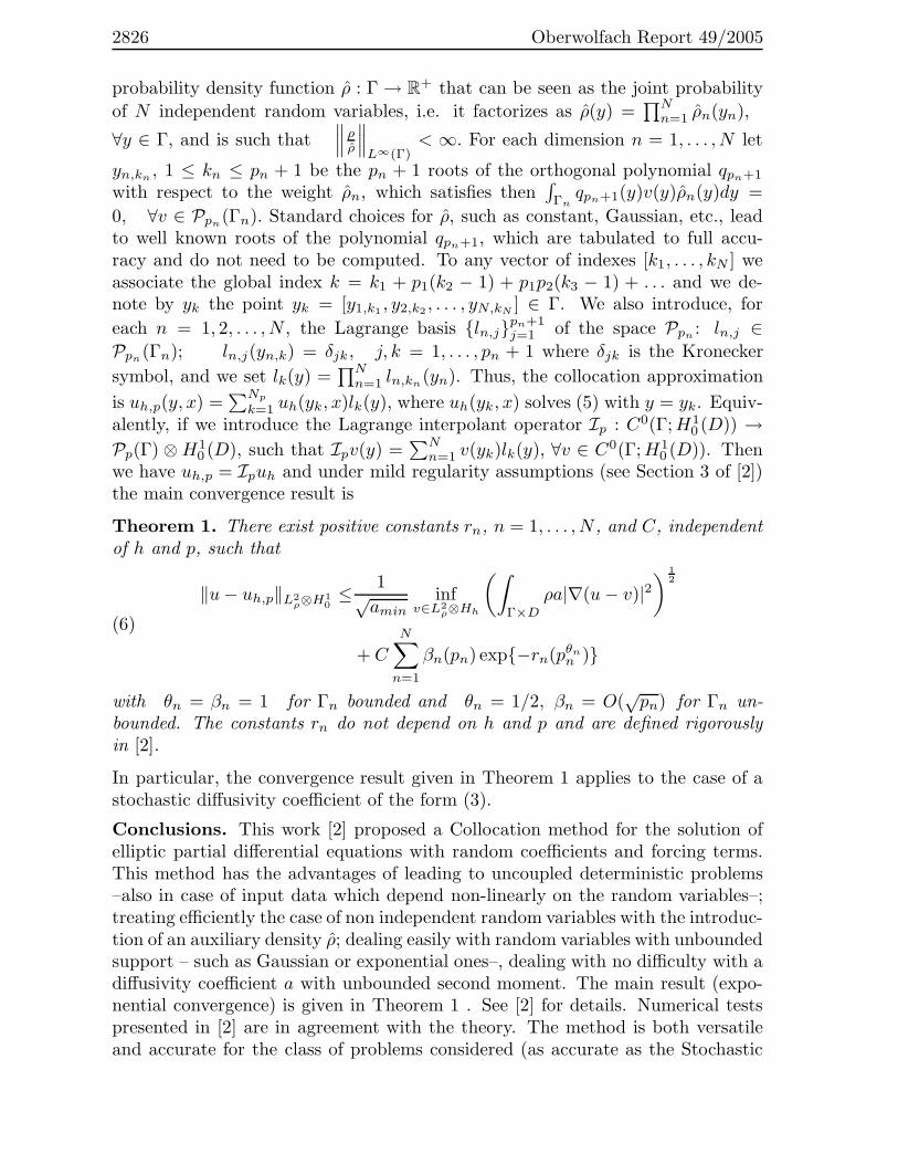
2826 Oberwolfach Report 49/2005
probability density function ρ : Γ → R+ that can be seen as the joint probability
of N independent random variables, i.e. it factorizes as ρ(y) =∏N
n=1 ρn(yn),
∀y ∈ Γ, and is such that∥∥∥ ρ
ρ
∥∥∥L∞(Γ)
< ∞. For each dimension n = 1, . . . , N let
yn,kn, 1 ≤ kn ≤ pn + 1 be the pn + 1 roots of the orthogonal polynomial qpn+1
with respect to the weight ρn, which satisfies then∫Γn
qpn+1(y)v(y)ρn(y)dy =
0, ∀v ∈ Ppn(Γn). Standard choices for ρ, such as constant, Gaussian, etc., lead
to well known roots of the polynomial qpn+1, which are tabulated to full accu-racy and do not need to be computed. To any vector of indexes [k1, . . . , kN ] weassociate the global index k = k1 + p1(k2 − 1) + p1p2(k3 − 1) + . . . and we de-note by yk the point yk = [y1,k1
, y2,k2, . . . , yN,kN
] ∈ Γ. We also introduce, for
each n = 1, 2, . . . , N , the Lagrange basis ln,jpn+1j=1 of the space Ppn
: ln,j ∈Ppn
(Γn); ln,j(yn,k) = δjk, j, k = 1, . . . , pn + 1 where δjk is the Kronecker
symbol, and we set lk(y) =∏N
n=1 ln,kn(yn). Thus, the collocation approximation
is uh,p(y, x) =∑Np
k=1 uh(yk, x)lk(y), where uh(yk, x) solves (5) with y = yk. Equiv-alently, if we introduce the Lagrange interpolant operator Ip : C0(Γ; H1
0 (D)) →Pp(Γ) ⊗ H1
0 (D), such that Ipv(y) =∑N
n=1 v(yk)lk(y), ∀v ∈ C0(Γ; H10 (D)). Then
we have uh,p = Ipuh and under mild regularity assumptions (see Section 3 of [2])the main convergence result is
Theorem 1. There exist positive constants rn, n = 1, . . . , N , and C, independentof h and p, such that
(6)
‖u − uh,p‖L2ρ⊗H1
0≤ 1√
amininf
v∈L2ρ⊗Hh
(∫
Γ×D
ρa|∇(u − v)|2) 1
2
+ C
N∑
n=1
βn(pn) exp−rn(pθnn )
with θn = βn = 1 for Γn bounded and θn = 1/2, βn = O(√
pn) for Γn un-bounded. The constants rn do not depend on h and p and are defined rigorouslyin [2].
In particular, the convergence result given in Theorem 1 applies to the case of astochastic diffusivity coefficient of the form (3).
Conclusions. This work [2] proposed a Collocation method for the solution ofelliptic partial differential equations with random coefficients and forcing terms.This method has the advantages of leading to uncoupled deterministic problems–also in case of input data which depend non-linearly on the random variables–;treating efficiently the case of non independent random variables with the introduc-tion of an auxiliary density ρ; dealing easily with random variables with unboundedsupport – such as Gaussian or exponential ones–, dealing with no difficulty with adiffusivity coefficient a with unbounded second moment. The main result (expo-nential convergence) is given in Theorem 1 . See [2] for details. Numerical testspresented in [2] are in agreement with the theory. The method is both versatileand accurate for the class of problems considered (as accurate as the Stochastic

Reactive Flow and Transport Through Complex Systems 2827
Galerkin approach). The extension of the analysis to other classes of linear andnon-linear problems is an ongoing research. Besides, the use of tensor productpolynomials suffers from the curse of dimensionality and it is efficient only for asmall number of random variables. For a moderate or large dimensionality of theprobability space one should use sparse tensor product spaces. This aspect will beinvestigated in a future work.
References
[1] I. Babuska , R. Tempone and G. Zouraris, Galerkin finite element approximations of sto-chastic elliptic partial differential equations, SIAM J. Numer. Anal.,42:2 (2004), 800–825.
[2] I. Babuska , F. Nobile and R. Tempone, A Stochastic Collocation method for elliptic PartialDifferential Equations with Random Input Data, ICES report 2005
Sparse Perturbation Algorithms for Elliptic Problems with StochasticData
Radu Alexandru Todor
We consider the moment problem for stochastic diffusion in a bounded physicaldomain D ⊂ R
d,
(1) −div(a(·, ω)∇u(·, ω)) = f(·, ω) in H−1(D), P -a.e. ω ∈ Ω,
with homogeneous boundary conditions. Here (Ω, Σ, P ) is a probability spacemodelling the data uncertainty.For k ∈ N+ the moment of order k of u solution to (1) is defined on the kd-dimensional domain Dk := D × D × · · · × D (k times) by
(2) Mk(u)(x1, x2, · · · , xk) =
∫
Ω
u(x1, ω)u(x2, ω) · · ·u(xk, ω) dP (ω).
For the moment computation of the stochastic solution u to (1) we developperturbation algorithms which combine classical ideas with modern techniquesfor efficient data representation and complexity reduction: sparse tensor productspaces, wavelet preconditioning and best N -term approximation.
For example, if ε > 0 denotes the accuracy to be achieved in the momentcomputation using one of the three well-established methods (MC, PA, SG), thecorresponding standard complexity estimates are expressed in the table below interms of the number N(ε) of deterministic model problems to be solved - intu-itively, N(ε) denotes the number of samples.

2828 Oberwolfach Report 49/2005
Method N(ε) as ε ց 0
Monte-Carlo Simulation Quadratic: N(ε) ∼ ε−2)
Perturbation Algorithms Superalgebraic: N(ε) > O(ε−n) ∀n
Stochastic Galerkin Method Superalgebraic: N(ε) > O(ε−n) ∀n
We prove that the new algorithms (which are of perturbation type), have nearlyoptimal complexity, that is
(3) N(ε) ≤ O(ε−o(1)) as ε ց 0,
under the assumption that the fluctuation in the stochastic diffusion coefficient ais piecewise analytic in the physical domain D. The central idea is a best N -termapproximation of higher order moments (2) based on the Legendre/Karhunen-Loeve expansion of the random fluctuation in the stochastic coefficient a. Weconclude that the moment problem can be solved for the stochastic equation (1) inessentially the same complexity as one deterministic diffusion problem, as ε ց 0(the number of needed samples is negligible compared to the effort needed tocompute one sample).
References
[1] P. Frauenfelder, Ch. Schwab and R.A.Todor, Finite elements for elliptic problems withstochastic coefficients, CMAME 194(2005), 205–228.
[2] Ch. Schwab and R.A.Todor, Sparse Finite Elements for Stochastic Elliptic Problems - higherorder moments, Computing 71(2003), 43–63.
[3] R.A. Todor, Sparse Perturbation Algorithms for Elliptic Problems with Stochastic Data,ETH Dissertation, Zurich 2005.
Reporters: Andro Mikelic and Christoph Schwab

Reactive Flow and Transport Through Complex Systems 2829
Participants
Prof. Dr. Assyr Abdulle
Mathematisches InstitutUniversitat BaselRheinsprung 21CH-4051 Basel
Dr. Peter Bastian
Interdisziplinares Zentrumfur Wissenschaftliches RechnenUniversitat HeidelbergIm Neuenheimer Feld 36869120 Heidelberg
Prof. Dr. Leonid Berlyand
Department of MathematicsPennsylvania State UniversityUniversity Park, PA 16802USA
Prof. Dr. Eric Bonnetier
Lab. de Modelisation et CalculInstitut IMAGUniv. Joseph Fourier Grenoble IB.P. 53F-38041 Grenoble Cedex 9
Prof. Dr. Rene de Borst
Delft University of TechnologyKluyverweg 1P.O. Box 5058NL-2600 GB Delft
Prof. Dr. Guy Bouchitte
U.F.R. des Sc. et Techn.Universite de Toulon et du VarB.P. 132F-83957 La Garde Cedex
Dr. Alain Bourgeat
Modelisation et Calcul ScientifiqueISTILUniversite Lyon 143, Bd. du onze novembreF-59622 Villeurbanne Cedex
Prof. Andrea Braides
Dipartimento di MatematicaUniversita di Roma ”Tor Vergata”V.della Ricerca Scientifica, 1I-00133 Roma
Prof. Dr. Gregory A. Chechkin
Dept. of Differential EquationsFac. of Mechanics and MathematicsLomonosov Moscow State University119899 MoscowRUSSIA
Vincent Devigne
Ecole Nationale Superieure desMines de Saint-Etienne158, Cours FaurielF-42023 Saint-Etienne Cedex

2830 Oberwolfach Report 49/2005
Prof. Dr. Cornelius J. van Duijn
Department of Mathematics andComputer ScienceEindhoven University of TechnologyPostbus 513NL-5600 MB Eindhoven
Prof. Dr. Bjorn Engquist
Department of MathematicsUniversity of Texas at Austin1 University Station C1200Austin, TX 78712-1082USA
Prof. Dr. Vincent Giovangigli
Centre de Mathematiques AppliqueesEcole PolytechniquePlateau de PalaiseauF-91128 Palaiseau Cedex
Prof. Dr. Yuri Golovaty
Faculty of Mechanicsand Mathematics LvivIvan Franko National Universityul. Universytetska 179000 LvivUKRAINE
Dr. Giovanna Guidoboni
Department of MathematicsUniversity of HoustonHouston TX 77204-3008USA
Dr. Rudolf Hilfer
Institut fur Computeranwendungen-1Numerik fur HochstleistungsrechnerUniversitat StuttgartPfaffenwaldring 2770569 Stuttgart
Dr. Viet Ha Hoang
Department of Applied Mathematics &Theoretical Physics (DAMTP),Centrefor Mathematical SciencesWilberforce RoadGB-Cambridge CB3 OWA
Prof. Dr.Dr.h.c. Willi Jager
Institut fur Angewandte MathematikUniversitat HeidelbergIm Neuenheimer Feld 29469120 Heidelberg
Jerome Jaffre
INRIAB.P. 105F-78153 Le Chesnay Cedex
Dr. Michel Kern
INRIA RocquencourtDomaine de VoluceauB. P. 105F-78153 Le Chesnay Cedex
Nina Khvoenkova
C.E.A.DEN/DM2S/SFME/MTMSCEA Saclay, Bat. 454 p.17 BF-91191 Gif-sur-Yvette

Reactive Flow and Transport Through Complex Systems 2831
Prof. Dr. Peter Knabner
Inst. fur Angewandte Mathematik 1Universitat ErlangenMartensstr. 391058 Erlangen
Severine Lacharme
Fakultat fur Mathematik- Dekanat -Universitat HeidelbergIm Neuenheimer Feld 28869120 Heidelberg
Michael Lenzinger
Institut fur Angewandte MathematikUniversitat HeidelbergIm Neuenheimer Feld 29469120 Heidelberg
Prof. Dr. Stephan Luckhaus
Fakultat fur Mathematik/InformatikUniversitat LeipzigAugustusplatz 10/1104109 Leipzig
Prof. Dr. Eduard Marusic-Paloka
Department of MathematicsUniversity of ZagrebBijenicka 3010000 ZagrebCROATIA
Prof. Dr. Hermann G. Matthies
Technische Universitat BraunschweigRechenzentrumHans-Sommer-Str. 6538106 Braunschweig
Prof. Dr. Andro Mikelic
UFR MathematiquesSite de Gerland, Bat.AUniversite Claude Bernard Lyon 150, avenue Tony GarnierF-69367 Lyon Cedex 07
Dr. Nicolas Neuss
Interdisziplinares Zentrumfur Wissenschaftliches RechnenUniversitat HeidelbergIm Neuenheimer Feld 36869120 Heidelberg
Dr. Maria Neuss-Radu
Institut fur Angewandte MathematikUniversitat HeidelbergIm Neuenheimer Feld 29469120 Heidelberg
Prof. Dr. Barbara Niethammer
Institut fur MathematikHumboldt-Universitat BerlinRudower Chaussee 2512489 Berlin
Prof. Dr. Felix Otto
Institut fur Angewandte MathematikUniversitat BonnWegelerstr. 1053115 Bonn
Dr. Sorin I. Pop
Department of Mathematics andComputer ScienceEindhoven University of TechnologyPostbus 513NL-5600 MB Eindhoven

2832 Oberwolfach Report 49/2005
Prof. Dr. Jerome Pousin
Centre de MathematiquesINSA de Lyon21, avenue Jean CapelleF-69621 Villeurbanne Cedex
Christian Reichert
Institut fur Angewandte MathematikUniversitat HeidelbergIm Neuenheimer Feld 29469120 Heidelberg
Prof. Dr. Carole Rosier
Lab. de Mathematique Pures etAppliquees, Centre UniversitaireBatiment Henri Poincare50 Rue Francois BuissonF-62228 Calais Cedex
Prof. Dr. Reinhold Schneider
Lehrstuhl fur Scientific ComputingUniversitats-Hochhaus 9 StockChristian-Albrechts-Platz 424098 Kiel
Prof. Dr. Christoph Schwab
Seminar fur Angewandte MathematikETH-ZentrumRamistr. 101CH-8092 Zurich
Dr. Ben Schweizer
Mathematisches InstitutUniversitat BaselRheinsprung 21CH-4051 Basel
Prof. Dr. Angela Stevens
Max-Planck-Institut fur Mathematikin den NaturwissenschaftenInselstr. 22 - 2604103 Leipzig
Prof. Dr. Nils Svanstedt
Dept. of MathematicsChalmers University of TechnologyS-41296 Gothenburg
Prof. Dr. Raul Tempone
Department of MathematicsFlorida State UniversityTallahassee, FL 32306-4510USA
Dr. Radu-Alexandru Todor
Departement MathematikETH-ZentrumRamistr. 101CH-8092 Zurich
Related Documents


