Training in multiple-antenna Rician fading wireless channels with deterministic specular component

IEEE TRANSACTIONS ON WIRELESS COMMUNICATIONS, VOL. 6, NO. 1, JANUARY 2007 1

Training in Multiple-AntennaRician Fading Wireless Channels with

Deterministic Specular ComponentMahesh Godavarti, Member, IEEE, and Alfred O. Hero-III, Fellow, IEEE

Abstract— We determine the optimum training strategy for amultiple-antenna wireless link in a Rician fading channel usinga training based lower bound on capacity. We consider the stan-dard Rician block fading channel where the channel coefficientsare modeled as independent circular Gaussian random variableswith non-zero means (the specular component). The specularcomponent is known to both the transmitter and receiver. Thechannel coefficients of this model are constant over a block ofT symbol periods but, independent over different blocks. Forsuch a model, it is shown that the training based capacity,the optimum training signals, the training period, transmit andtraining energy are dependent on the Rician factor r along withSNR ρ, the number of transmit antennas M , the number ofreceive antennas N and the coherence interval T . Also, unlike inthe case of Rayleigh fading channels, it can be shown using thelower bound for Rician fading channels that for low SNR Ricianfading channels behave like a purely AWGN channel and theoptimum strategy is to spend no effort in learning the channel.When SNR is not low and training is required then the optimumtraining period is as many symbol intervals as there are transmitantennas.

Index Terms— Capacity, asymptotic capacity, training, infor-mation theory, Rician fading, multiple antennas.

I. INTRODUCTION

DEPLOYING multiple antennas at the transmitter andreceiver has been demonstrated to be a viable solution to

the demand for high data rate in wireless communications [6],[7], [16], [20], [22]. A straightforward way for the transmitterand the receiver to transmit data would be for the receiverto first learn the channel and then use the channel estimateto decode the transmitted symbols. Such training methodsare prevalent in wireless communication systems like IS-95CDMA and GSM and have been investigated in [13], [14],[17], [22].

It is important to know whether training based signalschemes are practical and if they are how much time can bespent in learning the channel and what the optimum trainingsignal is like. Hassibi and Hochwald [14] have addressed these

Manuscript received DATE; revised DATE; accepted DATE. The associateeditor coordinating the review of this paper and approving it for publicationwas NAME. Parts of this work were presented at ISIT 2002 held in Laussane,Switzerland.

M. Godavarti is with Ditech Networks, Inc., 825 E. Middlefield Rd.,Mountain View, CA 94043 (email: [email protected], [email protected]). This work was performed while M. Godavarti was aPh.D. candidate at the University of Michigan.

A. Hero is with the Dept. of Electrical Engineering, University of Michigan,1301 Beal Ave., Ann Arbor, MI 48107 (email: [email protected]).

Digital Object Identifier 10.1109/TWC.2006.04579.

issues for the popular case of Rayleigh block fading channels.They used a capacity lower bound based on MMSE channelestimate to find the optimum training strategy by maximizingthe lower bound. They showed that 1) pilot symbol trainingbased communication schemes are highly suboptimum for lowSNR but practically optimum for high SNR; 2) when practicalthe optimum amount of time1 devoted to training is equal toM symbol intervals, where M is the number of transmitters,when the fraction of power devoted to training is allowed tovary and 3) the orthonormal signal is the optimum signal fortraining.

In [13], the authors investigated the same problem fora more general fading model and a more general trainingstrategy using a generalized mutual information lower boundbased on Gaussian codebooks with modified nearest neighbordecoding. Also, unlike in [14], they relaxed the assumptionof identity transmit signal covariance matrix and included thecovariance matrix to be one of the parameters to be optimized.The authors showed that for the special case of piecewiseblock fading channels with Gaussian fading and additiveGaussian noise the training based scheme as in [14] withminimum mean-squared error channel estimator is optimum inthe sense that it maximizes the generalized mutual informationlower bound. They showed that for low SNR the transmitsignal covariance matrix has only one non-zero eigenvalue.For high SNR, the results agree with the assumption ontransmit signal covariance matrix made in [14]. In this case, asexpected, for Rayleigh block fading the optimum lower boundbased on generalized mutual information is equal to the lowerbound derived in [14].

However, Rayleigh fading models are not sufficient todescribe many channels found in the real world. It is importantto consider other models and investigate their performanceas well. Rician fading is one such model [1], [4], [5], [18],[19]. Rician fading model is applicable when the wireless linkbetween the transmitter and the receiver has a direct pathcomponent in addition to the diffused Rayleigh component.

In this paper, we investigate how much training is necessaryfor a wireless link operating in a Rician fading channel underthe average energy constraint on the input signal. We usethe standard Rician fading channel throughout the paper, thatis, we assume that the specular component is deterministic,

1Note: time is always measured in terms of number of symbol intervals.This is tied to the initial assumption that channel coherence interval (theamount of time channel coefficients remain constant) is itself measured interms of number of symbol intervals.

1536-1276/07$20.00 c© 2007 IEEE

2 IEEE TRANSACTIONS ON WIRELESS COMMUNICATIONS, VOL. 6, NO. 1, JANUARY 2007

of general rank and known to both the transmitter and thereceiver. The Rayleigh component is never known to thetransmitter. The capacity when the receiver has completeknowledge about the channel will be referred to as coherentcapacity and the capacity when the receiver has no knowledgeabout the Rayleigh component will be referred to as non-coherent capacity.

Keeping in mind the results obtained in [13], we use thesame training signal based approach as that of [14]. However,we relax the assumption of identity transmit signal covariancematrix and we leave the matrix to be one of the parametersto be optimized. We draw similar conclusions about trainingfor non-coherent communications as in [14] with one bigdifference in the regime of low SNR. For Rayleigh fadingchannels the optimum training period is not zero for all valuesof SNR. However, for Rician fading channels there exists athreshold dependent on the Rician factor r such that for allSNRs below the threshold the optimum strategy is to haveno training at all. An interesting find regarding the optimumtransmit strategy, in this paper, is that the optimum strategyfor low SNR is to concentrate all the available energy inthe direction of strongest specular component whereas forhigh SNR it is to spread the energy equally in all directions.Note that this finding, for high SNR, is the same as that of[13] and [14] because the transmit signal covariance matrixin this region is an identity matrix. However, for low SNReventhough the optimum transmit covariance matrix consistsof a single non-zero eigenvalue as in [13] the eigenvectorcorresponding to this eigenvalue can not be arbitrary. Theeigenvector should point in the same direction as the strongestspecular component.

The training based lower bound derived in [14] and adaptedhere for Rician fading channels is suboptimum for low SNR asthe capacity for low SNR for block fading channels is a linearfunction of SNR [21]. The training based lower bound forRayleigh fading channels turns out to be a quadratic functionof SNR [14]. From this paper we find that for Rician fadingchannels it is a linear function of SNR. However, the boundis still suboptimum since the constant multiplying SNR inthe capacity expression is purely a function of the specularcomponent instead of the whole channel. That is, if ρ denotesSNR, λmax(A) the largest eigenvalue of matrix A, H theRician fading channel and Hm the specular component ofH then for low SNR the capacity of block fading Ricianchannel behaves as ρλmax(E[HH†]) [12] whereas the trainingbased lower bound on capacity of block fading Rician channelbehaves as ρλmax(E[HmH†

m]) = ρλmax(HmH†m). For high

SNRs and large coherent periods, the ratio of the trainingbound and the actual capacity tends to one and indicates thattraining based schemes can achieve rates close to capacity.

This paper is organized as follows. First, in Section IIthe model used in the paper is established and a simpletraining based lower bound is discussed. Then in SectionIII, a more general training based lower bound on capacityis established and its optimization is performed over variousparameters (choosing the parameters that maximize the lowerbound). More precisely, in Sub-section III-A, optimization isperformed for training over the transmitting signal, energydistribution and the training period. This is followed by

optimization over the same parameters under the constraintof equal training and transmit signal powers in Sub-sectionIII-B. Additional insights into the optimization problem areobtained from numerical simulation in Section IV. Then inSection V, optimization is performed in the regimes of lowand high SNR followed finally by Section VI in which theresults of this paper are summarized.

II. SIGNAL MODEL AND A

SIMPLE TRAINING BASED LOWER BOUND

We adopt the following model, which is the same as theone used in [12], for the Rician fading channel:

X = SH + W (1)

where X is the T×N matrix of received signals, H is the M×N matrix of propagation coefficients, S is the T ×M matrixof transmitted signals, W is the T×N matrix of additive noisecomponents. Note that T denotes the coherence interval, Mdenotes the number of transmit antennas and N the numberof receive antennas. The Rician fading channel H is definedas

H =√

rHm +√

1 − rG

where Hm is the deterministic specular component of Hand G denotes the Rayleigh component. G and W consistof Gaussian circular independent random variables and thecovariance matrices of G and W are given by IMN andσ2ITN , respectively. Hm is a deterministic matrix satisfyingtr{HmH†

m} = MN . G satisfies E[tr{GG†}] = MN and r isthe Rician parameter between 0 and 1 so that E[tr{HH†}] =MN . We assume that both the transmitter and receiver havecomplete knowledge of the probability density function of H .This means that Hm and the probability density function of Gare known to both the transmitter and receiver. We also assumethat communication is taking place under the average energyconstraint on the input signal given by E[tr{SS†}] ≤ MT .The SNR of the channel, given by the ratio of the energy ofthe elements of SH to the energy of the elements of W , istherefore ρ = M

σ2 when the constraint is satisfied with equality.

A. A Simple Training Based Lower Bound

In [22] the authors demonstrated a very simple trainingmethod that achieves the optimum rate of increase with SNR.The same training method can also be easily applied to theRician fading model with deterministic specular component.The training signal is the M × M diagonal matrix dIM . d ischosen such that the same power is used in the training and thecommunication phase. Therefore, d =

√M . Using S = dIM ,

the output of the MIMO channel in the training phase is givenby

X =√

M√

rHm +√

M√

1 − rG + W.

The Rayleigh channel coefficients G can be estimated in-dependently2 using scalar minimum mean squared error

2It might be useful to remind the readers at this point that Hm is alreadyknown to both the transmitter and receiver

GODAVARTI and HERO: TRAINING IN MULTIPLE-ANTENNA RICIAN FADING WIRELESS CHANNELS WITH DETERMINISTIC SPECULAR COMPONENT 3

(MMSE) estimates since the elements of W and G are i.i.d.Gaussian random variables

G =√

1 − r√

M

(1 − r)M + σ2[X −

√M

√rHm],

where we recall that σ2 is the variance of the components ofW . The elements of the estimate G are i.i.d. Gaussian withvariance (1−r)M

(1−r)M+σ2 . Similarly, the estimation error matrix

G− G has i.i.d Gaussian distributed elements with zero meanand variance σ2

(1−r)M+σ2 .The output of the channel in the communication phase is

given by

X = SH + W

=√

rSHm +√

1 − rSG +√

1 − rS(G − G) + W,

where S consists of zero mean i.i.d circular Gaussian randomvariables with zero mean and unit variance. This choice ofS is suboptimum as this might not be the capacity achievingsignal, but this choice gives us a lower bound on capacity.Let W =

√1 − rS(G − G) + W . For the choice of S given

above the entries of W are uncorrelated with each other andalso with S(

√rHm +

√1 − rG). The variance of each of the

entries of W is given by σ2 + (1 − r)M σ2

(1−r)M+σ2 . If W isreplaced with a white Gaussian noise with the same covariancematrix then the resulting mutual information is a lower boundon the actual mutual information [2, p. 263], [14, Theorem 1].In this section we deal with normalized capacity C/T insteadof capacity C. The lower bound on the normalized capacityis given by

C/T ≥ T − Tt

TE log det

(IM +

ρeff

MH1H

†1

)(2)

where Tt is number of symbol intervals devoted to trainingand ρeff in the expression above is the effective SNR at theoutput (explained at the end of the next paragraph) given asfollows:

ρeff =ρ[r + r(1 − r)ρ + (1 − r)2ρ]

[1 + 2(1 − r)ρ](3)

where ρ = Mσ2 is the actual SNR. H1 in (2) is a Rician channel

with a new Rician parameter reff where

reff =r

r + (1 − r) (1−r)M(1−r)M+σ2

. (4)

Note that reff > r in the effective channel because part ofthe energy from the unknown Rayleigh component has beendiverted to the additive noise in the new effective channelmodel.

The lower bound in (2) can be easily calculated becausethe lower bound is essentially the coherent capacity with Hreplaced by

√reffHm +

√1 − reff G. The signal covariance

structure was chosen to be an identity matrix as this is theoptimum covariance matrix for high SNR (refer to Result 2in the following section). The effective SNR is now givenby the ratio of the energy of the elements of S(

√rHm +√

1 − rG) to the energy of the elements of W . The energyin the elements of S(

√rHm +

√1 − rG) is given by M(r +

(1− r)2 M(1−r)M+σ2 ) and the energy in the elements of W are

0 50 100 150 200 250 300 350 400−50

0

50

100

150

200

250

300

350

SNR (dB)

Cap

acity

(bits

/T)

Coherent Capacity

Training Lower Bound

Asymptotic Capacity Upper Bound

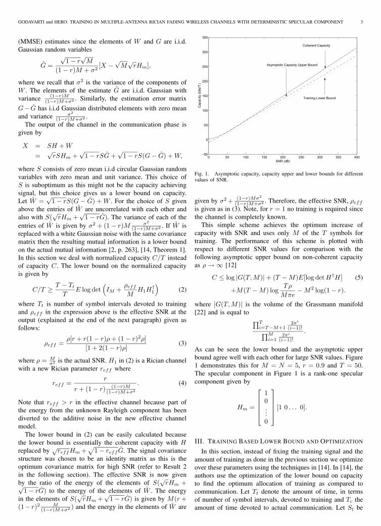
Fig. 1. Asymptotic capacity, capacity upper and lower bounds for differentvalues of SNR.

given by σ2 + (1−r)Mσ2

(1−r)M+σ2 . Therefore, the effective SNR, ρeff

is given as in (3). Note, for r = 1 no training is required sincethe channel is completely known.

This simple scheme achieves the optimum increase ofcapacity with SNR and uses only M of the T symbols fortraining. The performance of this scheme is plotted withrespect to different SNR values for comparison with thefollowing asymptotic upper bound on non-coherent capacityas ρ → ∞ [12]

C ≤ log |G(T,M)| + (T − M)E[log detH†H] (5)

+M(T − M) logTρ

Mπe− M2 log(1 − r).

where |G(T,M)| is the volume of the Grassmann manifold[22] and is equal to ∏T

i=T−M+12πi

(i−1)!∏Mi=1

2πi

(i−1)!

.

As can be seen the lower bound and the asymptotic upperbound agree well with each other for large SNR values. Figure1 demonstrates this for M = N = 5, r = 0.9 and T = 50.The specular component in Figure 1 is a rank-one specularcomponent given by

Hm =

⎡⎢⎢⎢⎣

10...0

⎤⎥⎥⎥⎦ [1 0 . . . 0].

III. TRAINING BASED LOWER BOUND AND OPTIMIZATION

In this section, instead of fixing the training signal and theamount of training as done in the previous section we optimizeover these parameters using the techniques in [14]. In [14], theauthors use the optimization of the lower bound on capacityto find the optimum allocation of training as compared tocommunication. Let Tt denote the amount of time, in termsof number of symbol intervals, devoted to training and Tc theamount of time devoted to actual communication. Let St be


the Tt ×M signal used for training and Sc the Tc ×M signalused for communication.

Let the “energy allocation factor” κ denote the fraction ofthe energy used for communication. Then T = Tt + Tc andtr{StS

†t } = (1 − κ)TM and tr{ScS

†c} = κTM .

Xt = St(√

rHm +√

1 − rG) + Wt

Xc = Sc(√

rHm +√

1 − rG) + Wc

where Xt is Tt × N and Xc is Tc × N . G is estimated fromthe training phase. For that we need Tt ≥ M . Since G andWt are Gaussian the MMSE estimate of G is also the linearMMSE estimate conditioned on S. The optimum estimate inthe MSE sense is given by

G =√

1 − r(σ2IM + (1 − r)S†t St)−1S†

t (Xt −√

rStHm).

Let G = G − G then

Xc = Sc(√

rHm +√

1 − rG) +√

1 − rScG + Wc.

Let Wc =√

1 − rStG + W . Note that elements of Wc areuncorrelated with each other and have the same marginaldensities when the elements of Sc are chosen to be i.i.dGaussian. If we replace Wc with Gaussian noise that is zero-mean and spatially and temporally independent the elementsof which have the same variance as the elements of Wc thenthe resulting mutual information is a lower bound to the actualmutual information in the above channel [14, Theorem 1].

The variance of the elements of Wc is given by

σ2wc

= σ2 +1 − r

NTctr{E[GG†]κTIM} (6)

= σ2 +(1 − r)κTM

Tc

1NM

tr{E[GG†]}

= σ2 +(1 − r)κTM

Tcσ2

G

where σ2G

is given in (33) and the lower bound is

Ct/T ≥ T − Tt

TE log det

(IM +

ρeff

MH1ΛH†

1

), (7)

where the “post training SNR” ρeff , is the ratio of the energiesin the elements of ScH and energies in the elements of Wc andH1 = √

reffHm+√

1 − reff G where reff = rr+(1−r)σ2

G

. To

calculate ρeff , the energy in the elements of ScH is given by

σ2ScH

=1

NTc[rtr{HmH†

mκTIM} +

(1 − r)tr{GG†κTIM}]=

κTM

Tc

1NM

[rNM + (1 − r)tr{GG†}]

=κTM

Tc[r + (1 − r)σ2

G],

which gives us

ρeff =κTρ[r + (1 − r)σ2

G]

Tc + (1 − r)κTρσ2G

. (8)

Λ in (7) is the optimum signal covariance matrix thestructure of which is determined from the following resultsobtained from [12].

Result 1: [12, Proposition 1] Let H be Rician (1) andlet the receiver have complete knowledge of the Rayleighcomponent G. For low SNR, the coherent capacity CH , isattained by the same signal covariance matrix that attainscapacity when r = 1 and

CH = Tρ[rλmax(HmH†m) + (1 − r)N ] + O(ρ2).

Result 2: [12, Theorem 2] Let H be Rician (1) then asρ → ∞, the coherent capacity CH , is attained by an identitysignal covariance matrix and

CH

T · E log det[ ρM HH†]

→ 1.

Therefore, For low SNR, Λ has only one non-zero eigenvaluesuch that all energy is concentrated in the direction of thelargest eigenvalue of Hm and for high SNR Λ is an identitymatrix.

A. Optimization of St, κ and Tt

We will optimize St, κ and Tt to maximize the lower bound(7).

Optimization of the lower bound over St is difficult as St

effects the distribution of H , the form of Λ as well as ρeff .To make the problem simpler we will just find the value ofSt that maximizes ρeff .

Proposition 1: The signal St that maximizes ρeff satisfiesthe following condition

S†t St = (1 − κ)TIM (9)

and the corresponding ρeff is

ρ∗eff=κTρ[Mr + ρ(1 − r)(1 − κ)T ]

Tc(M + ρ(1 − r)(1 − κ)T ) + (1 − r)κTρM. (10)

Proof: Refer to Appendix I.The optimum signal derived above is the same as the

optimum signal derived in [14] and the corresponding capacitylower bound using the St obtained above is given by (7) butwhere ρeff is as given below

ρeff=κTρ[Mr + ρ(1 − r)(1 − κ)T ]

Tc(M + ρ(1 − r)(1 − κ)T ) + (1 − r)κTρM(11)

and H1 = √reffHm +

√1 − reffG where reff =

r1+(1−r)(1−κ) ρ

M T

r+(1−r)(1−κ) ρM T

and as before G is a matrix consisting ofi.i.d. Gaussian circular random variables with mean zero andunit variance. Now, Λ is the covariance matrix of the sourceSc when the channel is Rician and known to the receiver.Therefore from Results 1 and 2, Λ is an identity matrix forρeff → ∞ and is a diagonal matrix with only one non-zerodiagonal element for ρeff → 0.

Optimization of (7) over the energy allocation factor κ, isstraightforward as κ affects the lower bound only through thepost training SNR ρeff , and can be stated as the followingproposition.

Proposition 2: For given Tt and Tc the optimum powerallocation κ in a training based scheme is given by

κ =

⎧⎪⎪⎪⎪⎪⎪⎨⎪⎪⎪⎪⎪⎪⎩

min{γ −√γ(γ − 1 − η), 1}

for Tc > (1 − r)Mmin{ 1

2 + rM2Tρ , 1}

for Tc = (1 − r)Mmin{γ +

√γ(γ − 1 − η), 1}

for Tc < (1 − r)M

(12)


where γ = MTc+TρTc

Tρ[Tc−(1−r)M ] and η = rMTρ . The corresponding

lower bound is given by

Ct/T ≥ T − Tt

TE log det

(IM +

ρeff

MH1ΛH†

1

)(13)

where for Tc > (1 − r)M :

ρeff =

⎧⎪⎨⎪⎩

TρTc−(1−r)M (

√γ −√

γ − 1 − η)2

when κ = γ −√γ(γ − 1 − η)

rρ1+(1−r)ρ when κ = 1

(14)

for Tc = (1 − r)M :

ρeff =

⎧⎪⎨⎪⎩

T 2ρ2

4(1−r)M(M+Tρ) (1 + rMTρ )2

when κ = 12 + rM

2TρrTρ

(1−r)(M+Tρ) when κ = 1(15)

and for Tc < (1 − r)M :

ρeff =

⎧⎪⎨⎪⎩

Tρ(1−r)M−Tc

(√−γ −√−γ + 1 + η)2

when κ = γ +√

γ(γ − 1 − η)rρ

1+(1−r)ρ when κ = 1(16)

and reff is given by substituting the appropriate value of κin the expression

r1 + (1 − r)(1 − κ) ρ

M T

r + (1 − r)(1 − κ) ρM T

.

Proof: Refer to Appendix II.We see from Proposition 2 that for ρ < rM

T the optimumsetting for κ is κ = 1. That is, rM

T is the threshold suchthat for all SNRs below it the optimum strategy is to have notraining at all. Note that eventhough the threshold increaseswith r it is not tight as can be gauged from the case r = 1.For r = 1, the threshold should actually be ∞ as it is obviousthat κ = 1 for all ρ whereas the threshold turns out to be onlyMT .

For optimization over Tt we draw similar conclusions asin [14]. In [14] the optimum setting for Tt was shown tobe Tt = M for all values of SNR. However, in this paperfor ρ < rM

T the optimum setting is Tt = 0. The argumentfollows from the fact that for these values of ρ we haveκ = 1 i.e., all energy is allocated to communications. It isclear that optimization of Tt makes sense only when κ isstrictly less than 1. When κ = 1 no power is devoted totraining and Tt can be made as small as possible which is zero.When training is required, the intuition is that increasing Tt

linearly decreases the capacity through the term (T − Tt)/T ,but only logarithmically increases the capacity through thehigher effective SNR ρeff [14]. Therefore, it makes sense tomake Tt as small as possible. Therefore, when κ < 1 thesmallest value Tt can be is M since it takes at least that manyintervals to completely determine the unknowns.

Proposition 3: The optimum length of the training intervalis Tt = M whenever κ < 1 for all values of ρ and T > M ,and the capacity lower bound is

Ct/T ≥ T − M

TE log det

(IM +

ρeff

MH1ΛH†

1

)(17)

where

ρeff =

⎧⎪⎪⎪⎪⎪⎪⎪⎨⎪⎪⎪⎪⎪⎪⎪⎩

TρT−(2−r)M (

√γ −√

γ − 1 − η)2

for T > (2 − r)MT 2ρ2

4(1−r)M(M+Tρ) (1 + rMTρ )2

for T = (2 − r)MTρ

T−(2−r)M (√−γ −√−γ + 1 + η)2

for T < (2 − r)M

The optimum power allocations are easily obtained fromProposition 2 by simply setting Tc = T − M .

Proof: Refer to Appendix III.

B. Equal Training and Data Power

As stated in [14], sometimes it is difficult for the transmitterto assign different powers for training and communicationphases. In this section, we will concentrate on setting thetraining and communication powers equal to each other inthe following sense

(1 − κ)TTt

=κT

Tc=

κT

T − Tt= 1

this means κ = 1 − Tt/T and that the power transmitted inTt and Tc are equal.

In this case,

ρeff =ρ[r + ρTt

M ]1 + ρ[Tt

M + (1 − r)]

and the capacity lower bound is

Ct/T ≥ T − Tt

TE log det(IM +

ρeff

MH1ΛH†

1) (18)

where ρeff is as given above and H1 = √reffHm +√

1 − reffG where reff = r1+(1−r) ρ

M Tt

r+(1−r) ρM Tt

.We can derive the optimum training period using the same

procedure as in the proof of Proposition 3. Using the definitionof Cl in Proposition 3, consider the following

dCl

dTc=

Q∑i=1

{1T

E log(1 + ρeffλi) + (19)

Tc

T

dρeff

dTcE

[λi

1 + ρeffλi

]}.

However, since

ρeff =ρ(r + ρT−Tc

M

)1 + ρ

[T−Tc

M + (1 − r)]

we have

dρeff

dTc= −

ρ2

M (1 − r)(1 + ρ)[1 + ρ

(T−Tc

M + (1 − r))]2 . (20)

Therefore,

dCl

dTc=

1T

Q∑i=1

E

[log(1 + ρeffλi) −

{ρeffλi

1 + ρeffλi× (21)

(1 + ρ) ρM (1 − r)(

r + ρT−Tc

M

) [1 + ρ

(T−Tc

M + (1 − r))]}]

.


0 0.1 0.2 0.3 0.4 0.5 0.6 0.7 0.8 0.9 10

0.2

0.4

0.6

0.8

1

r

dB = 20

dB = 0

dB = −20

r eff

Fig. 2. Plot of reff as a function of Rician parameter r.

Note that for large ρ,

(1 + ρ) ρM (1 − r)(

r + ρT−Tc

M

) [1 + ρ

(T−Tc

M + (1 − r))] < 1 (22)

if T −Tc ≥ M . This means that dCl

dTc> 0 and Cl is maximized

by choosing Tc = M . And if ρ is made small enough,

(1 + ρ) ρM (1 − r)(

r + ρT−Tc

M

) [1 + ρ

(T−Tc

M + (1 − r))] < 1 (23)

even for Tc = T . Therefore, for low SNR Cl is maximimizedby choosing Tc = T .

In this section we have seen that the optimum trainingperiod for low SNR is zero. This can be contrasted against theresult for Rayleigh fading channels [14] where the optimumtraining period is equal to T/2 for small ρ. But for large ρthe optimum training period here is M like in [14].

IV. NUMERICAL COMPARISONS

Throughout the section we have chosen the number oftransmit antennas M, and receive antennas N, to be equal andHm = IM .

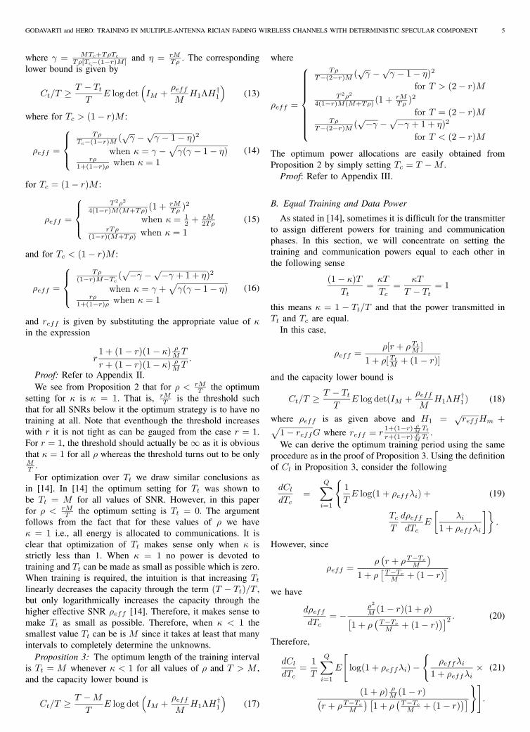
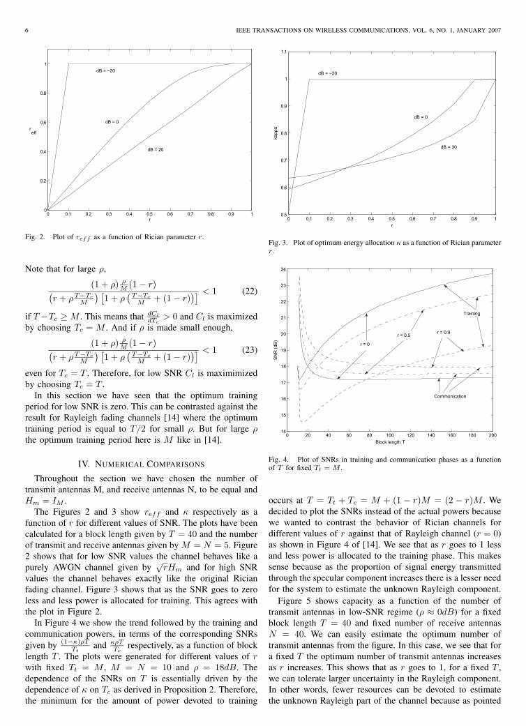
The Figures 2 and 3 show reff and κ respectively as afunction of r for different values of SNR. The plots have beencalculated for a block length given by T = 40 and the numberof transmit and receive antennas given by M = N = 5. Figure2 shows that for low SNR values the channel behaves like apurely AWGN channel given by

√rHm and for high SNR

values the channel behaves exactly like the original Ricianfading channel. Figure 3 shows that as the SNR goes to zeroless and less power is allocated for training. This agrees withthe plot in Figure 2.

In Figure 4 we show the trend followed by the training andcommunication powers, in terms of the corresponding SNRsgiven by (1−κ)ρT

Ttand κρT

Tcrespectively, as a function of block

length T . The plots were generated for different values of rwith fixed Tt = M , M = N = 10 and ρ = 18dB. Thedependence of the SNRs on T is essentially driven by thedependence of κ on Tc as derived in Proposition 2. Therefore,the minimum for the amount of power devoted to training

0 0.1 0.2 0.3 0.4 0.5 0.6 0.7 0.8 0.9 10.5

0.6

0.7

0.8

0.9

1

1.1

r

kapp

a

dB = 20

dB = 0

dB = −20

Fig. 3. Plot of optimum energy allocation κ as a function of Rician parameterr.

0 20 40 60 80 100 120 140 160 180 20014

15

16

17

18

19

20

21

22

23

24

Block length T

SN

R (d

B)

r = 0

r = 0.5 r = 0.9

Training

Communication

Fig. 4. Plot of SNRs in training and communication phases as a functionof T for fixed Tt = M .

occurs at T = Tt + Tc = M + (1 − r)M = (2 − r)M . Wedecided to plot the SNRs instead of the actual powers becausewe wanted to contrast the behavior of Rician channels fordifferent values of r against that of Rayleigh channel (r = 0)as shown in Figure 4 of [14]. We see that as r goes to 1 lessand less power is allocated to the training phase. This makessense because as the proportion of signal energy transmittedthrough the specular component increases there is a lesser needfor the system to estimate the unknown Rayleigh component.

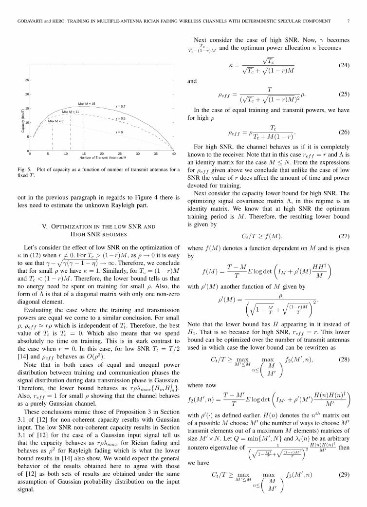
Figure 5 shows capacity as a function of the number oftransmit antennas in low-SNR regime (ρ ≈ 0dB) for a fixedblock length T = 40 and fixed number of receive antennasN = 40. We can easily estimate the optimum number oftransmit antennas from the figure. In this case, we see that fora fixed T the optimum number of transmit antennas increasesas r increases. This shows that as r goes to 1, for a fixed T ,we can tolerate larger uncertainty in the Rayleigh component.In other words, fewer resources can be devoted to estimatethe unknown Rayleigh part of the channel because as pointed


0 5 10 15 20 25 30 35 400

5

10

15

20

25

Number of Transmit Antennas M

Cap

acity

(bi

ts/T

)

r = 0

r = 0.5

r = 0.7

Max M = 6

Max M = 11

Max M = 15

Fig. 5. Plot of capacity as a function of number of transmit antennas for afixed T .

out in the previous paragraph in regards to Figure 4 there isless need to estimate the unknown Rayleigh part.

V. OPTIMIZATION IN THE LOW SNR AND

HIGH SNR REGIMES

Let’s consider the effect of low SNR on the optimization ofκ in (12) when r �= 0. For Tc > (1−r)M , as ρ → 0 it is easyto see that γ−√

γ(γ − 1 − η) → ∞. Therefore, we concludethat for small ρ we have κ = 1. Similarly, for Tc = (1− r)Mand Tc < (1 − r)M . Therefore, the lower bound tells us thatno energy need be spent on training for small ρ. Also, theform of Λ is that of a diagonal matrix with only one non-zerodiagonal element.

Evaluating the case where the training and transmissionpowers are equal we come to a similar conclusion. For smallρ, ρeff ≈ rρ which is independent of Tt. Therefore, the bestvalue of Tt is Tt = 0. Which also means that we spendabsolutely no time on training. This is in stark contrast tothe case when r = 0. In this case, for low SNR Tt = T/2[14] and ρeff behaves as O(ρ2).

Note that in both cases of equal and unequal powerdistribution between training and communication phases thesignal distribution during data transmission phase is Gaussian.Therefore, the lower bound behaves as rρλmax{HmH†

m}.Also, reff = 1 for small ρ showing that the channel behavesas a purely Gaussian channel.

These conclusions mimic those of Proposition 3 in Section3.1 of [12] for non-coherent capacity results with Gaussianinput. The low SNR non-coherent capacity results in Section3.1 of [12] for the case of a Gaussian input signal tell usthat the capacity behaves as rρλmax for Rician fading andbehaves as ρ2 for Rayleigh fading which is what the lowerbound results in [14] also show. We would expect the generalbehavior of the results obtained here to agree with thoseof [12] as both sets of results are obtained under the sameassumption of Gaussian probability distribution on the inputsignal.

Next consider the case of high SNR. Now, γ becomesTc

Tc−(1−r)M and the optimum power allocation κ becomes

κ =√

Tc√Tc +

√(1 − r)M

(24)

and

ρeff =T

(√

Tc +√

(1 − r)M)2ρ. (25)

In the case of equal training and transmit powers, we havefor high ρ

ρeff = ρTt

Tt + M(1 − r). (26)

For high SNR, the channel behaves as if it is completelyknown to the receiver. Note that in this case reff = r and Λ isan identity matrix for the case M ≤ N . From the expressionsfor ρeff given above we conclude that unlike the case of lowSNR the value of r does affect the amount of time and powerdevoted for training.

Next consider the capacity lower bound for high SNR. Theoptimizing signal covariance matrix Λ, in this regime is anidentity matrix. We know that at high SNR the optimumtraining period is M . Therefore, the resulting lower boundis given by

Ct/T ≥ f(M). (27)

where f(M) denotes a function dependent on M and is givenby

f(M) =T − M

TE log det

(IM + ρ′(M)

HH†

M

).

with ρ′(M) another function of M given by

ρ′(M) =ρ(√

1 − MT +

√(1−r)M

T

)2 .

Note that the lower bound has H appearing in it instead ofH1. That is so because for high SNR, reff = r. This lowerbound can be optimized over the number of transmit antennasused in which case the lower bound can be rewritten as

Ct/T ≥ maxM ′≤M

max

n≤(

MM ′

) f2(M ′, n), (28)

where now

f2(M ′, n) =T − M ′

TE log det

(IM ′ + ρ′(M ′)

H(n)H(n)†

M ′

)

with ρ′(·) as defined earlier. H(n) denotes the nth matrix outof a possible M choose M ′ (the number of ways to choose M ′

transmit elements out of a maximum M elements) matrices ofsize M ′×N . Let Q = min{M ′, N} and λi(n) be an arbitrarynonzero eigenvalue of 1(√

1−M′T +

√(1−r)M′

T

)2H(n)H(n)†

M ′ then

we have


max

n≤(

MM ′

) f3(M ′, n) (29)


where now

f3(M ′, n) =T − M ′

T

Q∑i=1

E log(1 + ρλi(n)).

At high SNR, the leading term involving ρ in∑Q

i=1 E log(1+ρλi(n)) is Q log ρ which is independent of n. Therefore,


{(1 − M ′

T )M ′ log ρ ifM ′ ≤ N

(1 − M ′T )N log ρ ifM > N.

(30)

The expression (1 − M ′T )M ′, is maximized by choosing

M ′ = T/2 when min{M,N} ≥ T/2 and by choosing M ′ =min{M,N} when min{M,N} ≤ T/2. This means that theexpression is maximized when M ′ = min{M,N, T/2}. Thisis a similar conclusion drawn in [14] and [22]. Also, theleading term in ρ for high SNR in the lower bound is givenby

Ct/T ≥ (1 − K

T)K log ρ (31)

where K = min{M,N, T/2}. This result suggests that thenumber of degrees of freedom available for communication islimited by the minimum of the number of transmit antennas,receive antennas and half the length of the coherence interval.Moreover, the results obtained in Section 3.4 of [12] for thecase when M ≤ N and large T show that the asymptoticcapacity behaves as M(T −M) log ρ from which we see thatthe lower bound is tight in the sense that the leading terminvolving ρ in the lower bound is the same as the one in theexpression for capacity.

VI. CONCLUSIONS AND FUTURE WORK

In this paper, we investigated the utility of training basedcommunication schemes in non-coherent communicationsover Rician fading channels with deteriministic specular com-ponent. The findings in this paper can be compared with thefindings on Rayleigh fading channels from [13] and [14]. Thesimilarities and differences are summarized below:

• Our study showed that for Rician fading channels, similarto Rayleigh fading, at low SNR training based schemesare suboptimum whereas for high SNRs training canattain capacity.

• For high SNR and large coherence interval Rayleighand Rician channels behave in a similar manner both interms of the parameters maximizing the training basedlower bound and the lower bound itself. This means thatthe number of degrees of freedom of a training basedscheme over a Rician fading channel (Section V) is thesame as that of a Rayleigh fading channel which ismin{M,N, T/2} [14], [22].

• The differences between Rayleigh fading and Rician fad-ing show up at low SNR. For low SNR from the analysisitself we conclude that for Rician fading channels no timeor energy should be spent in training the receiver to learnthe channel. More precisely, for Rician fading channelsthere exists a threshold that is an increasing function ofthe Rician factor r such that for all SNRs below thethreshold the best strategy is not to spend any effort inlearning the channel.

• Another difference between Rayleigh and Rician fadingchannels is that the lower bound on training based capac-ity for Rayleigh fading channels is a quadratic functionof SNR whereas for Rician fading it is a linear function.This linear function of SNR is still suboptimum exceptwhen r = 1 at which point the Rician fading channel issimply an AWGN channel.

• Finally, there exists a difference between Rician andRayleigh fading in the optimum transmit signal covari-ance matrix structure for low SNR. Eventhough, forlow SNR the optimum transmit signal covariance matrixconsists of a single non-zero eigenvalue in both cases; forthe case of Rician fading the eigenvector corresponding tothe non-zero eigenvalue has to point in the same directionas the specular component of maximum strength.

In the future, it would be very useful to obtain a solutionto the problem of finding maximum achievable rates on non-coherent block fading Rician channels without explicit channelestimation along the lines of [15]. Some progress in thisregard was made in [10], [11]. In addition, the assumption ofdeterministic specular component was relaxed and the specularcomponent was treated as unknown. However, research alongthese lines is challenging and a breakthrough would requireconsiderable efforts from the communications research com-munity.

APPENDIX IPROOF OF PROPOSITION 1

First we note that σ2G

= 1 − σ2G

. This means that

ρeff =κTρ + Tc

(1 − r)κTρσ2G

+ Tc− 1. (32)

Therefore, to maximize ρeff we just need to minimize σ2G

.Now,

σ2G =

1NM

tr{E[vec(G)vec(G)†]}where vec(G) is a column vector obtained by stacking thecolumns of G one on top of the other. Therefore,

σ2G =

1NM

tr{E[vec(G)vec(G)†]

}(33)

=1

NMtr{

(IM + (1 − r)ρ

MS†

t St)−1 ⊗ IN )}

where ρ = Mσ2 . Therefore, the problem is the following

minSt:tr{S†

t St}≤(1−κ)TM

1M

tr{(

IM + (1 − r)ρ

MS†

t St

)−1}

.

The problem above can be restated as

minλ1,...,λM :

∑λm≤(1−κ)TM

1M

M∑m=1

11 + (1 − r) ρ

M λm(34)

where λm, m = 1, . . . , M are the eigenvalues of S†t St. The

solution to the above problem is λ1 = . . . = λM = (1− κ)T .Therefore, the optimum St satisfies S†

t St = (1 − κ)TIM .This gives σ2

G= 1

1+(1−r) ρM (1−κ)T

. Also, for this choice of

St we obtain the elements of G to be zero mean independentwith Gaussian distribution. This gives (11) as the expressionfor ρeff .


APPENDIX IIPROOF OF PROPOSITION 2

First, from Proposition 1

ρeff =κTρ[Mr + ρ(1 − κ)T ]

Tc(M + ρ(1 − κ)T ) + (1 − r)κTρM

=

⎧⎪⎪⎪⎪⎪⎪⎨⎪⎪⎪⎪⎪⎪⎩

TρTc−(1−r)M

(1−κ)κ+κ rMT ρ

MTc+T ρTcT ρ[Tc−(1−r)M]−κ

when Tc �= (1 − r)M

T 2ρ2

Tc(M+Tρ) [(1 − κ)κ + κ rMTρ ]

when Tc = (1 − r)M.

Consider the following three cases for the maximization ofρeff over 0 ≤ κ ≤ 1.Case 1. Tc = (1 − r)M :

We need to maximize (1 − κ)κ + κ rMTρ over 0 ≤ κ < 1.

The maximum occurs at κ = κ0 = min{ 12 + rM

2Tρ , 1}. In thiscase

ρeff =T 2ρ2

(1 − r)M(M + Tρ)[κ0

rM

Tρ+ κ0(1 − κ0)]. (35)

Case 2. Tc > (1 − r)M :In this case,

ρeff =Tρ

Tc − (1 − r)M(1 − κ)κ + κη

γ − κ(36)

where η = rMTρ and γ = MTc+TρTc

Tρ[Tc−(1−r)M ] > 1. We need to

maximize (1−κ)κ+κηγ−κ over 0 ≤ κ ≤ 1 which occurs at κ =

min{γ −√

γ2 − γ − ηγ, 1}. Therefore,

ρeff =Tρ

Tc − (1 − r)M(√

γ −√

γ − 1 − η)2 (37)

when κ < 1. When κ = 1 we obtain Tc = T . Substitutingκ = 1 in the expression for ρeff

ρeff =κTρ[Mr + ρ(1 − κ)T ]

Tc(M + ρ(1 − κ)T ) + (1 − r)κTρM(38)

we obtain ρeff = rTρT+(1−r)Tρ .

Case 3. Tc < (1 − r)M :In this case,

ρeff =Tρ

(1 − r)M − Tc

(1 − κ)κ + κη

κ − γ(39)


Tρ[Tc−(1−r)M ] < 0. Maximizing (1−κ)κ+κηγ−κ over

0 ≤ κ ≤ 1 we obtain κ = min{γ +√

γ2 − γ − γη, 1}.Therefore, when κ < 1

ρeff =Tρ

Tc − (1 − r)M(√−γ −

√−γ + 1 + η)2 (40)

Similar to the case Tc < (1 − r)M , when κ = 1 we obtainTc = T and ρeff = rTρ

T+(1−r)Tρ .

APPENDIX IIIPROOF OF PROPOSITION 3

Note that optimization over Tc makes sense only when κ <1. If κ = 1 then Tc obviously has to be set equal to T . First,we examine the case Tc > (1 − r)M . The other two casesare similar. Let Q = min{M,N} and let λi denote the ith

non-zero eigenvalue of H1H†1

M , i = 1, . . . , Q. Then we have

Ct ≥Q∑

i=1

Tc

TE log(1 + ρeffλi).

Let Cl denote the RHS in the expression above. The idea isto maximize Cl as a function of Tc. We have

dCl

dTc=

Q∑i=1

{1T

E log(1 + ρeffλi) + (41)

Tc

T

dρeff

dTcE

[λi

1 + ρeffλi

]}.

Now, ρeff for Tc > (1 − r)M is given by

ρeff =Tρ

Tc − (1 − r)M(√

γ −√

γ − 1 − η)2


Tρ[Tc−(1−r)M ] and η = rMTρ . It can be easily

verified that

dρeff

dTc=

Tρ(√

γ −√γ − 1 − η)2

[Tc − (1 − r)M ]2×[√

(1 − r)M(M + Tρ)Tc(Tc + Tρ + rM)

− 1

].

Therefore,

dCl

dTc=

1T

Q∑i=1

E

[log(1 + ρeffλi) − (42)

{ρeffλi

1 + ρeffλi

Tc

Tc − (1 − r)M×(

1 −√

(1 − r)M(M + Tρ)Tc(Tc + Tρ + rM)

)}].

Since, Tc

Tc−(1−r)M

[1 −

√(1−r)M(M+Tρ)Tc(Tc+Tρ+rM)

]< 1 and log(1 +

x)−x/(1+x) ≥ 0 for all x ≥ 0 we have dCl

dTc> 0. Therefore,

we need to increase Tc as much as possible to maximize Cl

or Tc = T − M .

REFERENCES

[1] N. Benvenuto, P. Bisaglia, A. Salloum, and L. Tomba, “Worst caseequalizer for noncoherent HIPERLAN receivers,” IEEE Trans. Com-mun., vol. 48, no. 1, pp. 28–36, Jan. 2000.

[2] T. M. Cover and J. A. Thomas, Elements of Information Theory. WileySeries in Telecommunications, 1995.

[3] I. Csiszar and J. Korner, Information Theory: Coding Theorems forDiscrete Memoryless Systems. New York: Academic Press, 1981.

[4] P. F. Driessen and G. J. Foschini, “On the capacity formula for multipleinput-multiple output wireless channels: a geometric interpretation,”IEEE Trans. Commun., vol. 47, no. 2, pp. 173–176, Feb. 1999.

[5] F. R. Farrokhi, G. J. Foschini, A. Lozano, and R. A. Valenzuela,“Link-optimal space-time processing with multiple transmit and receiveantennas,” IEEE Commun. Lett., vol. 5, no. 3, pp. 85–87, Mar. 2001.

[6] G. J. Foschini, “Layered space-time architecture for wireless commu-nication in a fading environment when using multiple antennas,” BellLabs Technical J., vol. 1, no. 2, pp. 41–59, 1996.


[7] G. J. Foschini and M. J. Gans, “On limits of wireless communications ina fading environment when using multiple antennas,” Wireless PersonalCommun., vol. 6, no. 3, pp. 311–335, Mar. 1998.

[8] R. G. Gallager, Information Theory and Reliable Communication. NewYork: Wiley, 1968.

[9] R. G. Gallager, “A simple derivation of the coding theorem and someapplications,” IEEE Trans. Inf. Theory, vol. 11, no. 1, pp. 3–18, Jan.1965.

[10] M. Godavarti, A. O. Hero, and T. Marzetta, “Min-capacity of a multiple-antenna wireless channel in a static Ricean fading environment,” IEEETrans. Wireless Commun., vol. 4, no. 4, pp. 1715–1723, July 2005.

[11] M. Godavarti, T. Marzetta, and S. S. Shitz, “Capacity of a mobilemultiple-antenna wireless link with isotropically random Rician fading,”IEEE Trans. Inf. Theory, vol. 49, no. 12, pp. 3330–3334, Dec. 2003.

[12] M. Godavarti and A. O. Hero III, “Multiple antenna capacity in adeterministic Rician fading channel,” submitted to IEEE Trans. Inf.Theory.

[13] H. Weingarten, Y. Steinberg, and S. Shamai (Shitz), “Gaussian codes andweighted nearest neighbor decoding in fading multi-antenna channels,”IEEE Trans. Inf. Theory, vol. 50, no. 9, pp. 1665–1686, Sept. 2004.

[14] B. Hassibi and B. M. Hochwald, “How much training is needed inmultiple-antenna wireless links?” IEEE Trans. Inf. Theory, vol. 49, no.4, pp. 951–963, April 2003.

[15] Z. B. Krusevac, P. B. Rapajic, and R. A. Kennedy, “On channeluncertainty modeling: an information theoretic approach,” in Proc.Global Telecommunications Conference 2004, vol. 1, pp. 410–414.

[16] T. L. Marzetta and B. M. Hochwald, “Capacity of a mobile multiple-antenna communication link in Rayleigh flat fading channel,” IEEETrans. Inf. Theory, vol. 45, no. 1, pp. 139–157, Jan. 1999.

[17] T. L. Marzetta, “BLAST training: estimating channel characteristicsfor high-capacity space-time wireless,” in Proc. 37th Annuual AllertonConference Communications, Control, and Computing 1999.

[18] S. Rice, “Mathematical analysis of random noise,” Bell Systems Tech-nical J., vol. 23, 1944.

[19] V. Tarokh, N. Seshadri, and A. R. Calderbank, “Space-time codes forhigh data rate wireless communication: performance criterion and codeconstruction,” IEEE Trans. Commun., vol. 44, no. 2, pp. 744–765, March1998.

[20] I. E. Telatar, “Capacity of multi-antenna Gaussian channels,” EuropeanTrans. Telecommun., vol. 10, no. 6, pp. 585–596, Nov./Dec. 1999.

[21] S. Verdu, “Spectral efficiency in the wideband regime,” IEEE Trans. Inf.Theory. vol. 48, no. 6, pp. 1319–1343, June 2002.

[22] L. Zheng and D. N. C. Tse, “Packing spheres in the Grassmannmanifold: a geometric approach to the non-coherent multi-antennachannel,” IEEE Trans. Inf. Theory, vol. 48, no. 2, pp. 359–383, Feb.2002.

Mahesh Godavarti was born in Jaipur, India in1972. He received the B.Tech degree in Electricaland Electronics Engineering from the Indian Insti-tute of Technology, Madras, India in 1993 and theM.S. degree in Electrical and Computer Engineeringfrom the University of Arizona, Tucson, AZ in1995. He was at the University of Michigan from1997 to 2001 where he received the M.S. degreein Applied Mathematics and the Ph.D. degree inElectrical Engineering. Currently, he is employedas DSP Algorithm Manager with Ditech Networks,

Mountain View, CA, where he is researching new algorithms for speechenhancement. His research interests include topics in speech and signalprocessing, communications and information theory.

Alfred O. Hero, III was born in Boston, MA,in 1955. He received the B.S. degree in electri-cal engineering (summa cum laude) from BostonUniversity in 1980 and the Ph.D. from PrincetonUniversity, Princeton, NJ, in 1984, both in electricalengineering. While at Princeton, he held the G.V.N.Lothrop Fellowship in Engineering. Since 1984 hehas been with the University of Michigan, AnnArbor, where he is a Professor in the Departmentof Electrical Engineering and Computer Scienceand, by courtesy, in the Department of Biomedical

Engineering and the Department of Statistics. He has held visiting positionsat Massachusettes Institute of Technology (2006), I3S University of Nice,Sophia-Antipolis, France (2001), Ecole Normale Superieure de Lyon (1999),Ecole Nationale Superieure des Telecommunications, Paris (1999), ScientificResearch Labs of the Ford Motor Company, Dearborn, Michigan (1993),Ecole Nationale Superieure des Techniques Avancees (ENSTA), Ecole Su-perieure d’Electricite, Paris (1990), and M.I.T. Lincoln Laboratory (1987 -1989). His recent research interests have been in areas including: inferencefor sensor networks, adaptive sensing, inverse problems, bioinformatics, andstatistical signal and image processing.

He has served on the editorial boards of the IEEE Transactions on Infor-mation Theory (1995-1998, 1999), the IEEE Transactions on ComputationalBiology and Bioinformatics (2004-2006), and the IEEE Transactions on SignalProcessing (2002, 2004). He was Chairman of the Statistical Signal and ArrayProcessing (SSAP) Technical Committee (1997-1998) and Treasurer of theConference Board of the IEEE Signal Processing Society. He was Chairmanfor Publicity of the 1986 IEEE International Symposium on Information The-ory (Ann Arbor, MI) and General Chairman of the 1995 IEEE InternationalConference on Acoustics, Speech, and Signal Processing (Detroit, MI). Hewas co-chair of the 1999 IEEE Information Theory Workshop on Detection,Estimation, Classification and Filtering (Santa Fe, NM) and the 1999 IEEEWorkshop on Higher Order Statistics (Caesaria, Israel). He Chaired the 2002NSF Workshop on Challenges in Pattern Recognition. He co-chaired the 2002Workshop on Genomic Signal Processing and Statistics (GENSIPS). He wasVice President (Finance) of the IEEE Signal Processing Society (1999-2002).He was Chair of Commission C (Signals and Systems) of the US NationalCommission of the International Union of Radio Science (URSI) (1999-2002). He was member of the Signal Processing Theory and Methods (SPTM)Technical Committee of the IEEE Signal Processing Society (1999-2004). Heis currently President of the IEEE Signal Processing Society (2006-2007) anda member of the IEEE TAB Periodicals Committee (2006-2008).

Alfred Hero is a Fellow of the Institute of Electrical and Electronics Engi-neers (IEEE), a member of Tau Beta Pi, the American Statistical Association(ASA) , the Society for Industrial and Applied Mathematics (SIAM), andthe US National Commission (Commission C) of the International Unionof Radio Science (URSI). He has been plenary and keynote speaker andseveral major conferences and received a IEEE Signal Processing SocietyMeritorious Service Award (1998), a IEEE Signal Processing Society BestPaper Award (1998), a IEEE Third Millenium Medal (2000) and a 2002IEEE Signal Processing Society Distinguished Lecturership.

Training in multiple-antenna Rician fading wireless channels with deterministic specular component

Documents