1 Copyright © 2007 by ASME Proceedings of the ASME 2007 International Design Engineering Technical Conferences & Computers and Information in Engineering Conference IDETC/CIE 2007 September 4-7, 2007, Las Vegas, Nevada, USA DETC2007/DAC-34684 VISUAL STEERING COMMANDS FOR TRADE SPACE EXPLORATION: USER-GUIDED SAMPLING WITH EXAMPLE Gary Stump, Sara Lego, Mike Yukish The Applied Research Laboratory The Pennsylvania State University State College, PA 16804 USA {gms158, ses244, may106}@psu.edu Timothy W. Simpson* Mechanical & Nuclear Engineering The Pennsylvania State University University Park, PA 16802 USA [email protected] Joseph A. Donndelinger Vehicle Development Research Lab General Motors R&D Center Warren MI 48090 USA [email protected] ABSTRACT * Recent advancements in computing power and speed provide opportunities to revolutionize trade space exploration, particularly for the design of complex systems such as automobiles, aircraft, and spacecraft. In this paper, we introduce three Visual Steering Commands to support trade space exploration and demonstrate their use within a powerful data visualization tool that allows designers to explore multi- dimensional trade spaces using glyph, 1-D and 2-D histogram, 2-D scatter, scatter matrix, and parallel coordinate plots; linked views; brushing; preference shading and Pareto frontier display. In particular, we define three user-guided samplers that enable designers to explore (1) the entire design space, (2) near a point of interest, or (3) within a region of high preference. We illustrate these three samplers with a vehicle configuration model that evaluates the technical feasibility of new vehicle concepts. Future research is also discussed. 1 INTRODUCTION With recent advances in computing power and speed, designers can now simulate and evaluate thousands, if not millions, of design alternatives more cheaply and quickly than ever before 1 . These advancements provide new opportunities to revolutionize trade space exploration, particularly for the design of complex systems (e.g., automobiles, aircraft, and satellites) that consist of multiple, interacting subsystems and components that are designed by engineers from a variety of disciplines. The main challenge when designing such systems lies in resolving the inherent tradeoffs that exist both within and between subsystems and the overall system. For example, an aircraft is composed of the wings, fuselage, engines, and countless other subsystems and components. If we consider * Please address all correspondences to this author. 1 While some computer-based simulations may take a long time to run (e.g., a crash simulation of a full passenger car takes 36-160 hours to compute, according to engineers at Ford Motor Company [1]), metamodeling techniques such as response surface models and kriging [2] can be used to construct computationally efficient approximations of such simulations and then used as a surrogate to generate hundreds, or thousands, of design alternatives quickly and cost-effectively. the design of the wings, tradeoffs exist between aerodynamics, structures, and controls among others, yet wing designers are also driven by the goal to reduce the weight of the wing to minimize the overall weight of the aircraft. Given the complexity and tightly coupled nature of complex engineered systems, the following optimization problem is frequently used to help resolve these tradeoffs: Minimize: f i (x j ) i = 1, …, m; j = 1, …, n (1) Subject to: g k (x j ) > 0 k = 1, …, p h l (x j ) = 0 l = 1, …, q x j l.b. < x j < x j u.b. where x j are the input variables that the designer can control— they can vary between a specified lower (l.b.) and upper (u.b.) bound—while f i , g k , and h l are the objectives, inequality constraints, and equality constraints, respectively, that are based on the performance (output) of the system for a given set of inputs. For single objective problems ( m=1), solving Eq. (1) yields a single design point, the optimum design x j * , while multi-objective problems (m>2) yield a set of non- dominated designs that are referred to as Pareto points and form a Pareto frontier [3]. As a result, research has focused largely on novel formulations and algorithms for solving these problems (e.g., [4-6]), approximation methods to reduce the computational expense of related analyses (e.g., [2,7]), and computational frameworks to integrate analyses from multiple disciplines (e.g., [8,9]), among other areas. Despite these advances, design optimization still has many shortcomings and challenges to overcome [10]. Balling [11] has noted that the traditional optimization-based design process of “1) formulate the design problem, 2) obtain/develop analysis models, and 3) exe cute an optimization algorithm” often leaves designers unsatisfied with their results because the problem is usually improperly formulated: “the objectives and constraints used in optimization were not what the owners and stakeholders really wanted…in many cases, people don’t know what they really want until they see some designs”.

Welcome message from author
This document is posted to help you gain knowledge. Please leave a comment to let me know what you think about it! Share it to your friends and learn new things together.
Transcript
1 Copyright © 2007 by ASME
Proceedings of the ASME 2007 International Design Engineering Technical Conferences & Computers and Information in Engineering Conference
IDETC/CIE 2007 September 4-7, 2007, Las Vegas, Nevada, USA
DETC2007/DAC-34684
VISUAL STEERING COMMANDS FOR TRADE SPACE EXPLORATION: USER-GUIDED SAMPLING WITH EXAMPLE
Gary Stump, Sara Lego, Mike Yukish
The Applied Research Laboratory The Pennsylvania State University
State College, PA 16804 USA {gms158, ses244, may106}@psu.edu
Timothy W. Simpson* Mechanical & Nuclear Engineering The Pennsylvania State University University Park, PA 16802 USA
Joseph A. Donndelinger Vehicle Development Research Lab
General Motors R&D Center Warren MI 48090 USA
[email protected] ABSTRACT*
Recent advancements in computing power and speed provide opportunities to revolutionize trade space exploration, particularly for the design of complex systems such as automobiles, aircraft, and spacecraft. In this paper, we introduce three Visual Steering Commands to support trade space exploration and demonstrate their use within a powerful data visualization tool that allows designers to explore multi-dimensional trade spaces using glyph, 1-D and 2-D histogram, 2-D scatter, scatter matrix, and parallel coordinate plots; linked views; brushing; preference shading and Pareto frontier display. In particular, we define three user-guided samplers that enable designers to explore (1) the entire design space, (2) near a point of interest, or (3) within a region of high preference. We illustrate these three samplers with a vehicle configuration model that evaluates the technical feasibility of new vehicle concepts. Future research is also discussed.
1 INTRODUCTION With recent advances in computing power and speed,
designers can now simulate and evaluate thousands, if not millions, of design alternatives more cheaply and quickly than ever before1. These advancements provide new opportunities to revolutionize trade space exploration, particularly for the design of complex systems (e.g., automobiles, aircraft, and satellites) that consist of multiple, interacting subsystems and components that are designed by engineers from a variety of disciplines. The main challenge when designing such systems lies in resolving the inherent tradeoffs that exist both within and between subsystems and the overall system. For example, an aircraft is composed of the wings, fuselage, engines, and countless other subsystems and components. If we consider
* Please address all correspondences to this author. 1 While some computer-based simulations may take a long time to run
(e.g., a crash simulation of a full passenger car takes 36-160 hours to compute, according to engineers at Ford Motor Company [1]), metamodeling techniques such as response surface models and kriging [2] can be used to construct computationally efficient approximations of such simulations and then used as a surrogate to generate hundreds, or thousands, of design alternatives quickly and cost-effectively.
the design of the wings, tradeoffs exist between aerodynamics, structures, and controls among others, yet wing designers are also driven by the goal to reduce the weight of the wing to minimize the overall weight of the aircraft.
Given the complexity and tightly coupled nature of complex engineered systems, the following optimization problem is frequently used to help resolve these tradeoffs:
Minimize: fi(xj) i = 1, …, m; j = 1, …, n (1) Subject to: gk(xj) > 0 k = 1, …, p hl(xj) = 0 l = 1, …, q xj
l.b. < xj < xju.b.
where xj are the input variables that the designer can control—they can vary between a specified lower (l.b.) and upper (u.b.) bound—while fi, gk, and hl are the objectives, inequality constraints, and equality constraints, respectively, that are based on the performance (output) of the system for a given set of inputs. For single objective problems (m=1), solving Eq. (1) yields a single design point, the optimum design xj
*, while multi-objective problems (m>2) yield a set of non-dominated designs that are referred to as Pareto points and form a Pareto frontier [3]. As a result, research has focused largely on novel formulations and algorithms for solving these problems (e.g., [4-6]), approximation methods to reduce the computational expense of related analyses (e.g., [2,7]), and computational frameworks to integrate analyses from multiple disciplines (e.g., [8,9]), among other areas.
Despite these advances, design optimization still has many shortcomings and challenges to overcome [10]. Balling [11] has noted that the traditional optimization-based design process of “1) formulate the design problem, 2) obtain/develop analysis models, and 3) exe cute an optimization algorithm” often leaves designers unsatisfied with their results because the problem is usually improperly formulated: “the objectives and constraints used in optimization were not what the owners and stakeholders really wanted…in many cases, people don’t know what they really want until they see some designs”.
2 Copyright © 2007 by ASME
Similar findings have occurred in other fields. For instance, Shanteau [12] observed that when people are dissatisfied with the results of a rational decision making process, they often change their ratings to make it come out the way they want. Wilson and Schooler [13] have shown that people do worse at some decision tasks when asked to analyze the reasons for their preferences or evaluate all the attributes of their choices.
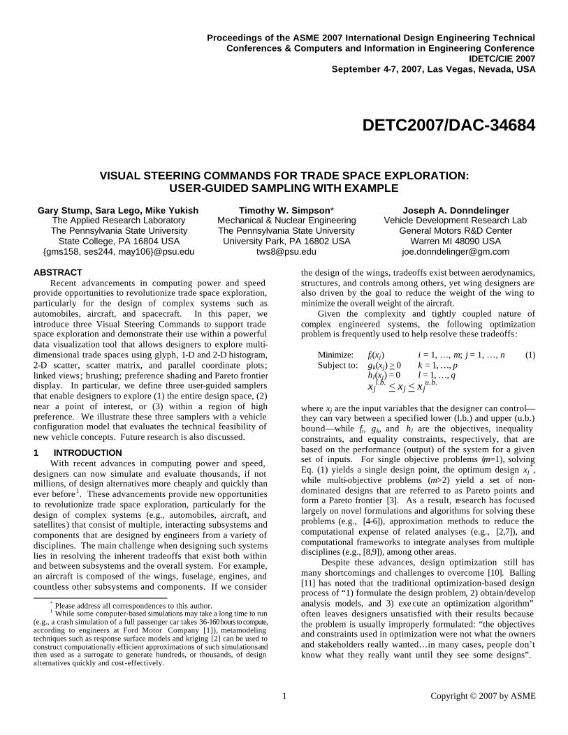
Consequently, there is an emerging paradigm of design exploration whereby designers “shop” for the best solution using visualization tools instead of relying solely on optimization. This Design by Shopping process – introduced by Balling [11] – allows designers to explore the design space first and then choose an optimal solution from a set of possible designs after “forming realistic expectations of what is possible”. This approach can be classified as an a posteriori articulation of preferences to solve a multi-objective optimization [14] in that designers first form their preferences based on visualization of the trade space, and then choose an optimal design that is based on their formed preference. The basic steps to this approach are shown in Figure 1. First, a simulation model, M, is created to analyze the system being designed. In many cases, this model is a “black box” where the relationships between design inputs, X, and performance outputs, Y, are not known, where X and Y combine to form what we call the trade space, Z = [X MY]T. Experiments are then run to simulate thousands of design alternatives by varying X and storing the corresponding values of Y for each alternative. Interactive visualization tools are then used to explore the trade space to find the most-preferred point Z*.
1.1 Review of Related Work Early work in engineering design sought to support this
type of approach concentrated on virtual reality to visualize design alternatives. Spherical mechanism design, for instance, has significantly benefited from virtual reality [15-17], as have large-scale manufacturing simulations [18,19], fluid mixing simulations [20], and a variety of other engineering design problems [21]. Many researchers have examined effective interface development for virtual environments [20,22-24], but most of these virtual environments do not support trade space exploration since they are typically intended to visualize a single point solution, not explore the entire trade space. Cloud Visualization [25], Visual Design Steering [26-28], and the U.S. Naval Research Laboratory’s visual steering methods in their Virtual Reality Lab and High Performance Computing Center [29] are some exceptions to this. For instance, Cloud Visualization [25] displays the input and output spaces of an engineering design problem using linked scatter plots, and points within the scatter plots can be shaded to identify if a design is feasible, infeasible, and Pareto optimal. Recent extensions to this work include BrickViz, which allows users to group uncertainty-related data into “bricks” to facilitate visualization [30] as well as novel methods to simplify the visualization of n-dimensional Pareto frontiers [31]. In the fields of data mining and knowledge discovery, existing software applications that offer multi-dimensional visualization capabilities for trade space exploration include Miner3D, Spotfire’s DecisionSite, XmdvTool, and GGobi – the capabilities of each are reviewed elsewhere [32].
Specify Point in the Input Space
Iterate until feasible design is calculated
Repeat 10,000+ times
Simulation Model (“Black Box”)
• Assemble simulation model and generate 10,000+ pts
• Models are based on domain-specific rules and analyses for the system being designed
• Focus on trade study of interest
• 3000-4000 designs• Augment each design with
geometry and related information
• Identify trends of interest• Apply constraints and
optimize• Visualize preference
structures and Pareto frontiers
Record Design and
Performance Variables
DesignDatabase
Build Model Run Experiments Explore
Visualize Data and Explore
Figure 1. Typical Approach to Trade Space Exploration
3 Copyright © 2007 by ASME
In the visualization community, interactive optimization-based methods fall mainly into the area of computational steering whereby the user (e.g., a designer) interacts with a simulation during the optimization process to help “steer” the search process toward what looks like an optimal solution. The designer observes some sort of a visualization of the optimization process and then uses intuition, heuristics, or some other method to adjust the design space to move toward something that may not have been intuitive at the beginning of the simulation. For instance, Wright, et al. [33] applied computational steering methods to the geometric and material design of glass for a furnace. Kesavadas and Sudhir [19] created large-scale manufacturing “simulations on the fly” by allowing users to make quick changes and continue with the simulation. Messac and Chen [34] proposed an interactive visualization method based on Physical Programming [35], where the progress of the optimization is visualized – but not steered – throughout the design process, not just at the beginning and end. Likewise, Visual Design Steering and Graph Morphing [26-28] allow users to stop and redirect the optimization process to improve the solution; however, their visualization capabilities are currently limited to 2-D and 3-D representations of constraints and objectives.
1.2 Overview of ARL Trade Space Visualizer
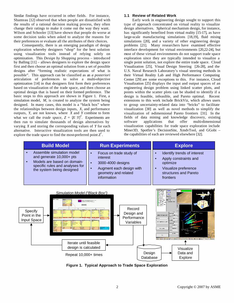
To support trade space exploration, researchers at the Applied Research Laboratory (ARL) and Penn State have developed the ARL Trade Space Visualizer (ATSV) [32,36-38], a Java-based application that displays multi-dimensional trade spaces using glyph, 1-D and 2-D histogram, 2-D scatter, scatter matrix, and parallel coordinate plots, linked views, and brushing – some examples are shown in Figure 2. The glyph plots have been developed on top of the Visualization Toolkit (VTK), an open source application that supports interactive 3-D plots within a Java application [39]. VTK provides the capability to view plots in 3-D stereoscopic mode, which can then be used within advanced visualization and virtual environments as desired. The ATSV is developed entirely in Java, making it cross-platform compatible unlike most commercially available software.
Scatter Matrices
Histograms
3D Glyph Plots
Figure 2. Three Views of Data in the ATSV
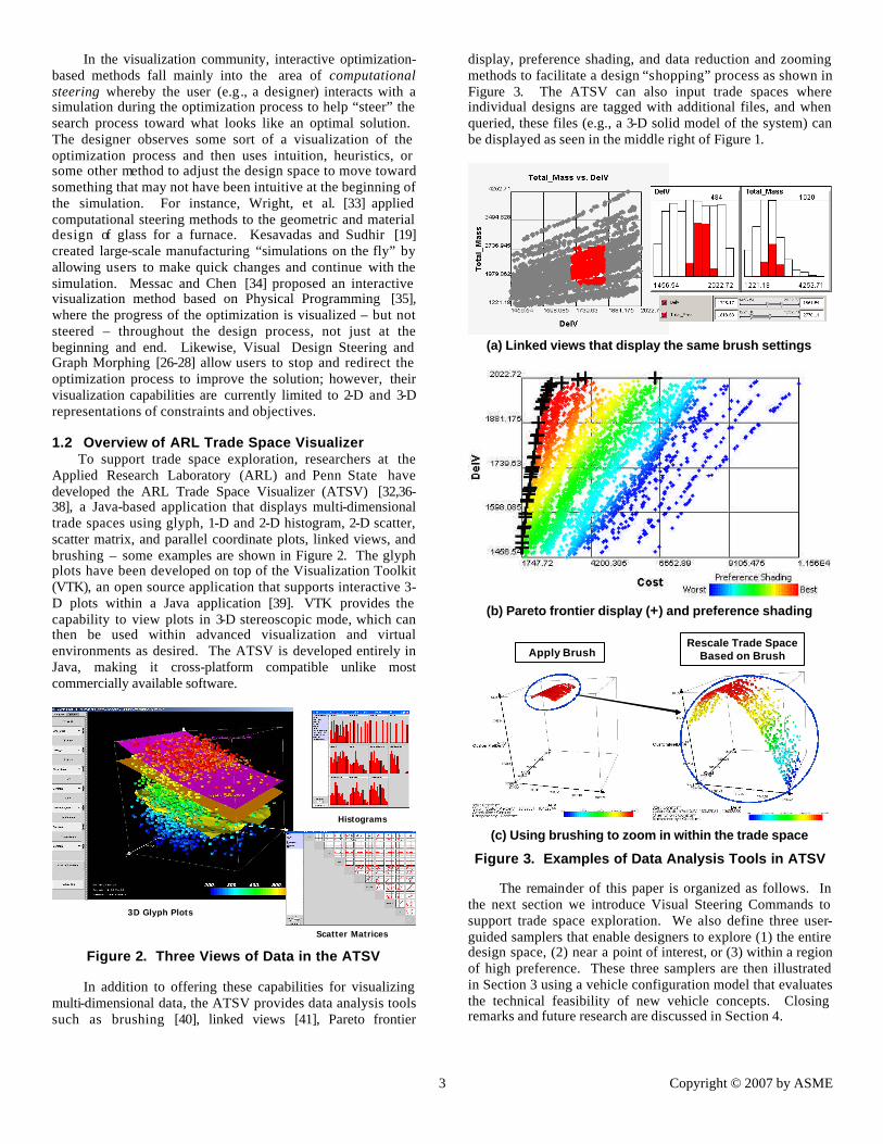
In addition to offering these capabilities for visualizing multi-dimensional data, the ATSV provides data analysis tools such as brushing [40], linked views [41], Pareto frontier
display, preference shading, and data reduction and zooming methods to facilitate a design “shopping” process as shown in Figure 3. The ATSV can also input trade spaces where individual designs are tagged with additional files, and when queried, these files (e.g., a 3-D solid model of the system) can be displayed as seen in the middle right of Figure 1.
(a) Linked views that display the same brush settings
(b) Pareto frontier display (+) and preference shading
Apply BrushRescale Trade Space
Based on Brush
(c) Using brushing to zoom in within the trade space
Figure 3. Examples of Data Analysis Tools in ATSV
The remainder of this paper is organized as follows. In the next section we introduce Visual Steering Commands to support trade space exploration. We also define three user-guided samplers that enable designers to explore (1) the entire design space, (2) near a point of interest, or (3) within a region of high preference. These three samplers are then illustrated in Section 3 using a vehicle configuration model that evaluates the technical feasibility of new vehicle concepts. Closing remarks and future research are discussed in Section 4.
4 Copyright © 2007 by ASME
2 VISUAL STEERING WITH SAMPLERS Before proceeding further, we first define the underlying
goal in trade space exploration as it differs from optimization. We assume the least informative starting point where the decision-makers have no knowledge of their preference on Z or the relationships in M. As they explore the trade space, they will simultaneously form their preference while searching for the most preferred point in the trade space. We further assume that there exis ts a utopia point, Z*, that the decision-makers would choose from Z if they had unlimited ability to explore the trade space completely. Recognizing the finite computing power available and the cost of search time, the goal is to have the decision-maker(s) choose a point Z+ as close as possible to Z* while minimizing the time to arrive at the choice of Z+. This differs from optimization in that the decision-makers’ preference is not known a priori or may change as a result of information gained during the exploration process, sending the search in an entirely different direction.
With this in mind, we are developing Visual Steering Commands that help decision-makers form their preference while exploring the trade space (i.e., “shopping”) to focus in on regions/points of interest as their preference sharpens. In this paper, Visual Steering Commands are embodied in three user-guided samplers that are created to sample (1) the entire design space, (2) near a point of interest, or (3) within a region of high preference. As echoed in the reinforcement learning literature [42], we have noticed a basic dichotomy when using Visual Steering Commands: (i) those that explore the trade space by broadly searching it and (ii) those that exploit knowledge gained during trade space exploration to guide and narrow the search. Initially users start out by conducting a broad search, then begin exploring localized regions of the trade space to increase knowledge of the underlying relationships, finally focusing their search in a region potentially containing Z*. When viewed in this light, the first sampler supports exploration of the entire trade space (case i) while the second two exploit knowledge about points or regions of interest to guide the sampling process (case ii). Descriptions and examples of each follow.
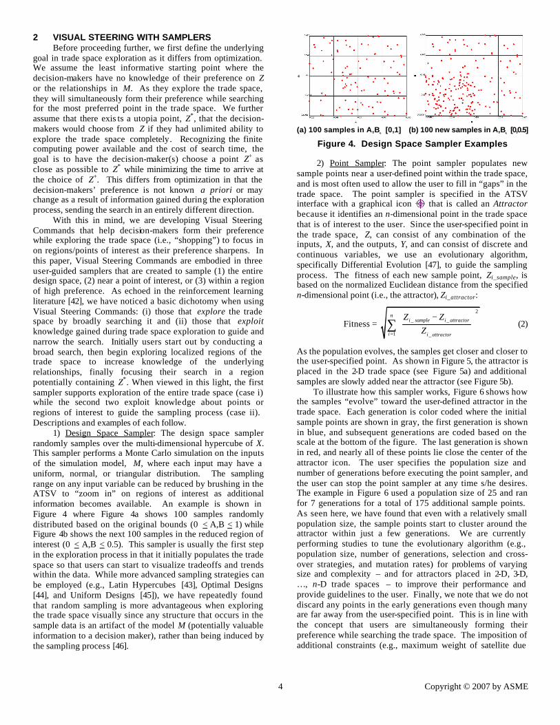
1) Design Space Sampler: The design space sampler randomly samples over the multi-dimensional hypercube of X. This sampler performs a Monte Carlo simulation on the inputs of the simulation model, M, where each input may have a uniform, normal, or triangular distribution. The sampling range on any input variable can be reduced by brushing in the ATSV to “zoom in” on regions of interest as additional information becomes available. An example is shown in Figure 4 where Figure 4a shows 100 samples randomly distributed based on the original bounds (0 < A,B < 1) while Figure 4b shows the next 100 samples in the reduced region of interest (0 < A,B < 0.5). This sampler is usually the first step in the exploration process in that it initially populates the trade space so that users can start to visualize tradeoffs and trends within the data. While more advanced sampling strategies can be employed (e.g., Latin Hypercubes [43], Optimal Designs [44], and Uniform Designs [45]), we have repeatedly found that random sampling is more advantageous when exploring the trade space visually since any structure that occurs in the sample data is an artifact of the model M (potentially valuable information to a decision maker), rather than being induced by the sampling process [46].
(a) 100 samples in A,B∈ [0,1] (b) 100 new samples in A,B∈[0,0.5]
Figure 4. Design Space Sampler Examples
2) Point Sampler: The point sampler populates new sample points near a user-defined point within the trade space, and is most often used to allow the user to fill in “gaps” in the trade space. The point sampler is specified in the ATSV interface with a graphical icon that is called an Attractor because it identifies an n-dimensional point in the trade space that is of interest to the user. Since the user-specified point in the trade space, Z, can consist of any combination of the inputs, X, and the outputs, Y, and can consist of discrete and continuous variables, we use an evolutionary algorithm, specifically Differential Evolution [47], to guide the sampling process. The fitness of each new sample point, Zi_sample, is based on the normalized Euclidean distance from the specified n-dimensional point (i.e., the attractor), Zi_attractor:
Fitness =
2
_ _
1 _
ni sample i attractor
i i attractor
Z ZZ=
−
∑ (2)
As the population evolves, the samples get closer and closer to the user-specified point. As shown in Figure 5, the attractor is placed in the 2-D trade space (see Figure 5a) and additional samples are slowly added near the attractor (see Figure 5b).
To illustrate how this sampler works, Figure 6 shows how the samples “evolve” toward the user-defined attractor in the trade space. Each generation is color coded where the initial sample points are shown in gray, the first generation is shown in blue, and subsequent generations are coded based on the scale at the bottom of the figure. The last generation is shown in red, and nearly all of these points lie close the center of the attractor icon. The user specifies the population size and number of generations before executing the point sampler, and the user can stop the point sampler at any time s/he desires. The example in Figure 6 used a population size of 25 and ran for 7 generations for a total of 175 additional sample points. As seen here, we have found that even with a relatively small population size, the sample points start to cluster around the attractor within just a few generations. We are currently performing studies to tune the evolutionary algorithm (e.g., population size, number of generations, selection and cross-over strategies, and mutation rates) for problems of varying size and complexity – and for attractors placed in 2-D, 3-D, …, n-D trade spaces – to improve their performance and provide guidelines to the user. Finally, we note that we do not discard any points in the early generations even though many are far away from the user-specified point. This is in line with the concept that users are simultaneously forming their preference while searching the trade space. The imposition of additional constraints (e.g., maximum weight of satellite due
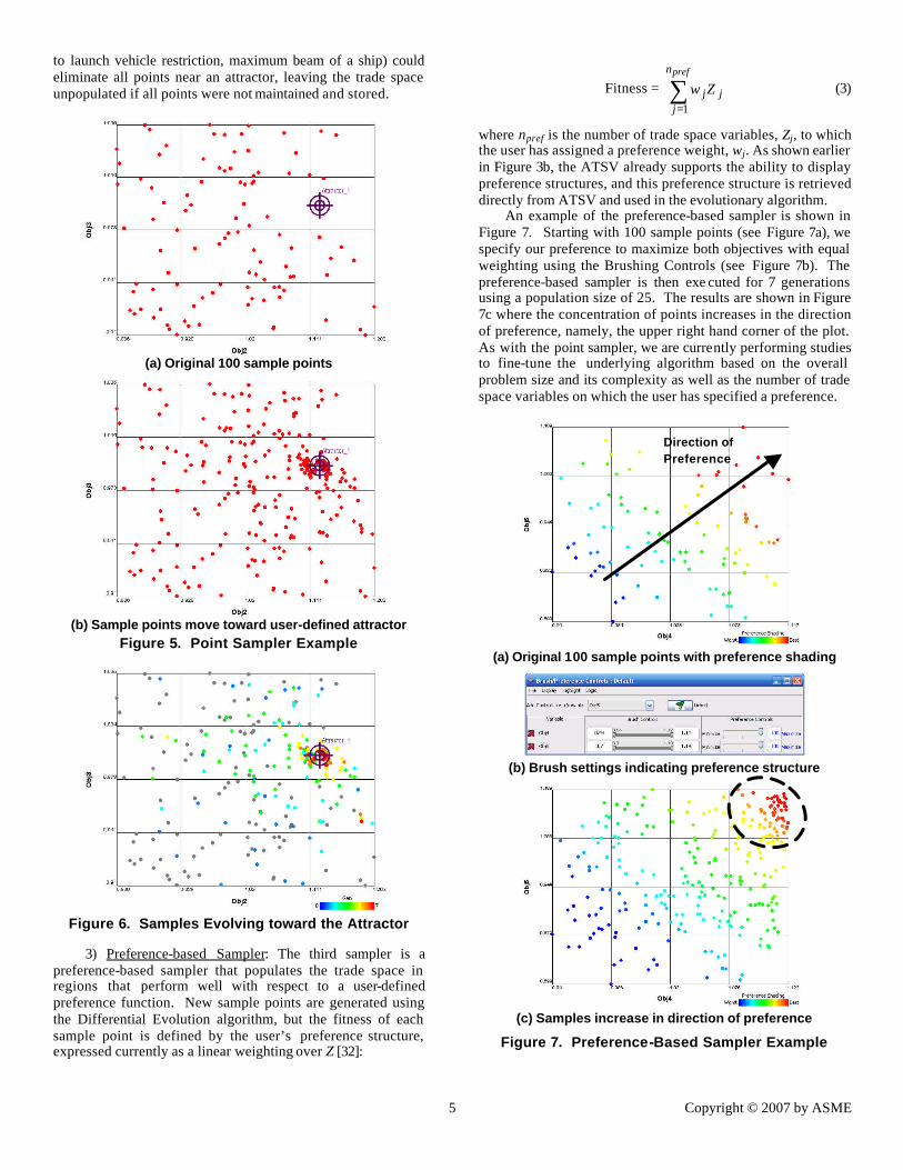
5 Copyright © 2007 by ASME
to launch vehicle restriction, maximum beam of a ship) could eliminate all points near an attractor, leaving the trade space unpopulated if all points were not maintained and stored.
(a) Original 100 sample points
(b) Sample points move toward user-defined attractor
Figure 5. Point Sampler Example
Figure 6. Samples Evolving toward the Attractor
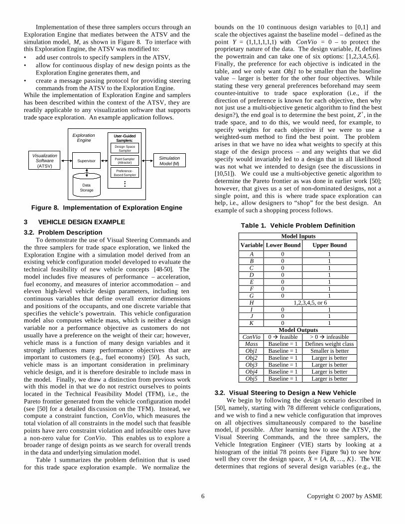
3) Preference-based Sampler: The third sampler is a preference-based sampler that populates the trade space in regions that perform well with respect to a user-defined preference function. New sample points are generated using the Differential Evolution algorithm, but the fitness of each sample point is defined by the user’s preference structure, expressed currently as a linear weighting over Z [32]:
Fitness = j
n
jjZw
pref
∑=1
(3)
where npref is the number of trade space variables, Zj, to which the user has assigned a preference weight, wj. As shown earlier in Figure 3b, the ATSV already supports the ability to display preference structures, and this preference structure is retrieved directly from ATSV and used in the evolutionary algorithm.
An example of the preference-based sampler is shown in Figure 7. Starting with 100 sample points (see Figure 7a), we specify our preference to maximize both objectives with equal weighting using the Brushing Controls (see Figure 7b). The preference-based sampler is then exe cuted for 7 generations using a population size of 25. The results are shown in Figure 7c where the concentration of points increases in the direction of preference, namely, the upper right hand corner of the plot. As with the point sampler, we are currently performing studies to fine-tune the underlying algorithm based on the overall problem size and its complexity as well as the number of trade space variables on which the user has specified a preference.
(a) Original 100 sample points with preference shading
(b) Brush settings indicating preference structure
(c) Samples increase in direction of preference
Figure 7. Preference-Based Sampler Example
Direction of Preference
6 Copyright © 2007 by ASME
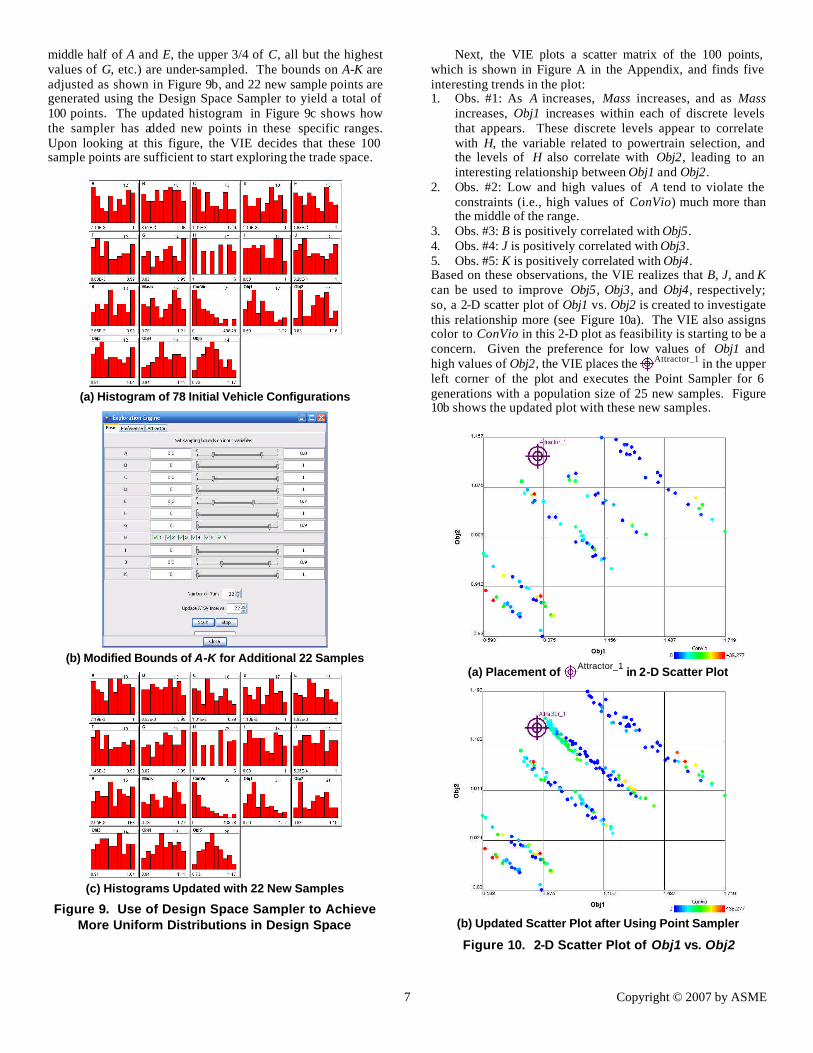
Implementation of these three samplers occurs through an Exploration Engine that mediates between the ATSV and the simulation model, M, as shown in Figure 8. To interface with this Exploration Engine, the ATSV was modified to: • add user controls to specify samplers in the ATSV, • allow for continuous display of new design points as the
Exploration Engine generates them, and • create a message passing protocol for providing steering
commands from the ATSV to the Exploration Engine. While the implementation of Exploration Engine and samplers has been described within the context of the ATSV, they are readily applicable to any visualization software that supports trade space exploration. An example application follows.
VisualizationSoftware(ATSV)
SimulationModel (M)
Supervisor
DataStorage
Design SpaceSampler
Point Sampler(Attractor)
Preference -Based Sampler
•••
User -GuidedSamplers:
Design SpaceSampler
Point Sampler(Attractor)
Preference -Based Sampler
•••
User -GuidedSamplers:
ExplorationEngine
Figure 8. Implementation of Exploration Engine
3 VEHICLE DESIGN EXAMPLE
3.2. Problem Description To demonstrate the use of Visual Steering Commands and
the three samplers for trade space exploration, we linked the Exploration Engine with a simulation model derived from an existing vehicle configuration model developed to evaluate the technical feasibility of new vehicle concepts [48-50]. The model includes five measures of performance – acceleration, fuel economy, and measures of interior accommodation – and eleven high-level vehicle design parameters, including ten continuous variables that define overall exterior dimensions and positions of the occupants, and one discrete variable that specifies the vehicle’s powertrain. This vehicle configuration model also computes vehicle mass, which is neither a design variable nor a performance objective as customers do not usually have a preference on the weight of their car; however, vehicle mass is a function of many design variables and it strongly influences many performance objectives that are important to customers (e.g., fuel economy) [50]. As such, vehicle mass is an important consideration in preliminary vehicle design, and it is therefore desirable to include mass in the model. Finally, we draw a distinction from previous work with this model in that we do not restrict ourselves to points located in the Technical Feasibility Model (TFM), i.e., the Pareto frontier generated from the vehicle configuration model (see [50] for a detailed dis cussion on the TFM). Instead, we compute a constraint function, ConVio, which measures the total violation of all constraints in the model such that feasible points have zero constraint violation and infeasible ones have a non-zero value for ConVio. This enables us to explore a broader range of design points as we search for overall trends in the data and underlying simulation model.
Table 1 summarizes the problem definition that is used for this trade space exploration example. We normalize the
bounds on the 10 continuous design variables to [0,1] and scale the objectives against the baseline model – defined as the point Y = (1,1,1,1,1,1) with ConVio = 0 – to protect the proprietary nature of the data. The design variable, H, defines the powertrain and can take one of six options: [1,2,3,4,5,6]. Finally, the preference for each objective is indicated in the table, and we only want Obj1 to be smaller than the baseline value – larger is better for the other four objectives. While stating these very general preferences beforehand may seem counter-intuitive to trade space exploration (i.e., if the direction of preference is known for each objective, then why not just use a multi-objective genetic algorithm to find the best design?), the end goal is to determine the best point, Z+, in the trade space, and to do this, we would need, for example, to specify weights for each objective if we were to use a weighted-sum method to find the best point. The problem arises in that we have no idea what weights to specify at this stage of the design process – and any weights that we did specify would invariably led to a design that in all likelihood was not what we intended to design (see the discussions in [10,51]). We could use a multi-objective genetic algorithm to determine the Pareto frontier as was done in earlier work [50]; however, that gives us a set of non-dominated designs, not a single point, and this is where trade space exploration can help, i.e., allow designers to “shop” for the best design. An example of such a shopping process follows.
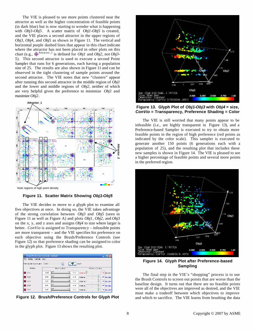
Table 1. Vehicle Problem Definition
Model Inputs Variable Lower Bound Upper Bound
A 0 1 B 0 1 C 0 1 D 0 1 E 0 1 F 0 1 G 0 1 H 1,2,3,4,5, or 6 I 0 1 J 0 1 K 0 1
Model Outputs ConVio 0 à feasible > 0 à infeasible Mass Baseline = 1 Defines weight class Obj1 Baseline = 1 Smaller is better Obj2 Baseline = 1 Larger is better Obj3 Baseline = 1 Larger is better Obj4 Baseline = 1 Larger is better Obj5 Baseline = 1 Larger is better
3.2. Visual Steering to Design a New Vehicle
We begin by following the design scenario described in [50], namely, starting with 78 different vehicle configurations, and we wish to find a new vehicle configuration that improves on all objectives simultaneously compared to the baseline model, if possible. After learning how to use the ATSV, the Visual Steering Commands, and the three samplers, the Vehicle Integration Engineer (VIE) starts by looking at a histogram of the initial 78 points (see Figure 9a) to see how well they cover the design space, X = {A, B, …, K}. The VIE determines that regions of several design variables (e.g., the
7 Copyright © 2007 by ASME
middle half of A and E, the upper 3/4 of C, all but the highest values of G, etc.) are under-sampled. The bounds on A-K are adjusted as shown in Figure 9b, and 22 new sample points are generated using the Design Space Sampler to yield a total of 100 points. The updated histogram in Figure 9c shows how the sampler has added new points in these specific ranges. Upon looking at this figure, the VIE decides that these 100 sample points are sufficient to start exploring the trade space.
(a) Histogram of 78 Initial Vehicle Configurations
(b) Modified Bounds of A-K for Additional 22 Samples
(c) Histograms Updated with 22 New Samples
Figure 9. Use of Design Space Sampler to Achieve More Uniform Distributions in Design Space
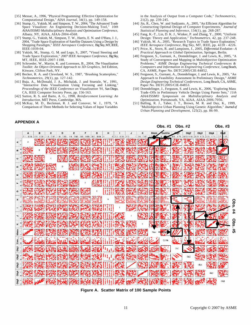
Next, the VIE plots a scatter matrix of the 100 points, which is shown in Figure A in the Appendix, and finds five interesting trends in the plot: 1. Obs. #1: As A increases, Mass increases, and as Mass
increases, Obj1 increases within each of discrete levels that appears. These discrete levels appear to correlate with H, the variable related to powertrain selection, and the levels of H also correlate with Obj2, leading to an interesting relationship between Obj1 and Obj2.
2. Obs. #2: Low and high values of A tend to violate the constraints (i.e., high values of ConVio) much more than the middle of the range.
3. Obs. #3: B is positively correlated with Obj5. 4. Obs. #4: J is positively correlated with Obj3. 5. Obs. #5: K is positively correlated with Obj4. Based on these observations, the VIE realizes that B, J, and K can be used to improve Obj5, Obj3, and Obj4, respectively; so, a 2-D scatter plot of Obj1 vs. Obj2 is created to investigate this relationship more (see Figure 10a). The VIE also assigns color to ConVio in this 2-D plot as feasibility is starting to be a concern. Given the preference for low values of Obj1 and high values of Obj2, the VIE places the Attractor_1 in the upper left corner of the plot and executes the Point Sampler for 6 generations with a population size of 25 new samples. Figure 10b shows the updated plot with these new samples.
(a) Placement of Attractor_1 in 2-D Scatter Plot
(b) Updated Scatter Plot after Using Point Sampler
Figure 10. 2-D Scatter Plot of Obj1 vs. Obj2
8 Copyright © 2007 by ASME
The VIE is pleased to see more points clustered near the attractor as well as the higher concentration of feasible points (in dark blue) but is now starting to wonder what is happening with Obj3-Obj5. A scatter matrix of Obj1-Obj5 is created, and the VIE places a second attractor in the upper regions of Obj3, Obj4, and Obj5 as shown in Figure 11. The vertical and horizontal purple dashed lines that appear in this chart indicate where the attractor has not been placed in other plots on this chart (e.g., Attractor_1 is defined for Obj1 and Obj2, not Obj3-5). This second attractor is used to execute a second Point Sampler that runs for 6 generations, each having a population size of 25. The results are also shown in Figure 11 and can be observed in the tight clustering of sample points around the second attractor. The VIE notes that new “clusters” appear after running this second attractor in the middle region of Obj1 and the lower and middle regions of Obj2, neither of which are very helpful given the preference to minimize Obj1 and maximize Obj2.
Attractor_1
Attracto
r_2
Note regions of high point density
Figure 11. Scatter Matrix Showing Obj1-Obj5
The VIE decides to move to a glyph plot to examine all five objectives at once. In doing so, the VIE takes advantage of the strong correlation between Obj3 and Obj5 (seen in Figure 11 as well as Figure A) and plots Obj1, Obj2, and Obj3 on the x, y, and z axes and assigns Obj4 to size where larger is better. ConVio is assigned to Transparency – infeasible points are more transparent – and the VIE specifies his preference on each objective using the Brush/Preference Controls (see Figure 12) so that preference shading can be assigned to color in the glyph plot. Figure 13 shows the resulting plot.
Figure 12. Brush/Preference Controls for Glyph Plot
Figure 13. Glyph Plot of Obj1-Obj3 with Obj4 = size, ConVio = Transparency, Preference Shading = Color
The VIE is still worried that many points appear to be infeasible (i.e., are highly transparent in Figure 13), and a Preference-based Sampler is executed to try to obtain more feasible points in the region of high preference (red points as indicated by the color scale). This sampler is executed to generate another 150 points (6 generations each with a population of 25), and the resulting plot that includes these new samples is shown in Figure 14. The VIE is pleased to see a higher percentage of feasible points and several more points in the preferred region.
Figure 14. Glyph Plot after Preference-based
Sampling
The final step in the VIE’s “shopping” process is to use the Brush Controls to screen out points that are worse than the baseline design. It turns out that there are no feasible points were all of the objectives are improved as desired, and the VIE must make a tradeoff between which objectives to improve and which to sacrifice. The VIE learns from brushing the data
9 Copyright © 2007 by ASME
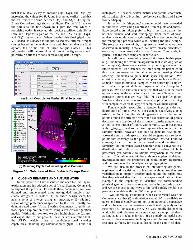
that it is relatively easy to improve Obj3, Obj4, and Obj5 (by increasing the values for B, J, and K as noted earlier), and that the real tradeoff occurs between Obj1 and Obj2. Using the Brush Control settings shown in Figure 15a, the VIE reduces the points to the few shown in Figure 15b from which a promising option is selected: this design sacrifices only 2% in Obj1 and Obj2 for a gain of 3%, 9%, and 13% in Obj3, Obj4, and Obj5, respectively. When creating this final glyph, the VIE added iso-surfaces to the plot to indicate different weight classes based on the vehicle mass and observed that the final options fell within one of three weight classes. This information will be useful as different configurations and powertrain options are considered during detail design.
(a) Brush Controls for Making Final Selection
(b) Resulting Glyph Plot including Mass Contours
Figure 15. Selection of Final Vehicle Design Point
4 CLOSING REMARKS AND FUTURE WORK In this paper, we have discussed the need for trade space
exploration and introduced a set of Visual Steering Commands to support the process. To enable these commands, we have defined and implemented three user-guided samplers that enable designers to explore (1) the entire design space, (2) near a point of interest using an attractor, or (3) within a region of high preference as specified by the user. Finally, we demonstrated these Visual Steering Commands to guide the trade space exploration process using a vehicle configuration model. Within this context, we also highlighted the features and capabilities of our powerful new data visualization tool, the ATSV, which offers a multi-dimensional viewing capabilities, including any combination of glyph, 1-D and 2-D
histogram, 2-D scatter, scatter matrix, and parallel coordinate plots; linked views; brushing; preference shading and Pareto frontier display.
In reality, the “shopping” example could have proceeded in numerous ways using countless different plots and charts. Experienced users might prefer to brush the data against the baseline vehicle and start “shopping” from there whereas novice users might want to gain insight into the model during the “shopping” process while also locating the best design. The story, as we have told it, is representative of what we have observed in industry; however, we have clearly articulated each step to demonstrate the Visual Steering Commands, in general, and the three samplers, in particular.
In addition to the ongoing research discussed in this paper (e.g., fine-tuning the evolution algorithm that is driving two of our samplers), there are a variety of promising avenues for future research. For instance, the three samplers presented in this paper represent our initial attempts at creating Visual Steering Commands to guide trade space exploration. We envision a variety of additional samplers such as a Pareto Sampler, Most Informative Sampler, Most Uncertain Sampler, etc., which support different aspects of the “shopping” process. We also envision a “repeller” that works in the exact opposite way as the attractor does in the Point Sampler, i.e., generates points that are NOT like the user-specified point. We have already encountered several applications working with companies where this type of sampler would be useful.
Fundamentally, specifying a sampler imposes a desired distribution of points over Z. For example, specifying a point using the Point Sampler should generate a distribution of points around the attractor, where the concentration of points decreases as a function of the distance from the sampler, e.g., a high concentration of points within +1σdistance, fewer points within +2σdistance, and so on. An important feature is that the sampler should, however, continue to generate new points across the entire trade space. It should not generate a series of points that converge to the point attractor; instead, it should converge to a distribution that is biased around the attractor. Similarly, the Preference-Based Sampler should converge to a distribution of points that are biased to values of high preference yet continue to sample everywhere in the trade space. The refinement of these three samplers is driving investigation into the properties of evolutionary algorithms and their usage as the underlying sampling engines.
We are also in the process of interviewing designers, engineers, and practitioners to learn more about how they use visualization to support decision-making and the capabilities that they wished they had for trade space exploration. One example is the capability to visualize the corresponding physical geometry for any selected point in the trade space, and we are investigating ways to link and quickly render 3-D parametric models within ATSV to support this.
Two underlying assumptions when using Visual Steering Commands are that (i) a simulation model, M, is available to query and (ii) the analyses are not computationally expensive and can be executed in real-time, or sufficiently quickly as the case may be. For case (i), the ATSV was initially designed to work with static datasets and can incorporate empirical data, as long as it is in tabular format. If an underlying model does not exist, then regression techniques could be used to create response surfaces, for instance, based on the empirical data,
10 Copyright © 2007 by ASME
which could then be “steered” and explored within ATSV. Likewise, for case (ii), a variety of metamodeling techniques exist that can be used to construct inexpensive surrogates of any computationally expensive analyses [2], and these could be queried directly by the Exploration Engine when executing any of these samplers. The steering commands could then be used to infer regions of interest, which can drive toward regions in the trade space wherein the computationally expensive analyses are executed next.
Finally, there is the issue of training users in how to use (a) the ATSV and (b) the Visual Steering Commands and samplers. We plan to begin developing videos and training protocols to improve proficiency with the ATSV and instruct users on how to utilize its visualization capabilities, including the Visual Steering Commands and samplers. Meanwhile, we have observed on several occasions that users already familiar with the ATSV can quickly learn how to utilize the Visual Steering Commands and samplers in the ATSV interface, which demonstrates to us that they are fairly intuitive to use.
ACKNOWLEDGEMENTS We are indebted to Scott Ferguson for providing us with
the source code for the vehicle configuration model as well as his help debugging the code. This work has been supported in part by the National Foundation under NSF Grant No. DMI-0620948. Any opinions, findings, and conclusions or recommendations presented in this paper are those of the authors and do not necessarily reflect the views of the National Science Foundation.
REFERENCES [1] Gu, L., 2001, "A Comparison of Polynomial Based Regression Models
in Vehicle Safety Analysis," ASME Design Engineering Technical Conferences - Design Automation Conference, Pittsburgh, PA, ASME, Paper No. DETC2001/DAC-21063.
[2] Simpson, T. W., Peplinski, J., Koch, P. N. and Allen, J. K., 2001, "Metamodels for Computer-Based Engineering Design: Survey and Recommendations," Engineering with Computers, 17(2), pp. 129-150.
[3] Pareto, V., 1906, Manuale di Econòmica Polìttica, Società Editrice Libràia, translated into English by A. S. Schwier, 1971, as Manual of Political Economy, Macmillan, New York, Milan, Italy.
[4] Sobieszczanski-Sobieski, J., Altus, T. D., Phillips, M. and Sandusky, R., 2003, "Bilevel Integrated System Synthesis for Concurrent and Distributed Processing," AIAA Journal, 41(10), pp. 1996-2003.
[5] Chen, W., Lewis, K. E. and Schmidt, L., 2000, "Decision-Based Design: An Emerging Design Perspective," Journal of Engineering Valuation & Cost Analysis, Special Edition on Decision-Based Design, 3, pp. 57-66.
[6] Deb, K., 2001, Multi-Objective Optimization Using Evolutionary Algorithms, New York, John Wiley & Sons.
[7] Haftka, R., Scott, E. P. and Cruz, J. R., 1998, "Optimization and Experiments: A Survey," Applied Mechanics Review, 51(7), pp. 435-448.
[8] Phoenix Integration, 1999, "ModelCenter v2.01," Blacksburg, VA, http://www.phoenix-int.com.
[9] Koch, P. N., Evans, J. P. and Powell, D., 2002, "Interdigitation for Effective Design Space Exploration using iSIGHT," Structural and Multidisciplinary Optimization, 23(2), pp. 111-126.
[10] Papalambros, P., 2002, "The Optimization Paradigm in Engineering Design: Promises and Challenges," Computer-Aided Design, 34(12), pp. 939-951.
[11] Balling, R., 1999, "Design by Shopping: A New Paradigm?," Proceedings of the Third World Congress of Structural and Multidisciplinary Optimization (WCSMO-3), Buffalo, NY, University at Buffalo, Vol. 1, pp. 295-297.
[12] Shanteau, J., 1992, "Competence in Experts: The Role of Task Characteristics," Organizational Behavior and Human Decision Processes, 53(2), pp. 252-266.
[13] Wilson, T. D. and Schooler, J. W., 1991, "Thinking Too Much: Introspection can Reduce the Quality of Preferences and Decisions," Journal of Personality and Social Psychology, 60(2), pp. 181-192.
[14] Hwang, C.-L. and Masud, A. S., 1979, Multiple Objective Decision Making - Methods and Applications, Springer-Verlag, New York.
[15] Evans, P. T., Vance, J. M. and Dark, V. J., 1999, "Assessing the Effectiveness of Traditional and Virtual Reality Interfaces in Spherical Mechanism Design," ASME Journal of Mechanical Design, 121(4), pp. 507-514.
[16] Furlong, T. J., Vance, J. M. and Larochelle, P. M., 1999, "Spherical Mechanism Synthesis in Virtual Reality," ASME Journal of Mechanical Design, 121(4), pp. 515-520.
[17] Kihonge, J. N., Vance, J. M. and Larochelle, P. M., 2002, "Spatial Mechanism Design in Virtual Reality with Networking," ASME Journal of Mechanical Design, 124(3), pp. 435-440.
[18] Kelsick, J., Vance, J. M., Buhr, L. and Moller, C., 2003, "Discrete Event Simulation Implemented in a Virtual Environment," ASME Journal of Mechanical Design, 125(3), pp. 428-433.
[19] Kesavadas, T. and Sudhir, A., 2000, "Computational Steering in Simulation of Manufacturing Systems," Proceedings of the 2000 IEEE International Conference on Robotics and Automation, San Francisco, CA, IEEE, Vol. 3, pp. 2654-2658.
[20] Duncan, T. J. and Vance, J. M., 2007, "Development of a Virtual Environment for Interactive Interrogation of Computational Mixing Data," ASME Journal of Mechanical Design, 129(3), pp. 361-367.
[21] Jayaram, S., Vance, J. M., Gadh, R., Jayaram, U. and Srinivasan, H., 2001, "Assessment of VR Technology and Its Applications to Engineering Problems," ASME Journal of Computing and Information Science in Engineering, 1(1), pp. 72-83.
[22] Mulder, J. D., van Liere, R. and van Wijk, J. J., 1998, "Computational Steering in the CAVE," Future Generation Computer Systems, 14(3), pp. 199-207.
[23] Volkov, S. and Vance, J. M., 2001, "Effectiveness of Haptic Sensation for the Evaluation of Virtual Prototypes," ASME Journal of Computing and Information Science in Engineering, 1(2), pp. 123-128.
[24] Balijepalli, A. and Kesavadas, T., 2004, "Value-Addition of Haptics in Operator Training for Complex Machining Tasks," ASME Journal of Computing and Information Science in Engineering, 4(2), pp. 91-97.
[25] Eddy, J. and Lewis, K., 2002, "Visualization of Multi-Dimensional Design and Optimization Data Using Cloud Visualization," ASME Design Engineering Technical Conferences - Design Automation Conference, Montreal, Quebec, Canada, ASME, Paper No. DETC2002/ DAC-02006.
[26] Winer, E. H. and Bloebaum, C. L., 2001, "Visual Design Steering for Optimization Solution Improvement," Structural Optimization, 22(3), pp. 219-229.
[27] Winer, E. H. and Bloebaum, C. L., 2002, "Development of Visual Design Steering as an Aid in Large-Scale Multidisciplinary Design Optimization. Part I: Method Development," Structural and Multidisciplinary Optimization, 23(6), pp. 412-424.
[28] Winer, E. H. and Bloebaum, C. L., 2002, "Development of Visual Design Steering as an Aid in Large-Scale Multidisciplinary Design Optimization. Part II: Method Validation," Structural and Multidisciplinary Optimization, 23(6), pp. 425-435.
[29] Smith, W. R., Anderson, W. L., Haftel, M. I., Kuo, E., Rosen, M. and Uhlmann, J. K., 1999, "Goal-Oriented Computational Steering," SPIE Conference on Enabling Technology for Simulation Science III, Orlando, FL, SPIE, Vol. 3696, pp. 250-260.
[30] Kanukolanu, D., Lewis, K. E. and Winer, E. H., 2006, "A Multidimensional Visualization Interface to Aid in Trade-off Decisions During the Solution of Coupled Subsystems Under Uncertainty," ASME Journal of Computing and Information Science in Engineering, 6(3), pp. 288-299.
[31] Agrawal, G., Lewis, K., Chugh, K., Huang, C.-H., Parashar, S. and Bloebaum, C. L., 2004, "Intuitive Visualization of Pareto Frontier for Multi-Objective Optimization in n-Dimensional Performance Space," 10th AIAA/ISSMO Multidisciplinary Analysis and Optimization Conference, Albany, NY, AIAA, AIAA-2004-4434.
[32] Stump, G., Yukish, M., Simpson, T. W. and Harris, E. N., 2003, "Design Space Visualization and Its Application to a Design by Shopping Paradigm," ASME Design Engineering Technical Conferences - Design Automation Conference, Chicago, IL, ASME, Paper No. DETC2003/ DAC-48785.
[33] Wright, H., Brodlie, K. and David, T., 2000, "Navigating High-Dimensional Spaces to Support Design Steering," Proceedings of IEEE Visualization 2000, Salt Lake City, UT, IEEE Computer Society Press, pp. 291-296.
[34] Messac, A. and Chen, X., 2000, "Visualizing the Optimization Process in Real-Time Using Physical Programming," Engineering Optimization, 32(6), pp. 721-747.
11 Copyright © 2007 by ASME
[35] Messac, A., 1996, "Physical Programming: Effective Optimization for Computational Design," AIAA Journal, 34(1), pp. 149-158.
[36] Stump, G., Yukish, M. and Simpson, T. W., 2004, "The Advanced Trade Space Visualizer: An Engineering Decision-Making Tool," 10th AIAA/ISSMO Multidisciplinary Analysis and Optimization Conference, Albany, NY, AIAA, AIAA-2004-4568.
[37] Stump, G., Yukish, M., Simpson, T. W., Harris, E. N. and O'Hara, J. J., 2004, "Trade Space Exploration of Satellite Datasets Using a Design by Shopping Paradigm," IEEE Aerospace Conference, Big Sky, MT, IEEE, IEEE-1039-04.
[38] Yukish, M., Stump, G. M. and Lego, S., 2007, "Visual Steering and Trade Space Exploration," 2007 IEEE Aerospace Conference, Big Sky, MT, IEEE, IEEE-2007-1188.
[39] Schroeder, W., Martin, K. and Lorensen, B., 2004, The Visualization Toolkit: An Object-Oriented Approach to 3D Graphics, 3rd Edition, Kitware, Clifton Park, NY.
[40] Becker, R. A. and Cleveland, W. S., 1987, "Brushing Scatterplots," Technometrics, 29(1), pp. 127-142.
[41] Buja, A., McDonald, J. A., Michalak, J. and Stuetzle, W., 1991, "Interactive Data Visualization Using Focusing and Linking," Proceedings of the IEEE Conference on Visualization '91, San Diego, CA, IEEE Computer Society Press, pp. 156-163.
[42] Sutton, R. S. and Barto, A. G., 1998, Reinforcement Learning: An Introduction, MIT Press, Cambridge, MA.
[43] McKay, M. D., Beckman, R. J. and Conover, W. J., 1979, "A Comparison of Three Methods for Selecting Values of Input Variables
in the Analysis of Output from a Computer Code," Technometrics, 21(2), pp. 239-245.
[44] Jin, R., Chen, W. and Sudjianto, A., 2005, "An Efficient Algorithm for Constructing Optimal Design of Computer Experiments," Journal of Statistical Planning and Inference, 134(1), pp. 268-287.
[45] Fang, K.-T., Lin, D. K. J., Winker, P. and Zhang, Y., 2000, "Uniform Design: Theory and Application," Technometrics, 42, pp. 237-248.
[46] Yukish, M. A., 2005, "Research Topics in Trade Space Exploration," IEEE Aerospace Conference, Big Sky, MT, IEEE, pp. 4220 - 4226.
[47] Price, K., Storn, R. and Lampinen, J., 2005, Differential Evolution - A Practical Approach to Global Optimization, Springer, Berlin.
[48] Ferguson, S., Gurnani, A., Donndelinger, J. and Lewis, K., 2005, "A Study of Convergence and Mapping in Multiobjective Optimization Problems," ASME Design Engineering Technical Conferences & Computers and Information in Engineering Conference, Long Beach, CA, ASME, Paper No. DETC2005/CIE-84852.
[49] Ferguson, S., Gurnani, A., Donndelinger, J. and Lewis, K., 2005, "An Approach to Feasibility Assessment In Preliminary Design," ASME Design Engineering Technical Conferences, Long Beach, CA, ASME, Paper No. DETC2005/CIE-84853.
[50] Donndelinger, J., Ferguson, S. and Lewis, K., 2006, "Exploring Mass Trade-Offs in Preliminary Vehicle Design Using Pareto Sets," 11th AIAA/ISSMO Symposium on Multidisciplinary Analysis and Optimization, Portsmouth, VA, AIAA, AIAA-2006-7056.
[51] Balling, R. J., Taber, J. T., Brown, M. R. and Day, K., 1999, "Multiobjective Urban Planning Using Genetic Algorithm," Journal of Urban Planning and Development, 125(2), pp. 86-99.
APPENDIX A Obs. #1 Obs. #2 Obs. #3
Ob
s. #4O
bs. #5
Figure A. Scatter Matrix of 100 Sample Points
Related Documents