APPLICATION OF TRADE SPACE EXPLORATION AND …

The Pennsylvania State University

The Graduate School

Harold and Inge Marcus Department of Industrial and Manufacturing Engineering

APPLICATION OF TRADE SPACE EXPLORATION AND SEQUENTIAL DECISION-

MAKING TO PORTFOLIO MANAGEMENT TO INFORM ARMY EQUIPPING AND

MODERNIZATION STRATEGIES

A Thesis in

Industrial Engineering and Operations Research

by

Thor K. Hanson

2016 Thor K. Hanson

Submitted in Partial Fulfillment

of the Requirements

for the Degree of

Master of Science

December 2016

The thesis of Thor K. Hanson was reviewed and approved* by the following:

Timothy W. Simpson

Professor, Industrial and Manufacturing Engineering

Thesis Advisor

Matthew Parkinson

Associate Professor, Engineering Design, Mechanical Engineering, and Industrial

Engineering

John I. Messner

Professor, Architectural Engineering

Janis P. Terpenny

Professor, Industrial and Manufacturing Engineering

Peter and Angela Dal Pezzo Department Head

*Signatures are on file in the Graduate School

iii

ABSTRACT

The basic element of portfolio decision-making is choosing which candidates are to be

included or excluded from a final portfolio. This choice can be addressed as a series of individual

decisions, one for each candidate. Alternatively, the decision-maker can view the portfolio as a

whole and make a decision on the inclusion or exclusion of all candidates simultaneously. This

work proposes an interactive decision-making process for portfolio management problems where

the decision-maker views the portfolio as a whole, simultaneously making the decision on the

inclusion or exclusion of all candidates. The proposed portfolio decision-making process follows

a sequential decision-making method, utilizing a trade space exploration approach. The

Pennsylvania State University’s Applied Research Laboratory Trade Space Visualizer, a

multidimensional data visualization tool, is employed to conduct trade space exploration and keep

the “human-in-the-loop” during the portfolio optimization process. The proposed decision-

making process is demonstrated through application to an army equipping and modernization

strategies portfolio problem. The application of the proposed portfolio management decision-

making process on the army equipping and modernization strategies portfolio problem

demonstrates the feasibility and usefulness of the proposed decision-making process.

Additionally, this demonstration verifies the feasibility of applying the trade space exploration

methodology to portfolio decision-making problems.

iv

TABLE OF CONTENTS

List of Figures ......................................................................................................................... vi

List of Tables ........................................................................................................................... viii

Chapter 1 Introduction and Overview ...................................................................................... 1

1.1 Thesis Scope and Objectives ...................................................................................... 1 1.2 Motivation .................................................................................................................. 1 1.3 Thesis Overview and Outline ..................................................................................... 4

Chapter 2 Review of Related Work ......................................................................................... 5

2.1 Decision-Making ........................................................................................................ 5 2.2 Portfolio Decision-Making......................................................................................... 8 2.3 Sequential Decision-Making ...................................................................................... 10 2.4 Trade Space Exploration & Typical Trade Space Exploration Approach ................. 11 2.5 ATSV Applied Research Laboratory Trade Space Visualizer ................................... 12

2.5.1 ATSV Visualization Capabilities .................................................................... 13 2.5.2 ATSV Brush and Preference Controls, Linked Views, and Pareto

Frontiers............................................................................................................ 13 2.5.3 ATSV Visual Steering Commands.................................................................. 14

2.6 Chapter Summary ...................................................................................................... 14

Chapter 3 Army Equipping and Modernization Strategies Portfolio Problem Background .... 16

3.1 U.S. Army Planning, Programming, Budgeting, and Execution ................................ 16 3.2 Equipping Program Evaluation Group POM Process ................................................ 18

3.2.1 Key Players ..................................................................................................... 18 3.2.2 Key Planning Documents ................................................................................ 19 3.2.3 Key Phases of the EE-PEG POM Production Process .................................... 20

3.3 The Army Equipping and Modernization Strategies Portfolio Problem .................... 23 3.4 Chapter Summary ...................................................................................................... 24

Chapter 4 A Proposed Process for the Army Equipping and Modernization Strategies

Portfolio Decision-Making Problem ................................................................................ 26

4.1 Proposed Process ........................................................................................................ 26 4.2 Chapter Summary ...................................................................................................... 32

Chapter 5 ATSV Capabilities to Support the Portfolio Decision-Making Process ................. 33

5.1 Portfolio Data Engine ................................................................................................. 33 5.2 Visualization Displays ............................................................................................... 34 5.3 Visual Steering Commands ........................................................................................ 41 5.4 Optimization Tools .................................................................................................... 44 5.5 Chapter Summary ...................................................................................................... 45

v

Chapter 6 Demonstration of Proposed Process for the AEMS Portfolio Problem ................... 46

6.1 Demonstration Scenario and AEMS Data Set............................................................ 46 6.2 In-Depth Demonstration of Requirements Prioritization Phase for FDL ................... 49

6.2.1 Prepare and Evaluate Input Data Step ............................................................. 50 6.2.2 Sample Trade Space and Initiate Exploration Step ......................................... 52 6.2.3 Exploration of Trade Space Step and Set Reduction Step .............................. 54 6.2.4 Make a Choice Step ......................................................................................... 57

6.3 Demonstration of Requirements Prioritization Phase for Remaining Divisions ........ 59 6.3.1 Abridged Demonstration for FDA .................................................................. 59 6.3.2 Abridged Demonstration for FDB ................................................................... 61 6.3.3 Abridged Demonstration for FDC ................................................................... 63 6.3.4 Abridged Demonstration for FDD .................................................................. 65 6.3.5 Abridged Demonstration for FDG .................................................................. 67 6.3.6 Abridged Demonstration for FDI .................................................................... 69 6.3.7 Abridged Demonstration for FDV .................................................................. 71 6.3.8 Director Reviews Step ..................................................................................... 74

6.4 Demonstration of Funding Solutions Phase ............................................................... 76 6.4.1 Prepare and Evaluate Input Data Step ............................................................. 77 6.4.2 Sample Trade Space and Initiate Exploration Step ......................................... 78 6.4.3 Exploration of Trade Space Step and Set Reduction Step .............................. 79 6.4.4 Make a Choice Step ......................................................................................... 81

6.5 Chapter Summary ...................................................................................................... 87

Chapter 7 Conclusions, Limitations, and Future Work............................................................ 89

7.1 Conclusions ................................................................................................................ 89 7.2 Limitations ................................................................................................................. 90 7.3 Future Work ............................................................................................................... 91

References ................................................................................................................................ 92

vi

LIST OF FIGURES

Figure 3-1. EE-PEG POM Production Key Players Relationship Diagram ............................ 18

Figure 3-2. EE-PEG POM Production Information Flow Diagram ......................................... 20

Figure 3-3. EE-PEG POM Production Event Timeline Diagram ............................................ 20

Figure 4-1. Proposed Process for Portfolio Decision-Making ................................................. 27

Figure 5-1. Demonstration of ATSV Portfolio Data Engine ................................................... 34

Figure 5-2. Demonstration of ATSV Candidate List Data Visualization Display ................... 35

Figure 5-3. Demonstration of ATSV Candidate Histogram and Plot Visualization Display .. 36

Figure 5-4. Demonstration of ATSV Portfolio Data Visualization Displays .......................... 37

Figure 5-5. Demonstration of ATSV 2D Scatter Plots and 3D Glyph Plots ............................ 38

Figure 5-6. Demonstration of ATSV Show Only Pareto Designs Function ............................ 39

Figure 5-7. Demonstration of ATSV Query Function ............................................................. 40

Figure 5-8. Demonstration of ATSV Group Compare Visualizations ..................................... 41

Figure 5-9. Demonstration of ATSV Random and Random at Cost Samplers........................ 43

Figure 5-10. Demonstration of ATSV Neighborhood Sampler ............................................... 43

Figure 5-11. Demonstration of ATSV Optimization Tools ..................................................... 44

Figure 6-1. FDL DOM Division ATSV Candidate List Data Visualization Display .............. 51

Figure 6-2. FDL DOM Division ATSV Candidate Histogram and Plot Visualization

Display ............................................................................................................................. 51

Figure 6-3. FDL DOM Division 2D Scatter Plots with 100 Samples and 2,500 Samples ...... 52

Figure 6-4. FDL DOM Division ATSV Portfolio Data Table ................................................. 53

Figure 6-5. FDL DOM Division ATSV Portfolio Histogram Plot and Scatter Matrix ............ 53

Figure 6-6. FDL DOM Division 2D Scatter Plot, Before and After use of Brush and

Preference Controls .......................................................................................................... 55

Figure 6-7. FDL DOM Division 2D Scatter Plot, Before and After use of Random at Cost

Sampler ............................................................................................................................ 55

vii

Figure 6-8. FDL DOM Division 2D Scatter Plot, Four Iterations of Using Samplers and

Applying Brush and Preference Controls to Explore the Trade Space ............................ 56

Figure 6-9. FDL DOM Division 2D Scatter Plot, Before and After use of Pareto Brush

Control ............................................................................................................................. 57

Figure 6-10. FDL DOM Division ATSV Group Compare Visualizations .............................. 58

Figure 6-11. FDB DOM Division ATSV Group Compare Visualizations .............................. 62

Figure 6-12. FDC DOM Division ATSV Group Compare Visualizations .............................. 64

Figure 6-13. FDD DOM Division ATSV Group Compare Visualizations .............................. 66

Figure 6-14. FDG DOM Division ATSV Group Compare Visualizations .............................. 68

Figure 6-15. FDI DOM Division ATSV Group Compare Visualizations ............................... 70

Figure 6-16. FDV DOM Division 2D Scatter Plot .................................................................. 72

Figure 6-17. FDV DOM Division ATSV Group Compare Visualizations .............................. 73

Figure 6-18. Consolidated DOM Division Requirements Prioritization Phase Results .......... 75

Figure 6-19. EE-PEG ATSV Candidate List Data Visualization Display ............................... 77

Figure 6-20. EE-PEG ATSV Candidate Histogram and Plot Visualization Display ............... 78

Figure 6-21. EE-PEG ATSV Portfolio Histogram Plot and Scatter Matrix ............................ 79

Figure 6-22. Scenario 1 - EE-PEG ATSV 2D Scatter Plot Highlighting Two Decision-

Makers’ Choice Sets ........................................................................................................ 82

Figure 6-23. Scenario 1 - EE-PEG ATSV Group Compare Visualization for ASA(ALT)

Choice Set ........................................................................................................................ 83

Figure 6-24. Scenario 1 - EE-PEG ATSV Group Compare Visualization for DCS G-8

Choice Set ........................................................................................................................ 83

Figure 6-25. Scenario 1 - EE-PEG Combined Decision-Makers’ ATSV Group Compare

Visualization .................................................................................................................... 84

Figure 6-26. Scenario 2 - EE-PEG Decision-Makers’ Choice Sets ATSV 2D Scatter Plot .... 85

Figure 6-27. Scenario 2 - EE-PEG Decision-Makers’ Choice Set ATSV Group Compare

Visualization .................................................................................................................... 85

Figure 6-28. EE-PEG Final Portfolio Results with Categorization and Prioritization of

Candidates ........................................................................................................................ 86

viii

LIST OF TABLES

Table 6-1. Mandated-Fund Candidates .................................................................................... 47

Table 6-2. Portfolio Summary Prior to Requirements Prioritization Phase ............................. 49

Table 6-3. FDL DOM Division Requirements Prioritization Phase Results ........................... 59

Table 6-4. FDA DOM Division Requirements Prioritization Phase Results ........................... 60

Table 6-5. FDB DOM Division Requirements Prioritization Phase Results ........................... 63

Table 6-6. FDC DOM Division Requirements Prioritization Phase Results ........................... 65

Table 6-7. FDD DOM Division Requirements Prioritization Phase Results ........................... 67

Table 6-8. FDG DOM Division Requirements Prioritization Phase Results ........................... 69

Table 6-9. FDI DOM Division Requirements Prioritization Phase Results ............................ 71

Table 6-10. FDV DOM Division Requirements Prioritization Phase Results ......................... 74

Table 6-11. Portfolio Summary Post Requirements Prioritization Phase ................................ 74

Table 6-12. Portfolio Summary Post Director Reviews .......................................................... 76

1

Chapter 1

Introduction and Overview

1.1 Thesis Scope and Objectives

This thesis proposes an interactive decision-making process for portfolio management

problems by following a sequential decision-making method, utilizing a trade space exploration

approach. Trade space exploration provides an opportunity to integrate decision-makers into the

optimization process where they can form and refine preferences as new information is obtained

and narrow the trade space during each iteration of exploration. The main objectives of this

thesis are: (1) to develop a decision-making process that applies trade space exploration to the

portfolio decision-making process; (2) to investigate the tools needed for portfolio decision-

making with a focus on keeping the “human-in-the-loop” during the optimization process; and (3)

to demonstrate the proposed portfolio management decision-making process utilizing an army

equipping and modernization strategies portfolio problem.

1.2 Motivation

Aspects of portfolio decision-making problems align with the application of the trade

space exploration methodology. Portfolio decision-making problems have complex decisions to

be made with conflicting decision criteria to be traded. Additionally, there exist a large set of

alternatives that the decision-maker must reduce to a choice while ensuring that no constraints are

being violated. Portfolio decision-making problems can be categorized as the well-known

combinatorial optimization problem known as the knapsack problem [1]. When the portfolio

2

problem is formulated with Boolean decision variables, the problem is a 0-1 Knapsack problem

with logical constraints and 2N-1 alternative solutions. The capabilities of trade space exploration

tools that make trade space exploration beneficial to engineering design problems also make it an

attractive methodology to apply to portfolio decision-making problems. Some of these

capabilities include the ability to produce a large number of alternatives quickly, visualizations of

the decision criteria trade space, and visualizations highlighting the effects that variables have on

the optimization solutions [2].

The following are issues that arise in portfolio decision-making. The first issue is

associated with large data sets comprised of a large number of decision-criteria variables.

Decision-makers can quickly become overwhelmed when attempting to simultaneously

comprehend even a small number of variables which can be attributed to Miller’s 7±2 rule [3].

This, combined with the exponential growth of the number of possible combinations of items

included in the outcome of a portfolio decision, limits a decision-maker’s ability to process the

raw data of the problem. However, through the use of computers, algorithms can be implemented

to assist decision-makers in processing and managing large data sets. The second issue is that

problem objectives are typically in conflict with one another. If one could simply maximize all

positive attributes while minimizing all negative attributes, hence producing no trade-offs

between objectives, then the problem would become trivial. However, if the problem is not the

trivial case, decision-makers must weigh the trade-offs between the problem objectives when

comparing their options. Although many decision-making methodologies have been developed to

address this issue, it cannot be completely resolved as it is inherent to the problems in which it

arises. The third issue arises when there are multiple decision-makers involved in determining

the solution to a portfolio problem. Each decision-maker will have their own preferences in

support of their decision-making agenda. When these decision-makers have divergent motives,

3

portfolio decision-making becomes more complex, and at times impossible, without decision-

makers compromising on their decision-making agenda [4].

Trade space exploration is a promising decision-making paradigm that provides an

approach where decision-makers are kept “in-the-loop” during the optimization process allowing

them to develop preferences as options are explored [5]. Decision-makers have the opportunity

to make on-the-fly decisions regarding the relative importance of goals and objectives, the

feasibility of options, and the need to impose or relax constraints on the system. Additionally,

trade space exploration allows for the decision-making model, sequential decision-making, where

decision-makers go through a sequential process of reducing the number of considered choices

into nested reduced sets prior to making a final decision.

The rapid growth of computational power in personal computers along with the increased

speed of graphics has supported the recent development of multi-dimensional data visualization

techniques utilizing visual steering commands that allow the decision-maker to more intuitively

explore their options. Trade space exploration has capitalized on this advancement and has been

applied to numerous engineering design problems where engineers have been able to simulate

and evaluate more design alternatives in less time by linking the underlying physics-based models

of the engineering design to visualization tools [5, 6, 7, 8, 9]. Additionally, decision-makers have

been able to explore multi-dimensional design spaces quickly and efficiently as they learn about

the design space and form their preferences. These advancements, along with the trade space

exploration methodologies, drastically improve the management of what could have once been an

overwhelming problem.

4

1.3 Thesis Overview and Outline

This thesis is structured as follows. Chapter 2 discusses related work in decision-making,

portfolio management, sequential decision-making, trade space exploration, and the Applied

Research Laboratory Trade Space Visualizer. Chapter 3 presents the army equipping and

modernization strategies portfolio problem. Chapter 4 proposes a decision-making process that

applies trade space exploration to portfolio decision-making, allowing for a sequential decision-

making process that keeps the “human-in-the-loop” during optimization. Fundamental tools for

the application of trade space exploration to portfolio decision-making are discussed in Chapter 5.

Chapter 6 provides a demonstration of the proposed decision-making process through application

to an army equipping and modernization strategies portfolio problem. Conclusions, limitations,

and future work are outlined in Chapter 7.

5

Chapter 2

Review of Related Work

This chapter provides background on decision-making, portfolio management decision-

making, sequential decision-making, trade space exploration, and the Applied Research

Laboratory Trade Space Visualizer. Note that this thesis uses the term candidate to describe an

element that is under consideration for inclusion in a portfolio.

2.1 Decision-Making

The decision-making process is often described as a cognitive process with a series of

steps that results in the selection of a course of action or belief [10, 11, 12, 13, 14]. Kahneman

and Tversky [10] analyze decision-making from three perspectives: (1) psychological, (2)

cognitive, and (3) normative. The psychological perspective examines individual decisions in the

context of a set of needs, preferences, and values the decision-maker has or seeks. The cognitive

perspective of the decision-making process is regarded as a continuous process integrated in the

interaction with the environment. In the normative perspective, individual decisions are analyzed

in the perspective of decision-making logic and rationality and the invariant choice to which it

leads.

There are numerous models for the decision-making process, each with their own focus

on the types of decisions being made, number of decision-makers, use of preference and

optimization, and number of steps. As an example, the Military Decision Making Process

(MDMP) used by the United States Army is a seven-step, iterative planning methodology with a

single decision-maker that is used at multiple echelons in the organization to understand the

6

situation and mission, develop a course of action, and produce an operation plan or order [11].

The seven basic steps of MDMP are receipt of mission, mission analysis, course of action (COA)

development, COA analysis, COA comparison, COA approval, and orders production. In the

COA analysis and COA comparison steps of MDMP, an optimization process that captures

preferences a priori is used in order to develop a recommended decision for the decision-maker

to be finalized during the COA approval step.

Another well-known method is the Delphi method which relies on a panel of experts and

the principle that decisions from a structured group are more accurate than those from

unstructured groups [12,13]. The Delphi method has multiple decision-makers answer a series of

questionnaires with a facilitator who summarizes the results of the questionnaires for the panel at

the end of each round. It is believed that the answers will converge to the correct answer. The

process is stopped after consensus is achieved, results have stabilized, or a predetermined number

of rounds have been completed. The results of the final round are averaged to finalize the

decision as the final optimization step.

Similarly, the nominal group technique is a group decision-making process that attempts

to take everyone’s opinions into account while making decisions quickly through a series of votes

[13]. Members of the decision-making panel rank the solutions after duplicate recommendations

have been eliminated and the most favored solution wins. As the results of each round of voting

are presented to the decision-making panel the attempt is to allow for a progressive articulation of

the decision-makers’ preferences.

Another well know structured decision-making technique is the Analytic Hierarchy

Process (AHP) developed by Saaty [14]. AHP organizes and analyzes complex decisions with

methodologies based in mathematics and psychology in order to help decision-makers define

their preference levels and find a solution that best suits their goals and their understanding of the

problem. Each decision-maker provides weighted pairwise comparisons between each of the

7

decision criteria as well as pairwise comparisons between each of the alternative solutions.

Although this method may be effective for problems with a relatively small number of decision

criteria and alternative solutions, it requires N(N-1)/2, where N is the number of alternative

solutions, pairwise comparisons to be made between the alternative solutions in respect to each of

the decision criteria. For example, a problem with 4 decision criteria and 5 alternative solutions

would only require 5(5-1)/2=10 alternative solution pairwise comparisons for each of the 4

decision criteria for a total of only 40 pairwise comparisons. However, a problem with 4 decision

criteria and 100 alternative solutions would require 100(100-1)/2=4950 alternative solution

pairwise comparisons for each of the 4 decision criteria, requiring a decision-maker to make a

total of 19,800 pairwise comparisons. In AHP the optimal solution to the problem is finally

determined using the weighting between the decision-makers’ preferences, as determined a priori

to the optimization step.

Balling [15] states that the traditional steps to optimization-based design have been: (1)

formulate the design problem, (2) obtain/develop analysis models, and (3) execute an

optimization algorithm. Optimization can be defined as the selection of a best element from some

set of available alternatives with regard to an applied set of criteria. In the simplest case, an

optimization problem consists of a real function to maximize (or minimize) by systematically

choosing input values from within an allowed set and computing the value of the function.

Multiple criteria optimization (also known as multi-criteria optimization, multi-objective

optimization, multiple criteria decision-making, or Pareto optimization) are mathematical

optimization problems that involve more than one objective function to be optimized

simultaneously. Adding more than one objective to an optimization problem adds complexity as

these multiple objectives typically conflict, creating trade-offs. For nontrivial multi-criteria

optimization problems, a single solution, that simultaneously optimizes all objectives, does not

exist. In this case, the objective functions are said to be conflicting, and there exists a (possibly

8

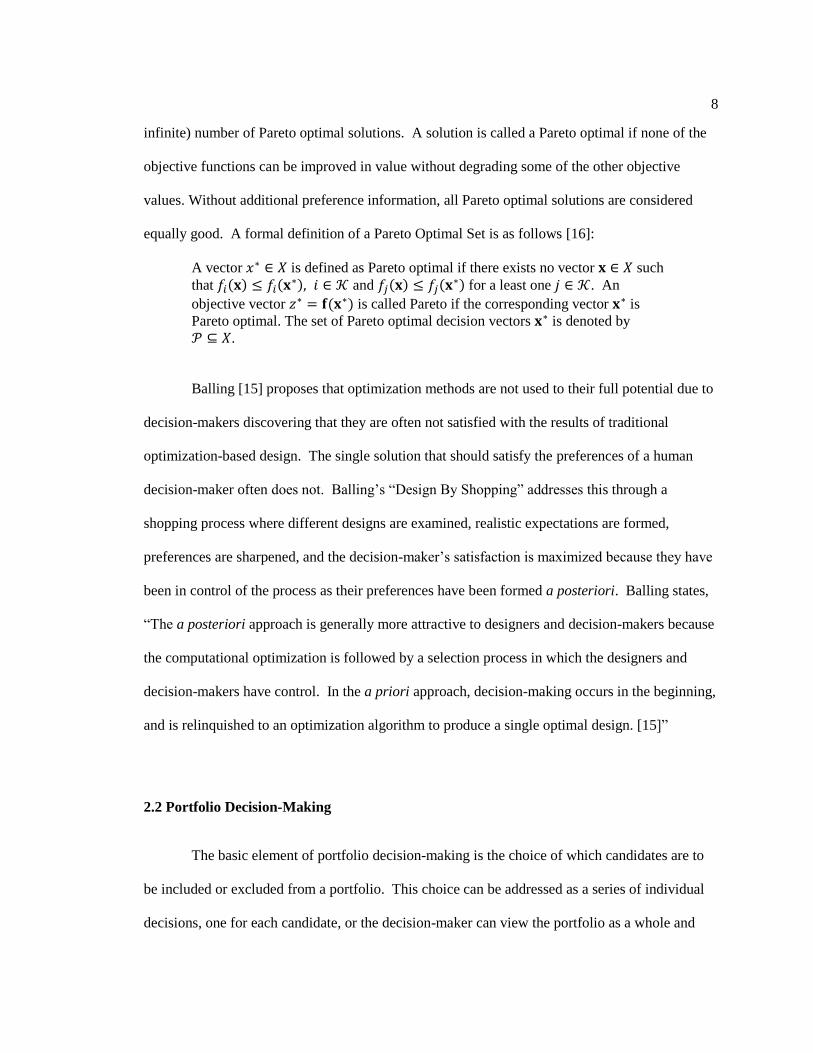
infinite) number of Pareto optimal solutions. A solution is called a Pareto optimal if none of the

objective functions can be improved in value without degrading some of the other objective

values. Without additional preference information, all Pareto optimal solutions are considered

equally good. A formal definition of a Pareto Optimal Set is as follows [16]:

A vector 𝑥∗ ∈ 𝑋 is defined as Pareto optimal if there exists no vector 𝐱 ∈ 𝑋 such

that 𝑓𝑖(𝐱) ≤ 𝑓𝑖(𝐱∗), 𝑖 ∈ 𝒦 and 𝑓𝑗(𝐱) ≤ 𝑓𝑗(𝐱∗) for a least one 𝑗 ∈ 𝒦. An

objective vector 𝑧∗ = 𝐟(𝐱∗) is called Pareto if the corresponding vector 𝐱∗ is

Pareto optimal. The set of Pareto optimal decision vectors 𝐱∗ is denoted by

𝒫 ⊆ 𝑋.

Balling [15] proposes that optimization methods are not used to their full potential due to

decision-makers discovering that they are often not satisfied with the results of traditional

optimization-based design. The single solution that should satisfy the preferences of a human

decision-maker often does not. Balling’s “Design By Shopping” addresses this through a

shopping process where different designs are examined, realistic expectations are formed,

preferences are sharpened, and the decision-maker’s satisfaction is maximized because they have

been in control of the process as their preferences have been formed a posteriori. Balling states,

“The a posteriori approach is generally more attractive to designers and decision-makers because

the computational optimization is followed by a selection process in which the designers and

decision-makers have control. In the a priori approach, decision-making occurs in the beginning,

and is relinquished to an optimization algorithm to produce a single optimal design. [15]”

2.2 Portfolio Decision-Making

The basic element of portfolio decision-making is the choice of which candidates are to

be included or excluded from a portfolio. This choice can be addressed as a series of individual

decisions, one for each candidate, or the decision-maker can view the portfolio as a whole and

9

make a decision on the inclusion or exclusion of all candidates simultaneously. Kester et al. [17]

propose that portfolio decision-making can be better understood when portfolios are considered

as an integrated system where decisions on including and excluding the individual elements are

considered simultaneously. Additionally, Barczak et al. [18] evaluated the 2003 Product

Development & Management Association’s best practices study of new product development and

found that organizations that performed the best followed a well-defined and structured portfolio

management process that was supported by the management and applied consistently while

considering decisions about all projects in a portfolio simultaneously.

Numerous processes have been proposed and studied to address the simultaneous

decision-making approach to portfolio decision-making, and they tend to fall into one of two

categories. The first of these categories is typically found in financial portfolio management with

most modern portfolio theory derived from Markowitz’s “Portfolio Selection” [19]. In this

category the problem is posed as a trade between a portfolio’s expected financial return and the

risk for a set of investments. A selected portfolio’s risk is formulated through the analysis of each

investment’s variance in price over a period of time along with the covariance between selected

investments’ prices and therefore requires historical data. An optimal mix of investments can be

calculated to maximize a portfolio’s expected financial return for a chosen level of acceptable

risk.

The second category of simultaneous decision-making approaches pose portfolio

problems using assessed value of the portfolio’s candidates to make the decision on which to

include. In non-trivial problems, the decision criteria used to assess the value of candidates will

conflict, creating trade-offs. Decision-makers must weigh their preference towards utilizing the

different decision criteria in making their decision of where to allocate their resources. This

formulation, where a decision-maker attempts to maximize a set’s value while utilizing only a

limited amount of resources, is consistent with the formulation of the previously described

10

knapsack problem [1]. This second category also encompasses such portfolio types as new

product development portfolios, project portfolios, resource allocation portfolios, and information

technology portfolios. The scope of this thesis is limited to the second category of portfolios

along with the decision-making processes inherent in determining the decision-maker’s relative

preferences for a problem’s established decision criteria.

2.3 Sequential Decision-Making

Shocker et al. [20] propose a decision-making model where consumers go through a

sequential process of reducing the space of considered choices into nested reduced sets. This

process has been widely adopted in the marketing field, and although this model is fundamentally

concerned with how consumers make choices, one can quickly see how it is complementary to

the trade space exploration approach. The initial set is the universal set and is an exhaustive set

of all alternatives from which the decision-maker may construct sets of greater interest. Next, the

awareness set is the subset of the universal set that the decision-maker is aware of and believes to

be appropriate for their goals and objectives. From the awareness set the consideration set is

purposefully constructed of potential feasible alternatives that would satisfy the decision-maker’s

goals. The consideration set may evolve through discovery, evaluation, exploration, and

acquisition of knowledge. The choice set is defined as the final consideration set prior to a

decision being made. The trade space exploration process, with its set of visualization tools,

supports decision-makers through this sequential decision-making process. It provides an avenue

for exploration expanding awareness of feasible alternatives and allows decision-makers to

construct their preferences while reducing consideration sets to a choice set and finally to a

decision [21].

11

2.4 Trade Space Exploration & Typical Trade Space Exploration Approach

Balling [15] advocates for a design approach with a goal of producing a rich set of good

designs versus a single optimum design. This set could consist of Pareto designs, requiring

decision-makers to only identify design objectives up front without having to quantify the relative

weights, equivalent costs, or allowable values of the design criteria. Additionally, this relieves

the decision-maker from the requirement to specify the relative importance of competing

objectives. Trade space exploration provides a method for exploring sets of designs in the trade

space. Ross and Hastings [22] define trade space as “the space spanned by the completely

enumerated design variables, which means given a set of design variables, the trade space is the

space of possible design options.” Trade space exploration is the exploration and assessment of

the trade space including the relevant design variables and the tradeoffs between them. Simpson

and Martins [8] address the importance of effective strategies for putting “humans-in-the-loop,”

so that they can explore and manage design spaces.

Simpson, et al. [5] characterize the trade space exploration process by three aspects: (1) it

is a shopping process as the decision-maker discovers what it is they want while they are looking

for it; (2) it is a negotiated process when decisions of real complexity involve multiple decision-

makers, each with their own motives and levels of expertise; and (3) it is an iterative process as

the trade space is first explored, and then the knowledge gained is exploited by focusing future

searches of decreasing breadth but of increasing depth and detail. The trade space exploration

process can be approached in three basic steps. First, a model is built to analyze the system,

capturing the relationships between the design inputs and performance outputs. Next,

experiments are run to simulate hundreds, thousands, or millions of design alternatives,

depending on the system model and available computational resources, by varying the inputs and

storing the corresponding values of the performance outputs for each alternative. Finally,

12

interactive visualization tools are used by the decision maker to explore the trade space in order to

identify trends of interest, apply constraints, visualize preference structures, and to find their most

preferred alternative. On the use of visualization in engineering optimization, Messac and Chen

[23] state: “If effectively exploited, visualizing the optimization process in real time can greatly

increase the effectiveness of practical engineering optimization.” Ng [24] supports data

visualization and “human-in-the-loop” interaction in exploring trade-offs and making informed

decisions during multi-objective optimization. Additionally, others advocate visualization as a

solution tool and “human-in-the-loop” optimization’s advantages over black-box search

algorithms [25,26].

2.5 ATSV Applied Research Laboratory Trade Space Visualizer

Balling [15] proposes the need for research in two areas in order to support his proposed

design by shopping paradigm: (1) efficient methods for obtaining rich Pareto sets and (2)

interactive graphical computer tools to assist decision-makers in the shopping process. The

Pennsylvania State University’s Applied Research Laboratory (ARL) developed the ARL Trade

Space Visualizer (ATSV) in order to support trade space exploration. This thesis adopts ATSV

as the tool to apply trade space exploration. ATSV is a stand-alone Java-based data visualization

program designed to help users explore multi-dimensional data sets and to dynamically apply

constraints and preferences in real-time in order to discover relationships between features [6,11].

The data used by ATSV can be either generated off-line and read into ATSV as a static data set,

or it can be generated dynamically by linking a simulation model directly to ATSV using ATSV’s

Exploration Engine [5]. The ATSV currently contains many different types of visualization tools

and visual steering features to support a shopping paradigm keeping the decision-maker “in-the-

13

loop”. The following subsections describe ATSV functions to include plots, preference and brush

controls, linked views, visual steering commands, and search techniques.

2.5.1 ATSV Visualization Capabilities

ATSV uses glyph, scatter, scatter matrix, histogram, and parallel coordinate plots to

visually display multi-dimensional trade spaces. The glyph plot is key to visualizing many

dimensions of multivariate data simultaneously. ATSV can display information in up to seven

dimensions within a glyph plot utilizing three spatial dimensions along with color, size,

orientation, and transparency of the icon [6]. Simpler problems can be displayed using a scatter

plot where two dimensions along with color are used to simultaneously display three dimensions

of the data. The scatter matrix plot allows the user to select which variables are displayed in a

matrix of scatter plots where variables are plotted against each other in order to quickly explore

relationships between each of the variables. The histogram plots support the user’s ability to

visualize statistical distributions of input variable and objective function values [6]. Multiple

histograms can be displayed within a single window for ease of comparison. Parallel coordinate

plots display multivariate data through the use of a polyline that intersects equally spaced axes

and are useful for identifying relationships between variables of interest [6]. Examples of the

ATSV Visualization Capabilities are demonstrated in later chapters.

2.5.2 ATSV Brush and Preference Controls, Linked Views, and Pareto Frontiers

ATSV allows the user to “brush” points in order to highlight, mask, or delete a region of

the trade space. Preference controls allow users to designate objective functions as minimization

or maximization as well as to vary the relative weights of those preferences. ATSV can display

the different preference structures in real-time using preference shading as well as generate a set

14

of non-dominated, Pareto optimal designs for display [6]. The use of brushing and preference

controls updates the displayed information across multiple linked views, simplifying the use of

ATSV [2].

2.5.3 ATSV Visual Steering Commands

ATSV provides numerous visual steering commands to help decision-makers and

designers navigate a multivariate trade space. The Design Space Sampler randomly samples the

multidimensional hypercube defined by the lower and upper bounds of the input variables [27].

This sampler performs a Monte Carlo simulation on the inputs of the simulation model using

either a uniform, normal, or triangular distribution. The Attractor Sampler is used to fill in gaps

in the trade space with samples near a user-defined point using a Differential Evolution algorithm

[5]. The Pareto Sampler generates samples along the Pareto frontier using the direction of the

preferences (minimize or maximize) set by the user for each of the variables of interest. The

Preference Sampler populates new samples in regions of the trade space that perform well with

respect to the user-defined preferences. Like the Attractor Sampler, the Preference Sampler

utilizes a Differential Evolution algorithm; however, the user’s preference structure is used to

define a sample’s fitness.

2.6 Chapter Summary

This chapter provides background on portfolio management decision-making, sequential

decision-making, trade space exploration, and the Applied Research Laboratory Trade Space

Visualizer (ATSV). One common element is the benefit of the “human-in-the-loop” aspect of all

of the reviewed processes. In portfolio decision-making, the number of possible combinations of

15

candidates making up the portfolio grows exponentially with the number of potential candidates

considered, requiring a process that excels in such an environment. In order for human decision-

makers to have an efficient and effective method to explore the decision space, the tools at their

disposal must be robust and tailored towards the types of decisions they are making along with

the data at their disposal. This thesis proposes an interactive decision-making method for

identifying optimal portfolio options by utilizing a trade space exploration approach where

decision-makers can follow a sequential decision-making process. The next chapter describes the

army equipping and modernization strategies portfolio problem.

16

Chapter 3

Army Equipping and Modernization Strategies Portfolio Problem

Background

In this chapter the Army Equipping and Modernization Strategies (AEMS) portfolio

problem is presented. Background information on the U.S. Army Planning, Programming,

Budgeting, and Execution process along with the Equipping Program Evaluation Group’s

Program Objective Memorandum production process is provided to frame the AEMS portfolio

problem. Additionally, the AEMS portfolio problem’s purpose, goals, objectives, decision

criteria, decision variables, and constraints are described.

3.1 U.S. Army Planning, Programming, Budgeting, and Execution

The U.S. Army must acquire fiscal and manpower resources in order to accomplish its

assigned missions in executing the National Military Strategy. The Planning, Programming,

Budgeting, and Execution (PPBE) process has been developed to establish, justify, and acquire

those needed resources [28]. Annually, during the Programming phase of PPBE, the U.S. Army

creates the Program Objective Memorandum (POM). The POM is the document by which the

Army establishes, justifies, and requests the needed resources for the upcoming Future Year

Defense Program (FYDP). The FYDP spans five years including the upcoming budget year as

well as the four years following the budget year. The POM goes through an extensive review and

approval process, during the May through July timeframe, which culminates with

recommendations by the Planning, Programming, and Budgeting Committee (PPBC) for approval

by the Senior Review Group (SRG), and the Senior Leaders of the Department of the Army

17

(SLDA). The PPBC is comprised of the Assistant Deputy Chief of Staff, G-3/5/7 for planning,

the Director of Program Analysis and Evaluation, G-8, for programming, and the Director of the

Army Budget for budgeting and execution and is responsible for monitoring the execution on the

PPBE process. The SRG is co-chaired by the Under Secretary of the Army and the Vice Chief of

Staff, Army. The SLDA is co-chaired by the Secretary of the Army and the Chief of Staff of the

Army [28,29,30].

In order to manage the PPBE process and produce the POM, the U.S. Army uses six

functionally aligned Program Evaluation Groups (PEG). These six groups set the scope, quantity,

priority, and qualitative nature of the resource requirements that define their function, and each

have their own process for producing their portion of the POM. The six PEG functional

groupings are as follows: (1) Manning, (2) Training, (3) Organizing, (4) Equipping, (5)

Sustaining, and (6) Installations. Each PEG is co-chaired by representatives of the Secretariat and

the PEG’s proponent who focus their efforts on policy determination and requirements

determination respectively. For example, the co-chairs of the Equipping PEG (EE-PEG) are the

Assistant Secretary of the Army (Acquisition, Logistics, and Technology) for policy

determination and the Deputy Chief of Staff, G-8 for requirements determination. The EE-PEG’s

mission is to provide resources for the integration of new doctrine, training, organization, and

equipment for developing and fielding warfighting capabilities for the Active Army, Army

National Guard, and the U.S. Army Reserve. EE-PEG’s main focus is on materiel acquisition

which is comprised of researching, developing, testing, evaluating, and procuring weapons and

equipment [28,30].

18

3.2 Equipping Program Evaluation Group POM Process

3.2.1 Key Players

The co-chairs of the EE-PEG are the Assistant Secretary of the Army (Acquisition,

Logistics, and Technology) and the Deputy Chief of Staff, Force Development Director, Army G-

8 [28, 31]. These co-chairs are the decision-making body within the EE-PEG. There are 5

additional extended members serving in an advisory role to the EE-PEG from the Army National

Guard, U.S. Army Reserve, Deputy Chief of Staff, G-2, Chief Information Officer and Army G-

6, and Office of the Surgeon General. The EE-PEG breaks down the equipping function into

eight capability categories each with their own Director of Material (DOM) Division Chief.

These eight DOM Division Chiefs are responsible for managing the twelve EE-PEG program

sub-portfolios and providing recommendations to the EE-PEG co-chairs regarding the funding of

programs within each of the sub-portfolios that they manage. Additionally, there are support staff

and analysts supporting the key players identified here [28, 30]. A diagram of the relationships

between entities involved in the EE-PEG POM production process can be seen in Figure 3-1.

Figure 3-1. EE-PEG POM Production Key Players Relationship Diagram

19

3.2.2 Key Planning Documents

There are numerous documents that provide strategy, guidance, and direction to the EE-

PEG during the programming phase of the PPBE process; however, the following three

documents provide the key direction and information needed in the POM production process.

First, the Army Program Guidance Memorandum is published annually by the Secretary of the

Army and contains programming guidance to the Headquarters Department of the Army staff.

This document provides guidance for force structure, manning, base and supplemental budget

activities, equipment modernization, operations and maintenance, and sustainment. Second, the

Army Technical Guidance Memorandum is published annually by the Director of Program

Analysis and Evaluation, G-8, and provides specific programming guidance to each of the PEGs

to include annual funding levels, used as budget caps in planning during the POM production

process. Additionally, the Army Technical Guidance Memorandum establishes the timeline for

key decisions throughout the PPBE process. The third key document is the EE-PEG Strategic

Planning Guidance Memorandum which is published by the EE-PEG leadership near the end of

January each year. The EE-PEG Strategic Planning Guidance Memorandum provides guidance

to the PEG, which provides the leadership’s mission and intent, outlines the metrics to be used

during POM development and divides the EE-PEG’s POM funding level amongst the eight DOM

divisions [28, 30, 31]. The information flow and timeline of the publication of the

aforementioned key planning documents can be viewed in Figure 3-2 and Figure 3-3.

20

Figure 3-2. EE-PEG POM Production Information Flow Diagram

Figure 3-3. EE-PEG POM Production Event Timeline Diagram

3.2.3 Key Phases of the EE-PEG POM Production Process

The initial phase of the EE-PEG POM production process is the Requirements

Identification Phase, which typically takes place November through January. In this phase,

21

program managers identify material requirements throughout the Army in the form of programs.

These material requirement programs include such items as weapons system

development/replacement, equipment modernization, and equipment shortages. Additionally,

during this phase, staff and analysts of the G-8, Force Development Directorate validate the

optimization models and decision support tools used to support the POM production process in

upcoming phases. A key aspect of this validation is the development of the metrics to be used to

evaluate the relative value of funding programs. These metrics are aligned with the EE-PEG

leadership’s goals and objectives and are published in the EE-PEG Strategic Planning Guidance

Memorandum. One-on-one interviews are conducted with the EE-PEG co-chairs and extended

members, where the EE-PEG leadership is asked to make pairwise comparisons between

objectives, (much like the process used in the Analytic Hierarchy Process) [14]. These pairwise

comparisons are then used to establish relative preference weights between the problem’s

objectives.

The next phase of the EE-PEG POM production process is the Validation Phase where all

identified programs go through a validation process. This validation includes establishing the

annual cost of funding the program for the FYDP. Validated programs are scored by four

organizations using the metrics identified in the previous phase. The details of this scoring

process, as explained in the Limitations section in Chapter 7, are confidential and therefore not

discussed in this thesis. The result of the requirements validation phase is a portfolio of validated

programs that includes the cost of funding the program, the value scores for each of the

established metrics, and an overall value score using the relative weights of the metrics.

The Requirements Prioritization Phase is typically conducted during February and

March. During this phase, the eight DOM Division Chiefs prioritize the validated programs

within their managed sub-portfolios. Limited by the funding levels established in EE-PEG

Strategic Planning Guidance Memorandum, the DOM Division Chiefs produce a

22

recommendation of which programs to fund and identify any critical unfunded requirements. A

series of reviews are held by the Army G-8, Force Development, Director of Resources (DOR) in

which each of the DOM Division Chiefs presents their funding recommendations with identified

critical unfunded requirements. This series of reviews becomes an iterative process as the

identification of critical unfunded requirements may lead to the shifting of funding levels for the

sub-portfolios.

The Funding Solutions Phase of the EE-PEG POM production process occurs during

March and April and is known as the “2-Star Reviews” [31]. The purpose of this phase is to

produce an EE-PEG POM submission recommendation, along with a list of critical unfunded

requirements, to the PPBC for approval by the SRG and SLDA. In this phase EE-PEG co-chairs

and extended members hold a series of reviews with each of the DOM Division Chiefs. The

DOM Division Chiefs each present their funding recommendations, with identified critical

unfunded requirements, as the EE-PEG leadership consider the recommendations along with the

need to adjust current constraints and impose new constraints on the sub-portfolios. The EE-PEG

leadership must produce a funding solution comprised of the sub-portfolios rolled up to produce

the EE-PEG portfolio that stays within the EE-PEG POM funding level.

The Capital Planning Model, a decision support/optimization tool, is used during the

funding solutions phase of the EE-PEG POM production process to identify optimal solutions to

program funding under different scenarios. The solutions to these scenarios are compared to the

current funding solution in order to determine how robust the current funding solution is to

changes in funding strategies. Additionally, the Capital Planning Model is used to develop

courses of action for the most likely changes that may be imposed as the POM goes through the

approval process. For example, if the EE-PEG funding level is cut by five percent, then the EE-

PEG leadership must decide which of the programs representing five percent of the required

funding will be removed from the EE-PEG POM submission.

23

The final phase of the EE-PEG POM production process is the Approval Phase, which

occurs April through July. In this phase, the EE-PEG POM is reviewed along with the POM

submissions from the other five PEGs by the PPBC, SRG, and SLDA. During this phase,

constraints on the EE-PEG, such annual funding levels, may change as cross-PEG trades are

made and critical unfunded requirements are addressed. The information flow and timeline of the

EE-PEG POM production process can be viewed in Figure 3-2 and Figure 3-3.

3.3 The Army Equipping and Modernization Strategies Portfolio Problem

The basis of the AEMS portfolio problem is to select the portfolio of candidate programs

for the EE-PEG POM submission that best meets the U.S. Army’s fundamental equipping

objectives. As discussed earlier in this chapter, the EE-PEG leadership annually publishes the

EE-PEG Strategic Planning Guidance Memorandum which outlines the metrics to be used during

POM development and divides the EE-PEG’s POM funding level amongst the eight DOM

divisions. The published metrics stem from the following three goals: (1) invest in the right

capability, (2) invest in the right quantity, and (3) be fiscally responsible. These three goals are

further broken down into five objectives. Objective 1, Satisfying Future Capability, represents

the desire to invest in prioritized capabilities to ensure the Army achieves success across a range

of potential missions. Objective 2, Meeting Current Demands, represents the desire to fill key

capability shortfalls identified by warfighters. Objective 3, Improving Modernization Levels,

represents the desire to invest in programs that increase the overall modernization levels of Army

capabilities. Objective 4, Filling Modified Table of Organization and Equipment Shortages,

represents the desire to eliminate equipment shortages within capabilities. Objective 5, Attaining

Economic Efficiency, represents the desire to give increased value to investments that obtain a

better unit procurement-cost or development-cost outcome [31].

24

The AEMS portfolio problem’s five decision criteria are derived directly from the five

objectives. One metric has been developed to capture the essence of each of the objectives and

provides a value score between zero and ten to be used as one of the decision criteria for the

AEMS portfolio problem [31]. Again, the details of this scoring process, as explained in the

Limitations section in Chapter 7, are confidential and therefore not discussed in this thesis. The

AEMS portfolio problem’s decision variables are Boolean variables representing a choice to

either fund a program or not. Although most programs are only considered for decision at a fully-

funded level, some programs have alternative discrete funding levels. These programs have been

validated at each alternative funding level and have received value scores for each of the decision

criteria for each funding level. Programs with multiple funding levels produce a constraint on the

system that allows only one of the possible funding levels for the program to be selected.

Additional constraints on the AEMS portfolio problem can be drawn from the key planning

documents. The documents establish a maximum funding level for the portfolio and may

mandate the funding of specific programs. Although these constraints are established in the

planning documents, they are often adjusted throughout the PPBE process.

3.4 Chapter Summary

The chapter presented the Army Equipping and Modernization Strategies (AEMS)

portfolio problem. Additionally, in order to frame the AEMS portfolio problem, background

information on the U.S. Army Planning, Programming, Budgeting and Execution process along

with the Equipping Program Evaluation Group’s Program Objective Memorandum production

process is provided. Finally, the AEMS portfolio problem’s purpose, goals, objectives, decision

criteria, decision variables, and constraints are presented. In the next chapter a decision-making

25

process for the AEMS portfolio problem using trade space exploration, sequential decision-

making, and portfolio management methods is proposed.

26

Chapter 4

A Proposed Process for the Army Equipping and Modernization Strategies

Portfolio Decision-Making Problem

In this chapter a portfolio decision-making process using trade space exploration,

sequential decision-making, and portfolio management methodologies is proposed for the Army

Equipping and Modernization Strategies (AEMS) portfolio problem. Changes to the status quo

process presented in Chapter 3 are highlighted along with efficiencies potentially gained through

the implementation of the new process.

4.1 Proposed Process

This section proposes a decision-making process for the AEMS portfolio problem. The

portions of the EE-PEG POM production process that are performed upstream and downstream of

the EE-PEG are unchanged from the description in Chapter 3. The initial changes to the EE-PEG

POM production process occur in the Requirements Identification Phase and Validation Phase

(see Figure 3.2). As trade space exploration methodologies will be applied in later phases, there

is no longer a need for the value model to produce an overall value score for candidates during

the Validation Phase. Without the need for an overall value score, there is no longer a need to

have decision-makers establish the relative preference weights between the problem’s objectives

during the Requirements Identification Phase. Additionally, this eliminates the need for the one-

on-one interviews with the EE-PEG co-chairs and extended members previously conducted

during the Requirements Identification Phase in order to identify the EE-PEG leadership’s

preferences and establish the relative weights between the problem’s objectives. Efficiencies

27

gained through these changes can be measured in the time saved by no longer conducting the

seven one-on-one interviews, calculating the objective’s relative weights, and producing the

overall value score of the candidates.

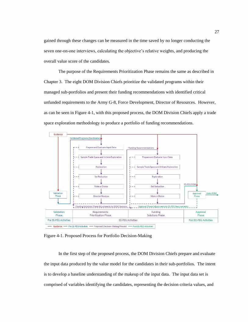
The purpose of the Requirements Prioritization Phase remains the same as described in

Chapter 3. The eight DOM Division Chiefs prioritize the validated programs within their

managed sub-portfolios and present their funding recommendations with identified critical

unfunded requirements to the Army G-8, Force Development, Director of Resources. However,

as can be seen in Figure 4-1, with this proposed process, the DOM Division Chiefs apply a trade

space exploration methodology to produce a portfolio of funding recommendations.

Figure 4-1. Proposed Process for Portfolio Decision-Making

In the first step of the proposed process, the DOM Division Chiefs prepare and evaluate

the input data produced by the value model for the candidates in their sub-portfolios. The intent

is to develop a baseline understanding of the makeup of the input data. The input data set is

comprised of variables identifying the candidates, representing the decision criteria values, and

28

additional information available to formulate constraints. For a simple baseline, decision-makers

can gain an understanding of the input data by determining how many variables and candidates

the set contains and determine what it would cost to fully fund all candidates in their sub-

portfolios. For a more in-depth baseline, decision-makers can explore the distribution of the

variables as well as correlations and dependencies between the input variables. ATSV has a

number of tools that decision-makers can apply to aid in obtaining a baseline understanding of the

input data. These tools, along with additional tools to support the proposed decision-making

process, are discussed in Chapter 5. Once decision-makers feel as though they have sufficient

insight into the input data, they can move on to the next step, and they can return to this step at

any time as this is an iterative process.

The next step of the proposed decision-making process is to sample the trade space and

initiate exploration. The DOM Division Chiefs will need a sampling of portfolios to sufficiently

gain insight into the sampling distributions, ranges, limits, and correlations between variables

within the trade space. This step can conclude when decision-makers feel as though they have

sufficient enough general insight into the parameters of the trade space to initiate exploration and

may return to this step for further interrogation at any time.

The exploration “shopping” step of the decision-making process has the purpose of

allowing decision-makers to develop their preferences while they explore the trade space [5,6].

Multi-dimensional data visualization tools such as those in ATSV provide users with the

capability to quickly and efficiently interrogate regions of the trade space. As users explore, they

become more knowledgeable about the interactions between the variables, the limits of the trade

space, and effects of constraints on the system. With ATSV, users can add or remove decision

criteria on the fly while applying and adjusting relative weights in accordance with their evolving

preferences. The ATSV visual steering commands allow users to populate targeted regions in

order to explore these regions in more depth. One powerful tool ATSV has is the efficient way it

29

identifies non-dominated portfolios within the trade space and samples regions of the Pareto

frontier [2, 5, 6]. This functionality can help to focus exploration efforts and develop preferences

more efficiently.

The set reduction step of the proposed decision process is most coupled with the

exploration step. These two steps are likely to iterate through the most cycles as the DOM

Division Chiefs develop their preferences and narrow their search towards a decision. As the

DOM Division Chiefs form their preferences, they may identify regions of the trade space they

wish to eliminate. These regions may be infeasible, out of alignment with the goals and

objectives, dominated, or just outside the preferred region. The DOM Division Chiefs will cull

undesirable portfolios to form a series of increasingly smaller consideration sets. During this

process, decision-makers may return to previous steps to further sample or explore the remaining

trade space. This iteration continues until the DOM Division Chiefs have reduced their

consideration set to the final choice set.

Once the consideration set has been reduced to the final choice set, the final step of

making a decision remains. There are a number of tools available in ATSV to assist decision-

makers in this final step. The ATSV linear program solver can be applied by the user to optimize

on their final set of preference weights. DOM Division Chiefs may also choose to use the ATSV

Group Compare function to compare commonalities between the remaining choices. This

function efficiently presents the commonalities between selected portfolios. This is accomplished

through the use of both lists and visualizations, allowing users to focus their efforts on the trades

between the remaining candidates. Additionally, after the DOM Division Chiefs arrive at a

decision, they may continue to explore. Miller et al. [21] describe this in their “Story Telling”

trade space exploration use case as a means of rationalizing a decision. The purpose of this

further exploration may be to assist the DOM Division Chiefs to justify their decision to others or

further understand the rationale of their decisions.

30

The Requirements Prioritization Phase concludes with Director Reviews where the DOM

Division Chiefs each present their funding recommendations with identified critical unfunded

requirements to the Army G-8, Force Development, Director of Resources (DOR). Previously,

Director Reviews required a minimum of one day for each of the eight DOM Division Chiefs to

present to the DOR with an additional four days to address adjustments made to constraints

during this process [31]. With the use of a tool such as ATSV, and the application of a trade

space exploration process, this can be reduced to half of a day for each of the eight DOM

Division Chiefs to present to the DOR with an additional day to address any additional required

adjustments resulting from the identification of critical unfunded requirements. These gains in

efficiency equate to a reduction of seven days to complete the Requirements Prioritization Phase

using the proposed process.

The purpose of the Funding Solutions Phase of the EE-PEG POM production process

remains unchanged. During the Funding Solutions Phase the EE-PEG leadership must produce

the EE-PEG POM recommendation document, containing a portfolio of candidates recommended

for funding and a list of critical unfunded requirements, for submission to the PPBC for approval

by the SRG and SLDA. To begin this phase, EE-PEG co-chairs and extended members hold a

series of reviews in order to allow each of the DOM Division Chiefs to present their prioritized

funding recommendations, with identified critical unfunded requirements. The next step is to

hold a consolidated working session to simultaneously address EE-PEG’s entire list of validated

candidates as a single portfolio. The input data containing EE-PEG’s entire list of validated

candidates can be loaded into ATSV. Next, all global-constraints, such as the EE-PEG POM

funding level limit known as the Total Obligation Authority (TOA) and required funding of

candidates identified in guidance documents, can be applied. Additionally, constraints that apply

to each of the sub-portfolios of the DOM Division can be applied. Next the EE-PEG leadership

can explore the trade space and identify the effects of cross-division trades that stem from

31

decisions made regarding the funding of critical unfunded requirements in one division over

recommended candidates in another division. When all trades are complete, the list of any

remaining critical unfunded requirements will be included with the EE-PEG POM

recommendation as it is forwarded to the PPBC.

The potential efficiencies gained during the Funding Solutions Phase of the EE-PEG

POM production process equate to a reduction of approximately seven days. Previously the

Funding Solutions Phase began with eight one-day meetings. In each meeting, one of the eight

DOM Division Chiefs presented their funding recommendations, with identified critical unfunded

requirements, and the EE-PEG Leadership consider the recommendations along with the need to

adjust current constraints and impose new constraints on the sub-portfolios. This series of

meetings was followed by an approximate additional four-day iterative process addressing the

identified critical unfunded requirements leading to the shifting of funding levels for the sub-

portfolios and the development of new funding solutions. With the application of trade space

exploration and the use of tools such as ATSV, this phase can be reduced to approximately five

days consisting to two days for the DOM Division Chiefs to present their funding

recommendations with identified critical unfunded requirements, and three days for the

consolidated working session.

The portions of the Approval Phase of the EE-PEG POM production process that are

performed downstream of the EE-PEG are unchanged from the description in Chapter 3. The EE-

PEG POM recommendation, containing a portfolio of candidates recommended for funding and a

list of critical unfunded requirements, is submitted to the PPBC for approval by the SRG and

SLDA. If the PPBC requires changes to the EE-PEG POM submission in response to adjustment

made in the Approval Phase, the EE-PEG reconvenes the consolidated working session, addresses

the constraint changes, and produces a new funding solution.

32

4.2 Chapter Summary

In this chapter a decision-making process was proposed for the portfolio management

problem that utilizes trade space exploration, sequential decision-making, and portfolio

management methodologies. Efficiencies gained through the implementation of these

methodologies in the proposed process would be the elimination of the seven one-on-one

interviews with the EE-PEG co-chairs and extended members in the Requirements Identification

Phase, a reduction of seven days to complete the Requirements Prioritization Phase, and a

reduction of an additional seven days to complete the Funding Solutions Phase of the EE-PEG

POM production process. Tools for applying the proposed process are discussed in the next

chapter with a demonstration of the proposed process applied to the AEMS portfolio problem

data set presented in Chapter 6.

33

Chapter 5

ATSV Capabilities to Support the Portfolio Decision-Making Process

A number of new capabilities have been added to ATSV to support the decision-making

process for the portfolio problem. These capabilities include a mix of new visual steering

commands, visualization displays, and optimization tools. Some of these capabilities are

previously developed ATSV tools that have been tailored to the portfolio problem and take

advantage of its unique formulation for increased efficiency. Others have been implemented

specifically to support portfolio decision-making. Additionally, this chapter reviews ATSV

capabilities that apply to the portfolio problem, addresses when they are most appropriate for use,

and demonstrates how they are applied during the proposed decision-making process.

5.1 Portfolio Data Engine

The Portfolio Data Engine is the link between the Candidate List, the user supplied input,

and the Portfolio Data Table, the matrix of data ATSV uses to store the variables pertaining to

each of the sample portfolios. The four functions performed by the Portfolio Data Engine are

demonstrated in Figure 5-1. The Portfolio Data Engine creates N columns in the Portfolio Data

Table to store the Boolean decision variables for the N candidates from the Candidate List. It

also creates columns for the input variables that are summed across those candidates that are

included in a sample portfolio. For example, the cost of each candidate included in a sample

portfolio may be summed and stored in a column representing the total cost of that sample

portfolio. The Portfolio Data Engine also performs a tallying function for categorical variables.

34

Figure 5-1. Demonstration of ATSV Portfolio Data Engine

A column is created for each of the represented category values of a variable from the Candidate

List. Next, counts of candidates included in a sample portfolio, which have each category’s

value, are recorded in their respective columns. The Portfolio Data Engine additionally evaluates

equations, to include logic equations, created using ATSV’s Query and Add Column functions.

The user can create an expression, using variables from the Portfolio Data Table, which are

evaluated for each sample portfolio and stored in the table.

5.2 Visualization Displays

This section presents ATSV’s visualization displays as they apply to the proposed

decision-making process in Chapter 4. The presentation of the visualization displays are

35

organized by the steps that they support; however, they are also useful during additional steps.

Decision-makers and ATSV users should not limit themselves to only using the visualization

displays as they are presented in this section.

The Prepare and Evaluate Input Data step of the decision-making process allows

decision-makers to gain sufficient enough insight into the input data to be able to explore the

trade space in an efficient and meaningful manner. The Candidate List visualization display

assists users in this task. The Data tab can be seen in Figure 5-2 and allows for users to view the

data set as it has been read into ATSV. Users then can quickly ascertain how many candidates

have been loaded as well as view what variables are available for each candidate. The Histogram

tab, as seen in Figure 5-3, presents a histogram for each of the variables in the input data set,

providing users with a tool to quickly view the distribution of each variable. An additional tool

provided to users is the 2D scatter plot on the Plot tab as can be seen in Figure 5-3. Users can

further interrogate variables of interest, identify any outliers, and examine for correlation between

two input variables.

Figure 5-2. Demonstration of ATSV Candidate List Data Visualization Display

36

Figure 5-3. Demonstration of ATSV Candidate Histogram and Plot Visualization Display

A number of visualization displays are available in ATSV to assist users in initiating

exploration of the trade space as shown in Figure 5-4. Users first need an initial set of sample

portfolios which can be obtained through the use of the Random Sample function that produces a

user-specified number of sample portfolios within the trade space. The Portfolio Data Table

allows users to view the data table columns produced by the Portfolio Data Engine after

processing the Candidate List. The columns of the Portfolio Data Table contain the variables

made available by the Portfolio Data Engine. The Histogram Plot provides a visualization of the

distribution of the number of sampled portfolios that contain a certain set of values for each of the

variables in the Portfolio Data Table. For most variables, after an initial random sampling, a user

would expect to see a relatively uniform distribution over the range of the variable. If the

distribution is skewed, then the user can typically resolve the issue by increasing the number of

random samples. The Scatter Matrix plot assists the user in conducting a pairwise comparison

between each of the portfolio variables where the user can identify any positive or negative

correlation between the variables. If any of the pairwise comparisons within the matrix warrant

further investigation, then the user can produce a 2D scatter plot of the variables. The parallel

coordinates plot allows users to visualize the data in n-dimensional space in order to gain further

insight into the parameters of the portfolio problem and the relationships between them.

37

Portfolio Data Table Histogram Plot

Scatter Matrix Parallel Coordinates Plot

Figure 5-4. Demonstration of ATSV Portfolio Data Visualization Displays

As users explore the trade space during the portfolio decision-making process, they

develop their preferences and gain knowledge that can be exploited by focusing future searches

and reducing the decision set. Two of the most powerful visualizations for this effort are 2D

scatter plots and 3D glyph plots. Examples of these two plots are provided in Figure 5-5. The

Filters and Preferences field in ATSV can be utilized to indicate a decision-maker’s preferences

towards decision criteria as well as apply constraints in order to identify and cull non-feasible

samples. The plots in ATSV are linked to the same Filters and Preferences field, allowing users

to make changes to all open visualizations simultaneously. In the 2D scatter plot on the left of

Figure 5-5, a minimum value constraint has been applied to the variable on the y-axis while a

maximum value constrain has been applied to the variable on the x-axis. The points in gray

indicate samples that are outside the constraint limits of this problem and are infeasible solutions.

38

Preference shading has been applied to both plots in Figure 5-5 to indicate which sample

portfolios are the most (red) and least (blue) preferred according to the preferences applied with

the Filters and Preferences field. This preference shading can be adjusted on the fly as users

explore the trade space and develop their preferences. An additional feature demonstrated in

Figure 5-5 is the ability to highlight the non-dominated portfolios. These portfolios are indicated

using the + symbol over the points on the plot. ATSV also has the capability to indicate the point

on the plot that is the most preferred sample portfolio based on the user’s preference. This point

indication will also adjust as users adjust the preference indicators in the Filters and Preferences

field.

Figure 5-5. Demonstration of ATSV 2D Scatter Plots and 3D Glyph Plots

The next set of tools are for the purpose of supporting users in reducing the set of

portfolios to the final choice set. The uses of these tools are tightly coupled with functions

provided for exploring the trade space as are their visualizations. The Hide Infeasible Designs

function reduces the sample set of portfolios to only those portfolios within the limiting

constraints of the problem as applied through the Filters and Preferences field discussed

previously. The Show Only Pareto Designs function hides any dominated sample, leaving only

those non-dominated portfolios in the sampled set. This is demonstrated in Figure 5-6 with the

39

plot in the upper left with only preference shading applied and the plot in the upper right showing

a sample set of portfolios with constraints applied and non-dominated points highlighted prior to

any culling of points. The plot in the lower left demonstrates the culling of points that violate the

applied constraints while the plot in the lower right has the Show Only Pareto Designs function

applied. An additional way to reduce the remaining set is to apply additional constraints. A new

variable representing the new constraint can be created utilizing the Query function displayed in

Figure 5-7. This new variable is added to the Portfolio Data Table and constraints can be applied

to it with the Filters and Preferences field as discussed previously.

Figure 5-6. Demonstration of ATSV Show Only Pareto Designs Function

40

Figure 5-7. Demonstration of ATSV Query Function

There are a number of visualizations available in ATSV to assist users in making their

final decision. By utilizing the Group Compare function on a small set of portfolios, users can

efficiently ascertain the commonalities between the selected portfolios. ATSV accomplishes this

through visualizations in both list and plot format. The purpose of these visualizations is to allow

users to focus their efforts on the trades between the remaining candidates. When these

capabilities are used for problems with multiple decision-makers, the Group Compare functions

help decision-makers identify the common ground between their respective perspectives and

focus their efforts on the required compromise needed to reach a collective decision. Figure 5-8

demonstrates the Group Compare visualizations with the list view summarizing commonly

selected and deselected candidates in the left field. When five or fewer sample portfolios are

selected, then Group Compare produces the Table tab where a summary of the uniquely selected

and not-selected candidates are listed for each of the selected portfolios. The Tallies tab, seen in

the bottom left of Figure 5-8, produces a bar chart of the candidates that are not commonly

included or excluded by all of the selected portfolios. Each bar displays the tally of the number

41

of portfolios that include that candidate. The radar plot, presented in the bottom right of Figure 5-

8, can be used to detect patterns in the characteristics of the group of selected portfolios. In the

example in Figure 5-8, three of the groupings have been highlighted with red, orange, and yellow

for easier viewing.

Figure 5-8. Demonstration of ATSV Group Compare Visualizations

5.3 Visual Steering Commands

The following visual steering commands were implemented to improve functionality of

ATSV for use in portfolio decision-making. The One Run Sampler provides users the capability

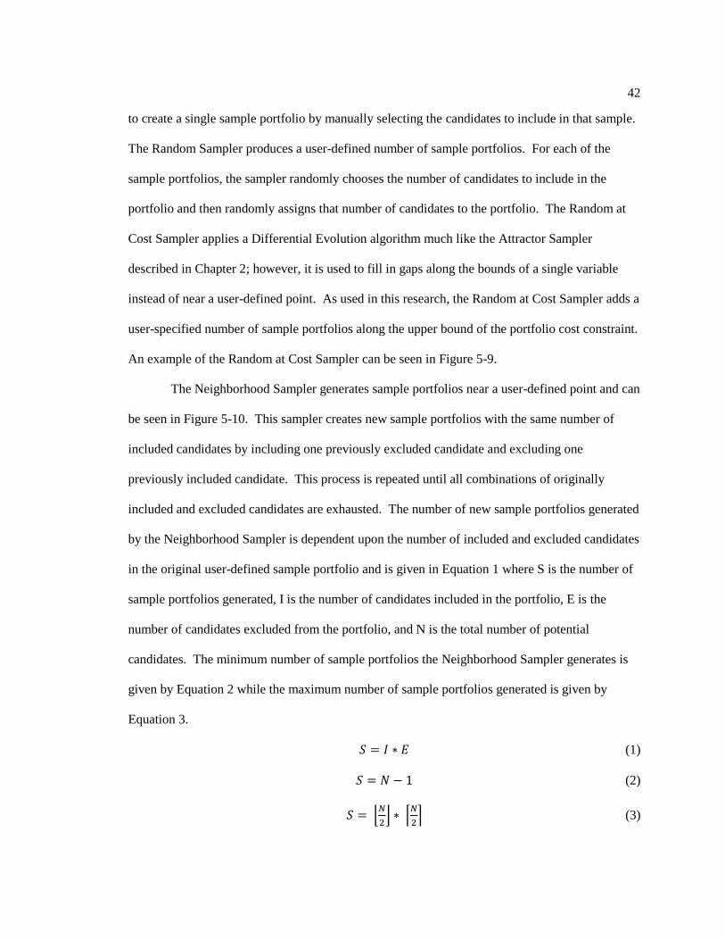
42

to create a single sample portfolio by manually selecting the candidates to include in that sample.

The Random Sampler produces a user-defined number of sample portfolios. For each of the

sample portfolios, the sampler randomly chooses the number of candidates to include in the

portfolio and then randomly assigns that number of candidates to the portfolio. The Random at

Cost Sampler applies a Differential Evolution algorithm much like the Attractor Sampler

described in Chapter 2; however, it is used to fill in gaps along the bounds of a single variable

instead of near a user-defined point. As used in this research, the Random at Cost Sampler adds a

user-specified number of sample portfolios along the upper bound of the portfolio cost constraint.

An example of the Random at Cost Sampler can be seen in Figure 5-9.

The Neighborhood Sampler generates sample portfolios near a user-defined point and can

be seen in Figure 5-10. This sampler creates new sample portfolios with the same number of

included candidates by including one previously excluded candidate and excluding one

previously included candidate. This process is repeated until all combinations of originally

included and excluded candidates are exhausted. The number of new sample portfolios generated

by the Neighborhood Sampler is dependent upon the number of included and excluded candidates

in the original user-defined sample portfolio and is given in Equation 1 where S is the number of

sample portfolios generated, I is the number of candidates included in the portfolio, E is the

number of candidates excluded from the portfolio, and N is the total number of potential

candidates. The minimum number of sample portfolios the Neighborhood Sampler generates is

given by Equation 2 while the maximum number of sample portfolios generated is given by

Equation 3.

𝑆 = 𝐼 ∗ 𝐸 (1)

𝑆 = 𝑁 − 1 (2)

𝑆 = ⌊𝑁

2⌋ ∗ ⌈

𝑁

2⌉ (3)

43

Before Random at Cost Sampler After Random at Cost Sampler

Figure 5-9. Demonstration of ATSV Random and Random at Cost Samplers

Before Neighborhood Sampler After Neighborhood Sampler

Figure 5-10. Demonstration of ATSV Neighborhood Sampler

44

5.4 Optimization Tools

The following optimization tools were implemented in ATSV to provide users with

improved functionality for identifying optimal points in the trade space as well as sampling

portfolios on the Pareto frontier. The ATSV Single Run LP optimizer implements a linear

program (LP) solver applied using the current settings in the Filters and Preferences field as the

objective function and constraints. The 2-D scatter plot in the upper right of Figure 5-11

identifies the solution found by the Single Run LP optimizer for the current Filters and

Preferences field settings by setting the icon to a black point. The ATSV Local LP function

Random as a Baseline After Single Run LP Optimizer

After Local LP Function After Global LP Refinement by Local Pareto

Search Function

Figure 5-11. Demonstration of ATSV Optimization Tools

45

implements an algorithm to sample portfolios along the Pareto frontier near the optimal LP

solution for the current Filters and Preferences field settings. During each iteration of the

algorithm, the previous linear optimal solution is added to a temporary list of constraints, and a

new optimal solution is found. Once the algorithm terminates, the temporary list of constraints is

removed, and the solution found in each iteration is added as a sample portfolio in the trade

space. The 2-D scatter plot in the lower left of Figure 5-11 highlights the sample points added by

the Local LP optimizer. The ATSV Global LP Refinement by Local Pareto Search function

samples portfolios along the Pareto frontier. This function implements the Local LP algorithm

using all of the non-dominated samples in the Portfolio Data Table as a starting point for the

Local LP algorithm. An example of the samples produced by the Global LP Refinement by Local

Pareto Search function along the Pareto frontier are highlighted in the lower right 2-D scatter plot

of Figure 5-11.

5.5 Chapter Summary

This chapter highlighted a number of new capabilities that were added to ATSV in order

to support the proposed decision-making process for the portfolio problem. This mix of new

visual steering commands, visualization displays, and optimization tools has been implemented

specifically to support portfolio decision-making. In the next chapter, a demonstration of the

portfolio decision-making process proposed in Chapter 4 using the tools discussed in this chapter

is presented.

46

Chapter 6

Demonstration of Proposed Process for the AEMS Portfolio Problem

In this chapter, the decision-making process proposed in Chapter 4 is demonstrated using

an AEMS portfolio problem in order to verify the feasibility of applying the trade space

exploration methodology to portfolio decision-making problems. ATSV is the tool chosen to

support the decision-making process while employing trade space exploration, sequential

decision-making, and portfolio management methodologies. Reductions in the size of the

decision set, from the universal set to the choice set, through utilization of sequential decision-

making methodology is quantified. The efficiencies potentially gained through the

implementation of this new process, in lieu of the status quo process presented in Chapter 3, are

highlighted. As the actual data set for the AEMS portfolio problem is confidential, as explained

in the Limitations section in Chapter 7, a representative data set is used to conduct this

demonstration.

6.1 Demonstration Scenario and AEMS Data Set

This section presents the scenario and data set that are used in the decision-making

process demonstration for the AEMS portfolio problem. The portions of the EE-PEG POM

production process that are performed upstream and downstream of the EE-PEG are unchanged

from the description in Chapter 3. To maintain the confidentiality of the AEMS portfolio

problem, guidance pertaining to the EE-PEG POM production decision-making has been

extracted from pertinent guidance documents, sanitized of any confidential information, and

realigned to the demonstration data set used in this chapter.

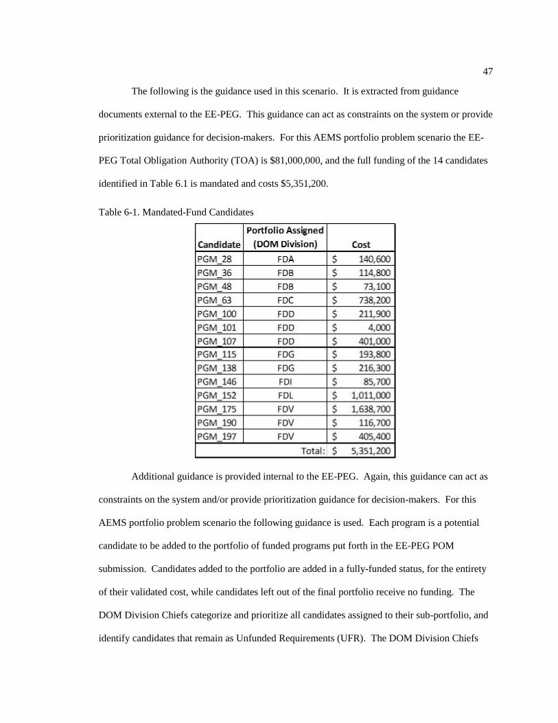
47

The following is the guidance used in this scenario. It is extracted from guidance

documents external to the EE-PEG. This guidance can act as constraints on the system or provide

prioritization guidance for decision-makers. For this AEMS portfolio problem scenario the EE-

PEG Total Obligation Authority (TOA) is $81,000,000, and the full funding of the 14 candidates

identified in Table 6.1 is mandated and costs $5,351,200.

Table 6-1. Mandated-Fund Candidates

Additional guidance is provided internal to the EE-PEG. Again, this guidance can act as

constraints on the system and/or provide prioritization guidance for decision-makers. For this

AEMS portfolio problem scenario the following guidance is used. Each program is a potential

candidate to be added to the portfolio of funded programs put forth in the EE-PEG POM

submission. Candidates added to the portfolio are added in a fully-funded status, for the entirety

of their validated cost, while candidates left out of the final portfolio receive no funding. The

DOM Division Chiefs categorize and prioritize all candidates assigned to their sub-portfolio, and

identify candidates that remain as Unfunded Requirements (UFR). The DOM Division Chiefs

48

categorize candidates by their recommended funded states, listed here in descending priority

order: Mandated-Fund, Critical-Fund, Critical-UFR, Priority-Fund, Priority-UFR, or Unfunded.

The Division Chiefs immediately notify the Director of Resources if the allotted TOA for their

sub-portfolio falls below a level sufficient to fully fund all of their assigned Mandated-Fund

candidates. Validated scores for five objective are provided in the AEMS portfolio problem

scenario data set for each of the candidates. The five objectives used in this scenario are:

Objective 1 - Satisfying Future Capability; Objective 2 - Meeting Current Demands; Objective 3 -

Improving Modernization Levels; Objective 4 - Filling Modified Table of Organization and

Equipment Shortages; and Objective 5 - Attaining Economic Efficiency. The DOM Division

Chiefs adjust their recommendations based on shifts in their allotted portion of the EE-PEG TOA

and represent the sub-portfolio in the combined portfolio decision-making process.

The data set for this scenario contains 197 candidates divided into eight sub-portfolios,

one for each of the eight DOM Divisions (FDA, FDB, FDC, FDD, FDG, FDI, FDL, and FDV).

The data element representing each candidate consists of the name of the program, the name of

the DOM Division to which it is assigned, the cost to fully fund the associated program, and

scores for metrics measuring each of the five objectives. As can be seen in Table 6.2, the sum of

the costs to fully fund all 197 candidates is $98,423,600. With a TOA of only $81M, there is a

budget shortage of $17,423,600. A summary of each division’s cost, budget, budget shortage,

possible portfolio combinations, and the cost of Mandated-Fund candidates is given in Table 6.2.

The following three assumptions are made with respect to the funding strategy that is

applied by the DOM Division Chiefs. (1) Mandated-Fund candidates receive the highest priority

for funding. (2) DOM Division Chiefs spend as much as possible within their TOA as long as

they have valid programs to fund. (3) DOM Division Chiefs identify programs that provide

redundant capabilities and recommend the funding for at most one of these programs and

recommend the remainder of the programs to be categorized as Unfunded.

49

Table 6-2. Portfolio Summary Prior to Requirements Prioritization Phase

Using this scenario, the Requirements Prioritization Phase is demonstrated including the

following steps: Prepare and Evaluate Input Data, Sample Trade Space and Initiate Exploration,

Exploration of Trade Space, Set Reduction, and Make a Choice. Next, any iterations of the

Requirements Prioritization Phase required as part of the Director Reviews are demonstrated.

This is followed by a demonstration of the Funding Solutions Phase of the AEMS portfolio

problem decision-making process.

6.2 In-Depth Demonstration of Requirements Prioritization Phase for FDL

As the process for the Requirements Prioritization Phase is nearly identical for each of

the DOM Divisions, this phase is only demonstrated in its entirety using the FDL DOM Division.

Although a full demonstration is only shown for the FDL DOM Division, any notable division

specific differences are highlighted along with each DOM Division’s results of the Requirements

Prioritization Phase prior to moving on to the demonstration of the Director Reviews.

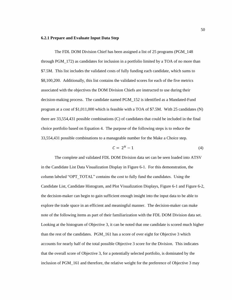
50

6.2.1 Prepare and Evaluate Input Data Step

The FDL DOM Division Chief has been assigned a list of 25 programs (PGM_148

through PGM_172) as candidates for inclusion in a portfolio limited by a TOA of no more than

$7.5M. This list includes the validated costs of fully funding each candidate, which sums to

$8,100,200. Additionally, this list contains the validated scores for each of the five metrics

associated with the objectives the DOM Division Chiefs are instructed to use during their

decision-making process. The candidate named PGM_152 is identified as a Mandated-Fund

program at a cost of $1,011,000 which is feasible with a TOA of $7.5M. With 25 candidates (N)

there are 33,554,431 possible combinations (C) of candidates that could be included in the final

choice portfolio based on Equation 4. The purpose of the following steps is to reduce the

33,554,431 possible combinations to a manageable number for the Make a Choice step.

𝐶 = 2𝑁 − 1 (4)

The complete and validated FDL DOM Division data set can be seen loaded into ATSV

in the Candidate List Data Visualization Display in Figure 6-1. For this demonstration, the

column labeled “OPT_TOTAL” contains the cost to fully fund the candidates. Using the

Candidate List, Candidate Histogram, and Plot Visualization Displays, Figure 6-1 and Figure 6-2,

the decision-maker can begin to gain sufficient enough insight into the input data to be able to

explore the trade space in an efficient and meaningful manner. The decision-maker can make

note of the following items as part of their familiarization with the FDL DOM Division data set.

Looking at the histogram of Objective 3, it can be noted that one candidate is scored much higher

than the rest of the candidates. PGM_161 has a score of over eight for Objective 3 which

accounts for nearly half of the total possible Objective 3 score for the Division. This indicates

that the overall score of Objective 3, for a potentially selected portfolio, is dominated by the

inclusion of PGM_161 and therefore, the relative weight for the preference of Objective 3 may

51

have limited value in assisting the decision-maker in this decision-making process. Looking at

the histogram of cost, it appears that there are a small number of candidates that could account for

a significant portion of the cost of the portfolio. PGM_156 has a cost of $4,223,800 which is

over 50% of the allotted TOA, and the inclusion of PGM_156 is therefore the most significant

factor in the excessive cost of the potentially selected portfolio.

There does not appear to be any other significant item to note during this step of the

process. However, this is an iterative process and the decision-maker can return any time to

explore the data set further. The next step in this demonstration is Sample Trade Space and

Initiate Exploration.

Figure 6-1. FDL DOM Division ATSV Candidate List Data Visualization Display

Figure 6-2. FDL DOM Division ATSV Candidate Histogram and Plot Visualization Display

52

6.2.2 Sample Trade Space and Initiate Exploration Step

Prior to exploring the trade space, a sample of the portfolios within the trade space must

be generated. There is no set number of how many samples must be generated in order to initiate

exploration of the trade space. If too few samples are produced, then the decision-maker will not

have the opportunity to sufficiently visualize the trade space. If too many samples are generated,

then the ATSV user may not have the computing power required to explore the trade space in a

practical amount of time. For this demonstration, 2,500 samples were generated using the ATSV

Random Sample function. A comparison of the trade space visualizations sampled with 100

samples and 2,500 samples can be seen in Figure 6-3. As this is an iterative process, more

samples can be generated any time the decision-maker feels more are needed. Additionally, the

Initiate Exploration portion of this step provides indicators if too few samples were taken.

Figure 6-3. FDL DOM Division 2D Scatter Plots with 100 Samples and 2,500 Samples

The Portfolio Data Engine processes the Candidate List and produces the Portfolio Data

Table as seen in Figure 6-4. The Portfolio Data Table for the AEMS portfolio problem contains

the following data elements for each sample portfolio: the cost of funding the selected candidates,

the sum of the scores for each objective, the number of funded candidates, a Boolean decision

variable for each of the considered candidates, and any additional variables such as logical

constraints imposed by the user. The Histogram Plot, as seen in Figure 6-5, provides a

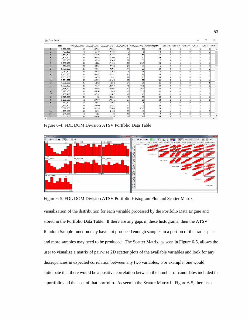
53

Figure 6-4. FDL DOM Division ATSV Portfolio Data Table

Figure 6-5. FDL DOM Division ATSV Portfolio Histogram Plot and Scatter Matrix

visualization of the distribution for each variable processed by the Portfolio Data Engine and

stored in the Portfolio Data Table. If there are any gaps in these histograms, then the ATSV

Random Sample function may have not produced enough samples in a portion of the trade space

and more samples may need to be produced. The Scatter Matrix, as seen in Figure 6-5, allows the

user to visualize a matrix of pairwise 2D scatter plots of the available variables and look for any

discrepancies in expected correlation between any two variables. For example, one would

anticipate that there would be a positive correlation between the number of candidates included in

a portfolio and the cost of that portfolio. As seen in the Scatter Matrix in Figure 6-5, there is a

54

positive correlation between cost and the number of candidates in a portfolio. Any correlations

that appear counterintuitive warrant further examination. As noted earlier, the cost of candidate

PGM_156 is over half of the total cost of funding all candidates assigned to FDL DOM Division.

This results in what appears to be two separate clouds of portfolios in each 2D scatter plot of the

cost row of the Scatter Matrix. The top cloud are portfolios that cost more due to containing

PGM_156, and the bottom cloud are portfolios that cost less and do not contain PGM_156. As

none of the variable correlations on this Scatter Matrix are counterintuitive and the Histograms

look relatively uniform, we conclude the Sample Trade Space and Initiate Exploration step for

now and proceed to the Exploration of Trade Space step.

6.2.3 Exploration of Trade Space Step and Set Reduction Step

The decision-makers will likely iterate through the Exploration of Trade Space step and

Set Reduction step the most while they develop their preferences. Therefore, the explanation for

these two parts of the decision-making process is combined in this demonstration.

A 2D Scatter Plot, as seen in Figure 6-6, is one of the ways to explore the trade space.

Relative preferences for the five objectives are initially set equal to each other. This has been

chosen since the guidance documents in this scenario did not provide any indication that decision-

makers place a greater value on any of the five objectives. An upper limit equal to the TOA has

been applied to the cost of portfolios. A brush control has been applied to the data, and the

visualization shows all portfolios with a cost greater than the $7.5M TOA limit as infeasible by

shading them in grey. Additionally, a brush control has been applied to mark any portfolio

excluding the Mandated-Fund candidate, PGM_152, as infeasible.

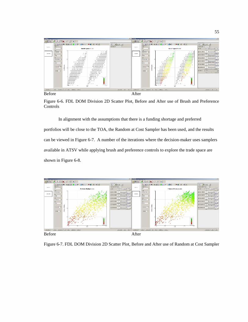
55

Before After

Figure 6-6. FDL DOM Division 2D Scatter Plot, Before and After use of Brush and Preference

Controls

In alignment with the assumptions that there is a funding shortage and preferred

portfolios will be close to the TOA, the Random at Cost Sampler has been used, and the results

can be viewed in Figure 6-7. A number of the iterations where the decision-maker uses samplers

available in ATSV while applying brush and preference controls to explore the trade space are

shown in Figure 6-8.

Before After

Figure 6-7. FDL DOM Division 2D Scatter Plot, Before and After use of Random at Cost Sampler

56

Iteration 1 Iteration 2

Iteration 3 Iteration 4

Figure 6-8. FDL DOM Division 2D Scatter Plot, Four Iterations of Using Samplers and Applying

Brush and Preference Controls to Explore the Trade Space

As the decision-maker continues to reduce the consideration set to the decision set, the

Pareto Brush Control becomes an effective tool for removing dominated portfolios from the

consideration set. The application of the Pareto Brush Control can be seen in Figure 6-9. Once

the decision-maker has explored the trades space thoroughly enough to develop his/her

preferences and reduce the consideration set to a decision set, they move on to the final step in

this phase, the Make a Choice step.

57

Figure 6-9. FDL DOM Division 2D Scatter Plot, Before and After use of Pareto Brush Control

6.2.4 Make a Choice Step

The universal set of portfolios, with all possible combinations of candidates, has been

reduced from 33,554,431 to four remaining portfolios in the choice set. This choice set of four

portfolios has commonality in that the 19 candidates listed in the Common Funded Programs

block, as seen in Figure 6-10, would receive funding no matter which of the four final portfolios

was chosen. Likewise, the two candidates listed in the Common Defunded Programs block

would not be funded regardless of which of the four final portfolios was chosen. This has

reduced the number of candidates the decision-maker has to consider from 25 to a more

manageable four candidates.

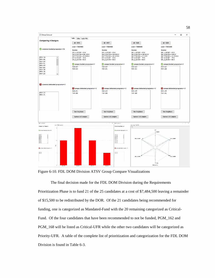
58

Figure 6-10. FDL DOM Division ATSV Group Compare Visualizations

The final decision made for the FDL DOM Division during the Requirements

Prioritization Phase is to fund 21 of the 25 candidates at a cost of $7,484,500 leaving a remainder

of $15,500 to be redistributed by the DOR. Of the 21 candidates being recommended for

funding, one is categorized as Mandated-Fund with the 20 remaining categorized as Critical-

Fund. Of the four candidates that have been recommended to not be funded, PGM_162 and

PGM_168 will be listed as Critical-UFR while the other two candidates will be categorized as

Priority-UFR. A table of the complete list of prioritization and categorization for the FDL DOM

Division is found in Table 6-3.

59

Table 6-3. FDL DOM Division Requirements Prioritization Phase Results

6.3 Demonstration of Requirements Prioritization Phase for Remaining Divisions

The Requirements Prioritization Phase is conducted for each of the DOM Divisions in the

same manner as for FDL DOM Division. In this section an abridged demonstration is shown for

the remaining DOM Divisions highlighting any notable division-specific differences from the

process shown in the in-depth demonstration for FDL DOM Division. The results of the

Requirements Prioritization Phase for each of the remaining DOM Divisions is presented

followed by demonstration of the Director Reviews Step.

6.3.1 Abridged Demonstration for FDA

The FDA DOM Division Chief has been assigned a list of 28 programs (PGM_1 through

PGM_28) as candidates for inclusion in a portfolio limited by a TOA of $20M. The candidate

named PGM_28 is identified as a Mandated-Fund program at a cost of $140,600 which is feasible

60

with a TOA of $20M. The cost to fully fund all candidates sums to $19,821,900 leaving a

remainder of $178,100 for the DOR to redistribute. One notable difference between this division

and the other seven divisions is that in this scenario there is enough funding within this division’s

TOA to fund all candidates. The requirement to prioritize and categorize all candidates for the

FDA DOM Division still remains. With 28 candidates there are over 268 million possible

combinations of candidates that could be included in the final choice portfolio; however, with a

TOA greater than the cost of the entire portfolio the size of the choice set is quickly reduced to

the one combination including all candidates. Of the 28 candidates being recommended for

funding, one is categorized as Mandated-Fund with the 27 remaining categorized as Critical-

Fund. A table of the complete list of prioritization and categorization for the FDA DOM Division

is found in Table 6-4.

Table 6-4. FDA DOM Division Requirements Prioritization Phase Results

61

6.3.2 Abridged Demonstration for FDB

The FDB DOM Division Chief has been assigned a list of 24 programs (PGM_29

through PGM_52) as candidates for inclusion in a portfolio limited by a TOA of $3M. Two

candidates, PGM_36 and PGM_48 are identified as Mandated-Fund programs at a cost of

$187,900 which is feasible with a TOA of $3M. The cost to fully fund all candidates sums to

$3,714,300. PGM_40 provides capabilities redundant to capabilities provided by the Mandated-

Fund programs PGM_36 and PGM_48, and therefore the FDB DOM Division Chief has

categorized it as Unfunded. One item of note from the Prepare and Evaluate Input Data step is

that candidates PGM_42 and PGM_49 dominate the scoring for Objective 3 much like what was

seen with the FDL DOM Division. With 24 candidates, there are over 16 million possible

combinations of candidates that could be included in the final choice set of portfolios. Through

the implementation of trade space exploration, sequential decision-making, and portfolio

management methodologies, the choice set has been reduced to five portfolios with the number of

candidates the decision-maker has to consider reduced from 24 to a more manageable seven

candidates. The ATSV Group Compare Visualizations for the final choice set can be seen in

Figure 6-11.

62

Figure 6-11. FDB DOM Division ATSV Group Compare Visualizations

The FDB DOM Division Chief is recommending the funding of 21 candidates at a cost of

$2,971,600 leaving a remainder of $28,400 for redistribution by the DOR. Of the 21 candidates

being recommended for funding, two are categorized as Mandated-Fund, 18 are categorized as

Critical-Fund, and one is categorized as Priority-Fund. Two of the remaining candidates are

categorized as Priority-UFR. A table of the complete list of prioritization and categorization for

the FDB DOM Division is found in Table 6-5.

63

Table 6-5. FDB DOM Division Requirements Prioritization Phase Results

6.3.3 Abridged Demonstration for FDC

The FDC DOM Division Chief has been assigned a list of 20 programs (PGM_53

through PGM_72) as candidates for inclusion in a portfolio limited by a TOA of $9M. Candidate

PGM_63 is identified as a Mandated-Fund program at a cost of $738,200 which is feasible with a

TOA of $9M. The cost to fully fund all candidates sums to $12,265,600. PGM_69 provides

capabilities redundant to the capabilities provided by the Critical-Fund program PGM_71, and

therefore it has been categorized as Unfunded as long as PGM_71 remains in a funded state.

With 20 candidates, there are over 1 million possible combinations of candidates that could be

included in the final choice set of portfolios. Through the proposed decision-making process the

choice set has been reduced to four portfolios with the number of candidates the decision-maker

has to consider reduced from 20 to a manageable five candidates. The ATSV Group Compare

Visualizations for the final choice set can be seen in Figure 6-12.

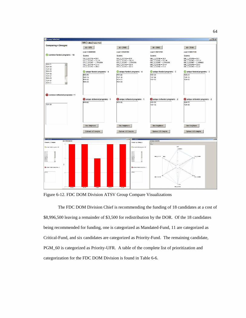
64

Figure 6-12. FDC DOM Division ATSV Group Compare Visualizations

The FDC DOM Division Chief is recommending the funding of 18 candidates at a cost of

$8,996,500 leaving a remainder of $3,500 for redistribution by the DOR. Of the 18 candidates

being recommended for funding, one is categorized as Mandated-Fund, 11 are categorized as

Critical-Fund, and six candidates are categorized as Priority-Fund. The remaining candidate,

PGM_60 is categorized as Priority-UFR. A table of the complete list of prioritization and

categorization for the FDC DOM Division is found in Table 6-6.

65

Table 6-6. FDC DOM Division Requirements Prioritization Phase Results

6.3.4 Abridged Demonstration for FDD

The FDD DOM Division Chief has been assigned a list of 39 programs (PGM_73

through PGM_111) as candidates for inclusion in a portfolio limited by a TOA of $10M.

Candidates PGM_100, PGM_101, and PGM_107 are identified as a Mandated-Fund programs at

a cost of $616,900 which is feasible with a TOA of $10M. The cost to fully fund all candidates

sums to $15,758,400. PGM_102 provides capabilities redundant to the capabilities provided by

the Mandated-Fund program PGM_101 and therefore has been categorized as Unfunded. With

39 candidates, there are over 549 billion possible combinations of candidates that could be

included in the final choice set of portfolios. This has been reduced to a choice set containing

three portfolios with the number of candidates the decision-maker has to consider reduced from

39 to a manageable four candidates. The ATSV Group Compare Visualizations for the final

choice set can be seen in Figure 6-13.

66

Figure 6-13. FDD DOM Division ATSV Group Compare Visualizations

The FDD DOM Division Chief is recommending the funding of 36 candidates at a cost of

$9,928,300 leaving a remainder of $71,700 for redistribution by the DOR. Of the 36 candidates

being recommended for funding, three are categorized as Mandated-Fund, 28 are categorized as

Critical-Fund, and five candidates are categorized as Priority-Fund. The remaining two

candidates are categorized as Priority-UFR. A table of the complete list of prioritization and

categorization for the FDD DOM Division is found in Table 6-7.

67

Table 6-7. FDD DOM Division Requirements Prioritization Phase Results

6.3.5 Abridged Demonstration for FDG

The FDG DOM Division Chief has been assigned a list of 28 programs (PGM_112

through PGM_139) as candidates for inclusion in a portfolio limited by a TOA of $10M.

Candidates PGM_115, and PGM_138 are identified as a Mandated-Fund programs at a cost of

$410,100 which is feasible with a TOA of $10M. The cost to fully fund all candidates sums to

$15,886,500. PGM_132 provides capabilities redundant to the capabilities provided by the

Mandated-Fund program PGM_138 and therefore has been categorized as Unfunded. With 28

candidates, there are over 268 million possible combinations of candidates that could be included

in the final choice set of portfolios. This has been reduced to a choice set containing four

portfolios with the number of candidates the decision-maker has to consider reduced from 28 to

only four candidates. The ATSV Group Compare Visualizations for the final choice set can be

seen in Figure 6-14.

68

Figure 6-14. FDG DOM Division ATSV Group Compare Visualizations

The FDG DOM Division Chief is recommending the funding of 25 candidates at a cost of

$9,565,100 leaving a remainder of $434,900 for redistribution by the DOR. Of the 25 candidates

being recommended for funding, two are categorized as Mandated-Fund, 20 are categorized as

Critical-Fund, and three candidates are categorized as Priority-Fund. The remaining two

candidates are categorized as Priority-UFR. A table of the complete list of prioritization and

categorization for the FDG DOM Division is found in Table 6-8.

69

Table 6-8. FDG DOM Division Requirements Prioritization Phase Results

6.3.6 Abridged Demonstration for FDI

The FDI DOM Division Chief has been assigned a list of eight programs (PGM_140

through PGM_147) as candidates for inclusion in a portfolio limited by a TOA of $2M.

Candidates PGM_146 has been identified as a Mandated-Fund program at a cost of $85,700

which is feasible with a TOA of $2M. The cost to fully fund all candidates sums to $2,211,300.

With eight candidates, there are 255 possible combinations of candidates that could be included

in the final choice set of portfolios. This has been reduced to a choice set containing three

portfolios with the number of candidates the decision-maker has to consider reduced from eight to

three candidates. The ATSV Group Compare Visualizations for the final choice set can be seen

in Figure 6-15.

70

Figure 6-15. FDI DOM Division ATSV Group Compare Visualizations

The FDI DOM Division Chief is recommending the funding of seven candidates at a cost

of $1,943,200 leaving a remainder of $56,800 for redistribution by the DOR. Of the seven

candidates being recommended for funding, one is categorized as Mandated-Fund, and six are

categorized as Critical-Fund. The remaining candidate, PGM_145, is categorized as Critical-

UFR. A table of the complete list of prioritization and categorization for the FDI DOM Division

is found in Table 6-9.

71

Table 6-9. FDI DOM Division Requirements Prioritization Phase Results

6.3.7 Abridged Demonstration for FDV

The FDV DOM Division Chief has been assigned a list of 25 programs (PGM_173

through PGM_197) as candidates for inclusion in a portfolio limited by a TOA of $19.5M.

Candidates PGM_175, PGM_190 and PGM_197 are identified as Mandated-Fund programs at a

cost of $2,160,800 which is feasible with a TOA of $19.5M. The cost to fully fund all candidates

sums to $20,665,400. An item to note from the Prepare and Evaluate Input Data step is that 22 of

the 25 candidates score a zero for Objective 3 while the remaining three have scores less than

1.05, resulting in Objective 3 providing little value to the decision-making process. An additional

item to note is that high cost candidates, PGM_177 and PGM_182, have a combined cost of over

half the TOA which can produce visualizations with separated groups of data points. This can be

seen in Figure 6-16 where the portfolios that contain PGM_177 or PGM_182 are highlighted in

green.

72

Figure 6-16. FDV DOM Division 2D Scatter Plot

With 25 candidates, there are over 33 million possible combinations of candidates that

could be included in the final choice set of portfolios. This has been reduced to a choice set

containing four portfolios with the number of candidates the decision-maker has to consider

reduced from 25 to only six candidates. The ATSV Group Compare Visualizations for the final

choice set can be seen in Figure 6-17.

73

Figure 6-17. FDV DOM Division ATSV Group Compare Visualizations

The FDV DOM Division Chief is recommending the funding of 23 candidates at a cost of

$19,460,400 leaving a remainder of $39,600 for redistribution by the DOR. Of the 23 candidates

being recommended for funding, three are categorized as Mandated-Fund, and 20 are categorized

as Critical-Fund. Of the remaining two candidates, PGM_180 is categorized as Critical-UFR

while the last one is categorized as a Priority-UFR. A table of the complete list of prioritization

and categorization for the FDG DOM Division is found in Table 6-10.

74

Table 6-10. FDV DOM Division Requirements Prioritization Phase Results

6.3.8 Director Reviews Step

The Requirements Prioritization Phase concludes by holding Director Reviews where the

DOM Division Chiefs each present their funding recommendations, with their candidates

categorized and prioritized, to the DOR. A summary of the initial data presented to the DOR

during the Director Reviews can be found in Table 6-11. The consolidated, by candidate, DOM

Division Requirements Prioritization Phase results prior to the Director Reviews can be seen in

Figure 6-18. The following four Critical-URFs, with their associated cost, have been identified

Table 6-11. Portfolio Summary Post Requirements Prioritization Phase

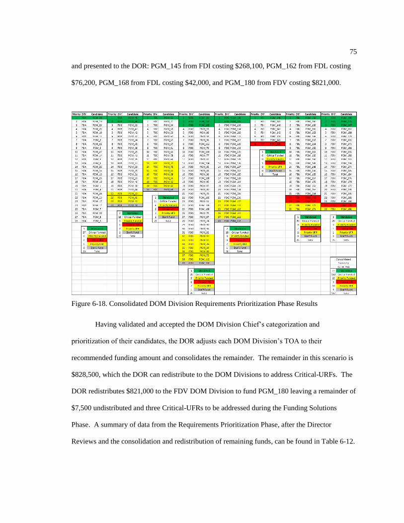
75

and presented to the DOR: PGM_145 from FDI costing $268,100, PGM_162 from FDL costing

$76,200, PGM_168 from FDL costing $42,000, and PGM_180 from FDV costing $821,000.

Figure 6-18. Consolidated DOM Division Requirements Prioritization Phase Results

Having validated and accepted the DOM Division Chief’s categorization and

prioritization of their candidates, the DOR adjusts each DOM Division’s TOA to their

recommended funding amount and consolidates the remainder. The remainder in this scenario is

$828,500, which the DOR can redistribute to the DOM Divisions to address Critical-URFs. The

DOR redistributes $821,000 to the FDV DOM Division to fund PGM_180 leaving a remainder of

$7,500 undistributed and three Critical-UFRs to be addressed during the Funding Solutions

Phase. A summary of data from the Requirements Prioritization Phase, after the Director

Reviews and the consolidation and redistribution of remaining funds, can be found in Table 6-12.

76

Table 6-12. Portfolio Summary Post Director Reviews

(Changes from Table 6-11 Highlighted)

6.4 Demonstration of Funding Solutions Phase

The purpose of the Funding Solutions Phase of the EE-PEG POM production process

remains unchanged for the AEMS scenario. The purpose is the production of the EE-PEG POM

recommendation, containing a portfolio of candidates recommended for funding and a list of

critical unfunded requirements, for submission to the PPBC for approval by the SRG and SLDA.

The phase begins with the EE-PEG leadership holding a series of reviews with each DOM

Division Chief to afford them the opportunity to present their portfolios for validation and

acceptance. If any portfolio is not accepted, then the DOM Division can iterate through the

Requirements Prioritization Phase with the additional guidance from the EE-PEG leadership. In

this scenario the EE-PEG leadership has validated the categorization and prioritization of the

candidates and accepts the DOM Division portfolios as presented at the end of the Requirements

Prioritization Phase from the previous section. The next step is to hold an EE-PEG consolidated

working session to simultaneously address EE-PEG’s entire list of validated candidates as a

single portfolio. The entire list of 197 candidates is loaded into ATSV and is taken through many

of the same steps demonstrated in the Requirements Prioritization Phase.

77

6.4.1 Prepare and Evaluate Input Data Step

The Prepare and Evaluate Input Data Step in the Funding Solutions Phase changes from

the Requirements Prioritization Phase only in that it is performed on the entire EE-PEG portfolio

data set. The EE-PEG Candidate List Data Visualization Displays can be seen in Figure 6-19 and

Figure 6-20. The decision-maker can use these visualizations to gain sufficient insight into the

input data to be able to explore the trade space in an efficient and meaningful manner.

Figure 6-19. EE-PEG ATSV Candidate List Data Visualization Display

78

Figure 6-20. EE-PEG ATSV Candidate Histogram and Plot Visualization Display

6.4.2 Sample Trade Space and Initiate Exploration Step

Prior to exploring the trade space, a sample of the portfolios within the trade space must

be taken. Again, for this demonstration, 2,500 samples are taken using the ATSV Random

Sample function. The Portfolio Data Engine processes the Candidate List and produces the

Portfolio Data Table in the same manner as it did in the demonstration of the Requirement

Prioritization Phase. The ATSV Portfolio Data Visualization Displays can be used to familiarize

decision-makers with the variables that define the trade space. One item to note at this point is

that the candidates that previously had a large influence over a particular variable when only

viewing a single DOM Division’s data has a proportionally smaller influence when viewing the

data for the entire EE-PEG. The Histogram Plot and the Scatter Matrix, as seen in Figure 6-21,

can aid in identifying gaps in the portfolio sampling and discrepancies in expected correlations

between variables.

79

Figure 6-21. EE-PEG ATSV Portfolio Histogram Plot and Scatter Matrix

6.4.3 Exploration of Trade Space Step and Set Reduction Step

Much like the Exploration of Trade Space and Set Reduction steps in the Requirements

Prioritization Phase, decision-makers are likely to iterate through the Exploration of Trade Space

step and Set Reduction step the most while developing their preferences and therefore, the

demonstration for these two steps is combined. At this time, global constraints such as the $81M

TOA budget limit and the funding of Mandated-Fund candidates can be loaded into ATSV and

applied using Brush Controls. Additionally, constraints that apply to each of the sub-portfolios

can now be applied globally to reduce the size of the consideration set.

For this scenario, constraints are created using the ATSV Query Function and are applied

with ATSV’s Brush Function to force the funding of candidates listed as Critical-Fund for each of

the DOM Divisions. Likewise, constraints are applied to force the defunding of candidates listed

as Unfunded and Priority-UFR for each of the DOM Divisions. Although numerous funding

strategies could be used in this scenario, applying these constraints aligns with a strategy that

allows the use of Priority-Fund candidates as bill-payers in order to fund all validated Critical-

UFRs. Since the total cost of all candidates marked as Priority-Fund, at this point in the process

80

($6,882,300) is greater than the total cost of the remaining three Critial-UFRs ($386,300) this is a

valid funding strategy for this scenario.

One item to note as discussed in the Requirements Prioritization Phase for FDC DOM

Division is the redundant capabilities provided by candidates PGM_69 and PGM_71. Under the

current funding strategy, candidate PGM_71 remains funded, and therefore PGM_69 has been

categorized as Unfunded. As long as the employed funding strategy keeps PGM_71 in a funded

state, an additional constraint is not needed; however, if this changes, then an additional

constraint keeping PGM_69 and PGM_71 from both being funded will need to be applied.

As in the Requirements Prioritization Phase, the decision-makers continue to reduce their

consideration set to the decision set. Once the decision-makers have explored the trade space

thoroughly enough to develop their preferences and reduce the consideration set to a decision set,

then they can move on to the final step in this phase, the Make a Choice step. However, contrary

to the Requirements Prioritization Phase, in the Funding Solutions Phase there are multiple-

decision-makers. The final decision-makers for the AEMS portfolio problem, as discussed in

Chapter 3, are the EE-PEG leadership, the ASA(ALT) and the DCS G-8. This demonstration of

the AEMS portfolio problem decision-making process addresses two scenarios for the Make a

Choice Step. The first scenario occurs when the two decision-maker’s preferences fail to

converge when reducing their consideration set to their final choice set. The second scenario

occurs when the two decision-maker’s preferences converge when reducing their consideration

set to a final choice set. Although initially these two scenarios can seem very different, the next

section demonstrates that the proposed decision-making process addresses these two scenarios in

a very similar manner.

81

6.4.4 Make a Choice Step

The phases and steps leading up to this final Make a Choice Step provide an opportunity

for decision-makers to develop their preferences while reducing the universal set of portfolios to a

manageable sized choice set. With multiple decision-makers in AEMS portfolio problem, each

with their own decision-making agenda, the preferences they develop may fail to converge,

leading to two discrete choice sets; however, there is a possibility that the decision-maker’s

preferences converge, leading to identical or overlapping choice sets. In either scenario, the same

tools and processes can be employed to aid the decision-makers in coming to a decision. First,

we combine all remaining portfolios from both of the decision-maker’s choice sets into a single

choice set. In doing this, the commonalities between the individual choice sets can be identified,

and the decision-makers can focus their efforts on the trades between the remaining candidates.

A 2D Scatter Plot of EE-PEG sampled portfolios for the first scenario, where the

decision-makers arrive at two discrete choice sets, is shown in Figure 6-22. The ATSV Group

Compare Visualization for the ASA(ALT) is shown in Figure 6-23 where the four portfolios

making up the decision-maker’s choice set can be seen. Note the four portfolios that make up the

choice set have the 14 Defunded and Priority-UFR candidates in common as well as, in this case,

one additional unique defunded candidate per portfolio. The ATSV Group Compare

Visualization for DCS G-8 is shown in Figure 6-24 where the four portfolios making up the

decision-maker’s choice set can be seen. Note the four portfolios that make up the choice set also

have the 14 Defunded and Priority-UFR candidates in common, as well as one additional unique

defunded candidate per portfolio. The Tallies view containing the seven remaining portfolios of

the combined choice sets from both decision-makers can be seen in the ATSV Group Compare

Visualization in Figure 6-25. Of the 197 candidates considered for inclusion in the final

portfolio, the decision-makers’ choice sets have commonality in funding 175 and defunding 14 of

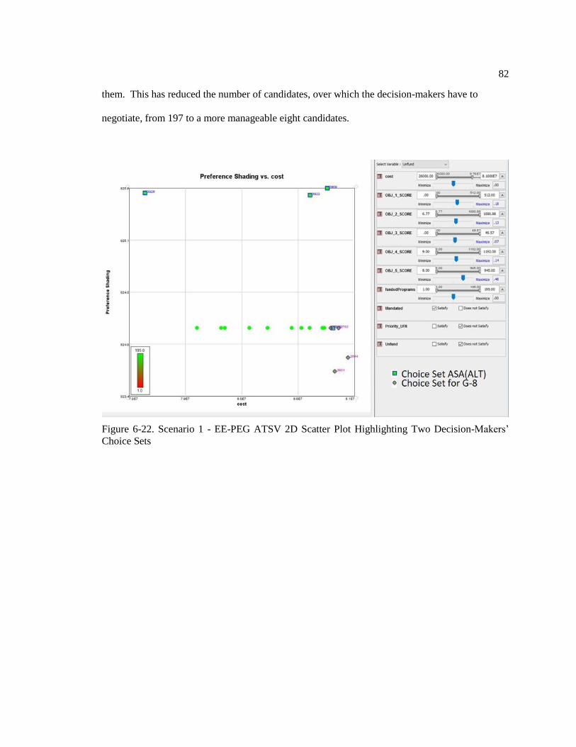
82

them. This has reduced the number of candidates, over which the decision-makers have to

negotiate, from 197 to a more manageable eight candidates.

Figure 6-22. Scenario 1 - EE-PEG ATSV 2D Scatter Plot Highlighting Two Decision-Makers’

Choice Sets

83

Figure 6-23. Scenario 1 - EE-PEG ATSV Group Compare Visualization for ASA(ALT) Choice Set

Figure 6-24. Scenario 1 - EE-PEG ATSV Group Compare Visualization for DCS G-8 Choice Set

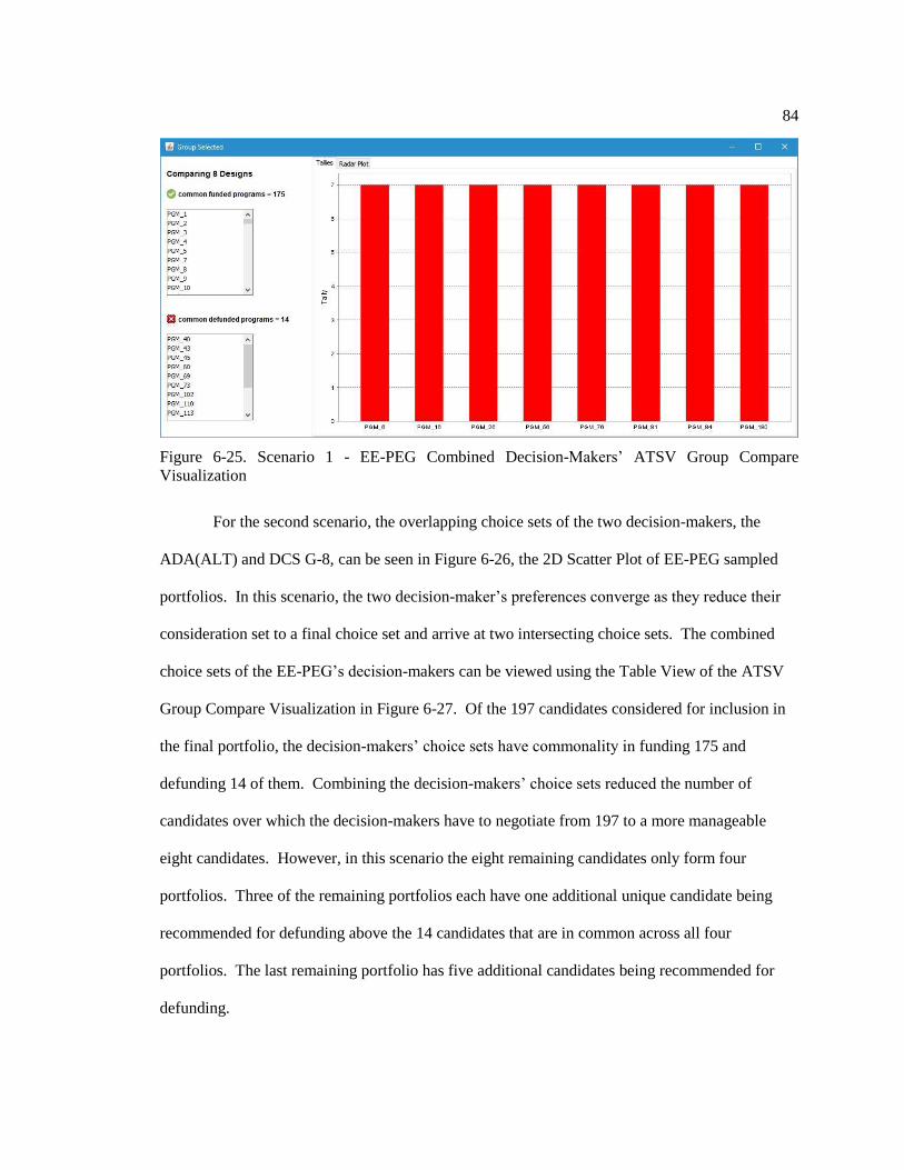
84

Figure 6-25. Scenario 1 - EE-PEG Combined Decision-Makers’ ATSV Group Compare

Visualization

For the second scenario, the overlapping choice sets of the two decision-makers, the

ADA(ALT) and DCS G-8, can be seen in Figure 6-26, the 2D Scatter Plot of EE-PEG sampled

portfolios. In this scenario, the two decision-maker’s preferences converge as they reduce their

consideration set to a final choice set and arrive at two intersecting choice sets. The combined

choice sets of the EE-PEG’s decision-makers can be viewed using the Table View of the ATSV

Group Compare Visualization in Figure 6-27. Of the 197 candidates considered for inclusion in

the final portfolio, the decision-makers’ choice sets have commonality in funding 175 and

defunding 14 of them. Combining the decision-makers’ choice sets reduced the number of

candidates over which the decision-makers have to negotiate from 197 to a more manageable

eight candidates. However, in this scenario the eight remaining candidates only form four

portfolios. Three of the remaining portfolios each have one additional unique candidate being

recommended for defunding above the 14 candidates that are in common across all four

portfolios. The last remaining portfolio has five additional candidates being recommended for

defunding.

85

Figure 6-26. Scenario 2 - EE-PEG Decision-Makers’ Choice Sets ATSV 2D Scatter Plot

Figure 6-27. Scenario 2 - EE-PEG Decision-Makers’ Choice Set ATSV Group Compare

Visualization

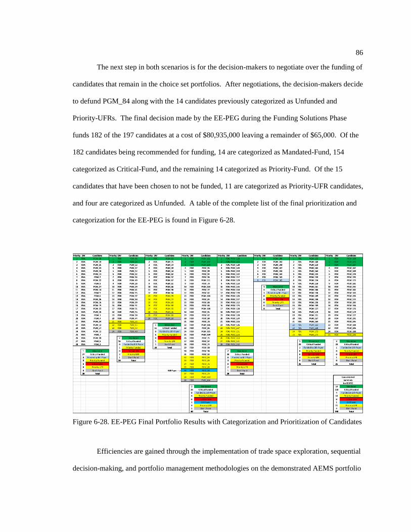
86

The next step in both scenarios is for the decision-makers to negotiate over the funding of

candidates that remain in the choice set portfolios. After negotiations, the decision-makers decide

to defund PGM_84 along with the 14 candidates previously categorized as Unfunded and

Priority-UFRs. The final decision made by the EE-PEG during the Funding Solutions Phase

funds 182 of the 197 candidates at a cost of $80,935,000 leaving a remainder of $65,000. Of the

182 candidates being recommended for funding, 14 are categorized as Mandated-Fund, 154

categorized as Critical-Fund, and the remaining 14 categorized as Priority-Fund. Of the 15

candidates that have been chosen to not be funded, 11 are categorized as Priority-UFR candidates,

and four are categorized as Unfunded. A table of the complete list of the final prioritization and

categorization for the EE-PEG is found in Figure 6-28.

Figure 6-28. EE-PEG Final Portfolio Results with Categorization and Prioritization of Candidates

Efficiencies are gained through the implementation of trade space exploration, sequential

decision-making, and portfolio management methodologies on the demonstrated AEMS portfolio

87

decision-making process. Consistent with the expected efficiencies discussed in Chapter 4, the

Requirements Prioritization Phase, and Funding Solutions Phase reduce the time required to

complete the EE-PEG POM production process along with time savings through the elimination

of the EE-PEG member interviews in the Requirements Identification Phase. Additionally, the

number of candidates the decision-makers had to consider was greatly reduced through

implementing the portfolio decision-making process. With 197 candidates originally being

considered for funding the universal set of portfolios contained over 2x1059 possible

combinations. The number of candidates was further reduced through the application of

constraints that defunded the 14 candidates categorized as Unfunded and Priority-UFRs reducing

the number of possible combinations to just over 1.2x1055 portfolios. Initially, 2,500 sample

portfolios were taken to initiate exploration of the trade space. Through iterations of the steps in

the Funding Solutions Phase a total of only 4,222 sample portfolios, out of the over 2x1059

possible, had to be taken in order to reach a final decision. Through implementation of the

decision-making process these 4,222 samples were quickly reduced to a manageable sized choice

set of eight and five portfolios for the two scenarios demonstrated in the Make a Choice Step. In

each of these two scenarios, the number of candidates, that had to be considered during the final

Make a Choice Step, was reduced from 197 to eight candidates increasing the efficiency at which

the decision-makers could make a final decision for the EE-PEG POM submission

recommendation.

6.5 Chapter Summary

In this chapter the decision-making process proposed in Chapter 4 was demonstrated on

an AEMS portfolio problem while employing ATSV tools discussed in Chapter 2 and Chapter 5.

This decision-making process employed trade space exploration, sequential decision-making, and

88

portfolio management methodologies to reduce the size of the portfolio problem’s decision set,

from the universal set made up of more than 2x1059 combinations to a manageable sized choice

set. It was demonstrated that this process can be performed on hierarchical decision-making

problems with multiple decision-makers. Conclusions, limitations, and future work are outlined

in the next chapter.

89

Chapter 7

Conclusions, Limitations, and Future Work

This thesis demonstrated the usefulness of an interactive decision-making process for

portfolio management problems by following a sequential decision-making method, utilizing a

trade space exploration approach. Chapter 2 discussed related work in decision-making, portfolio

management, sequential decision-making, trade space exploration, and an available tool for

conducting the trade space exploration. Chapter 3 presented background on the army equipping

and modernization strategies portfolio problem that was selected to demonstrate the proposed

decision-making process. Chapter 4 proposed a decision-making process that applied trade space

exploration to portfolio decision-making, allowing for a sequential decision-making process that

keeps the “human-in-the-loop” during optimization. Chapter 5 discussed fundamental tools for

the application of trade space exploration to portfolio decision-making. Chapter 6 provided a

demonstration of the decision-making process proposed in Chapter 4 through application to the

Army Equipping and Modernization Strategies (AEMS) portfolio problem discussed in Chapter

3. The purpose of this chapter is to conclude and discuss limitations of the work and suggest

future work.

7.1 Conclusions

The primary objectives for this thesis were: (1) to develop a decision-making process that

applies trade space exploration to the portfolio decision-making process; (2) to investigate the

tools needed for portfolio decision-making with a focus of keeping the “human-in-the-loop”

during the optimization process; and (3) to demonstrate the proposed portfolio management

90

decision-making process utilizing an AEMS portfolio problem. The decision-making process

developed keeps the “human-in-the-loop” while using trade space exploration methodologies and

tools to help decision-makers understand the trade space, develop their preferences, explore the

trade space, reduce the universal set of alternatives to a final choice set, and examine the

remaining trades in order to make a final decision. The application of the proposed portfolio

management decision-making process on the AEMS portfolio problem demonstrated the

feasibility and usefulness of the proposed decision-making process. Additionally, the

demonstration of proposed portfolio management decision-making process verified the feasibility

of applying the trade space exploration methodology to portfolio decision-making problems.

Efficiencies potentially gained through the implementation of the proposed decision-

making process were noted both in the process itself as well as through the elimination of steps

that previously had to be conducted upstream of the process. Through the implementation of

trade space exploration and its associated tools on a portfolio problem, the decision-maker can

efficiently reduce a universal set of alternatives, which grows exponentially with the number of

included candidates, to a manageable size. Additionally, decision makers can apply a tool such as

ATSV’s Group Compare Visualizations to display the commonalities between selected portfolios.

This type of visualization efficiently identifies the remaining trade space between selected

portfolios, potentially reducing the time needed to make a final decision.

7.2 Limitations

The AEMS Portfolio Problem contains data identified as business sensitive, procurement

sensitive, acquisition sensitive, proprietary or source selection information that may be associated

with ongoing competitive sourcing. To protect the confidentiality of the sensitive portions of the

data set, the data was sanitized of any element that would allow the discovery of the acquisition

91

program each record represented. Additionally, knowledge of specific details of current or future

AEMS decision-making processes could disrupt competitive sourcing. Therefore, any such

details were not included in this thesis. Although these limitations may preclude the reader from

fully understanding all aspects the current process of addressing the U.S. Army Equipping and

Modernization Strategies Portfolio Problem, it does not detract from the general understanding of

the proposed decision-making process and its demonstration.

7.3 Future Work

The work presented in this thesis demonstrated the functionality of applying trade space

exploration methodologies in a decision-making process for portfolio management problems.

The demonstration of this decision-making process however was only conducted on a single

portfolio problem using a single tool. Future work in this area of study should expand upon this

work through the application of trade space exploration on a number of different types of

portfolio problems using multiple tools beyond ATSV. Additionally, comparisons should be

made with alternative decision-making methodologies to validate that the application of trade

space exploration methodologies to portfolio decision-making problems is not only feasible but

also beneficial. The Group Compare Visualizations within ATSV proved to be beneficial in

supporting the decision-making process. Future work should be conducted into the Group

Compare Visualizations, their effectiveness as decision-making tools, and the expansion of

functions beyond what are currently available in ATSV.

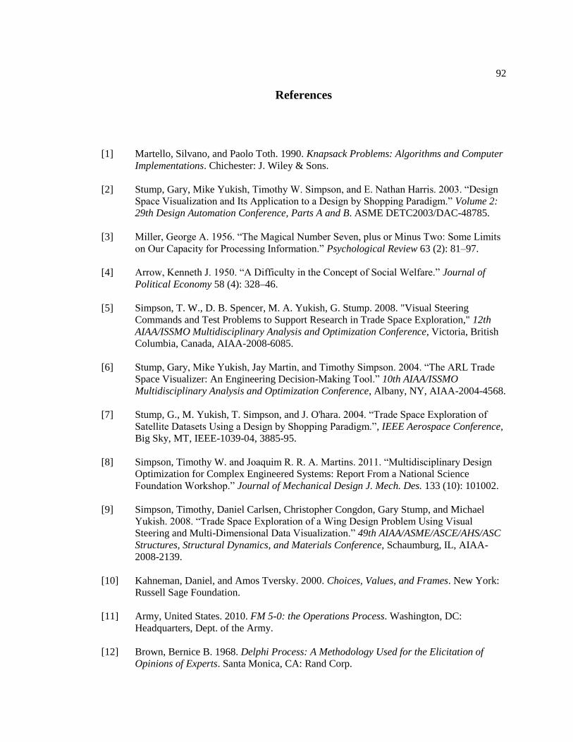
92

References

[1] Martello, Silvano, and Paolo Toth. 1990. Knapsack Problems: Algorithms and Computer

Implementations. Chichester: J. Wiley & Sons.

[2] Stump, Gary, Mike Yukish, Timothy W. Simpson, and E. Nathan Harris. 2003. “Design

Space Visualization and Its Application to a Design by Shopping Paradigm.” Volume 2:

29th Design Automation Conference, Parts A and B. ASME DETC2003/DAC-48785.

[3] Miller, George A. 1956. “The Magical Number Seven, plus or Minus Two: Some Limits

on Our Capacity for Processing Information.” Psychological Review 63 (2): 81–97.

[4] Arrow, Kenneth J. 1950. “A Difficulty in the Concept of Social Welfare.” Journal of

Political Economy 58 (4): 328–46.

[5] Simpson, T. W., D. B. Spencer, M. A. Yukish, G. Stump. 2008. "Visual Steering

Commands and Test Problems to Support Research in Trade Space Exploration," 12th

AIAA/ISSMO Multidisciplinary Analysis and Optimization Conference, Victoria, British

Columbia, Canada, AIAA-2008-6085.

[6] Stump, Gary, Mike Yukish, Jay Martin, and Timothy Simpson. 2004. “The ARL Trade

Space Visualizer: An Engineering Decision-Making Tool.” 10th AIAA/ISSMO

Multidisciplinary Analysis and Optimization Conference, Albany, NY, AIAA-2004-4568.

[7] Stump, G., M. Yukish, T. Simpson, and J. O'hara. 2004. “Trade Space Exploration of

Satellite Datasets Using a Design by Shopping Paradigm.”, IEEE Aerospace Conference,

Big Sky, MT, IEEE-1039-04, 3885-95.

[8] Simpson, Timothy W. and Joaquim R. R. A. Martins. 2011. “Multidisciplinary Design

Optimization for Complex Engineered Systems: Report From a National Science

Foundation Workshop.” Journal of Mechanical Design J. Mech. Des. 133 (10): 101002.

[9] Simpson, Timothy, Daniel Carlsen, Christopher Congdon, Gary Stump, and Michael

Yukish. 2008. “Trade Space Exploration of a Wing Design Problem Using Visual

Steering and Multi-Dimensional Data Visualization.” 49th AIAA/ASME/ASCE/AHS/ASC

Structures, Structural Dynamics, and Materials Conference, Schaumburg, IL, AIAA-

2008-2139.

[10] Kahneman, Daniel, and Amos Tversky. 2000. Choices, Values, and Frames. New York:

Russell Sage Foundation.

[11] Army, United States. 2010. FM 5-0: the Operations Process. Washington, DC:

Headquarters, Dept. of the Army.

[12] Brown, Bernice B. 1968. Delphi Process: A Methodology Used for the Elicitation of

Opinions of Experts. Santa Monica, CA: Rand Corp.

93

[13] Delbecq Andre L., Andrew H. de Ven, and David H. Gustafson. 1975. Group Techniques

for Program Planning: a Guide to Nominal Group and Delphi Processes. Glenview, IL:

Scott, Foresman.

[14] Saaty, Thomas L. 1990. “How to Make a Decision: The Analytic Hierarchy Process.”

European Journal of Operational Research 48 (1): 9–26.

[15] Balling, R. 1999. "Design by Shopping: A New Paradigm?," Proceedings of the Third

World Congress of Structural and Multidisciplinary Optimization (WCSMO-3), Buffalo,

New York, University at Buffalo, 295-297.

[16] Lindroth, Peter, Michael Patriksson, and Stromberg Ann-Brith. 2009. Approximating the

Pareto Optimal Set Using a Reduced Set of Objective Functions. Goteborg: Chalmers

University of Technology.

[17] Kester, Linda, Abbie Griffin, Erik Jan Hultink, and Kristina Lauche. 2011. “Exploring

Portfolio Decision-Making Processes.” Journal of Product Innovation Management, 28

(5): 641-661.

[18] Barczak, Gloria, Abbie Griffin, and Kenneth B. Kahn. 2009. “PERSPECTIVE: Trends

and Drivers of Success in NPD Practices: Results of the 2003 PDMA Best Practices

Study.” Journal of Product Innovation Management 26 (1): 3–23.

[19] Markowitz, Harry. 1952. “Portfolio Selection.” The Journal of Finance 7 (1): 77–91.

[20] Shocker, Allan D., Moshe Ben-Akiva, Bruno Boccara, and Prakash Nedungadi. 1991.

“Consideration Set Influences on Consumer Decision-Making and Choice: Issues,

Models, and Suggestions.” Marketing Letters 2 (3): 181–97.

[21] Miller, Simon W., Timothy W. Simpson, Michael A. Yukish, Lorri A. Bennett, Sara E.

Lego, and Gary M. Stump. 2013. “Preference Construction, Sequential Decision Making,

and Trade Space Exploration.” Volume 3A: 39th Design Automation Conference, ASME

DETC2013/DAC-13098.

[22] Ross, A.M. and D. E. Hastings. 2005. "The Tradespace Exploration Paradigm," INCOSE

International Symposium, Rochester, NY, 15 (1): 1706-18.

[23] Messac, Achille, and Xuan Chen. 2000. “Visualizing The Optimization Process In Real-

Time Using Physical Programming.” Engineering Optimization 32 (6): 721–47.

[24] Ng, W.Y. 1991. “Generalized Computer-Aided Design System: A Multiobjective

Approach.” Computer-Aided Design 23 (8): 548–53.

[25] Eddy, W.F., and A. Mockus. 1995. “Dynamic Visualization in Modeling and

Optimization of Ill-Defined Problems: Case Studies and Generalizations”, Technical

Report, Department of Statistics, Carnegie Mellon University, Pittsburgh, PA.

94

[26] Carlsen, D. E. 2008. “Assessment of User-Guided Visual Steering Commands During

Trade Space Exploration,” Master’s Thesis, Department of Mechanical and Nuclear

Engineering. The Pennsylvania State University, University Park, PA.

[27] Stump, Gary, Sara Lego, Mike Yukish, Timothy W. Simpson, and Joseph A.

Donndelinger. 2009. “Visual Steering Commands for Trade Space Exploration: User-

Guided Sampling With Example.” Journal of Computing and Information Science in

Engineering, 9 (4): 044501:1-10.

[28] Army, United States. 2013. How the Army Runs: a Senior Leader Reference Handbook,

2013-2014. Carlisle Barracks, PA, Army War College.

[29] Department of Defense, United States. 2013. DoD Directive 7045.14 "The Planning,

Programming, Budgeting, and Execution (PPBE) Process”, 25 January 2013.

Washington, DC.

[30] Army, United States. 2013. Army Equipping Roles, Responsibilities, Procedures and

Authorities, 10 September 2013. Washington, DC.

[31] Wilson, Alfred. 2015. “Fundamentals of Programming and Budgeting.” Lecture, Army,

United States, Fort Belvoir, VA, 20 March.