F Trace Metal Analysis in Lake Sediment A Study of Vällsjön as an Intermediate Source or Barrier Master of Science Thesis in Infrastructure and Environmental Engineering OFELIA KULLERSTEDT & THERESE ÖRNMARK Department of Civil and Environmental Engineering Water Environment Technology CHALMERS UNIVERSITY OF TECHNOLOGY Göteborg, Sweden 2014 Master’s Thesis 2014:71

Welcome message from author
This document is posted to help you gain knowledge. Please leave a comment to let me know what you think about it! Share it to your friends and learn new things together.
Transcript
F
Trace Metal Analysis in Lake Sediment A Study of Vällsjön as an Intermediate Source or Barrier Master of Science Thesis in Infrastructure and Environmental Engineering
OFELIA KULLERSTEDT & THERESE ÖRNMARK
Department of Civil and Environmental Engineering
Water Environment Technology
CHALMERS UNIVERSITY OF TECHNOLOGY
Göteborg, Sweden 2014
Master’s Thesis 2014:71

MASTER’S THESIS 2014:71
Trace Metal Analysis in Lake Sediment
A Study of Vällsjön as an Intermediate Source or Barrier
Master of Science Thesis in Infrastructure and Environmental Engineering
OFELIA KULLERSTEDT & THERESE ÖRNMARK
Department of Civil and Environmental Engineering
Water Environment Technology
CHALMERS UNIVERSITY OF TECHNOLOGY
Göteborg, Sweden 2014
Trace Metal Analysis in Lake Sediment
A Study of Vällsjön as an Intermediate Source or Barrier
Master of Science Thesis in Infrastructure and Environmental Engineering
OFELIA KULLERSTEDT & THERESE ÖRNMARK
© OFELIA KULLERSTEDT & THERESE ÖRNMARK, 2014
Examensarbete / Institutionen för Bygg- och miljöteknik,
Chalmers tekniska högskola 2014:71
Department of Civil and Environmental Engineering
Water Environment Technology
Chalmers University of Technology
SE-412 96 Göteborg
Sweden
Telephone: + 46 (0)31-772 1000
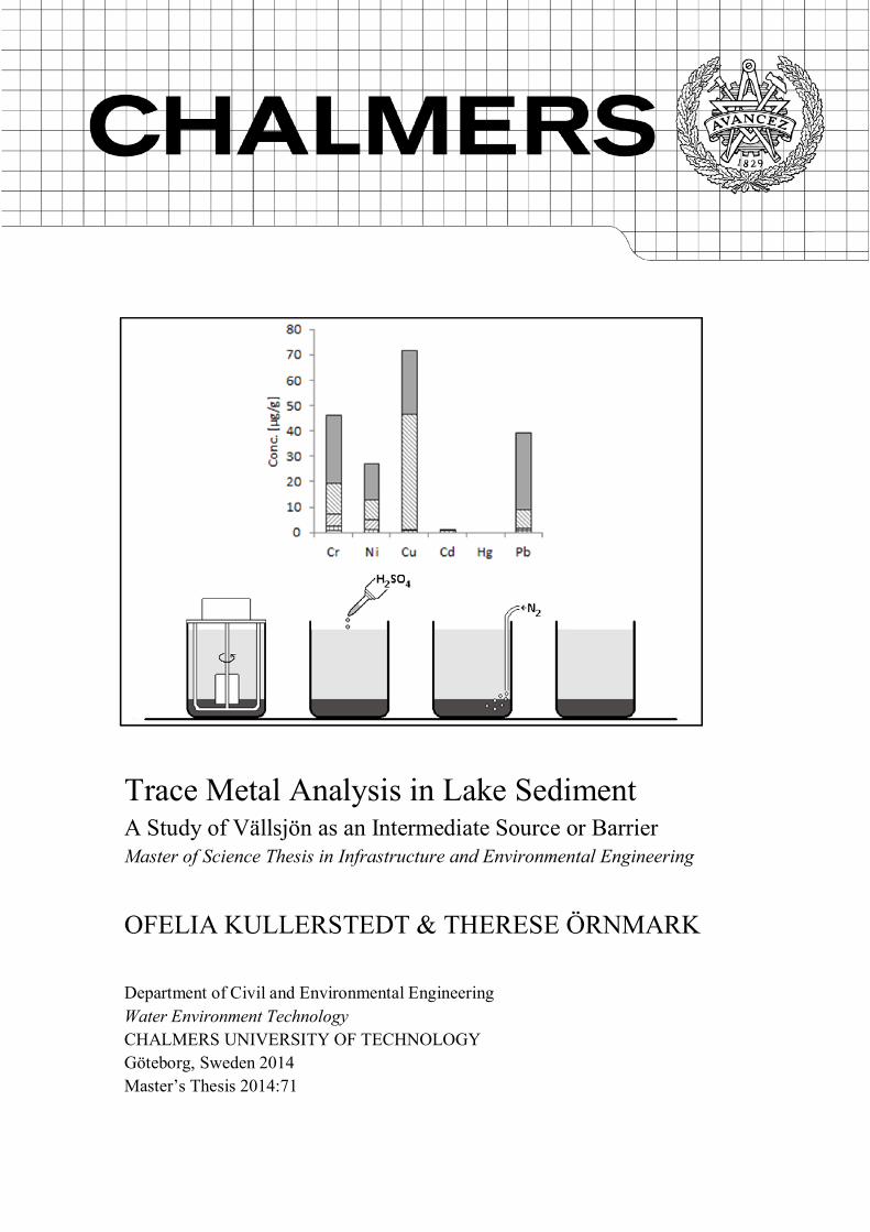
Cover: Results from the modified sequential extraction procedure and a schematic
drawing over the beaker tests.
Chalmers Reproservice / Department of Civil and Environmental Engineering
Göteborg, Sweden 2014
I
Trace Metal Analysis in Lake Sediment A Study of Vällsjön as an Intermediate Source or Barrier
Master of Science Thesis in Infrastructure and Environmental Engineering OFELIA KULLERSTEDT & THERESE ÖRNMARK Department of Civil and Environmental Engineering Water Environment Technology Chalmers University of Technology
ABSTRACT
Natural recipients can be contaminated by anthropogenic activity, for example through waterborne contaminants. Precipitation and groundwater entering a landfill result in contaminated leachate. The lake Vällsjön in Härryda municipality receives leachate from the former active municipal landfills Kikåstippen and Lahallstippen. The landfills have been closed since the 1970s, but Vällsjön still receives treated leachate. The sediment in the lake can therefore, if undisturbed, act as a historical archive of pollutants.
The aim of this master thesis was to determine the concentrations of selected trace metals in the water and sediment in Vällsjön. Water and sediment samples were collected and analysed.
Metal concentrations were analysed with an inductively coupled plasma-mass spectrometry (ICP-MS). The results indicate that the metal concentrations increase with increased sediment depth in the middle of the lake and decrease with increased depth in the outlet. The maximum concentrations found for some metals are approximately the same in the middle and the outlet, however at different depths. A hypothesis is that the metals first settles in the middle and then slowly moves towards the outlet of the lake. If so, Vällsjön can act as a source of contamination towards Rådasjön. The copper concentrations were highest in the shallow sediment in both cores, which indicates that it might have a different source.
A modified sequential extraction procedure (MSEP) was developed and performed on sediment samples in order to investigate how the metals are bound in the sediment. The result indicates that most metals in Vällsjön are relatively hard bound to the sediment.
Through beaker tests it was investigated how different changes in the lake environment could affect the solubility and mobility of the metals. The results indicated that mechanical mixing affects the metal concentrations, which in turn indicates that particles with high metal content might be released into Rådasjön if Vällsjön is dredged. The trace metal concentrations found in the sediment were high, especially zinc, according to Canadian guidelines and need to be further investigated. However, the water concentrations were not on a level where effects on aquatic life are probable. The results indicate that further investigations are needed to determine if Vällsjön acts as a source or a barrier.
Key words: Lake, Sediment, Trace metals, SEP, Beaker test, Leachate

II
III
Analys av metaller i sjösediment En studie av Vällsjön som en intermediär källa eller barriär
Examensarbete inom Infrastructure and Environmental Engineering OFELIA KULLERSTEDT & THERESE ÖRNMARK Examensarbete/Institutionen för Bygg- och miljöteknik Vatten Miljö Teknik Chalmers tekniska högskola
SAMMANFATTNING
Naturliga sjöar och vattendrag kan bli kontaminerade av mänsklig aktivitet, till exempel genom vattenburna föroreningar. Förorent lakvatten bildas av nederbörd som infiltrerar och grundvatten som läcker in på en soptipp. Sjön Vällsjön som ligger i Härryda kommun tar emot lakvatten från de tidigare aktiva kommunala soptipparna Kikåstippen och Lahallstippen. Avfallsupplagen har varit stängda sedan 1970-talet, delvis renat lakvatten rinner dock fortfarande ner till Vällsjön. Sedimentet på botten av sjön kan, om det är ostört, därför fungera som ett historiskt arkiv av föroreningar.
Syftet med detta examensarbete var att undersöka koncentrationerna av några utvalda metaller som förekommer i Vällsjöns vatten och sedimentet. Vatten- och sedimentprover hämtades från sjön och analyserades i laboratorium. Koncentrationen av metaller analyserades med induktivt kopplad plasma-masspektrometri (ICP-MS).
Resultatet indikerar att koncentrationerna av metaller ökar med ökande sedimentdjup i mitten av sjön. Vid utloppet minskar istället metallkoncentrationerna med ett ökat sedimentdjup. De högsta metallkoncentrationerna är ungefär lika höga i båda mätpunkterna, men återfinns på olika djup. En hypotes är att metallerna först sedimenterar i mitten av sjön, och sedan sakta rör sig mot utloppet. Om så är fallet, kan Vällsjön agera som en föroreningskälla för Rådasjön. Kopparkoncentrationen var högst i det ytliga sedimentet i båda sedimentpropparna, vilket tyder på att koppar kan ha en annan föroreningskälla.
En modifierad sekventiell extraktionsmetod utvecklades och genomfördes på sedimentprov, för att undersöka hur de olika metallerna är bundna i sedimentet. Extraktionsmetoden indikerar att de flesta metallerna i Vällsjön är hårt bundna i sedimentet.
De analyserade metallerna undersöktes också med bägartester. Detta gjordes för att utvärdera hur möjliga förändringar av sjöns kvalitet kan påverka lösligheten och rörligheten hos metallerna. Resultatet från testet tyder på att partiklar med högt metallinnehåll kan läcka ut i Rådasjön om Vällsjön i framtiden skulle muddras. Metallkoncentrationerna som uppmättes i sedimentet var höga, speciellt zinc, enligt Kanadensiska gränsvärden, varför fortsatta undersökningar behöver utföras. Halterna i sjövattnet var inte tillräckligt höga för att utgöra någon större risk för påverkan på vattenlevande organismer. Resultaten visar på att fortsatta undersökningar är nödvändiga för att utvärdera om Vällsjön fungerar som en källa eller en barriär.
Nyckelord: Sjö, Sediment, Metaller, Sekventiell Extraktion, Bägartest, Lakvatten

IV
V
Preface This master thesis has been carried out at the division of Water Environment Technology at Chalmers University of technology. The work performed during the spring semester has deepened our knowledge within the field studied. We have always felt very welcome to the division, where many have kindly shared their knowledge with us.
We want to give a deep thank to our supervisor and examiner Ann-Margret Strömvall for all her enthusiasm, help and always open door. We also want to thank our supervisor Jesper Knutsson for his knowledge and especially for helping us running all the ICP-MS analyses.
During the experimental work in the lab, Mona Pålsson was always there with a smiling face and positive attitude. She has encouraged us and given us great support, for which we are very grateful.
We would also like to thank Oskar Modin and Enikö Szabo who helped us running the IC in the lab and Aaro Pirhonen who helped us to build a cradle to support the sawing of the frozen sediment cores. For her kind help, and knowledge about sequential extraction procedures, we want to thank Karin Karlfeldt Fedje.
We also wish to express our gratitude for the information regarding the landfills and the interest in our master thesis work to the involved from Mölndals stad and Härryda municipality. We especially want to thank Anders Hjelm and Solweig Berlin at Mölndal stad and Johan Hagman and Anders Bruce from Härryda municipality.
Finally, we want to thank all the other master thesis students at Water Environment Technology for the social activities and the experience we shared during the spring semester.

VI
CHALMERS Civil and Environmental Engineering, Master’s Thesis 2014:71 VII
Table of Contents
1 Introduction ........................................................................................................... 1
1.1 Aim and goals ................................................................................................. 2
1.2 Methodology and limitations ........................................................................... 2
2 Case Study Area .................................................................................................... 3
3 Literature Review .................................................................................................. 5
3.1 Trace metals ................................................................................................... 5
3.2 Metal speciation .............................................................................................. 6
3.3 Sequential extraction procedure ...................................................................... 6
4 Method .................................................................................................................. 9
4.1 Field methods ................................................................................................. 9
4.2 Lab analysis .................................................................................................. 10
4.3 Modified sequential extraction procedure ...................................................... 12
4.4 Beaker tests................................................................................................... 14
5 Result and Discussion ......................................................................................... 17
5.1 Water quality parameters .............................................................................. 17
5.2 Total analysis of digestible metals ................................................................. 18
Quality assessment of the analytical procedure....................................... 19 5.2.1
Middle core ........................................................................................... 20 5.2.2
Outlet core ............................................................................................. 22 5.2.3
Reliability .............................................................................................. 23 5.2.4
5.3 Classification of metal concentrations ........................................................... 24
5.4 Modified sequential extraction procedure ...................................................... 26
5.5 Comparison between MSEP and total analysis .............................................. 29
5.6 Beaker test .................................................................................................... 30
6 Conclusions ......................................................................................................... 35
7 Recommendations for Further Investigations ....................................................... 37
References .................................................................................................................. 39
Appendices ................................................................................................................. 43

CHALMERS, Civil and Environmental Engineering, Master’s Thesis 2014:71 VIII
CHALMERS, Civil and Environmental Engineering, Master’s Thesis 2014:71 1
1 Introduction Natural recipients can be contaminated by anthropogenic activity, mainly through air- or waterborne contamination. Part of the pollutants entering the recipient, for example a lake, may dissolve into the water while the heavier particles will settle into the sediment at the bottom. The sediment in a lake can therefore, if undisturbed, act as a historical archive of pollutants. The pollutants can originate from point sources, which are sources of contamination with a known pathway into the lake, or diffuse sources where the contamination enters the lake with no known or defined specific point of discharge (European Environment Agency, 2008). Roads are examples of diffuse sources while a landfill with a specific point of release is a point source.
A landfill can be used for the disposal of municipal solid waste. After landfilling, the waste undergoes chemical, physical and biological changes (Kjeldsen et al., 2002). Precipitation entering a landfill can result in leaching of compounds into the infiltrating water. The resulting polluted water is called leachate and may contain many different substances, for example organic matter, organic pollutants and metals.
In the past, the waste deposited in landfills was not well controlled, leading to an unknown composition of the waste (Kjeldsen et al., 2002). Today, in countries like Sweden, the deposition is controlled and the landfills are sealed off to limit the production of leachate. However, for older landfills the leachate can contain hazardous compounds. The composition of the leachate is dependent on the type of waste, the age of the landfill and the landfilling technology. Leachate is in Sweden classified as waste (SFS, 2011). Untreated leachate is therefore not allowed to be released into the nature due to the health risks for humans and the ecosystem.
Common recipients of landfill leachate are rivers and lakes. An example of a recipient of landfill leachate is the small lake Vällsjön, located in Pixbo in Härryda municipality. The lake is a naturally nutrient rich, shallow lake which receives treated leachate from two old landfills: Kikåstippen and Lahallstippen (Boman & Olsson, 1986). The lake is mainly used for recreational activities, for example fishing and bathing, for the inhabitants in Pixbo. The outlet stream from Vällsjön leads into another lake named Rådasjön, which is used as the raw water source for Mölndal municipality and the reserve raw water source for Göteborg municipality.
Water quality measurements are performed regularly on the leachate but not on the lake water (Mölndals stad, 2012; Eliasson, 2006). Only a few investigations of trace metals have previously been made in Vällsjön. The investigations indicate that Vällsjön is affected by metal pollution but it cannot be verified that the lake is affected by the landfills (Boman & Olsson, 1986; Medin, 1990; Israelsson, 1990). The trace metals in the lake water and sediment have not been investigated in detail. Therefore there is a lack of information about how the metals will be affected by future changes in the lake environment, for example the mobility and solubility of the metals. Future changes can include for example changes of lake parameters or anthropogenic actions.
CHALMERS, Civil and Environmental Engineering, Master’s Thesis 2014:71 2
1.1 Aim and goals The aim of this master thesis is to investigate the concentrations of selected trace metals in the water and sediment in Vällsjön. The objective is also to investigate if changes in the lake conditions can cause an increase in the solubility or mobility of the trace metals.
The specific goals are:
To investigate how the trace metals are bound in the sediment.
To investigate if changes in the lake environment may result in release of trace metals from the sediment.
To analyse if future dredging or treatment of the sediment can cause leaching of metals into the water.
To classify the trace metal concentrations.
1.2 Methodology and limitations The aim and goals will be fulfilled through implementation of a literature study and analysis of a case study. The literature study will be based on scientific articles and books. The case study will include field work with sampling, experimental lab work and chemical analysis carried out with different methods. The metal concentrations found will be compared with quality guidelines. Due to limited time and budget only selected metals will be investigated, even though other pollutants are likely to be present in the lake water and sediment.
Sequential extraction will be performed in order to analyse how the metals are bound in the sediment. Changes in the lake environment will be simulated by beaker tests where the pH and oxygen content is changed. To analyse the effect of dredging, mechanical mixing will be applied in a beaker test.
CHALMERS, Civil and Environmental Engineering, Master’s Thesis 2014:71 3
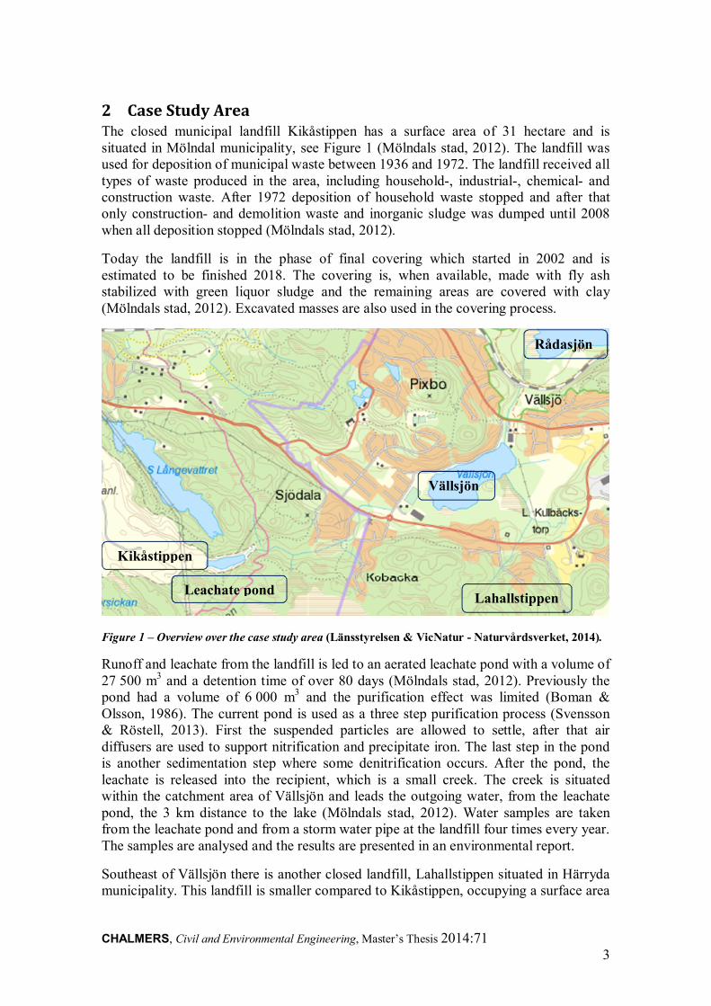
2 Case Study Area The closed municipal landfill Kikåstippen has a surface area of 31 hectare and is situated in Mölndal municipality, see Figure 1 (Mölndals stad, 2012). The landfill was used for deposition of municipal waste between 1936 and 1972. The landfill received all types of waste produced in the area, including household-, industrial-, chemical- and construction waste. After 1972 deposition of household waste stopped and after that only construction- and demolition waste and inorganic sludge was dumped until 2008 when all deposition stopped (Mölndals stad, 2012).
Today the landfill is in the phase of final covering which started in 2002 and is estimated to be finished 2018. The covering is, when available, made with fly ash stabilized with green liquor sludge and the remaining areas are covered with clay (Mölndals stad, 2012). Excavated masses are also used in the covering process.
Figure 1 – Overview over the case study area (Länsstyrelsen & VicNatur - Naturvårdsverket, 2014).
Runoff and leachate from the landfill is led to an aerated leachate pond with a volume of 27 500 m3 and a detention time of over 80 days (Mölndals stad, 2012). Previously the pond had a volume of 6 000 m3 and the purification effect was limited (Boman & Olsson, 1986). The current pond is used as a three step purification process (Svensson & Röstell, 2013). First the suspended particles are allowed to settle, after that air diffusers are used to support nitrification and precipitate iron. The last step in the pond is another sedimentation step where some denitrification occurs. After the pond, the leachate is released into the recipient, which is a small creek. The creek is situated within the catchment area of Vällsjön and leads the outgoing water, from the leachate pond, the 3 km distance to the lake (Mölndals stad, 2012). Water samples are taken from the leachate pond and from a storm water pipe at the landfill four times every year. The samples are analysed and the results are presented in an environmental report.
Southeast of Vällsjön there is another closed landfill, Lahallstippen situated in Härryda municipality. This landfill is smaller compared to Kikåstippen, occupying a surface area
Kikåstippen
Leachate pond Lahallstippen
Vällsjön
Rådasjön
CHALMERS, Civil and Environmental Engineering, Master’s Thesis 2014:71 4
of 3.1 hectare (Eliasson, 2006). Lahallstippen was in use between the years 1953 and 1971. The main waste deposited was household waste, sludge from the wastewater treatment plant, construction- and industry waste. The final covering of the landfill started during 1999 and was finished 2005. The leachate from the landfill is led to an aerated leachate pond with a volume of 500 m3 and an approximately detention time of 16 days (Eliasson, 2006). The primary aim of the pond is to precipitate iron. After the pond, the leachate is led to a wetland before the creek Lahallsbäcken leads it to Vällsjön, an approximate distance of 2.5 km. Previously the leachate from Lahallstippen was released into the creek without treatment (Boman & Olsson, 1986). Experiments with different solutions to trap iron have been made in the past, for example the leachate has been treated with lime as precipitant. A permanent solution for treatment of the leachate was however not in place earlier than 2000, when the current pond was constructed (Hagman, 2014).
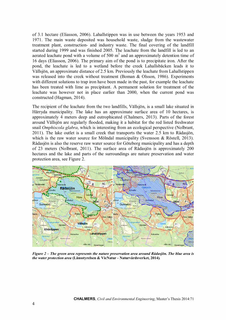
The recipient of the leachate from the two landfills, Vällsjön, is a small lake situated in Härryda municipality. The lake has an approximate surface area of 10 hectares, is approximately 4 meters deep and eutrophicated (Chalmers, 2013). Parts of the forest around Vällsjön are regularly flooded, making it a habitat for the red listed freshwater snail Omphiscola glabra, which is interesting from an ecological perspective (Nolbrant, 2011). The lake outlet is a small creek that transports the water 2.5 km to Rådasjön, which is the raw water source for Mölndal municipality (Svensson & Röstell, 2013). Rådasjön is also the reserve raw water source for Göteborg municipality and has a depth of 23 meters (Nolbrant, 2011). The surface area of Rådasjön is approximately 200 hectares and the lake and parts of the surroundings are nature preservation and water protection area, see Figure 2.
Figure 2 – The green area represents the nature preservation area around Rådasjön. The blue area is the water protection area (Länsstyrelsen & VicNatur - Naturvårdsverket, 2014).
CHALMERS, Civil and Environmental Engineering, Master’s Thesis 2014:71 5
3 Literature Review A literature study on trace metals and sequential extraction procedures is presented below.
3.1 Trace metals Metals are natural constituents of the earth crust that exists in higher or lower concentrations. Metals that occur in higher concentrations are referred to as major metals while metals occurring in very low concentrations are referred to as trace metals. There is no widely accepted, precise definition for trace elements (Kabata-Pendias & Mukherjee, 2007). Geochemists commonly use the definition that trace elements are constituents of the earth crust with concentrations lower than 0.1% (1000 mg/kg) and this definition will also be used in this report.
The metals with the highest concentration of the earth crust are aluminium and iron, which have a concentration of around 8% and 5% respectively (Lerner & Lerner, 2003; Kabata-Pendias & Mukherjee, 2007). Most metals exist in trace concentrations, but can however, due to variations in the mineral composition of the crust, locally exist naturally in higher concentrations as veins or ores (Mohammed et al., 2011). However, they can also be emitted in higher concentrations to the environment due to anthropogenic activities, in both organic and inorganic forms. Waste disposal and landfills are examples of anthropogenic sources of trace metals. Metals released to the environment are often emitted in an insoluble form but could, due to changes in environmental conditions, change to a more soluble form (Reeve, 2002).
Some of the metals are essential for all living organisms in low concentrations, for example: iron, manganese, zinc and copper (Mohammed et al., 2011). Other metals are direct toxic already at low concentrations. For example the trace metals lead and mercury are highly toxic, more likely to bioaccumulate in marine organisms and unlike most of the other trace metals they have no known natural biological function (Reeve, 2002; Baun et al., 2013).
Metals are not biodegradable which makes them persistent contaminants that accumulate in soils. Therefore soil and sediment constitute reservoirs of bioavailable trace metals (Gleyzes et al., 2002). A change in oxidizing or reducing nature of natural water may lead either to solubilisation or deposition of metal ions (Kabata-Pendias & Mukherjee, 2007). Metal ions can interact with sediment through adsorption, ion exchange and complex formation within the sediment (Reeve, 2002). Most of the transition metal ions can exist in different oxidation states. Metals in low concentrations can also co-precipitate with metals in higher concentrations, which means that traces of for example mercury will be deposited when iron sediments.
Changes in pH and oxygen conditions as well as mechanical mixing, for example dredging, can release bound metals from sediment to water (Drever, 1997). For most of the metals the solubility increases with a decreased pH (Reeve, 2002). An increased solubility leads to metals leaching out from sediment to water. The metals in natural water are often present at low concentrations as complexes or attached to colloids, small particles consisting of clay, humus or iron- or manganese hydroxides (Drever, 1997).
CHALMERS, Civil and Environmental Engineering, Master’s Thesis 2014:71 6
The metals analysed in this study are the major elements aluminium, iron and manganese, and the trace elements cadmium, copper, chromium, lead, mercury, nickel and zinc. The reason for analysing iron and manganese is mainly that they have extremely high adsorption capacities and therefore the amount of iron and manganese can indicate how other metals are bound (Drever, 1997).
3.2 Metal speciation The mobility of trace metals in the environment depends strongly on their chemical forms or type of bindings of the element. Determination of the total metal concentration in soil and sediment does not give sufficient information about the mobility (Zemberyová et al., 2006).
Some species of the metals are also more biologically available than others. The bioavailability of trace metals in soil is therefore dependent on the speciation (Zimmerman & Weindorf, 2010). Speciation is defined as “the distribution of an element amongst defined chemical species in a system” (Templeton et al., 2000). This definition includes the definition that a chemical species is a “specific form of an element defined as to isotopic composition, electronic or oxidation state, and/or complex or molecular structure”. A frequently used method for speciation of metals is sequential extraction procedure, which is a method for separation of specific elements from a mixture (Gleyzes et al., 2002; Ohlson, 2014).
3.3 Sequential extraction procedure Single and sequential extraction procedures (SEP) have been designed in order to determine the binding forms of trace metals in soil and sediment to give information on environmental contamination risks (Quevauviller et al., 1994). The use of SEP gives information about the origin, mode of occurrence, biological and physicochemical availability, mobilization and transport of trace metals (Tessier et al., 1979). The SEP that is most commonly used world-wide was proposed by Tessier et al. in 1979 and the second most used SEP was proposed by the Community Bureau of Reference (BCR) in 1992 (Zimmerman & Weindorf, 2010). These two methods will hereafter be referred to as Tessier and BCR.
All SEP facilitate fractionation (Zimmerman & Weindorf, 2010). The concept of the procedure is that the first fraction contains the most mobile metals and the last fraction the least mobile. Tessier’s SEP divides the metals into five fractions, which were named exchangeable, bound to carbonates, bound to iron and manganese oxides, bound to organic matter and residual. Generally metals of anthropogenic sources reside in the first four fractions and metals that occur naturally in the parent rock reside in the last and fifth fraction.
In Tessier’s SEP, and also in other SEP, the exchangeable fraction is commonly extracted by a salt solution. The salt solution changes the ionic composition of the water, thereby allowing metals adsorbed to the exposed surfaces of the sediment to be extracted easily (Zimmerman & Weindorf, 2010). The carbonate bound fraction is sensitive to changes in pH and is therefore solved by an acidic solution. Metals bound to iron and manganese oxides are extracted by a solution that is capable of dissolving insoluble sulphide salts since these metals are sensitive to anoxic conditions. The metals bound in the organic phase are extracted by oxidizing the organic material.
CHALMERS, Civil and Environmental Engineering, Master’s Thesis 2014:71 7
The metals in the residual fraction are integrated in the crystal structures of primary and secondary minerals and are therefore the hardest to remove. A strong acid which can break down silicate structures is needed to remove the last fraction, for example hydrofluoric acid, hydrochloric acid, perchloric acid or sulphuric acid (Gleyzes et al., 2002). The amount of metals in the residual fraction has also been evaluated, by some researchers, as the difference between the total metal concentration and the sum of the metals extracted in each of the other fractions.
The SEP proposed by Tessier was developed for partitioning of the trace metals cadmium, cobalt, copper, nickel, lead, zinc, iron and manganese into the five fractions named above (Tessier et al., 1979). An overview of the procedure is presented in Appendix 2. Several modifications of the original procedure developed by Tessier have been made by different researchers. This has led to that different projects have used different varieties of the SEP.
Due to the lack of uniformity of the different sequential extraction procedures, the results were hard to compare (Quevauviller et al., 1994). Because of this, the measurements and testing programme, former BCR, launched a programme to design a new SEP. The programme started in 1987 with a comparison of the existing SEP after which a new three step procedure was designed. The new SEP was similar to Tessier´s but with two differences. The steps exchangeable and bound to carbonates were combined to one first step called exchangeable and the residual fraction was not part of the procedure. The SEP proposed by BCR is based on a first step with acetic acid extraction, a second step with hydroxyl ammonium chloride extraction and a third step with hydrogen peroxide and ammonium acetate extraction.
Also the BCR SEP has been subject to modifications. In 1997 a small-scale interlaboratory study tested and compared a revised version of the SEP with the original procedure (Rauret et al., 1999). An overview of the improved BCR SEP is presented in Appendix 3.

CHALMERS, Civil and Environmental Engineering, Master’s Thesis 2014:71 8
CHALMERS, Civil and Environmental Engineering, Master’s Thesis 2014:71 9
4 Method The method behind the experiments performed in the case study is presented below, together with standards and equipment used. All equipment and laboratory wares used for sampling and metal analysis were either new or acid washed with 10% nitric acid to prevent metals present on the equipment from leaching out into the samples.
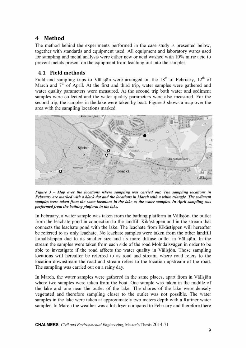
4.1 Field methods Field and sampling trips to Vällsjön were arranged on the 18th of February, 12th of March and 7th of April. At the first and third trip, water samples were gathered and water quality parameters were measured. At the second trip both water and sediment samples were collected and the water quality parameters were also measured. For the second trip, the samples in the lake were taken by boat. Figure 3 shows a map over the area with the sampling locations marked.
Figure 3 – Map over the locations where sampling was carried out. The sampling locations in February are marked with a black dot and the locations in March with a white triangle. The sediment samples were taken from the same locations in the lake as the water samples. In April sampling was performed from the bathing platform in the lake.
In February, a water sample was taken from the bathing platform in Vällsjön, the outlet from the leachate pond in connection to the landfill Kikåstippen and in the stream that connects the leachate pond with the lake. The leachate from Kikåstippen will hereafter be referred to as only leachate. No leachate samples were taken from the other landfill Lahallstippen due to its smaller size and its more diffuse outlet in Vällsjön. In the stream the samples were taken from each side of the road Mölndalsvägen in order to be able to investigate if the road affects the water quality in Vällsjön. Those sampling locations will hereafter be referred to as road and stream, where road refers to the location downstream the road and stream refers to the location upstream of the road. The sampling was carried out on a rainy day.
In March, the water samples were gathered in the same places, apart from in Vällsjön where two samples were taken from the boat. One sample was taken in the middle of the lake and one near the outlet of the lake. The shores of the lake were densely vegetated and therefore sampling closer to the outlet was not possible. The water samples in the lake were taken at approximately two meters depth with a Ruttner water sampler. In March the weather was a lot dryer compared to February and therefore there
CHALMERS, Civil and Environmental Engineering, Master’s Thesis 2014:71 10
was no flow from the outlet of the leachate pond. The water sample was therefore collected in the stream around 20 m downstream of the outlet, containing also the discharge from a stormwater pipe. In April, water was only collected from the bathing platform.
All water samples were collected, treated and stored in accordance with the guidance on the preservation and handling of samples in the standard ISO 5667-3:1995. All samples analysed for metals in this study were treated in according to the standard, except for mercury. All water samples were collected in new 1 litre bottles made of polyethene. The bottles were, after filled, brought to the lab and stored dark and cold at 5°C before the analyses were carried out. The water samples taken for the biochemical oxygen demand (BOD) were collected in small Wheaton glass bottles.
The water quality measurements made in field were carried out with a WTW Multiline P4, equipped with three different electrodes for measuring conductivity, temperature, pH and oxygen concentration. The multiliner was also brought in the boat and the parameters were measured in situ. The parameters were also measured directly in the stream. However, for the measurement of the leachate in February, the water quality parameters were measured in a 1 litre bottle.
Three sediment cores were gathered with a gravity core sampler, for the technique used see Appendix 1. Two cores were taken in the middle of the lake and one near the outlet. The sediment cores were collected in acrylic glass tubes which were assembled on the sampler. Each sediment core was brought to the beach where it was frozen in situ with carbon-dioxide ice to avoid mixing of the sediment during transportation. At the laboratory the frozen sediment cores were stored in a freezer.
For the analysis of the metals at different depths, the core from the outlet and one of the cores from the middle were sliced in unthawed condition with a metal saw. The saw had been equipped with a new blade cleaned with alcohol. A core of frozen MilliQ was also sliced with the same metal saw and analysed for metals, to estimate the level of metal contamination that originated from the saw. The core from the middle was cut in slices of approximately 2 cm each and the core from the outlet was cut in 4 cm thick slices.
Sediment was also collected with a grab sampler, of type Ekmanhuggare, to get surface sediment for the beaker tests. The sediment was collected from the sampler with a plastic beaker and put into two clean plastic bags aimed for sampling. The bags with the sediment were stored in a freezer until used.
4.2 Lab analysis In addition to the measurements made in field, some general water quality parameters were also measured at the laboratory to get an overview of the properties of the water. The methods and equipment used are presented in Table 1 and described below. Some of the water samples were diluted before chemical analysis due to high turbidity and high content of particles.
CHALMERS, Civil and Environmental Engineering, Master’s Thesis 2014:71 11
Table 1 – Water quality parameters measured in the water samples.
Parameter Method
Temperature WTW Multiline P4 Conductivity WTW Multiline P4 Turbidity HACH 8237 Alkalinity EN ISO 9963-2:1995 Oxygen WTW Multiline P4 Colour HACH 8025 DOC Total Organic Carbon Analyser (TOC-VCPH) TOC Total Organic Carbon Analyser (TOC-VCPH) Ions Ion chromatography TN Total Nitrogen Measuring Unit (TNM-1) pH WTW Multiline P4
The colour and turbidity of the water samples were measured with HACH spectrophotometry, using the method 8025 and 8237 respectively. Alkalinity was measured with the standard method EN ISO 9963-2:1995. Total organic carbon (TOC) and dissolved organic carbon (DOC) were analysed with a Total Organic Carbon Analyser, using the Swedish standard EN 1484:1997 for all water samples. Total nitrogen (TN) was analysed with Total Nitrogen Measuring Unit with the Swedish standard EN 12260 for all water samples. The samples analysed for DOC were filtered through a 0.45 µm polyethersulfone filter. BOD was measured following the standard EN 1899-2:1998.
Ion chromatography (IC) was used to analyse anions in the water samples. Especially chloride was analysed since high chloride concentrations have been observed at Kikåstippen (Mölndals stad, 2012). The samples were diluted with MilliQ and filtered through a 0.45 μm polyethersulfone filter before analysis. The Swedish standard EN ISO 10304-2:1996 was used.
The total concentration of metals in both the water and sediment samples were analysed with an inductively coupled plasma-mass spectrometry (ICP-MS). The instrument used was of the type Thermo Scientific iCAP Q ICP-MS and had been tuned and optimized according to manufacturer specifications. The analysis was performed on samples that had not been filtered, in order to investigate the total metal concentration, including possible particles with high metal content. Rhodium (10 ppb) was used as internal standard in the ICP-MS analysis to verify the results, and Merck Multi-Element standard (0.1-2000 μg L-1) was used for calibration of the instrument. After the water samples were collected in field they were stored in a freezer. Shortly before the analysis, the samples were thawed and acidified with one percentage by volume of an acidic solution consisting of 25% HCl and 75% HNO3 of suprapur quality. The water samples analysed from the beaker test were acidified with the exact same procedure as the other water samples.
For the total metal analyses of the sediment, samples taken from each slice in the core, both from the middle and from the outlet of the lake, were analysed. The sediment samples were thawed and dried in an oven, of type Memmert U15, at 105°C for 24 h.
CHALMERS, Civil and Environmental Engineering, Master’s Thesis 2014:71 12
The dried sediment samples were roughly pestled and stored in a desiccator before the total metal analysis was carried out. From the middle core, two replicates from two of the slices and four replicates from one slice were analysed to validate the method. A wet sample with two replicates from the grab sampler was also analysed together with one dried sample from the grab sampler, in order to evaluate the effect drying has on the metal content.
To extract the metals from the sediment, 10 or 20 ml of the acidic solution described above was used. Half a gram of each dry sediment sample was added to a microwave vessel, which had been machine washed and cleaned with MilliQ. After approximately 2 h, during which the samples were allowed to react with the acidic solution, the samples were boiled in a microwave oven for 25 min.
The microwave oven used was a MARS 5 where the pressure was controlled, however, the temperature meter was unfortunately out of order. The boiling consisted of three parts, the first one at 160 PSI for 10 min, the second at 160 PSI for 5 min and the last at 180 PSI for 10 min. After cooling, the acidic solution and the remaining sediment was transferred to new tubes of polypropylene and weighed to determine the amount in each tube. After this, new 10 ml tubes made of polypropylene were filled with 9.9 ml of MilliQ and 0.1 ml of sample. The tubes were stored in a refrigerator at 5°C before the concentrations of the metals were analysed for each fraction with the ICP-MS.
4.3 Modified sequential extraction procedure In this master thesis a modified sequential extraction procedure (MSEP) was developed, based on the procedure proposed by Tessier et al. (1979) and the procedure proposed by BCR (Rauret, 1998). The MSEP was performed with two replicates from a sediment sample. The same method was also applied to a vessel without sediment as reagent blank and a sediment sample from Järnbrott, a contaminated stormwater pond, for comparison. All reagents used in the extraction were of pro analysi (PA) grade.
Some of the reagents used in the procedures by Tessier and BCR are highly toxic and were therefore exchanged for less toxic alternatives, in accordance with Chalmers rules (Forshufvud, 2013). All the selected reagents in the MSEP have been used in other documented SEP. The hydroxyl ammonium chloride was exchanged for non-toxic ascorbic acid, which has the same metal extraction efficiency according to Shuman (1982). A concentration of 0.2 M ascorbic acid was used based on a previous procedure carried out by Karlfeldt Fedje et al. (2013). The volume of the ascorbic acid was set to 40 ml, the same volume as the hydroxyl ammonium chloride. In the last step of the procedure, the residual, 10 ml of an acidic solution consisting of 25% HCl and 75% HNO3 of suprapur quality was used instead of the highly toxic hydrofluoric acid, HF.
In the MSEP the samples were extracted into totally six fractions, the five fractions described in the procedure by Tessier et al. (1979) and an extra pre-fraction of water soluble metals. The fraction of water soluble metals has previously been used by Karlfeldt Fedje et al. (2013). Each step in the MSEP is presented in Table 2 and an overview of the procedure is described in Appendix 4.
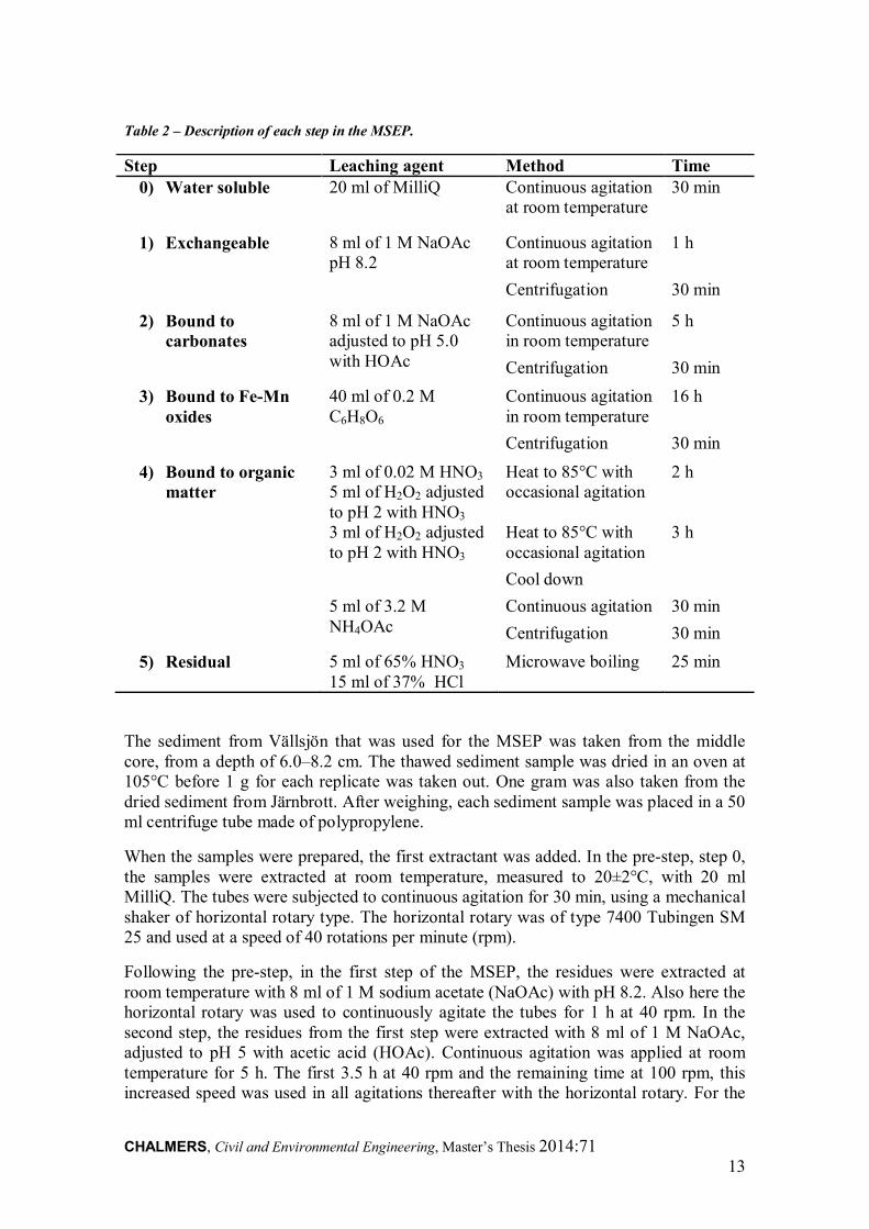
CHALMERS, Civil and Environmental Engineering, Master’s Thesis 2014:71 13
Table 2 – Description of each step in the MSEP.
Step Leaching agent Method Time 0) Water soluble 20 ml of MilliQ Continuous agitation
at room temperature .
30 min
1) Exchangeable 8 ml of 1 M NaOAc pH 8.2
Continuous agitation at room temperature
.
1 h
Centrifugation 30 min
2) Bound to carbonates
8 ml of 1 M NaOAc adjusted to pH 5.0 with HOAc
Continuous agitation in room temperature
.
5 h
Centrifugation 30 min
3) Bound to Fe-Mn oxides
40 ml of 0.2 M C6H8O6
Continuous agitation in room temperature
.
16 h
Centrifugation 30 min
4) Bound to organic matter
3 ml of 0.02 M HNO3 5 ml of H2O2 adjusted to pH 2 with HNO3
Heat to 85°C with occasional agitation
2 h
3 ml of H2O2 adjusted to pH 2 with HNO3
Heat to 85°C with occasional agitation
.
3 h
Cool down .
5 ml of 3.2 M NH4OAc
Continuous agitation .
30 min
Centrifugation 30 min
5) Residual 5 ml of 65% HNO3 15 ml of 37% HCl
Microwave boiling 25 min
The sediment from Vällsjön that was used for the MSEP was taken from the middle core, from a depth of 6.0–8.2 cm. The thawed sediment sample was dried in an oven at 105°C before 1 g for each replicate was taken out. One gram was also taken from the dried sediment from Järnbrott. After weighing, each sediment sample was placed in a 50 ml centrifuge tube made of polypropylene.
When the samples were prepared, the first extractant was added. In the pre-step, step 0, the samples were extracted at room temperature, measured to 20±2°C, with 20 ml MilliQ. The tubes were subjected to continuous agitation for 30 min, using a mechanical shaker of horizontal rotary type. The horizontal rotary was of type 7400 Tubingen SM 25 and used at a speed of 40 rotations per minute (rpm).
Following the pre-step, in the first step of the MSEP, the residues were extracted at room temperature with 8 ml of 1 M sodium acetate (NaOAc) with pH 8.2. Also here the horizontal rotary was used to continuously agitate the tubes for 1 h at 40 rpm. In the second step, the residues from the first step were extracted with 8 ml of 1 M NaOAc, adjusted to pH 5 with acetic acid (HOAc). Continuous agitation was applied at room temperature for 5 h. The first 3.5 h at 40 rpm and the remaining time at 100 rpm, this increased speed was used in all agitations thereafter with the horizontal rotary. For the
CHALMERS, Civil and Environmental Engineering, Master’s Thesis 2014:71 14
third step, the samples were extracted with 40 ml of 0.2 M ascorbic acid (C6H8O6) at room temperature with continuous agitation for 16 h.
In the fourth step the samples were extracted with 3 ml of 0.02 M HNO3 and 5 ml of 30% H2O2 which was adjusted to pH 2 with HNO3. The tubes were heated in a water bath of type Julabo SW-20C to 85°C for 2 h with occasional agitation in 15 min intervals. After this, an additional 3 ml of 30% H2O2, adjusted to pH 2 with HNO3, was added and the tubes were reheated to 85°C for another 3 h with occasional agitation in 15 min intervals. After cooling, 5 ml of 3.2 M ammonium acetate (NH4OAc) in 20% (v/v) HNO3 was added and the samples were diluted to 20 ml with MilliQ and agitated continuously for 30 min in the horizontal rotary.
After each of the first four steps and the pre-step in the MSEP, the extract was separated from the solid residue by centrifugation in a centrifuge of type Sigma 4-16 at 3000 G for 30 min. Ten millilitre of each supernatant, except for step 1 and 2 which only contained 8 ml, was acidified with one percentage by volume of the acidic solution described above, and stored in a refrigerator at 5°C before the trace metal analyse. For step 1 to 4, the residues were rinsed of the previous extractant with 10 ml of MilliQ. The rinsing step included agitation for 15 min on the horizontal rotary with a speed of 100 rpm and then centrifugation at 3000 G for 30 min. The volume was chosen to 10 ml because the rinse water should be kept to a minimum to avoid excessive solubilisation of solid material, particularly organic matter (Tessier et al., 1979). MilliQ was used and not simple de-ionised water since it may contain organically complexed metal ions (Rauret et al., 1999).
For the last step of the MSEP, the samples were moved to microwave vessels, which had been machine washed and then cleaned with MilliQ. Twenty millilitre of an acidic solution, consisting of a mix of 25% HCl and 75% HNO3, was added to the samples. The microwave boiling and treatment of the extract was then performed in the same way as the total metal analysis, which is described in chapter 4.2 Lab analysis.
4.4 Beaker tests The procedure and materials used for the beaker tests are described below. The beaker tests were performed in 1 litre borosilicate glass beakers. Thawed sediment from one of the cores taken in the middle and from grab sampling was used in the test. The water used was collected from Vällsjön one day before the start of the first test and stored in refrigerator until used.
The beaker tests were performed as five lines with four beakers in each, see Figure 4. Each of the lines consisted of three beakers where a condition was changed and one blank. The first four lines had the same changes applied to verify the results from the tests. The conditions in the beakers were changed according to Figure 4. In the first beaker continuous mixing was applied with a mixer of type Flocculator 2000 set on fast speed. The part of the mixer that was in contact with the water was made of plastic, which had been acid washed. The pH in the second beaker was lowered with sulphuric acid to 6 at the start of the test. In the third beaker the oxygen content was decreased by addition of nitrogen gas. In the fourth beaker only sediment and water were added as a blank for comparison.
CHALMERS, Civil and Environmental Engineering, Master’s Thesis 2014:71 15
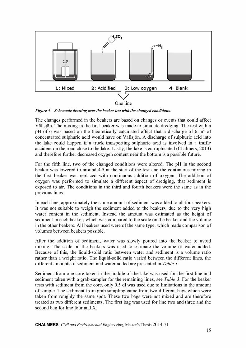
Figure 4 – Schematic drawing over the beaker test with the changed conditions.
The changes performed in the beakers are based on changes or events that could affect Vällsjön. The mixing in the first beaker was made to simulate dredging. The test with a pH of 6 was based on the theoretically calculated effect that a discharge of 6 m3 of concentrated sulphuric acid would have on Vällsjön. A discharge of sulphuric acid into the lake could happen if a truck transporting sulphuric acid is involved in a traffic accident on the road close to the lake. Lastly, the lake is eutrophicated (Chalmers, 2013) and therefore further decreased oxygen content near the bottom is a possible future.
For the fifth line, two of the changed conditions were altered. The pH in the second beaker was lowered to around 4.5 at the start of the test and the continuous mixing in the first beaker was replaced with continuous addition of oxygen. The addition of oxygen was performed to simulate a different aspect of dredging, that sediment is exposed to air. The conditions in the third and fourth beakers were the same as in the previous lines.
In each line, approximately the same amount of sediment was added to all four beakers. It was not suitable to weigh the sediment added to the beakers, due to the very high water content in the sediment. Instead the amount was estimated as the height of sediment in each beaker, which was compared to the scale on the beaker and the volume in the other beakers. All beakers used were of the same type, which made comparison of volumes between beakers possible.
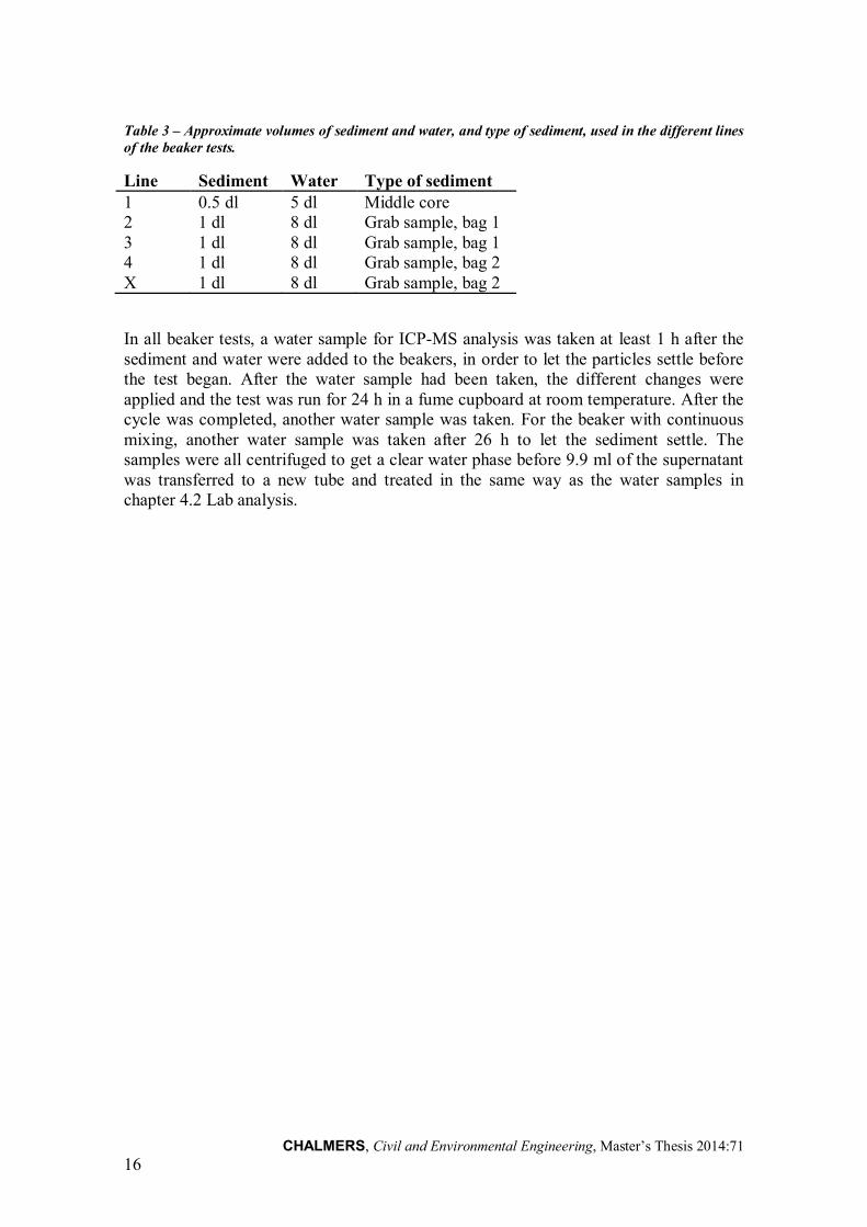
After the addition of sediment, water was slowly poured into the beaker to avoid mixing. The scale on the beakers was used to estimate the volume of water added. Because of this, the liquid-solid ratio between water and sediment is a volume ratio rather than a weight ratio. The liquid-solid ratio varied between the different lines, the different amounts of sediment and water added are presented in Table 3.
Sediment from one core taken in the middle of the lake was used for the first line and sediment taken with a grab-sampler for the remaining lines, see Table 3. For the beaker tests with sediment from the core, only 0.5 dl was used due to limitations in the amount of sample. The sediment from grab sampling came from two different bags which were taken from roughly the same spot. These two bags were not mixed and are therefore treated as two different sediments. The first bag was used for line two and three and the second bag for line four and X.
One line
CHALMERS, Civil and Environmental Engineering, Master’s Thesis 2014:71 16
Table 3 – Approximate volumes of sediment and water, and type of sediment, used in the different lines of the beaker tests.
Line Sediment Water Type of sediment 1 0.5 dl 5 dl Middle core 2 1 dl 8 dl Grab sample, bag 1 3 1 dl 8 dl Grab sample, bag 1 4 1 dl 8 dl Grab sample, bag 2 X 1 dl 8 dl Grab sample, bag 2
In all beaker tests, a water sample for ICP-MS analysis was taken at least 1 h after the sediment and water were added to the beakers, in order to let the particles settle before the test began. After the water sample had been taken, the different changes were applied and the test was run for 24 h in a fume cupboard at room temperature. After the cycle was completed, another water sample was taken. For the beaker with continuous mixing, another water sample was taken after 26 h to let the sediment settle. The samples were all centrifuged to get a clear water phase before 9.9 ml of the supernatant was transferred to a new tube and treated in the same way as the water samples in chapter 4.2 Lab analysis.
CHALMERS, Civil and Environmental Engineering, Master’s Thesis 2014:71 17
5 Result and Discussion The result from measurement of general water quality parameters and water content of the sediment are presented as tables in Appendix 5. Only selected results of the water quality parameters are discussed further in this chapter. The results from the metal analysis performed with the ICP-MS for all sediment and water samples are presented and discussed below. The results from the modified sequential extraction procedure (MSEP) and the beaker tests are also presented and discussed below. Tables with the results from the ICP-MS analysis can be found in Appendices 6–9.
5.1 Water quality parameters Generally it can be observed that many of the measured water quality parameters are high or very high in the landfill leachate, and that the values decrease through transportation and dilution in the stream before reaching Vällsjön, see Appendix 5. For example, the conductivity is very high in the landfill leachate compared to the lake, where it is approximately seven times lower. At the measuring location in the stream, the conductivity has decreased to half compared to the conductivity of the leachate.
The chloride concentration has increased steadily in the leachate from Kikåstippen since the last part of the 1990s (Mölndals stad, 2012). Mölndals stad assumes that the high concentrations of chloride can originate from road salt and the decreased dilution of the leachate, due to the final covering of the landfill. Also the groundwater in the catchment has a high chloride concentration. The high concentration in the groundwater is probably caused by intrusion of salt from a nearby road. Another source of chloride could be the clay used in the sealing process of the landfill, since it can originate from coastal areas. Also excavated masses, used as filling material in the final covering of the landfill, can contain high amounts of chloride. Previously salt has also been used on the roads at the landfill to bind dust. Also the fly ash could contain high concentration of chloride, therefore the composition of the fly ash needs to be further investigated. Another source of the high chloride concentration may be the household waste deposited on the landfill.
The chloride concentration measured in the leachate in this study is 120 mg/l, see Appendix 5. Even though the chloride concentration is high in the leachate, the concentrations measured in the lake water in Vällsjön, 56 mg/l, were low compared to the guidelines for Swedish drinking water. The guideline for chloride concentration in drinking water that is approved with a remark is 100 mg/l (Svenskt Vatten, n.d.). However, the water samples from the stream on both sides of the road contain much higher chloride concentrations, over 100 mg/l. This may be due to emissions from the road due to salting in the winter period, but it could also originate from chloride leaching from the landfill. The concentration in water from the bag containing the grab sample sediment was also measured and was above the guidelines, see sediment in Appendix 5. The origin of the high chloride concentrations needs to be further investigated.
No comparison has been made of the water quality parameters measured in the stream on each side of the road. Some differences can be seen, see Appendix 5, but since only spot measurements have been performed, it is hard to draw clear conclusions from the results. If replicates had been taken on several spots within the area of the road, maybe the results of the analysis would have been more representative and reliable.
CHALMERS, Civil and Environmental Engineering, Master’s Thesis 2014:71 18
Parts of the beaker tests were based on the measurements of water quality parameters in the lake. Vällsjön is eutrophicated with a high growth of biomass, however the measured BOD was lower than expected, see Appendix 5. This could be caused by that the measurement was made on shallow water in February. The oxygen concentration was high in the lake both in February and March. Since eutrophication is often associated with oxygen deficiency, one of the changes that were applied was low oxygen content through addition of nitrogen gas to the water.
The lake water in Vällsjön has a relatively high pH and a very high buffering capacity according to the alkalinity (SEPA, 2000), see Appendix 5. The result from the alkalinity test was mainly used for the design of the beaker test with changed pH. The high buffering capacity could be observed during the beaker test, the decreased pH at the start of the test increased to almost the original pH.
According to Mölndals stad (2012), one reason for the relatively high pH in the lake is likely stormwater discharge into the top of the stream. The stormwater had a pH of around 8, which is mainly due to that the water has been drained through concrete culverts. Concrete normally have a pH above 11. The pH in the leachate is around 7.8. Normal pH of leachate from stabilized landfills, often with an age of more than 5 years, is over 7.5 (Kurniawan et al., 2006). Another reason for the high pH could be the green liquor sludge and fly ashes used for the final covering of the landfill Kikåstippen. This hypothesis has to be investigated further.
However, the pH of the stream was higher than the pH of the landfill leachate, see measurements from February in Appendix 5. The water measured as leachate in March was taken from the stream since there was no flow from the pipe where the leachate is discharged. The measured concentrations and other parameters do therefore not really represent the leachate, but rather stormwater from the catchment area of the stream. It is however likely that the stream is affected by the landfill also here.
The alkalinity in the leachate from both February and March is very high. The alkalinity is lower in the stream. One reason for this could be that the surrounding areas consist at least partially of podsol soil, since there is a lot of coniferous wood in the area. Without the very high alkalinity the pH of the stream might have been considerably lower.
5.2 Total analysis of digestible metals The metal concentrations for ten selected metals, three major and seven trace metals, are presented for the cores taken in the middle and at the outlet of Vällsjön. The total metal analysis performed on the sediment with the acidic solution used does not result in a complete digestion of the metals. To achieve a complete digestion a stronger acid would be needed, for example hydrofluoric acid (Gleyzes et al., 2002). Because of this, the metal concentrations found in this study are likely lower than the total amount present in the sediment. However, the metals that were not digested are probably strongly bound to the sediment and therefore not likely to leach out into the water.
CHALMERS, Civil and Environmental Engineering, Master’s Thesis 2014:71 19
Quality assessment of the analytical procedure 5.2.1
The total metal concentrations has also been analysed in the sediment taken with the grab sampler. From the grab sampler one dry and two wet replicates of a sample were analysed. No clear differences in the metal concentrations can be noticed, except for the concentration of mercury, which has a higher concentration in the wet sample, see Appendix 6. The concentration of mercury in the dry sample is only 2/3 of the concentration in the wet sample. This is most likely due to that mercury compounds have evaporated during the drying in the oven at 105°C.
Also there was a loss of acidic solution due to gases created by the reactions with the sediment. It has been assumed that no metals evaporated. This assumption can have contributed to an underestimation of the metal concentrations in the sediment. For example the concentration of mercury, as previously mentioned, decreased due to the drying of the sediment. It is therefore not unlikely that the evaporation of acidic solution led to a loss of mercury and other metals.
The microwave digestion has also resulted in uncertainties in losses of material and solvent, caused by the need to transfer the samples from the microwave vessels to new tubes made of polypropylene. The weights of the samples were measured and a loss of 5% of sediment was estimated when calculating the metal concentrations as µg/g dry substance. The individual loss in each sample could have been determined through weighing the microwave vessels as well. This would have led to a lower uncertainty of the results.
The metal concentration measured by the ICP-MS is the concentration in the acidic solution. Therefore the concentration in the sediment has been based on the volume of acidic solution in each tube. The volume has been calculated based on the weight of the acidic solution for each sample and the density of the added acidic solution. The density of the acidic solution remaining after the microwave digestion is however unknown.
Some of the solution evaporated. There was a sharp smell of chlorine during one of the microwave digestions. However, the colour of the gas that was emitted when opening the microwave vessels had an orange colour, which could indicate the presence of nitrous gases. The remaining proportions of hydrochloric acid and nitric acid are therefore uncertain. Even though the used density for the remaining acidic solution might deviate from the actual density, it should not have affected the trends observed since the same density was used for all samples.
Another source that may have contributed to the uncertainties is the handling of the samples in the lab. The samples were sliced with a metal saw. The possible metal contamination caused by the saw was estimated by sawing in frozen MilliQ, which resulted in low metal concentrations. The exact amount of MilliQ was however not measured, so the real contribution is uncertain. However, the total contribution of the saw is considered to be small.
Also the sampling technique has contributed to an uncertainty in the metal concentrations at different depths. The fast freezing of the cores led to that the outer part of the core froze first, resulting in that the middle of the core rose up. This means that some displacement can have occurred. How large part of the core that is affected was uncertain, but this might have affected the trends.
CHALMERS, Civil and Environmental Engineering, Master’s Thesis 2014:71 20
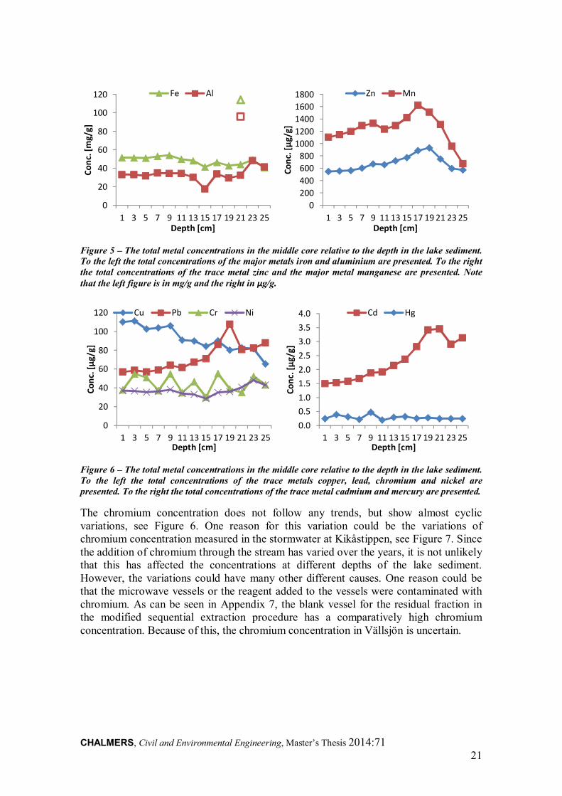
Middle core 5.2.2
Generally it is observed that some of the trace metal concentrations in the middle core are increasing with depth and have a clear maximum peak at approximate 19 cm depth. For manganese and zinc, the peak can be easily observed in Figure 5. Also cadmium and lead show peak values around 19 cm depth, see Figure 6. The major metals iron and aluminium are present in high concentrations at all levels of the core and therefore no clear peak can be observed, see Figure 5. This could indicate that zinc, cadmium and lead have co-precipitated with manganese.
To correlate the peak in metal concentrations with historical events in the catchment area, the sediment accumulation speed has to be known. The speed is normally low, often less than 1 mm per year (Bydén et al., 2003). In lakes that have a high growth of biomass, the sedimentation speed can however be up to one cm per year (Johansson, 2001). Since Vällsjön is a eutrophicated lake, with a high growth of biomass, it is not unreasonable to estimate an accumulation speed of a few mm per year.
One possible hypothesis is that the peak concentrations are correlated to the last years of landfilling at Kikåstippen. The deposition of household waste stopped at Kikåstippen in year 1972. If the peak concentrations correspond to the last years of landfilling household waste, it would result in an estimated sedimentation speed of approximately 4.5–5.0 mm per year in Vällsjön.
However, the leachate of metals into the water did not necessarily decrease immediately after the deposition stopped, since the transport of water within the landfill depends on the hydrogeological characteristics of the landfill. However, the highest concentrations in the leachate are found during the acidic phase of a landfill, which only lasts for a limited period of time (Kurniawan et al., 2006). Therefore the leaching of metals from the landfill into the water should have decreased shortly after the landfill was closed.
In contrast to the trend of increasing concentrations that some of the metals show, copper declines with depth in the sediment, see Figure 6. This could be an indication that the copper in the sediment does not majorly originate from the landfill. Copper is one of the metals that can originate from traffic (Hjortenkrans et al., 2007). Therefore, the increasing concentrations in the shallow layers of the sediment could be caused by an increase in the traffic on the roads in the vicinity. Another reason for the increase in copper concentration could be that the materials used in the covering of Kikåstippen leach copper. However, no clear increase has been seen in the leachate. The analysis performed by Mölndals stad at Kikåstippen is made on filtered samples (Mölndals stad, 2012). Therefore, if the landfill is the source for copper, the metal is most likely bound to particles. Because of this, it is recommended to perform metal analysis on unfiltered samples as well, to evaluate this possibility.
CHALMERS, Civil and Environmental Engineering, Master’s Thesis 2014:71 21
Figure 5 – The total metal concentrations in the middle core relative to the depth in the lake sediment. To the left the total concentrations of the major metals iron and aluminium are presented. To the right the total concentrations of the trace metal zinc and the major metal manganese are presented. Note that the left figure is in mg/g and the right in µg/g.
Figure 6 – The total metal concentrations in the middle core relative to the depth in the lake sediment. To the left the total concentrations of the trace metals copper, lead, chromium and nickel are presented. To the right the total concentrations of the trace metal cadmium and mercury are presented.
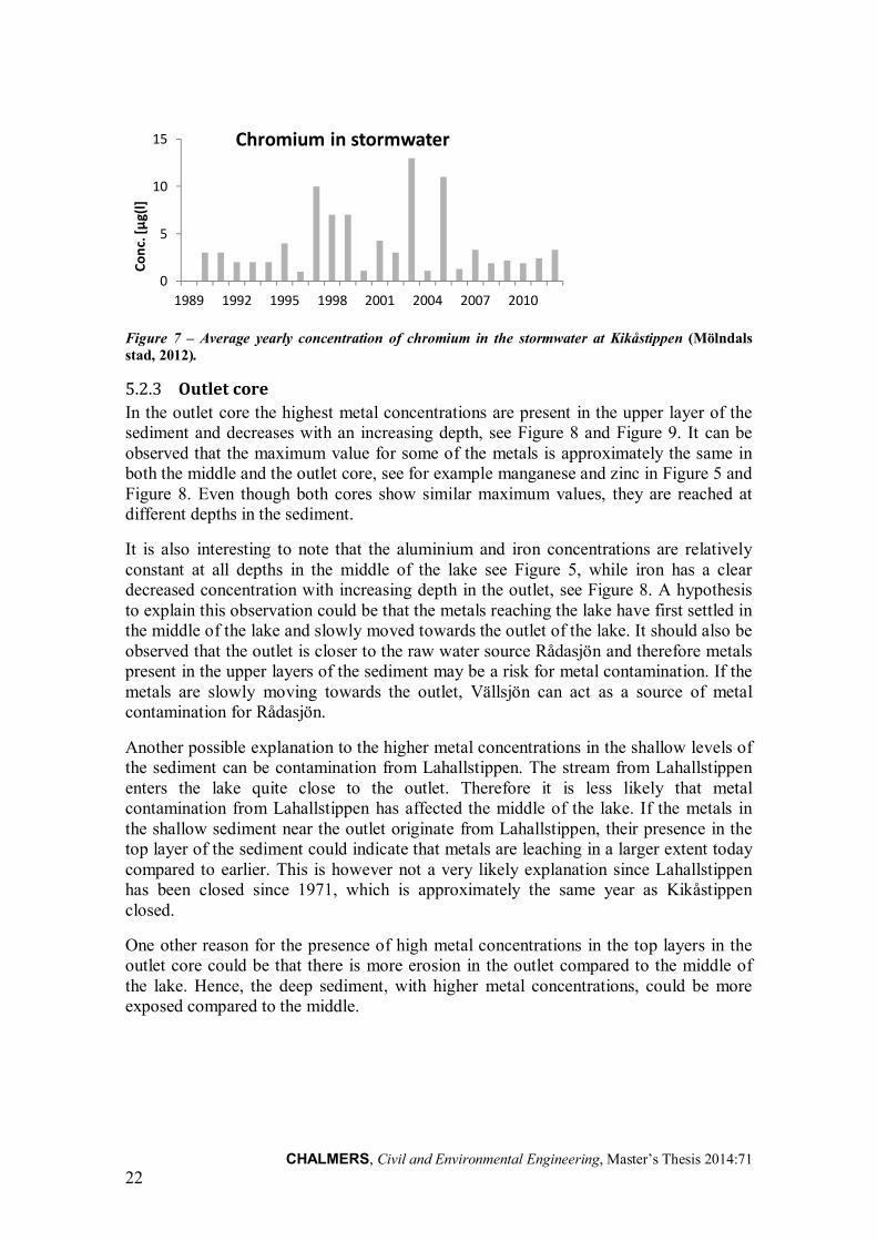
The chromium concentration does not follow any trends, but show almost cyclic variations, see Figure 6. One reason for this variation could be the variations of chromium concentration measured in the stormwater at Kikåstippen, see Figure 7. Since the addition of chromium through the stream has varied over the years, it is not unlikely that this has affected the concentrations at different depths of the lake sediment. However, the variations could have many other different causes. One reason could be that the microwave vessels or the reagent added to the vessels were contaminated with chromium. As can be seen in Appendix 7, the blank vessel for the residual fraction in the modified sequential extraction procedure has a comparatively high chromium concentration. Because of this, the chromium concentration in Vällsjön is uncertain.
0
20
40
60
80
100
120
1 3 5 7 9 11 13 15 17 19 21 23 25
Co
nc.
[m
g/g]
Depth [cm]
Fe Al
0
200
400
600
800
1000
1200
1400
1600
1800
1 3 5 7 9 11 13 15 17 19 21 23 25
Co
nc.
[µ
g/g]
Depth [cm]
Zn Mn
0
20
40
60
80
100
120
1 3 5 7 9 11 13 15 17 19 21 23 25
Co
nc.
[µ
g/g]
Depth [cm]
Cu Pb Cr Ni
0.0
0.5
1.0
1.5
2.0
2.5
3.0
3.5
4.0
1 3 5 7 9 11 13 15 17 19 21 23 25
Co
nc.
[µ
g/g]
Depth [cm]
Cd Hg
CHALMERS, Civil and Environmental Engineering, Master’s Thesis 2014:71 22
Figure 7 – Average yearly concentration of chromium in the stormwater at Kikåstippen (Mölndals stad, 2012).
Outlet core 5.2.3
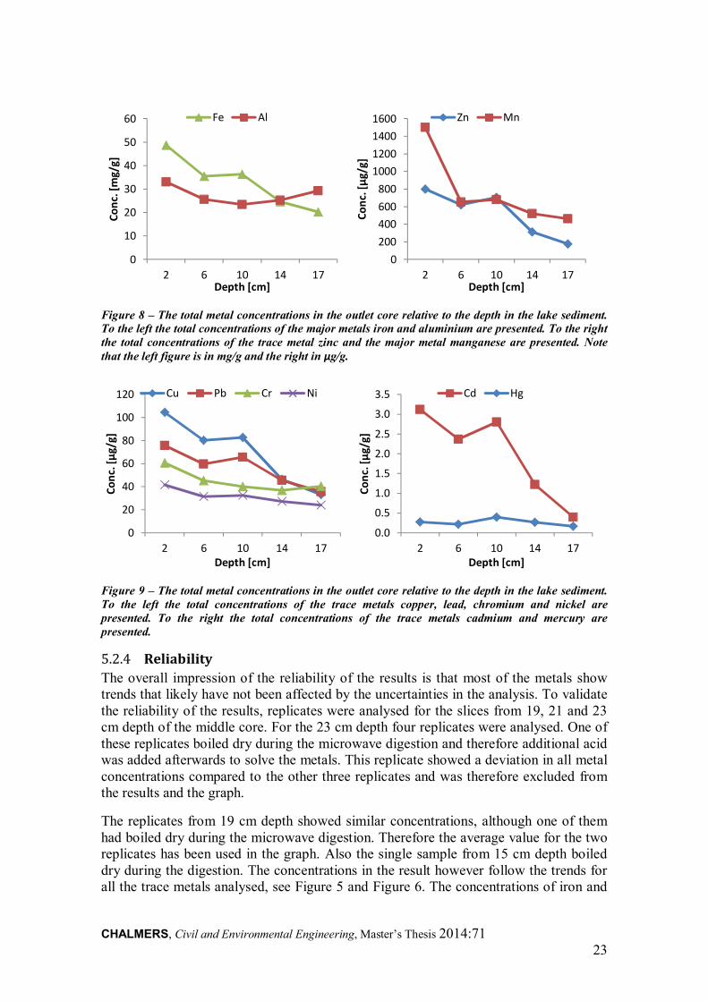
In the outlet core the highest metal concentrations are present in the upper layer of the sediment and decreases with an increasing depth, see Figure 8 and Figure 9. It can be observed that the maximum value for some of the metals is approximately the same in both the middle and the outlet core, see for example manganese and zinc in Figure 5 and Figure 8. Even though both cores show similar maximum values, they are reached at different depths in the sediment.
It is also interesting to note that the aluminium and iron concentrations are relatively constant at all depths in the middle of the lake see Figure 5, while iron has a clear decreased concentration with increasing depth in the outlet, see Figure 8. A hypothesis to explain this observation could be that the metals reaching the lake have first settled in the middle of the lake and slowly moved towards the outlet of the lake. It should also be observed that the outlet is closer to the raw water source Rådasjön and therefore metals present in the upper layers of the sediment may be a risk for metal contamination. If the metals are slowly moving towards the outlet, Vällsjön can act as a source of metal contamination for Rådasjön.
Another possible explanation to the higher metal concentrations in the shallow levels of the sediment can be contamination from Lahallstippen. The stream from Lahallstippen enters the lake quite close to the outlet. Therefore it is less likely that metal contamination from Lahallstippen has affected the middle of the lake. If the metals in the shallow sediment near the outlet originate from Lahallstippen, their presence in the top layer of the sediment could indicate that metals are leaching in a larger extent today compared to earlier. This is however not a very likely explanation since Lahallstippen has been closed since 1971, which is approximately the same year as Kikåstippen closed.
One other reason for the presence of high metal concentrations in the top layers in the outlet core could be that there is more erosion in the outlet compared to the middle of the lake. Hence, the deep sediment, with higher metal concentrations, could be more exposed compared to the middle.
0
5
10
15
1989 1992 1995 1998 2001 2004 2007 2010
Co
nc.
[µ
g(l]
Chromium in stormwater
CHALMERS, Civil and Environmental Engineering, Master’s Thesis 2014:71 23
Figure 8 – The total metal concentrations in the outlet core relative to the depth in the lake sediment. To the left the total concentrations of the major metals iron and aluminium are presented. To the right the total concentrations of the trace metal zinc and the major metal manganese are presented. Note that the left figure is in mg/g and the right in µg/g.
Figure 9 – The total metal concentrations in the outlet core relative to the depth in the lake sediment. To the left the total concentrations of the trace metals copper, lead, chromium and nickel are presented. To the right the total concentrations of the trace metals cadmium and mercury are presented.
Reliability 5.2.4
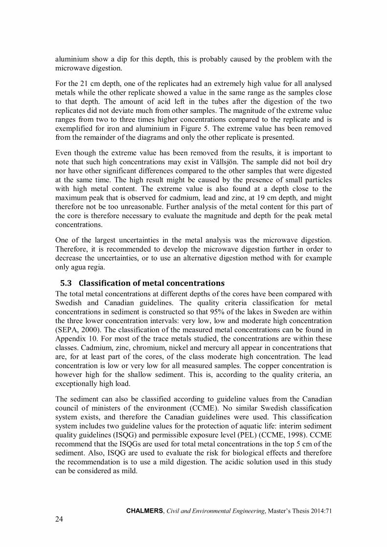
The overall impression of the reliability of the results is that most of the metals show trends that likely have not been affected by the uncertainties in the analysis. To validate the reliability of the results, replicates were analysed for the slices from 19, 21 and 23 cm depth of the middle core. For the 23 cm depth four replicates were analysed. One of these replicates boiled dry during the microwave digestion and therefore additional acid was added afterwards to solve the metals. This replicate showed a deviation in all metal concentrations compared to the other three replicates and was therefore excluded from the results and the graph.
The replicates from 19 cm depth showed similar concentrations, although one of them had boiled dry during the microwave digestion. Therefore the average value for the two replicates has been used in the graph. Also the single sample from 15 cm depth boiled dry during the digestion. The concentrations in the result however follow the trends for all the trace metals analysed, see Figure 5 and Figure 6. The concentrations of iron and
0
10
20
30
40
50
60
2 6 10 14 17
Co
nc.
[m
g/g]
Depth [cm]
Fe Al
0
200
400
600
800
1000
1200
1400
1600
2 6 10 14 17
Co
nc.
[µ
g/g]
Depth [cm]
Zn Mn
0
20
40
60
80
100
120
2 6 10 14 17
Co
nc.
[µ
g/g]
Depth [cm]
Cu Pb Cr Ni
0.0
0.5
1.0
1.5
2.0
2.5
3.0
3.5
2 6 10 14 17
Co
nc.
[µ
g/g]
Depth [cm]
Cd Hg
CHALMERS, Civil and Environmental Engineering, Master’s Thesis 2014:71 24
aluminium show a dip for this depth, this is probably caused by the problem with the microwave digestion.
For the 21 cm depth, one of the replicates had an extremely high value for all analysed metals while the other replicate showed a value in the same range as the samples close to that depth. The amount of acid left in the tubes after the digestion of the two replicates did not deviate much from other samples. The magnitude of the extreme value ranges from two to three times higher concentrations compared to the replicate and is exemplified for iron and aluminium in Figure 5. The extreme value has been removed from the remainder of the diagrams and only the other replicate is presented.
Even though the extreme value has been removed from the results, it is important to note that such high concentrations may exist in Vällsjön. The sample did not boil dry nor have other significant differences compared to the other samples that were digested at the same time. The high result might be caused by the presence of small particles with high metal content. The extreme value is also found at a depth close to the maximum peak that is observed for cadmium, lead and zinc, at 19 cm depth, and might therefore not be too unreasonable. Further analysis of the metal content for this part of the core is therefore necessary to evaluate the magnitude and depth for the peak metal concentrations.
One of the largest uncertainties in the metal analysis was the microwave digestion. Therefore, it is recommended to develop the microwave digestion further in order to decrease the uncertainties, or to use an alternative digestion method with for example only agua regia.
5.3 Classification of metal concentrations The total metal concentrations at different depths of the cores have been compared with Swedish and Canadian guidelines. The quality criteria classification for metal concentrations in sediment is constructed so that 95% of the lakes in Sweden are within the three lower concentration intervals: very low, low and moderate high concentration (SEPA, 2000). The classification of the measured metal concentrations can be found in Appendix 10. For most of the trace metals studied, the concentrations are within these classes. Cadmium, zinc, chromium, nickel and mercury all appear in concentrations that are, for at least part of the cores, of the class moderate high concentration. The lead concentration is low or very low for all measured samples. The copper concentration is however high for the shallow sediment. This is, according to the quality criteria, an exceptionally high load.
The sediment can also be classified according to guideline values from the Canadian council of ministers of the environment (CCME). No similar Swedish classification system exists, and therefore the Canadian guidelines were used. This classification system includes two guideline values for the protection of aquatic life: interim sediment quality guidelines (ISQG) and permissible exposure level (PEL) (CCME, 1998). CCME recommend that the ISQGs are used for total metal concentrations in the top 5 cm of the sediment. Also, ISQG are used to evaluate the risk for biological effects and therefore the recommendation is to use a mild digestion. The acidic solution used in this study can be considered as mild.
CHALMERS, Civil and Environmental Engineering, Master’s Thesis 2014:71 25
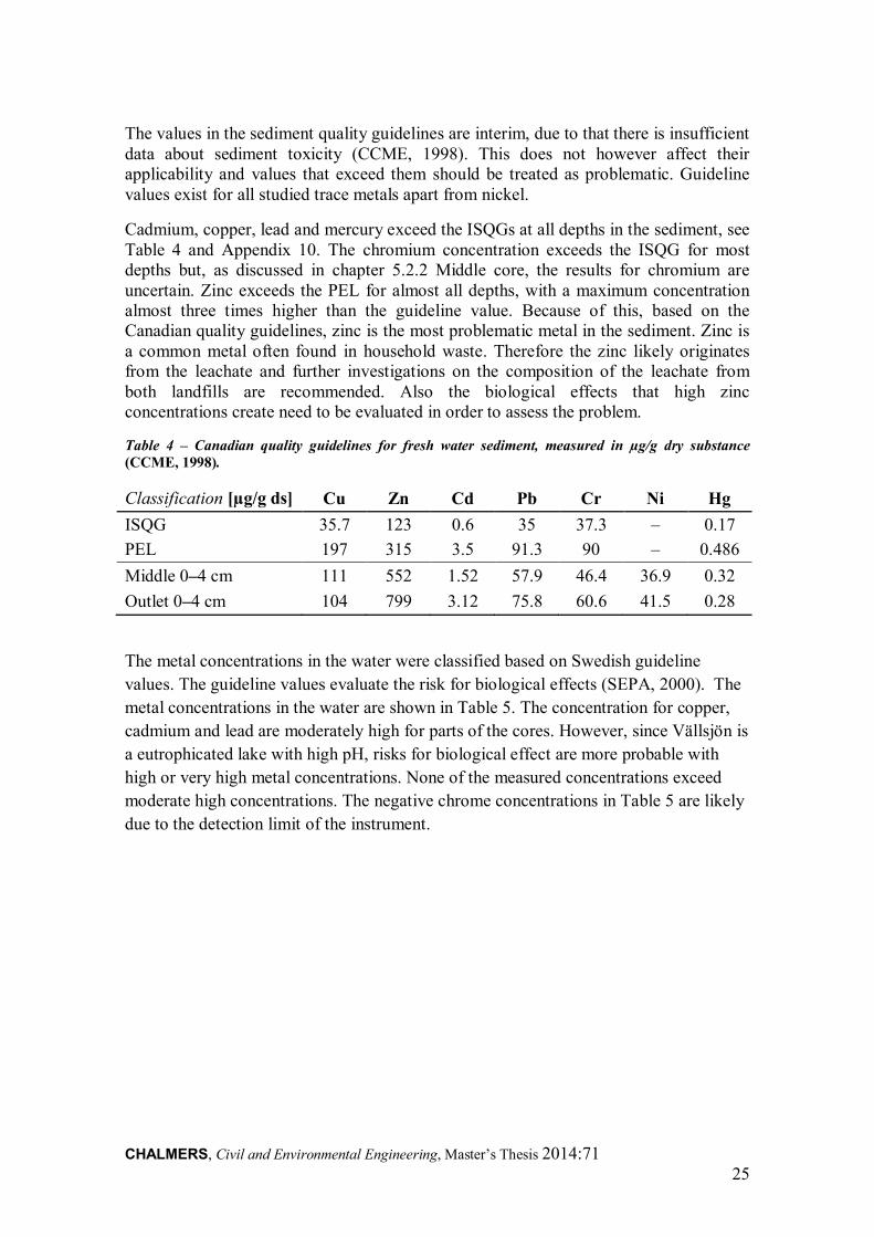
The values in the sediment quality guidelines are interim, due to that there is insufficient data about sediment toxicity (CCME, 1998). This does not however affect their applicability and values that exceed them should be treated as problematic. Guideline values exist for all studied trace metals apart from nickel.
Cadmium, copper, lead and mercury exceed the ISQGs at all depths in the sediment, see Table 4 and Appendix 10. The chromium concentration exceeds the ISQG for most depths but, as discussed in chapter 5.2.2 Middle core, the results for chromium are uncertain. Zinc exceeds the PEL for almost all depths, with a maximum concentration almost three times higher than the guideline value. Because of this, based on the Canadian quality guidelines, zinc is the most problematic metal in the sediment. Zinc is a common metal often found in household waste. Therefore the zinc likely originates from the leachate and further investigations on the composition of the leachate from both landfills are recommended. Also the biological effects that high zinc concentrations create need to be evaluated in order to assess the problem.
Table 4 – Canadian quality guidelines for fresh water sediment, measured in µg/g dry substance (CCME, 1998).
Classification [µg/g ds] Cu Zn Cd Pb Cr Ni Hg
ISQG 35.7 123 0.6 35 37.3 – 0.17
PEL 197 315 3.5 91.3 90 – 0.486
Middle 0–4 cm 111 552 1.52 57.9 46.4 36.9 0.32
Outlet 0–4 cm 104 799 3.12 75.8 60.6 41.5 0.28
The metal concentrations in the water were classified based on Swedish guideline
values. The guideline values evaluate the risk for biological effects (SEPA, 2000). The
metal concentrations in the water are shown in Table 5. The concentration for copper,
cadmium and lead are moderately high for parts of the cores. However, since Vällsjön is
a eutrophicated lake with high pH, risks for biological effect are more probable with
high or very high metal concentrations. None of the measured concentrations exceed
moderate high concentrations. The negative chrome concentrations in Table 5 are likely
due to the detection limit of the instrument.
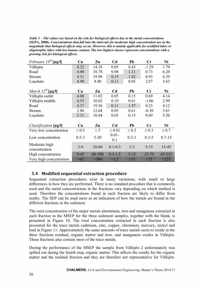
CHALMERS, Civil and Environmental Engineering, Master’s Thesis 2014:71 26
Table 5 – The values are based on the risk for biological effects due to the metal concentrations (SEPA, 2000). Concentrations that fall into the intervals for moderate high concentration are in the magnitude that biological effects may occur. However, this is mainly applicable for acidified lakes or oligotrophic lakes with low humus content. The two highest classes represent concentrations with a growing risk for biological effects.
February 18th [µg/l] Cu Zn Cd Pb Cr Ni
Vällsjön 4.22 14.18 0.05 0.45 -1.29 1.79 Road 4.00 18.78 0.08 1.11 0.73 6.20 Stream 4.51 19.98 0.15 1.42 0.93 6.39 Leachate 4.98 8.80 0.11 0.05 2.07 5.62
March 12th [µg/l] Cu Zn Cd Pb Cr Ni Vällsjön outlet 4.08 11.02 0.05 0.15 0.69 4.14 Vällsjön middle 4.53 10.02 0.10 0.61 -1.06 2.99 Road 4.37 19.56 0.11 1.57 0.23 4.12 Stream 2.86 12.64 0.05 0.61 -0.30 3.61 Leachate 3.31 10.84 0.05 0.15 0.69 5.50
Classification [µg/l] Cu Zn Cd Pb Cr Ni Very low concentration ≤ 0.5 ≤ 5 ≤ 0.01 ≤ 0.2 ≤ 0.3 ≤ 0.7
Low concentration 0.5-3 5-20 0.01-0.1
0.2-1 0.3-5 0.7-15
Moderate high concentration
3-9 20-60 0.1-0.3 1-3 5-15 15-45
High concentration 9-45 60-300 0.3-1.5 3-15 15-75 45-225 Very high concentration >45 >300 >1.5 >15 >75 >225
5.4 Modified sequential extraction procedure Sequential extraction procedures exist in many variations, with small or large differences in how they are performed. There is no standard procedure that is commonly used and the metal concentrations in the fractions vary depending on which method is used. Therefore the concentrations found in each fraction are likely to differ from reality. The SEP can be used more as an indication of how the metals are bound in the different fractions in the sediment.
The total concentration of the major metals aluminium, iron and manganese extracted in each fraction in the MSEP for the three sediment samples, together with the blank, is presented in Figure 10. The total concentration extracted in each fraction is also presented for the trace metals cadmium, zinc, copper, chromium, mercury, nickel and lead in Figure 11. Approximately the same amounts of trace metals seem to reside in the three fractions residual, organic matter and iron- and manganese oxides in Vällsjön. These fractions also contain most of the trace metals.
During the performance of the MSEP the sample from Vällsjön 2 unfortunately was spilled out during the fourth step, organic matter. This affects the results for the organic matter and the residual fraction and they are therefore not representative for Vällsjön.
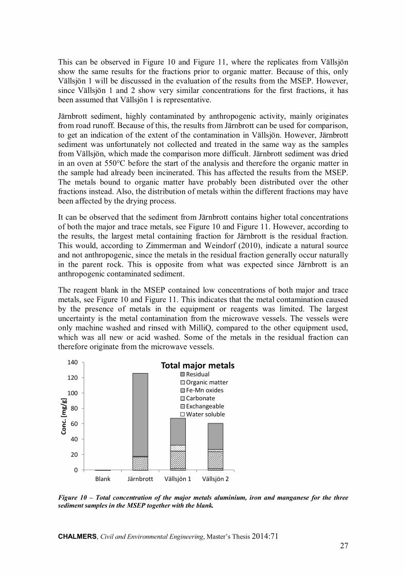
CHALMERS, Civil and Environmental Engineering, Master’s Thesis 2014:71 27
This can be observed in Figure 10 and Figure 11, where the replicates from Vällsjön show the same results for the fractions prior to organic matter. Because of this, only Vällsjön 1 will be discussed in the evaluation of the results from the MSEP. However, since Vällsjön 1 and 2 show very similar concentrations for the first fractions, it has been assumed that Vällsjön 1 is representative.
Järnbrott sediment, highly contaminated by anthropogenic activity, mainly originates from road runoff. Because of this, the results from Järnbrott can be used for comparison, to get an indication of the extent of the contamination in Vällsjön. However, Järnbrott sediment was unfortunately not collected and treated in the same way as the samples from Vällsjön, which made the comparison more difficult. Järnbrott sediment was dried in an oven at 550°C before the start of the analysis and therefore the organic matter in the sample had already been incinerated. This has affected the results from the MSEP. The metals bound to organic matter have probably been distributed over the other fractions instead. Also, the distribution of metals within the different fractions may have been affected by the drying process.
It can be observed that the sediment from Järnbrott contains higher total concentrations of both the major and trace metals, see Figure 10 and Figure 11. However, according to the results, the largest metal containing fraction for Järnbrott is the residual fraction. This would, according to Zimmerman and Weindorf (2010), indicate a natural source and not anthropogenic, since the metals in the residual fraction generally occur naturally in the parent rock. This is opposite from what was expected since Järnbrott is an anthropogenic contaminated sediment.
The reagent blank in the MSEP contained low concentrations of both major and trace metals, see Figure 10 and Figure 11. This indicates that the metal contamination caused by the presence of metals in the equipment or reagents was limited. The largest uncertainty is the metal contamination from the microwave vessels. The vessels were only machine washed and rinsed with MilliQ, compared to the other equipment used, which was all new or acid washed. Some of the metals in the residual fraction can therefore originate from the microwave vessels.
Figure 10 – Total concentration of the major metals aluminium, iron and manganese for the three sediment samples in the MSEP together with the blank.
0
20
40
60
80
100
120
140
Blank Järnbrott Vällsjön 1 Vällsjön 2
Co
nc.
[m
g/g]
Total major metals ResidualOrganic matterFe-Mn oxidesCarbonateExchangeableWater soluble
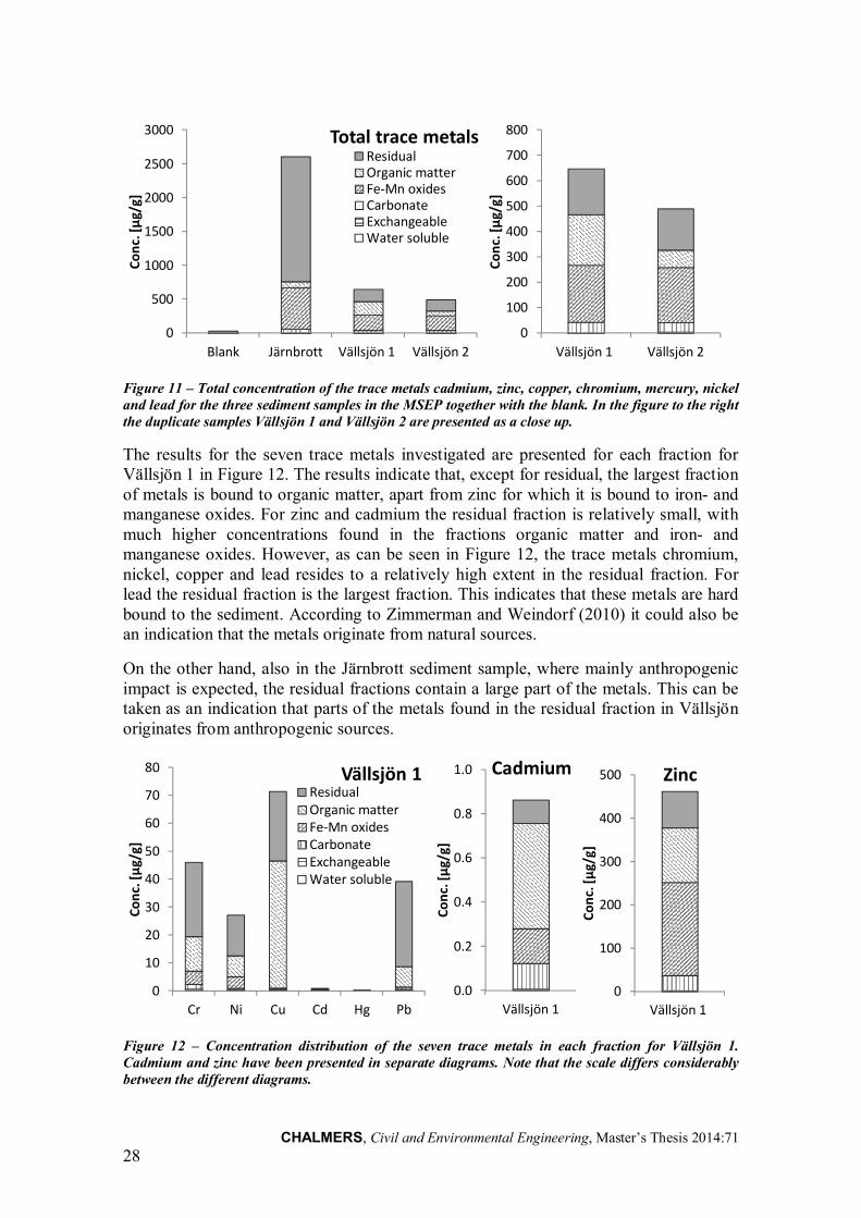
CHALMERS, Civil and Environmental Engineering, Master’s Thesis 2014:71 28
Figure 11 – Total concentration of the trace metals cadmium, zinc, copper, chromium, mercury, nickel and lead for the three sediment samples in the MSEP together with the blank. In the figure to the right the duplicate samples Vällsjön 1 and Vällsjön 2 are presented as a close up.
The results for the seven trace metals investigated are presented for each fraction for Vällsjön 1 in Figure 12. The results indicate that, except for residual, the largest fraction of metals is bound to organic matter, apart from zinc for which it is bound to iron- and manganese oxides. For zinc and cadmium the residual fraction is relatively small, with much higher concentrations found in the fractions organic matter and iron- and manganese oxides. However, as can be seen in Figure 12, the trace metals chromium, nickel, copper and lead resides to a relatively high extent in the residual fraction. For lead the residual fraction is the largest fraction. This indicates that these metals are hard bound to the sediment. According to Zimmerman and Weindorf (2010) it could also be an indication that the metals originate from natural sources.
On the other hand, also in the Järnbrott sediment sample, where mainly anthropogenic impact is expected, the residual fractions contain a large part of the metals. This can be taken as an indication that parts of the metals found in the residual fraction in Vällsjön originates from anthropogenic sources.
Figure 12 – Concentration distribution of the seven trace metals in each fraction for Vällsjön 1. Cadmium and zinc have been presented in separate diagrams. Note that the scale differs considerably between the different diagrams.
0
500
1000
1500
2000
2500
3000
Blank Järnbrott Vällsjön 1 Vällsjön 2
Co
nc.
[µ
g/g]
Total trace metals
ResidualOrganic matterFe-Mn oxidesCarbonateExchangeableWater soluble
0
100
200
300
400
500
600
700
800
Vällsjön 1 Vällsjön 2
Co
nc.
[µ
g/g]
0
10
20
30
40
50
60
70
80
Cr Ni Cu Cd Hg Pb
Co
nc.
[µ
g/g]
Vällsjön 1 ResidualOrganic matterFe-Mn oxidesCarbonateExchangeableWater soluble
0.0
0.2
0.4
0.6
0.8
1.0
Vällsjön 1
Co
nc.
[µ
g/g]
Cadmium
0
100
200
300
400
500
Vällsjön 1
Co
nc.
[µ
g/g]
Zinc
CHALMERS, Civil and Environmental Engineering, Master’s Thesis 2014:71 29
The MSEP performed in this study has been developed based on two other procedures and therefore it is not possible to directly compare the results with another SEP. This is partially a drawback of the MSEP, since it is harder to validate the results. However, the MSEP contained several changes compared to Tessier and BCR. Firstly a water soluble step was added to the procedure. This pre-step did not show to be effective in leaching metals from the sediment, see Figure 10 and Figure 11. The pre-step with water soluble fraction might be more effective when the MSEP is used for a soil, since the sediment already has been in contact with water. Therefore it is not recommended to include the pre-step when performing the MSEP on sediment.
Based on the observations made in this study, it is recommended to use a mechanical shaker at a high speed, preferably with more than only horizontal rotation. This would ensure that the whole sample gets in contact with the reagent.
Another change, compared to Tessier and BCR, was the last step of the procedure, which was performed with microwave digestion and an acidic solution. This step differs considerably from Tessier, where a stronger acid is used. The use of the acidic solution has likely affected the results and given lower concentrations in the residual fraction. However, the MSEP was performed with less toxic chemicals. Also, for the evaluation of the metal contamination from the perspective that the sediment in Vällsjön might pose a risk for Rådasjön, the residual fraction is not the most important.
The metals that are most likely to leach out from the sediment due to natural changes reside in the first fractions. As can be seen in Figure 12, carbonate bound metals make up a small part of the total amount, while the water soluble and exchangeable contain an almost negligible amount of metals. Because of this, only based on the results from the MSEP, Vällsjön seems to act as a barrier, locking the metals in the sediment and thereby keeping them from contaminating Rådasjön.
5.5 Comparison between MSEP and total analysis The total metal concentrations found in the modified sequential extraction procedure differ slightly from the metal concentrations found in the total analysis. As seen in Figure 13, none of the metals show exactly the same concentrations in the analysis performed with the different methods. Copper, lead and nickel show a lower concentration in the result from MSEP, while chromium has a higher concentration in the MSEP result.
The differences between the total analysis and the MSEP can have been caused by losses due to the rinse step with MilliQ that was applied between each of the MSEP steps. This would explain the lower concentrations found. Even though chromium does not follow this trend, chromium is also the metal that shows the largest variations between different depths in the core.
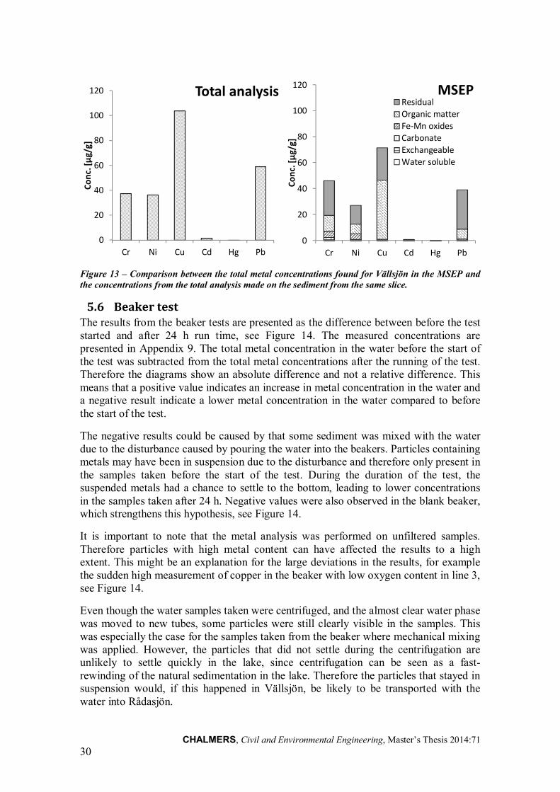
CHALMERS, Civil and Environmental Engineering, Master’s Thesis 2014:71 30
Figure 13 – Comparison between the total metal concentrations found for Vällsjön in the MSEP and the concentrations from the total analysis made on the sediment from the same slice.
5.6 Beaker test The results from the beaker tests are presented as the difference between before the test started and after 24 h run time, see Figure 14. The measured concentrations are presented in Appendix 9. The total metal concentration in the water before the start of the test was subtracted from the total metal concentrations after the running of the test. Therefore the diagrams show an absolute difference and not a relative difference. This means that a positive value indicates an increase in metal concentration in the water and a negative result indicate a lower metal concentration in the water compared to before the start of the test.
The negative results could be caused by that some sediment was mixed with the water due to the disturbance caused by pouring the water into the beakers. Particles containing metals may have been in suspension due to the disturbance and therefore only present in the samples taken before the start of the test. During the duration of the test, the suspended metals had a chance to settle to the bottom, leading to lower concentrations in the samples taken after 24 h. Negative values were also observed in the blank beaker, which strengthens this hypothesis, see Figure 14.
It is important to note that the metal analysis was performed on unfiltered samples. Therefore particles with high metal content can have affected the results to a high extent. This might be an explanation for the large deviations in the results, for example the sudden high measurement of copper in the beaker with low oxygen content in line 3, see Figure 14.
Even though the water samples taken were centrifuged, and the almost clear water phase was moved to new tubes, some particles were still clearly visible in the samples. This was especially the case for the samples taken from the beaker where mechanical mixing was applied. However, the particles that did not settle during the centrifugation are unlikely to settle quickly in the lake, since centrifugation can be seen as a fast-rewinding of the natural sedimentation in the lake. Therefore the particles that stayed in suspension would, if this happened in Vällsjön, be likely to be transported with the water into Rådasjön.
0
20
40
60
80
100
120
Cr Ni Cu Cd Hg Pb
Co
nc.
[µ
g/g]
Total analysis
0
20
40
60
80
100
120
Cr Ni Cu Cd Hg Pb
Co
nc.
[µ
g/g]
MSEP Residual
Organic matter
Fe-Mn oxides
Carbonate
Exchangeable
Water soluble
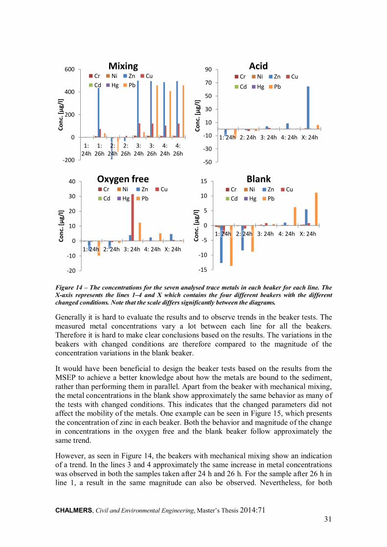
CHALMERS, Civil and Environmental Engineering, Master’s Thesis 2014:71 31
Figure 14 – The concentrations for the seven analysed trace metals in each beaker for each line. The X-axis represents the lines 1–4 and X which contains the four different beakers with the different changed conditions. Note that the scale differs significantly between the diagrams.
Generally it is hard to evaluate the results and to observe trends in the beaker tests. The measured metal concentrations vary a lot between each line for all the beakers. Therefore it is hard to make clear conclusions based on the results. The variations in the beakers with changed conditions are therefore compared to the magnitude of the concentration variations in the blank beaker.
It would have been beneficial to design the beaker tests based on the results from the MSEP to achieve a better knowledge about how the metals are bound to the sediment, rather than performing them in parallel. Apart from the beaker with mechanical mixing, the metal concentrations in the blank show approximately the same behavior as many of the tests with changed conditions. This indicates that the changed parameters did not affect the mobility of the metals. One example can be seen in Figure 15, which presents the concentration of zinc in each beaker. Both the behavior and magnitude of the change in concentrations in the oxygen free and the blank beaker follow approximately the same trend.
However, as seen in Figure 14, the beakers with mechanical mixing show an indication of a trend. In the lines 3 and 4 approximately the same increase in metal concentrations was observed in both the samples taken after 24 h and 26 h. For the sample after 26 h in line 1, a result in the same magnitude can also be observed. Nevertheless, for both
-200
0
200
400
600
1:24h
1:26h
2:24h
2:26h
3:24h
3:26h
4:24h
4:26h
Co
nc.
[µ
g/l]
Mixing
Cr Ni Zn Cu
Cd Hg Pb
-50
-30
-10
10
30
50
70
90
1: 24h 2: 24h 3: 24h 4: 24h X: 24h
Co
nc.
[µ
g/l]
Acid Cr Ni Zn Cu
Cd Hg Pb
-20
-10
0
10
20
30
40
1: 24h 2: 24h 3: 24h 4: 24h X: 24h
Co
nc.
[µ
g/l]
Oxygen free Cr Ni Zn Cu
Cd Hg Pb
-15
-10
-5
0
5
10
15
1: 24h 2: 24h 3: 24h 4: 24h X: 24h
Co
nc.
[µ
g/l]
Blank Cr Ni Zn Cu
Cd Hg Pb
CHALMERS, Civil and Environmental Engineering, Master’s Thesis 2014:71 32
samples in line 2 and the sample after 24 h in line 1, small or negative changes in metal concentrations are found.
It should however be noted that the concentrations in line 2 were in the same magnitude as after line 3 and 4 already before the test was started. This can have been caused by that the mixing was run for a few minutes before the first water sample had been taken out for metal analysis. This happened for one of the lines, it is unfortunately not certain for which line, but it was likely line 2.
Probably the clear increase of metal concentrations in the mixing tests was caused by that the mixing broke down larger particles. Since smaller particles are lighter they could therefore have stayed in suspension even though the water was centrifuged. However it is important to note that the results contain many uncertainties. Since only one water sample was taken from each beaker, it is possible that some particles containing high metal concentrations were present in some of the water samples. The different lines were performed as replicates, to reduce the uncertainties. However, replicates of all samples from each beaker would have increased the validity of the test.
To evaluate the tests, the behaviour of two metals has been studied. The test with mechanical mixing show a distinct increase in the concentrations of cadmium and zinc respectively, see Figure 15 and Figure 16. For zinc the increase in concentration is approximately 100 times larger compared to the blank.
For the acidified beaker almost no changes in the metal concentrations can be observed after the pH was decreased in the first four lines, see Figure 14. This could be caused by the high buffering capacity in the lake water, which caused the pH to increase from the lowered value to approximately the original value in the first four lines. For line X however, a more distinct change in the metal concentration can be observed. This is especially the case for cadmium, as seen in Figure 16.
The clear increase in line X is probably mainly due to that the pH was decreased to approximately 4 compared to approximately 6 in the other four lines. This result could be reliable, even though there is only one measurement, since the solubility of many metals increase with a decreased pH (Reeve, 2002). On the other hand, there are many uncertainties involved that could have caused the different behavior of the metal concentrations for line X. One possible explanation could be that a particle with a high metal content was present in the sample taken in the acidified beaker in line X.
However, it is not likely that Vällsjön will be acidified in the future, at least not by natural sources. The current pH and alkalinity are high in the lake and therefore a decrease of pH to below 6 is not likely. Leaching of metals due to acidification is therefore probably not an issue in Vällsjön. On the contrary, if only the effect on mobility of metals caused by pH is studied, the lake acts as a barrier, locking the metals in the sediment.
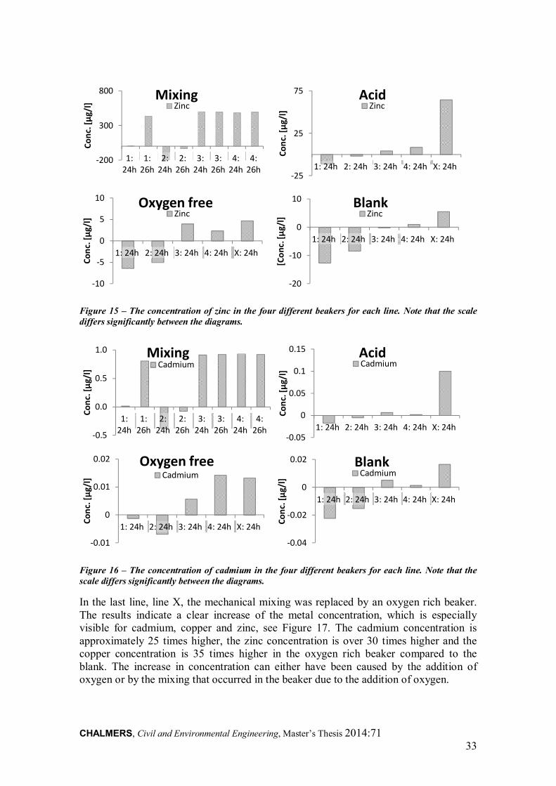
CHALMERS, Civil and Environmental Engineering, Master’s Thesis 2014:71 33
Figure 15 – The concentration of zinc in the four different beakers for each line. Note that the scale differs significantly between the diagrams.
Figure 16 – The concentration of cadmium in the four different beakers for each line. Note that the scale differs significantly between the diagrams.
In the last line, line X, the mechanical mixing was replaced by an oxygen rich beaker. The results indicate a clear increase of the metal concentration, which is especially visible for cadmium, copper and zinc, see Figure 17. The cadmium concentration is approximately 25 times higher, the zinc concentration is over 30 times higher and the copper concentration is 35 times higher in the oxygen rich beaker compared to the blank. The increase in concentration can either have been caused by the addition of oxygen or by the mixing that occurred in the beaker due to the addition of oxygen.
-200
300
800
1:24h
1:26h
2:24h
2:26h
3:24h
3:26h
4:24h
4:26h
Co
nc.
[µ
g/l]
Mixing Zinc
-25
25
75
1: 24h 2: 24h 3: 24h 4: 24h X: 24h
Co
nc.
[µ
g/l]
Acid Zinc
-10
-5
0
5
10
1: 24h 2: 24h 3: 24h 4: 24h X: 24h
Co
nc.
[µ
g/l]
Oxygen free Zinc
-20
-10
0
10
1: 24h 2: 24h 3: 24h 4: 24h X: 24h
[Co
nc.
[µg/
l]
Blank Zinc
-0.5
0.0
0.5
1.0
1:24h
1:26h
2:24h
2:26h
3:24h
3:26h
4:24h
4:26h
Co
nc.
[µ
g/l]
Mixing Cadmium
-0.05
0
0.05
0.1
0.15
1: 24h 2: 24h 3: 24h 4: 24h X: 24h
Co
nc.
[µ
g/l]
Acid Cadmium
-0.01
0
0.01
0.02
1: 24h 2: 24h 3: 24h 4: 24h X: 24h
Co
nc.
[µ
g/l]
Oxygen free Cadmium
-0.04
-0.02
0
0.02
1: 24h 2: 24h 3: 24h 4: 24h X: 24h
Co
nc.
[µ
g/l]
Blank Cadmium
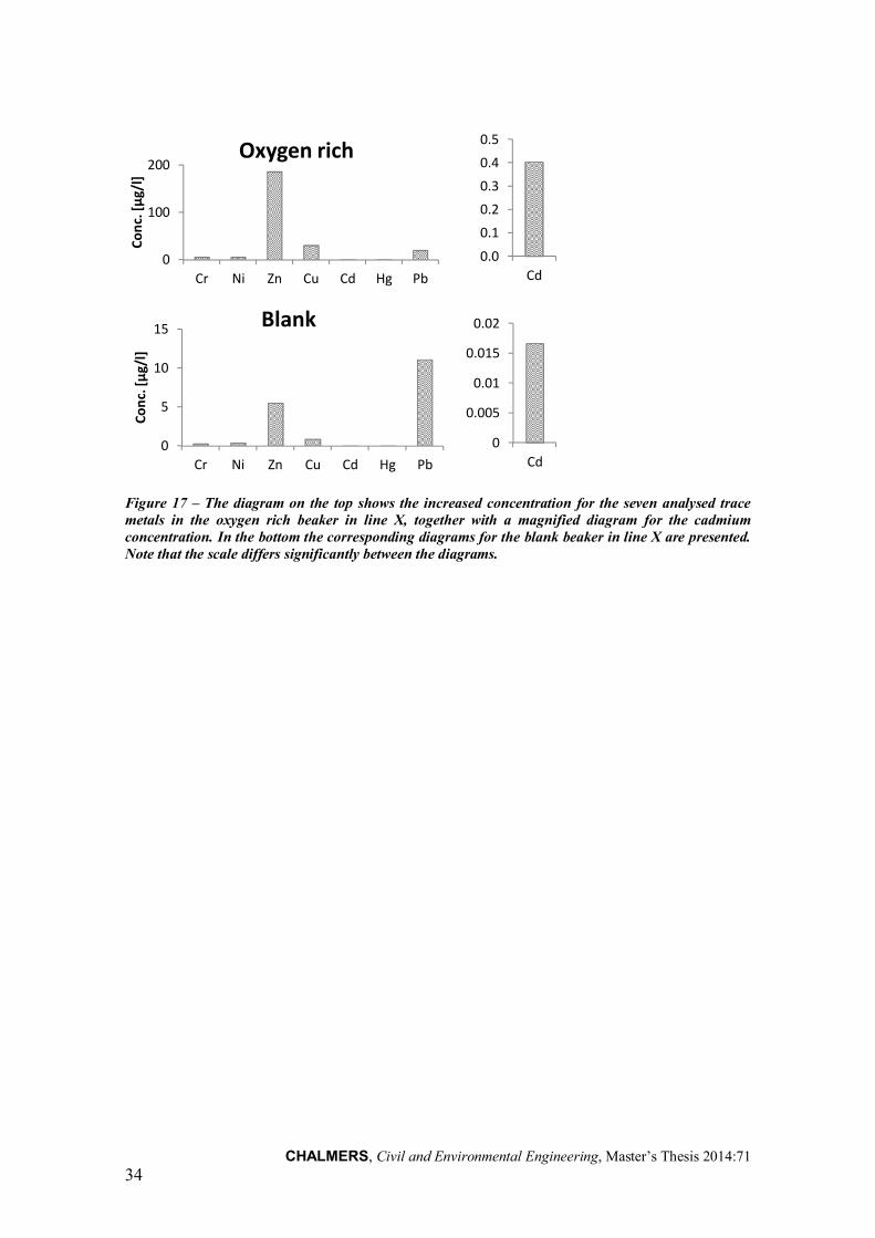
CHALMERS, Civil and Environmental Engineering, Master’s Thesis 2014:71 34
Figure 17 – The diagram on the top shows the increased concentration for the seven analysed trace metals in the oxygen rich beaker in line X, together with a magnified diagram for the cadmium concentration. In the bottom the corresponding diagrams for the blank beaker in line X are presented. Note that the scale differs significantly between the diagrams.
0
100
200
Cr Ni Zn Cu Cd Hg Pb
Co
nc.
[µ
g/l]
Oxygen rich
0.0
0.1
0.2
0.3
0.4
0.5
Cd
0
5
10
15
Cr Ni Zn Cu Cd Hg Pb
Co
nc.
[µ
g/l]
Blank
0
0.005
0.01
0.015
0.02
Cd
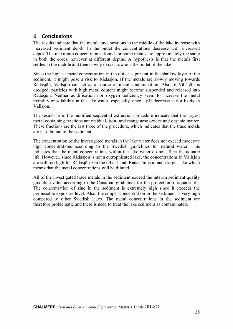
CHALMERS, Civil and Environmental Engineering, Master’s Thesis 2014:71 35
6 Conclusions The results indicate that the metal concentrations in the middle of the lake increase with increased sediment depth. In the outlet the concentrations decrease with increased depth. The maximum concentrations found for some metals are approximately the same in both the cores, however at different depths. A hypothesis is that the metals first settles in the middle and then slowly moves towards the outlet of the lake.
Since the highest metal concentration in the outlet is present in the shallow layer of the sediment, it might pose a risk to Rådasjön. If the metals are slowly moving towards Rådasjön, Vällsjön can act as a source of metal contamination. Also, if Vällsjön is dredged, particles with high metal content might become suspended and released into Rådasjön. Neither acidification nor oxygen deficiency seem to increase the metal mobility or solubility in the lake water, especially since a pH decrease is not likely in Vällsjön.
The results from the modified sequential extraction procedure indicate that the largest metal containing fractions are residual, iron- and manganese oxides and organic matter. These fractions are the last three of the procedure, which indicates that the trace metals are hard bound to the sediment.
The concentration of the investigated metals in the lake water does not exceed moderate high concentrations according to the Swedish guidelines for natural water. This indicates that the metal concentrations within the lake water do not affect the aquatic life. However, since Rådasjön is not a eutrophicated lake, the concentrations in Vällsjön are still too high for Rådasjön. On the other hand, Rådasjön is a much larger lake which means that the metal concentrations will be diluted.
All of the investigated trace metals in the sediment exceed the interim sediment quality guideline value according to the Canadian guidelines for the protection of aquatic life. The concentration of zinc in the sediment is extremely high since it exceeds the permissible exposure level. Also, the copper concentration in the sediment is very high compared to other Swedish lakes. The metal concentrations in the sediment are therefore problematic and there is need to treat the lake sediment as contaminated.

CHALMERS, Civil and Environmental Engineering, Master’s Thesis 2014:71 36
CHALMERS, Civil and Environmental Engineering, Master’s Thesis 2014:71 37
7 Recommendations for Further Investigations Since the beaker tests with mechanical mixing indicated an increased metal concentration in the water, it is recommended to investigate more about how dredging affects the mobility and solubility of the metals in the lake. Also the aspect of increased oxygen concentration, that dredging imposes on the sediment, needs to be further investigated if the sediment in Vällsjön should be dredged.
The origin for the high concentrations of chloride and the high pH in the stream from Kikåstippen has to be further investigated. Also the source of the increased concentration of copper during recent years should be investigated.
Metal analysis on a core taken in the sediment of the leachate pond at both Kikåstippen and Lahallstippen could be used to compare the distribution of metals with the lake sediment. This could help the investigation of the sources for the metals found in the lake sediment.
It is recommended to collect more sediment cores in Vällsjön. Duplicate cores taken in the inlet of the stream from Kikåstippen, in the middle of the lake and at the outlet could be used to investigate the metal transportation in the lake, especially to investigate if the metals are moving towards the outlet. The sedimentation speed in the lake is necessary to estimate the current deposition of metals, and also to be able to correlate the concentrations with historical discharges. This can be investigated by dating the sediment, for example using the lead 210 method.
The metal concentrations found in the lake are all based on analysis performed on samples that had not been filtered. Since the metal concentrations vary depending on if filtered or unfiltered samples are used, and could also be higher with filtered samples (Singer, 1973), it is recommended to perform analysis on both filtered and unfiltered samples.
This master thesis has only focused on selected trace metals. Further investigations should also contain the analysis of other trace metals and persistent organic pollutants, both in the sediment and in the lake water.

CHALMERS, Civil and Environmental Engineering, Master’s Thesis 2014:71 38
CHALMERS, Civil and Environmental Engineering, Master’s Thesis 2014:71 39
References Baun, A., Nyholm, N. & Kusk, K.O., 2013. Environmental Risk Assessment of
Chemicals. Lecture notes. Kgs. Lyngby: Technical University of Denmark Department
of Environmental Engineering.
Boman, J. & Olsson, M., 1986. Kikåstippen - Lahallstippen, Vällsjön - Rådasjön,
Miljötillstånd och förslag till åtgärder. Master Thesis. Göteborg: Göteborgs Universitet.
Bydén, S., Larsson, A.-M. & Olsson, M., 2003. Mäta vatten - Undersökningar av sött
och salt vatten. 3rd ed. Göteborg: Avdelningen för tillämpad miljövetenskap och
Avdelningen för oceanografi, Göteborgs universitet.
CCME, 1998. Canadian Environmental Quality Guidelines. [Online] Available at:
www.ccme.ca [Accessed 1st of June 2014].
Chalmers, 2013. Student projects in the course Environmental Analysis of Water.
Göteborg: Chalmers.
Drever, J.I., 1997. Heavy Metals and Metalloids. In R.A. McConnin, ed. The
Geochemistry of Natural Waters - Surface and Groundwater Environments. 3rd ed.
New Jersey: Prentice-Hall. pp.175-96.
Eliasson, A.-L., 2006. Slutrapport 2006-12-07 Återställning av Lahallsdeponin.
Härryda Kommun.
European Environment Agency, 2008. Water pollution - overview. [Online] Available
at: www.eea.europa.eu/themes/water/water-pollution [Accessed 11th February 2014].
Forshufvud, J., 2013. Chalmers insidan. [Online] Available at: www.chalmers.se
[Accessed 14th May 2014].
Gleyzes, C., Tellier, S. & Astruc, M., 2002. Fractionation studies of trace elements in
contaminated soils and sediments: a review of sequential extraction procedures. Trends
in analytical chemistry, 21(6+7), p.451.
Hagman, J., 2014. [Online] [Accessed 19th February 2014].
Hjortenkrans, D., Bergbäck, B. & Häggerud, A., 2007. Metal emissions from brake
linings and tires; case studies of Stockholm. Sweden 1995/1998 and 2005.
Environmental Science and Technology, 41, pp.5224-30.
Israelsson, B., 1990. Rapport avseende vattenkontroll Kikåstippen för perioden
december 1988 t o m december 1989. Mölndal: Mölndals kommun Konsultföretaget
GF.
Johansson, K., 2001. Metaller i sediment. [Online] Available at: www.slu.se [Accessed
25th May 2014].
CHALMERS, Civil and Environmental Engineering, Master’s Thesis 2014:71 40
Kabata-Pendias, A. & Mukherjee, A.B., 2007. Trace Elements from Soil to Human.
New York: Springer.
Karlfeldt Fedje, K., Yillin, L. & Strömvall, A.-M., 2013. Remediation of metal polluted
hotspot areas through enhanced soil washing - Evaluation of leaching methods. Journal
of Environmental Management, 128, pp.489-96.
Kjeldsen, P. et al., 2002. Present and Long-Term Composition of MSW Landfill
Leachate: A Review. Environmental Science and Technology, 32, pp.297-336.
Kurniawan, T.A., Lo, W.-h. & Chang, G.Y., 2006. Physico-chemical treatments for
removal of recalcitrant contaminants from landfill leachate. Journal of Hazardous
Materials B129, pp.89-100.
Lerner, K.K. & Lerner, B.W., eds., 2003. Crust. In World of Earth Science. Web ed.
Detroit: Gale Virtual Reference Library. pp.141-42.
Länsstyrelsen & VicNatur - Naturvårdsverket, 2014. VISS. [Online] (Rådasjön)
Available at: www.viss.lansstyrelsen.se [Accessed 17th February 2014].
Medin, M., 1990. Metallföroreningsläget i bäck från Vällsjön. Mölnlycke: Medins Sjö-
och åbiologi AB.
Mohammed, A.S., Kapri, A. & Goel, R., 2011. Heavy Metal Pollution: Source, Impact
and Remedies. In Biomanagement of Metal-Contaminated Soils. Springer. pp.1-28.
Mölndals stad, 2012. Miljörapport för Kikås avfallsanläggning och återvinningscentral
för 2012. Mölndal: Mölndals stad Tekniska förvaltningen.
Nolbrant, P., 2011. Vattenmiljöer i Mölndalsåns avrinningsområde - en resurs för
människor och ekosystem. Mölndal: Mölndalsåns vattenråd BioDivers
Naturvårdskonsult.
Ohlson, R., 2014. Extraktion. [Online] Available at: www.ne.se [Accessed 5th May
2014].
Quevauviller, P. et al., 1994. Evaluation of sequential extraction procedure for the
determiantion of extractable trace metal contents in sediment. Fredenius J Anal Chem,
349, pp.808-14.
Rauret, G., 1998. Extraction procedures for the determination of heavy metals in
contaminated soil and sediment. Talanta, 46(3), pp.449-55.
Rauret, G. et al., 1999. Improvement of the BCR three step sequential extraction
procedure prior to the certification of new sediment and soil reference materials.
Journal of Environmental Monitoring, 1, pp.57-61.
CHALMERS, Civil and Environmental Engineering, Master’s Thesis 2014:71 41
Reeve, R., 2002. Introduction to Environmental Analysis. West Sussex: John Wiley &
Sons.
SEPA, 2000. Environmental Quality Criteria Lakes and Watercourses. Stockholm:
Swedish Environmental Protection Agency Swedish Environmental Protection Agency.
SFS, 2011. Avfallsförordning 2011:927. [Online] Available at: www.riksdagen.se
[Accessed 5th March 2014].
Shuman, L.M., 1982. Separating soil iron- and manganese-oxide fractions for
microelement analysis. The soil science society of America journal, 46, pp.1099-102.
Singer, P.C., 1973. Trace Metals and Metal-Organic Interactions in Natural Waters.
Michigan: Ann Arbor Science Publishers.
Svenskt Vatten, n.d. Svenskt vatten. [Online] Available at: www.svensktvatten.se
[Accessed 28th May 2014].
Svensson, I. & Röstell, Å., 2013. Miljökonsekvensbeskrivning Kikås avfallsanläggning
och ÅVC. Mölndal: Mölndals stad Tyréns.
Templeton, D.M. et al., 2000. Guidelines for Terms Related to Chemical Speciation and
Fractionation of Elements. Definitions, Structural Aspects, and Methodological
Approaches. Pure and Applied Chemistry, 72(8), pp.1453-70.
Tessier, A., Campbell, P.G.C. & Bisson, M., 1979. Sequential Extraction Procedure for
the Speciation of Particulate Trace Metals. Analytical Chemistry, 51(7), pp.844-951.
Zemberyová, M., Barteková, J. & Hagarová, I., 2006. The utilization of modified BCR
three-step sequential extratcion procedure for the fractionation of Cd, Cr, Cu, Ni, Pb and
Zn in soil reference materials of different origins. Talanta, 70, pp.973-78.
Zimmerman, A.J. & Weindorf, D.C., 2010. Heavy metal and Trace Metal Analysis in
Soil by Sequential Extratcion: A Review of Procedures.

CHALMERS, Civil and Environmental Engineering, Master’s Thesis 2014:71 42
CHALMERS, Civil and Environmental Engineering, Master’s Thesis 2014:71 43
Appendices Appendix 1 – Gravity core sampler guideline
Appendix 2 – Tessier procedure
Appendix 3 – Improved BCR procedure
Appendix 4 – Extraction procedure of the MSEP
Appendix 5 – Water quality parameters
Appendix 6 – Metal concentrations in cores
Appendix 7 – Metal concentrations extracted in MSEP
Appendix 8 – Metal concentrations in water samples
Appendix 9 – Metal concentrations in beaker tests
Appendix 10 – Classification of metal concentrations

CHALMERS, Civil and Environmental Engineering, Master’s Thesis 2014:71 44
CHALMERS, Civil and Environmental Engineering, Master’s Thesis 2014:71 45
Appendix 1 Gravity core sampler
The procedure used while performing the core sampling is presented on the next pages.
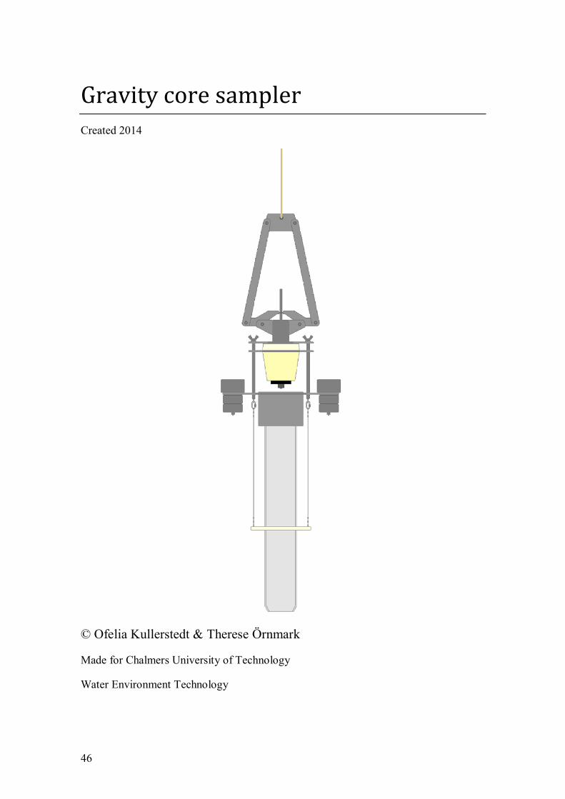
46
Gravity core sampler
Created 2014
© Ofelia Kullerstedt & Therese Örnmark
Made for Chalmers University of Technology
Water Environment Technology
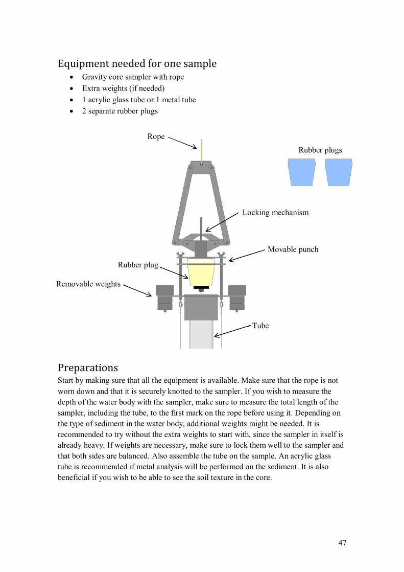
47
Equipment needed for one sample Gravity core sampler with rope
Extra weights (if needed)
1 acrylic glass tube or 1 metal tube
2 separate rubber plugs
Preparations Start by making sure that all the equipment is available. Make sure that the rope is not
worn down and that it is securely knotted to the sampler. If you wish to measure the
depth of the water body with the sampler, make sure to measure the total length of the
sampler, including the tube, to the first mark on the rope before using it. Depending on
the type of sediment in the water body, additional weights might be needed. It is
recommended to try without the extra weights to start with, since the sampler in itself is
already heavy. If weights are necessary, make sure to lock them well to the sampler and
that both sides are balanced. Also assemble the tube on the sample. An acrylic glass
tube is recommended if metal analysis will be performed on the sediment. It is also
beneficial if you wish to be able to see the soil texture in the core.
Locking mechanism
Movable punch
Tube
Rubber plug
Removable weights
Rubber plugs
Rope
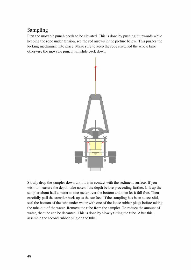
48
Sampling First the movable punch needs to be elevated. This is done by pushing it upwards while
keeping the rope under tension, see the red arrows in the picture below. This pushes the
locking mechanism into place. Make sure to keep the rope stretched the whole time
otherwise the movable punch will slide back down.
Slowly drop the sampler down until it is in contact with the sediment surface. If you
wish to measure the depth, take note of the depth before proceeding further. Lift up the
sampler about half a meter to one meter over the bottom and then let it fall free. Then
carefully pull the sampler back up to the surface. If the sampling has been successful,
seal the bottom of the tube under water with one of the loose rubber plugs before taking
the tube out of the water. Remove the tube from the sampler. To reduce the amount of
water, the tube can be decanted. This is done by slowly tilting the tube. After this,
assemble the second rubber plug on the tube.
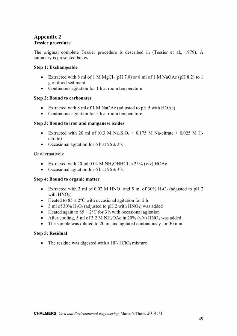
CHALMERS, Civil and Environmental Engineering, Master’s Thesis 2014:71 49
Appendix 2 Tessier procedure
The original complete Tessier procedure is described in (Tessier et al., 1979). A summary is presented below.
Step 1: Exchangeable
Extracted with 8 ml of 1 M MgCl2 (pH 7.0) or 8 ml of 1 M NaOAc (pH 8.2) to 1 g of dried sediment
Continuous agitation for 1 h at room temperature
Step 2: Bound to carbonates
Extracted with 8 ml of 1 M NaOAc (adjusted to pH 5 with HOAc) Continuous agitation for 5 h at room temperature
Step 3: Bound to iron and manganese oxides
Extracted with 20 ml of (0.3 M Na2S2O4 + 0.175 M Na-citrate + 0.025 M H-citrate)
Occasional agitation for 6 h at 96 ± 3°C
Or alternatively
Extracted with 20 ml 0.04 M NH2OHHCl in 25% (v/v) HOAc Occasional agitation for 6 h at 96 ± 3°C
Step 4: Bound to organic matter
Extracted with 3 ml of 0.02 M HNO3 and 5 ml of 30% H2O2 (adjusted to pH 2 with HNO3)
Heated to 85 ± 2°C with occasional agitation for 2 h 3 ml of 30% H2O2 (adjusted to pH 2 with HNO3) was added Heated again to 85 ± 2°C for 3 h with occasional agitation After cooling, 5 ml of 3.2 M NH4OAc in 20% (v/v) HNO3 was added The sample was diluted to 20 ml and agitated continuously for 30 min
Step 5: Residual
The residue was digested with a HF-HClO4 mixture

CHALMERS, Civil and Environmental Engineering, Master’s Thesis 2014:71 50
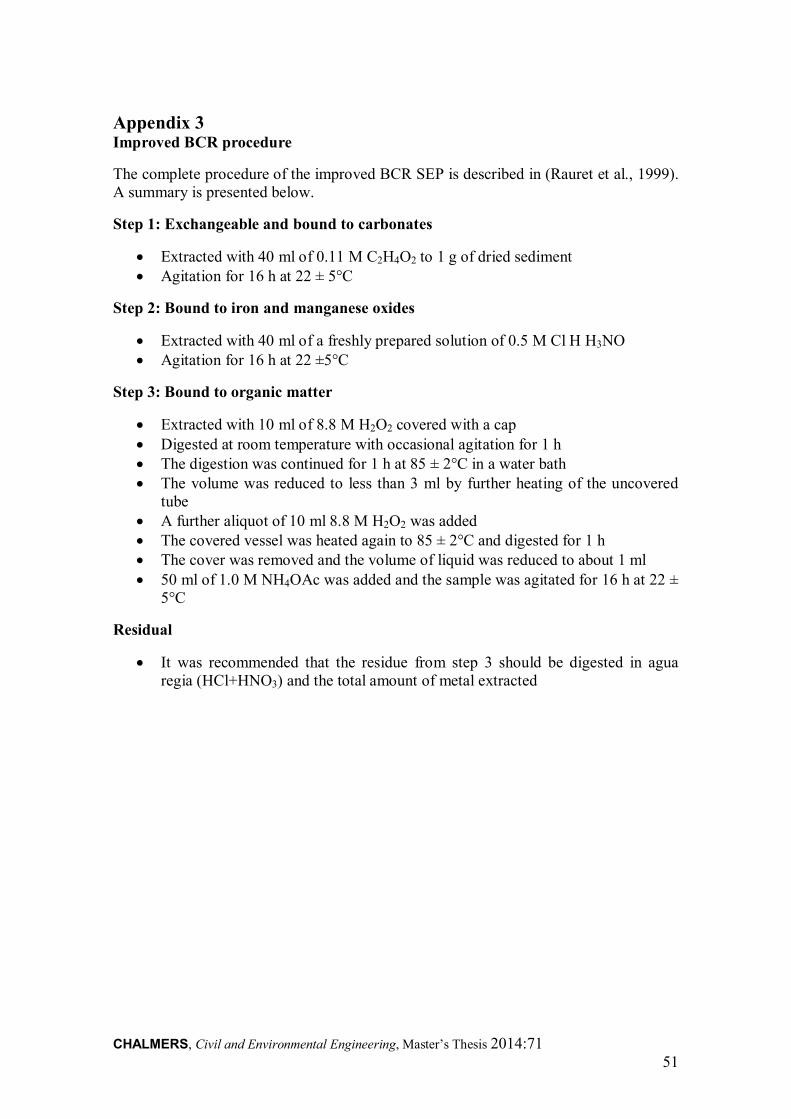
CHALMERS, Civil and Environmental Engineering, Master’s Thesis 2014:71 51
Appendix 3 Improved BCR procedure
The complete procedure of the improved BCR SEP is described in (Rauret et al., 1999). A summary is presented below.
Step 1: Exchangeable and bound to carbonates
Extracted with 40 ml of 0.11 M C2H4O2 to 1 g of dried sediment Agitation for 16 h at 22 ± 5°C
Step 2: Bound to iron and manganese oxides
Extracted with 40 ml of a freshly prepared solution of 0.5 M Cl H H3NO Agitation for 16 h at 22 ±5°C
Step 3: Bound to organic matter
Extracted with 10 ml of 8.8 M H2O2 covered with a cap Digested at room temperature with occasional agitation for 1 h The digestion was continued for 1 h at 85 ± 2°C in a water bath The volume was reduced to less than 3 ml by further heating of the uncovered
tube A further aliquot of 10 ml 8.8 M H2O2 was added The covered vessel was heated again to 85 ± 2°C and digested for 1 h The cover was removed and the volume of liquid was reduced to about 1 ml 50 ml of 1.0 M NH4OAc was added and the sample was agitated for 16 h at 22 ±
5°C
Residual
It was recommended that the residue from step 3 should be digested in agua regia (HCl+HNO3) and the total amount of metal extracted

CHALMERS, Civil and Environmental Engineering, Master’s Thesis 2014:71 52
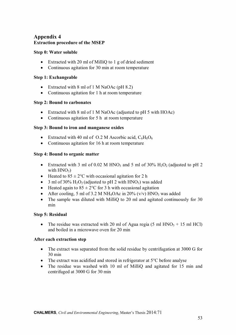
CHALMERS, Civil and Environmental Engineering, Master’s Thesis 2014:71 53
Appendix 4 Extraction procedure of the MSEP
Step 0: Water soluble
Extracted with 20 ml of MilliQ to 1 g of dried sediment Continuous agitation for 30 min at room temperature
Step 1: Exchangeable
Extracted with 8 ml of 1 M NaOAc (pH 8.2) Continuous agitation for 1 h at room temperature
Step 2: Bound to carbonates
Extracted with 8 ml of 1 M NaOAc (adjusted to pH 5 with HOAc) Continuous agitation for 5 h at room temperature
Step 3: Bound to iron and manganese oxides
Extracted with 40 ml of O.2 M Ascorbic acid, C6H8O6 Continuous agitation for 16 h at room temperature
Step 4: Bound to organic matter
Extracted with 3 ml of 0.02 M HNO3 and 5 ml of 30% H2O2 (adjusted to pH 2 with HNO3)
Heated to 85 ± 2°C with occasional agitation for 2 h 3 ml of 30% H2O2 (adjusted to pH 2 with HNO3) was added Heated again to 85 ± 2°C for 3 h with occasional agitation After cooling, 5 ml of 3.2 M NH4OAc in 20% (v/v) HNO3 was added The sample was diluted with MilliQ to 20 ml and agitated continuously for 30
min
Step 5: Residual
The residue was extracted with 20 ml of Agua regia (5 ml HNO3 + 15 ml HCl) and boiled in a microwave oven for 20 min
After each extraction step
The extract was separated from the solid residue by centrifugation at 3000 G for 30 min
The extract was acidified and stored in refrigerator at 5°C before analyse The residue was washed with 10 ml of MilliQ and agitated for 15 min and
centrifuged at 3000 G for 30 min

CHALMERS, Civil and Environmental Engineering, Master’s Thesis 2014:71 54
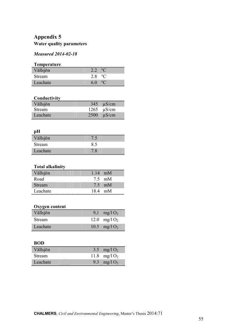
CHALMERS, Civil and Environmental Engineering, Master’s Thesis 2014:71 55
Appendix 5 Water quality parameters
Measured 2014-02-18
Temperature Vällsjön 2.2 °C
Stream 2.8 °C
Leachate 6.0 °C
Conductivity Vällsjön 345 µS/cm Stream 1265 µS/cm Leachate 2500 µS/cm
pH
Vällsjön 7.5
Stream 8.5
Leachate 7.8
Total alkalinity
Vällsjön 1.14 mM
Road 7.5 mM Stream 7.5 mM
Leachate 18.4 mM
Oxygen content
Vällsjön 9,1 mg/l O2
Stream 12.0 mg/l O2
Leachate 10.5 mg/l O2
BOD
Vällsjön 3.5 mg/l O2
Stream 11.8 mg/l O2
Leachate 9.3 mg/l O2
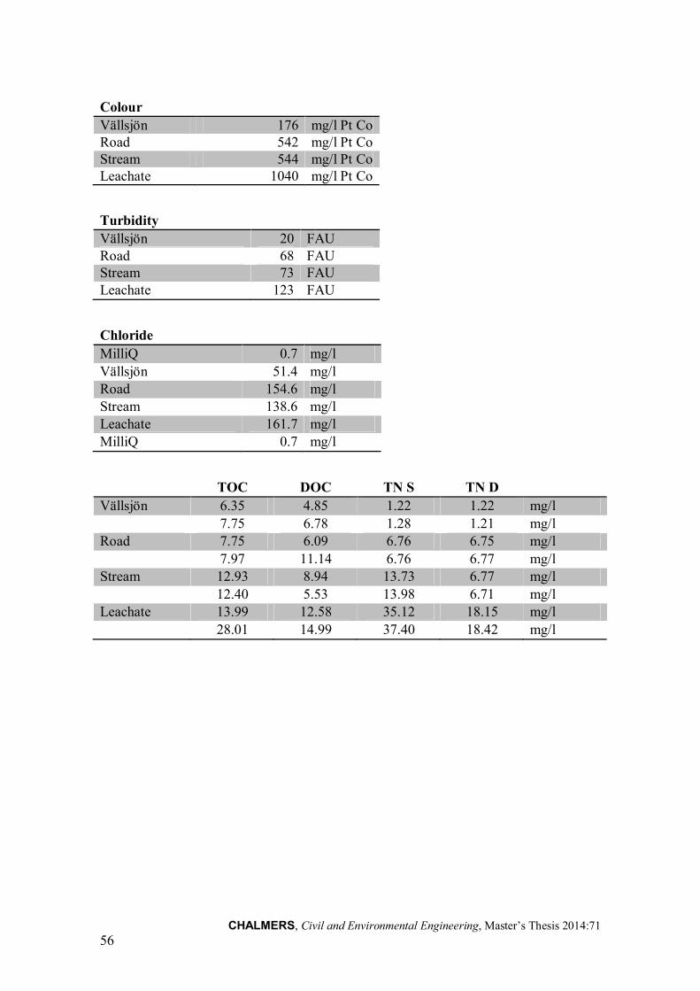
CHALMERS, Civil and Environmental Engineering, Master’s Thesis 2014:71 56
Colour
Vällsjön 176 mg/l Pt Co Road 542 mg/l Pt Co Stream 544 mg/l Pt Co Leachate 1040 mg/l Pt Co
Turbidity
Vällsjön 20 FAU Road 68 FAU Stream 73 FAU Leachate 123 FAU
Chloride
MilliQ 0.7 mg/l
Vällsjön 51.4 mg/l Road 154.6 mg/l Stream 138.6 mg/l Leachate 161.7 mg/l MilliQ 0.7 mg/l
TOC DOC TN S TN D
Vällsjön 6.35 4.85 1.22 1.22 mg/l
7.75 6.78 1.28 1.21 mg/l Road 7.75 6.09 6.76 6.75 mg/l
7.97 11.14 6.76 6.77 mg/l Stream 12.93 8.94 13.73 6.77 mg/l
12.40 5.53 13.98 6.71 mg/l Leachate 13.99 12.58 35.12 18.15 mg/l
28.01 14.99 37.40 18.42 mg/l
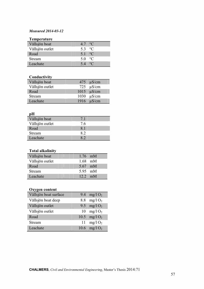
CHALMERS, Civil and Environmental Engineering, Master’s Thesis 2014:71 57
Measured 2014-03-12
Temperature Vällsjön boat 4.7 °C Vällsjön outlet 5.3 °C Road 5.1 °C Stream 5.0 °C Leachate 5.4 °C
Conductivity Vällsjön boat 475 µS/cm Vällsjön outlet 725 µS/cm Road 1015 µS/cm Stream 1030 µS/cm Leachate 1916 µS/cm
pH Vällsjön boat 7.1 Vällsjön outlet 7.6 Road 8.1 Stream 8.2 Leachate 8.2
Total alkalinity
Vällsjön boat 1.76 mM Vällsjön outlet 1.68 mM Road 5.67 mM Stream 5.95 mM Leachate 12.2 mM
Oxygen content Vällsjön boat surface 9.4 mg/l O2
Vällsjön boat deep 8.8 mg/l O2
Vällsjön outlet 9.5 mg/l O2
Vällsjön outlet 10 mg/l O2
Road 10.5 mg/l O2
Stream 11 mg/l O2
Leachate 10.6 mg/l O2
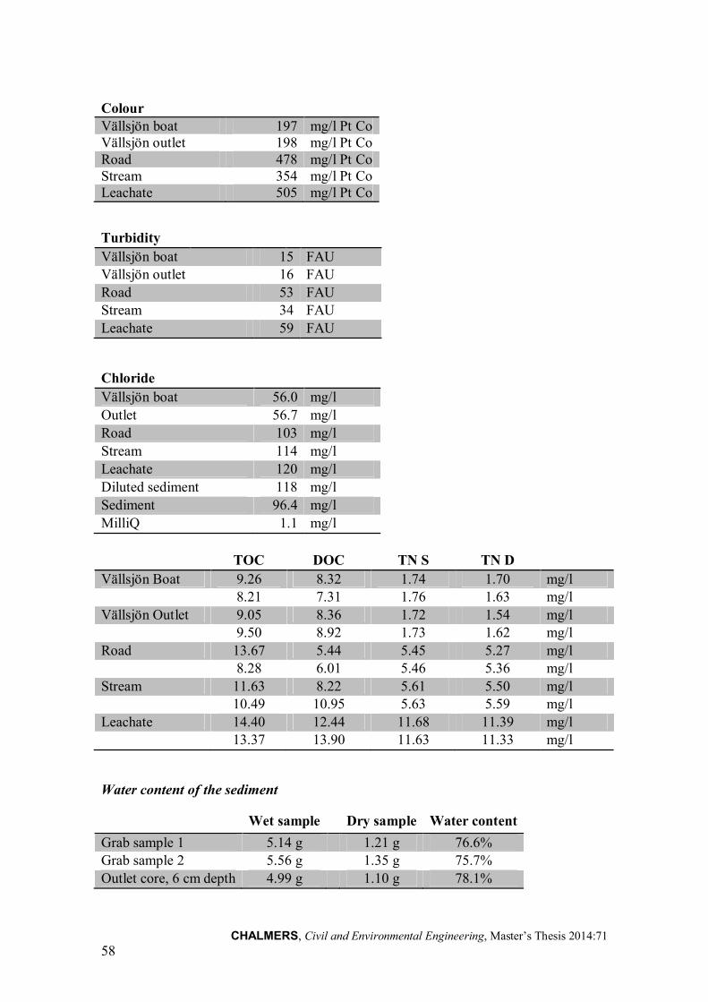
CHALMERS, Civil and Environmental Engineering, Master’s Thesis 2014:71 58
Colour
Vällsjön boat 197 mg/l Pt Co Vällsjön outlet 198 mg/l Pt Co Road 478 mg/l Pt Co Stream 354 mg/l Pt Co Leachate 505 mg/l Pt Co
Turbidity
Vällsjön boat 15 FAU Vällsjön outlet 16 FAU
Road 53 FAU Stream 34 FAU
Leachate 59 FAU
Chloride
Vällsjön boat 56.0 mg/l
Outlet 56.7 mg/l
Road 103 mg/l
Stream 114 mg/l
Leachate 120 mg/l
Diluted sediment 118 mg/l
Sediment 96.4 mg/l
MilliQ 1.1 mg/l
TOC DOC TN S TN D
Vällsjön Boat 9.26 8.32 1.74 1.70 mg/l 8.21 7.31 1.76 1.63 mg/l
Vällsjön Outlet 9.05 8.36 1.72 1.54 mg/l 9.50 8.92 1.73 1.62 mg/l
Road 13.67 5.44 5.45 5.27 mg/l 8.28 6.01 5.46 5.36 mg/l
Stream 11.63 8.22 5.61 5.50 mg/l 10.49 10.95 5.63 5.59 mg/l
Leachate 14.40 12.44 11.68 11.39 mg/l 13.37 13.90 11.63 11.33 mg/l
Water content of the sediment
Wet sample Dry sample Water content
Grab sample 1 5.14 g 1.21 g 76.6% Grab sample 2 5.56 g 1.35 g 75.7%
Outlet core, 6 cm depth 4.99 g 1.10 g 78.1%
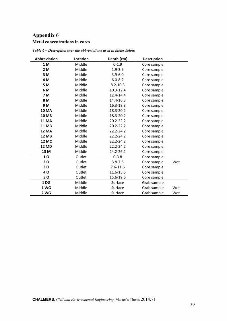
CHALMERS, Civil and Environmental Engineering, Master’s Thesis 2014:71 59
Appendix 6 Metal concentrations in cores
Table 6 – Description over the abbreviations used in tables below.
Abbreviation Location Depth [cm] Description
1 M Middle 0-1.9 Core sample 2 M Middle 1.9-3.9 Core sample 3 M Middle 3.9-6.0 Core sample 4 M Middle 6.0-8.2 Core sample 5 M Middle 8.2-10.3 Core sample 6 M Middle 10.3-12.4 Core sample 7 M Middle 12.4-14.4 Core sample 8 M Middle 14.4-16.3 Core sample 9 M Middle 16.3-18.3 Core sample
10 MA Middle 18.3-20.2 Core sample 10 MB Middle 18.3-20.2 Core sample 11 MA Middle 20.2-22.2 Core sample 11 MB Middle 20.2-22.2 Core sample 12 MA Middle 22.2-24.2 Core sample 12 MB Middle 22.2-24.2 Core sample 12 MC Middle 22.2-24.2 Core sample 12 MD Middle 22.2-24.2 Core sample 13 M Middle 24.2-26.2 Core sample
1 O Outlet 0-3.8 Core sample 2 O Outlet 3.8-7.6 Core sample Wet 3 O Outlet 7.6-11.6 Core sample 4 O Outlet 11.6-15.6 Core sample 5 O Outlet 15.6-19.6 Core sample
1 DG Middle Surface Grab sample 1 WG Middle Surface Grab sample Wet 2 WG Middle Surface Grab sample Wet
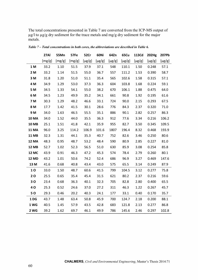
CHALMERS, Civil and Environmental Engineering, Master’s Thesis 2014:71 60
The total concentrations presented in Table 7 are converted from the ICP-MS output of µg/l to µg/g dry sediment for the trace metals and mg/g dry sediment for the major metals.
Table 7 – Total concentrations in both cores, the abbreviations are described in Table 6.
27Al 55Mn 57Fe 52Cr 60Ni 64Zn 65Cu 113Cd 202Hg 207Pb
[mg/g] [mg/g] [mg/g] [µg/g] [µg/g] [µg/g] [µg/g] [µg/g] [µg/g] [µg/g]
1 M 33.2 1.10 51.5 37.9 37.1 548 110.1 1.50 0.248 57.1
2 M 33.2 1.14 51.5 55.0 36.7 557 111.2 1.53 0.390 58.7
3 M 31.8 1.20 51.0 51.1 35.4 565 102.6 1.58 0.315 57.1
4 M 34.9 1.29 53.0 37.3 36.3 604 103.8 1.68 0.224 59.1
5 M 34.5 1.33 54.1 55.0 38.2 670 106.1 1.88 0.475 64.0
6 M 34.5 1.23 49.9 35.2 34.1 661 90.8 1.92 0.195 61.6
7 M 30.3 1.29 48.2 46.6 33.1 724 90.0 2.15 0.293 67.5
8 M 17.7 1.42 41.5 30.1 28.6 776 84.3 2.37 0.320 71.0
9 M 34.0 1.63 46.5 55.5 35.1 886 90.1 2.82 0.257 86.3
10 MA 34.0 1.52 44.0 35.5 36.3 912 77.6 3.34 0.216 106.2
10 MB 25.1 1.51 41.8 42.1 35.9 955 82.7 3.50 0.345 109.5
11 MA 96.0 3.25 114.2 106.9 101.6 1807 196.4 8.32 0.468 193.9
11 MB 32.3 1.31 44.1 35.3 40.7 752 82.6 3.46 0.250 80.6
12 MA 48.3 0.95 48.7 53.2 48.4 590 80.9 2.85 0.227 81.0
12 MB 52.7 1.02 52.3 56.5 51.0 630 85.9 3.08 0.254 85.8
12 MC 43.9 0.91 46.3 47.2 45.3 574 78.4 2.79 0.260 80.1
12 MD 43.2 1.01 50.6 74.2 52.4 686 96.9 3.27 0.469 147.6
13 M 41.6 0.68 40.8 43.4 43.0 575 65.5 3.14 0.249 87.9
1 O 33.0 1.50 48.7 60.6 41.5 799 104.5 3.12 0.277 75.8
2 O 25.5 0.65 35.4 45.4 31.5 621 80.2 2.37 0.216 59.6
3 O 23.4 0.68 36.3 40.1 32.3 705 82.8 2.80 0.400 65.5
4 O 25.3 0.52 24.6 37.0 27.2 311 46.3 1.22 0.267 45.7
5 O 29.3 0.46 20.2 40.3 24.1 177 33.1 0.40 0.170 35.7
1 DG 43.7 1.48 63.4 50.8 45.9 700 124.7 2.18 0.200 88.1
1 WG 40.5 1.45 57.9 43.5 42.8 683 121.8 2.13 0.277 86.8
2 WG 39.2 1.62 69.7 46.1 49.9 786 145.6 2.46 0.297 102.8
CHALMERS, Civil and Environmental Engineering, Master’s Thesis 2014:71 61
Appendix 7 Metal concentrations extracted in the MSEP
The total concentrations presented in Table 7the table on the next page are converted from the ICP-MS output of µg/l to µg/g dry sediment. V1 and V2 are the replicates of the sediment sample from Vällsjön and J is the sample from Järnbrott stormwater pond.
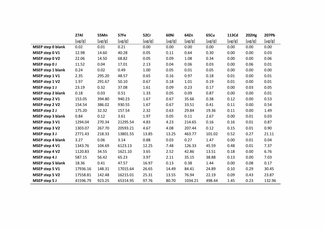
27Al 55Mn 57Fe 52Cr 60Ni 64Zn 65Cu 113Cd 202Hg 207Pb
[µg/g] [µg/g] [µg/g] [µg/g] [µg/g] [µg/g] [µg/g] [µg/g] [µg/g] [µg/g]
MSEP step 0 blank 0.02 0.01 0.21 0.00 0.00 0.00 0.00 0.00 0.00 0.00
MSEP step 0 V1 12.98 14.60 40.28 0.05 0.11 0.64 0.30 0.00 0.00 0.03
MSEP step 0 V2 22.06 14.50 68.82 0.05 0.09 1.08 0.34 0.00 0.00 0.06
MSEP step 0 J 11.52 0.04 17.01 2.13 0.04 0.06 0.03 0.00 0.06 0.01
MSEP step 1 blank 0.24 0.02 0.49 1.00 0.05 0.01 0.05 0.00 0.00 0.00
MSEP step 1 V1 2.35 295.20 48.57 0.65 0.16 0.97 0.18 0.01 0.00 0.01
MSEP step 1 V2 1.97 291.67 50.10 0.67 0.18 1.01 0.19 0.01 0.00 0.01
MSEP step 1 J 23.19 0.32 37.08 1.61 0.09 0.23 0.17 0.00 0.03 0.05
MSEP step 2 blank 0.18 0.03 0.51 1.33 0.05 0.09 0.87 0.00 0.00 0.01
MSEP step 2 V1 153.05 394.80 940.23 1.67 0.67 35.66 0.38 0.12 0.00 0.53
MSEP step 2 V2 154.54 386.02 930.55 1.67 0.67 33.51 0.41 0.11 0.00 0.54
MSEP step 2 J 175.20 32.32 157.54 2.32 0.63 29.84 19.36 0.11 0.00 1.49
MSEP step 3 blank 0.84 0.12 3.61 1.97 0.05 0.11 2.67 0.00 0.01 0.03
MSEP step 3 V1 1294.04 270.34 21295.54 4.83 4.23 214.65 0.16 0.16 0.01 0.87
MSEP step 3 V2 1303.07 267.70 20593.21 4.67 4.08 207.44 0.12 0.15 0.01 0.90
MSEP step 3 J 2771.43 218.33 13801.55 13.85 13.25 463.77 101.02 0.52 0.27 21.11
MSEP step 4 blank 3.27 0.06 3.14 0.88 0.03 0.27 1.47 0.00 0.01 0.04
MSEP step 4 V1 1343.76 104.69 6123.13 12.25 7.48 126.33 45.59 0.48 0.01 7.37
MSEP step 4 V2 1120.83 34.55 1621.10 3.65 2.52 42.86 13.51 0.18 0.00 6.76
MSEP step 4 J 587.15 56.42 65.23 3.97 2.11 35.15 38.88 0.13 0.00 7.03
MSEP step 5 blank 18.36 0.41 47.57 16.97 0.13 0.38 1.44 0.00 0.08 0.17
MSEP step 5 V1 17936.16 148.31 17015.64 26.65 14.49 84.41 24.89 0.10 0.29 30.45
MSEP step 5 V2 17558.81 142.48 16215.01 25.31 13.55 76.94 22.19 0.09 0.43 23.87
MSEP step 5 J 41596.79 923.25 65314.95 97.76 80.70 1034.21 498.44 1.45 0.23 132.96
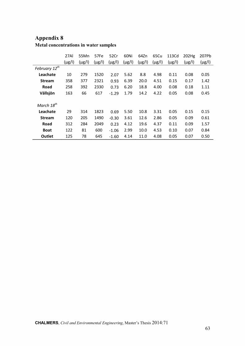
CHALMERS, Civil and Environmental Engineering, Master’s Thesis 2014:71 63
Appendix 8 Metal concentrations in water samples
27Al 55Mn 57Fe 52Cr 60Ni 64Zn 65Cu 113Cd 202Hg 207Pb
(µg/l) (µg/l) (µg/l) (µg/l) (µg/l) (µg/l) (µg/l) (µg/l) (µg/l) (µg/l)
February 12th
Leachate 10 279 1520 2.07 5.62 8.8 4.98 0.11 0.08 0.05
Stream 358 377 2321 0.93 6.39 20.0 4.51 0.15 0.17 1.42
Road 258 392 2330 0.73 6.20 18.8 4.00 0.08 0.18 1.11
Vällsjön 163 66 617 -1.29 1.79 14.2 4.22 0.05 0.08 0.45
March 18th
Leachate 29 314 1823 0.69 5.50 10.8 3.31 0.05 0.15 0.15
Stream 120 205 1490 -0.30 3.61 12.6 2.86 0.05 0.09 0.61
Road 312 284 2049 0.23 4.12 19.6 4.37 0.11 0.09 1.57
Boat 122 81 600 -1.06 2.99 10.0 4.53 0.10 0.07 0.84
Outlet 125 78 645 -1.60 4.14 11.0 4.08 0.05 0.07 0.50

CHALMERS, Civil and Environmental Engineering, Master’s Thesis 2014:71 64
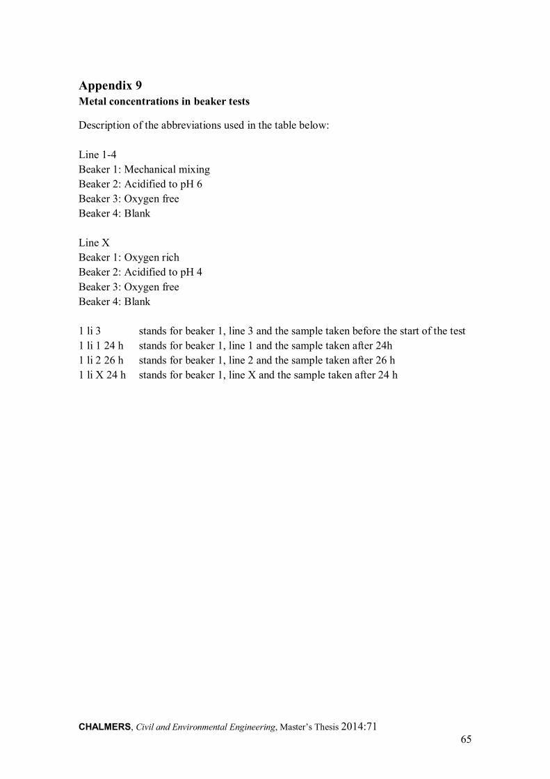
CHALMERS, Civil and Environmental Engineering, Master’s Thesis 2014:71 65
Appendix 9 Metal concentrations in beaker tests
Description of the abbreviations used in the table below:
Line 1-4
Beaker 1: Mechanical mixing
Beaker 2: Acidified to pH 6
Beaker 3: Oxygen free
Beaker 4: Blank
Line X
Beaker 1: Oxygen rich
Beaker 2: Acidified to pH 4
Beaker 3: Oxygen free
Beaker 4: Blank
1 li 3 stands for beaker 1, line 3 and the sample taken before the start of the test
1 li 1 24 h stands for beaker 1, line 1 and the sample taken after 24h
1 li 2 26 h stands for beaker 1, line 2 and the sample taken after 26 h
1 li X 24 h stands for beaker 1, line X and the sample taken after 24 h
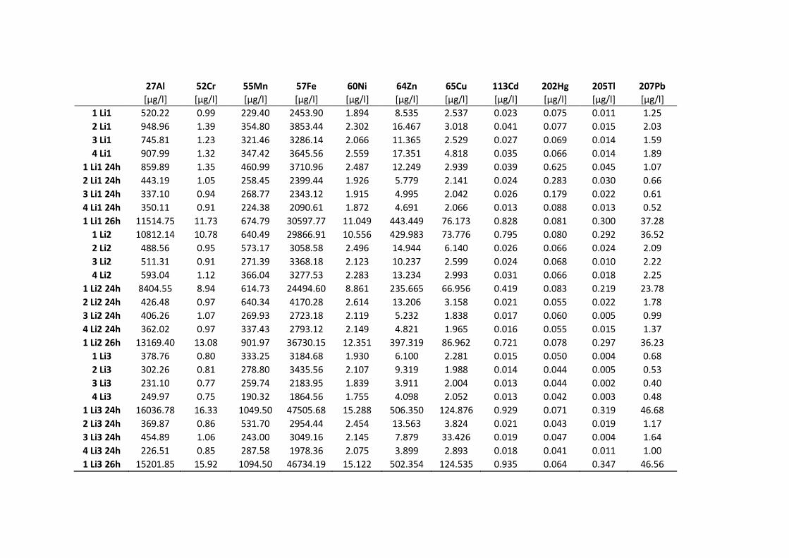
27Al 52Cr 55Mn 57Fe 60Ni 64Zn 65Cu 113Cd 202Hg 205Tl 207Pb
[µg/l] [µg/l] [µg/l] [µg/l] [µg/l] [µg/l] [µg/l] [µg/l] [µg/l] [µg/l] [µg/l]
1 Li1 520.22 0.99 229.40 2453.90 1.894 8.535 2.537 0.023 0.075 0.011 1.25
2 Li1 948.96 1.39 354.80 3853.44 2.302 16.467 3.018 0.041 0.077 0.015 2.03
3 Li1 745.81 1.23 321.46 3286.14 2.066 11.365 2.529 0.027 0.069 0.014 1.59
4 Li1 907.99 1.32 347.42 3645.56 2.559 17.351 4.818 0.035 0.066 0.014 1.89
1 Li1 24h 859.89 1.35 460.99 3710.96 2.487 12.249 2.939 0.039 0.625 0.045 1.07
2 Li1 24h 443.19 1.05 258.45 2399.44 1.926 5.779 2.141 0.024 0.283 0.030 0.66
3 Li1 24h 337.10 0.94 268.77 2343.12 1.915 4.995 2.042 0.026 0.179 0.022 0.61
4 Li1 24h 350.11 0.91 224.38 2090.61 1.872 4.691 2.066 0.013 0.088 0.013 0.52
1 Li1 26h 11514.75 11.73 674.79 30597.77 11.049 443.449 76.173 0.828 0.081 0.300 37.28
1 Li2 10812.14 10.78 640.49 29866.91 10.556 429.983 73.776 0.795 0.080 0.292 36.52
2 Li2 488.56 0.95 573.17 3058.58 2.496 14.944 6.140 0.026 0.066 0.024 2.09
3 Li2 511.31 0.91 271.39 3368.18 2.123 10.237 2.599 0.024 0.068 0.010 2.22
4 Li2 593.04 1.12 366.04 3277.53 2.283 13.234 2.993 0.031 0.066 0.018 2.25
1 Li2 24h 8404.55 8.94 614.73 24494.60 8.861 235.665 66.956 0.419 0.083 0.219 23.78
2 Li2 24h 426.48 0.97 640.34 4170.28 2.614 13.206 3.158 0.021 0.055 0.022 1.78
3 Li2 24h 406.26 1.07 269.93 2723.18 2.119 5.232 1.838 0.017 0.060 0.005 0.99
4 Li2 24h 362.02 0.97 337.43 2793.12 2.149 4.821 1.965 0.016 0.055 0.015 1.37
1 Li2 26h 13169.40 13.08 901.97 36730.15 12.351 397.319 86.962 0.721 0.078 0.297 36.23
1 Li3 378.76 0.80 333.25 3184.68 1.930 6.100 2.281 0.015 0.050 0.004 0.68
2 Li3 302.26 0.81 278.80 3435.56 2.107 9.319 1.988 0.014 0.044 0.005 0.53
3 Li3 231.10 0.77 259.74 2183.95 1.839 3.911 2.004 0.013 0.044 0.002 0.40
4 Li3 249.97 0.75 190.32 1864.56 1.755 4.098 2.052 0.013 0.042 0.003 0.48
1 Li3 24h 16036.78 16.33 1049.50 47505.68 15.288 506.350 124.876 0.929 0.071 0.319 46.68
2 Li3 24h 369.87 0.86 531.70 2954.44 2.454 13.563 3.824 0.021 0.043 0.019 1.17
3 Li3 24h 454.89 1.06 243.00 3049.16 2.145 7.879 33.426 0.019 0.047 0.004 1.64
4 Li3 24h 226.51 0.85 287.58 1978.36 2.075 3.899 2.893 0.018 0.041 0.011 1.00
1 Li3 26h 15201.85 15.92 1094.50 46734.19 15.122 502.354 124.535 0.935 0.064 0.347 46.56
27Al 52Cr 55Mn 57Fe 60Ni 64Zn 65Cu 113Cd 202Hg 205Tl 207Pb
[µg/l] [µg/l] [µg/l] [µg/l] [µg/l] [µg/l] [µg/l] [µg/l] [µg/l] [µg/l] [µg/l]
1 Li4 289.31 0.85 172.14 1379.18 1.828 5.903 3.617 0.024 0.040 0.003 0.58
2 Li4 274.44 0.87 155.02 1212.97 1.723 5.010 2.677 0.017 0.035 0.002 0.46
3 Li4 253.65 0.84 164.53 1322.13 1.689 5.172 2.472 0.012 0.035 0.002 0.49
4 Li4 274.42 0.86 169.21 1225.45 1.701 5.129 2.479 0.016 0.035 0.003 0.45
1 Li4 24h 14635.60 14.40 1028.88 40262.41 14.070 491.945 107.195 0.954 0.046 0.333 41.41
2 Li4 24h 316.79 0.77 442.83 1744.00 2.263 13.641 2.969 0.019 0.036 0.025 1.08
3 Li4 24h 369.07 1.00 230.21 1760.46 1.908 7.513 2.669 0.026 0.039 0.006 0.99
4 Li4 24h 307.16 0.84 229.57 1468.09 1.898 6.128 2.627 0.017 0.039 0.016 1.07
1 Li4 26h 14293.54 14.23 1084.85 39099.68 14.066 486.597 107.349 0.972 0.066 0.345 41.51
1 LiX 1069.45 1.55 394.52 3874.20 2.606 30.697 6.165 0.066 0.039 0.013 2.19
2 LiX 901.51 1.41 340.82 3310.74 2.430 24.651 5.236 0.055 0.037 0.012 1.87
3 LiX 1061.65 1.56 374.10 3750.86 2.561 29.835 5.898 0.068 0.035 0.014 2.19
4 LiX 666.11 1.18 331.30 2734.84 2.274 17.159 4.209 0.039 0.034 0.008 1.40
1 LiX 24h 6636.04 6.78 1576.04 19788.76 7.770 216.368 36.080 0.470 0.044 0.240 21.35
2 LiX 24h 828.65 1.26 1048.93 4744.03 3.824 89.161 5.909 0.155 0.033 0.048 2.50
3 LiX 24h 1299.51 1.77 242.96 4229.43 2.745 34.527 6.593 0.081 0.037 0.014 2.76
4 LiX 24h 900.70 1.45 402.15 3272.25 2.63 22.66 5.06 0.056 0.036 0.025 2.51

CHALMERS, Civil and Environmental Engineering, Master’s Thesis 2014:71 68
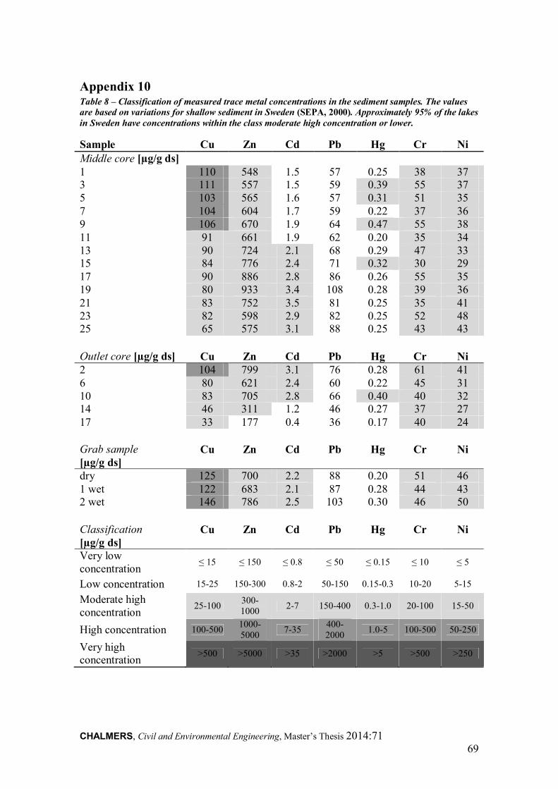
CHALMERS, Civil and Environmental Engineering, Master’s Thesis 2014:71 69
Appendix 10 Table 8 – Classification of measured trace metal concentrations in the sediment samples. The values are based on variations for shallow sediment in Sweden (SEPA, 2000). Approximately 95% of the lakes in Sweden have concentrations within the class moderate high concentration or lower.
Sample Cu Zn Cd Pb Hg Cr Ni Middle core [µg/g ds] 1 110 548 1.5 57 0.25 38 37 3 111 557 1.5 59 0.39 55 37 5 103 565 1.6 57 0.31 51 35 7 104 604 1.7 59 0.22 37 36 9 106 670 1.9 64 0.47 55 38 11 91 661 1.9 62 0.20 35 34 13 90 724 2.1 68 0.29 47 33 15 84 776 2.4 71 0.32 30 29 17 90 886 2.8 86 0.26 55 35 19 80 933 3.4 108 0.28 39 36 21 83 752 3.5 81 0.25 35 41 23 82 598 2.9 82 0.25 52 48 25 65 575 3.1 88 0.25 43 43
Outlet core [µg/g ds] Cu Zn Cd Pb Hg Cr Ni 2 104 799 3.1 76 0.28 61 41 6 80 621 2.4 60 0.22 45 31 10 83 705 2.8 66 0.40 40 32 14 46 311 1.2 46 0.27 37 27 17 33 177 0.4 36 0.17 40 24
Grab sample [µg/g ds]
Cu Zn Cd Pb Hg Cr Ni
dry 125 700 2.2 88 0.20 51 46 1 wet 122 683 2.1 87 0.28 44 43 2 wet 146 786 2.5 103 0.30 46 50
Classification [µg/g ds]
Cu Zn Cd Pb Hg Cr Ni
Very low concentration
≤ 15 ≤ 150 ≤ 0.8 ≤ 50 ≤ 0.15 ≤ 10 ≤ 5
Low concentration 15-25 150-300 0.8-2 50-150 0.15-0.3 10-20 5-15
Moderate high concentration
25-100 300-1000
2-7 150-400 0.3-1.0 20-100 15-50
High concentration 100-500 1000-5000
7-35 400-2000
1.0-5 100-500 50-250
Very high concentration
>500 >5000 >35 >2000 >5 >500 >250

Related Documents