Master Thesis A Vortex Lattice MATLAB Implementation for Linear Aerodynamic Wing Applications. Tomas Melin. Royal Institute of Technology (KTH). Department of Aeronautics. December 2000.

Welcome message from author
This document is posted to help you gain knowledge. Please leave a comment to let me know what you think about it! Share it to your friends and learn new things together.
Transcript
8/7/2019 tornado thesis
http://slidepdf.com/reader/full/tornado-thesis 1/45
8/7/2019 tornado thesis
http://slidepdf.com/reader/full/tornado-thesis 2/45
Tomas Melin. KTH, Department of Aeronautics. Page 2 (45)A Vortex Lattice MATLAB Implementation for Linear Aerodynamic Wing Applications.
SUMMARY.
This document is the Master thesis "A Vortex Lattice MATLAB Implementation for Linear
Aerodynamics Wing Applications" by Tomas Melin. A user's manual for the developed
vortex lattice code "Tornado" is also included.
The physical problem addressed was to find the aerodynamic forces acting on an aircraft
flying at low subsonic speeds, below the stall limit. The primary research issue was to detect
if it would be possible to code a vortex lattice method fast enough for real time application.
One of the requirements was that it must be possible to perform computations for most types
of wing layouts. The current version of Tornado handles tapered, swept, dihedraled and
twisted multi cranked wing configurations with trailing edge control surfaces.The governing equations used to solve the physical problem came from standard vortex lattice
theory. The law of Biot-Savart was used to get the flowfield around a finite straight vortex
line, one of the basic vortex segments needed for the lattice. These vortices induce a flow
field in the air, and their strength was determined by the boundary conditions that no air
should flow through the wings.
The forces acting on each vortex segment can be determined by employing the Kutta-
Jukovski theorem. These forces may then be integrated to yield a composite force in 3dimensions, which in turn may be used to compute aerodynamic coefficients and stability
derivatives.
The computational problem is to creating a good system for dealing with the mathematical
results. The Tornado code allows many different kinds of computations, which yields good
coherence with experimental data.
The Tornado code has shown very good coherence with theoretical data, such as Jones' small
aspect ratio theory and Prandtl's lifting line. Furthermore, Tornado gives good results when
comparing with commercial software and also yield accurate results when comparing to
experimental data. However, the computing time for more complex geometry consume
solution times in the order of minutes, which is too slow for a real time application, such as a
flight simulator.
The conclusion is that Tornado may be used for a wide variety of applications, but that the
real time vortex lattice method still requires more computing capacity than available in
desktop computers.
8/7/2019 tornado thesis
http://slidepdf.com/reader/full/tornado-thesis 3/45
Tomas Melin. KTH, Department of Aeronautics. Page 3 (45)A Vortex Lattice MATLAB Implementation for Linear Aerodynamic Wing Applications.
CONTENTS.
SUMMARY..... ................................................................. ................................................................ ...................... 2
CONTENTS. ..................................................... ............................................................ ......................................... 3
SYMBOLS. .................................................... ............................................................ ....................................... 5
1 INTRODUCTION. ............................................................ .......................................................... ....................... 7
1.1 BACKGROUND...........................................................................................................................................7
2 PHYSICAL PROBLEM. ................................................ ....................................................... ............................ 7
2.1 DIFFERENT FORCES.........................................................................................................................................82.1.1 Pressure forces. ................................................... ............................................................ ....................... 8
2.2.2 Friction forces. .......................................................................................................................................8
1.3 SEPARATING THE PROBLEM............................................................................................................................91.4 LINEAR AERODYNAMICS................................................................................................................................9
2.4.1 Potential Flow. ...................................................... .......................................................... ..................... 10
2.4.2 Vortices.................................................................................................................................................10
3. MATHEMATICAL PROBLEM................................................... .................................................... .............11
3.1 SOLUTION DOMAIN.......................................................................................................................................113.1.1 Potential flow........................................................................................................................................11
3.1.2 Biot-Savart............................................................................................................................................12
3.1.2 The Vortex Lattice Method. ..................................................................................................................13
4 COMPUTATIONAL METHOD..... ................................................................. ............................................... 16
4.1 VORTEX LATTICE..........................................................................................................................................164.1.1 Preprocessor.........................................................................................................................................16
4.1.2 Solver....................................................................................................................................................17 4.1.3 Postprocessor. ......................................................................................................................................20
4.2 COMPUTATION ACCURACY VS COMPUTATION SPEED. .................................................................................204.3 THE GEOMETRY PROBLEM IN 3D, FROM SIMPLE TO COMPLEX. .....................................................................21
4.3.1 Taper, Sweep and Dihedral on a quadrilateral wing. ..........................................................................21
4.3.2 Twist and the skewed vortex loop. .............................................. ...................................................... ....22
4.3.3 Camber and thin airfoil boundary application.....................................................................................22
4.3.4 The polyhedral wing. ................................................. ...................................................... ..................... 23
4.3.5 The multi wing configuration................................................................................................................24
4.4 KINKS AND QUIRKS. .....................................................................................................................................244.4.1 The panel normal..................................................................................................................................24
4.4.2 The panel area......................................................................................................................................25
4.4.3 Reference units .....................................................................................................................................26
4.4.4 Trailing vortices Wake..........................................................................................................................26 4.4.5 The far wake problem. .............................................. .................................................... ........................26
4.4.6 The piercing vortex remedy. .................................................. ........................................................... ....28
4.4.7 Analogy with the inwash problem.........................................................................................................29
4.4.8 Free wake. ............................................................................................................................................29
4.4.9 Rotations...............................................................................................................................................30
4.4.10 Deflected surfaces: ................................................................ ......................................................... ....30
5 VALIDATION. ..................................................... ............................................................ ................................ 31
5.1 METHOD.......................................................................................................................................................315.1.1 Prandtl's Lifting line and Jones small aspect ratio...............................................................................31
5.1.2 Bertin & Smith example........................................................................................................................32
5.1.3 Comparison with commercial software. ....................................................... ........................................ 34
5.1.4 Experimental Results. ............................................................ ........................................................... ....38
6 RESULTS. ........................................................... ............................................................... ............................... 40
8/7/2019 tornado thesis
http://slidepdf.com/reader/full/tornado-thesis 4/45
Tomas Melin. KTH, Department of Aeronautics. Page 4 (45)A Vortex Lattice MATLAB Implementation for Linear Aerodynamic Wing Applications.
6.1 LIFTING LINE. ...................................................... ........................................................... .............................. 406.2 SIMPLE WING................................................................................................................................................406.3 CESSNA 172..................................................................................................................................................406.4 ACCURACY...................................................................................................................................................406.5 SOLUTION TIME............................................................................................................................................406.6 SUITABILITY FOR REAL-TIME APPLICATIONS. ...............................................................................................41
7 DISCUSSION..................... ................................................................ .......................................................... .....41
7.1 ERROR SOURCES...........................................................................................................................................417.2 FUTURE WORK..............................................................................................................................................42
7.2.1 Supersonic vortex lattice method..........................................................................................................42
7.2.2 Time Dependent factors........................................................................................................................42
7.2.3 Vortex potential. ....................................................... ....................................................... ..................... 43
8 ACKNOWLEDGEMENTS. ................................................................ ......................................................... ...44
9 REFERENCES. ...................................................... ............................................................ .............................. 44
10 BIBLIOGRAPHY....................... .................................................... ............................................................ ....45
11 APPENDIX. ......................................................... ............................................................ ............................... 45
8/7/2019 tornado thesis
http://slidepdf.com/reader/full/tornado-thesis 5/45
8/7/2019 tornado thesis
http://slidepdf.com/reader/full/tornado-thesis 6/45
Tomas Melin. KTH, Department of Aeronautics. Page 6 (45)
A Vortex Lattice MATLAB Implementation for Linear Aerodynamic Wing Applications.
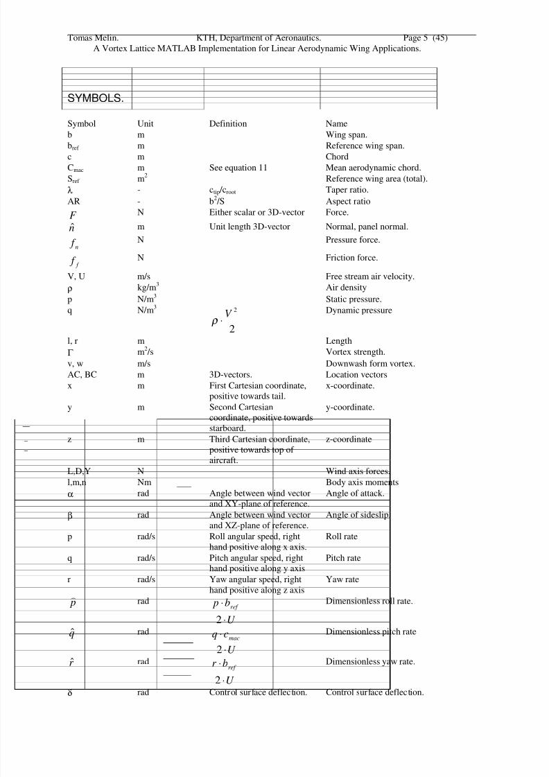
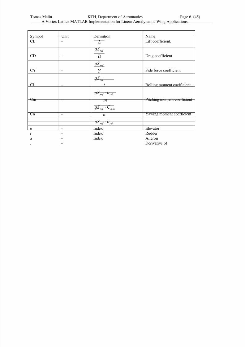
Symbol Unit Definition Name
CL -
ref qS
L Lift coefficient.
CD -
ref qS
D Drag coefficient
CY -
ref qS
Y Side force coefficient
Cl -
ref ref bqS
l
⋅
Rolling moment coefficient.
Cm -
macref C qS
m
⋅
Pitching moment coefficient
Cn -
ref ref bqS
n
⋅
Yawing moment coefficient
e - Index Elevator
r - Index Rudder
a - Index Aileron
, - Derivative of
8/7/2019 tornado thesis
http://slidepdf.com/reader/full/tornado-thesis 7/45
Tomas Melin. KTH, Department of Aeronautics. Page 7 (45)
A Vortex Lattice MATLAB Implementation for Linear Aerodynamic Wing Applications.
1 INTRODUCTION.
1.1 BACKGROUND.
When the project resulting in this thesis was defined, its aim was to researching whether or
not a vortex lattice method (VLM) could be used in a real time application such as an aircraft
simulator. The VLM would supply the aerodynamic force model for the simulation and
hopefully do this with a better resolution than a table lookup/interpolation routine would do.
Fairly soon it became clear that it was possible to do the computations in real time for coarse
aircraft models, but then the output would be no better than a table lookup routine. The focus
was then shifted towards producing a vortex lattice method implemented in Matlab with an
easily extendable interface.This thesis will deal mostly with the standard vortex lattice methodology even though the real
time issue will be addressed in the discussion.
It should be said however, that computer power is still increasing and that a real-time
application might very well be possible in only a few years.
2 PHYSICAL PROBLEM.
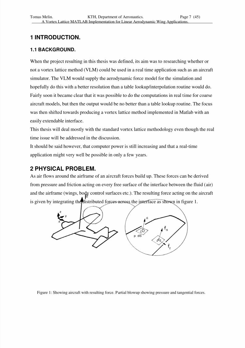
As air flows around the airframe of an aircraft forces build up. These forces can be derived
from pressure and friction acting on every free surface of the interface between the fluid (air)
and the airframe (wings, body control surfaces etc.). The resulting force acting on the aircraft
is given by integrating the distributed forces across the interface as shown in figure 1.
Figure 1: Showing aircraft with resulting force. Partial blowup showing pressure and tangential forces.
8/7/2019 tornado thesis
http://slidepdf.com/reader/full/tornado-thesis 8/45
Tomas Melin. KTH, Department of Aeronautics. Page 8 (45)
A Vortex Lattice MATLAB Implementation for Linear Aerodynamic Wing Applications.
2.1 Different forces.
The force acting on an infinitesimal area of the interface can be divided into two
components. One of them is perpendicular to the surface and the other is
parallel. The physical interpretation being that the perpendicular force is a
pressure force and the parallel force a shear, or friction, force.
2.1.1 Pressure forces.
The pressure forces are the forces acting along the normal of the interface. The
total pressure in the fluid is constant and consisting of the static and the dynamic
pressure. At rest, the total pressure is equal to the static pressure and constant at
every point of the interface. Once in motion, the airframe creates a flow field in
the air. As the interface is impenetrable the fluid must move to allow the passage
of the airframe thus creating the flow field. The shape of this field is highly
dependent of the shape of the interface. Thus parts of the airframe facing the
wind experience a higher static pressure than areas parallel to the wind or on the
off-wind side. This accounts for the pressure forces on the interface.
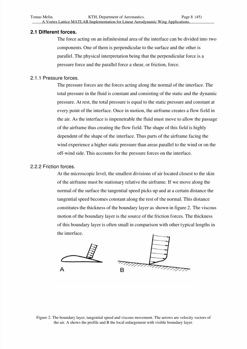
2.2.2 Friction forces.
At the microscopic level, the smallest divisions of air located closest to the skin
of the airframe must be stationary relative the airframe. If we move along thenormal of the surface the tangential speed picks up and at a certain distance the
tangential speed becomes constant along the rest of the normal. This distance
constitutes the thickness of the boundary layer as shown in figure 2. The viscous
motion of the boundary layer is the source of the friction forces. The thickness
of this boundary layer is often small in comparison with other typical lengths in
the interface.
Figure 2. The boundary layer, tangential speed and viscous movement. The arrows are velocity vectors of
the air. A shows the profile and B the local enlargement with visible boundary layer.
8/7/2019 tornado thesis
http://slidepdf.com/reader/full/tornado-thesis 9/45
Tomas Melin. KTH, Department of Aeronautics. Page 9 (45)
A Vortex Lattice MATLAB Implementation for Linear Aerodynamic Wing Applications.
1.3 Separating the problem.
The phenomenon with two different forces from different sources enables us to
separate the problem of aerodynamic forces. This is usually done by separately
assessing the outer problem concerning the pressure forces, and the inner
problem concerning friction forces. This study is focused on the outer problem,
since pressure forces are dominant in certain physical domains; the domain
addressed linear aerodynamics.
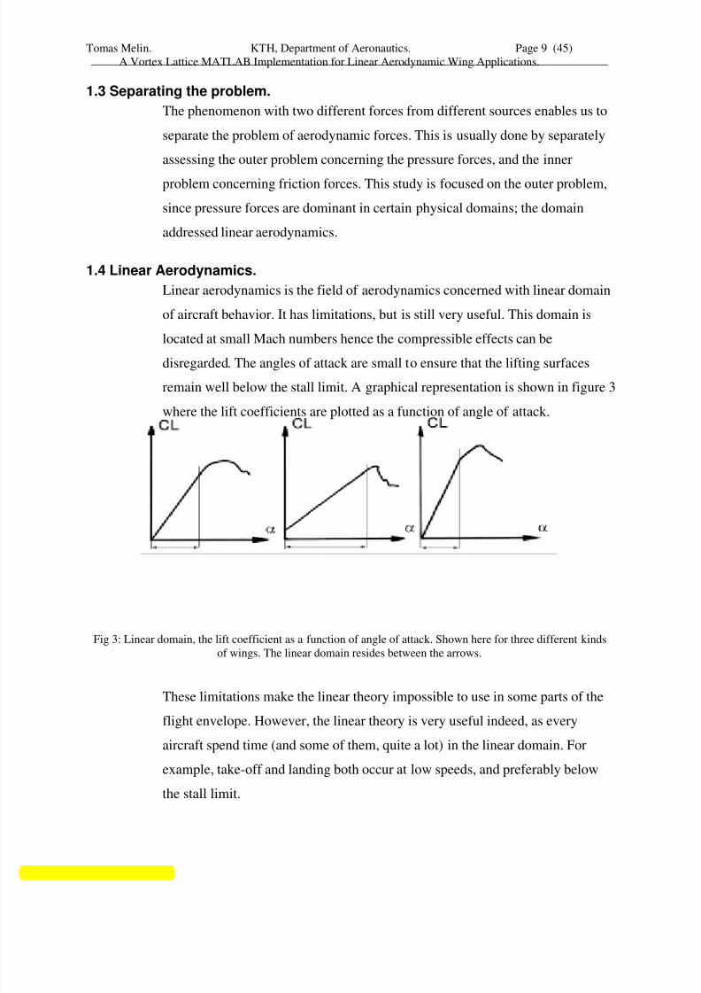
1.4 Linear Aerodynamics.
Linear aerodynamics is the field of aerodynamics concerned with linear domain
of aircraft behavior. It has limitations, but is still very useful. This domain is
located at small Mach numbers hence the compressible effects can be
disregarded. The angles of attack are small to ensure that the lifting surfaces
remain well below the stall limit. A graphical representation is shown in figure 3
where the lift coefficients are plotted as a function of angle of attack.
These limitations make the linear theory impossible to use in some parts of the
flight envelope. However, the linear theory is very useful indeed, as every
aircraft spend time (and some of them, quite a lot) in the linear domain. For
example, take-off and landing both occur at low speeds, and preferably below
the stall limit.
Fig 3: Linear domain, the lift coefficient as a function of angle of attack. Shown here for three different kinds
of wings. The linear domain resides between the arrows.
8/7/2019 tornado thesis
http://slidepdf.com/reader/full/tornado-thesis 10/45
Tomas Melin. KTH, Department of Aeronautics. Page 10 (45)
A Vortex Lattice MATLAB Implementation for Linear Aerodynamic Wing Applications.
2.4.1 Potential Flow.
The method described later is only accurate in the potential flow domain, which
is the same as the domain of linear aerodynamics, small angles of attack and
small Mach numbers
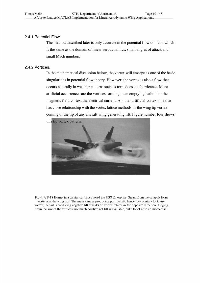
2.4.2 Vortices.
In the mathematical discussion below, the vortex will emerge as one of the basic
singularities in potential flow theory. However, the vortex is also a flow that
occurs naturally in weather patterns such as tornadoes and hurricanes. More
artificial occurrences are the vortices forming in an emptying bathtub or the
magnetic field vortex, the electrical current. Another artificial vortex, one that
has close relationship with the vortex lattice methods, is the wing tip vortex
coming of the tip of any aircraft wing generating lift. Figure number four shows
this tip vortex pattern.
Fig 4: A F-18 Hornet in a carrier cat-shot aboard the USS Enterprise. Steam from the catapult formvortices at the wing tips. The main wing is producing positive lift, hence the counter clockwise
vortex, the tail is producing negative lift thus it's tip vortex rotates in the opposite direction. Judging
from the size of the vortices, not much positive net lift is available, but a lot of nose up moment is.
8/7/2019 tornado thesis
http://slidepdf.com/reader/full/tornado-thesis 11/45
Tomas Melin. KTH, Department of Aeronautics. Page 11 (45)
A Vortex Lattice MATLAB Implementation for Linear Aerodynamic Wing Applications.
3. MATHEMATICAL PROBLEM.
3.1 Solution domain.
3.1.1 Potential flow.
When considering a vector field where the rotation along any closed path is
zero, the conclusion arises that the line integral between two points in the field is
independent of the path. Such a flow field is called conservative [A. Ramgard,
1992]. The concept of conservative fields allows the definition of the potential:
φ∇=A ...................................................................................( 1 )
where φ equals the potential of A.
This mathematical theory can be, and is, applied to many physical problems.
Among these are the theory of electric potential and the theory of velocity
potentials in flow fields.
In the case of a fluid flow the field is defined as follows for an irrotational,
incompressible flow. [J.D. Anderson, 1991]:
No mass is produced in the field so,
0=⋅∇ V .......................................................................................(2)
Further, as the flow is irrotational,
φ∇=V .........................................................................................(3)
Hence,
( ) 0=φ∇⋅∇ ...................................................................................(4)
or
02 =φ∇ .........................................................................................(5)
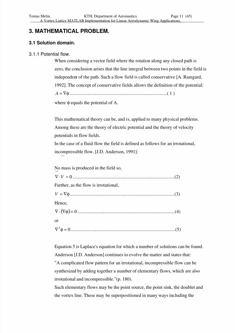
Equation 5 is Laplace's equation for which a number of solutions can be found.
Anderson [J.D. Anderson] continues to evolve the matter and states that:
"A complicated flow pattern for an irrotational, incompressible flow can be
synthesized by adding together a number of elementary flows, which are also
irrotational and incompressible."(p. 180).
Such elementary flows may be the point source, the point sink, the doublet and
the vortex line. These may be superpositioned in many ways including the
8/7/2019 tornado thesis
http://slidepdf.com/reader/full/tornado-thesis 12/45
Tomas Melin. KTH, Department of Aeronautics. Page 12 (45)
A Vortex Lattice MATLAB Implementation for Linear Aerodynamic Wing Applications.
formation of line sources, vortex sheets and so on. As one may use an arbitrary
number of singularities the concept of using numerical methods is close at hand.
Today, a wide variety of methods exist and one of them is the vortex lattice
method (VLM).
3.1.2 Biot-Savart.
One special kind of singularity is the vortex line. The infinite vortex line induces
a flow field around a line with the induced flow perpendicular to the radius and
the strength inversely proportional to the radius. The field is defined by equation
6.
Θ⋅π
Γ
= er U 2 ..............................................................................( 6 )
Where Γ is the field strength, r the radius to line and U the induced velocity.
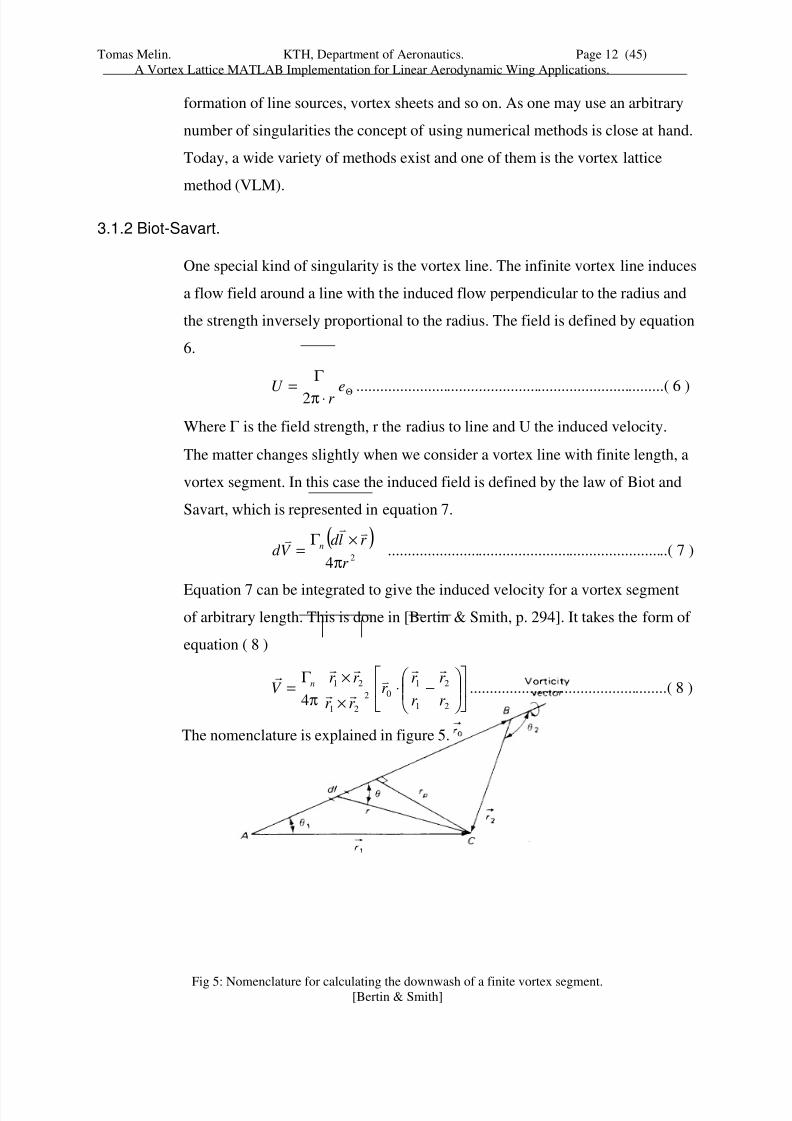
The matter changes slightly when we consider a vortex line with finite length, a
vortex segment. In this case the induced field is defined by the law of Biot and
Savart, which is represented in equation 7.
( )2
4 r
r ld V d n
π×Γ
=*
*
*
.......................................................................( 7 )
Equation 7 can be integrated to give the induced velocity for a vortex segment
of arbitrary length. This is done in [Bertin & Smith, p. 294]. It takes the form of
equation ( 8 )
−⋅
×
×π
Γ =
2
2
1
1
02
21
21
4 r
r
r
r r
r r
r r V n
&&
*
&&
&&
&
..................................................( 8 )
The nomenclature is explained in figure 5.
Fig 5: Nomenclature for calculating the downwash of a finite vortex segment.[Bertin & Smith]
8/7/2019 tornado thesis
http://slidepdf.com/reader/full/tornado-thesis 13/45
Tomas Melin. KTH, Department of Aeronautics. Page 13 (45)
A Vortex Lattice MATLAB Implementation for Linear Aerodynamic Wing Applications.
These vortex segments can be utilized to build very intricate vortex systems,
such as the meshwork of vortex segments used in the vortex lattice.
The traditional vortex lattice method uses three vortex segments for the "vortex
horse-shoe" used on every panel. Tornado on the other hand, uses 7 vortex
segments for each panel.
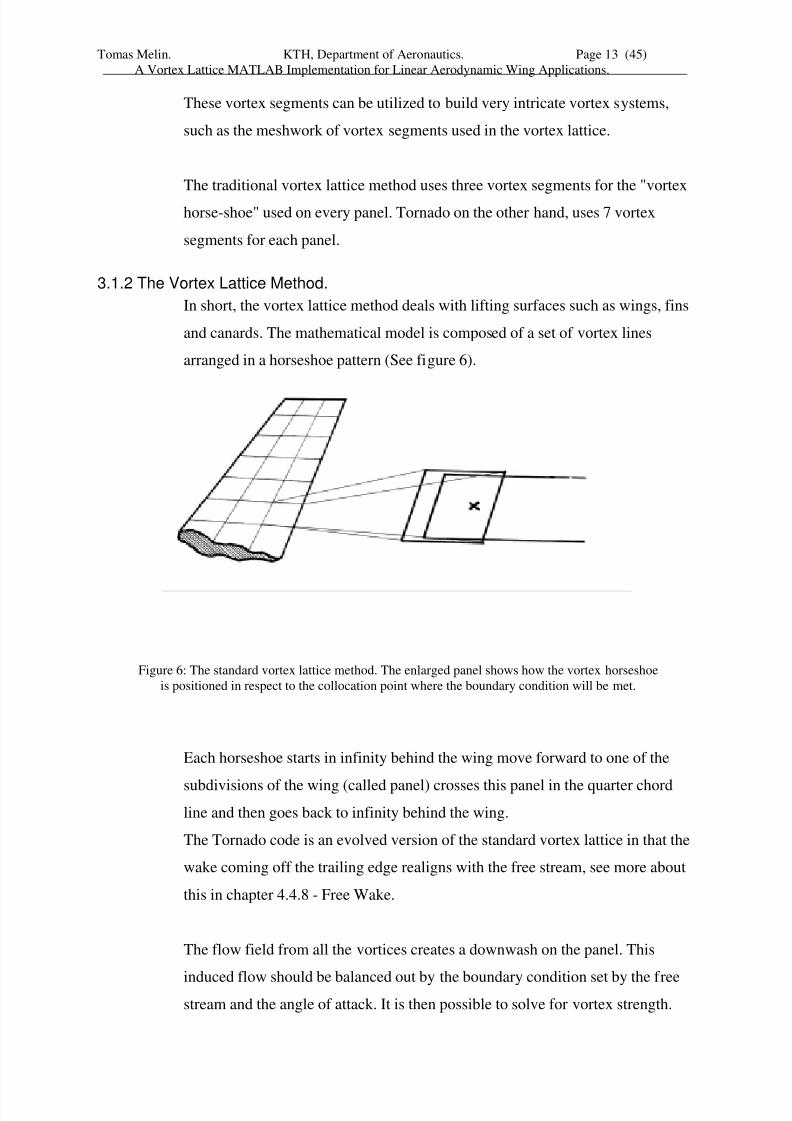
3.1.2 The Vortex Lattice Method.
In short, the vortex lattice method deals with lifting surfaces such as wings, fins
and canards. The mathematical model is composed of a set of vortex lines
arranged in a horseshoe pattern (See figure 6).
Each horseshoe starts in infinity behind the wing move forward to one of the
subdivisions of the wing (called panel) crosses this panel in the quarter chord
line and then goes back to infinity behind the wing.
The Tornado code is an evolved version of the standard vortex lattice in that the
wake coming off the trailing edge realigns with the free stream, see more about
this in chapter 4.4.8 - Free Wake.
The flow field from all the vortices creates a downwash on the panel. This
induced flow should be balanced out by the boundary condition set by the freestream and the angle of attack. It is then possible to solve for vortex strength.
Figure 6: The standard vortex lattice method. The enlarged panel shows how the vortex horseshoe
is positioned in respect to the collocation point where the boundary condition will be met.
8/7/2019 tornado thesis
http://slidepdf.com/reader/full/tornado-thesis 14/45
Tomas Melin. KTH, Department of Aeronautics. Page 14 (45)
A Vortex Lattice MATLAB Implementation for Linear Aerodynamic Wing Applications.
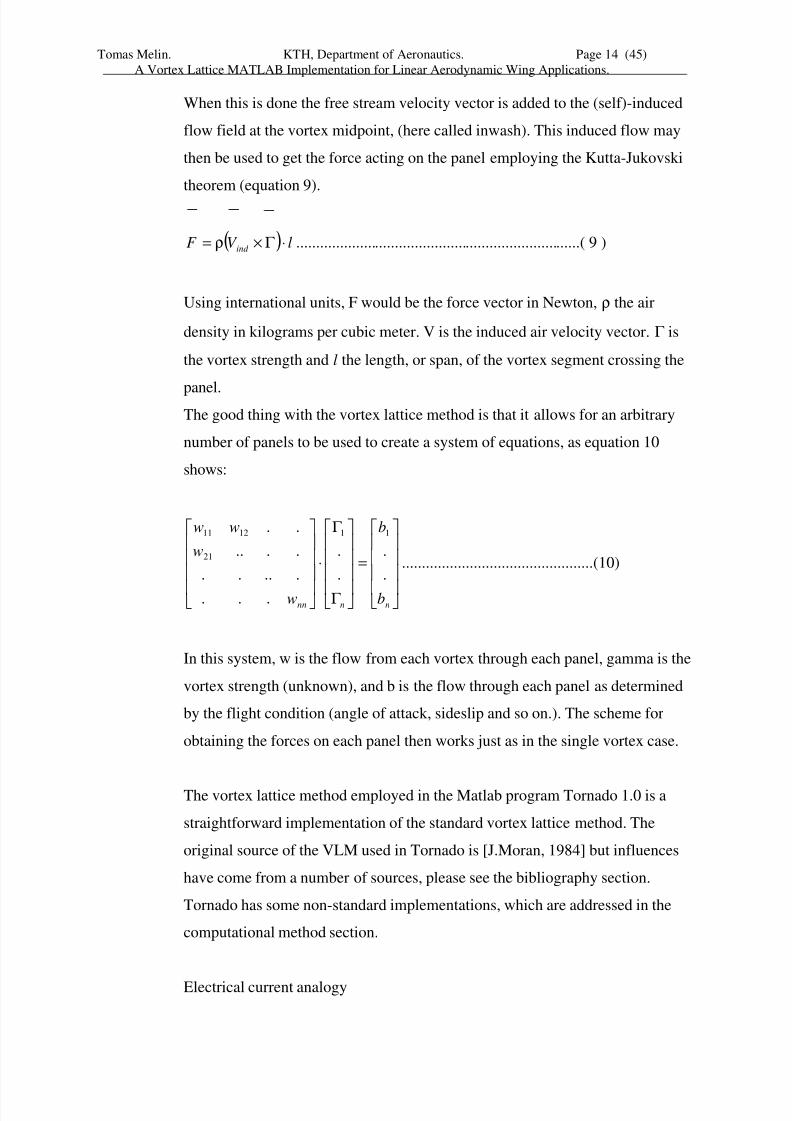
When this is done the free stream velocity vector is added to the (self)-induced
flow field at the vortex midpoint, (here called inwash). This induced flow may
then be used to get the force acting on the panel employing the Kutta-Jukovski
theorem (equation 9).
( ) lV F ind ⋅Γ ×ρ= ........................................................................( 9 )
Using international units, F would be the force vector in Newton, ρ the air
density in kilograms per cubic meter. V is the induced air velocity vector. Γ is
the vortex strength and l the length, or span, of the vortex segment crossing the
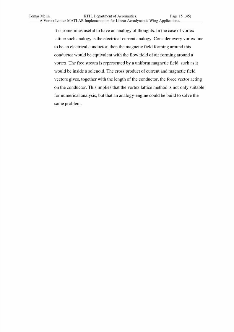
panel.The good thing with the vortex lattice method is that it allows for an arbitrary
number of panels to be used to create a system of equations, as equation 10
shows:
=
Γ
Γ
⋅
nnnn b
b
w
w
ww
.
.
.
.
...
.....
....
.. 11
21
1211
................................................(10)
In this system, w is the flow from each vortex through each panel, gamma is the
vortex strength (unknown), and b is the flow through each panel as determined
by the flight condition (angle of attack, sideslip and so on.). The scheme for
obtaining the forces on each panel then works just as in the single vortex case.
The vortex lattice method employed in the Matlab program Tornado 1.0 is a
straightforward implementation of the standard vortex lattice method. The
original source of the VLM used in Tornado is [J.Moran, 1984] but influences
have come from a number of sources, please see the bibliography section.
Tornado has some non-standard implementations, which are addressed in the
computational method section.
Electrical current analogy
8/7/2019 tornado thesis
http://slidepdf.com/reader/full/tornado-thesis 15/45
Tomas Melin. KTH, Department of Aeronautics. Page 15 (45)
A Vortex Lattice MATLAB Implementation for Linear Aerodynamic Wing Applications.
It is sometimes useful to have an analogy of thoughts. In the case of vortex
lattice such analogy is the electrical current analogy. Consider every vortex line
to be an electrical conductor, then the magnetic field forming around this
conductor would be equivalent with the flow field of air forming around a
vortex. The free stream is represented by a uniform magnetic field, such as it
would be inside a solenoid. The cross product of current and magnetic field
vectors gives, together with the length of the conductor, the force vector acting
on the conductor. This implies that the vortex lattice method is not only suitable
for numerical analysis, but that an analogy-engine could be build to solve the
same problem.
8/7/2019 tornado thesis
http://slidepdf.com/reader/full/tornado-thesis 16/45
Tomas Melin. KTH, Department of Aeronautics. Page 16 (45)
A Vortex Lattice MATLAB Implementation for Linear Aerodynamic Wing Applications.
4 COMPUTATIONAL METHOD.
4.1 Vortex lattice.
The problem of solving for pressure forces using the vortex lattice method was
set up in Matlab to ensure code portability across platforms. The developed code
has three main features, the preprocessor, the solver and the postprocessor.
Most of effort was put on the development of the preprocessor and the solver,
since these two parts required the most attention.
4.1.1 Preprocessor.
The preprocessor sets up the vortex lattice and the boundary conditions from theuser inputs. Tornado accepts file input as well as interactive input. The
preprocessor has a number of internal steps, described here.
Input.
The user should be able to define the aircraft shape, as he wants it. In the current
version of Tornado the input is either done through file or through interactive
input. The preprocessor takes care of this and forwards all relevant information
to the layout function.
Layout.
From the user input, the preprocessor must setup the wing layout, or the
planform. The wings should be located at specific coordinates with
predetermined geometric angle of attack, span, sweep, dihedral and so on. The
deflecting control surfaces should be located in the correct position and have the
proper size. The trick is to get the corner points of the wings to be positioned in
the appropriate coordinates.
Meshing.
When the planform is laid out, the meshing function divides the wings into
panels. In the very simplest case one panel per wing is sufficient but increasing
accuracy comes with greater numbers of panels. The corner points of each panel
are important as they are used in the computation of the area of each panel.Furthermore they are the source of the position of the collocation point, the
8/7/2019 tornado thesis
http://slidepdf.com/reader/full/tornado-thesis 17/45
Tomas Melin. KTH, Department of Aeronautics. Page 17 (45)
A Vortex Lattice MATLAB Implementation for Linear Aerodynamic Wing Applications.
point at ¾ panel chord where the boundary condition should be satisfied. From
the panel corner points the vortex coordinates are computed. The first point of
each vortex-sling should be in the infinity behind the aircraft, however it's more
appropriate for visualization to put this point somewhere 2-3 wing spans behind
the aircraft, it will be shown later that the influence from the truncated part can
be neglected. The second vortex point is located at the trailing edge, parallel to
the port side chord of the panel in question (see figure 8). The next vortex point
is located at the hinge line (if there is a deflecting control surface downstream of
the panel), the following vortex point is at the ¼ chord position on port side of
the panel in question. Here the vortex crosses the panel to the starboard side and
this vortex segment will later be producing lift. The vortex line then continues
rearwards on the starboard side in the same manner.
Furthermore, the normal of each panel at the collocation point must also be
calculated. The normal is a vital instrument when calculating the flow
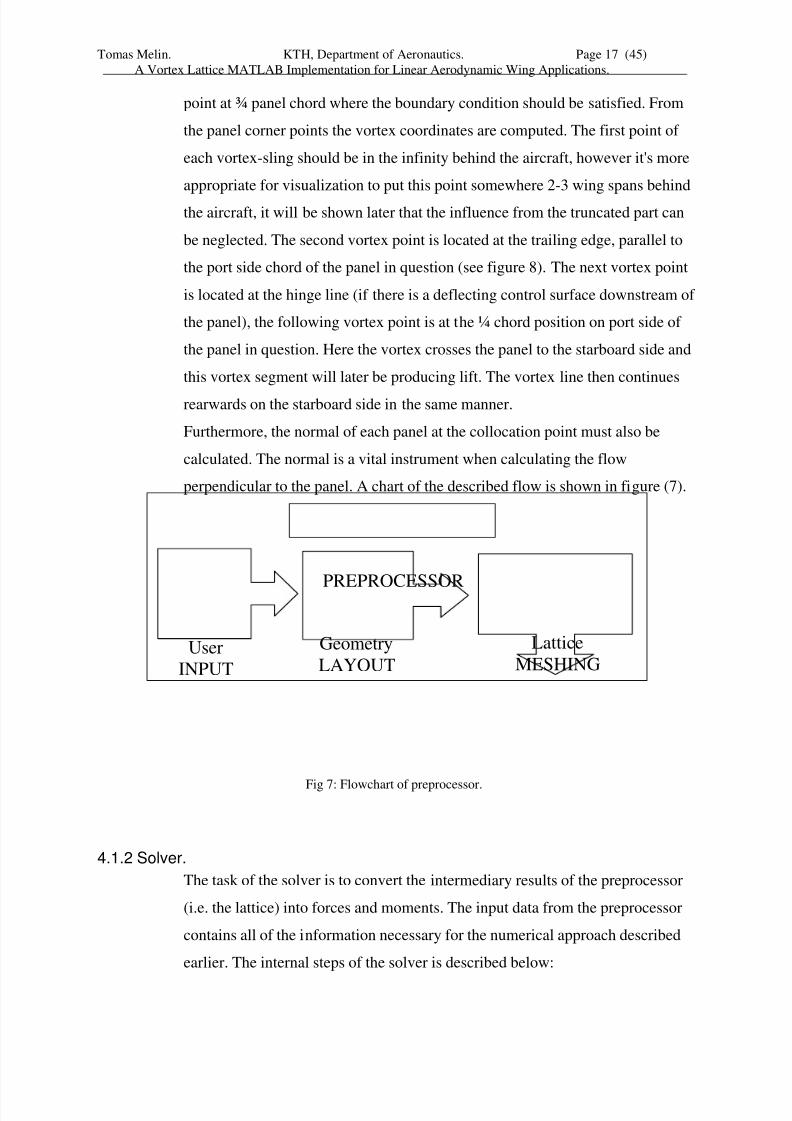
perpendicular to the panel. A chart of the described flow is shown in figure (7).
4.1.2 Solver.
The task of the solver is to convert the intermediary results of the preprocessor
(i.e. the lattice) into forces and moments. The input data from the preprocessor
contains all of the information necessary for the numerical approach described
earlier. The internal steps of the solver is described below:
Fig 7: Flowchart of preprocessor.
User
INPUT
Geometry
LAYOUT
Lattice
MESHING
PREPROCESSOR
8/7/2019 tornado thesis
http://slidepdf.com/reader/full/tornado-thesis 18/45
Tomas Melin. KTH, Department of Aeronautics. Page 18 (45)
A Vortex Lattice MATLAB Implementation for Linear Aerodynamic Wing Applications.
Downwash:
Firstly the downwash, or aerodynamic influence, from the vortex-slings is
calculated for every vortex at every collocation point. This is a very time
consuming event, which represents more than half of the actual computation
time.
Boundary condition:
Secondly the boundary conditions are set up, no flow parallel to the panel
normal at the collocation point. This means that the far field velocity vector,
together with any rigid body rotations of the aircraft, should equal the
downwash generated by the vortices. The vortex strength is then solved for with
usual Gaussian elimination.
Inwash:
When the vortex strengths have been determined, the inwash has to be
calculated. This is readily done by the same function that calculates the
downwash, but instead of computing the induced flow at the collocation point,
the vortex flow at the spanwise vortex segment's midpoint is computed. To
obtain the complete flow field the vortex flow field is added to the infinity air
stream and any rigid body rotation speeds.
Force computation:
Using equation 9 the force acting on each panel can be calculated. From this the
pressure on each panel is computed. The forces are integrated to yield resultant
forces in the body system. In the same way the Body fixed moments are
computed. With these two vectors, conversion to wind system vectors is
performed.
Coefficients:
When the resultant force and moments vectors in the wind system has been
determined, the creation of the aerodynamic coefficients is done in the standard
way.
8/7/2019 tornado thesis
http://slidepdf.com/reader/full/tornado-thesis 19/45
Tomas Melin. KTH, Department of Aeronautics. Page 19 (45)
A Vortex Lattice MATLAB Implementation for Linear Aerodynamic Wing Applications.
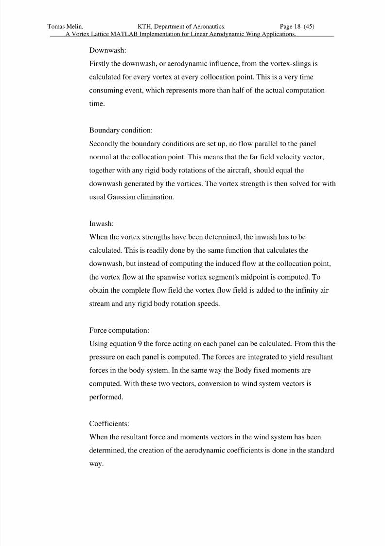
Stability derivatives.
The first order derivatives of the aerodynamic coefficients are called stability
derivatives, and they can be calculated in different manners. One way, which
yield visual results is to perform a parameter sweep, such as a sweep of angle of
attack, and plotting CL and CD versus alpha. To get more accurate numbers one
can perform a central difference approximation at a certain flight condition.
A flowchart of the solver is presented in figure 8.
Fig 8: Flowchart of solver.
PROCESSOR
Aerodynamic
Influence,
INWASH
Setup of BOUNDARY
CONDITIONS
Force
COMPUTA-TION
Aerodynamic
COEFFICI-
ENTS
Aerodynamic
Influence,
DOWNWASH
Stability
DERIVATIVES
8/7/2019 tornado thesis
http://slidepdf.com/reader/full/tornado-thesis 20/45
Tomas Melin. KTH, Department of Aeronautics. Page 20 (45)
A Vortex Lattice MATLAB Implementation for Linear Aerodynamic Wing Applications.
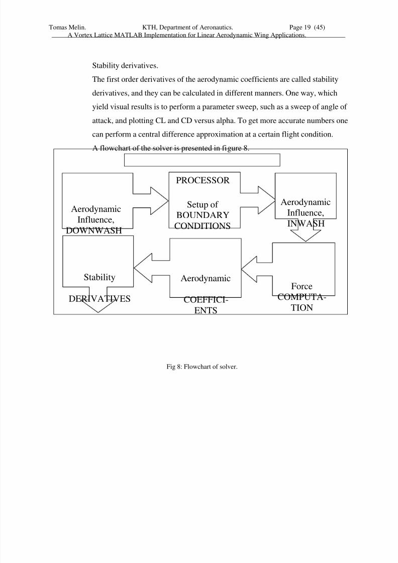
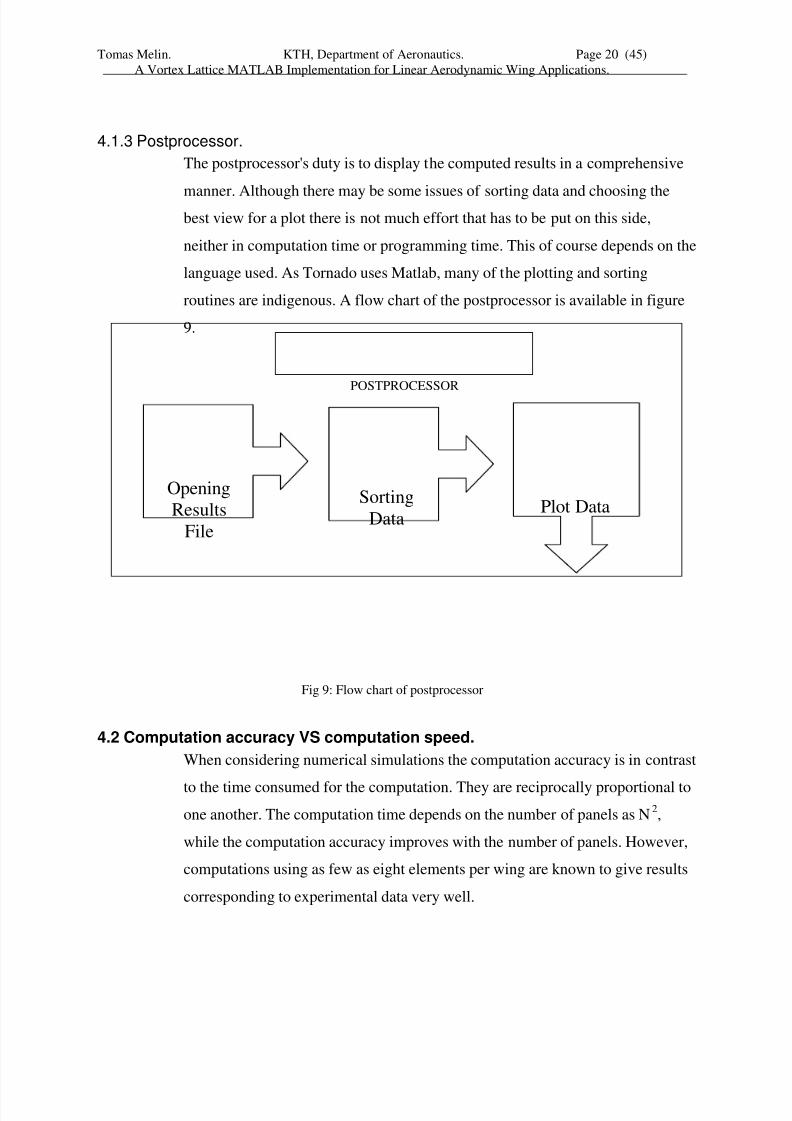
4.1.3 Postprocessor.
The postprocessor's duty is to display the computed results in a comprehensive
manner. Although there may be some issues of sorting data and choosing thebest view for a plot there is not much effort that has to be put on this side,
neither in computation time or programming time. This of course depends on the
language used. As Tornado uses Matlab, many of the plotting and sorting
routines are indigenous. A flow chart of the postprocessor is available in figure
9.
4.2 Computation accuracy VS computation speed.
When considering numerical simulations the computation accuracy is in contrast
to the time consumed for the computation. They are reciprocally proportional to
one another. The computation time depends on the number of panels as N2,
while the computation accuracy improves with the number of panels. However,
computations using as few as eight elements per wing are known to give results
corresponding to experimental data very well.
Fig 9: Flow chart of postprocessor
Opening
Results
File
Sorting
DataPlot Data
POSTPROCESSOR
8/7/2019 tornado thesis
http://slidepdf.com/reader/full/tornado-thesis 21/45
Tomas Melin. KTH, Department of Aeronautics. Page 21 (45)
A Vortex Lattice MATLAB Implementation for Linear Aerodynamic Wing Applications.
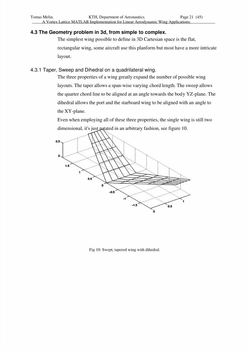
4.3 The Geometry problem in 3d, from simple to complex.
The simplest wing possible to define in 3D Cartesian space is the flat,
rectangular wing, some aircraft use this planform but most have a more intricate
layout.
4.3.1 Taper, Sweep and Dihedral on a quadrilateral wing.
The three properties of a wing greatly expand the number of possible wing
layouts. The taper allows a span-wise varying chord length. The sweep allows
the quarter chord line to be aligned at an angle towards the body YZ-plane. The
dihedral allows the port and the starboard wing to be aligned with an angle to
the XY-plane.
Even when employing all of these three properties, the single wing is still two
dimensional, it's just rotated in an arbitrary fashion, see figure 10.
Fig 10: Swept, tapered wing with dihedral.
8/7/2019 tornado thesis
http://slidepdf.com/reader/full/tornado-thesis 22/45
Tomas Melin. KTH, Department of Aeronautics. Page 22 (45)
A Vortex Lattice MATLAB Implementation for Linear Aerodynamic Wing Applications.
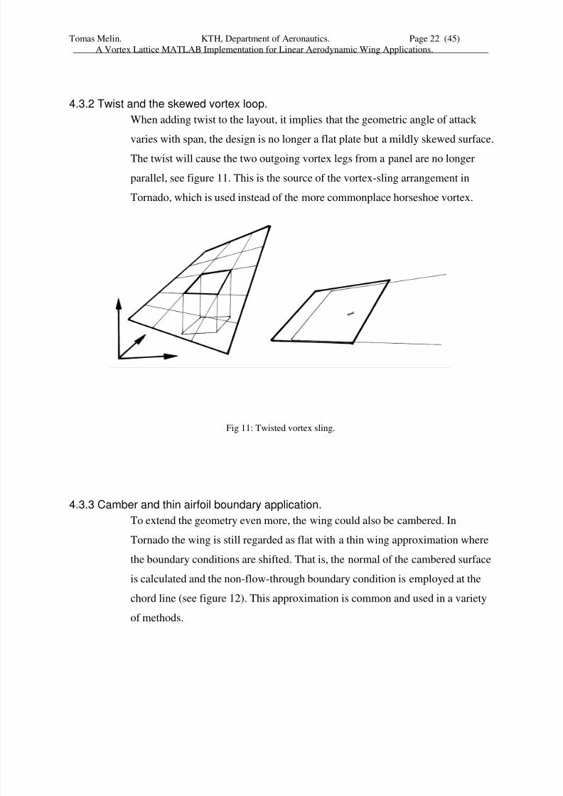
4.3.2 Twist and the skewed vortex loop.
When adding twist to the layout, it implies that the geometric angle of attack
varies with span, the design is no longer a flat plate but a mildly skewed surface.
The twist will cause the two outgoing vortex legs from a panel are no longer
parallel, see figure 11. This is the source of the vortex-sling arrangement in
Tornado, which is used instead of the more commonplace horseshoe vortex.
4.3.3 Camber and thin airfoil boundary application.
To extend the geometry even more, the wing could also be cambered. In
Tornado the wing is still regarded as flat with a thin wing approximation where
the boundary conditions are shifted. That is, the normal of the cambered surface
is calculated and the non-flow-through boundary condition is employed at the
chord line (see figure 12). This approximation is common and used in a variety
of methods.
Fig 11: Twisted vortex sling.
8/7/2019 tornado thesis
http://slidepdf.com/reader/full/tornado-thesis 23/45
Tomas Melin. KTH, Department of Aeronautics. Page 23 (45)
A Vortex Lattice MATLAB Implementation for Linear Aerodynamic Wing Applications.
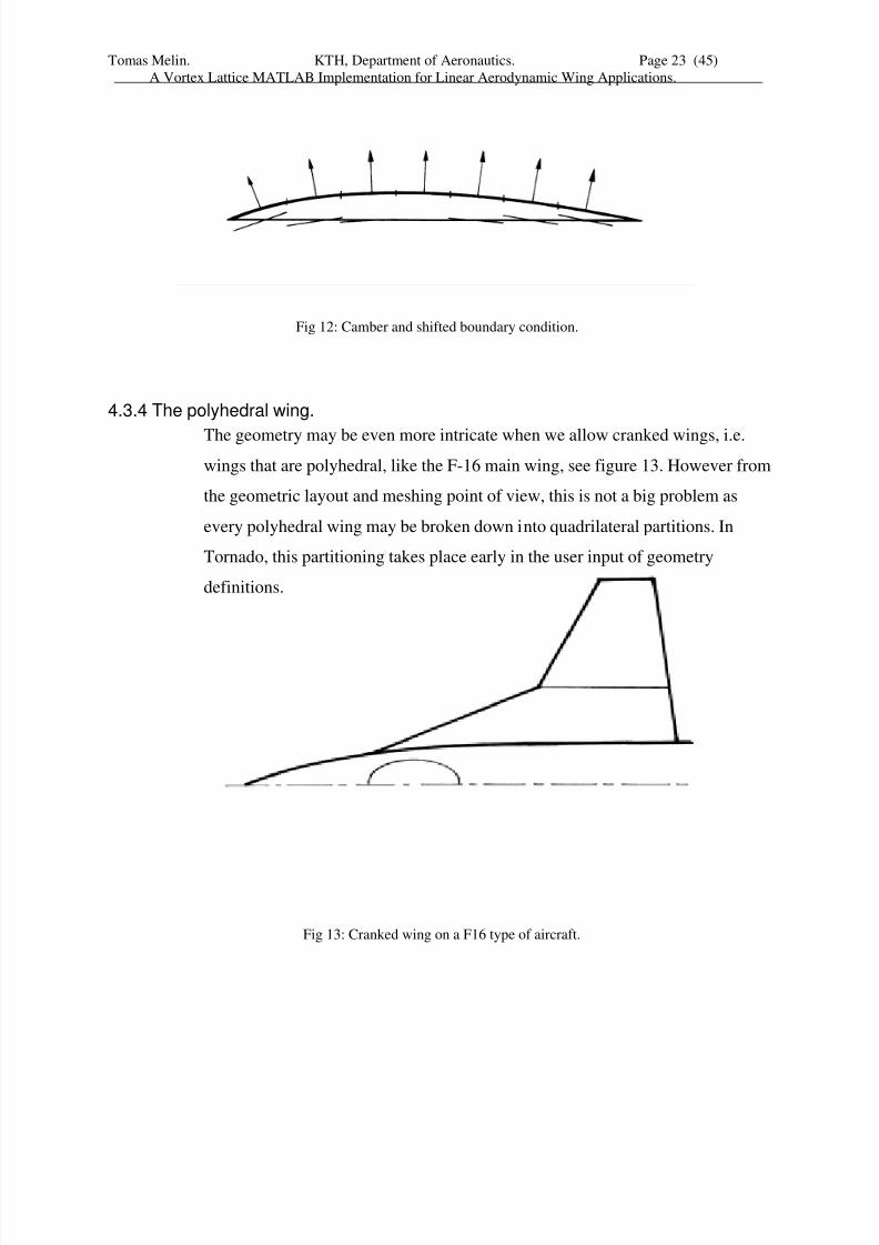
4.3.4 The polyhedral wing.
The geometry may be even more intricate when we allow cranked wings, i.e.
wings that are polyhedral, like the F-16 main wing, see figure 13. However from
the geometric layout and meshing point of view, this is not a big problem as
every polyhedral wing may be broken down into quadrilateral partitions. In
Tornado, this partitioning takes place early in the user input of geometry
definitions.
Fig 12: Camber and shifted boundary condition.
Fig 13: Cranked wing on a F16 type of aircraft.
8/7/2019 tornado thesis
http://slidepdf.com/reader/full/tornado-thesis 24/45
Tomas Melin. KTH, Department of Aeronautics. Page 24 (45)
A Vortex Lattice MATLAB Implementation for Linear Aerodynamic Wing Applications.
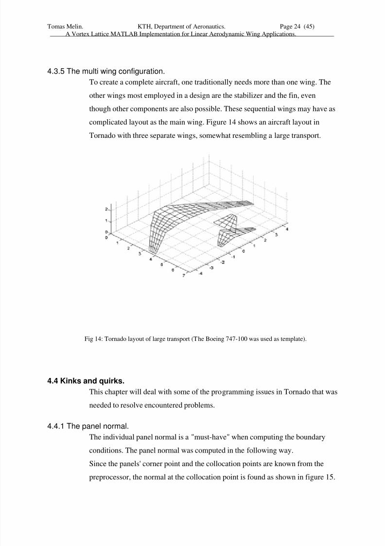
Fig 14: Tornado layout of large transport (The Boeing 747-100 was used as template).
4.3.5 The multi wing configuration.
To create a complete aircraft, one traditionally needs more than one wing. The
other wings most employed in a design are the stabilizer and the fin, even
though other components are also possible. These sequential wings may have as
complicated layout as the main wing. Figure 14 shows an aircraft layout in
Tornado with three separate wings, somewhat resembling a large transport.
4.4 Kinks and quirks.This chapter will deal with some of the programming issues in Tornado that was
needed to resolve encountered problems.
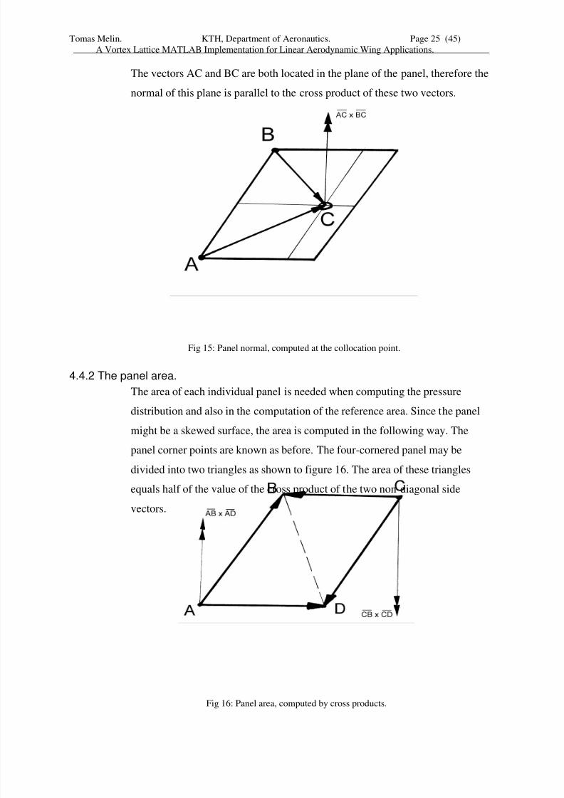
4.4.1 The panel normal.
The individual panel normal is a "must-have" when computing the boundary
conditions. The panel normal was computed in the following way.
Since the panels' corner point and the collocation points are known from the
preprocessor, the normal at the collocation point is found as shown in figure 15.
8/7/2019 tornado thesis
http://slidepdf.com/reader/full/tornado-thesis 25/45
Tomas Melin. KTH, Department of Aeronautics. Page 25 (45)
A Vortex Lattice MATLAB Implementation for Linear Aerodynamic Wing Applications.
The vectors AC and BC are both located in the plane of the panel, therefore the
normal of this plane is parallel to the cross product of these two vectors.
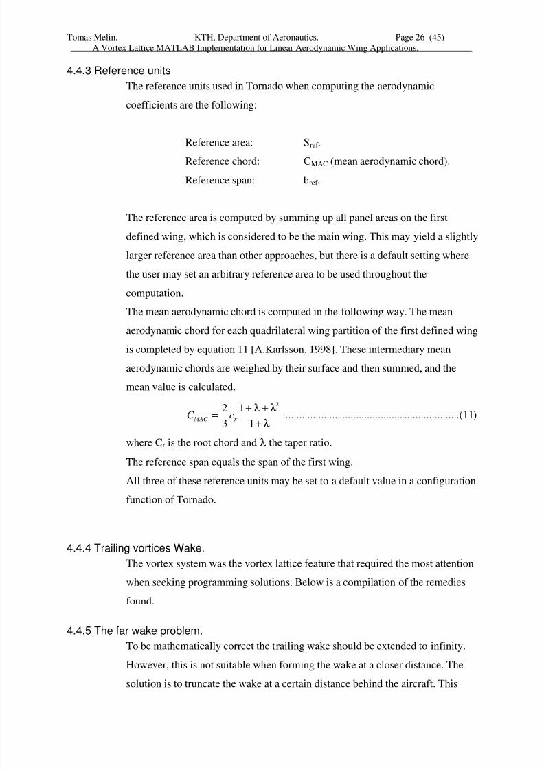
4.4.2 The panel area.
The area of each individual panel is needed when computing the pressure
distribution and also in the computation of the reference area. Since the panel
might be a skewed surface, the area is computed in the following way. The
panel corner points are known as before. The four-cornered panel may be
divided into two triangles as shown to figure 16. The area of these triangles
equals half of the value of the cross product of the two non-diagonal side
vectors.
Fig 15: Panel normal, computed at the collocation point.
Fig 16: Panel area, computed by cross products.
8/7/2019 tornado thesis
http://slidepdf.com/reader/full/tornado-thesis 26/45
Tomas Melin. KTH, Department of Aeronautics. Page 26 (45)
A Vortex Lattice MATLAB Implementation for Linear Aerodynamic Wing Applications.
4.4.3 Reference units
The reference units used in Tornado when computing the aerodynamic
coefficients are the following:
Reference area: Sref .
Reference chord: CMAC (mean aerodynamic chord).
Reference span: bref .
The reference area is computed by summing up all panel areas on the first
defined wing, which is considered to be the main wing. This may yield a slightly
larger reference area than other approaches, but there is a default setting where
the user may set an arbitrary reference area to be used throughout the
computation.
The mean aerodynamic chord is computed in the following way. The mean
aerodynamic chord for each quadrilateral wing partition of the first defined wing
is completed by equation 11 [A.Karlsson, 1998]. These intermediary mean
aerodynamic chords are weighed by their surface and then summed, and the
mean value is calculated.
λ+λ+λ+=
1
1
3
2 2
r MAC cC .................................................................(11)
where Cr is the root chord and λ the taper ratio.
The reference span equals the span of the first wing.
All three of these reference units may be set to a default value in a configuration
function of Tornado.
4.4.4 Trailing vortices Wake.
The vortex system was the vortex lattice feature that required the most attention
when seeking programming solutions. Below is a compilation of the remedies
found.
4.4.5 The far wake problem.
To be mathematically correct the trailing wake should be extended to infinity.
However, this is not suitable when forming the wake at a closer distance. The
solution is to truncate the wake at a certain distance behind the aircraft. This
8/7/2019 tornado thesis
http://slidepdf.com/reader/full/tornado-thesis 27/45
Tomas Melin. KTH, Department of Aeronautics. Page 27 (45)
A Vortex Lattice MATLAB Implementation for Linear Aerodynamic Wing Applications.
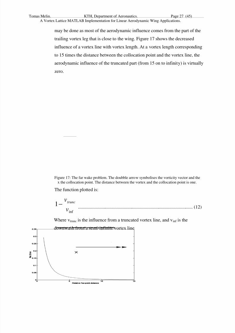
may be done as most of the aerodynamic influence comes from the part of the
trailing vortex leg that is close to the wing. Figure 17 shows the decreased
influence of a vortex line with vortex length. At a vortex length corresponding
to 15 times the distance between the collocation point and the vortex line, the
aerodynamic influence of the truncated part (from 15 on to infinity) is virtually
zero.
The function plotted is:
inf
1v
vtrunc−.................................................................................................. (12)
Where vtrunc is the influence from a truncated vortex line, and vinf is the
downwash from a semi-infinite vortex line
Figure 17: The far wake problem. The doubble arrow symbolises the vorticity vector and the
x the collocation point. The distance between the vortex and the collocation point is one.
8/7/2019 tornado thesis
http://slidepdf.com/reader/full/tornado-thesis 28/45
Tomas Melin. KTH, Department of Aeronautics. Page 28 (45)
A Vortex Lattice MATLAB Implementation for Linear Aerodynamic Wing Applications.
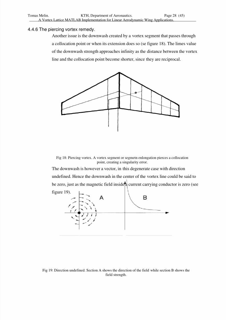
4.4.6 The piercing vortex remedy.
Another issue is the downwash created by a vortex segment that passes through
a collocation point or when its extension does so (se figure 18). The limes value
of the downwash strength approaches infinity as the distance between the vortex
line and the collocation point become shorter, since they are reciprocal.
The downwash is however a vector, in this degenerate case with direction
undefined. Hence the downwash in the center of the vortex line could be said to
be zero, just as the magnetic field inside a current carrying conductor is zero (see
figure 19).
Fig 18: Piercing vortex. A vortex segment or segmetn enlongation pierces a collocation
point, creating a singularity error.
Fig 19: Direction undefined. Section A shows the direction of the field while section B shows the
field strength.
8/7/2019 tornado thesis
http://slidepdf.com/reader/full/tornado-thesis 29/45
Tomas Melin. KTH, Department of Aeronautics. Page 29 (45)
A Vortex Lattice MATLAB Implementation for Linear Aerodynamic Wing Applications.
4.4.7 Analogy with the inwash problem.
The same problem arises when computing the inwash, or self-influence of the
vortexes, at the span-segment midpoint. It is solved in the same manner.
In Tornado this is solved by setting every influence, emanating from a vortex
closer than an epsilon distance of the collocation point, to zero.
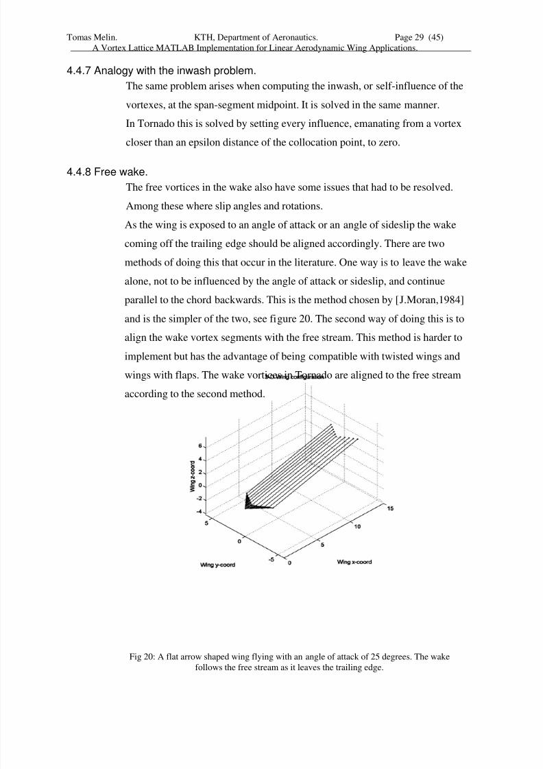
4.4.8 Free wake.
The free vortices in the wake also have some issues that had to be resolved.
Among these where slip angles and rotations.
As the wing is exposed to an angle of attack or an angle of sideslip the wake
coming off the trailing edge should be aligned accordingly. There are two
methods of doing this that occur in the literature. One way is to leave the wake
alone, not to be influenced by the angle of attack or sideslip, and continue
parallel to the chord backwards. This is the method chosen by [J.Moran,1984]
and is the simpler of the two, see figure 20. The second way of doing this is to
align the wake vortex segments with the free stream. This method is harder to
implement but has the advantage of being compatible with twisted wings and
wings with flaps. The wake vortices in Tornado are aligned to the free stream
according to the second method.
Fig 20: A flat arrow shaped wing flying with an angle of attack of 25 degrees. The wake
follows the free stream as it leaves the trailing edge.
8/7/2019 tornado thesis
http://slidepdf.com/reader/full/tornado-thesis 30/45
Tomas Melin. KTH, Department of Aeronautics. Page 30 (45)
A Vortex Lattice MATLAB Implementation for Linear Aerodynamic Wing Applications.
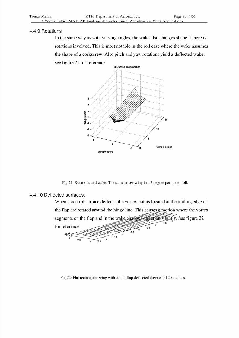
4.4.9 Rotations
In the same way as with varying angles, the wake also changes shape if there is
rotations involved. This is most notable in the roll case where the wake assumes
the shape of a corkscrew. Also pitch and yaw rotations yield a deflected wake,
see figure 21 for reference.
4.4.10 Deflected surfaces:
When a control surface deflects, the vortex points located at the trailing edge of
the flap are rotated around the hinge line. This causes a motion where the vortex
segments on the flap and in the wake changes direction slightly. See figure 22
for reference.
Fig 21: Rotations and wake. The same arrow wing in a 3 degree per meter roll.
Fig 22: Flat rectangular wing with center flap deflected downward 20 degrees.
8/7/2019 tornado thesis
http://slidepdf.com/reader/full/tornado-thesis 31/45
Tomas Melin. KTH, Department of Aeronautics. Page 31 (45)
A Vortex Lattice MATLAB Implementation for Linear Aerodynamic Wing Applications.
5 VALIDATION.
5.1 Method
This chapter deals with the code validation of Tornado. The validation was executed by
comparing Tornado computational results with:
Theoretical data
Other Vortex lattice methods and panel codes.
Experimental data.
The first comparison was between Tornado and the two theoretical values of the lift-curve
slope obtained through Jones' small aspect ratio theory and Prandtl's lifting line theory.
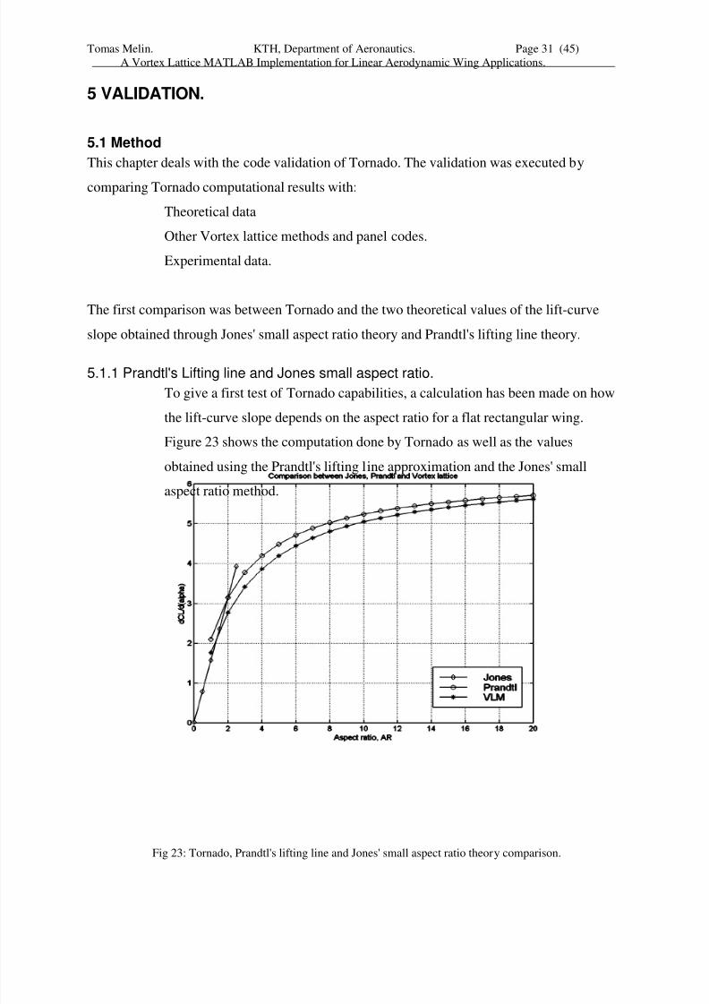
5.1.1 Prandtl's Lifting line and Jones small aspect ratio.
To give a first test of Tornado capabilities, a calculation has been made on how
the lift-curve slope depends on the aspect ratio for a flat rectangular wing.
Figure 23 shows the computation done by Tornado as well as the values
obtained using the Prandtl's lifting line approximation and the Jones' small
aspect ratio method.
Fig 23: Tornado, Prandtl's lifting line and Jones' small aspect ratio theory comparison.
8/7/2019 tornado thesis
http://slidepdf.com/reader/full/tornado-thesis 32/45
Tomas Melin. KTH, Department of Aeronautics. Page 32 (45)
A Vortex Lattice MATLAB Implementation for Linear Aerodynamic Wing Applications.
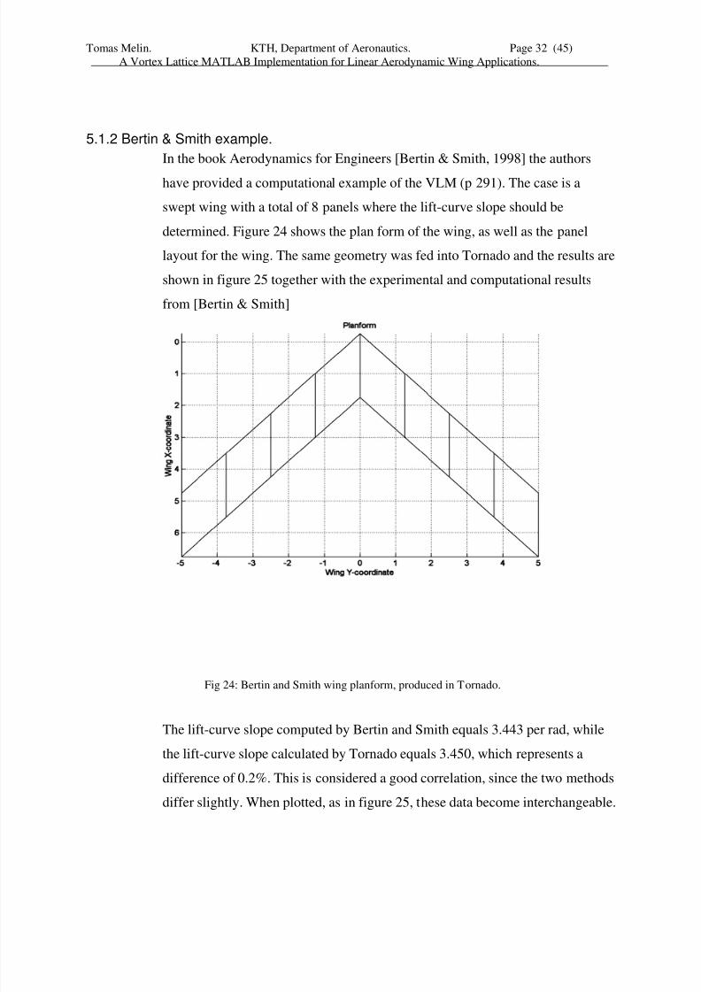
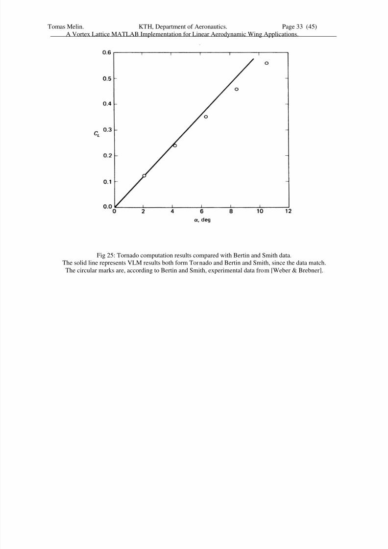
5.1.2 Bertin & Smith example.
In the book Aerodynamics for Engineers [Bertin & Smith, 1998] the authors
have provided a computational example of the VLM (p 291). The case is a
swept wing with a total of 8 panels where the lift-curve slope should be
determined. Figure 24 shows the plan form of the wing, as well as the panel
layout for the wing. The same geometry was fed into Tornado and the results are
shown in figure 25 together with the experimental and computational results
from [Bertin & Smith]
The lift-curve slope computed by Bertin and Smith equals 3.443 per rad, while
the lift-curve slope calculated by Tornado equals 3.450, which represents a
difference of 0.2%. This is considered a good correlation, since the two methods
differ slightly. When plotted, as in figure 25, these data become interchangeable.
Fig 24: Bertin and Smith wing planform, produced in Tornado.
8/7/2019 tornado thesis
http://slidepdf.com/reader/full/tornado-thesis 33/45
Tomas Melin. KTH, Department of Aeronautics. Page 33 (45)
A Vortex Lattice MATLAB Implementation for Linear Aerodynamic Wing Applications.
Fig 25: Tornado computation results compared with Bertin and Smith data.
The solid line represents VLM results both form Tornado and Bertin and Smith, since the data match.
The circular marks are, according to Bertin and Smith, experimental data from [Weber & Brebner].
8/7/2019 tornado thesis
http://slidepdf.com/reader/full/tornado-thesis 34/45
Tomas Melin. KTH, Department of Aeronautics. Page 34 (45)
A Vortex Lattice MATLAB Implementation for Linear Aerodynamic Wing Applications.
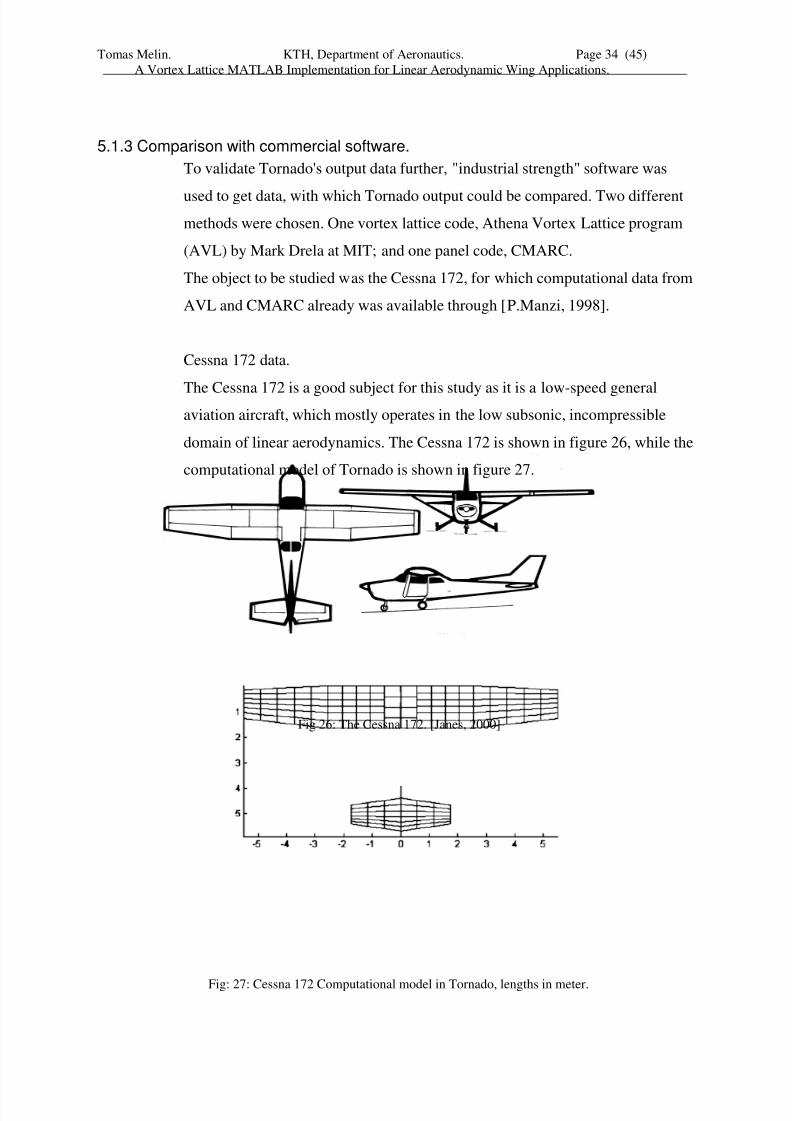
5.1.3 Comparison with commercial software.
To validate Tornado's output data further, "industrial strength" software was
used to get data, with which Tornado output could be compared. Two different
methods were chosen. One vortex lattice code, Athena Vortex Lattice program
(AVL) by Mark Drela at MIT; and one panel code, CMARC.
The object to be studied was the Cessna 172, for which computational data from
AVL and CMARC already was available through [P.Manzi, 1998].
Cessna 172 data.
The Cessna 172 is a good subject for this study as it is a low-speed generalaviation aircraft, which mostly operates in the low subsonic, incompressible
domain of linear aerodynamics. The Cessna 172 is shown in figure 26, while the
computational model of Tornado is shown in figure 27.
Fig: 27: Cessna 172 Computational model in Tornado, lengths in meter.
Fig 26: The Cessna 172. [Janes, 2000]
8/7/2019 tornado thesis
http://slidepdf.com/reader/full/tornado-thesis 35/45
Tomas Melin. KTH, Department of Aeronautics. Page 35 (45)
A Vortex Lattice MATLAB Implementation for Linear Aerodynamic Wing Applications.
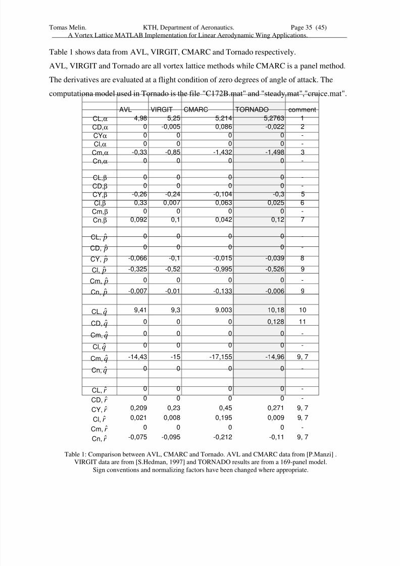
Table 1 shows data from AVL, VIRGIT, CMARC and Tornado respectively.
AVL, VIRGIT and Tornado are all vortex lattice methods while CMARC is a panel method.
The derivatives are evaluated at a flight condition of zero degrees of angle of attack. The
computationa model used in Tornado is the file "C172B.mat" and "steady.mat","cruice.mat".
AVL VIRGIT CMARC TORNADO comment
CL,α 4,98 5,25 5,214 5,2763 1
CD,α 0 -0,005 0,086 -0,022 2
CYα 0 0 0 0 -
Cl,α 0 0 0 0 -
Cm,α -0,33 -0,85 -1,432 -1,498 3
Cn,α 0 0 0 0 -
CL,β 0 0 0 0 -
CD,β 0 0 0 0 -
CY,β
-0,26 -0,24 -0,104 -0,3 5
Cl,β 0,33 0,007 0,063 0,025 6
Cm,β 0 0 0 0 -
Cn,β 0,092 0,1 0,042 0,12 7
CL, p̂ 0 0 0 0 -
CD, p̂ 0 0 0 0 -
CY, p̂ -0,066 -0,1 -0,015 -0,039 8
Cl, p̂ -0,325 -0,52 -0,995 -0,526 9
Cm, p̂ 0 0 0 0 -
Cn, p̂ -0,007 -0,01 -0,133 -0,006 9
CL, q̂ 9,41 9,3 9.003 10,18 10
CD, q̂ 0 0 0 0,128 11
Cm, q̂ 0 0 0 0 -
Cl, q̂ 0 0 0 0 -
Cm, q̂ -14,43 -15 -17,155 -14,96 9, 7
Cn, q̂ 0 0 0 0 -
CL, r ̂ 0 0 0 0 -
CD, r ̂ 0 0 0 0 -
CY, r ̂ 0,209 0,23 0,45 0,271 9, 7
Cl, r ̂ 0,021 0,008 0,195 0,009 9, 7
Cm, r ̂ 0 0 0 0 -
Cn, r ̂ -0,075 -0,095 -0,212 -0,11 9, 7
Table 1: Comparison between AVL, CMARC and Tornado. AVL and CMARC data from [P.Manzi] .
VIRGIT data are from [S.Hedman, 1997] and TORNADO results are from a 169-panel model.
Sign conventions and normalizing factors have been changed where appropriate.
8/7/2019 tornado thesis
http://slidepdf.com/reader/full/tornado-thesis 36/45
Tomas Melin. KTH, Department of Aeronautics. Page 36 (45)
A Vortex Lattice MATLAB Implementation for Linear Aerodynamic Wing Applications.
Comments:
1. CL, alpha: The value from Tornado is higher than both AVL and CMARC
data. The difference stems both from the difference in methods and from the
difference in the input geometry.
2. The drag-curve slope should be zero if we consider the slope at CL=0.
Tornado has negative lift at alpha =0 (geometric alpha), and VIRGIT probably
does to. CMARC probably also has an offset from the zero lift alpha.
3. Values differ due to different placements of the reference point. The Tornado
computation has the reference point at 31.9% CMAC, VIRGIT at 29.5%Cref and
AVL reference point placement unknown.
5. The vertical tail gets an angle of attack and produces lift. The offset in the
CMARC result could depend on the fuselage model.
6. Differences depend mostly on Z position of reference point.
7. Position of reference point has an affect here and the offset in the CMARC
result could depend on the fuselage model.
8. Differences could depend on Z position of reference point.
9 Results influenced by method and geometry differences. The offset in the
CMARC result could depend on the fuselage model.
10. Modeling and method differences.
11. Connected to #10, a change in lift should give a change in drag.
8/7/2019 tornado thesis
http://slidepdf.com/reader/full/tornado-thesis 37/45
Tomas Melin. KTH, Department of Aeronautics. Page 37 (45)
A Vortex Lattice MATLAB Implementation for Linear Aerodynamic Wing Applications.
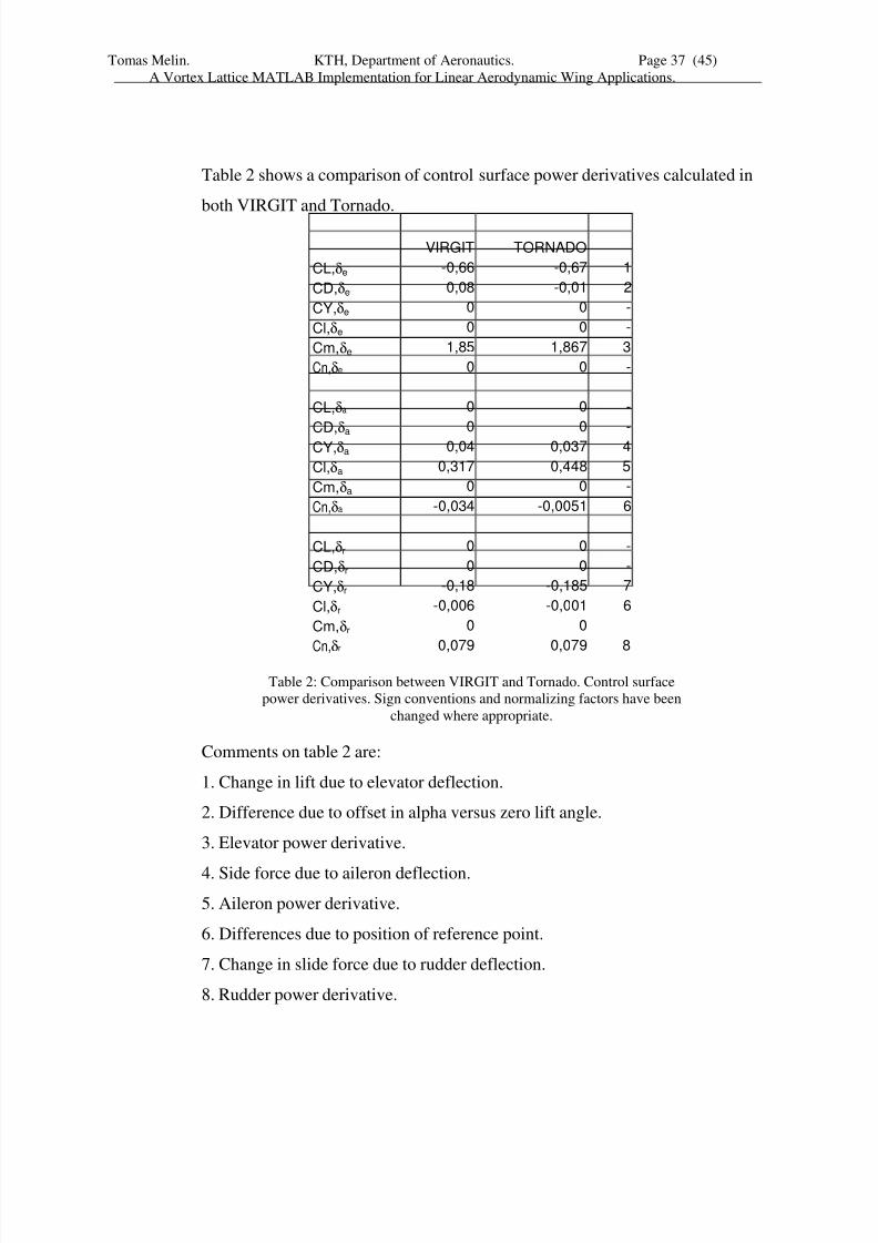
Table 2 shows a comparison of control surface power derivatives calculated in
both VIRGIT and Tornado.
Comments on table 2 are:
1. Change in lift due to elevator deflection.
2. Difference due to offset in alpha versus zero lift angle.
3. Elevator power derivative.
4. Side force due to aileron deflection.
5. Aileron power derivative.
6. Differences due to position of reference point.
7. Change in slide force due to rudder deflection.
8. Rudder power derivative.
VIRGIT TORNADO
CL,δe -0,66 -0,67 1
CD,δe 0,08 -0,01 2
CY,δe 0 0 -
Cl,δe 0 0 -
Cm,δe 1,85 1,867 3
Cn,δe 0 0 -
CL,δa 0 0 -
CD,δa
0 0 -
CY,δa 0,04 0,037 4
Cl,δa 0,317 0,448 5
Cm,δa 0 0 -
Cn,δa -0,034 -0,0051 6
CL,δr 0 0 -
CD,δr 0 0 -
CY,δr -0,18 -0,185 7
Cl,δr -0,006 -0,001 6
Cm,δr 0 0
Cn,δr 0,079 0,079 8
Table 2: Comparison between VIRGIT and Tornado. Control surface
power derivatives. Sign conventions and normalizing factors have been
changed where appropriate.
8/7/2019 tornado thesis
http://slidepdf.com/reader/full/tornado-thesis 38/45
Tomas Melin. KTH, Department of Aeronautics. Page 38 (45)
A Vortex Lattice MATLAB Implementation for Linear Aerodynamic Wing Applications.
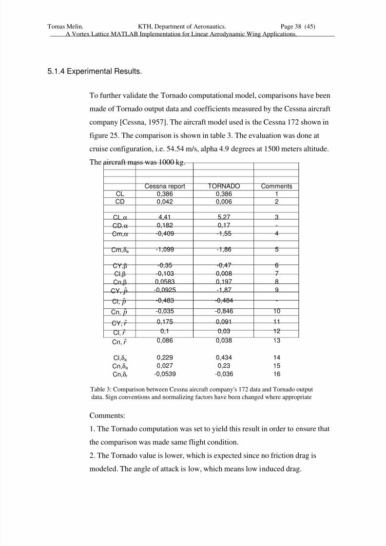
5.1.4 Experimental Results.
To further validate the Tornado computational model, comparisons have been
made of Tornado output data and coefficients measured by the Cessna aircraft
company [Cessna, 1957]. The aircraft model used is the Cessna 172 shown in
figure 25. The comparison is shown in table 3. The evaluation was done at
cruise configuration, i.e. 54.54 m/s, alpha 4.9 degrees at 1500 meters altitude.
The aircraft mass was 1000 kg.
Comments:
1. The Tornado computation was set to yield this result in order to ensure that
the comparison was made same flight condition.
2. The Tornado value is lower, which is expected since no friction drag is
modeled. The angle of attack is low, which means low induced drag.
Cessna report TORNADO Comments
CL 0,386 0,386 1CD 0,042 0,006 2
CL,α 4,41 5,27 3
CD,α 0,182 0,17 -
Cm,α -0,409 -1,55 4
Cm,δe -1,099 -1,86 5
CY,β -0,35 -0,47 6
Cl,β -0,103 0,008 7
Cn,β 0,0583 0,197 8
CY, p̂ -0,0925 -1,87 9
Cl, p̂ -0,483 -0,484 -
Cn, p̂ -0,035 -0,846 10
CY, r ̂ 0,175 0,091 11
Cl, r ̂ 0,1 0,03 12
Cn, r ̂ 0,086 0,038 13
Cl,δa 0,229 0,434 14
Cn,δa 0,027 0,23 15
Cn,δr -0,0539 -0,036 16
Table 3: Comparison between Cessna aircraft company's 172 data and Tornado output
data. Sign conventions and normalizing factors have been changed where appropriate
8/7/2019 tornado thesis
http://slidepdf.com/reader/full/tornado-thesis 39/45
Tomas Melin. KTH, Department of Aeronautics. Page 39 (45)
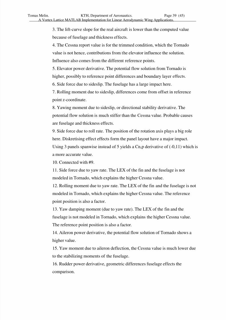
A Vortex Lattice MATLAB Implementation for Linear Aerodynamic Wing Applications.
3. The lift-curve slope for the real aircraft is lower than the computed value
because of fuselage and thickness effects.
4. The Cessna report value is for the trimmed condition, which the Tornado
value is not hence, contributions from the elevator influence the solution.
Influence also comes from the different reference points.
5. Elevator power derivative. The potential flow solution from Tornado is
higher, possibly to reference point differences and boundary layer effects.
6. Side force due to sideslip. The fuselage has a large impact here.
7. Rolling moment due to sideslip, differences come from offset in reference
point z-coordinate.
8. Yawing moment due to sideslip, or directional stability derivative. The
potential flow solution is much stiffer than the Cessna value. Probable causes
are fuselage and thickness effects.
9. Side force due to roll rate. The position of the rotation axis plays a big role
here. Diskretising effect effects form the panel layout have a major impact.
Using 3 panels spanwise instead of 5 yields a Cn,p derivative of (-0,11) which is
a more accurate value.
10. Connected with #9.
11. Side force due to yaw rate. The LEX of the fin and the fuselage is not
modeled in Tornado, which explains the higher Cessna value.
12. Rolling moment due to yaw rate. The LEX of the fin and the fuselage is not
modeled in Tornado, which explains the higher Cessna value. The reference
point position is also a factor.
13. Yaw damping moment (due to yaw rate). The LEX of the fin and the
fuselage is not modeled in Tornado, which explains the higher Cessna value.
The reference point position is also a factor.
14. Aileron power derivative, the potential flow solution of Tornado shows a
higher value.
15. Yaw moment due to aileron deflection, the Cessna value is much lower due
to the stabilizing moments of the fuselage.
16. Rudder power derivative, geometric differences fuselage effects the
comparison.
8/7/2019 tornado thesis
http://slidepdf.com/reader/full/tornado-thesis 40/45
Tomas Melin. KTH, Department of Aeronautics. Page 40 (45)
A Vortex Lattice MATLAB Implementation for Linear Aerodynamic Wing Applications.
6 RESULTS.
6.1 Lifting line.
Tornado output data shows good correspondence to both Prantdl's lifting line
theory as well as Jones' small aspect theory, as shown in figure 22.
6.2 Simple wing.
Tornado results for a simple swept wing are the same as the vortex lattice
method presented by Bertin & Smith.
6.3 Cessna 172.Tornado computational results for the examination of the Cessna 172 correlates
with both AVL data and CMARC data. Differences found where expected.
When comparing with the Cessna aircraft company's data for model 172,
Tornado data shows good results in most cases.
6.4 Accuracy.
The best accuracy of Tornado data is found for coefficients handling primaryand large forces such as lift, or pitching moment (when the reference point is
placed properly). Not surprisingly less accurate results are found for coefficients
which involve viscous forces, as drag.
The error in placement of the reference point transfers to the moment rotation
derivatives as n2
because this error depends on distance to reference point and
distance to rotational axis.
6.5 Solution Time.The Tornado solution time for the Cessna model was about 40 minuets on a 400
MHz personal computer with MS-Win98, Matlab version 5.3. The Tornado code
is currently not optimized for speed so this time could be cut by at least one
magnitude by code optimization and compilation.
8/7/2019 tornado thesis
http://slidepdf.com/reader/full/tornado-thesis 41/45
Tomas Melin. KTH, Department of Aeronautics. Page 41 (45)
A Vortex Lattice MATLAB Implementation for Linear Aerodynamic Wing Applications.
6.6 Suitability for real-time applications.
Using a vortex lattice method such as Tornado to obtain the aerodynamic forces
in real time applications, for example an aircraft simulator, would give very
flexible simulations with very small time usage for shifting models. However,
personal computers today are not fast enough to sustain the frame rate needed
for a good visual simulation. But, with the suggestions for optimization
mentioned in the previous paragraph, coupled with a general strip down of the
code (no need for computing the coefficients or derivatives in the simulator) and
a few generations of faster computers, the goal of real-time simulation will be
reached.
As a side note it should be mentioned that one function that consumes about
95% of the computing time. This function computes the aerodynamic influence
of every vortex on every panel. There are no arguments against a successful
parallelisation of this part of the code, which would give a much faster system.
Also, the downwash from some of the vortex segments does not change in time,
which means that they only has to be computed at initiation and then sorted out
during the real-time loop.
7 DISCUSSION.
7.1 Error sources.
Common error sources that occur when comparing Tornado results with the
commercial software, as well as with the Cessna aircraft company's data are the
uncertainties of the aircraft geometry. Only a slight offset in dihedral, twist or
reference units could have big impact on the coefficients in the study. Some of
the geometrical data could be found in [Jane's], while others had to be acquiredby measurements on scaled drawings. The lack of a correct position for the
centroid induced errors in the placements of the rotational axis. This error is
squared when looking at moment responses to rotations, as the errors in centroid
and reference point coincide.
Another, but well-known factor in the Cessna Company comparison is the lack
of viscous forces in the Vortex lattice method.
8/7/2019 tornado thesis
http://slidepdf.com/reader/full/tornado-thesis 42/45
Tomas Melin. KTH, Department of Aeronautics. Page 42 (45)
A Vortex Lattice MATLAB Implementation for Linear Aerodynamic Wing Applications.
A third error source is the fact that, although Tornado supports it, no camber
was modeled in this study. This has some impact on the moment coefficients, as
the load distribution would look different with camber.
7.2 Future work.
The Tornado code is designed to be modular in order to be easily developed for
future applications One of these could be the real-time application described
above. Others are the ones described below; some of them might require
substantial development to become useful.
7.2.1 Supersonic vortex lattice method.
Bertin and Smith (p 484) develop the concept of a supersonic vortex lattice
method. However, certain problems arise when considering the aerodynamic
influence between panels. As the influence from one panel on another may only
be in an on-or-off state in the Bertin and Smith approach, the method seems to
yield jagged results.
The influence from a discretised vortex horseshoe does on the other hand not
cause problems for Tornado. The code can be modified in such a way that the
influence of every vortex segment is treated correctly. Thus the aerodynamic
influence from a panel on another could take arbitrary values.
7.2.2 Time Dependent factors.
One big deficiency with vortex lattice methods today, both the standard form
and the Tornado implementation, is that they all produce results only for time
independent flight conditions. The time dependant factors, such as the to flight
mechanics so important CL-alpha-dot derivative, simply cannot be computed
with the standard VLM. This is because the wake is extended to infinity, and
when the lift changes in time, the whole wake changes immediately. This would
send a signal at infinite speed, clearly a violation of the law of physics.
The solution would be to model the start vortex of every vortex sling and
thereby closing every vortex path. In an implementation this would mean that
the lattice continues after the trailing edge some distance. Tornado could be
made to accommodate these changes, as it already features the segmented vortex
sling.
8/7/2019 tornado thesis
http://slidepdf.com/reader/full/tornado-thesis 43/45
Tomas Melin. KTH, Department of Aeronautics. Page 43 (45)
A Vortex Lattice MATLAB Implementation for Linear Aerodynamic Wing Applications.
7.2.3 Vortex potential.
Looking back on the electrical current analogy, where the vortex slings are
thought of as electrical conductors, the idea of employing a vortex potential
emerges. Consider the quarter chord points on every panel. A vortex runs from
one point to the other, the magnitude of this vortex could be described as a
function of a vortex potential. In the electrical current analogy, this would be the
voltage.
Examining this potential's distribution across the wing surface could tell us
something about the panel layout; whether it's good or not, and in a second step
whether the wing layout is optimal.
8/7/2019 tornado thesis
http://slidepdf.com/reader/full/tornado-thesis 44/45
Tomas Melin. KTH, Department of Aeronautics. Page 44 (45)
A Vortex Lattice MATLAB Implementation for Linear Aerodynamic Wing Applications.
8 ACKNOWLEDGEMENTS.
I want to thank my professor Arthur Rizzi for his concern and guidance during my work.
My gratitude to the beta testers of the Tornado code: Askin Isikveren, Shahram Naimi and
Anna Ekblom, all who have helped to develop the code for the better.Warm thanks to Sven Hedman and Jesper Oppelstrup for their comments and views on the
report and users manual.
Special thanks to my language consultant, Åsa Lindh.
Tomas Melin
9 REFERENCES.
[A.Ramgard] Anders Ramgard, Vektoranalys, 2nd Ed, THS AB, 1992
[J.D Andersson] John. D. Anderson Jr, Introduction to flight, 3rd Ed, McGraw-Hill,
1989.
[J. Moran] Jack Moran, An introduction to Theoretical and computational
aerodynamics, John Wiley & Sons, 1984.
[A. Karlsson] Arne Karlsson, Kompendium i flygteknik g.k, KTH, dept of
Aeronautics, 1998.
[Bertin & Smith] John J. Bertin & Michael L. Smith, Aerodynamics for Engineers3rd Ed, Prentice Hall, 1998.
[P.Manzi]. Patrick Manzi, Investigation of Modeling and Simulation Tool
Used in Aerospace Design Education, KTH, dept. of Aeronautics,
1998.
[S.Hedman, 1997] Sven Hedman, Calculation of Stability derivatives for the
Engineering Flight Simulator using the VIRGIT Vortex Lattice
Program., KTH Department of Aeronautics, 1997
[Cessna] L.L. Leisher et al, Stability derivatives of Cessna aircraft, CessnaAircraft Company, 1957.
[Jane's] Jane's All the worlds aircraft, Cessna 172 Skyhawk, 2000
[Weber & Brebner] Weber, J. and G.G. Brebner, "Low-Speed tests on 45-deg Swept-
back Wings, part I: Pressure measurements on wings of aspect
ratio 5," Reports and memoranda 2882, Aeronautical research
council, 1958.

8/7/2019 tornado thesis
http://slidepdf.com/reader/full/tornado-thesis 45/45
Tomas Melin. KTH, Department of Aeronautics. Page 45 (45)
A Vortex Lattice MATLAB Implementation for Linear Aerodynamic Wing Applications.
10 BIBLIOGRAPHY.
E.L. Houghton & P.W. Carpenter, Aerodynamics for engineering students, 4th ed, Arnold,
1993
B.L Steven & F. L. Lewis, Aircraft control and simulation, Weily and sons INC, 1992
11 APPENDIX.
Users guide and reference manual for Tornado.
Related Documents