Topological derivative as a tool for image processing: Image segmentation

1

Topological Derivative as a Tool for Image

Processing

Part I: Image SegmentationIgnacio Larrabide, Antonio A. Novotny,

Mohamed Masmoudi,

Raul A. Feijoo and Edgardo Taroco .

Abstract

The introduction to medicine of techniques coming from Computational Modeling among other areas,

made the use of imaging data such us Computed Tomography (CT), Magnetic Resonance Imaging (MRI),

Single Photon Emission Tomography (SPECT), Positron Emission Tomography (PET) and Ultrasound

(US) mandatory in order to apply these techniques to patient specific data. The process of identifying

different tissues and organs, called segmentation, is a major concern in this analysis. Our aim in this

paper is to present a novel image segmentation method based on the topological asymptotic expansion

of a cost functional endowed to quantify the cost associated to a specific segmentation of the image data.

This expansion leads to the so-called Topological Derivative, which allows us to quantify the sensitivity

of a problem when the domain is perturbed by the introduction of an heterogeneity (hole, inclusion,

source term, etc.). In particular, we use the Topological Derivative as a descent direction to minimize

the associated cost function, leading to a new image segmentation algorithm. Finally, some experimental

results are presented in order to show the robustness of this methodology even in the presence of very

large noise in the image data.

Index Terms

Topological derivative, topological asymptotic expansion, image segmentation, image processing.

I. Larrabide([email protected]), A.A.Novotny([email protected]) R.A.Feijoo([email protected]) and E. Taroco are with the LNCC -

National Laboratory for Scientific Computation, Petropolis - RJ - Brazil, M.Masmoudi is with MIP - Univesyte Paul Sabatier,

Toulouse - France.

December 6, 2006 DRAFT

2

I. INTRODUCTION

Image segmentation has been an important concern since the beginning of image processing. Extracting

different objects from the background in a digital image has been one of the most challenging problems

in this field. Many different applications for image segmentation can be mentioned in different areas of

research. For example, in satellite images, image segmentation is usually used to identify cities, roads,

crop fields and lakes. In motion tracking is of interest identifying a same object in a sequence of images

[1], [2], [3], [4]. Medical imaging techniques such as Computed Tomography (CT), Magnetic Reso-

nance Imaging (MRI), Single Photon Emission Tomography (SPECT), Positron Emission Tomography

(PET) and Ultrasound (US) provide useful information (anatomical and functional) to the specialists.

Consequently, the demand for segmentation tools that support activities such as disease diagnosis, cancer

detection and treatment, radio therapy application and dose estimation according to the tumor shape and

size, surgical planning and monitoring, among others has grown considerably since the appearance of

these technologies. Another important application of image segmentation in medicine is in the field of

hemodynamics where the identification of arteries for posterior geometry reconstruction to be used in

hemodynamic simulations is widely used [5], [6], [7], [8], [9]. In this work we are particularly concerned

with this kind of application.

In all of these applications, segmentation plays an important role on the process. With this in mind

we can state that segmentation is a process that separates an image in its constituent regions or objets.

The level to which the subdivision is carried depends on the problem under consideration.

Many contributions have been made to this area since the introduction of the Mumford and Shah

functional [10]. Moreover, the inherent complexity of this issue has motivated interdisciplinary research

and the use of techniques actually born in other areas into image processing and medical imaging.

Classical image segmentation techniques are based on two basic pixel characteristics: discontinuities and

similarities. Many of these classical techniques (e.g., multiple thresholds, region growing, morphologic

filtering and others [11], [12]) have been applied to try to solve this problem with variable outcomes [13],

[14]. Such techniques tend to be unreliable when segmenting a structure that is surrounded by others with

similar image intensity (e.g., low-contrast structures). More sophisticated techniques, like Level Sets, use

powerful numerical computations for tracking the evolution of moving surface fronts. These techniques

are based on computing linear/nonlinear hyperbolic equation solutions for the appropriate equations of

motion. An initial approximation of the solution (seed) evolves until it gets the limits of the region of

interest. In this case user interaction is needed to introduce one or more seeds for the algorithm to evolve


3

from [15], [16]. Although this approach brings good results, its computational cost may become too high.

A wide variety of works present the Active Contour (also called Snakes) technique as the most robust

for medical image segmentation [17], [18], [19], [20]. With this technique good results are obtained, in

particular for brain MRI segmentations. In this case input data must be pre-processed to extract spurious

structures before the segmentation algorithm is started. By means of Markov Random field, in [21] and

[22] are described fully automatic 3D segmentation techniques especially designed for brain MRI images.

This technique captures three main spatial features of MRI images: non-parametric distribution of tissue

intensities, neighborhood correlations and signal inhomogeneities. Once these fields are calculated (using

suitable probabilistic models), an iterative optimization algorithm (Iterated Conditional Modes, Simulated

Annealing, Expectation-Maximization, etc.) is used to recalculate them until the convergence is achieved.

Again, the limitation of this technique is its excessive computational cost.

The introduction of the Topological Derivative, originally conceived for the study of topology opti-

mization problems, has shown interesting results when applied to image processing [23], [24], [25], [26].

Our aim in this paper is to study the image segmentation problem via the well established concept of

topological derivative (see [27], [28], [29] and also [30], [31] and references therein). More specifically,

we compute the topological derivative for an appropriate functional associated to the image indicating the

cost endowed to a specific image segmentation. Further, we propose an image segmentation algorithm

based on this derivative. Roughly speaking, let J (Ω) = J (ϕ(Ω)) be the cost function to be minimized

and ϕ(Ω) the solution of an associated variational problem (VP) defined in the domain Ω. For a small

parameter ε ≥ 0, let Ωε be the perturbed domain obtained by the insertion of an heterogeneity on the

parameters governing the associated VP. This heterogeneity is defined in a small ball of radius ε centered

at any point x of the domain Ω. Furthermore, let ϕε be the solution of the VP defined in the perturbed

domain Ωε (see Figure 1). Then, for small values of parameter ε the topological sensitivity provides an

asymptotic expansion of J (Ωε):

J (Ωε) = J (Ω) + f(ε)DT (x) + o(f(ε)) (1)

where f(ε) is a known positive function going monotonically to zero with ε and DT (x) is the topological

derivative. Therefore, this derivative can be seen as a first order correction on J (Ω) to estimate J (Ωε).

Since f(ε) is positive, the heterogeneity must be introduced at any point x where DT is negative in order

to reduce the value of the cost function J . As will be shown later, the topological derivative can be easily

obtained and the segmentation method based on this information appears robust even in the presence of

very large noise in the image data.


4

Fig. 1. Topological derivative concept.

This paper is organized as follows: in Section II we present the formulation of the segmentation

problem. In particular, we define the cost functional associated to a specific segmentation of the image

data. We also define the variational problem which characterizes function ϕ. Moreover, the topological

derivative of this cost functional using the Topological-Shape Sensitivity Method [27], [28] is also

calculated in this section. The proposed segmentation algorithm and numerical approximation used to find

an approximated solution of the associated VP will be presented in Section III. Motivated by this approach,

in Section IV we discuss another algorithm, which can be viewed as a purely discrete approach of the

former method. Furthermore, an optimization algorithm is also presented in Section V, that allows the

automatic selection of the intensities characterizing the classes in which the image should be segmented.

Finally, in Section VI experimental results for several images with different levels of noise are presented

in order to show the computational performance and robustness of these two methods based on the

topological derivative.

II. THE IMAGE SEGMENTATION PROBLEM VIA TOPOLOGICAL DERIVATIVE

As mentioned, the growth and development of interdisciplinary research in the past years has motivated

the application of techniques born in different areas. Image processing is not the exception where the

topological derivative concept has also been applied. This derivative allows to quantify the sensitivity

of a cost function when the domain under consideration is perturbed by the introduction of a hole. For

this reason, the topological derivative was initially conceived to treat in an adequate manner topology

optimization problems (see [28], [29], [30] and references therein). Alternatively, this new idea can also be

used to calculate the sensitivity of the problem when instead of a hole, an heterogeneity (as an inclusion


5

or a source term) is introduced. Therefore, the topological derivative has been used in the context of

Inverse Problems and Image Processing [24], [25], [26], [32], [33]. In this work, this concept is applied

in the context of image segmentation.

A. Problem Formulation

In general, the image data could be characterized by a two-dimensional matrix of pixels or a three-

dimensional matrix of voxels. In what follows this basic element of the image (pixel/voxel) will be

recalled as image element. Thus, to each image element is associated an intensity. Then, the original

image data can be described by a real valued functions v which is constant at image element level, then:

v ∈ V = w ∈ L2(Ω) : w constant at image element level (2)

where Ω is an open bounded domain in Rn, n = 2, 3. In addition let us define the set os classes C:

C = ci ∈ R : i = 1, · · · , Nc, (3)

where Nc is the number of predefined classes in which the original image v will be segmented and ci

represents the intensity that characterizes the ith−class.

Therefore, the image segmentation problem can be stated as following: Given the image data v ∈ V

find the segmented image u∗ ∈ U such that minimizes a functional J : U 7→ R endowed to the cost of

a specific segmented image and being U defined as:

U = u ∈ V : u(x) ∈ C,∀x ∈ Ω. (4)

Motivated by the Mumford and Shah functional and on our works on image processing [24], [25], [26],

[32], [33] the following cost functional J associated to a segmented image u ∈ U will be adopted:

J (Ω) =12

∫Ω

K∇ϕ · ∇ϕ dΩ +12

∫Ω

(ϕ− (v − u))2 dΩ, (5)

where field ϕ is solution of the following variational problem: Find ϕ ∈ H1(Ω), such that:

a(ϕ, η) = l(η) ∀η ∈ H1(Ω) , (6)

with the bilinear form a(·, ·) : H1(Ω)×H1(Ω) → R and the linear form l(·) : L2(Ω) → R respectively

defined as:

a(ϕ, η) :=∫

ΩK∇ϕ · ∇η dΩ +

∫Ω

ϕη dΩ and l(η) := β

∫Ω(v − u)η dΩ. (7)


6

The parameter β should be chosen experimentally and the diffusivity second order tensor field K is

constant at image element level. Moreover these forms also satisfy:

|a(ϕ, η)| ≤ M ‖ ϕ ‖H1(Ω)‖ η ‖H1(Ω), (8)

a(ϕ, ϕ) ≥ m ‖ ϕ ‖2H1(Ω), (9)

|l(η)| ≤ ‖ v − u ‖L2(Ω)‖ η ‖H1(Ω) . (10)

ensuring, by the Lax-Milgram theorem, the existence and uniqueness of the solution ϕ of the variational

problem given by Eq.(6).

B. Perturbed Problem

Associated to ϕ is defined the function ϕε solution of a perturbed variational formulation. The per-

turbation is characterized by changing the segmented image u with a new one uT which is identical to

u at every point of the domain Ω except in the small region Bε centered at point x ∈ Ω. In Bε, uT

assumes one of the values ci ∈ C. Formally, uT (x) = u(x) ∀x ∈ Ω\Bε and uT (x) = ci, ci ∈ C ∀x ∈ Bε.

Therefore, the perturbed cost functional becomes:

J (Ωε) =12

∫Ω

K∇ϕε · ∇ϕε dΩ +12

∫Ω

(ϕε − (v − uT ))2 dΩ, (11)

where field ϕε is solution of the perturbed variational problem: Find ϕε ∈ H1(Ω) such that:

a(ϕε, η) = lε(η) ∀η ∈ H1(Ω) , (12)

with lε(·) : L2(Ω) → R defined as:

lε(η) = β

∫Ω(v − uT )η dΩ (13)

satisfying the same properties established by expressions (8-10). Moreover, from these properties the

following estimate holds (see Appendix I for details):

‖ ϕε − ϕ ‖H1(Ω)≤ C | Bε |1/2 (14)

where C is a constant independent of ε and | Bε | is the Lebesgue measure of Bε.

C. Topological Derivative Computation

The topological derivative allows us to quantify the sensitivity of the problem when the domain under

consideration Ω is perturbed by introducing a hole, an inclusion or a source term in a small region Bε


7

(in this work Bε is a ball of radius ε). From the topological asymptotic expansion of the cost function

given by Eq.(1), the topological derivative is given by the following limit (ε → 0):

DT (x) = limε→0

J (Ωε)− J (Ω)f(ε)

. (15)

Using the Topological-Shape Sensitivity Method [28] the topological derivative can be also written as:

DT (x) = limε→0

1f ′ (ε)

d

dεJ (Ωε) , (16)

where the derivative of the cost function with respect to the parameter ε may be seen as its classical

shape derivative. Formally, the shape derivative of the cost function J (Ωε) in relation to the parameter

ε reads: Calculate :d

dεJ (Ωε)

Subject to : a (ϕε, η) = lε(η) ∀ η ∈ H1(Ω). (17)

Let us relax the constraint of the above problem given by the state equation (Eq.17.2) through a Lagrangian

multiplier. Therefore, the Lagrangian is written as:

Lε(ξ, µ) = J (Ωε) + a(ξ, µ)− lε(µ) ∀ξ ∈ H1(Ω) and ∀µ ∈ H1(Ω) . (18)

Then, we have the following well-known result:

d

dεJ (Ωε) =

∂

∂εLε(ξ, µ)

∣∣∣∣ξ=ϕε

µ=λε

=

∂

∂εJ (Ωε) +

∂

∂εa(ξ, µ) +

∂

∂εlε(µ)

∣∣∣∣ξ=ϕε

µ=λε

, (19)

where ϕε is the solution of the state equation (Eq.12) and λε is the solution of the adjoint equation given

by: Find λε ∈ H1(Ω), such that:

a (λε, η) = −⟨

∂

∂ϕεJε(Ωε), η

⟩=

1− β

βlε(η) ∀η ∈ H1(Ω) . (20)

Hence:

λε =1− β

βϕε . (21)

Here we use a continuum approach for the evaluation of the shape derivative. This approach commonly

known as sensitivity analysis by distributed parameters was proposed originally by J. Cea [34] and by

J. P. Zolesio [35], and widely discussed by E. J. Haug et. al. [36], (see also [37], [38], [39], [40] and

references therein), this insight simulates a change in shape by a motion from an original to a deformed

configuration. With this in mind, let us consider the shape change velocity given by a smooth vector

field. Then, taking into account the Reynolds transport theorem and the concept of material derivatives

of spatial fields [41], we can obtain the shape derivative of the cost function:


8

• contribution of the cost function J (Ωε)

∂

∂εJ (Ωε) =

12

∫Ω

(ϕε − (v − uT ))2 divv +12

∫Ω

K∇ϕε · ∇ϕεdivv −

−∫

ΩK∇ϕε ⊗∇ϕε · ∇v , (22)

• contribution of the bilinear form a(ϕε, λε)

∂

∂εa(ϕε, λε) =

∫Ω

K∇ϕε · ∇λεdivv +∫

Ωϕελεdivv −

−∫

Ω(K∇ϕε ⊗∇λε + K∇λε ⊗∇ϕε) · ∇v , (23)

• contribution of the linear functional lε(λε)

∂

∂εlε(λε) = β

∫Ω(v − uT )λεdivv, (24)

where v is any continuous extension over Ω of the shape change velocity v defined along ∂Bε and since

no perturbation (shape change) along ∂Ω is allowed we have:

v(x) = 0 ∀x ∈ ∂Ω. (25)

From the above results, the shape derivative of the cost function can be written as:

d

dεJ (Ωε) =

∫Ω

Σε · ∇v , (26)

where Σε can be interpreted as a generalization of the Eshelby energy-momentum tensor [42] and, for

the present problem, is given by:

Σε =12

[(ϕε − (v − uT ))2 + K∇ϕε · ∇ϕε + 2 (K∇ϕε · ∇λε + ϕελε)− 2β(v − uT )λε

]I

− K [∇ϕε ⊗∇ϕε+∇ϕε ⊗∇λε +∇λε ⊗∇ϕε] . (27)

Considering the tensorial relation:

div(ΣTε v) = Σε · ∇v+divΣε · v , (28)

and the restriction over the shape change velocity field given by Eq.(25), the shape derivative given by

Eq.(26) can be rewritten as:

d

dεJ (Ωε) =

∫∂Bε

(Σεe −Σε

i)n · v −∫

ΩdivΣε · v . (29)

In the above expression, n is the outward normal unit vector along ∂Ωε (see Fig. 1) and Σεe and Σε

i

means the value along ∂Bε of the generalized Eshelby tensor coming from Ωε and from Bε respectively.

In addition, it is straightforward to verify that the generalized Eshelby tensor has null divergence, that is


9

divΣε = 0 (see Appendix II). Therefore, the shape derivative of the cost functional J (Ωε) becomes an

integral defined on the perturbed boundary ∂Bε, that is,

d

dεJ (Ωε) =

∫∂Bε

(Σεe −Σε

i)n · v . (30)

In other words and as expected, the shape sensitivity of the problem only depends on the definition of

this field along the boundary ∂Bε. Then, if the boundary ∂Bε is submitted to a perturbation given by the

following uniform expansion:

v = −n on ∂Bε (31)

and from Eq.(16), the topological derivative becomes an integral only defined on the boundary of the

ball ∂Bε, that is:

DT (x) = −limε→0

1f ′ (ε)

∫∂Bε

(Σe

ε −Σiε

)n · n . (32)

Since all the fields ϕε, ∇ϕε, λε, ∇λε and K are continuous on ∂Bε, we obtain:

2(Σe

ε −Σiε

)n · n =

[(ϕε − (v − uT ))2 − 2β(v − uT )λε

]e−

−[(ϕε − (v − uT ))2 − 2β(v − uT )λε

]i=

=[(ϕε − (v − u))2 + 2βuλε

]−

−[(ϕε − (v − ci))

2 + 2βciλε

]=

= (u− ci) [(ϕε − (v − u)) + (ϕε − (v − ci)) + 2βλε] (33)

where ci ∈ C, i = 1, · · · , Nc. Then, from the above result Eq.(32) takes the form:

DT (x) =12limε→0

1f ′(ε)

∫∂Bε

(ci − u) [(ϕε − (v − u)) + (ϕε − (v − ci)) + 2βλε] . (34)

Now, taking into account the estimation given by Eq.(14), f(ε) can be selected as:

f(ε) = πε2

and we are in conditions to apply the localization theorem in Eq.(34). Then, the topological derivative

becomes:

DT (x) =12(ci − u) [(ϕ (x)− (v − u)) + (ϕ (x)− (v − ci))+

+ 2 (1− β) ϕ (x)] ∀x ∈ Ω. (35)

From the above result the topological derivative at any point x ∈ Ω only depends on the value at that

point of the function ϕ solution of the variational problem given by Eq.(6) defined in the non perturbed


10

domain Ω, on the image data v, on the actual segmented image u and on the perturbation given by one

of the intensity values characterizing the Nc classes ci ∈ C in which the image data v will be segmented.

Moreover, from Eq.(1) and since f(ε) is positive, by introducing a perturbation at any point x where

DT (x) is negative we will obtain a cutback on the cost function value. Then, DT can be taken as an

indicator function defining the best places where the perturbations could be introduced. As we will show

in the next section this information can be used to develop a new algorithm for image segmentation.

III. AN IMAGE SEGMENTATION ALGORITHM

Since the solution ϕ of the variational problem given by Eq.(6) cannot, in general, be known explicitly

an approximate solution is mandatory. To this end the Finite Element Method [43] will be adopted for

the numerical experiments to be shown later. Then, using the simplest finite element given by linear

quadrilateral (for two-dimensional image data) or by linear parallelepiped (for three-dimensional image

data) with nodal points coincident with the centers of the image elements an approximate solution ϕh of

ϕ will be easily obtained for any image data v ∈ V and segmented image u ∈ U . Using this solution, a

finite element approximation of the topological derivative takes the form:

DhT (x) =

12(ci − uh)

[(ϕh (x)− (vh − uh)

)+

(ϕh (x)− (vh − ci)

)+

+ 2 (1− β) ϕh (x)]

∀x ∈ Ω, (36)

where vh and uh are the finite element interpolation at point x of the functions v and u respectively.

Furthermore, considering that the topological derivative depends on ci let us denote by ci the class ci

which minimizes DhT (x) that we will also denote by Dh

T (x).

As mentioned before, according to the topological asymptotic expansion in Eq. (1), for an image data

v ∈ V we must find the segmented image u∗ ∈ U which minimizes the cost functional J by successively

choosing the class that produces the most negative values of the topological derivative. With this in

mind we propose the following image segmentation algorithm (Algorithm 1) based on the topological

derivative and named from now on SDT-Continuous.


11

Algorithm 1 SDT-Continuous an image segmentation method based on the topological derivative

Require: An input image v ∈ V , the set C, an initial guess u ∈ U , the diffusivity tensor field K and the

parameters β and α ∈ (0, 1).

Ensure: The segmented image u∗ ∈ U

while DhTMIN < 0 do

solve the variational problem (6) to obtain ϕh

compute ci and DhT at the center of each image element s (finite element nodal points)

evaluate DTMIN = minsDhT (s), Dh

T (s) < 0

at each image element s make u = ci if DhT (s) ≤ αDTMIN

end while

u∗ = u

At this point it is interesting to remark that the diffusivity tensor K in general could be adopted as

an isotropic homogeneous tensor (K = k0I∀x ∈ Ω). However, when the noise removal is performed by

using some nonlinear anisotropic diffusion method [44], [45], [46] or a restoration method also based on

the topological derivative [26], [24], the tensor K could be taken equal to the diffusivity tensor furnished

by these methods.

IV. A FULLY DISCRETE SEGMENTATION ALGORITHM

In this section is presented an alternative segmentation algorithm based on a simplification of the

former idea. As we will show, in this new algorithm it is not necessary to compute the field ϕ to obtain

the topological derivative. In fact, taking β = 0 in Eq.(6) we obtain the trivial solution ϕ ≡ 0 for any

segmented image u ∈ U . In this case also the cost functional J (Ω) reduces to a functional defined in U

and given by:

J (u) =∫

Ω(v − u)2 dΩ. (37)

Moreover, since v and u are constant at image element level the above functional can be rewritten as:

J d(u) =∑

s

(vs − us)2, (38)

where vs and us mean the value of v and u at image element ws respectively and Ω =⋃

s ws.

According to this approach, the image segmentation problem could be reduced to: Given the original

image v ∈ V find u∗ ∈ U such that:

u∗ := arg minu∈U

J d(u). (39)


12

The above minimization problem is easy to be solved. In fact, it is only necessary to find for each image

element s the index i := arg min|vs − ci|; i = 1, · · · , Nc; ci ∈ C. Therefore, the segmented image u∗

is characterized by u∗s = ci. In other words and at each image element level s, the segmented image is

obtained taking the value of the class ci ∈ C which is closer to the value vs of the input image v.

In the above formulation there is no control on the measure of the boundary corresponding to the

subdomain Ωi = x ∈ Ω; u(x) = ci associated to the class ci ∈ C, i = 1, · · · , Nc. Then, in order to

obtain a segmented image with more smooth boundaries and from the ideas behind of the Mumford -

Shah functional[10], the following cost functional is proposed:

Fd(u) = θJ d(u) + (1− θ)Bd(u) , with θ ∈ (0, 1] ⊂ R , (40)

where the second term Bd(u) is associated to the measure of the interfaces between different regions. In

particular, this functional is taken as:

Bd(u) =14n

∑s

∑p

χ(us, up). (41)

Here, n = 2 (3) for two-dimensional (three-dimensional) images and χ(us, up) is a characteristic function

of the boundary that the image element s shares with the neighbor image element p and is defined taking

the value 1 (one) when us 6= up and 0 (zero) otherwise. The θ parameter controls the contribution of

each term (J d(u) and Bd(u)) to the cost function Fd(u).

Then, from de definition of the functional Fd(u) given by Eq.(40) the cost associated to a segmented

image u ∈ U is easily calculated. Moreover, if we perturb the value of u at a given image element s by

changing its corresponding class from us to some ci ∈ C we obtain a new perturbed segmented image

uT . Therefore, Fd(uT ) is given by:

Fd(uT ) = θJ d(uT ) + (1− θ)Bd(uT ) , (42)

where J d(uT ) and Bd(uT ) can be written as:

J d(uT ) = J d(u)− (vs − us)2 + (vs − ci)2,

Bd(uT ) = Bd(u)− 14n

∑p

[χ(us, up)− χ(ci, up)] (43)

since uT is equal to u everywhere except at image element level s where assumes the value ci ∈ C.

From the above expressions, the total variation of the functional Fd due to a perturbation at image

element s will be denoted by DT (s) and is given by:

DT (s) = Fd(uT )−Fd(u), (44)


13

where:

DT (s) = θ[(vs − us

T )2 − (vs − us)2]+ (1− θ)

14n

∑p

[χ(usT , up)− χ(us, up)] , (45)

for usT = ci, ci ∈ C, i = 1, · · · , Nc.

It is interesting to rewrite the total variation given by Eq.(44) in the following way:

Fd(uT ) = Fd(u) + DT (s). (46)

Then, comparing with Eq.(1) the above expression can be interpreted as a ”topological asymptotic

expansion” for this fully discrete approach. Moreover, at each image element s the perturbation usT

could be selected such that produces the minimum value for the total variation. The minimum value of

the total variation and the corresponding class ci will be denoted by DT (s) and ci respectively. Then,

for this fully discrete approach the total variation plays the same role than the topological derivative has

in the former section. In fact, the total variation DT could be taken as an indicator function that allow

us to select the image element at which the perturbation must be introduced in order to reduce the value

of the cost functional.

Using the above considerations a very fast fully discrete algorithm is proposed. As mentioned before,

according to the ”topological asymptotic expansion” (Eq. (46)), for an image v ∈ V we must find the

segmented image u∗ ∈ U that minimizes the cost functional Fd by successively choosing the class that

produces the most negative values of the topological derivative (total variation). With this in mind we

propose the following image segmentation algorithm (Algorithm 2) named from now on SDT-Discrete.

Algorithm 2 SDT-Discrete an image segmentation algorithm based on a fully discrete approach

Require: An input image v ∈ V , the set C, an initial guess u ∈ U and the parameters θ and α ∈ (0, 1).

Ensure: The segmented image u∗ ∈ U

normalize the image v and classes values to [0; 1]

while DTMIN < 0 do

compute ci and DT (s) at each image element s

evaluate DTMIN = minsDT (s); DT (s) < 0

at each image element s make us = ci if DT (s) ≤ αDTMIN

end while

u∗ = u

At this point is interesting to remark that in the two segmentation algorithms the adopted stop criteria

was DTMIN ≥ 0, however others could also be adopted. For example, a criteria associated to the


14

behavior of the cost functional could be used, i.e., if in two consecutive iterations the cost function

decreased less than a given tolerance the algorithm stops. Also, in the two algorithms we use the condition

DT (s) ≤ αDTMIN to determine the image elements whose class is to be modified. Another approach

could be adopted, e.g., let LDTbe a list of all image element s with negative topological derivative

ordered by this value, that is:

LDT(N) = s1, s2, · · · , sN, (47)

where DT (s1) ≤ DT (s2) ≤ · · · ≤ DT (sN ) < 0 and N is the number of image elements in this list.

Then, the new strategy is to modify the value of the segmented image elements us for s ∈ LDT(αN)

belonging to the αN first elements of the list LDT(N).

V. OPTIMIZATION OF CLASSES VALUES

It is easy to notice that the result could be greatly dependant on the values used to determine the

classes (namely, ci ∈ C). When precise information about the classes values is provided, we expect a

more accurate segmentation. On the other hand, when no such information is available the segmentation

result could be influenced by errors in these values. In order to solve this issue, a very simple technique

(based on ideas presented in [26]) is proposed to adjust the classes values.

The idea here is to adjust by a small factor, the classes values at each iteration. To do this, at the end

of each iteration of the segmentation algorithm, the classes values are revisited. The proposed algorithm

is presented in Algorithm 3.


15

Fig. 2. Synthetic image.

Algorithm 3 Class value optimizationRequire: An input image v ∈ V , the set C and the segmented image at iteration I , u ∈ U .

Ensure: The new set of classes C∗.

C∗ = [ ]

for c ∈ C do

for i = −1 to 1 do

set Ci = (C − c) ∪ c + i

set ui substituting C → Ci

compute ji = J (ui)

end for

cmin = c + i where i = mini

(ji)

C∗ = C∗ ∪ cmin

end for

This simple technique greatly improved the results for the different segmentations as will be shown in

Section VI-C and can be equally applied for SDT-Discrete and SDT

-Continuous.

VI. NUMERICAL EXPERIMENTS

Using the proposed algorithms several numerical experiments were performed in this section. In

particular, the comparison between these novel methods and others well known and widely used for

image segmentation is presented in Section VI-A where, using 4 different segmentation quality indexes,

the accuracy of the results is also analyzed.


16

As is well known, isotropic smoothing eliminates image features, making no distinction between noise

or relevant image details. With this in mind, we want to perform as few smoothing as possible on the

image, but we also want to eliminate noise from the image such that unwanted features do not perturb

the segmentation result. Then, in Section VI-B the sensitivity of the results with respect to the number

of smoothing iterations performed over the input image is studied.

Since both DT segmentation methods depend on the set C, the sensitivity with respect to the selection

of the predefined segmentation classes ci ∈ C is analyzed in Section VI-C. Furthermore, the influence on

the segmentation quality of the parameters associated to these methods is studied in Section VI-D.

Finally and as was mentioned at the beginning of the paper, our interest is in the application of image

segmentation in the identification of vascular vessels for hemodynamic simulation. Then, in Section VI-E

both methods are applied on a medical image (CTA - 256× 256× 90) in order to reconstruct the right

and left carotid arteries.

A. Test 1 - Validation and comparison to other methods

A synthetic image, presented in Figure 2, was segmented using different segmentation methods. This

is an 8bpp grayscale image composed of two concentric circles, a smaller one (50 pixels radius and

intensity 50) and a bigger one (100 pixels radius and intensity 100) and the background (of intensity

150). From this data, several test images (or test cases-TC) were generated by adding different levels of

White Gaussian Noise (WGN). The noise is obtained by adding a random WGN with different variances

σ2 (ranging from 0.01 to 0.1 for normalized intensities in the range [0,1]) and 0 mean to the synthetic

image. In order to filter the influence of the random noise over the results (indexes), for each variance

σ2 eight (8) images were generated. The indexes corresponding to the different images where averaged

to eliminate this influence. Moreover, these TC images were denoted as TCn01 to TCn10 for σ2 ranging

from 0.01 to 0.1 respectively (Table I).

The proposed segmentation methods were compared to others commonly used in medical images,

namely: Bootstrap [47], [48], K-Means [49], [50], Fuzzy C-means [51], [52] and Region Growing. In

the case of Region Growing, seven seeds where selected over the image to segment it: four seeds for

the background (one for each corner of the image) and three seeds for the interior circle. The region

growing was stopped when the intensity of a neighbor was above a given threshold (this threshold was

compared to the average intensity of the seeds and the threshold used was 20).

The quality of the corresponding segmented images was quantified using the following metrics ([53],

[54]):


17

TABLE I

NAME ASSIGNED TO THE DIFFERENT CASES BASED ON THE LEVEL OF NOISE OF THE IMAGE

Noise level(σ2) 0.01 0.02 0.03 0.04 0.05 0.06 0.07 0.08 0.09 0.10

Name TCn01 TCn02 TCn03 TCn04 TCn05 TCn06 TCn07 TCn08 TCn09 TCn10

• Tanimoto index: This index is calculated as

I(A1, A2) =n(A1 ∩A2)n(A1 ∪A2)

(48)

that is, the ratio between the quantity of pixels in the intersection of the original region A1 and the

corresponding region in the segmented image A2, and the quantity of pixels in the union of both

regions.

• Overlap index: Is defined as [54]:

O(A1, A2) = 2 · n(A1 ∩A2)n(A1) + n(A2)

(49)

that is, the ratio between the quantity of pixels in the intersection of the original region A1 and

the corresponding region in the segmented image A2, and the sum of the number of pixels in both

regions.

• Mass center deviation: This index is given by the distance (in pixels) between the centers of mass

of the original region and its segmented counterpart respectively.

• Distance between borders: This index is given by

D(C1, C2) =

np1∑i=1

d(xi1, C2) +

np2∑i=1

d(xi2, C1)

(np1 + np2)(50)

where d(x, C) means the distance (in pixels) of the point x to the curve C, C1 and C2 are the

boundaries of the original and segmented region respectively, np1 and np2 are the number of points

which characterize these boundaries, finally xi1 and xi

2 denote any of these points on the boundaries

C1 and C2 respectively.

After polluting the images with noise, a linear isotropic smoothing filter was used (a convolution with

a 5x5 Gaussian Kernel). As we shall see in the next section, some of the methods were not able to

segment the images for all levels of noise. In general, when the level of noise increases, more smoothing

iterations were necessary to ensure that the different methods were able to give an acceptable result. This

issue will be discussed in more detail in the following Section VI-B. In this first study, 6 smoothing


18

iterations were applied to the different TC images before being segmented with the methods mentioned

at the beginning of this section. In particular, Fig. 3 presentes the input data and Fig. 4 presents the

obtained results.

(a) Input images

Fig. 3. Input images corresponding to TCn02, TCn04, TCn06, TCn08 and TCn10 respectively.

In Figure 4 can be observed that for high levels of noise, Bootstrap and Fuzzy C-means have problems

to identify the different regions. Also, Bootstrap, Fuzzy C-means, K-means, Region Growing and the

SDT-Discrete identify noise features as being regions. On the other hand, even for high noise level the

SDT-Continuous method gives acceptable results.

The behavior of the different indexes with respect to the WGN noise (characterized by the associated

variance σ) is presented in Figure 5. In all cases, Bootstrap and Fuzzy C-means have problems even for

low noise levels (n04 and beyond). For Overlap and Tanimoto indexes (Fig.5(a) and Fig.5(b)) the best

results are obtained with K-means, Region Growing, SDT-Discrete and SDT

-Continuous. Moreover, the

behavior of SDT-Continuous appear to be superior than the others even for the largest noises. On the

other hand, the behavior of the SDT-Discrete and the K-Means methods is entirely similar.

For the Mass Center Deviation index (Fig. 5(c)), again the competing methods are K-means, Region

Growing, SDTDiscrete and SDT

Continuous. All these methods did not present a deviation higher than

1 (one) pixel. In this case, the SDTContinuous and SDT

Discrete are better than K-means. In particular,

SDTContinuous is considerably better than the others. Is important to notice that the regularity of the

segmented structure (two concentric circles), may affect the results (In particular for this index)1. This

issue will be analyzed for a non symmetric structure later on.

1As we are trying to identify an isotropic region, the isotropic smoothing does not affect its shape. For more complex structures

this might not be the case.


19

(a) Bootstrap method

(b) Fuzzy C-means method

(c) K-Means segmentation method

(d) Region Growing segmentation method

(e) Discrete topological derivative segmentation method

(f) Continuum topological derivative segmentation method

Fig. 4. Results for Bootstrap, Fuzzy C-means, K-Mean, Region Growing, SDT -Discrete and SDT -Continuous. The columns

correspond to TCn02, TCn04, TCn06, TCn08 and TCn10 respectively.


20

0 2 4 6 8 100

0.1

0.2

0.3

0.4

0.5

0.6

0.7

0.8

0.9

1

Ove

rlap

inde

x

Noise level (variance * 102)

DT Discrete

DT Continuous

BootstrapFuzzy C−meansK−meansReg. Growing

(a) Overlap index.

0 2 4 6 8 100

0.1

0.2

0.3

0.4

0.5

0.6

0.7

0.8

0.9

1

Tan

imot

o in

dex


DT Discrete

DT Continuous


(b) Tanimoto index.

0 2 4 6 8 100

1

2

3

4

5

6

Mas

s ce

nter

dev

iatio

n


DT Discrete

DT Continuous


(c) Mass center deviation index.

0 2 4 6 8 100

5

10

15

20

25

30

35

Dis

tanc

e be

twee

n bo

rder

s (in

pix

els)


DT Discrete

DT Continuous


(d) Distance between borders index.

Fig. 5. Indexes behavior as a function of noise variance σ.

In order to measure the distance between borders of neighboring regions, the boundary of region

corresponding to intensity 100 was determined. Once the contour of this region was found in the original

and segmented images, the distance between these curves was computed as stated above. When we

compare the distance between borders (Fig. 5(d)) of the regions detected by the different methods, there

is a clear superiority in the results obtained for the SDT-Discrete and SDT

-Continuous. As we shall see

in the following, the results are influenced by the number of smoothing iterations applied on the data.

When more smoothing is applied to the image, noise is removed, but also the borders of the different


21

regions are blurred and small features may be eliminated. For this reason we want a method that is able

of segmenting an image with as few smoothing iterations as possible retrieving a good result. As the

images tested in this section are fully symmetric and the regions in it are large when compared to the

size of the image (the circles size is of the same order as the image itself), an isotropic smoothing does

not affect its shape. But when more complicated images are introduced, this situation may change as will

be discussed later on.

B. Test 2 - Robustness

As mentioned before, depending on the number of smoothing iterations performed on the degraded

data, the methods may or may not be able to identify (segment) the different regions in the image. In

this section is studied how the number of smoothing iterations affect the segmentation result.

In the case of medical images, the capability of a method to capture geometry details and small

structures are very important to properly identify a tissue or an organ that may be immersed in structures

of similar intensities. The main disadvantage of over smoothing a noisy image is that these details may

be lost and potentially important image features could be erased.

In the following, the TCn10 image (corresponding to noise n10 mentioned in Section VI-A) will be

used. In this case and taking the same technique that was formerly described (convolution with a Gaussian

kernel), the noise of the image is partially removed with different number of iterations generating 4

different test case images corresponding to 2, 4, 6 and 8 smoothing iterations respectively (Table II). The

same indexes used before (namely Overlap, Tanimoto, Mass Center Deviation and Distance Between

Borders) were used to evaluate the quality of the segmentation obtained with each adopted methods. The

above is shown in Fig.6.

TABLE II

NAME ASSIGNED THE DIFFERENT CASES BASED ON THE NUMBER OF SMOOTHING ITERATIONS.

Smoothing iterations 2 4 6 8

Name TCn10-s02 TCn10-s04 TCn10-s06 TCn10-s08

In the case of Overlap and Tanimoto indexes (Figs. 6(a) and 6(b)) can be seen that SDT-Continuous and

SDT-Discrete behave similar to K-means and region growing above 6 iterations. However, both proposed

methods behave better for less smoothing iterations.


22

For the Mass Center deviation index (Fig. 6(c)), only after 6 smoothing iterations K-means was able to

return results that are similar to the SDT-Discrete and SDT

-Continuous2. Region Growing is the one that

gets closer to the DT methods, in particular to SDT-Discrete. In all the cases SDT

-Continuous appear to

be better than the other methods.

For the Distance Between Borders (Fig. 6(d)) we can appreciate that SDT-Continuous performs much

better than the other methods in all cases. The SDT-Discrete also is better than K-means.

As mentioned above, the regularity and symmetry of the synthetic image used (Fig.2) may have an

influence on the results of the different methods, specially when more smoothing is applied. In order to

analyze this dependance a different image was studied. This new image, named Synthetic Medical Image

(SMI), is presented in Fig. 7 and is composed of a series of regions of different intensities and shapes.

The intensities are 0, 50, 100, and 150 corresponding to regions bg, r3, r2, and r1 respectively. The image

was polluted with n05 noise to simulate a real medical image (Table I). This image was segmented using

the two DT segmentation methods (SDT-Discrete and SDT

-Continuous) and the K-Means.

2It is important to point out that the regularity and symmetry of the image may affect these results. With this in mind a

different and non symmetric image was segmented latter on.


23

2 3 4 5 6 7 80

0.1

0.2

0.3

0.4

0.5

0.6

0.7

0.8

0.9

1O

verla

p in

dex

Smoothing iterations

DT Discrete

DT Continuous


(a) Overlap index.

2 3 4 5 6 7 80

0.1

0.2

0.3

0.4

0.5

0.6

0.7

0.8

0.9

1

Tan

imot

o in

dex


DT Discrete

DT Continuous


(b) Tanimoto index.

2 3 4 5 6 7 80

0.5

1

1.5

2

2.5

3

3.5

4

4.5

5

Mas

s ce

nter

dev

iatio

n


DT Discrete

DT Continuous


(c) Mass center deviation.

2 3 4 5 6 7 80

5

10

15

20

25

30

35

40

45

Dis

tanc

e be

twee

n bo

rder

s (in

pix

els)


(d) Distance between borders.

Fig. 6. Index behavior as a function of number of smooth iterations for the TCn10-s02 to TCn10-s08 images.

The results obtained were evaluated using the same metrics used before and are presented in Fig. 8.

The curves presented here correspond to region of intensity 50 (region r3). For the Overlap and Tanimoto

indexes (Fig. 8(a) and 8(b)) we can observe that both SDTmethods are superior to K-Means. In the case of

Mass Center Deviation (Fig. 8(c)), we see that for smaller number of iterations the SDT-Discrete methods

perform slightly better but, in general, the difference between the methods is not very significative (as it

ranges between 0.5 and 1.2 pixels).

For the Distance Between Borders (Fig. 9(a) and Fig.9(b)), the borders of regions r2 (isolines cor-

responding to intensities 75 and 125) and r3 (isolines corresponding to intensities 25 and 75) were


24

Fig. 7. Synthetic medical image (SMI).

calculated. As we can see, in the case of r2 the DT segmentation methods perform better than K-Means

in all the cases keeping the distance between borders under 3 pixels for r2 and under 1 pixel for r3 in

all the cases.

2 3 4 5 6 7 8 9 100.6

0.65

0.7

0.75

0.8

0.85

0.9

0.95

1


Ove

rlap

inde

x

DT Discrete

DT Continuous

K−means

(a) Overlap index.

2 3 4 5 6 7 8 9 100.5

0.55

0.6

0.65

0.7

0.75

0.8

0.85

0.9


Tan

imot

o in

dex

DT Discrete

DT Continuous

K−means

(b) Tanimoto index.

2 3 4 5 6 7 8 9 100.5

0.6

0.7

0.8

0.9

1

1.1

1.2

1.3


Mas

s ce

nter

dev

iatio

nD

T Discrete

DT Continuous

K−means


Fig. 8. Behavior of the Overlap, Tanimoto and Mas Center Deviation indexes for the SMI image.


25

2 3 4 5 6 7 8 9 100

1

2

3

4

5

6

7

Dis

tanc

e be

twee

n bo

rder

s (in

pix

els)


DT Discrete

DT Continuous

K−means

(a) Distance between borders for region r2.

2 3 4 5 6 7 8 9 100

1

2

3

4

5

6

7

8

Dis

tanc

e be

twee

n bo

rder

s (in

pix

els)


DT Discrete

DT Continuous

K−means

(b) Distance between borders for region r3.

Fig. 9. Behavior of the Distance Between Borders index for the SMI image.

C. Test 3 - Dependance on the classes values

It is easy to notice that the segmentation result could be greatly influenced by the values in C. The

classical methods that were used for comparisons in the previous sections do not require this kind of

information. This difference between classical methods and those proposed in this work has both, an

advantage and a drawback. The advantage is that if we know a priory that a certain region, object or

tissue in which we are interested is characterized by a certain intensity, we can force the method to

specifically search for it (by setting one class to that value). On the other hand, if we do not know the

intensity for a determined region, an inspection over the data has to be performed to determine this value.

As this information might contain errors, it is important to evaluate how much an error in the estimation

of the class affects the quality of the resulting segmentation. With this in mind a new set of tests was

designed to analyze this particular characteristic.

In this section, the first synthetic image was segmented, but now only the DT methods were tested.

The objective of this analysis is to understand how the class values influences the segmentation result and

which method is more sensible to errors in the class estimation. As was mentioned before, the original

image contains intensities of 50, 100 and 150 in the different regions. Only one parameter was perturbed

on the different tests, the class corresponding to intensity value 100 was changed to different values. The

perturbations on the values of class c2 were done by adding an error ec(p) to it. This error was computed

as:

ec(p) = p×max(V) (51)

being p a value between 0 and 1 and max(V) the maximum value that an image v ∈ V can assume. In


26

Percent (p) -10% -9% -8% -7% -6% -5% -4% -3% -2% -1% 0%

Class c2 value 74.50 77.05 79.59 82.15 84.70 87.25 89.80 92.34 94.90 97.45 100

Percent (p) 1% 2% 3% 4% 5% 6% 7% 8% 9% 10%

Class c2 value 102.55 105.10 107.65 110.20 112.75 115.30 117.85 120.40 122.95 125.50

TABLE III

VALUES ASSIGNED TO THE CLASS c2 DEPENDING ON THE ERROR INTRODUCED.

the case of 8bpp grayscale images (as in the case of the test data used), this value is 255. In Table III

are presented the values of p used in the different tests. Here it is interesting to notice that for p = 0.10

the total error is ±25.5% in the value adopted for c2.

The TCn05 image, corresponding to noise n05, was segmented using the SDT-Discrete and SDT

-

Continuous methods and the class value c1 = 50, c3 = 150 and c2, perturbed as mentioned in Table III,

were taken as elements of the set C. The quality of this segmentation was evaluated using the indexes

adopted before and the results are presented in Fig.10.

In the case of Overlap and Tanimoto indexes (Fig.10(a) and Fig.10(b)), we observe that both methods

best performed for the exact value of the class. Nevertheless, the SDT-Continuous presents better results

for all the cases.

For the Mass Center Deviation index (Fig. 10(c)), we observe that the SDT-Continuous is more accurate.

In particular, for p ∈ (−0.1; 0) the Mass Center Deviation was almost constant around 1/3 pixel. In

general, it can be stated that SDT-Continuous is more accurate.

Figure 10(d) presents the behavior of the Distance Between the Borders for the region of intensity

100. Again, the SDT-Continuous is more accurate to find the border of the different regions. It can be

observed that for p ∈ (−0.1; 0) the border is found with an error of approximately 1 pixel for SDT-

Continuous and 5 pixels for SDT-Discrete. It is important to notice that the borders are computed for

all regions of intensity 100± p× 255 that the segmentation founded and then, computed the distance to

the corresponding border (100) in the original image without noise. So, every misclassified pixel has an

influence in the final result.

In all tests performed in the present section the value for each class was previously defined. At this point

a new question arises: is it possible to improve the quality of the segmentation by adjusting this value

using the optimization procedure described in Section V?. The answer is affirmative and the quality of


27

−0.1 −0.05 0 0.05 0.10.84

0.86

0.88

0.9

0.92

0.94

0.96

0.98O

verla

p in

dex

p (%)

DT Discrete

DT Continuous

(a) Overlap index.

−0.1 −0.05 0 0.05 0.10.75

0.8

0.85

0.9

0.95

1

Tan

imot

o in

dex

p (%)

DT Discrete

DT Continuous

(b) Tanimoto index.

−0.1 −0.05 0 0.05 0.10

0.5

1

1.5

2

2.5

3

3.5

4

4.5

Mas

s ce

nter

dev

iatio

n

p (%)

DT Discrete

DT Continuous


−0.1 −0.05 0 0.05 0.10

5

10

15

20

25

30

35

Dis

tanc

e be

twee

n bo

rder

s (in

pix

els)

p (%)

DT Discrete

DT Continuous


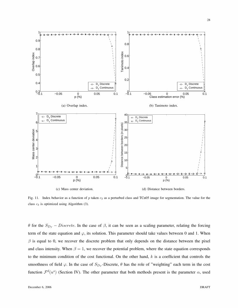
Fig. 10. Index behavior as a function of p taken c2 as a perturbed class and TCn05 image for segmentation. The value for the

class c2 was computed using Eq. (51): c2 = 100± p×max(V) = 100± p× 255.

the segmentations obtained with the SDT-Continuous-OP and SDT

-Discrete-OP methods are presented

in Fig. 11. As can be seen, this simple technique improves very much the quality of the result making

the dependance on the class value of the result almost negligible for all the indexes.

D. Test 4 - Parameter estimation

Besides the set of classes C, the methods have other parameters. The parameters are β and k (we limit

our analysis to the case of an isotropic diffusion tensor K = kI) for the SDT−Continuous and parameter


28

−0.1 −0.05 0 0.05 0.10.3

0.4

0.5

0.6

0.7

0.8

0.9

1O

verla

p in

dex

p (%)

DT Discrete

DT Continuous

(a) Overlap index.

−0.1 −0.05 0 0.05 0.10

0.2

0.4

0.6

0.8

1

Tan

imot

o in

dex

Class estimation error (%)

DT Discrete

DT Continuous

(b) Tanimoto index.

−0.1 −0.05 0 0.05 0.10

1

2

3

4

5

6

7

Mas

s ce

nter

dev

iatio

n

p (%)

DT Discrete

DT Continuous


−0.1 −0.05 0 0.05 0.10

5

10

15

20

25

30

35

40

Dis

tanc

e be

twee

n bo

rder

s (in

pix

els)

p (%)

DT Discrete

DT Continuous


Fig. 11. Index behavior as a function of p taken c2 as a perturbed class and TCn05 image for segmentation. The value for the

class c2 is optimized using Algorithm (3).

θ for the SDT−Discrete. In the case of β, it can be seen as a scaling parameter, relating the forcing

term of the state equation and ϕ, its solution. This parameter should take values between 0 and 1. When

β is equal to 0, we recover the discrete problem that only depends on the distance between the pixel

and class intensity. When β = 1, we recover the potential problem, where the state equation corresponds

to the minimum condition of the cost functional. On the other hand, k is a coefficient that controls the

smoothness of field ϕ. In the case of SDT-Discrete, θ has the role of ”weighting” each term in the cost

function Fd(us) (Section IV). The other parameter that both methods present is the parameter α, used


29

to select how many of the pixels are going to be changed at each iteration. In all the tests performed in

this work, the approach proposed in Eq. 47 was used taking α = 1.

As both methods present different parameters, they were analyzed independently using the images

corresponding to TCn05.

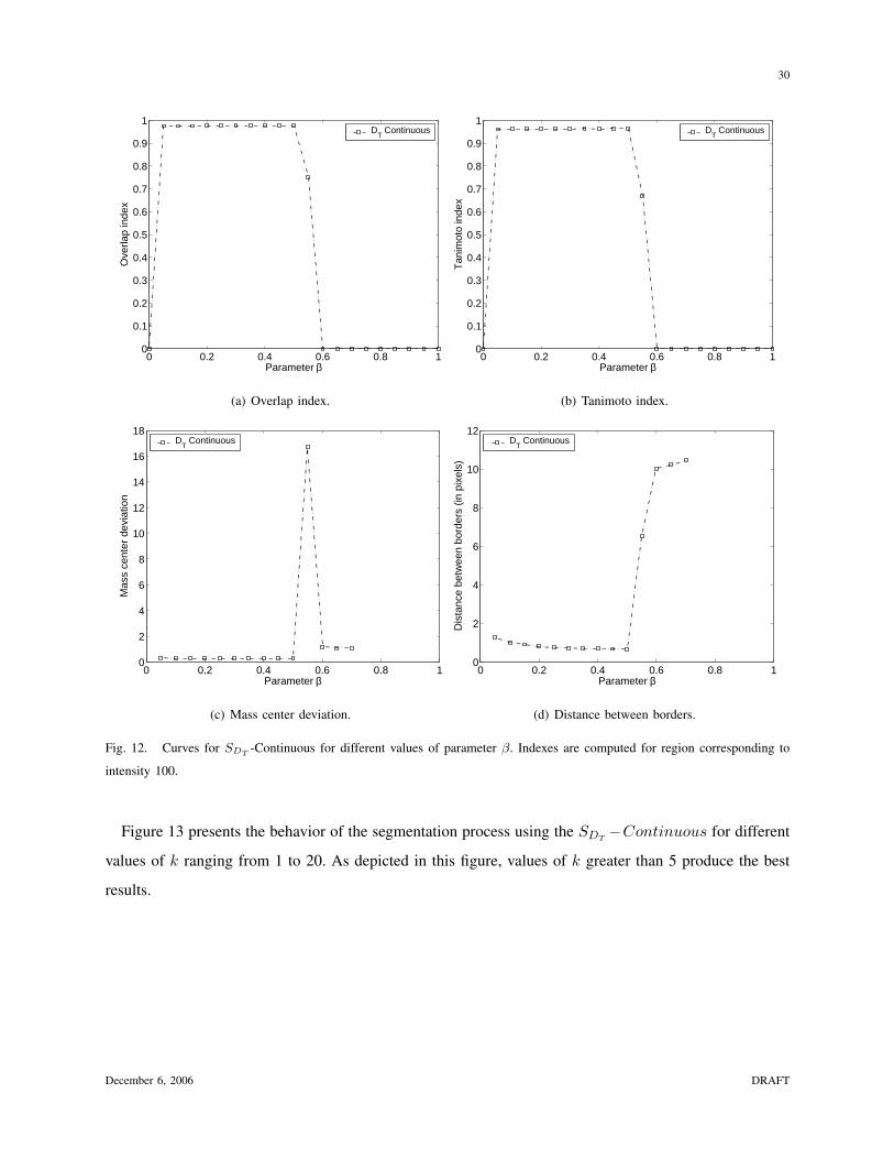
1) SDT− Continuous: The results for different values of parameter β are presented in Figure 12.

The range of values of β tested goes from 0 to 1 in increments of 0.05. In all the cases, the best values

for β range between 0.05 and 0.5. It is important to recall that for values of β above 0.5, the image

was not segmented at all (the initial condition, u0 ≡ ci was not modified for β above 0.5). This result is

evidenced by the different indexes. Only the Mass center deviation presents a better result for β = 0.7.

The reason for this is that in the particular case of the Mass center deviation, the values corresponding

to β = 0.6 · · · 1 correspond to the images that were not segmented at all. In this images, the mass center

corresponds to the center of the image, that is very close to the real mass center of region c2 (region

with intensity 100).


30

0 0.2 0.4 0.6 0.8 10

0.1

0.2

0.3

0.4

0.5

0.6

0.7

0.8

0.9

1O

verla

p in

dex

Parameter β

DT Continuous

(a) Overlap index.

0 0.2 0.4 0.6 0.8 10

0.1

0.2

0.3

0.4

0.5

0.6

0.7

0.8

0.9

1

Tan

imot

o in

dex

Parameter β

DT Continuous

(b) Tanimoto index.

0 0.2 0.4 0.6 0.8 10

2

4

6

8

10

12

14

16

18

Mas

s ce

nter

dev

iatio

n

Parameter β

DT Continuous


0 0.2 0.4 0.6 0.8 10

2

4

6

8

10

12

Dis

tanc

e be

twee

n bo

rder

s (in

pix

els)

Parameter β

DT Continuous


Fig. 12. Curves for SDT -Continuous for different values of parameter β. Indexes are computed for region corresponding to

intensity 100.

Figure 13 presents the behavior of the segmentation process using the SDT−Continuous for different

values of k ranging from 1 to 20. As depicted in this figure, values of k greater than 5 produce the best

results.


31

0 5 10 15 200.95

0.955

0.96

0.965

0.97

0.975

0.98

0.985O

verla

p in

dex

Parameter k

DT Continuous

(a) Overlap index.

0 5 10 15 200.91

0.92

0.93

0.94

0.95

0.96

0.97

Tan

imot

o in

dex

Parameter k

DT Continuous

(b) Tanimoto index.

0 5 10 15 200.2

0.3

0.4

0.5

0.6

0.7

0.8

0.9

1

Mas

s ce

nter

dev

iatio

n

Parameter k

DT Continuous


0 5 10 15 200

1

2

3

4

5

6

Dis

tanc

e be

twee

n bo

rder

s (in

pix

els)

Parameter k

DT Continuous


Fig. 13. Curves for SDT − Continuous for different values of parameter k. Indexes are computed for region corresponding

to intensity 100.

2) SDT−Discrete: The behavior of the method for different values of the parameter θ is presented

in Fig. 14. For θ > 0.85 the Tanimoto and Overlap indexes are not influenced by this parameter. For the

case Distance between borders the best results were obtained for θ ∈ (0.870.98). In the case of Mass

center deviation (Fig. 14(c)), we observe that the results are oscillatory, the variations are very small

(between 0.29 and 0.36 pixels).


32

0.8 0.85 0.9 0.95 10.92

0.93

0.94

0.95

0.96

0.97

0.98O

verla

p in

dex

Parameter θ

DT Discrete

(a) Overlap index.

0.8 0.85 0.9 0.95 10.87

0.88

0.89

0.9

0.91

0.92

0.93

0.94

0.95

0.96

0.97

Tan

imot

o in

dex

Parameter θ

DT Discrete

(b) Tanimoto index.

0.8 0.85 0.9 0.95 10.28

0.29

0.3

0.31

0.32

0.33

0.34

0.35

0.36

0.37

Mas

s ce

nter

dev

iatio

n

Parameter θ

DT Discrete


0.8 0.85 0.9 0.95 11

1.5

2

2.5

3

3.5

4

4.5

5

Parameter θ

Dis

tanc

e be

twee

n bo

rder

s (in

pix

els)

DT Discrete


Fig. 14. Curves for SDT −Discrete for different values of parameter θ.

E. Results for real images

As mentioned before, we are specially concerned with medical image segmentation for posterior artery

reconstruction. The objective here is to recover the artery internal wall geometry and, using fluid dynamics

models, simulate the blood flow in different arterial districts. This technique has diverse applications in

the field of medicine, in particular for disease diagnosis and surgical planning [5], [6], [7], [8], [9]. The

intention of this section is to present some results when the techniques introduced before are applied

to patient specific data. In this case, no quantitative evaluation of the results is made as we are only

interested in showing some of the applications of the proposed methods.

The image selected corresponds to a neck CTA composed of 90 equally spaced slices (BMP format),


33

each of 256 × 256 pixels. In Figure 15 are presented 10 different slices of the whole volume. In these

images the left and right carotid artery are clearly identified. In order to segment these arteries two

classes were selected. The first one representing the arteries (c1 = 200) and the second representing the

background (c2 = 160).

Fig. 15. Segmented CTA image (10 out of 90 slices).

In Fig. 16 are presented the 3D reconstructions for the right and left carotid artery for SDT−Discrete

(Fig. 16(a)) and SDT− Continuous (Fig. 16(b)) methods where the segmentation was processed as

independent 2D images and posteriorly joined as a hole volume. Figure 16(c) presents the surface for

SDT−Discrete (white) and the surface for SDT

− Continuous (red 50% opacity) superposed. Small

differences can be observed for both methods, in particular for the External Carotid Artery (ECA). In

both cases (left and right) the SDT− Continuous method has captured more details of the ECA.

Also, a 3D implementation of the SDT− Discrete (SDT

− Discrete 3D) method was used to

segment this image as a 3D volume. Several comparisons between the different approaches of the SDT

segmentation methods are made in Figs. (16(d)), (16(e)) and (16(f)).


34

(a) Result for SDT −Discrete. (b) Result for SDT − Continuous.

(c) Comparison between SDT − Continuous

(r) and SDT −Discrete (w) methods.

(d) Comparison between SDT − Continuous

(r) and SDT −Discrete 3D (w) methods.

(e) Comparison between SDT −Discrete (w)

and SDT −Discrete 3D (b) methods.

(f) Comparison between SDT − Continuous

(r), SDT −Discrete (w) and SDT −Discrete

3D (b) methods.

Fig. 16. 3D reconstruction for the results corresponding to SDT methods (r = red, b =blue and w = white).


35

In order to evaluate quantitatively the segmentations presented in Fig. (16(c)), Fig. (17(a)) shows the

behavior of the Overlap and Tanimoto indexes, were the worst result is observed for plane number 60.

The difference for both segmentations for plane number 60 is highlighted in Fig. (17(b)) where the yellow

pixels indicate the SDT−Continuous and the SDT

−Discrete corresponds to pixels in red and yellow.

0 20 40 60 80 1000.6

0.65

0.7

0.75

0.8

0.85

0.9

0.95

1

Tan

imot

o/O

verla

p in

dex

Plane number

OverlapTanimoto

(a) Overlap and Tanimoto index. (b) SDT −Continuous = yellow, SDT −Discrete

= yellow + red.

Fig. 17. Quantitative comparison between SDT − continuous and SDT −Discrete methods.

VII. CONCLUSIONS

In this work was studied the use of topological derivative as tool for image segmentation. The

topological derivative, originally conceived for topology optimization problems, has proved to be useful

when applied to image processing.

In particular, two image segmentation algorithms based on the topological derivative associated to an

appropriated functionals (indicating the cost endowed to a specific segmentation) were presented. In these

algorithms the segmentation process is driven by the information obtained with the topological derivative.

In the SDT− Continuous method the solution of a state and adjoint equation are necessary to be

obtained in order to evaluate the topological derivative. As a counterpart of its computational cost, the

SDT−Continuous appears to be robust giving good quality segmentations even for high levels of noise.

For the second method, named SDT−Discrete, finding the solution of these equations is not necessary,

leading to a very fast algorithm and allowing a full 3D implementation. Further, in the case that the

value of the classes are not known a priori a very simple optimization algorithm that can be used in

both methods is also proposed given excellent results.


36

APPENDIX I

ASYMPTOTIC ANALYSIS FOR SOURCE PERTURBATION

In this section is performed an asymptotic analysis for the problem presented in Sec. II taking K = kI.

A. Problem formulation associated to the original domain

Let the direct problem associated to the original domain, be defined as:

• Find ϕ ∈ H1(Ω), such that

a(ϕ, η) = l(η) ∀η ∈ H1(Ω) (52)

where

a(ϕ, η) =∫

Ωk∇ϕ · ∇η +

∫Ω

ϕη (53)

l(η) = β

∫Ω(v − u)η

= β

∫Ω\Bε

(v − u)η + β

∫Bε

(v − u)η (54)

• Let also λ ∈ H1(Ω), be the solution of the adjoint equation associated to the original domain given

by

λ =1− β

βϕ (55)

B. Problem formulation associated to the perturbed domain

Let the direct problem, associated to the perturbed domain, be defined as:

• Find ϕε ∈ H1(Ω), such that:

a(ϕε, η) = lε(η) ∀η ∈ H1(Ω) (56)

where

lε(η) = β

∫Ω\Bε

(v − u)η + β

∫Bε

(v − uT )η (57)

• Let also λε ∈ H1(Ω) be the solution of the adjoint equation associated to the original domain given

by

λε =1− β

βϕε (58)


37

C. Asymptotic Analysis

Theorem 1: Let us consider solutions of the state ϕε, ϕ and adjoint λε, λ equations, where each pair ϕ,

λ and ϕε, λε is associated to the original (Eqs. 52, 55) and perturbed (Eqs. 56, 58) problems respectively.

Then, the following estimate holds

‖ϕε − ϕ‖H1(Ω) ≤ C1 |Bε|1/2 and ‖λε − λ‖H1(Ω) ≤ C2 |Bε|1/2 (59)

where constants C1 and C2 are independents of parameter ε and |Bε| is the Lebesgue measure of the

ball Bε.

Proof: Taking the difference between the variational equations associated to the perturbed (Eq. 56)

and original (Eq. 52) problems respectively, we obtain

a(ϕε − ϕ, η) = β

∫Bε

(v − uT )η − β

∫Bε

(v − u)η

= β

∫Bε

(u− uT )η ∀η ∈ H1(Ω) (60)

Taking also η = ϕε − ϕ we have

a(ϕε − ϕ, ϕε − ϕ) = β

∫Bε

(u− uT )(ϕε − ϕ), (61)

then, the coercivity of a(·, ·)

m ‖ϕε − ϕ‖2H1(Ω) ≤ a(ϕε − ϕ, ϕε − ϕ) = β

∫Bε

(u− uT )(ϕε − ϕ). (62)

Considering at this point the Cauchy-Schwarz inequality we have

‖ϕε − ϕ‖2H1(Ω) ≤ β

m‖u− uT ‖L2(Bε)

‖ϕε − ϕ‖L2(Bε)

≤ c1β


‖ϕε − ϕ‖L2(Ω)

≤ c2β


‖ϕε − ϕ‖H1(Ω)

≤ c3β

mmaxx∈Bε

|u− uT ||Bε|1/2 ‖ϕε − ϕ‖H1(Ω) (63)

being c1, c2 and c3 constants independent of ε. Then

‖ϕε − ϕ‖H1(Ω) ≤ C1|Bε|1/2 (64)

with

C1 = c3β

mmaxx∈Bε

|u− uT |. (65)


38

Moreover, from Eqs. 55 and 58 we have

‖λε − λ‖H1(Ω) ≤(1− β)

mmaxx∈Bε

|u− uT ||Bε|1/2 = C2|Bε|1/2. (66)

Finally

‖λε − λ‖H1(Ω) ≤ C2|Bε|1/2 (67)

with

C2 = c3(1− β)

mmaxx∈Bε

|u− uT | (68)

what concludes the proof.

APPENDIX II

ON THE ESHELBY ENERGY-MOMENTUM TENSOR

Proposition 1: In the context of topological derivative applied to image segmentation presented above,

the following holds

div(Σε) = 0 (69)

Proof: Let ϕε be the solution for the perturbed problem of the state equation and λε the adjoint

equation, then

State equation: −div(k∇ϕε) + ϕε = β(v − u) x ∈ Ω \ Bε

−div(k∇ϕε) + ϕε = β(v − uT ) x ∈ Bε

∂ϕε

∂n = 0 x ∈ ∂Ω

(70)

Adjoint solution:

λε =1− β

βϕε (71)

For the problem under consideration, the Eshelby Energy-Momentum Tensor states as

Σeε =

12

(k∇ϕε · ∇ϕε + (ϕε − (v − u))2 + 2 (k∇ϕε · ∇λε + ϕελε)− 2β(v − u)λε

)I

− k (∇ϕε ⊗∇ϕε+∇ϕε ⊗∇λε +∇λε ⊗∇ϕε) , ∀ x ∈ Ω \Bε (72)

Σiε =

12

(k∇ϕε · ∇ϕε + (ϕε − (v − uT ))2 + 2(k∇ϕε · ∇λε + ϕελε)− 2β(v − uT )λε

)I

− k (∇ϕε ⊗∇ϕε+∇ϕε ⊗∇λε +∇λε ⊗∇ϕε) . ∀ x ∈ Bε (73)


39

We first consider Σeε . Taking into account Eq. 71 we obtain

Σeε =

12

(k∇ϕε · ∇ϕε + (ϕε − (v − u))2 + 2

1− β

β(k∇ϕε · ∇ϕε + ϕεϕε)− 2(1− β)(v − u)ϕε

)I

− k

(∇ϕε ⊗∇ϕε+2

1− β

β∇ϕε ⊗∇ϕε

)(74)

From the linearity of the operator div(·), we may calculate div(Σeε) term by term. Remembering that

div(ϕT) = ϕdiv(T) + T∇ϕ and ∇(v · u) = (∇v)T u + (∇u)T v, (75)

we obtain

div

(12(k∇ϕε · ∇ϕε)I

)=

12

k(∇ϕε · ∇ϕε) div(I)︸︷︷︸=0

+12∇(k(∇ϕε · ∇ϕε))

=12

(k(∇∇ϕε)T∇ϕε + k(∇∇ϕε)T∇ϕε

)= k(∇∇ϕε)T∇ϕε. (76)

For the second term, and considering that functions v and u are constant by parts, we have

div

(12

(ϕε − (v − u))2 I)

= ∇ϕε(ϕε − (v − u)) (77)

The third and fourth terms of div(·) can be rewritten as

div

(1− β

β(k∇ϕε · ∇ϕε + ϕεϕε)I

)= 2

1− β

β

(k(∇∇ϕε)T∇ϕε +∇ϕεϕε

)(78)

and

div(−(1− β)(v − u)ϕεI) = −(1− β)∇ϕε(v − u) (79)

respectively. Working on a similar way on the remainder terms we obtain

div(−k∇ϕε ⊗∇ϕε) = −∇ϕεdiv(k∇ϕε)− k(∇∇ϕε)∇ϕε (80)

div

(−2

1− β

βk∇ϕε ⊗∇ϕε

)= −2

1− β

β∇ϕεdiv(k∇ϕε)− 2

1− β

βk(∇∇ϕε)∇ϕε (81)

Joining all the terms together we obtain

div(Σeε) = k(∇∇ϕε)T∇ϕε +∇ϕε(ϕε − (v − u)) + 2

1− β

β

(k(∇∇ϕε)T∇ϕε

)+ 2

1− β

β∇ϕεϕε − (1− β)∇ϕε(v − u)−∇ϕεdiv(k∇ϕε)− k(∇∇ϕε)∇ϕε

− 21− β


1− β

βk(∇∇ϕε)∇ϕε (82)


40

As ϕε is a scalar field, the following holds

∇∇ϕε = (∇∇ϕε)T (83)

Then, from (83) we can write

div(Σeε) = k(∇∇ϕε)T∇ϕε︸︷︷︸

(1)

+∇ϕε(ϕε − (v − u)) + 21− β

β

(k(∇∇ϕε)T∇ϕε

)︸︷︷︸

(2)

+ 21− β

β∇ϕεϕε − (1− β)∇ϕε(v − u)−∇ϕεdiv(k∇ϕε)− k(∇∇ϕε)∇ϕε︸︷︷︸

(1)

− 21− β


1− β

β(k(∇∇ϕε)∇ϕε)︸︷︷︸

(2)

(84)

As the highlighted terms cancel each other, we can rewrite (84) in the following way

div(Σeε) = ∇ϕε(ϕε − (v − u))

+ 21− β

β∇ϕεϕε − (1− β)∇ϕε(v − u)−∇ϕεdiv(k∇ϕε)

− 21− β

β∇ϕεdiv(k∇ϕε) (85)

Adding and subtracting β(v − u) we obtain

div(Σeε) = ∇ϕε

ϕε − β(v − u)− div(k∇ϕε)︸︷︷︸state equation

+

β

1− β∇ϕε


+

β

1− β∇ϕε


(86)

Then

div(Σeε) = 0 (87)

The proof for div(Σiε) = 0 is equivalent.


41

ACKNOWLEDGMENT

This research was partly supported by the brazilian agencies CNPq/FAPERJ-PRONEX, under Grant

E-26/171.199/2003. Ignacio Larrabide was partly supported by the brazilian agency CNPq (141336/2003-

0). The support from these agencies is greatly appreciated. The authors would also like to thank Prof.

Paulo Sergio Rodriguez for many fruitful discussions during the preparation of this work.

REFERENCES

[1] C. Eveland, K. Konolige, and R. C. Bolles, “Background modeling for segmentation of video-rate stereo sequences,” in

International Conference on Computer Vision and Pattern Recognition, 1998, pp. 266–272.

[2] W. E. L. Grimson, C. Stauffer, R. Romano, and L. Lee, “Using adaptive tracking to classify and monitor activities in

a site,” in Proceedings of the International Conference on Computer Vision and Pattern Recognition. Santa Barbara -

California: IEEE Computer Society, June 1998, pp. 22–31.

[3] C. R. Wren, A. Azarbayejani, T. Darrell, and A. Pentland, “Pfinder: real time tracking of human body,” IEEE Tran. on

Pattern Analysis and Machine Intelligence, vol. 19, no. 7, pp. 780–785, July 1997.

[4] N. Paragios and R. Deriche, “A pde-based level set approach for detection and tracking of moving objects,” in Proceedings

of the 6th International Conference on Computer Vision, IEEE Computer Society. Bombay, India: IEEE Computer Society

Press, January 1998, pp. 1139–1145.

[5] J. R. Cebral and R. Lohner, “From medical images to cfd meshes,” in Proceedings, 8th International Meshing Roundtable,

South Lake Tahoe, CA, U.S.A., October 1999, pp. 321–331.

[6] L. Formaggia, F. Nobile, A. Quarteroni, and A. Veneziani, “Multiscale modelling of the circulatory system: a preliminary

analysis,” Comput. Visual Sci., vol. 2, pp. 75–83, 1999.

[7] J. Wan, B. Steele, S. A. Spicer, S. Strohband, G. R. Feijoo, T. J. Hughes, and C. A. Taylor, “A one-dimensional finite

element method for simulation-based medical planning for cardiovascular disease,” Comput. Methods Biomech. Biomed.

Engin., vol. 5, no. 3, pp. 195–206, 2002.

[8] S. A. Urquiza, P. J. Blanco, M. J. Venere, and R. A. Feijoo, “Multidimensional modelling for carotid artery blood flow,”

Computer Methods in Applied Mechanics and Engineering, vol. 195, no. 33-36, pp. 4002–4017, July 2006.

[9] I. Larrabide, P. Blanco, S. Urquiza, and R. Feijoo, “Sensitivity of blood flow in stenosed carotid bifurcation,” in Proceedings

of ICCB2006 - II International Conference on Computational Bioengineering, Rodrigues et al. eds. ,Lisbon, Portugal, 2005.

[10] D. Mumford and J. Shah, “Optimal approximations by piecewise smooth functions and associated variational problems,”

Communications on Pure and Applied Mathematics, vol. 42, pp. 577–684, 1989.

[11] A. K. Jain, Fundamentals of Digital Image Processing. Prentice Hall, 1989.

[12] C. R. Gonzalez and R. E. Woods, Digital Image Processing - Second Edition. Prentice Hall, 2001.

[13] J. Suri, S. Singh, and K. Setarehdan, Eds., Advanced algorithmic approaches to medical image segmentation: state-of-the-art

applications in cardiology, neurology, mammography and pathology. Springer-Verlag, 2001.

[14] K. H. Hohne, H. Fuchs, and S. M. Pizer, 3D imaging in medicine: algorithms, systems, applications. New York: Springer-

Verlag, 1990.

[15] J. A. Sethian, Level Set Methods and Fast Marching Methods. Cambridge University Press, 1999.


42

[16] R. Malladi and J. A. Sethian, “Level set methods for curvature flow, image enhancement, and shape recovery in medical

images.” in Proc. of Conf. on Visualization and Mathematics. Germany: Springer-Verlag, 1997, pp. 329–345.

[17] C. Xu, D. L. Pham, and J. L. Prince, Medical Image Segmentation Using Deformable Models. SPIE Handbook on Medical

Imaging - Volume III: Medical Image Analysis, 2000, pp. 129–174.

[18] C. Xu, D. L. Pham, M. E. Rettmann, D. N. Yu, and J. L. Prince, “Reconstruction of the human cerebral cortex from

magnetic resonance images,” IEEE Transactions on Medical Imaging, vol. 18, no. 6, pp. 467–480, 1999.

[19] H. Li, R. Deklerck, B. DeCuyper, A. Hermanusa, E. Nyssen, and J. Cornelis, “Object recognition in brain ct-scans:

knowledge-based fusion of data from multiple feature extractors,” IEEE Trans. Med. Imaging, vol. 14, pp. 212–229, 1995.

[20] R. Boscolo, M. Brown, and M. McNitt-Gray, “Medical image segmentation with knowledge-guided robust active contours,”

Radiographics, vol. 22, no. 2, pp. 437–448, 2002.

[21] K. Held, E. R. Kops, B. J. Krause, W. M. W. 3rd, R. Kikinis, and H. W. Muller-Gartner, “Markov random field segmentation

of brain mr images,” IEEE Trans. Med. Imaging, vol. 16, no. 6, pp. 878–886, 1997.

[22] Y. Zhang, M. Brady, and S. Smith, “Segmentation of brain mr images through a hidden markov random field model and

the expectation-maximization algorithm,” IEEE Transactions on Medical Imaging, vol. 20, no. 1, pp. 45–57, 2001.

[23] L. J. Belaid, M. Jaoua, M. Masmoudi, and L. Siala, “Image restoration and edge detections by topological asyptotic

expansion,” 2005, masmoudi personal communication.

[24] I. Larrabide, A. A. Novotny, R. A. Feijo, and E. Taroco, “A medical image enhancement algorithm based on topological

derivative and anisotropic diffusion,” in Proceedings of the XXVI Iberian Latin-American Congress on Computational

Methods in Engineering - CILAMCE 2005 - Guarapari, Esprito Santo, Brazil, 2005.

[25] I. Larrabide, R. A. Feijoo, A. A. Novotny, E. Taroco, and M. Masmoudi, “An image segmentation method based on a

discrete version of the topological derivative,” in World Congress Structural and Multidisciplinary Optimization 6, Rio de

Janeiro. International Society for Structural and Multidisciplinary Optimization, 2005.

[26] D. Auroux, M. Masmoudi, and L. Belaid, “Image restoration and classification by topological asymptotic expansion,”

Variational Formulations in Mechanics: Theory and Applications - CIMNE, Barcelona, Spain 2006 (In press), 2006.

[27] A. A. Novotny, “Analise de sensibilidade topologica,” PhD Thesis, Laboratorio Nacional de Computacao Cientıfica,

Petropolis - RJ - Brazil, 2003.

[28] A. Novotny, R. Feijoo, E. Taroco, and C. Padra, “Topological sensitivity analysis,” Computer Methods in Applied Mechanics

and Engineering, vol. 192, pp. 803–829, 2003.

[29] H. A. Eschenauer, V. V. Kobelev, and A. Schumacher, “Bubble method for topology and shape optimization of structures,”

Structural Optimization, vol. 8, pp. 42–51, 1994.

[30] J. Cea, S. Garreau, P. Guillaume, and M. Masmoudi, “The shape and topological optimizations connection,” Computer

Methods in Applied Mechanics and Engineering, vol. 188, no. 4, pp. 713–726, 2000.

[31] J. S. owski and A. Zochowski, “Topological derivatives for elliptic problems,” Inverse Problems, vol. 15, pp. 123–134,

1999.

[32] L. J. Belaid, M. Jaoua, M. Masmoudi, , and L. Siala, “Image restoration and edge detection by topological asymptotic

expansion,” C. R. Acad. Sci. Ser. I, vol. 342, no. 5, 2006.

[33] I. Larrabide, A. A. Novotny, R. A. Feijoo, and E. Taroco, “Topological derivative as a tool for image processing: Image

segmentation,” LNCC - Laboratorio Nacional de Computacao Cientıfica, Tech. Rep., 2006.

[34] J. Cea, “Problems of shape optimal design,” Optimization of Distributed Parameters Structures - Ed. E.J.Haug and J.Cea,

Sijthoff and Noordhoff, Alphen aan den Rijn, no. II, pp. 1005–1048, 1981.


43

[35] J. P. Zolesio, The material derivative (or speed) method for shape optimization, in: Optimization of Distributed Parameter

Structures. NATO Adv. Study Inst. Ser. E, Appl. Sci., 1981, vol. II, no. 50, pp. 1089–1151.

[36] E. J. Haug, K. K. Choi, and V. Komkov, Design Sensitivity Analysis of Structural Systems. Academic Press, 1986.

[37] M. Masmoudi, “Outils pour la conception optimale de formes,” PhD Thesis, Nice University, 1987.

[38] S. J. Arora, “An exposition of the material derivative approach for structural shape sensitivity analysis,” Comput. Methods

Appl. Mech. Engrg., no. 105, pp. 41–62, 1993.

[39] H. Petrik and Z. Mroz, “Time derivatives of integrals and functionals defined on varying volume and surface domains,”

Arch. Mech., vol. 38, no. 5–6, pp. 697–724, 1986.

[40] P. Guillaume and M. Masmoudi, “Derivees d’ordre superieur en optimisation de domaines,” C. R. Acad. Sci. Paris, vol.

t.315, no. Serie I, pp. 859–862, 1992.

[41] M. O. Gurtin, An Introduction to Continuum Mechanics. Academic Press, 1981.

[42] J. D. Eshelby, “The elastic energy-momentum tensor,” J. Elasticity 5, pp. 321–335, 1985.

[43] T. J. R. Hughes, The Finite Element Method - Linear Static and Dynamic Finite Element Analysis. Prentice-Hall, 2000.

[44] L. Alvarez, P. Lions, and J.-M. Morel, “Image selective smoothing and edge detection by nonlinear diffusion,” SIAM

Journal on Numerical Analisis, vol. 29, pp. 845–866, 1992.

[45] M.J.Black, G. Sapiro, D. Marimont, and D. Heeger, “Robust anisotropic diffusion,” IEEE Transactions on Image Processing,

vol. 7, no. 3, pp. 421–423, 1998.

[46] A. S. Frangakis and R. Hegerl, “Noise reduction in electron tomographic reconstructions using nonlinear anisotropic

diffusion,” J. Struct. Biol., vol. 1, no. 135, pp. 239–250, 2001.

[47] C. Banga and F. Ghorbel, “Optimal bootstrap sampling for fast image segmentation: application to retina images,” in IEEE

ICASP 93, vol. 5, Minneapolis USA, 1993, pp. 638–641.

[48] I. Koch and G. Marshall, “Bootstrap coverage plots for image segmentation,” in IEEE Proceedings of ICPR 1996, 1996,

pp. 447–451.

[49] R. M. Gray and Y. Linde, “Vector quantization and predictive quantizer for gauss-markov sources,” IEEE Transaction on

Communications, vol. 30, pp. 381–389, 1982.

[50] T. N. Pappas, “An adaptive clustering algorithm for image segmentation,” IEEE Transactions on Signal Processing, vol. 40,

pp. 901–914, April 1992.

[51] J. C. Dunn, “A fuzzy relative of the isodata process and its use in detecting compact, well separated clusters,” Journal of

Cybernetics, vol. 3, pp. 32–57, 1974.

[52] J. Bezdek, Pattern Recognition with fuzzy Objective Function Algorithms. New York: Plenum Press, 1981.

[53] F. Alonso, M. Algorri, and F. Flores-Mangas, “Composite index for the quantitative evaluation of image segmentation

results,” in Proceedings of the 26th Annual International Conference of the IEEE EMBS, San Francisco, CA, USA, 2004,

pp. 1794–1797.

[54] P. Zijdenbos, B. M. Dawant, R. A. Margolin, and A. C. Palmer, “Morphometric analysis of white matter lesions in mr

images: Method and validation,” IEEE Trans. Med. Imag., vol. 13, no. 4, pp. 716–724, December 1994.


Topological derivative as a tool for image processing: Image segmentation

Documents