Topological Equivalence between a 3D Object and the Reconstruction of Its Digital Image

Topological Equivalence between a 3D Objectand the Reconstruction of Its Digital Image

Peer Stelldinger, Longin Jan Latecki, and Marcelo Siqueira

Abstract—Digitization is not as easy as it looks. If one digitizes a 3D object even with a dense sampling grid, the reconstructed digital

object may have topological distortions and, in general, there exists no upper bound for the Hausdorff distance. This explains why so far

no algorithm has been known which guarantees topology preservation. However, as we will show, it is possible to repair the obtained

digital image in a locally bounded way so that it is homeomorphic and close to the 3D object. The resulting digital object is always well-

composed, which has nice implications for a lot of image analysis problems. Moreover, we will show that the surface of the original object

is homeomorphic to the result of the marching cubes algorithm. This is really surprising since it means that the well-known topological

problems of the marching cubes reconstruction simply do not occur for digital images of r-regular objects. Based on the trilinear

interpolation, we also construct a smooth isosurface from the digital image that has the same topology as the original surface. Finally, we

give a surprisingly simple topology preserving reconstruction method by using overlapping balls instead of cubical voxels. This is the first

approach of digitizing 3D objects which guarantees topology preservation and gives an upper bound for the geometric distortion. Since

the output can be chosen as a pure voxel presentation, a union of balls, a reconstruction by trilinear interpolation, a smooth isosurface, or

the piecewise linear marching cubes surface, the results are directly applicable to a huge class of image analysis algorithms. Moreover,

we show how one can efficiently estimate the volume and the surface area of 3D objects by looking at their digitizations. Measuring

volume and surface area of digital objects are important problems in 3D image analysis. Good estimators should be multigrid convergent,

i.e., the error goes to zero with increasing sampling density. We will show that every presented reconstruction method can be used for

volume estimation and we will give a solution for the much more difficult problem of multigrid-convergent surface area estimation. Our

solution is based on simple counting of voxels and we are the first to be able to give absolute bounds for the surface area.

Index Terms—r-regular, topology, digitization, 3D, marching cubes, trilinear interpolation, well-composed.

Ç

1 INTRODUCTION

A fundamental task of knowledge representation andprocessing is to infer properties of real objects or

situations given their representations. In spatial knowledgerepresentation and, in particular, in computer vision andmedical imaging, real objects are represented in a pictorialway as finite and discrete sets of pixels or voxels. The discretesets result from a quantization process in which real objectsare approximated by discrete sets. In computer vision, thisprocess is called sampling or digitization and is naturallyrealized by technical devices like computer tomographyscanners, CCD cameras, or document scanners. Afundamental question addressed in spatial knowledgerepresentation is: Which properties inferred from discreterepresentations of real objects correspond to properties oftheir originals, and under what conditions is this the case?While this problem is well-understood in the 2D case with

respect to topoology [1], [2], [3], [4], [5], [6], it is not as simplein 3D, as shown in [7]. In this paper, we present the firstcomprehensive answer to this question with respect toimportant topological and geometric properties of3D objects. Some of the results presented here can also befound without proofs in [8], [9], [10].

The description of geometric and, in particular, topolo-gical features in discrete structures is based on graph theory,which is widely accepted in the computer science commu-nity. A graph is obtained when a neighborhood relation isintroduced into a discrete set, e.g., a finite subset of ZZ2 or ZZ3,where ZZ denotes the integers. On the one hand, graphtheory allows investigation into connectivity and separ-ability of discrete sets (for a simple and natural definition ofconnectivity, see Kong and Rosenfeld [11], for example). Onthe other hand, a finite graph is an elementary structure thatcan be easily implemented on computers. Discrete repre-sentations are analyzed by algorithms based on graphtheory and the properties extracted are assumed torepresent properties of the original objects. Since practicalapplications, for example, in image analysis show that this isnot always the case, it is necessary to relate properties ofdiscrete representations to the corresponding properties ofthe originals. Since such relations allow us to describe andjustify the algorithms on discrete graphs, their characteriza-tion contributes directly to the computational investigationof algorithms on discrete structures. This computationalinvestigation is an important part of the research incomputer science and, in particular, in computer vision(Marr [12]), where it can contribute to the development of

IEEE TRANSACTIONS ON PATTERN ANALYSIS AND MACHINE INTELLIGENCE, VOL. 29, NO. 1, JANUARY 2007 1

. P. Stelldinger is with the Cognitive Systems Group, University ofHamburg, Vogt-Koelln-Str. 30, D-22527 Hamburg, Germany.E-mail: [email protected]

. L.J. Latecki is with the Department of Computer and Information Sciences,Temple University, 1805 North Broad Street, Philadelphia, PA 19122.E-mail: [email protected].

. M. Siqueira is with the Departamento de Computacao e Estatıstica,Universidade Federal de Mato Grosso do Sul, Av. Costa e Silva, S/N,Cidade Universitaria, Campo Grande (MS), Brasil, 79070-900.E-mail: [email protected].

Manuscript received 26 Jan. 2006; revised 2 May 2006; accepted 16 May2006; published online 13 Nov. 2006.Recommended for acceptance by R. Klette.For information on obtaining reprints of this article, please send e-mail to:[email protected], and reference IEEECS Log Number TPAMI-0049-0106.

0162-8828/07/$20.00 � 2007 IEEE Published by the IEEE Computer Society

more suitable and reliable algorithms for extracting re-quired shape properties from discrete representations.

It is clear that no discrete representation can exhibit all

features of the real original. Thus, one has to accept

compromises. The compromise chosen depends on the

specific application and on the questions which are typical

for that application. Real objects and their spatial relations

can be characterized using geometric features. Therefore,

any useful discrete representation should model the

geometry faithfully in order to avoid false conclusions.

Topology deals with the invariance of fundamental geo-

metric features like connectivity and separability. Topolo-

gical properties play an important role since they are the

most primitive object features and our visual system seems

to be well-adapted to cope with topological properties.However, we do not have any direct access to spatial

properties of real objects. Therefore, we represent real objects,

as commonly accepted from the beginning of mathematics as

bounded subsets of the Euclidean space IR3 and their

2D views (projections) as bounded continuous subsets of

the plane IR2. Hence, from the theoretical point of view of

knowledge representation, we will relate two different

pictorial representations of objects in the real-world: a

discrete and a continuous representation.Already two of the first books in computer vision deal

with the relation between the continuous object and itsdigital images obtained by modeling a digitization process.Pavlidis [1] and Serra [2] proved independently in 1982 thatan r-regular continuous 2D set S and the continuous analogof the digital image of S have the same shape in atopological sense. Pavlidis used 2D square grids and Serraused 2D hexagonal sampling grids.

An analogous result in 3D case remained an open question

for over 20 years. Only recently one of the authors proved,

together with Stelldinger and Kothe, that the connectivity

properties are preserved when digitizing a 3D r-regular

object with a sufficiently dense sampling grid [7]. But, the

preservation of connectivity is much weaker than topology.

They also found out that topology preservation can even not

be guaranteed with sampling grids of arbitrary density if one

uses the straightforward voxel resonstruction since the

surface of the continuous analog of the digital image may

not be a 2D manifold. Thus, the question of how to guarantee

topology preservation during digitization in 3D remained

unsolved up to now.In this paper, we provide a solution to this question. We

use the same digitization model as Pavlidis and Serra used,

and we also use r-regular sets (but in IR3) to model the

continuous objects. As already shown in [7], the general-

ization of Pavlidis’ straightforward reconstruction method

to 3D fails since the reconstructed surface may not be a

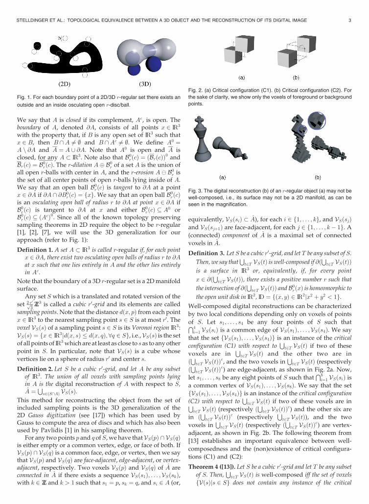
2D manifold. For example, Figs. 3a and 3b show a continuous

object and its digital reconstruction whose surface is not a

2D manifold. However, as we will show, it is possible to use

several other reconstruction methods that all result in a

3D object with a 2D manifold surface. Moreover, we will show

that these reconstructions and the original continuous object

are homeomorphic and their surfaces are close to each other.

The first reconstruction method, Majority interpolation,is a voxel-based representation on a grid with doubledresolution. It always leads to a well-composed set in thesense of Latecki [13], which implies that a lot of problems in3D digital geometry become relatively simple.

The second method is the simplest one. We just use ballswith a certain radius instead of cubical voxels. Whenchoosing an appropriate radius, the topology of an r-regularobject will not be destroyed during digitization.

The third method is a modification of the well-knownMarching Cubes algorithm [14]. The original Marching Cubesalgorithm does not always construct a topologically soundsurface due to several ambiguous cases [15], [16]. We willshow that most of the ambiguous cases cannot occur in thedigitization of an r-regular object and that the only remainingambiguous case always occurs in an unambiguous way,which can be dealt with by a slight modification of the originalMarching Cubes algorithm. Thus, the generated surface is notonly topologically sound, but it also has exactly the sametopology as the original object before digitization.

Moreover, we show that one can use trilinear interpola-tion and that one can even blend the trilinear patchessmoothly into each other such that one gets smooth objectsurfaces with the correct topology.

Each of these methods has its own advantages such thatour results are applicable for a lot of very different imageanalysis algorithms.

We also analyze the question of whether these reconstruc-tion methods are suitable to estimate object properties likevolume and surface area. We show that all the reconstructionmethods can be used for multigrid convergent volumeestimation, but that surface area estimation requires othermethods. We analyze the problem of multigrid convergentsurface area estimation and suggest that one should usesemilocal algorithms since local algorithms do not seem to bemultigrid-convergent and there exists no proof for any globalalgorithm. We give an example of a semilocal surface areaestimator and prove that it is multigrid-convergent.

2 PRELIMINARIES

The (Euclidean) distance between two points x and y in IRn

is denoted by dðx; yÞ, and the (Hausdorff) distance betweentwo subsets of IRn is the maximal distance between eachpoint of one set and the nearest point of the other. Let A �IRn and B � IRm be sets. A function f : A! B is calledhomeomorphism if it is bijective and both it and its inverse arecontinuous. If f is a homeomorphism, we say that A and Bare homeomorphic. Let A, B be two subsets of IR3. Then, ahomeomorphism f : IR3 ! IR3 such that fðAÞ ¼ B anddðx; fðxÞÞ � r, for all x 2 IR3, is called an r-homeomorphismof A to B and we say that A and B are r-homeomorphic. AJordan curve is a set J � IRn which is homeomorphic to acircle. Let A be any subset of IR3. The complement of A isdenoted by Ac. All points in A are foreground, while thepoints in Ac are called background. The open ball in IR3 ofradius r and center c is the set B0

rðcÞ ¼ fx 2 IR3jdðx; cÞ < rg,and the closed ball in IR3 of radius r and center c is the setBrðcÞ ¼ fx 2 IR3jdðx; cÞ � rg. Whenever c ¼ ð0; 0; 0Þ 2 IR3,we write B0

r and Br. We say that A is open if, for eachx 2 A, there exists a positive number r such that B0

rðxÞ � A.

2 IEEE TRANSACTIONS ON PATTERN ANALYSIS AND MACHINE INTELLIGENCE, VOL. 29, NO. 1, JANUARY 2007

We say that A is closed if its complement, Ac, is open. Theboundary of A, denoted @A, consists of all points x 2 IR3

with the property that, if B is any open set of IR3 such thatx 2 B, then B \A 6¼ ; and B \Ac 6¼ ;. We define A0 ¼A n @A and A ¼ A [ @A. Note that A0 is open and A isclosed, for any A � IR3. Note also that B0

rðcÞ ¼ ðBrðcÞÞ0 and

BrðcÞ ¼ B0rðcÞ. The r-dilation A� B0

r of a set A is the union ofall open r-balls with center in A, and the r-erosion A� B0

r isthe set of all center points of open r-balls lying inside of A.We say that an open ball B0

rðcÞ is tangent to @A at a pointx 2 @A if @A \ @B0

rðcÞ ¼ fxg. We say that an open ball B0rðcÞ

is an osculating open ball of radius r to @A at point x 2 @A ifB0rðcÞ is tangent to @A at x and either B0

rðcÞ � A0 orB0rðcÞ � ðAcÞ0. Since all of the known topology preserving

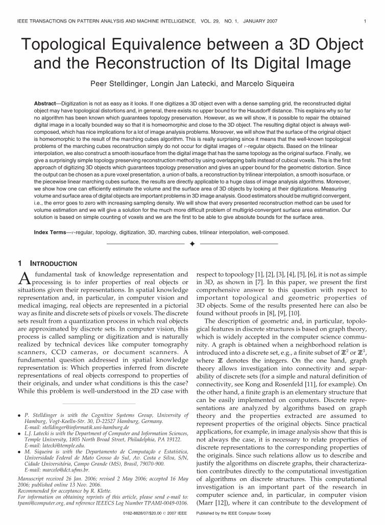
sampling theorems in 2D require the object to be r-regular[1], [2], [7], we will use the 3D generalization for ourapproach (refer to Fig. 1):

Definition 1. A set A � IR3 is called r-regular if, for each pointx 2 @A, there exist two osculating open balls of radius r to @Aat x such that one lies entirely in A and the other lies entirelyin Ac.

Note that the boundary of a 3D r-regular set is a 2D manifoldsurface.

Any set S which is a translated and rotated version of the

set 2�r0ffiffi3p ZZ3 is called a cubic r0-grid and its elements are called

sampling points. Note that the distance dðx; pÞ from each point

x 2 IR3 to the nearest sampling point s 2 S is at most r0. The

voxel VSðsÞ of a sampling point s 2 S is its Voronoi region IR3:

VSðsÞ ¼ fx 2 IR3jdðx; sÞ � dðx; qÞ; 8q 2 Sg, i.e.,VSðsÞ is the set

of all points of IR3 which are at least as close to s as to any other

point in S. In particular, note that VSðsÞ is a cube whose

vertices lie on a sphere of radius r0 and center s.

Definition 2. Let S be a cubic r0-grid, and let A be any subsetof IR3. The union of all voxels with sampling points lyingin A is the digital reconstruction of A with respect to S,A ¼

Ss2ðS\AÞ VSðsÞ.

This method for reconstructing the object from the set ofincluded sampling points is the 3D generalization of the2D Gauss digitization (see [17]) which has been used byGauss to compute the area of discs and which has also beenused by Pavlidis [1] in his sampling theorem.

For any two points p and q ofS, we have that VSðpÞ \ VSðqÞis either empty or a common vertex, edge, or face of both. IfVSðpÞ \ VSðqÞ is a common face, edge, or vertex, then we saythat VSðpÞ and VSðqÞ are face-adjacent, edge-adjacent, or vertex-adjacent, respectively. Two voxels VSðpÞ and VSðqÞ of A areconnected in A if there exists a sequence VSðs1Þ; . . . ;VSðskÞ,with k 2 ZZ and k > 1 such that s1 ¼ p, sk ¼ q, and si 2 A (or,

equivalently, VSðsiÞ � A), for each i 2 f1; . . . ; kg, and VSðsjÞand VSðsjþ1Þ are face-adjacent, for each j 2 f1; . . . ; k� 1g. A

(connected) component of A is a maximal set of connected

voxels in A.

Definition 3. Let S be a cubic r0-grid, and let T be any subset of S.

Then, we say thatSt2T VSðtÞ is well-composed if @ð

St2T VSðtÞÞ

is a surface in IR3 or, equivalently, if, for every point

x 2 @ðSt2T VSðtÞÞ, there exists a positive number r such that

the intersection of @ðSt2T VSðtÞÞ andB0

rðxÞ is homeomorphic to

the open unit disk in IR2, ID ¼ fðx; yÞ 2 IR2jx2 þ y2 < 1g.Well-composed digital reconstructions can be characterized

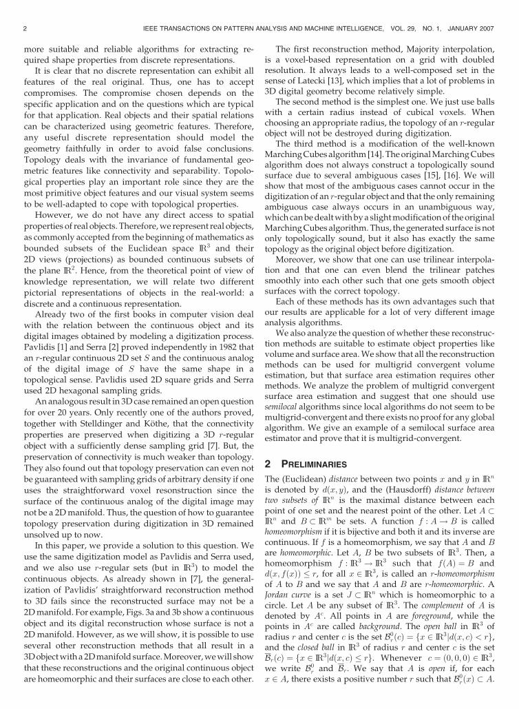
by two local conditions depending only on voxels of points

of S. Let s1; . . . ; s4 be any four points of S such thatT4i¼1 VSðsiÞ is a common edge of VSðs1Þ; . . . ;VSðs4Þ. We say

that the set fVSðs1Þ; . . . ;VSðs4Þg is an instance of the critical

configuration (C1) with respect toSt2T VSðtÞ if two of these

voxels are inSt2T VSðtÞ and the other two are in

ðSt2T VSðtÞÞ

c, and the two voxels inSt2T VSðtÞ (respectively

ðSt2T VSðtÞÞ

c) are edge-adjacent, as shown in Fig. 2a. Now,

let s1; . . . ; s8 be any eight points of S such thatT8i¼1 VSðsiÞ is

a common vertex of VSðs1Þ; . . . ;VSðs8Þ. We say that the set

fVSðs1Þ; . . . ;VSðs4Þg is an instance of the critical configuration

(C2) with respect toSt2T VSðtÞ if two of these voxels are inS

t2T VSðtÞ (respectively ðSt2T VSðtÞÞ

c) and the other six are

in ðSt2T VSðtÞÞ

c (respectivelySt2T VSðtÞ), and the two

voxels inSt2T VSðtÞ (respectively ð

St2T VSðtÞÞ

c) are vertex-

adjacent, as shown in Fig. 2b. The following theorem from

[13] establishes an important equivalence between well-

composedness and the (non)existence of critical configura-

tions (C1) and (C2):

Theorem 4 ([13]). Let S be a cubic r0-grid and let T be any subset

of S. Then,St2T VSðtÞ is well-composed iff the set of voxels

fVðsÞjs 2 Sg does not contain any instance of the critical

STELLDINGER ET AL.: TOPOLOGICAL EQUIVALENCE BETWEEN A 3D OBJECT AND THE RECONSTRUCTION OF ITS DIGITAL IMAGE 3

Fig. 1. For each boundary point of a 2D/3D r-regular set there exists an

outside and an inside osculating open r-disc/ball.

Fig. 2. (a) Critical configuration (C1). (b) Critical configuration (C2). For

the sake of clarity, we show only the voxels of foreground or background

points.

Fig. 3. The digital reconstruction (b) of an r-regular object (a) may not be

well-composed, i.e., its surface may not be a 2D manifold, as can be

seen in the magnification.

configuration (C1) nor any instance of the critical configura-tion (C2) with respect to

St2T VSðtÞ.

3 DIGITAL RECONSTRUCTION OF rr-REGULAR SETS

Let A � IR3 be an r-regular object, let S be a cubic r0-grid,and consider the digital reconstruction A of A withrespect to S. Assume that no sampling point of S lies on@A. This assumption is not a restriction as there alwaysexists an � > 0 such that the �-opening A� B� is ðr� �Þ-regular with r� � > r0 and A� B� has the same digitalreconstruction as A. In what follows, we will locallycharacterize the topology and geometry of A.

Consider any cube in IR3 whose (eight) vertices are pointsof S whose corresponding voxels share a common vertex.By the above assumption, each vertex of such a cube iseither inside (i.e., a foreground point) or outside (i.e., abackground point) A. So, there are at most 256 distinctconfigurations for a cube with respect to the binary “status”of its vertices. However, it has been shown [18] that, up torotational symmetry, reflectional symmetry, and comple-mentarity (switching foreground and backgroud points),these 256 configurations are equivalent to the 14 canonicalconfigurations in Fig. 5. In well-composed sets, only Cases 1to 7 can occur.

In order to analyze the local topology changes due todigitization, we need to define certain paths and surfacepatches spanned between sampling points and the regionsinside which these can be localized:

Definition 5. Let x; y be two points in IR3. Further, lets > dðx; yÞ. Then, the intersection Psðx; yÞ of all closed s-ballscontainingx and y,Psðx; yÞ ¼

TfBsðvÞjx; y 2 BsðvÞg, is called

s-path region between x and y. Now, let x; y; z be three points inIR3 and assume that s > 1

2 maxfdðx; yÞ; dðx; zÞ; dðy; zÞg. Then,the intersection Psðx; y; zÞ of all closed s-balls containing x, y,and z, Psðx; y; zÞ ¼

TfBsðvÞjx; y; z 2 BsðvÞg, is called the

s-surface region between x, y, and z. Further, a nonemptyconvex set B such that at no point x 2 @B exists an insideosculating r-ball, is called an r-simple-cut set.

As we will show below (Lemma 8), under certain condi-tions, Psðx; yÞ is an r-simple-cut set.

Theorem 6. Let A be an r-regular set and x; y be two differentpoints in A with dðx; yÞ < 2r. Further, let L be the straightline segment from x to y. Then, the function f mapping eachpoint of L to the nearest point in A is well-defined, continuousand bijective, and the range of f is a simple path from x to y.

Proof. Each point L \A is its own nearest point in A. Due tor-regularity, there exists for each point inL nA exactly onenearest point in@A since each of these points has a distancesmaller than r to the boundary. Thus, f must be acontinuous function since, if f would not be continuousat some point, this point would have more than one nearestpoint in @A. Note that any point of L lies on the normalvector of @A in its nearest boundary point. Now, supposeone point p of @Awould be the nearest point to at least twodifferent points l1 and l2 ofL. Then, l1 and l2 both lie on thenormal of @A in p. This implies that any point in Lincluding x and y lies on this normal. Since the normalvectors of length r of an r-regular set do not intersect, the

distance between x and y has to be at least 2r whichcontradicts dðx; yÞ < 2r. Thus, f is bijective. Since everybijective continuous function of a compact metric space iscontinuous in both directions, f must be a homeomorph-ism and range is a simple path from x to y. tu

Definition 7. Let A be an r-regular set and x; y be two differentpoints inAwith dðx; yÞ < 2r. Further, let L be the straight linesegment from x to y. Then, the range of the function f mappingeach point ofL to the nearest point inA is called the direct pathfrom x to y regarding A.

Lemma 8. Let A be an r-regular set and x; y be two points bothinsideA or both outsideAwith dðx; yÞ < 2r. Then, Psðx; yÞ is asimple-cut set for any s with 1

2 � dðx; yÞ � s < r, the direct pathfrom x to y regarding A lies inside A \ Psðx; yÞ and the directpath fromx toy regardingðA� B"Þc lies insideAc \ Psðx; yÞ, fora sufficiently small " > 0.

Proof. First, let x; y 2 A. Since dðx; yÞ < 2r,Psðx; yÞ is a simple

cut set for any s with 12 � dðx; yÞ � s < r. Now, suppose

there exists a point p on the direct path lying outside of

Psðx; yÞ. Then, the outside osculating open r-ball of A in p

must cover either x or y, which implies that they cannot lie

on @A or inside A. Thus, the direct path has to be inside

Psðx; yÞ. If x; y 2 Ac, the analog is true by looking at the

ðr� "Þ-regular set ðA� B"Þc for a sufficiently small " > 0

since there alway exists an " such that x and y remain

outside A� B" and s < ðr� "Þ. tuLemma 9. LetA be an r-regular set and letB be an s-simple-cut set

with s < r. Further, letB0 \A0 6¼ ; andB \Ac 6¼ ;. Then, theintersection @A \ @B of the boundaries is a Jordan curve.

Proof. Let c1 and c2 be two arbitrary points inB \A and letPbe the direct path from c1 to c2. Then,P lies inside ofB dueto Lemma 8 and B � Psðc1; c2Þ. This implies that B \Amust be one connected component. Now, consider the twopoints c1 and c2 lying inB \Ac. Then, the direct path doesnot necessarily lie in Ac, since this set is open, but in Ac.Thus, for any open superset of the intersection of all r-ballscontaining c1 and c2, there exists a path from c1 to c2 insidethis superset having a minimal distance to the direct pathinAc. Due to the higher curvature, not onlyB \Ac but alsoðB \AcÞ0 is such a superset. Thus, both B \A and B \Ac

have to be one component and, thus, the intersection of theboundaries, I ¼ @A \ @B, must also be one component. Itremains to be shown that I is a Jordan curve. Since Iseparates @B in one part inside ofA and one part outside ofA, it is a Jordan curve iff there exists no point whereB andA meet tangentially. Such a point would imply that eitherthe inside or the outside osculating ball of A at this pointcoversB. Both cases are impossible since thenB0 \A0 ¼ ;or B \Ac ¼ ;. Thus, @A \ @B is a Jordan curve. tu

Definition 10. Let A be an r-regular set and let x; y; z be three

arbitrary points inside of A0 � Br. Then, the inner surface

patch Isðx; y; zÞ of x; y; z regarding A is the set defined by

mapping each point of the triangle T spanned by points x; y; z to

itself if it lies inside ofA and mapping it to the nearest boundary

point in @A otherwise. Now, let x; y; z be three arbitrary points

inside of Ac � Br. Then, the outer surface patch Osðx; y; zÞof x; y; z regardingA is the set defined by mapping each point of


the triangleT between the points to itself inside of ðA� B"Þc and

mapping them to the nearest boundary point @ðA� B"Þc

otherwise, with " being half the minimal distance from the

sampling points inAc to @A.

Lemma 11. Let A be an r-regular set and x; y; z be three points

inside A with maxfdðx; yÞ; dðx; zÞ; dðy; zÞg < 2r. Then,

Psðx; y; zÞ is a simple cut set for any s with 12 � dðx; yÞ � s <

r and the inner surface patch is homeomorphic to a disc, lies

inside A \ Psðx; yÞ, and is bounded by three paths, one going

from x to y inside of Psðx; y; zÞ \ Psðx; yÞ, another going from

y to z inside of Psðx; y; zÞ \ Psðy; zÞ, and the third going from

z to x inside of Psðx; y; zÞ \ Psðz; xÞ. The analog is true for

x; y; z lying outside of A and the outer surface patch.

Proof. The mapping used in Definition 10 is a direct

generalization of the mapping in Definition 7 and it is a

homeomorphism for the same reasons if x; y; z lie insideA

and maxfdðx; yÞ; dðx; zÞ; dðy; zÞg < 2r. Its boundaries are

equal to the direct paths between each two of the three

points. If x; y; z lie outside of A, the proof is analogous. tuThe problem of topology preserving digitization is that

several of the 14 cases are ambiguous, which means that

there are more than one possibilities to reconstruct the

object locally. This is not true for sufficiently dense sampled

r-regular objects, as shown by the following theorems:

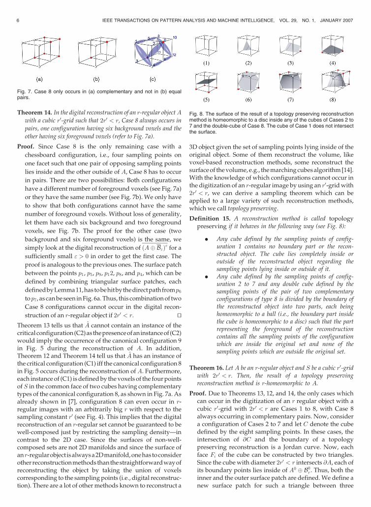
Theorem 12. Configurations 12 to 14 in Fig. 5 cannot occur in the

digital reconstruction of an r-regular object with a cubic r0-grid

with 2r0 < r.

Proof. We only have to show that the configuration shown in

Fig. 5 (12 to 14) does not occur. In the following, let the red

sampling points in Fig. 5 (12 to 14) be in the foreground and

the white sampling points in the background. Further, let

the sampling points p1; p2; . . . p8 be numbered as shown in

Fig. 5 (12 to 14). Suppose to the contrary, such a

configuration occurs in the digital reconstruction of an

r-regular objectA. Further, suppose the point c in the center

of the configuration is in the foreground. Since the distance

from c to p2 is r0, there exists a foreground path between

these points lying completely insidePsðc; p2Þ. On the other

side, the three background points p1; p4; p6 each have a

distance being smaller than 2r. Thus, due to Lemma 11,

there exists a surface patch between them lying completely

outside A. This patch lies inside Psðp1; p4; p6Þ with its

surface boundary lying inside the union of Psðp1; p4Þ,Psðp1; p6Þ, and Psðp4; p6Þ. Fig. 6b shows that Psðc; p2Þ goes

through the s-surface region without intersecting the

bounding s-path regions. Since both c and p2 lie outside

Psðp1; p4; p6Þ, the path from c to p2 must go through the

surface patch and, thus, there has to exist a point lying both

in A and Ac. It follows that c cannot be in the foreground.

Analogously, c cannot be in the background since Psðc; p1Þintersects Psðp2; p3; p5Þ in the same way as can be seen in

Fig. 6c. Thus, Cases 12 to 14 cannot occur in the digital

reconstruction of an r-regular object if 2r0 < r. tu

Theorem 13. Configurations 9 to 11 in Fig. 5 cannot occur in the

digital reconstruction of an r-regular object with a cubic

r0-grid with 2r0 < r.

Proof. We only have to show that the configuration shownin Fig. 5 (9 to 11) is impossible since this is a general-ization of the three mentioned cases. The proof isanalogous to the previous one. The surface patchbetween the points p1, p6, p8, and p3 which can bedefined by combining the two triangular surface patchesbetween p1, p6, and p8, respectively, p1, p3, and p8 has tobe hit by the direct path from p2 to p7 (which both lieoutside the region Psðp1; p6; p8Þ [ Psðp1; p3; p8Þ) as can beseen in Fig. 6a. Thus, Cases 9 to 11 cannot occur in thedigital reconstruction of an r-regular object if 2r0 < r. tu


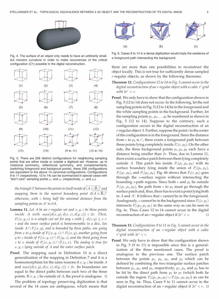
Fig. 4. The surface of an object only needs to have an arbitrarily small,

but nonzero curvature in order to make occurrences of the critical

configuration (C1) possible in the digital reconstruction.

Fig. 5. There are 256 distinct configurations for neighboring samplingpoints that are either inside or outside a digitized set. However, up torotational symmetry, reflectional symmetry, and complementarity(switching foreground and backgroud points), these 256 configurationsare equivalent to the above 14 canonical configurations. Configurations9 to 11 (respectively, 12 to 14) can be summarized in special cases with“don’t care” sampling points p4 and p5 (respectively, p7 and p8).

Fig. 6. Cases 9 to 14 in a dense digitization would imply the existence of

a foreground path intersecting the background.

Theorem 14. In the digital reconstruction of an r-regular objectA

with a cubic r0-grid such that 2r0 < r, Case 8 always occurs in

pairs, one configuration having six background voxels and the

other having six foreground voxels (refer to Fig. 7a).

Proof. Since Case 8 is the only remaining case with a

chessboard configuration, i.e., four sampling points on

one facet such that one pair of opposing sampling points

lies inside and the other outside of A, Case 8 has to occur

in pairs. There are two possibilities: Both configurations

have a different number of foreground voxels (see Fig. 7a)

or they have the same number (see Fig. 7b). We only have

to show that both configurations cannot have the same

number of foreground voxels. Without loss of generality,

let them have each six background and two foreground

voxels, see Fig. 7b. The proof for the other case (two

background and six foreground voxels) is the same, we

simply look at the digital reconstruction of ðA� B"Þc for a

sufficiently small " > 0 in order to get the first case. The

proof is analogous to the previous ones. The surface patch

between the points p1, p5, p9, p12, p8, and p4, which can be

defined by combining triangular surface patches, each

definedbyLemma11,hastobehitbythedirectpathfromp6

top7, as can be seen in Fig. 6a. Thus, this combination of two

Case 8 configurations cannot occur in the digital recon-

struction of an r-regular object if 2r0 < r. tuTheorem 13 tells us that A cannot contain an instance of thecriticalconfiguration(C2)asthepresenceofaninstanceof (C2)would imply the occurrence of the canonical configuration 9in Fig. 5 during the reconstruction of A. In addition,Theorem 12 and Theorem 14 tell us that A has an instance ofthe critical configuration (C1) iff the canonical configuration 8in Fig. 5 occurs during the reconstruction of A. Furthermore,each instance of (C1) is defined by the voxels of the four pointsof S in the common face of two cubes having complementarytypes of the canonical configuration 8, as shown in Fig. 7a. Asalready shown in [7], configuration 8 can even occur in r-regular images with an arbitrarily big r with respect to thesampling constant r0 (see Fig. 4). This implies that the digitalreconstruction of an r-regular set cannot be guaranteed to bewell-composed just by restricting the sampling density—incontrast to the 2D case. Since the surfaces of non-well-composed sets are not 2D manifolds and since the surface ofanr-regularobject isalwaysa2Dmanifold,onehastoconsiderotherreconstructionmethodsthanthestraightforwardwayofreconstructing the object by taking the union of voxelscorresponding to the sampling points (i.e., digital reconstruc-tion). There are a lot of other methods known to reconstruct a

3D object given the set of sampling points lying inside of theoriginal object. Some of them reconstruct the volume, likevoxel-based reconstruction methods, some reconstruct thesurface of the volume, e.g., the marching cubes algorithm [14].With the knowledge of which configurations cannot occur inthe digitization of an r-regular image by using an r0-grid with2r0 < r, we can derive a sampling theorem which can beapplied to a large variety of such reconstruction methods,which we call topology preserving.

Definition 15. A reconstruction method is called topologypreserving if it behaves in the following way (see Fig. 8):

. Any cube defined by the sampling points of config-uration 1 contains no boundary part or the recon-structed object. The cube lies completely inside oroutside of the reconstructed object regarding thesampling points lying inside or outside of it.

. Any cube defined by the sampling points of config-uration 2 to 7 and any double cube defined by thesampling points of the pair of two complementaryconfigurations of type 8 is divided by the boundary ofthe reconstructed object into two parts, each beinghomeomorphic to a ball (i.e., the boundary part insidethe cube is homeomorphic to a disc) such that the partrepresenting the foreground of the reconstructioncontains all the sampling points of the configurationwhich are inside the original set and none of thesampling points which are outside the original set.

Theorem 16. Let A be an r-regular object and S be a cubic r0-gridwith 2r0 < r. Then, the result of a topology preservingreconstruction method is r-homeomorphic to A.

Proof. Due to Theorems 13, 12, and 14, the only cases whichcan occur in the digitization of an r regular object with acubic r0-grid with 2r0 < r are Cases 1 to 8, with Case 8always occurring in complementary pairs. Now, considera configuration of Cases 2 to 7 and let C denote the cubedefined by the eight sampling points. In these cases, theintersection of @C and the boundary of a topologypreserving reconstruction is a Jordan curve. Now, eachface Fi of the cube can be constructed by two triangles.Since the cube with diameter 2r0 < r intersects @A, each ofits boundary points lies inside of A0 � B0

r . Thus, both theinner and the outer surface patch are defined. We define anew surface patch for such a triangle between three


Fig. 7. Case 8 only occurs in (a) complementary and not in (b) equalpairs.

Fig. 8. The surface of the result of a topology preserving reconstructionmethod is homeomorphic to a disc inside any of the cubes of Cases 2 to7 and the double-cube of Case 8. The cube of Case 1 does not intersectthe surface.

sampling points in the following way: If all three samplingpoints p1; p2; p3 lie inside of A, we take the inner surfacepatch. Analogously, if all three sampling points lie outsideofA, we take the outer surface patch. If only one samplingpoint p1 lies inside of A, we use the mapping of the innersurface patch for each point lying inside the smallertriangle 4ðp1;

p1þp2

2 ; p1þp3

2 Þ and the mapping of the outersurface patch otherwise, see Fig. 9 for an illustration. Inorder to get a connected surface, we further add thestraight line connections between the inner and the outersurface patch for any point lying on the straight line fromp1þp2

2 to p1þp3

2 . If one sampling point lies outside and theother two inside ofA, we define the mapping analogously.This leads to a surface patch between the three pointswhich is always homeomorphic to a disc. Furthermore,since any of the added straight line connections follows anormal of @A and, thus, cuts @A exactly once, theintersection of the surface patch with @A is a simple curve.By combining the surface patches of the cube faces, we geta surface homeomorphic to the cube surface intersecting@A in a Jordan curve. For Case 8, we simply look at theunion of the cube pair. This box also cuts the surface of thetopology preserving reconstruction in one Jordan curve,see Fig. 10(8)a+b. By using surface patches in the same wayas above, we get a surface homeomorphic to the box

intersecting @A in a Jordan curve. If we have a cube ofCase 1, we also can take the above surface patchconstruction since it only consists of triangles lyingcompletely inside, respectively, outside of A and, thus,the surface patches are well-defined. The resultingcombined surface does not intersect @A at all. Thus, wehave partitioned the whole space into regions separated bythe surface patches. The original object is homeomorphicto the result of the topology preserving reconstructioninside each of the regarded cubes/cube pairs. Thecombination of the local homeomorphisms (each beingan ð2r0 þ "Þ-homeomorphism) leads to a global r-home-omorphism from A to the reconstructed set. tu

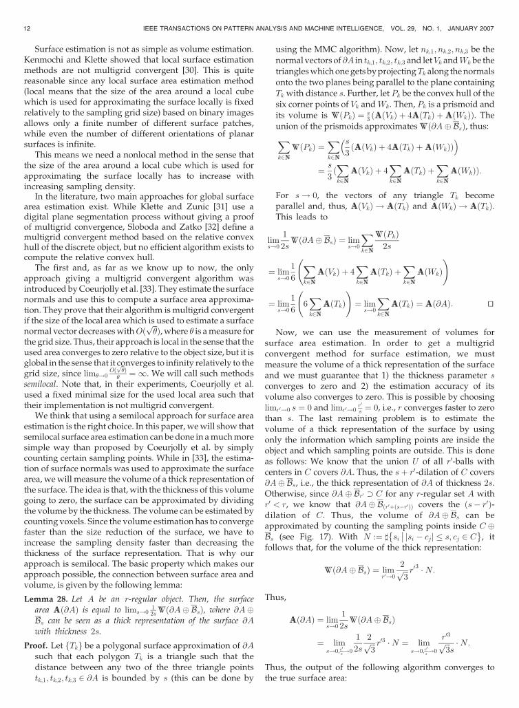
Now, we are able to define reconstruction methods whichguarantee to preserve the original topology of an r-regularobject if one uses a cubic r0-grid with 2r0 < r, see Fig. 16.

4 WELL-COMPOSED DIGITIZATION BY MAJORITY

INTERPOLATION

As shown in [13], a lot of difficult problems in 3D digitalgeometry are much easier if the images are well-composed,e.g., there exists only one type of connected component, adigital version of the Jordan-Brouwer-theorem holds and theEuler characteristic can be computed locally. Unfortunately,most 3D binary images are not well-composed. In contrast tothe 2D case, where the digital reconstruction of an r-regularshape is always well-composed, no such criterion is knownfor the 3D case. In [7], it is proven that r-regularity is notenough to imply well-composedness. To deal with thisproblem, there are two different approaches known: First, assuggested by two of the authors together with Siqueira et al.in a previous paper, nondeterministic changing of the voxelsat positions where well-composedness is not fulfilled [19]and, second, interpolating voxels on a grid with higherresolution in a well-composed way. There is a method knownfor the 2D case using this approach [20], which can be directlygeneralized to three dimensions in order to guarantee3D well-composedness.

The advantage of the first approach is that it does not needto increase the number of sampling points. The disadvantageis that changes can propagate, which makes it impossible toguarantee the preservation of topology. The second approachis purely local and deterministic and, thus, control oftopology is possible, but it has the disadvantage that itrequires increasing the sampling density. In the case of thementioned method [20] the resolution has to be tripled in anydimension, i.e., there are 27 times as many sampling pointsused as in the original grid. We show that this is also possibleby only doubling the resolution in any direction, i.e., using


Fig. 9. In order to construct a surface between three sampling points being not all in the foreground (a), we combine (b) the inner and (c) the outer

surface patch such that (d) the result is cut by @A into exactly two parts.

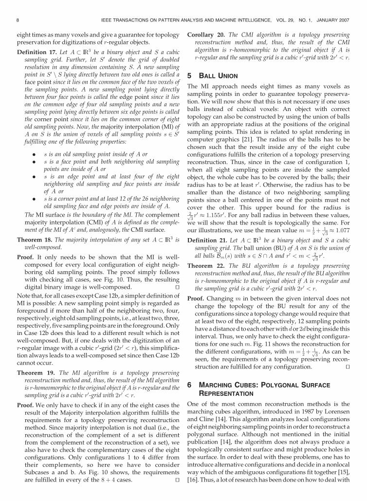
Fig. 10. The 22 different cases of Majority Interpolation (14 cases pluscomplementary cases). The complementary occurences (8)a and (8)b ofCase 8 can be combined such that the surface inside the double cube ishomeomorphic to a disc (8)a+b.

eight times as many voxels and give a guarantee for topologypreservation for digitizations of r-regular objects.

Definition 17. Let A � IR3 be a binary object and S a cubicsampling grid. Further, let S0 denote the grid of doubledresolution in any dimension containing S. A new samplingpoint in S0 n S lying directly between two old ones is called aface point since it lies on the common face of the two voxels ofthe sampling points. A new sampling point lying directlybetween four face points is called the edge point since it lieson the common edge of four old sampling points and a newsampling point lying directly between six edge points is calledthe corner point since it lies on the common corner of eightold sampling points. Now, the majority interpolation (MI) ofA on S is the union of voxels of all sampling points s 2 S0fulfilling one of the following properties:

. s is an old sampling point inside of A or

. s is a face point and both neighboring old samplingpoints are inside of A or

. s is an edge point and at least four of the eightneighboring old sampling and face points are insideof A or

. s is a corner point and at least 12 of the 26 neighboringold sampling face and edge points are inside of A.

The MI surface is the boundary of the MI. The complementmajority interpolation (CMI) of A is defined as the comple-ment of the MI of Ac and, analogously, the CMI surface.

Theorem 18. The majority interpolation of any set A � IR3 iswell-composed.

Proof. It only needs to be shown that the MI is well-composed for every local configuration of eight neigh-boring old sampling points. The proof simply followswith checking all cases, see Fig. 10. Thus, the resultingdigital binary image is well-composed. tu

Note that, for all cases except Case 12b, a simpler definition ofMI is possible: A new sampling point simply is regarded asforeground if more than half of the neighboring two, four,respectively, eight old sampling points, i.e., at least two, three,respectively, five sampling points are in the foreground. Onlyin Case 12b does this lead to a different result which is notwell-composed. But, if one deals with the digitization of anr-regular image with a cubic r0-grid (2r0 < r), this simplifica-tion always leads to a well-composed set since then Case 12bcannot occur.

Theorem 19. The MI algorithm is a topology preservingreconstruction method and, thus, the result of the MI algorithmis r-homeomorphic to the original object ifA is r-regular and thesampling grid is a cubic r0-grid with 2r0 < r.

Proof. We only have to check if in any of the eight cases theresult of the Majority interpolation algorithm fulfills therequirements for a topology preserving reconstructionmethod. Since majority interpolation is not dual (i.e., thereconstruction of the complement of a set is differentfrom the complement of the reconstruction of a set), wealso have to check the complementary cases of the eightconfigurations. Only configurations 1 to 4 differ fromtheir complements, so here we have to considerSubcases a and b. As Fig. 10 shows, the requirementsare fulfilled in every of the 8þ 4 cases. tu

Corollary 20. The CMI algorithm is a topology preservingreconstruction method and, thus, the result of the CMIalgorithm is r-homeomorphic to the original object if A isr-regular and the sampling grid is a cubic r0-grid with 2r0 < r.

5 BALL UNION

The MI approach needs eight times as many voxels assampling points in order to guarantee topology preserva-tion. We will now show that this is not necessary if one usesballs instead of cubical voxels: An object with correcttopology can also be constructed by using the union of ballswith an appropriate radius at the positions of the originalsampling points. This idea is related to splat rendering incomputer graphics [21]. The radius of the balls has to bechosen such that the result inside any of the eight cubeconfigurations fulfills the criterion of a topology preservingreconstruction. Thus, since in the case of configuration 1,when all eight sampling points are inside the sampledobject, the whole cube has to be covered by the balls; theirradius has to be at least r0. Otherwise, the radius has to besmaller than the distance of two neighboring samplingpoints since a ball centered in one of the points must notcover the other. This upper bound for the radius is2ffiffi3p r0 1:155r0. For any ball radius in between these values,we will show that the result is topologically the same. Forour illustrations, we use the mean value m ¼ 1

2þ 1ffiffi3p 1:077

Definition 21. Let A � IR3 be a binary object and S a cubic

sampling grid. The ball union (BU) of A on S is the union of

all balls BmðsÞ with s 2 S \A and r0 < m < 2ffiffi3p r0.

Theorem 22. The BU algorithm is a topology preservingreconstruction method and, thus, the result of the BU algorithmis r-homeomorphic to the original object if A is r-regular andthe sampling grid is a cubic r0-grid with 2r0 < r.

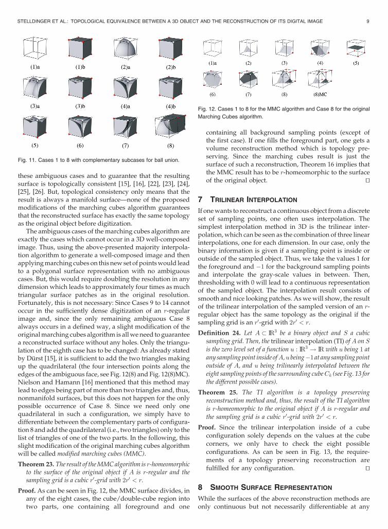
Proof. Changing m in between the given interval does notchange the topology of the BU result for any of theconfigurations since a topology change would require thatat least two of the eight, respectively, 12 sampling pointshave a distance d to each other withdor 2dbeing inside thisinterval. Thus, we only have to check the eight configura-tions for one such m. Fig. 11 shows the reconstruction forthe different configurations, with m ¼ 1

2þ 1ffiffi3p . As can be

seen, the requirements of a topology preserving recon-struction are fulfilled for any configuration. tu

6 MARCHING CUBES: POLYGONAL SURFACE

REPRESENTATION

One of the most common reconstruction methods is themarching cubes algorithm, introduced in 1987 by Lorensenand Cline [14]. This algorithm analyzes local configurationsof eight neighboring sampling points in order to reconstruct apolygonal surface. Although not mentioned in the initialpublication [14], the algorithm does not always produce atopologically consistent surface and might produce holes inthe surface. In order to deal with these problems, one has tointroduce alternative configurations and decide in a nonlocalway which of the ambiguous configurations fit together [15],[16]. Thus, a lot of research has been done on how to deal with


these ambiguous cases and to guarantee that the resultingsurface is topologically consistent [15], [16], [22], [23], [24],[25], [26]. But, topological consistency only means that theresult is always a manifold surface—none of the proposedmodifications of the marching cubes algorithm guaranteesthat the reconstructed surface has exactly the same topologyas the original object before digitization.

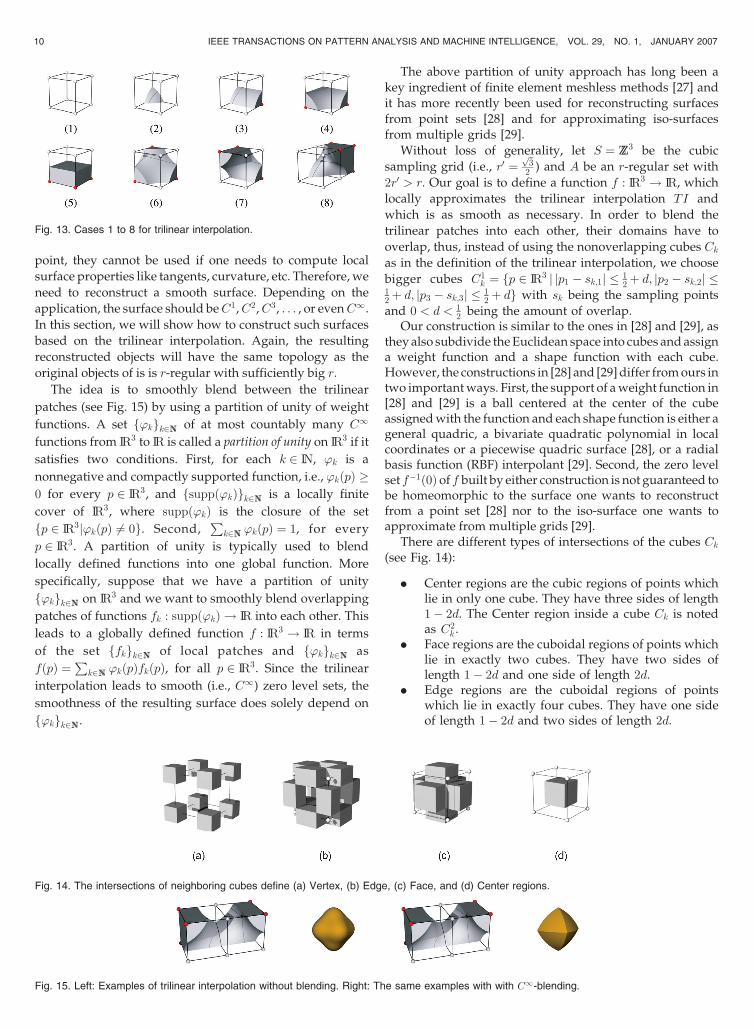
The ambiguous cases of the marching cubes algorithm areexactly the cases which cannot occur in a 3D well-composedimage. Thus, using the above-presented majority interpola-tion algorithm to generate a well-composed image and thenapplying marching cubes on this new set of points would leadto a polygonal surface representation with no ambiguouscases. But, this would require doubling the resolution in anydimension which leads to approximately four times as muchtriangular surface patches as in the original resolution.Fortunately, this is not necessary: Since Cases 9 to 14 cannotoccur in the sufficiently dense digitization of an r-regularimage and, since the only remaining ambiguous Case 8always occurs in a defined way, a slight modification of theoriginal marching cubes algorithm is all we need to guaranteea reconstructed surface without any holes. Only the triangu-lation of the eighth case has to be changed: As already statedby Durst [15], it is sufficient to add the two triangles makingup the quadrilateral (the four intersection points along theedges of the ambiguous face, see Fig. 12(8) and Fig. 12(8)MC).Nielson and Hamann [16] mentioned that this method maylead to edges being part of more than two triangles and, thus,nonmanifold surfaces, but this does not happen for the onlypossible occurrence of Case 8. Since we need only onequadrilateral in such a configuration, we simply have todifferentiate between the complementary parts of configura-tion 8 and add the quadrilateral (i.e., two triangles) only to thelist of triangles of one of the two parts. In the following, thisslight modification of the original marching cubes algorithmwill be called modified marching cubes (MMC).

Theorem 23. The result of the MMC algorithm is r-homeomorphicto the surface of the original object if A is r-regular and thesampling grid is a cubic r0-grid with 2r0 < r.

Proof. As can be seen in Fig. 12, the MMC surface divides, inany of the eight cases, the cube/double-cube region intotwo parts, one containing all foreground and one

containing all background sampling points (except ofthe first case). If one fills the foreground part, one gets avolume reconstruction method which is topology pre-serving. Since the marching cubes result is just thesurface of such a reconstruction, Theorem 16 implies thatthe MMC result has to be r-homeomorphic to the surfaceof the original object. tu

7 TRILINEAR INTERPOLATION

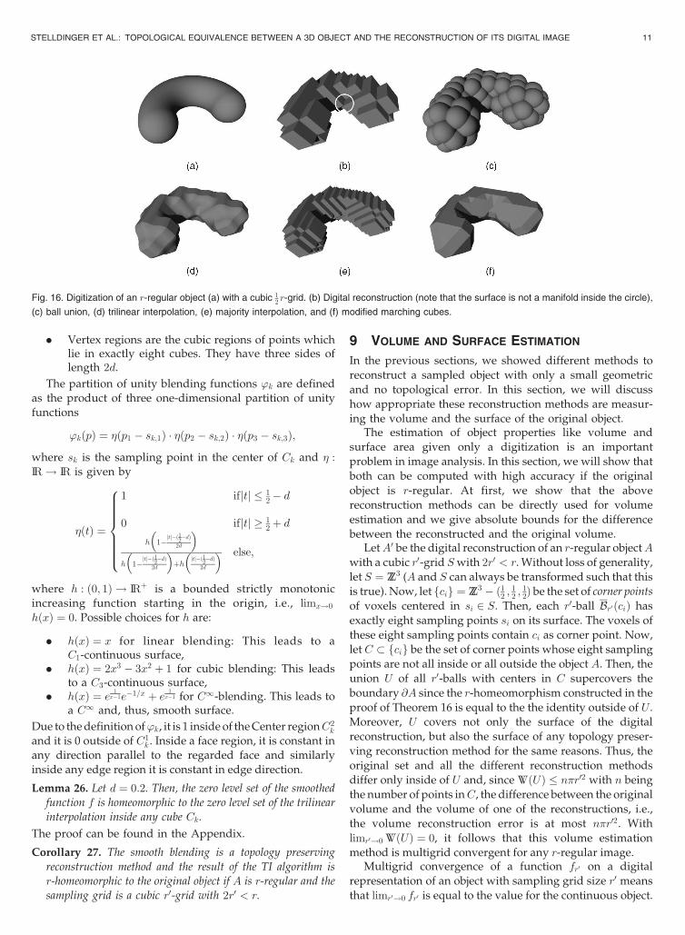
If one wants to reconstruct a continuous object from a discreteset of sampling points, one often uses interpolation. Thesimplest interpolation method in 3D is the trilinear inter-polation, which can be seen as the combination of three linearinterpolations, one for each dimension. In our case, only thebinary information is given if a sampling point is inside oroutside of the sampled object. Thus, we take the values 1 forthe foreground and �1 for the background sampling pointsand interpolate the gray-scale values in between. Then,thresholding with 0 will lead to a continuous representationof the sampled object. The interpolation result consists ofsmooth and nice looking patches. As we will show, the resultof the trilinear interpolation of the sampled version of an r-regular object has the same topology as the original if thesampling grid is an r0-grid with 2r0 < r.

Definition 24. Let A � IR3 be a binary object and S a cubic

sampling grid. Then, the trilinear interpolation (TI) ofA on S

is the zero level set of a function u : IR3 ! IR with u being 1 at

any sampling point inside ofA,u being�1 at any sampling point

outside of A, and u being trilinearly interpolated between the

eight sampling points of the surrounding cubeCk (see Fig. 13 for

the different possible cases).

Theorem 25. The TI algorithm is a topology preserving

reconstruction method and, thus, the result of the TI algorithm

is r-homeomorphic to the original object if A is r-regular and

the sampling grid is a cubic r0-grid with 2r0 < r.

Proof. Since the trilinear interpolation inside of a cubeconfiguration solely depends on the values at the cubecorners, we only have to check the eight possible

configurations. As can be seen in Fig. 13, the require-ments of a topology preserving reconstruction arefulfilled for any configuration. tu

8 SMOOTH SURFACE REPRESENTATION

While the surfaces of the above reconstruction methods areonly continuous but not necessarily differentiable at any


Fig. 11. Cases 1 to 8 with complementary subcases for ball union.

Fig. 12. Cases 1 to 8 for the MMC algorithm and Case 8 for the original

Marching Cubes algorithm.

point, they cannot be used if one needs to compute local

surface properties like tangents, curvature, etc. Therefore, we

need to reconstruct a smooth surface. Depending on the

application, the surface should beC1,C2,C3, . . . , or evenC1.

In this section, we will show how to construct such surfaces

based on the trilinear interpolation. Again, the resulting

reconstructed objects will have the same topology as the

original objects of is is r-regular with sufficiently big r.

The idea is to smoothly blend between the trilinear

patches (see Fig. 15) by using a partition of unity of weight

functions. A set f’kgk2NN of at most countably many C1

functions from IR3 to IR is called a partition of unity on IR3 if it

satisfies two conditions. First, for each k 2 IN, ’k is a

nonnegative and compactly supported function, i.e., ’kðpÞ 0 for every p 2 IR3, and fsuppð’kÞgk2NN is a locally finite

cover of IR3, where suppð’kÞ is the closure of the set

fp 2 IR3j’kðpÞ 6¼ 0g. Second,P

k2NN ’kðpÞ ¼ 1, for every

p 2 IR3. A partition of unity is typically used to blend

locally defined functions into one global function. More

specifically, suppose that we have a partition of unity

f’kgk2NN on IR3 and we want to smoothly blend overlapping

patches of functions fk : suppð’kÞ ! IR into each other. This

leads to a globally defined function f : IR3 ! IR in terms

of the set ffkgk2NN of local patches and f’kgk2NN as

fðpÞ ¼P

k2NN ’kðpÞfkðpÞ, for all p 2 IR3. Since the trilinear

interpolation leads to smooth (i.e., C1) zero level sets, the

smoothness of the resulting surface does solely depend on

f’kgk2NN.

The above partition of unity approach has long been akey ingredient of finite element meshless methods [27] andit has more recently been used for reconstructing surfacesfrom point sets [28] and for approximating iso-surfacesfrom multiple grids [29].

Without loss of generality, let S ¼ ZZ3 be the cubic

sampling grid (i.e., r0 ¼ffiffi3p

2 ) and A be an r-regular set with

2r0 > r. Our goal is to define a function f : IR3 ! IR, which

locally approximates the trilinear interpolation TI and

which is as smooth as necessary. In order to blend the

trilinear patches into each other, their domains have to

overlap, thus, instead of using the nonoverlapping cubes Ckas in the definition of the trilinear interpolation, we choose

bigger cubes C1k ¼ fp 2 IR3 j jp1 � sk;1j � 1

2þ d; jp2 � sk;2j �12þ d; jp3 � sk;3j � 1

2þ dg with sk being the sampling points

and 0 < d < 12 being the amount of overlap.

Our construction is similar to the ones in [28] and [29], asthey also subdivide the Euclidean space into cubes and assigna weight function and a shape function with each cube.However, the constructions in [28] and [29] differ from ours intwo important ways. First, the support of a weight function in[28] and [29] is a ball centered at the center of the cubeassigned with the function and each shape function is either ageneral quadric, a bivariate quadratic polynomial in localcoordinates or a piecewise quadric surface [28], or a radialbasis function (RBF) interpolant [29]. Second, the zero levelset f�1ð0Þ of f built by either construction is not guaranteed tobe homeomorphic to the surface one wants to reconstructfrom a point set [28] nor to the iso-surface one wants toapproximate from multiple grids [29].

There are different types of intersections of the cubes Ck(see Fig. 14):

. Center regions are the cubic regions of points whichlie in only one cube. They have three sides of length1� 2d. The Center region inside a cube Ck is notedas C2

k .. Face regions are the cuboidal regions of points which

lie in exactly two cubes. They have two sides oflength 1� 2d and one side of length 2d.

. Edge regions are the cuboidal regions of pointswhich lie in exactly four cubes. They have one sideof length 1� 2d and two sides of length 2d.


Fig. 13. Cases 1 to 8 for trilinear interpolation.

Fig. 14. The intersections of neighboring cubes define (a) Vertex, (b) Edge, (c) Face, and (d) Center regions.

Fig. 15. Left: Examples of trilinear interpolation without blending. Right: The same examples with with C1-blending.

. Vertex regions are the cubic regions of points whichlie in exactly eight cubes. They have three sides oflength 2d.

The partition of unity blending functions ’k are definedas the product of three one-dimensional partition of unityfunctions

’kðpÞ ¼ �ðp1 � sk;1Þ � �ðp2 � sk;2Þ � �ðp3 � sk;3Þ;

where sk is the sampling point in the center of Ck and � :

IR! IR is given by

�ðtÞ ¼

1 ifjtj � 12� d

0 ifjtj 12þ d

h 1�jtj�ð1

2�dÞ

2d

� �h 1�

jtj�ð12�dÞ

2d

� �þh

jtj�ð12�dÞ

2d

� � else;

8>>>>>><>>>>>>:

where h : ð0; 1Þ ! IRþ is a bounded strictly monotonicincreasing function starting in the origin, i.e., limx!0

hðxÞ ¼ 0. Possible choices for h are:

. hðxÞ ¼ x for linear blending: This leads to aC1-continuous surface,

. hðxÞ ¼ 2x3 � 3x2 þ 1 for cubic blending: This leadsto a C3-continuous surface,

. hðxÞ ¼ e 1x�1e�1=x þ e 1

x�1 for C1-blending. This leads toa C1 and, thus, smooth surface.

Due to the definition of’k, it is 1 inside of the Center regionC2k

and it is 0 outside of C1k . Inside a face region, it is constant in

any direction parallel to the regarded face and similarlyinside any edge region it is constant in edge direction.

Lemma 26. Let d ¼ 0:2. Then, the zero level set of the smoothed

function f is homeomorphic to the zero level set of the trilinear

interpolation inside any cube Ck.

The proof can be found in the Appendix.

Corollary 27. The smooth blending is a topology preserving

reconstruction method and the result of the TI algorithm is

r-homeomorphic to the original object if A is r-regular and the

sampling grid is a cubic r0-grid with 2r0 < r.

9 VOLUME AND SURFACE ESTIMATION

In the previous sections, we showed different methods to

reconstruct a sampled object with only a small geometric

and no topological error. In this section, we will discuss

how appropriate these reconstruction methods are measur-

ing the volume and the surface of the original object.The estimation of object properties like volume and

surface area given only a digitization is an important

problem in image analysis. In this section, we will show that

both can be computed with high accuracy if the original

object is r-regular. At first, we show that the above

reconstruction methods can be directly used for volume

estimation and we give absolute bounds for the difference

between the reconstructed and the original volume.LetA0 be the digital reconstruction of an r-regular objectA

with a cubic r0-grid S with 2r0 < r. Without loss of generality,

let S ¼ ZZ3 (A and S can always be transformed such that this

is true). Now, let fcig ¼ ZZ3 � ð12 ; 12 ;

12Þ be the set of corner points

of voxels centered in si 2 S. Then, each r0-ball Br0 ðciÞ has

exactly eight sampling points si on its surface. The voxels of

these eight sampling points contain ci as corner point. Now,

let C � fcig be the set of corner points whose eight sampling

points are not all inside or all outside the object A. Then, the

union U of all r0-balls with centers in C supercovers the

boundary @A since the r-homeomorphism constructed in the

proof of Theorem 16 is equal to the the identity outside of U .

Moreover, U covers not only the surface of the digital

reconstruction, but also the surface of any topology preser-

ving reconstruction method for the same reasons. Thus, the

original set and all the different reconstruction methods

differ only inside of U and, since VVðUÞ � n�r02 with n being

the number of points inC, the difference between the original

volume and the volume of one of the reconstructions, i.e.,

the volume reconstruction error is at most n�r02. With

limr0!0 VVðUÞ ¼ 0, it follows that this volume estimation

method is multigrid convergent for any r-regular image.Multigrid convergence of a function fr0 on a digital

representation of an object with sampling grid size r0 means

that limr0!0 fr0 is equal to the value for the continuous object.


Fig. 16. Digitization of an r-regular object (a) with a cubic 12 r-grid. (b) Digital reconstruction (note that the surface is not a manifold inside the circle),

(c) ball union, (d) trilinear interpolation, (e) majority interpolation, and (f) modified marching cubes.

Surface estimation is not as simple as volume estimation.Kenmochi and Klette showed that local surface estimationmethods are not multigrid convergent [30]. This is quitereasonable since any local surface area estimation method(local means that the size of the area around a local cubewhich is used for approximating the surface locally is fixedrelatively to the sampling grid size) based on binary imagesallows only a finite number of different surface patches,while even the number of different orientations of planarsurfaces is infinite.

This means we need a nonlocal method in the sense thatthe size of the area around a local cube which is used forapproximating the surface locally has to increase withincreasing sampling density.

In the literature, two main approaches for global surfacearea estimation exist. While Klette and Zunic [31] use adigital plane segmentation process without giving a proofof multigrid convergence, Sloboda and Zatko [32] define amultigrid convergent method based on the relative convexhull of the discrete object, but no efficient algorithm exists tocompute the relative convex hull.

The first and, as far as we know up to now, the onlyapproach giving a multigrid convergent algorithm wasintroduced by Coeurjolly et al. [33]. They estimate the surfacenormals and use this to compute a surface area approxima-tion. They prove that their algorithm is multigrid convergentif the size of the local area which is used to estimate a surfacenormal vector decreases withOð

ffiffiffi�pÞ, where � is a measure for

the grid size. Thus, their approach is local in the sense that theused area converges to zero relative to the object size, but it isglobal in the sense that it converges to infinity relatively to thegrid size, since lim�!0

Oðffiffi�pÞ

� ¼ 1. We will call such methodssemilocal. Note that, in their experiments, Coeurjolly et al.used a fixed minimal size for the used local area such thattheir implementation is not multigrid convergent.

We think that using a semilocal approach for surface areaestimation is the right choice. In this paper, we will show thatsemilocal surface area estimation can be done in a much moresimple way than proposed by Coeurjolly et al. by simplycounting certain sampling points. While in [33], the estima-tion of surface normals was used to approximate the surfacearea, we will measure the volume of a thick representation ofthe surface. The idea is that, with the thickness of this volumegoing to zero, the surface can be approximated by dividingthe volume by the thickness. The volume can be estimated bycounting voxels. Since the volume estimation has to convergefaster than the size reduction of the surface, we have toincrease the sampling density faster than decreasing thethickness of the surface representation. That is why ourapproach is semilocal. The basic property which makes ourapproach possible, the connection between surface area andvolume, is given by the following lemma:

Lemma 28. Let A be an r-regular object. Then, the surfacearea AAð@AÞ is equal to lims!0

12sVVð@A� BsÞ, where @A�

Bs can be seen as a thick representation of the surface @A

with thickness 2s.

Proof. Let fTkg be a polygonal surface approximation of @Asuch that each polygon Tk is a triangle such that thedistance between any two of the three triangle pointstk;1; tk;2; tk;3 2 @A is bounded by s (this can be done by

using the MMC algorithm). Now, let nk;1; nk;2; nk;3 be the

normal vectors of @A in tk;1; tk;2; tk;3 and letVk andWk be the

triangles which one gets by projectingTk along the normals

onto the two planes being parallel to the plane containing

Tk with distance s. Further, let Pk be the convex hull of the

six corner points of Vk and Wk. Then, Pk is a prismoid and

its volume is VVðPkÞ ¼ s3 ðAAðVkÞ þ 4AAðTkÞ þAAðWkÞÞ. The

union of the prismoids approximates VVð@A� BsÞ, thus:Xk2NN

VVðPkÞ ¼Xk2NN

s

3ðAAðVkÞ þ 4AAðTkÞ þAAðWkÞÞ

� �

¼ s

3ðXk2NN

AAðVkÞ þ 4Xk2NN

AAðTkÞ þXk2NN

AAðWkÞÞ:

For s! 0, the vectors of any triangle Tk becomeparallel and, thus, AAðVkÞ ! AAðTkÞ and AAðWkÞ ! AAðTkÞ.This leads to

lims!0

1

2sVVð@A� BsÞ ¼ lim

s!0

Xk2NN

VVðPkÞ2s

¼ lims!0

1

6

Xk2NN

AAðVkÞ þ 4Xk2NN

AAðTkÞ þXk2NN

AAðWkÞ !

¼ lims!0

1

66Xk2NN

AAðTkÞ !

¼ lims!0

Xk2NN

AAðTkÞ ¼ AAð@AÞ: ut

Now, we can use the measurement of volumes forsurface area estimation. In order to get a multigridconvergent method for surface estimation, we mustmeasure the volume of a thick representation of the surfaceand we must guarantee that 1) the thickness parameter sconverges to zero and 2) the estimation accuracy of itsvolume also converges to zero. This is possible by choosinglimr0!0 s ¼ 0 and limr0!0

r0

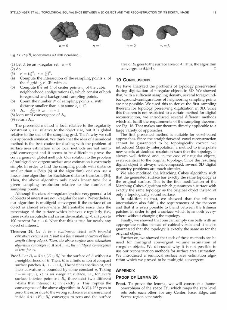
s ¼ 0, i.e., r converges faster to zerothan s. The last remaining problem is to estimate thevolume of a thick representation of the surface by usingonly the information which sampling points are inside theobject and which sampling points are outside. This is doneas follows: We know that the union U of all r0-balls withcenters in C covers @A. Thus, the sþ r0-dilation of C covers@A� Bs, i.e., the thick representation of @A of thickness 2s.Otherwise, since @A� Br0 � C for any r-regular set A withr0 < r, we know that @A� Bðr0þðs�r0ÞÞ covers the ðs� r0Þ-dilation of C. Thus, the volume of @A� Bs can beapproximated by counting the sampling points inside C �Bs (see Fig. 17). With N :¼ ] si

�� jsi � cjj � s; cj 2 C� �, it

follows that, for the volume of the thick representation:

VVð@A� BsÞ ¼ limr0!0

2ffiffiffi3p r0

3 �N:

Thus,

AAð@AÞ ¼ lims!0

1

2sVVð@A� BsÞ

¼ lims!0;r

0s!0

1

2s

2ffiffiffi3p r03 �N ¼ lim

s!0;r0s!0

r03ffiffiffi3p

s�N:

Thus, the output of the following algorithm converges tothe true surface area:


(1) Let A be an r-regular set; n ¼ 0(2) do(3) r0 ¼ 1

2

� n; s ¼ 3

4

� n.

(4) Compute the intersection of the sampling points si ofthe r0-grid 2ffiffi

3p r0 � ZZ3 with A.

(5) Compute the set C of center points cj of the cubicneighborhood configurations Cj which consist of bothforeground and background sampling points.

(6) Count the number N of sampling points si withdistance smaller than s to some cj 2 C.

(7) AAn ¼ r03ffiffi3p

s�N ;n ¼ nþ 1

(8) loop until convergence of AAn.(9) return AAn.

The presented method is local relative to the regularityconstraint r, i.e., relative to the object size, but it is globalrelative to the size of the sampling grid. That’s why we callour approach semilocal. We think that the idea of a semilocalmethod is the best choice for dealing with the problem ofsurface area estimation since local methods are not multi-grid convergent and it seems to be difficult to prove theconvergence of global methods. Our solution to the problemof multigrid convergent surface area estimation is extremelysimple. In order to find the sampling points with distancesmaller than s (Step (6) of the algorithm), one can use alinear-time algorithm for Euclidean distance transform [34].Then, the above algorithm only needs linear time for agiven sampling resolution relative to the number ofsampling points.

Although the class of r-regular objects is very general, a lotof objects of interest are not r-regular for any r. Nevertheless,our algorithm is multigrid convergent if the surface of anobject is almost everywhere differentiable since then thepercentage of the surface which behaves r-regularly (i.e.,there exists an outside and an inside osculating r-ball) goes to100 percent for r! 0. Note that this is true for nearly anyobject of interest.

Theorem 29. Let A be a continuous object with boundedcurvature except a set E that is a finite union of curves of finitelength (sharp edges). Then, the above surface area estimationalgorithm converges to AAð@AÞ, i.e., the mulitgrid convergenceis true for A.

Proof. Let Bt ¼ @A n ðE � BtÞ be the surface of A without at-neighborhood ofE. Then,Bt is a finite union of compactsurface patchesA1 [ � � � [An. The patches are disjoint, andtheir curvature is bounded by some constant u. Takingr ¼ minðt; uÞ, Bt is an r-regular surface, i.e., for everysurface interior point x 2 Bt, there exist two differentr-balls that intersect Bt in exactly x. This implies theconvergence of the above algorithm to AAðBtÞ. If t goes tozero, the error due to the wrong surface area measurementinside @A \ ðE �BtÞ converges to zero and the surface

area ofBt goes to the surface area ofA. Thus, the algorithmconverges to AAð@AÞ. tu

10 CONCLUSIONS

We have analyzed the problems of topology preservationduring digitization of r-regular objects in 3D. We showedthat, with a sufficient sampling density, several foreground-background-configurations of neighboring sampling pointsare not possible. We used this to derive the first samplingtheorem for topology preserving digitization in 3D. Sincethis theorem is not restricted to a certain method for digitalreconstruction, we introduced several different methodswhich all fulfill the requirements of the sampling theorem,see Fig. 16. That makes our theorem directly applicable to alarge variety of approaches.

The first presented method is suitable for voxel-basedapproaches. Since the straightforward voxel reconstructioncannot be guaranteed to be topologically correct, weintroduced Majority Interpolation, a method to interpolatenew voxels at doubled resolution such that the topology isalways well-defined and, in the case of r-regular objects,even identical to the original topology. Since the resultingdigital object is always well-composed, several 3D digitalgeometry problems are much simpler.

We also modified the Marching Cubes algorithm suchthat the generated surface has exactly the same topology asthe original surface. This is the first modification of theMarching Cubes algorithm which guarantees a surface withexactly the same topology as the original object instead ofonly a topologically sound surface.

In addition to that, we showed that the trilinearinterpolation also fulfills the requirements of the theoremand that it is even possible to blend between the trilinearpatches in order to get a surface which is smooth every-where without changing the topology.

Finally, we showed that one can simply use balls with anappropriate radius instead of cubical voxels and it is alsoguaranteed that the topology is exactly the same as for theoriginal object.

Further on, we showed that each of these methods can beused for multigrid convergent volume estimation ofr-regular objects. We discussed why it is not possible touse our reconstruction methods for surface area estimation.We introduced a semilocal surface area estimation algo-rithm which we proved to be multigrid-convergent.

APPENDIX

PROOF OF LEMMA 26

Proof. To prove the lemma, we will construct a home-omorphism of the space IR3, which maps the zero levelsets onto each other, for any Center, Face, Edge, andVertex region separately.


Fig. 17. C � Bs appoximates @A with increasing n.

Inside a Center region C2k , the blending function ’k is

1 and all other ’i are zero. Thus, f is equal to thetrilinear interpolation and the homeomorphism is givenby the identity.

Inside a Vertex region the homeomorphism can also

be chosen as the identity if it is guaranteed that the zero

level set never touches a Vertex region. Suppose the

sampling point inside a Vertex region has value 1. Then,

the smallest possible value of the trilinear interpolant

inside the Vertex region is achieved at the point ðd; d; dÞ if

all surrounding sampling points have the value �1. This

value is 2 � ð1� dÞ3 � 1 ¼ 0:024 > 0. Analogously, for a

background sampling point (value �1), the trilinear

interpolation inside the Vertex region is always smaller

than or equal to �0:024. Since f is at any point a convex

combination of trilinear interpolants which all have the

same sign inside a Vertex region, the zero level set of f

cannot go through any such region.Inside an Edge region ’ is constant in edge direction.

In this direction, any trilinear interpolation is linear.Since all trilinear interpolants inside the Edge regionalong such a direction have the same signs at theirendpoints (where the Edge region meets the Vertexregions), any convex combination of them is also a linearfunction along such a direction with the same signs at theendpoints. Thus, by defining a homeomorphic mappingalong any such line, we get a homeomorphism mappingthe zero level set of f onto the zero level set of thetrilinear interpolant.

Inside a Face region, f is a blending between twotrilinear interpolation patches. For any plane that isparallel to the face, the weights for these two patches areconstant and, thus, f is equal to a bilinear interpolationbetween the weighted sums of values at four corner points.In any case, except for configuration 8, the zero level set is ahyperbolic arc as shown by Lopes and Brodlie [18] and,thus, always has the same shape such that a home-omorphism can easily be constructed. It remains to provethe case of an ambiguous face of configuration 8. In thiscase, the zero level set on the plane which is incident withthe face consists of two crossed straight lines and, for allother planes, it consists of two hyperbolic arcs separatingtwo diagonal corner points such that the plane beingincident with the face separates the other planes into twogroups which separate different pairs of diagonal cornerpoints. Such a saddle surface has exactly the sametopology as the surfaces of the trilinear interpolations,which allows us to construct a homeomorphism. tu

ACKNOWLEDGMENTS

P. Stelldinger was partially supported by the GermanAcademic Exchange Service (DAAD).

REFERENCES

[1] T. Pavlidis, Algorithms for Graphics and Image Processing. ComputerScience Press. 1982.

[2] J. Serra, Image Analysis and Mathematical Morphology. AcademicPress, 1982.

[3] L.J. Latecki, C. Conrad, and A. Gross, “Preserving Topology by aDigitization Process,” J. Math. Imaging and Vision, vol. 8, pp. 131-159, 1998.

[4] M. Tajine and C. Ronse, “Topological Properties of HausdorffDiscretization, and Comparison to Other Discretization Schemes,”Theoretical Computer Science, vol. 283, no. 1, pp. 243-268, 2002.

[5] U. Kothe and P. Stelldinger, “Shape Preserving Digitization ofIdeal and Blurred Binary Images,” Proc. Discrete Geometry forComputer Imagery, pp. 82-91, Nov. 2003.

[6] P. Stelldinger and U. Kothe, “Shape Preservation DuringDigitization: Tight Bounds Based on the Morphing Distance,”Proc. Symp. Deutsche Arbeitsgemeinschaft fur Mustererkennung,pp. 108-115, Sept. 2003.

[7] P. Stelldinger and U. Kothe, “Towards a General Sampling Theoryfor Shape Preservation,” Image and Vision Computing J., specialissue on discrete geometry for computer imagery, vol. 23, no. 2,pp. 237-248, 2005.

[8] P. Stelldinger and L.J. Latecki, “3D Object Digitization: TopologyPreserving Reconstruction,” Proc. IEEE Int’l Conf. Image Analysis,2006.

[9] P. Stelldinger and L.J. Latecki, “3D Object Digitization: MajorityInterpolation and Marching Cubes,” Proc. IEEE Int’l Conf. ImageAnalysis, 2006.

[10] P. Stelldinger and L.J. Latecki, “3D Object Digitization: Volumeand Surface Area Estimation,” Proc. IEEE Int’l Conf. Image Analysis,2006.

[11] T. Kong and A. Rosenfeld, “If We Use 4- or 8-Connectedness forBoth the Objects and the Background, the Euler Characteristics IsNot Locally Computable,” Pattern Recognition Letters, vol. 11, no. 4,pp. 231-232, 1990.

[12] D. Marr, Vision. Freeman, 1983.[13] L.J. Latecki, “3D Well-Composed Pictures,” Graphical Models and

Image Processing, vol. 59, no. 3, pp. 164-172, 1997.[14] W.E. Lorensen and H.E. Cline, “Marching Cubes: A High

Resolution 3D Surface Construction Algorithm,” SIGGRAPH ’87:Proc. 14th Ann. Conf. Computer Graphics and Interactive Techniques,pp. 163-169, 1987.

[15] M.J. Durst, “Letters: Additional Reference to ‘Marching Cubes’,”Proc. SIGGRAPH Computer Graphics, vol. 22, no. 2, p. 243, 1988.

[16] G.M. Nielson and B. Hamann, “The Asymptotic Decider:Resolving the Ambiguity in Marching Cubes,” Proc. Second IEEEConf. Visualization, pp. 83-91, Oct. 1991.

[17] R. Klette and A. Rosenfeld, Digital Geometry. Morgan Kaufman,2004.

[18] A. Lopes and K. Brodlie, “Improving the Robustness andAccuracy of the Marching Cubes Algorithm for Isosurfacing,”IEEE Trans. Visualization and Computer Graphics, vol. 9, no. 1,pp. 16-27, Jan.-Mar. 2003.

[19] M. Siqueira, L.J. Latecki, and J. Gallier, “Making 3D Binary DigitalImages Well-Composed,” Proc. IS&T/SPIE Conf. Vision GeometryXIII, pp. 150-163, Jan. 2005.

[20] A. Rosenfeld, T. Kong, and A. Nakamura, “Topology-PreservingDeformations of Two-Valued Digital Pictures,” Graphical Modelsand Image Processing, vol. 60, no. 1, pp. 24-34, 1998.

[21] L. Westover, “Interactive Volume Rendering,” Proc. Chapel HillWorkshop Volume Visualization, 1989.

[22] E. Chernyaev, “Marching Cubes 33: Construction of TopologicallyCorrect Isosurfaces,” Technical Report CN/95-17, Conseil Eur-opeen pour la Recherche Nucleaire (CERN), 1995.

[23] J. Wilhelms and A.V. Gelder, “Topological Considerations inIsosurface Generation,” Computer Graphics, vol. 24, no. 5, pp. 79-86,1990.

[24] L.A. Francis, “Dualing Cubes,” Proc. 37th Ann. Southeast RegionalConf., 1999.

[25] G.M. Nielson, “Dual Marching Cubes,” Proc. 15th IEEE Visualiza-tion, pp. 489-496, 2004.

[26] T. Lewiner, H. Lopes, A. Wilson, and G. Tavares, “EfficientImplementation of Marching Cubes Cases with TopologicalGuarantee,” J. Graphics Tools, vol. 8, pp. 1-15, 2003.

[27] N. Sukumar, “Meshless Methods and Partition of Unity FiniteElements,” Proc. Sixth Int’l ESAFORM Conf. Material Forming,pp. 603-606, Apr. 2003.

[28] Y. Ohtake, A. Belyaev, M. Alexa, G. Turk, and H-.P. Seidel,“Multi-Level Partition of Unity Implicits,” ACM Trans. Graphics,vol. 22, no. 3, pp. 463-470, 2003.

[29] C.S. Co, S.D. Porumbescu, and K.I. Joy, “Meshless IsosurfaceGeneration from Multiblock Data,” Proc. Joint Eurographics-IEEETCVG Symp. Visualization, pp. 273-282, May 2004.


[30] Y. Kenmochi and R. Klette, “Surface Area Estimation for DigitizedRegular Solids,” Proc. IS&T/SPIE Conf. Vision Geometry IX,vol. 4117, pp. 100-111, Jan. 2001.

[31] R. Klette and J. Zunic, “Multigrid Convergence of CalculatedFeatures in Image Analysis,” J. Math. Imaging and Vision, vol. 13,pp. 173-191, 2000.

[32] F. Sloboda and B. Zatko, “On Approximation of Jordan Surfaces in3D,” Proc. Discrete Geometry for Computer Imagery, pp. 365-388,2001.

[33] D. Coeurjolly, F. Flin, O. Teytaud, and L. Tougne, “MultigridConvergence and Surface Area Estimation,” Proc. Geometry,Morphology, and Computational Imaging, pp. 101-119, 2003.

[34] D. Bailey, “An Efficient Euclidean Distance Transform,” Proc.Combinatorial Image Analysis, pp. 394-408, 2004.

Peer Stelldinger has studied computer scienceand mathematics at the University of Hamburg,Germany, and received the diploma degree incomputer science in 2003. As a researchscientist and PhD student in the CognitiveSystems Group at the University of Hamburg,he has already written 12 conference and fourjournal papers. His main interests are in digitiza-tion, discrete geometry, and topology.

Longin Jan Latecki is the winner of the PatternRecognition Society Award together with AzrielRosenfeld for the best paper published in thejournal Pattern Recognition in 1998. He receivedthe main annual award from the German Societyfor Pattern Recognition (DAGM), the 2000Olympus Prize. He cochairs the IS&T/SPIEannual conference series on Vision Geometry.He has published more than 100 researchpapers and books. He is an associate professor

of computer science at Temple University in Philadelphia.

Marcelo Siqueira received the BSc degree incomputer science from the Universidade Feder-al do Rio Grande do Norte, Brazil, in 1992, andthe MSc degree in computer science from theUniversidade de Sao Paulo, Brazil, in 1994. In1995, he joined the Universidade Federal deMato Grosso do Sul, Brazil. In 2006, he receivedthe PhD degree in computer science from theUniversity of Pennsylvania. His teaching andresearch interests are in computational geome-

try, geometric modeling of curves and surfaces, digital geometry andtopology, and mesh generation.

. For more information on this or any other computing topic,please visit our Digital Library at www.computer.org/publications/dlib.


Topological Equivalence between a 3D Object and the Reconstruction of Its Digital Image

Documents