01/27/22 1 Operations Management Topic 2 – Forecasting Topic 2 – Forecasting

Welcome message from author
This document is posted to help you gain knowledge. Please leave a comment to let me know what you think about it! Share it to your friends and learn new things together.
Transcript

04/28/23 1
Operations ManagementTopic 2 – ForecastingTopic 2 – Forecasting
04/28/23 2
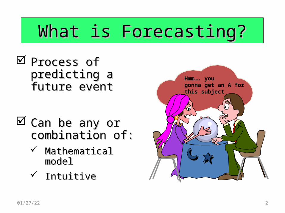
What is Forecasting?What is Forecasting? Process of predicting a Process of predicting a
future eventfuture event
Can be any or Can be any or combination of:combination of: Mathematical modelMathematical model IntuitiveIntuitive
Hmm…. you gonna get an A for this subject
04/28/23 3
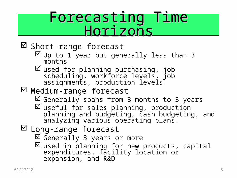
Short-range forecast Up to 1 year but generally less than 3 months used for planning purchasing, job scheduling,
workforce levels, job assignments, production levels. Medium-range forecast
Generally spans from 3 months to 3 years useful for sales planning, production planning and
budgeting, cash budgeting, and analyzing various operating plans.
Long-range forecast Generally 3 years or more used in planning for new products, capital
expenditures, facility location or expansion, and R&D
Forecasting Time HorizonsForecasting Time Horizons

04/28/23 4
Types of ForecastsTypes of Forecasts Economic forecasts
Address business cycle – inflation rate, money supply, housing starts, etc. Technological forecasts
Predict rate of technological progress Impacts development of new products
Demand forecasts Predict sales of existing products and servicesWe can also forecast the economy or the technology. But for OM, demand
forecasting the most relevant.The forecast is the only estimate of demand until actual demand becomes
known.
04/28/23 NY - KJP 585 2009 5
Importance of ForecastingImportance of Forecasting
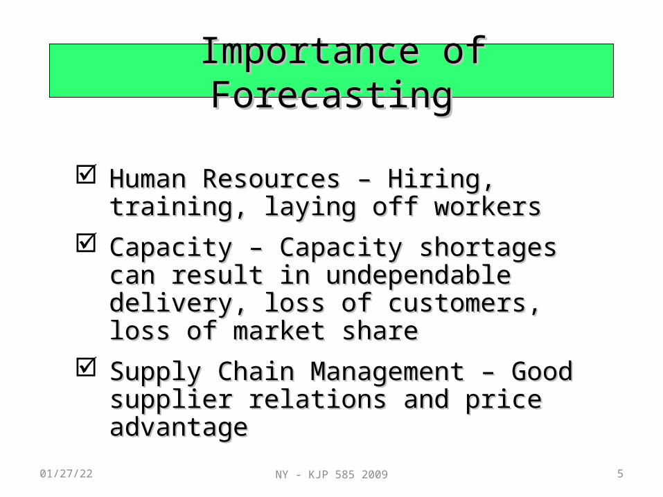
Human Resources – Hiring, training, laying off Human Resources – Hiring, training, laying off workersworkers
Capacity – Capacity shortages can result in Capacity – Capacity shortages can result in undependable delivery, loss of customers, undependable delivery, loss of customers, loss of market shareloss of market share
Supply Chain Management – Good supplier Supply Chain Management – Good supplier relations and price advantagerelations and price advantage
04/28/23 6
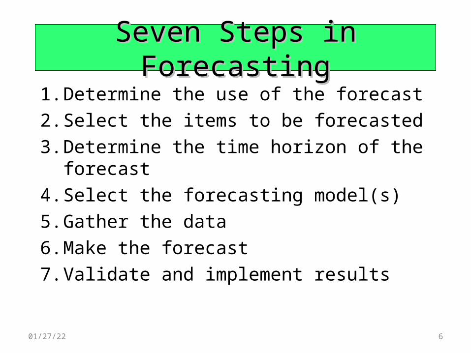
Seven Steps in ForecastingSeven Steps in Forecasting1. Determine the use of the forecast2. Select the items to be forecasted3. Determine the time horizon of the
forecast4. Select the forecasting model(s)5. Gather the data6. Make the forecast7. Validate and implement results
04/28/23 NY - KJP 585 2009 7
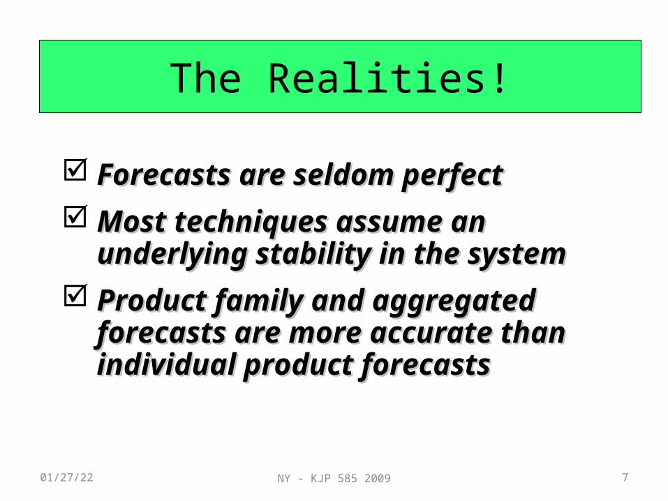
The Realities!
Forecasts are seldom perfectForecasts are seldom perfect Most techniques assume an Most techniques assume an
underlying stability in the systemunderlying stability in the system Product family and aggregated Product family and aggregated
forecasts are more accurate than forecasts are more accurate than individual product forecastsindividual product forecasts

04/28/23 NY - KJP 585 2009 8
Forecasting ApproachesForecasting Approaches
Qualitative (subjective) Forecast incorporates the decision maker’s intuition, emotion, personal experiences, and value system in reaching a forecast.
Quantitative Forecast use a variety of mathematical models/ techniques that rely on historical data and/or causal variables to forecast demand.

04/28/23 NY - KJP 585 2009 9
Forecasting ApproachesForecasting Approaches
Used when situation is vague and little Used when situation is vague and little data existdata exist New productsNew products New technologyNew technology e.g., forecasting sales on Internete.g., forecasting sales on Internet
Qualitative MethodsQualitative Methods
04/28/23 NY - KJP 585 2009 10
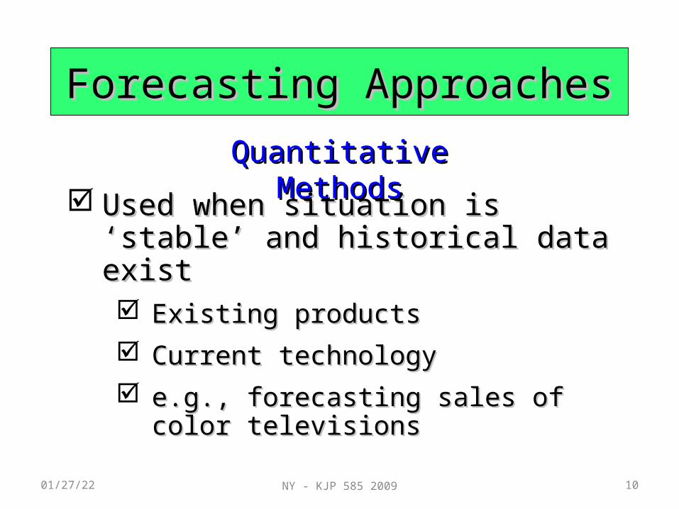
Forecasting ApproachesForecasting Approaches
Used when situation is ‘stable’ and Used when situation is ‘stable’ and historical data existhistorical data exist Existing productsExisting products Current technologyCurrent technology e.g., forecasting sales of color televisionse.g., forecasting sales of color televisions
Quantitative MethodsQuantitative Methods
04/28/23 11
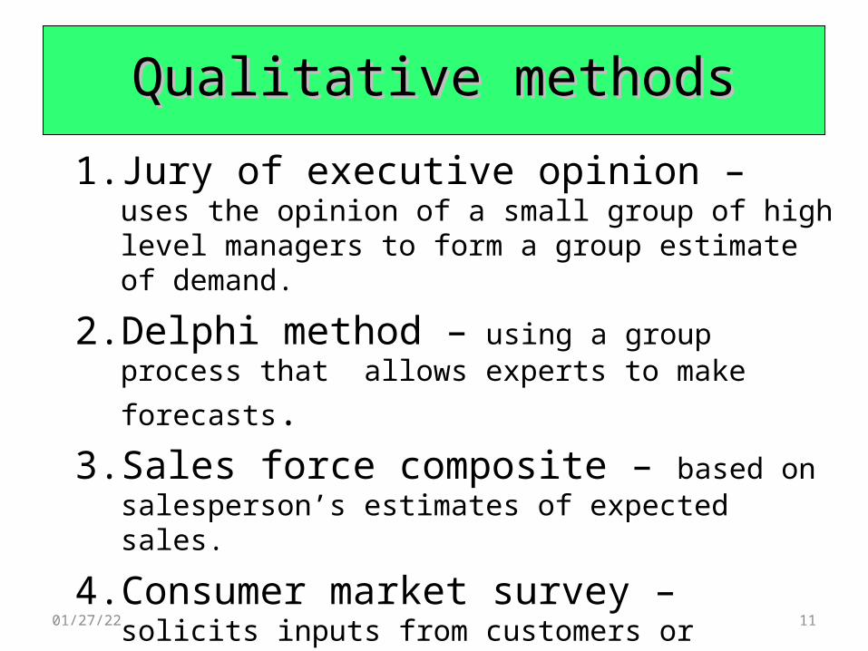
Qualitative methodsQualitative methods
1. Jury of executive opinion – uses the opinion of a small group of high level managers to form a group estimate of demand.
2. Delphi method – using a group process that allows
experts to make forecasts.3. Sales force composite – based on salesperson’s
estimates of expected sales.
4. Consumer market survey – solicits inputs from customers or potential customers regarding future purchasing plans.
04/28/23 NY - KJP 585 2009 12
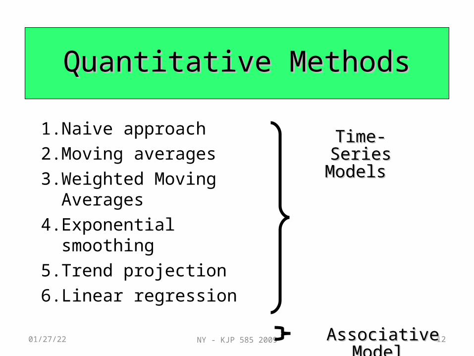
Quantitative MethodsQuantitative Methods
1. Naive approach2. Moving averages3. Weighted Moving
Averages4. Exponential smoothing5. Trend projection6. Linear regression
Time-Series Time-Series Models Models
Associative Model Associative Model
04/28/23 NY - KJP 585 2009 13
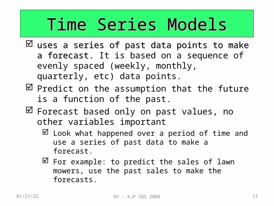
uses a series of past data points to make a forecast. uses a series of past data points to make a forecast. It is based on a sequence of evenly spaced (weekly, monthly, quarterly, etc) data points.
Predict on the assumption that the future is a function of the past.
Forecast based only on past values, no other variables important Look what happened over a period of time and use a
series of past data to make a forecast. For example: to predict the sales of lawn mowers, use
the past sales to make the forecasts.
Time Series ModelsTime Series Models
04/28/23 NY - KJP 585 2009 14
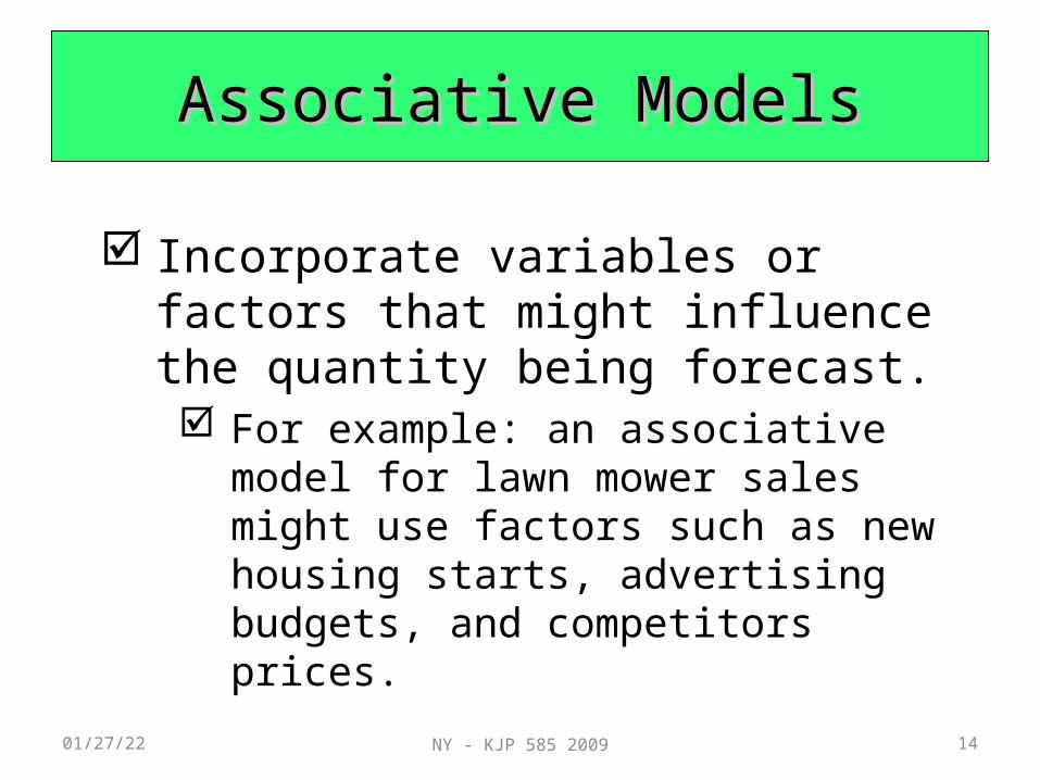
Associative ModelsAssociative Models
Incorporate variables or factors that might influence the quantity being forecast. For example: an associative model for lawn
mower sales might use factors such as new housing starts, advertising budgets, and competitors prices.

04/28/23 NY - KJP 585 2009 15
Components of DemandComponents of DemandDe
man
d fo
r pro
duct
or s
ervi
ce
| | | |1 2 3 4
Year
Average demand over four years
Seasonal peaks
Trend component
Actual demand
Random variation
Figure 4.1Figure 4.1Product demand charted over 4 years with a Growth Trend and Seasonality added:
04/28/23 NY - KJP 585 2009 16
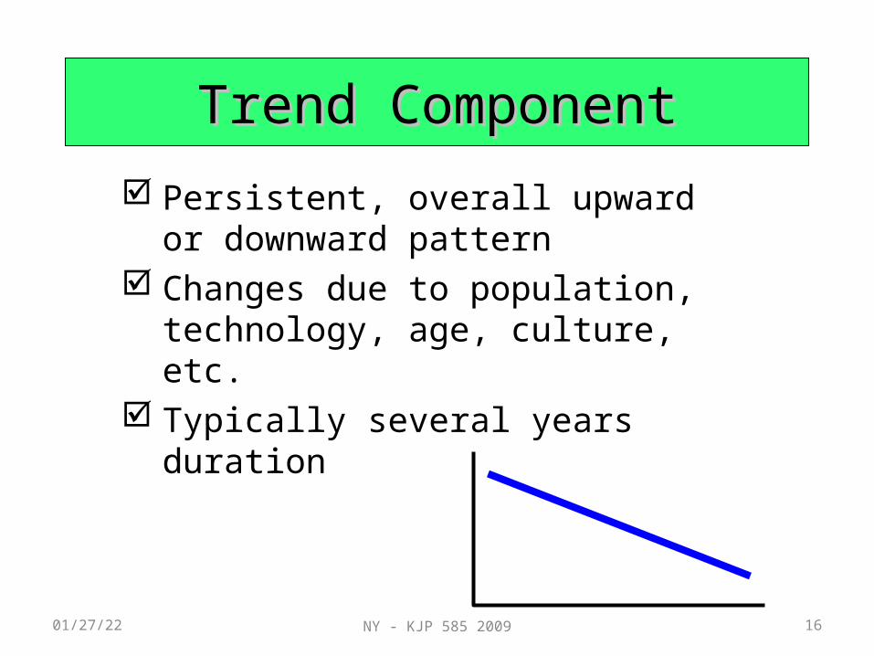
Persistent, overall upward or downward pattern
Changes due to population, technology, age, culture, etc.
Typically several years duration
Trend ComponentTrend Component
04/28/23 NY - KJP 585 2009 17
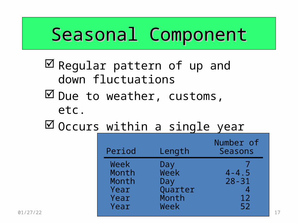
Regular pattern of up and down fluctuations
Due to weather, customs, etc. Occurs within a single year
Seasonal ComponentSeasonal Component
Number ofPeriod Length Seasons
Week Day 7Month Week 4-4.5Month Day 28-31Year Quarter 4Year Month 12Year Week 52
04/28/23 NY - KJP 585 2009 18
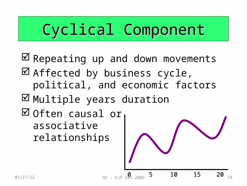
Repeating up and down movements Affected by business cycle, political, and
economic factors Multiple years duration Often causal or
associative relationships
Cyclical ComponentCyclical Component
00 55 1010 1515 2020
04/28/23 NY - KJP 585 2009 19
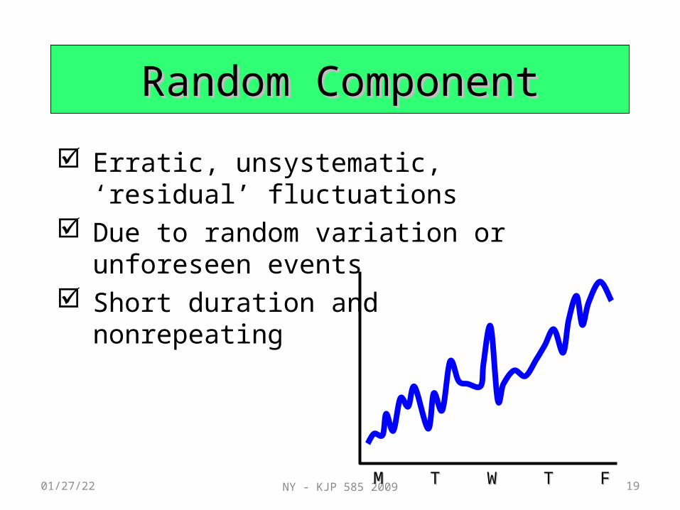
Erratic, unsystematic, ‘residual’ fluctuations
Due to random variation or unforeseen events
Short duration and nonrepeating
Random ComponentRandom Component
MM TT WW TT FF

04/28/23 NY - KJP 585 2009 20
Naive ApproachNaive Approach
Assumes demand in next Assumes demand in next period is the same as period is the same as demand in most recent perioddemand in most recent period e.g., If e.g., If JanJanuary sales were uary sales were 6868, , thenthen
FebFebruary sales will be ruary sales will be 6868
Sometimes cost effective and efficientSometimes cost effective and efficient Can be good starting pointCan be good starting point

04/28/23 NY - KJP 585 2009 21
Moving averageWeighted moving averageExponential smoothing
Techniques for AveragingTechniques for Averaging
04/28/23 NY - KJP 585 2009 22
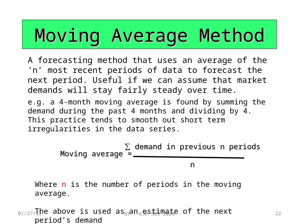
Moving Average MethodMoving Average Method
Moving average =Moving average =∑ ∑ demand in previous n periodsdemand in previous n periods
nn
A forecasting method that uses an average of the ‘n’ most recent periods of data to forecast the next period. Useful if we can assume that market demands will stay fairly steady over time.
e.g. a 4-month moving average is found by summing the demand during the past 4 months and dividing by 4. This practice tends to smooth out short term irregularities in the data series.
Where n is the number of periods in the moving average.
The above is used as an estimate of the next period’s demand

04/28/23 23
Moving Average Example
Storage shed sales at a Garden Supply shop are as shown in the following Table.
Example 1:
Calculate the 3-month moving average forecast.
04/28/23 NY - KJP 585 2009 24
JanuaryJanuary 1010FebruaryFebruary 1212MarchMarch 1313AprilApril 1616MayMay 1919JuneJune 2323JulyJuly 2626
ActualActual 3-Month3-MonthMonthMonth Shed SalesShed Sales Moving AverageMoving Average
(12 + 13 + 16)/3 = 13 (12 + 13 + 16)/3 = 13 22//33
(13 + 16 + 19)/3 = 16(13 + 16 + 19)/3 = 16(16 + 19 + 23)/3 = 19 (16 + 19 + 23)/3 = 19 11//33
Moving Average Example
101012121313
((1010 + + 1212 + + 1313)/3 = 11 )/3 = 11 22//33
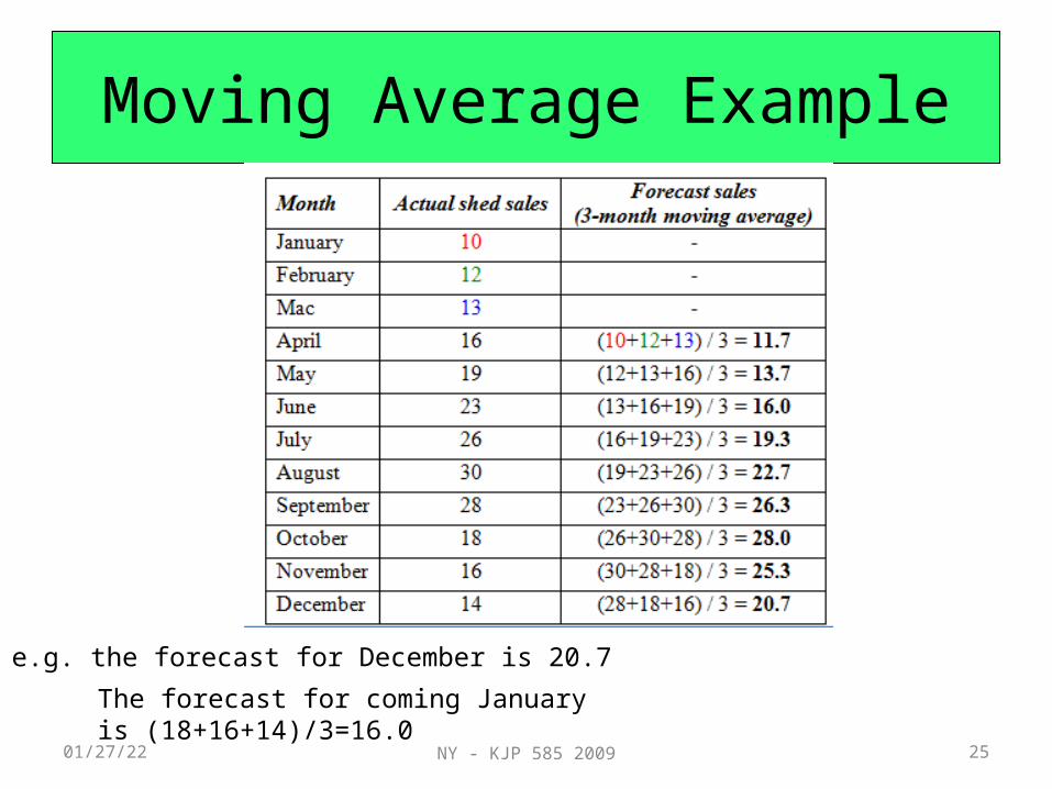
04/28/23 NY - KJP 585 2009 25
Moving Average Example
e.g. the forecast for December is 20.7The forecast for coming January is (18+16+14)/3=16.0
04/28/23 NY - KJP 585 2009 26
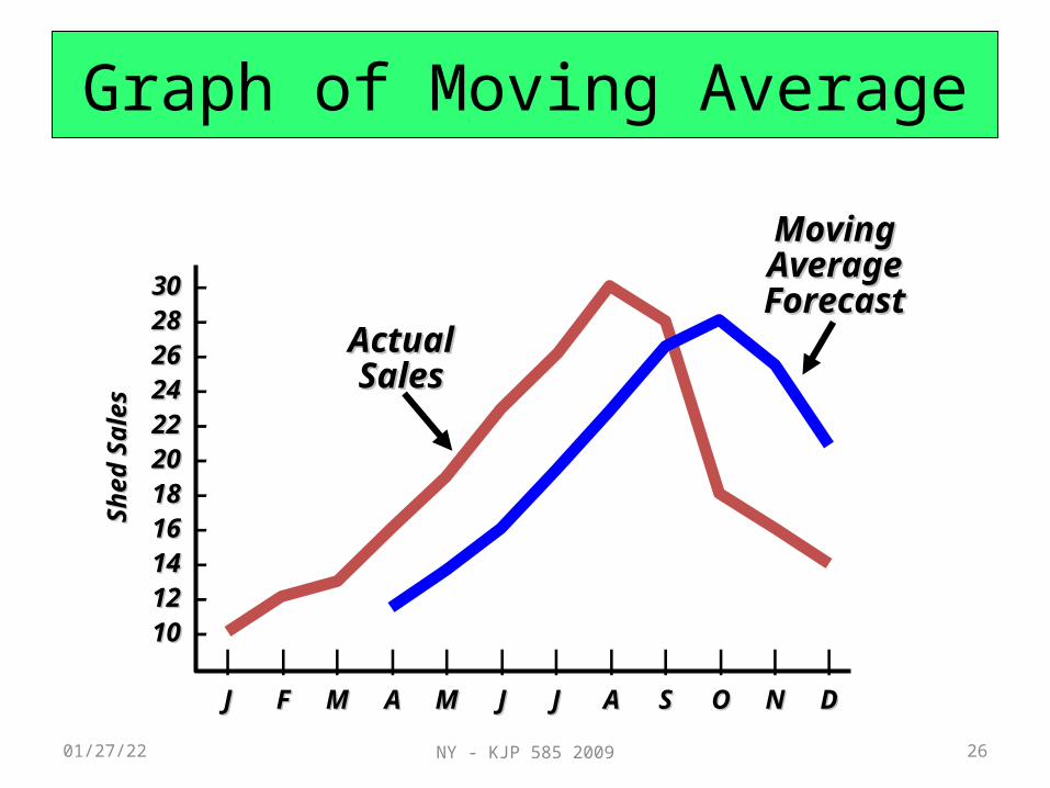
Graph of Moving Average
| | | | | | | | | | | |JJ FF MM AA MM JJ JJ AA SS OO NN DD
Shed
Sal
esSh
ed S
ales
30 30 –28 28 –26 26 –24 24 –22 22 –20 20 –18 18 –16 16 –14 14 –12 12 –10 10 –
Actual Actual SalesSales
Moving Moving Average Average ForecastForecast
04/28/23 NY - KJP 585 2009 27
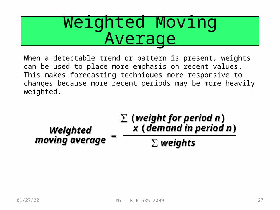
Weighted Moving Average
WeightedWeightedmoving averagemoving average ==
∑∑ ((weight for period nweight for period n)) x x ((demand in period ndemand in period n))
∑∑ weightsweights
When a detectable trend or pattern is present, weights can be used to place more emphasis on recent values. This makes forecasting techniques more responsive to changes because more recent periods may be more heavily weighted.

04/28/23 NY - KJP 585 2009 28
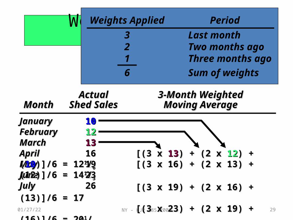
Weighted Moving Average Ex:Example 2The shop in Example 1 decides to forecast storage shed sales by weighting the past 3 months as
follows:Period Weight appliedLast month 32 months ago 23 months ago 1_____________________________Solution:∑ (weights) = 6
Based on the weightings above, the forecast for any month [(3 x Sales last month) + (2 x Sales 2 months ago) + (1 x Sales 3 months ago)]
= ------------------------------------------------------------------------------------------------- ∑ (weights)
04/28/23 NY - KJP 585 2009 29
JanuaryJanuary 1010FebruaryFebruary 1212MarchMarch 1313AprilApril 1616MayMay 1919JuneJune 2323JulyJuly 2626
ActualActual 3-Month Weighted3-Month WeightedMonthMonth Shed SalesShed Sales Moving AverageMoving Average
[(3 x 16) + (2 x 13) + (12)]/6 = 14[(3 x 16) + (2 x 13) + (12)]/6 = 1411//33
[(3 x 19) + (2 x 16) + (13)]/6 = 17[(3 x 19) + (2 x 16) + (13)]/6 = 17[(3 x 23) + (2 x 19) + (16)]/6 = 20[(3 x 23) + (2 x 19) + (16)]/6 = 2011//22
Weighted Moving Average
101012121313
[(3 x [(3 x 1313) + (2 x ) + (2 x 1212) + () + (1010)]/6 = 12)]/6 = 1211//66
Weights Applied Period3 Last month2 Two months ago1 Three months ago6 Sum of weights

04/28/23 NY - KJP 585 2009 30
Weighted Moving Average Ex:
Note that in this situation more heavily weighting the latest month provides a much more accurate projection.Note also that moving averages are effective in smoothing out sudden fluctuations in the demand pattern to provide stable estimates.
04/28/23 NY - KJP 585 2009 31
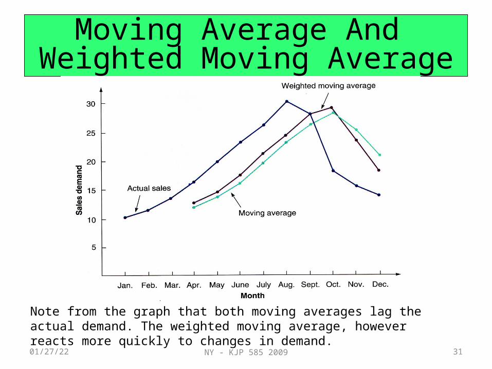
Moving Average And Weighted Moving Average
Note from the graph that both moving averages lag the actual demand. The weighted moving average, however reacts more quickly to changes in demand.
04/28/23 32
Increasing n smooths the forecast but makes it less sensitive to real changes in the data.
Cannot pick up trends very well. Because they are averages, they will always stay within past levels and will not predict changes to either higher or lower levels.
Require extensive historical of past data.
Potential Problems With Moving Average
04/28/23 NY - KJP 585 2009 33
Exponential Smoothing
Is a weighted moving average forecasting technique in which data points are weighted by an exponential function.
This technique involves little record keeping of past data.
Easy to use.
04/28/23 NY - KJP 585 2009 34
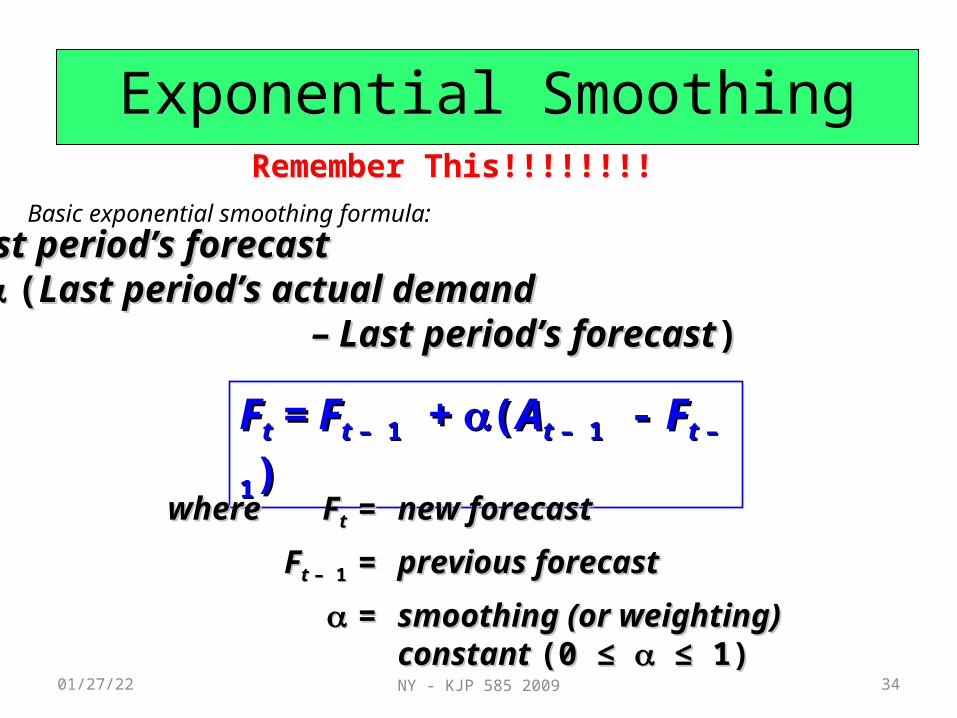
Exponential Smoothing
New forecast =New forecast = Last period’s forecastLast period’s forecast+ + ((Last period’s actual demand Last period’s actual demand
– – Last period’s forecastLast period’s forecast))
FFtt = F = Ft t – 1– 1 + + ((AAt t – 1– 1 - - F Ft t – 1– 1))
wherewhere FFtt == new forecastnew forecastFFt t – 1– 1 == previous forecastprevious forecast
== smoothing (or weighting) smoothing (or weighting) constant constant (0 ≤ (0 ≤ ≤ 1) ≤ 1)
Remember This!!!!!!!!Basic exponential smoothing formula:
04/28/23 NY - KJP 585 2009 35
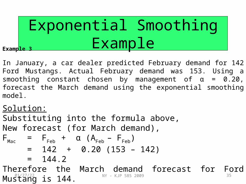
Exponential Smoothing Example
Example 3
In January, a car dealer predicted February demand for 142 Ford Mustangs. Actual February demand was 153. Using a smoothing constant chosen by management of α = 0.20, forecast the March demand using the exponential smoothing model.
Solution:Substituting into the formula above,New forecast (for March demand), FMac = FFeb + α (AFeb – FFeb)
= 142 + 0.20 (153 – 142)= 144.2
Therefore the March demand forecast for Ford Mustang is 144.
04/28/23 NY - KJP 585 2009 36
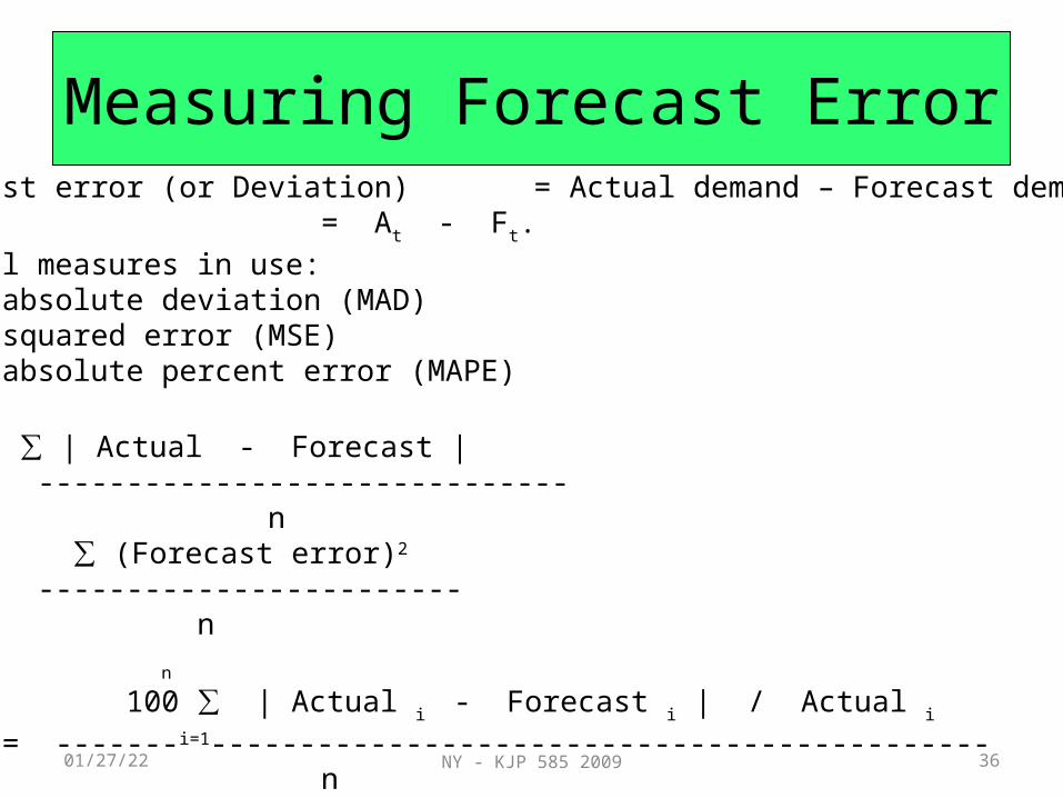
Measuring Forecast ErrorForecast error (or Deviation) = Actual demand – Forecast demand = At - Ft.Several measures in use:•Mean absolute deviation (MAD)•Mean squared error (MSE)•Mean absolute percent error (MAPE)
∑ | Actual - Forecast |MAD = ------------------------------
n ∑ (Forecast error)2
MSE = ------------------------ n n
100 ∑ | Actual i - Forecast i | / Actual i
MAPE = -------i=1--------------------------------------------n

04/28/23 NY - KJP 585 2009 37
Trend Projection
•A time-series forecasting method that fits a trend line to a series of historical data points and then projects the line into the future for forecasts.
•It is usually for medium-to-long range forecasts.
04/28/23 NY - KJP 585 2009 38
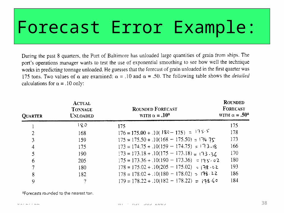
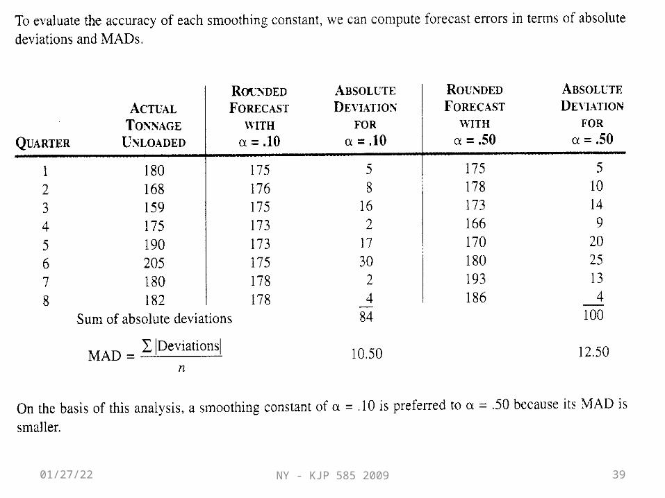
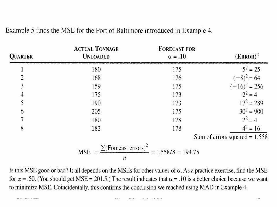
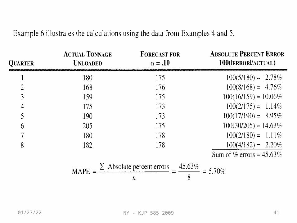
Forecast Error Example:
04/28/23 NY - KJP 585 2009 39
04/28/23 NY - KJP 585 2009 40
04/28/23 NY - KJP 585 2009 41
04/28/23 NY - KJP 585 2009 42
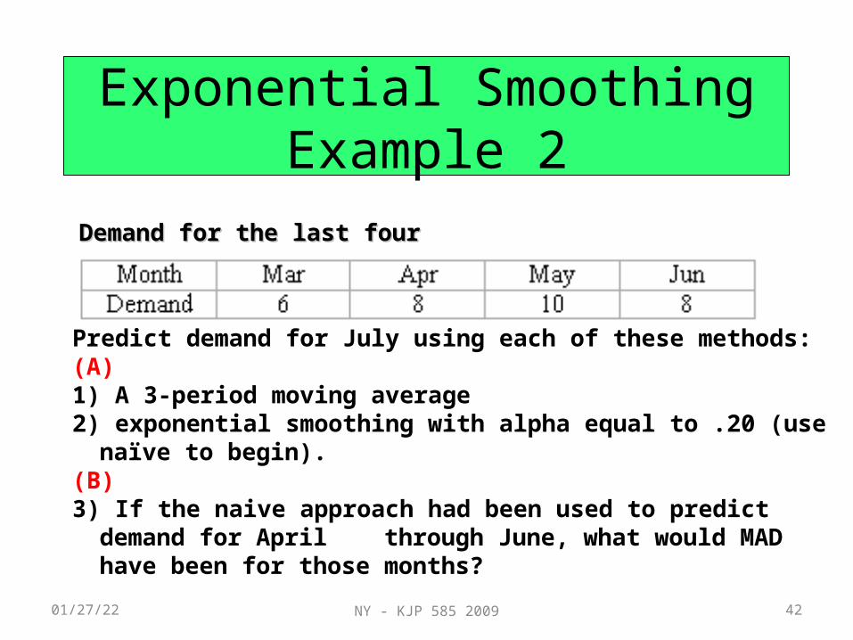
Exponential Smoothing Example 2
Demand for the last four months was:Demand for the last four months was:
Predict demand for July using each of these methods:(A)1) A 3-period moving average 2) exponential smoothing with alpha equal to .20 (use naïve to
begin).(B)3) If the naive approach had been used to predict demand for April
through June, what would MAD have been for those months?
04/28/23 NY - KJP 585 2009 43
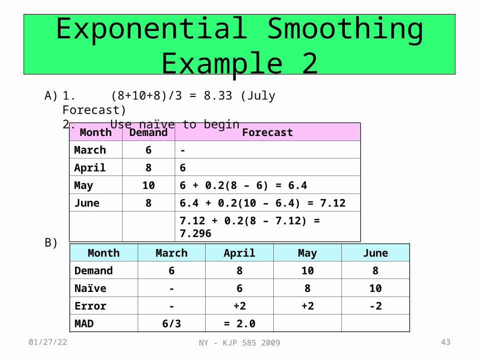
Exponential Smoothing Example 2
Month Demand Forecast
March 6 -
April 8 6
May 10 6 + 0.2(8 – 6) = 6.4
June 8 6.4 + 0.2(10 – 6.4) = 7.12
7.12 + 0.2(8 – 7.12) = 7.296
A) 1. (8+10+8)/3 = 8.33 (July Forecast)2. Use naïve to begin
B)Month March April May June
Demand 6 8 10 8
Naïve - 6 8 10
Error - +2 +2 -2
MAD 6/3 = 2.0
04/28/23 NY - KJP 585 2009 44
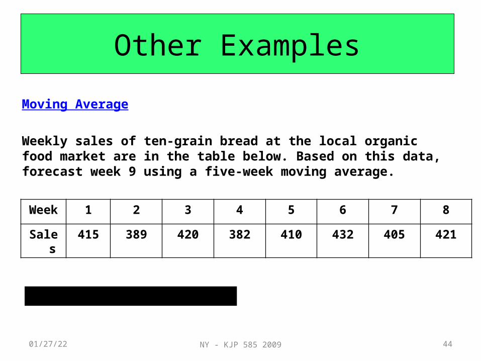
Moving Average
Weekly sales of ten-grain bread at the local organic food market are in the table below. Based on this data, forecast week 9 using a five-week moving average.
Other Examples
Week 1 2 3 4 5 6 7 8
Sales 415 389 420 382 410 432 405 421
(382+410+432+405+421)= 410.0
04/28/23 NY - KJP 585 2009 45
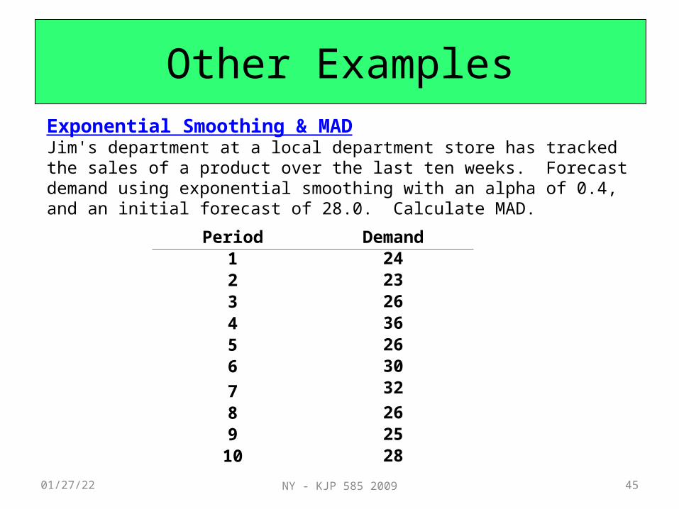
Exponential Smoothing & MADJim's department at a local department store has tracked the sales of a product over the last ten weeks. Forecast demand using exponential smoothing with an alpha of 0.4, and an initial forecast of 28.0. Calculate MAD.
Other Examples
Period Demand1 242 233 264 365 266 307 328 269 25
10 28

04/28/23 NY - KJP 585 2009 46
Period Demand Forecast Error Absolute1 24 28.002 23 26.40 -3.40 3.403 26 25.04 0.96 0.964 36 25.42 10.58 10.585 26 29.65 -3.65 3.656 30 28.19 1.81 1.817 32 28.92 3.08 3.088 26 30.15 -4.15 4.159 25 28.49 -3.49 3.49
10 28 27.09 0.91 0.91Total 2.64 32.03
Average 0.29 3.56Bias MAD
Other Examples –Exponential Smoothing
04/28/23 NY - KJP 585 2009 47
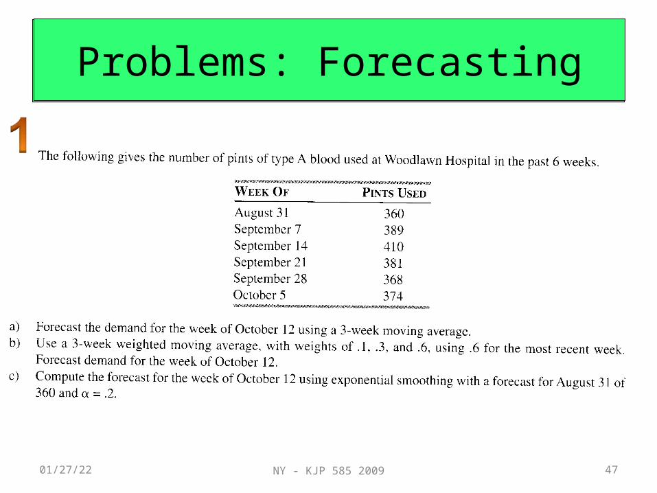
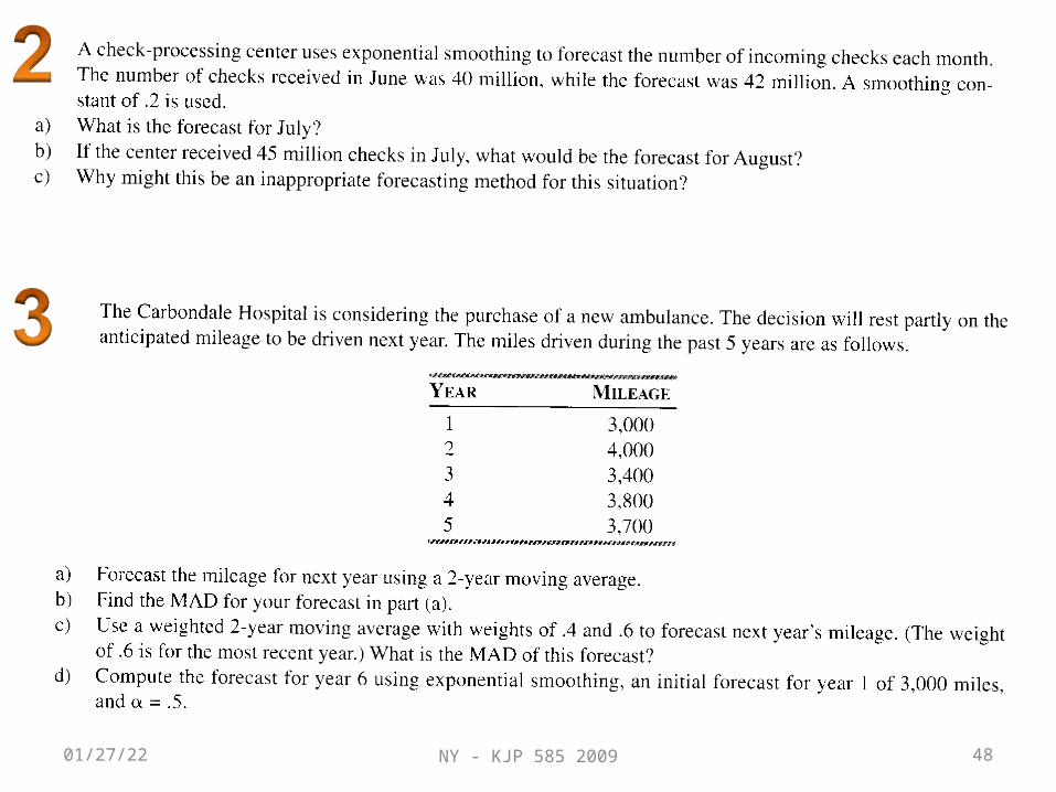
Other ExamplesProblems: Forecasting
04/28/23 NY - KJP 585 2009 48
04/28/23 NY - KJP 585 2009 49
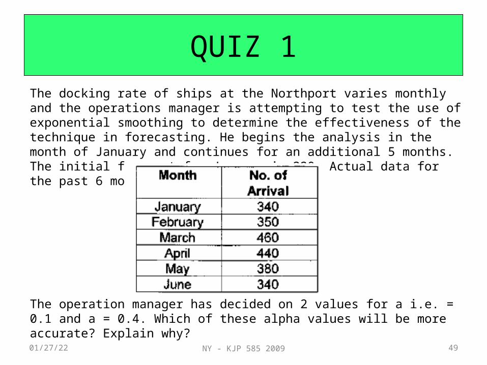
QUIZ 1The docking rate of ships at the Northport varies monthly and the operations manager is attempting to test the use of exponential smoothing to determine the effectiveness of the technique in forecasting. He begins the analysis in the month of January and continues for an additional 5 months. The initial forecast for January is 320. Actual data for the past 6 month are as follows:
The operation manager has decided on 2 values for a i.e. = 0.1 and a = 0.4. Which of these alpha values will be more accurate? Explain why?
Related Documents