NUMERICAL MODELLING AND MODEL UPDATING BASED ON EXPERIMENTAL MODAL PARAMETERS OF CEIRA VIADUCT FABIO LUCCHETTA MASTER DEGREE IN CIVIL ENGINEERING — SPECIALISATION IN STRUCTURAL ENGINEERING Professor Filipe Manuel Rodrigues Leite de Magalhães Professor Bertagnoli Gabriele APRIL 2019

Welcome message from author
This document is posted to help you gain knowledge. Please leave a comment to let me know what you think about it! Share it to your friends and learn new things together.
Transcript

NUMERICAL MODELLING AND MODEL UPDATING BASED ON EXPERIMENTAL
MODAL PARAMETERS OF CEIRA VIADUCT
FABIO LUCCHETTA
MASTER DEGREE IN CIVIL ENGINEERING — SPECIALISATION IN STRUCTURAL ENGINEERING
Professor Filipe Manuel Rodrigues Leite de Magalhães
Professor Bertagnoli Gabriele
APRIL 2019

MESTRADO INTEGRADO EM ENGENHARIA CIVIL 2017/2018
DEPARTAMENTO DE ENGENHARIA CIVIL
Tel. +351-22-508 1901
Fax +351-22-5081446
Editado por
FACULDADE DE ENGENHARIA DA UNIVERSIDADE DO PORTO
Rua Dr. Roberto Frias
4200-465 PORTO
Portugal
Tel. +351-22-508 1400
Fax +351-22-5081440
http://www.fe.up.pt
Reproduções parciais deste documento serão autorizadas na condição que seja mencionado o Autor e feita referência a Mestrado Integrado em Engenharia Civil - 2017/2018 - Departamento de Engenharia Civil, Faculdade de Engenharia da Universidade do Porto, Porto, Portugal, 2018.
As opiniões e informações incluídas neste documento representam unicamente o ponto de vista do respetivo Autor, não podendo o Editor aceitar qualquer responsabilidade legal ou outra em relação a erros ou omissões que possam existir.
Este documento foi produzido a partir de versão eletrónica fornecida pelo respetivo Autor.

To my parents
To my brother Davide
To my girlfriend Giorgia
I am the master of my fate
Nelson Mandela


Numerical Modelling and Model Updating Based on Experimental Modal Parameters of Ceira Viaduct
i
ACKNOWLEDGEMENTS
To all those who, during this Erasmus, supported me in this experience and in this work. To my friends and colleagues who shared this choice and, taking part in brief periods of this experience abroad, helped me in many ways. To my girlfriend, who gave me all possible moral support during these months. To all of them I want to express my most heartfelt thanks.
I would warmly thank my flatmates of the city of Porto, with whom I have shared my everyday life and special moments during this semester.
Special thanks to my family and my parents, they morally and economically supported my experience and they believed in me and in this project.
And to all of my colleagues of the Polytechnic University of Turin, who have always been loyal fellow travellers during these five years. To all of them I have to say thank you; thank you for backing me up during the hardest moment of studies, thank you for the most beautiful shared moments and thank you for the time spent together.
Very important thanks:
To my professor Filipe Magalhães, who, as thesis advisor, accompanied this work step by step following the development and giving me the equipment required for the success of this thesis.
To my professor Gabriele Bertagnoli, who authorized the redaction of a thesis abroad during the Erasmus period.
To the colleagues and the doctoral candidates of the civil engineering department of the FEUP, who helped me during the work with the utilization of the software.
Very sincere thanks are for the Engineering Faculty of the University Of Porto (FEUP) and for the Polytechnic of Turin, which, as institutions, accepted the request of my Erasmus and allowed the involvement of this experience.

Numerical Modelling and Model Updating Based on Experimental Modal Parameters of Ceira Viaduct
ii
Numerical Modelling and Model Updating Based on Experimental Modal Parameters of Ceira Viaduct
iii
ABSTRACT
The main purpose of this work is the validation of the model of the Ceira Viaduct with the calculation of the modal parameters and, in particular, with the comparison between numerical and experimental results.
To do this, the most important aspects of modal are initially presented. The contents are presented providing, at first, a theoretical background of the topic. The theoretical aspects are addressed using the classical approach commonly used for dynamic structural analysis, by posing particular attention on the aspects then considered in some applications.
The examples presented are implemented by the software MATLAB and Autodesk Robot Structural Analysis. In some cases the results obtained can be compared to some analytical results, this allows the validation of the implement routines.
Additionally, some aspects of the ambient vibration tests are shown in order to understand the processes to obtain the experimental modal parameters. Some practical procedures are applied, at first, to a simple frame and then to the bridge.
In the end, the application of the theoretical concepts in the structure of the bridge is presented. The modelling of the structure is described in several steps and the calculation of the modal parameters is done by using this model.
The comparison between experimental and numerical parameters represents the point of arrival of the work, making possible the validation of the numerical model. In this way, it is possible to understand the importance of the presence of the experimental data when finite elements models are used to get the results.
KEYWORDS: Structural Dynamics, Modal Analysis, Dynamic Testing, Bridge Modelling, Model Updating.

Numerical Modelling and Model Updating Based on Experimental Modal Parameters of Ceira Viaduct
iv
Numerical Modelling and Model Updating Based on Experimental Modal Parameters of Ceira Viaduct
v
GENERAL INDEX
ACKNOWLEDGEMENTS.............................................................................................................. i
ABSTRACT .............................................................................................................................. iii
1. INTRODUCTION.................................................................................................. 1
1.1. MOTIVATION AND PURPOSES ............................................................................................. 1
1.2. ORGANIZATION OF THE THESIS .......................................................................................... 3
2. BASIC CONCEPTS OF STRUCTURAL MODAL ANALYSIS 5
2.1. MODAL ANALYSIS OF DISCRETE MULTI DEGREE OF FREEDOM SYSTEMS .............................. 5
2.2. MODAL ANALYSIS OF CONTINUOUS SYSTEMS.................................................................... 16
2.3. MODAL ANALYSIS IN A STRUCTURAL ANALYSIS SOFTWARE ............................................... 25
3. AMBIENT VIBRATION TESTING METHODS ................................ 31
3.1. GENERAL DESCRIPTION................................................................................................... 31
3.2. THEORETICAL BACKGROUND ........................................................................................... 32
3.2.1. FOURIER TRANSFORM OPERATOR ................................................................................................33
3.2.2. MODAL IDENTIFICATION ..............................................................................................................35
3.3. STOCHASTIC MODAL IDENTIFICATION METHODS ................................................................ 40
3.3.1. RESPONSE OF A STRUCTURE UNDER A STOCHASTIC EXCITATION .....................................................40
3.3.2. CALCULATION OF THE POWER SPECTRA .......................................................................................42
3.3.1. PEAK PICKING METHOD ..............................................................................................................44
4. CASE OF STUDY: THE CEIRA BRIDGE........................................... 49
4.1. INTRODUCTION ............................................................................................................... 49
4.2. GENERAL DESCRIPTION OF THE STRUCTURE..................................................................... 49
4.3. DEFINITION OF THE STRUCTURAL MODEL .......................................................................... 53
4.4. RESULTS FROM AN AMBIENT VIBRATION TEST ................................................................. 58
4.4.1. METHOD AND INSTRUMENTS .......................................................................................................59
4.4.2. IDENTIFICATION OF THE MODAL PARAMETERS ................................................................................60
4.5. MODEL UPDATING ........................................................................................................... 66

Numerical Modelling and Model Updating Based on Experimental Modal Parameters of Ceira Viaduct
vi
4.5.1. FIRST ANALYSIS .........................................................................................................................66
4.5.2. SECOND MODEL: VARIATION OF THE STIFFNESS .............................................................................72
4.5.3. THIRD MODEL: INTRODUCTION OF THE VIADUCT .............................................................................77
4.6. FINAL MODEL.................................................................................................................. 83
5. CONCLUSIONS AND FUTURE DEVELOPMENTS ................... 87
5.1. CONCLUSIONS ................................................................................................................ 87
5.2. FUTURE DEVELOPMENTS ................................................................................................. 88
REFERENCES ........................................................................................................................ 89

Numerical Modelling and Model Updating Based on Experimental Modal Parameters of Ceira Viaduct
vii
INDEX OF FIGURES
Figure 2.1 - Discrete three degrees of freedom system ......................................................................10
Figure 2.2 - Modal deformation of the frame ......................................................................................12
Figure 2.3 - Modal deformation by MATLAB ......................................................................................13
Figure 2.4 - Applied force in the MDOF system .................................................................................13
Figure 2.5 - Time history of the force .................................................................................................14
Figure 2.6 - Steady state response of the MDOF system without damping .........................................15
Figure 2.7 - Geometrical displacements of the MDOF system with damping ......................................16
Figure 2.8 - Simply supported beam ..................................................................................................17
Figure 2.9 - Simply supported beam ..................................................................................................19
Figure 2.10 - Simply supported beam ................................................................................................22
Figure 2.11 - Analytical mode shape: Mode 1 ....................................................................................23
Figure 2.12 - Analytical mode shape: Mode 2 ....................................................................................23
Figure 2.13 - Analytical mode shape: Mode 3 ....................................................................................23
Figure 2.14 - Analytical mode shape: Mode 4 ....................................................................................24
Figure 2.15 - Analytical mode shape: Mode 5 ....................................................................................24
Figure 2.16 - Mode shape from the software: Mode 1 ........................................................................24
Figure 2.17 - Mode shape from the software: Mode 2 ........................................................................25
Figure 2.18 - Mode shape from the software: Mode 3 ........................................................................25
Figure 2.19 - Mode shape from the software: Mode 4 ........................................................................25
Figure 2.20 - Mode shape from the software: Mode 5 ........................................................................25
Figure 2.21 - Structure static scheme ................................................................................................26
Figure 2.22 - 3D view of the structure ................................................................................................26
Figure 2.23 - Dimensions of the deck ................................................................................................27
Figure 2.24 - Dimensions of the piers ................................................................................................27
Figure 2.25 - Structure mode shape: Mode 1 .....................................................................................28
Figure 2.26 - Structure mode shape: Mode 2 .....................................................................................28
Figure 2.27 - Structure mode shape: Mode 3 .....................................................................................29
Figure 2.28 - Structure mode shape: Mode 4 .....................................................................................29
Figure 2.29 - Structure mode shape: Mode 5 .....................................................................................29
Figure 3.1 - Discrete three degrees of freedom system ......................................................................36
Figure 3.2 - Amplitude of the Frequency Response Functions ...........................................................37

Numerical Modelling and Model Updating Based on Experimental Modal Parameters of Ceira Viaduct
viii
Figure 3.3 - Accelerations amplitude in frequency domain .................................................................38
Figure 3.4 - Combination of the accelerations amplitude in the frequency domain ..............................38
Figure 3.5 - Responses amplitude of the normalized coordinates ......................................................39
Figure 3.6 - Combination of the responses amplitude of the three storeys in the frequency domain ...39
Figure 3.7 - Time series of the input ..................................................................................................41
Figure 3.8 - Responses of the frame in the time domain (output) .......................................................41
Figure 3.9 - Elements of the spectra matrix .......................................................................................43
Figure 3.10 - Average auto-spectrum ................................................................................................45
Figure 3.11 - Transfer functions .........................................................................................................46
Figure 3.12 - Representation of the mode shapes .............................................................................47
Figure 3.13 - Representation of the phases .......................................................................................48
Figure 3.14 - Comparison of the mode shapes ..................................................................................48
Figure 4.1 - Location of the Ceira Bridge ...........................................................................................50
Figure 4.2 - View of the Ceira Bridge .................................................................................................50
Figure 4.3 - Front view of the bridge ..................................................................................................51
Figure 4.4 - Top view of the bridge ....................................................................................................51
Figure 4.5 - Front view of the viaduct .................................................................................................52
Figure 4.6 - Top view of the viaduct ...................................................................................................52
Figure 4.7 - Cross-sections of the bridge deck ...................................................................................53
Figure 4.8 - Cross-sections of the bridge piers ...................................................................................55
Figure 4.9 - Cross-section of the viaduct deck ...................................................................................57
Figure 4.10 - Cross-sections of the viaduct piers ...............................................................................57
Figure 4.11 - 3D model of Ceira Bridge .............................................................................................58
Figure 4.12 - Seismograph used for measurements...........................................................................59
Figure 4.13 - Positions of the seismographs along the bridge ............................................................60
Figure 4.14 - Average auto-spectrum of vertical accelerations ...........................................................61
Figure 4.15 - Average auto-spectrum of transverse accelerations ......................................................61
Figure 4.16 - Vertical modes .............................................................................................................63
Figure 4.17 - Transverse modes ........................................................................................................63
Figure 4.18 - Average normalized spectrum of vertical accelerations .................................................64
Figure 4.19 - Modal configuration of the most relevant vertical modes ...............................................64
Figure 4.20 - Average normalized spectrum of transverse accelerations ............................................65
Figure 4.21 - Modal configuration of the most relevant lateral modes .................................................65

Numerical Modelling and Model Updating Based on Experimental Modal Parameters of Ceira Viaduct
ix
Figure 4.22 - 3D model of the bridge .................................................................................................66
Figure 4.23 - Mode 4, frequency: 0.78 Hz ..........................................................................................67
Figure 4.24 - Mode 7, frequency: 1.45 Hz ..........................................................................................68
Figure 4.25 - Mode 8, frequency: 1.67 Hz ..........................................................................................68
Figure 4.26 - Mode 9, frequency: 2.03 Hz ..........................................................................................68
Figure 4.27 - Mode 16, Frequency: 3.44 Hz .......................................................................................69
Figure 4.28 - Mode 1, frequency: 0.33 Hz ..........................................................................................69
Figure 4.29 - Mode 2, frequency: 0.42 Hz ..........................................................................................70
Figure 4.30 - Mode 3, frequency: 0.73 Hz ..........................................................................................70
Figure 4.31 - Mode 4, frequency: 0.78 Hz ..........................................................................................70
Figure 4.32 - Mode 5, frequency: 1.20 Hz ..........................................................................................70
Figure 4.33 - Mode 6, frequency: 1.34 Hz ..........................................................................................71
Figure 4.34 - Mode 10, frequency: 2.18 Hz ........................................................................................71
Figure 4.35 - Mode 13, frequency: 2.94 Hz ........................................................................................71
Figure 4.36 - Mode 4, frequency: 0.85 Hz ..........................................................................................73
Figure 4.37 - Mode 7, frequency: 1.56 Hz ..........................................................................................74
Figure 4.38 - Mode 8, frequency: 1.82 Hz ..........................................................................................74
Figure 4.39 - Mode 9, frequency: 2.20 Hz ..........................................................................................74
Figure 4.40 - Mode 16, frequency 3.73 Hz .........................................................................................74
Figure 4.41 - Mode 1, frequency: 0.35 Hz ..........................................................................................75
Figure 4.42 - Mode 2, frequency: 0.45 Hz ..........................................................................................75
Figure 4.43 - Mode 3: frequency: 0.79 Hz ..........................................................................................75
Figure 4.44 - Mode 4, frequency: 0.85 Hz ..........................................................................................76
Figure 4.45 - Mode 5, frequency: 1.30 Hz ..........................................................................................76
Figure 4.46 - Mode 6, frequency: 1.45 Hz ..........................................................................................76
Figure 4.47 - Mode 9, frequency: 2.20 Hz ..........................................................................................76
Figure 4.48 - Mode 13, frequency: 3.18 Hz ........................................................................................77
Figure 4.49 - 3D model of the bridge and the viaduct .........................................................................78
Figure 4.50 - Mode 5, frequency: 0.85 Hz ..........................................................................................79
Figure 4.51 - Mode 9, frequency: 1.57 Hz ..........................................................................................79
Figure 4.52 - Mode 11, frequency: 1.82 Hz ........................................................................................79
Figure 4.53 - Mode 12, frequency: 2.20 Hz ........................................................................................79
Figure 4.54 - Mode 21, frequency: 3.41 Hz ........................................................................................80
Numerical Modelling and Model Updating Based on Experimental Modal Parameters of Ceira Viaduct
x
Figure 4.55 - Mode 1, frequency: 0.36 Hz ..........................................................................................80
Figure 4.56 - Mode 2, frequency: 0.52 Hz ..........................................................................................80
Figure 4.57 - Mode 3, frequency: 0.75 Hz ..........................................................................................81
Figure 4.58 - Mode 4, frequency: 0.83 Hz ..........................................................................................81
Figure 4.59 - Mode 5, frequency: 0.85 Hz ..........................................................................................81
Figure 4.60 - Mode 6, frequency: 1.29 Hz ..........................................................................................81
Figure 4.61 - Mode 7, frequency: 1.36 Hz ..........................................................................................82
Figure 4.62 - Mode 10, frequency: 1.68 Hz ........................................................................................82
Figure 4.63 - Mode 12, frequency: 2.20 Hz ........................................................................................82
Figure 4.64 - Mode 15, frequency: 2.82 Hz ........................................................................................82
Figure 4.65 - Mode 15, frequency 2.92 Hz, torsion movements .........................................................85

Numerical Modelling and Model Updating Based on Experimental Modal Parameters of Ceira Viaduct
xi
INDEX OF TABLES
Table 2.1 - Input data for the modal analysis of the discrete MDOF system .......................................11
Table 2.2 - Results of MDOF system .................................................................................................12
Table 2.3 - Element properties ..........................................................................................................22
Table 2.4 - Analytical results of the modal analysis ............................................................................23
Table 2.5 - Results of the modal analysis from the software...............................................................24
Table 2.6 - Geometrical properties of the deck ..................................................................................27
Table 2.7 - Geometrical properties of the piers ..................................................................................27
Table 2.8 - Results of the modal analysis ..........................................................................................28
Table 3.1 - Natural and damped frequencies of the frame ..................................................................37
Table 3.2 - Comparison of the frequencies values .............................................................................45
Table 4.1 - Dimensions of deck sections ...........................................................................................54
Table 4.2 - Dimensions of the box shaped piers sections...................................................................55
Table 4.3 - Dimensions of the full piers sections ................................................................................55
Table 4.4 - Positions of the seismographs of each setup ...................................................................60
Table 4.5 - Natural frequencies from the auto-spectra .......................................................................62
Table 4.6 - Elastic modulus of the first model.....................................................................................66
Table 4.7 - Results of modal analysis ................................................................................................67
Table 4.8 - Comparison of numerical and experimental results for vertical modes ..............................69
Table 4.9 - Comparison of numerical and experimental results for transverse modes ........................71
Table 4.10 - Elastic modulus of the second model .............................................................................72
Table 4.11 - Results of modal analysis ..............................................................................................73
Table 4.12 - Comparison of numerical and experimental results for vertical modes ............................75
Table 4.13 - Comparison of numerical and experimental results for transverse modes .......................77
Table 4.14 - Results of modal analysis ..............................................................................................78
Table 4.15 - Comparison of numerical and experimental results for vertical modes ............................80
Table 4.16 - Comparison of numerical and experimental results for transverse modes .......................83
Table 4.17 - Comparison of numerical and experimental results for vertical modes ............................83
Table 4.18 - Comparison between model and experimental results for transverse modes ..................84
Table 4.19 - Comparison of numerical and experimental results for vertical modes ............................84
Table 4.20 - Comparison of numerical and experimental results for transverse modes .......................85

Numerical Modelling and Model Updating Based on Experimental Modal Parameters of Ceira Viaduct
xii

Numerical Modelling and Model Updating Based on Experimental Modal Parameters of Ceira Viaduct
xiii
SYMBOLS, ACRONYMS AND ABBREVIATIONS
m - Mass matrix
c - Damping matrix
k - Stiffness matrix
u - Geometrical displacements
y - Normalized geometrical displacements
Φ - Mode shapes
x - Longitudinal abscissa
ω - Angular frequency
f - Frequency
T - Period
m* - Diagonal mass matrix
k* - Diagonal stiffness matrix
Q - Normalized mode shapes
p - Modal displacements
ζ - Relative damping
Г - Participation factor
u i t - Imposed acceleration
h t - Impulse Response Function
t - Time
M - Concentrated mass
M - Internal moment
m - Distributed mass
E - Young modulus
I - Inertia
L - Length
u x,t - Displacements
u (x,t) - First derivative of displacements respect to the time (velocity)
u'' x,t - Second derivative of displacements respect to the abscissa
Es - Strain energy
Ek - Kinetic energy
φ x - Mode shapes

Numerical Modelling and Model Updating Based on Experimental Modal Parameters of Ceira Viaduct
xiv
f(t) - Time dependent function
E - Elastic modulus of the concrete
F t - Forcing function in the time domain
F f - Forcing function in the frequency domain
U f - Fourier transform of time series
H(f) - Frequency Response Function
ℑ[ ] - Fourier transform operator
s t - Generic signal in the time domain
X f - Fourier transform of a generic signal
Y f - Response of a system in the frequency domain
P ω - Modal displacements in the frequency domain
Sy ω - Spectra matrix
Ru - White noise matrix
Ti,j - Transfer function
FEUP - Faculdade de Engenharia da Universidade do Porto
FEM - Finite Element Model
EMA - Experimental Modal Analysis
OMA - Operating Modal Analysis
SDOF - Single Degree Of Freedom
MDOF - Multi Degree Of Freedom
IRF - Impulse Response Function
FRF - Frequency Response Function
AVT - Ambient Vibration Test
PP - Pick Peaking
DFT - Discrete Fourier Transform
FFT - Fast Fourier Transform
PSD - Power Spectral Density
ANPSD - Average Normalized Power Spectral Density
eq. - Equation
fig. - Figure
tab. - Table

Numerical Modelling and Model Updating Based on Experimental Modal Parameters of Ceira Viaduct
xv

Numerical Modelling and Model Updating Based on Experimental Modal Parameters of Ceira Viaduct
xvi

Numerical Modelling and Model Updating Based on Experimental Modal Parameters of Ceira Viaduct
1
1 INTRODUCTION
1.1. MOTIVATION AND PURPOSES
The dynamic behaviour of structures can be today considered one of the most important topics of structural civil engineering; in this field takes particular importance the knowledge of the modal parameters.
The knowledge of the structural behaviour of structures is usually characterized by using two main approaches: the analytical approach and the experimental approach.
When an analytical approach is used, the knowledge of the structural characteristics as mass, stiffness and damping matrices represents the starting point of this kind of methods. These parameters are then used to solve the eigenvalues problem which allows to obtain the natural frequencies and the mode shapes of the structure.
The experimental approach consists on the measurement of the structural response. This procedure allows to get the experimental data from which the modal parameters can be obtained.
The main reason of interest of modal analysis in structural field is due to the fact that the dynamic behaviour of a structure is an intrinsic characteristic of the structure because it depends only on the properties of the structure (mass, stiffness, damping and constraint conditions) and not on the loads directly applied. It involves that, if the build is not modified during time, the structural behaviour remains unchanged. In fact the dynamic behaviour can change because of important structural damages or artificial alterations of the building.
Furthermore, the modal identification process is a non destructive testing applicable both to new and old structures. In the first case it is about commissioning tests, while in the second one may be about historical structures on which a modal analysis may be useful in case of monitoring processes.
In this thesis both the identification methods will be presented by posing particular attention to the experimental ones which are then applied to a real structure.
The theory of the experimental modal analysis follows these hypotheses:
Linearity:
The dynamic behaviour of the structure is linear, namely the response under a combination of inputs on the system is equal to the same combination of the respective responses, it implies that the superposition of effect principle can be applied.
Stationary:

Numerical Modelling and Model Updating Based on Experimental Modal Parameters of Ceira Viaduct
2
The dynamic characteristics of the structure do not change over time; therefore the coefficients of the differential equations of the problem are constant over time.
Possibility of observation:
The necessary data to determine the dynamic characteristics of interest must be measured, the instrumented points must be carefully chosen.
During the development of the topics we will observe how the experimental analysis becomes important for dynamic scope. Even though the advent of modern software allows to create very advanced Finite Elements Models (FEM), the results derived from experimental analysis represent often a method for the validation of the models. The finite elements methods have an intrinsic limit which is the discretization procedure of the system, because of the approximation of the structure compared to the real one. There are definitely always some differences between the structure and the model.
The experimental analysis becomes fundamental in order to improve the models until the results become similar to the experimental ones. In this context the experimental analysis represents a filter to the structural modelling for dynamic scopes.
The modelling procedures to analyze the dynamic behaviour of linear systems by using experimental tests are called Experimental Modal Analysis (EMA): these procedures allow to identify the dynamic properties of the structure in terms of natural frequencies, mode shapes and damping ratios. The parameters determined in this way can be used to make a mathematical model of the dynamic behaviour of the structure.
The experimental analysis procedures consider, in general, known inputs, the structures can be stressed by artificial excitation source. The structural response is then measured in several points of the structure identifying the response functions under the applied signals.
Modal analysis may be also done in case of ambient excitations, in this case the structure is excited by natural actions and, in most of the cases, the input is not known. We can talk about Operating Modal Analysis (OMA), it is usually applied in case of large structures, for instance bridges. For this kind of structures the facilities to generate the forced excitation to apply an EMA procedure may be expensive and bulky, making more suitable the application of an OMA procedure.
Only these second procedures will be described in this work, they present the following advantages. At first the tests are fast and cheap, and they do not need particular facilities. The tests are usually done in operative conditions of the structures and the modal parameters are representative of the real behaviour of the structure in serviceability situations. The tests do not interfere with the structure operating conditions (the closing of the traffic is not necessary).
Performing a modal analysis process needs several previous operations: the first one is a careful planning of the tests. It is often bound to the available resources in terms of number of sensors, by considering that a minimum number of sensors is needed to get a correct behaviour of the structure. Furthermore, the data must be correctly elaborated to obtain the modal parameters. In the end, the model validation processes can be created.
The results coming from a modal analysis can be used for several purposes: structural monitoring, identification of damages and their development.
Numerical Modelling and Model Updating Based on Experimental Modal Parameters of Ceira Viaduct
3
1.2. ORGANIZATION OF THE THESIS
Disregarding the introduction, the work is developed in three chapters: the second chapter presents the theoretical background of the main basic topics about modal analysis of structures. The concepts are shown in a simple and linear way considering only the most relevant aspects commonly used in the modal analysis theory.
The third chapter shows the principal concepts of the ambient vibration tests. The development of this topic has been necessary to present the experimental procedures to get the modal parameters.
The fourth chapter contains an application of the theoretical concepts when real bridge is considered. The procedure of modal analysis will be applied considering the Ceira Bridge. Starting from experimental data, the modal parameters will be obtained and then they will compare with results coming from a FEM.
The development of this chapter will also show the procedures applied making the structural model and the way how it should be improved in order to get proper results. The model will be improved in different steps in order to get results as close as possible to the experimental ones.
In the last chapter some conclusions are presented with possible future developments of the methods shown in the previous chapters.

Numerical Modelling and Model Updating Based on Experimental Modal Parameters of Ceira Viaduct
4

Numerical Modelling and Model Updating Based on Experimental Modal Parameters of Ceira Viaduct
5
2 CHAPTER 2 - BASIC CONCEPTS OF
STRUCTURAL MODAL ANALYSIS
2.1. MODAL ANALYSIS OF DISCRETE MULTI DEGREE OF FREEDOM SYSTEMS
The modal analysis for discrete multi degree of freedom systems will be presented in the form currently used in the field of dynamic analysis. The theoretical aspects put forward are then applied in a three degrees of freedom system in order to have a comparison between the analytical results and the results calculated by the software MATLAB.
At first, a short theory background is presented to introduce the topic of modal analysis. The purpose is to show the most used procedure to obtain natural frequencies and mode shapes for a generic multi degree of freedom system.
For generic MDOF systems the motion equation can be written as follows:
𝑚 ∙ 𝑢 𝑡 + 𝑐 ∙ 𝑢 𝑡 + 𝑘 ∙ 𝑢 𝑡 = 𝐹 𝑡 (2.1)
If the eigenvalues problem depends on the stiffness and mass matrices, the system that solves the problem is:
𝑚 ∙ 𝑢 𝑡 + 𝑘 ∙ 𝑢 𝑡 = 0 (2.2)
The second order equation system can be solved using an exponential solution that provides the displacements.
𝑢1
𝑢2
⋮𝑢𝑛
=
𝜙1
𝜙2
⋮𝜙𝑛
∙ 𝑒𝑖𝜔𝑘𝑡 (2.3)
In this equation “n” is the number of the degrees of freedom and 𝜙𝑖 are the constants of the problem. Deriving twice and substituting in the equation 2.2 we obtain:

Numerical Modelling and Model Updating Based on Experimental Modal Parameters of Ceira Viaduct
6
−𝜔𝑘
2 ∙
𝜙1
𝜙2
⋮𝜙𝑛
∙ 𝑚 ∙ 𝑒𝑖𝜔𝑘𝑡 +
𝜙1
𝜙2
⋮𝜙𝑛
∙ 𝑘 ∙ 𝑒𝑖𝜔𝑘𝑡 =
00⋮0
(2.4)
Or in a compact form:
𝑘 − 𝜔𝑘2 ∙ 𝑚 ∙ 𝜙 = 0 (2.5)
In order to have non null solutions for this system the following must hold:
𝑑𝑒𝑡 𝑘 − 𝜔𝑘2 ∙ 𝑚 = 0 (2.6)
The last equation provides the eigenvalues (𝜔𝑘2) of the problem. Each of them can be used to
calculate “n” eigenvectors 𝜙 (mode shapes). In terms of matrices we have:
𝜔2 =
𝜔1
2 0 0 0
0 𝜔22 0 0
0 0 ⋱ 00 0 0 𝜔𝑛
2 𝜙 =
𝜙11
𝜙21
⋮𝜙𝑛1
𝜙12
𝜙22
⋮𝜙𝑛2
⋯
𝜙1𝑛
𝜙2𝑛
⋮𝜙𝑛𝑛
(2.7)
For each value of 𝜔𝑘 the value of frequency and period can be calculated as:
𝑓𝑘 =
𝜔𝑘
2𝜋 𝑇𝑘 =
1
𝑓𝑘 (2.8)
If free vibration is initiated, for example by imposed displacements, corresponding to the eigenmode “k”, the vibration of each mass will be harmonic with a frequency 𝑓𝑘 and the structure will vibrate with a constant deflected shape corresponding to the eigenmode “k”. In a general case, the total vibration will result from the superposition of the vibration associated to each mode.
The problem of modal analysis needs some previous considerations. At first the mode superposition approach is used in order to calculate the response of a linear MDOF system under an applied load vector. Otherwise, the mode shapes vector, satisfying the symmetric eigenvalue problem, possesses the important property of the orthogonality. Considering two particular modes “r” and “s”, we can write:
𝑘 − 𝜔𝑟2 ∙ 𝑚 ∙ 𝜙 𝑟 = 0 (2.9)

Numerical Modelling and Model Updating Based on Experimental Modal Parameters of Ceira Viaduct
7
𝑘 − 𝜔𝑠2 ∙ 𝑚 ∙ 𝜙 𝑠 = 0 (2.10)
Pre-multiplying the first equation by 𝜙 𝑠𝑇, transposing and post-multiplying the second one by 𝜙 𝑟 ,
applying the Betti’s theorem to the second one, the two equations become:
𝜙 𝑠𝑇 ∙ 𝑘 − 𝜔𝑟
2 ∙ 𝑚 ∙ 𝜙 𝑟 = 0 (2.11)
𝜙 𝑠𝑇 ∙ 𝑘 − 𝜔𝑠
2 ∙ 𝑚 ∙ 𝜙 𝑟 = 0 (2.12)
Using one of these equations, by posing r = s, we obtain:
𝜙 𝑟𝑇 ∙ 𝑘 ∙ 𝜙 𝑟 = 𝜔𝑟
2 ∙ 𝜙 𝑟𝑇 ∙ 𝑚 ∙ 𝜙 𝑟 (2.13)
Thus:
𝜔𝑟
2 = 𝜙 𝑟
𝑇 ∙ 𝑘 ∙ 𝜙 𝑟 𝜙 𝑟
𝑇 ∙ 𝑚 ∙ 𝜙 𝑟=𝑘𝑟𝑚𝑟
(2.14)
Where 𝑘𝑟 and 𝑚𝑟 are the generalized stiffness and mass of mode “r”. Considering all the possible
combinations of “r” and “s” and introducing the matrix 𝜙 , we may state the modal model orthogonality as follow:
𝜙 𝑇 𝑚 𝜙 = 𝑚∗ (2.15)
𝜙 𝑇 𝑘 𝜙 = 𝑘∗ (2.16)
This new couple of matrices is diagonal and allows to re-write the motion equation as:
𝑚∗ ∙ 𝑦 𝑡 + 𝜙 𝑇 𝑐 𝜙 ∙ 𝑦 𝑡 + 𝑘∗ ∙ 𝑦 𝑡 = 𝜙 𝑇 ∙ 𝐹 𝑡 (2.17)
Where:
𝑢 𝑡 = 𝜙 ∙ 𝑦 𝑡 (2.18)
The equation 2.17 is obtained by substituting eq. 2.18 in eq. 2.1 and pre-multiplying 2.1 by Ф 𝑇. The operations shown above allow to solve a problem with diagonal matrices.

Numerical Modelling and Model Updating Based on Experimental Modal Parameters of Ceira Viaduct
8
Considering systems on which damping is present the matrix obtained from the operation Ф 𝑇 𝑐 Ф is usually diagonal in case of classical damped systems. In cases on which the matrix is not diagonal, the solution usually adopted is to neglect the terms out of the diagonal, obtaining a damping matrix here defined:
2𝜁𝜔𝑚 =
2𝜁1𝜔1𝑚1 0 0 00 2𝜁2𝜔2𝑚2 0 00 0 ⋱ 00 0 0 2𝜁𝑛𝜔𝑛𝑚𝑛
(2.19)
Sometimes another operation is done before solving the modal analysis, this operation consists on the normalization of the modal matrix with respect to the masses, as follows:
𝑄1𝑖
𝑄2𝑖
⋮𝑄𝑛𝑖
=1
𝜙 𝑇 ∙ [𝑚] ∙ 𝜙 ∙
𝜙1𝑖
𝜙2𝑖
⋮𝜙𝑛𝑖
(2.20)
Obtaining the Q matrix as follows:
𝑄 =
𝑄11
𝑄21
⋮𝑄𝑛1
𝑄21
𝑄22
⋮𝑄𝑛2
⋯
𝑄𝑛1
𝑄𝑛2
⋮𝑄𝑛𝑛
(2.21)
Thanks to this operation the procedure of modal decoupling can be introduced, this operation allows to solve a second order equation separately for each mode. The introduction of the modal displacements “p” can be written as:
𝑢 𝑡 = 𝑄 ∙ 𝑝 𝑡 (2.22)
Substituting 2.22 in 2.1 and pre-multiplying the equation 2.1 by the matrix [Q]T, we obtain the equation in terms of modal displacements:
𝐼 ∙ 𝑝 + 2𝜁𝜔 ∙ 𝑝 + 𝜔2 ∙ 𝑝 = 𝑄 𝑇𝐹 𝑡 (2.23)
The identity matrix and the squared omega matrix are:
𝑄 𝑇 𝑚 𝑄 = 𝐼 (2.24)
Numerical Modelling and Model Updating Based on Experimental Modal Parameters of Ceira Viaduct
9
𝑄 𝑇 𝑘 𝑄 = 𝜔2 (2.25)
Also in this case the matrix obtained from the operation 𝑈 𝑇 𝑐 𝑈 is not diagonal, so the same operation already done allows to obtain a diagonal matrix as:
2𝜁𝜔 =
2𝜁1𝜔1 0 0 00 2𝜁2𝜔2 0 00 0 ⋱ 00 0 0 2𝜁𝑛𝜔𝑛
(2.26)
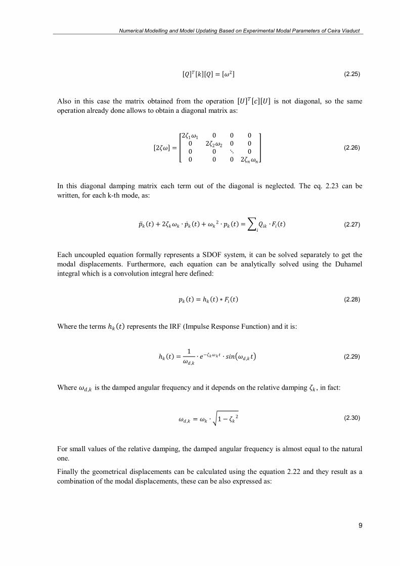
In this diagonal damping matrix each term out of the diagonal is neglected. The eq. 2.23 can be written, for each k-th mode, as:
𝑝 𝑘 𝑡 + 2𝜁𝑘𝜔𝑘 ∙ 𝑝 𝑘 𝑡 + 𝜔𝑘2 ∙ 𝑝𝑘 𝑡 = 𝑄𝑖𝑘 ∙
𝑖𝐹𝑖 𝑡 (2.27)
Each uncoupled equation formally represents a SDOF system, it can be solved separately to get the modal displacements. Furthermore, each equation can be analytically solved using the Duhamel integral which is a convolution integral here defined:
𝑝𝑘 𝑡 = 𝑘 𝑡 ∗ 𝐹𝑖 𝑡 (2.28)
Where the terms 𝑘 𝑡 represents the IRF (Impulse Response Function) and it is:
𝑘 𝑡 =
1
𝜔𝑑 ,𝑘
∙ 𝑒−𝜁𝑘𝜔𝑘𝑡 ∙ 𝑠𝑖𝑛 𝜔𝑑 ,𝑘 𝑡 (2.29)
Where 𝜔𝑑 ,𝑘 is the damped angular frequency and it depends on the relative damping 𝜁𝑘 , in fact:
𝜔𝑑 ,𝑘 = 𝜔𝑘 ∙ 1 − 𝜁𝑘
2 (2.30)
For small values of the relative damping, the damped angular frequency is almost equal to the natural one.
Finally the geometrical displacements can be calculated using the equation 2.22 and they result as a combination of the modal displacements, these can be also expressed as:

Numerical Modelling and Model Updating Based on Experimental Modal Parameters of Ceira Viaduct
10
𝑢 𝑡 = 𝑄1 𝑝1 𝑡 + 𝑄2 𝑝2 𝑡 + ⋯+ 𝑄𝑛 𝑝𝑛 𝑡 (2.31)
Finding in this way the deformation of the system in the dynamic field. The vector 𝑢 𝑡 has a dimension equal to the number of the degrees of freedom, each of its components represents the time history of a single degree of freedom.
If a multi degree of freedom system is excited by a harmonic force with a frequency which is one of the natural frequencies, after a certain time (when permanent state is reached) the system will vibrate with the same frequency of the imposed force and the deformed shape will be the one associated to the mode having that frequency (resonance).
Example
A first application of modal analysis is presented in order to show some results. The model taken in consideration is a shear-type frame simulating a simple three degrees of freedom system. The frame consists of three storeys supported by four columns.
At first, the natural frequencies and the mode are identified by the eigenvalues problem and, in the end, the displacements of the frame are calculated considering a harmonic force applied at the second storey.
The example here shown is considering a really simple model, it means that the results of the modal analysis are easily understandable and they do not present computational errors when calculated using a software. The modal analysis will be done using the software MATLAB.
Figure 2.1 - Discrete three degrees of freedom system
Some properties of the frame are shown in order to have an idea of the type of model is being analyzed. The storeys masses are 2 kg each one and the “L” dimension is 200 mm. The columns have rectangular section (b = 10 mm and h = 1 mm). The elastic modulus is considered of 200 GPa.
At first the inertia of the columns can be calculated, it allows to find the stiffness “k”, we have:
𝐼 =
𝑏 ∙ ℎ3
12 𝑘 = 4 ∙
12 ∙ 𝐸 ∙ 𝐼
𝐿3 (2.32)
Numerical Modelling and Model Updating Based on Experimental Modal Parameters of Ceira Viaduct
11
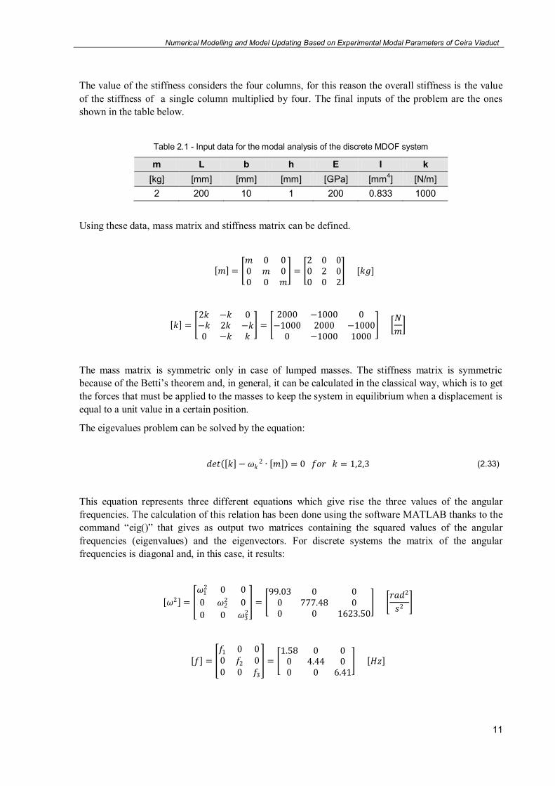
The value of the stiffness considers the four columns, for this reason the overall stiffness is the value of the stiffness of a single column multiplied by four. The final inputs of the problem are the ones shown in the table below.
Table 2.1 - Input data for the modal analysis of the discrete MDOF system
m L b h E I k [kg] [mm] [mm] [mm] [GPa] [mm4] [N/m] 2 200 10 1 200 0.833 1000
Using these data, mass matrix and stiffness matrix can be defined.
𝑚 =
𝑚 0 00 𝑚 00 0 𝑚
= 2 0 00 2 00 0 2
[𝑘𝑔]
𝑘 =
2𝑘 −𝑘 0−𝑘 2𝑘 −𝑘0 −𝑘 𝑘
= 2000 −1000 0−1000 2000 −1000
0 −1000 1000
𝑁
𝑚
The mass matrix is symmetric only in case of lumped masses. The stiffness matrix is symmetric because of the Betti’s theorem and, in general, it can be calculated in the classical way, which is to get the forces that must be applied to the masses to keep the system in equilibrium when a displacement is equal to a unit value in a certain position.
The eigevalues problem can be solved by the equation:
𝑑𝑒𝑡 𝑘 − 𝜔𝑘2 ∙ 𝑚 = 0 𝑓𝑜𝑟 𝑘 = 1,2,3 (2.33)
This equation represents three different equations which give rise the three values of the angular frequencies. The calculation of this relation has been done using the software MATLAB thanks to the command “eig()” that gives as output two matrices containing the squared values of the angular frequencies (eigenvalues) and the eigenvectors. For discrete systems the matrix of the angular frequencies is diagonal and, in this case, it results:
𝜔2 =
𝜔12 0 0
0 𝜔22 0
0 0 𝜔32
= 99.03 0 0
0 777.48 00 0 1623.50
𝑟𝑎𝑑2
𝑠2
𝑓 =
𝑓1 0 00 𝑓2 00 0 𝑓3
= 1.58 0 0
0 4.44 00 0 6.41
𝐻𝑧

Numerical Modelling and Model Updating Based on Experimental Modal Parameters of Ceira Viaduct
12
Appling the equations 2.8 the calculation of the frequencies and the periods becomes possible, the values are shown in the table below.
Table 2.2 - Results of MDOF system
Angular frequency Frequency Period [rad/s] [Hz] [s] 9.95 1.58 0.63 27.88 4.44 0.23 40.29 6.41 0.16
The eigenvectors are here presented in a normalized form in order to have the top displacement equal to 1. This operation can be realized dividing each value 𝜙𝑖𝑗 by the value 𝜙3𝑗 which represents the modal displacement of the third mass.
𝜙 =
𝜙11
𝜙21
𝜙31
𝜙12
𝜙22
𝜙32
𝜙13
𝜙23
𝜙33
= 0.4450.8021.000
−1.247−0.5551.000
1.802−2.2471.000
According to this kind of normalization the modal deformation of the structure can be represented as shown in figure 2.2.
Figure 2.2 - Modal deformation of the frame
The results obtained using MATLAB are the expected ones, exactly the same shown in figure 2.2.

Numerical Modelling and Model Updating Based on Experimental Modal Parameters of Ceira Viaduct
13
Figure 2.3 - Modal deformation by MATLAB
The modal analysis for this system follows the procedures presented in the section 2.1. A harmonic force 𝐹0 is applied at the second storey.
𝐹0 ∙ 𝑠𝑖𝑛 2𝜋𝑡 =
010 ∙ 𝑠𝑖𝑛 2𝜋𝑡 (2.34)
Figure 2.4 - Applied force in the MDOF system
In figure 2.5 only the second component on the force will be plotted because the other two components are equal to zero.
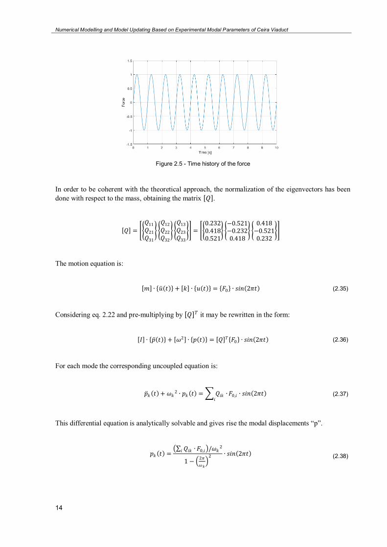
Numerical Modelling and Model Updating Based on Experimental Modal Parameters of Ceira Viaduct
14
Figure 2.5 - Time history of the force
In order to be coherent with the theoretical approach, the normalization of the eigenvectors has been done with respect to the mass, obtaining the matrix 𝑄 .
𝑄 =
𝑄11
𝑄21
𝑄31
𝑄12
𝑄22
𝑄32
𝑄13
𝑄23
𝑄33
= 0.2320.4180.521
−0.521−0.2320.418
0.418−0.5210.232
The motion equation is:
𝑚 ∙ 𝑢 𝑡 + 𝑘 ∙ 𝑢 𝑡 = 𝐹0 ∙ 𝑠𝑖𝑛 2𝜋𝑡 (2.35)
Considering eq. 2.22 and pre-multiplying by 𝑄 𝑇 it may be rewritten in the form:
𝐼 ∙ 𝑝 𝑡 + 𝜔2 ∙ 𝑝 𝑡 = 𝑄 𝑇 𝐹0 ∙ 𝑠𝑖𝑛 2𝜋𝑡 (2.36)
For each mode the corresponding uncoupled equation is:
𝑝 𝑘 𝑡 + 𝜔𝑘2 ∙ 𝑝𝑘 𝑡 = 𝑄𝑖𝑘 ∙
𝑖𝐹0,𝑖 ∙ 𝑠𝑖𝑛 2𝜋𝑡 (2.37)
This differential equation is analytically solvable and gives rise the modal displacements “p”.
𝑝𝑘 𝑡 =
𝑄𝑖𝑘 ∙𝑖 𝐹0,𝑖 /𝜔𝑘2
1 − 2𝜋
𝜔𝑘
2 ∙ 𝑠𝑖𝑛 2𝜋𝑡 (2.38)
Numerical Modelling and Model Updating Based on Experimental Modal Parameters of Ceira Viaduct
15
Appling the equation 2.22, the geometrical displacements can be calculated and they result:
𝑢1 𝑡
𝑢2 𝑡
𝑢3 𝑡 = 𝑄 ∙
𝑝1 𝑡
𝑝2 𝑡
𝑝3 𝑡 (2.39)
𝑢1 𝑡
𝑢2 𝑡
𝑢3 𝑡 =
1.73.23.4
∙ 10−3 ∙ 𝑠𝑖𝑛 2𝜋𝑡
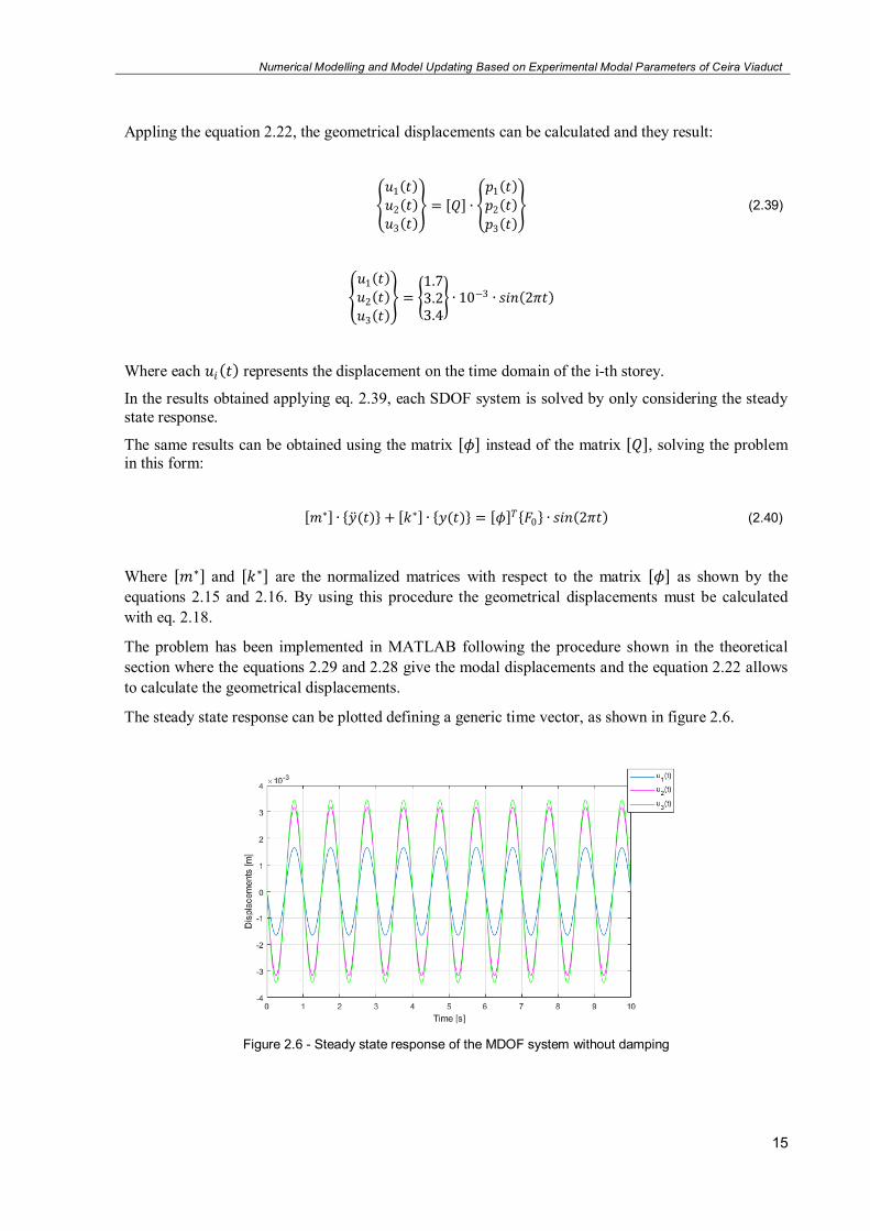
Where each 𝑢𝑖 𝑡 represents the displacement on the time domain of the i-th storey.
In the results obtained applying eq. 2.39, each SDOF system is solved by only considering the steady state response.
The same results can be obtained using the matrix 𝜙 instead of the matrix 𝑄 , solving the problem in this form:
𝑚∗ ∙ 𝑦 (𝑡) + 𝑘∗ ∙ 𝑦(𝑡) = 𝜙 𝑇 𝐹0 ∙ 𝑠𝑖𝑛 2𝜋𝑡 (2.40)
Where 𝑚∗ and 𝑘∗ are the normalized matrices with respect to the matrix 𝜙 as shown by the equations 2.15 and 2.16. By using this procedure the geometrical displacements must be calculated with eq. 2.18.
The problem has been implemented in MATLAB following the procedure shown in the theoretical section where the equations 2.29 and 2.28 give the modal displacements and the equation 2.22 allows to calculate the geometrical displacements.
The steady state response can be plotted defining a generic time vector, as shown in figure 2.6.
Figure 2.6 - Steady state response of the MDOF system without damping

Numerical Modelling and Model Updating Based on Experimental Modal Parameters of Ceira Viaduct
16
Having null damping these deformations have the same amplitude over time. In particular, each amplitude represents the three values of the vector that pre-multiply the sinusoidal function.
If damping is introduced the analytical solution becomes more complicated but, using the software, the introduction of damping is an easy operation that consists of putting a non null value of damping in the equation 2.29. Doing that, the displacements will be damped over time until values close to zero.
In this application, a 5% of damping is applied and considered constant for each mode, thus the damping matrix results a diagonal 3 by 3 matrix as:
2𝜁𝜔 =
2𝜁𝜔1 0 00 2𝜁𝜔2 00 0 2𝜁𝜔3
= 0.994 0 0
0 2.785 00 0 4.024
Figure 2.7 - Geometrical displacements of the MDOF system with damping
The figure shows only the free decay component of the displacements starting from the moment on which the force is not applied anymore, in this case after 100 seconds.
2.2. MODAL ANALYSIS OF CONTINUOUS SYSTEMS
In this second section continuous systems are considered. Also in this case the theoretical part allows to obtain analytical results for a simply supported beam system. They can be then compared to the results calculated using the software Autodesk Robot Structural Analysis.
For this kind of systems the solutions in terms of lowest natural frequencies and vibration shapes can be calculated approximately using two different procedures: the Rayleigh method and the elastic procedure.
Rayleigh’s method
This method considers an energetic procedure that consists on three different steps:
Estimating the vibrating shapes (eigenmodes). Calculate the strain energy and the kinetic energy.

Numerical Modelling and Model Updating Based on Experimental Modal Parameters of Ceira Viaduct
17
Using the principle of energy conservation to get the natural frequencies.
The following structure has been considered.
Figure 2.8 - Simply supported beam
The figure shows the properties of the system: Young modulus (E), inertia (I), length of the span (L) and mass (M), while “u” represents the vertical displacements depending on abscissa “x” and on time
“t”. The solution of this problem can be found writing the vertical displacements as follows:
𝑢 𝑥, 𝑡 = 𝐷 ∙ 𝑠𝑖𝑛 𝜋𝑥
𝐿 ∙ 𝑠𝑖𝑛 𝜔𝑡 (2.41)
Where “D” is integration constant. Deriving 2.41 twice with respect to the abscissa, we have:
𝑢′′ 𝑥, 𝑡 =
𝜕2𝑢 𝑥, 𝑡
𝜕𝑥2= −
𝜋2
𝐿2∙ 𝐷 ∙ 𝑠𝑖𝑛
𝜋𝑥
𝐿 ∙ 𝑠𝑖𝑛 𝜔𝑡 (2.42)
The strain energy results:
𝐸𝑠 =
1
2∙ 𝑢′′ 𝑥, 𝑡 2𝑑𝑥 =
1
2∙ 𝐸𝐼𝐷2 ∙
𝜋4
𝐿4∙ 𝑠𝑖𝑛2 𝜔𝑡 ∙ 𝑠𝑖𝑛2
𝜋𝑥
𝐿
𝐿
0
𝑑𝑥𝐿
0
(2.43)
Remembering that:
𝑠𝑖𝑛2
𝜋𝑥
𝐿
𝐿
0
𝑑𝑥 =1
2∙ 1 − 𝑐𝑜𝑠
2𝜋𝑥
𝐿 𝑑𝑥 =
𝐿
2 (2.44)
We obtain the strain energy as:
𝐸𝑠 =
𝐸𝐼𝐷2 ∙ 𝜋4
4 ∙ 𝐿3∙ 𝑠𝑖𝑛2 𝜔𝑡 (2.45)
The maximum value of this function is the amplitude of the sinusoidal function, in fact:

Numerical Modelling and Model Updating Based on Experimental Modal Parameters of Ceira Viaduct
18
𝐸𝑠,𝑚𝑎𝑥 =
𝐸𝐼𝐷2 ∙ 𝜋4
4 ∙ 𝐿3 (2.46)
The kinetic energy is obtained deriving displacements with respect to the time.
𝑢 𝑥, 𝑡 =
𝜕𝑢 𝑥, 𝑡
𝜕𝑡= 𝐷 ∙ 𝜔 ∙ 𝑠𝑖𝑛
𝜋𝑥
𝐿 ∙ 𝑐𝑜𝑠 𝜔𝑡 (2.47)
Considering the mass “M” and the beam, the kinetic energies are:
𝐸𝑘 ,𝑀 =
1
2∙ 𝑀 ∙ 𝑢 𝐿 2 , 𝑡 2 =
1
2∙ 𝑀 ∙ 𝐷2 ∙ 𝜔2 ∙ 𝑐𝑜𝑠2 𝜔𝑡 (2.48)
𝐸𝑘 ,𝑏𝑒𝑎𝑚 =
1
2∙ 𝑚 ∙ 𝑢 𝑥, 𝑡 2𝑑𝑥
𝐿
0
=1
2∙ 𝑚 ∙ 𝐷2 ∙ 𝜔2 ∙ 𝑐𝑜𝑠2 𝜔𝑡 ∙ 𝑠𝑖𝑛2
𝜋𝑥
𝐿 𝑑𝑥
𝐿
0
(2.49)
The total kinetic energy results:
𝐸𝑘 = 𝐸𝑘 ,𝑀 + 𝐸𝑘 ,𝑏𝑒𝑎𝑚 (2.50)
Substituting the equations 2.48 and 2.49 in eq. 2.50, considering eq. 2.44 we obtain:
𝐸𝑘 =
1
2∙ 𝐷2 ∙ 𝜔2 ∙ 𝑀 +
𝑚𝐿
2 ∙ 𝑐𝑜𝑠2 𝜔𝑡 (2.51)
And the maximum is:
𝐸𝑘 ,𝑚𝑎𝑥 =
1
2∙ 𝐷2 ∙ 𝜔2 ∙ 𝑀 +
𝑚𝐿
2 (2.52)
The principle of the energy conservation can be applied:
𝐸𝑘 ,𝑚𝑎𝑥 = 𝐸𝑠,𝑚𝑎𝑥 (2.53)
𝐸𝐼𝑌2 ∙ 𝜋4
4 ∙ 𝐿3=
1
2∙ 𝐷2 ∙ 𝜔2 ∙ 𝑀 +
𝑚𝐿
2 (2.54)

Numerical Modelling and Model Updating Based on Experimental Modal Parameters of Ceira Viaduct
19
𝜔2 =
𝜋4 ∙ 𝐸𝐼
𝐿3 ∙ 2𝑀 + 𝑚𝐿 (2.55)
The particular case analyzed in the following section is not considering the presence of the mass “M”.
In that case the solution can be found setting M = 0.
𝜔2 =
𝜋4 ∙ 𝐸𝐼
𝑚 ∙ 𝐿4 (2.56)
Considering the equation 2.8, the natural frequencies result:
𝑓 =
𝜋
2∙
𝐸𝐼
𝑚 ∙ 𝐿4 (2.57)
Where “k” indicates the generic mode. In conclusion some considerations must be done. The Rayleigh’s method allows to calculate an estimated value of the natural frequencies, the accuracy of the result depends entirely on the shape function which is assumed to represent the eigenmodes and the values of the natural frequencies calculated by this method are always greater than the real ones. Otherwise the shape functions must be cinematically admissible and must satisfy the displacements boundary conditions at the supports.
The main interest of the Rayleigh’s method lies in its capacity to provide useful estimation of the
natural frequencies for any reasonable assumption of the eigenmodes.
Elastic procedure
The second procedure considers an elastic approach that allows to obtain the same results as the previous procedure and getting the mode shapes analytically. We are now considering the same beam without the concentrated mass.
Figure 2.9 - Simply supported beam
The solution in terms of displacement is a product of a time dependent function and a space dependent function.
Numerical Modelling and Model Updating Based on Experimental Modal Parameters of Ceira Viaduct
20
𝑢 𝑥, 𝑡 = 𝜑 𝑥 ∙ 𝑓 𝑡 (2.58)
The internal moment can be expressed as:
𝑀 = 𝐸𝐼 ∙
𝜕2𝑢
𝜕𝑥2= 𝐸𝐼 ∙ 𝜑′′ 𝑥 ∙ 𝑓 𝑡 (2.59)
The boundary conditions for the simply supported beam are:
𝑢 𝑥 = 0 = 0𝑢 𝑥 = 𝐿 = 0𝑀 𝑥 = 0 = 0𝑀 𝑥 = 𝐿 = 0
→
𝜑 0 = 0
𝜑 𝐿 = 0
𝜑′′ 0 = 0
𝜑′′ 𝐿 = 0
(2.60)
A solution with respect to the abscissa “x” can be found as follows:
𝜑 𝑥 = 𝐴 𝑠𝑖𝑛 𝑎𝑥 + 𝐵 𝑐𝑜𝑠 𝑎𝑥 + 𝐶 𝑠𝑖𝑛ℎ 𝑎𝑥 + 𝐷 𝑐𝑜𝑠ℎ 𝑎𝑥 (2.61)
And deriving twice we have:
𝜑′′ 𝑥 = 𝑎2 −𝐴𝑠𝑖𝑛 𝑎𝑥 − 𝐵 𝑐𝑜𝑠 𝑎𝑥 + 𝐶 𝑠𝑖𝑛ℎ 𝑎𝑥 + 𝐷 𝑐𝑜𝑠ℎ 𝑎𝑥 (2.62)
Applying the boundary conditions, a four equations system provides the constant A,B,C and D. The calculation gives:
𝐵 = 𝐶 = 𝐷 = 0 (2.63)
𝐴 𝑠𝑖𝑛 𝑎𝐿 = 0 → 𝑎𝐿 = 𝑛𝜋 → 𝑎 =𝑛𝜋
𝐿 (2.64)
To find the time dependent solution in a free vibration field we can consider the motion equation:
𝐸𝐼 ∙
𝜕4𝑢
𝜕𝑥4+ 𝑚 ∙
𝜕2𝑢
𝜕𝑡2= 0 (2.65)
Considering eq. 2.59 we obtain:

Numerical Modelling and Model Updating Based on Experimental Modal Parameters of Ceira Viaduct
21
𝐸𝐼 ∙ 𝜑𝐼𝑉 𝑥 ∙ 𝑓 𝑡 + 𝑚 ∙ 𝜑 𝑥 ∙ 𝑓 𝑡 = 0 (2.66)
The constant “a” can be defined dividing by 𝐸𝐼 ∙ 𝜑(𝑥) ∙ 𝑓 𝑡 .
𝜑𝐼𝑉 𝑥
𝜑 𝑥 = −
𝑚 ∙ 𝑓 𝑡
𝐸𝐼 ∙ 𝑓 𝑡 = 𝑎4 (2.67)
The final equations are:
𝜑𝐼𝑉 𝑥 − 𝑎4 ∙ 𝜑 𝑥 = 0 (2.68)
𝑓 𝑡 + 𝜔2 ∙ 𝑓 𝑡 = 0 (2.69)
Dividing eq. 2.66 by 𝑓 𝑡 and considering eq. 2.67 and 2.69 we obtain the value of the angular frequency:
𝜔2 =
𝐸𝐼 ∙ 𝑎4
𝑚 (2.70)
Substituting 2.64 in 2.70 the final solution results:
𝜔𝑘 = 𝑘2𝜋2 ∙
𝐸𝐼
𝑚 ∙ 𝐿4 (2.71)
𝑓𝑘 =
𝑘2𝜋
2∙
𝐸𝐼
𝑚 ∙ 𝐿4 (2.72)
𝑇𝑘 =
1
𝑓𝑘 (2.73)
And considering eq. 2.61, the generic eigenmode is:
𝜑𝑘 𝑥 = 𝐴 𝑠𝑖𝑛
𝑘𝜋
𝐿∙ 𝑥 (2.74)

Numerical Modelling and Model Updating Based on Experimental Modal Parameters of Ceira Viaduct
22
For several values of the natural number “k” the different modes can be analyzed considering a generic value of the constant “A”.
Considering continuous systems an infinite number of natural frequencies and mode shapes can be found while the number of frequencies and mode shapes for discrete systems is always equal to the number of the degrees of freedom of the system.
As we will see in the example, this method gives the exact values of the natural frequencies and mode shapes in case of simple systems. When a more complicated structure is considered, the two methods may provide only approximated results.
Example
An example will be shown for continuous systems and some comparison between analytical results and results calculated by the software will be analyzed.
The system taken in consideration is a simply supported beam, unloaded and with the following characteristics:
Length of the span........................... 50 m
Rectangular cross section.............. (0.8 x 1.0 m2)
Materials........................................... Reinforced concrete (C40/50)
Figure 2.10 - Simply supported beam
Table 2.3 shows the assumption about the properties of the element.
Table 2.3 - Element properties
E I A m L [MPa] [mm4] [m2] [kg/m] [m]
35547.1 6.67E+10 0.8 2039 50
These characteristics have been chosen in order to have the correct input to solve the equations shown in the theoretical part for the calculation of the natural frequencies. This example shows how the modal parameters depend only on the intrinsic properties of the system (mass, stiffness and geometrical properties).
In this first step the calculation of the modal parameters using the theoretical results will be shown.
The values of the frequencies and the periods are given by the equations 2.71, 2.72 and 2.73, these results are shown in table 2.4. For this example five modes have been considered.

Numerical Modelling and Model Updating Based on Experimental Modal Parameters of Ceira Viaduct
23
Table 2.4 - Analytical results of the modal analysis
Mode Angular frequency Frequency Period
[rad/s] [Hz] [s] 1 4.26 0.68 1.48 2 17.03 2.71 0.37 3 38.31 6.10 0.16 4 68.10 10.84 0.09 5 106.41 16.94 0.06
According to the eq. 2.74 the mode shapes may be analytically calculated setting A = 1 and by varying the abscissa “x” from 0 to 50. The results are shown in the set of figures below.
Figure 2.11 - Analytical mode shape: Mode 1
Figure 2.12 - Analytical mode shape: Mode 2
Figure 2.13 - Analytical mode shape: Mode 3
0 5 10 15 20 25 30 35 40 45 50
x [m]
0 5 10 15 20 25 30 35 40 45 50
x [m]
0 5 10 15 20 25 30 35 40 45 50
x [m]

Numerical Modelling and Model Updating Based on Experimental Modal Parameters of Ceira Viaduct
24
Figure 2.14 - Analytical mode shape: Mode 4
Figure 2.15 - Analytical mode shape: Mode 5
In a second step, natural frequencies, periods and mode shapes have been calculated using the software Autodesk Robot Structural Analysis defining the materials and the characteristics shown in table 2.3. Table 2.5 contains the values of the frequencies and the periods for each mode.
Table 2.5 - Results of the modal analysis from the software
Mode Frequency Period
[Hz] [s] 1 0.68 1.47 2 2.72 0.37 3 6.15 0.16 4 11.08 0.09 5 18.75 0.05
The values obtained by the software are very similar to the analytical ones and so the same approach will be used to analyze other kind of structures. Finally the mode shapes got by the software are shown in the figures below.
Figure 2.16 - Mode shape from the software: Mode 1
0 5 10 15 20 25 30 35 40 45 50
x [m]
0 5 10 15 20 25 30 35 40 45 50
x [m]

Numerical Modelling and Model Updating Based on Experimental Modal Parameters of Ceira Viaduct
25
Figure 2.17 - Mode shape from the software: Mode 2
Figure 2.18 - Mode shape from the software: Mode 3
Figure 2.19 - Mode shape from the software: Mode 4
Figure 2.20 - Mode shape from the software: Mode 5
2.3. MODAL ANALYSIS IN A STRUCTURAL ANALYSIS SOFTWARE
More advanced numerical model will be presented to become familiar with the use of the software that will be adopted to model the full scale bridge presented in chapter 4.
This second case of study is a structure simulating a four spans straight bridge. The purpose of this example is to create a model representing a system quite similar to a real structure. This allowed to have a first approach with the modelling of a structure in the software and to understand how a FEM works in terms of calculation of natural frequencies and representation of mode shapes. The software which has been utilized is the same already used for the previous example.
Some conditions are introduced in the model: the sections of the piers and the deck are constant along the structure, an internal hinge is placed in correspondence of the pier 7, the piers are considered fixed on the ground and the deck is continuous over piers 8 and 9.
The static scheme of the structure is presented in figure 2.21.

Numerical Modelling and Model Updating Based on Experimental Modal Parameters of Ceira Viaduct
26
Figure 2.21 - Structure static scheme
Length of the elements:
Element 1........................... 30 m
Element 2........................... 60 m
Element 3........................... 90 m
Element 4........................... 60 m
Element 7........................... 50 m
Element 8........................... 70 m
Element 9........................... 70 m
Figure 2.22 - 3D view of the structure
In terms of material properties we have:
Material.......................... Reinforced concrete (C40/50).
Numerical Modelling and Model Updating Based on Experimental Modal Parameters of Ceira Viaduct
27
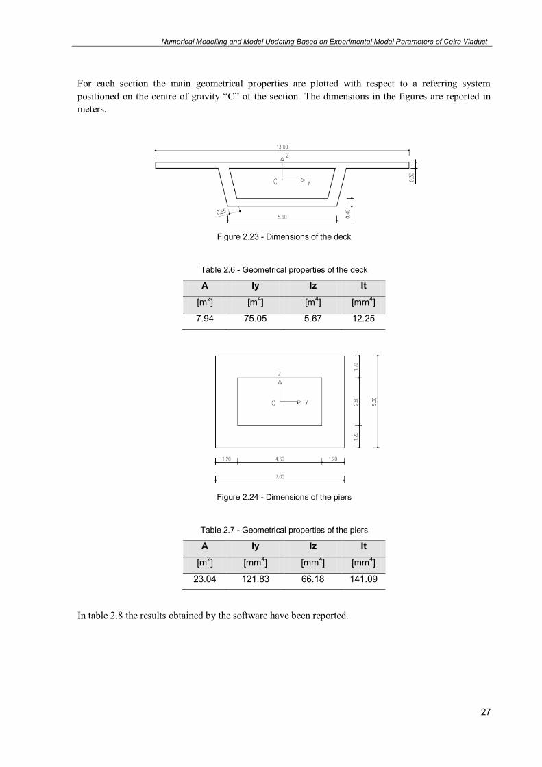
For each section the main geometrical properties are plotted with respect to a referring system positioned on the centre of gravity “C” of the section. The dimensions in the figures are reported in meters.
Figure 2.23 - Dimensions of the deck
Table 2.6 - Geometrical properties of the deck
A Iy Iz It
[m2] [m4] [m4] [mm4]
7.94 75.05 5.67 12.25
Figure 2.24 - Dimensions of the piers
Table 2.7 - Geometrical properties of the piers
A Iy Iz It
[m2] [mm4] [mm4] [mm4]
23.04 121.83 66.18 141.09
In table 2.8 the results obtained by the software have been reported.

Numerical Modelling and Model Updating Based on Experimental Modal Parameters of Ceira Viaduct
28
Table 2.8 - Results of the modal analysis
Mode Frequency Period
[Hz] [s] 1 2.39 0.42 2 2.75 0.36 3 2.97 0.34 4 3.88 0.26 5 4.43 0.23
In this case the modal parameters cannot be easily calculated with an analytical procedure, in fact, in chapter 4, we will see how, for a real structure, the validation of the numerical model is done using different procedures. Also for this structure the mode shapes are represented.
Figure 2.25 - Structure mode shape: Mode 1
Figure 2.26 - Structure mode shape: Mode 2

Numerical Modelling and Model Updating Based on Experimental Modal Parameters of Ceira Viaduct
29
Figure 2.27 - Structure mode shape: Mode 3
Figure 2.28 - Structure mode shape: Mode 4
Figure 2.29 - Structure mode shape: Mode 5
Looking at the mode shapes it can be seen that the deformed shapes in correspondence to the nodes between piers and deck show how the internal connections of the structure affects the mode shapes. In correspondence of the element 7 the behaviour is completely different respect to elements 8 and 9. It

Numerical Modelling and Model Updating Based on Experimental Modal Parameters of Ceira Viaduct
30
means that the restraints represent one of the intrinsic characteristics that have an important role in the modal analysis.
In the end of this chapter we could say that the problem of the modal analysis may be easily solved by using appropriate software.
Once the model is done the calculation is an automatic process. As we will see in the next chapters the models always have some approximations that will make the results different to the real ones. It means that other ways to get the modal parameters must be used and they will be the topics of the following sections.

Numerical Modelling and Model Updating Based on Experimental Modal Parameters of Ceira Viaduct
31
3 CHAPTER 3 - AMBIENT VIBRATION
TESTING METHODS
3.1. GENERAL DESCRIPTION
In this chapter the process of the identification of the modal parameters for a structure is analyzed. This process is considered starting from the measurements done during an AVT (Ambient Vibration Test). In this kind of tests the response of the structure is recorded usually in terms of accelerations coming from ambient actions like wind or traffic.
The frame already considered in the previous chapter is used again to demonstrate the theoretical concepts and validate the routines developed in MATLAB. The frame was modelled in MATLAB and, being just a theoretical model, the excitations are generated by the software.
Vibration testing methods are usually divided into two different main categories: forced vibration tests and ambient vibration tests. When an ambient vibration test is done, the structure is considered excited by wind, micro tremors and traffic. It means that the control of the force applied to vibrate the structure is not permitted. This represents the main difference between this kind of tests and the forced vibration ones.
Forced Vibration Tests
In forced vibration tests controlled forces are applied to a structure introducing some vibrations. By measuring the structure response under these known forces, it is possible to determine the structure dynamic properties. The controlled excitation force can be applied in several ways, the three most used ones are: shaker, impact and pullback tests. These methods are briefly described in order to have a comparison with the ambient vibration tests.
Shaker tests are used to apply forces to structures in a controlled manner to excite them dynamically, the shaker must produce sufficiently large forces to excite a bridge in the frequency range of interest. If the frequencies of interest are low (less than 1 Hz) the shaker cannot provide very large forces.
In an impact testing method the test object is instrumented with accelerometers and is struck with a hammer containing a force transducer. The impact force and acceleration response time histories are then used to compute Frequency Response Functions (FRFs). Natural frequencies, mode shapes and damping ratios are calculated from the FRFs.
The pullback testing method generally involves displacing a structure and quickly releasing it, causing the structure to vibrate freely. This static displacement can be applied thanks to hydraulic rams, cables,
Numerical Modelling and Model Updating Based on Experimental Modal Parameters of Ceira Viaduct
32
bulldozers, tug boats or chain blocks. When the load is released the free vibrations of the structure are recorded as the structure returns to its position of static equilibrium. The results from these tests allow to determine natural frequencies, mode shapes and damping ratios only for the structure principal modes.
Ambient Vibration Tests
In an ambient vibration test the modal parameters are obtained by measuring the vibrations simultaneously at several positions of the structure. Reliable estimates of natural frequencies and mode shapes can be obtained if the following conditions are met:
Linearity:
The structure behaves as a linear system, it means that a linear combination of individual force inputs will result in the same linear combination of the corresponding individual response.
Excitation:
It is assumed that the most relevant modes are excited.
Modes well separated and lightly damped:
It is assumed that the modes of interest are well separated and with a damping lower than the 5 % of the critical damping
Classical damping:
The structure must be classical damped.
More recent processing techniques may still provide good results if some of the previous conditions are not fully fulfilled.
3.2. THEORETICAL BACKGROUND
Before starting to describe the procedures for the application of an ambient vibration test some theoretical aspects must be analyzed. In the application of AVT the analysis are often done in the frequency domain, for this reason a short a theoretical introduction for the signal processing in the frequency domain, by using the Fourier operator, is presented.
Subsequently, the frame will be introduced to show how to get the natural frequencies starting from the frequency response functions or from acceleration signals. The results will be compared to the ones already obtained in chapter 2 by the eigenvalues problem.
In section 3.2.1 the response of the structure will be calculated using the FRFs and these are calculated knowing the natural frequencies (eq. 3.13). This first approach is thus completely theoretical.
In section 3.3 the problem will be present in a more practical way because of the generation of a random excitation and so it will reflect a more real situation.

Numerical Modelling and Model Updating Based on Experimental Modal Parameters of Ceira Viaduct
33
3.2.1. FOURIER TRANSFORM OPERATOR
The frequency domain is often used in dynamic analysis, it means that signals must be transformed from the time domain to the frequency domain. In this section it is possible to see how, for this purpose, the Fourier transformation must be applied.
Fourier transform extends Fourier analysis of signals defined in –𝑇/2, +𝑇/2 to signals defined in −∞, +∞ . When a complex signal is given and it is decomposable in a Fourier series, it results:
𝑠 𝑡 = 𝜇𝑛 ∙ 𝑒
𝑖𝑛2𝜋
𝑇𝑡
+∞
−∞ 𝑡 ∈ −
𝑇
2, +
𝑇
2 (3.1)
The exponential functions represent a complete basis for all finite energy signals. The term 𝜇𝑛 may be expressed as:
𝜇𝑛 =
1
𝑇∙ 𝑠 𝑡
𝑇/2
−𝑇/2
∙ 𝑒−𝑖𝑛2𝜋
𝑇𝑡𝑑𝑡 (3.2)
Considering the discrete field the frequency is:
𝑓𝑛 =𝑛
𝑇 (3.3)
∆𝑓 = 𝑓𝑛 − 𝑓𝑛−1 = 𝑓0 =
1
𝑇 (3.4)
Where 𝑓0 represents the frequency resolution and indicates the spacing on the frequency axis between two consecutive samples.
Substituting 𝜇𝑛 in the eq. 3.1 and considering eq. 3.3, the signal assumes this form:
𝑠 𝑡 = 𝑠 𝜏
𝑇/2
−𝑇/2
∙ 𝑒−𝑖𝑛 ∙2𝜋𝑓𝑛 𝜏𝑑𝜏 ∙ 𝑒𝑖𝑛 ∙2𝜋𝑓𝑛 𝑡+∞
−∞∙ ∆𝑓 (3.5)
In order to pass from discrete to continuous we have: 𝑇 → ∞ 𝑎𝑛𝑑 ∆𝑓 → 𝑑𝑓. Thus the discrete variable 𝑓𝑛 becomes a continuous variable 𝑓. The signal is:
𝑠 𝑡 = 𝑠 𝜏
+∞
−∞
∙ 𝑒−𝑖𝑛∙2𝜋𝑓𝜏𝑑𝜏 ∙ 𝑒𝑖𝑛 ∙2𝜋𝑓𝑡+∞
−∞
𝑑𝑓 𝑡 ∈ −∞, +∞ (3.6)
Hence:

Numerical Modelling and Model Updating Based on Experimental Modal Parameters of Ceira Viaduct
34
𝑠 𝑡 = 𝑋 𝑓 ∙ 𝑒𝑖𝑛 ∙2𝜋𝑓𝑡
+∞
−∞
𝑑𝑓 (3.7)
Having defined:
𝑋 𝑓 = 𝑠 𝑡
+∞
−∞
∙ 𝑒−𝑖𝑛 ∙2𝜋𝑓𝑡𝑑𝑡 (3.8)
It represents the Fourier transform of the signal 𝑠 𝑡 . In a compact form the Fourier transform operator is indicated as:
𝑋 𝑓 = ℑ 𝑠 𝑡 (3.9)
The inverse operation allows defining the anti-transform operator as:
s 𝑡 = ℑ−1 𝑋 𝑓 = 𝑋 𝑓
+∞
−∞
∙ 𝑒𝑖𝑛 ∙2𝜋𝑓𝑡𝑑𝑓 (3.10)
The Fourier transform can be applied to signals like time dependent load or acceleration signals. This operation allows to calculate the response of a system under a generic excitation in the frequency domain using the following expression:
𝑌 𝑓 = 𝐻 𝑓 ∙ 𝐹 𝑓 (3.11)
Where 𝐻 𝑓 is the FRF (Frequency Response Function) and, according to eq. 3.9, 𝐹 𝑓 is the Fourier transform of the load signal in the frequency domain, it can be written as:
𝐹 𝑓 = ℑ 𝐹 𝑡 (3.12)
In most of literature references this equation is presented using the angular frequency as variable, this is the reason why the following expressions are functions of 𝜔 instead of 𝑓. In general the variable can be chosen according to the expressions form.
Two procedures are usually applied for the calculation of the FRF: the first one is an analytical procedure, for each mode the frequency response function results:
Numerical Modelling and Model Updating Based on Experimental Modal Parameters of Ceira Viaduct
35
𝐻𝑘 𝜔 =
1
𝜔𝑘2 − 𝜔2 + 2 ∙ 𝑖 ∙ 𝜁𝑘 ∙ 𝜔 ∙ 𝜔𝑘
(3.13)
Applying this operation for each mode the FRF matrix can be defined and it is a diagonal matrix on which each 𝐻𝑘 𝜔 is situated in the principal diagonal.
The second procedure considers the calculation of the FRF numerically, sometimes this operation is done using software like MATLAB and consists on the inversion of the IRF using the Fourier transform operator.
𝐻𝑘 𝜔 = ℑ 𝑘 𝑡 (3.14)
In MATLAB the “fft” function allows the application of the Fourier transform.
3.2.2. MODAL IDENTIFICATION
In this section the problem of the identification of the modal parameters of a structure is presented. In a first part the general problem is shown and an example shows how it is possible to get the natural frequencies of a structure under a specific applied force.
In a second part the problem is developed considering stochastic excitations applied to the structure. In this context the estimates of the spectra are use to obtain the modal parameters.
Using an ambient vibration test, for each instrumented degree of freedom of the structure, it is possible to evaluate displacements, velocities or accelerations. As shown in eq. 2.18, the displacements for a multi degree of freedom system (with “n” degrees of freedom) can be expressed as a combination of
the mode shapes as follows:
𝑢 𝑡 = 𝜙1 ∙ 𝑦1 𝑡 + 𝜙2 ∙ 𝑦2 𝑡 + ⋯+ 𝜙𝑛 ∙ 𝑦𝑛 𝑡 (3.15)
Appling the Fourier transform to both terms, the solution in the frequency domain can be obtained.
𝑈 𝜔 = 𝜙1 ∙ 𝑌1 𝜔 + 𝜙2 ∙ 𝑌2 𝜔 + ⋯+ 𝜙𝑛 ∙ 𝑌𝑛 𝜔 (3.16)
Considering eq. 3.16 and the relation between displacements and accelerations:
𝑈 𝜔 = 𝜔2 ∙ 𝑈 𝜔 (3.17)
The acceleration of the structure in the frequency domain can be expressed as:
𝑈 𝜔 = 𝜔2 ∙ 𝜙1 ∙ 𝐻1 𝜔 ∙ 𝑌1 𝜔 + 𝜙2 ∙ 𝐻2 𝜔 ∙ 𝑌2 𝜔 + ⋯+ 𝜙𝑛 ∙ 𝐻𝑛 𝜔 ∙ 𝑌𝑛 𝜔 (3.18)

Numerical Modelling and Model Updating Based on Experimental Modal Parameters of Ceira Viaduct
36
Defining the term:
𝐷𝑗𝑖 = 𝜙𝑗𝑖 ∙ 𝑌𝑗 𝜔 (3.19)
An individual complex valued acceleration response can be expressed as:
𝑈 𝑓 = 𝜔2 ∙ 𝐷1𝑖 ∙ 𝐻1 𝜔 + 𝐷2𝑖 ∙ 𝐻2 𝜔 + ⋯+ 𝐷𝑛𝑖 ∙ 𝐻𝑛 𝜔 (3.20)
And imposing 𝐷𝑗𝑖 = 1, for each mode it is possible to obtain the value of 𝑈 𝜔 .
Plotting the acceleration 𝜔2 𝐻𝑗 𝜔 and the combination 𝑈 𝜔 some peaks give rise in correspondence of the damped frequencies. In case of small damping, these values are similar to the natural frequencies. It means that the natural frequencies of a structure can be estimated using the Fourier transform of an ambient vibration acceleration record.
Example
The same frame already considered in chapter 2 can be taken in consideration to show some results in terms of application of the Fourier transform and the identification of natural frequencies using the FRFs and acceleration plots.
For this application the structure is considered with a damping of 5 % for each mode.
In this example the structure in consideration is loaded with a harmonic force and not subjected to ambient vibrations, only FRFs and acceleration in the frequency domain are analyzed. In the end, it does not reflect a real case but it allows to understand how natural frequencies can be found using a FRF diagram.
Figure 3.1 - Discrete three degrees of freedom system
Table 3.1 shows the natural and damped frequencies for the frame obtained by the eigenvalues problem. In chapter 2 the damped frequencies were not reported, the table shows how these are close to the natural ones:

Numerical Modelling and Model Updating Based on Experimental Modal Parameters of Ceira Viaduct
37
Table 3.1 - Natural and damped frequencies of the frame
Natural Frequency Damped frequency [Hz] [Hz] 1.58 1.58 4.44 4.43 6.41 6.40
Remembering that in this example the displacements have been calculated using the normalized mode shape vectors 𝑄 , the transformation in the frequency domain results:
𝑈 𝜔 = 𝑄1 ∙ 𝑃1 𝜔 + 𝑄2 ∙ 𝑃2 𝜔 + 𝑄3 ∙ 𝑃3 𝜔 (3.21)
Where the normalize coordinates 𝑃𝑘 𝜔 are calculated as:
𝑃𝑘 𝜔 = 𝐻𝑘 𝜔 ∙ 𝐹𝑘 𝜔 (3.22)
The term 𝐹𝑘 ω results from the vector 𝐹 𝜔 that can be calculated using the Fourier transformation of the load signal, according to the normalization used for the application, it results:
𝐹 𝜔 = ℑ 𝑈 𝑇 𝐹 𝑡 (3.23)
In this application each FRF has been calculated with both methods shown above. At first, they have been calculated applying the Fourier transformation to the IRFs and then using the analytical procedure. The results must be the same and they are plotted below.
Figure 3.2 - Amplitude of the Frequency Response Functions

Numerical Modelling and Model Updating Based on Experimental Modal Parameters of Ceira Viaduct
38
About the calculation of the acceleration in the frequency domain is sufficient to apply eq. 3.17 that, in this case, can be written as:
𝑈 (𝜔) = 𝜔2 ∙ 𝐻1 𝜔 + 𝐻2 𝜔 + 𝐻3 𝜔 (3.24)
At first, the three acceleration responses 𝐴𝑗 𝜔 = 𝜔2 𝐻𝑗 𝜔 and then the combination 𝑈 𝜔 have been plotted.
Figure 3.3 - Accelerations amplitude in frequency domain
Figure 3.4 - Combination of the accelerations amplitude in the frequency domain

Numerical Modelling and Model Updating Based on Experimental Modal Parameters of Ceira Viaduct
39
We can see that the results are the expected ones, the peaks are in correspondence with the damped frequencies and, approximately, with the natural frequencies.
In the end the normalized coordinates for each mode can be calculated using eq. 3.21 and they are shown in figure 3.5, while in figure 3.6 we can find the combination of the modes plotted for each degree of freedom of the frame, that means, in this example, the response of each storey.
Figure 3.5 - Responses amplitude of the normalized coordinates
Figure 3.6 - Combination of the responses amplitude of the three storeys in the frequency domain
As can be seen in both figures there is a first peak in correspondence with the value 1, this peak comes from the applied force on the frame that can be written as:
𝑓0 = 𝑠𝑖𝑛 2𝜋𝑡 = 𝑠𝑖𝑛 𝜔𝑡 → 2𝜋 = 𝜔 (3.25)
Considering the relation between frequency and angular frequency we obtain:
Numerical Modelling and Model Updating Based on Experimental Modal Parameters of Ceira Viaduct
40
𝑓 =
𝜔
2𝜋=
2𝜋
2𝜋= 1 (3.26)
The other peaks are in correspondence with the natural frequencies.
3.3. STOCHASTIC MODAL IDENTIFICATION METHODS
In the previous section the procedure to obtain the natural frequencies of a structure under a harmonic excitation by using the frequency response functions has been analyzed. In this section the main goal will be the modal identification for a system subjected to a generic excitation simulating ambient vibrations.
In this context the structure can be considered under wind or traffic actions, thus under any kind of action referable to a random signal identified as a stochastic excitation. This is the reason why we can talk about stochastic modal identification methods.
Considering an ambient vibration test, the modal identification starts from the signals recorded in several points of the structure. As will be seen in the next chapter, in a real application, several sensors are positioned on the structure and these allow the recording of the acceleration time series caused by ambient excitations. These records are then used to get the response of the structure.
A good estimate of the responses can be obtained if many points in the structure are instrumented, but most of the time the number of available sensors is less than the number of the points that must be instrumented. For this reason some sensors are moved during the test in several positions.
The stochastic modal identification methods are divided into two main categories: identification methods in time domain and identification methods in the frequency domain.
In this thesis only the second category will be analyzed, in particular one method will be described. The method is called Peak Picking method (PP) and it allows to identify the natural frequencies and the mode shapes of the structure.
Before the description of this method the response identification procedures and the power spectra calculation will be presented. They represent the starting point for the application of the method.
From a theoretical point of view, as eq. 3.27 will show, the application of the next procedures (in particular the calculation of the power spectra) needs the responses in the frequency domain. This can be done applying the Discrete Fourier Transform (DFT), calculated by the Fast Fourier Transform operator (FFT).
All the procedures of the modal identification are illustrated using the three degrees of freedom frame already considered in the previous chapters.
3.3.1. RESPONSE OF A STRUCTURE UNDER A STOCHASTIC EXCITATION
The first part of the modal identification process consists on the measurement of the response of the structure. As already referred, in a real application it would come from an ambient vibration test by using the sensors positioned in several points of the structure. From a theoretical point of view each instrumented point represents a degree of freedom from which the response is obtained and that, in general, is an acceleration record.
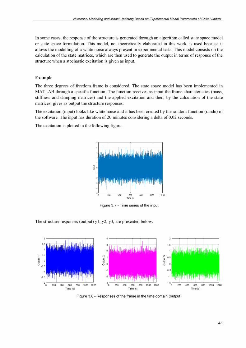
Numerical Modelling and Model Updating Based on Experimental Modal Parameters of Ceira Viaduct
41
In some cases, the response of the structure is generated through an algorithm called state space model or state space formulation. This model, not theoretically elaborated in this work, is used because it allows the modelling of a white noise always present in experimental tests. This model consists on the calculation of the state matrices, which are then used to generate the output in terms of response of the structure when a stochastic excitation is given as input.
Example
The three degrees of freedom frame is considered. The state space model has been implemented in MATLAB through a specific function. The function receives as input the frame characteristics (mass, stiffness and damping matrices) and the applied excitation and then, by the calculation of the state matrices, gives as output the structure responses.
The excitation (input) looks like white noise and it has been created by the random function (randn) of the software. The input has duration of 20 minutes considering a delta of 0.02 seconds.
The excitation is plotted in the following figure.
Figure 3.7 - Time series of the input
The structure responses (output) y1, y2, y3, are presented below.
Figure 3.8 - Responses of the frame in the time domain (output)
Numerical Modelling and Model Updating Based on Experimental Modal Parameters of Ceira Viaduct
42
3.3.2. CALCULATION OF THE POWER SPECTRA
The calculation of the power spectra PSD (Power Spectral Density) represents the starting point of the modal identification method that will be presented. In the context of ambient vibration tests the response is calculated doing measurements of the responses in several points of the structure. Each response is used to calculate the spectra as shown in eq. 3.27.
In general we can talk about auto-spectra if the response is measured for a single degree of freedom “i” while in the cross-spectra the response is calculated relating the measurement in the degree of freedom “i” with the degree of freedom “j”. In this way the spectra can be presented in a matrix on which in the principal diagonal we can find the auto-spectra and out of it there are the cross-spectra.
If the measurements in the structure are done simultaneously, the spectra matrix will result a square matrix with a dimension equal to the instrumented points. In most of the applications the number of the degrees of freedom that should be instrumented to find a good behaviour of the structure will be too high, for this reason, in practice, a sequence of measurements is done by using different positioning of the sensors. Each arrangement is usually called “setup”. To grant the relationship
between the measures, some degrees of freedom must be measured in every setup. These will represent the reference degrees of freedom.
As it will be presented in the next chapter, there are usually some sensors remaining fixed in every setup, these are the reference degrees of freedom.
Proceeding in this way, in practical applications, it is not possible to get square spectra matrices but only rectangular ones with “l” by “r” dimensions. In these matrices “l” represents the number of the
points on which the response is measured and “r” is the number of the reference degrees of freedom.
The calculation of the spectra has been implemented in MATLAB and it is based on a procedure called Welch procedure (Welch 1967).
From a theoretical point of view, the calculation of the power spectra, considering a generic structure, is given by:
𝑆 𝑦
𝑟𝑒𝑓 𝜔 =
𝑌 𝜔 ∗ ∙ 𝑌𝑟𝑒𝑓 𝜔 𝑇
𝑁 ∙ ∆𝑡 (3.27)
Where 𝑌 𝜔 ∗ represents a column vector containing the FFTs of the response vectors with a number of lines equal to the instrumented degrees of freedom. 𝑌𝑟𝑒𝑓 𝜔 is a column vector with an “r”
dimension containing the FFTs of the responses of the degrees of freedom instrumented in every setup (reference degrees of freedom). 𝑁 is the number of acquired points and ∆𝑡 the discrete time interval.
Example
In case of the discrete degree of freedom system already analyzed, the spectra matrix is a 3 by 3 matrix because the vectors in eq. 3.27 have dimension equal to the number of the degrees of freedom. The multiplication between a line vector by a column one with the same dimension gives rise to a square matrix (3 by 3).
The spectra matrix will be symmetric, the terms out of the principal diagonal result 𝑆𝑦(𝜔)𝑗 ,𝑖 =
𝑆𝑦(𝜔)𝑖 ,𝑗 .

Numerical Modelling and Model Updating Based on Experimental Modal Parameters of Ceira Viaduct
43
Applying the Welch procedure, it is possible to calculate the nine components of the spectra matrix (3 auto-spectra and 6 cross-spectra). The software MATAB allows to do this with two different commands: “pwelch” gives rise to the auto-spectra while “cpsd” provides the cross-spectra. Both of them need as input the response “y” of the frame, in particular the command “cpsd” needs two different inputs according to the position of the cross-spectra in the matrix.
The spectra are plotted below with amplitude and phase, the auto-spectra have null phases.
Figure 3.9 - Elements of the spectra matrix

Numerical Modelling and Model Updating Based on Experimental Modal Parameters of Ceira Viaduct
44
In the first column of the figure the auto-spectra are plotted, while in the column on the right there are the cross-spectra with amplitude and phase. The subscripts indicate the positions in the spectra matrix.
3.3.1. PEAK PICKING METHOD
This identification method is a frequency domain method and it is today acknowledged as the first applied method in the dynamic identification field for structures under ambience vibrations. In this work the theoretical background of this method is omitted, the main theoretical fundamentals of the actual format of the method have been developed by Bendat and Piersol (Bendat and Piersol 1980).
This method consists on the frequency and mode shapes identification of a structure starting from the spectra definition. It allows to identify the modal parameters considering the structure excited by a generic signal.
In this section the application of this method will be shown using the same frame already considered.
Frequencies identification
In this first part the identification of the natural frequencies of the structure is analyzed. When a structure is subjected to a white noise, the spectra matrix can be derived from the FRF matrix through the following relation:
𝑆𝑦 𝜔 = 𝐻 𝜔 ∙ 𝑅𝑢 ∙ 𝐻𝐻 𝜔 (3.28)
Where 𝐻𝐻 𝜔 is the transpose of the 𝐻 𝜔 and contains the conjugated complex values of the same matrix.
Considering white noise, the matrix 𝑅𝑢 is a constant matrix, it means that, as the FRFs, also the spectra in the matrix 𝑆𝑦 𝜔 will have the peaks in correspondence with the damped frequencies and thus very close to the natural ones.
In this way the identification of the natural frequencies becomes possible starting from the matrix of the power spectral density. In a real structure, on which the analyzed degrees of freedom are many, the analysis of only one power auto-spectrum (one in the principal diagonal of the matrix) may not be enough to identify the natural frequencies with a good approximation, for this reason sometimes a procedure of normalization and averaging of the auto-spectra is applied. This operation provides the ANPSD (Average Normalized Power Spectral Density), obtained by the average of the auto-spectra normalized by their N own ordinates (Felber 1993).
Example
Looking at the spectra got in the previous section the consideration about the presence of the peaks is immediately evident.
In order to get better approximation of the natural frequencies the average spectrum has been calculated and plotted. Moreover a table shows the differences between the theoretical values and the ones got with the average spectrum.

Numerical Modelling and Model Updating Based on Experimental Modal Parameters of Ceira Viaduct
45
Figure 3.10 - Average auto-spectrum
Table 3.2 - Comparison of the frequencies values
Analytical natural Frequency Natural frequency by spectra Percentage gap [Hz] [Hz] [%] 1.58 1.59 0.20 4.44 4.37 1.53 6.41 6.47 0.89
The errors by using this model are very low, in real cases the errors will depend on the complexity of the structure and the quality of the measurements.
Mode shapes identification
The method currently used in this context to get mode shapes consists on the calculation of the ratios between the cross-spectra of a reference degree of freedom and the correspondent auto-spectrum. It is possible to demonstrate how, in this way, for each frequency value associated to an instrumented degree of freedom “k”, the ratio between the cross-spectrum of a reference degree of freedom and the correspondent auto-spectrum is equal to the modal ratio for that specific k-th frequency.
𝑆𝑦(𝜔𝑘)𝑟𝑒𝑓 ,𝑗
𝑆𝑦(𝜔𝑘)𝑟𝑒𝑓 ,𝑟𝑒𝑓=
𝜙𝑗 𝑘 𝜙𝑟𝑒𝑓 𝑘
(3.29)
The mode shapes will result normalized according to the chosen reference degree of freedom. The procedure usually used is to calculate the ratios for each value of the frequency. Defining the transfer function, it will result:

Numerical Modelling and Model Updating Based on Experimental Modal Parameters of Ceira Viaduct
46
𝑇𝑟𝑒𝑓 ,𝑗 =
𝑆𝑦(𝜔)𝑟𝑒𝑓 ,𝑗
𝑆𝑦(𝜔)𝑟𝑒𝑓 ,𝑟𝑒𝑓
(3.30)
Identifying the ordinate values in correspondence with a specific value of a natural frequency it is possible to get the modal ratios between a generic degree of freedom and the reference one, with the ratios in several points the mode shapes can be plotted. Proceeding in this way only one reference degree of freedom is needed to get all the modes, it means that only one column of the PSD matrix is sufficient to obtain all the mode shapes.
Example
The implementation of the procedure to get the mode shapes has been done by MATLAB and considering as reference the degree of freedom of the third storey of the frame, it means that the elements in the third columns on the PSD matrix are considered.
Figure 3.11 - Transfer functions
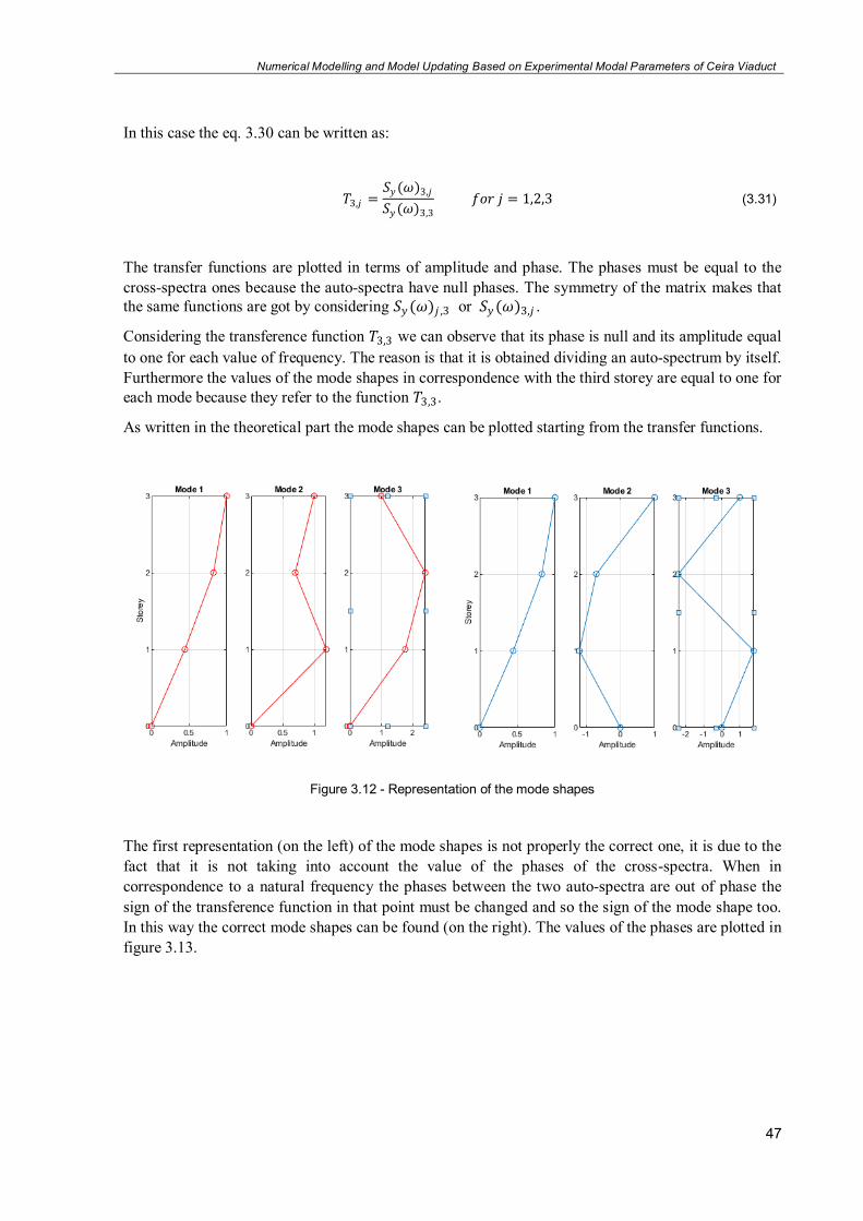
Numerical Modelling and Model Updating Based on Experimental Modal Parameters of Ceira Viaduct
47
In this case the eq. 3.30 can be written as:
𝑇3,𝑗 =
𝑆𝑦(𝜔)3,𝑗
𝑆𝑦(𝜔)3,3
𝑓𝑜𝑟 𝑗 = 1,2,3 (3.31)
The transfer functions are plotted in terms of amplitude and phase. The phases must be equal to the cross-spectra ones because the auto-spectra have null phases. The symmetry of the matrix makes that the same functions are got by considering 𝑆𝑦(𝜔)𝑗 ,3 or 𝑆𝑦(𝜔)3,𝑗 .
Considering the transference function 𝑇3,3 we can observe that its phase is null and its amplitude equal to one for each value of frequency. The reason is that it is obtained dividing an auto-spectrum by itself. Furthermore the values of the mode shapes in correspondence with the third storey are equal to one for each mode because they refer to the function 𝑇3,3.
As written in the theoretical part the mode shapes can be plotted starting from the transfer functions.
Figure 3.12 - Representation of the mode shapes
The first representation (on the left) of the mode shapes is not properly the correct one, it is due to the fact that it is not taking into account the value of the phases of the cross-spectra. When in correspondence to a natural frequency the phases between the two auto-spectra are out of phase the sign of the transference function in that point must be changed and so the sign of the mode shape too. In this way the correct mode shapes can be found (on the right). The values of the phases are plotted in figure 3.13.

Numerical Modelling and Model Updating Based on Experimental Modal Parameters of Ceira Viaduct
48
Figure 3.13 - Representation of the phases
In figure 3.14 a comparison between the mode shapes is shown. The green mode shapes are obtained with the modal analysis while the blue ones are obtained using the theory of the PP method. As expected the mode shapes present a very good correspondence.
Figure 3.14 - Comparison of the mode shapes

Numerical Modelling and Model Updating Based on Experimental Modal Parameters of Ceira Viaduct
49
4 CHAPTER 4 - CASE OF STUDY: THE
CEIRA BRIDGE
4.1. INTRODUCTION
In this chapter an application of the concepts previously addressed is presented. The main purpose is to make a modal analysis of a real structure in order to get the natural frequencies and the mode shapes by modelling the bridge. In several steps a model of the structure will be created and it will be improved step by step getting results as close as possible to the experimental ones.
The structure analyzed is a large bridge situated in Portugal, its main characteristics will be provided in the next sections.
As it will be seen afterwards, the bridge is connected with an access viaduct which will be analyzed at a later stage.
At first, the model of the main bridge was created. With this model, the first results of the modal analysis have been obtained. The creation of the model has firstly done using AutoCAD, where deck and piers cross sections have been modelled. They were then uploaded in another Autodesk software (Autodesk Robot Structural Analysis) used to get the modal parameters trough the modal analysis.
The same procedure will be used for the viaduct. Its modelling is necessary to get better results because of the connection that it provides on the main bridge.
The general procedure followed for the dynamic analysis of the structure was about the increasing of the level of accuracy of the model in several steps. It allowed getting results closer to the real ones.
The goodness of the results has been observed thanks to the experimental data collected during an ambient vibration test. These data, initially given as final results, have been obtained by MATLAB starting from the acceleration records.
The accuracy of the model is, in this context, an important reference point to obtain results similar to the experimental ones, the choice of the properties of the structure as masses, stiffness and supports will be a key step in the creation of the structural model to make it as close as possible to the real structure.
4.2. GENERAL DESCRIPTION OF THE STRUCTURE
The Ceira Bridge is a bridge crossing the Ceira river, it is located in Coimbra (Portugal) and it marks the northern terminus of the A13 motorway, at the southern entrance to the city of Coimbra, which is

Numerical Modelling and Model Updating Based on Experimental Modal Parameters of Ceira Viaduct
50
now connected to Tomar to the south. With its 250 meters span and 140 meters high is the longest span high level beam bridge ever built in Portugal. The total length of the bridge can be considered of 582 meters if the access viaduct is not taking into account while, considering the viaduct, the length reaches 930 meters.
Figure 4.1 - Location of the Ceira Bridge
Figure 4.2 - View of the Ceira Bridge
The whole structure includes the main bridge and the viaduct. In the first part the main bridge is described while the viaduct is taken in consideration in a second step.
The structure of the bridge is a continuous beam of different long spans made in reinforced pre-stressed concrete. The creation has made using the balanced cantilever segmental construction. The spans from the embankment E1 and the pier P4 are the following ones:
65 – 140 – 250 – 127 m

Numerical Modelling and Model Updating Based on Experimental Modal Parameters of Ceira Viaduct
51
The cross sections of the deck are box shaped sections on which the variation of the height follows a parabolic curvature starting from 14.50 meters of the section 0 until the minimum height of 5.50 meters in section 26. The top slab is 26.40 meters wide with a constant depth while the bottom slab depth is decreasing from 1.80 meters in section 0 to 0.25 meters in section 26.
The webs of the section have a constant inclination, starting from the vertical axle of the pier P2 and P3, the webs are 0.95 meters deep for 44 meters, then they vary linearly until 0.80 meter in a length of 5 meters, after 39.50 meters there is a new linear variation from 0.80 to 0.50 and finally they remain constant for 32.50 meters, reaching a length of 125 meters (an half of the longest span between P2 and P3).
The cross sections of the deck have a transverse inclination of 7 % from E1 to P3 and variable inclination from P3 and P4, there the variation of the slope is from 7 % to 2.4 %.
The piers sections of the bridge are box sections on which the external perimeter is a rectangle with re-entrance in the shorter side. The dimensions of the external perimeter are variable for each pier but constant along a single pier.
Piers P1 and P2 are constituted of two columns coupled in longitudinal direction with different height, in these piers the dimensions of the hole in the box are variable along the height because of the increase of the web size. The first variation of the webs is at one third of the height starting from the base, where the thickness increases from 0.5 meters to 0.75 meters. A second linear variation is under the connection with the deck where the thickness of the web increases significantly.
In piers P1 and P4 the webs are 0.35 meters thick along all the height. Also P4 is made of two columns but in this pier the columns are coupled in the transverse direction.
Figure 4.3 - Front view of the bridge
Figure 4.4 - Top view of the bridge

Numerical Modelling and Model Updating Based on Experimental Modal Parameters of Ceira Viaduct
52
To complete the description of the bridge the materials are shown below.
Foundations.................................... C 30/37
Embankment E1............................. C 30/37
Piers P1 and P4.................................. C 45/55
Piers P2 and P3............................... C 50/60
Ordinary reinforcement.................. A 500 NR SD
Pre-stressing reinforcement............. Y 1670/1860
In correspondence of pier P4, the viaduct starts and it consists of a continuous beam supported by eight piers (P5…P12) thanks to some bearings placed on the top of each pier.
This viaduct is 345.50 meters long with the following spans length:
35.5 – 7 x 40.0 – 30.0 m
The cross section of the deck is constant and the piers cross sections are box shaped sections with constant dimensions along a pier and also for each pier.
The cross sections of the deck are inclined because of the curved shape of the viaduct; the inclination starts from 1.4 % in pier P5 and becomes 7 % in pier P8, then the inclination remains constant until the embankment E2.
Figure 4.5 - Front view of the viaduct
Figure 4.6 - Top view of the viaduct
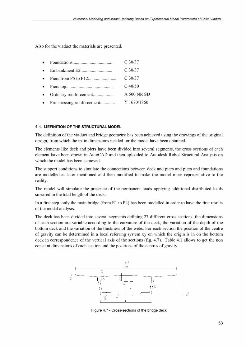
Numerical Modelling and Model Updating Based on Experimental Modal Parameters of Ceira Viaduct
53
Also for the viaduct the materials are presented.
Foundations................................... C 30/37
Embankment E2............................ C 30/37
Piers from P5 to P12......................... C 30/37
Piers top......................................... C 40/50
Ordinary reinforcement.................. A 500 NR SD
Pre-stressing reinforcement............. Y 1670/1860
4.3. DEFINITION OF THE STRUCTURAL MODEL
The definition of the viaduct and bridge geometry has been achieved using the drawings of the original design, from which the main dimensions needed for the model have been obtained.
The elements like deck and piers have been divided into several segments, the cross sections of each element have been drawn in AutoCAD and then uploaded to Autodesk Robot Structural Analysis on which the model has been achieved.
The support conditions to simulate the connections between deck and piers and piers and foundations are modelled as later mentioned and then modified to make the model more representative to the reality.
The model will simulate the presence of the permanent loads applying additional distributed loads smeared in the total length of the deck.
In a first step, only the main bridge (from E1 to P4) has been modelled in order to have the first results of the modal analysis.
The deck has been divided into several segments defining 27 different cross sections, the dimensions of each section are variable according to the curvature of the deck, the variation of the depth of the bottom deck and the variation of the thickness of the webs. For each section the position of the centre of gravity can be determined in a local referring system xy on which the origin is in on the bottom deck in correspondence of the vertical axis of the sections (fig. 4.7). Table 4.1 allows to get the non constant dimensions of each section and the positions of the centres of gravity.
Figure 4.7 - Cross-sections of the bridge deck

Numerical Modelling and Model Updating Based on Experimental Modal Parameters of Ceira Viaduct
54
Table 4.1 - Dimensions of deck sections
Section H L B W yc
[m] [m] [m] [m] [m]
B0 14.51 10.00 1.80 0.95 7.02
B1 14.26 10.08 1.76 0.95 6.92
B2 13.72 10.28 1.66 0.95 6.70
B3 13.19 10.47 1.57 0.95 6.49
B4 12.67 10.65 1.48 0.95 6.29
B5 12.18 10.82 1.40 0.95 6.10
B6 11.64 11.02 1.30 0.95 5.89
B7 11.12 11.20 1.21 0.95 5.69
B8 10.62 11.38 1.13 0.95 5.50
B9 10.15 11.55 1.05 0.95 5.33
B10 9.65 11.72 0.96 0.82 5.15
B11 9.17 11.89 0.88 0.80 4.98
B12 8.68 12.07 0.79 0.80 4.80
B13 8.22 12.23 0.71 0.80 4.64
B14 7.80 12.38 0.64 0.80 4.47
B15 7.41 12.52 0.58 0.80 4.30
B16 7.06 12.64 0.52 0.80 4.15
B17 6.75 12.75 0.46 0.80 4.02
B18 6.47 12.85 0.42 0.80 3.90
B19 6.22 12.94 0.37 0.50 3.87
B20 6.02 13.01 0.34 0.50 3.78
B21 5.84 13.07 0.31 0.50 3.70
B22 5.71 13.12 0.29 0.50 3.64
B23 5.60 13.16 0.27 0.50 3.59
B24 5.54 13.18 0.26 0.50 3.56
B25 5.51 13.19 0.25 0.50 3.54
B26 5.50 13.20 0.25 0.50 3.54
B27 5.50 13.20 0.70 0.80 3.11
In the following part, the sections of the piers are considered. The dimensions of each section are described in table 4.2 according to figure 4.8. In the figure a full section is shown in order to have a very stiff section to model the last part of the piers and the rigid connections between the piers and the deck. For different piers the only variable value is “H”.

Numerical Modelling and Model Updating Based on Experimental Modal Parameters of Ceira Viaduct
55
Figure 4.8 - Cross-sections of the bridge piers
Table 4.2 - Dimensions of the box shaped piers sections
Section H B1 B2 T1 T2 T3
[m] [m] [m] [m] [m] [m]
P29 15.00 12.30 4.30 0.35 0.35 0.35
P31 13.00 8.96 2.98 1.01 0.77 1.27
P32 13.00 10.00 4.00 0.50 0.50 0.50
P33 13.00 9.50 3.50 0.75 0.75 0.75
P35 5.00 4.300 2.800 0.35 0.35 0.35
Table 4.3 - Dimensions of the full piers sections
Section H
[m]
P28 15.00
P30 13.00
P34 5.00
The section P33 is taken in the middle of the zone where the web thickness is variable in order to model that segment.
Having the position of the centres of gravity of the deck and the piers sections, it is possible to create a 3D model placing all the points in a global referring system X,Y,Z. The curved shape of the bridge makes that a definition of two longitudinal abscissas is needed, the values of the abscissa “s” represent
the positions of the points in the curved axis of the bridge while the “x” coordinates represent the
position in a straight axis.

Numerical Modelling and Model Updating Based on Experimental Modal Parameters of Ceira Viaduct
56
The procedure adopted to make the model was the creation of a drawing in AutoCAD on which all the points have been positioned in the global referring system and then their coordinates have been measured creating a table with the correct positions of the points.
The coordinates of the points have been uploaded to the software Autodesk Robot Structural Analysis creating the model of the bridge. Every point has been connected to another one with segments. For each segment between two points a section must be assigned, all the sections shown in figures 4.7 and 4.8 are used to create the model.
With regards to the deck, it is modelled with bigger sections in correspondence of the piers and smaller sections in the middle of the spans. For instance, the section B0 is located in correspondence of the piers and the other ones are ever more distant from the piers until section B26 placed in the mid spans. The section B27 has been assigned in few segments close to the pier P1.
The cross-section of the piers is the box shaped one along almost all the pier and the full section is on the top, close to the deck.
To simulate the internal and external connections as well as possible, the following supports have been considered: a pinned support under E1, an internal hinge connecting P1 and P4 to the deck and the deck is considered continuous under P2 and P3. Fixed supports are used for the piers foundations.
Additional points and segments will be defined during the updating process in order to model some transversal bars along the deck, the material of these ones is a very low density and high stiffness material. They allow seeing the torsion deformations without sensitive changes in the overall mass and the global behaviour of the structure.
To complete the structural model of the bridge a distributed load must be added, it takes into account all the remaining permanent loads present on the bridge, that are:
Guard rail....................................... 1.00 kN/m
Parapet........................................... 1.00 kN/m
Sidewalk......................................... 6.12 kN/m
Edge beams.................................... 8.00 kN/m
Curb............................................... 6.50 kN/m
Asphalt........................................... 66.24 kN/m
New – Jersey.................................. 8.00 kN/m
These ones give rise to a total load of 97.00 kN/m. In the model, this load is considered distributed on the deck.
In a second step also the viaduct has been modelled in order to obtain better results as explained in the section of the modal analysis.
The deck is modelled using a constant section shown in figure 4.9.

Numerical Modelling and Model Updating Based on Experimental Modal Parameters of Ceira Viaduct
57
Figure 4.9 - Cross-section of the viaduct deck
In reality, the cross-section of the viaduct deck is not constant but the variations are very small and they were neglected during the creation of the model.
This deck was uploaded on the model using the same procedure of the bridge. For this kind of deck it is better to consider a grillage and to model it like that. Despite this, for the final goal of this thesis, a simple model has been created using some bars in the centre of gravity of the section.
The modelling of the viaduct is used to create a better connection between the bridge and the viaduct in order to improve the results of the modal analysis of the bridge, so the deck of the viaduct is not modelled using a grillage.
The piers of the viaduct have the same dimensions for each pier. Also in this case a box section is used for the piers but a full section must be used for the last part of the piers, near the top. It is also used to model the rigid link from the points at the end of the piers and the centres of gravity of the deck.
Figure 4.10 - Cross-sections of the viaduct piers
The foundations are modelled like fixed supports while the connections between piers and deck are internal hinges in order to simulate the presence of the bearings. The support in the embankment E4 is at first considered as a pinned support.
Also in the viaduct distributed loads have been added to consider the remaining permanent loads.
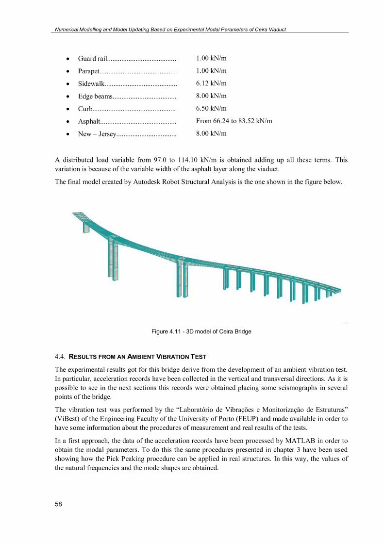
Numerical Modelling and Model Updating Based on Experimental Modal Parameters of Ceira Viaduct
58
Guard rail....................................... 1.00 kN/m
Parapet........................................... 1.00 kN/m
Sidewalk......................................... 6.12 kN/m
Edge beams.................................... 8.00 kN/m
Curb............................................... 6.50 kN/m
Asphalt........................................... From 66.24 to 83.52 kN/m
New – Jersey.................................. 8.00 kN/m
A distributed load variable from 97.0 to 114.10 kN/m is obtained adding up all these terms. This variation is because of the variable width of the asphalt layer along the viaduct.
The final model created by Autodesk Robot Structural Analysis is the one shown in the figure below.
Figure 4.11 - 3D model of Ceira Bridge
4.4. RESULTS FROM AN AMBIENT VIBRATION TEST
The experimental results got for this bridge derive from the development of an ambient vibration test. In particular, acceleration records have been collected in the vertical and transversal directions. As it is possible to see in the next sections this records were obtained placing some seismographs in several points of the bridge.
The vibration test was performed by the “Laboratório de Vibrações e Monitorização de Estruturas”
(ViBest) of the Engineering Faculty of the University of Porto (FEUP) and made available in order to have some information about the procedures of measurement and real results of the tests.
In a first approach, the data of the acceleration records have been processed by MATLAB in order to obtain the modal parameters. To do this the same procedures presented in chapter 3 have been used showing how the Pick Peaking procedure can be applied in real structures. In this way, the values of the natural frequencies and the mode shapes are obtained.

Numerical Modelling and Model Updating Based on Experimental Modal Parameters of Ceira Viaduct
59
Other more accurate procedures should be applied to get better results respect to the ones shown in this first section. Furthermore, the amount of work to obtain the mode shape is quite high, so it will be done for some of the mode shapes. These are the reasons why the comparison of the results between experimental results and numerical results will be done using more accurate data.
In a second step, in fact, the final results of the modal analysis have been made available in order to have a better comparison. These results have been obtained from the document “Ensaio de vibração ambiental da ponte sobre o rio Ceira” (ambient vibration tests on the Ceira Bridge), an official report made by the ViBest in the University of Porto. Some parts of this document are presented in the following sections.
4.4.1. METHOD AND INSTRUMENTS
The experimental identification of the most representative modal parameters of the dynamic behaviour of the bridge was the main goal of the vibration test. The modal parameters have been identified according to the dynamic response to the structure under the environmental actions such as wind or vehicular traffic.
The measurements were performed with seismographs containing a tri-axial “force balance”
accelerometer and a 24 bits analogy-digital converter. The synchronization of the measuring instruments has been provided thanks to GPS sensors placed on each instrument.
Figure 4.12 - Seismograph used for measurements
The acquisition has been done using a sampling frequency of 100 Hz during a period of 16 minutes.
During the measurements, time series of vertical, horizontal and longitudinal accelerations have been collected positioning the instruments in 22 sections of the deck (not in correspondence with the sections in the model). Six seismographs have been used. Two of them had a fixed position while the other four were moved step by step along the top of the bridge realizing several setups. All of them have been placed on the curbs on the each side of the carriageway.
The figure below shows the position of the sensors on the bridge. Each of the three colours has a different meaning: the blue points are the ones on which the sensors were moved for each setup, the

Numerical Modelling and Model Updating Based on Experimental Modal Parameters of Ceira Viaduct
60
green ones are the point on which the instrument remains fixed for each setup and the red ones identify the positions on which some problems did not allow to use the records in the analysis.
Figure 4.13 - Positions of the seismographs along the bridge
Each point is numbered making possible the knowledge of the positions of the six seismographs in each setup according to the table 4.4.
Table 4.4 - Positions of the seismographs of each setup
Setup
1 2 3 4 5 6 7 8 9 10 11 Seismograph 1 31 33 35 37 39 41 43 45 47 49 51 Seismograph 2 32 34 36 38 40 42 44 46 48 50 52 Seismograph 3 1 3 5 7 9 - 13 15 17 19 21 Seismograph 4 2 4 6 8 10 - 14 16 18 20 22 Seismograph 5 11 11 11 11 11 11 11 11 11 11 11 Seismograph 6 12 12 12 12 12 12 12 12 12 12 12
Comparing figure 4.13 and table 4.4 it is possible to see how the fourth seismograph had some problems during the records in most of the sections where it was placed. It means that these records will not be used in the procedure of the identification of the modal parameters.
As it can be seen in table 4.4, the fixed instruments are the fifth and the sixth, they were always placed in sections 11 and 12 and they represent the reference degrees of freedom.
Thanks to these 11 setups, all the 22 positions could be instrumented by using only six instruments, this operation provided the acceleration records for all of those points.
4.4.2. IDENTIFICATION OF THE MODAL PARAMETERS
The procedure of the identification of the modal parameters starts from the implementation of the acceleration records getting at first the natural frequencies and then the mode shapes.
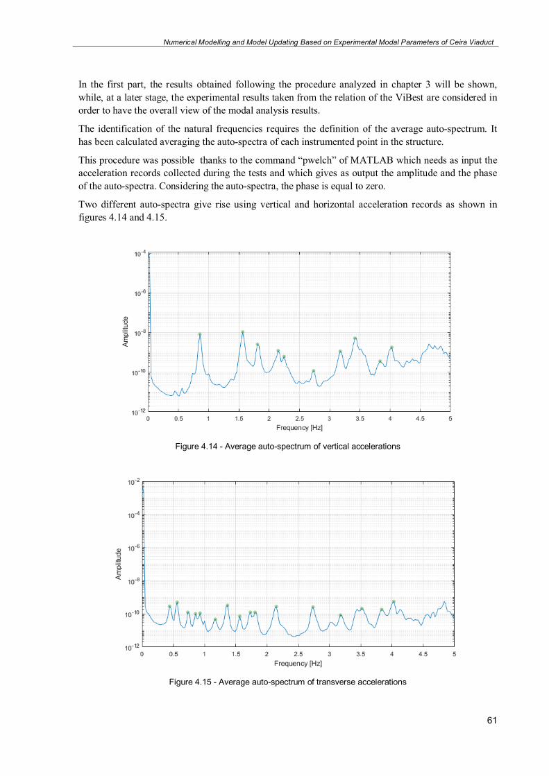
Numerical Modelling and Model Updating Based on Experimental Modal Parameters of Ceira Viaduct
61
In the first part, the results obtained following the procedure analyzed in chapter 3 will be shown, while, at a later stage, the experimental results taken from the relation of the ViBest are considered in order to have the overall view of the modal analysis results.
The identification of the natural frequencies requires the definition of the average auto-spectrum. It has been calculated averaging the auto-spectra of each instrumented point in the structure.
This procedure was possible thanks to the command “pwelch” of MATLAB which needs as input the acceleration records collected during the tests and which gives as output the amplitude and the phase of the auto-spectra. Considering the auto-spectra, the phase is equal to zero.
Two different auto-spectra give rise using vertical and horizontal acceleration records as shown in figures 4.14 and 4.15.
Figure 4.14 - Average auto-spectrum of vertical accelerations
Figure 4.15 - Average auto-spectrum of transverse accelerations

Numerical Modelling and Model Updating Based on Experimental Modal Parameters of Ceira Viaduct
62
The green dots indicate the peaks on which the natural frequencies are individuated, they are also reported in table 4.5.
Table 4.5 - Natural frequencies from the auto-spectra
Frequency [Hz] Vertical Transverse 0.855 0.440 1.563 0.562 1.807 0.732 2.148 0.855 2.295 0.928 2.734 1.172 3.174 1.367 3.418 1.563 3.442 1.733 4.028 1.807
2.148
2.734
3.174
3.540
3.857
4.028
The definition of the mode shapes is based on the calculation of the transfer functions. To do this, a reference point is needed in order to calculate the auto-spectrum of that degree of freedom and the related cross-spectra.
As it is possible to see in figure 4.13 there are two reference points in the bridge. The presence of two reference degrees of freedom is due to the fact that in a comprehensive analysis the reference points must be chosen according to the mode taken in consideration. It allows avoiding the presence of null values of the auto-spectra. In this first procedure the reference point is the number 5 for each mode represented. In the real procedure both points were considered.
Each transfer function is calculated by the ratio between the cross-spectra and the auto-spectrum related to the point 5 for each instrumented point. The cross-spectra can be obtained using the “cpsd”
command of MATLAB.
In each function a single value is individuated in correspondence of a natural frequency. Each value of these ratios represents the percentage of the ordinates of the mode shape respect to the unit value of the point 5 (in point 5 the transfer function is equal to one because is obtained dividing two equal spectra).
As figure 4.13 shows, there are points on which it was not possible to calculate the value of the transfer functions (the red points). For this reason the mode shapes of that side of the bridge present some gaps. The mode shapes are calculated considering the two first frequencies for horizontal and for vertical modes.

Numerical Modelling and Model Updating Based on Experimental Modal Parameters of Ceira Viaduct
63
Figure 4.16 - Vertical modes
Figure 4.17 - Transverse modes
The measurement in both sides of the bridge allows checking the presence of torsion movements. The superposition of the dots of the two sides may indicate that the torsion movements are not relevant. The modes shown in figures 4.16 and 4.17 do not present relevant torsion movements while in the full results it will be seen how there are some modes on which important torsion component exists.
The following section shows the experimental results obtained using the MATLAB procedure developed in the ViBest laboratory, also this procedure considers the Peak Picking method. The
0 100 200 300 400 500 600
x [m]
f=0.855 Hz Downstream side
Upstream side
0 100 200 300 400 500 600x [m]
f=1.563 Hz
0 100 200 300 400 500 600
x [m]
f=0.440 Hz Downstream side
Upstream side
0 100 200 300 400 500 600
x [m]
f=0.562 Hz

Numerical Modelling and Model Updating Based on Experimental Modal Parameters of Ceira Viaduct
64
analysis considers separately vertical and lateral directions even if the deck curvature involves the interaction by vertical and lateral modes.
In figure 4.18 an average normalized spectrum is shown. It includes all the vertical accelerations measured during the test. The most relevant peaks (highlighted in the graph) give a good approximation of the natural frequencies of the bridge.
Figure 4.18 - Average normalized spectrum of vertical accelerations
Figure 4.19 - Modal configuration of the most relevant vertical modes
In figure 4.19 there are the modal configuration associated to the values of the frequencies shown in figure 4.18. Blue dots refers to the deformation of downstream side while orange ones refers to the upstream side, the superposition of the dots may indicate the perfect bending without torsion movements.
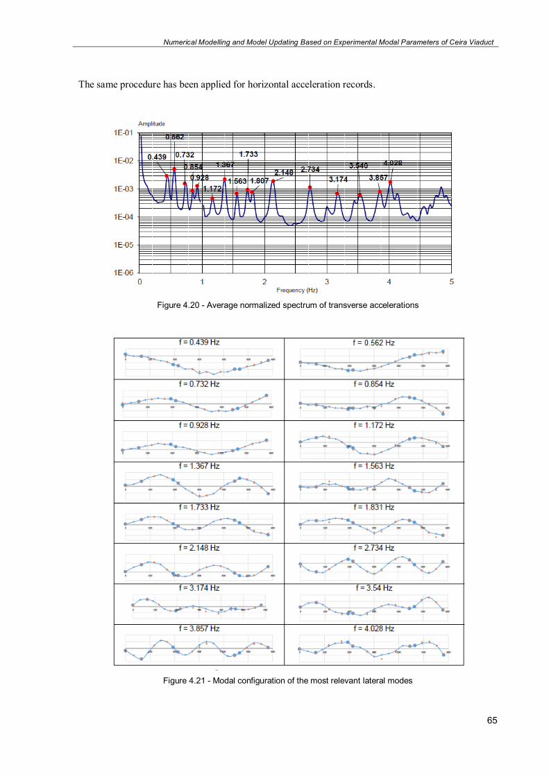
Numerical Modelling and Model Updating Based on Experimental Modal Parameters of Ceira Viaduct
65
The same procedure has been applied for horizontal acceleration records.
Figure 4.20 - Average normalized spectrum of transverse accelerations
Figure 4.21 - Modal configuration of the most relevant lateral modes

Numerical Modelling and Model Updating Based on Experimental Modal Parameters of Ceira Viaduct
66
4.5. MODEL UPDATING
The modal analysis of the bridge has been done using the software Autodesk Robot Structural Analysis. The results have been calculated in different steps modifying the modelled structure step by step in order to have a model as similar as possible to the real structure. For each analysis the results can be compared to the measured ones presented in the previous sections.
The process of model updating is the one commonly done when a finite elements model is created. In this way the results coming from the model can be filtered with the experimental ones.
4.5.1. FIRST ANALYSIS
The first analyzed model considers only the main bridge from E1 to P4 disregarding the viaduct from P4 to E2.
Figure 4.22 - 3D model of the bridge
The material assigned to the structure are exactly those presented in section 4.2, in particular the elastic modulus of the concrete are reported to have a comparison to the different values used in the second model.
Table 4.6 - Elastic modulus of the first model
Concrete Elastic modulus
[MPa] C 30/37 33000 C 40/50 35000 C 45/55 36000 C 50/60 37000
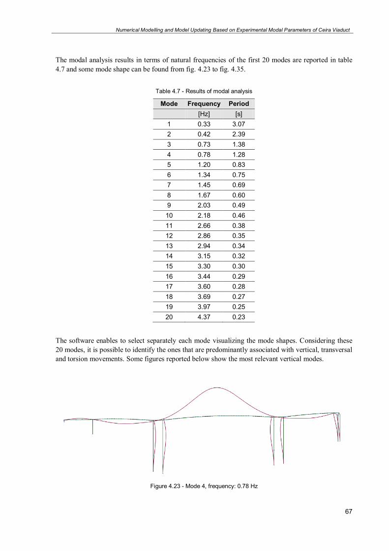
Numerical Modelling and Model Updating Based on Experimental Modal Parameters of Ceira Viaduct
67
The modal analysis results in terms of natural frequencies of the first 20 modes are reported in table 4.7 and some mode shape can be found from fig. 4.23 to fig. 4.35.
Table 4.7 - Results of modal analysis
Mode Frequency Period
[Hz] [s] 1 0.33 3.07 2 0.42 2.39 3 0.73 1.38 4 0.78 1.28 5 1.20 0.83 6 1.34 0.75 7 1.45 0.69 8 1.67 0.60 9 2.03 0.49 10 2.18 0.46 11 2.66 0.38 12 2.86 0.35 13 2.94 0.34 14 3.15 0.32 15 3.30 0.30 16 3.44 0.29 17 3.60 0.28 18 3.69 0.27 19 3.97 0.25 20 4.37 0.23
The software enables to select separately each mode visualizing the mode shapes. Considering these 20 modes, it is possible to identify the ones that are predominantly associated with vertical, transversal and torsion movements. Some figures reported below show the most relevant vertical modes.
Figure 4.23 - Mode 4, frequency: 0.78 Hz

Numerical Modelling and Model Updating Based on Experimental Modal Parameters of Ceira Viaduct
68
Figure 4.24 - Mode 7, frequency: 1.45 Hz
Figure 4.25 - Mode 8, frequency: 1.67 Hz
Figure 4.26 - Mode 9, frequency: 2.03 Hz

Numerical Modelling and Model Updating Based on Experimental Modal Parameters of Ceira Viaduct
69
Figure 4.27 - Mode 16, Frequency: 3.44 Hz
Table 4.8 compares the experimental values of the natural frequencies with the numerical ones. The percentage differences are referred to the experimental data and they allow, step by step, to compare the accuracy of the results.
Table 4.8 - Comparison of numerical and experimental results for vertical modes
Mode Frequency by model Experimental frequency Percentage gap
[Hz] [Hz] [%] 4 0.78 0.85 8.24 7 1.45 1.56 7.05 8 1.67 1.81 7.73 9 2.03 2.30 11.74 16 3.44 3.44 0.00
A second set of figures shows the most relevant transversal modes.
Figure 4.28 - Mode 1, frequency: 0.33 Hz

Numerical Modelling and Model Updating Based on Experimental Modal Parameters of Ceira Viaduct
70
Figure 4.29 - Mode 2, frequency: 0.42 Hz
Figure 4.30 - Mode 3, frequency: 0.73 Hz
Figure 4.31 - Mode 4, frequency: 0.78 Hz
Figure 4.32 - Mode 5, frequency: 1.20 Hz

Numerical Modelling and Model Updating Based on Experimental Modal Parameters of Ceira Viaduct
71
Figure 4.33 - Mode 6, frequency: 1.34 Hz
Figure 4.34 - Mode 10, frequency: 2.18 Hz
Figure 4.35 - Mode 13, frequency: 2.94 Hz
Table 4.9 - Comparison of numerical and experimental results for transverse modes
Mode Frequency by model Experimental frequency Percentage gap
[Hz] [Hz] [%] 1 0.33 0.44 25.00 2 0.42 0.66 36.36 3 0.73 0.73 0.00 4 0.78 0.85 8.24 5 1.2 0.93 29.03 6 1.34 1.17 14.53 10 2.18 2.15 1.40 13 2.94 2.73 7.69
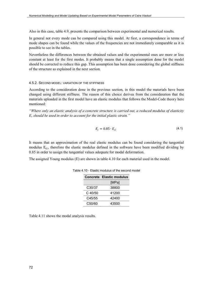
Numerical Modelling and Model Updating Based on Experimental Modal Parameters of Ceira Viaduct
72
Also in this case, table 4.9, presents the comparison between experimental and numerical results.
In general not every mode can be compared using this model. At first, a correspondence in terms of mode shapes can be found while the values of the frequencies are not immediately comparable as it is possible to see in the tables.
Nevertheless the differences between the obtained values and the experimental ones are more or less constant at least for the first modes. It probably means that a single assumption done for the model should be corrected to reduce this gap. This assumption has been done considering the global stiffness of the structure as explained in the next section.
4.5.2. SECOND MODEL: VARIATION OF THE STIFFNESS
According to the consideration done in the previous section, in this model the materials have been changed using different stiffness. The reason of this choice derives from the consideration that the materials uploaded in the first model have an elastic modulus that follows the Model-Code theory here mentioned:
“Where only an elastic analysis of a concrete structure is carried out, a reduced modulus of elasticity
Ec should be used in order to account for the initial plastic strain.”
𝐸𝑐 = 0.85 ∙ 𝐸𝑐𝑖 (4.1)
It means that an approximation of the real elastic modulus can be found considering the tangential modulus Eci , therefore the elastic modulus defined in the software have been modified dividing by 0.85 in order to assign the tangential values adequate for modal deformation.
The assigned Young modulus (E) are shown in table 4.10 for each material used in the model.
Table 4.10 - Elastic modulus of the second model
Concrete Elastic modulus
[MPa] C30/37 38800 C 40/50 41200 C45/55 42400 C50/60 43500
Table 4.11 shows the modal analysis results.
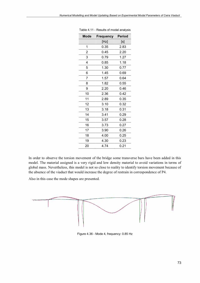
Numerical Modelling and Model Updating Based on Experimental Modal Parameters of Ceira Viaduct
73
Table 4.11 - Results of modal analysis
Mode Frequency Period
[Hz] [s] 1 0.35 2.83 2 0.45 2.20 3 0.79 1.27 4 0.85 1.18 5 1.30 0.77 6 1.45 0.69 7 1.57 0.64 8 1.82 0.55 9 2.20 0.46 10 2.36 0.42 11 2.89 0.35 12 3.10 0.32 13 3.18 0.31 14 3.41 0.29 15 3.57 0.28 16 3.73 0.27 17 3.90 0.26 18 4.00 0.25 19 4.30 0.23 20 4.74 0.21
In order to observe the torsion movement of the bridge some transverse bars have been added in this model. The material assigned is a very rigid and low density material to avoid variations in terms of global mass. Nevertheless, this model is not so close to reality to identify torsion movement because of the absence of the viaduct that would increase the degree of restrain in correspondence of P4.
Also in this case the mode shapes are presented.
Figure 4.36 - Mode 4, frequency: 0.85 Hz
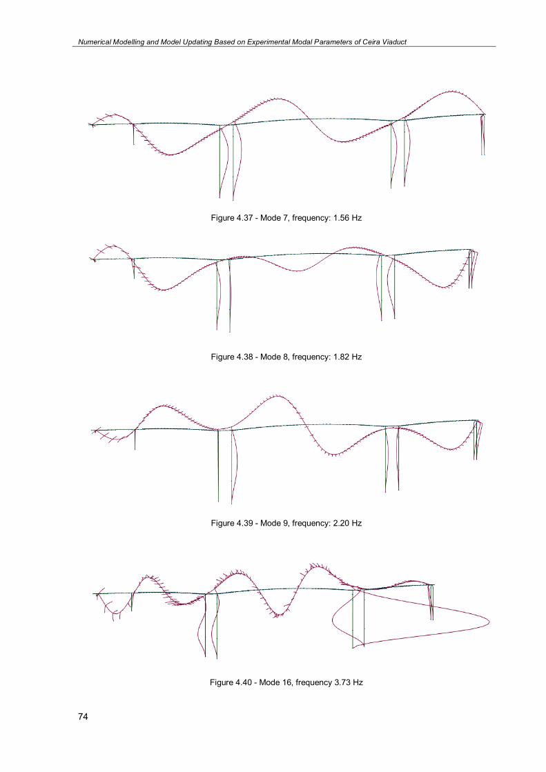
Numerical Modelling and Model Updating Based on Experimental Modal Parameters of Ceira Viaduct
74
Figure 4.37 - Mode 7, frequency: 1.56 Hz
Figure 4.38 - Mode 8, frequency: 1.82 Hz
Figure 4.39 - Mode 9, frequency: 2.20 Hz
Figure 4.40 - Mode 16, frequency 3.73 Hz
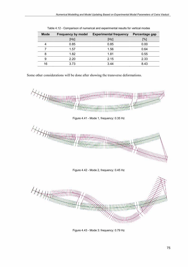
Numerical Modelling and Model Updating Based on Experimental Modal Parameters of Ceira Viaduct
75
Table 4.12 - Comparison of numerical and experimental results for vertical modes
Mode Frequency by model Experimental frequency Percentage gap
[Hz] [Hz] [%] 4 0.85 0.85 0.00 7 1.57 1.56 0.64 8 1.82 1.81 0.55 9 2.20 2.15 2.33 16 3.73 3.44 8.43
Some other considerations will be done after showing the transverse deformations.
Figure 4.41 - Mode 1, frequency: 0.35 Hz
Figure 4.42 - Mode 2, frequency: 0.45 Hz
Figure 4.43 - Mode 3: frequency: 0.79 Hz

Numerical Modelling and Model Updating Based on Experimental Modal Parameters of Ceira Viaduct
76
Figure 4.44 - Mode 4, frequency: 0.85 Hz
Figure 4.45 - Mode 5, frequency: 1.30 Hz
Figure 4.46 - Mode 6, frequency: 1.45 Hz
Figure 4.47 - Mode 9, frequency: 2.20 Hz
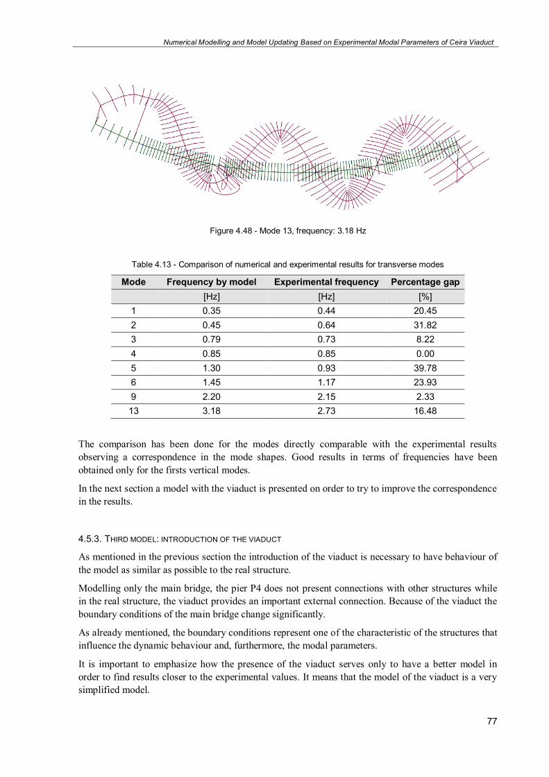
Numerical Modelling and Model Updating Based on Experimental Modal Parameters of Ceira Viaduct
77
Figure 4.48 - Mode 13, frequency: 3.18 Hz
Table 4.13 - Comparison of numerical and experimental results for transverse modes
Mode Frequency by model Experimental frequency Percentage gap
[Hz] [Hz] [%] 1 0.35 0.44 20.45 2 0.45 0.64 31.82 3 0.79 0.73 8.22 4 0.85 0.85 0.00 5 1.30 0.93 39.78 6 1.45 1.17 23.93 9 2.20 2.15 2.33 13 3.18 2.73 16.48
The comparison has been done for the modes directly comparable with the experimental results observing a correspondence in the mode shapes. Good results in terms of frequencies have been obtained only for the firsts vertical modes.
In the next section a model with the viaduct is presented on order to try to improve the correspondence in the results.
4.5.3. THIRD MODEL: INTRODUCTION OF THE VIADUCT
As mentioned in the previous section the introduction of the viaduct is necessary to have behaviour of the model as similar as possible to the real structure.
Modelling only the main bridge, the pier P4 does not present connections with other structures while in the real structure, the viaduct provides an important external connection. Because of the viaduct the boundary conditions of the main bridge change significantly.
As already mentioned, the boundary conditions represent one of the characteristic of the structures that influence the dynamic behaviour and, furthermore, the modal parameters.
It is important to emphasize how the presence of the viaduct serves only to have a better model in order to find results closer to the experimental values. It means that the model of the viaduct is a very simplified model.
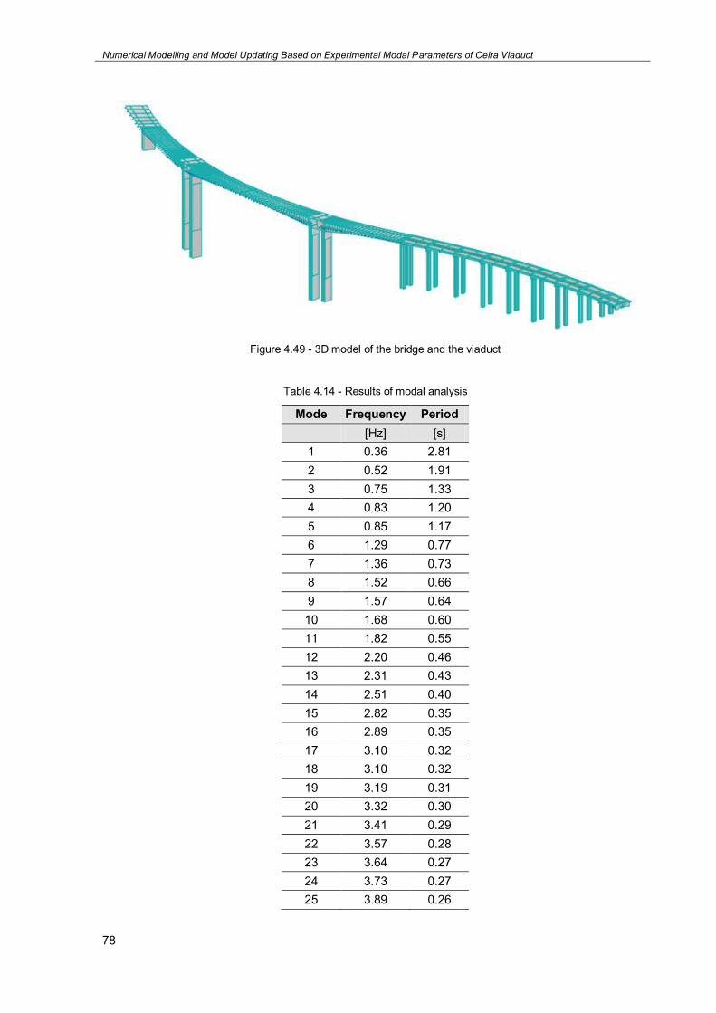
Numerical Modelling and Model Updating Based on Experimental Modal Parameters of Ceira Viaduct
78
Figure 4.49 - 3D model of the bridge and the viaduct
Table 4.14 - Results of modal analysis
Mode Frequency Period
[Hz] [s] 1 0.36 2.81 2 0.52 1.91 3 0.75 1.33 4 0.83 1.20 5 0.85 1.17 6 1.29 0.77 7 1.36 0.73 8 1.52 0.66 9 1.57 0.64 10 1.68 0.60 11 1.82 0.55 12 2.20 0.46 13 2.31 0.43 14 2.51 0.40 15 2.82 0.35 16 2.89 0.35 17 3.10 0.32 18 3.10 0.32 19 3.19 0.31 20 3.32 0.30 21 3.41 0.29 22 3.57 0.28 23 3.64 0.27 24 3.73 0.27 25 3.89 0.26

Numerical Modelling and Model Updating Based on Experimental Modal Parameters of Ceira Viaduct
79
The materials assigned to this model are mentioned in section 4.5.2 and the distributed load on the access viaduct is considered 114.0 kN/m.
In this model a higher number of modes have been calculated to try to find more correspondences.
At first vertical modes are shown.
Figure 4.50 - Mode 5, frequency: 0.85 Hz
Figure 4.51 - Mode 9, frequency: 1.57 Hz
Figure 4.52 - Mode 11, frequency: 1.82 Hz
Figure 4.53 - Mode 12, frequency: 2.20 Hz
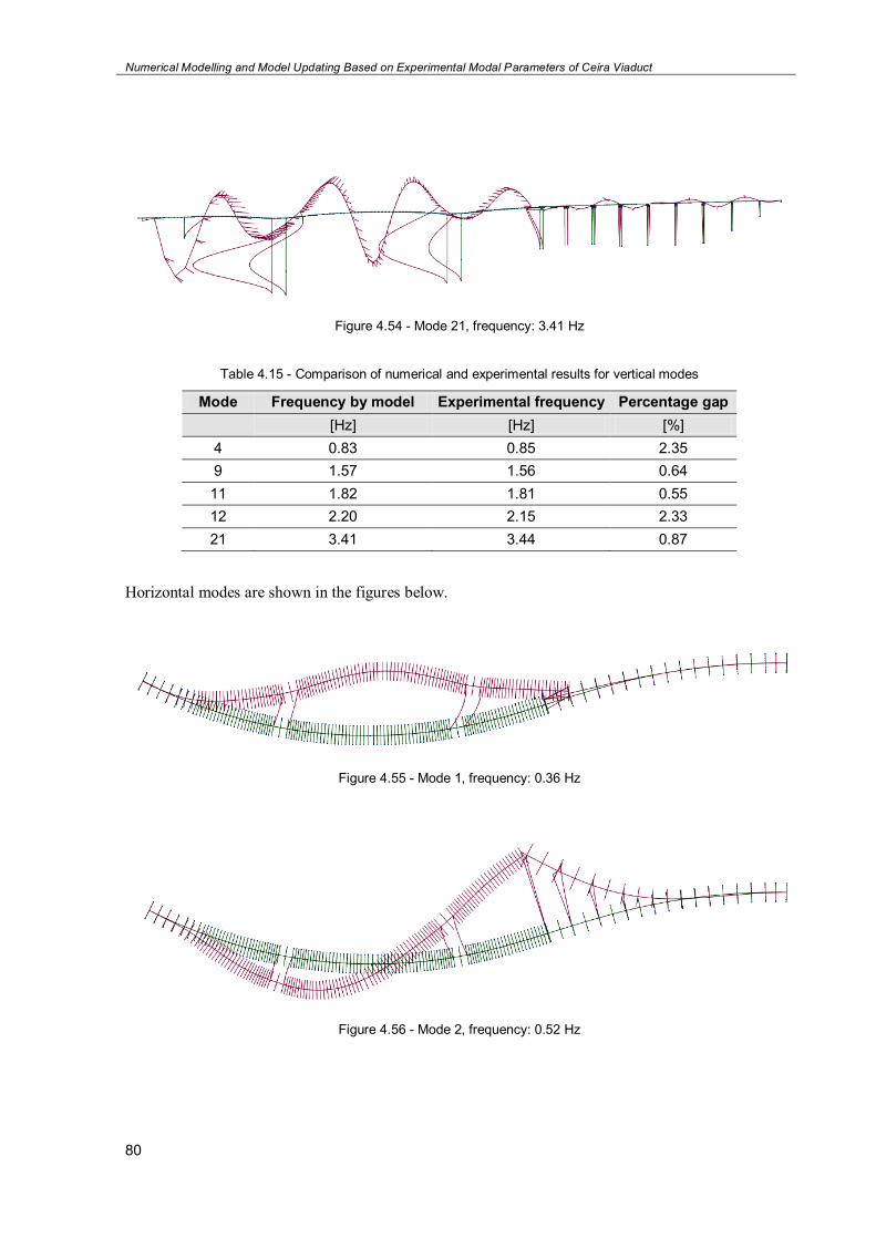
Numerical Modelling and Model Updating Based on Experimental Modal Parameters of Ceira Viaduct
80
Figure 4.54 - Mode 21, frequency: 3.41 Hz
Table 4.15 - Comparison of numerical and experimental results for vertical modes
Mode Frequency by model Experimental frequency Percentage gap
[Hz] [Hz] [%] 4 0.83 0.85 2.35 9 1.57 1.56 0.64 11 1.82 1.81 0.55 12 2.20 2.15 2.33 21 3.41 3.44 0.87
Horizontal modes are shown in the figures below.
Figure 4.55 - Mode 1, frequency: 0.36 Hz
Figure 4.56 - Mode 2, frequency: 0.52 Hz

Numerical Modelling and Model Updating Based on Experimental Modal Parameters of Ceira Viaduct
81
Figure 4.57 - Mode 3, frequency: 0.75 Hz
Figure 4.58 - Mode 4, frequency: 0.83 Hz
Figure 4.59 - Mode 5, frequency: 0.85 Hz
Figure 4.60 - Mode 6, frequency: 1.29 Hz
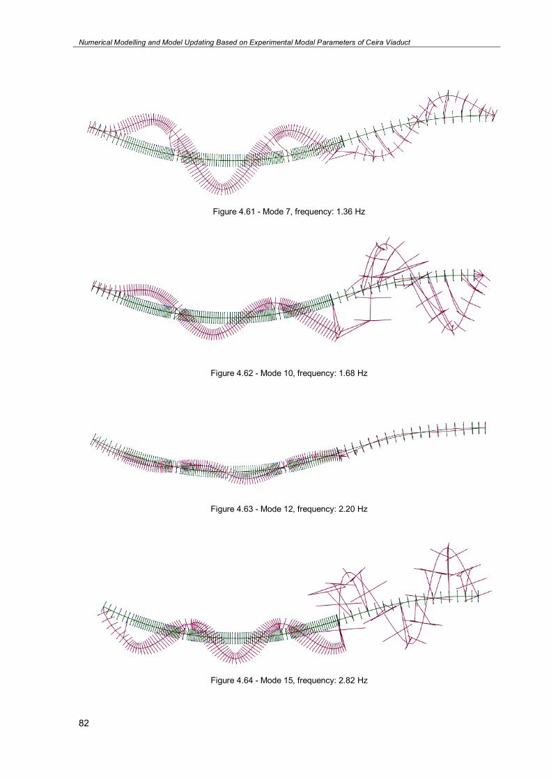
Numerical Modelling and Model Updating Based on Experimental Modal Parameters of Ceira Viaduct
82
Figure 4.61 - Mode 7, frequency: 1.36 Hz
Figure 4.62 - Mode 10, frequency: 1.68 Hz
Figure 4.63 - Mode 12, frequency: 2.20 Hz
Figure 4.64 - Mode 15, frequency: 2.82 Hz
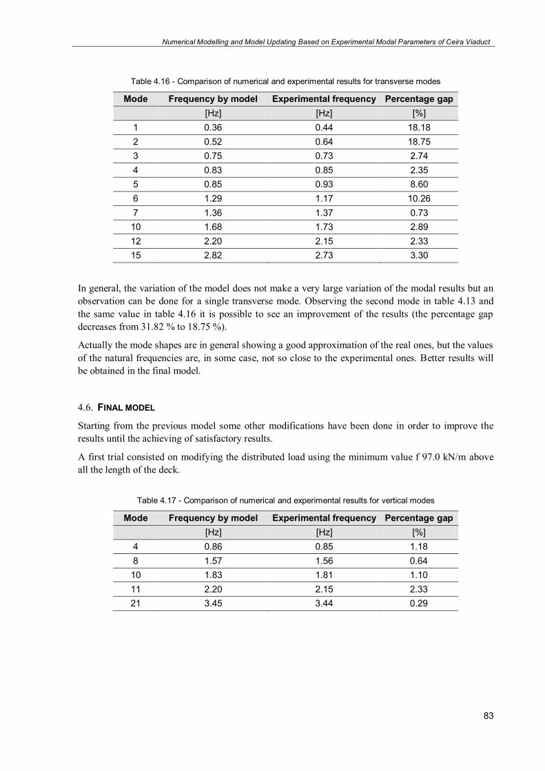
Numerical Modelling and Model Updating Based on Experimental Modal Parameters of Ceira Viaduct
83
Table 4.16 - Comparison of numerical and experimental results for transverse modes
Mode Frequency by model Experimental frequency Percentage gap
[Hz] [Hz] [%] 1 0.36 0.44 18.18 2 0.52 0.64 18.75 3 0.75 0.73 2.74 4 0.83 0.85 2.35 5 0.85 0.93 8.60 6 1.29 1.17 10.26 7 1.36 1.37 0.73 10 1.68 1.73 2.89 12 2.20 2.15 2.33 15 2.82 2.73 3.30
In general, the variation of the model does not make a very large variation of the modal results but an observation can be done for a single transverse mode. Observing the second mode in table 4.13 and the same value in table 4.16 it is possible to see an improvement of the results (the percentage gap decreases from 31.82 % to 18.75 %).
Actually the mode shapes are in general showing a good approximation of the real ones, but the values of the natural frequencies are, in some case, not so close to the experimental ones. Better results will be obtained in the final model.
4.6. FINAL MODEL
Starting from the previous model some other modifications have been done in order to improve the results until the achieving of satisfactory results.
A first trial consisted on modifying the distributed load using the minimum value f 97.0 kN/m above all the length of the deck.
Table 4.17 - Comparison of numerical and experimental results for vertical modes
Mode Frequency by model Experimental frequency Percentage gap
[Hz] [Hz] [%] 4 0.86 0.85 1.18 8 1.57 1.56 0.64 10 1.83 1.81 1.10 11 2.20 2.15 2.33 21 3.45 3.44 0.29

Numerical Modelling and Model Updating Based on Experimental Modal Parameters of Ceira Viaduct
84
Table 4.18 - Comparison between model and experimental results for transverse modes
Mode Frequency by model Experimental frequency Percentage gap
[Hz] [Hz] [%] 1 0.48 0.44 9.09 2 0.54 0.64 15.63 3 0.77 0.73 5.48 4 0.86 0.85 1.18 5 0.93 0.93 0.00 6 1.32 1.37 3.65 9 1.69 1.73 2.31 12 2.30 2.15 6.98 15 2.90 2.73 6.23
This first modification give rise better results, probably the load considered at first was too high compared to the real one. In fact in the design the loads are in general overestimated to be in safety conditions. So the minimum value is probably more representative of the real conditions.
Another modification of the model concerns the real behaviour of the supports under the embankment E1 and E2.
As already mentioned they may be considered as fixed supports because they actually do not allow movements as sliding or pinned supports considered in the model should do. For this reason the model has been changed placing fixed support under E1 and E2.
Table 4.19 - Comparison of numerical and experimental results for vertical modes
Mode Frequency by model Experimental frequency Percentage gap
[Hz] [Hz] [%] 4 0.86 0.85 1.18 8 1.61 1.56 3.21 10 1.89 1.81 4.42 11 2.22 2.30 3.48 21 3.49 3.44 1.45
The value of the vertical modes are not changing a lot but the following table will show how the values for horizontal movement are changing more obtaining better results.
Probably the real behaviour of the supports is between fixed and pinned supports.

Numerical Modelling and Model Updating Based on Experimental Modal Parameters of Ceira Viaduct
85
Table 4.20 - Comparison of numerical and experimental results for transverse modes
Mode Frequency by model Experimental frequency Percentage gap
[Hz] [Hz] [%] 1 0.49 0.44 11.36 2 0.54 0.64 15.63 3 0.77 0.73 5.48 4 0.86 0.85 1.18 5 0.93 0.93 0.00 6 1.35 1.37 1.46 8 1.61 1.56 3.21 9 1.69 1.73 2.31 10 1.89 1.81 4.42 12 2.33 2.15 8.37 15 2.92 2.73 6.96
In this case it has been possible to find a correspondence in terms of torsion in the mode 15, looking at the experimental data in the horizontal the first mode which gives important torsion movement is the one with a frequency of 2.73 Hz. The shape is horizontally comparable with mode 15 of the model and the torsion movements are also comparable.
Figure 4.65 - Mode 15, frequency 2.92 Hz, torsion movements
Also in this last model some gaps are present in the results.
As already mentioned, the model does not reflect the reality because of several approximation: the structure is divided into segments and each segment has its characteristics while the real structure is a continuous system; the properties of the materials are assigned according to the design but they may be a bit different respect to the ones in the real structure; the model cannot represent the serviceability conditions of the structure while the ambient vibration tests are commonly done under operating conditions; the connection between the structure and the environment on which is placed (foundation and restraint conditions) are modelled using supports or links that do not represent the real behaviour of these elements.
In short, the model will always have some intrinsic defects that make that the results are different to the experimental ones.

Numerical Modelling and Model Updating Based on Experimental Modal Parameters of Ceira Viaduct
86
In the end other modifications of the model have been done trying to get even better results. In a first trial some rotational springs have been placed in correspondence of the central piers trying to recreate better the behaviour of the foundations. In a second moment a better connection between the viaduct and the bridge has been realized.
In all these cases some improvements gave rise for some frequencies or mode shapes but, at the same time, they generated worst results in some other modes. It means that the model presented in this section is considered, for this work, the most accurate.
In conclusion we could say that with the last model the results are sufficiently satisfactory. In general the mode shapes can be related to the real ones even if the frequencies still are quite different to the ones obtained during the ambient vibration test.
This confirms the fact that the results coming from a finite element model are in general not sufficient to do a proper and complete modal analysis. Even if the model is really close to the reality, it still does not ensure the accuracy of the results, making necessary the presence of experimental tests.
Numerical Modelling and Model Updating Based on Experimental Modal Parameters of Ceira Viaduct
87
5 CHAPTER 5 - CONCLUSIONS AND
FUTURE DEVELOPMENTS
5.1. CONCLUSIONS
The main purpose of this work was to show how the modal analysis can represent an important means for the validation of the FEM and, in particular, how the use of the numerical models requires the presence of the experimental data in the field of modal analysis.
It was possible to observe how the structural modelling presents some limits that generate inaccuracies on the results.
In this context the modelling of a structure needs a special attention in order to create a model as close as possible to the real structure. As mentioned in the fourth chapter, this process required some arrangements in the model. For instance, it was important an appropriate choice of: the geometric characteristics of the structure, the materials properties and the internal and external connections.
In this way was possible to reach, step by step, a good approximation of the model to the real structure.
The approach followed for the calculation of the modal parameters was to present initially the theoretical aspects concerning the modal analysis in order to get some analytical results through the analysis of simple systems.
This allowed to do some validation processes of the model created by the software of the same systems.
The modelling of the Ceira Bridge required the prior creation of simple model in order to become familiar with the modelling software and with the modal analysis results obtained for this system.
On the other hand, experimental results from an ambient vibration test have been analyzed obtaining the modal parameters starting from the acceleration records. The procedures for obtaining these results allowed to process some data and to understand the way to get the final experimental results. These ones were used for the comparison with the numerical results.
Even though there are several procedure to realize a test to obtain the modal parameters, in this work only the ones where the structure is excited by ambient vibrations were presented in detail. This choice was also because the experimental data of the Ceira Bridge comes from an AVT done some years ago by the ViBest in the University of Porto.
The final results highlighted the difficulties of the creation of a FEM model but, at the same time, allowed to observe as a good approximation of the modal parameters can be obtained from the model.

Numerical Modelling and Model Updating Based on Experimental Modal Parameters of Ceira Viaduct
88
Otherwise, the final results confirm the importance of the presence of the experimental parameters in modal analysis procedures.
5.2. FUTURE DEVELOPMENTS
The experimental modal analysis is today an important tool for the implementation of a structural analysis and for the assessment of the behaviour of a structure in operative conditions.
The knowledge of the modal characteristics becomes important in terms of the performance evaluation in case of extreme environmental situation.
In addition to the traditional techniques, based on a known input, in the last years, the methods of the modal identification in the presence of the ambient vibration, became more and more common. These methods provide the dynamic characteristics of the structure in the effective serviceability conditions.
Today the methods considering a unknown input are more commonly used than the ones considering a known input because the tests can be done with lower cost and without interfering with the normal use of the structure.
Because the measurements are done during the operative conditions, the modal parameters are representative of the dynamic behaviour in serviceability conditions.
The modal parameters obtained with these methods can be used for the validation or the improvement of the numerical results: the validation of the finite element models allows their use, for instance, in the evaluation of the seismic risk.
In this context the increasing software performances can provide the creation of more accurate FEM that can be used in dynamic field for structure monitoring, starting from the calculation of the modal parameters.

Numerical Modelling and Model Updating Based on Experimental Modal Parameters of Ceira Viaduct
89
REFERENCES
Ceravolo Rosario, Pecorelli Marica, Miraglia Gaetano, Matta Emiliano. (2017). Earthquake Enginnering Lesson 3. Politecnico di Torino, Torino.
Ceravolo Rosario, Pecorelli Marica, Miraglia Gaetano, Matta Emiliano. (2017). Earthquake Enginnering Lesson 5. Politecnico di Torino, Torino.
Ceravolo Rosario, Pecorelli Marica, Miraglia Gaetano, Matta Emiliano. (2017). Earthquake Enginnering Lesson 6. Politecnico di Torino, Torino.
Ceravolo Rosario, Pecorelli Marica, Miraglia Gaetano, Matta Emiliano. (2017). Earthquake Enginnering Lesson 10. Politecnico di Torino, Torino.
Ceravolo Rosario, Pecorelli Marica, Miraglia Gaetano, Matta Emiliano. (2017). Earthquake Enginnering Lesson E1. Politecnico di Torino, Torino.
http://www.robotoffice.com/rsa/. 16 March 2018.
CXCO.E.PRCE.180.C1-Parte I-Rev_2.doc. (2011).
CXCO.E.PRCE.180.C1-Parte II-Rev_2.doc. (2011).
Andreas Johann Felber. (1993). Development of a hybrid bridge evaluation system. A thesis in partial fulfillment of the requirements for the degree of doctor of philosophy. The University of British Columbia.
Filipe Manuel Rodrigues Leite de Magalhães. Identificação estocatica para validação experimental de modelos numéricos. Master thesis, Faculdade de Engenharia da Universidade do Porto.
Filipe Manuel Rodrigues Leite de Magalhães. (2014). Ensaio de vibração ambiental da ponte sobre o rio Ceira (subconcessão pinhal interior).
Giovanni Fabbrocino, C. Rainieri, G. M. Verderame. L’analisi dinamica sperimentale e il
monitoraggio delle strutture esistenti. http://www.reluis.it/doc/pdf/Pubblicazioni/Bari_Fabbrocino.pdf. 4th May 2018.

Numerical Modelling and Model Updating Based on Experimental Modal Parameters of Ceira Viaduct
90
Related Documents