Time-resolved stereo PIV measurements of the … · Simpson 2006; Paik et al. 2007; Praisner and Smith 2006a; ... system is driven by the characteristics of the imping-ing turbulent

1 3

Exp Fluids (2016) 57:5 DOI 10.1007/s00348-015-2091-7

RESEARCH ARTICLE

Time‑resolved stereo PIV measurements of the horseshoe vortex system at multiple locations in a low‑aspect‑ratio pin–fin array

Corey D. Anderson1,2 · Stephen P. Lynch1

Received: 11 May 2015 / Revised: 10 November 2015 / Accepted: 18 November 2015 © Springer-Verlag Berlin Heidelberg 2015

minimal variation with respect to either Reynolds number or row location. Regions of maximum streamwise and wall-nor-mal turbulent fluctuations around the HSV were a result of its quasiperiodic oscillation between so-called backflow and zero-flow modes, which were present even in downstream rows despite the extremely high mid-channel turbulence. In the downstream rows, normalized TKE across the entire field of view decreased with increased Reynolds number, likely due to dissipation rates proportionally outpacing increases in mean channel velocity and Reynolds number. The flowfield results from this study corroborate prior findings from heat transfer measurements that indicate a fully developed condi-tion is established at around the fifth row in an array.

List of symbolsD Pin–fin diameterdt Time between S-PIV image-pair exposuresf S-PIV sampling frequencyH Pin–fin height, H = DHSV Horseshoe vortexn′n′ Variance of component of velocity, n (where n is

u, v, or w)S-PIV Stereo particle image velocimetryReD Reynolds number based on D and Um,

ReD =D∗Um

ν

SL Streamwise array spacing, SL = 3.46 * DSw Spanwise array spacing, Sw = 2 * DΔt+ Sampling timestep in inner coordinates,

∆t+ =

u2τ/fν

Tu Turbulence level, Tu =

(

√

2

3TKE

)/

Um

TKE Turbulent kinetic energy,

TKE =1

2

√

u′u′ + v′v′ + w′w′

u Streamwise component of velocityuτ Friction velocity

Abstract Pin–fin arrays are a type of cooling feature found in heat exchangers, with elements (generally cylindri-cal or square) that span between two endwalls. Flow around the pin–fins generates highly turbulent mixing that increases convective heat transfer from the pins to the cooling flow. At the junction of a pin–fin and the endwall, a complex flow known as the horseshoe vortex (HSV) system is present. Although the HSV is a well-studied phenomenon, its behav-ior is not understood in the highly turbulent flow of a pin–fin array. Furthermore, the presence of close confining endwalls for low-aspect-ratio (short) pin–fins may have an impact on HSV dynamics. The present study utilized time-resolved ste-reo particle image velocimetry to examine the fluid dynam-ics of the HSV system in rows 1, 3, and 5 of a low-aspect-ratio pin–fin array, for a range of Reynolds numbers. In the first row, instantaneous flowfields indicated a clearly defined HSV at the leading edge, with dynamics similar to previ-ous studies of bluff-body junction flows. The time-averaged HSV system moved closer to the pin with increasing Reyn-olds number, with more concentrated vorticity and turbulent kinetic energy (TKE). For downstream rows, there was a sig-nificant increase in the amount of mid-channel vorticity, with levels on the same order as the value in the core of the HSV. The time-averaged HSV system in downstream rows showed

* Stephen P. Lynch [email protected]

Corey D. Anderson [email protected]

1 Department of Mechanical and Nuclear Engineering, Pennsylvania State University, University Park, PA 16802, USA

2 Present Address: United Technologies–Pratt & Whitney, East Hartford, CT, USA

Exp Fluids (2016) 57:5

1 3

5 Page 2 of 18

u+ Streamwise component of velocity in inner coor-dinates, u+ =

uuτ

Um Channel mean velocity upstream of arrayUmax Maximum average velocity in the channel,

Umax = 2 * Um

v Endwall normal component of velocity|V| Velocity magnitudew Spanwise component of velocityX Streamwise directiony+ Wall-normal direction in inner coordinates,

y+ =yuτν

Y Endwall normal directionZ Spanwise directionν Kinematic viscosity

1 Introduction

Pin–fin arrays are a type of compact heat exchanger used in a variety of applications ranging from gas turbine engines to electronics cooling. Compact, or low-aspect-ratio, pin–fin arrays are composed of pin–fins with a height to diam-eter ratio on the order of unity. Flow through compact pin–fin arrays is complex—blockage effects, near-wall effects, and wake shedding, among others, all contribute to high turbulence and high convective heat transfer. An impor-tant flow feature within the array is the horseshoe vortex system, present at the junction of the pins and the chan-nel wall. As flow approaches the pins in the array, three-dimensional pressure gradients drive separation of the end-wall boundary layer. At the endwall, as the flow separates to move around the pin, the horseshoe vortex (HSV) sys-tem develops. This system is composed of several unsteady vortices. The HSV system has been studied in single bluff-body systems and been shown to oscillate between two modes in a quasiperiodic manner. Experiments have shown that the quasiperiodic manner of the system contributes to high-pressure fluctuations and heat transfer at the junc-tion. Although single bluff-body HSV systems have been well studied, the behavior of the HSV system is not well understood in short-aspect-ratio channels, and within pin–fin arrays that have significant mid-channel turbulence. This paper presents experimental results that categorize the behavior of the HSV system at several locations within a staggered pin–fin array. The intent of this study is to under-stand the fluid dynamics of the HSV in the presence of high turbulence generated by a pin–fin array.

2 Background

In a review of junction flows by Simpson (2001), the behavior of the horseshoe vortex system in turbulent and

laminar flow regimes is outlined. The HSV system devel-ops when flow over a wall impinges on a bluff body extrud-ing from the wall. As the wall boundary layer approaches the bluff body, it encounters an adverse pressure gradient in the streamwise direction that causes separation and the eventual formation of the HSV upstream of the leading edge of the bluff body. Spanwise pressure gradients about the obstacle cause the HSV to split and wrap around the bluff body. The pressure gradients driving the HSV for-mation are dependent upon several parameters such as the bluff-body geometry, size, blockage of the flow, and whether there are flow-altering features nearby such as fil-lets or fences (Fleming et al. 1993; Olcmen and Simpson 1994; Simpson 2001).

In the turbulent regime, Simpson (2001) highlights several of the key features of the HSV system. Multiple vortices are likely to form, and they interact in a complex manner involving merging, leapfrogging, and decay. In a time-average sense, the turbulent HSV system is often composed of a primary horseshoe vortex nearest the body, a counter-rotating secondary vortex immediately upstream of the primary horseshoe vortex, and a tertiary vortex upstream of the secondary vortex. Although this time-aver-age description is complex, it does not adequately describe the unsteady nature of the HSV system.

Devenport and Simpson (1990) first described the com-plex bimodal nature of the HSV in front of a wing–body junction, which has since been documented by many other researchers for a variety of bluff bodies (Agui and Andreo-poulos 1992; Kirkil and Constantinescu 2015; Ölçmen and Simpson 2006; Paik et al. 2007; Praisner and Smith 2006a; Sabatino and Smith 2009). Probability density functions of the streamwise component of velocity show two distinct peaks in an elliptical region near the wall, slightly upstream of the bluff body. The existence of a bimodal distribu-tion of velocity appears to be independent of the approach flow Reynolds number in the turbulent regime. Within the endwall region containing the bimodal distribution, the bimodal behavior is postulated to be responsible for both high surface pressure fluctuations and enhanced heat trans-fer levels. The physical mechanism responsible for this is the quasiperiodic destruction of the primary HSV, by vor-tex stretching around the bluff body and interaction with upstream vortices. Interestingly, the dynamic behavior of the HSV appears to be unrelated to the frequency of the Karman vortex shedding in the wake of the bluff body (Agui and Andreopoulos 1992).

Particle image velocimetry (PIV) has been used to rein-force the fact that the HSV system oscillates consistently, but not predictably, between two modes (Praisner and Smith 2006a). In the first mode, the near-wall reverse flow travels under the horseshoe vortex, upstream over the sec-ondary vortex (if present), and eventually under the tertiary

Exp Fluids (2016) 57:5

1 3

Page 3 of 18 5

vortex. This mode dominates approximately 80 % of the time. However, the reverse-flow region beneath the horse-shoe vortex eventually changes to a mode that only feeds into the secondary and horseshoe vortices. At that point, outer region flow penetrates to the endwall surface and causes the secondary vortex to erupt outwards. After erup-tion, the system eventually resets to the dominant mode. This process, while not periodic, occurs regularly.

Subsequent studies have attempted to determine the exact cause of the shift from the dominant HSV mode to the secondary mode. The work of Sabatino and Smith (2009) suggests that the temporal behavior of the HSV system is driven by the characteristics of the imping-ing turbulent boundary layer. Specifically, they argue that hairpin vortex packets interact with the HSV, causing it to strengthen and change its streamwise position. Paik et al. (2007) modeled the wing–body junction of Devenport and Simpson (1990). Their results showed that the HSV system remains in a dominant state until upstream hairpin vortices wrap around and amalgamate with the HSV, resulting in a disorganized state. The authors argue that the hairpin vor-tices emerge as a result of centrifugal instability caused by the backward-turning flow of the HSV near the wall.

The unsteadiness of the HSV has direct consequences to endwall heat transfer. A region of high endwall heat transfer is present at the base of the bluff body, where flow impinging on the body’s leading edge flows down the face of the bluff body, and impinges on the endwall (Praisner and Smith 2006b). Upstream of this location, however, there are areas that exhibit amplified heat transfer relative to an undisturbed turbulent boundary layer (Blair 1974; Giel et al. 1998; Graziani et al. 1980; Hunt et al. 1978; Kang et al. 1999). Simultaneous time-resolved flow and heat transfer measurements by Praisner and Smith (2006a, b) showed that the primary band of high heat transfer at the base of the bluff body was 350 % greater than in an undisturbed turbulent boundary-layer flow, with a second-ary upstream band that was 250 % higher. This secondary band coincided with the location of the secondary vortex in the HSV system, and it was concluded to be a direct result of the inrush phenomenon during the dominant mode breakdown.

Relative to prior studies of the HSV, the flow within low-aspect-ratio pin–fin arrays is complicated, due to the effect of the close confining walls and the high turbulence gener-ated by wake shedding in downstream rows. However, most work to date to understand pin–fin flowfields has looked at the pin–fin midline, or at surface quantities. Ames and Dvorak (2006) found that pin–fin surface pressure distribu-tions varied significantly from row to row in the first few rows, but remained relatively consistent after row 4. Heat transfer measurements by Ames et al. (2005) indicated that effective approach velocity was highest in row 3, due to the

blockages of row 2, which resulted in highest overall heat transfer in this row. However, heat transfer augmentation solely due to turbulence was highest in row 4 and beyond. Scholten and Murray (1998) examined time-resolved heat transfer in a high-aspect-ratio array and found that the lev-els of heat flux fluctuation between the front and back of a cylinder were distinct in the first row but were similar by the third row. The transition was attributed to the row-by-row increasingly turbulent flow.

Streamwise and spanwise spacing effects on time-aver-aged array heat transfer and pressure loss were studied by Lawson et al. (2011). They established that reduced span-wise spacing has a larger effect than streamwise spacing on increasing pressure drop across a pin–fin array, but reduced streamwise spacing had a larger effect than spanwise spac-ing in increasing array heat transfer. Flow measurements by Ostanek and Thole (2012b) of pin–fin mid-channel wakes found that decreasing streamwise spacing resulted in increased Strouhal number as the near-wake length scales were confined. Through proper orthogonal decomposition, Ostanek and Thole (2012a) found that coherent wake fluc-tuations were weakened at close streamwise spacings, but random turbulent fluctuations were relatively insensitive. Together, these results imply that the heat transfer augmen-tation seen at reduced streamwise spacings may not be a direct result of wake behavior and should be investigated further.

Only a few studies have examined the effects of close endwalls on the HSV structure. A computational study by Borello and Hanjali (2011) found that instabilities in the HSV system for a short cylinder bounded by flat walls were suppressed compared to an unbounded junction and that vortex topology was highly dependent on whether the incoming flow was or was not fully developed. Deli-bra et al. (2010) found that endwall heat transport in a low-aspect-ratio array was associated with the dynamics of large vortices shed from upstream pin–fins. Flowfield measurements in a very short-aspect-ratio channel with a cylinder by Sahin et al. (2008) indicated that the HSV on the upper and lower endwalls alternated in strength due to mutual interactions.

It is also not clear whether the HSV dynamics are affected by the substantial turbulence levels typical within downstream rows of a pin–fin array. Several researchers have found that mid-channel turbulence levels in short-aspect-ratio arrays are low in the first two rows, but quickly reach levels of 30–40 % in subsequent rows for widely (SL/D > 2) and closely spaced (SL/D < 2) arrays, respec-tively (Ames et al. 2007; Metzger and Haley 1982; Simo-neau and Van Fossen 1984). Radomsky and Thole (2000) measured the HSV in front of a vane with 20 % freestream turbulence (generated by a bar grid) and found bimodal behavior in the HSV region, although the peaks of the

Exp Fluids (2016) 57:5

1 3

5 Page 4 of 18

velocity PDF were more closely spaced than for the low-turbulence case of 0.6 %.

As indicated, the behavior of the HSV system is dynami-cally rich. Many studies of the system have been performed for a single bluff body in the turbulent regime, and it is commonly understood that the system is unstable. How-ever, the effect of nonuniform inlet boundary conditions on the HSV is not well understood. The low aspect ratio of the channel in this study, and its fully developed condition are distinctly different from the open-channel experiments used for many of the prior HSV studies. Furthermore, flow in a low-aspect-ratio pin–fin array is extremely complicated due to interaction of wake shedding and endwall effects. The goal of the present work is to explore the nature of the complex flowfield, and its impact on the HSV system, within an array of low-aspect-ratio pin–fins.

3 Experimental facilities

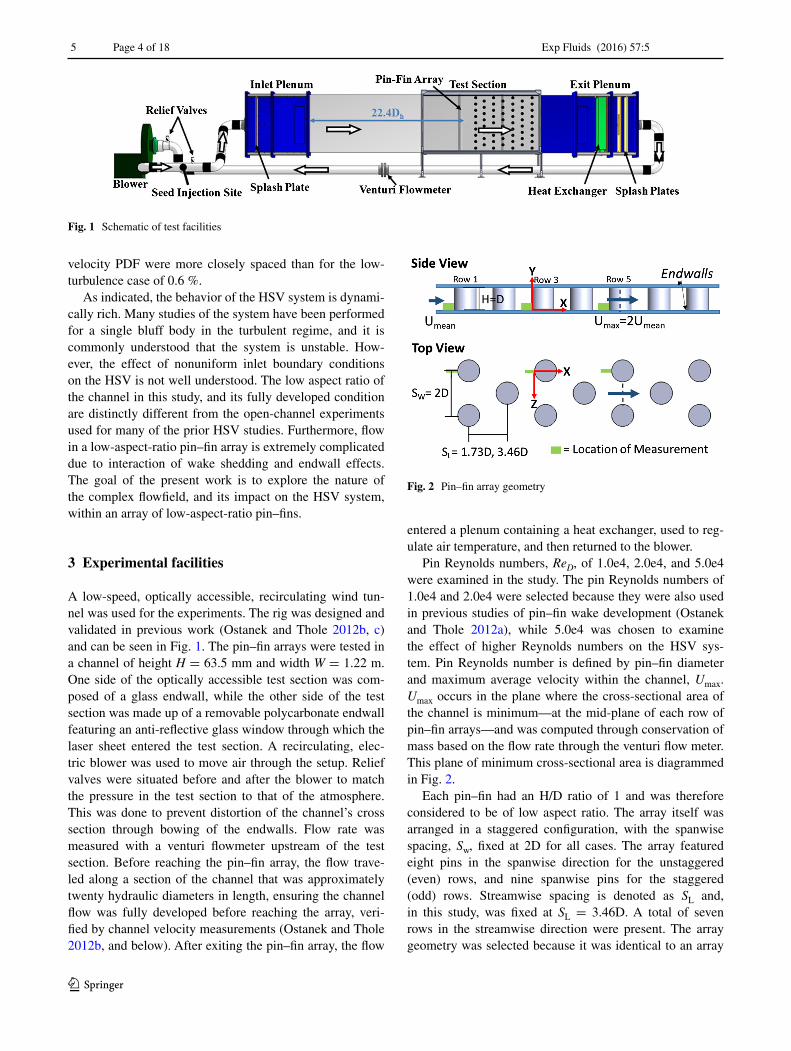
A low-speed, optically accessible, recirculating wind tun-nel was used for the experiments. The rig was designed and validated in previous work (Ostanek and Thole 2012b, c) and can be seen in Fig. 1. The pin–fin arrays were tested in a channel of height H = 63.5 mm and width W = 1.22 m. One side of the optically accessible test section was com-posed of a glass endwall, while the other side of the test section was made up of a removable polycarbonate endwall featuring an anti-reflective glass window through which the laser sheet entered the test section. A recirculating, elec-tric blower was used to move air through the setup. Relief valves were situated before and after the blower to match the pressure in the test section to that of the atmosphere. This was done to prevent distortion of the channel’s cross section through bowing of the endwalls. Flow rate was measured with a venturi flowmeter upstream of the test section. Before reaching the pin–fin array, the flow trave-led along a section of the channel that was approximately twenty hydraulic diameters in length, ensuring the channel flow was fully developed before reaching the array, veri-fied by channel velocity measurements (Ostanek and Thole 2012b, and below). After exiting the pin–fin array, the flow

entered a plenum containing a heat exchanger, used to reg-ulate air temperature, and then returned to the blower.

Pin Reynolds numbers, ReD, of 1.0e4, 2.0e4, and 5.0e4 were examined in the study. The pin Reynolds numbers of 1.0e4 and 2.0e4 were selected because they were also used in previous studies of pin–fin wake development (Ostanek and Thole 2012a), while 5.0e4 was chosen to examine the effect of higher Reynolds numbers on the HSV sys-tem. Pin Reynolds number is defined by pin–fin diameter and maximum average velocity within the channel, Umax. Umax occurs in the plane where the cross-sectional area of the channel is minimum—at the mid-plane of each row of pin–fin arrays—and was computed through conservation of mass based on the flow rate through the venturi flow meter. This plane of minimum cross-sectional area is diagrammed in Fig. 2.

Each pin–fin had an H/D ratio of 1 and was therefore considered to be of low aspect ratio. The array itself was arranged in a staggered configuration, with the spanwise spacing, Sw, fixed at 2D for all cases. The array featured eight pins in the spanwise direction for the unstaggered (even) rows, and nine spanwise pins for the staggered (odd) rows. Streamwise spacing is denoted as SL and, in this study, was fixed at SL = 3.46D. A total of seven rows in the streamwise direction were present. The array geometry was selected because it was identical to an array

Fig. 1 Schematic of test facilities

Fig. 2 Pin–fin array geometry

Exp Fluids (2016) 57:5

1 3

Page 5 of 18 5

used in previous research (Ostanek and Thole 2012a, b). Figure 2 shows a sectional view of the pin–fin array and overviews the coordinate system, relative to each pin–fin, used throughout the paper. The streamwise direction was denoted as X, and the wall-normal and spanwise directions were Y and Z, respectively.

4 PIV setup and processing

4.1 PIV equipment and settings

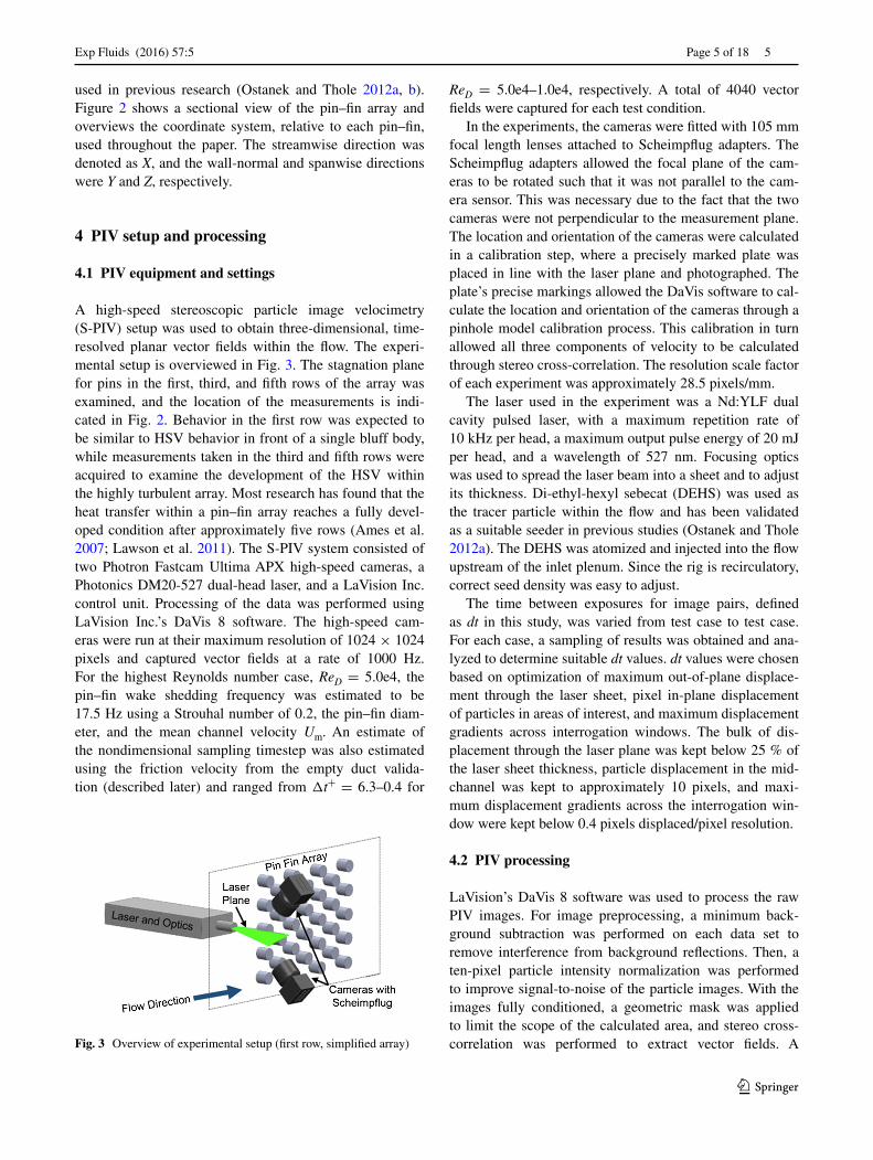
A high-speed stereoscopic particle image velocimetry (S-PIV) setup was used to obtain three-dimensional, time-resolved planar vector fields within the flow. The experi-mental setup is overviewed in Fig. 3. The stagnation plane for pins in the first, third, and fifth rows of the array was examined, and the location of the measurements is indi-cated in Fig. 2. Behavior in the first row was expected to be similar to HSV behavior in front of a single bluff body, while measurements taken in the third and fifth rows were acquired to examine the development of the HSV within the highly turbulent array. Most research has found that the heat transfer within a pin–fin array reaches a fully devel-oped condition after approximately five rows (Ames et al. 2007; Lawson et al. 2011). The S-PIV system consisted of two Photron Fastcam Ultima APX high-speed cameras, a Photonics DM20-527 dual-head laser, and a LaVision Inc. control unit. Processing of the data was performed using LaVision Inc.’s DaVis 8 software. The high-speed cam-eras were run at their maximum resolution of 1024 × 1024 pixels and captured vector fields at a rate of 1000 Hz. For the highest Reynolds number case, ReD = 5.0e4, the pin–fin wake shedding frequency was estimated to be 17.5 Hz using a Strouhal number of 0.2, the pin–fin diam-eter, and the mean channel velocity Um. An estimate of the nondimensional sampling timestep was also estimated using the friction velocity from the empty duct valida-tion (described later) and ranged from Δt+ = 6.3–0.4 for

ReD = 5.0e4–1.0e4, respectively. A total of 4040 vector fields were captured for each test condition.

In the experiments, the cameras were fitted with 105 mm focal length lenses attached to Scheimpflug adapters. The Scheimpflug adapters allowed the focal plane of the cam-eras to be rotated such that it was not parallel to the cam-era sensor. This was necessary due to the fact that the two cameras were not perpendicular to the measurement plane. The location and orientation of the cameras were calculated in a calibration step, where a precisely marked plate was placed in line with the laser plane and photographed. The plate’s precise markings allowed the DaVis software to cal-culate the location and orientation of the cameras through a pinhole model calibration process. This calibration in turn allowed all three components of velocity to be calculated through stereo cross-correlation. The resolution scale factor of each experiment was approximately 28.5 pixels/mm.

The laser used in the experiment was a Nd:YLF dual cavity pulsed laser, with a maximum repetition rate of 10 kHz per head, a maximum output pulse energy of 20 mJ per head, and a wavelength of 527 nm. Focusing optics was used to spread the laser beam into a sheet and to adjust its thickness. Di-ethyl-hexyl sebecat (DEHS) was used as the tracer particle within the flow and has been validated as a suitable seeder in previous studies (Ostanek and Thole 2012a). The DEHS was atomized and injected into the flow upstream of the inlet plenum. Since the rig is recirculatory, correct seed density was easy to adjust.

The time between exposures for image pairs, defined as dt in this study, was varied from test case to test case. For each case, a sampling of results was obtained and ana-lyzed to determine suitable dt values. dt values were chosen based on optimization of maximum out-of-plane displace-ment through the laser sheet, pixel in-plane displacement of particles in areas of interest, and maximum displacement gradients across interrogation windows. The bulk of dis-placement through the laser plane was kept below 25 % of the laser sheet thickness, particle displacement in the mid-channel was kept to approximately 10 pixels, and maxi-mum displacement gradients across the interrogation win-dow were kept below 0.4 pixels displaced/pixel resolution.

4.2 PIV processing

LaVision’s DaVis 8 software was used to process the raw PIV images. For image preprocessing, a minimum back-ground subtraction was performed on each data set to remove interference from background reflections. Then, a ten-pixel particle intensity normalization was performed to improve signal-to-noise of the particle images. With the images fully conditioned, a geometric mask was applied to limit the scope of the calculated area, and stereo cross-correlation was performed to extract vector fields. A Fig. 3 Overview of experimental setup (first row, simplified array)

Exp Fluids (2016) 57:5

1 3

5 Page 6 of 18

multi-pass, decreasing size, deformed interrogation win-dow process was used in the calculation process. Two ini-tial passes were performed at 96 × 96 pixels with 50 % overlap, and two final passes were performed at 32 × 32 pixels with 75 % overlap. The multi-pass, decreasing size, stereo cross-correlation algorithm used intermediate inter-rogation windows that were half the size of the initial pass windows.

Following the computation of an initial vector field, vec-tor postprocessing was applied. A two-pass median filter, universal outlier detection method was used. The universal outlier detection operation was performed on each vector. This operation compares the vector in question to a neigh-borhood of surrounding vectors. A residual value is com-puted by subtracting the component of velocity in question from the corresponding mean value of the neighboring vec-tors. This residual value is then normalized by the mean residual of the surrounding vectors. For the data presented, vectors in question were removed if this normalized resid-ual was greater than 1.5, in a 5 × 5 filter region. Removed vectors were replaced by a “next best” vector. If subsequent “next best” vectors failed subsequent filtering tests, they were deleted and filled via interpolation. Across all tests, approximately 90 % of final vectors were calculated based on the first-choice correlation peak and less than 0.5 % of vectors were filled via interpolation. All other vectors were calculated using second-, third-, or fourth-choice correla-tion peaks.

4.3 PIV validation

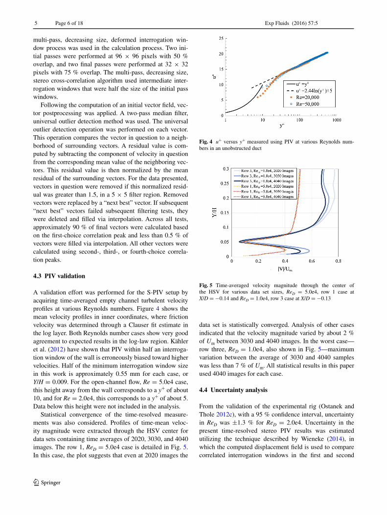
A validation effort was performed for the S-PIV setup by acquiring time-averaged empty channel turbulent velocity profiles at various Reynolds numbers. Figure 4 shows the mean velocity profiles in inner coordinates, where friction velocity was determined through a Clauser fit estimate in the log layer. Both Reynolds number cases show very good agreement to expected results in the log-law region. Kähler et al. (2012) have shown that PIV within half an interroga-tion window of the wall is erroneously biased toward higher velocities. Half of the minimum interrogation window size in this work is approximately 0.55 mm for each case, or Y/H = 0.009. For the open-channel flow, Re = 5.0e4 case, this height away from the wall corresponds to a y+ of about 10, and for Re = 2.0e4, this corresponds to a y+ of about 5. Data below this height were not included in the analysis.

Statistical convergence of the time-resolved measure-ments was also considered. Profiles of time-mean veloc-ity magnitude were extracted through the HSV center for data sets containing time averages of 2020, 3030, and 4040 images. The row 1, ReD = 5.0e4 case is detailed in Fig. 5. In this case, the plot suggests that even at 2020 images the

data set is statistically converged. Analysis of other cases indicated that the velocity magnitude varied by about 2 % of Um between 3030 and 4040 images. In the worst case—row three, ReD = 1.0e4, also shown in Fig. 5—maximum variation between the average of 3030 and 4040 samples was less than 7 % of Um. All statistical results in this paper used 4040 images for each case.

4.4 Uncertainty analysis

From the validation of the experimental rig (Ostanek and Thole 2012c), with a 95 % confidence interval, uncertainty in ReD was ±1.3 % for ReD = 2.0e4. Uncertainty in the present time-resolved stereo PIV results was estimated utilizing the technique described by Wieneke (2014), in which the computed displacement field is used to compare correlated interrogation windows in the first and second

Fig. 4 u+ versus y+ measured using PIV at various Reynolds num-bers in an unobstructed duct

Fig. 5 Time-averaged velocity magnitude through the center of the HSV for various data set sizes, ReD = 5.0e4, row 1 case at X/D = −0.14 and ReD = 1.0e4, row 3 case at X/D = −0.13

Exp Fluids (2016) 57:5

1 3

Page 7 of 18 5

image-pair frames. Differences in these frames are related to correlation functions and are then used to calculate the random uncertainty of displacement vectors. These result-ing uncertainties are both spatially and temporally resolved.

To quantify the uncertainties in the time-averaged vec-tors, the spatially resolved uncertainties were studied at multiple instants throughout a representative data set. For each location, the sampled values were used to calculate the root-mean-square uncertainty in order to estimate the uncertainty in these regions on a time-averaged basis. Near the mid-channel, the uncertainty in the local magnitude of velocity was calculated to be an estimated ±2.7 %, or ±0.16 pixel displacement. Near the center of the HSV, the percent uncertainty in the local magnitude of velocity was estimated to be ±16.3 %; however, note that the magnitude of velocity at the HSV center tends to zero (driving the local percent uncertainty upward), and the absolute mag-nitude of uncertainty was the same as at the mid-channel. Position uncertainty in the flowfield measurements was estimated to be less than 1.4 % of the pin diameter.

5 Results and discussion

5.1 Instantaneous versus time‑average HSV behavior

The SPIV results were examined for temporal sequences that represent the dynamic HSV motion that has been described by other researchers. Figures 6 and 7 show a time sequence of the instantaneous normalized vorticity field in front of the first and third row pins for ReD = 2.0e4, where the approach condition to the junction is the fully devel-oped turbulent channel flow in the low-aspect-ratio chan-nel. The nondimensional time at each instant is inset into the subfigures of Fig. 6, where t+ is calculated using the empty channel friction velocity obtained from the bench-marking described earlier. In Fig. 6, and subsequent fig-ures, the wall-normal component is Y, which is normalized by channel height H. The fluid flows from left to right in positive X, which is normalized by pin–fin diameter D. The endwall sits at Y/H = 0, while the leading edge of the pin–fin spans the channel at X/D = 0. X/D is defined relative to

Fig. 6 Temporal sequence of instantaneous nondimensional z-vorticity at the first row leading edge for ReD = 2.0e4, with typical HSV break-down indicated

Exp Fluids (2016) 57:5

1 3

5 Page 8 of 18

the leading edge of each pin–fin and is not a reference to a global coordinate system. Refer to Fig. 2 for a visual repre-sentation of the measurement planes.

Figure 6 for the first row in the array (at ReD = 2.0e4) indicates temporal behavior of the HSV system in this study that is consistent with other findings in external flow approach conditions. At t+=0, the presence of large nega-tive vorticity at X/D = −0.15 is due to the backflow mode of the HSV. Positive vorticity located beneath this mode, generated by the instability of the backflow near the wall (Paik et al. 2007), is eventually ejected from underneath the HSV (t+ = 26.0) and wraps around the HSV, engulf-ing it and causing it to break down to the zero-flow mode. Other vortices are forming upstream as this process hap-pens, and they merge and leapfrog in a turbulent fashion. These dynamics play an important role in the distribution of the mean velocity and turbulent kinetic energy that will be shown later.

Instantaneous normalized vorticity for the third row in the array, at the same Reynolds number (ReD = 2.0e4), is shown in Fig. 7. Note that the nondimensional time is still based on the empty duct friction velocity for the given ReD,

although the actual local friction velocity at this location in the array may be different (the SPIV measurements could not capture the viscous sublayer). The most apparent dif-ference between Figs. 6 and 7 is the significant amount of vorticity present in the freestream for the third row. This vorticity is the result of the shear layer breakdown and wake shedding of upstream pins, and its strength is of the same order as the HSV vorticity; in fact, in many frames, it is difficult to pick out the vorticity associated with the HSV. There are still some indications of HSV vortex back-flow (t+ = 6.5) and zero-flow (t+ = 52.0) modes, but in an instantaneous sense, these are less coherent than in the first row. The instantaneous vorticity for row 5 (not shown) was similar to the row 3 results. Because of the significant freestream vorticity, the turbulent kinetic energy in the downstream rows of the array (discussed later) is signifi-cantly higher relative to the first row of the array. This is a unique freestream condition that has not yet been consid-ered for the HSV flow in the literature.

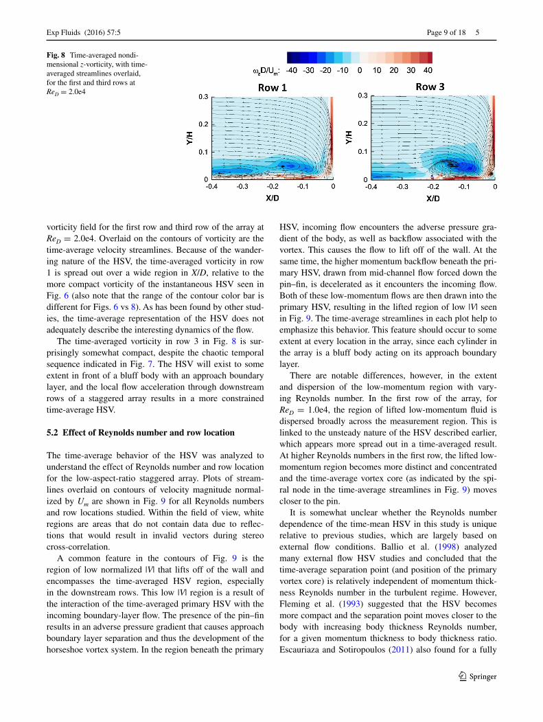
It is interesting to compare the instantaneous vorticity field for the cases described above to the time-averaged field. Figure 8 indicates the time-averaged normalized

Fig. 7 Temporal sequence of instantaneous nondimensional z-vorticity at the third row leading edge for ReD = 2.0e4

Exp Fluids (2016) 57:5

1 3

Page 9 of 18 5

vorticity field for the first row and third row of the array at ReD = 2.0e4. Overlaid on the contours of vorticity are the time-average velocity streamlines. Because of the wander-ing nature of the HSV, the time-averaged vorticity in row 1 is spread out over a wide region in X/D, relative to the more compact vorticity of the instantaneous HSV seen in Fig. 6 (also note that the range of the contour color bar is different for Figs. 6 vs 8). As has been found by other stud-ies, the time-average representation of the HSV does not adequately describe the interesting dynamics of the flow.

The time-averaged vorticity in row 3 in Fig. 8 is sur-prisingly somewhat compact, despite the chaotic temporal sequence indicated in Fig. 7. The HSV will exist to some extent in front of a bluff body with an approach boundary layer, and the local flow acceleration through downstream rows of a staggered array results in a more constrained time-average HSV.

5.2 Effect of Reynolds number and row location

The time-average behavior of the HSV was analyzed to understand the effect of Reynolds number and row location for the low-aspect-ratio staggered array. Plots of stream-lines overlaid on contours of velocity magnitude normal-ized by Um are shown in Fig. 9 for all Reynolds numbers and row locations studied. Within the field of view, white regions are areas that do not contain data due to reflec-tions that would result in invalid vectors during stereo cross-correlation.

A common feature in the contours of Fig. 9 is the region of low normalized |V| that lifts off of the wall and encompasses the time-averaged HSV region, especially in the downstream rows. This low |V| region is a result of the interaction of the time-averaged primary HSV with the incoming boundary-layer flow. The presence of the pin–fin results in an adverse pressure gradient that causes approach boundary layer separation and thus the development of the horseshoe vortex system. In the region beneath the primary

HSV, incoming flow encounters the adverse pressure gra-dient of the body, as well as backflow associated with the vortex. This causes the flow to lift off of the wall. At the same time, the higher momentum backflow beneath the pri-mary HSV, drawn from mid-channel flow forced down the pin–fin, is decelerated as it encounters the incoming flow. Both of these low-momentum flows are then drawn into the primary HSV, resulting in the lifted region of low |V| seen in Fig. 9. The time-average streamlines in each plot help to emphasize this behavior. This feature should occur to some extent at every location in the array, since each cylinder in the array is a bluff body acting on its approach boundary layer.

There are notable differences, however, in the extent and dispersion of the low-momentum region with vary-ing Reynolds number. In the first row of the array, for ReD = 1.0e4, the region of lifted low-momentum fluid is dispersed broadly across the measurement region. This is linked to the unsteady nature of the HSV described earlier, which appears more spread out in a time-averaged result. At higher Reynolds numbers in the first row, the lifted low-momentum region becomes more distinct and concentrated and the time-average vortex core (as indicated by the spi-ral node in the time-average streamlines in Fig. 9) moves closer to the pin.

It is somewhat unclear whether the Reynolds number dependence of the time-mean HSV in this study is unique relative to previous studies, which are largely based on external flow conditions. Ballio et al. (1998) analyzed many external flow HSV studies and concluded that the time-average separation point (and position of the primary vortex core) is relatively independent of momentum thick-ness Reynolds number in the turbulent regime. However, Fleming et al. (1993) suggested that the HSV becomes more compact and the separation point moves closer to the body with increasing body thickness Reynolds number, for a given momentum thickness to body thickness ratio. Escauriaza and Sotiropoulos (2011) also found for a fully

Fig. 8 Time-averaged nondi-mensional z-vorticity, with time-averaged streamlines overlaid, for the first and third rows at ReD = 2.0e4

Exp Fluids (2016) 57:5

1 3

5 Page 10 of 18

developed open-channel flow that the location of the sepa-ration point of the low-momentum fluid moves closer to a bluff body with increasing flow Reynolds number. Unfortu-nately, it is unclear from this work, due to the limited field of view that was necessary to capture HSV detail, what effect the short channel aspect ratio has on the HSV behav-ior. It could be possible that the HSV on the upper endwall has a significant impact on the dynamics of the lower end-wall HSV, due to their close proximity.

At the low ReD = 1.0e4 in Fig. 9, there is a striking dif-ference in the distribution of velocity magnitude contours in the HSV region in rows 3 and 5, relative to the first row. For the downstream rows, the region of low-momentum fluid is much less dispersed and the time-average HSV core is much closer to the pin. Flow acceleration around upstream pins and buffeting from the high levels of turbu-lence due to upstream pin–fin wakes results in a time-aver-age HSV that is more compact, and appears to be nearly invariant in either of the two downstream rows studied. This evidence of a fully developed state in the array has

been seen in endwall heat transfer measurements by other researchers (Ames et al. 2007; Lawson et al. 2011), but is infrequently documented for the array flowfield.

At increasing Reynolds numbers in Fig. 9, the differ-ence in the time-average velocity field between the first row and downstream rows becomes less noticeable. This is par-ticularly apparent for ReD = 5.0e4, where the lifted low-velocity region around the HSV looks very similar for the first row relative to rows 3 and 5. This is because the fluid, with its increased momentum at high Reynolds numbers, is less affected by the disturbing influence of the cylinders in the staggered array. This result helps to explain why array heat transfer enhancement, relative to an empty channel, decreases with increasing Reynolds number (Ames et al. 2007; Lawson et al. 2011; Metzger and Haley 1982).

Also interesting in Fig. 9 is that the flowfields in the downstream rows 3 and 5 are very similar, regardless of the wide range in pin Reynolds number. This is an impor-tant distinction from the first row where the behavior is clearly Reynolds number dependent. It suggests that the

Fig. 9 Time-averaged normalized |V| contours and time-average streamlines for each row position and Reynolds number

Exp Fluids (2016) 57:5

1 3

Page 11 of 18 5

disturbance events generated by upstream pins (i.e., wake shedding and flow acceleration) are relatively independent of Reynolds number in the range tested here. Furthermore, those disturbance events are having a strong impact on the time-average HSV. This Reynolds number independence in downstream rows should be corroborated for lower Reyn-olds numbers, since it is likely that the disturbance events will have some Reynolds number dependence at lower ReD than tested here.

The location of the primary horseshoe vortex’s spi-ral node in Fig. 9 is summarized in Table 1 for all of the cases. The uncertainty of the HSV spiral node position is estimated to be the same as the position uncertainty of the flowfield measurements (0.014D). In pin–fin row 1, increases in Reynolds number resulted in a spiral node with an X/D location closer to the pin. However, in pin–fin rows 3 and 5, the location of the spiral node did not appear to show regard for Reynolds number, as described earlier. Again, this is likely due to the dominating influence of upstream disturbance events on the time-average HSV in front of a downstream row pin.

Paik et al. (2007) proposed that the instability that breaks down the HSV arises from the inflection in the backflow velocity profile underneath the HSV. The near-wall flow below the inflection, which is turned upward by the HSV, conceptually resembles a boundary layer on a concave surface (i.e., the Görtler vortex flow). To

examine this for the different cases, profiles of velocity were extracted along a wall-normal line passing through the time-average spiral node for each case (coordinates in Table 1). Figure 10 shows the normalized time-average u velocity profiles for the various cases. Below the spiral node, in the backflow region, the u component of velocity is negative. Despite the lack of very close wall measure-ments, an inflection in the velocity profile is clearly vis-ible at Y/H = 0.02. For ReD ≤ 2.0e4, the magnitude of this peak varied from row to row, with the first row having the least negative value, the third row having the most negative value, and the fifth row falling in between. The increase in peak negative u velocity from the first to the third row is a result of local channel flow acceleration through the first two rows of pin–fins. Mid-channel flow with higher veloc-ity magnitude (see Fig. 9) is entrained by the third row HSV, resulting in a large backflow velocity. This might suggest that the breakdown phenomenon is occurring more strongly in the third row relative to the first row. Unfortu-nately, this is difficult to determine in the present data sets; the freestream vorticity levels in row 3 are on the same order as the vorticity generated by the HSV breakdown, as seen in Fig. 7.

The row-to-row variation in the backflow velocity pro-file in the HSV region decreases with increasing Reyn-olds number and is almost identical for the various rows of the ReD = 5.0e4 case. At high Reynolds numbers, the

Table 1 Location of time-mean spiral node across all rows and Reynolds numbers

Reynolds number Row 1 Row 3 Row 5

X/D Y/H X/D Y/H X/D Y/H

1.0E+04 −0.293 0.041 −0.129 0.052 −0.133 0.053

2.0E+04 −0.167 0.049 −0.140 0.053 −0.128 0.050

5.0E+04 −0.129 0.050 −0.132 0.050 −0.135 0.053

Fig. 10 u/Um through the center of the time-mean spiral node

Exp Fluids (2016) 57:5

1 3

5 Page 12 of 18

channel flow is less sensitive to the blockage of the pins and they are less effective at creating local variations in flow.

The nondimensional vorticity of the time-averaged flow for all cases is depicted in Fig. 11, with time-average veloc-ity streamlines from Fig. 9 overlaid on the contours for reference. Contrary to computational studies using steady RANS turbulence models (Levchenya et al. 2010), vorticity and streamline patterns in these results do not consistently indicate distinct time-averaged secondary, tertiary, and corner vortices. Instead, the significant motion of the vor-tices (see Fig. 6) causes the time-averaged flow to appear smeared out. For this reason, only very coherent vortices, such as the primary horseshoe vortex, appear during time averaging for each independent case.

The vorticity associated with the primary HSV is gen-erally indicated by a large, concentrated, negative vor-ticity region in Fig. 11. For a low Reynolds number of ReD = 1.0e4, the vorticity associated with the HSV becomes more concentrated in rows 3 and 5, relative to row 1. This is consistent with the previous discussion of

velocity magnitude earlier that suggests a more concen-trated mean vortex structure with increasing distance into the array. For increasing Reynolds numbers, the HSV vorti-city becomes more concentrated in row 1, and there is little apparent change in downstream rows. In these cases, peak vorticity does not generally correspond to the center of the spiraling streamlines, although it is not required to (Yates and Chapman 1992).

5.3 Bimodal analysis

As first discussed by Devenport and Simpson (1990), a histogram of the u component of velocity in the region beneath the time-average HSV is known to have a bimodal distribution. This is an indication of two qua-sistable modes of the HSV—the zero-flow and backflow modes. In the backflow mode, the flow beneath the pri-mary vortex travels far upstream in a strong jet-like form and is associated with the negative u velocity peak on a bimodal histogram of u. During the zero-flow mode, the strong backward jet beneath the primary vortex has

Fig. 11 Time-averaged normalized z-vorticity for each row location and Reynolds number

Exp Fluids (2016) 57:5

1 3

Page 13 of 18 5

broken down and the recirculating fluid is instead pulled into the primary HSV, which corresponds to a peak at zero on the histogram.

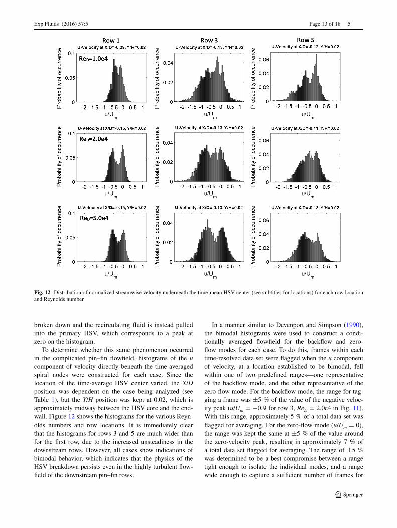
To determine whether this same phenomenon occurred in the complicated pin–fin flowfield, histograms of the u component of velocity directly beneath the time-averaged spiral nodes were constructed for each case. Since the location of the time-average HSV center varied, the X/D position was dependent on the case being analyzed (see Table 1), but the Y/H position was kept at 0.02, which is approximately midway between the HSV core and the end-wall. Figure 12 shows the histograms for the various Reyn-olds numbers and row locations. It is immediately clear that the histograms for rows 3 and 5 are much wider than for the first row, due to the increased unsteadiness in the downstream rows. However, all cases show indications of bimodal behavior, which indicates that the physics of the HSV breakdown persists even in the highly turbulent flow-field of the downstream pin–fin rows.

In a manner similar to Devenport and Simpson (1990), the bimodal histograms were used to construct a condi-tionally averaged flowfield for the backflow and zero-flow modes for each case. To do this, frames within each time-resolved data set were flagged when the u component of velocity, at a location established to be bimodal, fell within one of two predefined ranges—one representative of the backflow mode, and the other representative of the zero-flow mode. For the backflow mode, the range for tag-ging a frame was ±5 % of the value of the negative veloc-ity peak (u/Um = −0.9 for row 3, ReD = 2.0e4 in Fig. 11). With this range, approximately 5 % of a total data set was flagged for averaging. For the zero-flow mode (u/Um = 0), the range was kept the same at ±5 % of the value around the zero-velocity peak, resulting in approximately 7 % of a total data set flagged for averaging. The range of ±5 % was determined to be a best compromise between a range tight enough to isolate the individual modes, and a range wide enough to capture a sufficient number of frames for

Fig. 12 Distribution of normalized streamwise velocity underneath the time-mean HSV center (see subtitles for locations) for each row location and Reynolds number

Exp Fluids (2016) 57:5

1 3

5 Page 14 of 18

averaging. The flagged frames for each case were aver-aged to create time-average profiles of the backflow and zero-flow modes. Normalized magnitude of velocity con-tours, with streamlines overlaid, can be found in Fig. 13 for these two modes in the row 3, ReD = 2.0e4 case. A discus-sion of these two modes’ variation with Reynolds number and row location is deferred to a subsequent paper. With relatively few frames used to generate the conditional time averages, the quantitative results contain a large amount of uncertainty. However, even with a relatively small number of frames, there is a clear distinction between the backflow and zero-flow modes in terms of the vortex size and posi-tion upstream of the cylinder. The conditionally averaged result is useful in describing the nature of the turbulent HSV flowfield in the following section.

5.4 Effect of bimodal behavior on turbulent quantities

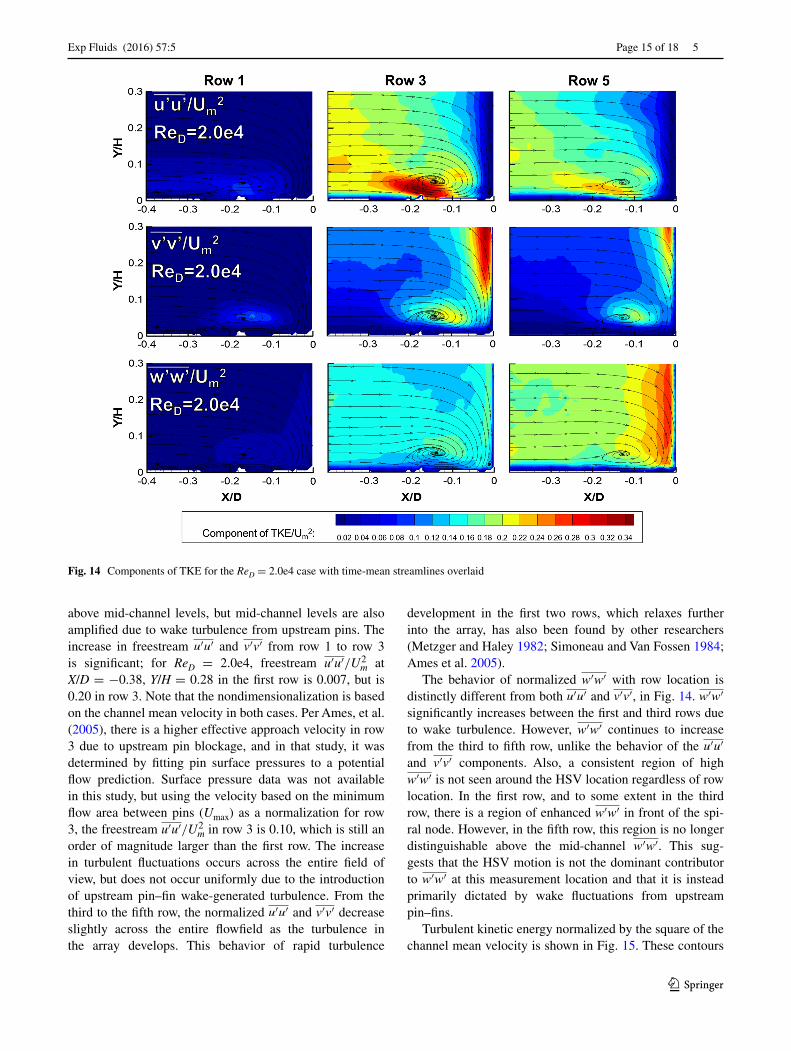
The components of turbulent kinetic energy (u′u′, v′v′, w′w′ ) were examined for each row location and Reynolds number. Figure 14 shows contours of these components normalized by the square of the mean channel velocity for each row of the ReD = 2.0e4 case, with time-average streamlines overlaid. Equivalent plots for the ReD = 1.0e4 and 5.0e4 cases are not shown for the sake of space; how-ever, the trends discussed here hold for those cases as well. For each pin–fin row shown in Fig. 14, the region of peak normalized u′u′ occurs in the backflow region—below and slightly behind the spiral node. In the row 3 case of Fig. 14, this region is found in the vicinity of X/D = −0.17, Y/H = 0.03. This region of highly normal-ized u′u′ is a direct consequence of the HSV’s oscillation between the backflow and zero-flow modes. This is illus-trated by considering the conditionally averaged results for row 3 in Fig. 13. In the area around X/D = −0.17, Y/H = 0.03 in Fig. 13a, the velocity is of moderate magni-tude and is traveling in the negative u direction. In the same area in Fig. 13b, the velocity is of nearly zero magnitude. The difference in behavior of u in this area, as the system switches between backflow and zero-flow modes, results

in this region of peak u′u′. Although plots of the backflow and zero-flow modes are not shown for rows 1 and 5, this region of maximum HSV-associated u′u′ occurs in each row and is driven by the same phenomenon.

For each of the rows in Fig. 14, a secondary region of enhanced u′u′ exists slightly downstream and above the spiral node. In the row 3 case, this region is approximately at X/D = −0.08, Y/H = 0.07. Once again, the bimodal behavior of the HSV drives this region of heightened fluc-tuations. Based on the streamlines in Fig. 13 at the same location, the time-average u velocity is nearly zero in the backflow mode and is positive in the zero-flow mode. The differences in u between the two modes are not as large as in the backflow region, so the magnitude of the overall nor-malized u′u′ is not of the same magnitude, but the region is still amplified above levels of turbulence seen in the mid-channel.

The backflow to zero-flow mode switching also affects the v′v′ turbulence component. In the HSV region of each row, peak normalized v′v′ occurs slightly downstream of the HSV spiral node. In the row 3 case, this region occurs at about X/D = −0.11, Y/H = 0.06 in Fig. 14. Referring back to Fig. 13, in the backflow mode, velocity in this region is almost entirely in the negative Y direction with moderate magnitude. In the zero-flow mode, this region contains flow of very low magnitude, in a variety of directions. The dif-ference in magnitude of v results in a region of enhanced normalized v′v′ seen in Fig. 14. Examining the w′w′ con-tour levels, the peak levels around the HSV region do not reach magnitudes as great as the u and v counterparts. The region as a whole, though, does experience mild fluctua-tions in w, with the maximum occurring above and in front of the spiral node.

Row location has a distinct impact on the magni-tudes for each component of TKE. In the first row case in Fig. 14, the components of TKE associated with the HSV system are amplified over mid-channel levels by an order of magnitude, a result consistent with Devenport and Simpson (1990). In the third and fifth rows, peak regions of u′u′ and v′v′ associated with the HSV are still distinct

Fig. 13 Conditionally averaged backflow and zero-flow modes for the row 3, ReD = 2.0e4 case

Exp Fluids (2016) 57:5

1 3

Page 15 of 18 5

above mid-channel levels, but mid-channel levels are also amplified due to wake turbulence from upstream pins. The increase in freestream u′u′ and v′v′ from row 1 to row 3 is significant; for ReD = 2.0e4, freestream u′u′/U2

m at X/D = −0.38, Y/H = 0.28 in the first row is 0.007, but is 0.20 in row 3. Note that the nondimensionalization is based on the channel mean velocity in both cases. Per Ames, et al. (2005), there is a higher effective approach velocity in row 3 due to upstream pin blockage, and in that study, it was determined by fitting pin surface pressures to a potential flow prediction. Surface pressure data was not available in this study, but using the velocity based on the minimum flow area between pins (Umax) as a normalization for row 3, the freestream u′u′/U2

m in row 3 is 0.10, which is still an order of magnitude larger than the first row. The increase in turbulent fluctuations occurs across the entire field of view, but does not occur uniformly due to the introduction of upstream pin–fin wake-generated turbulence. From the third to the fifth row, the normalized u′u′ and v′v′ decrease slightly across the entire flowfield as the turbulence in the array develops. This behavior of rapid turbulence

development in the first two rows, which relaxes further into the array, has also been found by other researchers (Metzger and Haley 1982; Simoneau and Van Fossen 1984; Ames et al. 2005).

The behavior of normalized w′w′ with row location is distinctly different from both u′u′ and v′v′, in Fig. 14. w′w′ significantly increases between the first and third rows due to wake turbulence. However, w′w′ continues to increase from the third to fifth row, unlike the behavior of the u′u′ and v′v′ components. Also, a consistent region of high w′w′ is not seen around the HSV location regardless of row location. In the first row, and to some extent in the third row, there is a region of enhanced w′w′ in front of the spi-ral node. However, in the fifth row, this region is no longer distinguishable above the mid-channel w′w′. This sug-gests that the HSV motion is not the dominant contributor to w′w′ at this measurement location and that it is instead primarily dictated by wake fluctuations from upstream pin–fins.

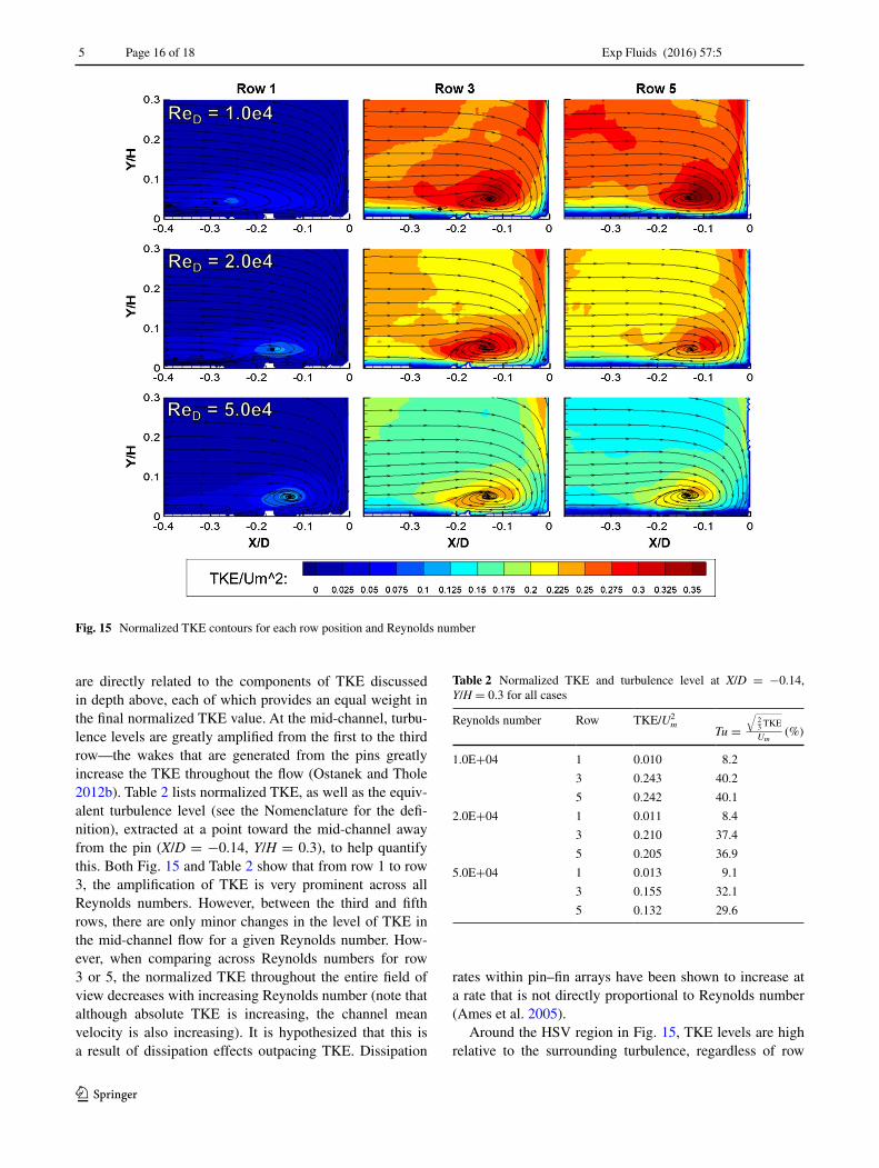
Turbulent kinetic energy normalized by the square of the channel mean velocity is shown in Fig. 15. These contours

Fig. 14 Components of TKE for the ReD = 2.0e4 case with time-mean streamlines overlaid

Exp Fluids (2016) 57:5

1 3

5 Page 16 of 18

are directly related to the components of TKE discussed in depth above, each of which provides an equal weight in the final normalized TKE value. At the mid-channel, turbu-lence levels are greatly amplified from the first to the third row—the wakes that are generated from the pins greatly increase the TKE throughout the flow (Ostanek and Thole 2012b). Table 2 lists normalized TKE, as well as the equiv-alent turbulence level (see the Nomenclature for the defi-nition), extracted at a point toward the mid-channel away from the pin (X/D = −0.14, Y/H = 0.3), to help quantify this. Both Fig. 15 and Table 2 show that from row 1 to row 3, the amplification of TKE is very prominent across all Reynolds numbers. However, between the third and fifth rows, there are only minor changes in the level of TKE in the mid-channel flow for a given Reynolds number. How-ever, when comparing across Reynolds numbers for row 3 or 5, the normalized TKE throughout the entire field of view decreases with increasing Reynolds number (note that although absolute TKE is increasing, the channel mean velocity is also increasing). It is hypothesized that this is a result of dissipation effects outpacing TKE. Dissipation

rates within pin–fin arrays have been shown to increase at a rate that is not directly proportional to Reynolds number (Ames et al. 2005).

Around the HSV region in Fig. 15, TKE levels are high relative to the surrounding turbulence, regardless of row

Fig. 15 Normalized TKE contours for each row position and Reynolds number

Table 2 Normalized TKE and turbulence level at X/D = −0.14, Y/H = 0.3 for all cases

Reynolds number Row TKE/Um2

Tu =

√

2

3TKE

Um (%)

1.0E+04 1 0.010 8.2

3 0.243 40.2

5 0.242 40.1

2.0E+04 1 0.011 8.4

3 0.210 37.4

5 0.205 36.9

5.0E+04 1 0.013 9.1

3 0.155 32.1

5 0.132 29.6

Exp Fluids (2016) 57:5

1 3

Page 17 of 18 5

location. This is an important finding, as it implies that even with mid-channel turbulence that is amplified by upstream wake fluctuations, the TKE related to the HSV is still distinguishable.

Similar to the trends in the mean velocity results, the concentrated region of TKE associated with the HSV moves closer to the pin and becomes more compact for rows further into the array. In the first row in Fig. 15, the TKE is concentrated in an oval manner near the spiral node. By row three, the region of high TKE is more dis-tributed and appears to have two local maxima around the HSV, with one local maximum upstream of the spi-ral node, closer to the wall, and the other local maximum just slightly downstream of the spiral node and further away from the endwall. This is especially apparent in the ReD = 2.0e4 case, where the first local maximum is near X/D = −0.19, Y/H = 0.04 and the second local maximum is near X/D = −0.12, Y/H = 0.06. In the fifth row, the TKE remains concentrated only in the region downstream and slightly above the spiral node.

The distributions of concentrated TKE associated with the HSV system can be explained in context of the com-ponents of TKE. Only the ReD = 2.0e4 case is examined here because contours of the components of TKE are pro-vided for each row in Fig. 14; however, the qualitative trends hold across all Reynolds numbers. In the first row, the peak region of TKE near X/D = −0.15, Y/H = 0.05 is a result of overlap between all components of TKE from Fig. 14. Upstream of this region, TKE is amplified above mid-channel levels, primarily as a result of u′u′. In the third row, the peak in TKE at X/D = −0.19, Y/H = 0.04 is driven by the high u′u′ there. However, a second peak in TKE is found downstream and slightly above the spiral node at X/D = −0.12, Y/H = 0.06, where moderate levels of all turbulence components combine to form a second region of peak TKE. In the fifth row, the single region of peak TKE is a result of the simultaneous decay of u′u′ and amplifica-tion of w′w′ from rows 3 to 5.

6 Conclusions

The present study examines the unsteady and time-mean behavior of the horseshoe vortex system across multiple Reynolds numbers and multiple row locations within a low-aspect-ratio pin–fin array. Velocity field measurements were obtained by a high-speed stereo PIV system at the leading edge–endwall junction for the first, third, and fifth rows of the array. Reynolds numbers from 1.0e4 to 5.0e4 were investigated at each of the measurement locations.

In the first row of the array, instantaneous measurements of vorticity demonstrated HSV behavior similar to that found in external flow studies, such as the quasiperiodic

breakdown of the HSV system into the backflow and zero-flow modes, despite the fully developed channel flow con-dition and short channel height in this study. However, unlike some external flow HSV studies, the position of the time-mean HSV core was noticeably affected by Reynolds number. Specifically, for increasing ReD, the time-mean HSV became more concentrated at the pin–endwall junc-tion and normalized TKE around the HSV core increased. This is thought to be an effect of the fully developed approach flow condition in this study.

In the third and fifth rows, wakes from upstream cylin-drical pin–fins resulted in significant levels of instantane-ous freestream vorticity, on the same order of magnitude as the HSV. This significant disturbance resulted in turbu-lence levels of up to 40 % in the mid-channel flow, which are higher than any ever reported for studies of HSV behav-ior. Despite these high levels of turbulence, the bimodal nature of the HSV was still present in the downstream rows. At low Reynolds numbers, the time-mean HSV was more compact and closer to the pin–endwall junction for downstream rows relative to the first row, but there was lit-tle difference in the time-mean HSV shape among rows for higher Reynolds numbers. The lack of relative change in HSV behavior with row location for high Reynolds num-bers is related to the behavior found by other researchers studying array heat transfer. They find that the augmenta-tion of heat transfer in a pin–fin array, relative to an unob-structed duct, decreases as Reynolds number is increased, because the high-Re flow is not as drastically affected by the blockage of the pins.

All three components of the turbulent fluctuations were examined for each case. In the first row, u′u′, v′v′, and w′w′ in the HSV region were all an order of magnitude higher than the mid-channel flow, as expected. Distinct regions of maximum u′u′ and v′v′ were observed and were attrib-uted to the HSV system’s oscillation between the backflow and zero-flow modes; that is, they are largely due to semi-deterministic motions and not purely random turbulent motions. These regions of maximum u′u′ and v′v′ dramati-cally increased from the first to the third row, but slightly decreased from the third to fifth row. Weak w′w′ fluctua-tions were observed around the time-averaged spiral node for the first row, but large w′w′ in downstream rows were more likely due to upstream wake shedding than to fluc-tuations arising from the HSV system. Unlike u′u′ and v′v′, w′w′ continued to increase from row 3 to row 5, suggesting that the various turbulence components evolve at different rates through the array.

The distribution of turbulent kinetic energy through the array incorporated the various changes in the indi-vidual components. Normalized turbulent kinetic energy decreased across the entire field of view as Reynolds num-ber increased, due to increased dissipation that was not

Exp Fluids (2016) 57:5

1 3

5 Page 18 of 18

proportional to increases in Um and Reynolds number. The shape of the high-TKE regions associated with the HSV system varied from row to row, but remained independent of Reynolds number for downstream rows.

Overall, the behavior of the HSV was similar in down-stream rows relative to the first row, with the exception of reduced Reynolds number dependence. Further experi-ments should probe the dynamics of the HSV in more detail, particularly for its sensitivity to large-amplitude forcing like the wake shedding experienced here in the pin–fin array.

References

Agui JH, Andreopoulos J (1992) Experimental investigation of a three-dimensional boundary layer flow in the vicinity of an upright wall mounted cylinder (data bank contribution). J Fluids Eng 114:566–576

Ames F, Dvorak L (2006) The influence of Reynolds number and row position on surface pressure distributions in staggered pin fin arrays. Paper published in ASME Turbo Expo 2006: Power for Land, Sea, and Air, pp 149–159

Ames FE, Dvorak LA, Morrow MJ (2005) Turbulent augmentation of internal convection over pins in staggered-pin fin arrays. J Tur-bomach 127:183–190

Ames FE, Nordquist CA, Klennert LA (2007) Endwall heat transfer measurements in a staggered pin fin array with an adiabatic pin. Paper published in ASME Turbo Expo 2007: Power for Land, Sea, and Air, pp 423–432

Ballio F, Bettoni C, Franzetti S (1998) A survey of time-averaged characteristics of laminar and turbulent horseshoe vortices. J Flu-ids Eng 120:233–242

Blair MF (1974) An experimental study of heat transfer and film cool-ing on large-scale turbine endwalls. J Heat Transf 96(4):524–529. doi:10.1115/1.3450239

Borello D, Hanjali K (2011) LES of fluid and heat flow over a wall-bounded short cylinder at different inflow conditions. J Phys: Conf Ser 318:042046

Delibra G, Hanjalić K, Borello D, Rispoli F (2010) Vortex structures and heat transfer in a wall-bounded pin matrix: LES with a RANS wall-treatment. Int J Heat Fluid Flow 31:740–753

Devenport WJ, Simpson RL (1990) Time-dependent and time-aver-aged turbulence structure near the nose of a wing-body junction. J Fluid Mech 210:23–55

Escauriaza C, Sotiropoulos F (2011) Reynolds number effects on the coherent dynamics of the turbulent horseshoe vortex system. Flow Turbul Combust 86:231–262

Fleming JL, Simpson RL, Cowling JE, Devenport WJ (1993) An experimental study of a turbulent wing-body junction and wake flow. Exp Fluids 14:366–378

Giel PW, Thurman DR, Fossen GJV, Hippensteele SA, Boyle RJ (1998) Endwall heat transfer measurements in a transonic tur-bine cascade. J Turbomach 120:305–313

Graziani RA, Blair MF, Taylor JR, Mayle RE (1980) An experimental study of endwall and airfoil surface heat transfer in a large scale turbine blade cascade. J Eng Power 102:257–267

Hunt J, Abell C, Peterka J, Woo H (1978) Kinematical studies of the flows around free or surface-mounted obstacles; applying topol-ogy to flow visualization. J Fluid Mech 86:179–200

Kähler CJ, Scharnowski S, Cierpka C (2012) On the uncertainty of digital PIV and PTV near walls. Exp Fluids 52:1641–1656

Kang MB, Kohli A, Thole KA (1999) Heat transfer and flowfield measurements in the leading edge region of a stator vane end-wall. J Turbomach 121:558–568

Kirkil G, Constantinescu G (2015) Effects of cylinder reynolds num-ber on the turbulent horseshoe vortex system and near wake of a surface-mounted circular cylinder. Phys Fluids 27:075102

Lawson SA, Thrift AA, Thole KA, Kohli A (2011) Heat transfer from multiple row arrays of low aspect ratio pin fins. Int J Heat Mass Transf 54:4099–4109

Levchenya AM, Smirnov EM, Goryachev VD (2010) RANS-based numerical simulation and visualization of the horseshoe vortex system in the leading edge endwall region of a symmetric body. Int J Heat Fluid Flow 31:1107–1112

Metzger D, Haley S (1982) Heat transfer experiments and flow visualization for arrays of short pin fins. Paper published in ASME 1982 International Gas Turbine Conference and Exhibit: V004T009A007-V004T009A007

Olcmen SM, Simpson RL (1994) Influence of wing shapes on surface pressure fluctuations at wing-body junctions. AIAA J 32:6–15

Ölçmen SM, Simpson RL (2006) Some features of a turbulent wing-body junction vortical flow. Int J Heat Fluid Flow 27:980–993

Ostanek J, Thole K (2012a) Effect of streamwise spacing on periodic and random unsteadiness in a bundle of short cylinders confined in a channel. Exp Fluids 53:1779–1796

Ostanek J, Thole K (2012b) Wake development in staggered short cyl-inder arrays within a channel. Exp Fluids 53:673–697

Ostanek JK, Thole KA (2012c) Flowfield measurements in a single row of low aspect ratio pin fins. J Turbomach 134:051034

Paik J, Escauriaza C, Sotiropoulos F (2007) On the bimodal dynamics of the turbulent horseshoe vortex system in a wing-body junc-tion. Phys Fluids (1994-present) 19

Praisner TJ, Smith CR (2006a) The dynamics of the horseshoe vortex and associated endwall heat transfer—part I: temporal behavior. J Turbomach 128:747–754

Praisner TJ, Smith CR (2006b) The dynamics of the horseshoe vortex and associated endwall heat transfer—part II: time-mean results. J Turbomach 128:755–762

Radomsky RW, Thole KA (2000) High free-steam turbulence effects on endwall heat transfer for a gas turbine stator vane. J Turbom-ach 122:699–708

Sabatino DR, Smith CR (2009) Boundary layer influence on the unsteady horseshoe vortex flow and surface heat transfer. J Tur-bomach 131:011015–011018

Sahin B, Ozturk NA, Gurlek C (2008) Horseshoe vortex studies in the passage of a model plate-fin-and-tube heat exchanger. Int J Heat Fluid Flow 29:340–351

Scholten JW, Murray DB (1998) Heat transfer and velocity fluctua-tions in a staggered tube array. Int J Heat Fluid Flow 19:233–244

Simoneau R, Van Fossen G (1984) Effect of location in an array on heat transfer to a short cylinder in crossflow. J Heat Transf 106:42–48

Simpson RL (2001) Junction flows. Ann Rev Fluid Mech 33:415–443Wieneke B (2014) Generic a posteriori uncertainty quantification for

PIV vector fields by correlation statistics. Paper published in 17th international symposium on applications of laser techniques to fluid mechanics (Lisbon, Portugal)

Yates LA, Chapman GT (1992) Streamlines, vorticity lines, and vorti-ces around three-dimensional bodies. AIAA J 30:1819–1826