Time of Deterministic Broadcasting in Radio Networks with Local Knowledge

TIME OF DETERMINISTIC BROADCASTING INRADIO NETWORKS WITH LOCAL KNOWLEDGE∗

DARIUSZ R. KOWALSKI† AND ANDRZEJ PELC‡

SIAM J. COMPUT. c© 2004 Society for Industrial and Applied MathematicsVol. 33, No. 4, pp. 870–891

Abstract. We consider broadcasting in radio networks, modeled as undirected graphs, whosenodes know only their own label and labels of their neighbors. In every step every node acts either asa transmitter or as a receiver. A node acting as a transmitter sends a message which can potentiallyreach all of its neighbors. A node acting as a receiver in a given step gets a message if and only ifexactly one of its neighbors transmits in this step.

Bar-Yehuda, Goldreich, and Itai [J. Comput. System Sci., 45 (1992), pp. 104–126] consideredbroadcasting in this model. They claimed a linear lower bound on the time of deterministic broad-casting in such radio networks of diameter 3. This claim turns out to be incorrect in this model(although it is valid in a more pessimistic model [R. Bar-Yehuda, O. Goldreich, and A. Itai, ErrataRegarding “On the time complexity of broadcast in radio networks: An exponential gap betweendeterminism and randomization,” http://www.wisdom.weizmann.ac.il/mathusers/oded/p bgi.html,2002]). We construct an algorithm that broadcasts in logarithmic time on all graphs from the Bar-Yehuda, Goldreich, and Itai paper (BGI). Moreover, we show how to broadcast in sublinear timeon all n-node graphs of diameter o(log logn). On the other hand, we construct a class of graphs ofdiameter 4, such that every broadcasting algorithm requires time Ω( 4

√n) on these graphs. In view

of the randomized algorithm from BGI, running in expected time O(D logn + log2 n) on all n-nodegraphs of diameter D (cf. also a recent O(D log(n/D) + log2 n)-time algorithm from [D. Kowalskiand A. Pelc, Proceedings of the 22nd Annual ACM Symposium on Principles of Distributed Com-puting, Boston, 2003, pp. 73–82; A. Czumaj and W. Rytter, Proceedings of the 44th Annual IEEESymposium on Foundations of Computer Science, Cambridge, MA, 2003, pp. 492–501]), our lowerbound gives the first correct proof of an exponential gap between determinism and randomization inthe time of radio broadcasting, under the considered model of radio communication.

Key words. broadcasting, distributed, deterministic, radio network

AMS subject classifications. 68W15, 68Q25, 68Q17

DOI. 10.1137/S0097539702419339

1. Introduction. A radio network is modeled as an undirected connected graphwhose nodes are transmitter-receiver devices. An edge e between two nodes meansthat the transmitter of one end of e can reach the other end. Nodes send messages insynchronous steps (time slots), measured by a global clock which indicates the currentstep number. In every step every node acts either as a transmitter or as a receiver.A node acting as a transmitter sends a message which can potentially reach all of itsneighbors. A node acting as a receiver in a given step gets a message if and only ifexactly one of its neighbors transmits in this step. The message received in this case isthe one that was transmitted. If at least two neighbors of u transmit simultaneously

∗Received by the editors December 7, 2002; accepted for publication (in revised form) Novem-ber 12, 2003; published electronically May 5, 2004. A preliminary version of this paper appeared inthe Proceedings of the 43rd Annual IEEE Symposium on Foundations of Computer Science (FOCS2002), November 2002, Vancouver, Canada, under the title “Deterministic Broadcasting Time inRadio Networks of Unknown Topology.”

http://www.siam.org/journals/sicomp/33-4/41933.html†Instytut Informatyki, Uniwersytet Warszawski, Banacha 2, 02-097 Warszawa, Poland, and

Max-Planck-Institut fur Informatik, Stuhlsatzenhausweg 85, Saarbrucken, 66123 Germany ([email protected]). This work was done in part during this author’s stay at the Research Chair inDistributed Computing of the Universite du Quebec en Outaouais, as a postdoctoral fellow. Thisauthor’s research was supported in part by KBN grant 4T11C04425.

‡Departement d’informatique, Universite du Quebec en Outaouais, Hull, QC J8X 3X7, Canada([email protected]). This author’s research was supported in part by NSERC grant OGP 0008136 and bythe Research Chair in Distributed Computing of the Universite du Quebec en Outaouais.

870

DETERMINISTIC BROADCASTING IN RADIO NETWORKS 871

in a given step, none of the messages is received by u in this step. In this case we saythat a collision occurred at u. It is assumed that the effect at node u of more thanone of its neighbors transmitting is the same as that of no neighbor transmitting (i.e.,a node cannot distinguish a collision from silence). We assume that nodes know onlytheir own label and the labels of their neighbors. Apart from that, the only a prioriinformation on the network available to nodes is a polynomial upper bound on thenumber of nodes.

One of the fundamental tasks in network communication is broadcasting. Its goalis to transmit a message from one node of the network, called the source, to all othernodes. Remote nodes get the source message via intermediate nodes, along paths inthe network. In this paper we concentrate on one of the most important and widelystudied performance parameters of a broadcasting scheme, which is the total time—that is, the number of steps it uses to inform all the nodes of the network. We measurecomplexity in terms of the number of nodes in the network.

1.1. Our results. In a seminal paper [3], Bar-Yehuda, Goldreich, and Itai con-sidered broadcasting in radio networks in the model described above. They claimed alinear lower bound on the time of deterministic broadcasting in such radio networksof diameter 3. This claim turns out to be incorrect, although it is valid in a more pes-simistic model [4]. In fact, as pointed out in [4], the error is due to a gap between twomodels handling collisions in radio broadcasting: that from [3] and a more pessimisticbut equally reasonable one. (See more comments on this point in subsection 1.2.) Asdiscussed below, a lot of work on radio broadcasting has been done following [3], mostof it modeling collisions as in [3].

Using the same model as in [3], we construct an algorithm that broadcasts in log-arithmic time on all graphs from [3]. Moreover, we show how to broadcast in sublineartime on all n-node graphs of diameter o(log log n). On the other hand, we constructa class of graphs of diameter 4, such that every broadcasting algorithm requires timeΩ( 4

√n) on one of these graphs. In view of the randomized algorithm from [3] running

in expected time O(D log n + log2 n) on all n-node graphs of diameter D (cf. also arecent O(D log(n/D) + log2 n)-time algorithm from [23, 15]), our lower bound givesthe first correct proof of an exponential gap between determinism and randomizationin the time of radio broadcasting, in the model from [3].

1.2. Related work. Most of the results concerning broadcasting in radio net-works can be divided into two parts: those which assume complete knowledge of thetopology of the network at all nodes, or equivalently, dealing with centralized broad-casting for a given network, and those assuming only limited knowledge of the networkat all nodes and dealing with distributed broadcasting in arbitrary networks.

Deterministic centralized broadcasting assuming complete knowledge of the net-work was first considered in [10], where a O(D log2 n)-time broadcasting algorithmwas given for all n-node networks of diameter D. In [18], O(D + log5 n)-time broad-casting was proposed. On the other hand, in [1] the authors proved the existenceof a family of n-node networks of radius 2, for which any broadcast requires timeΩ(log2 n).

The study of deterministic distributed broadcasting in radio networks whose nodeshave only limited knowledge of the topology was initiated in [3]. The authors assumedthat nodes know only their own label and the labels of their neighbors (and thatcollision at a node has the same effect as silence). Under this scenario, a simpleO(n)-time broadcasting algorithm based on depth-first search (DFS) follows from [2].In [3] the authors constructed a class of n-node graphs of diameter 3, and claimed

872 DARIUSZ R. KOWALSKI AND ANDRZEJ PELC

that every broadcasting algorithm requires time Ω(n) on one of these graphs. In [19]this claim was further strengthened to a lower bound of n − 1 on broadcasting timerequired on one of these graphs. It follows from the present paper that both theseclaims (concerning lower bounds) are incorrect.

As pointed out in [4], the linear lower bound from [3] is valid in a more pessimisticmodel than that of [3]. Namely, one could assume that in the case of a collision at u theeffect can be either the same as if no neighbor of u transmitted or the same as if anysingle neighbor of u transmitted, the choice of the effect being left to the adversary.That is, either noise caused by many transmitting neighbors may be undistinguishablefrom background noise or else one of the competing neighbors may prevail, and it isimpossible to predict which situation occurs for a given collision. For this model,which seems equally reasonable to that from [3], the argument and the linear lowerbound of [3] are valid (cf. [4]). In fact, as explained in [4], the error in [3] is due tothe gap between these two models.

Many authors [5, 7, 8, 9, 11, 12, 13, 14, 16, 26] studied deterministic distributedbroadcasting in radio networks under the even weaker assumption that nodes knowonly their own label (but do not know the labels of their neighbors). In all thesepapers the collision issue was modeled as in [3]. In [11] the authors gave a broadcastingalgorithm working in time O(n) for arbitrary n-node networks, assuming that nodescan transmit spontaneously before getting the source message. It was shown in [24]that if nodes know only their own label, the argument from [3] can be modified toprove a lower bound Ω(n) on broadcasting time for networks of radius 2. Thus thealgorithm from [11] is optimal.

In [11, 12, 13, 14, 16, 26] the model of directed graphs was used. Increasingly fasterbroadcasting algorithms working on arbitrary n-node (directed) radio networks wereconstructed, culminating with the O(n log2 n)-time algorithm from [13]. Recently, aO(n log n logD)-time broadcasting algorithm was shown in [22] for n-node networks ofradius D. This was further improved to O(n log2 D) in [15]. In [14] the authors showeda lower bound Ω(n logD) on broadcasting time for n-node networks of radius D. Onthe other hand, in [5, 7, 8, 9, 12, 14] the problem was to find efficient broadcastingalgorithms on radio networks of maximum in-degree ∆.

Finally, randomized broadcasting algorithms in radio networks were studied, e.g.,in [3, 15, 25, 23]. For these algorithms no topological knowledge of the network wasassumed. In [3] the authors showed a randomized broadcasting algorithm runningin expected time O(D log n + log2 n). A faster algorithm, running in expected timeO(D log(n/D)+ log2 n) was presented in [23] (see also [15]). In [25] it was shown thatfor any randomized broadcasting algorithm (and parameters D ≤ n), there exists ann-node network of diameter D requiring expected time Ω(D log(n/D)). It should benoted that the lower bound Ω(log2 n) from [1], for some networks of radius 2, holds forrandomized algorithms as well. This shows that the algorithm from [23] is optimal.

1.3. Organization of the paper. In section 2 we summarize the communi-cation model (taken from [3]) and the terminology used in this paper. Section 3 isdevoted to showing a logarithmic broadcasting algorithm for the class of networksfor which a linear lower bound was claimed in [3]. In this section we first describethe novel Procedure Echo, which is later used for more complicated algorithms. Insection 4 we describe and analyze a broadcasting algorithm working in sublinear timeon all shallow networks. This indicates that if a linear lower bound on broadcastingtime can at all be proved (for networks of sublinear diameter), then it requires theconstruction of quite complicated networks. Section 5 is devoted to the proof of the


lower bound Ω( 4√n) on broadcasting time in networks of bounded diameter. Finally,

section 6 contains concluding remarks and open problems.

2. Model and terminology. We consider undirected graphs whose nodes havedistinct labels belonging to the set 0, 1, . . . , r, where r is polynomial in the number nof nodes. The parameter r is known to all nodes. In the lower bounds we assumethat n itself is known to all nodes. A distinguished node with label 0 is called thesource. We denote by D the radius of the graph, i.e., the distance from the sourceto the farthest node. (For undirected graphs, the diameter is of the order of theradius.) The jth layer of a graph is the set of nodes at distance j from the source.We adopt the communication model used by Bar-Yehuda, Goldreich, and Itai [3]. Itis summarized in the following definition.

Definition 2.1 (see [3]). A broadcast protocol for radio networks is a multi-processor (multinode) protocol, the execution of which proceeds in steps (time-slots)(numbered 0, 1, . . . ) as follows:

1. In the initial step 0, only the source transmits a message called the sourcemessage.

2. In each step each node acts either as a transmitter or as a receiver (or isinactive).

3. A node receives a message in a specific step if and only if it acts as a receiverin this step and exactly one of its neighbors acts as a transmitter in that step.The message received in this case is the message transmitted by that neighbor.

4. The action of a node in a specific step is determined as a function of its initialinput (which consists of its own label and the labels of its neighbors) and the(sequence of) messages that it has received in previous steps. All nodes haveidentical copies of the same program.

5. A node may act as a transmitter in a step > 0 only if it has received amessage in a previous time-slot (there are no “spontaneous” transmissions ofnodes other than the source in step 0).

6. The broadcast is completed at step t if all nodes have received the sourcemessage at one of the steps 0, 1, . . . , t.

As in [3], we assume that a node cannot distinguish whether more than oneneighbor or no neighbor transmitted in a given step; i.e., we work in the modelwithout collision detection.

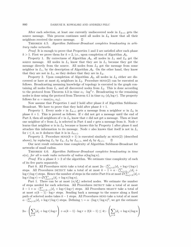
3. Logarithmic broadcasting in BGI networks. In [3] the following classof (n+2)-node networks was defined. Let S be a nonempty subset of 1, . . . , n. Thenetwork GS is a graph (of radius 2) whose nodes are labeled 0, 1, . . . , n+1. The set ofedges of GS is E = (0, i) : 1 ≤ i ≤ n∪(i, n+1) : i ∈ S. Node 0 is the source, andnode n + 1 (the only node in layer 2) is called the sink. We refer to all networks GS

as BGI-n networks (see Figure 3.1).It was claimed in [3] that for any broadcast protocol there is a BGI-n network on

which this protocol works in time Ω(n). However, assuming the model from [3], whichis the same as that from the present paper, the proof in [3] contains the following flaw.Predetermined sets of nodes transmitting in consecutive steps are fixed, and then anetwork is constructed in which some node is not informed during any of these steps.However, during the broadcasting process, the source may potentially acquire someinformation, which it may pass to other nodes, thus modifying the sets of nodestransmitting in subsequent steps. So, in fact, under the considered model, the prooffrom [3] works only for oblivious algorithms, in which sets of nodes transmitting in agiven step must be fixed in advance.


0

1

n+1 L

L

L

S

0

2

Fig. 3.1. BGI-n network GS .

It turns out that not only is the argument from [3] erroneous under the consideredmodel but, in fact, the above result itself is incorrect. (As mentioned in the introduc-tion, the argument and the proof remain correct in a more pessimistic communicationmodel.) Below we give an algorithm that broadcasts in all BGI-n networks in timeO(log n). The technique of selecting one out of many simultaneously transmittingneighbors, which is the main ingredient of this algorithm, will be further used in theconstruction of a much more involved algorithm which guarantees fast broadcastingin arbitrary networks of small radius.

The main idea of our algorithm is to simulate the collision detection capabilityin some nodes of the network. (Recall that collision detection is not available a prioriin our model.) In order to get logarithmic broadcasting for BGI-n networks, it isenough to simulate collision detection at the source. To get sublinear broadcastingin all networks of radius o(log log n), we will need to simulate this capability in manynodes from different levels.

Let A be a set of neighbors of the source (possibly unknown to it), and let i /∈ Abe another neighbor of the source. Suppose that nodes in A want to transmit. Ourgoal is to let the source distinguish whether A has 0, 1, or more than 1 element. Thiscan be done using the following 2-step procedure.

Procedure Echo (i, A).Step 1. Every node in A transmits its label.Step 2. Every node in A ∪ i transmits its label.

There are 3 possible effects of Procedure Echo (i, A) at the source.Case 1. A message is received in Step 1 and no message in Step 2. In this case

the source knows that A has 1 node and knows the label of this unique node.Case 2. No message is received in Step 1 and a message (from i) is received in

Step 2. In this case the source knows that A is empty.Case 3. No message is received in either step. In this case the source knows that

A has at least 2 nodes.Procedure Echo is used to select one node in the set S of nodes connected to the

sink, in a BGI-n network GS . Once such a unique node is selected and transmits, thesink receives the source message, and broadcast is completed. This is done using thefollowing algorithm. (In the original definition of BGI-n networks, nodes are labeledby consecutive numbers 0, 1, . . . , n + 1, but we formulate our algorithm in the moregeneral case, when labels are chosen arbitrarily from a set 0, 1, . . . , r, where r ispolynomial in the number of nodes. Without loss of generality, assume that r is apower of 2.)

Algorithm Binary-Selection-Broadcast. In step 0, the source transmitsthe source message and the lowest label i of its neighbor (in the original definition of


BGI-n networks, i = 1). In step 1, node with label i transmits the source messageand its degree. If this degree is 2 (i ∈ S), the sink receives the message and broadcaststops. Assume that the degree of i is 1.

All remaining steps 2, 3, . . . are divided into segments of length 3. In the first stepof each segment, the source transmits a range R of labels and orders the execution ofProcedure Echo (i, R ∩ S) during the last two steps of the segment. (Notice that allnodes from layer 1 know if they are in R∩S.) In the first segment, R := 1, . . . , r/2.If a range R = x, . . . , y is transmitted in a given segment, the range to transmit inthe next segment is chosen according to the three possible effects of Procedure Echo(i, R ∩ S), described above. In Case 1, the sink is informed and broadcast stops. InCase 2, R := y+1, . . . , y+(y−x+1)/2. In Case 3, R := x, . . . , (y+x−1)/2.

Theorem 3.1. Algorithm Binary-Selection-Broadcast completes broadcasting inany BGI-n network in time O(log n).

Proof. Since the size of R transmitted in the ith segment is r/2i, after at mostlog r ∈ O(log n) steps, the set R ∩ S contains exactly one node, and hence broadcastis completed in time O(log n).

4. Sublinear time broadcasting in networks of radius o(log log n). Inthis section we construct a broadcasting algorithm working in time o(n) on all n-nodenetworks of radius o(log log n). We will use the following results from the literature.The following two theorems assume that nodes know parameters r and d but do notassume any knowledge of the network topology.

Theorem 4.1 (see [14]). Consider a radio network modeled by an arbitrary graph(V,E), where V is a subset of 1, . . . , r. Let A and B be a partition of V such thatall nodes in A have the same message m. Then there exists a protocol working in timeO(min(r, d log(r/d))), which makes message m known to all nodes v ∈ B having atleast one and at most d neighbors in A.

Theorem 4.2 (see [17, 14]). Given a radio network modeled by an arbitrarygraph (V,E), where V is a subset of 1, . . . , r and in which every node has a (possiblydifferent) message, there exists a protocol working in time O(min(r, d2 log r)), uponthe completion of which, every node of degree at most d learns the messages of all itsneighbors.

It should be mentioned that, while the protocols in the above theorems wereobtained in a nonconstructive way, constructive counterparts of both these results(involving polynomial time local computations) are known and yield only slightlyslower protocols. A constructive counterpart of Theorem 4.1 yielding a O(min(r,d · polylog r))-time protocol follows from [20, 27], and a constructive counterpartof Theorem 4.2 yielding a O(min(r, d2 log2 r))-time protocol follows from [21]. Inour algorithm we use protocols from Theorems 4.1 and 4.2, but these constructivecounterparts could be used as well, and our resulting broadcasting algorithm wouldstill work in sublinear time.

The next result refers to radio networks of known topology.Theorem 4.3 (see [10]). Consider a radio network modeled by an arbitrary graph

(V,E), where V is a subset of 1, . . . , r, and assume that all nodes know the topologyof the graph. Let A and B be a partition of V such that all nodes in A have the samemessage m. Then there exists a protocol working in time O(log2 r), which makesmessage m known to all nodes v ∈ B having a neighbor in A.

4.1. Broadcasting in networks of radius 2. We first describe a sublineartime broadcasting algorithm working for all networks of radius 2. More generally, inevery network G, this algorithm informs all nodes in levels 1 and 2 in sublinear time.


L

0

1

v

select

0

0

v

L2

1

i

discovered

newly

nodes

v L2

PART 1

LL1 2

0

0

0

L2i

L1

PART 0

i

newly

discovered

v

L21L

i

newly

informed

node

L21

PART 2

L

node

2< d> d

B

i i

0

y

L L1 2 L1 2

newly

discovered

L2L1

0

0

y

y L2

select

node

PART 4PART 3

L

X

Z

w w

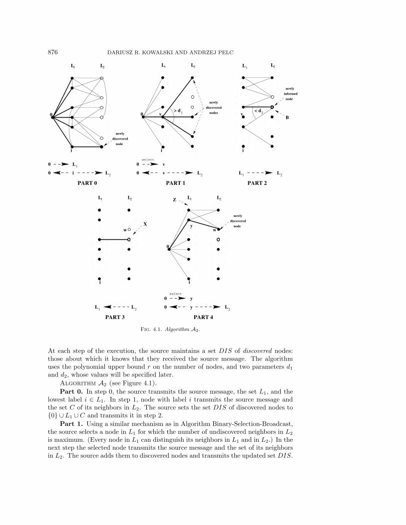
Fig. 4.1. Algorithm A2.

At each step of the execution, the source maintains a set DIS of discovered nodes:those about which it knows that they received the source message. The algorithmuses the polynomial upper bound r on the number of nodes, and two parameters d1

and d2, whose values will be specified later.

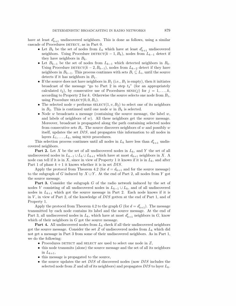
Algorithm A2 (see Figure 4.1).

Part 0. In step 0, the source transmits the source message, the set L1, and thelowest label i ∈ L1. In step 1, node with label i transmits the source message andthe set C of its neighbors in L2. The source sets the set DIS of discovered nodes to0 ∪ L1 ∪ C and transmits it in step 2.

Part 1. Using a similar mechanism as in Algorithm Binary-Selection-Broadcast,the source selects a node in L1 for which the number of undiscovered neighbors in L2

is maximum. (Every node in L1 can distinguish its neighbors in L1 and in L2.) In thenext step the selected node transmits the source message and the set of its neighborsin L2. The source adds them to discovered nodes and transmits the updated set DIS.


This process is repeated until there are no nodes in L1 with more than d1 undiscoveredneighbors in L2.

Part 2. Apply the protocol from Theorem 4.1 (with d = d2) to the subgraph of Ginduced by L1 ∪ B and to the partition (L1, B), where B is the set of undiscoverednodes in L2. This protocol makes the source message known to all undiscovered nodesfrom L2 which have at most d2 neighbors in L1.

Part 3. Let X be the set of all nodes from L2 which received the source mes-sage during Part 2 and have at most d2 neighbors in L1. Apply the protocol fromTheorem 4.2 (for d = d1) to the subgraph of G induced by X ∪ L1. The messagetransmitted by each node contains its label and the source message.

Part 4. All nodes from L1 check if all their neighbors in L2 got the source mes-sage. Nodes selected in Part 1 know that all their neighbors in L2 were informed anddiscovered. Let Z be the set of nodes in L1 which did not get a message in Part 3from some of their undiscovered neighbors in L2. Using a similar mechanism as inAlgorithm Binary-Selection-Broadcast, the source selects one node in Z; then thisnode transmits (alone) the source message and the set of all its neighbors in L2, andthe source adds these neighbors to the set DIS of discovered nodes. After each selec-tion, at least one currently undiscovered node gets the source message. This processcontinues until all nodes in L1 know that all their neighbors in L2 received the sourcemessage.

Theorem 4.4. Algorithm A2 completes broadcasting in any n-node network ofradius 2 in O(n2/3 log n) time.

Proof. Correctness is straightforward. The complexity of the algorithm is esti-mated as follows. Part 0 takes 3 steps. Each selection in Part 1 takes O(log r) stepsand there are at most n/d1 selections; hence the entire Part 1 takes O((n/d1) · log r)steps. In view of Theorem 4.1, Part 2 takes O(d2 ·log r) steps. In view of Theorem 4.2,Part 3 takes O(d2

1 log r) steps. Each selection in Part 4 takes O(log r) steps andthere are at most nd1/d2 selections; hence the entire Part 4 takes O((nd1/d2) · log r)

steps. Taking d1 = 3√n and d2 =

3√n2, this adds up to O(n2/3 log r) = O(n2/3 log n)

steps.

4.2. Extension to arbitrary networks of radius o(log log n). We now de-scribe an algorithm which broadcasts in sublinear time in arbitrary networks of ra-dius o(log log n). The algorithm uses the polynomial upper bound r on the numberof nodes, and parameters dj , d

′j , for j = 2, 3, . . . , whose values will be specified later.

The algorithm is constructed inductively. The construction is local, in the sense thatevery node constructs its part of the algorithm, using some coordination guaranteedby the properties and remarks listed below. After the kth phase of the algorithm,where k is an integer larger than 1, the following properties will be satisfied for somepositive constant α.

Property 1. All nodes from layers Lj , j = 1, . . . , k, know the source message andknow to which layer they belong.

Property 2. For all j = 1, . . . , k, a Procedure send(j), coordinated by the source,can be constructed, which has the following effect: if all nodes in Lj−1 havethe same message m and start at the same time, then all nodes in Lj learnmessage m. (send(1) consists of one step in which the source transmits.)Procedure send(j) lasts at most α · (dj + log r) log r time.

Remarks.1. Let j = 1, . . . , k − 1, and A ⊆ Lj+1 be a set of nodes that want to transmit.

It follows from Property 2 that a Procedure detect(j, A), coordinated by


the source, can be constructed, which enables every node in Lj to distinguishwhether it has 0, 1, or more than 1 neighbor in A. Procedure detect(j, A)works as follows. Starting at a given time step t0, all nodes in A repeattransmission in 1+α ·(dj +log r) log r consecutive time steps. Simultaneously,nodes in Lj−1 perform Procedure send(j).Each node v ∈ Lj detects the number of its neighbors in A similarly as in Pro-cedure Echo. By Property 2, v would get message m, during α·(dj+log r) log rsteps after t0, if nodes from A did not transmit. Hence v decides as fol-lows. If it receives a message from a neighbor not in Lj−1 during Proceduredetect(j, A), it knows that it has exactly one neighbor in A and knows itslabel. Otherwise, two cases are possible. (1) If v receives only messages fromLj−1 during Procedure detect(j, A), then it knows that none of its neigh-bors is in A. (2) If v receives no messages during Procedure detect(j, A),then it knows that at least two of its neighbors are in A.

2. Let j = 0, . . . , k − 1, i ∈ Lj , and let A ⊆ Lj+1 be a subset of neighbors of ithat want to transmit. A Procedure select(j, i, A), coordinated by node i,can be constructed, in which node i selects one element in A. This can bedone in α · log r steps, similarly as in Algorithm Binary-Selection-Broadcast,where node i plays the role of the source.

Algorithm Sublinear-Broadcast. In phase 1 do nothing. In phase 2 performalgorithm A2. Let k > 1. Suppose that Properties 1 and 2 are satisfied after phasek. We describe phase k + 1. The source maintains a set DIS of discovered nodes:these are nodes from Lk−1∪Lk ∪Lk+1 whose labels the source learned in phase k+1.At the beginning of phase k + 1 this set is empty. Each node from Lk appends thenumber k of its layer to all its messages.Description of phase k + 1:

Part 0. The aim of this part is the verification of whether layer Lk is empty ornot. If Lk = ∅, then the radius of the network is D = k − 1 and broadcasting wascompleted at the end of phase k − 1, by Property 1 for k. In this case the sourcesends a stop message. Otherwise, the source sends a message requesting the start ofPart 1. Here is a detailed description of Part 0.

• The source initiates broadcast of the message “start verification in step t,”by consecutive use of Procedures send(j), for j = 1, . . . , k, according toProperty 2 for k. Step t is calculated to guarantee reception of this message byall nodes in Lj , for j = 1, . . . , k, i.e., to guarantee completion of all Proceduressend(j).

• Verification of whether layer Lk is empty starts in step t.– Using Procedure detect(k−1, Lk), nodes from Lk−1 detect if they have

neighbors in Lk.– Let Ak−1 be the set of nodes from Lk−1 which detected neighbors in Lk.

Using Procedure detect(k − 2, Ak−1), nodes from Lk−2 detect if theyhave neighbors in Ak−1. This process continues with sets Ai ⊆ Li, untilthe source detects if it has neighbors in A1.

• If the source does not have neighbors in A1 (i.e., A1 is empty, which meansthat Lk is empty as well), then it initiates broadcast of the message “stop instep t1” (for an appropriately calculated t1), by consecutive use of Proceduressend(j), for j = 1, . . . , k − 1, according to Property 2 for k. Otherwise, amessage requesting the start of Part 1 in an appropriately calculated step issent similarly as above (to all layers Lj for j = 1, . . . , k).

Part 1. The aim of this part is selection of consecutive nodes from Lk which


have at least d′k+1 undiscovered neighbors. This is done as follows, using a similarcascade of Procedures detect, as in Part 0.

• Let Bk be the set of nodes from Lk which have at least d′k+1 undiscoveredneighbors. Using Procedure detect(k − 1, Bk), nodes from Lk−1 detect ifthey have neighbors in Bk.

• Let Bk−1 be the set of nodes from Lk−1 which detected neighbors in Bk.Using Procedure detect(k − 2, Bk−1), nodes from Lk−2 detect if they haveneighbors in Bk−1. This process continues with sets Bi ⊆ Li, until the sourcedetects if it has neighbors in B1.

• If the source does not have neighbors in B1 (i.e., B1 is empty), then it initiatesbroadcast of the message “go to Part 2 in step t2” (for an appropriatelycalculated t2), by consecutive use of Procedures send(j) for j = 1, . . . , k,according to Property 2 for k. Otherwise the source selects one node from B1,using Procedure select(0, 0, B1).

• The selected node v performs select(1, v, B2) to select one of its neighborsin B2. This is continued until one node w in Bk is selected.

• Node w broadcasts a message (containing the source message, the label w,and labels of neighbors of w). All these neighbors get the source message.Moreover, broadcast is propagated along the path containing selected nodesfrom consecutive sets Bi. The source discovers neighbors of w and possibly witself, updates the set DIS, and propagates this information to all nodes inlayers L1, . . . , Lk, using send procedures.

This selection process continues until all nodes in Lk have less than d′k+1 undis-covered neighbors.

Part 2. Let X be the set of all undiscovered nodes in Lk, and Y the set of allundiscovered nodes in Lk−1 ∪Lk ∪Lk+1 which have at most dk+1 neighbors in X. Anode can tell if it is in X, since in view of Property 1 it knows if it is in Lk, and afterPart 1 of phase k + 1 it knows whether it is in set DIS.

Apply the protocol from Theorem 4.2 (for d = dk+1 and for the source message)to the subgraph of G induced by X ∪ Y . At the end of Part 2, all nodes from Y gotthe source message.

Part 3. Consider the subgraph G of the radio network induced by the set ofnodes V consisting of all undiscovered nodes in Lk−1 ∪ Lk, and of all undiscoverednodes in Lk+1 which got the source message in Part 2. Each node knows if it isin V , in view of Part 2, of the knowledge of DIS gotten at the end of Part 1, and ofProperty 1.

Apply the protocol from Theorem 4.2 to the graph G (for d = d′k+1). The messagetransmitted by each node contains its label and the source message. At the end ofPart 3, all undiscovered nodes in Lk, which have at most d′k+1 neighbors in G, knowwhich of their neighbors in G got the source message.

Part 4. All undiscovered nodes from Lk check if all their undiscovered neighborsgot the source message. Consider the set Z of undiscovered nodes from Lk which didnot get a message in Part 3 from some of their undiscovered neighbors. As in Part 1,we do the following:

• Procedures detect and select are used to select one node in Z,• this node transmits (alone) the source message and the set of all its neighbors

in Lk+1,• this message is propagated to the source,• the source updates the set DIS of discovered nodes (now DIS includes the

selected node from Z and all of its neighbors) and propagates DIS to layer Lk.


After each selection, at least one currently undiscovered node in Lk+1 gets thesource message. This process continues until all nodes in Lk know that all theirneighbors received the source message.

Theorem 4.5. Algorithm Sublinear-Broadcast completes broadcasting in arbi-trary radio networks.

Proof. It is enough to prove that Properties 1 and 2 are satisfied after each phasek > 1. First we prove them for k = 2, i.e., upon completion of Algorithm A2.

Property 1. By correctness of Algorithm A2, all nodes in L1 and L2 get thesource message. All nodes in L1 know that they are in L1 because they got themessage directly from the source. All nodes from L2 got the message from someneighbor in L1, by the description of Algorithm A2. On the other hand, they knowthat they are not in L1, so they deduce that they are in L2.

Property 2. Upon completion of Algorithm A2, all nodes in L2 either are dis-covered or have at most d2 neighbors in L2. Procedure send(2) can be executed asfollows. Broadcasting assuming knowledge of topology is executed in the graph con-taining all nodes from L1 and all discovered nodes from L2. This is done accordingto the protocol from Theorem 4.3 in time α1 · log2 r. Broadcasting to the remainingnodes is done using the protocol from Theorem 4.1 in time α2 ·(d2 log r). The propertyfollows for α = max(α1, α2).

Now assume that Properties 1 and 2 hold after phase k of Algorithm Sublinear-Broadcast. We have to prove that they hold after phase k + 1.

Property 1. Every node v in Lk+1 gets a message from a neighbor w in Lk inphase k + 1. This is proved as follows. If v did not get a message until the end ofPart 3, then all neighbors of v in Lk know that v did not get a message. Then at leastone neighbor of v from Lk is selected in Part 4 and v gets a message from it. Node vlearns that neighbor w is in Lk because w knows this by Property 1 after phase k andattaches this information to its message. Node v also knows that itself is not in Li

for i ≤ k, so it deduces that it is in Lk+1.Property 2. Procedure send(k + 1) is executed similarly as send(2) (described

above), by replacing L1 by Lk, L2 by Lk+1, and d2 by dk+1.Our next result estimates time complexity of Algorithm Sublinear-Broadcast for

networks of small radius.Theorem 4.6. Algorithm Sublinear-Broadcast completes broadcasting in time

o(n), for all n-node radio networks of radius o(log log n).Proof. Fix a phase k > 2 of the algorithm. We estimate time complexity of each

of its five parts separately.Part 0. All Procedures send take a total of at most 2α · (

∑j<k(dj + log r) log r)

steps. All Procedures detect take a total of at most k − 1 + α · (∑

j<k−1(dj +log r) log r) steps. Hence the number of steps in the entire Part 0 is at most O(

∑j<k(dj+

log r) log r) = O(∑

j<k(dj + log n) log n).Part 1. There can be at most (n/d′k) selected nodes. We estimate the number

of steps needed for each selection. All Procedures detect take a total of at mostk − 1 + α · (

∑j<k−1(dj + log r) log r) steps. All Procedures select take a total of

at most α(k − 1) · log r steps. Sending back a message to the source along a fixedpath of selected nodes takes k− 1 steps. All Procedures send take a total of at mostα · (

∑j<k(dj + log r) log r) steps. Defining γ = α · (log r/ log n)2, we get the estimate

2α ·

⎛⎝∑

j<k

(dj + log r) log r

⎞⎠ + α(k − 1) · log r + 2(k − 1) ≤ 4γ ·

⎛⎝∑

j<k

(dj + log n) log n

⎞⎠


on the number of steps for each selection. Hence the number of steps in the entirePart 1 is at most 4γ · ((n/d′k) ·

∑j<k(dj + log n) log n) ∈ O((n/d′k) ·

∑j<k(dj +

log n) log n).

Part 2. By Theorem 4.2, this part takes O(d2k log r) = O(d2

k log n) steps.

Part 3. By Theorem 4.2, this part takes O((d′k)2 log r) = O((d′k)

2 log n) steps.

Part 4. Every node in set Z has at most d′k undiscovered neighbors (otherwise itwould be selected in Part 1). Every undiscovered neighbor w of a node v ∈ Z, fromwhich v did not get a message in Part 3, is not in the graph G (defined in Part 3),hence it does not have the source message yet. By the description of Part 2, node whas more than dk neighbors in Lk−1. Hence at most nd′k/dk selections of nodes in Zwill be performed. The number of steps for each node is O(

∑j<k(dj + log n) log n),

similarly as in Part 1. This gives a total of O((nd′k/dk)∑

j<k(dj + log n) log n).

We now choose the following parameters: d1 = log r, d′i+1 = d2i , and di+1 =

(d′i+1)2. This gives the following estimates of the numbers of steps in different parts

of phase k:

Part 0: O(dk−1 log n) ⊆ O(d2k log n).

Part 1: O((n/d′k) · dk−1 log n) ⊆ O((n log n)/dk−1).

Part 2: O(d2k log n).

Part 3: O((d′k)2 log n) ⊆ O(d2

k log n).

Part 4: O((nd′k/dk) · dk−1 log n) ⊆ O((n log n)/dk−1).

Thus the entire phase k lasts O((n/dk−1) · log n + d2k log n) steps.

The last phase of the algorithm run on a radio network of radius D is D + 2 (infact only Part 0 of phase D+2 is executed). The total time of phases k = 3, . . . , D+2

is at most O(d2D+2 log n+ (n log n)/d2) ⊆ O(min(n, (log n)4

D+3+1 + n/ log2 n)). SinceD ∈ o(log log n), we get that this time is o(n). By Theorem 4.4 the time of the firsttwo phases (occupied by execution of Algorithm A2) is O(n2/3 log n), which is o(n)as well. Hence the entire Algorithm Sublinear-Broadcast completes broadcasting intime o(n).

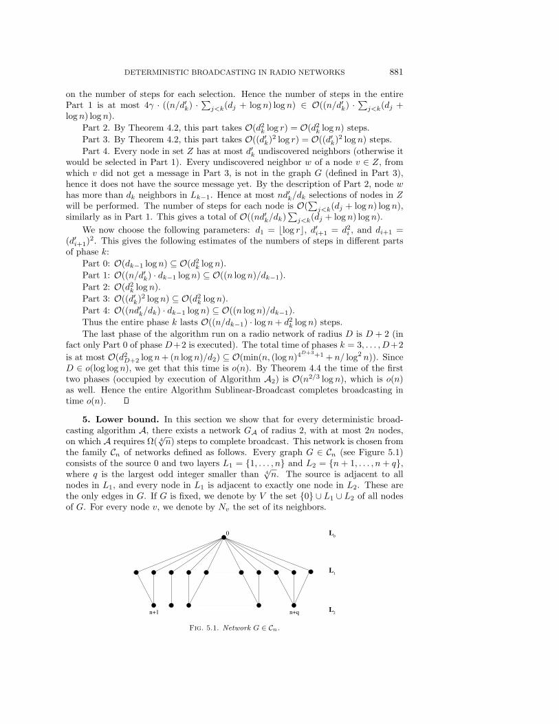
5. Lower bound. In this section we show that for every deterministic broad-casting algorithm A, there exists a network GA of radius 2, with at most 2n nodes,on which A requires Ω( 4

√n) steps to complete broadcast. This network is chosen from

the family Cn of networks defined as follows. Every graph G ∈ Cn (see Figure 5.1)consists of the source 0 and two layers L1 = 1, . . . , n and L2 = n + 1, . . . , n + q,where q is the largest odd integer smaller than 4

√n. The source is adjacent to all

nodes in L1, and every node in L1 is adjacent to exactly one node in L2. These arethe only edges in G. If G is fixed, we denote by V the set 0 ∪ L1 ∪ L2 of all nodesof G. For every node v, we denote by Nv the set of its neighbors.

0

L1

L0

n+1 n+q L2

Fig. 5.1. Network G ∈ Cn.


The idea of the proof is the following. We construct the network step by step,using consecutive steps of the fixed broadcasting algorithm A, and assuming thatparticular nodes got particular messages in given steps. In order to express this, weuse the notion of abstract history of a node, formally defined below. Intuitively, anabstract history of a node v at a given step k consists of a neighborhood of node vand of a sequence of messages received by this node until step k. Since the network isnot yet constructed, neighborhoods of some nodes are not determined by step k, andconsequently it is not yet known which abstract history will become the real one—theone given by algorithm A running on the final network. We can ensure that, if agiven node had some abstract history up to a certain step, then it would behave in agiven way (this is captured by the notion of abstract action function, defined below).Based on that we do the next step of the construction of the network (by determiningneighborhoods of two nodes in layer L2) and simultaneously define abstract historiesof nodes in this step. These abstract histories are defined so as to prevent some nodesin layer L2 of the network from getting any message for a long time. In particular,nodes of L2 whose neighborhood is not yet determined have not gotten the sourcemessage so far.

When the construction is finished, we prove that if the algorithm A runs on theresulting network, then the real histories of all nodes are identical to the abstract(assumed) ones, and consequently some nodes of layer L2 will indeed fail to receivethe source message for Ω( 4

√n) steps.

5.1. Construction. Fix a deterministic broadcasting algorithm A. For thisalgorithm, running on any network, we define the following objects.

Histories and message format. Hk denotes the history of computation ofalgorithm A until the end of step k. This is the set Hk(v) : v ∈ V , where Hk(v) isthe history of computation at node v, until the end of step k. For any v and k, Hk(v)is a sequence of (received) messages (M0(v),M1(v), . . . ,Mk(v)). Messages are definedinductively, as follows. M0(v) is either the triple (∅, ∅, ∅), called the empty message,or the triple (0, N0, source message). Ml(v) (for l = 1, . . . , k) is the empty messageif node v did not get any message in step l. Otherwise, it is a triple consisting of

• the label of node w from which node v received a message in step l,• the set Nw,• history Hl−1(w).

Notice that we restrict attention to messages conveying the entire history of thetransmitter. If a particular protocol requires transmitting specific information, thereceiver can deduce this information from the received history, since programs of allnodes are the same. History Hk(v) containing only empty messages is called theempty history.

Action function and sets of transmitters. Given algorithm A, we denote byπ(v,Nv, Hk−1(v)) the action of node v in step k, if its set of neighbors is Nv and itshistory until the end of step k−1 is Hk−1(v). The values of the function π can be 1 or 0:if the value is 1, node v is sending the message (v,Nv, Hk−1(v)) in step k, otherwiseit is receiving in step k. Under a fixed history Hk−1, we define the set of neighborsof v transmitting in step k as follows: Tk(v) = w ∈ Nv : π(w,Nw, Hk−1(w)) = 1.

We construct a network GA ∈ Cn on which A will work inefficiently. We firstpresent the general overview of the construction and abstracts objects used in it.The construction is by induction on steps of the algorithm A. The set of nodes0∪L1 ∪L2, where L1 = 1, . . . , n and L2 = n+ 1, . . . , n+ q, as well as all edges(0, i) : i = 1, . . . , n are given in the beginning. At each step of the induction some


edges between nodes from L1 and L2 are added. Since at each stage of the constructiononly a part of the network GA is specified, the new edges are constructed usingalgorithm A and some abstract history Hk until this step. Abstract histories at eachnode are parametrized with a nonempty set A representing a possible neighborhoodof v to be constructed in a later step.

Abstract objects. Abstract objects (messages, histories, action function, trans-mitters) are abstract versions of real objects, used in the construction because realones do not exist until the network is completely defined. Let v ∈ V and A ⊆ V . Anabstract history Hk(v,A) of node v, assuming that its neighborhood is A, is definedas a sequence (M0(v,A), M1(v,A), . . . , Mk(v,A)) of abstract messages. M0(v,A) =M0(v), and Ml(v,A), for l > 0, either is the empty message or is of the format(w,B, Hl−1(w,B)), for some w ∈ V and B ⊆ V . We will construct the abstracthistory step by step, in parallel with the construction of network GA. Notice that,in general, abstract histories and abstract messages are not necessarily linked to anyparticular protocol.

We also define the abstract action function π(v,A, Hk−1(v,A)) as an extension ofthe action function π described above. For every v and A, if π(v,A, Hk−1(v,A)) is de-fined, then π(v,A, Hk−1(v,A)) = π(v,A, Hk−1(v,A)). Otherwise, π(v,A, Hk−1(v,A))= 0.

We now define sets of abstract transmitters. First consider a node v with neighbor-hood Nv fixed at the end of step k of the construction, and assume that neighborhoodsNw of all nodes w ∈ Nv are also fixed. Under a fixed abstract history Hk−1, we definethe set of abstract transmitters Tk(v,Nv) = w ∈ Nv : π(w,Nw, Hk−1(w,Nw)) = 1.

Now define sets of abstract transmitters for nodes whose neighborhood is not yetfixed. Suppose that Sk is the set of all nodes j in L2 for which the neighborhood Nj

is not fixed until the end of step k of the construction. Suppose that Rk is the set ofnodes in L1 that do not belong to any fixed neighborhood at the end of step k, i.e.,Rk = L1 \

⋃j∈L2\Sk

Nj . (Additionally, let S0 = L2 and R0 = L1.) For nodes of Rk

and Sk, we define the sets of abstract transmitters in step k as follows:• if v ∈ Rk, then for any j ∈ Sk, Tk(v, 0, j) = 0 if π(0, L1, Hk−1(0, L1)) = 1,

and Tk(v, 0, j) = ∅ otherwise;• if v ∈ Sk and R ⊆ L1, then Tk(v,R) = i ∈ R : π(i, 0, v, Hk−1(i, 0, v)) =

1.Sets Rk and Sk will be defined dynamically in a formal way, during step k of the

construction. We will prove that these formal definitions correspond to the meaningintended above for Rk and Sk, by proving Property 1 of the invariant after step k.

We now describe the inductive construction of the graph GA. We begin by defin-ing the abstract history H0. H0(v,A) = (M0(v,A)), for all nodes v and sets A, whereM0(v,A) is the empty message for all v /∈ L1, and M0(v,A) = (0, L1, source message),for all v ∈ L1.

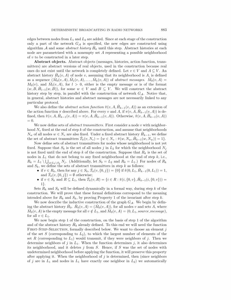
We now begin step 1 of the construction, on the basis of step 1 of the algorithmand of the abstract history H0 already defined. To this end we will need the functionFirst-Step-Selection, formally described below. We want to choose an element jof the set S (corresponding to L2), to which the largest number of elements of theset R (corresponding to L1) would transmit, if they were neighbors of j. Then wedetermine neighbors of j in L1. When the function determines j, it also determinesits neighborhood, and it deletes j from S. Hence, if S was the set of nodes withundetermined neighborhood before applying the function, it will preserve this propertyafter applying it. When the neighborhood of j is determined, then (since neighborsof j are in L1 and nodes in L1 have exactly one neighbor in L2) we automatically


determine neighborhoods of neighbors of j. These neighbors are deleted from R, andhence R preserves the property of containing nodes with undetermined neighborhood,similar to S.

Function First-Step-Selection(R,S).

• Choose some node j ∈ S such that the size of X = T1(j, R) is maximal, andput two nodes from X to Nj (or one if X has one element, or nothing if X isempty); then remove these nodes from R. Remove j from S.

• Modify Nj as follows:if Nj = ∅, then put an arbitrary i ∈ R to Nj and remove i from R;

while there exists a node i ∈ R such that T1(v,R) = i, for some v ∈ Sdo put i into Nj and remove i from R.

• Return (R,S, j,Nj).

Step 1 of the construction. The goal of step 1 of the construction is choosingtwo nodes j′1 and j1 in L2, together with their neighborhoods, in such a way that ifsome node from R1 transmits in the first step of algorithm A, then at least one othernode from R1 transmits as well. This is essential to guarantee the following propertyof abstract history H1(0, L1): no node from L1 with yet undetermined neighborhoodis heard by the source.

0. Initialize R := L1 and S := L2.1. (R,S, j′1, Nj′1

) := First-Step-Selection(R,S);R′

1 := R;(R,S, j1, Nj1) := First-Step-Selection(R,S);R1 := R and S1 := S.

2. We construct the abstract history H1. Its definition corresponds to the def-inition of the “real” history, if neighborhoods are determined. Otherwise,the definition depends on the conditions on nodes and neighborhoods, thecrucial case being the last item of the description below. History H0 is fixed;hence it is enough to define M1(v,A), for all v,A. If π(v,A, H0(v,A)) = 1,then M1(v,A) is the empty message (transmitting nodes should not receivemessages). Otherwise, M1(v,A) is defined as follows:

• Since nodes in (L1 \R1) ∪ (L2 \ S1) have fixed neighborhoods, and alsotheir neighbors have fixed neighborhoods, for each v ∈ (L1\R1)∪(L2\S1)we define M1(v,Nv) = (w,Nw, H0(w,Nw)), if T1(v,Nv) = w, and wedefine M1(v,A) as the empty message in all other cases.

• We define M1(v,A) as the empty message, for all nodes v ∈ S1 and allsets A.

• We define M1(0, L1) as follows:– if |T1(j

′1, Nj′1

) ∪ T1(j1, Nj1)| = 1, then M1(0, L1) is empty;

– if T1(j′1, Nj′1

)∪T1(j1, Nj1) = i, then M1(0, L1) = (i,Ni, H0(i,Ni)).(Note that Ni is already defined at this point.)

M1(0, A) is defined as the empty message, for all A = L1.• For every v ∈ R1 and j ∈ S1, if T1(v, 0, j) = 0, then M1(v, 0, j) =

(0, L1, H0(0, L1)), and M1(v,A) is the empty message in all other cases.

This concludes the first step of the construction.

For any k ≥ 1, the following invariant will be preserved after step k of the con-struction.

Invariant after step k. The following objects are defined:sets Sl ⊆ L2 for l = 0, 1, . . . , k;sets Rl ⊆ L1 for l = 0, 1, . . . , k;


sets R′l ⊆ L1 for l = 1, . . . , k;

nodes j′l , jl such that Sl−1\Sl = j′l , jl and Rl−1\Rl = Nj′l∪Njl for l = 1, . . . , k.

The following properties hold:

1. Neighborhoods of nodes in 0 ∪ (L1 \Rk) ∪ (L2 \ Sk) are defined.2. Histories Hk(v,A) are defined, for all nodes v and all sets A.3. For all sets A, histories Hk(j, A) are empty for all j ∈ Sk, and histories

Hk−1(j, A) are empty for all j ∈ Sk−1 \ Sk.4. For all nodes j ∈ Sk ∪ jk and steps l ≤ k, we have |Tl(j, R

′k)| = 1.

5. For all nodes j ∈ Sk and steps l ≤ k, we have |Tl(j, Rk)| = 1.6. For all nodes j ∈ Sk−1 \ Sk and steps l < k, we have |Tl(j,Nj)| = 1.

We now begin step k + 1 of the construction, on the basis of step k + 1 of thealgorithm and of the invariant after step k. We will need a function similar to FunctionFirst-Step-Selection. Its aim is to choose j ∈ S with the property as before (seethe comment preceding the description of Function First-Step-Selection). Thisis done in the first item of the formal description given below. We also need tomodify the neighborhood of j, so that choices (and elimination) of such nodes inprevious steps of the construction do not yield a single transmitter to nodes with yetundetermined neighborhood. This is required in order to preserve Properties 4, 5,and 6 of the invariant. Modification of the neighborhood is done in the second itemof the following formal description.

Function (k + 1)st-Step-Selection(R,S).

• Choose some node j ∈ S such that the size of X = Tk+1(j, R) is maximaland put two nodes from X to Nj (or one if X has one element, or nothing ifX is empty), then remove these nodes from R. Remove j from S.

• Modify Nj as follows:if Nj = ∅, then put an arbitrary i ∈ R to Nj and remove i from R;

– set stop := 0,– while stop = 0 do

∗ set stop := 1,∗ while there exists a node i ∈ R such that Tl(j

′, R) = i, for somel ≤ k + 1, j′ ∈ Sdo put i into Nj and remove i from R,

∗ while there exists a node i ∈ Nj such that Tl(j,Nj) = i, for somel ≤ kdo find another node i′ ∈ Tl(j, R) (if it exists), put i′ into Nj , andremove i′ from R, set stop := 0;

• Return (R,S, j,Nj).

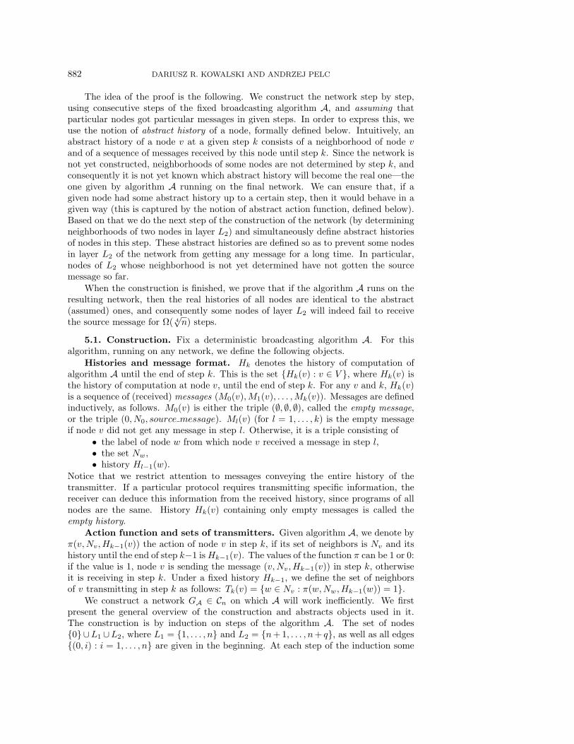
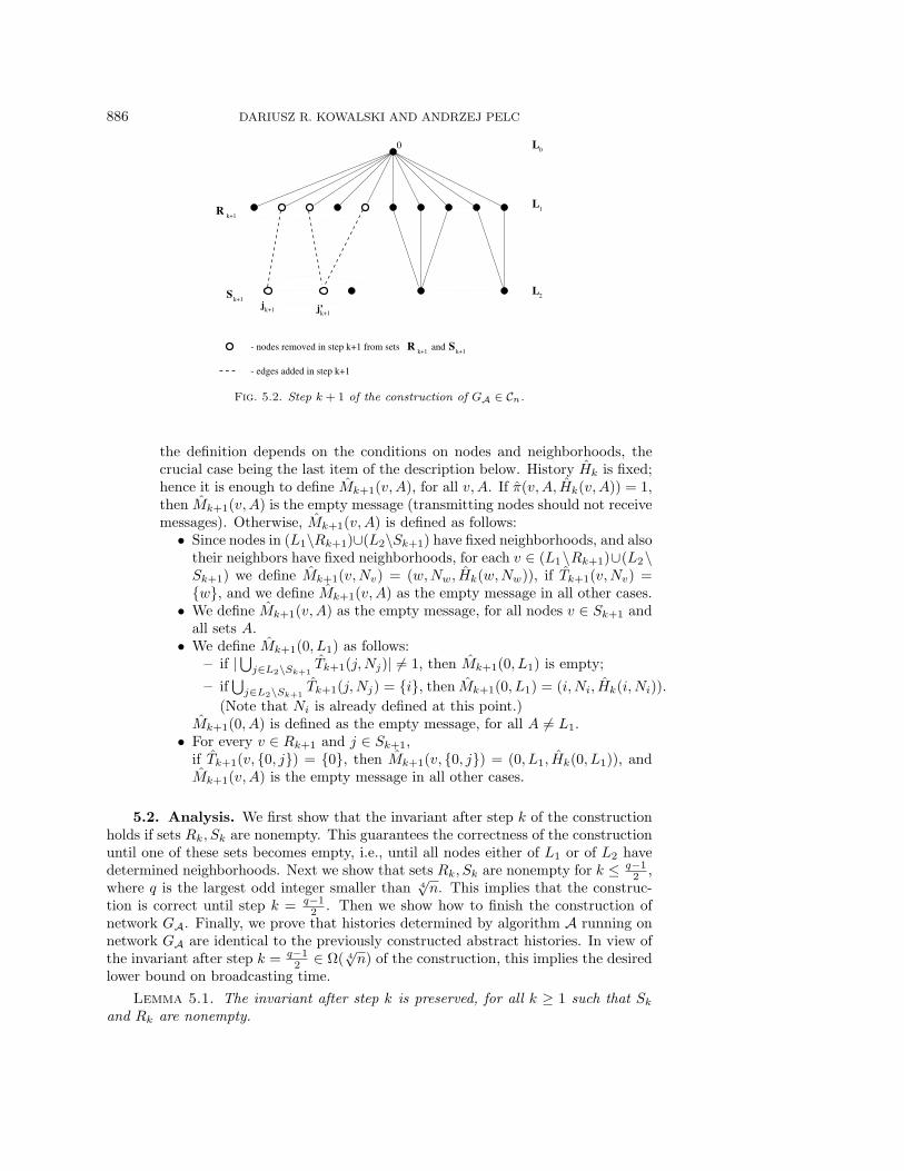
Step (k + 1) of the construction (see Figure 5.2). The goal of step (k + 1) ofthe construction is choosing two nodes, j′k+1, jk+1 ∈ Sk (in L2), together with their

neighborhoods (included in Rk), and defining abstract history Hk+1, so as to satisfythe invariant after step (k + 1) of the construction. Note that we do not initializevariables R and S because their values have been fixed after step k of the construction;indeed, at the beginning of step k + 1, we have R = Rk and S = Sk.

1. (R,S, j′k+1, Nj′k+1) := (k + 1)st-Step-Selection(R,S);

R′k+1 := R;

(R,S, jk+1, Njk+1) := (k + 1)st-Step-Selection(R,S);

Rk+1 := R and Sk+1 := S.2. We construct the abstract history Hk+1. Its definition corresponds to the

definition of the “real” history, if neighborhoods are determined. Otherwise,


j’

- edges added in step k+1

- nodes removed in step k+1 from sets

L

0

1

jk+1 k+1

k+1

k+1

S

R

R k+1 and Sk+1

0 L

2L

Fig. 5.2. Step k + 1 of the construction of GA ∈ Cn.

the definition depends on the conditions on nodes and neighborhoods, thecrucial case being the last item of the description below. History Hk is fixed;hence it is enough to define Mk+1(v,A), for all v,A. If π(v,A, Hk(v,A)) = 1,then Mk+1(v,A) is the empty message (transmitting nodes should not receivemessages). Otherwise, Mk+1(v,A) is defined as follows:

• Since nodes in (L1\Rk+1)∪(L2\Sk+1) have fixed neighborhoods, and alsotheir neighbors have fixed neighborhoods, for each v ∈ (L1\Rk+1)∪(L2\Sk+1) we define Mk+1(v,Nv) = (w,Nw, Hk(w,Nw)), if Tk+1(v,Nv) =w, and we define Mk+1(v,A) as the empty message in all other cases.

• We define Mk+1(v,A) as the empty message, for all nodes v ∈ Sk+1 andall sets A.

• We define Mk+1(0, L1) as follows:– if |

⋃j∈L2\Sk+1

Tk+1(j,Nj)| = 1, then Mk+1(0, L1) is empty;

– if⋃

j∈L2\Sk+1Tk+1(j,Nj) = i, then Mk+1(0, L1) = (i,Ni, Hk(i,Ni)).

(Note that Ni is already defined at this point.)Mk+1(0, A) is defined as the empty message, for all A = L1.

• For every v ∈ Rk+1 and j ∈ Sk+1,if Tk+1(v, 0, j) = 0, then Mk+1(v, 0, j) = (0, L1, Hk(0, L1)), andMk+1(v,A) is the empty message in all other cases.

5.2. Analysis. We first show that the invariant after step k of the constructionholds if sets Rk, Sk are nonempty. This guarantees the correctness of the constructionuntil one of these sets becomes empty, i.e., until all nodes either of L1 or of L2 havedetermined neighborhoods. Next we show that sets Rk, Sk are nonempty for k ≤ q−1

2 ,where q is the largest odd integer smaller than 4

√n. This implies that the construc-

tion is correct until step k = q−12 . Then we show how to finish the construction of

network GA. Finally, we prove that histories determined by algorithm A running onnetwork GA are identical to the previously constructed abstract histories. In view ofthe invariant after step k = q−1

2 ∈ Ω( 4√n) of the construction, this implies the desired

lower bound on broadcasting time.

Lemma 5.1. The invariant after step k is preserved, for all k ≥ 1 such that Sk

and Rk are nonempty.


Proof. The validity of the invariant after step 1 follows from the exit conditions inthe first and second executions of function First-Step-Selection(R,S), in Part 1of step 1 of the construction.

Assume that the invariant holds after step k and that Sk+1 and Rk+1 are nonempty.We prove that it holds after step k + 1.

All required objects are defined by the construction in step k+1, using nonempti-ness of Sk+1 and Rk+1. It remains to prove the six properties.

1. This follows from Property 1 of the invariant after step k and from the con-struction of j′k+1, jk+1, and of their neighborhoods during Part 1 of theconstruction in step k + 1.

2. Hk+1 was defined in Part 2 of step (k + 1) of the construction.3. The fact that Hk+1(v,A) is empty for all nodes v ∈ Sk+1 and all sets A

follows from the assumption in Part 2 of step (k+1) of the construction. Thefact that Hk(j

′k+1, A) and Hk(jk+1, A) are empty (j′k+1, jk+1 are the only

elements of Sk \ Sk+1) follows from Property 3 of the invariant after step k.4. We prove that, for all nodes j ∈ Sk ∪ jk and steps l ≤ k + 1, we have

|Tl(j, R′k+1)| = 1. This follows from the exit conditions of the external and

of the first internal loop in function (k + 1)st-Step-Selection(R,S) (moreprecisely, in the first execution of this function in Part 1 of step (k + 1) ofthe construction). The execution of the external loop ends if and only ifthe value of stop becomes 1, which means that the condition in the secondinternal loop is always false in the last turn of the external loop. Hence thecondition of the first internal loop must be false at the end of the last turn ofthe external loop. This implies |Tl(j, R

′k+1)| = 1, for all nodes j ∈ Sk+1 and

steps l ≤ k + 1.5. We prove that for all nodes j ∈ Sk+1 and steps l ≤ k+1 we have |Tl(j, Rk+1)|

= 1. This follows by an argument similar as above, applied to function(k + 1)st-Step-Selection(R,S) (now we refer to the second execution ofthis function in Part 1 of step (k + 1) of the construction).

6. The property |Tl(j,Nj)| = 1, for all nodes j ∈ Sk \ Sk+1 and steps l < k + 1,follows from the exit condition of the second internal loop in the first andsecond executions of function (k + 1)st-Step-Selection(R,S), in Part 1 ofstep (k+1) of the construction. Observe that the existence of i′ in the secondinternal loop follows from Property 5 of the invariant after step k and from(the just proved) Property 4 of the invariant after step k + 1.

Lemma 5.2. The inductive construction of the network can be carried out for atleast q−1

2 steps, where q is the largest odd integer smaller than 4√n.

Proof. Let k ≤ (q − 1)/2. Sets Sk are decreased by two nodes during one step;hence Sk = ∅, since |S0| = q.

Claim. Sets Rk are decreased by at most 2q3 nodes during one step, at most q3

for each of the chosen nodes j′k, jk.This can be computed by analyzing loops in both executions of function kth-

Step-Selection(R,S) in Part 1 of step k of the construction. Every turn of each ofthe internal loops increases the neighborhood Nj′k

(resp., Njk) by at most one elementand consequently decreases R by at most one element.

Consider the first execution. During the first internal loop, at most kq ≤ q2/2nodes can be added to Nj′k

, since each action makes one set Tl(j, R) empty, wherel ≤ k, and n + 1 ≤ j ≤ n + q. (Since we analyze subsequent executions of the loopin the function, symbol R in the expressions containing R corresponds to the currentvalue of this variable, which changes dynamically. Hence values of these expressions


may also change dynamically.)

During the second internal loop, at most k− 1 ≤ q/2 nodes can be added to Nj′k,

since each action makes one set Tl(j′k, Nj′k

) of size at least 2, where l ≤ k − 1. Theremay be at most k − 1 ≤ q/2 executions of the external loop, since every execution ofthe external loop increases the size |Tl(j

′k, Nj′k

)| to at least 2 for some l ≤ k− 1 while

performing the second internal loop. When |Tl(j′k, Nj′k

)| = 1, for all l ≤ k − 1, the

execution of the external loop stops. Hence Nj′kis bounded by (q2/2+q/2)·(q/2) ≤ q3,

and consequently R is decreased at the rate of at most q3 nodes per step. The same istrue for the second execution. Hence Rk is smaller than Rk−1 by at most 2q3 nodes,which concludes the proof of the claim.

Since q < 4√n, we have Rk = ∅ for all k ≤ (q−1)/2. It follows that the construction

can be carried out for (q − 1)/2 steps.

Using Lemma 5.2, the construction of the network GA can be now concludedas follows. All nodes in R(q−1)/2 are made adjacent to the only node in S(q−1)/2. Itfollows from the construction that GA belongs to the class Cn defined in the beginningof this section.

The histories Hk in consecutive steps of the construction were abstract historiesdefined in order to continue the construction in subsequent steps. The next lemmashows that the actual histories Hk(v) of all nodes v of network GA obtained by runningalgorithm A on this network, are identical to abstract histories Hk(v,Nv).

Lemma 5.3. Let k ≤ (q − 1)/2 be a step of the execution of algorithm A onnetwork GA. Then Hk(v) = Hk(v,Nv), for all nodes v of network GA.

Proof. In the first step of the algorithm execution, the source transmits andall nodes in L1 receive the message. Nodes in L2 receive nothing. Hence H0(v) =H0(v,Nv) by definition of H0.

Note that the definition of abstract history in step 1 of the construction is thesame as that in step k + 1, taken for k = 0. Hence it is not necessary to separatelyanalyze step 1, and we can proceed with the argument by induction, for an arbitraryk.

Assume by induction that Hk(v) = Hk(v,Nv), where k < (q − 1)/2 . We proveHk+1(v) = Hk+1(v,Nv) by showing Mk+1(v) = Mk+1(v,Nv). (Since k+1 ≤ (q−1)/2,the abstract history Hk+1 is well defined, in view of Lemma 5.2.) Observe that,since π is an extension of π and Hk(v) = Hk(v,Nv), we have π(v,Nv, Hk(v,Nv)) =π(v,Nv, Hk(v)). Hence, if π(v,Nv, Hk(v,Nv)) = 1, then v acts as a transmitter instep k + 1, and hence both Mk+1(v) and Mk+1(v,Nv) are empty messages. Thus weassume in the following that π(v,Nv, Hk(v,Nv)) = 0, i.e., that v acts as a receiver.

Case 1. v ∈ (L1 \Rk+1) ∪ (L2 \ Sk+1).

By Property 1 of the invariant after step k + 1 of the construction, v has a fixedneighborhood and all of its neighbors w have fixed neighborhoods. Since Hk(w,Nw) =Hk(w), we get Mk+1(v) = Mk+1(v,Nv).

Case 2. v ∈ Sk+1.

Mk+1(v,Nv) is the empty message by Property 3 of the construction invariantafter step k + 1. Let k′ be the step in which the neighborhood Nv was constructed.Since v ∈ Sk+1, we have k′ > k + 1. By Property 6 of the invariant after step k′ ofthe construction, |Tl(v,Nv)| = 1, for all steps l < k′. In particular, |Tk+1(v,Nv)| = 1.Since Hk(w,Nw) = Hk(w) for all w ∈ Nv, we have Tk+1(v) = Tk+1(v,Nv), and henceTk+1(v) is not a singleton. It follows that Mk+1(v) is the empty message.

Case 3. v = 0.


If j ∈ L2 \ Sk+1, then Tk+1(j,Nj) = Tk+1(j), since Hk(w,Nw) = Hk(w), for

all w ∈ Nj . Hence⋃

j∈L2\Sk+1Tk+1(j,Nj) =

⋃j∈L2\Sk+1

Tk+1(j). We consider threecases.

If |⋃

j∈L2\Sk+1Tk+1(j,Nj)| > 1, then Mk+1(0, L1) is empty. In this case, |Tk+1(0)|

= |⋃

j∈L2Tk+1(j)| > 1 and hence Mk+1(0) is the empty message.

If⋃

j∈L2\Sk+1Tk+1(j,Nj) = i, then Mk+1(0, L1) = (i,Ni, Hk(i,Ni)). In this

case,⋃

j∈L2\Sk+1Tk+1(j) = i. By construction of jk+1, we have Tk+1(jk+1, Rk+1) =

∅, and hence Tk+1(j, Rk+1) = ∅, for all j ∈ Sk+1. Consequently, Tk+1(j) = Tk+1(j,Nj)

⊆ Tk+1(j, Rk+1) = ∅. It follows that Mk+1(0) = (i,Ni, Hk(i)). In view of Hk(i) =Hk(i,Ni), we get Mk+1(0) = Mk+1(0, L1).

If⋃

j∈L2\Sk+1Tk+1(j,Nj) = ∅, then Mk+1(0, L1) is the empty message. In this

case,⋃

j∈L2\Sk+1Tk+1(j) = ∅. The same reasoning as above gives Tk+1(j, Rk+1) = ∅

for all j ∈ Sk+1. Consequently, Mk+1(0) is the empty message.Case 4. v ∈ Rk+1.Since for all j ∈ Sk+1, Hk+1(j,Nj) = Hk+1(j) is the empty history, it follows

that each node v ∈ Rk+1 can receive a message in step k + 1 of A only from node 0,if this node transmits. If node 0 transmits in step k + 1 of A, then v receives themessage Mk+1(v) = (0, L1, Hk(0)). Since Hk(0) = Hk(0, L1), by definition we haveTk+1(v,Nv) = 0. By construction of message Mk+1(v,Nv) we get Mk+1(v,Nv) =(0, L1, Hk(0, L1)). Since Hk(0) = Hk(0, L1), we have Mk+1(v,Nv) = Mk+1(v). Ifnode 0 does not transmit in step k + 1 of A, then Mk+1(v) is empty. Since Hk(0) =Hk(0, L1), by definition we have Tk+1(v,Nv) = ∅. By construction, Mk+1(v,Nv) isthe empty message.

Theorem 5.4. For any deterministic broadcasting algorithm A, there exists anetwork GA of radius 2, with at most 2n nodes, for which this algorithm requires timeΩ( 4

√n).Proof. Network GA constructed above has n + 1 + q ≤ 2n nodes, since q is the

largest odd integer smaller than 4√n. It has radius 2 by construction. Let k = (q−1)/2.

By Lemma 5.2, Sk is nonempty. By Lemma 5.1 and Property 3 of the invariant afterstep k, histories Hk(j,Nj) are empty for all j ∈ Sk. By Lemma 5.3, histories Hk(j)are empty for all j ∈ Sk. Hence no node in Sk receives the source message by step kof algorithm A. It follows that algorithm A requires time Ω( 4

√n) to broadcast on

network GA.Using the above technique we can prove the following more general result.Corollary 5.5. For any deterministic broadcasting algorithm A and any pa-

rameters D ≤ n, there exists an n-node network of radius D, for which this algorithmrequires time Ω(

4√nD3).

6. Conclusion. In this paper we studied deterministic broadcasting time in ra-dio networks whose nodes know only their immediate neighborhood. We presented analgorithm for broadcasting in sublinear time in all networks of radius o(log log n) andwe proved a lower bound Ω( 4

√n) on broadcasting time even in networks of radius 2. In

view of the randomized algorithm from [3] running in expected time O(D log n+log2 n)on all n-node graphs of diameter D, our lower bound proves an exponential gap be-tween time of deterministic and randomized broadcasting in radio networks.

The main problem that remains open is the following. Is there a deterministicbroadcasting algorithm running in sublinear time on all networks with sublinear ra-dius, if nodes know only their immediate neighborhood? If complete knowledge of thenetwork is available, the positive answer follows from [18].


REFERENCES

[1] N. Alon, A. Bar-Noy, N. Linial, and D. Peleg, A lower bound for radio broadcast, J.Comput. System Sci., 43 (1991), pp. 290–298.

[2] B. Awerbuch, A new distributed depth-first-search algorithm, Inform. Process. Lett., 20 (1985),pp. 147–150.

[3] R. Bar-Yehuda, O. Goldreich, and A. Itai, On the time complexity of broadcast in multi-hopradio networks: An exponential gap between determinism and randomization, J. Comput.System Sci., 45 (1992), pp. 104–126.

[4] R. Bar-Yehuda, O. Goldreich, and A. Itai, Errata Regarding “On the time complexity ofbroadcast in radio networks: An exponential gap between determinism and randomization,”http://www.wisdom.weizmann.ac.il/mathusers/oded/p bgi.html, 2002.

[5] S. Basagni, D. Bruschi, and I. Chlamtac, A mobility-transparent deterministic broadcastmechanism for ad hoc networks, IEEE/ACM Trans. on Networking, 7 (1999), pp. 799–807.

[6] S. Basagni, A. D. Myers, and V. R. Syrotiuk, Mobility-independent flooding for real-timemultimedia applications in ad hoc networks, in Proceedings of the IEEE Emerging Tech-nologies Symposium on Wireless Communications & Systems, Richardson, TX, 1999.

[7] D. Bruschi and M. Del Pinto, Lower bounds for the broadcast problem in mobile radionetworks, Distr. Comp., 10 (1997), pp. 129–135.

[8] I. Chlamtac and A. Farago, Making transmission schedule immune to topology changes inmulti-hop packet radio networks, IEEE/ACM Trans. on Networking, 2 (1994), pp. 23–29.

[9] I. Chlamtac, A. Farago, and H. Zhang, Time-spread multiple access (TSMA) protocols formultihop mobile radio networks, IEEE/ACM Trans. on Networking, 5 (1997), pp. 804–812.

[10] I. Chlamtac and O. Weinstein, The wave expansion approach to broadcasting in multihopradio networks, IEEE Trans. on Communications, 39 (1991), pp. 426–433.

[11] B. S. Chlebus, L. Gasieniec, A. Gibbons, A. Pelc, and W. Rytter, Deterministic broad-casting in unknown radio networks, Distributed Computing, 15 (2002), pp. 27–38.

[12] B. S. Chlebus, L. Gasieniec, A. Ostlin, and J. M. Robson, Deterministic radio broadcast-ing, in Proceedings of the 27th International Colloquium on Automata, Languages andProgramming (ICALP’2000), Lecture Notes in Comput. Sci. 1853, Springer-Verlag, Berlin,2000, pp. 717–728.

[13] M. Chrobak, L. Gasieniec, and W. Rytter, Fast broadcasting and gossiping in radio net-works, in Proceedings of the 41st Annual Symposium on Foundations of Computer Science,IEEE Computer Society Press, Redondo Beach, CA, 2000, pp. 575–581.

[14] A. E. F. Clementi, A. Monti, and R. Silvestri, Selective families, superimposed codes, andbroadcasting on unknown radio networks, in Proceedings of the 12th Annual ACM-SIAMSymposium on Discrete Algorithms, SIAM, Philadelphia, 2001, pp. 709–718.

[15] A. Czumaj and W. Rytter, Broadcasting algorithms in radio networks with unknown topology,in Proceedings of the 44th Annual IEEE Symposium on Foundations of Computer Science,Cambridge, MA, 2003, pp. 492–501.

[16] G. De Marco and A. Pelc, Faster broadcasting in unknown radio networks, Inform. Process.Lett., 79 (2001), pp. 53–56.

[17] P. Erdos, P. Frankl, and Z. Furedi, Families of finite sets in which no set is covered by theunion of r others, Israel J. Math., 51 (1985), pp. 79–89.

[18] I. Gaber and Y. Mansour, Broadcast in radio networks, in Proceedings of the 6th AnnualACM-SIAM Symposium on Discrete Algorithms, SIAM, Philadelphia, 1995, pp. 577–585.

[19] F. K. Hwang, The time complexity of deterministic broadcast radio networks, Discrete Appl.Math., 60 (1995), pp. 219–222.

[20] P. Indyk, Explicit constructions of selectors and related combinatorial structures, with applica-tions, in Proceedings of the 13th Annual ACM-SIAM Symposium on Discrete Algorithms,SIAM, Philadelphia, 2002, pp. 697–704.

[21] W. H. Kautz and R. R. C. Singleton, Nonrandom binary superimposed codes, IEEE Trans.on Inform. Theory, 10 (1964), pp. 363–377.

[22] D. Kowalski and A. Pelc, Faster deterministic broadcasting in ad hoc radio networks, inProceedings of the 20th Annual Symposium on Theoretical Aspects of Computer Science,Berlin, Lecture Notes in Comput. Sci. 2607, Springer-Verlag, Berlin, 2003, pp. 109–120.

[23] D. Kowalski and A. Pelc, Broadcasting in undirected ad hoc radio networks, in Proceedingsof the 22nd Annual ACM Symposium on Principles of Distributed Computing, Boston,2003, pp. 73–82.

[24] D. Kowalski and A. Pelc, Time of radio broadcasting: Adaptiveness vs. obliviousness andrandomization vs. determinism, in Proceedings of the 10th Colloquium on Structural In-formation and Communication Complexity, Umea, Sweden, 2003, pp. 195–210.


[25] E. Kushilevitz and Y. Mansour, An Ω(D log(N/D)) lower bound for broadcast in radionetworks, SIAM J. Comput., 27 (1998), pp. 702–712.

[26] D. Peleg, Deterministic Radio Broadcast with No Topological Knowledge, manuscript, 2000.[27] A. Ta-Shma, C. Umans, and D. Zuckerman, Loss-less condensers, unbalanced expanders, and

extractors, in Proceedings of the 33rd Annual ACM Symposium on Theory of Computing,2001, pp. 143–152.

Time of Deterministic Broadcasting in Radio Networks with Local Knowledge

Documents