Time delays, population, and economic development Luca Gori, Luca Guerrini, and Mauro Sodini Citation: Chaos 28, 055909 (2018); doi: 10.1063/1.5024397 View online: https://doi.org/10.1063/1.5024397 View Table of Contents: http://aip.scitation.org/toc/cha/28/5 Published by the American Institute of Physics

Welcome message from author
This document is posted to help you gain knowledge. Please leave a comment to let me know what you think about it! Share it to your friends and learn new things together.
Transcript

Time delays, population, and economic developmentLuca Gori, Luca Guerrini, and Mauro Sodini
Citation: Chaos 28, 055909 (2018); doi: 10.1063/1.5024397View online: https://doi.org/10.1063/1.5024397View Table of Contents: http://aip.scitation.org/toc/cha/28/5Published by the American Institute of Physics

Time delays, population, and economic development
Luca Gori,1,a) Luca Guerrini,2,b) and Mauro Sodini3,c)
1Department of Political Science, University of Genoa, Piazzale E. Brignole, 3a, I–16125 Genoa (GE), Italy2Department of Management, Polytechnic University of Marche, Piazza Martelli 8, 60121 Ancona (AN), Italy3Department of Economics and Management, University of Pisa, Via Cosimo Ridolfi, 10, I–56124 Pisa (PI), Italy
(Received 31 January 2018; accepted 6 April 2018; published online 22 May 2018)
This research develops an augmented Solow model with population dynamics and time delays. The
model produces either a single stationary state or multiple stationary states (able to characterise
different development regimes). The existence of time delays may cause persistent fluctuations in
both economic and demographic variables. In addition, the work identifies in a simple way the
reasons why economics affects demographics and vice versa. Published by AIP Publishing.https://doi.org/10.1063/1.5024397
The coevolution between economic and population
dynamics is a relevant and multidisciplinary objective
studied by economists, mathematicians, demographers,
ecologists, and biologists. The relationships between eco-
nomics and demographics have characterised both
ancient and modern civilisations (Livi-Bacci, 2017) with
phases where cycles were observed in both income and
total population and phases where only one of these two
variables fluctuated. This work aims at clarifying the
links between these two variables by considering a Solow-
like growth model augmented with time delays in tech-
nology and population dynamics. This allows us to
account for a lag from the time the initial investment was
carried out to the time it actually becomes productive
and a lag from the time people were born to the time they
will be economically active (belonging to the working
population) and sexually active. Then, the Solow model
becomes able to explain both the convergence towards a
high equilibrium or a Malthusian trap and long-term
fluctuations. The analysis was performed by combining
stability and bifurcation results of delay differential
equations and simulative exercises.
I. INTRODUCTION
The relationship between economic and population
dynamics is a complex phenomenon that (especially in
recent decades) has drawn the attention of several econo-
mists and demographers (Ehrlich and Lui, 1997; Galor,
2011, 2012; Dalgaard and Strulik, 2013; and Livi-Bacci,
2017). Since the pioneering contributions of Leibenstein
(1957) and Becker (1960) until the more recent works that
gave rise to the Unified Growth Theory (Galor and Weil,
2000; Galor and Moav, 2002; and 2004), which represents
the economic theory of the demographic transition (DT), the
link between economic and demographic variables was
certainly recognised to be essential to explain economic
development, which is a phenomenon related—amongst
other things—to fertility, mortality, migration, the environ-
ment, the distribution of income, and so on. However, it is
often difficult (given the complexity of the models used) to
identify the chain of causation between these variables. In
addition, much of the neoclassical theory of economic
growth is characterised by the results following the (stan-
dard) assumption for which population is allowed to grow
without bounds [for example, the version of the Ramsey
model popularised by Barro and Sala-i-Martin (2003)],
although this is at odds with the historical pattern of the DT.
In fact, the course of total population (that depends on fertil-
ity and mortality rates) has experienced phases of stagnation
(first stage of the DT), growth (second, third, and fourth
stages), and a new phase of stagnation or even decline (fifth
stage). This last phase is due to the fact that mortality rates
worldwide are estimated to remain low, whereas fertility
rates will tend to follow a decreasing trajectory landing on
below-replacement values (Fig. 1).
As is known, the dynamics of an isolated population is
often described by a logistic (differential) equation charac-
terised by a carrying capacity representing the state to which
the population tends in the long term, that is, the maximum
number of agents that can be sustained by the environment.
Certainly, economic development can affect the carrying
capacity of human population (which is driven by technolog-
ical changes in a broad sense or by the accumulation of phys-
ical capital and the accumulation of human capital). From an
economic point of view, although it does not consider opti-
mising agents—as instead is usual in growth models with
and without demographic variables—the pioneering contri-
bution of Solow (1956) represents a paradigm able to
describe from both theoretical and empirical points of view
the long-term behaviours of countries. In this regard, we
recall the different (augmented) versions of the Solow model
developed over the decades that include the contribution of
Mankiw et al. (1992) employing physical and human capital
(as well as the subsequent empirical literature that originated
from it) and the contribution of Brock and Scott Taylor
(2010), formerly known as the Green Solow model, where
the Solow set up is used to study environmental issues.
a)Author to whom correspondence should be addressed: [email protected]
or [email protected]. Tel.: þ39 010 209 95 03. Fax: þ39 010 209
55 36.b)E-mail: [email protected]. Tel.: þ39 071 22 07 055.c)E-mail: [email protected]. Tel.: þ39 050 22 16 234. Fax: þ39 050 22
10 603.
1054-1500/2018/28(5)/055909/9/$30.00 Published by AIP Publishing.28, 055909-1
CHAOS 28, 055909 (2018)

Recently, in two similar works, Cai (2010) and Cai (2012)
augmented Solow by considering that total population
evolves according to the logistic law with an endogenous
carrying capacity positively correlated with the accumulation
of physical capital. He studied the dynamics of the resulting
system described by two ordinary differential equations that
can generate either a globally attracting stationary state or
three stationary states (two of which are attracting). The for-
mer case resembles Solow (1956) allowing to explain the
standard convergence process of countries towards the same
long-term equilibrium. The latter case instead is useful for
explaining the emergence of a Malthusian trap. Therefore,
converging towards an under-development regime, where
income and total population are low, or a development
regime, where income and total population are high, depends
on the initial conditions (history matters).
A feature that, however, does not emerge in all the
works cited above is represented by the possibility of captur-
ing and describing (persistent) economic and demographic
fluctuations, as instead was observed in some empirical
works (Doepke et al., 2015 and Jones and Schoonbroodt,
2016). In particular, income fluctuations are a long-term phe-
nomenon involving both advanced and developing countries.
Two relevant (implicit) assumptions of this kind of models
are that investments in physical capital become immediately
productive (there is no lag between the investment in new
capital stock and the time it is used in the production pro-
cess), and the entire population can immediately give birth
to children that are in turn immediately employed in a full
employment setting. Some works in the literature have
shown how the introduction of time delays in this framework
can actually generate cycles. In particular, by considering an
otherwise standard Solow model with constant population,
Zak (1999) showed that the introduction of a time-to-build
technology (that is, there are gestation lags in the investment
process) is able to generate fluctuations (business cycles and
persistent fluctuations). From a mathematical point of view,
it is well known that the delayed logistic equation can
undergo a Hopf bifurcation and generate attracting cycles
[see Banks (1994) for details and applications in biology and
demography]. Differently, Fanti and Manfredi (2003) intro-
duced an age structure captured by distributed time delays in
a Solow model where population (that was assumed to grow
indefinitely) is endogenous and depends on the production
activity. They showed that a demographically founded for-
mulation of the total population may actually cause eco-
nomic cycles.
The present research enters the debate about economic
and demographic cycles in neoclassical growth models by
augmenting Cai (2010) with a time-to-build technology and
also assuming the existence of a delay from the time people
were born to the time they will be economically active
(belonging to the working population) and sexually active.
Under these assumptions, the Solow model becomes able to
identify how population cycles may cause economic cycles
or vice versa. The work also provides an analysis of the
interactions between cycles generated independently by the
two equations of the system (i.e., when there is a one-way
effect of capital dynamics on population dynamics or vice
versa) as well as when there exists a double feedback
between capital dynamics and population dynamics. This
result is important as it helps in clarifying some transmission
mechanisms between economic and demographic variables
that are often difficult to identify in growth models belonging
to the Unified Growth Theory because of the complexity of
the mixture of influences that demographics and economics
have in this class of models.
The rest of the work proceeds as follows: Section II
builds on the model with fixed delays. Sections III and IV
provide analytical results on the existence and stability of the
FIG. 1. Demographic transition. Reproduced with permission from M. Roser and E. Ortiz-Ospina, “World Population Growth,” 2018, see https://ourworldinda-
ta.org/world-population-growth. Copyright 2018 Creative Commons License (Roser and Ortiz-Ospina, 2018).
055909-2 Gori, Guerrini, and Sodini Chaos 28, 055909 (2018)

stationary state equilibria in some particular cases. Section V
introduces the technique of the stability crossing curves
developed by Lin and Wang (2012) to analyse the local sta-
bility properties of the dynamic system. In addition, it pro-
vides some insights (through simulative exercises) on model
dynamics when the equilibria turn out to be unstable. Section
VI outlines the conclusions.
II. THE MODEL
In a recent work, Cai (2010) has studied a Solow-type
growth model augmented with carrying capacity of human
population, which is assumed to depend on capital accumula-
tion. Capital accumulation in fact can be considered as a
proxy of economic growth and development that can move
the carrying capacity forward. This has allowed the author to
overcome the standard assumption of the growth literature
for which population is assumed to grow without bounds
( _L=L ¼ n > 0), which is, however, not empirically well sup-
ported (see the Introduction for a discussion on this issue).
His model is summarised here in system (1)
_K ¼ sAKaL1�a � dK;
_L ¼ cL 1� L
gðKÞ
� �;
8<: (1)
where K is capital, L denotes s 2 (0, 1) is the fixed saving rate,
A> 0 is the exogenous total factor productivity, a 2 (0, 1) is
the output elasticity of capital, d 2 (0, 1) is the depreciation
rate, and c> 0 measures the growth coefficient of the popula-
tion. Function g represents (a logistic-type) capital-dependent
carrying capacity for the population and it is specified in the
following way:
gðKÞ ¼�L
1þ ð�L=L0 � 1Þe�cK; (2)
where L0 is the initial population, �L > L0 is the final carrying
capacity, and c> 0 is the growth coefficient of the carrying
capacity. The first expression of system (1) is the standard
equation of Solow (1956) that drives capital accumulation
over time, which employs a Cobb-Douglas production
function
Y ¼ AKaL1�a: (3)
The second equation instead describes the dynamics of
human population through a modified logistic equation,
which comes from assuming the population growth rate _L=Lbe dependent negatively on the size of the population (as is
standard in biological models) and positively on the level of
capital accumulation. This last assumption tells us that the
constraint given by the natural carrying capacity is relaxed
by technological changes in a broad sense.
The augmented Solow model of Cai (2010) allows to
have a theoretical framework able to explain the existence of
long-term stationary states representing two relevant para-
digms, that is, sustained development on one hand and
Malthusian trap on the other hand. However, the model of
Cai cannot explain some features that are instead relevant in
growth models that explicitly include demographic variables.
In order to overcome this lacuna, we have revisited Cai
(2010) by assuming the existence of a time-to-build technol-
ogy with respect to which the use of capital in production
requires time. This implies that investments can effectively
be employed by the existing technology as a capital input in
production only with a time delay s1� 0 (Zak, 1999). In
addition, there exists a delay s2� 0 from the time people
were born to the time they will become economically active
(belonging to the working population) and sexually active.
Then, the growth rate of population _L=L depends on both the
capital stock currently used in production (which was
installed at time t – s1) and economically and sexually active
individuals (born at time t – s2). As will be shown later in
this article, this version of the (augmented) Solow model
with endogenous population and time delays will allow
explaining economic development and persistent fluctua-
tions. It is also able to identify the chain of causation and the
interplay between economic and demographic variables.
Given the assumptions discussed above, system (1)
modifies to become the following:
_K ¼ sAKas1
L1�as2� dKs1
;
_L ¼ cL 1� Ls2
gðKs1Þ
� �;
8>><>>: (4)
where Ks1:¼ Kðt� s1Þ and Ls2
:¼ Lðt� s2Þ.Equilibria or steady states of system (4) coincide with
the corresponding steady states for the case of zero delays.
From Cai (2010), we know that there exist either one or three
non-trivial equilibria (K*, L*) such that
sAðK�Þa�1ðL�Þ1�a ¼ d and gðK�Þ ¼ L�:
As regards the model without delays (s1¼ s2¼ 0), it is easy
to check that when the steady state equilibrium is unique it is
globally asymptotically stable. This implies that a generic
trajectory generated by any positive couples (K, L) of initial
conditions will converge towards the steady state [this is in
line with the stylised fact of Solow’s convergence, as pointed
out in Mankiw et al. (1992)]. Differently, when there exist
three steady states ðK�1 ; L�1Þ; ðK�2 ; L�2Þ, and ðK�3 ; L�3Þ such that
K�1 < K�2 < K�3 and L�1 < L�2 < L�3, the first and the third equi-
libriums are attracting, whereas the second one is a saddle
whose stable manifold separates the basins of attraction of
the two attractors. In this case, the model is able to describe
the coexistence of a high equilibrium capturing the paradigm
of developed countries and a low equilibrium capturing the
paradigm of developing or under-developed countries
(Malthusian trap). Converging towards ðK�1 ; L�1Þ or ðK�3 ; L�3Þis a matter of initial conditions. This result is in line with
empirical evidence about the existence of multiple growth
paths and different convergence groups of countries with dis-
tinct values of income and population growth rates (Palivos,
1995).
In order to study the stability of equilibria of system (4),
we consider the characteristic equation of the linearisation of
(4) at a generic equilibrium (K*, L*) and get
055909-3 Gori, Guerrini, and Sodini Chaos 28, 055909 (2018)

k2 þ ake�ks1 þ cke�ks2 þ acð1�MiÞe�kðs1þs2Þ ¼ 0; (5)
where
a¼ð1�aÞd>0; Mi¼g0KðK�i ÞK�iL�i>0; with i¼ 1;2;3f g: (6)
In the case of no delays (s1¼ 0 and s2¼ 0), Cai (2010)
(Theorem 2, p. 3466) showed that a positive equilibrium
point (K*, L*) of system (4) is asymptotically stable if Mi< 1
(it is a sink), it is unstable if Mi> 1 (it is a saddle), and
nonhyperbolic if Mi¼ 1. In what follows, we assume that
Mi 6¼ 1.
III. CASE s1 5 0, s2 > 0
The characteristic equation (5) becomes
k2 þ akþ acð1�MiÞ þ ck½ �e�ks2 ¼ 0: (7)
We first note that Eq. (7) has no zero root being Mi 6¼ 1. Let
k¼ ix (x> 0) be a root of (7). Then, plugging it into (7),
and separating the real and the imaginary parts, yields
x2 ¼ acð1�MiÞ cos xs2 þ cx sin xs2;
ax ¼ �cx cos xs2 þ acð1�MiÞ sin xs2: (8)
Squaring both sides and adding them up lead to the following
polynomial equation in x2:
x4 þ a2 � c2� �
x2 � acð1�MiÞ½ �2 ¼ 0: (9)
It is clear that Eq. (9) has a positive root xþ. Furthermore,
solving Eq. (8) for s2 gives
sin xs2 ¼1þ a2ð1�MiÞ� �
x
cx2 þ a2cð1�MiÞ2;
cos xs2 ¼ �aMix2
cx2 þ a2cð1�MiÞ2:
Hence, we can derive the values of s2 at which there exists
the root ixþ of (7).
In conclusion, we have the following result.
Lemma 1. Let a and Mi be defined as in (6). There existsa sequence of positive numbers sðþÞ2;j ðj ¼ 0; 1; 2;…Þ suchthat 0 < sðþÞ2;0 < sðþÞ2;1 < � � � < sðþÞ2;j < � � �, and (7) has a pairof purely imaginary roots 6ixþ when s2 ¼ sðþÞ2;j , where
xþ ¼
ffiffiffiffiffiffiffiffiffiffiffiffiffiffiffiffiffiffiffiffiffiffiffiffiffiffiffiffiffiffiffiffiffiffiffiffiffiffiffiffiffiffiffiffiffiffiffiffiffiffiffiffiffiffiffiffiffiffiffiffiffiffiffiffiffiffiffiffiffiffiffiffiffiffiffiffiffiffiffiffiffiffiffiffiffiffiffi� a2 � c2ð Þ þ
ffiffiffiffiffiffiffiffiffiffiffiffiffiffiffiffiffiffiffiffiffiffiffiffiffiffiffiffiffiffiffiffiffiffiffiffiffiffiffiffiffiffiffiffiffiffiffiffiffiffiffiffiffiffiffia2 � c2ð Þ2 þ 4 acð1�MiÞ½ �2
q2
vuut;
and
sðþÞ2;j ¼
1
xþcos�1 � aMix2
cx2 þ a2cð1�MiÞ2
( )þ 2jp
xþ; if 1þ a2ð1�MiÞ � 0;
2ðjþ 1Þpxþ
� 1
xþcos�1 � aMix2
cx2 þ a2cð1�MiÞ2
( ); if 1þ a2ð1�MiÞ < 0:
8>>>>><>>>>>:
(10)
Let k(s2) be the root of (7) such that
ReðsðþÞ2;j Þ ¼ 0; ImðsðþÞ2;j Þ ¼ xþ. The variation direction of its
real part with respect to the time delay s2 can be studied
through the sign of ½dðRekÞ=ds2�s2¼sðþÞ2;j
. The next result
shows that each crossing of the roots through the imaginary
axis in the complex plane occurs from left to right
Proposition 2. k¼6ixþ are simple roots of (7) ats2 ¼ sðþÞ2;j and
dðRekÞds2
� �s2¼sðþÞ
2;j
> 0:
Proof. Differentiating Eq. (7) with respect to s2, we get
2kþ aþ ce�ks2 � acð1�MiÞ þ ck½ �s2e�ks2 dk
ds2
� �
¼ acð1�MiÞ þ ck½ �e�ks2 : (11)
Notice that ixþ must be a simple root of (7), otherwise, from
(11), ½acð1�MiÞ þ cixþ�e�ixþsðþÞ2;j ¼ 0, i.e., the absurd
xþ¼ 0. Then, we have
dkds2
� ��1
¼ ð2kþ aÞeks2 þ cacð1�MiÞ þ ck
� s2
k;
which implies
signdðRekÞ
ds2
� �k¼ixþ
¼ sign Redkds2
� ��1" #
k¼ixþ
¼ sign c2 � a2 þ 2x2þ
¼ sign
ffiffiffiffiffiffiffiffiffiffiffiffiffiffiffiffiffiffiffiffiffiffiffiffiffiffiffiffiffiffiffiffiffiffiffiffiffiffiffiffiffiffiffiffiffiffiffiffiffiffiffiffiffiffiffia2 � c2ð Þ2 þ 4 acð1�MiÞ½ �2
q �:
This completes the proof. �
055909-4 Gori, Guerrini, and Sodini Chaos 28, 055909 (2018)

Based on the above transversality condition and the
Hopf bifurcation theorem, one has the following results.
Theorem 3. Let sðþÞ2;0 be defined as in (10).
(1) If Mi > 1, then system (4) is unstable for any given timedelay s2.
(2) If Mi < 1, then there exists exactly one critical time delaysðþÞ2;0 > 0 such that the system remains locally asymptoti-cally stable when 0 � s2 < sðþÞ2;0 and becomes unstablewhen s2 > sðþÞ2;0 . System (4) undergoes a Hopf bifurcationat ðK�; L�Þ for s2 ¼ sðþÞ2;0 .
IV. CASE s1 > 0, s2 FIXED
We now let s2 be fixed at a non-negative given value
and assume s1 be a bifurcation parameter. Let k¼ ix (x> 0)
be a root of (5), i.e.,
�x2 þ aixe�ixs1 þ cixe�ixs2 þ acð1�MiÞe�ixðs1þs2Þ ¼ 0:
Separating real and imaginary parts leads to
�x2þcxsinxs2¼ acð1�MiÞsinxs2�ax½ �Þ�sinxs1�acð1�MiÞcosxs1 cosxs2;
(12)
cx cos xs2 ¼ acð1�MiÞ sin xs2 � ax½ �Þ cos xs1
þ acð1�MiÞ sin xs1 cos xs2: (13)
Equations (12) and (13) are simplified to give
GðxÞ ¼ x4 þ ð�2c sin xs2Þx3 þ ðc2 � a2Þx2
þ 2a2cð1�MiÞ sin xs2
� �x� a2c2ð1�MiÞ2 ¼ 0:
(14)
Noticing that G(þ1)¼þ1 and Gð0Þ¼�a2c2ð1�MiÞ2 < 0,
we can conclude that Eq. (14) has at least one positive solution.
Let x1, x2, …, xN denote the positive roots of (14). For every
xk (k¼1, 2, …, N), solving Eqs. (12) and (13) for s1, one can
determine the corresponding critical value sðjÞ1;k (j¼0, 1, 2, …) of
s1. By setting
s�1 ¼ min sðjÞ1;k; k ¼ 1; 2;…;N; j ¼ 0; 1; 2;…n o
; (15)
then Eq. (5) has a pair of purely imaginary roots k¼6ix* at
s1 ¼ s�1. To verify the transversality condition of Hopf bifur-
cation, taking the derivative with respect to s1 in (5), it is
obtained that
signdðRekÞ
ds1
� �s1¼s�
1
¼ sign Redkds1
� ��1" #
s1¼s�1
¼ sign Hðx�; s�1� �
Þ;
with
Hðx�; s�1Þ ¼ ABþ CD; (16)
where
A ¼ �ax�s�1 sin x�s�1 þ a cos x�s�1þ �cx�s2 þ acð1�MiÞðs�1 þ s2Þ sin x�s�1� �
sin x�s2
þ c� acð1�MiÞðs�1 þ s2Þ cos x�s�1� �
cos x�s2;
B ¼ acð1�MiÞ sin x�s2 � ax�½ �cos x�s�1þ acð1�MiÞ sin x�s�1 cos x�s2gx�;
C ¼ x�ðas�1 cos x�s�1 � 2Þ þ a sin x�s�1þ cx�s2 � acð1�MiÞðs�1 þ s2Þ sin x�s�1� �
cos x�s2
þ c� acð1�MiÞðs�1 þ s2Þ cos x�s�1� �
sin x�s2;
D ¼ acð1�MiÞ sin x�s2 � ax�½ �sin x�s�1� acð1�MiÞ cos x�s�1 cos x�s2gx�:
A positive sign of Hðx�; s�1Þ corresponds to crossings of
the imaginary axis from right to left as s1 increases, while a
negative sign of Hðx�; s�1Þ means crossings of the imaginary
axis from left to right.
According to the previous analysis, we get the following
conclusions.
Theorem 4. Let GðxÞ; s�1 and Hðx�; s�1Þ be defined as in(14), (15), and (16), respectively.
(1) If G(x) has only one simple positive root, then(a) if system (4) without time delays is locally asymp-
totically stable (resp. unstable) and Hðx�; s�1Þ < 0
(resp. Hðx�; s�1Þ > 0Þ, then it remains stable (resp.unstable) for s1 � 0;
(b) if system (4) without time delays is locally asymp-totically stable (resp. unstable) and Hðx�; s�1Þ > 0
(resp. Hðx�; s�1Þ < 0Þ, then system (4) is stable fors1 2 ½0; s�1Þ and the equilibrium point (K*, L*) loses(resp. acquires) its stability via a Hopf bifurcationat s1 ¼ s�1.
(2) If G(x) has at least two positive roots and these roots aresimple, then a finite number of stability switches may occuras the time delay s1 increases from zero to the positive infin-ity, with the occurrence of a Hopf bifurcation at eachswitch.
V. STABILITY CROSSING CURVES AND SIMULATIVEEXERCISES
In order to characterise the stability properties of the
equilibria ðK�1 ; L�1Þ and ðK�3 ; L�3Þ, we will use the stability
crossing curves technique allowing to geometrically analyse
the problem in the plane (s1, s2). By following Lin and
Wang (2012), we now introduce the polynomials
P0ðkÞ :¼ k2; (17)
P1ðkÞ :¼ ak; (18)
P2ðkÞ :¼ ck; (19)
P3ðkÞ :¼ acð1�MiÞ; (20)
and the function
055909-5 Gori, Guerrini, and Sodini Chaos 28, 055909 (2018)
ZðxÞ : ¼ jP0ðixÞj2 þ jP1ðixÞj2 � jP2ðixÞj2 � jP3ðixÞj2� �2
� 4 L1ðxÞ2 þ L2ðxÞ2� �
;
defined on W :¼ x 2 R : x > 0f g, where
L1ðxÞ :¼ ReðP2ðixÞP3ðixÞÞ � ReðP0ðixÞP1ðixÞÞ;
and
L2ðxÞ :¼ ReðP1ðixÞP3ðixÞÞ � ReðP0ðixÞP2ðixÞÞ:
As assumptions of Lin and Wang (2012, p. 521)
ðiÞ degðP0ðkÞÞ ¼ 2 � maxdeg P1ðkÞ;P2ðkÞ;P3ðkÞ
¼ 1, (ii)P0ð0Þ þ P1ð0Þ þ P2ð0Þ þ P3ð0Þ ¼ acð1�MiÞ 6¼ 0, (iii)P0(k), P1(k), P2(k), and P3(k) are coprime polynomials and (iv)
limk!1
����P1ðkÞP0ðkÞ
����þ����P2ðkÞP0ðkÞ
����þ����P3ðkÞP0ðkÞ
���� !
¼ 0 < 1
are fulfilled, it is possible to identify the x-intervals such
that Z(x) is negative and the corresponding stability crossing
curves. In our case, Z(x) reads as follows:
ZðxÞ :¼x8�2ða2þc2Þx6þ c4�2a2ðMiþ2Mi�2Þc2þa4� �
�x4�2a2c2ð1�MiÞ2ða2þc2Þx2þa4c4ð1�MiÞ4:(21)
Given the particular form of polynomial (21), it can be
factorized to obtain analytical solutions (as a function of the
state variables K and L that can be obtained only numeri-
cally) of Z(x)< 0 on set W [see, for instance, Pecora and
Sodini (2018)]. In what follows, we will consider two differ-
ent parameter sets for which there exists either a unique
steady-state equilibrium or multiple steady-state equilibria.
A. Unique steady-state equilibrium
By using the parameter values s¼ 0.3, A¼ 1, a¼ 0.35,
d¼ 0.32, L0¼ 1, �L ¼ 1:2, and c¼ 3.1, it is possible to verify
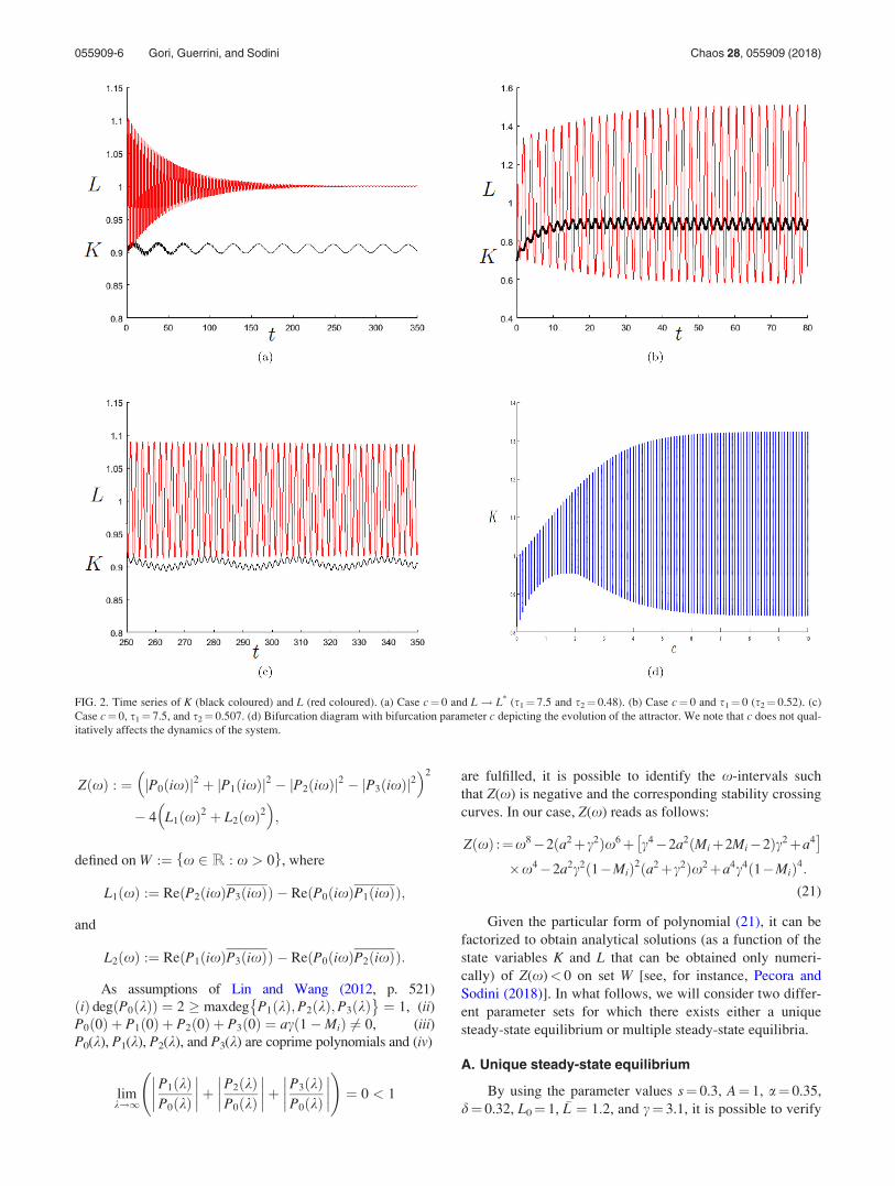
FIG. 2. Time series of K (black coloured) and L (red coloured). (a) Case c¼ 0 and L! L* (s1¼ 7.5 and s2¼ 0.48). (b) Case c¼ 0 and s1¼ 0 (s2¼ 0.52). (c)
Case c¼ 0, s1¼ 7.5, and s2¼ 0.507. (d) Bifurcation diagram with bifurcation parameter c depicting the evolution of the attractor. We note that c does not qual-
itatively affects the dynamics of the system.
055909-6 Gori, Guerrini, and Sodini Chaos 28, 055909 (2018)
that the system admits a unique stationary state. In particular,
as can be seen by looking at Eq. (4), the value of L enters the
dynamics of capital accumulation through the production
function given by Eq. (3), whereas the value of K enters the
dynamics of total population through function g specified in
(2). We will now present numerical examples by distinguish-
ing between two cases, that is, c¼ 0 and c> 0 in (2). When
c¼ 0, the equilibrium is (K*, L*)¼ (0.9054, 1) and there are
no links between the dynamics of total population and
the capital stock. Then, if L converges to its
stationary state value L*, the dynamics of capital are driven
by _K ¼ sAKas1ðL�Þ1�a � dKs1
so that fluctuations in K can be
obtained only for technological reasons [see Zak (1999) for a
stability analysis of this case]. This is shown in Panel (a) of
Fig. 2 by setting s1¼ 7.5 and s2¼ 0.48. When c¼ 0 and
s1¼ 0, the opposite result holds so that fluctuations in K are
caused by fluctuations in L [see Banks (1994) for a stability
analysis of this case]. This is shown in Panel (b) of Fig. 2
plotted for s2¼ 0.52. By assuming now that both delays are
positive and fixed at sufficiently large values (s1¼ 7.5 and
s2¼ 0.507), the fixed point of the system is unstable (This
result can be ascertained through the use of the stability
crossing curves technique.) and it is possible to identify a
mutual relationship between the two dynamics. This phe-
nomenon is well illustrated by the behaviour of the dynamics
of K (black coloured) in Panel (c) of Fig. 2, where short-term
fluctuations (almost two years) sum up to long-term fluctua-
tions (almost thirty years). Finally, by starting from this last
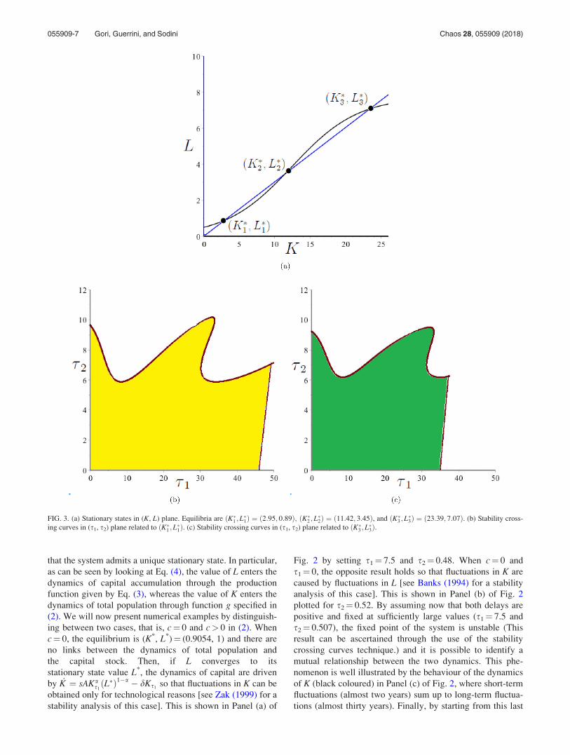
FIG. 3. (a) Stationary states in (K, L) plane. Equilibria are ðK�1 ;L�1Þ ¼ ð2:95; 0:89Þ; ðK�2 ; L�2Þ ¼ ð11:42; 3:45Þ, and ðK�3 ;L�3Þ ¼ ð23:39; 7:07Þ. (b) Stability cross-
ing curves in (s1, s2) plane related to ðK�1 ;L�1Þ. (c) Stability crossing curves in (s1, s2) plane related to ðK�3 ; L�3Þ.
055909-7 Gori, Guerrini, and Sodini Chaos 28, 055909 (2018)
case, the bifurcation diagram with bifurcation parameter cplotted in Panel (d) shows how the feedback given by the
production side of the economy can stabilise the system.
B. Multiple steady-state equilibria
In the previous paragraph, we have shown that parameter cdoes not qualitatively affect the dynamics of the system when
only one attractor exists and a change in it does not cause saddle
node bifurcations. In this paragraph, instead, we shall consider a
value of c such that three equilibria do exist and show the role
played by the delays in defining the dynamics of the system. For
instance, by using the parameter set s¼ 0.3, A¼ 0.9, a¼ 0.17,
d¼ 0.1, L0¼ 0.5, �L ¼ 7:74, c¼ 0.2, and c¼ 0.215, we obtain
the equilibria ðK�1 ;L�1Þ¼ ð2:95;0:89Þ; ðK�2 ;L�2Þ¼ ð11:42; 3:45Þ,and ðK�3 ;L�3Þ¼ ð23:39;7:07Þ. This is shown in Panel (a) of
Fig. 3, and Panels (b) and (c) depict the stability crossing
curves related to ðK�1 ;L�1Þ and ðK�3 ;L�3Þ in (s1, s2) plane. In par-
ticular, the yellow and green regions represent, respectively, the
areas in which ðK�1 ;L�1Þ and ðK�3 ;L�3Þ are stable, whereas the
boundaries of these regions identify the points at which the sta-
tionary states generically (that is, if the transversality conditions
are satisfied) undergo a Hopf bifurcation. In this model, identify-
ing whether this bifurcation is supercritical or subcritical is diffi-
cult to be handled in a neat analytical form. Thus, we will tackle
the problem numerically. First, by comparing the two equilibria
ðK�1 ;L�1Þ and ðK�3 ;L�3Þ, we note that for a given value of s2 the
latter loses stability for a lower value of s1, as Figs. 3(b) and
3(c) clearly show. This means that in developed countries
investments should provide shorter-term returns than in underde-
veloped or developing countries to avoid instability. Differently,
there are several switches between the position of the crossing
curves defining the stability region with respect to s2 in the two
cases.
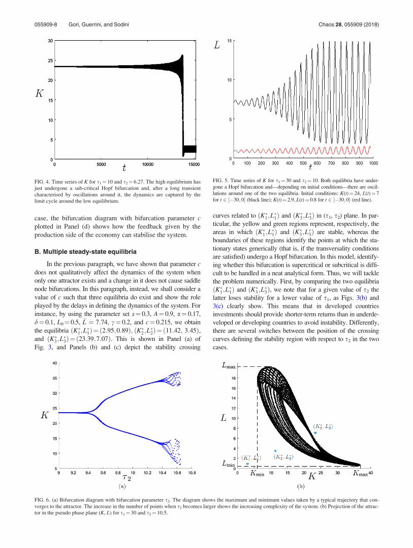
FIG. 4. Time series of K for s1¼ 10 and s2¼ 6.27. The high equilibrium has
just undergone a sub-critical Hopf bifurcation and, after a long transient
characterised by oscillations around it, the dynamics are captured by the
limit cycle around the low equilibrium.
FIG. 5. Time series of K for s1¼ 30 and s2¼ 10. Both equilibria have under-
gone a Hopf bifurcation and—depending on initial conditions—there are oscil-
lations around one of the two equilibria. Initial conditions: K(t)¼ 24, L(t)¼ 7
for t 2 ½�30; 0� (black line); K(t)¼ 2.9, L(t)¼ 0.8 for t 2 ½�30; 0� (red line).
FIG. 6. (a) Bifurcation diagram with bifurcation parameter s2. The diagram shows the maximum and minimum values taken by a typical trajectory that con-
verges to the attractor. The increase in the number of points when s2 becomes larger shows the increasing complexity of the system. (b) Projection of the attrac-
tor in the pseudo phase plane (K, L) for s1¼ 30 and s2¼ 10.5.
055909-8 Gori, Guerrini, and Sodini Chaos 28, 055909 (2018)

By referring to the parameter set used in the case of mul-
tiple steady-state equilibria, the simulation portrayed in Fig.
4 shows that trajectories are captured by the low equilibrium
once the high equilibrium has been destabilised through a
sub-critical Hopf bifurcation. This is an important result
stressing the existence of a reversal towards underdevelop-
ment (the poverty trap) caused by the presence of a time-to-
build technology from which there exists a delay from the
time an investment is made to the time it becomes productive
(s1) and delays from the time people were born to the time
they will be economically active (belonging to the working
population) and sexually active (s2). We note that an
increase in the value of s1 produces a change in the nature of
the Hopf bifurcation (which becomes super-critical) under-
gone by the high equilibrium allowing the coexistence of
limit cycles, as is shown in Fig. 5. However, we have verified
that large fluctuations around the low equilibrium (induced
by larger values of s2) cause the death of the attractor and
the high equilibrium just remains the unique attractor of the
system so that trajectories are captured by the limit cycle
around the high equilibrium. By using the same value of s1
as in Fig. 5, Fig. 6(a) shows the evolution (bifurcation dia-
gram) of the “high” attractor when s2 varies. In particular,
Fig. 6(b) depicts the attractor of the system for s2¼ 10.5 in
the pseudo phase plane (K, L). By increasing the value of s2,
it is possible to observe an enlargement of the attractor. To
this purpose, Fig. 6(b) shows that the trajectories captured by
the attractor are such that Lmax > L�3; Lmin < L�1 and
Kmax > K�3 ; Kmin < K�2 , where Xmax and Xmin are the maxi-
mum and minimum values of variable X, respectively.
VI. CONCLUSIONS
This work analysed a Solow model augmented with a
time-to-build technology and population dynamics employ-
ing carrying capacity constraints and time delays. The main
aim is to characterise the existence of economic and demo-
graphic cycles and identify the chain of causation between
the main variables. This result deserves a attention as it is
not usual finding clear prediction about one-way or double
feedback effects between economic and demographic vari-
able in the neoclassical growth literature (ranging from mod-
els �a la Solow to the more recent contributions belonging to
the Unified Growth Theory). Then, the Solow model
becomes able to understand the reasons why production and
capital dynamics affect population dynamics or vice versa
and therefore the reasons why some countries lie on trajecto-
ries leading to sustained development, whereas others remain
entrapped in a Malthusian trap.
In the article, we assumed that the delays were fixed.
However, a part of the scientific literature—especially the
literature on demographic issues—has focused also on the
study of models with distributed delays. This is to capture in
a more appropriate way the role played by the population
age structure (Fanti et al., 2013 and Beretta and Breda,
2016) and the existence of economies where production
takes place through the use of some kinds of vintage
technologies (Boucekkine et al., 2002). These issues will be
accounted for in our future research agenda.
Banks, R. B., Growth and Diffusion Phenomena–Mathematical Frameworksand Applications (Springer-Verlag, NY, 1994).
Barro, R. J. and Sala-i-Martin, X., Economic Growth, 2nd ed. (MIT Press,
Cambridge (MA), US, 2003).
Becker, G. S., “An economic analysis of fertility,” in Demographic andEconomic Change in Developing Countries, National Bureau Committeefor Economic Research (Princeton University Press, Princeton (NJ),
1960).
Beretta, E. and Breda, D., “Discrete or distributed delay? Effects on stability
of population growth,” Math. Biosci. Eng. 13, 19–41 (2016).
Boucekkine, R., de la Croix, D., and Licandro, O., “Vintage human capital,
demographic trends, and endogenous growth,” J. Econ. Theory 104,
340–375 (2002).
Brock, W. A. and Taylor, S., “The Green Solow model,” J. Econ. Growth
15, 127–153 (2010).
Cai, D., “Multiple equilibria and bifurcations in an economic growth model
with endogenous carrying capacity,” Int. J. Bifurcation Chaos Appl. Sci.
Eng. 20, 3461–3472 (2010).
Cai, D., “An economic growth model with endogenous carrying capacity
and demographic transition,” Math. Comput. Modell. 55, 432–441 (2012).
Dalgaard, C.-J. and Strulik, H., “The history augmented Solow model,” Eur.
Econ. Rev. 63, 134–149 (2013).
Doepke, M., Hazan, M., and Maoz, Y. D., “The baby boom and World War
II: A macroeconomic analysis,” Rev. Econ. Stud. 82, 1031–1073 (2015).
Ehrlich, I. and Lui, F., “The problem of population and growth: A review of
the literature from Malthus to contemporary models of endogenous popu-
lation and endogenous growth,” J. Econ. Dyn. Control 21, 205–242
(1997).
Fanti, L. and Manfredi, P., “The Solow’s model with endogenous popula-
tion: A neoclassical growth cycle model,” J. Econ. Dev. 28, 103–115
(2003).
Fanti, L., Iannelli, M., and Manfredi, P., “Neoclassical growth with endoge-
nous age distribution. Poverty vs low-fertility traps,” J. Popul. Econ. 26,
1457–1484 (2013).
Galor, O., Unified Growth Theory (Princeton University Press, Princeton
(NJ), 2011).
Galor, O., “The demographic transition: Causes and consequences,”
Cliometrica 6, 1–28 (2012).
Galor, O. and Moav, O., “Natural selection and the origin of economic
growth,” Q. J. Econ. 117, 1133–1191 (2002).
Galor, O. and Moav, O., “From physical to human capital accumulation:
Inequality and the process of development,” Rev. Econ. Stud. 71,
1001–1026 (2004).
Galor, O. and Weil, D. N., “Population, technology, and growth: From
Malthusian stagnation to the demographic transition and beyond,” Am.
Econ. Rev. 90, 806–828 (2000).
Jones, L. E. and Schoonbroodt, A., “Baby busts and baby booms: The fertil-
ity response to shocks in dynastic models,” Rev. Econ. Dyn. 22, 157–178
(2016).
Leibenstein, H. M., Economic Backwardness and Economic Growth (Wiley,
New York (NY), 1957).
Lin, X. and Wang, H., “Stability analysis of delay differential equations
with two discrete delays,” Can. Appl. Math. Q. 20, 519–533 (2012).
Livi-Bacci, M., A Concise History of World Population, 6th ed. (Wiley-
Blackwell, Malden, 2017).
Mankiw, N. G., Romer, D., and Weil, D. N., “A contribution to the empirics
of economic growth,” Q. J. Econ. 107, 407–437 (1992).
Palivos, T., “Endogenous fertility, multiple growth paths, and economic con-
vergence,” J. Econ. Dyn. Control 19, 1489–1510 (1995).
Pecora, N. and Sodini, M., “A heterogeneous Cournot duopoly with delay
dynamics: Hopf bifurcations and stability switching curves,” Commun.
Nonlinear Sci. Numer. Simul. 58, 36–46 (2018).
Roser, M. and Ortiz-Ospina, E., https://ourworldindata.org/world-popula-
tion-growth for World Population Growth, 2018.
Solow, R. M., “A contribution to the theory of economic growth,” Q. J.
Econ. 70, 65–94 (1956).
Zak, P. J., “Kaleckian lags in general equilibrium,” Rev. Polit. Econ. 11,
321–330 (1999).
055909-9 Gori, Guerrini, and Sodini Chaos 28, 055909 (2018)
Related Documents