Time-average and asymptotically optimal flow control policies in networks with multiple transmitters

Time-Average and Asymptotically Optimal

Flow Control Policies in Networks

with Multiple Transmitters

Redha M. Bournas, Frederick J. Beutler

and Demosthenis Teneketzis

Department of Electrical Engineering and Computer Science

The University of Michigan

Ann Arbor, Michigan 48109

September 10, 1991

Abstract

We consider M transmitting stations sending packets to a single receiver over

a slotted time-multiplexed link. For each phase consisting of T consecutive slots,

the receiver dynamically allocates these slots among the M transmitters. Our

objective is to characterize policies that minimize the long-term average of the

total number of messages awaiting service at the M transmitters.

We establish necessary and su�cient conditions on the arrival processes at the

transmitters for the existence of �nite cost time-average policies; it is not enough

that the average arrival rate is strictly less than the slot capacity. We construct a

pure strategy that attains a �nite average cost under these conditions. This in turn

leads to the existence of an optimal time-average pure policy for each phase length

T , and to upper and lower bounds on the cost this policy achieves. Furthermore, we

show that such an optimal time-average policy has the same properties as those

of optimal discounted policies investigated by the authors in a previous paper.

Finally, we prove that in the absence of costs accrued by messages within the

phase, there exists a policy such that the time-average cost tends toward zero as

the phase length T !1.

Key words: COMMUNICATION NETWORKS; STABILITY; RANDOM

WALKS; G=G=1 QUEUES; TIME-AVERAGE OPTIMALITY; ASYMPTOTIC

OPTIMALITY.

1. Introduction

We consider a ow control problem that arises in the performance modelling

of the `hop-by-hop' layer of computer communication networks. For a detailed

overview on the architectural layers and ow control mechanisms, the reader is

referred to [7, 8, 17]. The hop-by-hop scheme studied in this paper is the same

as the one in [2, 3, 4, 5], its purpose being to maintain a smooth ow of tra�c

between M transmitting stations attempting to send messages through a single

communication channel to an adjacent receiving station. The time axis is divided

into equal segments called slots. All messages consist of packets of equal length; the

transmission time of a packet is one slot and a packet transmission may only begin

on a slot boundary. Each transmitter j has an independent generally distributed

arrival process of packets per slot with �nite �rst moment �

(j)

and a bu�er of

in�nite size. We assume that the arrival processes to distinct transmitters are mu-

tually independent. Only one station is allowed to transmit during any particular

slot.

T consecutive slots form a phase. Prior to the beginning of each phase, the re-

ceiver informs each transmitter of the number of packets (referred to as a window

size) that it is prepared to accept and the particular slots during which each trans-

mitter is allowed to transmit. In making a decision on the assigned window size,

the receiver uses the knowledge of arrival statistics, the number of queued packets

for each transmitter at the beginning of the preceding phase, and the window size

assigned for the preceding phase. The number of queued packets at a phase is

sent by each transmitter to the receiver with negligible overhead some time before

the beginning of the next phase. Due to the arrival of new packets, the number

of queued packets changes by the time the receiver is able to use the information

for the next window assignment. The window allocations by the receiver thus

constitute a discrete-time Markov decision process with partial information.

Optimal ow control allocations were �rst analyzed by Rosberg and Gopal [16],

who considered a single transmitter, and a cost function re ecting the number of

queued packets together with the number of unutilized (i.e., wasted) transmission

slots. Subsequently, Cansever and Milito [3] investigated the problem for two

transmitters (M = 2) with identical arrival statistics, with later generalizations to

heterogeneous arrivals [4]. Cansever and Milito also conjectured results for M > 2

transmitters. Later, they extended their work to more complex networks with

multiple states in a layered, tree-like network [5].

Our model in [2] is similar to that of [3, 4]. As in these references, the cost

per phase in [2] is the expectation of the sum of the number of untransmitted

packets at the respective stations. Our objective then was to dynamically allocate

a �xed number T of slots among the M � 2 transmitters to minimize the total

discounted cost. Our results in [2] include a partial characterization of a set of

1

optimal allocation policies. These structural properties enable us to prove that,

for the set of all discount factors � < 1, a �nite number of dynamic optimal

allocations su�ce to complete describe an optimal allocation policy. For M = 2,

we prove in addition that the optimal policy is a monotone function of a state,

and that the total cost is convex. When the process of message generation at one

transmitter is stochastic larger than the message generation process at the other

transmitter, we further characterize an optimal allocation. Finally, if the message

generating processes at theM � 2 transmitters are iid, we �nd an explicit form of

the optimal allocation policy (compare [3]) that does not depend on the discount

factor �.

Here, we turn our attention to time-average policies. We believe that a time-

average cost criterion is a more natural setting for ow control problems, since

it represents the long-term performance measure of the ow control algorithm.

Moreover, in the time scale under which a ow control system generally operates,

any discount attached to past data ought to be minimal; hence, discounting appears

to us to be an arti�ce that facilitates solutions, at the cost of detracting from the

validity of the model.

It is not surprising that the existence of time-average policies of �nite cost

requires that the average arrival rate is strictly less than the slot capacity, i.e,

� < 1 in terms of a tra�c intensity. We show that more is required: if � < 1, a

necessary and su�cient condition for the existence of �nite cost strategies is the

�niteness of the second moment of the number of arrivals during a phase.

We exhibit a pure strategy that attains a �nite average cost under the condition

of the preceding paragraph. This in turn leads to four further results:

1. For each phase length T , there exists an optimal time-average policy.

2. The time-average optimal policy can be obtained as a limit of in�nite horizon

optimal discounted policies as the discounting factor � ! 1.

3. The properties of the time-average optimal policy are the same as those

derived in [2] for optimal discounted policies.

4. Upper and lower performance bounds are obtained for the cost attained by

the optimal policy.

For each phase length T , the existence of time-average optimal policies and the

derivation of their structural properties are based on: (1) the work of Bournas et

al. [2] on the in�nite horizon optimal discounted cost and structural properties of

the optimal discounted stationary policies, and (2) the work of Sennott [18].

Finally, we prove that in the absence of costs accrued by messages within the

phase, there exists a policy such that the time-average cost tends toward zero as

2

the phase length T !1. This result is motivated by our interest in investigating

the long-term average cost as a function of the phase length T , which in turn leads

to an optimal phase length size. This problem turns out to be a very di�cult

one and we have not solved it in this paper. However, we have been able to solve

a closely related problem as we shall explain. For each phase, the cost has two

additive components: (1) the number of packets awaiting transmission at the be-

ginning of the phase, and (2) the waiting times accumulated by packets arriving

during the phase, and not being available for transmission until the beginning of

the next phase. Using the strong law of large numbers and the theory of conver-

gence of probability measures as in Billingsley [1], we have been able to show that

the cost component (1) asymptotically goes to zero as T ! 1. In addition, the

corresponding asymptotically optimal policies are state independent and propor-

tional to the arrival processes rates. The asymptotic behaviour of component (1)

as T !1 combined with the monotonicity in T of the cost component (2) shed

more light into the issues that should be addressed to determine the optimal phase

length. Some of these issues are discussed in Section 5.

The paper is organized as follows. In Section 2, we formalize the model and

formulate the problem. In Section 3, we �rst derive necessary conditions on the

statistics of the arrivals processes that ensure system stable behaviour. Under

these conditions, we then construct a pure strategy possessed of �nite long-term

average cost. In Section 4, we demonstrate the existence of optimal time-average

stationary policies, and show that these policies have the same properties as those

derived in [2] for optimal discounted stationary strategies. In Section 5, we exhibit

the existence of a stationary nonrandomized policy under which the long-term

average number of packets awaiting transmission at the beginning of each phase

converges to zero as T ! 1. The ow control problem with priorities is brie y

discussed in Section 6. Finally, conclusions are presented in Section 7.

2. Model Formulation

2.1 De�nitions and Problem Statement

Consider a hop-by-hop scheme that operates as follows. There areM transmit-

ting nodes attempting to send messages to a single receiver. All messages consist

of packets of �xed length and time is divided into equal slots, one slot being long

enough to transmit a packet. A packet transmission may begin only on a slot

boundary. The window allocation proceeds in phases, a phase being a �xed prede-

termined number of slots, say T slots. Only one transmitter is allowed to transmit

during a particular slot. We also assume that each transmitter has a bu�er of

in�nite size. We place two further restrictions on the model : (1) packets arriving

in a particular phase may not be transmitted in that phase, and (2) packets that

3

are being transmitted during a phase are not penalized for the delay within the

phase. These assumptions may be considered as a restriction on the model. Relax-

ing them results in formulating a problem whose action space consists of not only

the window sizes allocated to each transmitter but of the order in which the slots

are scheduled for transmission also. This is a considerably more di�cult problem

which will not be addressed here.

The processes of message generation at each transmitter are stochastic processes

with known statistics. The number of packets generated at transmitter j during

slot i, f�

(j)

i

g

1

i=1

, are iid random variables with �nite �rst moment �

(j)

. We assume

that the arrival processes to distinct stations are mutually independent.

Let Y

(j)

k

be the number of packets generated at transmitter j (j = 0; 1; . . . ;M)

during phase k (k = 0; 1; . . .). For each j, the Y

(j)

k

are iid in k. Indeed, each Y

(j)

k

is

the sum of T iid random variables representing packets generated at the respective

slots of the phase. For simplicity, we often use the notation Y

k

to denote the vector

whose M components are the Y

(j)

k

.

We now write the evolution equations for the ow control system. The number

of packets in the bu�er at the beginning of phase k is called N

k

; the same vector

convention holds as for Y

k

. In a similar vein, de�ne w

k

as the allocation vector

for phase k, w

(j)

k

being the number of slots assigned to transmitter j for phase k.

Finally, we let X

k

be the number of packets \left over" at the beginning of phase

k, in the sense that they had been bu�ered at the beginning of phase k � 1, but

not transmitted during the course of that phase. More precisely, we shall de�ne

X

k

by the relation

X

k

4

=(N

k�1

� w

k�1

)

+

; (2:1)

where we adopt the vector notation

x

+

4

=

M

X

j=1

max(0; x

(j)

)

Inherent in (2.1) is the assumption that arrivals during phase k � 1 cannot be

transmitted during that phase, but are available for transmission in phase k. It

follows that the numbers of bu�ered packets for the respective transmitters at the

beginning of phase k is described by

N

k

= X

k

+ Y

k�1

: (2:2)

Observe that (2.2) holds only for k � 1; to complete the set of dynamic equations,

we assume that N

0

and w

0

given. From (2.1) and (2.2), we thus arrive at the

dynamical equations of evolution

X

k

=

(

(X

k�1

+ Y

k�2

� w

k�1

)

+

if k � 2

x

1

if k = 1.

(2:3)

4

It will be seen that fX

k

g turns out to be the more natural state variable, not only

for the evolution equations, but also for the cost expressions and the allocation

rules.

It is convenient as well as reasonable to de�ne for the cost function during a

single phase

r(N) =

M

X

j=1

T�1

X

k=0

"

N

(j)

+

k

X

m=1

�

(j)

i;m

#

: (2:4)

where we have used �

(j)

i;m

to denote the number of packet arrivals to transmitter j

during slot m of any phase i. The cost (2.4) may be interpreted as a total waiting

time via Little's formula, except that we have not found it feasible to take account

of the particular slot during which a packet is transmitted. From (2.3), it follows

that the expected cost per phase is furnished by

E[r(N)] = T

M

X

j=1

E

h

X

(j)

i

+

T (T + 1)

2

M

X

j=1

�

(j)

: (2:5)

For the allocation w determined by the receiver, we �rst de�ne the action space

A to describe the possible allocations of slots within a phase, namely

A

4

=fw = (w

(1)

; w

(2)

; . . . ; w

(M)

) 2 Z

M

+

:

M

X

j=1

w

(j)

� Tg: (2:6)

During the course of phase k�1, each transmitter is able (with negligible overhead)

to apprise the receiver of his value of N

(j)

k�1

. Since the receiver also knows w

(j)

k�1

, he

can deduceX

(j)

k

by the relation (2.1). It follows further from the evolution equation

(2.3) that fX

k

g is a Markov decision process, whose optimal control requires only

the most recently available state (cf. [13], Sec. 6.7). In short, we need only consider

the set of admissible control policies � =

Q

1

k=1

�

k

, where

�

k

: Z

M

+

! A : (2:7)

More succinctly, we write w

k

(X

k

) to indicate that the allocation of slots for phase

k is based on the current state X

k

. We emphasize once again that our allocation is

based on imperfect information; at phase k;X

k

represents data from the beginning

of phase k� 1, and does not take into account the arrivals Y

k�1

that contribute to

the current bu�er content N

k

. For future reference, the set of admissible controls

as described above will be called P

T

. Finally, when we consider only stationary

policices, we shall omit the subscript from w

k

.

When a policy � is employed, we de�ne the long-term average cost for phase

length T by taking the time average of the expected cost (2.5), and conditioning

5

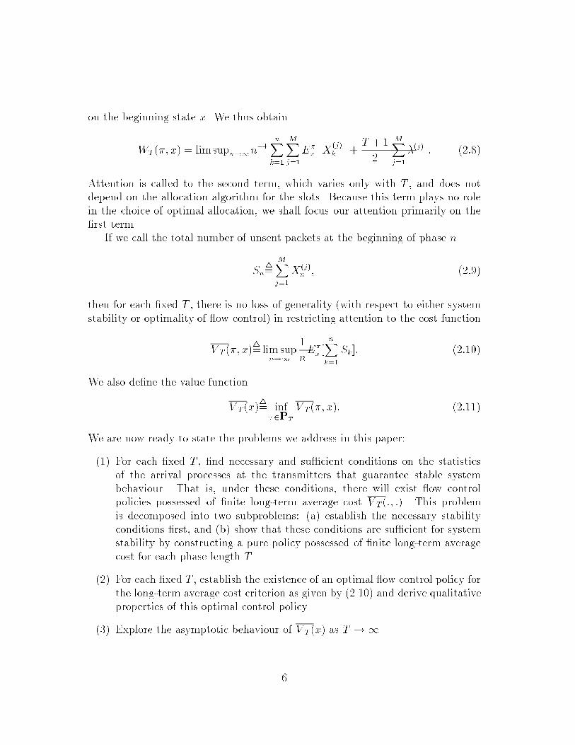
on the beginning state x. We thus obtain

W

T

(�; x) = limsup

n!1

n

�1

n

X

k=1

M

X

j=1

E

�

x

h

X

(j)

k

i

+

T + 1

2

M

X

j=1

�

(j)

: (2:8)

Attention is called to the second term, which varies only with T , and does not

depend on the allocation algorithm for the slots. Because this term plays no role

in the choice of optimal allocation, we shall focus our attention primarily on the

�rst term.

If we call the total number of unsent packets at the beginning of phase n

S

n

4

=

M

X

j=1

X

(j)

n

; (2:9)

then for each �xed T , there is no loss of generality (with respect to either system

stability or optimality of ow control) in restricting attention to the cost function

V

T

(�; x)

4

=lim sup

n!1

1

n

E

�

x

[

n

X

k=1

S

k

]: (2:10)

We also de�ne the value function

V

T

(x)

4

= inf

�2P

T

V

T

(�; x): (2:11)

We are now ready to state the problems we address in this paper:

(1) For each �xed T , �nd necessary and su�cient conditions on the statistics

of the arrival processes at the transmitters that guarantee stable system

behaviour. That is, under these conditions, there will exist ow control

policies possessed of �nite long-term average cost V

T

(:; :). This problem

is decomposed into two subproblems: (a) establish the necessary stability

conditions �rst, and (b) show that these conditions are su�cient for system

stability by constructing a pure policy possessed of �nite long-term average

cost for each phase length T .

(2) For each �xed T , establish the existence of an optimal ow control policy for

the long-term average cost criterion as given by (2.10) and derive qualitative

properties of this optimal control policy.

(3) Explore the asymptotic behaviour of V

T

(x) as T !1.

6

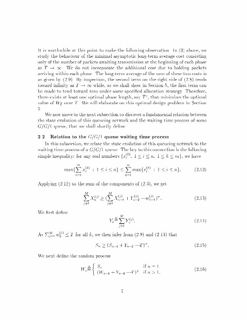
It is worthwhile at this point to make the following observation. In (3) above, we

study the behaviour of the minimal asymptotic long-term average cost consisting

only of the number of packets awaiting transmission at the beginning of each phase

as T ! 1. We do not incorporate the additional cost due to holding packets

arriving within each phase. The long-term average of the sum of these two costs is

as given by (2.9). By inspection, the second term on the right side of (2.8) tends

toward in�nity as T !1 while, as we shall show in Section 5, the �rst term can

be made to tend toward zero under some speci�ed allocation strategy. Therefore,

there exists at least one optimal phase length, say T

�

, that minimizes the optimal

value of W

T

over T . We will elaborate on this optimal design problem in Section

5.

We now move to the next subsection to discover a fundamental relation between

the state evolution of this queueing network and the waiting time process of some

G=G=1 queue, that we shall shortly de�ne.

2.2 Relation to the G=G=1 queue waiting time process

In this subsection, we relate the state evolution of this queueing network to the

waiting time process of a G=G=1 queue. The key to this connection is the following

simple inequality: for any real numbers fx

(k)

i

; 1 � i � n; 1 � k � mg, we have

maxf

m

X

k=1

x

(k)

i

: 1 � i � ng �

m

X

k=1

maxfx

(k)

i

: 1 � i � ng: (2:12)

Applying (2.12) to the sum of the components of (2.3), we get

M

X

j=1

X

(j)

n

� (

M

X

j=1

X

(j)

n�1

+ Y

(j)

n�2

� w

(j)

n�1

)

+

: (2:13)

We �rst de�ne

Y

n

4

=

M

X

j=1

Y

(j)

n

: (2:14)

As

P

M

j=1

w

(j)

k

� T for all k, we then infer from (2.9) and (2.13) that

S

n

� (S

n�1

+ Y

n�2

� T )

+

: (2:15)

We next de�ne the random process

W

n

4

=

(

S

n

if n = 1

(W

n�1

+ Y

n�2

� T )

+

if n > 1:

(2:16)

7

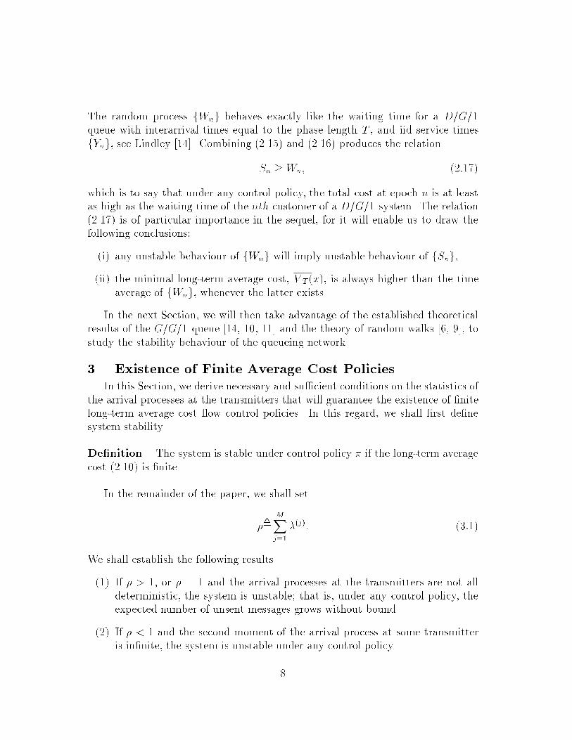
The random process fW

n

g behaves exactly like the waiting time for a D=G=1

queue with interarrival times equal to the phase length T , and iid service times

fY

n

g, see Lindley [14]. Combining (2.15) and (2.16) produces the relation

S

n

�W

n

; (2:17)

which is to say that under any control policy, the total cost at epoch n is at least

as high as the waiting time of the nth customer of a D=G=1 system. The relation

(2.17) is of particular importance in the sequel, for it will enable us to draw the

following conclusions:

(i) any unstable behaviour of fW

n

g will imply unstable behaviour of fS

n

g,

(ii) the minimal long-term average cost, V

T

(x), is always higher than the time

average of fW

n

g, whenever the latter exists.

In the next Section, we will then take advantage of the established theoretical

results of the G=G=1 queue [14, 10, 11] and the theory of random walks [6, 9], to

study the stability behaviour of the queueing network.

3. Existence of Finite Average Cost Policies

In this Section, we derive necessary and su�cient conditions on the statistics of

the arrival processes at the transmitters that will guarantee the existence of �nite

long-term average cost ow control policies. In this regard, we shall �rst de�ne

system stability.

De�nition. The system is stable under control policy � if the long-term average

cost (2.10) is �nite.

In the remainder of the paper, we shall set

�

4

=

M

X

j=1

�

(j)

: (3:1)

We shall establish the following results.

(1) If � > 1, or � = 1 and the arrival processes at the transmitters are not all

deterministic, the system is unstable; that is, under any control policy, the

expected number of unsent messages grows without bound.

(2) If � < 1 and the second moment of the arrival process at some transmitter

is in�nite, the system is unstable under any control policy.

8

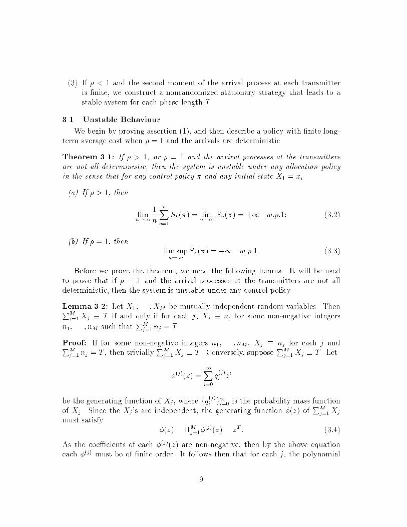
(3) If � < 1 and the second moment of the arrival process at each transmitter

is �nite, we construct a nonrandomized stationary strategy that leads to a

stable system for each phase length T .

3.1 Unstable Behaviour

We begin by proving assertion (1), and then describe a policy with �nite long-

term average cost when � = 1 and the arrivals are deterministic.

Theorem 3.1: If � > 1, or � = 1 and the arrival processes at the transmitters

are not all deterministic, then the system is unstable under any allocation policy

in the sense that for any control policy � and any initial state X

1

= x,

(a) If � > 1, then

lim

n!1

1

n

n

X

k=1

S

k

(�) = lim

n!1

S

n

(�) = +1 w:p:1; (3:2)

(b) If � = 1, then

lim sup

n!1

S

n

(�) = +1 w:p:1: (3:3)

Before we prove the theorem, we need the following lemma. It will be used

to prove that if � = 1 and the arrival processes at the transmitters are not all

deterministic, then the system is unstable under any control policy.

Lemma 3.2: Let X

1

; . . . ;X

M

be mutually independent random variables. Then

P

M

j=1

X

j

� T if and only if for each j, X

j

� n

j

for some non-negative integers

n

1

; . . . ; n

M

such that

P

M

j=1

n

j

= T .

Proof: If for some non-negative integers n

1

; . . . ; n

M

, X

j

� n

j

for each j and

P

M

j=1

n

j

= T , then trivially

P

M

j=1

X

j

� T . Conversely, suppose

P

M

j=1

X

j

� T . Let

�

(j)

(z) =

1

X

i=0

q

(j)

i

z

i

be the generating function of X

j

, where fq

(j)

i

g

1

i=0

is the probability mass function

of X

j

. Since the X

j

's are independent, the generating function �(z) of

P

M

j=1

X

j

must satisfy

�(z) = �

M

j=1

�

(j)

(z) = z

T

: (3:4)

As the coe�cients of each �

(j)

(z) are non-negative, then by the above equation

each �

(j)

must be of �nite order. It follows then that for each j, the polynomial

9

�

(j)

(z) must divide z

T

. This is possible if and only if �

(j)

(z) = q

(j)

n

j

z

n

j

for some

integer n

j

; 0 � n

j

� T . This then implies that q

(j)

n

j

= 1 and

P

M

j=1

n

j

= T .

Proof of Theorem 3.1: Let us remind the reader of the relation (2.17), which

we state here again for convenience:

S

n

�W

n

: (3:5)

Recall thatW

n

, as de�ned by (2.16), is the waiting time process of a D=G=1 queue.

The inequality (3.5) is the key to the following proof.

If � > 1, W

n

does not possess a limiting distribution, see [14]. In addition,

lim

n!1

W

n

= 1 almost surely. This result is not explicitly stated in [14], but it

can be seen as follows. De�ne the sequence of iid random variables

U

k

4

= Y

k

� T; (3:6)

and the random walk

V

n

4

=

(

0 if n = 0

P

n�1

k=0

U

k

if n � 1.

(3:7)

We �rst prove by induction that

W

n

� V

n�1

: (3:8)

Equation (3.8) is trivial for n = 1. We now suppose it holds for n and prove it for

n+ 1. Since V

n

= V

n�1

+ Y

n�1

� T , then

W

n+1

= (W

n

+ Y

n�1

� T )

+

= (W

n

� V

n�1

+ V

n

)

+

� V

n

; (3:9)

the last inequality following from the induction hypothesis. If � > 1, then the drift

of V

n

, E(U

0

) = (��1)T , is positive so that lim

n!1

V

n

=1 almost surely, see Feller

[6] or Gut [9]. Thus (3.2) follows immediately from (3.5) and (3.8). Assume next

that � = 1, and the arrival processes at the transmitters are not all deterministic,

i.e, for some i and all n 2 Z

+

, P [Y

(i)

0

= n] < 1. This implies by Lemma 3.2 that

P [U

0

= 0] < 1, so that lim sup

n!1

V

n

= +1 w.p.1, by [5] or [6]. (3.3) is now

immediate upon invoking (3.5) and (3.8).

Remark. We note that if � = 1 and the arrival processes at all transmitters are de-

terministic, a control policy with �nite long-term average cost exists. Suppose that

for each j, Y

(j)

0

� n

j

for some non-negative integers n

1

; . . . ; n

M

such that

P

M

j=1

n

j

=

T . Consider the stationary control policy (w

(1)

i

; . . . ; w

(M)

i

) = (n

1

; . . . ; n

M

) for all

10

i � 1. By (2.3), X

(j)

n

= x

(j)

, for all n � 1, and this strategy possesses a long-term

average cost equal to

P

M

j=1

x

(j)

.

We next show that in addition to � < 1, �niteness of the second moment of

the arrival process at each transmitter is a necessary condition for the existence

of control policies that lead to a stable system. Let fX

(j)

n

(�); n � 2g denote the

state of transmitter j at epoch n when policy � = �

1

i=1

�

i

is employed, starting

with the initial state X

(j)

1

= x

(j)

.

Theorem 3.3: Assume � < 1. If for some i, E[(�

(i)

1

)

2

] = 1, then the system is

unstable under any control policy, i.e, for any control policy � and any initial state

X

1

= x,

lim

n!1

1

n

n

X

k=1

S

k

(�) = lim

n!1

E

x

[S

n

(�)] =1 w:p:1: (3:10)

Proof: When � < 1, the waiting time process fW

n

g, as de�ned by (2.16), tends

in distribution to a �nite random variable, say W , see Lindley [14] or Kiefer and

Wolfowitz [10]. Since E[(�

(i)

1

)

2

] = 1 implies that E[U

2

0

] = 1, then by Theorem

3 of Kiefer and Wolfowitz [11], E(W ) = 1. In addition, by [11], Theorem 1, we

have

P [ lim

n!1

1

n

n

X

k=1

W

k

= E(W )] = 1: (3:11)

This result together with (3.5) and (3.8) imply (3.10).

Having established the necessary stability conditions through Theorem 3.1 and

Theorem 3.3, we shall show next that these conditions are su�cient for stable

system behaviour.

3.2 Stable Behaviour: Construction of a �nite average cost pure policy

In this subsection, we exhibit the existence of a nonrandomized stationary

strategy that leads to a stable system for each phase length T . Before proceeding

with the construction of this pure strategy, we shall remind the reader of a key

lemma that will enable us to interchange limits in distribution (or probability, or

with probability 1) and expectations of a sequence of random variables. The key

to this interchange is the uniform integrability of the sequence as indicated in [1],

Theorem 5.4. In this regard, we shall often make use of the following facts:

Lemma 3.4: (Uniform Integrability)

(a) Let Z, fZ

n

g be a sequence of non-negative integrable random variables,

and suppose that Z

n

converges in distribution (or with probability 1, or

in probability) to Z. Then fZ

n

g is uniformly integrable if and only if

E(Z

n

) �! E(Z).

11

(b) Any sequence of iid random variables with �nite mean is uniformly integrable.

(c) Suppose fZ

n

g is a sequence such that jZ

n

j � Z w.p.1 and E(Z) <1. Then

fZ

n

g is uniformly integrable.

In the remainder of the paper, we shall consistently suppose that

� < 1; (3.12)

E[(�

(j)

1

)

2

] < 1; 1 � j �M: (3.13)

To avoid trivialities, also assume

0 < P [�

(j)

1

= 0] < 1; 1 � j �M ; (3:14)

the inequality on the right precludes channels without messages inputs, while the

left hand inequality is implied by the stability requirement (3.12). We recall that

(cf. (2.14))

Y

n

4

=

M

X

j=1

Y

(j)

n

: (3:15)

For future reference, we call

p

k

4

=P [Y

0

= k]; (3:16)

and note that (3.14) implies p

0

> 0.

We also recall that (cf. (2.9))

S

n

=

M

X

j=1

X

(j)

n

; (3:17)

fS

n

g need not be a Markov chain under an arbitrary policy, but it is one under the

policy we shall describe. Let w

(j)

n

be the number of slots allocated to transmitter

j at epoch n. Apply the following nonrandomized stationary policy to fX

n

g:

if S

n

� T , take w

(j)

n

= x

(j)

n

; (3.18)

if S

n

> T , take w

(j)

n

� x

(j)

n

and

P

M

j=1

w

(j)

n

= T . (3.19)

This is actually a description of a class of policies, but any such policy will be

adequate for our purpose. The motivation of policies of this class is provided by

the properties of optimal discounted policies, as given in Theorem 3.8 of [2]. Such

a policy, applied to fX

n

g, induces an fS

n

g that will meet our needs. In fact, fS

n

g

is simply the total cost at epoch n, so that the time-average of fS

n

g becomes

12

the time-average of the total cost. The state evolution of fS

n

g then follows the

recursive equations

S

n+1

=

(

Y

n�1

S

n

� T

S

n

+ Y

n�1

� T S

n

> T:

(3:20)

The remainder of this Section is devoted to proving that the stated pure policy

indeed leads to a �nite average cost, i.e.

lim sup

n!1

n

X

k=1

E[S

k

(x)] <1 ; (3:21)

where S

n

(x) is as in (3.17), except that the parameter x now indicates the initial

number of packets stored at the respective transmitters. For (3.21) to be valid, it

su�ces to demonstrate that

sup

n

E[S

n

(x)] <1 (3:22)

from which (3.21) follows immediately.

We shall again obtain the desired result by comparing the average cost asso-

ciated with the allocation policy (3.18) and (3.19), and the average waiting time

cost for a D/G/1 queue. For this purpose, we introduce the notation W

n

(x) to

denote the waiting time for the D/G/1 queue, under the supposition that the ze-

roeth customer undergoes waiting time x. We shall prove that S

n

(x) and W

n

(x)

are related by

W

n

(x) � S

n

(x) �W

n

(x) + T (3:23)

for all n when both receive the same inputs fY

n

g. In addition, we verify that

E[W

n

(x)] remains bounded in n by virtue of uniform integrability.

We use induction to prove (3.23). It is clearly true that (3.23) holds for n = 0

where S

n

(x) and W

n

(x) are equal. Now assume (3.23) holds for n. In case S

n

(x) �

T , S

n+1

(x) = Y

n�1

by (3.20). On the other hand, we have (see (3.9))

W

n+1

(x) = (W

n

(x) + Y

n�1

� T )

+

; (3:24)

whence

Y

n�1

� T �W

n+1

(x) � (S

n

(x) + Y

n�1

� T )

+

= Y

n�1

:

The complementary case, S

n

(x) > T , yields

S

n+1

(x)� S

n

(x) = W

n+1

(x)�W

n

(x)

by (3.20) and (3.24), so the result (3.23) again follows.

13

We now show that fW

n

(x)g is uniformly integrable; this implies that

sup

n

E[W

n

(x)] <1 (3:25)

for each x. Under the condition � < 1, it was established in [10] and [11] (see also

[14]) that there is the limit in distribution

W

n

(x)

d

! W (3:26)

where W does not depend on x. In addition, it is shown in [11] that

lim

n!1

E[W

n

(0)] = E[W ] <1 ; (3:27)

with the convergence and the �niteness of E[W ] following from the existence of a

�nite second moment for Y

n

. Then (3.26) (with x = 0), taken together with (3.27)

implies that fW

n

(0)g is uniformly integrable; this follows from Lemma 3.4(a).

To compare W

n

(0) and W

n

(x), we note that (3.24) can be extended by an easy

calculation to

W

n

(x) = max(0; x�

0;k

+

n�1

X

k=r

Y

k

� (n� r)T : k = 0; . . . ; n� 1) ; (3:28)

where � is the Kronecker delta. We therefore obtain

W

n

(x) � W

n

(0) + x : (3:29)

For each x, the uniform integrability of fW

n

(0)g conveys the same property to

fW

n

(x)g. Thus, fE[W

n

(x)]g satis�es (3.25), and by (3.23) the same must be true

for fE[S

n

(x)]g. Then (3.21) holds also, and our argument is complete.

Remark 1. Before leaving this Section, we make the following observation that

will be used in Section 4. From the state transition matrix of fS

n

g, one checks

that state zero is reachable from any other state; this follows because p

0

> 0, as

we have already mentioned (see (3.14) and (3.16)). Moreover, the �niteness of the

long-term average cost of fS

n

g, starting from any initial state, implies that the

total expected cost to reach state zero from state x is �nite.

Remark 2. Through use of the inequality (3.22), one also proves that

E[S

x

(x)] � E[W

n

(x)] + �T : (3:30)

For this purpose, consider E[S

n+1

(x)jS

n

(x)]. On the event fS

n

(x) � Tg we have

from (3.20)

E[S

n+1

(x)jS

n

(x)] = E(Y

n�1

) (= �T ) :

14

On the other hand, on the event fS

n

(x) > Tg an application of (3.20) yields

E[S

n+1

(x)jS

n

(x)] = S

n

(x) + E(Y

n�1

)� T

so that by the right hand inequality of (3.22)

E[S

n+1

(x)jS

n

(x)] � W

n

(x) + �T : (3:31)

Thus, (3.20) holds with probability one, and taking expections leads to (3.30).

Remark 3. Using more subtle arguments, one shows that E[S

n

(x)]! E(W )+�T

for all x.

3.3 An upper and a lower bound for V

T

(x)

We shall derive an upper and lower bound for the minimal achievable long-

term average cost V

T

(x). The optimal time-average policy certainly achieves a

cost at most as high as the one of the pure policy of Section 3.2 as de�ned by

(3.18)�(3.19). Hence, by Remark 2 of the preceding section,

V

T

(x) � E(W ) + �T: (3:32)

On the other hand, since under any policy, S

n

� W

n

, (cf. (2.17)), we also obtain

V

T

(x) � E(W ): (3:33)

For completeness, we need an expression for E(W ) in terms of the arrival processes

statistics. In general, there is no such explicit formula. However, from the bounds

of [12] on the waiting time process of the G=G=1 queue, we obtain

E[(

P

M

j=1

Y

(j)

0

� T )

+

]

2

2(1 � �)T

� E(W ) �

P

M

j=1

(�

(j)

)

2

2(1 � �)

; (3:34)

where (�

(j)

)

2

= V ar(�

(j)

). Combining (3.32), (3.33) and (3.34) leads to

E[(

P

M

j=1

Y

(j)

0

� T )

+

]

2

2(1 � �)T

� V

T

(x) � �T +

P

M

j=1

(�

(j)

)

2

2(1 � �)

: (3:35)

Observe that the magnitude of the di�erence between the bounds of (3.32) and

(3.33) tends to in�nity as T ! 1. These bounds therefore do not give us any

insight on the asymptotic behaviour of V

T

(x) as T !1. We are however able to

solve this problem in Section 5 using a di�erent approach.

In summary, the pure policy of this Section enabled us to conclude that the

minimal achievable long-term average cost, V

T

(x), is �nite for each phase length

T . We now move to the next Section to show that V

T

(x) is achieved by a Markov

policy. Additionally, we derive qualitative properties of this optimal control strat-

egy.

15

4. Existence and Properties of Time-Average Optimal

Policies

In this Section, we establish the existence of an optimal nonrandomized sta-

tionary strategy for the long-term average cost criterion and derive qualitative

properties of this optimal control strategy. Throughout this Section, T is arbi-

trary but �xed. To be precise, we seek a pure policy, say �

�

, such that

V

T

(�

�

; x) = inf

�2P

T

V

T

(�; x); (4:1)

where (cf. (2.10))

V

T

(�; x)

4

=lim sup

n!1

1

n

E

�

x

[

n

X

k=1

S

k

]; (4:2)

x = (x

(1)

; . . . ; x

(M)

) is the initial system state, S

n

=

P

M

j=1

X

(j)

n

and X

(j)

k

is the

number of packets awaiting transmission at the beginning of phase k at transmitter

j. Recall that for each j (cf. (2.3))

X

(j)

k+1

= (Y

(j)

k�1

+X

(j)

k

� w

(j)

k

)

+

; (4:3)

where w

(j)

k

is the number of packets allocated to transmitter j at phase k. We

remind the reader that the cost (4.2) represents the long-term average number of

packets awaiting transmission at the beginning of each phase. Since the long-term

average cost of holding packets arriving in each phase is constant (cf. (2.9)), there

is no loss of optimality in restricting attention to the cost (4.2).

We shall prove the existence of time-average optimal policies and investigate

their qualitative properties based on the following results: (1) the properties of

the total expected discounted in�nite horizon cost of [2], (2) the properties of the

Markov chain induced by the pure policy of the previous section, and (3) the work

of Sennott [18] on average cost optimal stationary policies.

We �rst summarize the properties of the minimal achievable total expected

discounted cost and the properties of the optimal discounted policies as given in

[2]. For 0 � � < 1, the total expected �-discounted cost incurred by a policy � is

given by

V

�

(�; x)

4

=E

�

x

[

1

X

n=1

�

n�1

S

n+1

]: (4:4)

Let

V

�

(x)

4

= inf

�2P

T

V

�

(�; x) (4:5)

be the minimal achievable total expected �-discounted cost when the initial system

state is x. In [2], the authors study the properties of the discounted value function

16

V

�

(x) and of the optimal policies that attain the in�mum (4.5). It is shown in [2],

Lemma 2.2, Lemma 3.1, equations (3.8) and (3.16), respectively, that V

�

(x) has

the following properties:

(P1) For every state x and discount factor �, V

�

(x) is �nite.

(P2) V

�

(x) is non-decreasing in x; that is, for each i, V

�

(x+ e

i

) � V

�

(x), where

e

i

is an M -component row vector with 1 in the ith entry and zeroes in all

the other entries.

(P3) V

�

(x) satis�es the optimality equation of dynamic programming

V

�

(x) = min

w2A

fL(x;w) + �E[V

�

([Y + x�w]

+

)]g

4

= min

w2A

G

�

(x;w); (4:6)

where A

4

=f(w

(1)

; . . . ; w

(M)

) 2 Z

M

+

:

P

M

j=1

w

(j)

= Tg, Y

4

=(Y

(1)

; . . . ; Y

(M)

),

Y

(j)

denotes the random sequence fY

(j)

n

g

1

n=0

, and L(x;w) is the expected

cost per phase, i.e, L(x;w) =

P

M

j=1

E[(Y

(j)

+ x

(j)

�w

(j)

)

+

].

The properties of the �-discounted optimal policies are as follows (see [2], The-

orem 3.8 and Lemma 3.6). Let x be the initial system state and �

4

=

P

M

j=1

x

(j)

;

then

(P4) if � � T , any decision rule w(x) 2 A such that w

(l)

(x) � x

(l)

for each l is

optimal, i.e, V

�

(x) = G

�

(x;w(x));

(P5) if � � T , there exists an optimal decision rule w(x) 2 A such that w

(l)

(x) �

x

(l)

for each l, i.e, V

�

(x) = G

�

(x;w(x)).

Property (P4) assures that for a large number of messages, the slots are allocated so

that each one will carry a packet, none of them being \empty" and hence possibly

wasted. By similar reasoning, property (P5) assures that the slots are allocated so

that all the queued messages that are known to the receiver are transmitted and

hence the number of wasted slots is minimized.

We now verify that Assumptions 1-3 of [18] which ensure the existence of an

average cost optimal stationary policy are satis�ed. Assumption 1 is exactly prop-

erty (P1). From property (P2), V

�

(x)� V

�

(0) � 0, so that Assumption 2 is met.

To verify Assumption 3 without irreducibility conditions, we need to show that for

every x = (x

(1)

; . . . ; x

(M)

), there exists nonnegative M(x) <1 such that

V

�

(x)� V

�

(0) �M(x); (4:7)

17

and that there exists an allocation rule w(x) such that

X

y

p

xy

(w(x))M(y) <1; (4:8)

where p

xy

(w(x)) is the probability of a transition from x to y under the allocation

scheme w(x). For every x, let w(x) = (w

(1)

(x); . . . ; w

(M)

(x)) be the allocation of

slots under the stationary policy of section 3.2, as de�ned by (3.18)�(3.19). Let

c

x0

be the expected cost of a �rst passage from x to zero under this policy. While

c

x0

depends on �, by Remark 1 at the end of Section 3.2, c

x0

<1 for every x even

in the worst case, which is � equals 1. Starting from state x, suppose now that

we apply policy w(x) until we reach state zero and then we continue according to

an optimal policy afterwards. We then incur a cost of no more than c

x0

+ V

�

(0).

Since any optimal policy is at least as good as the one employed above, it must be

that V

�

(x) � c

x0

+ V

�

(0). Letting M(x) = c

x0

for every x, (4.7) is then satis�ed.

In addition, under policy w(x), we have

c

x0

= [maxf

M

X

j=1

x

(j)

; Tg � T + E(Y

0

)] + [

X

y 6=0

p

xy

(w(x))c

y0

]; (4:9)

where the �rst term in [. . .] on the RHS of (4.9) is the instantaneous cost incurred

when in state x. Since c

x0

<1, then the second term in [. . .] on the RHS of (4.9)

is �nite. As M(y) = c

y0

for every y, (4.8) is then satis�ed.

We next construct a stationary allocation policy f that is a limit point of a

sequence of optimal allocation policies ff

�

n

g associated with a sequence of discount

factors f�

n

g ! 1; indeed, starting with a sequence � ! 1, we shall be able to

choose a subsequence such that f = f

�

n

for all n. By the Lemma on p. 628 of

[18] we already know that a convergent subsequence of ff

�

n

g exists, and from the

Theorem on the same page, it follows from Assumptions one to three in [18] that

the limit of f is a time-average optimal allocation.

To prove that all the allocation policies f

�

n

can be chosen to be the same, it

su�ces to demonstrate that there exists a �nite set of allocation strategies among

which the optimal strategy may be chosen for all � < 1. Since the action space A

can consist of no more than M

T

elements when all T slots are allocated, the set of

all possible allocations on any �nite subspace of the state space Z

M

+

is necessarily

�nite. Thus, the restriction of optimal policies to the subspace fx : x 2 Z

M

+

; � <

MTg is �nite. On the other hand, for any x 2 Z

M

+

such that � � MT , there

exists a �rst index i such that its i

th

component x

i

satis�es x

i

� T . For this x,

(P4) indicates that an optimal allocation is w(x) = Te

i

, where e

i

is the unit vector

along component i; moreover, the same allocation is optimal for any � < 1.

With the application of the quoted results from [18], together with the �niteness

of the set of optimal allocation strategies, we obtain

18

Theorem 4.1: Every sequence of discount factors � converging to unity has a

subsequence f�

n

g such that the corresponding optimal stationary allocation policies

ff

�

n

g satisfy f = f

�

n

for all n. This stationary allocation policy f is average cost

optimal with average cost

g = lim

�!1

(1 � �)V

�

(x) : (4:10)

where the limit does not depend on x. Furthermore, f satis�es properties (P4) and

(P5) of the optimal discounted policies, as well as the properties found in Sections

4 and 5 of [2] for M = 2.

5. An Asymptotically Optimal Stationary Policy

In this Section, we study the asymptotic behaviour of the queueing system as

a function of the phase length T . We remind the reader that we do not incorpo-

rate the waiting cost of packets arriving within a phase in the cost function. A

cost is incurred only when packets awaiting service at the beginning of a phase,

are not transmitted. We exhibit the existence of a stationary nonrandomized

strategy under which the long-term average number of queued packets at the be-

ginning of each phase converges to zero as T tends to in�nity. This strategy is

only de�ned for large values of T , and depends only on T and the average arrival

processes rates. It is described in words as follows. There is a T

0

such that for each

T � T

0

: allocate to each transmitter at each phase of the decision process some

�xed number of slots that is higher than the average number of arrivals per phase.

Brie y recall that, f�

(j)

i

; i � 0g, the number of arrivals per slot at transmitter

j, is an iid sequence with �nite mean �

(j)

. To avoid unstable behaviour, we require

M

X

j=1

�

(j)

< 1; (5.1)

E[(�

(j)

1

)

2

] < 1; 1 � j �M: (5.2)

Choose �

(j)

1

> �

(j)

for each j, such that

P

M

j=1

�

(j)

1

< 1, and let

T

0

4

=d

M

1�

P

M

j=1

�

(j)

1

e; (5:3)

where dxe is the smallest integer not less than x. Consider the allocation scheme

w

(j)

(T )

4

=d�

(j)

1

T e; 1 � j �M: (5:4)

Under the speci�c strategy considered here, the assignment of slots does not depend

on the information state x. The assignment does vary with the phase length T ,

19

which is the parameter we are studying in this Section. With this in mind, we

shall refer to w

(j)

(T ), rather than to w

(j)

(x) we used in referring to �xed T and

an arbitrary policy. The allocation scheme (5.4) is well de�ned for T � T

0

and

satis�es

w

(j)

(T ) � �

(j)

1

T > �

(j)

T; 1 � j �M; 8T � T

0

: (5:5)

Indeed, (5.5) is implied by (5.4), and as d�

(j)

1

T e < �

(j)

1

T +1, we then obtain using

(5.3)

M

X

j=1

w

(j)

(T ) < T; for all T � T

0

: (5:6)

By the strong law of large numbers, the number of arrivals at transmitter j

is about �

(j)

T for su�ciently large T . In addition, as strategy (5.4) allocates

invariably more than �

(j)

T slots to transmitter j, it is then intuitive that the mean

queue size of transmitter j tends to be empty at the beginning of each phase

whenever T is su�ciently large. To be precise, under the allocation scheme (5.4)

with the phase length �xed at T , let X

(j)

n

(T; x

(j)

) be the state of transmitter j at

epoch n, where x

(j)

4

=X

(j)

1

(T ) is the initial state. The number of packets arriving

during phase n at transmitter j will be denoted by Y

(j)

n

(T ). Our goal is to prove

the following theorem.

Theorem 5.1: For each initial system state fX

(j)

1

(T ) = x

(j)

; 1 � j � Mg, we

have

8j; 1 � j �M; lim

T!1

lim

n!1

1

n

n

X

k=1

E[X

(j)

k

(T; x

(j)

)] = 0: (5:7)

Remark. Since we prove (5.7) separately for each transmitter, we will omit the

superscript j throughout the proof of Theorem 5.1 for simplicity. We will reference

each transmitter individually only when making a formal statement such as in a

theorem, lemma, or corollary.

The main idea behind the proof of Theorem 5.1 is that as T !1, E[X

n

(T; x)]

converges to zero uniformly in n for each initial state x. To establish the latter,

we introduce an auxiliary random walk W

n

(T; x) that is equal in distribution to

X

n

(T; x) and show that :

(i) sup

n�2

fW

n

(T; x)g �! 0 almost surely as T !1.

(ii) fsup

n�2

fW

n

(T; x)g; T � T

0

g is uniformly integrable.

Statements (i) and (ii) then ensure that E[sup

n�2

fW

n

(T; x)g] converges to zero

as T ! 1, and this also entails that lim

T!1

sup

n�2

fE[W

n

(T; x)]g = 0. Since

X

n

(T; x)

d

=W

n

(T; x), the last assertion then implies that the expected number of

20

packets awaiting transmission at the beginning of each phase converges uniformly

to zero as T ! 1, that is, lim

T!1

sup

n�2

fE[X

n

(T; x)]g = 0. This result then

immediately entails the assertion of Theorem 5.1. We shall next proceed to prove

(i) and (ii).

Under the allocation scheme (5.4), the system state equations (2.3) are express-

ible, following an induction step, as

X

n+1

(T; x) = maxf

i

X

k=1

Y

n�k

(T )� iw(T ) + x�(n� i) : 0 � i � ng; (5:8)

where by convention the sum on the RHS of (5.8) is zero when i = 0. Introduce

the auxiliary random process

W

n+1

(T; x) = maxf

i

X

k=1

Y

k�1

(T )� iw(T ) + x�(n� i) : 0 � i � ng; (5:9)

and note that since fY

k

(T ); k � 0g is an iid sequence, X

n

(T; x)

d

=W

n

(T; x). This

technique of substituting a random walk is a well known approach to G=G=1

queues, as in Lindley [14]. Our �rst result is that W

n

(T; x) converges uniformly

to zero w.p.1 as T ! 1, and this entails convergence to zero in probability of

X

n

(T; x) for each n � 2 as T ! 1. Remark that for the proof of this result, we

only require that assumption (5.1) be met.

Theorem 5.2: For each initial system state fX

(j)

1

(T ) = x

(j)

; 1 � j � Mg, we

have

8j; 1 � j �M; sup

n�2

fW

(j)

n

(T; x

(j)

)g �! 0 w.p.1 as T !1: (5:10)

Proof: Write Y

m

(T ) =

P

(m+1)T

k=mT+1

�

k

, where f�

k

g, the number of arrivals per slot,

is an iid sequence with E(�

1

) = �, and de�ne the iid zero mean sequence

Z

k

4

=�

k

� �: (5:11)

(5.9) is then equivalent to

W

n+1

(T; x) = maxf

iT

X

k=1

Z

k

+ i[�T � w(T )] + x�(n� i) : 0 � i � ng: (5:12)

Let

�

4

=

�

1

� �

2

> 0; (5.13)

A

(T )

m

(�)

4

= f! :

1

mT

mT

X

k=1

Z

k

(!) > �g; (5.14)

T

x

4

= minfi 2 N : i > maxfT

0

;

x

�

gg: (5.15)

21

By (5.12) and straightforward algebra, we get

8T � T

x

; f! : W

n+1

(T; x; !) > 0g � [[

n�1

i=1

A

(T )

i

(2�)] [A

(T )

n

(�) � [

n

i=1

A

(T )

i

(�)

(5:16)

From (5.16), we obtain

P [sup

n�2

fW

n

(T; x)g > 0] � P [[

1

i=1

A

T

i

(�)] (5.17)

� P [ sup

m�T

fm

�1

m

X

k=1

Z

k

> �g]; (5.18)

and the right hand side goes to zero as T !1 by the strong law of large numbers.

But since W

n

(T; x) � 0, (5.10) is then established.

An immediate consequence of (5.10) is that the number of packets awaiting

transmission at the beginning of each phase converges to zero in probability as the

phase length increases inde�nitely.

Corollary 5.3: For each initial system state fX

(j)

1

(T ) = x

(j)

; 1 � j � Mg, we

have

8j; 1 � j �M; X

(j)

n

(T; x

(j)

)

p

�!0; 8n � 2; as T !1: (5:19)

Proof: By an earlier remark, X

n

(T; x)

d

=W

n

(T; x), so that for any Borel set B,

P [X

n

(T; x) 2 B] = P [W

n

(T; x) 2 B]. In addition, since for each n, almost

sure convergence of fW

n

(T; x)g entails convergence in probability of fW

n

(T; x)g as

T !1, (5.19) immediately follows from (5.10).

We next show that the random variables fsup

n�2

fW

n

(T; x)g; T � T

0

g are

dominated by an integrable random variable, which then implies (cf. Lemma 3.4

(c)) that they are uniformly integrable. Recalling (5.11), we �rst writeW

n+1

(T; x),

as given by (5.12), under the equivalent form

W

n+1

(T; x) = maxf

iT

X

k=1

�

k

� iw(T ) + x�(n� i) : 0 � i � ng: (5:20)

We next introduce the auxiliary random process

W

n+1

(T; x)

4

=maxf

iT

X

k=1

�

k

� i�

1

T + x�(n� i) : 0 � i � ng; (5:21)

and note that as w(T ) � �

1

T (cf. (5.5)), we have the simple relationship

W

n+1

(T; x) � W

n+1

(T; x): (5:22)

Our aim is to prove the following.

22

Lemma 5.4: For each initial system state fX

(j)

1

(T ) = x

(j)

; 1 � j �Mg, we have

8j; 1 � j �M; 8T � T

0

; sup

n�2

fW

(j)

n

(T; x

(j)

)g � sup

n�2

fW

(j)

n

(1; 0)g+ x

(j)

: (5:23)

Furthermore, E[sup

n�2

fW

(j)

n

(1; 0)g] <1.

Proof: Let us �rst de�ne

W (T; x)

4

= sup

n�2

fW

n

(T; x)g; (5.24)

W (T; x)

4

= sup

n�2

fW

n

(T; x)g: (5.25)

By (5.21), we get

W

nT+1

(1; x) = maxf

i

X

k=1

�

k

� i�

1

+ x�(n� i) : 0 � i � nTg

� maxf

i

X

k=1

�

k

� i�

1

+ x�(n� i) : i 2 f0; T; 2T; . . . ; nTgg

= maxf

iT

X

k=1

�

k

� i�

1

T + x�(n� i) : 0 � i � ng

= W

n+1

(T; x): (5.26)

Combining (5.22) and (5.26), we obtain W

n+1

(T; x) � W

nT+1

(1; x). Recalling

(5.24)�(5.25), the latter inequality then entails

W (T; x) � W (1; x): (5:27)

Since x � 0, we obtain from (5.21)

8T; 8x; 8n; W

n

(T; x) � maxf

iT

X

k=1

�

k

� i�

1

T + x : 0 � i � ng;

= W

n

(T; 0) + x; (5.28)

so that invoking (5.25), we get W (1; x) � W (1; 0) + x. This result together with

(5.27) yield (5.23). Furthermore, by [11], Theorem 5, the negative drift of the

random walk underlying fW

n

g and (5.2) ensure that W (1; 0) is integrable.

From Lemma 3.4 (c) and Lemma 5.4 we then deduce that fW (T; x); T � T

0

g

is uniformly integrable. This result and the almost sure convergence to zero of

W (T; x) as T !1, imply the following (cf. Lemma 3.4 (a)).

23

Theorem 5.5: For each initial system state fX

(j)

1

(T ) = x

(j)

; 1 � j � Mg, we

have

8j; 1 � j �M; lim

T!1

E[sup

n�2

fW

(j)

n

(T; x

(j)

)g] = 0: (5:29)

An immediate consequence of Theorem 5.5 is that the expected number of

untransmitted packets at the beginning of each phase converges uniformly to zero

as the phase length tends to in�nity.

Corollary 5.6: For each initial system state fX

(j)

1

(T ) = x

(j)

; 1 � j � Mg, we

have

8j; 1 � j �M; lim

T!1

sup

n�2

fE[X

(j)

n

(T; x

(j)

)]g = 0: (5:30)

Proof: The proof is immediate by (5.29) and the inequality

sup

n�2

fE[X

n

(T; x)]g = sup

n�2

fE[W

n

(T; x)]g � E[sup

n�2

fW

n

(T; x)g]: (5:31)

The proof of Theorem 5.1 (cf. (5.7)) is now a direct consequence of (5.30).

Remark. Suppose that we generalize assumption (5.2) to

E[(�

(j)

1

)

m+1

] <1; for some integer m � 1, 1 � j �M: (5:32)

Applying Theorem 5 of [9] to W (1; 0), we get that E[W

m

(1; 0)] < 1. This ob-

servation and the majorization of W

k

(T; x) by (W (1; 0) + x)

k

for positive values

of k (cf. (5.23)), then imply that the family fW

k

(T; x); T � T

0

g is uniformly

integrable for each k, 0 < k � m. This result and the almost sure convergence to

zero of W (T; x) as T ! 1, then entail that lim

T!1

E[W

k

(T; x)] = 0 for each k,

0 < k � m. By the inequality for positive k

sup

n�2

fE[X

k

n

(T; x)]g = sup

n�2

fE[W

k

n

(T; x)]g � E[sup

n�2

fW

n

(T; x)g]

k

; (5:33)

we deduce that for each k, 0 < k � m, the kth moment of the number of unsent

packets at the beginning of each phase converges uniformly to zero as the phase

length tends to in�nity, that is, lim

T!1

sup

n�2

fE[X

k

n

(T; x)]g = 0. Suppose now

that we generalize the cost function, say f(x

n

), to a polynomial of the number of

untransmitted packets at the beginning of each phase, x

n

, satisfying: (1) f(0) = 0,

and (2) the degree of f is at most m. Then using (5.33), we have the following

generalization of Theorem 5.1.

24

Theorem 5.7: Let the cost function at transmitter j, f

(j)

, be a polynomial of

the number of untransmitted packets at the beginning of each phase. If the de-

gree of f

(j)

is at most m, and f

(j)

(0) = 0, then for each initial system state

fX

(j)

1

(T ) = x

(j)

; 1 � j �Mg, we have under assumption (5.32)

8j; 1 � j �M; lim

T!1

lim

n!1

1

n

n

X

k=1

Eff

(j)

[X

(j)

k

(T; x

(j)

)]g = 0: (5:34)

We conclude this Section by a discussion of the following open problem. In the

derivation of the zero asymptotic cost as T !1, we neglected the holding costs of

arrivals within the phase. When these costs are incorporated in the cost function

per phase, one would like to study the behaviour of the minimal long-term average

cost as function of the phase length T . This will then lead to an optimal design of

the phase length, a problem of practical importance.

Theorem 5.7 states that, by an appropriate choice of �, the �rst term V

T

(�; x)

of the total cost W

T

(�; x) in (2.8) can be made to go to zero as T !1. However,

the second term grows with T , independently of any allocation policy choice �.

It follows that there exists at least one optimal T , that is, one phase length that

minimizes the total cost. Our results on the behavior of V

T

(�; x) do not reveal the

form of this function, so we cannot guarantee that the optimality on T is unique,

nor can we suggest how such an optimal T is to be calculated. For example, if we

could prove (as we conjecture), that the optimal cost V

T

(x) is monotone in T , the

uniqueness of the optimal T is obvious, and some trial-and-error scheme might be

suitable for its determination.

6. Flow Control with Priorities

Priorities among the messages at the respective M transmitters are often dis-

cussed in the context of di�erent types of transmissions, such as voice and data.

We shall discuss optimal ow control allocation policies with priorities in a future

paper. At this juncture, we shall limit ourselves to some simple generalizations

involving priorities.

In our model, priorities appear in terms of weighting factors c

(j)

for the various

transmitters. Thus, as a direct extension of (2.8), we write

W

C

T

(�; x) = limsup

n!1

n

�1

n

X

k=1

M

X

j=1

c

(j)

E

�

x

h

X

(j)

k

i

+

T + 1

2

M

X

j=1

c

(j)

�

(j)

: (6:1)

If we de�ne

c

4

=min c

(j)

and c

4

=max c

(j)

we obtain

cW

T

(�; x) � W

c

T

(�; x) � cW

T

(�; x): (6:2)

25

It follows that none of the results on system stable behavior are changed. The

conditions of Theorem 3.3 on instability, and the stability of the allocation policy

of Section 3.2 remain una�ected. In Section 3.3, the upper and lower bounds

are modi�ed in an obvious manner that we shall not detail here. Moreover, the

asymptotic values of the two types of costs as T !1 are as indicated in Section

5 without any change in the applicable arguments. Indeed, the only modi�cation

comes in Section 4, since Properties (P4) and (P5) may no longer hold. We then

obtain a weaker version of Theorem 4.1. There is still a limiting allocation policy

f as a pointwise limit of a subsequence of the f

�

n

. This policy continues to satisfy

(4.10), but one must be content with lesser properties than (P4) and (P5).

7. Conclusions

In this paper, we have shown that for each phase length T , optimal pure policies

exist for the average cost criterion under the conditions: (1) the tra�c intensity

is less than unity, and (2) the intensity of the arrival stream has �nite second

moment. We also proved that these time-average optimal strategies have the same

properties as those derived in [2] for optimal discounted strategies. This result is

of practical importance since: (1) the time-average cost criterion is a more natural

setting for ow control problems, and (2) these qualitative properties are very

useful in the search for optimal time-average policies. Finally, we proved that in

the absence of costs accrued by messages within the phase, there exists a policy

such that the time-average cost tends toward zero as the phase length T ! 1.

We believe that this result is a �rst step in understanding the system behaviour

as a function of the phase length T when the holding costs of messages arriving

within the phase are incorporated in the cost function. Our ultimate goal in this

direction is to determine the optimal value of the phase length T . This is a di�cult

problem that we have reserved for possible future publication.

Acknowledgements

The work of R. Bournas was supported by IBM Endicott, N.Y., 13760 and the

work of D. Teneketzis was supported by ONR Grant No. N00014-87-K-0540.

References

[1] P. Billingsley, Convergence of Probability Measures, John Wiley, NY, 1968.

[2] R. M. Bournas, F. J. Beutler and D. Teneketzis, Properties of Optimal Hop-

By-Hop Allocation Policies in Networks with Multiple Transmitters and Lin-

ear Equal Holding Costs, Technical Report No. CGR-32, EECS Dept., The

University of Michigan, January 1991; submitted for publication to IEEE

Transactions on Automatic Control.

26

[3] D.H. Cansever and R.A. Milito, \Optimal Hop-by-Hop Flow Control policies

with Multiple Transmitters," Proceedings of the 26

th

Conference on Decision

and Control, Los Angeles, CA, December 1987, pp. 1858{1862.

[4] D.H. Cansever and R.A. Milito, \Optimal Hop-by-Hop Flow Control policies

with Multiple Transmitters," Proceedings of the 27

th

Conference on Decision

and Control, Austin, TX, December 1988, pp. 1291{1296.

[5] D.H. Cansever and R.A. Milito, \Optimal Multistage Hop-by-Hop Flow Con-

trol Policies," Proceedings of the 28

th

Conference on Decision and Control,

Tampa, FL, December 1989, pp. 2530{2535.

[6] W. Feller, An Introduction to Probability Theory and Its Applications, Vol. 2,

2nd edition, John Wiley, NY, 1971.

[7] M. Gerla and L. Kleinrock, \Flow Control: A Comparative Survey," IEEE

Transactions on Communications, Vol. COMM-28, pp. 533-574, 1980.

[8] M. Gerla and L. Kleinrock, \Flow Control Protocols," Computer Network

Architectures and Protocols, P. E. Green, Jr., Ed. New York: Plenum, 1982,

pp. 361-412.

[9] A. Gut, Stopped Random Walks, Limit Theorems and Applications, Springer-

Verlag, NY, 1988.

[10] J. Kiefer and J. Wolfowitz, \On the Theory of Queues with Many Servers,"

Transactions of the American Mathematical Society, Vol. 78, pp. 1-18, January

1955.

[11] J. Kiefer and J. Wolfowitz, \On the Characteristics of the General Queueing

Process with Applications to Random Walk," Ann. Math. Stat. No. 27, pp.

147-161, 1956.

[12] J. F. C. Kingman, \Inequalities in the Theory of Queues," J. Roy. Statist.

Soc. Ser. B 32, pp. 102-110, 1970.

[13] P. Kumar and P. Varaiya, Stochastic Systems: Estimation, Identi�cation and

Adaptive Control, Prentice-Hall, Englewood Cli�s, NJ, 1986.

[14] D. V. Lindley, \The Theory of Queues with a Single Server," Proceedings of

the Cambridge Philosophical Society, Vol. 48, pp. 277-289, 1952.

[15] S. A. Lippman, \On Dynamic Programming with Unbounded Rewards,"Man-

agement Science, Vol. 21, No. 11, pp. 1225-1233, 1975.

27

[16] Z. Rosberg and I.S. Gopal, \Optimal Hop-By-Hop Flow Control in Computer

Networks," IEEE Transactions on Automatic Control, Vol. AC-31, pp. 813{

822, 1986.

[17] M. Schwartz, Computer Communication Networks, Design and Analysis. En-

glewood Cli�s, NJ: Prentice-Hall, 1977.

[18] L. I. Sennott, \Average Cost Optimal Stationary Policies in In�nite State

Markov Decision Processes with Unbounded Costs," Operations Research,Vol.

37, No. 4,pp. 626-633, 1989.

28