ASYMPTOTICALLY OPTIMAL TESTS FOR CONDITIONAL ...

The Annals of Statistics 1993, Vol. 21, No. 1, 45~60

ASYMPTOTICALLY OPTIMAL TESTS FOR CONDITIONAL DISTRIBUTIONS

By M, FALK AND F, MAROHN

Katholische Universität Eichstätt

Let (Xl' Y1), ... , (Xn , Yn ) be independent replicates of the random vector (X, Y) E [Rd+m, where X is [Rd-valued and Y is [Rm-valued. We assume that the conditional distribution P(Y E ·IX = x) = QiI(') of Y given X = x is a member of a parametrie family, where the parameter space 0 is an open subset of [Rh with 0 E 0. Under suitable regularity conditions we establish upper bounds for the power functions of asymptotic level-a tests for the problem {} = 0 against a sequence of contiguous alternatives, as weil as asymptotically optimal tests which attain these bounds. Since the testing problem involves the joint density of (X, Y) as an infinite dimensional nuisance parameter, its solution is not standard. A Monte Carlo simulation exemplifies the influence of this nuisance parameter. As a main tool we establish local asymptotic normality (LAN) of certain Poisson point processes which approximately describe our initial sampie.

O. Introduction. Let (XI> Y1), •.. , (Xn , Yn ) be independent replicates of the random vector (X, Y), where X is jRd-valued and Y is jRm-valued. The main topic of dassical regression analysis is the estimation of the conditional mean

m(x) = E(YIX = x)

of Y given X = x that is of particular interest in applied statistics [see, e.g., Eubank (1988) and the literature cited therein]. Only in recent years the estimation of a broader dass of conditional quantities such as the conditional median has received increasing attention due to the robustness against outliers of their corresponding empirical counterparts [Härdle, Janssen and Serfling (1988), Truong (1989), Jones and Hall (1990), Bhattacharya and Gangopadhyay (1990), Manteiga (1990) and Chaudhuri (1991) among others].

While the estimation of conditional quantities has been playing a preeminent role in regression analysis, conditional testing problems do not seem to be deeply developed. By conditional testing problems we do not mean the problem whether a specific parameter of the underlying conditional distribution Q( ·Ix) = P(Y E ·IX = x) of Y given X = x such as the mean m(x) or the median coincides with the hypothetical one, but we are rather interested in the problem whether the underlying conditional distribution Q( ·Ix) itself coincides with the hypothetical one. We assume that Q( ·Ix) is a member of a parametric family, where the parameter space 0 is an open subset of jRk with 0 E jRk, and

Received November 1990; revised March 1992. AMS 1991 subject classifications. Primary 62F03; secondary 62F05. Key words and phrases. Conditional distribution, optimal tests, contiguous alternatives, LAN,

empirical point process, Poisson point process, Monte Carlo simulation.

45

46 M. FALKAND F. MAROHN

we will investigate the simple conditional testing problem

Q(-Ix) = Qo(-Ix) against Q(-Ix) = Q,')(-Ix),

where {j =1= O. Statistical inference on conditional quantities naturally focuses on those

observations 1'; among the sampie YI , ... , Yn whose corresponding X values are dose to the given x: Nearest neighbor, kernel and recursive partition estimators of m(x) are based on local averages, the conditional median of Y given X = x is computed from a local sampie.

Since we observe data 1'; whose Xi values are only close to x in a way specified below, say VI' ... , VK(n)' our set of data VI' ... , VK(n)' on which we will base statistical inference, is usually not generated according to our target conditional distribution Q(' Ix) of Y given X = x but to so me distribution which is dose to Q( ·Ix). This error is determined by the joint density f of (X, Y) which is therefore some kind of infinite dimensional nuisance parameter.

Bounds for the error wh ich one commits if the V; are replaced by their ideal counterparts W; being independently generated according to Q( ·Ix), were established by Falk and Reiss (1992b). This approach, by which one may study the fairly general problem of evaluating functional parameters T(Q( . lXI)' " ., Q( 'Ixp » is as follows:

We consider only those observations 1'; among the sampie (Xl' Y1), ... ,

(Xn , Yn ), whose corresponding X values He in a small cube in [Rd with center x, that is,

X E S := [x - a I/

d j2 x + a 1/

d j2] t n n' n ,

where an = (a n l' ... , an d) E (O,oo)d converges to zero as n increases. The operations a;(d;2 are m~ant componentwise.

Speaking in terms of empirical point processes, we observe n

B E IBm,

where Ez(') denotes the Dirac measure with mass one at z and IBm is the Borel O"-algebra of [Rm. As follows from Lemma 1 in Falk and Reiss (1992a), we can write

K(n)

Nn(B) = L EvJB), i~l

where K(n) := NnClRm) = L7~I EXi(Sn) is the number of Xi in Sn' VI>"" VK(n) denote those 1'; whose X values fall into Sn, arranged in the original order of their outcome, and K(n), VI' V2 , ••• are independent random variables (rvs).

Note that K(n) is a Binomial rv with parameters n and

p(n) = P{X E Sn} ~ vol(Sn)g(x),

where vol(Sn) = n1~1 a;('1 is the volume ofthe cube Sn' and g(x) denotes the marginal density of X at x which we assume to exist near x and to be positive at x. Moreover, the distribution of V; is the conditional distribution of Y given

TESTS FOR CONDITIONAL DISTRIBUTIONS

X E Sn, denoted by Q( ·ISn), that is,

P{V; E B} = P(Y E BIX E Sn)

P{YEB,XESn} P{XES

n} =Q(BISn)·

47

The Poisson approximation of the Binomial distribution therefore suggests the approximation of the empirical point process N n(·) by the Poisson point process

r(n)

N;;(-) = Lewi(-), i~l

where ren) is a Poisson rv with parameter n vol(Sn)g(x), Wv W2 , .•• are independent rvs with common distribution Q( ·Ix) and ren), W1, W2 , ..• are independent.

In Falk and Reiss (1992b) bounds for the Hellinger distance between Nn

and N;; were established and consequently, within these error bounds those observations 1';, whose X values fall into the cube Sn, can jointly be handled like the ideal rvs W;, and the number of those like the independent Poisson rv ren). By this approach one can therefore reduce conditional statistical problems to unconditional ones.

The size of our local data set from which we will deduce statistical inference is Nn(lR m

) = K(n) which has expectation np(n) being of order n vol(Sn). The adequate rate at which the alternatives 1tn for the sampie size n have to converge to zero is therefore

nE N.

With this choice we will investigate in this paper the following three problems associated with the simple testing problem

Qo( ·Ix) against Q;t8n

( ·Ix).

1. Find a semiparametric model of possible distributions of (X, Y) with conditional distribution of Y given X = x being an element of {Q;t( . Ix): 1t E 0}, such that the Poisson process approximation described above holds uniformlyon it. The joint distributions P of (X, Y) are (infinite dimensional) nuisance parameters within our approach.

2. Establish a minimum asymptotic upper bound ß p( 1t) such that for any test sequence 'Pn of asymptotic level a based on Nn, that is, lim sUPn -'00 EP('Pn(Nn)) ~ a with P such that 1t = 0, we have along alternatives Pn with 1tn = 1tl3n,

limsupEPn('Pn(Nn)) ~ßp(1t). n->oo

3. Find an asymptotically optimal test sequence 'P~ of (asymptotic) level a whose corresponding power functions attain this bound:

lim EP('P~(Nn)) = ßp(1t). n~oo n


Suppose that for i} E 0 the probability measure Q{}( ·Ix) is absolutely continuous with respect to Qo< ·Ix). The ad hoc test statistic based on N n for testing a particular value i} "* 0 against the null hypothesis i} = 0 is

(

K(n) dQ{}( ·Ix) ) <peNn) = l(u. oo) i~l log dQo(-lx) (\1;)

( n ( dQ{}( .IX)) )

= l(u. oo) i~l log dQo(.lx) (Y;) l sn(XJ

with some level determining critical value u, which is suggested by the Neyman-Pearson lemma. Notice, however, that the distribution of the iid random variables VI> V2 , ••• Is neither exactly Qi ·Ix) nor Qo( ·Ix), but it is only elose to one of these. This error is in addition intertwined with the marginal density g(x) of X at x, which determines the asymptotic behavior of the sampie size K(n) = Nn(~m).

In view of this it becomes obvious that the conditional testing problem described above is actually a semiparametric one and the (asymptotic) properties of <p(Nn) cannot be judged immediately but have to be investigated in more detail. The results in this paper show that <p(Nn)-being essentially <P~,oPt(Nn) in Theorem 1. 7-is in fact asymptotically optimal for particular sequences i}n of alternatives iff the corresponding sequence of marginal densities gn(x) can be neglected in a proper sense; if this sequence cannot be neglected, then <p(Nn ) loses its asymptotic optimality along i}n. Our investigations will be carried out within the framework of LAN theory [see Le Cam (1986), Strasser (1985) and Ibragimov and Has'minskii (1981, 1991)]. For a general theory on semiparametric problems we refer to Pfanzagl (1990) and the literature cited therein.

By < . , . ) we denote the usual inner product of the Euclidean space and by 11 11 the norm induced by < . , . ). We denote by J(Nn ) the distribution of Nn

with (X, Y) and so on. By H(·, . ) we denote the Hellinger distance between two distributions on the same space.

1. Model assumptions and main results. We suppose that the rv (X, Y) has a density f on a strip [x - eo, x + eo] X ~m (c ~d+m), which we decompose as

f(z,y) = g(z)q(ylz), Z E [x - eo,X + eo],y E ~m,

where g denotes the marginal density of X and q( ·Iz) the conditional density of Y given X = z.

We require (g, q) to be a member of the following elass of smooth functions

(~,.P):= (~,.P)(Cl,C2,C3)

:= {( g , q): g: [x - e 0' x + e 0] ~ [0, 00 ), q ( . I .): ~ m

x[x - eo,X + eo] ~ [0,00)

TESTS FOR CONDITIONAL DISTRIBUTIONS 49

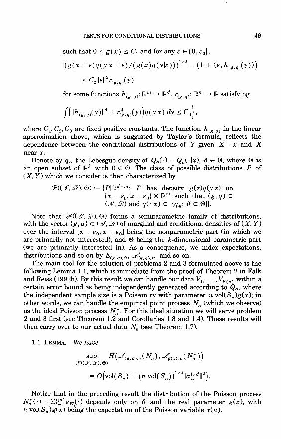
such that ° < g( x) S Cl and for any S E (0, SO],

I(g(x + s)q(ylx + s)j(g(x)q(YIX)))1/2 - (1 + (s, h(g,q)(y))1

S C21IsI12r(g,q)(Y)

where Cl' C2, C3 are fixed positive constants. The function h(g,q) in the linear approximation above, which is suggested by Taylor's formula, refiects the dependence between the conditional distributions of Y given X = x and X near x.

Denote by q{J the Lebesgue density of Q{J(') = Qi . Ix), i} E 0, where 0 is an open sub set of [Rk with ° E 0. The class of possible distributions P of (X, Y) which we consider is then characterized by

9«&<,2),0) := {PI[Rd+m: P has density g(z)q(ylz) on [x - SO' x + sol X [Rm such that (g, q) E

(&<,2) and q( ·Ix) E {q{J: i} E 0}}.

Note that 9«&<,2),0) forms a semiparametric family of distributions, with the vector (g, q) E (&<,9) ofmarginal and conditional densities of(X, Y) over the interval [x - SO, X + sol being the nonparametric part (in which we are primarily not interested), and 0 being the k-dimensional parametric part (we are primarily interested in). As a consequence, we index expectations, distributions and so on by E(g, q), {J' ..f(g, q), {J and so on.

The main tool for the solution of problems 2 and 3 formulated above is the following Lemma 1.1, which is immediate from the proof of Theorem 2 in Falk and Reiss (1992b). By this result we can handle our data VI>" ., VK(n) within a certain error bound as being independently generated according to Q{J' where the independent sampie size is a Poisson rv with parameter n vol(Sn)g(x); in other words, we can handle the empirical point process N n (which we observe) as the ideal Poisson process N;:. For this ideal situation we will serve problem 2 and 3 first (see Theorem 1.2 and Corollaries 1.3 and 1.4). These results will then carry over to our actual data Nn (see Theorem 1. 7).

1.1 LEMMA. We haue

sup H(..f(g,q),{J(Nn) , ~(x),{J(N;:)) .9«.#,9), EJ)

= O(vol(Sn) + (n vol(Sn))1/21Ia;,/d112).

Notice that in the preceding result the distribution of the Poisson process N;:(') = Li~nl sw(-) depends only on i} and the real parameter g(x), with n vol(Sn)g(x) being the expectation of the Poisson variable -ren).


By the preceding model approximation we can reduce the semiparametric problem ~g,q),,')(Nn) with unknown (g, q) E (.#,9) and iJ E 0 to the (k + l}-dimensional parametric problem

~,,')(N:) =~,,')C~>Wi)' where T(n) is a Poisson variable with expectation n vol(Sn)c' C E (0, Cl]' W l , W2, ... are iid rvs with distribution Q,') and T(n) and W l , W2,. .. are independent.

Note that a Binomial process approximation of Nn , where V; is replaced by W; but their number K(n) being kept, does not improve the bound in Lemma 1.1 essentially. We may therefore benefit from the technical ease which we gain by utilizing the Poisson process approximation.

If Q,') is absolutely continuous w.r.t. Qo we obtain from Theorem 3.1.1 in Reiss (1993) that ~,')8 (N:) is absolutely continuous w.r.t. ~ o(N:) with density , n '

d~,')8 (N:) L!,d,,')(J.L):= dj (n N *) (J.L)

c,o n

( 1) (

J.L(lJ;lm) dQ (d) = exp i~l log d~:n (W i ) + J.L(lRm)log -;;-

+ n vol( Sn )( C - d) ) ,

where J.L = Lr~~m) e w' J.L(IR m) < 00, is an atomization of a (finite) point measure J.L on IR m. .

Fix C > 0. By the Neyman-Pearson lemma, the best test oflevel a based on N: for the testing problem

(c,iJ) = (c,O) against (cn,iJn )

( ( d ~ ,') ( Nn*) ) )

+ y n 1{u n,u} log d~:o(N:n (J.L) ,

Yn E [0,1] and U n a' Yn satisfy

Ec,o( cp~( N:» = a.

If we choose (c n, iJn) = (c + o(on)' iJon), then the remainder term

N;;mm) dQ log(L~,cn,,')(N:)) - i~l log d~:(W;)


vanishes asymptotically under (C, 0) and (C n , itn ), and thus,

is asymptotically equivalent to 'P~ (whenever the randomization can asymptotically be neglected), compare the proof of Theorem 1.2.

Notice that

is the ad hoc statistic which one would use for testing it = 0 against itn based on N::. We will show in the following that 'Pn,opt(N::) is in fact an asymptotically optimal level lY test for this problem along the alternatives

Since 'Pn,opt(N::) does not depend on C as shown below, it is asymptotically optimal along these alternatives uniformly in c.

If we allow however a slower rate of convergence of C n' that is, if we consider

then the nuisance parameter cn becomes relevant and 'Pn,oPt(N::) loses its asymptotic optimality along the alternatives (C n , itn ); see Corollary 1.3 and 1.4. By the bound for the model approximation established in Lemma 1.1, the considerations carry over to 'Pn,opt applied to our real data set, that is, the empirical point process Nn •

In order to establish the limit of the power functions E c {j ('P~(N::)), we require Hellinger differentiability of q {j at zero: n' n

(A)

with derivative v = (V l , . .• , vk ), vj E JiQo), j = 1, ... , k, and Ilf{jIIL 2(Qo) =

(j f; dQO)l/2 = o(llitllo). In the following we consider alternatives of the form

TJ E IR,

itn = it°n

and the corresponding sequence of binary experiments

By M([R;m) we denote the set ofpoint-measures on IR m and A'([R;m) denotes the smallest u-algebra such that for any B E Iffim the projection '7TB: Mmm) ~ {O, 1,2, ... }, '7TB(P.) := p.(B) is measurable.


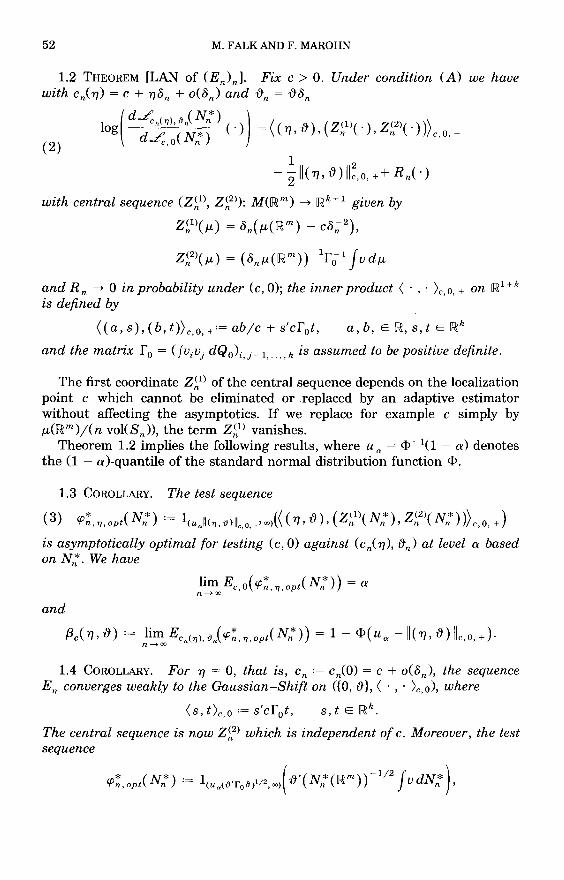
1.2 THEOREM [LAN of (EJn]' Fix c > O. Under condition (A) we have with cn( 1/) = c + 1/0n + o(on) and iJn = iJon

(2)

I (dJ'"n(T/)'l1JNn*) (.») =(( iJ) (Z{l)(·) Z(2)(.»)) og dL (N*) 1/" n 'n C,O,+

C,o n

1 2 - '211( 1/, iJ) Ilc,o, + + RnC)

with central sequence (Z~l), Z~2»): M([Rm) ~ [Rk+l given by

Z~l)(f.L) = 0n(f.L([Rm) - CO;;-2),

Z~2)(f.L) = (onf.L([Rm»-lfü1 fVdf.L

and Rn ~ 0 in probability under (c, 0); the inner product < . , . \0, + on [R1+k is defined by

«(a, s), (b, t»c,o, +:= ablc + s'cfot, a, b, E [R, s, tE [Rk

and the matrix f o = (fvivj dQO)i,j~l, ... ,k is assumed to be positive definite.

The first co ordinate Z~l) of the central sequence depends on the localization point c which cannot be eliminated or .replaced by an adaptive estimator without affecting the asymptotics. If we replace for example c simply by f.L([Rm)/(n vol(Sn)), the term Z~l) vanishes.

Theorem 1.2 implies the following results, where u" = <p- 1(1 - 0:) denotes the (1 - o:)-quantile of the standard normal distribution function <P.

1.3 COROLLARY. The test sequence

(3) CP~'T/,oPt( N:) := l(u)I(T/,l1)l!c.o.+'OO)(( (1/, iJ), (Z~l)( N:), Z~2)( N n*»)) c,o, +) is asymptotically optimal tor testing (c, 0) against (c n ( 1/), iJ n) at level 0: based on N n*. We have

and

1.4 COROLLARY. For 1/ = 0, that is, cn := cn(O) = c + o(on)' the sequence E n converges weakly to the Gaussian-Shi{t on ({O, iJ}, < . , . >c,o), where

<s,t>c,o:= s'cfot, s,t E [Rk.

The central sequence is now Z~2) which is independent o{ c. Moreover, the test sequence


whieh is independent of e, is asymptotieally equivalent to cp~, 0, op/N:n. Consequently, CP~,oPt(Nn*) is asymptotieally optimal for (e, 0) against (e n, itn) at level a uniformly for e > 0. In this ease, the upper bound is ßc(O, it) = 1 - <J:>(u" -Ilitllc,o).

PROOF. The asymptotical equivalence follows from the fact that 0;; 1e1/2 ~ N,;"mm )1/2 under (e, 0) and, by contiguity, also under (e n , itn ). 0

Notice that in the case of a one-dimensional parameter space, that is, k = 1, the test sequence CP~,opt(Nn*) is independent of it up to the sign of it. Hence, CP~,oPt(Nn*) is also optimal uniformly for it > ° or it < 0. We do not know whether there exists a test sequence which is asymptotically optimal uniformly in e if TI "* 0.

In order to prove Theorem 1.2, we need the following auxiliary results which are of interest of their own.

1.5 LEMMA. Let (D,.sat) be a measurable spaee supporting a Poisson proeess N,;". Suppose that under Pt> tE (-E, E), Nn* has the intensity measure A/n)Q/'), where A/n) E (0,00) and Qt is a probability measure on [Rm dominated by the m-dimensional Lebesgue measure. Ifthe eurve t ~ Qt is Hellinger differentiable at ° with derivative v and Ao(n) ~ 00 as n ~ 00, then the following expansion holds with on = (Ain»-1/2:

dQ 1 flog Qon dN,;" = OnfvdN,;" - - f v2dQo + Rn(N,;"),

d 0 2

where Po{lRn(N,;")1 > E} = -Z"'o(N,;"){IRnl > E} eonverges to zero for n ~ 00 and eaeh E> 0.

PROOF. Using conditioning techniques, the proof runs along the lines of the proof in the classical situation [see, e.g., Strasser (1985), Chapter 12]. Note that T(n)o~ ~ 1 in Po probability. 0

The following result is immediate from Lemma 1 in Falk and Reiss (1992b) and the Cramer-Wold device.

1.6 LEMMA. Let N,;" = Li~l EX be a Poisson proeess [over so me probability space (D,.sat, P)] with intensity m~asure EN,;"(') = A(n)Q('), where T(n) is a Poisson rv with ET(n) = A(n) ~ 00 as n ~ 00 and Q denotes the distribution of the independent, [Rm-valued rvs Xv X 2, ... being independent of T(n). Let Vi EL2(Q), fvidQ = 0, i = 1,oo.,k, and f = (fViVjdQ)i,j~1, ... ,k' Then

(A(n»-1/2 fVdN,;" ~~ f(O,f),

where ~~ denotes eonvergenee in distribution and f(?, I) denotes the normal distribution on the Euclidean spaee with mean veetor ? and eovarianee matrix I.


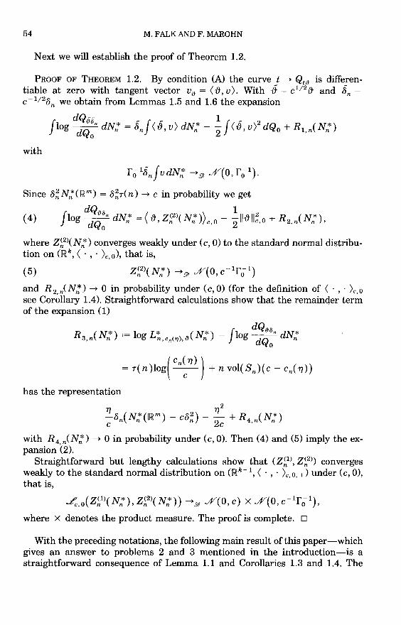
Next we will establish the proof of Theorem 1.2.

PROOF OF THEOREM 1.2. By condition (A) the curve t ~ Qt1J is differentiable at zero with tangent vector vi} = < {}, v). With J = C

1/

2{} and §n =

C-1

/28n we obtain from Lemmas 1.5 and 1.6 the expansion

with

f o1§nfvdN: ~9 .#'(0, f ( 1).

Since 8~N:(lRm) = o~7(n) ~ c in probability we get

(4) dQ 1

flog d~:n dNn* =( {},Z~2)(N:))c,0 - 211{}11~,0 + R 2,n(Nn*),

where Z~2)(N:) converges weakly under (c, 0) to the standard normal distribution on (1Rk, < . , . )c,o), that is,

( 5)

and R 2,n(N:) ~ ° in probability under (c, 0) (for the definition of< . , . \,0 see Corollary 1.4). Straightforward calculations show that the remainder term of the expansion (1)

R 3 ,n(N:) := log L~,Cn(1»,i}(N:) - flog d::n dN:

has the representation

2

2!..on(N:(lRm) - co~) - ~ + R 4 n(N:) C 2c '

with R 4 n(Nn*) ~ ° in prob ability under (c, 0). Then (4) and (5) imply the expansion (2).

Straightforward but lengthy calculations show that (Z~l), Z~2» converges weakly to the standard normal distribution on (!Rk+!, < . , . )c,o, +) under (c, 0), that is,

../",0(Z~1)(N:),Z~2)(N:)) ~9 .#'(O,c) X .#'(0,c- 1f o1),

where X denotes the product measure. The proof is complete. 0

With the preceding notations, the following main result ofthis paper-which gives an answer to problems 2 and 3 mentioned in the introduction-is a straightforward consequence of Lemma 1.1 and Corollaries 1.3 and 1.4. The


asymptotieally optimal test sequenee CP~,T),opt defined in (3) turns out to be also an asymptotieally optimal level a test for testing Qo< ·Ix) against Q1}Ö ('Ix) if applied to the empirieal point proeess Nn • n

1. 7 THEOREM. Consider the testing problem

Qo( 'Ix) against Q1}öJ ·Ix).

Let (CPn)n be a test sequence of asymptotic level a based on N n, that is,

lim supE(g,q),o( CPn( Nn)) :::; a n-">oo

for any (g, q) E C~,.,P) with q( ·Ix) = qo(·)' If Ilanll ~ 0, n vol(Sn)lla;(dI14 ~ 0 and n vol(Sn) ~ 00, then under condition (A) we have for any sequence (gn' qn) E (S',.,p) with gn(x) = g(x) + TJOn + o(on) and qn( ·Ix) = q1}ön('):

(i) limsuPn~ooE(gn,qn),1}Ön(CPn(Nn»:::; ßg(xlTJ,M = 1- <I>(u a -11(TJ,tt)llg(x),o,+)

(ii) lim n ~oo E(g,q),o(CP~,T),op/Nn» = a and

limE(gn,qn),1}Ön(CP~,T),oPt(Nn)) = 1- <t>(u a -11(TJ,tt)llg(x),o,+), n-->oo

that is, (cp~,T),oPt)n as defined in (3) yields an asymptotically optimal test sequence for (g(x),O) against (gn(x), tton) = (g(x) + TJOn + o(on), tton) based on Nn which is of asymptotic level a.

In the case TJ = 0 the test sequence CP~,T),oPt(Nn) is asymptotically equivalent to

CP~,oPt( Nn) = 1(uaWr01})1/2,OO)( tt' (Nn(lRm) r 1/2 f v dNn ) ,

which does not depend on g n(x), g(x) and which is therefore asymptotically optimal, uniformly in (g, q), for (g(x), 0) against (gn(x), tton).

The preeeding results show in partieular that the test sequenee CP~,oPt(Nn), whieh is asymptotieally equivalent to the ad hoe test

(

K(n) )

1(un,a'OO) i~l log( q1}JV;)/qo(V;))

defined in the introduetion, is an asymptotie level a test for tt = 0 for any (g,q) E (S',9) with q('lx) = qo(·)' But it is asymptotieally optimal along alternatives ttn with (gn' qn) E (S', 9), qn( ·Ix) = q1} (.) if and only if gn(x) =

g(x) + o(on), in whieh ease the nuisanee parameter g(x) ean be negleeted.

REMARK. If we ehoose an 1 = ... = an d = bn, then we obtain vol(Sn) =

bn, n vol(Sn)lla;(dI1 4 = O(nb~d+4)/d) and 8n = (nbn)-1/2. The ehoiee bn =

E2n -d/(d+4) with E ~ 0 results in ° of minimum order O(E-ln -2/(d+4» n n n n·

Note that this is up to E;;l the optimal (Ioeal) aeeuraey of estimation of a twiee eontinuously differentiable (i.e., nonparametrie) mean regression eurve [ef. Stone (1982), Millar (1982), Nussbaum (1985), Truong (1989) and Chaudhuri


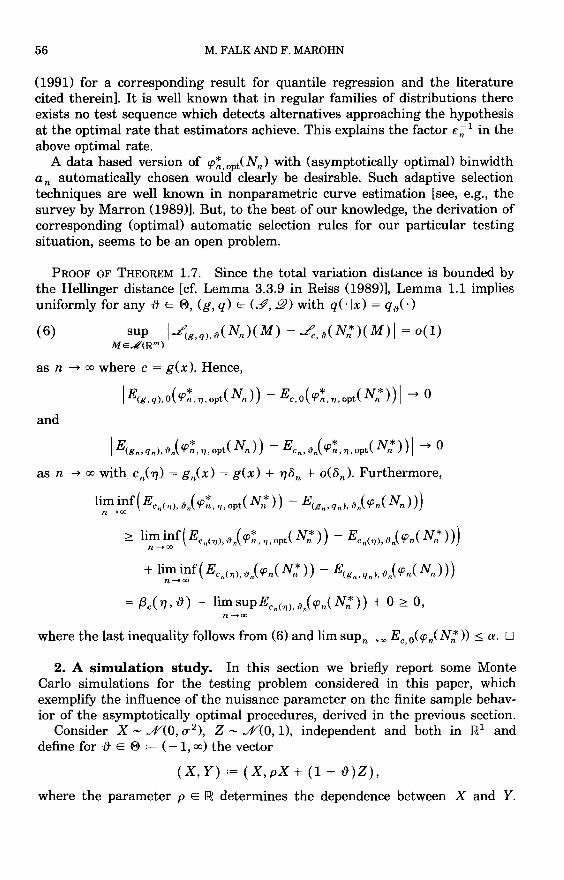
(1991) for a corresponding result for quantile regression and the literature cited therein]. It is well known that in regular families of distributions there exists no test sequence which detects alternatives approaching the hypothesis at the optimal rate that estimators achieve. This explains the factor E;; 1 in the above optimal rate.

A data based version of rp~,opt(Nn) with (asymptotically optimal) binwidth an automatically chosen would clearly be desirable. Such adaptive selection techniques are well known in nonparametrie curve estimation [see, e.g., the survey by Marron (1989)]. But, to the best of our knowledge, the derivation of corresponding (optimal) automatie selection rules for our particular testing situation, seems to be an open problem.

PROOF OF THEOREM 1. 7. Since the total variation distance is bounded by the Hellinger distance [cf. Lemma 3.3.9 in Reiss (1989)], Lemma 1.1 implies uniformly for any {} E 0, (g, q) E (.#,9) with q( ·Ix) = qi·)

(6) sup ld(g,q),ß(Nn)(M) -~,ß(N,;")(M)I = 0(1) ME..R(IT;lm)

as n ~ 00 where c = g(x). Hence,

IE(g,q),o(rp~,1),oPt(Nn») - Ec,o(rp~,1),oPt(N,n)1 ~ 0

and

IE(gn,qn),ßn(rp~,1),oPt(Nn») - ECn,ßn(rp~,1),oPt(N,;"»)1 ~ 0

as n ~ 00 with cn(7J) = gn(x) = g(x) + 7J8n + 0(8n). Furthermore,

lim inf( ECn(1),ßn( rp~, 1), opt( N,;"») - E(gn' qn)' ßn( rpn( Nn») n~OO

n~OO

where the last inequality follows from (6) and lim suPn .... oo Ec O(rpn(N,;"» ::::; a. D

2. A simulation study. In this section we briefly report some Monte Carlo simulations for the testing problem considered in this paper, which exemplify the influence of the nuisance parameter on the finite sampie behavior of the asymptotically optimal procedures, derived in the previous section.

Consider X - ..#'(0, (]"2), Z - ..#'(0,1), independent and both in 1R1 and define for {} E 0 := (-1, (0) the vector

(X, Y) := (X,pX + (1 + {})Z),

where the parameter p E IR determines the dependence between X and Y.


Obviously, we have in this case with x = 0

independent of P and er 2 > 0, whereas Y - uY(O, p2er 2 + (1 + {} )2). Our testing problem is now {} = 0 against {} =1= O.

The joint density of (X, Y) is given by

1 (Z) 1 (Y - pz ) ((z,y) = -;;<P -;; 1 + {} <P 1 + {} = g(z)q(ylz), z,y E IR,

where <p denotes the standard normal density, and the conditional density q iJ of Y given X = 0 is simply

qiJ(Y) = 1 ~ {}<p( 1 ~ {}), Y E IR.

Notice that in this specific example the joint density { depends on the three parameters {} > -1, p E IR and er> 0 with p and er being nuisance parameters of a different character: While er essentially determines the expected sampie size,

of our Y; data with Xi E [ - a n/2, a n/2], the structural parameter p roughly controls the joint distribution of the vector (X, Y).

Taylor expansion of the exponential function at zero implies the expansion

-1=E +OEex (g(E)q(YIc))1/2 P (2 (IYPI+p2)) g(O)q(yIO) 2(1 + {})2 Y P (1 + {})2

=: Eh(g,q)(Y) + O( E2r(g,q)(Y))

uniformly for y, p E IR, {} > -1, E small and I/er::;; Cl' Observe that f(h(g,q/y)4 + r(g,q)(y)4)q(yI0)dy < 00.

Easy calculations show that the family {Qij} = {uY(O, (1 + {} )2)} is Hellinger differentiable at {} = 0 with derivative v(z) = Z2 - 1 and variance f o =

f v2(z)Qo(dz) = f(Z2 - 1)2uY(0, l)(dz) = 2. Up to a normalizing factor, the central sequence Nn(IR)-1/2fvdNn = K(n)-1/2fvdNn becomes in this case

n

Zn:= K(n)-1/2 L (Y;2 - 1)1[-an/2,a

n/2j(X;),

i~ 1

which is approximately normal with mean zero and variance 2 under (g, q) E

(.ß, 9) with q( ·Ix) = qo(·)' According to Theorem 1. 7, the asymptotically optimal test for testing {} = 0

against {}n = {}on = {}(na n)-1/2 uniformly for {} > 0 along (g n' q n) E (.ß, 9)


Zn(i:N)/v"2 4

3

2

1

o

-1

-2

Zn( i: N) / v"2 5

4

3

2

o

-1

-2

/

-3~~~~~~~~~~~~ -3~~~~~.~~~~~~~

-3 -2 -1 0 1 2 3 -3 -2 -1 0 1 2 3

inv( <P(i/(N + 1))) inv(<P(i/(N+l}))

(a) rho=O.l theta=O (b) rho=O.l theta=O.Ol

Zn(i:N)/v"2 4

Zn(i:N)/v"2 5

3 4

3 2

2 1

1

o o

-1 -1

-2 -2

-3~~~~~~~~~~~~ -3~~~~~~~~~~~~

-3 -2 -1 0 1 2 3 -3 -2 -1 0 1 2 3

inv( <P(i/(N + 1})) inv(<P(i/(N + 1 )))

(c) rho=l theta=O (d) rho=l theta=O.Ol

FlG. 1.

TESTS FOR CONDITIONAL DISTRIBUTIONS

with

gn(O) = (21T) -1/20-;1 = g(O) + O(On) = (21T) -1/20-- 1 + O(On)

<=> o-n = 0- + o((na n )-1/2)

and

is in this case

cp~, opt( N n ) = 1(U"I11121/2, 00)( t}Zn)

= 1(um oo)(2- 1

/2 t} /1t}IZn )

= 1(u",00)(2- 1/

2Z n)·

59

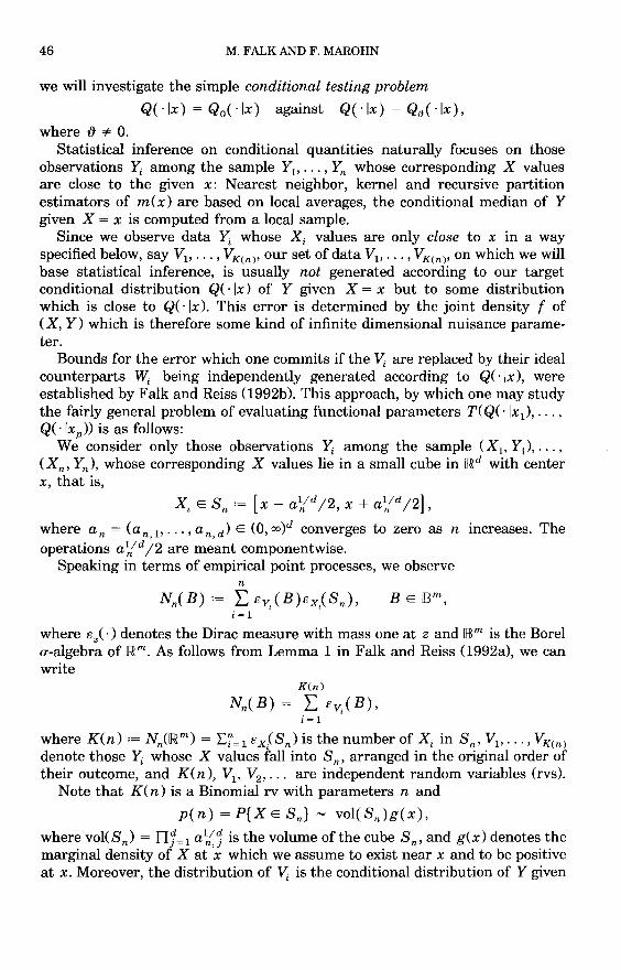
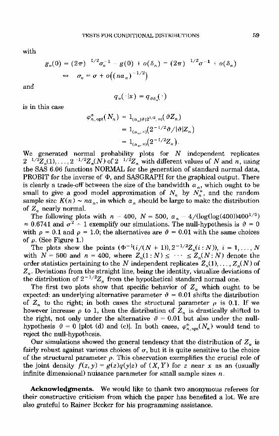
We generated normal probability plots for N independent replicates 2- 1/ 2Z n(1), ... , 2- 1/ 2Z n(N) of2- 1/ 2Z n with different values of N and n, using the SAS 6.06 functions NORMAL for the generation of standard normal data, PROBIT for the inverse of <1>, and SASGRAPH for the graphical output. There is clearly a trade-off between the size of the bandwidth an' which ought to be small to give a good model approximation of Nn by N;:, and the random sampIe size K(n) - na n, in which an should be large to make the distribution of Zn nearly normal.

The following plots with n = 400, N = 500, an = 4/(log(log(400))4001/ 5 )

::::: 0.6741 and 0-2 = 1 exemplify our simulations. The null-hypothesis is t} = 0

with p = 0.1 and p = 1.0; the alternatives are t} = 0.01 with the same choices of p. (See Figure 1.)

The plots show the points (<I>-l(i/(N + 1)), 2- 1/

2Z n(i : N)), i = 1, ... , N with N = 500 and n = 400, where Zn(1: N) =::; ••• =::; Zn(N: N) denote the order statistics pertaining to the N independent replicates Zn(1), ... , Zn(N) of Zn. Deviations from the straight line, being the identity, visualize deviations of the distribution of 2- 1

/2Z n from the hypothetical standard normal one.

The first two plots show that specific behavior of Zn which ought to be expected: an underlying alternative parameter t} = 0.01 shifts the distribution of Zn to the right; in both cases the structural parameter p is 0.1. If we however increase p to 1, then the distribution of Zn is drastically shifted to the right, not only under the alternative t} = 0.01 but also under the nullhypothesis t} = 0 [plot (d) and (c)]. In both cases, CP~,opt(Nn) would tend to reject the null-hypothesis.

Our simulations showed the general tendency that the distribution of Zn is fairly robust against various choices of 0-, but it is quite sensitive to the choice of the structural parameter p. This observation exemplifies the crucial role of the joint density f(z,y) = g(z)q(ylz) of (X, Y) for z near x as an (usually infinite dimensional) nuisance parameter for small sampIe sizes n.

Acknowledgments. We would like to thank two anonymous referees for their constructive criticism from which the paper has benefited a lot. We are also grateful to Rainer Becker for his programming assistance.


REFERENCES BHATTACHARYA, P. K. and GANGOPADHYAY, A. K. (1990). Kernel and nearest neighbor estimation of

a conditional quantile. Ann. Statist. 18 1400-1415. CHAUDHURI, P. (1991). Nonparametrie estimates of regression quantiles and their loeal Bahadur

representation. Ann. Statist. 19760-777. EUBANK, R L. (1988). Spline Smoothing and Nonparametric Regression. Dekker, New York. FALK, M. and REISS, R-D. (1992a). Poisson approximation of empirieal processes. Statist. Probab.

Lett. 14 39-48. FALK, M. and REISS, R-D. (1992b). Statistical inference for eonditional eurves: Poisson proeess

approach. Ann. Statist. 20 779-796. HÄRDLE, W., JANSSEN, P. and SERFLING, R J. (1988). Strong uniform eonsisteney rates for

estimators of eonditional funetionals. Ann. Statist. 16 1428-1449. IBRAGIMov, 1. A. and HAS'MINSKII, R Z. (1981). Statistical Estimation. Application of Mathematics

16. Springer, New York. IBRAGIMOv, 1. A. and KHAS'MINSKII, R Z. (1991). Asymptotieally normal families of distributions

and efficient estimation. Ann. Statist. 19 1681-1724. JONES, M. C. and HALL, P. (1990). Mean squared error properties of kernel estimates of regression

quantiles. Statist. Probab. Lett. 10 283-289. LE CAM, L. (1986). Asymptotic Methods in Statistical Decision Theory. Springer, New York. MANTEIGA, W. G. (1990). Asymptotie normality of generalized functional estimators dependent on

eovariables. J. Statist. Plann. Inference 24 377-390. MARRON, J. S. (1989). Automatie smoothing parameter seleetion: a survey. In Semiparametric

and Nonparametric Economics (A. Ullah, ed.) 65-86. Physiea, Heidelberg. MILLAR, P. W. (1982). Optimal estimation of a general regression function. Ann. Statist. 10

717-740. NUSSBAUM, M. (1985). Spline smoothing in regression models and asymptotie effieieney in L 2 .

Ann. Statist. 13984-997. PFANZAGL, J. (1990). Estimation in Semiparametric Models. Lecture Notes in Statist. 63. Springer,

New York. REISS, R-D. (1989). Approximate Distributions ofOrder Statistics (With Applications to Nonpara

metric Statistics). Springer, New York. REISS, R-D. (1993). A Course on Point Processes. Springer, New York. STONE, C. J. (1982). Optimal global rates of eonvergenee for nonparametrie regression. Ann.

Statist. 10 1040-1053. STRASSER, H. (1985). Mathematical Theory of Statistics. Studies in Mathematics 7. de Gruyter,

Berlin. TRUONG, Y. K. (1989). Asymptotie properties of kernel estimators based on loeal medians. Ann.

Statist. 17 606-613.

MATHEMATISCH-GEOGRAPHISCHE FAKULTÄT KATHOLISCHE UNIVERSITÄT EICHSTÄTT OSTENSTRASSE 26-28 D-8078 EICHSTÄTT GERMANY

ASYMPTOTICALLY OPTIMAL TESTS FOR CONDITIONAL ...

Documents