Three Essays in Dividend Policy. - LSU Digital Commons

Louisiana State University Louisiana State University

LSU Digital Commons LSU Digital Commons

LSU Historical Dissertations and Theses Graduate School

1992

Three Essays in Dividend Policy. Three Essays in Dividend Policy.

Jaisik Gong Louisiana State University and Agricultural & Mechanical College

Follow this and additional works at: https://digitalcommons.lsu.edu/gradschool_disstheses

Recommended Citation Recommended Citation Gong, Jaisik, "Three Essays in Dividend Policy." (1992). LSU Historical Dissertations and Theses. 5382. https://digitalcommons.lsu.edu/gradschool_disstheses/5382

This Dissertation is brought to you for free and open access by the Graduate School at LSU Digital Commons. It has been accepted for inclusion in LSU Historical Dissertations and Theses by an authorized administrator of LSU Digital Commons. For more information, please contact [email protected].

https://digitalcommons.lsu.edu/

https://digitalcommons.lsu.edu/gradschool_disstheses

https://digitalcommons.lsu.edu/gradschool

https://digitalcommons.lsu.edu/gradschool_disstheses?utm_source=digitalcommons.lsu.edu%2Fgradschool_disstheses%2F5382&utm_medium=PDF&utm_campaign=PDFCoverPages

https://digitalcommons.lsu.edu/gradschool_disstheses/5382?utm_source=digitalcommons.lsu.edu%2Fgradschool_disstheses%2F5382&utm_medium=PDF&utm_campaign=PDFCoverPages

mailto:[email protected]

INFORMATION TO USERS

This manuscript has been reproduced from the microfilm master. UMI films the text directly from the original or copy submitted. Thus, some thesis and dissertation copies are in typewriter face, while others may be from any type of computer printer.

The quality of this reproduction is dependent upon the quaiity of the copy submitted. Broken or indistinct print, colored or poor quality illustrations and photographs, print bleedthrough, substandard margins, and improper alignment can adversely affect reproduction.

In the unlikely event that the author did not send UMI a complete manuscript and there are missing pages, these will be noted. Also, if unauthorized copyright material had to be removed, a note will indicate the deletion.

Oversize materials (e.g., maps, drawings, charts) are reproduced by sectioning the original, beginning at the upper left-hand comer and continuing from left to right in equal sections with small overlaps. Each original is also photographed in one exposure and is included in reduced form at the back of the book.

Photographs included in the original manuscript have been reproduced xerographically in this copy. Higher quality 6" x 9" black and white photographic prints are available for any photographs or illustrations appearing in this copy for an additional charge. Contact UMI directly to order.

UMIUniversity Microfilms International

A Beil & Howell Information Company 300 North Zeeb Road. Ann Arbor. Ml 48106-1346 USA

313.'761-4700 800.'521-0600

Reproduced with permission of the copyright owner. Further reproduction prohibited without permission.


Order Number 8S02900

Three essays in dividend policy

Gong, Jaisik, Ph.D.

The Louisiana State University and Agricultural and Mechanical Col., 1992

Copyright ©1998 by Gong, Jaisik. All rights reserved.

U M I300 N. Zeeb Rd.Ann Arbor, MI 48106



THREE ESSAYS IN DIVIDEND POLICY

A Dissertation

Submitted to the Graduate Faculty of Louisiana State University and

Agricultural and Mechanical College in partial fulfillment of the

requirements for the degree of Doctor of Philosophy

in

The Interdepartmental Programs in Business Administration

byJaisik GONG

B.A., Seoul National University, 1981 M.B.A., Seoul National University, 1984

August 1992


ACKNOWLEDGMENTS

I would like to thank Professor George M. Frankfurter, the chairman of my

dissertation committee, for his guidance and encouragement. I am equally grateful to the

other members of the committee: Professors G. Geoffrey Booth, William R. Lane, Joh ' S.

Howe, and Robert E. Martin.

I am also indebted to many other people for their assistance. I appreciate the help

of Professors Carter Hill, Douglas McMillin, and Tae-Hwy Lee. I also wish to thank Joan

Payne, Shirley Young, Bessie Avera, Yvonne Day, Quang Do, Minbo Kim, and my colleagues

in the Department of Finance.

My most heartfelt thanks go to my family. The support and sacrifice of my mother

was crucial to my completion of this dissertation. The love and encouragement of my wife,

Gilwon, kept me on the right track. My two sons, David and Richard, deserve my deepest

appreciation for their tolerance and understanding.


TABLE OF CONTENTS

Acknowledgments List of Tables List of Figures Abstract

Page

Vviivlli

CHAPTER 1: INTRODUCTION

CHAPTER 2: REVIEW OF LITERATURE

A. Dividend PolicyB. Dividends and TaxesC. Dividends and Stock PriceD. Dividend Signalling

5121718

CHAPTER 3: THE DETERMINANTS OF DIVIDEND POLICY 23

A. IntroductionB. Data

1. Sample Selection2. Variable Definitions

C. Methodology1. Time-Series Cross-Sectional Analysis2. Vector Autoregressive Model

D. Empirical Results1. Sample Characteristics2. Time-Series Cross-Sectional Regression Results3. Vector Autoregression Results4. The Lagged Dividend Model5. Interpretation of Results

E. Chapter Summary and Conclusions

23252526 28 28 29 34 34 37 44 57 64 66

CHAPTER 4: DIVIDENDS. TAXES, and PORTFOLIO CHOICES 68

A.B.

C.

IntroductionThe Tax Reform Acts of 1984 and 1986

1. The Tax Reform Act of 19842. The Tax Reform Act of 1986

Models and Testable Hypotheses1. The Tax-Effect Model2. Short-Term Trading Model3. The Portfolio Model

6870707374 74 77 79

III


D. Data and Methodology1. Data2. Methodology

E. Empirical Results1. Descriptive Results of Consistency2. Test of Short-Term Trading Hypothesis3. Test of Tax-Effect Hypothesis4. Portfolio Test Results

F. Chapter Summary and Conclusions

82828485 85 89 96 99 110

CHAPTER 5: EMPIRICAL TESTS OF DIVIDEND SIGNALLING 113

A. IntroductionB. The John and Williams Model

1. Narrative2. Testable Analytical Models

C. MethodologyD. Data and Proxy Variables

1. Liquidity2. Firm Size3. Dividend Policy4. Accounting Variables

E. Testing1. Sample Statistics2. Hypothesis #1 : Demand for Liquidity Causes

Dividend Payments.3. Hypothesis #2: The Equilibrium Price Is Monotonie

in the Dividend Signal (or Private Information).4. Hypothesis 43: Announcement Effects (Excess Returns

during the Event Period) Are an Endogenous Function of Dividend Levels, the Demand for Liquidity, Market Value, and Firm Size.


113115115116 118 120123124124125 127 127

129

139

152160

CHAPTER 6: SUMMARY, CONCLUSIONS, AND FUTURE RESEARCH

BIBLIOGRAPHY

163

168

APPENDIX A: THE RELATIONSHIP BETWEEN DIV AND FCASH 178

APPENDIX B: THE EFFECTS OF 1986 TRA

APPENDIX C: SIGNALUNG MODEL

VITA

180

182

188

IV


LIST OF TABLES

TabI# Page

3.1 Sample Characteristics 35

3.2 Time-Series Cross-Sectional Estimates from Regressing Fuller and Battese Model for 446 Firms in the Samplefrom 1979:11 to 1990:IV 38

3.3 Time-Series Cross-Sectional Regression Analysis Using AlternativeModel Specifications 41

3.4 Tests of Stationarity 45

3.5 Decompositions of Forecast Error Variance 48

3.6 Sensitivity Analysis for Dividend Variance DecompositionsUsing Randomly Selected Samples 53

3.7 Time-Series Cross-Sectional Regressions with Lagged Dependent Variables 59

3.8 Robustness Tests of Lagged Dividend Model 62

4.1 Summary of Changes in the Tax Reform Acts of 1984 and 1986 71

4.2 Number of Sample Firms and Dividend Payment Eventsfrom January 1980 through December 1989 83

4.3 Sample Descriptive Statistics on Ex-Dividend Day Excess Returnsand Dividend Yields 86

4.4 Non-Parametric Tests of Equality of Ex-Dividend Day Excess ReturnsBetween the two periods 90

4.5 Average Excess Returns Around the Ex-Dividend Dayfor the Period January 1, 1980, to July 17, 1984 93

4.6 Average Excess Returns Around the Ex-Dividend Dayfor the Period July 18, 1984, to December 31, 1986 94

4.7 Average Excess Returns Around the Ex-Dividend Dayfor the Period January 1, 1987, to December 31,1989 95

4.8 Cross-Sectional Regression of Ex-Dividend Day Excess Returnson Dividend Yields 98

4.9 Comparison of Cum-Dividend and Ex-Dividend Efficient Portfolios Between the Pre-1984 Tax Reform Period and the Post-1984Tax Reform Period 100


Table Page

4.10 Comparison of Cum-Dividend Efficient Portfolios Between the Pre-1986Tax Reform Period and the Post-1986 Tax Reform Period 107

5.1 Number of Quarterly Dividend Payments in the Sample, by Group 122

5.2 COMPUSTAT Variable Names and Definitions 126

5.3 Quarterly Summary Statistics of the Final Sample, 1986 1/4 - 1990 4/4 128

5.4 Correlation Matrix of Proxy Variables 130

5.5 Average Volume Prediction Error for Quarterly Dividend Announcements1986/1 - 1990/4 132

5.6 Regressions of Dividend Yield on Liquidity Variables 138

5.7 Average Return Prediction Error for Quarterly Dividend Announcements1986/1 - 1990/4 140

5.8 Tests of Firm Size Effects on the Relationship Between Signal and Price 145

5.9 Tests of the Polynomial Pricing Functions 147

5.10 Likelihood Ratio Tests of the JW Model: Constrained and UnconstrainedEstimation of Equation (5.21) 151

5.11 Tests of Cross-Sectional Relations by Dividend for Three Windows,Equation (5.23) 154

5.12 Tests of Liquidity Related Variables by Firm Size, Equation (5.23) 156

5.13 Other Liquidity Tests 159

VI


LIST OF FIGURES

Figure Page

3.1 impulse Response Functions of Dividends 55

4.1 Comparison of Efficient Frontiers (Before 1984 TRA) 104

4.2 Comparison of Efficient Frontiers (After 1984 TRA) 105

4.3 Comparison of Efficient Frontiers(Before 1986 TRA Versus After 1986 TRA) 109

5.1 Information-Motivated Trading VolumeVolume APEs and CAPEs 134

5.2 Liquidity Trading Around the Dividend Announcement Day 136

5.3 The Relationship Between Signal and PriceReturn APEs and CAPEs 143

VII


ABSTRACT

This dissertation focuses on three leading theoretical and empirical issues in the

anomaly of dividend policy. The first essay analyzes the explanatory power of the various

theories of dividend determinants, many of which have not been tested yet. In this essay,

time-series cross sectional tests are undertaken using individual firm data, while the

structural vector autoregressive (VAR) methodology is applied to the aggregate data.

The second essay proposes an alternative approach to the ex-dividend anomalies

that fully incorporates both the tax-effect hypothesis and the short-term trading hypothesis.

This approach draws on normative portfolio selection models to examine the relationships

between the ex-dividend anomalies and the ex-post portfolio choice in the context of the

1984 and 1986 federal tax reforms.

The third essay tests signalling equilibrium models empirically. In this essay, tests

are conducted to provide statistical evidence of the empirical validity of dividend signalling

models. Empirical validation of the notion of a signalling equilibrium is examined for a

sample of dividend-paying firms selected from the NYSE and AMEX.

VIII


Chapter 1. INTRODUCTION

The objective of thii dissertation is to extend empirical work on dividend policy

in three ways. The first essay investigates the determinants of dividend policy. The

extant dividend theories suggest that dividends should be distributed depending on the

firm's attributes such as earnings, investments, free cash flow, tax, firm size, industry

classification, etc. Empirical work on these dividend determinants has lagged behind

theoretical research, and the econometric techniques used thus far leave something to

be desired.

The first essay examines a wide range of theoretical determinants of dividend

policy, including free cash flows. In this essay, time-series cross-sectional tests are

undertaken using individual firm data, while the vector autoregressive (VAR)

methodology is applied to the aggregate data. These methodologies are desirable

because previous studies, which employed cross-sectional analysis of either firm-specific

or aggregate data, failed to capture important information explaining differences in

dividend policy over time. This essay, furthermore, analyzes the explanatory power of

the various theories of dividend policy.

The second assay examines the relationships between ex-dividend anomalies and

ex post portfolio choice in the context of the 1984 and 1986 federal tax reforms. Ex-

dividend anomalies are addressed through competing hypotheses of tax effects and

short-term trading. The two tax reforms are expected to have a significant effect on

dividend policy. The 1984 Tax Reform Act extended the minimum holding period for the

dividend tax deduction, exposing tax-induced short-term traders to more risks. The

1986 Tax Reform Act equalized tax rates on dividends and capital gains, reducing the

dissipative costs of dividends. Transition periods between the two tax reforms provide a

valuable opportunity to analyze the validity of each hypothesis.


2

The second essay draws on normative portfolio selection models and

incorporates both tax effects and short-term trading around the ex-dividend day. The

underlying conjecture of this essay is that any change in the risk-expected return trade

off induced by the two tax reforms should be manifested in the portfolio choices. This

portfolio approach seems more appropriate since it is an equilibrium model with proper

measures of risk and return, rather than a model of behavior.

The third essay tests signalling equilibrium models empirically. Signalling

equilibrium models imply that firms distribute dividends in order to convey favorable

insider information and thus achieve a higher stock price. For example, corporate

insiders are proposed to have incentives to signal more valuable future cash flows by

paying larger dividends if the firm's current shareholders require more liquidity than

internally generated funds.' This signal would result in a bidding up of stock price, thus

benefiting the firm or current shareholders selling stocks. The third essay tests the

explicit relations among the announcement effect, the dividends, and the cum-dividend

market values, suggested by signalling models.

Dividend issues are addressed in a vast body of theoretical and empirical

literature. The literature can be categorized into several broad groups. The first group

has sought to identify the determining factors of dividend policy. The seminal works of

Lintner (19561 and Miller and Modigliani (1961) have motivated many people (see, for

example, Dhrymes and Kurz (1964, 1967), Fama and Babiak (1968), Higgins (1972),

Fama (1974), McCabe (1979), Smirlock and Marshall (1983), and Partington (1985)1 to

investigate empirically the determinants of dividend policy with mixed results. Rozeff

(1982), Easterbrook (1984), and Jensen (1986) draw on agency theory to explain

dividend payments, whereas Myers (1984) and Myers and Majluf (1984) view dividend

policy in terms of pecking order theory. In addition, many authors (see, for example,

Michel (1979), Feldstein and Green (1983), Michel and Shaked (1986), and Dyl and

^This argument ia originally attributable to John and Williams (1985).


3

Hoffmeister (1986)] have extended theoretical and empirical works on other dividend

determinants such as industry classifications, firm size, and beta coefficients.

The second group focuses on the ex-dividend anomaly. In order to explain

excess ex-dividend returns, some authors [see, for example, Elton and Gruber (1970),

Booth and Johnston (1984), Elton, Gruber and Rentzler (1984), Barclay (1987), and

Michaely (1991)] follow the tax-effect hypothesis, which is challenged by Eades, Hess

and Kim (1984), and Grinblatt, Masulis and Trtman (1984). Others [see, for example,

Miller and Scholes (1978, 1982), Kalay (1982, 1984), Lakonishok and Vermaelen

(1983, 1986), Karpoff and Walkling (1988, 1990), Grammatikos (1989), and Fedenia

and Grammatikos (1991)] relate this ex-dividend anomaly to the short-term trading

hypothesis, by allowing for transaction costs around the ex-dividend day.

The third strand of literature began with studies dealing with dividend

announcement effects (see, for example, Pettit (1972), Watts (1973), Aharony and

Swary (1980), Asquith and Mullins (1983), Penman (1983), Patell and Wolfson (1984),

and Kalay and Loewenstein (1985)]. These studies, which document the informational

contents of dividends, have evolved into recent dividend signalling models [see, for

example, Bhattacharya (1979), Miller and Rock (1985), John and Williams (1985),

Ambarish, John and Williams (1987), Ofer and Thakor (1987), Williams (1988), and

Kumar (1988)]. Even though empirical testing of signalling is in its infancy, these

dividend-signalling models have emerged as one of the most appealing theories that

seemingly explain the enigma of dividend policy.

The remaining body of this dissertation is organized as follows. Chapter 2

presents a more detailed discussion and review of the extensive literature relating to the

three essays comprised in this dissertation. Chapter 3 encompasses various

econometric analyses of dividend determinants using time-series cross-sectional tests

and the vector autoregressive (VAR) methodology. In Chapter 4, a portfolio approach is

proposed that can explain the ex-dividend anomalies. In Chapter 5, some empirical tests


4

of dividend signalling are attempted. A summary of this dissertation and some

suggestions for future research are presented in Chapter 6.


Chapter 2. REVIEW OF LITERATURE

The vast body of literature on dividends includes numerous theoretical and

empirical papers. This chapter reviews several bodies of literature that are directly

related to the dissertation. The first body of literature, focusing on dividend policy,

investigates the determining factors of dividends. The second body encompasses

studies associated with two hypotheses tnat attempt to explain the ex-dividend

anomalies: the tax-effect and short-term trading hypotheses. The other two bodies of

literature cover studies dealing with dividend announcement effects and discuss many

recent theoretical studies on dividend signalling.

A. Dividend Policy

Dividend policy has long been an issue of interest in financial literature. The

seminal paper on dividend policy is that of Lintner (19561, which was based on field

interviews with managers at 28 companies. The results of these interviews indicate that

a company's dividend decisions depend on current earnings and previous dividends,

where the relationship between the two determinants constitutes a target pay-out ratio.

Lintner (1956) encapsulizes these observations in a theoretical model, as follows:

D IV / . 0,EARNh (2.1)

DIV, - DIV,,., « a, + d, ( D IV / ■ DIV,.,., ) + 12.2)

whereDIV,* = target dividends in the current year,0, = target pay-out ratio,EARN, > current earnings, andDIV,, DIV,,., = dividends paid in the current and previous years.

(Lintner (1956), p. 107]

Equation (2.2) can be rearranged as

DIV, . o, + A EARN, + K, DIV,.,., + f,. (2.3)


6

Lintner fitted equation (2.3) to the aggregate data that he secured from the national

income accounts. The dividend prediction equations that he obtained are

DIV - 352.3 + 0.15 EARN^ + 0.70 DIV^„ (2.4)

when earnings are adjusted for inventory gains, or

DIV . 106.0 + 0.145 EARN„„^ + 0.788 DIV,.,, (2.5)

when earnings are not adjusted.' {ibid., p. 109]

This Lintner model has drawn two criticisms. First, as Dhrymes and Kurz (1964)

point out, the Lintner model gives a satisfactory prediction of short run dividend policy,

but it does not explain intertemporal variations in dividend policy. Second, Miller (1986)

argues that the Lintner model remains a behavioral model because no author has been

able to solve it as a maximization problem.

The "two variable" Lintner model is supported by Fama and Babiak (1968). They

examine the predictive powers of various dividend models including the Lintner model by

using data for individual firms. Fama and Babiak conclude that the Lintner model

performs well, but the best is the model deleting the constant term and adding the

lagged term for earnings.

Miller and Modigliani (1961) present a strong challenge to the conventional view

of dividend preference. They are concerned with the effect of a firm's dividend policy

on stock price in an ideal economy where perfect capital markets, rational behavior, and

perfect certainty are assumed. Miller and Modigliani develop the irrelevance proposition

on dividend policy in the sense that the value of a firm is not affected by dividend policy.

Miller and Modigliani derive a firm's value as the following expression:

VAL, * [EARN,,, • INV„, + VAL,., ) / ( I + p ,„ ) (2.6)

whereVAL,,VAL,,, « the values of a firm at t and t+ 1 ,EARN,,, » the firm's earnings,INV„, = the firm's investment, andp „ , - the rate of return. (Miller and Modigliani (1961), p. 414]

^The units dsnotad are billions of dollars.


7

Miller and Modigliani show that •• since the firm's earnings, investment, and the value at

t+ 1 are all independent of dividend in equation (2.6) ~ the dividend decisions are

irrelevant for the value of the firm. They also argue that dividend decisions are still

irrelevant for a growing firm with debt and taxes or under uncertainty. This "dividend

irrelevance” proposition is possible because investors can create "homemade dividends"

by selling off portions of the stock of the non dividend paying firm or reinvesting the

dividends paid by the dividend paying firm.

Another major thrust of their paper on dividend policy is an implication of the

Fisherian model of the firm, in which the value of a firm is independent of its method of

financing. Miller and Modigliani propose that dividend decisions are independent of

investments because the higher dividends would induce the more external financing

through the issue of new shares to keep the investment level unchanged. They argue

that the firm undertakes the investment opportunities that maximize its current value,

which is independent of dividend decisions. These imply that there are no "financial

illusions" in a rational and perfect environment. In a world of well-functioning capital

markets, a firm's dividend policy is essentially an exercise in financial packaging. The

value of the shares is determined solely by the underlying real, economic factors, and

not by "mere financial packaging."

This separation proposition on dividends and investments has motivated many

researchers to undertake empirical tests. Higgins (1972) designed a dividend model for

a firm maximizing stockholders' wealth and conducted a two-stage least squares

estimation as follows:

INVRATIO - 0.0280 + 0.7194 SALRATIO + 0.0437 DIVRATIO (2.77) (11.68) (0.19)

andDIVRATIO . 0.0033 + 0.5903 EARRATIO - 0.0625 INVRATIO,

(2.16) (30.20) (-5.25) (2.7)where

INVRATIO " investments/assets,DIVRATIO * dividends/assets,SALRATIO - sales/assets.EARRATIO ” eamings/assets, andt-values are in parentheses. (Higgins (1972), p. 15391


8

Higgins concludes that dividends are considered a residual in the corporate decision

nexus and that investments are not significantly influenced by dividends.

In a more rigorous study, Fama (1974) applies simultaneous equations models to

the data for individual firms. His findings are that dividend decisions are not determined

by investment, and, furthermore, that investment decisions are not affected by

dividends. These results are very consistent with the separation proposition of Miller

and Modigliani (1961) on dividends and investments, even though the proposition

assumes a perfect capital market.

Smirlock and Marshall (1983) provide an extension of Fame's work on the

separation proposition of Miller and Modigliani (1961) by using the Granger-causality

tests. Their use of causality tests has some appeal because "they were developed to

test for statistical exogeneity without specification of structural models" [Smirlock and

Marshall (1983), p. 1660). Smirlock and Marshall do not find any Granger-causality

between dividends and investments. These results, consistent with Fame's (1974), fully

support the separation proposition on dividends and investments.

Another test in support of the separation proposition is offered by Partington

(1985). He conducts a questionnaire survey with 93 large Australian companies to

analyze the relationship among dividend, investment, and financing decisions. His

results indicate non-residual determination of dividends. He concludes that firms would

usually make dividend and investment decisions independently, and that external

financing is residually determined.

On the other hand, Dhrymes and Kurz (1964, 1967) go against the separation

proposition. The motivation for their study (1964) stems from arguments that Untner's

(1956) hypothesis is vulnerable to the explanation of long-run dividend policy. In order

to account for the observed variety of dividend payment practices in firms, Dhrymes and

Kurz (1964) examine several explanatory variables such as size, investment,

indebtedness, liquidity position, control, and income variability in electric utility firms.


9

They find that a firm's dividend policy is affected by investment, indebtedness, size, and

the regulatory status of the firm.

Dhrymes and Kurz (1967) provide an interesting argument and empirical

evidence of dividend policy. They note that, contrary to the assumption of Miller and

Modigliani (1961), capital markets are characterized by imperfections, and that external

financing, including new equity and bond issues, is a more expensive vehicle of

financing than internal funds. They argue that dividends and investments are

competitive outlays, both of which rely on limited internal funds. Their hypothesis

relates that dividends, investments, and external financing are interrelated. Consistent

with the hypothesis, their results indicate that a firm's dividend decisions are

significantly affected by its investment requirements, while investment decisions are

impeded by the rigid dividend policy, and that investments and dividends induce external

financing.

McCabe (1979) examines Dhrymes and Kurz's (1967) study and Fame's (1974)

study, and stresses the role of new debt as a determinant of dividend policy. McCabe

argues that Fama (1974) failed to consider all the relevant variables, which led to a

biased result supporting the Miller and Modigliani separation proposition. His hypothesis

follows arguments of Dhrymes and Kurz (1967) that funds raised from profits and

external financing are allocated between investments and dividends, but his contribution

is that new debts have significant effects on dividend decisions. He finds strong

interdependence among dividends, investments, and new debts, which is against the

separation proposition. This implies that dividend decisions are influenced by new debt

decisions as well as investment decisions.

Agency theory explanations of dividend payments build on Ross (1973), Jensen

and Meckiing (1976), Fama (1980), Rozeff (1982), Fama and Jensen (1983),

Easterbrook (1984), and Jensen (1986). Of these authors, Ross (1973), Fama (1980),

and Fama and Jensen (1983) are dealing with the general agency problems that arise

when the agents do not act in the best interests of the principal. They argue that these


10

agency problems developing In any princlpal-agent relationship are characterized by the

aberrant activities of the agent from the principal's viewpoint. They also suggest that,

since the purpose of a firm Is to maximize the utility of the principals, control of agency

problems Is necessary for the survival of a firm. In this regard, the contribution of

Jensen and Meckiing (1976) Is In viewing agency problems as quantifiable costs Incurred

In agency relationships; monitoring costs, bonding costs, and the residual loss.

Rozeff (1982) Is among the first authors who attempt to explain dividend

payment In light of agency theory. He argues that "a wealth maximizing firm adopts an

optimal "monitoring/bonding" package which acts to reduce agency costs. — the

payment of a dividend Is a device, like a bonding cost or an auditing cost, which Is

employed to reduce agency cost of equity* (Rozeff (1982), p. 2501. Assuming that the

firm Is raising new funds to finance the payment of dividends, Rozeff posits that a firm

seeks an optimum dividend policy minimizing the sum of dividend agency costs and

external financing costs. He suggests that a higher dividend payout ratio associated

with smaller agency costs should be linked to lower Inside ownership and a large number

of stockholders. Consistent with his hypotheses, Rozeff finds that the dividend payout

ratios are negatively related to the percentage of stock held by Insiders, whereas they

are positively related to the firm's number of common stockholders.

Pointing out that Rozeff (1982) does not show any dividend mechanism of

mitigating agency problems, Easterbrook (1984) attempts to explain simultaneous

payment of dividends and raising of new funds In view of agency theory. Easterbrook

defines two forms of agency cost as monitoring cost and risk aversion of managers, and

he presumes that dividend payment forces firms to tap new funds from the capital

market. Easterbrook argues that agency problems characterized by monitoring and risk-

aversion problems are reduced when firms enter capital markets for external financing,

because those firms are efficiently reviewed and monitored by Investment banks and

Intermediaries In the market. His conjecture Is that dividends are paid In order to keep

firms In the market subjecting managers to consistent monitoring. Since other financial


11

devices can be supposed to keep firms in the capital market, his argument is considered

a naive explanation of dividends that does not explain the dividend itself. Easterbrook

himself acknowledges this criticism by saying that "dividends exist because they

influence the firms' financing policies, because they dissipate cash and induce firms to

float new securities" (Easterbrook (1984), p. 652).

Jensen (1986), elaborating on takeovers, emphasizes the role of dividends in

reducing free cash flows at managers' disposal. Defining free cash flows as cash flows

exceeding the funds required for investments. Jensen argues that a firm's substantial

free cash flow aggravates agency problems between stockholders and managers. Under

this theory, managers have strong incentives to expand the resources under their control

and they are likely to waste funds on inefficient projects. Jensen suggests that

dividends should be paid out in ways that instigate managers to gorge the cash beyond

the optimal amount. This implies that free cash flow positively determines dividend

payments.

Pecking order theory, suggested by Myers (1984) and Myers and Majluf (1984),

is at variance with agency theory. Although both theories imply that dividends are paid

to reduce asymmetric information problems, pecking order explanation considers

dividend payments when managers have superior information, whereas agency theory

explanation is concerned with how the interests of agents can be aligned with those of

shareholders.

According to Myers and Majluf (1984), a firm's issue invest decisions are

affected when managers know more about the true value of the firm than outsiders do.

The managers having access to true information are assumed to act in the interest of the

shareholders. If the stock is undervalued, the firm would be reluctantly forced to either

issue stock at a low price for a good investment opportunity, or pass it up. If the stock

is overvalued, the firm would have incentives to take advantage of investors by issuing

stock at a high price. These adverse selection problems can be averted if the firm has

ample financial slack. With adequate financial slack, the firm can avoid having to issue


12

stock at a low price when it needs funds for investments. Financial slack also prevents

the firm from exploiting investors by sending a strong negative signal, if the firm

attempts to finance investments by issuing risky stock rather than using internal cash

flows or safe debts.

Myers and Majluf (19841 therefore argue that, since the financing pecking order

ranks internally generated cash flows first, followed by debt and finally equity, firms are

interested in building up financial slack by restricting dividends. In pecking order theory,

a firm's free cash flow representing financial slack is negatively related to dividend

payments.

B. Dividends and Taxes

Elton and Gruber (1970) originally proposed the tax-effect hypothesis, which

suggests that the differential tax rates of dividends and capital gains affect the ex-

dividend behavior of a stock. They assume long-term investors who have already

decided to sell a stock around the ex-dividend day. The only concern of these investors

is the timing decision of whether to sell before or after the ex-dividend day. In the case

of no transaction costs, equilibrium market ex-dividend prices will be determined such

that a stockholder with different tax rates on dividends and capital gains will be

indifferent as to selling the stock between, before, or after the ex-dividend day. This

indicates that the equilibrium market price on the ex-dividend day should reflect the

value of dividends vis-a-vis capital gains to the marginal shareholders.

Elton and Gruber argue that price change on ex-dividend days implies the

marginal shareholders' tax rates. Observing the relationship between this implied

stockholders' tax rates and the firm's payout ratio, they support a clientele effect

hypothesized by Miller and Modigliani (1961). The clientele effect suggests that

stockholders in lower tax brackets prefer high-yield stock, whereas those in higher tax

brackets prefer low-yield stock. Elton and Gruber find that, with the exception of the

first and eighth decile out of ten deciles, the price change-to-dividend ratio increases up


13

to 1 as the dividend yield rises. Since the price change to dividend ratios less than 1

indicate low dividend yields and high implied tax rates, they argue that low dividend

yields should attract stockholders in relatively higher tax brackets.

Criticism of the tax-effect hypothesis dates to Black and Scholes (1973). They

document unusual returns for several days on each side of the ex-dividend day. This

phenomenon is referred to as the ex-dividend period anomaly because the tax-effect

hypothesis is unable to interpret this behavior. The tax-effect hypothesis is later

exposed to serious criticism by Eades, Hess and Kim (1984) and Grinblatt, Masulis and

Titman (1984). They examine the ex-dividend day returns for non-taxable cash

dividends, stock dividends, and splits and find that the returns behave as if dividends are

taxable. These findings may seriously weaken the validity of the tax-effect hypothesis.

Miller and Scholes (1982), on the other hand, offer an alternative explanation,

arguing that the excess returns on the ex-dividend day, if any, are expected to be

eliminated by short-term traders. Every investor, taxable or not, has a strong incentive

to take advantage of profit opportunities on the ex-dividend day. Individual investors are

likely to be constrained from cum-ex trading by regulatory provisions because of their

tax status. But corporate traders such as brokers and dealers are induced to exploit

profit opportunities on ex-dividend days, because they are eligible for the 85% corporate

dividend tax deduction and taxable at the same rates on dividends and capital gains.

These traders have to face the round-trip costs in their trading. Transaction costs may

well provide a short-term trading equilibrium, securing above-normal returns on the ex-

dividend day.

Kalay (1982) reviews past studies evidencing the ex-dividend day anomalies and

finds potential biases inherent in those studies. He argues that these biases may result

from improper use of closing prices on ex-dividend day or correlation techniques with

some of dependent observations. He adjusts for these biases, but obtains similar results

consistent with the tax-effect hypothesis. However, the striking insight of Kalay (1982)

is in showing that, because of short-term profit elimination on ex-dividend day.


ustockholders' marginal tax rates cannot be inferred from those ex dividend price drops

less than dividend per share.

Elton, Gruber and Rentzler 11984) dispute Kalay (1982) by arguing that Kalay

has underestimated transaction costs to the extent that short term trading is profitable

to investors. Their argument is that the costs associated with bid and ask spread,

clearance, and transfer taxes should be included in transaction costs; then, short-term

trading around ex-dividend days would no longer be profitable. Responding to Elton,

Gruber and Rentzler (1984), Kalay (1984) provides evidence that transaction costs are

not actually large enough to constrain short-term trading. Kalay concludes that short

term trading, as well as long-term tax rates, is a determining factor of equilibrium prices

around the ex-dividend day.

Lakonishok and Vermaelen (1983) and Booth and Johnston (1984) extend the

Elton and Gruber technique to test a Canadian tax reform. They note that, under the

Canadian 1971 tax reform, dividends and capital gains are not differentially treated for

tax purposes. Examining the ex-dividend stock prices during the post-Canadian tax

reform period, Lakonishok and Vermaelen (1983) find the price changes smaller than the

dividend per share on the ex-dividend day. This is interpreted as the result of short-term

trading activities, which is inconsistent with the tax-effect hypothesis.

The concern of Booth and Johnston (1984) is to investigate whether marginal

tax rates can be inferred from the price changes on ex-dividend days in Canada. They

do not obtain much evidence consistent with dividend tax clienteles. Booth and

Johnston also find ex-dividend day price ratios between zero and one. This shows that

the market prefers capital gains to dividends. Booth and Johnston thus argue that

capital gains may still be treated more favorably than dividends because individual

investors can maintain a tax timing option on the realization of capital gains.

Barclay (1987) supports the tax-effect hypothesis by testing the ex-dividend

stock prices before the enforcement of federal income tax. His findings are that in a

world without taxes, dividends are perfect substitutes for capital gains, and stock price


15

drop on ex-dividend days is always equal to the full amount of dividends. Barclay argues

that, in a world with taxes, investors receive a compensating premium for the tax

penalization of dividends relative to capital gains on the ex-dividend day. Positive excess

returns are observed on ex-dividend day, which reflects the higher dividend taxes

compared to taxes on capital gains. This means that the relative taxation of dividends

and capital gains alone determines the ex-dividend prices. It is thus predicted that the

higher the effective dividend tax is than capital gains tax, the greater is dividend tax

penalization and the larger are positive excess returns on ex-dividend day.

Lakonishok and Vermaelen (1986) analyze trading volume around ex-dividend

days to test for tax-induced trading. The original contribution of Lakonishok and

Vermaelen is in realizing the importance of trading activities by short-term traders and in

investigating trading volumes around the ex-dividend day. Their hypothesis is that an

observed increase in trading volume will be followed by short-term trading around ex-

dividend days. They also predict that abnormal trading volume caused by short-term

trading has a negative relationship with transaction costs.

Consistent with their hypothesis, Lakonishok and Vermaelen (1986) find that

trading volume increases significantly around ex-dividend days. They ascribe this result

to the existence of short-term traders who are tempted to capitalize on profit

opportunities around ex-dividend days. It is interpreted that pressures by the short-term

traders result in abnormal trading volume on ex-dividend day.

Another test in support of short-term trading is undertaken by Karpoff and

Walkling (1988). They argue that short-term trading complements the dividend tax

penalty explanation of positive ex-day returns. Karpoff and Walkling propose that ex

day returns positively related to transaction costs are eliminated up to marginal

transaction costs. Using four proxies for transaction costs, they find positive

relationships between transaction costs and ex-day returns, which turn out to be

apparent in high-yield stocks after the enactment of negotiated commissions.


16

Green (1980) and Grundy (1985) suggest the delay and acceleration hypothesis.

Their arguments state that trading activities around the ex dividend day will concentrate

on the last cum dividend day and on the first ex dividend day, because investors attempt

to avoid costs resulting from delaying or accelerating transactions relative to their

optimum trading date for tax purposes. High dividend taxed sellers and low dividend-

taxed buyers who want to trade cum-dividend will be induced to transact on the last

cum-dividend day. High dividend-taxed buyers and low dividend-taxed sellers who want

to trade ex-dividend will be induced to transact on the first ex-dividend day.

On the other hand. Long (1977) is the first author to consider dividend and tax

problems in view of portfolio choice. The basic idea of his portfolio approach is that the

ex-dividend value of stock and short-term trading behavior around ex-dividend day

should reflect the trade-off of risk and expected return. Long argues that the market

value of stock is given by a linear function of its expected end-of-period value, the

covariance of its end-of-period value with the end-of-period value of all risk assets, and

its end-of-period dividend. He suggests that "the portfolio dividend yield choice cannot

be made independently of the risk-expected return trade-off, since the dividend yield of

all mean variance efficient portfolios is a linear function of their non-diversifiable risk”

(Kalay (1982), p. 1059).

Long (1977) shows that, with the introduction of income taxation, investors will

demand after-tax efficient portfolios, which may not be before-tax efficient. For

example, under the tax regime that raised dividend tax rate relative to capital gains tax,

investors are induced to revise their portfolio holdings to reflect new tax differentials.

That sort of portfolio revision will lead to an efficiency gain at the new tax rates because

"such a move will both increase the expected after-tax return at the new tax rates and

reduce the after-tax variance of the portfolio" (Long (1977), p. 391. An increase in the

expected return is to be anticipated in the tax-effect hypothesis since the tax premiums

occur with an increase in dividend tax or a decrease in capital gains tax, but its variance

is not considered in the tax-effect hypothesis.


17

Accordingly, the after-tax efficient portfolio will dominate any given before-tax

efficient portfolio on an after-tax basis. Furthermore, Long predicts that the potential

after-tax efficiency gains due to moving from the before-tax efficient portfolio to the

dominating after-tax frontier will be smaller if the correlations between two portfolios are

large.

C. Dividends and Stock Price

It has been accepted by many authors [Graham and Dodd 11951); Walters

(1956): Gordon (1963); and Asquith and Mullins (1983)1 that investors prefer dividends

to capital gains, and that firms could increase the market value of their shares by

choosing a generous dividend policy. These arguments belong to the "bird in the hand"

hypothesis and are perhaps the most popular and durable arguments for dividends. This

notion implies that, because stock prices are highly variable, dividends represent a more

reliable form of return than capital gains.

Among the first authors in favor of this dividend preference are Graham and

Dodd (1951). Graham and Dodd state, "The considered and continuous verdict of the

stock market is overwhelmingly in favor of liberal dividends as opposed to niggardly

ones." Elaborating on his "bird in the hand" argument, Gordon (1963) shows that

dividend has an influence on stock price because investors discount the expected stream

of future dividends. According to Frankfurter and Lane (1990), this "bird in the hand"

hypothesis implicitly assumes that there are two rates of return for evaluating future

cash flows: the investors' opportunity rate and the firm's opportunity rate. These two

rates are completely known under symmetric information. Dividend policy is then the

consequence of the relationship of these two rates.

On the other hand. Miller and Modigliani (1961) note that their dividend

irrelevance proposition holds even under uncertainty, but they puzzle over the observed

fact. They observe that in the real world a change in the dividend rate is often followed

by a change in the market price. Miller and Modigliani hint that the "informational


18

content of dividends” may be considered as a way of reconciling the dividend irrelevance

theory with this observed fact. But what they had in mind is different from the formal

signalling models that Spence (1973) invented later. Asquith and Mullins (19831

demonstrate that dividend policy affects shareholders' wealth because dividends

provide valuable information to investors. Asquith and Mullins recognize that dividends

may contain information.

The major problem with these dividend preference models - thougn it is very

common to other dividend models ~ is the inability to explain observed behavior

thoroughly. Some firms do not pay dividends, whereas other firms pay dividends

following distinct patterns of dividend policy. For example, one explanation for observed

dividend policies may be "the needs of individual investors.” Feldstein and Green (19831

point out that "there is the desire on the part of small investors, fiduciaries, and

nonprofit organizations for a steady stream of dividends with which to finance

consumption” {ibid., p. 17). This argument germinates a signalling model such as that

of John and Williams (1985).

D. Dividend Signalling

Signalling models were developed under the assumption of asymmetric

information, with corporate insiders being better informed than the market as a whole.

These models seek to explain dividend payment in the context of its informational

content. Signalling models originate in the works of Akerlof (1970), Spence (1973), and

Riley (1979). Bhattacharya (1979) is the first to view a dividend as a signal of

management's private information about future cash flows. Later, Miller and Rock

(1985), John and Williams (1985), and Kumar (1988) have developed different models

of dividend signalling. In dividend signalling models, dividends are assumed to affect

stock price because the market believes that they signal favorable insider information.

Management is motivated to pay dividends in order to convey information and thus

achieve a higher stock price.


19

As Miller (19871 specified, dividend signalling models are characterized by three

key conditions. First, the dividend is intended to signal the firm's attributes such as its

current and future earnings, which are asymmetrically known to insiders. Insiders act in

the best interest of shareholders. Second, the beneficiaries of signalling must exist. The

higher stock price induced by signalling benefits (11 the firm having easy access to

future public floatations (e.g., Leland and Pyle (19771 and Harris and Raviv (1986)]; (2)

the current shareholders selling their shares [e.g.. Miller and Rock (1985) and John and

Williams (1985)1; and (3) management who is compensated by the rise of stock price

[see, for example, Ross's (1977) incentive'Signailing model]. Third, dividend payments

should incur cost penalties including personal taxes, the firm's transaction costs of

funding liquidity shortfalls, and costs of underinvestments.

In signalling models, these sufficient conditions for signalling equilibrium are

manifested in the form of maximizing shareholders' objective function. This qualitatively

differs from other dividend models dealing with its announcement effects. Thakor

(1989) raises another puzzling question: "Why dividends are chosen as a signal when

less costly signals are apparently available 7 Why management does not convey

information in some other way involving less tax cost to the stockholders than the

payment of dividends?" [Thakor (1989), p. 433].

The first model in dividend signalling is that of Bhattacharya (1979). He

assumes that current shareholders care about their firm's present value and that outside

investors cannot differentiate the quality of projects undertaken by the firm. Outsiders

correctly appreciate the firm's stock and then buy its stocks at the correct price in the

perfect capital market. Bhattacharya develops an equilibrium model that relates the

benefits and costs of dividend signalling. In his signalling model, taxable dividends are

paid in order to signal expected cash flows of the firm. This dividend maximizes the

after tax objective function of shareholders, which incorporates the signalling benefit of

dividends coming from the increase in liquidation value, conditional on dividend payment.


20

The tax-based cost structure generates feasible signalling equilibria because it is

negatively related to true expected cash flows. An asymmetric transaction cost is also

embodied in his signalling model. Bhattacharya (1979) argues that larger values of

corporate private attribute reduce the extent of outside financing. If the firm has

insufficient cash flows to make up its promised dividend, then it must rely on outside

financing and incur a higher transaction cost relative to the case of sufficient cash flows.

This transaction cost is asymmetric in the sense that larger values of private attribute

known only to insiders decrease the present value of future transaction costs and

thereby decrease the marginal signalling cost. This marginal signalling cost, which is

strictly negatively related to true expected cash flows, weighs the marginal benefits of

dividend signalling and produces a signalling equilibrium.

Miller and Rock's model (1985) works with the similar assumption that outside

investors cannot observe the firm's current cash flows. The investor infers that, since

corporate earnings have a great deal of persistence, current earnings convey information

about the firm's future prospects. Investment opportunities are available to all firms

with diminishing marginal returns, and outside financings are costlessly raised through

sales of corporate bonds. Dividends are perfect substitutes for repurchases of bonds,

and they are not taxable differentially from capital gains. Miller and Rock also assumes

that, unlike Miller and Modigliani (1961), investments are determined as a residual in the

financial nexus.

Miller and Rock (1985) argue that, in the context of information asymmetry,

paying dividends instigates the market to believe higher current earnings in the firm, thus

bidding up the stock price. Corporate insiders then have incentives to signal by

distributing more dividends and cutting investment below the optimal level. Even

insiders with less valuable projects attempt to mimic more valuable firms by paying more

dividends and forgoing profitable projects. Since dividend payments reveal cash inflows

and firms forgo projects with positive net present values, the Fisherian optimum

investment policy breaks down.


21

Miller and Rock (1985) suggest one possible route for achieving a signalling

equilibrium, as follows. Outsiders understand that more informed insiders are tempted

to take advantage of their superior information. Outsiders are therefore induced to

discount the stock price offered on dividend announcement day, while corporate insiders

are exploiting a departure from the Fisherian optimum. These conflicting pressures lead

to an equilibrium, restoring the consistent dividend and investment policies even at the

sacrifice of efficiency.

John and Williams (1985) develop a signalling equilibrium with dividends and

personal tax on dividends. In their model, capital gains are not taxable, and issuing,

retiring, or trading shares does not incur any cost. According to their arguments, if the

liquidity demand by the firm and its current shareholders exceeds internally generated

funds, corporate insiders are motivated to distribute a taxable cash dividend and to

reveal to outside investors the present value of their firm's future cash inflows. This

signal would result in a raising of stock price and a benefit to current stockholders.

John and Williams (1985) attempt to explain why some firms do not pay dividends,

whereas others do pay dividends and simultaneously sell new shares to investors. In

order to finance investments, a firm needs to either issue new shares or retire fewer

outstanding shares. Similarly, to collect cash for personal use, current stockholders

must sell their shares. In either case, stockholders have to suffer some dilution in their

fractional ownership of the firm. Current shareholders desire to reduce this dilution on

corporate or personal accounts, and insiders, in the best interest of current stockholders,

are induced to convey their favorable information by paying a taxable dividend.

Recognizing the relationship between favorable information and stock price, the market

bids up the stock price and thereby mitigates stockholders' dilution.

The signalling equilibrium of John and Williams (1985) is achieved because the

marginal gains from paying dividends are balanced against the marginal cost incurred by

dividend tax. In the market, stocks with marginally larger dividends are responded with

the premiums, following the reduction in dilution for current shareholders. These


22

benefits compensate shareholders for taking proportional costs due to dividend taxes.

For firms paying marginally smaller dividends, the marginal dead-weight costs of

dividends outstrip the marginal benefits of reducing ownership dilution. In John and

Williams' (1985) model, an optimal signalling equilibrium is derived when firms with

favorable inside information distribute higher dividends and receive higher stock prices

for their shareholders.

Following Miller and Rock (1985), Kumar (1988) assumes that the dividend

signal produces endogenous investment. He then argues that dividend changes can be

used as a "coarse" signal kwcause dividends reflect partitioned spaces of all possible

corporate prospects and thereby dividend changes represent "broad" changes in these

prospects. Kumar states that these coarse signalling equilibria attain the simultaneous

explanation of several extant dividend anomalies such as (1) information effects of

dividend changes (e.g.. Petit (1972) and Aharony and Swary (1980)]; (2) dividend

smoothing [e.g., Lintner (1956), Fame and Babiak (1968), and leub (1972)1; and (3)

dividends as a poor predictor of future earnings [e.g.. Penman (1983)1.


Chapter 3. THE DETERMINANTS OF DIVIDEND POLICY

A. Introduction

This essay empirically investigates the determining factors of dividend policy. In

this study, a structural model is specifically designed and tested, encompassing

determinants from previous dividend theories. The motivation for this study is that

many of these previous theories have not been tested, and that the econometric

techniques used thus far are inappropriate.

The vast body of literature dealing with dividend determinants can be grouped

into two distinct categories: symmetric and asymmetric information, in the symmetric

information milieu, the seminal work is that of Lintner (1956). According to Lintner's

model, the current dividends are predicted on the current profits and past dividends.

This "two-variable* model is supported by evidence by Fame and Babiak (1968). On the

other hand, in an idealized world. Miller and Modigliani (1961) show that the dividend

decision must be independent of the investment decision. This is because higher

dividends would induce more external financing through the issue of new shares to keep

the investment level unchanged. Miller and Modigliani (1961) also argue that the

dividend decision is irrelevant for a growing firm under the conditions of taxes and debt

financing. This separation proposition on dividend and investment has motivated many

people to investigate empirically the dividend subject with mixed results. Higgins

(1972), Fame (1974), Smiriock and Marshall (1983), and Partington (1985), for

example, find that corporate dividend and investment decisions are separable and

independent. Ohrymes and Kura (1964, 1967) show that dividend and investment

decisions are strongly interrelated. McCabe (1979) also provides strong evidence of

interdependence among the dividend, investment, and financing decisions, and he

argues that dividends are affected by new long-term debts.

23


24

Theories based on the premise of asymmetric Information Includes agency,

pecking order theory, and dividend signalling. Agency theory explanations of dividend

behavior build on the works of Jensen and Meckling (1976), Fama (1980), Rozeff

(1982), Easterbrook (1984), and Jensen (1986). The argument Is that agency costs

associated with free cash flows positively determine dividend payments. Pecking order

theory, suggested by Myers (1984) and Myers and Majluf (1984), Is at variance with

agency theory. In these papers it Is argued that, since the financing pecking order ranks

Internally generated cash flows first, followed by debt and finally equity, firms are

Interested In building up financial slack by restricting dividends. In the pecking order

theory, a firm's free cash flows are negatively related to dividend payments.

In addition, many authors have extended theoretical and empirical works on

other dividend determinants. Michel (1979) and Michel and Shaked (1986) consider

Industry Influence on dividend policy. In Feldstein and Green (1983), size and risk

aversion are assumed to Influence the dividend decision. Dyl and Hoffmeister (1986)

suggest that dividend policy should be reflected In the beta coefficient as a proxy of the

riskiness of a firm.'

The work here differs from earlier studies in three ways. First, in this essay,

time series cross-sectional tests are undertaken using individual firm data, while the

vector autoregressive (VAR) methodology is applied to aggregate data. These

methodologies are more appropriate In the sense that previous studies employed cross-

sectional analysis of either firm-specific or aggregate data and they lost Important

Information explaining differences in dividend policy over time. Second, this study

includes empirical tests of agency theory and pecking order theory associated with free

cash flows. The literature In this area Is limited or non-existent. Third, this study

'Rozeff (1982) also shows that beta coefficients are negatively correlated with dividend payout ratios.


25

examines a wide scope of dividend determination theories including industry, size, and

beta. Section B is a description of the sample and the variable definitions. In Section C,

the methodology is explained. Section D presents tests, results, and their interpretation.

Section E is the conclusion.

B. Data

The tests are undertaken using both individual firms' data and aggregate data.

Five firm-specific accounting variables - dividends, earnings, investments, long-term

debts, and free cash flows - are analyzed over the 1979-1990 period using quarterly

data because firms usually pay dividends on a quarterly basis. The aggregate data are

obtained by cumulating individual firms’ data.' The effects of firm size, beta, and

industry are also tested. The data sources are the Quarterly COMPUSTAT tapes and the

CRSP files.

1. Sêoipl» SeheHon

The sample used in this study is taken from two COMPUSTAT quarterly tapes

for the period 1979-1990. The 1991 COMPUSTAT tape is used to obtain the data for

1980-1990. The 1990 COMPUSTAT tape is used only for 1979.

To be included in the sample, the data must meet several screening criteria.

First, all data required for this study must be complete for the sample period for each

firm. All data items used to represent or calculate dividends, earnings, investments,

long-term debts, free cash flows, and firm sizes must be in the COMPUSTAT files

throughout the sample period. Second, the firms must keep a December fiscal year-end

for the sample period. This screening allows matching of quarterly data items across

The tests conducted for aggregated data may be affected by the aggregation bias because some of the variables are not necessarily non-negative. This aggregation problem will be explored later by testing for sensitivity to sample sizes.


26

firms. Third, the firms must be listed on the Center for Research in Security Prices's

(CRSP) monthly file for the sample period. The firms' SIC codes for classification of

industries are also obtained from the CRSP file. Application of these criteria during the

screening process yielded a final sample of 446 firms.

2. Variabh OefhA&vrs

Variable definitions used in the analysis and their sources are as follows. All

accounting variables are seasonally unadjusted quarterly data, it is assumed that

because of budget constraints, firms are more interested in the levels of accounting

variables than in their percentage changes. Since the purpose of this study is to

investigate the relationships among five quarterly variables, flow variables that uniquely

accrue to each quarter are needed for dividends, earnings, investments, long-term debts,

and free cash flows. Investment and long-term debt are stock data obtained from each

firm's balance sheet, whereas earnings and free cash flows are flow data calculated

from the firm's income statement. Accordingly, net quarterly changes are calculated for

investments and long-term debts in order to get the amounts allocated to each quarter.

DIV: Three different proxies of dividend are usually discussed in the literature:

(1) amounts of common stock dividends paid (Lintner (1956), Dhrymes and Kurz (1967), Higgins (1972), McCabe (1979), and Smiriock and MashalK 1983)1;

(2) change in dividends (Fama and Babiak (1968), Fama (1974)1; and(3) dividend payout ratio [Rozeff (1982)1.

The dividend proxy used in this study is the amounts of common stock dividends

paid. This measure is calculated by COMPUSTAT data item #15 (common

shares used to calculate earnings per share) * data item *16 (dividends per

share).

/NV: Proxies of investments include;

(1) change in net plant and equipment (Higgins (1972), Fama (1974)1; and(2) investment in fixed assets (Ohrymes and Kurz (1967)1.


27

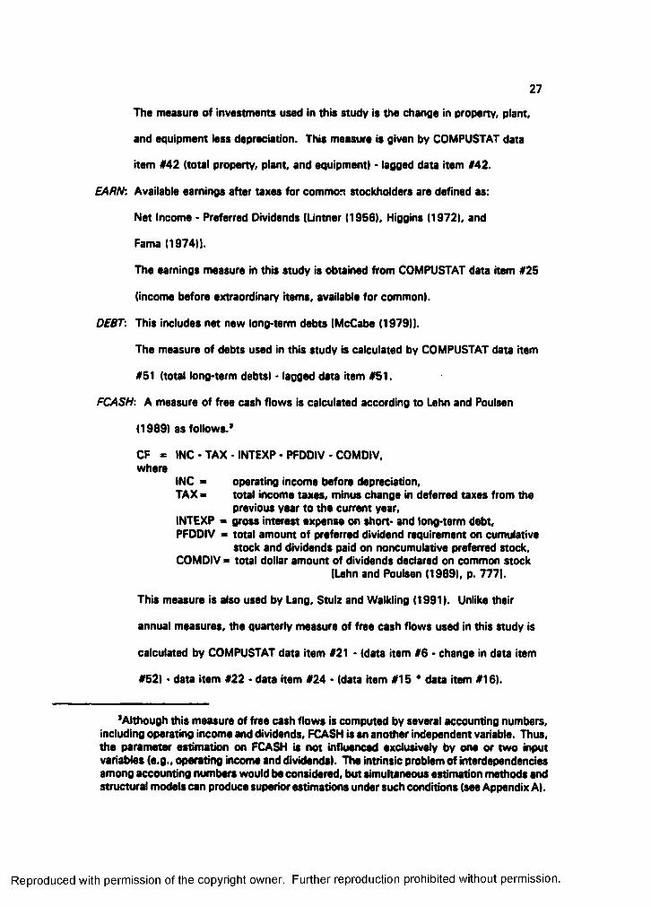
The measure of investments used In this study is the change in property, plant,

and equipment less depreciation. This measure is given by COMPUSTAT data

item *42 (total property, plant, and equipment) • lagged data item #42.

EARN'. Available earnings after taxes for common stockholders are defined as:

Net Income • Preferred Dividends [Lintner (1956), Higgins (1972), and

Fama (1974)1.

The earnings measure in this study is obtained from COMPUSTAT data item #25

(income before extraordinary items, available for common).

DEBT'. This includes net new long-term debts (McCabe (1979)1.

The measure of debts used in this study is calculated by COMPUSTAT data item

#51 (total long-term debts) - lagged data item #51.

FCASH: A measure of free cash flows is calculated according to Lehn and Poulsen

(1989) as follows.*

CF = INC - TAX - INTEXP - PFDDIV - COMDIV, where

INC > operating income before depreciation,TAX “ total income taxes, minus change in deferred taxes from the

previous year to the current year,INTEXP « gross interest expense on short- and long-term debt,PFDDIV > total amount of preferred dividend requirement on cumulative

stock and dividends paid on noncumulative preferred stock, COMDIV > total dollar amount of dividends declared on common stock

(Lehn and Poulsen (1989), p. 7771.

This measure is also used by Lang, Stulz and Walkling (1991). Unlike their

annual measures, the quarterly measure of free cash flows used in this study is

calculated by COMPUSTAT data item #21 - (data item #8 - change in data item

#52) - data item #22 - data item #24 - (data item #15 * data item #18).

'Although this measure of free cash flows is computed by several accounting numbers, including operating income and dividends, FCASH is an another independent variable. Thus, the parameter estimation on FCASH is not influancad axclusivaly by ona or two input variables (e.g., operating income and dividends). The intrinsic problem of interdependencies among accounting numbers would be considered, but simultaneous estimation methods and structural models can produce superior estimations under such conditions (see Appendix A).


28

SIZE: Two proxies of firm size are:

(1) the logarithm of book assets [Wansiey and Lane (1987), Friend and Hasbrouck (1988) I; and

(2) market value of equity outstanding.

The proxy of firm size used in this study is the logarithm of book assets, which

is given by COMPUSTAT data item *44 (total assets).

INDUSTRY: Four digit SIC industries are obtained from CRSP.

The first two-digit SIC codes are used to determine industry.

BETA: The market model is used to obtain beta coefficients (see Sharpe (1963)1.

C. Methodology

1. Tim»-S9ri9S Cross-Sêctionêl Aniyais

First, a time-series cross-sectional model is applied to individual firms' data. A

generalized linear model is considered, where observations occur at T time periods for

each of N firms. The model at time t for each firm I is designed as

DIVg~9f , * e , INVg * 02 EARNg * 8 , DEBTg * 8 4 FCASH, * u , , , 3 ^ ,

/■i,...,Af Ni,...,r

where 9 are the coefficients, and Un is a regression error term.

To estimate 0 , the error components model of Fuller and Battese (1974) is

followed. In the error components model, the regression error u* is assumed to consist

of three independent components.

Wt ■ Y; ♦ */•*•«# • 13 2)

where k, is an unique cross-sectional effect, k ~ (0,o /);d, is an unique time effect, d, (0 ,a /); andf* is an error term, f , ~ (0 ,0,').


29

Under these assumptions, the covariance matrix of the regression error term u„ is

a[ « / ' ) - o j ♦ 0* <3.3)

where I* is an NxN identity matrix,® is the Kronecker product matrix, andJt is a TxT matrix of ones.

Fuller and Battese found that premultiplying equation (3.1) by the covariance

matrix yields the uncorrelated errors with variance a /. The observations are thus

transformed by the covariance matrix, and an OLS regression is run on this transformed

data. Then, unbiased and efficient generalized least squares (GLS) estimates are

obtained.

The estimated 9 values and t statistics for H,: 8 = 0 are used to determine the

relationship between dividends and explanatory variables.

2. V«etof Autongfttsiv* Modt!

Vector autoregressions are employed to analyze the aggregate data (see, for

example, Sims (1980), Lhterman (1986), Lupoletti and Webb (1986), Holtz Eakin,

Newey and Rosen (1988), Blanchard (1989), Keating (1990), and Clements and Mizon

(1991)1. Under the VAR model, a system of dynamic linear equations are constructed

such that a vector of dependent variables is related to lagged vectors of all variables in

the system. For example, the dividend equation takes the form;

M M M(3.4)

where the a, f u, x and « are the coefficients, m is the lag length, ande, is a white noise error term.


30

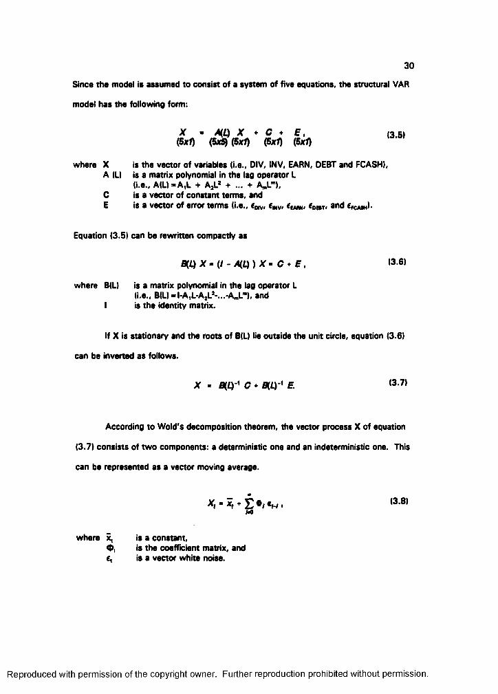
Since the model is assumed to consist of a system of five equations, the structural VAR

model has the following form:

X • Am X * C * E , (3.5)aSxl) (5*5) (5x1) (5x1) (5xf)

where X is the vector of variables (i.e., DIV, INV, EARN, DEBT and FCASH),A (LI is a matrix polynomial in the lag operator L

(i.e., A(L) -A ,L + AjL* + ... + A^L"),C is a vector of constant terms, andE is a vector of error terms (i.e., eo*v> <mv> (omT, and Ckash)-

Equation (3.5) can be rewritten compactly as

X ~ (I - A m ) X • C * E , 136)

where B(L) is a matrix polynomial in the lag operator L(i.e., B(U-l-A,L-A,L*-...-A„L"’), and

I is the identity matrix.

If X is stationary and the roots of B(L) lie outside the unit circle, equation (3.6)

can be inverted as foilows.

X - Bm'^ c ♦ ' E 13 7)

According to Wold's decomposition theorem, the vector process X of equation

(3.7) consists of two components: a deterministic one and an indeterministic one. This

can be represented as a vector moving average.

♦ E • / «r-/ >hO

where \ is a constant,0 , is the coefficient matrix, ande, is a vector white noise.


31

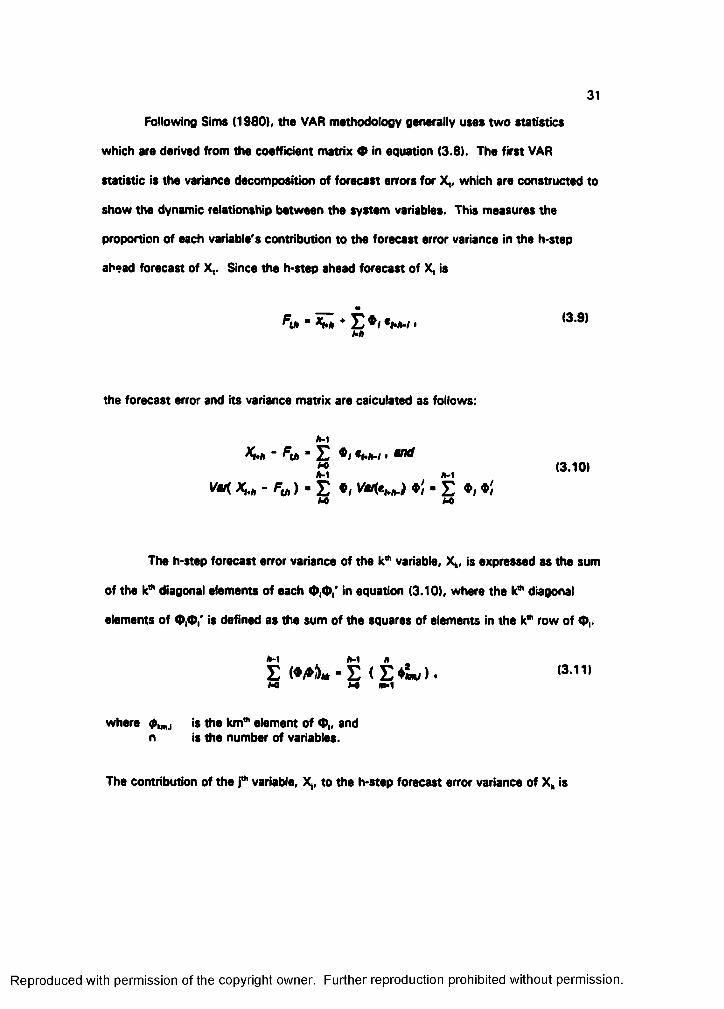
Following Sims (1980), the VAR methodology generally uses two statistics

which are derived from the coefficient matrix 0 in equation (3.8). The first VAR

statistic is the variance decomposition of forecast errors for X,, which are constructed to

show the dynamic relationship between the system variables. This measures the

proportion of each variable's contribution to the forecast error variance in the h-step

ahead forecast of X,. Since the h-step ahead forecast of X, is

♦ E ♦/ «►*-/ •hh

the forecast error and its variance matrix are caiculated as foilows:

*-i" E •/ *hh-i.K

vuKh - - E •/ ♦/' -EK M)

(3.10)

The h-step forecast error variance of the variable, X», is expressed as the sum

of the k"* diagonal elements of each 0 ,0 ,' in equation (3.10), where the k*** diagonal

elements of 0 ,0 ,' is defined as the sum of the squares of elements in the k" row of 0 ,.

E (Ê C ) .M Ml m>1

where 0kmj the km* element of 0„ and n is the number of variables.

The contribution of the j* variable, X,, to the h-step forecast error variance of X„ is


32

*•1

M

where is the kj'” element of 0 ,.

Then, the relative proportion of the j"" variable, X,, to the h-step forecast error variance

of Xk is measured by

»-i »E ( E OM M>1

(3.13)

Variance decomposition allocates the h-step forecast error variance for each

variable into the components accounted for by its own surprise movements and by

shocks to other variables in the system. Since the error variance of a variable is

identified as the sum of contributions by all variables in the system, variance

decomposition can be used to investigate the influences of a variable on another

variable. For example, if investment makes significant contributions to the forecast error

variance of dividend, then this will imply that investment is a major influence on

dividend.

The second test statistic in VAR is an impulse response function (IRF), which is

meant to trace out the response path of the system variables to an unexpected unit

shock in a variable. The normalized unit shock to a variable is given by a one standard

deviation surprise movement in that variable.*

*This is often called innovation accounting in the sense that it traces out the system's reaction to a shock (innovation) in a variable [see Sims (1980)1.


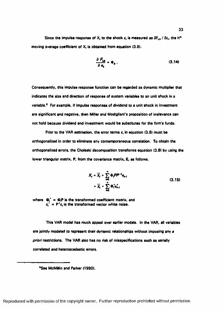
33

Since the impulse response of X, to the shock e, is measured as the h*”

moving average coefficient of X, is obtained from equation (3.9).

. (3.14)a«, *

Consequently, this impulse response function can be regarded as dynamic multiplier that

indicates the size and direction of response of system variables to an unit shock in a

variable.* For example, if impulse responses of dividend to a unit shock in investment

are significant and negative, then Miller and Modigliani's proposition of irrelevance can

not hold because dividend and investment would be substitutes for the firm's funds.

Prior to the VAR estimation, the error terms e, in equation (3.8) must be

orthogonalized in order to eliminate any contemporaneous correlation. To obtain the

orthogonalized errors, the Choleski decomposition transforms equation (3.8) by using the

lower triangular matrix, P, from the covariance matrix, E, as follows.

M (3.15)

M

where O,* = (P,P is the transformed coefficient matrix, and 6,* > P‘'e, is the transformed vector white noise.

This VAR model has much appeal over earlier models. In the VAR, all variables

are jointly modeled to represent their dynamic relationships without imposing any «

priori restrictions. The VAR also has no risk of misspecifications such as serially

correlated and heteroscedastic errors.

*See McMillin and Parker (1990).


34

D. Empirical Rasults

1. SiflipH» ChênetÊristha

Table 3.1 presents sample characteristics for the 446 firms included in this

study. The cross sectional medians, means, and standard deviations for each variable's

averages from the second quarter of 1979 to the fourth quarter of 1990 are shown in

Panel A of Table 3.1. It is interesting to note from the mean column that the sum of

DIV and INV representing outflows of corporate funds approximates the sum of EARN,

DEBT, and FCASH representing inflows of corporate funds. This seems to be consistent

with Dhrymes and Kurz's (1967) suggestion that one of the firm's long-term objectives

is to grow while keeping the cash flow balance. The standard deviation of SIZE is quite

large compared to that of other variables, which may be the cause of heteroscedasticity.

The correlation matrix between the variables is shown in Panel 8 of Table 3.1.

Accounting variables are standardized on SIZE in order to adjust for potential

heteroscedasticity. There are also several other points to note in Panel B. First, the

correlations between DIV and other explanatory variables provide a preliminary picture of

the subsequent tests. The correlations with INV and DEBT are not significant. The

correlation with EARN is positive and significant, whereas the correlations with FCASH

and BETA are negative and significant.

Second, although some correlations between the explanatory variables are

significant, they do not produce serious multicollinearity.* The correlations of INV with

EARN, DEBT, FCASH, and BETA are significant. The correlation between EARN and

"Multicollinearity Is not a problem in this study for several reasons. First, the coefficients of simple correlations are not high. Second, this kind of multicollinearity can be remedied when time-series cross-sectional regressions follow the estimated generalized least-squares (GLS) procedure with more than 20,000 observations. Third, the VAR analysis focuses on forecast error variance decompositions and impulse response functions, which are not affected by multicollinearity.


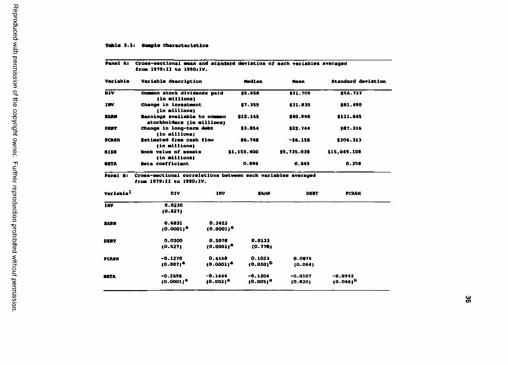
::üCD■DI sQ.

Tabl# 3.1# BêmpXm Character

■DCD

%O3

CD

8■DC5-3"

i3CD

C3.3"CD

CD■DICaO3

■DS

&

OC

%

PaiMl Ai Croaa-aacClonal aaan and atandard daviation of aach variablaa avaragad from 1979:11 to 1990tlV.

Varlablm varlabla daacrlptlon Madlan Haan Standard daviatlon

OIV Common atoek dlvldanda paid (in milllona)

$5.658 «21.709 $56.717

INV Changa In invaatawnt (in milliona)

$7.359 «31.830 $81.490

M M Earninga availabla to common atockholdara (in milliona)

«12.145 «40.996 «111.645

DEBT Changa in long-tarm dabt (in milliona)

«3.854 «22.744 «87.316

PCA8H Eatimatad fraa caah flow (in milliona)

«6.746 -$6.158 $306.313

SI» Book valua of aaaata $1, (in milliona)

155.400 $5.735.038 $15,049.108

BETA Bata coafficiant 0.894 0.845 0.358

Panal 8i Croaa-aactional correlations batwaan from 1979:11 to 1990ilV.

Variabla^ DIV INV EAHN DEBT FCASH

INV 0.0230(0.627)

EAM 0.6831(0.0001)*

0.2452(0.0001)*

DEBT 0.0300(0.527)

0.5078(0.0001)*

0.0133(0.778)

FCASH -0.1270(0.007)*

0.4158(0.0001)*

0.1023(0.030)**

0.0875(0.064)

BETA -0.2696(0.0001)*

-0.1444(0.002)*

-0.1304(0.005)*

-0.0107(0.820)

-0.0942(0.046)**

%O3

%

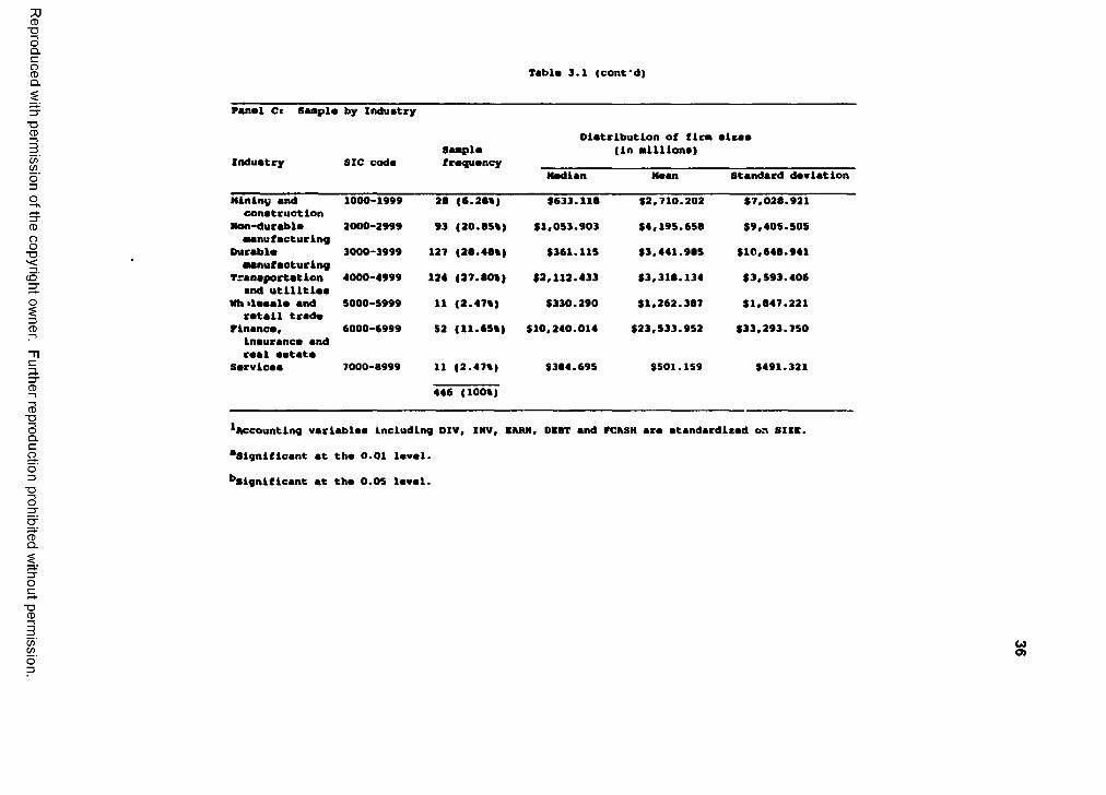
CD■DOQ.C

gQ.

■DCD

COWo"30

CD

8■D( O '3"

13CD

3.3"CD

CD■DOQ.C

aO3

■DO

Tmbl# 3.1 (cont'd)

P*n#l Cl Smmpl* by Industry

Industry SIC codsSamplefrequency

Distribution of firm (in millions)

sisss

Median Mean standard deviation

Mining snd construction

1000-1999 28 (6.28%) $633.118 $2,710.202 $7,028.921

Non-dursblo swnu fscturing

2000-2999 93 (20.85%) $1,053.903 $4,195.658 $9,405.505

DursbisSMnuCscturing

3000-3999 127 (28.48%) $361.115 $3,441.985 $10,648.941

Trsnsportstion mnd utilities

4000-4999 124 (37.80%) $2,112.433 $3,318.134 $3,593.406

Mh •isssis snd rotsii trsde

5000-5999 11 (2.47%) $330.290 $1,262.387 $1,847.221

Pinsncs,insurance and real estate

6000-6999 52 (11.65%) $10,240.014 $23,533.952 $33,293.750

Services 7000-8999 11 (2.47%)

446 (100%)

$384.695 $501.159 $491.321

Âccounting variable# Including DIV, INV, BARN, DBBT and FCASH ara atandardisad on SISE.

^Significant at tha 0.01 laval.


CDQ.

■DCD

I(/)Wo"

wo>

37

BETA is negative and significant. Since these correlations are not high, they imply that

controlling for heteroscedasticity yields less multicollinearity.

Panel C of Table 3.1 displays the sample by industry classification. The firms in

each industry are distributed by size of the firm. It would appear that cross industrial

variations in firm size are evident. The finance, insurance, and real estate industry has

the largest mean of firm size. The smallest mean of firm size is found in industries such

as services, wholesale, and retail trade.

2. Tbn»-S9ri0s Crost-Saetionsl R tgntthn Rasults

Time-series and cross-sectional regressions are estimated using the error

components model of Fuller and Battese (1974). The error components model is an

estimated generalized least-squares method for estimating regression parameters when

time-series and cross-sectional data are simultaneously used. This procedure can take

care of heteroscedasticity as well as serial correlation in the error terms.’

The estimates of time-series cross-sectional regressions are presented in Table

3.2, which is divided into four panels. Panel A shows the estimates for the full sample.

The most striking result is the verification of Miller and Modigliani's (1961) dividend

irrelevance proposition; the coefficient estimates on INV and DEBT are not significant.

Equally surprising is the coefficient estimate of FCASH, which is negative and

significant. This seems to imply that pecking order theory explanation holds.* The

coefficient of EARN is positive and significant, consistent with Lintner's (1956)

prediction. The F-test rejects the null hypothesis at probability less than 0.01.

’Since this procedure transforms the variables by the covariance matrix of residuals, it can control heteroscedasticity in a less restrictive way than simply dividing the variables by firm size, while it adjusts for serial correlations due to time-series data.

"As shown in Sections D.3 and D.4, the effect of FCASH should be explored in the context of dynamic interactions between FCASH and DIV.


38

b

I I

oV

so

iP»vn

::iio d

OV

md

oV

md

idV

idV

inS

idV

soi moMomp^MQ^ # » # m » o w . 3 Mo «o * m # m N o ## M # # 0% »M

orômoowtootdi OtfÔ * ## » ## *o• • * M *0 «0 »0O M O ^ O M O M O I

m m m m^ ^ ^ # I"»m N * ^ 0 0 0 O P » Me « o « M M 0 o •

• « o * M • • * mOÔ« « O^ O0 O* 4

^ ^ 0 -»r* ^ m m <•» O # o ^ o » O M m 0 om^0^p»r i f <4O^ O O O N O 0 O 0 O Mo o o m o r n o m o mI l ^ I I m# ^

- • - • # « «m # r * M m O 0 N 0 0m##mv o 0 o# m0 0m O M I » 0 O 0 V M 0

0 0 p» 0 ## %» 0 %#O 0 P# 0 0 I»

O0 0

0O0

U w

8 8

S si % % iV V

idV

0m

OV

00

idV

M0m

idV

idV

0n

A ^ «M ^ p# 0 0 ^m 0 0 0 0 M§ 5 §®

S o o 0 o SS'îg' îgmd V d V d i*

p* 0 0 0 ^ m0 m 0 0 0 MM 0 0 pk 0 0M • O • O •• «4 t ^ # 0O N O ^ O m

#4 0 0 1»P* 0 0 OM , M 'o N m p# o 7 o T

00 0 0 0 P# 0 0 mo 0 o *o l ô t

0 0 0m g 0 0 0

ô i à i

A r» «» # # #n ^ e ^ i A M a i n M i og s g T g : s 3 s ;o N o I O 0 O 0 O 0

« «0 ^ m ^ 0 A «n0 0 0 O m 0 r > P i 0 mm 0 0 0 m « 4 p » 0 m o0 O 0 0 0 P * O 0 P # mp# #4 0 0 M 0 *0 . 0P l # 4 0 » # m » ^ 0 w 0 ^

s

0

p#

oV

OV

m00

dV

0p*


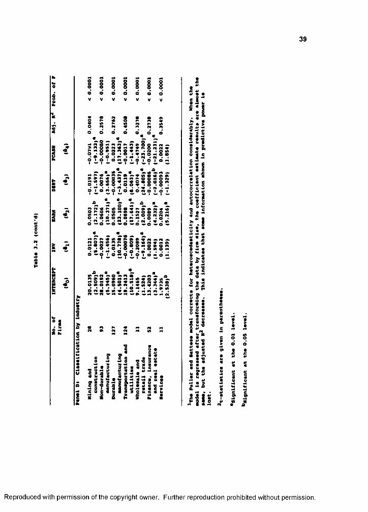
39

I

î

n

oV

ooo

oV

e

oV

3

eV

e«n«o

oV

oV

IdV

is::

M *» 0% »8;? i d m

«•-

g s i ;ogS

g f l *

S “ e S g *e ■ e N

-8 % 3 §

8

O #

«

8 M o 3d # d #4I V *—

A M «»m »S o o n• d • n

O l d ?

2 n « o • n o n o n n n 0 * 0 » ' # ' • 0 ^ 0 ^

n • I I n • IS t 8 :sMi?

i l i l

n • n •8 883O n d n

A « # ## #M A C i A O ^ n o #% m Anooi A«nnni A<«ov i AAS g S S 8 8 S t 8 S 3 S 3 g

• # *o n o n m ^ o n * m n n * *n ^ n ^ n ^ n »» o ^ #4 ^ M e#

I ! !i_ • 9 9 U

g 2 S 8 8 t : a Z . __

- 1 3 ■? ? 8.3 : 3 8 “ 8

i i n

Îi|ijiîl|ilî

I

1 1 1>1A 4»

2 S Î

III^ # 0

IIIu n 41

m1 , 5X

illU «M •

hiÎ!1

II

IC 04 A

J i i iIi.

od#

I8

Od

*>4»

8j"


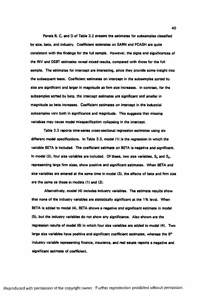
40

Panais B, C, and D of Table 3.2 present the estimates for subsamples classified

by size, beta, and industry. Coefficient estimates on EARN and FCASH are quite

consistent with the findings for the full sample. However, the signs and significances of

the INV and DEBT estimates reveal mixed results, compared with those for the full

sample. The estimates for intercept are interesting, since they provide some insight into

the subsequent tests. Coefficient estimates on intercept in the subsamples sorted by

size are significant and larger in magnitude as firm size increases. In contrast, for the

subsamples sorted by beta, the intercept estimates are significant and smaller in

magnitude as beta increases. Coefficient estimates on intercept in the industrial

subsamples vary both in significance and magnitude. This suggests that missing

variables may cause model misspecification collapsing in the intercept.

Table 3.3 reports time series cross sectional regression estimates using six

different model specifications. In Table 3.3, model (1) is the regression in which the

variable BETA is included. The coefficient estimate on BETA is negative and significant.

In model 12), four size variables are included. Of these, two size variables, S* and S„

representing large firm sizes, show positive and significant estimates. When BETA and

size variables are entered at the same time in model (3), the effects of beta and firm size

are the same as those in models (1) and (2).

Alternatively, model (4) includes industry variables. The estimate results show

that none of the industry variables are statistically significant at the 1 % levai. When

BETA is added to model (41, BETA shows a negative and significant estimate in model

(5), but the industry variables do not show any significance. Also shown are the

regression results of model (6) in which four size variables are added to model (4). Two

large size variables have positive and significant coefficient estimates, whereas the 6^

industry variable representing finance, insurance, and real estate reports a negative and

significant estimate of coefficient.


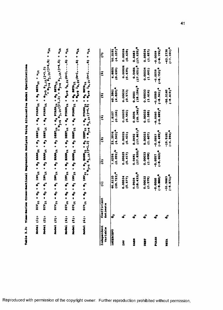
41

î

u

1

a9

g

g

&

ü9

*

^ IM «mI «4

* *

♦

iJX

Ü9

+Ü9

4iS9

*Ü9

♦

♦

H

1ID

• S S S1 " * < 41

I I I I {• e

i i

♦

>Q

♦

IAlw>

O

• Mf

s * f# ft9 • • • ?♦ ♦ ♦A# AIw «4 W #4A

s gM M MN #4

• • • •A * A AO O o o• • • •■ ■ ■ I*» AI AI AIW W «4

> > > >MQ O Q o

m tn

•H W M *4 #4 #4

I I I I I IS

« ^ • « A « «V| 2 §5 3 : i s i f

m M3 2

2 d 2 * 2 ds i d s O M O ^ 7 X

o o<9O « ♦ ^ * • -

s m tn §5 i s i : 0 3o 2 * 8 tü

® « O ^ ? ?

^ « •• m «

S STÎT # 2 § S s " § 3 1 s M ft

®d 2S 2Ü; 2 d 2 2«0 o — e —

•d ^ ? " S ?

HI » tn m «%e « i s 1 2 i s s s

« d 2S g 2 dd 2. o *» d ^ d ?

»•-« 9 •

» « S S s i 3 S 3 S 5 Sm m in

2S 2 ! § : 225 Z o ^ e ? " s X

min ^ o a a0» w § ; 52 ii f** ft m lO

3 ® 2d 2 S 82 2 d

«

d S o ^

m

d Z d ?«

2S m a 5T m 2*s g 5 S2 p r* ii isJS 2d 2 5 0 2 dd ® o ^ d 3, ? " s ?

u •

■d* <•*

;1 I I X 1


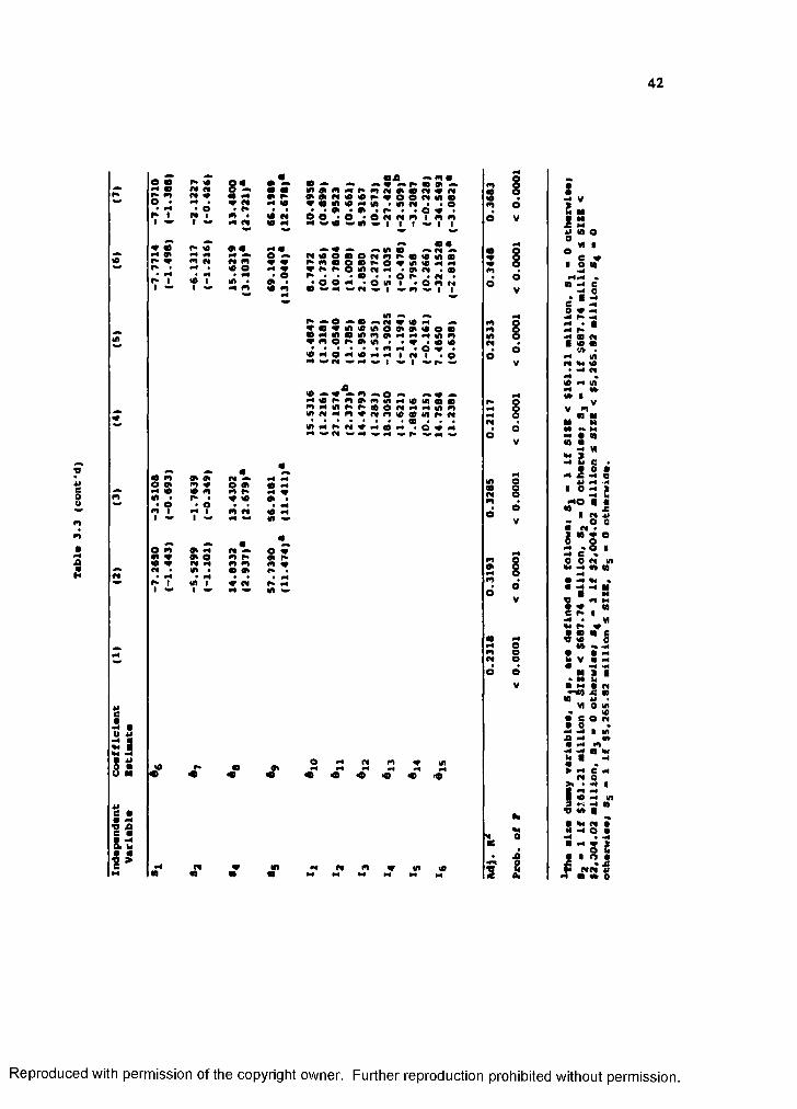
42

I

t

11Ii

SSo 1

SS

§57 Î

SSm M

8 *-

33 1!

0 m 0 0«

« M

m

g 0 m « O 0 0 M0 0 m m r* M 0

0 r* « 0 0o o «4

m 1 M 1 m rS 0 M1 1 0

o m 0 M « •- o

«

00 « 0 o m r* 0 00 « n M m m m 0M 0 0 0 P»

M •H mf» r 0 1 « w 01 1 #4 0

_ « A

S s 5 s s 5 s s s s : s• t0k # # # ^ # @ #SSL^ 2L« 2.7 7 ? 1 ? ?

A 0 •p# ^C! ' SS59Mmr*#0%mm ^ m 0 g 0 * » o # 0 0 M N 0 f* «» O 0 N w ' 0 m « 0^ • • «0 • * 0 ^ tp i •' o o M * O 0 I * o m N

0 M m# p# ^ I %# m V I I

lA A^ ^ 0 #»N00#4 ^« 0 ^ 0 0 0 0 0 0 0 0 0 0 M 0 0 0 m 0 N N M 0 m « m o 0 0 • •« «00• • • • • # m #4 * 0 « •0 # 4 0 M 0 # 4 # 4 # p# I , Q ^ M ^ W * # I w | v f » « M

0 ^ « ^ 0 4 » 0 # »M 0 p . m 0 m 0 # # 0 0 @ emM0p*p%eop####40m0M##m«m#m000p»p#0 Wr*p#0 M 0 W , O « M M f# M m ^ M

O M

^ <£*

IÔV

IoV

ooV

odV

IdV

oV

IdV

In

* î i

Is41 0 O

> '■ O fiT

ill-I-3 . 30 M 0 0 1**V

=1:- i l s■ o 3 S, - » î i

i'î:Is:a 3 " §S V 8 S".a I ■•il:W iw « " S» : § " Ï S S "I s 5 -j = s |

i - yJ «"3 %


CD■DOQ .C

8Q . Tabla 3.3 (cont'd)

^Th# Industry dummy variables, I%e, are defined ae follows: 1 % - l l f mining and construction industry, ■ 0 otherwise; Ig » 1 If non-durable awnufacturlng industry, %2 - O otherwise; Ij • 1 if durable manufacturing industry, I 3 • 0 otherwise; I4 ■ 1 If transportation and utility industry, I 4 • 0 otherwise; Ig - 1 if wholeaale and retail trade industry, Ig • 0 otherwise; Ig - 1 if finance, insurance and real estate

% industry, Ig * 0 otherwise; ly • 1 if service industry, ly • 0 otherwise.

^fbr the purpose of estimation, each one dummy variables ere lost. The dummy variables not represented in the table are 83 for 81:8 variable and ly for INDU8T8T variable.

T3CD

(/)

CDQ.

T3CD

(/)(/)

*t-etatietice are given in parentheses.

*8ignificant at the 0.01 level.

^Significant at the 0.05 level.

8^Significant at tha OeOl la v a le

CD

3 .3"CD

CD■DOQ.C

aO3"Oo

w

44

Finally, in model (7), all the variables are included in the regression. The sets of

coefficient estimates on BETA and size variables are consistent with the estimate results

in other models of Table 3.3. While other industry variables are insignificant at the 1 %

level, the industry variable for finance, insurance, and real estate also shows significant

estimate results, similar to those of model (6). This casts doubt on the industry effects

in dividend policy. As noted in Table 3.1, the finance, insurance, and real estate

industry has the largest mean of firm size. Also that industry variable has a significant

estimate of coefficient only when size variables enter the model. This evidence, along

with the insignificant estirnates of other industry variables, suggests that industry effect

might not exist and that industrial variations in dividend policy as documented in Michel

(1979) might be only the manifestation of size effects.

The estimate results of INV, EARN, DEBT, and FCASH In model (7) are entirely

consistent with the findings for the full sample in Table 3.2, as well as those for other

models in Table 3.3. The coefficient estimates on INV and DEBT are insignificant. The

EARN coefficient estimate is positively large and has highly significant t-statistics,

whereas the FCASH coefficient estimate is negative and significant.

3. Vector Autorsgrotsion Results

The assumption of VAR is that the regression variables are stationary over time.

Since statistical inference based on non stationary variables results in incorrect

conclusions, it is imperative to scrutinize the stationarity of the variables. The tests of

stationarity applied here are the unit root tests and cointegration tests.

In Panel A of Table 3.4, unit root tests are conducted by using the augmented

Dickey Fuller (ADR statistic. The existence of a unit root implies non stationarity.

Thus, the null hypothesis of a single unit root or H*: p - 0 is tested against the

alternative or H : p < 0 that the variable is stationary. Since the t statistic does not


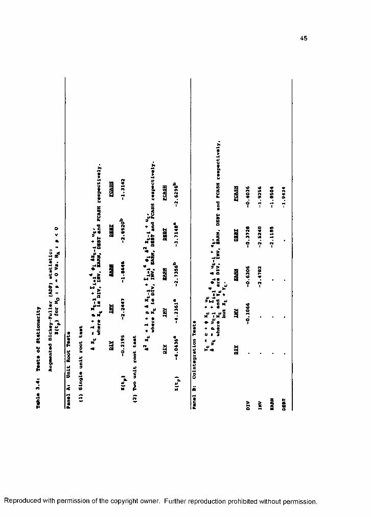
45

a

oV

; s !iîUQ

1î

t

#

I

?

%tA«

«S

mm

?s

I -

riJ"S

ISM M

i!: s

H**

t

%

««

0V1

K-

mo w»

s

?

«oy)o

?

oinm

m o inf# CDpk Nm in #4O n (M

no

s Ê

mVmo M #4 M


46

U

I?

?

>1ÎSui% sn # #

? u * # —k ?50 #4 W O 01U 4» *» Irt *4

^ : gV 4f y ou

9ï 1; •l

: i -4i 41 0 U

> n t

• ' î - ..** n # mI l 15 : 5“ 41 -

I L£ .>1 * * S o O

50 4» # O

o 6 # #

*4 0 0 4»# M * *U I 4» 4»

!Hs I I9 % %« *4 w IM# *» «U «4 -4_ m» e c e« î i I /


47

have Student's t-distribution under the null hypothesis of non stationarity, critical values

for the t statistic on p, Z(t,), are simulated by Fuller (1976).

The single unit root test in Table 3.4 with the exception of DEBT does not reiect

the null hypothesis of a unit root at the 10% significance*. For the two-unit root test,

the procedure is repeated for first difference data. The null hypothesis of a unit root in

the differenced variables is rejected at the 10% level for all variables. Overall, the

results suggest that the variables become stationary only after first differencing. This

means that the variables follow an 1(1) process.

Panel B of Table 3.4 details the cointegration tests. Cointegration means that

the difference between two variables becomes stationary when these variables move

closely over time. If the variables are cointegrated, tests for stationarity may not be

reliable. Furthermore, Engle and Granger (1987) suggest that vector autoregressions

using differenced data will be misspecified because of omitted constraints when

cointegrated variables are used. Cointegration tests are conducted by repeating unit

root tests on the cointegrating residuals. The null hypothesis of no cointegration is that

the cointegrating residuals have a unit root. As it can be seen from Panel B of Table

3.4, no ADF statistic exhibits significance at the 10% level. Therefore, the null

hypothesis that the variables are not cointegrated cannot be rejected.

Based on these results, the first-order differenced data are used in the following

VAR analysis to satisfy the stationarity condition. The variance decompositions from

vector autoregressions are presented in Table 3.5. The ordering of variables used in this

analysis is INV, DIV, EARN, FCASH, and DEBT. The results reported here appear to be

quite robust to ordering since almost the same results are obtained with several different

orderings. Confidence intervals of 99% for the point estimates are computed by a

'It is customary to refer to the 10% critical values in stationarity tests.


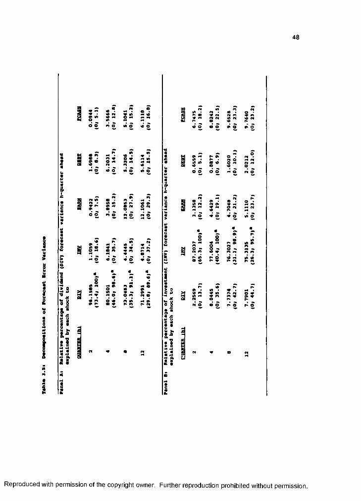
48

S

II

î

ïO

II

s"2d d

S "

e»d d

n îsi

A

I s

e Met

d d

• s

s :m d

« m

« o

e *4

d d

i =

Ê:# O

«

MlO m

Sd

«d d

M o

M Nr * m

•o

d

g :? a

g

ili l

I

g

d d

o •et m

S " « et

O9* e» o» o etin e* et O etlA W) a 10 O m et #4«0 « «0 O

o o o o O et O

et n r*m 0% OD Otf) et et 0» # M mm « O et et#4 <0 e»

m O « o # O lA O

# «« «

0»o oo o d Ml

r» #4 # e* Ot Ml »m O et mo O o Met m «0 « m m m

e* «A r* o 10 Ml 10« «0 e* V e* m e* et

r* %0 e* r*in # 44

«0 m ♦ w r* et o «in M V m m V met o r* e*

et O m o e* o e* O


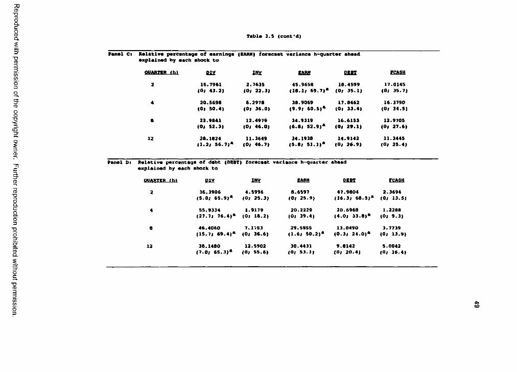
::oa>■oI8Û. Tabl# 3.5 (cont'd)

"OCD

%o=JoSCD

8T3

C5-zro3CDn"nc3.3"CD

cB■D3Q .CaO3

"OO

CDQ.

Panal Ci Relative percentage of earning, explained by each ahock to

(BARM) forecaat variance h-quarter ahead

QUARTIR ihi DIV U U BARM DBBT FCASH

2 15.7961 <0» 43.2)

2.7635 (0, 22.3)

45.9658 (18.1, 69.7)*

18.4599 (0, 35.1)

17.0145 (0, 35.7)

4 20.5698 (G| 50.4)

6.2978 (0, 36.0)

38.9069 (9.9; 60.5)*

17.8462 (0, 33.4)

16.3790 (0, 34.5)

• 22.9841 (0| 52.3)

12.4979 (0, 46.0)

34.9319 (6.8, 52.9)*

16.6153 (0, 29.1)

12.9705 (0, 27.6)

12 28.1824 (1.2, 56.7)*

11.3649 (0, 46.7)

34.1938 (5.8, 51.1)*

14.9142 (0, 26.9)

11.3445 (0, 25.4)

Panel Oi Relative percentage of debt (DEBT) forecaat explained by each ahock to

QS2MITEB. ihi BIV 1ÜÏ BARM DBBT FCASH

2 36.3906 (5.0, 65.9)*

4.5996 (0, 25.3)

8.6597 (0, 25.9)

47.9804 (16.3, 68.5)"

2.3694 (0, 13.5)

4 55.9334 (27.7, 76.4)*

1.9179 (0, 18.2)

20.2229 (0, 39.4)

20.6968 (4.0, 33.8)*

1.2288 (0, 9.3)

8 46.4060 (15.7, 69.4)*

7.1753 (0, 36.6)

29.5955 (1.6, 50.2)*

13.0490 (0.3, 24.0)*

3.7739 (0, 13.9)

12 38.1480 (7.0, 65.3)*

12.5902 (0, 55.6)

30.4431 (0, 53.1)

9.8142 (0, 20.4)

5.0042 (0, 16.4)

■DCD

C/)C/) (O

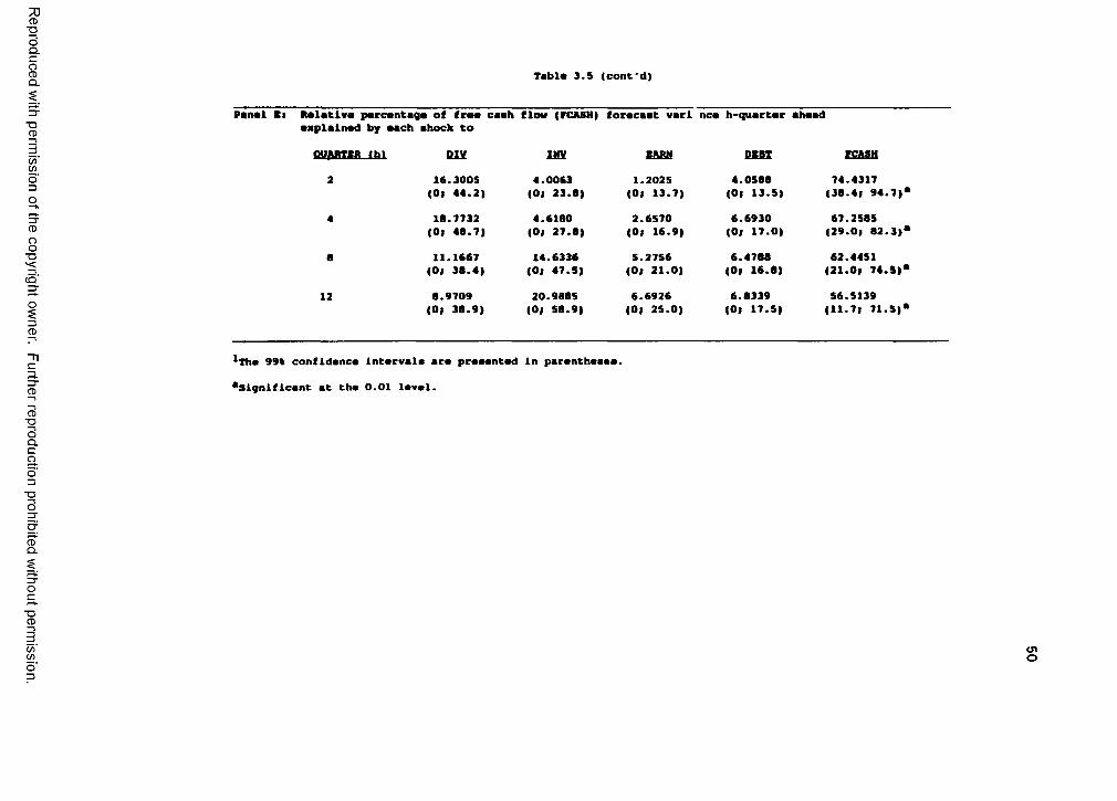
73CD■D3Q .C

gQ .

■DCD

(/)(Oo"30SCD

8"OC5-3"

13CDn"nc3.3-CD

Table 3.5 (cont'd)

Panai li Ralativa parcantaga of fraa caah aaplainad by aach ahock to

flow (PCASH) forecaat vari nca h-quartar ahead

OUARTIR ihl BIX IBX BMW DBBT PCASH

2 16.3005 4.0063 1.2025 4.0588 74.4317<0| 44.2) (0| 23.8) (0| 13.7) (0| 13.5) (38.4; 94.7)"

4 18.1732 4.6180 2.6570 6.6930 67.2585(0| 48.7) (0| 27.8) (0} 16.9) (0; 17.0) (29.0; 82.3)"

a 11.1667 14.6336 5.2756 6.4788 62.4451(0| 38.4) (0, 47.5) (0| 21.0) (0| 16.8) (21.0; 74.8)"

12 8.9709 20.9885 6.6926 6.8339 56.5139(0| 38.9) (0> 58.9) (0| 25.0) (0| 17.5) (11.7; 71.5)"

*Tha 99% confidence Intervale are preaented


CD■D3acaO3

■D3

CDQ .

■DCD

C/)(fi

CJlO

51

Monte Carlo simulation'^ with 1,000 replications. This confidence interval is bounded

by 0% and 100%. If the confidence interval includes 0. the null hypothesis of no

impact cannot be rejected.

Point estimates in Table 3.5 measure the degree of exogeneity for a given

variable in the sense that the h quarter ahead forecast error variance in a variable is

allocated to each source, and that a strictly exogenous variable explains all its forecast

error variance. If the forecast error variance in a variable is largely due to unexpected

shocks to itself in the last h quarters, then the implication is that there are no strong

interactions with other variables.

Panel A of Table 3.5 provides variance decompositions for DIV at the horizons of

2, 4, 8, and 12 quarters. At a horizon of two quarters, 96.15% of the variance in DIV

is explained by its own disturbances, whereas only 1.10% of the variance in DIV is

accounted for by INV. Other variables, including EARN, DEBT, and FCASH, also have

little impact on DIV. At the 12 quarter horizon, DIV explains 71.29% of its own

variance. However, INV explains only 4.87% of the variance in DIV, while EARN, DEBT,

and FCASH account for 12.10%, 5.61%, and 6.11% of the variance in DIV,

respectively. This suggests that nearly all variance in DIV is attributable to the shocks

to DIV itself, and that DIV has no dynamic interaction with other variables.

Variance decompositions for INV are shown in Panel B of Table 3.5. At the two-

quarter horizon, 87.20% of the variance in INV is attributed to its own shocks. The

percentage of the variance in INV explained by other variables ranges from 0.65% to

6.74%. At the 12-quarter horizon, the percentage of INV variance due to its own

shocks is a still dominating 75.31 %. DIV explains only 7.79% of the variance in INV,

which is insignificant at the 1 % level. The contributions of EARN, DEBT, and FCASH to

the variance in INV are 5.11%, 2.02%, and 9.76% respectively, insignificant at the

'This method constructs the posterior distributions of the estimate.


52

0.01 level. These results imply that the variance in INV is fully explained by its own

shocks and thus INV appears to be exogenous.

Panel C of Table 3.5 presents variance decompositions for EARN. At the two-

quarter horizon, less than half the variance in EARN is accounted for by its own shocks.

At this short horizon, INV explains only 2.76% of the variance in EARN, while DIV,

DEBT, and FCASH account for 15.79%, 18.45%, and 17.01%, respectively. At a

longer horizon of 12 quarters, INV gradually becomes more important, explaining

11.36% of the variance in EARN. DIV accounts for 28.18% of the variance in EARN,

which is significant at the 1 % level. This would suggest that dividends explain future

earnings. DEBT and FCASH explains 14.91% and 11.34% of the variance in EARN,

respectively. EARN has 34.19% of its variance accounted for by its own shocks,

suggesting strong interactions among the variables.

Variance decompositions for DEBT are presented in Panel D of Table 3.5. An

interesting feature at the two-quarter horizon is that DIV explains 36.39% of the

variance in DEBT, which is significant. Of the variance in DEBT, 47.98% is attributable

to its own shocks. EARN explains only 8.65% of the variance in DEBT, while the

contributions by INV and FCASH are 4.59% and 2.36%, respectively. At the 12-quarter

horizon, the proportion of the variance in DEBT explained by DIV is 38.14%, which is

still significant. However, the proportion of the variance in DEBT attributable to its own

shocks decreases to 9.81 %, which is not significant. EARN contributes 30.44% to the

variance in DEBT, while INV and FCASH are responsible for 12.59% and 5.00%,

respectively. This result suggests that DEBT is set as a residual after all corporate

decisions are made. In particular, this implies that since DIV has a significant effect on

DEBT, firms borrow in order to finance dividend payments.

Variance decompositions for FCASH are also portrayed in Panel E of Table 3.5.

At the horizon of two quarters, DIV explains 16.30% of the variance in FCASH, implying


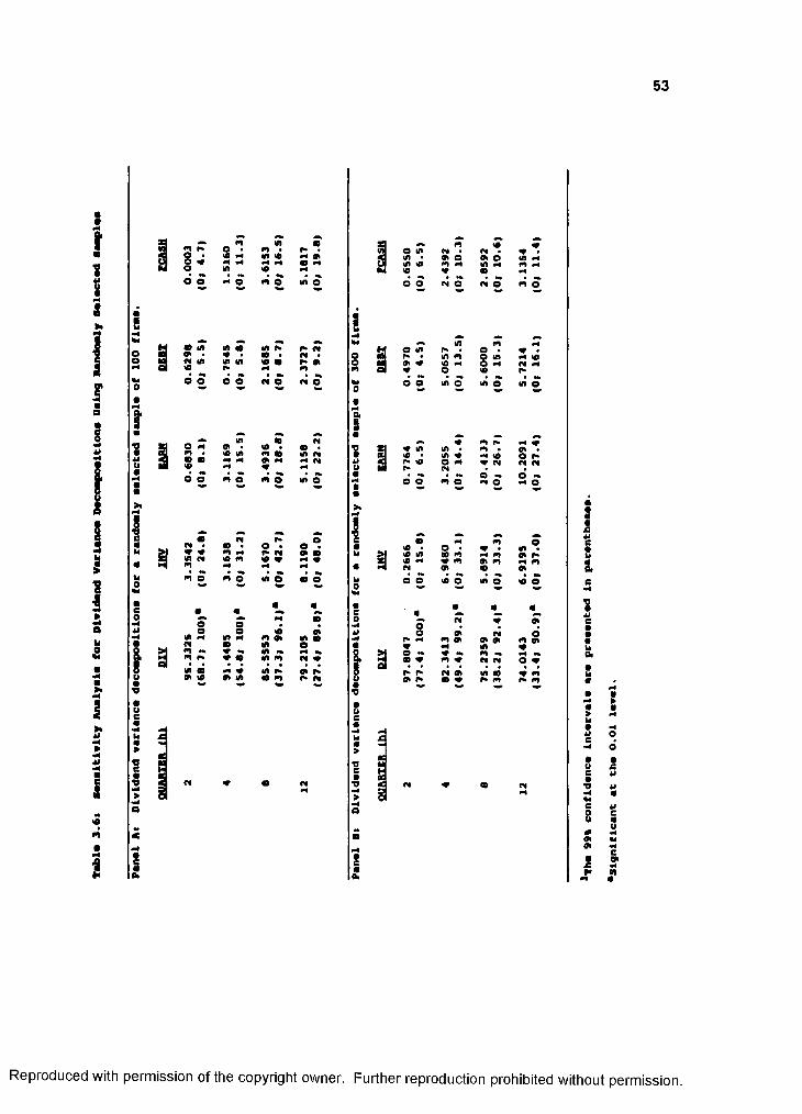
53

I

5-i4i

m

I

I

o o m o

- «0 (AO

e o

S S

m o

»

s :

• d r» oM 0 • o • oV « m M r* d 0 0lA d 0 m 0 0 0m M M

m o m e 0 O 0 o

« «0 «

M 0o oo o 0 0

lA M tn M m 0 0 0W 0 0 om V •» 0 «»m 0 0 0 m d 0(A « M 0 0 d 0 d

%0 0 0 0 m r * d

O (A 9* «

g «0o o

g :

I !c! o

# !«Â o

; sSo

# .m «0

SSS o -

0 m o0 O • 0 . 00 0 m m 0 d0 M 0 m 0 m Mmd 0 0 0

O o 0 O 0 O 0 o

• 4 44

d 0 0oO 0 d O

m 0 0 0 m 00 «4 0 0O 0 «% n —0 0 m 0 d d O 0

d d 0 0 0 0 m0 d 0 0 d m d m

•8.e

1I5ni#

S

I

S.


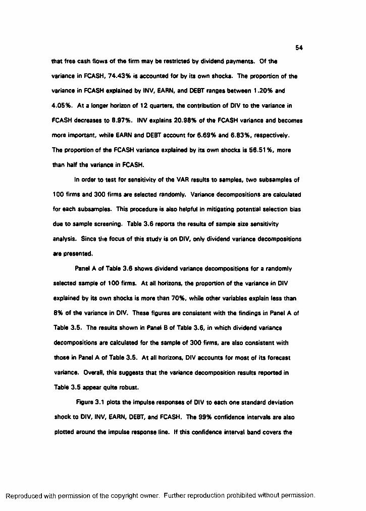
54

that frea cash flows of the firm may be restricted by dividend payments. Of the

variance in FCASH, 74.43% is accounted for by its own shocks. The proportion of the

variance in FCASH explained by INV, EARN, and DEBT ranges between 1.20% and

4.05%. At a longer horizon of 12 quarters, the contribution of DIV to the variance in

FCASH decreases to 8.97%. INV explains 20.98% of the FCASH variance and becomes

more important, while EARN and DEBT account for 6.69% and 6.83%, respectively.

The proportion of the FCASH variance explained by its own shocks is 56.51%, more

than half the variance in FCASH.

In order to test for sensitivity of the VAR results to samples, two subsamples of

100 firms and 300 firms are selected randomly. Variance decompositions are calculated

for each subsamples. This procedure is also helpful in mitigating potential selection bias

due to sample screening. Table 3.6 reports the results of sample size sensitivity

analysis. Since tiie focus of this study is on DIV, only dividend variance decompositions

are presented.

Panel A of Table 3.6 shows dividend variance decompositions for a randomly

selected sample of 100 firms. At all horizons, the proportion of the variance in DIV

explained by its own shocks is more than 70%, while other variables explain less than

8% of the variance in DIV. These figures are consistent with the findings in Panel A of

Table 3.5. The results shown in Panel B of Table 3.6, in which dividend variance

decompositions are calculated for the sample of 300 firms, are also consistent with

those in Panel A of Table 3.5. At all horizons, DIV accounts for most of its forecast

variance. Overall, this suggests that the variance decomposition results reported in

Table 3.5 appear quite robust.

Figure 3.1 plots the impulse responses of DIV to each one standard deviation

shock to DIV, INV, EARN, DEBT, and FCASH. The 99% confidence intervals are also

plotted around the impulse response line. If this confidence interval band covers the


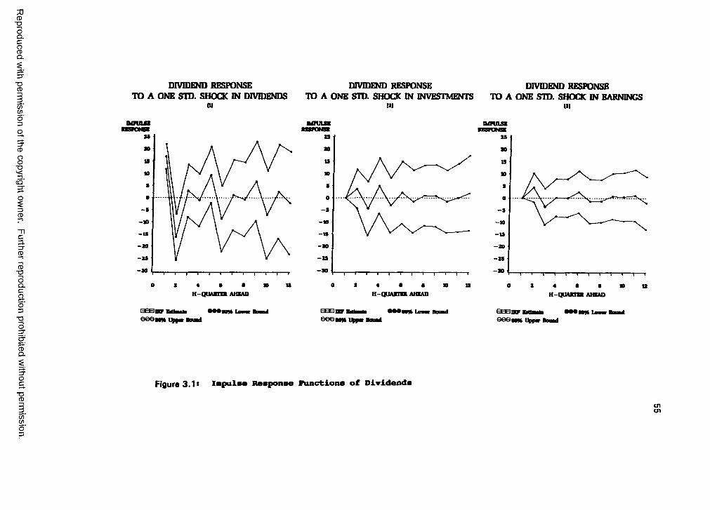
■oIc8Û.

■OCD

C/)(gO3

CD

85c5'Si3CD

Cp.

CD■OICaO3

■OO

DIVIDEND RESPONSE TO A ONE SID. SHOCK IN DIVIDENDS

(II

DIVIDEND RESPONSE TO A ONE STD. SHOCK IN INVESTMO^TS

m

DIVIDEND RESPONSE TO A ONE SID. SHOCK IN EARNINGS

(IIB0ULS1

U

-m

-zs

u10

ao

- •

■10

-11

-25-9 0

» 12H -q U M C m AHIAO H -Q U A K in AKIAD

eeeooik 13^ BraidQBBHF fadrafeeeewmvsfrn

as

ao

-1

-IS

» oH -Q M A K in A « A O

B d tra tieeesoM u|ip« Bond

&

oc%

C/)Ç2o'3

Figure 3 .11 Impulee Response Functions of Dividends

ayay

CD"O

OQ .C

gQ .

■OCD

C/)Wo"303CD

8TD'<(O '3"

13CD

3.3"CD

CD"OOQ .C

aO3

"OO

DIVIDEND RESPONSE TO A ONE STD. SHOCK IN DEBTS

W

DIVIDEND RESPONSE TO A ONE SID. SHOCK IN FREE CASH

2$

10

- •

-a s

12

as

ao

- s

as

ttH - q U A X m t AHEAD H - q u A n n a i b a d

ErtSasli e e e tm vpfm naumà

L L U U V E r t iM t i

OOOwrnVppmBamA

CDQ.

"DCD

(/)(/)

Figure 3.1 (cont'd)

cno>

57

value of zero, the null hypothesis of no effects cannot be rejected. Diapram (1) shows

that a one standard deviation shock to DIV has significant short run effects on itself. At

a horizon of one quarter ahead, the effects are positive and significant. At a horizon of

two quarters ahead, negative and significant effects are found. At longer horizons, the

effects are insignificant since confidence interval bands fluctuate around the value of

zero. By contrast, diagrams (2)*(5) indicate that dividend responses to each one

standard deviation shock to INV, EARN, DEBT, snd FCASH are not significant at all

horizons. It appears that this evidence is consistent with the results using variance

decompositions.

4. Th» Laggtd-DMdênd Modê!

The results from Section D.2 suggest current relationships among dividends,

earnings, free cash flows, beta, and firm size. The analysis in Section D.3 provides

evidence of short memory in dividends. It is found that dividends are associated with

short memory of its own past, while any given shocks in all other variables under study

do not induce significant deviations in dividends. This would suggest that stronger lag

specifications might be useful in investigating determinants of dividend policy.

Accordingly, this section estimates several additional specifications of the time series

cross sectional regression model including lagged dividend variables, and tests for their

robustness. Since the early study of Lintner (1956), the empirical literature testing

lagged dividend models has been scant with the exception of Fama and Babiak 11968)

and Fama (1974). These studies also failed to explain the reason for the inclusion of

lagged dividends."

"Moreover, many econometric problems due to lagged dependent variable models or time series cross sectional data have not been effectively adjusted.


58

Estimating lagged dependent variables in the regression causes many

econometric problems. If the disturbances are serially correlated in the lagged

dependent variable models, OLS estimates are inconsistent. Even if the disturbances are

"well-behaved", OLS estimation produces biased coefficients in finite samples. In order

to adjust for these problems in the context of time-series cross-sectional regressions, the

method of instrumental variables is suggested. The lagged-dividend variable is first

regressed on ali other explanatory variables. The resulting predicted values are then

used in an error components model to obtain time-series cross-sectional regression

estimates.

Table 3.7 reports time-series cross-sectional regression results using lagged

dividend variables. Model (1) is Lintner's (19561 model in which current dividends are

determined by the previous dividends and current earnings. The coefficient estimates on

DIV., and EARN are positive and significant. The adjusted R' is 51.89% and the F-test

reiects the nuli hypothesis at the level less than 0.01. Model (2) includes additional

lagged variables of dividends in the model of EARN and FCASH, which turned out

significant in Table 3.2. As predicted, the coefficient estimates are positive-significant

for EARN and negative-significant for FCASH. With the introduction of more lagged-

dividend variables, the first, second, and fourth lags show significant estimates and the

adjusted R' increases to 65.74%. This implies some persistence of dividend poiicy since

current dividends seem to be affected by the dividends paid one quarter, two quarters,

or four quarters before.

Similarly, models (3) and (4) introduce BETA and size dummy variables which

proved significant earlier. The coefficient estimate of BETA is negative-significant at the

0.01 level, whereas the coefficient estimates on the two largest size variables are

positive-significant at the 0.01 level. The positive impacts of the first, second, and

fourth lagged-dividend variables are the same as in model (2). In model (51, all variables


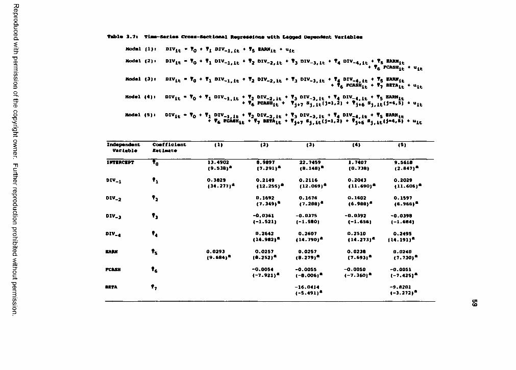
CD■DOQ .C

gQ .

■DCD

C/)Wo"3O

8"O(O '3"

i3CD

3.3"CD

CD■DOQ .C

aO3

■DO

CDQ .

■DCD

(/)(/)

Table 3.7t Tt— Parle» Croaa-Sectlonal Regreaalone with Lagged Dependent Variable#

Model (1)1 DlVit - Tg * * 5

»0 ♦ ♦ *2 0:V-2,it * »3 “IV-3.lt ♦ 4 “IV-4,itNodal (2)1

Nodal (3)1

Nodal (4)1

Nodal (5)1

DIV,'It

“:Vit

DIV,»

»0 ♦ ♦ »2 “IV-2.lt ♦ »3 “IV-a.lt ♦ % “*V-4. It

. ♦ Ts EANNit♦ Tg rCASH^g ♦ “It

: ♦ »S ««"it♦ BCTA^t * "It♦ Tg EANNit

* “It♦ Tg BARNit“ :V it - *0 + *1 “ : v _ i , i t ♦ »2 “ :v _ 2 .it ♦ »3 “ :v _ 3 .it ♦ 4 “ *v _ 4 .it

♦ Tft ♦ 1? — TAlt ♦ »J47 »J.lt<l-»*a» ♦ *j*6 “j.ltO-^.S) ♦

IndapandantVariable

CoafflclantBatlmata

(1) (2) (3) (4) (5)

INTBRCBPT *0 13.4902 (9.538)*

8.9897(7.291)*

22.7459(8.148)*

1.7407(0.738)

9.5618(2.847)*

DIV_i *1 0.3829(34.277)*

0.2149(12.255)*

0.2116(12.069)*

0.2043(11.690)*

0.2029(11.606)*

DlV.j *2 0.1692(7.349)*

0.1676(7.288)*

0.1602(6.988)*

0.1597(6.966)*

01V_3 *3 -0.0361(-1.521)

-0.0375(-1.580)

-0.0392(-1.656)

-0.0398(-1.684)

DIV_4 *4 0.2642(14.982)*

0.2607(14.790)*

0.2510(14.273)*

0.2495(14.191)*

BABM *5 0.0293(9.684)*

0.0257(8.252)*

0.0257(8.279)*

0.0238(7.693)*

0.0240(7.730)*

FCASH *6 -0.0054(-7.921)*

-0.0055(-8.006)*

-0.0050(-7.360)*

-0.0051(-7.425)*

BETA *7 -16.0414(-5.491)*

-9.8201(-3.272)*

Ol<o

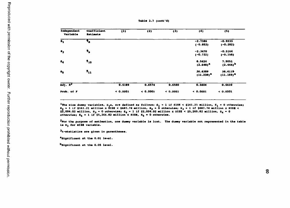
CD"OOQ .C

gQ . Tmbl# 3.7 (cont'd)

"DCD

C/)Wo"305CD

8■DC Q '2

13CD

3.3"CD

CD■DOQ .

O3

■DO

&

IndapandantVarlabla

Coafflclant datInata

( 1) ( 2 | (3) Ml (S)

'10

'11

AdJ. M

Prob. of r0.5109

< 0.0001

0.6574

< 0.0001

0.6580

< 0.0001

-2.7386 -0.9233(-0.852) (-0.282)

-2.3470 -0.5164(-0.732) (-0.158)

8.5426 7.9051(2.648)* (2.444)'

36.6389 36.4119(11.2381* (11.159)'

0.6604

< 0.0001

0.6610

< 0.0001

3Tha aima duany varlablaa, Sja, ara daflnad an followai Sj - 1 If SIZE < $161.21 million, Sj > O otharwlaa; S; - 1 If $161.21 million s SIEE < $687.74 million. S; - O otharwlaa; S3 • 1 If $687.74 million S SIEE < $2,004.02 million, S3 - 0 otharwlaa; S* - 1 If $2,004.02 million S SIEE < $5,265.82 million. S* - 0 otharwlaa; Sj • 1 If $5,265.82 million S SIEE, Sj • 0 otharwlaa.

^Por tha purpoaa of aatlmatlon, ona dummy varlabla la leat. Tha dummy varlabla not rapraaantad In tha tabla la S3 for SIEE varlabla.

^t-atatlatlca ara glvan In paranthaaaa.

"significant at tha 0.01 laval.

^significant at tha 0.05 laval.

Oc■oCD

%O3

O

61

used in models (1)-(4) are added. The estimate results are essentially the same as in

other models, indicating the insensitivity of parameter estimates. The adjusted R' is

66.10%.

The findings in Table 3.7 have several interesting implications. First, unlike

Lintner's argument, more lags in dividends are important determinants of dividend policy.

With the addition of more lags reflecting the past memory of dividends, the explanatory

power of the model increases considerably. Second, as shown in Section 0.2, current

earnings have positive impacts on dividends, while free cash flows and beta have

negative effects. Also the firm size appears to play an important role in dividend policy.

Since the sensitivity of the estimates to alternative model specifications has been

established in previous sections, conducted in Table 3.8 are robustness analyses of the

time-series cross-sectional model (7) in Table 3.7 for randomly selected subsamples and

subperiods. In order to test for robustness of the model, the full sample is first split into

three subsamples: randomly selected samples of 100 firms, 200 firms, and 300 firms.

Then, the time-series cross-sectional model (7) in Table 3.7 is estimated on each

subsample. As shown in Table 3.8, the sets of coefficient estimates on DIV.,, DIV.*,

EARN, S*, and S, are the same as the findings in Table 3.7. However, the coefficient

estimates on DIV., and DIV., show mixed results for each subsample. The coefficient

estimate of BETA is insignificant in the subsample of 100 firms, whereas it is significant

in the subsamples of 200 firms and 300 firms.

To test for coefficient stability over time, the time-series and cross-sectional

model is also estimated for two subperiods; 1979:11-1984:1V and 1985:1-1990:IV. The

coefficient estimates on explanatory variables for the two subperiods shown in Table 3.8

are quite consistent with those in Table 3.7, except for the third lagged dividend variable

during the subperiod 1979:11-1984:1V.


62

♦

»• ♦♦ — N %

• I

O ««CO

Cr* »•

>Q

>Q

I

>O

« W

II«0 M ; ;

III

g

i iu

I

# m # #lA O « P* f t m 4

2 2 « O m 0 O 0 « « 0 « W M N AT S 2 • • O « 0 o « 0 0 0 P# 0 0f** M W 0» M o o • « • N O O 0 O M• o M M o • o • • 0» fC o » O 0 O 1 • r* • 0 o •

Ô O O 1 M P#1 1

8 :

4 4 4 44 4

f * O 0 « 0 0 OPCm 0 M 0 0 0 0 M 0 0 PC o m0 O r* p* O 0 M e 0 0M # M 0 O P» « P»

0 • 0 . m PC M o • o •o e —’ O 1 • M • « t m mo o T

(

4 4A 4 4 4« T m 0PC 0 P» M 0 PC « #4 0 #c Pi£ fi 5 0 0 0 « 0 ^ 0 P» 0 « m

« 0 0 0 « • m « O 0 0Pi p o Pi O O • O •

3 2 • M • « • 0 • 0 PCo ^ O ? 1 d O -»? 1 T

—* A4 4 4 4

4_ 0 PC « m

PC 2 P» 0 0 O m 0 0 « 0 M m2 ^ 0 0 0 M M PC O «0 PC • « 0 « • 0 • PC •0 Pi O • • P» 0 PC 3 * O PC• M • o O 1 • mf* o %» O d Z O i l 7

4 44 4 40 m 0 « p* m 0 PC « p*0 « 0 « P* PC P» m m 0 o m

« « o n « m PC 0 mm o • M , O • P• m • 0 • «o O o O <-4 O ? 1

N>■ >

O 2O

0» mID m m r*m M7 1

&


CD■DOQ .C

gQ .

Table 3.8 |cont*d)

■DCD

C/)Wo"303CD

8■DC Q '3"

13CD

"nc3.3"CD

CD■DOQ .C

aO3

■DO

CDQ .

Iadap.nd.ntVarlobl.

Co.fflci.ntI.tiaat.

Randomly a.lMtad Sampl.a (79iII-90iIV)

Total Sampl.a

446 firms 446 firm.100 flnw 200 firm. 300 firm. (79iII-84iIV) (85:1-90:IV)

1 *8 -1.3309(-0.1431

-0.5976(-0.155)

-1.0523(-0.244)

-0.4959(-0.185)

-1.0510(-0.251)

♦9 -2.0229(-0.272)

0.1095(0.028)

-0.7056(-0.171)

-0.1524(-0.057)

-0.6896(-0.165)

*4 *10 2.2909(0.2841

6.6538(1.757)

8.7361(2.001)**

6.9132(2.606)*

8.0647(1.941)

»5 *11 36.9703(5.032)*

22.5234(5.447)*

29.3538(6.961)*

34.9107(13.106)*

36.4564(8.576)*

Adj. 0.7427 0.4990 0.5754 0.6664 0.5530

Prob. of F < 0.0001 < 0.0001 < 0.0001 < 0.0001 < 0.0001

^the aime diumy variable#, Sj#, are defined ae followes « 1 if SUE < $161.21 million. S* - 0 otherwiee; S, " 1 if $161.21 million d SISE < $687.74 million, Sg " 0 otherwiee; S3 • 1 if $687.74 million S SISE < $2,004.02 million. S3 - 0 otherwiee; S, - 1 if $2,004.02 million & SISE < $5,265.82 million. S* - 0 otherwiee; Sg - 1 if $5,265.82 million S SISE, Sg » O otherwiee.

^for the purpose of estimation, one dummy variable is lost. The dummy variable not represented in the tabl# is 83 for SISE variable.

^t-etatietice are given in parentheses.

"significant at the 0.01 level.

"OCD

"significant at the 0.05 level.

(/)(/) S

64

Therefore, in spite of small differences, all coefficients of the time series cross-

sectional regression in Table 3.8 display consistent signs and significances of estimates

in all subsamples and subperiods. This confirms that the regression model and its

coefficient estimates in this study are quite robust.

5. Intarprêtaddn of RtsultM

The empirical results of this study are as follows: (1) contemporaneously,

dividends are not affected by investments and long-term debts; (2) as in Linter (1956),

dividends are positively predicted by current earnings; (3) dividends are negatively

related to current free cash flows; (4) dynamically, dividends are not influenced by any

other past variables except for lagged dividends;'' (5) dividends are negatively related

to beta and positively related to firm size; and (6) there are no significant industry

effects.

The main results of this study concern the relationship between a firm's

investments and financing decisions. According to the Miller and Modigliani (MM)

proposition, investment decisions are independent of financing decisions such as new

debts or dividends, since in perfect capital markets the value of a firm is not affected by

financing but by investment. Dhrymes and Kurz (1964, 1967) claim that the complete

separation of investments and financing decisions is implausible because in imperfect

capital markets financing should be considered as part of the firm's investment

decisions.

The empirical literature associated with the MM proposition has shown mixed

results. Dhrymes and Kurz (1967) and McCabe (1979) found that the firm's investment

decision is linked to its financing decision. Higgins (1972), Fama (1974), and Smirlock

"Moreover, investments and free cash flows are not dynamically affected by any other past variables. But, long-term debts are influenced by the past dividends and earnings.


65

and Marshall 119831 documented no interdependence between investments and

dividends. It is argued here that these tests seem to be misspecified or inappropriate

because they have omitted important explanatory variables and/or lagged variables.

The dynamic analysis in this study provides strong results. The MM proposition

indicates that investments should not be influenced by dividends and debts. A stronger

formulation of this proposition is that investment and financing variables also should not

affect each other dynamically. For instance, current investment decisions should be

determined independently of the previous debt and dividend decisions. Based on the

dynamic investigation as wall as the contemporaneous tests, the results in this study

support the MM proposition.

The results of this study also show that dividends and new debts are

contemporaneously independent, but that current dividend decisions affect future debt

decisions. This is an indication that new debt decisions are subordinated to dividend

decision. On the other hand, the results of this study confirm that, as Untner (1956)

argues, current earnings and the first lagged dividends serve to predict current

dividends. Furthermore, this study shows a stronger persistence in dividend policy. It is

found that current dividend decision is affected by the dividends paid two quarters or

four quarters before, in addition to the immediately previous dividends.

The test results of free cash flows involve an intriguing interpretation. Although

the contemporaneous relationship between dividends and free cash flows is negative,

dividends are dynamically unaffected by free cash flows. The agency theory explanation

of dividend payments is that the firm should pay dividends to reduce agency costs

associated with excess cash flows [see Jensen (1986)]'*. In contrast, the pecking

order theory states that dividend payments would be negatively influenced by free cash

''Furthermore, Easterbrook (1984) argues that paying dividends can reduce agency costs such as monitoring cost and risk aversion of managers, by keeping firms in the market for consistent monitoring.


66

flows. Myers and Majluf (1984) claim that "firms can build up financial slack by

restricting dividends when investment requirements are modest" [ibid., p. 220). Since in

this study the current free cash flows are generated from the current accounting

numbers including current dividends, an interpretation of this result should resort to the

stronger implication whether current dividends are affected by the previous free cash

flows (see Appendix A). Thus, the dynamic results provided here are not consistent

with agency theory argument or pecking order theory explanation.

A final interpretation concerns beta, size, and industry effects The negative

correlation between dividends and beta indicates that firms with higher betas pay lower

dividends to reduce the costs of external financing, since higher betas are associated

with higher leverage [Rozeff (1982)1, or that firms distribute dividends to affect the

systematic risk of their stocks (Dyl and Hoffmeister (1986)1. Since the variables related

to firm size are adjusted explicitly, it should be noted that the differences in dividend

policy between small firms and large firms are substantial. The evidence in this study

seems to indicate that the larger firms would choose to increase dividend payments

rather than to retain earnings for their faster growth. The tests in this study find no

evidence for the systematic relationship between dividend policy and industrial

classification, inconsistent with Michel (1979).'* This suggests that industrial

variations in dividend policy might be attributable to firm size effects.

E. Chapter Summary and Conclusions

The purpose of this study was to analyze empirically a wide scope of dividend

determinants including investments, earnings, debts, free cash flows, firm size, beta,

and industry classification.

'*Higgins (1972) also found no pervasive industry effects, whereas Dhrymes and Kurz (1967) documented significant inter industry differences.


67

First, time-series cross-sectional regressions using an error components model

were estimated to test for the contemporaneous relationships among these potential

dividend determinants. It was found that a firm's dividend payments are significantly

related to earnings, free cash flows, beta, and firm sizes. Perhaps the most important

finding is that dividends are not influenced by investments and debts, consistent with

the irrelevance proposition of Miller and Modigliani (1961). It was also shown that

industry effects might not exist or might be only the manifestation of firm size effects.

Second, in order to examine the dynamic relationships among these variables,

the VAR analyses were conducted. The variance decompositions and impulse response

analyses consistently demonstrated that dividends have significant short-run effects on

itself, whereas other variables have no dynamic effects on dividends. It also appears

that dividends have short memory of their own past and that other variables have no

dynamic interactions with dividends.

Finally, on the basis of both time-series cross-sectional regression results and

vector autoregression analysis, a lagged-dividend model was developed and tested for

robustness. The evidence suggests that dividend payments are heavily influenced by a

series of past dividend payments, as well as contemporaneous factors such as earnings

and free cash flows.

Although this lagged-dividend model may be exploratory, it sheds some light on

the dividend puzzle. One fruitful avenue for future study may be to apply a structural

vector autoregression which simultaneously incorporates both contemporaneous

variables and dynamic factors.


Chapter 4. DIVIDENDS, TAXES, AND PORTFOLIO CHOICES:

The Effects of the Tax Reform Acts of 1984 and 1986

A. Introduction

There have been two hypotheses relating to the ex dividend anomalies: (1) the

tax-effect hypothesis; and (2) the short-term trading hypothesis. The tax-effect

hypothesis predicts that positive excess returns are observable on the ex-dividend day

because of the dividend tax compensation. This tax-effect hypothesis is first put forth

by Elton and Gruber (1970). Later, Booth and Johnston (1984), Elton, Gruber and

Rentzler (1984), Barclay (1987), and Michaely (1991) follow this reasoning. These

authors find that, on ex-dividend day, stock prices fall by less than the dividend per

share. These authors ascribe this phenomenon to the tax premium effect in which

investors receive a compensating premium for the dividend tax penalization. This tax-

effect hypothesis is questioned by Eades, Hess, and Kim (1984) and Grinblatt, Masulis,

and Titman (1984), who find abnormal ex-dividend returns in non-taxable distributions.

The short-term trading hypothesis predicts that positive excess volumes are

observable around the ex-dividend day because there exist tax-induced arbitrage

opportunities around the ex-dividend day for short-term traders, given transaction costs.

Miller and Scholes (1982), Kalay (1982), and Karpoff and Walkling (1988, 1991) argue

that short-term traders have incentives to eliminate arbitrage profits up to their marginal

transaction costs around the ex-dividend day. Lakonishok and Vermaelen (1983) and

Grammatikos (1989) investigate major tax reform options to support the short-term

trading hypothesis. Lakonishok and Vermaelen (1986) and Fedenia and Grammatikos

(1991) also examine excess trading volume around ex-dividend day and conclude that

short-term traders are responsible for abnormal volume behavior, or that portfolio

rebalancing takes place.

68


69

The motivation for this essay is that empirical tests of these two hypotheses in

the context of the 1984 and 1986 tax reforms show mixed evidences (e.g., Michaely

(1991) vs. Robin (1991)1', and that these two hypotheses seem to be mutually

exclusive and neither is sufficient to fully explain the ex dividend anomalies.

The purposes of this essay are; (1) to test the tax-effect hypothesis and the

short-term trading hypothesis in the context of the 1984 and 1986 tax reforms; and 12)

to propose an alternative approach to the ex-dividend anomalies that fully incorporates

both the tax-effect hypothesis and the short-term trading hypothesis. In this essay, a

portfolio approach is proposed that predicts some observable differences between cum

and ex-dividend efficient portfolios based on a portfolio selection model to investigate

the impact of the tax reform acts on portfolio choice.

Portfolio theories allowing for personal taxes are divided into two camps.

Brennan (1970) and Elton and Gruber (1978) derive a post-tax CAPM model, and Long

(1977) posits a positive portfolio theory on an after-tax basis. Talmor (1985) and

(amoureux (1990), on the other hand, take a normative portfolio approach, which

allows for the differential taxation of dividends and capital gains.

The portfolio model used in this essay follows that of Long (1977). Long (1977)

focuses on the implausibility of the efficiency equivalence hypothesis between before-

and after-tax portfolios, noting that (1) "the after-tax efficiency gains to shifts from

portfolios that are before tax efficient to portfolios that are after-tax efficient" (Long

(1977), p. 251; (2) "the greater the risk level of a before-tax efficient portfolio, the less

efficient it is on any given after-tax basis" {ibid., p. 411; and (3) "any given before-tax

efficient portfolio will be less efficient on an after-tax basis the greater the difference

between an investor's marginal tax rates on dividends and capital gains" [ibid., p. 41 ].

^Michaely (1991) teste the effect of the 1986 Tax Reform Act on ex- dividend day stock prices. He finds no support for the tax-effect hypothesis. In contrast, Robin (1991) argues the impact of the 1986 Tax Reform Act on ex-dividend day returns, which is consistent with the tax- effect hypothesis.


70

The portfolio approach has several advantages over the other approaches. First,

it fully incorporates the tax-effect since it differentiates between the tax treatments of

dividends and capital gains. Second, it also encompasses the short-term trading

hypothesis, according to which the firm's clientele is shifting and portfolio revisions are

taking piace. Third, but not least, the portfolio approach is an equilibrium model with

appropriate measures of risk and return, rather than a model of behavior.

The remainder of this essay is organized as follows. Section B summarizes major

changes in the Tax Reform Acts of 1984 and 1986. Section C reviews the extant

models that have been advanced to explain the ex-dividend anomalies, and testable

hypotheses are derived in light of the 1984 and 1986 tax reforms. Most important, this

section presents the portfolio approach that is proposed to explain effectively the

portfolio choices around the ex-dividend day. Section D describes the data and

methodology used in the tests. Section E reports the results of the tests of the tax-

effect hypothesis, the short-term trading hypothesis, and the proposed portfolio

approach, and it explores the usefulness of the portfolio approach in explaining ex-

dividend behavior. Section F summarizes and concludes the essay.

8. The Tax Reform Acts of 1984 and 1986

1. Th9 Têx Raform Act of 1984

Under the Tax Reform Act of 1984, the required holding period for the dividend

income tax deduction is extended from 16 to 46 days (see Panel A of Table 4.1). A

taxable corporation owning stock of another corporation is allowed a deduction of

85%: gf fffg 3n,ount of any dividend received for that stock. At the same time, the

corporation can claim the loss resulting from the ex-dividend decline in value of the

stock as a short-term capital loss. This short-term loss can be used to offset an

unrelated short-term gain otherwise taxable at the maximum corporate tax rate of 46%.

^The Tax Reform Act of 1986 decreased the dividend income tax deduction from 85% to 75%.


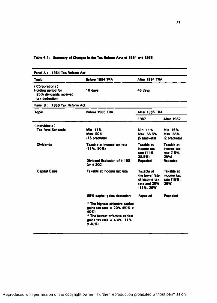
71

TmW# 4.1: Sununarv of Chong## in th# T#x Roform Acts of 1984 #nd 1986

Pantl A : 1984 Tax Reform Act

Topic Before 1984 TRA After 1984 TRA

( Corporation» i Holding period for

85% dividends received tax deduction

16 days 46 days

PaneiB: 1986 Tax Reform Act

Topic Before 1986 TRA After 1986 TRA

1987 After 1987

( Individuais )Tex Rate Schedule Min 11%

Max 50% (IS bracketsi

Min 11% Max 38.5% (5 bracketsi

Min 15% Max 28% (2 brackets)

Dividends Taxable at income tax rate (11% 50%)

Dividend Exclusion of ) 100 (Of $ 200)

Taxable at income tax rate (11 %, 38.5%) Repealed

Taxable at income tax rate (15%, 28%) Repealed

Capital Gains Taxable at income tax rate Taxable at the lower rate of income tax rate and 28% (11%. 28%)

Taxable at Income tax rate (15%, 28%)

60% capital gains deduction Repealed Repealed

* The highest effective capitai gains tax rate ■ 20% (50% x 40%)* The lowest effective capitai gains tax rate - 4.4% (11 % x40%)


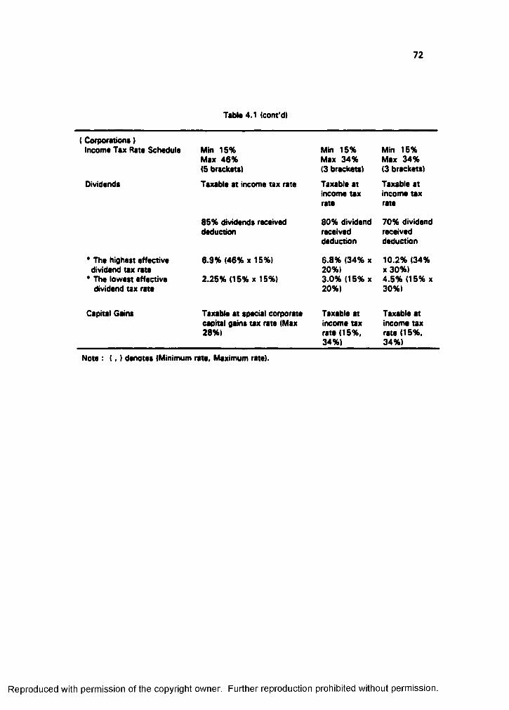
72

Tabla 4.1 (cont'd)

I Corporationa I Income Tax Rate Schedule

Dividende

* The highest effective dividend tax rate

* The lowest effective dividend tax rate

Capital Gains

Min 15%Max 46%IS brackets)

Taxable at income tax rate

85% dividends received deduction

6.9% (46% X 15%)

2.25% (15% X 15%)

Taxable at special corporate capital gains tax rate (Max 28%)

Min 15% Min 15%Max 34% Max 34%(3 brackets) (3 brackeu)

Taxable at Taxable atincome tax income taxrate rate

80% dividend 70% dividendreceived receiveddeduction deduction

6 .8 % (34% X 10.2% (34%20%) x30%)3.0% 115% X 4.5% (15% X20%) 30%)

Taxable at Taxable atincome tax income taxrate (15%, rate (15%,34%) 34%)

Note : I , ) denotes (Minimum rate. Maximum rate).


73

If the corporation is financing an Investment in stock with borrowed funds, interest on

the indebtedness is also tax deductible. These corporations are generally taxed at a

lower rate on dividends than on capital gains.

2. Th» T»x R»fom Act of 1986

The Tax Reform Act of 1986 equalizes the nominal taxation of dividends and

capital gains for individuals (see Panel 8 of Table 4.1). 8efore passage of the act,

capital gains were preferantially taxed compared to dividends for individuals. Individuals

we;e taxable in as many as 15 brackets at rates thst varied from 11% to 50%.

Dividends were taxable at these ordinary income tax rates for individuals and were

subject to a maximum tax rate of 50% after deducting dividend exclusion'. Individuals

cc'uld deduct 60% of net capital gain from gross income. As a result, the highest tax

rate applicable to an individual's net capital gain was only 20% (the 50% maximum

individual tax rate times the 40% of net capital gain).

Under the 1986 Tax Reform Act, the tax schedule was reduced to two brackets

of 15% and 28%, starting with the 1988 tax year. There was a blended rate schedule

for 1987 with five brackets, varying from 11% to 38.5%. The dividend exclusion for

individuals also was repealed. Thus, dividends were taxed at a maximum rate of 38.5%

in the transitional year of 1987 and were subject to a maximum rate of 28%' after

1987. In addition, the 1986 Tax Reform Act repealed the 60% net capital gain

deduction for individuals. Beginning in 1987, capital gains are taxed at a maximum rate

of 28%. Thus, for 1988, there was no longer a distinction between dividends and

capital gains for tax purposes for individuals.

The 1986 Tax Reform Act generally reduced corporate tax rates, but did not

change much the effective tax differentials between dividends and capital gains. Prior to

the 1986 tax reform, corporations were taxed from a five bracket tax schedule ranging

^The exclueion amount# were $100 of dividend# received by an individual atockholder and $200 by a married couple.


74

from 15% to 46%. Since corporations could deduct 85% of the dividends received,

corporate income from dividends was taxed at a maximum effective rate of 6.9% (the

15% of dividends received times the maximum corporate tax rate of 46%). Capital

gains were also subject to a preferential tax rate of 28% under prior law.

Under the 1986 Tax Reform Act, the old-five bracket corporate tax schedule was

reduced to a three-bracket schedule varying from 15% to 34%, effective July 1987.

Under the new act, the 85% dividends received deduction is lowered to 70%. Thus, the

highest effective tax rate of corporate dividends received became 10.2% (the 30% of

dividends received times the maximum corporate tax rate of 34%). Also, prior law's

preferential 28% tax rate for corporate capital gains is repealed. Beginning in July

1987, corporate capital gains were taxed as ordinary income and were subject to a

maximum tax rate of 34%.

C. Models and Testable Hypotheses

7. Th* Tax-£ff$et Modxt

The tax-effect model was originally proposed by Elton and Gruber (1970). Later,

Kalay (1982), Booth and Johnston (1984), Barclay (1987), and Michaely (1991) pursue

this logic.

Elton and Gruber (1970) suggest that the ex-dividend price of a stock should be

related to the tax rates of marginal stockholders. Because dividends and capital gains

are taxed at different rates, they argue that the equilibrium market price on the ex-

dividend day should reflect the value of dividends vis-a-vis capital gains to the marginal

stockholders.

Elton and Gruber (1970) assume long-term traders who have already decided to

sell a stock around the ex-dividend day. These investors' only concern is whether to sell

before or after the ex-dividend day. In case of no transaction costs, the long-term trader

would be indifferent between selling the stock cum- or ex-dividend day as long as the

returns are the same.


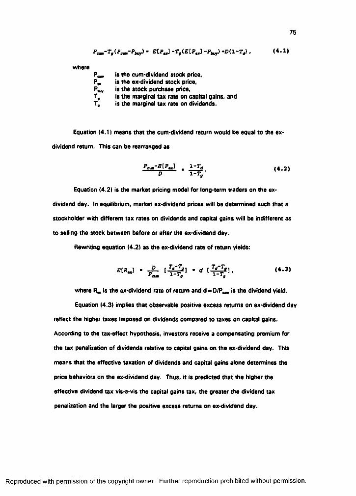
75

- E{P„] -r,(E[P„] -Phy) *D{1-Ta) . (« 1)

wherePan is the cum dividend stock price,P* is the ex-dividend stock price,Ptuy is the stock purchase price,T, is the marginal tax rate on capital gains, andTy is the marginal tax rate on dividends.

Equation (4.1) means that the cum-dividend return would be equal to the ex-

dividend return. This can be rearranged as

(4*2)D 1-T,

Equation (4.2) is the market pricing model for long-term traders on the ex-

dividend day. In equilibrium, market ex-dividend prices will be determined such that a

stockholder with different tax rates on dividends and capital gains will be indifferent as

to selling the stock between before or after the ex-dividend day.

Rewriting equation (4.2) as the ex-dividend rate of return yields;

^where P., is the ex-dividend rate of return and d = is the dividend yield.

Equation (4.3) implies that observable positive excess returns on ex-dividend day

reflect the higher taxes imposed on dividends compared to taxes on capital gains.

According to the tax-effect hypothesis, investors receive a compensating premium for

the tax penalization of dividends relative to capital gains on the ex-dividend day. This

means that the effective taxation of dividends and capital gains alone determines the

price behaviors on the ex-dividend day. Thus, it is predicted that the higher the

effective dividend tax vis-a-vis the capital gains tax, the greater the dividend tax

penalization and the larger the positive excess returns on ex-dividend day.


76

Hypothesis 1 : Prior to the 1986 tax reform act, significant positive excess returns wifi

be observed on the ex-dividend day.

Since the 1986 Tax Reform Act eliminated the nominal tax differentials between

dividends and capital gains, the tax-effect hypothesis predicts that positive excess

returns observed on the ex-dividend day will be drastically reduced to an insignificant

level during the post-1986 tax reform period compared to the pre-1986 tax reform

period. However, as Booth and Johnston (1984) argue, capital gains may be still treated

more favorably than dividends because individual investors can maintain a tax timing

option on the realization of capital gains. The effects of tax deferral of capital gains may

prevent excess ex-dividend returns from being completely eliminated.

Hypothesis 2; During the post-1986 tax reform period, average ex-dividend day excess

returns will be significantly lower than those during the pre-1986 tax reform period, or

will not be different from zero.

Based on the tax-effect hypothesis, many studies document the positive

correlation of the price change-to-dividend ratio with the dividend yield of the stock,

suggesting dividend clientele effects. For example, Elton and Gruber (1970) report that

with the exception of the first and eighth decile, the price change-to-dividend ratio

increases up to one as the dividend yield rises. Since price change-to-dividend ratios

less than unit would indicate low dividend yields and high implied tax rates, thay argue

that low dividend yields should attract stockholders in higher tax brackets. This can be

interpreted in terms of excess returns on the ex-dividend day. If dividend clientele

effects exist, negative correlations between the dividend yields and ex-dividend day

excess returns will be observed. Marginal stockholder's tax rates can be inferred from

those ex-dividend day excess returns.

Hypothesis 3: There will be negative correlation between dividend yields and ex-

dividend day excess returns. This correlation will be weakened between the pre-1986

tax reform period and the post-1986 tax reform period.


77

2. Short'Ttm Tnding Modal

The short-term trading model was first studied by Miller and Scholes (1982) and

Kalay (1982). Later, Lakonishok and Vermaelen (1983, 1986) and Karpoff and Walkling

(1988, 1991) follow this reasoning.

Miller and Scholes (1982) argue that every investor can exploit profit

opportunities from short-term trading, buying cum-dividend shares and selling them ex-

dividend. Such trading activities are expected to eliminate the excess returns on the ex-

dividend day, but transaction costs may well prevent the excess returns from being

completely eliminated.

The marginal short-term traders include taxable corporations and dealers in

securities. Since individual short-term traders may be constrained by the capital loss

limitations and the wash-sale rules. Miller and Scholes (1982) point out that corporations

eligible for the dividend income deduction or security dealers taxable at the same rates

on dividends and capital gains could have incentives to make short-term trading profits.

Taxable corporations are considered to have stronger incentives to make short-term

trading than dealers (see Grammatikos (1989)1.

Generally, the preferential tax treatment of dividends relative to capital gains

may give a taxable corporation strong incentives for short-term trading around the ex-

dividend day. As a result, a corporation can buy shares of stock in another corporation

cum-dividend in anticipation of receiving a dividend that will be eligible for the dividend

income tax deduction. The corporation may finance the cost of an investment in stock

with borrowed money having tax-deductible interest. After receiving the dividend, the

corporation can sell the stock ex-dividend and claim any capital loss from selling the

stock at a lower ex-dividend price in order to offset other capital gains taxable at a

higher tax rate.

However, this dividend tax deduction is not allowed unless the corporation holds

the dividend-paying stock for a minimum period. This implies that firms must expose

themselves to capital loss risks in order to exploit the dividend tax deduction. The 1984


78

Tax Reform Act requires that. In order to qualify for the dividend tax deduction, the

corporation must hold the stock for a minimum 46 days instead of a minimum 16 days,

as allowed under prior law. This change increases the capital loss risk of firms that

engage in short-term trading around the ex-dividend day. Since the risk exposure of

short-term traders has been increased after the 1984 tax reform,* it is predicted that

excess returns on the ex-dividend day for those short-term traders will increase during

the post-1984 tax reform period, compared to the pre-1984 tax reform period.

Hypothesis 4: Average ex-dividend day excess raturns will increase significantly during

the post-1984 tax reform period compared to the pre-1984 tax reform period.

Since the 1984 tax reform increased the exposure risks of short-term traders,

these increased risks would be reflected in the stock prices for several short-term trading

days before and after the ex-dividend day, in addition to on the ex-dividend day during

the post-1984 tax reform period.

Hypothesis 5; During the post-1984 tax reform period, more significant excess returns

will be observed for several trading days before and after the ex-dividend day than in the

pre-1984 tax reform period.

In order to investigate the effects of the 1986 Tax Reform Act on short-term

trading, the marginal rates of substitution of dividends and capital gains between the

pre- and post-1986 tax reform period are compared. Under the 1986 Tax Reform Act,

the effective corporate tax differentials between dividends and capital gains increased

slightly to 23.8% (the capital gains tax rate of 34% minus the effective dividend tax

rate of 10.2%| from 21.1% (the capital gains tax rate of 28% minus the effective

dividend tax rate of 6.9%) during the pre-1986 tax reform period. Michaely (1991)

argues that, because the marginal rate of substitution between dividends and capital

gains for highly taxed investors decreased from 1.72 in 1986 to 1.36 in 1987, the

corporation's incentives to engage in short-term trading is reduced. The calculation.

*The rieke of ahort-term traders due to the 1984 Tax Reform Act seemed to be largely systematic (see Brown and Lunmer (1986) and Grammatikos (1989)].


79

however, shows that the marginal rate of substitution between dividends and capital

gains during the post-1986 tax reform period is 1.29 (> (1-0.0691/(1-0.28)1, whereas

the marginal rate of substitution between dividends and capital gains during the post-

1986 tax reform period is 1.36 ( - (1-0.1021/(1-0.34)). It is argued that, if one allows

for transaction costs, the 1986 Tax Reform Act seems to give little incentive to firms to

engage in tax-induced short-term trading (see Appendix B).

3. Th* Portfolio Mod*!

The basic idea of our portfolio approach is that the ex-dividend value of stock

and short-term trading behavior around ex-dividend day should reflect the trade off

between risk and expected return. Long (1977) argues that 'the portfolio dividend yield

choice cannot be made independently of the risk-expected return trade-off, since the

dividend yield of all mean variance efficient portfolios is a linear function of their non-

diversifiable risk' [Kalay (1982), p. 1059). Thus, it can be inferred that any change in

the risk-expected return trade-off induced by the tax reforms should be manifested in the

portfolio choices around the ex-dividend day.

To show how a change in the risk-expected return trade-off is reflected in

portfolio choices around the ex-dividend day, we construct efficient portfolios using the

portfolio selection model posed by Markowitz (1952, 1959, 1981) as follows:

Maximize

subject to

wherei f is the transpose of the expected return vector,W is the optimal portfolio weights,V is the covariance matrix of the returns,A is the investor's risk aversion parameter, andA and b form a set of linear constraints.


80

Efficient portfolio frontiers are computed. First, the efficient portfolio frontiers

between the pre-1984 tax reform period and the post-1984 tax reform period are

compared. Within each period, cum-dividend efficient frontiers and ex-dividend efficient

frontiers are compared. Short-selling is not considered because it seems not to be a

common practice around the ex-dividend day [see Karpoff and Walkling (1991)1. While

the portfolio optimization model is usually applied in a normative context, our approach

is positive.

Before the 1984 tax reform, the required holding period for dividend income tax

deduction was 16 days. It is predicted that cum-dividend portfolios will be more

efficient than ex-dividend portfolios, because ex-dividend portfolios are more likely to be

restricted from trading. This inference is supported by the arguments of Green (1980),

Grundy (1985)*, and Pogue (1970)*.

Hypothesis 6: Cum-dividend portfoiio efficient frontiers wiil dominete ex-dividend

portfolio efficient frontiers.

The 1984 Tax Reform Act extended the minimum holding period for the dividend

income tax deduction to 46 days. Since trading may be restricted for longer ex-dividend

days, the efficiency gap between cum-dividend efficient frontiers and ex-dividend

efficient frontiers will be greater after the 1984 tax reform than before the 1984 tax

reform.

Hypothesis 7: The efficiency gap between cum-dividend efficient frontiers and ex-

dividend efficient frontiers will be greater during the post-1984 tax reform period than

during the pre-1984 tax reform period.

^Green (1980) and Grundy (1985) suggest the delay and acceleration hypothesis. Their arguments state that trading activities around the ex-dividend day will concentrate on the last cum-dividend day and on the first ex-dividend day, because investors attempt to avoid costs resulting from delaying or accelerating transactions relative to their optimum trading date for tax purposes.

^Pogue (1970) reports that portfolios restricted from trading are dominated by the unrestricted portfolios.


81

Long (1977) shows that, with the Introduction of Income taxation, Investors will

demand after tax efficient portfolios and that those portfolios may not be before tax

efficient. For example, under the tax regime that raised the dividend tax rate relative to

the capital gains tax. Investors are Induced to revise their portfolio holdings to reflect

these differential taxes. That sort of portfolio revision will result in an efficiency gain at

the new tax rates because It will Increase the expected after tax return at the new tax

rates and reduce the after tax variance of the portfolio [see Long (1977)1. Accordingly,

the after tax efficient portfolio will dominate any given before-tax efficient portfolio on

an after tax basis. Furthermore, Long predicts that the potential after tax efficiency

gains due to moving from the before-tax efficient portfolio to the dominating after-tax

frontier will be smaller If the correlations between two portfolios are large.

The 1986 Tax Reform Act decreased the dividend tax rate from a maximum rate

of 50% to 2 8 % \ According to the Long's hypothesis. Investors are motivated to

restructure their portfolio holdings to reflect the new tax rates. However, since the

dividend tax rate under the 1986 Tax Reform Act has decreased. It Is expected that the

expected after-tax return will decrease and that the after-tax variance will Increase at

the new tax rates (see Long (1977), p. 391. Thus, It Is predicted that the after-1986

tax reform efficient portfolios will be dominated by the before-1986 tax reform efficient

portfolios.

Hypothesis 8: The efficient portfolio frontier under the pre-1986 tax reform period will

dominate the efficient portfolio frontier under the post-1986 tax reform period.

Ûnless the individual must pay a 5% surcharge, he is taxed at a maximum rate o f 28%.

decrease in the expected return is to be anticipated in the tax- effect hypothesis since the tax premiums decrease with a drop in dividend tax rate, but its variance is not considered in the tax-effect hypothesis.


82

D. Data and Mathodology

1. Data

The sample for this study consists of taxable dividend payment events by all

firms listed on the New York Stock Exchange (NYSE) and American Stock Exchange

(AMEX) from January 1, 1980, to December 31, 1989. In order to examine the effects

of the Tax Reform Acts of 1984 and 1986, the entire sample period is divided into three

periods: Period I (1/1/80-7/17/84), Period II (7/18/84-12/31/86), and Period III (1/1/87-

12/31/89).

To obtain uncontaminated samples, the following selection criteria are used for

each sub-sample period. First, dividend payments whose ex-dividend date are less than

57 trading days apart from the ex-dividend date of the previous dividend payment are

deleted. Second, a dividend payment is not considered unless its ex-dividend dates are

at least 11 trading days away from the declaration (announcement) date of the

subsequent dividend payment. Third, dividend payment events that have missing

returns during the period - including the estimation period and the test period (-55

through +10 days relative to the ex-dividend day) - are eliminated.

After this screening, the sample consists of the following dividend payments and

number of firms by subperiods: 21,334 dividend payments by 2,000 firms in Period I;

10,335 dividend payments by 1,643 firms in Period II; and 12,525 dividend payments

by 1,776 firms in Period III. These are reported in Table 4.2. All dividend payments are

taxable, and cash dividends are paid in U.S. dollars. Stock dividends and splits are

excluded. Quarterly dividends, semi annual dividends, and annual dividends are

identified by the CRSP distribution type codes 1232, 1242, and 1252, respectively.

Reproduced witli permission of the copyright owner. Further reproduction prohibited without permission.

83

Tabla 4.2: Numbar of Sainpia Rmia and Oividand Paymant Evants from January 1980 throuQh Oaeambar 1989

Data wara obtainad from tha CRSP daily maatar tapa. AH dividand paymanu ara taxabla and cash dividands paid in U.S. dollars. CRSP distribution typa codas ara 1232 for quarterly dividends. 1242 for semi annual dividands, and 1252 for annual dividands.

Period 111/1/80 - 7/17/84)

Period II17/18/84 - 12/31/86)

Period III(1/1/87 • 12/31/89)

Numbar of Firms 2,000 1,643 1,776

Numbar of Dividand Payment Evants 21,334 10,335 12,525

Dividand Types

Quarterly dividand 20,622 9,912 11,851

Sami annual dividand

292 121 148

Annual dividand 82 37 33

Others 338 265 493


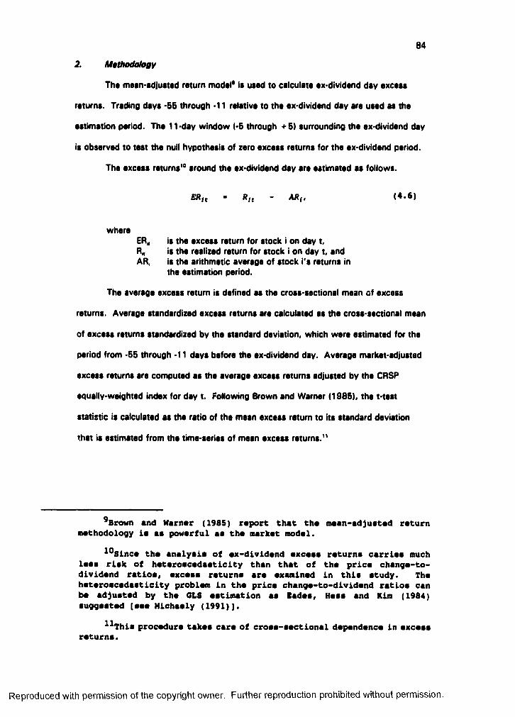
84

2. Mtthodahgy

The mean mdjueted return model* Is used to calculate ex dividend day excess

returns. Trading days 55 through 11 relative to the ex dividend day are used as the

estimation period. The 11 day window (-5 through +5) surrounding the ex dividend day

is observed to teat the null hypothesis of zero excess returns for the ex dividend period.

The excess returns'* around the ex dividend day are estimated as follows.

ER,t • R,t - AR,. (4.6)

whereERj, is the excess return for stock i on day t,Rh is the realized return for stock i on day t. andAR| is the arithmetic average of stock i’a returns in

the estimation period.

The average excess return is defined as the cross-sectional mean of excess

returns. Average standardized excess returns are calculated as the cross-sectional mean

of excess returns standardized by the standard deviation, which were estimated for the

period from -55 through -11 days before the ex-dividend day. Average market-adjusted

excess returns are computed as the average excess returns adjusted by the CRSP

equally-weighted index for day t. Following Brown and Warner (1985), the t-test

statistic is calculated as the ratio of the mean excess return to its standard deviation

that is estimated from the time-series of mean excess returns."

^Brown and Warner (1985) report that the mean-adjusted return methodology ie ae powerful as the market model.

^^Since the analyeia of ex-dividend excess returns carries much leas risk of heteroscedaaticity than that of the price change-to- dividend ratios, exceae returns are examined in this study. The heteroacedaeticity problem in the price change-to-dividend ratios can be adjusted by the GLS estimation as fades, Hess and Kim (1984) euggeated (see Michaely (1991)].

^^Thia procedure takes care of croaa-eectional dependence in excess returns.


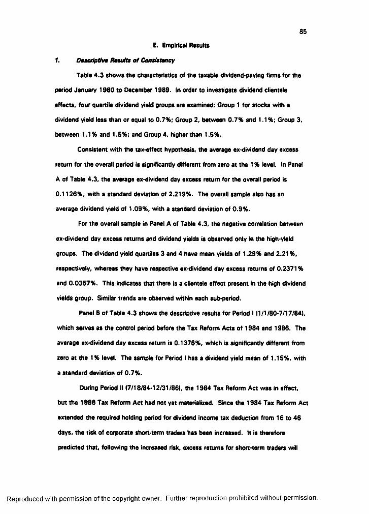
85

E. Empirical Rasuitt

1. D»$e/iptivm R»suttM of Conslstoney

Tabla 4.3 shows the characteristics of the taxable dividend-paying firms for the

period January 1980 to December 1989. In order to investigate dividend clientele

effects, four quartile dividend yield groups are examined: Group 1 for stocks with a

dividend yield less than or equal to 0.7%; Group 2, between 0.7% and 1.1%; Group 3,

between 1.1% and 1.5%: and Group 4. higher than 1.5%.

Consistent with the tax-effect hypothesis, the average ex-dividend day excess

return for the overall period is significantly different from zero at the 1 % level. In Panel

A of Table 4.3, the average ex-dividend day excess return for the overall period is

0.1126%, with a standard deviation of 2.219%. The overall sample also has an

average dividend yield of 1.09%, with a standard deviation of 0.9%.

For the overall sample in Panel A of Table 4.3, the negative correlation between

ex-dividend day excess returns and dividend yields is observed only in the high-yield

groups. The dividend yield quartiles 3 and 4 have mean yields of 1.29% and 2.21 %,

respectively, whereas they have respective ex-dividend day excess returns of 0.2371 %

and 0.0357%. This indicates that there is a clientele effect present in the high dividend

yields group. Similar trends are observed within each sub-period.

Panel B of Table 4.3 shows the descriptive results for Period I (1/1/80-7/17/84),

which serves as the control period before the Tax Reform Acts of 1984 and 1986. The

average ex-dividend day excess return is 0.1376%, which is significantly different from

zero at the 1% level. The sample for Period I has a dividend yield mean of 1.15%, with

a standard deviation of 0.7%.

During Period II (7/18/84-12/31/86), the 1984 Tax Reform Act was in effect,

but the 1986 Tax Reform Act had not yet materialized. Since the 1984 Tax Reform Act

extended the required holding period for dividend income tax deduction from 16 to 46

days, the risk of corporate short-term traders has been increased. It is therefore

predicted that, following the increased risk, excess returns for short-term traders will


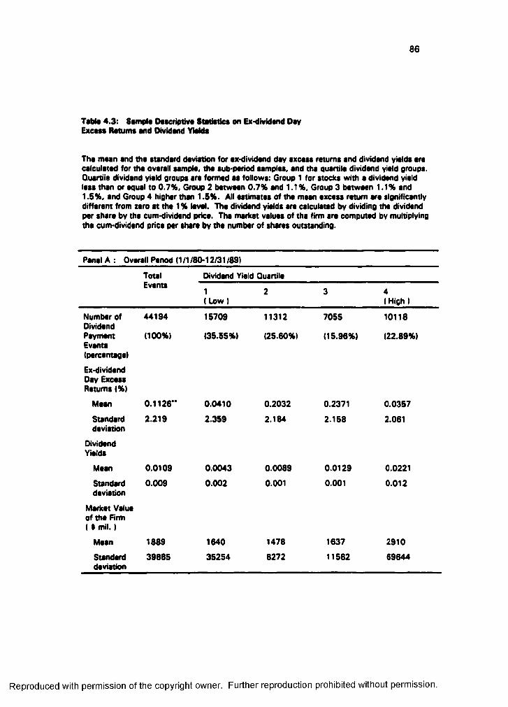
86

Tabto 4.3: Sampl* Dncriptiva Statistics on Ex-dividsnd Day Excasa Ratums and Dividand YWda

Tha mean and tha standard deviation for ax-dividand day axcass returns and dividend yields are calculated for tha overall sampla. tha sub-period samples, and tha quartila dividend yield groups. Quartiia dividand yield groups are formed as follows: Group 1 for stocks with a dividend yield less than or equal to 0.7%, Group 2 batwoan 0.7% and 1.1%, Group 3 batwaan 1.1% and 1.5%, and Group 4 higher than 1.5%. All estimâtes of tha mean axcass return are significantly different from zero at tha 1 % lavai. The dividand yields are calculated by dividing the dividend par share by tha cum-dividend price. Tha market values of tha firm are computed by multiplying the cum-dividand price par share by tha numbar of shares outstanding.

Panel A : Overall Panod (1/1/80-12/31/891

Total Dividand Yield QuartileEvants

1( lAW 1

2 3 4( High )

Numbar ofDividandPaymentEvants(parcantagal

44194

(100%)

15709

(35.55%)

11312

(25.60%)

7055

(15.96%)

10118

(22.89%)

Ex-dividand Day Excess Returns (%)

Moan 0.1126** 0.0410 0.2032 0.2371 0.0357

Standarddeviation

2.219 2.359 2.184 2.158 2.061

DividendYields

Mean 0.0109 0.0043 0.0089 0.0129 0.0221

Standarddeviation

0.009 0.002 0.001 0.001 0.012

Market Value of the Firm ( $ mil. )

Mean 1889 1640 1478 1637 2910

Standarddeviation

39885 35254 8272 11582 69644


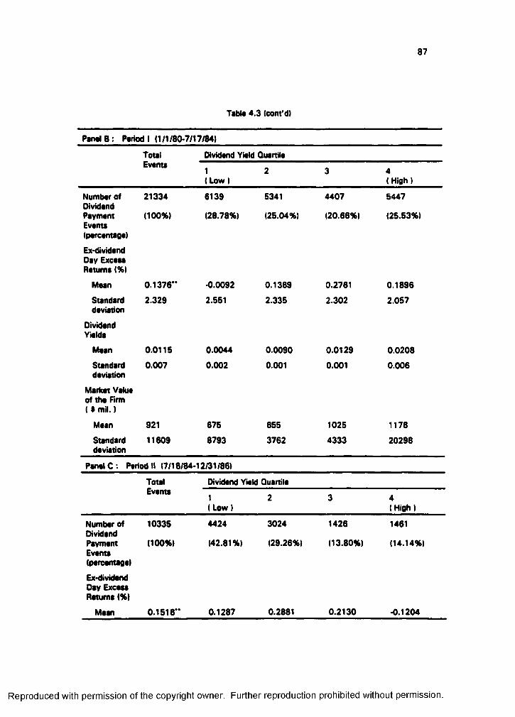
87

Table 4.3 (cont'd)

Panel B: Period 1 (1/1/80-7/17/84)

Total Dividend Yield QuartileEvents

1(Low)

2 3 4( High )

Number of 21334 6139 5341 4407 5447DividendPayment (100%) (28.78%) (25.04%) (20.88%) (25.53%)Eventa(percentage)

Ex-dividandDay ExceaaReturns (%)

Mean 0.1378" •0.0092 0.1389 0.2781 0.1898

Standard 2.329 2.551 2.335 2.302 2.057deviation

DividendYields

Mean 0.0115 0.0044 0.0090 0.0129 0.0208

Standard 0.007 0.002 0.001 0.001 0.008deviation

Market Valueof the Firm( $ mil. )

Mean 921 875 855 1025 1178

Standard 11809 8793 3782 4333 20298deviation

Panel C : Period II (7/18/84-12/31/86)


1( Low )

2 3 4( High )

Number of 10335 4424 3024 1428 1461DividendPayment (100%) (42.81%) (29.26%) (13.80%) (14.14%)Events(percentage)

Ex-dividendDay ExcessReturns (%)

Mean 0.1518" 0.1287 0.2881 0.2130 •0.1204


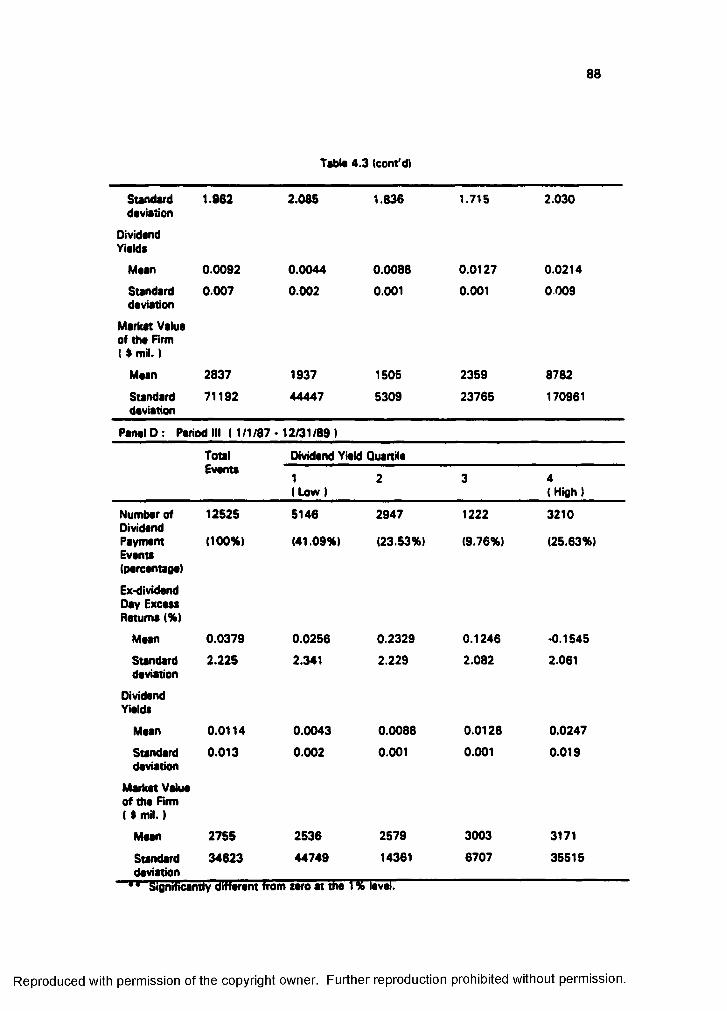
88

Tabla 4.3 (corn'd)

Standarddeviation

1.962 2.085 1.836 1.715 2.030

OividandYialda

Mean 0.0092 0.0044 0.0088 0.0127 0.0214

Standarddeviation

0.007 0.002 0.001 0.001 0 009

Market Value of the Firm( $ mil. )

Mean 2837 1937 1505 2359 8782

Standarddeviation

71192 44447 5309 23765 170961

Panel D: Period III (1/1/87* 12/31/89 )


1( Low )

2 3 4( High )

Number ofDividendPaymentEvents(percentage)

12525

(100%)

5146

(41.09%)

2947

(23.53%)

1222

(9.76%)

3210

(25.63%)

Ex-dividend Day Excess Returns (%)

Mean 0.0379 0.0256 0.2329 0.1246 *0.1545

Standarddeviation

2.225 2.341 2.229 2.082 2.061

DividendYields

Mean 0.0114 0.0043 0.0088 0.0128 0.0247

Sundarddeviation

0.013 0.002 0.001 0.001 0.019

Markat Valueof the Firm ( $ mil. 1

Mean 2755 2536 2579 3003 3171

Standarddeviation

• 9 CixeeeSdaMAM

34623 44749

H M em 1 9 L

14361 6707 35515


89

increase. Consistent with this expectation, the average ex dividend day excess return

increased from 0.1376% during control Period I (1/1/80-7/17/84) to 0.1518% during

Period II (7/18/84-12/31/86). This is shown in Panel C of Table 4.3. Dividend clientele

behavior is also observed in the high dividend yield quartiles of Period II, which is the

same pattern as that observed during Period I.

Panel D of Table 4.3 presents the results observed during Period III (1/1/87-

12/31/89) when the 1986 Tax Reform Act had been implemented. Since the 1986 Tax

Reform Act has equalized the tax rates on dividends and capital gains, the tax-effect

hypothesis predicts that the price change-to-dividend ratio would be statistically

indistinguishable from one, or that excess return on the ex-dividend day would not be

statistically different from zero. During the post-1986 tax reform period, ex dividend

day excess return decreased to 0.0379%, which is not different from zero at the 1 %

level of significance. This finding is consistent with the tax-effect hypothesis.

2. Ttst of Short-Torn Troding Hypothosis

Table 4.4 reports non-parametric test results of equality of ex-dividend day

excess returns between the two periods. In Panel A of Table 4.4, ex-dividend day

excess returns during the pre-1984 tax reform act are compared to those during the

post-1984 tax reform act. Average ex-dividend day excess returns after the 1984 tax

reform increased to 0.1518% from 0.1376% before the 1984 tax reform, and this

increased percentage seems to be statistically different from zero at the 1 % level. This

finding is similar to what Grammatikos (1989)" obtained by using the raw price ratios

on the ex-dividend day. Grammatikos reports that the overall raw price ratio declines

my beet Itnowledge, cramnetikos (1989) is the only study that deals with the effects of the 1984 Tax Reform Act.


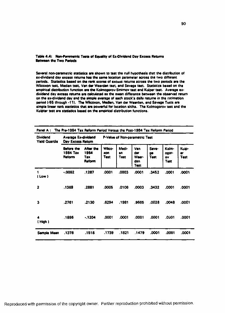
90

Taw* 4.4: Nflfi-Paramatrie Tnta of EquaUty of Ex-Oividand Day Exeau Ratuma Batwaan tho Two Pariods

Savaral non-paramatric ttatittica ara ahown to taat tha null hypothatit that tha distribution of ax-dividand day axcats ratuma haa tha sama location paramatar across tha two diffarant pariods. Statistics basad on tha rank scoras of axcuss ratuma across the two pariods ara tha Wilcoxon test. Median test. Van dor Waardan test, and Savage test. Statistics basad on tha empirical distribution function ara tho Kolmogorov Smimov test and Kuipar test. Average ax- dividand day axcasa returns ara cakulatad as tha maan diffaranca batwaan tha obsarvad ratum on tha ax-dividand day and tha simpla avaraga of aach stock's daily ratuma in tha estimation period (-55 through -11). Tha Wilcoxon, Madian, Van dar Waardan, and Savage Tests ara simpla linaar rank statistics that ara powerful for location shifts. Tha Kolmogorov test and the Kuiptar test ara statistics basad on tha empirical distribution functions.

Panel A : Tha Pra-1984 Tax Reform Period Versus tha Post-1984 Tax Reform Period

Dividend Yield Quartila

Avaraga Ex-divldand Day Exeau Ratum

P-Valua of Non-paramatric Test

Safora tha 1984 Tax Reform

After tha 1984 Tax Reform

WilcoxonTest

MedianTest

VandarWaardanTest

SavageTest

KolmogorovTest

KuiparTest

1( Low I

-.0092 .1287 .0001 .0003 .0001 .3452 .0001 .0001

2 .1389 .2881 .0005 .0106 .0003 .3432 .0001 .0001

3 .2761 .2130 .6294 .1981 .9665 .0028 .0048 .0001

4( High )

.1896 -.1204 .0001 .0001 .0001 .0001 .0001 .0001

Sample Maan .1378 .1518 .1739 1821 .1479 .0001 .0001 .0001


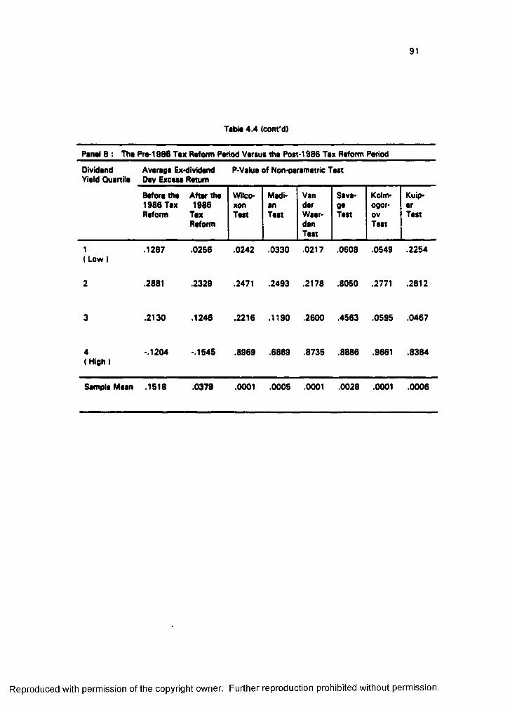
91

Tabit 4.4 (corn'd)

Panal B : Tha Pra-1986 Tax Raform Pariod Vartus tha Post-1986 Tax Raform Pariod

Dividand Yiald Quartila

Avaraga Ex-dividand Day Excaaa Ratum

P-Valua of Non-paramatric Taat

Bafora tha 1986 Tax Raform

Attar tha 1986

Tax Raform

WilcoxonTaat

MadianTaat

VandarWaardanTaat

Sava-0«Taat

KolmogorovTeat

KuiparTaat

1I Low 1

.1287 .0256 .0242 .0330 .0217 .0608 .0549 .2254

2 .2881 .2329 .2471 .2493 .2178 .8050 .2771 .2812

3 .2130 .1246 .2216 .1190 .2600 .4563 .0595 .0467

4( High )

-.1204 -.1545 .8969 .6889 .8735 .8886 .9661 .8384

Sampla Maan .1518 .0379 .0001 .0005 .0001 .0028 .0001 .0006


92

from 0.877 before the 1984 tax reform (1/1/75-7/17/84) to 0.796 after the 1984 tax

reform (7/18/84-12/31/85).'*

To further examine the changes in behavior of short-term traders between the

before- and after-1984 tax reform period, uniiice Grammatilcos (1989), we compare

excess returns for 11 days (-5 through + 5) surrounding the ex-dividend day. Because

the 1984 Tax Reform Act was intended to expose short-term traders to more risic,

increased exposure would be reflected in the return behavior for several short-term

trading days before and after the ex-dividend day in addition to on the ex-dividend day

during the post-1984 tax reform period. According to the short-term trading hypothesis,

it is furthermore predicted that there more significant excess returns will occur for 11

days surrounding the ex-dividend day during the post-1984 tax reform than prior to the

1984 tax reform.

Table 4.5 shows average excess returns around the ex-dividend day for the

period from January 1, 1980, to July 17,1984, before implementation of the 1984 and

1986 Tax Reform Acts. The 11-day window for average excess return has two

significant excess returns at the 5% level, when the ex-dividend day excess returns are

excluded.

Tables 4.6 and 4.7 present average excess returns around the ex-dividend day

for Period II (7/18/84-12/31/86) and Period III (1/1/87-12/31/89) when the 1984 Tax

Reform Act was in effect. During the latter period, the 1986 Tax Reform Act was also

in effect, but it does not appear to have affected the behavior of short-term traders (see

Section C.2 for discussion). Consistent with expectation, the 11-day window for

average excess returns during Period II (7/18/84-12/31/86) has six significant excess

returns on each side, excluding the ex-dividend day, two of which are significant at the

1% level. During Period III (1/1/87-12/31/89), the 11-day window for average excess

^^GranmatDcce (1989) compares a sample of 19,407 observations before the 1984 tax reform (1/1/75-7/17/85) and a sample of 2,032 observations after the 1984 tax reform (7/18/84-12/31/85). His samples appear to be seriously unbalanced.


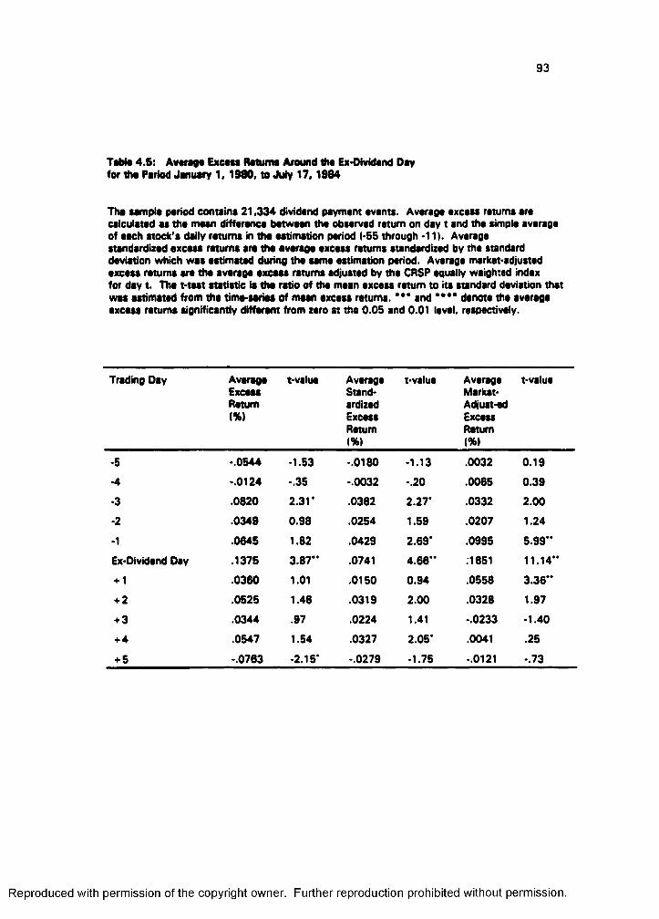
93

TaWt 4.5: Avtrag* Excms RMwnt Around Iho Ex>Oividmd Day for tha Pariod January 1, 1980. to July 17.1984

Tha «ample pariod contains 21.334 dividend payment event*. Average excess returns are calculated as tha mean difference between the observed return on day t and the simple average of each stock's daily ratuma in the estimation period 1-55 through -11). Average standardized excess returns are the average excess returns standardized by the standard deviation which was estimated during the same estimation period. Average market-adjusted excess returns are the average excess ratuma adjustad by the CRSP equally waighted index for day t. Tha t-tast statistic is the ratio of the mean excess retum to its standard deviation that was astimatsd from the time-serle* of mean excess retums. * * ’ and ' denote the average excess retums significantly different from zero at the 0.05 and 0.01 level, respectively.

Trading Day AverageExcessReturn(%)

t-value AverageStandardizedExcessRetum(%)

t-value AverageMarkat-Adjust-edExcessRetum{%)

t-value

-5 -.0544 -1.53 -.0160 -1.13 .0032 0.19

-4 -.0124 -35 -.0032 -.20 .0065 0.39

3 .0820 2.31* .0362 2.27* .0332 2.00

-2 .0349 0.96 .0254 1.59 .0207 1.24

-1 .0645 1.62 .0429 2.69* .0995 5.99**

Ex-Dividend Day .1375 3.67" .0741 4.66** ;1651 11.14**

+ 1 .0360 1.01 .0150 0.94 .0556 3.36*

+ 2 .0525 1.46 .0319 2.00 .0326 1.97

+ 3 .0344 .97 .0224 1.41 -.0233 -1.40

+ 4 .0547 1.54 0327 2.05* .0041 .25

+ 5 -.0763 -2.15* -.0279 -1.75 -.0121 -.73


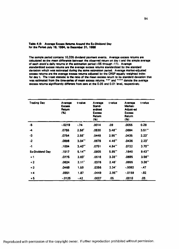
94

Tibto 4.6: Avtrigc Excm* R#lwm# Around 6w Ex-OivMond Day for Iho Poriod July 18.1984. to Docombor 31,1986

Tho sompio poriod comoino 10.335 dividond poymont ovonts. Avorago oxcou ratuma ara calculatad aa tha maan diffaranea batwaan tha obaarvad ratum on day t and tha almpla average of each atock'a daily retuma in tha aatimatkm period i-S5 through -11). Avaraga atandardizad axcaaa returns are tha avaraga axcaaa ratuma atandardizad by the atandard daviation which waa eadmatad during the aama eadmation period. Average market edjuated exceaa ratuma ara the avaraga axcaaa ratuma adjuatad by the CRSP equally weighted index for day t. Tho t taat atadadc la the redo of tha maan axcaaa ratum to ita atandard daviadon that waa aadmatad from tha dma-tarlas of maan axcaaa ratuma. and " " denote the average exceaa retuma aignificandy diffarant from zero at the 0.05 and 0.01 level, respectively.

Trading Day AvaragaExceaaReturn

t-value AverageStandardizedExceaaRetum1%)

t-value AverageMarkat-Adjuat-odExcaaaRatum(%)

t-value

-5 .0219 -.74 .0014 .09 .0055 0.28

-4 .0755 2.56* .0530 3.48* .0684 3.51"

-3 .0754 2.55* .0448 2.95*' .0435 2.23*

-2 .0896 3.04** .0678 4.46** .0436 2.23*

-1 .1004 3.40** .0751 4.94* .0722 3.70"

Ex Dividend Day .1517 5.14** .0905 5.95" .1840 9.43"

+ 1 .0775 2.63* .0516 3.39" .0695 3.56"

+ 2 .0624 2.11* .0378 2.48* .0655 3.36"

+ 3 .0469 1.59 .0356 2.34" -.0092 -.47

+ 4 .0551 1.87 .0449 2.95" -.0159 -.82

+ 5 -.0125 -.42 .0007 .05 .0010 .05


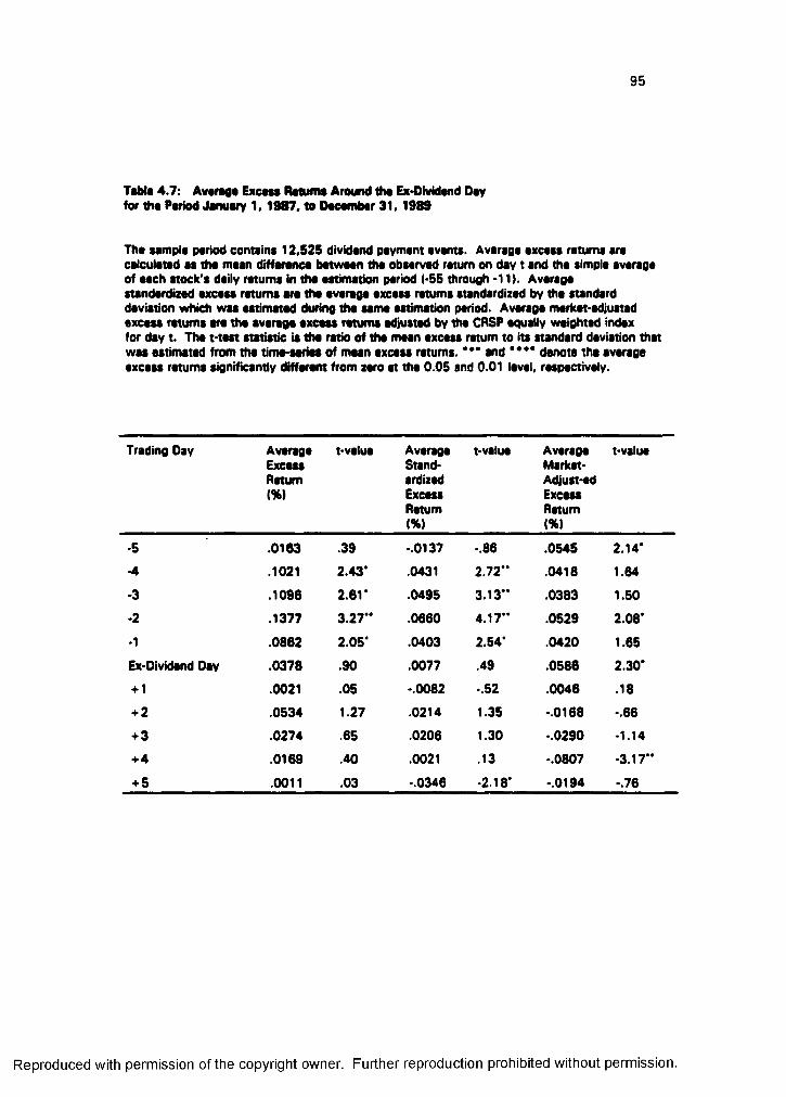
95

Tabla 4.7: Avaraga Excaaa Ratuma Around tha Ex«Dlvldand Day for tha Pariod January 1.1987. to Daeambar 31.1989

Tha aampla pariod containa 12.525 dividand payment avants. Avaraga axcasa retums ara caiculatad as tha maan diffaranca batwaan tha obsarvad ratum on day t and tha simple avaraga of aach atock's daiiy ratums in tfia aatimation pariod ( 55 through -11). Avaraga atandardizad axcasa ratums ara tha avaraga axcasa ratums standardized by tha standard daviation which waa aatimatad during tha aama estimation pariod. Avaraga markot-adjustad axcasa ratums ara tha avaraga axcasa ratums adiustad by tha CRSP aquaily waightad indax for day t. Tha t-tast statistic ia tha ratio of tha maan excess ratum to its standard daviation that was estimated from tha tims-sarias of maan excess ratums. *** and ' denote tha average excess ratums significantly different from zero at tha 0.05 and 0.01 level, raspactivaly.

Trading Day AverageExcessRetum(%)

t-value AverageStandardizedExcessRatum(%)

t-valua AvaragaMarfcat-Adjust-edExcessRatum(%)

t-valua

-5 .0163 .39 -.0137 -.86 .0545 2.14*

-4 .1021 2.43" .0431 2.72" .0418 1.64

-3 .1096 2.6 V .0495 3.13" .0383 1.50

-2 .1377 3.27" .0660 4.17" .0529 2.08’

-1 .0862 2.05* .0403 2 54" .0420 1.65

Ex-Dividand Day .0378 .90 .0077 .49 .0586 2.30*

+ 1 .0021 .05 -.0082 .52 .0046 .18

+ 2 .0534 1.27 .0214 1.35 -.0168 -.66

+ 3 .0274 .65 .0206 1.30 -.0290 -1.14

+ 4 .0169 .40 .0021 .13 -.0807 -3.17"

+ 5 .0011 .03 -.0346 -2.18' -.0194 -.76


96

retums has four cum dividand significant excess returns, one of which is significant at

the 1 % level. During periods II and III, excess returns appear to concentrate cum-

dividend because ex-dividend days are likely to include a minimum period of 46 days in

which short-term traders are restricted to trade by the law. Thus, these evidences

strengthen the short-term trading hypothesis, predicting that the 1984 Tax Reform Act

would have an effect on the retum behavior of short-term traders.

When average excess retums are compared for 11 days, including the ex-

dividend day between the before- and after-1984 Tax Reform Act by using average

standardized excess return and average market-adjusted excess return, the evidence is

consistent with what is shown in Tables 4.5, 4.6, and 4.7.

3. Têst of TêX’Effoct HypothoMis

Panel B of Table 4.4 compares average excess returns on the ex-dividend day

between the before-1986 tax reform period and the after-1986 tax reform period.

Consistent with the predictions of tax-effect hypothesis, the overall average excess

return on the ex-dividend day has decreased from 0.1518% before the 1986 tax reform

to 0.0379% after the 1986 tax reform. The null hypothesis of equality of excess

retums between the two periods is rejected at the 1 % level of significance in five non-

parametric tests.

Further comparisons of ex-dividend day excess retums between the before- and

after-1986 tax reform are reported in Tables 4.5, 4.6, and 4.7. Tables 4.5 and 4.6

show that, prior to the 1986 tax reform, average standardized excess returns and

market-adjusted excess retums, as well as average raw excess returns, are positively

significant at the 1 % level. However, as shown in Table 4.7, after the 1986 tax reform,

both average raw excess retum and average standardized excess retum are reduced to

levels which are not different from zero at the 1 % and 5% levels of significance. Only

market-adjusted ex-dividend excess returns are significant at the 5% level.


97

These results lend strong support to the tax-effect hypothesis. It can be also

inferred that the differential taxation of dividends and capital gains has affected the

market valuation of the stock on the ex-dividend day.

Previous studies'* on the ex-dividend day effects of the 1986 Tax Reform Act

show mixed evidences. For example, Michaely (1991) reports that the 1986 average

price change-to-dividend ratio is not significantly lower than those of 1987, rejecting the

tax interpretation of the ex-dividend day behavior. In contrast, Robin (1991)'* argues

that the ex-day abnormal retums declined between the pre 1986 tax reform period and

the post-1986 tax reform period. The finding reported is consistent with Robin's.

Dividend clientele effects imply the negative correlation of ex-dividend day

excess returns with dividend yields. In order to examine possible changes in the

dividend clientele behavior, we regress ex-dividend day excess retums on dividend yields

for the pre- and post-1986 tax reform periods. The cross-sectional regression results are

reported in Table 4.8. The coefficient estimates of dividend yields are negative and

statistically significant at the 1 % level for each of the two periods. A comparison of the

coefficient estimates of dividend yields between the pre- and post-1986 tax reform

periods shows an interesting evidence on the change of dividend clientele behavior.

Since the coefficient estimate of dividend yields changed from -8.6683 during the pre-

1986 tax reform period to -4.9625 during the post-1986 tax reform period, it can be

argued that the 1986 Tax Reform Act somewhat discouraged dividend clientele behavior

of investors through the equalization of differential tax rates on dividends and capital

gains.

^Ôther ceeearchera who examine the effect of the 1986 Tax Reform Act include Bolster. Lindsey and Mitrusi (1989). and Fedenia and Grammatikos (1991). Bolster. Lindsey and Mitrusi (1989) compare trading behavior in December 1986 and January 1987 and find that relative trading volume was considerably high in December 1986 for long-term winners. Fedenia and Grammatikos (1991) argue that the abnormal volume around the ex-dividend day increased in 1986 and 1987.

^^Robin (1991) was published at the end of June 1991, at which time this study had been completed.


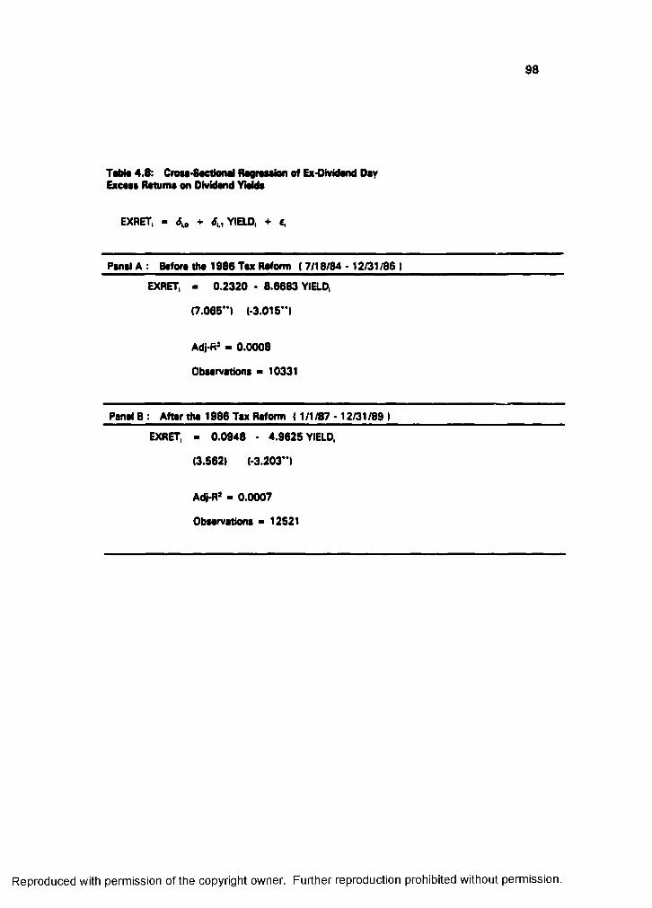
98

T#W# 4.8: Crou-SaetioiMl ftosrtsaion of Ex*Oivid«nd Day Exeoss Ratuma on Dividand Yialda

EXRET, - dto + YIELD, + (

Panal A : Bafora tho 1986 Tax Raform ( 7/18/84 . 12/31/861

EXRET, - 0.2320 • 8.6683 YIELD,

(7.085"! (-3.015")

Adi-R: - 0.0008

Obaarvationa » 10331

Panal 8 : Aftar tha 1886 Tax Raform ( 1/1/87- 12/31 /88 I

EXRET, - 0.0848 • 4.8625 YIELD,

(3.562! (-3.203"!

Adj-R* - 0.0007

Obaarvationa - 12521


99

4. Portfolio Tost RosuNs

This section reports the main results of this study. The aim of this section is to

investigate the relationships between the ex-dividend retum behavior and the ex-post

portfolio choice around the ex-dividend day in the context of the 1984 and 1986 tax

reforms. Previous studies [see, e.g., Lakonishok and Vermaelen (1986) and Fedenia and

Grammatikos (1990)1 which advance or support the short-term trading hypothesis seem

to have followed a model of trading volume behavior, rather than an equilibrium model

with appropriate measure of risk and return. Thus, the portfolio approach is taken in this

section.

Following Long's (1977) argument, it is expected that the Tax Reform Acts of

1984 and 1986 have effects on the risk-expected retum trade-off of investors, which

wiil be reflected in the portfolio choices around the ex-dividend day. To show possible

changes in the risk-expected retum trade-off of investors, efficient portfolios around the

ex-dividend day are constructed, using Markowitz's (1959) portfolio selection model.

Assuming that investors take into account short-term trading activities after the

announcement of dividend payments, the windows between the dividend announcement

day and the ex-dividend day should be chosen for their portfolio selection." In order

to examine the effects of the 1984 Tax Reform Act, which increased minimum holding

period from 16 days to 46 days, it would be reasonable to consider the windows from

-25 to 2 days and from +2 to +25 days relative to the ex-dividend day." To this

aim, securities are omitted whose ex-dividend dates are 25 or fewer trading days apart

l*Thia can alao iaolata potential bias due to the proximity of the announcement day and the ex-dividend day [see Bades, Hess and Kim (1984)).

^^To test for the sensitivity, these procedures can be repeated on different windows. However, these efforts may be restricted by the inefficiencies of the extant portfolio selection algorithms in dealing with sparse matrices. Nevertheless, we repeated the window of 10 days, which yielded consistent results with our conclusion reported in this study.


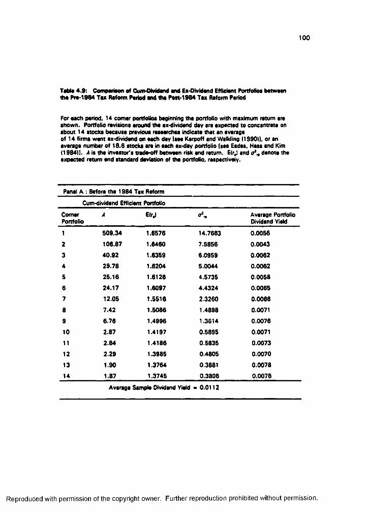
100

Tabic 4.9: Comparison of Cum Dividand and Ex-Oividand Efficient Portfoiioa batwaan lha Pra 1984 Tax Raform Pariod and tha Pott-1984 Tax Raform Pariod

For aach pariod, 14 comar portfoiioa baginning tha portfolio with maximum ratum ara shown. Portfolio revisions around tha ax-dividand day ara axpactad to concantrate on about 14 stocks bacausa pravious rasaarchaa indicate that an avaraga of 14 firms want ax-dividand on aach day Isaa Karpoff and Walkling i1990)1, or an avaraga number of 18.6 stocks arc in aach ax-day portfolio isaa Eadas, Hess and Kim (1984)1. 4 is tha investor's trada-off batwaan risk and ratum. E(r,| and o ', denote tha axpactad ratum and standard daviation of tha portfolio, raspactivaly.

Panal A ;: Bafora tha 1984 Tax Raform

Cum-dividand Efficient Portfolio

ComarPortfolio

À E(r^ Average Portfolio Dividand Yiald

1 509.34 1.8578 14.7883 0.0058

2 108.87 1.8480 7.5858 0.0043

3 40.92 1.8359 8.0959 0.0082

4 29.78 1.8204 5.0044 0.0082

5 25.18 1.8128 4.5735 0.0058

6 24.17 1.8097 4.4324 0.0085

7 12.05 1.5518 2.3280 0.0088

8 7.42 1.5088 1.4898 0.0071

9 8.78 1.4998 1.3814 0.0078

10 2.87 1.4197 0.5895 0.0071

11 2.84 1.4188 0.5835 0.0073

12 2.29 1.3985 0.4805 0.0070

13 1.90 1.3784 0.3881 0.0078

14 1.87 1.3745 0.3808 0.0078

Avaraga Sampla Dividand Yield - 0.0112


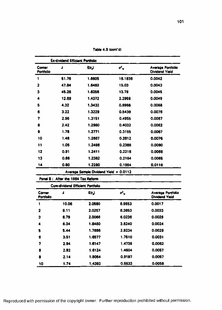
101

Tabla 4.9 (corn'd)

Ex*dividand Efliciant Portfolio

ComarPortfolio

À EIrp Avaraga Portfolio Dividand Yield

1 51.76 1.6605 16.1636 0.0042

2 47.84 1.6469 15.03 0.0043

3 45.26 1.6356 13.79 0.0045

4 12.69 1.4372 2.2959 0.0049

5 4.32 1.3432 0.6966 0.0066

6 3.22 1.3229 0.5436 0.0076

7 2.96 1.3151 0.4955 0.0067

8 2.42 1.2960 0.4032 0.0062

9 1.76 1.2771 0.3155 0.0067

10 1.46 1.2667 0.2612 0.0076

11 1.05 1.2496 0.2366 0.0060

12 0.91 1.2411 0.2216 0.0066

13 0.66 1.2362 0.2164 0.006514 0.60 1.2260 0.1994 0.0116

Avaraga Sampla Dividand Yiald - 0.0112

Panal B : Aftar tfw 1964 Tax Raform

Cum-dividand Efficiant Portfolio

ComarPortfolio

À Elr.) Avaraga Portfolio Dividand Yield

1 10.06 2.0560 6.9653 0.0017

2 9.11 2.0257 6.3653 0.0033

3 6.79 2.0066 6.0236 0.0029

4 6.34 1.6460 3.6240 0.0024

5 5.44 1.7666 2.9234 0.0029

6 3.51 1.6577 1.7510 0.0031

7 2.94 1.6147 1.4739 0.0062

a 2.92 1.6124 1.4604 0.0057

9 2.14 1.5054 0.9197 0.0057

10 1.74 1.4392 0.6633 0.0056


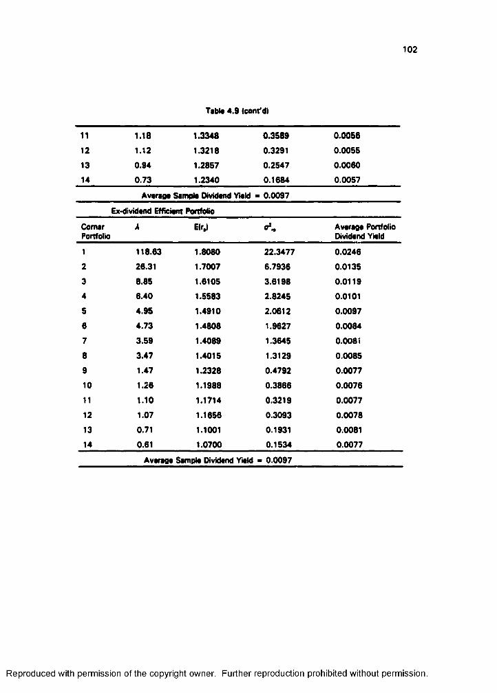
102

Tabla 4.9 (cant'd)

11 1.18 1J348 0.3589 0.0056

12 1.12 1.3218 0.3291 0.0055

13 0.94 1.2857 0.2547 0.0060

14 0.73 1.2340 0.1684 0.0057


Ex-dividand Efficiant Portfdie

ComarPortfolio

À Elr.) a*-. Avaraga Portfolio Dividand Yiald

1 118.63 1.8080 22.3477 0.0246

2 26.31 1.7007 6.7936 0.0135

3 8.85 1.6105 3.6198 0.01194 6.40 1.5583 2.8245 0.0101

5 4.95 1.4910 2.0612 0.0097

6 4.73 1.4808 1.9627 0.0084

7 3.59 1.4089 1.3645 0.0081

8 3.47 1.4015 1.3129 0.0085

9 1.47 1.2328 0.4792 0.0077

10 1.26 1.1988 0.3866 0.0076

11 1.10 1.1714 0.3219 0.0077

12 1.07 1.1656 0.3093 0.0078

13 0.71 1.1001 0.1931 0.008114 0.61 1.0700 0.1534 0.0077



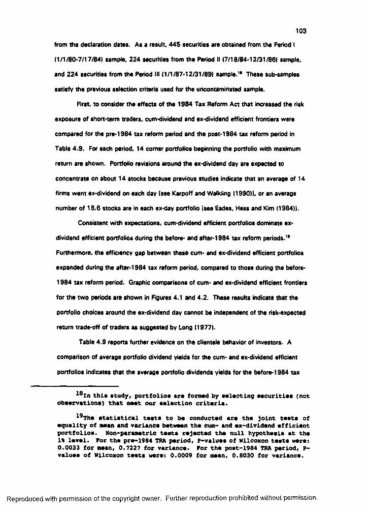
103

from the declaration dates. As a result, 445 securities are obtained from the Period I

(1/1/80-7/17/84) sample, 224 securities from the Period II (7/18/84-12/31/86) sample,

and 224 securities from the Period III (1/1/87-12/31/89) sample.'* These sub-samples

satisfy the previous selection criteria used for the uncontaminated sample.

Rrst, to consider the effects of the 1984 Tax Reform Act that increased the risk

exposure of short-term traders, cum-dividend and ex-dividend efficient frontiers were

compared for the pre-1984 tax reform period and the post-1984 tax reform period in

Table 4.9. For each period, 14 corner portfolios beginning the portfolio with maximum

return are shown. Portfolio revisions around the ex-dividend day are expected to

concentrate on about 14 stocks because previous studies indicate that an average of 14

firms went ex-dividend on each day [see Karpoff and Walkling (1990)1, or an average

number of 18.6 stocks are in each ex-day portfolio (see Eades, Hess and Kim (1984)1.

Consistent with expectations, cum-dividend efficient portfolios dominate ex-

dividend efficient portfolios during the before- and after-1984 tax reform periods.'*

Furthermore, the efficiency gap between these cum- and ex-dividend efficient portfolios

expanded during the after-1984 tax reform period, compared to those during the before-

1984 tax reform period. Graphic comparisons of cum- and ex-dividend efficient frontiers

for the two periods are shown in Rgures 4.1 and 4.2. These results indicate that the

portfolio choices around the ex-dividend day cannot be independent of the risk-expected

retum trade-off of traders as suggested by Long (1977).

Table 4.9 reports further evidence on the clientele behavior of investors. A

comparison of average portfolio dividend yields for the cum- and ex-dividend efficient

portfolios indicates that the average portfolio dividends yields for the before-1984 tax

this study, portfolios ars formed by selecting securities (not observations) that meet our selection criteria.

l*The statistical tests to be conducted are the joint tests of equality of mean and variance between the cum- and ex-dividend efficient portfolios. Non-parametric tests rejected the null hypothesis at the 1% level. For the pre-1984 TRA period, P-values of Wilcoxon tests were: 0.0033 for mean, 0.7227 for variance. For the post-1984 TRA period, P- values of Wilcoxon tests were: 0.0009 for mean, 0.8030 for variance.


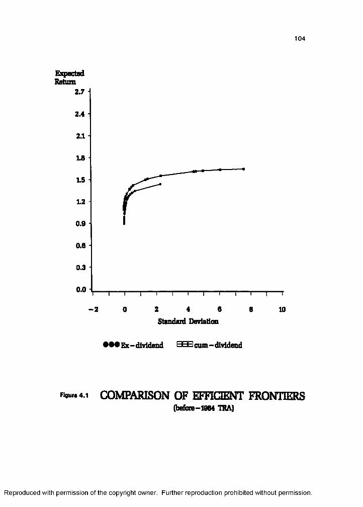
104

Ejqwcted Return

2.7

2.4

2.1

18

15 H

12

0.9

0.6

0.3

0.0 I I I I

- 2 0

T 1 r

2 4 6Standard Deviation

n I r

6 10

•••Ex-dividend BBB cum—dividend

Figura 4.1 COMPARISON OF EFFICIENT FRONTIERS(befme-1964 TRA)


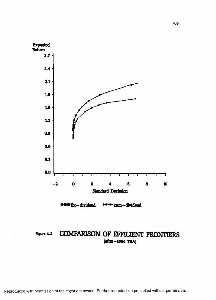
105

E)qiectedRatum

2.7

2.4

2.1

18

15

12

0.9

0.6

0.3

0.0

- 2 60 2 4 8 10Standard Deviation

# # # Ex—dividend BSS cum—dividand

Rguw4.2 COMPARISON OF EFFICIENT FRONTIERS(after-1984 TRA)


106reform period and those for the cum-dividend efficient portfolio after the 1984 tax

reform show an increasing trend as comer portfolios increase. The average portfolio

dividend yields for ex-dividend efficient portfolios after the 1984 tax reform show a

decreasing trend vis-a-vis corner portfolios. An interpretation of this result is as follows.

If tax-induced short-term trading occurs, investors are likely to have more interest in the

capital loss deduction and financial cost deduction than in the dividend income tax

deduction because dividends are progressively taxed. Thus, tax-induced short-term

traders are motivated to choose first the securities with lower dividend yields in their

portfolios. However, if tax-induced trading is restricted such as in the ex-dividend days

after the 1984 tax reform, there will exist only dividend capture traders who are

interested in buying and selling securities to strip dividends for purposes other than

taxes."

Next, to examine the effects of the 1986 Tax Reform Act, cum-dividend efficient

portfolios between the before-1986 tax reform period and the after-1986 tax reform

period were compared. Table 4.10 presents evidence that the after-1986 tax reform

portfolios are dominated by the before-1986 tax reform portfolios.'' This result is also

depicted in Figure 4.3. These findings are consistent with Long's prediction that, under

the new tax regime, investors are motivated to restructure their portfolio holdings to

reflect the new tax rates.

Another evidence reported in Table 4.10 is that the average portfolio dividend

yields, vis-a-vis corner portfolios, show an increasing trend during the before-1986 tax

reform period, whereas those average portfolio dividend yields display a stabilized trend

during the after-1986 tax reform period. Prior to the 1986 Tax Reform Act, long-term

traders are taxable at the unfavorable tax rates on dividends relative to capital gains.

20on# exemple is Jepsnese life insurance companies which have a preference for dividend income because of regulatory laws. These traders have incentives to buy the securities with higher dividend yields.

21p-.values of Wilcoxon tests ttere: 0.0009 for mean, 0.9S33 for variance.


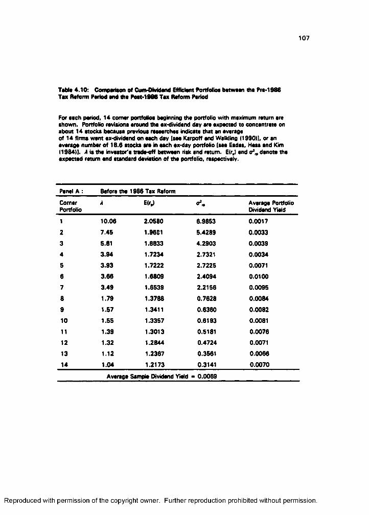
107

T#W# 4.10: Comparison of Cum4Nvidand Efficlsnt Portfolios botwssn tha Pro 1986 Tax Raform Poriod snd tha Post 1988 Tax Raform Poriod

For aach poriod, 14 comar portfolios boginninp tho portfolio with maximum rotum ara shown. Portfolio ravisions around tho ox-dividond day sro oxpoctod to concantrate on about 14 stocks bacausa pravious rasaarchaa indicsto that an avorago of 14 firms wont ox*dividond on aach day (sao Karpoff and Walkling (1990)1, or an avaraga numbar of 18.6 stocks ara in aach ax-day portfolio Isaa Eadas, Haas and Kim(1984)1. 4 ia tha invaator'a trada-off batwaan risk and ratum. Eir,) and o ', danote tha axpactad ratum and atandard daviation of tha portfolio, raspactivaly.

Panel A : 8afore tha 1986 Tax Raform

ComerPortfolio

À Eir o*. Avaraga Portfolio Dividand Yiald

1 10.06 2.0580 6.9853 0.0017

2 7.45 1.96S1 5.4289 0.0033

3 5.81 1.8833 4.2903 0.00394 3.94 1.7234 2.7321 0.0034

5 3.93 1.7222 2.7225 0.0071

6 3.66 1.6809 2.4094 0.0100

7 3.49 1.6539 2.2156 0.0095

8 1.79 1.3788 0.7628 0.0084

9 1.57 1.3411 0.6360 0.0082

10 1.55 1.3357 0.6193 0.0081

11 1.39 1.3013 0.5181 0.0076

12 1.32 1.2844 0.4724 0.0071

13 1.12 1.2367 0.3561 0.0066

14 1.04 1.2173 0.3141 0.0070



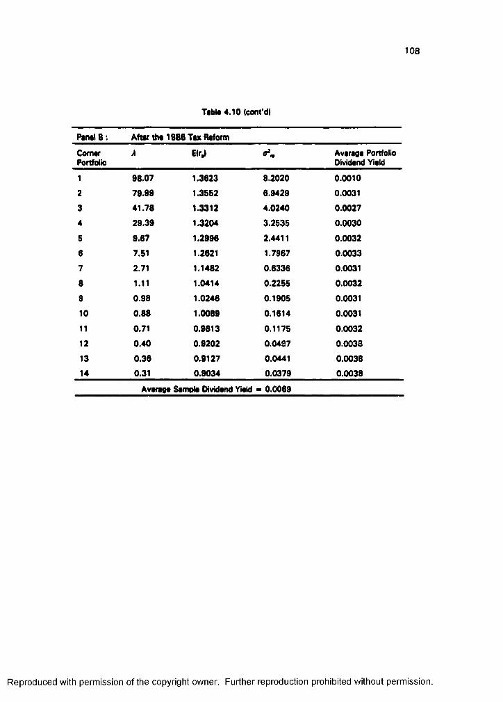
108

Tabto 4.10 (corn'd)

Pant) B ; Aftar tha 1986 Tax Raform

ComarPortfolio

À E(r Avaraga Portfolio Dividand Yiald

1 98.07 1.3623 8.2020 0.0010

2 79.99 1.3552 6.9429 0.0031

3 41.78 1.3312 4.0240 0.0027

4 29.39 1.3204 3.2535 0.0030

5 9.67 1.2996 2.4411 0.0032

6 7.51 1.2621 1.7967 0.0033

7 2.71 1.1482 0.6336 0.0031

8 1.11 1.0414 0.2255 0.0032

9 0.98 1.0246 0.1905 0.0031

10 0.88 1.0089 0.1614 0.0031

11 0.71 0.9813 0.1175 0.0032

12 0.40 0.9202 0.04S7 0.0038

13 0.36 0.9127 0.0441 0.003814 0.31 0.9034 0.0379 0.0038



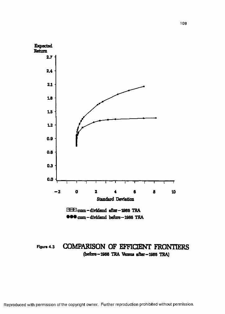
109

ExpectedRetajzn

2.7

2.4

2.1

18

15

12 i

0.9

0.6

0.3

0.0I I I I I I I I I “ I 1 I I

-2 0 2 4 6 8 10Standard Deviation

BBB cum-dividend after-1986 TRA 1 cum-dividend befiote-1988 THA

Raure4.3 œMPARISON OF EFFICIENT FRONTIERS(befare-1986 TRA \%nua after-1986 TRA)


110Thus, during the before-1986 tax reform period, dividend clientele effects would be in

effect, and it is expected that the negative correlations between dividend yields and

excess returns will be observed during the same period.

After the 1986 tax reform, since investors are taxed at the same rates on

dividends and capital gains, the clientele incentives of long-term traders are predicted to

be reduced. Average portfolio dividend yields are expected to maintain a stable trend

regardless of the expected return during the post-1986 tax reform period. These

evidences are consistent with the expectations of the dividend clientele hypothesis. As

shown in Table 4.10, the average portfolio dividend yields show a negative correlation

with the expected portfolio return during the before-1986 tax reform period, but the

dividend yields seem to have remained at a stable level during the after-1986 tax reform

period.


This essay has investigated the portfolio choice around the ex-dividend day in

the context of the 1984 and 1986 tax tax reforms. The fundamental idea has been to

show that the ex-dividend value of stock and short-term trading behavior around ex-

dividend day reflect the trade-off of risk and expected return. The 1984 Tax Reform Act

increased the risk exposure of tax-induced short-term traders by extending the minimum

holding period for the dividend income tax deduction. The 1986 Tax Reform Act

decreased the dividend tax rate from a maximum rate of 50% to 28%, leading to the

equalization of the tax rates on dividends and capital gains. By comparing the efficient

portfolio frontiers between the pre-tax reform period and the post-tax reform period, an

attempt was made to report changes in the risk-expected retum trade-off around the ex-

dividend day. These portfolio results was related to the excess retum behaviors on

which the 1984 and 1986 Tax Reform Acts are also documented to have had effects.

First, the effects of the 1984 and 1986 Tax Reform Acts on the retum behaviors

around the ex-dividend day were documented. Numerous studies have evidenced the


I l l

tax-effect hypothesis and the short-term trading hypothesis. But, although these tax

reforms provide a valuable laboratory to test the extant hypotheses, researches on the

ex-dividend day effects of the 1984 and 1986 Tax Reform Acts are very few (see

Grammatikos (1989), Michaely (1991), and Robin (1991)], and ihei, evidences are

mixed. The findings in this essay are consistent with both the tax-effect hypothesis and

the short-term trading hypothesis, and they are summarized as follows:

(1) Prior to the 1986 tax reform, significant positive excess returns were observed on the ex-dividend day.

(2) During the post-1986 tax reform period, average ex-dividend excess returns were not different from zero at the 1 % significance level.

(3) There existed the negative correlationships between the dividends yields and ex-dividend day excess retums, which correlationships decreased from the pre-1986 tax reform period to the post-1986 tax reform period.

(4) Average ex-dividend day excess returns increased significantly during the post-1984 tax reform period compared to the pre-1984 tax reform period.

(5) During the post-1984 tax reform period, more significant excess returns were observed for 11 trading days before and after the ex-dividend day compared to the pre-1984 tax reform period.

The second approach is quite different from the extant researches, and more

insightful and consistent conclusions were obtained. The cum- and ex-dividend efficient

portfolios between the pre-1984 tax reform period and the post-1984 tax reform period

were compared. The following evidences to support the short-term trading hypothesis

were found.

(6) Cum-dividend efficient portfolios dominate ex-dividend efficient portfolios.(7) The efficiency gap between cum-dividend efficient frontiers and ex-dividend

efficient frontiers has expanded more during the post-1984 tax reform period than during the pre-1984 tax reform period.

Following Long's (1977) argument, it was predicted that the 1986 Tax Reform Act

would decrease the expected after-tax return ar the new tax rates and increase the

after-tax variance of the portfolio. Consistent with this expectation, it was found that

(8) The efficient portfolio frontier during the post-1986 period was dominated by the efficient portfolio frontier during the pre-1986 tax reform period.

This result may be interpreted as a tax effect since the tax premiums decrease with an

decrease in dividend tax rate. But, the variance as risk factor was not considered in the

tax-effect hypothesis.


112To conclude, the evidence of excess return behaviors supports the existence of

both tax effects and short-term trading around the ex-dividend day. These tax effects

and short-term trading are not mutually exclusive, but co-existent as long as short-term

trading is tax-induced. They interact to have an impact on the ex-dividend return and

volume behaviors. This finding was effectively supported by portfolio test results. The

portfolio approach is quite advantageous over the extant approaches, because this

approach incorporates the tax effect as well as the short-term trading. The portfolio

approach also seems to be useful in explaining dividend capture tradings by Japanese

life insurance companies that are not tax-induced.

It can be emphasized that the ex-dividend behavior cannot be understood

independently of the risk-expected return trade-off. Also, it is proposed that this

portfolio approach can be best used in many branches of corporate finance ( for

example, turn of-the-year effect ) where portfolio revisions are considered to occur.


Chapter 5. EMPIRICAL TESTS OF DIVIDEND SIGNALLING

A. Introduction

With the publication of Bhattacharya’s (1979) paper, the notion of imparting

information to shareholders with dividends (commonly referred to as dividend signalling)

has attracted considerable attention among financial economists. Miller and Rock

(1985), John and Williams (1985), Ambarlsh, John and Williams (1987), Ofer and

Thakor (1987), and Williams (1988) develop formal models of dividend signalling. These

models, in general, derive their logic from the seminal papers of Spence (1973, 1974)

and Riley (1979). Miller's (1987) suggestion of the stringency conditions necessary for

a sustainable dividend signalling equilibrium notwithstanding, signalling still appears to be

one of the most catching theories explaining the enigma of dividend policy.

The need and opportunity for dividend signalling arise when corporate agents

know more about the quality of the enterprise than outsiders do. Outside investors

cannot differentiate the quality of projects undertaken by the firm, because they lack

perfect information. They value and buy the firm's stock at the price that corresponds

to only the average quality of projects. Agents (insiders) are the only ones who know

the true prospects facing their firms and attempt to optimize the objective function of

shareholders. Thus, they have an incentive to avoid the adverse selection problem by

informing the market of their firms' excellence. They can signal high cash flows of the

firm by paying higher dividends. If this signal is correctly received in the market, the

shares of the firm will command a higher price, benefiting the firm and its shareholders.

The intention of this essay is to test empirically the John and Williams' (1985)

(JW) signalling equilibrium model. This test is conducted in order to provide statistical

evidence of the empirical validity of this model. The reason for selecting this model is

twofold. First, the authors argue that their model is empirically testable and provide

guidelines for such testing. Second, this model is a reasonable representation, given its

113


114

assumption, of the class of models dealing with the so-called signalling equilibrium.

There are no reports of large-scale empirical validation of this model.

The JW model implies that, in equilibrium, corporate insiders with superior

information about future cash inflows have incentives to signal by distributing larger

dividends "... if and only if the demand for cash by both their firm for investment and

their stockholders for liquidity exceeds the internal supply of corporate cash" (John and

Williams (1985). p. 1055]. The signal of larger dividends results in raising the stock

price and consequently benefiting the firm or current shareholders when selling the

stock. The JW model attempts to explain why many firms prefer paying dissipative'

dividends to repurchasing shares, while others simultaneously pay dividends and float

new shares. It is argued that the payment of dividends is induced by clienteles of

stockholders who demand current cash. Their model also shows the explicit relationship

among the announcement effect, dividends and eu/n-dividend market values.

The intrinsic weakness of signalling models is the difficulty in testing empirically

their theoretical implications. JW assert that their signalling model is testable, because

the cross-sectional impact of dividends is a simple function of observable variables. In

the remainder of this chapter, the task of empirical testing is undertaken. Section B

contains a more detailed discussion and review of the JW model. In Section C. the

methodology is explained. Section D describes the data and the proxy variables.

Section E presents tests, results, and their interpretation. Section F is a summary,

including some guidelines for future research.

^The term "dissipative" originates from electrical engineering and it means wasteful. In this context, the meaning is that shareholders are required to bear the cost of this signal via their tax liability for the dividend payments.


115

B. Th# John and WBliams Modal

1. Nênativ»

JW develop a signalling equilibrium with dividends and single dissipative costs

(i.e., a proportional tax on dividends). In this model, capital gains are not taxable, and

issuing, retiring, and trading shares are costless. According to their arguments, if the

liquidity demand by the firm and its current shareholders exceeds internally generated

funds, corporate insiders are motivated to distribute a taxable cash dividend and to

reveal to outside investors the present value of their firm's future cash inflows. This

signal would result in raising the stock price to the benefit of current stockholders.

JW attempt to explain why some firms do not pay dividends, whereas others do

and simultaneously sell new shares to investors. In order to finance investments, a firm

must either issue new shares or retire fewer outstanding shares. Similarly, to collect

cash for personal use, current stockholders must sell their shares. In either case,

stockholders have to suffer some dilution in their fractional ownership of the firm.

Current shareholders desire to reduce this dilution on corporate or personal accounts.

Hence, insiders, in the best interest of current stockholders, are inclined to convey

favorable information by paying a taxable dividend. Recognizing the relationship

between favorable information and the value of the shares, the market bids up the stock

price, mitigating stockholders' dilution.

The JW signalling equilibrium is achieved because the marginal gain from paying

dividends is balanced against the marginal cost incurred by the tax on dividends. In the

market, stocks with marginally larger dividends are rewarded with a premium,

compensating current shareholders for the dissipative effect of their marginal income

tax. For firms paying marginally smaller dividends, the dead weight cost of dividends

outstrips the marginal benefit of reducing ownership dilution. In the JW model, an

optimal signalling equilibrium is reached when firms with favorable inside information

distribute higher dividends than firms without favorable information.


116

2. Tntêblu Analytkêl Modêl

The JW formulation of the problem is anchored in the idea that "... other things

equal, firms which pay dividends have clienteles of stockholders who demand current

cash-such as widows, senior citizens, and financial institutions" {ibid., p. 1065). This

concept is expressed mathematically, as a signalling equilibrium. In their Equation 13.'

Accordingly,

D{X) ~ ' l M a x { I - C * L . 0 ) ' L a ( X ) ] fOT X i L. (5.1)t

where D(X) is the optimal dividend at equilibrium;t is the constant, marginal personal tax rate on the dividend;I is investment;C is corporate cash available;L is the liquidity need of the shareholders; andX is the present value of the future cash inflow.

Equation (5.1) implies the equilibrium condition. At equilibrium, the dividend increases

proportionally to the logarithm of the stock's present value, a property common to

many other dividend models. Equation (5.1) also shows that dividends decrease in t and

C and increase in L. The key element of this model is that the firm has exogenous

demand for liquidity by its shareholders. The demand for cash is the catalyst to signal

via dividends. This, in turn, implies that the boundary condition for insiders to pay

dividends is

C g I + L;

that is, the demand for cash from the firm is non negative.

HYPOTHESIS #1 : Demand for liquidity causes dividend payments.

^The models in this section build on John and Williams (1985) to posit JW'e model correctly for this testing.

^The mathsmatical proof of JW's models is presented in Appendix C of this dissertation.


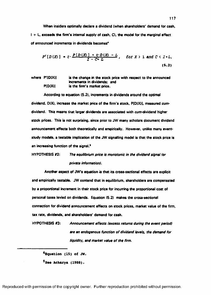
117

When insiders optimally declare a dividend (when shareholders' demand for cash,

I + L, exceeds the firm's internal supply of cash. Cl, the model for the marginal effect

of announced increments in dividends becomes*

P'[D{X)] . g. - L for X > 1 and C < I*L,

(5.2)

where P'(D(X)] is the change in the stock price with respect to the announcedincrements in dividends; and

P[D(X|] is the firm's market price.

According to equation (5.2), increments in dividends around the optimal

dividend, D(X), increase the market price of the firm's stock, P(D(X)1, measured cum-

dividend. This means that larger dividends are associated with cum-dividend higher

stock prices. This is not surprising, since prior to JW many scholars document dividend

announcement effects both theoretically and empirically. However, unlike many event-

study models, a testable implication of the JW signalling model is that the stock price is

an increasing function of the signal.*

HYPOTHESIS #2: The equilibrium price is monotonie in the dividend signel (or

private information!.

Another aspect of JW's equation is that its cross-sectional effects are explicit

and empirically testable. JW contend that in equilibrium, shareholders are compensated

by a proportional increment in their stock price for incurring the proportional cost of

personal taxes levied on dividends. Equation (5.2) makes the cross-sectional

connection for dividend announcement effects on stock prices, market value of the firm,

tax rate, dividends, and shareholders' demand for cash.

HYPOTHESIS #3: Announcement effects (excess returns during the event period)

are an endogenous function of dividend levels, the demand for

liquidity, and market value of the firm.

Êquation (15) of JW.

^Sm Acharya (1988).


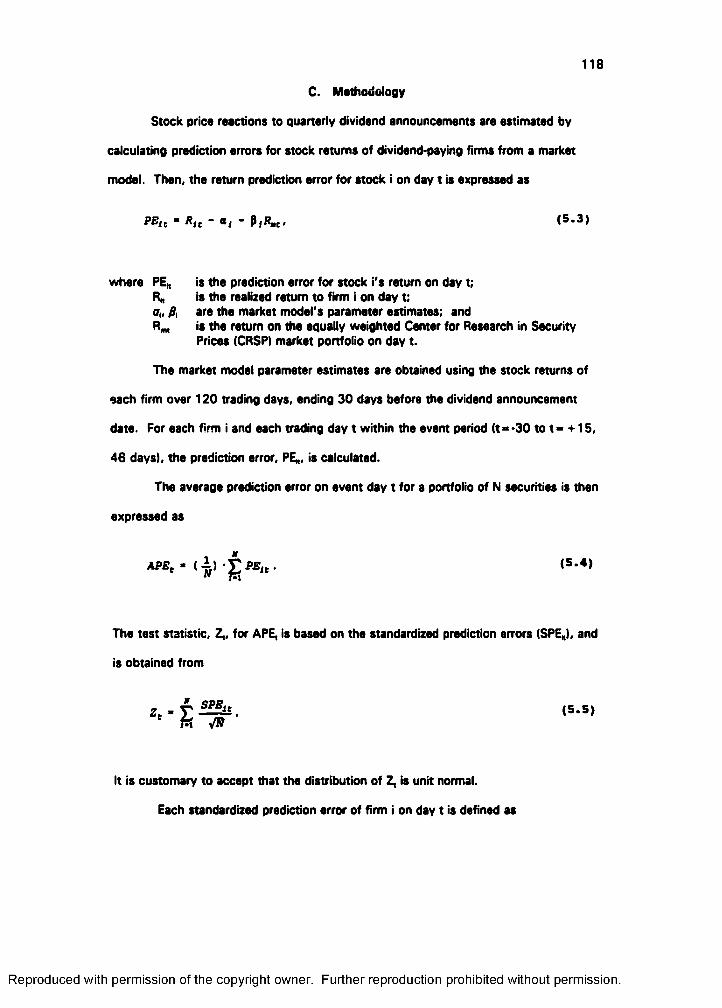
118

C. Mathodoiogy

Stock price reactions to quarterly dividend announcements are estimated by

calculating prediction errors for stock returns of dividend paying firms from a market

model. Then, the return prediction error for stock i on day t is expressed as

PEic - Rte ■ «i - (5*3)

where PE,, is the prediction error for stock i's return on day t;Rh is the realized return to firm i on day t:a„ fii are the market model's parameter estimates; andRm, is the return on the equally weighted Center for Research in Security

Prices (CRSP) market portfolio on day t.

The market model parameter estimates are obtained using the stock returns of

each firm over 120 trading days, ending 30 days before the dividend announcement

date. For each firm i and each trading day t within the event period It = 30 to t = + 15,

46 days), the prediction error, PE*, is calculated.

The average prediction error on event day t for a portfolio of N securities is then

expressed as

APB • ( 1 ) (5 4)

The test statistic, Z,, for APE, is based on the standardized prediction errors (SPE*), and

is obtained from

It is customary to accept that the distribution of Z, is unit normal.

Each standardized prediction error of firm i on day t is defined as


119

. I D -S ’ 1*SPE,,» P E u / lo ^ a * ) 1 , (5 .6 )

i j

where a, is the standard deviation of the residuals in the market modei estimationperiod:

T is the number of days in the estimation period;Rm, is the return on the market portfolio for day t;Rm is the mean return on the market portfolio over the estimation period;

andRmk is the return on the market portfolio for the k th day of the estimation

period.

The cumulative prediction error for stock i, CPE,. is obtained by summing prediction

errors over the event time,

(5-7)

while the cumulative average prediction error over the event time is calculated from

CAPE • (1) CPEi . (5.8)

The prediction error for trading volume is also estimated, using a "trade-volume”

model, similar to equation (5.31:

“ Ti ♦ «1 V e ♦ 5ie (5 .9 )

where V„ is the rate of change in the trading volume from day t * 1 to day t forfirm i. V„ > (trading volume for firm i on day t - trading volume for firmi on day t * 1 ) / trading volume for firm i on day t ■ 1 );

Vm, is the rate of change in the trading volume from day t 1 to day t for themarket. - (trading volume for the market portfolio on day t minus trading volume for the market portfolio on day t * 1 ) / trading volume for the market portfolio on day t -1 );

K„d, are trade volume model parameter estimates; andC, is the prediction error for the trading volume of stock i on day t.

In order to obtain the average prediction error, the Z-statistic and the cumulative average

prediction error, the procedure outlined for equations (5.4), (5.5), and (5.8),

respectively, is followed.

This "trade-volume" model [equation (5.9)1 is different from prior models-i.e.,

those that typically follow Beaver (1968)"in two ways. First, prior models regress each


120firm's percentage of shares traded to its shares outstanding on the percentage of total

shares traded on exchange to the market shares outstanding. These models carry an

inherent tendency of heteroscedasticity in spite of attempts by several authors (e.g.,

Pincus (1983), Richardson, Sefcik and Thompson (1986)1 to correct for this problem.

The model here is more analogous to the market model and less heteroscedastic since

each firm's trading change rate is regressed on the market trading change rate.

Second, the focus of prior models has been restricted to the abnormal trading

volume to model information effects. More important, this paper highlights the role of

normal trading volume, which has been mentioned only sparingly in prior research.

Traders in the market are generally divided into two groups; information traders and

liquidity traders. While abnormal trading volume may reflect the trading activities of

information traders, normal trading volume itself may exhibit a perpetual level of demand

of liquidity traders. The rationale for using this normal trading volume is that the level of

liquidity demand may vary with market conditions, but it is independent of any

information motivated trading.

D. Data and Proxy Variables

Firms traded on either the New York Stock Exchange (NYSE) or the American

Stock Exchange (AMEX) are selected to form a primary data base. In order to be

included in the primary selection, firms must appear in both the CRSP Daily Returns,

1991 Files and the Quarterly Industrial COMPUSTAT, 1991 File. For selection, stocks

must also have consecutive data for 1986 through 1990. The study period is limited to

20 quarters, commencing from the first quarter of 1986. The constraint on the starting

quarter is due to the availability of daily trading volume data on the CRSP tape.* This

database is called the "initial sample."

^Trading volume data on stocks appear in the CRSP file only after January 1986.


121For a firm to be included in the final aample, quarterly dividend announcement

dates must be both available and verifiable. Quarterly dividend announcement dates are

identified from the declaration dates of quarterly dividend payments on the CRSP tape

by assuming that these events are known to investors on the next business day through

public media. Other sources of announcement dates are the Wall Street Journal Index

and Moody's Annual Dividend Record. All stocks for which these dates cannot be

ascertained are excluded from the final sample. Stocks that report stock splits and

stock dividends are also eliminated from consideration.

For each quarter, the sample data are grouped according to the direction of

changes in dividend per share from the previous quarter to the current quarter. The vast

majority of the data are for firms whose dividends are unchanged from quarter to

quarter. Consequently, the final sample consists of firms that increase dividend per

share, decrease dividend per share, and do not change dividend per share on a quarter-

to-quarter basis. Table 5.1 presents the quarterly frequencies for each category, for

both the initial and the final samples, by year.

The cardinal problem of testing models such as (5.1) and (5.2) is the derivation

of the theoretical variables for the purpose of empirical measurement. Even variables

that are unambiguously defined are hard to measure because of lack or inaccuracy of

data. Other variables are more troublesome in that they are defined only in a theoretical

sense and cannot be observed directly. Thus, empirical research has to face the

impasse of (1) resorting to the use of proxy variables, or (2) grinding to a halt. Option

(1) is followed in this study, and the uneasy task of the empirical derivation of the

theoretical variables is undertaken.

Data used in this study are obtained from the CRSP tape and the COMPUSTAT

1991 Quarterly Industrial File. Because firms use different fiscal years, those listed on

the CRSP tape are matched with those in the COMPUSTAT file, on a calendar basis.

Table 5.2 shows the names and definitions of COMPUSTAT variables and their data item


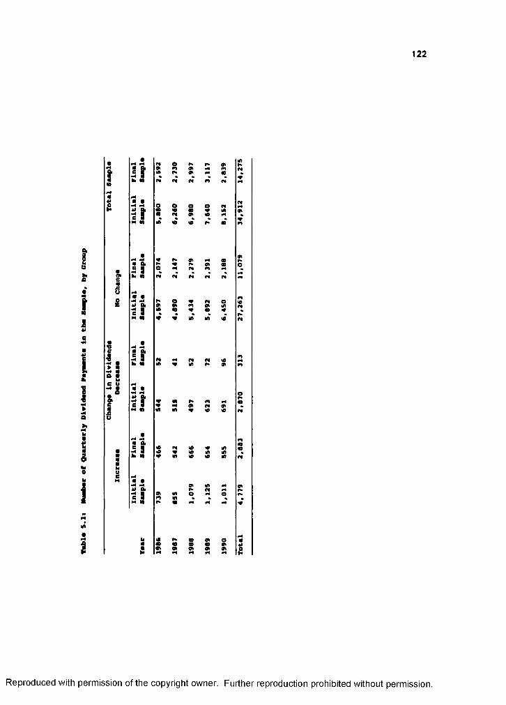
122

î

iS#

i

I!0u

i

Iui?

I l

e aM « I

IfM m

I I

III Iil

i

s»

i«

o««

s ss

CD«

Otn

S

wo«0

h» I S»


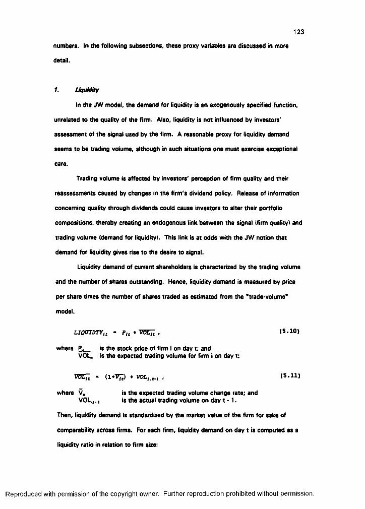
123

numbers. In the following subsections, these proxy variables are discussed in more

detail.

1. UquU itv

In the JW model, the demand for liquidity is an exogenously specified function,

unrelated to the quality of the firm. Also, liquidity is not influenced by investors'

assessment of the signal used by the firm. A reasonable proxy for liquidity demand

seems to be trading volume, although in such situations one must exercise exceptional

care.

Trading volume is affected by investors' perception of firm quality and their

reassessments caused by changes in the firm's dividend policy. Release of information

concerning quality through dividends could cause investors to alter their portfolio

compositions, thereby creating an endogenous link between the signal (firm quality) and

trading volume (demand for liquidity). This link is at odds with the JW notion that

demand for liquidity gives rise to the desire to signal.

Liquidity demand of current shareholders is characterized by the trading volume

and the number of shares outstanding. Hence, liquidity demand is measured by price

per share times the number of shares traded as estimated from the "trade volume"

model.

LIQUlDTYit - . (5.10)

where ^ is the stock price of firm i on day t; andVOL* is the expected trading volume for firm i on day t:

vsüTt ■ (i*? n ) • v o i-f.t-i. (5 .1 1 )

where V* is the expected trading volume change rate: andVOLi,,., is the actual trading volume on day t 1.

Then, liquidity demand is standardized by the market value of the firm for sake of

comparability across firms. For each firm, liquidity demand on day t is computed as a

liquidity ratio in relation to firm size:


- - IS C T ^

124

L IQ U ID ^ (5.12)

Finally, the unique liquidity proxy for each firm is obtained by taking the average of the

liquidity ratios for trading days t - 30 through t - 8, in order to nullify possible

informational effects. Consequently, RATIOBAR, is a proxy for a normal level of liquidity

demand the firm attempts to maintain.

RATIOBAR, . L Ig M T IO ,, ( » • « !

In order to double check the validity of this proxy, an alternative measure of

liquidity demand, the natural logarithm of the number of shares outstanding before the

dividend announcement date, is also used.

LNSHARt > iTi (SHAR^m ,) , (5.14)

where SHARESNO) is the number of shares outstanding as of t - 30.

2. Fim SU»

Arm size is measured by the natural logarithm of the firm's market value, which

is obtained by multiplying the number of common shares outstanding at t« 30 by the

average stock price for t= 30 through t= 8.

MKTVALi » SHARESNOi • 7 ]1 i (5.15)

. SHARESNOi * ^ ^ Pit■* e— 30

where P* is the stock price for firm i on day t.

3. Dhridtnd PoSey

In the JW model, the firm attempts to satisfy a certain perpetual level of liquidity

by maintaining its level of dividends. The firm's dividend policy is measured by its


125

dividend yield before the dividend announcement. The dividend yield for firm i is

estimated as the dividend per share divided by its average stock price.

DIVYIELDi - (5.16)

where DjVIPSHA, is the dividend per share for firm i; andPRC, is the average stock price for t « 30 through t= 8.

Larger changes in dividends are construed as stronger signals and are expected

to draw larger price reactions, ceteris peribus. To control for the actual magnitude of

the dividend change, the difference between the current and previous dividend yields is

considered.

DIVYDIFF, • DIVYIELDi^t - DIVYIELD,,^.^ , (5.17)

where Dl WIELD,,, is the dividend yield for the current quarter; andDl WIELD,,,., is the dividend yield for the previous quarter.

DIWDIFF represents the dividend signal corporate agents use to signal the firm's quality

to the market.

4. Aeeountihg Veriebles

Accounting data are collected from the quarterly COMPUSTAT tape. They

include increases in investment (INVEST), long-term debt issued (DEBTISSU), long-term

debt retired (DEBTRETI), sale of common and preferred stock (EQUSELL), purchase of

common and preferred stock (EOUBUY), cash dividend (DIVIDEND), cash and cash

equivalents (CASH), and increase in short-term working capital (WORKCAP).'

The demand for cash by the firm, if measured by net investment, may ignore

demands for cash for other purposes. Other reasons for cash needs may include

repayment of debt, repurchase of shares, and increases in short-term working capital

needs. As a result, the level of investment may vary, cross-sectionally. To control for

^Definitions of COMPOSTAT data are presented in Table 5.2.


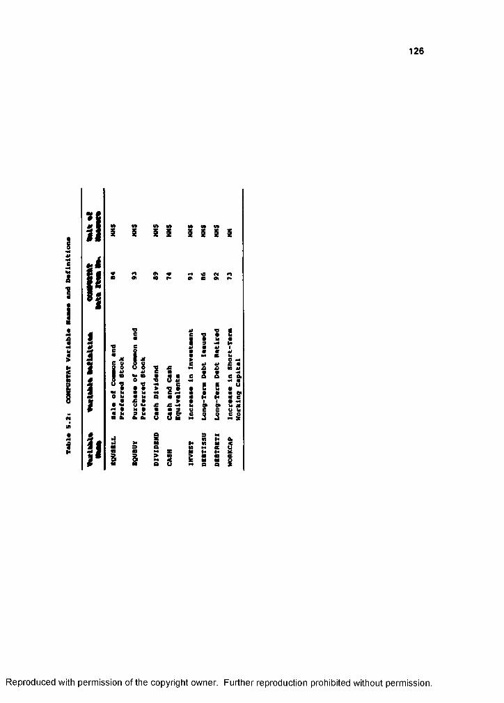
126

ae

I

I'i

1I

I'

Î i S S i S S

S

5

I I 1 1 I

! g

E E?? ?

5 3 a

?

I 2

if; 5


127

the cross-sectional effect of external financing, an approach of grouping firms by

external financial needs is taken.

The cross-sectionally observable model of the theoretical equilibrium condition of

Equation (5.1) is then

DEHANDi • mVEST, * LIOUIDTY, - CASH,, i»l N. (5.18)

where DEMAND, is the demand for cash from firm i;INVEST, is the increase in investments in firm i;CASH, is the cash and cash equivalents of firm i; andLIQUIDTY, is the liquidity demand of current shareholders.

E. Testing

1. Sêmplê StsH$Hes

Table 5.3 presents quarterly summary statistics of the variables included in the

tests. The contrast of the quarterly statistics for dividend-increasing and dividend-

decreasing firms suggests several interesting differences.

First, a simple one-way analysis of variance for the variables in the table

indicates that the dividend-increasing and dividend-decreasing groups are different at the

0.01 level for stock repurchase.' This is a fascinating observation in and of itself. It

suggests that the amounts dissipated by firms that show a propensity to increase

dividends is in fact larger than the amount of dividends paid. This is so since the

repurchase, de facto, amounts to a selective dividend disbursement scheme.

Second, at the 0.01 level of significance, the null hypothesis of the ANOVA (no

difference between the two groups) is also rejected for the market value of the firm.

This difference may suggest that larger firms are more willing (or perhaps better

expected) to pay dividends.

Finally, at the 0.01 level, there are significant differences in dividend yields for

dividend-increasing, dividend-decreasing, and dividend-unchanging firms. However, no

significant differences in total dividend payments are found, although net stock

ie speculated that this difference is due to the influence of the repurchase component.


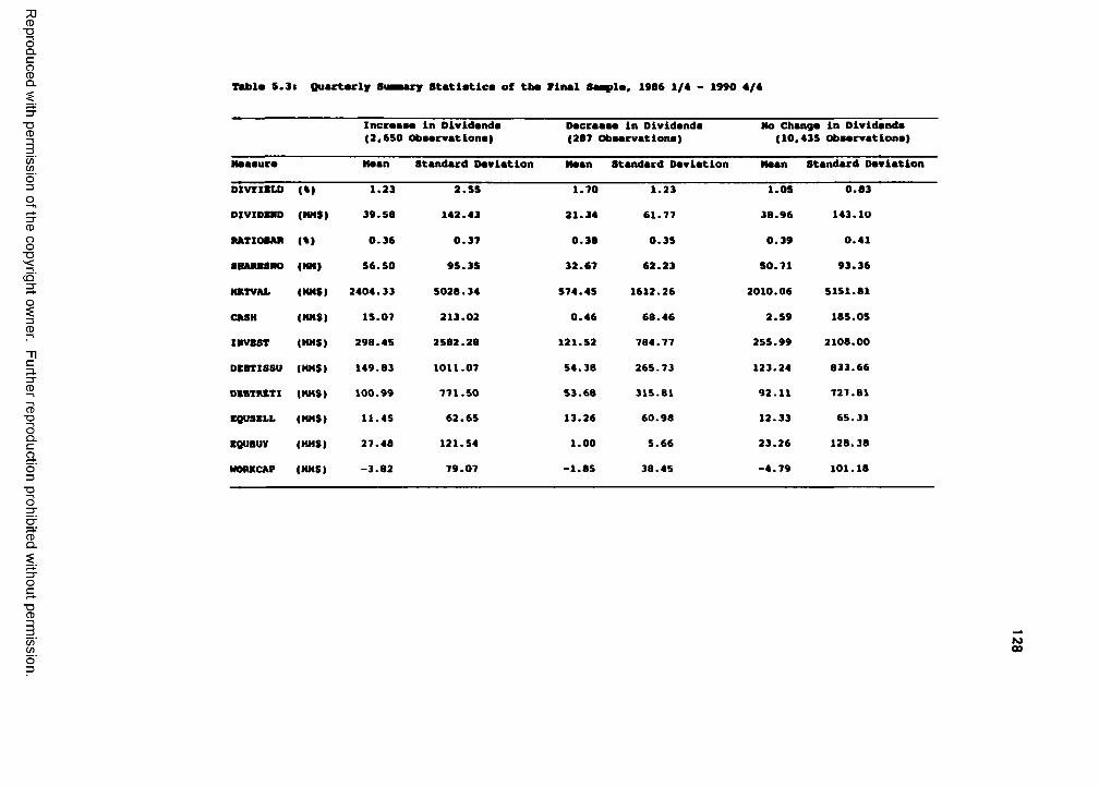
CD■DOQ.C

gQ . Tmbl# S.3i Quarterly SuBary Statistica of tba Pimal Saapla, 1986 1/4 - 1990 4/4

■DCD

C/)Wo"303CD

8■D(O '3"

13CD

"nc3.3"CD

CD■DOQ .C

aO3

■DO

Incraasa in Dividend# (3,650 Obaarvationa)

Oacraaaa in Oividanda (287 Obaarvationa)

Mo Change in Oividanda (10,435 Obaarvationa)

Naan Standard Oaviation Maan Standard Oaviation Maan Standard Oaviation

OIWIILO (») 1.23 2.55 1.70 1.23 1.05 0.83

DIVIOBNO 39. SB 142.43 31.34 61.77 38.96 143.10

MTIOUK («> 0.36 0.37 0.38 0.35 0.39 0.41

•HAMS NO |MM) 56.50 95.35 32.67 62.23 50.71 93.36

NKTVAL (HHS) 2404.33 502B.34 574.45 1612.26 2010.06 5151.81

CASH (HMS) 15.07 213.02 0.46 68.46 2.59 185.05

INVEST (HHS) 29B.45 25B2.2B 121.52 784.77 255.99 2108.00

DEBTISSU (HHS) 149.B3 1011.07 54.38 265.73 123.24 833.66

DEBTBETI (HHS) 100.99 771.50 53.68 315.81 92.11 727.81

EQUSELL (HHS) 11.45 62.65 13.26 60.98 12.33 65.31

EQUBUy (HHS) 27.48 121.54 1.00 5.66 23.26 128.38

MORKCAP (HHS) -3.B2 79.07 -1.85 38.45 -4.79 101.18

CDQ .

■DCD

(/)(/)ro00

129

repurchases are significantly greater for dividend paying firms. Since the bulk of the

data is post-1986, this cannot be attributable to a tendency to reduce shareholders' tax

liability.

Table 5.4 presents the Pearson correlation matrix of the proxy variables. Each

cell in the table contains the correlation coefficients of dividend-increasing, dividend-

decreasing, and dividend-unchanging firms.

The correlation coefficient of DIVYIELD with all the other variables and their level

of significance are shown in italics in the table. For dividend-increasing firms, DIVYIELD

is negatively correlated with RATIOBAR and MKTVAL at the 0.05 level. However, the

correlation with EQUSELL is positive and significant at the 0.01 level. Correlations are

not significant for CASH, INVEST, DEBTISSU, and EQUBUY.

For dividend-decreasing firms, the picture is quite different. Except for the

negative correlation with RATIOBAR (-0.251, the correlations with all other variables are

insignificant. This is consistent with the JW argument to the extent that the model

should hold for increases in dividends only.

2. HYPOTHESIS #1: Demand for UguiditY eêus»s divkfend paynMnts.

a. Information-Motivated Trading

Several studies, notably in the accounting literature, are concerned with

abnormal trading volume to explore the information content of a corporate event. Some

authors (e.g., Bamber (19B6)] acknowledge that using abnormal trading volume does not

provide a better theoretical tool to determine the information content of an event. Still,

it is believed that abnormal trading volumes are indicative of the depth of the market's

response to information, while abnormal returns reflect the breadth of such response.

Accordingly, by regressing each firm's trading volume change rate on the market trading

volume change rate, the market's reaction to the dividend announcement can be

measured.


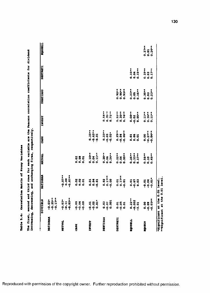
130

I0

sIIn

IlA

I

I5V

0

S88U

:

Ifi s

I!r§

a| i

i l

M îm m r*

o e oI IMOOo d oI I

Ml # O MOOO O o

I I

« « «m Ml m O M M

o d dI I I

O O Oe o oI I

m M mo M o

???

o o o d e d

o o od d d

o o od d d

M M o O #4 O

o o oI

S I i5s H i

M #4 ^ M O M

M> « Ml MOM o m M MOMGOO

«M o m m Ml o G m mO o o M G M m O M

d d d d d d d d d

s s sG O O O G G G G G

MOMGOGG G G

G M t G M O

# ««

G G o M 4» G o m o o MlG M G M M G M M m Ml Od d d d d d d d d d d d d d d

M M m G o G

G G G G G G I I I

o 2 G M G G M G oG G O G G G G G G G G G M o G G S G

9 ? d d d d d d d d d d d d d d d d

5

I I

II

iiAl

« *ilII


131

Table 5.5 exhibits the statistical properties of the trading model [equation (5.9)1.

For a 7-day window around the announcement day. the dividend-increasing firms have

two of the APE'S significant and positive at the 0.01 level.

In contrast, dividend-decreasing firms have three significant APE's, one prior to

the announcement day and two after the announcement. When one looks at the plot of

the ACPE's for the entire 46-day time horizon (Figure 5.1), it seems that just prior to the

announcement, for both types of firms, trading volume changes are mostly random. The

trading volume changes become systematic at and after the announcement day.

Dividend-increasing firms have decreasing trading volumes. Dividend-decreasing firms

also have declining trading volumes. For this subsample, all APE's are negative with the

exception of days 6, 11, and 15.

The data and Figure 5.1 indicate that, while the market correctly anticipates the

positive price effect of dividends, trading decreases for both declining and increasing

firms. The anticipation of dividend changes should have been coupled with a change in

trading around the same days. Instead, it is shown that the increase in dividends

decreases trading considerably.

For stable dividend firms, trading increases. Thus, the paradox here is that

trading decreases with a change in dividend policy and increases in the absence of

change. The ad-hoc conclusion is that a change in policy, whether it is construed as

good or bad, thwarts trading. This evidence is in complete juxtaposition to the JW

model and are perplexing as well.

The findings of stock volume responses to dividend announcements reported

here are different from the empirical studies of Harris (1986) and Richardson, Sefcik and

Thompson (1986). These two papers document a positive correlation between daily

stock volume and stock price changes. The evidence reported here, however, is

consistent with a recent study by John and Lang (1991). John and lang demonstrate

the impact of insider trading around dividend announcements, congruous with the


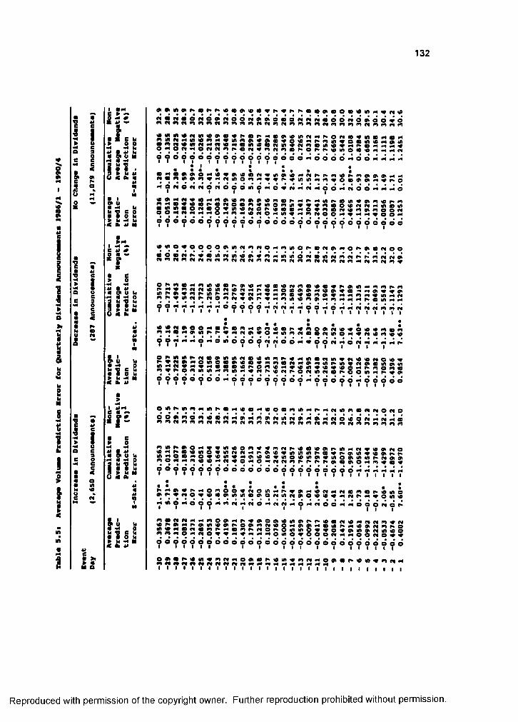
132

II

Imn

iIIIg

1lA

m!

#

1So

i -

s1

" I1oinlO

h

filll | î

lii?

SSRSSRSSSSSRRSgSSRâsâggâgSSSSga e a a w x a r i a

S:O O O O O O O O O MI I I I I I O O O O N O O N M M M

?

' omMvinmiowom«#vvr*vi m m I# p* m »# o m » m0% @1 W M M # p. O

s s s s s s g se e

Oi n OMO# N Mf 4 MO OMMOO WWw6

mm# i mo mi n v # # lONOPî oemwo#Mi oMONi mvNmwo o e o e o o o o oI I I I

ip*mm#a%miAp»mimo%ewMMinminm M i o m w m o o M» c S d o d o d o e dII II I

i A i A O # o e o o » i n M m p # O M m # n o r * * N A » N o # » » m M o o

S S S R S S S S R a S S S S R S a S R S S R S R S ^

o P» m • m £ « • p» 9t 40 #4 40 « 40 Pi m m 0 0 05 n « m n 40 n f* « O «0 04 9t 0 0m S #4 r*» # Pi M m OD « 0 m 0 44 0 Mp* n o M 04 P» m m 40 m 0 44 m P* 0 0 44 0? ? M

I 1 1M1

M1

M1 d ? dI ? 9 7 Pi1

fi1

#41 7 ? d1 44

t 9 1•Ht 7 7 Pi1 m1 mt N

lA « g 2 e S •««p» m m 04 m i m P»

«m o 0 0 0 «O :

9 fi 04 « o m m Pi 0 0 Pi 0 O 0 S 0 5 0 0? ?

#!1

M M? O m d 61 d 9 Pi

1 7 d d #4 0 9 9 Pi 441 d fi1 7 Pi

7 r»

O 5 « Ml m* 2 m 2 £ in M « 40 m m # 0 0 0 02 £ o e • 40 m # m m Pi 0 44 0 0 0 M 3g 2 V #4 m S • 40 f* O m 40 V 40 0 0 0 0 p r» m 0 0o M tfl Ml V fi p* 40 Pi p» O Pi 0 Pi 0 p» S O 0 S 0 0

? ? ? ? o ? d o ? 9 9 d 9 9 9 d d d 9 d d d 4 d d d d O

O 0 p%0 0 0 P*0 0 0 0 0 O 0 0 0 44 P» 44 0 0 0 0 0 0 O 0 Od d 0 0 d 0 0 0 2 0 0 0 0 0 0 0 0 0 0 0 44 0 O 0 O 0 4«î0 0 0 Pi 0 0 Ci 0 0 f i 0 Pi 0 Ci 0 0 0 0 0 0 0 0 0 0 0 0

2 O 0 0 0 0 O 0 0 0 0 0 P* 0 « 0 0 r* 0 0 01g 0 O 2 0 0 0 0 n 0 0 0 0 0 0 P*» 0 0 P» 0 0o 2 0 0 0 0 0 0 0 0 O 0 0 0 0 0 O 0 0 00 0 0 0 o O 0 0 P* P* P" 0 m 0 O m 0 0 0

? 9 9 9 9 d d d d d d d di 9 d

19 9 d1 9 9 9

441

441

441

M

« « # «0 44 e 0 o o 0 0 o 0 0 0 44 0 0 • m 00 o 0 0 0 0 0 0 0 0 O 0 0 0 0 o 0 0 0 0 p» 0 O 0 0

d 9 9 0 0 0 0 0 d 0 0 0 44 9 0 d d 44 d d d 0 d P*

r> a a « n n •<m M M o a a ^ a a a m w M O aI I I I I I I I .............................................I I I I I I I I I I


133

Itf>

I

6 rMtf) Or* « o mCi p A» P p Ci A» o

• • # Md d PA d PA Ci P mPA Ci d Ci Ci

1 g■

«mmmmMmmCi mmmmmmCi m

1 • 1 g b r* w mPA P A* PA p p p PA p mp r tf S 0 p in O# A»WPP mo A» P OOp p m

> s w V m m P O Pi mmPA Pp S O po § t & 0 £

m m • P mP mp A* P mmm m

e g 2Md d dd M Pi Pi PA CiCiNCiCi

1 1 g ï< 3 ►MAl

• 0 < flU« r* lAmlAp PP p P PA CiOp p

SS w

MpAmP#p P P OA» p mO p po

:M

?w M

?mdCi PA mCid d m

w •2* u # o Mp Cip p PpP Ci PA O

g g b » lA# PA p Cip p A* p PA PO o pg g P g » 2 mp mPA pP p A» m o

• g 0 b O M o e p mCiCio PA po o» w b< flb Al m

? ?e

? ?Oo

?d d

?d d

? ?o

5

2mm PA fp pp p mo p Ci A* p o p

j i d mPA p A» A» mp Pi Ci Pi P p p d5 ? m A# M CiCiCiCiCinCimCiCiCime # %# e • e1 > 0> I b » mlAOp P p p p p mp

9 ■2 # 2 0 « » «0« A» OP p p p O pu g u b A» m lAp P PA Op OP p

5 I 11

£pA

?

n7

r»7

r*7

•

P

m

p

P

7m

p

p

7p

pp

m

7p

7p

7P

7p

P

S £K at

2 4# # *• m « m» 2 PA p p p P p mCio8 M

O#APA O PA pCiOmo PA p Ci o M

& £pA7 PA

?dd PA

? Td

7 7d

7P

& 1 « 2 mp p P mp mp mp Cig w g m*a M pmPp pp Cip p p o Og b g e V * p P P p p p p p p p O

8%0 2 O V Oo p Pp p Cip p mp p p

i £ «4Al a ? ? ? ? d ?d dd ? dd d

5

6 li-L p%#AA»mmOo O A* p P o p

■ g g# • 2 d d PA d p p d p Ci d d p d p? AI 2

« A# mmmCimCimCimmmCiCiCi# e« tI # e» 9 > 0w m4 M O g p* p PA o OA» A* A»lAp

2 £ 2 r* » o mp mP P P Ci2 g 0 b tfi mV lAmP P P Omp p mI «MSi 2 « p#mmmmp P CiPmp P P p p

# g 1 s s MpA ? ? 7 7

Ci7 7

Ci7 7 7

CiCiCiCi# < fr2 e# « •

2 M2 P P P p CiPA P P mP Op P P

g f# 3« mo « P p p Ci'î P A» CiP P P

? PA ? d PA Cid d d P d PA d dd PdM '

• 1 O # o mPA p p mp O p p P pg 0 Q2 2 mP p p p p o P p p p p pg b « • o MPA p mp p Q P p o Ci

S% 0 2 pA #A OOo Ci PA p Ci PA Ci mm2 £

—4Al 6 ? ? ? ?d ? i d d? dd d d d d

I

1 S p

MÛ

&

?I?

c o dÎ2 ® 5“O f AI

AI

III"«1 e


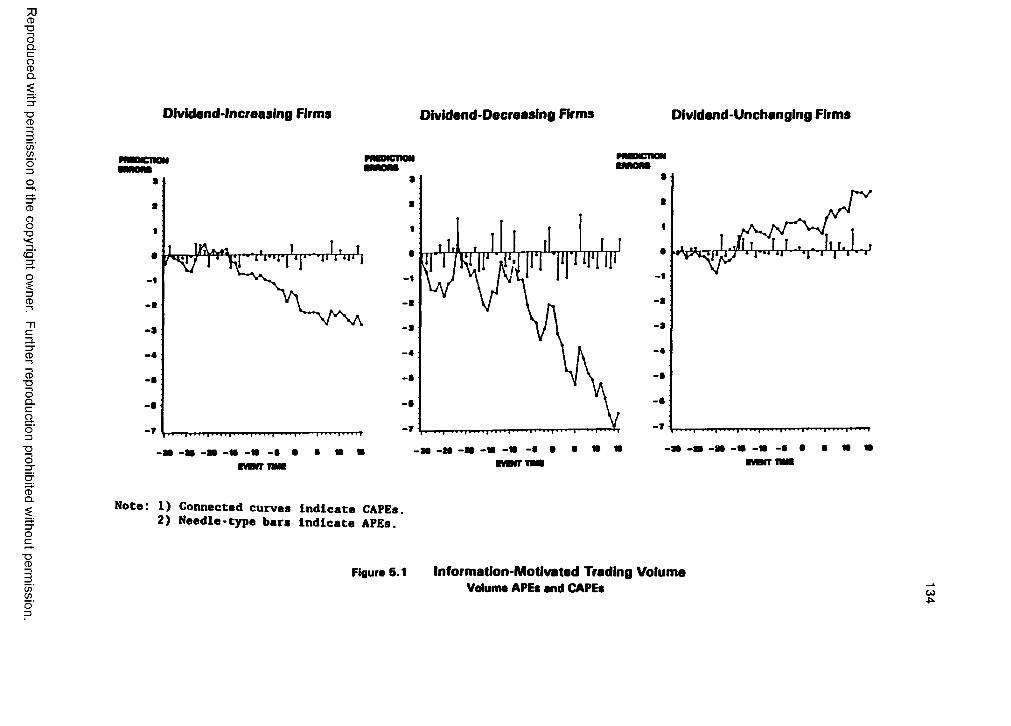
CD■DOQ.C

gQ.

"OCD

Dividend-Increasing Firms Dividend-Decreasing Firms Dividend-Unchanging Firms

C/)wo'30 3CD

8■D(O '3"

13CD

"nc3.3"CD

CD■DOQ.CaO3■DO # # # m

W

« • ■ « # «'M

CDQ. Note: 1) Connected curves indicate CAPEs. 2) Needle type bars indicate AFEs.

■DCD

(/)(/)

F ig u re 5 .1 In form ation-M otivated Trading Volum e Volume APE# and CAPEs w

135

results reported in Table 5.5 and Figure 5.1. All data considered, the verification of the

empirical validity of the JW model is still missing.

b. Liquidity Trading

The motivation of liquidity traders is different from that of information traders

Information traders enter the market with information that must have changed the

fundamental price of the stock. Liquidity traders sell their stocks because they desire

liquidity to meet consumption or savings objectives. Liquidity demand by shareholders

reflects the unique ownership structure of the firm. Consequently, it can be safely

assumed that (1) liquidity demand shows a stable or perpetual trend over time ("normal"

trading volume): (21 it is firm-unique: and (3) it does not reflect unexpected information

in the market.

"Normal" trading volume is obtained from the predicted values of model (5.9),

theoretically clear of any noise in volume created by information flows. The approach

that is taken here is to extract the "normal" level of trading as a proxy for liquidity

demand. Predicted trading volume is standardized by firm size and averaged before the

dividend announcement for each firm.

In Figure 5.2, the ratio of normal liquidity trading to the market value of the firm

around the dividend announcement day is charted. For dividend-increasing firms,

liquidity ratios maintain a stable level before the dividend announcement date, increase

slightly on the announcement day, and come back to the "normal" level thereafter.

Dividend-decreasing firms also display a rather stable liquidity ratio before the dividend

announcement date. The ratio Jumps dramatically at the announcement date, only to

regress to the normal level three days after the announcement. Dividend-unchanging

firms always maintain a normal level of liquidity, even around announcement days.

The evidence that liquidity ratios rise sharply at the dividend announcement date

for dividend-decreasing firms appears to be radically at odds with JW's argument that a

higher level of liquidity trading should occur only for dividend-increasing firms. Unlike

the JW signalling model, it is argued here that dividend policy is useo to satisfy liquidity


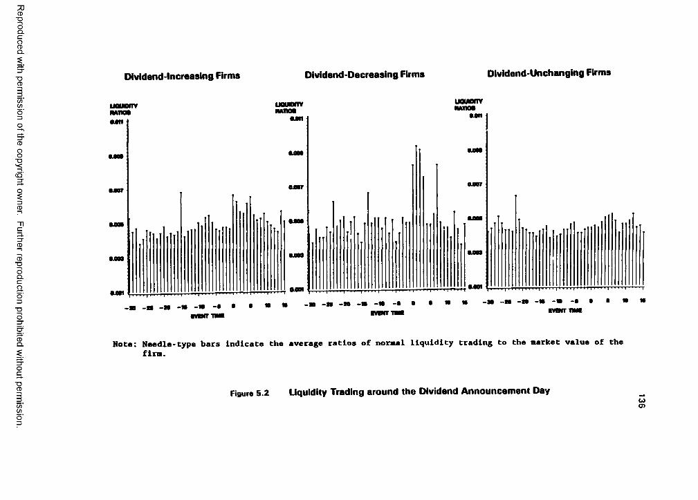
CD■DOQ .C

gQ .

■DCD

Dividend-Increasing Firms Dividend Decreasing Firms Dividend Unchanging Firms

C/)Wo'303CD

8■D(O '3"

13CD

"nc3.3"CD

CD■DOQ.Cao3

T3O

uQUonv UQunnvHMioa

< I I i I I I I I I ' I I I ' -T

•an

•OM

UM

UQunnv M •on

,, 11 ......

CDQ. Note: Needle-type bars Indicate the average ratios of normal liquidity trading to the market value of the firm.

■DCD

(/)(/)

Figure 5.2 Liquidity Trading around the Dividend Announcement Daywo>

137

demands of current shareholders. When the level of liquidity trading is low. the firm

increases dividends to satisfy the liquidity needs of shareholders. When the normal

trading level is too high, the firm decreases dividends, lowering the liquidity level of

shareholders. Consequently, shareholders faced with declining dividends increase

liquidity trading to boost their liquidity level. In the long term, a separating equilibrium

will be achieved, and a certain perpetual level of liquidity trading will be maintained as

portrayed by the case of dividend unchanging firms,

c. Regressions of Dividends on Liquidity Demends

Feldstein and Green (1983) argue that "... there is the desire on the part of small

investors, fiduciaries, and nonprofit organizations for a steady stream of dividends with

which to finance consumption" [ibid., p. 17). JW encapsulates this argument in the

firm's value maximization problem for its current shareholders such that liquidity

demands may cause dividend payments because of information asymmetry.

In the JW model, the demand for cash from the firm (DEMAND) is the total of

the demand by current stockholders on personal accounts (LIQUIDTY) and the liquidity

demand on corporate account (INVEST), less the firm's internal supply of cash (CASH).

JW argue that the dividend is paid if and only if DEMAND is positive. Whenever

DEMAND is positive, current stockholders and the firm collectively sell shares to new

investors, thereby diluting the fractional claim of current owners. As a consequence,

stock prices go up to reduce the dilution and to meet the cash demand of current

stockholders.

In this scenario, the line of causality goes from the demand for cash from the

firm (DEMAND) that should motivate the payment of dividends. The optimal dividend

condition of the JW signalling equilibrium of equation (5.1) implies that insiders pay

dividends whenever C < I + L. In addition, when insiders pay dividends, the magnitude

of dividends increases on the demand for personal liquidity (LIQUIDTY) and investment

(INVEST) and decreases on the supply of corporate cash (CASH).


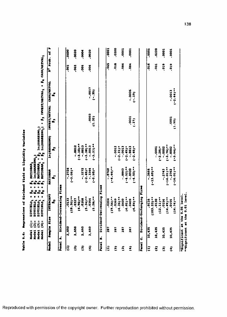
138

II3

I8?

II

I I

» (0

"c c

t

i ♦ ♦fiff3 3 3 3

III!1

I I I Im w* tog § g

g%I r

8 :

8 0 o • o n M o m o mI m I m # m

I I I

RSI M

I

5 ÎT S om V m inI N # f!

I I

O me p*° S ss

in^ m m mom

8«

O

sn

i ; s

V0

82 I I

O

8R

M « n cO #4o m

in o in V o V

P# I MI I

I

« o «PIPI 91 O mom7 ' f

« 91 «o m o m on o OD o o

on

on

o >4 o> atM O #4 MC O C O

8 :

88

88■7

n « n «0 ^ 0 ^ o m o « o n o «

m # n «O O «"* r* #4 p" Mn O n o

' i ' iI I

1*8 1* m #4 wn o #4

s ' s

o « m •lA A m #4 91 #4 Vo # o n

11

u •

i l&


139

In order to examine the causal relationship between liquidity demands and

dividend payments, two puxy variables of shareholders' liquidity demand, RATIOBAR

and SHARESNO, are regressed on dividend yield, DIVYIELD. The estimates obtained

from these two regressions are shown in Table 5.6. Models (1), (21, and (3) are

designed to prevent potential multicollinearity between two liquidity variables and assess

each variable's marginal explanation for variations in dividend policy. Model (4) is

constructed to control for cash demand by the firm itself. Toward this objective,

INVEST and CASH are standardized by the market value of the firm.

In the table, all the regressions have significant t statistics for RATIOBAR and

In(SHARESNO). CASH is insignificant for all samples but dividend unchanging firms. As

discussed earlier (see correlation matrix), a strong, negative correlation between

RATIOBAR/SHARESNO and DIVYIELD persists in these regressions. This significantly

negative relationship between liquidity demand and dividend policy contradicts the JW's

optimal dividend condition [Equation (5.1)1 that higher demand for liquidity motivates the

firm to pay larger dividends. Instead, this outcome lends strong support to the

contention posited in the previous section: that higher (lower) levels of liquidity demand

are associated with lower (higher) dividend payments. Since the estimates for INVEST

and CASH are not significant, it appears that cash demand by the firm and the firm's

cash holdings do not play a significant role in dividend policy. In short, this finding

shows that liquidity demand by shareholders is one of the negative determinants for the

firm's dividend policy.

3. HYPOTHESIS #2: The aquXbrium prie» is monotonie in the dividend signei

lor privets kiformetionl.

e. Single Lineer Pricing Reietion in Signelling

Table 5.7 presents the average return prediction error. As the table shows, the

announcements of quarterly dividend increases generate, on average, significant positive

return prediction errors around the announcement day. In a 7-day window around the


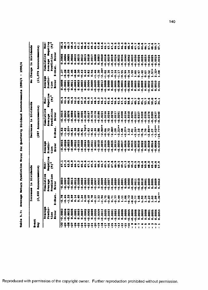
140

I

SI

1i

?

II

t

I i

1»o

I i

g

IoM«0

i Ï

6 r -!!,Ô. gII

i ' i

i pi t Û

«4 O ^ «4 ^ O

« M N M

I .

Î I '%

f i l l

■ h

I f p

?

f i l l

m m ^ îm P»

“ > 0 0 0 0 0 0 0 0 0 0 00 0 0 0 0 0 0 0 0 0 0

0 0 0 0 0 0 0 0 0 0 0 0 0 0 0 0 0 0 0 0 0 0 0 0 0 0 0 0I I I I t I I I I I I I I I I I

m M «

§ §??

r# w o # o 8 ; 3 3 % : 8 8 8 % 3 % : s ; 3 3 g ; s s 3 ;0 0 0 0 « 4 M M , # O O O M O O O M WO N O O MI I I I I I I I I I I I I

o m o m o N O mo o o 9 o o o0 0 0 0 0 0 0 0

• • • • • # # • • • • • •o o e e e e o e e o e e o e e o o o e e e o o e e e o e’ * I I I I I I I I I I I II

: 3

g#o d

m HI ti III m 0 0 f* 0 M M m 0 <0 0 m 0 • M 0 p* <0 05 2 0 r* » md « <0 <0 10 m « m 0 d in A inm m « in in V m m m m

i no v e t r ^ MOr ^ o ol i i i i i i i s i s> 0 0 0 0 0 0 0 0 0 0I I I I I I I I I I

o M $ 0 # o r*o M m # P» mM P# M N M M0 0 0 0 0 00 0 0 0 0 01 I I I I I

Mmmmwmmmmmm0 0 0 0 0 0 0 0 0 0 00 0 0 0 0 0 0 0 0 0 0

23??

! 3 o S n S o ? S 3 n S 3 S ? o S 3 S r ; 3 o 3 S l ? ? S K

g g g g g g g • • • • • • ■ • • • 0 0 0 0 0 0 0 0 0 0

g g g g g ^

0 0 0 0 0 01 I I I Ig g g g g g g g g g g0 0 0 0 0 0 0 0 0 0 0I I I I I I I I

ii? ?

nmor >c<i r ( i 0«4 i n^«r > i n«a» i nr <n«r t mn«oo««a>

ômf #op#mi mw^NO#p* «a#%m#4i mooMOO#40i moMo s s i i i i i i i i i i g g g i i i i i ? ? ? ? ? ? ? f ? ? * ? ? ? ? ? ? ? ® ® ? ? ? ? ? ® ® ® ®

i i i s i i i i i ig 3 : : : S 2 g s g : : ; i c g : p ; : g p 3 p g 5 : 3 3 s %

i o 6 6 6 # 4 w 6 d 6 6 6 # 4 M 6 6I I I I I I I O « ^ O ^ O H ^ 0 i

I « n tfi H 0 M O O....ôôiiiiiiiiiiiiiiiii

0 0 0 0 0 0 0 0 0 0 0 0 0 0 0 0 0 0 0 0 0 0 0 0 0 0 0w M O O o ^ o i m # m w MM m M M M

I I I I I I I I I I I I I I

? ? ?

7 7 7 7 7 7 7 7 7 7 7 T 7 7 7 T -


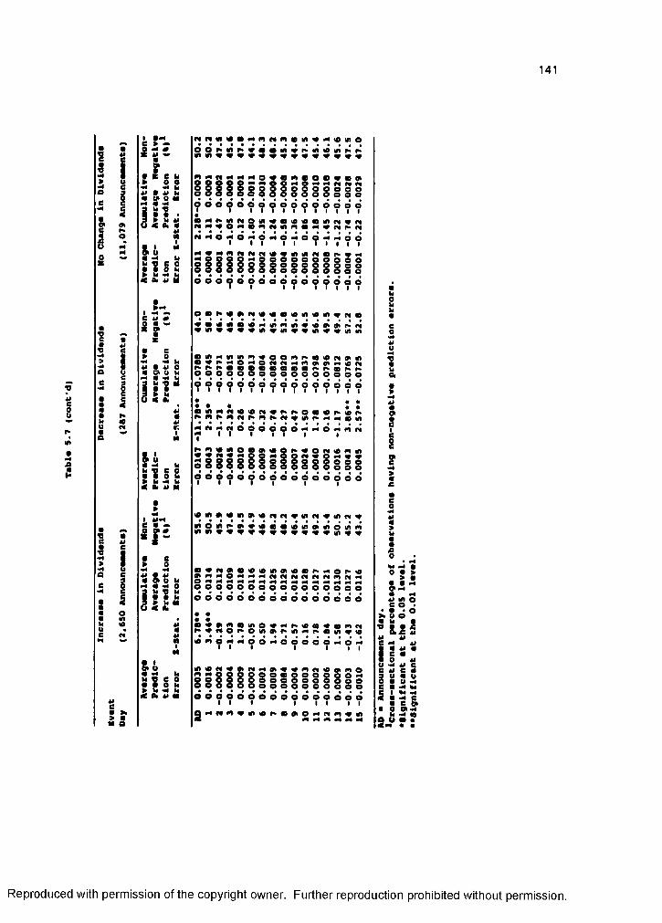
141

I

I

8

I01O

I i8

12 -

m8

iOs

eI I

i t

l l II?

î l l l

• m « »4 « lA oI ^ P» HI «0 lA r>

iillissiil0 0 0 ^ 0 0

: : ; 8 3 gM M O M Ô M

? ? ? ?

0 O « « « 9' g m m w m wg g g o o oo o o o o o0 o o d Ô d1 I I I I I

# 0 0 0 0 i m N V M0-4, 0 0 - - 0 0

!S CÎ • ^ î i | S i §o o oo o o g e o o o ? ? o o o o o

a in >4 ^ ! C ? ; o o m ^ * i O M » i nSSg8SSSS8SSS85S? ? ? ? ? ? ? ? ? T Ï T ÎI o o o o o o

8888

i 0 i n » i a M » i o i < i i < t « i n n «

S S 8 S 9 8 8 8 8 S 8 S 8

0 0 M g 0 0 0 0 9 O 0 r » # - O r » 0o o o o o o o o o e o o o o o oo o o o o o o o o o o e o c o o

o g 9 g • 0 o p* # f# o P» o 0o r n o M N O O M O d o d o m O N I I I I I I I

0 0 M # 9 P I M 9 V # m M 0 9 m OS o S S e o o o Q O o o o o oo o o o oM Md d o d

I I

a MMm0 0 0 # » O9 O# 4 MmV ^ m4 0* m m

O O O O O O O O O O O O O O OI I I I I I I

!i

I

Î?

IIlf8 8 =

■1iin

I


142

announcement day (15 days total), three average prediction errors are significantly

positive at the 0.01 level. Of the three, one each is at, prior to, and after the

announcement day. This is a strong indication that the market correctly anticipates a

rise in dividends. The largest prediction error occurs one day prior to the announcement

day (0.53 percent), more than any other prediction error in the same window. The

announcement day and the following day have significant prediction errors of 0.35 and

0.16 percent, respectively. This is interesting because it is evidence of a somewhat

slow reaction speed to "favorable" information. Still, even these errors may be deemed

immaterial in magnitude.

The cumulative average return prediction error, CAPE, is plotted in Figure 5.3 for

visual dramatization. The CAPE rises to 0.98 percent by the announcement day and

continues to drift upward through event day t - + 13, when it reaches its peak at 1.30

percent.

In contrast with dividend increases, firms that announce quarterly dividend

decreases, on average, experience significant negative return prediction errors around

the announcement day. For an identical 7 day window for this sub-group, four average

prediction errors are significantly negative at the 0.01 level. Three of the four are prior

to the announcement day, and one is at the announcement day. This may indicate that

while "bad news" is not very well anticipated, the reaction time to bad news is short.

In the interest of visual contrast, the CAPE for dividend reducing firms is plotted

in Figure 5 3. For these firms, the CAPE decreases to -4.37 percent by event day t= -2

and drops significantly after that until it reaches a minimum of -8.37 percent on event

day t> +10. The only conclusion one may draw from these data and the figure (in

addition to what was already surmised) is rather trivial: the market considers a dividend

increase good news and a reduction in dividend unfavorable news.

These findings are not at all surprising. Several empirical studies document the

announcement e ffects wf dividends, supporting the information content of dividends

(Aharony and Swary (1980), Asquith and Mullins (1983), Penman (1983), Patell and


(D"OOQ.C

gQ.

"OCD

C/)

o"3O

8■D(O '3"

i3CD

3.3"CD

CD■DOQ.C

aO3■DO

Dividend-Increasing Firms pwmcnoii

Dividend-Decreesing Firms Dividend Unchanging Firms

n - M - « - « - t e B « «'M

-a «

t « «M - w - « -i e

&« I l. H ■ If H 11111111111 n I I ■ . » Il ■ I ■ \

9 t - t t - 1 0 - tS i • 10 10

wmttvm

CDQ.

Note; 1) Connected curves indicate CAPEs. 2) Needle-type bars indicate AFEs.

■DCD

(/)o'3

F ig u re S 3 The Reiationship between Signei end Price R e tu rn A P E e a n d C A P E e

w

144

Wolfson (1984), Kalay and Loawenstein (1985) and Richardson, Sefcik and Thompson

(1986)]. Hence, the empirical evidence that is shown here in the context of the JW

model is not forthright. JW's contention is the formulation of a theoretical model for the

announcement effects of dividends, documented in numerous empirical studies. Their

model is a pricing function, dependent on dividends culminating in a signalling

equilibrium. The positive relation between the dividend signal and price is just one of the

outcomes of the signalling equilibrium.

b. Firm Size and the Signai-Price Relationship

in order to examine a potential size effect in signalling, every subsample is

grouped into quintiles, based on the market value (MKTVAL) of the firm. Since it was

shown in the previous section that the stock price at the dividend announcement date is

an increasing function of dividend changes, three return interval prediction errors

(CPE(k), k - 7, 5, 1) are regressed on dividend changes (DIVYDIFF) for each size-

quintile. CPE(k), is the cumulative return prediction error of firm i for a k-day window,

respectively.

Table 5.8 reports the regression results by size quintiles. Regressions for the

three smallest size quintiles (quintiles 1, 2 and 3) show significant t-statistics for

DIVYDIFF. In contrast, the two largest size quintiles (quintiles 4 and 5) have

insignificant t-statistics for DIVYDIFF. When the R* and the P-value of the F-statistics

are compared across each size quintile, it is found that dividend changes (DIVYDIFF)

explain much better the variation in price changes for the three smallest size quintiles

than for the two largest size quintiles. These differences are consistent with the "small-

firm effect" reported in many other studies (e.g., Banz (1981), Zeghal (1983), Barry and

Brown (1984) and others).

To interpret the differences between the small and large quintiles in the

regression results here, it is argued that larger firms present easier and more timely

access to information than do smaller firms. Further, more individuals disseminate this

information. Because small firms present to outsiders more limited information.


145

£

CO

i1Iîs

■4i

lA

I

î

I fH? îs

il

S i

IIH

oe M tt <

m « «A oi f i f M# I I

« «A A 10 IO O# m ## Oo M m #4 o

SSSS8!

M e M # M10 -0 po QS S i S i S S i

M' - J

i s ^ i iI I

M # 10

8 S l s l

M $ 10 # #S ^ 0 ^ 10 O 0 0 0 ^ 0 0 O M M 0 O O

m M m

a i s î . , 3s s s a s s

f# # m « M 0 0 0 O8 3 3 3 8 8

S = Sis 1 £

S

N M 8 S 3 3 8 :

0 « «4 « *4—‘ M A tfi e^ S 8 S83

m « o # #49 A 10 A 0 oo N 0 0 w oe 0 0 0 O Q

I oS -ë " S "T , £

I ISL in en

i !

I s


146

invastors require a compensating premium in the form of stock price increases when

evaluating their investment risk.

What the small-firm effect implies in the context of signalling is that the signal-

price relationship may occur only in small firms and that signalling is not evident in large

firms. JW argue that dividend and market value of the firm combine to increase stock

prices positively at the dividend announcement date. The evidence presented here is not

consistent with this argument.

c. Polynomial Transformations of tha JW Signalling Equilibrium

To test the empirical validity of the JW signalling equilibrium, the consistency of

the signalling-pricing function with the data must be explored. Toward this end, the

independent variables of the regressions of dividend changes (DIVYDIFF) on the return

interval prediction errors (CPEIk], k« 7, 5, 1) are introduced as polynomials. This non

linear transformation is permissible because it does not affect the parameters of the

model, but provides a better fit for estimation. Three models are fitted and tested, and

their results shown in Table 5.9.

In order to control for possible correlations among the independent variables, a

step-wise regression is applied, where the independent variables enter one at a time.

Since the JW dividend-signalling model implies a separating equilibrium, no regressions

for dividend-decreasing firms show significance. When (DIVYDIFF)* is entered in the

dividend-unchanging and dividend-increasing samples, its coefficients are significant and

negative. Coincidentally, the coefficients of DIVYDIFF remain significant and positive.

Likewise, adding (DIVYDIFF)* shows a much greater explanatory power of the model as

evidenced by the significant increase of the R*’s (adjusted for degrees of freedom) in

each sample. When (DIVYDIFF)* enters the regression, it always has a significant and

positive coefficient in each sample, while the significance and signs of the other

coefficient estimates remain unchanged. Adding (DIVYDIFF)* also raises significantly the

explanatory power of the model. From the test results shown in Table 5.9, it can be

concluded that the polynomial form of an empirically estimable signalling-pricing model


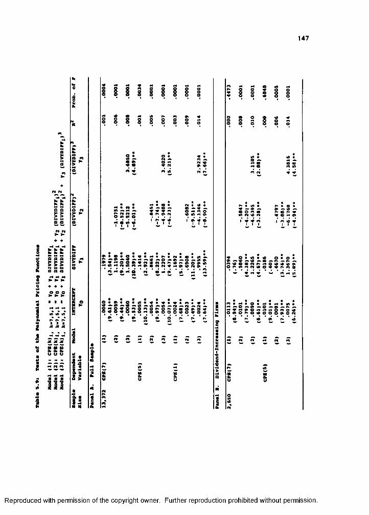
147

!0#

î

III

*N <N

II♦ ♦

t t tM M M

IIIo o o

r» r* r*i i i

Î Î Î

t ’I Z Z

i IIIÎ

k0

in

t t

n

I1 "o

"4

sI ”o

hew

1-o

t8S fg

1#

S 2 !

II g

<2II 1

§ § §

i l s

Sî.« •

I I I Is s 3 s :o o o o o

» 10

#4 # f# #^ #4 O S S o

????

M « O «OD ô #4 m o « in 9»r » W «

# « « « J# e #4 p* Pi # « in

2 10 o 01 o mo e o n#10 n P4 r* lO P» 01 o o mp#Mm o • n n V 0» 10 Pi 0*m M o P4 m 01 in

%

s L sS3S

o.3183

m «83 83

m #» n# #» MS O

d58

u u

i I II 3

5:

II I

I s

in « 2?

r> « o «01 A «0 Ap* o p* # # O M 01I m lO # I I I

. o # m # 10 o « o «Oi O MlO ^ ^m i o o o w p ^ N O i o i o o o o * » m # 4 M i o o ^ v P * m o

^ V N V ^ m #4 in

3 ? S fo o o r«

o «

83O

83in « 82

u


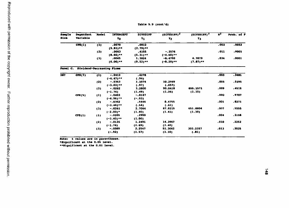
73CD■DOQ .C

gQ .

■DCD

C/)Wo"3O

8■D

a3*CD

CD■DOQ .

O3■DO

CDQ .

Tabla 5.9 (cont'd)

Dapandant Modal INTBRCBPT DivyoïFP (DIVYDIPP)^ (DlVrOIPP)-* R' Pcob. of PSlsa Vaclabla TO Tl T2 »3

CPlfl» m .0070 .0812 .003 .0052(9.91)** (2.79)**

(21 .0063 .4155 -.3576 .011 .0001|8.66)** (5.31)** (-4.60)**

(3) .0045 1.3824 -6.4790 4.7079 .034 .0001(6.061** (9.52)** (-8.29)** (7-87)**

Panai C. Olvldand-Oacraaalng Plraa

287 CPB(7) (1> -.0413 .4278 .003 .3481(-4.471** (.94)

(2) -.0363 1.1074 10.2969 .005 .5195(-3.03)** (.97) (.657)

(3| -.0262 3.2800 90.0410 655.1571 .009 4515(-1.76) (1.49) (1-26) (1-15)

CPE(5| (1) -.0403 -.0147 .000 .9707(-4.96)** (-.03)

(2| -.0362 .5446 6.4755 .001 .8271(-3.44)** (.54) (.61)

(3| -.0261 2.7064 87.8215 651.8804 .007 .5555(-2.00)* (1.40) (1-41) (1-30)

CPB(l) (1) -.0205 .2990 .004 .3158(-3.40)** (1.00)

(2) -.0136 1.2491 14.3967 .010 .2252(-1.74) (1.69) (1-40)

(3) -.0089 2.2547 51.3062 303.2357 .013 .3025(-.92) (1.57) (1-10) (-81)

Mot#* t valu## ar# in paranth####. «Significant at th# 0.05 laval. •«Significant at th# 0.01 laval.

■DCD

C/)C/) A00

149

fits the data well. This polynomial pattern is inconsistent with the monotonie

relationship between price and signal that other authors assume (e.g., Acharya (1988)1.

d. Likelihood Retio Tests of Non-UnearitY in Peremeters

In this section, the cross sectional model of dividend announcements of equation

(5.2) is examined. Equation (5.2) is the testable cross-sectional relation among the

dividend announcement effect, the market value of equity, dividends, liquidity demand

by current shareholders, and the cash demand from the firm.

The non linear equation (5.2) is proposed to be tested with the following

regression model:

CPE(k) IC- (MKTVALj * fPIVIDENDi - LIQUIDTYj) (5.19)

DEMAND

where CPE(k), is the cumulative return prediction error of firm i for a k-daywindow;

k is 7, 5, and 1, respectively;t is the constant, marginal personal tax rate on dividends;MKTVAL, is the market value of firm i at the announcement date;DIVIDEND, is the gross dollar amount of dividends;LIQUIDTY, is total liquidity demand by current stockholders; andDEMAND, is the combined net demand for cash on personal and corporate

accounts.

Multiplying the numerator by t and carrying through the division, equation (5.19)

can be rewritten as

CPE{k)t ■ t-MKTADJ, * C^-DIVADJ, - C-LIQADJ,. (5.20)

where MKTADJ, is MKTVAL, / DEMAND,;DIVAOJ, is DIVIDEND, / DEMAND,;LIQADJ, is LIQUIDTY, / DEMAND,; andall other variables are as defined in equation (5.19).

Using proxy variables and imposing non-linear parameter constraints on equation

(5.20), the testable equation (5.21) is obtained:

CPEik)i - Po * P,ln(AarvaL), ♦ PjOJVYDIFF, ♦ fijRATIOBAJi, , (5.21)

subject to the constraints:

A) ” 0;A — A ;A - (fi)'.


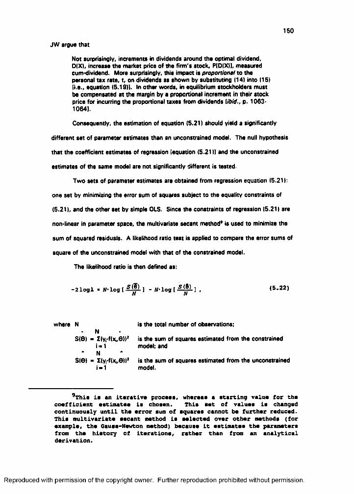
150

JW argue that

Not surprisingly. Increments In dividends around the optimal dividend,D(X), Increase the market price of the firm's stock, P(D(X)1, measured cum-dividend. More surprisingiy, this Impact Is proportional to the personal tax rate, t, on dividends as shown by substituting (14) into (151 (i.e., equation (5.19)1. In other words, in equilibrium stockholders must be compensated at the margin by a proportional increment in their stock price for Incurring the proportional taxes from dividends [ibid., p. 1063- 10641.

Consequently, the estimation of equation (5.21) should yield a significantly

different set of parameter estimates than an unconstrained model. The null hypothesis

that the coefficient estimates of regression (equation (5.21)1 and the unconstrained

estimates of the same model are not significantly different Is tested.

Two sets of parameter estimates are obtained from regression equation (5.21);

one set by minimizing the error sum of squares subject to the equality constraints of

(5.21), and the other set by simple OLS. Since the constraints of regression (5.21) are

non linear In parameter space, the multivariate secant method* Is used to minimize the

sum of squared residuals. A likelihood ratio test Is applied to compare the error sums of

square of the unconstrained model with that of the constrained model.

The likelihood ratio Is then defined as:

■21ogX •= W l o g ( . ^ ^ l - W l o g [ . ^ ^ ] , (5-22)

where N Is the total number of observations;N

8(6) = Z(y,-f(x„0))* Is the sum of squares estimated from the constrainedI « 1 model; andN

8(6) - Z(y,-f(x„6)l* Is the sum of squares estimated from the unconstrainedI m 1 model.

^This is an iterative process, whereas a starting value for the coefficient estimatee is chosen. This set of values is changedcontinuously until the error sum of squares cannot be further reduced. This multivariate secant method is selected over other methods (for example, the Gause-Newton method) because it estimates the parameters from the history of iterations, rather than from an analytical derivation.


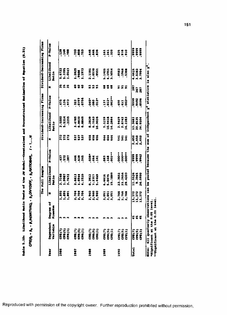
151

i

tfi

t

I

?

II

I S

lis

• 0 • m 0 m 0 0 0 #4 O 0 0 o00 s SV m o 0 0 0 m 0 0 PI m p4 0 0 0

r* 0 P* 0 0 0 #4 PI m 0 0 0 0 0 0

lA m 0 m #4 O N 0 #4 0 m 0 0 0s £J 0 P» 0 P» 0 o 0 0 0 0 0 #4 0 0

2 «A 0 0 0 0 0 0 0 o 0 0 n 0 0Q f# 0 #4 #4 0 0 #4 0 0 0 0 O

0lA lA #4 P# #4 0 0 m 0 m m

lA lA lA O o o m m m 0 0 0m m m 0 0 0 0 0 0 0 0 0 0 0 0 0 p* p*P I 0 0

PI M

f* 0 0 PI0 m m 0 0 o o P I P» P I PI O P I 0 0 0m r* N P* 2 0 0 m Q o #4 o 0#4 0 m o O o e e #4 o 5 0 0 o 0 0 0

o V tA 2 M 0 0 m 0 0 0 0 0 PI mo in 0 m 0 m 0 PI 0 #4 0 #4 0 0 oo N p* 0 0 0 0 o 0 0 0 0M 0 0 0 P# P* 0 0 0 PI 0 0 P I m 0 0

n m m 0 0 0 0 o 0 O 0 P I PI 0 m o 0#4 #4 PI m

JN M M P» P» P» 0 0 0 0 0 0 #4m m m 0 0 0 0 0 0 0 0 0n f# n 0 0 0 0 0 0 0 0 0 0 0 0 0 0 0

PI P I M

r* M p* 0 0 0 0 0 *4 m 0e «

o Ô o0 0

95 s 0 0 m 0 m 0 0 0 0 O o o o 0 0lA n 0 0 n o O o #4 O o o o 0 0 0

• 2 m 2 e P I pk 0 0 000 0

00 3 0 0

s• p4 0 #4 (A 0 0 0 0 02 0 0 0 0 0 m 0 0 0 m PI 0 0 m 0

f* 0 0 #4 m P I 0 0 o0 m #4 0 «4 0

t i M 0 0 p* 0 0 0 PI PI P I #4 P I

M 0 0 0 O O o #4 0 0 0 PI2 2 2 O O O 0 0 0 0 0 0 0 0 0 P» P» (3

0 P* P» r* 0 0 0 o o O P* P» P» m m mM M M M p# M P I P I m m m C4 PI P I m m m

M m

0

? lA r* 0 #4 0 #4 f* 0 #4 0 P» 0

# M M 0 M 0 M 0 M 0 M 0 M 0 0 0 M M

O S w & 6 W o 8 8 80U 8 8 8 8 8 8

<0 2 0 0 O5 0 0 0 0 «1

0 0 0 0 0•*4 #4 #4

u!

**SU •

1 1 1l ? f


152

Asymptotically,

2lo(M - / I f ) ,

where r It the number of restrictions.

Table 5.10 reports the results of these likelihood ratio tests for dividend-

increasing, dividend-decreasing, and dividend-unchanging firms, for each year and for

the combined sample. For each subsample, the number of observations, the likelihood

ratio statistic, and its probability are show n.N one of the likelihood ratio test

statistics for the total sample is significant at the 0.01 or less level. For dividend-

increasing firms, only the statistics of 1989 and 1990 using CPEID are significant at the

0.01 level. But the same results are obtained for the full sample as well. Otherwise,

probabilities (of no difference) are high for both types of firms and for the pooled

sample. Hence, the null hypothesis of "no difference" between the constrained and

unconstrained models cannot be rejected. This is interpreted as strong empirical

evidence that the proportionality condition of equation (5.21) and the implied signalling

equilibrium of equation (5.2) posited by JW is either inconsistent with the data, or the

empirical model is misspecified.

4. HYPOTHESIS #3: Announemnmtt «fftaets (9xeess ntums during thn nvnnt

pnriod) «r* en nndogtnous function o f dMdond hvois, the

domond for Squidity. morkot vaiuo ond fkm sin.

a. Tests of the Cross-Sectional Relation of the JW Mode!

Equation (5.2) implies that the potential causes for stock price reactions to

dividend announcements are the market value of the firm, gross dividends, liquidity

demand by current stockholders, and the demand for cash from the firm. To test the

intensity and duration of the prediction errors, the same windows around the

announcement day as before are examined. The linear relationship between the

quarterly obeorvatione can be pooled because the sum of independent etatietice is also


153

cumulative return prediction error (CPE(k), k « 7, 5, 1) and the proxy variables

MKTVAL, DIVIDEND, LIQUIDTY, and DEMAND is studied. One should note, however,

that DEMAND is defined as the sum of INVEST and LIQUIDTY, less CASH. In a linear

relation, this presents a potential multicollinearity problem. In order to circumvent this

problem arising from the correlation between LIQUIDTY and DEMAND, the latter variable

is excluded from the cross-sectional regression.

CPEIkl's are regressed on In(MKTVAL), DIVYDIFF and RATIOBAR for each

sample. The linear relation to be estimated is

CPE(k)i - «0 ♦ t^ln(HKTVAL), ♦ b^DIVYDIFF, * ijMTIOBARj, (5.23)

where CPE(k), is the cumulative return prediction error of firm i; and k is a 7-, 5-, and 1-day window, respectively.

The parameter estimates obtained from regressing each quarter's observations

are checked for the OLS assumptions of normality and homoscedasticity. The analysis

of residuals indicate that the assumptions of normality and homoscedasticity are not

violated. Interestingly, contrary to recent arguments" by Eckbc, Maksimovic, and

Williams (1990), no evidence of distribution truncation of the standardized residuals at

the dividend announcement date for dividend-increasing and dividend-decreasing firms is

found.

The analysis of "condition indices" is applied as the multicollinearity diagnostic.

The condition index number is the square root of the ratio of the largest eigen value to

each individual eigen value. When this number is very large, estimates may be biased.

Belsley, Kuh and Welsch (1980) suggest that condition indices greater than 10 indicate

weak dependence and that condition indices of 30 to 100 indicate moderate to strong

^^Bckbo, MakalnoviCr and William# (1990) argue that bocauae of corporate inaider# ' private information, the diatributiona of reaiduala at the voluntary event announcement date will be truncated, and that thia truncation biaa will lead to the inconalatent eatimatora of OLS and GLS.


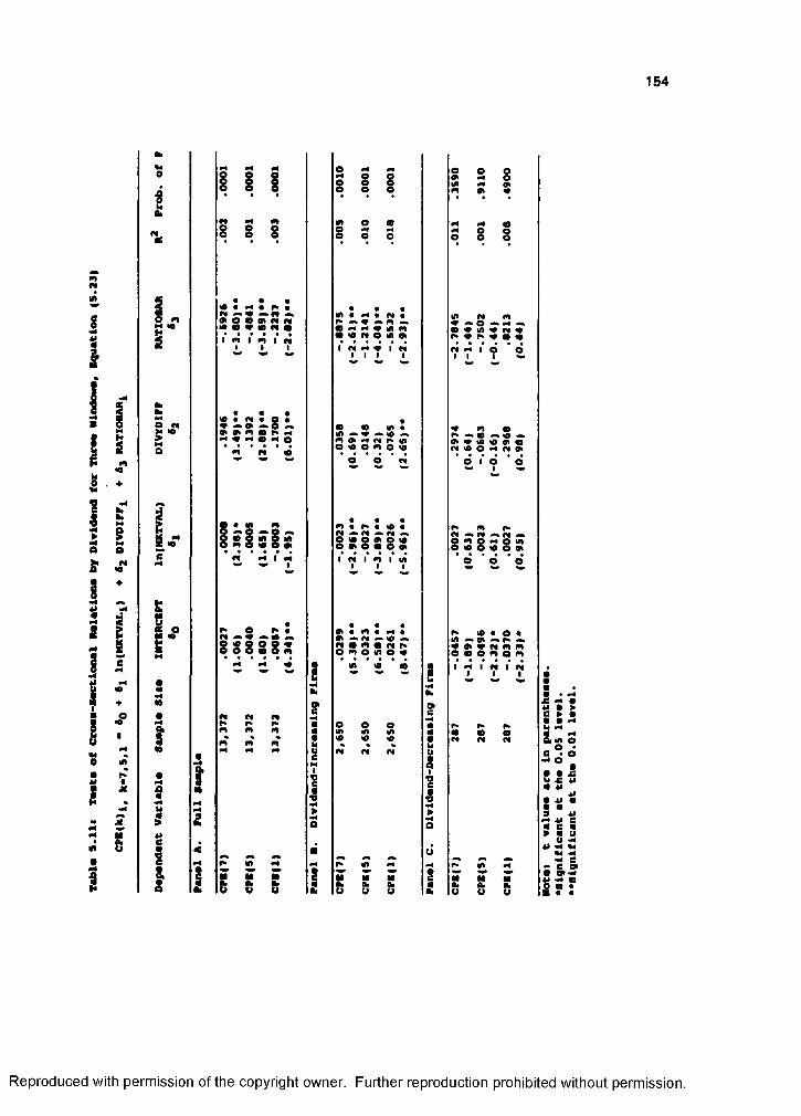
154

f#

ni

M

i

if♦

ê0

♦

w

1e*4M

«P

♦O

i

s

h0i

i i i 8 1 I 8 3 8lA f4 9m m #a

Tc 8 8 8 I s s #4 #4 to3 8 8

V

« « «S13Î .R13 8 8 8 : 3i m t m ! fi

« « «#m # #4 # M «m #4 #4 # W» m • «0 M O « 0k

lA et m# A O A m ^* ? S 5 S 5

L L L 1 w #4 V I riL ' L L

et d r d d I I 1 ^

t «0 « «4 « o « V o ^0k 9 p4 S S ^ # m 05o #4 # M * M O m e ! # m » #4 p# vk O O m O k0

A 0 0 Ok # 0 0 01 0et 0 o #4 pt OkO d * et d i d d

1 • « M m « « «m # 9» # 10 «s.-c i s i s i s

f! M # met et -i* et 8 8 8 : 8 8 1 et 1 et 1 d

L '

5 -• S — m -• 8 3 8 3 8 8

d d ’ d

;Ï f 2 S • ^ * * •# # m # #4 « 1- 0 « o •1

3 — V *•« — 8 8 8 8 8 :

» «a. e| Ok «ibet m m m et f» O m O k0 O V # m 0 N m m o 0 o m o ms s * a d d d a i d r et r et 1 1 1• b-4 C

k k• : : : 1 1a : o o o s S 2 2I m m m I

« « 10 S 8 8 :a g 8

i Ï i is «

1p42 s a

1 < m c! _ _ _1 1 S S 9 a |T M M 2 0 0 0i 2 & u 8 2 o u u 2 U V o

i!iiiîliiill


155

collinearity. All condition index numbers are found to be less than 10. Hence, it is

concluded that the parameter estimates are unbiased.

The estimated coefficients, F statistic probabilities, and the R"s of regression

equation (5.23) for each sample for the three types of firms for the three different

windows are displayed in Table 5.11. The table is organized in three panels: Panel A

portrays the estimates and statistics of the full sample, while panels B and C show the

same for dividend-increasing and dividend decreasing subsamples, respectively.

In Panel A of Table 5.11, the full sample has a positive and significant coefficient

for DIVYDIFF and negative and significant coefficient for RATIOBAR, as reported already

In the previous sections. The MKTVAL estimate is significant for the 7-day window

only. For dividend-decreasing firms, none of the variables have significant coefficients.

This seems to be consistent with the JW model since dividend-decreasing firms may not

signal in a separating signalling equilibrium.

Panel B of the table demonstrates negative and significant coefficient estimates

for RATIOBAR and MKTVAL. Nevertheless, DIVYDIFF is significant only for the 1 -day

window, as a result of controlling for the magnitude of the dividend changes. The

striking evidence reflected in the table is that the signs of the MKTVAL estimates are

negative for dividend-increasing firms. This is completely unexplainable by the JW

model. JW suggests that when the firm announces a dividend payment to signal, the

magnitude of the dividend and the market value of the firm impact positively on the

stock price.'' The inescapable conclusion is that the JW model cannot be supported

by empirical evidence. Stock price reactions to dividend announcements are not too

well explained by the market value of the firm’s equity, dividends, and cash demand

the JW model, the market value of the firm is endogenously determined when dividend payments affect the stock price. In order to verify the results of Table 3.11, the market value of the firm at the announcement day is estimated using the stock price. With these estimated values, in place of the actual values, the tests in this section are repeated. Results identical to those of Table S.11 are obtained with those estimated values.


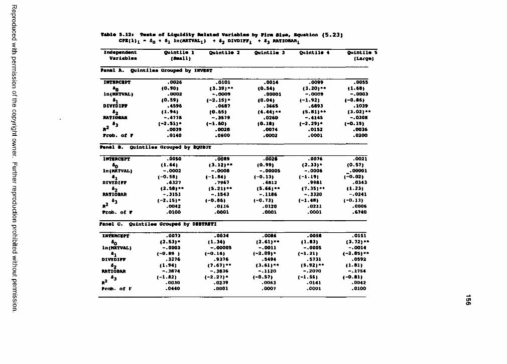
CD■DOQ .C

gQ .

Table 5.12$ Teate of Liquidity belated Variables by Pire Sise, Squat loo (5.23) CPB(1)£ - 5o + InlMRTVALj ) + 63 DIVDIPPj + 63 SATIOBAR^

"OCD

C/)C/)

8■D

CD

3 .3"CD

CD■DOQ.C

aO3"Oo

CDQ.

■DCD

C/)C/)

Ind.pand.ntV.riabl.a

Quintll. 1 (Sa.ll)

Qulntil. 2 Qulntil. 3 Qulntil. 4 Oiintlli(Largi

Pan.1 A. Qulntil.a Groupad by INVI8T

m m c i P T .0026 .0101 .0014 .0099 .0055«0 (0.90) (3.39)» (0.54) (3.20)" (1.68)

ln(MXTVAL| .0002 -.0009 .00001 -.0009 -.0003«1 (0.59) (-2.15)' (0.04) (-1.92) (-0.86)

olvioirr .4596 .0687 .3665 .6893 .1039«2 (1.94) (0.65) (4.44)" (5.81)" (3.02)'

RAtlOWUl -.4778 -.3579 .0260 -.4145 -.0308_ «3 (-2.51)* (-1.60) (0.18) (-2.29)' (-0.19)

.0039 .0028 .0074 .0152 .0036Prob. of r .0140 .0600 .0002 .0001 .0200

Panel B. Quintiles Grouped by BQUBUY

INTIRC8PT .0050 .0089 .0028 .0076 .0021«0 (1.64) (3.12)" (0.99) (2.33)' (0.57)

In(NKTVAL) -.0002 -.0008 -.00005 —.0006 .00001«1 (-0.58) (-1.84) (-0.13) (-1.19) (-0.02)

DIWDIPP .6327 .7967 .4812 .9981 .0343«2 (2.58)" (5.21)" (5.66)" (7.35)" (1.23)

RATIOBAR -.3151 -.1543 -.1186 -.3320 -.0241, *3 (-2.15)' (-0.86) (-0.73) (-1.48) (-0.13)

R* .0042 .0116 .0120 .0211 .0006Pcob. of P .0100 .0001 .0001 .0001 .6740

Panel C. Qulntil.. Groupad by DBBTRBTI

IRTRRCBPT .0073 .0034 .0086 .0058 .0151«0 (2.53)' (1.34) (2.61)" (1.83) (3.72)"

In(HXTVAL) -.0003 -.00005 -.0011 -.0005 -.0014«1 (-0.89 ) (-0.14) (-2.09)' (-1.21) (-2.85)"

DIVTDIPP .3276 .9376 .5494 .5731 .0592*2 (1.94) (7.67)" (3.61)" (5.92)" (1.81)

RATIOBAR -.3874 -.3836 -.1120 -.2070 -.1754, S3 (-1 02) (-2.27)' (-0.57) (-1.55) (-0.81)R* .0030 .0239 .0063 .0141 .0042Prob. of r .0440 .0001 .0007 .0001 .0100

(XIO)

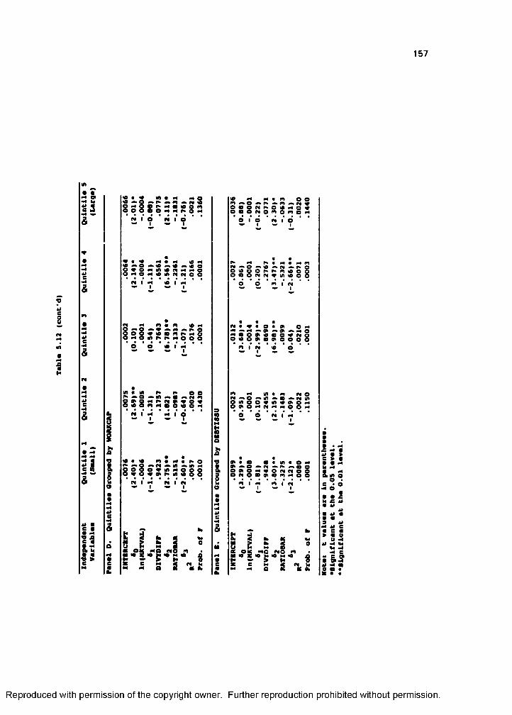
157

I

t

Ü

i l&

li

«A # g M* # N M Os s i s s s s —S83M I o M # O

# # 2 N # M 10*4« ^ O *» 10 # oO«O*4in«0f«l*«*4Qo*40*4i o««4ei oo

N I M « I fH

25 M m # m «o M P * P V *»*4*fcÔ P P P « P « m ^ * 4 p P M O * O I » # » W O P PP # I N

in « 10 I ^ M o I

8 3 8 : :* f î I* H

^ P P

8 3 8 :. ' ? ■ ■

p # p m # M # ^ o^ ^ p ^ p *»p838S3Ü!SS8 8

n I *4

w%#0

!

p #4 *4 e m o PM O ^ m *»O# Pg S g ^ ^ O P ^ p pO I

O m o m o M

m / o

r# o p N r»O p o P r » r » m p oP P P M N P P P P

N « P « O « 0 i 0* 4^ ^ m ^ ^ ^ o i #4 oM P O P P P P P N O P P P P P P O O P O

m I M P O

m M p « *4 <4 025 <ô ^ P ^ 9 —*M p P P P P P P P ^ O # 4 0 P P # 4 ( 4 M * 4 0 P M

* • • • • • • • • •o o M I M

P « P P e _P ^ O w ô p Q p oO <4 O P P P

1 83 8

î î i ît f g •-S •'*2 ^g î H 1

Üîti« «I

nii!i


158

from the firm (or liquidity demand by current shareholders). Stated differently, the

theoretical equilibrium relationship described by equation (5.2) empirically does not hold.

As it was indicated earlier, the results of likelihood ratio tests are evidence that

the JW's dividend signalling model is inconsistent with the data and is possibly

misspecified. The results of the cross sectional analyses give additional weight to this

argument.

b. Controlling for Liquidity Factors

In addition to the liquidity demand by current shareholders, cash demand from

the firm may be influenced by investment, repayment of debt, repurchase of shares, and

funding increases in short-term working capital. These other liquidity factors may

impact the analysis in two ways. It may have an effect on the cross-sectional relation

between dividend levels, liquidity demands, and firm size. It may also provide biased

estimates of coefficients. In addition, in a Modigliani and Miller (1958) world, the firm's

external financing is construed as the residual of its investment decision. Since levels of

investment vary across firms, external financing also varies cross-sectionally. It follows

that differences in external financing across firms must be isolated.

To control for liquidity-related factors and to verify the robustness of the

estimator function, the regression of the previous section is repeated for each quintile

grouped by INVEST, EQUBUY. DEBTRETI, WORKCAP, and DEBTISSU, respectively. The

parameter estimates for each of these regressions are reported in Table 5.12.

Comparisons between five quintiles and with the previous results indicate that the

estimates between quintiles are at variance with each other.

In the interest of brevity, the results are given only for the regression in which

CPE(1)'s are used as the dependent variable." The figures shown in the table imply

that estimates obtained from the linear model might be biased. Accordingly, the

robustness of the tests of the previous section can be scrutinized. Clearly, more

^^The cegreseione using CPE(7) and CPE(5) result in similar estimates.


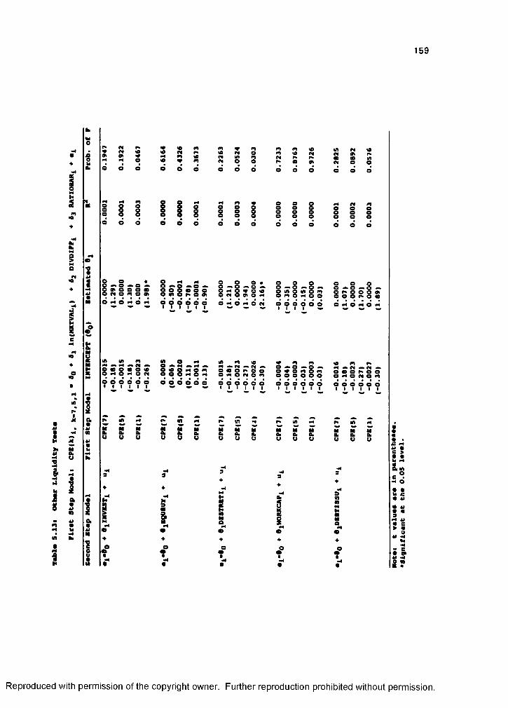
159

S

gQ

*

WIC

<o+o

IIIlA

I

O

&

I

S I

i I

o oi s i f io M o M o M

§ : 8 : § :o o o o o o

S s

3 :

isl- 0 - 0 - e<p

W O ##p A M A

8 8 8 3 8 : :o e e d ô e

8 § 8

9

4

ie4

8 3 d d

A o 8 83 8 S 8 M 8

V ? d zd3 8 3

«m m 1#M ^ g# m. M Ô « O r» O OO m o f# O m

????

8

i4

O

U 8

i

<0r»«d

i

Pd

od

8 : 8 3 8 8e e O 6 6 bI I I I

u 8 S

i4

O

i

id

Id

od

8

O O Ps s s f s s

b d M d M d #î

o A o o A9 î ® 5 o no o o o o o0 o o d d d1 I I I I I

o o o o o o o #4 o M o m

o o o o o

s94•4IIP4

8 S

i8 5

!le S»o m


160rigorous testing of the effects of the liquidity-related variables on the cross-sectional

model is required.

An additional set of tests of the liquidity-related variables (INVEST, EQUBUY,

DEBTRETI, WORKCAP, and DEBTISSU) is performed, applying a two-step procedure. At

the first step, the error terms are estimated from the cross-sectional regression equation

(5.23). At the second step, the estimated error terms are regressed on each of the

liquidity-related variables. The null hypothesis is that the errors obtained at the first step

are unrelated to each one of the explanatory variables of the second step.

The results of this last set of tests are reported in Table 5.13. The estimated

coefficients of the liquidity-related variables are insignificant in each secondary

regression except for two cases: regressions using CPE(I) show significant estimates for

INVEST and DEBTRETI at the 0.05 level. Overall, it is safe to conclude that the cross-

sectional model of equation (5.23) appears to be robust enough to portray the firm's

liquidity-related variables.


In this essay, the dividend signalling model developed by John and Williams

(1985) is empirically tested. First, it is examined whether the demand for cash from the

firm motivates the payment of dividends as JW, or Feldstein and Green (1983) suggest.

JW assert that, in equilibrium, larger dividends are paid only if the demand for cash from

the firm is high. It is found that there is a negative relation between liquidity demands

and dividend payments, inconsistent with the JW contention. Instead, it seems that the

empirical evidence supports Feldstein and Green's reasoning that firms have a strong

desire to satisfy liquidity demands of their current shareholders by paying dividends. It

is documented here that liquidity demand by shareholders is one of the determinants of

the firm's dividend policy.

Second, stock price and volume reactions to quarterly dividend announcements

are studied. It is observed that announcements of dividend increases bid up the stock


161

price while trading volume decreases. In contrast, announcements of dividend

decreases reduce both stock price and trading volume. The JW model posits that higher

(lower) dividends are associated with higher (lower) stock price and trading volume and

dividends can be used as a signal (see also Miller's (1987) signalling conditions). Hence,

the findings of stock price and volume reaction to dividend announcements are not

consistent with some of the basic relations of the JW model.

Third, it is also discovered that the positive relationship between dividend

changes and price changes is significant for smaller firms and insignificant for larger

ones. This may imply that a signal price relationship exists for small firms, but not for

large firms. At best, the indication is that the signal price relationship is cross-

sectionally negatively related to firm size. This finding is not consistent with the JW

model's notion that dividends and the market value of the firm combine to increase

stock prices positively at the dividend announcement date. The likelihood ratio tests

indicate that the cross-sectional model of JW [equation (5.2)1 is inconsistent with the

data or empirically may be misspecified.

Fourth, it is found that the polynomial form for the signalling-pricing function fits

the data very well. This polynomial pattern is neither consistent with the monotonie

relationship between signal and price that many authors assume, nor compatible with

the non-linear relationship that JW posits.

Fifth, the key argument that JW assert to be empirically testable is examined. It

is this argument around which are developed the tests of the cross-sectional model that

relate the dividend announcement effects, the market value of the firm, dividends,

liquidity demand by current shareholders, and the cash demand from the firm. A cross-

sectional regression analysis shows that stock price reactions to dividend

announcements are not explained by the JW model (and that the latter is also

inconsistent with the data).

Despite all the empirical evidence reported here, a caveat is in order. It is quite

possible that some of the conclusions reached here may hinge on measurement


162

problems. Unfortunately, these problems will exist in all empirical work, making the

verifiability (or perhaps, more important, the refutabilityl of a theory impossible.

Notwithstanding, while scores of studies focus on formulating theoretical models of

signalling, empirical research is a must for the testing of the validity of these models.


Chapter 6. SUMMARY, CONCLUSIONS, AND FUTURE RESEARCH

The objective of this dissertation has been to extend empirical work on dividend

policy in three ways. The dissertation encompasses three essays.' The first essay

empirically investigated a wide range of dividend determinants including investments,

earnings, debt, free cash flows, firm size, beta, and industry classification. This essay

employed time series cross sectional tests and vector autoregression (VAR) methodology

to analyze the explanatory power of the various theories of dividend policy. The second

essay proposed an alternative approach to the ex dividend anomalies that fully

incorporates both the tax effect hypothesis and the short-term trading hypothesis. This

essay investigated some observable differences between cum and ex-dividend efficient

portfolios based on a portfolio selection model in the context of the 1984 and 1986 tax

reforms. The third essay analyzed the empirical validity of a dividend signalling

equilibrium model and tested the explicit relationship among the announcement effect,

the dividends, and the cum-dividend market values, suggested by a signalling equilibrium

model.

In Chapter 3, time-series cross-sectional regressions using an error components

model were estimated to test for the contemporaneous relationships among theoretical

dividend determinants. It was found that a firm's dividend payments are significantly

related to earnings, free cash flows, beta, and firm sizes. Perhaps the most important

finding is that dividends are not influenced by investments and debts, consistent with

the irrelevance proposition of Miller and Modigliani (1961). It was also shown that

industry effects might not exist or might be only the manifestation of firm size effects.

'These essays did not converge to certain unified conclusions because they empirically examined separate dividend theories based on different assumptions and models.

163


164

On the other hand, in order to examine the dynamic relationships among these variables,

the vector autoregression analyses were conducted. The variance decompositions and

impulse response analyses consistently demonstrated that dividends have significant

short-term effects on itself, whereas other variables have no dynamic effects on

dividends. It appears that only dividends have short memory of its own past and that

other variables have no dynamic interactions with dividends.

Based on these results, a lagged dividend model was developed and tested for

robustness. The evidence suggests that dividend payments are heavily influenced by a

series of the past dividend payments as well as contemporaneous factors such as

earnings and free cash flows. Although this lagged dividend model may be rather

exploratory, it will shed some light on the model of puzzling dividend policy. One fruitful

avenue for future study may be to apply a structural vector autoregression which

simultaneously incorporates both contemporaneous variables and dynamic factors.

Chapter 4 attempted to report changes in the risk-expected return trade-off

around the ex-dividend day by comparing the efficient portfolio frontiers between the

pre-tax reform period and the post-tax reform period. These portfolio results were

related to the excess return behaviors on which the 1984 and 1986 Tax Reform Acts

are also documented to have had effects.

First, the effects of the 1984 and 1986 Tax Reform Acts on the return behaviors

around the ex-dividend day were documented. The results are consistent with both the

tax-effect hypothesis and the short-term trading hypothesis, and they are summarized as

follows: (1) prior to the 1986 tax reform, significant positive excess returns were

observed on the ex-dividend day; (2) during the post-1986 tax reform period, average

ex-dividend excess returns were not different from zero at the 1 % significance level; (3)

there existed the negative correlationships between the dividends yields and ex-dividend

day excess returns, which correlationships decreased from the pre-1986 tax reform


165

period to the post-1986 tax reform period; (4) average ex-dividend day excess returns

increased significantly during the post-1984 tax reform period compared to the pre-1984

Tax Reform period; (51 during the post-1984 tax reform period, more significant excess

returns were observed for 11 trading days before and after the ex-dividend day

compared to the pre-1984 tax reform period.

Second, the cum- and ex-dividend efficient portfolios between the pre-1984 tax

reform period and the post-1984 tax reform period were compared. The following

evidences supporting the short-term trading hypothesis were found: ID cum-dividend

efficient portfolios dominated ex-dividend efficient portfolios; and (2) the efficiency gap

between cum-dividend efficient frontiers and ex-dividend efficient frontiers expanded

more during the post-1984 tax reform period than during the pre-1984 tax reform

period.

Following Long's (1977) argument, it was predicted that the 1986 Tax Reform

Act would decrease the expected after-tax return at the new tax rates and increase the

after-tax variance of the portfolio. Consistent with this expectation, it was also found

that the efficient portfolio frontier during the post-1986 tax reform period was

dominated by the efficient portfolio frontier during the pre-1986 tax reform period. This

result may be interpreted as the tax-effects since the tax premiums decrease with an

decrease in dividend tax rate. But, the variance as risk factor was not considered in the

tax-effect hypothesis.

To conclude, the evidence of excess return behaviors supported the existence of

both tax effects and short-term trading around the ex-dividend day. It appeared that

these tax effects and short-term trading are not mutually exclusive, but co-existent as

long as short-term trading is tax-induced. And this finding was effectively supported by

portfolio test results. It was argued that portfolio approach is quite advantageous over

the extant approaches, because this approach incorporates the tax effect as well as


166short-term trading. It was noted that ex-dividend behavior cannot be understood

independently of the risk-expected return trade-off. It was also proposed that this

portfolio approach can best be used in many branches of corporate finance (e.g., turn-of-

the-year effect I where portfolio revisions are considered to occur.

In Chapter 5, the dividend signalling model developed by John and Williams

(1985) was empirically tested. It was examined whether the demand for cash from the

firm motivates the payment of dividends (see John and Williams (1985) or Feldstein and

Green (1983)]. It was found that there is a negative relation between liquidity demands

and dividend payments, inconsistent with the JW contention. The empirical evidence

supported Feldstein and Green's reasoning that firms have a strong desire to satisfy

liquidity demands of their current shareholders by paying dividends.

Stock price and volume reactions to quarterly dividend announcements were

studied. It was observed that announcements of dividend increases bid up the stock

price while trading volume decreases. In contrast, announcements of dividend

decreases reduce both stock price and trading volume. The JW model posits that higher

(lower) dividends are associated with higher (lower) stock price and that trading volume

and dividends can be used as a signal. Hence, the findings of stock price and volume

reaction to dividend announcements are not consistent with some of the basic relations

of the JW model. It was also found that the polynomial form for the signalling-pricing

function fits the data very well. This polynomial pattern was neither consistent with the

monotonie relationship between signal and price that many authors assume, nor was it

compatible with the non-linear relationship that JW posits.

The key argument that JW assert to be empirically testable was examined. The

cross-sectional model that relates the dividend announcement effects, the market value

of the firm, dividends, liquidity demand by current shareholders, and the cash demand

from the firm were tested. The regression analysis showed that stock price reactions to


167

dividend announcements were not explained by the JW model. The likelihood ratio tests

also indicated that the cross sectional model of JW is inconsistent with the data or

empirically may be misspecified. While scores of studies focus on formulating

theoretical models of signalling, empirical research is a must for the testing of the

validity of these models.


BIBLIOGRAPHY

Acharya, S.. 1988, "A Generalized Econometric Model and Tests of a Sionallinc Hypothesis with Two Discrete Signals," Journal of Finance 43:413-429.

Aharony, J., and I. Swary, 1980, * Quarterly Dividend and Earnings Announcements and Stockholders' Returns: An Empirical Analysis," Journal of Finance 35:1-12.

Akerlof, George A., 1970, "The Market for Lemon: Quality Uncertainty and the Market Mechanism," Quarterly Journal of Economics (August), 488-500.

Ambarish, R., K. John, and J. Williams, 1987, "Efficient Signaling with Dividends and Investment," Journal of Finança 42:321-344.

Asquith, P., and D. Mullins, 1983, "The Impact of Initiating Dividend Payments on Stockholders' Wealth," Journal of Business 56:77-96.

____________ , 1986, "Equity Issues and Offering Dilution," Journal of FinancialEconomics 15:61-89.

Bamber, L.S., 1986, "The Information Content of Annual Earnings Releases: A Trading Volume Approach," Journal of Accounting Research 24:40-56.

Banz, R., 1981, "The Relationship between Return and Market Value of Common Stocks," Journal of Financial Economics 9:3-18.

Barclay, Michael J., 1987, "Dividends, Taxes and Common Stock Prices: The Ex- Dividend Day Behavior of Common Stock Prices Before the Income Tax," Journal of Financial Economics 19:31-44.

Barnea, Amir, Robert A. Haugen, and Lemma W. Senbet, 1985, Agency Problems and Financial Contracting, Englewood Cliffs, NJ: Prentice-Hall.

Barry, C., and S. Brown, 1984, "Differential Information and the Smail Firm Effect," Journal of Financial Economics 13:283-294.

Bar-Yosef, Season, Jeffrey L Callen, and Joshua Livnat, 1987, "Autoregressive Modelling of Eamings-lnvestment Causality," Journal of Finance 42:11-28.

, and Lucy Huffman, 1986, "The Information Content of Dividends: A SignallingApproach," Journal of Financial and Quantitative Analysis 21:47-58.

Baskin, Jonathan, 1989, "An Empirical Investigation of the Pecking Order Hypothesis," Financial Management (Spring), 26-35.

Beaver, W.H., 1968, "The information Content of Annual Earnings Announcements," Journal o f Accounting Research Supplement 6:67-92.

Belsley, D.A., E. Kuh, and R E. Welsch, 1980, Regression Diagnostics: Identifying Influerrtial Data and Sources of Multicollinearity, New York: Wiley.

168


169

Bhattacharya, Sudipto, 1979, "Imperfect Information, Dividend Policy and the Bird In the Hand Fallacy," BeilJoumtl of Economics 10:259-270.

, and Jay R. Ritter, 1983, "Innovation and Communication: Signalling with PartialDisclosure," Review of Economic Studies 5:331-346.

Black, Fischer, 1976, "The Dividend Puzzle," Journal of Portfolio Management (Winter), 5-8.

Black, Fischer, and Myron Scholes, 1974, "The Effects of Dividend Yield and Dividend Policy on Common Stock Prices and Returns," Journal of Financial Economics 1:1-22.

____________ , 1973, "The Behavior of Security Returns around Ex-dividend Days,"Working Paper, Universitv of Chicago.

Blanchard, O.J., 1989, "A Traditional Interpretation of Macroeconomic Fluctuations," American Economic Review 79:1146-1164.

Blazenko, George W., 1987, "Managerial Preference, Asymmetric Information, and Financial Structure," Journal of Finance 42:839-862.

Bolster, Paul J., Lawrence B. Lindsey, and Andrew Mitrusi, 1989, "Tax-Induced Trading: The Effect of the 1986 Tax Reform Act on Stock Market Activity," Journal of Finance 44:327-344.

Booth, L.D., and D.J. Johnston, 1984, "The Ex-Dividend Day Behavior of Canadian Stock Prices: Tax Changes and Clientele Effects," Journal of Finance 39:457- 476.

Brennan, Michael J., 1970, "Taxes, Market Valuation and Corporate Financial Policy," National Tax Journal 23:417-427.

, and Alan Kraus, 1987, "Efficient Financing Under Asymmetric Information,"Journal of Finance 42:1225-1243.

, and Anjan V. Thakor, 1990, "Shareholder Preferences and Dividend Policy,"Journal of Finance 45:993-1018.

Brown, Keith C., and Scott L. Lummer, 1984, "The Cash Management Implications of a Hedged Dividend Capture Strategy," Financial Management (Winter), 7-17.

Brown, Stephen, and Jerold B. Warner, 1985, "Using Daily Stock Returns: The Case of Event Studies," Journal of Financial Economics 14:3-31.

Clements, M.P., and G.E. Mizon, 1991, "Empirical Analysis of Macroeconomic Time Series," European Economic Review, 887-932.

Campbell, John Y., and Robert J. Shiller, 1987, "Cointegration and Tests of Present Value Models, " Journal of Political Economy 95:1062-1088.

Campbell, T., 1979, "Optimal Investment Financing Decisions and the Value of Confidentiality, " Journal of Finandal Quantitativa Analysis 14:913-924.

Crockett, Jean, and Irwin Friend, 1988, "Dividend Policy in Perspective: Can Theory Explain Behavior?" Review of Economics and Statistics (November), 603-613.


170

Crutchley, Claire E., and Robert S. Hansen. 1989, "A Test of Agency Theory ofManagerial Ownership, Corporate Leverage, and Corporate Dividends,” Financial Management (Winter), 36*47.

DeAngelo, Harry, and Ronald W. Masulis, 1980, "Leverage and Dividend Irrelevancy Under Corporate and Personal Taxation,” Journal of Finance 35:453-467.

Denis, David J., 1990, "Defensive Changes in Corporate Payout Policy: Share Repurchases and Special Dividends,” Journal of Finance 45:1433-1456.

Dhrymes, P.J., and M. Kurz, 1964, "On the Dividend Poiicy of Electric Utilities,” Review of Economics and Statiitics (February), 76-81.

, 1967, "Investment, Dividend, and External Finance Behavior of Firms,”In R. Ferber, ed.. Determinants of Investment Behavior, New York, 427-467.

Diamond, D., 1984, "Financiai intermediation and Delegated Monitoring,” Review of Economic Studies 51:393-414.

Dyl, E.A., and J.R. Hoffmeister, 1986, "A Note on Dividend Policy and Beta,” Journal of Business Finance and Accounting 13:107-115.

Eades, Kenneth M., Patrick J. Hess, and E. Han Kim, 1984, "On Interpreting Security Returns During the Ex-Dividend Period,” Journal of Financial Economics 13:3- 34.

Easterbrook, F., 1984, "Two Agency Cost Explanations for Dividend Payments,” American Economic Review 74:680-689.

Eckbo, B., V. Maksimovic, and J. Williams, 1990, "Consistent Estimation of Cross- Sectional Models in Event Studies,” Review of Financial Studies 3:343-365.

Elton, Edwin J., and Martin J. Gruber, 1970, "Marginal Stockholder Tax Rates and the Clientele Effect,” Review of Economics and Statistics 52:68-74.

____________ , 1978, "Taxes and Portfolio Composition,” Journal of FinancialEconomics 6:399-410.

______ , and Joel Rentzler, 1984, "The Ex-Dividend Behavior of Stock Prices; ARe-Examination of the Clientele Effect: A Comment,” Journal of Finance 39:551- 556.

Engle, Robert P., and Byung Sam Yoo, 1987, "Forecasting and Testing in Co-Integrated Systems,” Journal of Econometrics 35:143-159.

, and Clive W. J. Granger, 1987, "Cointegration and Error Correction:Representation, Estimation, and Testing,” Econometrics 55:251-276.

Fame, Eugene F., 1974, "The Empirical Relationships Between the Dividend and Investment Decisions of Firms,” American Economic Review 64:304-318.

, 1980, "Agency Problems and the Theory of the Firm,” Journal o f PoliticalEconomy 88:288-307.

, and H. Babiak, 1968, "Dividend Policy: An Empirical Analysis,” Journal ofAmerican Statistical Association 63:1132-1161.


171

, and Michael C. Janaen, 1983, "Agency Problems and Residual Claims," Journalof Law and Economies 26:327*349.

, Lawrence Fisher, Michael C. Jensen, and Richard Roll, 1969, "The Adjustmentof Stock Prices to New Information," Intarnational Economic Raviaw 10:1*21.

Fedenia, Mark, and Theoharry Grammatikos, 1991, "Portfolio Rebalancing and theEffective Taxation of Dividends and Capital Gains Following the Tax Reform Act of 1966," Journal of Banking and Finança 15:501*519.

Feldstein, M., and J. Green, 1963, "Why Companies Pay Dividends," Amarican Economic Review 73:17*30.

Frankfurter, George, and William Lane, (1990), "The Rationality of Dividends," Unpublished working paper, Louisiana State University.

Friend, I., and J. Hasbrouck, 1966, "Determinants of Capital Structure," Research in Finance 7:1*19.

Fuller, W. A., 1976, Introduction to Statistical Tima Saries, New York; John Wiley.

, and G. E. Battese, 1974, "Estimation of Linear Models with Crossed ErrorStructure," Journal of Econometrics 2:67*76.

Garcia, Beatrice E.. 1966, "Trading to Nab Dividends Captures Investors' Fancy," Waii Street Journal, May 19, 1966.

Ghosh, Chinmoy, and J. Randall Woolridge, 1991, "Dividend Omissions and Stock Market Rationality," Journal of Business Finance & Accounting 16:315*330.

Goldfeld, S. M., and R. E. Quandt, 1976, Nonlinear Methods in Econometrics, New York: North*Holland Inc.

Gordon, Myron, 1963, "Optimal Investment and Financing Policy," Journal of Finance (May), 264*272.

Graham, Benjamin, and David Dodd, 1951, Security Analysis; Principles and Technique, New York: McGraw-Hill.

Grammatikos, Theoharry, 1969, "Dividend Stripping, Risk Exposure, and the Effect of the 1964 Tax Reform Act on the Ex-Dividend Day Behavior," Journal of Business 62:157*173.

Green, J., 1960, "Taxation and the Ex-dividend Day 6ehavior of Common Stock Prices," NBER Working Paper 496.

Grinblatt, Mark S., Ronald W. Masulis, and Sheridan Titman, 1964, "The Valuation Effects of Stock Splits and Stock Dividends," Journal of Financial Economics 13:461*490.

Grundy, B., 1965, "Trading Volume and Stock Returns around Ex-dividend Dates," Working Paper University of Chicago.

Harris, L., 1966, "Cross-Security Tests of the Mixture of Distributions Hypothesis," Journal of Financial and Quantitative Analysis 21:39*46.


172

Harris, Milton, and Artur Raviv, 1986, ”A Sequential Signalling Model of Convertible Debt Call Policy,” Journê! of Finança 40:1263*1281.

Hess, Patrick J., 1982, "The Ex Dividend Day Behavior of Stock Returns: Further Evidence on Tax Effects,” Journal of Finança 37:445-456.

Higgins, R.C., 1972, "The Corporate Dividend-Saving Decision,” Journal of Financial and Quantitative Analysis 7:1527-1541.

Holtz-Eakin, D„ W. Newey, and H. S. Rosen, 1988, 'Estimating Vector Autoregressions with Panel Data,” Econometrics 56:1371-1395.

Jensen, M.C., 1986, "Agency Costs of Free Cash Flow, Corporate Finance and Takeovers,” American Economic Raviaw 76:323-339.

, and W. Meckling, 1976, "Theory of the Rim: Managerial Behavior, AgencyCosts, and Ownership Structure,” Journal of Financial Economics 3:305-360.

John, K., and J. Williams, 1985, "Dividends, Dilution, and Taxes : A Signaling Equilibrium,” Journal of Finance 40:1053-1070.

, and A. Kalay, 1985, 'Informational Content of Optimal Debt Contracts,” In E.Altman and M. Subrahmanyam, eds.. Recent Advances in Corporate Finance, Homewood, IL: Irwin, 133-161.

, and L.H.P. Lang, 1991, "Insider Trading around Dividend Announcements:Theory and Evidence,” Journal of Finance 46:1361-1389.

Kalay, Avner, 1982, "The Ex-Dividend Day Behavior of Stock Prices: A Re-Examination of the Clientele Effect,” Journal of Finance 37:1059-1070.

, 1984, "The Ex-Dividend Day Behavior of Stock Prices: A Re-Examination of theClientele Effect: A Reply,” Journal of Finance 39:557-561.

Kalay, A., and U. Loewenstein, 1985, "Predictable Events and Excess Returns,” Journal of Financial Economics 14:423-449.

Karpoff, Jonathan M.. and Ralph A. Walkling, 1988, "Short-Term Trading around Ex- Dividend Days: Additional Evidence,” Journal of Financial Economics 21:291- 298.

____________ , 1990, "Dividend Capture in NASDAQ Stocks,” Journal of FinancialEconomics 28:39-65.

Keating, J. W., 1990, "Identifying VAR Models Under Rational Expectations,” Journal of Monetary Economics 25:453-476.

Keim, Donald 8., 1985, "Dividend Yields and Stock Returns: Implications of Abnormal January Returns,” Journal of Financial Economics 14:473-489.

Kmenta, Jan., 1986, Elements of Econometrics, New York: Macmillan.

Kumar, P., 1988, "Shareholder-Manager Conflict and the Information Content of Dividends,” The Review of Financial Studies 1:111-136.


173

Laderman, Jeffrey M., 1985, ”Capture>the-Oividend: The Street's Hottest Game,’ Business Week, December 2, 1985, 129-130.

Lakonishok, Josef, and Theo Vermaelen, 1983, 'Tax Reform and Ex-Dividend Day Behavior,” Journal of Finance 38:1157-1179.

____________ , 1986, 'Tax-Induced Trading around Ex-Dividend Days,' Journal ofFinancial Economics 16:287-319.

Lamoureux, Christopher G., 1990, 'Dividends, Taxes, and Normative Portfolio Theory,' Journal of Economics and Businass 42:121 -131.

Lang, Larry H.P., René M. Stulz, and Ralph A. Walkling, 1991, 'A Test of the Free Cash Flow Hypothesis: The Case of Bidder Returns,' Journal of Financial Economics 29:315-335.

Lang, Larry H.P., and Robert H. Litzenberger, 1989, 'Dividend Announcements: Cash Flow Signalling vs. Free Cash Flow Hypothesis?' Journal of Financial Economics 24:181-192.

Lastrapes, William D., and Faik Koray, 1990, 'International Transmission of Aggregate Shocks under Fixed and Flexible Exchange Rate Regimes: United Kingdom,France, and Germany, 1959 to 1985,' Journal of Intarnational Money and Finance 9:402-423.

Laub, M„ 1972, 'Some Aspects of the Aggregates Problems in Dividend Earnings Relationship,' Journal of Amarican Statistical Association, 792-805.

Lehn, K., and A. Poulsen, 1989, 'Free Cash Flow and Stockholder Gains in Going Private Transactions,' Journal of Finance 44:771-787.

Leland, Hsyne E., and David H. Pyle, 1977, 'Informational Asymmetries, Financial Structure, and Financial Intermediation,' Journal of Finance 32:371-387.

Lintner, J., 1956, "Distribution of Incomes of Corporations among Dividends, Retained Earnings and Taxes,' American Economic Review 46:97-113.

Litterman, R.B., 1986, 'Forecasting with Bayesian Vector Autoregressions: Five Years of Experience,' Journal of Business and Economic Statistics 4:25-38.

Litzenberger, Robert H., and Krishna Ramaswamy, 1979, 'The Effect of Personal Taxes and Dividends on Capital Asset Prices,' Journal of Financial Economics 7:163- 195.

____________ , 1980, "Dividends, Short Selling Restrictions, Tax-Induced InvestorClienteles and Market Equilibrium,' Journal of Finança 35:469-482.

_______, 1982, 'The Effects of Dividends on Common Stock Prices: Tax Effectsor Information Effects?” Journal of Finance 37:429-443.

Long, John S., Jr., 1977, 'Efficient Portfolio Choice with Differential Taxation of Dividends and Capital Gains,” Journal of Financial Economics 5:25-53.

Lupoletti, W.M., and R.H. Webb, 1986, ”Defining and Improving the Accuracy of Macroeconomic Forecasts: Contributions from a VAR Model,” Journal of Business 59:263-285.


174

Markowitz, H. M„ 1952, "Portfolio Selection," Journal of Finance 7:77-91.

, 1959, "Portfolio Selection, Efficient Diversification of Investments," CowlesFoundation Monograph 16.

, 1987, Maan-Variance Analysis in Portfolio Choice and Capital Markets, NewYork: Basil Blackwell.

, and A.F. Perold, 1981, "Sparsity and Piecewise Linearity in Large PortfolioOptimization Problems," In Sparse Matrices and Their Uses, New York: Academic Press, 89-108.

Masulis, R., and A. Korwar, 1988, "Seasoned Equity Offerings: An Empirical Investigation," Journal of Financial Economics 15:91 -118.

McCabe, G.M., 1979, "The Empirical Relationship Between Investment and Financing: A New Look," Journal of Financial and Quantitative Analysis 14:119-135.

McMillin, W. Douglas, and Randall E. Parker, 1990, "Federal Debt, Tax-Adjusted q, and Macroeconomic Activity," Journal of Money, Credit, and Banking 22:100-109.

Michaely, Roni, 1991, "Ex-Dividend Day Stock Price Behavior: The Case of the 1986 Tax Reform Act, Journal of Finance 48:845-859.

Michel, A., 1979, "Industry Influence on Dividend Policy," Financial Management (Autumn), 22-28.

, and I. Shaked, 1988, "Country and Industry Influence on Dividend Policy:Evidence from Japan and the U.S.A.," Journal of Business Finance and Accounting 13:365-381.

Mikkelson, W., and M. Partch, 1988, "Valuation Effects of Security Offerings and the Issuance Process," Journal of Financial Economics 15:31 -80.

Miller, Merton H., 1988, "Behavioral Rationality in Finance: The Case of Dividends," Journal of Business (October), 451-488.

Miller, M., 1987, "The Information Content of Dividends," In Dornbusch, Fisher and Bossons (éd.). Macroeconomics and Finance: Essays in Honor of Franco Modigliani, Cambridge, MA: MIT Press, 37-58.

Miller, Merton H., and Franco Modigliani, 1981, "Dividend Policy, Growth, and the Valuation of Shares," Journal of Business 34:411 -433.

, and K. Rock, 1985, "Dividend Policy under Asymmetric Information," Journal ofFinance 40:1031 1051.

, and Myron S. Scholes, 1978, "Dividends and Taxes," Journal of FinancialEconomics 8:333-384.

____________ , 1982, "Dividends and Taxes: Some Empirical Evidence," Journal ofPolitical Economy 90:1118-1141.

Modigliani, Franco, and Merton H. Miller, 1958, "The Cost of Capital, CorporationFinance and the Theory of Investment," American Economic Review 48:281- 297.


175

Mundlak, Yair, 1978, "On the Pooling of Time Series and Cross Section Data," Econometric» 46:69-85.

Myers, B.C., 1964, "The Capital Structure Puzzle," Journal of Finance 39:575-592.

, and N.S. Majluf, 1964, "Corporate Financing and Investment Decisions WhenFirms Have Information that Investors Do Not Have," Journal of Financial Economics 13:167-221.

Narayanan, M.P., 1966, "Debt Versus Equity Under Asymmetric Information," Journal of Financial and Quantitative Anaiysis 23:39-51.

Ofer, Aharon R., and Daniel R. Siegel, 1967, "Corporate Financial Policy, Information, and Market Expectations: An Empirical Investigation of Dividends," Journal of Finance 42:669-911.

, and Anjan V. Thakor, 1967, "A Theory of Stock Price Responses to AlternativeCorporate Cash Disbursement Methods: Stock Repurchases and Dividends," Journal of Finance 42:365-394.

Partington, G.H., 1965, "Dividend Policy and Its Relationship to Investment and Financing Policies: Empirical Evidence," Journal of Business Finance and Accounting 12:531-542.

Patell, J., 1976, "Corporate Forecasts of Earnings Per Share and Stock Price Behavior: Empirical Tests," Journal of Accounting Research 14:246-276.

, and M. Wolfson, 1964, "The Intraday Speed of Adjustment of Stock Prices toEarnings and Dividend Announcements," Journal of Financial Economics 13:223- 252.

Pechman, Joseph A., 1967, Federal Tax Policy, Washington, D C.: Brookings Institution.

Penman, S., 1963, "The Predictive Content of Earnings Forecasts and Dividends,” Journal of Finance 36:1161 -1199.

Pettit, R. R., 1972, "Dividend Announcements, Security Performance, and Capital Market Efficiency," Journal of Finance (December), 993-1007.

Pincus, M., 1963, "Information Characteristics of Earnings Announcements and Stock Market Behavior," Journal of Accounting Research 21:155-163.

Pogue, G. A., 1970, "An Extension of the Markowitz Portfolio Selection Model toInclude Variable Transactions' Costs, Short Sales, Leverage Policies and Taxes,” Journal of Finance 25:1005-1027.

Poterba, James M., and Lawrence H. Summers, 1964, "New Evidence That Taxes Affect the Valuation of Dividends," Journal of Finance 39:1397-1415.

Richardson, G., S. E. Sefcik, and R. Thompson, 1966, "A Test of Dividend Irrelevance Using Volume Reaction to a Change in Dividend Policy," Journal of Financial Economics 17:313-333.

Riley, J., 1979, "Informational Equilibrium," Econometrics 47:331-359.


176

Robin, Ashok .1., 1991, "The Impact of the 1986 Tax Reform Act on Ex-Dividend Day Returns,” Finêneiê! Managtmtnt (Spring), 60-70.

Ross, S.A., 1973, "The Economic Theory of Agency: The Principal's Problem," American Economic Review 63:134-139.

, 1977, "The Determination of Financial Structure : The Incentive-SignallingApproach," BettJournal of Economics 8:23-29.

Rozeff, M.S., 1982, "Growth, Beta and Agency Costs As Determinants of Dividend Payout Ratios," Journal of Financial Research 5:249-259.

Runkle, David E., 1987, "Vector Autoregressions and Reality," Journal of Business & Economic Statistics 5:437-454.

Sharpe, William P., 1963, "A Simplified Model for Portfolio Analysis," Management Science 9:277-293.

Shaw, Wayne H., 1991, "An Examination of Ex-Dividend Day Stock Price Movements: The Case of Nontaxable Master Limited Partnership Distributions," Journal of Finance 46:755-771.

Sims, C., 1980, "Macroeconomics and Reality," Econometrica 48:1-49.

Smirlock, M., and W. Marshall, 1983, "An Examination of the Empirical Relationship between the Divid^rd grd Investment Decisions: A Note " ■i'».r'nal of Finance 38:1659-1667.

Spence, M., 1973, "Job Market Signaling," Quarterly Journal of Economics 87:355- 379.

, 1974, "Competitive and Optimal Response to Signals : An Analysis ofEfficiency and Distribution," Journal of Economic Theory 7:296-332.

Spencer, David E., 1989, "Does Money Matter? The Robustness of Evidence fromVector Autoregressions," Journal of Money, Credit, and Banking 21:442-454.

Talmor, Eli, 1985, "Personal Tax Considerations in Portfolio Construction: Tilting the Optimal Portfolio Selection," Quarterly Review of Economics and Business 25:55-71.

Thakor, Anjan V., 1989, "Strategic Issues in Financial Contracting: An Overview," Financial Management (Summer), 39-58.

Wallace, T.D., and Ashiq Hussain, 1969, "The Use of Error Components Models in Combining Cross Section with Time Series Data," Econometrica 37:55-72.

Walters, James E., 1956, "Dividend Policy and Common Stock Prices," Journal of Finance (March), 29-41.

Wansley, J.W., and W.R. Lane, 1987, "A Financial Profile of the Dividend Initiating Firm," Journal of Business Finance and Accounting 14:425-436.

Watts, R., 1973, "The Information Content of Dividends," Journal of Business (April), 191-211.


177

White, Halbert, 1980, "A Heterotkedasticity-Consistent Covariance Matrix Estimator and a Direct Test for Heteroskedaaticitv," Econonwtrie* 48:817 838.

Williams, J., 1988, "Efficient Signallino with Dividends, Investment, and Stock Repurchases," Journal of Finança 43:737-747.

Zeghal, D., 1983, "Firm Size and the Informational Content of Financial Statements," Journal of Financial Economics 12:299-310.

Zivney, Terry L , and Michael J. Alderson, 1986, "Hedged Dividend Capture with Stock Index Options," Financial Management (Summer), 5-12.


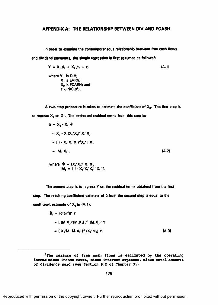
APPENDIX A: THE RELATIONSHIP BETWEEN DIV AND FCASH

In order to examine the contemporaneous relationship between free cash flows

and dividend payments, the simple regression is first assumed as follows’ :

Y * X ,^ , + X j^ , + e, (A.1)

where Y is DiV;X, is EARN;X, is FCASH; and e ~ N(O.o').

A two-step procedure is taken to estimate the coefficient of X,. The first step is

to regress X% on X,. The estimated residual terms from this step is:

Û = X j - X, ♦

= X; - X,(X,'X,) ’X,'X,

= ( I - X,|X,'X,) ’X,' I X,

- M, X, , (A.2)

where $ - |X,'X,) ’X,'X,M, - I ! - X,|X,'X,) ’X,' 1.

The second step is to regress Y on the residual terms obtained from the first

step. The resulting coefficient estimate of 0 from the second step is equal to the

coefficient estimate of X, in (A.1).

- (û'û)’û' Y

- [ |M,X,)'|M,Xa) r' (M,Xj)' Y

- ( X,'M, M,X, )•’ (X,'M,) Y. IA.3)

^The masure of free cash flows is estimated by the operating incom minus inccm taxes, minus interest expenses, minus total amounts of dividends paid (see Section B.2 of Chapter 3).

178


179

Substituting X, > X, • Y into (A.3),

ht - ( Xj'M, M,X, )•' (X, - V)' M, Y

- [ X,'M, M,Xj )•’ X,' M, Y - ( X,'M, M,X, ) ’ Y'M, Y. (A.4I

Since M, is an idempotent matrix,

M,* » M,; and

X,'M , - X / l I • X,(X,'X,) 'X ,' I

- X ,' - X,'X,(X,'X,| ’X,'

- X ,' - X,'

- 0 .

Thus,

ht - • (X,’M,X,1’ Y' M,Y < 0 . (A.5)

Now, let X , - X, - Y - X„ where X, may be interest expenses, and substitute

this constraint into (A.3).

ht - I X,'M, M,X, ]•' (X, - Y - X,)' M, Y

= (Xj'M, ' X,' M, Y - (Xj'M, M,Xjl ’ Y'M, Y • (X /M , M,X,1’ X,'M, Y.

= - (X,'M, M,X,I ’ Y'M, Y - [X,'M, M,X,) ’ X,'M, Y. (A.6)

The sign of the first term in equation (A.6) is always negative, but the sign of

the second term depends on the correlation between X, and Y. Then, it is not easy to

predict the sign of

Therefore, it is evident that, as more terms such as taxes are added to the

constraint, the sign of hi will be affected by the complex correlations between the

dependent variable and those elements in the constraint.


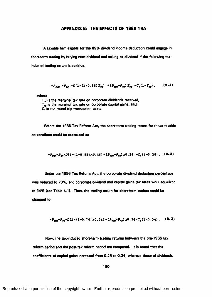
APPENDIX B: THE EFFECTS OF 1986 TRA

A taxable firm aligibla for tha 85% dividend income deduction could engage In

short-term trading by buying cum-dividend and selling ex-dividend if the following tax-

induced trading return is positive.

-fgu. +D[l-(l-0.85)T^] -Ccd-Tq,), (S.l)

whereTed ie the marginal tax rate on corporate dividends received,T„ is the marginal tax rate on corporate capital gains, and C, is the round trip transaction costs.

Before the 1986 Tax Reform Act, the short-term trading return for these taxable

corporations could be expressed as

♦(Pe^-P^)x0.28 -Cgll-O.Ze) . (B.2)

Under the 1986 Tax Reform Act, the corporate dividend deduction percentage

was reduced to 70%, and corporate dividend and capital gains tax rates were equalized

to 34% (see Table 4.1). Thus, the trading return for short-term traders could be

changed to

(1-0-70) XO. 34] 34-0,(1-0.34) . (B.3)

Now, the tax-induced short-term trading returns between the pre-1986 tax

reform period and the post-tax reform period are compared. It is noted that the

coefficients of capital gains increased from 0.28 to 0.34, whereas those of dividends

180


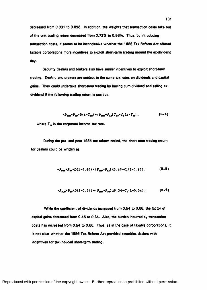
181

decreased from 0.931 to 0.898. In addition, the weights that transaction costs take out

of the unit trading return decreased from 0.72% to 0.66%. Thus, by introducing

transaction costs, it seems to be inconclusive whether the 1986 Tax Reform Act offered

taxable corporations more incentives to exploit short-term trading around the ex-dividend

day.

Security dealers and brokers also have similar incentives to exploit short-term

trading. Denier and brokers are subject to the same tax rates on dividends and capital

gains. They could undertake short-term trading by buying cum-dividend and selling ex-

dividend if the following trading return is positive.

*(PoM-P,ri r„-Ce(l-r„) , (B-4)

where T„ is the corporate income tax rate.

During the pre- and post-1986 tax reform period, the short-term trading return

for dealers could be written as

( 1 -0.46) + (f X O .46-Cg( 1 -0.46) . (B.5)

( 1 -0 .34) * ( XO . 34-C,( 1 -0.34) . (B.6)

While the coefficient of dividends increased from 0.54 to 0.66, the factor of

capital gains decreased from 0.46 to 0.34. Also, the burden incurred by transaction

costs has increased from 0.54 to 0.66. Thus, as in the case of taxable corporations, it

is not clear whether the 1986 Tax Reform Act provided securities dealers with

incentives for tax-induced short-term trading.


APPENDIX C: SIGNALLING MODEL'

A representative firm is modeled. Corporate management in the best interests of

current shareholders can make an investment of I, and pay a dividend of D. Funds for

both investment. I, and dividends, D, are obtained from either internally retained cash, C,

or net new shares of stock, N, which are issued at the ex dividend price per share, p„.

The constraint for a firm's sources and uses of funds is:

D + I - C + p„N. (C.1I

Suppose that Q is the number of shares outstanding before N shares are sold.

At the ex dividend day, current shareholders receive the dividend per share, (1-tlD/Q,

where t is a single tax rate on dividends. In equilibrium, the cum-dividend price per

share, p, is equal to the sum of the ex-dividend price por share, p^, and the after tax

dividend per share, (1-t)D/Q:

P * P., + <1-t) D/Q. (0.2)

Assume that management has strong incentives to signal for the firm's stock to

command a higher price in the market. This signalling is generally induced when the firm

issues new shares or current shareholders sell some fraction of their outstanding shares.

Suppose that the liquidity demand from the firm by its current shareholders is L. Current

shareholders can sell some portion of their shares either cum or ex-dividend to satisfy

their consumption needs. They are supposed to sell M outstanding shares to new

investors at the ex-dividend day. The liquidity supplied to these current shareholders is

measured by;

L « D p„ M. (C.3)

Management's objective is to maximize current shareholders' wealth. This can

be achieved by maximizing current shareholders' cash inflow, (1-t)D + p,M. Since the

Âppendix c proves the signalling model of John and Williams (1985).

182


183

current shareholders' equity in the firm is diluted after the sale of shares on both

personal and corporate account, the fractional equity of current shareholders is (Q-M) /

(Q + N), where M outstanding shares and N new shares are sold to new investors.

Therefore, the true present value of current shareholders' remaining equity is

X(Q-M)/(Q+N), where X is the present value of the future cash inflow (X is inside

information, known to insiders but not observed directly by outsiders).

Consequently, management's job is to select the optimal dividend, DIX), and net

new funds, p, N(X), which maximize the firm's present value to its current shareholders.

Q -MMax{ |1-t)D + p„M + X }. (0.4)D, p„N Q + N

Substituting the above constraints, (C D through (C.3), into the maximand (C.4),

we get the equivalent maximand:

From (C.3), p„M - L • D.

From (C.l), P „ N - D + I -C.

From (C.2), pQ = p„Q + (1-t)D,

P * p„Q + (1-t)D,

p«,Q ■ P • (1-t)D.

p„Q - p„M “ IP -(1-t)D ] - [ L-D] = P - D + tD -L + D

“ P + to - L.

P«Q + P«N “ IP -(1 -tD ) ] + I D +1 -C l = P - D +tD +D +1 -C

“ P + tD + I - C.

P«Q • P«M p„ (Q-M) P + tD - L

p„Q + p„N p« (Q+N) P + tO + I - C


184

Thus,Q -M

U ID, P, X) - |1-t)D + p„M +Q + N

P + to - L|1-t)D + (L-D) + ------------------------ X

P + tD + I - C

P + tD - LL - t D + ------------------------X. (C.5)

P + tD + I - C

In short, management's problem simplifies to deciding the optimal dividend DIX).

Max U |D,P,X). IC.6)D>0

If the firm's private attribute, X, were known to outsiders, then a market price,

P, would be equal to its true value, V. Substituting the value V into the maximand

IC.5), we get

V + tD - LV = I L- tD) + ------------------- X

V + tD + I - C

V * I V + tD + I - C ) - IL - tD ) * I V + tD + I -C)

+ I V + tD - L) X

V» + I tD + I -C) V I L-tD) V + IL-td) * I tD + I - Cl

+ V X + I tD - L) X

V* + [ iD + I - C - X - IL-td) 1 V - IL-tD)* ( tD + I -C-Xl

V* - [ IL-tD) + IC + X-l-tD) ] V + IL-tD)* I C + X-l-tDJ - 0

{ V - IL-tD) } { V - 1C + X - 1 -tD )) = 0

Thus,

V ID.XI » PIDIXI) - C + X - 1 - tD. IC.7)


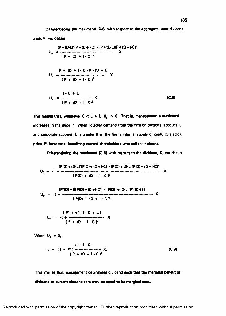
185

Oifferentiating the maximand (C.5) with respect to the aggregate, cum-dividend

price, P, we obtain

IP+tD-U'IP+tD + l-C) ■ (P+tD-U(P + tD + l-C)'

( P + tD + I - O *

P + tD + l - C - P - t D + L

( P + to + I - O*

l - C + LUp * ------ ---------— — X . (C.8)

I P + to + I - o *

This means that, whenever C < L + I, U, > 0 . That is, management's maximand

increases in the price P. When liquidity demand from the firm on personal account, L,

and corporate account. I, is greater than the firm's internal supply of cash, C, a stock

price, P, increases, benefiting current shareholders who sell their shares.

Differentiating the maximand (C.5) with respect to the dividend, D, we obtain

(P(D)+tD-Ll'(P(D)+tD + l-C) - (P(D)+tD-U(P(D) + tD + l-C)' Un ■ -t + ----

P(D) + tD + I - C ]*

[P'(D)+t](P(D)+tD + l-C] - (P(D) +tD-LI[P'(D) + t)

[ P(D) + tD + I - C )*

[ P' + 1 1 [ I - C + L ]Uo = -t + ---------------------------- X

( P + tD + I - C P

When Uo = 0,

L + I -Ct . ( t + P' ) X. (C.9)

( P + tD + I - C )*

This implies that management determines dividend such that the marginal benefit of

dividend to current shareholders may be equal to its marginal cost.


186Now, we substitute (C.7) into the first-order condition (C.9) for the

announcement effect.

From (C.9),

L + l-C L + l-Ct . t --------------X + P '-------------------- X

(P + tD + l-O* (P+tD + l-O*

L + l - C L + l -CP '-------------- X - t [ 1 ----------------------X ]

(P+tD + l-O* (P+tD + l-O*

P " (L + I - O X = t [ (P + tD + l-O* • (L + l-C) X 1

Since (P+tD + l-C) = X in (C.7),

P " (L + l-C) X - t [ X* - (L + l-C) X )

- f X * [ X - ( L + l - C ) 1

P'*(L +1-0 - 11 X - ( L + l-C) I

- t [ (P + tD + 1 - 0 - ( L + l-C) )

» t ( P + tO - L 1

( P + tD - L )P' - t -----------------

(L + l - C )

Thus, the dividend announcement effect is

PID(X)1 + tD(X) - LP'[D(X)1 - t --------------------------- . (C.10)

Finally, for the dividend signalling function, we substitute both (C.7) and the

derivative of (C.7) with respective to X into (C.l).


187

From (C.7), PID(X)j - C + X - 1 -tD.

P'[D(X)1* D IX) - 1 - tO'IX).

1 - tD'IX)P'(D(X)) --------------

□MX)

From (C.10).

1 ■ tD'(X) [C + X-l-tD(X)] + tO(X) - L

D'(X) I ■ C + L

(1-tD') (l-C+ L) = t D ' * ( (C + X-l-tD) +tD-L]

(1-tD') (l-C + L) - t D '* [ C + X - 1 - L )

( l-C + L ) - t D * ( (l-C + L) + (C + X-l-L) )

- tD * X.

l - C + LD' . (C.11)

tX

Integrating (C.l 1) subject to the condition (C.9) gives the optimal dividend condition.

1D(X) = — Max (l-C + L, 0) Ln(X). (C .l2)

t


VITA

Jaisik Gong has been a doctoral candidate in Finance at Louisiana State University from

1988 to 1992. His dissertation directed by Or. George M. Frankfurter encompasses three

leading issues in the anomaly of dividend policy: (1 ) the determinants of dividend policy; (2)

dividends, taxes, and portfolio choices; and (31 empirical tests of dividend signalling. While

pursuing his Ph.D. in Finance, he taught undergraduate courses including investments and

worked on financial databases at LSU. Immediately prior to joining LSU, he served in the

Korea Development Bank, Seoul, as bank economist from 1984 to 1987 and conducted

research in Euro-bonds, syndicated loans, and international banking. He earned his M.B.A.

in Accounting from Seoul National University in 1984 and received the B.A. degree from

Seoul National University in 1981.

188


DOCTORAL EXAMINATION AND DISSERTATION REPORT

Candidate: Jalslk Gong

Major Field: Business Administration (Finance)

Title of Diaaertation: Three Essays in Dividend Policy

Dean of the Grafluaiiuate School

ITTEE:

Date of Examination:

May 20, 1992


Three Essays in Dividend Policy. - LSU Digital Commons

Documents