Three Dimensional Microstructures: Statistical Analysis of Second Phase Particles in AA7075-T651

Three Dimensional Microstructures: Statistical Analysis of Second Phase Particles in AA7075-T651

Anthony D. Rollett1, a, Robert Campman1,b and David Saylor2,c 1 Department of Materials Science and Engineering

Carnegie Mellon University

5000 Forbes Avenue

Pittsburgh, PA 15213

2FDA-CDRH-OSEL

HFZ-150, Rm. 226

12725 Twinbrook Parkway

Rockville, MD 20852

arollett@andrew.cmu.edu, bcampman@andrew.cmu.edu, cdavid.saylor@fda.hhs.gov

Keywords: 3D Microstructures, statistical reconstruction, constituent particles,

aluminum alloys, pair correlation functions.

1. Abstract. This paper describes some aspects of reconstruction of microstructures

in three dimensions. A distinction is drawn between tomographic approaches that

seek to characterize specific volumes of material, either with or without diffraction,

and statistical approaches that focus on particular aspects of microstructure. A

specific example of the application of the statistical approach is given for an

aerospace aluminum alloy in which the distributions of coarse constituent particles are

modeled. Such distributions are useful for modeling fatigue crack initiation and

propagation.

2. Introduction

Most polycrystalline materials are self-evidently three dimensional with respect to

microstructure and yet characterization is generally confined to two dimensional

cross-sections. Clearly in order to progress with establishing microstructure-behavior

relationships, we need to be able to describe microstructures in all three dimensions.

This in turn, presupposes that we can make the descriptions suitable for use by

numerical systems such as finite element models, which entails detailed geometrical

descriptions. Many materials properties such as plasticity are strongly anisotropic and

this means that it is desirable to include crystallographic orientation (texture) in the

descriptions. One approach to the problem is to use tomography, which for metals

generally requires high energy x-rays from a synchrotron source [1, 2]. Such

investigations are relatively rare because of the expertise required to use such

instruments and the small number of suitable sources. Another approach is to use

serial sectioning that permits microstructure to be reconstructed in a straightforward

manner from the multiple cross sections through the material [3, 4]. The advent of

automated equipment is facilitating more frequent application but it remains a time

consuming process. The approach described here is to exploit statistical stereological

approaches, combined with reasonable assumptions about the microstructural features

of a particular material. In the example described here for an aerospace aluminum, the

relevant features in the polycrystalline microstructure are taken to be the grains and

the constituent particles. Statistical analysis of 3D grain structures has been described

elsewhere [5]. Analysis of the coarse particle content is also feasible but requires that

the clustering be quantified.

Aluminum alloy 7075, (AA7075), is a high strength aluminum alloy commonly used

for construction of airframes. The composition of AA7075 is listed in Table 1.

During the casting of the alloy, large (micron sized) second phase “constituent”

particles are precipitated out of solution. During hot rolling, these coarse particles are

broken up into smaller particles and “stringered” out through the matrix. These

constituents make up approximately 2% by volume of the total matrix. It has been

determined by several groups that the majority of the constituent particles are either

iron-aluminum compounds or magnesium silicide [6, 7]. During plastic deformation,

the non-deforming particles are sites of stress concentration in the matrix and many of

them eventually crack or debond from the matrix. Some of these cracked or

debonded particles will then produce a matrix crack and eventually lead to failure [8,

9]. The variation in placement, size, and concentration of these particles is a cause of

variation in the S-N curve [10,11] used to quantify fatigue behavior.

Knowing that the second phase particles play a crucial role in the fatigue crack

initiation their sizes and relative locations must be quantitatively determined before

crack initiation can be incorporated into any model. The current study uses pair

correlation functions, (PCF’s), to characterize the spatial distribution of the

constituent particles. The correlation statistics are then used in creation of a 3-D

digital microstructure, which can be subsequently meshed and used in a fatigue

simulation [12]. Although a specific application to fatigue in AA7075 is described

here, the analysis is general and can be applied to any similar material. This method

has been used previously, for example, to describe the clustering of recrystallization

nuclei [13]. Use of 2-point correlation statistics has been applied to composites and

other materials [14].

Table 1. Composition of AA7075; components listed in wt% Zn Mg Cu Fe Si Mn Cr Ti Other*

5.1-6.1 2.1-2.9 1.2-2.0 0.5 0.4 0.3 0.18-

0.28

0.2 0.15

*Other components may be present in quantities up to 0.05 wt%, but the total of all

other components may not exceed 0.15 wt%.

3. Experimental

The characterization of the material was performed by making sections on three

orthogonal planes. An alternate technique would have been to perform serial

sectioning on the sample. Serial sectioning can give detailed information of a specific

grain and/or particle in all three dimensions. The disadvantage of serial sectioning is

that it requires specialized equipment to ensure the accuracy of the depth for each

slice and it is an extremely time consuming process. Due to the limitations of the

equipment and time constraints, serial sectioning is generally used to analyze only one

or two grains. The method of observing three orthogonal planes can be accomplished

with equipment readily available in most metallography labs. Also significantly

larger areas can be characterized that include thousands of particles. The large area

scans on the three orthogonal planes makes it possible to determine average grain

sizes and particle distributions in all three dimensions using statistical methods.

3.1 Sample Preparation

Samples were all obtained from a bulk section of rolled AA 7075, which was

provided by the Alcoa Technical Center. The bulk material was two inches thick. It

was known that the composition of the bulk sample varied with depth. To limit the

number of variables in the study, each sample was cut from the bulk material to allow

for the observations to be made inch below the surface. Each sample was

progressively ground with SiC paper from 120 grit down to 1200 grit. After grinding

with SiC paper, the samples were polished with a 1 µm alumina suspension, followed

by a final polishing with a 0.05 µm silica suspension.

3.2 Image Analysis

Observations were made from images captured on a Nikon ME600 optical

microscope with Diagnostic Instrument’s RT Spot high resolution camera attached.

Images were taken at a resolution of 0.71 µm/pixel. A series of images was taken in a

regular overlapping grid pattern starting from a previously marked point. After the

first series of images was taken the sample was sonicated in methanol for 1 minute

and then a second series of images were obtained covering the same area. The two

sets of images were each stitched together via Adobe PhotoShop™. The purpose of

taking two images covering the same area was to be able to compare them and

determine if the observed particles were actually particles or dirt on the sample

surface. After all artifacts were digitally removed, the images were binarized. The

binarization of the images was accomplished by removing small sections of the large

image and setting a threshold value for that section. Each binarized section was

visually compared with the original to determine the optimum threshold setting. After

achieving the optimum threshold the section was then placed back into the large

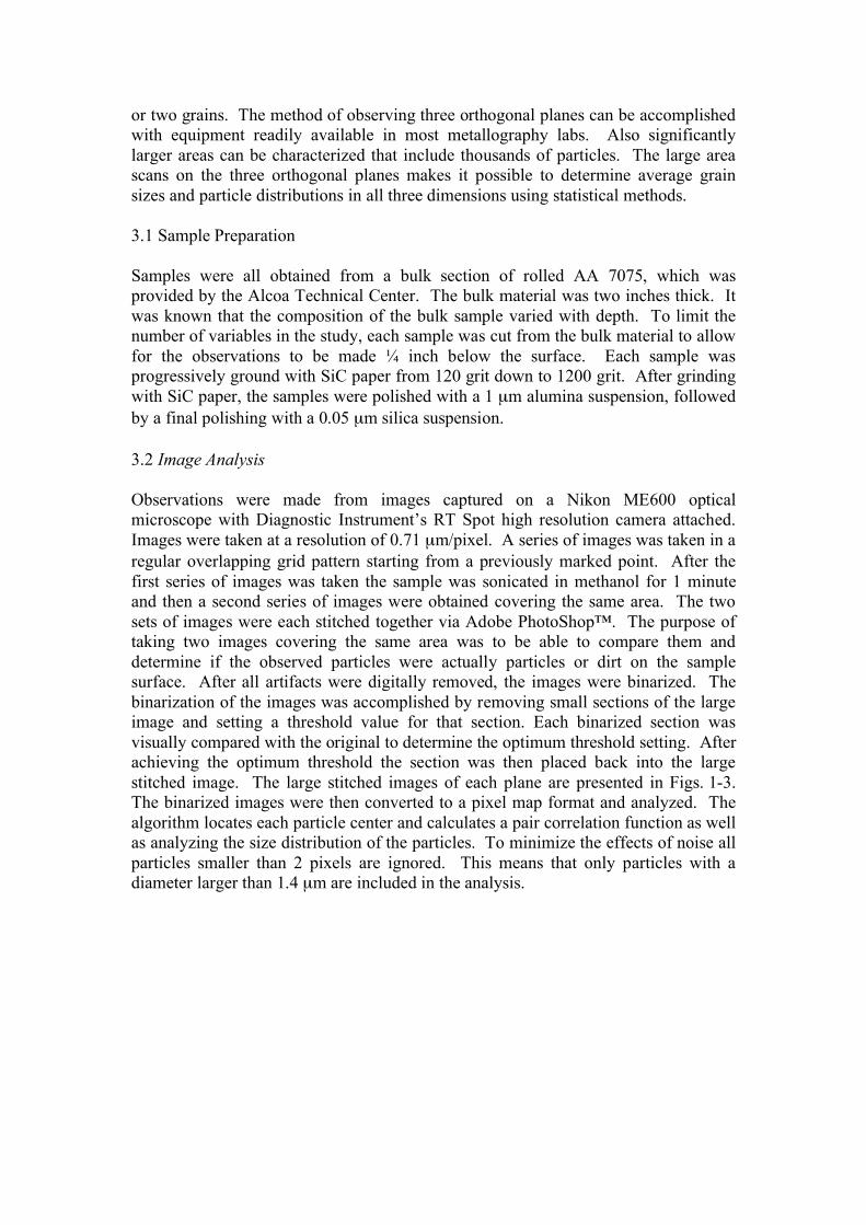
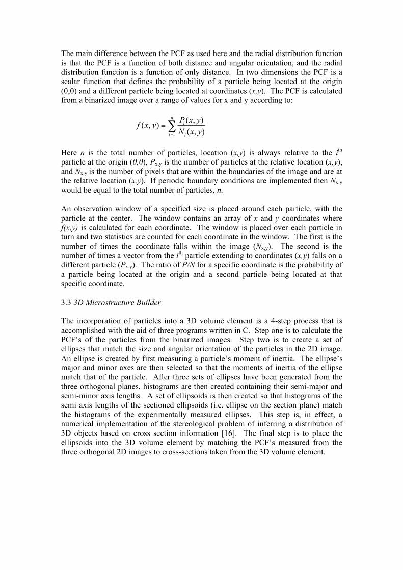
stitched image. The large stitched images of each plane are presented in Figs. 1-3.

The binarized images were then converted to a pixel map format and analyzed. The

algorithm locates each particle center and calculates a pair correlation function as well

as analyzing the size distribution of the particles. To minimize the effects of noise all

particles smaller than 2 pixels are ignored. This means that only particles with a

diameter larger than 1.4 µm are included in the analysis.

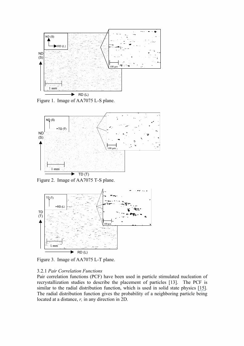
Figure 1. Image of AA7075 L-S plane.

Figure 2. Image of AA7075 T-S plane.

Figure 3. Image of AA7075 L-T plane.

3.2.1 Pair Correlation Functions

Pair correlation functions (PCF) have been used in particle stimulated nucleation of

recrystallization studies to describe the placement of particles [13]. The PCF is

similar to the radial distribution function, which is used in solid state physics [15].

The radial distribution function gives the probability of a neighboring particle being

located at a distance, r, in any direction in 2D.

RD (L)

TD (T)

TD (T)

ND (S)

RD (L)

ND (S)

RD (L)

ND (S)

The main difference between the PCF as used here and the radial distribution function

is that the PCF is a function of both distance and angular orientation, and the radial

distribution function is a function of only distance. In two dimensions the PCF is a

scalar function that defines the probability of a particle being located at the origin

(0,0) and a different particle being located at coordinates (x,y). The PCF is calculated

from a binarized image over a range of values for x and y according to:

=

=n

i i

i

yxN

yxPyxf

1 ),(

),(),(

Here n is the total number of particles, location (x,y) is always relative to the ith

particle at the origin (0,0), Px,y is the number of particles at the relative location (x,y),

and Nx,y is the number of pixels that are within the boundaries of the image and are at

the relative location (x,y). If periodic boundary conditions are implemented then Nx,y

would be equal to the total number of particles, n.

An observation window of a specified size is placed around each particle, with the

particle at the center. The window contains an array of x and y coordinates where

f(x,y) is calculated for each coordinate. The window is placed over each particle in

turn and two statistics are counted for each coordinate in the window. The first is the

number of times the coordinate falls within the image (Nx,y). The second is the

number of times a vector from the ith

particle extending to coordinates (x,y) falls on a

different particle (Px,y). The ratio of P/N for a specific coordinate is the probability of

a particle being located at the origin and a second particle being located at that

specific coordinate.

3.3 3D Microstructure Builder

The incorporation of particles into a 3D volume element is a 4-step process that is

accomplished with the aid of three programs written in C. Step one is to calculate the

PCF’s of the particles from the binarized images. Step two is to create a set of

ellipses that match the size and angular orientation of the particles in the 2D image.

An ellipse is created by first measuring a particle’s moment of inertia. The ellipse’s

major and minor axes are then selected so that the moments of inertia of the ellipse

match that of the particle. After three sets of ellipses have been generated from the

three orthogonal planes, histograms are then created containing their semi-major and

semi-minor axis lengths. A set of ellipsoids is then created so that histograms of the

semi axis lengths of the sectioned ellipsoids (i.e. ellipse on the section plane) match

the histograms of the experimentally measured ellipses. This step is, in effect, a

numerical implementation of the stereological problem of inferring a distribution of

3D objects based on cross section information [16]. The final step is to place the

ellipsoids into the 3D volume element by matching the PCF’s measured from the

three orthogonal 2D images to cross-sections taken from the 3D volume element.

4. Quantitative Characterization

4.1 Pair Correlation Functions

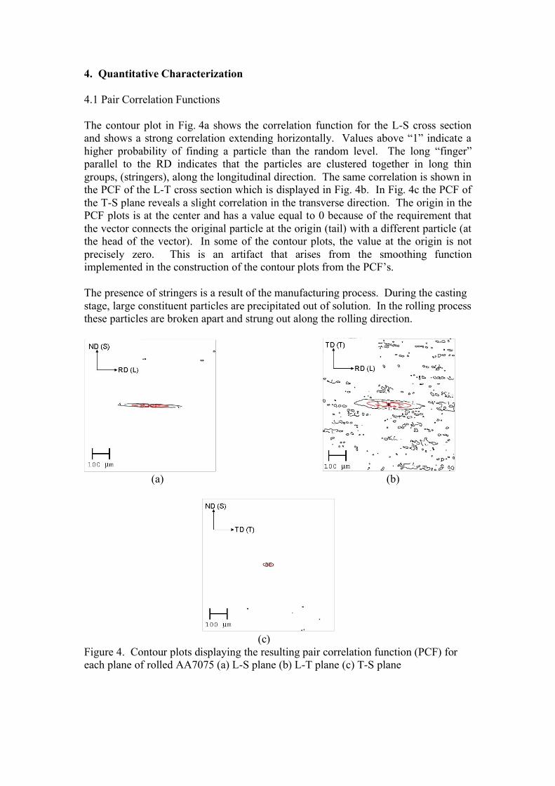
The contour plot in Fig. 4a shows the correlation function for the L-S cross section

and shows a strong correlation extending horizontally. Values above “1” indicate a

higher probability of finding a particle than the random level. The long “finger”

parallel to the RD indicates that the particles are clustered together in long thin

groups, (stringers), along the longitudinal direction. The same correlation is shown in

the PCF of the L-T cross section which is displayed in Fig. 4b. In Fig. 4c the PCF of

the T-S plane reveals a slight correlation in the transverse direction. The origin in the

PCF plots is at the center and has a value equal to 0 because of the requirement that

the vector connects the original particle at the origin (tail) with a different particle (at

the head of the vector). In some of the contour plots, the value at the origin is not

precisely zero. This is an artifact that arises from the smoothing function

implemented in the construction of the contour plots from the PCF’s.

The presence of stringers is a result of the manufacturing process. During the casting

stage, large constituent particles are precipitated out of solution. In the rolling process

these particles are broken apart and strung out along the rolling direction.

(a) (b)

(c)

Figure 4. Contour plots displaying the resulting pair correlation function (PCF) for

each plane of rolled AA7075 (a) L-S plane (b) L-T plane (c) T-S plane

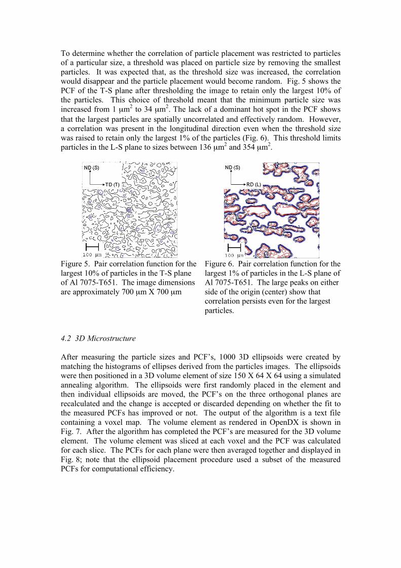
To determine whether the correlation of particle placement was restricted to particles

of a particular size, a threshold was placed on particle size by removing the smallest

particles. It was expected that, as the threshold size was increased, the correlation

would disappear and the particle placement would become random. Fig. 5 shows the

PCF of the T-S plane after thresholding the image to retain only the largest 10% of

the particles. This choice of threshold meant that the minimum particle size was

increased from 1 µm2 to 34 µm

2. The lack of a dominant hot spot in the PCF shows

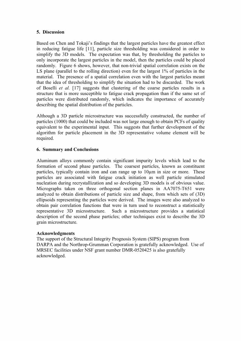
that the largest particles are spatially uncorrelated and effectively random. However,

a correlation was present in the longitudinal direction even when the threshold size

was raised to retain only the largest 1% of the particles (Fig. 6). This threshold limits

particles in the L-S plane to sizes between 136 µm2 and 354 µm

2.

Figure 5. Pair correlation function for the

largest 10% of particles in the T-S plane

of Al 7075-T651. The image dimensions

are approximately 700 µm X 700 µm

Figure 6. Pair correlation function for the

largest 1% of particles in the L-S plane of

Al 7075-T651. The large peaks on either

side of the origin (center) show that

correlation persists even for the largest

particles.

4.2 3D Microstructure

After measuring the particle sizes and PCF’s, 1000 3D ellipsoids were created by

matching the histograms of ellipses derived from the particles images. The ellipsoids

were then positioned in a 3D volume element of size 150 X 64 X 64 using a simulated

annealing algorithm. The ellipsoids were first randomly placed in the element and

then individual ellipsoids are moved, the PCF’s on the three orthogonal planes are

recalculated and the change is accepted or discarded depending on whether the fit to

the measured PCFs has improved or not. The output of the algorithm is a text file

containing a voxel map. The volume element as rendered in OpenDX is shown in

Fig. 7. After the algorithm has completed the PCF’s are measured for the 3D volume

element. The volume element was sliced at each voxel and the PCF was calculated

for each slice. The PCFs for each plane were then averaged together and displayed in

Fig. 8; note that the ellipsoid placement procedure used a subset of the measured

PCFs for computational efficiency.

Figure 7. Digital 3D element with particles placed based on matching the measured

PCF’s (Fig. 4).

(a) (b)

(c)

Figure 8. Average PCF’s of each plane in the constructed 3-D volume element (a) T-

S plane (b) L-S plane (c) L-T plane.

5. Discussion

Based on Chen and Tokaji’s findings that the largest particles have the greatest effect

in reducing fatigue life [11], particle size thresholding was considered in order to

simplify the 3D models. The expectation was that, by thresholding the particles to

only incorporate the largest particles in the model, then the particles could be placed

randomly. Figure 6 shows, however, that non-trivial spatial correlation exists on the

LS plane (parallel to the rolling direction) even for the largest 1% of particles in the

material. The presence of a spatial correlation even with the largest particles meant

that the idea of thresholding to simplify the situation had to be discarded. The work

of Boselli et al. [17] suggests that clustering of the coarse particles results in a

structure that is more susceptible to fatigue crack propagation than if the same set of

particles were distributed randomly, which indicates the importance of accurately

describing the spatial distribution of the particles.

Although a 3D particle microstructure was successfully constructed, the number of

particles (1000) that could be included was not large enough to obtain PCFs of quality

equivalent to the experimental input. This suggests that further development of the

algorithm for particle placement in the 3D representative volume element will be

required.

6. Summary and Conclusions

Aluminum alloys commonly contain significant impurity levels which lead to the

formation of second phase particles. The coarsest particles, known as constituent

particles, typically contain iron and can range up to 10 m in size or more. These

particles are associated with fatigue crack initiation as well particle stimulated

nucleation during recrystallization and so developing 3D models is of obvious value.

Micrographs taken on three orthogonal section planes in AA7075-T651 were

analyzed to obtain distributions of particle size and shape, from which sets of (3D)

ellipsoids representing the particles were derived. The images were also analyzed to

obtain pair correlation functions that were in turn used to reconstruct a statistically

representative 3D microstructure. Such a microstructure provides a statistical

description of the second phase particles; other techniques exist to describe the 3D

grain microstructure.

Acknowledgments

The support of the Structural Integrity Prognosis System (SIPS) program from

DARPA and the Northrop-Grumman Corporation is gratefully acknowledged. Use of

MRSEC facilities under NSF grant number DMR-0520425 is also gratefully

acknowledged.

References

[1] B. C. Larson, W. Yang, G. E. Ice, J. D. Budai, J. Z. Tischler: Nature Vol. 415,

(2002), p. 887.

[2] S. F. Nielsen, A. Wolf, H. F. Poulsen, M. Ohler, U. Lienert, R. A. Owen: J.

Synchrotron Radiation Vol. 7, (2000), p. 103.

[3] C. Y. Hung, G. Spanos, R. O. Rosenberg, M. V. Kral: Acta mater. Vol. 50,

(2002), p. 3781.

[4] J.E. Spowart, H.M. Mullens, B.T. Puchala: JOM Vol. 55, (2003), p. 35.

[5] D.M. Saylor, J. Fridy, B.S. El-Dasher, K.-Y. Jung, A.D. Rollett: Met. Mater.

Trans. Vol. 35A, (2004), p. 1969.

[6] K.M. Gruenberg, B.A. Craig, and B.M. Hillberry: AIAA Journal Vol. 37, No.

10 October, (1999) p. 1304.

[7] R.P. Wei, C. Liao, and M. Gao: Metall. Mater. Trans. A Vol. 20A, April,

(1998) p. 1153.

[8] G. Patton, C. Rinaldi, Y. Brechet, G. Lormand, R. Fougeres: Mater. Sci. Eng. Vol.

A254, (1998) p. 207.

[9] K. Tanaka and T. Mura: Metall. Trans. A Vol. 13A, (1982) p.117.

[10] N. Chawla, C. Andres, J.W. Jones, and J.E. Allison: Metall. Mater. Trans. A Vol.

29A, (1998) p. 2843.

[11] Z.Z. Chen, K. Tokaji: Materials Lett., 58, (2004) p. 2314.

[12] A. Ural, G. Heber, P.A. Wawrzynek, A.R. Ingraffea, D.G. Lewicki, J.B.C.

Neto: Eng. Fract. Mech. Vol. 72, (2005), p. 1148.

[13] K. Marthinsen, J.M. Fridy, T.N. Rouns, K.B. Lippert, and E. Nes: Scripta

Mater. Vol. 39 (1998), p. 1177-1183.

[14] A. M. Gokhale, A. Tewari, H. Garmestani: Scripta mater. Vol. 53, (2005), p.

989.

[15] S. Torquato: Random heterogeneous materials : microstructure and

macroscopic properties, (Springer, New York, 2002).

[16] E.E. Underwood: Quantitative Stereology, (Addison Wesley Publishing

Company, 1970).

[17] J. Boselli, P.D. Pitcher, P.J. Gregson, and I. Sinclair: Mater. Sci. Eng. Vol.

A300 (2001), p 72; ibid. p. 113.