Three-dimensional geological modelling of potential-field data

Computers & Geosciences 27 (2001) 455–465

Three-dimensional geological modelling of potential-fielddata$

Mark Jessell*

Department of Earth Sciences, Australian Geodynamics Cooperative Research Centre, Monash University, Clayton, VIC, 3168, Australia

Received 19 November 1998; received in revised form 24 February 1999; accepted 24 February 1999

Abstract

This paper reviews different ways potential-field modelling systems represent the 3D structure of the Earth’s crust. 3Dstructures may be represented by discrete objects, voxels, surfaces or as a kinematic history and each technique providesthe user with a different path through the model-building process and different abilities to honour the available

geological and geophysical observations. At present, no one system is capable of supporting the range of uses for whichpotential-field data are collected, and one emphasis for future development is the ability to translate between thedifferent representations that are used. # 2001 Elsevier Science Ltd. All rights reserved.

Keywords: Geophysics; Imaging

1. Introduction

Geologists have focussed over the last 200 years on

mapping the Earth’s surface, and in many parts of theworld this task still remains to be completed. High-resolution gravity and magnetic surveys have advanced

this process by allowing scattered geological observa-tions to be integrated into regional interpretations(Gunn, 1997 and references therein). The challenge forthe next generation of geological mapmakers is to

develop three- or even four-dimensional maps (i.e. thosethat include a time axis). The additional constraintsprovided by geophysical surveys will be extremely

important for this task. At present, seismic surveys inbasin settings and gravity and magnetic surveys in‘‘basement’’ terrains provide the most commonly

applied geophysical constraints. This paper focuses onthe techniques available for forward and inverse

modelling of potential-field data as applied to the taskof developing 3D crustal models.

The principles behind calculating the gravity-field

variations with the Earth’s crust were established in thelast century, and were successfully applied at that timeto continental scale issues such as isostasy. As ground

geophysical surveys became important tools for mineralexploration, new techniques allowed 2D models ofgeological structures to be constrained using the resultsof gravity and magnetic fields along individual profiles

(Nettleton, 1942). In the early 1980s, the development ofairborne surveying techniques for measuring magneticfields combined with the ability to display these data in

image formats (Hinze and Zietz, 1985), led to therecognition that these data provide important con-straints for regional-scale geological mapping. There are

now a plethora of modelling tools available for building2D and 3D geological models (excellent collections ofpapers can be found in Pflug and Harbaugh, 1992;Hamilton and Jones, 1992; Turner, 1992; Houlding,

1994) and in principle they all could use potential-fielddata as part of their inputs, or could be tested bypotential-field data sets.

The aim of this paper is to review the variousassumptions that underlie different modelling systems,

$Accompanying files on server at http://www.iamg.org/

CGEditor/index.htm

*Tel.: +61-3-990-54902; fax: +61-3-990-54903.

E-mail addresses: [email protected], mark

@earth.monash.edu.au (M. Jessell).

0098-3004/01/$ - see front matter # 2001 Elsevier Science Ltd. All rights reserved.

PII: S 0 0 9 8 - 3 0 0 4 ( 0 0 ) 0 0 1 4 2 - 4

and discuss the role that these tools have in developing3D geological models of the crust. Although there are

many valuable potential-field processing algorithms thataim to improve the quality (Luyendyk, 1997) or visualimpact of a data set (Milligan and Gunn, 1997), this

discussion is restricted to systems that involve aparametric description of the crustal geology, whichcan be directly applied to the problem of building 3Dmodels.

2. Modelling gravity and magnetic fields

In the context of building 3D crustal models, the

fundamental role of potential-field data is to provideconstraints on the distribution of relevant geophysicalrock properties. The interpretation of gravity and

magnetic data sets is highly ambiguous and as Nettletonemphasised in 1942:

Unless certain controls other than the gravity andmagnetic data are available the inherent ambiguities of

the physically possible distributions of material whichcan produce the observed effects make accuratecalculations meaningless even though the geophysical

data may be of any desired precision.

This point was amusingly re-stated by Hornby et al.(1997). It is therefore necessary to include other types ofinformation during the modelling process, either as

mathematical constraints on the types of models thatmay be built, or alternatively by including geologicalinformation during the model-building process. To

understand which constraints can be placed on relevantgeophysical rock-property distributions for gravity andmagnetic surveys, we need to briefly consider the

geological controls on these distributions.

2.1. Geological controls on geophysical rock properties

The three primary controls on the density, magnetic

susceptibility and remanent magentisation of a rockvolume are the original lithology, the structural evolu-tion, and the metamorphic and metasomatic mineral

assemblages. As a first-order approximation, lithologycontrols the density and magnetic properties via themineralogy (Clark, 1997), and sharp variations in rockproperties typically coincide with lithological contacts

(i.e. unconformities or intrusive contacts). Having saidthis, generally only part of a stratigraphic interval willhave a high magnetic susceptibility, so that a geophy-

sical rock-property map need not correlate directly withthe equivalent geological map. The structural evolutionof an area will change the position and orientation of

these contacts, and may introduce new ones (e.g. faults).The role of metamorphism and metasomatism is to alter

the mineralogy either locally (e.g. within shear zones, oras contact aureoles) or regionally (e.g. the gradual

densification associated with burial). Finally, individuallithologies may posses a remanent or anisotropiccomponent of magnetisation that may also be affected

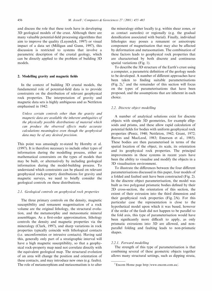
by deformation and metasomatism. The combination ofthese factors leads to geophysical rock properties thatare characterised by both discrete and continuousspatial variations (Fig. 1).

To describe the 3D structure of the Earth’s crust usinga computer, a parametric definition of the geology needsto be developed. A number of different approaches have

been taken to finding suitable parameterisations(Fig. 2),1 and the remainder of this section will focuson the types of parameterisations that have been

proposed, and the assumptions that are inherent in eachchoice.

2.2. Discrete object modelling

A number of analytical solutions exist for discreteobjects with simple 3D geometries, for example ellip-

soids and prisms, and these allow rapid calculation ofpotential fields for bodies with uniform geophysical rockproperties (Pentz, 1940; Nettleton, 1942; Grant, 1972;

Reeves and MacLeod, 1983; Emerson et al., 1985).These bodies are then parameterised in terms of thespatial location of the object, its scale, its orientationand its geophysical rock properties. The principal

improvements in these systems in recent years havebeen the ability to visualise and modify the objects in a3D visualisation environment.

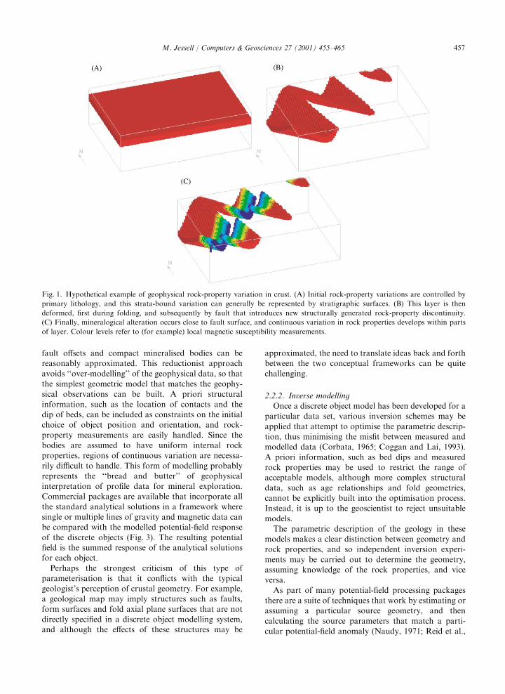
To illustrate the differences between the four differentparameterisations discussed in this paper, four models ofa folded and faulted unit have been constructed (Fig. 2).

In the discrete object parameterisation, the model wasbuilt as two polygonal prismatic bodies defined by their2D cross-section, the orientation of this section, the

extent of their extrusion into the third dimension andtheir geophysical rock properties (Fig. 2A). For thisparticular case the representation is close to thehypothetical model upon which it was based, however

if the strike of the fault did not happen to be parallel tothe fold axis, this type of parameterisation would havebeen significantly more difficult to apply, as only

prismatic extrusions into 3D are allowed, and non-parallel folding and faulting leads to non-prismaticshapes.

2.2.1. Forward modellingThe strength of this type of parameterisation is that

combining several of these geometric objects together

allows many structural settings, such as dipping strata,

1Encom Home page http:/www.encom.com.au/.

M. Jessell / Computers & Geosciences 27 (2001) 455–465456

fault offsets and compact mineralised bodies can bereasonably approximated. This reductionist approach

avoids ‘‘over-modelling’’ of the geophysical data, so thatthe simplest geometric model that matches the geophy-sical observations can be built. A priori structural

information, such as the location of contacts and thedip of beds, can be included as constraints on the initialchoice of object position and orientation, and rock-

property measurements are easily handled. Since thebodies are assumed to have uniform internal rockproperties, regions of continuous variation are necessa-

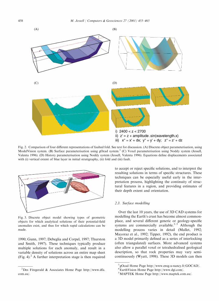
rily difficult to handle. This form of modelling probablyrepresents the ‘‘bread and butter’’ of geophysicalinterpretation of profile data for mineral exploration.Commercial packages are available that incorporate all

the standard analytical solutions in a framework wheresingle or multiple lines of gravity and magnetic data canbe compared with the modelled potential-field response

of the discrete objects (Fig. 3). The resulting potentialfield is the summed response of the analytical solutionsfor each object.

Perhaps the strongest criticism of this type ofparameterisation is that it conflicts with the typicalgeologist’s perception of crustal geometry. For example,a geological map may imply structures such as faults,

form surfaces and fold axial plane surfaces that are notdirectly specified in a discrete object modelling system,and although the effects of these structures may be

approximated, the need to translate ideas back and forthbetween the two conceptual frameworks can be quite

challenging.

2.2.2. Inverse modellingOnce a discrete object model has been developed for a

particular data set, various inversion schemes may be

applied that attempt to optimise the parametric descrip-tion, thus minimising the misfit between measured andmodelled data (Corbata, 1965; Coggan and Lai, 1993).

A priori information, such as bed dips and measuredrock properties may be used to restrict the range ofacceptable models, although more complex structural

data, such as age relationships and fold geometries,cannot be explicitly built into the optimisation process.Instead, it is up to the geoscientist to reject unsuitable

models.The parametric description of the geology in these

models makes a clear distinction between geometry androck properties, and so independent inversion experi-

ments may be carried out to determine the geometry,assuming knowledge of the rock properties, and viceversa.

As part of many potential-field processing packagesthere are a suite of techniques that work by estimating orassuming a particular source geometry, and then

calculating the source parameters that match a parti-cular potential-field anomaly (Naudy, 1971; Reid et al.,

Fig. 1. Hypothetical example of geophysical rock-property variation in crust. (A) Initial rock-property variations are controlled by

primary lithology, and this strata-bound variation can generally be represented by stratigraphic surfaces. (B) This layer is then

deformed, first during folding, and subsequently by fault that introduces new structurally generated rock-property discontinuity.

(C) Finally, mineralogical alteration occurs close to fault surface, and continuous variation in rock properties develops within parts

of layer. Colour levels refer to (for example) local magnetic susceptibility measurements.

M. Jessell / Computers & Geosciences 27 (2001) 455–465 457

1990; Gunn, 1997; Debeglia and Corpel, 1997; Thurstonand Smith, 1997). These techniques typically produce

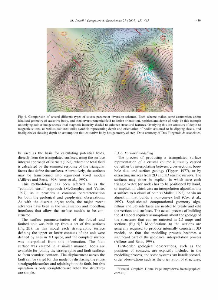
multiple solutions for each anomaly, and result in avariable density of solutions across an entire map sheet(Fig. 4).2 A further interpretation stage is then required

to accept or reject specific solutions, and to interpret theresulting solutions in terms of specific structures. These

techniques can be especially useful early in the inter-pretation process, highlighting the continuity of struc-tural features in a region, and providing estimates of

their depth extent and orientation.

2.3. Surface modelling

Over the last 10 years, the use of 3D CAD systems formodelling the Earth’s crust has become almost common-

place, and several different generic or geology-specificsystems are commercially available.3–5 Although themodelling process varies in detail (Mallet, 1992;

Mayoraz et al., 1992; Tipper, 1992), the end product isa 3D model primarily defined as a series of interlocking(often triangulated) surfaces. More advanced systems

also allow a parallel voxel or tetrahedralised geologicaldescription, so that rock properties may vary semi-continuously (Wyatt, 1998). These 3D models can then

Fig. 2. Comparison of four different representations of faulted fold. See text for discussion. (A) Discrete object parameterisation, using

ModelVision system. (B) Surface parameterisation using gOcad system.3 (C) Voxel parameterisation using Noddy system (Jessell,

Valenta 1996). (D) History parameterisation using Noddy system (Jessell, Valenta 1996). Equations define displacements associated

with (i) vertical extent of blue layer in initial stratigraphy, (ii) fold and (iii) fault.

Fig. 3. Discrete object model showing types of geometric

objects for which analytical solutions of their potential-field

anomalies exist, and thus for which rapid calculations can be

made.

2Des Fitzgerald & Associates Home Page http://www.dfa.

com.au/.

3 gOcad Home Page http://www.ensg.u-nancy.fr/GOCAD/.4EarthVision Home Page http://www.dgi.com/.5MAPTEK Home Page http://www.maptek.com.au/.


be used as the basis for calculating potential fields,directly from the triangulated surfaces, using the surface

integral approach of Barnett (1976), where the total fieldis calculated by the summed response of the triangularfacets that define the surfaces. Alternatively, the surfaces

may be transformed into equivalent voxel models(Ailleres and Betts, 1998; Ames et al., 1997).

This methodology has been referred to as the

‘‘common earth’’ approach (McGaughey and Vallee,1997), as it provides a common parameterisationfor both the geological and geophysical observations.

As with the discrete object tools, the major recentadvances have been in the visualisation and modellinginterfaces that allow the surface models to be con-structed.

The surface parameterisation of the folded andfaulted unit was built up from a set of five surfaces(Fig. 2B). In this model each stratigraphic surface

defining the upper or lower contacts of the unit weredefined by lines in 3D space, and the complete surfacewas interpolated from this information. The fault

surface was created in a similar manner. Tools areavailable for joining the stratigraphic and fault surfacesto form seamless contacts. The displacement across the

fault can be varied for this model by displacing the entirestratigraphic surface and rejoining it to the fault, but thisoperation is only straightforward when the structuresare simple.

2.3.1. Forward modellingThe process of producing a triangulated surface

representation of a crustal volume is usually carriedout either by interpolating between cross-sections, bore-hole data and surface geology (Tipper, 1977), or by

extracting surfaces from 2D and 3D seismic surveys. Thesurfaces may either be explicit, in which case eachtriangle vertex (or node) has to be positioned by hand,

or implicit, in which case an interpolation algorithm fitsa surface to a cloud of points (Mallet, 1992), or via analgorithm that builds a non-convex hull (Cox et al.,

1997). Sophisticated computational geometry algo-rithms and 3D interfaces are needed to create and editthe vertices and surfaces. The actual process of buildingthe 3D model requires assumptions about the geology of

the structures that can go untested in 2D maps andsections (Fig. 5).6 Modifications to the sections aregenerally required to produce internally consistent 3D

models, so that the modelling process becomes asignificant part of the geological interpretation process(Ailleres and Betts, 1998).

First-order geological observations, such as thepositions of contacts, are explicitly included in themodelling process, and some systems can handle second-

order observations such as the orientation of structures,

Fig. 4. Comparison of several different types of source-parameter inversion schemes. Each scheme makes some assumption about

idealised geometry of causative body, and then inverts potential field to derive orientation, position and depth of body. In this example

underlying colour image shows total magnetic intensity shaded to enhance structural features. Overlying this are contours of depth to

magnetic source, as well as coloured strike symbols representing depth and orientation of bodies assumed to be dipping sheets, and

finally circles showing depth on assumption that causative body has geometry of step. Data courtesy of Des Fitzgerald & Associates.

6Fractal Graphics Home Page http://www.fractalgraphics.

com.au/.


although the visualisation and integration of these typesof observations remains an area of fundamental research

(DeKemp, 1998). Some modelling systems, such asEarthVision,4 assume a fundamental stratigraphy andhierarchy of faults to handle complex fault arrays, and

although this may be appropriate in the basin settingsthat many of the modelling packages were originallydeveloped for, they are somewhat limiting in hard rockterrains. One of the major strengths of this type of model

is that it can become the repository for all the geologicaland geophysical observations made for an area, and ifthe models are linked to a GIS, can form the core of a

general geoscience data-manipulation system. However,the modification of a model following acquisition of newdata can be difficult, especially for explicit modelling

systems, and thus they do not lend themselves toscenario modelling, in which a range of conceptualmodels need to be tested. The turn-around time fordeveloping a 3D model of a complex region is very high

compared to the time taken to calculate the potentialfields, so the direct constraints provided by thepotential-field modelling only become available rela-

tively late in the modelling process.

2.3.2. Inverse modellingInversion schemes associated with surface parameter-

isations are common in 2D systems (Phillips, 1997),7 andequivalent 3D systems are currently being developed.However, since the parameterisation consists of a very

large number of nodes, it is generally best to invert smallsubsets of these nodes at any one time. Trying to allowcompletely free inversion of all nodes and rock proper-ties simultaneously would probably lead to a complete

loss of the original (and probably fairly accurate)structure.

2.4. Voxel modelling

An alternative to the surface modelling approach to

modelling rock-property variations in 3D is to dividespace into a regular 3D grid, and assign rock propertiesto each position (voxel) in the grid (Mueller and Morris,

1995; Tchernychev and Makris, 1996; Bosch, 1998).Voxel models handle continuously varying rock proper-ties; however, sharp discontinuities reveal the underlyingvoxel boundaries unless a very fine grid resolution is

used, with resulting increase in calculation time. Unlikediscrete object and surface models, voxel models do notseparate the geometric and rock-property parameterisa-

tions, as the geometry is only defined by considering theproperties at each voxel. Voxel, or block models, areoften used for ore reserve estimation (Hamilton and

Didur, 1992).The voxel model of the folded and faulted unit

(Fig. 2C) shows the individual cubes that form the

model, with the cubes from the upper layer madeinvisible. Many surface and history modelling systemsare capable of producing voxel models from their nativerepresentation. In this example, the folded and faulted

unit is represented by a set of cubes with identicalgeophysical rock properties, although there is no need(except for the sake of computational efficiency) for any

two cubes to share the same properties. Once created,these voxel models are hard to modify in a systematicmanner.

2.4.1. Forward modellingOne of the advantages of this type of model is that the

geophysical calculations are independent of the modelcomplexity, and can include geophysical rock propertiesthat vary within lithologies. The potential-field responseis calculated as the summed response of the analytical

solution for a dipping prism, treating each voxel as oneprism (Hjelt, 1972, 1974). These calculations can also beperformed in the Fourier domain (Oldenburg, 1974),

which significantly speeds up the calculation, althoughboundary effects must be handled in a more complex

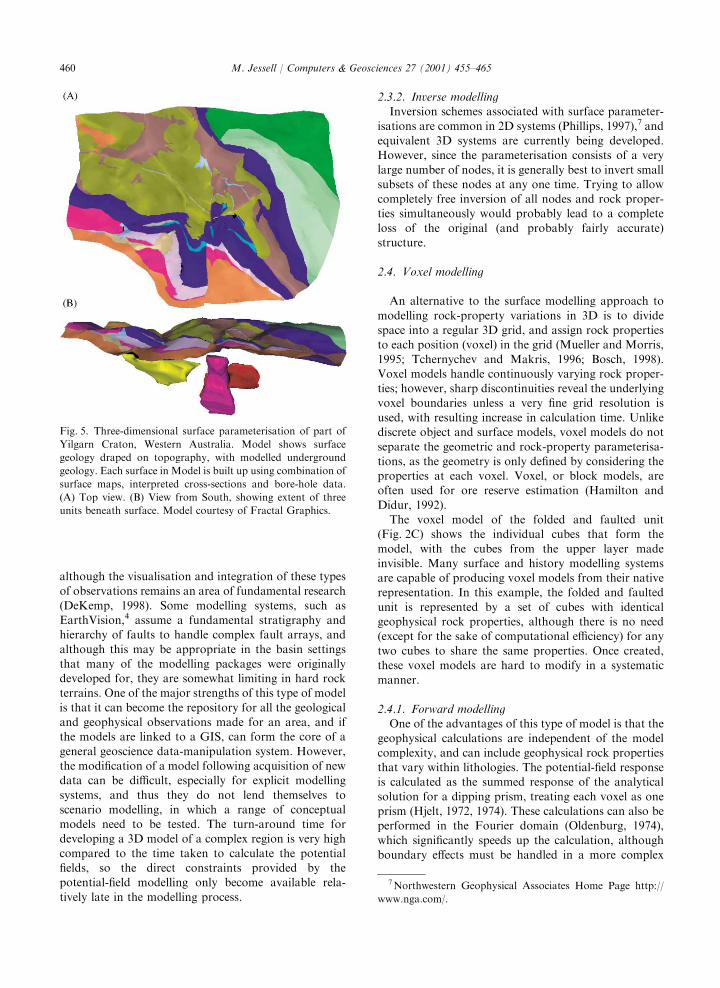
Fig. 5. Three-dimensional surface parameterisation of part of

Yilgarn Craton, Western Australia. Model shows surface

geology draped on topography, with modelled underground

geology. Each surface in Model is built up using combination of

surface maps, interpreted cross-sections and bore-hole data.

(A) Top view. (B) View from South, showing extent of three

units beneath surface. Model courtesy of Fractal Graphics.

7Northwestern Geophysical Associates Home Page http://

www.nga.com/.


manner. The real difficulty associated with a pure voxelmodelling system is at the model-building stage, when

the model must be treated as a series of parallel grids,and each row, column or layer in the 3D grid has to beassigned rock properties. As mentioned in the previous

section, surface models can be converted into voxelmodels as a step towards performing the geophysicalcalculations. Perhaps the best application of voxelmodelling is when dense rock property measurements

are already available, such as at the development stageof a mine, or when a seismic velocity–density correlationcan be made.8 In these situations the rock properties

commonly vary smoothly, so that geostatistical inter-polation techniques may be used (Houlding, 1994,Chapter 8), resulting in a complete voxel model of rock

properties, which may then be used to calculate thepotential-fields.

2.4.2. Inverse modelling

Voxel parameterisation of geology has provided thebasis for a number of different inversion schemes, inwhich the rock properties associated with each voxel act

as the parameters to be optimised (Li and Oldenburg,1996a, 1998; Pilkington, 1997; Boschetti et al., 1997;Bosch, 1998).9 To reduce the search space for theoptimisation schemes, a number of assumptions are

made as to the nature of the rock-property variations.The most important of these is the assumption of asmoothness constraint, which preferentially weights

solutions that minimise the rock-property variationsbetween neighbouring voxels. The resulting models havesmoothly varying rock-property variations, and if a

model with sharp boundaries is required, a manual re-interpretation must be made (Oldenburg et al., 1997).Solutions can also be weighted according to rock-property observations made at known locations, and in

principle complete starting models may be built andused as a constraint. However, if too many constraintsare applied the model may not be able to vary

significantly from the starting configuration. As withsurface modelling inversion schemes, a priori second-order structural data such as dips are not generally

incorporated as a constraints to the inversion process,although Li and Oldenburg (1996b) have recentlysuggested one mechanism whereby this may be achieved.

A different approach has been taken by Farrell (1998),who uses the boundaries between contiguous volumes ofvoxels with similar properties to mimic a surface modelinversion scheme. In this scheme, individual voxels at

boundaries between rock types can switch values in a

Monte Carlo scheme reminiscent of the Ising modelsused in magnetic domain behaviour simulations (Chand-

ler, 1987). This scheme assumes that a complete 3Dvoxel model has been built, and that the model isdominated by sharp changes in rock properties.

2.5. History modelling

A fundamental goal of many geological studies is to

interpret the geological observations in terms of achronological history, and a number of modellingsystems have been developed to investigate aspects of

these histories. In these systems the parameterisation ispartly geometric, and partly kinematic, so that kine-matic events act upon pre-existing geometries. Some ofthese were developed to perform structural reconstruc-

tions starting from the current geological state, to testthe consistency of these models.10,11 Others (Jessell,1981; Perrin et al., 1988; Jessell and Valenta, 1996) are

aimed at building conceptual models to test ideas aboutthe 3D structure in areas where direct observationalconstraints are limited, and it is this type of system that

has been applied to the potential-field modellingproblem.

The folded and faulted unit is represented as a set ofequations in the history parameterisation (Fig. 2D).

These equations define the initial position of the unit,and the displacements associated with the folding andfaulting events. As a consequence, changing the

orientation, position or scale of the fault does notimpose any overhead beyond the actual model re-calculation. However, it can be more difficult to make

direct use of geological observations during the model-ling process.

2.5.1. Forward modelling

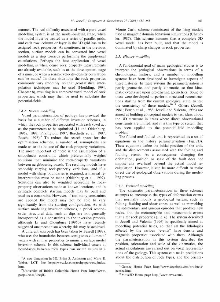
The kinematic parameterisation in these schemesattempts to encompass the types of deformation eventsthat normally modify a geological terrain, such as

folding, faulting and shear zones, as well as mimickingthe sedimentary and igneous episodes that produce newrocks, and the metamorphic and metasomatic eventsthat alter rock properties (Fig. 6). The system described

in Jessell and Valenta (1996) is specifically aimed atmodelling potential fields, so that all the lithologiesaffected by the various ‘‘events’’ have density and

magnetic properties associated with them. Althoughthe parameterisation in this system describes theposition, orientation and scale of the kinematics, the

actual calculations are carried out on voxel representa-tions of the geology. This system can make predictionsabout the distribution of rock types, and the orienta-8A new dimension in 3D, Brian S. Anderson and Mark E.

Weber, LCT, Inc http://www.lct.com/techpapers/otc/index.

htm.9University of British Columbia Home Page http://www.

geop.ubc.ca/ubcgif/.

10Geosec Home Page http://www.cogniseis.com/products/

geosec.htm.11Move3D Home page http://www.mve.com/.


tions of structures in 3D, together with their resultingpotential fields.12 Some geological constraints such as

fault orientation, and age relationships between struc-tures, can be explicitly input into the modelling process;however the system does not currently lend itself to

direct inclusion of large amounts of detailed geologicalinformation. One advantage of this system is that themodel parameterisation coincides closely with the typeof geological information sought as output of the

modelling process, such as the sense and amount ofdisplacement on a fault. Even though this approachminimises the number of parameters needed to describe

a 3D structure, there are still a large number of possible

models that may result from the superimposition of eventwo or three deformation events.

2.5.2. Inverse modelling

The modelling of deformation kinematics has beenrecently used as part of a potential-field inversionscheme by Farrell (1998), who used a genetic algorithmto search through the possible combinations of para-

meters. At present, this inversion scheme only considersthe potential fields for the cost function to determine thequality of the match between model and observation,

and it assumes a fixed order and type of events. There isno reason that a penalty function based on comparingthe geological predictions could not also be added, and

the work of Simmons (1992) and Flewelling et al. (1992)suggests that it may also be feasible to allow the order of

Fig. 6. Noddy sequence showing evolution of part of Pine Creek Geosyncline, Northern Territory, Australia. History consists of:

(A) deposition of flat-lying sediments; (B) NW-SE trending folds; (C) intrusion of granite bodies in NW and SW; (D) shearing of sedi-

ments against granites, and finally (E) gentle folding around steeply plunging fold axis. (F) Resulting magnetic image calculated from

final stage of model.

12Atlas of Structural Geophysics http://www.earth.monash.

edu.au/AGCRC/ASG/.


events to vary freely. Farrell (1998) demonstrated thatthe inversion of kinematic models can be more efficient if

each event is inverted individually, and the work ofRouby et al. (1993) and Gratier et al. (1991) shows howmore sophisticated inversion schemes may be applied to

specific structural problems.

3. Discussion and conclusions

If we look back over the last 20 years, it is apparentthat the equations needed to perform potential-field

calculations were already in place for all of theparametric descriptions discussed in this paper. Withthe exception of the history parameterisation, potential-

field modelling systems based on these equations alsoexisted. The major advances in those systems have comein the ability to visualise and manipulate the models in

3D, and the implementation of more robust inversionschemes.

Geological contacts, the gravity field, and themagnetic field together provide three distinct sets of

observations that can be used to constrain the 3Dstructure, and therefore systems that simultaneouslymodel all three types of information should in principle

provide less ambiguous solutions. At the same time thelithological, density and magnetic distributions will infact not vary in exactly the same ways. As a result, any

given model is likely to honour the potential-fields andgeological observations to differing degrees, so anindividual geoscientist must place different notional

weighting on the degree of matching required betweengeological and geophysical models and the primaryobservations. The four types of modelling schemesdiscussed in this paper tend to inherently weight the

geological and geophysical observations differently.Voxel inversion schemes, at one extreme, are able toproduce 3D rock-property distributions that result in

potential fields that reproduce all the detail of anobserved geophysical data set; however, they may onlymatch the geological observations in a schematic way.

At the other extreme, surface modelling systems are ableto match geological observations (at a given scale) verywell, but the resulting potential field models may still not

be all that similar. The discrete object and historyparameterisations typically produce ‘‘compromise’’models that may fit both the geological and potential-field observations well, but not perfectly.

The choice of which parameterisation to use dependson both the goals of the modelling exercise and theavailability of external constraints. Tools that use a

discrete object or history parameterisation will typicallybe applied to problems where conceptual models need tobe developed and compared. Model construction and

potential-field calculation with these tools is rapid, sothat different 3D models can be easily compared. In

contrast, as the final repository for all availablegeological information, combined surface/voxel model-

ling tools provide a means of building complex 3Dmodels and simultaneously allowing visualisation ofmultiple attributes. Unfortunately, the time taken to

build the 3D models is much longer, so that multiplemodels will probably not be built to test alternatehypotheses.

Owing to the different strengths of the various

approaches, the choice of modelling scheme may notonly vary according to the nature of the project, butseveral techniques will commonly need to be combined

to extract the maximum amount of information fromthe data. A typical project may involve a period ofdetailed modelling of single structures using a concep-

tual modelling system, prior to a regional modelconstruction phase using a surface modelling approach.It thus becomes increasingly important to be able to

convert models built in one system to a format suitablefor another. For example, a model built by a discreteobject modelling system should be exportable to asurface modelling scheme, and custom solutions for this

task do exist (Caleb Ames, pers. comm., 1998).Future potential-field modelling systems will combine

elements of the four parametric descriptions found in

this paper, or at least provide links so that the differenttasks required of potential-field data can be dealt withmore easily. It is also likely that as other geophysical

techniques such as the electromagnetic methods aredeveloped further, more complex parametric descrip-tions will become appropriate, and unified descriptionsof the crustal structure will be built using the multiple

geological and geophysical constraints then available.

Acknowledgements

I would like to thank Laurent Ailleres, Caleb Ames,

Des Fitzgerald and Associates Pty Ltd, and FractalGraphics Pty Ltd for permission to reproduce themodels and illustrations they have developed. I would

also like to thank Scott Johnson for translating thismanuscript into English. This paper is published withthe permission of the Director of the AustralianGeodynamics Cooperative Research Centre.

References

Ailleres, L., Betts, P., 1998. Geometrical and geophysical

modelling of an inverted Middle Proterozoic fault system,

Mount Isa Terrain, Australia. Conference Abstracts: 3D

Modelling of Natural Objects: a Challenge for the 2000,

Vol. 2. Nancy, France, 4–5th June.

Ames, C., Jessell, M.W., Valenta, R.K., 1997. Three-dimen-

sional geological and magnetic modelling, Isa Valley,


Queensland, Australia. Extended Abstracts, Society of

Exploration Geophysics Annual Meeting, Dallas.

Barnett, C.T., 1976. Theoretical modeling of the magnetic and

gravitational fields of an arbitrarily shaped three-dimensional

body. Geophysics 41, 1353–1364.

Bosch, M., 1998. Lithologic tomography: method and applica-

tion to the Cote dıArmor region (France). Conference

Abstracts: 3D Modelling of Natural Objects: a Challenge

for the 2000, Vol. 2. Nancy, France, 4–5th June.

Boschetti, F., Dentith, M., List, R., 1997. Inversion of

potential-field data by genetic algorithms. Geophysical

Prospecting 45, 461–478.

Chandler, D., 1987. Introduction to Modern Statistical

Mechanics. Oxford University Press, New York, 274pp.

Clark, D.A., 1997. Magnetic petrophysics and magnetic

petrology: aids to geological interpretation of magnetic

surveys. Australian Geological Survey Organisation Journal

of Australian Geology and Geophysics 17 (2), 83–103.

Coggan, J., Lai, J., 1993. 3D magnetic model inversion for

structure mapping. Exploration Geophysics 24, 415–428.

Corbata, C.E., 1965. A least-squares procedure for gravity

interpretation. Geophysics 30, 228–233.

Cox, S.J.D., Hornby, P., Watson, D., Gunn, C., 1997. 3D

complex geology modelling. Geodynamics and Ore Deposits

Conference. Australian Geodynamics Cooperative Research

Centre, Ballarat, Victoria, pp. 76–79.

Debeglia, N., Corpel, J., 1997. Automatic 3-D interpretation of

potential field data using analytic signal derivatives. Geo-

physics 62, 87–96.

DeKemp, E.A., 1998. Three-dimensional projection of curvi-

linear geological features through direction cosine interpola-

tion of structural field observations. Computers &

Geosciences 24 (3), 269–284.

Emerson, D.W., Clark, D.A., Saul, S.J., 1985. Magnetic

exploration models incorporating remanence, demagnetiza-

tion and anisotropy } HP 41C handheld computer

algorithms. Experimental Geophysics 16 (1), 1–122.

Farrell, S.M., 1998. Gamin; a new approach to the inversion of

geological and potential field data. PhD Dissertation,

Monash University, Melbourne, Australia.

Flewelling, D.M., Frank, A.U., Egenhofer, M.J., 1992. Con-

structing geologic cross-sections with a chronology of

geologic events. Proceedings of the 5th International

Symposium on Spatial Data Handling, Charleston SC,

USA, pp. 544–553.

Grant, F.S., 1972. Review of data processing and interpretation

methods in gravity and magnetics, 1964–1971. Geophysics

37, 647–661.

Gratier, J.-P., Guillier, B., Delorme, A., Odoinne, F., 1991.

Restoration and balance of a folded and faulted surface by

best-fitting of finite elements: principle and applications.

Journal of Structural Geology 13, 111–115.

Gunn, P.J., 1997. Quantitative methods for interpreting aero-

magnetic data. Australian Geological Survey Organisation

Journal of Australian Geology and Geophysics 17, 105–114.

Hamilton, D.E., Didur, R.S., 1992. Three-dimensional geologic

block modeling of the Kutcho Creek massive sulphide

deposit, British Columbia. In: Hamilton, D.E., Jones, T.A.

(Eds.), Computer Modeling of Geologic Surfaces and

Volumes. AAPG Computer Applications in Geology,

No. 1, pp. 203–218.

Hamilton, D.E., Jones, T.A. (Eds.), 1992. Computer Modeling

of Geologic Surfaces and Volumes. AAPG Computer

Applications in Geology, No. 1, 297pp.

Hinze, W.J., Zietz, I., 1985. The composite magnetic-anomaly

map of the conterminous United States. In: Heintz, W.J.

(Ed.), The Utility of Regional Gravity and Magnetic

Anomaly Maps. Society of Exploration Geophysics, Tulsa

Oklahoma, pp. 1–24.

Hjelt, S.E., 1972. Magnetostatic anomalies of dipping prisms.

Geoexploration 10, 239–246.

Hjelt, S.E., 1974. The gravity anomaly of a dipping prism.

Geoexploration 12, 29–39.

Hornby, P., Horowitz, F., Boschetti, F., Archibald, N., 1997.

Inferring geology from geophysics. Abstracts Geodynamics

and Ore Deposits Conference. Australian Geodynamics

Cooperative Research Centre, Ballarat, Victoria, pp. 120–122.

Houlding, S.W., 1994. 3D Geoscience Modeling. Springer,

Berlin, 309pp.

Jessell, M.W., 1981. Noddy } an interactive map creation

package. MSc Thesis, University of London, England.

Jessell, M.W., Valenta, R.K., 1996. Structural geophysics:

integrated stuctural and geophysical mapping. In: DePaor,

D. (Ed.), Structural Geology and Personal Computers.

Elsevier, Oxford, pp. 303–324.

Li, Y., Oldenburg, D.W., 1996a. 3-D inversion of magnetic

data. Geophysics 61, 394–408.

Li, Y., Oldenburg, D.W., 1996b, Incorporating geological dip

information into geophysical inversions, 66th Annual

International Meeting of Society Exploration Geophysics,

Expanded Abstracts, pp. 1290–1293.

Li, Y., Oldenburg, D.W., 1998. 3-D inversion of gravity data.

Geophysics 63, 109–119.

Luyendyk, A.P.J., 1997. Processing of airborne magnetic data.

Australian Geological Survey Organisation Journal of

Australian Geology and Geophysics 17, 31–38.

Mallet, J.-L., 1992. Discrete smooth interpolation in geometric

modelling. Computer Aided Design 24, 199–219.

Mayoraz, R., Mann, C.E., Parriaux, A., 1992. Three-dimen-

sional modeling of complex geological structures: new

development tools for creating 3-D volumes. In: Hamilton,

D.E., Jones, T.A. (Eds.), Computer Modeling of Geologic

Surfaces and Volumes. AAPG Computer Applications in

Geology, No. 1, pp. 261–272.

McGaughey, W.J., Vallee, M.A., 1997. Ore delineation in three

dimensions. In: Gubbins, A.G. (Ed.), Proceedings of

Exploration 97: 4th Decennial International Conference on

Mineral Exploration, pp. 639–650.

Milligan, P.R., Gunn, P.J., 1997. Enhancement and presenta-

tion of airborne geophysical data, Australian Geological

Survey Organisation Journal of Australian Geology and


Mueller, E.L., Morris, W.A., 1995, A 3-D model of the

Sudbury Igneous Complex: 65th Annual International Meet-

ing of Society Exploration Geophysics, Expanded Abstracts

95, pp. 777–780.

Naudy, H., 1971. Automatic determination of depth on

areomagnetic profiles. Geophysics 36, 717–722.

Nettleton, L.L., 1942, Gravity and magnetic calculations:


Oldenburg, D.W., 1974. The inversion and interpretation of

gravity anomalies. Geophysics 39, 526–536.


Oldenburg, D.W., Li, Y., Ellis, R.G., 1997. Inversion of

geophysical data over a copper gold porphyry deposit: a

case history for Mt. Milligan. Geophysics 62, 1419–1431.

Pentz, H.H., 1940. Formulas and curves for the interpretation

of certain two-dimensional magnetic and gravitational

anomalies. Geophysics 3, 295–306.

Perrin, M., Oltra, P.H., Coquillart, 1988. Progress in the study

and modelling of similar fold interferences. Journal of

Structural Geology 10, 593–605.

Pflug, R., Harbaugh, J. (Eds.), 1992. Computer Graphics in

Geology. Lecture Notes in Earth Sciences, Vol. 41. Springer,

New York, 298pp.

Phillips, J.D., 1997. Potential-field geophysical software for the

PC, version 2.2. US Geological Survey Open-File Report,

pp. 97–725.

Pilkington, M., 1997. 3-D magnetic imaging using conjugate

gradients. Geophysics 62, 1132–1142.

Reeves, C.V., MacLeod, I.N., 1983. Modelling of potential field

anomalies } some applications for the microcomputer, First

Break 1 (8), 18–24.

Reid, A.B., Allsop, J.M., Granser, H., Millet, A.J., Somerton,

I.W., 1990. Magnetic interpretation in three dimensions using

Euler deconvolution. Geophysics 55, 80–91.

Rouby, D., Cobbold, P.R., Szatmari, P., Demercian, S.,

Coehlo, D., Rici, J.A., 1993. Least-squares palinspastic

restoration of regions of normal faulting } applications to

the Campos basin (Brazil). Tectonophysics 221, 439–452.

Simmons, R., 1992. The roles of associational and causal

reasoning in problem solving. Artificial Intelligence 53,

159–207.

Tchernychev, M., Makris, J., 1996. Fast calculations of gravity

and magnetic anomalies based on 2-D and 3-D grid

approach. 65th Annual International Meeting of Society of

Exploration Geophysics, Expanded Abstracts.

Thurston, J.B., Smith, R.S., 1997. Automatic conversion of

magnetic data to depth, dip, and susceptibility contrast using

the SPI (TM) method. Geophysics 62, 807–813.

Tipper, J., 1977. A method and FORTRAN program for

the computerized reconstruction of three-dimensional

objects from serial sections. Computers & Geosciences 3 (4),

579–599.

Tipper, J., 1992. Surface modelling for sedimentary

basin simulation. In: Hamilton, D.E., Jones, T.A. (Eds.),

Computer Modeling of Geologic Surfaces and Volumes.

AAPG Computer Applications in Geology, No. 1, pp.

93–104.

Turner, A.K. (Ed.), 1992. Three-dimensional Modeling with

Geoscientific Information systems. NATO ASI Series C, Vol.

354. Kluwer, Dordrecht, 327pp.

Wyatt, S.B., 1998. Anisotropic tessellations for geo-

science applications using anomaly projection tetrahedraliza-

tion. Conference abstracts: 3D Modelling of Natural

Objects: A Challenge for the 2000, Vol. 1. Nancy, France,

4–5th June.


Three-dimensional geological modelling of potential-field data

Documents