University of Cape Town THEORETICAL ASPECTS OF SORPTION REFRIGERATION USING ORGANIC COMPOUNDS by Meihua Jin A dissertation submitted to the University of Cape Town in fulfillment of the requirements for the degree of Master of Science in the Department of Mechanical Engineering Cape Town May 2016 Supervised by A/Professor George Vicatos

Welcome message from author
This document is posted to help you gain knowledge. Please leave a comment to let me know what you think about it! Share it to your friends and learn new things together.
Transcript
Univers
ity of
Cap
e Tow
nTHEORETICAL ASPECTS OF SORPTION
REFRIGERATION USING ORGANIC COMPOUNDS
byMeihua Jin
A dissertation submitted to the University of Cape Townin fulfillment of the requirements for the degree of
Master of Science in the Department of Mechanical Engineering
Cape TownMay 2016
Supervisedby
A/Professor George Vicatos
The copyright of this thesis vests in the author. No quotation from it or information derived from it is to be published without full acknowledgement of the source. The thesis is to be used for private study or non-commercial research purposes only.
Published by the University of Cape Town (UCT) in terms of the non-exclusive license granted to UCT by the author.
Univers
ity of
Cap
e Tow
n
Contents
Declaration i
Ethics Form ii
Abstract iii
Nomenclature iv
Acknowledgements vii
Introduction 4
1.1 Dissertation aims and organisation 5
1.2 Classification and review of refrigerators 5
1.2.1 Vapour-compression refrigerator using refrigerant of HCFCs/HFCs 6
1.2.2 Vapour absorption refrigerator using working pair of NH3 (R717) and H2O 7
1.2.3 Vapour absorption Einstein refrigerator 8
1.2.4 Vapour absorption refrigerator using working pair of H2O and LiBr 9
1.2.5 Vapour absorption refrigerator using working pair of organic compounds 9
1.2.6 Solid-gas type adsorption refrigerator 9
2 Absorption Cooling Study 12
2.1 Principle and Design 12
2.2 Theoretical Model 17
2.3 Construction and Testing of the Prototype 23
2.3.1 Experimental Preparation 23
2.3.2 Experimental Procedure 26
2.3.3 Analysis of experimental failure 27
3 Adsorption Cooling Study 32
3.1 Introduction and aim of the study 32
3.2 Operating Principle 33
3.3 Experimental procedure 36
3.3.1 Charging the unit 37
3.4 Mass And Heat Transfer Performance 40
3.4.1 Data acquisition procedure 40
3.4.2 Mass And Heat Transfer Analysis 43
4 Conclusions and Future Work 49
Bibliography 51
Appendices 58
Appendix A: TEG.DME thermogravimetric analysis result 59
Appendix B: Certificate of prototype pressure testing 60
Appendix C: Design calculations 61
Appendix D: Property tables of saturated water and R134a 78
Appendix E: P-h Diagram of R134a 80
Appendix F: MATLAB Code 81
Declaration
I, the undersigned, hereby declare that this dissertation entitled “Theoretical aspects ofsorption refrigeration using organic compounds” is my own work, and that all the sources Ihave used or quoted have been indicated or acknowledged by means of completed references.
15/02/2016
i
EBE Faculty: Assessment o,f Ethics In Research Projects
I hereby und'e:rtako to carry out my rosearch In such a w.ay tin if • there n0 opp n I I o,tlil'!ie111!\M lO fh n� ure a, the Rlethod of r .., • the researdl not compromise s.taft o, stud n=sor t e otherres.po,isl orthe un· ersily; • the sfated objec e ... w be ec-hieved,, and h ings l Mf.lG a high egiree or validity; • it.etions: encr a tema1ive i 'terpret81iio.ns. m be oonsld• the tli s could be su�ct t!I peer re · and publi.ely b : andl • r wil ciomp "rjth e convontions o · copyr.lgh and avoid any p e ue tha would con�tm, e plagiansm.
SI
t'.> 1aned 1y_
Ponclpal Researooer/Sttrde t
HOD (er de: egaled no ee): Fi aJ autflortt)' for 1111 asse:ssmen'ls h all RS. and or unde,-research
Chair : Faculty EIR C For nts r tRan a�ra ia1e sl.udeJl1s � , · e. w red YES ,o any i:, Ile, al)()ye e$1lons.
full, name ::ind sl�mature Date
,r;/,:r/ r6-
,. -
Abstract
Refrigeration devices for essential food storage and preservation of medicine are among the most
significant techniques developed in the past few decades. In many regions of Africa, the shortage of
sustainable power sources and the abundance of solar energy make solar refrigerators a promising
solution for basic refrigeration needs. Among all the solar cooling techniques, the solar sorption
refrigerator is considered to be a promising alternative to the dominant vapour-compression
refrigerator, which encompasses both absorption and adsorption refrigerators. It has advantages of
being silent, having no compressor, lasting a long life cycle, and utilising waste heat or solar energy.
In this work, the development of sorption refrigerators is outlined, and as a part of it, a theoretical
diffusion absorption chiller using organic compounds is designed. The alternative working fluids used
is R134a as the refrigerant, tetraethylene glycol dimethyl ether (TEG.DME) as the absorbent, and
helium as the auxiliary gas. The corresponding modelling is carried out as a potential cooling system
based on calculations.
Furthermore, as a second part of this work, a laboratory prototype of a solid adsorption system being
developed by the “Institute of Chemical Process Engineering (ICVT)” in Stuttgart University, is
studied and compared. The study focuses on adsorption properties of methanol on activated carbon in
adsorption process. Adsorption equilibrium data has been measured, and a good agreement between
the measured equilibrium data and theoretical Dubinin-Astakhov model has been obtained. This
prediction model can now be used to provide accurate data-sets, and consequently help to optimise the
adsorption performance of the cooling unit.
The results of the project lead to a two-fold conclusions with respect to the liquid-gas absorption and
solid-gas adsorption systems based on laboratory-size prototypes. The derived experimental hardware
and procedures of the absorption system and the experiments conducted in determining
pressure/temperature relationships of the adsorption system can help to optimise proposed designs
and operating conditions that will facilitate the development of a new energy-efficient cooling plant.
iii
Nomenclature
Acronym:
AC: Activated carbonCFC: ChlorofluorocarbonHCFC: HydrochlorofluorocarbonHFC: HydrofluorocarbonHFO: HydrofluoroolefinCOP: For refrigerator: The ratio of the refrigeration capacity to the power absorbed bythe compressor. For heat pump: The total heat delivered to the power absorbed by thecompressor.DAR: Diffusion absorption refrigerationDMAC: N,N-Dimethyl acetamideDMEU: Dimethyl-Ethylene UreaDMF: N,N-Dimethyl formamideGHX: Gas heat exchangerGWP: Global warming potential(A measure of how much heat a greenhouse gas traps inthe atmosphere relative to carbon dioxide).Heat Sink: A destination, to where a device provides heat energy from a source of heat(e.g. eternal temperatures). Corresponding to the low temperature heat source.HTC: Heat transfer coefficientMCL: N-methyl ε-caprolactamNREL: American national renewable energy laboratoryNu: Nusselt numberODP: Ozone depletion potential. The potential of a substance to destroy stratosphericozone.
iv
PAC: Powdered activated carbonPr: Prandtl numberRe: Reynolds numberR134a: 1,1,1,2-tetrafluoroethane(HFC)SCP: Specific cooling power, the ratio of cooling capacity to mass of adsorbent in theabsorbers.SEM: Scanning electron microscopeSHE: Solution heat exchangerTEG.DME: Tetraglyme, or tetraethylene glycol dimethyl etherTGA: Thermogravimetric analysisVOC: Volatile organic compounds
Units and Symbols:
A: Angströmc: Specific heat capacity (kJ/kg ·K)f ′: Circulation ratio(solution circulation rate per unit of refrigerant generated)f : Darcy friction factork: Thermal conductivity (W/m ·K)m: mass flow rate (kg/s)∆Hvap: Latent heat of vaporization (kJ)ν: Momentum diffusivity (kinematic viscosity) (m2/s)α: Thermal diffusivity (m2/s)c: Specific heat (J/kg ·K)µ: Dynamic viscosity (kg/m · s)M : Molecular weight of methanol (J/kg)R: The universal gas constant (J/mol/K)U : Overall heat transfer coefficient (W/m2 ·◦ C).hi/ho: The individual convection heat transfer coefficient of the inside or the outside of theheat transfer wall (W/m2 ·K).Ai/Ao: The area of the inner or outer surface of the heat transfer wall.
v
Subscripts:
c: Condensercr: Refrigerant states at the condensercw: Cooling water states at the condensere: Evaporatorer: Refrigerant states at the evaporatorew: Cooling water states at the evaporatorpc: Pre-coolerpcr: Refrigerant states at the pre-coolerpcw: Cooling water states at the pre-coolera: Absorberar: Refrigerant states at the absorberaw: Cooling water states at the absorber
vi
Acknowledgements
I wish to express my sincere appreciation and gratitude to A/Prof. George Vicatos, who undertook
to act as my supervisor. His wisdom, knowledge and philosophy to the highest standards inspired
and motivated me.
Besides my supervisor, I would like to thank Mr. Hubert Tomlinson, who has played a pivotal role
in this dissertation. He has far exceeded his duty as a technical advisor, helping me through the
completion of the prototype.
In Germany, I acknowledge my mentor, Mr. Philipp Günther, who has shared his invaluable knowledge
in the chemical process engineering field, diffusion and adsorption theories, experimental operation
methods, MATLAB coding, and data calibration, etc. He was and remains my best role model for
an academic, mentor, and friend.
My sincere thanks also goes to Mr. Michael Young, a loyal friend and an enthusiastic partner in
this endeavour, who has shown me great passion in the HVAC industry and always acted as a
co-supervisor, guiding me through the project.
I’d like to extend my profound gratitude to my friend, Dr. Chen Wei, from the department of
computer science, for his help not only with computational techniques and software in general, but
also in giving me invaluable support and encouragement on my way pursuing the master degree and
my entire graduate career.
I thank my friend and colleague, Niran Ilangakoon, who selflessly put much effort in helping me with
the final dissertation proof-reading. Many thanks for your time.
I am also very grateful to my friends Rui Zhang, Qiao Xiong, Ebrahim Osman, Naomi Li, Danny
Cheung, Roberto Gomes, Louis Feng, and David Zhang. Without their on-going support, I could not
have finished this dissertation and had the most glorious time of my life in this beautiful country.
Last but by far not the least, I would love to express my sincerest thanks to my parents, Wenguo Jin
and Jingai Shi, who have always supported, encouraged and believed in me, in all my endeavours.
This dissertation is dedicated to them.
vii
List of Figures
1.1 Solar-driven cooling systems category . . . . . . . . . . . . . . . . . . . . . . . 41.2 Vapour-compression refrigerator and its Pressure-Enthalpy diagram . . . . . . . 61.3 The first version of diffusion absorption refrigerator(DAR) by Baltzar von Platen
and Munters . . . . . . . . . . . . . . . . . . . . . . . . . . . . . . . . . . . . 71.4 Einstein refrigerator . . . . . . . . . . . . . . . . . . . . . . . . . . . . . . . . 81.5 Operational phases of an intermittent solar adsorption ice maker by Giulio et al. [40] 11
2.1 Schematic layout for a diffusion-absorption system [39] . . . . . . . . . . . . . . 142.2 Configuration of bubble pump generator . . . . . . . . . . . . . . . . . . . . . 152.3 Schematic diagram for absorption refrigeration prototype . . . . . . . . . . . . . 182.4 100 W diffusion absorption refrigerator prototype using an electrical heating element
as heating source. The yellow arrow indicates the position of the solar heater when
the unit will be connected to use solar energy. . . . . . . . . . . . . . . . . . . . 242.5 Preliminary non-integrated as-built of 100 W diffusion absorption refrigerator . . 252.6 Copper pipe connection with olive . . . . . . . . . . . . . . . . . . . . . . . . . 262.7 Perspective of “one-way” connection between boiler and heat exchanger . . . . . 282.8 A numerical prediction of COP vs. generator temperature and evaporator outlet
temperature(T5b) using H2 and He respectively on an aqua-ammonia DAR system [63]. 292.9 Thermogravimetric analysis graph . . . . . . . . . . . . . . . . . . . . . . . . . . 31
3.1 Scanning electron microscope (SEM) picture of a sample granular activated carbon
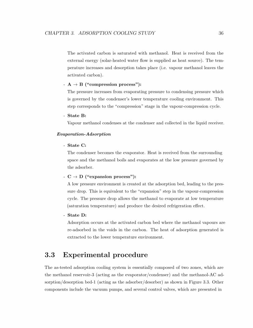
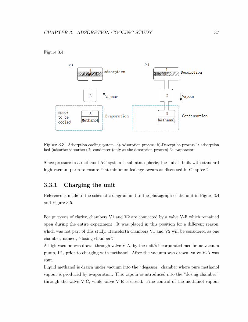
from coconut shell [61]. . . . . . . . . . . . . . . . . . . . . . . . . . . . . . . 343.2 Adsorption prototype cooling cycle . . . . . . . . . . . . . . . . . . . . . . . . 353.3 Adsorption cooling system. a)-Adsorption process, b)-Desorption process 1: ad-
sorption bed (adsorber/desorber) 2: condenser (only at the desorption process) 3:
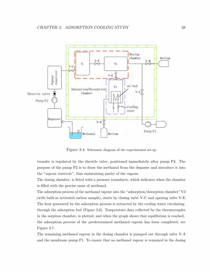
evaporator . . . . . . . . . . . . . . . . . . . . . . . . . . . . . . . . . . . . 373.4 Schematic diagram of the experimental set-up . . . . . . . . . . . . . . . . . . . 38
1
LIST OF FIGURES 2
3.5 Dosing and adsorption/desorption chamber of the adsorption prototype . . . . . 393.6 Adsorption/desorption chamber, where adsorption/desorption processes occur . . 403.7 Adsorption temperature responses at the AC measurement chamber . . . . . . . . 413.8 Flow chart of the valves and pumps control in the adsorption prototype during the
charging up (preparation) and test operation procedures. . . . . . . . . . . . . . 423.9 Adsorption equilibrium dynamics [19] . . . . . . . . . . . . . . . . . . . . . . . 433.10 Langmuir adsorption isotherm of Nitrogen on AC at 77 K [35] . . . . . . . . . . 443.11 Adsorption isotherms of methanol-AC . . . . . . . . . . . . . . . . . . . . . . . 453.12 Adsorbed micro-pore volume as a function of adsorption potential for the tested
sample . . . . . . . . . . . . . . . . . . . . . . . . . . . . . . . . . . . . . . . 47
List of Tables
1.1 Refrigerant representatives of CFCs, HFCs and HFOs [28] . . . . . . . . . . . . 71.2 Some working combination for three-fluid single pressure absorption refrigerator 101.3 Common working pairs for adsorption refrigeration . . . . . . . . . . . . . . . . 10
2.1 Comparison of two-fluid and three-fluid absorption systems . . . . . . . . . . . . 122.2 Properties of the working fluids . . . . . . . . . . . . . . . . . . . . . . . . . 132.3 Prototype basic design parameters . . . . . . . . . . . . . . . . . . . . . . . . . 192.4 Enthalpy values at the main points . . . . . . . . . . . . . . . . . . . . . . 192.5 Calculation parameters for the evaporator . . . . . . . . . . . . . . . . . . . 202.6 Components dimensions of the prototype . . . . . . . . . . . . . . . . . . . 232.7 Log sheet . . . . . . . . . . . . . . . . . . . . . . . . . . . . . . . . . . . . . 262.8 Thermophysical properties of Helium and Hydrogen [39] . . . . . . . . . . . 28
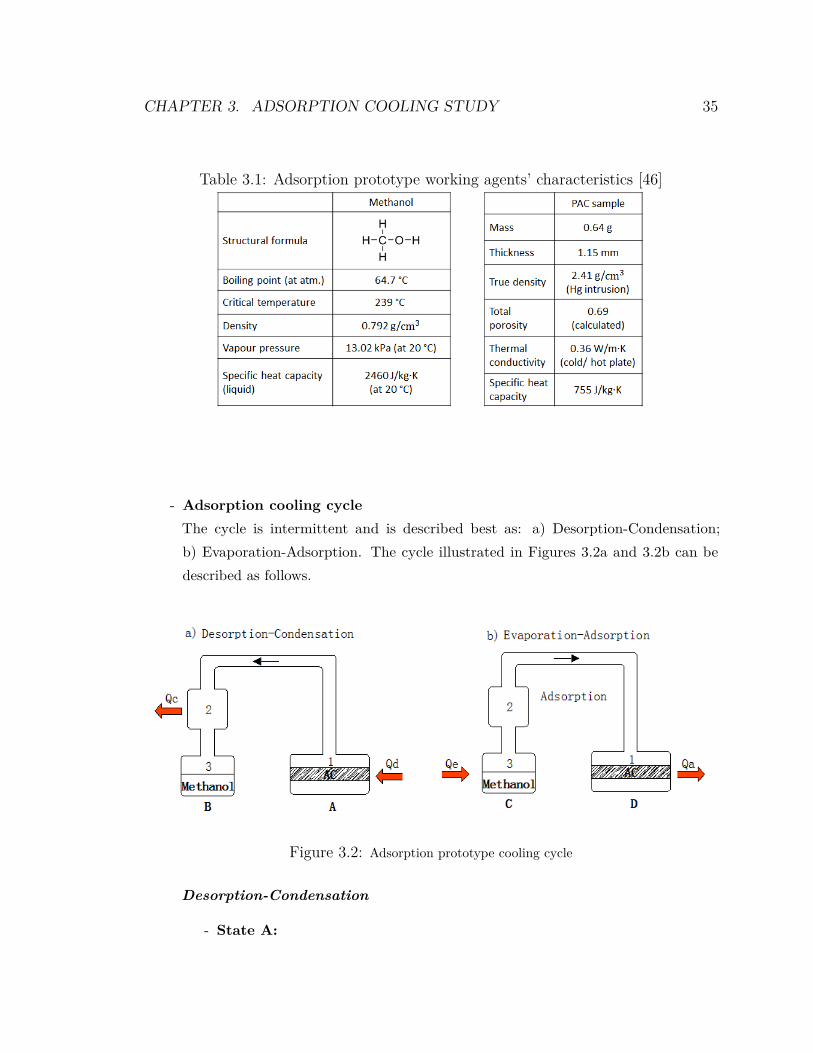
3.1 Adsorption prototype working agents’ characteristics [46] . . . . . . . . . . 35
3
Chapter 1
Introduction
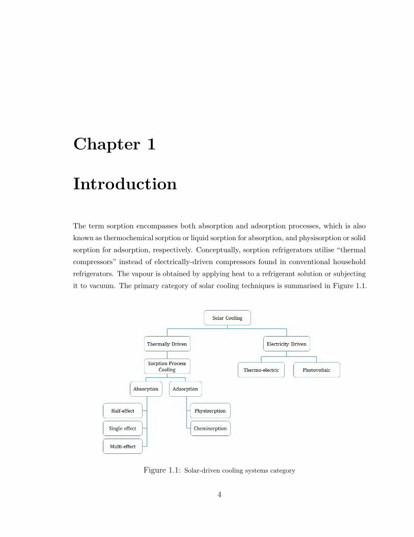
The term sorption encompasses both absorption and adsorption processes, which is alsoknown as thermochemical sorption or liquid sorption for absorption, and physisorption or solidsorption for adsorption, respectively. Conceptually, sorption refrigerators utilise “thermalcompressors” instead of electrically-driven compressors found in conventional householdrefrigerators. The vapour is obtained by applying heat to a refrigerant solution or subjectingit to vacuum. The primary category of solar cooling techniques is summarised in Figure 1.1.
Figure 1.1: Solar-driven cooling systems category
4
CHAPTER 1. INTRODUCTION 5
According to the International Institute of Refrigeration, refrigeration technology and airconditioning account for approximately 15 % of the worldwide electricity consumption [60] [15].In Mediterranean countries, solar-driven cooling systems are predicted to reduce energycosts by approximately 50 % [6].Although this appealing concept has been studied for centuries and has become a relativelyadvanced technology, the lack of economic viability is the biggest hindrance to its large scaleadaptation. The majority of the latest installed solar cooling systems are still prototype-based,although some manufacturers have entered the market with series production [14].
1.1 Dissertation aims and organisationThe dissertation mainly encompasses two branches of study of sorption refrigeration. Itstarts with a background literature survey on the classification of existing refrigerators,followed by specific study of absorption and adsorption cooling techniques, respectively.In the absorption cooling study, the primary focus was on the macroscopic design, which aimsat modelling of a three-fluid diffusion absorption refrigeration unit using organic compounds(R134a and TEG.DME). Helium was used as the third fluid instead of Hydrogen for thediffusion process.In the adsorption cooling study, the focus was on the particle level about working pairs’(methanoland activated carbon) characteristics and thermochemical performance, which aims at theo-retical modelling of an intermittent adsorption system and experimental verification of thepredictive performance. Computerised control of the adsorption unit was employed, intensivepressure and temperature responses were captured and used to fit theoretical models.Both theoretical study and experimental investigation were combined in this work for abetter understanding of sorption refrigeration.
1.2 Classification and review of refrigeratorsIn this section, the existing literature on cold generation technologies is outlined, the resultwill build the accumulation of solar refrigeration know-how in our research.
CHAPTER 1. INTRODUCTION 6
1.2.1 Vapour-compression refrigerator using refrigerant ofHCFCs/HFCs
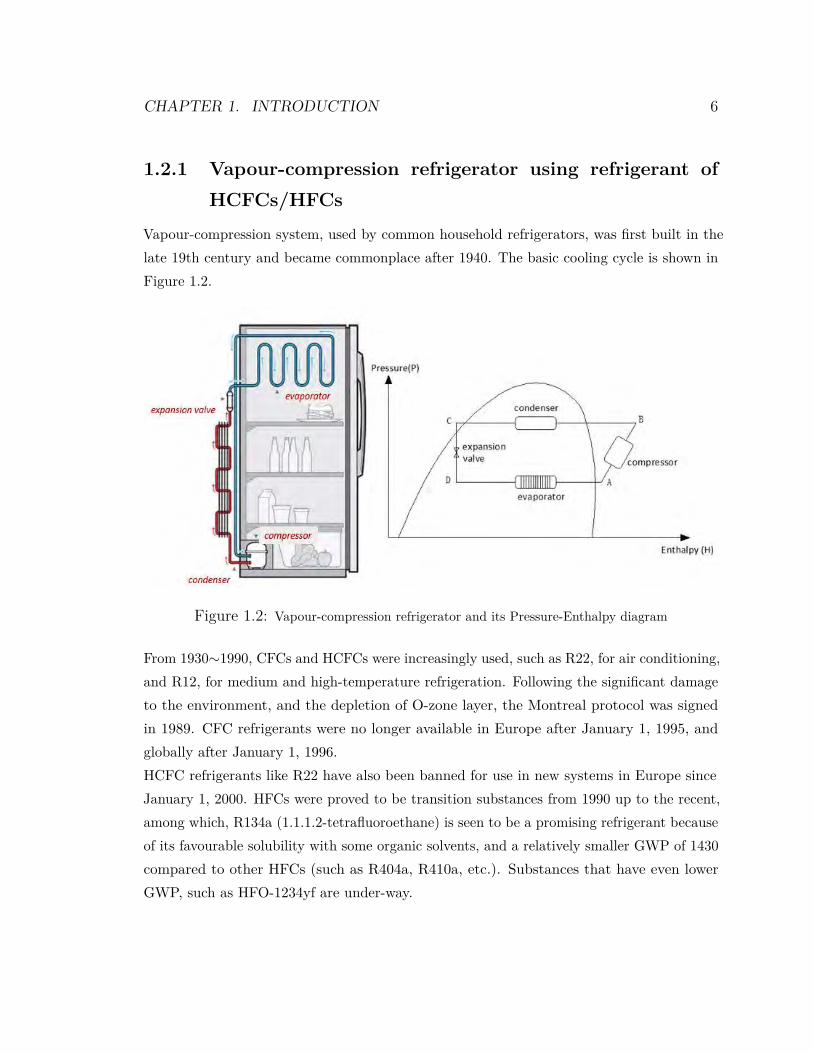
Vapour-compression system, used by common household refrigerators, was first built in thelate 19th century and became commonplace after 1940. The basic cooling cycle is shown inFigure 1.2.
Figure 1.2: Vapour-compression refrigerator and its Pressure-Enthalpy diagram
From 1930∼1990, CFCs and HCFCs were increasingly used, such as R22, for air conditioning,and R12, for medium and high-temperature refrigeration. Following the significant damageto the environment, and the depletion of O-zone layer, the Montreal protocol was signedin 1989. CFC refrigerants were no longer available in Europe after January 1, 1995, andglobally after January 1, 1996.HCFC refrigerants like R22 have also been banned for use in new systems in Europe sinceJanuary 1, 2000. HFCs were proved to be transition substances from 1990 up to the recent,among which, R134a (1.1.1.2-tetrafluoroethane) is seen to be a promising refrigerant becauseof its favourable solubility with some organic solvents, and a relatively smaller GWP of 1430compared to other HFCs (such as R404a, R410a, etc.). Substances that have even lowerGWP, such as HFO-1234yf are under-way.
CHAPTER 1. INTRODUCTION 7
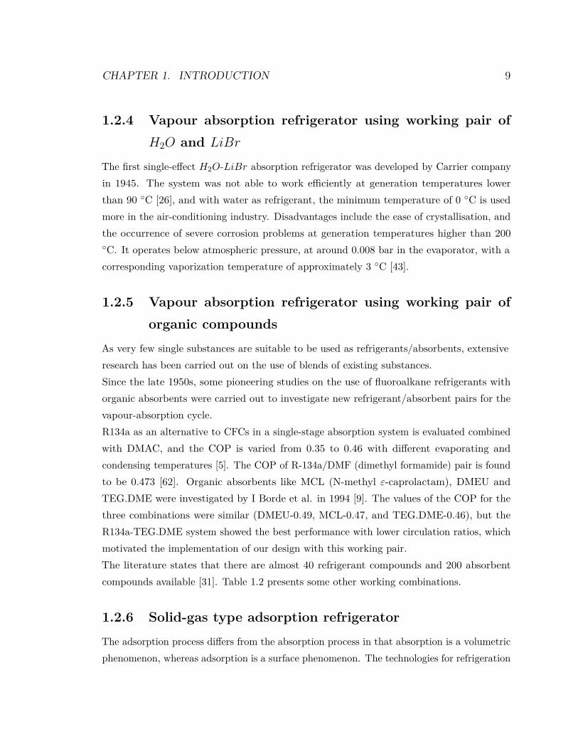
Table 1.1: Refrigerant representatives of CFCs, HFCs and HFOs [28]Refrigerant R-12 R134a R1234-yf
Dichlorodifluoromethane Tetrafluoroethane TetrafluoropropODP 0.82 0 0GWP 10900 1430 4
STATUS No manufacture universally 2030 in developed countries Potential replacementafter-1996-01-01 2040 in developing countries for R134a
1.2.2 Vapour absorption refrigerator using working pair ofNH3 (R717) and H2O
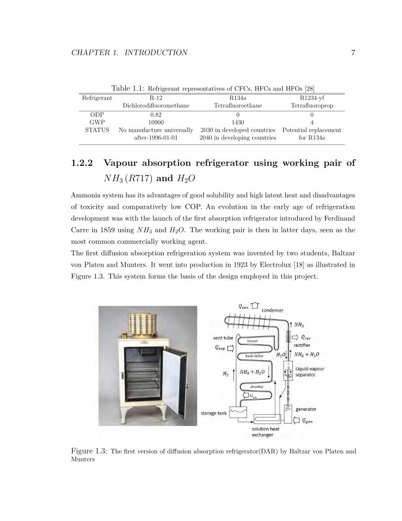
Ammonia system has its advantages of good solubility and high latent heat and disadvantagesof toxicity and comparatively low COP. An evolution in the early age of refrigerationdevelopment was with the launch of the first absorption refrigerator introduced by FerdinandCarre in 1859 using NH3 and H2O. The working pair is then in latter days, seen as themost common commercially working agent.The first diffusion absorption refrigeration system was invented by two students, Baltzarvon Platen and Munters. It went into production in 1923 by Electrolux [18] as illustrated inFigure 1.3. This system forms the basis of the design employed in this project.
Figure 1.3: The first version of diffusion absorption refrigerator(DAR) by Baltzar von Platen andMunters
CHAPTER 1. INTRODUCTION 8
1.2.3 Vapour absorption Einstein refrigerator
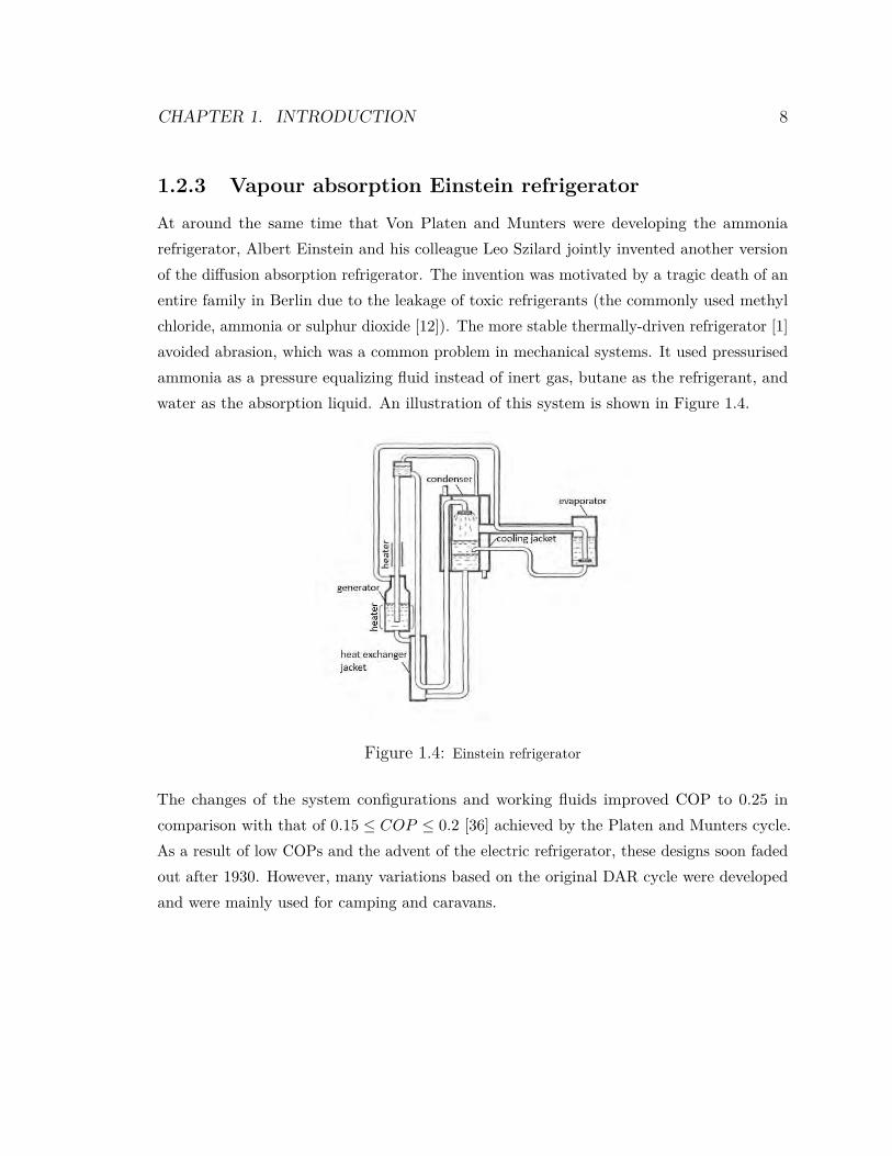
At around the same time that Von Platen and Munters were developing the ammoniarefrigerator, Albert Einstein and his colleague Leo Szilard jointly invented another versionof the diffusion absorption refrigerator. The invention was motivated by a tragic death of anentire family in Berlin due to the leakage of toxic refrigerants (the commonly used methylchloride, ammonia or sulphur dioxide [12]). The more stable thermally-driven refrigerator [1]avoided abrasion, which was a common problem in mechanical systems. It used pressurisedammonia as a pressure equalizing fluid instead of inert gas, butane as the refrigerant, andwater as the absorption liquid. An illustration of this system is shown in Figure 1.4.
Figure 1.4: Einstein refrigerator
The changes of the system configurations and working fluids improved COP to 0.25 incomparison with that of 0.15 ≤ COP ≤ 0.2 [36] achieved by the Platen and Munters cycle.As a result of low COPs and the advent of the electric refrigerator, these designs soon fadedout after 1930. However, many variations based on the original DAR cycle were developedand were mainly used for camping and caravans.
CHAPTER 1. INTRODUCTION 9
1.2.4 Vapour absorption refrigerator using working pair ofH2O and LiBr
The first single-effect H2O-LiBr absorption refrigerator was developed by Carrier companyin 1945. The system was not able to work efficiently at generation temperatures lowerthan 90 ◦C [26], and with water as refrigerant, the minimum temperature of 0 ◦C is usedmore in the air-conditioning industry. Disadvantages include the ease of crystallisation, andthe occurrence of severe corrosion problems at generation temperatures higher than 200◦C. It operates below atmospheric pressure, at around 0.008 bar in the evaporator, with acorresponding vaporization temperature of approximately 3 ◦C [43].
1.2.5 Vapour absorption refrigerator using working pair oforganic compounds
As very few single substances are suitable to be used as refrigerants/absorbents, extensiveresearch has been carried out on the use of blends of existing substances.Since the late 1950s, some pioneering studies on the use of fluoroalkane refrigerants withorganic absorbents were carried out to investigate new refrigerant/absorbent pairs for thevapour-absorption cycle.R134a as an alternative to CFCs in a single-stage absorption system is evaluated combinedwith DMAC, and the COP is varied from 0.35 to 0.46 with different evaporating andcondensing temperatures [5]. The COP of R-134a/DMF (dimethyl formamide) pair is foundto be 0.473 [62]. Organic absorbents like MCL (N-methyl ε-caprolactam), DMEU andTEG.DME were investigated by I Borde et al. in 1994 [9]. The values of the COP for thethree combinations were similar (DMEU-0.49, MCL-0.47, and TEG.DME-0.46), but theR134a-TEG.DME system showed the best performance with lower circulation ratios, whichmotivated the implementation of our design with this working pair.The literature states that there are almost 40 refrigerant compounds and 200 absorbentcompounds available [31]. Table 1.2 presents some other working combinations.
1.2.6 Solid-gas type adsorption refrigerator
The adsorption process differs from the absorption process in that absorption is a volumetricphenomenon, whereas adsorption is a surface phenomenon. The technologies for refrigeration
CHAPTER 1. INTRODUCTION 10
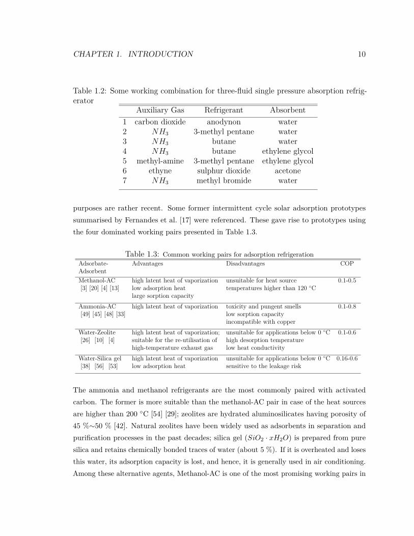
Table 1.2: Some working combination for three-fluid single pressure absorption refrig-erator
Auxiliary Gas Refrigerant Absorbent1 carbon dioxide anodynon water2 NH3 3-methyl pentane water3 NH3 butane water4 NH3 butane ethylene glycol5 methyl-amine 3-methyl pentane ethylene glycol6 ethyne sulphur dioxide acetone7 NH3 methyl bromide water
purposes are rather recent. Some former intermittent cycle solar adsorption prototypessummarised by Fernandes et al. [17] were referenced. These gave rise to prototypes usingthe four dominated working pairs presented in Table 1.3.
Table 1.3: Common working pairs for adsorption refrigerationAdsorbate- Advantages Disadvantages COPAdsorbentMethanol-AC high latent heat of vaporization unsuitable for heat source 0.1-0.5[3] [20] [4] [13] low adsorption heat temperatures higher than 120 ◦C
large sorption capacityAmmonia-AC high latent heat of vaporization toxicity and pungent smells 0.1-0.8[49] [45] [48] [33] low sorption capacity
incompatible with copperWater-Zeolite high latent heat of vaporization; unsuitable for applications below 0 ◦C 0.1-0.6[26] [10] [4] suitable for the re-utilisation of high desorption temperature
high-temperature exhaust gas low heat conductivityWater-Silica gel high latent heat of vaporization unsuitable for applications below 0 ◦C 0.16-0.6[38] [56] [53] low adsorption heat sensitive to the leakage risk
The ammonia and methanol refrigerants are the most commonly paired with activatedcarbon. The former is more suitable than the methanol-AC pair in case of the heat sourcesare higher than 200 ◦C [54] [29]; zeolites are hydrated aluminosilicates having porosity of45 %∼50 % [42]. Natural zeolites have been widely used as adsorbents in separation andpurification processes in the past decades; silica gel (SiO2 · xH2O) is prepared from puresilica and retains chemically bonded traces of water (about 5 %). If it is overheated and losesthis water, its adsorption capacity is lost, and hence, it is generally used in air conditioning.Among these alternative agents, Methanol-AC is one of the most promising working pairs in
CHAPTER 1. INTRODUCTION 11
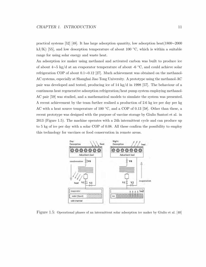
practical systems [52] [48]. It has large adsorption quantity, low adsorption heat(1800∼2000kJ/K) [55], and low desorption temperature of about 100 ◦C, which is within a suitablerange for using solar energy and waste heat.An adsorption ice maker using methanol and activated carbon was built to produce iceof about 4∼5 kg/d at an evaporator temperature of about -6 ◦C, and could achieve solarrefrigeration COP of about 0.1∼0.12 [27]. Much achievement was obtained on the methanol-AC systems, especially at Shanghai Jiao Tong University. A prototype using the methanol-ACpair was developed and tested, producing ice of 14 kg/d in 1998 [57]. The behaviour of acontinuous heat regenerative adsorption refrigeration/heat pump system employing methanol-AC pair [59] was studied, and a mathematical models to simulate the system was presented.A recent achievement by the team further realised a production of 2.6 kg ice per day per kgAC with a heat source temperature of 100 ◦C, and a COP of 0.13 [58]. Other than these, arecent prototype was designed with the purpose of vaccine storage by Giulio Santori et al. in2013 (Figure 1.5). The machine operates with a 24h intermittent cycle and can produce upto 5 kg of ice per day with a solar COP of 0.08. All these confirm the possibility to employthis technology for vaccines or food conservation in remote areas.
Figure 1.5: Operational phases of an intermittent solar adsorption ice maker by Giulio et al. [40]

Chapter 2
Absorption Cooling Study
2.1 Principle and DesignA solar absorption refrigerator is a device that utilises the phase-change of the refrigerant,which can be obtained by changing system temperatures and pressures, to generate anendothermic and exothermic process. Current absorption technology can provide variousabsorption machines with COPs ranging from 0.3 to 1.2 [22].Conventional refrigeration systems (two-fluid design) are dual-pressure cycles where thesaturation temperature difference is produced by a system pressure difference betweenthe condenser and evaporator. However, three-fluid single-pressure diffusion absorptionrefrigeration (DAR) maintains a single pressure, and requires no mechanical or electricalenergy, thus making it more economically viable due to fewer construction complications.Table 2.1 presents the comparison between single-pressure and dual-pressure systems.
Table 2.1: Comparison of two-fluid and three-fluid absorption systemsCriteria Two-fluid Three-fluid
Mechanic component pump and expansion valve noneDriving force heat and electricity heat only
Moving components pump and valves noneMaintenance yes noFatigue crack likely (pressure change) unlikely (constant pressure)
12
CHAPTER 2. ABSORPTION COOLING STUDY 13
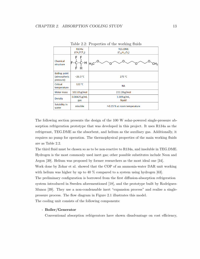
Table 2.2: Properties of the working fluids
The following section presents the design of the 100 W solar-powered single-pressure ab-sorption refrigeration prototype that was developed in this project. It uses R134a as therefrigerant, TEG.DME as the absorbent, and helium as the auxiliary gas. Additionally, itrequires no pump for operation. The thermophysical properties of the main working fluidsare as Table 2.2.The third fluid must be chosen so as to be non-reactive to R134a, and insoluble in TEG.DME.Hydrogen is the most commonly used inert gas; other possible substitutes include Neon andArgon [39]. Helium was proposed by former researchers as the most ideal one [34].Work done by Zohar et al. showed that the COP of an ammonia-water DAR unit workingwith helium was higher by up to 40 % compared to a system using hydrogen [63].The preliminary configuration is borrowed from the first diffusion-absorption refrigerationsystem introduced in Sweden aforementioned [18], and the prototype built by Rodríguez-Munoz [39]. They use a non-condensable inert “expansion process” and realise a single-pressure process. The flow diagram in Figure 2.1 illustrates this model.The cooling unit consists of the following components:
- Boiler/GeneratorConventional absorption refrigerators have shown disadvantage on cost efficiency,
CHAPTER 2. ABSORPTION COOLING STUDY 14
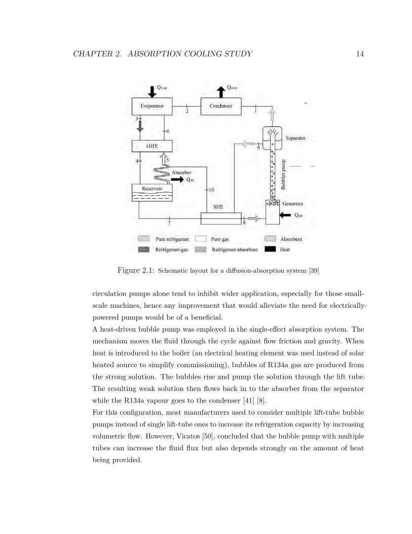
Figure 2.1: Schematic layout for a diffusion-absorption system [39]
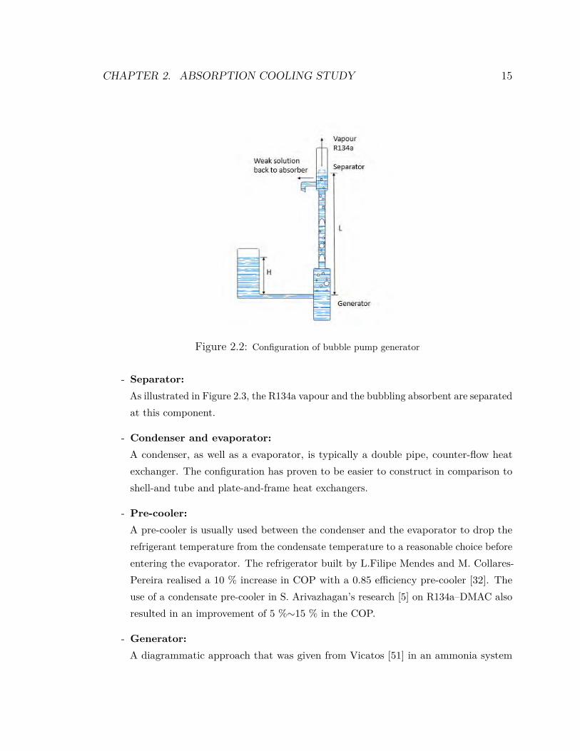
circulation pumps alone tend to inhibit wider application, especially for those small-scale machines, hence any improvement that would alleviate the need for electrically-powered pumps would be of a beneficial.A heat-driven bubble pump was employed in the single-effect absorption system. Themechanism moves the fluid through the cycle against flow friction and gravity. Whenheat is introduced to the boiler (an electrical heating element was used instead of solarheated source to simplify commissioning), bubbles of R134a gas are produced fromthe strong solution. The bubbles rise and pump the solution through the lift tube.The resulting weak solution then flows back in to the absorber from the separatorwhile the R134a vapour goes to the condenser [41] [8].For this configuration, most manufacturers used to consider multiple lift-tube bubblepumps instead of single lift-tube ones to increase its refrigeration capacity by increasingvolumetric flow. However, Vicatos [50], concluded that the bubble pump with multipletubes can increase the fluid flux but also depends strongly on the amount of heatbeing provided.
CHAPTER 2. ABSORPTION COOLING STUDY 15
Figure 2.2: Configuration of bubble pump generator
- Separator:As illustrated in Figure 2.3, the R134a vapour and the bubbling absorbent are separatedat this component.
- Condenser and evaporator:A condenser, as well as a evaporator, is typically a double pipe, counter-flow heatexchanger. The configuration has proven to be easier to construct in comparison toshell-and tube and plate-and-frame heat exchangers.
- Pre-cooler:A pre-cooler is usually used between the condenser and the evaporator to drop therefrigerant temperature from the condensate temperature to a reasonable choice beforeentering the evaporator. The refrigerator built by L.Filipe Mendes and M. Collares-Pereira realised a 10 % increase in COP with a 0.85 efficiency pre-cooler [32]. Theuse of a condensate pre-cooler in S. Arivazhagan’s research [5] on R134a–DMAC alsoresulted in an improvement of 5 %∼15 % in the COP.
- Generator:A diagrammatic approach that was given from Vicatos [51] in an ammonia system
CHAPTER 2. ABSORPTION COOLING STUDY 16
was used to determine the conditions in the generator. Heat supplied to the generatorraises the temperature of the non-equilibrium liquor from the heat exchanger to itssaturation condition. Extra heat supplied to the generator will liberate R134a andincrease the saturation temperature of the solution.
- Absorber:The main purpose of the absorber is to absorb all the R134a vapour coming fromthe evaporator into the TEG.DME, and to separate the inert gas from the R134avapour in the process. The weak solution (TEG.DME) coming from the solution heatexchanger enters the inner pipe of the absorber, while cold water counter flows at theannular space.
- Solution Tank:The level of the fluid in the solution tank is the same level as the solution in the boiler.It is equipped with a glass window to visually monitor the level of the solution bothin the solution tank and in the generator/boiler.
- Solution Heat Exchanger:As depicted in Figure 2.3, the weak solution (TEG.DME) flowing into the inner pipeis the hot fluid and the strong solution (R134+TEG.DME) in the annulus is the coldfluid. The heat exchanger results in a reduction in both the heat supplied to thegenerator and in the cooling required by the absorber.
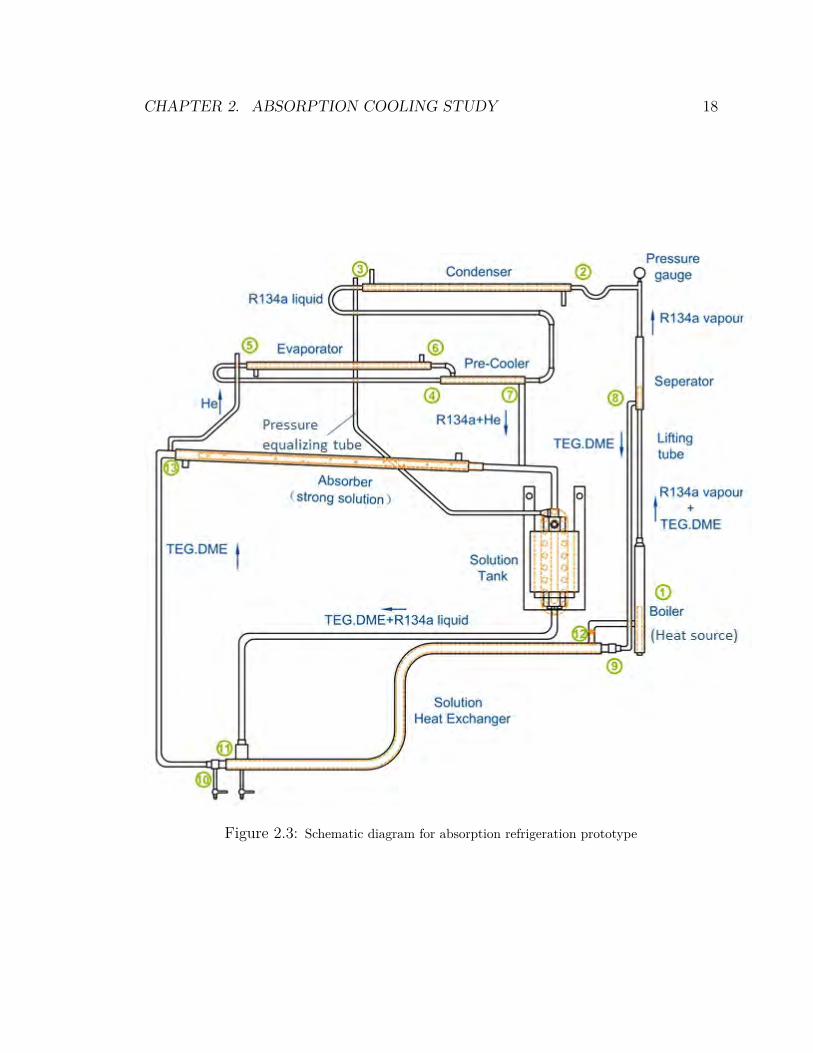
The cycle is as follows (reference to Figure 2.3):The strong solution is heated by the heat source and produces high-pressure saturatedrefrigerant vapour. The vapour escapes through the lift-tube and the separator, and flowsto the inner pipe of the condenser through the inverted “U” tube. Meanwhile, the separatedhot weak solution flows to the absorber by gravity (hydraulic potential difference), throughthe inner pipe of the heat exchanger, entering the solution tank.The liquid refrigerant passes through the pre-cooler to the evaporator and evaporates byabsorbing surrounding heat at low pressure (its partial pressure).The low-pressure vapour passes through the pre-cooler in a counter-flow direction to theliquid refrigerant from the condenser, and is entrapped by the absorbent in the absorber,liberating the inert gas, which will be free to return to the evaporator. The heat released bythe absorption process will be taken away by cooling water (counter flow through the outer
CHAPTER 2. ABSORPTION COOLING STUDY 17
tube of the absorber).The strong solution is collected in the solution tank and flows to the generator (boiler) bygravity. The solution is then re-heated and the process is repeated.The system remains at constant pressure by partial pressure regulation of the third fluid,which predetermines the saturation temperature of the refrigerant, and expedites theevaporation process in the evaporator. A pressure equalising tube is fitted between thecondenser and the solution tank. In comparison to the vapour-compression refrigeration,the absorber, SHE, and the generator are collectively equivalent to a compressor. Furthertheories can be found in Waterman Gore’s literature [47].
2.2 Theoretical ModelAn absorption refrigeration system is based on the working fluid’s characteristics, includingmass and heat transfer, and chemical compositions. In order to size and build a workingmodel, the following assumption were made:
• Steady state flow
• Kinetic and potential energy change are negligible
• The specific heat of a fluid is constant
• Axial heat conduction along the tube is negligible
• The outer surface of the heat exchangers are perfectly insulated
• Laminar flow regime expected
• Thin walled pipe neglect the conduction rate through the pipe
• Overall heat transfer coefficient based on the outside area of the inner pipe
• Average temperature used to evaluate other fluid properties
With the objective of a 100 W three-fluid DAR system in mind, the unit was designedwith the assumption of a 40 ◦C condensing temperature, a 15 ◦C pre-cooler temperature,and a -5 ◦C evaporating temperature. From the condenser condition and the properties ofsaturated R-134a, the overall system pressure is 10 bar [11]. At the evaporator temperature
CHAPTER 2. ABSORPTION COOLING STUDY 18
Figure 2.3: Schematic diagram for absorption refrigeration prototype
CHAPTER 2. ABSORPTION COOLING STUDY 19
of -5 ◦C, the saturation pressure of R134a liquid is supposed to be roughly 2.5 bar [11].In order to establish a uniform pressure in the system, and yet to maintain the pressuredifference between the condensing and evaporating pressures, a third fluid (Helium) wasadded. This would enable the refrigerant to evaporate at its partial pressure in the evapora-tor. The value of this partial pressure was identified from Dalton’s law as 7.5 bar according to:
Ptotal = PHe + PR134a (2.1)
The basic design parameters are summarised in Table 2.3.
Table 2.3: Prototype basic design parametersWorking Fluid Generator Type Tubing Material Assumed Parameter
R134a Vapour-driven 100 W Condenser Temp. Tc=40 ◦CTEG.DME “Pump” Three-fluid Copper Pre-cooler Temp.Tpc=15 ◦CHelium DAR Evaporator Temp.Te=-5 ◦C
The enthalpy values are shown in Table 2.4 from the p-h diagram in Appendix E. Thesection below presents a part of the design calculations, details of which can be found inAppendix C. The subscript numbers correspond to the numbers shown in Figure 2.3.
- EvaporatorThe basic parameters and values, presented in Table2.5, are taken from the propertiestables ( [11] and Appendix D).1)Confirm the mass flow rateAssuming steady flow and negligible changes in kinetic and potential energies, eachcomponent has one inlet and one outlet. Thus the first law is applied for each deviceas:
Q = W + mr(hout − hi) (2.2)
Since there is no work in the evaporator, we can find the heat removed from the
Table 2.4: Enthalpy values at the main pointsState point enthalpy Refrigerant conditions Temperature (◦C) Enthalpy (kJ/kg)
h2 superheated vapour at the inlet of the condenser 90 375hst saturated vapour state at the condenser 40 322h3 de-superheated at the outlet of the condenser 40 158
h4 = h5 saturated liquid at the inlet of the evaporator 15 123h6 saturated vapour at the outlet of evaporator -5 298
CHAPTER 2. ABSORPTION COOLING STUDY 20
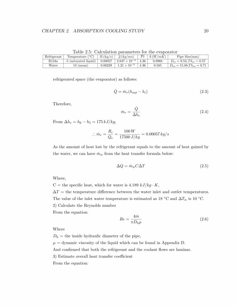
Table 2.5: Calculation parameters for the evaporatorRefrigerant Temperature (◦C) m (kg/s) µ (kg/ms) Pr k (W/mK) Pipe Size(mm)
R134a -5 (saturated liquid) 0.00057 2.947× 10⁻⁴ 4.36 0.0968 Dei = 9.53, Thei = 0.57Water 13 (mean) 0.00239 1.21× 10⁻³ 4.36 0.585 Deo = 15.88,Theo = 0.71
refrigerated space (the evaporator) as follows:
Q = mr(hout − hi) (2.3)
Therefore,
mr = Q
∆he(2.4)
From ∆he = h6 − h5 = 175 kJ/kg,
∴ mr = Rc
Qe= 100W
17500 J/kg = 0.00057 kg/s
As the amount of heat lost by the refrigerant equals to the amount of heat gained bythe water, we can have mw from the heat transfer formula below:
∆Q = mwC∆T (2.5)
Where,C = the specific heat, which for water is 4.189 kJ/kg ·K,∆T = the temperature difference between the water inlet and outlet temperatures.The value of the inlet water temperature is estimated as 18 ◦C and ∆Tw is 10 ◦C.2) Calculate the Reynolds numberFrom the equation:
Re = 4mπDhµ
(2.6)
WhereDh = the inside hydraulic diameter of the pipe,µ = dynamic viscosity of the liquid which can be found in Appendix D.And confirmed that both the refrigerant and the coolant flows are laminar.3) Estimate overall heat transfer coefficientFrom the equation:
CHAPTER 2. ABSORPTION COOLING STUDY 21
Nu = hiDh
k(2.7)
We got:
hi = Nuk
Dh(2.8)
And as Nusselt number is a constant of 4.36 throughout the fully developed region [37].Thermal conductivity values can be found from Appendix D.From the total thermal resistance equation:
R = 1hiAi
+ln Do
Di
2πkL + 1hoAo
(2.9)
For the pipes with thin wall and high thermal conductivity material, it is estimatedthat:
UA = 1R≈ 1hi
+ 1ho
(2.10)
4) Confirm the lengthThe heat transfer rate across a heat exchanger is usually expressed in the form:
Q = UA∆Tlm (2.11)
WhereQ = heat transfer rate,U = overall heat transfer coefficient,A= heat transfer surface area,∆Tlm= logarithmic mean temperature difference.
∆Tlm = ∆T1 −∆T2
ln ∆T1∆T2
(2.12)
Also,
A = πDL (2.13)
CHAPTER 2. ABSORPTION COOLING STUDY 22
Therefore, the equation below is used for the confirmation of the length:
L = Q
UπD∆T (2.14)
- CondenserSimilar steps were taken for the calculation of the condenser, while it needs to beseparated as one part from the superheated vapour state to the saturated vapour state,and the other part from the saturated vapour state to the saturated liquid state.As for the first part, turbulent flow is involved, and the following equation is used forcalculation of Prandtl number:
Pr = ν
α= Cµ
k(2.15)
Whereν = momentum diffusivity (kinematic viscosity) (m2/s),α = thermal diffusivity (m2/s),µ = dynamic viscosity (kg/m · s),k = thermal conductivity (W/m ·K),c = specific heat (J/kg ·K).And for turbulent flow, Gnielinski correlation is used for Nusselt number for 0.5 ≤Pr ≤ 2000, and 3000 ≤ Re ≤ 5× 10⁶.
Nu =(f
8 )(Re− 1000)Pr1 + 12.7(f
8 )1/2(Pr2/3 − 1)(2.16)
Where friction factor f follows the equation:
f = (0.790 lnRe− 1.64)−2, 3000 ≤ Re ≤ 5× 10⁶ (2.17)
And with similar calculation steps for the overall heat transfer coefficient and thelogarithmic mean temperature difference, the length of the condenser can be confirmed.
Other values confirmed by the calculation (Appendix C) are presented in Table 2.6.
CHAPTER 2. ABSORPTION COOLING STUDY 23
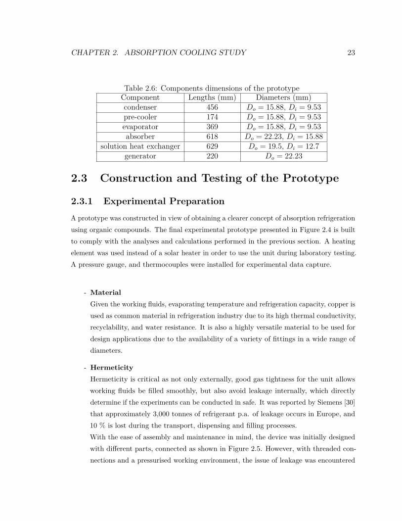
Table 2.6: Components dimensions of the prototypeComponent Lengths (mm) Diameters (mm)condenser 456 Do = 15.88, Di = 9.53pre-cooler 174 Do = 15.88, Di = 9.53evaporator 369 Do = 15.88, Di = 9.53absorber 618 Do = 22.23, Di = 15.88
solution heat exchanger 629 Do = 19.5, Di = 12.7generator 220 Do = 22.23
2.3 Construction and Testing of the Prototype
2.3.1 Experimental Preparation
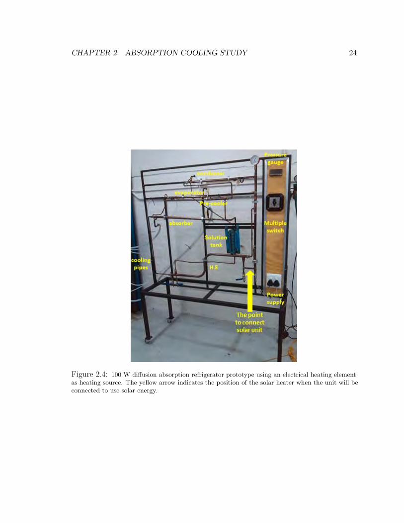
A prototype was constructed in view of obtaining a clearer concept of absorption refrigerationusing organic compounds. The final experimental prototype presented in Figure 2.4 is builtto comply with the analyses and calculations performed in the previous section. A heatingelement was used instead of a solar heater in order to use the unit during laboratory testing.A pressure gauge, and thermocouples were installed for experimental data capture.
- MaterialGiven the working fluids, evaporating temperature and refrigeration capacity, copper isused as common material in refrigeration industry due to its high thermal conductivity,recyclability, and water resistance. It is also a highly versatile material to be used fordesign applications due to the availability of a variety of fittings in a wide range ofdiameters.
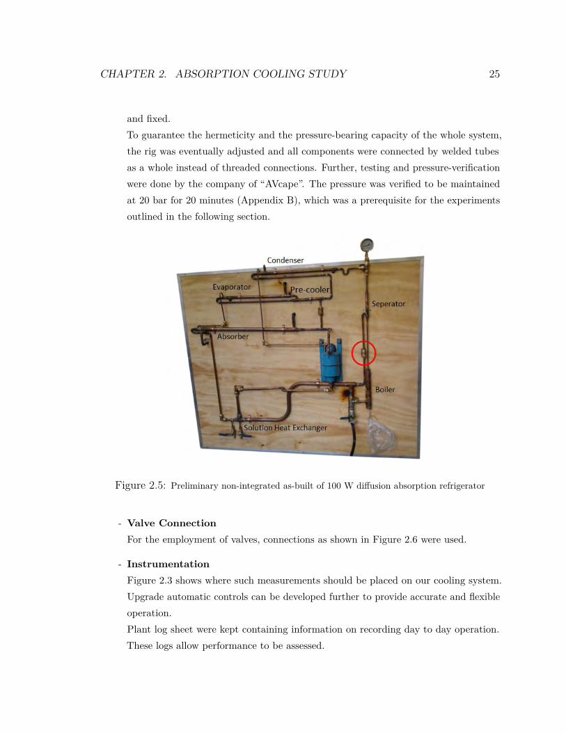
- HermeticityHermeticity is critical as not only externally, good gas tightness for the unit allowsworking fluids be filled smoothly, but also avoid leakage internally, which directlydetermine if the experiments can be conducted in safe. It was reported by Siemens [30]that approximately 3,000 tonnes of refrigerant p.a. of leakage occurs in Europe, and10 % is lost during the transport, dispensing and filling processes.With the ease of assembly and maintenance in mind, the device was initially designedwith different parts, connected as shown in Figure 2.5. However, with threaded con-nections and a pressurised working environment, the issue of leakage was encountered
CHAPTER 2. ABSORPTION COOLING STUDY 24
Figure 2.4: 100 W diffusion absorption refrigerator prototype using an electrical heating elementas heating source. The yellow arrow indicates the position of the solar heater when the unit will beconnected to use solar energy.
CHAPTER 2. ABSORPTION COOLING STUDY 25
and fixed.To guarantee the hermeticity and the pressure-bearing capacity of the whole system,the rig was eventually adjusted and all components were connected by welded tubesas a whole instead of threaded connections. Further, testing and pressure-verificationwere done by the company of “AVcape”. The pressure was verified to be maintainedat 20 bar for 20 minutes (Appendix B), which was a prerequisite for the experimentsoutlined in the following section.
Figure 2.5: Preliminary non-integrated as-built of 100 W diffusion absorption refrigerator
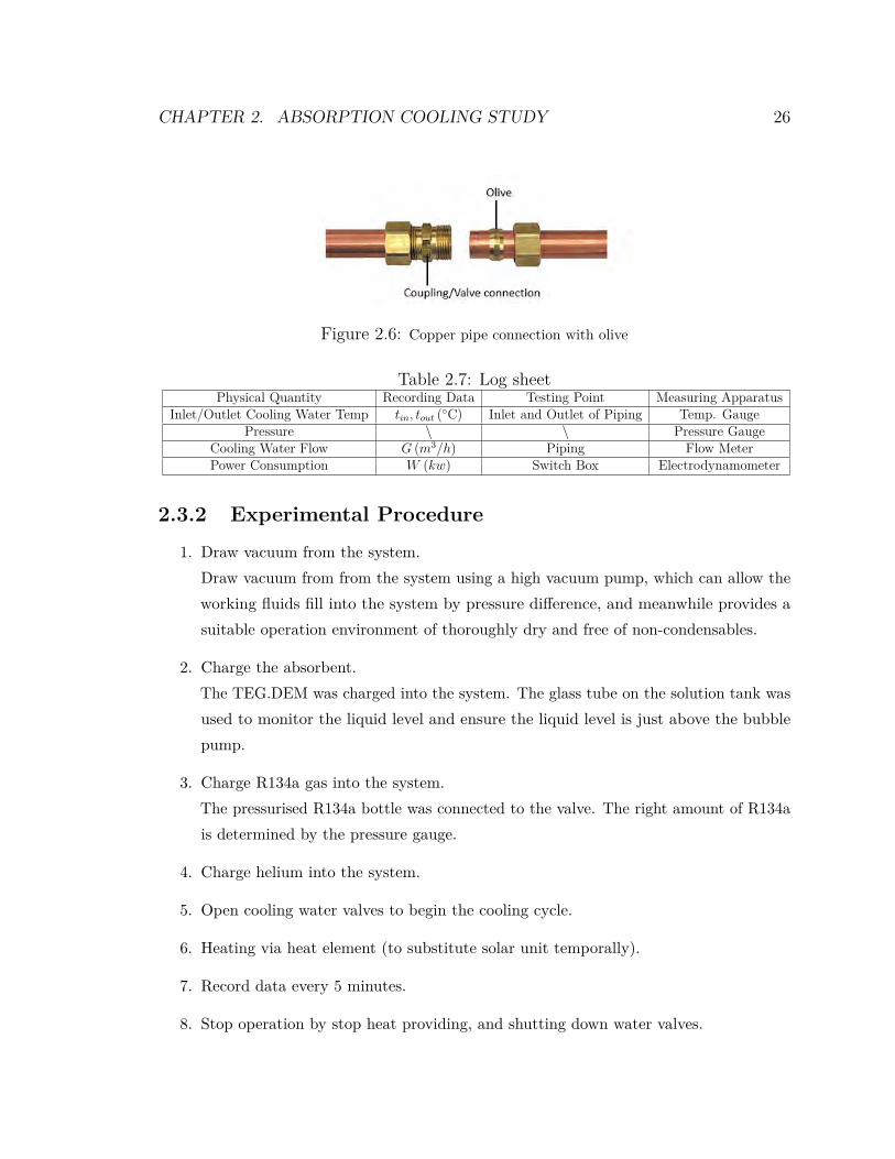
- Valve ConnectionFor the employment of valves, connections as shown in Figure 2.6 were used.
- InstrumentationFigure 2.3 shows where such measurements should be placed on our cooling system.Upgrade automatic controls can be developed further to provide accurate and flexibleoperation.Plant log sheet were kept containing information on recording day to day operation.These logs allow performance to be assessed.
CHAPTER 2. ABSORPTION COOLING STUDY 26
Figure 2.6: Copper pipe connection with olive
Table 2.7: Log sheetPhysical Quantity Recording Data Testing Point Measuring Apparatus
Inlet/Outlet Cooling Water Temp tin, tout (◦C) Inlet and Outlet of Piping Temp. GaugePressure \ \ Pressure Gauge
Cooling Water Flow G (m3/h) Piping Flow MeterPower Consumption W (kw) Switch Box Electrodynamometer
2.3.2 Experimental Procedure
1. Draw vacuum from the system.Draw vacuum from from the system using a high vacuum pump, which can allow theworking fluids fill into the system by pressure difference, and meanwhile provides asuitable operation environment of thoroughly dry and free of non-condensables.
2. Charge the absorbent.The TEG.DEM was charged into the system. The glass tube on the solution tank wasused to monitor the liquid level and ensure the liquid level is just above the bubblepump.
3. Charge R134a gas into the system.The pressurised R134a bottle was connected to the valve. The right amount of R134ais determined by the pressure gauge.
4. Charge helium into the system.
5. Open cooling water valves to begin the cooling cycle.
6. Heating via heat element (to substitute solar unit temporally).
7. Record data every 5 minutes.
8. Stop operation by stop heat providing, and shutting down water valves.
CHAPTER 2. ABSORPTION COOLING STUDY 27
2.3.3 Analysis of experimental failure
Experiment is the most efficient and visible way to verify a mechanism design. It is not onlyto have a better understanding of the operation but also to give suggestions for retrofit andreference for other similar designs.Ideally, the prototype is supposed to perform circuit and function refrigeration. However,with the experiments carrying forward, series of concerns were met inevitably, like the heatedvapour can be only lifted up to roughly 250 mm and stopped at the separator region; Orno bubbling in the boiler after several times of running. The discussion below is going topresent these on-site malfunctions, retrofit was carried out using the procedure detail in thefollowing. Some of the anomalies can be commonly confronted in experimental processes forsimilar designs.
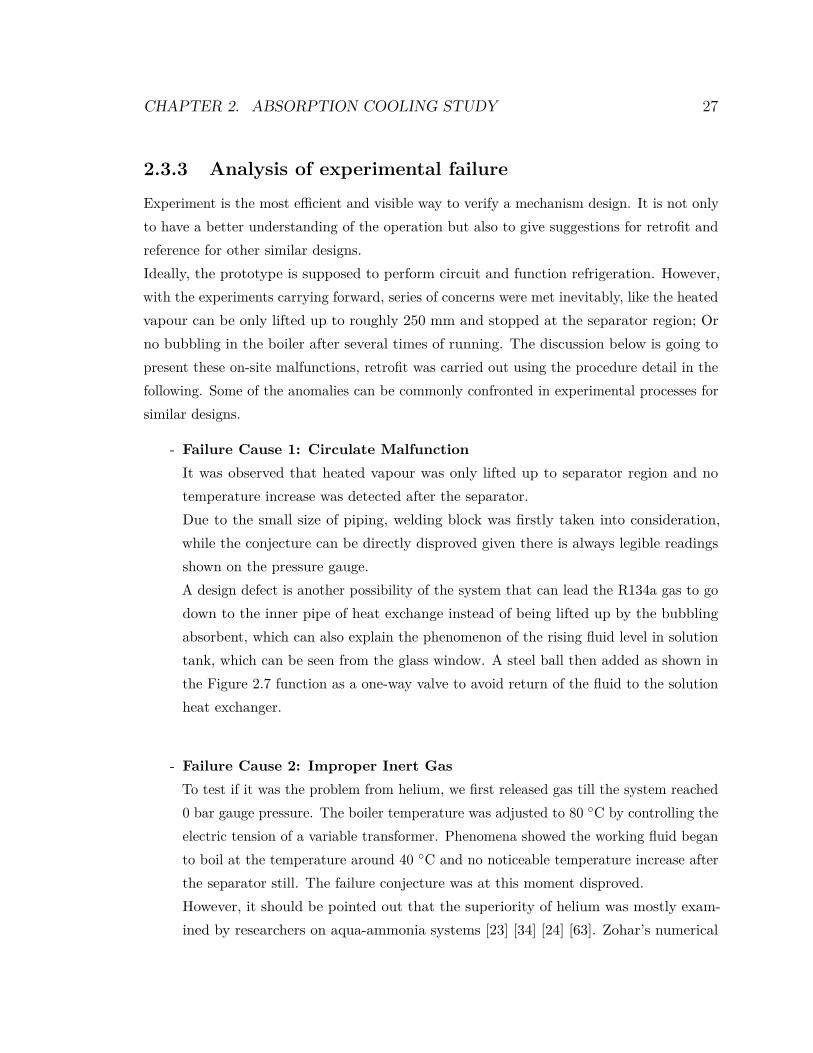
- Failure Cause 1: Circulate MalfunctionIt was observed that heated vapour was only lifted up to separator region and notemperature increase was detected after the separator.Due to the small size of piping, welding block was firstly taken into consideration,while the conjecture can be directly disproved given there is always legible readingsshown on the pressure gauge.A design defect is another possibility of the system that can lead the R134a gas to godown to the inner pipe of heat exchange instead of being lifted up by the bubblingabsorbent, which can also explain the phenomenon of the rising fluid level in solutiontank, which can be seen from the glass window. A steel ball then added as shown inthe Figure 2.7 function as a one-way valve to avoid return of the fluid to the solutionheat exchanger.
- Failure Cause 2: Improper Inert GasTo test if it was the problem from helium, we first released gas till the system reached0 bar gauge pressure. The boiler temperature was adjusted to 80 ◦C by controlling theelectric tension of a variable transformer. Phenomena showed the working fluid beganto boil at the temperature around 40 ◦C and no noticeable temperature increase afterthe separator still. The failure conjecture was at this moment disproved.However, it should be pointed out that the superiority of helium was mostly exam-ined by researchers on aqua-ammonia systems [23] [34] [24] [63]. Zohar’s numerical
CHAPTER 2. ABSORPTION COOLING STUDY 28
Figure 2.7: Perspective of “one-way” connection between boiler and heat exchanger
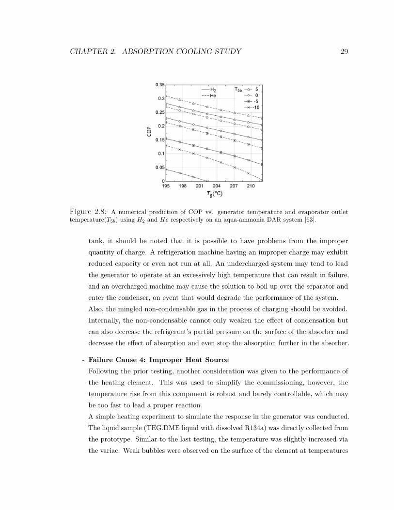
investigation (Figure 2.8) elucidates an evidently better performance by using heliumas the inert gas at different experimental conditions.Thermodynamically, helium has a smaller heat capacity than hydrogen, i.e. more heatcan be absorbed by the evaporating refrigerant instead of heating of the inert gas.Consequently, more heat is absorbed from the cooling chamber, thus increasing theCOP.However, the friction losses for helium may be higher since its viscosity and densityare twice as much as hydrogen (Table 2.8). But nevertheless it performs better inH2O-NH3 system, literature does not give evidence how a Helium would behave withorganic compounds. Therefore, more experiments are needed to establish the influenceon the currently used mixture of TEG.DME-R134.
Table 2.8: Thermophysical properties of Helium and Hydrogen [39]Mass (g/mol) Specific Heat (kJ/kg ·K) Viscosity (µPa/s)) Density (kg/m3)
Helium 4 5.19 19.850 0.1635Hydrogen 2 14.312 9.011 0.0823
- Failure Cause 3: Improper chargeAlthough we can know the system is charged through the glass window of the solution
CHAPTER 2. ABSORPTION COOLING STUDY 29
Figure 2.8: A numerical prediction of COP vs. generator temperature and evaporator outlettemperature(T5b) using H2 and He respectively on an aqua-ammonia DAR system [63].
tank, it should be noted that it is possible to have problems from the improperquantity of charge. A refrigeration machine having an improper charge may exhibitreduced capacity or even not run at all. An undercharged system may tend to leadthe generator to operate at an excessively high temperature that can result in failure,and an overcharged machine may cause the solution to boil up over the separator andenter the condenser, on event that would degrade the performance of the system.Also, the mingled non-condensable gas in the process of charging should be avoided.Internally, the non-condensable cannot only weaken the effect of condensation butcan also decrease the refrigerant’s partial pressure on the surface of the absorber anddecrease the effect of absorption and even stop the absorption further in the absorber.
- Failure Cause 4: Improper Heat SourceFollowing the prior testing, another consideration was given to the performance ofthe heating element. This was used to simplify the commissioning, however, thetemperature rise from this component is robust and barely controllable, which maybe too fast to lead a proper reaction.A simple heating experiment to simulate the response in the generator was conducted.The liquid sample (TEG.DME liquid with dissolved R134a) was directly collected fromthe prototype. Similar to the last testing, the temperature was slightly increased viathe variac. Weak bubbles were observed on the surface of the element at temperatures
CHAPTER 2. ABSORPTION COOLING STUDY 30
above 40 ◦C. When the temperature at the surface of the element was increased to160 ◦C, the temperature of the liquid reached only 92◦C, followed by weak bubblingand combustion.This gave information that: there is a significant gap between the temperature ofthe heat source and the temperature of our working fluid, while the heating processwas neither even nor smooth. The heat source from the heating element as a “pointheating” was not favourable.
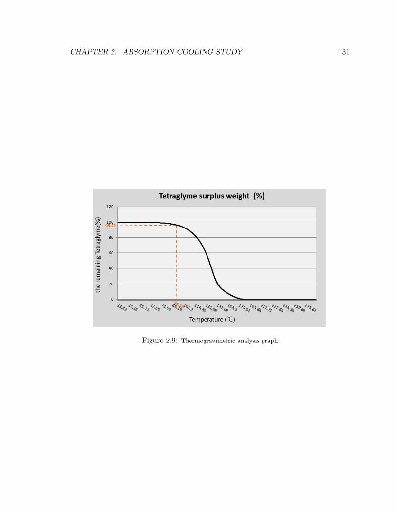
- Failure Cause 5: Contaminated Working FluidAfter all the failure tests performed as described above, chemical decomposition issueswere concerned. This can be either contamination of the fluid by external objects, orchemical decomposition.It is worthwhile to mention that both the refrigerant and absorbent are soluble inwater. TEG.DME may form peroxides during prolonged and careless storage, andshould be stored in a tightly closed container and avoid contact with light.To gather more information about the sample fluid, a thermogravimetric analysis(TGA) was carried out. Mass loss can be detected during this investigation to verifydecomposition, oxidation, or loss of volatiles and it cannot be influenced by pressure.A sample of pure Tetraglyme was analysed. The temperature program was set from30 ◦C to 300 ◦C at 10 ◦C/minute heating in a Nitrogen atmosphere. As shown inFigure 2.9, the descending TGA thermal curve indicates a weight-loss has occurred. 5% loss occurs when the temperature reaches 95 ◦C, and only 1 % of the Tetraglyme isleft when the temperature reaches to 178 ◦C. The diagram of the full results is shownin Appendix A. It was concluded that the liquid used to reach a temperature above160 ◦C experienced pyrolysis.
CHAPTER 2. ABSORPTION COOLING STUDY 31
Figure 2.9: Thermogravimetric analysis graph
Chapter 3
Adsorption Cooling Study
3.1 Introduction and aim of the studyGas-solid interfaced adsorption is most commonly used in cooling aimed adsorption tech-nology. As previously mentioned, compared to the bulk-phenomenon absorption chillers,the surface-based adsorption process, is seen as capable of operating with heat sourcetemperatures as low as 50 ◦C (the lowest heat source temperature for absorption systembeing 90 ◦C [26]), and can use refrigerants having zero ozone depletion potential (ODP)and low global warming potential (GWP) such as methanol and water. Higher efficiencyadvanced adsorption refrigeration cycles have been developed in the past, namely continuous,heat recovery cycle, mass recovery cycle, and forced convective thermal wave cycle [2]. Dueto their solid character, adsorption systems are more viable for vibration applications likevehicles, fishing boats and even space missions.To provide quasi-continuous commissioning, predecessors of this project, Ana Markovic et al.developed a multi-sorption-bed system, in which half the modules operate a heat recoveryprocess while the others are adsorbing. The study was carried out at Stuttgart University,where the as-built prototype was initially developed for commercial use in an automotiveair-conditioning application using methanol and activated carbon. However, the COP ofthese units is barely satisfactory (Table 1.3).The key operation in the adsorption systems is the proper analysis and understanding of theheat and mass transfer of the working agents between the components of the unit. The majormotivation behind the present work was to investigate the theoretical steady state behaviour
32
CHAPTER 3. ADSORPTION COOLING STUDY 33
of a basic, intermittent adsorption cycle. The focus was to commission an adsorption unit,working with methanol and activated carbon in order to collect experimental data andcreate a theoretical model, which would predict its performance. This data was collectedat different temperatures in the adsorption process. The Dubinin-Astakhov equation (3.3)was used for fitting the experimental data, from which the adsorption process and the COPcan be analysed and calculated. As in all cooling sorption systems, the absorption andadsorption processes are the most crucial processes involving mass and heat transfer. Thecurrent investigation is focussed only in the adsorption of methanol vapour into the activatedcarbon, and not in the desorption process. The theoretical model developed helped theongoing research of the “Institute of Chemical Process Engineering” in Stuttgart University,on solid adsorption and organic compounds.
3.2 Operating Principle- Adsorption mechanismAdsorption is the accumulation of ions, atoms, or molecules from the adsorbate thatadhere onto the surface of the solid adsorbent surface. Two types of adsorptionprocesses are considered, which are physisorption and chemisorption. The formerreversible physisorption is processed with electrostatic forces, van der Waals forces,and the adsorbate remains chemically stable during the process. In contrast, the latter,chemisorption, is caused by strong interaction between ionic or covalent bonds. Theadsorbed molecule is therefore chemically altered in its structure.
- Working agentsActivated carbon (AC) is one of the most exploited and variously applied substancesin the current century due to its micro-porosity. Except for its cooling applications,the adsorption of VOCs onto these porous adsorbents has been also widely used forenvironmental treatment.AC is obtained by thermal decomposition (at temperatures lower than 1000 ◦C) orcombustion of carbonaceous source materials, such as charcoal, coconuts, wood, andlignite [7]. In this process, the internal structure of the charcoal particle is eroded,creating an internal network of even smaller pores, which makes the AC two to threetimes more efficient in its adsorption capability. From these diverse raw materials,
CHAPTER 3. ADSORPTION COOLING STUDY 34
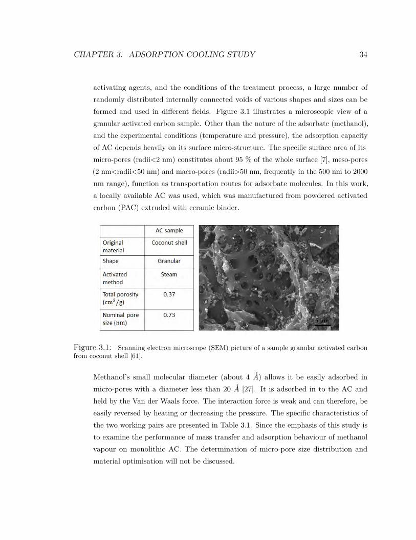
activating agents, and the conditions of the treatment process, a large number ofrandomly distributed internally connected voids of various shapes and sizes can beformed and used in different fields. Figure 3.1 illustrates a microscopic view of agranular activated carbon sample. Other than the nature of the adsorbate (methanol),and the experimental conditions (temperature and pressure), the adsorption capacityof AC depends heavily on its surface micro-structure. The specific surface area of itsmicro-pores (radii<2 nm) constitutes about 95 % of the whole surface [7], meso-pores(2 nm<radii<50 nm) and macro-pores (radii>50 nm, frequently in the 500 nm to 2000nm range), function as transportation routes for adsorbate molecules. In this work,a locally available AC was used, which was manufactured from powdered activatedcarbon (PAC) extruded with ceramic binder.
Figure 3.1: Scanning electron microscope (SEM) picture of a sample granular activated carbonfrom coconut shell [61].
Methanol’s small molecular diameter (about 4 A) allows it be easily adsorbed inmicro-pores with a diameter less than 20 A [27]. It is adsorbed in to the AC andheld by the Van der Waals force. The interaction force is weak and can therefore, beeasily reversed by heating or decreasing the pressure. The specific characteristics ofthe two working pairs are presented in Table 3.1. Since the emphasis of this study isto examine the performance of mass transfer and adsorption behaviour of methanolvapour on monolithic AC. The determination of micro-pore size distribution andmaterial optimisation will not be discussed.
CHAPTER 3. ADSORPTION COOLING STUDY 35
Table 3.1: Adsorption prototype working agents’ characteristics [46]
- Adsorption cooling cycleThe cycle is intermittent and is described best as: a) Desorption-Condensation;b) Evaporation-Adsorption. The cycle illustrated in Figures 3.2a and 3.2b can bedescribed as follows.
Figure 3.2: Adsorption prototype cooling cycle
Desorption-Condensation
- State A:
CHAPTER 3. ADSORPTION COOLING STUDY 36
The activated carbon is saturated with methanol. Heat is received from theexternal energy (solar-heated water flow is supplied as heat source). The tem-perature increases and desorption takes place (i.e. vapour methanol leaves theactivated carbon).
- A → B (“compression process”):The pressure increases from evaporating pressure to condensing pressure whichis governed by the condenser’s lower temperature cooling environment. Thisstep corresponds to the “compression” stage in the vapour-compression cycle.
- State B:Vapour methanol condenses at the condenser and collected in the liquid receiver.
Evaporation-Adsorption
- State C:The condenser becomes the evaporator. Heat is received from the surroundingspace and the methanol boils and evaporates at the low pressure governed bythe adsorber.
- C → D (“expansion process”):A low pressure environment is created at the adsorption bed, leading to the pres-sure drop. This is equivalent to the “expansion” step in the vapour-compressioncycle. The pressure drop allows the methanol to evaporate at low temperature(saturation temperature) and produce the desired refrigeration effect.
- State D:Adsorption occurs at the activated carbon bed where the methanol vapours arere-adsorbed in the voids in the carbon. The heat of adsorption generated isextracted to the lower temperature environment.
3.3 Experimental procedureThe as-tested adsorption cooling system is essentially composed of two zones, which arethe methanol reservoir-3 (acting as the evaporator/condenser) and the methanol-AC ad-sorption/desorption bed-1 (acting as the adsorber/desorber) as shown in Figure 3.3. Othercomponents include the vacuum pumps, and several control valves, which are presented in
CHAPTER 3. ADSORPTION COOLING STUDY 37
Figure 3.4.
Figure 3.3: Adsorption cooling system. a)-Adsorption process, b)-Desorption process 1: adsorptionbed (adsorber/desorber) 2: condenser (only at the desorption process) 3: evaporator
Since pressure in a methanol-AC system is sub-atmospheric, the unit is built with standardhigh-vacuum parts to ensure that minimum leakage occurs as discussed in Chapter 2.
3.3.1 Charging the unit
Reference is made to the schematic diagram and to the photograph of the unit in Figure 3.4and Figure 3.5.
For purposes of clarity, chambers V1 and V2 are connected by a valve V-F which remainedopen during the entire experiment. It was placed in this position for a different reason,which was not part of this study. Henceforth chambers V1 and V2 will be considered as onechamber, named, “dosing chamber”.A high vacuum was drawn through valve V-A, by the unit’s incorporated membrane vacuumpump, P1, prior to charging with methanol. After the vacuum was drawn, valve V-A wasshut.Liquid methanol is drawn under vacuum into the “degasser” chamber where pure methanolvapour is produced by evaporation. This vapour is introduced into the “dosing chamber”,through the valve V-C, while valve V-E is closed. Fine control of the methanol vapour
CHAPTER 3. ADSORPTION COOLING STUDY 38
Figure 3.4: Schematic diagram of the experimental set-up
transfer is regulated by the throttle valve, positioned immediately after pump P2. Thepurpose of the pump P2 is to draw the methanol from the degasser and introduce it intothe “vapour reservoir”, thus maintaining purity of the vapour.The dosing chamber, is fitted with a pressure transducer, which indicates when the chamberis filled with the precise mass of methanol.The adsorption process of the methanol vapour into the “adsorption/desorption chamber” V3(with built-in activated carbon sample), starts by closing valve V-C and opening valve V-E.The heat generated by the adsorption process is extracted by the cooling water circulatingthrough the adsorption bed (Figure 3.6). Temperature data collected by the thermocouplesin the sorption chamber, is plotted, and when the graph shows that equilibrium is reached,the adsorption process of the predetermined methanol vapour has been completed, seeFigure 3.7.The remaining methanol vapour in the dosing chamber is pumped out through valve V-Aand the membrane pump P1. To ensure that no methanol vapour is remained in the dosing
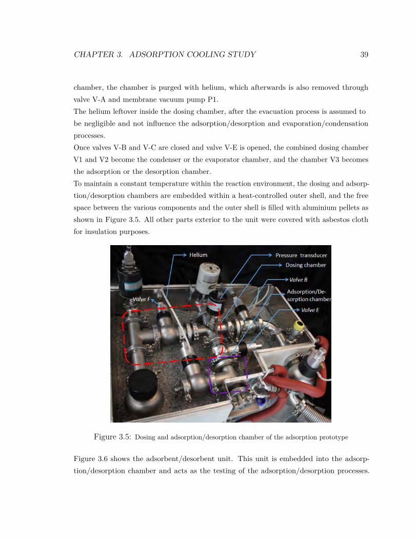
CHAPTER 3. ADSORPTION COOLING STUDY 39
chamber, the chamber is purged with helium, which afterwards is also removed throughvalve V-A and membrane vacuum pump P1.The helium leftover inside the dosing chamber, after the evacuation process is assumed tobe negligible and not influence the adsorption/desorption and evaporation/condensationprocesses.Once valves V-B and V-C are closed and valve V-E is opened, the combined dosing chamberV1 and V2 become the condenser or the evaporator chamber, and the chamber V3 becomesthe adsorption or the desorption chamber.To maintain a constant temperature within the reaction environment, the dosing and adsorp-tion/desorption chambers are embedded within a heat-controlled outer shell, and the freespace between the various components and the outer shell is filled with aluminium pellets asshown in Figure 3.5. All other parts exterior to the unit were covered with asbestos clothfor insulation purposes.
Figure 3.5: Dosing and adsorption/desorption chamber of the adsorption prototype
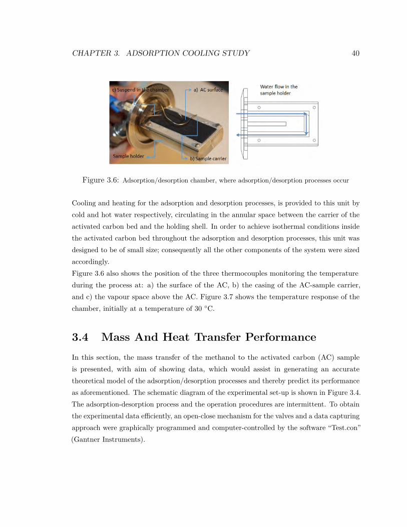
Figure 3.6 shows the adsorbent/desorbent unit. This unit is embedded into the adsorp-tion/desorption chamber and acts as the testing of the adsorption/desorption processes.
CHAPTER 3. ADSORPTION COOLING STUDY 40
Figure 3.6: Adsorption/desorption chamber, where adsorption/desorption processes occur
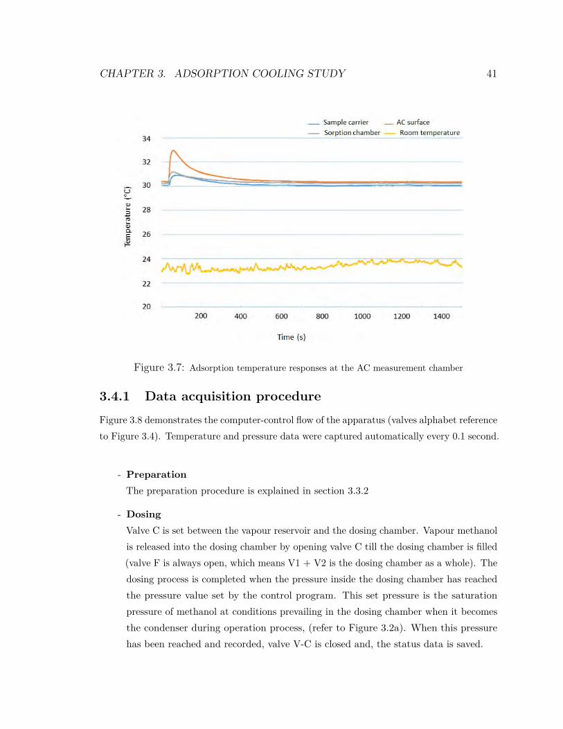
Cooling and heating for the adsorption and desorption processes, is provided to this unit bycold and hot water respectively, circulating in the annular space between the carrier of theactivated carbon bed and the holding shell. In order to achieve isothermal conditions insidethe activated carbon bed throughout the adsorption and desorption processes, this unit wasdesigned to be of small size; consequently all the other components of the system were sizedaccordingly.Figure 3.6 also shows the position of the three thermocouples monitoring the temperatureduring the process at: a) the surface of the AC, b) the casing of the AC-sample carrier,and c) the vapour space above the AC. Figure 3.7 shows the temperature response of thechamber, initially at a temperature of 30 ◦C.
3.4 Mass And Heat Transfer PerformanceIn this section, the mass transfer of the methanol to the activated carbon (AC) sampleis presented, with aim of showing data, which would assist in generating an accuratetheoretical model of the adsorption/desorption processes and thereby predict its performanceas aforementioned. The schematic diagram of the experimental set-up is shown in Figure 3.4.The adsorption-desorption process and the operation procedures are intermittent. To obtainthe experimental data efficiently, an open-close mechanism for the valves and a data capturingapproach were graphically programmed and computer-controlled by the software “Test.con”(Gantner Instruments).
CHAPTER 3. ADSORPTION COOLING STUDY 41
Figure 3.7: Adsorption temperature responses at the AC measurement chamber
3.4.1 Data acquisition procedure
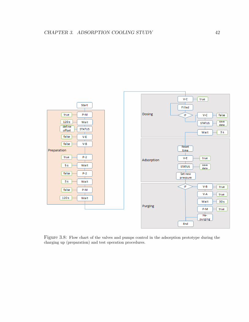
Figure 3.8 demonstrates the computer-control flow of the apparatus (valves alphabet referenceto Figure 3.4). Temperature and pressure data were captured automatically every 0.1 second.
- PreparationThe preparation procedure is explained in section 3.3.2
- DosingValve C is set between the vapour reservoir and the dosing chamber. Vapour methanolis released into the dosing chamber by opening valve C till the dosing chamber is filled(valve F is always open, which means V1 + V2 is the dosing chamber as a whole). Thedosing process is completed when the pressure inside the dosing chamber has reachedthe pressure value set by the control program. This set pressure is the saturationpressure of methanol at conditions prevailing in the dosing chamber when it becomesthe condenser during operation process, (refer to Figure 3.2a). When this pressurehas been reached and recorded, valve V-C is closed and, the status data is saved.
CHAPTER 3. ADSORPTION COOLING STUDY 42
Figure 3.8: Flow chart of the valves and pumps control in the adsorption prototype during thecharging up (preparation) and test operation procedures.
CHAPTER 3. ADSORPTION COOLING STUDY 43
- AdsorptionAdsorption starts when the valve E is opened (V-E true), and the vapour methanolstarts gaining access to the activated carbon sample (measurement chamber, Fig-ure 3.4). The temperature response curves are tracked till the equilibrium is reached.
- PurgingAfter each experiment, the adsorbed vapour in chamber V3 is evacuated, by using themembrane pump P1, for 24 hours until the pressure is stable. Then helium is usedto purge the dosing and V3 chambers through valves V-B and V-E and facilitatingdispersion due to its chemically inert nature . The last step is to open the valves V-Aand V-B (V-A and V-B true) and to operate the membrane pump P1 to draw vacuumof the measurement chamber V3, in preparation for the next testing run.
3.4.2 Mass And Heat Transfer Analysis
Adsorption isotherms
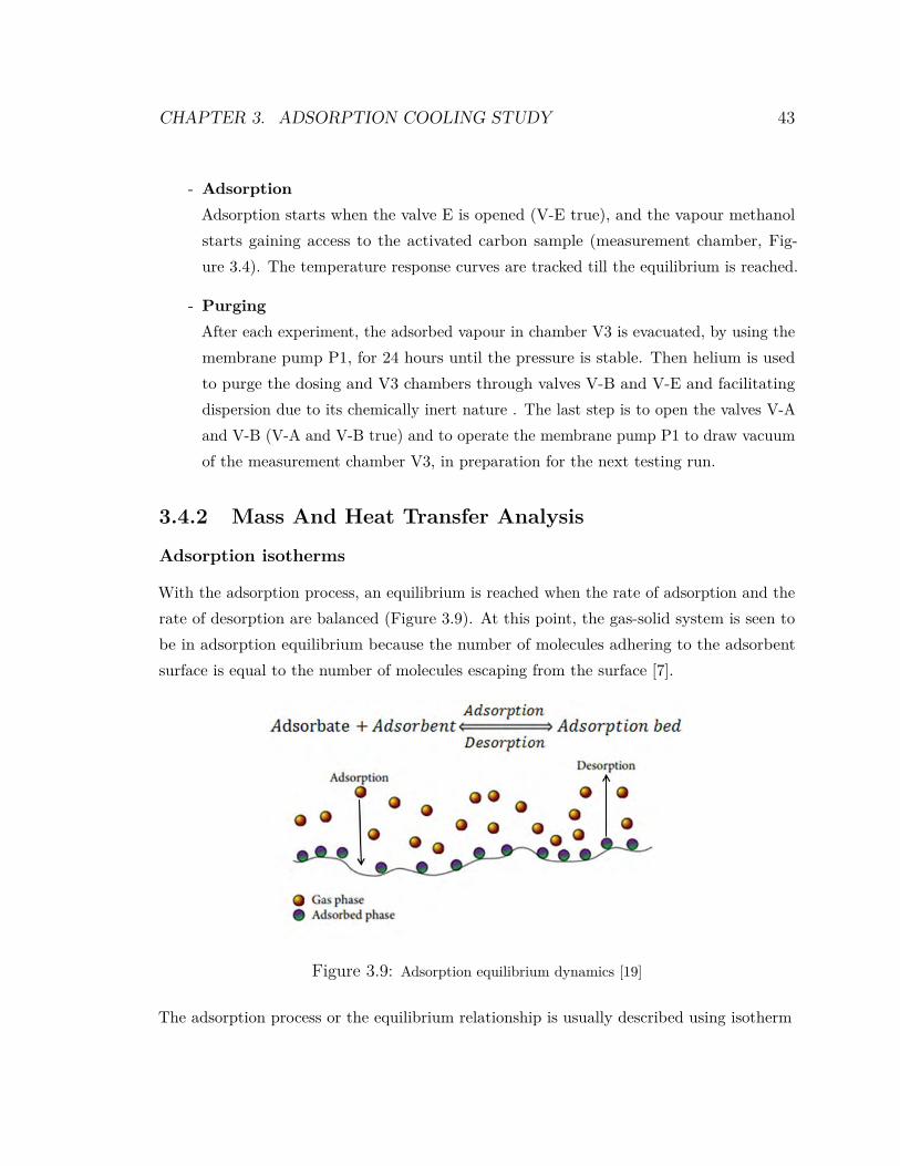
With the adsorption process, an equilibrium is reached when the rate of adsorption and therate of desorption are balanced (Figure 3.9). At this point, the gas-solid system is seen tobe in adsorption equilibrium because the number of molecules adhering to the adsorbentsurface is equal to the number of molecules escaping from the surface [7].
Figure 3.9: Adsorption equilibrium dynamics [19]
The adsorption process or the equilibrium relationship is usually described using isotherm
CHAPTER 3. ADSORPTION COOLING STUDY 44
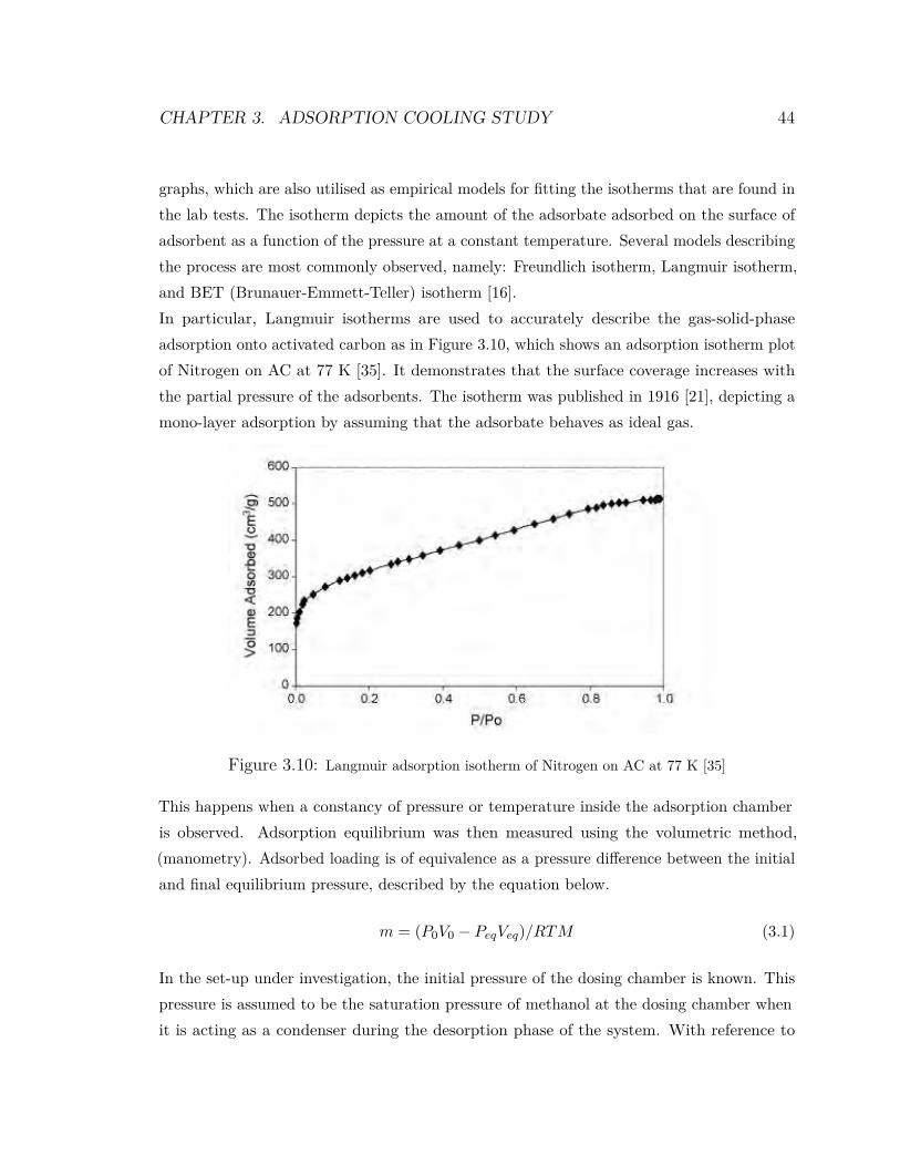
graphs, which are also utilised as empirical models for fitting the isotherms that are found inthe lab tests. The isotherm depicts the amount of the adsorbate adsorbed on the surface ofadsorbent as a function of the pressure at a constant temperature. Several models describingthe process are most commonly observed, namely: Freundlich isotherm, Langmuir isotherm,and BET (Brunauer-Emmett-Teller) isotherm [16].In particular, Langmuir isotherms are used to accurately describe the gas-solid-phaseadsorption onto activated carbon as in Figure 3.10, which shows an adsorption isotherm plotof Nitrogen on AC at 77 K [35]. It demonstrates that the surface coverage increases withthe partial pressure of the adsorbents. The isotherm was published in 1916 [21], depicting amono-layer adsorption by assuming that the adsorbate behaves as ideal gas.
Figure 3.10: Langmuir adsorption isotherm of Nitrogen on AC at 77 K [35]
This happens when a constancy of pressure or temperature inside the adsorption chamberis observed. Adsorption equilibrium was then measured using the volumetric method,(manometry). Adsorbed loading is of equivalence as a pressure difference between the initialand final equilibrium pressure, described by the equation below.
m = (P0V0 − PeqVeq)/RTM (3.1)
In the set-up under investigation, the initial pressure of the dosing chamber is known. Thispressure is assumed to be the saturation pressure of methanol at the dosing chamber whenit is acting as a condenser during the desorption phase of the system. With reference to
CHAPTER 3. ADSORPTION COOLING STUDY 45
Figure 3.4, the adsorbed amount can be computed by:
m = (P0(V1 + V2)− Peq(V1 + V2 + V3 − Vac))/RTM (3.2)
Wherem is the weight of the AC sample,P0 is the initial pressure in the methanol vapour reservoir in V1 + V2 (before opening valveV-E),V3 is the volume of the recipient reservoir (measurement chamber),Vac is the volume of AC sample,Peq is the equilibrium pressure in V1 + V2 + V3.
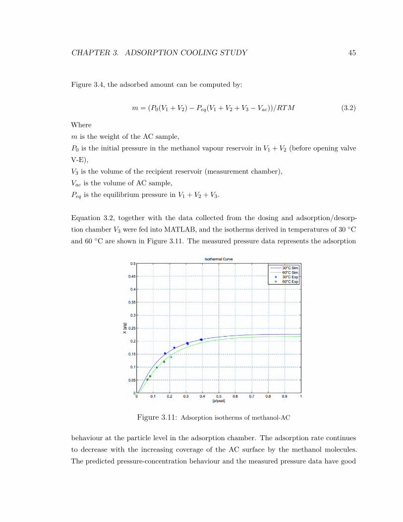
Equation 3.2, together with the data collected from the dosing and adsorption/desorp-tion chamber V3 were fed into MATLAB, and the isotherms derived in temperatures of 30 ◦Cand 60 ◦C are shown in Figure 3.11. The measured pressure data represents the adsorption
Figure 3.11: Adsorption isotherms of methanol-AC
behaviour at the particle level in the adsorption chamber. The adsorption rate continuesto decrease with the increasing coverage of the AC surface by the methanol molecules.The predicted pressure-concentration behaviour and the measured pressure data have good
CHAPTER 3. ADSORPTION COOLING STUDY 46
correlation. From Figure 3.11, it can also be seen that at the initial adsorption process, theisotherm for 30 ◦C has a steeper slope than the 60 ◦C isotherm curve. This indicates thatthe adsorption rate decreases with the increase of temperature.
Dubinin-Astakhov-Theory
The Dubinin-Astakhov (DA) theory has wide application for the methanol-AC systemto evaluate adsorption equilibrium in microporous material like AC [25]. As for physicaladsorption of gasses on micro-porous solids, it permits the calculation of the surface areaand the pore volume distribution, if:1. The area of AC occupied by a single adsorbed molecule is known;2. The number of adsorbed molecules of a fluid that covers the adsorbent with a monomolec-ular layer could be determined;3. Surface area available to the adsorbate molecules could be calculated.Its equation is one of the most popular isotherm equations in adsorption theory. It is aboutthe volume filling of micro-pores, the analysis of the capillary structure, and was foundto be the most ideal isotherm to simulate experimental data. The experimental data wasused to evaluate the isotherms by using the DA theory to characterise the strength of theadsorbent-adsorbate affinity. The equation is expressed as:
W = W0exp[−[bRT ln(Ps/Peq)]n] (3.3)
Where the meanings of the variables are:W (cm3/g) = the volume of the micro-pores filled with the adsorbate;W0(cm3/g) = the maximum volume of the adsorbent micro-pores (maximum loading);Peq = the equilibrium pressure;Ps = saturated pressure corresponding to the adsorbent temperature T;Parameters b and n depend on the chosen adsorbent/adsorbate pair.Equation 3.3 can be re-written as :
W = W0exp(−(A(Ea))n) (3.4)
Where A = RTln(P0/P ) is the adsorption potential energy (J/g) on the adsorbent surfacepores;
CHAPTER 3. ADSORPTION COOLING STUDY 47
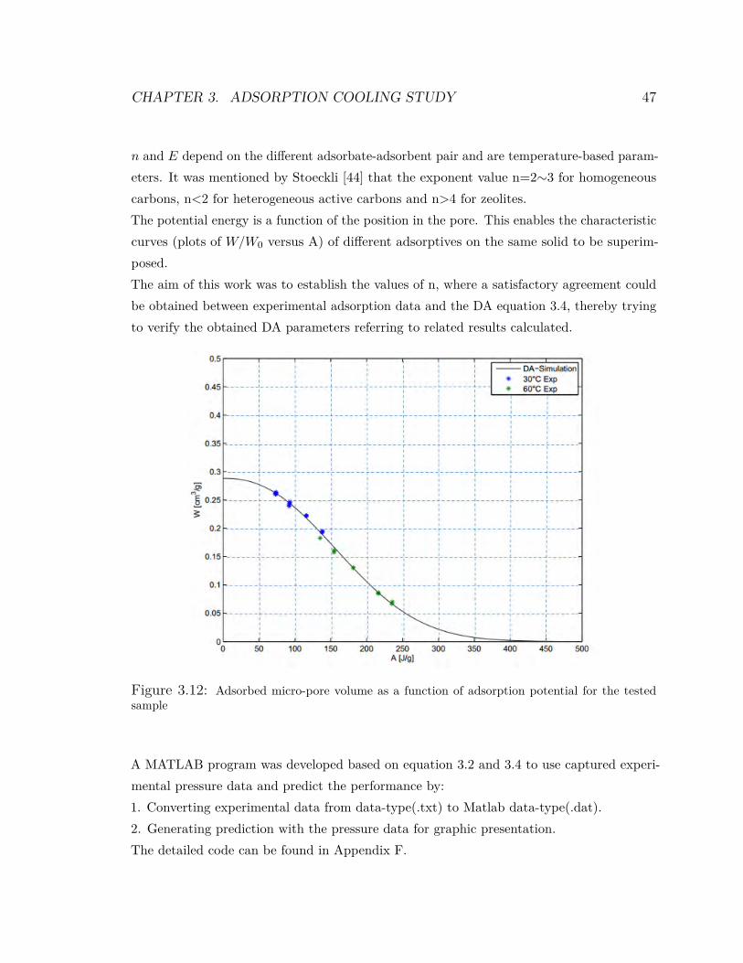
n and E depend on the different adsorbate-adsorbent pair and are temperature-based param-eters. It was mentioned by Stoeckli [44] that the exponent value n=2∼3 for homogeneouscarbons, n<2 for heterogeneous active carbons and n>4 for zeolites.The potential energy is a function of the position in the pore. This enables the characteristiccurves (plots of W/W0 versus A) of different adsorptives on the same solid to be superim-posed.The aim of this work was to establish the values of n, where a satisfactory agreement couldbe obtained between experimental adsorption data and the DA equation 3.4, thereby tryingto verify the obtained DA parameters referring to related results calculated.
Figure 3.12: Adsorbed micro-pore volume as a function of adsorption potential for the testedsample
A MATLAB program was developed based on equation 3.2 and 3.4 to use captured experi-mental pressure data and predict the performance by:1. Converting experimental data from data-type(.txt) to Matlab data-type(.dat).2. Generating prediction with the pressure data for graphic presentation.The detailed code can be found in Appendix F.
CHAPTER 3. ADSORPTION COOLING STUDY 48
From the result in Figure 3.12, a satisfactory agreement is seen between the experimentaladsorption data and the DA simulation. This programme can be used to predict and linearisemethanol-AC adsorption data over different ranges of relative pressure on an adsorptionisotherm.The validation of the experimental data against the standard adsorption isotherms arehereby completed. As a regression approximation, this is of long-standing importance foran accurate data correlation, as well as a true reflection of the activated carbon adsorptioncapability.
Chapter 4
Conclusions and Future Work
Both absorption and adsorption cooling methods were investigated. A further understandingof the sorption processes from the macroscopic to the microscopic scales was achieved.Some problems arose when running the absorption prototype, causing break-down of theexperimental procedures. These were discussed in the text, from which, the followingconclusions are drawn.It is of importance that heat is supplied evenly over the surface of the heating element. Aheating element may have surface “hot-spots”, which could denature the absorbent andrender it unable to absorb the refrigerant. The pyrolysis temperature for Tetraglyme wasverified to be 95 ◦C, hence the operation of any absorption system with TEG.DME shouldnot be higher than this value.In spite of the absorption hardware difficulties encountered during construction and furtherduring its testing, thermodynamic and equilibrium properties show that such a system is ofpotential use at low generator temperatures.With respect to the adsorption section, temperature dependent experiments of methanoladsorption on monolithic activated carbon were carried out and pressures were recorded,which gave rise to estimation of the methanol concentration in the activated carbon. Itwas concluded that faster adsorption equilibrium was observed at a lower temperature forthe same concentration. Mass transfer and adsorption kinetics parameters were fitted tothe pressure-temperature experimental data, which verified Dubinin-Astakhov equation’sapplicability to characterise methanol-AC adsorption equilibrium.The study focussed mainly on prototype testing, and the design of these units was based
49

CHAPTER 4. CONCLUSIONS AND FUTURE WORK 50
on their thermodynamic parameters and experimental data. The data and the theoreticalmodel developed are in agreement, allowing precise prediction of methanol-AC adsorptionprocess.
51
Bibliography
[1] Albert, E. and Leo, S. Refrigeration. US Patent 1,781,541. 1930. [2] Alghoul, M., Sulaiman, M., Azmi, B., and Wahab, M. A. “Advances on multipurpose solar
adsorption systems for domestic refrigeration and water heating”. Applied thermal engineering
27.5 (2007), pp. 813–822.
[3] Allouhi, A, Kousksou, T, Jamil, A, El Rhafiki, T, Mourad, Y, and Zeraouli, Y. “Optimal
working pairs for solar adsorption cooling applications”. Energy 79 (2015), pp. 235–247.
[4] Anyanwu, E. “Review of solid adsorption solar refrigeration II: An overview of the principles
and theory”. Energy Conversion and Management 45.7 (2004), pp. 1279–1295.
[5] Arivazhagan, S, Murugesan, S., Saravanan, R, and Renganarayanan, S. “Simulation studies on
R134a-DMAC based half effect absorption cold storage systems”. Energy Conversion and
anagement 46.11 (2005), pp. 1703–1713.
[6] Balaras, C. A., Grossman, G., Henning, H.-M., Ferreira, C. A. I., Podesser, E.,Wang, L., and
Wiemken, E. “Solar air conditioning in Europe–an overview”. Renewable and sustainable energy
reviews 11.2 (2007), pp. 299–314.
[7] Bansal, R. and Goyal, M. Activated Carbon Adsorption. CRC Press, 2005.
[8] Benhmidene, A., Chaouachi, B., and Gabsi, S. “Effect of operating conditions on the
performance of the bubble pump of absorption-diffusion refrigeration cycles”. Thermal Science
15.3 (2011), pp. 793–806.51
BIBLIOGRAPHY 52
[9] Borde, I, Jelinek, M, and Daltrophe, N. “Absorption system based on the refrigerant R134a”.
International Journal of Refrigeration 18.6 (1995), pp. 387–394.
[10] Castillo, J. M., Silvestre-Albero, J., Rodriguez-Reinoso, F., Vlugt, T. J., and Calero, S. “Water
adsorption in hydrophilic zeolites: experiment and simulation”. Physical Chemistry Chemical
Physics 15.40 (2013), pp. 17374–17382.
[11] Cengel, Y. and Boles, M. Property Tables Booklet for Use with Thermodynamics: An
Engineering Approach. McGraw-Hill series in mechanical engineering. McGraw-Hill, 2001.
[12] Dannen, G. “The Einstein-Szilárd refrigerators”. Scientific American 276.1 (1997), pp. 90–95.
[13] Dieng, A. and Wang, R. “Literature review on solar adsorption technologies for ice-making
and air-conditioning purposes and recent developments in solar technology”. Renewable and
Sustainable Energy Reviews 5.4 (2001), pp. 313–342.
[14] Ehrismann, B. Collated and updated list of solar cooling installations in participating
countries.
[15] El-Sharkawy, I. I., AbdelMeguid, H., and Saha, B. B. “Potential application of solar powered
adsorption cooling systems in the Middle East”. Applied Energy 126 (2014), pp. 235–245.
[16] Faeth, P. “Adsorption and vacuum technique” (1962).
[17] Fernandes, M., Brites, G., Costa, J., Gaspar, A., and Costa, V. “Review and future trends of
solar adsorption refrigeration systems”. Renewable and Sustainable Energy Reviews 39 (2014), pp.
102–123.
[18] Georg, M. C. and Von, P. B. C. Refrigerator. US Patent 1,685,764. 1928.
[19] Hassan, H. “Energy analysis and performance evaluation of the adsorption refrigeration
system”. ISRN Mechanical Engineering 2013 (2013).
[20] Kai Wang Edward A. Vineyard, P. “Adsorption refrigeration”. ASHRAE Journal (2011).
BIBLIOGRAPHY 53
[21] Keller, J. and Staudt, R. Gas Adsorption Equilibria: Experimental Methods and Adsorptive
sotherms. Springer ebook collection / Chemistry and Materials Science 2005-2008. Springer US,
2006.
[22] Kim, D. and Ferreira, C. I. “Solar refrigeration options–a state-of-the-art review”.
International Journal of refrigeration 31.1 (2008), pp. 3–15.
[23] Kouremenos, D. and Stegou-Sagia, A. “Use of helium instead of hydrogen in
inert gas absorption refrigeration”. International journal of refrigeration 11.5 (1988), pp. 336–341.
[24] Kouremenos, D., Stegou-Sagia, A, and Antonopoulos, K. “Three-dimensional
evaporation process in aqua-ammonia absorption refrigerators using helium as inert gas”.
International journal of refrigeration 17.1 (1994), pp. 58–67.
[25] Leite, A. P. F., Belo, F. A., Martins, M. M., and Riffel, D. B. “Central air conditioning based
on adsorption and solar energy”. Applied Thermal Engineering 31.1 (2011), pp. 50–58.
[26] Li, T., Wang, R., and Li, H. “Progress in the development of solid–gas sorption
refrigeration thermodynamic cycle driven by low-grade thermal energy”. Progress in Energy and
Combustion Science 40 (2014), pp. 1–58.
[27] Li, Z. and Sumathy, K. “A solar-powered ice-maker with the solid adsorption
pair of activated carbon and methanol”. International Journal of Energy Research 23.6 (1999), pp.
517–527.
[28] LindeAG. Managing refrigerants the responsible way. Tech. rep.
[29] Louajari, M., Mimet, A., and Ouammi, A. “Study of the effect of finned tube adsorber on the
performance of solar driven adsorption cooling machine using activated carbon–ammonia pair”.
Applied energy 88.3 (2011), pp. 690–698.
[30] Ltd, S. S. Refrigeration Technology. url: https://www.downloads.siemens.com / download -
center / Download . aspx ? pos = download \ &fct = getasset \&id1=8359.
BIBLIOGRAPHY 54
[31] Marcriss, R., Gutraj, J., and Zawacki, T. “Absorption fluid data survey: final report on
worldwide data, ORLN/sub/8447989/3, Inst”. Gas Tech (1988).
[32] Mendes, L. and Collares-Pereira, M. “A solar assisted and air cooled absorption machine to
provide small power heating and cooling”. International Sorption Heat Pump Conference, Munich,
Germany. 1999, pp. 129–136.
[33] Miles, D. J., Sanborn, D. M., Nowakowski, G. A., and Shelton, S. V. “Gas fired sorption heat
pump development”. Heat Recovery Systems and CHP 13.4 (1993), pp. 347–351.
[34] Narayankhedkar, K. and Maiya, M. P. “Investigations on triple fluid vapour absorption
refrigerator”. International journal of refrigeration 8.6 (1985), pp. 335–342.
[35] Önal, Y. “Kinetics of adsorption of dyes from aqueous solution using activated carbon
prepared from waste apricot”. Journal of hazardous materials 137.3 (2006), pp. 1719–1728.
[36] Paurine, A, Maidment, G., Eames, I., Missenden, J, and Day, A. “A REVIEW OF
"PUMPLESS" ABSORPTION REFRIGERATION CYCLES”.
[37] Rathore, M. and Kapuno, R. Engineering Heat Transfer. Jones & Bartlett Learning, 2011.
[38] Rezk, A. R. and Al-Dadah, R. K. “Physical and operating conditions effects on silica gel/water
adsorption chiller performance”. Applied Energy 89.1 (2012), pp. 142–149.
[39] Rodríguez-Muñoz, J. and Belman-Flores, J. “Review of diffusion–absorption refrigeration
technologies”. Renewable and Sustainable Energy Reviews 30 (2014), pp. 145–153.
[40] Santori, G., Santamaria, S., Sapienza, A., Brandani, S., and Freni, A. “A standalone solar
adsorption refrigerator for humanitarian aid”. Solar energy 100 (2014), pp. 172–178.
[41] Shelton, S. V., Stewart, S. W., Erickson, D., et al. “Bubble pump design for single pressure
absorption refrigeration cycles”. ASHRAE Transactions 108.1 (2002), pp. 867–876.
BIBLIOGRAPHY 55
[42] Solmuş, İ., Yamalı, C., Kaftanoğlu, B., Baker, D., and Çağlar, A. “Adsorption properties of a
natural zeolite–water pair for use in adsorption cooling cycles”. Applied energy 87.6 (2010), pp.
2062–2067.
[43] Srikhirin, P., Aphornratana, S., and Chungpaibulpatana, S. “A review of absorption
refrigeration technologies”. Renewable and sustainable energy reviews 5.4 (2001), pp. 343–372.
[44] Stoeckli, H. and Kraehenbuehl, F. “The enthalpies of immersion of active carbons in relation
to the Dubinin theory for the volume filling of micropores”. Carbon 19.5 (1981) pp. 353–356
[45] Tamainot-Telto, Z and Critoph, R. “Adsorption refrigerator using monolithic carbon-ammonia
pair”. International Journal of Refrigeration 20.2 (1997). pp. 146–155.
[46] Touloukian, Y. and Vargaftik, N. Handbook of Physical Properties of Liquids and Gases:
Pure Substances and Mixtures. Springer Berlin Heidelberg, 2014.
[47] Tozer, R. M. and James, R. W. “Fundamental thermodynamics of ideal absorption cycles”.
International journal of refrigeration 20.2 (1997), pp. 120–135.
[48] Ullah, K., Saidur, R, Ping, H., Akikur, R., and Shuvo, N. “A review of solar thermal
refrigeration and cooling methods”. Renewable and Sustainable Energy Reviews 24 (2013), pp.
499–513.
[49] Vasiliev, L., Mishkinis, D., Antukh, A., and Vasiliev Jr, L. “Solar-gas solid sorption
refrigerator”. Adsorption 7.2 (2001), pp. 149–161.
[50] Vicatos, G and Bennett, A. “Multiple lift tube pumps boost refrigeration capacity in absorption
plants”. Journal of Energy in Southern Africa 18.3 (2007), pp. 49–57.
[51] Vicatos, G. Heat and mass transfer characteristics: Design and optimisation of absorption
refrigeration machines. PhD Thesis, UCT, 1995.
BIBLIOGRAPHY 56
[52] Wang, D., Li, Y., Li, D, Xia, Y., and Zhang, J. “A review on adsorption refrigeration
technology and adsorption deterioration in physical adsorption systems”. Renewable and
Sustainable Energy Reviews 14.1 (2010), pp. 344–353.
[53] Wang, D., Zhang, J., Tian, X., Liu, D., and Sumathy, K. “Progress in silica gel–water
adsorption refrigeration technology”. Renewable and Sustainable Energy Reviews 30 (2014), pp.
85–104.
[54] Wang, L., Wang, R., Lu, Z., Chen, C., Wang, K, and Wu, J. “The performance of two
adsorption ice making test units using activated carbon and a carbon composite as adsorbents”.
Carbon 44.13 (2006), pp. 2671–2680.
[55] Wang, R., Wang, L., and Wu, J. Adsorption Refrigeration Technology: Theory and
Application. Wiley, 2014.
[56] Wang, R. and Oliveira, R. “Adsorption refrigeration-an efficient way to make good use of
waste heat and solar energy”. Progress in Energy and Combustion Science 32.4 (2006), pp. 424–
458.
[57] Wang, R., Wu, J., Xu, Y., Teng, Y, and Shi, W. “Experiment on a continuous heat
regenerative adsorption refrigerator using spiral plate heat exchanger as adsorbers”. Applied
thermal engineering 18.1 (1998), pp. 13–23.
[58] Wang, R., Wu, J., Xu, Y., and Wang, W. “Performance researches and improvements on heat
regenerative adsorption refrigerator and heat pump”. Energy conversion and management 42.2
(2001), pp. 233–249.
[59] Wu, J., Wang, R., and Xu, Y. “Dynamic simulation and experiments of a heat regenerative
adsorption heat pump”. Energy conversion and management 41.10 (2000), pp. 1007–1018.
[60] Xi, H., Luo, L., and Fraisse, G. “Development and applications of solar-based thermoelectric
technologies”. Renewable and Sustainable Energy Reviews 11.5 (2007), pp. 923–936.
BIBLIOGRAPHY 57
[61] Xu, D., Zhang, J., Li, G., Xiao, P., Webley, P., and Zhai, Y.-C. “Adsorption equilibrium and
kinetics of CO (2) and H (2) O on activated carbon”. Wuji Cailiao Xuebao(Journal of Inorganic
materials) 27.2 (2012), pp. 139–145.
[62] Yokozeki, A. “Theoretical performances of various refrigerant–absorbent pairs in a vapour-
absorption refrigeration cycle by the use of equations of state”. Applied Energy 80.4 (2005), pp.
383– 399.
[63] Zohar, A, Jelinek, M, Levy, A, and Borde, I. “Numerical investigation of a diffusion
absorption refrigeration cycle”. International Journal of Refrigeration 28.4 (2005), pp. 515–525.

Appendices
58
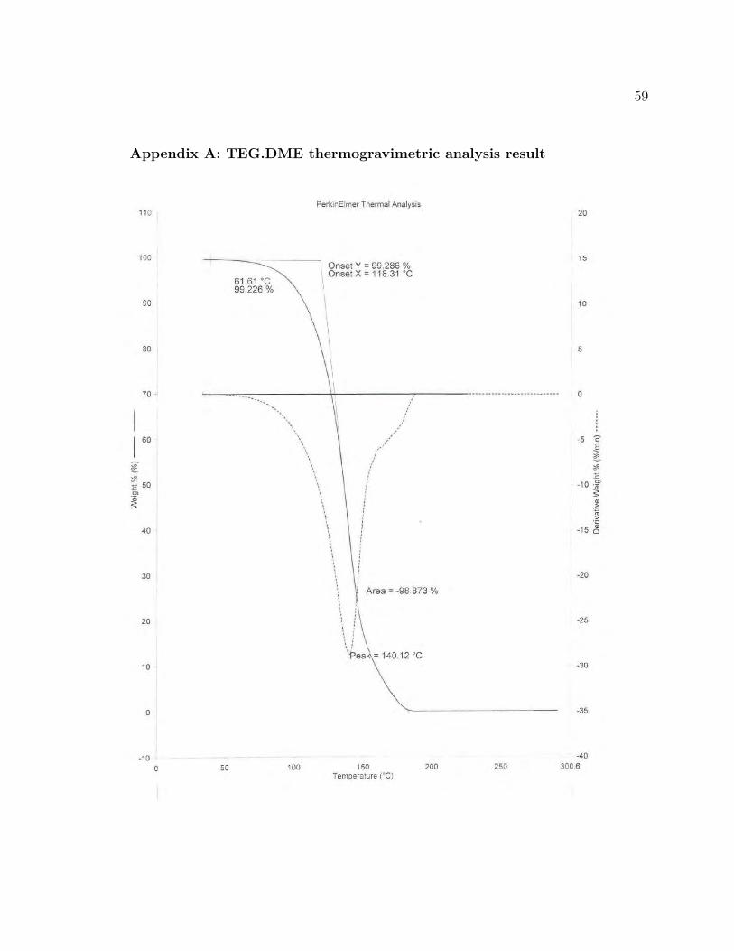
59
Appendix A: TEG.DME thermogravimetric analysis result
110
100
90
80
70
I 60
'# :E 50 0)
~
40
30
20
10
o
-10 o
61.61 · c 99.226 %
PerkinElmer Thermal Analysis
Onset Y = 99.286 % Onset X = 118.31 •c
~-~~------------------- - ----------------------------· ....... .
',\
'
50 ,oo
'
/~··
/ ' '
Area = -98.873 %
' ' '. \~ea =140.12 °c
150 Temperature (0 C}
200 250
20
15
10
5
0
-20
-25
-30
-35
-40
300.6
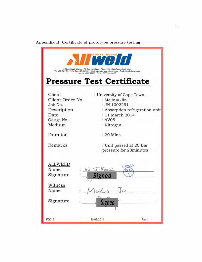
60
Appendix B: Certificate of prototype pressure testing
Subscripts:
c: condenser; cr: refrigerant states at the condenser; cw: cooling water states at the condenser; e: evaporator; er: refrigerant states at the evaporator; ew: cooling water states at the evaporator;
pc: pre-cooler; pcr: refrigerant states at the pre-cooler; pcw: cooling water states at the pre-cooler; a: absorber; ar: refrigerant states at the absorber; aw: cooling water states at the absorber;
Given:
Table C-1: Prototype basic design parameters
Parameters Assumed values Refrigeration capacity 100 W Condenser temperature 40 Pre-cooler temperature 15 Evaporator temperature -5
Table C-2: Selected pipe sizes
Parameters Pipe sizes Condenser ⁄ , 0.71mm thickness
⁄ , 0.57 mm thickness
Pre-cooler Evaporator Absorber ⁄ , 0.81mm thickness
⁄ , 0.71mm thickness
Solution heat exchanger ⁄ , 0.71mm thickness ⁄ , 0.61mm thickness
Generator ⁄ , 0.81mm thickness
61
Appendix C: Design calculations
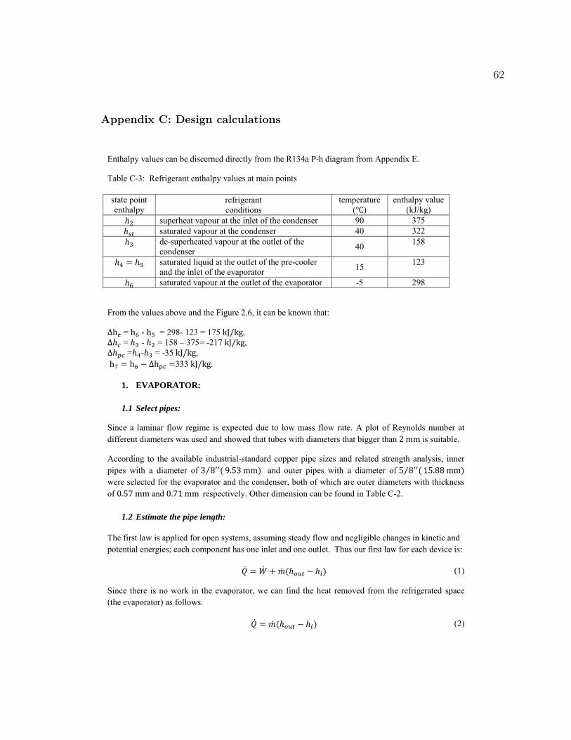
Enthalpy values can be discerned directly from the R134a P-h diagram from Appendix E.
Table C-3: Refrigerant enthalpy values at main points
state point enthalpy
refrigerant conditions
temperature ( )
enthalpy value (kJ/kg)
superheat vapour at the inlet of the condenser 90 375 saturated vapour at the condenser 40 322 de-superheated vapour at the outlet of the
condenser 40 158
saturated liquid at the outlet of the pre-cooler and the inlet of the evaporator 15 123
saturated vapour at the outlet of the evaporator -5 298
From the values above and the Figure 2.6, it can be known that:
= - = 298- 123 = 175 , = - = 158 – 375= -217 , = - = -35 , 333 .
1. EVAPORATOR:
1.1 Select pipes:
Since a laminar flow regime is expected due to low mass flow rate. A plot of Reynolds number at different diameters was used and showed that tubes with diameters that bigger than is suitable.
According to the available industrial-standard copper pipe sizes and related strength analysis, inner pipes with a diameter of ⁄ and outer pipes with a diameter of ⁄ were selected for the evaporator and the condenser, both of which are outer diameters with thickness of and respectively. Other dimension can be found in Table C-2.
1.2 Estimate the pipe length:
The first law is applied for open systems, assuming steady flow and negligible changes in kinetic and potential energies; each component has one inlet and one outlet. Thus our first law for each device is:
(1)
Since there is no work in the evaporator, we can find the heat removed from the refrigerated space (the evaporator) as follows.
(2)
62
Appendix C: Design calculations
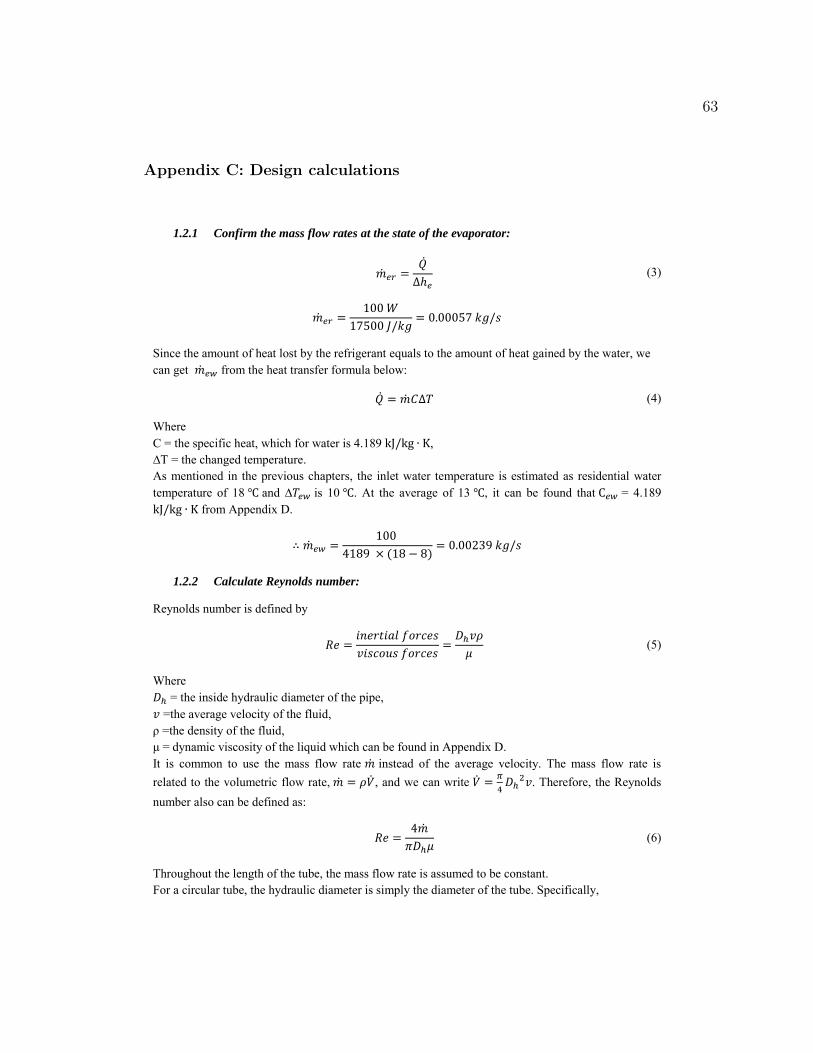
1.2.1 Confirm the mass flow rates at the state of the evaporator:
(3)
Since the amount of heat lost by the refrigerant equals to the amount of heat gained by the water, we can get from the heat transfer formula below:
(4)
Where C = the specific heat, which for water is 4.189 , ∆T = the changed temperature. As mentioned in the previous chapters, the inlet water temperature is estimated as residential water temperature of 18 and ∆ is 10 . At the average of 13 , it can be found that = 4.189 from Appendix D.
1.2.2 Calculate Reynolds number:
Reynolds number is defined by
(5)
Where = the inside hydraulic diameter of the pipe, =the average velocity of the fluid, ρ =the density of the fluid, μ = dynamic viscosity of the liquid which can be found in Appendix D. It is common to use the mass flow rate instead of the average velocity. The mass flow rate is related to the volumetric flow rate, , and we can write
. Therefore, the Reynolds number also can be defined as:
(6)
Throughout the length of the tube, the mass flow rate is assumed to be constant. For a circular tube, the hydraulic diameter is simply the diameter of the tube. Specifically,
63
Appendix C: Design calculations
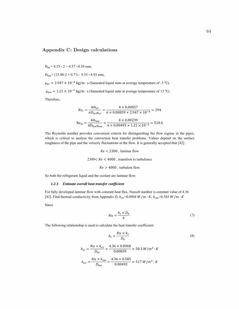
= 9.53 - 2 × 0.57 =8.39 mm,
= (15.88-2 × 0.71) - 9.53 =4.93 mm,
(Saturated liquid state at average temperature of -5 ),
(Saturated liquid state at average temperature of 13 ).
Therefore,
The Reynolds number provides convenient criteria for distinguishing the flow regime in the pipes, which is critical to analyse the convection heat transfer problems. Values depend on the surface roughness of the pipe and the velocity fluctuations in the flow. It is generally accepted that [42]:
, laminar flow
2300 , transition to turbulence
, turbulent flow
So both the refrigerant liquid and the coolant are laminar flow.
1.2.3 Estimate overall heat transfer coefficient
For fully developed laminar flow with constant heat flux, Nusselt number is constant value of 4.36 [42]. Find thermal conductivity from Appendix D, =0.0968 ⁄ ; =0.585 ⁄
Since
(7)
The following relationship is used to calculate the heat transfer coefficient:
(8)
64
Appendix C: Design calculations
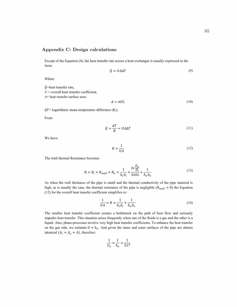
Except of the Equation (4), the heat transfer rate across a heat exchanger is usually expressed in the form: (9)
Where
=heat transfer rate, U = overall heat transfer coefficient, A= heat transfer surface area. (10)
= logarithmic mean temperature difference (K);
From
(11)
We have:
(12)
The total thermal Resistance becomes
(13)
As when the wall thickness of the pipe is small and the thermal conductivity of the pipe material is high, as is usually the case, the thermal resistance of the pipe is negligible the Equation (12) for the overall heat transfer coefficient simplifies to:
(14)
The smaller heat transfer coefficient creates a bottleneck on the path of heat flow and seriously impedes heat transfer. This situation arises frequently when one of the fluids is a gas and the other is a liquid. Also, phase-processes involve very high heat transfer coefficients. To enhance the heat transfer on the gas side, we estimate . And given the inner and outer surfaces of the pipe are almost identical , therefore:
65
Appendix C: Design calculations
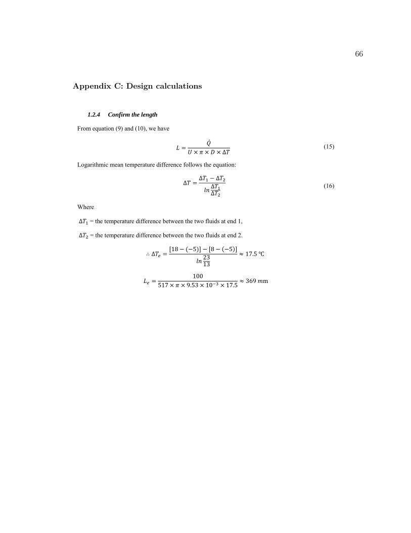
1.2.4 Confirm the length
From equation (9) and (10), we have
(15)
Logarithmic mean temperature difference follows the equation:
(16)
Where
= the temperature difference between the two fluids at end 1,
= the temperature difference between the two fluids at end 2.
66
Appendix C: Design calculations
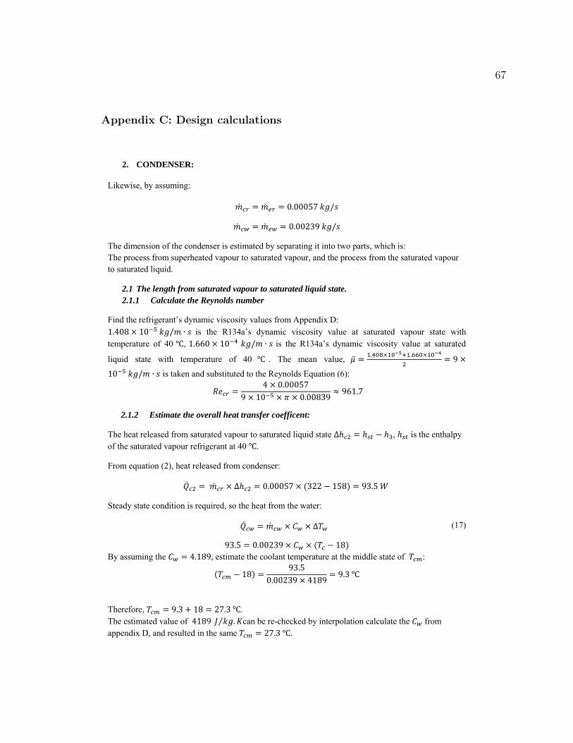
2. CONDENSER:
Likewise, by assuming:
The dimension of the condenser is estimated by separating it into two parts, which is: The process from superheated vapour to saturated vapour, and the process from the saturated vapour to saturated liquid.
2.1 The length from saturated vapour to saturated liquid state.
2.1.1 Calculate the Reynolds number
Find the refrigerant’s dynamic viscosity values from Appendix D: is the R134a’s dynamic viscosity value at saturated vapour state with temperature of 40 , is the R134a’s dynamic viscosity value at saturated
liquid state with temperature of 40 . The mean value,
is taken and substituted to the Reynolds Equation (6):
2.1.2 Estimate the overall heat transfer coefficent:
The heat released from saturated vapour to saturated liquid state , is the enthalpy of the saturated vapour refrigerant at 40 .
From equation (2), heat released from condenser:
Steady state condition is required, so the heat from the water:
(17)
By assuming the , estimate the coolant temperature at the middle state of :
Therefore, . The estimated value of ⁄ can be re-checked by interpolation calculate the from appendix D, and resulted in the same .
67
Appendix C: Design calculations
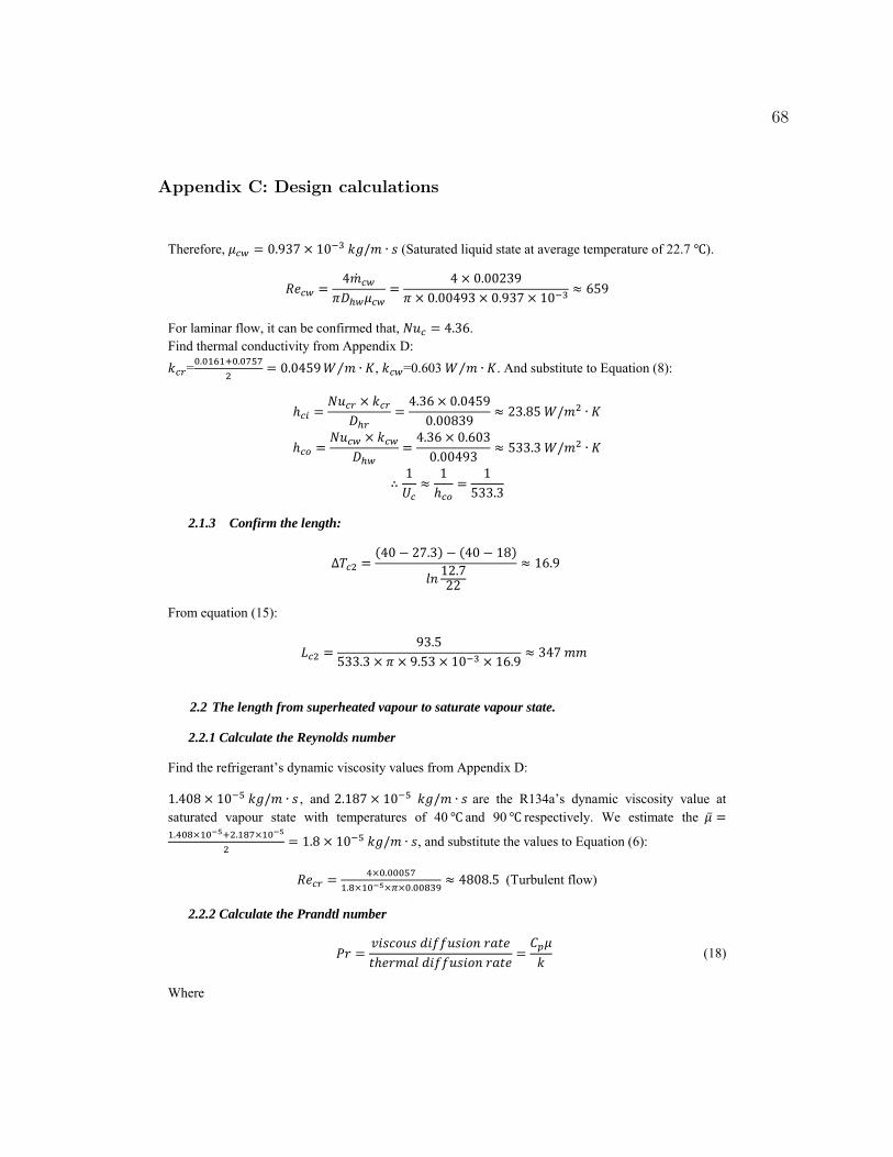
Therefore, (Saturated liquid state at average temperature of 22.7 ).
For laminar flow, it can be confirmed that, . Find thermal conductivity from Appendix D: =
⁄ , =0.603 ⁄ . And substitute to Equation (8):
2.1.3 Confirm the length:
From equation (15):
2.2 The length from superheated vapour to saturate vapour state.
2.2.1 Calculate the Reynolds number
Find the refrigerant’s dynamic viscosity values from Appendix D:
, and are the R134a’s dynamic viscosity value at saturated vapour state with temperatures of 40 and 90 respectively. We estimate the
, and substitute the values to Equation (6):
(Turbulent flow)
2.2.2 Calculate the Prandtl number
(18)
Where
68
Appendix C: Design calculations
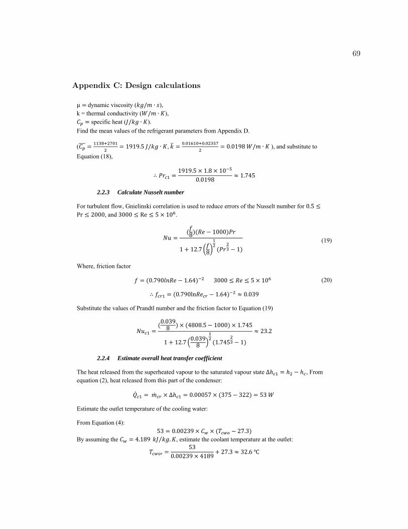
dynamic viscosity ( ), k = thermal conductivity ( ), specific heat ( ). Find the mean values of the refrigerant parameters from Appendix D.
(
,
), and substitute to
Equation (18),
2.2.3 Calculate Nusselt number
For turbulent flow, Gnielinski correlation is used to reduce errors of the Nusselt number for
, and .
( )
(19)
Where, friction factor
(20)
Substitute the values of Prandtl number and the friction factor to Equation (19)
(
)
2.2.4 Estimate overall heat transfer coefficient
The heat released from the superheated vapour to the saturated vapour state , From equation (2), heat released from this part of the condenser:
Estimate the outlet temperature of the cooling water:
From Equation (4):
By assuming the ⁄ , estimate the coolant temperature at the outlet:
69
Appendix C: Design calculations
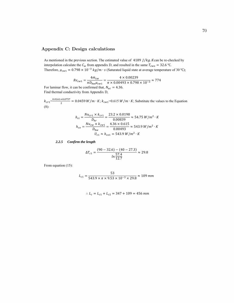
As mentioned in the previous section. The estimated value of ⁄ can be re-checked by interpolation calculate the from appendix D, and resulted in the same . Therefore, (Saturated liquid state at average temperature of 30 );
For laminar flow, it can be confirmed that, . Find thermal conductivity from Appendix D,
=
⁄ ; =0.615 ⁄ ; Substitute the values to the Equation
(8):
2.2.5 Confirm the length
From equation (15):
70
Appendix C: Design calculations
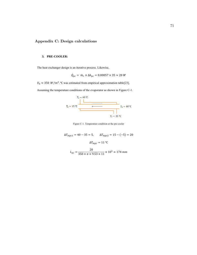
3. PRE-COOLER:
The heat exchanger design is an iterative process. Likewise,
⁄ was estimated from empirical approximation table[23].
Assuming the temperature conditions of the evaporator as shown in Figure C-1.
Figure C-1. Temperature condition at the pre-cooler
71
Appendix C: Design calculations
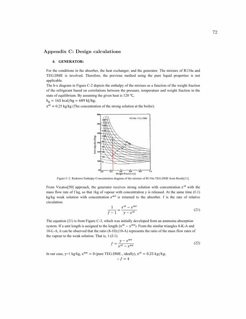
4. GENERATOR:
For the conditions in the absorber, the heat exchanger, and the generator. The mixture of R134a and TEG.DME is involved. Therefore, the previous method using the pure liquid properties is not applicable. The h-x diagram in Figure C-2 depicts the enthalpy of the mixture as a function of the weight fraction of the refrigerant based on correlations between the pressure, temperature and weight fraction in the state of equilibrium. By assuming the given heat is 120 , ; 0.25 kg/kg (The concentration of the strong solution at the boiler).
Figure C-2. Redrawn Enthalpy-Concentration diagram of the mixture of R134a-TEG.DME from Borde[11].
From Vicatos[50] approach, the generator receives strong solution with concentration with the mass flow rate of f kg, so that 1kg of vapour with concentration y is released. At the same time (f-1) kg/kg weak solution with concentration is returned to the absorber. f is the rate of relative circulation.
(21)
The equation (21) is from Figure C-3, which was initially developed from an ammonia absorption system. If a unit length is assigned to the length ). From the similar triangles 8-K-A and 10-L-A, it can be observed that the ratio (8-10):(10-A) represents the ratio of the mass flow rates of the vapour to the weak solution. That is, 1:(f-1).
(22)
In our case, y=1 kg/kg, (pure TEG.DME., ideally), ,
72
Appendix C: Design calculations
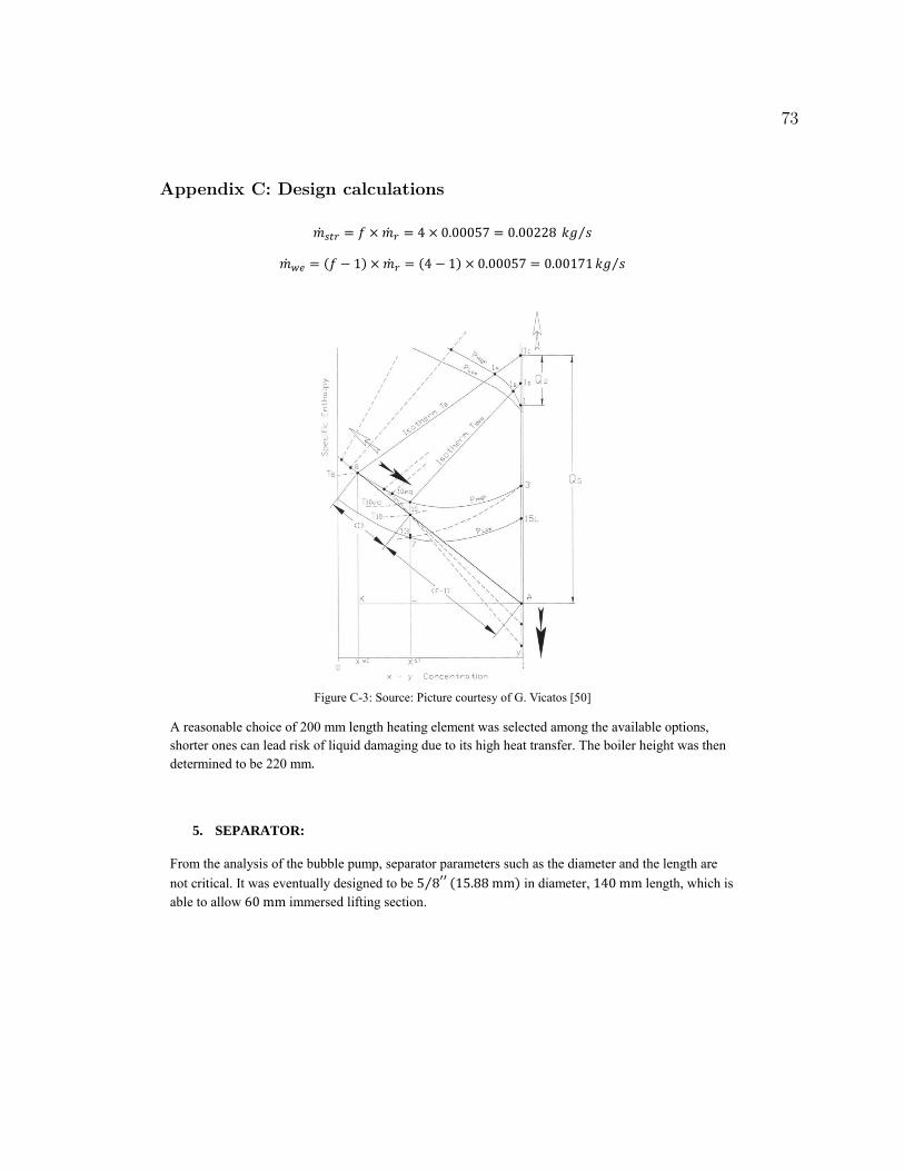
⁄
⁄
Figure C-3: Source: Picture courtesy of G. Vicatos [50]
A reasonable choice of 200 mm length heating element was selected among the available options, shorter ones can lead risk of liquid damaging due to its high heat transfer. The boiler height was then determined to be 220 mm
5. SEPARATOR:
From the analysis of the bubble pump, separator parameters such as the diameter and the length are not critical. It was eventually designed to be ⁄ in diameter, length, which is able to allow immersed lifting section.
73
Appendix C: Design calculations
6. ABSORBER:
A heat balance of the system gives: (23)
=
By estimating:
At an average temperature of 23
⁄ ⁄
From Equation (20)
Find the mean values from Appendix D.
,
,
.
Substitute to Equation (18):
74
Appendix C: Design calculations
( )
⁄
75
Appendix C: Design calculations
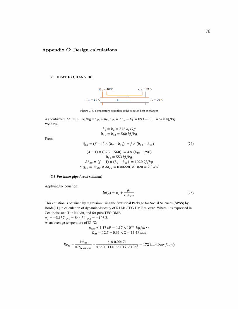
7. HEAT EXCHANGER:
Figure C-4. Temperature condition at the solution heat exchanger
As confirmed: = = , , We have:
From (24)
7.1 For inner pipe (weak solution)
Applying the equation:
(25)
This equation is obtained by regression using the Statistical Package for Social Sciences (SPSS) by Borde[11] in calculation of dynamic viscosity of R134a-TEG.DME mixture. Where is expressed in Centipoise and T in Kelvin, and for pure TEG.DME: , , . At an average temperature of 85 :
⁄
~ (1 ' 1
76
Appendix C: Design calculations
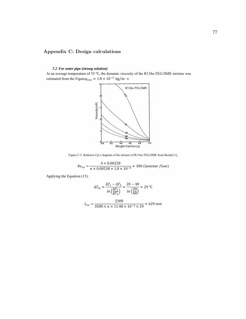
7.2 For outer pipe (strong solution)
At an average temperature of 55 , the dynamic viscosity of the R134a-TEG.DME mixture was estimated from the Figure ⁄
Figure C-5. Redrawn Cp-x diagram of the mixture of R134a-TEG.DME from Borde[11].
Applying the Equation (15):
(
)
(
)
77
Appendix C: Design calculations
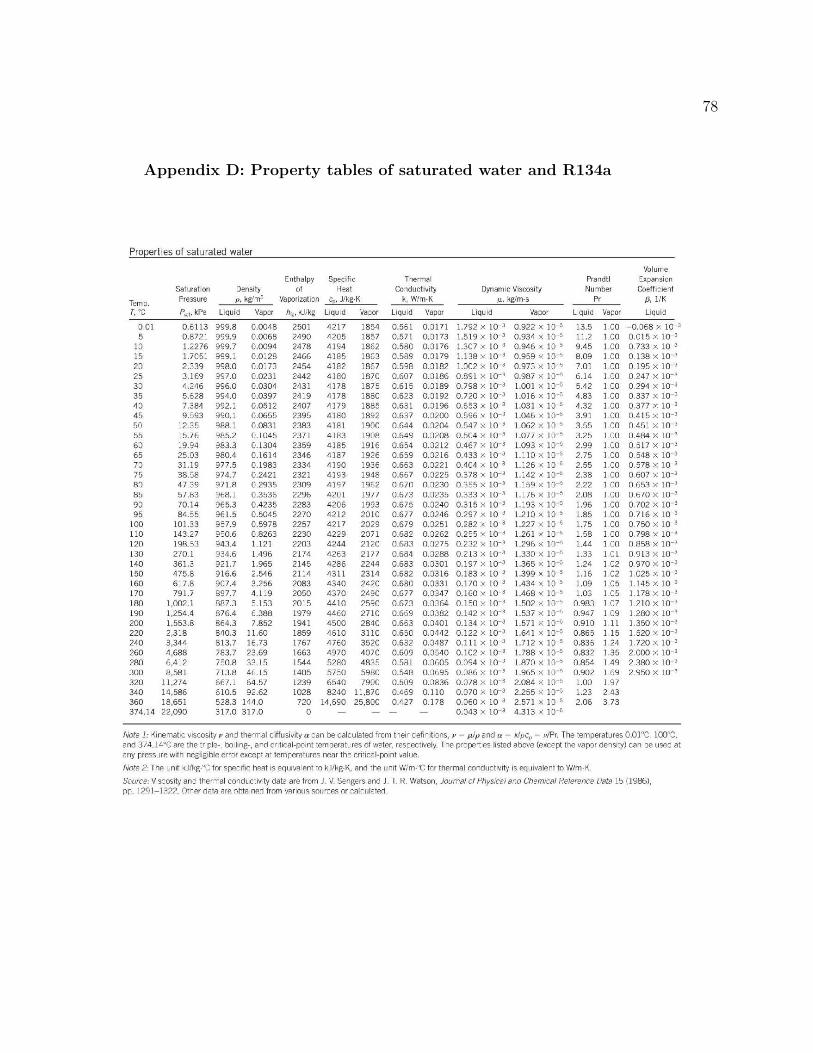
78
Appendix D: Property tables of saturated water and R134a
Proeerties of saturated water
Volume Enthalpy Specific T1erma! Prandtl Expansion
Saturation Density o1 Heat Co1ductil1ity Dynamic Viscosity Number Coefficierit
Temp. Pressure p, kg'm' Vaporization 5,, J/kg·K k, W/m·K µ,, kg/m•S Pr /3. 1/K r •~ ,u r,..t, kPa Liquid Vapor h,,., kJ/kg L1qu d Vai:or L1qu1d Vapor Liquid Vapo· Liquid Vapor L1qu1d
0.01 0.6113 999.8 0.0048 2501 4217 1854 0.561 0.0171 1.792 X 10⁻³ 0.922 >< 10-5 l3.5 1.00 -0.0E8 >< to-3
5 0.8721 999.9 0.0068 2490 4205 1857 0.571 0.0173 l.519Xl0 3 0.931, )( JJ s ll .2 1.00 0.015 X LO 3 10 1.2276 999.7 0.0094 2478 4194 1862 0.580 0.0176 1.307 X 10 3 0.946 >< 10 ' 9.45 1.00 0.733 X 10 3
15 1.7051 999.1 0.0:28 24GG 4185 1863 0.589 0.0179 :.138 X 10- ; 0.959 X lQ- > 8.09 1.00 0.138 X 10- , ?O ?.339 998.0 0.0·73 ?454 418? 1867 0598 0.018? 1.00? X 10-3 0.973 >< 10-• 7.01 1 00 0 195 X 10- 3
25 3.169 997.0 0.0231 2442 4180 1870 0.607 0.0186 O.B9l X 10-• 0.987 X 10-, 6.11. 1.00 0.247 X 10-> 30 4.246 996.0 0.0304 2431 4178 1875 0.615 0.0189 0.798 X 10⁻³ 1.00) X 10- 5 5.42 1.00 0.294 X 10- 3
35 5.628 994.0 0.0397 2419 4178 1880 0.623 0.0192 0.720 X 10 3 1.016 >< 10 s 4.83 1.00 0.337 X 10 3 40 7.384 992.1 0.0512 2407 4179 1885 0.631 0.0196 0.653 X 10 3 1.031 X 10 S 4.32 1.00 0.377 X 10 3 45 9. 593 990.1 0.0655 2395 4180 1892 0 .637 0.0200 0.59G X 10-; 1.046 X 10-> 3.91 1.00 0.415 X lQ-' 50 1? .15 gRA.l 0.08.11 ?.1R1 41R I 1goo O.fi44 o.n204 0.547 X 10⁻³ I.()(,? X l [)-• :l.55 1.00 0.45' X 10- 3
55 15.76 985.2 0.1045 2371 4183 1906 0.649 0.0208 0.504 X 10- • 1.077 X 10-• 3.25 1.00 0.484 X 10-> 60 19.94 983.3 0.1304 2359 4185 1916 0.654 0.0212 0.467 X 10⁻³ 1.093 X lQ-5 2.99 1.00 0.517 X 10-> 65 25.03 980.4 0.1614 2346 4187 1926 0.659 0.0216 0.433 X 10 3 LlO x 10 s 2.75 1.00 0.548 X 10 3
70 31.19 977.5 0.1983 2334 4190 1936 0.663 0.022l 0.404 X 10 3 L26 x JO s 2.55 1.00 0.578 x LO 3 75 38.58 974.7 0.2421 2321 4193 1948 0.667 0.0225 0.378 X 10- 3 t.:42 X 10- > 2.38 1.00 0.607 X lQ- 3
RO 47.~g g71 _R O.?g:15 23oq 4Vi7 1%? 0.670 0.0230 0.355 X 10⁻³ 1." 5g X 18-• ?.?? 100 0 .653 X 10-3
85 57.83 968.1 0.3536 2296 4201 1977 0.673 0.0235 0.333 X 10- • t. : 76 X JO- ' 2.08 1.00 0.670 X LO- ' 90 70.14 965.3 0.4235 2283 4206 1993 0.675 0.0240 0.315 X 10-> 1.:93 X 10-s 1.96 1.00 0.702 X 10⁻³
95 84.55 961.5 0.5045 2270 4212 2010 0.677 0.0246 0.297 X 10⁻³ 1.210 X lQ-S l.85 1.00 0.716 X lQ-J 100 101.33 957.9 0.5978 2257 4217 2029 0.679 0.025l 0.282 X 10 3 1.227 x 10 s l.75 1.00 0.750 X 10 3
110 l43.27 950.6 0.8263 2230 4229 2071 0 .682 0.0262 0.255 X 10⁻³ 1.26) X JO-> 1.58 1.00 0.798 X LQ-3
120 198.53 943.4 1.121 2203 4244 2120 O.fi81 0.0275 0.232 X 10- 3 1.296 X ]8- ' 1.44 1.00 0 858 X )0- 3
130 270.1 934.6 1.496 2 174 4263 2177 0.684 0.0288 0.213 X 10-• 1.330 X rn-• l.33 1.01 0.9 l3 X LO-' 140 361.3 921.7 1.965 2145 4286 2244 0.683 0.0301 0.197 X lQ-3 1.365 >< 10- 5 1.24 1.02 0.970 X l0-3 150 475.8 916.6 2.546 2114 4311 2314 0.682 0.0316 0.)83 X lQ-J 1.399 X lJ-S 1.16 1.02 1.025 X 10⁻³ 160 617.8 907.4 3.256 2083 4340 2420 0.680 0.033l 0.)70 X 10 3 1.434 X JO S l.09 1.05 1.145 X LO 3 170 791.7 897.7 4.1:9 2050 4370 2490 0.677 0.0347 0.160 X 10⁻³ 1.468 X IO- ' l.03 1.05 1.178 X 10- 3
180 1,002.1 887.3 5.153 2015 4410 2590 0 .673 0.0364 0.150 X 10⁻³ 1.502 X 10-' 0.983 1.07 1 210 X 10-3
190 1,254.4 876.4 6.388 1979 4460 2710 0.669 0.0382 0.142 X 10- • l.537 X JO- ' 0.947 1.09 J.280 X LO- ' 200 1,553.8 864.3 7.852 1941 4500 2840 0.663 0.0401 0.134 X 10⁻³ 1.571 X t:)-5 0.910 I.I l 1.350 X 10⁻³ 220 2,318 840.3 ll.60 1859 4610 3))0 0 .650 0.0442 0.122 X 10⁻³ 1.64) X 10-s 0.865 1.15 1.520 X 10⁻³
240 3,344 813.7 16.73 1767 4760 3520 0.632 0.0487 O.lllxl0 3 l.712 xl0 5 0.835 1.24 1.720 X 10 3
260 4,688 783.7 23.69 1663 4970 4070 0.609 0.0540 0.102 X 10⁻³ l.788 X JO-S 0.832 1.35 2.000 X LQ- 3
280 6,412 750.8 33.15 1544 5280 4835 0.581 0.0605 0.094 X lQ- • 1.870 X JQ- > 0.854 1.49 2.380 X lQ- 3
300 8,581 713.8 46.15 1405 57::0 5980 0.54R 0.0695 0.086 X 10- • 1.965 X 10-s 0.902 1.69 2.%0 X 10- ' 320 11.274 667.1 64.57 1239 6540 7900 0.509 0.0836 0.078 X 10⁻³ 2.084 >< w-• 1.00 1.97 340 14,586 6 10.5 92.62 1028 8240 11,870 0.469 0.110 0.070 X 10-J 2.255 X 10-s 1.23 2.43 360 18,651 528.3 144.0 720 14,690 25,800 OA27 0.1 78 0.060 X 10 3 2.57) X 10 S 2.06 3.73 374.14 22,090 317.0 317.0 0 0.043 X lQ-3 4.313 X 1()-S
Note 1: ~inemat c viscositt ,, an:J the·rral diffusivity" can be calculated 'rom their deficrtions, ,, - µIp and u - k!µc" - v/Pr. The temperatures O.Ol'C. lOO'C, end 374. l 4°C are the triple-, bolling-, ard critical-point :emperaues of water, respectively. Tre pr:ipe1es listed abcve (e,cept the vap:ir dens1:y) can be used at my pessure wit~ negligible error except a: tempera·ures near the cn·ic;i~point value.
Nnte 2: The unit <Jlkg-•c fnr sperifir he.at is e~1J1va ent ·o kJ/kg-K, and the urit Wim-"f: for thermal cnr nur,t,vity is e<}tHvalent to W/m-K
Source: Viscosity and therT'al conductiv ly data are from J. V. Sengers and J. T. R. Watson, Journal of Physical and Chemical Reference Data 15 (]986), pp. I ?g 1-1.~??. Other r1ata are nhta1ne<1 from 'll'l rious sources or r.al~ulate<1.
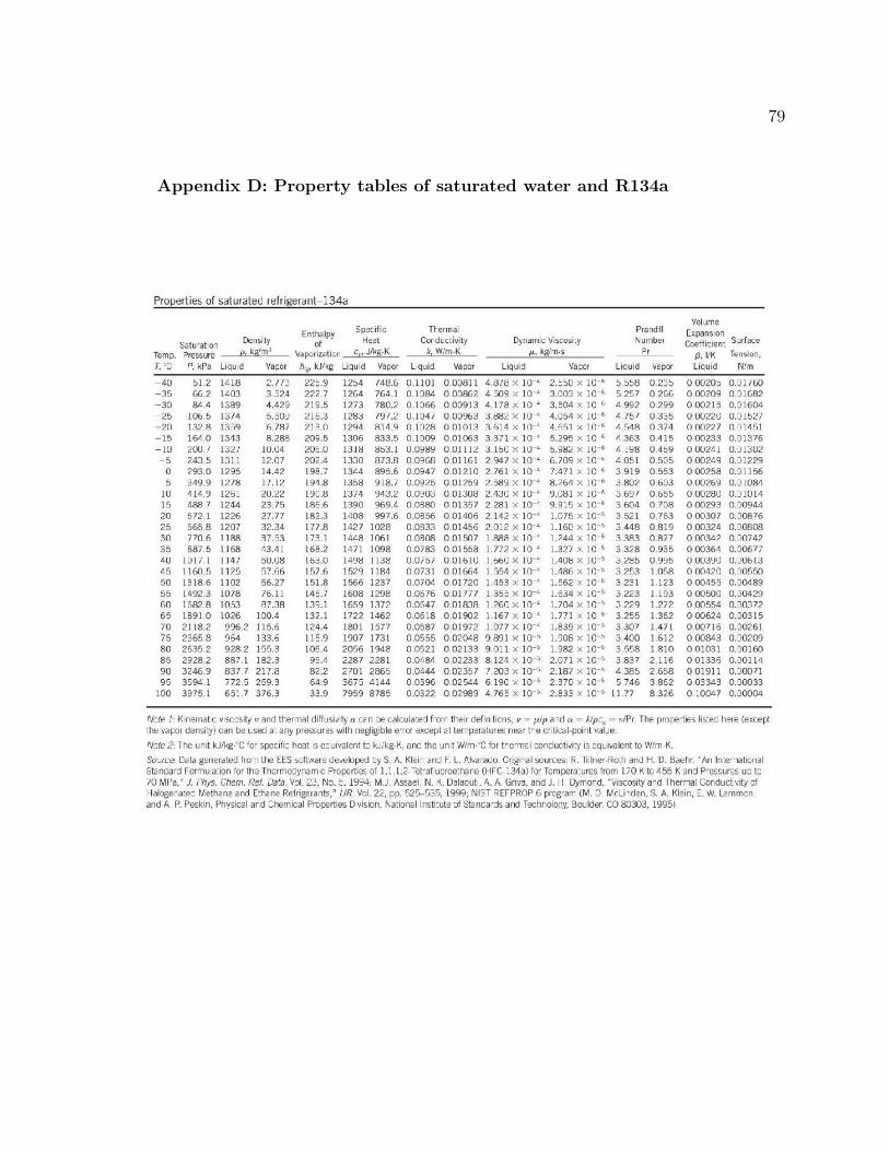
79
Appendix D: Property tables of saturated water and R134a
Properties of saturated rt! lri~erant-134a
Vol,me Enthalpy Specific Thermal Prandtl [xpansion
Satu·at on Densi1y of Heat Cor di.,ctivit:, Dynamic Viscosity t\umber Coefficient Surface
Temp. Pressure e, kglm3 Vaporization c0, J/kg,K k, W/m,K µ., kEJl•ri,s Pr ll, VK Tension, T, 'C P, kPa Liqu d Vapor h1g, kJ/kg Li~uid Vapor liquid Vapor Liqui:I Vapor Liquid Vapor Liquid Wm
4U !>1.2 1418 2.113 22~.Y 1204 t4e.b U.1101 O.OU8l l 4 .8/ti X 10- • 2.t!>U X iu- ' !>.!>08 0 .2;J!, U.0020!> O.Jl /60 -35 66 2 1403 3 .524 222.7 1264 764.l 0.1084 0 00862 4.509 X 10⁻⁴ 3.003 X 10⁻⁶ 5 257 0 266 0 .00209 O.J l 682 -30 84.4 1389 4.429 219.5 1273 780.2 0.1066 0.00913 4.178 X 10- • 3.504 X JO- G 4 .992 0 .299 0.00215 O.J \ 604
25 !06.5 1374 5.509 216.3 1283 797.2 0.1047 0.00963 3.882 X w-• 4.054 X w-• 4.757 0 .335 0.00220 O.J J527 - ?n 13? 8 135q f, 787 ?1.,.0 17q4 814.q n.JO?R 0010B 3.fi! 4 X 10- < 4.f.!11 X ]()- 6 4.!i48 0 374 0 .00?77 0.:1 \4:il - 15 164.0 13-13 8.288 209.5 1306 833.5 0.1009 0.01063 3.371 X 10 4 5.295 X JO ' 4.363 0 .415 0 .00233 0.J l376 -JO 200./ U2/ JU.04 206.0 1318 8!>3.1 0 .0989 0.011!2 3.1!>0 X J0- 4 !>.982 X J0-6 4.198 0 .4!,9 0 .00241 O.J l 302 - 5 243.5 131: 12.07 202.4 1330 873.8 0.0968 0.01 !GI 2.947 X 10- • G.709 X 10-• 4.051 0 .505 0 .00249 0.J l229
0 293.0 1295 14.42 198.7 1344 895.6 0.0947 0.01210 2.761 X 10- 4 7.471 X 10- 6 3.919 0.553 0.00258 O.J ll56 5 3,19,9 1278 17.12 191.8 1358 918.7 0.0925 0.01259 2.589 X 10- 4 8.264 X 10- 6 3.802 0 .603 0.00269 O.Jl084
JO 414.9 126: 20.22 19:;,s 1374 943.2 0.0903 0.01308 2.430 X 10-• 9.081 X 10-• 3 .697 0 .655 0 .00280 O.J l014 15 488.7 1244 23.75 186.6 1390 969.A 0.0380 0 .01357 2.281 X 10- < 9.9'.5 X 10- 6 3.604 0 708 0.00293 O.J0944 20 572.1 1226 27.77 182.3 1408 997.6 0.0856 0.01405 2.142 X 10-• 1.075 X 10-o 3 .521 0 .763 0 .00307 0.J0876 25 665.8 1207 32.34 177.8 1427 1028 0.0833 0.01456 2.012 X 10-• 1.160 X 10- 5 3.448 0 .819 0.00324 O.J0808 30 770 6 1188 37.53 173.J 1448 1061 0.0808 0 01507 1.886 X lQ-< 1.244 X J0-5 3 383 0 877 0 .00342 O.J0742 35 887.5 1168 13.11 168.2 117 l 1098 0.0783 0.01558 1.772 X 10 ' 1.327 X 10 S 3.328 0 .935 0 .0036,1 O.J0677 LU LUL/.1 114/ a0.U8 163.0 l4Y8 I 13~ U.07:,/ 0 .01610 l.bbU X 10- 4 1.408 X w-o 3.28:, U.Y~!> U.U03YU U.:JObl3 l5 1 ] (,() 5 1125 57.G6 157.fi l!i29 1184 0.0731 O.Ollif,4 1.554 X JO-• 1.48G X 10-, '.\.253 1.058 0 .00420 O.J0550 50 1318.6 1102 56.27 151.8 1566 1237 0.0704 0.01720 1.453 X 10 4 1.562 X JO S 3.231 1.123 0.00455 O.J0489 55 1492.3 1078 76.11 145.7 1608 1298 0.0676 0.01777 1.355 X 10-• l.E34 X 10-5 3.223 1.193 0 .00500 O.J0429 r,o l nA?.A 10.'i:l i'LlA 1:iq_1 lf,5q 137? n.or.47 O.Olll.1A l .?60 X 10 4 1.704 X 1 o- s :l.??CJ l .?7? 0.00554 0.Jn:l7? 65 1891.0 1026 100.4 132.1 1722 1462 0.0618 0.01902 J. 167 X 10' 1. 771 X 10 5 3.255 1.362 0 .00624 0.J0315 70 2118.2 996.2 115.6 124.4 1801 1577 0.0:,87 O.QJ972 J.077 X JO- • l.839 X 10- , 3 .307 1.471 0 .00716 O.J0261 75 2365.8 964 133.6 115.9 1907 1731 0.0555 0.02~8 9.891 X 10-, l.908 X JO- > 3 .400 1.612 0 .00843 O.J0209 80 2635 2 928.2 155.3 106.4 2056 1948 0 .0521 0 02133 9.011 X lQ- S 1.982 X 10- • 3 .558 1810 0 01031 O.J0160 85 2928.2 887.1 182.3 95.4 2287 2281 0.0484 0.02233 8.124 X 10 S 2.071 X 10 S 3.837 2. 116 0 .01336 O.J0114 90 3246 9 837.7 217.8 82.2 2701 2865 0.0444 0.02357 7.203 X 10-s 2.187 X 10-, 4.385 2.658 0 .01911 0.J0071 95 %94. l 772.5 269.3 64.9 367G 4144 0.0396 0.02~4 6.190 X 10 S 2.370 X 10- s !; 746 3 862 0 .03343 O.J0033
100 3975.1 65:.7 376.3 33.9 7959 8785 0.0322 0.02989 4.765, X 10- 5 2.833 X 10⁻⁵ 11.77 8.326 0 .10047 O.J0004
rJcte 1: K nemat c visc -Jsity v and thermal cliffusi',ity " cz n Je calculatecl fun, their def in ticns. v ; µIp and " ; k!pc0 ; u!Pr. The propei ies listec here (exce1)t the var;or densHy) can ba csed a: any pressures with negligible e·ror except at lerrperatures near t"e cntical-point val Je.
Note 2: The u1it kJ/kg·°C fo• spec1f1: heat 1s ecu1valent tc kJfkg·K, and !he un t Wlm·°C for tre·msl conductivity is equivalent to W/mK
Socrce: Dala generated fro·11 tile EES sort-.. are developed t y S. A. Klein and F. L. Alvarado. Grigi"1al source,: R. Tillner-Ro.11 and H. D. Baehr, "An lnte··1ational otlndar,:J Formu a:ion for the Thermo:Jynam c PropertieE of 1.1. l.2·-Tet·af u:roethane (HFC-:34a) for Tempera:ures from 170 K to 455 K an,:J P·essurcs ur: tc JO Ml •a. " J. /'hyS. Chem, fl~!. Data. Vol. 23, N~. : . 1994: M.J. Assael, N. K. lJalaouti. A. A. Griv3. and J. 11. l)ymond. "'viscosity ar d thermal Conduct1\'ity cf -ialogeratec Methane and E:hane Refrigerants," /JR. Vol. 22, pp. S25-':i3S, 1999; NIST REFPROP 6 progca1T (M. 0. tlclir den. S. A. Klcain, E.W. Lemmen. and A. P. Pesf:ln, Physical and Shemlcal Properties O vision, t\atlonal lnstl:ute Jf Stanca·ds and Technolo;w, Boulder. CO 80303, 1995)
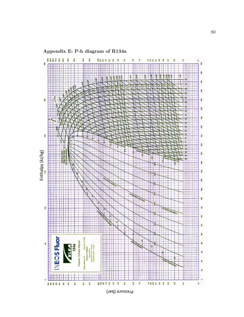
Enth
alp
y (k
J/kg
)
Pressure (bar)
80
Appendix E: P-h diagram of R134a
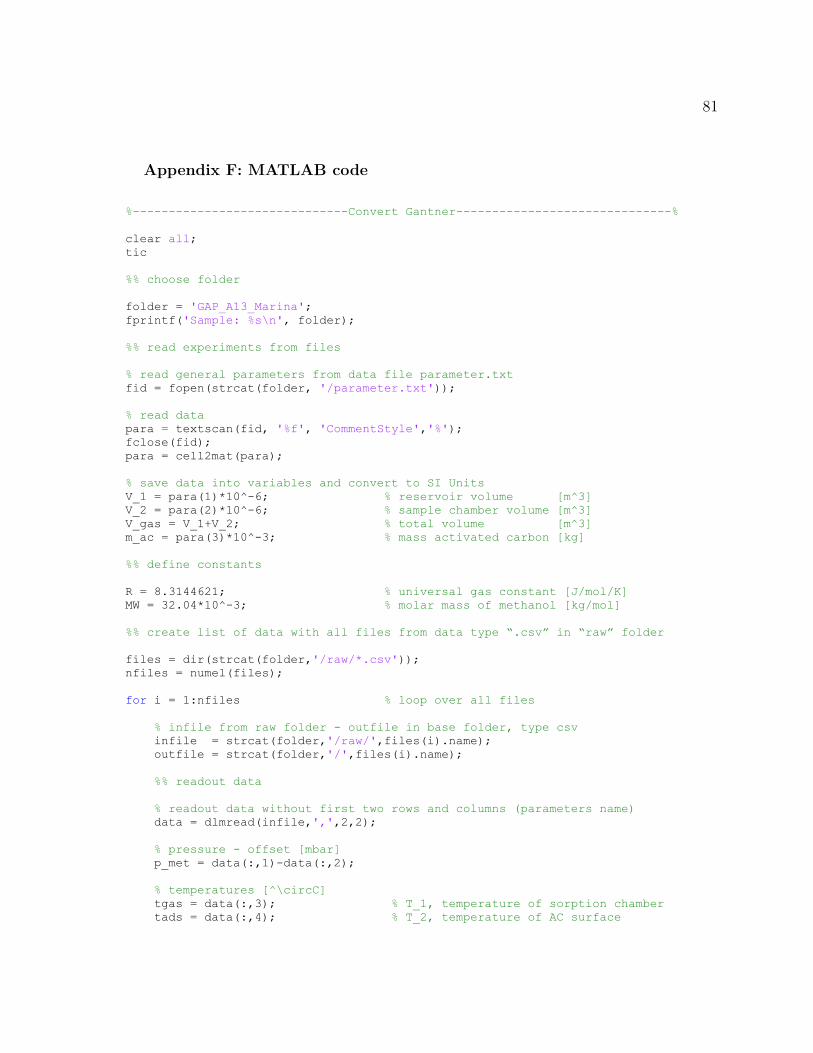
%------------------------------Convert Gantner------------------------------%
clear all;
tic
%% choose folder
folder = 'GAP_A13_Marina';
fprintf('Sample: %s\n', folder);
%% read experiments from files
% read general parameters from data file parameter.txt
fid = fopen(strcat(folder, '/parameter.txt'));
% read data
para = textscan(fid, '%f', 'CommentStyle','%');
fclose(fid);
para = cell2mat(para);
% save data into variables and convert to SI Units
V_1 = para(1)*10^-6; % reservoir volume [m^3]
V_2 = para(2)*10^-6; % sample chamber volume [m^3]
V_gas = V_1+V_2; % total volume [m^3]
m_ac = para(3)*10^-3; % mass activated carbon [kg]
%% define constants
R = 8.3144621; % universal gas constant [J/mol/K]
MW = 32.04*10^-3; % molar mass of methanol [kg/mol]
%% create list of data with all files from data type “.csv” in “raw” folder
files = dir(strcat(folder,'/raw/*.csv'));
nfiles = numel(files);
for i = 1:nfiles % loop over all files
% infile from raw folder - outfile in base folder, type csv
infile = strcat(folder,'/raw/',files(i).name);
outfile = strcat(folder,'/',files(i).name);
%% readout data
% readout data without first two rows and columns (parameters name)
data = dlmread(infile,',',2,2);
% pressure - offset [mbar]
p_met = data(:,1)-data(:,2);
% temperatures [^\circC]
tgas = data(:,3); % T_1, temperature of sorption chamber
tads = data(:,4); % T_2, temperature of AC surface
81
Appendix F: MATLAB code
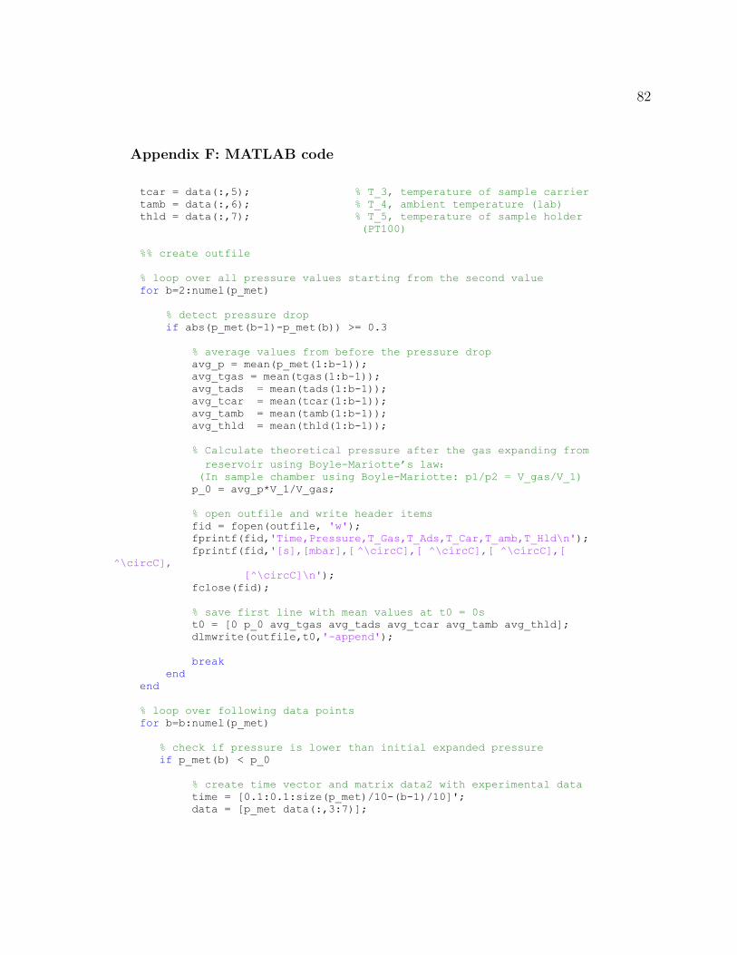
tcar = data(:,5); % T_3, temperature of sample carrier
tamb = data(:,6); % T_4, ambient temperature (lab)
thld = data(:,7); % T_5, temperature of sample holder
(PT100)
%% create outfile
% loop over all pressure values starting from the second value
for b=2:numel(p_met)
% detect pressure drop
if abs(p_met(b-1)-p_met(b)) >= 0.3
% average values from before the pressure drop
avg_p = mean(p_met(1:b-1));
avg_tgas = mean(tgas(1:b-1));
avg_tads = mean(tads(1:b-1));
avg_tcar = mean(tcar(1:b-1));
avg_tamb = mean(tamb(1:b-1));
avg_thld = mean(thld(1:b-1));
% Calculate theoretical pressure after the gas expanding from
reservoir using Boyle-Mariotte’s law:
(In sample chamber using Boyle-Mariotte: p1/p2 = V_gas/V_1)
p_0 = avg_p*V_1/V_gas;
% open outfile and write header items
fid = fopen(outfile, 'w');
fprintf(fid,'Time,Pressure,T_Gas,T_Ads,T_Car,T_amb,T_Hld\n');
fprintf(fid,'[s],[mbar],[ ^\circC],[ ^\circC],[ ^\circC],[ ^\circC],
[^\circC]\n');
fclose(fid);
% save first line with mean values at t0 = 0s
t0 = [0 p_0 avg_tgas avg_tads avg_tcar avg_tamb avg_thld];
dlmwrite(outfile,t0,'-append');
break
end
end
% loop over following data points
for b=b:numel(p_met)
% check if pressure is lower than initial expanded pressure
if p_met(b) < p_0
% create time vector and matrix data2 with experimental data
time = [0.1:0.1:size(p_met)/10-(b-1)/10]';
data = [p_met data(:,3:7)];
82
Appendix F: MATLAB code
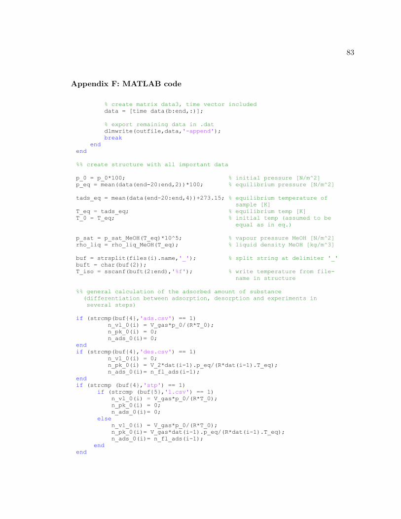
% create matrix data3, time vector included
data = [time data(b:end,:)];
% export remaining data in .dat
dlmwrite(outfile,data,'-append');
break
end
end
%% create structure with all important data
p_0 = p_0*100; % initial pressure [N/m^2]
p_eq = mean(data(end-20:end,2))*100; % equilibrium pressure [N/m^2]
tads_eq = mean(data(end-20:end,4))+273.15; % equilibrium temperature of
sample [K]
T_eq = tads_eq; % equilibrium temp [K]
T_0 = T_eq; % initial temp (assumed to be
equal as in eq.)
p_sat = p_sat_MeOH(T_eq)*10^5; % vapour pressure MeOH [N/m^2]
rho_liq = rho_liq_MeOH(T_eq); % liquid density MeOH [kg/m^3]
buf = strsplit(files(i).name,'_'); % split string at delimiter '_'
buft = char(buf(2));
T_iso = sscanf(buft(2:end),'%f'); % write temperature from file-
name in structure
%% general calculation of the adsorbed amount of substance
(differentiation between adsorption, desorption and experiments in
several steps)
if (strcmp(buf{4},'ads.csv') == 1)
n_vl_0(i) = V_gas*p_0/(R*T_0);
n_pk_0(i) = 0;
n_ads_0(i)= 0;
end
if (strcmp(buf{4},'des.csv') == 1)
n_vl_0(i) = 0;
n_pk_0(i) = V_2*dat(i-1).p_eq/(R*dat(i-1).T_eq);
n_ads_0(i)= n_fl_ads(i-1);
end
if (strcmp (buf{4},'stp') == 1)
if (strcmp (buf{5},'1.csv') == 1)
n_vl_0(i) = V_gas*p_0/(R*T_0);
n_pk_0(i) = 0;
n_ads_0(i)= 0;
else
n_vl_0(i) = V_gas*p_0/(R*T_0);
n_pk_0(i)= V_gas*dat(i-1).p_eq/(R*dat(i-1).T_eq);
n_ads_0(i)= n_fl_ads(i-1);
end
end
83
Appendix F: MATLAB code
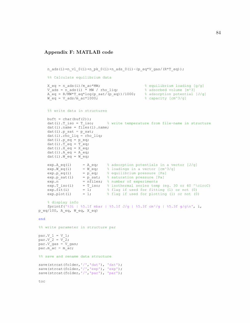
n_ads(i)=n_vl_0(i)+n_pk_0(i)+n_ads_0(i)-(p_eq*V_gas/(R*T_eq));
%% Calculate equilibrium data
X_eq = n_ads(i)/m_ac*MW; % equilibrium loading [g/g]
V_ads = n_ads(i) * MW / rho_liq; % adsorbed volume [m^3]
A_eq = R/MW*T_eq*log(p_sat/(p_eq))/1000; % adsorption potential [J/g]
W_eq = V_ads/m_ac*1000; % capacity [cm^3/g]
%% write data in structures
buft = char(buf(2));
dat(i).T_iso = T_iso; % write temperature from file-name in structure
dat(i).name = files(i).name;
dat(i).p_sat = p_sat;
dat(i).rho_liq = rho_liq;
dat(i).p_eq = p_eq;
dat(i).T_eq = T_eq;
dat(i).X_eq = X_eq;
dat(i).A_eq = A_eq;
dat(i).W_eq = W_eq;
exp.A_eq(i) = A_eq; % adsorption potentials in a vector [J/g]
exp.W_eq(i) = W_eq; % loadings in a vector [cm^3/g]
exp.p_eq(i) = p_eq; % equilibrium pressure [Pa]
exp.p_sat(i) = p_sat; % saturation pressure [Pa]
exp.n = nfiles; % number of experiments
exp.T_iso(i) = T_iso; % isothermal series temp (eg. 30 or 60 ^\circC)
exp.fit(i) = 1; % flag if used for fitting (1) or not (0)
exp.plot(i) = 1; % flag if used for plotting (1) or not (0)
% display info
fprintf('%3i | %5.1f mbar | %5.1f J/g | %5.3f cm³/g | %5.3f g/g\n', i,
p_eq/100, A_eq, W_eq, X_eq)
end
%% write parameter in structure par
par.V_1 = V_1;
par.V_2 = V_2;
par.V_gas = V_gas;
par.m_ac = m_ac;
%% save and rename data structure
save(strcat(folder,'/','dat'), 'dat');
save(strcat(folder,'/','exp'), 'exp');
save(strcat(folder,'/','par'), 'par');
toc
84
Appendix F: MATLAB code
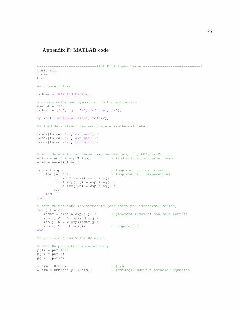
%---------------------------Plot Dubinin-Asthakov ---------------------------%
clear all;
close all;
tic
%% choose folder
folder = 'GAP_A13_Marina';
% choose color and symbol for isothermal series
symbol = '*';
color = ['b'; 'g'; 'r'; 'c'; 'y'; 'm'];
fprintf('\nSample: %s\n', folder);
%% load data structures and prepare isothermal data
load([folder,'/','dat.mat']);
load([folder,'/','exp.mat']);
load([folder,'/','par.mat']);
% sort data into isothermal exp series (e.g. 30, 60^\circC)
utiso = unique(exp.T_iso); % find unique isothermal temps
niso = numel(utiso);
for i=1:exp.n % loop over all experiments
for j=1:niso % loop over all temperatures
if exp.T_iso(i) == utiso(j)
A_exp(i,j) = exp.A_eq(i);
W_exp(i,j) = exp.W_eq(i);
end
end
end
% save values into iso structure (one entry per isothermal series)
for j=1:niso
index = find(A_exp(:,j)); % generate index of non-zero entries
iso(j).A = A_exp(index,j);
iso(j).W = W_exp(index,j);
iso(j).T = utiso(j); % temperature
end
%% generate A and W for DA model
% save DA parameters into vector p
p(1) = par.W_0;
p(2) = par.E;
p(3) = par.n;
A_sim = 0:500; % [J/g]
W_sim = Dubinin(p, A_sim); % [cm^3/g], Dubinin-Asthakov equation
85
Appendix F: MATLAB code
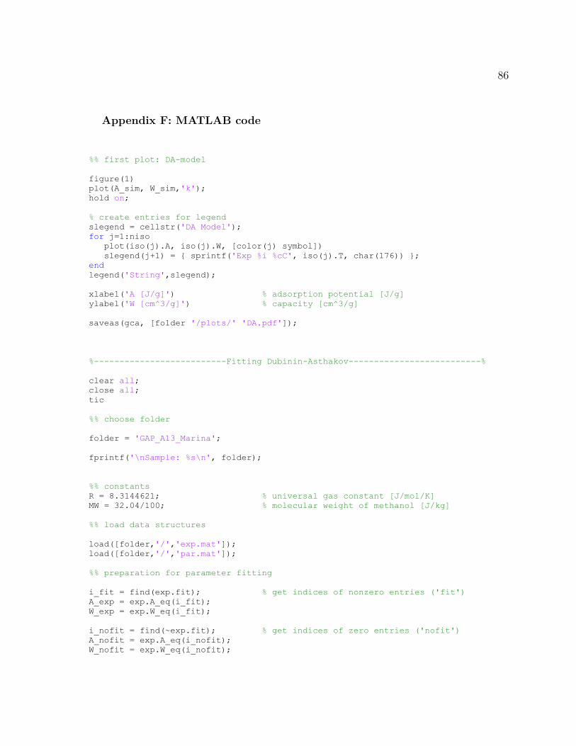
%% first plot: DA-model
figure(1)
plot(A_sim, W_sim,'k');
hold on;
% create entries for legend
slegend = cellstr('DA Model');
for j=1:niso
plot(iso(j).A, iso(j).W, [color(j) symbol])
slegend(j+1) = { sprintf('Exp %i %cC', iso(j).T, char(176)) };
end
legend('String',slegend);
xlabel('A [J/g]') % adsorption potential [J/g]
ylabel('W [cm^3/g]') % capacity [cm^3/g]
saveas(gca, [folder '/plots/' 'DA.pdf']);
%--------------------------Fitting Dubinin-Asthakov--------------------------%
clear all;
close all;
tic
%% choose folder
folder = 'GAP_A13_Marina';
fprintf('\nSample: %s\n', folder);
%% constants
R = 8.3144621; % universal gas constant [J/mol/K]
MW = 32.04/100; % molecular weight of methanol [J/kg]
%% load data structures
load([folder,'/','exp.mat']);
load([folder,'/','par.mat']);
%% preparation for parameter fitting
i_fit = find(exp.fit); % get indices of nonzero entries ('fit')
A_exp = exp.A_eq(i_fit);
W_exp = exp.W_eq(i_fit);
i_nofit = find(~exp.fit); % get indices of zero entries ('nofit')
A_nofit = exp.A_eq(i_nofit);
W_nofit = exp.W_eq(i_nofit);
86
Appendix F: MATLAB code
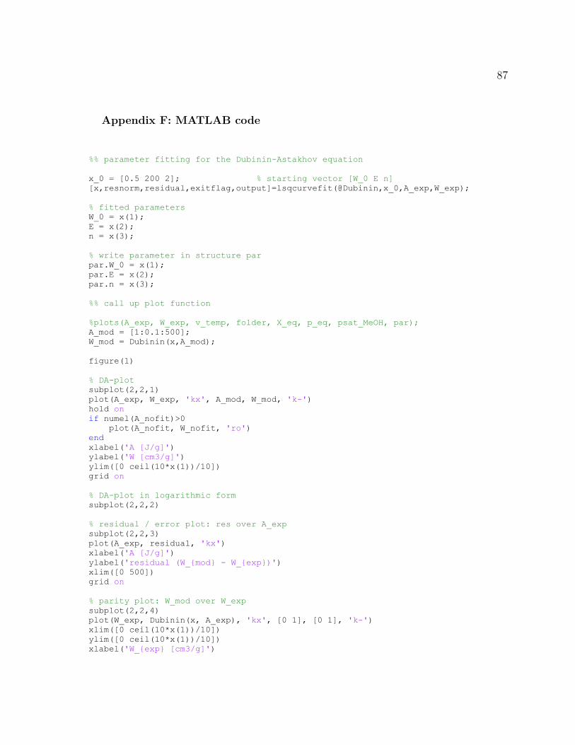
%% parameter fitting for the Dubinin-Astakhov equation
x_0 = [0.5 200 2]; % starting vector [W_0 E n]
[x,resnorm,residual,exitflag,output]=lsqcurvefit(@Dubinin,x_0,A_exp,W_exp);
% fitted parameters
W_0 = x(1);
E = x(2);
n = x(3);
% write parameter in structure par
par.W_0 = x(1);
par.E = x(2);
par.n = x(3);
%% call up plot function
%plots(A_exp, W_exp, v_temp, folder, X_eq, p_eq, psat_MeOH, par);
A_mod = [1:0.1:500];
W_mod = Dubinin(x,A_mod);
figure(1)
% DA-plot
subplot(2,2,1)
plot(A_exp, W_exp, 'kx', A_mod, W_mod, 'k-')
hold on
if numel(A_nofit)>0
plot(A_nofit, W_nofit, 'ro')
end
xlabel('A [J/g]')
ylabel('W [cm3/g]')
ylim([0 ceil(10*x(1))/10])
grid on
% DA-plot in logarithmic form
subplot(2,2,2)
% residual / error plot: res over A_exp
subplot(2,2,3)
plot(A_exp, residual, 'kx')
xlabel('A [J/g]')
ylabel('residual (W_{mod} - W_{exp})')
xlim([0 500])
grid on
% parity plot: W_mod over W_exp
subplot(2,2,4)
plot(W_exp, Dubinin(x, A_exp), 'kx', [0 1], [0 1], 'k-')
xlim([0 ceil(10*x(1))/10])
ylim([0 ceil(10*x(1))/10])
xlabel('W_{exp} [cm3/g]')
87
Appendix F: MATLAB code
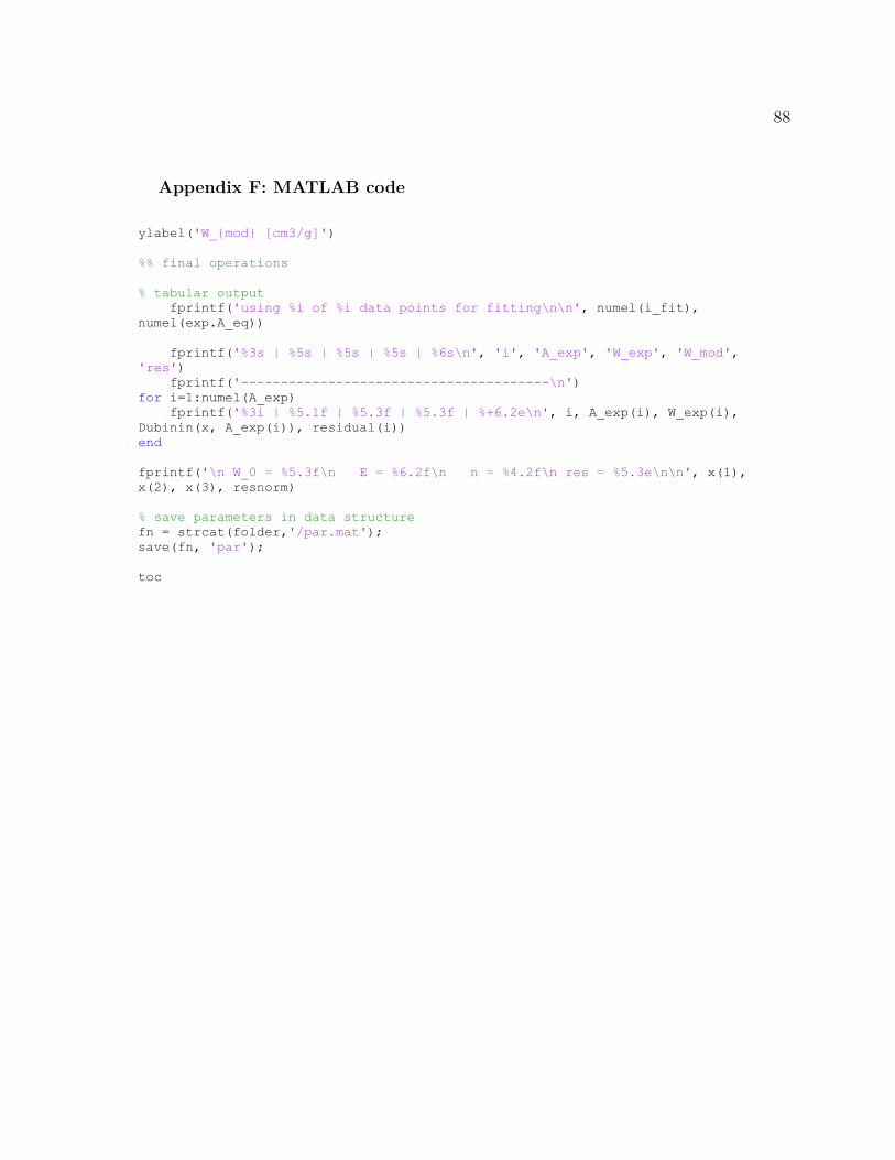
ylabel('W_{mod} [cm3/g]')
%% final operations
% tabular output
fprintf('using %i of %i data points for fitting\n\n', numel(i_fit),
numel(exp.A_eq))
fprintf('%3s | %5s | %5s | %5s | %6s\n', 'i', 'A_exp', 'W_exp', 'W_mod',
'res')
fprintf('---------------------------------------\n')
for i=1:numel(A_exp)
fprintf('%3i | %5.1f | %5.3f | %5.3f | %+6.2e\n', i, A_exp(i), W_exp(i),
Dubinin(x, A_exp(i)), residual(i))
end
fprintf('\n W_0 = %5.3f\n E = %6.2f\n n = %4.2f\n res = %5.3e\n\n', x(1),
x(2), x(3), resnorm)
% save parameters in data structure
fn = strcat(folder,'/par.mat');
save(fn, 'par');
toc
88
Appendix F: MATLAB code
Related Documents


