Learning with Large-Scale Social Media Networks by Lei Tang A Dissertation Presented in Partial Fulfillment of the Requirements for the Degree Doctor of Philosophy ARIZONA STATE UNIVERSITY August 2010

Welcome message from author
This document is posted to help you gain knowledge. Please leave a comment to let me know what you think about it! Share it to your friends and learn new things together.
Transcript

Learning with Large-Scale Social Media Networks
by
Lei Tang
A Dissertation Presented in Partial Fulfillmentof the Requirements for the Degree
Doctor of Philosophy
ARIZONA STATE UNIVERSITY
August 2010

Learning with Large-Scale Social Media Networks
by
Lei Tang
has been approved
July 2010
Graduate Supervisory Committee:
Huan Liu, ChairSubbarao Kambhampati
Pat LangleyJieping Ye
ACCEPTED BY THE GRADUATE COLLEGE

ABSTRACT
Social media such as blogs, Facebook, Twitter, YouTube and Flickr enables people of all walks
of life to express their thoughts, voice their opinions, and connect to each other more conveniently
than ever. The boom of social media opens up a vast range of possibilities to study human inter-
actions and collective behavior on an unprecedented scale. This dissertation presents a framework
for learning with large-scale social media networks in order to understand human interactions and
to predict collective behavior. Network interactions are typically heterogeneous, representing dis-
parate relations, but most social media sites present only connections with no or limited relation
information. Hence, social dimension is introduced to differentiate heterogeneous relations. A
learning approach based on social dimensions is proposed, achieving substantial improvement over
the state of the art. It is then extended to unify some unsupervised learning methods to handle net-
works with various types of entities and interactions. As social media networks are often of colossal
size, an edge-clustering method is proposed to extract sparse social dimensions in order to address
the scalability challenge. In sum, this research provides novel concepts and efficient algorithms to
harness the power of social media networks, enables the integration of data in heterogeneous for-
mat and information from networks of multiple modes or dimensions, and offers a learning-based
solution to social computing.
iii

To My Parents and Xinru
iv

ACKNOWLEDGEMENTS
Thanks...
First and foremost, to my advisor, Professor Huan Liu. Huan helped me to cultivate a taste in
research problems, and was a constant source of invaluable advice to navigate through the academic
world. Most importantly, I learned from him many philosophical principles and disciplines that are
not only beneficial for academic research, but also apply to many situations in life. I feel very lucky
to have him as my advisor and I sincerely hope that we will remain both collaborators and friends
for many years to come.
To my thesis committee, Professor Subbarao Kambhampati, Professor Pat Langley, and Profes-
sor Jieping Ye, for their inspiring feedback and advice. My research has also benefited tremendously
from various collaborations over the years. I would particularly like to thank Prof. Sun-Ki Chai (at
University of Hawaii), Dr. Vijay K. Narayanan (at Yahoo! Labs), Dr. John J. Salerno (at Air Force
Research Laboratory), Dr. Lei Wang (at The Australian National University), and Dr. Jianping
Zhang (at MITRE) for many thoughtful conversations.
To the Data Mining and Machine Learning Group. It has been a great pleasure working with
them during my journey as a doctoral student, particularly Nitin Agarwal, Geoffrey Barbier, Bill
Cole, Huiji Gao, Sai Moturu, Lance Parson, Payam Refaeilzadeh, Surendra Singhi, Xufei Wang,
Lei Yu, Reza Zafarani and Zheng Zhao. This would never be possible without their incessant help
and insightful discussions.
To my friends met at Arizona State University, Rui Cao, Jianhui Chen, Amanda Hendershot,
Neil Hendershot, Shuiwang Ji, Wen Li, Jun Liu, Jun Shi, Liang Sun, Joshua Bin Wu, Yue Yang,
Jicheng Zhao, and all other friends who have made Tempe feel like a home over the past six years.
To my parents who has been working hard to support me all the way. Their endless love and
optimistic attitude toward life taught me how to be enthusiastic and happy no matter what kind of
difficulty I encounter in my career. Also to my sister who is always proud of me.
Finally, to my lovely wife Xinru Xu for her understanding and warm support in the past five
years. I own her too many weekends and holidays. The best part of finishing this dissertation is that
we finally decided to move to a location that she likes most. I believe it is going to be great.
v

TABLE OF CONTENTS
Page
TABLE OF CONTENTS . . . . . . . . . . . . . . . . . . . . . . . . . . . . . . . . . . . . vi
LIST OF FIGURES . . . . . . . . . . . . . . . . . . . . . . . . . . . . . . . . . . . . . . ix
LIST OF TABLES . . . . . . . . . . . . . . . . . . . . . . . . . . . . . . . . . . . . . . . x
1 INTRODUCTION . . . . . . . . . . . . . . . . . . . . . . . . . . . . . . . . . . . . . 1
1.1 Social Media . . . . . . . . . . . . . . . . . . . . . . . . . . . . . . . . . . . . . 1
1.2 Learning with Social Media Networks . . . . . . . . . . . . . . . . . . . . . . . . 3
1.2.1 Unsupervised Learning and Community Detection . . . . . . . . . . . . . 3
1.2.2 Supervised Learning . . . . . . . . . . . . . . . . . . . . . . . . . . . . . 4
1.3 Challenges . . . . . . . . . . . . . . . . . . . . . . . . . . . . . . . . . . . . . . . 5
1.4 Roadmap . . . . . . . . . . . . . . . . . . . . . . . . . . . . . . . . . . . . . . . 6
2 SUPERVISED LEARNING WITH SOCIAL MEDIA NETWORKS . . . . . . . . . . . 8
2.1 Problem Statement . . . . . . . . . . . . . . . . . . . . . . . . . . . . . . . . . . 9
2.2 Motivation . . . . . . . . . . . . . . . . . . . . . . . . . . . . . . . . . . . . . . . 10
2.2.1 Collective Inference . . . . . . . . . . . . . . . . . . . . . . . . . . . . . 10
2.2.2 Heterogeneous Relations . . . . . . . . . . . . . . . . . . . . . . . . . . . 11
2.3 SocioDim: A Learning Framework based on Social Dimensions . . . . . . . . . . 12
2.3.1 Phase I: Extraction of Social Dimensions . . . . . . . . . . . . . . . . . . 13
2.3.2 Phase II: Classification Learning based on Social Dimensions . . . . . . . 16
2.3.3 Prediction . . . . . . . . . . . . . . . . . . . . . . . . . . . . . . . . . . . 16
2.4 Experiment Setup . . . . . . . . . . . . . . . . . . . . . . . . . . . . . . . . . . . 17
2.4.1 Data Sets . . . . . . . . . . . . . . . . . . . . . . . . . . . . . . . . . . . 17
2.4.2 Baseline Methods . . . . . . . . . . . . . . . . . . . . . . . . . . . . . . . 18
2.4.3 Evaluation Measure . . . . . . . . . . . . . . . . . . . . . . . . . . . . . 20
2.5 Experiment Results . . . . . . . . . . . . . . . . . . . . . . . . . . . . . . . . . . 21
2.5.1 Prediction Accuracy on BlogCatalog Data . . . . . . . . . . . . . . . . . . 21
2.5.2 Prediction Accuracy on Flickr Data . . . . . . . . . . . . . . . . . . . . . 23
2.5.3 Efficiency Comparison . . . . . . . . . . . . . . . . . . . . . . . . . . . . 23
2.5.4 Understanding SocioDim Framework . . . . . . . . . . . . . . . . . . . . 24
vi

Chapter Page
2.5.5 Visualization of Extracted Social Dimensions . . . . . . . . . . . . . . . . 28
2.5.6 Integration of Actor Network and Actor Features . . . . . . . . . . . . . . 29
2.6 Related Work . . . . . . . . . . . . . . . . . . . . . . . . . . . . . . . . . . . . . 30
2.6.1 Collective Classification . . . . . . . . . . . . . . . . . . . . . . . . . . . 31
2.6.2 Semi-Supervised Learning . . . . . . . . . . . . . . . . . . . . . . . . . . 33
2.7 Summary . . . . . . . . . . . . . . . . . . . . . . . . . . . . . . . . . . . . . . . 33
3 UNSUPERVISED LEARNING WITH SOCIAL MEDIA NETWORKS . . . . . . . . . 35
3.1 Types of Social Media Networks . . . . . . . . . . . . . . . . . . . . . . . . . . . 35
3.2 Motivation . . . . . . . . . . . . . . . . . . . . . . . . . . . . . . . . . . . . . . . 37
3.3 Social Dimension Integration for Unsupervised Learning . . . . . . . . . . . . . . 39
3.4 Communities in Multi-Dimensional Networks . . . . . . . . . . . . . . . . . . . . 40
3.4.1 Instantiation of SocioDim Integration . . . . . . . . . . . . . . . . . . . . 41
3.4.2 Experiment Setup . . . . . . . . . . . . . . . . . . . . . . . . . . . . . . . 43
3.4.2.1 YouTube Data . . . . . . . . . . . . . . . . . . . . . . . . . . . 43
3.4.2.2 Baseline Methods . . . . . . . . . . . . . . . . . . . . . . . . . 46
3.4.2.3 Evaluation Strategy . . . . . . . . . . . . . . . . . . . . . . . . 48
3.4.3 Experiment Results . . . . . . . . . . . . . . . . . . . . . . . . . . . . . . 48
3.5 Generalization to Communities in Dynamic Multi-Modal Networks . . . . . . . . 50
3.5.1 Problem Formulation . . . . . . . . . . . . . . . . . . . . . . . . . . . . . 51
3.5.2 Theoretical Derivation . . . . . . . . . . . . . . . . . . . . . . . . . . . . 54
3.5.3 Instantiation of SocioDim Integration . . . . . . . . . . . . . . . . . . . . 57
3.6 Related Work . . . . . . . . . . . . . . . . . . . . . . . . . . . . . . . . . . . . . 59
3.6.1 Community Detection with Multiple Networks . . . . . . . . . . . . . . . 60
3.6.2 Community Detection in Multi-Modal Networks . . . . . . . . . . . . . . 61
3.6.3 Community Evolution in Dynamic Networks . . . . . . . . . . . . . . . . 61
3.7 Summary . . . . . . . . . . . . . . . . . . . . . . . . . . . . . . . . . . . . . . . 62
4 SCALABLE LEARNING BASED ON SPARSE SOCIAL DIMENSIONS . . . . . . . 64
4.1 Problem Statement . . . . . . . . . . . . . . . . . . . . . . . . . . . . . . . . . . 64
4.2 Motivation . . . . . . . . . . . . . . . . . . . . . . . . . . . . . . . . . . . . . . . 65vii

Chapter Page
4.3 Learning with Sparse Social Dimensions . . . . . . . . . . . . . . . . . . . . . . . 66
4.3.1 Communities in Edge-Centric View . . . . . . . . . . . . . . . . . . . . . 66
4.3.2 Edge Partition via Partitioning Line Graph . . . . . . . . . . . . . . . . . . 70
4.3.3 Edge Partition via Clustering Edge Instances . . . . . . . . . . . . . . . . 72
4.3.4 Regularization on Communities . . . . . . . . . . . . . . . . . . . . . . . 75
4.4 Experiment Setup . . . . . . . . . . . . . . . . . . . . . . . . . . . . . . . . . . . 77
4.5 Experiment Results . . . . . . . . . . . . . . . . . . . . . . . . . . . . . . . . . . 78
4.5.1 Prediction Accuracy . . . . . . . . . . . . . . . . . . . . . . . . . . . . . 78
4.5.2 Scalability Study . . . . . . . . . . . . . . . . . . . . . . . . . . . . . . . 80
4.5.3 Regularization Effect . . . . . . . . . . . . . . . . . . . . . . . . . . . . . 82
4.5.4 Visualization of Extracted Social Dimensions . . . . . . . . . . . . . . . . 82
4.6 Related Work . . . . . . . . . . . . . . . . . . . . . . . . . . . . . . . . . . . . . 83
4.7 Summary . . . . . . . . . . . . . . . . . . . . . . . . . . . . . . . . . . . . . . . 84
5 CONCLUSIONS AND FUTURE WORK . . . . . . . . . . . . . . . . . . . . . . . . . 86
5.1 Key Contributions . . . . . . . . . . . . . . . . . . . . . . . . . . . . . . . . . . . 86
5.2 Future Work . . . . . . . . . . . . . . . . . . . . . . . . . . . . . . . . . . . . . . 87
5.2.1 Effective Extraction of Social Dimensions . . . . . . . . . . . . . . . . . . 87
5.2.2 Quantifying Crowd Behavior . . . . . . . . . . . . . . . . . . . . . . . . . 89
5.2.3 Learning with Streaming Network Data . . . . . . . . . . . . . . . . . . . 91
BIBLIOGRAPHY
93
A COMMUNITY DETECTION . . . . . . . . . . . . . . . . . . . . . . . . . . . . . . . 108
A.1 Latent Space Models . . . . . . . . . . . . . . . . . . . . . . . . . . . . . . . . . 108
A.2 Block Model Approximation . . . . . . . . . . . . . . . . . . . . . . . . . . . . . 109
A.3 Spectral Clustering . . . . . . . . . . . . . . . . . . . . . . . . . . . . . . . . . . 110
A.4 Modularity Maximization . . . . . . . . . . . . . . . . . . . . . . . . . . . . . . . 111
A.5 A Unified View . . . . . . . . . . . . . . . . . . . . . . . . . . . . . . . . . . . . 111
B CONVERGENCE ANALYSIS . . . . . . . . . . . . . . . . . . . . . . . . . . . . . . 116
viii

LIST OF FIGURES
Figure Page
2.1 A Toy Example . . . . . . . . . . . . . . . . . . . . . . . . . . . . . . . . . . . . . . 11
2.2 Node 1’s local Network . . . . . . . . . . . . . . . . . . . . . . . . . . . . . . . . . . 12
2.3 Different Affiliations . . . . . . . . . . . . . . . . . . . . . . . . . . . . . . . . . . . 12
2.4 SocioDim: A Classification Framework based on Social Dimensions . . . . . . . . . . 14
2.5 Performance on BlogCatalog with 10,312 Nodes (Better viewed in color) . . . . . . . 21
2.6 Performance on Flickr with 80,513 Nodes (Better viewed in color) . . . . . . . . . . . 22
2.7 Performances of Collective Inference by Expanding the Neighborhood . . . . . . . . . 25
2.8 Performance of SocioDim of Individual Categories . . . . . . . . . . . . . . . . . . . 26
2.9 Performance Improvement of SocioDim over wvRN wrt. Category Ncut . . . . . . . . 26
2.10 Classification Performance on imdb Network . . . . . . . . . . . . . . . . . . . . . . 28
2.11 Social dimensions Selected by Health and Animal . . . . . . . . . . . . . . . . . . . . 29
2.12 Performance of Network with Actor Features on BlogCatalog . . . . . . . . . . . . . . 30
3.1 Communications in Social Media are Multi-Dimensional . . . . . . . . . . . . . . . . 36
3.2 An example of 3-Mode Network in YouTube . . . . . . . . . . . . . . . . . . . . . . 36
3.3 SocioDim Integration for Unsupervised Learning . . . . . . . . . . . . . . . . . . . . 40
3.4 Algorithm: Social Dimension Integration for Multi-Dimensional Networks . . . . . . 43
3.5 Power Law Distribution on Different Dimensions of Interaction . . . . . . . . . . . . . 45
3.6 CDNV: Cross-Dimension Network Validation . . . . . . . . . . . . . . . . . . . . . . 48
3.7 SocioDim Integration for Dynamic Multi-Modal Networks . . . . . . . . . . . . . . . 57
4.1 A Toy Network . . . . . . . . . . . . . . . . . . . . . . . . . . . . . . . . . . . . . . 67
4.2 Edge Clusters . . . . . . . . . . . . . . . . . . . . . . . . . . . . . . . . . . . . . . . 67
4.3 Density Upperbound of Social Dimensions . . . . . . . . . . . . . . . . . . . . . . . 69
4.4 Algorithm for Scalable K-means Variant . . . . . . . . . . . . . . . . . . . . . . . . . 74
4.5 Algorithm for Scalable Learning Based on Sparse Social Dimensions . . . . . . . . . 76
4.6 Regularization Effect on Flickr . . . . . . . . . . . . . . . . . . . . . . . . . . . . . . 82
4.7 Social Dimensions Selected by Autos and Sports, Respectively . . . . . . . . . . . . . 83
A.1 Basic Idea of Block Model Approximation . . . . . . . . . . . . . . . . . . . . . . . 109
A.2 A Unified View of Representative Community Detection Methods . . . . . . . . . . . 112
ix

LIST OF TABLES
Table Page
1.1 Various Forms of Social Media . . . . . . . . . . . . . . . . . . . . . . . . . . . . . 2
1.2 Top Websites in US based on Internet Traffic as reported by Alexa on 7/10/2010 . . . . 2
1.3 Challenges Discussed in Each Chapter . . . . . . . . . . . . . . . . . . . . . . . . . . 7
2.1 Social Dimensions Corresponding to Affiliations in Figure 2.3 . . . . . . . . . . . . . 13
2.2 Social Dimensions Extracted According to Spectral Clustering . . . . . . . . . . . . . 15
2.3 Statistics of Social Media Data . . . . . . . . . . . . . . . . . . . . . . . . . . . . . . 18
2.4 Computation Time of Different Methods on Flickr in terms of Seconds . . . . . . . . . 24
2.5 Statistics of imdb Data . . . . . . . . . . . . . . . . . . . . . . . . . . . . . . . . . . 27
3.1 The Density of Each Dimension in the Constructed 5-Dimensional Network . . . . . . 44
3.2 Performance When Actors are Partitioned into 20, 40, and 60 Communities . . . . . . 49
3.3 Symbols and Denotations . . . . . . . . . . . . . . . . . . . . . . . . . . . . . . . . . 53
4.1 Social Dimension(s) of the Toy Example Following Different Approaches . . . . . . . 67
4.2 Edge Instances of the Toy Network in Figure 4.1 . . . . . . . . . . . . . . . . . . . . 73
4.3 Statistics of Social Media Data . . . . . . . . . . . . . . . . . . . . . . . . . . . . . . 77
4.4 Performance on Social Media Networks . . . . . . . . . . . . . . . . . . . . . . . . . 79
4.5 Scalability Comparison on Social Media Data of Varying Sizes . . . . . . . . . . . . . 81
x

Chapter 1
INTRODUCTION
The past decade has witnessed a rapid development and change of the Web and Internet. The ad-
vancement in computing and communication technologies is drawing people together in innovative
ways. Numerous participatory web and social networking sites have been cropping up, empower-
ing new forms of collaboration, communication and emergent intelligence. Prodigious numbers of
online volunteers collaboratively write encyclopedia articles of previously impossible scopes and
scales; Online marketplaces recommend products by investigating user shopping behavior and in-
teractions; Political movements are also creating new forms of engagement and collective action.
The boom of social media opens up a vast range of possibilities to study human interactions and
collective behavior on an unprecedented scale. This chapter first introduces social media and its
characteristics, then defines the task of leveraging social media networks for learning, followed by
a discussion of challenges associated with the task.
1.1 Social Media
With the pervasive availability of Web 2.0 and social networking sites, people can interact with
each other easily through various social media. Table 1.1 lists assorted forms of social media sites,
including wikis, social networking sites, social bookmarking sites, media sharing sites, social news,
Blogs, microblogging platforms, and forums. Though they may look quite different, they share
one common feature that distinguishes them from the classical web and traditional media: the
“consumers” of content or information online are also the “producers”. Essentially, everybody in
social media can be an information outlet [114], resulting in mountains of user-generated content.
This new type of mass publication enables the production of timely and grassroots information.
This was evidenced in the London terrorist attack in 2005, during which some witnesses blogged
their experience to provide first-hand reports of the event [137]. Another example was the bloody
clash ensuing the Iranian presidential election in 2009, for which many provided live updates on
Twitter, a microblogging platform. Social media also allows collaborative writing to produce high-
quality bodies of work otherwise impossible. Take Wikipedia as an example. “Since its creation

2
Table 1.1: Various Forms of Social Media
Wikis Wikipedia, Scholarpedia, ganfyd, AskDrWikiSocial Networking Facebook, MySpace, LinkedIn, Orkut, PatientsLikeMe
Social Tagging Del.icio.us, StumbleUponMedia Sharing Flickr, YouTube, Justin.tv, Ustream, ScribdSocial News Digg, Reddit
Blogs Wordpress, Blogspot, LiveJournal, BlogCatalogMicroblogging Twitter, foursquare
Forums Yahoo! answers, Epinions
in 2001, Wikipedia has grown rapidly into one of the largest reference web sites, attracting around
65 million visitors monthly as of 2009. There are more than 85,000 active contributors working on
more than 14,000,000 articles in more than 260 languages1.”
Another distinctive characteristic of social media is its rich user interaction. The success of so-
cial media relies on the engagement of users. More interactions encourage more user participation,
and vice versa. For example, Facebook claims to have more than 500 million active users as of
July 20, 20102. The huge amount of user participation and interaction result in eight social me-
dia sites in the top 20 websites as shown in Table 1.2. This rich user interaction forms a connected
network of users, providing unparalleled opportunities to study human interaction and collective be-
havior. Many computational challenges ensue, urging the development of advanced computational
techniques and algorithms.
Table 1.2: Top Websites in US based on Internet Traffic as reported by Alexa on 7/10/2010
Rank Site Rank Site1 google.com 11 blogger.com2 facebook.com 12 msn.com3 yahoo.com 13 go.com4 youtube.com 14 myspace.com5 amazon.com 15 aol.com6 wikipedia.org 16 bing.com7 craigslist.org 17 espn.go.com8 ebay.com 18 linkedin.com9 twitter.com 19 cnn.com10 live.com 20 wordpress.com
1http://en.wikipedia.org/wiki/Wikipedia:About2http://www.facebook.com/press/info.php?statistics

3
1.2 Learning with Social Media Networks
Millions of users in social media are playing, working, and socializing online. This offers vast
troves of digital information for mining patterns about users, their friends, likes, dislikes, etc. In
this dissertation, I investigate how we can leverage user interaction information to understand hu-
man interactions and predict collective behavior in social media. A clear understanding of social
connections and collective behavior in social media has a broad range of applications. Take social
networking advertising as an example. A common approach to targeted marketing is to build a
model mapping from user profiles (e.g., the geography location, education level, gender) to ads cat-
egories. Since social media often comes with a friendship network between users and many daily
interactions, we may be able to exploit this interaction information to infer more accurately about
the ads that might attract a user. In order to understand how users interact with and influence each
other, we address both unsupervised and supervised learning with social media networks.
1.2.1 Unsupervised Learning and Community Detection
Understanding human interaction is one of the core problems in conventional social network anal-
ysis [53, 147]. It aims to answer questions such as which groups of people tend to interact with
each other more frequently? Why are two users connected? What propels a user to join a certain
group? Given one group, what are the group norm [67] and shared profiles [126]? In the context
of social media, we study a fundamental task: how to extract communities (a.k.a., cohesive groups)
from social media networks?
This problem is known as community detection [43], or clustering on graphs [52]. This clus-
tering problem is one form of unsupervised learning. But here data instances are presented in
a network rather than conventional attribute format. Clustering on graphs has been well studied.
Many algorithms have been proposed. Please see [123] and [43] for detailed surveys. For conve-
nience, I also review several representative approaches and summarize them in a unified process in
Appendix A.
Social media, however, presents characteristics that were seldom considered in earlier work.
Various types of networks commonly coexist in social media. Interactions in social media are often
multi-dimensional, multi-modal, and highly dynamic. One network may involve heterogeneous
4
types of entities. YouTube, for instance, includes users, videos, tags and comments. Users are
also encouraged to interact with each other in various forms such as sending a message, leaving a
comment, thumbing up or down for one’s post, etc. Moreover, interactions between users can shift
rapidly due to external events. Some communities in social media are highly dynamic, forming
and dissolving swiftly. In sum, social media networks are often more than just a static friendship
network. Correspondingly, it poses new challenges to extract communities by integrating all kinds
of network information.
1.2.2 Supervised Learning
In a connected environment, individual behaviors tend to be correlated with his/her friends. For ex-
ample, if our friends buy something, there is a better-than-average chance that well buy it, too. Such
correlation between user behavior can be attributed to both influence and homophily [92]. When an
individual is exposed to a social networking environment, their behavior or decision are likely to
be influenced by each other. This influence naturally leads to correlations between connected users.
On the other hand, we tend to link up with one another in ways that confirm rather than test our
core beliefs. In other words, we are more likely to connect to others sharing certain similarities.
Consequently, it is no wonder that connected users demonstrate correlations in terms of behavior.
Since a social network provides valuable information concerning actor classes (one class refers
to users of the same behavior, preference or property), it is natural to ask how we can use the
correlation presented in a social network to predict classes of users. That is, given a social network
with class information of some actors, how can we infer the class of the remaining actors within
the same network? This supervised learning problem assumes that we can observe classes of some
individuals so that social learning is attainable. The amount of information that we can collect
depends on tasks. For instance, if we want to know whether a user will click on an ad, we can collect
this information when the ad is displayed to the user. To determine behavior concerning voting for
a presidential candidate, we can collect some voluntary responses using online surveys. With such
class information, we might be able to unravel the class of other users with no class information.
Both supervised and unsupervised learning tasks are complementary to each other. As we show
later, unsupervised learning is one key step in our proposed supervised learning approach. On the

5
other hand, the success of the proposed supervised learning framework sheds lights for us to unify
unsupervised learning for various kinds of social media networks.
1.3 Challenges
The analysis of social structures based on network topology is not new. That is exactly what con-
ventional social science [147] trying to address. As social media thrives, many challenges arise.
They were seldom encountered and addressed in traditional social sciences, thus novel approaches
have to be developed.
A traditional social science study often involves the circulation of questionnaires, asking re-
spondents to detail their interaction with others. Then a network can be constructed based on the
response, with nodes representing individuals and edges the interactions between them. This type
of data collection confines most traditional social network analysis to a limited scale, typically hun-
dreds of actors at most in one study. Various relations can present in one network, and relations
between actors are typically explicitly known, e.g., actor a is the mother of actor b; actors b and c
are colleagues.
Social media, on the one hand, provides readily-available interactions between human beings on
an unprecedented scale. For example, Leskovec and Horvitz [77] analyzed a network constructed
based on instant messenger communication between 180 million users. This kind of scale can
hardly be possible in traditional social sciences, thus offering a new opportunity to study human
interactions and behavior in the large. On the other hand, social media also poses some challenges
to be addressed:
• Limited information. Diverse relations are intertwined with connections in a social network.
One user, for instance, might connect to her friends, relatives, college classmates, colleagues,
or online buddies with similar hobbies. Connections in a social network can represent various
kinds of relationship between users. However, when a network is collected from social media,
most of the time, no explicit information is available why these users connect to each other
and what their relationships are. This missing relation information can limit the performance
of some techniques when they are applied to a social media network.
• Scalability. Networks in social media can be huge, often involving millions of actors and

6
hundreds of millions of connections, while traditional network analysis normally deals with
hundreds of subjects or fewer. Twitter, for example, claims to have more than 100 million
users, and Facebook 500 million active users. Existing network analysis techniques might
fail to handle networks of this astronomical size.
• Heterogeneity. In social media, it is very likely that heterogeneous types of interaction exist
between the same set of users. Moreover, multiple types of entities can also be involved in
a network. Take YouTube as an example, users, tags, videos are all weaved into the same
network. Analysis of social media networks with heterogeneous entities and interactions
requires new theories and tools.
• Evolution. Social media emphasizes timeliness. For example, in content sharing sites and
blogosphere, people quickly lose their interest in most shared contents and blog posts. This
differs from classical web mining. It is common that new users jump in, new connections
establish between existing members, and old users become dormant or simply leave. Behind
noisy interactions, communities can also emerge, grow, shrink, or dissolve. How can we
capture the dynamics of individuals and communities? Can we find the die-hard members
that are the backbone of communities and determine the rise and fall of their communities?
• Evaluation. A research barrier concerning mining social media is evaluation. In traditional
data mining, we are so used to the training-testing model of evaluation. It differs in social
media. Since many social media sites are required to protect user privacy information, limited
benchmark data is available. Another frequently encountered problem is lack of ground truth
for many social computing tasks, which further hinders some comparative study of different
works. Without ground truth, how can we conduct fair comparison and evaluation?
1.4 Roadmap
Before I discuss a framework for learning with large-scale social media networks, I present a cursory
overview of the dissertation.
In chapter 2, we formulate the problem of supervised learning with social media networks, and
review existing state-of-the-art algorithms. We pinpoint limitations of these methods when they are

7
Table 1.3: Challenges Discussed in Each Chapter
Chapter 2 Chapter 3 Chapter 4Challenges Supervised Learning Unsupervised Learning Scalable Learning
Limited Information X XScalability X
Heterogeneity XEvolution X XEvaluation X
applied to social media networks. Then, we propose a social dimension based learning framework
for classification with network data and present comprehensive empirical results.
Based on the concept of social dimension and the core idea in the proposed learning framework,
we show that the framework can be extended to handle unsupervised learning with various types
of social media networks in Chapter 3. We start from one type of network with heterogeneous in-
teractions, and derive a unsupervised learning approach following the proposed social dimension
concept in the previous chapter. This approach is then generalized to handle networks of hetero-
geneous entities, interactions or evolutions. We also demonstrate that such a simple unsupervised
learning approach corresponds to a sensible objective function through a series of derivation. This
deepens our understanding of the framework. Due to the lack of ground truth, novel evaluation
strategies are also presented.
Since most social media networks are often huge, it is imperative to develop scalable methods.
Chapter 4 discusses the possibilities of extracting sparse social dimensions in order to achieve scal-
able learning of collective behavior. We propose a simple yet effective algorithm. It is able to extract
sparse social dimensions from a network of millions of nodes in minutes, significantly advancing
the applicability of our proposed framework in dealing with large-scale networks.
Table 1.3 summarizes the challenges we are trying to address in these chapters. In essence, this
research provides the concept of social dimension, as well as efficient algorithms to harness the pre-
dictive power of social media networks. It enables the integration of data in heterogeneous format
and information from networks of multiple modes or dimensions, and offers a novel and feasible
solution for social computing. In Chapter 5, we conclude and point out some future directions based
on findings and lessons learned from this research.

Chapter 2
SUPERVISED LEARNING WITH SOCIAL MEDIA NETWORKS
With the rapid development of participatory web and social networking sites like YouTube, Twitter,
and Facebook, social media has reshaped the way people interact with each other. This blossom of
social networks provides opportunities to predict user-related attributes or behavior. In this chapter,
we investigate the task of supervised learning with social media networks. In particular, how we
can leverage social media networks to infer user attributes or behavior in the network.
It is noticed that diverse relations are intertwined with connections in social media networks.
For example, one user might connect to her relatives, college classmates, colleagues, or online
buddies with similar hobbies. The connections in a social network are inherently heterogeneous,
representing various kinds of relationship between users. However, when a social network is col-
lected from social media, most of the time, no explicit information is available why these users
connect to each other and what their relationships are. Existing methods that address classifica-
tion problems with network data seldom consider this heterogeneity. Direct application of existing
methods treats connections homogeneously, though they are inhomogeneous. This can lead to an
unsatisfactory performance Hence, we propose to differentiate connections and employ different
relations in building a discriminative classifier for classification.
We present social dimension, a concept dealing with connection heterogeneity, and propose a
classification framework (denoted as SocioDim) based on latent social dimensions. Each dimension
can be considered as the description of potential affiliations of social actors, which accounts for
the their interactions. With these social dimensions, we can take advantage of the power of dis-
criminative learning such as support vector machines or logistic regression to automatically select
relevant social dimensions for classification. The proposed learning framework is flexible to allow
the plug-in of different modules. It is demonstrated that our framework outperforms alternative
representative methods on social media data. SocioDim also offers a simple yet effective approach
to integrating network information with other features associated with actors such as social content
or profile information. Such a learning framework also applies to other domains with network data.

9
2.1 Problem Statement
In this chapter, we study supervised learning with networked data. For instance, in an advertising
campaign, advertisers attempt to deliver ads to those users who are interested in their products, or
similar categories. The outcome of user interests can be represented using + or -, with + denoting
a user is interested in the product and - otherwise. We assume that the interests of some users are
already known. This can be extracted from user profiles or their response to a displayed ad. The
task is to infer the preference of the remaining users within the same network.
Individual interests cannot be captured by merely one class. It is normal to have multiple inter-
ests in a user profile. Rather than concentrating on univariate cases of classification in networked
data [90] (each node has only one class label), here we examine a more challenging task that each
node in a network can have multiple labels, i.e., a multi-label classification problem [142] or a
multi-task learning problem [21]. In this setup, the univariate classification is just a special case.
Following other standard setup for collective classification [112], the multi-label classification prob-
lem with network data can be formally described below:
Given:
– K categories Y = Y1, · · · ,YK;
– a network A = (V,E,Y ) representing the interactions between nodes, where
V is the vertex set, E is the edge set, and each node vi is associated with class
labels yi whose value can be unknown;
– the known labels Y L for a subset of nodes V L in the network, where V L ⊆
V and yi j ∈ +,− denotes the class label of the vertex vi with respect to
category Y j.
Find:
– the unknown labels YU for the remaining vertices VU = V −V L.
Each vertex in the network represents one actor or one user in social media. Thereafter, data in-
stances, actors, vertices, nodes, entities and objects are used interchangeably in the context of a
network.

10
The problem above is referred as within-network classification [90]. The classification is based
on network information alone. In reality, there might be features associated with each node (actor).
For example, in blogosphere, the content of blog posts are available besides the blog network. While
it is an essential task to piece together these distinctive types of information, it is not the main
focus here. In this chapter, we examine different approaches to classification based on network
information alone, and then discuss their extensions to include actor features for learning.
2.2 Motivation
We briefly review collective inference, a commonly used method that has been proposed to address
classification with network data, and discuss its limitations when it is applied directly to networks
in social media.
2.2.1 Collective Inference
When data instances are connected in a network, they are not identically independently distributed
(i.i.d.) as in conventional data mining. It is empirically demonstrated that linked entities have
a tendency to belong to the same class [90]. This correlation in the class variable of connected
objects can be explained by the concept of homophily in social science [92]. Homophily suggests
a connection between similar people occurs at a higher rate than among dissimilar ones. It is one
of the first characteristics studied by early social network researchers [5, 148, 18], and holds for a
wide variety of relationships [92]. Homophily is also observed in social media [40, 138, 76].
Based on the empirical observation that labels of neighboring entities (nodes) are correlated,
the prediction of one node cannot be made independently, but also depends on its neighbors. To
handle the interdependency, collective inference is widely used to address the classification problem
in networked data [64, 90, 112]. A common Markov assumption is that, the labels of one node
depends on the labels (plus other attributes if applicable) of its neighbors. In particular,
P(yi|A ) = P(yi|Ni) (2.1)
where A is the network, yi the label of node vi, and Ni a set of its “neighbors”. The neighbors
are typically defined as nodes that are 1-hop or 2-hop away from vi in the network [64, 44]. For
training, a relational classifier based upon the labels (plus other available node attributes) of neigh-
11
bors is learned via the labeled nodes V L. For prediction, collective inference [64] is applied to
find an equilibrium status such that the inconsistency between neighboring nodes in the network is
minimized. Relaxation labeling [25], iterative classification [87] and Gibbs sampling [46] are the
commonly used techniques. All the collective inference variants share the same basic principle: it
initializes the labels of unlabeled nodes VU , and then applies the constructed relational classifier
to assign class labels (or update class membership) for each node while fixing the labels (or class
membership) of its neighboring nodes. This process is repeated until convergence.
2.2.2 Heterogeneous Relations
A social network is often a composite of various relations. People communicate with their friends
online. They may also communicate with their parents or random acquaintances. The diversity of
connections indicates that two connected users do not necessarily share certain class labels. When
relation type information is not available, directly applying collective inference to such a network
cannot differentiate connections between nodes, thus fails to predict the class membership of actors
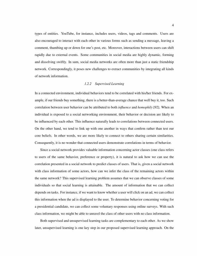
in the network. Let us look at a concrete example in Figure 4.1. Actor 1 connects to Actor 2 because
they work in the same IT company, and connects to Actor 3 because they often meet each other in
the same sports club. Given the label information that Actor 1 is interested in both Biking and IT
Gadgets, can we infer Actors 2 and 3’s labels? Treating these two connections homogeneously, we
guess that both Actors 2 and 3 are also interested in biking and IT gadgets. But if we know how
Actor 1 connects to other actors, it is more reasonable to conjecture that Actor 2 is more interested
in IT gadgets and Actor 3 likes biking.
Figure 2.1: A Toy Example
The example above assumes the cause of connections is explicitly known. But this kind of
information is rarely explicit in real-world applications, though some social networking sites like
Facebook do ask connected users about the reason why they know each other. Most of the time,

12
only network connections (as in Figure 2.2) are available. If we can somehow differentiate the
connections into different affiliations (as shown in Figure 2.3) and find out which affiliation is
correlated more with the targeted class label, we can infer the class membership of each actor more
precisely. Notice that an actor can present in multiple affiliations, e.g., actor 1 belongs to both
Affiliation-1 and Affiliation-2 in the example.
Figure 2.2: Node 1’s local Network Figure 2.3: Different Affiliations
Given a network, differentiating its connections into distinct affiliations is not an easy task as
the same actor is involved in multiple affiliations. Moreover, the same connection can be associated
with more than one affiliation. For instance, one can connect to another as they are colleagues as
well as going to the same sports club frequently. Instead of capturing affiliations among actors
via differentiating connections directly, we resort to latent social dimensions, with each dimension
representing a plausible affiliation of actors. Next, we introduce the concept of social dimensions,
and illustrate a classification framework based on that.
2.3 SocioDim: A Learning Framework based on Social Dimensions
To handle network heterogeneity as we have mentioned in the previous section, we propose to
extract social dimensions [121, 124] to capture the latent affiliations of actors and utilize them for
classification. Below, we introduce the concept of social dimensions and a fundamental assumption
for our framework.
Social dimensions are the vector-format representation of actors’ involvement in different affil-
iations. Given the extracted affiliations in Figure 2.3, we can represent them as social dimensions
in Table 2.1. If an actor is involved in one affiliation, then the entry of social dimensions corre-
sponding to the actor and the affiliation is non-zero. Note that one actor can participate in multiple
different affiliations (e.g., Actor 1 is associated with both affiliations). Different actors participate

13
in disparate affiliations in varying extent. So weighted values, instead of boolean values, can also
be used to represent affiliation membership.
Table 2.1: Social Dimensions Corresponding to Affiliations in Figure 2.3
Actor Affiliation-1 Affiliation-21 1 12 1 03 0 1· · · · · · · · ·
We assume one actor’s label depends on its latent social dimensions. Specifically, we assume
P(yi|A ) = P(yi|Si) (2.2)
where Si ∈ IRk denotes the social dimensions (latent affiliations) of node vi. This is fundamentally
different from the Markov assumption in Eq.(2.1) used in collective inference. Collective infer-
ence assumes the labels of one node relies on that of its neighbors. It does not capture the weak
dependency between nodes that are not close or directly connected. Here we assume the labels
are dependent on its latent social dimensions so the nodes within the same affiliations tend to have
similar labels even though they are not directly connected. Based on the assumption in Eq. (2.2),
we propose a learning framework SocioDim to handle the network heterogeneity for classification.
The overview of the framework is shown in Figure 2.4. It is composed of two phases: we first ex-
tract the latent social dimensions Si for each node, and then build a classifier based on the extracted
dimensions to learn P(yi|Si).
2.3.1 Phase I: Extraction of Social Dimensions
For the first phase, we require the following:
• an undirected network represented as a sparse matrix A ∈ Rn×n,
• the number of social dimensions to extract k.
The output should be social dimensions S ∈Rn×k of all nodes in the network. It is desirable that the
extracted social dimensions satisfy the following properties:
• Informative. The social dimensions should be indicative of latent affiliations of actors.

14
Input: A social network A ,the labels of some nodes in the network Y L,the number of social dimensions to extract k;
Output: the labels of unlabeled nodes YU .1. given A and k, extract social dimensions S ∈ Rn×k via soft clustering;2. based on SL and Y L, construct a discriminative classifier C;3. based on SU and C, output YU for unlabeled nodes.
Figure 2.4: SocioDim: A Classification Framework based on Social Dimensions
• Plural. The same actor can be involved in multiple affiliations, thus having non-zero entries
in different social dimensions.
• Continuous. The actors might have different degree of associations to one affiliation. Hence,
a continuous value rather than discrete 0,1 is more favorable.
One key observation is that when actors belong to the same affiliation, they tend to connect to
each other. For example, people of the same department interact with each other more frequently
than any two random people in a network. In order to infer the latent affiliations, we need to find out
a group of people who interact with each other more frequently than random. This boils down to a
classical community detection problem in networks. Most existing community detection methods
partition the nodes of a network into disjoint sets. But in reality, each actor is likely to subscribe
to more than one affiliation. Henceforth, a soft clustering scheme is preferred to extract social
dimensions.
Many approaches developed for clustering on graphs serve the purpose of social dimension
extraction, including modularity maximization [101], latent space models [57, 110], block mod-
els [105, 3] and spectral clustering [88]. In Appendix A, we show that all these methods can follow
a similar procedure for community detection as shown in Figure A.2. Given a network, we construct
15
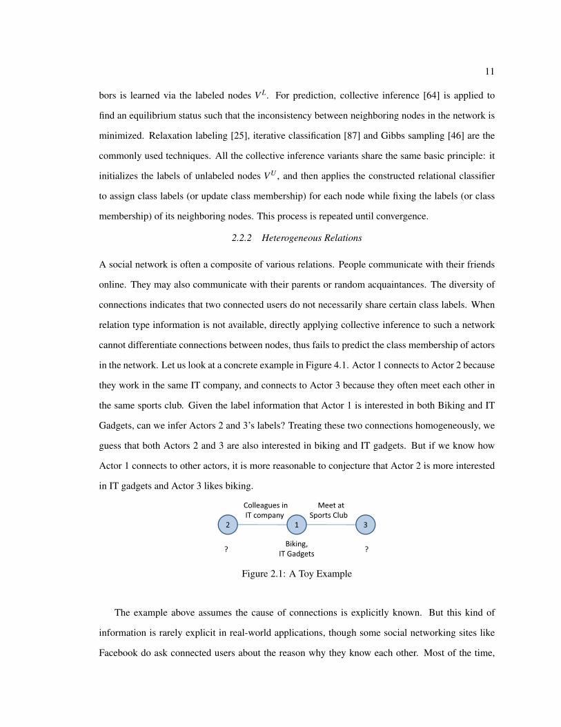
Table 2.2: Social Dimensions Extracted According to Spectral Clustering
Node Ideal Case Spectral Clustering1 1 1 -0.08932 1 0 0.27483 0 1 -0.45524 0 1 -0.45525 0 1 -0.46436 1 0 0.18647 1 0 0.24158 1 0 0.31449 1 0 0.3077
a utility matrix, extract its top (largest or smallest depending on the objective function) eigenvec-
tors as the soft community indicator, and then recover community partition via k-means clustering.
Since a soft clustering is preferred for community detection, we use the soft community indicator
as social dimensions.
Take spectral clustering as an example. Spectral clustering is originally proposed to address the
partition of nodes in a graph. Spectral clustering has been shown to work reasonably well in various
domains including graphs, text, images and microarray data. It is also proved [157] to be equivalent
to a soft version of the classical k-means algorithm for clustering. Social dimensions in this case
correspond to the smallest eigenvector of the utility matrix, i.e., the graph Laplacian defined in
Eq. (A.9). We want to emphasize that spectral clustering is not the only method of choice. Different
alternatives can be plugged in for this phase. This is also one nice feature of our framework as it
allows for convenient plug-in of existing soft clustering packages.
For example, if we apply spectral clustering to the toy network in Figure 2.2, we obtain the
social dimension in the last column in Table 2.2. In the table, we also show the ideal representation
of the two affiliations in the network. Nodes 3, 4 and 5 belong to the same affiliation, thus share
similar negative values in the extracted social dimension. Nodes 2, 6, 7, 8 and 9, associated with
Affiliation-1, have similar positive values. Node 1, which bridges these two affiliations, has a value
in between. The social dimension extracted based on spectral clustering do capture actor affiliations
in certain degree.

16
In summary, given a network A, we construct the normalized graph Laplacian L as in Eq. (A.9),
and then compute its first k smallest eigenvectors as the nodes’ social dimensions. Note that L is
sparse. So the power method or Lanczos method [50] can be used to calculate the top eigenvectors
if k is not too large. Many existing numerical optimization software can be employed.
2.3.2 Phase II: Classification Learning based on Social Dimensions
This phase constructs a classifier with the following inputs:
• the labels YL of labeled nodes in the network A ,
• the social dimensions SL of the labeled nodes.
The social dimensions extracted in the first phase are deemed as features of data instances
(nodes). We conduct conventional supervised learning based on the social dimensions and the label
information. A discriminative classifier like support vector machine (SVM) or logistic regression
can be used. Other features associated with the nodes, if available, can also be included during the
discriminative learning. This phase is critical as the classifier will determine which dimensions are
relevant to the class label. A linear SVM is exploited due to its simplicity and scalability [128].
2.3.3 Prediction
The prediction phase requires:
• The constructed classifier based on training,
• The social dimensions SU of those unlabeled nodes in the network.
Prediction is straightforward once the classifier is ready, because social dimensions have been
calculated in Phase I for all the nodes, including the unlabeled ones. We treat social dimensions
of the unlabeled nodes as features and apply the constructed classifier to make predictions. Differ-
ent from existing within-network classification methods, collective inference becomes unnecessary.
Though the distribution of actors does not follow the conventional i.i.d. assumption, the extracted
social dimensions in Phase I already encode correlations between actors along with the network.
Each node can be predicted independently without collective inference. Hence, this framework is
efficient in terms of prediction.

17
We emphasize that this proposed framework SocioDim is flexible. We choose spectral clustering
to extract social dimensions and SVM to build the classifier. This does not refrain us from using
alternative choices. Any soft clustering scheme can be used to extract social dimensions in the
first phase. The classification learning phase can also be replaced with any classifier other than
SVM. This flexibility enables the immediate use of many existing software packages developed for
clustering or classification.
2.4 Experiment Setup
In the experiment, we will compare our proposed SocioDim framework with representative collective-
inference methods when heterogeneity is present in a network. Before we proceed to the details of
experiments, we describe the data collected for experiments and baseline methods for comparison.
2.4.1 Data Sets
We focus on classification tasks specifically in social media. We shall examine how different ap-
proaches behave on real-world social networks. Two data sets are collected: one from BlogCatalog1
and the other from a popular photo sharing site Flickr2:
• BlogCatalog is a blog directory that hosts various information pieces like the categories a
blog is listed under, blog level tags, snippets of 5 most recent blog posts, and blog post level
tags. Bloggers submit their blogs to BlogCatalog and specify the metadata mentioned above
for improved access to their blogs. This way the blog sites are organized under pre-specified
categories. A blogger also specifies his social network with other bloggers. A blogger’s
interests could be gauged by the categories he publishes his blogs in. Each blogger could
list his blog under more than one category. Note that we only crawl a small portion of the
whole network. Some categories occur rarely and they demonstrate no positive correlation
between neighboring nodes in the network. Thus, we pick 39 categories with a reasonably
large sample pool for evaluation purpose. On average, each blogger lists their blog under
1.6 categories.
1http://www.blogcatalog.com/2http://www.flickr.com/

18
Table 2.3: Statistics of Social Media Data
Data BlogCatalog FlickrCategories (K) 39 195
Actors (n) 10, 312 80, 513Links (m) 333, 983 5, 899, 882
Network Density 6.3×10⁻³ 1.8×10⁻³
Maximum Degree 3, 992 5,706Average Degree 65 146Average Labels 1.4 1.3
Category Normalized Cut 0.48 0.46
• Flickr is a popular website to host personal photos uploaded by users, and also an online
community platform. Users in Flickr can tag photos and add contacts. Users can also sub-
scribe to different interest groups ranging from black and white photos3 to a specific subject
(say bacon4). Among the huge network and numerous groups collected from Flickr, we
randomly pick around 200 interest groups as the class labels and crawl the contact network
among the users subscribed to these groups for our experiment. The users with only one
single connection are removed from the data set.
Table 2.3 lists some statistics of the network data. As seen in the table, the connections among
social actors are extremely sparse. The degree distribution is highly imbalanced, a typical phe-
nomenon in scale-free networks. We also compute the normalized cut score (see Eq. (A.7)) for each
category and report the average score. Note that if a category is nearly-isolated from the rest of a
network, the normalized cut score should be close to 0. Clearly, for both data sets, the categories are
not well-separated from the rest of the network, implying the difficulty of the classification tasks.
Both data sets are publicly available from the first author’s homepage.
2.4.2 Baseline Methods
We apply SocioDim to both data sets. Spectral clustering is employed to extract social dimensions.
The number of latent dimensions is set to 500 and one-vs-rest linear SVM is used for discrimina-
tive learning. We also compare SocioDim to two representative relational learning methods based
3http://www.flickr.com/groups/blackandwhite/4http://www.flickr.com/groups/everythingsbetterwithbacon/

19
on collective inference (Weighted-Vote Relational Neighbor Classifier [89] and Link-Based Classi-
fier [87]), and two baseline methods without learning (a Majority Model and a Random Model):
• Weighted-Vote Relational Neighbor Classifier (wvRN). wvRN [89] works like a lazy learner.
No learning is conducted during training. In prediction, the relational classifier estimates the
class membership p(yi|Ni) as the weighted mean of its neighbors.
p(yi|Ni) =1
∑ j wi j∑
v j∈Ni
wi j · p(y j|N j) (2.3)
=1|Ni| ∑
j:(vi,v j)∈Ep(y j|N j) (2.4)
where wi j in (2.3) are the weights associated with the edge between node vi and v j. Eq. (2.4) is
derived, because the networks studied here use 0,1 to represent connections between actors
and we only consider the first order Markov assumption (The labels of one actor depend on
his connected friends). Collective inference is exploited for prediction. We iterate over each
node of the network to predict its class membership until the change of all the nodes is small
enough. wvRN has been shown to work reasonably well for classification in the univariate
case. It is recommended as a baseline method for comparison [90].
• Network Only Link-Based Classifier (LBC) [87]. This classifier creates relational features of
one node by aggregating the label information of its neighbors. Then a relational classifier
can be constructed based on labeled data. In particular, we use averaged class membership (as
in Eq. (2.4)) of each class as relational features, and employ SVM to build the relational clas-
sifier. For prediction, relaxation labeling [25] is utilized as the collective inference scheme.
• Majority Model (MAJORITY). This baseline method uses the label information only. It does
not leverage any network information for learning or inference. It simply predicts the class
membership as the proportion of positive instances in the labeled data. All nodes are assigned
the same class membership. This model is inclined to predict categories of larger size.
• Random Model (RANDOM). As indicated by the name, this model predicts the class mem-
bership for each node randomly. Neither network nor label information is used. This model
is included for relative comparison of various methods.
20
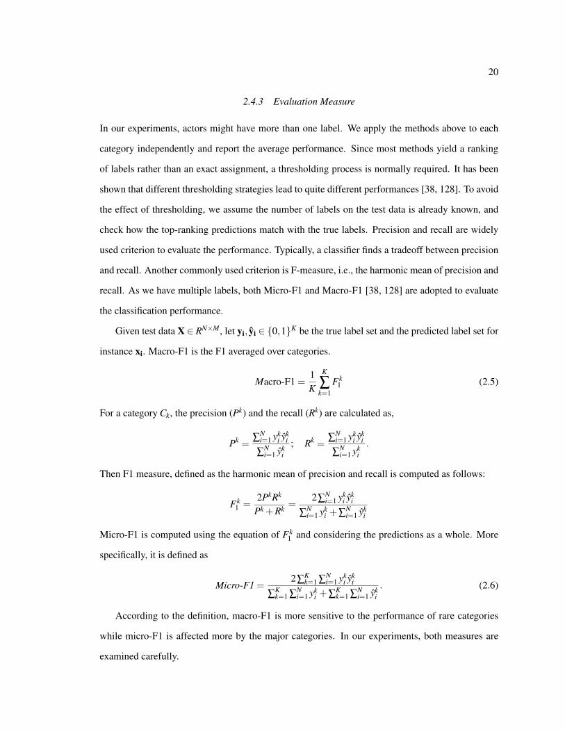
2.4.3 Evaluation Measure
In our experiments, actors might have more than one label. We apply the methods above to each
category independently and report the average performance. Since most methods yield a ranking
of labels rather than an exact assignment, a thresholding process is normally required. It has been
shown that different thresholding strategies lead to quite different performances [38, 128]. To avoid
the effect of thresholding, we assume the number of labels on the test data is already known, and
check how the top-ranking predictions match with the true labels. Precision and recall are widely
used criterion to evaluate the performance. Typically, a classifier finds a tradeoff between precision
and recall. Another commonly used criterion is F-measure, i.e., the harmonic mean of precision and
recall. As we have multiple labels, both Micro-F1 and Macro-F1 [38, 128] are adopted to evaluate
the classification performance.
Given test data X ∈ RN×M, let yi, yi ∈ 0,1K be the true label set and the predicted label set for
instance xi. Macro-F1 is the F1 averaged over categories.
Macro-F1 =1K
K
∑k=1
Fk1 (2.5)
For a category Ck, the precision (Pk) and the recall (Rk) are calculated as,
Pk = ∑Ni=1 yk
i yki
∑Ni=1 yk
i; Rk = ∑
Ni=1 yk
i yki
∑Ni=1 yk
i.
Then F1 measure, defined as the harmonic mean of precision and recall is computed as follows:
Fk1 =
2PkRk
Pk +Rk =2∑
Ni=1 yk
i yki
∑Ni=1 yk
i +∑Ni=1 yk
i
Micro-F1 is computed using the equation of Fk1 and considering the predictions as a whole. More
specifically, it is defined as
Micro-F1 =2∑
Kk=1 ∑
Ni=1 yk
i yki
∑Kk=1 ∑
Ni=1 yk
i +∑Kk=1 ∑
Ni=1 yk
i. (2.6)
According to the definition, macro-F1 is more sensitive to the performance of rare categories
while micro-F1 is affected more by the major categories. In our experiments, both measures are
examined carefully.

21
0 20 40 60 80 1000
0.05
0.1
0.15
0.2
0.25
0.3
0.35
Proportion of Labeled Nodes (%)
Macro
−F
1
0 20 40 60 80 1000
0.05
0.1
0.15
0.2
0.25
0.3
0.35
0.4
0.45
Proportion of Labeled Nodes (%)
Mic
ro−
F1
SocioDim wvRN LBC MAJORITY RANDOM
Figure 2.5: Performance on BlogCatalog with 10,312 Nodes (Better viewed in color)
2.5 Experiment Results
In this section, we will experimentally examine the following questions: How is the classification
performance of our proposed framework compared to that of collective inference? Does differenti-
ating heterogeneous connections presented in a network help yield a better performance?
2.5.1 Prediction Accuracy on BlogCatalog Data
We gradually increase the number of labeled nodes from 10% to 90%. For each setting, we ran-
domly sample a portion of nodes as labeled. This process is repeated 10 times and the average
performance are recorded. The performances of different methods and the standard deviation are
plotted in Figure 2.5. Clearly, our proposed SocioDim outperforms all the other methods. wvRN,
as shown in the figure, is the runner-up most of the time. MAJORITY performs even worse than
RANDOM in terms of Macro-F1 as it always picks the majority class for prediction.

22
0 2 4 6 8 10−0.05
0
0.05
0.1
0.15
0.2
0.25
0.3
Proportion of Labeled Nodes (%)
Ma
cro
−F
1
0 2 4 6 8 10−0.05
0
0.05
0.1
0.15
0.2
0.25
0.3
0.35
0.4
Proportion of Labeled Nodes (%)
Mic
ro−
F1
SocioDim wvRN LBC MAJORITY RANDOM
Figure 2.6: Performance on Flickr with 80,513 Nodes (Better viewed in color)
The superiority of SocioDim over other relational learning methods with collective inference
is evident. As shown in the figure, the link based classifier (LBC) performs poorly with few la-
beled data. This is because LBC requires to learn a relational classifier on labeled data before the
inference. When samples are few, the learned classifier is not robust enough. This is indicated by
the large deviation of LBC in the figure when labeled samples are less than 50%. We notice that
LBC in this case takes many iterations to converge. wvRN is more stable, but its performance is not
comparable to SocioDim. Even with 90% of nodes being labeled, a substantial difference between
wvRN and SocioDim is still observed. Comparing all the three methods (SocioDim, wvRN and
LBC), SocioDim is most stable and achieves the best performance. A similar trend is observed for
both precision and recall as well.

23
2.5.2 Prediction Accuracy on Flickr Data
Compared with BlogCatalog, the Flickr data is on a larger scale, with around 100,000 nodes. In
practice, the label information in large-scale networks is often very limited. Here we examine a
similar case. We change the proportion of labeled nodes from 1% to 10%. Roughly, the number of
labeled actors increases from around 1,000 to 10,000. The performances are reported in Figure 2.6.
The methods based on collective inference, such as wvRN and LBC, perform poorly. The LBC
fails most of the time (almost like random) and is highly unstable. This can be verified by the
fluctuation of Micro-F1 of LBC. LBC tries to learn a classifier based on the features aggregated
from a node’s neighbors. The classifier can be problematic when the labeled data are extremely
sparse and the network is noisy as presented here. While alternative collective inference methods
fail, SocioDim performs consistently better than other methods by differentiating heterogeneous
connections in the network.
It is noticed the prediction performance on both data sets is around 20-30% for F1-measure, sug-
gesting that social media networks are very noisy. As shown in later experiments, the performance
can be improved when other actor features are also included for learning.
2.5.3 Efficiency Comparison
In social media, the populace involved are normally immense. The scalability and efficiency of
different methods should be considered carefully for practical deployment. Thus, we examine the
efficiency of our proposed framework with wvRN, the runner-up in terms of classification perfor-
mance. Table 2.4 lists the computation time of pre-processing, training and prediction for both
methods on the Flickr data set as measured by a Core2Duo E8400 CPU.
Our proposed framework SocioDim is computationally expensive in data pre-processing and
training. The major computational burden lies on the extraction of social dimensions from a given
network. For the Flickr data, it takes almost 50 minutes to extract 500 social dimensions. This step
does not require the label information. Hence it is considered as pre-processing step and can be
finished before learning the classifier. Methods based on collective inference, on the other hand,
are normally quite efficient for training. The method wvRN is a lazy learner. No computation is
involved for pre-processing and training but it is very slow during testing, thus wvRN does not show
24
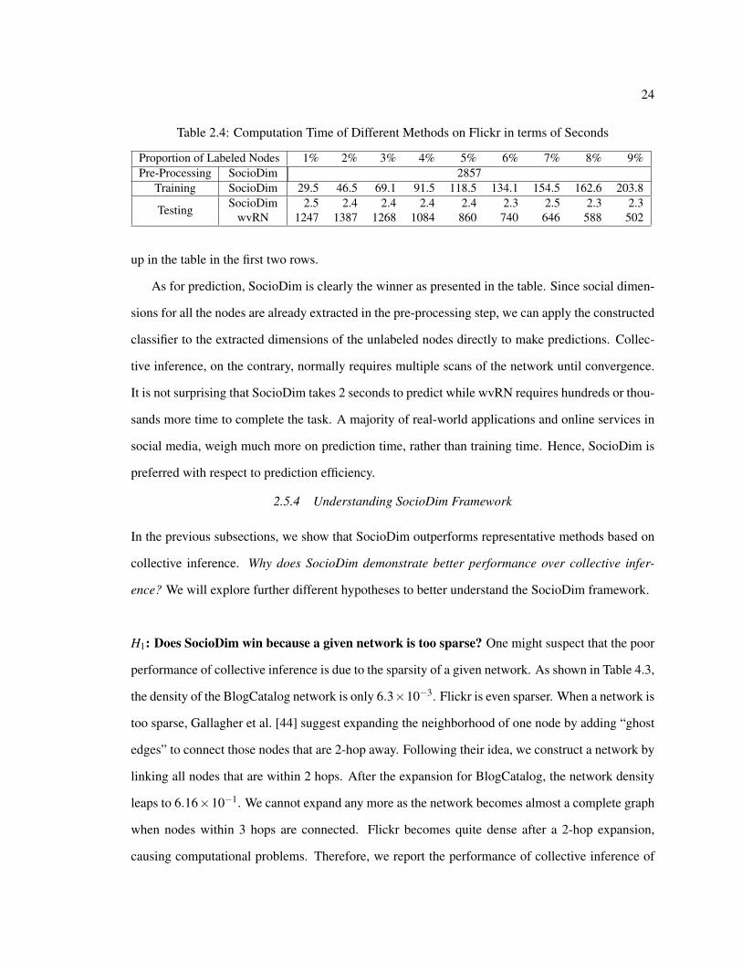
Table 2.4: Computation Time of Different Methods on Flickr in terms of Seconds
Proportion of Labeled Nodes 1% 2% 3% 4% 5% 6% 7% 8% 9%Pre-Processing SocioDim 2857
Training SocioDim 29.5 46.5 69.1 91.5 118.5 134.1 154.5 162.6 203.8
Testing SocioDim 2.5 2.4 2.4 2.4 2.4 2.3 2.5 2.3 2.3wvRN 1247 1387 1268 1084 860 740 646 588 502
up in the table in the first two rows.
As for prediction, SocioDim is clearly the winner as presented in the table. Since social dimen-
sions for all the nodes are already extracted in the pre-processing step, we can apply the constructed
classifier to the extracted dimensions of the unlabeled nodes directly to make predictions. Collec-
tive inference, on the contrary, normally requires multiple scans of the network until convergence.
It is not surprising that SocioDim takes 2 seconds to predict while wvRN requires hundreds or thou-
sands more time to complete the task. A majority of real-world applications and online services in
social media, weigh much more on prediction time, rather than training time. Hence, SocioDim is
preferred with respect to prediction efficiency.
2.5.4 Understanding SocioDim Framework
In the previous subsections, we show that SocioDim outperforms representative methods based on
collective inference. Why does SocioDim demonstrate better performance over collective infer-
ence? We will explore further different hypotheses to better understand the SocioDim framework.
H1: Does SocioDim win because a given network is too sparse? One might suspect that the poor
performance of collective inference is due to the sparsity of a given network. As shown in Table 4.3,
the density of the BlogCatalog network is only 6.3×10⁻³. Flickr is even sparser. When a network is
too sparse, Gallagher et al. [44] suggest expanding the neighborhood of one node by adding “ghost
edges” to connect those nodes that are 2-hop away. Following their idea, we construct a network by
linking all nodes that are within 2 hops. After the expansion for BlogCatalog, the network density
leaps to 6.16×10⁻¹. We cannot expand any more as the network becomes almost a complete graph
when nodes within 3 hops are connected. Flickr becomes quite dense after a 2-hop expansion,
causing computational problems. Therefore, we report the performance of collective inference of

25
10 20 30 40 50 60 70 80 900
0.05
0.1
0.15
0.2
0.25
0.3
0.35
Percentage of Labeled Nodes (%)
Ma
cro
−F
1
wvRN−1wvRN−2LBC−1LBC−2SocioDim
Figure 2.7: Performances of Collective Inference by Expanding the Neighborhood
the expanded network on BlogCatalog only in Figure 2.7, where i denotes the number of hops to
consider for defining neighborhood. For both wvRN and LBC, the performance deteriorates after
the neighborhood is expanded. This is because the increase of connections, though alleviating the
sparsity problem, seems to introduce more heterogeneity. Collective inference, no matter how we
define the neighborhood, is not comparable to SocioDim.
H2: Does SocioDim win because nodes within a category are well isolated from the rest of a
network? Another hypothesis is related to the community effect presented in a network. Since
SocioDim relies on soft community detection to extract social dimensions and the data we studied
are extremely sparse, one might suspect SocioDim wins because there are very few inter-category
edges. Intuitively, when a category is well isolated from the whole network, the clustering in the
first Phase of SocioDim captures this structure, thus it defeats collective inference. Surprisingly, this
intuition is not correct. Based on our empirical observation, when a category is well isolated, there
is not much difference between wvRN and SocioDim. SocioDim’s superiority is more observable
when the nodes of one category are blended into the whole network.
In order to calibrate whether the nodes of one category are isolated from the rest of a given
network, we compute the category normalized cut (NCut) following Eq. (A.7). Given a category,

26
0 50 100 150 2000
0.1
0.2
0.3
0.4
0.5
0.6
0.7
0.8
0.9
F1
Categories sorted in ascending order by NCut
Ncut=0.39
Ncut=0.12
Ncut=0.50
Ncut=0.48
Figure 2.8: Performance of SocioDim of Indi-vidual Categories
0.1 0.15 0.2 0.25 0.3 0.35 0.4 0.45 0.5−0.1
0
0.1
0.2
0.3
0.4
0.5
0.6
Category Ncut
Perf
orm
ance D
iffe
rence
Figure 2.9: Performance Improvement of So-cioDim over wvRN wrt. Category Ncut
we split a network into two sets: one set containing all the nodes of the category, the other set all the
nodes not belonging to that category. The normalized cut can be computed. If a category is well-
isolated from a network, the Ncut should be close to 0. The larger the NCut is, the less the category is
isolated from the remaining network. The average category Ncut scores on BlogCatalog and Flickr
are 0.48 and 0.46 respectively as reported in Table 2.3. This implies that most categories are actually
well connected to the remaining network, rather than being an isolated group as one supposes.
Figure 2.8 shows the performance of SocioDim on the 195 individual categories of the Flickr
data when 90% of nodes are labeled. As expected, SocioDim performance tends to decrease when
the Ncut increases. An interesting pattern emerges when we plot the improvement of SocioDim over
wvRN with respect to category Ncut in Figure 2.9. The performance improvement multiplies when
Ncut increases. Notice the plus at the bottom left, which corresponds to the case when Ncut = 0.12.
For this category, SocioDim achieves 90% F1 as shown in Figure 2.9. But the improvement over
wvRN is almost 0 as in Figure 2.9. That is, wvRN is comparable. Most of SocioDim’s improve-
ments occur when Ncut > 0.35. Essentially, when a category is not well-isolated from the remaining
network, SocioDim tends to outperform wvRN substantially.
H3: Does SocioDim win because it addresses network heterogeneity? In the previous subsection,
we notice that SocioDim performs considerably better than wvRN when a category is not so well

27
Table 2.5: Statistics of imdb Data
Data Size Density Ave. Degree Base Acc. Category Ncutimdbprodco 1126 0.035 38.8 0.501 0.24
imdball 1371 0.049 67.3 0.562 0.36
separated. We attribute the gain to taking into account connection heterogeneity. Hence, we adopt
a benchmark relational data (imdb used in [90]) with varying heterogeneity. The imdb network is
collected from the Internet Movie Data base, with nodes representing 1377 movies released between
1996 and 2001. The goal is to estimate whether the opening weekend box-office receipts of a
movie “will” exceed 2 million. Two versions of network data are constructed: imdbprodco and
imdball . In imdbprodco, two movies are connected if they share a production company. While
in imdball , two are connected if they share actors, directors, producers or production companies.
Clearly, the connections in imdball are more heterogeneous. Both network data sets have one giant
connected component each, with others being singletons or trivial-size components. Here we report
the performance on the largest components.
We notice that these two data sets demonstrate different characteristics from the previously-
studied social media data: 1) the connections are denser. For instance, the density of imdball is
0.049 (7 times denser than BlogCatalog and 27 times than Flickr); 2) the classification task is
also much easier. It is a binary classification task. The class distribution is balanced, different
from the imbalanced distribution present in the social media data. Hence, we report classification
performance in terms of accuracy as in [90]; and 3) classes are well separated as suggested by the
low category Ncut in Table 2.5.
Figure 2.10 plots the performance of SocioDim and wvRN on imdbprodco and imdball . When
connections are relatively homogeneous (e.g., imdbprodco data), SocioDim and wvRN demonstrate
comparable classification performance, wvRN being slightly better by 1%. When connections be-
come heterogeneous, the category NCut increases from 0.24 to 0.36. Both methods’ performance
decreases as shown in Figure 2.10b. For instance, with 50% of nodes are labeled, SocioDim’s ac-
curacy decreases from 80% to about 77%, but wvRN’s performance drops severely, from 80% to
around 66% with introduced heterogeneity.

28
0 20 40 60 80 10050
55
60
65
70
75
80
85
Accura
cy (
%)
Percentage of Labeled Nodes (%)
SocioDim
wvRN
(a) imdbprodco
0 20 40 60 80 10050
55
60
65
70
75
80
85
Accura
cy (
%)
Percentage of Labeled Nodes (%)
SocioDim
wvRN
(b) imdball
Figure 2.10: Classification Performance on imdb Network
We notice that the performance decrease of wvRN is most observable when labeled data are
few. With increasing available labeled data, wvRN’s performance climbs up. The comparison on
the two networks of distinctive degree of heterogeneity confirms our original hypothesis: SocioDim,
by differentiating heterogeneous connections, performs better than collective inference. This effect
is more observable when a network presents heterogeneity and labeled data are few.
2.5.5 Visualization of Extracted Social Dimensions
In order to get some tangible idea of extracted social dimensions, we examine tags associated with
each dimension. It is impractical to show tag clouds of all the extracted dimensions (500 social
dimensions for both data sets). Thus, given a category, we investigate its dimension with the maxi-
mum SVM weight, and check whether it is really informative of the category.
A minor issue is that each dimension is represented by continuous values (as in the last column
in Table 2.2), because we use soft clustering to extract social dimensions. For simplicity, we pick
the top 20 nodes with the maximum positive values as representatives of one dimension. For ex-
ample, nodes 8, 9, 7 and 6 are the top 4 nodes for the social dimension extracted following spectral
clustering in Table 2.2. Tags of those representative nodes in one dimension are aggregated as the
tags of that dimension. For the sake of clear visualization, only the tags occurring more than once
are presented as in a tag cloud with font size denoting their relative frequency.
Here we just showcase some examples from BlogCatalog. Figure 2.11 lists the tag clouds
of selected social dimensions for categories Health and Animal, respectively. In the clouds, the

29
(a) Health (b) Animal
Figure 2.11: Social dimensions Selected by Health and Animal
position and direction of tags do not matter. Only the font size are meaningful, represent the relative
frequency of each tag. Clearly, both are quite relevant to their target categories. Based on the tag
cloud in Figure 2.11a, it is not difficult to figure out that the social dimension is about food and
weight loss, which is highly relevant to Health. Similarly, the social dimension in Figure 2.11b
is about dogs and pets, thus relevant to Animal. These examples suggest that our extracted social
dimension are sensible, and relevant dimensions can be selected accordingly by the classification
learning phase of the SocioDim framework.
2.5.6 Integration of Actor Network and Actor Features
In social media, various kinds of user information besides social networks can be collected. For
instance, in blogosphere, people post blogs, write comments and upload tags. Some users also
provide some profile information. It is desirable to utilize all the information available to achieve
more accurate classification. However, the actor features (e.g., user profiles, social content or tag
information) and the networks are presented in disparate formats, hence some efforts are required
for the integration.
One nice property of SocioDim is that it converts a network into features. Thus, if actor fea-
tures are available, it is straightforward to couple the network features with actor features: simply
combine the extracted social dimensions with actor features, and let the discriminative learning pro-
cedure to determine which features are more informative of a class label. This simple combination
of network information and actor features allows for integration of data in disparate format and can
lead to more accurate classification in general. Here we take BlogCatalog as an example to show the
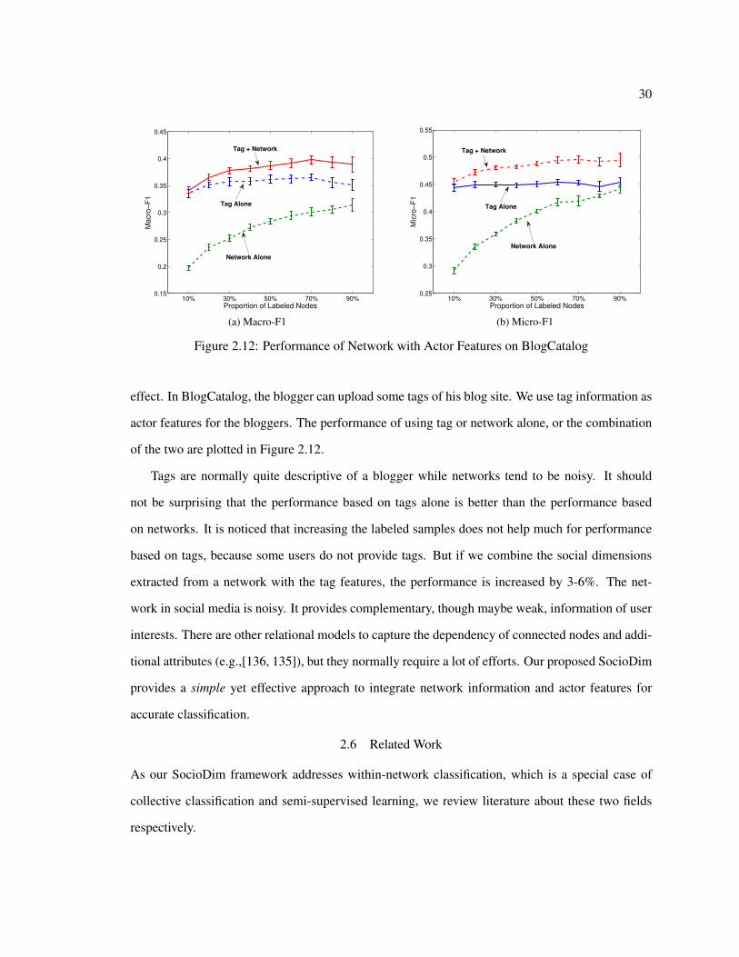
30
10% 30% 50% 70% 90%0.15
0.2
0.25
0.3
0.35
0.4
0.45
Proportion of Labeled Nodes
Ma
cro
−F
1Tag + Network
Tag Alone
Network Alone
(a) Macro-F1
10% 30% 50% 70% 90%0.25
0.3
0.35
0.4
0.45
0.5
0.55
Proportion of Labeled Nodes
Mic
ro−
F1
Tag + Network
Tag Alone
Network Alone
(b) Micro-F1
Figure 2.12: Performance of Network with Actor Features on BlogCatalog
effect. In BlogCatalog, the blogger can upload some tags of his blog site. We use tag information as
actor features for the bloggers. The performance of using tag or network alone, or the combination
of the two are plotted in Figure 2.12.
Tags are normally quite descriptive of a blogger while networks tend to be noisy. It should
not be surprising that the performance based on tags alone is better than the performance based
on networks. It is noticed that increasing the labeled samples does not help much for performance
based on tags, because some users do not provide tags. But if we combine the social dimensions
extracted from a network with the tag features, the performance is increased by 3-6%. The net-
work in social media is noisy. It provides complementary, though maybe weak, information of user
interests. There are other relational models to capture the dependency of connected nodes and addi-
tional attributes (e.g.,[136, 135]), but they normally require a lot of efforts. Our proposed SocioDim
provides a simple yet effective approach to integrate network information and actor features for
accurate classification.
2.6 Related Work
As our SocioDim framework addresses within-network classification, which is a special case of
collective classification and semi-supervised learning, we review literature about these two fields
respectively.

31
2.6.1 Collective Classification
Collective classification [112] refers to the classification when objects or entities are presented in
multiple relations or network format. In this work, we study a special case: within-network classifi-
cation [90] when the objects are connected in one network. The data instances in the network are not
independently identically distributed (i.i.d.) as in conventional data mining. In order to capture the
correlation between labels of neighboring data objects, a Markov dependency assumption is widely
adopted. That is, the labels of one node depend on the labels (and attributes) of its neighbors. Based
on the assumption, collective inference [64] is proposed for prediction. Normally, a relational clas-
sifier is constructed based on the relational features of labeled data, and then an iterative process
is required to determine class labels for unlabeled data. It is shown that a simple weighted vote
relational neighborhood classifier [89] works reasonably well on some benchmark relational data
and is recommended as a baseline for comparison [90].
In our implementation of collective inference, we define the neighborhood to be the nodes that
are only 1-hop away. Gallagher et al. [44] propose to add “ghost edges” before relational learning
when the network is too sparse. The ghost edges essentially connect nodes that are 2 hops away.
After the expansion of the neighborhood of one node for collective inference, they observe a better
classification performance. However, this strategy cannot be applied to networks in social media.
In social networks, the small-world effect [140] is often observed [23]. That is, any pair of nodes
in a large-scale social network are only several hops away, relating to the well-known “six degree
of separation”. For instance, in our Flickr data, the average degree of one node is 146. Roughly,
the nodes that are two hops away from one node can be as high as 146×146 = 21,316. Of course,
this number is not precise as the friends of friends may overlap. This huge number of neighbors
brings in much more noise and heterogeneity in connections, which can worsen the performance of
collective inference. This is empirically verified in a smaller BlogCatalog network in Section 2.5.4.
Often, a network becomes very dense after neighborhood expansion. As a result, the scalability can
also be a concern.
There are many more complicated relational models to model the dependence between con-
nected entities. For instance, probabilistic relational model (PRM) as introduced in [136, 135].
32
Please refer to [47] for a comprehensive treatment. No doubt that such models are quite powerful
to model various dependencies amongst entities, though the subsequent inference always requires
certain approximation. Their complexity and scalability are often a barrier for practical use. In-
deed, Macskassy and Provost compared wvRN with PRM, and found that wvRN outperforms PRM
on several relational data sets [90]. Given the extreme simplicity of wvRN and its outstanding
performance, wvRN is adopted as a baseline in our experiments.
Many relational classifiers only capture the local dependency based on the Markov assumption.
To capture the long-distance correlation, the latent group model [98] and the nonparametric infinite
hidden relational model [152] are presented. Both present generative models such that the links
(and actor attributes) are generated based on actors’ latent cluster membership. They share a similar
spirit as SocioDim. But the model intricacy and high computational cost for inference hinders their
direct application to huge networks. So Neville and Jensen in [98] propose to use a clustering
algorithm to find the hard cluster membership of each actor first, and then fix the latent group
variables for later inference. In social media, a network is often very noisy. Some nodes do not
show a strong community membership and hard clustering might assign them randomly [58]. The
resultant community structure can change drastically even with the removal of one single edge in
the network. Our social dimensions are represented as continuous values. Each node is allowed
to be involved in different dimensions in a flexible manner. It is also empirically verified that
hard partition is not comparable to soft clustering as shown in [121]. Another difference is that
both latent group model and nonparametric infinite hidden relational model are generative, while
SocioDim allows the plug-in of discriminative classifier. In conjunction with the discriminative
power of SVM, SocioDim yields more accurate and stable performances.
Recently, Neville [97] suggested that simple random sampling for cross validation on network
data tends to yield elevated Type-I error when comparing two algorithms. That is, such an evaluation
scheme might report two algorithms to be significantly different when the two are indeed similar. A
refined network cross validation scheme is proposed. We hope to evaluate our algorithm following
the new evaluation strategy as well.

33
2.6.2 Semi-Supervised Learning
Another related field is semi-supervised learning [162]. Semi-supervised learning is original pro-
posed to address the label shortage problem by exploiting unlabeled data. One branch of semi-
supervised learning is the graph-based approach [163, 158]. Indeed, they share quite a similar
assumption as collective inference. The performances of wvRN and Zhu’s method [163] are nearly
identical as reported in [90]. Considering that Zhu’s method involves the computation of the inverse
of a matrix of the same size as a given network, wvRN is used as the baseline in our experiments.
Some work [82, 26] attempts to address semi-supervised learning with multiple labels by utiliz-
ing the relationship between different labels. The relationship can be obtained either from external
experts or computed based on the labeled data. But its computational cost is prohibitive. We tried
the method presented in [26], which constructs a graph between different labels and then compute
a label assignment such that it is smooth on both the instance graph and the label graph. It requires
to solve a Sylvester equation [50] and direct implementation takes extremely long time to find a
solution, preventing us from reporting any comparative results.
On the other hand, some papers try to construct kernels based on graphs for SVM. Diffusion
kernel [71] is a commonly used one. However, it requires full SVD of the graph Laplacian, which
is not applicable for large-scale networks. Empirically, the classification performance is sensitive
to the diffusion parameter. Cross validation or some variant of kernel learning is required to select
a proper diffusion kernel [143].
2.7 Summary
Social media provides a virtual social networking environment. The presence of partial label in-
formation and networking information allows us to build better classifiers. This work proposes a
novel approach to deal with heterogeneous connections prevalent in social media. To differentiate
heterogeneous connections, we propose to extract latent social dimensions via soft clustering such
as modularity maximization and spectral clustering. Based on the extracted social dimensions, a
discriminative classifier like SVM can be constructed to determine which dimensions are informa-
tive for classification. Extensive experiments on social media data demonstrated that our proposed
social dimension approach outperforms alternative relational learning methods based on collective

34
inference, especially when labeled data are few. It is noticed that some relational models perform
poorly in social media data. This is due to the heterogeneity of connections and high irregularity
of human interactions in social media. Our approach, by differentiating connections among social
actors and converting network information into conventional features, achieves effective learning
for classification. Of course, our proposed learning framework is not confined to social media only.
In other domains, such as cellular networks, email communications, traditional Web and Internet,
SocioDim might also demonstrate its power.

Chapter 3
UNSUPERVISED LEARNING WITH SOCIAL MEDIA NETWORKS
A community (or group) is a set of users that interact with each other frequently [147]. Unsuper-
vised learning with social media networks refers to community detection. It has a broad range of
applications to discover groups. For example, some communities can be extracted as social di-
mensions for supervised learning as presented in last chapter. Other applications include network
visualization, intelligence analysis [10], network compression [116], behavioral study [56], influ-
ence modeling [1], and collaborative filtering [27]. A variety of community detection (a.k.a. finding
cohesive subgroups [147]) methods have been proposed to capture such social structures in a net-
work. However, some new properties prevail in social media networks, requiring novel techniques.
In this chapter, we show that the social-dimension based learning framework proposed in the pre-
vious chapter can be adapted to handle unsupervised learning with social media networks. We will
first discuss several types of networks in social media, and then present techniques to extract com-
munities for each type of networks. It turns out that all the methods can be nicely covered by the
social-dimension based learning framework.
3.1 Types of Social Media Networks
Social media enables rich interaction between users. Networks in social media can consist of hetero-
geneous types of interactions or entities. They can also be highly dynamic with interaction changes.
Accordingly, social media networks can be categorized into the following: multi-dimensional net-
works [129], multi-modal networks [127] or dynamic networks with evolutions.
• Multi-dimensional networks. Communications in social media are multi-dimensional. Each
dimension represents one type of activity between users. A multi-dimensional network has
multiple types of interactions between the same set of users. For instance, in Figure 3.1, at
popular photo and video sharing sites (e.g., Flickr and YouTube), a user can connect to his
friends through email invitation or the provided “add as contacts” function; users can also
tag/comment on the social contents like photos and videos; a user at YouTube can respond
to another user by uploading a video; and a user can also become a fan of another user by

36
Contacts/friends
Tagging on Social Content
Fans/Subscriptions
Response to Social Content
………………
Figure 3.1: Communications in Social Media are Multi-Dimensional
subscription to the user’s contributions of social contents. A network among these users can
be constructed based on each form of activity, in which each dimension represents one type
of interaction.
• Multi-modal Networks. A multi-modal network (a.k.a. multi-mode network, multi-type rela-
tional network) [84, 127] involves heterogeneous actors. Each mode represents one type of
entity. For instance, in the YouTube example above, a 3-mode network can be constructed,
with videos, tags and users each representing a mode, as seen in Figure 3.2. There are dis-
parate interactions among the three types of entities: users can upload videos. They can also
provide tags for some videos. Intuitively, two users contributing similar videos or tags are
likely to share interests. Videos sharing similar tags or users are more likely to be related.
Note that in the network, both tags, and videos are also considered as “actors”, though users
are probably the major mode under consideration.
Figure 3.2: An example of 3-Mode Network in YouTube
• Dynamic networks. In social media, networks are highly dynamic. Each day, new members
might join a network and new connections are established. Some existing members might
become dormant as well. This yields a highly dynamic network. Kumar et al. [73] show that
the number of communities and some other network statistics such as degrees and size of

37
the maximum connected component observe a significant change around 2001 in the blogo-
sphere. Some social media sites like Facebook and Twitter has been observing a tremendous
growth in recent years. As for a dynamic network, we obtain a sequence of similar yet evolv-
ing observations if we take multiple snapshots.
With the growth of networks, communities can also expand, shrink, or dissolve. As argued
by [73], communities in social media, in particular blogspace, are different from conventional
web communities. “Within a community of interacting bloggers, a given topic may become
the subject of intense debate for a period of time, then fade away. These bursts of activity are
typified by heightened hyperlinking amongst the blogs involved — within a time interval.” It
entails a new task to discover communities behind noisy network interactions across time.
Essentially, social media networks are highly heterogeneous. It is often more than just a single
social network. Heterogeneous types of interactions, entities are involved, and temporal evolution
also comes into play. Note that these different types of networks are not exclusive. In reality, it
is very likely that a network is multi-dimensional, multi-modal and dynamic simultaneously. Fac-
ing evolving networks with heterogeneous entities or interactions, communities in one dimension,
one mode or one snapshot becomes correlated to other dimensions, mode or snapshots. Existent ap-
proaches for unsupervised learning on graphs have to be extended to handle new forms of networks.
3.2 Motivation
Social media offers an easily-accessible platform for diverse online social activities, but also intro-
duces heterogeneity in networks. Thus, it calls for solutions to extract communities in heteroge-
neous networks. However, it remains unanswered why one cannot reduce a heterogeneous network
to several homogeneous ones (i.e., only one dimension, one mode or one snapshot) for investigation.
The reason is that the interaction information in one mode or one dimension might be too
noisy to detect meaningful communities. For instance, in the YouTube example in Figure 3.2. It
seems acceptable if we only consider the user mode. In other words, just study the friendship
network. On the one hand, some users might not have any online friends either because they are
too introvert to talk to other online users, or because they just join the network and are not ready
for or not interested in connections. On the other hand, some users might abuse connections, since
38
it is relatively easy to make connections in social media compared with in the physical world. As
mentioned in [121], a user in Flickr can have thousands of friends. This can hardly be true in the
real world. It might be the case that two online users get connected but they never talk to each other.
Thus, these online connections of one mode or one dimension can hardly paint a true picture of
what is happening. A single type of interaction provides limited (often sparse) information about
the community membership of online users. Fortunately, social media provides more than just a
single friendship network. A user might engage in other forms of activities besides connecting
to friends. It is helpful to utilize information from other modes or dimensions for more effective
community detection.
As for identifying community evolution in a dynamic network, one straightforward approach
is to apply community detection to each snapshot of the network Such a scheme is adopted in [59,
73, 107, 7]. However, most community detection methods, such as classical k-means clustering
algorithm, might return a local optimal. The initialization, the processing order of nodes, a slight
change of network connection might lead to a dramatically different community structure result.
For example, Hopcroft et al. [58] show that the community structure based on hierarchical agglom-
erative clustering can change sharply with the removal of one single edge in the network. Some
communities are essentially random. Thus, for a community detection method that is unstable or
have multiple local optimal solutions, it is difficult to conclude whether there is a community evolu-
tion between consecutive timestamps. Perhaps, it is simply the randomization due to the community
detection algorithm being used. However, it is noticed that a network tend to evolve smoothly [28].
Rather than conducting community detection independently at each network snapshot, we may ob-
tain more a robust community structure if temporal smoothness is employed smartly.
In sum, by integrating network information of multiple dimensions, modes or snapshots, we
may be able to extract more robust communities, thus achieving accurate unsupervised learning.
In the previous chapter, we proposed the concept of social dimension. By extracting social dimen-
sions from a network, we convert a network into conventional attribute format for nodes. Below,
we discuss strategies for integration of different types of networks following the social-dimension
learning framework.

39
3.3 Social Dimension Integration for Unsupervised Learning
As mentioned in the previous section, social media networks can be multi-dimensional, multi-modal
and dynamic. Communities of one dimension, one mode or one snapshot become correlated to
other dimensions, mode or snapshots. We need to integrate heterogeneous information together in
order to identify a more accurate community structure. For presentation convenience, we abbreviate
dimension, mode or snapshot as DMS.
In order to find communities in one target DMS, we can follow a similar procedure as the
SocioDim framework proposed in the previous chapter. The unsupervised learning for a target
DMS can also be decomposed into two phases:
• Phase I: Extraction of social dimensions from related DMSs;
• Phase II: Integration of social dimensions via Spectral Analysis for target DMS.
As introduced in the previous chapter, by extracting social dimensions from a network, we con-
vert the network into conventional attribute format, and the social dimensions can be considered
as features of nodes in the network. Similarly, as for unsupervised learning, we also extract so-
cial dimensions from related DMSs. By integrating these related features, we can update the social
dimension of one DMS via spectral analysis. In particular, we compute the singular value decompo-
sition (SVD) of the integrated social dimensions. This process is quite similar to the latent semantic
indexing (LSI) [12] commonly applied in text mining. Essentially, we extract the principal interac-
tion patterns by integrating interaction information from related dimensions, modes or snapshots.
Here, the unsupervised learning procedure differs from the supervised learning framework in the
second phase. For supervised learning, we build a classifier based on social dimensions. Unsuper-
vised learning, nevertheless, extracts communities by integrating related social dimensions. As the
above procedure is just for one target DMS, we may iteratively update social dimensions for each
DMS. Thus, we have a general framework for unsupervised learning in Figure 3.3. In each iteration,
we extract social dimensions from related DMSs and conduct integration.
Here, we present a general unsupervised learning approach to handle various kinds of social
media networks. So far, the proposed unsupervised learning approach seems quite abstract and ad
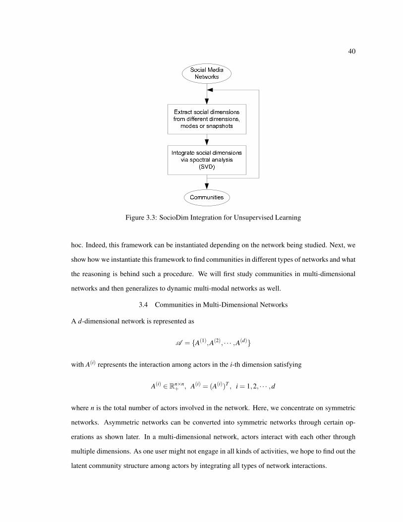
40
Figure 3.3: SocioDim Integration for Unsupervised Learning
hoc. Indeed, this framework can be instantiated depending on the network being studied. Next, we
show how we instantiate this framework to find communities in different types of networks and what
the reasoning is behind such a procedure. We will first study communities in multi-dimensional
networks and then generalizes to dynamic multi-modal networks as well.
3.4 Communities in Multi-Dimensional Networks
A d-dimensional network is represented as
A = A(1),A(2), · · · ,A(d)
with A(i) represents the interaction among actors in the i-th dimension satisfying
A(i) ∈ Rn×n+ , A(i) = (A(i))T , i = 1,2, · · · ,d
where n is the total number of actors involved in the network. Here, we concentrate on symmetric
networks. Asymmetric networks can be converted into symmetric networks through certain op-
erations as shown later. In a multi-dimensional network, actors interact with each other through
multiple dimensions. As one user might not engage in all kinds of activities, we hope to find out the
latent community structure among actors by integrating all types of network interactions.
41
3.4.1 Instantiation of SocioDim Integration
Social dimensions capture the diverse relations involved in a network. They can also be considered
as structural features of nodes extracted from a network. Following the general framework in Fig-
ure 3.3, we can perform integration over social dimensions extracted from each type of interaction.
One might conjecture that we can simply take the average of social dimensions as follows:
S =1d
d
∑i=1
S(i) (3.1)
where S(i) ∈ Rn×` denotes the social dimensions extracted from the i-th dimension of the network
A(i). and d is the number of different types of interaction. Unfortunately, this straightforward exten-
sion does not apply to social dimensions. Because the social dimensions obtained through represen-
tative community detection methods such as latent space models, block models, spectral clustering
or modularity maximization as discussed in Appendix A, are not unique. The social dimensions S(i)
correspond to the top eigenvector of a utility matrix (see Eq. (A.14)). In the simplest case, if S(i)
represents the top eigenvectors, then −S(i) is also a valid solution. Consequently, dissimilar social
dimensions do not suggest that drastically different community structures.
Alternatively, we expect S(i) of different type of interaction to be highly correlated after cer-
tain transformations. To capture the correlations between multiple sets of variables, (generalized)
canonical correlation analysis (CCA) [62, 69] is the standard statistical technique. CCA attempts
to find a transformation for each set of variables such that the pairwise correlations are maximized.
Here we briefly illustrate one scheme of generalized CCA which turns out to reduce to SVD in our
specific case.
Let S(i) ∈ Rn×` denote the social dimensions extracted from the i-th dimension of the network,
and wi ∈ R` be the linear transformation applied to S(i). The correlation between two sets of social
dimensions (S(i) and S( j)) after transformation is
R(i, j) = (S(i)wi)T (S( j)wj) = wiT((S(i))T S( j)
)wj = wi
TCi jwj
with Ci j = (S(i))T S( j) representing the covariance between the social dimensions of the i-th and the
j-th dimensions. Generalized CCA attempts to maximize the summation of pairwise correlations
42
as in the following form:
maxd
∑i=1
d
∑j=1
wiTCi jwj (3.2)
s.t.d
∑i=1
wiTCiiwi = 1 (3.3)
Using standard Lagrange multiplier and setting the derivatives respect to wi to zero, we obtain the
equation below:
C11 C12 · · · C1d
C21 C22 · · · C2d
......
. . ....
Cd1 Cd2 · · · Cdd
w1
w2...
wd
= λ
C11 0 · · · 0
0 C22 · · · 0...
.... . .
...
0 0 · · · Cdd
w1
w2...
wd
(3.4)
Recall that our social dimensions extracted from each dimension is essentially the top eigen-
vectors of a utility matrix. They satisfy the orthogonal constraint, (S(i))T S(i) = I. Thus, matrix
diag(C11,C22, · · · ,Cdd) in Eq. (3.4) becomes an identity matrix. Therefore w = [w1T ,w2
T , · · · ,wdT ]T
corresponds to the top eigenvector of the full covariance matrix on the left side of Eq. (3.4), which
is equivalent to PCA applied to data of the following form:
X =[S(1),S(2), · · · ,S(d)
](3.5)
Suppose the SVD of X is X = UΣV T , then w corresponds to the first column of V . Thus we have
1d
d
∑i=1
S(i)wi =1d
[S(1),S(2), · · · ,S(d)
]w =
1d
XV1 =σ1
dU1
Since σ1/d is a scalar, U1 is essentially the average feature values of each actor after we aggregate
the structural features of different dimensions along with the transformation w. There are k− 1
degrees of freedom with k communities. To compute the (k− 1)-dimension embedding, we just
need to project the data X onto the top (k− 1) principal vectors. It follows that the top (k− 1)
vectors of U are the aggregated structural features.
The detailed social dimension integration algorithm is summarized in Figure 2.4. We first ex-
tract social dimensions from each type of interaction of the network via representative community
detection methods; then PCA is applied on the concatenated data as in Eq. (3.5) to select the top

43
Algorithm: Unsupervised Learning based on Social DimensionsInput: Net = A(1),A(2), · · · ,A(d),
number of communities k,number of social dimensions to extract `;
Output: community assignment idx for each node.1. Extract ` social dimensions S(i) for each A(i);2. Compute slim SVD of X = [S(1),S(2), · · ·S(d)] = UDV T ;3. Obtain lower-dimensional embedding U = U(:,k−1);4. Normalize the rows of U to unit length;5. Calculate the cluster idx with k-means on U .
Figure 3.4: Algorithm: Social Dimension Integration for Multi-Dimensional Networks
eigenvectors. After projecting the data onto the principal vectors, we obtain a lower-dimensional
embedding which captures the principal pattern across all the dimensions of the network. Then we
can perform k-means on this embedding to find out the discrete community assignment.
Note that in the algorithm, we do not conduct iterative process as suggested in the framework
in Figure 3.3. This is because we aim to find out the shared community structure across different
types of interactions, rather than the community structure in each type of interaction. Next, we
will compare the proposed social dimension integration with other approaches to deal with multi-
dimensional networks.
3.4.2 Experiment Setup
In this part, we introduce the data set and baseline methods for comparison. As the data does
not have the ground truth information about communities, we develop a novel evaluation strategy
cross-dimension network validation following typical cross validation.
3.4.2.1 YouTube Data
YouTube1 is currently the most popular video sharing web site. It is reported to “attract 100 million
video views per day”2. As of March 17th, 2008, there had been 78.3 million videos uploaded, with
over 200, 000 videos uploaded per day3. This media sharing site allows users to interact with each
other in various forms such as contacts, subscriptions, sharing favorite videos, etc. We use YouTube
1http://www.youtube.com/2http://www.usatoday.com/tech/news/2006-07-16-youtube-views x.htm3http://ksudigg.wetpaint.com/page/YouTube+Statistics?t=anon

44
Table 3.1: The Density of Each Dimension in the Constructed 5-Dimensional Network
Network Dimension DensityA(1) contact 6.74×10⁻⁴
A(2) co-contact 1.71×10⁻²
A(3) co-subscription 4.90×10⁻²
A(4) co-subscribed 1.97×10⁻²
A(5) favorite 3.34×10⁻²
Data API to crawl the contacts network, subscription network as well as each user’s favorite videos.
We choose 100 authors who recently uploaded videos as the seed set for crawling, and expand the
network via their contacts and subscriptions. We obtain a small portion of the whole network, with
30,522 user profiles reaching in total 848,003 contacts and 1,299,642 favorite videos. After remov-
ing those users who decline to share their contact information, we have 15,088 active user profiles
as presented in three different interactions: two adjacency matrices of size 15,088×848,003 repre-
senting contact relationship, and subscriptions and a matrix of size 15,088×1,299,642 representing
users’ favorite videos.
One issue is that the collected subscription network is directional while most community detec-
tion methods such as block models, spectral clustering and modularity maximization, are proposed
for undirected networks. For such cases, simply ignoring the direction can confuse the two roles of
the directional interaction. Instead, we decompose the asymmetric interaction A into two unidirec-
tional interactions:
A′ = AAT ; (3.6)
A′′ = AT A. (3.7)
Essentially, if two social actors both subscribe to the same set of users, it is likely that they are
similar and share the same community; On the other hand, if two are referred by the same set of
actors, their similarity tends to be higher than that of random pairs. This is similar to the two roles
of hub and authority of web pages as mentioned in [70].
To utilize all aspects of information in our collected data, we construct a 5-dimensional network:
A(1): contact network: the contact network among those 15,088 active users;

45
100
101
102
103
100
101
102
103
104
Degree
Fre
qu
en
cy
(a) Contact Dimension
100
101
102
103
104
100
101
102
103
104
Degree
Fre
qu
en
cy
(b) Favorite Dimension
Figure 3.5: Power Law Distribution on Different Dimensions of Interaction
A(2): co-contact network: two active users are connected if they both add another user as contact;
This is constructed based on all the reachable 848,003 users (excluding those active ones) in
our collected data following Eq. (3.6).
A(3): co-subscription network: the connection between two users denotes they subscribe to the
same user; constructed following Eq. (3.6);
A(4): co-subscribed network: two users are connected if they are both subscribed by the same user;
constructed following Eq. (3.7);
A(5): favorite network: two users are connected if they share favorite videos.
All these different interactions are correlated with user interests. According to homophily effect
well studied in social science [92], people tend to connect to others sharing certain similarities.
Thus, we expect that connected friends in the contact network A(1) is more likely to share certain
interests. Similarly, if both users connect to another user or a favorite video (as A(2), A(3) or A(5)),
they are likely to share certain interests. On the other hand, if two users are subscribed by the same
set of users (as in A(4)), their shared content, thus their interests, are similar. Essentially, we hope to
extract communities share similar interests by integrating heterogeneous interactions.
Table 3.1 shows the connection density of each dimension. Contact dimension is the most sparse
one, while the other dimensions, due to the construction, are denser. Figure 3.5 shows the degree
distribution in contacts network and favorite network. Both, as expected, follow a power law [30].

46
3.4.2.2 Baseline Methods
We compare our social dimension integration scheme in Figure 3.4 with other baseline methods.
Modularity maximization is used as the base community detection method to show the efficacy of
our proposed approach. We will examine the following two questions:
• Is it necessary to integrate multiple types of interactions?
• If yes, which type of integration is more effective?
Thus, one baseline is to extract communities from only one type of interaction. Besides social di-
mension integration, other integration strategies following the general community detection process
in Figure A.2 are:
• Network Integration. A simple strategy to handle a multi-dimensional network is to treat it
as single-dimensional. One straightforward approach is to calculate the average interaction
network among social actors:
A =1d
d
∑i=1
A(i) (3.8)
Correspondingly,
m =1d
d
∑i=1
m(i), d =1d
d
∑i=1
d(i) (3.9)
With A, this boils down to classical community detection in a single-dimensional network.
Based on the average network, we can follow the community detection process as stated in the
unified view. Take modularity maximization as an example. we can maximize the modularity
as follows:
maxS
12m
Tr(
ST[
A− ddT
2m
]S)
(3.10)
• Utility Integration. Another variant for integration is to combine utility matrices instead of
networks. We can obtain an average utility matrix as follows:
M =1d
d
∑i=1
M(i)

47
where M(i) denotes the utility matrix constructed in the i-th dimension. The community
indicators can be computed via the top eigenvectors of the utility matrix. This is equivalent to
optimizing the objective function over all the dimensions simultaneously. As for modularity
maximization, the average utility matrix in this case would be
M =1d
d
∑i=1
B(i) =1d
d
∑i=1
A(i)
2m(i) −d(i)(d(i))T
(2m(i))2
(3.11)
Finding out the top eigenvectors of the average utility matrix is equivalent to maximizing the
average modularity as follows:
maxS
1d
d
∑i=1
Tr(ST B(i)S) = maxS
Tr(ST MS) (3.12)
• Partition Integration. Partition integration takes effect after the community partition of each
network dimension is ready. This problem has been studied as the cluster ensemble prob-
lem [115], which combines multiple clustering results of the same data from a variety of
sources into a single consensus clustering. Strehl and Ghoph [115] propose three effective
and comparable approaches: cluster-based similarity partitioning algorithm (CPSA), Hyper-
gGraph Partition Algorithm and Meta-Clustering Algorithm. For brevity, we only present the
basic idea of CPSA here. CPSA constructs a similarity matrix from each clustering. Two ob-
jects’ similarity is 1 if they belong to the same group, 0 if they belong to different groups. Let
H(i) ∈ 0,1n×k denote the community indicator matrix of clustering based on interactions at
dimension i. The similarity between nodes can be computed as
1d
d
∑i=1
H(i)(H(i))T =1d
d
∑i=1
HHT where H =[H(1),H(2), · · · ,H(d)
]Based on this similarity matrix between nodes, we can apply similarity-based community
detection methods we introduced before to find out clusters. A disadvantage of this CPSA
is that the computed similarity matrix can be dense, which might not be applicable to large
networks. Instead, we can treat H as the feature representation of actors and cluster them
based on k-means directly. Intuitively, if two actors are assigned to the same group in the
majority of dimensions, they would share features. Thus, the two actors are likely to reside
within the same community in the final consensus cluster as well.

48
Input: Net = A(1),A(2), · · · ,A(d);a multi-dimensional integration scheme f ;
Output: a community quality measure Q(i) for each network dimension.1. for p = 1, . . . ,d2. hold out A(p) for testing;3. obtain community structure H by applying f to
training dimensions A(1), · · · ,A(p−1),A(p+1), · · · ,A(d);4. compute the quality measure Q(p) based on H and A(p).5. end
Figure 3.6: CDNV: Cross-Dimension Network Validation
3.4.2.3 Evaluation Strategy
We now discuss evaluation methods that are suitable for multi-dimensional networks. As we
emphasized in the introduction of this dissertation, many social media networks do not provide
ground truth information of communities. When ground truth is not available, an alternative evalu-
ation method is needed to quantify community structures extracted employing different integration
strategies. If a latent community structure is shared across network dimensions, we can perform
cross-dimension network validation (CDNV) as in Figure 3.6. Given a multi-dimensional network
Net = A(i)|1≤ i≤ d, we can learn a community structure from d−1 dimensions of the network
and check how well the structure matches the left-out dimension (A(p)). In other words, we use
d− 1 dimensions for training and the remaining one for testing. During the training, we obtain
some communities (C), and use C to calculate modularity for the data of A(p) as follows:
Q =1
2m ∑C
∑i∈C, j∈C
Ai j−did j/2m. (3.13)
A larger modularity indicates a more accurate community structure discovered from training data.
3.4.3 Experiment Results
The four multi-dimensional integration schemes as well as community detection methods on a sin-
gle dimension are compared. We cluster actors involved in the network into different numbers of
communities. The clustering performance of single-dimensional and multi-dimensional methods
when k = 20, 40 and 60 are presented in Table 3.2. In the table, R(i)(1≤ i≤ 5) denotes the ranking
of each method based on CDNV as using A(i) for testing, and Raverage the average ranking across
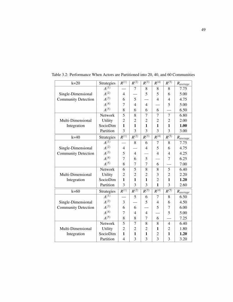
49
Table 3.2: Performance When Actors are Partitioned into 20, 40, and 60 Communities
k=20 Strategies R(1) R(2) R(3) R(4) R(5) Raverage
A(1) — 7 8 8 8 7.75Single-Dimensional A(2) 4 — 5 5 6 5.00
Community Detection A(3) 6 5 — 4 4 4.75A(4) 7 4 4 — 5 5.00A(5) 8 6 6 6 — 6.50
Network 5 8 7 7 7 6.80Multi-Dimensional Utility 2 2 2 2 2 2.00
Integration SocioDim 1 1 1 1 1 1.00Partition 3 3 3 3 3 3.00
k=40 Strategies R(1) R(2) R(3) R(4) R(5) Raverage
A(1) — 8 6 7 8 7.75Single-Dimensional A(2) 4 — 4 5 6 4.75
Community Detection A(3) 5 4 — 4 4 4.25A(4) 7 6 5 — 7 6.25A(5) 8 7 7 6 — 7.00
Network 6 5 8 8 5 6.40Multi-Dimensional Utility 2 2 2 3 2 2.20
Integration SocioDim 1 1 1 2 1 1.20Partition 3 3 3 1 3 2.60
k=60 Strategies R(1) R(2) R(3) R(4) R(5) Raverage
A(1) — 5 6 7 8 6.50Single-Dimensional A(2) 3 — 5 4 6 4.50
Community Detection A(3) 6 6 — 5 7 6.00A(4) 7 4 4 — 5 5.00A(5) 8 8 7 6 — 7.25
Network 5 7 8 8 4 6.40Multi-Dimensional Utility 2 2 2 1 2 1.80
Integration SocioDim 1 1 1 2 1 1.20Partition 4 3 3 3 3 3.20

50
all network dimensions. Bold entries denote the best in each column for each case. In the table,
rows represent methods and columns denote the Note that in our cross-dimension network vali-
dation procedure, the test dimension is not available during training, thus the diagonal entries for
single-dimensional methods are not shown.
SocioDim integration is clearly the winner most of the time, except for certain rare cases (e.g.,
using A(4) as the test dimension when k = 40 or 60). We notice that the rankings of different
integration strategies do not change much with different k. A closer examination reveals that utiliz-
ing information of all the dimensions (except network integration) outperforms single-dimensional
clustering. Network integration does not work well, because the network studied here are weighted
and simple average blurs the latent community structure information presented in each dimension.
In terms of performance ranking, SocioDim integration ≺ utility integration ≺ integration ≺ net-
work integration, with SocioDim integration being the winner. SocioDim integration, by removing
noise in each dimension, yields the most accurate community structure among all the methods.
Multi-dimensional networks commonly exist in many social networking sites, reflecting diverse
user interactions. We formally describe the community detection problem in multi-dimensional net-
works and present one approach based on social dimensions to handle the problem. We show that
SocioDim integration, which extracts social dimensions from each dimension of a multi-dimensional
network and treat them as structural features to integrate them via singular value decomposition, out-
performs other integration schemes. Next, we will show that the learning framework in Figure 3.3
can also be instantiated to handle dynamic multi-modal networks.
3.5 Generalization to Communities in Dynamic Multi-Modal Networks
Within a multi-modal network, different types of entities tend to form groups or communities. In
the YouTube example in Figure 3.2, users sharing similar interests are more likely to form a group;
videos are clustered naturally if they relate to similar contents; and tags are clustered if they are
associated with similar users and videos. Generally, a user group may interact with multiple groups
of another mode, i.e., users might have multiple interests, thus relating to various video groups.
In a multi-modal network, actors of different modes can evolve differently. For instance, in
the previous Youtube example, the video clusters tend to be stable based on their semantic close-
51
ness. But users might divert their personal interest and join a different community for interaction.
Facing heterogeneous entities with dynamic interactions, extracting evolving groups can lead to a
clear understanding of interaction between disparate modes as well as long-term evolution patterns.
This can benefit visualization of a complex network with heterogeneous entities and interactions,
aid decision making in various domains, and signal an event alarm if undesirable evolution patterns
are observed in the early stage. For example, to detect user interests shift for more effective tar-
geted marketing, or to detect suspicious financial activities if an abnormal change in transactions is
detected. However, the problem of discovering community evolution becomes challenging in dy-
namic multi-modal networks because 1) the evolutions of different modes become correlated; and
2) disparate modes demonstrate distinctive evolution patterns.
Below, we show that through a series of derivation, it reduces to the general framework pre-
sented in Figure 3.3 to find communities in a dynamic multi-modal network.
3.5.1 Problem Formulation
In order to extract communities in a multi-modal network, we follow the framework presented
in [84]. With a little bit abuse, we use similar notations as in [84] which are different from the
rest of this work. Given an m-mode network with m types of actors X1,X2, · · · ,Xm, we aim to
find how the latent community of each mode evolves. In our framework, we only consider discrete
timestamps by taking a series of snapshots, which is commonly adopted in network analysis with
temporal information [9, 78]. For a snapshot at time t, a network Nt is represented as multiple
interactions between different modes. Let Rti, j ∈ Rni×n j denote the interaction between two modes
Xi and X j at timestamp t, ni and n j the number of actors at mode i and j, ki and k j the number of
latent communities for Xi and X j respectively.
In order to extract communities at each mode, we assume interactions between modes can be ap-
proximated by interactions between groups [85, 34]. Thus we can approximate the original network
through interaction blocks. In particular,
Rti, j ≈C(i,t)At
i, j(C( j,t))T
where C(i,t) ∈ 0,1ni×ki denotes latent cluster (block) membership for Xi at timestamp t, and Ai, j
represents the density of group (block) interaction. In other words, the group membership de-
52
termines how two actors interact. This essentially hinges on a similar assumption as stochastic
block models [105]. The difference is that stochastic block models deal with the problem from
a probabilistic aspect. Here we identify the block structure of multi-modal networks via matrix
approximation:
min ||Rti, j−C(i,t)At
i, j(C( j,t))T ||2F (3.14)
s.t. C(i,t) ∈ 0,1ni×ki ,ki
∑k=1
C(i,t)∗k = 1 (3.15)
C( j,t) ∈ 0,1n j×k j ,k j
∑k=1
C( j,t)∗k = 1 (3.16)
The constraints in (3.15) and (3.16) force each row of the indicator matrix to have only one entry
being 1. That is, each actor belongs to only one community. Unfortunately, the discreteness of
the constraints makes the problem NP-hard. A strategy that has been well studied in spectral clus-
tering [157] is to allow the cluster indicator matrix to be continuous and relax the hard clustering
constraint as follows:
(C(i,t))TC(i,t) = Iki
In a multi-modal network, diverse interactions occur between different modes. Hence, the objective
in Eq. (3.14) can be changed to
min ∑1≤i< j≤m
w(i, j)a ||Rt
i, j−C(i,t)Ati, j(C
( j,t))T ||2F (3.17)
with w(i, j)a being the weights associated with different interactions.
With a dynamic multi-modal network, we have multiple snapshots of the network. Naturally,
the objective function without considering its temporal effect can be formulated as F1:
minT
∑t=1
∑1≤i< j≤m
w(i, j)a ||Rt
i, j−C(i,t)Ati, j(C
( j,t))T ||2F (3.18)
s.t.(C(i,t))TC(i,t) = Iki i = 1, · · · ,m, t = 1, · · ·T (3.19)
Then we have the following theorem:
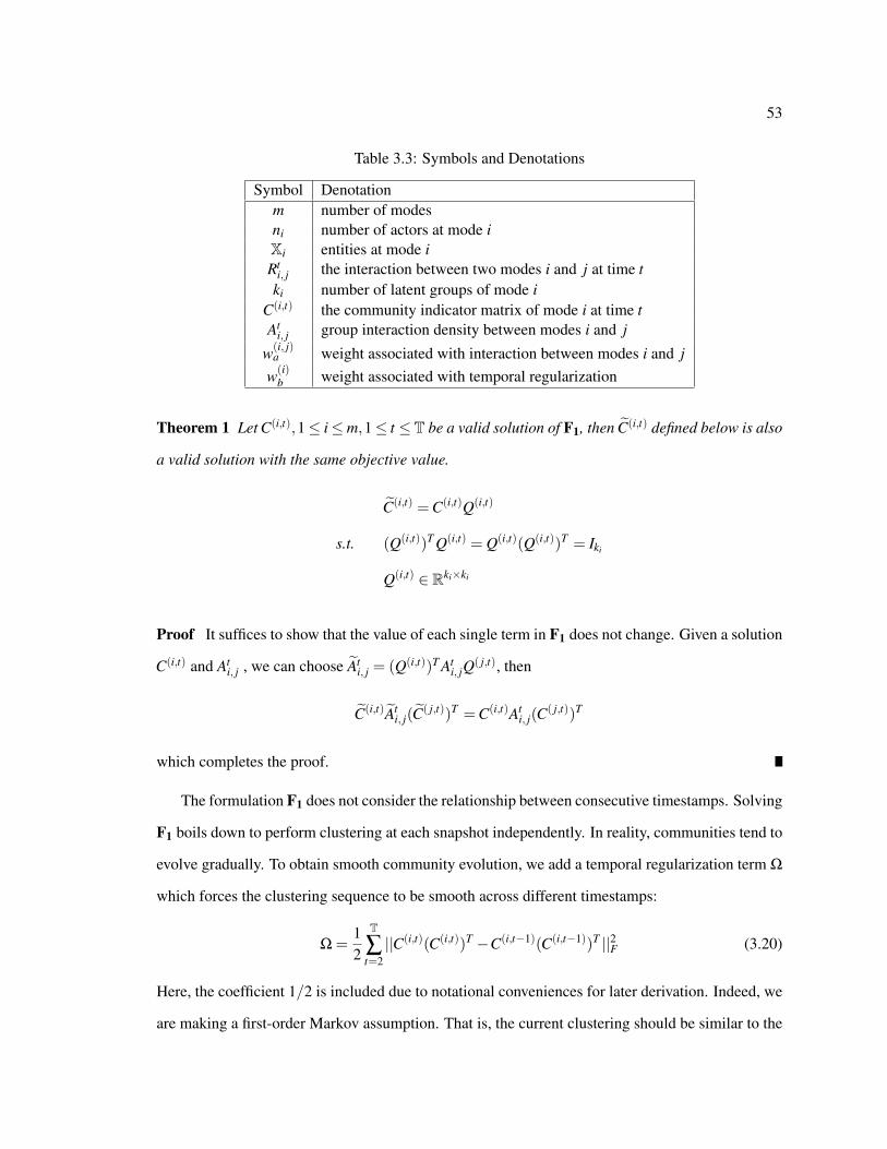
53
Table 3.3: Symbols and Denotations
Symbol Denotationm number of modesni number of actors at mode iXi entities at mode iRt
i, j the interaction between two modes i and j at time tki number of latent groups of mode i
C(i,t) the community indicator matrix of mode i at time tAt
i, j group interaction density between modes i and j
w(i, j)a weight associated with interaction between modes i and j
w(i)b weight associated with temporal regularization
Theorem 1 Let C(i,t),1≤ i≤m,1≤ t ≤T be a valid solution of F1, then C(i,t) defined below is also
a valid solution with the same objective value.
C(i,t) = C(i,t)Q(i,t)
s.t. (Q(i,t))T Q(i,t) = Q(i,t)(Q(i,t))T = Iki
Q(i,t) ∈ Rki×ki
Proof It suffices to show that the value of each single term in F1 does not change. Given a solution
C(i,t) and Ati, j , we can choose At
i, j = (Q(i,t))T Ati, jQ
( j,t), then
C(i,t)Ati, j(C
( j,t))T = C(i,t)Ati, j(C
( j,t))T
which completes the proof.
The formulation F1 does not consider the relationship between consecutive timestamps. Solving
F1 boils down to perform clustering at each snapshot independently. In reality, communities tend to
evolve gradually. To obtain smooth community evolution, we add a temporal regularization term Ω
which forces the clustering sequence to be smooth across different timestamps:
Ω =12
T
∑t=2||C(i,t)(C(i,t))T −C(i,t−1)(C(i,t−1))T ||2F (3.20)
Here, the coefficient 1/2 is included due to notational conveniences for later derivation. Indeed, we
are making a first-order Markov assumption. That is, the current clustering should be similar to the

54
clustering at the previous timestamp. Note that we do not take the regularization as
Ω =T
∑t=2||C(i,t)−C(i,t−1)||2F (3.21)
which seems more natural at first glimpse. As demonstrated in Theorem 1, C(i,t) is equivalent under
an orthogonal transformation. Hence, comparing C(i,t) and C(i,t−1) directly as in Eq. (3.21) does
not necessarily capture the difference between the cluster indicators at different timestamps. On the
contrary, the regularization term of Eq.(3.20) is independent of the orthogonal transformation, thus
captures the difference of community structure of neighboring timestamps. With this regularization,
the problem of identifying evolving groups can be formulated as:
F2 : minT
∑t=1
∑i< j
w(i, j)a ||Rt
i, j−C(i,t)Ati, j(C
( j,t))T ||2F +
12
m
∑i=1
w(i)b
T
∑t=2||C(i,t)(C(i,t))T −C(i,t−1)(C(i,t−1))T ||2F (3.22)
s.t. (C(i,t))TC(i,t) = Iki i = 1, · · · ,m, t = 1, · · ·T (3.23)
with w(i)b being the trade-off between the block model approximation of interactions and the tem-
poral regularization. As evolution takes effect gradually, we aim to find a community structure
that is consistent with current interaction matrix, whereas not drastically different from that of the
previous timestamp.
3.5.2 Theoretical Derivation
To capture evolving groups in dynamic multi-modal networks, we have to solve F2. There is no ana-
lytical solution to the problem, but an iterative algorithm can be derived. We show that a closed-form
solution exists for Ati, j and C(i,t) if other variables are fixed [125]. Then we present the algorithm in
an attribute view for easy comprehension and extension.
Theorem 2 Given C(i,t), the optimal group interaction matrix Ati, j can be calculated as
Ati, j = (C(i,t))T Rt
i, jC( j,t)

55
Proof Since Ati, j appears in only one term in F2, we can focus on the single term to optimize At
i, j.
||Rti, j−C(i,t)At
i, j(C( j,t))T ||2F
= tr[(Rti, j−C(i,t)At
i, j(C( j,t))T )(Rt
i, j−C(i,t)Ati, j(C
( j,t))T )T ]
= tr[Rti, j(R
ti, j)
T −2C(i,t)Ati, j(C
( j,t))T (Rti, j)
T +Ati, j(A
ti, j)
T ]
The last equation follows as tr(AB) = tr(BA) and C(i,t) and C( j,t) are column orthogonal as in
Eq. (3.23). Taking the derivative of the last equation with respect to Ati, j to zero, we have
Ati, j = (C(i,t))T Rt
i, jC( j,t).
Given the optimal Ati, j, it can be verified that
||Rti, j−C(i,t)At
i, j(C( j,t))T ||2F = ||Rt
i, j||2F −||(C(i,t))T Rti, jC
( j,t)||2F . (3.24)
Meanwhile,
12||C(i,t)(C(i,t))T −C(i,t−1)(C(i,t−1))T ||2F
=12
tr[C(i,t)(C(i,t))T +C(i,t−1)(C(i,t−1))T −2C(i,t)(C(i,t))TC(i,t−1)(C(i,t−1))T
]= ki−||(C(i,t))TC(i,t−1)||2F . (3.25)
Since ||Rti, j||2F in (3.24) and ki in (3.25) are constants, we can transform F2 into the following
objective:
F3 : maxT
∑t=1
m
∑l≤i< j≤m
w(i, j)a ||(C(i,t))T Rt
i, jC( j,t)||2F
+w(i)b
T
∑t=2
m
∑i=1||(C(i,t))TC(i,t−1)||2F (3.26)
Note that C(i,t) is interrelated with both C( j,t) and C(i,t−1). In general, there is no analytical
closed-form solution. But the optimal C(i,t) can be obtained directly if C( j,t) and C(i,t±1) are given,
which is stated in the following theorem.
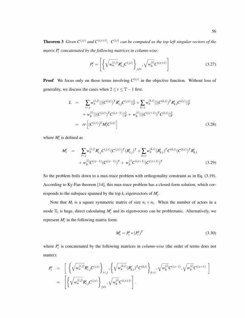
56
Theorem 3 Given C( j,t) and C(i,t±1), C(i,t) can be computed as the top left singular vectors of the
matrix Pti concatenated by the following matrices in column-wise:
Pti =
[√w(i, j)
a Rti, jC
( j,t)
j 6=i,
√w(i)
b C(i,t±1)
](3.27)
Proof We focus only on those terms involving C(i,t) in the objective function. Without loss of
generality, we discuss the cases when 2≤ t ≤ T−1 first.
L = ∑i< j
w(i, j)a ||(C(i,t))T Rt
i, jC( j,t)||2F + ∑
k<iw(k,i)
a ||(C(k,i))T Rtk,iC
(i,t)||2F
+ w(i)b ||(C
(i,t))TC(i,t−1)||2F + w(i)b ||(C
(i,t+1))TC(i,t)||2F
= tr[(C(i,t))T Mt
iC(i,t)]
(3.28)
where Mti is defined as
Mti = ∑
i< jw(i, j)
a Rti, jC
( j,t)(C( j,t))T (Rti, j)
T + ∑k<i
w(k,i)a (Rt
k,i)TC(k,t)(C(k,t))T Rt
k,i
+ w(i)b C(i,t−1)(C(i,t−1))T + w(i)
b C(i,t+1)(C(i,t+1))T (3.29)
So the problem boils down to a max-trace problem with orthogonality constraint as in Eq. (3.19).
According to Ky-Fan theorem [14], this max-trace problem has a closed-form solution, which cor-
responds to the subspace spanned by the top ki eigenvectors of Mti .
Note that Mi is a square symmetric matrix of size ni× ni. When the number of actors in a
mode Xi is huge, direct calculating Mti and its eigenvectors can be problematic. Alternatively, we
represent Mti in the following matrix form:
Mti = Pt
i ∗ (Pti )
T (3.30)
where Pti is concatenated by the following matrices in column-wise (the order of terms does not
matter):
Pti =
[ √w(i, j)
a Rti, jC
( j,t)
i< j,
√w(k,i)
a (Rtk,i)
TC(k,t)
k<i,
√w(i)
b C(i,t−1),
√w(i)
b C(i,t+1)]
=
[√w(i, j)
a Rti, jC
( j,t)
j 6=i,
√w(i)
b C(i,t±1)
].

57
Input: R, ki, w(i, j)a , w(i)
b ;Output: idx(i,t), C(i,t), At
i, j.1. Generate initial cluster indicator matrix C(i,t).2. Repeat3. For t = 1 : T, i = 1 : m4. shrink / expand C(i,t±1) if necessary;5. calculate Pt
i (or Mti ) as in Theorem 3;
6. calculate SVD of Pti (or eigenvectors of Mt
i );7. update C(i,t) as top left singular (eigen) vectors;8. Until the relative change of the objective (F3) ≤ ε .9. calculate At
i, j as in Theorem 2;10. calculate the cluster idx(i,t) with k-means on C(i,t).
Figure 3.7: SocioDim Integration for Dynamic Multi-Modal Networks
For t = 1 or t = T, we only need to keep C(i,t+1) or C(i,t−1) respectively, instead of C(i,t±1).
Typically the size of Pti is much smaller compared to Mt
i if the number of clusters of each mode is
small. Let the SVD of Pi as Pti = UΣV , then Mt
i = UΣ2UT . That is, the top left-singular vectors of
Pti correspond to the top eigenvectors of Mt
i , which completes the proof.
3.5.3 Instantiation of SocioDim Integration
To solve the problem F3 in Eq. (3.26), we resort to alternating optimization. That is, we fix all the
other variables while solving C(i,t). This process is iterated until convergence4. After convergence,
C(i,t) are the approximate community indicator matrices. One problem to be addressed is to
recover the discrete partition of communities. One commonly used post-processing scheme is to
apply k-means clustering to the community indicators [8]. Combined with the results of previous
sections, we have the algorithm in Figure 2.4.
Note that this is exactly an instantiation of the unsupervised learning framework in Figure 3.3.
Each step to update C(i,t) corresponds to the left singular vectors of Pti , which is defined as in
Eq. (3.27). Pti is constructed based on social dimensions from related modes and timestamps. The
related social dimensions are concatenated together to form an “instance-attribute” matrix for nodes
at mode i. By performing SVD, we obtain the corresponding social dimension Cti in mode i.
4The convergence property is discussed in detail in Appendix B.

58
Based on the proposed SocioDim integration algorithm, it is simple to extend our framework to
handle networks of various properties.
Within-Mode Interactions. A social media network, for instance, can be both multi-modal
and multi-dimensional. One can combine the two algorithms to handle multi-modal and multi-
dimensional challenges. The combination is straightforward: if there are within-mode interactions
that are multi-dimensional, we can simply append to Pi in Eq. (3.27) with social dimensions from
each type of interaction. That is,
Pi =[√
wi j Ri, jC j
i< j ,√
wki RTk,iCk
k<i , C
di ]
(3.31)
where Cdi denotes the structural features extracted from dth dimension of interaction in the ith
mode. In this way the presented unsupervised learning algorithm is able to handle diverse evolving
heterogeneous networks in social media.
Actor Attributes. The attribute view of the algorithm allows for the integration of entity at-
tributes in a convenient way. When a multi-modal network has attributes for certain modes of actors,
we can simply add these attributes as features in Pti (Eq. (3.27)) when updating the cluster indicator
matrix. That is:
Pti =
[√w(i, j)
a Rti, jC
( j,t)
j 6=i,
√w(i)
b C(i,t±1),
√w(i)
c F ti
]
where F ti denotes the attributes for actors in mode i, and w(i)
c the weight for actor attributes.
Higher-Order Temporal Regularization. In our formulation, we make the first-order Markov
assumption that a community snapshot should be similar to its previous snapshot. In some domains,
it might be necessary to include higher-order temporal regularization. An `-th order temporal regu-
larization enforces the community structure at timestamp t to be similar to that of t− 1, t− 2, · · · ,
t− `. Based on the attribute view of the algorithm, we just need to modify Pti as follows to reflect
the higher-order dependency:[√w(i, j)
a Rti, jC
( j,t)
j 6=i,
√w(i)
b αk−1C(i,t±k)
k=1,··· ,`
]
Here, 0 < α ≤ 1 is a decay factor to tune the regularization effect of different snapshots. Those
snapshots that are close to current timestamp play a more important role in regularization.

59
Dormant and Emerging Actors. Some actors might become inactive at a certain time period.
Meanwhile, new actors might join the network at a specific timestamp. The framework earlier
assumes actors do not change. Here, we analyze more realistic cases where actors become dormant
or join a network.
Note that our derived algorithm just uses C(i,t±1) as attributes for current timestamp. When an
actor leaves or hibernates at certain timestamp, we can delete his corresponding entry in C(i,t±1)
when updating C(i,t). However, after deletion, the orthogonality constraints might not be satisfied.
Since our framework is an approximation to hard clustering, a tiny deviation from orthogonality
does not affect the performance. However, when many actors become inactive, the total weights of
remaining actors in C(i,t±1) is relatively small, thus playing a less important role in the computation
of the similarity matrix Mti in Eq. (3.29). This is reasonable. A drastic membership change denotes
the latent community is experiencing an “overhaul”, thus it is not necessary to over-regularize the
temporal change. When mode Xi at timestamp t has new actors, we simply set their entries in
C(i,t±1) to 0.
Online Clustering. In some real-world scenarios, one might need to track the group evolution
in an online fashion, and the algorithm should be modified accordingly. Instead of iteratively up-
dating C(i,t), we update the community structure at different timestamps only once. Moreover, the
corresponding updating matrix Pti and Mt
i involve only fixed C(i,t−1), but not C(i,t+1). That is,
Pti =
[√w(i, j)
a Rti, jC
( j,t)
j 6=i,
√w(i)
b C(i,t−1)
].
In a nutshell, actor attributes, social dimensions at different snapshots and interactions provide
additional information for community detection. Based on the SocioDim integration framework, it
is easy to extend the algorithm 3.7 to handle various cases. Such a unsupervised learning approach
has been shown to outperform those without integration [125].
3.6 Related Work
As we presented unsupervised learning tasks concerning various types of social media networks,
we discuss the related work for each, respectively.
60
3.6.1 Community Detection with Multiple Networks
Some work attempts to address unsupervised learning with multiple data sources or clustering re-
sults, such as cluster ensemble [115, 139, 39] and consensus clustering [95, 63, 103, 49]. These
methods essentially fall into partition integration scheme presented in our framework. Most of the
algorithms aim to find a robust clustering based on multiple clustering results, which are prepared
via feature or instance sampling or disparate clustering algorithms. A similar idea is applied to
community detection in social networks [58]. A small portion of connections between nodes are
randomly removed before each run, leading to multiple different clustering results. Those clusters
occurring repeatedly are considered more stable, and are deemed to reflect the natural communities
in reality. However, all the cluster ensemble methods concentrate on either attribute-based data or
one-dimensional networks.
Another related field is multi-view clustering. Bickel and Scheffere [15] propose co-EM and an
extension of k-means and hierarchical clustering to handle data with two conditional independent
views. Sa [31] creates a bipartite based on the two views and tries to minimize the disagreement.
Different spectral frameworks with multiple views are studied in [159] and [83]. The former defines
a weighted mixture of random walk over each view to identify communities. The latter assumes
clustering membership of each view is provided and finds an optimal community pattern via mini-
mizing the divergence of the transformed optimal pattern and the community membership of each
view. A variant of utility integration based on block model approximation plus regularization is pre-
sented in [132]. Similarly, [6] suggests combining graph Laplacians for semi-supervised learning.
It is empirically verified that our proposed integration schemes also apply to spectral clustering and
block model approximation, and feature integration tends to be the most robust one.
Unsupervised multiple kernel learning [144] is relevant to network integration if we deem each
dimension of the network as a similarity or kernel matrix. Multiple kernel learning [119] aims to
find a combination of kernels to optimize for classification or clustering. Unfortunately, its limited
scalability hinders its application even to a medium-size network.
61
3.6.2 Community Detection in Multi-Modal Networks
An extensive body of work studies the structural property of interactions between actors. One
probabilistic approach is the stochastic block model [105], in which the link between actors is
generated conditioned on the latent cluster membership of actors. Two actors within the same
cluster are stochastically equivalent. That is, the interactions between (A1,B1) and (A2,B2) have
the same probability if A1 and A2, B1 and B2 belong to the same cluster, respectively. Long et
al. [86] propose a similar probabilistic framework to handle multi-modal networks with interac-
tions and actor attributes. Topic models [16] are also extended to model documents within a social
network [160, 146, 91]. Typically, they are specific for one type of document like Emails or papers.
Another attempt to model the structure is the latent space model. Intuitively, latent space models
map actors to a latent low-dimensional space such that the actors whose positions are closer are more
likely to interact with each other [57, 52]. Globerson et al. [48] study a two-mode network (authors
and words) and map both authors and words into the same Euclidean space.
Spectral relational clustering, relevant to multi-modal networks, tries to discover latent com-
munity structures based on multiple relational tables. As the original problem of finding discrete
cluster assignment (e.g., the entries of membership vector are either 0 or 1) is NP-hard, spectral
clustering relaxes the constraint to allow the membership vector to be continuous. The initial work
of co-clustering [33, 157, 85] tries to address the problem of clustering both words and documents
simultaneously by taking advantage of the structure of a bipartite. Gao et al. [45] extend the problem
to a star-typed network with multiple heterogeneous objects, and propose semi-definite program-
ming to solve the problem. Alternatively, reinforcement clustering is proposed [145]. Long et
al. [84] present a general spectral clustering framework to handle multi-type relational clustering
with different kinds of objects and attributes, and an alternating optimization algorithm is presented
to find a solution.
3.6.3 Community Evolution in Dynamic Networks
Temporal change of social networks has been attracting increasing attention [20, 107, 7]. It is empir-
ically observed that some real-world networks are evolving [72]. Practitioners try to investigate how
a network evolves and what might be a reasonable generative process to model the dynamics [78].
62
The critical factors to determine the group evolution are also reported [9].
On the other hand, evolutionary clustering [24] is developed. It assumes clustering result of
current situation is similar to that of previous timestamps. Given multiple snapshots of network
data, evolutionary clustering finds out a sequence of clustering with temporal smoothness [28, 81].
A Bayesian interpretation is presented in [154]. The latent space model with temporal change
is also developed [110]. Tantipathananandh et al.[134] propose a general framework to handle
dynamic single-mode network by casting it as a graph coloring problem and some greedy heuristics
or approximation algorithms [133] are developed to handle large-scale data. Sun et al. [116] address
the group evolution problem from an information-theoretic view. They present a scheme that detects
not only the community structure but also the change point. As existing evolutionary approaches
often require a specified number of clusters at each time stamp, (hierarchical) Dirichlet process is
employed so that this parameter can be learned automatically from data [151, 150]. Most of the
aforementioned works focus on data with attributes or single-mode networks. In this work, we
explore the community evolution in multi-modal networks and show that it reduces to our proposed
SocioDim integration framework for unsupervised learning.
3.7 Summary
Social media networks present many forms of heterogeneity. The interactions in social media can
be multi-dimensional, multi-modal and dynamic with evolutions. As most interactions online are
very noisy, it is imperative to integrate interaction information from multiple dimensions, modes
or snapshots in order to infer the latent community structure among actors more accurately. In
this chapter, we extend the SocioDim framework proposed in Chapter 2 and propose a SocioDim
integration framework for unsupervised learning A key component in the SocioDim integration
framework is to extract social dimensions from related network dimensions, modes or snapshots,
and then concatenate them all as conventional attributes for integration via spectral analysis. To
show the effect of the framework, we present two instantiations. One is to find shared community
structure across multiple types of interactions in a multi-dimensional network and it is empirically
shown to outperform community detection on a single type of interaction and other strategies of in-
tegration. The other is to identify evolving communities in a dynamic multi-modal network. In this

63
case, the SocioDim integration strategy indeed has a tight bond to block models and evolutionary
clustering extended to dynamic multi-modal networks. Though the objective function and subse-
quent derivation might look a little bit twisted, the final algorithm reduces to SocioDim integration
exactly. This explains why the proposed framework is sensible. With this unified SocioDim inte-
gration framework for unsupervised learning, it is easy to handle social media networks of various
properties, and identify accurate latent community structures by integrating network information
from multi-dimensional, multi-modal and dynamic interactions.
Chapter 4
SCALABLE LEARNING BASED ON SPARSE SOCIAL DIMENSIONS
In the previous two chapters, based on the concept of social dimension, we have presented a frame-
work for learning with social media networks. The proposed learning framework is composed of
two steps: 1) social dimension extraction, and 2) discriminative learning for supervised learning or
spectral analysis for unsupervised learning. In the first step, latent social dimensions are extracted
based on network topology to capture the potential affiliations of actors. These extracted social di-
mensions represent how each actor is involved in diverse relations. These social dimensions can be
treated as features of actors for the subsequent learning. As one actor is likely to participate in multi-
ple different relations, a soft clustering method is employed to extract social dimensions. However,
as we show below, this soft clustering strategy has a serious limitation, i.e., it produces dense social
dimensions, posing thorny challenges about scalability for both the extraction of social dimensions
and the subsequent learning. In this chapter, following the proposed learning framework, we present
techniques that are scalable to deal with networks of millions of nodes.
4.1 Problem Statement
In this chapter, we mainly focus on supervised learning. The derived techniques can be applied to
unsupervised learning as well. Essentially, we focus on the same supervised learning problem in
Chapter 2. For presentation convenience, we restate the problem again.
Given:
– K categories Y = Y1, · · · ,YK;
– a network A = (V,E,Y ) representing the interactions between nodes, where
V is the vertex set, E is the edge set, and each node vi is associated with class
labels yi whose value can be unknown;
– the known labels Y L for a subset of nodes V L in the network, where V L ⊆
V and yi j ∈ +,− denotes the class label of the vertex vi with respect to
category Y j.
65
Find:
– the unknown labels YU for the remaining vertices VU = V −V L.
The emphasis in this chapter is about scalability. In particular, the given network A consists of
millions of nodes that many methods might suffer from its size. We will analyze the bottleneck of
existent methods and then propose alternative effective methods to address the scalability.
4.2 Motivation
In the initial instantiation of the learning framework SocioDim (see section 2.3), a spectral variant
of modularity maximization [100] is adopted to extract social dimensions. The social dimensions
correspond to the top eigenvectors of a modularity matrix. It has been empirically shown that this
framework outperforms other representative relational learning methods on social media data. How-
ever, there are several concerns about the scalability of SocioDim with modularity maximization:
• Social dimensions extracted according to modularity maximization are dense. Suppose there
are 1 million actors in a network and 1,000 dimensionsare extracted. If standard double
precision numbers are used, holding the full matrix alone requires 1M×1K×8 = 8G memory.
This large-size dense matrix poses thorny challenges for the extraction of social dimensions
as well as subsequent discriminative learning.
• Modularity maximization requires the computation of the top eigenvectors of a modularity
matrix of the same size as a given network. When the network scales to millions of actors,
the eigenvector computation becomes a daunting task.
• Networks in social media tend to evolve, with new members joining, and new connections oc-
curring between existing members each day. This dynamic nature of networks entails efficient
update of the model for collective behavior prediction. Efficient online update of eigenvectors
with expanding matrices remains a challenge.
Such a limitation applies to other commonly used soft community detection approaches such as
spectral clustering[88], block models[3] and probabilistic soft clustering[155]. Consequently, it is
imperative to develop scalable methods that are capable of handling large-scale networks efficiently
without extensive memory requirement.

66
4.3 Learning with Sparse Social Dimensions
Though SocioDim with soft clustering for social dimension extraction demonstrates promising re-
sults, its scalability is limited. A network could be sparse, the extracted social dimensions, however,
are not sparse. Let’s look at the toy network in Figure 4.1. Its social dimensions following modu-
larity maximization are shown in Table 4.1. Clearly, none of the entries is zero. When a network
expands into millions of actors, a reasonably large number of social dimensions need to be ex-
tracted. The corresponding memory requirement hinders both the extraction of social dimensions
and the subsequent discriminative learning. Hence, it is imperative to develop some approach such
that the extracted social dimensions are sparse.
4.3.1 Communities in Edge-Centric View
It seems reasonable that the number of affiliations one user can participate in is upperbounded by his
connections. Consider one extreme case that an actor has only one connection. It is expected that
he is probably active in only one affiliation. It is not necessary to assign a non-zero score for each
affiliation. Assuming each connection represents one dominant affiliation, we expect the number of
affiliations of one actor is no more than his connections. Rather than defining a community as a set
of nodes, we redefine it as a set of edges. Thus, communities can be identified by partitioning edges
of a network into disjoint sets.
For instance, the two communities in the network in Figure 4.1 can be represented by two edge
sets in Figure 4.2, where the dashed edges represent one affiliation, and the remaining edges denote
another affiliation. One actor is considered associated with one affiliation as long as any of his
connections is assigned to that affiliation. Hence, the disjoint edge clusters in Figure 4.2 can be
converted into the social dimensions as the last two columns for edge partition in Table 4.1. Actor
1 is involved in both affiliations under this edge partition scheme.
To extract sparse social dimensions, we partition edges rather than nodes into disjoint sets. The
edges of those actors involving in multiple affiliations (e.g., actor 1 in the toy network) are likely to
be separated into different clusters. Though the partition in edge view is disjoint, the affiliations in
the node-centric view can overlap. Each node can engage in multiple affiliations. In addition, the
extracted social dimensions following edge partition are guaranteed to be sparse. This is because

67
Figure 4.1: A Toy Network Figure 4.2: Edge Clusters
Table 4.1: Social Dimension(s) of the Toy Example Following Different Approaches
Actors Modularity EdgeMaximization Partition
1 -0.1185 1 12 -0.4043 1 03 -0.4473 1 04 -0.4473 1 05 0.3093 0 16 0.2628 0 17 0.1690 0 18 0.3241 0 19 0.3522 0 1
the number of one’s affiliations is no more than her connections. Suppose we have a network with
m edges and n nodes, and k social dimensions are extracted. Then each node vi has no more than
min(di,k) non-zero entries in its social dimensions, where di is the degree of node vi. We have the
following theorem about the density of extracted social dimensions.
Theorem 4 Suppose k social dimensions are extracted from a network with m edges and n nodes.
The density (proportion of nonzero entries) of the social dimensions based on edge partition is
bounded by the following:
density ≤ ∑ni=1 min(di,k)
nk=
∑i|di≤k di +∑i|di>k knk
(4.1)
Moreover, for many real-world networks whose node degree follows a power law distribution, the
upperbound in Eq. (4.1) can be approximated as follows:
α−1α−2
1k−(
α−1α−2
−1)
k−α+1 (4.2)
where α > 2 is the exponent of the power law distribution.

68
Proof It is observed that the node degree in a social network follows power law [99]. For simplic-
ity, we use a continuous power-law distribution to approximate the node degrees. Suppose
p(x) = Cx−α , x≥ 1
where x is a variable denoting the node degree and C is a normalization constant. It is not difficult
to verify that
C = α−1.
Hence,
p(x) = (α−1)x−α , x≥ 1.
It follows that the probability that a node with degree larger than k is
P(x > k) =∫ +∞
kp(x)dx = k−α+1.
Meanwhile, we have
∫ k
1xp(x)dx
= (α−1)∫ k
1x · x−αdx
=α−1−α +2
x−α+2|k1
=α−1α−2
(1− k−α+2)
Therefore,
density ≤∑i|di≤k di +∑i|di>k k
nk
=1k
k
∑d=1
|i|di = d|n
·d +|i|di ≥ k|
n
≈ 1k
∫ k
1xp(x)dx+P(x > k)
=1k
α−1α−2
(1− k−α+2)+ k−α+1
=α−1α−2
1k−(
α−1α−2
−1)
k−α+1
The proof is completed.

69
102
103
104
2.1
2.2
2.3
2.4
2.5
2.6
2.7
2.8
2.9
3
K
α
−3.5
−3
−2.5
−2
−1.5
Density in log scale
(−2 denotes 10−2
)
Figure 4.3: Density Upperbound of Social Dimensions
To give a concrete example, we examine a YouTube network1 with more than 1 million ac-
tors and verify the upperbound of the density. The YouTube network has 1,128,499 nodes and
2,990,443 edges. Suppose we want to extract 1,000 dimensions from the network. Since 232
nodes have degree larger than 1000, following Eq.(4.1), the density is upperbounded by
(5,472,909+232×1,000)/(1,128,499×1,000) = 0.51%.
The node distribution in the network follows a power law with the exponent α = 2.14 based on
maximum likelihood estimation [99]. Thus, the upperbound following Eq.(4.2) is 0.54%.
Note that the upperbound in Eq. (4.1) is network specific whereas Eq.(4.2) gives an approximate
upperbound for a family of networks. It is observed that most power law distributions occurring in
nature have 2≤α ≤ 3 [99]. Hence, the bound in Eq. (4.2) is valid most of the time. Figure 4.3 shows
the function in terms of α and k. Note that when k is huge (close to 10,000), the social dimensions
become extremely sparse (< 10−3). In reality, the extracted social dimensions is typically even more
sparse than this upperbound as shown in later experiments. Therefore, with communities defined in
edge view, the extracted social dimensions are sparse, alleviating the memory demand and enabling
scalable discriminative learning.
1More details are in the experiment part.

70
Now, the remaining question is how to partition edges efficiently. Below, we will discuss two
different approaches to accomplish this task: partitioning a line graph or clustering edge instances.
4.3.2 Edge Partition via Partitioning Line Graph
In order to partition edges into disjoint sets, one way is to look at the “dual” view of a network,
i.e., the line graph [54]. We will show that this is not a practical solution. In a line graph L(G),
each node corresponds to an edge in the original network G, and edges in a line graph represent the
adjacency between two edges in the original graph. Given a network, graph partition algorithms can
be applied to its corresponding line graph. The resultant communities in the line graph corresponds
to a disjoint edge partition in the original graph. Recently, such a scheme has been used to detect
overlapping communities [36, 2]. It is, however, prohibitive to construct a line graph for a mega-
scale network. We notice that edges connecting to the same node in the original network form a
clique in the corresponding line graph. This property leads to much more edges in a line graph than
that in the original network.
Theorem 5 Let n and m denote the numbers of nodes and connections in a network, and N and M
the numbers of nodes and connections in its line graph. It follows that
N = m, M ≥ m(
2mn−1)
(4.3)
The equation is achieved if and only if each node in the original graph share the same degree.
Proof Let G and L(G) denote a graph and its line graph respectively, di the degree of node i in G.
Suppose G has n nodes and m edges, L(G) has N nodes and M edges. As each edge in G becomes
a node in L(G), it is straightforward that
N = m (4.4)

71
Because the connections of one node in G form a clique in L(G), we have
M =12 ∑
idi(di−1)
=12 ∑
id2
i −12 ∑
idi
=12n
(d21 +d2
2 + · · ·+d2n)(1+1+ · · ·+1︸ ︷︷ ︸
n
)−m
≥ 12n
(d1 ·1+d2 ·1+ · · ·+dn ·1)2−m (4.5)
=1
2n4m2−m
= m(
2mn−1)
(4.6)
The inequality (4.5) is derived following Cauchy-Schwarz inequality [55]. The equation is achieved
if and only if d1 = d2 = · · ·= dn.
For many real-world large-scale networks, the lower bound is never achievable as hardly did we
observe any real-world network with the same degree for all nodes. Most networks obey the power
law [99]. Consequently, the connections of a line graph tend to multiply without a constant bound
with respect to the size of a given network as stated in the following theorem.
Theorem 6 Let α denote the exponent of a power law distribution for node degrees of a given
network, n the size of the network, and M the number of connections in its corresponding line
graph. It follows that
E[2M/n]
diverges if 2 < α <= 3
= α−1(α−3)(α−2) if α > 3
(4.7)
Proof
E[2M/n] = E
[1n
(n
∑i=1
d2i −
n
∑i=1
di
)]= E[X2]−E[X ]

72
where X denotes the random variable (node degree). For a power law distribution p(x) = (α −
1)x−α , it follows that [99],
E[X ] =α−1α−2
, if α > 2;
E[X2] =α−1α−3
, if α > 3.
Hence,
E[2M/n]
diverges if 2 < α <= 3
= α−1(α−3)(α−2) if α > 3
(4.8)
The divergence of the expectation tells us that as we go to larger and larger data sets, our estimate
of number of connections in the line graph with respect to the original network size will increase
without bound.
The divergence of the expectation tells us that as we go to larger and larger data sets, our estimate
of number of connections with respect to the original network size will increase without bound. As
we have mentioned, the majority of large-scale networks follow a power law with α lying between
2 and 3. Consequently, the number of connections in a line graph can be extremely huge. Take the
aforementioned YouTube network as an example again. It contains approximate 1 million nodes
and 3 million links. Its resultant line graph will contain 4,436,252,282 connections, too large to be
even loaded into memory. Recall that the original motivation to use sparse social dimensions is to
address the scalability concern. Now we end up with dealing with a much larger sized line graph.
Hence, the line graph is not a suitable representation for practical use. Next, we will present an
alternative approach to edge partition, which is much more efficient and scalable.
4.3.3 Edge Partition via Clustering Edge Instances
In order to partition edges into disjoint sets, we treat edges as data instances with their terminal
nodes as features. For instance, we can treat each edge in the toy network in Figure 4.1 as one
instance, and the nodes that define edges as features. This results in a typical feature-based data
format as in Table 4.2. Then a typical clustering algorithm like k-means clustering can be applied
to find out disjoint partitions.

73
Table 4.2: Edge Instances of the Toy Network in Figure 4.1
EdgeFeatures
1 2 3 4 5 6 7 8 9(1, 3) 1 0 1 0 0 0 0 0 0(1, 4) 1 0 0 1 0 0 0 0 0(2, 3) 0 1 1 0 0 0 0 0 0
... · · · · · · · · ·
One concern with this scheme is that the total number of edges might be too huge. Owing to
the power law distribution of node degrees presented in social networks, the total number of edges
is normally linear, rather than square, with respect to the number of nodes in the network. That is,
m = O(n) as stated in the following theorem.
Theorem 7 The total number of edges is usually linear, rather than quadratic, with respect to the
number of nodes in the network with a power law distribution. In particular, the expected number
of edges is given as
E[m] =n2
α−1α−2
, (4.9)
where α is the exponent of the power law distribution.
Proof Suppose a network with n nodes follows a power law distribution as
p(x) = Cx−α , x≥ xmin > 0
where α is the exponent and C is a normalization constant. Then the expected number of degree for
each node is [99]:
E[x] =α−1α−2
xmin
where xmin is the minimum nodal degree in a network. This can be verified via the properties
of power law distribution. In reality, we normally deal with nodes with at least one connection,
so xmin ≥ 1. Hence, the expected number of connections in a network following a power law
distribution is
E[m] =12
α−1α−2
n.

74
Input: data instances xi|1≤ i≤ mnumber of clusters k
Output: idxi1. construct a mapping from features to instances2. initialize the centroid of cluster C j|1≤ j ≤ k3. repeat4. Reset MaxSimi, idxi5. for j=1:k6. identify relevant instances S j to centroid C j
7. for i in S j
8. compute sim(i,C j) of instance i and C j
9. if sim(i,C j) > MaxSimi
10. MaxSimi = sim(i,C j)11. idxi = j;12. for i=1:m13. update centroid Cidxi
14. until no change in idx or change of objective < ε
Figure 4.4: Algorithm for Scalable K-means Variant
Still, millions of edges are the norm in a large-scale network. Direct application of some existing
k-means implementation cannot handle the problem. E.g., the k-means code provided in Matlab
package requires the computation of the similarity matrix between all pairs of data instances, which
would exhaust the memory of normal PCs in seconds. Therefore, implementation with an online
fashion is preferred.
On the other hand, the data of edge instances is quite sparse and structured. As each edge
connects two nodes in the network, the corresponding edge instance has exactly only two non-
zero features as shown in Table 4.2. This sparsity can help accelerate the clustering process if
exploited wisely. We conjecture that the centroids of k-means should also be feature-sparse. Often,
only a small portion of the data instances share features with the centroid. Thus, we only need to
compute the similarity of the centroids with their relevant instances. In order to efficiently identify
the instances relevant to one centroid, we build a mapping from features (nodes) to instances (edges)
beforehand. Once we have the mapping, we can easily identify the relevant instances by checking
the non-zero features of the centroid.
By taking care of the two concerns above, we have a k-means variant as in Figure 4.4 for edge-
centric clustering. We only keep a vector of MaxSim to represent the maximum similarity between
75
one data instance with a centroid. In each iteration, we first identify the set of relevant instances
to a centroid, and then compute similarities of these instances with the centroid. This avoids the
iteration over each instance and each centroid, which would cost O(mk) otherwise. Note that the
centroid contains one feature (node) if and only if any edge of that node is assigned to the cluster.
In effect, most data instances (edge) are associated with few (much less than k) centroids. By taking
advantage of the feature-instance mapping, the cluster assignment for all instances (lines 5-11 in
Figure 4.4) can be fulfilled in O(m) time. To compute the new centroid (lines 12-13), it costs O(m)
time as well. Hence, each iteration costs O(m) time only. Moreover, the algorithm only requires
the feature-instance mapping and network data to reside in main memory, which costs O(m + n)
space. Thus, as long as the network data can be held in memory, this clustering algorithm is able to
partition its edges into disjoint sets. Later as we show, even for a network with millions of actors, this
clustering can be finished in tens of minutes while modularity maximization becomes impractical.
As a simple k-means is adopted to extract social dimensions, it is easy to update the social
dimensions if the network changes. If a new member joins a network and a new connection emerges,
we can simply assign the new edge to the corresponding clusters. The update of centroids with the
new arrival of connections is also straightforward. This k-means scheme is especially applicable for
dynamic large-scale networks.
4.3.4 Regularization on Communities
The extracted social dimensions are treated as features of nodes. A conventional supervised learning
is applied. In order to handle large-scale data with high dimensionality and enormous instances, we
adopt linear SVM which can be finished in linear time [37]. Generally, the larger a community size
is, the weaker the connections inside the community are. Hence, we would like to build a SVM
relying more on communities of smaller sizes. In order to achieve this, we modify typical SVM
objective function as follows:
minλ
n
∑i=1|1− yi(xT
i w+b)|+ +wTΣw (4.10)
where λ is a regularization parameter for SVM2, |z|+ = max(0,z) represents SVM hinge loss, Σ
is a diagonal matrix to regularize the weights assigned to different communities. In particular,
2A different notation λ is used to avoid the confusion with community C.

76
Input: network data, labels of some nodesOutput: labels of unlabeled nodes1. convert network into edge-centric view as in Table 4.22. perform clustering on edges via algorithm in Figure 4.43. construct social dimensions based on edge clustering4. build classifier based on labeled nodes’ social dimensions5. apply regularization on both community size and node affiliation6. use the classifier to predict the labels of unlabeled ones
based on their social dimensions
Figure 4.5: Algorithm for Scalable Learning Based on Sparse Social Dimensions
Σ j j = h(|C j|) is the penalty coefficient associated with community C j. The penalty function h
should be monotonically increasing with respect to community size. In other words, a larger weight
assigned to a large community results in a higher cost.
Interestingly, with a little manipulation, the formula in Eq. (4.10) can be solved using standard
SVM package with modified input. Let X represent the input data with each row being an instance
(e.g., Table 4.1), and w = Σ1/2w. Then the formula can be rewritten as
minλ ∑i|1− yi(xT
i w+b)|+ +12
wTΣ
12 Σ
12 w
= minλ ∑i|1− yi(xT
i Σ− 1
2 Σ12 w+b)|+ +
12‖w‖2
2
= minλ ∑i|1− yi(xT
i w+b)|+ +12‖w‖2
2
where xTi = xT
i Σ−12 . Hence, given an input data matrix X , we only need to left multiply X by Σ−
12 .
It is observed that community sizes of a network tend to follow a power law distribution as shown
in the experiment part. Hence, we recommend h(|C j|) = log |C j| or (log |C j|)2.
On the other hand, one node is likely to engage in multiple communities. The node affiliation
also observes a heavy-tail distribution. Intuitively, a node participating in many communities influ-
ences less on other group members compared with those devoted ones. For effective classification
learning, we regularize node affiliations by normalizing each nodes social dimensions to sum up to
1. Later in the experiment, we will study which regularization affects more on classification.
In sum, to learn a model for collective behavior, we take the edge-centric view of the network
data and partition the edges into disjoint sets. Based on the edge clustering, social dimensions

77
Table 4.3: Statistics of Social Media Data
Data BlogCatalog Flickr YouTubeCategories 39 195 47Nodes (n) 10, 312 80, 513 1, 138, 499Links (m) 333, 983 5, 899, 882 2, 990, 443
Network Density 6.3×10⁻³ 1.8×10⁻³ 4.6×10⁻⁶
Maximum Degree 3, 992 5, 706 28, 754Average Degree 65 146 5
can be constructed and regularization can be applied. Then, discriminative learning and prediction
can be accomplished by considering these social dimensions as features. The detailed algorithm is
summarized in Figure 4.5.
4.4 Experiment Setup
Two data sets reported in Chapter 2 are used again here. To examine the scalability, we also include
a mega-scale network crawled from YouTube [94]. We remove those nodes without connections
and select the interest groups subscribed by at least 500 members. Some statistics of the three data
sets can be found in Table 4.3. The experiment set up and evaluation measure are the same as in
Chapter 2.
As we discussed in Section 4.3.2, constructing a line graph is prohibitive for large-scale net-
works. Hence, the line-graph approach is not included for comparison. Alternatively, the edge-
centric clustering (or EdgeCluster) in Section 4.3.2 is used to extract social dimensions on all the
data sets. We adopt cosine similarity while performing the clustering. Based on cross validation, the
dimensionality is set to 5000, 10000, and 1000 for BlogCatalog, Flickr, and YouTube, respectively.
A linear SVM classifier [37] is exploited for discriminative learning.
Another related approach to finding edge partitions is bi-connected components [60]. Bi-
connected components of a graph are the maximal subsets of vertices such that the removal of a
vertex from a particular component will not disconnect the component. Essentially, any two nodes
in a bi-connected component are connected by at least two paths. It is highly related to cut ver-
tices (a.k.a. articulation points) in a graph, whose removal will result in an increase in the number
of connected components. Those cut vertices are the bridges connecting different bi-connected
components. Thus searching for bi-connected components boils down to searching for articulation

78
points in the graph which can be solved efficiently by O(n + m). Here n and m represent the num-
ber of vertices and edges in a graph respectively. Each bi-connected component is considered a
community and converted into one social dimension for learning.
We also compare our proposed sparse social dimension approach with classification perfor-
mance based on dense representations. In particular, we extract social dimensions according to
modularity maximization (denoted as ModMax) [121]. ModMax has been shown to outperform
other representative relational learning methods based on collective inference. We study how the
sparsity in social dimensions affects the prediction performance as well as the scalability.
Note that social dimensions allow one actor to be involved in multiple affiliations. As a proof of
concept, we also examine the case when each actor is associated with only one affiliation. Essen-
tially, we construct social dimensions based on node partition. A similar idea has been adopted in
latent group model [98] for efficient inference. To be fair, we adopt k-means clustering to partition
nodes in a network into disjoint sets, and convert the node clustering result as social dimensions.
Then, SVM is utilized for discriminative learning. For convenience, we denote this method as
NodeCluster.
4.5 Experiment Results
In this section, we first examine how the performance varies with social dimensions extracted fol-
lowing different approaches. Then we verify the sparsity of social dimensions and its implication for
scalability. We also study how the performance varies with social dimensionality. Finally, concrete
examples of extracted social dimensions are given.
4.5.1 Prediction Accuracy
The prediction performance on all the data sets are shown in Table 4.4. The entries in bold face
denote the best one in each column. Evidently, EdgeCluster is the winner most of the time. Edge-
centric clustering shows comparable performance as modularity maximization on BlogCatalog net-
work. yet outperforms ModMax on Flickr. ModMax on YouTube is not applicable due to the
scalability constraint. Clearly, with sparse social dimensions, we are able to achieve comparable
performance as that of dense social dimensions. However, the benefit in terms of scalability will be
tremendous as discussed in the next subsection.

79
Table 4.4: Performance on Social Media Networks
BlogCatalog 10% 20% 30% 40% 50% 60% 70% 80% 90%EdgeCluster 27.94 30.76 31.85 32.99 34.12 35.00 34.63 35.99 36.29
Micro- BiComponents 16.54 16.59 16.67 16.83 17.21 17.26 17.04 17.76 17.61F1(%) ModMax 27.35 30.74 31.77 32.97 34.09 36.13 36.08 37.23 38.18
NodeCluster 18.29 19.14 20.01 19.80 20.81 20.86 20.53 20.74 20.78EdgeCluster 16.16 19.16 20.48 22.00 23.00 23.64 23.82 24.61 24.92
Macro BiComponents 2.77 2.80 2.82 3.01 3.13 3.29 3.25 3.16 3.37-F1(%) ModMax 17.36 20.00 20.80 21.85 22.65 23.41 23.89 24.20 24.97
NodeCluster 7.38 7.02 7.27 6.85 7.57 7.27 6.88 7.04 6.83
Flickr 1% 2% 3% 4% 5% 6% 7% 8% 9%EdgeCluster 25.75 28.53 29.14 30.31 30.85 31.53 31.75 31.76 32.19
Micro- BiComponents 16.45 16.46 16.45 16.49 16.49 16.49 16.49 16.48 16.55F1(%) ModMax 22.75 25.29 27.30 27.60 28.05 29.33 29.43 28.89 29.17
NodeCluster 22.94 24.09 25.42 26.43 27.53 28.18 28.32 28.58 28.70EdgeCluster 10.52 14.10 15.91 16.72 18.01 18.54 19.54 20.18 20.78
Macro- BiComponents 0.45 0.46 0.45 0.46 0.46 0.46 0.46 0.46 0.47F1(%) ModMax 10.21 13.37 15.24 15.11 16.14 16.64 17.02 17.10 17.14
NodeCluster 7.90 9.99 11.42 11.10 12.33 12.29 12.58 13.26 12.79
YouTube 1% 2% 3% 4% 5% 6% 7% 8% 9%EdgeCluster 23.90 31.68 35.53 36.76 37.81 38.63 38.94 39.46 39.92
Micro- BiComponents 23.90 24.51 24.80 25.39 25.20 25.42 25.24 24.44 25.62F1(%) ModMax — — — — — — — — —
NodeCluster 20.89 24.57 26.91 28.65 29.56 30.72 31.15 31.85 32.29EdgeCluster 19.48 25.01 28.15 29.17 29.82 30.65 30.75 31.23 31.45
Macro- BiComponents 6.80 7.05 7.19 7.44 7.48 7.58 7.61 7.63 7.76F1(%) ModMax — — — — — — — — —
NodeCluster 17.91 21.11 22.38 23.91 24.47 25.26 25.50 26.02 26.44
BiComponents, though also separates edges into disjoint sets, which in turn deliver a sparse
representation of social dimensions as EdgeCluster, yields a poor performance. This is because
BiComponents outputs highly imbalanced communities. For example, BiComponents extracts 271
bi-connected components in the BlogCatalog network. In these 271 components, a dominant one
contains 10,042 nodes while others are all of size 2. When a network is getting more connected (say,
Flickr with average degree 146), BiComponents is even worse. Only 10 bi-connected components
are found. No wonder its Macro-F1 is close to 0. In short, BiComponents, though very efficient and
scalable, cannot extract informative social dimensions for classification.
The NodeCluster scheme, by contrast, forces each actor to be involved in only one affiliation,
yielding inferior performance compared with EdgeCluster. Among all the compared methods,

80
EdgeCluster is often the winner. This indicates that its extracted sparse social dimensions do help
in collective behavior prediction.
4.5.2 Scalability Study
As we have introduced in Theorem 4, the social dimensions constructed according to edge-centric
clustering are guaranteed to be sparse because the density is upperbounded by a small value. Here,
we examine how sparse the social dimensions are in practice. We also study how the computational
time (with a Core2Duo E8400 CPU and 4GB memory) varies with the number of edge clusters.
The computational time, the memory footprint of social dimensions, their density and other related
statistics on all the three data sets are reported in Table 4.5.
Concerning the time complexity, it is interesting that computing the top eigenvectors of a modu-
larity matrix actually is quite efficient as long as there is no memory concern. This is observable on
the Flickr data. However, when the network scales to millions of nodes (YouTube Data), modular-
ity maximization becomes impossible due to its excessive memory requirement, while our proposed
EdgeCluster method can still be computed efficiently. The computation time of EdgeCluster on
YouTube network is much smaller than Flickr, because the YouTube network is extremely sparse
and the total number of edges and the average degree in YouTube are actually smaller than those of
Flickr as shown in Table 4.3.
Another observation is that the computation time of Edge-Cluster does not change much with
varying numbers of clusters. No matter what the cluster number is, the computation time of
EdgeCluster is of the same order. This is due to the efficacy of the proposed k-means variant in
Figure 4.4. In the algorithm, we do not iterate over each cluster and each centroid to do the cluster
assignment, but exploit the sparsity of edge-centric data to compute only the similarity of a cen-
troid and those relevant instances. This, in effect, makes the computational time independent of the
number of edge clusters.
As for the memory footprint reduction, sparse social dimension did an excellent job. On
Flickr, with only 500 dimensions, the social dimensions of ModMax require 322.1M, whereas
EdgeCluster requires only less than 100M. This effect is stronger on the mega-scale YouTube
network where ModMax becomes impractical to compute directly. It is expected that the social

81
Table 4.5: Scalability Comparison on Social Media Data of Varying Sizes
Methods Time Space Density UpperboundModMax−500 194.4 41.2M 1 —
EdgeCluster−100 300.8 3.8M 1.1×10⁻¹ 2.2×10⁻¹
EdgeCluster−500 357.8 4.9M 6.0×10⁻² 1.1×10⁻¹
EdgeCluster−1000 307.2 5.2M 3.2×10⁻² 6.0×10⁻²
EdgeCluster−2000 294.6 5.3M 1.6×10⁻² 3.1×10⁻²
EdgeCluster−5000 230.3 5.5M 6×10⁻³ 1.3×10⁻²
EdgeCluster−10000 195.6 5.6M 3×10⁻³ 7×10⁻³
Methods Time Space Density UpperboundModMax−500 2.2×10³ 322.1M 1 —
EdgeCluster−200 1.2×10⁴ 31.0M 1.2×10⁻¹ 3.9×10⁻¹
EdgeCluster−500 1.3×10⁴ 44.8M 7.0×10⁻² 2.2×10⁻¹
EdgeCluster−1000 1.6×10⁴ 57.3M 4.5×10⁻² 1.3×10⁻¹
EdgeCluster−2000 2.2×10⁴ 70.1M 2.7×10⁻² 7.2×10⁻²
EdgeCluster−5000 2.6×10⁴ 84.7M 1.3×10⁻² 2.9×10⁻²
EdgeCluster−10000 1.9×10⁴ 91.4M 7×10⁻³ 1.5×10⁻²
Methods Time Space Density UpperboundModMax−500 N/A 4.6G 1 —
EdgeCluster−200 574.7 36.2M 9.9×10⁻³ 2.3×10⁻²
EdgeCluster−500 606.6 39.9M 4.4×10⁻³ 9.7×10⁻³
EdgeCluster−1000 779.2 42.3M 2.3×10⁻³ 5.0×10⁻³
EdgeCluster−2000 558.9 44.2M 1.2×10⁻³ 2.6×10⁻³
EdgeCluster−5000 554.9 45.6M 5.0×10⁻⁴ 1.0×10⁻³
EdgeCluster−10000 561.2 46.4M 2.5×10⁻⁴ 5.1×10⁻⁴
EdgeCluster−20000 507.5 47.0M 1.3×10⁻⁴ 2.6×10⁻⁴
EdgeCluster−50000 597.4 48.2M 5.2×10⁻⁵ 1.1×10⁻⁴
dimensions of ModMax would occupy 4.6G memory. On the contrary, the sparse social dimensions
based on EdgeCluster only requires 30-50M.
The steep reduction of memory footprint can be explained by the density of the extracted di-
mensions. Take YouTube data as an example. When we have 50000 dimensions following edge
partition, the density is only 5.2×10⁻⁵ . Consequently, even if the network has more than 1 million
nodes, the extracted social dimensions still occupy tiny memory space. The upperbound of the den-
sity is not tight when the number of clusters k is small. As k increases, the bound is getting close to
the truth. In general, the true density is roughly half of the estimated bound.

82
1 2 3 4 5 6 7 8 9 100.1
0.12
0.14
0.16
0.18
0.2
0.22
Percentage of Training set(%)
Ma
cro
F1
−M
ea
su
re
Normalization Effect on Flickr
None
Node Affiliation
Community Size
Both
(a) Macro-F1
1 2 3 4 5 6 7 8 9 100.22
0.24
0.26
0.28
0.3
0.32
0.34
Percentage of Training set(%)
Mic
ro F
1−
Me
asu
re
Normalization Effect on Flickr
None
Node Affiliation
Community Size
Both
(b) Micro-F1
Figure 4.6: Regularization Effect on Flickr
4.5.3 Regularization Effect
In this part, we study how EdgeCluster performance varies with different regularization schemes.
Three different regularizations are implemented: regularization based on community size, node
affiliation and both (we first apply community size regularization, then node affiliation). The re-
sults without any regularization are also included as a baseline for comparison. In our experiments,
the community size regularization penalty function is set to (log(|Ci|))2, and node affiliation reg-
ularization normalizes each node’s community membership’s summation into 1. As is shown in
Figures 4.6, regularization on both community size and node affiliation consistently boost the per-
formance on Flickr data. It is also observed that applying regularization on node affiliation sig-
nificantly improves performance. It seems like community-size regularization is not as important
as the node-affiliation regularization. Similar trends are observed in the other two data sets. After
all, we have to point out that, when both community-size regularization and node-affiliation are ap-
plied, it is indeed quite similar to the tf-idf weighting scheme for representation of documents [111].
Such a weighting scheme actually can lead to a quite different performance for dealing with social
dimensions extracted from a network.
4.5.4 Visualization of Extracted Social Dimensions
As shown in previous subsections, EdgeCluster yields a outstanding performance. But are the
extracted social dimensions really sensible? To understand what the extracted social dimensions
are, we investigate tag clouds associated with different dimensions. Tag clouds, with font size

83
(a) Autos (b) Sports
Figure 4.7: Social Dimensions Selected by Autos and Sports, Respectively
denoting tags’ relative frequency, is widely used in social media websites to summarize the most
popular ongoing topics. In particular, we aggregate tags of individuals in one social dimension as
the tags of that dimension. However, it is impossible to showcase all the extracted dimensions.
Hence, we pick the dimension with the maximum SVM weight given a category.
Due to the space limit, we just show two examples in BlogCatalog. To make the figure legible,
we include only those tags whose frequency is greater than 2. The dimension in Figure 4.7a is
about cars, autos, automobile, pontiac, ferrari and etc. It is highly relevant to the category Autos.
Similarly, the dimension in Figure 4.7b is about baseball, mlb, basketball, and football. No wonder
it is informative for classification of category Sports. There are a few less frequent tags, such
as movies, and ipod associated with selected dimensions as well, suggesting the diverse interests
of each person. EdgeCluster, by analyzing connections in a network, is able to extract social
dimensions that are meaningful for classification.
4.6 Related Work
In order to extract sparse social dimensions for scalable learning, we resort to edge partition. This
essentially returns a set of overlapping communities. Finding overlapping communities is attracting
increasing attentions. Note that finding overlapping communities is quite a different task from soft
clustering [155]. Soft clustering often returns a dense community indicator matrix. It destroys
the genuine sparsity presented in a network, thus causing many computational problems. On the
contrary, the community indicator matrix of overlapping communities is often quite sparse.
Palla et al. propose a clique percolation method to discover overlapping dense communi-
ties [108]. It is composed of two steps: first enumerate all the cliques of size k in a graph; and
then find connected cliques. Two k-cliques are connected if they share k− 1 nodes. Based on the

84
connections between cliques, we can find the connected components with respect to k-cliques. Each
component then corresponds to one community. Since a node can be involved in multiple different
k-cliques, the resultant community structure allows one node to be associated with multiple differ-
ent communities. A similar idea is presented in [113], in which the authors suggest finding out all
the maximal cliques in a network, followed by traditional hierarchical clustering.
On the other hand, Gregory [51] extends the Newman-Girvan method [102] to handle overlap-
ping communities. The original Newman-Girvan method recursively removes edges with highest
betweenness until a network is separated into prespecified number of disconnected components. But
it only outputs non-overlapping communities. Therefore, Gregory proposes to add one more action
(node splitting) besides edge removal. The algorithm recursively splits nodes that are likely to reside
in multiple communities into two, or removes edges that seem to bridge two different communities.
This process is repeated until the network is disconnected into desired number of communities.
The aforementioned methods enumerate all the possible cliques or shortest paths in a network,
whose computational cost is daunting for real-world large-scale networks. Recently, a simple
scheme proposed to detect overlapping communities is to define communities as a set of edges,
instead of nodes [36, 2]. The network can be converted a line graph and then existing methods to
find disjoint communities can be applied. However, the scalability of constructing a line graph is
prohibitive as we discussed in section 4.3.2.
In our proposed EdgeCluster algorithm, k-means clustering is used to partition the edges of a
network into disjoint sets. We also propose a k-means variant to take advantage of its special spar-
sity structure, which can handle the clustering of millions of edges efficiently. More complicated
data structures such as kd-tree [11, 68] can be exploited to accelerate the process. In certain cases,
the network might be too huge to reside in memory. Then other k-means variants to handle ex-
tremely large data sets like online k-means [4], scalable k-means [19], incremental k-means [106]
and distributed k-means [65] can be considered.
4.7 Summary
In this chapter, we examine we can scale up the SocioDim learning framework to predict the online
behavior of users in social media, given the behavior information of some actors in the network.
85
We propose an edge-centric clustering scheme to extract sparse social dimensions and a scalable
k-means variant to handle edge clustering. Essentially, each edge is treated as one data instance, and
the connected nodes are the corresponding features. Then, the proposed k-means clustering algo-
rithm can be applied to partition the edges into disjoint sets, with each set representing one possible
affiliation. With this edge-centric view, the extracted social dimensions are warranted to be sparse.
Our model based on the sparse social dimensions shows comparable prediction performance as ear-
lier proposed approaches of social dimensions. An incomparable advantage of our model is that it
can easily scale to handle networks with millions of actors while the earlier model fails. Recently,
an extension to extract sparse social dimensions at multiple resolutions [130] also demonstrates
promising result, indicating strong potential of scalable learning based on sparse social dimensions.

Chapter 5
CONCLUSIONS AND FUTURE WORK
Social media is a rich data source of large quantity and high variety. It is a fertile field with many
great challenges for data mining. This dissertation proposes the concept of social dimension and
presents a social-dimension based learning framework to handle supervised and unsupervised learn-
ing in large-scale social media networks. The key contributions of this work are summarized below,
followed by future work.
5.1 Key Contributions
Fist, we propose a general supervised learning framework to harness the predictive power of social
media networks. Before our work, collective inference was proposed to capture the local depen-
dency of labels between neighboring nodes. However, it treats connections within the network
homogeneously. In reality, the connections within a network are often heterogeneous, representing
assorted relations. To capture different relations among actors in a network, we propose to extract
social dimensions via soft clustering. Based on the extracted social dimensions, a discriminative
classifier like SVM can be constructed to determine which dimensions are informative for classifica-
tion. Extensive experiments on social media data demonstrated that our proposed social-dimension
approach (SocioDim) outperforms alternative collective inference, especially when labeled data are
few. In the SocioDim framework, a network is converted into attribute format as in conventional
data mining. Thus, existing software that is optimized for attribute data can be plugged in to handle
social media networks. Moreover, it offers a simple yet effective approach to integrating two types
of seemingly orthogonal information: network of actors and actor attributes.
For anther, we extend the general learning framework to handle community detection in social
media networks. Based on the concept of social dimensions, we can integrate information in var-
ious kinds of social media networks including multi-dimensional networks, multi-modal networks
and dynamic networks with evolutions. The unsupervised learning also follows two steps: extract
social dimensions from each type of network interaction, modes or snapshots and then integrate
them to perform spectral analysis. This unsupervised learning approach connects network anal-
87
ysis to conventional data mining, thus providing a comprehensible approach to detect groups in
various types of social media networks, and leading to a more accurate understanding of human
interactions online.
Last but not least, we propose effective solutions to extract sparse social dimensions to make
the learning framework scalable to handle real-world large-scale networks. By defining a commu-
nity in an edge-centric view, we rigorously prove that sparse social dimensions can be obtained via
edge partition. EdgeCluster is proposed to take advantage of sparsity in networks. It is extremely
scalable to handle sparse large-scale networks, which are common in social media. Such a scalable
learning scheme based on sparse social dimensions avoids heavy computation, yet shows compara-
ble performance as that based on dense social dimensions. By sifting through noisy interactions in
social media, it provides a viable solution for large-scale social computing.
5.2 Future Work
In the previous chapters, we have discussed about supervised learning, unsupervised learning and
scalable learning with social media networks. Following the proposed learning framework, there
are many promising directions to explore for future work. We highlight some below.
5.2.1 Effective Extraction of Social Dimensions
The success of our proposed learning framework hinges on social dimensions. Social dimensions
can be extracted via soft clustering as discussed in Chapter 2 or EdgeCluster proposed in Chap-
ter 4. Current methods for extracting social dimensions do not use label information. It is not
clear whether the supervised extraction of social dimensions would improve the classification per-
formance. Menon and Elkan [93] investigate this question by empirical comparison on several data
sets. Quite surprisingly, unsupervised extraction of social dimensions works pretty well, sometimes
even better than supervised ones. It requires further investigation to effectively incorporate label
information into social dimension extraction.
On the other hand, communities in social media demonstrate strong statistical properties. Ku-
mar et al. [74] found that real-world networks consist of a giant connected components with others
being singletons and small-size connected components. Leskovec studied the statistical properties
of communities on the giant connected component and found a similar pattern [79]. The optimal

88
spectral cut always returns a community of size 100 to 200, loosely connected (say, one or two
edges) to the remaining of the whole network. What is the implication of these properties to extrac-
tion of social dimensions? A further comprehensive comparison of various community detection
algorithms is reported in [80]. In these papers, most community detection methods focus on discrete
binary cases, i.e., extracting one community from a network based on certain criterion. Whereas So-
cioDim employs soft clustering to extract social dimensions, and typically many more dimensions
instead of just one or two are extracted. We believe a comprehensive comparison of different soft
clustering approaches for the extraction of social dimensions is an interesting line of future work.
Furthermore, the current approach requires practitioners to specify the number of social dimen-
sions, and this parameter can be critical to the final classification performance as shown in [122].
Consequently, some procedure like cross-validation has to be used to determine a proper parameter.
Considering a network with millions of actors, the community extraction can be time-consuming,
as each time a new value is set, the whole community extraction procedure has to be restarted again.
It thus remains a challenge to determine the parameter automatically.
In reality, actors are involved in multiple relations of which some are associated with a natural
hierarchy. For instance, employees working on a small project form a community, which is within
a department, which might reside in another larger community representing the whole company.
Similarly, the students of a class form a group, which is within the department group. And the
department group resides in another group representing the whole university. These groups at dif-
ferent resolutions can pose assorted regulations on one’s behavior [56]. Instead of picking a proper
parameter, we conjecture that, by extracting communities at all possible resolutions, we may be able
to avoid a tedious cross-validation procedure.
To find communities of varying resolutions, a natural solution is hierarchical clustering. Hier-
archies have been used to organize concepts [41] and for classification [131]. However, the over-
lapping nature of different relations complicates the problem. One user is likely to be involved in
multiple different communities, and these communities each reside in a hierarchical path. For ex-
ample, one student might connect to some of his former classmates online. These classmates span
in different departments, which in turn form a university-wide group. At the same time, he might
connect to his current colleagues, which also reside in a hierarchical structure. In other words, one

89
actor is allowed to reside in multiple different paths in the resultant dendrogram, instead of a sin-
gle one as commonly studied in existing hierarchical community detection approaches. It requires
advanced techniques to find multi-resolution overlapping communities which lead to sparse social
dimensions of different resolutions.
Toward this direction, we have developed a bottom-up hierarchical clustering to extract sparse
social dimensions at different resolutions [130]. It considers the local social circle of each user
as seed communities and merge them based on community overlap. The resultant classification
performance improvement is substantial over that based on predefined number of social dimensions.
By exploiting the sparsity present in network connections, the hierarchical clustering can be finished
efficiently. Only hours are required to deal with a network of millions of nodes. Essentially, we
extract sparse social dimensions at all resolutions. We also hypothesize that by using the label
information, we might prune certain branches just like decision trees. At the end, we may obtain a
decision tree for network data.
In all, there is no conclusion which method is more effective for the extraction of social dimen-
sions. We expect more research along this direction to emerge in the near future.
5.2.2 Quantifying Crowd Behavior
In Chapter 2, we presented a supervised learning framework that can be utilized to predict the
behavior of individuals based on their friends’ behavior, such as whether or not one user likes one
product, whether or not he supports a presidential candidate, etc. In many applications and domains,
however, it is the aggregated mass, in other words, the prevalence of one class, that plays a key role
in decision making. Here are some examples:
• In the US presidential election, the candidate who wins a plurality of individual votes in a
state wins the state vote.
• A senator might need to collect the mass opinion [156], and prioritize requests based on the
urgency and the number of requests [96].
• An accurate estimation of the prevalence of influenza incidents in a certain area can help the
authority to allocate attentions, money and resources accordingly [66].

90
• Companies may want to estimate the proportion of positive or negative responses from cus-
tomers to take corresponding strategic actions toward a new-generation product.
All the example above share one common characteristic: it is the aggregated mass of certain prop-
erties that matters.
The problem of accurately estimating the prevalence of one class in samples is referred as
quantification [42]. It has been studied in various domains. For example, in the medical statistics
field, Zhou et al. estimate the prevalence of a disease in a test population with an imperfect binary
diagnostic test with known sensitivity and specificity [161]; Sociologists perform content analysis
of blog posts to examine the support with respect to two different candidates [61]; Forman compares
various strategies of quantification, aiming at quantifying the counts and costs of different classes
in HP customer calls [42] so that HP can allocate human resources accordingly. Quantification is
also applied to help semi-supervised learning when labeled samples and unlabeled samples follow
different class distributions [153].
Quantification calls for attention because 1) The basic assumption of training and test sharing
the same distribution as the foundation in many machine learning techniques are not necessarily
true in reality; 2) Many classifiers are optimized for individual predictions. It might induce biases
in quantification, especially when the class are imbalanced and insufficient; 3) The accuracy of
classifiers can be highly dependent on the availability of training samples, which often involves
tremendous human efforts. However, the prevalence might be estimated precisely even with few
labeled samples if a robust quantification method is exploited.
All the aforementioned studies focus on quantification when data are presented in conventional
attribute format. But in many situations, the data are presented in a relational network, such as the
citations among papers, the transportation network and financial transactions between different en-
tities. Recently, with the expanded use of web and social media, oceans of user interaction data are
produced in network format. This flood of network data provides valuable opportunities to study
collective behavior such as the political views of users, the happiness of people, the opinions and
sentiments of online users, the likelihood of product sales online, etc. Essentially, networks offers a
new type of information source. With abundant information provided online, we aim to quantify the

91
collective behavior, i.e., the number of users that are involved in certain type of activities, prefer-
ences, or behaviors. Generally, both attribute data (e.g., user tweets, status updates, blog posts, tags,
shared content) and network data (e.g., user interaction, friendship network, following/follower net-
work) are available. Ultimately, we hope to exploit both kinds of information collected from social
media to quantify the prevalence of users of certain classes.
As an initial attempt, we compared several strategies to estimate prevalence with network data
alone in [120]. Two kinds of quantification are presented and compared. 1) Classification-based
quantification do not model the prevalence directly, but hinge on post-processing to correct the
bias with labels. One specific method Median Sweep (MS) is quite robust and outperforms other
methods; 2) The link-based approach relies on link analysis to estimate the class prevalence. It
does not require classification and prediction, thus saving tremendous computational cost. But its
quantification performance is not comparable to MS. It remains an open problem to model the class
prevalence more effectively and efficiently. We hope to encourage more research to address this
quantification problem to understand crowd behavior online.
5.2.3 Learning with Streaming Network Data
So far, all the methods we have discussed assume a network is available for learning. In reality,
electronic interaction is widespread and frequent. It is likely that a network is growing so rapidly
that only streaming methods can handle the learning problem. Ideas of incremental clustering and
online learning may be adapted to handle streaming network data.
• Incremental clustering. Incremental spectral clustering [104] can be applied to cluster stream-
ing network data. But this does not change the number of clusters according to incoming data
instances. A more appropriate algorithm is COBWEB [41]. Given a sequential presentation
of objects and their associated descriptions, COBWEB outputs a hierarchical organization of
concepts with a description for each concept. A concept is a collection of objects, correspond-
ing to a cluster. Fisher treats a concept clustering task as a search problem in the hierarchy
space. He uses category utility as a heuristic evaluation measure to guide the search, and
defines a variety of operators to incorporate objects into a classification tree. Following a hill
climbing search strategy, COBWEB explores possible operations when a new object arrives,

92
and adjusts the concept hierarchy accordingly following the operation which maximizes the
utility measure. However, COBWEB is proposed to handle objects with attributes, not net-
work data as studied in this dissertation. It remains a challenge to accomplish unsupervised
learning with streaming network interactions.
• Online learning. In our learning framework, social dimensions are extracted and treated as
actor attributes for learning. If a network evolves, its social dimensions also changes. Es-
sentially, we have a learning problem in which data instances continuously change its latent
feature representation, while in conventional online learning deal with new arriving data in-
stances [117, 22, 75]. Moreover, it is difficult to draw a one-to-one correspondence between
latent features between two different timestamps. It is not clear how a classifier constructed
based on past network interactions should be updated based on social dimensions extracted
from new interaction information.
To conclude, social media offers vast troves of digital information for learning about human
beings. It is a young and vibrant field that has shown many promises. However, for the learning
tasks presented in this work, only the surfaces are scratched. We expect that more research on
learning with large-scale social media networks will emerge to answer challenges from real-world
applications.
BIBLIOGRAPHY
[1] Nitin Agarwal, Huan Liu, Lei Tang, and Philip S. Yu. Identifying the influential bloggers in acommunity. In WSDM ’08: Proceedings of the international conference on Web search andweb data mining, pages 207–218, New York, NY, USA, 2008. ACM.
[2] Yong-Yeol Ahn, James P. Bagrow, and Sune Lehmann. Link communities reveal multi-scalecomplexity in networks, 2009.
[3] Edoardo M. Airodi, David Blei, Stephen E. Fienberg, and Eric P. Xing. Mixed membershipstochastic blockmodels. J. Mach. Learn. Res., 9:1981–2014, 2008.
[4] Masa aki Sato and Shin Ishii. On-line em algorithm for the normalized gaussian network.Neural Computation, 1999.
[5] John C. Almack. The influence of intelligence on the selection of associates. School andSociety, 16:529–530, 1922.
[6] Andreas Argyriou, Mark Herbster, and Massimiliano Pontil. Combining graph Laplaciansfor semi-supervised learning. Advances in Neural Information Processing Systems, 18:67,2006.
[7] Sitaram Asur, Srinivasan Parthasarathy, and Duygu Ucar. An event-based framework forcharacterizing the evolutionary behavior of interaction graphs. In KDD ’07: Proceedings ofthe 13th ACM SIGKDD international conference on Knowledge discovery and data mining,pages 913–921, New York, NY, USA, 2007. ACM.
[8] Francis R. Bach and Michael I. Jordan. Learning spectral clustering. In NIPS, 2004.
[9] Lars Backstrom, Dan Huttenlocher, Jon Kleinberg, and Xiangyang Lan. Group formationin large social networks: membership, growth, and evolution. In KDD ’06: Proceedings ofthe 12th ACM SIGKDD international conference on Knowledge discovery and data mining,pages 44–54, New York, NY, USA, 2006. ACM.
[10] Jeffrey Baumes, Mark Goldberg, Malik Magdon-Ismail, and William Wallace. Discoveringhidden groups in communication networks. In 2nd NSF/NIJ Symposium on intelligence andSecurity Informatics, 2004.
[11] Jon Louis Bentley. Multidimensional binary search trees used for associative searching.Comm. ACM, 18:509–175, 1975.
[12] Michael W. Berry, Susan T. Dumais, and Gavin W. O’Brien. Using linear algebra for intelli-gent information retrieval. SIAM Rev., 37(4):573–595, 1995.

94
[13] James C. Bezdek and Richard J. Hathaway. Convergence of alternating optimization. Neural,Parallel Sci. Comput., 11(4):351–368, 2003.
[14] Rajendra Bhatia. Matrix Analysis. Springer, 1997.
[15] Steffen Bickel and Tobias Scheffere. Multi-view clustering. In ICDM ’04: Proceedings ofthe Fourth IEEE International Conference on Data Mining, pages 19–26, Washington, DC,USA, 2004. IEEE Computer Society.
[16] David M. Blei, Andrew Y. Ng, and Michael I. Jordan. Latent dirichlet allocation. J. Mach.Learn. Res., 3:993–1022, 2003.
[17] Ingwer Borg and Patrick Groenen. Modern Multidimensional Scaling: theory and applica-tions. Springer, 2005.
[18] Helen Bott. Observation of play activities in a nursery school. Genetic Psychology Mono-graphs, 4:44–88, 1928.
[19] Paul S. Bradley, Usama M. Fayyad, and Cory A. Reina. Scaling clustering algorithms tolarge databases. In ACM KDD Conference, 1998.
[20] Ronald Breiger, Kathleen Carley, and Philippa Pattison, editors. Dynamic Social NetworkModeling and Analysis: Workshop Summary and Papers. The National Academies Press,2003.
[21] Rich Caruana. Multitask learning. Mach. Learn., 28(1):41–75, 1997.
[22] Gert Cauwenberghs and Tomaso Poggio. Incremental and decremental support vector ma-chine learning. Advances in neural information processing systems, pages 409–415, 2001.
[23] Deepayan Chakrabarti and Christos Faloutsos. Graph mining: Laws, generators, and algo-rithms. ACM Comput. Surv., 38(1):2, 2006.
[24] Deepayan Chakrabarti, Ravi Kumar, and Andrew Tomkins. Evolutionary clustering. InKDD ’06: Proceedings of the 12th ACM SIGKDD international conference on Knowledgediscovery and data mining, pages 554–560, New York, NY, USA, 2006. ACM.
[25] Soumen Chakrabarti, Byron Dom, and Piotr Indyk. Enhanced hypertext categorization us-ing hyperlinks. In SIGMOD ’98: Proceedings of the 1998 ACM SIGMOD internationalconference on Management of data, pages 307–318, New York, NY, USA, 1998. ACM.

95
[26] Gang Chen, Fei Wang, and Changshui Zhang. Semi-supervised multi-label learning by solv-ing a sylvester equation. In SDM, 2008.
[27] Wen-Yen Chen, Jon-Chyuan Chu, Junyi Luan, Hongjie Bai, Yi Wang, and Edward Y. Chang.Collaborative filtering for orkut communities: discovery of user latent behavior. In WWW’09: Proceedings of the 18th international conference on World wide web, pages 681–690,New York, NY, USA, 2009. ACM.
[28] Yun Chi, Xiaodan Song, Dengyong Zhou, Koji Hino, and Belle L. Tseng. Evolutionaryspectral clustering by incorporating temporal smoothness. In KDD ’07: Proceedings ofthe 13th ACM SIGKDD international conference on Knowledge discovery and data mining,pages 153–162, New York, NY, USA, 2007. ACM.
[29] Moody T. Chu and Nickolay T. Trendafilov. The orthogonally constrained regression revis-ited. Journal of Computational and Graphical Statistics, 10(4):746–771, Dec. 2001.
[30] Aaron Clauset, Cosma Rohilla Shalizi, and M. E. J. Newman. Power-law distributions inempirical data. arXiv, 706, 2007.
[31] Virginia R. de Sa. Spectral clustering with two views. In Proceedings of Workshop of Learn-ing with Multiple Views, 2005.
[32] James Demmel, Jack Dongarra, Axel Ruhe, and Henk van der Vorst. Templates for thesolution of algebraic eigenvalue problems: a practical guide. Society for Industrial andApplied Mathematics, Philadelphia, PA, USA, 2000.
[33] Inderjit S. Dhillon. Co-clustering documents and words using bipartite spectral graph parti-tioning. In KDD ’01: Proceedings of the seventh ACM SIGKDD international conference onKnowledge discovery and data mining, pages 269–274, New York, NY, USA, 2001. ACM.
[34] Chris Ding, Tao Li, Wei Peng, and Haesun Park. Orthogonal nonnegative matrix t-factorizations for clustering. In KDD, pages 126–135, New York, NY, USA, 2006. ACM.
[35] Alan Edelman, Tomas A. Arias, and Steven T. Smith. The geometry of algorithms withorthogonality constraints. SIAM J. Matrix Anal. Appl., 20(2):303–353, 1999.
[36] Tim Evans and Renaud Lambiotte. Line graphs, link partitions, and overlapping communi-ties. Physical Review E, 80(1):16105, 2009.
[37] Rong-En Fan, Kai-Wei Chang, Cho-Jui Hsieh, Xiang-Rui Wang, and Chih-Jen Lin. Liblin-ear: A library for large linear classification. J. Mach. Learn. Res., 9:1871–1874, 2008.

96
[38] Rong-En Fan and Chih-Jen Lin. A study on threshold selection for multi-label classication.2007.
[39] Xiaoli Zhang Fern and Carla E. Brodley. Solving cluster ensemble problems by bipartitegraph partitioning. In ICML ’04: Proceedings of the twenty-first international conference onMachine learning, page 36, New York, NY, USA, 2004. ACM.
[40] Andrew T. Fiore and Judith S. Donath. Homophily in online dating: when do you likesomeone like yourself? In CHI ’05: CHI ’05 extended abstracts on Human factors incomputing systems, pages 1371–1374, New York, NY, USA, 2005. ACM.
[41] Douglas H. Fisher. Knowledge acquisition via incremental conceptual clustering. Mach.Learn., 2(2):139–172, 1987.
[42] George Forman. Quantifying counts and costs via classification. Data Min. Knowl. Discov.,17(2):164–206, 2008.
[43] Santo Fortunato. Community detection in graphs. Physics Reports, 486(3-5):75 – 174, 2010.
[44] Brian Gallagher, Hanghang Tong, Tina Eliassi-Rad, and Christos Faloutsos. Using ghostedges for classification in sparsely labeled networks. In KDD ’08: Proceeding of the 14thACM SIGKDD international conference on Knowledge discovery and data mining, pages256–264, New York, NY, USA, 2008. ACM.
[45] Bin Gao, Tie-Yan Liu, Xin Zheng, Qian-Sheng Cheng, and Wei-Ying Ma. Consistent bipar-tite graph co-partitioning for star-structured high-order heterogeneous data co-clustering. InKDD ’05: Proceeding of the eleventh ACM SIGKDD international conference on Knowledgediscovery in data mining, pages 41–50, New York, NY, USA, 2005. ACM.
[46] Stuart Geman and Donald Geman. Stochastic relaxation, gibbs distributions, and thebayesian restoration of images. pages 452–472, 1990.
[47] Lise Getoor and Ben Taskar, editors. Introduction to Statistical Relational Learning. TheMIT Press, 2007.
[48] Amir Globerson, Gal Chechik, Fernando Pereira, and Naftali Tishby. Euclidean embeddingof co-occurrence data. J. Mach. Learn. Res., 8:2265–2295, 2007.
[49] Andrey Goder and Vladimir Filkov. Consensus clustering algorithms: Comparison and re-finement. In SDM, 2008.
[50] Gene H. Golub and Charles F. Van Loan. Matrix computations (3rd ed.). Johns HopkinsUniversity Press, Baltimore, MD, USA, 1996.
97
[51] Steve Gregory. An algorithm to find overlapping community structure in networks. In PKDD,pages 91–102, 2007.
[52] Mark S. Handcock, Adrian E. Raftery, and Jeremy M. Tantrum. Model-based clustering forsocial networks. Journal of The Royal Statistical Society Series A, 127(2):301–354, 2007.
[53] Robert Hanneman and Mark Riddle. Introduction to Social Network Methods.http://faculty.ucr.edu/ hanneman/, 2005.
[54] F. Harary and R.Z. Norman. Some properties of line digraphs. Rendiconti del Circolo Matem-atico di Palermo, 9(2):161–168, 1960.
[55] Michiel Hazewinkel, editor. Encyclopaedia of Mathematics. Springer, 2001.
[56] Michael Hechter. Principles of Group Solidarity. University of California Press, 1988.
[57] Peter D. Hoff, Adrian E. Raftery, and Mark S. Handcock. Latent space approaches to socialnetwork analysis. Journal of the American Statistical Association, 97(460):1090–1098, 2002.
[58] John Hopcroft, Omar Khan, Brian Kulis, and Bart Selman. Natural communities in largelinked networks. In KDD ’03: Proceedings of the ninth ACM SIGKDD international confer-ence on Knowledge discovery and data mining, pages 541–546, New York, NY, USA, 2003.ACM.
[59] John Hopcroft, Omar Khan, Brian Kulis, and Bart Selman. Tracking evolving communitiesin large linked networks. Proceedings of the National Academy of Sciences of the UnitedStates of America, 101(Suppl 1):5249–5253, 2004.
[60] John Hopcroft and Robert Tarjan. Algorithm 447: efficient algorithms for graph manipula-tion. Commun. ACM, 16(6):372–378, 1973.
[61] Daniel J. Hopkins and Gary King. A method of automated nonparametric content analysisfor social science. American Journal of Political Science, 54(1):229–247, January 2010.
[62] Harold Hotelling. Relations between two sets of variates. Biometrika, 28(3/4):321–377,1936.
[63] Tianming Hu and Sam Yuan Sung. Consensus clustering. Intell. Data Anal., 9(6):551–565,2005.
[64] David Jensen, Jennifer Neville, and Brian Gallagher. Why collective inference improvesrelational classification. In KDD ’04: Proceedings of the tenth ACM SIGKDD international

98
conference on Knowledge discovery and data mining, pages 593–598, New York, NY, USA,2004. ACM.
[65] Ruoming Jin, Anjan Goswami, and Gagan Agrawal. Fast and exact out-of-core and dis-tributed k-means clustering. Knowl. Inf. Syst., 10(1):17–40, 2006.
[66] Bryan D. Jones and Frank R. Baumgartner. The Politics of Attention: How GovernmentPrioritizes Problems. The University of Chicago Press, 2005.
[67] Daniel Kahneman and Dale T. Miller. Norm theory: Comparing reality to its alternatives.Psychological review, 93(2):136–153, 1986.
[68] Tapas Kanungo, David M. Mount, Nathan S. Netanyahu, Christine D. Piatko, Ruth Silver-man, and Angela Y. Wu. An efficient k-means clustering algorithm: Analysis and imple-mentation. IEEE Transactions on Pattern Analysis and Machine Intelligence, 24:881–892,2002.
[69] Jon R. Kettenring. Canonical analysis of several sets of variables. Biometrika, 58:433–451,1971.
[70] Jon M. Kleinberg. Authoritative sources in a hyperlinked environment. Journal of the ACM,46(5):604–632, 1999.
[71] Risi Imre Kondor and John Lafferty. Diffusion kernels on graphs and other discrete struc-tures. In ICML, 2002.
[72] Gueorgi Kossinets and Duncan J. Watts. Empirical analysis of an evolving social network.Science, 311(5757):88–90, 2006.
[73] Ravi Kumar, Jasmine Novak, Prabhakar Raghavan, and Andrew Tomkins. On the burstyevolution of blogspace. World Wide Web, 8(2):159–178, 2005.
[74] Ravi Kumar, Jasmine Novak, and Andrew Tomkins. Structure and evolution of online socialnetworks. In KDD ’06: Proceedings of the 12th ACM SIGKDD international conference onKnowledge discovery and data mining, pages 611–617, New York, NY, USA, 2006. ACM.
[75] Pavel Laskov, Christian Gehl, Stefan Kruger, and Klaus-Robert Muller. Incremental supportvector learning: Analysis, implementation and applications. J. Mach. Learn. Res., 7:1909–1936, 2006.
[76] Hady W. Lauw, John C. Shafer, Rakesh Agrawal, and Alexandros Ntoulas. Homophily in thedigital world: A livejournal case study. IEEE Internet Computing, 14:15–23, 2010.

99
[77] Jure Leskovec and Eric Horvitz. Planetary-scale views on a large instant-messaging network.In WWW ’08: Proceeding of the 17th international conference on World Wide Web, pages915–924, New York, NY, USA, 2008. ACM.
[78] Jure Leskovec, Jon Kleinberg, and Christos Faloutsos. Graphs over time: densification laws,shrinking diameters and possible explanations. In KDD, pages 177–187, 2005.
[79] Jure Leskovec, Kevin J. Lang, Anirban Dasgupta, and Michael W. Mahoney. Statisticalproperties of community structure in large social and information networks. In WWW ’08:Proceeding of the 17th international conference on World Wide Web, pages 695–704, NewYork, NY, USA, 2008. ACM.
[80] Jure Leskovec, Kevin J. Lang, and Michael Mahoney. Empirical comparison of algorithmsfor network community detection. In WWW ’10: Proceedings of the 19th internationalconference on World wide web, pages 631–640, New York, NY, USA, 2010. ACM.
[81] Yu-Ru Lin, Yun Chi, Shenghuo Zhu, Hari Sundaram, and Belle L. Tseng. Facetnet: a frame-work for analyzing communities and their evolutions in dynamic networks. In WWW, pages685–694, 2008.
[82] Yi Liu, Rong Jin, and Liu Yang. Semi-supervised multi-label learning by constrained non-negative matrix factorization. In AAAI, 2006.
[83] Bo Long, Philip S. Yu, and Zhongfei (Mark) Zhang. A general model for multiple viewunsupervised learning. In SDM, 2008.
[84] Bo Long, Zhongfei (Mark) Zhang, Xiaoyun Wu, and Philip S. Yu. Spectral clustering formulti-type relational data. In ICML ’06: Proceedings of the 23rd international conferenceon Machine learning, pages 585–592, New York, NY, USA, 2006. ACM.
[85] Bo Long, Zhongfei (Mark) Zhang, and Philip S. Yu. Co-clustering by block value decompo-sition. In KDD ’05: Proceedings of the eleventh ACM SIGKDD international conference onKnowledge discovery in data mining, pages 635–640, New York, NY, USA, 2005. ACM.
[86] Bo Long, Zhongfei Mark Zhang, and Philip S. Yu. A probabilistic framework for relationalclustering. In KDD ’07: Proceedings of the 13th ACM SIGKDD international conference onKnowledge discovery and data mining, pages 470–479, New York, NY, USA, 2007. ACM.
[87] Qing Lu and Lise Getoor. Link-based classification. In ICML, 2003.
[88] Ulrike von Luxburg. A tutorial on spectral clustering. Statistics and Computing, 17(4):395–416, 2007.

100
[89] Sofus A. Macskassy and Foster Provost. A simple relational classifier. In Proceedings of theMulti-Relational Data Mining Workshop (MRDM) at the Ninth ACM SIGKDD InternationalConference on Knowledge Discovery and Data Mining, 2003.
[90] Sofus A. Macskassy and Foster Provost. Classification in networked data: A toolkit and aunivariate case study. J. Mach. Learn. Res., 8:935–983, 2007.
[91] Andrew McCallum, Xuerui Wang, and Andres Corrada-Emmanuel. Topic and role discoveryin social networks with experiments on enron and academic email. Journal of ArtificialIntelligence Research, (0):249–272, 2007.
[92] Miller McPherson, Lynn Smith-Lovin, and James M Cook. Birds of a feather: Homophilyin social networks. Annual Review of Sociology, 27:415–444, 2001.
[93] Aditya Krishna Menon and Charles Elkan. Predicting labels for dyadic data. In ECML, 2010.
[94] Alan Mislove, Massimiliano Marcon, Krishna P. Gummadi, Peter Druschel, and Bobby Bhat-tacharjee. Measurement and analysis of online social networks. In IMC ’07: Proceedings ofthe 7th ACM SIGCOMM conference on Internet measurement, pages 29–42, New York, NY,USA, 2007. ACM.
[95] Stefano Monti, Pablo Tamayo, Jill Mesirov, and Todd Golub. Consensus clustering: Aresampling-based method for class discovery and visualization of gene expression microar-ray data. Mach. Learn., 52(1-2):91–118, 2003.
[96] Diana C. Mutz. Impersonal Influence: How Perceptions of Mass Collectives Affect PoliticalAttitudes. Cambridge University Press, 1998.
[97] Jennifer Neville, Brian Gallagher, and Tina Eliassi-Rad. Evaluating statistical tests forwithin-network classifiers of relational data. In ICDM ’09: Proceedings of the 2009 NinthIEEE International Conference on Data Mining, pages 397–406, Washington, DC, USA,2009. IEEE Computer Society.
[98] Jennifer Neville and David Jensen. Leveraging relational autocorrelation with latent groupmodels. In MRDM ’05: Proceedings of the 4th international workshop on Multi-relationalmining, pages 49–55, New York, NY, USA, 2005. ACM.
[99] Mark Newman. Power laws, Pareto distributions and Zipf’s law. Contemporary physics,46(5):323–352, 2005.
[100] Mark Newman. Finding community structure in networks using the eigenvectors of matrices.Physical Review E (Statistical, Nonlinear, and Soft Matter Physics), 74(3), 2006.

101
[101] Mark Newman. Modularity and community structure in networks. PNAS, 103(23):8577–8582, 2006.
[102] Mark Newman and Michelle Girvan. Finding and evaluating community structure in net-works. Physical Review E, 69:026113, 2004.
[103] Nam Nguyen and Rich Caruana. Consensus clusterings. In ICDM ’07: Proceedings of the2007 Seventh IEEE International Conference on Data Mining, pages 607–612, Washington,DC, USA, 2007. IEEE Computer Society.
[104] Huazhong Ning, Wei Xu, Yun Chi, Yihong Gong, and Thomas Huang. Incremental spectralclustering with application to monitoring of evolving blog communities. 2007.
[105] Krzysztof Nowicki and Tom A. B. Snijders. Estimation and prediction for stochastic block-structures. Journal of the American Statistical Association, 96(455):1077–1087, 2001.
[106] Carlos Ordonez. Clustering binary data streams with k-means. In DMKD ’03: Proceed-ings of the 8th ACM SIGMOD workshop on Research issues in data mining and knowledgediscovery, pages 12–19, New York, NY, USA, 2003. ACM.
[107] Gergely Palla, Albert-Laszlo Barabasi, and Tamas Vicsek. Quantifying social group evolu-tion. Nature, 446(7136):664–667, April 2007.
[108] Gergely Palla, Imre Derenyi, Illes Farkas, and Tamas Vicsek. Uncovering the overlappingcommunity structure of complex networks in nature and society. Nature, 435:814–818, 2005.
[109] Michael J. D. Powell. On search directions for minimization algorithms. MathematicalProgramming, 4(1):193–201, December 1973.
[110] Purnamrita Sarkar and Andrew W. Moore. Dynamic social network analysis using latentspace models. SIGKDD Explor. Newsl., 7(2):31–40, 2005.
[111] Fabrizio Sebastiani. Machine learning in automated text categorization. ACM Comput. Surv.,34(1):1–47, 2002.
[112] Prithviraj Sen, Galileo Namata, Mustafa Bilgic, Lise Getoor, Brian Galligher, and TinaEliassi-Rad. Collective classification in network data. AI Magazine, 29(3):93, 2008.
[113] Huawei Shen, Xueqi Cheng, Kai Cai, and Mao-Bin Hu. Detect overlapping and hierarchicalcommunity structure in networks. Physica A: Statistical Mechanics and its Applications,388(8):1706–1712, 2009.

102
[114] Clay Shirky. Here Comes Everybody: The Power of Organizing without Organizations. ThePenguin Press, 2008.
[115] Alexander Strehl and Joydeep Ghosh. Cluster ensembles — a knowledge reuse frameworkfor combining multiple partitions. J. Mach. Learn. Res., 3:583–617, 2003.
[116] Jimeng Sun, Christos Faloutsos, Spiros Papadimitriou, and Philip S. Yu. Graphscope:parameter-free mining of large time-evolving graphs. In KDD ’07: Proceedings of the 13thACM SIGKDD international conference on Knowledge discovery and data mining, pages687–696, New York, NY, USA, 2007. ACM.
[117] Nadeem Ahmed Syed, Huan Liu, and Kah Kay Sung. Incremental learning with support vec-tor machines. In International Joint Conference on Artificial Intelligence (IJCAI99), Work-shop on Support Vector Machines,, 1999.
[118] Pang-Ning Tan, Michael Steinbach, and Vipin Kumar. Introduction to Data Mining. AddisonWesley, 2005.
[119] Lei Tang, Jianhui Chen, and Jieping Ye. On multiple kernel learning with multiple labels. InProceedings of the 21st International Joint Conference on Artificial Intelligence, 2009.
[120] Lei Tang, Huiji Gao, and Huan Liu. Network quantification despite biased labels. In MLG’10: Proceedings of the Eighth Workshop on Mining and Learning with Graphs, pages 147–154, New York, NY, USA, 2010. ACM.
[121] Lei Tang and Huan Liu. Relational learning via latent social dimensions. In KDD ’09:Proceedings of the 15th ACM SIGKDD international conference on Knowledge discoveryand data mining, pages 817–826, New York, NY, USA, 2009. ACM.
[122] Lei Tang and Huan Liu. Scalable learning of collective behavior based on sparse socialdimensions. In CIKM ’09: Proceeding of the 18th ACM conference on Information andknowledge management, pages 1107–1116, New York, NY, USA, 2009. ACM.
[123] Lei Tang and Huan Liu. Graph mining applications to social network analysis. In CharuAggarwal and Haixun Wang, editors, Managing and Mining Graph Data, chapter 16, pages487–513. Springer, 2010.
[124] Lei Tang and Huan Liu. Toward predicting collective behavior via social dimension extrac-tion. IEEE Intelligent Systems, 25:19–25, 2010.
[125] Lei Tang, Huan Liu, and Jianping Zhang. Identifying evolving groups in dynamic multi-modenetworks. IEEE Transactions on Knowledge and Data Engineering (TKDE), forthcoming.

103
[126] Lei Tang, Huan Liu, Jianping Zhang, Nitin Agarwal, and John J. Salerno. Topic taxonomyadaptation for group profiling. ACM Trans. Knowl. Discov. Data, 1(4):1–28, 2008.
[127] Lei Tang, Huan Liu, Jianping Zhang, and Zohreh Nazeri. Community evolution in dynamicmulti-mode networks. In KDD ’08: Proceeding of the 14th ACM SIGKDD internationalconference on Knowledge discovery and data mining, pages 677–685, New York, NY, USA,2008. ACM.
[128] Lei Tang, Suju Rajan, and Vijay K. Narayanan. Large scale multi-label classification viametalabeler. In WWW ’09: Proceedings of the 18th international conference on World wideweb, pages 211–220, New York, NY, USA, 2009. ACM.
[129] Lei Tang, Xufei Wang, and Huan Liu. Uncovering groups via heterogeneous interactionanalysis. In ICDM ’09: Proceedings of IEEE International Conference on Data Mining,pages 503–512, 2009.
[130] Lei Tang, Xufei Wang, Huan Liu, and Lei Wang. A multi-resolution approach to learningwith overlapping communities. In Proceedings of Workshop on Social Media Analytics,2010.
[131] Lei Tang, Jianping Zhang, and Huan Liu. Acclimatizing taxonomic semantics for hierarchicalcontent classification. In KDD ’06: Proceedings of the 12th ACM SIGKDD internationalconference on Knowledge discovery and data mining, pages 384–393, New York, NY, USA,2006. ACM.
[132] Wei Tang, Zhengdong Lu, and Inderjit S. Dhillon. Clustering with multiple graphs. In ICDM’09: Proceedings of the 2009 Ninth IEEE International Conference on Data Mining, pages1016–1021, Washington, DC, USA, 2009. IEEE Computer Society.
[133] Chayant Tantipathananandh and Tanya Berger-Wolf. Constant-factor approximation algo-rithms for identifying dynamic communities. In KDD ’09: Proceedings of the 15th ACMSIGKDD international conference on Knowledge discovery and data mining, pages 827–836, New York, NY, USA, 2009. ACM.
[134] Chayant Tantipathananandh, Tanya Berger-Wolf, and David Kempe. A framework for com-munity identification in dynamic social networks. In KDD ’07: Proceedings of the 13thACM SIGKDD international conference on Knowledge discovery and data mining, pages717–726, New York, NY, USA, 2007. ACM.
[135] Ben Taskar, Pieter Abbeel, and Daphne Koller. Discriminative probabilistic models for rela-tional data. In UAI, pages 485–492, 2002.

104
[136] Ben Taskar, Eran Segal, and Daphne Koller. Probabilistic classification and clustering in rela-tional data. In IJCAI’01: Proceedings of the 17th international joint conference on Artificialintelligence, pages 870–876, San Francisco, CA, USA, 2001. Morgan Kaufmann PublishersInc.
[137] Mike Thelwall. Bloggers under the london attacks:top information sources and topics. InWWW:3rd annual workshop on webloging ecosystem: aggreation, analysis and dynamics,2006.
[138] Mike Thelwall. Homophily in myspace. J. Am. Soc. Inf. Sci. Technol., 60(2):219–231, 2009.
[139] Alexander Topchy, Anil K. Jain, and William Punch. Combining multiple weak clusterings.In ICDM ’03: Proceedings of the Third IEEE International Conference on Data Mining,page 331, Washington, DC, USA, 2003. IEEE Computer Society.
[140] Jeffrey Travers and Stanley Milgram. An experimental study of the small world problem.Sociometry, 32(4):425–443, 1969.
[141] Paul Tseng. Convergence of a block coordinate descent method for nondifferentiable mini-mization. J. Optim. Theory Appl., 109(3):475–494, 2001.
[142] G. Tsoumakas and I. Katakis. Multi label classification: An overview. International Journalof Data Warehousing and Mining, 3(3):1–13, 2007.
[143] Koji Tsuda and William Stafford Noble. Learning kernels from biological networks by max-imizing entropy. Bioinformatics, 20:326–333, 2004.
[144] Hamed Valizadegan and Rong Jin. Generalized maximum margin clustering and unsuper-vised kernel learning. In NIPS, 2007.
[145] Jidong Wang, Huajun Zeng, Zheng Chen, Hongjun Lu, Li Tao, and Wei-Ying Ma. Recom:reinforcement clustering of multi-type interrelated data objects. In SIGIR, pages 274–281,2003.
[146] Xuerui Wang, Natasha Mohanty, and Andrew McCallum. Group and topic discovery fromrelations and their attributes. In Y. Weiss, B. Scholkopf, and J. Platt, editors, Advances inNeural Information Processing Systems 18, pages 1449–1456. MIT Press, Cambridge, MA,2006.
[147] Stanley Wasserman and Katherine Faust. Social Network Analysis: Methods and Applica-tions. Cambridge University Press, 1994.

105
[148] Beth Wellman. The school child’s choice of companions. Journal of Educational Research,14:126–132, 1926.
[149] Scott White and Padhraic Smyth. A spectral clustering approaches to finding communitiesin graphs. In SDM, 2005.
[150] Tianbing Xu, Zhongfei (Mark) Zhang, Philip S. Yu, and Bo Long. Dirichlet process basedevolutionary clustering. In ICDM ’08: Proceedings of the 2008 Eighth IEEE InternationalConference on Data Mining, pages 648–657, Washington, DC, USA, 2008. IEEE ComputerSociety.
[151] Tianbing Xu, Zhongfei (Mark) Zhang, Philip S. Yu, and Bo Long. Evolutionary clusteringby hierarchical dirichlet process with hidden markov state. In ICDM ’08: Proceedings of the2008 Eighth IEEE International Conference on Data Mining, pages 658–667, Washington,DC, USA, 2008. IEEE Computer Society.
[152] Zhao Xu, Volker Tresp, Shipeng Yu, and Kai Yu. Nonparametric relational learning for socialnetwork analysis. In KDD’2008 Workshop on Social Network Mining and Analysis, 2008.
[153] Jack Chongjie Xue and Gary M. Weiss. Quantification and semi-supervised classificationmethods for handling changes in class distribution. In KDD ’09: Proceedings of the 15thACM SIGKDD international conference on Knowledge discovery and data mining, pages897–906, New York, NY, USA, 2009. ACM.
[154] Tianbao Yang, Yun Chi, Shenghuo Zhu, Yihong Gao, and Rong Jin. A bayesian approachtoward finding communities and their evolutions in dynamic social networks. In SDM ’09:Proceedings of SIAM International Conference on Data Mining, 2009.
[155] Kai Yu, Shipeng Yu, and Volker Tresp. Soft clsutering on graphs. In NIPS, 2005.
[156] John R. Zaller. The nature and origins of mass opinion. Cambridge University Press, 1992.
[157] Hongyuan Zha, Xiaofeng He, Chris H. Q. Ding, Ming Gu, and Horst D. Simon. Spectralrelaxation for k-means clustering. In NIPS, pages 1057–1064, 2001.
[158] D. Zhou, O. Bousquet, T.N. Lal, J. Weston, and B. Scholkopf. Learning with local and globalconsistency. In Advances in Neural Information Processing Systems 16: Proceedings of the2003 Conference, page 321. Bradford Book, 2004.
[159] Dengyong Zhou and Christopher J. C. Burges. Spectral clustering and transductive learningwith multiple views. In ICML ’07: Proceedings of the 24th international conference onMachine learning, pages 1159–1166, New York, NY, USA, 2007. ACM.

106
[160] Ding Zhou, Eren Manavoglu, Jia Li, C. Lee Giles, and Hongyuan Zha. Probabilistic modelsfor discovering e-communities. In WWW, pages 173–182, 2006.
[161] Xiao-Hua Zhou, Donna K. McClish, and Nancy A. Obuchowski. Statistical Methods inDiagnostic Medicine. Wiley, 2002.
[162] Xiaojin Zhu. Semi-supervised learning literature survey. 2006.
[163] Xiaojin Zhu, Zoubin Ghahramani, and John Lafferty. Semi-supervised learning using gaus-sian fields and harmonic functions. In ICML, 2003.

Appendix A
COMMUNITY DETECTION

108
In this chapter, we review existing representative methods for community detection. It is shown that
all these methods can be unified with the same process.
Let G(V,E) denote a network with V the set of n vertices and E the m edges, and A ∈ 0,1n×n
denote the adjacency matrix (network interactions). The degree of node i is di. Ai j = 1 if there is
an edge between nodes i and j. Unless specified explicitly, we assume the network is undirected.
A community is defined as a group of actors with frequent interactions occurring between them.
Community detection attempts to uncover the community membership of each actor. In particular,
the problem is defined below:
Community Detection: Given a network A ∈ 0,1n×n with n being the number of
actors, and k the number of communities in the network, community detection aims
to determine the community assignment of each actor. The community assignment is
denoted as H ∈ 0,1n×k with
Hi j =
1, if actor i belongs to community j
0, otherwise(A.1)
One common assumption in community detection is that each actor belongs to only one commu-
nity. That is, ∑kj=1 Hi j = 1. To resolve the community detection problem, various approaches have
been developed including latent space models, block model approximation, spectral clustering and
modularity maximization. Below, we briefly review these representative methods and show that
they can be interpreted in a unified view.
A.1 Latent Space Models
A latent space model maps nodes in a network into a low-dimensional Euclidean space such that the
proximity between nodes based on network connectivity are kept in the new space, then the nodes
are clustered in the low-dimensional space using methods like k-means [118]. One representative
approach is multi-dimensional scaling (MDS) [17]. Typically, MDS requires the input of a proxim-
ity matrix P ∈Rn×n, with each entry Pi j denoting the distance between a pair of nodes i and j in the
network. For a network, a commonly used proximity measure is geodesic distance [147], i.e., the
length of the shortest path between two nodes. Let S ∈ Rn×` denote the coordinates of nodes in the

109
50 100 150 200 250 300
50
100
150
200
250
30050 100 150 200 250 300
50
100
150
200
250
300
Figure A.1: Basic Idea of Block Model Approximation
`-dimensional space such that S are column orthogonal. It can be shown [17, 110] that
SST ≈−12(I− 1
n11T )(PP)(I− 1
n11T ) = P (A.2)
where I is the identity matrix, 1 an n-dimensional column vector with each entry being 1, and
the element-wise matrix multiplication. It follows that S can be obtained via minimizing the
discrepancy between P and SST as follows:
min‖SST − P‖2F (A.3)
Suppose V are the top ` eigenvectors of P with largest eigenvalues, Λ a diagonal matrix of top `
eigenvalues Λ = diag(λ1,λ2, · · · ,λ`). The optimal S is S = V Λ12 . Note that this multi-dimensional
scaling corresponds to an eigenvector problem of matrix P. Then classical k-means algorithm can
be applied to to S to find community partitions.
A.2 Block Model Approximation
The block model is to approximate a given network by a block structure. The basic idea can be
visualized in Figure A.1 where the left graph shows a network and the right one is the block struc-
ture after we reorder the index of actors according to their community membership. Each block
represents one community. Therefore, we approximate the network interaction A as follows:
A≈ SΣST (A.4)
where S ∈ 0,1n×k is the block indicator matrix, Σ the block (group) interaction density, and k the
number of blocks. A natural objective is to minimize the following formula:
min‖A−SΣST‖2F (A.5)

110
The discreteness of S makes the problem NP-hard. We can relax S to be continuous but satisfy
certain orthogonal constraints, i.e., ST S = Ik, then the optimal S corresponds to the top k eigenvectors
of A with maximum eigenvalues. Similar to the latent space model, k-means clustering can be
applied to S to recover the community partition H.
A.3 Spectral Clustering
Spectral clustering [88] derives from the problem of graph partition. Graph partition aims to find
out a partition such that the cut (the total number of edges between two disjoint sets of nodes)
is minimized. Though this cut minimization can be solved efficiently, it often returns trivial and
non-interesting singletons, i.e., a community consisting of only one node. Therefore, practitioners
modify the objective function so that the group size of communities is considered. Two commonly
used variants are Ratio Cut and Normalized Cut. Suppose we partition the nodes of a network into
k non-overlapping communities π = (C1,C2, · · · ,Ck), then
Ratio Cut(π) =k
∑i=1
cut(Ci,Ci)|Ci|
(A.6)
Normalized Cut(π) =k
∑i=1
cut(Ci,Ci)vol(Ci)
(A.7)
where Ci is the complement of Ci, and vol(Ci) = ∑v∈Ci dv. Both objectives attempt to minimize the
number of edges between communities, yet avoid the bias of trivial-size communities like single-
tons. Both can be formulated as a min-trace problem like below
minS∈0,1n×k
Tr(ST LS) (A.8)
with L (graph Laplacian) defined as follows:
L =
D−A (Ratio Cut)
I−D−1/2AD−1/2 (Normalized Cut)(A.9)
Akin to block model approximation, we solve the following spectral clustering problem based on a
relaxation to S.
minS
Tr(ST LS) s.t. ST S = Ik (A.10)
Then, S corresponds to the top eigenvectors of L with smallest eigenvalues.

111
A.4 Modularity Maximization
Modularity [101] is proposed specifically to measure the strength of a community partition for real-
world networks by taking into account the degree distribution of nodes. Given a random network
with n nodes and m edges with desired degree for each node, the expected number of edges between
nodes i and j is did j/2m where di and d j are the degrees of node i and j, respectively. So Ai j−
did j/2m measures how far the network interaction between nodes i and j (Ai j) deviates from the
expected random connections. Given a group of nodes C, the strength of community effect is defined
as
∑i∈C, j∈C
Ai j−did j/2m.
If a network is partitioned into multiple groups, the overall community effect can be summed up as
follows:
∑C
∑i∈C, j∈C
Ai j−did j/2m.
Modularity is defined as
Q =1
2m ∑C
∑i∈C, j∈C
Ai j−did j/2m. (A.11)
where the coefficient 1/2m is introduced to normalize the value between -1 and 1. Modularity
calibrates the quality of community partitions thus can be used as an objective measure to optimize.
Let B = A− ddT
2m , sC ∈ 0,1n be the community indicator of group C, and S the community
indicator matrix, it follows that
Q =1
2m ∑C
sTCBsC =
12m
Tr(ST BS) = Tr(ST BS) (A.12)
where
B =1
2mB =
A2m− ddT
(2m)2 . (A.13)
With a spectral relaxation to allow S to be continuous, the optimal S can be computed as the top-k
eigenvectors of matrix B [100] with maximum eigenvalues.
A.5 A Unified View
We briefly present four representative community detection methods: latent space models, block
models, spectral clustering and modularity maximization. Interestingly, all these methods can be
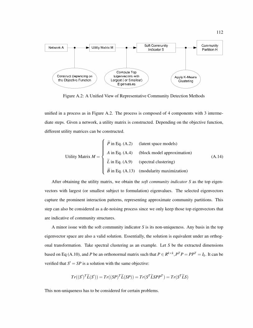
112
Figure A.2: A Unified View of Representative Community Detection Methods
unified in a process as in Figure A.2. The process is composed of 4 components with 3 interme-
diate steps. Given a network, a utility matrix is constructed. Depending on the objective function,
different utility matrices can be constructed.
Utility Matrix M =
P in Eq. (A.2) (latent space models)
A in Eq. (A.4) (block model approximation)
L in Eq. (A.9) (spectral clustering)
B in Eq. (A.13) (modularity maximization)
(A.14)
After obtaining the utility matrix, we obtain the soft community indicator S as the top eigen-
vectors with largest (or smallest subject to formulation) eigenvalues. The selected eigenvectors
capture the prominent interaction patterns, representing approximate community partitions. This
step can also be considered as a de-noising process since we only keep those top eigenvectors that
are indicative of community structures.
A minor issue with the soft community indicator S is its non-uniqueness. Any basis in the top
eigenvector space are also a valid solution. Essentially, the solution is equivalent under an orthog-
onal transformation. Take spectral clustering as an example. Let S be the extracted dimensions
based on Eq (A.10), and P be an orthonormal matrix such that P ∈ Rk×k,PT P = PPT = Ik. It can be
verified that S′ = SP is a solution with the same objective:
Tr((S′)T L(S′)) = Tr((SP)T L(SP)) = Tr(ST LSPPT ) = Tr(ST LS)
This non-uniqueness has to be considered for certain problems.
113
To recover the discrete partition H, a k-means clustering algorithm is applied. Note that all the
aforementioned approaches differ subtly by constructing different utility matrices.
The community detection methods presented above, except the latent space model, are normally
applicable to most medium-size networks (say, 100,000 nodes). The latent space model requires
an input of a proximity matrix of the geodesic distance of any pair of nodes, which costs O(n3)
to compute the pairwise shortest path distances. Moreover, the utility matrix of the latent space
model is neither sparse nor structured, leading to O(n3) to compute its eigenvectors. This high
computational cost hinders its application to real-world large-scale networks.
On the contrary, the other methods, block model approximation, spectral clustering, and mod-
ularity maximization, construct a sparse or structured (a sparse matrix plus low rank update) utility
matrix, whose computational cost is almost negligible1. Asymptotically, the cost to construct a
utility matrix is
Tutility = O(m). (A.15)
Implicitly Restarted Lanczos method (IRLM) can be applied to compute the top eigenvectors effi-
ciently [32, 149]. Let ` denote the number of soft community indicators to extract. If one makes
the conservative assumption that O(`) extra Lanczos steps be involved, IRLM has the worst time
complexity of
Teig = O(h(m`+n`2 + `3)) (A.16)
where h, m and n are the number of iterations, the number of edges and nodes in the network,
respectively. Typically, m∼O(n) in a social network with power law distribution [122] and ` << n.
In practice, the computation tends to be linear with respect to n if ` is small. The post-processing
step to extract community partition relies on k-means clustering, which has time complexity
Tkmeans = O(nk`e) (A.17)
where ` is the number of structural features, e is the number of iterations.
In summary, the representative community detection methods can be unified in the same pro-
cess. The only difference is how to construct the utility matrix. This also affects the time complexity
1The utility matrix of modularity maximization is dense but structured, thus it is rarely computedout. Its structure is exploited directly for eigenvector computation [100, 129].

114
of different methods. Block model approximation, spectral clustering, and modularity maximiza-
tion share similar time complexity. They can be solved much more efficiently than latent space
models.

Appendix B
CONVERGENCE ANALYSIS
116
In section 3.5.3, we provide an iterative algorithm to find communities in dynamic multi-mode
networks. In this chapter, we study its convergence properties.
Theorem 8 The objective of formulation F2 in Eq. (3.22) following the temporally-regularized
multi-mode clustering algorithm in Figure 3.7 is guaranteed to converge.
Proof Our algorithm essentially implements an alternating optimization strategy for each C(i,t). At
each step, we find an optimal solution for one variable while fixing the other variables. Hence, the
objective F2 is non-increasing. Since the objective of F2 has a lower bound 0, it must converge to a
constant value.
However, it is impractical to compute F2 explicitly. The involved terms Rti, j−C(i,t)At
i, j(C( j,t))T
is a full matrix of size ni× n j. The temporal regularization term C(i,t)(C(i,t))T −C(i,t−1)(C(i,t−1))T
is also huge, of size ni×ni. It can be problematic to compute them as that might require excessive
computational resource. Alternatively, we can compute the equivalent formulation F3 in (3.26).
It involves matrices of size ki× k j or ki× ki. Since ki << ni, F3 can be computed much more
efficiently.
Though the objective converges to a constant, it does not necessarily indicate that the algorithm
converges to a (local) optimal, whose gradient is non-negative (non-positive) along with any direc-
tion within the feasible domain for a minimization (maximization) problem. For certain problems,
the objective function approaches a constant value while the solution is far from even a local opti-
mal (refer to [109] for concrete examples). Below, we further examine the convergence property in
terms of community indicators C(i,t).
It can be shown that Cti is guaranteed to converge to a local stationary point under mild con-
ditions. Let Q(i,t) = C(i,t)(C(i,t))T . Then we have some weak convergence result with respect
to Q(i,t). The formulation F3 in (3.26) can be reformulated in terms of Q(i,t) as follows:
F4 : maxT
∑t=1
m
∑1≤i< j≤m
w(i, j)a tr
[Q( j,t)RT
i, jQ(i,t)Ri, j
]+w(i)
b
T
∑t=2
m
∑i=1
tr[Q(i,t)Q(i,t−1)
](B.1)
s.t. Q(i,t) ∈M , i = 1, · · · ,m, t = 1, · · · ,T
M (i,t) = S|S = C(i,t)(C(i,t))T (B.2)
117
It can be shown that Q(i,t) converges to a coordinate-wise optimal point under some mild condi-
tions. Before we proceed to the details, we would like to introduce some basic concepts and results
of block coordinate descent (BCD) method [141] (a.k.a. alternating optimization [13]). Without
loss of generality, we discuss the case of minimizing a function f (x1,x2, · · · ,xN) with each xi de-
noting one block of variables. In each iteration, BCD optimizes one block of variables while fixing
the other blocks. A basic cyclic rule is to choose the same block for iterations k, k +N, k +2N, · · · ,
for k = 1, · · · ,N. We restate Theorem 4.1(c) in [141] as a lemma below:
Lemma 1 Assume that the level set X0 = x : f (x) ≤ f (x0) is compact and that f is continuous
on X0. Then the sequence xr = (xr1,x
r2, · · · ,xr
N)r=0,1,··· generated by block coordinate descent is
defined and bounded. Moreover, if f (x1, · · · ,xN) has at most one minimum in xk for k = 2, · · · ,N−1,
and the cyclic rule is used, then every cluster point z of xrr≡(N−1) mod N is a coordinate-wise
minimum point of f .
Based on the lemma, we have the following theorem:
Theorem 9 Q(i,t) converges to a coordinate-wise optimal point following our algorithm, if the ki-th
and (ki +1)-th singular values of Pti defined in Eq. (3.27) are different in each iteration.
Proof Clearly, F4 in (B.1) is continuous with respect to Q(i,t). If the ki and (ki + 1)-th singular
values of Pti defined in Eq. (3.27) are different, we have a unique Q(i,t) that equals to the outer
product of the top kti left singular vectors of Pt
i . If this is always the case, i.e., F4 has at most one
minimum for each block optimization, Q(i,t) converges to a coordinate-wise minimum point of F4
according to Lemma 1.
Theorem 10 Our temporally-regularized clustering algorithm approaches a stationary point for
C(i,t) if the ki-th and (ki + 1)-th singular values of Pti defined in Eq. (3.27) are different in each
iteration.
Proof Based on Theorem 9, Q(i,t) converges to a coordinate-wise minimum point if the ki-th and
(ki +1)-th singular values of Pti are always different. Let C(i,t) be the corresponding decomposition
of the limiting point Q(i,t) following Eq. (B.2). To prove that the limiting point C(i,t) is a stationary
118
point, we can show that the gradient of the objective function within the feasible domain is 0.
Specifically, we show that the gradient of the objective function projected into the tangent space
of the feasible domain is 0. For notation convenience, we write C(i,t) as C, and Mti as M in the
subsequent proof.
Let Q(i,t) denote the limiting point, i.e. a coordinate-wise optimal point. Its corresponding C
must satisfy Theorem 3. In other words,
MC = CΛ (B.3)
where Λ denotes a diagonal matrix of the top eigenvalues of M. Following Eq. (3.28), F3 in terms
of C can be written as
F3(C) = tr[CT MC
]+ const
with M defined in Eq. (3.30). So the gradient of F3 with respect to C is
g(C) = 2MC. (B.4)
Recall that C ∈ Rni×ki is column orthogonal, which forms a smooth Stiefel manifold [35] of
dimension niki− ki(ki +1)/2. The projection of any Z ∈ Rni×ki onto the tangent space of the mani-
fold [29] is:
πT (Z) := CCT Z−ZTC
2+(I−CCT )Z. (B.5)
Hence, the gradient g(C) projected into C’s tangent space is
πT (g(C))
= C2CT MC−2CT MTC
2−2(I−CCT )MC
= −2(I−CCT )MC (B.6)
= −2(I−CCT )CΛ (B.7)
= 0
where Eq. (B.6) follows from the symmetry of M, and Eq. (B.7) follows from the fact that C corre-
sponds to the top eigenvectors of M as stated in Eq. (B.3). Hence, the projected gradient of F3 with

119
respect to C within the feasible domain (the Stiefel manifold) is zero. Since the objective function
is continuously differentiable and the projected gradient is zero for all the blocks of variables, the
final solution of C is a stationary point (critical point).
In Theorems 9 and 10, we require each block optimization step to satisfy certain properties for
singular values. A simple strategy to check whether or not our solution is a stationary point, is to
verify whether there is any case that the ki and (ki +1)-th singular values of Pti are exactly the same.
In real-world multi-mode networks, this rarely happens due to noise. Hence, this convergence result
is valid in general.
We want to emphasize that it is improper to use the difference of C(i,t) between iterations as a
guide for convergence verification. As shown in Theorem 3, the optimal Cti corresponds to the top
left-singular vectors, which is not unique. But this does not refrain the algorithm from reaching a
stationary point at the end. A proper convergence criterion is the difference of Q(i,t) between itera-
tions is sufficiently small. But Q(i,t) is a full matrix of size ni×ni, which might be computationally
expensive. Since the obtained C(i,t) is an approximate community indicator matrix, exact conver-
gence may not be necessary. For practical use, it works fine to simply check whether the objective
value of F3 stabilizes.
Related Documents