FREQUENCY CONTROL SCHEME FOR ISLANDED DISTRIBUTION NETWORK WITH HIGH PV PENETRATION MOHAMMAD HUSSEIN MOHAMMAD DREIDY FACULTY OF ENGINEERING UNIVERSITY OF MALAYA KUALA LUMPUR 2017

Welcome message from author
This document is posted to help you gain knowledge. Please leave a comment to let me know what you think about it! Share it to your friends and learn new things together.
Transcript

FREQUENCY CONTROL SCHEME FOR ISLANDED
DISTRIBUTION NETWORK WITH HIGH PV PENETRATION
MOHAMMAD HUSSEIN MOHAMMAD DREIDY
FACULTY OF ENGINEERING
UNIVERSITY OF MALAYA
KUALA LUMPUR
2017

FREQUENCY CONTROL SCHEME FOR ISLANDED DISTRIBUTION NETWORK WITH HIGH PV
PENETRATION
MOHAMMAD HUSSEIN MOHAMMAD DREIDY
THESIS SUBMITTED IN FULFILMENT OF THE REQUIREMENTS FOR THE DEGREE OF DOCTOR OF
PHILOSOPHY
FACULTY OF ENGINEERING UNIVERSITY OF MALAYA
KUALA LUMPUR
2017

ii
UNIVERSITY OF MALAYA
ORIGINAL LITERARY WORK DECLARATION
Name of Candidate: Mohammad Hussein Mohammad Dreidy (I.C/Passport No: T858244)
Registration/Matric No: KHA140004
Name of Degree: Doctor of Philosophy
Title of Project Paper/Research Report/Dissertation/Thesis (“this Work”):
FREQUENCY CONTROL SCHEME FOR ISLANDED DISTRIBUTION
NETWORK WITH HIGH PV PENETRATION
Field of Study: RENEWABLE ENERGY (POWER SYSTEM)
I do solemnly and sincerely declare that:
(1) I am the sole author/writer of this Work; (2) This Work is original; (3) Any use of any work in which copyright exists was done by way of fair dealing
and for permitted purposes and any excerpt or extract from, or reference to or reproduction of any copyright work has been disclosed expressly and sufficiently and the title of the Work and its authorship have been acknowledged in this Work;
(4) I do not have any actual knowledge nor do I ought reasonably to know that the making of this work constitutes an infringement of any copyright work;
(5) I hereby assign all and every right in the copyright to this Work to the University of Malaya (“UM”), who henceforth shall be owner of the copyright in this Work and that any reproduction or use in any form or by any means whatsoever is prohibited without the written consent of UM having been first had and obtained;
(6) I am fully aware that if in the course of making this Work I have infringed any copyright whether intentionally or otherwise, I may be subject to legal action or any other action as may be determined by UM.
Candidate’s Signature Date:
Subscribed and solemnly declared before,
Witness’s Signature Date:
Name:
Designation
Safri
Highlight
iii
ABSTRACT
Air pollution due to fossil fuel power plants are causing serious environmental problems,
which affect all aspects of life. Due to this, many governments and power utility
companies are expressing great interest in Renewable Energy Sources (RESs). Generally,
using RESs in a distribution system such as solar Photovoltaic (PV) decreases dependence
on fossil fuel. However, at high PV penetration levels, an islanded distribution network
suffers from critical frequency stability issues. This occurs due to two main reasons: first,
the reduction of the distribution network inertia with high PV penetration, where in this
condition, the rate of change of frequency (ROCOF) will be high enough to activate the
load shedding controller, even for small power disturbance, and second, this type of
networks has a small spinning reserve, where the PV generations are normally providing
the maximum output power.
The main aim of this research is to develop a comprehensive frequency control scheme
for islanding distribution networks with high PV penetration. This scheme is used to
stabilize the frequency of the network to a value that is suitable for the islanded and
reconnection processes. To achieve this aim, three different controllers were proposed in
this scheme; inertia, frequency regulation, and under-frequency load shedding (UFLS)
controllers. The inertia controller is designed for PV generation to reduce the network
frequency deviation, which is initiated immediately during disturbance event. After a few
seconds, a frequency regulation controller, which consists of primary and secondary
frequency controllers, is activated. This frequency regulation controller was proposed to
provide sufficient power from the Battery Storage System (BSS) to stabilize the
frequency within a few minutes. When inertia and frequency regulation controllers fail to
stop the frequency deviation, an optimal (UFLS) controller is initiated from Centralized
iv
Control System (CCS) to shed the required loads. On top of shedding loads, the CCS is
used to manage the operation of frequency control scheme and reconnect the grid.
The proposed frequency control scheme and centralized control system were tested using
a part of Malaysia’s distribution network (29-bus). The distribution network was modeled
and simulated for different PV penetration levels using PSCAD//EMTDC software. The
simulation results confirmed that the proposed scheme is able to stabilize the frequency
of an islanded distribution network, with 50% PV penetration. This scheme is also capable
of recovering the network frequency for small load and radiation changes just before it
reaches the load shedding limit (49.5 Hz). Furthermore, at high PV penetration and large
disturbance events, the proposed scheme can still recover the frequency by shedding the
required loads within (0.254 seconds) without overshooting the frequency. Moreover,
when the proposed frequency control scheme is coordinated with CCS, the islanded
distribution network will be smoothly reconnected to the main grid. Therefore, this
frequency control scheme has potential to be applied in real distribution networks with
high PV penetration.
v
ABSTRAK
Pencemaran udara disebabkan oleh loji-loji janakuasa bahan api fosil telah
menyebabkan masalah persekitaran yang serius, yang mempengaruhi semua aspek
kehidupan. Oleh kerana itu, banyak kerajaan dan syarikat-syarikat utiliti kuasa
menunjukkan minat yang mendalam terhadap sumber tenaga yang boleh diperbaharui
(RESs). Secara amnya, penggunaan RESs dalam sistem pengagihan seperti solar
fotovoltaik (PV) mengurangkan pergantungan kepada bahan api fosil.
Walaubagaimanapun, pada tahap penembusan PV yang tinggi, rangkaian pengedaran
terpulau akan menderita daripada isu-isu kestabilan frekuensi yang kritikal. Ini berlaku
kerana dua sebab utama: pertama, pengurangan dalam inersia pengagihan rangkaian
dengan penembusan PV yang tinggi, di mana dalam keadaan ini, kadar perubahan
frekuensi (ROCOF) adalah cukup tinggi untuk mengaktifkan pengawal pengurangan
beban, bahkan untuk gangguan kuasa kecil, dan kedua, rangkaian jenis ini mempunyai
simpanan putaran kecil, di mana penghasilan PV biasanya menyediakan kuasa keluaran
yang maksimum.
Tujuan utama kajian ini adalah untuk membangunkan satu skim kawalan frekuensi
yang komprehensif untuk pemulauan rangkaian pengedaran dengan penembusan PV
yang tinggi. Skim ini akan digunakan untuk menstabilkan frekuensi rangkaian kepada
nilai yang sesuai untuk proses pemulauan dan penyambungan semula. Untuk mencapai
matlamat ini, tiga pengawal yang berbeza telah dicadangkan dalam skim ini; inersia,
peraturan frekuensi dan pengawal frekuensi-terkurang pengurangan beban (UFLS).
Pengawal inersia direka untuk generasi PV bagi mengurangkan sisihan frekuensi
rangkaian, yang dimulakan dengan serta-merta semasa kejadian gangguan. Selepas
beberapa saat, pengawal peraturan frekuensi, yang terdiri daripada pengawal frekuensi
rendah dan menengah, diaktifkan. Pengawal kawalan frekuensi ini telah dicadangkan
untuk memberikan kuasa yang mencukupi dari sistem penyimpanan bateri (BSS) untuk
vi
menstabilkan frekuensi dalam beberapa minit. Apabila inersia dan pengawal peraturan
frekuensi gagal untuk menghentikan sisihan frekuensi, pengawal (UFLS) yang optimum
dimulakan dari Pusat Kawalan Sistem (CCS) untuk mengurangkan beban yang
diperlukan. Di samping mengurangkan beban, CCS tersebut digunakan untuk mengurus
operasi skim kawalan frekuensi dan penyambungan semula grid.
Cadangan skim kawalan frekuensi dan sistem kawalan berpusat telah diuji
menggunakan sebahagian daripada rangkaian pengedaran di Malaysia (29-bas).
Rangkaian pengedaran dimodelkan dan disimulasikan bagi tahap penembusan PV yang
berbeza menggunakan perisian PSCAD//EMTDC. Keputusan simulasi mengesahkan
bahawa cadangan skim ini dapat menstabilkan frekuensi pemulauan rangkaian
pengedaran, dengan penembusan PV sebanyak 50%. Skim ini juga mampu memulihkan
frekuensi rangkaian bagi beban kecil dan perubahan radiasi sejurus sebelum ia mencapai
had bagi pengurangan beban (49.5 Hz). Selain itu, pada penembusan PV yang tinggi dan
acara-acara gangguan yang besar, skim yang dicadangkan masih boleh memulihkan
frekuensi dengan mengurangkan beban diperlukan dalam (0.254 saat) tanpa frekuensi
terlebih. Selain itu, apabila skim kawalan frekuensi yang dicadangkan diselaraskan
dengan CCS, pemulauan rangkaian pengedaran akan dipasang semula ke grid utama
dengan lancar. Oleh yang demikian, skim kawalan frekuensi ini mempunyai potensi
untuk digunakan dalam rangkaian pengedaran yang sebenar dengan penembusan PV yang
tinggi.

vii
ACKNOWLEDGEMENT

viii
TABLE OF CONTENTS
2.2.1 Solar Photovoltaic ....................................................................................... 9
2.2.1.1 Global Trends of Photovoltaic ........................................................... 10
2.2.1.2 Malaysian Trends Towards Photovoltaic .......................................... 11
2.2.2 Hydropower ............................................................................................... 12
2.2.2.1 Classification of Hydropower Plant ................................................... 13
2.2.2.2 Potential of Hydropower in Malaysia ................................................ 16

ix
2.3.1 Issues of Distributed Generation Operating in Grid Connected Mode ..... 16
2.3.2 Issues of Distributed Generation Operating in Islanding Mode ................ 17
2.3.2.1 Issue of Small Inertial Response ........................................................ 18
2.3.2.2 Issue of Small Reserves Power .......................................................... 19
2.4.1 Inertia and Frequency Regulation Controllers Proposed for RESs without
ESS 22
2.4.1.1 Inertia and Frequency Regulation Controllers Proposed for Wind
Turbine without ESS ...................................................................................... 22
2.4.1.2 Frequency Regulation Controllers Proposed for PV without ESS .... 37
2.4.2 Inertia and Frequency Regulation Controllers Proposed for RESs with ESS
41
2.4.2.1 Inertia and Frequency Regulation Controllers Proposed for Wind
Turbines with ESS .......................................................................................... 41
2.4.2.2 Frequency Regulation Controllers Proposed for Solar PV with ESS 43
2.4.3 Inertia and Frequency Regulation Controllers Based on Intelligent
Algorithms ............................................................................................................. 45
2.5.1 Conventional Load Shedding Techniques ................................................. 49
2.5.1.1 Under Voltage Load Shedding (UVLS) Techniques ......................... 49
2.5.1.2 Under Frequency Load Shedding (UFLS) Techniques ..................... 49
2.5.2 Adaptive Load Shedding Technique ......................................................... 50
2.5.3 Computational Intelligence Based Load Shedding Techniques ................ 51
x
3.2.1 Proposed Frequency Control Scheme ....................................................... 59
3.2.1.1 Inertia Controller................................................................................ 59
3.2.1.2 Frequency Regulation Controllers ..................................................... 62
3.2.1.3 Proposed UFLS Technique ................................................................ 64
3.2.2 Modelling of Centralized Control System ................................................. 75
3.2.2.1 Frequency Management Unit............................................................. 76
3.2.2.2 Reconnection Controller .................................................................... 78
3.2.2.3 Phase Synchronization Controller ..................................................... 81
3.2.2.4 Voltage Synchronization Controllers................................................. 81
4.2.1 Modelling of Mini-Hydro DG ................................................................... 86
4.2.1.1 Hydraulic Turbine .............................................................................. 87
4.2.1.2 Governor Model ................................................................................. 88
4.2.1.3 Synchronous Generator Model .......................................................... 89
4.2.1.4 Exciter Model for Synchronous Generators ...................................... 90
4.2.2 Load Modelling of Distribution Network ................................................. 92
4.2.3 Modelling of Photovoltaic System ............................................................ 93
4.3.1 Case Study 1: Comparison Between Metaheuristic UFLS Technique (BEP)
and Adaptive UFLS Technique ........................................................................... 101
4.3.2 Case Study 2: Comparison Between Different Metaheuristic Techniques in
Term of Execution Time ...................................................................................... 103
xi
4.3.3 Case Study 3: Comparison Between Different Load Shedding Techniques
106
5.2.1 Mini-hydro DG Modelling ...................................................................... 112
5.2.2 Modelling of Photovoltaic System .......................................................... 112
5.2.3 Bio-Mass DG Modelling ......................................................................... 113
5.2.4 Modelling of Battery Storage System ..................................................... 114
5.2.4.1 The Battery Bank Model.................................................................. 115
5.2.4.2 Bi-directional buck-boost converter Model ..................................... 119
5.2.4.3 Three Phase Bidirectional Inverter Model ....................................... 121
5.3.1 First case study (80% rotary DGs and 0% PV penetration level) ........... 123
5.3.2 Second case study (53% rotary DGs and 25% PV penetration level) ..... 126
5.3.3 Third case study (53% rotary DGs and 33% PV penetration level) ........ 130
5.3.4 Fourth case study (27% rotary DGs and 50% PV penetration level) ...... 130
xii
Figure 1.1: Flow chart of research methodology ............................................................. 5
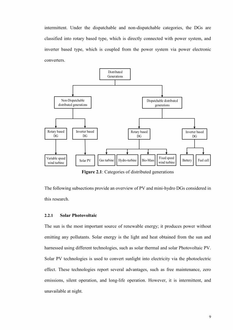
Figure 2.1: Categories of distributed generations ............................................................ 9
Figure 2.2: Solar PV installed capacity for different country for 2014-2015 (REN, 2016) ......................................................................................................................................... 11
Figure 2.3: Cumulative growth of PV Installed capacities since inception of FiT (MW) (SEDA, 2015) .................................................................................................................. 12
Figure 2.4: Hydropower global capacity for top six countries, 2015 (REN, 2016) ....... 13
Figure 2.5: Kenyir (Sultan Mahmud) Hydroelectric Power Project Malaysia (KualaLumbur-Post, 2016) ............................................................................................. 14
Figure 2.6: Geesthacht pumped-storage power plant (VATTENFALL, 2016) ............ 15
Figure 2.7: Run-of-River hydropower plant (Energypedia, 2016) ............................... 15
Figure 2.8: Time frames involved in system frequency response (Gonzalez-Longatt, Chikuni, & Rashayi, 2013).............................................................................................. 18
Figure 2.9: The ROCOF of the distribution network for two types of RES supply 3.8MW load (Jayawardena et al., 2012) ....................................................................................... 19
Figure 2.10: Types of reserve services ........................................................................... 20
Figure 2.11: Frequency deviation for different reserve power....................................... 21
Figure 2.12: Inertia and frequency controllers designed for RESs ................................ 22
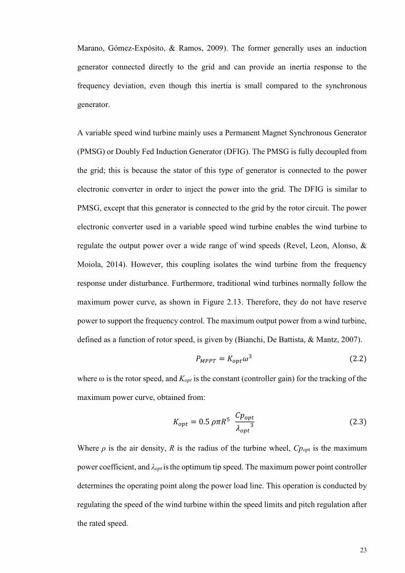
Figure 2.13: Power against rotating speed characteristics at (Pitch angle β=0) (Lamchich & Lachguer, 2012) .......................................................................................................... 24
Figure 2.14: Inertia emulation for variable speed wind turbines ................................... 25
Figure 2.15: Torque demand due to inertia response ..................................................... 27
Figure 2.16: Supplementary control loops for inertia response .................................... 28
Figure 2.17: Fast power reserve controller for a wind turbine ...................................... 29
Figure 2.18: Block diagram of fast power reserve controller ........................................ 29
Figure 2.19: Power characteristics for fast power reserve control ................................. 30

xiii
Figure 2.20: Frequency support scheme with droop speed control................................ 31
Figure 2.21: Wind turbine droop characteristics ............................................................ 31
Figure 2.22: (a) MPPT and deloaded power curves of the wind turbine. (b) Calculation of power reference for 6% deloaded operation (Castro et al., 2012) .............................. 33
Figure 2.23: Power- rotor speed curves with different pitch angles (Castro et al., 2012) ......................................................................................................................................... 34
Figure 2.24: Primary frequency control of wind turbine based on deloading control ... 35
Figure 2.25: 90% sub-optimal operation curve (Z.-S. Zhang et al., 2012) .................... 36
Figure 2.26: Controller for deloaded solar PV ............................................................... 38
Figure 2.27: Solar PV with deloading technique (Zarina, Mishra, & Sekhar, 2014) ..... 39
Figure 2.28: The improved controller for deloaded PV ................................................. 39
Figure 2.29: Solar PV frequency regulator .................................................................... 41
Figure 2.30: Schematic diagram of frequency regulation of wind turbine and flywheel ......................................................................................................................................... 42
Figure 2.31: PV and super-capacitor used in frequency regulation ............................... 43
Figure 2.32: Frequency controller using limiter block ................................................... 43
Figure 2.33: DFIG wind turbine frequency regulation using fuzzy tuning-based PI ..... 45
Figure 2.34: Frequency regulation controller using DFIG wind turbine ....................... 46
Figure 2.35: Fuzzy-based frequency regulation control for PV diesel system .............. 47
Figure 3.1: The schematic diagram of control architecture for frequency control scheme ......................................................................................................................................... 58
Figure 3.2: Block diagram of inertia controller.............................................................. 60
Figure 3.3: Block diagram of special tracking algorithm .............................................. 61
Figure 3.4: Photovoltaic system P-V curve illustrates the de-loading technique........... 62
Figure 3.5: Proposed frequency regulation controller .................................................... 63
Figure 3.6: Flow chart of proposed load shedding technique ....................................... 65
xiv
Figure 3.7: Flow chart of FCU ....................................................................................... 66
Figure 3.8: Flow chart of the LSU ................................................................................. 69
Figure 3.9: Flow chart of BEP method .......................................................................... 70
Figure 3.10: LSU connected with fixed and random priority loads ............................... 70
Figure 3.11: Flow chart of BGA method ....................................................................... 73
Figure 3.12: Single point cross over used by BGA optimization method...................... 74
Figure 3.13: Flowchart of frequency management unit ................................................. 76
Figure 3.14: Flow diagram of reconnection controller .................................................. 80
Figure 3.15: The distribution network illustrates the reconnection procedure .............. 80
Figure 3.16: Phase synchronization controller ............................................................... 81
Figure 3.17: Voltage synchronization controllers .......................................................... 82
Figure 4.1: Distribution network used for validation of proposed UFLS technique...... 85
Figure 4.2: Layout of Run of River Hydropower Plant (Sharma & Singh, 2013) ......... 86
Figure 4.3: Block diagram of hydraulic turbine ............................................................. 87
Figure 4.4: Block diagram of turbine speed control with governor .............................. 88
Figure 4.5: Block diagram of electro-hydraulic PID based governor ............................ 89
Figure 4.6: Block Diagram of IEEE type AC1A excitation system model.................... 91
Figure 4.7: Mini-hydro power plant model in PSCAD/EMTDC software .................... 92
Figure 4.8: PSCAD model of solar PV generation unit ................................................. 93
Figure 4.9: PV module connected in series and parallel in array ................................... 94
Figure 4.10: I-V curve of solar PV generation unit........................................................ 95
Figure 4.11: P-V curve of solar PV generation unit ....................................................... 95
Figure 4.12: Buck DC-DC converter of solar PV unit ................................................... 96
Figure 4.13: Converter control of solar PV unit............................................................. 97

xv
Figure 4.14: I-V curves of SM 380 PV module and various resistive loads .................. 98
Figure 4.15: Active and reactive power controller of solar PV Inverter ........................ 99
Figure 4.16: Firing pulse generation of solar PV inverter.............................................. 99
Figure 4.17: PSCAD model of solar PV inverter ......................................................... 100
Figure 4.18: The Frequency response for 1.0 MW load increment scenario .............. 102
Figure 4.19: The Frequency response for 1.8 MW load increment scenario. ............. 103
Figure 4.20: The convergence trend of BEP technique. .............................................. 105
Figure 4.21: The convergence trend of BGA technique. ............................................. 105
Figure 4.22: The convergence trend of BPSO technique. ............................................ 106
Figure 4.23: Frequency response for 1-MW load increment. ...................................... 107
Figure 4.24: Frequency response of intentional islanding at 1.56 MW imbalance power ....................................................................................................................................... 108
Figure 4.25: Frequency response for mini hydro DG tripping event. .......................... 109
Figure 5.1: Distribution network used for validation of frequency control scheme .... 112
Figure 5.2: Mechanical-hydraulic control system governor model ............................. 113
Figure 5.3: Block diagram of generic turbine mode including intercept valve effect . 114
Figure 5.4: Block diagram of BSS. .............................................................................. 115
Figure 5.5: The construction of battery bank ............................................................... 115
Figure 5.6: Generic dynamic battery model ................................................................. 116
Figure 5.7: Typical Discharge Curve ........................................................................... 118
Figure 5.8: Discharge characteristics of (Vision CL200 2V 200Ah) ........................... 118
Figure 5.9: Bidirectional buck-boost converter........................................................... 119
Figure 5.10: Frequency response of intentional islanding followed by load increment (first scenario/first case study) ...................................................................................... 123
xvi
Figure 5.11: a) Phase difference between distribution network and main grid for (first scenario/first case study) b) the voltage difference between distribution network and main grid for (first scenario/first case study) ......................................................................... 124
Figure 5.12: Frequency response for intentional islanding followed by Bio-Mass trip (first case study) ............................................................................................................ 125
Figure 5.13: a) The phase difference between distribution network and main grid for (second scenario/first case study) b) the voltage difference between distribution network and main grid for (second scenario/first case study) ..................................................... 125
Figure 5.14: Frequency response for intentional islanding followed by Bio-Mass DG trip without BSS (first case study) ....................................................................................... 126
Figure 5.15: Frequency response of intentional islanding followed by load increament (0.5MW) without inertia controller ............................................................................... 127
Figure 5.16: a) The phase difference between distribution network and main grid (first scenario/second case study) b) The voltage difference between distribution network and main grid for (First scenario/Second case study) .......................................................... 127
Figure 5.17: Frequency response for intentional islanding followed by mini-hydro trip (Second scenario/Second case study)............................................................................ 128
Figure 5.18: Frequency response of intentional islanding followed by mini-hydro trip without BSS .................................................................................................................. 129
Figure 5.19: Frequency response of intentional islanding followed by mini-hydro trip during night ................................................................................................................... 129
Figure 5.20: Frequency response of intentional islanding followed by load increment (0.5MW) for (first scenario/third case study) ............................................................... 130
Figure 5.21: Frequency response of intentional islanding followed by load increment (0.5MW) for (first scenario/fourth case study) ............................................................. 131
Figure 5.22: Frequency response of intentional islanding followed by load increment (0.5MW) for (second scenario/fourth case study)......................................................... 131
Figure 5.23: Frequency response comparison between different PV penetration levels ....................................................................................................................................... 132
Figure 5.24: Frequency response for 50% PV penetration with and without inertia ... 133
Figure 5.25: Frequency response for 25% PV penetration with and without inertia ... 133

xvii
Figure 5.26: Frequency responses for two penetration level of PV with fixed penetration level of mini-hydro generation ...................................................................................... 134
xviii
LIST OF TABLES
Table 2.1: Summary of inertia and frequency regulation controllers proposed in the literature .......................................................................................................................... 48
Table 2.2: Summary of UFLS techniques proposed in the literature ............................. 55
Table 3.1: The initial population and fitness values for each individual........................ 71
Table 3.2: The binary mutation operation used in BEP method .................................... 72
Table 3.3: The initial population and fitness values of the FRPLS technique ............... 74
Table 4.1: Value of hydro turbine parameters ................................................................ 88
Table 4.2: Parameters of the hydraulic governor .......................................................... 89
Table 4.3: Synchronous generator parameters ............................................................... 90
Table 4.4: Sample data of IEEE AC1A excitation model parameters ........................... 91
Table 4.5: Load data and their priority ........................................................................... 93
Table 4.6: Parameters of solar PV module (SM 380(48) P1946×1315) ........................ 94
Table 4.7: Parameters of buck DC-DC converter .......................................................... 96
Table 4.8: UFLS parameters for load increment of 1.0 MW after islanding ............... 101
Table 4.9: UFLS parameters for load increment of 1.8 MW after islanding ............... 103
Table 4.10: The execution time for different load shedding ........................................ 104
Table 4.11: The UFLS parameters for load increment of 1.0 MW after islanding ...... 107
Table 4.12: UFLS parameter of intentional islanding at 1.56 MW imbalance power . 108
Table 4.13: The UFLS parameters for mini hydro DG tripping event ......................... 109
Table 5.1: Mechanical-hydraulic governor parameters ................................................ 113
Table 5.2: Values of generic turbine model including intercept valve ........................ 114
Table 5.3: Technical specifications of lead acid battery cell (Vision CL200) ............. 116
Table 5.4: Parameters of bidirectional buck boost converter ....................................... 121

xix
Table 5.5: The simulation case studies ......................................................................... 122
Table 5.6: Comparison between inertia and frequency regulation controllers proposed in this research and controllers proposed in the literature ................................................. 136
Table 5.7: Comparison between UFLS technique proposed in this research and technique proposed in the literature ............................................................................................... 137

xx
LIST OF SYMBOLS AND ABBREVIATIONS
UFLS : Under Frequency Load Shedding
MPPT : Maximum Power Point Tracking
DGs : Distribution Generations
DG : Distribution Generation
RESs : Renewable energy sources
BEP : Binary Evolutionary Programming
BGA : Binary Genetic algorithm
BPSO : Binary Particle swarm optimization
ROCOF : Rate of Change of Frequency
FiT : Feed-in Tariff
SEDA : Sustainable Energy Development Authority
MBIPV : Malaysian Building Integrated Photovoltaic
UVLS : Under Voltage Load Shedding
IPCU : Imbalance Power Calculator Unit
FCU : Frequency Calculator Unit
LSU : Load shedding Unit
RE : Renewable Energy IEA :
International energy Agency
PV :
Photovoltaic
HPPs : Hydropower Plants RoR : Run-of-River PMSG : Permanent Magnet Synchronous Generator DFIG : Doubly Fed Induction Generator
CCS : Centralized Control System

xxi
PMU : Phasor Measurement Unit
TNB : Tenaga National Berhad
SOC : State of Charge
IC : Incremental Conductance
CV : Constant Voltage
P&O : Perturb and Observe
ANN : Artificial Neural Network

xxii
LIST OF APPENDICES
Appendix A..………………………………………………………………………….149
Appendix B...…………………………………………………………………………157
1
CHAPTER 1: INTRODUCTION
1.1 Overview
The consumption and usage of fossil fuels for generating electricity causes several
environmental problems. One of the most critical environmental problems pertains to the
emission of carbon dioxide (CO2), which is released from generation power plants. It is
one of the main agents for global warming. The fossil fuel power plants in United States
(US), China, Russia, and Germany emit 2.2, 2.7, 0.661, and 0.356 billion tons of CO2
annually, respectively (Lashof et al., 2014).
Interest in environmental problems forced the power industry to increasingly utilize
Renewable Energy (RE) to produce electricity. RESs such as photovoltaic, wind, and
hydro power plants are able to decrease environmental pollutions by reducing the usage
of fossil fuels. Hence, many governments and agencies around the world set targets
towards increasing the application of RESs to generate electricity. China and Germany,
for example, expects to draw 15% and 35% of their energy needs from renewable energy
sources by 2020, respectively (REN, 2012). Malaysia has also begun utilizing RESs for
power generation. According to (Shekarchian, Moghavvemi, Mahlia, & Mazandarani,
2011), Malaysia seeks to replace its power production to 11 % from RESs by the end of
2020.
The necessity of providing sufficient energy alongside interest in clean technologies
results in increased use of Distributed Generations based on RESs (DG-RESs). In
Malaysia, a mini-hydro power plant and photovoltaic generation have been widely
installed in the distribution network, as both are cost effective and environmentally
friendly (Mekhilef et al., 2012). Currently, based on IEEE std.1547–2003, when the
distribution network is islanded from the grid, all DGs must be disconnected from the

2
network within 2 seconds (Basso, 2004). This operation is important, as it ensures the
safety of power system workers and avoid faults that could occur due to re-closure
activation. However, separating the DGs after islanding will prevent the grid maximizing
the benefits that could be gained from these sources. Research related to islanding
operation is progressing to the level that allows islanded distribution network to operate
autonomously when disconnected from the main grid. However, after islanding, the
distribution networks with high PV penetration will be exposed to critical frequency
stability issues. For this reason, the distribution will completely blackout if these issues
are not addressed.
1.2 Problem Statement
In the near future, the penetration level of RESs, such as PV generation, will be increased
in the distribution network. Therefore, the distribution network will be exposed to several
frequency stability issues during the islanding and reconnection processes. Issues
pertaining to these processes are discussed in the following paragraphs.
At high PV penetration, the islanded distribution network will suffer from low inertial
response because PV generations do not provide any physical inertia. Hence, the system’s
frequency will quickly drop, preventing frequency restoration via primary frequency
controller even if reserve power is available. Many researchers propose installing
different inertia controllers for islanded distribution networks (El Itani, Annakkage, &
Joos, 2011; Hansen, Altin, Margaris, Iov, & Tarnowski, 2014; Wachtel & Beekmann,
2009). However, most of them proposed increasing the inertia of the distribution networks
using only wind turbine technology and Energy Storage Systems (ESS).
Besides reducing inertia, islanded distribution network also faces frequency regulation
issues. Due to insufficient reserve power, mainly in a distribution network with high PV
penetration, the imbalance of power between the generation and demand commonly takes

3
place, which result in quick frequency drops. This occurs because PV generation units
commonly operate at its maximum power point. In literature, several control techniques,
such as droop control and deloading control were proposed for RESs to regulate the
frequency of grid-connected distribution systems during disturbances (Eid, Rahim,
Selvaraj, & El Khateb, 2014; Josephine & Suja, 2014; Mishra & Sekhar, 2013). However,
these techniques may be ineffective for islanded distribution systems, as islanded system
is not as stable as grid-connected system. The intermittent nature of the RESs will also
contribute to frequency fluctuations in an islanded system. Therefore, many researchers
proposed the usage of batteries to provide a stable energy reserve for frequency regulation
services. However, most of these techniques used a battery to provide primary frequency
controller without taking into account the secondary controller, which is important for
grid reconnection.
In the case where the inertia and frequency regulation controllers fail to stabilize the
frequency in an islanded distribution network, a potential solution is to apply load
shedding. Load shedding is a technique that stabilizes system frequency by removing
some loads to ensure a balanced condition between generation and load demands.
Although there are various load shedding techniques, only a few were proposed for
islanded distribution systems with RESs. However, these techniques do not consider high
PV penetration in the distribution system, where the system has a small inertia. For a
system with this condition, fast load shedding is required, since its frequency will drop
quickly when islanded takes place. Besides fast load shedding, a suitable amount of load
shed is also required to ensure that the frequency is within an acceptable limit. (Laghari,
Mokhlis, Karimi, Bakar, & Mohamad, 2015) proposed a new Fixed and Random Priority
Load Shedding (FRPLS) technique to determine a suitable combination of loads to be
shed. This technique is time consuming, since all possible combinations of loads shed
need to be determined beforehand. Therefore, it is unsuitable for application in a
4
distribution network with high PV penetration, which require a fast and correct load
shedding technique. Taking into account this shortcoming, metaheuristic optimization
methods can be explored to determine the optimal combination of load to be shed within
a short period of time.
1.3 Research Objectives
The main aim of this research is to develop a comprehensive frequency control scheme
for islanded distribution network with high PV penetration, where the scheme consists of
inertia controller, frequency regulation controllers, and UFLS controller. The following
are the main objectives of this research:
(A) To design an inertia controller for PV systems based on the deloading technique to
address the reduction of inertia response caused by high PV penetration.
(B) To propose frequency regulation controllers (primary and secondary) based on a
Battery Storage System (BSS).
(C) To propose an optimal under-frequency load shedding controller based on
metaheuristic techniques.
(D) To model a centralized control system to manage the operation of frequency control
scheme, load shedding, and grid reconnection process.
1.4 Research Scope and Methodology
This research focuses on an islanded distribution system. The islanding detection and grid
disconnection process are beyond the scope of this research. All of the proposed
controllers in this research are developed for islanded distribution system with high PV
penetration. In this research, technical issues are studied without taking into account
economic analyses considerations. Figure 1.1 shows the research methodology pertaining
to this work.
5
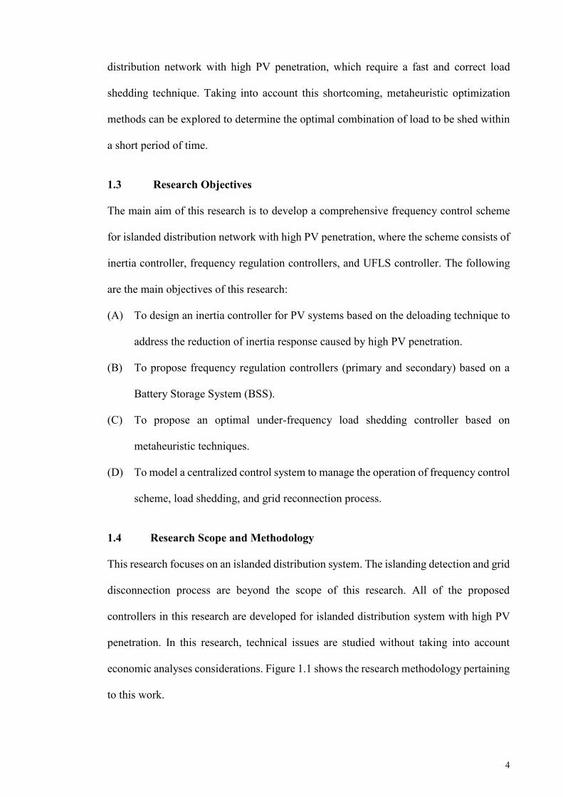
Figure 1.1: Flow chart of research methodology
Review the existing load shedding techniques proposed for distribution network
Design and modelling of inertia controller using PSCAD\ EMTDC software
Review the existing inertia and frequency controllers proposed for RESs
Modelling of 29-bus distribution network consisting of two mini-hydro generators, four PV generation units using PSCAD\EMTDC software
Design and modelling of new UFLS controller using MATLAB and PSCAD\EMTDC software
Compare the execution time for different optimization methods (BEP, BPSO, BGA) using MATLAB software to select the fastest method suitable for
proposed load shedding technique
Compare the performance of proposed UFLS technique based on BEP method with conventional and adaptive techniques.
Modelling of 30-bus distribution network consisting of two mini-hydro generators, one Bio-mass generator, PV generation units, two battery storage
systems using PSCAD\EMTDC software
Design and modelling of frequency regulation controller (primary, secondary) using PSCAD\EMTDC software
Design and modelling a centralized control system to manage the operation of frequency control scheme, perform shedding loads and reconnection
process
Validate the performance of proposed frequency control scheme and centralized control system using a 30-bus distribution network for different
PV penetration levels
Validate the performance of proposed UFLS technique in the 29-Bus distribution network during islanding mode, load increment, and DG tripping.
6
1.5 Thesis Outline
Chapter 1 describes the changes that took place in the distribution network due to the
continual integration of inverter based DGs. The frequency issue following the
distribution network islanding will be presented. The importance of stabilizing the
frequency of islanding distribution network by inertia, frequency regulation and load
shedding controllers will then be discussed. The objectives and research methodology
will consequently be presented, followed by the thesis outline.
Chapter 2 will provide an overview of the distributed generation, presenting the various
types, the global trend of solar PV and hydropower, and the Malaysian trend of solar PV
and hydropower. It will also discuss the operation modes and challenges pertaining to
DGs. This chapter will detail the frequency stability issues related to the islanded
distribution network. Various frequency control schemes proposed for DGs-RESs will
also be discussed, and several types of existing load shedding techniques will be
reviewed.
Chapter 3 will present the proposed frequency control scheme for distribution networks
with high PV penetration. This scheme consists of inertia controller, frequency regulation
controller, and a UFLS controller. The modelling of three controllers will be discussed in
this chapter. This chapter will also describe the centralized control system that can be
used to manage the operation of the frequency control system and reconnect the grid.
Chapter 4 will detail the modelling of the distribution network used to validate the
proposed UFLS technique. The proposed UFLS technique was validated using a 29-bus
distribution network for different islanding, DG tripping, and load increments cases. This
distribution network is a part of Malaysia’s distribution network. In order to show the
preference of the proposed UFLS technique compared with existing techniques, various
PSCAD simulation results will be presented in this chapter. It will also describe the

7
utilized metaheuristic optimization methods with the proposed UFLS technique for the
selection of the optimal combination of loads to be shed from random and fixed priority
loads.
Chapter 5 will detail the modelling of distribution network used to validate the proposed
frequency control scheme. The proposed frequency control scheme was validated using
a 30-bus distribution network for different islanding, DG tripping, and load increments
cases. In order to show the ability of proposed frequency control scheme on stabilizing
the distribution network frequency, this chapter will present several simulation case
studies such as islanding, generator trip, and load increment. Moreover, various
simulation scenarios have been implemented for grid reconnection.
Chapter 6 concludes this thesis by summarizing the research contributions and presents
the possible future works for this research.
8
CHAPTER 2: LITERATURE REVIEW
2.1 Introduction
Recently the world has experienced severe climate changes due to increased
environmental pollution levels. Global warming is one of the most serious environmental
changes that threatens life on Earth. It is therefore necessary to decrease environmental
pollution, particularly air pollution, which are emitted from fossil fuel power plants. The
necessity to reduce air pollution alongside growing demand represents the main
motivation of using the DGs-RESs. According to (IEEE, IEA), a general definition of DG
is a small-scale electric generation technology (sub-kW to a few MW) located close to
the power demand.
This chapter provides an overview of the distributed generation, presenting various types,
global, and local trends of solar PV generation. It also discusses operation modes and
challenges pertaining to DGs. The major subject that will be discussed in this chapter is
the frequency stability issue of an islanded distribution network. It also discusses various
frequency control schemes implemented alongside renewable energy DGs to stabilize the
frequency of islanded distribution network. At the end, this chapter reviews various types
of load shedding techniques for recovering system frequency.
2.2 Distributed Generation
Over the last decade, the world has seen a significant development in distributed
generation technologies. These DGs are generally classified according to their operation
technologies and applications. For frequency stability application, the DG technologies
are classified into two main categories: Dispatchable and Non-Dispatchable DGs, as
shown in Figure 2.1. The former includes all sources that can adjust their output power at
the request of power grid operators, while the latter contains all sources that are naturally
9
intermittent. Under the dispatchable and non-dispatchable categories, the DGs are
classified into rotary based type, which is directly connected with power system, and
inverter based type, which is coupled from the power system via power electronic
converters.
Figure 2.1: Categories of distributed generations
The following subsections provide an overview of PV and mini-hydro DGs considered in
this research.
2.2.1 Solar Photovoltaic
The sun is the most important source of renewable energy; it produces power without
emitting any pollutants. Solar energy is the light and heat obtained from the sun and
harnessed using different technologies, such as solar thermal and solar Photovoltaic PV.
Solar PV technologies is used to convert sunlight into electricity via the photoelectric
effect. These technologies report several advantages, such as free maintenance, zero
emissions, silent operation, and long-life operation. However, it is intermittent, and
unavailable at night.
Distributed Generations
Non-Dispatchable distributed generations
Dispatchable distributed generations
Rotary based DG
Inverter based DG
Rotary based DG
Inverter based DG
Variable speed wind turbine Solar PV Gas turbine Fuel cellHydro-turbine Battery Bio-Mass Fixed speed
wind turbine
10
2.2.1.1 Global Trends of Photovoltaic
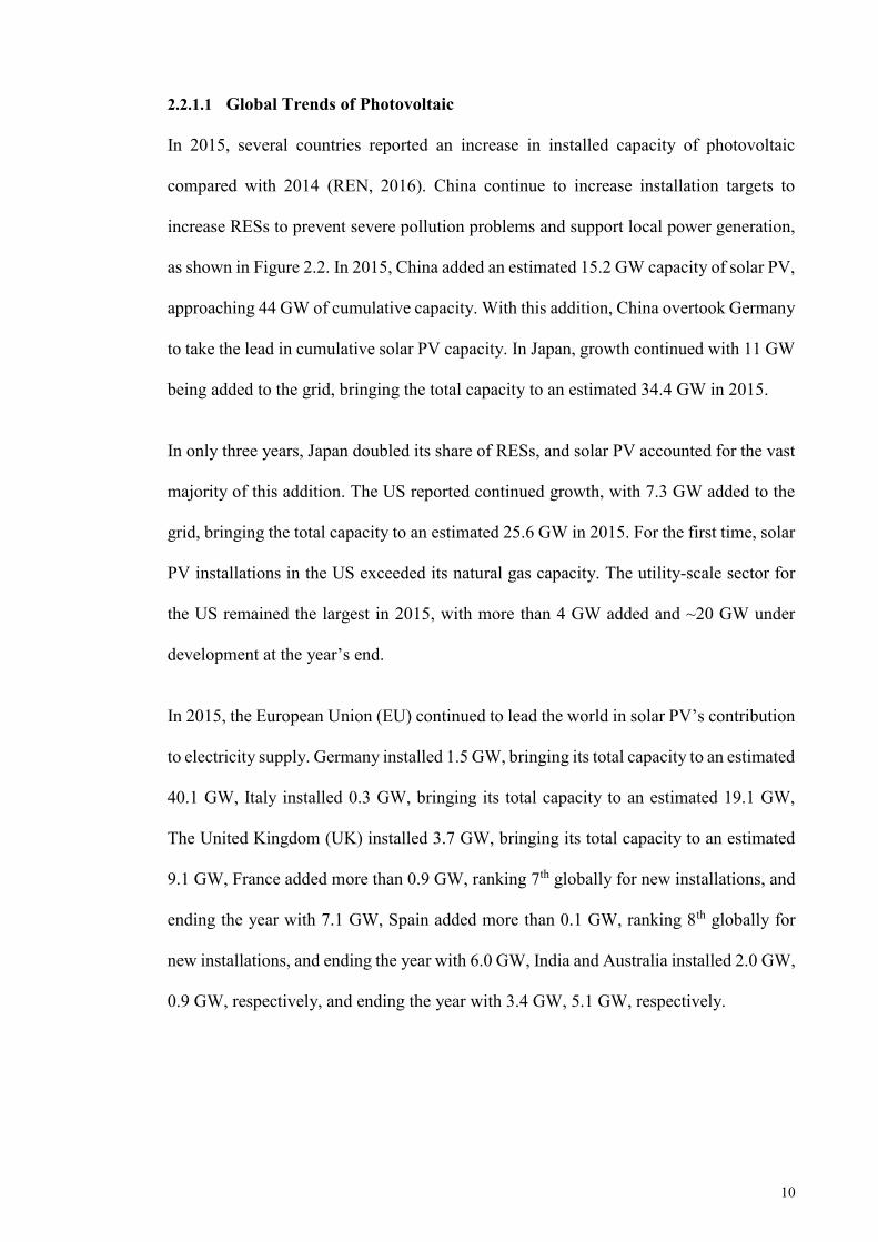
In 2015, several countries reported an increase in installed capacity of photovoltaic
compared with 2014 (REN, 2016). China continue to increase installation targets to
increase RESs to prevent severe pollution problems and support local power generation,
as shown in Figure 2.2. In 2015, China added an estimated 15.2 GW capacity of solar PV,
approaching 44 GW of cumulative capacity. With this addition, China overtook Germany
to take the lead in cumulative solar PV capacity. In Japan, growth continued with 11 GW
being added to the grid, bringing the total capacity to an estimated 34.4 GW in 2015.
In only three years, Japan doubled its share of RESs, and solar PV accounted for the vast
majority of this addition. The US reported continued growth, with 7.3 GW added to the
grid, bringing the total capacity to an estimated 25.6 GW in 2015. For the first time, solar
PV installations in the US exceeded its natural gas capacity. The utility-scale sector for
the US remained the largest in 2015, with more than 4 GW added and ~20 GW under
development at the year’s end.
In 2015, the European Union (EU) continued to lead the world in solar PV’s contribution
to electricity supply. Germany installed 1.5 GW, bringing its total capacity to an estimated
40.1 GW, Italy installed 0.3 GW, bringing its total capacity to an estimated 19.1 GW,
The United Kingdom (UK) installed 3.7 GW, bringing its total capacity to an estimated
9.1 GW, France added more than 0.9 GW, ranking 7th globally for new installations, and
ending the year with 7.1 GW, Spain added more than 0.1 GW, ranking 8th globally for
new installations, and ending the year with 6.0 GW, India and Australia installed 2.0 GW,
0.9 GW, respectively, and ending the year with 3.4 GW, 5.1 GW, respectively.
11
Figure 2.2: Solar PV installed capacity for different country for 2014-2015 (REN,
2016)
2.2.1.2 Malaysian Trends Towards Photovoltaic
Since independence, Malaysia began to realize the importance of RE replacing traditional
sources to provide electricity in the country. Malaysia, due to its close proximity to the
equator, reports an average solar radiation of 400–600 MJ/m2 per month, rendering it
viable for solar energy harvesting.
Prior to 2005, limited numbers of off-grid PV systems were installed under the rural
electrification project. For this reason, the Malaysian Building Integrated Photovoltaic
(MBIPV) project was initiated in 2005 for promoting the solar PV market. The United
Nations Development Program (UNDP) supported this project to encourage the growth
of grid-connected PV systems. The MBIPV project played an important role in the growth
of the solar PV market (Mekhilef et al., 2012). From 2006 to 2010, the MBIPV project
funded the installation of a 2 MW grid-connected PV systems for residential and
commercial buildings. In 2011, Malaysian government introduced the Feed-in Tariff
28.8
38.6
23.4
18.3 18.8
5.4 6.2 5.9
1.44.2
44
40.1
34.4
25.6
19.1
9.17.1 6
3.45.1
0
5
10
15
20
25
30
35
40
45
50
China Germany Japan Unitedstates
Italy Unitedkingdom
France Spain India Australia
Ins
tall
ca
pa
cit
y (
GW
)
2014 2015
12
(FiT) mechanism to address the shortcomings found in the Small Renewable Energy
Power (SREP) Program from 2001 to 2010. The FiT mechanism is defined as the
mechanism that allows for the selling of the electricity produced from RESs to the power
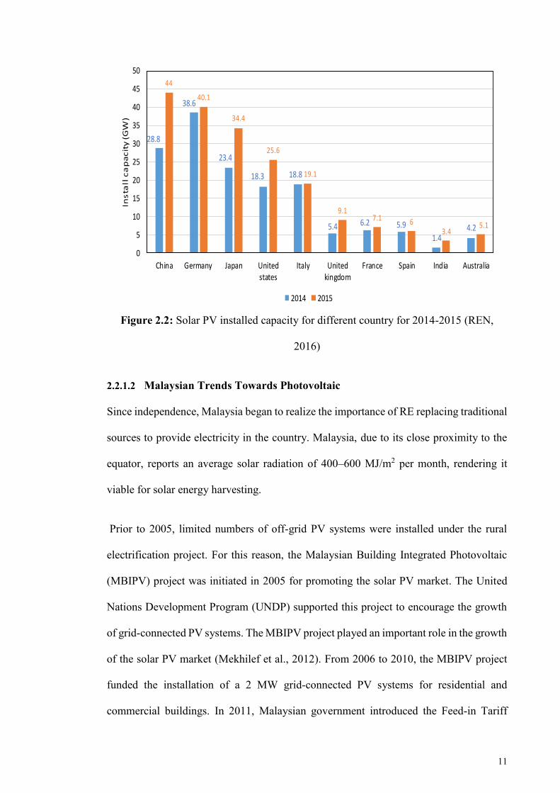
grid at a fixed rate and for a specific period of time. According to the Sustainable Energy
Development Authority (SEDA), the cumulative growth of installed capacities for solar
photovoltaic connected to the grid increase year by year, as shown in Figure 2.3.
Figure 2.3: Cumulative growth of PV Installed capacities since inception of FiT (MW)
(SEDA, 2015)
2.2.2 Hydropower
Hydropower is considered as one of the cleanest technology for producing electricity. It
transforms the potential energy of water flowing in a river or stream at a certain vertical
fall. Hydroelectricity is the most widely used form of renewable energy, with relatively
low electricity generation cost, and several countries take advantage of this fact to install
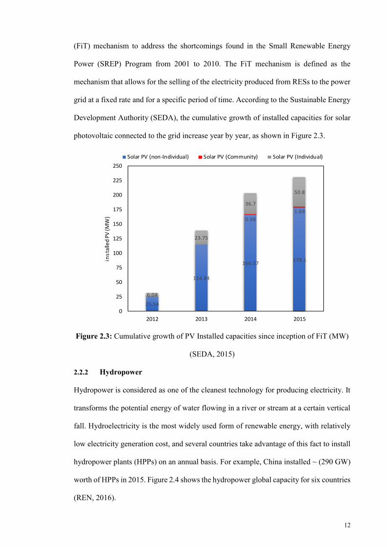
hydropower plants (HPPs) on an annual basis. For example, China installed ~ (290 GW)
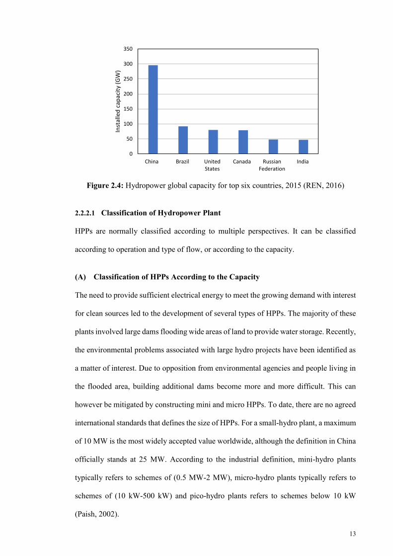
worth of HPPs in 2015. Figure 2.4 shows the hydropower global capacity for six countries
(REN, 2016).
25.54
114.84
166.07178.1
0.98
1.69
6.04
23.75
36.7
50.8
0
25
50
75
100
125
150
175
200
225
250
2012 2013 2014 2015
inst
alle
d PV
(MW
)
Solar PV (non-Individual) Solar PV (Community) Solar PV (Individual)
13
Figure 2.4: Hydropower global capacity for top six countries, 2015 (REN, 2016)
2.2.2.1 Classification of Hydropower Plant
HPPs are normally classified according to multiple perspectives. It can be classified
according to operation and type of flow, or according to the capacity.
(A) Classification of HPPs According to the Capacity
The need to provide sufficient electrical energy to meet the growing demand with interest
for clean sources led to the development of several types of HPPs. The majority of these
plants involved large dams flooding wide areas of land to provide water storage. Recently,
the environmental problems associated with large hydro projects have been identified as
a matter of interest. Due to opposition from environmental agencies and people living in
the flooded area, building additional dams become more and more difficult. This can
however be mitigated by constructing mini and micro HPPs. To date, there are no agreed
international standards that defines the size of HPPs. For a small-hydro plant, a maximum
of 10 MW is the most widely accepted value worldwide, although the definition in China
officially stands at 25 MW. According to the industrial definition, mini-hydro plants
typically refers to schemes of (0.5 MW-2 MW), micro-hydro plants typically refers to
schemes of (10 kW-500 kW) and pico-hydro plants refers to schemes below 10 kW
(Paish, 2002).
0
50
100
150
200
250
300
350
China Brazil UnitedStates
Canada RussianFederation
India
Inst
alle
d c
apac
ity
(GW
)

14
(B) Classification According to Flow Type
Based on the type of water flow, HPPs are categorized into HPPs with storage (reservoir),
pumped storage, and run-of-river (RoR).
i Hydropower Plant with Reservoir
Hydropower projects with a reservoir store water behind a dam for times when river flow
is low is shown in Figure 2.5. Therefore, power generation is more stable and less
variable. The generating stations are located at the dam toe or further downstream,
connected to the reservoir via tunnels or pipelines. Reservoir hydropower plants can have
major environmental and social impacts due to the flooding of the land for the reservoir.
Figure 2.5: Kenyir (Sultan Mahmud) Hydroelectric Power Project Malaysia
(KualaLumbur-Post, 2016)
ii Pump Storage Hydropower Plant
Pumped storage plants are not energy sources, instead, they are storage devices. Water is
pumped from a lower reservoir to an upper reservoir, usually during off-peak hours, while
flow is reversed to generate electricity during the daily peak load period or at other times
of need. Although the losses of the pumping process make such a plant a net energy
consumer, the plant provides large-scale energy storage system benefits. Pumped storage
is the largest capacity form of grid energy storage that is now readily available worldwide.
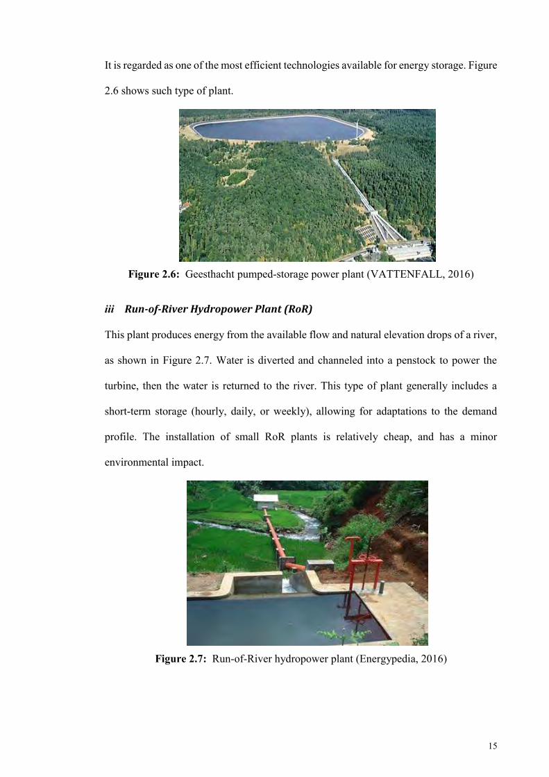
15
It is regarded as one of the most efficient technologies available for energy storage. Figure
2.6 shows such type of plant.
Figure 2.6: Geesthacht pumped-storage power plant (VATTENFALL, 2016)
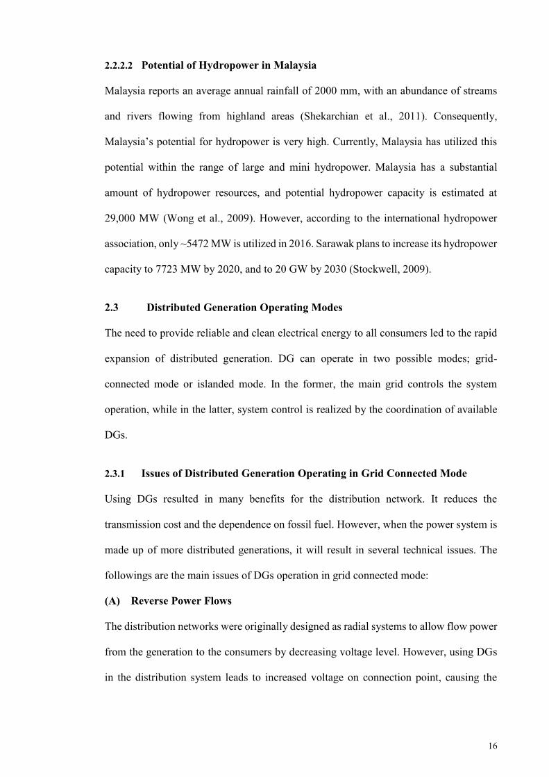
iii Run-of-River Hydropower Plant (RoR)
This plant produces energy from the available flow and natural elevation drops of a river,
as shown in Figure 2.7. Water is diverted and channeled into a penstock to power the
turbine, then the water is returned to the river. This type of plant generally includes a
short-term storage (hourly, daily, or weekly), allowing for adaptations to the demand
profile. The installation of small RoR plants is relatively cheap, and has a minor
environmental impact.
Figure 2.7: Run-of-River hydropower plant (Energypedia, 2016)
16
2.2.2.2 Potential of Hydropower in Malaysia
Malaysia reports an average annual rainfall of 2000 mm, with an abundance of streams
and rivers flowing from highland areas (Shekarchian et al., 2011). Consequently,
Malaysia’s potential for hydropower is very high. Currently, Malaysia has utilized this
potential within the range of large and mini hydropower. Malaysia has a substantial
amount of hydropower resources, and potential hydropower capacity is estimated at
29,000 MW (Wong et al., 2009). However, according to the international hydropower
association, only ~5472 MW is utilized in 2016. Sarawak plans to increase its hydropower
capacity to 7723 MW by 2020, and to 20 GW by 2030 (Stockwell, 2009).
2.3 Distributed Generation Operating Modes
The need to provide reliable and clean electrical energy to all consumers led to the rapid
expansion of distributed generation. DG can operate in two possible modes; grid-
connected mode or islanded mode. In the former, the main grid controls the system
operation, while in the latter, system control is realized by the coordination of available
DGs.
2.3.1 Issues of Distributed Generation Operating in Grid Connected Mode
Using DGs resulted in many benefits for the distribution network. It reduces the
transmission cost and the dependence on fossil fuel. However, when the power system is
made up of more distributed generations, it will result in several technical issues. The
followings are the main issues of DGs operation in grid connected mode:
(A) Reverse Power Flows
The distribution networks were originally designed as radial systems to allow flow power
from the generation to the consumers by decreasing voltage level. However, using DGs
in the distribution system leads to increased voltage on connection point, causing the
17
power to flow bi-directionally. Accordingly, this situation could negatively impact
protective devices, such as over-current, fuses, and automatic re-closers.
(B) Voltage Flickers
The intermittent nature of some distribute generation output can cause fluctuations in the
operating voltage. According to (IEEE) 1453TM-2011, voltage flicker is defined as
“Voltage fluctuations on electric power systems due to illumination changes from lighting
equipment”. These voltage fluctuations increase the possibility of operation malfunction
of devices.
(C) Harmonics
Sometimes, the integration of distributed generation to the main grid takes place via
power electronics converters, which might cause harmonics due to the switching
operation. The magnitude and order of this harmonic depend on the technology of the
converter. Injection harmonics via the grid can distort the voltage profile and increase
losses in the distribution system.
2.3.2 Issues of Distributed Generation Operating in Islanding Mode
According to IEEE standard, islanding operation is defined as “A condition in which a
portion of a utility system that contains both load and distributed resources remains
energized while isolated from the remainder of the utility system”. However, separating
the DGs after islanding will prevent the grid from exploiting the benefits garnered from
these sources. For this reason, at a high penetration level of RESs, there is an increased
need for the RESs to power some critical loads of the islanded micro-grid. When the
islanding mode occurs, the distribution network is disconnected from the grid using the
main circuit breaker, which results in the instability frequency issue.
18
2.3.2.1 Issue of Small Inertial Response
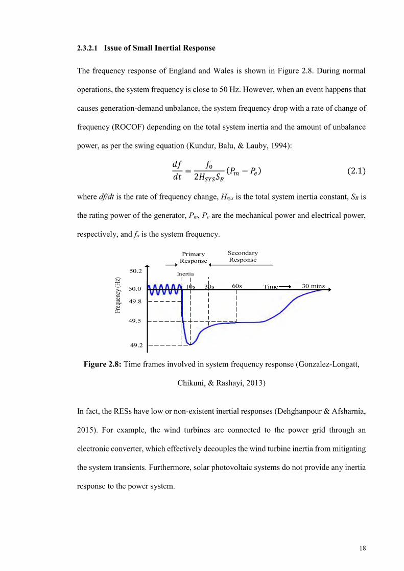
The frequency response of England and Wales is shown in Figure 2.8. During normal
operations, the system frequency is close to 50 Hz. However, when an event happens that
causes generation-demand unbalance, the system frequency drop with a rate of change of
frequency (ROCOF) depending on the total system inertia and the amount of unbalance
power, as per the swing equation (Kundur, Balu, & Lauby, 1994):
𝑑𝑓
𝑑𝑡=
𝑓02𝐻𝑆𝑌𝑆𝑆𝐵
(𝑃𝑚 − 𝑃𝑒) (2.1)
where df/dt is the rate of frequency change, Hsys is the total system inertia constant, SB is
the rating power of the generator, Pm, Pe are the mechanical power and electrical power,
respectively, and fo is the system frequency.
Figure 2.8: Time frames involved in system frequency response (Gonzalez-Longatt,
Chikuni, & Rashayi, 2013)
In fact, the RESs have low or non-existent inertial responses (Dehghanpour & Afsharnia,
2015). For example, the wind turbines are connected to the power grid through an
electronic converter, which effectively decouples the wind turbine inertia from mitigating
the system transients. Furthermore, solar photovoltaic systems do not provide any inertia
response to the power system.
Time
50.2
50.0
49.8
49.5
49.2
10s 30s 60s 30 mins
Freq
uenc
y (Hz
)
Primary Response
Secondary Response
Inertia

19
This fact is supported by (Jayawardena, Meegahapola, Perera, & Robinson, 2012), where
they predicted that the increasing number of RESs in the UK could reduce the inertia
constant by up to 70% between 2013/14 and 2033/34. In (Jayawardena et al., 2012),
different penetration levels of RESs were used with a Synchronous Generator (SG) to
meet the 3.8 MW load demand. As reported in (Jayawardena et al., 2012) and shown in
Figure 2.9, the ROCOF of the power system increase whenever the percentage-installed
capacity of the RESs increases.
Figure 2.9: The ROCOF of the distribution network for two types of RES supply
3.8MW load (Jayawardena et al., 2012)
According to Figure 2.9, when the conventional sources are replaced by RESs, the rate of
change of frequency increases due to the reduced inertia constant. For this reason, the
system frequency decreases rapidly, thus wasting the opportunity for other controllers to
recover the frequency.
2.3.2.2 Issue of Small Reserves Power
Immediately after an islanding or disturbance event, the inertia controller releases the
kinetic energy stored in the rotating mass of synchronous generator, which lasts for 10s
(Díaz-González, Hau, Sumper, & Gomis-Bellmunt, 2014). After that, a new controller,
called a primary frequency controller, is immediately activated. This controller use the
0.00
0.05
0.10
0.15
0.20
0.25
0.30
0% 25% 50% 75%
Max
imum
RO
COF
(Hz/
s)
Installed capacity of RESs
DFIG and SG PV and SG
20
governor to restore the frequency to acceptable frequency levels within 30s (Yu, Dyśko,
Booth, Roscoe, & Zhu, 2014). After 30s, a secondary frequency controller is activated in
order restore the system frequency. Finally, the remaining power deviation activates the
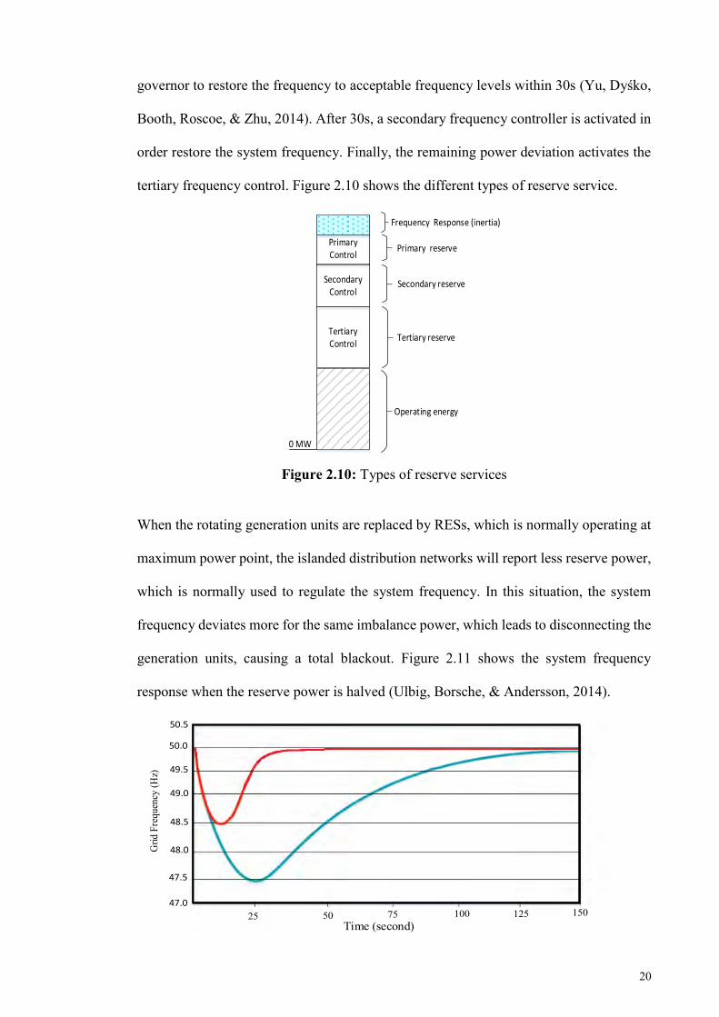
tertiary frequency control. Figure 2.10 shows the different types of reserve service.
Figure 2.10: Types of reserve services
When the rotating generation units are replaced by RESs, which is normally operating at
maximum power point, the islanded distribution networks will report less reserve power,
which is normally used to regulate the system frequency. In this situation, the system
frequency deviates more for the same imbalance power, which leads to disconnecting the
generation units, causing a total blackout. Figure 2.11 shows the system frequency
response when the reserve power is halved (Ulbig, Borsche, & Andersson, 2014).
Grid
Fre
quen
cy (H
z)
25 50 75 100 125 150
50.5
50.0
49.5
49.0
48.5
48.0
47.5
47.0
Time (second)
0 MW
Frequency Response (inertia)
Primary reserve
Secondary reserve
Tertiary reserve
Operating energy
Primary Control
Secondary Control
Tertiary Control
21
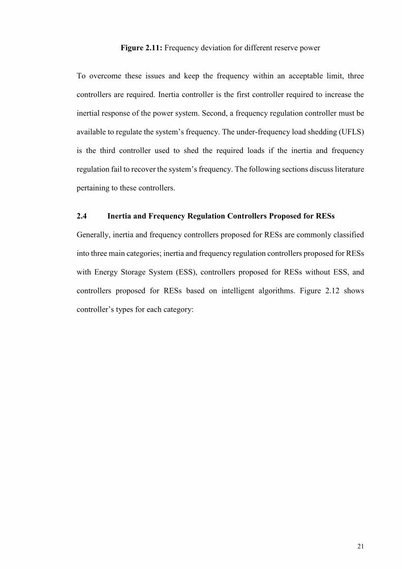
Figure 2.11: Frequency deviation for different reserve power
To overcome these issues and keep the frequency within an acceptable limit, three
controllers are required. Inertia controller is the first controller required to increase the
inertial response of the power system. Second, a frequency regulation controller must be
available to regulate the system’s frequency. The under-frequency load shedding (UFLS)
is the third controller used to shed the required loads if the inertia and frequency
regulation fail to recover the system’s frequency. The following sections discuss literature
pertaining to these controllers.
2.4 Inertia and Frequency Regulation Controllers Proposed for RESs
Generally, inertia and frequency controllers proposed for RESs are commonly classified
into three main categories; inertia and frequency regulation controllers proposed for RESs
with Energy Storage System (ESS), controllers proposed for RESs without ESS, and
controllers proposed for RESs based on intelligent algorithms. Figure 2.12 shows
controller’s types for each category:
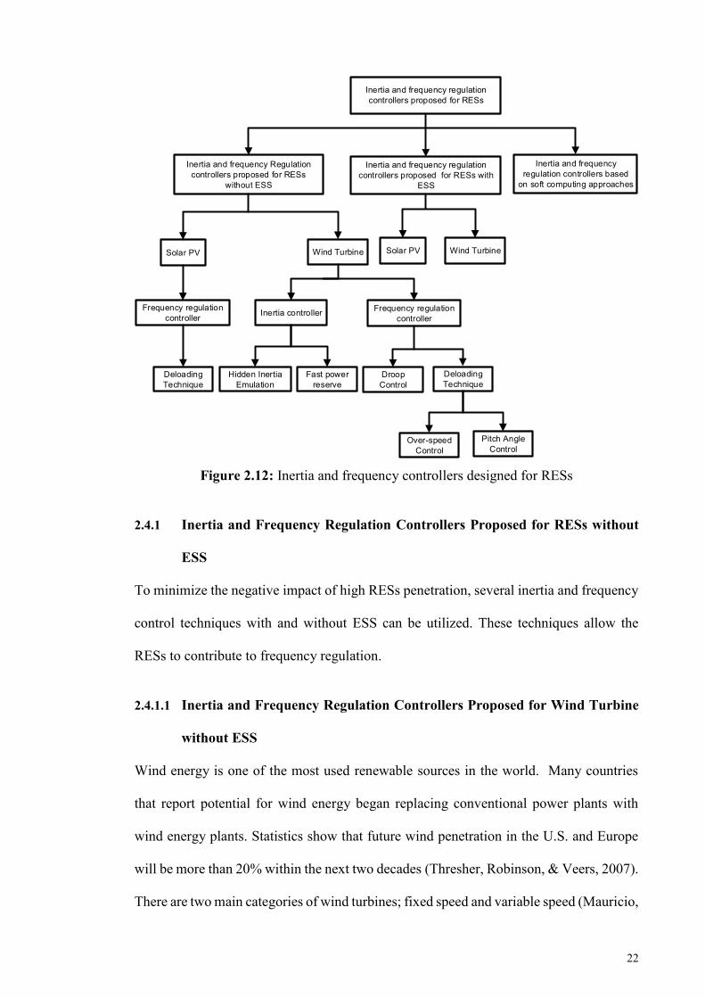
22
Figure 2.12: Inertia and frequency controllers designed for RESs
2.4.1 Inertia and Frequency Regulation Controllers Proposed for RESs without
ESS
To minimize the negative impact of high RESs penetration, several inertia and frequency
control techniques with and without ESS can be utilized. These techniques allow the
RESs to contribute to frequency regulation.
2.4.1.1 Inertia and Frequency Regulation Controllers Proposed for Wind Turbine
without ESS
Wind energy is one of the most used renewable sources in the world. Many countries
that report potential for wind energy began replacing conventional power plants with
wind energy plants. Statistics show that future wind penetration in the U.S. and Europe
will be more than 20% within the next two decades (Thresher, Robinson, & Veers, 2007).
There are two main categories of wind turbines; fixed speed and variable speed (Mauricio,
Inertia and frequency regulation controllers proposed for RESs
Inertia and frequency Regulation controllers proposed for RESs
without ESS
Inertia and frequency regulation controllers proposed for RESs with
ESS
Solar PV Wind Turbine Solar PV Wind Turbine
Inertia controller
Fast power reserve
Hidden Inertia Emulation
Deloading Technique
Pitch Angle Control
Over-speed Control
Deloading Technique
Droop Control
Frequency regulation controller
Frequency regulation controller
Inertia and frequency regulation controllers based
on soft computing approaches
23
Marano, Gómez-Expósito, & Ramos, 2009). The former generally uses an induction
generator connected directly to the grid and can provide an inertia response to the
frequency deviation, even though this inertia is small compared to the synchronous
generator.
A variable speed wind turbine mainly uses a Permanent Magnet Synchronous Generator
(PMSG) or Doubly Fed Induction Generator (DFIG). The PMSG is fully decoupled from
the grid; this is because the stator of this type of generator is connected to the power
electronic converter in order to inject the power into the grid. The DFIG is similar to
PMSG, except that this generator is connected to the grid by the rotor circuit. The power
electronic converter used in a variable speed wind turbine enables the wind turbine to
regulate the output power over a wide range of wind speeds (Revel, Leon, Alonso, &
Moiola, 2014). However, this coupling isolates the wind turbine from the frequency
response under disturbance. Furthermore, traditional wind turbines normally follow the
maximum power curve, as shown in Figure 2.13. Therefore, they do not have reserve
power to support the frequency control. The maximum output power from a wind turbine,
defined as a function of rotor speed, is given by (Bianchi, De Battista, & Mantz, 2007).
𝑃𝑀𝑃𝑃𝑇 = 𝐾𝑜𝑝𝑡𝜔3 (2.2)
where ω is the rotor speed, and Kopt is the constant (controller gain) for the tracking of the
maximum power curve, obtained from:
𝐾𝑜𝑝𝑡 = 0.5 𝜌𝜋𝑅5 𝐶𝑝𝑜𝑝𝑡
𝜆𝑜𝑝𝑡3 (2.3)
Where ρ is the air density, R is the radius of the turbine wheel, Cpopt is the maximum
power coefficient, and λopt is the optimum tip speed. The maximum power point controller
determines the operating point along the power load line. This operation is conducted by
regulating the speed of the wind turbine within the speed limits and pitch regulation after
the rated speed.
24
0.6 0.7 0.8 0.9 1 1.1 1.2 1.3
0.4
0.6
0.8
1
1.2
1.4
0.2
0
1.6
A
B
C
D
Tracking Characteristic
16.2 m/s
5 m/s
12 m/s
Turbine speed (pu)
Turb
ine ou
tput p
ower
(pu)
Figure 2.13: Power against rotating speed characteristics at (Pitch angle β=0)
(Lamchich & Lachguer, 2012)
Researchers proposed two main techniques to support frequency control using a variable
speed wind turbine; inertia response and power reserve control. Inertia control enables
the wind turbine to release the kinetic energy stored in the rotating blades within 10
seconds to arrest frequency deviation, while reserve control technique uses the pitch angle
controller, speed controller, or a combination of both to enhance the power reserve margin
during unbalanced power events.
(A) Inertia Response Control
Wind turbines lack the ability to automatically release the kinetic energy stored in their
rotating mass, unlike conventional generator. For this reason, a suitable controller is
needed to provide the wind turbine with an inertia response. Generally, there are two
control techniques that can be used to do this; hidden inertia emulation and fast power
reserve. The former is the first technique; it proposes new control loops to release the
kinetic energy stored in the rotating blades of the wind turbine. This additional power can
be used to terminate the frequency deviation during unbalance events. Fast power reserve
25
is the second technique, which can also be used to terminate the frequency deviation.
However, it responds to frequency deviation by releasing constant power for a definite
time.
i Hidden Inertia Emulation
Using a power electronic converter with a suitable controller enables variable speed wind
turbines to release the kinetic energy stored in their rotating blades. This kinetic energy
is used as an inertia response in the range 2-6 seconds (Knudsen & Nielsen, 2005).
Generally, there are two types of inertia response; the first one is single-loop inertia
response, and the other is the double-loop inertia response. The first type is based on
ROCOF, and it is used to release the kinetic energy stored in the rotating blades, while
the second type uses two loops based on ROCOF and frequency deviation. In (Gonzalez-
Longatt et al., 2013; Sun, Zhang, Li, & Lin, 2010), one-loop inertia response is added to
the speed control system to enable the wind turbine to respond to ROCOF. This control
loop is called inertia emulation, which exactly emulates the inertia response of
conventional power plants, as shown in Figure 2.14.
Figure 2.14: Inertia emulation for variable speed wind turbines
The output power from the wind turbine Pmeas determines the reference rotor speed ωr,ref
that is compared to the measuring rotor speed ωr,meas and used by the PI controller to
provide maximum power. During normal operations, the reference power transferred to
ωsys
ωr,meas
d/dt 2H
PI
Pin
∆ωr
+-
Pmeas ωr,ref PMPPT
++ Converter
Pref
Filter
ωr
pMPPT
26
the converter is equal to the maximum power without any contribution from the inertia
control loop. After a power deficit, a certain amount of power Pin, based on the value of
ROCOF and virtual inertia constant Hv, will be added to the power of maximum power
point tracking (PMPPT). Due to this power increment, the generator speed will slow down,
and the kinetic energy stored in the rotating wind turbine blades will be released. The
additional power Pin comes from the inertia response loop given by (Morren, Pierik, &
De Haan, 2006):
𝑃𝑖𝑛 = 2𝐻𝑣 × 𝜔𝑠𝑦𝑠 ×𝑑𝜔𝑠𝑦𝑠
𝑑𝑡 (2.4)
Due to the constant additional power resulting from the inertial control loop, this type of
control has two disadvantages. First, the rotor speed is rapidly reduced, leading to big
losses in aerodynamic power. Second, the controller takes time to recover energy during
rotor speed recovery. These disadvantages can be avoided using the techniques proposed
in (L. Wu & Infield, 2013), where they formulated a new inertia response constant. This
inertia constant is called the effective inertia response, which is based on the frequency
value. Generally, the inertia constant for a wind turbine is defined by:
𝐻 =𝐸𝑘𝑖𝑛𝑆𝐵
=𝐽𝜔2
2𝑆𝐵 (2.5)
where Ekin is the kinetic energy stored in the rotating mass of the wind turbine, SB is the
rated power, and J is the moment of inertia. Equation (2.5) can be rewritten by substituting
the corresponding power from equation (2.2), making the effective inertia constant:
𝐻𝑒(𝜔) =𝐽𝜆𝑜𝑝𝑡
3
𝜌𝜋𝑅5𝐶𝑝𝑜𝑝𝑡 1
𝜔 (2.6)
The main idea is to increase the value of the inertia constant as long as the system
frequency continues to decrease. Consequently, the torque transfer to the converter is
reduced, as shown in Figure 2.15.
27
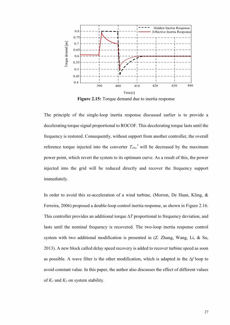
Figure 2.15: Torque demand due to inertia response
The principle of the single-loop inertia response discussed earlier is to provide a
decelerating torque signal proportional to ROCOF. This decelerating torque lasts until the
frequency is restored. Consequently, without support from another controller, the overall
reference torque injected into the converter Telec* will be decreased by the maximum
power point, which revert the system to its optimum curve. As a result of this, the power
injected into the grid will be reduced directly and recover the frequency support
immediately.
In order to avoid this re-acceleration of a wind turbine, (Morren, De Haan, Kling, &
Ferreira, 2006) proposed a double-loop control inertia response, as shown in Figure 2.16.
This controller provides an additional torque ∆T proportional to frequency deviation, and
lasts until the nominal frequency is recovered. The two-loop inertia response control
system with two additional modification is presented in (Z. Zhang, Wang, Li, & Su,
2013). A new block called delay speed recovery is added to recover turbine speed as soon
as possible. A wave filter is the other modification, which is adapted in the ∆f loop to
avoid constant value. In this paper, the author also discusses the effect of different values
of K1 and K2 on system stability.
0.4
0.45
0.5
0.55
0.6
0.65
0.7
0.75
0.8Hidden Inertia Response
Effective Inertia Response
390 400 410 420 430 440
Time[s]
Torq
ue de
mand
[pu]
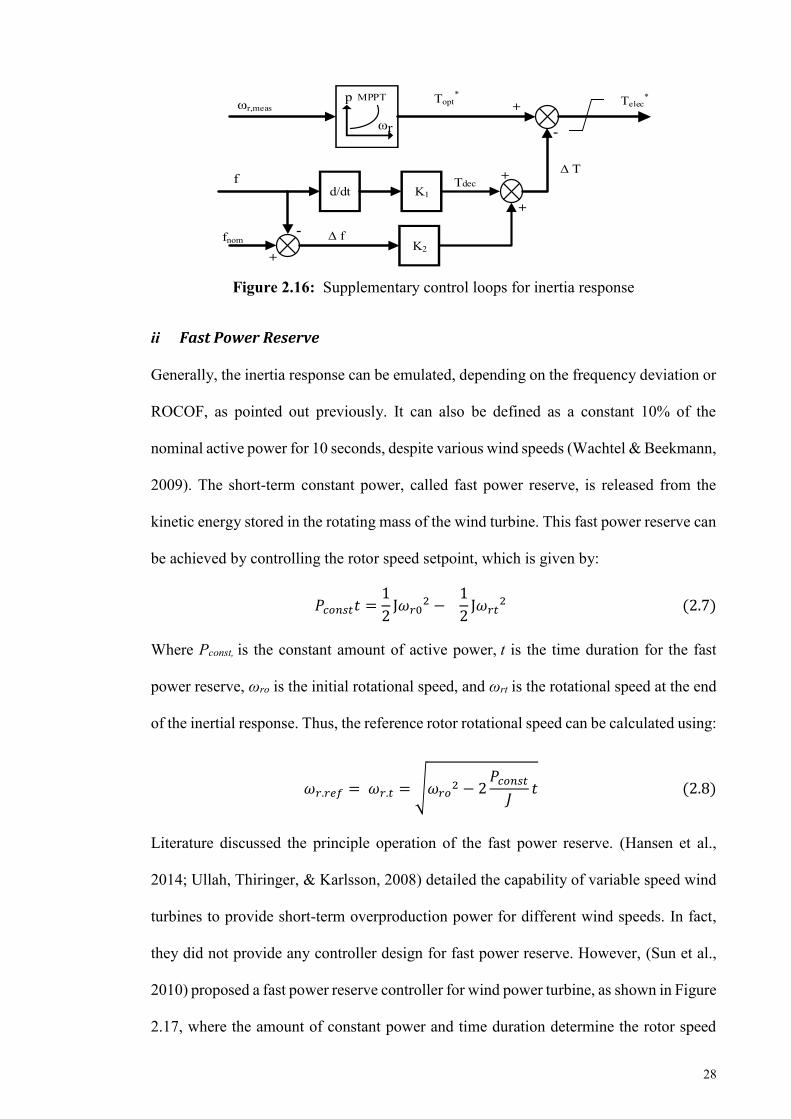
28
Figure 2.16: Supplementary control loops for inertia response
ii Fast Power Reserve
Generally, the inertia response can be emulated, depending on the frequency deviation or
ROCOF, as pointed out previously. It can also be defined as a constant 10% of the
nominal active power for 10 seconds, despite various wind speeds (Wachtel & Beekmann,
2009). The short-term constant power, called fast power reserve, is released from the
kinetic energy stored in the rotating mass of the wind turbine. This fast power reserve can
be achieved by controlling the rotor speed setpoint, which is given by:
𝑃𝑐𝑜𝑛𝑠𝑡𝑡 =1
2J𝜔𝑟0
2 − 1
2J𝜔𝑟𝑡
2 (2.7)
Where Pconst, is the constant amount of active power, t is the time duration for the fast
power reserve, ωro is the initial rotational speed, and ωrt is the rotational speed at the end
of the inertial response. Thus, the reference rotor rotational speed can be calculated using:
𝜔𝑟.𝑟𝑒𝑓 = 𝜔𝑟.𝑡 = √𝜔𝑟𝑜2 − 2𝑃𝑐𝑜𝑛𝑠𝑡𝐽
𝑡 (2.8)
Literature discussed the principle operation of the fast power reserve. (Hansen et al.,
2014; Ullah, Thiringer, & Karlsson, 2008) detailed the capability of variable speed wind
turbines to provide short-term overproduction power for different wind speeds. In fact,
they did not provide any controller design for fast power reserve. However, (Sun et al.,
2010) proposed a fast power reserve controller for wind power turbine, as shown in Figure
2.17, where the amount of constant power and time duration determine the rotor speed
+
+
+
Topt*
d/dt K1
K2
-
Telec*
∆ T
+
- ∆ f
Tdec
ωr,meas
f
fnom
ωr
p MPPT
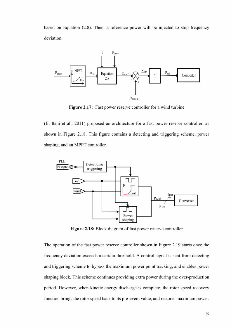
29
based on Equation (2.8). Then, a reference power will be injected to stop frequency
deviation.
Figure 2.17: Fast power reserve controller for a wind turbine
(El Itani et al., 2011) proposed an architecture for a fast power reserve controller, as
shown in Figure 2.18. This figure contains a detecting and triggering scheme, power
shaping, and an MPPT controller.
Figure 2.18: Block diagram of fast power reserve controller
The operation of the fast power reserve controller shown in Figure 2.19 starts once the
frequency deviation exceeds a certain threshold. A control signal is sent from detecting
and triggering scheme to bypass the maximum power point tracking, and enables power
shaping block. This scheme continues providing extra power during the over-production
period. However, when kinetic energy discharge is complete, the rotor speed recovery
function brings the rotor speed back to its pre-event value, and restores maximum power.
PI∆ωr
+-
Pmeas ωro ConverterPrefEquation 2.8
t Pconst
ωr,meas
ωr,ref
ωr
p MPPT
Frequency
ωr
P
PLLDetection&triggering
ωr
wind
Power shaping
1pu
0 pu
Pe,ref Converter
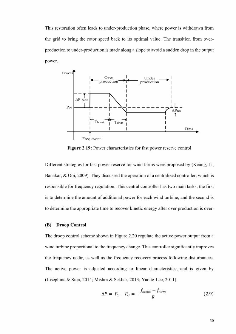
30
This restoration often leads to under-production phase, where power is withdrawn from
the grid to bring the rotor speed back to its optimal value. The transition from over-
production to under-production is made along a slope to avoid a sudden drop in the output
power.
Figure 2.19: Power characteristics for fast power reserve control
Different strategies for fast power reserve for wind farms were proposed by (Keung, Li,
Banakar, & Ooi, 2009). They discussed the operation of a centralized controller, which is
responsible for frequency regulation. This central controller has two main tasks; the first
is to determine the amount of additional power for each wind turbine, and the second is
to determine the appropriate time to recover kinetic energy after over production is over.
(B) Droop Control
The droop control scheme shown in Figure 2.20 regulate the active power output from a
wind turbine proportional to the frequency change. This controller significantly improves
the frequency nadir, as well as the frequency recovery process following disturbances.
The active power is adjusted according to linear characteristics, and is given by
(Josephine & Suja, 2014; Mishra & Sekhar, 2013; Yao & Lee, 2011).
∆𝑃 = 𝑃1 − 𝑃𝑂 = −𝑓𝑚𝑒𝑎𝑠 − 𝑓𝑛𝑜𝑚
𝑅 (2.9)
Time
Over production
Under production
∆P boost
∆Prec
TdropTboost
Freq event
Peo
Power
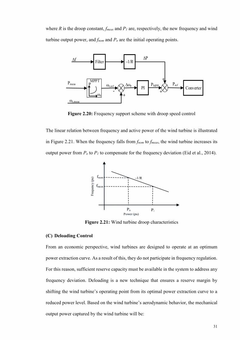
31
where R is the droop constant, fmeas and P1 are, respectively, the new frequency and wind
turbine output power, and fnom and Po are the initial operating points.
Figure 2.20: Frequency support scheme with droop speed control
The linear relation between frequency and active power of the wind turbine is illustrated
in Figure 2.21. When the frequency falls from fnom to fmeas, the wind turbine increases its
output power from Po to P1 to compensate for the frequency deviation (Eid et al., 2014).
Figure 2.21: Wind turbine droop characteristics
(C) Deloading Control
From an economic perspective, wind turbines are designed to operate at an optimum
power extraction curve. As a result of this, they do not participate in frequency regulation.
For this reason, sufficient reserve capacity must be available in the system to address any
frequency deviation. Deloading is a new technique that ensures a reserve margin by
shifting the wind turbine’s operating point from its optimal power extraction curve to a
reduced power level. Based on the wind turbine’s aerodynamic behavior, the mechanical
output power captured by the wind turbine will be:
∆f
ωr,meas
Filter -1/R
PI
∆P
∆ωr
+-
Pmeas ωr,ref PMPP
+
+Converter
Pref
ωr
PMPPT
Po
fnom -1/R
P1
fmeas
Freq
uenc
y (p
u)
Power (pu)
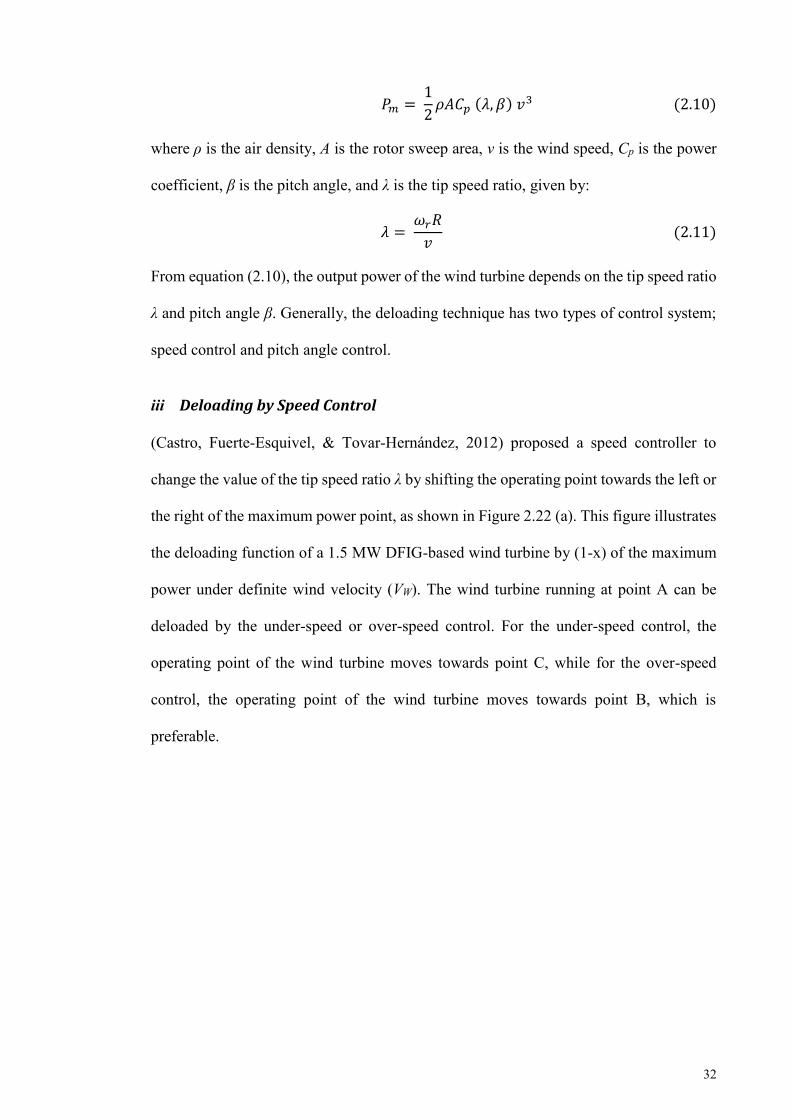
32
𝑃𝑚 = 1
2𝜌𝐴𝐶𝑝 (𝜆, 𝛽) 𝑣
3 (2.10)
where ρ is the air density, A is the rotor sweep area, v is the wind speed, Cp is the power
coefficient, β is the pitch angle, and λ is the tip speed ratio, given by:
𝜆 = 𝜔𝑟𝑅
𝑣 (2.11)
From equation (2.10), the output power of the wind turbine depends on the tip speed ratio
λ and pitch angle β. Generally, the deloading technique has two types of control system;
speed control and pitch angle control.
iii Deloading by Speed Control
(Castro, Fuerte-Esquivel, & Tovar-Hernández, 2012) proposed a speed controller to
change the value of the tip speed ratio λ by shifting the operating point towards the left or
the right of the maximum power point, as shown in Figure 2.22 (a). This figure illustrates
the deloading function of a 1.5 MW DFIG-based wind turbine by (1-x) of the maximum
power under definite wind velocity (VW). The wind turbine running at point A can be
deloaded by the under-speed or over-speed control. For the under-speed control, the
operating point of the wind turbine moves towards point C, while for the over-speed
control, the operating point of the wind turbine moves towards point B, which is
preferable.
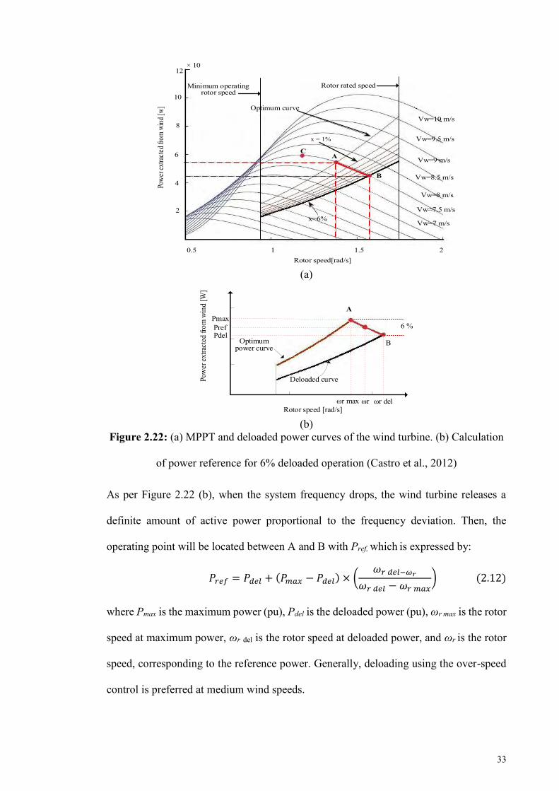
33
(a)
(b)
Figure 2.22: (a) MPPT and deloaded power curves of the wind turbine. (b) Calculation
of power reference for 6% deloaded operation (Castro et al., 2012)
As per Figure 2.22 (b), when the system frequency drops, the wind turbine releases a
definite amount of active power proportional to the frequency deviation. Then, the
operating point will be located between A and B with Pref, which is expressed by:
𝑃𝑟𝑒𝑓 = 𝑃𝑑𝑒𝑙 + (𝑃𝑚𝑎𝑥 − 𝑃𝑑𝑒𝑙) × (𝜔𝑟 𝑑𝑒𝑙−𝜔𝑟
𝜔𝑟 𝑑𝑒𝑙 − 𝜔𝑟 𝑚𝑎𝑥) (2.12)
where Pmax is the maximum power (pu), Pdel is the deloaded power (pu), ωr max is the rotor
speed at maximum power, ωr del is the rotor speed at deloaded power, and ωr is the rotor
speed, corresponding to the reference power. Generally, deloading using the over-speed
control is preferred at medium wind speeds.
0.5 1 1.5 2Rotor speed[rad/s]
2
4
6
8
10
12 × 10
A
B
C
x=6%
x = 1%
Optimum curve
Minimum operating rotor speed
Rotor rated speed
Vw=7 m/s
Vw=7.5 m/s
Vw=8 m/s
Vw=8.5 m/s
Vw=9 m/s
Vw=9.5 m/s
Vw=10 m/s
Powe
r extr
acted
from
win
d [w]
ωr max ωr delωr
A
B
6 %
Rotor speed [rad/s]
Pow
er e
xtra
cted
from
win
d [W
]
PmaxPrefPdel
Optimum power curve
Deloaded curve
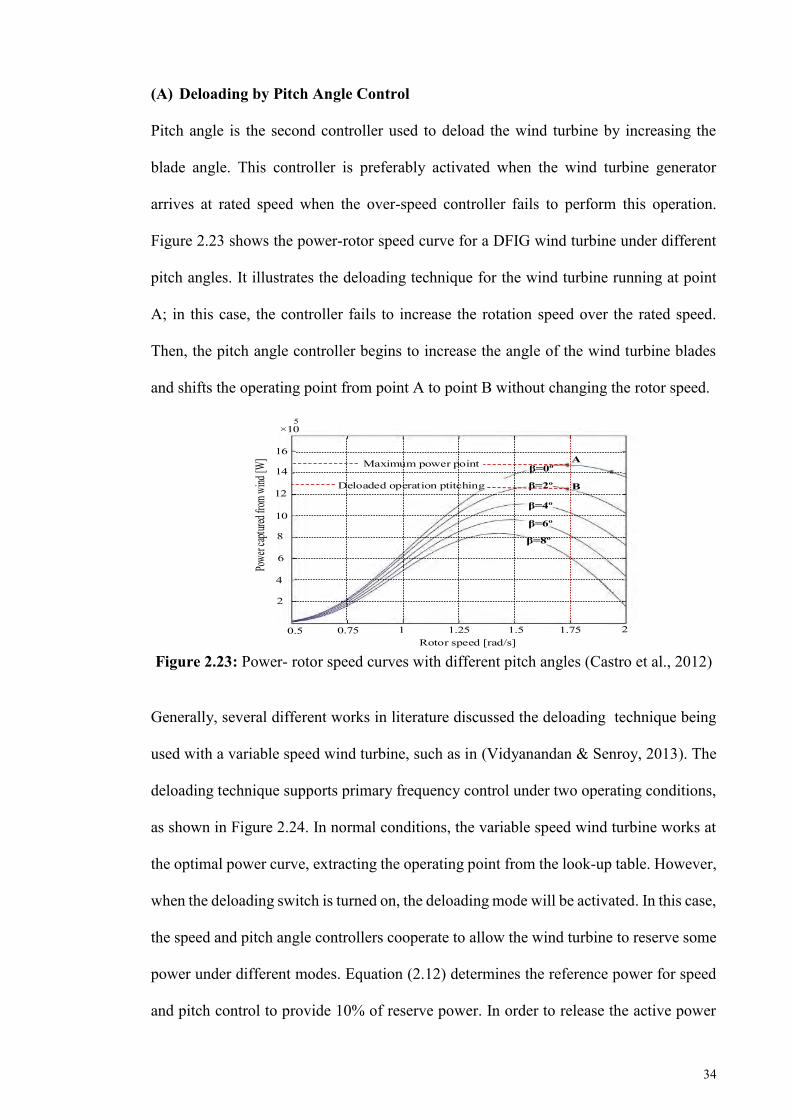
34
(A) Deloading by Pitch Angle Control
Pitch angle is the second controller used to deload the wind turbine by increasing the
blade angle. This controller is preferably activated when the wind turbine generator
arrives at rated speed when the over-speed controller fails to perform this operation.
Figure 2.23 shows the power-rotor speed curve for a DFIG wind turbine under different
pitch angles. It illustrates the deloading technique for the wind turbine running at point
A; in this case, the controller fails to increase the rotation speed over the rated speed.
Then, the pitch angle controller begins to increase the angle of the wind turbine blades
and shifts the operating point from point A to point B without changing the rotor speed.
Figure 2.23: Power- rotor speed curves with different pitch angles (Castro et al., 2012)
Generally, several different works in literature discussed the deloading technique being
used with a variable speed wind turbine, such as in (Vidyanandan & Senroy, 2013). The
deloading technique supports primary frequency control under two operating conditions,
as shown in Figure 2.24. In normal conditions, the variable speed wind turbine works at
the optimal power curve, extracting the operating point from the look-up table. However,
when the deloading switch is turned on, the deloading mode will be activated. In this case,
the speed and pitch angle controllers cooperate to allow the wind turbine to reserve some
power under different modes. Equation (2.12) determines the reference power for speed
and pitch control to provide 10% of reserve power. In order to release the active power
0.5 0.75 1 1.25 1.5 1.75 2
2
4
6
8
10
12
14
16
×105
β=0º
β=2º
β=4º
β=6º
β=8º
A
B
Rotor speed [rad/s]
Powe
r capt
ured f
rom w
ind [W
] Maximum power point
Deloaded operation ptitching
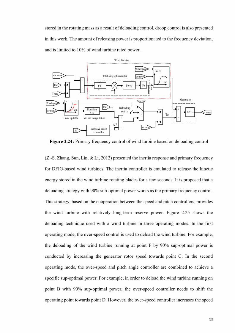
35
stored in the rotating mass as a result of deloading control, droop control is also presented
in this work. The amount of releasing power is proportionated to the frequency deviation,
and is limited to 10% of wind turbine rated power.
Figure 2.24: Primary frequency control of wind turbine based on deloading control
(Z.-S. Zhang, Sun, Lin, & Li, 2012) presented the inertia response and primary frequency
for DFIG-based wind turbines. The inertia controller is emulated to release the kinetic
energy stored in the wind turbine rotating blades for a few seconds. It is proposed that a
deloading strategy with 90% sub-optimal power works as the primary frequency control.
This strategy, based on the cooperation between the speed and pitch controllers, provides
the wind turbine with relatively long-term reserve power. Figure 2.25 shows the
deloading technique used with a wind turbine in three operating modes. In the first
operating mode, the over-speed control is used to deload the wind turbine. For example,
the deloading of the wind turbine running at point F by 90% sup-optimal power is
conducted by increasing the generator rotor speed towards point C. In the second
operating mode, the over-speed and pitch angle controller are combined to achieve a
specific sup-optimal power. For example, in order to deload the wind turbine running on
point B with 90% sup-optimal power, the over-speed controller needs to shift the
operating point towards point D. However, the over-speed controller increases the speed
Wind speed
1/2Hs
Inertia & droop controller
+
_
Equation 2.12
+
_
Tmec
Pref
+
_
+
_
Look up tableTe
Generator
Wind Turbine
deload computation
P I
Pitch Angle Controller
Selector
Deloading switch
∆ P
Servoβ
ωr
P
ωr
Pmec
ωr meas
ωr meas
1/s
∆f
Prefωr meas
Wind speed
ωr measωr meas

36
until the wind turbine arrives at point G. After that, the over-speed controller cannot
increase the rotation speed anymore. As a result of this, the pitch angle controller
increases the blade pitch angle shifting the operating point towards point A. In the third
region, the pitch controller is used on its own to achieve the target deloading value.
The cooperation between pitch angle and speed controller for a variable speed wind
turbine is also presented in (Díaz-González et al., 2014). They proposed three operating
modes, depending on the range of wind speed, and a decision algorithm to manage the
cooperation between pitch angle and the over-speed controller. This algorithm determines
the power set value for the pitch angle controller and the power margin for the over-speed
controller.
Figure 2.25: 90% sub-optimal operation curve (Z.-S. Zhang et al., 2012)
(De Almeida & Lopes, 2007) used the cooperation between pitch angle and over-speed
controller to allow the wind turbine to participate in frequency regulation. However, this
time, the controllers decided on the reserve power value based on the network operator
request. (Z. Wu, Gao, Wang, & Gu, 2012) reported that the same frequency regulation
controllers used for the DFIG wind turbine were redesigned and implemented in the
PMSG to enable this type of wind turbine to contribute to primary frequency control.
Mode 1
```
Rotor speed (p.u)
0
0
0.2
0.2 0.4
0.4
0.6
0.6
0.8
0.8
1 1.2 1.4 1.81.6
1
Mode 2
Mode 3MPPT
90% sub optimal right curve
AD
GB
E
Vw = 8 m/s
Vw =9.6 m/s
Vw =10.7 m/s
Vw =11.8 m/s
FCM
echa
nical
activ
e pow
er (p.
u)
37
(Tielens et al., 2012; Zhangjie, Xiaoru, & Jin, 2012) proposed the pitch angle and over-
speed controllers, coordinated with the droop control. These controllers are activated by
wind speed ranges to enable the DFIG-based wind turbine to participate in frequency
regulation. Furthermore, the over-speed control strategy uses wind speed measurements
to determine the sub-optimal power based on the deloading tracking curve, and saves this
value in the lookup table.
2.4.1.2 Frequency Regulation Controllers Proposed for PV without ESS
Recently, the penetration of solar photovoltaic (PV) into distribution networks has
significantly increased. As a result of this, reserve power from the remaining conventional
source unit is insufficient to regulate system’s frequency under island conditions.
Moreover, due to the high cost of solar photovoltaic systems, different MPPT techniques
have been introduced to extract maximum power from this source (De Brito, Galotto,
Sampaio, e Melo, & Canesin, 2013; Faranda & Leva, 2008; Hua & Shen, 1998). However,
the use of MPPT techniques enables the solar photovoltaic (PV) to operate without any
reserve power. For these reasons, different modifications have been made to the design
of controllers used with a (PV) converter to allow them to effectively participate in
frequency regulation.
According to (Hoke & Maksimović, 2013), smart photovoltaic inverters do not have the
full commercial control capability to change the output power from (PV) systems, even
if they have the ability to provide frequency down-regulation by curtailing power.
Moreover, research related to this type of control is still in the early stages, and mainly
depends on two types of controller. The first uses solar photovoltaic (PV) supported by
ESS to regulate the frequency, which will be discussed later, while the second proposes
the deloading technique for solar photovoltaic (PV) without ESS, as presented in
(Rahmann & Castillo, 2014; Zarina, Mishra, & Sekhar, 2012a, 2012b). These papers

38
present a comprehensive control scheme that allows the photovoltaic system to participate
in frequency regulation. Figure 2.26 shows the deloading technique, which is performed
by increasing the dc voltage beyond MPP. This is achieved by increasing the value from
VMPP by voltage Vdeload, which allows the PV array to maintain some reserve power. This
reserve power is not released until the system frequency deviates. Under these conditions,
a control signal proportional to frequency deviation Vdc∆f is added to the dc reference
voltage.
Figure 2.26: Controller for deloaded solar PV
It can be seen in Figure 2.26 that the change in output power from the PV will not only
depend on the VMPP value, but also on the frequency deviation, as per equation (2.13).
𝑉𝑑𝑐 𝑟𝑒𝑓 = 𝑉𝑀𝑃𝑃 + 𝑉𝑑𝑒𝑙𝑜𝑎𝑑 − 𝑉𝑑𝑐 ∆𝑓 (2.13)
The operation of the deloaded controller is illustrated in Figure 2.27, where PV is working
at point 3 to reserve some power. This continues until the system’s frequency begins to
decline, at which point a control signal related to frequency deviation will reduce the PV
voltage and make the PV work at point 2.
∆f
idref+VMPP
PI
PI
Vdeload
+Vdc
_
+
Vdc∆f
Vdc ref
_ Voc
VMPP

39
Figure 2.27: Solar PV with deloading technique (Zarina, Mishra, & Sekhar, 2014)
In fact, the controller discussed in Figure 2.26 has a big problem in that it does not take
into consideration the remaining reserve power for each PV unit. For this reason, all PV
units will release the same amount of active power needed for frequency regulation, even
if the reserve power of each unit will not be equal. As a result of this, some of the PV
units, which have less reserve power, will reach MPP faster, and will not be able to
contribute any further to frequency regulation. This will lead to a non-uniform distribution
of frequency regulation. (Zarina et al., 2014) proposed a new modification to the previous
controller by adding a new control signal to represent the remaining reserve power
∆Vreserve, as shown in Figure 2.28. The reference voltage of the new controller is given by
equation (2.14), which clearly shows that the output power released from the PV units is
not equal and depends on the reserve power available for each.
𝑉𝑑𝑐 𝑟𝑒𝑓 = (𝑉𝑀𝑃𝑃 + 𝑉𝑑𝑒𝑙𝑜𝑎𝑑 − 𝑉𝑑𝑐 ∆𝑓) − (∆𝑓 × ∆𝑉𝑟𝑒𝑠𝑒𝑟𝑣𝑒 × 𝐾𝑃2) (2.14)
Figure 2.28: The improved controller for deloaded PV
Power
Pmax
Pdeload
VMPP VMPP +Vdeload
∆Vreserve Vdc∆f
Voltage
Total Reserve
1
2
3
∆f
idref+VMPP
PI Controller 1
PI Controller 2
Vdeload
+
Vdc
_
+
V dc∆f
Vdc ref
_
PController
∆Vreserve
_+
Voc
VMPP
40
Another technique was proposed in (Pappu, Chowdhury, & Bhatt, 2010) to enable a solar
PV plant to participate in frequency regulation. Two algorithms were implemented, the
first was the traditional MPPT controller, which is responsible for operating the PV plant
on MPP during normal operations. For transient conditions, a control signal would
activate the deloading algorithm, which uses a modified fractional open circuit voltage.
This modification proposed the use of ratio K as a controlled variable, which determines
the amount of reserve power for PV plants limited to the range (0.8-0.95). The main
findings of this paper show that a PV generator has the ability to regulate the frequency
and follow load changes. Furthermore, (Watson & Kimball, 2011) discussed a control
scheme designed for a PV panel to regulate the frequency of an islanded micro-grid. Their
main objective was to use a tracking algorithm to follow a command signal, which
changes according to the frequency deviation of the micro-grid. Following this, the
control system continues until the controller reaches the maximum power point, and stays
running at this point.
Generally, all control techniques discussed in this paper were designed to provide the
solar PV system with reliable control to regulate the frequency in grid connected or off-
grid mode. These techniques were mainly based on the MPPT controller running the PV
array in the deloading mode. In contrast, (Okou, Akhri, Beguenane, & Tarbouchi, 2012)
proposed a frequency regulator consisting of an adaptive frequency scheme, using a
nonlinear control to calculate the active power signal P*, depending on the frequency
deviation, as shown in Figure 2.29. This signal is needed to update the reference power
Pref used by the power controller to determine the output power of the solar PV by
regulating the duty cycle (D) of the power converter.
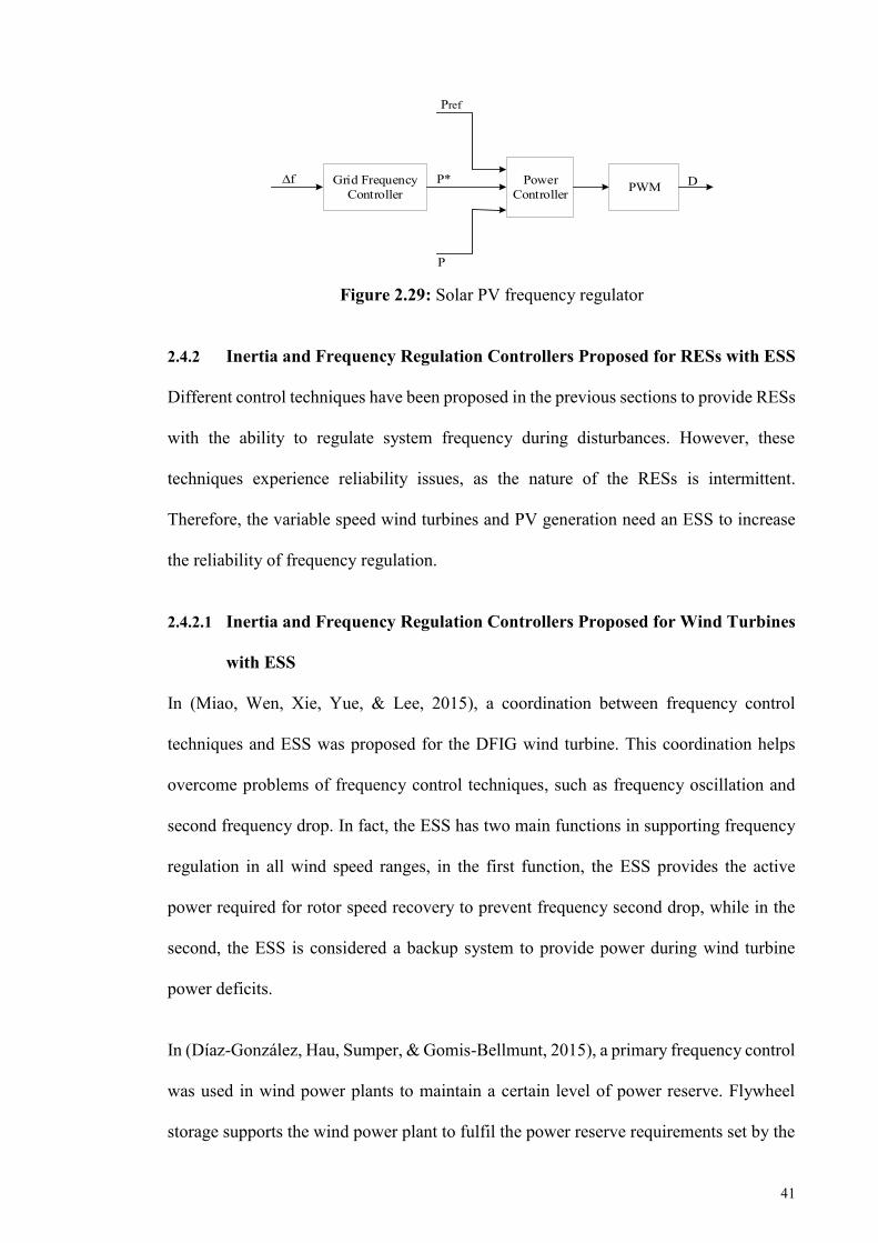
41
Figure 2.29: Solar PV frequency regulator
2.4.2 Inertia and Frequency Regulation Controllers Proposed for RESs with ESS
Different control techniques have been proposed in the previous sections to provide RESs
with the ability to regulate system frequency during disturbances. However, these
techniques experience reliability issues, as the nature of the RESs is intermittent.
Therefore, the variable speed wind turbines and PV generation need an ESS to increase
the reliability of frequency regulation.
2.4.2.1 Inertia and Frequency Regulation Controllers Proposed for Wind Turbines
with ESS
In (Miao, Wen, Xie, Yue, & Lee, 2015), a coordination between frequency control
techniques and ESS was proposed for the DFIG wind turbine. This coordination helps
overcome problems of frequency control techniques, such as frequency oscillation and
second frequency drop. In fact, the ESS has two main functions in supporting frequency
regulation in all wind speed ranges, in the first function, the ESS provides the active
power required for rotor speed recovery to prevent frequency second drop, while in the
second, the ESS is considered a backup system to provide power during wind turbine
power deficits.
In (Díaz-González, Hau, Sumper, & Gomis-Bellmunt, 2015), a primary frequency control
was used in wind power plants to maintain a certain level of power reserve. Flywheel
storage supports the wind power plant to fulfil the power reserve requirements set by the
Grid Frequency Controller PWMPower
Controller∆f
Pref
P*
P
D
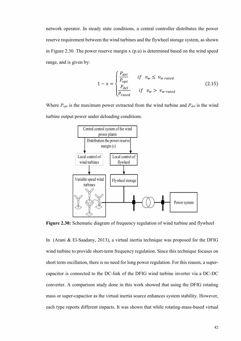
42
network operator. In steady state conditions, a central controller distributes the power
reserve requirement between the wind turbines and the flywheel storage system, as shown
in Figure 2.30. The power reserve margin x (p.u) is determined based on the wind speed
range, and is given by:
1 − 𝑥 =
{
𝑃𝑑𝑒𝑙𝑃𝑜𝑝𝑡
𝑖𝑓 𝑣𝑤 ≤ 𝑣𝑤 𝑟𝑎𝑡𝑒𝑑
𝑃𝑑𝑒𝑙𝑃𝑟𝑎𝑡𝑒𝑑
𝑖𝑓 𝑣𝑤 > 𝑣𝑤 𝑟𝑎𝑡𝑒𝑑
(2.15)
Where Popt is the maximum power extracted from the wind turbine and Pdel is the wind
turbine output power under deloading conditions.
Figure 2.30: Schematic diagram of frequency regulation of wind turbine and flywheel
In (Arani & El-Saadany, 2013), a virtual inertia technique was proposed for the DFIG
wind turbine to provide short-term frequency regulation. Since this technique focuses on
short term oscillation, there is no need for long power regulation. For this reason, a super-
capacitor is connected to the DC-link of the DFIG wind turbine inverter via a DC-DC
converter. A comparison study done in this work showed that using the DFIG rotating
mass or super-capacitor as the virtual inertia source enhances system stability. However,
each type reports different impacts. It was shown that while rotating-mass-based virtual
Local control of wind turbines
Variable speed wind turbines
Local control of flywheel
Flywheel storage
Power system
Distribution the power reserve margin (x)
Central control system of the wind power plants
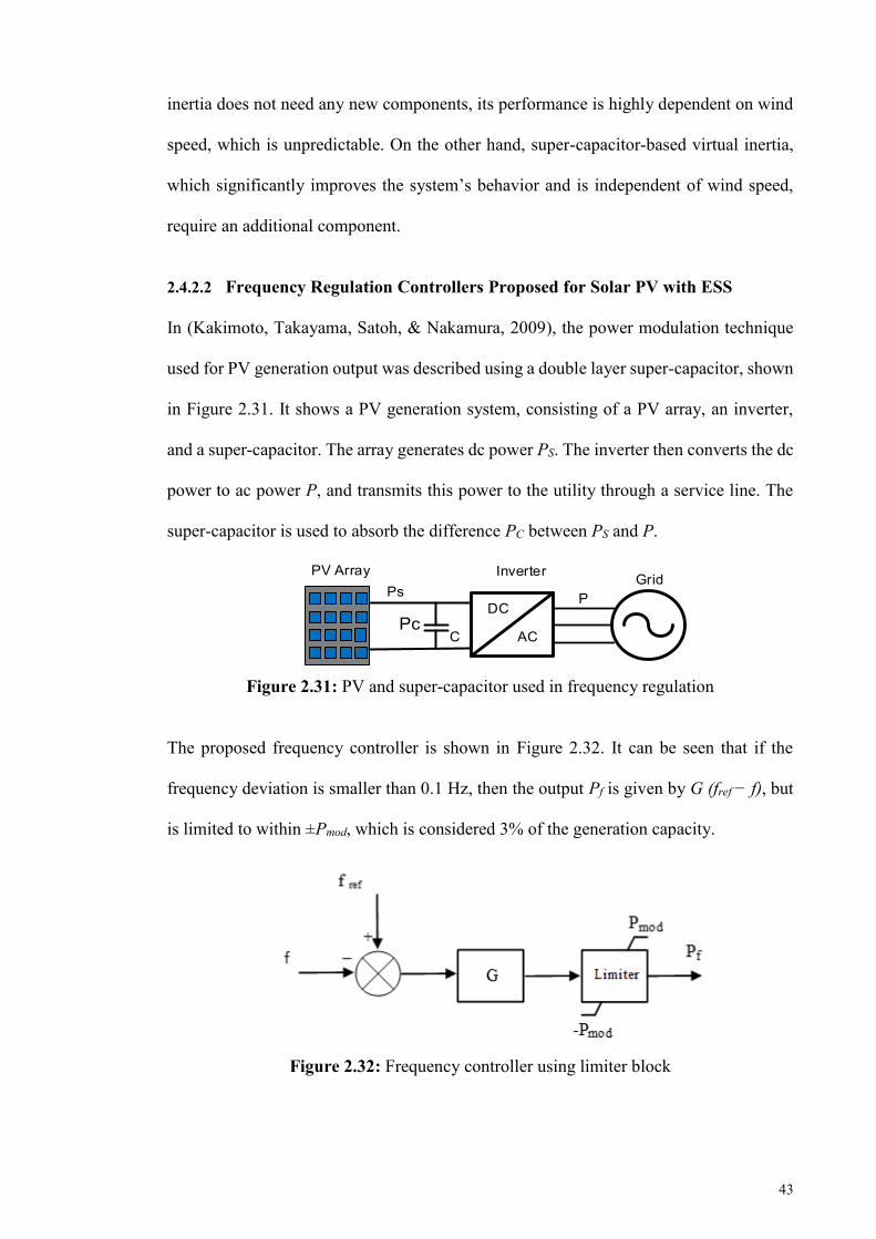
43
inertia does not need any new components, its performance is highly dependent on wind
speed, which is unpredictable. On the other hand, super-capacitor-based virtual inertia,
which significantly improves the system’s behavior and is independent of wind speed,
require an additional component.
2.4.2.2 Frequency Regulation Controllers Proposed for Solar PV with ESS
In (Kakimoto, Takayama, Satoh, & Nakamura, 2009), the power modulation technique
used for PV generation output was described using a double layer super-capacitor, shown
in Figure 2.31. It shows a PV generation system, consisting of a PV array, an inverter,
and a super-capacitor. The array generates dc power PS. The inverter then converts the dc
power to ac power P, and transmits this power to the utility through a service line. The
super-capacitor is used to absorb the difference PC between PS and P.
Grid
DC
AC
InverterPV ArrayPs
PcP
C
Figure 2.31: PV and super-capacitor used in frequency regulation
The proposed frequency controller is shown in Figure 2.32. It can be seen that if the
frequency deviation is smaller than 0.1 Hz, then the output Pf is given by G (fref − f), but
is limited to within ±Pmod, which is considered 3% of the generation capacity.
Figure 2.32: Frequency controller using limiter block
44
A frequency and voltage regulation technique using PV systems and Li-ion BSS coupled
to the grid was presented in (Bhatt & Chowdhury, 2011). This technique allows effective
control over the active and reactive power available from the system. Two approaches
were suggested in this work to allow the system to participate in frequency regulation;
the first was down-regulation, where the output power from the PV system and excess
power from the grid are absorbed by the storage battery, and the second was up-
regulation, where the PV/battery system injects active power into the grid. A proposed
system, comprising a 2 kW PV array, 2.64 kWh batteries with bi-directional dc-dc
converter, a three-phase inverter, and the grid, was modelled and simulated in MATLAB.
The results showed that the PV plant can respond quickly and participate in frequency
regulation.
Frequency regulation using a PV plant supported by an Battery Storage System (BSS)
was presented in (Chamana & Chowdhury, 2013). This paper proposed a comprehensive
control system using P-Q based droop control. This control system automatically
regulates the active and reactive power when the demand power exceeds the PV array
generation. However, when the power demanded by the grid is less than the PV array, the
inverter control switches to regulate the frequency and voltage based on active and
reactive set points. The output power from the PV system and battery SOC are included
in the proposed controller in order to make the best decision for frequency regulation.
Another research using the same principles of P-Q control for a microgrid with PV
generator and BSS was presented in (Adhikari & Li, 2014). This paper proposed the
smooth transition of the PV from P-Q control in the grid connected mode to V-f control
in the islanded mode. The proposed transition of solar PV to V-f control performed very
well in restoring voltage and frequency back to nominal values in a matter of only 2
seconds. The control strategy presented in this paper is operating the PV generator on
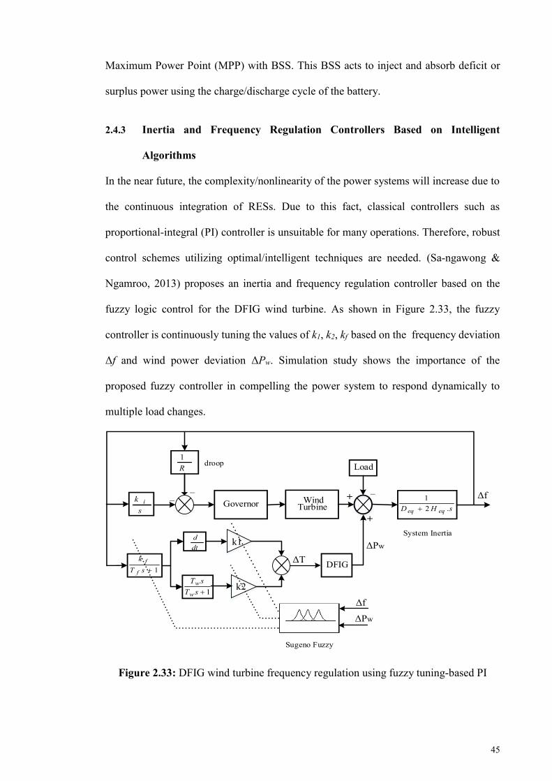
45
Maximum Power Point (MPP) with BSS. This BSS acts to inject and absorb deficit or
surplus power using the charge/discharge cycle of the battery.
2.4.3 Inertia and Frequency Regulation Controllers Based on Intelligent
Algorithms
In the near future, the complexity/nonlinearity of the power systems will increase due to
the continuous integration of RESs. Due to this fact, classical controllers such as
proportional-integral (PI) controller is unsuitable for many operations. Therefore, robust
control schemes utilizing optimal/intelligent techniques are needed. (Sa-ngawong &
Ngamroo, 2013) proposes an inertia and frequency regulation controller based on the
fuzzy logic control for the DFIG wind turbine. As shown in Figure 2.33, the fuzzy
controller is continuously tuning the values of k1, k2, kf based on the frequency deviation
Δf and wind power deviation ΔPw. Simulation study shows the importance of the
proposed fuzzy controller in compelling the power system to respond dynamically to
multiple load changes.
Figure 2.33: DFIG wind turbine frequency regulation using fuzzy tuning-based PI
_
Δf
ΔPw
Sugeno Fuzzy
Load
sHD eqeq .21
R1
Governor Wind Turbine
DFIG1sT
k
f
f
1sTsT
w
w
dtd
k2
k1
sk i
Δf
System Inertia
droop
ΔT
_
ΔPw
+
+_
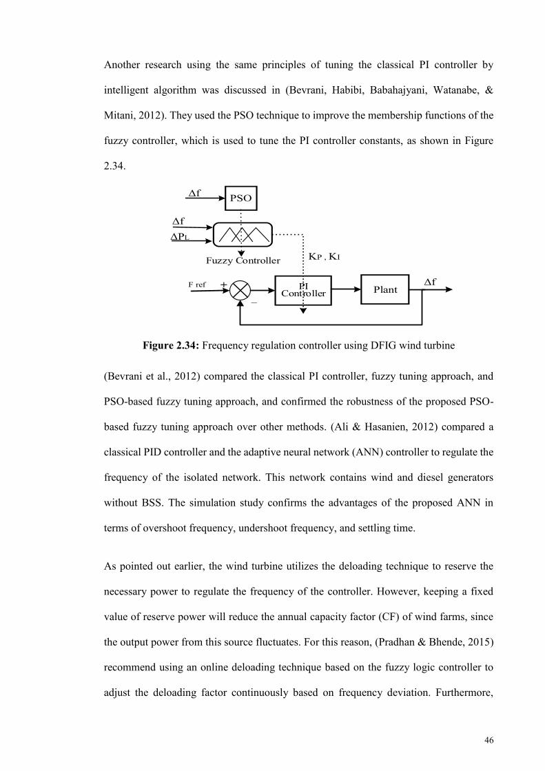
46
Another research using the same principles of tuning the classical PI controller by
intelligent algorithm was discussed in (Bevrani, Habibi, Babahajyani, Watanabe, &
Mitani, 2012). They used the PSO technique to improve the membership functions of the
fuzzy controller, which is used to tune the PI controller constants, as shown in Figure
2.34.
Figure 2.34: Frequency regulation controller using DFIG wind turbine
(Bevrani et al., 2012) compared the classical PI controller, fuzzy tuning approach, and
PSO-based fuzzy tuning approach, and confirmed the robustness of the proposed PSO-
based fuzzy tuning approach over other methods. (Ali & Hasanien, 2012) compared a
classical PID controller and the adaptive neural network (ANN) controller to regulate the
frequency of the isolated network. This network contains wind and diesel generators
without BSS. The simulation study confirms the advantages of the proposed ANN in
terms of overshoot frequency, undershoot frequency, and settling time.
As pointed out earlier, the wind turbine utilizes the deloading technique to reserve the
necessary power to regulate the frequency of the controller. However, keeping a fixed
value of reserve power will reduce the annual capacity factor (CF) of wind farms, since
the output power from this source fluctuates. For this reason, (Pradhan & Bhende, 2015)
recommend using an online deloading technique based on the fuzzy logic controller to
adjust the deloading factor continuously based on frequency deviation. Furthermore,
ΔPL
_PI
ControllerΔf
Plant
Δf PSO
Δf
KP , KI
F ref +
Fuzzy Controller
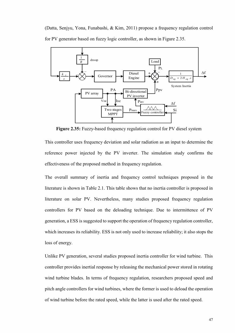
47
(Datta, Senjyu, Yona, Funabashi, & Kim, 2011) propose a frequency regulation control
for PV generator based on fuzzy logic controller, as shown in Figure 2.35.
Figure 2.35: Fuzzy-based frequency regulation control for PV diesel system
This controller uses frequency deviation and solar radiation as an input to determine the
reference power injected by the PV inverter. The simulation study confirms the
effectiveness of the proposed method in frequency regulation.
The overall summary of inertia and frequency control techniques proposed in the
literature is shown in Table 2.1. This table shows that no inertia controller is proposed in
literature on solar PV. Nevertheless, many studies proposed frequency regulation
controllers for PV based on the deloading technique. Due to intermittence of PV
generation, a ESS is suggested to support the operation of frequency regulation controller,
which increases its reliability. ESS is not only used to increase reliability; it also stops the
loss of energy.
Unlike PV generation, several studies proposed inertia controller for wind turbine. This
controller provides inertial response by releasing the mechanical power stored in rotating
wind turbine blades. In terms of frequency regulation, researchers proposed speed and
pitch angle controllers for wind turbines, where the former is used to deload the operation
of wind turbine before the rated speed, while the latter is used after the rated speed.
_
Δf
Si Fuzzy controller
Load
sHD eqeq .21
R1
Governor s
k iΔf
System Inertia
droop
_
Ppv
+
+_
PV array
PL
Pmax
Pinv
PA
Voc Isc
Bi-directional PV inverter
Diesel Engine
Two stages MPPT

48
Table 2.1: Summary of inertia and frequency regulation controllers proposed in the literature
Type of RESs
Issues of high penetration
level
Proposed technique
Proposed controller
References Reliability Power loss Time response The ability to
adapt according to different changes
Solar PV Frequency regulation issue Deloading
Voltage controller based on classical PI
(Rahmann & Castillo, 2014; Zarina et al.,
2012b) Low
Some power is
lost due to the
deloading technique
Fast response due to the electronic
converter
The controller does not adapt, instead, a classical PI is used without tuning
Voltage controller based on Intelligent Algorithm
tuning PI (Datta et al., 2011)
The controller adapts according to
the changes
Solar PV with ESS
Frequency regulation issue
Deloading + ESS
Voltage controller (PV) + Primary frequency
controller (ESS)
(Adhikari & Li, 2014; Bhatt & Chowdhury,
2011; Chamana & Chowdhury, 2013)
High reliability
due to ESS
No power loss
Fast response due to the electronic
converter
The controller does not adapt, instead, a classical PI is used without tuning
Variable
speed wind turbine
Reduced inertia response
Inertia response
controllers
Hidden inertia Emulation
(Gonzalez-Longatt et al., 2013; Morren, De
Haan, et al., 2006)
Low reliability
No power loss Fast response
Fast power reserve (Wachtel & Beekmann, 2009)
Frequency regulation Deloading
Speed control (Castro et al., 2012) Some
power is lost due to
the deloading technique
Fast response
Pitch control (Vidyanandan &
Senroy, 2013; Z.-S. Zhang et al., 2012)
Slow response due to mechanical
control
Speed control based on Intelligent Algorithm
tuning PI
(Sa-ngawong & Ngamroo, 2013) Fast response
The controller adapts according to
changes
Variable speed wind turbine with ESS
Frequency regulation
Deloading + ESS
Speed control + Primary frequency controller
(ESS)
(Díaz-González et al., 2015; Miao et al.,
2015)
High reliability
due to ESS
No power loss Fast response
The controller does not adapt, a classical PI is used without tuning

49
2.5 Load Shedding Techniques
As previously discussed, to ensure a successful transition from the grid connected mode
to the islanding mode, the frequency and voltage should be within their respective
permissible limits, or the distribution network could experience total blackouts (Vahedi
& Karrari, 2013). In this situation, the load shedding technique is necessary to prevent
total system blackout during frequency and voltage instability issues. In literature, several
load shedding techniques have been proposed for selecting the efficient and optimal
technique. Generally, load shedding techniques are classed into three main categories;
conventional, adaptive, and computational intelligence-based techniques.
2.5.1 Conventional Load Shedding Techniques
The conventional load shedding technique is commonly divided into two main categories;
under-voltage load shedding technique (UVLS) and under frequency load shedding
technique (UFLS).
2.5.1.1 Under Voltage Load Shedding (UVLS) Techniques
Under voltage load shedding techniques can be used to prevent voltage collapse in power
system. From studying major power blackouts, it can be clearly seen that most power
blackouts were caused by voltage instability problems (El-Sadek, 1998; Yusof et al.,
2017). Generally, voltage collapse occurs due to either tripping generator or overloading,
where the reactive power demand changes very quickly, and could cause a blackout if left
untreated. For this reason, power utilities typically utilize the UVLS technique to restore
power system voltage to its nominal value.
2.5.1.2 Under Frequency Load Shedding (UFLS) Techniques
Under frequency load shedding techniques are used to prevent frequency drop due to the
loss of generators or overloading, where the active power demand changes very quickly.
The UFLS relay is initialized to shed a fixed amount of load in predefined steps when the
50
frequency falls below a certain predefined threshold value (Tang, Liu, Ponci, & Monti,
2013). Generally, threshold values vary from one country to another, depending on the
power system requirements. An example of conventional under frequency load shedding
was reported in 1999 for the Malaysian power system (Zin, Hafiz, & Aziz, 2004). This
research proposed a 15-stage load shedding scheme to reflect 5600 MW generation loss.
Although this technique is low cost and simple, it is unable to shed the optimal load
because it does not estimate the actual amount of the power imbalance, which leads to
either over-shedding or under-shedding problems.
2.5.2 Adaptive Load Shedding Technique
The adaptive UFLS technique is advantageous as it uses the swing equation to estimate
the imbalance power. The power imbalance can be obtained using this equation:
∆𝑃 =2𝐻
𝑓×𝜕𝑓
𝜕𝑡 (2.16)
Where ∆P is the power imbalance; H is the Inertia constant of generator; f is the nominal
frequency (Hz); df/dt is the rate of change of frequency (Hz/s).
When the power system is exposed to disturbance such as faults or overloading, its
frequency and its associated rate of change drops quickly. Using these values in the power
swing equation will allow us to estimate the power imbalance. After doing so, the
adaptive load shedding technique shed the required amount of load in order to stabilize
the frequency.
Many adaptive UFLS techniques have been reported in literature. (Terzija, 2006) showed
that the adaptive UFLS technique shed less amount of load compared to its conventional
counterpart. However, this technique suffers from overshoot frequency, which means that
the amount of the shed load is not optimal.

51
Calculating the power imbalance using the frequency of the center of inertia was reported
by (Rudez & Mihalic, 2011). In their work, they proposed shedding lower amounts of
load from an islanded power system. The calculated imbalance power is distributed
among the different stages; for a large power imbalance, the author suggested using larger
steps prior to smaller ones. Two centralized adaptive algorithms were presented in
(Pasand & Seyedi, 2007). They proposed these algorithms to protect the power system
blackouts, following combinational disturbance by a combination of response-based and
event-based techniques. This load shedding technique was proposed to overcome the
improper imbalance power, as well as the slow response of under-frequency relays for
the conventional load shedding technique. To enhance the conventional UFLS technique
operation, (Marzband, Moghaddam, Akorede, & Khomeyrani, 2016; Saffarian & Sanaye-
Pasand, 2011) proposed an adaptive load shedding technique based on three
combinational factors. This technique utilizes ROCOF, disturbance location, and system
voltage status. The load priority of shedding load was determined according to the system
voltage, in other words, loads with high voltage will be shed first. In literature, the
adaptive UFLS techniques were based on fixed priority load shedding. Accordingly, load
shedding techniques suffer from surplus or insufficient loads being shed, which led to
total blackouts. To address this issue, (Laghari et al., 2015) proposed a new adaptive
UFLS technique with random and fixed priority loads. By using this feature, the UFLS
technique can shed the appropriate combination of loads. However, this technique takes
quite a while, which is unsuitable for fast frequency changes.
2.5.3 Computational Intelligence Based Load Shedding Techniques
Recently, the structure of power systems is becoming very complex due to the integration
of more distribution generation. In this situation, traditional load shedding techniques
cannot function efficiently in disturbance events. Thus, an efficient load shedding
technique is necessary to shed the optimal load and maintain power system stability. Since

52
the late 1980s, interest in using computational intelligence techniques in power systems
has increased. Accordingly, various load shedding technique based on computational
intelligence have been proposed. An ANN-based load shedding technique was proposed
by (Cheng-Ting Hsu, Chuang, & Chen, 2011). This technique considers the total
generation, total load demand, and frequency drop rate as inputs and the minimum amount
of load shedding as an output. They did a comparative study to show that the proposed
load shedding is faster than the conventional technique. Other applications of ANN for
shedding the optimal load in the isolated power system are reported by (Hooshmand &
Moazzami, 2012). They use a 39-bus New England power system to verify the operation
of this technique. From the simulation results, it can be clearly seen that the proposed
technique can stabilize the power system by shedding the optimal load. To increase the
reliability of Taiwan’s power system, an ANN-based load shedding technique was
proposed in (C-T Hsu, Kang, & Chen, 2005). The simulation results showed that the
proposed technique can shed the exact amount of load, making it suitable for real-time
applications. (Javadian, Haghifam, Bathaee, & Firoozabad, 2013) proposed an ANN-
based load shedding technique to protect the DG-based distribution network from severe
faults and disturbances. They split the distribution network into several zones, each of it
capable of operating in islanding mode. Despite the advantages of ANN over
conventional techniques, research has proven that ANN will not give accurate results for
cases not included in the training process.
(Sallam & Khafaga, 2002) proposed a new fuzzy UFLS technique for islanded micro-
grid. This technique is dynamic and robust in regulating frequencies in different cases.
Using the fuzzy logic application to prevent the voltage collapse by shedding the optimal
load is reported by (Sasikala & Ramaswamy, 2011). It was verified on IEEE 14, 30, and
57-bus systems. The simulation results confirmed that the proposed technique can be
successfully implemented on a system of any size. (Mokhlis, Laghari, Bakar, & Karimi,
53
2012) proposed a new fuzzy logic based UFLS technique for islanded distribution
network that is able to restore the frequency as soon as possible. It uses frequency, the
rate of change of frequency, and load priority to do this.
The GA is also applicable in some load shedding problems. (Sanaye-Pasand &
Davarpanah, 2005) proposed a genetic algorithm application for load shedding technique.
It was verified on an IEEE 30-bus system. Another GA-based load shedding technique to
minimize the amount of load shed is proposed in (Chen et al., 2011). A comparative
simulation study between the proposed and conventional techniques was performed to
confirm the ability of GA-based technique in shedding optimal loads.
Furthermore, an optimal load shedding technique based on the PSO method is reported
by (Amraee, Mozafari, & Ranjbar, 2006) to determine the maximum loading point. The
technique was verified on an IEEE 14-bus system. A comparative simulation study
between PSO and GA methods was also performed, and it was clearly shown that the
UFLS technique based on the PSO method can find the optimal solution more quickly
compared with genetic algorithm method. (Sadati, Amraee, & Ranjbar, 2009) is another
research involving the usage of a particle swarm-based-simulated annealing optimization
method to provide long-term voltage stability. The most important feature of the proposed
method is its capability to determine the global optimum solution within a smaller number
of iterations. (Ketabi & Fini, 2017) proposed an UFLS technique based on the forecast of
the minimum frequency. In this technique, the system frequency samples are taken after
disturbance; then, PSO method is used to forecast the minimum frequency and shed the
required loads.
The overall summary of inertia and frequency control techniques proposed in literature is
shown in Table 2.2. It can be seen that the conventional, adaptive, and computational
intelligence UFLS techniques have over-shedding or under-shedding problems. In fact,

54
these problems occur due to the fixed priority shedding loads. For this reason, (Laghari
et al., 2015) proposed a Fixed and Random Priority Load Shedding (FRPLS) technique
to shed the optimal combination of loads. However, this technique need time to select the
optimal combination of shedding loads.
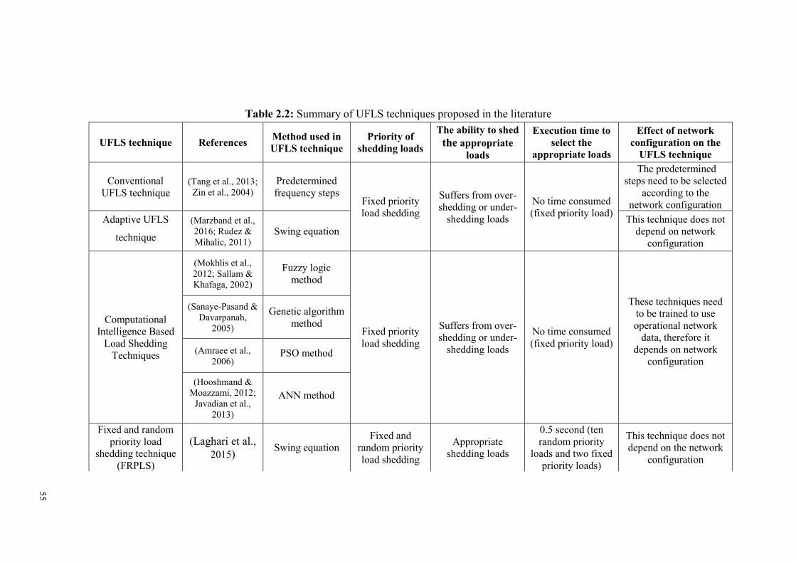
55
Table 2.2: Summary of UFLS techniques proposed in the literature
UFLS technique References Method used in UFLS technique
Priority of shedding loads
The ability to shed the appropriate
loads
Execution time to select the
appropriate loads
Effect of network configuration on the
UFLS technique
Conventional UFLS technique
(Tang et al., 2013; Zin et al., 2004)
Predetermined frequency steps
Fixed priority load shedding
Suffers from over-shedding or under-
shedding loads
No time consumed (fixed priority load)
The predetermined steps need to be selected
according to the network configuration
Adaptive UFLS
technique
(Marzband et al., 2016; Rudez & Mihalic, 2011)
Swing equation This technique does not
depend on network configuration
Computational Intelligence Based
Load Shedding Techniques
(Mokhlis et al., 2012; Sallam & Khafaga, 2002)
Fuzzy logic method
Fixed priority load shedding
Suffers from over-shedding or under-
shedding loads
No time consumed (fixed priority load)
These techniques need to be trained to use operational network
data, therefore it depends on network
configuration
(Sanaye-Pasand & Davarpanah,
2005)
Genetic algorithm method
(Amraee et al., 2006)
PSO method
(Hooshmand & Moazzami, 2012;
Javadian et al., 2013)
ANN method
Fixed and random priority load
shedding technique (FRPLS)
(Laghari et al., 2015)
Swing equation Fixed and
random priority load shedding
Appropriate shedding loads
0.5 second (ten random priority
loads and two fixed priority loads)
This technique does not depend on the network
configuration
56
2.6 Summary
This chapter provided an overview of distributed generation, detailing various types,
global, and local trends of hydropower and solar PV. The major topic addressed
throughout this chapter is the frequency issues experienced in islanded distribution
network due to the high penetration level of RESs. To overcome these issues, various
inertia and frequency regulation controllers were developed for RESs.
Based on literature, it was observed that most of existing inertia controller proposed to
increase the inertia of the distribution networks using only wind turbine technology and
ESS. Furthermore, most frequency regulation controllers may be ineffective for islanded
distribution systems, as islanded system is not as stable as grid-connected system.
Therefore, many researchers proposed the usage of batteries to provide a stable energy
reserve for frequency regulation services. However, most of these techniques used a
battery to provide primary frequency controller without taking into account the secondary
controller. In addition, this chapter presented several types of load shedding technique. It
can be seen that the existing load shedding techniques experience an over-shedding
problem due to fixed priority shedding loads. Thus, this research will propose a new
UFLS technique for shedding optimal combination of loads.

57
CHAPTER 3: RESEARCH METHODOLOGY
3.1 Introduction
This chapter details the modelling of the proposed frequency control scheme using
PSCAD and MATLAB software. This scheme consists of the inertia controller, frequency
regulation controllers, and UFLS controller. This chapter discusses the modelling of
Centralized Control System (CCS), which is used to coordinate the operation of frequency
control scheme and grid reconnection process. It consists of a reconnection controller, the
frequency management unit, and UFLS controller.
3.2 Overview of the Overall Proposed System
This research proposes a frequency control scheme for islanded distribution network with
high PV penetration. Figure 3.1 shows the interaction between (A) distribution network,
(B) proposed frequency control scheme, (C) Centralized Control System, (D) Phase
synchronization controller, and (E) Voltage synchronization controller. Each part will be
discussed in the following sub-sections.
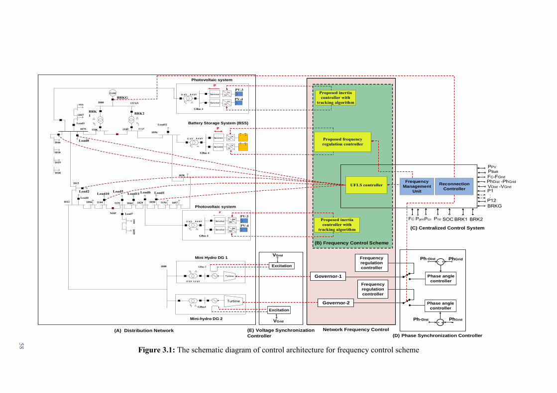
58
Figure 3.1: The schematic diagram of control architecture for frequency control scheme
Excitation
Excitation
SOCFC PgridPG1 PG2
PPVPBatt
BRK1 BRK2
BRKG
Network Frequency Control
(C) Centralized Control System
Reconnection
Controller
Frequency
Management
Unit
FC-FGrid PhDist -PhGrid VDist -VGrid P1
P12..
Phase angle
controller
Phase angle
controller
VGrid
VGrid
(D) Phase Synchronization Controller
(E) Voltage Synchronization
Controller
Ph-Dist
+- PhGrid
+- PhGridPh-Dist
Load9
PV-3
PV-4
GBus 4
0.4 kV11 kV DCDC
DCDCInverter
P
GBus 4
0.4 kV11 kV DCDC
DCDCInverter
+-
+-
Inverter
Inverter
P
PV-3
PV-4
GBus 4
0.4 kV11 kV DCDC
DCDCInverter
P
Inverter
Photovoltaic system
1012
1013
1075
2000
Grid
1004 1144 1151 1044 1029 1050 1154 1057
NOP
10391010
1058
1056
1047
1026
1046
1018
1019
1020
132 kV
11 kV1106 1105
Load4Load10
Load5
Load7
Load11 Load6 Load1Load2
Load8
Load3
BRKG
BRK1 BRK2
Load12
Mini-hydro DG 2
1000
Mini Hydro DG 1
GBus1
GBus 2
11 kV 3.3 kV
Turbine
Turbine
Governor-2
Governor-1
Frequency
regulation
controller
Frequency
regulation
controller
UFLS controller
Proposed inertia controller with
tracking algorithm
Proposed frequency regulation controller
Proposed inertia controller with
tracking algorithm
(B) Frequency Control Scheme
(A) Distribution Network
Photovoltaic system
Battery Storage System (BSS)
59
3.2.1 Proposed Frequency Control Scheme
The frequency control scheme proposed in this thesis is developed for distribution
networks with high PV penetration. After the distribution network is islanded from the
main grid, the frequency control scheme can be used to restore the network’s frequency.
As shown in Figure 3.1 b), the frequency control scheme consists of an inertia controller,
frequency regulation controllers, and under-frequency load shedding controller. The
operation of frequency control scheme is discussed below.
Immediately after islanding, the inertia controllers start releasing reserve power from
PV units to improve the overall network inertial response and reduce the rate of change
of frequency. After 10 seconds, a primary frequency controller of Battery Storage System
(BSS) is initiated in the parallel with governor system of mini-hydro governors to stop
the frequency deviation and restore it within an acceptable level. After that, a secondary
frequency controller of BSS is used to offset the frequency deviation by synchronizing
the frequency of islanding distribution network with the main grid; this controller is
necessary for the reconnection operation. According to Malaysian grid code, the
secondary controller starts after 30 seconds, and continue for 30 minutes. When the
proposed inertia and frequency regulation controllers fail to recover the system’s
frequency, a proposed UFLS controller activates to shed the optimal combination of
loads. Since the formation of an island operation is only temporary, a reconnection
process with main grid is necessary. When the synchronization requirements (frequency,
voltage, and phase) are achieved, the islanded network is reconnected with the main grid.
3.2.1.1 Inertia Controller
The solar PV arrays normally work on the maximum power point. Therefore, integrating
more PV units will reduce the inertia response, which leads to increased rate of change
of frequency. Therefore, it necessary to operate the solar PV below the maximum power

60
point to keep some amount of reserve power that can be released at disturbance events.
The main parts of inertia controller are shown in Figure 3.2. It consists of de-loading
process, inertia response, and PV voltage controller. The parameters of the inertia
controller are included in Appendix A, section A.9.
Figure 3.2: Block diagram of inertia controller
Like most inertia controllers applied in a variable speed wind turbine, the PV generation
can operate below their maximum power point to maintain power reserves required for
an inertial response, which can be achieved by increasing the PV voltage. In this block
diagram, the deloading voltage (Vdel) is calculated by adding a specific value ΔV to the
maximum power point voltage (VMPP), as expressed in Equation 3.1.
𝑉𝑑𝑒𝑙 = 𝑉𝑀𝑃𝑃 + ∆𝑉 (3.1)
Where ΔV is a specific value determined by a special tracking algorithm as shown in
Figure 3.3, and VMPP is the maximum power point voltage calculated using open circuit
voltage technique (OCV), as per equation 3.2:
𝑉𝑀𝑃𝑃 = 𝐾 × 𝑉𝑂𝐶 (3.2)
Where VOC is the open circuit voltage of reference module, and K is a constant estimated
to be within the range of (0.7–0.80) (Zhou et al., 2010).
Solar PV Array Terminal Voltage Controller
fs
VMPP
ΔV
dfs/dt
deloading Block
Inertia Response
D -
F
+A
B Compar-ator
++
+ - T1
*2 HPVG
1 + sT
I
P
VPV
sT | X |
VRefEquation
3.2
f0
VdelVoc
Special tracking
algorithm

61
As shown in Figure 3.3, special tracking algorithm is used to track the PV generation unit
below the Maximum Power Point (MPP) based on the deloading factor (X%). A fixed
value of deloading factor is set in this research.
Figure 3.3: Block diagram of special tracking algorithm
Figure 3.4 is used to illustrate the operation of inertia controller and de-loading technique
of PV generation, which represents the relationship between PV voltage and power,
Pdeload =X% * Pmax
Measure the output power from the PV unit (Pmax) and
restore it
Set ΔV= zero
VMPP=K*VOC
Measure VOC from the reference PV module
P =? Pdeload
ΔV= ΔV+0.05
Measure the output power from the PV unit (P)
Yes
Send ΔV
No
Start
End
Delay (10s)
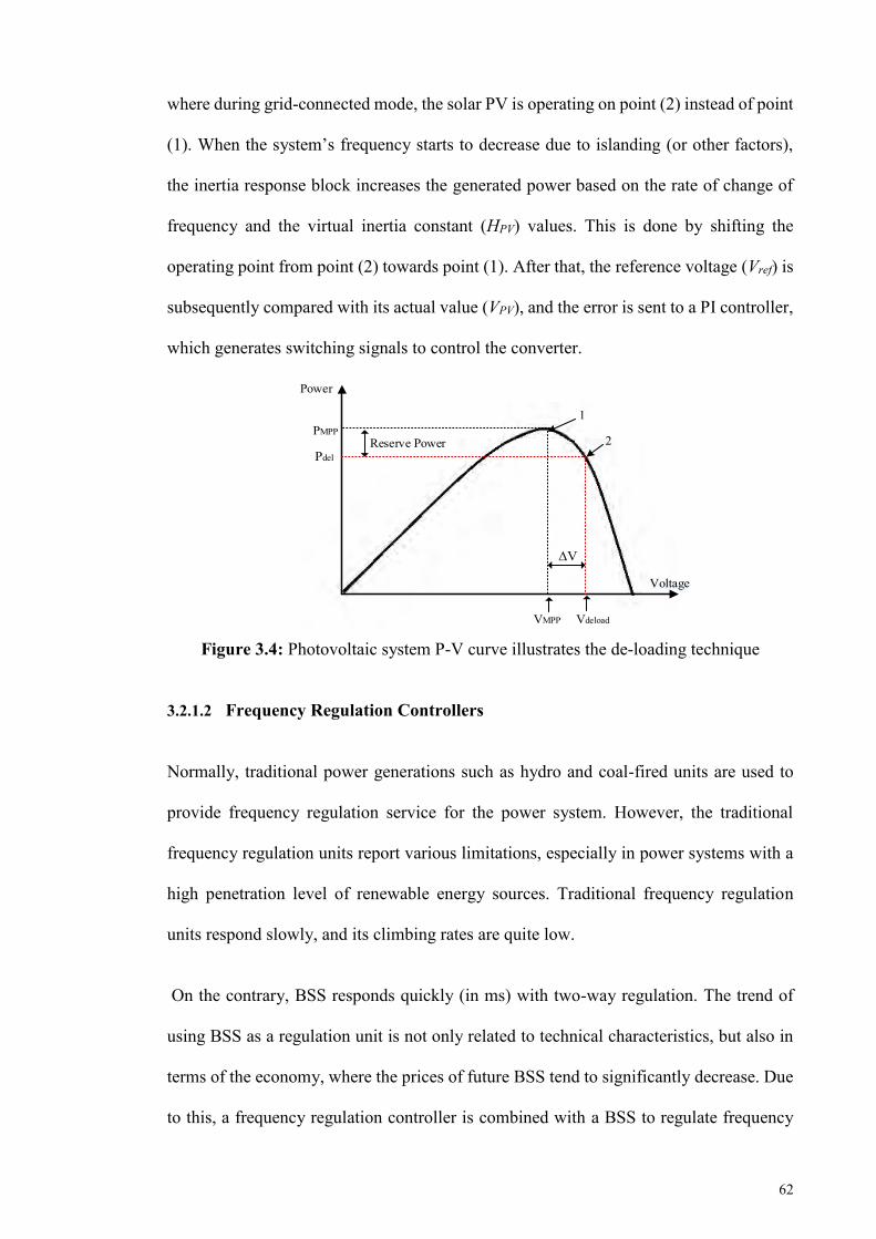
62
where during grid-connected mode, the solar PV is operating on point (2) instead of point
(1). When the system’s frequency starts to decrease due to islanding (or other factors),
the inertia response block increases the generated power based on the rate of change of
frequency and the virtual inertia constant (HPV) values. This is done by shifting the
operating point from point (2) towards point (1). After that, the reference voltage (Vref) is
subsequently compared with its actual value (VPV), and the error is sent to a PI controller,
which generates switching signals to control the converter.
Figure 3.4: Photovoltaic system P-V curve illustrates the de-loading technique
3.2.1.2 Frequency Regulation Controllers
Normally, traditional power generations such as hydro and coal-fired units are used to
provide frequency regulation service for the power system. However, the traditional
frequency regulation units report various limitations, especially in power systems with a
high penetration level of renewable energy sources. Traditional frequency regulation
units respond slowly, and its climbing rates are quite low.
On the contrary, BSS responds quickly (in ms) with two-way regulation. The trend of
using BSS as a regulation unit is not only related to technical characteristics, but also in
terms of the economy, where the prices of future BSS tend to significantly decrease. Due
to this, a frequency regulation controller is combined with a BSS to regulate frequency
Power
PMPP
VMPP Vdeload
1
2Pdel
Voltage
Reserve Power
ΔV
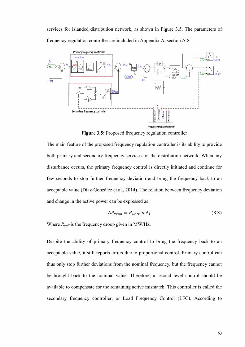
63
services for islanded distribution network, as shown in Figure 3.5. The parameters of
frequency regulation controller are included in Appendix A, section A.8.
Figure 3.5: Proposed frequency regulation controller
The main feature of the proposed frequency regulation controller is its ability to provide
both primary and secondary frequency services for the distribution network. When any
disturbance occurs, the primary frequency control is directly initiated and continue for
few seconds to stop further frequency deviation and bring the frequency back to an
acceptable value (Díaz-González et al., 2014). The relation between frequency deviation
and change in the active power can be expressed as:
∆𝑃𝑃𝑟𝑖𝑚 = 𝑅𝐵𝑎𝑡𝑡 × ∆𝑓 (3.3)
Where RBatt is the frequency droop given in MW/Hz.
Despite the ability of primary frequency control to bring the frequency back to an
acceptable value, it still reports errors due to proportional control. Primary control can
thus only stop further deviations from the nominal frequency, but the frequency cannot
be brought back to the nominal value. Therefore, a second level control should be
available to compensate for the remaining active mismatch. This controller is called the
secondary frequency controller, or Load Frequency Control (LFC). According to
I
P
ILb
Compar-ator
+ -
N
D
N/D
FC1
50.0 +-
ILRef
Vbat
PRef-
P
+Δf
ΔPSec
ΔPPri
f0
Primary frequency controller
Secondary frequency controller
50.02
49.98f
P
dead band
0.5
0.5
1
𝑅𝐵𝑎𝑡𝑡
0.5
0.5I
+-
1
0
0
Boost
Buck
Dis
char
ge
Cha
rge
Dis
con
nect
Frequency Management Unit
Sec
ond
ary
SW

64
Malaysian grid code, the LFC starts after 30 seconds, and return the frequency to its
nominal value within 30 minutes.
As shown in Figure 3.4, the summation of primary and decentralized secondary frequency
controller output is divided by battery voltage to determine the reference current. The
reference current is then injected to the PI controller, which provide suitable control
signals required for charging and discharging the battery via a bidirectional DC-DC
converter. Two BSS were used in this work, where each can provide 0.5 MW for primary
frequency control and 0.5 MW for secondary frequency control. A frequency
management unit was developed to control the BSS.
3.2.1.3 Proposed UFLS Technique
From the literature, it is clear that the existing UFLS techniques are limited by over-
shedding or under-shedding loads, due to fixed load priorities. Therefore, a Fixed and
Random Priority Load shedding (FRPLS) technique is proposed in (Laghari et al., 2015)
for shedding the optimal combination of loads. However, this technique takes too long,
since all possible combination of loads needs to be accounted for in the calculations. Due
to this fact, we used three metaheuristic methods with the UFLS technique to shed the
optimal combination of loads from islanded distribution network; Binary Genetic
Algorithm (BGA) method, Binary Particle Swarm Optimization (BPSO) method, and
Binary Evolutionary Programming (BEP) method.
The most important advantages of the proposed load shedding technique are (A) it is
designed to shed the optimal combination of loads for under frequency events, and (B) it
is designed to restore the distribution network frequency after it gets islanded. In this
technique, the application of metaheuristic methods is used to select the optimal
combination of loads needed to be shed from ten-random priority loads and two-fixed
priority loads.
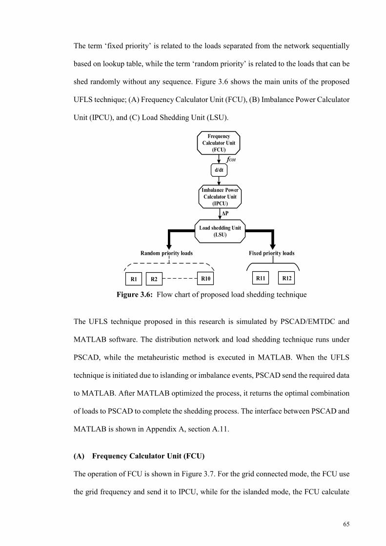
65
The term ‘fixed priority’ is related to the loads separated from the network sequentially
based on lookup table, while the term ‘random priority’ is related to the loads that can be
shed randomly without any sequence. Figure 3.6 shows the main units of the proposed
UFLS technique; (A) Frequency Calculator Unit (FCU), (B) Imbalance Power Calculator
Unit (IPCU), and (C) Load Shedding Unit (LSU).
Figure 3.6: Flow chart of proposed load shedding technique
The UFLS technique proposed in this research is simulated by PSCAD/EMTDC and
MATLAB software. The distribution network and load shedding technique runs under
PSCAD, while the metaheuristic method is executed in MATLAB. When the UFLS
technique is initiated due to islanding or imbalance events, PSCAD send the required data
to MATLAB. After MATLAB optimized the process, it returns the optimal combination
of loads to PSCAD to complete the shedding process. The interface between PSCAD and
MATLAB is shown in Appendix A, section A.11.
(A) Frequency Calculator Unit (FCU)
The operation of FCU is shown in Figure 3.7. For the grid connected mode, the FCU use
the grid frequency and send it to IPCU, while for the islanded mode, the FCU calculate
Frequency Calculator Unit
(FCU)
Imbalance Power Calculator Unit
(IPCU)
d/dt
fCOI
Load shedding Unit (LSU)
R1 R2 R11 R12R10
ΔP
Random priority loads Fixed priority loads

66
the value of fCOI based on Equation (3.4) (Terzija, 2006) and send it to IPCU. Furthermore,
at every moment of time, the FCU checks the connection state of each generator. When
any disconnection event occurs, a new equivalent value of fCOI will be calculated.
𝑓𝐶𝑂𝐼 =∑ 𝐻𝑖𝑁𝑖=1 𝑓𝑖∑ 𝐻𝑖𝑁𝑖=1
(3.4)
Where fCOI is center of inertia frequency (Hz); Hi is inertia constant of each generator
(seconds); fi is the frequency of each generator (Hz); N is the number of DGs.
Figure 3.7: Flow chart of FCU
Start
Send Frequency to IPCU
End
Send grid frequency to IPCU
Grid islanded ?
Yes
No
H1 = f1 = 0
Measure f1, f2, …, fgrid
No
No
...
YesNo
∑∑N
ii
N
iiiCOI HfHf
1=1=
/=
H2 = f2 = 0Yes
HN = fN = 0Yes
Generator 1 is disconnected?
Generator 2 is disconnected?
Generator N is disconnected?
maxmin ≤≤ fff COI
Trip all generators
67
Besides frequency calculation, FCU provides a type of frequency protection for
connected generators. It will check whether the value of fCOI lies within the frequency
protection range. If the value of fCOI lies beyond that range, the protection relays will
directly disconnect the generators from the network. Generally, the frequency protection
range for each generator are based on the distribution network and generator types.
According to the Malaysian distribution code, the protection frequency range is (47.5Hz
– 52.5Hz). The PSCAD model of FCU is shown in Appendix A, section A.3.
(B) Imbalance Power Calculator Unit (IPCU)
Depending on the value of ROCOF received from FCU and breaker state of grid and DGs,
the IPCU has two different strategies to determine the imbalance power, which are:
i Event Based
In this work, the IPCU algorithm is designed to follow the event based in three cases: (A)
intentional islanding; (B) DG tripping; (C) irradiance change. For the islanding event, the
imbalance power will be equal to the grid power, which is supplied to the distribution
network. For the DG tripping event, the power imbalance will be equal to the output
power of DG tripped from the network, while for irradiance change, the imbalance power
will be calculated based on Equation (3.5):
∆𝑃 = 𝑃𝑉0 − 𝑃𝑉 (3.5)
Where Pv0 is the total PV power at the radiation change event, and Pv is the total PV power
at 0.01 ms after radiation changing event.
ii Response Based
Response based occurs due to the sudden increment of load demand in the islanded
distribution network. In this case, the load shedding amount is based on the disturbance
value that can be estimated by the swing equation (Kundur et al., 1994)

68
∆𝑃 = ((2 ×∑𝐻𝑖𝑓𝑛
𝑁
𝑖=1
) ×𝑑𝑓𝐶𝑂𝐼𝑑𝑡
) (3.6)
Where ΔP is the imbalance power; Hi is the inertia constant of each generator (s); dfCOI/dt
is the rate of change of center of inertia frequency (Hz/s); N is the number of rotating
based DG; fn is the nominal frequency (Hz). In order to determine the amount of load to
be shed for event or response based strategies, the same equation will be followed:
𝐿𝑜𝑎𝑑 𝑠ℎ𝑒𝑑𝑑𝑖𝑛𝑔 𝑎𝑚𝑜𝑢𝑛𝑡 = ∆𝑃 − 𝑇𝑅 (3.7)
Where the TR is the total reserve power, and can be calculated by Equation (3.8).
𝑇𝑅 =∑𝑀𝑎𝑥. 𝑃𝐺𝑖
𝑁
𝑖=1
− ∑𝑃𝐺𝑖
𝑁
𝑖=1
(3.8)
Where Max PGi is the maximum generator power of ith DG; PGi is the generator power of
ith DG; N is the number of DGs. Finally, the PICM send the load-shed amount to the LSU
via a communication link to shed the optimal load combination. The PSCAD model of
IPCU is shown in Appendix A, section A.4.
(C) Load Shedding Unit (LSU)
The LSU is the most important part of the proposed UFLS technique. It reports the
preference of the proposed technique over existing techniques. As shown in Figure 3.8,
when the load shedding value exceeds the total random priority loads, the LSU directly
shed all random priority loads and start shedding from fixed priority loads. Otherwise,
one metaheuristic method is initialized to shed the optimal combination of loads. Since
the PSCAD//EMTDC software does not provide a toolbox for metaheuristic methods, the
proposed UFLS technique is modelled in MATLAB and integrated with PSCAD. The
PSCAD model of the FCU is shown in Appendix A, section A.5.

69
Figure 3.8: Flow chart of the LSU
i Implementation of Binary Evolutionary Programming (BEP)
For the past two decades, the interest in solving real-world search problems by Stochastic
optimization techniques and metaheuristic methods has invariably increased. These
methods use some biological principles to search for the best solutions. The Evolutionary
Programming (EP) method is regarded as a special case of Evolutionary Computation
(EC) methods, which was first utilized by Dr. Fogel in 1960.
It is proposed that a BEP method be used to determine the optimal combination of loads
that needs to be shed from the distribution network, as shown in Figure 3.9. Similar to
other evolutionary methods, the BEP is made up of five phases; initialization, fitness,
mutation, recombination, and selection.
Start
Yes
End
ΔP<=0
i = i + 1
Yes
No
Load shed amount > = Total random priority
loads ?
Shed ith fixed priority load
Shed all random priority loads
Receive the load shed amount and the values of random and fixed priority loads
i = 1i <= M (no. of Fixed
Priority loads)
Select the optimal combination of the random priority loads
Shed the optimal load combination
Activate the EP algorithm
No

70
Figure 3.9: Flow chart of BEP method
➢ Initialization
In this phase, an initial population of (xi) chromosomes will be randomly generated, as
shown in Table 3.1, where each chromosome represents the connection status of 10
random priority loads. Figure 3.10 shows the random and fixed priority loads connection
with the distribution network.
Figure 3.10: LSU connected with fixed and random priority loads
Offsprings (N=20)
Fitness
Initial Population(N=20)
1234
20
Combine(N=40)
Termination condition?
Sort and select best 20
Optimum solution
Yes
No
New Population
.
1100101010110111100111000100011010101011
1000010111
.
..
Mutation
Parents
1
2
3
4
20
.
1100101010
1101111001
1100010001
1010101011
1000010111
.
..
Load-10.044 MW
Load-20.069 MW
Load-30.15 MW
Load-40.314 MW
Load-50.435 MW
Load-60.520 MW
Load-70.583 MW
Load-80.645 MW
Load-90.760 MW
Load-100.119 MW
Load-110.420
Load-120.210
R1
R2
R3
R5
R6
R7
R8
R9
R10
R11
R12
Distribution Network
R4
Fixed priority loads
Random priority loads
LSU
R1
R2
R3
R4
R5
R6
R7
R8
R9
R10
R11
R12
1/0
1/0
1/0
1/0
1/0
1/0
1/0
1/0
1/0
1/0
1/0
1/0
Load shedding amount
P1
P2
P3
P4
P5P6P7P8
P9P10P11P12

71
➢ Fitness
This phase involves calculating the fitness value for each chromosome using the fitness
function:
𝑓𝑖 = 𝑀𝑖𝑛(𝐸𝑖) = |𝐿𝑜𝑎𝑑 𝑠ℎ𝑒𝑑 𝑎𝑚𝑜𝑢𝑛𝑡 −∑𝑃𝑖−𝑐𝑜𝑚𝑏𝑖𝑛𝑎𝑡𝑖𝑜𝑛| (3.9)
Where ∑Pi-combination is the summation of loads power for each chromosome.
To illustrate the calculation of fitness values, an example of 1 MW load shedding amount
is considered, as shown in Table 3.1, where the number 1 means that the load is connected
to the distribution network, while the number 0 means that the load is separated from the
distribution network.
Table 3.1: The initial population and fitness values for individual
xi xi10 xi9 xi8 xi7 xi6 xi5 xi4 xi3 xi2 xi1 ∑ Pi-combination (MW) (fi)
(MW) x1 1 1 0 1 0 1 0 1 0 1 P1+P3+P5+P7+P9+P10=2.091 1.091 x2 0 1 0 1 0 1 0 1 1 1 P1+P2+ P3+ P5+ P7+P9=2.041 1.041 x3 0 0 0 0 1 0 0 1 1 1 P1+P2+ P3+ P6=0.783 0.217 x4 0 0 0 1 1 0 0 0 1 0 P2+P6+ P7=1.172 0.172 - - - - - - - - - - - - x20 0 0 0 0 0 1 1 1 1 1 P1+P2+ P3 +P4+P5=1.012 0.012
➢ Mutation
The mutation is an operator used to avoid the local optima by preventing the generations
from becoming similar to one another. In this phase, one bit in each chromosome is
checked for possible mutation, as shown in Table 3.2 (Aman, Jasmon, Naidu, Bakar, &
Mokhlis, 2013). This is done by generating a random number in the range of (0-1), and if
this number is less than or equal to the mutation probability L, then the bit state will be
changed. The probability of a mutation for each bit is 1/L, where L is the number of bit
in each chromosome.
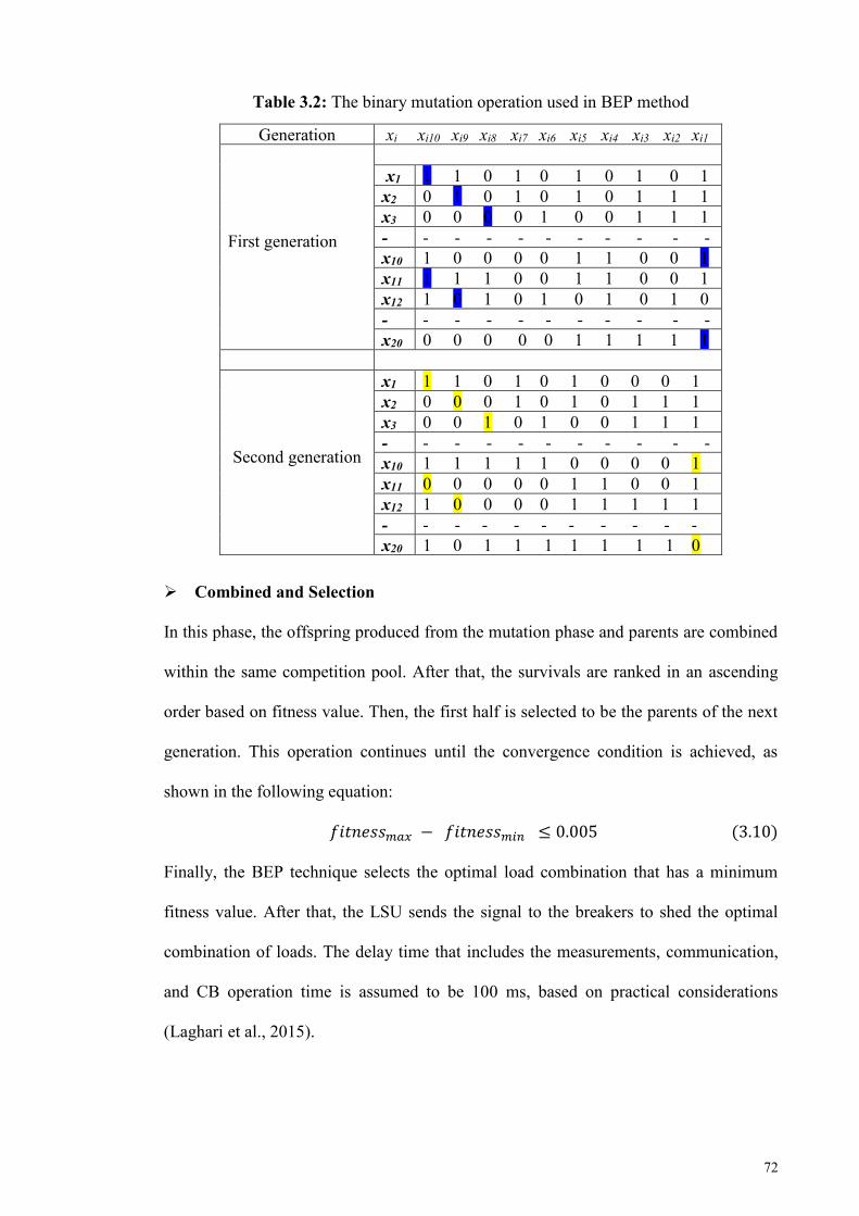
72
Table 3.2: The binary mutation operation used in BEP method
➢ Combined and Selection
In this phase, the offspring produced from the mutation phase and parents are combined
within the same competition pool. After that, the survivals are ranked in an ascending
order based on fitness value. Then, the first half is selected to be the parents of the next
generation. This operation continues until the convergence condition is achieved, as
shown in the following equation:
𝑓𝑖𝑡𝑛𝑒𝑠𝑠𝑚𝑎𝑥 − 𝑓𝑖𝑡𝑛𝑒𝑠𝑠𝑚𝑖𝑛 ≤ 0.005 (3.10)
Finally, the BEP technique selects the optimal load combination that has a minimum
fitness value. After that, the LSU sends the signal to the breakers to shed the optimal
combination of loads. The delay time that includes the measurements, communication,
and CB operation time is assumed to be 100 ms, based on practical considerations
(Laghari et al., 2015).
Generation xi xi10 xi9 xi8 xi7 xi6 xi5 xi4 xi3 xi2 xi1
First generation
x1 1 1 0 1 0 1 0 1 0 1 x2 0 1 0 1 0 1 0 1 1 1 x3 0 0 0 0 1 0 0 1 1 1 - - - - - - - - - - - x10 1 0 0 0 0 1 1 0 0 1 x11 1 1 1 0 0 1 1 0 0 1 x12 1 0 1 0 1 0 1 0 1 0 - - - - - - - - - - - x20 0 0 0 0 0 1 1 1 1 1
Second generation
x1 1 1 0 1 0 1 0 0 0 1 x2 0 0 0 1 0 1 0 1 1 1 x3 0 0 1 0 1 0 0 1 1 1 - - - - - - - - - - - x10 1 1 1 1 1 0 0 0 0 1 x11 0 0 0 0 0 1 1 0 0 1 x12 1 0 0 0 0 1 1 1 1 1 - - - - - - - - - - - x20 1 0 1 1 1 1 1 1 1 0
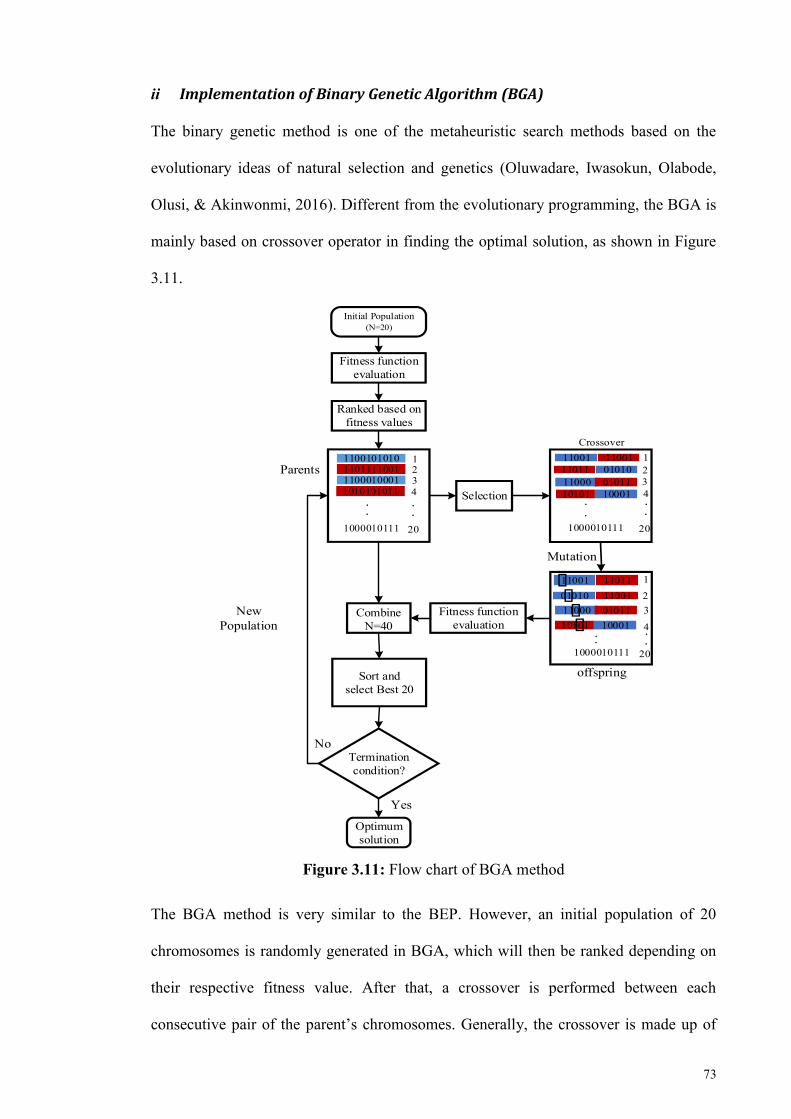
73
ii Implementation of Binary Genetic Algorithm (BGA)
The binary genetic method is one of the metaheuristic search methods based on the
evolutionary ideas of natural selection and genetics (Oluwadare, Iwasokun, Olabode,
Olusi, & Akinwonmi, 2016). Different from the evolutionary programming, the BGA is
mainly based on crossover operator in finding the optimal solution, as shown in Figure
3.11.
Figure 3.11: Flow chart of BGA method
The BGA method is very similar to the BEP. However, an initial population of 20
chromosomes is randomly generated in BGA, which will then be ranked depending on
their respective fitness value. After that, a crossover is performed between each
consecutive pair of the parent’s chromosomes. Generally, the crossover is made up of
Initial Population(N=20)
1234
20 1000010111
Combine N=40
Termination condition?
Sort andselect Best 20
Optimum solution
Yes
No
1234
20
New Population
Crossover
...
. .
1100101010110111100111000100011010101011
1000010111
.
..
1000010111
1
23
4
20
... .
01010 11001
11011 0101011001 11001
Mutation
Fitness function evaluation
Ranked based on fitness values
Selection
Parents
offspring
Fitness function evaluation
11000 0101110101 10001
11000 01011
11001 11011
10101 10001

74
many types, such as single-point crossover, two-point crossover, and uniform crossover
(Thakur & Singh, 2014). In this work, a single point crossover is used, as per Figure 3.12.
Figure 3.12: Single point cross over used by BGA optimization method
iii Implementation of FRPLS Technique Proposed in (Laghari et al., 2015)
When the LCU receive the imbalance power, it generates all possible combinations of ten
random priority loads. This research proposes ten loads as a random priority loads,
accordingly the number of combinations of loads will be (1023) based on Equation (3.11).
After that, the algorithm of LCU calculates the fitness value for all combinations of loads,
and select the combination with lesser fitness value to be shed from the distribution
network.
𝑁𝑢𝑚𝑏𝑒𝑟 𝑜𝑓 𝑐𝑜𝑚𝑏𝑖𝑛𝑎𝑡𝑖𝑜𝑛 = 2𝑛 − 1 (3.11)
Where n is the number of random priority loads. Table 3.3 shows the possible
combinations of ten random priority loads when the imbalance power is 0.15 MW.
Table 3.3: The initial population and fitness values of the FRPLS technique No. Load combinations ∑ Pi-combination (MW) Fitness=| load shedding-∑ Pi-combination |
1 0000000001 P1=0.044 0.106 2 0000000010 P2=0.069 0.081 3 0000000100 P3=0.15 0 4 0000001000 P4=0.314 0.164 5 0000010000 P5=0.435 0.285 - - - -
11 0000000011 P1+P2=0.113 0.037 - - - -
1023 1111111111 P1+P2+ P3 +P4+P5
+P6+P7+ P8
+P9+P10=3.639 3.489
1 1 0 0 1 0 1 0 1 0
1 1 0 1 1 1 1 0 0 1
Crossover point
0 1 0 1 01 1 0 1 1
1 1 0 0 11 1 0 0 1
Parent
offspring
Best combination Minimum value
75
iv Implementation of Binary Particle Swarm Optimization (BPSO)
The PSO is a parallel intelligent method that consists of particles, which search in a
multidimensional space to find the optimal solution. The particle position and velocity of
are adjusted according to its own experience and other particles experience, where this
process is expressed by equations (3.12) & (3.13) (Eberhart & Shi, 2000).
𝑣𝑖𝑛+1 = 𝑤 × 𝑣𝑖
𝑛 + 𝑐1 × 𝑟1 (𝑝𝑖𝑛 − 𝑥𝑖
𝑛) + 𝑐2 × 𝑟2 (𝑝𝑔𝑛 − 𝑥𝑖
𝑛) (3.12)
𝑥𝑖𝑛+1 = 𝑥𝑖
𝑛 + 𝑣𝑖𝑛+1 (3.13)
where i is the number of particles; n, w are the generation number and the inertia weight
respectively; xi n , vi
n , pi n are the position, velocity, and particle best position; pg
n
represents the global best position; c1, c2 are the cognitive and social components,
respectively; r1, r2 are uniform random numbers between 0 and 1. In the BPSO, the global
and previous best positions are mutated to a manner similar to the real PSO method. The
main difference between the BPSO and the real PSO is that the component of each particle
is represented by a binary value of 0 or 1, where this value is updated according to
equation (3.14).
{𝑥𝑖𝑑
𝑛+1 = 1 𝑖𝑓 𝑟𝑎𝑛𝑑 < 𝑠(𝑣𝑖𝑑𝑛+1)
𝑥𝑖𝑑𝑛+1 = 0 𝑖𝑓 𝑟𝑎𝑛𝑑 > 𝑠(𝑣𝑖𝑑
𝑛+1) (3.14)
Where the sigmoid limiting transformation is expressed by:
𝑠(𝑣𝑖𝑑𝑛+1) =
1
(1 + 𝑒−𝑣𝑖𝑑𝑛+1) (3.15)
Where xidn+1 and vid
n+1 represent the dth component of xin+1and vi
n+1, respectively; rand
represent random numbers uniformly distributed between 0 and 1
3.2.2 Modelling of Centralized Control System (CCS)
CCS plays an important role in managing the operation of frequency control scheme,
shedding loads and reconnecting grids. It receives/transmit the signal from/to the grid and
the islanded distribution network via a fast and reliable communication link. The CCS
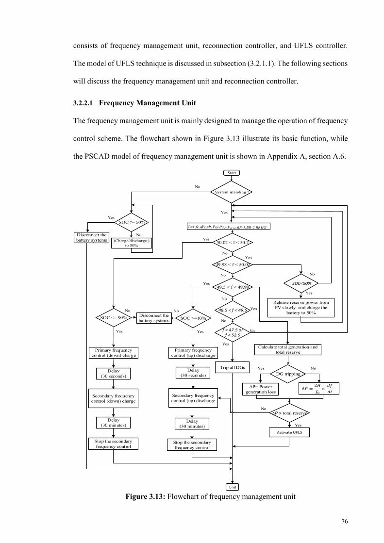
76
consists of frequency management unit, reconnection controller, and UFLS controller.
The model of UFLS technique is discussed in subsection (3.2.1.1). The following sections
will discuss the frequency management unit and reconnection controller.
3.2.2.1 Frequency Management Unit
The frequency management unit is mainly designed to manage the operation of frequency
control scheme. The flowchart shown in Figure 3.13 illustrate its basic function, while
the PSCAD model of frequency management unit is shown in Appendix A, section A.6.
Figure 3.13: Flowchart of frequency management unit
Start
Yes No
Calculate total generation and total reserve
Get , / , 1, G ,
ΔP= Power generation loss
49.5 < f < 49.98
Yes
48.5 < f < 49.5 Yes
(Charge/discharge ) to 50%
SOC ?= 50%
No
50.02 < f < 50.2
49.98 < f < 50.02
Yes
Primary frequency control (up) discharge
Primary frequency control (down) charge
Delay (30 seconds)
Delay (30 seconds)
Secondary frequency control (up) discharge
Secondary frequency control (down) charge
SOC >=10%SOC <= 90%
Activate UFLS
Yes
No
No
ΔP > total reserve
∆𝑃 =2𝐻
𝑓0× 𝑑𝑓
𝑑𝑡
No
Yes
No
PgridPGdf C dtfC P 2 ,BR-1,BR-2,BRKG
DG tripping ?
End
System islanding ?
f < 47.5 or f < 52.5
Trip all DGs
Yes
No
Yes
SOC<50%
Release reserve power from PV slowly and charge the
battery to 50%
Yes
Yes
Yes
No
No
Disconnect the battery systems
Yes
No
No
No
Disconnect the battery systems
Delay (30 minutes)
Stop the secondary frequency control
Delay (30 minutes)
Stop the secondary frequency control
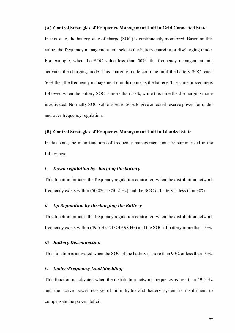
77
(A) Control Strategies of Frequency Management Unit in Grid Connected State
In this state, the battery state of charge (SOC) is continuously monitored. Based on this
value, the frequency management unit selects the battery charging or discharging mode.
For example, when the SOC value less than 50%, the frequency management unit
activates the charging mode. This charging mode continue until the battery SOC reach
50% then the frequency management unit disconnects the battery. The same procedure is
followed when the battery SOC is more than 50%, while this time the discharging mode
is activated. Normally SOC value is set to 50% to give an equal reserve power for under
and over frequency regulation.
(B) Control Strategies of Frequency Management Unit in Islanded State
In this state, the main functions of frequency management unit are summarized in the
followings:
i Down regulation by charging the battery
This function initiates the frequency regulation controller, when the distribution network
frequency exists within (50.02< f <50.2 Hz) and the SOC of battery is less than 90%.
ii Up Regulation by Discharging the Battery
This function initiates the frequency regulation controller, when the distribution network
frequency exists within (49.5 Hz < f < 49.98 Hz) and the SOC of battery more than 10%.
iii Battery Disconnection
This function is activated when the SOC of the battery is more than 90% or less than 10%.
iv Under-Frequency Load Shedding
This function is activated when the distribution network frequency is less than 49.5 Hz
and the active power reserve of mini hydro and battery system is insufficient to
compensate the power deficit.

78
v Charging the Battery
This function is activated when the islanded distribution network is operating in normal
condition (49.98 Hz < f < 50.02 Hz). In this situation, the frequency management unit
sends a control signal to charge the battery systems by using the solar PV reserve power,
which is released slowly so as not to increase the frequency value.
vi Trip all Distribution Generators
This function is activated when (f > 52.5 Hz or f < 47.5 Hz), then the frequency
management unit sends a command to separate all DGs.
In this research, the frequency bands are chosen based on Tenaga National Berhad
technical guide book (TNB, 2013).
3.2.2.2 Reconnection Controller
The formation of an island is only temporary, and it must be reconnected to the main grid
once the fault has been identified and removed. For this reason, the island must remain
synchronized with the main grid at all times even when it is electrically disconnected. It
is a crucial issue, and need a governor and an excitation controller to regulate the voltage,
frequency, and voltage angle of the island so that it remains within the permissible limit.
(Best, Morrow, McGowan, & Crossley, 2007; Caldon, Stocco, & Turri, 2008) utilized a
Phasor Measurement Unit (PMU) to keep the island synchronized with the main grid. The
reference signal from the grid is compared with the signal in the island and sent to the
controller to reduce the difference between the two signals.
The practical technique is to reconnect manually based on the indication of synchroscope.
However, the manual reconnection needs to be done by substation personnel, which could
delay operations. Therefore, a fast reconnection controller is proposed in this research,
which utilizes the deadline charging procedure. By using this procedure, a breaker at one

79
end of a tripped line is reclosed first to allow the line to be re-energized. The breaker at
the other end of the line is reclosed after synchronism between the two has established.
The flowchart shown in Figure 3.14 illustrates the reconnection controller operation.
When an island is detected, the voltage and frequency response is first controlled to their
synchronization limit. After the fault is cleared and the island response is stabilized, the
dead line charging procedure is initiated.
As indicated in Figure 3.15, for the dead line charging, breaker BRK1-BRK4 are closed.
Subsequently, the bus section breaker, which connects feeder 1105 and 1106, is
disconnected. After a specific interval of time, the phase controller receives the phase
measurements at both ends of BRKG to minimize the phase difference to achieve a nearly
zero value. Finally, when the synchronization requirement of frequency, voltage, and
phase angle on both ends are fulfilled, the reconnection is issued by closing BRKG.
Details for phase and voltage synchronization controllers are discussed in the following
sub-sections. The FCU PSCAD model is shown in Appendix A, section A.7.
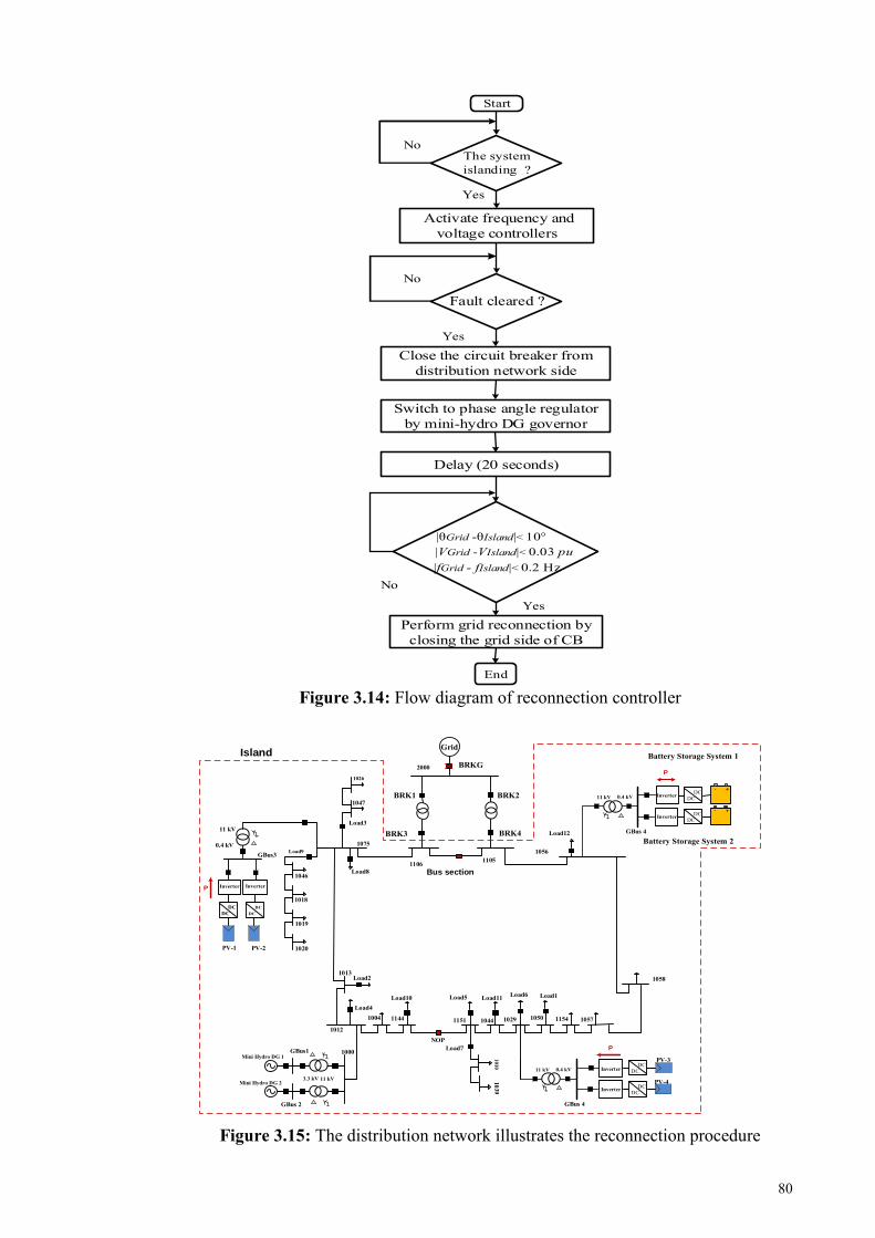
80
Figure 3.14: Flow diagram of reconnection controller
Figure 3.15: The distribution network illustrates the reconnection procedure
Activate frequency and voltage controllers
Start
Fault cleared ?
Yes
Perform grid reconnection by closing the grid side of CB
No
End
The system islanding ?
No
No
Yes
Yes
Close the circuit breaker from distribution network side
Switch to phase angle regulator by mini-hydro DG governor
Delay (20 seconds)
|θGrid -θIsland|< 10°
|fGrid - fIsland|< 0.2 Hz |VGrid -VIsland|< 0.03 pu
PV-3
PV-4
Mini Hydro DG 11000
Mini Hydro DG 2
1012
1013
1075
2000
GBus1
GBus 2 GBus 4
Grid
1004 1144 1151 1044 1029 1050 1154 1057
NOP
10391010
1058
1056
1047
1026
1046
1018
1019
1020
0.4 kV
11 kV
1106 1105
11 kV3.3 kV
GBus3
DCDC
DCDC
InverterInverter
PV-1 PV-2
11 kV
0.4 kV
Load4Load10 Load5
Load7
Load11 Load6 Load1
Load2
Load8
Load9
Load3
BRKG
BRK1 BRK2
DCDC
DCDCInverter
Load12
P
P
GBus 4
0.4 kV11 kV DCDC
DCDCInverter
+-
+-
Inverter
Inverter
P
Battery Storage System 1
Battery Storage System 2
Bus section
BRK3 BRK4
Island
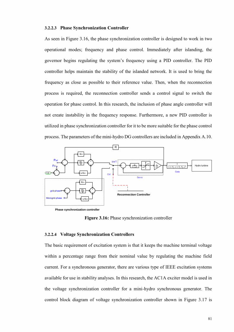
81
3.2.2.3 Phase Synchronization Controller
As seen in Figure 3.16, the phase synchronization controller is designed to work in two
operational modes; frequency and phase control. Immediately after islanding, the
governor begins regulating the system’s frequency using a PID controller. The PID
controller helps maintain the stability of the islanded network. It is used to bring the
frequency as close as possible to their reference value. Then, when the reconnection
process is required, the reconnection controller sends a control signal to switch the
operation for phase control. In this research, the inclusion of phase angle controller will
not create instability in the frequency response. Furthermore, a new PID controller is
utilized in phase synchronization controller for it to be more suitable for the phase control
process. The parameters of the mini-hydro DG controllers are included in Appendix A.10.
Figure 3.16: Phase synchronization controller
3.2.2.4 Voltage Synchronization Controllers
The basic requirement of excitation system is that it keeps the machine terminal voltage
within a percentage range from their nominal value by regulating the machine field
current. For a synchronous generator, there are various type of IEEE excitation systems
available for use in stability analyses. In this research, the AC1A exciter model is used in
the voltage synchronization controller for a mini-hydro synchronous generator. The
control block diagram of voltage synchronization controller shown in Figure 3.17 is
1
1 + 𝑇𝐶 𝑠 + 𝑇𝐶 𝑇𝐷 𝑠2
Gate Ctrl
grid-phase-
+
-+ 1
sT
s KD1
G1 + sT
KI1
KP1
++
+
1.0-
+
Microgrid-phase
sFc
s KD2
KI2
KP2
++
+s
-+
-
Pref
R
sw1
Phase synchronization controller
Servo
Hydro turbine
Reconnection Controller

82
designed to work in two operational modes; islanded and grid connected. During the grid-
connected mode, the voltage synchronization controller regulates the excitation voltage
based on a predetermined reactive power, while for islanding mode, the voltage
synchronization controller tries to keep the terminal voltage at its typical nominal value
of 1 p.u or within the permissible value.
Figure 3.17: Voltage synchronization controllers
3.3 Summary
This chapter discuss the methodology of the proposed frequency control scheme proposed
for distribution network with high PV penetration. This scheme is expected to overcome
frequency stability issues occurring after islanding; it consists of inertia controller,
frequency regulation controller, and an optimal UFLS controller. Inertia controller
proposed for PV units increases the total inertia of distribution network. The main
principle of inertia controller is operating the PV generation below the maximum power
point to keep a definite reserve power, which is delivered directly after the disturbance
events and last for a few seconds. After 10s, a frequency regulation controller is used to
provide the required power from BSS.
When the two previous controllers fail to stop the frequency deviation, an UFLS
technique is initiated to stop the frequency deviation. It has been observed that placing
all of the loads in the distribution system with fixed priority results in un-optimum load
shedding. For this reason, the proposed UFLS technique uses metaheuristics methods to
select the optimal combination of loads from fixed and random priority shedding loads.
Qref
-+
Q
sw2
Islanding
PIExciter_(AC1A)
1
Grid-connected
Control

83
This chapter also described the coordination between frequency control scheme and
synchronization system, where this coordination is necessary to stabilize the islanded
network frequency and achieve a seamless reconnection process with the main grid.
84
CHAPTER 4: VALIDATION OF PROPOSED UFLS TECHNIQUE
4.1 Introduction
This chapter discusses modelling of the distribution network used to validate the proposed
load shedding technique. It also deals with the validation of the proposed load shedding
techniques using various case studies, such as including islanding, DG tripping, and load
increments. Furthermore, the proposed UFLS is compared with the adaptive UFLS
techniques in order to confirm its ability in shedding the optimal amount of power from
the distribution network. Different metaheuristic optimization methods (BEP, BGA,
BPSO) are applied for load shedding, and their performance are presented here.
4.2 Modelling of 29-Bus Distribution network for Proposed UFLS Technique
The test system considered in this research is a part of the Malaysian distribution network
shown in Appendix A, section A.2. The test system consists of two mini-hydro DGs
operated at a voltage level of 3.3 kV, each DG rated 2 MVA capacity (maximum power
dispatch is 1.8 MW). The distribution network also consists of one Bio-Mass DG; the
total load demand of the distribution network is 6 MW, 2 Var. The mini-hydro units were
connected to the distribution network using two step-up transformers (3.3 kV-11 kV).
The mini-hydro DGs are modelled using the PSCAD/EMTDC library models of the
exciter, the governor, and hydraulic turbine. The turbine chosen for mini-hydro units is
the hydraulic turbine with non-elastic water column without a surge tank model. For
excitation and governor system, the IEEE type AC1A model and PID governor with pilot
and servo dynamics were selected. The entire line is modelled according to a nominal π
form. The length of each line does not exceed 6 km.
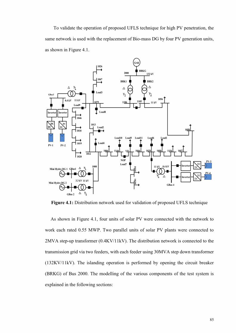
85
To validate the operation of proposed UFLS technique for high PV penetration, the
same network is used with the replacement of Bio-mass DG by four PV generation units,
as shown in Figure 4.1.
Figure 4.1: Distribution network used for validation of proposed UFLS technique
As shown in Figure 4.1, four units of solar PV were connected with the network to
work each rated 0.55 MWP. Two parallel units of solar PV plants were connected to
2MVA step-up transformer (0.4KV/11kV). The distribution network is connected to the
transmission grid via two feeders, with each feeder using 30MVA step down transformer
(132KV/11kV). The islanding operation is performed by opening the circuit breaker
(BRKG) of Bus 2000. The modelling of the various components of the test system is
explained in the following sections:
PV-3
PV-4Mini Hydro DG 1
1000
Mini Hydro DG 2
1012
1013
1075
2000
GBus1
GBus 2
GBus 4
Grid
1004 1144 1151 1044 1029 1050 1154 1057
NOP
10391010
1058
1056
1047
1026
1046
1018
1019
1020
132 kV
11 kV
0.4 kV
11 kV
1106 1105
11 kV
3.3 kV
GBus3
DCDC
DCDC
InverterInverter
PV-1 PV-2
Inverter
11 kV0.4 kV
Load4
Load10 Load5
Load7
Load11 Load6 Load1
Load2
Load8
Load9
Load3
BRKG
BRK1 BRK2
DCDC
DCDCInverter
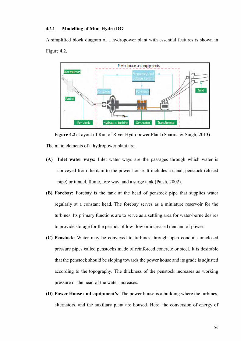
86
4.2.1 Modelling of Mini-Hydro DG
A simplified block diagram of a hydropower plant with essential features is shown in
Figure 4.2.
Figure 4.2: Layout of Run of River Hydropower Plant (Sharma & Singh, 2013)
The main elements of a hydropower plant are:
(A) Inlet water ways: Inlet water ways are the passages through which water is
conveyed from the dam to the power house. It includes a canal, penstock (closed
pipe) or tunnel, flume, fore way, and a surge tank (Paish, 2002).
(B) Forebay: Forebay is the tank at the head of penstock pipe that supplies water
regularly at a constant head. The forebay serves as a miniature reservoir for the
turbines. Its primary functions are to serve as a settling area for water-borne desires
to provide storage for the periods of low flow or increased demand of power.
(C) Penstock: Water may be conveyed to turbines through open conduits or closed
pressure pipes called penstocks made of reinforced concrete or steel. It is desirable
that the penstock should be sloping towards the power house and its grade is adjusted
according to the topography. The thickness of the penstock increases as working
pressure or the head of the water increases.
(D) Power House and equipment’s: The power house is a building where the turbines,
alternators, and the auxiliary plant are housed. Here, the conversion of energy of
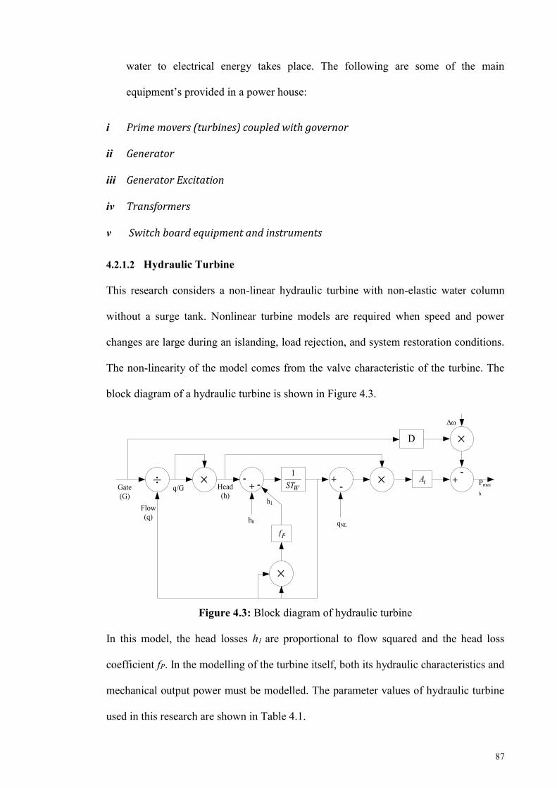
87
water to electrical energy takes place. The following are some of the main
equipment’s provided in a power house:
i Prime movers (turbines) coupled with governor
ii Generator
iii Generator Excitation
iv Transformers
v Switch board equipment and instruments
4.2.1.2 Hydraulic Turbine
This research considers a non-linear hydraulic turbine with non-elastic water column
without a surge tank. Nonlinear turbine models are required when speed and power
changes are large during an islanding, load rejection, and system restoration conditions.
The non-linearity of the model comes from the valve characteristic of the turbine. The
block diagram of a hydraulic turbine is shown in Figure 4.3.
Figure 4.3: Block diagram of hydraulic turbine
In this model, the head losses h1 are proportional to flow squared and the head loss
coefficient fP. In the modelling of the turbine itself, both its hydraulic characteristics and
mechanical output power must be modelled. The parameter values of hydraulic turbine
used in this research are shown in Table 4.1.
Gate (G)
D
1
WST
-+ -
Pfh0
Flow (q)
q/G
h1
+- tA +
-
qNL
Head (h)
Pmec
h
∆ω
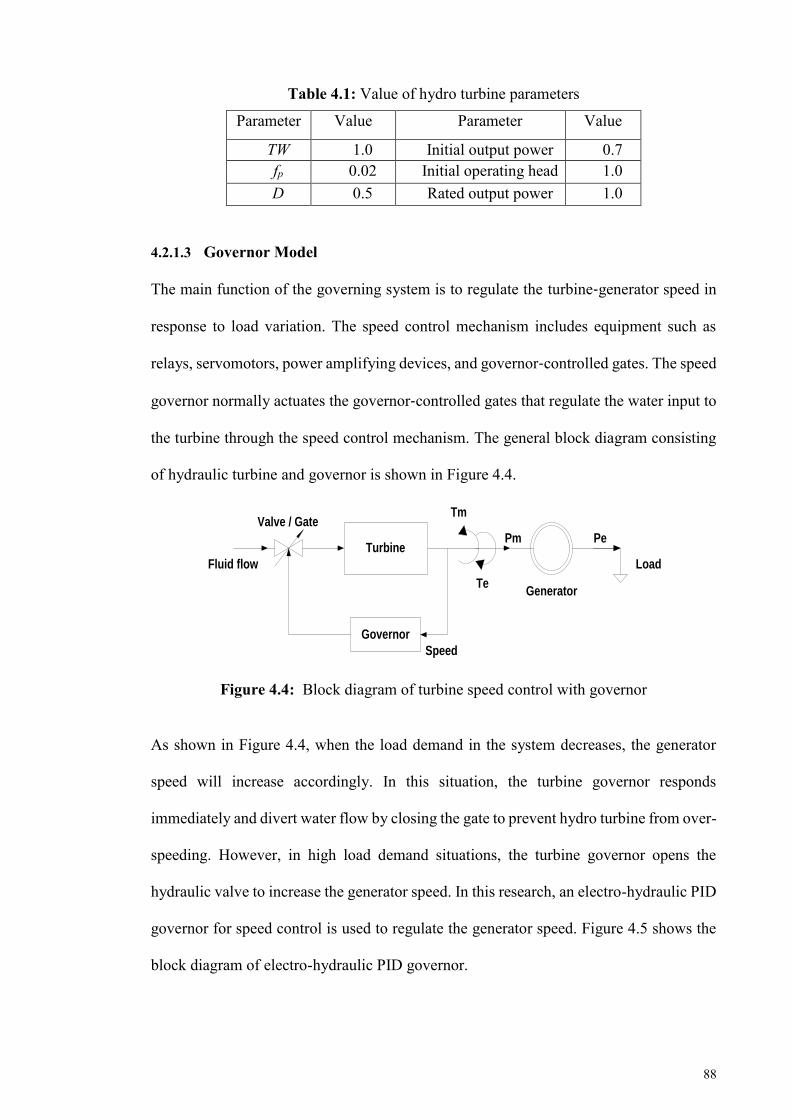
88
Table 4.1: Value of hydro turbine parameters
Parameter Value Parameter Value
TW 1.0 Initial output power 0.7 fp 0.02 Initial operating head 1.0 D 0.5 Rated output power 1.0
4.2.1.3 Governor Model
The main function of the governing system is to regulate the turbine‐generator speed in
response to load variation. The speed control mechanism includes equipment such as
relays, servomotors, power amplifying devices, and governor‐controlled gates. The speed
governor normally actuates the governor‐controlled gates that regulate the water input to
the turbine through the speed control mechanism. The general block diagram consisting
of hydraulic turbine and governor is shown in Figure 4.4.
Figure 4.4: Block diagram of turbine speed control with governor
As shown in Figure 4.4, when the load demand in the system decreases, the generator
speed will increase accordingly. In this situation, the turbine governor responds
immediately and divert water flow by closing the gate to prevent hydro turbine from over-
speeding. However, in high load demand situations, the turbine governor opens the
hydraulic valve to increase the generator speed. In this research, an electro-hydraulic PID
governor for speed control is used to regulate the generator speed. Figure 4.5 shows the
block diagram of electro-hydraulic PID governor.
Generator
Turbine
Governor
Load
Valve / Gate
Fluid flow
Tm
Te
Pm Pe
Speed
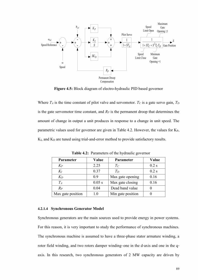
89
Figure 4.5: Block diagram of electro-hydraulic PID based governor
Where TA is the time constant of pilot valve and servomotor. TC is a gate servo gain, TD
is the gate servomotor time constant, and RP is the permanent droop that determines the
amount of change in output a unit produces in response to a change in unit speed. The
parametric values used for governor are given in Table 4.2. However, the values for KP,
KI, and KD are tuned using trial-and-error method to provide satisfactory results.
Table 4.2: Parameters of the hydraulic governor
Parameter Value Parameter Value KP 2.25 TC 0.2 s KI 0.37 TD 0.2 s KD 0.9 Max gate opening 0.16 TA 0.05 s Max gate closing 0.16 RP 0.04 Dead band value 0
Max gate position 1.0 Min gate position 0
4.2.1.4 Synchronous Generator Model
Synchronous generators are the main sources used to provide energy in power systems.
For this reason, it is very important to study the performance of synchronous machines.
The synchronous machine is assumed to have a three‐phase stator armature winding, a
rotor field winding, and two rotors damper winding–one in the d‐axis and one in the q‐
axis. In this research, two synchronous generators of 2 MW capacity are driven by
ωref + -Speed Reference
ωSpeed
+ -- + +
+
PK
IKS
DSK
Pref
PR
Pilot Servo
Permanent Droop Compensation
11 AST 2
11 C C DST S T T
Speed Limit Open
Maximum Gate
Opening ≤1
Speed Limit Close
Minimum Gate
Opening =1
Gate PositionZ
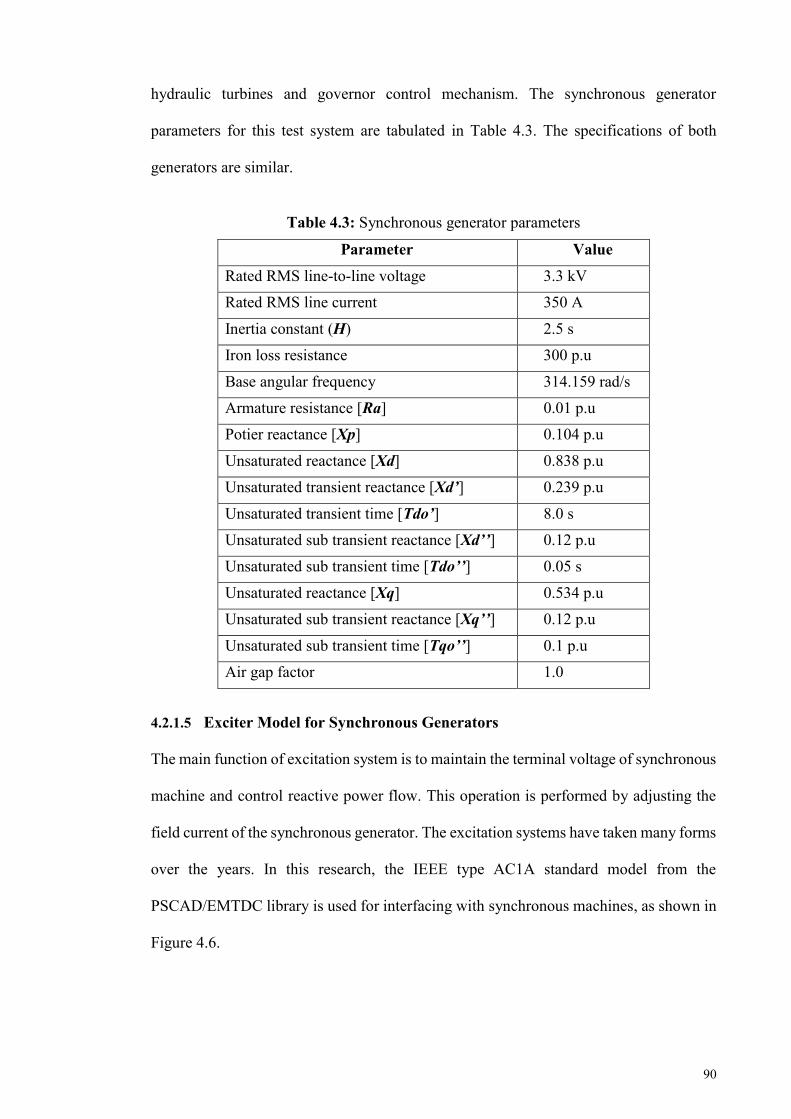
90
hydraulic turbines and governor control mechanism. The synchronous generator
parameters for this test system are tabulated in Table 4.3. The specifications of both
generators are similar.
Table 4.3: Synchronous generator parameters
Parameter Value
Rated RMS line-to-line voltage 3.3 kV
Rated RMS line current 350 A
Inertia constant (H) 2.5 s
Iron loss resistance 300 p.u
Base angular frequency 314.159 rad/s
Armature resistance [Ra] 0.01 p.u
Potier reactance [Xp] 0.104 p.u
Unsaturated reactance [Xd] 0.838 p.u
Unsaturated transient reactance [Xd’] 0.239 p.u
Unsaturated transient time [Tdo’] 8.0 s
Unsaturated sub transient reactance [Xd’’] 0.12 p.u
Unsaturated sub transient time [Tdo’’] 0.05 s
Unsaturated reactance [Xq] 0.534 p.u
Unsaturated sub transient reactance [Xq’’] 0.12 p.u
Unsaturated sub transient time [Tqo’’] 0.1 p.u
Air gap factor 1.0
4.2.1.5 Exciter Model for Synchronous Generators
The main function of excitation system is to maintain the terminal voltage of synchronous
machine and control reactive power flow. This operation is performed by adjusting the
field current of the synchronous generator. The excitation systems have taken many forms
over the years. In this research, the IEEE type AC1A standard model from the
PSCAD/EMTDC library is used for interfacing with synchronous machines, as shown in
Figure 4.6.

91
Figure 4.6: Block Diagram of IEEE type AC1A excitation system model
This model provides a field-controlled alternator excitation system with un-controlled
rectifiers, and is applicable to brushless excitation systems. The typical parameters used
in this research are presented in Table 4.4.
Table 4.4: Sample data of IEEE AC1A excitation model parameters
Parameter Value Parameter Value
Tc 0 KF 0.03
TB 0 TF 1
KA 400 TE 0.8
TA 0.02 KE 1
VAMAX 14.5 KC 0.2
VAMIN -14.5 KD 0.38
VRMAX 6.03 VRMIN -5.43
SE(VE1) 0.1 SE(VE2) 0.03
VE1 4.18 VE2 3.14
Figure 4.7 shows the synchronous generator with PID based governor, hydraulic turbine,
and excitation control modelled in PSCAD.
∑
VS
VC
VREF
+
+-
-
11
C
B
STST
1A
A
KST
VAMIN
VAMAX
HVGate
VUEL
VOELVRMIN
VRMAX
∑ VR +
0
∏ VE EFD1
EST
[ ]X E E EV V S V
∑
∑
++
+
VX
EK
DK+
1F
F
SKST VFE
-
C FD
E
K IV
( )Nf I
FFE
IFD
IN
LVGate
VF
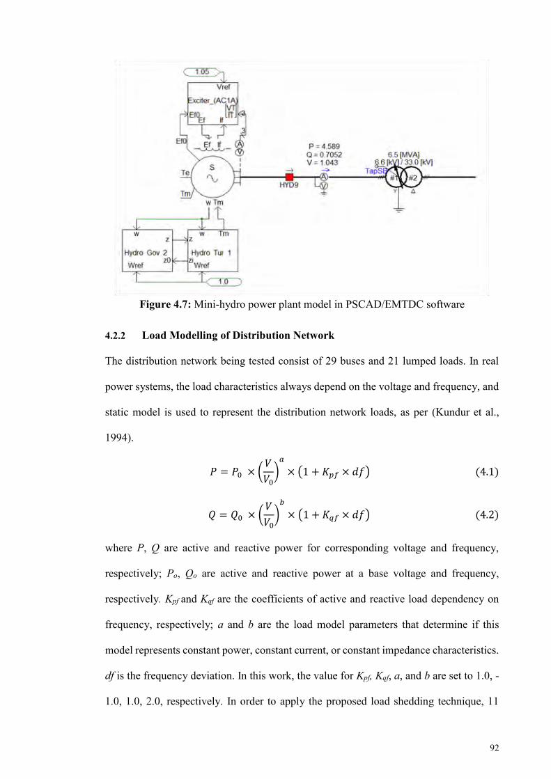
92
Figure 4.7: Mini-hydro power plant model in PSCAD/EMTDC software
4.2.2 Load Modelling of Distribution Network
The distribution network being tested consist of 29 buses and 21 lumped loads. In real
power systems, the load characteristics always depend on the voltage and frequency, and
static model is used to represent the distribution network loads, as per (Kundur et al.,
1994).
𝑃 = 𝑃0 × (𝑉
𝑉0)𝑎
× (1 + 𝐾𝑝𝑓 × 𝑑𝑓) (4.1)
𝑄 = 𝑄0 × (𝑉
𝑉0)𝑏
× (1 + 𝐾𝑞𝑓 × 𝑑𝑓) (4.2)
where P, Q are active and reactive power for corresponding voltage and frequency,
respectively; Po, Qo are active and reactive power at a base voltage and frequency,
respectively. Kpf and Kqf are the coefficients of active and reactive load dependency on
frequency, respectively; a and b are the load model parameters that determine if this
model represents constant power, constant current, or constant impedance characteristics.
df is the frequency deviation. In this work, the value for Kpf, Kqf, a, and b are set to 1.0, -
1.0, 1.0, 2.0, respectively. In order to apply the proposed load shedding technique, 11

93
loads from the distribution network have been determined. Generally, loads are typically
divided into commercial, industrial, and residential types. Since industrial and
commercial loads are more important than the residential loads, commercial loads (Load
11 and Load 12) take the fixed priority, while residential loads (Load1- Load 10) take the
random priority. The loads, with their priority rankings, are tabulated in Table 4.5.
Table 4.5: Load data and their priority
Load Ranked Bus No. P (MW) Load Priority
Load 1 1050 0.044 Random Load 2 1013 0.069 Random Load 3 1047,1026 0.15 Random Load 4 1012 0.314 Random Load 5 1151 0.5 Random Load 6 1029 0.55 Random Load 7 1010,1039 0.583 Random Load 8 1075 0.645 Random
Load 9 1018-1020, 1046 0.7 Random
Load 10 1144 0.119 Fixed Load 11 1044 0.223 Fixed
4.2.3 Modelling of Photovoltaic System
The PSCAD model used in this research is shown in Figure 4.8; It mainly consists of PV
array model, DC-DC converter, DC link capacitor, three phase-inverter, AC filter,
transformer. The following sections detail these devices.
Figure 4.8: PSCAD model of solar PV generation unit
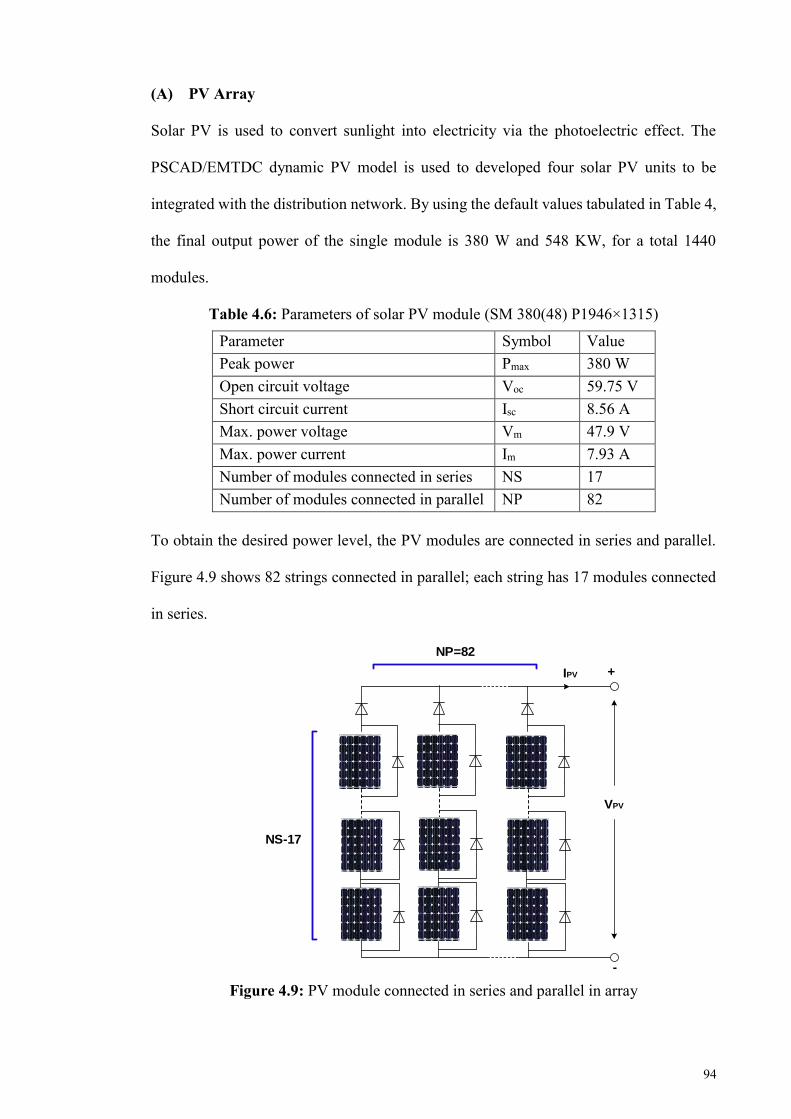
94
(A) PV Array
Solar PV is used to convert sunlight into electricity via the photoelectric effect. The
PSCAD/EMTDC dynamic PV model is used to developed four solar PV units to be
integrated with the distribution network. By using the default values tabulated in Table 4,
the final output power of the single module is 380 W and 548 KW, for a total 1440
modules.
Table 4.6: Parameters of solar PV module (SM 380(48) P1946×1315)
Parameter Symbol Value Peak power Pmax 380 W Open circuit voltage Voc 59.75 V Short circuit current Isc 8.56 A Max. power voltage Vm 47.9 V Max. power current Im 7.93 A Number of modules connected in series NS 17 Number of modules connected in parallel NP 82
To obtain the desired power level, the PV modules are connected in series and parallel.
Figure 4.9 shows 82 strings connected in parallel; each string has 17 modules connected
in series.
Figure 4.9: PV module connected in series and parallel in array
NS-17
IPV +
VPV
-
NP=82
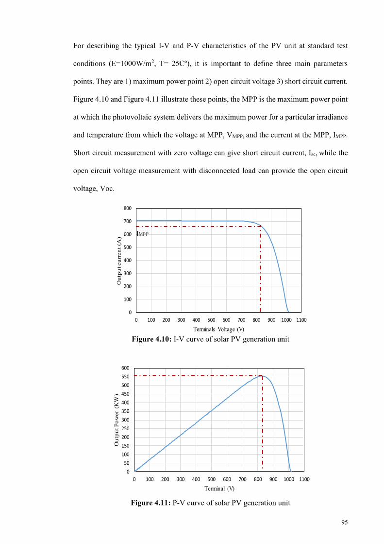
95
For describing the typical I-V and P-V characteristics of the PV unit at standard test
conditions (E=1000W/m2, T= 25Cº), it is important to define three main parameters
points. They are 1) maximum power point 2) open circuit voltage 3) short circuit current.
Figure 4.10 and Figure 4.11 illustrate these points, the MPP is the maximum power point
at which the photovoltaic system delivers the maximum power for a particular irradiance
and temperature from which the voltage at MPP, VMPP, and the current at the MPP, IMPP.
Short circuit measurement with zero voltage can give short circuit current, Isc, while the
open circuit voltage measurement with disconnected load can provide the open circuit
voltage, Voc.
Figure 4.10: I-V curve of solar PV generation unit
Figure 4.11: P-V curve of solar PV generation unit
0
100
200
300
400
500
600
700
800
0 100 200 300 400 500 600 700 800 900 1000 1100
Out
put c
urre
nt (A
)
Terminals Voltage (V)
IMPP
0
50
100
150
200
250
300
350
400
450
500
550
600
0 100 200 300 400 500 600 700 800 900 1000 1100
Out
put P
ower
(K
W)
Terminal (V)
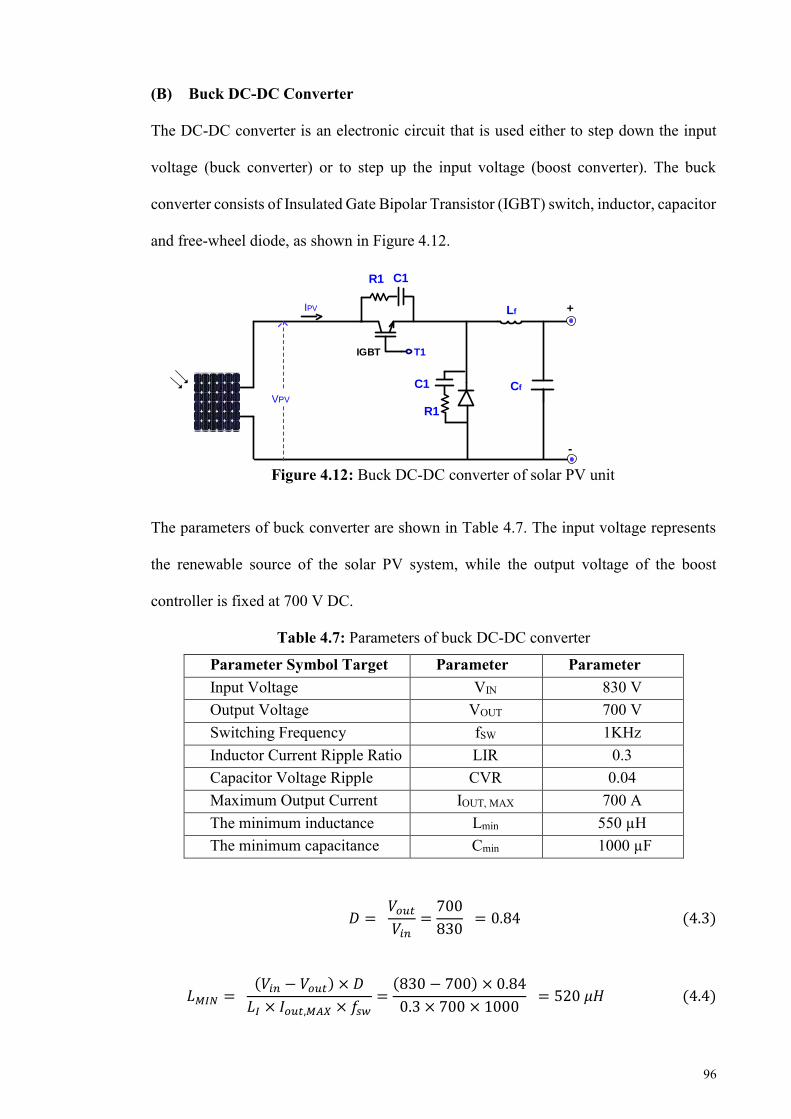
96
(B) Buck DC-DC Converter
The DC-DC converter is an electronic circuit that is used either to step down the input
voltage (buck converter) or to step up the input voltage (boost converter). The buck
converter consists of Insulated Gate Bipolar Transistor (IGBT) switch, inductor, capacitor
and free-wheel diode, as shown in Figure 4.12.
Figure 4.12: Buck DC-DC converter of solar PV unit
The parameters of buck converter are shown in Table 4.7. The input voltage represents
the renewable source of the solar PV system, while the output voltage of the boost
controller is fixed at 700 V DC.
Table 4.7: Parameters of buck DC-DC converter
Parameter Symbol Target Parameter Symbol Symbol
Parameter value Input Voltage VIN 830 V
Output Voltage VOUT 700 V Switching Frequency fSW 1KHz Inductor Current Ripple Ratio LIR 0.3 Capacitor Voltage Ripple
Ratio CVR 0.04
Maximum Output Current IOUT, MAX 700 A The minimum inductance
value Lmin 550 µH
The minimum capacitance value
Cmin 1000 µF
𝐷 = 𝑉𝑜𝑢𝑡𝑉𝑖𝑛
=700
830 = 0.84 (4.3)
𝐿𝑀𝐼𝑁 = (𝑉𝑖𝑛 − 𝑉𝑜𝑢𝑡) × 𝐷
𝐿𝐼 × 𝐼𝑜𝑢𝑡,𝑀𝐴𝑋 × 𝑓𝑠𝑤=(830 − 700) × 0.84
0.3 × 700 × 1000 = 520 𝜇𝐻 (4.4)
IGBT
IPV
VPV
T1
Cf
Lf +
-
C1R1
R1
C1
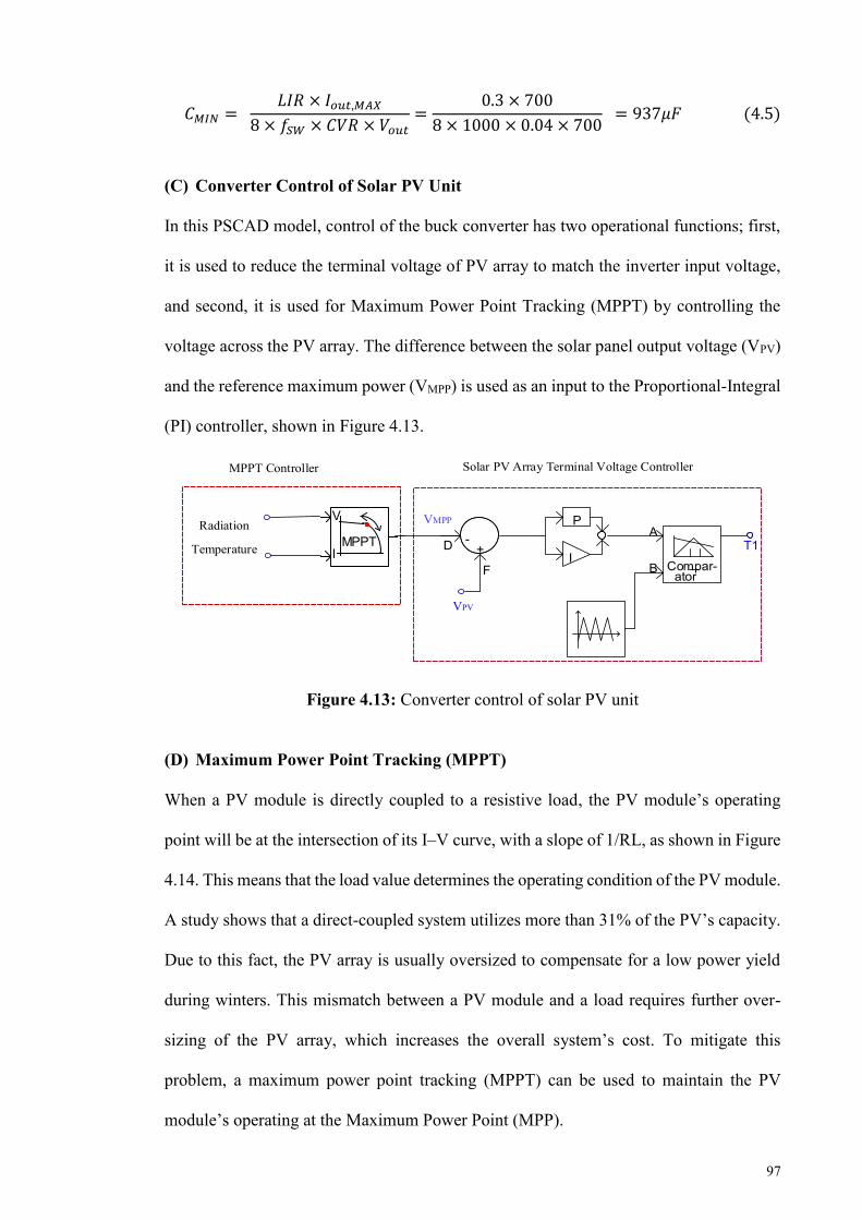
97
𝐶𝑀𝐼𝑁 = 𝐿𝐼𝑅 × 𝐼𝑜𝑢𝑡,𝑀𝐴𝑋
8 × 𝑓𝑆𝑊 × 𝐶𝑉𝑅 × 𝑉𝑜𝑢𝑡=
0.3 × 700
8 × 1000 × 0.04 × 700 = 937𝜇𝐹 (4.5)
(C) Converter Control of Solar PV Unit
In this PSCAD model, control of the buck converter has two operational functions; first,
it is used to reduce the terminal voltage of PV array to match the inverter input voltage,
and second, it is used for Maximum Power Point Tracking (MPPT) by controlling the
voltage across the PV array. The difference between the solar panel output voltage (VPV)
and the reference maximum power (VMPP) is used as an input to the Proportional-Integral
(PI) controller, shown in Figure 4.13.
Figure 4.13: Converter control of solar PV unit
(D) Maximum Power Point Tracking (MPPT)
When a PV module is directly coupled to a resistive load, the PV module’s operating
point will be at the intersection of its I–V curve, with a slope of 1/RL, as shown in Figure
4.14. This means that the load value determines the operating condition of the PV module.
A study shows that a direct-coupled system utilizes more than 31% of the PV’s capacity.
Due to this fact, the PV array is usually oversized to compensate for a low power yield
during winters. This mismatch between a PV module and a load requires further over-
sizing of the PV array, which increases the overall system’s cost. To mitigate this
problem, a maximum power point tracking (MPPT) can be used to maintain the PV
module’s operating at the Maximum Power Point (MPP).
Solar PV Array Terminal Voltage Controller
D -
F
+A
B Compar-ator
T1I
P
VPV
VMPPRadiation
Temperature
MPPT Controller
MPPT
V
I

98
Figure 4.14: I-V curves of SM 380 PV module and various resistive loads
The MPPT techniques are used to control DC converters in order to extract the maximum
output power from a PV array under given weather conditions. The DC converter is
continuously controlled to operate the array at its maximum power point despite possible
changes in the load’s impedance. Several techniques have been proposed for this, such as
Constant Voltage (CV) method, Incremental Conductance (IC) method, Perturb and
Observe (P&O) method, and Artificial Neural Network (ANN) method. The PSCAD
model of converter control use Perturb and Observe (P&O) methods to determine the
maximum power voltage VMPP.
(E) Three Phase Inverter
The inverter is an electronic circuit that converts the DC output power of the DC-DC
converter into a three phase AC power suitable for utility connection. In this PSCAD
model, the three-phase inverter consists of a simple active and reactive power controller,
a firing pulse generator, and a three-phase inverter bridge.
i Active and Reactive Power Controllers
The active power controller is used to establish a constant DC bus voltage (dcvag) at 0.7
kV between the DC-DC converter and the inverter. The output of the controller will be
0
1
2
3
4
5
6
7
8
9
10
0 10 20 30 40 50 60
Mo
du
le c
urr
ent
(A)
Module Voltage (V)
RL=4 Ω
Increasing RLRL=7.5 Ω
RL=15 Ω1/RL
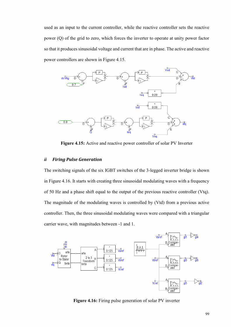
99
used as an input to the current controller, while the reactive controller sets the reactive
power (Q) of the grid to zero, which forces the inverter to operate at unity power factor
so that it produces sinusoidal voltage and current that are in phase. The active and reactive
power controllers are shown in Figure 4.15.
Figure 4.15: Active and reactive power controller of solar PV Inverter
ii Firing Pulse Generation
The switching signals of the six IGBT switches of the 3-legged inverter bridge is shown
in Figure 4.16. It starts with creating three sinusoidal modulating waves with a frequency
of 50 Hz and a phase shift equal to the output of the previous reactive controller (Vtq).
The magnitude of the modulating waves is controlled by (Vtd) from a previous active
controller. Then, the three sinusoidal modulating waves were compared with a triangular
carrier wave, with magnitudes between -1 and 1.
Figure 4.16: Firing pulse generation of solar PV inverter

100
iii Three Phase Inverter Bridge
Three phase inverter bridge is used to convert the DC bus voltage to AC voltage of 400
V/50 Hz. As shown in Figure 4.17, three phase bridge consists of six IGBT, where each
IGBT switch is controlled by a firing signal. Due to the switching operation of IGBT, the
output voltage of the inverter will be distorted. For this reason, an LC filter was
implemented to improve the shape of the output voltage of the inverter.
Figure 4.17: PSCAD model of solar PV inverter
4.3 Simulation Results for Proposed UFLS Technique
The validation of the proposed UFLS technique are divided into three case studies;
Case study 1: Comparison Between Metaheuristic UFLS Technique (BEP) and
Adaptive UFLS Technique, represents the comparative study between the UFLS
technique based on BEP method and the adaptive UFLS technique, which is conducted
to show the importance of assuming some flexibility in load shedding priority.
Case study 2: comparison between different Metaheuristic techniques in term of
execution time, represents a comparative simulation results between FRPLS technique
proposed in (Laghari et al., 2015), BGA, BPSO, and BEP techniques in terms of execution
time and convergence curves.
gb1
gb2
gb3
gb4
gb5
gb6
R f L fC
0.4 /11 KV

101
Case study 3: comparison between different load shedding techniques, represents a
comparative simulation results between proposed UFLS controller, which uses the BEP
technique compared with other UFLS techniques.
4.3.1 Case Study 1: Comparison Between Metaheuristic UFLS Technique (BEP)
and Adaptive UFLS Technique
This comparative study is required to show the preference of the proposed UFLS
technique over the adaptive UFLS technique, where this preference is due to the
flexibility in load shedding priority. This comparative study is performed for load
increments of 1.0 MW and 1.8 MW occurring at 40s.
(A) Load Increment of 1.0 MW
Immediately after islanding at 10s, the system frequency begins to decline in response to
an excess load of 0.32 MW. Accordingly, the mini-hydro generators use their spinning
reserves 0.48 MW to cover the unbalance of power. The UFLS controller will only be
activated when the total load power exceeds 5.8 MW. At 40s, the total power demand
will be 6.68 MW. For this reason, the UFLS automatically activate its event-based to stop
the frequency declination by shedding the loads 2, 3, 8 for BEP UFLS or loads1-5 for
adaptive UFLS, as shown in Table 4.8. The frequency responses of proposed UFLS
controller and adaptive UFLS controller are shown in Figure 4.18.
Table 4.8: UFLS parameters for load increment of 1.0 MW after islanding
Parameter UFLS controller based BEP Adaptive UFLS controller ΔP (MW) 1.0 1.0 Reserve (MW) 0.16 0.16 Total Load Shed Power (MW) 0.84 0.84
Shedding loads (MW) Load 2 (0.069) Load 3 (0.15) Load 8 (0.645)
Load 1 (0.044), Load 2 (0.069) Load 3 (0.15), Load 4 (0.314) Load 5 (0.5)
Nadir Frequency (Hz) 49.3 49.5 Frequency Overshoot (Hz) - 50.25
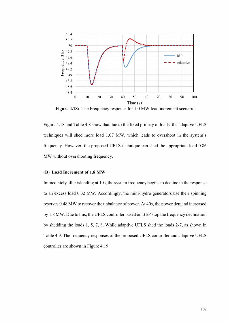
102
Figure 4.18: The Frequency response for 1.0 MW load increment scenario
Figure 4.18 and Table 4.8 show that due to the fixed priority of loads, the adaptive UFLS
techniques will shed more load 1.07 MW, which leads to overshoot in the system’s
frequency. However, the proposed UFLS technique can shed the appropriate load 0.86
MW without overshooting frequency.
(B) Load Increment of 1.8 MW
Immediately after islanding at 10s, the system frequency begins to decline in the response
to an excess load 0.32 MW. Accordingly, the mini-hydro generators use their spinning
reserves 0.48 MW to recover the unbalance of power. At 40s, the power demand increased
by 1.8 MW. Due to this, the UFLS controller based on BEP stop the frequency declination
by shedding the loads 1, 5, 7, 8. While adaptive UFLS shed the loads 2-7, as shown in
Table 4.9. The frequency responses of the proposed UFLS controller and adaptive UFLS
controller are shown in Figure 4.19.
48.448.648.8
4949.249.449.649.8
5050.250.4
0 10 20 30 40 50 60 70 80 90 100
Freq
uenc
y (H
z)
Time (s)
BEP
Adaptive
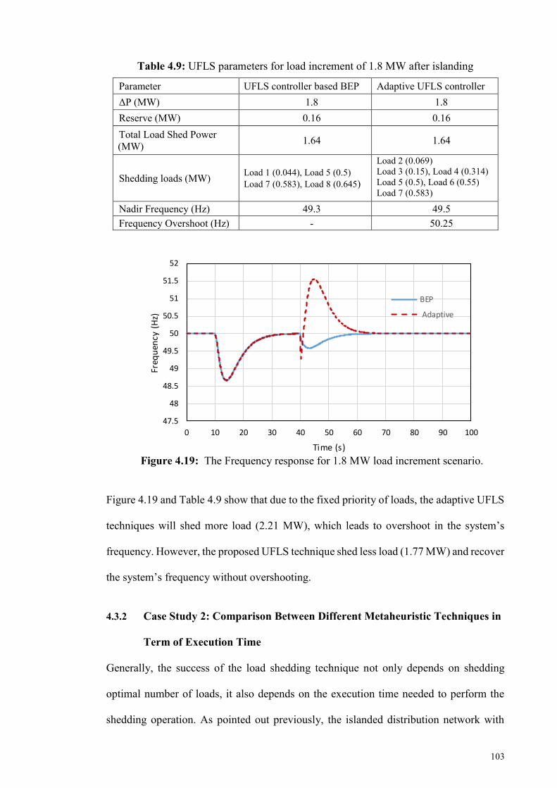
103
Table 4.9: UFLS parameters for load increment of 1.8 MW after islanding
Parameter UFLS controller based BEP Adaptive UFLS controller ΔP (MW) 1.8 1.8 Reserve (MW) 0.16 0.16 Total Load Shed Power (MW) 1.64 1.64
Shedding loads (MW) Load 1 (0.044), Load 5 (0.5) Load 7 (0.583), Load 8 (0.645)
Load 2 (0.069) Load 3 (0.15), Load 4 (0.314) Load 5 (0.5), Load 6 (0.55) Load 7 (0.583)
Nadir Frequency (Hz) 49.3 49.5 Frequency Overshoot (Hz) - 50.25
Figure 4.19: The Frequency response for 1.8 MW load increment scenario.
Figure 4.19 and Table 4.9 show that due to the fixed priority of loads, the adaptive UFLS
techniques will shed more load (2.21 MW), which leads to overshoot in the system’s
frequency. However, the proposed UFLS technique shed less load (1.77 MW) and recover
the system’s frequency without overshooting.
4.3.2 Case Study 2: Comparison Between Different Metaheuristic Techniques in
Term of Execution Time
Generally, the success of the load shedding technique not only depends on shedding
optimal number of loads, it also depends on the execution time needed to perform the
shedding operation. As pointed out previously, the islanded distribution network with
47.5
48
48.5
49
49.5
50
50.5
51
51.5
52
0 10 20 30 40 50 60 70 80 90 100
Freq
uen
cy (
Hz)
Time (s)
BEP
Adaptive
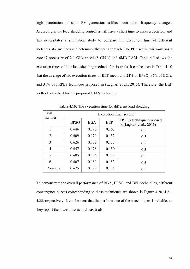
104
high penetration of solar PV generation suffers from rapid frequency changes.
Accordingly, the load shedding controller will have a short time to make a decision, and
this necessitates a simulation study to compare the execution time of different
metaheuristic methods and determine the best approach. The PC used in this work has a
core i7 processor of 2.1 GHz speed (8 CPUs) and 6MB RAM. Table 4.9 shows the
execution times of four load shedding methods for six trials. It can be seen in Table 4.10
that the average of six execution times of BEP method is 24% of BPSO, 85% of BGA,
and 31% of FRPLS technique proposed in (Laghari et al., 2015). Therefore, the BEP
method is the best for the proposed UFLS technique.
Table 4.10: The execution time for different load shedding
Trial number
Execution time (second)
BPSO BGA BEP FRPLS technique proposed in (Laghari et al., 2015)
1 0.646 0.196 0.162 0.5 2 0.609 0.179 0.152 0.5 3 0.626 0.172 0.155 0.5 4 0.657 0.178 0.150 0.5 5 0.605 0.176 0.153 0.5 6 0.607 0.189 0.153 0.5
Average 0.625 0.182 0.154 0.5
To demonstrate the overall performance of BGA, BPSO, and BEP techniques, different
convergence curves corresponding to these techniques are shown in Figure 4.20, 4.21,
4.22, respectively. It can be seen that the performance of these techniques is reliable, as
they report the lowest losses in all six trials.
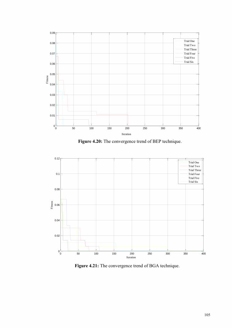
105
Figure 4.20: The convergence trend of BEP technique.
Figure 4.21: The convergence trend of BGA technique.
0 50 100 150 200 250 300 350 4000
0.01
0.02
0.03
0.04
0.05
0.06
0.07
0.08
0.09
Iteration
Fitn
ess
Trial OneTrial TwoTrial ThreeTrial FourTrial FiveTrial Six
0 50 100 150 200 250 300 350 4000
0.02
0.04
0.06
0.08
0.1
0.12
Iteration
Fitn
ess
Trial OneTrial TwoTrial ThreeTrial FourTrial FiveTrial Six
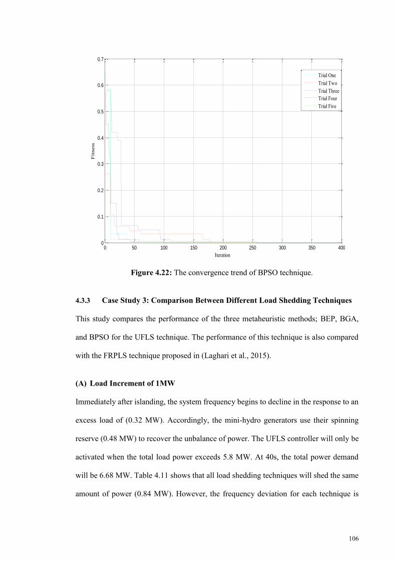
106
Figure 4.22: The convergence trend of BPSO technique.
4.3.3 Case Study 3: Comparison Between Different Load Shedding Techniques
This study compares the performance of the three metaheuristic methods; BEP, BGA,
and BPSO for the UFLS technique. The performance of this technique is also compared
with the FRPLS technique proposed in (Laghari et al., 2015).
(A) Load Increment of 1MW
Immediately after islanding, the system frequency begins to decline in the response to an
excess load of (0.32 MW). Accordingly, the mini-hydro generators use their spinning
reserve (0.48 MW) to recover the unbalance of power. The UFLS controller will only be
activated when the total load power exceeds 5.8 MW. At 40s, the total power demand
will be 6.68 MW. Table 4.11 shows that all load shedding techniques will shed the same
amount of power (0.84 MW). However, the frequency deviation for each technique is
0 50 100 150 200 250 300 350 4000
0.1
0.2
0.3
0.4
0.5
0.6
0.7
Iteration
Fit
ness
Trial OneTrial TwoTrial ThreeTrial FourTrial Five
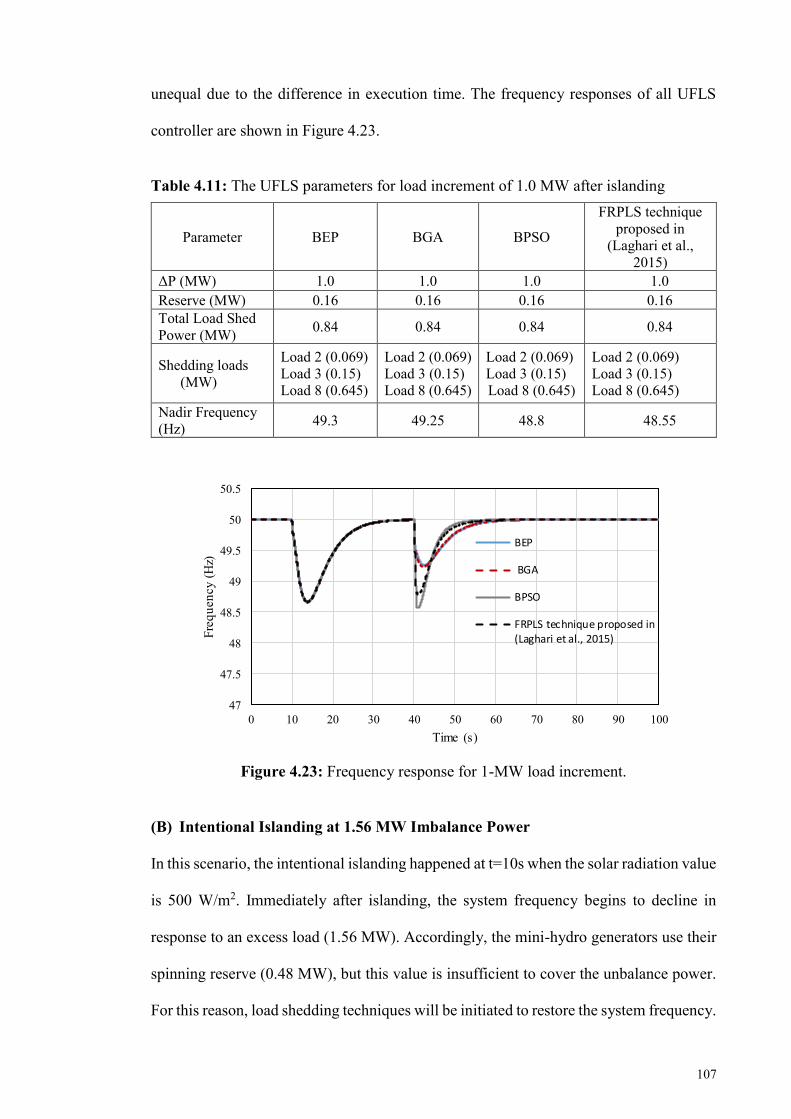
107
unequal due to the difference in execution time. The frequency responses of all UFLS
controller are shown in Figure 4.23.
Table 4.11: The UFLS parameters for load increment of 1.0 MW after islanding
Parameter BEP BGA BPSO
FRPLS technique proposed in
(Laghari et al., 2015)
ΔP (MW) 1.0 1.0 1.0 1.0 Reserve (MW) 0.16 0.16 0.16 0.16 Total Load Shed Power (MW) 0.84 0.84 0.84 0.84
Shedding loads (MW)
Load 2 (0.069) Load 3 (0.15) Load 8 (0.645)
Load 2 (0.069) Load 3 (0.15) Load 8 (0.645)
Load 2 (0.069) Load 3 (0.15) Load 8 (0.645)
Load 2 (0.069) Load 3 (0.15) Load 8 (0.645)
Nadir Frequency (Hz) 49.3 49.25 48.8 48.55
Figure 4.23: Frequency response for 1-MW load increment.
(B) Intentional Islanding at 1.56 MW Imbalance Power
In this scenario, the intentional islanding happened at t=10s when the solar radiation value
is 500 W/m2. Immediately after islanding, the system frequency begins to decline in
response to an excess load (1.56 MW). Accordingly, the mini-hydro generators use their
spinning reserve (0.48 MW), but this value is insufficient to cover the unbalance power.
For this reason, load shedding techniques will be initiated to restore the system frequency.
47
47.5
48
48.5
49
49.5
50
50.5
0 10 20 30 40 50 60 70 80 90 100
Freq
uenc
y (H
z)
Time (s)
BEP
BGA
BPSO
FRPLS technique proposed in(Laghari et al., 2015)
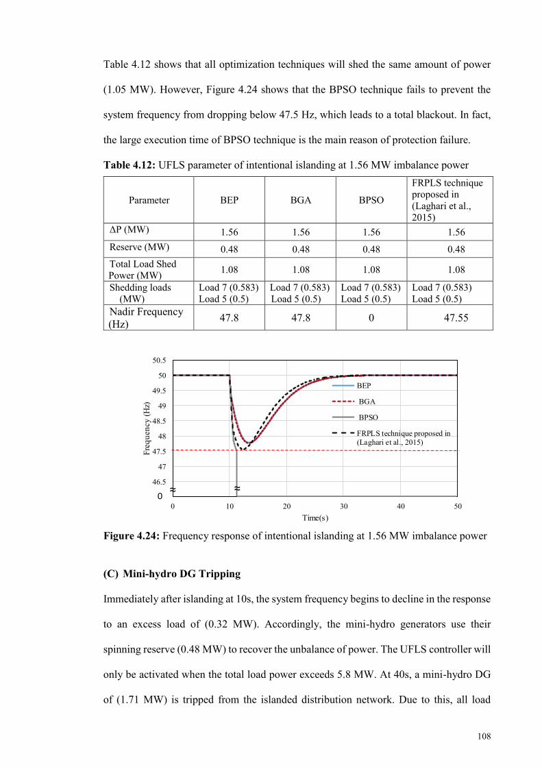
108
Table 4.12 shows that all optimization techniques will shed the same amount of power
(1.05 MW). However, Figure 4.24 shows that the BPSO technique fails to prevent the
system frequency from dropping below 47.5 Hz, which leads to a total blackout. In fact,
the large execution time of BPSO technique is the main reason of protection failure.
Table 4.12: UFLS parameter of intentional islanding at 1.56 MW imbalance power
Parameter BEP BGA BPSO
FRPLS technique proposed in (Laghari et al., 2015)
ΔP (MW) 1.56 1.56 1.56 1.56 Reserve (MW) 0.48 0.48 0.48 0.48 Total Load Shed Power (MW) 1.08 1.08 1.08 1.08
Shedding loads (MW)
Load 7 (0.583) Load 5 (0.5)
Load 7 (0.583) Load 5 (0.5)
Load 7 (0.583) Load 5 (0.5)
Load 7 (0.583) Load 5 (0.5)
Nadir Frequency (Hz) 47.8 47.8 0 47.55
Figure 4.24: Frequency response of intentional islanding at 1.56 MW imbalance power
(C) Mini-hydro DG Tripping
Immediately after islanding at 10s, the system frequency begins to decline in the response
to an excess load of (0.32 MW). Accordingly, the mini-hydro generators use their
spinning reserve (0.48 MW) to recover the unbalance of power. The UFLS controller will
only be activated when the total load power exceeds 5.8 MW. At 40s, a mini-hydro DG
of (1.71 MW) is tripped from the islanded distribution network. Due to this, all load
46
46.5
47
47.5
48
48.5
49
49.5
50
50.5
0 10 20 30 40 50
Freq
uenc
y (H
z)
Time(s)
BEP
BGA
BPSO
FRPLS technique proposed in(Laghari et al., 2015)
0≈≈

109
shedding techniques are initiated to restore the system frequency. Table 4.13 shows that
all load shedding techniques will shed the same amount of power (1.63 MW). However,
Figure 4.25 shows that the BPSO technique and the FRPLS technique fail to stop the
frequency deviation below 47.5 Hz. In fact, the large execution time of BPSO technique
and FRPLS technique proposed in (Laghari et al., 2015) is the main reason of operation
inability.
Table 4.13: The UFLS parameters for mini hydro DG tripping event
Parameter BEP BGA BPSO FRPLS technique proposed in (Laghari et al., 2015)
ΔP (MW) 1.71 1.71 1.71 1.71 Reserve(MW) 0.08 0.08 0.08 0.08 Total Load Shed Power (MW) 1.63 1.63 1.63 1.63
Shedding loads (MW)
Load 1(0.044) Load 4 (0.314) Load 6 (0.55) Load 9 (0.7)
Load 1(0.044) Load 4 (0.314) Load 6 (0.55) Load 9 (0.7)
Load 1(0.044) Load 4 (0.314) Load 6 (0.55) Load 9 (0.7)
Load 1(0.044) Load 4 (0.314) Load 6 (0.55)
Load 9 (0.7) Nadir Frequency (Hz) 49.2 49.1 0 0
Figure 4.25: Frequency response for mini hydro DG tripping event.
4.4 Discussions
As discussed previously, it has become clear that the load shedding controller with fixed
priority loads cannot shed the optimal combination of loads. Contrarily, the FRPLS
technique is able to shed the optimal combination of loads. However, this technique still
suffers from time delay, which affects the operation of the load shedding controller. For

110
this reason, three metaheuristic techniques; BEP, BGA, and BPSO can be applied to
determine the optimal combination of load to be shed. Through comparative simulation
study, the BEP technique requires less time to shed the optimal combination of loads
compared to the BGA and BPSO method. Accordingly, the BEP method is selected for
use with the UFLS technique to shed the optimal combination of loads from the islanding
distribution network.
4.5 Summary
This chapter discusses modelling the distribution network used to validate the proposed
UFLS technique. The effectiveness and robustness of this technique was investigated on
29-Bus test system for islanding events, DG tripping event, and load increment cases.
Through the simulation results, it was proven that the proposed UFLS technique shed the
optimal combination of loads compared to the conventional and adaptive techniques. This
was achieved via metaheuristic methods and flexibility towards load shedding priority.
Accordingly, the proposed UFLS technique is capable of restoring the network frequency
without overshooting.
111
CHAPTER 5: VALIDATION OF PROPOSED FREQUENCY CONTROL
SCHEME
5.1 Introduction
This chapter discusses the validation of proposed frequency control scheme by using the
distribution network model. Various case studies, such as islanding, DG tripping event,
load increments are performed to demonstrate the effectiveness of the proposed frequency
control scheme for different PV penetration. In this chapter, the coordination between
frequency control scheme and synchronization system is conducted to ensure a seamless
reconnection process with the main grid.
5.2 Test System for Proposed Frequency Control Scheme
The test system considered in this research is a part of the Malaysian distribution network,
which was modelled using PSCAD/EMTDC software, as shown in Appendix A, section
A.2. To demonstrate the impact of high PV penetration level on frequency stability of
islanded distribution network, four penetration scenarios were conducted. The first
scenario considers the same network without any PV units, which represents a zero-
penetration level. The second scenario considering the same network, while this time, the
Bio-Mass generator is replaced by three PV units, each rated 0.5 MW, which represent
25% penetration level. The third scenario is similar to the second scenario however, four
PV generation units are used to represent 33% penetration level, as shown in Figure 5.1.
In the fourth scenario, Biomass and mini-hydro DGs are replaced by six PV units to
represent 50% penetration level, which is expressed by the following equation
Penetration level =Total PV Power
Total load power× 100% (5.1)
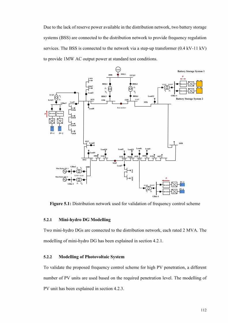
112
Due to the lack of reserve power available in the distribution network, two battery storage
systems (BSS) are connected to the distribution network to provide frequency regulation
services. The BSS is connected to the network via a step-up transformer (0.4 kV-11 kV)
to provide 1MW AC output power at standard test conditions.
Figure 5.1: Distribution network used for validation of frequency control scheme
5.2.1 Mini-hydro DG Modelling
Two mini-hydro DGs are connected to the distribution network, each rated 2 MVA. The
modelling of mini-hydro DG has been explained in section 4.2.1.
5.2.2 Modelling of Photovoltaic System
To validate the proposed frequency control scheme for high PV penetration, a different
number of PV units are used based on the required penetration level. The modelling of
PV unit has been explained in section 4.2.3.
PV-3
PV-4
Mini Hydro DG 11000
Mini Hydro DG 2
1012
1013
1075
2000
GBus1
GBus 2
GBus 4
Grid
1004 1144 1151 1044 1029 1050 1154 1057
NOP
10391010
1058
1056
1047
1026
1046
1018
1019
1020
132 kV
11 kV
0.4 kV
11 kV
1106 1105
11 kV
3.3 kV
GBus3
DCDC
DCDC
InverterInverter
PV-1 PV-2
11 kV
0.4 kV
Load4Load10 Load5
Load7
Load11 Load6 Load1
Load2
Load8
Load9
Load3
BRKG
BRK1 BRK2
DCDC
DCDCInverter
Load12
P
P
GBus 4
0.4 kV11 kV DCDC
DCDCInverter
+-
+-
Inverter
Inverter
P
Battery Storage System 1
Battery Storage System 2
Bus section
BRK3 BRK4
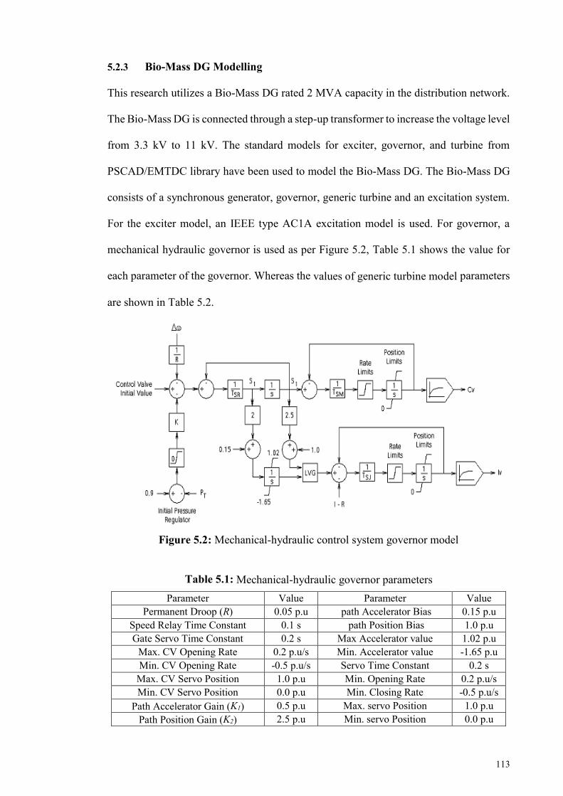
113
5.2.3 Bio-Mass DG Modelling
This research utilizes a Bio-Mass DG rated 2 MVA capacity in the distribution network.
The Bio-Mass DG is connected through a step-up transformer to increase the voltage level
from 3.3 kV to 11 kV. The standard models for exciter, governor, and turbine from
PSCAD/EMTDC library have been used to model the Bio-Mass DG. The Bio-Mass DG
consists of a synchronous generator, governor, generic turbine and an excitation system.
For the exciter model, an IEEE type AC1A excitation model is used. For governor, a
mechanical hydraulic governor is used as per Figure 5.2, Table 5.1 shows the value for
each parameter of the governor. Whereas the values of generic turbine model parameters
are shown in Table 5.2.
Figure 5.2: Mechanical-hydraulic control system governor model
Table 5.1: Mechanical-hydraulic governor parameters Parameter Value Parameter Value
Permanent Droop (R) 0.05 p.u path Accelerator Bias 0.15 p.u Speed Relay Time Constant 0.1 s path Position Bias 1.0 p.u Gate Servo Time Constant 0.2 s Max Accelerator value 1.02 p.u
Max. CV Opening Rate 0.2 p.u/s Min. Accelerator value -1.65 p.u Min. CV Opening Rate -0.5 p.u/s Servo Time Constant 0.2 s
Max. CV Servo Position 1.0 p.u Min. Opening Rate 0.2 p.u/s Min. CV Servo Position 0.0 p.u Min. Closing Rate -0.5 p.u/s
Path Accelerator Gain (K1) 0.5 p.u Max. servo Position 1.0 p.u Path Position Gain (K2) 2.5 p.u Min. servo Position 0.0 p.u
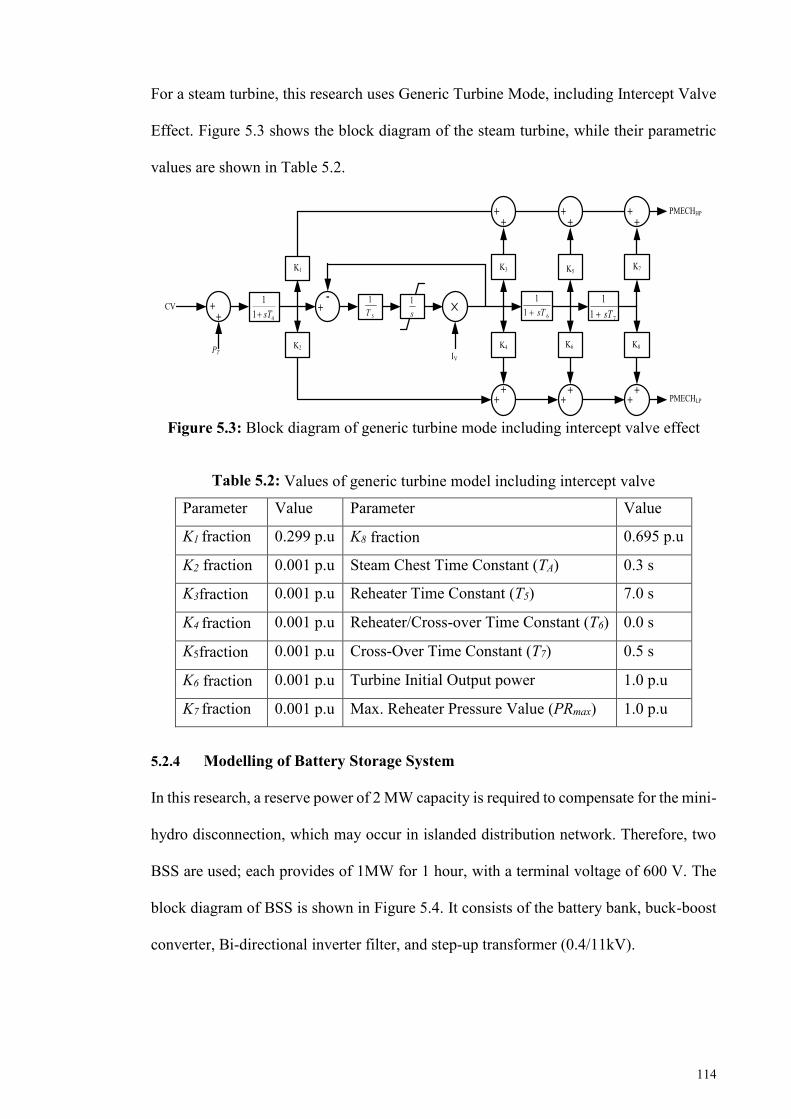
114
For a steam turbine, this research uses Generic Turbine Mode, including Intercept Valve
Effect. Figure 5.3 shows the block diagram of the steam turbine, while their parametric
values are shown in Table 5.2.
Figure 5.3: Block diagram of generic turbine mode including intercept valve effect
Table 5.2: Values of generic turbine model including intercept valve
Parameter Value Parameter Value
K1 fraction 0.299 p.u K8 fraction 0.695 p.u
K2 fraction 0.001 p.u Steam Chest Time Constant (TA) 0.3 s
K3fraction 0.001 p.u Reheater Time Constant (T5) 7.0 s
K4 fraction 0.001 p.u Reheater/Cross-over Time Constant (T6) 0.0 s
K5fraction 0.001 p.u Cross-Over Time Constant (T7) 0.5 s
K6 fraction 0.001 p.u Turbine Initial Output power 1.0 p.u
K7 fraction 0.001 p.u Max. Reheater Pressure Value (PRmax) 1.0 p.u
5.2.4 Modelling of Battery Storage System
In this research, a reserve power of 2 MW capacity is required to compensate for the mini-
hydro disconnection, which may occur in islanded distribution network. Therefore, two
BSS are used; each provides of 1MW for 1 hour, with a terminal voltage of 600 V. The
block diagram of BSS is shown in Figure 5.4. It consists of the battery bank, buck-boost
converter, Bi-directional inverter filter, and step-up transformer (0.4/11kV).
CV
PT
++ 41
1sT
K1
K2
+-
5
1T s
1
IV
K3
K4
+
+
611sT
711sT
+
+ +
+
K5
K6
K7
K8
++ ++ ++
PMECHHP
PMECHLP
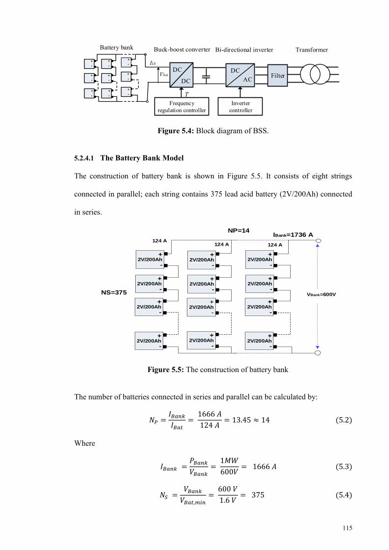
115
Figure 5.4: Block diagram of BSS.
5.2.4.1 The Battery Bank Model
The construction of battery bank is shown in Figure 5.5. It consists of eight strings
connected in parallel; each string contains 375 lead acid battery (2V/200Ah) connected
in series.
Figure 5.5: The construction of battery bank
The number of batteries connected in series and parallel can be calculated by:
𝑁𝑃 =𝐼𝐵𝑎𝑛𝑘𝐼𝐵𝑎𝑡
= 1666 𝐴
124 𝐴= 13.45 ≈ 14 (5.2)
Where
𝐼𝐵𝑎𝑛𝑘 =𝑃𝐵𝑎𝑛𝑘𝑉𝐵𝑎𝑛𝑘
= 1𝑀𝑊
600𝑉= 1666 𝐴 (5.3)
𝑁𝑆 =𝑉𝐵𝑎𝑛𝑘𝑉𝐵𝑎𝑡,𝑚𝑖𝑛
= 600 𝑉
1.6 𝑉= 375 (5.4)
Transformer
DCAC
Bi-directional inverter
DC
DCFilter
Buck-boost converter
Vbat
ILb
TInverter
controllerFrequency
regulation controller
+
-
+
-
+
-
+
-
+
-
+
-
+
-
+
-
+
-
Battery bank
IBank=1736 ANP=14
NS=375 VBank=600V
+
-2V/200Ah
+
-2V/200Ah
+
-2V/200Ah
+
-2V/200Ah
+
-2V/200Ah
+
-2V/200Ah
+
-2V/200Ah
+
-2V/200Ah
+
-2V/200Ah
+
-2V/200Ah
+
-2V/200Ah
+
-2V/200Ah
124 A124 A 124 A
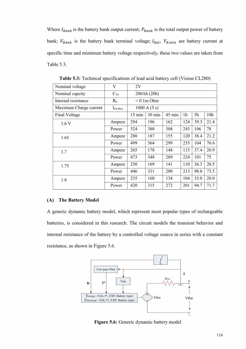
116
Where 𝐼𝐵𝑎𝑛𝑘 is the battery bank output current; 𝑃𝐵𝑎𝑛𝑘 is the total output power of battery
bank; 𝑉𝐵𝑎𝑛𝑘 is the battery bank terminal voltage; 𝐼𝐵𝑎𝑡, 𝑉𝐵,𝑚𝑖𝑛 are battery current at
specific time and minimum battery voltage respectively, these two values are taken from
Table 5.3.
Table 5.3: Technical specifications of lead acid battery cell (Vision CL200) Nominal voltage V 2V Nominal capcity C10 200Ah (20h) Internal resistance R0 < 0.1m Ohm Maximum Charge current Ich,Max 1000 A (5 s) Final Voltage 15 min 30 min 45 min 1h 5h 10h
1.6 V Ampere 294 196 162 124 39.3 21.4 Power 524 380 308 245 106 78
1.65 Ampere 280 187 155 120 38.4 21.2 Power 499 364 299 235 104 76.6
1.7 Ampere 265 178 148 115 37.4 20.9 Power 473 348 289 224 101 75
1.75 Ampere 250 169 141 110 36.3 20.5 Power 446 331 280 213 98.0 73.5
1.8 Ampere 235 160 134 104 35.0 20.0 Power 420 315 272 201 94.7 71.7
(A) The Battery Model
A generic dynamic battery model, which represent most popular types of rechargeable
batteries, is considered in this research. The circuit models the transient behavior and
internal resistance of the battery by a controlled voltage source in series with a constant
resistance, as shown in Figure 5.6.
Figure 5.6: Generic dynamic battery model
+-
Echarge = f1(It, I*, EXP, Battery type)Edischarge = f2(It, I*, EXP, Battery type)
I*
EBat
RSer+
-
VBat
ʃ 0
t
Low pass filter
ExpIt
I
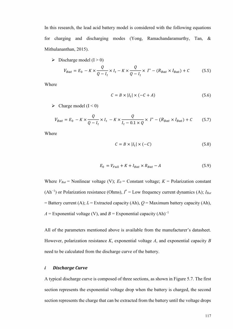
117
In this research, the lead acid battery model is considered with the following equations
for charging and discharging modes (Yong, Ramachandaramurthy, Tan, &
Mithulananthan, 2015).
➢ Discharge model (I > 0)
𝑉𝐵𝑎𝑡 = 𝐸0 − 𝐾 ×𝑄
𝑄 − 𝐼𝑡× 𝐼𝑡 − 𝐾 ×
𝑄
𝑄 − 𝐼𝑡× 𝐼∗ − (𝑅𝐵𝑎𝑡 × 𝐼𝐵𝑎𝑡) + 𝐶 (5.5)
Where
𝐶 = 𝐵 × |𝐼𝑡| × (−𝐶 + 𝐴) (5.6)
➢ Charge model (I < 0)
𝑉𝐵𝑎𝑡 = 𝐸0 − 𝐾 ×𝑄
𝑄 − 𝐼𝑡× 𝐼𝑡 − 𝐾 ×
𝑄
𝐼𝑡 − 0.1 × 𝑄× 𝐼∗ − (𝑅𝐵𝑎𝑡 × 𝐼𝐵𝑎𝑡) + 𝐶 (5.7)
Where
𝐶 = 𝐵 × |𝐼𝑡| × (−𝐶) (5.8)
𝐸0 = 𝑉𝐹𝑢𝑙𝑙 + 𝐾 + 𝐼𝐵𝑎𝑡 × 𝑅𝐵𝑎𝑡 − 𝐴 (5.9)
Where VBat = Nonlinear voltage (V); E0 = Constant voltage; K = Polarization constant
(Ah−1) or Polarization resistance (Ohms), I* = Low frequency current dynamics (A); IBat
= Battery current (A); It = Extracted capacity (Ah), Q = Maximum battery capacity (Ah),
A = Exponential voltage (V), and B = Exponential capacity (Ah)−1
All of the parameters mentioned above is available from the manufacturer’s datasheet.
However, polarization resistance K, exponential voltage A, and exponential capacity B
need to be calculated from the discharge curve of the battery.
i Discharge Curve
A typical discharge curve is composed of three sections, as shown in Figure 5.7. The first
section represents the exponential voltage drop when the battery is charged, the second
section represents the charge that can be extracted from the battery until the voltage drops
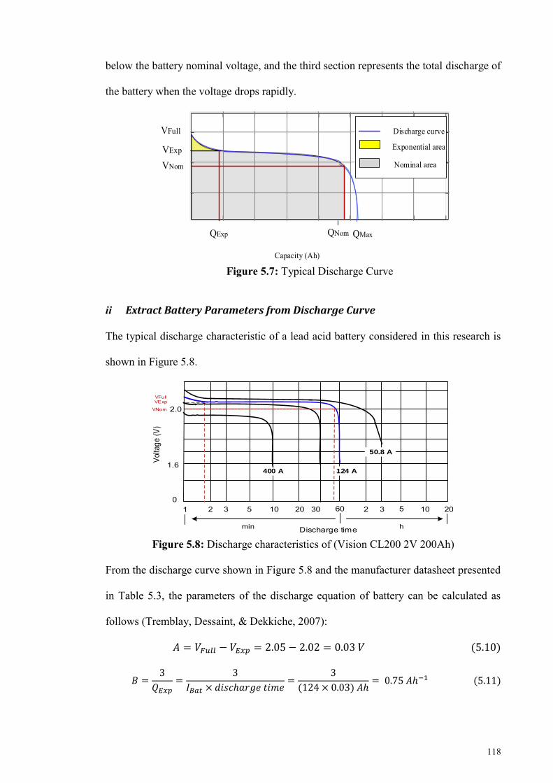
118
below the battery nominal voltage, and the third section represents the total discharge of
the battery when the voltage drops rapidly.
Figure 5.7: Typical Discharge Curve
ii Extract Battery Parameters from Discharge Curve
The typical discharge characteristic of a lead acid battery considered in this research is
shown in Figure 5.8.
Figure 5.8: Discharge characteristics of (Vision CL200 2V 200Ah)
From the discharge curve shown in Figure 5.8 and the manufacturer datasheet presented
in Table 5.3, the parameters of the discharge equation of battery can be calculated as
follows (Tremblay, Dessaint, & Dekkiche, 2007):
𝐴 = 𝑉𝐹𝑢𝑙𝑙 − 𝑉𝐸𝑥𝑝 = 2.05 − 2.02 = 0.03 𝑉 (5.10)
𝐵 =3
𝑄𝐸𝑥𝑝=
3
𝐼𝐵𝑎𝑡 × 𝑑𝑖𝑠𝑐ℎ𝑎𝑟𝑔𝑒 𝑡𝑖𝑚𝑒=
3
(124 × 0.03) 𝐴ℎ= 0.75 𝐴ℎ−1 (5.11)
QMaxQNom
VFull
VExp
QExp
Capacity (Ah)
Discharge curve
Exponential area
Nominal areaVNomVo
ltage
(V)
VNom
VFullVExp
1 2 3 5 60 2 3 5 10 20302010
Discharge time hmin
1.6
2.0
400 A
50.8 A
0
124 A
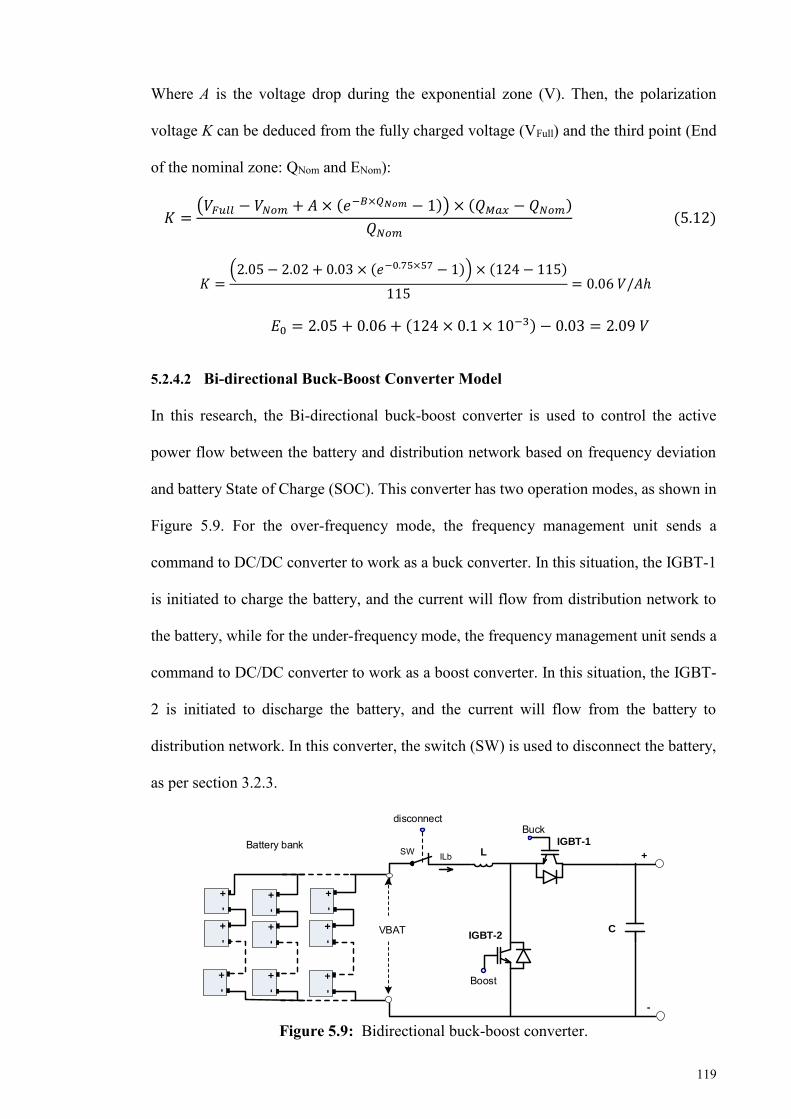
119
Where A is the voltage drop during the exponential zone (V). Then, the polarization
voltage K can be deduced from the fully charged voltage (VFull) and the third point (End
of the nominal zone: QNom and ENom):
𝐾 =(𝑉𝐹𝑢𝑙𝑙 − 𝑉𝑁𝑜𝑚 + 𝐴 × (𝑒
−𝐵×𝑄𝑁𝑜𝑚 − 1)) × (𝑄𝑀𝑎𝑥 − 𝑄𝑁𝑜𝑚)
𝑄𝑁𝑜𝑚 (5.12)
𝐾 =(2.05 − 2.02 + 0.03 × (𝑒−0.75×57 − 1)) × (124 − 115)
115= 0.06 𝑉/𝐴ℎ
𝐸0 = 2.05 + 0.06 + (124 × 0.1 × 10−3) − 0.03 = 2.09 𝑉
5.2.4.2 Bi-directional Buck-Boost Converter Model
In this research, the Bi-directional buck-boost converter is used to control the active
power flow between the battery and distribution network based on frequency deviation
and battery State of Charge (SOC). This converter has two operation modes, as shown in
Figure 5.9. For the over-frequency mode, the frequency management unit sends a
command to DC/DC converter to work as a buck converter. In this situation, the IGBT-1
is initiated to charge the battery, and the current will flow from distribution network to
the battery, while for the under-frequency mode, the frequency management unit sends a
command to DC/DC converter to work as a boost converter. In this situation, the IGBT-
2 is initiated to discharge the battery, and the current will flow from the battery to
distribution network. In this converter, the switch (SW) is used to disconnect the battery,
as per section 3.2.3.
Figure 5.9: Bidirectional buck-boost converter.
Boost
ILb
VBAT
Buckdisconnect
C
L +
-
IGBT-1
IGBT-2
SW
+
-
+
-
+
-
+
-
+
-
+
-
+
-
+
-
+
-
Battery bank
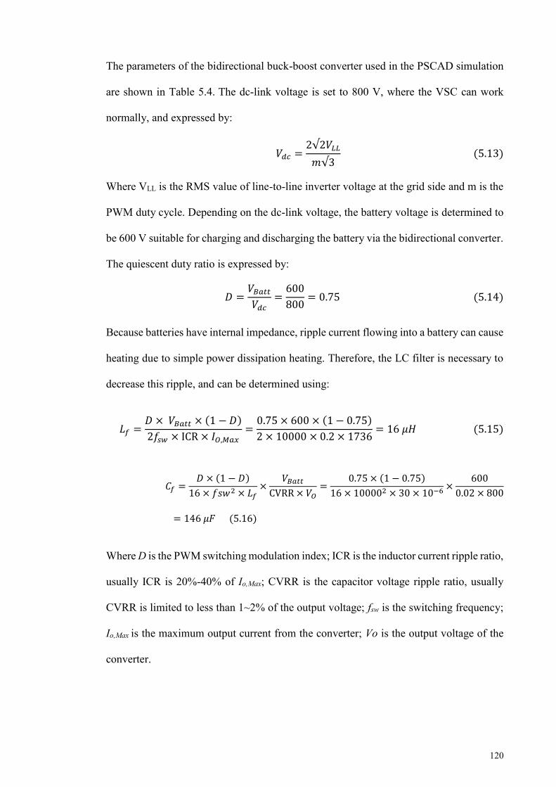
120
The parameters of the bidirectional buck-boost converter used in the PSCAD simulation
are shown in Table 5.4. The dc-link voltage is set to 800 V, where the VSC can work
normally, and expressed by:
𝑉𝑑𝑐 =2√2𝑉𝐿𝐿
𝑚√3 (5.13)
Where VLL is the RMS value of line-to-line inverter voltage at the grid side and m is the
PWM duty cycle. Depending on the dc-link voltage, the battery voltage is determined to
be 600 V suitable for charging and discharging the battery via the bidirectional converter.
The quiescent duty ratio is expressed by:
𝐷 =𝑉𝐵𝑎𝑡𝑡𝑉𝑑𝑐
=600
800= 0.75 (5.14)
Because batteries have internal impedance, ripple current flowing into a battery can cause
heating due to simple power dissipation heating. Therefore, the LC filter is necessary to
decrease this ripple, and can be determined using:
𝐿𝑓 =𝐷 × 𝑉𝐵𝑎𝑡𝑡 × (1 − 𝐷)
2𝑓𝑠𝑤 × ICR × 𝐼𝑂,𝑀𝑎𝑥=0.75 × 600 × (1 − 0.75)
2 × 10000 × 0.2 × 1736= 16 𝜇𝐻 (5.15)
𝐶𝑓 =𝐷 × (1 − 𝐷)
16 × 𝑓𝑠𝑤2 × 𝐿𝑓×
𝑉𝐵𝑎𝑡𝑡CVRR × 𝑉𝑂
=0.75 × (1 − 0.75)
16 × 100002 × 30 × 10−6×
600
0.02 × 800
= 146 𝜇𝐹 (5.16)
Where D is the PWM switching modulation index; ICR is the inductor current ripple ratio,
usually ICR is 20%-40% of Io,Max; CVRR is the capacitor voltage ripple ratio, usually
CVRR is limited to less than 1~2% of the output voltage; fsw is the switching frequency;
Io,Max is the maximum output current from the converter; Vo is the output voltage of the
converter.
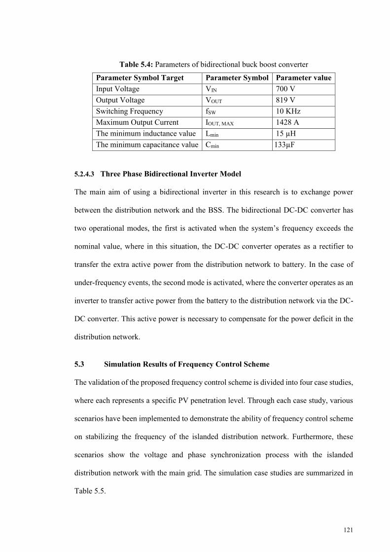
121
Table 5.4: Parameters of bidirectional buck boost converter
Parameter Symbol Target Parameter Symbol Parameter value Input Voltage VIN 700 V Output Voltage VOUT 819 V Switching Frequency fSW 10 KHz Maximum Output Current IOUT, MAX 1428 A The minimum inductance value Lmin 15 µH The minimum capacitance value Cmin 133µF
5.2.4.3 Three Phase Bidirectional Inverter Model
The main aim of using a bidirectional inverter in this research is to exchange power
between the distribution network and the BSS. The bidirectional DC-DC converter has
two operational modes, the first is activated when the system’s frequency exceeds the
nominal value, where in this situation, the DC-DC converter operates as a rectifier to
transfer the extra active power from the distribution network to battery. In the case of
under-frequency events, the second mode is activated, where the converter operates as an
inverter to transfer active power from the battery to the distribution network via the DC-
DC converter. This active power is necessary to compensate for the power deficit in the
distribution network.
5.3 Simulation Results of Frequency Control Scheme
The validation of the proposed frequency control scheme is divided into four case studies,
where each represents a specific PV penetration level. Through each case study, various
scenarios have been implemented to demonstrate the ability of frequency control scheme
on stabilizing the frequency of the islanded distribution network. Furthermore, these
scenarios show the voltage and phase synchronization process with the islanded
distribution network with the main grid. The simulation case studies are summarized in
Table 5.5.
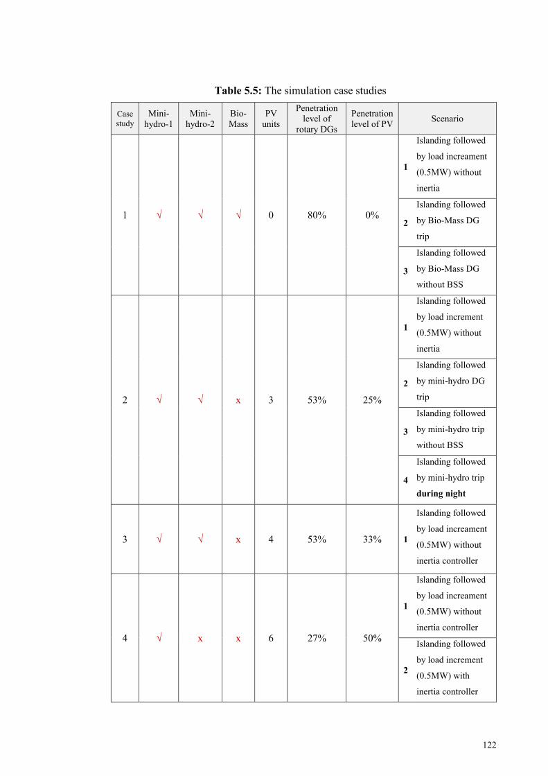
122
Table 5.5: The simulation case studies
Case study
Mini-hydro-1
Mini-hydro-2
Bio-Mass
PV units
Penetration level of
rotary DGs
Penetration level of PV Scenario
1 √ √ √ 0 80% 0%
1
Islanding followed
by load increament
(0.5MW) without
inertia
2
Islanding followed
by Bio-Mass DG
trip
3
Islanding followed
by Bio-Mass DG
without BSS
2 √ √ x 3 53% 25%
1
Islanding followed
by load increment
(0.5MW) without
inertia
2
Islanding followed
by mini-hydro DG
trip
3
Islanding followed
by mini-hydro trip
without BSS
4
Islanding followed
by mini-hydro trip
during night
3 √ √ x 4 53% 33% 1
Islanding followed
by load increament
(0.5MW) without
inertia controller
4 √ x x 6 27% 50%
1
Islanding followed
by load increament
(0.5MW) without
inertia controller
2
Islanding followed
by load increment
(0.5MW) with
inertia controller

123
5.3.1 First case study (80% rotary DGs and 0% PV penetration level)
First scenario: Islanding followed by load increment (0.5MW) without inertia controller
In this scenario, the intentional islanding occurred at t=10s. Immediately after islanding,
the system frequency begins to decrease in the response to an excess load of (1.1 MW).
Accordingly, both primary frequency control of BSS and the governor system of mini-
hydro provide the required power to restore the frequency to an acceptable level. At 30s,
a secondary frequency control from BSS is activated to bring back the distribution
network to its nominal value of (50Hz), as shown in Figure 5.10. At 40s, the load
increment will be 0.5 MW. Immediately after load increment, the system frequency
begins to decline again in response to an excess load. In this situation, the UFLS controller
will not be initiated because the least reserve power (mini-hydro & battery reserve) is
sufficient to recover the network frequency. At 70 s, the phase controller is activated to
synchronize the distribution network phase angle with the main grid. When the
synchronization criteria of phase and voltage are achieved, the distribution network will
be smoothly reconnected to the main grid, as shown in Figure 5.11 a) and b).
Figure 5.10: Frequency response of intentional islanding followed by load increment
(first scenario/first case study)
48
48.5
49
49.5
50
50.5
51
0 10 20 30 40 50 60 70 80 90 100 110
Freq
uen
cy (
Hz)
Time (s)
Load increament
Primary Secondary Primary Secondary
Phase control ReconnectionIslanding

124
a) b)
Figure 5.11: a) Phase difference between distribution network and main grid for (first
scenario/first case study) b) the voltage difference between distribution network and
main grid for (first scenario/first case study)
Second scenario: Islanding followed by Bio-Mass DG trip
In this scenario, the distribution network will report the same response to the first
scenario, however, at 40s, a biomass DG of (1.7 MW) is tripped from the network.
Therefore, the system’s frequency begins to decline in response to an excess load, as
shown in Figure 5.12. In this situation, the UFLS controller will be initiated and shed load
4 (0.314 MW), because the least reserve power (1.4 MW) is insufficient to recover the
network frequency. When the synchronization criteria of phase and voltage are achieved,
as shown in Figure 5.13 a) and b), the distribution network will be smoothly reconnected
to the main grid.
-500
-400
-300
-200
-100
0
100
200
300
400
500
0 10 20 30 40 50 60 70 80 90 100 110
Ph
as
e d
iffe
re
nc
e (
de
gre
e)
Time (s)
0
0.02
0.04
0.06
0.08
0.1
0.12
0.14
0.16
0.18
0.2
0 10 20 30 40 50 60 70 80 90 100 110
Vo
lta
ge
dif
fere
nc
e (
V)
Time (s)
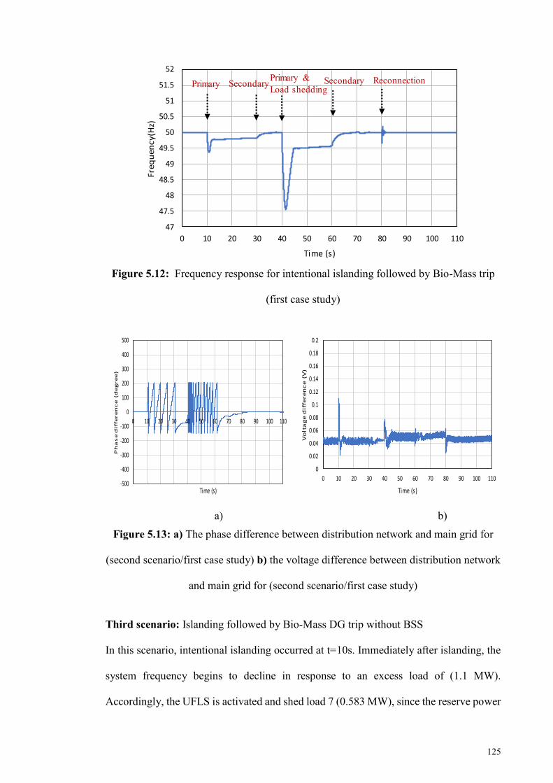
125
Figure 5.12: Frequency response for intentional islanding followed by Bio-Mass trip
(first case study)
a) b)
Figure 5.13: a) The phase difference between distribution network and main grid for
(second scenario/first case study) b) the voltage difference between distribution network
and main grid for (second scenario/first case study)
Third scenario: Islanding followed by Bio-Mass DG trip without BSS
In this scenario, intentional islanding occurred at t=10s. Immediately after islanding, the
system frequency begins to decline in response to an excess load of (1.1 MW).
Accordingly, the UFLS is activated and shed load 7 (0.583 MW), since the reserve power
47
47.5
48
48.5
49
49.5
50
50.5
51
51.5
52
0 10 20 30 40 50 60 70 80 90 100 110
Freq
uen
cy(H
z)
Time (s)
Primary SecondaryPrimary &Load shedding
Secondary Reconnection
-500
-400
-300
-200
-100
0
100
200
300
400
500
0 10 20 30 40 50 60 70 80 90 100 110
Ph
as
e d
iffe
re
nc
e (
de
gre
e)
Time (s)
0
0.02
0.04
0.06
0.08
0.1
0.12
0.14
0.16
0.18
0.2
0 10 20 30 40 50 60 70 80 90 100 110
Vo
lta
ge
dif
fere
nc
e (
V)
Time (s)
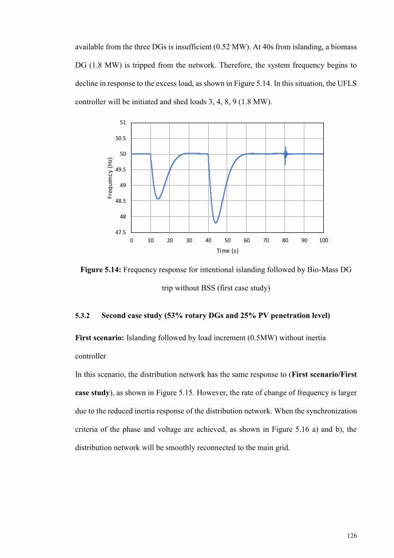
126
available from the three DGs is insufficient (0.52 MW). At 40s from islanding, a biomass
DG (1.8 MW) is tripped from the network. Therefore, the system frequency begins to
decline in response to the excess load, as shown in Figure 5.14. In this situation, the UFLS
controller will be initiated and shed loads 3, 4, 8, 9 (1.8 MW).
Figure 5.14: Frequency response for intentional islanding followed by Bio-Mass DG
trip without BSS (first case study)
5.3.2 Second case study (53% rotary DGs and 25% PV penetration level)
First scenario: Islanding followed by load increment (0.5MW) without inertia
controller
In this scenario, the distribution network has the same response to (First scenario/First
case study), as shown in Figure 5.15. However, the rate of change of frequency is larger
due to the reduced inertia response of the distribution network. When the synchronization
criteria of the phase and voltage are achieved, as shown in Figure 5.16 a) and b), the
distribution network will be smoothly reconnected to the main grid.
47.5
48
48.5
49
49.5
50
50.5
51
0 10 20 30 40 50 60 70 80 90 100
Freq
uen
cy (
Hz)
Time (s)
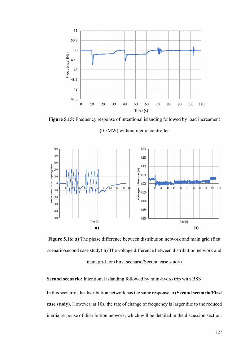
127
Figure 5.15: Frequency response of intentional islanding followed by load increament
(0.5MW) without inertia controller
a) b)
Figure 5.16: a) The phase difference between distribution network and main grid (first
scenario/second case study) b) The voltage difference between distribution network and
main grid for (First scenario/Second case study)
Second scenario: Intentional islanding followed by mini-hydro trip with BSS
In this scenario, the distribution network has the same response to (Second scenario/First
case study). However, at 10s, the rate of change of frequency is larger due to the reduced
inertia response of distribution network, which will be detailed in the discussion section.
47.5
48
48.5
49
49.5
50
50.5
51
0 10 20 30 40 50 60 70 80 90 100 110
Freq
uen
cy (
Hz)
Time (s)
-500
-400
-300
-200
-100
0
100
200
300
400
500
0 10 20 30 40 50 60 70 80 90 100 110
Ph
as
e d
iffe
re
nc
e(d
eg
re
e)
Time (s)-0.200
-0.150
-0.100
-0.050
0.000
0.050
0.100
0.150
0.200
0 10 20 30 40 50 60 70 80 90 100 110
Vo
lta
ge
dif
fern
ce
(V
)
Time (s)
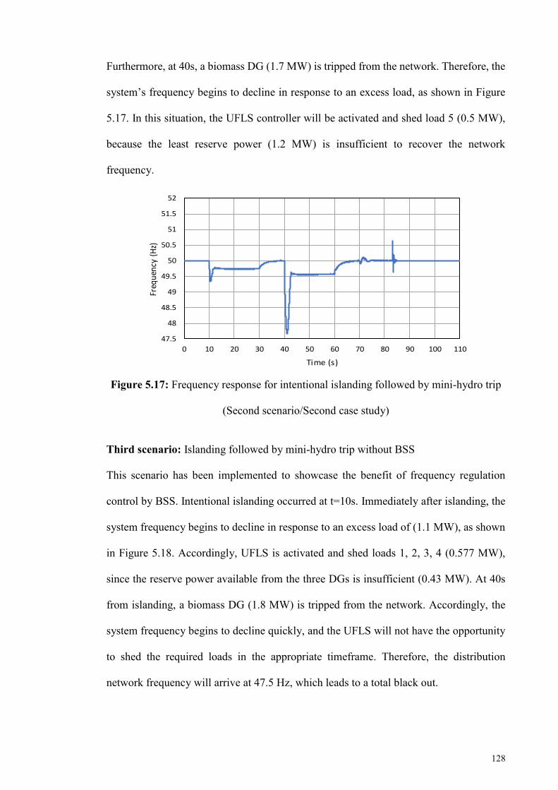
128
Furthermore, at 40s, a biomass DG (1.7 MW) is tripped from the network. Therefore, the
system’s frequency begins to decline in response to an excess load, as shown in Figure
5.17. In this situation, the UFLS controller will be activated and shed load 5 (0.5 MW),
because the least reserve power (1.2 MW) is insufficient to recover the network
frequency.
Figure 5.17: Frequency response for intentional islanding followed by mini-hydro trip
(Second scenario/Second case study)
Third scenario: Islanding followed by mini-hydro trip without BSS
This scenario has been implemented to showcase the benefit of frequency regulation
control by BSS. Intentional islanding occurred at t=10s. Immediately after islanding, the
system frequency begins to decline in response to an excess load of (1.1 MW), as shown
in Figure 5.18. Accordingly, UFLS is activated and shed loads 1, 2, 3, 4 (0.577 MW),
since the reserve power available from the three DGs is insufficient (0.43 MW). At 40s
from islanding, a biomass DG (1.8 MW) is tripped from the network. Accordingly, the
system frequency begins to decline quickly, and the UFLS will not have the opportunity
to shed the required loads in the appropriate timeframe. Therefore, the distribution
network frequency will arrive at 47.5 Hz, which leads to a total black out.
47.5
48
48.5
49
49.5
50
50.5
51
51.5
52
0 10 20 30 40 50 60 70 80 90 100 110
Freq
uenc
y (H
z)
Time (s)
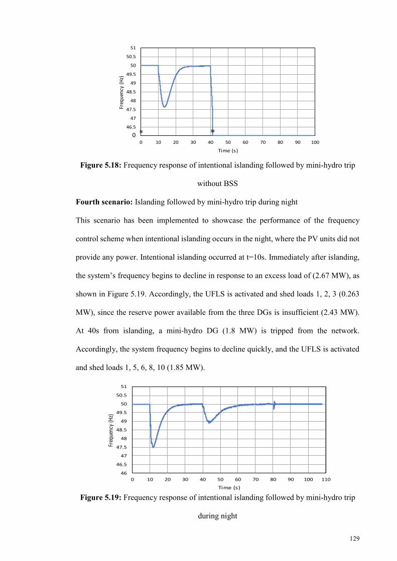
129
Figure 5.18: Frequency response of intentional islanding followed by mini-hydro trip
without BSS
Fourth scenario: Islanding followed by mini-hydro trip during night
This scenario has been implemented to showcase the performance of the frequency
control scheme when intentional islanding occurs in the night, where the PV units did not
provide any power. Intentional islanding occurred at t=10s. Immediately after islanding,
the system’s frequency begins to decline in response to an excess load of (2.67 MW), as
shown in Figure 5.19. Accordingly, the UFLS is activated and shed loads 1, 2, 3 (0.263
MW), since the reserve power available from the three DGs is insufficient (2.43 MW).
At 40s from islanding, a mini-hydro DG (1.8 MW) is tripped from the network.
Accordingly, the system frequency begins to decline quickly, and the UFLS is activated
and shed loads 1, 5, 6, 8, 10 (1.85 MW).
Figure 5.19: Frequency response of intentional islanding followed by mini-hydro trip
during night
46
46.5
47
47.5
48
48.5
49
49.5
50
50.5
51
0 10 20 30 40 50 60 70 80 90 100
Freq
uenc
y (H
z)
Time (s)
0≈ ≈
46
46.5
47
47.5
48
48.5
49
49.5
50
50.5
51
0 10 20 30 40 50 60 70 80 90 100 110
Freq
uenc
y (H
z)
Time (s)
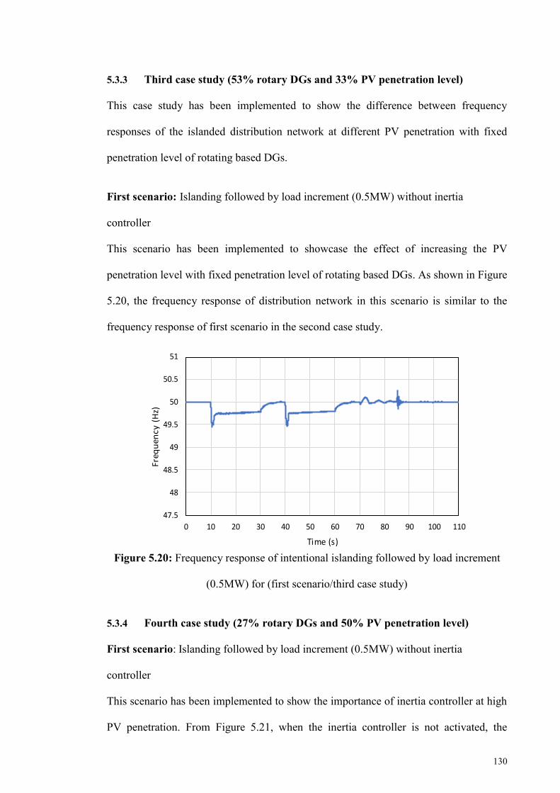
130
5.3.3 Third case study (53% rotary DGs and 33% PV penetration level)
This case study has been implemented to show the difference between frequency
responses of the islanded distribution network at different PV penetration with fixed
penetration level of rotating based DGs.
First scenario: Islanding followed by load increment (0.5MW) without inertia
controller
This scenario has been implemented to showcase the effect of increasing the PV
penetration level with fixed penetration level of rotating based DGs. As shown in Figure
5.20, the frequency response of distribution network in this scenario is similar to the
frequency response of first scenario in the second case study.
Figure 5.20: Frequency response of intentional islanding followed by load increment
(0.5MW) for (first scenario/third case study)
5.3.4 Fourth case study (27% rotary DGs and 50% PV penetration level)
First scenario: Islanding followed by load increment (0.5MW) without inertia
controller
This scenario has been implemented to show the importance of inertia controller at high
PV penetration. From Figure 5.21, when the inertia controller is not activated, the
47.5
48
48.5
49
49.5
50
50.5
51
0 10 20 30 40 50 60 70 80 90 100 110
Freq
uen
cy (
Hz)
Time (s)
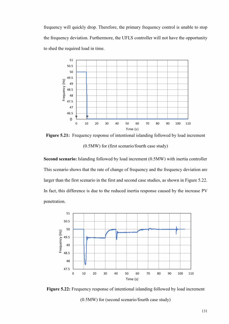
131
frequency will quickly drop. Therefore, the primary frequency control is unable to stop
the frequency deviation. Furthermore, the UFLS controller will not have the opportunity
to shed the required load in time.
Figure 5.21: Frequency response of intentional islanding followed by load increment
(0.5MW) for (first scenario/fourth case study)
Second scenario: Islanding followed by load increment (0.5MW) with inertia controller
This scenario shows that the rate of change of frequency and the frequency deviation are
larger than the first scenario in the first and second case studies, as shown in Figure 5.22.
In fact, this difference is due to the reduced inertia response caused by the increase PV
penetration.
Figure 5.22: Frequency response of intentional islanding followed by load increment
(0.5MW) for (second scenario/fourth case study)
46
46.5
47
47.5
48
48.5
49
49.5
50
50.5
51
0 10 20 30 40 50 60 70 80 90 100 110
Freq
uen
cy (
Hz)
Time (s)
0≈ ≈
47.5
48
48.5
49
49.5
50
50.5
51
0 10 20 30 40 50 60 70 80 90 100 110
Freq
uen
cy (
Hz)
Time (s)
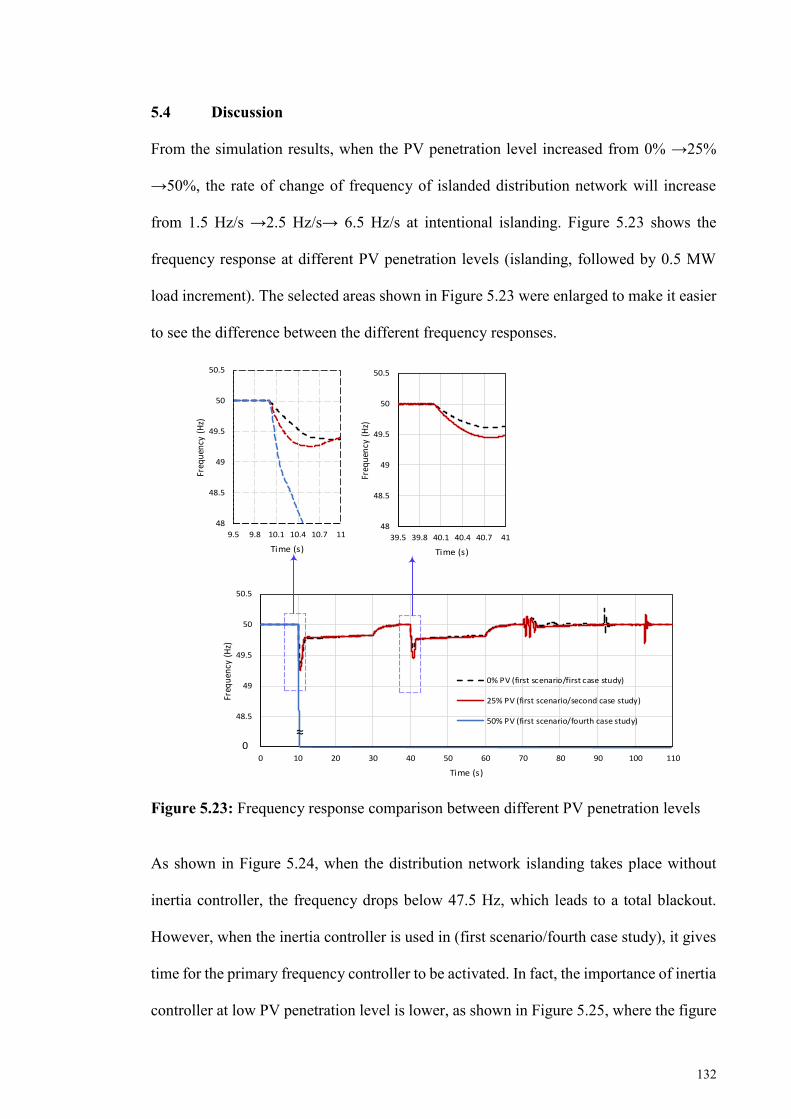
132
5.4 Discussion
From the simulation results, when the PV penetration level increased from 0% →25%
→50%, the rate of change of frequency of islanded distribution network will increase
from 1.5 Hz/s →2.5 Hz/s→ 6.5 Hz/s at intentional islanding. Figure 5.23 shows the
frequency response at different PV penetration levels (islanding, followed by 0.5 MW
load increment). The selected areas shown in Figure 5.23 were enlarged to make it easier
to see the difference between the different frequency responses.
Figure 5.23: Frequency response comparison between different PV penetration levels
As shown in Figure 5.24, when the distribution network islanding takes place without
inertia controller, the frequency drops below 47.5 Hz, which leads to a total blackout.
However, when the inertia controller is used in (first scenario/fourth case study), it gives
time for the primary frequency controller to be activated. In fact, the importance of inertia
controller at low PV penetration level is lower, as shown in Figure 5.25, where the figure
48
48.5
49
49.5
50
50.5
0 10 20 30 40 50 60 70 80 90 100 110
Freq
uen
cy (
Hz)
Time (s)
0% PV (first scenario/first case study)
25% PV (first scenario/second case study)
50% PV (first scenario/fourth case study)
0≈
48
48.5
49
49.5
50
50.5
9.5 9.8 10.1 10.4 10.7 11
Freq
uen
cy (
Hz)
Time (s)
48
48.5
49
49.5
50
50.5
39.5 39.8 40.1 40.4 40.7 41
Freq
uen
cy (
Hz)
Time (s)

133
shows that the rate of change of frequency slightly changes when the inertia controller is
used.
Figure 5.24: Frequency response for 50% PV penetration with and without inertia
Figure 5.25: Frequency response for 25% PV penetration with and without inertia
47
47.5
48
48.5
49
49.5
50
50.5
0 10 20 30 40 50 60 70 80 90 100
Freq
uenc
y (H
z)
Time (s)
50 % PV and 27% mini-hydro (without inertia )
50 % PV and 27% mini-hydro (with inertia )
0≈
48.5
48.7
48.9
49.1
49.3
49.5
49.7
49.9
50.1
50.3
50.5
9.7 10 10.3 10.6 10.9
Fre
qu
en
cy
(H
z)
Time (s)
48.5
48.7
48.9
49.1
49.3
49.5
49.7
49.9
50.1
50.3
50.5
0 10 20 30 40 50 60 70 80 90 100
Freq
uen
cy (
Hz)
Time (s)
25 % PV and 53% mini-hydro (with inertia)
25 % PV and 53% mini-hydro (without inertia)
48.5
48.7
48.9
49.1
49.3
49.5
49.7
49.9
50.1
50.3
50.5
39.5 39.8 40.1 40.4 40.7 41
Fre
qu
en
cy
(H
z)
Time (s)
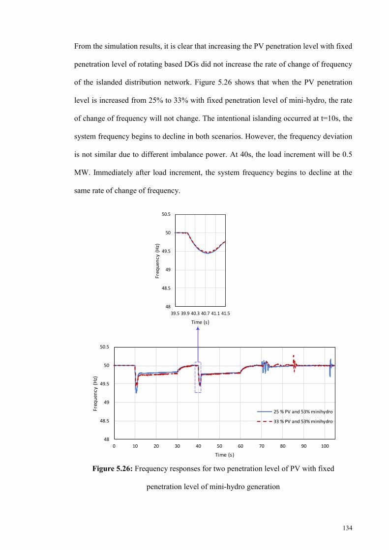
134
From the simulation results, it is clear that increasing the PV penetration level with fixed
penetration level of rotating based DGs did not increase the rate of change of frequency
of the islanded distribution network. Figure 5.26 shows that when the PV penetration
level is increased from 25% to 33% with fixed penetration level of mini-hydro, the rate
of change of frequency will not change. The intentional islanding occurred at t=10s, the
system frequency begins to decline in both scenarios. However, the frequency deviation
is not similar due to different imbalance power. At 40s, the load increment will be 0.5
MW. Immediately after load increment, the system frequency begins to decline at the
same rate of change of frequency.
48
48.5
49
49.5
50
50.5
0 10 20 30 40 50 60 70 80 90 100
Freq
uen
cy (
Hz)
Time (s)
25 % PV and 53% minihydro
33 % PV and 53% minihydro
48
48.5
49
49.5
50
50.5
39.5 39.9 40.3 40.7 41.1 41.5
Freq
uen
cy (
Hz)
Time (s)
Figure 5.26: Frequency responses for two penetration level of PV with fixed
penetration level of mini-hydro generation
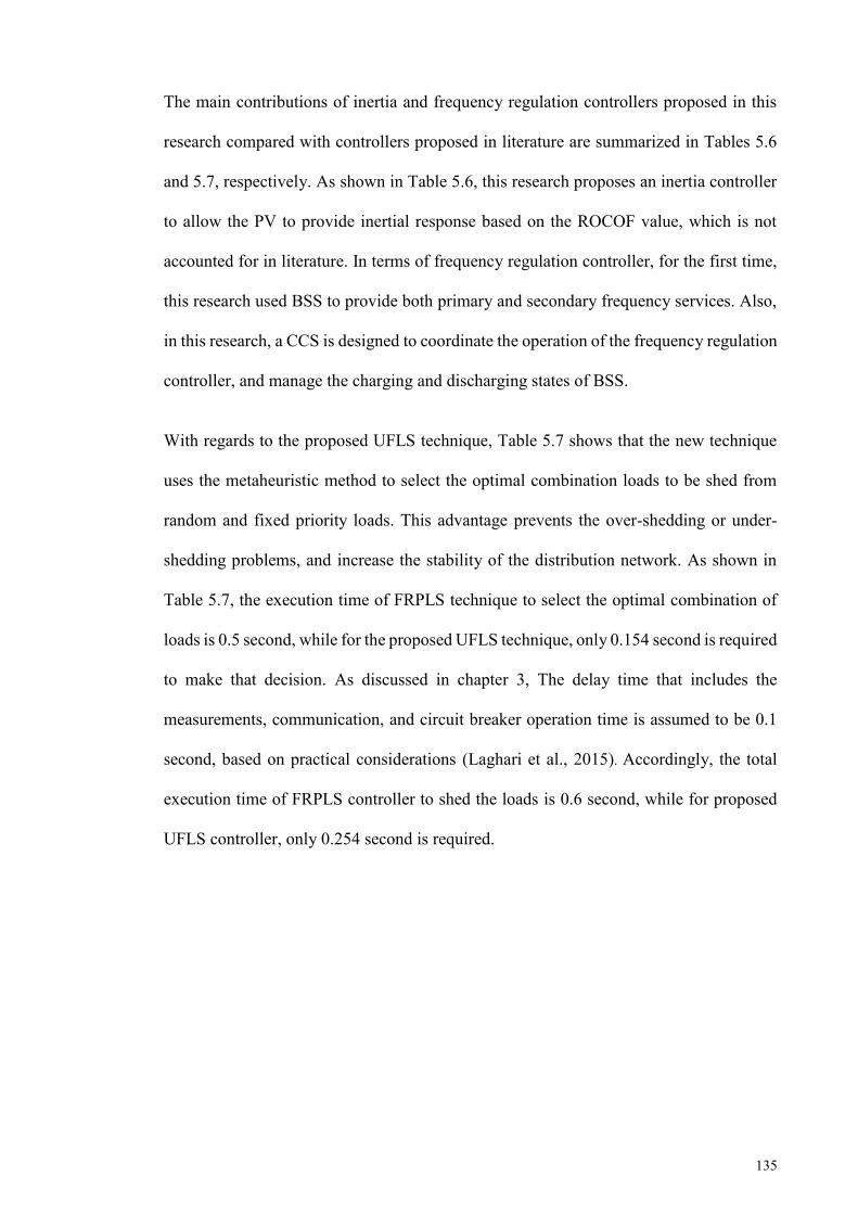
135
The main contributions of inertia and frequency regulation controllers proposed in this
research compared with controllers proposed in literature are summarized in Tables 5.6
and 5.7, respectively. As shown in Table 5.6, this research proposes an inertia controller
to allow the PV to provide inertial response based on the ROCOF value, which is not
accounted for in literature. In terms of frequency regulation controller, for the first time,
this research used BSS to provide both primary and secondary frequency services. Also,
in this research, a CCS is designed to coordinate the operation of the frequency regulation
controller, and manage the charging and discharging states of BSS.
With regards to the proposed UFLS technique, Table 5.7 shows that the new technique
uses the metaheuristic method to select the optimal combination loads to be shed from
random and fixed priority loads. This advantage prevents the over-shedding or under-
shedding problems, and increase the stability of the distribution network. As shown in
Table 5.7, the execution time of FRPLS technique to select the optimal combination of
loads is 0.5 second, while for the proposed UFLS technique, only 0.154 second is required
to make that decision. As discussed in chapter 3, The delay time that includes the
measurements, communication, and circuit breaker operation time is assumed to be 0.1
second, based on practical considerations (Laghari et al., 2015). Accordingly, the total
execution time of FRPLS controller to shed the loads is 0.6 second, while for proposed
UFLS controller, only 0.254 second is required.
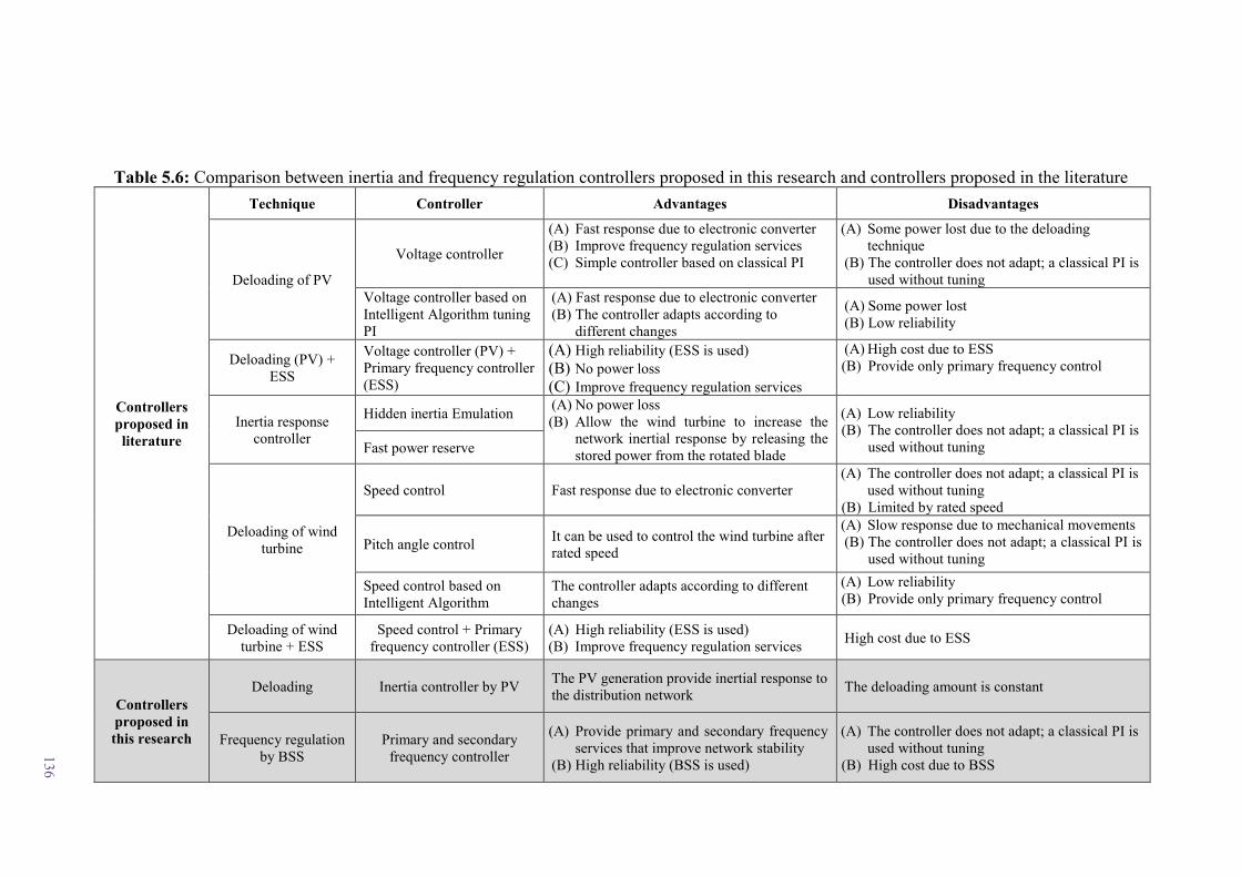
136
Table 5.6: Comparison between inertia and frequency regulation controllers proposed in this research and controllers proposed in the literature
Controllers proposed in literature
Technique Controller Advantages Disadvantages
Deloading of PV
Voltage controller
(A) Fast response due to electronic converter (B) Improve frequency regulation services (C) Simple controller based on classical PI
(A) Some power lost due to the deloading technique
(B) The controller does not adapt; a classical PI is used without tuning
Voltage controller based on Intelligent Algorithm tuning PI
(A) Fast response due to electronic converter (B) The controller adapts according to
different changes
(A) Some power lost (B) Low reliability
Deloading (PV) + ESS
Voltage controller (PV) + Primary frequency controller (ESS)
(A) High reliability (ESS is used) (B) No power loss (C) Improve frequency regulation services
(A) High cost due to ESS (B) Provide only primary frequency control
Inertia response controller
Hidden inertia Emulation (A) No power loss (B) Allow the wind turbine to increase the
network inertial response by releasing the stored power from the rotated blade
(A) Low reliability (B) The controller does not adapt; a classical PI is
used without tuning Fast power reserve
Deloading of wind turbine
Speed control Fast response due to electronic converter (A) The controller does not adapt; a classical PI is
used without tuning (B) Limited by rated speed
Pitch angle control It can be used to control the wind turbine after rated speed
(A) Slow response due to mechanical movements (B) The controller does not adapt; a classical PI is
used without tuning
Speed control based on Intelligent Algorithm
The controller adapts according to different changes
(A) Low reliability (B) Provide only primary frequency control
Deloading of wind turbine + ESS
Speed control + Primary frequency controller (ESS)
(A) High reliability (ESS is used) (B) Improve frequency regulation services High cost due to ESS
Controllers proposed in this research
Deloading Inertia controller by PV The PV generation provide inertial response to the distribution network The deloading amount is constant
Frequency regulation by BSS
Primary and secondary frequency controller
(A) Provide primary and secondary frequency services that improve network stability
(B) High reliability (BSS is used)
(A) The controller does not adapt; a classical PI is used without tuning
(B) High cost due to BSS
137
Table 5.7: Comparison between UFLS technique proposed in this research and technique proposed in the literature
UFLS technique References Method used in UFLS technique
Priority of shedding loads
The ability to shed the optimal combination of loads
Time consumed in selecting the optimal combination of loads
Effect of network configuration on the UFLS technique
Conventional UFLS technique
(Tang et al., 2013; Zin et al., 2004)
Predetermined frequency steps
Fixed priority load
Suffers from over-shedding or under-shedding
No time consumed (fixed priority load)
The predetermined steps need to be selected according to the network’s configuration
Adaptive UFLS
technique
(Marzband et al., 2016; Rudez & Mihalic, 2011)
Swing equation This technique does not depend on the network’s configuration
Computational Intelligence Based Load Shedding Techniques
(Mokhlis et al., 2012; Sallam & Khafaga, 2002)
Fuzzy logic method
Suffers from over-shedding or under-shedding
No time consumed (fixed priority load)
These techniques need to be trained using network data, therefore, it depends on network configuration
(Sanaye-Pasand & Davarpanah, 2005)
Genetic algorithm method
(Amraee et al., 2006) PSO method
(Hooshmand & Moazzami, 2012; Javadian et al., 2013)
ANN method
Fixed and random priority load shedding technique
(Laghari et al., 2015) Swing equation
Fixed and random priority load (consider all combinations of loads)
Shedding the optimal combination of loads
0.5 second (ten random priority loads and two fixed priority loads)
This technique does not depend on the network’s configuration
Proposed UFLS technique In this research Swing equation
Fixed and random priority load with metaheuristic methods
Shedding the optimal combination of loads
0.154 second (ten random priority loads and two fixed priority loads)
This technique does not depend on the network’s configuration
138
5.5 Summary
This chapter detailed the modelling of the distribution network used to validate the
proposed frequency control scheme. The effectiveness and robustness of the proposed
frequency control scheme were investigated on a part of the Malaysian distribution
network for islanding events, DG tripping event, and load increment cases. Through
simulation results, the proposed scheme can stabilize the frequency of the islanded
distribution network. Furthermore, when the proposed frequency control scheme was
coordinated with the synchronization system, the islanded distribution network can
smoothly reconnect to the main grid. Therefore, the frequency control scheme proposed
in this thesis is applicable to real distribution networks.
139
CHAPTER 6: CONCLUSION AND FUTURE WORK
6.1 Introduction
Research on the islanding operation of distribution networks is progressing to the level
that allows the DG-RES such as PV to continue working after being islanded from the
main grid. However, the islanding of distribution network with high PV penetration is
normally accompanied by several frequency stability issues. First, after islanding, the
power reserve is insufficient for the load demand, which subsequently decreases the
frequency of the network. Second, the islanding distribution network suffers from low
inertial constant, which increases the rate of change of frequency. Therefore, this research
proposed a frequency control scheme for the distribution network to address the
frequency stability issues occurring after islanding.
6.2 Overall Conclusion
The four main objectives of this research, as outlined in Chapter 1, have been fulfilled.
The following describes the outcome for each objective:
An inertia controller is proposed for PV units using the deloading technique. Through this
technique, the PV units can be set to operate below the maximum power point to reserve
some amount of power. This reserve power is released immediately whenever needed,
such as when there is a disturbance in the distribution network. This operation mimics the
synchronous generator’s inertial response. From the simulation results presented in
Chapter 5, it was found that the proposed inertia controller reduced the rate of change of
frequency, and therefore provides an opportunity for frequency regulation controller to
be activated. In the case where the frequency is decreasing under the allowable limit, the
frequency regulation controllers will react.
140
These frequency regulation controllers consist of primary and secondary frequency
controllers. These controllers will regulate the discharge power from the Battery Storage
System (BSS) into the distribution network. Through the simulation results presented in
Chapter 4, it was found that the primary frequency controller is able to stabilize the
network frequency within the acceptable limit (49.5 Hz to 50 Hz). Furthermore, the
secondary frequency controller was able to return the network frequency to its nominal
value (50Hz). In the case where the frequency controllers fail to restore the frequency,
the proposed UFLS controller will be activated.
The proposed UFLS controller used metaheuristic techniques (BEP, BGA, BPSO)
technique to determine the optimal combination of loads to be shed from ten random
priority loads. A comparison in terms of computation time between these metaheuristic
techniques revealed that UFLS based on BEP was 30% and 82% less than BPSO and
BGA, respectively. Based on this result, the performance of UFLS based on BEP was
then compared with Adaptive and FRPLS techniques. It was found that the proposed
UFLS shed the most optimal combination of loads, which is indicated by the none
overshot of frequency.
To manage the operation of frequency control scheme and perform grid reconnection, a
Centralized Control System (CCS) was modeled in this research. This CCS consist of a
frequency management unit, UFLS controller, and reconnection controller. Through the
simulation results presented in Chapter 5, the CCS succeeded in coordinating between
frequency control scheme and other synchronization controllers. Therefore, the islanded
distribution network was smoothly reconnected to the main grid.

141
6.3 Future Work
This research proposes a frequency control scheme for islanded distribution network with
high PV penetration. To improve the proposed research, the following are
recommendations for future works:
(1) In this research, only the technical aspect of proposed frequency control scheme has
been considered. It is recommended to investigate the economic feasibility of this
scheme as follows:
A) Investigate the economic analysis of inertia controller, considering the power loss
caused by PV deloading and the market power price for inertia response.
B) Calculate the revenue from using battery storage system to provide frequency
regulation, considering the price of battery storage system, life time of battery,
and the market power price for frequency regulation.
C) Implement an economical comparison study between different energy storage
systems to select the most revenue system.
(2) This research assumes that the BSS provides frequency regulation services. It is
recommended that the impact of using other storage systems, such as hydro pumping,
super-capacitor, and flywheel be studied as well.
(3) It is recommended that the grid disconnection process and islanding detection
techniques, such as passive, active and remote techniques, be investigated to realize
a comprehensive control system.
(4) In this work, the frequency control scheme was applied for a 29-bus part of Malaysian
distribution network. In future works, the researcher can use models with larger scale
network. Thus, the efficiency and competency of the proposed scheme can be
observed and compared.
142
REFERENCES
Adhikari, S., & Li, F. (2014). Coordinated vf and pq control of solar photovoltaic generators with mppt and battery storage in microgrids. IEEE Transactions on Smart Grid, 5(3), 1270-1281.
Ali, S.Q., & Hasanien, H.M. (2012). Frequency control of isolated network with wind
and diesel generators by using adaptive artificial neural network controller. International Review of Automatic Control, Praise Worthy Prize, 5(2).
Aman, M., Jasmon, G., Naidu, K., Bakar, A., & Mokhlis, H. (2013). Discrete evolutionary
programming to solve network reconfiguration problem. Paper presented at the IEEE TENCON Spring Conference.
Amraee, T., Mozafari, B., & Ranjbar, A. (2006). An improved model for optimal under
voltage load shedding: Particle swarm approach. Paper presented at the IEEE Power India Conference.
Anderson, P., & Mirheydar, M. (1992). An adaptive method for setting underfrequency
load shedding relays. IEEE Transactions on Power Systems, 7(2), 647-655. Arani, M.F.M., & El-Saadany, E.F. (2013). Implementing virtual inertia in dfig-based
wind power generation. IEEE Transactions on Power Systems, 28(2), 1373-1384. Basso, T. (2004). Ieee standard for interrconnecting distributed resources with the electric
power system. Paper presented at the IEEE Pes Meeting. Best, R.J., Morrow, D.J., McGowan, D.J., & Crossley, P.A. (2007). Synchronous islanded
operation of a diesel generator. IEEE Transactions on Power Systems, 22(4), 2170-2176.
Bevrani, H., Habibi, F., Babahajyani, P., Watanabe, M., & Mitani, Y. (2012). Intelligent
frequency control in an ac microgrid: Online pso-based fuzzy tuning approach. IEEE Transactions on Smart Grid, 3(4), 1935-1944.
Bhatt, R., & Chowdhury, B. (2011). Grid frequency and voltage support using pv systems
with energy storage. Paper presented at the North American Power Symposium (NAPS).
Bianchi, F.D., De Battista, H., & Mantz, R.J. (2007). Wind turbine control systems.
143
Caldon, R., Stocco, A., & Turri, R. (2008). Feasibility of adaptive intentional islanding operation of electric utility systems with distributed generation. Electric Power Systems Research, 78(12), 2017-2023.
Castro, L.M., Fuerte-Esquivel, C.R., & Tovar-Hernández, J.H. (2012). Solution of power
flow with automatic load-frequency control devices including wind farms. IEEE Transactions on Power Systems, 27(4), 2186-2195.
Chamana, M., & Chowdhury, B.H. (2013). Droop-based control in a photovoltaic-centric
microgrid with battery energy storage. Paper presented at the North American Power Symposium (NAPS).
Chen, C.-R., Tsai, W.-T., Chen, H.-Y., Lee, C.-Y., Chen, C.-J., & Lan, H.-W. (2011).
Optimal load shedding planning with genetic algorithm. Paper presented at the IEEE Industry Applications Society Annual Meeting (IAS).
Datta, M., Senjyu, T., Yona, A., Funabashi, T., & Kim, C.-H. (2011). A frequency-control
approach by photovoltaic generator in a pv–diesel hybrid power system. IEEE Transactions on Energy Conversion, 26(2), 559-571.
De Almeida, R.G., & Lopes, J.P. (2007). Participation of doubly fed induction wind
generators in system frequency regulation. IEEE transactions on power systems, 22(3), 944-950.
De Brito, M.A.G., Galotto, L., Sampaio, L.P., e Melo, G.d.A., & Canesin, C.A. (2013).
Evaluation of the main mppt techniques for photovoltaic applications. IEEE transactions on industrial electronics, 60(3), 1156-1167.
Dehghanpour, K., & Afsharnia, S. (2015). Electrical demand side contribution to
frequency control in power systems: A review on technical aspects. Renewable and Sustainable Energy Reviews, 41, 1267-1276.
Delille, G., François, B., & Malarange, G. (2010). Dynamic frequency control support: A
virtual inertia provided by distributed energy storage to isolated power systems. Paper presented at the IEEE PES Innovative Smart Grid Technologies Conference Europe (ISGT Europe).
Díaz-González, F., Hau, M., Sumper, A., & Gomis-Bellmunt, O. (2014). Participation of
wind power plants in system frequency control: Review of grid code requirements and control methods. Renewable and Sustainable Energy Reviews, 34, 551-564.
144
Díaz-González, F., Hau, M., Sumper, A., & Gomis-Bellmunt, O. (2015). Coordinated operation of wind turbines and flywheel storage for primary frequency control support. International Journal of Electrical Power & Energy Systems, 68, 313-326.
Dong, J., Xue, G., Dong, M., & Xu, X. (2015). Energy-saving power generation
dispatching in china: Regulations, pilot projects and policy recommendations—a review. Renewable and Sustainable Energy Reviews, 43, 1285-1300.
Dreidy, M., Mokhlis, H., & Mekhilef, S. (2017). Application of meta-heuristic techniques
for optimal load shedding in islanded distribution network with high penetration of solar pv generation. Energies, 10(2), 150.
Eberhart, R.C., & Shi, Y. (2000). Comparing inertia weights and constriction factors in
particle swarm optimization. Paper presented at the Evolutionary Computation Conference.
Eid, B.M., Rahim, N.A., Selvaraj, J., & El Khateb, A.H. (2014). Control methods and
objectives for electronically coupled distributed energy resources in microgrids: A review. IEEE Systems Journal, 1-13.
El-Sadek, M. (1998). Preventive measures for voltage collapses and voltage failures in
the egyptian power system. Electric power systems research, 44(3), 203-211. El Itani, S., Annakkage, U.D., & Joos, G. (2011). Short-term frequency support utilizing
inertial response of dfig wind turbines. Paper presented at the IEEE Power and Energy Society General Meeting.
Energypedia.(2016).Hydropower basics. Retrieved from
https://Energypedia.info/wiki/Hydro_Power_Basics. Faranda, R., & Leva, S. (2008). Energy comparison of mppt techniques for pv systems.
WSEAS transactions on power systems, 3(6), 446-455. Gonzalez-Longatt, F., Chikuni, E., & Rashayi, E. (2013). Effects of the synthetic inertia
from wind power on the total system inertia after a frequency disturbance. Paper presented at the International IEEE Conference of Industrial Technology (ICIT).
Hansen, A.D., Altin, M., Margaris, I.D., Iov, F., & Tarnowski, G.C. (2014). Analysis of
the short-term overproduction capability of variable speed wind turbines. Renewable Energy, 68, 326-336.
145
Hoke, A., & Maksimović, D. (2013). Active power control of photovoltaic power systems. Paper presented at the IEEE Technologies for Sustainability (SusTech) Conference.
Hooshmand, R., & Moazzami, M. (2012). Optimal design of adaptive under frequency
load shedding using artificial neural networks in isolated power system. International Journal of Electrical Power & Energy Systems, 42(1), 220-228.
Hsu, C.-T., Chuang, H.-J., & Chen, C.-S. (2011). Adaptive load shedding for an industrial
petroleum cogeneration system. Expert Systems with Applications, 38(11), 13967-13974.
Hsu, C.-T., Kang, M.-S., & Chen, C.-S. (2005). Design of adaptive load shedding by
artificial neural networks. IEE Proceedings-Generation, Transmission and Distribution, 152(3), 415-421.
Hua, C., & Shen, C. (1998). Study of maximum power tracking techniques and control
of dc/dc converters for photovoltaic power system. Paper presented at the 29th Annual IEEE Power Electronics Specialists Conference.
Javadian, S., Haghifam, M.-R., Bathaee, S., & Firoozabad, M.F. (2013). Adaptive
centralized protection scheme for distribution systems with DG using risk analysis for protective devices placement. International Journal of Electrical Power & Energy Systems, 44(1), 337-345.
Jayawardena, A., Meegahapola, L., Perera, S., & Robinson, D. (2012). Dynamic
characteristics of a hybrid microgrid with inverter and non-inverter interfaced renewable energy sources: A case study. Paper presented at the IEEE International Power System Technology Conference (POWERCON).
Josephine, R., & Suja, S. (2014). Estimating pmsg wind turbines by inertia and droop
control schemes with intelligent fuzzy controller in indian development. Journal of Electrical Engineering and Technology, 9(4), 1196-1201.
Kakimoto, N., Takayama, S., Satoh, H., & Nakamura, K. (2009). Power modulation of
photovoltaic generator for frequency control of power system. IEEE Transactions on Energy Conversion, 24(4), 943-949.
Ketabi, A., & Fini, M.H. (2017). Adaptive underfrequency load shedding using particle
swarm optimization algorithm. Journal of Applied Research and Technology, 15(1), 54-60.

146
Keung, P.-K., Li, P., Banakar, H., & Ooi, B.T. (2009). Kinetic energy of wind-turbine generators for system frequency support. IEEE Transactions on Power Systems, 1(24), 279-287.
Knudsen, H., & Nielsen, J.N. (2005). Introduction to the modeling of wind turbines. Wind
power in power systems, 525-585. Kuala Lumpur-Post (Producer). (2016). Earthquake: No signs of structural damage to
kenyir dam. Retrieved from http://www.kualalumpurpost.net/earthquake-no-signs-of-structural-damage-to-kenyir-dam/kenyir-dam/.
Kundur, P., Balu, N.J., & Lauby, M.G. (1994). Power system stability and control (Vol.
7): McGraw-hill New York. Laghari, J., Mokhlis, H., Bakar, A.H.A., Karimi, M., & Shahriari, A. (2012). An
intelligent under frequency load shedding scheme for islanded distribution network. Paper presented at the International IEEE Power Engineering and Optimization Conference (PEDCO) Melaka, Malaysia.
Laghari, J., Mokhlis, H., Karimi, M., Bakar, A.H.A., & Mohamad, H. (2015). A new
under-frequency load shedding technique based on combination of fixed and random priority of loads for smart grid applications. IEEE Transactions on Power Systems, 30(5), 2507-2515.
Lamchich, M.T., & Lachguer, N. (2012). Matlab simulink as simulation tool for wind
generation systems based on doubly fed induction machines: INTECH Open Access Publisher.
Lashof, D., Yeh, S., Carter, S., Doniger, D., Murrow, D., & Johnson, L. (2014). Cleaner
and cheaper: Using the clean air act to sharply reduce carbon pollution from existing power plants, delivering health, environmental, and economic benefits. Natural Resources Defence Council (NRDC). Retrieved from http://assets.fiercemarkets.net/public/sites/energy/reports/nrdcreport1.pdf
Marzband, M., Moghaddam, M.M., Akorede, M.F., & Khomeyrani, G. (2016). Adaptive
load shedding scheme for frequency stability enhancement in microgrids. Electric Power Systems Research, 140, 78-86.
Mauricio, J.M., Marano, A., Gómez-Expósito, A., & Ramos, J.L.M. (2009). Frequency
regulation contribution through variable-speed wind energy conversion systems. IEEE Transactions on Power Systems, 24(1), 173-180.

147
Mekhilef, S., Safari, A., Mustaffa, W., Saidur, R., Omar, R., & Younis, M. (2012). Solar energy in malaysia: Current state and prospects. Renewable and Sustainable Energy Reviews, 16(1), 386-396.
Miao, L., Wen, J., Xie, H., Yue, C., & Lee, W.-J. (2015). Coordinated control strategy of
wind turbine generator and energy storage equipment for frequency support. IEEE Transactions on Industry Applications, 51(4), 2732-2742.
Mishra, S., & Sekhar, P. (2013). A novel controller for frequency regulation in a hybrid
system with high pv penetration. Paper presented at the IEEE Power & Energy Society General Meeting.
Mokhlis, H., Laghari, J., Bakar, A., & Karimi, M. (2012). A fuzzy based under-frequency
load shedding scheme for islanded distribution network connected with DG. International Review of Electrical Engineering, 7, 4992-5000.
Morren, J., De Haan, S.W., Kling, W.L., & Ferreira, J. (2006). Wind turbines emulating
inertia and supporting primary frequency control. IEEE Transactions on Power Systems, 21(1), 433-434.
Morren, J., Pierik, J., & De Haan, S.W. (2006). Inertial response of variable speed wind
turbines. Electric power systems research, 76(11), 980-987. Okou, A., Akhri, O., Beguenane, R., & Tarbouchi, M. (2012). Nonlinear control strategy
insuring contribution of pv generator to voltage and frequency regulation. Paper presented at the 6th International Power Electronics, Machines and Drives (PEMD) Conference.
Oluwadare, S.A., Iwasokun, G.B., Olabode, O., Olusi, O., & Akinwonmi, A.E. (2016).
Genetic algorithm-based cost optimization model for power economic dispatch problem. British Journal of Applied Science & Technology, 15(6).
Paish, O. (2002). Small hydro power: Technology and current status. Renewable and
sustainable energy reviews, 6(6), 537-556. Pappu, V.A.K., Chowdhury, B., & Bhatt, R. (2010). Implementing frequency regulation
capability in a solar photovoltaic power plant. Paper presented at the North American Power Symposium (NAPS), 2010.
Pasand, M.S., & Seyedi, H. (2007). New centralized adaptive under frequency load
shedding algorithms. Paper presented at the Large Engineering Systems Conference on Power Engineering.

148
Pradhan, C., & Bhende, C. (2015). Adaptive deloading of stand-alone wind farm for
primary frequency control. Energy Systems, 6(1), 109-127. Rahmann, C., & Castillo, A. (2014). Fast frequency response capability of photovoltaic
power plants: The necessity of new grid requirements and definitions. Energies, 7(10), 6306-6322.
REN, R. (2012). Global status report. Renewable energy policy network. Retrieved from
http://www.ren21.net/Portals/0/documents/Resources/GSR2012_low%20res_FINAL.pdf
REN, R. (2016). Renewables global status report. Renewable energy policy network.
Retrieved from http://www.ren21.net/wp-content /uploads/ 2016/05/ GSR_2016_Full_Report_lowres.pdf
Revel, G., Leon, A.E., Alonso, D.M., & Moiola, J.L. (2014). Dynamics and stability
analysis of a power system with a pmsg-based wind farm performing ancillary services. IEEE Transactions on Circuits and Systems I: Regular Papers, 61(7), 2182-2193.
Rudez, U., & Mihalic, R. (2011). Monitoring the first frequency derivative to improve
adaptive underfrequency load-shedding schemes. IEEE Transactions on Power Systems, 26(2), 839-846.
Sa-ngawong, N., & Ngamroo, I. (2013). Optimal fuzzy logic-based adaptive controller
equipped with dfig wind turbine for frequency control in stand alone power system. Paper presented at the IEEE Innovative Smart Grid Technologies-Asia (ISGT Asia).
Sadati, N., Amraee, T., & Ranjbar, A. (2009). A global particle swarm-based-simulated
annealing optimization technique for under-voltage load shedding problem. Applied Soft Computing, 9(2), 652-657.
Saffarian, A., & Sanaye-Pasand, M. (2011). Enhancement of power system stability using
adaptive combinational load shedding methods. IEEE Transactions on Power Systems, 26(3), 1010-1020.
Sallam, A., & Khafaga, A. (2002). Fuzzy expert system using load shedding for voltage
instability control. Paper presented at the Large Engineering Systems Conference.
149
Sanaye-Pasand, M., & Davarpanah, M. (2005). A new adaptive multidimensioanal load shedding scheme using genetic algorithm. Paper presented at the Canadian Conference on Electrical and Computer Engineering, 2005.
Sasikala, J., & Ramaswamy, M. (2011). Fuzzy based load shedding strategies for
avoiding voltage collapse. Applied Soft Computing, 11(3), 3179-3185. SEDA. (2015). Annual report. Retrieved from http://seda.gov.my Serban, I., Teodorescu, R., & Marinescu, C. (2013). Energy storage systems impact on
the short-term frequency stability of distributed autonomous microgrids, an analysis using aggregate models. IET Renewable Power Generation, 7(5), 531-539.
Sharma, H., & Singh, J. (2013). Run off river plant: Status and prospects. International
Journal of Innovative Technology and Exploring Engineering (IJITEE), 3, 210-213.
Shekarchian, M., Moghavvemi, M., Mahlia, T., & Mazandarani, A. (2011). A review on
the pattern of electricity generation and emission in malaysia from 1976 to 2008. Renewable and Sustainable Energy Reviews, 15(6), 2629-2642.
Stockwell, A. (2009). ‘The crucible of the malayan nation’: The university and the
making of a new malaya, 1938–62. Modern Asian Studies, 43(05), 1149-1187. Sun, Y.-z., Zhang, Z.-s., Li, G.-j., & Lin, J. (2010). Review on frequency control of power
systems with wind power penetration. Paper presented at the International Conference of Power System Technology (POWERCON).
Tang, J., Liu, J., Ponci, F., & Monti, A. (2013). Adaptive load shedding based on
combined frequency and voltage stability assessment using synchrophasor measurements. IEEE Transactions on power systems, 28(2), 2035-2047.
Terzija, V.V. (2006). Adaptive underfrequency load shedding based on the magnitude of
the disturbance estimation. IEEE Transactions on Power Systems, 21(3), 1260-1266.
Thakur, P., & Singh, A.J. (2014). Study of various crossover operators in
geneticalgorithms. International Journal of Advanced Research in Computer Science and Software Engineering, 4(3).

150
Thresher, R., Robinson, M., & Veers, P. (2007). To capture the wind. IEEE Power and Energy Magazine, 5(6), 34-46.
Tielens, P., De Rijcke, S., Srivastava, K., Reza, M., Marinopoulos, A., & Driesen, J.
(2012). Frequency support by wind power plants in isolated grids with varying generation mix. Paper presented at the IEEE Power and Energy Society General Meeting.
TNB. (2013). TNB technical guidebook on grid-interconnection of photovoltaic power
generation system to LV and MV networks. Retrieved from http://www.seda.gov.my
Tremblay, O., Dessaint, L.-A., & Dekkiche, A.-I. (2007). A generic battery model for the
dynamic simulation of hybrid electric vehicles. Paper presented at the IEEE Vehicle Power and Propulsion Conference.
Ulbig, A., Borsche, T.S., & Andersson, G. (2014). Impact of low rotational inertia on
power system stability and operation. IFAC Proceedings Volumes, 47(3), 7290-7297.
Ullah, N.R., Thiringer, T., & Karlsson, D. (2008). Temporary primary frequency control
support by variable speed wind turbines—potential and applications. IEEE Transactions on Power Systems, 23(2), 601-612.
Vahedi, H., & Karrari, M. (2013). Adaptive fuzzy sandia frequency-shift method for
islanding protection of inverter-based distributed generation. IEEE Transactions on Power Delivery, 28(1), 84-92.
Van, T.V., Visscher, K., Diaz, J., Karapanos, V., Woyte, A., Albu, M., . . . Federenciuc,
D. (2010). Virtual synchronous generator: An element of future grids. Paper presented at the IEEE PES Innovative Smart Grid Technologies Conference Europe (ISGT Europe).
VATTENFALL. (2016). Geesthacht pumped-storage power plant. Retrieved from
http://powerplants.vattenfall.com/geesthacht Vidyanandan, K., & Senroy, N. (2013). Primary frequency regulation by deloaded wind
turbines using variable droop. IEEE Transactions on Power Systems, 28(2), 837-846.
Wachtel, S., & Beekmann, A. (2009). Contribution of wind energy converters with inertia
emulation to frequency control and frequency stability in power systems. Paper
151
presented at the 8th international workshop on large-scale integration of wind power into power systems as well as on transmission networks for offshore wind farms, Bremen, Germany.
Watson, L.D., & Kimball, J.W. (2011). Frequency regulation of a microgrid using solar
power. Paper presented at the Twenty-Sixth Annual IEEE Applied Power Electronics Conference and Exposition (APEC).
Wharburton, D., Fisher, B., & Zema, M. (2014). Renewable energy target scheme. report
of the expert panel. Retrieved from http://apo.org.au/system/files/41058/apo-nid41058-82456.pdf
Wong, E., Yusof, M., Mansor, M., Anbazhagan, D., Ong, S., & Sekaran, S. (2009).
Disruption of adeb gene has a greater effect on resistance to meropenems than adea gene in acinetobacter spp. Isolated from university malaya medical centre. Singapore medical journal, 50(8), 822-826.
Wu, D., Tang, F., Dragicevic, T., Vasquez, J.C., & Guerrero, J.M. (2014). Autonomous
active power control for islanded ac microgrids with photovoltaic generation and energy storage system. IEEE Transactions on Energy Conversion, 29(4), 882-892.
Wu, L., & Infield, D.G. (2013). Towards an assessment of power system frequency
support from wind plant—modeling aggregate inertial response. IEEE Transactions on Power Systems, 28(3), 2283-2291.
Wu, Z., Gao, W., Wang, J., & Gu, S. (2012). A coordinated primary frequency regulation
from permanent magnet synchronous wind turbine generation. Paper presented at the IEEE Power Electronics and Machines in Wind Applications.
Xu, D., & Girgis, A.A. (2001). Optimal load shedding strategy in power systems with
distributed generation. Paper presented at the IEEE Power Engineering Society Winter Meeting.
Yao, W., & Lee, K.Y. (2011). A control configuration of wind farm for load-following
and frequency support by considering the inertia issue. Paper presented at the IEEE Power and Energy Society General Meeting.
Yong, J.Y., Ramachandaramurthy, V.K., Tan, K.M., & Mithulananthan, N. (2015). Bi-
directional electric vehicle fast charging station with novel reactive power compensation for voltage regulation. International Journal of Electrical Power & Energy Systems, 64, 300-310.
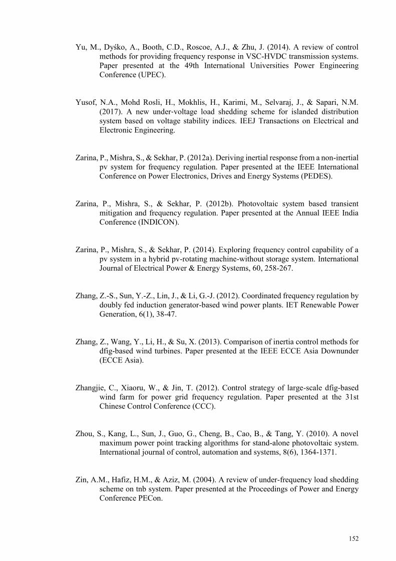
152
Yu, M., Dyśko, A., Booth, C.D., Roscoe, A.J., & Zhu, J. (2014). A review of control methods for providing frequency response in VSC-HVDC transmission systems. Paper presented at the 49th International Universities Power Engineering Conference (UPEC).
Yusof, N.A., Mohd Rosli, H., Mokhlis, H., Karimi, M., Selvaraj, J., & Sapari, N.M.
(2017). A new under‐voltage load shedding scheme for islanded distribution system based on voltage stability indices. IEEJ Transactions on Electrical and Electronic Engineering.
Zarina, P., Mishra, S., & Sekhar, P. (2012a). Deriving inertial response from a non-inertial
pv system for frequency regulation. Paper presented at the IEEE International Conference on Power Electronics, Drives and Energy Systems (PEDES).
Zarina, P., Mishra, S., & Sekhar, P. (2012b). Photovoltaic system based transient
mitigation and frequency regulation. Paper presented at the Annual IEEE India Conference (INDICON).
Zarina, P., Mishra, S., & Sekhar, P. (2014). Exploring frequency control capability of a
pv system in a hybrid pv-rotating machine-without storage system. International Journal of Electrical Power & Energy Systems, 60, 258-267.
Zhang, Z.-S., Sun, Y.-Z., Lin, J., & Li, G.-J. (2012). Coordinated frequency regulation by
doubly fed induction generator-based wind power plants. IET Renewable Power Generation, 6(1), 38-47.
Zhang, Z., Wang, Y., Li, H., & Su, X. (2013). Comparison of inertia control methods for
dfig-based wind turbines. Paper presented at the IEEE ECCE Asia Downunder (ECCE Asia).
Zhangjie, C., Xiaoru, W., & Jin, T. (2012). Control strategy of large-scale dfig-based
wind farm for power grid frequency regulation. Paper presented at the 31st Chinese Control Conference (CCC).
Zhou, S., Kang, L., Sun, J., Guo, G., Cheng, B., Cao, B., & Tang, Y. (2010). A novel
maximum power point tracking algorithms for stand-alone photovoltaic system. International journal of control, automation and systems, 8(6), 1364-1371.
Zin, A.M., Hafiz, H.M., & Aziz, M. (2004). A review of under-frequency load shedding
scheme on tnb system. Paper presented at the Proceedings of Power and Energy Conference PECon.
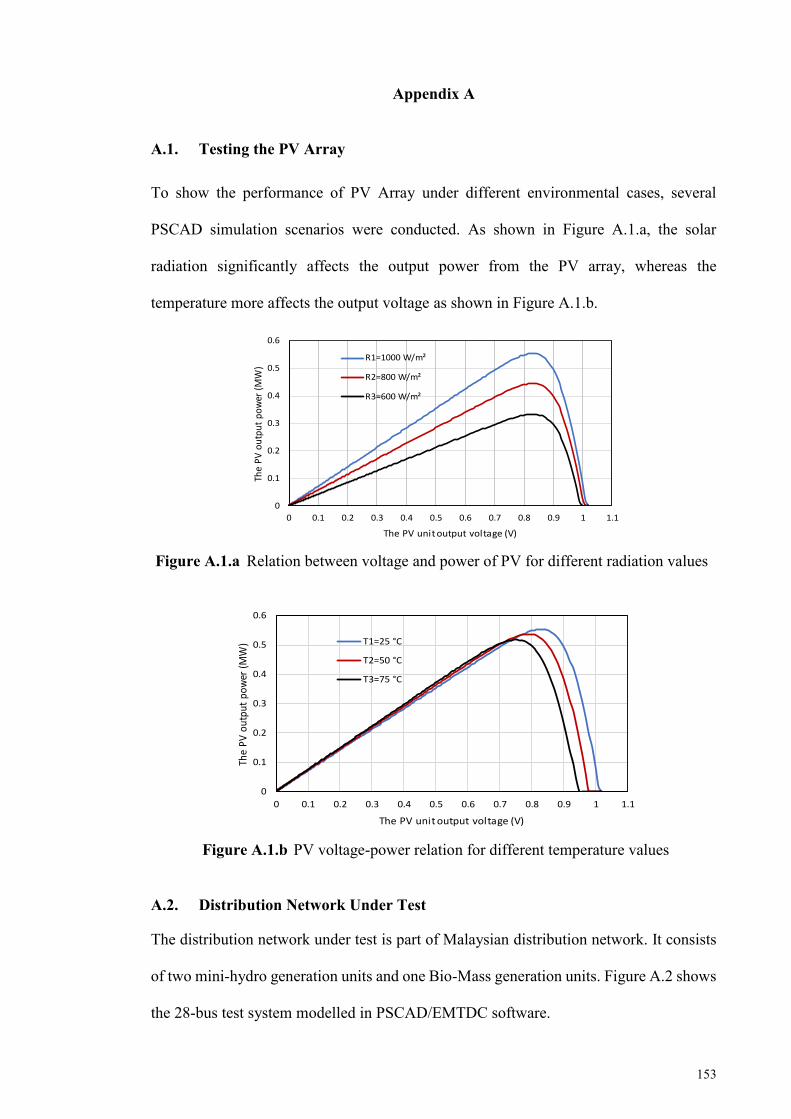
153
Appendix A
A.1. Testing the PV Array
To show the performance of PV Array under different environmental cases, several
PSCAD simulation scenarios were conducted. As shown in Figure A.1.a, the solar
radiation significantly affects the output power from the PV array, whereas the
temperature more affects the output voltage as shown in Figure A.1.b.
Figure A.1.a Relation between voltage and power of PV for different radiation values
Figure A.1.b PV voltage-power relation for different temperature values
A.2. Distribution Network Under Test
The distribution network under test is part of Malaysian distribution network. It consists
of two mini-hydro generation units and one Bio-Mass generation units. Figure A.2 shows
the 28-bus test system modelled in PSCAD/EMTDC software.
0
0.1
0.2
0.3
0.4
0.5
0.6
0 0.1 0.2 0.3 0.4 0.5 0.6 0.7 0.8 0.9 1 1.1
The
PV
ou
tpu
t p
ow
er (
MW
)
The PV unit output voltage (V)
R1=1000 W/m²
R2=800 W/m²
R3=600 W/m²
0
0.1
0.2
0.3
0.4
0.5
0.6
0 0.1 0.2 0.3 0.4 0.5 0.6 0.7 0.8 0.9 1 1.1
The
PV o
utpu
t po
wer
(MW
)
The PV unit output voltage (V)
T1=25 °C
T2=50 °C
T3=75 °C
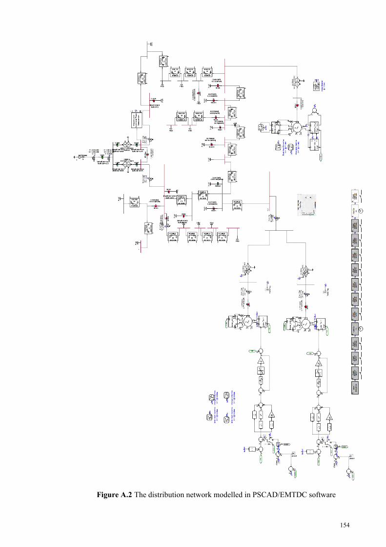
154
Figure A.2 The distribution network modelled in PSCAD/EMTDC software
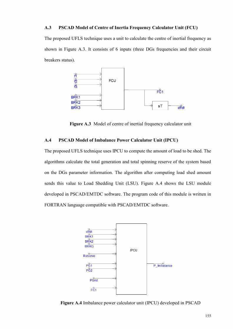
155
A.3 PSCAD Model of Centre of Inertia Frequency Calculator Unit (FCU)
The proposed UFLS technique uses a unit to calculate the centre of inertial frequency as
shown in Figure A.3. It consists of 6 inputs (three DGs frequencies and their circuit
breakers status).
Figure A.3 Model of centre of inertial frequency calculator unit
A.4 PSCAD Model of Imbalance Power Calculator Unit (IPCU)
The proposed UFLS technique uses IPCU to compute the amount of load to be shed. The
algorithms calculate the total generation and total spinning reserve of the system based
on the DGs parameter information. The algorithm after computing load shed amount
sends this value to Load Shedding Unit (LSU). Figure A.4 shows the LSU module
developed in PSCAD/EMTDC software. The program code of this module is written in
FORTRAN language compatible with PSCAD/EMTDC software.
Figure A.4 Imbalance power calculator unit (IPCU) developed in PSCAD

156
A.5 PSCAD Model of Load Shedding Unit (LSU)
This module is used to shed the optimal combination of loads by using the combination
of fixed and random priority of loads. Figure A.5 shows the LSU developed in
PSCAD/EMTDC software and interfaced with MATLAB software for distribution
network under test.
Figure A.5 Load Shedding Unit (LSU) developed in PSCAD
A.6 PSCAD Model of Frequency Management Unit
In this research, the frequency management unit is continuously monitoring both the
centre of inertial of frequency and battery state of charge (SOC) values to select the
battery charging, discharging or disconnecting mode. Figure A.6 shows the frequency
management unit developed in PSCAD.

157
Figure A.6 Frequency management unit developed in PSCAD
A.7 PSCAD Model of Reconnection Controller
This controller is proposed to reconnect the distribution network with the main grid when
the synchronization criteria of frequency, voltage and phase have been fulfilled. Figure
A.7 shows the reconnection controller.
Figure A.7 Reconnection Controller developed in PSCAD

158
A.8 The Parameters of Frequency Regulation Controller
The parameters of frequency regulation controllers developed in PSCAD are shown in
Table A.1.
Table A.1 The parameters of frequency regulation controller
Parameter Symbol Value Period of oscillation (Ziegler–Nichols) Tu 3s Gain of oscillation (Ziegler–Nichols) Ku 11 Proportional gain KP=0.45* Ku 5 Integral Gain KI = (1.2* KP)/ Tu 2 Battery droop constant RBatt 0.02 The maximum battery power PBMax 2 MW The maximum primary frequency control power
Pprim 0.5 MW
A.9 The Parameters of Inertia controller
The parameters of inertia controller developed in PSCAD are shown in Table A.2.
Table A.2 The parameters of inertia controller
Parameter Symbol Value Frequency droop constant HPV 2 The time constant of differentiator T 1 s The time constant of low bass filter T 1 s The gain of low bass filter G 1.5
A.10 The Parameters of Mini-hydro Generation Units
The parameters of mini-hydro generation units developed in PSCAD are shown in Table
A.3.
Table A.3 The parameters of mini-hydro generation
Parameter Symbol Value Proportional gain KP1 2 Integral Gain KI1 0.35 Derivative Gain KD1 0.9 Permanent droop R 0.04 Pilot servomotor time constant TA 0.05 Gate servo time constant TC 0.2 Gate servomotor time constant TD 0.2 Water starting time TW 2 s
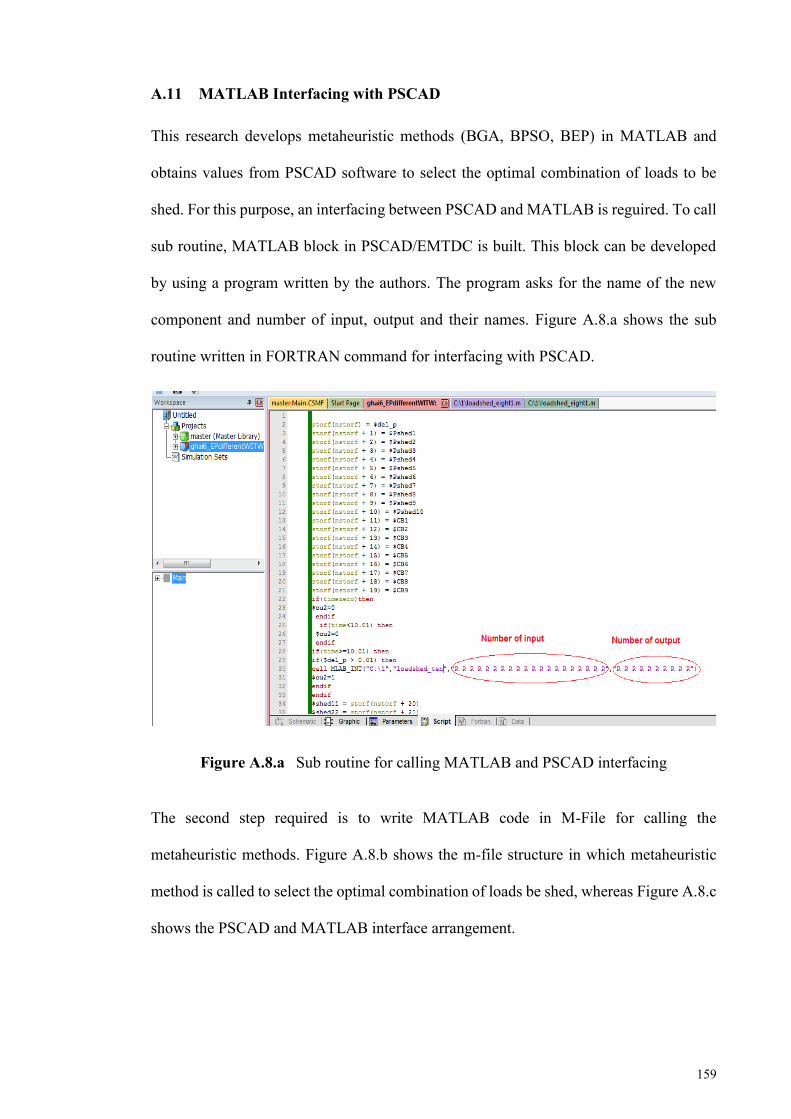
159
A.11 MATLAB Interfacing with PSCAD This research develops metaheuristic methods (BGA, BPSO, BEP) in MATLAB and
obtains values from PSCAD software to select the optimal combination of loads to be
shed. For this purpose, an interfacing between PSCAD and MATLAB is reguired. To call
sub routine, MATLAB block in PSCAD/EMTDC is built. This block can be developed
by using a program written by the authors. The program asks for the name of the new
component and number of input, output and their names. Figure A.8.a shows the sub
routine written in FORTRAN command for interfacing with PSCAD.
Figure A.8.a Sub routine for calling MATLAB and PSCAD interfacing
The second step required is to write MATLAB code in M-File for calling the
metaheuristic methods. Figure A.8.b shows the m-file structure in which metaheuristic
method is called to select the optimal combination of loads be shed, whereas Figure A.8.c
shows the PSCAD and MATLAB interface arrangement.
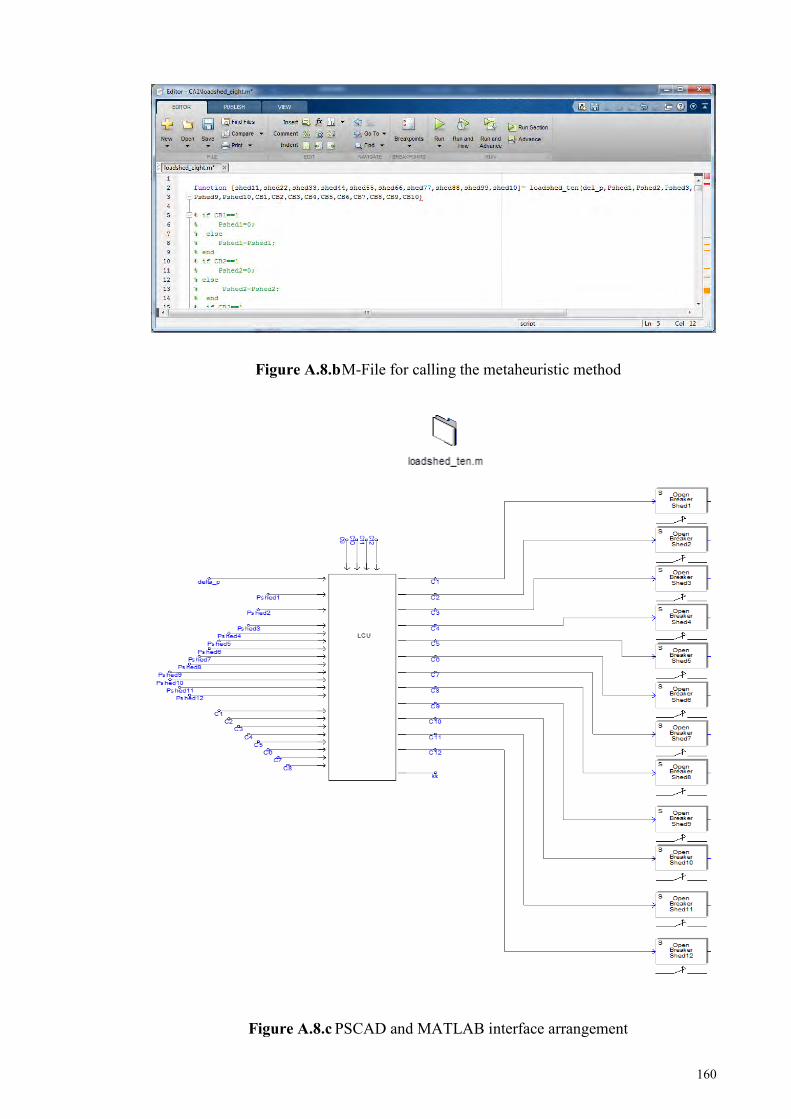
160
Figure A.8.b M-File for calling the metaheuristic method
Figure A.8.c PSCAD and MATLAB interface arrangement

161
Appendix B
Following papers have been published and submitted to journals and conferences from
this research study.
JOURNALS
(A) Dreidy, M., Mokhlis, H., & Mekhilef, S. (2017). Inertia response and frequency
control techniques for renewable energy sources: A review. Renewable and
Sustainable Energy Reviews, 69, 144-155. (ISI-Cited Publication)
(B) Dreidy, M., Mokhlis, H., & Mekhilef, S. (2017). Application of Meta-Heuristic
Techniques for Optimal Load Shedding in Islanded Distribution Network with High
Penetration of Solar PV Generation. Energies, 10(2), 150. (ISI-Cited Publication)
(C) Dreidy, M., Mokhlis, H., & Mekhilef, S. (2017). Frequency Control Scheme and
Synchronization System for Seamless Reconnection of islanded distribution
network with high PV penetration. International journal of electrical power and
energy systems. Revised. (ISI-Cited revision)
CONFERENCES
(A) Dreidy, M., Mokhlis, H., & Mekhilef, S. New Under-Frequency Load Shedding
Scheme Based on Adaptive Neuro-Fuzzy Inference System and Evolutionary
Programming Shedding Priority. 2nd International Conference on Energy and
Environmental Science (ICEES 2018),16-18 January 2018.

162
Related Documents