Local Stopping Rules for Gossip Algorithms Ali Daher Department of Electrical & Computer Engineering McGill University Montreal, Canada April 2011 A thesis submitted to McGill University in partial fulfillment of the requirements for the degree of Master of Engineering. c 2011 Ali Daher 2011/04/20

Welcome message from author
This document is posted to help you gain knowledge. Please leave a comment to let me know what you think about it! Share it to your friends and learn new things together.
Transcript

Local Stopping Rules for Gossip Algorithms
Ali Daher
Department of Electrical & Computer EngineeringMcGill UniversityMontreal, Canada
April 2011
A thesis submitted to McGill University in partial fulfillment of the requirements for thedegree of Master of Engineering.
c© 2011 Ali Daher
2011/04/20

i
Abstract
The increasing importance of gossip algorithms is beyond dispute. Randomized gossip
algorithms are attractive for collaborative in-network processing and aggregation because
they are fully asynchronous, they require no overhead to establish and form routes, and
they do not create any bottleneck or single point of failure. All nodes maintain independent
asynchronous random clocks, and when a node’s clock ticks it initiates a new round of
gossip: it randomly selects a neighboring node, exchanges information with the neighbor,
and the two nodes compute local updates. When these updates involve averaging the values
of the two nodes that gossiped, the algorithm solves the widely-studied average consensus
problem which is the focus in this thesis. To analyze the energy-accuracy tradeoff for
randomized gossip, previous studies have focused on analyzing the worst-case number of
transmissions required to reach a specified level of accuracy, over all initial conditions. In
a practical implementation, though, rather than always running for the worst-case number
of transmissions, one would like to fix a desired level of accuracy in advance and have
the algorithm run for as many iterations as are necessary to achieve this accuracy with
high probability. This thesis describes and analyzes an implicit local stopping rule with
theoretical performance guarantees. After a node’s estimate has not changed significantly
for a number of consecutive iterations, it ceases to initiate new gossip rounds. To avoid
stopping early and biasing the computation, stopped nodes still participate in gossip rounds
when contacted by a neighbor. We provide theoretical guarantees on the final accuracy
of the estimates across the network as a function of the algorithm parameters. Through
simulation, we show that applying the local stopping rule leads to significant savings in the
number of transmissions for many relevant initial conditions. In practical applications one
often wishes to track a time-varying average, rather than compute a static quantity. In
this scenario, we illustrate that our local stopping rule can be viewed as an event-triggered
gossip algorithm. Simulations illustrate the benefits of the proposed approach.

ii
Sommaire
L’importance croissante des algorithmes decentralises de passage de messages est incon-
testable. Ces algorithmes sont attrayants pour le traitement d’information dans les reseaux
de collaboration et l’agregation parce qu’ils sont totalement asynchrones, ils ne necessitent
pas de frais generaux pour etablir et former les routes, il n’exige pas de coordination
centralisee et consequemment ils ne creent pas de goulot d’etranglement ou de point de
defaillance unique dans le reseau. Tous les noeuds maintiennent independamment des hor-
loges asynchrone, lorsque l’horloge d’un noeud tiques, le noeud initie un nouveau cycle de
passage de messages: il selectionne aleatoirement un noeud voisin, echange des informa-
tions avec le voisin, et les deux noeuds calculent et mettent a jour leur variables. Lorsque
ces mises a jour incluent le calcul de la moyenne des valeurs des deux noeuds, l’algorithme
permet de resoudre le probleme du calcul du consensus moyen qui est le sujet de discussion
du present document. Afin d’analyser le compromis entre l’energie de transmission et la
precision de la valeur du consensus, des etudes anterieures ont porte sur l’analyse du nom-
bre base sur le pire des cas pour atteindre un niveau de precision. Dans une mise en oeuvre
pratique, cependant, au lieu d’etre toujours en cours d’execution du nombre de pire des cas
de transmissions, on voudrait fixer un niveau de precision desire a l’avance et l’algorithme
executera consequemment un nombre d’iterations necessaires pour obtenir cette precision
avec haute probabilite. Ce document decrit et analyse une regle d’arret implicite locale
avec garanties de performance theorique. Quand un noeud estime qu’il n’a pas change de
maniere significative pour un certain nombre d’iterations consecutives, il cesse l’echange de
donnee la prochaine fois que son horloge tique. Nous soulignons ici que pour eviter l’arret
precoce de l’algorithme, le noeud participe au passge de message lorsqu’il est contacte par
un voisin. Nous offrons des garanties theoriques sur la precision finale des estimations sur
le reseau en fonction des parametres de l’algorithme. En se basant sur les simulations, nous
montrons que l’application de la regle d’arret local conduit a des economies importantes
dans le nombre de transmissions pour de nombreuses conditions initiales. Dans les appli-
cations pratiques on souhaite souvent suivre une moyenne variante dans le temps, au lieu
de calculer une quantite statique. Dans cette these nous developperons des algorithmes de
passage de messages declenches par les evenements pour suivre les signaux variables dans
le temps. Des simulations illustrent les avantages de l’approche proposee.

iii
Acknowledgments
I had good fortune to collaborate and interact with many people who influenced my re-
search. First, I cannot say enough for my supervisor, professor Michael Rabbat, for all
the skills he had in coaching, motivating and teaching. Without your gracious assistance,
I would not have gotten to where I am. Big thanks to my supervisor Vincent Lau, who
kindly hosted me in his lab in the Hong Kong University of Science and Technology and
for all the interesting talks and discussions. I gratefully acknowledge the financial support
from Natural Sciences and Engineering Research Council of Canada (NSERC) as well as
the Fonds Quebecois de la Recherche sur la Nature et les Technologies (FQRNT). Thanks
to my brother Rabih, my family and my friends who were always here and made this ride
bearable. Last but not least, members of the lab in HKUST and McGill. Thank you all
for the useful (and useless!) discussions and debates we had during these months. Each
one of you has enriched my time in McGill and HKUST, special thanks to Deniz, Karama
and Bassel.

iv
To the children of Qana...
v
Contents
1 Introduction 1
1.1 Motivation . . . . . . . . . . . . . . . . . . . . . . . . . . . . . . . . . . . . 1
1.2 Introduction to GossipLSR . . . . . . . . . . . . . . . . . . . . . . . . . . . 2
1.3 Thesis Outline . . . . . . . . . . . . . . . . . . . . . . . . . . . . . . . . . . 4
1.4 Published Work . . . . . . . . . . . . . . . . . . . . . . . . . . . . . . . . . 4
2 Literature review 5
2.1 Characteristics of gossip algorithms . . . . . . . . . . . . . . . . . . . . . . 6
2.1.1 Synchronous and asynchronous gossip . . . . . . . . . . . . . . . . 6
2.2 Related research on gossiping . . . . . . . . . . . . . . . . . . . . . . . . 7
2.2.1 Distributed Average Consensus . . . . . . . . . . . . . . . . . . . . 7
2.2.2 Graph connectivity in gossip algorithms . . . . . . . . . . . . . . . 10
2.2.3 Quantization in gossip algorithms . . . . . . . . . . . . . . . . . . 11
2.2.4 Tracking using gossip algorithms . . . . . . . . . . . . . . . . . . . 11
3 Local Stopping Rule for Gossip Algorithm 13
3.1 Problem Setup . . . . . . . . . . . . . . . . . . . . . . . . . . . . . . . . . 13
3.2 Randomized Gossip . . . . . . . . . . . . . . . . . . . . . . . . . . . . . . . 14
3.3 Main Result . . . . . . . . . . . . . . . . . . . . . . . . . . . . . . . . . . . 17
3.4 Summary . . . . . . . . . . . . . . . . . . . . . . . . . . . . . . . . . . . . 25
4 Convergence analysis of GossipLSR 26
4.1 Guaranteed Stopping . . . . . . . . . . . . . . . . . . . . . . . . . . . . . . 26
4.2 Error When Stopping . . . . . . . . . . . . . . . . . . . . . . . . . . . . . . 29
Contents vi
5 Simulation Results 34
5.1 Convergence results . . . . . . . . . . . . . . . . . . . . . . . . . . . . . . . 34
5.2 Impact of the network size . . . . . . . . . . . . . . . . . . . . . . . . . . . 37
5.3 Impact of the network topology . . . . . . . . . . . . . . . . . . . . . . . . 40
5.4 Impact of the network initialization . . . . . . . . . . . . . . . . . . . . . . 43
5.5 Number of transmissions to convergence . . . . . . . . . . . . . . . . . . . 45
5.6 Number of iterations to convergence . . . . . . . . . . . . . . . . . . . . . . 46
5.7 Illustration of GossipLSR . . . . . . . . . . . . . . . . . . . . . . . . . . . . 51
5.8 Comparison to other finite time consensus algorithms . . . . . . . . . . . . 53
5.8.1 Linear Iterative Strategies . . . . . . . . . . . . . . . . . . . . . . . 54
5.8.2 Information Coalescence . . . . . . . . . . . . . . . . . . . . . . . . 55
5.9 Summary of the Chapter . . . . . . . . . . . . . . . . . . . . . . . . . . . . 57
6 Generalization to other gossip algorithms 59
6.1 Pairwise Gossip algorithms . . . . . . . . . . . . . . . . . . . . . . . . . . . 59
6.1.1 Geographic Gossip . . . . . . . . . . . . . . . . . . . . . . . . . . . 59
6.1.2 Greedy Gossip with Eavesdropping . . . . . . . . . . . . . . . . . . 61
6.2 Path Averaging using GossipLSR . . . . . . . . . . . . . . . . . . . . . . . 64
6.3 Summary of the chapter . . . . . . . . . . . . . . . . . . . . . . . . . . . . 67
7 Event-Driven Tracking of Time-Varying Averages 71
7.1 Introduction to Time-Varying Averages . . . . . . . . . . . . . . . . . . . . 71
7.2 Background . . . . . . . . . . . . . . . . . . . . . . . . . . . . . . . . . . . 72
7.3 Gossip Error with Time-Varying Signals . . . . . . . . . . . . . . . . . . . 74
7.3.1 Serial gossip . . . . . . . . . . . . . . . . . . . . . . . . . . . . . . . 74
7.3.2 Parallel gossip . . . . . . . . . . . . . . . . . . . . . . . . . . . . . . 78
7.4 Application of the local stopping rule to event triggered Time-Varying Net-
works . . . . . . . . . . . . . . . . . . . . . . . . . . . . . . . . . . . . . . . 79
7.5 Admissible change frequency with GossipLSR . . . . . . . . . . . . . . . . 83
7.6 Lag characterization for GossipLSR with respect to the network size . . . . 84
7.7 Distributed Kalman Filter with Embedded Consensus Filters . . . . . . . . 86
7.8 Summary of the chapter . . . . . . . . . . . . . . . . . . . . . . . . . . . . 89
Contents vii
8 Conclusion and Future Work 91
8.1 Summary of the thesis . . . . . . . . . . . . . . . . . . . . . . . . . . . . . 91
8.2 Future work . . . . . . . . . . . . . . . . . . . . . . . . . . . . . . . . . . . 92
A Coupon collector proof 94
B Bounds on the averaging time for tracking using gossip algorithms 96
B.1 Algorithm Description . . . . . . . . . . . . . . . . . . . . . . . . . . . . . 96
B.2 Upper bound on the ε-averaging time . . . . . . . . . . . . . . . . . . . . . 98
C Graph topology structures 102
D Initialization fields 105
E Second smallest eigenvalue of the graph Laplacian 107
E.1 Background work on λ2 . . . . . . . . . . . . . . . . . . . . . . . . . . . . . 107
E.2 Simulation results of sparsification . . . . . . . . . . . . . . . . . . . . . . . 108
E.3 Summary . . . . . . . . . . . . . . . . . . . . . . . . . . . . . . . . . . . . 110
References 111

viii
List of Figures
1.1 The Social Gossip by Norman Percevel Rockwell (1948) . . . . . . . . . . . 2
2.1 An illustration of a simple Gossip update for node averaging with averaging
weight matrix W(t) and a network of 5 nodes deployed randomly, note that
W(t) is symmetric and all the row’s sum equal 1, also the spectral radius
of W(t) satisfies the condition defined by Xiao and Boyd [1]: ρ(W−11T
n) ≤ 1.
X(0) is the initial vector of node values, X(1) is the vector of node values
after averaging. At the gossip iteration shown in this figure, nodes of indices
1 and 3 are gossiping. . . . . . . . . . . . . . . . . . . . . . . . . . . . . . . 8
3.1 Graphical representation of the GossipLSR with τ = 0.45. Red links rep-
resent links whose difference between nodes is bigger than τ , black links
represent links whose difference between nodes is smaller than τ . A dashed
line represents the pair of nodes that will be gossiping in the next iteration.
As discussed previously nodes wake up randomly to gossip. For a more
simplistic representation and less iterations we use C = 1. Note that from
iteration T = 3 to T = 4 we reduce the number of transmissions by one
since the values of the gossiping pair of the nodes is close with respect to τ .
Ideally if C existed, this would imply a cost to pay in terms of number of
transmission to do before a node decides locally that it should stop. . . . . 18
3.2 Flow diagram of the GossipLSR, the diagram represents the behavior model
and transitions between states while gossiping, observing the previous dia-
gram allows us to follow the way logic runs in local stopping rule and when
stopping conditions are met. . . . . . . . . . . . . . . . . . . . . . . . . . . 19

List of Figures ix
3.3 Variation of δ with respect to τ for different graph topologies in a network
of 25 nodes and taking C = dmax
(log(dmax) + 2 log(n)
). . . . . . . . . . . 22
5.1 Distribution histogram of the edge differences |xi(K) − xj(K)| for a 0/100
initial condition in a 200 nodes network deployed according to a RGG with
different parameter C, Recall that C is the number of times a nodes needs
to pass the test of the edge difference before it decides to stop. . . . . . . . 35
5.2 Distribution histogram of the edge differences |xi(K) − xj(K)| for different
initial conditions in a 200 nodes network deployed according to a RGG with
C = dmax log(dmax) and τ=0.1. Note that the x-axis and y-axis for the Spike
initialization is different than the other types of initializations. . . . . . . . 36
5.3 Distribution histogram of the edge differences |xi(K) − xj(K)| for a 0/100
initial condition in a 200 nodes network deployed according to a RGG with
C = log(dmax). . . . . . . . . . . . . . . . . . . . . . . . . . . . . . . . . . . 37
5.4 Relative error ||x(k)−x||||x(0)−x|| and Number of transmissions with respect to τ for
different network sizes in a RGG with an IID initialization. Each point on
this graph corresponds to the average error with respect to a certain value
of τ where C = dmax log dmax. We plot each curve for values of τ ranging
from 0.01 to 0.5. . . . . . . . . . . . . . . . . . . . . . . . . . . . . . . . . 38
5.5 Relative error ||x(k)−x||||x(0)−x|| with respect to the Number of transmissions at stop-
ping, we use different network sizes in a RGG with an IID initialization.
Each point on this graph corresponds to the average error and average num-
ber of transmissions until stopping over 100 trial for C = dmax log dmax and
for values of τ ranging from 0.01 to 0.5. . . . . . . . . . . . . . . . . . . . . 39
5.6 Relative error ||x(k)−x||||x(0)−x|| and Number of transmissions with respect to τ for
different network topologies. Each point on this graph corresponds to the
average error with respect to a certain value of τ where C = dmax log dmax.
We plot each curve for values of τ ranging from 0.01 to 0.5. . . . . . . . . 41
5.7 Relative error ||x(k)−x||||x(0)−x|| with respect to the number of transmissions at stop-
ping, we use two different network topologies. Each point on this graph
corresponds to the average error and average number of transmissions until
stopping for C = dmax log dmax and for values of τ ranging from 0.01 to 0.5. 42

List of Figures x
5.8 Snapshot of the network values at stopping using GossipLSR for a Chain
graph scenario where the local stopping criterion τ = 0.05 is satisfied between
each pair of nodes but the overall error is very high. . . . . . . . . . . . . . 42
5.9 Relative error ||x(k)−x||||x(0)−x|| and Number of transmissions with respect to τ for
different node initializations. Each point on this graph corresponds to the
average of the number of transmissions until stopping for C = dmax log dmax
and for values of τ ranging from 0.01 to 0.5. . . . . . . . . . . . . . . . . . 44
5.10 Number of transmissions required for different values of τ where C = dmax log dmax
in a network of 200 nodes deployed according to a RGG topology and having
a Gaussian bumps initial condition. . . . . . . . . . . . . . . . . . . . . . . 45
5.11 Number of iterations corresponding to different values of τ , where C =
dmax log dmax in a 200 nodes network deployed according to a RGG topology
and having different initial condition. . . . . . . . . . . . . . . . . . . . . . 47
5.12 Number of iterations it takes for different initialization with different orders
of magnitude. The number of iterations is averaged over 100 trials. The
higher the curve, then, the worst the gain in terms of number of iteration
reduction. All five curves fit an increasing function, which verifies that higher
stopping time is required for bigger scale of initial values. We use τ=0.5. . 48
5.13 Number of iterations with respect to the network sizes for different node
initializations in a random geometric graph using τ=0.5. The number of
iterations is averaged over 100 trials. The higher the curve, then, the worst
the gain in terms of number of iteration reduction. . . . . . . . . . . . . . . 49
5.14 Snapshot of a network of 20 nodes deployed according to a RGG with 0/100
initialization for different time instants during a GossipLSR round. We color
the nodes according to their values. Local stopping parameter τ=0.05. . . 52
5.15 Snapshot of a network of 15 nodes deployed according to a RGG with a
spike initialization for different time instants during a GossipLSR round.
We color the nodes according to their values. Indeed, the node at the spike
initial condition averages its value with its neighborhood and we can see how
it “dissolves” in the network in order to reach the final consensus. Local
stopping parameter τ=0.05. . . . . . . . . . . . . . . . . . . . . . . . . . . 53
List of Figures xi
6.1 Relative error ||x(k)−x||||x(0)−x|| vs the number of iterations using a geographic gossip
algorithm in a network of 200 nodes deployed according to a random geomet-
ric graph with a Gaussian Bumps initialization. Note that C = dmax log dmax.
Each data point is an ensemble average of 100 trials. . . . . . . . . . . . . 61
6.2 Relative error ||x(k)−x||||x(0)−x|| vs the number of transmissions using a greedy gossip
with eavesdropping algorithm in a network of 200 nodes deployed according
to a random geometric graph with a Gaussian Bumps initialization. Each
data point is an ensemble average of 100 trials. . . . . . . . . . . . . . . . 62
6.3 Relative error ||x(k)−x||||x(0)−x|| vs the number of transmissions comparison using Gos-
sipLSR with three different gossip algorithms: greedy gossip with eavesdrop-
ping, geographic gossip and randomized gossip. The network is composed of
200 nodes deployed according to a random geometric graph with a Gaussian
Bumps initialization and the GossipLSR is used with τ = 0.01. . . . . . . 63
6.4 Relative error ||x(k)−x||||x(0)−x|| with respect to the number of transmissions using
path averaging algorithm in a network of 200 nodes deployed according to
a random geometric graph and different values of τ each data point is an
average of 100 trials. . . . . . . . . . . . . . . . . . . . . . . . . . . . . . . 65
7.1 Trajectories of the information for each node in a 20 nodes network deployed
according to a RGG topology. It can be seen that the algorithm converges
toward the average of the initial measurements. . . . . . . . . . . . . . . . 73
7.2 Trajectories of the information for each node in a 20 nodes network deployed
according to a RGG topology with a linearly varying average. . . . . . . . 73
7.3 Error performance with respect to the number of transmissions to conver-
gence in a changing average scenario for different cosine amplitudes of the
form A cos(ft) where A is the amplitude and f is the frequency, the unit of
the time t is in clock ticks. We utilize C = dmax log dmax in a 200 nodes net-
work deployed according to a RGG topology. Each data point is the average
of 50 trials. In the legend, big change is when A=4, small change is when
A=1 and finally without change is when A=0. . . . . . . . . . . . . . . . 78

List of Figures xii
7.4 Time-varying average and state of one node for a network of 200 nodes
network deployed according to a RGG topology and two different τ values.
We use a sinusoidal change of the form ∆u(t)=A cos(ft) where A=0.5 is the
amplitude and f=3×10⁻⁴ is the frequency, the unit of the time t is in clock
ticks. . . . . . . . . . . . . . . . . . . . . . . . . . . . . . . . . . . . . . . . 81
7.5 Time-varying average and state of one node for a network of 200 nodes
network deployed according to a RGG topology and with τ=0.5. We use a
sinusoidal change of the form ∆u(t)=A cos(ft) where A=0.5 is the amplitude
and f=25×10−4 is the frequency, the unit of the time t is in clock ticks. The
graph is simulated over a total time of 2× 10⁴ clock ticks. . . . . . . . . . 81
7.6 Illustration of the delay measurement. . . . . . . . . . . . . . . . . . . . . 85
7.7 Lag characterization vs the network size for a network deployed according
to a RGG with an initial i.i.d initialization in a setting where τ=0.01 and a
cosine change of amplitude ‘0.5’ and period of 40 iterations. The graph is
simulated over a period of 104 clock ticks. . . . . . . . . . . . . . . . . . . 85
7.8 Mean Square Error between different distributed tracking approaches. We
use a sinusoidal change of the form ∆u(t)=A cos(ft) where A=1 is the am-
plitude and f=10−4 is the frequency. The graph is simulated over a period
of 2×10⁴ clock ticks. . . . . . . . . . . . . . . . . . . . . . . . . . . . . . . 88
7.9 Estimate at one node of the real average using a distributed Kalman filter
with embedded consensus for a network of 200 nodes deployed according to
RGG topology. We use a sinusoidal change of the form ∆u(t)=A cos(ft)
where A=0.5 is the amplitude and f=2×10⁻⁵ is the frequency. The graph
is simulated over a period of 15000 clock ticks. . . . . . . . . . . . . . . . . 89
C.1 Illustration of different Network topolgies . . . . . . . . . . . . . . . . . . . 104
D.1 Illustration of different Initialization fields . . . . . . . . . . . . . . . . . . 106
E.1 Maximum node degree for a network of 250 nodes that are initially deployed
according to different topologies. The graph is later reduced by removing
the links of the nodes with maximum degree. . . . . . . . . . . . . . . . . . 108

List of Figures xiii
E.2 Second smallest eigenvalue of the graph Laplacian for a network of 250 nodes
that are initially deployed according to different topologies. The graph is
later reduced by removing the links of the nodes with maximum degree. . . 109

xiv
List of Tables
5.1 Average number of iteration required before one single node becomes passive
for different types of topologies and initializations in a network of 50 nodes
in a setting where τ=0.5 and such that the initial value ‖x(0)‖=10. . . . . 50
5.2 Average number of iteration required to convergence for different types of
topologies and initializations in network of 50 nodes in a setting where τ=0.5
and such that the initial value ‖x(0)‖=10. . . . . . . . . . . . . . . . . . . 51
5.3 Final error at convergence for a network of 50 nodes for the linear itera-
tive strategy and GossipLSR (τ=5×10⁻⁴) algorithms with different network
initializations and topologies . . . . . . . . . . . . . . . . . . . . . . . . . 55
5.4 Final error at convergence for a network of 50 nodes for the Information
Coalescence and GossipLSR (τ=5×10⁻⁴) algorithms with different network
initializations and topologies. . . . . . . . . . . . . . . . . . . . . . . . . . 56
5.5 Average number of iteration required to convergence for a network of 50
nodes in the Information Coalescence and GossipLSR (τ=5×10⁻⁴) algo-
rithms with different initializations and topologies. . . . . . . . . . . . . . 57
5.6 Average number of transmissions required to convergence for a network of
50 nodes in the Information Coalescence and GossipLSR (τ=5×10⁻⁴) algo-
rithms with different network initializations and topologies. . . . . . . . . 57
6.1 Number of transmissions and Relative Error at stopping for GossipLSR with
different values of τ and different types of gossip algorithms, greedy gossip
with eavesdropping, geographic gossip, path averaging and randomized gos-
sip. We use a network of N=200 nodes deployed according to a RGG topol-
ogy and Gaussian Bumps initialization. Each data point is an ensemble
average of 100 trials. . . . . . . . . . . . . . . . . . . . . . . . . . . . . . . 67
List of Tables xv
7.1 Number of transmissions for different values of τ and different amplitude
of the change for 200 nodes deployed according to a RGG with an initial
Gaussian Bumps initialization. We use a sinusoidal change of the form
∆u(t)=A cos(ft) where A is the amplitude and f=25×10−3 is the frequency.
The graph is simulated over a period of 2×10⁴ clock ticks. . . . . . . . . . 83
7.2 Number of transmissions vs the period of the change for a 200 nodes network
deployed according to a RGG with an initial Gaussian Bumps initialization
in a setting where τ=0.005 and a cosine change of amplitude ‘1’. The graph
is simulated over a period of 2×10⁴ clock ticks. . . . . . . . . . . . . . . . . 83

xvi
List of Acronyms
LSR Local Stopping Rule
GB Gaussian Bumps
GGE Greedy Gossip with Eavesdropping
GEO Geographic Gossip
RG Randomized Gossip
RGG Random Geometric Graph
WSN Wireless Sensor Networks
IID Independant Identically Distributed
PA Path Averaging
LMS Least Mean Square
LIT Linear Iterative Strategy
MSE Mean-Squared Error
CP Consensus Propagation
DTMC Discrete Time Markov Chain
P2P Peer to Peer
DKF Distributed Kalman Filter

1
Chapter 1
Introduction
1.1 Motivation
Wireless sensor networks, or WSN, are networks formed by a number of sensor nodes which
continuously examine the environment by capturing measurements, processing these mea-
surements (through averaging, for example) and communicating with other sensor nodes [2].
One of the major challenges is to devise resource efficient wireless sensor networks [3]. The
key resource in most WSN is battery power since it allows the network to operate au-
tonomously for long periods of time [4]. Conserving battery power in the sensors can be
attained by reducing the number of wireless transmissions in the network.
Conventionally, the task of calculating the average value of a set of sensors in a WSN
has been addressed by constructing a central authority that gathers the information from
all the network sensors, calculates the averages and communicates the result back to the
sensors. Nonetheless, this centralized based approach faces challenges since it has a single
point of failure. For example, if the central sensor fails, all the sensors will not receive the
average.
On other hand, in a decentralized scenario we assume sensors to repeatedly average
their value with other neighboring sensors chosen independently at random. One can show
that, with high probability, assuming the choice of the sensors is uniformly random, after a
certain number of rounds, every sensor will get an accurate estimate of the network average.
In the course of this thesis we use the term gossip algorithm to describe the decentralized
averaging method described above.
The concept of gossip communication can be modeled by the analogy of office workers
2011/04/20
1 Introduction 2
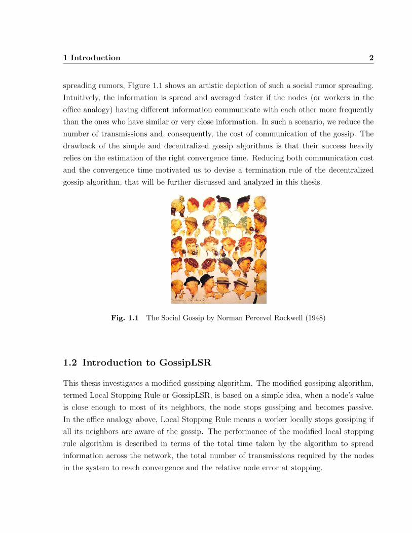
spreading rumors, Figure 1.1 shows an artistic depiction of such a social rumor spreading.
Intuitively, the information is spread and averaged faster if the nodes (or workers in the
office analogy) having different information communicate with each other more frequently
than the ones who have similar or very close information. In such a scenario, we reduce the
number of transmissions and, consequently, the cost of communication of the gossip. The
drawback of the simple and decentralized gossip algorithms is that their success heavily
relies on the estimation of the right convergence time. Reducing both communication cost
and the convergence time motivated us to devise a termination rule of the decentralized
gossip algorithm, that will be further discussed and analyzed in this thesis.
Fig. 1.1 The Social Gossip by Norman Percevel Rockwell (1948)
1.2 Introduction to GossipLSR
This thesis investigates a modified gossiping algorithm. The modified gossiping algorithm,
termed Local Stopping Rule or GossipLSR, is based on a simple idea, when a node’s value
is close enough to most of its neighbors, the node stops gossiping and becomes passive.
In the office analogy above, Local Stopping Rule means a worker locally stops gossiping if
all its neighbors are aware of the gossip. The performance of the modified local stopping
rule algorithm is described in terms of the total time taken by the algorithm to spread
information across the network, the total number of transmissions required by the nodes
in the system to reach convergence and the relative node error at stopping.
1 Introduction 3
In this thesis, we focus on the average consensus problem where each node initially has
a measurement, and the goal is to compute the average of all these measurements at all
nodes in the network. Although the average is an extremely simple function, previous work
has shown that it can be used as a basic element to carry out a variety of complex tasks
including source localization [5], data aggregation, compression [6], subspace tracking [7]
and optimization [8, 9]. Randomized gossip [10] solves the average consensus problem in
the following manner. Each node preserves and updates a local estimate of the average,
which it initializes with its own measurement. Each node also runs an independent random
(Poisson) clock. When the clock at a node i ticks, signaling the start of a new iteration, it
contacts one of its neighbors (chosen randomly); they exchange estimates, and then update
their value by fusing their previous estimates with the new information obtained from their
neighbor.
Previous studies of randomized gossip for information processing have focused on study-
ing scaling laws and on developing efficient randomized gossip algorithms for typical mod-
els of wireless network topologies such as two dimensional grids and random geometric
graphs [10]. Much previous work has focused on characterizing the ε-averaging time, which
is the worst-case number of iterations the algorithm must be run to guarantee with high
probability that the estimates of the average at all nodes are ε away from the true average,
relative to the initial condition1.
This thesis describes implicit local stopping rules for randomized gossip algorithms with
theoretical performance guarantees. Existing gossip algorithms do not incorporate such a
stopping criterion. Instead, they utilize a number of transmissions which is based on the
worst-case scenario. This can, however, be extremely inefficient, especially when the worst-
case scenario is pathological and unlikely to occur in practice. Rather than fixing a total
number of iterations to execute in advance, each node monitors its estimate and decides to
stop when the estimate has not changed significantly after a prescribed number of iterations.
When a node decides to stop, it no longer initiates gossip exchanges with neighbors when its
clock ticks. However, to avoid stopping prematurely, nodes that are stopped still respond to
requests to gossip from other neighbors, and they may even resume initiating gossip rounds
if these updates cause a considerable change in their value. We prove through simulations
that the proposed scheme will stop almost surely after a finite number of iterations.
In scenarios where the goal is to track a time-varying average, rather than performing a
1A precise definition is given in Section 3.1.
1 Introduction 4
static computation, our local stopping rule translates directly to a mechanism for adaptively
triggering gossip events. In particular, when tracking a slowly-varying quantity, rather than
wasting transmissions to gossip between neighbors that have identical or nearly-identical
information, the proposed rule encourages nodes to only gossip when they have something
significantly “new” to add to the computation.
1.3 Thesis Outline
Chapter 2 makes a comprehensive review of the previous work found in the literature for
different types of gossip algorithms, their description and their main results. Technical
background of gossip algorithm and the description of the modified gossip algorithm with
local stopping rule is discussed in Chapter 3. Chapter 3 also presents the statement of the
GossipLSR main theorem. Chapter 4 develops the main result and the proof of the gossip
with local stopping rule. It also covers the algorithm convergence analysis and error when
stopping. This chapter will help the reader understand the advantages of the local stopping
rule compared to existing gossip algorithms. Chapter 5 contains simulation results with
different initial conditions, followed by a comparison to other finite time algorithms. It also
illustrates the reduction achieved in terms of the number of transmissions and iterations at
stopping. Chapter 6 studies the generalization of the GossipLSR to other gossip algorithms
such as Greedy Gossip with Eavesdropping (GGE) [11], Geographic gossip (GEO) [12]
and path averaging gossip [13]. Later in Chapter 7, we introduce the use of the gossip
algorithms in the event-driven tracking of time-varying averages networks. We compare
the GossipLSR performance in tracking to other tracking approaches using distributed
Kalman filters. This chapter also discusses the conditions on the admissible change in
order to converge. Finally, Chapter 8 concludes this thesis and reviews the main ideas
and contributions introduced. It also opens the door to future work in this area and the
possible applications in telecommunications and signal processing.
1.4 Published Work
Some parts of this thesis have been published in the 2011 International Conference on
Distributed Computing in Sensor Systems (DCOSS)

5
Chapter 2
Literature review
Distributed consensus refers to a class of algorithms where n nodes connected through a
graph G jointly interact with each other in order to attain an agreement or a consensus
regarding some parameters (for example, the maximum value or the average value in the
network).
Distributed consensus algorithms have received substantial research consideration in
the past decade. De Groot [14], Borkar and Varaiya [15] and later Tsitsiklis [16] were
the pioneers among many researchers who studied distributed consensus problems. For a
complete historical review of the main consensus algorithms and their development over
the past years, interested readers are referred to Alexander Olshevsky’s PhD thesis [17].
Among different distributed consensus algorithms, Gossip algorithms have received lots
of research attention in the recent years and have been applied for solving a wide range of
problems in distributed computing. The applications of such algorithms include: informa-
tion dissemination [18], averaging [19], computing aggregate information [20], tracking [7]
and organizing the network components into structures. Additionally, the development of
P2P, wireless sensors and ad hoc wireless networks has inspired many related research on
this category of distributed algorithms.
This chapter provides an overview of the most relevant published work as well as an
analysis of their advantages and disadvantages.
2011/04/20
2 Literature review 6
2.1 Characteristics of gossip algorithms
As said previously, in many of today’s networks, with link erasures and node mobility, gossip
based algorithms are emerging as an approach to maintain scalability and simplicity while
achieving acceptable performance. When a network has a failure in some of its nodes or
when a random message is lost, the gossip algorithm is not altered at all and no “recovery”
action is required.
Briefly, the raison d′etre of gossip algorithms is their simplicity, scalability and de-
centralization. Simplicity implies that the gossip algorithm is undemanding and easy to
deploy and doesn’t require any organized infrastructure. Scalability stands for the fact
that each node has the same rate of gossiping even if the network size changes, and finally,
decentralization implies that there is no single bottleneck or point of failure in the network.
Among the gossip disadvantages compared to fully centralized approaches, we mention
that the number of time units it takes for a gossip algorithm to converge is higher than the
centralized case, since intuitively, a decentralized approach might induce some redundant
messages. The same applies also for the total number of transmissions to convergence.
2.1.1 Synchronous and asynchronous gossip
Before we describe different gossip algorithms, we point out the difference between syn-
chronous and asynchronous gossip. In the synchronous version of gossip algorithms, every
node wakes up to gossip with a certain probability at each time step. A node that wakes
up then randomly picks a neighbor, once this is done, both nodes gossip and average their
own variables. In this scenario, each node sends one message per round of communication.
In asynchronous gossip, the difference is that we replace the discrete time by a continuous
time. Every node wakes up following an exponentially distributed time instead of a discrete
clock tick. Each node picks a random neighbor, and both nodes average their variables.
Therefore, unlike the synchronous version, transmissions take place successively over time,
and not at the same time. In other words, many iterations of the asynchronous version
correspond to a single iteration of the synchronous model. Put differently, for the same in-
terval of time, synchronous gossip consumes more transmissions compared to asynchronous
gossip.

2 Literature review 7
2.2 Related research on gossiping
The interest in the field of gossip algorithms has recently grown so large that a fair literature
review of all the related work in the field is beyond the capacity of a single chapter in this
thesis. The choice of citations in the present work is not meant to establish a hierarchy of
more important and less important results, it is mostly a review of the previous work close
in spirit to our topic of research.
We broadly group the related literature into four groups, each group will be explained
separately in the following subsections: The first group concerns different gossip algorithms
for averaging, this was discussed in [10–13, 18, 21–27]. The second group surveys the work
discussing the impact of graph connectivity on gossip algorithms [28–30]. The third group
reviews the effect of quantization on gossip algorithms [19, 31, 32]. Finally, in the fourth
group we examine a certain number of publications that surveyed the wide field of the
distributed tracking in connected networks [25, 32–36]. Our research is actually in the
intersection of most of the previous work listed above.
2.2.1 Distributed Average Consensus
First, we examine the different distributed averaging algorithms proposed over the past few
years. Some papers discussed in this section will be revisited later in Chapter 6 where we
generalize the local stopping rule algorithm to different gossip algorithms.
Xiao and Boyd [1] studied the Distributed average consensus algorithms over a
symmetric network and proposed a semidefinite programming optimization method in order
to find the fastest convergence rate, they later defined the convergence conditions on the
consensus weight matrix W(t). Roughly speaking, matrix W(t) represents the consensus
weight matrix and is constrained to the graph topology.
In 2006, Boyd et al. [10] analyzed the Randomized Gossip algorithm and derived
scaling laws for these algorithms. They defined a relative tight upper bound on averag-
ing time (i.e., time when all the nodes converge) and defined the relationship between the
averaging time (or mixing time) and the second largest eigenvalue of a doubly stochas-
tic matrix. Furthermore, they analyzed both synchronous and asynchronous settings and
solved an optimization problem to design the fastest gossip algorithm for a random geo-
metric graph. Although randomized gossip is fast for some topologies, such as complete
graphs, unfortunately, its convergence is slow, for topologies like random geometric graphs

2 Literature review 8
or grids. An illustration of a simple gossip update using the averaging weight matrix W(t)
is shown in Figure 2.1. In Figure 2.1 two nodes in the network wake up and average their
value according to the averaging matrix W(t). In the rest of this subsection we discuss
different gossip algorithms inspired by the randomized gossip of Boyd et al. [10] and having
a faster convergence rate.
1
2 1
3
4
8
2
2
1/2 0 1/2 0 0
0 1 0 0 0
1/2 0 1/2 0 0
0 0 0 1 0
0 0 0 0 1
1 1 3 4 8
x(0) W(1)
=
2 1 2 4 8
x(1)
Fig. 2.1 An illustration of a simple Gossip update for node averaging withaveraging weight matrix W(t) and a network of 5 nodes deployed randomly,note that W(t) is symmetric and all the row’s sum equal 1, also the spectralradius of W(t) satisfies the condition defined by Xiao and Boyd [1]: ρ(W −11T
n ) ≤ 1. X(0) is the initial vector of node values, X(1) is the vector of nodevalues after averaging. At the gossip iteration shown in this figure, nodes ofindices 1 and 3 are gossiping.
W =
0.5 0 0.5 0 0
0 1 0 0 0
0.5 0 0.5 0 0
0 0 0 1 0
0 0 0 0 1
X(0) =
1
1
3
4
8
X(1) =
2
1
2
4
8
X(1) = WX(0)
As can be seen from Figure 2.1, the matrix W (k) has a diagonal value of 1 for nodes that

2 Literature review 9
are not gossiping, and a value of 0.5 at the intersection of the row and column corresponding
to the indices of the gossiping nodes at iteration k.
Faster modified gossip algorithms
In recent work three main approaches to speed up the convergence rate of previously dis-
cussed randomized gossip algorithms with RGG and grid topologies can be identified: Using
long-range and multi-hop communication [12, 13, 23] , exploiting the broadcast nature of
wireless sensors [11,18,26,27] and incorporating memory in each node [22,37].
Motivated by the slow convergence of randomized gossip in grids and RGG, Geo-
graphic Gossip uses the assumption of knowledge of the location of each node and builds
a new modified gossip algorithm in order to speed up the convergence time. In geographic
gossip, nodes average their values with non-neighboring nodes; the communication between
distant nodes is achieved through routing. Since the nodes are not restricted to a limited
number of neighbors, Geographic gossip has a better convergence rate compared to existing
randomized gossip algorithms. Dimakis et al. [12] demonstrated that this approach offers
substantial gains over previously proposed gossip algorithms. The disadvantage of this
gossip method is that this algorithm needs a global coordinate system and also needs to
send messages on long routes. This can create congestion issues.
Another line of work exploited the broadcast nature of wireless sensor networks and
proposed other modified gossip algorithms. Ustebay et al. gave an overview of a faster
averaging approach that can be used to gossip. In Greedy gossip with eavesdropping
(GGE) [11] , nodes use the wireless medium to eavesdrop and keep track of other node’s
values. When a node gossips, instead of picking a random neighbor, it picks the neighbor
which has the value most different from its own. Authors have demonstrated that greedy
gossip with eavesdropping is guaranteed to converge to the accurate average for connected
graphs. They later derived the theoretical bounds of the convergence rate and demonstrated
through simulations, that GGE converges faster than randomized gossip. On the other
hand, the disadvantage of GGE is the requirements in terms of memory in order to store
values of the neighbors at each node.
In [27] Aysal et al. suggested a broadcast-based gossip algorithm to calculate the
distributed average. Briefly, the asynchronous Broadcast Gossip algorithm is described
as follows. When node i’s clock ticks, it broadcasts its own value to all the neighbors located
2 Literature review 10
within a distance R. Once the broadcasted value is received from i, each neighboring node j
update its value with a weighted average of its own value and the received value according
to the following equation: xj(t+ 1) = γxj(t) + (1− γ)xi(t), with γ ∈ (0, 1) symbolizing a
mixing parameter. The disadvantage of this algorithm is that it converges to an estimate
that is close to the desired average but not precisely the average itself (because of the
fact that the sum of all x’s is not conserved when γ is different than 0.5). Many other
papers that discuss improving the gossip broadcast algorithms in terms of time and energy
performances appeared later.
Recently, a promising fast gossiping technique using local node memory have also been
proposed. Oreshkin et al. [22] proposed Accelerated consensus. This method improves
the convergence speed of conventional consensus using one memory register. The main
contribution of accelerated consensus is by incorporating a linear predictive step in the
algorithm. In other words, each node utilizes both its current and previous information to
calculate the updated value. The authors in [22] demonstrated that this filtering technique
reached convergence faster than the standard approach. This approach to gossip using
memory registers triggered other similar studies to gossip using memory registers.
2.2.2 Graph connectivity in gossip algorithms
We surveyed a few of the numerous work that proposed, discussed and analyzed gossip
algorithms. Secondly in this section, we survey a set of papers that discuss the impact of
graph connectivity on the performance of gossip. Results with graph theoretic emphasis
were considered by several authors. In [30] Olfati-Saber, Fax and Murray covered a range
of topics. They discussed the use of algebraic graph theory to study convergence towards
consensus and demonstrated that algebraic connectivity of graphs and digraphs plays a key
role in the analysis of consensus algorithms. They also covered topics such as time delays,
performance guarantees and general information consensus. As an extension to the previous
survey work, Olfati-Saber and Murray [29] proved the convergence of a modified agreement
algorithm for the distributed averaging problem when the connectivity of the graph changes
with time. Other similar work have also been proposed. Fang and Antsaklis [28] surveyed
recent existing research on consensus and considered some communication assumptions
such as graph connectivity, and direction of communication. Their main result shows that
consensus is reachable under directional, time-varying and asynchronous topologies with

2 Literature review 11
nonlinear algorithms.
2.2.3 Quantization in gossip algorithms
In most of the previous work mentioned above, whenever nodes gossip, they exchange
real-valued data. As such, there are no bit constraints. As consensus, averaging and
broadcasting problems continue to receive wide interest, researchers have considered some
model variations such as studying the effect of quantization on gossip algorithms. Kashyap,
Basar and Srikant proposed in [31] an average consensus algorithm over integers, which is
a quantized version of pairwise gossip algorithms. They studied systems limited to integer-
valued states and proposed a modified gossip algorithms that preserves the average at
convergence. Also motivated by the quantization effect, Frasca et. al. studied in [38], for
an unchanging topology, the impact of a uniform quantization on the distributed average
calculation. They proposed a simple modification capable of preserving the average and
achieving a reasonably close value to the consensus.
2.2.4 Tracking using gossip algorithms
Finally, we survey a set of work that discussed tracking problems in gossip algorithms.
The tracking problem is essentially the task of estimating over time the evolving state of a
given target or signal. Applications of distributed averaging algorithms with time-varying
information in the presence of noise and variable information can be found in various recent
work [33,39]. In [25], Deming et al. considered the distributed gossip algorithm with real-
time measurements, they later quantized the data and provided a result characterizing the
convergence performance. In another line of work Sun et al. [32] proved that all the nodes
in a connected graph converge asymptotically in networks of dynamic agents given that
they have a reasonable bound on the time-varying delays. Another interesting work [34]
discusses a distributed LMS algorithm based on consensus mechanisms that relies on node
hierarchy to reduce communication. The main disadvantage of this method is the high
complexity it requires to establish and maintain the hierarchies. Also in distributed LMS
algorithms Cattivelli et al. [35] proposed a diffusion-based LMS algorithm that outperforms
the technique proposed previously in [34]. Finally, in [36] Olfati-Saber et al. suggested
a distributed averaging filter to track the varying measurements of sensors. They later
showed that the tracking uncertainty is inversely proportional to the network density, this
2 Literature review 12
implies that in order to track with more accuracy a more dense network is needed. In
other words, if the network is not dense, the tracking capabilities of the network decreases.
Furthermore, they illustrated their analysis with simulation results of a signal that has
multiple sinusoidal components. These simulations demonstrated tracking capabilities of
their distributed filter for different networks and sinusoids frequencies and amplitudes.
The work of Olfati-Saber [36] and their main result will be revisited later in the tracking
discussion of Chapter 7.
Our research is in fact in the intersection of most of the previously mentioned topics.
Motivated to speed up the convergence rate of the existing gossip algorithms, we propose
a termination rule that reduces the number of redundant transmissions during gossip. We
later derive the scaling laws of the modified algorithm, study its applications in tracking
problems and investigate its performance with graphs having different connectivity.
The next chapter proposes a modification of randomized gossip which incorporates a
local stopping rule. This stopping rule allows nodes to adaptively determine when their
value is close enough to the network average and consequently this permits the nodes to
stop gossiping. Subsequent chapters analyze this local stopping rule and provide theoretical
guarantees of convergence as well as simulation results. The last part of the thesis concerns
a practical application of GossipLSR in distributed signal tracking.

13
Chapter 3
Local Stopping Rule for Gossip
Algorithm
This chapter explains the main result and key steps of the gossip with local stopping rule
algorithm. It describes the proposed technique to speed up the convergence of randomized
gossip and presents the statement of the GossipLSR stopping criterion.
3.1 Problem Setup
Let the graph G = (V,E) denote the communication topology of a network with n = |V |nodes and edges (i, j) ∈ E ⊆ V 2 if and only if nodes i and j communicate directly. We
assume that G is connected. We take V = {1, . . . , n} to index the nodes. Let xi(0) ∈ Rdenote the initial value at node i ∈ V ; this could, e.g., correspond to a measurement taken
at this node. In randomized gossip, nodes iteratively exchange information and update
their estimates, xi(t). Our goal is to estimate the average x = 1n
∑ni=1 xi(0) at every node
of the network; that is, we would like xi(t)→ x for all i as t→∞.
One can argue, when the decentralization is less of an issue, instead of letting a node
choose another node randomly for averaging, we can specify a tree of communication to
average information. By doing so, we direct the path of averaging and consequently the
total number of transmissions can be reduced even without using the local stopping rule.
Such an approach has a single point of failure and this is why GossipLSR has an advantage
of being decentralized.
Following [10, 16], we adopt an asynchronous update model where each node runs an
2011/04/20

3 Local Stopping Rule for Gossip Algorithm 14
independent Poisson clock that ticks at a rate of 1 per unit time (i.e., ticks are spaced by iid
random durations according to an exponential distribution). In this model, the probability
that two clocks tick at precisely the same time instant is zero. Let tk denote the time of
the kth clock tick in the network, and let i(k) denote the index of the node at which this
tick occurs. It is easy to show, using properties of Poisson processes, that the sequence
of nodes i(1), i(2), . . . , i(k), . . . is independent and uniformly distributed over V , since all
nodes’ clocks tick at the same rate. Moreover, via simple probabilistic arguments [21, 40],
one can show that each block of O(n log n) consecutive nodes in the sequence {i(k)}∞k=1
contains every node in V with high probability.
3.2 Randomized Gossip
In the randomized gossip algorithm described in [10], when i(k)’s clock ticks at time tk,
it contacts a neighboring node, which we will denote by j(k) according to a pre-specified
distribution Pi,j = Pr(i contacts j
∣∣i ticked). Then i(k) and j(k) update their values by
setting
xi(k)(tk) = xj(k)(tk) =1
2
(xi(k)(tk−1) + xj(k)(tk−1)
), (3.1)
and all nodes v ∈ V \{i(k), j(k)} hold their estimates at xv(tk) = xv(tk−1). The probability
Pi,j can only be positive if there is a connection (i, j) ∈ E between nodes i and j. Let
Ni = {j : (i, j) ∈ E} denote the set of neighbors of i. Often, we use the natural random
walk probabilities Pi,j = 1/|Ni| for the graph G.
We assume that i(k) and j(k) exchange information instantaneously at time tk. As
mentioned above, no two clocks tick simultaneously, so we can order the events sequentially
t1 < t2 < · · · < tk < . . . . To simplify notation, we write xi(k) instead of xi(tk) in the sequel,
and we refer to the operations taking place at time tk as the kth iteration.
We note that this problem setup—having local clocks operate at a rate of 1 tick per
unit time—is purely for the sake of analysis. In practice, one would tune the clock rate
taking into consideration a number of parameters (e.g., radio transmission rates and ranges,
packet lengths, the average number of neighbors per node, and interference patterns), and
the clock rates could be chosen sufficiently large so that no two gossip events interfere with
high probability. Determining the appropriate rate is beyond the scope of this paper and
is an interesting open problem.

3 Local Stopping Rule for Gossip Algorithm 15
Algorithm 1 Randomized Gossip
1: Initialize: {xi(0)}i∈V and k = 12: repeat3: Draw i(k) uniformly from V4: Draw j(k) according to {Pi,j}j∈V5: xi(k)(k)← 1
2
(xi(k)(k − 1) + xj(k)(k − 1)
)6: xj(k)(k)← 1
2
(xi(k)(k − 1) + xj(k)(k − 1)
)7: for all v ∈ V \ {i(k), j(k)} do8: xv(k) = xv(k − 1)9: end for
10: k ← k + 111: until Satisfying some stopping condition
Pseudo-code for simulating randomized gossip is shown in Algorithm 1. The stopping
condition recommended in previous work is to fix a maximum number of iterations to
execute based on the worst-case initial condition and size of the network. In particular,
previous work has analyzed the ε-averaging time, Tε(P ), for gossip algorithms which we
define next. Let x(t) ∈ Rn the estimates at each node at time t stacked into a vector, and
let x denote a vector with all entries equal to the initial average. Then the ε-averaging
time for the algorithm defined by neighbor-selection probabilities P is defined as
Tε(P ) = supx(0)
inf
{t : Pr
(‖x(t)− x‖‖x(0)‖
≥ ε
)≤ ε
}; (3.2)
that is, Tε(P ) is the smallest time t for which the error ‖x(t) − x‖ ≤ ε‖x(0)‖ is small
relative to the initial condition x(0) with respect to a prescribed level of accuracy ε, with
high probability, for the worst-case (and, thus, any) initial condition x(0). Note that the
dependence of Tε(P ) on P is implicit in the evolution of x(t). Also note that the matrix of
probabilities P captures the network topology G, since Pi,j > 0 only if (i, j) ∈ E, and so
averaging time depends strongly on the network topology through the evolution of x(t).
The 2-dimensional random geometric graph [41,42] is a typical model for connectivity in
wireless networks: n nodes are placed in the unit square, and two nodes are connected if the
distance between them is less than the connectivity radius r(n) = Θ(√
log(n)/n). Gupta
and Kumar [42] showed that such a connectivity radius guarantees with high probability
that the graph is connected. It was shown in [10] that, for random geometric graphs, the
3 Local Stopping Rule for Gossip Algorithm 16
ε-averaging time is
Tε(P ) = Θ(n log ε−1) (3.3)
time units, regardless of whether P is the natural probabilities or is optimized with respect
to the topology. Since each node ticks once per time unit, in expectation, this means we
should stop after Θ(n2 log ε−1) iterations. Each iteration involves two transmissions, so this
result implies that the total number of transmissions required scales quadratically in the
size of the network.
Motivated to achieve better scaling, previous work has focused on developing general-
izations and variations on the randomized gossip algorithm described above (see [11–13,22,
23,27,37,43–48] and references therein). These algorithms have significantly improved the
scaling laws, and existing state-of-the-art schemes require a total number of transmissions
that scales linearly or nearly-linearly (e.g., as npolylog(n)) in the network size.
However, a very practical question remains unanswered: How can nodes locally deter-
mine when their estimate is accurate enough to stop gossiping? The analyses involving
ε-averaging time are asymptotic and order-wise, and the constants in the bounds such
as (3.3) are generally unknown. This bound defines accuracy as ‖x(t) − x‖ ≤ ε‖x(0)‖,relative to the magnitude of the initial condition, ‖x(0)‖, and so one must also bound this
magnitude to guarantee an error of the form ‖x(t)− x‖ ≤ δ. Moreover, the time Tε(P ) is
based on the worst-case initial condition. Because the bounds are pessimistic by design,
taking into consideration the worst case initial condition and topology, the number of it-
erations specified can be significantly larger than the actual number of iterations required
to get an accurate estimate at all nodes. In practice, this condition may be pathological,
but it is difficult to specify a tighter time without assuming knowledge of the distribution
of the initial condition. However, accurate models for measurements are often not avail-
able, especially when deploying wireless sensor networks for exploratory monitoring and
surveying.
In a practical implementation of randomized gossip, one would like to fix a desired level
of accuracy δ > 0 in advance and have the algorithm run for as many iterations as are
needed to ensure that ‖x(k)− x‖ ≤ δ with high probability.

3 Local Stopping Rule for Gossip Algorithm 17
3.3 Main Result
As nodes gossip, using the algorithm described in the previous section, their local estimates
change over time. Previous results [10] show that gossip converges asymptotically, in the
sense that the error ‖x(k) − x‖ vanishes as k → ∞. Intuitively, once x(k) is close to x,
the changes to each node’s estimate become small. In particular, each node should be able
to examine the recent history of its iterations and determine when to stop. If the changes
were not significant, the node should locally decide that its current value is close enough
to the accurate average.
With this in mind, we propose a local stopping rule based on two parameters: a toler-
ance, τ > 0, and a positive integer Count that we denote as C. In addition to maintaining
a local estimate, node i also maintains a count ci(k) which is initialized to ci(0) = 0. Each
time a node gossips, it tests whether its local estimate has changed by more than τ in ab-
solute value. If the change was less than or equal to τ , then the count ci(k) is incremented,
and if the change was greater than τ , then ci(k) is reset to 0. Intuitively, the count ci(k) is
incremented when the change of the local value of the node is smaller than the tolerance,
τ . Note that the test only occurs at nodes i(k) and j(k) for iteration k, and all other nodes
hold their counts fixed.
After the absolute change in the estimate at node i has been less than τ for C of its
consecutive gossip rounds, or equivalently, when ci(k) ≥ C, this node ceases to initiate
gossip rounds when its clock ticks. In order to avoid premature stopping, even if ci(k) ≥ C,
if node i is contacted by a neighbor then it will still gossip and test whether its value has
changed. In this manner, even if the count ci(k0) ≥ C has exceeded C at iteration k0, if
at a future iteration k1 > k0 node i gossips and its estimate changes by more than τ , then
it will reset ci(k1) = 0 and resume actively gossiping. If all nodes reach counts ci(k) ≥ C,
then no node will initiate another round of gossip and we say the algorithm has stopped.
A flow diagram of the GossipLSR is represented in Figure 3.2. Pseudo-code for simulating
randomized gossip with the proposed local stopping rule is also given in Algorithm 2. A
graphical representation of the GossipLSR for averaging and how some times a node wakes
up and does not gossip is illustrated in Figures 3.1.

3 Local Stopping Rule for Gossip Algorithm 18
1.5
1.5 2
2
1
2 2
2
1.5
1.75 1.75
2
1.5
1.75 1.75
2
1.75
1.75 1.75
1.75
T=1 T=2
T=3 T=4
T=5
1.5
1.5 2
2
1
2 2
2
1.5
1.75 1.75
2
1.5
1.75 1.75
2
1.75
1.75 1.75
1.75
T=1 T=2
T=3 T=4
T=5
Fig. 3.1 Graphical representation of the GossipLSR with τ = 0.45. Redlinks represent links whose difference between nodes is bigger than τ , blacklinks represent links whose difference between nodes is smaller than τ . Adashed line represents the pair of nodes that will be gossiping in the nextiteration. As discussed previously nodes wake up randomly to gossip. For amore simplistic representation and less iterations we use C = 1. Note thatfrom iteration T = 3 to T = 4 we reduce the number of transmissions by onesince the values of the gossiping pair of the nodes is close with respect to τ .Ideally if C existed, this would imply a cost to pay in terms of number oftransmission to do before a node decides locally that it should stop.

3 Local Stopping Rule for Gossip Algorithm 19
Random node i
wakes up
Ci < C
Node i randomly
picks a neighbor j
and gossips
Node i calculates
difference between
its actual and
previous value
difference < τ
Ci =Ci +1
Ci =0No
Yes
Yes
No
Fig. 3.2 Flow diagram of the GossipLSR, the diagram represents the be-havior model and transitions between states while gossiping, observing theprevious diagram allows us to follow the way logic runs in local stopping ruleand when stopping conditions are met.
3 Local Stopping Rule for Gossip Algorithm 20
Algorithm 2 Randomized Gossip with Local Stopping Rule
1: Initialize: {xi(0)}i∈V , ci(0) = 0 for all i ∈ V , and k = 12: repeat3: Draw i(k) uniformly from V4: if ci(k)(k − 1) < C then5: Draw j(k) according to {Pi,j}j∈V6: xi(k)(k)← 1
2
(xi(k)(k − 1) + xj(k)(k − 1)
)7: xj(k)(k)← 1
2
(xi(k)(k − 1) + xj(k)(k − 1)
)8: if |xi(k)(k)− xi(k)(k − 1)| ≤ τ then9: ci(k)(k) = ci(k)(k − 1) + 1;
10: cj(k)(k) = cj(k)(k − 1) + 1;11: else12: ci(k)(k) = 0;13: cj(k)(k) = 0;14: end if15: for all v ∈ V \ {i(k), j(k)} do16: xv(k) = xv(k − 1)17: cv(k) = cv(k − 1)18: end for19: k ← k + 120: else21: for all v ∈ V do22: xv(k) = xv(k − 1)23: cv(k) = cv(k − 1)24: end for25: end if26: until cv(k) ≥ C for all v ∈ V
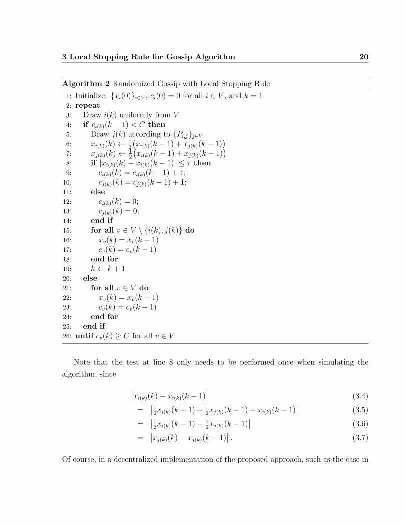
Note that the test at line 8 only needs to be performed once when simulating the
algorithm, since
∣∣xi(k)(k)− xi(k)(k − 1)∣∣ (3.4)
=∣∣1
2xi(k)(k − 1) + 1
2xj(k)(k − 1)− xi(k)(k − 1)
∣∣ (3.5)
=∣∣1
2xi(k)(k − 1)− 1
2xj(k)(k − 1)
∣∣ (3.6)
=∣∣xj(k)(k)− xj(k)(k − 1)
∣∣ . (3.7)
Of course, in a decentralized implementation of the proposed approach, such as the case in

3 Local Stopping Rule for Gossip Algorithm 21
this thesis, each of the nodes i(k) and j(k) would perform the test in parallel.
A number of questions immediately come to mind about the proposed stopping rule:
Are we guaranteed that all nodes eventually stop gossiping? If they all stop, what is the
error in their estimates? Which parameters influence how big is the error at stopping?
Our main theoretical results answer these questions as summarized in Theorem 1 below.
The final error depends on the characteristics of the network topology and connectivity,
and so we first introduce some notation. For a graph G = (V,E) with n = |V | nodes, let
A ∈ Rn×n denote the adjacency matrix; i.e., Ai,j = 1 if and only if the graph contains the
edge (i, j) ∈ E. Also, let D denote a diagonal matrix whose ith element Di,i = |Ni| is equal
to the degree of node i (number of neighbors). The graph Laplacian of G is the matrix
L = D−A. Our bounds depend on the network topology through:
(1) the second smallest eigenvalue of the graph Laplacian L, which we denote by λ2,
(2) the number of edges m = |E| in the network (also called lines or links between nodes),
(3) the maximum degree (or number of neighbors), dmax = maxiDi,i.
Theorem 1. Let δ > 0 be given. Assume that ‖x(0)‖ < ∞, and assume that {Pi,j}correspond to the natural random walk probabilities on G. After running randomized gossip
(Algorithm 2) with stopping rule parameters,
C = dmax
(log(dmax) + 2 log(n)
)(3.8)
τ =
√λ2δ2
8m(C − 1)2, (3.9)
the following two statements hold.
a. All nodes eventually stop gossiping almost surely; i.e., with probability one, there
exists a K ≥ 0 such that ci(k) ≥ C for all i ∈ V and all k ≥ K.
b. Let K = min{k : ci(k) ≥ C for all i ∈ V } denote the first iteration when all nodes
stop gossiping. With probability at least 1− 1/n, the final error is bounded by
‖x(K)− x‖ ≤ δ. (3.10)
3 Local Stopping Rule for Gossip Algorithm 22
0 1 2 3 4 5
x 10−3
0
1
2
3
4
5
6
τ
δ
Complete GraphRGGStarChainGrid
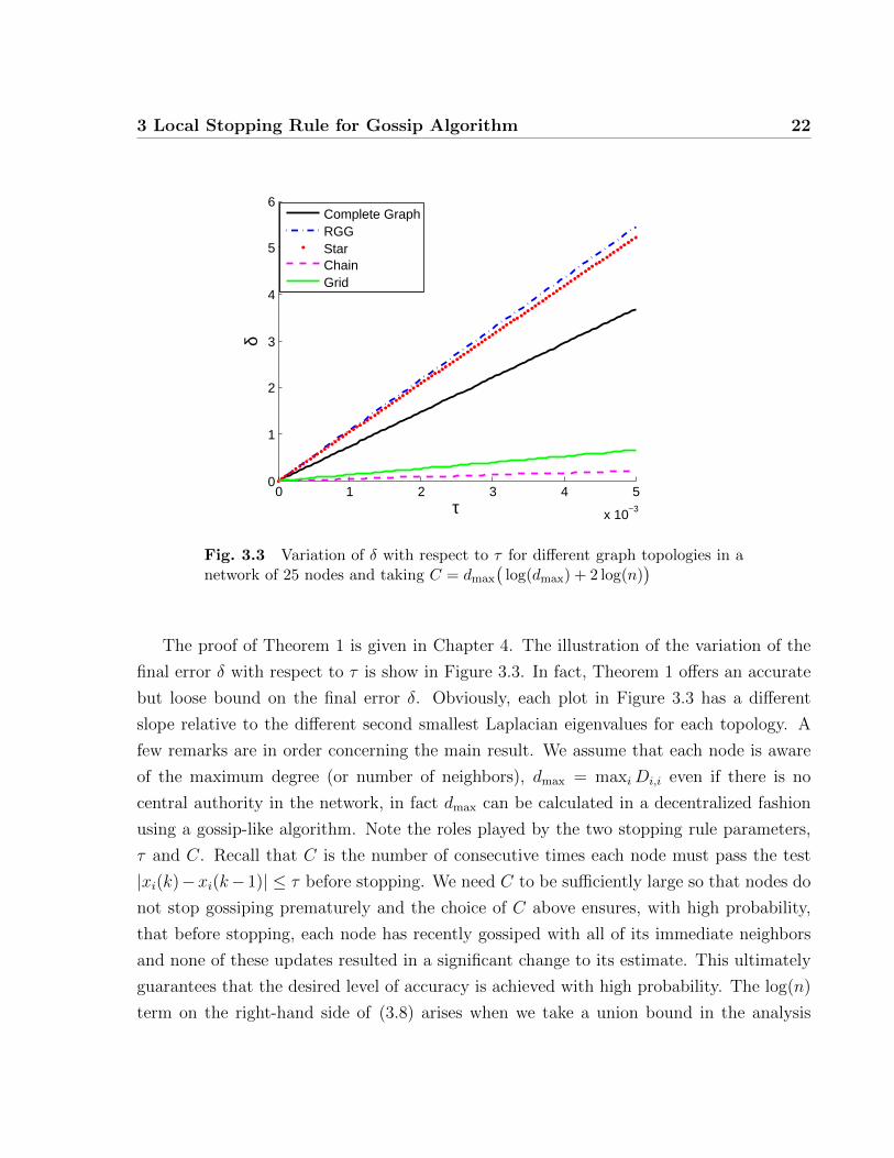
Fig. 3.3 Variation of δ with respect to τ for different graph topologies in anetwork of 25 nodes and taking C = dmax
(log(dmax) + 2 log(n)
)
The proof of Theorem 1 is given in Chapter 4. The illustration of the variation of the
final error δ with respect to τ is show in Figure 3.3. In fact, Theorem 1 offers an accurate
but loose bound on the final error δ. Obviously, each plot in Figure 3.3 has a different
slope relative to the different second smallest Laplacian eigenvalues for each topology. A
few remarks are in order concerning the main result. We assume that each node is aware
of the maximum degree (or number of neighbors), dmax = maxiDi,i even if there is no
central authority in the network, in fact dmax can be calculated in a decentralized fashion
using a gossip-like algorithm. Note the roles played by the two stopping rule parameters,
τ and C. Recall that C is the number of consecutive times each node must pass the test
|xi(k)−xi(k− 1)| ≤ τ before stopping. We need C to be sufficiently large so that nodes do
not stop gossiping prematurely and the choice of C above ensures, with high probability,
that before stopping, each node has recently gossiped with all of its immediate neighbors
and none of these updates resulted in a significant change to its estimate. This ultimately
guarantees that the desired level of accuracy is achieved with high probability. The log(n)
term on the right-hand side of (3.8) arises when we take a union bound in the analysis

3 Local Stopping Rule for Gossip Algorithm 23
below, and we believe that this result in the bound being loose. In the simulation results
presented in Chapter 5 we show that even taking C = ddmax log dmaxe generally suffices to
achieve the target accuracy. On the other hand, the parameter τ allows us to control the
final level of accuracy, δ. Clearly, more accurate solutions require smaller τ . Also note
that τ and the number of edges m are inversely proportional, this implies that in order to
guarantee the same performance, in terms of the level of accuracy δ, a larger value of τ can
be used for networks with fewer edges.
Next, note that we assume that {Pi,j} are the natural random walk probabilities to
simplify the discussion below, but our analysis can easily be generalized for any choice of
probabilities {Pi,j} that conform to topology, G, albeit, at the expense of more cumbersome
notation.
From (8), we see that C is proportional to the maximum degree, which implies that for
networks with few neighbors, the parameter C is small. One could generalize the approach
described here to allow for a different stopping count, Ci, at each node, proportional to its
local degree, at the cost of more cumbersome notation. Although the same analysis would
go through directly, we omit the generalization here to simplify presentation. Recall that
when C is not sufficiently large, nodes are not given sufficient time to gossip with all of their
neighbors and consequently stop gossiping prematurely. A worst case scenario would be a
ring topology where the difference between each two neighbors satisfies the local stopping
rule, but the overall difference between two nodes diametrically opposed is very big and
thus, the final level of accuracy at convergence is very high. The same applies for grid
topologies where the small number of neighbors restricts the improvement that the local
stopping rule can achieve relative to randomized gossip.
Appendix E investigates the relationship between the graph topology and the second
smallest eigenvalue of the Laplacian. It also explains the relationship between the graph
connectivity and both the node degree and the second smallest eigenvalue λ2 through
simulations. Roughly speaking, large values of λ2 are related to graph topologies that are
hard to disconnect. Another interesting fact is that λ2 decreases for graphs with sparse
cuts.
For random geometric graph topologies, the expected node degree, scales as log(n),
in this case, the number of iterations required to reach convergence becomes increasingly
large. Consider the irregular graph topologies (such as star topologies) where the number
of neighbors varies drastically between nodes. In this case one can define Ci=dilogdi where

3 Local Stopping Rule for Gossip Algorithm 24
Ci and di are respectively the count and degree parameters of each node i. The same
analysis would go through directly at the cost of more cumbersome notation. By reducing
the parameter C for some nodes, we reduce the number of redundant transmitted messages
during a gossip iteration and obviously accelerate the algorithm.
In order to reduce the value of C, we can employ a Graph Sparsification. Sparsification
is a very important yet easy method to implement. Roughly speaking it is based on the
simple principle of modifying the underlaying topology of a graph by deleting some of its
links. Theoretically it has been shown in [49] that given a graph G, if we remove some links
between nodes of this graph, we get a new equivalent graph H for which the number of
links is reduced and such that λ2(H) ≤ λ2(G). By applying the previous property one can
adapt Theorem 1 in order to accelerate the local stopping rule in certain topologies such
as complete graphs. The notion of sparsifying a network will be revisited more in details
in Appendix E.
Another question of interest is: How long will it take until all nodes stop? We investigate
this issue via simulation in Chapter 5. Intuitively, because nodes only stop initiating
gossip rounds when their values are already close enough to their neighbors, the rate of
convergence of Algorithm 2 is essentially the same as that of randomized gossip without
the local stopping rule (Algorithm 1). However, for certain initial conditions, using the
local stopping rule can result in significant savings in terms of the number of transmissions
by temporarily stopping certain nodes when they have nothing significant to tell their
neighbors. For example, consider an initial condition where all nodes have xi(0) = 0
except one node that differs dramatically, e.g., x1(0) = 1000. In this case, most nodes will
have the same value as their neighbors initially, and so they will cease to gossip until the
measurement from node 1 diffuses and reaches their region of the network. We revisit this
point and illustrate it further in Chapter 5. The main importance of the GossipLSR is that
for some initializations, it induces less transmission cost at each iteration step at a cost
of having slight smaller final consensus precision with respect to randomized gossip. The
answer to the question of how long will it take until all nodes stop is not derived in a nice
mathematical formula (since it depends on the initialization type and scale as well as the
size and topology of the network and the parameter τ) but we can definitely confirm that
this time to stop is smaller than the rate of convergence of randomized gossip without the
local stopping rule (Algorithm 1).
Finally, note that there is an overhead associated with using a local stopping rule, in
3 Local Stopping Rule for Gossip Algorithm 25
the following sense. Even if the network is initialized to a consensus (i.e., x(0) = x), a
minimum number of gossip rounds must occur before the network stops gossiping. This is
the price one must pay for using a decentralized stopping rule, and this price is precisely C,
the number of rounds each node must participate in before it decides to stop initiating a
gossip round when its clock ticks. In grids, dmax = Θ(1), and so C = Θ(log n). For random
geometric graphs, dmax = Θ(log n) with high probability, and so C = Θ(log(n) log log(n)).
In any case, this is no worse than the best known scaling laws for randomized gossip
algorithms in wireless networks. This shows the method to be promising in a number of
ways compared to existing randomized gossip algorithms.
It is worth noting that GossipLSR utilizes some local node values such as dmax, n, m
and λ2. One can argue that the GossipLSR algorithm is not fully decentralized. In fact, all
these parameters can be calculated in a decentralized fashion. Decentralized computation
of the second smallest eigenvalue of the Laplacian λ2 can be carried out using a gossip-like
variant of the Lanczos iteration [22]. Similarily, parameters n andm, measuring the network
size and number of edges, can be calculated using the Push-Sum gossip algorithm [20].
Finally, The maximum degree dmax can be computed in a decentralized manner using a
max consensus randomized algorithm, but where instead of averaging, nodes update their
states with the maximum.
3.4 Summary
We have presented a general, local stopping rule that defines a finite time stopping rule
to existing randomized gossip algorithms. The convergence properties were studied in the
last section of this chapter. Theorem 1 summarized the main result of this thesis, later
we discussed the different parameters of this Theorem. In the sequel, we will give some
additional explanations and the proof of our main result. We show the derivations leading
to Theorem 1 and give some comments concerning the role that both τ and C plays in the
GossipLSR.
26
Chapter 4
Convergence analysis of GossipLSR
In previous chapters, with the aim of minimizing the number of transmissions in a network,
we proposed a gossip algorithm with explicit stopping rule. This chapter examines the proof
of Theorem 1 and the necessary and sufficient conditions for convergence. More precisely,
we first explore the theoretical guarantees of convergence and later investigate the error
when stopping.
4.1 Guaranteed Stopping
In the standard gossip setting, we fix the initial values x(0) at time 0, and let the algorithm
run. By the nature of the gossip updates, we get monotonic convergence to the average.
Consequently, every time we do a gossip update, the error decreases at the end (or, techni-
cally, is non-increasing, since if we try to average a pair of nodes that already have the same
value, then nothing changes) . We begin by proving part (a) of Theorem 1 which claims
that all nodes eventually stop gossiping. Consider the squared error, ‖x(k) − x‖2, after
iteration k. Since two nodes average their values whenever they gossip, we are guaranteed
that ‖x(k)− x‖2 is non-increasing, and we can quantify the decrease at iteration k in terms
of the values at nodes i(k) and j(k).
Lemma 1. After i(k) and j(k) gossip at iteration k,
‖x(k)− x‖2 = ‖x(k − 1)− x‖2 − 12
(xi(k)(k − 1)− xj(k)(k − 1)
)2. (4.1)
Proof. After nodes i(k) and j(k) gossip at iteration k, the recursive update for GossipLSR

4 Convergence analysis of GossipLSR 27
is
x(k) = x(k − 1)− 12f(k) (4.2)
where f(k) is defined as
fl(k) =
xi(k)(k − 1)− xj(k)(k − 1) if l = ik
−(xi(k)(k − 1)− xj(k)(k − 1)
)if l = jk
0 otherwise
where the subscript l is the index of the components of the vector f .
Using equation (4.2) we can derive the squared error such that
‖x(k)− x‖2 = ‖x(k − 1)− 12f(k)− x‖2. (4.3)
= ‖x(k − 1)− x‖2 + 14‖f(k)‖2 − 〈x(k − 1)− x, f(k)〉 (4.4)
Based on the definition of f(k) we have
‖f(k)‖2 = 2(xi(k)(k − 1)− xj(k)(k − 1)
)2. (4.5)
and
〈x(k − 1)− x, f(k)〉 =(xi(k)(k − 1)− xj(k)(k − 1)
)2. (4.6)
Therefore using (4.4) we have
‖x(k)− x‖2 = ‖x(k−1)− x‖2 + 12
(xi(k)(k−1)−xj(k)(k−1)
)2−(xi(k)(k−1)−xj(k)(k−1)
)2.
(4.7)
and consequently we can say that,
‖x(k)− x‖2 = ‖x(k − 1)− x‖2 − 12
(xi(k)(k − 1)− xj(k)(k − 1)
)2. (4.8)
From equations (3.6) and (3.7), we can also make the following interesting observations
about the relationship between values at nodes i(k) and j(k) immediately after they gossip.
Lemma 2. After i(k) and j(k) gossip at iteration k,
a.∣∣xi(k)(k)− xi(k)(k − 1)
∣∣ > τ if and only if∣∣xj(k)(k)− xj(k)(k − 1)
∣∣ > τ ;

4 Convergence analysis of GossipLSR 28
b.∣∣xi(k)(k)− xi(k)(k − 1)
∣∣ > τ if and only if∣∣xi(k)(k − 1)− xj(k)(k − 1)
∣∣ > 2τ .
Let I{A} denote the indicator function of the event A. Since by design, all nodes’
clocks tick according to independent Poisson processes with identical rates, it follows that
all nodes tick infinitely often, or lim sup I{i(k) = v} = 1 for all v ∈ V . In particular,
pathological sample paths—e.g., where one node ticks consecutively an infinite number of
times, or where one node’s clock does not tick for an unbounded period of time—occur with
probability zero. Formally, since Pr(i(k) = v) = 1/n for all nodes v ∈ V , from the second
Borel-Cantelli Lemma about sequences of events, we can say that the set of outcomes that
node’s clock does not tick for an infinite number of events occurs with probability zero and
consequently it follows that v’s clock ticks infinitely often with probability 1. Interested
reader can find a detailed explanation about the Borel-Cantelli Lemma in [50].
Suppose, for the sake of a contradiction, that claim (a) of Theorem 1 does not hold,
and the network does not stop. This implies that there exists a node v ∈ V such that
lim sup I{cv(k) < C} = 1; i.e., v never reaches a state where it permanently stops initiating
gossip iterations. According to steps 8–14 of Algorithm 2, one of two things happens each
time v participates in a gossip round: either the absolute change in its estimate is small and
it increments cv(k), or the absolute change is larger than τ and it resets cv(k) = 0. Since v
participates in infinitely many gossip rounds and lim sup I{cv(k) < C} = 1, it must be that
v resets its counter infinitely often; i.e., lim sup I{cv(k) = 0} = 1. Let k1, k2, . . . , denote
the iterations when v resets its counter. Each time v resets its counter, it gossiped and the
change was greater than τ . By Lemma 2, this implies that each time v resets its counter,
the absolute difference between xv(kl) and the value of the node it gossiped with is at least
2τ , and by Lemma 1, this implies that the squared error ‖x(kl)− x‖2 decreases by at least
4τ 2 at that iteration. By assumption, the initial condition has finite norm, ‖x(0)‖ < ∞,
which implies that the initial squared error is also finite, ‖x(0)− x‖2 <∞. If the squared
error decreases by 4τ 2 each time v resets its counter, and if it resets its counter infinitely
often, then ‖x(k)− x‖2 → −∞ as k →∞. However, this is a contradiction, since V (k) ≥ 0
by definition. Hence, it cannot happen that some node gossips infinitely often, and so all
nodes eventually stop gossiping, which proves claim (a) of Theorem 1.

4 Convergence analysis of GossipLSR 29
4.2 Error When Stopping
Next, we prove part (b) of Theorem 1, which bounds the error ‖x(K)− x‖ at the time K
when all nodes stop gossiping. The error ‖x(K)− x‖ is the deviation of the node values at
time K from the average. Our proof of the error bound involves two main steps. First, we
show that the choice of C = Θ(dmax log dmax) ensures that when all nodes stop gossiping,
their estimates are relatively close to all of their immediate neighbors. Then we show that
if all nodes estimates are close to their neighbors’, then they must be close to the average
of the global network.
The first part of the proof is based on a standard result from the study of occupancy
problems, and in particular the Coupon Collector’s problem [21,40]. In this problem, there
are d different types coupons. At each iteration, the coupon collector is given a new coupon
drawn uniformly and randomly from a pool of coupons (with replacement). The following
is a standard tail-bound for the number of iterations required to collect all types of coupons.
Lemma 3 (Coupon Collector [21,40]). Let T be the number of iterations it takes the coupon
collector to get one of each of the d types of coupons, and let β ≥ 1. Then
Pr(T > βd log d) ≤ d1−β. (4.9)
Details about coupon collector proof is listed in Appendix A. In particular, this bound
suggests that after T = Θ(d log d) iterations, the collector has one of each coupon with
high probability. We apply this result to guarantee that a node has recently gossiped with
each one of its neighbors without seeing a significant change before it stops gossiping. In
particular, for each node, we map its neighbors to coupons, and require that it collects one
coupon from each neighbor (which it does only when gossiping with that neighbor results
in an absolute change of less than τ) before stopping, with high probability. Consequently,
when a node stops gossiping, with high probability, its estimate was recently close to all
of its neighbors: if node i stops gossiping at iteration Ki, then minl=0,...,C−1 |xi(Ki − l) −xj(Ki − l)| ≤ τ for all neighbors j ∈ Ni. Unfortunately, this is not sufficient to guarantee
that |xi(K) − xj(K)| ≤ τ for all pairs (i, j) ∈ E, since it could happen that after i and j
gossip with each other for the last time, i still gossips with another neighbor. However, we
can guarantee these differences do not grow too large.

4 Convergence analysis of GossipLSR 30
Lemma 4. If C = dmax(log dmax + 2 log n), then at the time K = inf{k : ci(k) ≥C for all i ∈ V } when the network stops gossiping, with probability at least 1− 1/n,
|xi(K)− xj(K)| ≤ 2(C − 1)τ (4.10)
for all pairs of neighboring nodes, (i, j) ∈ E.
Let β ≥ 1 whose value is to be determined, and let Bi denote the event that node i
stopped without having contacted all of its neighbors in the last C rounds. We associate
with each node i a coupon collector trying to collect di = |Ni| coupons at a time instant
Ti, so that Bi = {Ti > βdi log di}. By Lemma 3,
Pr(Bi) ≤ d1−βi ≤ d1−β
max. (4.11)
Applying the union bound, we can bound the probability that some node stopped without
having contacted all of its neighbors in the last C rounds by
Pr (∪i∈VBi) ≤∑i∈V
Pr(Bi) = nd1−βmax. (4.12)
Then, taking β = 1 + 2 log(n)/ log(dmax), and accordingly setting
C = βdmax log dmax = dmax(log dmax + 2 log n), (4.13)
we have that, with probability at least 1− 1/n, all nodes gossip with all of their neighbors
in the iterations when ci(k) goes from 1 to C. By Lemma 2, when i(k) and j(k) increment
their counts, ci(k)(k) and cj(k)(k), we know that |xi(k)(k−1)−xj(k)(k−1)| ≤ 2τ . Moreover,
immediately after they gossip, xi(k)(k) = xj(k)(k). Suppose that nodes i(k) and j(k) set
ci(k)(k) = 1 and cj(k)(k) = 1 at iteration k. In the worst case, they each gossip C − 1
more times with different neighbors and their estimates change by τ each time, moving
in opposite directions (e.g., xi(k)(k) increasing and xj(k)(k) decreasing). Then their final
estimates have drifted by 2(C − 1)τ . Since this is true for every pair of nodes when they
stop, we have proved the Lemma.
We restrict Pi,j to be the natural random walk probabilities on G in order to apply
the standard form of the Coupon Collector’s problem, where all coupons have identical
4 Convergence analysis of GossipLSR 31
probability. The above result can be immediately generalized to other distributions Pi,j by
application of variations of the weighted Coupon Collector’s problem [51].
We have established that when the network stops gossiping all nodes have estimates
at most 2(C − 1)τ from their neighbors with high probability. Next, we show that this
implies all nodes are close to the average at stopping. Even though neighboring nodes have
similar estimates, the difference between estimates can propagate across the network. We
will quantify how much this error can propagate in terms of characteristics of the network
topology and the specific stopping criterion τ .
For a graph G, let A ∈ Rn×n denote the adjacency matrix; i.e., Ai,j = 1 if and only
if the graph contains the edge (i, j) ∈ E. Also, let D denote a diagonal matrix whose ith
element Di,i = |Ni| is equal to the degree of node i. The graph Laplacian of G is the matrix
L = D−A. For a vector x ∈ Rn, it is easy to verify that
xTLx =∑i∈V
∑j∈Ni
(xi − xj)2. (4.14)
The results of Lemma 4 can be applied to each term on the right-hand side of (4.14) to
bound the magnitude of the Laplacian quadratic form. The following lemma relates the
quadratic form on left-hand side of (4.14) to the squared error, ‖x− x‖2.
Lemma 5. Let λ1 ≤ λ2 ≤ · · · ≤ λn denote the eigenvalues of L sorted in ascending order.
Then,1
λnxTLx ≤ ‖x− x‖2 ≤ 1
λ2
xTLx. (4.15)
Proof. The proof follows from basic principles of linear algebra and spectral graph theory.
Let {ui ∈ Rn}ni=1 denote the orthonormal eigenvectors of L, with ui being the eigenvector
corresponding to eigenvalue λi.
A well-known fact from spectral graph theory (see, e.g., [52,53]) is that, for a connected
graph G, the smallest Laplacian eigenvalue λ1 = 0 is zero, and the corresponding orthonor-
mal eigenvector is u1 = 1√n1, where 1 denotes the vector of all 1’s. Expanding L in terms
of its eigendecomposition, we see that
xTLx = xT
(n∑i=1
λiuiuTi
)x (4.16)

4 Convergence analysis of GossipLSR 32
=n∑i=2
λi〈x,ui〉2, (4.17)
where 〈x,u〉 = xTu denotes the inner product between x and u.
Next, consider the squared distance ‖x− x‖2 from x to its corresponding average con-
sensus vector x. Recall that the average consensus vector x can be written in terms of x
as
x =1
n11Tx = u1u
T1 x = 〈x,u1〉u1. (4.18)
Since the eigenvectors {ui} form an orthonormal basis for Rn, we can expand x in terms
of {ui}:
x =n∑i=1
〈x,ui〉ui. (4.19)
Then, it is clear that subtracting x from x simply cancels out the portion of x spanned by
u1, leaving x− x =∑n
i=2〈x,ui〉ui. Thus, the squared error is easily expressed in terms of
the eigenbasis {ui} as
‖x− x‖2 =n∑i=2
〈x,ui〉2. (4.20)
Compare equations (4.17) and (4.20). To complete the proof, observe that because
we have ordered the eigenvalues in ascending order, λi/λ2 ≥ 1 and λi/λn ≤ 1 for all
i = 2, . . . , n. Thus,
n∑i=2
λiλn〈x,ui〉2 ≤
n∑i=2
〈x,ui〉2 ≤n∑i=2
λiλ2
〈x,ui〉2, (4.21)
which is what we wanted to show.
Now, to complete the proof of Theorem 1(b) we just need to put the various pieces
together. Recall that m = |E| denotes the number of edges in G (number of links in the
graph), and the sum on the right-hand side of (4.14) contains two terms for each edge
(once from i to j, and once from j to i). Combining Lemma 4 and Lemma 5 gives the error
bound,
‖x(K)− x‖2 ≤ λ−12
∑i∈V
∑j∈Ni
(xi(K)− xj(K)
)2(4.22)

4 Convergence analysis of GossipLSR 33
≤ 8m(C − 1)2τ 2
λ2
, (4.23)
which holds with probability at least 1 − 1/n. Plugging in the expression for τ from
the statement of Theorem 1(b) yields the desired bound, and thus completes the proof
of Theorem 1, and bounds the error ‖x(K) − x‖ at the time K when all nodes stop
gossiping. This result is very important since it describes how distant nodes can be from
the true average at convergence. It also helps choosing the parameter τ to get a specific
error at convergence. Our Theorem holds under fairly general assumptions on the network
connectivity and size.
Inspired from the results of this chapter, in the sequel, we study the simulation results of
GossipLSR under different conditions and initializations; additionally next chapter explains
the reduction achieved by the modified algorithm in terms of number of transmissions and
iterations to convergence.
34
Chapter 5
Simulation Results
In this chapter, we provide simulation outcomes to complement our theoretical findings
and compare the simulation results of Algorithm 2, randomized gossip with local stopping
rule (or GossipLSR for short), with different network topologies, initializations and network
sizes. Important criteria that decide the effectiveness of any gossip algorithm are the num-
ber of transmissions required to convergence, the number of iterations to reach convergence
as well as the relative error ||x(k)−x||||x(0)−x|| when stopping. Unless otherwise specified, we use a
random geometric graph with 200 nodes. As initialization fields, we use spike, slope, 0/100,
i.i.d and Gaussian Bumps initializations. Details about these initialization fields as well as
the description of their generation can be found in Appendix D.
5.1 Convergence results
Figure 5.1a shows the histogram of the differences on network edges at convergence |xi(K)−xj(K)| for (i, j) ∈ E for a 0/100 initialization. We can conclude that with very high
probability, when C = dmax log(dmax) all the edge differences are below τ . In the his-
togram depicted in the Figure 5.1a, the percentage of links having a difference above
τ is equal to 0.15%. The histogram depicted in Figure 5.1b represents the case when
C = dmax
(log(dmax) + 2 log(n)
). We can see that the percentage of links having a differ-
ence above τ is almost equal to zero. Since the difference between Figures 5.1a and 5.1b
is minimal, in the sequel, we use C = dmax log(dmax). Decreasing C implies that nodes
check their neighborhood less often before going passive and this implies a smaller number
of iterations to convergence.

5 Simulation Results 35
0 0.02 0.04 0.06 0.08 0.1 0.12 0.14 0.160
500
1000
1500
2000
2500
3000
Edge difference at convergence
Num
ber
of e
dges
Predefined local error
(a) C = dmax log(dmax).
0 0.02 0.04 0.06 0.08 0.1 0.12 0.14 0.160
500
1000
1500
2000
2500
3000
Edge difference at convergence
Num
ber
of e
dges
Predefined local error
(b) C=dmax
(log(dmax) + 2 log(n)
)Fig. 5.1 Distribution histogram of the edge differences |xi(K)− xj(K)| fora 0/100 initial condition in a 200 nodes network deployed according to a RGGwith different parameter C, Recall that C is the number of times a nodesneeds to pass the test of the edge difference before it decides to stop.

5 Simulation Results 36
0 0.02 0.04 0.06 0.08 0.10
0.5
1
1.5
2
2.5
3
3.5
4x 10
4
Edge difference at convergence
Num
ber
of e
dges
(a) Spike initialization
0 0.02 0.04 0.06 0.08 0.1 0.120
500
1000
1500
2000
2500
3000
Edge difference at convergence
Num
ber
of e
dges
Predefined local error
(b) Slope initialization
0 0.02 0.04 0.06 0.08 0.1 0.120
500
1000
1500
2000
2500
3000
Edge difference at convergence
Num
ber
of e
dges
Predefined local error
0.04%
(c) Independant identically distributed ini-tialization
0 0.02 0.04 0.06 0.08 0.1 0.120
500
1000
1500
2000
2500
3000
Edge difference at convergence
Num
ber
of e
dges
Predefined local error
0.008%
(d) Gaussian Bumps inialization
Fig. 5.2 Distribution histogram of the edge differences |xi(K)− xj(K)| fordifferent initial conditions in a 200 nodes network deployed according to aRGG with C = dmax log(dmax) and τ=0.1. Note that the x-axis and y-axis forthe Spike initialization is different than the other types of initializations.
Repeating the same simulation with C = dmax log(dmax) for a Spike initialization, all the
edge differences at convergence are situated below the threshold τ=0.1. This is illustrated
in Figure 5.2a. This shows that the local stopping rule achieves total convergence for
the case of Spike initialization. Figure 5.2 illustrates the convergence results for different
initialization types and shows that GossipLSR achieves convergence for all types of initial
conditions. It also shows that the edges above the threshold τ are above the threshold by
a very small amount (0.01 to 0.02). Later in this section, we show that the total number
of transmissions spent to achieve convergence is reduced by cutting down the redundant
transmissions in a Spike initialization. We also illustrate the total number of iterations
required to reach convergence.
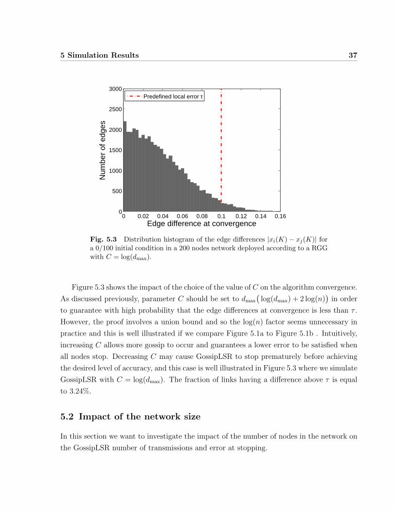
5 Simulation Results 37
0 0.02 0.04 0.06 0.08 0.1 0.12 0.14 0.160
500
1000
1500
2000
2500
3000
Edge difference at convergence
Num
ber
of e
dges
Predefined local error τ
Fig. 5.3 Distribution histogram of the edge differences |xi(K)− xj(K)| fora 0/100 initial condition in a 200 nodes network deployed according to a RGGwith C = log(dmax).
Figure 5.3 shows the impact of the choice of the value of C on the algorithm convergence.
As discussed previously, parameter C should be set to dmax
(log(dmax) + 2 log(n)
)in order
to guarantee with high probability that the edge differences at convergence is less than τ .
However, the proof involves a union bound and so the log(n) factor seems unnecessary in
practice and this is well illustrated if we compare Figure 5.1a to Figure 5.1b . Intuitively,
increasing C allows more gossip to occur and guarantees a lower error to be satisfied when
all nodes stop. Decreasing C may cause GossipLSR to stop prematurely before achieving
the desired level of accuracy, and this case is well illustrated in Figure 5.3 where we simulate
GossipLSR with C = log(dmax). The fraction of links having a difference above τ is equal
to 3.24%.
5.2 Impact of the network size
In this section we want to investigate the impact of the number of nodes in the network on
the GossipLSR number of transmissions and error at stopping.

5 Simulation Results 38
0 0.05 0.1 0.15 0.2 0.25 0.3 0.35 0.4 0.45 0.510
−3
10−2
10−1
100
τ
Rel
ativ
e er
ror
Error vs Transmissions for different sized networks
N=100N=200N=400
(a) Relative error at stopping
0 0.1 0.2 0.3 0.4 0.5102
103
104
τ
Num
ber
of tr
ansm
issi
ons
N=50N=200N=400
(b) Number of transmissions
Fig. 5.4 Relative error ||x(k)−x||||x(0)−x|| and Number of transmissions with respect
to τ for different network sizes in a RGG with an IID initialization. Each pointon this graph corresponds to the average error with respect to a certain valueof τ where C = dmax log dmax. We plot each curve for values of τ ranging from0.01 to 0.5.

5 Simulation Results 39
In Figure 5.4a we plot the relative error with respect to τ for different network sizes.
Each data point is an ensemble average of 100 trials, for each trial, we evaluate the relative
error for each value of τ ranging from 0.01 to 0.5 at intervals of 0.01. Figure 5.4a illustrates
clearly that in bigger networks we need smaller τ to achieve the same level of accuracy and
this was well anticipated in Theorem 1. In Figure 5.4b we plot the number of transmissions
with respect to τ for different network sizes. This figure provides a better understanding of
how the number of transmissions might be affected by different sized networks. Comparing
Figures 5.4a and 5.4b we can see that increasing τ decreases the number of transmissions
but the price to pay is in terms of relative error at convergence.
0 1000 2000 3000 4000 5000 6000 7000 8000 9000 1000010
−3
10−2
10−1
100
Number of transmissions
Rel
ativ
e er
ror
N=100N=200N=400
tau=0.01
tau=0.5
Fig. 5.5 Relative error ||x(k)−x||||x(0)−x|| with respect to the Number of transmissions
at stopping, we use different network sizes in a RGG with an IID initialization.Each point on this graph corresponds to the average error and average numberof transmissions until stopping over 100 trial for C = dmax log dmax and forvalues of τ ranging from 0.01 to 0.5.
Figure 5.5 shows, in logarithmic scale, the change in relative error with respect to
the number of transmissions, using GossipLSR on a random geometric graph (RGG) with
independent identically distributed initialization and different network sizes (each data
point is an ensemble average of 100 trials). The graph shows very clearly that increasing

5 Simulation Results 40
the network size n requires more transmissions to reach convergence and gives a higher
relative error at convergence. By increasing the network size from 100 to 400, the number
of transmissions increases by 4000 transmissions and the relative error increases.
5.3 Impact of the network topology
The connectivity and shape of the network plays a key role in dictating the performance
of any gossip algorithm in terms of the number of transmissions, iterations as well as the
final error at convergence.
In Figure 5.6a we plot the number of transmissions with respect to τ , each curve repre-
sents a different network topology and we can clearly observe the impact of the parameter
τ on the reduction of the number of transmissions. Similarly, in Figure 5.6b we can clearly
observe the impact of the parameter τ on the relative error at stopping. Although attrac-
tive from the number of transmissions point of view, we need to mention that high node
degree in Complete Graphs restricts the improvements in terms of the number of iterations
that the local stopping rule can achieve relative to randomized gossip. This was well antici-
pated theoretically in Chapter 4 and will be revisited later in the current chapter. From the
properties of random geometric graph, the estimated degree at each node is proportional
to log(n), where n is the size of the network, in contrast to the case of Complete Graphs
where the node degree is always equal to n − 1 for each node. High node degree, implies
a higher count variable C, and consequently the number of iterations to reach convergence
increases. Although in Figure 5.6b, it is clearly shown that for the same level of accuracy,
RGG requires more transmissions than the Complete Graph, the price to pay when having
a Complete Graph is in the number of iterations (time to locally decide that we reached
convergence).
Figure 5.7 plots the relative error with respect to the number of transmissions for differ-
ent network topologies. We consider the well-connected complete graph as well as the RGG,
typically used in most wireless sensor networks. Each data point corresponds to the average
over 100 trial for different values of τ . Observing Figure 5.7, we can say that, comparing
both Complete Graphs and RGG network topologies, the optimal performance would be
for Complete Graphs since GossipLSR achieves a lower relative error while consuming less
transmissions.

5 Simulation Results 41
0 0.1 0.2 0.3 0.4 0.5102
103
104
τ
Num
ber
of tr
ansm
issi
ons
Complete Graph RGG
(a) Number of transmissions
0 0.1 0.2 0.3 0.4 0.510−3
10−2
10−1
100
τ
Rel
ativ
e er
ror
Complete Graph RGG
(b) Relative error at stopping
Fig. 5.6 Relative error ||x(k)−x||||x(0)−x|| and Number of transmissions with respect
to τ for different network topologies. Each point on this graph corresponds tothe average error with respect to a certain value of τ where C = dmax log dmax.We plot each curve for values of τ ranging from 0.01 to 0.5.

5 Simulation Results 42
0 2000 4000 6000 8000 1000010−3
10−2
10−1
100
Number of transmissions
Rel
ativ
e er
ror
Complete GraphRGG
tau=0.5
tau=0.01
Fig. 5.7 Relative error ||x(k)−x||||x(0)−x|| with respect to the number of transmissions
at stopping, we use two different network topologies. Each point on this graphcorresponds to the average error and average number of transmissions untilstopping for C = dmax log dmax and for values of τ ranging from 0.01 to 0.5.
5.65.2
5.45
5.5
5.55
5.35
5.3
5.25
5.4
5.55
5.5
5.45
5.4
5.25
5.3
5.35
Fig. 5.8 Snapshot of the network values at stopping using GossipLSR for aChain graph scenario where the local stopping criterion τ = 0.05 is satisfiedbetween each pair of nodes but the overall error is very high.
5 Simulation Results 43
Figure 5.8 illustrates why the network topology plays an important role in the Gossi-
pLSR ability to converge and how it impacts the relative error when stopping. As can be
seen from Figure 5.8 the local stopping condition is satisfied between each pair of neighbors
in the graph with τ=0.05 . Though, there is a difference of 0.4 between the edge nodes
‘5.2’ and ‘5.6’ and consequently, we have a high relative error even if the local stopping
rule is satisfied. This intuitively predicts that the application of the GossipLSR for some
topologies is not optimal and can give a very high relative error. The upper bound on the
worst case error was previously derived in Chapter 3. Note that each node in a chain graph
is restricted to two neighbors (independently of the network size). This implies that both
dmax and consequently the variable C are small. Appendix C and E investigates different
graph topologies and how they impact the GossipLSR performance through the second
smallest eigenvalue of their Laplacian. A method to reduce the complexity of the graphs
known as Graph Sparsification is surveyed in Appendix E.
5.4 Impact of the network initialization
We next observe the number of transmissions to convergence with respect to τ for many net-
work initializations. We examine the performance for a Slope linearly-varying field, a field
with the “Spike” signal, 0/100 initialization, Gaussian Bumps as well as the independent
identically distributed node initialization with mean 0 and variance 1. As can be seen from
Figure 5.9a, the local stopping rule reduces the number of transmissions for all the types of
initial condition. The reduction rate achieved by increasing τ is strikingly higher for i.i.d
and spike initialization, while the reduction is less pronounced for the case of 0/100 and
Slope initialization. In fact, regular differences between nodes at initialization introduced
by a Slope field causes the gossip with local stopping rule to offer minimal gain compared
to gossip without local stopping rule. On the other hand, Figure 5.9b shows how the error
increases with τ for different initializations. Spike initialization achieves the lowest relative
error while the slope is the worst case. Comparing both Figures 5.9a and 5.9b we can
clearly observe that the gain in terms of the number of transmission reduction comes at
the price of a small hit in relative error. We can also see the similarities between curves of
i.i.d zero-mean unit-variance Gaussian, and GB mixture of Gaussians. As expected Spike
seems to be an easy initialization for distributed averaging since nodes far away from the
spike only needs to gossip a few times prior to convergence.

5 Simulation Results 44
0 0.1 0.2 0.3 0.4 0.5102
103
104
τ
Num
ber
of tr
ansm
issi
ons
0/100GBIIDSlopeSpike
(a) Number of transmissions
0 0.1 0.2 0.3 0.4 0.510−3
10−2
10−1
100
τ
Rel
ativ
e er
ror
0/100GBIIDSlopeSpike
(b) Relative error at stopping
Fig. 5.9 Relative error ||x(k)−x||||x(0)−x|| and Number of transmissions with respect to
τ for different node initializations. Each point on this graph corresponds to theaverage of the number of transmissions until stopping for C = dmax log dmax
and for values of τ ranging from 0.01 to 0.5.
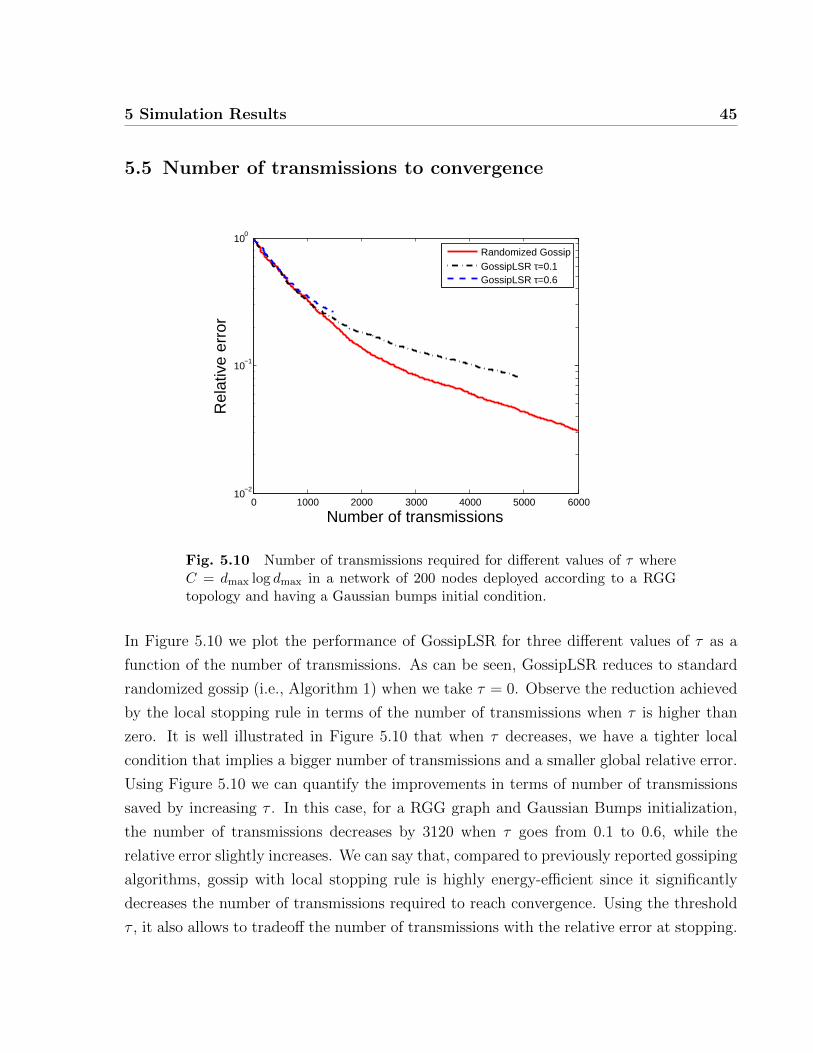
5 Simulation Results 45
5.5 Number of transmissions to convergence
0 1000 2000 3000 4000 5000 600010
−2
10−1
100
Number of transmissions
Rel
ativ
e er
ror
Randomized GossipGossipLSR τ=0.1GossipLSR τ=0.6
Fig. 5.10 Number of transmissions required for different values of τ whereC = dmax log dmax in a network of 200 nodes deployed according to a RGGtopology and having a Gaussian bumps initial condition.
In Figure 5.10 we plot the performance of GossipLSR for three different values of τ as a
function of the number of transmissions. As can be seen, GossipLSR reduces to standard
randomized gossip (i.e., Algorithm 1) when we take τ = 0. Observe the reduction achieved
by the local stopping rule in terms of the number of transmissions when τ is higher than
zero. It is well illustrated in Figure 5.10 that when τ decreases, we have a tighter local
condition that implies a bigger number of transmissions and a smaller global relative error.
Using Figure 5.10 we can quantify the improvements in terms of number of transmissions
saved by increasing τ . In this case, for a RGG graph and Gaussian Bumps initialization,
the number of transmissions decreases by 3120 when τ goes from 0.1 to 0.6, while the
relative error slightly increases. We can say that, compared to previously reported gossiping
algorithms, gossip with local stopping rule is highly energy-efficient since it significantly
decreases the number of transmissions required to reach convergence. Using the threshold
τ , it also allows to tradeoff the number of transmissions with the relative error at stopping.
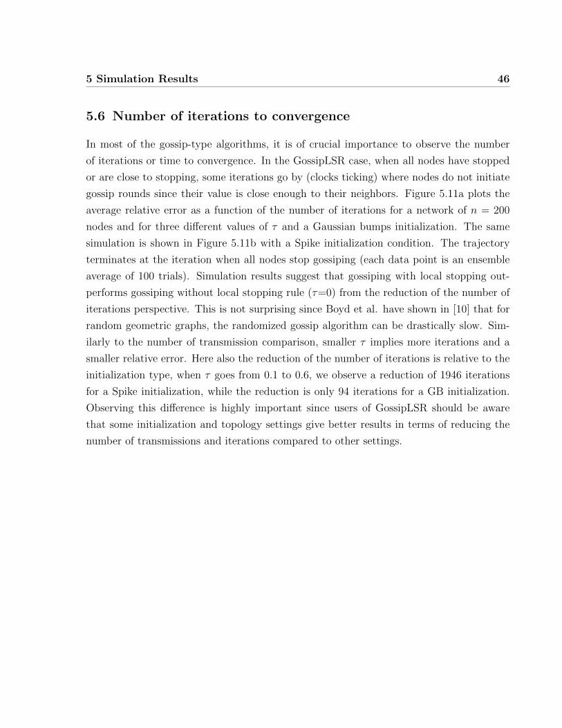
5 Simulation Results 46
5.6 Number of iterations to convergence
In most of the gossip-type algorithms, it is of crucial importance to observe the number
of iterations or time to convergence. In the GossipLSR case, when all nodes have stopped
or are close to stopping, some iterations go by (clocks ticking) where nodes do not initiate
gossip rounds since their value is close enough to their neighbors. Figure 5.11a plots the
average relative error as a function of the number of iterations for a network of n = 200
nodes and for three different values of τ and a Gaussian bumps initialization. The same
simulation is shown in Figure 5.11b with a Spike initialization condition. The trajectory
terminates at the iteration when all nodes stop gossiping (each data point is an ensemble
average of 100 trials). Simulation results suggest that gossiping with local stopping out-
performs gossiping without local stopping rule (τ=0) from the reduction of the number of
iterations perspective. This is not surprising since Boyd et al. have shown in [10] that for
random geometric graphs, the randomized gossip algorithm can be drastically slow. Sim-
ilarly to the number of transmission comparison, smaller τ implies more iterations and a
smaller relative error. Here also the reduction of the number of iterations is relative to the
initialization type, when τ goes from 0.1 to 0.6, we observe a reduction of 1946 iterations
for a Spike initialization, while the reduction is only 94 iterations for a GB initialization.
Observing this difference is highly important since users of GossipLSR should be aware
that some initialization and topology settings give better results in terms of reducing the
number of transmissions and iterations compared to other settings.
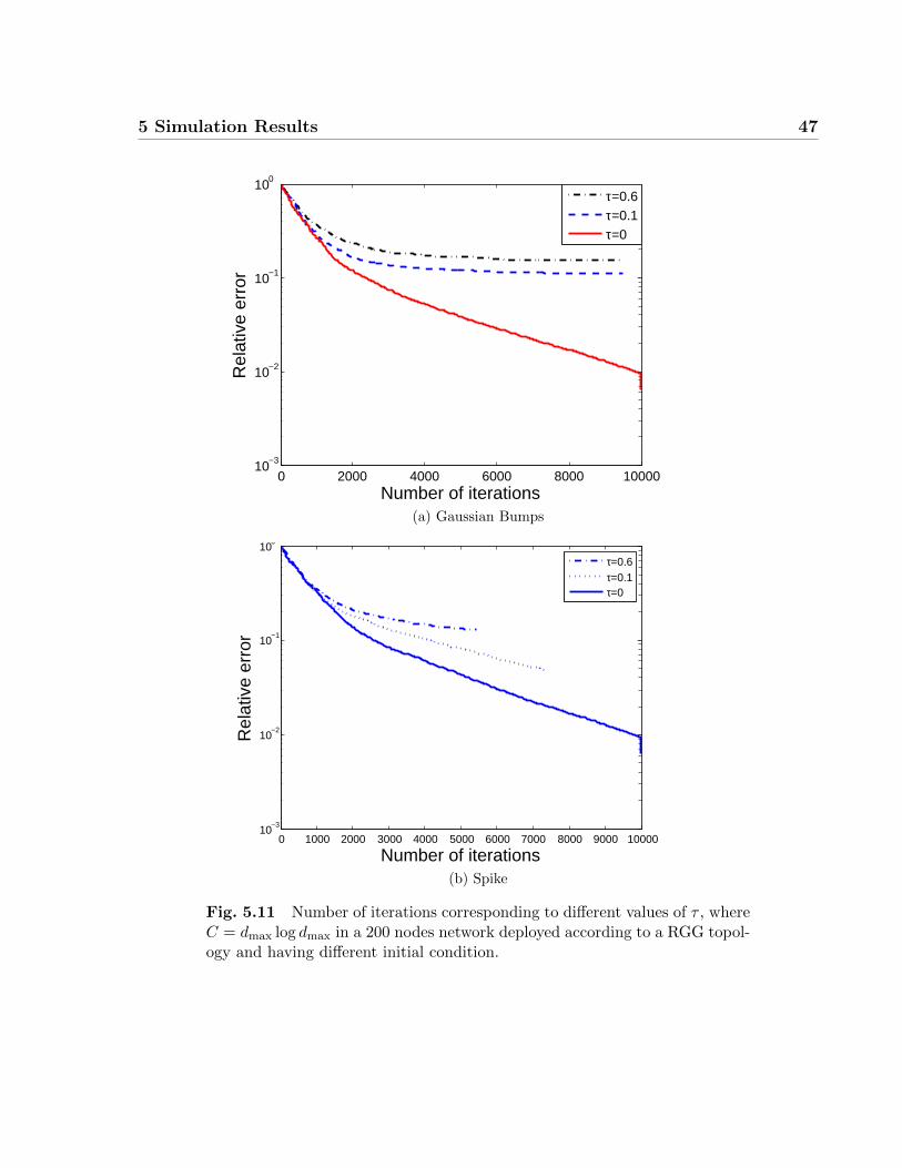
5 Simulation Results 47
0 2000 4000 6000 8000 1000010−3
10−2
10−1
100
Number of iterations
Rel
ativ
e er
ror
τ=0.6τ=0.1τ=0
(a) Gaussian Bumps
0 1000 2000 3000 4000 5000 6000 7000 8000 9000 1000010
−3
10−2
10−1
100
200 nodes, RGG topology, Spike field
Number of iterations
Rel
ativ
e er
ror
τ=0.6τ=0.1τ=0
(b) Spike
Fig. 5.11 Number of iterations corresponding to different values of τ , whereC = dmax log dmax in a 200 nodes network deployed according to a RGG topol-ogy and having different initial condition.

5 Simulation Results 48
0 50 100 150 200 250 300500
1000
1500
2000
2500
3000
3500
||x(0)||
Ave
rage
num
ber
of it
erat
ions
0/100SpikeGBiidSlope
Fig. 5.12 Number of iterations it takes for different initialization with differ-ent orders of magnitude. The number of iterations is averaged over 100 trials.The higher the curve, then, the worst the gain in terms of number of iterationreduction. All five curves fit an increasing function, which verifies that higherstopping time is required for bigger scale of initial values. We use τ=0.5.
The initialization scale plays a key role in influencing the convergence time, intuitively it
is faster to average a network where all the nodes have values 1 and 2 as an initial condition,
compared to a network where all the nodes have values 0 and 1000 as an initial condition.
Figure 5.12 illustrates the number of iterations it takes relative to the magnitude of the
initial condition, ‖x(0)‖, intuitively when the order of the initial value is big it takes longer
in order to reach the stopping time. We use a network of 50 nodes deployed according to a
RGG; The x-axis of the graph represents the initialization vector. Note that, since we are
changing the scale of the initial vector, the initial values of the 0/100 initialization turns
out to be different than just 0 and 100 (when ‖x(0)‖=5, half the nodes at initialization
are equal to 0 and the other half is equal to 10). While the scale range of the initial value
increases, the average number of iterations undergoes a smooth transition and increases
and this is true for all the types of initializations considered in this thesis. Comparing
curves representing different initial conditions we note from Figure 5.12 that the optimal
reduction in the number of iterations is achieved for a Spike initialization, while the i.i.d
5 Simulation Results 49
initialization has the worst performance in reducing the number of iterations. Repeating
the same simulation for different values of τ does not impact the order of the curves.
0 50 100 150 200 250 3000
0.2
0.4
0.6
0.8
1
1.2
1.4
1.6
1.8
2x 10⁴
Network size
Ave
rage
num
ber
of it
erat
ions
Fifty Fifty
GB
IID
Fig. 5.13 Number of iterations with respect to the network sizes for differentnode initializations in a random geometric graph using τ=0.5. The number ofiterations is averaged over 100 trials. The higher the curve, then, the worstthe gain in terms of number of iteration reduction.
We also investigated the average convergence time with respect to the number of nodes
in the network. Our results are shown in Figure 5.13, we use τ=0.5 for a network deployed
according to a random geometric graph. In Figure 5.13, each data point is an ensemble
average of 100 trials. We can see that the convergence time increases approximately linearly
with the number of nodes in the network and this is illustrated for i.i.d , GB and 0/100
initialization.
Figures in this section provided useful information on the rate of convergence of Gossi-
pLSR. We can deduce that the time to stopping is inferior to the one of the gossip algorithm
with continuous exchange of information (without stopping criterion). As a conclusion, we
can say that the convergence rate depends on five key elements: The stopping criterion
τ , the size of the network N , the graph topology (through the second smallest Laplacian
eigenvalue λ2), the initialization scale ‖x(0)‖ and the type of the initialization field. The

5 Simulation Results 50
numerical evidence is not completely analyzed yet and giving clear theoretical results is
still an open question, despite our various efforts.
In fact, although the basic idea behind local stopping rule is simple, analyzing its conver-
gence rate is non-trivial since the update matrix W (t) changes according to nodes becoming
passive and active. Additionally each local stopping rule update depends explicitly on the
dynamics between the local values at a node and the local values at its neighbors. Random-
ized gossip algorithms were generally associated with a homogeneous Markov chain where
transition probabilities and state of convergence were easily calculated after n iterations.
Since the local stopping rule depends on the gossip values at each node, x(k), our algorithm
can not be equally related to a discrete time homogeneous Markov chain. One approach
may be to study a Markov Chain where states depends on all the possible combinations of
the node value x(t) and the node variable C.
A first step to characterize the convergence rate, would be through determining the
time it takes for one node in a network to become passive. Theoretically, if all the nodes
in the network are initialized at the exact average value, each time a node wakes up it
increments its Count variable by one. It needs to wake up dmax
(log(dmax)) times in order
to become passive.
Table 5.1 Average number of iteration required before one single node be-comes passive for different types of topologies and initializations in a networkof 50 nodes in a setting where τ=0.5 and such that the initial value ‖x(0)‖=10.
i.i.d Spike 0/100 Slope
Complete Graph 412 4029 4117 4027
RGG 347 266 302 243
Star 255 252 80 236
Grid 5 5 5 5
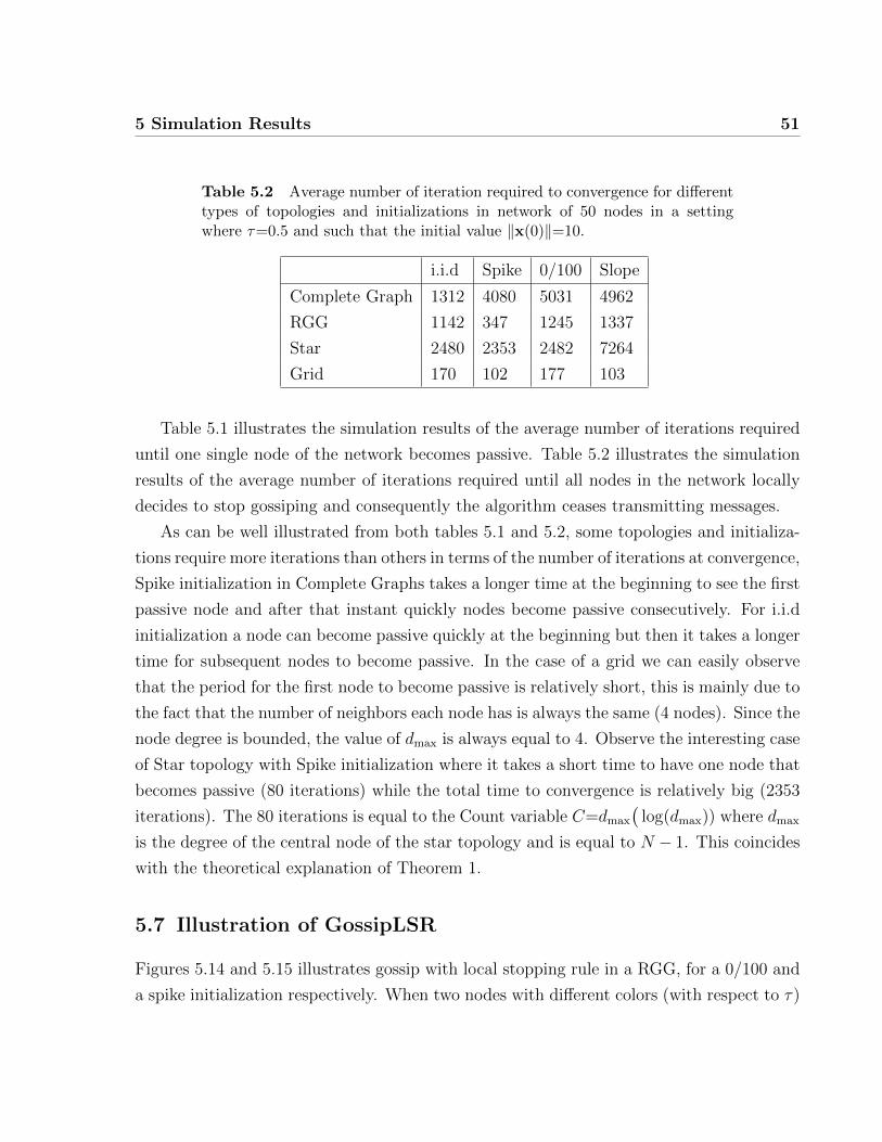
5 Simulation Results 51
Table 5.2 Average number of iteration required to convergence for differenttypes of topologies and initializations in network of 50 nodes in a settingwhere τ=0.5 and such that the initial value ‖x(0)‖=10.
i.i.d Spike 0/100 Slope
Complete Graph 1312 4080 5031 4962
RGG 1142 347 1245 1337
Star 2480 2353 2482 7264
Grid 170 102 177 103
Table 5.1 illustrates the simulation results of the average number of iterations required
until one single node of the network becomes passive. Table 5.2 illustrates the simulation
results of the average number of iterations required until all nodes in the network locally
decides to stop gossiping and consequently the algorithm ceases transmitting messages.
As can be well illustrated from both tables 5.1 and 5.2, some topologies and initializa-
tions require more iterations than others in terms of the number of iterations at convergence,
Spike initialization in Complete Graphs takes a longer time at the beginning to see the first
passive node and after that instant quickly nodes become passive consecutively. For i.i.d
initialization a node can become passive quickly at the beginning but then it takes a longer
time for subsequent nodes to become passive. In the case of a grid we can easily observe
that the period for the first node to become passive is relatively short, this is mainly due to
the fact that the number of neighbors each node has is always the same (4 nodes). Since the
node degree is bounded, the value of dmax is always equal to 4. Observe the interesting case
of Star topology with Spike initialization where it takes a short time to have one node that
becomes passive (80 iterations) while the total time to convergence is relatively big (2353
iterations). The 80 iterations is equal to the Count variable C=dmax
(log(dmax)) where dmax
is the degree of the central node of the star topology and is equal to N − 1. This coincides
with the theoretical explanation of Theorem 1.
5.7 Illustration of GossipLSR
Figures 5.14 and 5.15 illustrates gossip with local stopping rule in a RGG, for a 0/100 and
a spike initialization respectively. When two nodes with different colors (with respect to τ)
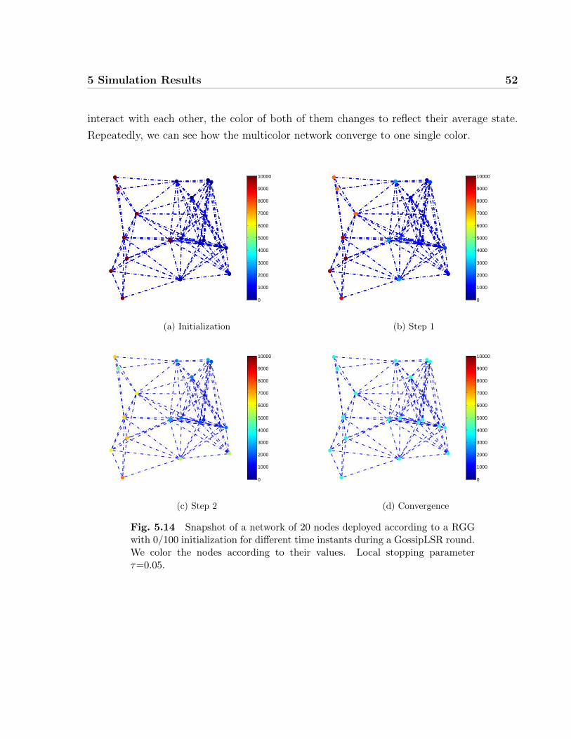
5 Simulation Results 52
interact with each other, the color of both of them changes to reflect their average state.
Repeatedly, we can see how the multicolor network converge to one single color.
0
1000
2000
3000
4000
5000
6000
7000
8000
9000
10000
(a) Initialization
0
1000
2000
3000
4000
5000
6000
7000
8000
9000
10000
(b) Step 1
0
1000
2000
3000
4000
5000
6000
7000
8000
9000
10000
(c) Step 2
0
1000
2000
3000
4000
5000
6000
7000
8000
9000
10000
(d) Convergence
Fig. 5.14 Snapshot of a network of 20 nodes deployed according to a RGGwith 0/100 initialization for different time instants during a GossipLSR round.We color the nodes according to their values. Local stopping parameterτ=0.05.

5 Simulation Results 53
0
0.5
1
1.5
2
x 1094
(a) Initialization
0
0.5
1
1.5
2
x 1094
(b) Step 1
0
0.5
1
1.5
2
x 1094
(c) Step 2
0
0.5
1
1.5
2
x 1094
(d) Convergence
Fig. 5.15 Snapshot of a network of 15 nodes deployed according to a RGGwith a spike initialization for different time instants during a GossipLSR round.We color the nodes according to their values. Indeed, the node at the spikeinitial condition averages its value with its neighborhood and we can see how it“dissolves” in the network in order to reach the final consensus. Local stoppingparameter τ=0.05.
5.8 Comparison to other finite time consensus algorithms
In this section, we study two existing finite time consensus algorithms, namely linear itera-
tive strategies and information coalescence, and compare their performance to GossipLSR
algorithms.
5 Simulation Results 54
5.8.1 Linear Iterative Strategies
Recently, Sundram et. al. in [54] proposed an algorithm using a linear iterative strategy
and permitting the network to achieve consensus in a sufficiently large but finite number
of iterations (assuming each node knows the size of the network and the number of its
neighbors). The key steps in the algorithms are based first on calculating the Observability
Matrix. To do this each node needs to store in memory a number of bytes that depends on
the number of its neighbors. Later, repeatedly using the Observability Matrix consensus
is achieved using a finite number of transmissions relative to the maximum node degree in
the network.
We compare here the performance of GossipLSR algorithm to the linear iterative strat-
egy proposed in [54]. Even if linear iterative strategies have a finite time to stopping, the
savings in terms of the number of transmissions is not taken directly into consideration.
GossipLSR achieves an energy-efficient approach saving transmissions for some initial con-
ditions, and additionally it does not necessitate any memory requirements compared to
linear iterative strategies where finding the Observability Matrix requires each node to
store values. Roughly speaking, each node in the linear iterative protocol needs to store
N(N − d)(d+ 1) where N is the network size, and d represents the number of neighbors of
the node.
We implemented the algorithm of [54] in Matlab and simulated different network topolo-
gies and initializations types in a network of 50 nodes. Table 5.3 illustrates the error at
stopping compared to the error with GossipLSR when τ=5×10⁻⁴ . As can be clearly seen,
the error is smaller for the case of the linear iterative strategy compared to the GossipLSR
error. A few remarks are in order, first note that the error in GossipLSR can be decreased
by decrementing the value of τ . The disadvantage of such an approach is to increment the
number of transmissions significantly. In some applications where a final error of the order
of 10−4 is sufficient compared to an error of 10−10, GossipLSR achieves a big reduction
in terms of the number of transmissions and iterations. For the sake of comparison, The
simulation of linear iterative strategies consumes 2550 iterations. Since it is a synchronous
strategy, the number of transmissions is equal to the number of iterations with a factor of
the network size. Consequently, this method consumes 127500 transmissions for a network
size of 50. GossipLSR consumes more iterations as illustrated in Table 5.5 and much fewer
transmissions as illustrated in Table 5.6. The number of transmissions to convergence is a

5 Simulation Results 55
critical disadvantage of the linear iterative strategy compared to GossipLSR.
Table 5.3 Final error at convergence for a network of 50 nodes for thelinear iterative strategy and GossipLSR (τ=5×10⁻⁴) algorithms with differentnetwork initializations and topologies
Complete Graphs RGG
Linear Iterative Strategy GossipLSR Linear Iterative Strategy GossipLSR
i.i.d 1.29×10⁻⁷ 4.49×10⁻⁴ 7.43×10⁻¹¹ 0.14×10⁻³
0/100 3.717×10⁻⁵ 6.2×10⁻⁴ 5.38×10⁻¹¹ 2.8×10⁻⁴
Slope 1.6312×10⁻⁴ 2.67×10⁻⁴ 3.2752×10⁻¹¹ 7×10⁻⁴
5.8.2 Information Coalescence
Another line of work aiming the reduction of the number of transmissions was introduced
by Savas et al. [44]. The proposed algorithm goes as follows. Instead of having nodes
that keep updating their information, a node can transmit only if it is has a token. The
token passes from the initiating node to the receiving node. In other words, it moves with
information such that, an idle node stays idle until it receives a message from its neighbor.
On the other hand, an active node becomes idle as soon as it has delivered the token. The
stopping rule occurs when all the nodes are in the idle state. The algorithm has an exact
stopping time in connected graphs, and it consumes a minimal number of transmissions to
reach convergence for approximately all types of initializations and topologies.
Similarly to GossipLSR this algorithm achieves a gain in the energy requirement by
reducing the number of transmissions. The disadvantage of such a token-based algorithm
compared to GossipLSR is that it consumes more transmissions to terminate and thus the
number of transmissions at stopping is not optimal. GossipLSR has a stopping criterion
based on the knowledge of each node to its neighboring environment, while token-based
algorithm are less related to the node information and consequently this causes their rate
of convergence to be slow.
We implemented the algorithm using information coalescence by Savas et al. [44] and
compared the token-based method with the GossipLSR. Our results are shown in the fol-
lowing tables. Table 5.4 illustrates the error at stopping for the Coalescence algorithm and
the GossipLSR with τ=5×10⁻⁴. One advantage of the GossipLSR is that the final error
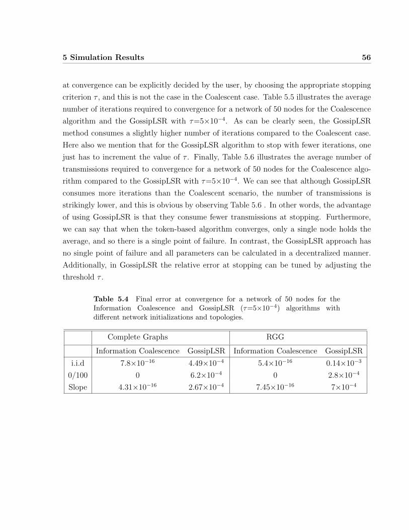
5 Simulation Results 56
at convergence can be explicitly decided by the user, by choosing the appropriate stopping
criterion τ , and this is not the case in the Coalescent case. Table 5.5 illustrates the average
number of iterations required to convergence for a network of 50 nodes for the Coalescence
algorithm and the GossipLSR with τ=5×10⁻⁴. As can be clearly seen, the GossipLSR
method consumes a slightly higher number of iterations compared to the Coalescent case.
Here also we mention that for the GossipLSR algorithm to stop with fewer iterations, one
just has to increment the value of τ . Finally, Table 5.6 illustrates the average number of
transmissions required to convergence for a network of 50 nodes for the Coalescence algo-
rithm compared to the GossipLSR with τ=5×10⁻⁴. We can see that although GossipLSR
consumes more iterations than the Coalescent scenario, the number of transmissions is
strikingly lower, and this is obvious by observing Table 5.6 . In other words, the advantage
of using GossipLSR is that they consume fewer transmissions at stopping. Furthermore,
we can say that when the token-based algorithm converges, only a single node holds the
average, and so there is a single point of failure. In contrast, the GossipLSR approach has
no single point of failure and all parameters can be calculated in a decentralized manner.
Additionally, in GossipLSR the relative error at stopping can be tuned by adjusting the
threshold τ .
Table 5.4 Final error at convergence for a network of 50 nodes for theInformation Coalescence and GossipLSR (τ=5×10⁻⁴) algorithms withdifferent network initializations and topologies.
Complete Graphs RGG
Information Coalescence GossipLSR Information Coalescence GossipLSR
i.i.d 7.8×10⁻¹⁶ 4.49×10⁻⁴ 5.4×10⁻¹⁶ 0.14×10⁻³
0/100 0 6.2×10⁻⁴ 0 2.8×10⁻⁴
Slope 4.31×10⁻¹⁶ 2.67×10⁻⁴ 7.45×10⁻¹⁶ 7×10⁻⁴

5 Simulation Results 57
Table 5.5 Average number of iteration required to convergence for a net-work of 50 nodes in the Information Coalescence and GossipLSR (τ=5×10⁻⁴)algorithms with different initializations and topologies.
Complete Graphs RGG
Information Coalescence GossipLSR Information Coalescence GossipLSR
i.i.d 2517 5741 2698 3280
0/100 2587 5703 3011 5741
Slope 3211 5625 2781 3685
Table 5.6 Average number of transmissions required to convergence fora network of 50 nodes in the Information Coalescence and GossipLSR(τ=5×10⁻⁴) algorithms with different network initializations and topologies.
Complete Graphs RGG
Information Coalescence GossipLSR Information Coalescence GossipLSR
i.i.d 411 242 415 250
0/100 410 185 428 212
Slope 366 224 439 232
5.9 Summary of the Chapter
This chapter presented the simulations that illustrate important practical aspects of Gossi-
pLSR under different scenarios. The main results have shown the reduction achieved by the
proposed algorithm in terms of the number of transmissions and iterations. An important
conclusion of our simulations is that GossipLSR implies a small hit in error compared to
randomized case. We later compared the performance of GossipLSR to other finite time
distributed algorithms and presented the numerical results as well as the advantages and
disadvantages of each method. Our main conclusion, is that among the few existing finite
time distributed algorithms, GossipLSR is the first one that allows the user to tradeoff the
number of transmissions until termination with the final accuracy using the threshold τ .
In previous chapters we demonstrated how GossipLSR is supported by both simulation
evidences and theoretical proofs. In the sequel, we discuss the generalization of GossipLSR

5 Simulation Results 58
to other gossip algorithms such as greedy gossip with eavesdropping, geographic gossip and
path averaging.

59
Chapter 6
Generalization to other gossip
algorithms
It was mentioned in the previous chapters that decentralized gossip with local stopping
rule can alleviate important gossiping issues such as reducing the number of iterations
and transmissions as well as implicitly specifying a stopping criterion. We would like to
investigate if the local stopping criterion can be generalized to other gossip algorithms that
perform faster than randomized gossip such as Geographic Gossip [12], Greedy Gossip with
Eavesdropping [11] and Path Averaging [13].
6.1 Pairwise Gossip algorithms
In this section we concentrate on generalizing the GossipLSR algorithm described previ-
ously to other pairwise gossip algorithms such as geographic gossip (GEO) [12] or greedy
gossip with eavesdropping (GGE) [11]. The important conclusion of our simulations is that
GossipLSR significantly improves the performance in terms of the reduction of the number
of iterations and transmissions for this type of gossip algorithms.
6.1.1 Geographic Gossip
The key steps in the GEO gossip algorithm without local stopping rule goes as follows:
Each node has a tuple constituted of its own value, its location and its target. When a
node “wakes” up to gossip it selects any target node in the network. The generating node

6 Generalization to other gossip algorithms 60
sends a packet containing its information to his neighbor situated nearby the target node.
The node that receives the message sends it again to its neighbor situated nearby the target
node. Once the message reaches the target, the average value of the target node and the
originating node is calculated and a version is sent back to the originating node using the
same process. If for any reason the packet is rejected or does not reach the target, the
originating node chooses a new target and repeats the same procedure. The difference
between the gossip algorithm described above and the randomized gossip is that we allow
distant nodes to gossip even without being directly connected [12]. On the other hand, the
disadvantage of GEO gossip is that it requires a computational complexity for routing the
information between distant nodes.
With this in mind, we add the local stopping rule on top of geographic gossip algorithm.
Each time a node finishes gossiping and gets back the packet sent from the target node,
it tests whether its local estimate has changed by more than τ in absolute value. If the
change was less than or equal to τ , then the local count at each node ci(k) is incremented,
and if the change was greater than τ , then ci(k) is reset to 0. The node stops, after its
absolute change in the estimate has been less than τ for C consecutive gossip rounds. The
only difference now is that the nodes can gossip with all the nodes in the network instead of
just gossiping with its neighbors. Pseudo-code for simulating geographic gossip with local
stopping rule is shown in Algorithm 3.
Figure 6.1 illustrates the performance of the local stopping rule with geographic gossip
implementation. Note the improvement that the local stopping rule brings to the geographic
gossip by comparing the curves when τ is equal to 0 to the curves where τ is above 0. The
number of iterations decreases by almost 900 iterations when τ goes from 0.1 to 0.6, while
the relative error slightly increases. Obviously since GEO performs faster than RG [12],
and since GEO with GossipLSR performs better than GEO without GossipLSR, we can say
that the combination of both GossipLSR and GEO can perform drastically better than the
randomized gossip. We highlight that GEO algorithms need more computational resources
to achieve routing compared to randomized gossip and that the relative error at stopping
can be tuned by adjusting the threshold τ in GossipLSR.
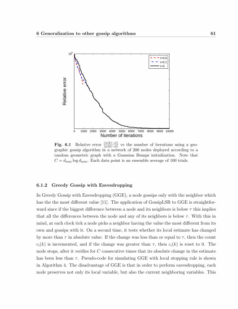
6 Generalization to other gossip algorithms 61
0 1000 2000 3000 4000 5000 6000 7000 8000 9000 10000
100
Number of iterations
Rel
ativ
e er
ror
τ=0.6τ=0.1τ=0
Fig. 6.1 Relative error ||x(k)−x||||x(0)−x|| vs the number of iterations using a geo-
graphic gossip algorithm in a network of 200 nodes deployed according to arandom geometric graph with a Gaussian Bumps initialization. Note thatC = dmax log dmax. Each data point is an ensemble average of 100 trials.
6.1.2 Greedy Gossip with Eavesdropping
In Greedy Gossip with Eavesdropping (GGE), a node gossips only with the neighbor which
has the the most different value [11]. The application of GossipLSR to GGE is straightfor-
ward since if the biggest difference between a node and its neighbors is below τ this implies
that all the differences between the node and any of its neighbors is below τ . With this in
mind, at each clock tick a node picks a neighbor having the value the most different from its
own and gossips with it. On a second time, it tests whether its local estimate has changed
by more than τ in absolute value. If the change was less than or equal to τ , then the count
ci(k) is incremented, and if the change was greater than τ , then ci(k) is reset to 0. The
node stops, after it verifies for C consecutive times that its absolute change in the estimate
has been less than τ . Pseudo-code for simulating GGE with local stopping rule is shown
in Algorithm 4. The disadvantage of GGE is that in order to perform eavesdropping, each
node preserves not only its local variable, but also the current neighboring variables. This

6 Generalization to other gossip algorithms 62
results in an increasing computational complexity.
Figure 6.2 illustrates the relative error with respect to the number of transmissions for
three different values of τ and gives us an idea of the performance of the local stopping
rule with the greedy gossip with eavesdropping implementation. Here also comparing the
curves for τ , equal to and above zero, note the improvement the GossipLSR brings to
the greedy gossip case in terms of the reduction of the number of transmissions. The
number of transmission decreases by almost 1000 transmission when τ goes from 0.1 to
0.6. The disadvantage of applying GossipLSR to GGE is the high error at stopping when
increasing τ . Here also we highlight that the relative error at stopping can be tuned by
adjusting the threshold τ . In other words, choosing a value of τ between 0 and 0.1 can
give us a reduction of the number of transmissions as well as an acceptable relative error
at stopping.
0 2000 4000 6000 8000 1000010−4
10−3
10−2
10−1
100
Number of transmission
Rel
ativ
e er
ror
τ=0.6τ=0.1τ=0
Fig. 6.2 Relative error ||x(k)−x||||x(0)−x|| vs the number of transmissions using a
greedy gossip with eavesdropping algorithm in a network of 200 nodes deployedaccording to a random geometric graph with a Gaussian Bumps initialization.Each data point is an ensemble average of 100 trials.
Figure 6.3 illustrates the performance comparison of the local stopping rule using three
different gossip algorithms: greedy gossip with eavesdropping, geographic gossip and ran-

6 Generalization to other gossip algorithms 63
domized gossip. The network is composed of 200 nodes deployed according to a random
geometric graph with a Gaussian Bumps initialization and the GossipLSR is used with
a local stopping criterion τ = 0.01. Note that, as anticipated previously, we notice that
the GGE algorithm is the best in terms of the number of transmissions saved. On the
other hand the randomized gossip scenario takes more transmissions but is more efficient
in terms of relative error reduction. Between both curves lies the GEO gossip performance
with a fewer number of transmissions than randomized gossip and a smaller relative error
compared to GGE. We mention here that the disadvantage of the GGE is that it requires
an additional memory overhead to store neighbors’ values while the disadvantage of the
GEO gossip is that it requires nodes to know their locations and route the information to
distant targets.
0 2000 4000 6000 8000 10000 12000 1400010−3
10−2
10−1
100
Number of transmissions
Rel
ativ
e er
ror
GGEGeographic GossipRandomized Gossip
Fig. 6.3 Relative error ||x(k)−x||||x(0)−x|| vs the number of transmissions compari-
son using GossipLSR with three different gossip algorithms: greedy gossipwith eavesdropping, geographic gossip and randomized gossip. The network iscomposed of 200 nodes deployed according to a random geometric graph witha Gaussian Bumps initialization and the GossipLSR is used with τ = 0.01.
The next section explains the path averaging gossip algorithms and their performance
under gossip with local stopping rule.

6 Generalization to other gossip algorithms 64
6.2 Path Averaging using GossipLSR
Until now we only explained gossip algorithms with pairwise node exchange, and there
was no averaging along paths. One modification of geographic gossip averaging algorithms
is to average on the way all the nodes from xi to xj. These algorithms are called Path
averaging [13]. The average path connecting two nodes is the shortest way that a message
has to traverse from one node to the other while routing. The key steps in the path-
averaging algorithm are naturally inspired from the geographic gossip, such that at a first
time, one node chosen randomly wakes up and picks another target node randomly. Second,
it creates a message containing its estimate, position, number of visited nodes so far (zero
at the beginning) and the targeted node. Consequently, it send this message to the nearest
node to the target, the first destination node passes it also to the closest node to the target
and so on along the path. After each time, each node adds their estimate to the sum and
increases the counter of the number of visited nodes by one. When the packet reaches
its final destination, the target node calculates the average of all the nodes on the path
by dividing the accumulated sum by the number of visited nodes, and reroutes the result
backwards on the same path. Consecutively each node in the path updates its value. Path
averaging is an attractive scheme since it combines the idea of decentralized averaging and
optimal routing. With this in mind, we add local stopping rule characteristics on top of the
existing path averaging algorithm. In other words, on each time a node updates its value
after a gossip it tests whether its local estimate has changed by more than τ in absolute
value. If the change was less than or equal to τ , then the count ci(k) is incremented, and
if the change was greater than τ , then ci(k) is reset to 0. The node stops, after it verifies
for C consecutive times that its absolute change in the estimate has been less than τ .
Figure 6.4 illustrates the relative error with respect to the number of transmissions for
three different values of τ in the case of gossip with path averaging. We can see that, like
other gossip algorithms, path averaging with local stopping rule decreases the number of
transmissions compared to path averaging without local stopping rule with the tradeoff of
a hit in performance (relative error at stopping). There is a strikingly big difference in
terms of error when τ increases. Just like the pairwise case, the relative error at stopping
can be tuned by adjusting the threshold τ .
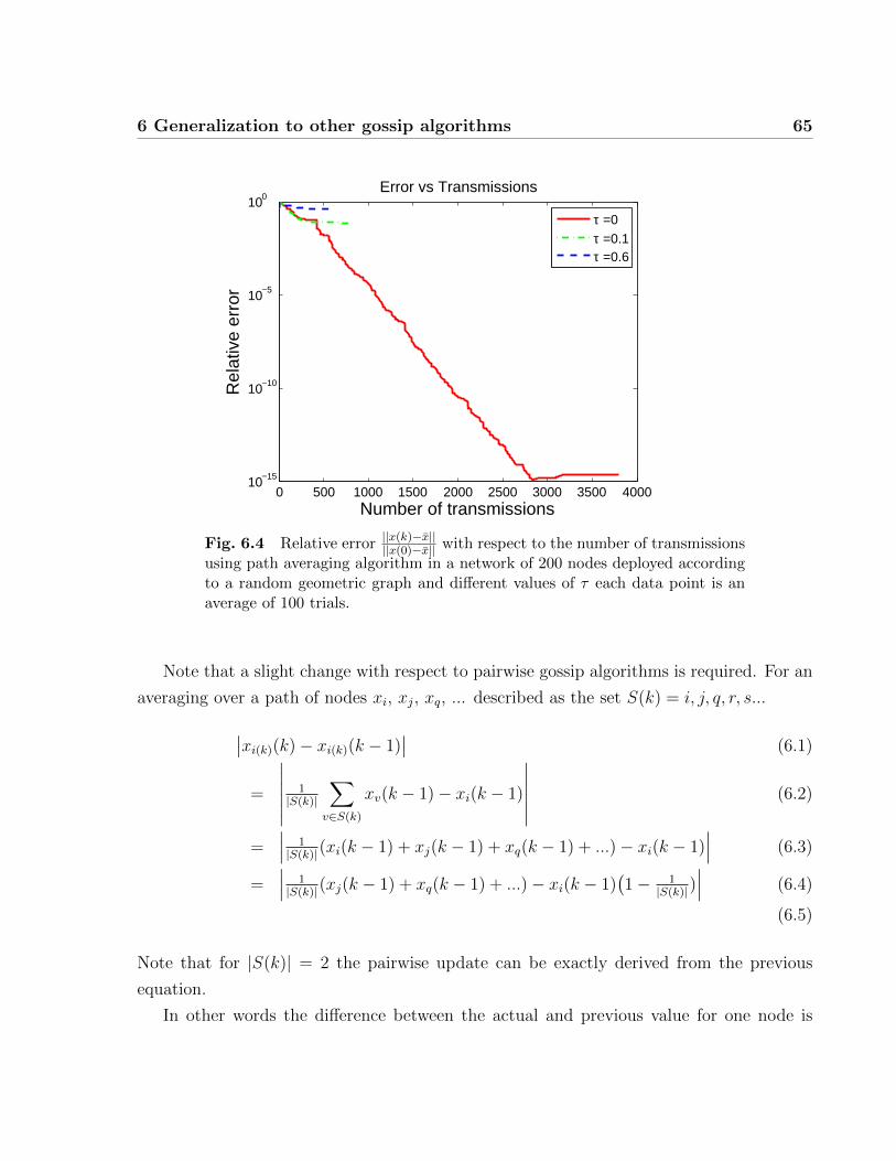
6 Generalization to other gossip algorithms 65
0 500 1000 1500 2000 2500 3000 3500 400010−15
10−10
10−5
100
Number of transmissions
Rel
ativ
e er
ror
Error vs Transmissions
τ =0τ =0.1τ =0.6
Fig. 6.4 Relative error ||x(k)−x||||x(0)−x|| with respect to the number of transmissions
using path averaging algorithm in a network of 200 nodes deployed accordingto a random geometric graph and different values of τ each data point is anaverage of 100 trials.
Note that a slight change with respect to pairwise gossip algorithms is required. For an
averaging over a path of nodes xi, xj, xq, ... described as the set S(k) = i, j, q, r, s...
∣∣xi(k)(k)− xi(k)(k − 1)∣∣ (6.1)
=
∣∣∣∣∣∣ 1|S(k)|
∑v∈S(k)
xv(k − 1)− xi(k − 1)
∣∣∣∣∣∣ (6.2)
=∣∣∣ 1|S(k)|(xi(k − 1) + xj(k − 1) + xq(k − 1) + ...)− xi(k − 1)
∣∣∣ (6.3)
=∣∣∣ 1|S(k)|(xj(k − 1) + xq(k − 1) + ...)− xi(k − 1)
(1− 1
|S(k)|)∣∣∣ (6.4)
(6.5)
Note that for |S(k)| = 2 the pairwise update can be exactly derived from the previous
equation.
In other words the difference between the actual and previous value for one node is

6 Generalization to other gossip algorithms 66
equal to the difference between the average of all the nodes over the path at iteration k− 1
and the value of the node at iteration k − 1.
We can say that:
∣∣xi(k)(k)− xi(k)(k − 1)∣∣ (6.6)
=
∣∣∣∣∣∣ 1|S(k)|
∑v∈S(k)
xv(k − 1)− xi(k − 1)
∣∣∣∣∣∣ (6.7)
=
∣∣∣∣∣∣ 1|S(k)|
∑v∈S(k)
xv(k − 1)− |S(k)||S(k)|
xi(k − 1)
∣∣∣∣∣∣ (6.8)
=
∣∣∣∣∣∣ 1|S(k)|
∑v∈S(k)
(xv(k − 1)− xi(k − 1)
)∣∣∣∣∣∣ (6.9)
= 1|S(k)|
∑v∈S(k)
|xv(k − 1)− xi(k − 1)|)
(6.10)
and finally the updated stopping rule for the path averaging case is equal to∣∣∣∣∣∣ 1|S(k)|
∑v∈S(k)
(xv(k − 1)− xi(k − 1)
)∣∣∣∣∣∣ ≤ τ (6.11)
In path averaging nodes are not restricted to gossip with their neighbors and can com-
municate with any node in the network. In such a setting we define a new lifted graph G’
from the initial underlying network, where an edge exists between two nodes if and only
if they communicate with each other during gossip. The edges in graph G’ are conceptual
and do not illustrate real physical links between nodes. The error at stopping depends on
the second smallest eigenvalue of the Laplacian of the new lifted graph G’. Using the new
“abstract” topology, we can generalize the pairwise results to prove the convergence of path
averaging and bound the error when stopping.

6 Generalization to other gossip algorithms 67
Table 6.1 Number of transmissions and Relative Error at stopping for Gos-sipLSR with different values of τ and different types of gossip algorithms,greedy gossip with eavesdropping, geographic gossip, path averaging and ran-domized gossip. We use a network of N=200 nodes deployed according toa RGG topology and Gaussian Bumps initialization. Each data point is anensemble average of 100 trials.
τ = 0 τ = 0.1 τ = 0.6
Transmissions Error Transmissions Error Transmissions Error
GEO 10000 0.6540 1621 0.6148 941 0.6529
GGE 10000 10−5 1519 0.0182 632 0.0932
PA 10000 10−15 752 0.068 354 0.378
RG 10000 0.0095 4939 0.0299 1484 0.1114
Tables 6.1 gives a numerical illustration of the performance of the local stopping rule
in terms of the number of transmissions and relative error at stopping for different gossip
algorithms GEO, GGE, PA and RG and for different values of τ . As can be seen numer-
ically, for pairwise gossip GGE achieves the biggest reduction in terms of the number of
transmissions and the smallest relative error at stopping for the three tested values of τ .
Also note that randomized gossip with local stopping rule consumes more transmissions
compared to greedy gossip or geographic gossip with local stopping rule. And this is not
surprising since it was demonstrated previously that both GGE and GEO performs better
than randomized gossip.
6.3 Summary of the chapter
This chapter discussed an extension of the local stopping rule to modified gossip algorithms
such as GGE, GEO and path averaging. Following the description of how these algorithms
can be adapted to include a local stopping rule, we simulated each setting, and demon-
strated that all the algorithms perform better with local stopping rule in terms of reducing
the number of transmissions and iterations at stopping. An interesting future work includes
further analysis of GEO under local stopping rule. Since in geographic gossip nodes can
gossip with any other node in the network even if it is not a neighbor, taking the maximum
degree dmax = n− 1 might improve the performance in terms of relative error at stopping

6 Generalization to other gossip algorithms 68
(at the expense of more iterations and transmissions) . The early chapters of this thesis
focused on describing the GossipLSR algorithm and discussing its characteristics through
simulations. The next chapter covers an interesting application of GossipLSR to networks
with time-varying averages. We demonstrate how the local stopping criterion in gossiping
can be a very useful adjunct to the arsenal of tracking techniques.

6 Generalization to other gossip algorithms 69
Algorithm 3 Geographic Gossip with Local Stopping Rule.
1: Initialize: {xi(0)}i∈V , ci(0) = 0 for all i ∈ V , and k = 12: repeat3: Draw i(k) uniformly from V4: if ci(k)(k − 1) < C then5: Draw j(k) randomly in the network6: Define li(k − 1) as node i’s location7: Node i forms the tuple mi = (xi(k − 1), li(k − 1), j)8: repeat9: Send mi to node’s i one hop neighbor closest to j
10: until mi reaches j11: xj(k)(k)← 1
2
(xi(k)(k − 1) + xj(k)(k − 1)
)12: Define lj(k − 1) as node j’s location13: Node j forms the tuple mj = (xj(k − 1), lj(k − 1), i)14: repeat15: Send mj to node’s j one hop neighbor closest to i16: until mj reaches i17: xi(k)(k)← 1
2
(xi(k)(k − 1) + xj(k)(k − 1)
)18: if |xi(k)(k)− xi(k)(k − 1)| ≤ τ then19: ci(k)(k) = ci(k)(k − 1) + 1;20: cj(k)(k) = cj(k)(k − 1) + 1;21: else22: ci(k)(k) = 0;23: cj(k)(k) = 0;24: end if25: for all v ∈ V \ {i(k), j(k)} do26: xv(k) = xv(k − 1)27: cv(k) = cv(k − 1)28: end for29: k ← k + 130: else31: for all v ∈ V do32: xv(k) = xv(k − 1)33: cv(k) = cv(k − 1)34: end for35: end if36: until cv(k) ≥ C for all v ∈ V

6 Generalization to other gossip algorithms 70
Algorithm 4 Greedy Gossip with eavesdropping with Local Stopping Rule.
1: Initialize: {xi(0)}i∈V , ci(0) = 0 for all i ∈ V , and k = 12: repeat3: Draw i(k) uniformly from V4: if ci(k)(k − 1) < C then5: Draw j(k) that currently has the value xj(k − 1) most different from xi(k − 1)6: xi(k)(k)← 1
2
(xi(k)(k − 1) + xj(k)(k − 1)
)7: xj(k)(k)← 1
2
(xi(k)(k − 1) + xj(k)(k − 1)
)8: if |xi(k)(k)− xi(k)(k − 1)| ≤ τ then9: ci(k)(k) = ci(k)(k − 1) + 1;
10: cj(k)(k) = cj(k)(k − 1) + 1;11: else12: ci(k)(k) = 0;13: cj(k)(k) = 0;14: end if15: for all v ∈ V \ {i(k), j(k)} do16: xv(k) = xv(k − 1)17: cv(k) = cv(k − 1)18: end for19: k ← k + 120: else21: for all v ∈ V do22: xv(k) = xv(k − 1)23: cv(k) = cv(k − 1)24: end for25: end if26: until cv(k) ≥ C for all v ∈ V

71
Chapter 7
Event-Driven Tracking of
Time-Varying Averages
7.1 Introduction to Time-Varying Averages
Gossip algorithms find applications in various fields; they can be applied for military and
disaster recovery operations as well as in civilian mobile communications. One of their
major challenges is a reliable, scalable and efficient convergence time. Practically, when
transmitting over a physical channel, one must take into consideration issues of time-
varying information at nodes and how gossip accommodates these variations to track the
time-varying averages. Rather than taking a measurement, gossiping until convergence, and
then re-initializing gossip with new measurements, it may be desirable to incorporate new
measurements while executing the gossip computation. For example, consider the real-time
gossip in a network of dynamic indoor environment parameters such as air flow, smoke,
inhabitant distribution as well as temperature state. Waiting for the gossip algorithm to
converge before taking into consideration the new emergent changes in the value of one of
the nodes (e.g. when detecting temperature or smoke sensor) can be hazardous.
Previous work has considered tracking variations (Kalman filter and LMS [34, 35, 55])
of randomized gossip. Most of the proposed variations operate continuously over time
and are synchronous [55–60]. Additionally, we can mention that in recent years, many
researchers have focused on distributed computing in dynamic network topologies where
nodes can join or leave the network. To avoid confusion, it is important to highlight

7 Event-Driven Tracking of Time-Varying Averages 72
that this thesis considers a network with static topology and time-varying average due to
external information and does not take into consideration the changing topology.
In the following sections, we first survey the extensive body of literature on dynamic
tracking and filtering, later we describe how the asynchronous GossipLSR can be applied in
scenarios with time-varying measurements, incorporating new information while performing
gossip, we will use the term nodes as a common word for sensors of the varying data. We will
extend the local stopping rule approach and will design adaptive, event-triggered algorithm
to handle the tracking of dynamic, time-varying signals. As mentioned above, if the sensed
phenomenon, such as airflow, gaseous flow or occupant distribution, does not change much,
then our method will adaptively reduce the number of messages transmitted to save battery
power at each node. Another assumption we will be making is that the communication
links are reliable. In such a setting, the local stopping rule leads to a natural event-driven
algorithm. We first describe the tracking algorithm for time-varying averages without
using the local stopping rule and later we discuss how the local stopping rule proposes an
elegant way to accommodate the dynamically changing information in real-time algorithms
and simultaneously reduces the number of transmissions and consequently battery power
at sensors. We finally compare our approach to tracking using synchronous distributed
Kalman filters.
Figures 7.1 and 7.2 illustrate the difference between gossip in the standard case and
gossiping in the network varying average case. We can see clearly that convergence means
nodes to reach gossip over the varying average and being able to keep track of the new up
to date average.
7.2 Background
There have been numerous articles, papers and books written on the topic of tracking since
Kalman’s filters were first introduced in 1961 [61–64]. One of the first uses of Kalman fil-
ters was in the development of space and military technology. But since then, the number
of their applications has increased exponentially. Particularly, their utility in the track-
ing problems in the gossip algorithms have been considered in many modern papers on
consensus and averaging [1,32]. Obviously, the difference between static and dynamic dis-
tributed estimation is related to whether the estimated quantities are fixed or time-varying.
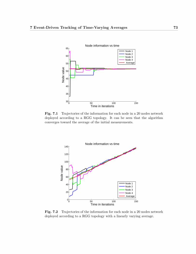
7 Event-Driven Tracking of Time-Varying Averages 73
0 50 100 15030
35
40
45
50
55
60
65
Time in iterations
Nod
e va
lue
Node information vs time
Node 1Node 2Node 3Node 4 Average
Fig. 7.1 Trajectories of the information for each node in a 20 nodes networkdeployed according to a RGG topology. It can be seen that the algorithmconverges toward the average of the initial measurements.
0 50 100 1500
20
40
60
80
100
120
140
Time in iterations
Nod
e va
lue
Node information vs time
Node 1Node 2Node 3Node 4 Average
Fig. 7.2 Trajectories of the information for each node in a 20 nodes networkdeployed according to a RGG topology with a linearly varying average.

7 Event-Driven Tracking of Time-Varying Averages 74
Basically the problem of dynamic tracking can be summarized as follows: consider a
graph where information at each node varies slowly and sporadically over time, if all the
node’s information were instantaneously available to a single central authority in a network,
using centralized Kalman filter one can estimate the average of all the measurements. In the
decentralized version, it is not realistic to assume that all measurements are immediately
available at a single specific location, since the information of some distant nodes, at best,
arrives to all the other nodes with some delay, which depends on the network’s properties of
size and topology. Distributed Kalman filters when used jointly with consensus filters, offer
a good tool for tracking node varying averages [56]. Later in this chapter we discuss more
in details such algorithms and compare their performance to tracking using GossipLSR.
In the next section we estimate the error at stopping for a scenario of changing averages
in randomized gossip without local stopping rule and later we describe the application of
GossipLSR in such a scenario.
7.3 Gossip Error with Time-Varying Signals
7.3.1 Serial gossip
We consider a network of geographically distributed sensor nodes. Consider graph G =
(V,E) with n = |V | nodes and edges (i, j) ∈ E ⊆ V 2 if and only if nodes i and j commu-
nicate directly. We assume that G is connected. Consider xi(0) as the initial value at node
i; x(t) as the up to date average value of the nodes at time t.
The goal is to calculate locally at each node the average value of the measurements of
all nodes in the network taking into consideration all the fresh observations that arrived to
the nodes while gossiping. Here we consider a variation of randomized gossip where nodes
start gossiping on their initial measurements. When a new measurement is taken, the node
continuously incorporates the change in the measured value with its current state xi(k).
This will ensure that a snapshot over the entire system will always give the right value of
the average in real-time, although the estimates at nodes may be momentarily not true.
One of the main challenges in this setting is that when node i at time t wakes up, it uses
the value of node j, meanwhile, if the network received new information through nodes far
away from i and j, the value that i received could be an outdated version of the average.
However we can confirm that nodes will eventually converge to the true average, once no

7 Event-Driven Tracking of Time-Varying Averages 75
more new information arrives for a long time. We also show that the size of the network is
a key factor in determining the time to accommodate the new arriving information. This
section analyzes the expected error at stopping for this approach.
We denote the vector of node states as x(t) and the vector of measurements as ∆u(t),
with x(0) = u(0). When there is no tracking ∆u(t)=0 for t > 0. We begin by defining the
node update equation when receiving new information:
x(t+ 1) = x(t) + ∆u(t). (7.1)
In other words, each node can receive at any instant of time (clock tick) a new measurement.
This new measurement is added to its current value. By current value we mean the updated
value that the node gossiped so far.
Assume L instantaneous changes occurred up to a time instant t. Note that each vector
of measurements ∆u(t) can imply more than a single node change. We define the vector
of the accumulated node measurements as U(t) ∈ Rn, so that U(t) is equal to the sum of
all the L instantaneous changes vectors that occurred up to a time instant t.
U(t) =L∑l=1
∆ul(t). (7.2)
From [10] we know that in conventional randomized gossip algorithms, where we do not
take into consideration the changes, each node has the following update equation:
x(t+ 1) = W(t)x(t). (7.3)
where W(t) are randomly selected averaging matrices, drawn i.i.d. at time t. In order to
reach convergence, we assume that the averaging matrix W(t) satisfies the characteristics
derived in [1] and listed below.
Theorem 2 (Xiao and Boyd [1], Theorem 1).
1TW = 1T , (7.4)
W1 = 1, (7.5)
ρ(W − 11T
n) ≤ 1, (7.6)
7 Event-Driven Tracking of Time-Varying Averages 76
where ρ denotes the spectral radius of a matrix1.
Obviously by repeating Equation (7.3) we can define a relationship between the instan-
taneous node state x(t+ 1), the averaging matrix W(t) and the initial condition x(0) such
that:
x(t+ 1) =t∏
j=0
W(j)x(0). (7.7)
We would like to calculate the expected error at time t, E[||x(t) − x(t)|| | x(0)]. In
the time-varying case, we add the most recent value of the nodes to the value of the
measurement and gossip the result. This is similar to continuously considering new initial
condition related to the value gossiped so far at each step of the gossip. We assume that
the averaging matrix W(t) is the same at each iteration. By adapting Equation (7.7)
considering new initial condition at each arrival of new information and since W(t) are
i.i.d we can see that
E[x(t) | x(0)] = E[ t∏j=0
W(j)(x(0) + U(t)
)| x(0)
]=
t∏j=0
E[W(j)]E[x(0) + U(t) | x(0)]
It is reasonable to assume that the first measurement ∆ul(0) occurred at a time l < t.
Recall that the vector of measurements U(t) and the vector of initial node values x(0) are
independent. Using the linearity of expectation, the previous equation can be written as
E[x(t) | x(0)] =t∏
j=0
E[W(j)]E[x(0)] +t∏j=l
E[W(j)]E[U(t)]
= Wtx(0) + Wt−lU,
where W represents the expectation of the averaging matrix E[W(t)] and U represents
the expectation of the node measurement. Note that t − l is equal to the elapsed time
between the first instant a change occurred and the instant t when we calculate the error.
1For a detailed study about matrix analysis interested readers are referred to [65]
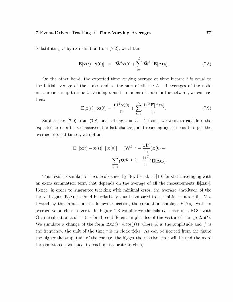
7 Event-Driven Tracking of Time-Varying Averages 77
Substituting U by its definition from (7.2), we obtain
E[x(t) | x(0)] = Wtx(0) +L∑l=1
Wt−lE[∆ul]. (7.8)
On the other hand, the expected time-varying average at time instant t is equal to
the initial average of the nodes and to the sum of all the L − 1 averages of the node
measurements up to time t. Defining n as the number of nodes in the network, we can say
that:
E[x(t) | x(0)] =11Tx(0)
n+
L∑l=1
11TE[∆ul]
n. (7.9)
Subtracting (7.9) from (7.8) and setting t = L − 1 (since we want to calculate the
expected error after we received the last change), and rearranging the result to get the
average error at time t, we obtain:
E[||x(t)− x(t)|| | x(0)] = (WL−1 − 11T
n)x(0) +
L∑l=1
(WL−1−l − 11T
n)E[∆ul].
This result is similar to the one obtained by Boyd et al. in [10] for static averaging with
an extra summation term that depends on the average of all the measurements E[∆ul].
Hence, in order to guarantee tracking with minimal error, the average amplitude of the
tracked signal E[∆ul] should be relatively small compared to the initial values x(0). Mo-
tivated by this result, in the following section, the simulation employs E[∆ul] with an
average value close to zero. In Figure 7.3 we observe the relative error in a RGG with
GB initialization and τ=0.5 for three different amplitudes of the vector of change ∆u(t).
We simulate a change of the form ∆u(t)=A cos(ft) where A is the amplitude and f is
the frequency, the unit of the time t is in clock ticks. As can be noticed from the figure
the higher the amplitude of the change, the bigger the relative error will be and the more
transmissions it will take to reach an accurate tracking.
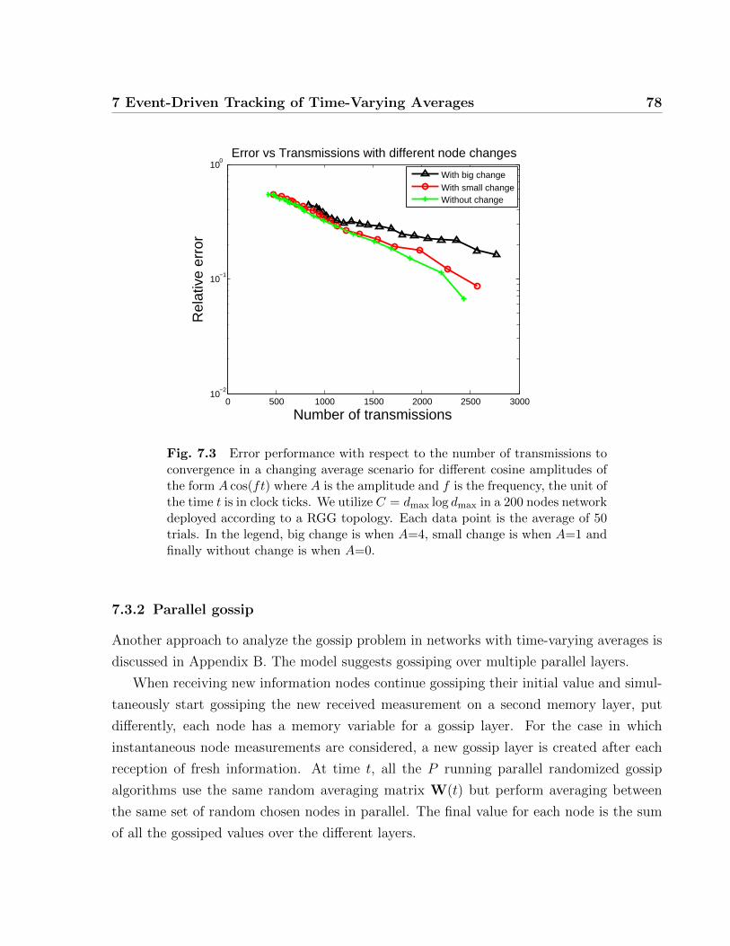
7 Event-Driven Tracking of Time-Varying Averages 78
0 500 1000 1500 2000 2500 300010
−2
10−1
100
Error vs Transmissions with different node changes
Number of transmissions
Rel
ativ
e er
ror
With big changeWith small changeWithout change
Fig. 7.3 Error performance with respect to the number of transmissions toconvergence in a changing average scenario for different cosine amplitudes ofthe form A cos(ft) where A is the amplitude and f is the frequency, the unit ofthe time t is in clock ticks. We utilize C = dmax log dmax in a 200 nodes networkdeployed according to a RGG topology. Each data point is the average of 50trials. In the legend, big change is when A=4, small change is when A=1 andfinally without change is when A=0.
7.3.2 Parallel gossip
Another approach to analyze the gossip problem in networks with time-varying averages is
discussed in Appendix B. The model suggests gossiping over multiple parallel layers.
When receiving new information nodes continue gossiping their initial value and simul-
taneously start gossiping the new received measurement on a second memory layer, put
differently, each node has a memory variable for a gossip layer. For the case in which
instantaneous node measurements are considered, a new gossip layer is created after each
reception of fresh information. At time t, all the P running parallel randomized gossip
algorithms use the same random averaging matrix W(t) but perform averaging between
the same set of random chosen nodes in parallel. The final value for each node is the sum
of all the gossiped values over the different layers.
7 Event-Driven Tracking of Time-Varying Averages 79
The upper bound on the averaging time (the time it takes to be ε close to the varying
average) is studied and the result is shown in Appendix B. The main disadvantage of the
proposed parallel gossiping model is in terms of memory usage over time. For very frequent
changes, the number of gossiping layers increases linearly and this implies more memory
allocations for each node. Note that for a network of n nodes, L changes leads to a usage
of nL extra memory registers. The idea to run separate gossip algorithms in parallel is
possible with infinite memory but is unrealistic in practice. Another disadvantage of this
method is in terms of error estimation at stopping. Roughly speaking, at the end of the
Lth gossip, the sum of the estimated average of all the previous L gossip algorithms will be
treated as the current global estimate of the parallel gossip. When L is small, each gossip
algorithm stops with a certain relative small error. When L is very big (a big number of
gossip layers occurred due to L node measurements), there are L error terms, which implies
that the accumulated error increases linearly with the number of changes L. The impact
of the frequency of the change will be illustrated numerically later in this chapter. In the
sequel, we discuss the application of the local stopping rule to the networks with varying
averages.
7.4 Application of the local stopping rule to event triggered
Time-Varying Networks
In this section, we present a practical application to illustrate the use of the local stopping
rule algorithm. We discuss the ability of GossipLSR to accommodate the dissemination
of information in settings where the average varies slowly with time and the advantage of
such a method in saving battery-power in sensors. Ideally, if the change at one node tends
to drift away the node value from the updated average, the GossipLSR should compensate
the change in a short time by gossiping the new value to the neighborhood of the changing
node. We discuss the question of how much the new measurement will affect the updated
prediction of the average and the time it takes for the new information to be disseminated
through the network.
Our main contribution in this section is to explain how GossipLSR can dynamically
trigger a gossip iteration after receiving a message from one of the nodes. This would,
in turn, trigger other gossip iterations among the network. When node i stops gossip-
ing it sets ci(k) ≥ K, when all the nodes in a network stops, the network is considered

7 Event-Driven Tracking of Time-Varying Averages 80
idle and this remains true as long as no new information arrives to any node. At this
instant, we consider that the network has converged to a common value. When receiving
new information |∆ui(k + 1)| > τ from the outside environment, node i automatically
resets ci(k + 1) to zero and the next time it wakes up to gossip it will diffuse the new
received information to its neighbors. Since the value of the neighbors will change after
averaging, some neighbors who similarly stopped gossiping previously might also decide to
reset their variable C to zero and gossip with their neighbors. In this way a change in
node information triggers a gossip between neighbors and spreads across the network. It is
worthwhile to notice the following characteristics with respect to the proposed approach:
First and most importantly, the proposed approach does not require any additional header
to the GossipLSR, no extra computational complexity or filtering is required. On the other
hand, the proposed approach triggers a gossip iteration only if the amplitude of the change
exceeds a certain threshold (equal to the stopping criterion τ) and this guarantees that
small noise signals cannot trigger unnecessary iterations in the network and consequently
we do not waste battery-power of the sensors gossiping noise. However, it is important
to highlight the impact of the frequency of the change on the tracking accuracy. If the
frequency of the change is small (i.e., measurement values change slowly over time), nodes
running GossipLSR may reach a value close enough to their neighbors to temporarily stop
gossiping, and our method will adaptively reduce the number of messages transmitted to
save battery power at each node. On the other hand, if the change occurs very rapidly over
time, and if it changes faster than nodes are able to gossip, GossipLSR reverts to being
equivalent to simply gossiping every time one node’s clock ticks and this reduces to the
case of randomized gossip without local stopping rule. Simulation results of the frequency
of the change impact on the performance of GossipLSR are shown in the next section of
this chapter. Conducting a theoretical analysis and defining a bound on the frequency of
the change is beyond the scope of this thesis and is the subject of future work.
The discussion above implies that the event-triggered algorithm is equivalent to a local
stopping rule. That is, when there is not too much new information at a node, the network
will automatically stop gossiping, reducing the number of transmissions and consequently
saving the battery consumption at each node.

7 Event-Driven Tracking of Time-Varying Averages 81
0 0.5 1 1.5 2
x 104
−2
0
2
4
6
8
10
12
Time in iterations
Nod
e va
lue
Average valueNode value with τ=0.01Node value with τ=0
Fig. 7.4 Time-varying average and state of one node for a network of 200nodes network deployed according to a RGG topology and two different τvalues. We use a sinusoidal change of the form ∆u(t)=A cos(ft) where A=0.5is the amplitude and f=3×10⁻⁴ is the frequency, the unit of the time t is inclock ticks.
0 0.2 0.4 0.6 0.8 1 1.2 1.4 1.6 1.8 2
x 104
2.5
3
3.5
4
4.5
5
5.5
6
6.5
Time
Nod
e va
lue
Node Tracking for Time−Varying Averages
Average valueValue at Node 1
Fig. 7.5 Time-varying average and state of one node for a network of 200nodes network deployed according to a RGG topology and with τ=0.5. We usea sinusoidal change of the form ∆u(t)=A cos(ft) where A=0.5 is the amplitudeand f=25×10−4 is the frequency, the unit of the time t is in clock ticks. Thegraph is simulated over a total time of 2× 10⁴ clock ticks.
7 Event-Driven Tracking of Time-Varying Averages 82
At each clock tick, a node l is selected randomly and a change of the form ∆ul(t)=A cos(ft)
is applied where A is the amplitude and f is the frequency (the unit of the time t is in clock
ticks). Results of gossiping to track a time-varying average with GossipLSR in a RGG with
τ = 0.01 and τ = 0 are shown in the Figure 7.4. We simulate a sinusoid time-varying aver-
age and a small frequency of the change (f=3×10⁻⁴) up to time 2× 10⁴ ticks. It is evident
that the arrival of new information is incorporated within gossip to obtain a fixed-lag esti-
mate. Comparing both curves τ = 0 and τ = 0.01 we can see that they are almost the same.
The advantage of increasing the value of τ is in order to reduce the number of transmissions
when the amplitude of the change is not significantly high. On the other hand, results of
gossiping to track a time-varying average with GossipLSR in a RGG with τ = 0.5 and a
higher frequency of the change are shown in the Figure 7.5. Figure 7.5 provides the node
states in comparison with the time-varying average and gives us an idea of the “recovery
time” required for a node to be notified when the network receives a new information. We
can say that the delay between the actual node value and the actual average is related to
the network size and topology. Additionally, we can show using the simulations that by
increasing τ from 0.01 to 0.05, the number of transmissions (up to time 2× 10⁴) decreases
from 17538 to 12861 transmissions, and this was well anticipated previously. Consequently,
we can say that local stopping rule allows the node to accommodate the extra information
that it received while simultaneously reducing the number of transmissions.
Figure 7.8a clearly illustrates the mean square error performance of tracking with dif-
ferent values of τ . Varying τ changes the tracking quality. The optimal tracking in terms of
error reduction is when gossip is without a local stopping rule (τ=0). On the other hand,
the advantage of having a local stopping threshold τ is the strikingly big reduction of the
number of transmissions and iterations compared to the standard gossip case, Table 7.1
illustrates this reduction in numbers. Observing the reduction in the number of transmis-
sions for the smallest amplitude tested we observe 625 transmissions with τ=0.1 vs 2×10⁴
transmissions in the worst case (without GossipLSR) and this confirms the practical rel-
evance of GossipLSR in implementing an energy-efficient gossip. Also from Table 7.1 for
different values of τ we can confirm our conclusions in Chapter 5 that increasing τ reduces
the number of transmissions. Comparing the results, for the same values of τ and different
amplitudes of the change, we can say that increasing the amplitude of the change increases
the number of transmissions at stopping. This behavior is expected since, roughly speak-
ing, when the amplitude of the change increases, nodes need to perform more transmissions

7 Event-Driven Tracking of Time-Varying Averages 83
in order to satisfy the halting criterion (dictated by τ) at stopping.
Table 7.1 Number of transmissions for different values of τ and differentamplitude of the change for 200 nodes deployed according to a RGG with aninitial Gaussian Bumps initialization. We use a sinusoidal change of the form∆u(t)=A cos(ft) where A is the amplitude and f=25×10−3 is the frequency.The graph is simulated over a period of 2×10⁴ clock ticks.
A τ=0 τ=0.05 τ=0.1
0.15 20 000 938 6250.5 20 000 1725 8211 20 000 1849 900
7.5 Admissible change frequency with GossipLSR
The central idea of the proposed application of GossipLSR to networks with varying av-
erages is to track time-varying information with minimal error and minimal number of
transmissions and iterations at stopping. Characterizing the admissible change frequency
is of crucial importance since it can give us an idea of the advantages and limitations of
the GossipLSR. In this section we quantify the impact of the frequency of the information
variation on the number of transmissions required until stopping. Similarly to previous
sections we simulate the change for a sinusoidal wave A cos(ft) where A is the amplitude
and f is the frequency, the unit of the time t is in clock ticks. We define the period of the
change T= 1f
clock ticks.
Table 7.2 Number of transmissions vs the period of the change for a 200nodes network deployed according to a RGG with an initial Gaussian Bumpsinitialization in a setting where τ=0.005 and a cosine change of amplitude ‘1’.The graph is simulated over a period of 2×10⁴ clock ticks.
Period in clock ticks 10 50 100 150 200 inf
Number of transmissions 18818 17812 17552 17019 16823 16464
For a better understanding of the impact of the frequency on the GossipLSR perfor-
mance, we have carried out simulations to evaluate the performance of the GossipLSR with
respect to the frequency of change. Table 7.2 shows how many transmissions are required
for different changes. As can be seen, increasing the period of the cosine from 100 iterations

7 Event-Driven Tracking of Time-Varying Averages 84
per cycle to 150 iterations per cycle (decreasing the frequency from 10×10−3 to 66×10−4)
implied a decrease of the number of transmissions from 17552 transmissions to 17019 trans-
missions. The table also gives us an idea of the usefulness of the local stopping rule for
node varying information cases. Note that when the frequency increases the performance of
the GossipLSR approaches the performance of the existing randomized gossip. This is not
surprising and can be explained in the following way: when very frequent changes occur,
nodes need to gossip continuously and GossipLSR offers no gain in terms of transmission
reduction. In this case, the gossiping procedure never stops since the stopping criteria τ
is never reached. Finally, we mention that the admissible frequency of the change with
GossipLSR is intrinsically related to the network size. In other words, stopping can be
reached with a certain frequency in a network of 200 nodes, while it is not reached for the
same frequency in a smaller network of 10 nodes.
7.6 Lag characterization for GossipLSR with respect to the
network size
Delay issues are discussed in this section. This is highly important because a node that is
engaged in tracking a varying signal needs to wait for certain time before it gets informed
about the updated average. Consensus with delays and the characterization of the tracking
rate has been a topic of interest for many authors in the past decade [66, 67]. As can
be seen from Figure 7.4 there exists a short lapse of time between the time the average
value changes and the time the node value can “see” this change. We define the lag as the
number of iterations it takes for one node in order to mimic the total average change. This
parameter is intrinsically related to the network size. In Figure 7.6 we define the delay as
the number of iterations between the peak of a signal and the closest peak of the delayed
signal. In other words, it is the time it takes for the information to propagate to the node.
For the sake of comparison, we simulate GossipLSR and calculate the average delay of one
of the nodes with respect to the actual average for a network deployed according to a RGG
with an initial i.i.d initialization in a setting where τ=0.01 and a cosine change of amplitude
‘0.5’ and period of 40 iterations is applied. The results are summarized in Figure 7.7. As
can be clearly seen, the delay increases as the network size increases.

7 Event-Driven Tracking of Time-Varying Averages 85
0 5 10 15−2
−1.5
−1
−0.5
0
0.5
1
1.5
2
2.5
Delay
Fig. 7.6 Illustration of the delay measurement.
50 100 150 200 250 300500
1000
1500
2000
2500
3000
3500
4000
Network Size
Del
ay in
Iter
atio
ns
Fig. 7.7 Lag characterization vs the network size for a network deployedaccording to a RGG with an initial i.i.d initialization in a setting where τ=0.01and a cosine change of amplitude ‘0.5’ and period of 40 iterations. The graphis simulated over a period of 104 clock ticks.

7 Event-Driven Tracking of Time-Varying Averages 86
In Figure 7.7 we run our GossipLSR algorithm for tracking over a period of 10000 clock
ticks with different network sizes ranging from 50 to 300 nodes with intervals of 10. At each
iteration we measure the average time it takes for one node to be informed about the new
information that arrived to the network previously. Observing Figure 7.7 we can confirm
that the network size determines the ability of the network in reacting to changing inputs.
This was well expected previously since it takes the gossip more time to “spread” accross
larger networks. Additionally, we can say that tracking using the GossipLSR performs
better in terms of delay reduction for smaller networks.
7.7 Distributed Kalman Filter with Embedded Consensus Filters
Earlier work studied distributed information tracking using filters [56,57,59,60,68]. In [56],
Olfati-Saber proposes a distributed Kalman filtering approach for tracking over arbitrary
connected graphs. Consider graph G = (V,E) with n = |V | sensors where each sensor has
a micro-Kalman filter with local communication. Suppose at a time instant t, a sensor i
collects its measures and the ones of its neighbors and stores them in memory. It was shown
in [56] that replicating nth order Kalman filters at each sensor and by judiciously sharing
the sensor observations, this network is able to jointly provide tracking of a time-varying
signal. The key steps of the algorithm for each node involves two dynamic consensus
problems solved using two consensus filters. First, they use a low-pass consensus filter
to average the measurements. Second, a band-pass consensus filter is utilized to average
the inverse-covariance matrices at each sensor. Once this is done, using the local average
of the measurement and inverse-covariance matrices, each node in the network, using the
update equations of its micro-Kalman filter, can compute the estimate of the initial network
average. Finally, note that this approach is synchronous over time and is fully decentralized
(but assumes nodes to know the network size n).
In [56], the author show through simulations that the distributed Kalman filter provides
almost perfect estimates of the varying target. We implement the distributed Kalman filter
with consensus filters algorithm in Matlab for a RGG graph with 200 nodes and consider
a target moving at the frequency of f=10−4. We plot the squared estimation error at
one node, our results are shown in Figure 7.8b. One can argue about the high scale of
the mean square error. In fact, since the distributed estimation is performed without
central authority, there is no specific fusion center and consequently there is a relatively

7 Event-Driven Tracking of Time-Varying Averages 87
big disagreement in the estimates of different nodes. Olfati-Saber states in [69] that the
mean square error can not fully characterize the distributed estimation in sensor networks
since there exist a disagreement for different nodes. In Figure 7.9 we plot the estimate
through distributed Kalman filters with embedded consensus at one of the nodes as well as
the real average. As can be clearly seen, the tracked value is almost the same as the real
average and there is no delay issues.
Comparing the error for GossipLSR in Figure 7.8a and Figure 7.8b, we can say that
the advantage of distributed Kalman filters is that, first they considerably improve the
tracking performance in terms of error reduction and second the rate at which the error
decreases is drastically faster than the tracking with GossipLSR while their disadvantage
is that they require a complex filtering process on top of the gossiping process and they
do not achieve any energy-efficient reduction in terms of the number of transmissions re-
duction compared to GossipLSR. In fact, since the distributed Kalman filter approach is
synchronous, the number of transmissions is proportional to both: the network size and
the number of iterations. In the simulation settings depicted in Figure 7.8b the number of
transmissions over a period of 2×10⁴ clock ticks is equal to 4×10⁶ transmissions and this is
a critical disadvantage in distributed Kalman filtering strategies compared to GossipLSR
where we consume just 625 transmissions with τ=0.1 and 2×10⁴ transmissions in the worst
case (τ=0). Also, the price to pay for using a filtering scheme is in terms of a high compu-
tational and memory requirements per node. Depending on the tracking application, and
depending whether we would like to have more accurate or a more energy-efficient system,
the system designer can select GossipLSR or distributed Kalman filtering algorithms for
tracking. When the energy constraint is less of an issue and most importantly when a syn-
chronous algorithm is required, distributed Kalman filtering are more suitable compared to
GossipLSR algorithms since they have minimal tracking delays. Another interesting fact is
that the estimation in distributed Kalman filters requires a high connectivity of the graph,
which is not the case in the GossipLSR. Finally, a note concerning noise resilience of both
algorithms, we can point out that while both algorithms are suitable for noisy settings,
Kalman filters are particularly optimal for Gaussian noise while GossipLSR are resilient to
any type of noise as long as the amplitude of the noise component is below the stopping
criterion τ .
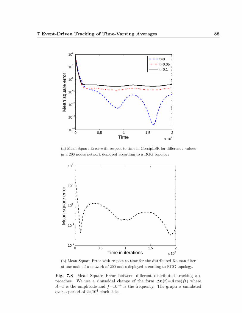
7 Event-Driven Tracking of Time-Varying Averages 88
0 0.5 1 1.5 2
x 104
10−4
10−3
10−2
10−1
100
101
102
Mea
n sq
uare
err
or
Time
τ=0τ=0.05τ=0.1
(a) Mean Square Error with respect to time in GossipLSR for different τ values
in a 200 nodes network deployed according to a RGG topology
0 0.5 1 1.5 2
x 104
10−2
10−1
100
101
102
Time in iterations
Mea
n sq
uare
err
or
(b) Mean Square Error with respect to time for the distributed Kalman filter
at one node of a network of 200 nodes deployed according to RGG topology.
Fig. 7.8 Mean Square Error between different distributed tracking ap-proaches. We use a sinusoidal change of the form ∆u(t)=A cos(ft) whereA=1 is the amplitude and f=10−4 is the frequency. The graph is simulatedover a period of 2×10⁴ clock ticks.

7 Event-Driven Tracking of Time-Varying Averages 89
0 5000 10000 150003.4
3.6
3.8
4
4.2
4.4
4.6
4.8
5
Time in iterations
Nod
e va
lue
Real averageDKF estimate
Fig. 7.9 Estimate at one node of the real average using a distributed Kalmanfilter with embedded consensus for a network of 200 nodes deployed accordingto RGG topology. We use a sinusoidal change of the form ∆u(t)=A cos(ft)where A=0.5 is the amplitude and f=2×10⁻⁵ is the frequency. The graph issimulated over a period of 15000 clock ticks.
7.8 Summary of the chapter
Tracking techniques have been widely used in many fields; as a result of their widespread
practical applications a number of gossip algorithms discussed distributed tracking capa-
bilities.
In this chapter, we have presented an energy efficient method for tracking a varying
average in a network. We proved that in the case of average calculation over networks
with varying information, GossipLSR can be used in order to model an event triggered
approach. When there is not enough “new” information to gossip, a node shuts down
and becomes passive and consequently saves battery power. We modeled the error with
respect to the mean value of the change and later our discussions have been validated
through simulation results. The performance of the GossipLSR in terms of reducing the
number of transmissions decreases as the frequency of change increases, and the time of

7 Event-Driven Tracking of Time-Varying Averages 90
information dissemination increases with the network size. The technique presented differ
from existing solutions since there is no filtering process and each node tracks the average
based on a real-time information available from other nodes in the network, additionally a
reduction of the number of transmission is achieved when the changing information has a
low frequency, this characteristic is very useful in energy constrained environments where
low-power wireless devices are used.
Next chapter concludes the thesis by summarizing the problems studied and results
obtained in the thesis and discussing the future work.
91
Chapter 8
Conclusion and Future Work
8.1 Summary of the thesis
One of the major challenges for next-generation wireless systems is to be as resource-efficient
as possible [4]. Conserving battery power in wireless sensor networks and increasing battery
lifetime can be done by reducing the number of wireless transmissions for most of the
network topologies. This thesis puts together in one place some results spread throughout
the literature concerning gossip algorithms and error tracking in time varying networks,
and at the same time proposes a finite time stopping gossip algorithm: GossipLSR.
We presented and investigated a modified model for information gossiping in networks,
The Local stopping rule, and discussed its application to event-driven gossip with varying
averages. GossipLSR defines a positive threshold τ on the difference between the actual
and previous value of each node after each gossip round. If this threshold is reached for C
consecutive times, the node becomes passive and stops gossiping. The main advantage of
this approach is to provide an accurate and simple gossip algorithm while simultaneously
reducing the number of transmissions and the total power consumption needed to converge.
Additionally, the primary and most important objective of this thesis was to introduce a
finite time decentralized gossip algorithm. We saw that in GossipLSR, a small hit in per-
formance (error at stopping) results in considerable savings in the number of iterations and
transmissions. Our simulations have shown, that under certain initial conditions, Gossi-
pLSR significantly reduces the number of transmissions until convergence. Additionally,
inspired by the probabilistic model of the coupon collector problem, we proved convergence
theoretically and analyzed its performance in terms of convergence speed and number of

8 Conclusion and Future Work 92
transmissions for different network sizes, topologies and initializations. We also provided
the results of extensive simulations using GossipLSR in order to examine the effect of var-
ious model parameters such as the threshold τ and the maximum number of edges. Our
simulation results also indicated that our algorithm can be generalized to other gossip al-
gorithms such as GGE, GEO and Path Averaging. The application of the local stopping
rule to these algorithms was later described and illustrated by simulation results. We later
discussed tracking algorithms and distributed dynamic estimation in networks with varying
averages. We have also presented a novel energy-efficient approach allowing information
tracking in networks with varying averages, and examined the impact of the frequency
of the information change on the performance of the GossipLSR. Finally, we compared
GossipLSR performance to other existing finite time gossip algorithms and discussed the
advantages and disadvantages of each method. Extensive evaluations, including analysis
and simulations have been conducted to examine the performance of our proposed algo-
rithm as well as its application. The results show that our objectives are well fulfilled.
Broadly speaking, our main results differ from previous works in several key aspects:
• Our model, which involves totally decentralized gossip algorithms, does not require
the network to consider worst initial conditions scenarios and is different from what
was considered in almost all of the relevant literature. This characteristic has a direct
impact on the number of transmissions to reach convergence.
• We saw how GossipLSR offers a natural framework for situations of varying averages.
Our focus was on identifying a realistic, yet easy, solution to the tracking problem in
networks with real-time averaging and we achieved our goal as evidenced by Chap-
ter 9. For completeness purposes, we compared the GossipLSR tracking approach to
previous studies on distributed Kalman filtering.
8.2 Future work
The work in this thesis paves the way for many new directions. This thesis explored
the advantages of GossipLSR and the number of messages and transmissions saved via
simulation. A theoretical approach to describe the exact convergence rate is a potentially
interesting future work. In the case where GossipLSR is not used for tracking, there is
room for designing better algorithms such as an algorithm where a node knows when the
8 Conclusion and Future Work 93
network has converged so it won’t wake up anytime later to gossip (this reduces latency and
the number of iterations at stopping). Such an algorithm would be useful for cases when
nodes are expected to deliver their final average to an application. Another line of future
work is related to the selection of gossip nodes within a round. Random node selection
seems to be an essential aspect of gossip algorithms. If this selection is not random and if
only nodes with enough “new” information can be selected to gossip, the performance of
the GossipLSR can increase drastically.
As mentioned previously, in the case of tracking, the local stopping rule fits perfectly in
the node varying networks scenarios. Also, the GossipLSR algorithm needs to be further
experimentally analyzed under time-varying scenarios, where a node receives fresh infor-
mation during the gossip round. Also it is interesting to characterize more precisely in
the tracking scenario how many nodes transmissions are saved, and under what conditions.
Additionally in this thesis we assumed an ideal MAC layer and ideal links conditions; one
of the obvious questions of interest is what can be done to improve the performance of
GossipLSR in realistic settings (with link erasure and limited bandwidth). Also in this
thesis we assumed that the communication links between pairs of nodes allow the transfer
of real numbers accurately. However, in a more realistic context, it should be assumed that
the channel has a finite digital capacity. This clearly forces us to investigate the GossipLSR
performance in a context where a quantization on real numbers is performed. This study
can be inspired from a large repository of previous work on gossip and the quantization
effect [19, 25, 38]. Last but not least, extending the current work to the synchronous time
model described in Boyd et al [10] would be straightforward and very important in the real
life application of GossipLSR to synchronous networks.
Although gossip algorithms have gathered much attention from the scientific community
in the past decade, there remains much work to be done for these algorithms to be applicable
in practical domains and to make them accessible to local industries. We hope that the
research efforts in the area of gossip algorithms and the local stopping rule will continue,
bringing new exciting results.
94
Appendix A
Coupon collector proof
The coupon collector problem is one of the most known topics in discrete probability, and
its proof can be found in many standard articles on probability. In this appendix, we show
the proof of the coupon collector in a gossip setting for a network where each coupon is
considered as a neighbor.
Let G = (V,E) denote the communication topology of a network with |V | nodes and
edges (i, j) ∈ E ⊆ V 2 if and only if nodes i and j communicate directly. Assume there are
n neighbors for each node, and at each iteration, one neighbor is picked at random. Let m
be the number of gossip trials a node needs to perform until all the neighbors are averaged
with high probability. We want to derive the probability that m exceeds a certain number
of trials, and we have not picked every single one of the neighbors at least once.
Theorem 3. The expected number of trials needed to contact n neighbor grows as n log(n).
Proof. Suppose Ci is the neighbor picked at the i-th attempt. The j-th attempt is con-
sidered as a success, if Cj was chosen for the first time (i.e. the information reached a
new neighbor). Denote Xi the number of attempts required to go from the i-th success to
after the (i + 1)-th success. Obviously, the total number of attempts can be calculated as
X =∑n−1
i=0 Xi. Therefore, the probability of Xi to reach a new neighbor in an attempt is
pi =n−in
. From this expression, note that, the probability to pick the first few neighbors
is higher than the probability to pick the last few neighbors. On the other hand, this
probability decreases for the last few neighbors and consequently it takes a longer time to
achieve the last few successes. Since Xi is either of two discrete probability distributions
(success to reach a new node or failure), it follows a geometric distribution with probability
2011/04/20

A Coupon collector proof 95
pi with expected value equal to E[Xi] = 1/pi , Since the expection is linear we can say that
E[X] =∑n−1
i=0 E[Xi]. This implies that E[X] =∑n−1
i=0nn−i= n
∑n−1i=0
1n−i
Using the summation property and from the asymptotics of the harmonic numbers we
have∑n−1
i=01n−i = log(n) + O(n). Consequently, we can say that E[X] =n log(n) + O(n).
This means that on average, an overall of n log(n) trials are needed in order to ensure that
every neighbor is averaged with high probability.
2011/04/20

96
Appendix B
Bounds on the averaging time for
tracking using gossip algorithms
B.1 Algorithm Description
We consider a connected graph G = (V,E), where V is the vertex set with n nodes and E
is the edge set. Let t denote the time index in clock ticks. We denote the node information
as u(t) (which is the state at all the nodes at time t) and the node measurement as ∆u(t),
which follows certain distribution and is finite and i.i.d. with respect to time t. The node
update equation is
u(t+ 1) = u(t) + ∆u(t). (B.1)
The time-varying average is given by
xave(t) =1
n
n∑i=1
ui(t). (B.2)
The proposed gossip algorithm generates many parallel iterations for both the informa-
tion gossip and the new measurements gossip. In order to better accommodate multiple
change of nodes, we define a constant parameter TP as the time interval of two parallel
gossip algorithms. At time t, the total number of running parallel gossip algorithms is
denoted as P (t) = b tTPc + 1. The reason behind having Tp is to wait for a certain time
before taking into consideration all the changes that arrived to the nodes in a given interval

B Bounds on the averaging time for tracking using gossip algorithms 97
of time. In other words, after each Tp clock ticks a new parallel layer is created and the
latest new measurements are gossiped on this layer.
Denote p as the index of the parallel running gossip algorithm, where p = 0, · · · , P (t)−1.
The p-th parallel gossip algorithm starts at time pTp with the initial node information
defined as
up =
{u(0), p = 0∑pTp−1
t=(p−1)Tp∆u(t), p ≥ 1
.
In other words, the zeroth gossip algorithm tries to obtain the average of the initial node
information u(0) at time 0, while the p-th gossip algorithm tries to obtain the average
of the node information change during the p-th interval, i.e., time [(p − 1)Tp, pTp). The
number of intervals is equal to the number of gossip layers in parallel.
Next, we shall introduce the update equation of the parallel Gossip algorithm. First,
we define xp(t) as the node value (which is the updated value of the gossip algorithm) of
the p-th parallel gossip algorithm at time t (i.e., xp(0)=u(0)). Then, the average of the
p-th gossip algorithm is given by.
xpave =1
n
n∑i=1
upi (B.3)
The update equation of the p-th (0 ≤ p ≤ P (t)− 1) parallel Gossip algorithm is given by
xp(t+ 1) =
0, 0 ≤ t < pTP − 1
up, t = pTP − 1
W(t)xp(t), t ≥ pTP
.
Where W (t) is a doubly stochastic matrix that must satisfy the constraints imposed by
the gossip criterion and the graph topology, the conditions on this matrix were studied
previously by [1] and listed below:
Theorem 4 (Xiao and Boyd [1], Theorem 1).
1TW = 1T , (B.4)
W1 = 1, (B.5)
ρ(W − 11T
n) ≤ 1, (B.6)

B Bounds on the averaging time for tracking using gossip algorithms 98
Therefore, the equivalent node value of the overall P parallel gossip algorithms is given
by the summation of all the individual parallel gossip algorithms that occurred up to the
time P (t).
x(t) =
P (t)−1∑p=0
xp(t) (B.7)
with the average value of the P parallel gossip algorithm given by
xparave =
P (t)−1∑p=0
xpave. (B.8)
Define yp(t) = xp(t)−xpave as the individual parallel error at each gossip ‘layer’ and y(t) =∑P (t)−1p=0 yp(t) = x(t)− xparave1 as the total error over all the parallel gossip. For the sake of
less heavy notations in the sequel, we note ypu = yp(pTp).
Inspired by previous work [10], we derive in next section an upper bound on the ε-
averaging time of parallel gossip algorithm for time varying information. The ε-averaging
time is the time it takes to be ε close to the average. The characterization of the upper
bound enables us to observe the impact of parameters such as the frequency and amplitude
of the change on the tracking capabilities.
B.2 Upper bound on the ε-averaging time
Lemma 6. The upper bound on the averaging time for the asynchronous algorithm in
networks with varying averages (in terms of number of clock ticks) is:
Tavg ≤ ε−2((A(−λ2(W )Tp)−B(λ2(W )2Tp) + 2A((P − 1)λ2(W )Tp)
)(B.9)
where
A =E[ypTu ypu]
x0(0)Tx0(0)
λ2(W )−Tp
1− λ2(W )−Tp(B.10)
B =2E[ypTu ypu]
x0(0)Tx0(0)
( λ2(W )−Tp
1− λ2(W )−Tp
)2(B.11)
λ2(W ) is the second largest eigenvalue of matrix W , Tp is the time to wait before incorpo-
rating the measurements.

B Bounds on the averaging time for tracking using gossip algorithms 99
Proof. Our proof is inspired by the work of Boyd et al. [10]. We start by showing the
previous upper bound derived by Boyd et al. and later adapt it to the case of varying
averages. In [10], authors define the ε-averaging time, or the time to get within ε from the
average, such as for any initial vector x(0), for k ≥ K∗(ε)
Pr
[||x(k)− xave1||||x(0)||
≥ ε
]≤ ε (B.12)
where K∗(ε) = 3 log ε−1
log λ2(W )−1 is the upper bound.
The key steps in the proof are as follows: First, they show that
E[y(t)Ty(t)
]≤ λ2(W )ty(0)Ty(0) (B.13)
where λ2(W ) is the second largest eigenvalue of a doubly stochastic matrix W (t) charac-
terizing the algorithm.
By Markov’s inequality, they conclude that
Pr
[||x(t)− xave1||||x(0)||
≥ ε
]= Pr
[y(t)Ty(t)
x0(0)Tx0(0)≥ ε2
]≤ ε−2E[y(t)Ty(t)]
x0(0)Tx0(0)≤ ε−2λ2(W )t
By letting ε−2λ2(W )t = ε, they finally get t = 3 log ε−1
log λ2(W )−1 , K∗(ε).
In our case, taking the node information change update into consideration, at time
t, ∀l,m ∈ {0, · · · , P (t) − 1}, where l and m are the index of the parallel gossip, and
considering the interval Tp we define the ε-averaging time as the time to get within ε from
the varying average. We assume each gossip to be processed separately on a different layer
and consequently we can adapt the result in [10] considering new initial measurements at
each gossip layer. Similarily to equation ( B.13) we can say that:
E[yl(t)Tym(t)] ≤ (λ2(W ))t−max{l,m}TPE[yl(max{l,m}TP )Tym(max{l,m}TP )] (B.14)
Using the averaging matrix W(t), for l ≤ m, we have:
yl(mTp) =
mTp−1∏t=lTp
W(t)yl(lTp) (B.15)

B Bounds on the averaging time for tracking using gossip algorithms 100
Where yl(mTp) is the initial error value at each parallel layer.
We develop the right hand side of Equation ( B.14) using Equation ( B.15) and get as
a conclusion:
E[yl(max{l,m}TP )Tym(max{l,m}TP )] =
{E[ylTu ymu ], l = m
E[ylTu ]W (l−m)TPE[ymu ], l < m
Consequently, Equation ( B.14) can be written as:
E[yl(t)Tym(t)]] ≤
{(λ2(W ))t−lTPE[ylTu ymu ], l = m
(λ2(W ))t−mTPE[ylTu ]W (l−m)TPE[ymu ], l < m(B.16)
Additionnaly, we can say that y(t)Ty(t) at instant t is the summation of all the parallel
y(t)Ty(t) at all the parallel layers :
y(t)Ty(t) =∑
0≤l,m≤P (t)−1
yl(t)Tym(t) =∑
0≤p≤P (t)−1
yp(t)Typ(t) + 2∑
0≤l<m≤P (t)−1
yl(t)Tym(t)
Now adding all the pieces together and using Markov’s inequality, we derive an upper
bound for the ε-averaging time defined as:
Pr
[||x(t)− xparave1||||x(0)||
≥ ε
]= Pr
[y(t)Ty(t)
x0(0)Tx0(0)≥ ε2
]≤ ε−2E[y(t)Ty(t)]
x0(0)Tx0(0)
= ε−2E[∑
0≤l,m≤P (t)−1 yl(t)Tym(t)]
x0(0)Tx0(0)
= ε−2
∑0≤p≤P (t)−1 E[yp(t)Typ(t)] + 2
∑0≤l<m≤P (t)−1 E[yl(t)Tym(t)]
x0(0)Tx0(0)
Now using Equation ( B.16) we can say that:
Pr
[||x(t)− xparave1||||x(0)||
≥ ε
]≤ ε−2((λ2(W ))t +
∑1≤p≤P (t)−1(λ2(W ))t−pTPE[ypTu ypu]
x0(0)Tx0(0)
+2∑
0≤l<m≤P (t)−1(λ2(W ))t−max{l,m}TPE[ylTu ]W (l−m)TPE[ymu ]
x0(0)Tx0(0))
Note that the extra terms depending on P and Tp are affected by the node information
change frequency (higher frequency requires smaller Tp and this implies bigger P) and the

B Bounds on the averaging time for tracking using gossip algorithms 101
node change amplitude since yp is bigger when the amplitude of the change is higher.
By letting the right hand side of the previous inequality equal to ε we get as an upper
bound of the convergence time:
Tavg ≤ ε−2((A(−λ2(W )Tp)−B(λ2(W )2Tp) + 2A((P − 1)λ2(W )Tp)
)(B.17)
where
A =E[ypTu ypu]
x0(0)Tx0(0)
λ2(W )−Tp
1− λ2(W )−Tp(B.18)
B =2E[ypTu ypu]
x0(0)Tx0(0)
( λ2(W )−Tp
1− λ2(W )−Tp
)2(B.19)
Note that the upper bound depends on the second largest eigenvalue λ2 of matrix W (t),
which depends on the graph connectivity (not to be confused with the second smallest
Laplacian eigenvalue previously used in this thesis). Also, the upper bound depends on the
initialization vector x0(0). Finally, note that when Tp is equal to 1 in the previous bound,
it means that instantaneously we are taking the new arriving information and gossiping it
on a separate parallel layer. This results in a drastically big number of parallel layers and
consequently a high consumption in terms of memory.
2011/04/20
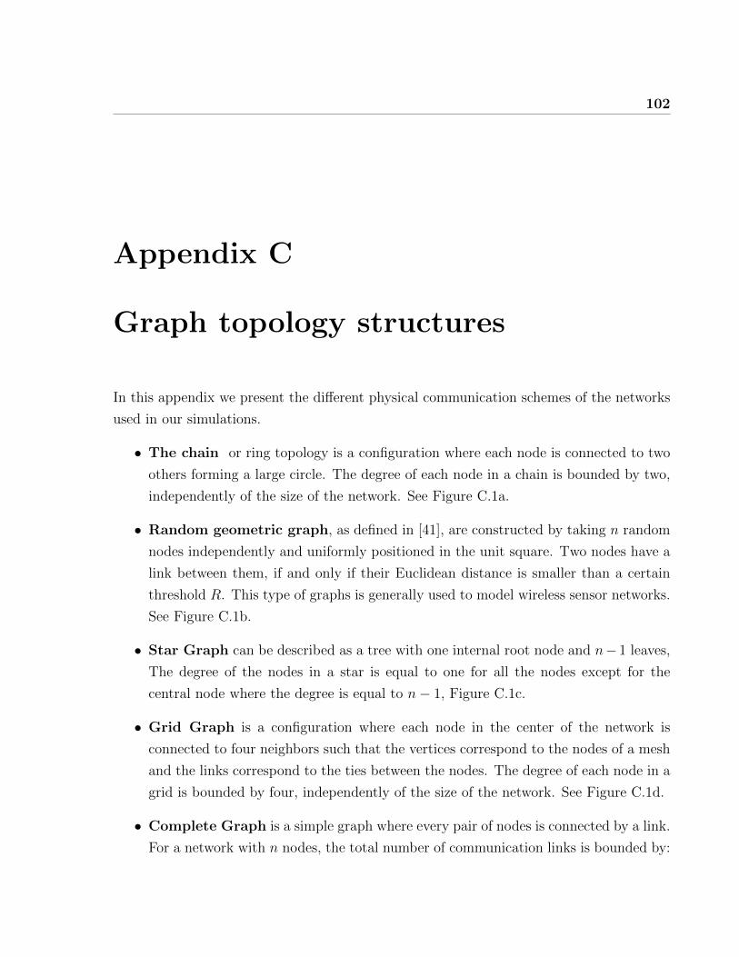
102
Appendix C
Graph topology structures
In this appendix we present the different physical communication schemes of the networks
used in our simulations.
• The chain or ring topology is a configuration where each node is connected to two
others forming a large circle. The degree of each node in a chain is bounded by two,
independently of the size of the network. See Figure C.1a.
• Random geometric graph, as defined in [41], are constructed by taking n random
nodes independently and uniformly positioned in the unit square. Two nodes have a
link between them, if and only if their Euclidean distance is smaller than a certain
threshold R. This type of graphs is generally used to model wireless sensor networks.
See Figure C.1b.
• Star Graph can be described as a tree with one internal root node and n− 1 leaves,
The degree of the nodes in a star is equal to one for all the nodes except for the
central node where the degree is equal to n− 1, Figure C.1c.
• Grid Graph is a configuration where each node in the center of the network is
connected to four neighbors such that the vertices correspond to the nodes of a mesh
and the links correspond to the ties between the nodes. The degree of each node in a
grid is bounded by four, independently of the size of the network. See Figure C.1d.
• Complete Graph is a simple graph where every pair of nodes is connected by a link.
For a network with n nodes, the total number of communication links is bounded by:

C Graph topology structures 103
n(n−1)2
. The degree of each node in a complete graph is proportional to the network
size and is equal to n− 1. See Figure C.1e.
2011/04/20
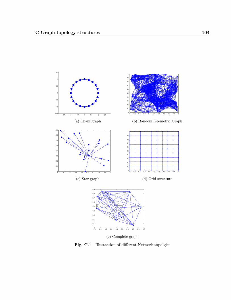
C Graph topology structures 104
−1.5 −1 −0.5 0 0.5 1 1.5−1.5
−1
−0.5
0
0.5
1
1.5
(a) Chain graph
0 0.1 0.2 0.3 0.4 0.5 0.6 0.7 0.8 0.9 10
0.1
0.2
0.3
0.4
0.5
0.6
0.7
0.8
0.9
1
(b) Random Geometric Graph
0.1 0.2 0.3 0.4 0.5 0.6 0.7 0.8 0.9 10
0.1
0.2
0.3
0.4
0.5
0.6
0.7
0.8
(c) Star graph
0 0.1 0.2 0.3 0.4 0.5 0.6 0.7 0.8 0.9 10
0.1
0.2
0.3
0.4
0.5
0.6
0.7
0.8
0.9
1
(d) Grid structure
0 0.1 0.2 0.3 0.4 0.5 0.6 0.7 0.8 0.90
0.1
0.2
0.3
0.4
0.5
0.6
0.7
0.8
0.9
(e) Complete graph
Fig. C.1 Illustration of different Network topolgies

105
Appendix D
Initialization fields
In this appendix we present the different network initializations used in the simulation
setup. In order to clarify the presentations and facilitate the reading of the figures we
illustrate only the field and omit the representations of the nodes.
• Independent identically distributed initialization : each initial value has the
same probability as the others and all are mutually independent. In this thesis, initial
i.i.d values are between 0 and 100. See Figure D.1a.
• Spike initialization: all nodes have xi(0) = 0 except one node that differs dramat-
ically, e.g., x1(0) = 100. Such an initialization is of importance because it can be
utilized to describe the case where only a single sensor has a large value compared to
other sensors in the network. See Figure D.1b.
• Fifty/Fifty initialization : half the nodes located in the same region have an
initial value of 0 and the other half differ dramatically, e.g., have initial value 100
(later we denote this setting as 0/100 initialization), See Figure D.1c.
• Slope initialization : the field is linearly varying and nodes sample this field, in
such an initialization there is a constant difference between nodes. See Figure D.1d.
• Gaussian Bumps initialization : there are several mixtures of two dimensional
Gaussians with different means and covariances in the field and nodes sample this
field. In our settings, we mix four two-dimensional Gaussian functions with variances
equal to 0.0078; 0.0137; 0.0048; 0.0138 and with amplitudes equal to 7, 8, 18 and 25

D Initialization fields 106
respectively. The Gaussian peaks are centered at (0.3; 0.4), (0.65; 0.3), (0.19; 0.19)
and (0.15; 0.75) respectively for the four functions.
0
10
20
30
40
50
60
70
80
90
100
(a) Independent identically distributed
0
10
20
30
40
50
60
70
80
90
100
(b) Spike
0
10
20
30
40
50
60
70
80
90
100
(c) 0/100 field
10
15
20
25
30
35
40
45
50
55
60
(d) Slope
Fig. D.1 Illustration of different Initialization fields
107
Appendix E
Second smallest eigenvalue of the
graph Laplacian
Theorem 1 in Chapter 3 showed that the second smallest Laplacian eigenvalue λ2 dictates
how near and how fast the algorithm approaches the average consensus, thus it makes sense
to investigate what properties can be derived from the Laplacian eigenvalues of a graph.
E.1 Background work on λ2
In this section, we will consider the relationship between the graph topology and the second
smallest eigenvalue of the Laplacian (also called algebraic connectivity of the graph G). As
mentioned previously, the Laplacian can be used in a number of ways to describe inter-
esting geometric representations of a graph. It can also imply many general applications
to graphs in the telecommunication domain (see [70] for a survey). Inspired by the well-
known Fiedler’s result in his 1973 paper, we first survey the properties of the second smallest
Laplacian eigenvalue λ2.
Informally, it was shown that large values of λ2 are associated with graphs that are hard
to disconnect [71]. In fact, we can say that λ2=0 if and only if the graph is disconnected,
and additionally the number of connected components is equal to the multiplicity of 0 as
an eigenvalue. In [72] authors have also shown that the second smallest eigenvalue λ2 is
related to the sparsity of cuts in the graph, in other words, for a graph with sparse cuts,
λ2 is small. They later described a method for calculating the upper bound of the second
smallest eigenvalue λ2 over a family of graphs with small cuts and investigated the problem

E Second smallest eigenvalue of the graph Laplacian 108
of choosing a graph that maximizes the algebraic connectivity. This motivates us to study
how modifying the graph topology can be applied to change λ2 and consequently to speed
up the convergence of GossipLSR. The explanation and simulation of graph sparsification
is shown in the next section.
E.2 Simulation results of sparsification
Sparsification is the procedure of approximating a graph G by a sparser graph G′ by
removing links. In this section, we investigate the sparsification effect on two variables
that play a key role in Theorem 1: the maximum node degree dmax and the second smallest
Laplacian eigenvalue λ2. As a benchmark, we simulate a method that gradually selects a set
of links to be removed from the original network. We consider the two most commonly used
topologies, namely barely connected random geometric graphs, and the complete graph.
Simulation results are shown in Figures E.1a and E.1b for complete and random geo-
metric graphs respectively. For each graph, we plot the curve of the maximum number of
neighbors with respect to the percentage of removed links. Roughly speaking, removing
links decreases the average node degree in the network and makes the graph less connected.
0 10 20 30 40 50 60150
160
170
180
190
200
210
220
230
240
250
Percentage of the removed links
Max
imum
num
ber
of n
eigh
bors
(a) Complete graph
0 10 20 30 40 50 6020
25
30
35
40
45
50
Percentage of the removed links
Max
imum
num
ber
of n
eigh
bors
(b) RGG
Fig. E.1 Maximum node degree for a network of 250 nodes that are initiallydeployed according to different topologies. The graph is later reduced byremoving the links of the nodes with maximum degree.
In Figures E.2a and E.2b, we plot the algebraic connectivity for complete and random
geometric graphs respectively. Each curve represents the second smallest eigenvalue with

E Second smallest eigenvalue of the graph Laplacian 109
respect to the percentage of removed links. It is clearly shown that the second smallest
eigenvalue gets smaller as the network becomes less connected. This coincides perfectly
with the results discussed in [73] that the Laplacian eigenvalue decreases strictly when
a link is removed from the graph. As mentioned previously, removing links from nodes,
can actually induce a graph sparsification and reduces the number of iterations to reach
convergence [74].
0 10 20 30 40 50 6060
80
100
120
140
160
180
200
220
240
260
Percentage of the removed links
Sec
ond
smal
lest
eig
enva
lue
(a) Complete graph
0 10 20 30 40 50 600.4
0.5
0.6
0.7
0.8
0.9
1
1.1
1.2
1.3
1.4
Percentage of the removed links
Sec
ond
smal
lest
eig
enva
lue
(b) RGG
Fig. E.2 Second smallest eigenvalue of the graph Laplacian for a networkof 250 nodes that are initially deployed according to different topologies. Thegraph is later reduced by removing the links of the nodes with maximumdegree.
We saw previously that sparsifying the graph implies decreasing both dmax and λ2. With
this in mind, we re-observe the main result in Theorem 1.
τ =
√λ2δ2
8m(dmax
(log(dmax) + 2 log(n)
)− 1)2
, (E.1)
When sparsifying, the denominator in (E.1) decreases faster than the λ2 in the nu-
merator and obviously the error at stopping δ decreases for a constant stopping criterion
τ . On the other hand, as discussed previously in this thesis, decreasing dmax implies a
smaller value of C at each node and consequently this results in a faster stopping time.
As a conclusion we can say that graph sparsification in GossipLSR leads to a faster gossip
and a smaller error at stopping. A more formal study on the benefits of sparsification on
GossipLSR would be an interesting direction in future work.

E Second smallest eigenvalue of the graph Laplacian 110
E.3 Summary
Dependence on the graph topology is unavoidable since intuitively in different topologies
nodes may be sparser and can have different number of neighbors, in which case nodes can
receive different gossip requests and consequently different number of messages. In this
appendix, we investigated the impact of the graph topology and its influence on the second
smallest eigenvalue of the Laplacian. Finally, as a conclusion we can say that the sparsifica-
tion of graphs plays an important role in speeding up GossipLSR and reducing the number
of transmissions. This is true since it modifies the number of links, and consequently, the
second eigenvalue of the Laplacian and the maximum node degree.

111
References
[1] L.Xiao and S. Boyd, “Fast linear iterations for distributed averaging,” Systems ControlLetters, vol. 53, no. 1, pp. 65–78, 2004.
[2] I. F. Akyildiz, W. Su, Y. Sankarasubramaniam, and E. Cayirci, “Wireless sensornetworks: a survey,” Comput. Netw., vol. 38, no. 4, pp. 393–422, 2002.
[3] P. Gupta and P. Kumar, “The capacity of wireless networks,” IEEE Trans. Info.Theory, vol. 46, pp. 388–404, March 2000.
[4] V. Raghunathan, C. Schurgers, S. Park, and M. B. Srivastava, “Energy-aware wirelessmicrosensor networks,” IEEE Signal Processing Magazine, vol. 19, pp. 40–50, March2002.
[5] M. Rabbat, R. Nowak, and J. Bucklew, “Robust decentralized source localization viaaveraging,” in Proc. IEEE ICASSP, (Philadelphia, PA), March 2005.
[6] M. Rabbat, J. Haupt, A. Singh, and R. Nowak, “Decentralized compression and pre-distribution via randomized gossiping,” in Proc. ACM/IEEE Conf. on InformationProcessing in Sensor Networks, (Nashville, TN), April 2006.
[7] L. Li, X. Li, A. Scaglione, and J. Manton, “Decentralized subspace tracking via gos-siping,” in Proc. IEEE Conf. on Distributed Computing in Sensor Systems, (SantaBarbara, CA), Jun. 2010.
[8] S. Ram, A. Nedic, and V. Veeravalli, “Distributed stochastic subgradient projectionalgorithms for convex optimization,” in Optimization Theory and Applications, 2010.
[9] J. Duchi, A. Agarwal, and M. Wainwright, “Dual averaging for distributed optimiza-tion: Convergence analysis and network scaling,” tech. report, U.C. Berkeley, May2010.
[10] S. Boyd, A. Ghosh, B. Prabhakar, and D. Shah, “Randomized gossip algorithms.,”IEEE Trans. Inf. Theory, vol. 52, pp. 2508–2530, Jun. 2006.

References 112
[11] D. Ustebay, B. Oreshkin, M. Coates, and M. Rabbat, “Greedy gossip with eavesdrop-ping,” IEEE Trans. Signal Processing, vol. 58, pp. 3765–3776, Jul. 2010.
[12] A. Dimakis, A. Sarwate, and M. Wainwright, “Geographic gossip: Efficient averagingfor sensor networks,” IEEE Trans. Signal Processing, vol. 56, pp. 1205–1216, Mar.2008.
[13] F. Benezit, A. Dimakis, P. Thiran, and M. Vetterli, “Gossip along the way: Order-optimal consensus through randomized path averaging,” in Proc. Allerton Conf. onComm., Control, and Comp., (Urbana-Champaign, IL), Sep. 2007.
[14] De Groot and H. Morris, “Reaching a consensus,” J. Am. Stat. Assoc., vol. 69, no. 345,pp. 118–121, 1974.
[15] V. Borkar and P. Varaiya, “Asymptotic agreement in distributed estimation,” IEEETrans. Automatic Control, vol. 27, pp. 650–655, Jun. 1982.
[16] J. Tsitsiklis, D. Bertsekas, and M. Athans, “Distributed asynchronous deterministicand stochastic gradient optimization algorithms,” IEEE Trans. Automatic Control,vol. AC-31, pp. 803–812, Sep. 1986.
[17] A. Olshevsky, Efficient Information Aggregation Strategies for Distributed Controland Signal Processing. Doctor of philosophy, Massachusetts institute of technology,September 2010.
[18] M. Medidi, J. Ding, and S. Medidi., “Data dissemination using gossiping in wirelesssensor networks,” vol. 5819, pp. 316–327, SPIE, 2005.
[19] T. C. Aysal, M. Coates, and M. Rabbat, “Distributed average consensus using proba-bilistic quantization,” Statistical Signal Processing SSP ’07. IEEE, pp. 640–644, Aug2007.
[20] D. Kempe, A. Dobra, and J. Gehrke, “Computing aggregate information using gossip,”in Proc. Foundations of Computer Science, (Cambridge, MA), Oct. 2003.
[21] R. Motwani and P. Raghavan, Randomized Algorithms. Cambridge Univ. Press, 1995.
[22] B. Oreshkin, M. Coates, and M. Rabbat, “Optimization and analysis of distributedaveraging with short node memory,” IEEE Trans. Signal Processing, vol. 58, pp. 2850–2865, May 2010.
[23] K. Tsianos and M. Rabbat, “Fast decentralized averaging via multi-scale gossip,” inProc. IEEE Conf. on Distributed Computing in Sensor Systems, (Santa Barbara, CA),Jun. 2010.

References 113
[24] R. Karp, C. Schindelhauer, S. Shenker, and B. Vocking., “Randomized rumor spread-ing.,” in 41st IEEE Symp. on Foundations of Comp. Science, 2000.
[25] D. Yuan, S. Xu, H. Zhao, and Y. Chu, “Distributed average consensus via gossipalgorithm with real-valued and quantized data,” System and Control Letters, vol. 59,pp. 536–542, Aug. 2010.
[26] P. Kouznetsov, R. Guerraoui, S. B. Handurukande, and A. M. Kermarrec., “Reducingnoise in gossip-based reliable broadcast,” in IEEE Symposium on Reliable DistributedSystems, p. 186, 2001.
[27] T. Aysal, E. Yildiz, A. Sarwate, and A. Scaglione, “Broadcast gossip algorithms forconsensus,” IEEE Trans. Signal Processing, vol. 57, pp. 2748–2761, Jul. 2009.
[28] L. Fang and P. Antsaklis, “On communication requirements for muli-agent consensusseeking,” NESC, 2005.
[29] R. Olfati-Saber and R. Murray, “Consensus problems in networks of agents withswitching topology and time-delays,” IEEE Transacationson Automatic Control,vol. 49, September 2004.
[30] R. Olfati-Saber, J. A. Fax, and R. M. Murray, “Consensus and cooperation in net-worked multi-agent systems,” No. 95, Jan 2007.
[31] A. Kashyap, T. Basar, and R. Srikant, “Quantized consensus,” in International Sym-posium on Information Theory, no. 9-14, pp. 635–639, July 2006.
[32] Y.Sun, L. Wang, and G.Xie, “Average consensus in networks of dynamic agentswith switching topologies and multiple time-varying delays,” Systems Control Letters,vol. 57, no. 2, pp. 175–183, 2008.
[33] W.Ren, “Multi-vehicle consensus with time varying reference state,” Systems ControlLetters, vol. 56, no. 2, pp. 474–483, 2007.
[34] D. Schizas, G. Mateos, and G. B. Giannakis, “Distributed LMS for consensus-basedin-network adaptive processing,” IEEE Trans. Signal Processing, vol. 57, June 2009.
[35] Cattivelli, F.S, and A. H. Sayed, “Diffusion least-mean squares strategies for dis-tributed estimation,” IEEE Trans. Signal Processing, vol. 58, pp. 1035–1048, march2010.
[36] R. Olfati-Saber and J. Shamma, “Diffusion least-mean squares over adaptive networks:Formulation and performance analysis,” 44th IEEE Conference on Decision and Con-trol, pp. 6698 – 6703, Dec 2005.
References 114
[37] E. Kokiopoulou and P. Frossard, “Polynomial filtering for fast convergence in dis-tributed consensus,” IEEE Trans. Signal Processing, vol. 57, pp. 342–354, Jan. 2009.
[38] P. Frasca, R. Carli, F. Fagnani, and S. Zampieri, “Average consensus on networks withquantized communication,” International Journal of Robust and Nonlinear Control,2008.
[39] T. He, P. Vicaire, T. Yan, L. Luo, L. Gu, G. Zhou, R. Stoleru, Q. Cao, J. A. Stankovic,and T. Abdelzaher, “Achieving real-time target tracking using wireless sensor net-works,” in Proc. 12th IEEE Real-Time Embedded Tech. Appl. Symp., (San Jose, CA),pp. 37–48, Apr. 2006.
[40] M. Mitzenmacher and E. Upfal, Probabilty and Computing: Randomized Algorithmsand Probabilistic Analysis. Cambridge Univ. Press, 2005.
[41] M. Penrose, Random Geometric Graphs. Oxford University Press, 2003.
[42] P. Gupta and P. R. Kumar, “Critical power for asymptotic connectivity,” in Proc.IEEE Conf. on Decision and Control, (Tampa, FL), Dec. 1998.
[43] V. Saligrama, M. Alanyali, and O. Savas, “Distributed detection in sensor networkswith packet loss and finite capacity links,” IEEE Trans. Signal Processing, vol. 54,pp. 4118–4132, Nov. 2006.
[44] O. Savas, M. Alanyali, and V. Saligrama, “Efficient in-network processing throughinformation coalescence,” in Proc. Dist. Comp. in Sensor Sys., (San Francisco), Jun.2006.
[45] K. Jung, D. Shah, and J. Shin, “Fast gossip through lifted Markov chains,” in Proc.Allerton Conf. on Comm., Control, and Comp., (Urbana-Champaign, IL), Sep. 2007.
[46] W. Li and H. Dai, “Location-aided distributed averaging algorithms,” in Proc. AllertonConf. on Comm., Control, and Comp., (Urbana-Champaign, IL), Sep. 2007.
[47] B. Johansson and M. Johansson, “Faster linear iterations for distributed averaging,”in Proc. IFAC World Congress, (Seoul, South Korea), Jul. 2008.
[48] A. Dimakis, S. Kar, J. Moura, M. Rabbat, and A. Scaglione, “Gossip algorithms fordistributed signal processing.” to appear, Proceedings of the IEEE, Jan. 2011.
[49] C. Asensio-Marco and B. Beferull-Lozano, “Accelerating consensus gossip algorithms:Sparsifying networks can be good for you,” IEEE ICC, 2010.
[50] R. Durrett, Probability: Theory and Examples. Cambridge Univ. Press, 4th ed., 2010.
References 115
[51] P. Berenbrink and T. Sauerwald, “The weighted coupon collector’s problem and ap-plications,” in Proc. COCOON, (Niagra Falls, NY), Jul. 2009.
[52] F. Chung, Spectral Graph Theory. American Math. Society, 1997.
[53] C. Godsil and G. Royle, Algebraic Graph Theory. Springer-Verlag, 2001.
[54] S. Sundaram and C. N. Hadjicostis, “Distributed function calculation and consensususing linear iterative strategies,” in IEEE J. Selected Areas in Communications, vol. 26,pp. 650–660, May 2008.
[55] C. G. Lopes and A. H. Sayed, “Diffusion least-mean squares over adaptive networks:Formulation and performance analysis,” IEEE Trans. Signal Processing, vol. 56,pp. 3122–3136, July 2008.
[56] R. Olfati-Saber, “Distributed Kalman filters with embedded consensus filters,” in 44thIEEE Conference on Decision and Control, (Seville, Spain), pp. 8179 – 8184, Dec.2005.
[57] S. Kirti and A. Scaglione, “Scalable distributed Kalman filtering through consensus,”in Proceedings of the 33rd International Conference on Acoustics, Speech, and SignalProcessing, (Las Vegas, Nevada, USA), pp. 2725–2728, April 1-4 2008.
[58] U. A. Khan and J. M. F. Moura, “Distributing the Kalman filter for large-scale sys-tems,” Accepted for publication, IEEE Transactions on Signal Processing, 2008.
[59] A. Ribeiro, I. D. Schizas, S. I. Roumeliotis, and G. B. Giannakis, “Kalman filteringin wireless sensor networks: Incorporating communication cost in state estimationproblems,” IEEE Control Systems Magazine, 2009.
[60] R. Carli, A. Chiuso, L. Schenato, and S. Zampieri, “Distributed Kalman filtering usingconsensus strategies,” IEEE Journal on Selected Areas in Communications, vol. 26,no. 4, 2008.
[61] R. R. Brooks, P. Ramanathan, and A. Sayeed, “Distributed target classification andtracking in sensor networks,” Proc. IEEE, vol. 91, pp. 1163–1171, Aug. 2003.
[62] F. Zhao, J. Shin, and J. Reich, “Information-driven dynamic sensor collaboration,”IEEE Signal Process. Magazine, vol. 19, pp. 61–72, Mar. 2002.
[63] G. Werner-Allen, J. Johnson, M. Ruiz, J. Lees, and M. Welsh, “Monitoring volcaniceruptions with a wireless sensor network,” in Proc. EWSN, (Istanbul, Turkey), pp. 108–120, Jan. 2005.

References 116
[64] N. Ahmed, Y. Dong, T. Bokareva, S. Kanhere, S. Jha, T. Bessell, M. Rutten, B. Ristic,and N. Gordon, “Detection and tracking using wireless sensor networks,” in Proc. 5thACM Conf. Embedded Netw. Sens. Syst., (Sydney, Australia), pp. 425–426, 2007.
[65] R. Horn and C. Johnson, Matrix Analysis. Cambridge, 1985.
[66] A. Nedic and A. Ozdaglar, “Convergence rate for consensus with delays,” J. GlobalOptim, pp. pp.1–23.
[67] D. Kempe, J. Kleinberg, and A. Demers, “Spatial gossip and resource location pro-tocols,” J. of the Association for Computing Machinery, vol. 51, pp. 943–967, Nov.2004.
[68] N. Dziengel, G. Wittenburg, and J. Schiller., “Towards distributed event detection inwireless sensor networks,” in Proc. DCOSS, (Santorini, Greece), Jun. 2008.
[69] R. Olfati-Saber, “Distributed Kalman filtering for sensor networks,” in 46th IEEEConf. Decision and Control, (New Orleans, LA), December 2007.
[70] J. van den Heuvel and S. Pejic, “Using Laplacian eigenvalues and eigenvectors in theanalysis of frequency assignment problems,” Ann. Oper. Res. 107, pp. pp. 349–368,2001.
[71] M. Ashbaugh, “Open problems on eigenvalues of the Laplacian, analytic and geometricinequalities and their applications,” Kluwer Academic Publishers, vol. 4787, pp. 13–28,1999.
[72] A. Ghosh, “Designing well-connected networks,” Ph.D. Dissertation, vol. StanfordUniversity, 2006.
[73] M. Holroyd, “Synchronization and connectivity of discrete complex systems,” in In-ternational Conference on Complex Systems, 2006.
[74] D. A. Spielman and S.-H. Teng, “Nearl-linear time algorithms for graph partitioning,graph sparsification, and solving linear systems,” STOC, pp. 81–90, 2004.
Related Documents