arXiv:1110.6730v2 [cond-mat.soft] 10 Jan 2012 Thermodynamic and structural anomalies of the Gaussian-core model in one dimension Cristina Speranza ∗ , Santi Prestipino † , and Paolo V. Giaquinta ‡ Universit` a degli Studi di Messina, Dipartimento di Fisica, Contrada Papardo, I-98166 Messina, Italy Abstract We investigated the equilibrium properties of a one-dimensional system of classical particles which interact in pairs through a bounded repulsive potential with a Gaussian shape. Notwith- standing the absence of a proper fluid-solid phase transition, we found that the system exhibits a complex behaviour, with “anomalies” in the density and in the thermodynamic response functions which closely recall those observed in bulk and confined liquid water. We also discuss the emer- gence in the cold fluid under compression of an unusual structural regime, characterized by density correlations reminiscent of the ordered arrangements found in clustered crystals. Keywords: one-dimensional models; Gaussian-core model; clustered crystals; water-like anomalies * Email: [email protected] † Email: [email protected] ‡ Email: [email protected] (corresponding author) 1

Welcome message from author
This document is posted to help you gain knowledge. Please leave a comment to let me know what you think about it! Share it to your friends and learn new things together.
Transcript

arX
iv:1
110.
6730
v2 [
cond
-mat
.sof
t] 1
0 Ja
n 20
12
Thermodynamic and structural anomalies
of the Gaussian-core model in one dimension
Cristina Speranza ∗, Santi Prestipino †, and Paolo V. Giaquinta ‡
Universita degli Studi di Messina, Dipartimento di Fisica,
Contrada Papardo, I-98166 Messina, Italy
Abstract
We investigated the equilibrium properties of a one-dimensional system of classical particles
which interact in pairs through a bounded repulsive potential with a Gaussian shape. Notwith-
standing the absence of a proper fluid-solid phase transition, we found that the system exhibits a
complex behaviour, with “anomalies” in the density and in the thermodynamic response functions
which closely recall those observed in bulk and confined liquid water. We also discuss the emer-
gence in the cold fluid under compression of an unusual structural regime, characterized by density
correlations reminiscent of the ordered arrangements found in clustered crystals.
Keywords: one-dimensional models; Gaussian-core model; clustered crystals; water-like anomalies
∗ Email: [email protected]† Email: [email protected]‡ Email: [email protected] (corresponding author)
1
I. INTRODUCTION
Renewed interest has recently emerged in the thermodynamic and transport properties of
one-dimensional (1D) systems, also in view of their potential relevance to the modelling of in-
teracting colloidal particles diffusing within narrow channels [1]. The spontaneous emergence
in such systems of (even intense) local ordering phenomena, not necessarily accompanied by
proper phase transitions, is a topical issue that continues to be investigated also in relation
to its effects on the dynamics of the particles [2]. In this regard, a landmark result still is the
celebrated van Hove’s theorem [3] according to which a system of identical particles with a
hard core and pairwise interactions extending over a finite range has no phase transition in
1D, in the absence of external fields. The general issue of the existence (or non-existence) of
phase transitions in 1D systems with short-ranged interactions has been critically reviewed
in more recent years, among others, by Cuesta and Sanchez [4]. A way to potentially escape
the negative verdict of van Hove’s theorem is to allow for bounded repulsive interactions be-
tween particles. The simplest of such models is a system of penetrable spheres (PS), whose
interaction potential takes a finite positive value whenever two particles overlap, while van-
ishing otherwise [5, 6]. In the absence of an infinite repulsive barrier, interactions are no
longer restricted to nearest neighbours. As a result, at variance with the Tonks gas [7], no
analytical solution of the PS model is currently known. Fantoni [8] has recently provided
robust arguments against the existence of a phase transition in a 1D system of penetrable
particles with a negative short-ranged square well outside the repulsive core [9].
A largely studied variant of bounded repulsive interactions is the Gaussian potential [10].
Its continuing interest also stems from its frequent applications as a model interaction in
soft-matter systems, such as the dilute solutions of highly ramified polymers in a good
solvent (star polymers), where the “effective” repulsion between the centres of mass of two
polymer chains can be typically described through a Gaussian law [11]. The corresponding
Gaussian-core model (GCM) can at most exhibit fluid-solid and, possibly, solid-solid phase
transitions since a liquid-vapour transition is clearly excluded by the absence of an attractive
component in the potential. In fact, at low enough temperature three-dimensional (3D)
Gaussian particles crystallize, upon compression, in a cubic solid structure, with either a
face-centred or a body-centred symmetry [12]. However, a further increase of the density
does eventually lead to a reentrant melting of the solid. This phenomenon has been observed
2
also in two dimensions (2D) where, at variance with the 3D case, a narrow hexatic region
appears between the isotropic fluid phase and the triangular solid phase all along the melting
line [13].
As for the phase stability of the GCM in 1D, no rigorous proof of the absence of a phase
transition has been presented so far. However, Fantoni conjectured that his arguments
against the existence of a phase transition in a 1D system of attractive penetrable spheres
apply equally well, under appropriate conditions, to a larger class of model fluids with a
decaying long-ranged repulsive tail, including the GCM [8].
Whether or not the GCM fluid crystallizes in 1D, one can safely expect a far from triv-
ial phase behaviour because of the ever-increasing occurrence, under compression, of soft
particle-core overlaps. A natural candidate for the macrostate of minimum Gibbs free en-
ergy is a diffusely ordered arrangement formed by more or less equally spaced particles, as
is the case of 1D hard rods at high density [14]. However, the thermodynamic competition
between energy and entropy may also lead, in a fluid with a soft bounded potential, to even
more complex arrangements such as those found in “clustered” or “tower” crystals, where
two or more (superimposed) particles are confined within the same cell [11].
II. MODEL AND METHOD
We consider a system of point particles repelling each other, at a relative distance r,
through a Gaussian pair potential
u(r) = ǫ exp[
−(r/σ)2]
, (1)
where ǫ and σ fix the energy and length scales, respectively. The GCM potential has an inflec-
tion point at r0 = σ/√2, where its curvature changes from concave to convex. Correspond-
ingly, for r ≤ r0 the strength of the force between two particles, f(r) = −du(r)/dr, decreases
as the particles approach each other. However, it is over a larger range (0 ≤ r ≤ σ) that the
local virial function, rf(r), and thus the contribution of a pair of interacting molecules to
the pressure of the system, decreases when the separation also decreases. This condition is
typically taken as the signature of “core softening” [15]. As is well known, a core-softened
– in the just specified sense – potential can generate a density anomaly, associated with
a negative thermal expansion coefficient. This circumstance was originally verified for the
3
GCM fluid in 3D by Stillinger and Weber [16]. Indeed, a number of thermodynamic, struc-
tural and dynamical properties of the GCM fluid have been already found to exhibit, both
in 2D and 3D, “waterlike” anomalies which render the behaviour of this model qualitatively
different from that of a “simple” (i.e., Lennard-Jones-like) fluid.
To our knowledge, no systematic numerical study of the 1D GCM fluid has been un-
dertaken so far. In this paper we present the results of an investigation carried out with
the Monte Carlo (MC) method in the isothermal-isobaric ensemble. The data we present
were obtained with samples of N = 200 particles, unless otherwise specified; however, we
also tested the stability and convergence of the results with larger samples of 500 and 1000
particles. No qualitatively significant changes emerged upon increasing the “size” of the cal-
culation. We collected data over trajectories of, typically, five million sweeps, every sweep
consisting of N + 1 elementary MC moves, including one attempt, on average, to change
the volume V of the system. During the equilibration runs, we adjusted the maximum par-
ticle displacement and the volume change so as to maintain the acceptance rates of both
types of moves close to 50% in the production runs. We carried out our simulations along
a number of isothermal and isobaric paths, from low to high density and from high to low
temperatures, continuing at each state point from the last system configuration produced
in the previous run. We computed, for given values of T and P , the following properties:
the average number density, n = N/〈V 〉; the average energy, E = NkBT/2 + 〈U〉, where kB
is Boltzmann’s constant and U is the total potential energy; the specific heat at constant
pressure, CP = T (∂s/∂T )P , where s is the entropy per particle; the isothermal compress-
ibility, KT = −v−1(∂v/∂P )T , where v = n−1 is the average volume per particle; the thermal
expansion coefficient, αP = v−1(∂v/∂T )P . The three thermodynamic response functions
were obtained as thermal averages of covariances of the fluctuating variables (energy and
volume): CP/kB = 〈[∆(E + PV )]2〉/(kBT )2, αT /kB = 〈∆(E + PV )∆V 〉/ [〈V 〉(kBT )2], andKT = 〈(∆V )2〉/ [〈V 〉(kBT )], where ∆X = X − 〈X〉.
We also calculated the radial distribution function (RDF), g(|r|) = v〈∑
k 6=1 δ(xk−x1−r)〉,and the associated structure factor, S(|q|) = 1 + n
∫∞
−∞dx exp(−iqx) [g(|x|)− 1].
The Monte Carlo study was complemented with the results obtained with the
hypernetted-chain (HNC) approximation and with exact total-energy calculations carried
out at T = 0 with increasing pressure for several candidates for the solid phase, in order to
gain insight into the preferred forms of particle aggregation at low temperatures.
4

In the following, we shall also make use of reduced units for density, temperature, and
pressure: ρ = nσ, τ = kBT/ǫ, and Π = Pσ/ǫ.
III. RESULTS
In the GCM fluid the growth of density correlations upon compression is eventually
frustrated by the finite strength of the repulsion between particles and by the decreasing
strength of their mutual force as they approach each other. We anticipate that for densities
larger than the value corresponding to a nearest-neighbour (NN) distance roughly equal
to 1.5σ (Π ≃ 0.35), a further increase of the pressure causes a suppression, rather than a
sharpening, of the local structure of the fluid since in a sufficiently dense environment the
overlapping of two particles entails an entropy gain that is larger than the associated energy
penalty. Lang and coworkers [17] coined the term “infinite-density ideal gas” to represent
the uncorrelated (g(r) = 1) behaviour of Gaussian particles at very high densities.
Such a trend is already manifest in the RDF calculated through the HNC approximation
at the reduced temperature τ = 0.1 (see Fig. 1) which, though quantitatively accurate only
for ρ >∼ 2, yields the correct qualitative trend of the local fluid structure with increasing
pressure. We see from the picture that the NN distance, corresponding to the position
of the first maximum in the RDF, steadily decreases upon compression but its statistical
definition as a microscopic length scale is highest at an intermediate pressure corresponding
to a reduced density ρ ≃ 0.5.
A. Phase stability at T = 0
Before examining the MC findings, it is worth considering the thermodynamic behaviour
of the fluid at zero temperature. Stillinger proved that in the limit of low T and n the
thermodynamics of the GCM fluid reduces, for any space dimensionality, to that of hard
spheres with a temperature-dependent diameter d(β) = σ√
ln(βǫ), where β = (kBT )−1 [10].
In one dimension, the hard-rod behaviour sets in for ρHS = σ/d; below this threshold the
equilibrium properties of the 1D GCM fluid can be mapped onto those of the Tonks gas.
However, ρHS is too small a density (about 0.40 for τ = 0.002, corresponding to a pressure
slightly smaller than 0.05) for the hard-sphere connection to be of any relevance to the
5

FIG. 1: Radial distribution function in the HNC approximation plotted as a function of the distance
for a reduced temperature τ = 0.1 and for reduced densities ρ = 0.1, 0.2, . . . , 1.9, 2 (the density
increases along the direction indicated by the arrow).
present inquiry into the existence of phase transitions in the 1D GCM fluid at high pressure.
The competition for thermodynamic stability between single-occupancy and clustered
solids is ruled by the chemical potential which, at zero temperature, is equal to the enthalpy
per particle: µ = e + Pv; moreover, any crystalline phase consists of just one microstate
(modulo a translation). We first consider an arrangement of equally spaced particles:
µ1 = minn
{
∞∑
m=1
exp
(
−m2
n2
)
+P
n
}
. (2)
We then compare µ1 with the chemical potentials of clustered phases with equidistant lumps
of k = 2, 3, . . . particles, all lying at the same positions:
µk =k − 1
2+ min
n
{
k∞∑
m=1
exp
(
−k2m2
n2
)
+P
n
}
. (3)
6

FIG. 2: Excess chemical potential, relative to the value (µ1) in an ordered state of equally spaced
particles, plotted as a function of pressure at T = 0, for clustered crystalline phases: continuous
blue line, 2-clustered crystal; dashed cyanide line, 3-clustered crystal; long-dashed green line, 4-
clustered crystal. The dotted red line yields the excess chemical potential of the state formed by
regularly alternating singles and pairs.
A further possibility that we have considered is a state in which isolated particles regularly
alternate with pairs:
µ(1,2) =1
3+ min
n
{
4
3
∑
m=1,3,...
exp
(
−9m2
4n2
)
+5
3
∑
m=2,4,...
exp
(
−9m2
4n2
)
+P
n
}
. (4)
In Fig. 2 we plot all such chemical potentials as a function of the pressure. The comparison
shows that the crystal formed by equidistant particles is the most stable phase at zero
temperature, whatever the pressure. No better solution was obtained upon allowing for a
small fixed separation between the particles forming a pair in either the 2− 2− 2− 2− . . .
or the 1 − 2 − 1 − 2 − . . . arrangement. This result is a strong indication of the absence
7

of any kind of phase transition in the 1D GCM fluid. However, the free-energy penalties
associated with the nucleation of clustered solids progressively decrease with the pressure,
the faster the smaller the number of particles in a given cell. Hence, one cannot exclude a
priori the possibility that, at non-zero temperature and high enough pressure, such phases
may enter the thermodynamic game for entropic reasons. In passing, we note that for Π >∼ 3
the 2-clustered crystal is almost degenerate with the single-occupancy crystal.
B. Thermodynamic properties
Following the computational procedure described in Sect. II, we investigated the phase
behaviour of the 1D GCM fluid at reduced temperatures 0.002 ≤ τ ≤ 1 and for reduced
pressures 0.05 ≤ Π ≤ 3.5. We verified that neither the number density nor the energy exhibit
any (even rounded-off) jump discontinuity over the explored domain. We also performed a
chain of isothermal simulations at high pressure starting from an ordered 2-clustered con-
figuration but did not find any sign of hysteresis in either the density or the energy. Hence,
on a strictly thermodynamic basis, the equilibrium state of the investigated model is always
that of a fluid. However, we found out that at low enough temperatures this fluid under-
goes remarkable structural changes, with an anomalous (i.e., nonstandard) thermodynamic
behaviour which, in many respects, closely resembles that observed in liquid water, when
gradually cooled from above the freezing temperature into the deeply metastable region
(possibly in a confined environment).
The signature of such a “complex-fluid” behaviour is the emergence of a volumetric
anomaly in the dense fluid: as shown in Fig. 3, at low pressure the density decreases mono-
tonically with the temperature; however, for Π >∼ 1.2 the trend turns from decreasing to
increasing over a limited temperature range Tmin(P ) ≤ T ≤ Tmax(P ). Correspondingly, a
maximum shows up in n(T, P ) at T = Tmax(P ) which, for Π <∼ 1.5, is preceded by a min-
imum at a nonzero temperature, Tmin(P ). For Π >∼ 1.5, the density increases with T from
T = 0, until it inverts its trend at the temperature of maximum density (TMD).
A maximum in the density of the GCM fluid had already been observed in higher space
dimensions [13, 16]: in this respect, it is altogether remarkable to verify the persistence of
this feature in one dimension. But even more remarkable is the emergence of a shallow
minimum in n(T ) over a range of pressures: the fluid behaves in an anomalous way for
8
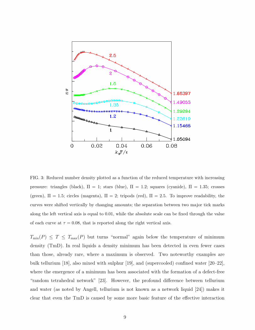
FIG. 3: Reduced number density plotted as a function of the reduced temperature with increasing
pressure: triangles (black), Π = 1; stars (blue), Π = 1.2; squares (cyanide), Π = 1.35; crosses
(green), Π = 1.5; circles (magenta), Π = 2; tripods (red), Π = 2.5. To improve readability, the
curves were shifted vertically by changing amounts; the separation between two major tick marks
along the left vertical axis is equal to 0.01, while the absolute scale can be fixed through the value
of each curve at τ = 0.08, that is reported along the right vertical axis.
Tmin(P ) ≤ T ≤ Tmax(P ) but turns “normal” again below the temperature of minimum
density (TmD). In real liquids a density minimum has been detected in even fewer cases
than those, already rare, where a maximum is observed. Two noteworthy examples are
bulk tellurium [18], also mixed with sulphur [19], and (supercooled) confined water [20–22],
where the emergence of a minimum has been associated with the formation of a defect-free
“random tetrahedral network” [23]. However, the profound difference between tellurium
and water (as noted by Angell, tellurium is not known as a network liquid [24]) makes it
clear that even the TmD is caused by some more basic feature of the effective interaction
9

FIG. 4: Location of the density and response functions extrema in the (P, T ) plane. Density: open
red circles, temperature maxima (TMD); solid red circles, temperature minima (TmD). Coefficient
of thermal expansion: magenta tripods, temperature minima; open magenta squares, pressure
maxima; solid magenta squares, pressure minima. Isobaric specific heat: open blue triangles,
temperature maxima; open blue squares, pressure maxima; solid blue triangles (inset), temperature
minima. Isothermal compressibility: open black squares, temperature maxima; solid black squares,
temperature minima. The locations of the symbols correspond to numerical estimates of the
thermodynamic coordinates of the extrema obtained via Monte Carlo simulations along either
isothermal or isobaric paths. The lines through the data are guides to the eye.
potential.
The relevant thermodynamic loci corresponding to the location of the extrema of the
density and of the response functions are plotted in Fig. 4. The volumetric anomaly region,
corresponding to a negative value of the coefficient of thermal expansion, is the region
10

bounded by a maximum and (possibly) a minimum of the density; all along this boundary
the expansivity vanishes. The TMD and TmD lines are seen to originate from point C (with
coordinates ΠC ≃ 1.169 and τC ≃ 0.029), where the first and second isobaric temperature
derivatives of the density both vanish [αP = (∂αP /∂T )P=PC= 0]. This point marks the
onset of the volumetric anomaly in the fluid and is apparently reached with infinite slope
along the TMD and TmD lines. The TMD line is seen to pass through a maximum (M), with
coordinates ΠM ≃ 1.267 and τM ≃ 0.037; correspondingly, the TMD locus has a positive
slope for PC ≤ P < PM, while decreasing asymptotically to zero with increasing pressure
for P > PM. Instead, the TmD shows a rapidly decreasing monotonic trend on compression
and appears to vanish at a finite reduced pressure just larger than 1.5.
The temperature TM is the highest temperature at which the fluid manifests the volumet-
ric anomaly, associated with the emergence of a single or double extremum in the density.
This anomaly obviously reverberates in the thermodynamic response functions. Rolle’s the-
orem applied to an isothermal or isobaric “cut” of the anomalous region, producing two
distinct intersections with the density extrema lines where αP = 0, implies that the expan-
sivity must have a minimum at some point in between. The isobaric minimum of αP as
a function of T (see Fig. 5) goes along (though not exactly coinciding) with an inflection
point of the density; both such features were found to survive well outside the anomalous
region, down to Π ≃ 0.6 (see also Fig. 3). The minimum-expansivity locus radiates out of
this region at the point C of confluence of the TMD and TmD lines (see Fig. 4).
Sastry and coworkers [25] have showed that the isothermal compressibility increases
on cooling at any point along the TMD line wherever its slope is negative and the
second temperature derivative of the volume, evaluated at the same point, is positive
[(∂2v/∂T 2)P, atTMD = v(∂αP /∂T )P, at TMD > 0]. The above conditions apply for P > PM.
A similar thermodynamic constraint implies that the isothermal compressibility increases
on heating at any point along the TmD line where the slope is negative and such also is
the second temperature derivative of the volume, which is the case of the 1D GCM fluid.
The necessary consequence of this twofold constraint is the emergence of a maximum in
the isothermal compressibility at some temperature in the interval Tmin(P ) < T < Tmax(P ).
As shown in Figs. 4 and 6, the maximum persists even for Π > 1.5, when the minimum
of the density has disappeared. We can see that, as originally predicted by Sastry and
coworkers [25], the locus of the compressibility maxima intersects the TMD line exactly at
11

FIG. 5: Thermal expansion coefficient plotted as a function of the reduced temperature for different
pressures (left panel) and of the pressure for different temperatures (right panel); left panel: same
legends as in Fig. 3; right panel: triangles (black), τ = 0.002; stars (blue), τ = 0.005; squares
(cianide), τ = 0.03; crosses (green), τ = 0.05; circles (magenta), τ = 0.1; tripods (red), τ = 1.
its maximum M, where (dTmax(P )/dP )PM= 0.
Thermodynamic consistency implies [25] that the anomalous temperature dependence of
KT should also reflect in the behaviour of CP as a function of T at fixed P (see the left panel
of Fig. 7). As the temperature drops to zero, the isochoric specific heat approaches unity
(i.e., the value of an interacting 1D fluid at T = 0), as also does the isobaric specific heat
since CP = CV + Tvα2P/KT (see Fig. 8); CP shows then a maximum, whose (P, T ) locus
runs very close to the isobaric minimum-expansivity line (see Fig. 4). We also note that the
height of the CP maximum changes very little with either the pressure or the temperature,
an aspect that we shall return to soon.
12
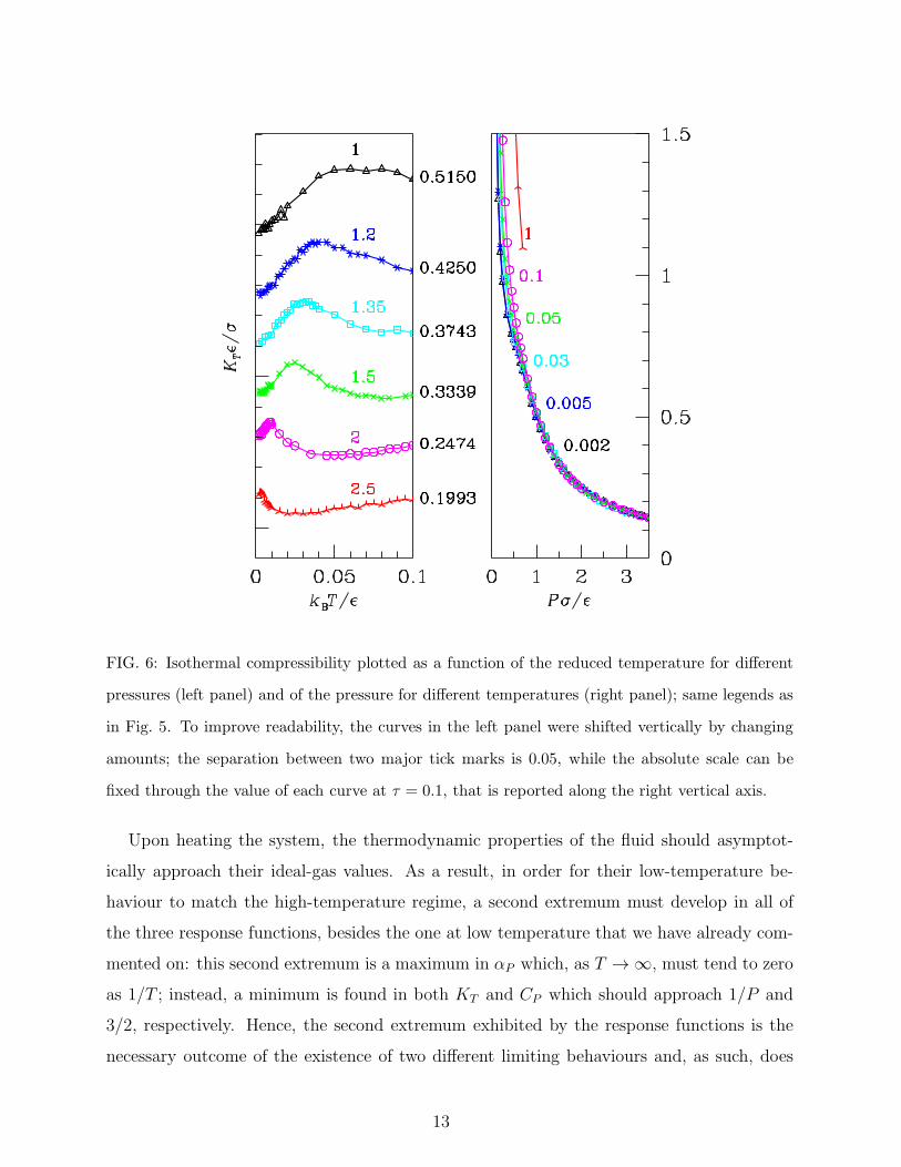
FIG. 6: Isothermal compressibility plotted as a function of the reduced temperature for different
pressures (left panel) and of the pressure for different temperatures (right panel); same legends as
in Fig. 5. To improve readability, the curves in the left panel were shifted vertically by changing
amounts; the separation between two major tick marks is 0.05, while the absolute scale can be
fixed through the value of each curve at τ = 0.1, that is reported along the right vertical axis.
Upon heating the system, the thermodynamic properties of the fluid should asymptot-
ically approach their ideal-gas values. As a result, in order for their low-temperature be-
haviour to match the high-temperature regime, a second extremum must develop in all of
the three response functions, besides the one at low temperature that we have already com-
mented on: this second extremum is a maximum in αP which, as T → ∞, must tend to zero
as 1/T ; instead, a minimum is found in both KT and CP which should approach 1/P and
3/2, respectively. Hence, the second extremum exhibited by the response functions is the
necessary outcome of the existence of two different limiting behaviours and, as such, does
13
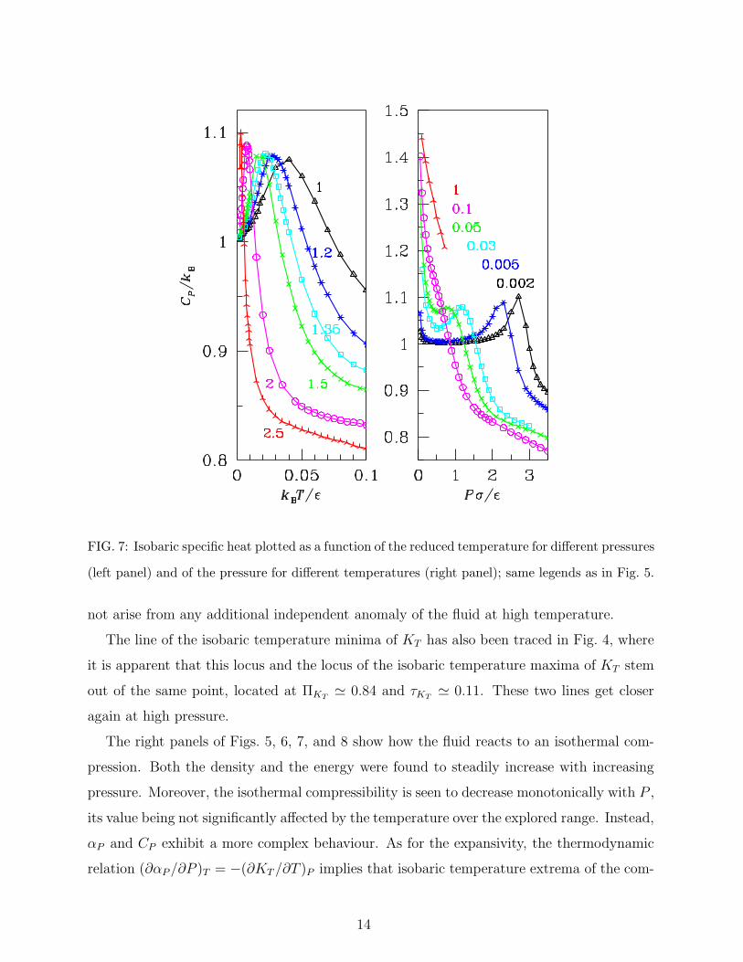
FIG. 7: Isobaric specific heat plotted as a function of the reduced temperature for different pressures
(left panel) and of the pressure for different temperatures (right panel); same legends as in Fig. 5.
not arise from any additional independent anomaly of the fluid at high temperature.
The line of the isobaric temperature minima of KT has also been traced in Fig. 4, where
it is apparent that this locus and the locus of the isobaric temperature maxima of KT stem
out of the same point, located at ΠKT≃ 0.84 and τKT
≃ 0.11. These two lines get closer
again at high pressure.
The right panels of Figs. 5, 6, 7, and 8 show how the fluid reacts to an isothermal com-
pression. Both the density and the energy were found to steadily increase with increasing
pressure. Moreover, the isothermal compressibility is seen to decrease monotonically with P ,
its value being not significantly affected by the temperature over the explored range. Instead,
αP and CP exhibit a more complex behaviour. As for the expansivity, the thermodynamic
relation (∂αP/∂P )T = −(∂KT /∂T )P implies that isobaric temperature extrema of the com-
14

FIG. 8: Isochoric specific heat plotted as a function of the reduced temperature for different
pressures (left panel) and of the pressure for different temperatures (right panel); same legends as
in Fig. 5.
pressibility should map onto isothermal pressure extrema of the expansivity [26]. In fact,
Fig. 4 shows that the isothermal pressure minima (maxima) of αP do actually fall, to within
the numerical uncertainty of the calculations, along the locus of the isobaric temperature
maxima (minima) of KT .
A maximum is also present, at low temperature, in the isobaric specific heat as a function
of P at constant T (see the right panel of Fig. 7); as expected, this quantity is 3/2 at P = 0
and, correspondingly, CV = 1/2. We found that the locus of the pressure extrema of CP runs
on top of the temperature minima locus of the expansivity (see Fig. 4). The thermodynamic
relation [27](
∂CP
∂P
)
T
= −vT
[
α2P +
(
∂αP
∂T
)
P
]
(5)
15

states that, if αP = 0, an isobaric temperature extremum of αP should coincide with an
isothermal pressure extremum of CP . This is precisely what happens at the confluence point
of the TMD and TmD lines. Elsewhere, the balance between α2P and a negative temperature
derivative of αP locates the zero of (∂CP/∂P )T at lower temperatures with respect to the
locus of vanishing (∂αP/∂T )P . However, upon moving inside the anomaly region, the first
term on the r.h.s of Eq. 5 turns out to be very small (of the order of 10−4) for pressures just
greater than ΠC, and becomes even smaller with increasing pressure because of the gradual
drop of both the volume and temperature. As a result, the pressure maxima locus of CP
runs very close to the temperature extrema loci of αP and of CP itself (see Fig. 4). This
latter circumstance, i.e., the nearby coincidence (to within the uncertainty of the present
calculations) of the pressure and temperature maxima loci of CP , can be explained by the
implicit function theorem:
(
∂X
∂P
)
T
= −(
∂X
∂T
)
P
·(
∂T
∂P
)
X
(6)
where X(P, T ) is a generic property of the system and the second partial derivative on the
r.h.s. of Eq.(6) is evaluated along a constant-X thermodynamic path. In general, whenever
X has an extremum as a function of P at given T (i.e., (∂X/∂P )T = 0), the derivative
(∂T/∂P )X , evaluated along a constant-X path, vanishes as well (a similar argument natu-
rally holds upon inverting P with T ). This obviously implies that a pressure (temperature)
extremum of X is not necessarily associated with a temperature (pressure) extremum of
the same quantity. However, it can be shown that, when X(T, P ) displays a “ridge” of
equal-height extrema, both the pressure and the temperature derivatives of X vanish there
(and vice versa), which means that the extremum is such along both thermodynamic axes.
To a very good approximation, this is actually what happens for the isobaric specific heat
of the 1D GCM fluid.
At very low temperature the peak of the isobaric specific heat is preceded by a broad
minimum, actually almost a plateau at one. This latter circumstance is explained by the
very small values attained by the quantity vTα2P/KT , which yields the difference between
CP and CV ; moreover, αP vanishes at a point located within the implicated pressure interval.
In passing, we note that CP = CV along the TMD and TmD lines.
One more aspect of this thermodynamic scenario still needs to be outlined. The volu-
metric anomaly is accompanied by an anomaly of the entropy in that, whenever αP < 0, the
16
entropy increases with P at constant temperature since (∂S/∂P )T = −(∂V/∂T )P . In order
to illustrate this aspect, we calculated the total entropy per particle of the fluid through the
Euler relation, s = β(u + Pv − µ). As for the chemical potential, given its value at some
reference state, one can calculate its value at any other state upon integrating a suitable
thermodynamic property along either an isothermal or isobaric path, under the condition
that no coexistence locus is being crossed along the path:
µ(T, P2) = µ(T, P1)−∫ P2
P1
dP v(T, P ) , (7)
µ(T2, P )
T2=
µ(T1, P )
T1−
∫ T2
T1
dT
[
u(T, P ) + Pv(T, P )
T 2
]
. (8)
Equations 7 and 8 readily follow from the Euler and Gibbs-Duhem relations. The chemical
potential at the reference thermodynamic state (a dilute-fluid state) can be estimated using
Widom’s particle-insertion method [28]. Upon performing a NVT simulation for ρ = 0.2
and τ = 0.1, we obtained the value βµ = −0.7341 at a reduced pressure of 0.0296. Using
this value as a parameter in a NPT simulation, carried out at the same temperature as in
the constant-volume simulation, we obtained the value βµ = −0.7348, which coincides with
the corresponding NVT estimate to within the statistical error of the calculation.
The left panel of Fig. 9 shows the results for the total entropy per particle of the 1D
GCM fluid. As expected, at high temperature this quantity decreases with P , because
of the increasing strength of the positional correlations, a process which typically leads to
a reduction of the number of microstates available to the system in a given macrostate.
However, as soon as the fluid enters the anomalous region, viz., when the temperature drops
below TM, the total entropy develops a minimum that is followed by a maximum at larger
pressure, a state beyond which the entropy starts decreasing again. This counterintuitive
behaviour is a direct consequence of the volumetric anomaly; correspondingly, the locations
of the two pressure extrema change with the temperature, following the TMD and TmD
lines.
The right panel of Fig. 9 shows that a minimum is also present, at lower pressure, in the
excess entropy of the fluid, Sex = S − Sid, where Sid is the entropy of an ideal gas having
the same density and temperature of the GCM fluid. However, three notable differences
show up in the thermodynamic behaviours of the excess and total entropy, respectively: i)
the minimum of the excess entropy is located at Π(sex)min ≃ 0.35 and its position does not
17

FIG. 9: Total entropy (left panel) and excess entropy (right panel) per particle plotted as a function
of the pressure for different reduced temperatures: triangles (black), τ = 0.002; stars (blue),
τ = 0.005; squares (cianide), τ = 0.03; crosses (green), τ = 0.05; circles (magenta), τ = 0.1. The
total entropy reported on the left panel does not include the additive constant ln[
2πm/(ǫh2)]1/2
;
the arrows indicate the positions of the extrema; a dotted line has been traced for Π = 0.35 in the
right panel.
appreciably shift with T over the explored range; ii) for Π > Π(sex)min the excess entropy
rises to zero and does not exhibit any other extremum; iii) the minimum persists in sex
even for T > TM. All such circumstances suggest that the pressure threshold at Π(sex)min
may be a significant indication of the existence of two markedly different structural regimes
in the fluid. We shall come back to this point in the following section. However, before
concluding this outline of the thermodynamic properties of the model, we note that the
excess entropy of the GCM fluid displays a minimum also in upper dimensions (2D, 3D).
For temperatures slightly above the maximum melting temperature, this minimum occurs
18

at a reduced density corresponding to an average interparticle distance of approximately
1.53σ, a value that is fairly congruent with the values in 1D, which range between 1.46σ
and 1.56σ as the reduced temperature rises from 0.002 to 0.1. In 2D and 3D the excess-
entropy minimum falls just beyond the density corresponding to the maximum melting
temperature, which unambiguously marks the border between two different thermodynamic
conditions: a low-density regime in which the system behaves as a normal fluid and, upon
compression, eventually freezes; a high-pressure regime in which, instead, the crystal re-
melts, with increasing pressure, into a fluid whose properties are very different from the
ordinary ones.
C. Structural properties
In this section we shall focus on the structural properties of the 1D GCM at low tempera-
ture (τ = 0.002). Upon isothermally compressing the initially dilute fluid, the local order is
more and more enhanced, and also extends to larger and larger distances. As seen in Fig. 10,
the RDF already looks highly structured at a relatively low pressure (Π = 0.05, ρ = 0.47),
showing a quasi-crystalline profile characterized by a series of sharply defined coordination
shells (each subtending an integrated conditional number density of one particle), with pe-
riod equal to the average interparticle distance and no appreciable overlap between adjacent
shells up to fairly large distances. Such a regularly equispaced arrangement is analogous to
that exhibited by a 1D gas of hard particles for packing fractions approximately larger than
83% [14], a value corresponding to a reduced density of the present model equal to 0.33 at a
reduced temperature of 0.002. In this respect, the core-softened GCM fluid matches and ex-
tends to higher densities the quasi-crystalline phase behaviour observed in the “isomorphic”
hard-core Tonks gas approaching close packing.
As expected for an ordinary simple fluid, the peaks of the RDF get, with increasing
pressure, sharper and taller; contextually, the size (R0) of the domain over which the minima
between adjacent peaks have, to practical effects, dropped to zero also expands with P . Such
a trend comes to a stop and is eventually reversed when the pressure increases to values
close to the minimum threshold discussed above for the excess entropy (see Figs. 11 and 12).
In fact, for Π ≃ 0.30, both the height of the first RDF peak as well as R0 attain a maximum
(of about 11 and 20v, respectively) and start decreasing thereon with P . Figure 13 shows
19

FIG. 10: Radial distribution function at τ = 0.002 plotted as a function of the distance between
particles, relative to their average separation at the corresponding number density, for Π = 0.05
(blue) and Π = 0.35 (red); the lower panel shows the decay of the total correlation function at
larger distances on a semilogarithmic scale.
that a similar inversion of the low-density trend is also observed in the other maxima of the
RDF at reduced pressures close to 0.35. Hence, this threshold corresponds to the maximum
growth and expansion of the local (hard-core-like) crystalline order in the fluid: in fact, for
larger pressures, we observe a global attenuation of the density correlations which reduces
the entropic distance of the fluid from its ideal-gas counterpart.
The modifications of the local density profile outlined above prelude the emergence, pro-
moted by the pressure, of a different spatial organization of the fluid. Figure 13 shows that
the larger the distance of a given coordination shell from the particle sitting at the origin,
the slower the decay of the corresponding peak height with increasing pressure. As a result,
20
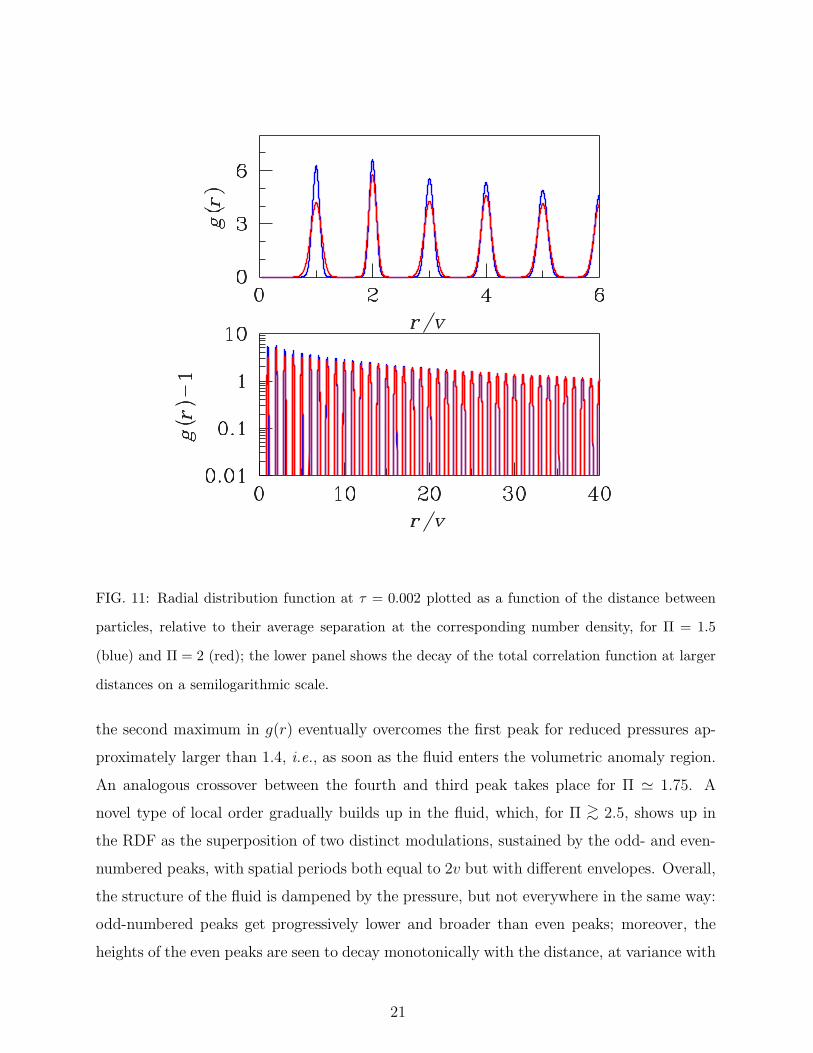
FIG. 11: Radial distribution function at τ = 0.002 plotted as a function of the distance between
particles, relative to their average separation at the corresponding number density, for Π = 1.5
(blue) and Π = 2 (red); the lower panel shows the decay of the total correlation function at larger
distances on a semilogarithmic scale.
the second maximum in g(r) eventually overcomes the first peak for reduced pressures ap-
proximately larger than 1.4, i.e., as soon as the fluid enters the volumetric anomaly region.
An analogous crossover between the fourth and third peak takes place for Π ≃ 1.75. A
novel type of local order gradually builds up in the fluid, which, for Π >∼ 2.5, shows up in
the RDF as the superposition of two distinct modulations, sustained by the odd- and even-
numbered peaks, with spatial periods both equal to 2v but with different envelopes. Overall,
the structure of the fluid is dampened by the pressure, but not everywhere in the same way:
odd-numbered peaks get progressively lower and broader than even peaks; moreover, the
heights of the even peaks are seen to decay monotonically with the distance, at variance with
21

FIG. 12: Radial distribution function at τ = 0.002 plotted as a function of the distance between
particles, relative to their average separation at the corresponding number density, for Π = 2.7
(blue) and Π = 3.5 (red); the lower panel shows the decay of the total correlation function at larger
distances on a semilogarithmic scale.
those of the odd-numbered peaks which display a maximum at some intermediate distance
Rc; this distance grows with the pressure and appears to saturate, for Π >∼ 3, to a size
corresponding to the first 12 coordination shells. For r > Rc, the two trains of oscillations
do eventually merge into one single oscillation with period v.
An indication on the nature of the new spatial organization spawned by the fluid upon
compression emerges from a typical snapshot taken at the reduced pressure Π = 3: the
presence of patches of particle pairs (“dimers”), regularly spaced with period 2v and width
of the order of Rc, is rather evident in Fig. 14. The fact that the even-numbered peaks of the
RDF are taller and sharper indicates that the average distance between successive dimers
22
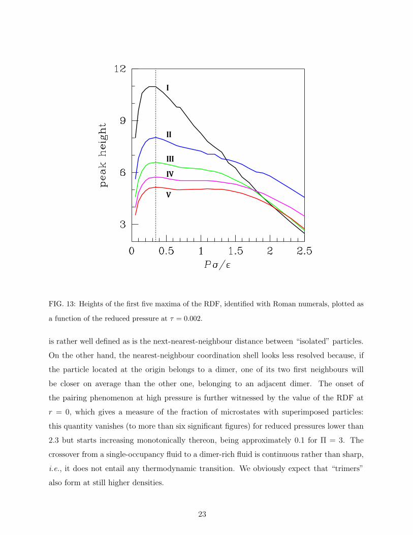
FIG. 13: Heights of the first five maxima of the RDF, identified with Roman numerals, plotted as
a function of the reduced pressure at τ = 0.002.
is rather well defined as is the next-nearest-neighbour distance between “isolated” particles.
On the other hand, the nearest-neighbour coordination shell looks less resolved because, if
the particle located at the origin belongs to a dimer, one of its two first neighbours will
be closer on average than the other one, belonging to an adjacent dimer. The onset of
the pairing phenomenon at high pressure is further witnessed by the value of the RDF at
r = 0, which gives a measure of the fraction of microstates with superimposed particles:
this quantity vanishes (to more than six significant figures) for reduced pressures lower than
2.3 but starts increasing monotonically thereon, being approximately 0.1 for Π = 3. The
crossover from a single-occupancy fluid to a dimer-rich fluid is continuous rather than sharp,
i.e., it does not entail any thermodynamic transition. We obviously expect that “trimers”
also form at still higher densities.
23
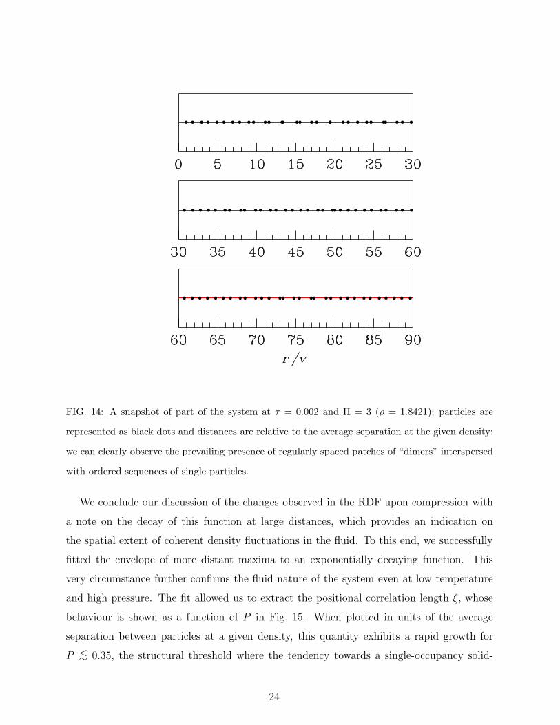
FIG. 14: A snapshot of part of the system at τ = 0.002 and Π = 3 (ρ = 1.8421); particles are
represented as black dots and distances are relative to the average separation at the given density:
we can clearly observe the prevailing presence of regularly spaced patches of “dimers” interspersed
with ordered sequences of single particles.
We conclude our discussion of the changes observed in the RDF upon compression with
a note on the decay of this function at large distances, which provides an indication on
the spatial extent of coherent density fluctuations in the fluid. To this end, we successfully
fitted the envelope of more distant maxima to an exponentially decaying function. This
very circumstance further confirms the fluid nature of the system even at low temperature
and high pressure. The fit allowed us to extract the positional correlation length ξ, whose
behaviour is shown as a function of P in Fig. 15. When plotted in units of the average
separation between particles at a given density, this quantity exhibits a rapid growth for
P <∼ 0.35, the structural threshold where the tendency towards a single-occupancy solid-
24
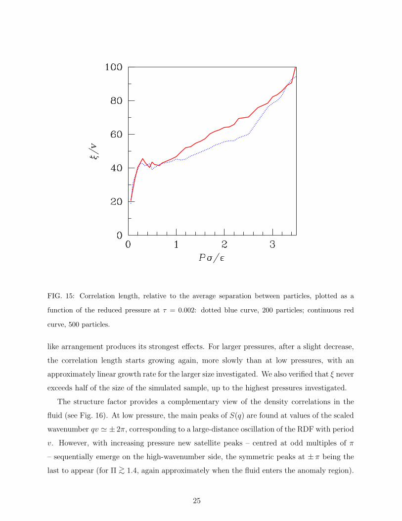
FIG. 15: Correlation length, relative to the average separation between particles, plotted as a
function of the reduced pressure at τ = 0.002: dotted blue curve, 200 particles; continuous red
curve, 500 particles.
like arrangement produces its strongest effects. For larger pressures, after a slight decrease,
the correlation length starts growing again, more slowly than at low pressures, with an
approximately linear growth rate for the larger size investigated. We also verified that ξ never
exceeds half of the size of the simulated sample, up to the highest pressures investigated.
The structure factor provides a complementary view of the density correlations in the
fluid (see Fig. 16). At low pressure, the main peaks of S(q) are found at values of the scaled
wavenumber qv ≃ ± 2π, corresponding to a large-distance oscillation of the RDF with period
v. However, with increasing pressure new satellite peaks – centred at odd multiples of π
– sequentially emerge on the high-wavenumber side, the symmetric peaks at ± π being the
last to appear (for Π >∼ 1.4, again approximately when the fluid enters the anomaly region).
25

FIG. 16: Structure factor plotted as a function of the reduced wavevector at τ = 0.002 for Π = 1
(black), 1.5 (blue), 2 (cyanide), 2.5 (green), 3 (magenta), 3.5 (red); a specular spectrum is found
for negative values of the wavevector. The dotted vertical lines lie in correspondence to the first
four multiples of π.
Such additional maxima initially concur to modify the profile of the first coordination shell
in the RDF, the more so the larger the pressure. However, the increasing relevance of the
peaks at ± π, which eventually overcome in height the peaks at ± 3π for reduced pressures
close to 3, also signals the emergence of an additional spatial modulation in the local density
profile, with period 2v.
26
IV. CONCLUDING REMARKS
In this paper we have illustrated the equilibrium properties of a model system of particles
interacting, in one dimension, through a bounded repulsive potential with a Gaussian shape.
The study of the model was largely carried out using numerical sampling techniques based
on the Monte Carlo method.
As far as the thermodynamic phase stability of the model is concerned, no indication
emerged from our analysis of any singular behaviour possibly associated with a fluid-solid or
solid-solid transition. However, this very circumstance allowed us to carry out a thorough
study of the unexpectedly complex behaviour of the Gaussian-core model fluid in one di-
mension, all the way from high to low temperatures, without incurring any “break” caused
by phase changes. As a result, we could highlight the full thermal unfolding of a volumet-
ric anomaly – i.e., the increase of the density upon isobarically heating the system – as a
function of pressure, with the emergence of both a maximum and a minimum of the density
with decreasing temperature. While the existence of a maximum in the density of the model
had already been observed both in three and two dimensions, evidence of the existence of
a minimum, at lower temperature and under appropriate pressure conditions, has never
been reported and is being provided here, for the first time, for the one-dimensional fluid.
This feature is more unusual than the maximum itself and has been recently observed in
metastable states of real substances, most notably in confined supercooled water.
In the light of such findings, we can safely conclude that a soft bounded repulsion like that
modelled with a bare Gaussian potential, devoid of any additional repulsive or attractive
component, possesses the “minimal” requisites that make it possible for the fluid to exhibit
waterlike anomalies even in a one-dimensional hosting space. Sadr-Lahijany and cowork-
ers [29] had already described the nonstandard thermodynamic properties that emerge from
a core-softened potential, explicitly designed to mimic the effect of hydrogen bonding: a re-
pulsion with two length scales set by a hard core and by a finite negative shoulder, followed
at larger distances by an attractive well. In this respect, the main result of this paper is that
definitely much less is needed to “turn on” a volumetric anomaly, even in a one-dimensional
fluid: in fact, a finite softened repulsion, modelled as a one-scale potential with a downward
concavity at short distances and an upward one at larger distances, is sufficient to generate
the density anomaly, also bounded by two temperature extrema, as well as a cascade of
27

related peculiarities in all of the three thermodynamic response functions.
Crucial for the thermodynamic onset of the volumetric anomaly in the currently inves-
tigated model is the average separation between particles at a given pressure: in fact, we
may conjecture that, if such a distance is smaller than the distance r0 = σ/√2 where the
concavity of the Gaussian potential changes from upward to downward, the density will grow
upon isobarically heating the fluid even at zero temperature, because the particles will find
it (thermodynamically) more advantageous to reduce their average mutual distance, since
this will ultimately entail a significant gain in the entropy of the fluid which overcomes the
corresponding increase of internal energy. Such a “marginal” condition corresponds to a
threshold density ρ0 =√2 which, in the ordered ground state formed by equally spaced
particles, is attained with a reduced pressure Π0 ≃ 1.77. Indeed, a similar mechanism is at
work in liquid water, in which the breaking of hydrogen bonds, with their hybrid attractive
and repulsive nature [30], produces a gradual “collapse” of nearest-neighbour molecules in-
side the inner region of close-contact distances, with a corresponding increase of the density
upon heating.
On the other hand, we can also presume that, if the average separation between particles
is larger than r0, the density of the fluid will initially decrease upon heating the system from
a state at T = 0 (because the energy decreases as well) until the particles acquire enough
kinetic energy to sample the inner region of the potential and thus discover that they may
exploit there a more favourable condition, leading to an inversion of the density trend as
a function of T . On this basis, we may then expect that for Π < Π0, and for not too low
pressures, the anomalous region is bounded from below by a nonzero temperature at which
the density shows a minimum.
The investigation of the structural properties of the model also revealed an interesting and
unusual scenario. Two structural regimes were distinguished in the equilibrium behaviour of
the 1D GCM: for reduced pressures lower than 0.35, the system behaves as a “normal” fluid
in that the local order is progressively enhanced by an isothermal compression. Instead,
upon trespassing the above threshold, a further increase of the pressure induces an overall
attenuation of density correlations, an effect associated with the bounded nature of the
repulsion. However, the ensuing approach of the system to the thermodynamic condition
of an “infinite-density ideal gas” is accompanied by the emergence of a new type of local
order, with pairs of almost superimposed particles giving rise to extended quasi-crystalline
28

clusters of “dimers”. This phenomenon is clearly resolved in the radial distribution function
as an extra modulation, which is also signalled by the appearance of satellite peaks in the
structure factor at relative wavenumbers equal to odd multiples of π.
Acknowledgments
One of the authors (PVG) wishes to thank Professor Luciano Reatto – to whom this paper
is presented as a homage for this special issue in his honour – for his long-lasting friendship,
which has accompanied the author across the years. Luciano has always been a guide and an
inspiring example, not only for his wide and acknowledged scientific competences but also
for his severe and demanding attitude towards academic research, as well as for his enduring
service to the Italian condensed-matter-physics community.
[1] X. Xu, B. Lin, B. Cui, A. R. Dinner, and S. A. Rice, J. Chem. Phys. 132, 084902 (2010).
[2] S. Herrera-Velarde, A. Zamudio-Ojeda, and R. Castaneda-Priego, J. Chem. Phys. 133, 114902
(2010).
[3] L. van Hove, Physica 16, 137 (1950).
[4] J. A. Cuesta and A, Sanchez, J. Stat. Phys. 115, 869 (2004).
[5] C. Marquest and T. A. Witten, J. Phys. (France) 50, 1267 (1989).
[6] A. Malijevsky and A. Santos, J. Chem. Phys. 124, 074508 (2006).
[7] L. Tonks, Phys. Rev. 50, 955 (1936).
[8] R. Fantoni, J. Stat. Mech., P07030 (2010).
[9] A. Santos, R. Fantoni and A. Giacometti, Phys. Rev. E 77, 051206 (2008).
[10] F. H. Stillinger, J. Chem. Phys. 65, 3968 (1976).
[11] C. N. Likos, Phys. Reports 348, 267 (2001).
[12] S. Prestipino, F. Saija, and P. V. Giaquinta, Phys. Rev. E 71, 050102(R) (2005).
[13] S. Prestipino, F. Saija, and P. V. Giaquinta, Phys. Rev. Lett. 106, 235701 (2011).
[14] P. V. Giaquinta, Entropy 10, 248 (2008).
[15] P. G. Debenedetti, V. S. Raghavan, and S. S. Borick, J. Phys. Chem. B 95, 4540 (1991).
[16] F. H. Stillinger and T. A. Weber, J. Chem. Phys. 68, 3837 (1978); 69, 4322 (1978); 70, 1074
29
(1979).
[17] A. Lang, C. N. Likos, M. Watzlawek, and H. Lowen, J. Phys.: Condens. Matter 12, 5087
(2000).
[18] Y. Tscuchiya, J. Phys.: Condens. Matter 3, 3163 (1991).
[19] Y. Tscuchiya, J. Phys.: Condens. Matter 4, 4335 (1992).
[20] D. Liu, Y. Zhang, C.-C. Chen, C.-Y. Mou, P. H. Poole, and S.-H. Chen, Proc. Natl. Acad.
Sci. USA 104, 9570 (2007).
[21] Y. Zhang, A. Faraone, W. K. Kamitakahara, K.-H. Liu, C.-Y. Mou, J. B. Leao, S. Chang,
and S.-H. Chen, arXiv:1005.5387v3 [cond-mat.soft].
[22] F. Mallamace, P. Baglioni, C. Corsaro, J. Spooren, H. E. Stanley, and S.-H. Chen, Riv. N.
Cimento 34, 2011 (2011).
[23] P. H. Poole, I. Saika-Voivod, and F. Sciortino, J. Phys.: Condens. Matter 17, L431 (2005).
[24] A. Angell, Nature Nanotech. 2, 396 (2007).
[25] S. Sastry, P. G. Debenedetti, F. Sciortino, and H. E. Stanley, Phys. Rev. E 53, 6144 (1996).
[26] L. P. N. Rebelo, P. G. Debenedetti, and S. Sastry, J. Chem. Phys. 109, 626 (1998).
[27] H. B. Callen, Thermodynamics and an Introduction to Thermostatistics (John Wiley and Sons,
New York, 1985), second edition.
[28] B. Widom, J. Chem. Phys. 39, 2808 (1963).
[29] M. R. Sadr-Lahijany, A. Scala, S. V. Buldyrev, and H.. E. Stanley, Phys. Rev. E 60, 6714
(1999).
[30] M. J. Blandamer, J. Burgess, and J. B. F. N. Engberts, Chem. Soc. Rev. 14, 237 (1985); M. J.
Blandamer, J. Burgess, and A. W. Hakin, J. Chem. Soc., Faraday Trans. 1 83, 1783 (1987).
30
Related Documents