Thermochemical Behaviour and Syngas Production from Co ...

Thermochemical Behaviour and Syngas Production from Co-gasification of Biomass and Coal Blends

Author

Vhathvarothai, Navirin

Published

2013

Thesis Type

Thesis (PhD Doctorate)

School

Griffith School of Engineering

DOI

https://doi.org/10.25904/1912/850

Copyright Statement

The author owns the copyright in this thesis, unless stated otherwise.

Downloaded from

http://hdl.handle.net/10072/367479

Griffith Research Online

https://research-repository.griffith.edu.au

Thermochemical Behaviour and Syngas Production

from Co-gasification of Biomass and Coal Blends

Navirin Vhathvarothai

B. Eng., M. Eng.

Submitted in fulfilment of the requirements of the degree of

Doctor of Philosophy

Griffith School of Engineering

Science, Environment, Engineering and Technology

Griffith University, Queensland, Australia

May 2013

i

Abstract

This research project investigated the thermochemical behaviour of biomass (cypress

wood chips and macadamia nut shells), coal (Australian bituminous coal) and their

blends during pyrolysis and combustion using thermogravimetric analysis (TGA) as well

as studied the syngas production from gasification of the fuels and their blends at

blending ratios (biomass:coal) of 95:5, 90:10, 85:15 and 80:20 on a laboratory scale

downdraft gasifier. The key aims of the research were to study the influence of the

blending ratios on the performances of the thermochemical processes and to develop

a mathematical model that can be used for predicting the results of the co-gasification

technology.

The results from the proximate and ultimate analyses found that cypress wood chips

and macadamia nut shells had relatively similar approximate composition and absolute

elemental composition. However, major differences between these two types of

biomass and the Australian bituminous coal were observed in several properties

including volatile matter, fixed carbon, carbon content and oxygen content.

The biomass, coal and their blends at the four blending ratios were pyrolysed under a

nitrogen environment at four different heating rates comprising 5, 10, 15 and 20 °C per

minute to investigate their pyrolytic behaviour and to determine kinetic parameters of

thermochemical decomposition through Kissinger’s corrected kinetic equation using

the TGA results. The activation energy of both types of biomass was less than that of

coal, being 168.7 (cypress wood chips), 164.6 (macadamia nut shells) and 199.6

(Australian bituminous coal) kJ/mol. The activation energy of the blends of biomass

and coal followed that of the weighted average of the individual samples in the blends.

Char production of the samples and the blends was also analysed to observe any

synergetic effects and thermochemical interaction between biomass and coal. The

char production of the blends corresponded to the sum of the results for the individual

samples with the coefficient of determination of 0.999. The TGA analysis of the

samples and the blends under an air environment was also carried out to investigate

their thermochemical behaviour during combustion. Similar trends of results of

ii

thermochemical decomposition during combustion of the samples and the blends

were found as compared to during pyrolysis. There was no evidence for any significant

synergetic effects and thermochemical interaction between either type of biomass and

coal during pyrolysis and combustion. Thermochemical decomposition of biomass and

coal appeared to take place independently and thus the activation energy of the

blends can be calculated from that of the two components.

Gasification of biomass and co-gasification of biomass as a primary fuel and coal as a

supplementary fuel were run on a laboratory-scale downdraft gasifier using air as a

gasifying agent. The quality of the syngas was analysed in terms of its composition

using the Gas Chromatography Mass Spectrometry (GCMS) analytical methods,

combustibility (total combustible gas, TCG) and energy content (HHV and LHV).

Gasification of cypress wood chips and macadamia nut shells yielded the syngas with

relatively similar quality with the average total combustible gas of 10.2 and 10.6%,

mainly due to the similarity in their properties. Although thermochemical processes of

the biomass and coal samples occurred individually, improvement in the quality of the

syngas was observed in the co-gasification of biomass and coal, yielding the syngas

with the average total combustible gas of 20.5% in the blends of both types of biomass

with the highest ratio of coal (20%). The plots of the blending ratio of biomass to coal

and the syngas quality (TCG, HHV and LHV) also showed linear relationships with the

coefficient of determination of 0.951 and 0.992, respectively. The linear relationships

indicated that properties of a fuel, especially its carbon content, have a direct effect on

the composition of the final product of the gasification process. The lack of synergy

suggested that coal can be blended with biomass at any blending ratio for use in

thermochemical conversion systems.

A neural network model was developed to predict the quality of the syngas produced

from gasification and co-gasification of the biomass and coal fuels using their carbon

content, hydrogen content and oxygen content as the input data and the percentage

of TCG in the syngas as the target data. The feed forward backpropagation neural

network model developed was suitable for predicting the syngas quality produced

from the process under these particular experimental conditions.

iii

Statement of Originality

This work has not previously been submitted for a degree or diploma in any university.

To the best of my knowledge and belief, the thesis contains no material previously

published or written by another person except where due reference is made in the

thesis itself.

(Signed)_____________________________

Navirin Vhathvarothai

iv

Table of Contents

Abstract ..................................................................................................................... i

Statement of Originality ................................................................................................... iii

Table of Contents ............................................................................................................. iv

List of Figures ................................................................................................................... vi

List of Tables ................................................................................................................... ix

List of Symbols and Acronyms .......................................................................................... xi

Acknowledgment ............................................................................................................ xiii

Publications arising from this work ................................................................................ xiv

1. Introduction ................................................................................................................ 1

2. Literature review ........................................................................................................ 4

2.1 Biomass and coal as fuels ............................................................ 4

2.2 Biomass conversion technologies .............................................. 16

2.3 Gasification system and syngas production .............................. 19

2.4 Application of gasification technology ...................................... 33

2.5 Co-gasification technology ........................................................ 38

2.6 Thermogravimetric analysis (TGA) studies ................................ 42

2.7 Kinetics in thermal analysis ....................................................... 44

2.8 Artificial neural network models ............................................... 45

2.9 Economics of power generation from gasification .................... 56

2.10 Summary of literature review .................................................... 59

3. Objectives and scope of the study ........................................................................... 63

3.1 Objectives .................................................................................. 63

3.2 Scope of the study ..................................................................... 63

4. Materials and methods ............................................................................................ 65

4.1 Materials .................................................................................... 67

4.2 Sample preparation ................................................................... 70

4.3 Instruments and apparatus ....................................................... 72

4.4 Analytical methods and experimental procedures ................... 80

v

5. Properties of fuels .................................................................................................... 93

5.1 Proximate analysis and ultimate analysis .................................. 93

5.2 Determination of heating values of fuels .................................. 95

5.3 Summary .................................................................................... 97

6. Investigation of thermochemical behaviour of biomass and coal using TGA .......... 99

6.1 Pyrolysis behaviour .................................................................... 99

6.2 Combustion behaviour ............................................................ 111

6.3 Summary .................................................................................. 122

7. Investigation of gasification and co-gasification in a downdraft gasifier .............. 124

7.1 Gasification process and control ............................................. 124

7.2 Gasification products ............................................................... 126

7.3 Results of the syngas analysis .................................................. 126

7.4 Summary .................................................................................. 135

8. Development of syngas production model using neural network ......................... 138

8.1 Selection of data ...................................................................... 138

8.2 Design of the neural network model ....................................... 140

8.3 Performance of the neural network model ............................. 143

8.4 Summary .................................................................................. 146

9. Financial analysis of two sizes of small scale gasification plants ........................... 148

9.1 Investment analysis ................................................................. 148

9.2 Sensitivity analysis ................................................................... 151

9.3 Discussion on the investment opportunity ............................. 152

9.4 Summary .................................................................................. 153

10. Conclusions ............................................................................................................. 154

References ................................................................................................................ 158

Appendix A ................................................................................................................ 184

Appendix B ................................................................................................................ 191

Appendix C ................................................................................................................ 198

Appendix D ................................................................................................................ 206

Appendix E ................................................................................................................ 211

vi

List of Figures

Figure 2–1: Van Krevelen diagram (Van Krevelen 1993) ................................................... 8

Figure 2–2: HHV and LHV of biomass against moisture content (Quaak et al. 1999)....... 9

Figure 2–3: Primary energy supply by fuel in 2009 (IEA 2011) ....................................... 10

Figure 2–4: Biomass gasification process chart ............................................................... 18

Figure 2–5: Updraft and downdraft gasifiers (All Power Labs 2010) .............................. 21

Figure 2–6: Diagram of a basic fluidised bed gasifier (FAO 1986) ................................... 22

Figure 2–7: A simple illustration of a biological neuron (Kalogirou 2007) ...................... 46

Figure 2–8: An artificial neuron ....................................................................................... 47

Figure 2–9: One hidden layer feed forward network ...................................................... 48

Figure 2–10: Common transfer functions (MathWorks 2012) ........................................ 50

Figure 4–1: Cypress wood chips (Redback Garden Centre 2012) ................................... 68

Figure 4–2: Macadamia nut shells obtained from Hidden Valley Plantations ................ 69

Figure 4–3: Bituminous coal obtained from the Swanbank Power Station .................... 70

Figure 4–4: The measuring part and its cross sectional image (Netzsch 2010) .............. 72

Figure 4–5: The downdraft fixed bed gasifier unit (All Power Labs 2010) ...................... 74

Figure 4–6: The CAD drawing of the downdraft reactor (All Power Labs 2010) ............. 75

Figure 4–7: Agilent 6890 GC with 5973 MSD (Agilent Technologies 2001) .................... 77

Figure 4–8: ThermoStar GSD 301 T Mass Spectrometer (ALT Inc 2011) ......................... 79

Figure 4–9: Flow chart to create a baseline (Netzsch 2010) ........................................... 82

Figure 4–10: Flow chart to perform a TGA measurement (Netzsch 2010) ..................... 83

Figure 4–11: Schematic of the operation of the gasification unit ................................... 84

Figure 4–12: Schematic of the injector with septum purge (Chasteen 2000) ................ 87

Figure 4–13: Process flow for developing a neural network ........................................... 91

Figure 5–1: Elemental distribution of the samples ......................................................... 95

Figure 6–1: TG curves of the samples under N2 at 10 °C min-1 ..................................... 100

Figure 6–2: DTG curves of the samples under N2 at 10 °C min-1 ................................... 102

Figure 6–3: TG curves of wood chips and coal blends under N2 at 10 °C min-1 ............ 103

Figure 6–4: TG curves of nut shells and coal blends under N2 at 10 °C min-1 ............... 103

vii

Figure 6–5: DTG curves of wood chips and coal blends under N2 at 10 °C min-1 .......... 104

Figure 6–6: DTG curves of nut shells and coal blends under N2 at 10 °C min-1 ............. 104

Figure 6–7: Char yield of wood chips, coal and their blends at 10 °C min-1 .................. 105

Figure 6–8: Char yield of nut shells, coal and their blends at 10 °C min-1 ..................... 106

Figure 6–9: TG curves of 90 % wood chips and 10% coal blends under N2 .................. 107

Figure 6–10: TG curves of 90 % nut shells and 10% coal blends under N2 ................... 107

Figure 6–11: DTG curves of 90 % wood chips and 10% coal blends under N2 .............. 108

Figure 6–12: DTG curves of 90 % nut shells and 10% coals blends under N2 ............... 108

Figure 6–13: Ea of wood chips, coal and their blends during pyrolysis ......................... 110

Figure 6–14: Ea of nut shells, coal and their blends during pyrolysis ............................ 110

Figure 6–15: TG curves of the samples under air at 10 °C min-1 ................................... 112

Figure 6–16: DTG curves of the samples under air at 10 °C min-1 ................................ 113

Figure 6–17: TG curves of wood chips and coal blends under air at 10 °C min-1 .......... 114

Figure 6–18: TG curves of nut shells and coal blends under air at 10 °C min-1 ............. 114

Figure 6–19: DTG curves of wood chips and coal blends under air at 10 °C min-1 ....... 115

Figure 6–20: DTG curves of nut shells and coal blends under air at 10 °C min-1 .......... 116

Figure 6–21: T50 and R50 of wood and coal blends under air at 10 °C min-1.................. 116

Figure 6–22: T50 and R50 of nut shells and coal blends under air at 10 °C min-1 ........... 117

Figure 6–23: TG curves of 90 % wood chips and 10% coal blends under air ................ 118

Figure 6–24: TG curves of 90 % nut shells and 10% coal blends under air ................... 118

Figure 6–25: DTG curves of 90 % wood chips and 10% coal blends under air .............. 119

Figure 6–26: DTG curves of 90 % nut shells and 10% coal blends under air ................. 119

Figure 6–27: Ea of wood chips, coals and the blends during combustion ..................... 121

Figure 6–28: Ea of nut shells, coals and the blends during combustion........................ 121

Figure 7–1: The carbon monoxide calibration curve ..................................................... 127

Figure 7–2: Trends of average nitrogen content in the syngas ..................................... 129

Figure 7–3: Syngas composition from wood chips and their blends with coal ............. 130

Figure 7–4: Syngas composition from nut shells and their blends with coal ................ 131

Figure 7–5: Relationship between ratio of biomass to coal and average TCG ............. 132

Figure 7–6: Relationship between ratio of biomass to coal and average HHV ............. 135

viii

Figure 7–7: Relationship between ratio of biomass to coal and average LHV ............. 135

Figure 8–1: Schematic diagram of the feed forward neural network ........................... 140

Figure 8–2: The neural network diagram generated from MATLAB ............................. 143

Figure 8–3: The neural network training obtained from MATLAB ................................ 144

Figure 8–4: Regression plots of the neural network ..................................................... 146

ix

List of Tables

Table 2–1: Proximate analysis, ultimate analysis and heating value of some fuels ......... 6

Table 2–2: Comparison between characteristics of fixed and fluidised bed gasifiers .... 20

Table 2–3: Operating parameters in support of maximum gasification results ............. 24

Table 2–4: Key advantages and disadvantages of different gasifying agents ................. 26

Table 2–5: Main chemical reactions occurring in the gasification process ..................... 28

Table 2–6: Contaminants in syngas produced from the gasification process ................. 30

Table 2–7: Production of transport fuel synthesis .......................................................... 35

Table 2–8: Production of chemical synthesis .................................................................. 36

Table 2–9: Approximate capital costs of medium sized gasification system .................. 57

Table 4–1: Experimental variables for the study of thermochemical behaviour ............ 65

Table 4–2: Experimental variables for the study of syngas production .......................... 66

Table 4–3: Capabilities of the Agilent 6890 GC oven ...................................................... 77

Table 4–4: Lists of the main measuring and sampling apparatus ................................... 80

Table 4–5: Methods and instruments used to analyse composition of the syngas ........ 88

Table 4–6: Control parameters of the GC instrument for carbon monoxide analysis .... 89

Table 5–1: Proximate and ultimate analyses of the biomass and coal samples ............. 93

Table 5–2: HHV (dry basis) and LHV (as-fired) of the samples ........................................ 96

Table 5–3: HHV and LHV of the individual samples and their blends ............................. 97

Table 6–1: Cumulative mass loss of the samples during pyrolysis................................ 101

Table 6–2: Thermokinetic analysis during pyrolysis and co-pyrolysis ........................... 109

Table 6–3: Cumulative mass loss of the samples during combustion .......................... 112

Table 6–4: Thermokinetic analysis during combustion and co-combustion ................ 120

Table 7–1: Key variables measured from the gasification process ............................... 125

Table 7–2: Average syngas composition from wood chips and the blends with coal .. 127

Table 7–3: Average syngas composition from nut shell and the blends with coal ....... 128

Table7–4: Average TCG of the syngas produced from gasification .............................. 132

Table 7–5: HHV and LHV of carbon dioxide, hydrogen and methane ........................... 133

Table 7–6: Average HHV and LHV of the syngas produced from different ratios ......... 134

x

Table 8–1: Characteristics of variables for developing the nueral network model ...... 139

Table 8–2: Performance of the neural network as assessed by MSE and R ................. 145

Table 9–1: Variables used in the investment analysis model ....................................... 149

Table 9–2: Results of the investment analysis model ................................................... 150

Table 9–3: Results of the sensitivity analysis ................................................................ 151

xi

List of Symbols and Acronyms

A Pre-exponential factor

adb air-dried basis

ANN Artificial neural network

APR Annual Percentage Rate

b bias value of the neuron

BIGCC Biomass Integrated Gasification Combined Cycle

CAD Computer Aided Design

CHP Combined Heat and Power

db dry basis

daf dry ash-free basis

DME Dimethyl Ether

DTG Differential Thermal Gravimetry

Ea Activation energy

Eave Average activation energy

EBITDA Earnings before Interest, Taxes, Depreciation and Amortisation

ESP electrostatic filters

FC Fixed Carbon

f(α) The kinetic model

GC Gas Chromatograph

GUIs Graphical User Interfaces

HHV Higher Heating Value

HRSG Heat Recovery Steam Generator

ID Inner Diameter

IGCC Integrated Gasification Combined Cycle

IRR Internal Rate of Return

LHV Lower Heating Value

M Moisture content

MARR Minimum Acceptable Rate of Return

MS Mass Spectrometry

xii

MSE Mean Squared Error

MSD Mass Selective Detector

MSW Municipal Solid Waste

NPV Net Present Value

O&M Operation and Maintenance

p input of the neuron

PB Payback Period

R regression R value

The universal gas constant

R2 Coefficient of determination

R50 The intensity of mass loss at T50

SCR Selective Catalytic Reduction

SIM Selected Ion Monitoring

SNG Synthesis Natural Gas

Syx standard error of the estimate

T The absolute temperature

T50 The temperature at the degree of 50% mass loss

Tm Peak temperature

TCG Total Combustible Gas

TGA Thermogravimetric analysis

THB Thai Baht

VM Volatile Matter

W connection weight

mean

Yi mole fraction of chemical compound i

Zi mass factions of substance i

α The extent of conversion

β The linear heating rate

standard deviation

xiii

Acknowledgment

I would like to express my acknowledgement in the support of my supervisors,

scientific officers at Griffith University, as well as my family and friends.

First of all, I am grateful to my principal supervisor, Dr Jim Ness, for supporting my

research, for providing valuable guidance and for allowing me to grow as a research

engineer. I would also like to thank my co-supervisor, Dr Jimmy Yu, for the good

advice, encouragement and friendship.

I would like to acknowledge the technical support of the University and its staff,

particularly Mr Rene Diocares, Mr Radoslaw Bak and Mr Scott Byrnes. I am also

thankful to all who directly or indirectly helped me in this venture. Last but not least, I

wish to place on record my deep gratitude to my family and friends for their unceasing

support throughout the entire process.

xiv

Publications arising from this work

Vhathvarothai, N., Ness, J., & Yu, J. (2013). An investigation of the thermal behaviour of

biomass and coal during co-combustion using thermogravimetric analysis (TGA).

International Journal of Energy Research, Published online in Wiley Online Library, DOI:

10.1002/er.3083

Vhathvarothai, N., Ness, J., & Yu, J. (2013). An investigation of the thermal behaviour of

biomass and coal during co-pyrolysis using thermogravimetric analysis (TGA).

International Journal of Energy Research, Published online in Wiley Online Library, DOI:

10.1002/er.3120

1

Chapter 1

Introduction

The energy sectors worldwide have faced immense challenges resulting from the

increase in energy consumption and the decrease in availability of fuels (IEA, 2011). For

that reason, the utilisation of biomass fuels has prominently gained interest over the

past two decades. Biomass is basically referred to as biological substances derived

from organisms and/or their wastes. A broad variety of types of biomass fuels have

been used around the world (Bassam, 2010; Callé, 2007; Chen and Kuo, 2010;

Demirbas and Demirbas, 2007; McKendry, 2002a, Seo et al., 2010), currently

accounting for 10.2% of primary energy supply worldwide (IEA, 2010). Biomass fuels,

as a renewable energy resource, have proved to contribute to increasing energy supply

security owing to their widely dispersed availability, decreasing the dependency on

fossil fuels, as well as offering opportunities for mitigating greenhouse gases, acid rain

and global warming to protect the environment (Demirbas et al., 2009; EGAT, 2011;

Hall and House, 1995; Hall and Scrase, 1998; Sims, 2004; Timmons and Mejía, 2010).

As the global demand for energy has continued to grow; biomass can provide a great

potential to be a key alternative for renewable energy supply today and in the future.

Technologies to convert biomass fuels into usable forms of energy can be categorised

into two principal types which comprise biochemical conversion and thermochemical

conversion. Technologies for biochemical conversion consist primarily of anaerobic

digestion and fermentation while thermochemical conversion technologies are

composed of pyrolysis, combustion and gasification (Balat et al., 2009; Bridgwater,

2003; Evans et al., 2010; Kirkels and Verbong, 2011; Kirubakaran et al., 2009;

McKendry, 2002b; Speight et al., 2011; Zhang and Champagne, 2010). These

conversion technologies can be promising ways for energy generation from biomass

fuels. However, the choice of conversion technology is driven by several factors, in

particular the type of energy needed and the type of biomass available. Gasification is

regarded as one of the most efficient technologies to convert biomass fuels into

energy for a number of applications. Syngas produced from the gasification process

can be used for generating heat and/or electricity or can be further extracted to

2

provide energy services such as synthetic fuels and chemicals (Bassam, 2010; Callé,

2007; Chen and Kuo, 2010; Demirbas and Demirbas, 2007; Seo, et al. 2010).

The development and utilisation of biomass gasification technology have progressed

extensively in recent years; as a result, many types of biomass gasification

configurations and systems have been available for both experimental and commercial

purposes (Bauen et al., 2004; Kirubakaran et al., 2009; McKendry, 2002b). Although

biomass is sustainable and carbon neutral, it is not an ideal fuel for the gasification

process due to some of its properties. It is clear that almost any solid carbonaceous

fuels including biomass, lignite, as well as other grades of coal can be gasified under

certain conditions. However, not all of those fuels can give rise to successful

gasification which is a complex process involving a range of chemical and physical sub-

processes. This is in view of the fact that chemical and physical properties of fuels have

a significant influence on the gasification process as well as the gasification outcome

(Bridgwater, 2003; Brown and Stevens, 2011; McGowan, 2009; Obernberger et al.

2006). Research and practice have therefore continued to come up with a wide range

of approaches to enhance the performance of biomass gasification systems.

Co-gasification is an interesting, cost effective and practical approach that can be

applied to improve biomass gasification performance. It is a technique to

simultaneously gasify two or more types of fuels in the same gasifier (Kumabe et al.,

2007; Li et al., 2010; Ricketts et al., 2002). Adding coal to biomass gasification can be

expected to promote the syngas production. This is because coal generally has more

suitable properties for gasification than biomass fuels. Under proper operating

conditions, co-gasification can not only enhance thermochemical performance but also

increase availability of fuels. However, most of the reported research and practice

have extensively studied coal-based co-gasification in existing coal gasification systems

with additions of biomass fuels at low mass ratios so as to introduce sustainable fuels

into the systems (Hayter et al., 2004; Kumabe et al., 2007; Pan et al., 2000; Veijonen et

al., 2003; Winslow et al., 1996; Zulfiqar et al., 2006). There is still an absence of reliable

studies on co-gasification of biomass as a primary fuel and coal as a supplementary

3

fuel. To fill the knowledge gap, this research focuses on studying biomass based co-

gasification in the context of gasification processes and outcomes.

One of the keys to successful gasification is to understand the thermochemical

behaviour of fuels fed to the system and how that behaviour is affected by the fuel’s

chemical and physical properties. In most cases, the properties of biomass fuels are

relatively different from that of typical coals (Jenkins et al., 1998; Patel and Gami,

2012; van Krevelen, 1993). This tends to result in different behaviours during

thermochemical processes. Co-utilisation of two different types of fuels may or may

not have desirable or anticipated effects on the process. It is accordingly important to

investigate the influence of properties of both biomass and coal on the co-gasification

performance in an attempt to bring in favourable blends of the subsidies. This research

accordingly seeks to understand thermochemical behaviour of selected types of

biomass, coal and their blends during pyrolysis and combustion processes using

thermogravimetric analysis and a kinetic study.

Moreover, different properties of fuels normally lead to different contents of the

syngas produced. It is therefore important to analyse co-gasification performance in

terms of quality and energy value of the syngas produced from the co-gasification of

biomass and coal at low blending ratios of coal (up to 20%). The study also constructs a

co-gasification model to determine the correlation between properties of different

fuels and the syngas quality using an artificial neural network methodology. Artificial

neural networks, which have been successfully used in a wide range of applications,

have the ability to organise dispersed data and recognise non-linear relationships.

Aside from increasing the availability of fuels for energy production to supply the

global growing demand, co-gasification with biomass as a primary fuel and coal as a

supplementary fuel proposes an alternative to improve the energy result. Significant

advances can be made in biomass based co-gasification in order to bring a contribution

to energy generation while maintaining greenhouse gas emissions within acceptable

levels.

4

Chapter 2

Literature review

2.1 Biomass and coal as fuels

2.1.1 Properties of biomass and coal

Biomass is referred to as biological substances derived from organisms and/or their

wastes (Callé, 2007; van Loo and Koppejan, 2012). It comes in a variety of fuel types

such as wood products, short-rotation plants, aquatic plants, algae, agricultural wastes,

animal wastes, industrial waste and municipal solid waste (Demirbas, 2004; Jenkins et

al., 1998). However, the diversity of biomass resources makes it difficult to forecast

thermochemical characteristics, compositions of products and their emissions, as well

as energy outputs. Biomass fuels may have undesirable or unanticipated impacts on

thermochemical conversion processes. Knowing parameters that affect process

performance is considered necessary in the utilisation of biomass as a fuel for energy

production.

Coal, on the other hand, is a combustible carbonaceous substance. Basically coal was

formed through the process of coalification that converted organic matters, mainly

vegetation, to coal by various amounts of heat and pressure over hundreds of millions

of years. Coal is composed mainly of rings of six carbon atoms bonded together in a

very complex composition. Based on a number of chemical and physical factors, coals

can be typically classified into four rankings which consist of lignite, subbituminous

coal, bituminous coal and anthracite. Lignite and sub-bituminous coal are regarded as

low rank coals which contain lower carbon content and lower energy content as

compared to bituminous coal and anthracite which are high rank coals. Coal is also

diverse in its composition even among the same deposit (Stracher et al., 2011). Even

though coal is often referred to as a valuable source of fuel due to its high energy

value, its drawbacks still present such as a finite supply of the resource, extensive

concern about environmental emissions and high amount of incombustible material

remaining (Collot, 2006; Minchener, 2005; Prins et al., 2004). Thus, it is very important

5

to understand properties of biomass and coal relevant to the thermochemical

conversion processes in order to utilise them effectively and avoid possible problems.

Thermochemical processes of carbonaceous fuels depend not only on the operating

conditions but also on the properties of the fuels (Chen et al., 2003; Kirubakaran et al.,

2009; Quaak et al., 1999; Tinaut et al., 2008; Zulfiqar et al., 2006). This is because

physical characteristics and chemical compositions of fuels have a significant influence

on gasification which has a number of thermochemical sub-processes (Demirbas, 2003;

Obernberger et al. 2006; Prins et al., 2004; Wright et al., 2006; van Loo and Koppejan,

2012). Properties of biomass and coal are usually different in a variety of aspects. It

can be seen from the differences of their proximate analysis, ultimate analysis and

heating value. Proximate analysis determines the proximate principles of a fuel in

terms of its moisture content (M), volatile matter (VM), fixed carbon (FC) and ash

content. Proximate analysis appears to be a quick and practical way of evaluating the

quality of a fuel. Moisture content, which is the amount of water in a fuel, has a major

effect on its conversion efficiency and heating value. Volatile matter is the percentage

of volatile products, exclusive of moisture, released from a fuel during the heating

under controlled conditions. It is deemed as an important determination for evaluating

burning characteristics. Fixed carbon is the solid carbon residue that remains after

volatile products are driven off; while ash content is a measure of inorganic residue

that remains after organic matters are removed. Ultimate analysis reports element

composition of C, H, N, S and O in a fuel (Basu, 2010; Obernberger et al., 2006).

Heating value is a measure of the amount of heat released during the combustion of a

unit quantity of fuel. It is commonly reported on two bases: higher heating value (HHV)

and lower heating value (LHV). The difference between the higher heating value and

the lower heating value is the latent heat of water vaporisation formed by the

combustion. Often, thermal efficiency of a system is expressed in the context of

heating value; so it is of great importance to know the heating value of a fuel used

(Basu, 2010; Miller and Tillman, 2008; Raja and Srivastava, 2007). Properties of some

types of biomass fuels including wood derived biomass and agriculture derived

biomass as well as some types of coals including bituminous coal and lignite are given

6

in Table 2–1 (Abbas et al., 1994; CSIRO, 2002; Brown and Stevens, 2011; Hartiniati and

Youvial, 1989; Higman and van der Burgt, 2008; Miller and Tillman, 2008; Paul and

Buchele, 1980; Schobert, 1995).

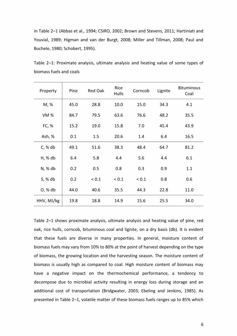
Table 2–1: Proximate analysis, ultimate analysis and heating value of some types of

biomass fuels and coals

Property Pine Red Oak Rice Hulls

Corncob Lignite Bituminous

Coal

M, % 45.0 28.8 10.0 15.0 34.3 4.1

VM % 84.7 79.5 63.6 76.6 48.2 35.5

FC, % 15.2 19.0 15.8 7.0 45.4 43.9

Ash, % 0.1 1.5 20.6 1.4 6.4 16.5

C, % db 49.1 51.6 38.3 48.4 64.7 81.2

H, % db 6.4 5.8 4.4 5.6 4.4 6.1

N, % db 0.2 0.5 0.8 0.3 0.9 1.1

S, % db 0.2 < 0.1 < 0.1 < 0.1 0.8 0.6

O, % db 44.0 40.6 35.5 44.3 22.8 11.0

HHV, MJ/kg 19.8 18.8 14.9 15.6 25.5 34.0

Table 2–1 shows proximate analysis, ultimate analysis and heating value of pine, red

oak, rice hulls, corncob, bituminous coal and lignite, on a dry basis (db). It is evident

that these fuels are diverse in many properties. In general, moisture content of

biomass fuels may vary from 10% to 80% at the point of harvest depending on the type

of biomass, the growing location and the harvesting season. The moisture content of

biomass is usually high as compared to coal. High moisture content of biomass may

have a negative impact on the thermochemical performance, a tendency to

decompose due to microbial activity resulting in energy loss during storage and an

additional cost of transportation (Bridgwater, 2003; Ebeling and Jenkins, 1985). As

presented in Table 2–1, volatile matter of these biomass fuels ranges up to 85% which

7

is much higher than that of both types of coals. The higher volatile matter of biomass

fuels makes them more readily devolatilised than coals, liberating less fixed carbon,

and thus making them more useful for pyrolysis, gasification and combustion (Balat et

al., 2009; Seo et al., 2010). Fixed carbon of these types of biomass fuels are

considerably less than that of both types of coals, proximate in the range of 7–19% and

44–45%, respectively. All biomass fuels, except for rice hulls, have considerably low ash

content which is preferable in the thermochemical processes. This is because the low

ash content helps to enhance the thermal balance, reducing the loss and occlusion of

carbon in the residues, in addition to lessening operating problems of sintering and

slagging (Reichel and Schirmer, 1989).

According to the ultimate analysis, the major components of these biomass and coal

fuels are carbon, oxygen and hydrogen. Carbon is actually a key component of solid

fuels in which their energy content is released through the oxidation process.

Hydrogen then supplies further energy to the oxidation process. However, oxygen only

functions as a component to sustain the progress of the oxidation process. As shown in

Table 2–1, all biomass fuels have relatively low carbon content ranging around 50% or

lower while the carbon content of coals is generally around 60–85%. There is also a

major difference in the oxygen content of these biomass and coal fuels. Through the

increase in the degree of transforming from wood to anthracite, the oxygen content

considerably decreases. Biomass fuels are characterised by high oxygen content,

typically 35–45%; while lignite and bituminous coal contain approximately 20% and

10% of oxygen, respectively. The hydrogen content of both types of fuels is in the

range of 4–6%, as presented in Table 2–1. It was explained that the content of carbon

and hydrogen in solid fuels contributes to their higher heating value positively; in

contrast, the oxygen content does not do so. However, for gasification and combustion

processes, high oxygen content of a fuel can be beneficial; since these processes need

less amount of oxygen to be added based on chemical exergy. High hydrogen content

of a fuel, on the other hand, can lower heating value of the product gas as a result of

the formation of water during the operation (Prins et al., 2004; Ptasinski et al., 2007).

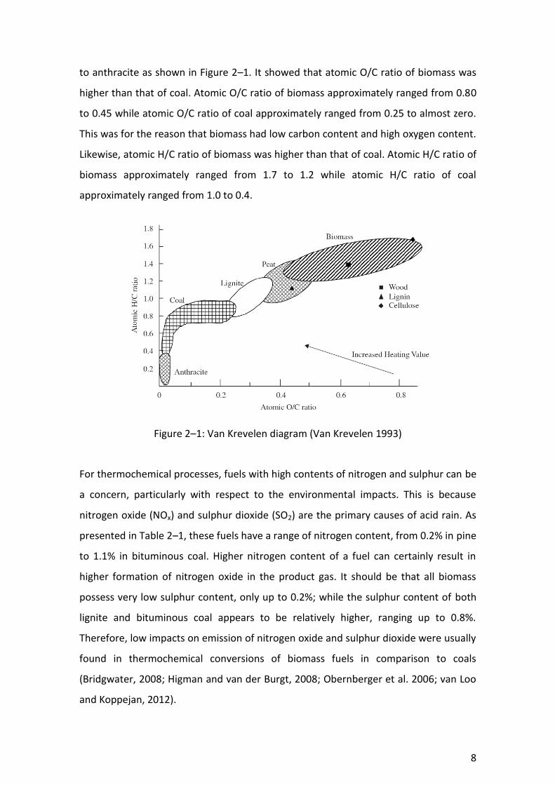
To compare the composition of the main elements (C, H, O) of solid fuels, Van Krevelen

(1993) developed a diagram which illustrated the change in composition from biomass

8

to anthracite as shown in Figure 2–1. It showed that atomic O/C ratio of biomass was

higher than that of coal. Atomic O/C ratio of biomass approximately ranged from 0.80

to 0.45 while atomic O/C ratio of coal approximately ranged from 0.25 to almost zero.

This was for the reason that biomass had low carbon content and high oxygen content.

Likewise, atomic H/C ratio of biomass was higher than that of coal. Atomic H/C ratio of

biomass approximately ranged from 1.7 to 1.2 while atomic H/C ratio of coal

approximately ranged from 1.0 to 0.4.

Figure 2–1: Van Krevelen diagram (Van Krevelen 1993)

For thermochemical processes, fuels with high contents of nitrogen and sulphur can be

a concern, particularly with respect to the environmental impacts. This is because

nitrogen oxide (NOx) and sulphur dioxide (SO2) are the primary causes of acid rain. As

presented in Table 2–1, these fuels have a range of nitrogen content, from 0.2% in pine

to 1.1% in bituminous coal. Higher nitrogen content of a fuel can certainly result in

higher formation of nitrogen oxide in the product gas. It should be that all biomass

possess very low sulphur content, only up to 0.2%; while the sulphur content of both

lignite and bituminous coal appears to be relatively higher, ranging up to 0.8%.

Therefore, low impacts on emission of nitrogen oxide and sulphur dioxide were usually

found in thermochemical conversions of biomass fuels in comparison to coals

(Bridgwater, 2008; Higman and van der Burgt, 2008; Obernberger et al. 2006; van Loo

and Koppejan, 2012).

9

According to Table 2–1, the higher heating value (HHV) of biomass fuels is in the range

of 15–20 MJ/kg which is much lower than that of coals, ranging from 25 to 34 MJ/kg.

Heating value of a fuel is a measure of the energy bound in the fuel per amount of

matter. A fuel often contains some moisture content which is released during heating.

This means that some of the heat liberated during the thermochemical reactions is

absorbed by the process of evaporation. For that reason, heating value of a fuel is also

influenced by its moisture content. High moisture content in a fuel reduces not only

the heating value of the fuel itself but also the heating value of the product gas (Quaak

et al., 1999; van der Drift et al., 2001). Quaak et al. (1999) plotted HHV and LHV of

biomass as a function of moisture content, as shown in Figure 2–2.

Figure 2–2: HHV and LHV of biomass against moisture content (Quaak et al. 1999)

According to Figure 2–2, both HHV and LHV of the fuel decreases as its moisture

content increased. It should be recognised that the HHV of the fuel decreased by

approximately 50% (from 10,000 to 5,000 kJ/kg) when its moisture content increased

by only 20% (from 40 to 60%).

2.1.2 Potential of biomass and coal

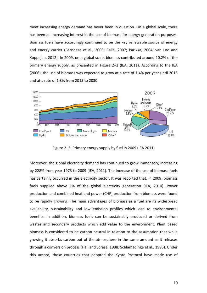
The world total primary energy consumption in year 2009 was 12,150 Mtoe which is

equivalent to 5.09 x 1020 J, as presented in Figure 2–3. It increased by 98.8% from year

1973 (IEA, 2011). The energy consumption has continued to rise worldwide even in the

face of high fuel prices and during the world economic recession; this is mainly due to

the growth in population around the world. Utilising alternative sources of energy to

10

meet increasing energy demand has never been in question. On a global scale, there

has been an increasing interest in the use of biomass for energy generation purposes.

Biomass fuels have accordingly continued to be the key renewable source of energy

and energy carrier (Berndesa et al., 2003; Callé, 2007; Parikka, 2004; van Loo and

Koppejan, 2012). In 2009, on a global scale, biomass contributed around 10.2% of the

primary energy supply, as presented in Figure 2–3 (IEA, 2011). According to the IEA

(2006), the use of biomass was expected to grow at a rate of 1.4% per year until 2015

and at a rate of 1.3% from 2015 to 2030.

Figure 2–3: Primary energy supply by fuel in 2009 (IEA 2011)

Moreover, the global electricity demand has continued to grow immensely, increasing

by 228% from year 1973 to 2009 (IEA, 2011). The increase of the use of biomass fuels

has certainly occurred in the electricity sector. It was reported that, in 2009, biomass

fuels supplied above 1% of the global electricity generation (IEA, 2010). Power

production and combined heat and power (CHP) production from biomass were found

to be rapidly growing. The main advantages of biomass as a fuel are its widespread

availability, sustainability and low emission profiles which lead to environmental

benefits. In addition, biomass fuels can be sustainably produced or derived from

wastes and secondary products which add value to the environment. Plant based

biomass is considered to be carbon neutral in relation to the assumption that while

growing it absorbs carbon out of the atmosphere in the same amount as it releases

through a conversion process (Hall and Scrase, 1998; Schlamadinge et al., 1995). Under

this accord, those countries that adopted the Kyoto Protocol have made use of

11

biomass as a fuel source to reduce carbon emissions and obtain carbon credits

(McGowan, 2009).

Estimates of the ultimate potential of biomass, as a renewable energy source, vary

widely depending on many assumptions such as agricultural forecasts, waste reduction

by industry, paper recycling programs and so forth. The global potential of biomass for

energy purposes was estimated between 33 and 1,135 EJ per year by the use of

geographical potential and biomass productivity (Hoogwijk et al., 2003). By 2050,

projections of IEA suggested that the biomass share might increase up to 20% for the

total primary energy supply and up to 3–5% for the electricity generation (IEA, 2010).

In fact, there are a number of factors that determine the potential availability of

biomass for energy supply. These factors take mainly account of biomass production

systems, demand for food as a function of population and diet consumed, productivity

of forests and energy crops and competing options for other uses of land. A shortage

of agricultural lands may occur as the global population and the food intake increase

dramatically. Significant transitions are therefore required for the production of

biomass for energy purposes in order to achieve high biomass energy potential.

Several aspects related to biomass production systems including soil quality, climate

situation, water availability and management factors need to be taken into account

(Hoogwijk et al., 2003; Hoogwijk et al., 2009).

On the other hand, coal has been used for energy generation in the form of both heat

and electricity for a very long period of time. Coal is deemed as the largest fossil fuel

resource with the proven reserves of over 847 billion tonnes worldwide. These

reserves were estimated to last for 118 years at current rates of consumption, as of

2011. Coal is a plentiful fossil fuel but not a renewable energy source. The location and

size of coal resources are quite clearly known subsequent to centuries of mineral

exploration. Coal reserves are currently available in over 70 countries around the

world. The largest proven reserves are in the United States, Russia, China, India and

Australia; while top coal producing countries are China, the United States, India,

Australia and South Africa, respectively. In recent times, coal has provided almost 28%

of the global primary energy and generated approximately 42% of the global

12

electricity. Coal has also remained as the world’s largest source of energy for electricity

generation for a number of decades (World Coal Association, 2011). In Australia, due

to the large availability, coal is inexpensive in comparison with other energy sources.

Australian coal has been a key source of energy providing around 40% of primary

energy supply and 76% of all electricity in the country (Geoscience Australia, 2010).

Although emerging renewable energy sources have offered great promise, coal has

been expected to still be a main electricity generation source for many years to come.

Improvements in mining and utilisation of coal have to be continuingly made with the

purpose of enhancing efficiency of coal energy generation as well as mitigating

possible environmental problems.

2.1.3 Barriers and supports for biomass

Barriers to adoption and implementation of biomass energy production systems have

gained more attention. This is since the energy sector has shifted to focus more on

alternative fuels. From economic perspectives, competition is a fundamental risk to be

considered. The competition may arise in two markets which are composed of the

market for input and the consumer market. The market for input is rivalry of the fuel

market while the consumer market is rivalry with conventional fuels derived products

(Roos, 1999). Sourcing biomass fuels has become a concern.

Biomass fuels can come in a variety of forms; these fuels can be secondary products or

purpose-grown as fuels. The choice on biomass depends on local availability, its cost

and its suitability for technological and environmental requirements. The use of

biomass derived from secondary products or wastes can be less expensive than that of

purpose-grown biomass. However, major diversities in the local availability and quality

of potential biomass fuels are often found in biomass derived from secondary

products. These biomass fuels are likely to arrive in small quantities from a large

number of suppliers. It therefore requires comprehensive management and

coordination at the energy generation facility in order to efficiently obtain and use

those biomass fuels. For purpose-grown biomass, even though it provides stable

supply and allows increased efficiency in the yield of biomass, purpose-grown biomass

competes with other uses for the land or of the product. A key challenge for the use of

13

purpose-grown biomass as an energy resource is the competition with fossil fuels on a

direct cost of production. As a result of increasing demand of biomass for energy

generation, prices of biomass have tended to be higher over the last few years, while

inexpensive biomass at desirable conditions is barely available in abundance. However,

the cost of biomass fuels depends highly on the region. Other limiting factor in

sourcing the biomass is the investment required to collect and pre-treat it to make

transportation economic. Storage and handling infrastructure for biomass also play an

important role since biomass is not likely to be as durable as coal (Chen and Kuo, 2010;

Demirbas et al., 2009; Jirjis, 2005; Roos, 1999).

From technological perspectives, uncertainty in biomass conversion technologies and

applications is an issue that may raise technological risks (IEA, 2007; Purohit, 2009).

Although technologies and applications to convert biomass into forms of energy are

widely available and amenable to a choice of functions (Babu, 2005; Bain et al., 2003),

those technologies still suffer from some technical problems, especially elimination of

contaminant, which tends to prohibit the economical and efficient operation (Fryda et

al., 2008; Leung et al., 2004). Furthermore, it is important to note that economies of

scale are a significant issue for the adoption and utilisation of biomass conversion

technologies. The minimum economic scale is however difficult to define because it

highly depends on a technology itself and a region operating in. The development of

modern small biomass conversion systems is still ongoing; it is expected to help

overcome many technical concerns such as machine reliability, cleaning system and

emission reduction methodologies (Bain et al., 2003).

Commercialisation of energy generation from biomass fuels can be promoted through

three main routes including technical enhancement, economical prospects and policy

supports. Customarily, industry scale has an impact on cost effectiveness of biomass

energy generation systems. The basic concept to raise revenue in smaller scales

engages in the improvement of conversion efficiency in order to grow its economy.

Market demand showed that the most beneficial biomass application is electricity

generation systems. Leung et al. (2004) claimed that the keys to economic success in

the biomass industry are to reduce the capital cost and to extend its application areas.

14

To boost the biomass industry, governmental policies may enforce compulsory

greenhouse gas reduction while financial incentives from governments may

deliberately foster the biomass energy market (IEA, 2007). Biomass energy systems

provide not only the environmental benefits but also public share by the local

community. The policy supports may be achieved by facilitating the establishment and

justifying the expenditure, increasing the support funds, enhancing the investment in

system innovation, guaranteeing the purchase of electricity and offering tax relaxation

(Bryana et al., 2008; Leung et al., 2004)

2.1.4 Environmental concerns

It becomes clear that the use of an enormous amount of fossil fuels has created

various adverse effects on the environment, including greenhouse gases, acid rain and

global warming. The greenhouse effect is the phenomenon in which the infrared

radiation is trapped by the atmosphere resulting in warming the earth and changing

the climate. The principal greenhouse gas is carbon dioxide (CO2) which is mainly

produced by burning carbonaceous materials and through deforestation. Hansen

(2005) reported that carbon dioxide has increased from about 313 parts per million in

1960 to about 375 parts per million in 2005. Global climate change is predominantly

driven by the strong increase of greenhouse gases especially carbon dioxide. During

the last 100 years, the global average air temperature has increased 0.74 ± 0.18 °C;

moreover, the temperature is predicted to increase by up to 5.8 °C over the next

hundred years (Watson, 2001). It was claimed that when the temperature increased by

2 °C; the ecosystems could be damaged as well as the climate system could be

disrupted dramatically (EREC, 2007). People and ecosystems have been harmed by

climate change. From the negative impacts include disintegrating polar ice, thawing

permafrost, dying coral reefs, rising sea levels and fatal heat waves. A rapid reduction

in the emission of greenhouse gases into the atmosphere is urgently needed in order

to mitigate the global warming. For that reason, it has brought about increasing

interest in energy production from biomass fuels. Biomass fuels can be deemed as a

main renewable energy resource on account of the environmental benefits derived

from their use (Hall and House, 1995).

15

Also, there are environmental concerns about sulphur oxides (SOx), nitrogen oxides

(NOx) and ash contamination. Due to differences in the chemical composition of

biomass fuels and fossil fuels, emissions of acid rain precursor gases which contain

sulphur oxides and nitrogen oxides can be reduced by increasing the utilisation of

biomass fuels. The reductions of sulphur oxides emissions occur on a one-to-one basis

with the amount of fossil fuels (heat input) offset by the biomass fuels; for the

example, increasing the supply of biomass fuels to the system by 10% can reduce

sulphur oxides emissions by 10%. This is for the reason that most biomass has almost

zero sulphur content (Hayter et al., 2004). Mechanisms that lead to nitrogen oxides

reductions are more complicated than sulphur oxides. The relative reductions are less

dramatic than the sulphur oxides on a percentage basis. However, some studies have

shown that nitrogen oxide levels could decrease when biomass fuels were mixed with

coals (Veijonen et al., 2003).

During thermochemical processes, amounts of the solid waste in form of ash are

always produced. For gasification, ash derived from the process consists of bottom ash

and fly ash. The analysis of constituents of both bottom ash and fly ash from

gasification by Rosen et al. (1997) have found that biomass ash contained high organic

carbon, calcium, potassium, chlorine and very low trace of heavy metals; while trace of

heavy metals has been found in fly ash from coal including arsenic, beryllium,

cadmium, barium, chromium, lead, mercury, uranium and other metals. However,

according to the Environmental Protection Agency‎ (EPA, 2000), fly ash produced from

coal did not have to be regulated as a hazardous waste. Conversely, instead of

dispersion of fly ash into the atmosphere or disposal in landfills, fly ash recycling is a

useful way to utilise fly ash to diminish the environmental and health concerns and

also to increase the value added of the waste. Fly ash can be used in construction as

well as its use in agriculture (Gómez-Barea et al., 2009). Fly ash used in construction

consists of raw feed for cement clinkers, soil stabilisation, road base, embankments

and structural fill, lightweight bricks and synthetic aggregate. Fly ash can be moreover

used as fertiliser or soil improver in agricultural purpose. In consequence, it could be

stated that co-utilisation of biomass and low degree of coal with careful planning tends

not to have adverse impacts on the environment.

16

2.2 Biomass conversion technologies

As a key renewable energy alternative, different ways of converting biomass fuels into

usable forms of energy have been developed. There are two major pathways of

extracting energy from biomass fuels; these consist of biochemical and

thermochemical conversion technologies. Research into these conversion technologies

has contributed to making more effective use of the available biomass resources and

producing substantial advances.

2.2.1 Biochemical conversion

Essentially, biochemical conversion technologies for biomass fuels consist of anaerobic

digestion and fermentation. Anaerobic digestion is a biochemical process in the

absence of oxygen in which microorganisms break down biodegradable materials. Two

main products produced from anaerobic digestion are biogas and digestate. Energy

derived from the anaerobic digestion is commonly in the form of biogas which typically

contains 60% methane and 40% carbon dioxide. Digestate which is also generated

from the process is solid and liquid residue. It can be further used as land fertiliser

(Speight et al., 2011). Common types of biomass fuels used for anaerobic digestion

include agricultural waste, livestock manure, sewage sludge, municipal sewage waste,

as well as wastewater (Klass, 1998; Sims, 2004).

Fermentation is the conversion of organic compounds using an endogenous electron

acceptor into energy products. Various types of the fermentation process are methane

fermentation, ethanol fermentation and lactic acid fermentation. Methane

fermentation is the process in which polymers are biochemically broken down to

methane and carbon dioxide in an environment where microorganisms grow and

produce reduced end-products. Ethanol fermentation can be explained as the process

in which sugars are biochemically converted into cellular energy and then generate

ethanol and carbon dioxide (Speight et al., 2011; Lens et al., 2005; Miyamoto, 1997).

Types of biomass fuels which are most widely used and proper for methane

fermentation and ethanol fermentation consist of bagasse, corn, municipal waste,

domestic food waste and all that (Chemistry World, 2009). Anaerobic digestion and

17

fermentation can be simple, secure and low cost technologies that enhance the

utilisation of several types of biomass fuels to benefit the economy and environment.

2.2.2 Thermochemical conversion

Thermochemical processes for biomass energy generation primarily include pyrolysis,

gasification and combustion. Pyrolysis is a thermochemical decomposition process of

solid carbonaceous substances occurring in the absence of oxygen that involves a

range of complex reactions. It can be an individual technique to form energy products

as well as an initial process of gasification and combustion (Basu, 2010; Sadhukhan et

al., 2008). The pyrolysis process of solid fuels generates a variety of products including

volatiles, tar and char. Pyrolysis, as a thermochemical conversion process, can be

influenced by many factors such as fuel properties, temperature, heating rate,

residence time and so forth (Colantoni et al., 2010; Zhang et al., 2010). The proportion

of solid, liquid and gas products from pyrolysis is determined by operating conditions

of the process consisting mainly of heating rate, residence time and operating

temperatures. The solid product produced from biomass pyrolysis is typically referred

to as bio-char which can be used as a fuel for gasification, as a soil amendment and

more several other uses. Bio-oil, as the liquid product from biomass pyrolysis, has a

high energy density; it can be used in many applications such as heat, power, transport

fuels and chemicals (Colantoni et al., 2010; Sadhukhan et al., 2008; Zhang et al., 2010).

Pyrolysis for heat applications is simple and also the most widely used. High yields of

bio-oil occur at fast heating rates, short residence times and moderate operating

temperatures. Pyrolysis gas products mainly contain carbon dioxide, hydrogen and

methane. The gases can be used for fuel drying or power generation. Under proper

operating conditions, pyrolysis which is a versatile conversion technology can offer

high yields of preferred products to be used directly or upgraded (Altman and

Hasegawa, 2011).

Gasification is a thermochemical conversion of solid fuels into combustible gases. The

gasification process involves partial oxidation of solid carbonaceous substances at

elevated temperatures (Bauen et al., 2004; Bridgwater, 2003; Kirubakaran et al., 2009;

18

McKendry, 2002b). Partial oxidation can be simply described as a process carried out in

less air than that required for stoichiometric reaction while a fuel-air mixture is

partially combusted in a gasifier (Yang, 2003). As a result of the partial combustion

rather than complete combustion of solid fuels, the process requires operating in an

oxygen-lean environment. The product of gasification is a combustible synthesis gas

which is usually referred to as syngas, product gas, or producer gas. The heating value

of the syngas varies over a wide range; it depends on the type(s) of fuels fed and the

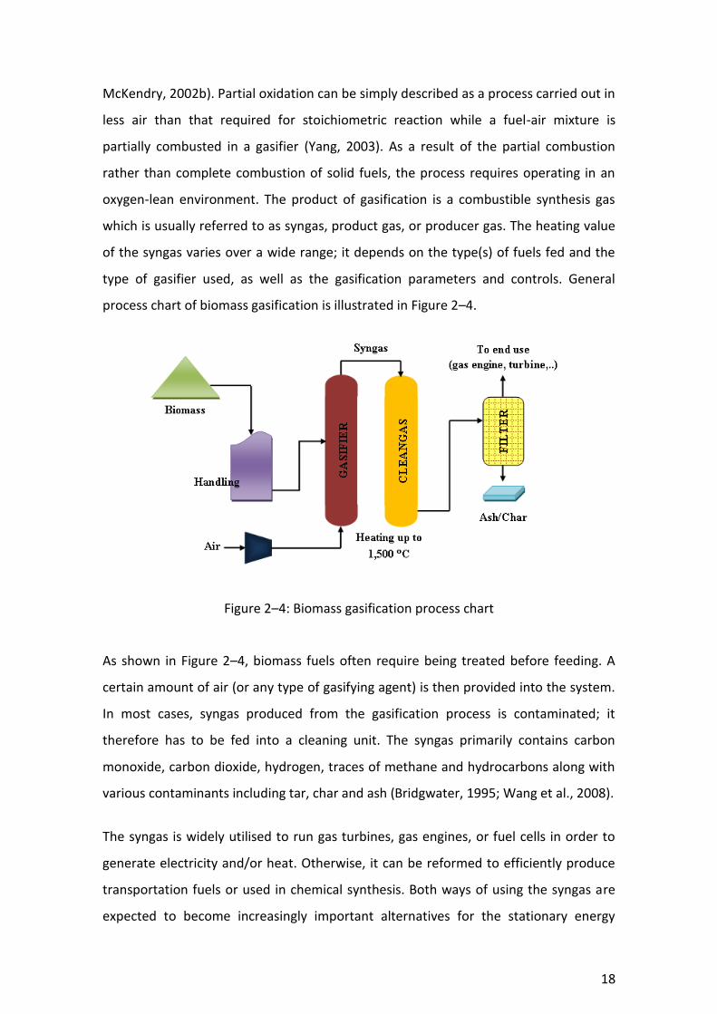
type of gasifier used, as well as the gasification parameters and controls. General

process chart of biomass gasification is illustrated in Figure 2–4.

Figure 2–4: Biomass gasification process chart

As shown in Figure 2–4, biomass fuels often require being treated before feeding. A

certain amount of air (or any type of gasifying agent) is then provided into the system.

In most cases, syngas produced from the gasification process is contaminated; it

therefore has to be fed into a cleaning unit. The syngas primarily contains carbon

monoxide, carbon dioxide, hydrogen, traces of methane and hydrocarbons along with

various contaminants including tar, char and ash (Bridgwater, 1995; Wang et al., 2008).

The syngas is widely utilised to run gas turbines, gas engines, or fuel cells in order to

generate electricity and/or heat. Otherwise, it can be reformed to efficiently produce

transportation fuels or used in chemical synthesis. Both ways of using the syngas are

expected to become increasingly important alternatives for the stationary energy

19

market and conventional chemical feedstocks (Bauen et al., 2004; Bridgwater, 2003;

Kirubakaran et al., 2009; McKendry, 2002b; Wang et al., 2008). It is also important to

note that the gasification technology offers significant advantages over traditional

combustion technology in terms of higher thermal efficiency (up to 40%) in addition to

ability to reduce emissions (Bain et al., 2003; Bauen et al., 2004; US Dept. of Energy,

1997; Worldbank, 2008). Further details of the gasification process, its key operating

parameters and syngas production are covered in Section 2.3.

Combustion is the most common application to convert solid biomass fuels into

energy. It involves the oxidation of carbonaceous fuels with excess air that generates

hot flue gases (Jenkins et al., 1998; Nino and Nino, 1997; Quaak et al., 1999; US Dept.

of Energy, 1997). Traditional combustion of biomass fuels was found in cooking and

heating. In later technology, to generate electricity, the combustion process is applied

to produce high-pressure steam which is normally introduced into a steam turbine

where it flows over a series of aerodynamic turbine blades, causing the turbine to

rotate. Although combustion is a conventional technology used for electricity

generation, it still suffers from relatively low conversion efficiency, limited ability to

produce other end-product gases and limited ability to reduce toxic gas emissions

without an additional pollution capture unit (Altman and Hasegawa, 2011; van Loo and

Koppejan, 2012).

2.3 Gasification system and syngas production

2.3.1 Gasification configuration

Identifying a suitable gasification configuration is imperative in bringing about the best

possible gasification outcomes. The selection of a gasifier is determined by many

factors such as size, capital cost, availability, type of fuels used and type of preferred

products. There are various types of gasification configurations that have been

developed over the past decades. Two major types of gasifiers classified by the

condition of the solid fuels during the gasification process are the fixed bed and the

fluidised bed. Each type of gasifiers has its own benefits and drawbacks in respect of its

utilisation and the type of biomass fed. Accordingly, the comparison between

20

characteristics of both fixed bed and fluidised bed gasifiers is summarised in Table 2–2

(Basu, 2006; Bridgwater et al., 1999; Chopra and Jain 2003; FAO Forestry Department,

1986; Warnecke, 2000).

Table 2–2: Comparison between characteristics of fixed bed and fluidised bed gasifiers

Characteristic Fixed Bed Fluidised Bed

Technology Low specific capacity High specific capacity

Investment Higher investment (by around 10%)

Lower investment

Feedstock:

Size (mm)

Ash content (% wt)

10–100

< 15

0.02–50

< 25

Reaction temperature (°C) 800–1500 700–1000

Turndown ratio 4 3

Load range Feasible for partial load (20–110%)

Feasible for partial load (50–110%)

Carbon conversion 90–99% 90%

LHV (MJ/Nm3) Low High

Cold gas efficiency 45–55% 70–75%

Tar content (g/Nm3) 0–3 < 5

Start-up/ Shutdown Long period to heat-up Simply start/shut down

Control Simple Average

Environmental issue Possible molten slag Problem with Ash not molten

Fixed bed gasifiers are of simple design, reliable and favourable on a small scale

operation. This type of gasifiers offers very high carbon conversion up to 99%.

However, as a result of operating at high temperatures, these gasifiers often suffer

from relatively low thermal efficiency as well as low heating value of syngas produced.

21

Based on the reactor geometry, fixed bed gasifiers can be furthermore classified into

updraft and downdraft, as illustrated in Figure 2–5.

Figure 2–5: Updraft and downdraft gasifiers (All Power Labs 2010)

For updraft gasifiers, the air (or any type of gasifying agent) enters at the bottom while

the syngas leaves from the top. The combustion reactions occur near the grate at the

bottom of the gasifier followed by the reduction reactions. In the upper part, pyrolysis

and drying of the fuel occur on account of heat transfer from the lower zones by

forced convention and radiation. The syngas, volatiles and tar produced during the

reactions leave at the top of the gasifier; these products can be then separated by the

use of cyclone and filter. Updraft gasifiers are designed to handle fuels with high ash

content, up to 15 % as well as high moisture content, up to 50%. The main advantages

of updraft gasifiers are their suitability for many types of fuels ranging from biomass to

coal, high equipment efficiency, high charcoal burn out and low gas exit temperature.

In contrast, the key drawback of updraft gasifiers is that the syngas produced always

contains a high level of tar (Brown and Stevens, 2011; Chopra and Jain, 2003; Kreith

and Goswami, 2011).

Due to tar entrainment in the syngas leaving stream of updraft gasifiers, the design of

downdraft gasifiers was to solve the problem by introducing the air at or above the

combustion zone of the gasifier, as illustrated in Figure 2–5. The fuel and gas are both

moved downward in the same direction; then the syngas produced is taken out from

22

the bottom. The acid and tarry distillation products from the fuel are passed through a

bed of charcoal and subsequently converted into carbon dioxide, carbon monoxide,

hydrogen and methane gases. However, downdraft gasifiers are only suitable for fuels

with low ash content (less than 5%) and low moisture content (less than 20%). The

principal prospect of downdraft gasifiers is to generate tar free syngas, even though

generating tar free syngas seems to be very rare in practice. The tar level from the

downdraft system is often low, approximately less than 3 g/Nm3, as compared to the

updraft system which may yield the tar level up to 5 g/Nm3. Downdraft gasifiers

however give lower efficiency and heating value than updraft gasifiers because there is

no provision for internal exchange (Brown and Stevens, 2011; Chopra and Jain, 2003;

Kreith and Goswami, 2011).

Fluidised bed gasifiers are regarded as a state-of-the-art technology. These gasifiers

appear to be more attractive as compared to fixed bed gasifiers for commercial

gasification. The design of this type of gasifiers is to resolve difficulties in fixed bed

gasifiers such as lack of bunkerflow and intense pressure drop in the gasifier (FAO

Forestry Department, 1986). A diagram of a basic fluidised bed gasifier is illustrated in

Figure 2–6.

Figure 2–6: Diagram of a basic fluidised bed gasifier (FAO 1986)

A flow of a gasifying agent, which can be air, oxygen, or stream is introduced to the

gasifier to well mix or stir particles of the fuel at a proper velocity in order to keep

them in a state of suspension within the bed. The particles are rapidly mixed and

23

almost instantly heated up to the temperature of the bed. Thus, those particles are

pyrolysed very fast, leading to a component mix with a large amount of gaseous

matters. Further thermochemical reactions and conversions of tar take place in the gas

phase. Ash particles are carried over the top of the gasifier and are typically removed

from the gas stream using cyclone and candle filter. As the fuel particles are gasified;

these particles become smaller and then entrained out of the bed. The temperatures

within the bed therefore require being lower than the initial ash fusion temperature of

the fuels to avoid particle agglomeration. It remains clear that this fluidising technique

can result in uniform temperatures within the bed and extensive recycling of particles.

This type of gasifiers can increase the heating value of the syngas by more than 20%

compared to that of the fixed bed gasifiers (Basu, 2006; Bingyan et al., 1994;

Warnecke, 2000).

Bubbling and circulating beds are the two commonly available choices of fluidised bed

gasifiers. The fundamental differences between them are their fluidising velocity and

gas path (Warnecke, 2000). Fluidised bed gasifiers are very functional for a wide range

of fuels and particle sizes, especially types of fuels that form highly corrosive ash like

biomass fuels. These gasifiers operate at relatively low temperatures, approximately

700–1,000 °C; thus, high ash content fuels can be gasified without ash sintering and

agglomeration problems (Arena and Mastellone, 2006). Corrosive ash normally results

in a high potential to damage the gasifier slagging wall. However, drawbacks of

fluidised bed gasifiers include high tar content in the syngas produced as well as

incomplete carbon conversion.

2.3.2 Operating parameters

Operating parameters play a very important role in the gasification process and syngas

production. The parameters that affect the reactivity of gasification encompass type of

biomass fuels and their pre-treatment, composition and inlet temperature of the

gasifying agent, type of catalyst used, reaction temperature, heating rate, residence

time and so forth. The proper choice of these variables is also governed by geometry of

the gasifier. Suitable operating conditions can lead to an increase in quality and

quantity of the syngas produced as well as a decrease in formation of tars. Various

24

studies have generally determined the operating parameters in support of maximum

biomass gasification results, as summarised in Table 2–3 (Basu, 2010; Chen et al., 2003;

Devi et al., 2003; FAO Forestry Department, 1986; Kirubakaran et al., 2009; Quaak et

al., 1999).

Table 2–3: Operating parameters in support of maximum gasification results

Parameter Maximum result

Properties of Fuels:

Size/ Shape

Moisture content

20–200 mm/ Pellets, Chips or Small Lumps

Less than 25% moisture dry basis

Gasification environment Reactive environment

Operating temperature 750–950 C

Heating rate High heating rate

Residence time Long residence time

Active catalyst Dolomite

The particle size of biomass fuels has an effect on not only the gasification process but

also the quality during their storage (Jirjis, 2005). Larger biomass particles have a lower

surface-to-volume ratio which causes complexity in the gasification process. A larger

size can also result in a greater volume voidage of the mass in the gasifier, which

allows for an increase in air flow velocity. For that reason, it is essential for the fuels to

be homogenous and properly sized with sufficient heat transfer surface. Tinaut et al.

(2008) studied the effect of biomass particle size and air velocity. It was found that the

maximum efficiency was given by smaller particle size and lower air velocity. However,

the pressure drop across the gasifier can increase as the particle size is reduced. As

indicated in Table 2–3, the optimal particle size of biomass fuels for the gasification

process ranges from 20–200 millimetres depending on their type and reactor

configuration. Biomass fuels in the shapes of chips and small lumps can be gasified

conveniently (Kirubakaran et al., 2009; Quaak et al., 1999).

25

The gasification process requires reactive environments such as air, oxygen and steam

to create complete gasification of the fuels, while inert environments such as nitrogen

and argon give rise to devolatilisation of volatile matters which yield a large amount of

char (Kirubakaran et al., 2009; Brenes, 2006). Reactive environments of gasification are

furthermore discussed in the sub-section of gasifying agents. Temperature range can

be generally divided into below and above 500 °C. Pyrolysis is carried out at

temperatures below 500 °C for maximum yields of char under inert medium while

gasification is normally operated at temperatures above 500 °C with air flowing in

order to reduce carbon dioxide by carbon to carbon monoxide (Kirubakaran et al.,

2009). High operating temperatures which are over 800 °C are preferred for biomass

gasification to facilitate high carbon conversion of biomass fuels and low tar

contamination in the syngas. Aromatic hydrocarbon and oxygen compounds including

phenol, cresol and benzofuran significantly destruct at temperatures above 800 °C

(Devi et al., 2003). However, major drawbacks of operating with higher temperatures

take account of higher risk of sintering and lower syngas heating value. The optimal

operating temperatures therefore range between 750 and 950 °C depending

substantially on the type of gasifiers and the property of biomass fuels. Heating rates

also influence the yield and composition of the products derived. During

thermochemical processes, higher heating rates usually bring about more the gas yield

and less formation of char (Basu, 2010; Chen et al., 2003; Kirubakaran et al., 2009).

However, to obtain a high heating rate, a supplementary heater of high thermal energy

input to the system is required (Chen et al., 2003).

Longer residence time is preferred for biomass gasification. The explanation is the

longer the residence time of the volatile phase, the better the cracking reaction. Chen

et al. (2003) found that an increase in residence time of the volatile phase produces

the syngas with increasing heating values. Under these particular experimental

conditions, the increase of gas yield significantly took place between two and three

seconds, for the reason that the components decomposed with a residence time of 2–

3 seconds. It was also mentioned that the use of catalysts is an effective way of

removal of tars in the syngas produced from biomass gasification even at low

operating temperatures. Many catalysts such as dolomite catalysts, alkali metal and

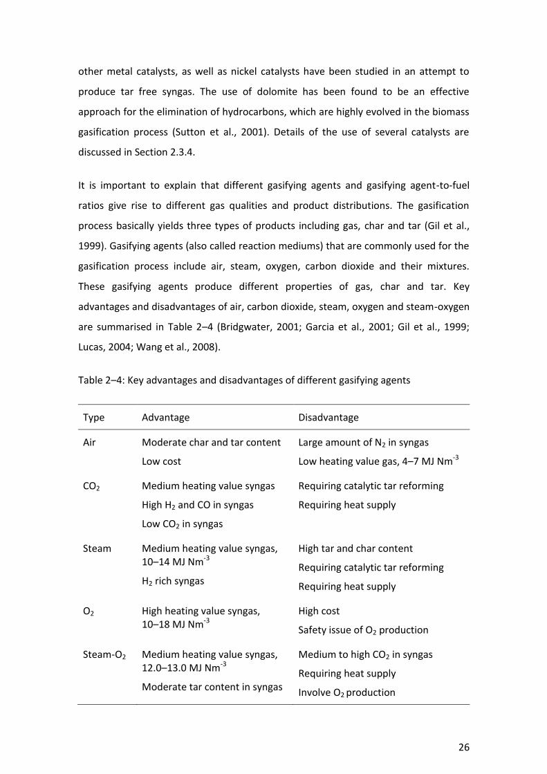
26

other metal catalysts, as well as nickel catalysts have been studied in an attempt to

produce tar free syngas. The use of dolomite has been found to be an effective

approach for the elimination of hydrocarbons, which are highly evolved in the biomass

gasification process (Sutton et al., 2001). Details of the use of several catalysts are

discussed in Section 2.3.4.

It is important to explain that different gasifying agents and gasifying agent-to-fuel

ratios give rise to different gas qualities and product distributions. The gasification

process basically yields three types of products including gas, char and tar (Gil et al.,

1999). Gasifying agents (also called reaction mediums) that are commonly used for the

gasification process include air, steam, oxygen, carbon dioxide and their mixtures.

These gasifying agents produce different properties of gas, char and tar. Key

advantages and disadvantages of air, carbon dioxide, steam, oxygen and steam-oxygen

are summarised in Table 2–4 (Bridgwater, 2001; Garcia et al., 2001; Gil et al., 1999;

Lucas, 2004; Wang et al., 2008).

Table 2–4: Key advantages and disadvantages of different gasifying agents

Type Advantage Disadvantage

Air Moderate char and tar content

Low cost

Large amount of N2 in syngas

Low heating value gas, 4–7 MJ Nm-3

CO2 Medium heating value syngas

High H2 and CO in syngas

Low CO2 in syngas

Requiring catalytic tar reforming

Requiring heat supply

Steam Medium heating value syngas, 10–14 MJ Nm-3

H2 rich syngas

High tar and char content

Requiring catalytic tar reforming

Requiring heat supply

O2 High heating value syngas, 10–18 MJ Nm-3

High cost

Safety issue of O2 production

Steam-O2 Medium heating value syngas, 12.0–13.0 MJ Nm-3

Moderate tar content in syngas

Medium to high CO2 in syngas

Requiring heat supply

Involve O2 production

27

2.3.3 Chemical reactions and products in the gasification process

Basically, the four distinct processes which occur during gasification in a fix bed gasifier

are drying, pyrolysis, combustion and gasification (FAO Forestry Department, 1986;

Higman and van der Burgt, 2008; Quaak et al., 1999). Even though there is an overlap

of these processes, each process can be assumed to engage in a separate zone on

account of different chemical and thermal reactions taking place. It is however

important to address that a fluidised bed gasifier has no distinct reaction zones unlike

a fixed bed gasifier. All reactions in a fluidised bed gasifier happen simultaneously

during mixing. The four distinct processes occurring in the downdraft system are

explained as follows:

2.3.3.1 Drying zone

At the top of the bed, in the drying zone, the fuel is heated and dried by introducing a

gasifying agent. Subsequently, the moisture content is driven off, in most cases with

the temperature up to 200 °C. This typically allows changes in the structures of the fuel

and its physical properties (Basu, 2010; Higman and van der Burgt, 2008; Teislev,

2000).

2.3.3.2 Pyrolysis or devolatilisation zone

After drying, in the pyrolysis zone, the temperatures begin to get higher. Pyrolysis

reactions arise between the temperatures of 250–500 °C; the reactions release the

volatile components of the fuel by a set of complex reactions (FAO Forestry

Department, 1986; Teislev, 2000). The driven off volatiles consist mainly of tar,

polycyclic aromatic hydrocarbon gases, hydrogen, carbon monoxide, carbon dioxide

and steam. The non-vaporised by-products of pyrolysis are referred to as char and ash.

The products derived from pyrolysis reactions are tar, hydrogen, carbon monoxide,

carbon dioxide, water vapour, methane, acetylene, char and ash (Bridgwater, 2003;

Higman and van der Burgt, 2008; Goswami, 1986; Ricketts et al., 2002), as presented in

Table 2–5.

28

Table 2–5: Main chemical reactions occurring in the gasification process

Zone Reaction

Pyrolysis Dry biomass + Heat → H2 + CO + CO2 + H2O + CH4 + C2H2 + Tar,

Char, Ash

Combustion C + O2

2H2 + O2

→

→

CO2

2H2O

(2–1)

(2–2)

Gasification C + CO2

C + H2O

C + 2H2O

C + 2H2

CO + H2O

→

→

→

→

→

2CO

CO + H2

CO2 + 2H2

CH4

CO2 + H2

(2–3)

(2–4)

(2–5)

(2–6)

(2–7)

2.3.3.3 Combustion or oxidation zone

The combustible substance of the biomass fuel is generally made up of elements of

carbon, hydrogen and oxygen. The carbon compounds remaining from pyrolysis go

through the combustion reactions in which carbon and hydrogen react with oxygen

from a gasifying agent, forming carbon dioxide and water. The combustion reactions

are exothermic reactions and thus provide the heat required to drive the gasification

reactions in the next zone. Temperatures in the combustion zone are in the range of

1,100 to 1,500‎C. However, this depends on the reactor configuration (FAO Forestry

Department, 1986; Higman and van der Burgt, 2008; Quaak et al., 1999). Main

combustion reactions are summarised in Table 2–5, Equation (2–1) and Equation (2–2).

2.3.3.4 Gasification or reduction zone

The actual gasification reactions, which are endothermic, usually take place at

temperatures above 700 C. The heated carbons are reacted with carbon dioxide and

steam (H2O) from the combustion zone and then broken down into gases consisting of

carbon monoxide, carbon dioxide and hydrogen. The reactions in the gasification zone

are presented in Table 2–5, Equation (2–3) – (2–7). The gas produced from this zone,

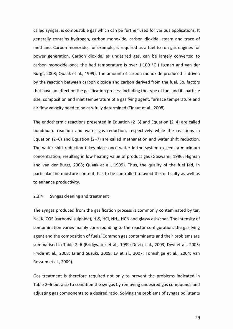
29

called syngas, is combustible gas which can be further used for various applications. It

generally contains hydrogen, carbon monoxide, carbon dioxide, steam and trace of

methane. Carbon monoxide, for example, is required as a fuel to run gas engines for

power generation. Carbon dioxide, as undesired gas, can be largely converted to

carbon monoxide once the bed temperature is over 1,100 C (Higman and van der

Burgt, 2008; Quaak et al., 1999). The amount of carbon monoxide produced is driven

by the reaction between carbon dioxide and carbon derived from the fuel. So, factors

that have an effect on the gasification process including the type of fuel and its particle

size, composition and inlet temperature of a gasifying agent, furnace temperature and

air flow velocity need to be carefully determined (Tinaut et al., 2008).

The endothermic reactions presented in Equation (2–3) and Equation (2–4) are called

boudouard reaction and water gas reduction, respectively while the reactions in

Equation (2–6) and Equation (2–7) are called methanation and water shift reduction.

The water shift reduction takes place once water in the system exceeds a maximum

concentration, resulting in low heating value of product gas (Goswami, 1986; Higman

and van der Burgt, 2008; Quaak et al., 1999). Thus, the quality of the fuel fed, in

particular the moisture content, has to be controlled to avoid this difficulty as well as

to enhance productivity.

2.3.4 Syngas cleaning and treatment

The syngas produced from the gasification process is commonly contaminated by tar,

Na, K, COS (carbonyl sulphide), H2S, HCl, NH3, HCN and glassy ash/char. The intensity of

contamination varies mainly corresponding to the reactor configuration, the gasifying

agent and the composition of fuels. Common gas contaminants and their problems are

summarised in Table 2–6 (Bridgwater et al., 1999; Devi et al., 2003; Devi et al., 2005;

Fryda et al., 2008; Li and Suzuki, 2009; Lv et al., 2007; Tomishige et al., 2004; van

Rossum et al., 2009).

Gas treatment is therefore required not only to prevent the problems indicated in

Table 2–6 but also to condition the syngas by removing undesired gas compounds and

adjusting gas components to a desired ratio. Solving the problems of syngas pollutants

30

can ensure higher quality of the syngas, extended functionality and availability of the

gasification system and compliance with exhaust gas emission limits. The gas

treatment can be categorised into three major categorises which are composed of

removal of particulates, elimination of organic contaminations mainly tars and

elimination of inorganic contaminations such as metals, nitrogen, sulphur and chlorine

containing compounds.

Table 2–6: Contaminants in syngas produced from the gasification process

Category Contaminant Problem

Particulates Ash, Char Erosion

Organic compound Tar Filter clogs,

Burning difficulties

Alkali metals Sodium, Potassium Hot corrosion

Sulphur/ Chlorine compounds COS, H2S, HCl, Corrosion, Emission

Nitrogen compounds NH3, HCN NOx formation

2.3.4.1 Particulates

Several methods can be used to remove particulates from the syngas such as barrier

filters, electrostatic filters (ESP), cyclones and solvent scrubbers. It was furthermore

claimed that barrier filtration techniques, consisting of sintered metal or ceramic

filters, are preferred since cyclones cannot decrease the level of particulates to less

than 5–30 g/Nm3 (Kurkela et al., 1993).

2.3.4.2 Tar

The syngas produced by low temperature gasification always contains an unacceptable

level of tar. Biomass tar is composed of aromatic hydrocarbons and phenolic

compounds (Wang et al., 2008; Li and Suzuki, 2009). Even though formation of tar

increases at low operating temperatures, tar concentration is also influenced by other

factors such as the gasifier configuration and the fuel characteristics. It was found that

31

tar formation is a more significant problem in biomass gasification than in coal

gasification. The formation of tar often causes fouling and blockage of process

equipment, which is considered as one of the most practical problems in the biomass

gasification system. Thus several research and development programmes have focused

on methods for tar elimination. Elimination of tar from the gasification process is

principally made up of secondary methods and primary methods.

Secondary methods are defined as hot syngas treatments which mainly involve tar

cracking and tar removal. For tar cracking, there are two basic approaches including

catalytic cracking and thermal cracking. Tar can be destroyed by reforming reactions

which require additional catalysts. Many experiments indicated that catalytic cracking

of tar could be very effective (Devi et al., 2005; Lv et al., 2007; Tomishige et al., 2004;

van Rossum et al. 2009). According to Devi et al. (2005) and Wang et al. (2008),

catalysts regularly applied to raw syngas are dolomite, olivine, Ni-based, alkali metal

and alkalis (such as KOH, KHCO3 and K2CO3). It was reported that catalytic cracking is

one of the most promising methods for gas cleaning resulting in up to 99% conversion

of tar at elevated temperatures (Bridgwater et al., 1999).

Thermal cracking is referred to as high temperature destruction which can be

accomplished by three different methods. First, raw syngas is treated by injecting

oxygen or air to increase the temperature. This can effectively result in cracking and

destruction of organic compounds at high temperatures up to 1300 °C or more

(Bridgwater et al., 1999). However, this approach is not preferred due to low

efficiency, high oxygen production cost and high levels of carbon dioxide produced

(Bridgwater et al., 1999; Haq, 2002). The second technique is carried out by increasing

residence time after initial gasification; likewise, this approach is not quite effective.

Third, the raw syngas can be directly contacted with a separate heated hot surface;

but, this is also only partially effective. In addition, a significant energy supply is

required for this approach causing the overall system efficiency to decline (Anis and

Zainal, 2011; Bridgwater et al., 1999; Haq, 2002). The deployment of thermal

treatment does not seem to be an attractive option as a result of these obstacles.

32

For tar removal, mechanical methods can be applied such as cyclones, bag filters,

baffle filters, ceramic filters, fabric filters, rotating particle separators, electrostatic

precipitators and water scrubbers. However, most mechanical methods, especially the

types of filters and separators, are less efficient to remove tar than to remove

particulate dust from the syngas. Electrostatic precipitators and water scrubbers are

also not preferred because of economical and environmental problems (Anis and

Zainal, 2011).

Primary methods are defined as the prevention and conversion of tar formed in the

gasifier by taking in all relevant parameters. Ideally, the objective is to produce a tar

free syngas that does not require secondary treatments (Devi et al., 2003; Li and

Suzuki, 2009). The fundamental concerns take account of the proper choice of

operation conditions, the deployment of suitable active bed additives or catalysts

during the gasification process, as well as the suitable reactor configuration. Primary

methods are more complex to occupy; however it can decrease the overall costs of

operation. The crucial operating parameters needed to be taken into account consist

of gasifying agent, gasification temperature, pressure, residence time, as well as

equivalent ratio, which is the ratio of O2 required for gasification to O2 required for full

combustion.

The determination of parameters is also dependent on the type of gasifier

configuration used. For the use of bed additives, only few catalysts have been tried as

the active bed additive in the gasifier itself during the gasification process (Devi et al.,

2003). The active bed additive performs as catalyst influencing chemical reactions. This

leads to reducing tar yield, preventing solid agglomeration and improving quality of

syngas. Currently, dolomite appears to be one of the most popular chemical used for

this purpose and studies of its use as an in-bed additive have produced successful

results (Devi et al., 2003; Devi et al., 2005; Lv et al., 2007). In due course, the selection

of the treatment method for elimination of tar from the syngas ought to follow the

level of acceptable tar concentration, which strongly depends upon syngas utilisation

and application, as well as financial availability for the tar elimination.

2.3.4.3 Inorganic contaminations

33

As indicated in Table 2–6, inorganic impurities in syngas produced from biomass

gasification include Na, K, COS, H2S, HCl, NH3 and HCN. Several clean-up techniques for

inorganic contaminations are applicable and economically available. To eliminate alkali

metals, gas cooling at temperatures below 600 C effectively condenses vapour alkali

metals onto entrained solids which can be removed at the particulate removal stage.

Sulphur compounds are not regarded as a serious problem for the reason that biomass

fuels usually have very low sulphur content as presented in Table 2–1. However, some

specific types of gas turbines require sulphur removal which is regularly successfully

achieved by a sulphur guard. Also, dolomite, which is widely used as tar cracker, can

absorb significant amounts of sulphur (Bridgwater et al., 1999). Chlorine compounds

can be eliminated by dissolution in a wet scrubbing process or by absorption in active

materials. Nitrogen compounds which cause NOx emission can be reduced by two

approaches encompassing the use of selective catalytic reduction (SCR) and the use of

low NOx combustion techniques. The techniques for low NOx combustion include the

reduction of temperature in combustion zone by the injection direction close by the

piston surface and stable combustion by using strong swirl flow (Nagayoshi et al.,

2006; Seita et al., 1999).

2.4 Application of gasification technology

Syngas produced from the gasification process can be used in many applications. The

utilisation of the syngas is governed by the gasification process, the syngas quality and

the syngas treatment technology. The major applications of gasification technology

include electricity, combined heat and power, transport fuels and chemical synthesis.

2.4.1 Electricity and heat

To generate electricity, the syngas can be used in a gas engine, gas turbine or fuel cell;

it depends on composition and viable proportion of the syngas. Gas condition, cleaning

and treatment play an important role to make use of the syngas (Haq, 2002). The

specifications of gas turbine fuel are much stricter than those of gas engine fuel. The

minimum requirements for gas turbine include gas LHV of 4–6 MJ/Nm3, gas hydrogen

content of 10–20% and no tar tolerated (Bridgwater, 1995; Bridgwater et al., 1999).

34

Gas engines can usually tolerate higher contaminants; in some cases, up to 30 ppm

tars can be accepted (Bridgwater et al., 1999). Moreover, the syngas can be employed

in fuel cells for advanced production of electricity. Fuel cells can covert H2, CO or CH4

to produce electricity directly through electrochemical reactions. It should be noted

that fuel cells can theoretically achieve high electrical efficiency as compared to

combustion systems or gas turbines.

Advanced gasification combined cycle has been addressed as a potential application

for recovering waste heat presented in the gasification system. The combined cycle is

the characteristic of a power generation system which employs more than one

thermodynamic cycle. Typically, it focuses on combination of gas turbine and steam

turbine which are Brayton cycle and Rankine cycle, respectively. Heat is reclaimed by a

heat recovery steam generator (HRSG) which produces steam. In a cycle, the steam is

utilised via steam turbine to generate extra electricity; then it is cooled and condensed

before once again passing through the steam generator. This phase promotes the

efficiency of electricity generation. Integrated gasification combined cycle (IGCC) was

furthermore developed to offer more efficient energy generation. The IGCC system

retrieves the energy from an orthodox combined cycle and integrates with many

energy recoveries along the process. In recent times, biomass integrated gasification

combined cycle (BIGCC) offers maximised overall thermal efficiency as well as

improves economic performance (Ashizawa et al. 2005; Boerrigter and Rauch, 2005;

Bridgwater et al., 1999; Carpentieri et al., 2005; Dornburg and Faaij, 2001; Klimantos et

al., 2009). Klimantos et al. (2009) suggested that a commercially viable BIGCC system

which is reliable and efficient ranges from 10–40 MWe.

2.4.2 Transport fuel

High temperature gasification or catalytic gasification can produce syngas that is rich in

hydrogen and carbon monoxide. The syngas composition can be conditioned to

optimise for its final use by thermo cracking, catalytic reforming and operating

conditions (Boerrigter and Rauch, 2005; Maschio et al., 1994). Syngas produced from

biomass gasification has become progressively important in the production of green

fuels such as Fischer-Tropsch synthesis and methanol/DME (Dimethyl Ether).

35

In the Fischer-Tropsch process, syngas with a mixture of carbon monoxide and

hydrogen are catalysed to produce liquid hydrocarbon in various forms, along with

other aliphatic compounds. Iron and cobalt are the most common catalysts used,

though nickel and ruthenium are feasible. The basic process conditions involve a

temperature range of 200–350 C and pressure range of 2.5–6.0 MPa (Boerrigter and

Rauch, 2005). High temperature process yields rapid reactions and high conversion

rates, but also tends to yield more methane which is undesirable. The Fischer-Tropsch

basic reaction is presented Equation (2–8), Table 2–7 (NETL, 2013a). To produce a

synthetic petroleum substitute, hydrocarbon compounds derived from Fischer-Tropsch

reaction has to be further refined (Brown and Stevens, 2011; de Klerk, 2011). The end

products of Fischer-Tropsch process include synthetic lubrication oil, synthetic

gasoline, light olefins, diesel fuel and waxes. Also, direct production of gasoline and

light olefines can be achieved by high temperature Fischer-Tropsch process,

approximately 330–350 °C (Boerrigter and Rauch, 2005).

Table 2–7: Production of transport fuel synthesis

Fuel synthesis Basic reaction

Fischer-Tropsch synthesis (2n+1) H2 + n CO → CnH(2n+2) + n H2O (2–8)

Methanol synthesis CO + 2 H2

CO2 + 3 H2

→

→

CH3OH

CH3OH + H2O

(2–9)

(2–10)

Similarly to Fischer-Tropsch synthesis, the syngas can be used to produce methanol by

means of catalytic reaction of carbon monoxide and carbon dioxide with hydrogen.

Methanol synthesis process carries out in a liquid phase and different H2/CO ratio as

compared to Fischer-Tropsch synthesis, which brings about a higher methanol yield as

presented in Equations (2–9) and (2–10), Table 2–7. Methanol synthesis can be

achieved at varied pressures ranging from 5–30 MPa (Boerrigter and Rauch, 2005). The

catalysts commonly used for methanol synthesis are copper-zinc-chromium and zinc-

chromium. Methanol synthesis is promoted as high octane rating fuel used for internal

combustion and other engines. The production of methanol also allows for the

36

formation of by-products such as methane and dimethyl ether (DME) (Intelligent

Energy Europe, 2008).

2.4.3 Chemical synthesis

Moreover, the syngas from the gasification process can be used as a feedstock in

synthesis reaction to produce chemical synthesis such as synthesis natural gas (SNG),

ammonia, oxo synthesis and hydrogen. Chemical synthesis is the execution of chemical

reactions in order to obtain various types of products. Gasification can generate SNG

by yielding the syngas with high content of methane. SNG is produced by catalytic

methanation of H2 and CO in the gasification process as presented in Equation (2–11),

Table 2–8 (Andersson et al., 2008). Owing to similarity of properties of SNG and natural

gas, SNG can exclusively substitute natural gas. At ambient condition, SNG is in

gaseous state; in order to use it as an automotive fuel, it then has to be compressed or

liquefied. SNG can be also produced by supercritical biomass gasification which has

recently been performed on a laboratory scale. Biomass fuels are treated in

supercritical water and converted into fuel gases and easily separated from the water

phase by cooling to ambient temperatures. The process separates a mixture of carbon

dioxide, carbon monoxide and methane (Boerrigter and Rauch, 2005; Basu, 2010).

Table 2–8: Production of chemical synthesis

Chemical synthesis Basic reaction

Synthesis natural gas CO + 3 H2 → CH4 + H2O (2–11)

Ammonia synthesis N2 + 3 H2 → 2 NH3 (2–12)

Oxo synthesis H2 + CO + CH3CH=CH2

→ CH3CH2CH2CHO (2–13)

As presented in Equation (2–12), Table 2–8, the synthesis of ammonia is based on the

production of nitrogen and hydrogen. Principally, ammonia is applied for the

production of fertiliser; but it can also be applied for the production of explosives and

animal feed. The ammonia production is generally derived from catalytic gasification

37

process carried out at pressures between 10 and 25 MPa and temperatures of 350–

550 °C (Boerrigter and Rauch, 2005; Doran, 2012; Khanal et al., 2010). The common

catalyst used for ammonia synthesis is iron-based catalyst. This synthesis reaction is an

exothermic reaction. The ammonia is retrieved from the gas as a liquid by cooling and

condensation. The reaction is quite limited by equilibrium conditions leading to a poor

conversion factor, approximately 20–30% per cycle. The ammonia synthesis is different

from other syngas-based processes. This is because a high concentration of nitrogen is

required; and oxygen-containing gases (such as CO2 and CO) presented in syngas are

very strict to be lower than 20 ppmV in total (Wiley-VCH, 2003).

Oxo synthesis, also known as hydroformylation, is referred to as the aldehyde

synthesis process which is similar to the classical Fischer-Tropsch reaction except that

an addition of an olefin is fed in company with carbon monoxide and hydrogen. It is

exothermic reaction, utilising propylene as an olefin as presented in Equation (2–13),

Table 2–8. This is carried out in the presence of homogeneous catalysts (such as

cobalt-based and rhodium) to yield aldehydes containing an additional carbon atom.

The oxo synthesis is widely used on an industrial scale for the production of aldehydes.

Moreover, the oxo products may be transformed to alcohols, carboxylic acids, aldol-

condensation products and primary amines. Although oxo synthesis is a well-

developed process, further research is needed to increase the selectivity to linear or

branched aldehydes, to diminish by-product formation, as well as to accomplish more

environmentally friendly reaction conditions (Boerrigter and Rauch, 2005).

Hydrogen demand in refineries has been increasing due to more environmental

regulation and concern. Hydrogen used in refineries is mainly obtained from syngas

production. To obtain clean fuels, refineries require hydrogen to feed to the hydro-

treating and hydro-processing operations. Hydro-treating process in a refinery consists

of hydrodesulfurisation, hydroisomerisation, dearomatisation and hydrocracking. The

process is also used for pre-treatment of the feedstock in catalytic cracking processes.

Hydro processing is employed in order to decrease the heavy oil portions to

insubstantial products. These products can then be utilised in the production of

transportation fuels. In the industry process, the specifications for hydrogen are quite

38

lenient. For example, the requirements for a hydro-cracker are H2 content ≥ 98 vol%,

total CO and CO2 ≤ 10 – 50 ppmV, O2 ≤ 100 ppmV and inert gases (such as N2, Ar and

CH4) below 2 vol% (Wiley-VCH, 2003).

2.5 Co-gasification technology

2.5.1 Perspective of co-gasification

Co-gasification can be defined as a technique to simultaneously gasify different types

of fuels in the same gasifier. Instead of gasifying a single fuel, a blend of fuels can offer

several opportunities such as adding limited individual fuels to obtain a sufficient

amount and enhancing economies of scale. In general practice, co-gasification focuses

on the gasification of a primary fuel such as coal with an alternative fuel such as

biomass. It has been widely adopted as a method to introduction renewable energy

resources to existing fossil fuel energy generation facilities for environmental

purposes. It is regarded as a technique proposed for reducing emissions of CO2, SO2

and NOx from supplementing fossil fuels with biomass fuels in energy generation

(Kumabe et al., 2007; Li et al., 2010; Moghtaderi, 2007; Moghtaderi and Ness, 2007;

Ricketts et al., 2002). The net production of carbon dioxide is inherently lower based

on the assumption that biomass fuels are carbon-neutral. The emissions of sulphur

oxides and nitrogen oxides can be reduced in most co-gasification practice, depending

on the type of biomass fuels used and the operating conditions. Carbon credit can be

moreover received in accordance with the amount of biomass fuels used. Thus, co-

gasification is considered as the most effective option for the environmental purposes

due to its lowest risk and least expensive approach (Baxter, 2005).

Many literatures have established that co-gasifying fossil fuels with biomass fuels could

provide positive impacts on not only the environment but also the economics of

electricity generation (Al-Mansour and Zuwala, 2010; Costello, 1999; Sami et al., 2001;

Tillman, 2000; van Loo and Koppejan, 2012). It also increases the amount of available

fuels that can be supplied to the system. However, a decrease in efficiency has been

found in co-utilisation with biomass fuels (De and Assadi, 2009). Technical issues of co-

gasification that lead to problems in the operation need to be identified and resolved

39

in order to improve gasification efficiency and increase overall benefits to energy

production.

2.5.2 Technical issues of co-gasification

Co-gasification of biomass and coal has been studied in both fixed-bed and fluidised

bed, mostly at a bench scale level (Kumabe et al., 2007; Uson et al., 2004). Key

research areas of co-gasification include feeding mechanism and pre-treatment of

fuels, interactions of different fuels and effects of the blends. A wide variety of

biomass fuels are available for the co-gasification; especially, wood derived fuels have

become the most common type of biomass fuels in commercial operations. In co-

gasification, the type and size of gasifier highly influence the types of both fuels as well

as the blending ratio of those fuels. However, there is a challenge in the co-gasification

process due to the use of different fuels with different properties. It is clear that

biomass and coal are relatively different in a number of aspects, in particular chemical

and physical properties, as indicated in Section 2.1.1. Even though gasifiers are usually

designed to gasify a wide range of organic fuels ranging from agricultural residues,

types of wood, peat, lignite to coal (Prins, 2005), it is important to a successful co-

gasification operation for a mixed-feed to size both fuels appropriately and

consistently according to the requirements of the type of gasifier used (Hayter et al.,

2004). Biomass often contains high moisture contents as compared to coal, in

particular agricultural derived biomass. The higher moisture content of biomass leads

to relatively low heating value of the syngas, because of the production of water shift

reduction. Biomass also has high tendency to cause thermodynamic losses, decrease

overall conversion efficiency and increase levels of tar.

Biomass pre-treatment, which focuses on modifying properties of biomass, is

therefore considered necessary in order to reduce or avoid the difficulties in co-

gasification. Pre-treatment of biomass can also make it possible to use low quality

biomass which may be essential due to a growing demand for biomass. Options of

biomass pre-treatment take account of drying, sizing, pelletising, torrefaction and so

forth (Maciejewska et al., 2006; Svoboda et al., 2009; Wang et al., 2008). Moisture

removal is often needed, although natural drying may happen during storage. Forced

40

drying is a beneficial pre-treatment approach for biomass fuels. Brammer and

Bridgwater (1999) stated that the key selections of dryer involve economic issues,

capacity range, available supply of heat and alternative utilisations of that heat. It is

recommended that the moisture content is controlled to below 20% but not

necessarily too low for some processes because water is still required for the

gasification reactions.

The size of biomass particles can be relatively larger than that of coal particles. This is

for the reason that the content of volatile matter in biomass is around 75%; while it is

only around 35% in coals. In addition, torrefaction, which is a pre-treatment

technology used to improve properties of biomass to be more suitable for co-

gasification applications, can be adopted. This is a thermochemical process carried out

at a temperature between 200 and 300 °C in the absence of oxygen at approximately

an hour residence time. Properties of biomass that can be enhanced during

torrefaction include higher heating value per mass unit, better uniformity and

durability, better hydrophobic nature, as well as better grinding properties. However,

torrefaction is not fully commercially available yet.

Interactions between different fuels in co-gasification have gained interest in recent

years. Several studies have indicated the absence of synergetic effects during the

gasification process while some studies have disagreed with them. It was reported that

no obvious synergetic effects have been found based on various parameters such as

the increase in syngas yield, the decrease in tar and char conversion, as well as the

carbon distribution of products (Collot et al., 1999; Kumabe et al., 2007; Pan et al.,

2000). However, some studies found that the experimental results of carbon

conversion during co-gasification of coal as a primary fuel and biomass as a

supplementary fuel were higher than the theoretical values (de Jong et al., 1999;

Sjostrom et al., 1999). This could indicate the existence of interactions between fuels

that contributed to a rise in carbon conversion. It was explained that high reactivity of

biomass might set off interactions occurred between biomass itself and coal (Fermoso

et al., 2009). According to Shen et al. (2012), the better co-gasification performance,

which might be caused by the synergetic effect of the blends of two fuels, was found in

41

the blending ratio of 50:50. Furthermore, the study of the effects of the coal and

biomass blends on syngas produced from co-gasification indicated that as a ratio of

biomass in the blend increased; the content of CO2 increased; while the H2 content of

decreased (Kumabe et al., 2007). The CO and CH4 contents were however found to be

independent from the biomass ratio. Li et al. (2009) moreover claimed that the

increase in the ratio of biomass decreased the amount of carbon gasified in the blends,

due to low fixed carbon content of biomass as compared to coal. It therefore inhibited

boudouard reduction (Equation 2–3) and water gas reduction (Equation 2–7) which

gave rise to decreases in the H2 and CO content and increases in the CO2 content.

2.5.3 Co-gasification of biomass as a primary fuel and coal as a supplementary fuel

In thermochemical conversion processes including gasification, biomass is often

referred to as a low quality fuel as compared to coal (Clarke and Preto, 2011;

Grammelis, 2010; Prins et al., 2004). Implementing co-gasification of biomass as a

primary fuel and coal as a supplementary fuel is expected to enhance gasification

performance while maintaining their emissions within regulatory levels (Hayter et al.,

2004; Kumabe et al., 2007; Pan et al., 2000; Winslow et al., 1996; Zulfiqar et al., 2006).

It remains clear that co-gasification of biomass and coal is simple, attractive and low

cost method that can be applied to promote the performance outcomes and to

increase the availability of fuels. However, the information on biomass based co-

gasification is quite limited, as aforementioned. It is thus important to find out co-

gasification behaviour between different chemical elements originating from blends of

biomass and coal as well as to investigate the effects of the blends. Expected results

from biomass and coal co-gasification are to derive benefits from both types of fuels

and some extra advantages in an optimal situation. Due to some chemical properties

of coal, co-gasification of biomass with coal may help promoting reduction of losses in

gasifier efficiency and increasing in syngas quality. As a result, an increase in blending

ratio of coal is disposed to increase contents of carbon monoxide which is desired

compositions in the syngas. Nevertheless, types of fuels, gasifier design and operating

conditions have to be selected properly as the improper choices could minimise or

even negate several of the advantages of co-gasification and in some cases may even

42

lead to damage to the equipment. Gasification of fuels with varying relative amounts

of biomass and coal has posed new challenges for the energy generation system. In

particular, understanding the deposition formation and behaviour during of co-

gasification is a key issue in optimising the operation and securing high performance.

2.6 Thermogravimetric analysis (TGA) studies

2.6.1 Brief overview of TGA

Thermogravimetric analysis (TGA) is an analytical technique which measures the

amount of mass change in a substance as a function of temperature under a controlled

atmosphere such as air, oxygen, nitrogen, helium and so forth. These measurements

can be used to measure characterisation of substances as well as to determine their

thermal stability. Key advantages of TGA are its simplicity in implementation and good

repeatability (Chen et al., 1997; Chen et al., 1993; Gabbott, 2008; Khandpur, 2006; Kotz

et al., 2009; Norton, 1993; Theodore et al., 2009).

2.6.2 The use of TGA for investigation of thermal behaviour

Thermogravimetric analysis has proved to be a useful technique in investigating

thermal behaviour of solid samples during their thermal decomposition. By the use of

TGA, the kinetics of thermal events such as activation energy and pre-exponential

factor can be determined by the application of kinetic model corresponding to slopes

of mass degradation. Thus, several studies have applied the TGA technique to

investigate thermal decomposition profiles and kinetics during pyrolysis and

combustion of various types of samples including biomass fuels, coals and their blends

(Chen and Wu, 2009; Chen et al., 1993; Idris et al., 2010; Kastanaki et al., 2002;

Sadhukhan et al., 2008; Sutcu, 2007; Zhang et al., 2010). Vuthaluru (2003) observed

thermal behaviours during co-pyrolysis of biomass fuels (wood waste and wheat straw)

and coal using TGA. During the co-pyrolysis, three thermal events were identified. The

first two events were linked to the biomass pyrolysis while the third event was

dominated by the coal pyrolysis, which arose at higher temperatures. No interactions

between the biomass and coal were found during the co-pyrolysis since the pyrolytic

behaviours of the blends seemed to follow those of the individual fuels in an additive

43

manner. Moghtaderi et al. (2004) investigated pyrolytic behaviours of the blends of

Radiata pine sawdust and Drayton coal and found that the behaviours of the blends

followed that of their individual fuels. Under inert conditions, chemical interaction

between the two fuels was not found suggesting a lack of synergetic effects. The

gaseous product compositions from the blends were also found to be linearly

proportional to those from individual fuels. Meesri and Moghtaderi (2002) also

concluded that woody biomass and coal blends undertook independent thermal

conversion with no chemical interactions under inert conditions. However, Park et al.

(2010) studied of co-pyrolysis characteristics of sawdust and sub-bituminous coal

blend through TGA. The study found the different devolatilisation rate between

sawdust and sub-bituminous coal, mainly because of their structural properties. It was

also indicated that more volatiles were generated from thermal decomposition of the

blend in comparison to the individual thermal decomposition of sawdust and sub-

bituminous coal. Thus, these experimental results exhibited some synergy effect in

terms of the volatile yields.

Gil et al. (2010) studied thermal characteristics of biomass (pine sawdust), coal and

their blends under combustion conditions using non-isothermal TGA. It was found that

the blends presented three steps of combustion corresponding to the sum of stages of

individual biomass and coal. No synergetic effect during co-combustion of the blends

was observed in the experiments. According to Sahu et al. (2010), co-combustion

performance and kinetic parameters of blends of different biomass chars (rice husk

and saw dust) and a medium volatile coal were assessed using TGA. This study claimed

that combustion performance of blends of more reactive char with coal did not

suggest better performance in comparison to blends of less reactive char. Kinetic

parameters including activation energy and pre-exponential factor of biomass chars,

coal and their blends were also determined. Activation energies (Ea) for combustion of

biomass chars were found to be significantly lower than that of coal. Activation

energies (Ea) for combustion of rice husk char at 300 °C, saw dust char at 300 °C and

coal were estimated to be 73.9, 74.0 and 132.4 kJ/mol, respectively while pre-

exponential factors (log A) of the respective fuels were estimated to be 3.0, 3.1 and 7.5

S−1. Activation energies of the blends decreased with increased blending ratio of

44

biomass chars; however, the values of activation energies were less than those

expected from weighted average line. This consequently implied positive interaction of

the components in the blends resulting in decreasing of activation energy of the

combustion. Varol et al. (2010) used TGA to compare the combustibility and reactivity

of biomass fuels (oak wood chips, olive cake and hazelnut shells) and Turkish coals

(Tuncbilek, Orhaneli and Seyitomer) during combustion and co-combustion. Biomass

fuels, which were more reactive than coals, ignited at much lower temperatures. It was

explained that ignition temperature increased as the volatile matter content of the fuel

decreased. The maximum combustion rate was achieved at lower temperate for the

more reactive fuels. For the co-combustion, improvements on the combustion

characteristics of coals by addition of biomass fuels were found; it could signify

possible synergetic effect between these biomass fuels and coals.

2.7 Kinetics in thermal analysis

Thermodynamics states whether or not a process (or reaction) can proceed. If it

proceeds; kinetics determines rate of the process (or reaction) under particular

conditions. Therefore, the key purpose of kinetic analysis is to predict the behaviour of

a process, basically in terms of reaction rate, stability, etc.

Kinetic analysis of thermal decomposition of solid materials can be generally expressed

by a single step kinetic equation (Chen and Fong, 1977; Chen et al., 1993; Kotz et al.,

2009; Llópiz et al., 1995; Reger et al., 2009; Reich and Stivala, 1978; Seo et al., 2010).

( ) ( ) (2–14)

where α is the extent of conversion; f(α) is the kinetic model which describes the

influence of conversion; the simple model of nth order kinetics can be as ( )

( ) ; k(T) is the rate constant at temperature T, which generally obeys the

Arrhenius equation (Chen and Fong, 1977; Chen et al., 1993; Kotz et al., 2009; Llópiz et

al., 1995; Reger et al., 2009; Reich and Stivala, 1978).

( )

(2–15)

45

where Ea is the activation energy of the kinetic process (J/mol); A is the pre-

exponential factor (1/sec); is the universal gas constant (J/mol K); and T is the

absolute temperature (K).

If β = dT/dt is the linear heating rate, then

( ) (2–16)

On this basis, Kissinger developed a kinetic model based on successive integration by

part of the above relationship. The degree of conversion at the peak temperature is a

constant under various heating rates. The Kissinger’s corrected kinetic equation, where

Tm is peak temperature (K), is expressed (Chan and Balke, 1997; Liu et al., 2009; López-

Fonseca et al., 2006; Seo et al., 2010; Yi et al., 2008).

(2–17)

Therefore, kinetic parameters including activation energy (Ea) and pre-exponential

factor (A) can be determined using the Kissinger’s corrected kinetic equation based on

data derived from thermogravimetric analysis.

If there are no synergetic effects from blending, then the average activation energy of

a blend can be calculated by adding up the activation energy of each sample based on

their mass fractions in the blend, that is:

(2–18)

where Eab is activation energy of biomass (kJ/mol); Eac is activation energy of coal

(kJ/mol); Zb is mass fraction of biomass in the blend; and Zc is mass fraction of coal in

the blend.

2.8 Artificial neural network models

2.8.1 The basics of artificial neural networks

46

Artificial neural networks (ANNs), or often called simply neural networks, are non-

linear mathematical models with adjustable interconnections in response to varying

external stimuli in place of the traditional model based approach. Neural networks are

a relatively new paradigm for information processing and computing. Even though

neural network models are considered to be a recent development, the concept was

actually created prior to the advent of computers. Over the past few years, the

approach of neural networks has experienced a boost of interest and has been

successfully applied across a wide range of problem domains in various fields of study

such as engineering, physics, geology, biology, medicine, finance and many more

(Kamruzzaman et al., 2006; Liu et al., 2011; Paliwal and Kumar, 2009; Rojas, 1996).

Neural networks appear to be one the most efficient methods of modelling complex

problems. Through a neural network model, a complex system could be decomposed

into a series of simple elements in order to understand it. On the other hand, simple

elements could be gathered to create a complex system. Several studies revealed that

neural network models outdid multiple linear regression models, as a consequence of

handling non-linear interconnections among variables (Arbib 2003; Samarasinghe,

2007; Yadav and Chandel, 2012).

The concept of artificial neural networks is inspired by the way that the biological

nervous system processes information. In the nervous system, a biological neuron

which is a nerve cell operates by receiving signals from other connected neurons. The

neuron is composed of soma with nucleus, axon, synapses and dendrites, as presented

in Figure 2–7.

Figure 2–7: A simple illustration of a biological neuron (Kalogirou 2007)

47

The dendrites act as the input devices while the axon acts as the output device. The

synapse is the point of connection between the axon branch and the receiving neuron.

So, the synapse serves as a unique interface to transfer coded information towards the

axon. If the signals received surpass a certain threshold; the neuron is activated to

transmit signals through the axon. This brings about the neuron firing. Some signals act

as inhibitions to the neuron firing while others act as excitations. However, it is

important to note that each biological neuron receives stimuli from a very large

number of other neurons, perhaps as many as 10,000 neurons. Although a computing

network is significantly simpler than the biological nervous system, an artificial neural

network can be created by simulating a simplified function of the biological neuron

into a mathematical model (Celebi, 2012; Hanrahan, 2011; Kalogirou, 2007; Priddy and

Keller, 2005; Rojas, 1996).

2.8.2 Architecture of artificial neural networks

The neural networks are typically made up of layers of interconnected artificial

neurons or sometimes called nodes. The neuron can be perceived as a computational

unit that receives inputs and processes them to obtain a single output, as presented in

Figure 2–8. Each input is characterised by a weight; then the neuron integrates these

weighted inputs in connection with a threshold value and activation function in order

to determine the output. This processing could be very simple or really complex.

Figure 2–8: An artificial neuron

where pi = Input of the neuron

Wij = Connection weight

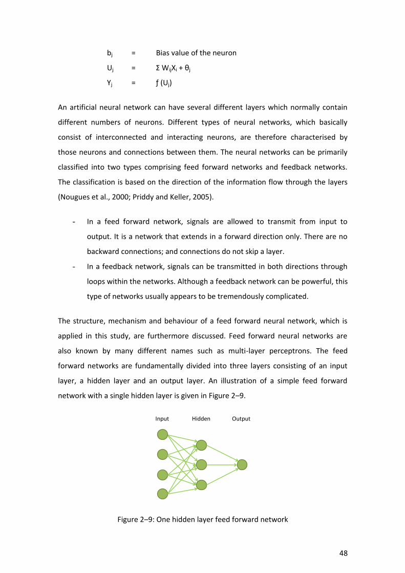
48

bj = Bias value of the neuron

Uj = Σ WijXi + θj

Yj = ƒ (Uj)

An artificial neural network can have several different layers which normally contain

different numbers of neurons. Different types of neural networks, which basically

consist of interconnected and interacting neurons, are therefore characterised by

those neurons and connections between them. The neural networks can be primarily

classified into two types comprising feed forward networks and feedback networks.

The classification is based on the direction of the information flow through the layers

(Nougues et al., 2000; Priddy and Keller, 2005).

- In a feed forward network, signals are allowed to transmit from input to

output. It is a network that extends in a forward direction only. There are no

backward connections; and connections do not skip a layer.

- In a feedback network, signals can be transmitted in both directions through

loops within the networks. Although a feedback network can be powerful, this

type of networks usually appears to be tremendously complicated.

The structure, mechanism and behaviour of a feed forward neural network, which is

applied in this study, are furthermore discussed. Feed forward neural networks are

also known by many different names such as multi-layer perceptrons. The feed

forward networks are fundamentally divided into three layers consisting of an input

layer, a hidden layer and an output layer. An illustration of a simple feed forward

network with a single hidden layer is given in Figure 2–9.

Figure 2–9: One hidden layer feed forward network

OutputInput Hidden

49

The first layer of the neurons is the input layer, followed by the interconnected layer of

neurons and then the output layer. All links proceed from all input neurons toward the

output neuron. As depicted in Figure 2–9, no processing occurs in an input neuron; it

basically feeds data into the network. It is important to note that this type of network

is often applied with the backpropagation algorithm. The feed forward networks and

the backpropagation training algorithm are regarded as the most generalised and the

most widely used models in a range of practical applications (Hanrahan 2011; Parker,

2007; Priddy and Keller, 2005; Rojas, 1996).

One layer of hidden neurons appears to be the most common structure of the feed

forward neural networks. There is no explicit rule of for determining the number of

hidden layers for a neural network. However, many studies mentioned that a single

hidden layer with the proper number of hidden neurons is sufficient for the majority of

problems (Franco et al., 2009; Hastie et al., 2009; Priddy and Keller, 2005). A hidden

layer can be generally made up of any number of neurons in parallel. Each neuron in

the hidden layer receives input from all the neurons in the input layer that are

weighted and then summed while the output is then formed by another weighted

summation from the neurons in the hidden layer. The number of neurons in an output

layer is equivalent to the number of outputs of the approximation problem. For

example, in Figure 2–9, there is one output corresponding to a single-output problem

(Franco et al., 2009; Parker, 2007; Priddy and Keller, 2005; Rojas, 1996). Determining

the number of input and output neurons is clear from the application; however,

determining the number of hidden neurons requires a bit of trial and error

experimentation to find out the best number of hidden neurons. An insufficient

number of hidden neurons prevents the neural network from learning the required

function, due to insufficient degrees of freedom. However, too many hidden neurons

usually cause the neural network to overfit the training data, resulting in a decrease in

generalisation accuracy (Parker, 2007; Priddy and Keller, 2005; Rojas, 1996).

2.8.3 Transfer functions in artificial neural networks

Clearly, a neuron in a neural network transforms data by using an activation function,

also called a transfer function, resulting in an activation value. Except for an output

50

neuron, the activation value is then fed to one or more other neurons. Transfer

functions that are extensively used in neural networks include the logarithm sigmoid

transfer function or logsig, the hyperbolic tangent sigmoid transfer function or tansig,

the linear transfer function or purelin and so forth (Lingireddy and Brion, 2005;

Sivanandam and Deepa, 2006; Zhang, 2010). Graphs of these commonly used transfer

functions are depicted in Figure 2–10.

Figure 2–10: Common transfer functions (MathWorks 2012)

The log-sigmoid transfer function, as shown in Figure 2–10 (a), is one of the most

commonly used non-linear transfer functions. It is often applied in multilayer neural

networks trained by the use of the backpropagation algorithm. This is because the log-

sigmoid transfer function is differentiable which can significantly decrease the

computation load for the training. The function takes any value of the input and yields

the output in the range of 0 to 1. According to Hanrahan (2011), the log-sigmoid

transfer function can be mathematically expressed as:

( )

(2–19)

Alternatively, as shown in Figure 2–10 (b), the hyperbolic tangent sigmoid transfer

function is another sigmoid function that is used in a number of neural networks. The

hyperbolic tangent is relatively similar to the log-sigmoid except for exhibiting learning

dynamics in the training phrase. It is important to note that the sigmoid function aims

to create a degree of nonlinearity between the input and the output. The hyperbolic

51

tangent sigmoid function produces the output in the range of –1 to 1. The form of the

hyperbolic tangent sigmoid transfer function is given below (Hanrahan, 2011).

( )

(2–20)

Although most models have non-linear characteristics between their input and output,

several models, when operated with nominal parameters, have behaviour that is close

to linear. The purelin transfer function, as shown in Figure 2–10 (c), can be a suitable

representation of those types of situation (Dorofki et al., 2012; Hanrahan, 2011). This

transfer function can be mathematically expressed as:

( ) (2–21)

2.8.4 Training artificial neural networks

An artificial neural network, which acts like the biological nervous system, learns by

samples. Therefore, it is necessary to configure the neural networks so that the inputs

are able to produce the desired outputs. The neural networks have the ability to learn

from their surroundings and the potential to improve their performance through

learning. In fact, the functionality of the neural networks is governed by the number of

layers, the number of neurons in the layers, the pattern of the connection between the

layers, as well as the weights of the connection. The weights are furthermore

determined by a particular training or learning algorithm. Training or learning is a

mathematical process of adjusting the weights and biases in order for the neural

network to learn the relationship between the inputs and the targets. The process

dictates an algorithm which is a prewritten set of rules to influences all the weights

and biases of the network (Priddy and Keller, 2005; Sivanandam and Deepa, 2006;

Wunsch et al. 2003; Zhang, 2010).

Training needs to be stopped at the proper time. Overlearning or overtraining may

takes place if the network is trained on the same inputs for too long. As a result, the

network loses the ability to generalise. This is because overlearning causes the

52

network to extract too much information from individual cases that leads to

overlooking the related information for the general case. Many training algorithms are

available for determining an optimum set of weights to solve the problems. Training

algorithms can be principally divided into two approaches which include supervised

training and unsupervised training (MathWorks, 2012; Priddy and Keller, 2005;

Sivanandam and Deepa, 2006).

- In supervised training, inputs and target values (desired outputs) are provided

to train the network. The difference between the desired outputs and the

actual outputs is used by the algorithm to adjust the weights.

- In unsupervised training, the network is only provided with inputs, not target

values. The network has to discover features to group the input data

automatically. It is commonly referred to as self-adaption.

The backpropagation algorithm, which is the most common form of supervised

training, is often applied in layered feed forward neural networks, as abovementioned.

However, it is not a requirement. The backpropagation algorithm is founded on the

error-correction rule. In the training phase of a feed forward backpropagation

network, the data is fed into the input layer and then propagated to the hidden layer

and to the output layer. The backpropagation algorithm fundamentally seeks the

minimum of the error function by the use of the method of gradient descent (Liu et al.,

2011; Priddy and Keller, 2005; Sivanandam and Deepa, 2006).

There are steps involved in each iteration of training by the use of the backpropagation

algorithm. The training data are fed into the network only in a forward direction,

generating result(s) at the output layer. Errors are calculated at the output neurons in

accordance with known target data while the required changes to the weights that

pass to the output layer are established based on this error calculation. The changes to

the weights are determined as a function of the errors calculated for all succeeding

layers, executing backward toward the input layer, until all required weight changes

are determined for the entire network. Then the calculated weight changes are applied

throughout the network. The next iteration then begins; the entire process is

reiterated using the next training pattern. Once appropriately trained, the feed

53

forward backpropagation neural network can be used for the classification of new data

(Priddy and Keller, 2005; Rojas, 1996; Sivanandam and Deepa, 2006).

In the training phase, data are divided into a training data set and a validation data set.

The training data set is used for calculating the error gradients and adjusting the

weights in order to obtain the desired output while the validation data set allows the

selection of the optimal number of iterations where the network learns information

from the training data set. Since the number of iterations increases; the training and

validation errors drop until reaching a minimum. Then the errors begin to increase.

Continuing the training process after the point of minimum error causes overfitting

(Hanrahan, 2011; Priddy and Keller, 2005).

Subsequently, it is important to evaluate performance of the completely trained neural

network. The process of neural network validation can be performed using two basic

methods. The first method is re-substitution which assesses the accuracy of the

network using the same set of data applied for building the network. However, this

validation method tends to be over optimistic or biased as it uses the entire set of data

for model construction and validation. The second method is train-and-test which is

most commonly used for neural network validation. It applies different sets of data to

construct and validate the model. Thus, error can be directly estimated from the

testing set (Priddy and Keller, 2005; Iliadis and Jayne, 2011).

2.8.5 Artificial neural network models for gasification applications

The efficient operation of the gasification process is determined by a range of complex

chemical reactions including pyrolysis, partial oxidation of products from pyrolysis,

gasification of the consequent char, conversion of tar and hydrocarbons, as well as the

water shift reduction. The development of mathematical models that can be used for

predicting the gasification characteristics and results or evaluating the effect of the key

input variables on the output variables is accordingly imperative. However, most

models for the gasification process are likely to be tremendously complex, difficult to

develop and time-consuming. In addition, most of the studies primarily engaged in coal

gasification (de Souza et al., 2012).

54

Puig-Arnavat et al. (2010) reviewed and analysed different approaches of biomass

gasification modelling. The approaches could be mainly divided into thermodynamic

equilibrium models, kinetic rate models, Advanced System for Process Engineering Plus

(Aspen Plus) models, in addition to artificial neural network models. However, a

number of studies illustrated the difficulties and limitations of developing the models

using equilibrium equations, kinetic equations, mass and energy balance equations

(Bridgwater, 2008; Corella and Sanz, 2005; Nemtsov and Zabaniotou, 2008; Thunman

et al., 2001; Tinaut et al., 2008). To avoid complex processes of modelling, some

studies have successfully developed and used artificial neural networks for gasification

applications. Neural networks concentrate on important inputs and disregard

insignificant excess data. In consequence, neural network models are flexible and

suitable among data-based modelling without requiring explicit mathematical

representation (Priddy and Keller, 2005; Sivanandam and Deepa, 2006). Even though

the neural network modelling approach has a great potential, it was found from a

study of the literature that neural network modelling for biomass gasification

applications is still limited.

Guo et al. (2001) developed a hybrid neural network model to simulate biomass

gasification processes in a fluidised bed gasifier with steam as the gasifying agent. The

study applied multilayer feed forward neural networks to identify gas production rate

and its composition (H2, CH4, CO and CO2) of four types of biomass (bagasse, cotton

stem, pine sawdust and poplar). The neural networks were trained separately for each

type of biomass. The results generated by the neural networks were able to reflect the

actual gasification profiles. The study also mentioned the potential to apply neural

network models for the research in this area.

Dong et al. (2002) studied co-firing of municipal solid waste (MSW) and coal in a

circulating fluidised bed. In that research, a three-layer feed forward backpropagation

network was constructed using experimental data. Mixing ratio and bed temperature

were employed as inputs while gaseous pollutants consisting of SO2, HCl, NO and N2O

were used as outputs. It was found that the neural network model was able to predict

55

gaseous pollutants with varied mixing ratio and bed temperature. The predicted

results obtained from the model agreed with the experimental data.

Furthermore, Dong et al. (2003) analysed and compared the ability of the neural

network model and the traditional multiple linear regression model in predicting the

heating value of MSW. Although the heating value of MSW could be determined by

many empirical approaches, it was difficult to identify relationship of interacting

factors, because of its complex composition. Similarly, a three-layer feed forward

network to predict the heating value of MSW was developed and then trained with the

backpropagation algorithm. The weight percentages of plastic, paper, food, grass and

textile were selected as the inputs while the lower heat value (LHV) of the syngas was

applied as the output. The number of hidden neurons in the hidden layer was

determined by experiments. The results indicated that the predicted values obtained

from the neural network model have more precision than the traditional multiple

linear regression models.

An artificial neural network prediction model was also developed by Xiao et al. (2009).

The key aim of the study was to predict gasification characteristics of MSW in a

laboratory scale fluidised bed gasifier. The experimental data of five kinds of organic

components (wood, paper, kitchen garbage, plastic and textile) as well as three types

of simulated MSW were used to create and train a three-layer feed forward neural

network model. The input layer contained seven neurons including the percentage of

wood, percentage of paper, percentage of kitchen garbage, percentage of plastic,

percentage of textile, ER (equivalence ratio) and temperature. Five hidden neurons

were employed in the hidden layer. Three neurons included in the output layer were

the LHV of the gas, the LHV of the gas with tar and char, as well as the gas yield. It was

found that the neural network model could be used to predict the gasification

characteristics within acceptable degrees of errors.

Satonsaowapak et al. (2011) built an artificial neural network to identify gasifier

systems suitable for biomass power plants. Similarly to other studies, a three-layer

feed forward backpropagation network was created using experimental data. The

input layer consisted of three neurons including biomass consumption rate,

56

temperature and ash discharge rate while the output layer contained only one neuron

which was the gas flow rate. Their results demonstrated that the neural network

model was a viable approach to estimate gas flow rate for biomass power plants.

2.9 Economics of power generation from gasification

Investment in power generation from the gasification technology, like any other

systems, is addressed by many forms of costs including fuel prices, power generation

technology costs, as well as operation and maintenance (O&M) expenditure. The

region of operation is also one of the key factors that drive the total investment of

energy business (Bridgwater, 1995; Bryana et al., 2008; IRENA, 2012; Leung et al.,

2004; Mitchell et al., 1995).

2.9.1 Fuel prices

The economics of power generation from the gasification technology critically relies on

the availability of a secure supply of a suitable feedstock at a reasonable cost. In some

cases, fuel costs can characterise up to 50% of the total cost of power generation

(IRENA, 2012). This is because it requires a large amount of fuel. It is also important to

mention that the fuel costs comprise not only the cost of fuel itself but also its

transportation and pre-processing costs (Bridgwater, 1995; Mitchell et al., 1995).

In the case of biomass, Bauen et al. (2004) reported that the cost of biomass fuels can

be either negative values in some residues requiring disposal or relatively high costs in

some dedicated energy crops. The cost of waste based biomass such as agriculture

waste and municipal solid waste (MSW), which require some form of disposal, are

often negative. Various residues from agricultural products and wood processing

industries can be available at zero or low cost but require some handling. Plant based

biomass is usually a seasonal resource; accordingly its availability and cost may vary

throughout the year. The cost of forestry biomass is incurred from its collection,

handling and transportation; thus it is possible to operate at a high cost. Energy crops

usually incur at the highest cost, similar to agricultural production. The cost is

dominated by land cost and land preparation, planting and agrochemical cost, as well

as harvesting cost (Bauen et al., 2004; IRENA, 2012).

57

Biomass typically requires pre-treatment prior to delivery to a power plant. Fuel

standardisation is needed to ensure proper quality of biomass acquired. The cost of

transporting biomass fuels is usually high; hence, distance of transportation becomes a

concern in its economics. The low energy density of biomass fuels can place a limit on

the distance that is economical for transportation. It is difficult for biomass gasification

systems to take advantage of economies of scale because a large amount of biomass at

a reasonable price may not be available (Bauen et al., 2004; IRENA, 2012).

Similarly to biomass, the price of coal is also driven by several factors including the

type, quality, pre-treatment, transportation and tax. In most cases, the price of coal

per unit mass basis was found to be higher than that of biomass. As a result, for the co-

gasification system, the selection of the types and blending ratios of fuels must be

within technical and economic feasibility (Bauen et al., 2004; Bridgwater, 1995; Leung

et al., 2004; Mitchell et al., 1995).

2.9.2 Power generation technology costs

The cost of gasification technology is mainly dominated by equipment costs which vary

significantly by the region of operation and the nature of the feedstock (IRENA, 2012).

The capital costs of medium sized power generation from the gasification system (up

to 75 MW) in different regions were approximated by Bauen et al. (2004) and Leung et

al. (2004), as presented in the Table 2–9.

Table 2–9: Approximate capital costs of medium sized power generation from

gasification system in different regions

Region The capital costs

Europe $2,000 - $3,000 per kWe range

North America $1,800 - $2,000 per kWe range

Asia $1,000 - $1,500 per kWe range

58

In most cases, the scale of operation has an impact on the economic feasibility of the

gasification system. Many studies indicated that a smaller scale system is often

characterised by a higher technology cost per energy unit (Bridgwater, 1995; Bryana et

al., 2008; Leung et al., 2004; Mitchell et al., 1995). Several aspects need to be taken

into consideration for selecting the gasification technology such as the type and cost of

available feedstock and the demand for electricity and heat of the local markets. These

factors also determine the scale of the project and the type of equipment. The total

cost of the gasification technology consist primarily of the engineering and

construction cost, gasification equipment, fuel handling machinery, as well as grid

connection and any new infrastructure required for the project (Bauen et al., 2004;

IRENA, 2012). The requirements for these components are usually different in different

projects at different regions of operation.

2.9.3 Operation and maintenance expenditure

The operation and maintenance (O&M) expenditure refers to the costs associated with

the operation of the gasification system. The O&M expenditure mainly includes labour,

scheduled maintenance, equipment replacement, insurance and so forth. The

economies of scale also have an impact on the O&M expenditure (IRENA, 2012).

2.9.4 Cost reduction potentials for the gasification technology

The analysis of the potentials for cost reduction in the gasification technology is

complicated. The potentials are highly dominated by the states of commercialisation.

There is a potential for cost reduction in the gasification system with internal

combustion engines which appears to be an established technology in many regions

around the world. However, shifting to greater efficiency systems still requires further

demonstration. In particularly, it needs an efficient gas cleaning and treatment

technology which is still characterised at an expensive cost (IRENA, 2012).

It is noticed that the viability of the gasification system lies in several factors consisting

mainly of the development of a reliable fuel supply chain and the selection of suitable

technology and equipment. The total investment cost of the gasification critically

varies by the region of operation and the economies of scale. In many countries,

59

government incentives or subsidies have been available for biomass gasification plants

to support energy generation from renewable resources.

2.10 Summary of literature review

The interest in development and utilisation of biomass for energy production has

gained momentum over the last two decades, mainly due to the increase in energy

consumption around the world, the decrease in availability of fuels and the concern

about environmental impacts from utilising fossil fuels. Many conversion technologies

have been available to convert biomass into several usable forms of energy.

Gasification, as a thermochemical conversion process, is one of the most promising

technologies to generate energy from biomass. Although biomass can be claimed as a

carbon neutral source of sustainable energy, it is often referred to as a low quality fuel

for thermochemical conversion processes compared to coal. Co-gasification has

accordingly become an attractive option not only to enhance gasification outcomes

but also to increase availability of fuels. Even though thermal behaviours of biomass

and coal blends under different conditions were studied, research on blending coal in a

biomass based system to facilitate thermochemical performance is still limited. The

review of literature has made it clear that there were little experiences with co-

gasification of biomass as a primary fuel and coal as a supplementary fuel for

improving gasification performance. The study of this co-gasification approach can

help to better understand the behaviour of biomass and coal blends and potentially

predict gasification outcomes in practical biomass based systems in order to support

energy supply security.

To achieve successful outcomes of the co-gasification, it is important to understand a

range of factors affecting the gasification system. The literature review sought to

identify and analyse key considerations of the gasification system, principally

consisting of properties of fuels used and their treatments, gasification configurations,

operating parameters, gasification products and contaminants, applications of

gasification products and economy of gasification. Biomass is referred to as biological

substances derived from organisms and/or their wastes while coal is a fossil fuel that

was formed by coalification of vegetation over hundreds of millions of years.

60

Therefore, chemical and physical properties of biomass are relatively different from

those of coal, in particular volatile matter (VM), fixed carbon (FC), carbon content,

oxygen content and higher heating value (HHV). Pre-treatment of biomass to modify

some of it properties may be required to reduce or avoid the difficulties in biomass

and coal co-gasification. Methods of biomass pre-treatment include drying, sizing,

pelletising and torrefaction.

Gasification is a process that partially oxidises solid carbonaceous fuels at elevated

temperatures. There are many types of gasification configurations which can be

principally classified into fixed bed gasifiers and fluidised bed gasifiers. Each type of

gasifier offers different benefits and drawbacks; so, the selection of a gasifier depends

on size, capital cost, availability of fuel used and type of preferred products. Downdraft

fixed bed gasifiers appear to be favourable on a small scale operation offering high

carbon conversion but low heating value of syngas produced. Operating parameters

substantially affect the gasification process and syngas production. Key operating

parameters that were generally found to support maximum gasification results include

the operating temperature range of 750–950 C, high heating rate, long residence time

and the use of dolomite as catalyst. For the gasifying agent used, different types

(oxygen, steam, air, carbon dioxide or their mixtures) have different advantages and

disadvantages; the choice of the gasifying agent used is determined by the heating

value of the product required, the acceptable level of the tar content and the available

cost. Proper operating conditions for the type of gasifier used can result in an increase

in quality and quantity of products and a decrease in formation of contaminants.

The gasification process occurring in a fix bed gasifier can be divided into four distinct

sub-processes encompassing drying, pyrolysis, combustion and gasification. The drying

process arises at the temperature up to 200 °C and allows changes in the fuel

structures and its thermophysical properties. Then, the pyrolysis process occurs at the

temperature range of 250–500 °C, releases the volatile components of the fuel and

creates many products including hydrogen, carbon monoxide, carbon dioxide, steam,

methane, acetylene, tar, char and ash. The carbon and hydrogen remaining from

pyrolysis go through the combustion process by reacting with oxygen from a gasifying

61

agent to produce carbon dioxide and steam. Subsequently, the actual gasification

reactions take place at temperatures above 700 C yielding a combustible synthesis gas

(also known as syngas), tar, char, ash and a small amount of other contaminants. The

syngas can be used for heat and/or electricity applications or further extracted to

provide energy services such as synthetic fuels and chemicals. The utilisation of the

syngas is determined by the gasification process and its operating conditions, the

quality of the syngas produced, in addition to the syngas treatment technology. The

syngas essentially consists of hydrogen, carbon monoxide, carbon dioxide, steam and a

trace of methane. Several approaches including co-gasification can be applied to

increase desired contents of the syngas (usually hydrogen and carbon monoxide) and

decrease contents of carbon dioxide and steam which are unfavourable.

The literature review furthermore covered previous studies on thermochemical

behaviour and kinetic analysis during pyrolysis and combustion of various types of

samples including biomass fuels, coals and their blends using TGA. Clearly, pyrolysis

and combustion are significant parts of the gasification process; so, investigation of

thermochemical behaviour during pyrolysis and combustion could help to better

understand the process. The study conducted by Vuthaluru (2003) concluded that no

interactions between biomass fuels (wood waste and wheat straw) and coal were

found during the co-pyrolysis. The pyrolytic behaviours of the blends seemed to follow

those of the individual fuels in an additive manner. However, the results from the

study conducted by Park et al. (2010) suggested some synergetic effect of the blend of

sawdust and sub-bituminous coal during co-pyrolysis in terms of the volatile yields.

Studies on thermochemical behaviour during co-combustion also indicated

controversial results. By the use of TGA, the kinetics of thermal events such as

activation energy and pre-exponential factor can be usefully determined by the

application of an appropriate kinetic model, in particular the Kissinger’s corrected

kinetic equation.

Modelling gasification process and performance is very complex, difficult and time-

consuming owing to the complexity of chemical reactions occurring during the process.

However, it was found that artificial neural networks (ANNs) could be used in biomass

62

gasification modelling. Artificial neural networks are a computational paradigm that is

inspired by the operation of the biological nervous system. The neural networks have

proved to be a powerful method of modelling complex non-linear relationships. Three-

layer feed forward backpropagation neural networks are the most widely used. Due to

the ability to learn and organise disperse data, some studies have successfully applied

the neural networks for gasification applications.

In practice, it is necessary to consider the economics of gasification in support of

successful energy production. The cost of power generation from the gasification

technology is mainly driven by fuel prices, power generation technology costs, in

addition to operation and maintenance (O&M) expenditure. The region of operation is

considered as one of the key factors that dominates the differences in the total

investment of energy business. It was found that the cost of fuel has a significant

impact on the economics of power generation from the gasification technology.

Therefore, a successful investment in the gasification system requires the

development of a reliable and affordable fuel supply chain as well as the selection of

suitable gasification technology and equipment. For the co-gasification system, fuels

and blending ratios have to be selected carefully to maintain a financially viable

operation.

63

Chapter 3

Objectives and scope of the study

3.1 Objectives

The objectives of this research were:

- To review the current literature on gasification technology with an

emphasis on co-gasification of biomass and coal for the syngas

production

- To analyse properties of selected biomass and coal samples in terms of

proximate and ultimate analyses

- To investigate thermochemical behaviour of biomass, coal and their

blends during pyrolysis and combustion processes using the techniques

of Thermogravimetric Analysis (TGA)

- To analyse and compare the composition of syngas produced from

gasification and co-gasification in terms of total combustible gas (TCG),

carbon dioxide which is a main greenhouse gas and energy content

(HHV and LHV).

- To evaluate the effects of fuels fed to the gasification system on the

final product

- To investigate relationships between the ratio of fuels and the syngas

quality under controlled conditions

- To develop a co-gasification model to determine concentration of TCG in

the syngas using an artificial neural network methodology

- To develop a financial model for small scale biomass gasification plants

to investigate the impact of fuel prices on the financial performance.

3.2 Scope of the study

This study focused on investigating the influence of selected biomass, coal and their

blends on the thermochemical behaviour and syngas production at four levels of

blending ratios of biomass to coal (95:5, 90:10, 85:15 and 80:20). These levels were

64

limited by the ability of the gasifier used (a laboratory-scale downdraft fixed bed

gasifier unit for biomass gasification). It covered the investigation of thermochemical

behaviour of the samples and their blends during pyrolysis and combustion using

thermogravimetric analysis (TGA). Kissinger’s corrected kinetic equation was applied to

determine kinetic parameters of the samples and the blends under nitrogen and air

environments using the TGA results. The study also included the analysis of syngas

produced from gasification and co-gasification. The results from the syngas analysis

were used to develop an artificial neural network model to predict the quality of the

syngas as assessed by its combustibility.

65

Chapter 4

Materials and methods

The experiments contained in this research project were carried out in two parts. The

first part studied the thermochemical behaviour of the samples using the TGA

techniques while the second part investigated the syngas production from gasification

and co-gasification, for which a neural network model was also developed and used to

predict the quality of the syngas produced in term of its combustibility. It is important

to address that the design of experiments for the experiments followed scientific

protocols in order to generate reliable data as well as to minimise any variations of the

results.

The design of experiments included defining objectives of the experiment, selecting

experimental variables, selecting the range of the independent variables, selecting

methods for measuring these variables, selecting instruments and tools, as well as

determining the number of data points needed for each type of measurements.

Experimental variables of these two experimental programmes, which consist of

independent variables, dependent variables and control variables, are listed in Table

4–1 and Table 4–2, respectively. To ensure reliability and validity of the research, the

data were collected and averaged over three separate run sessions for each set of

tests.

Table 4–1: Experimental variables for the study of thermochemical behaviour using the

TGA techniques

Type of variables Selected variables

Input factors (Independent variables)

Type of blending samples and blending ratio of the samples

Response variables (Dependent variables)

Activation energy and pre-exponential factor

Control variables Sample pre-treatment, type of carrier gas, gas flow rate, heating rate and temperature program

66

Table 4–2: Experimental variables for the study of syngas production from the

gasification and co-gasification

Type of variables Selected variables

Input factors (Independent variables)

Type of blending samples and blending ratio of the samples

Response variables (Dependent variables)

Syngas quality in terms of combustibility and energy content

Control variables Sample pre-treatment, operating conditions (air flow rate and residence time) and gas treatment

The values of response variables are basically assumed to depend on the values of

input factors. In the study of thermo-chemical behaviours using the TGA technique, the

blending ratio of the samples and type of blending samples were defined as input

factors while activation energy and pre-exponential factor were defined as response

variables.

Response Variable Y = Activation energy

= Pre-exponential factor

Factor A = Types of blending fuels

Factor B = Blending ratios of biomass and coal, % by mass

In the study of the syngas production from gasification and co-gasification, the

blending ratio of the samples and type of blending samples were defined as input

factors while syngas quality in terms of total combustible gas and heating value was

defined as response variables.

Response Variable Y = Combustibility

= Energy content

Factor A = Types of blending fuels

Factor B = Blending ratios of biomass and coal, % by mass

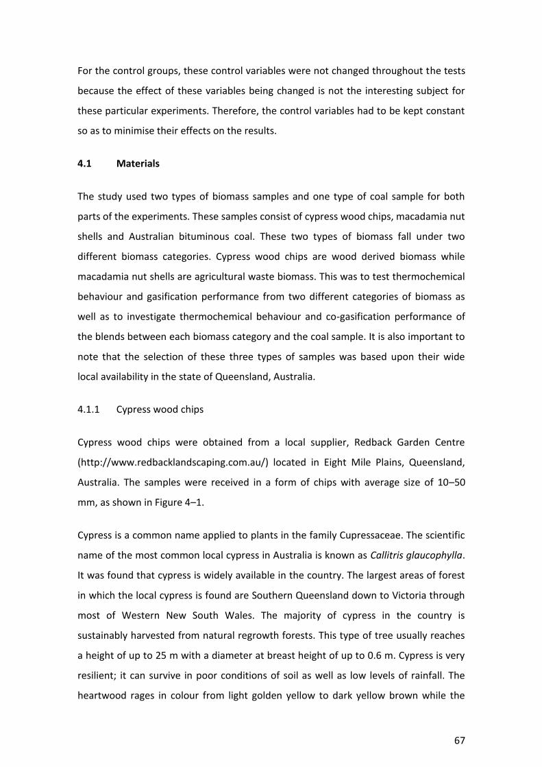
67

For the control groups, these control variables were not changed throughout the tests

because the effect of these variables being changed is not the interesting subject for

these particular experiments. Therefore, the control variables had to be kept constant

so as to minimise their effects on the results.

4.1 Materials

The study used two types of biomass samples and one type of coal sample for both

parts of the experiments. These samples consist of cypress wood chips, macadamia nut

shells and Australian bituminous coal. These two types of biomass fall under two

different biomass categories. Cypress wood chips are wood derived biomass while

macadamia nut shells are agricultural waste biomass. This was to test thermochemical

behaviour and gasification performance from two different categories of biomass as

well as to investigate thermochemical behaviour and co-gasification performance of

the blends between each biomass category and the coal sample. It is also important to

note that the selection of these three types of samples was based upon their wide

local availability in the state of Queensland, Australia.

4.1.1 Cypress wood chips

Cypress wood chips were obtained from a local supplier, Redback Garden Centre

(http://www.redbacklandscaping.com.au/) located in Eight Mile Plains, Queensland,

Australia. The samples were received in a form of chips with average size of 10–50

mm, as shown in Figure 4–1.

Cypress is a common name applied to plants in the family Cupressaceae. The scientific

name of the most common local cypress in Australia is known as Callitris glaucophylla.

It was found that cypress is widely available in the country. The largest areas of forest

in which the local cypress is found are Southern Queensland down to Victoria through

most of Western New South Wales. The majority of cypress in the country is

sustainably harvested from natural regrowth forests. This type of tree usually reaches

a height of up to 25 m with a diameter at breast height of up to 0.6 m. Cypress is very

resilient; it can survive in poor conditions of soil as well as low levels of rainfall. The

heartwood rages in colour from light golden yellow to dark yellow brown while the

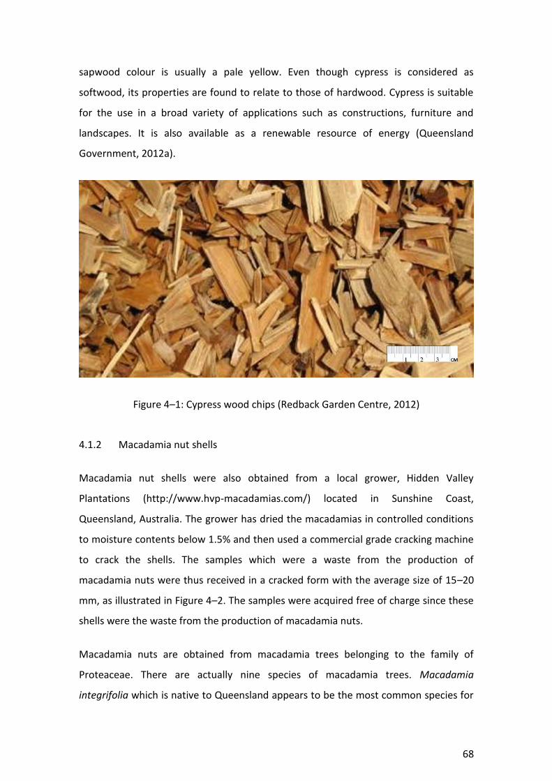
68

sapwood colour is usually a pale yellow. Even though cypress is considered as

softwood, its properties are found to relate to those of hardwood. Cypress is suitable

for the use in a broad variety of applications such as constructions, furniture and

landscapes. It is also available as a renewable resource of energy (Queensland

Government, 2012a).

Figure 4–1: Cypress wood chips (Redback Garden Centre, 2012)

4.1.2 Macadamia nut shells

Macadamia nut shells were also obtained from a local grower, Hidden Valley

Plantations (http://www.hvp-macadamias.com/) located in Sunshine Coast,

Queensland, Australia. The grower has dried the macadamias in controlled conditions

to moisture contents below 1.5% and then used a commercial grade cracking machine

to crack the shells. The samples which were a waste from the production of

macadamia nuts were thus received in a cracked form with the average size of 15–20

mm, as illustrated in Figure 4–2. The samples were acquired free of charge since these

shells were the waste from the production of macadamia nuts.

Macadamia nuts are obtained from macadamia trees belonging to the family of

Proteaceae. There are actually nine species of macadamia trees. Macadamia

integrifolia which is native to Queensland appears to be the most common species for

69

commercial growers. It is important to note that Australia has over six million

macadamia trees covering the areas of approximately 17,000 hectares. The country is

ranked as the world's largest macadamia nut producer accounted for 56% of total

production around the world. Macadamia plantings are mostly in the areas of

Queensland to New South Wales with minor plantings in Western Australia. There are

around 850 macadamia growers in the country. In recent years, Australian macadamia

nut production has been reported to be approximately 35,000 tonnes per year

(Australian Macadamia Society, 2012; Queensland Government, 2012b; Rural

Industries Research and Development Corporation, 2012). As a result, a large amount

of macadamia nut shells has become a waste and available in the country. Instead of

being discarded, those nut shells can be used in many applications such as carbon and

plastic products as well as a fuel for energy generation.

Figure 4–2: Macadamia nut shells obtained from Hidden Valley Plantations

4.1.3 Australian bituminous coal

An Australian bituminous coal sample was obtained from the Swanbank Power Station

(http://www.stanwell.com/swanbank-e-power-station.aspx) located in Swanbank, a

suburb of Ipswich, in South East Queensland, Australia. The coal sample was received

in a granular shape with the average size of 10–40 mm, as illustrated in Figure 4–3.

70

Figure 4–3: Bituminous coal obtained from the Swanbank Power Station

Australian bituminous coal, which is considered a high quality black coal, is mainly

found in Queensland and New South Wales. This type of coal is currently used for

power production not only in the country but also for exports. Queensland is a key

player in the coal production; in fact, 190.5 million tonnes of the coal were produced

during 2008 and 2009 (Queensland Government, 2010). As a result, in Australia, coal

still plays a dominant role in electricity production. It was found to generate over 54%

of the country’s electricity used by households, business and industry (Australian Coal

Association, 2012).

4.2 Sample preparation

Sample preparation usually plays a crucial role in experimental studies. It is influenced

by not only the quality of the sample but also the consistency of the sample. In thermal

analysis, temperature variations can be minimised with proper sample preparation. As

this research consisted of two principal parts comprising the study of thermochemical

behaviour using the TGA technique and the study of syngas production from the

gasification and co-gasification in a laboratory-scale downdraft gasifier, the samples for

these two different experimental parts were prepared differently. Sample preparation

is definitely considered to be an important factor for both experiments.

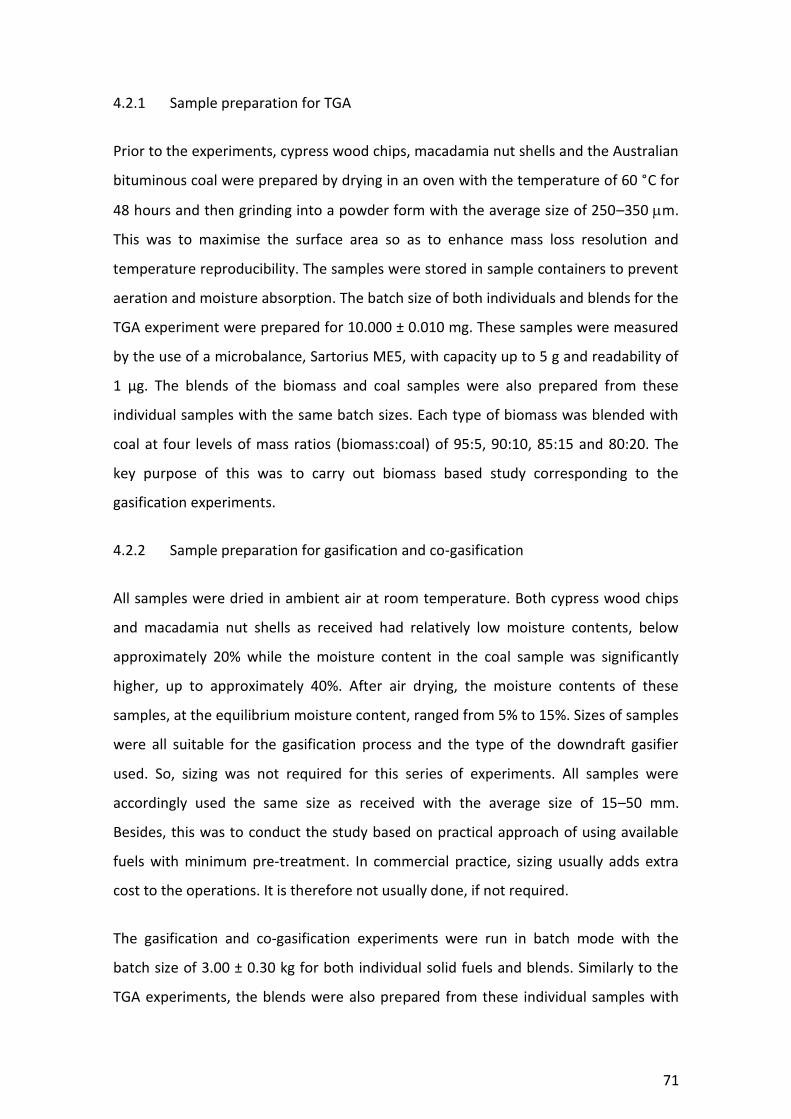
71

4.2.1 Sample preparation for TGA

Prior to the experiments, cypress wood chips, macadamia nut shells and the Australian

bituminous coal were prepared by drying in an oven with the temperature of 60 °C for

48 hours and then grinding into a powder form with the average size of 250–350 m.

This was to maximise the surface area so as to enhance mass loss resolution and

temperature reproducibility. The samples were stored in sample containers to prevent

aeration and moisture absorption. The batch size of both individuals and blends for the

TGA experiment were prepared for 10.000 ± 0.010 mg. These samples were measured

by the use of a microbalance, Sartorius ME5, with capacity up to 5 g and readability of

1 µg. The blends of the biomass and coal samples were also prepared from these

individual samples with the same batch sizes. Each type of biomass was blended with

coal at four levels of mass ratios (biomass:coal) of 95:5, 90:10, 85:15 and 80:20. The

key purpose of this was to carry out biomass based study corresponding to the

gasification experiments.

4.2.2 Sample preparation for gasification and co-gasification

All samples were dried in ambient air at room temperature. Both cypress wood chips

and macadamia nut shells as received had relatively low moisture contents, below

approximately 20% while the moisture content in the coal sample was significantly

higher, up to approximately 40%. After air drying, the moisture contents of these

samples, at the equilibrium moisture content, ranged from 5% to 15%. Sizes of samples

were all suitable for the gasification process and the type of the downdraft gasifier

used. So, sizing was not required for this series of experiments. All samples were

accordingly used the same size as received with the average size of 15–50 mm.

Besides, this was to conduct the study based on practical approach of using available

fuels with minimum pre-treatment. In commercial practice, sizing usually adds extra

cost to the operations. It is therefore not usually done, if not required.

The gasification and co-gasification experiments were run in batch mode with the

batch size of 3.00 ± 0.30 kg for both individual solid fuels and blends. Similarly to the

TGA experiments, the blends were also prepared from these individual samples with

72

mass ratios (biomass:coal) of 95:5, 90:10, 85:15 and 80:20. These levels are limited by

the ability of the biomass downdraft gasifier used. Pure biomass or zero percentage of

coal acted as a baseline for the gasification experiments to compare the quality of the

syngas from each level of blending ratios and to test the hypothesis that higher levels

of coal could improve the syngas quality as assessed by its combustibility.

4.3 Instruments and apparatus

4.3.1 Thermogravimetric Analyser

Thermogravimetric analysis of cypress wood chips, macadamia nut shells, an

Australian bituminous coal and their blends was performed by the use of a

Thermogravimetric Analyser, Netzsch TG 209 F3 Tarsus - Thermo-Microbalance. The

TG 209 F3 Tarsus is composed of three main parts including measuring part TG 209 F3,

circulating bath cooler and a personal computer system. The instrument is equipped

with a thermostat which is used to operate the instrument by handling thermostatic

control of instrument components related to the measurement. The measuring part

TG 209 F3 and its cross sectional image of are illustrated in Figure 4–4

Figure 4–4: The measuring part and its cross sectional image (Netzsch 2010)

The measuring part TG 209 F3 is made up of thermo microbalance system, furnace,

purge gas system and data collection system. The thermo microbalance system

contains a sample holder that resides in a furnace above the microbalance. The sample

73

holder is connected to the microbalance by a sample holder support. The

microbalance, which is enclosed by a tight housing, operates in accordance with the

concept of electromagnetic power compensation. It is thermostatically controlled in

order to prevent temperature influences. A sample is placed on the sample holder and

heated by a furnace which is enclosed by a cooling jacket. The thermostatic process is

carried out by water circuit. The thermocouple is included in the furnace through the

heating coil. The thermostatic control and radiation shield are used to avoid the

influence of heat emitted from the furnace on the balance system, which may result in

incorrect data. A purge gas is used to control the environment of the sample. This can

be oxidising, inert, static or dynamic atmosphere. The purge gas, under controlled

parameters, flows into the furnace and exits through an exhaust. The TG 209 F3 Tarsus

is a top loader with the reliable vertical construction which is safe and easy to use. The

sample temperature is accurately detected by a thermocouple in direct contact with a

sample crucible.

Netzsch TG 209 F3 Tarsus can measure the amount of mass change in a sample with a

resolution of 0.1 µg as a function of increasing temperature up to 1,000 °C. A heating

rate is selectable from 0.001 to 50 K/min while a cooling time ranges from 20 to 25

minutes (from 1000°C to 100°C). The instrument runs under Proteus Software on the

Microsoft Windows operating system. The software includes all important features

required for carrying out a measurement and evaluating the resulting data. Also, the

Proteus Software allows sophisticated analysis with a variety of functions such as mass

changes in mg or percentage, evaluation of mass changing steps, determination of the

residual mass, determination of mass-/temperature pair of variates, peak

temperatures of the 1st and 2nd derivative of the curve of mass changes, extrapolated

onset and endset, automatic baseline and buoyancy correction and so forth. The TG

209 F3 Tarsus facilitates reliable and automatic operation with microprocessor control

as well as provides digital data processing and acquisition using a personal computer.

4.3.2 Gasifier

The gasification and co-gasification experiments were run on a laboratory-scale

downdraft fixed bed gasifier unit through a wide range of chemical reactions and

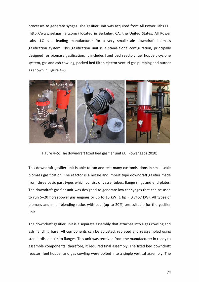
74

processes to generate syngas. The gasifier unit was acquired from All Power Labs LLC

(http://www.gekgasifier.com/) located in Berkeley, CA, the United States. All Power

Labs LLC is a leading manufacturer for a very small-scale downdraft biomass

gasification system. This gasification unit is a stand-alone configuration, principally

designed for biomass gasification. It includes fixed bed reactor, fuel hopper, cyclone

system, gas and ash cowling, packed bed filter, ejector venturi gas pumping and burner

as shown in Figure 4–5.

Figure 4–5: The downdraft fixed bed gasifier unit (All Power Labs 2010)

This downdraft gasifier unit is able to run and test many customisations in small scale

biomass gasification. The reactor is a nozzle and imbert type downdraft gasifier made

from three basic part types which consist of vessel tubes, flange rings and end plates.

The downdraft gasifier unit was designed to generate low tar syngas that can be used

to run 5–20 horsepower gas engines or up to 15 kW (1 hp = 0.7457 kW). All types of

biomass and small blending ratios with coal (up to 20%) are suitable for the gasifier

unit.

The downdraft gasifier unit is a separate assembly that attaches into a gas cowling and

ash handling base. All components can be adjusted, replaced and reassembled using

standardised bolts to flanges. This unit was received from the manufacturer in ready to

assemble components; therefore, it required final assembly. The fixed bed downdraft

reactor, fuel hopper and gas cowling were bolted into a single vertical assembly. The

75

filter housing was bolted on the top of the cyclone which was attached to the reactor

through the gas outlet flange of the cyclone while the ejector venturi and burner are

attached on the filter housing. The CAD drawing of the downdraft reactor with air

preheating tubes is illustrated in Figure 4–6.

Figure 4–6: The CAD drawing of the downdraft reactor (All Power Labs 2010)

The key steps for the assembly of the unit to give a desired gasifier configuration are

presented here. The assembly can be divided into six parts encompassing gas cowling

assembly, downdraft reactor insert assembly, cyclone and filter assembly, ejector

venturi and swirl burner assembly, manometer, as well as lid and stir bar. The steps

required for the gas cowling assembly consisted of attaching the bottom plate,

attaching legs, adding ash port lid, inserting ash rotary grate and inserting insulation.

The downdraft reactor insert assembly was composed of attaching gas lines, installing

reduction bell, inserting air inlet nozzles, assembling reactor insert and gas cowling,

installing stainless steel reactor insulation and assembling ignition port. To increase the

insulation around the reduction bell, an insulating material which can be charcoal dust,

76

ash, perlite or pumice can be added into the annular ring of the reactor. For this study,

ash was used.

For cyclone and filter, the key assembly steps included attaching the cyclone to the gas

cowling, attaching Mason jar and installing packed bed filter. Ejector venturi and swirl

burner assembly required installing the ejector venturi and attaching the swirl burner

to the ejector venturi. Then, the last steps consisted of installing the manometer and

attaching the lid and stir bar. Sealing is considered as an important factor for the final

assembly of the gasification unit in order to avoid compromising the system and

resulting in failed runs and leaking of syngas. Thus, clay weather stripping was used for

all attachment of metal to metal flange as air tight sealant. Moreover there were

several measuring tools which had to be incorporated into the gasifier unit. These tools

consisted of a two channel digital thermocouple reader (type K), two type K soft

thermocouples 40” (1020 mm) long, one type K hard probe of 24″ (610 mm) length

with handle (Omega instrument) and a low pressure water manometer including a dual

column manometer.

4.3.3 Gas Chromatograph/Mass Selective Detector (GC/MSD)

The composition of the syngas produced from the gasification process of the solid fuels

and their blends was analysed by the use of Agilent Technologies 6890 Series Gas

Chromatograph with Agilent Technologies 5973Network Mass Selective Detector, as

presented in Figure 4–7.

Key components of the GC/MS instrument include injectors, ovens, columns and

transfer lines. Injectors are used to introduce the sample into the GC column. There

are two modes of injection commonly employed for capillary GC. These modes consist

of split and splitless. The selection of injection mode is dependent on the

concentration of the analyte(s) to be tested in the sample (Concha et al., 2002;

Sparkman et al., 2011). An oven is also a key component of the GC instrument. The GC

oven is used for a gradual increase in temperature, known as ramping. Ramping can

facilitate better separating forces and stationary phase interactions. As the

temperature of the oven increases, the compounds contained within the sample are

77

heated to reach their boiling points. For that reason, compounds that have lower

boiling points are eluted faster than compounds that have higher boiling points (Grob

and Barry, 2004; Sparkman et al., 2011). The Agilent Technologies 6890 GC oven was

used in this study. The capabilities of the Agilent Technologies 6890 GC oven are

summarised in Table 4–3.

Figure 4–7: Agilent 6890 GC with 5973 MSD (Kitmondo 2013)

Table 4–3: Capabilities of the Agilent 6890 GC oven

Capability Range

Temperature range –80 °C (liquid N2) or –60 °C (CO2) to the configured limit

Maximum temperature 450 °C

Temperature programming up to 6 ramps

Maximum run time 999.99 minutes

Temperature ramp rates 0 to 120 °C/min, conditional on instrument configuration

In Gas Chromatography, the column is the core of the system since separation of

sample components occurs at the GC column and a stationary phase. Basically, sample

components are injected into the GC column and carried via a stationary phase. There

are a variety of types of GC column. These can be principally classified into packed

78

columns and open tubular columns (also known as capillary columns). Open tubular

columns can be furthermore classified into three types including support-coated open

tubular (SCOT), wall-coated open tubular (WCOT) and porous-layer open tubular

(PLOT). Choosing the most suitable column is considered to be of great importance for

an analysis (Hoffman and Stroobant, 2007). The GC column selected in this study was

Agilent Technologies Agilent J&W GS-GasPro GC Column, Model 113-4332. The GS-

GasPro capillary column is a unique bonded PLOT column that is suitable for ambient

and higher temperature analysis of C1 to C12 hydrocarbons, CO2, sulphur gases and a

range of volatile inorganic gases. High surface area along with a bonded phase

technology allows the GS-GasPro column to be efficient and rinsible. This type of

column is very functional GC/MS applications since it has no particles to dislodge.

Retention stability of the GS-GasPro column is not affected by water. CO and CO2 can

be moreover separated on a single column. The GS-GasPro 113-4332 GC Column has

an inner diameter (ID) of 0.32 mm, length of 30 m and temperature range of - 80 to

260/300 °C.

A transfer line typically contains fused silica; it is used to transfer sample components

from the Gas Chromatograph to the Mass Detector. It basically serves as a connection

between the GC machine and the MS machine; therefore, it becomes essential that

the distance between these instruments is kept to a minimum. The transfer line is

often heated but it can be non-heated for more specialised use. It is usually connected

directly to the GC column. The exposed area of the line is insulated. This is to ensure

that heat is retained and components are eluted properly. Voids in the transfer lines

can cause retention time or noise ratio in the Mass Detector. These voids are often

experienced once there is a gap between connections of the transfer line. Even a small

gap can lead to many unexpected results. To reduce or eliminate gaps, it is necessary

to routinely check the connections for voids. Moreover, the transfer line needs to be

changed when it is cracked from age or has a build-up of other compounds bound to

its walls (Daas, 2007).

The Agilent Technologies 6890 GC is equipped the Agilent Technologies 5973Network

Mass Selective Detector, as shown in Figure 4–7. This Mass Selective Detector (MSD)

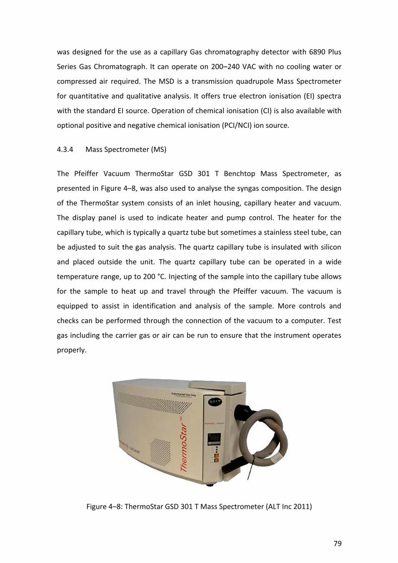
79

was designed for the use as a capillary Gas chromatography detector with 6890 Plus

Series Gas Chromatograph. It can operate on 200–240 VAC with no cooling water or

compressed air required. The MSD is a transmission quadrupole Mass Spectrometer

for quantitative and qualitative analysis. It offers true electron ionisation (EI) spectra

with the standard EI source. Operation of chemical ionisation (CI) is also available with

optional positive and negative chemical ionisation (PCI/NCI) ion source.

4.3.4 Mass Spectrometer (MS)

The Pfeiffer Vacuum ThermoStar GSD 301 T Benchtop Mass Spectrometer, as

presented in Figure 4–8, was also used to analyse the syngas composition. The design

of the ThermoStar system consists of an inlet housing, capillary heater and vacuum.

The display panel is used to indicate heater and pump control. The heater for the

capillary tube, which is typically a quartz tube but sometimes a stainless steel tube, can

be adjusted to suit the gas analysis. The quartz capillary tube is insulated with silicon

and placed outside the unit. The quartz capillary tube can be operated in a wide

temperature range, up to 200 °C. Injecting of the sample into the capillary tube allows

for the sample to heat up and travel through the Pfeiffer vacuum. The vacuum is

equipped to assist in identification and analysis of the sample. More controls and

checks can be performed through the connection of the vacuum to a computer. Test

gas including the carrier gas or air can be run to ensure that the instrument operates

properly.

Figure 4–8: ThermoStar GSD 301 T Mass Spectrometer (ALT Inc 2011)

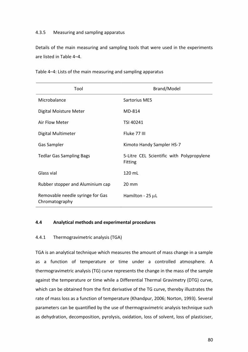
80

4.3.5 Measuring and sampling apparatus

Details of the main measuring and sampling tools that were used in the experiments

are listed in Table 4–4.

Table 4–4: Lists of the main measuring and sampling apparatus

Tool Brand/Model

Microbalance Sartorius ME5

Digital Moisture Meter MD-814

Air Flow Meter TSI 40241

Digital Multimeter Fluke 77 III

Gas Sampler Kimoto Handy Sampler HS-7

Tedlar Gas Sampling Bags 5-Litre CEL Scientific with Polypropylene Fitting

Glass vial 120 mL

Rubber stopper and Aluminium cap 20 mm

Removable needle syringe for Gas Chromatography

Hamilton - 25 L

4.4 Analytical methods and experimental procedures

4.4.1 Thermogravimetric analysis (TGA)

TGA is an analytical technique which measures the amount of mass change in a sample

as a function of temperature or time under a controlled atmosphere. A

thermogravimetric analysis (TG) curve represents the change in the mass of the sample

against the temperature or time while a Differential Thermal Gravimetry (DTG) curve,

which can be obtained from the first derivative of the TG curve, thereby illustrates the

rate of mass loss as a function of temperature (Khandpur, 2006; Norton, 1993). Several

parameters can be quantified by the use of thermogravimetric analysis technique such

as dehydration, decomposition, pyrolysis, oxidation, loss of solvent, loss of plasticiser,

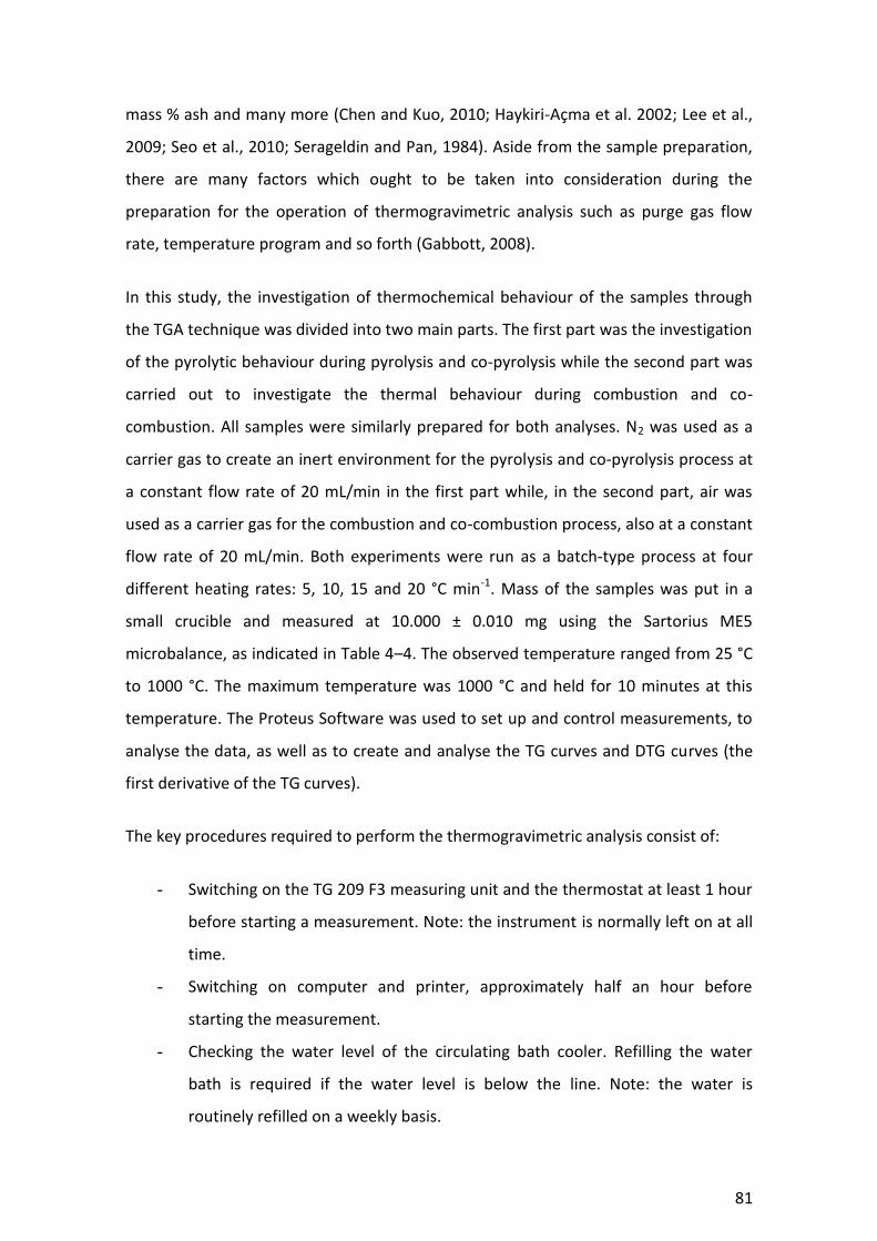
81

mass % ash and many more (Chen and Kuo, 2010; Haykiri-Açma et al. 2002; Lee et al.,

2009; Seo et al., 2010; Serageldin and Pan, 1984). Aside from the sample preparation,

there are many factors which ought to be taken into consideration during the

preparation for the operation of thermogravimetric analysis such as purge gas flow

rate, temperature program and so forth (Gabbott, 2008).

In this study, the investigation of thermochemical behaviour of the samples through

the TGA technique was divided into two main parts. The first part was the investigation

of the pyrolytic behaviour during pyrolysis and co-pyrolysis while the second part was

carried out to investigate the thermal behaviour during combustion and co-

combustion. All samples were similarly prepared for both analyses. N2 was used as a

carrier gas to create an inert environment for the pyrolysis and co-pyrolysis process at

a constant flow rate of 20 mL/min in the first part while, in the second part, air was

used as a carrier gas for the combustion and co-combustion process, also at a constant

flow rate of 20 mL/min. Both experiments were run as a batch-type process at four

different heating rates: 5, 10, 15 and 20 °C min-1. Mass of the samples was put in a

small crucible and measured at 10.000 ± 0.010 mg using the Sartorius ME5

microbalance, as indicated in Table 4–4. The observed temperature ranged from 25 °C

to 1000 °C. The maximum temperature was 1000 °C and held for 10 minutes at this

temperature. The Proteus Software was used to set up and control measurements, to

analyse the data, as well as to create and analyse the TG curves and DTG curves (the

first derivative of the TG curves).

The key procedures required to perform the thermogravimetric analysis consist of:

- Switching on the TG 209 F3 measuring unit and the thermostat at least 1 hour

before starting a measurement. Note: the instrument is normally left on at all

time.

- Switching on computer and printer, approximately half an hour before

starting the measurement.

- Checking the water level of the circulating bath cooler. Refilling the water

bath is required if the water level is below the line. Note: the water is

routinely refilled on a weekly basis.

82

- Opening the TG 209 F3 measuring unit (the furnace lid on the top)

- Pressing the push button (on the left side of the TG 209 F3 measuring unit) to

move the sample holder into the top position.

- Placing an empty crucible for baseline (correction measurement)

- Ensuring that the crucible has been correctly placed on the centre by looking

from the top view

- Pressing the push button (on the left side of the TG 209 F3 measuring unit) to

move the sample holder back into the bottom position

- Closing the measuring unit (the furnace lid on the top)

- Starting the TG 209 F3 measurement program (Proteus Software)

- Setting the amount of gases required

- Following the steps as shown in Figure 4–9 to create a baseline

File Menu

New

TG 209 F3 Test Parameters

Measurement Type: Correction

Open Temperature Recalibration

Set Temperature Program

Set Evacuation (if required)

Define File Name

The program switches to the

Adjustment Menu

Figure 4–9: Flow chart to create a baseline (Netzsch 2010)

- Setting the Initial Cond. ON

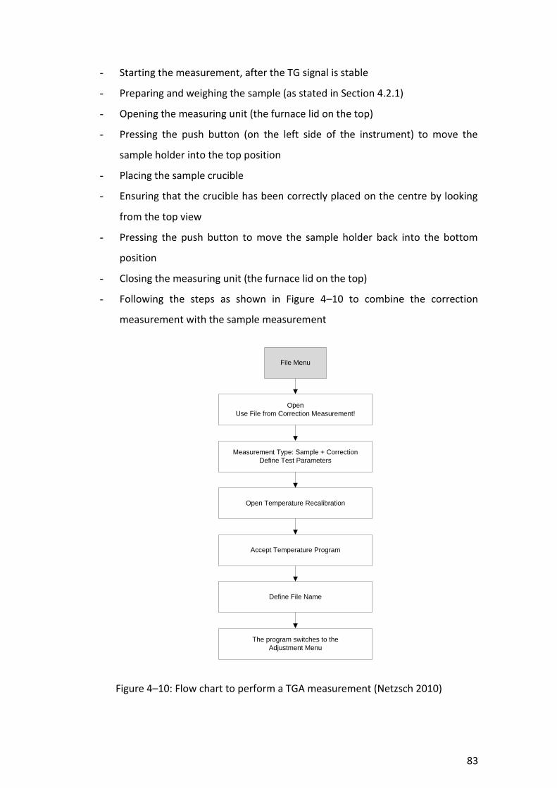
83

- Starting the measurement, after the TG signal is stable

- Preparing and weighing the sample (as stated in Section 4.2.1)

- Opening the measuring unit (the furnace lid on the top)

- Pressing the push button (on the left side of the instrument) to move the

sample holder into the top position

- Placing the sample crucible

- Ensuring that the crucible has been correctly placed on the centre by looking

from the top view

- Pressing the push button to move the sample holder back into the bottom

position

- Closing the measuring unit (the furnace lid on the top)

- Following the steps as shown in Figure 4–10 to combine the correction

measurement with the sample measurement

File Menu

Open

Use File from Correction Measurement!

Measurement Type: Sample + Correction

Define Test Parameters

Open Temperature Recalibration

Accept Temperature Program

Define File Name

The program switches to the

Adjustment Menu

Figure 4–10: Flow chart to perform a TGA measurement (Netzsch 2010)

84

- Setting the Initial Cond. ON

- Starting the measurement, after the TG signal is stable

- After the measurement is finished, pressing the push button (on the left side

of the instrument) to move the sample holder to the top position

- Removing the sample crucible

- Opening the Proteus Analysis program. The analysis can be carried out

through the Proteus Software

4.4.2 Operation of the gasification unit

The gasification and co-gasification experiments were operated as a batch-type

process using air as a gasifying agent. It was carried out in accordance with proper

safety precautions. The key experimental procedures for the process of gasification

and co-gasification of the solid fuels and their blends were broken down into three

parts including preparation procedures, starting up and running procedures and

shutting down procedures. Schematic of the operation of the gasification unit is

illustrated in Figure 4–11.

Figure 4–11: Schematic of the operation of the gasification unit

4.4.2.1 Preparation procedures

- The bottom of the downdraft reactor and the reduction bell were filled to

about 25 mm above the nozzles with charcoal in the size range of 15 to 25

mm diameter. Care was taken to avoid generating dust which may foul the

85

reduction process on start-up. The ash grate was turned vigorously to ensure

the charcoal settled in the reactor.

- The solid fuel (cypress wood chips or macadamia nut shells) or the blend of

biomass and coal was added to the top of the reactor. It was made sure that

the solid fuel or the blend was properly prepared as indicated in Section 4.2.2

Sample preparation for gasification and co-gasification.

- The ash grate was turned again to check that the solid fuel or the blend was

settled properly.

- The lid seal was checked prior to closing of the reactor. Nuts on the lid were

tightened to make sure that no leaks would occur.

4.4.2.2 Starting up and running procedures

- The downdraft reactor was started with the lid on. The lighting fluid, which

was 50 to 100 millilitres of Methylated Spirits, was injected into the reactor

through the ignition port.

- The regular air inlet on the top of the downdraft reactor was closed using the

1-inch cap.

- The flare side gate valve was opened. The compressed air valve was opened

until 1–2 (25–50 mm) inches of H2O in the reactor manometer was achieved.

The manual premix air valve was closed.

- It was rechecked that all caps and plugs were in place to ensure no air leaked

into the gasifier.

- The downdraft reactor was lit through the ignition port by using a hand held

propane torch.

- The air inlet cap was then taken off when the ignition was established. This

usually took about two to five minutes.

- The flare was lit to assist in burning off the tar and steam smoke during start

up. The handheld propane torch flame was held at the bottom of the flare

swirl burner until a large pilot flame was obtained. This also helped in

removing the tar until the stable syngas flame was achieved.

86

- The handheld propane torch was turned off. Care was taken in avoiding

breathing in unburned gas.

- The compressed air valve was adjusted to operate approximately 3–8 (76 –

200 mm) inches of H2O in the reactor manometer.

- (Optional) The manual premix air valve could be adjusted to add more or less

air to the syngas to achieve proper combustion in the flare.

- The air flow rate, bed temperature, pressure, gas flow rate were monitored

and recorded every two minutes.

- The level of the solid fuel or the blend was monitored approximately every

five minutes through the fill port in the data tables, based on the

experimental design.

- The gas sampler (Kimoto Handy Sampler HS-7) was used to pump the syngas.

Then the syngas was collected in a Tedlar gas sampling bag (5 Litter CEL

Scientific).

4.4.2.3 Shutting down procedures

- The compressed air valve was closed to stop the reactions and allow the

downdraft reactor to cool down.

- The manual premix air valve and the flare side gate valve were closed. The air

inlet was capped. Very little to no gas exited the reactor when the reactor was

cool.

4.4.3 The use of GC/MS and MS techniques to analyse the syngas

Syngas produced from the gasification process is mainly composed of carbon

monoxide, hydrogen, methane, carbon dioxide, steam, oxygen and nitrogen. The

GC/MS and MS analytical methods were adopted for the analysis of the syngas.

The Gas Chromatography (GC) is an analytical method that measures the content of

organic compounds in a sample. To increase the ability to identify the information

produced from the Gas Chromatograph, it is commonly linked with a Mass

Spectrophotometer. It is thereby called Gas Chromatography Mass Spectrometry or

GC/MS (Grob and Barry, 2004; Niessen, 2001). The GC/MS is one of the most

87

established and the best analytical techniques available for the identification and

quantitation of many organic compounds contained in complex matrices. The GC part

separates a sample which is usually a mixture of compounds into individual

compounds while the MS part quantifies and identifies those compounds by the mass

of analyte molecule. The GC/MS instrument is widely used in a range of fields such as

environmental science, forensics, health care, medical research, biological research,

health and safety and food science (Grob and Barry, 2004).

When using the GC method, a mixture of organic compounds is injected into the inlet

valve and the mixture then passes through into the GC column where it is heated and

separated into its constituents. With the aid of a carrier gas, the mixture is pushed into

the detector. A schematic of the injector with septum purge is illustrated in Figure 4–

12.

Figure 4–12: Schematic of the injector with septum purge (Chasteen 2000)

As noted above, the split and splitless techniques are two common modes of injections

for capillary GC. The split mode is mostly used for higher concentration samples while

the splitless mode is suitable for lower concentration samples. In split mode, the

sample is injected and vaporised into the carrier gas. The majority of the sample passes

out the split vent to atmosphere while only a small amount of the sample flows into

the GC column, usually about 1–2%. Thus, the split injection is not appropriate for

ultra-trace analysis (Concha et al., 2002; Sparkman et al., 2011). In this study, the split

88

mode was applied in order to narrow analyte band on the column and to protect the

column from non-volatile components of the sample.

The GC technique separates organic compounds by their volatility or retention time.

Basically, smaller molecules travel through a GC column more quickly compared to

larger molecules. It is based upon the principle that the separation of the mixture into

individual compounds occurs when heated. The heated sample is carried through a GC

column with an inert gas, commonly helium (Grob and Barry, 2004; Niessen, 2001).

Helium was used as a carrier gas for the gas analysis in this study. The development of

operating methods for the GC/MS technique involves understanding of the melting

point(s) of the compound(s) being analysed. The understanding of the melting point of

the compound contributes to better volatilisation of the sample. Moreover, the sample

ought to be transferred through the column in as narrow a band as possible with the

absence of air. The column serves the purpose of separating the components of the

mixture while decreasing the broadness of the band corresponding to the compound.

The column pushes the components through it and allows for the components to be

eluted as a sharp peak. This can maximise the signal to noise ratio for each analyte

analysed (Sparkman et al., 2011). The methods and instruments used to analyse the

composition of the syngas in this study are listed in Table 4–5.

Table 4–5: Methods and instruments used to analyse composition of the syngas

Composition of Syngas Method Instrument

CO GC/MS Agilent 6890 GC with 5973 MSD

H2, CH4, CO2, H2O, O2 and N2 MS ThermoStar GSD 301 T MS

4.4.3.1 Analysis of CO in the syngas

The GC/MS instrument (Agilent 6890 GC with 5973 MSD) was used in this study to

detect carbon monoxide content in the syngas. Control parameters of the GC

instrument used in this study is accordingly summarised in Table 4–6.

89

Table 4–6: Control parameters of the GC instrument (6890 GC method) for carbon

monoxide analysis

Oven

Initial temp: 27 °C (On)

Initial time: 3.00 min

Ramps:

# Rate Final temp Final time

1 0.0 (Off)

Post time: 0.00 min

Post time: 0.00 min

Run time: 3.00 min

Maximum temp: 325 °C

Equilibration time: 0.50 min

Front Inlet (CIS3)

Mode: Split

Initial temp: 0 °C (Off)

Pressure: 3.35 psi (On)

Split Ratio: 1:1

Split Flow: 2.0 mL/min

Total Flow: 7.0 mL/min

Gas saver: Off

Gas Type: Helium

Back Inlet: (Unknown)

Column 1 Column 2

Capillary Column

Model No.: Agilent 113-4332

GS-GasPro, 0.32 mm * 30 m

Max temperature: 300 °C

Nominal length: 30.0 m

Nominal diameter: 320 m

Nominal film thick’: 0.00 m

Mode: Constant pressure

Pressure: 3.35 psi

Nominal initial flow: 2.0 mL/min

Average velocity: 51 cm/sec

Inlet: Front Inlet

Outlet: MSD

Outlet pressure: Vacuum

(Not Install)

90

Key procedures of analysis of carbon monoxide in the syngas using the GC/MS

instrument are composed of:

- Generating the acquisition and quantitation method through GC/MS Selected

Ion Monitoring (SIM) technique.

- Preparing a set of carbon monoxide standards with known concentrations.

Noted: the carbon monoxide standard solution was prepared in glass vials. It

was diluted with Nitrogen to eight different concentrations consisting of 0.1%

or 1000 ppm, 0.5% or 5000 ppm, 1%, 2%, 5%, 10%, 15% and 20%.

- Running the analysis of all carbon monoxide concentrations through the SIM

technique to find out their corrected areas.

- Using Microsoft Excel to create the calibration curve based on the

measurements of the corrected areas of the known carbon monoxide

concentrations in order to determine the concentration of unknown samples.

Note: the known concentrations were put on the X axis and the corrected

areas were put on the Y axis. The results are shown in Figure 7–1.

- Using Microsoft Excel to calculate the regression line equation for the

calibration curve.

- Running the analysis of the syngas to find out its carbon monoxide content

corresponding to the regression line equation.

4.4.3.2 Analysis of H2, CH4, CO2, H2O, O2 and N2 in the syngas

In this study, the MS instrument (Pfeiffer Vacuum ThermoStar GSD 301 T Mass

Spectrometer) was used to measure hydrogen, methane, carbon dioxide, steam,

oxygen and nitrogen content in the syngas. The basic principle of the MS instrument is

to produce ions from inorganic or organic compounds. The instrument separates the

ions based on their mass to charge ratio and detects them both qualitatively and

quantitatively. The sample can be ionised thermally by inputting energy. The common

scheme of the Mass Spectrometer consists of an ion source, a mass analyser and a

detector.

91

The newer MS system, which was used in this study, incorporates vacuums and

automated systems. To identify the analyte, the Mass Spectrometer is considered

destructive. This is due to the process of ionisation and translational motion through

the mass analyser and analysis by the detector. It needs low levels of analyte to

complete analysis of the sample (Becker, 2008; Watson and Sparkman, 2007).

However, in conducting the analysis, some changes may be required to better purity to

identify the analytes in the sample (Schalley and Springer, 2009). The key steps to

perform the measurements of the syngas through the ThermoStar GSD 301 T Mass

Spectrometer consist of choosing operating mode (simulation), calibrating the mass

scale, calibrating the mass spectrometer, in addition to measuring and storing

concentrations.

4.4.4 Neural network modelling procedures

MATLAB 7.11.0 (R2010b) and Neural Network Toolbox 7.0 were applied for the

development of the neural network model. MATLAB is a numerical computing

programme. It allows matrix manipulation, implementation of algorithms, plotting of

data and functions, as well as interfacing with other programming languages. The

Neural Network Toolbox in MATLAB contains a range of tools for designing, training,

visualising as well as simulating neural networks. It offers comprehensive support for

several network paradigms and graphical user interfaces (GUIs) that allow the user to

simply design and manage neural networks. Neural Network Toolbox is also provided

with a useful user guide. Basic process flow for developing a neural network model is

illustrated in Figure 4–13.

Data Preparation

Building Network

Training Network Testing Network

Problem Identification

Figure 4–13: Process flow for developing a neural network

92

Key procedures for developing a neural network using Neural Network Toolbox are

summarised below:

- Problem identification:

Deciding on a problem to solve is the first step in developing an artificial

neural network.

- Data preparation:

Gathering data is then required for the training purposes. General steps of

data preparation take account of data consolidation and cleaning, data

selection and pre-processing, data transformation and encoding (if needed).

- Building network:

In the stage of building the network, it is to choose architecture of the

network which involves determining the number of nodes in input layer and

output layer, the number of hidden layers and their number of nodes, transfer

functions between the layers, weight and bias learning function, as well as

performance function. Custom network architectures for specific problem can

be constructed using Neural Network Toolbox.

- Training network:

Neural Network Toolbox offers a range of training algorithms which are

mathematical procedures employed automatically adjust weights and biases

of the network. A neural network must be trained properly in order to achieve

good generalisation accuracy on new sets of data.

- Testing network:

The final step is to evaluate performance of the model developed. Commonly,

an unseen set of data are used for testing. The evaluation of the performance

can be achieved through statistical analysis, such as mean squared error

(MSE) and regression R value (R).

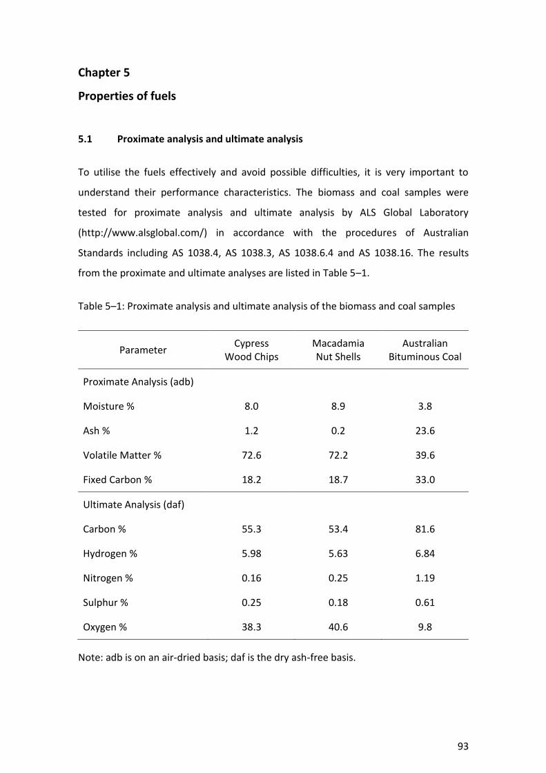
93

Chapter 5

Properties of fuels

5.1 Proximate analysis and ultimate analysis

To utilise the fuels effectively and avoid possible difficulties, it is very important to

understand their performance characteristics. The biomass and coal samples were

tested for proximate analysis and ultimate analysis by ALS Global Laboratory

(http://www.alsglobal.com/) in accordance with the procedures of Australian

Standards including AS 1038.4, AS 1038.3, AS 1038.6.4 and AS 1038.16. The results

from the proximate and ultimate analyses are listed in Table 5–1.

Table 5–1: Proximate analysis and ultimate analysis of the biomass and coal samples

Parameter Cypress

Wood Chips Macadamia Nut Shells

Australian Bituminous Coal

Proximate Analysis (adb)

Moisture % 8.0 8.9 3.8

Ash % 1.2 0.2 23.6

Volatile Matter % 72.6 72.2 39.6

Fixed Carbon % 18.2 18.7 33.0

Ultimate Analysis (daf)

Carbon % 55.3 53.4 81.6

Hydrogen % 5.98 5.63 6.84

Nitrogen % 0.16 0.25 1.19

Sulphur % 0.25 0.18 0.61

Oxygen % 38.3 40.6 9.8

Note: adb is on an air-dried basis; daf is the dry ash-free basis.

94

The results from the proximate analysis indicated that cypress wood chips and

macadamia nut shells had relatively similar approximate composition. Volatile matter

of cypress wood chips and macadamia nut shells was 72.6% and 72.2% respectively,

while volatile matter of the Australian bituminous coal was only 39.6%. The higher

volatile matter of both types of biomass would have more impact on the

devolatilisation process during pyrolysis. On the other hand, the fixed carbon of

cypress wood chips and macadamia nut shells was less than that of coal, being 18.2%,

18.7% and 33.0%, respectively. This suggested that the residue of the coal sample

would be greater than that of both types of biomass samples after decomposition of

the solid residue. Both types of biomass had very much lower ash content than the

coal sample. Even though the ash content in a sample does not have a significant

influence on the composition of the syngas produced, high ash content, typically above

10%, is likely to cause slagging problems in a downdraft gasifier. This is due to melting

and agglomeration of ashes in the gasifier. Therefore, in the co-gasification

experiment, slagging issue was addressed since high blending ratio of the coal sample

could result in blockages of the gasification process.

From the ultimate analysis, concentrations for the key elements C, H and O of these

two types of biomass were comparable. This indicated that cypress wood chips and

macadamia nut shells had relatively similar absolute elemental composition. However

differences in the key elements were found between the biomass samples and coal.

Both types of biomass samples had a low percentage of carbon and a high percentage

of oxygen compared to the coal sample. The comparison of chemical compositions of

the respective samples is illustrated in Figure 5–1.

As shown in Figure 5–1, carbon was the principal component of the coal sample, found

at 81.6%, while the coal sample had only 9.8% of oxygen. On the other hand, cypress

woodchips and macadamia nutshells had 55.3% and 53.4% of carbon and 38.3% and

40.6% of oxygen, respectively. It can be noticed that percentages of carbon, hydrogen,

nitrogen, sulphur and oxygen of both types of biomass were almost the same.

Therefore these two types of biomass samples could be assumed to show similar

thermal behaviour during thermochemical conversion processes.

95

Figure 5–1: Elemental distribution of the samples

5.2 Determination of heating values of fuels

The heating value of a fuel is an important property as it measures the chemical energy

contained in a quantity of fuel. The heating value of a solid fuel can be mainly

determined by the use of two different methods consisting of measurement and

calculation. In the measurement method, the heating values can be obtained by

combustion of the fuel in a calorimeter. The bomb calorimeter is regarded as the most

common device used for measuring the heating value. On the other hand, the heating

values can be calculated from a number of formulae proposed which are commonly

based on the proximate or ultimate analyses. Higher heating value (HHV) and lower

heating value (LHV) of the biomass and coal samples in this study were not determined

by the measurement method. Instead, heating values were calculated from

correlations in the literature. A close determination of the heating values can be made

with the Milne formula (Energy research Centre of the Netherlands, 2012) and the

Dulong formula (Culp, 1979). The Milne formula has been widely applied for a

determination of the HHV of biomass, while the Dulong formula, which is widely used

for estimating the HHV of coal, tends to have a bias for biomass estimation. Therefore,

in this study, the HHV of biomass was calculated with the Milne formula as presented

in Equation (5–1) and the HHV of coal was calculated with the Dulong formula as

illustrated in Equation (5–2). Moreover, the LHV can be calculated from the HHV by

0%

10%

20%

30%

40%

50%

60%

70%

80%

90%

100%

Wood chips Nut shells Coal

Mas

s Fr

acti

on Oxygen

Sulphur

Nitrogen

Hydrogen

Carbon

96

subtracting the influence of the moisture and hydrogen contents as presented in

Equation (5–3).

HHVMilne = 34,100·C + 132,200·H – 12,000·O – 12,000·N + 6,860·S – 1,530·Ash (5–1)

HHVDulong = 33,950·C + 144,200·(H – O/8) + 9,400·S (5–2)

LHV = HHV – 2,442·{8.936·H·(1 – M) + M} (5–3)

where C, H, O, N, S and Ash are the mass fractions of carbon, hydrogen, oxygen,

nitrogen, sulphur and ash expressed on a dry basis; M is the mass fraction of moisture

in the samples derived from the proximate analysis. The units of both HHV and LHV are

kJ/kg.

The heating values of the samples are summarised in Table 5–2. If the results from the

analyses are expressed on a dry basis then the Milne formula yields the HHV of the

biomass on a dry basis. The HHV is then converted to the LHV on the as-received or as-

fired basis; hence the inclusion of M in the formula for the LHV above.

Table 5–2: HHV (dry basis) and LHV (as-fired) of the samples

Parameter Cypress Wood Chips Macadamia Nut Shells Australian

Bituminous Coal

HHV, kJ/kg 21,856 20,714 27,061

LHV, kJ/kg 18,727 17,536 24,856

The HHV of cypress wood chips and macadamia nut shells calculated with the Milne

formula was 21,856 and 20,714 kJ per kg, respectively while the HHV of the Australian

bituminous coal calculated with the Dulong formula was higher, being 27,061 kJ per kg.

Furthermore, the heating values of the blends of these samples were estimated from

their mass fractions as shown in Equation (5–4) and Equation (5–5) and then

summarised in Table 5–3.

97

HHVBlend = Zb·HHVbiomass + Zc·HHVcoal (5–4)

LHVBlend = Zb·LHVbiomass + Zc·LHVcoal (5–5)

where Zb is mass fraction of biomass in the blend; and Zc is mass fraction of coal in the

blend.

Table 5–3: HHV and LHV of the individual samples and their blends

Ratio of Biomass to

Coal

Wood chips and Coals Nut shells and Coals

HHV, kJ/kg LHV, kJ/kg HHV, kJ/kg LHV, kJ/kg

100:0 (Pure Biomass)

21,856 18,727 20,714 17,536

95:05 22,116 19,033 21,031 17,902

90:10 22,377 19,340 21,349 18,268

85:15 22,637 19,646 21,666 18,634

80:20 22,897 19,953 21,983 19,000

0:100 (Pure Coal)

27,061 24,856 27,061 24,856

5.3 Summary

Properties of solid fuels can be effectively determined using proximate analysis and

ultimate analysis. Basically, proximate analysis evaluates the approximate composition

of a fuel in terms of moisture, ash, volatile matter and fixed carbon while ultimate

analysis measures the absolute elemental composition in terms of carbon, hydrogen,

nitrogen, sulphur and oxygen. The results from the proximate and ultimate analyses

indicated that cypress wood chips and macadamia nut shells had relatively similar

approximate composition and absolute elemental composition. Similar properties of

cypress wood chips and macadamia nut shells lead one to expect similar performance

characteristics during thermochemical processes. However, major differences between

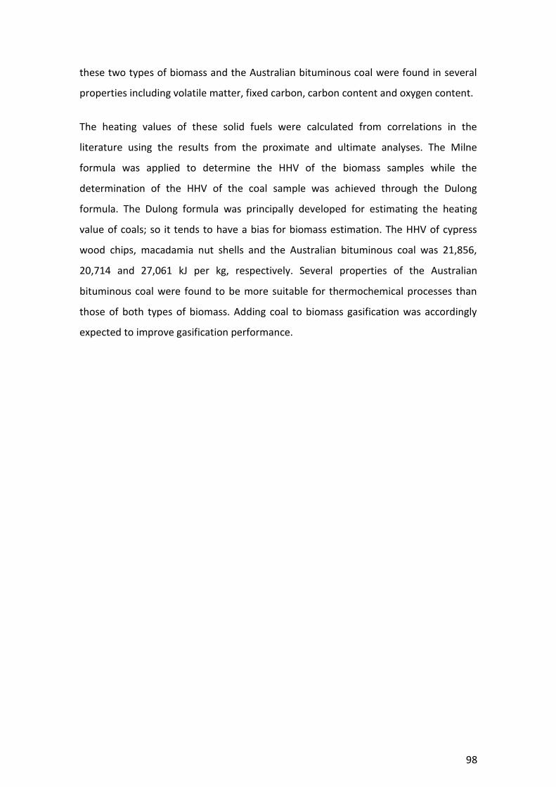
98

these two types of biomass and the Australian bituminous coal were found in several

properties including volatile matter, fixed carbon, carbon content and oxygen content.

The heating values of these solid fuels were calculated from correlations in the

literature using the results from the proximate and ultimate analyses. The Milne

formula was applied to determine the HHV of the biomass samples while the

determination of the HHV of the coal sample was achieved through the Dulong

formula. The Dulong formula was principally developed for estimating the heating

value of coals; so it tends to have a bias for biomass estimation. The HHV of cypress

wood chips, macadamia nut shells and the Australian bituminous coal was 21,856,

20,714 and 27,061 kJ per kg, respectively. Several properties of the Australian

bituminous coal were found to be more suitable for thermochemical processes than

those of both types of biomass. Adding coal to biomass gasification was accordingly

expected to improve gasification performance.

99

Chapter 6

Investigation of thermochemical behaviour of biomass and coal using

TGA

6.1 Pyrolysis behaviour

Pyrolysis is a thermochemical degradation of solid fuels in the absence of oxygen that

produces volatiles, tar and char (Basu, 2010; Sadhukhan et al., 2008). As well as being

an individual technology for energy systems, pyrolysis is also the initial reaction of both

combustion and gasification processes. Successful gasification of a fuel is determined

not only by the operating conditions but also by properties of the fuel itself. However,

the proximate and ultimate analyses indicated that the biomass samples used in this

study (cypress wood chips and macadamia nut shells) had poorer properties for

thermochemical processes compared to the coal sample (Australian bituminous coal)

in terms of higher moisture content, lower carbon content and lower hydrogen

content. Thus, it can be assumed that the blends of coal as a supplementary fuel with

biomass as a base fuel may foster the thermochemical processes and increase the

quality of the products.

To better understand pyrolysis, which is a complex process due to a number of

thermochemical reactions occurring in parallel and in series, thermogravimetric

analysis (TGA) was carried out to investigate pyrolytic behaviour of biomass, coal and

their blends in the context of thermal decomposition and reaction kinetics.

Thermogravimetric analysis and a kinetic study were used to determine whether

blending coal with biomass could create synergetic effects and interaction during co-

pyrolysis.

6.1.1 Thermal decomposition of the individual samples during pyrolysis

A thermogravimetric (TG) curve represents the percentage mass loss of a sample in

relation to its initial mass. The cypress wood chips, macadamia nut shells and

Australian bituminous coal were individually pyrolysed under a nitrogen environment

at heating rates of 5, 10, 15 and 20 °C min-1. The TG curves of cypress wood chips,

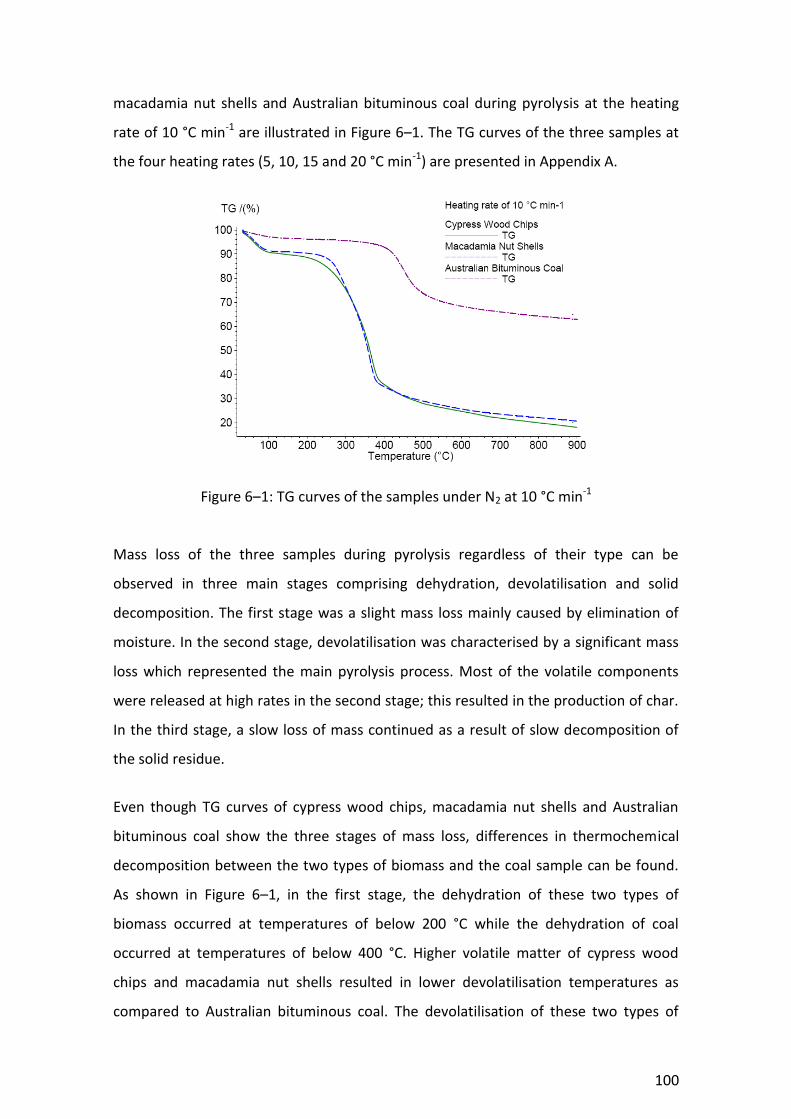
100

macadamia nut shells and Australian bituminous coal during pyrolysis at the heating

rate of 10 °C min-1 are illustrated in Figure 6–1. The TG curves of the three samples at

the four heating rates (5, 10, 15 and 20 °C min-1) are presented in Appendix A.

Figure 6–1: TG curves of the samples under N2 at 10 °C min-1

Mass loss of the three samples during pyrolysis regardless of their type can be

observed in three main stages comprising dehydration, devolatilisation and solid

decomposition. The first stage was a slight mass loss mainly caused by elimination of

moisture. In the second stage, devolatilisation was characterised by a significant mass

loss which represented the main pyrolysis process. Most of the volatile components

were released at high rates in the second stage; this resulted in the production of char.

In the third stage, a slow loss of mass continued as a result of slow decomposition of

the solid residue.

Even though TG curves of cypress wood chips, macadamia nut shells and Australian

bituminous coal show the three stages of mass loss, differences in thermochemical

decomposition between the two types of biomass and the coal sample can be found.

As shown in Figure 6–1, in the first stage, the dehydration of these two types of

biomass occurred at temperatures of below 200 °C while the dehydration of coal

occurred at temperatures of below 400 °C. Higher volatile matter of cypress wood

chips and macadamia nut shells resulted in lower devolatilisation temperatures as

compared to Australian bituminous coal. The devolatilisation of these two types of

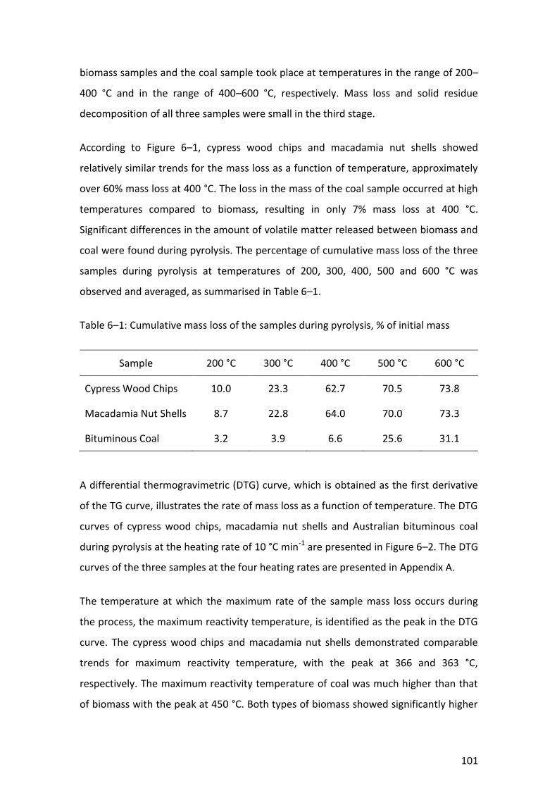
101

biomass samples and the coal sample took place at temperatures in the range of 200–

400 °C and in the range of 400–600 °C, respectively. Mass loss and solid residue

decomposition of all three samples were small in the third stage.

According to Figure 6–1, cypress wood chips and macadamia nut shells showed

relatively similar trends for the mass loss as a function of temperature, approximately

over 60% mass loss at 400 °C. The loss in the mass of the coal sample occurred at high

temperatures compared to biomass, resulting in only 7% mass loss at 400 °C.

Significant differences in the amount of volatile matter released between biomass and

coal were found during pyrolysis. The percentage of cumulative mass loss of the three

samples during pyrolysis at temperatures of 200, 300, 400, 500 and 600 °C was

observed and averaged, as summarised in Table 6–1.

Table 6–1: Cumulative mass loss of the samples during pyrolysis, % of initial mass

Sample 200 °C 300 °C 400 °C 500 °C 600 °C

Cypress Wood Chips 10.0 23.3 62.7 70.5 73.8

Macadamia Nut Shells 8.7 22.8 64.0 70.0 73.3

Bituminous Coal 3.2 3.9 6.6 25.6 31.1

A differential thermogravimetric (DTG) curve, which is obtained as the first derivative

of the TG curve, illustrates the rate of mass loss as a function of temperature. The DTG

curves of cypress wood chips, macadamia nut shells and Australian bituminous coal

during pyrolysis at the heating rate of 10 °C min-1 are presented in Figure 6–2. The DTG

curves of the three samples at the four heating rates are presented in Appendix A.

The temperature at which the maximum rate of the sample mass loss occurs during

the process, the maximum reactivity temperature, is identified as the peak in the DTG

curve. The cypress wood chips and macadamia nut shells demonstrated comparable

trends for maximum reactivity temperature, with the peak at 366 and 363 °C,

respectively. The maximum reactivity temperature of coal was much higher than that

of biomass with the peak at 450 °C. Both types of biomass showed significantly higher

102

mass loss and lower maximum reactivity temperature compared to coal due to their

higher volatile contents. As indicated by the TG and DTG curves, these three stages

manifested as different features on the rate of mass loss, maximum reactivity

temperature and end residue.

Figure 6–2: DTG curves of the samples under N2 at 10 °C min-1

6.1.2 Thermal decomposition of the blends during co-pyrolysis

To investigate synergetic effects and interaction between biomass and coal during co-

pyrolysis, thermal decomposition of their blends was observed. The TG curves of the

blends of cypress wood chips and the Australian bituminous coal and the blends of

macadamia nut shells and the Australian bituminous coal at blending ratios of 95:5,

90:10, 85:15 and 80:20 at the heating rate of 10 °C min-1 are illustrated in Figure 6–3

and Figure 6–4, respectively. The TG curves of these blends at the four heating rates

are presented in Appendix A.

The mass loss curves of these blends are similar to that of the biomass, except they are

shifted slightly along the temperature axis and the residual mass is higher. During co-

pyrolysis, mass loss behaviour of the blends reflected the behaviour of the individual

materials, depending on the blending ratios. A small increase of coal proportion in the

blends resulted in a decline in mass loss. This implies that the low volatile content of

coal had an effect on reducing the mass loss of the blends.

103

Figure 6–3: TG curves of wood chips and coal blends under N2 at 10 °C min-1

Figure 6–4: TG curves of nut shells and coal blends under N2 at 10 °C min-1

The percentage of cumulative mass loss of the blends of cypress wood chips and the

Australian bituminous coal at blending ratios of 95:5, 90:10, 85:15 and 80:20 during co-

pyrolysis at temperature of 400 °C was 61, 58, 55 and 51%, respectively. Under the

same experimental conditions, similar trends of the percentage of cumulative mass

loss of the blends of macadamia nut shells and the Australian bituminous coal were

found, being 63, 60, 56 and 53%, respectively.

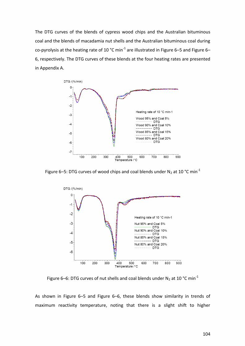
104

The DTG curves of the blends of cypress wood chips and the Australian bituminous

coal and the blends of macadamia nut shells and the Australian bituminous coal during

co-pyrolysis at the heating rate of 10 °C min-1 are illustrated in Figure 6–5 and Figure 6–

6, respectively. The DTG curves of these blends at the four heating rates are presented

in Appendix A.

Figure 6–5: DTG curves of wood chips and coal blends under N2 at 10 °C min-1

Figure 6–6: DTG curves of nut shells and coal blends under N2 at 10 °C min-1

As shown in Figure 6–5 and Figure 6–6, these blends show similarity in trends of

maximum reactivity temperature, noting that there is a slight shift to higher

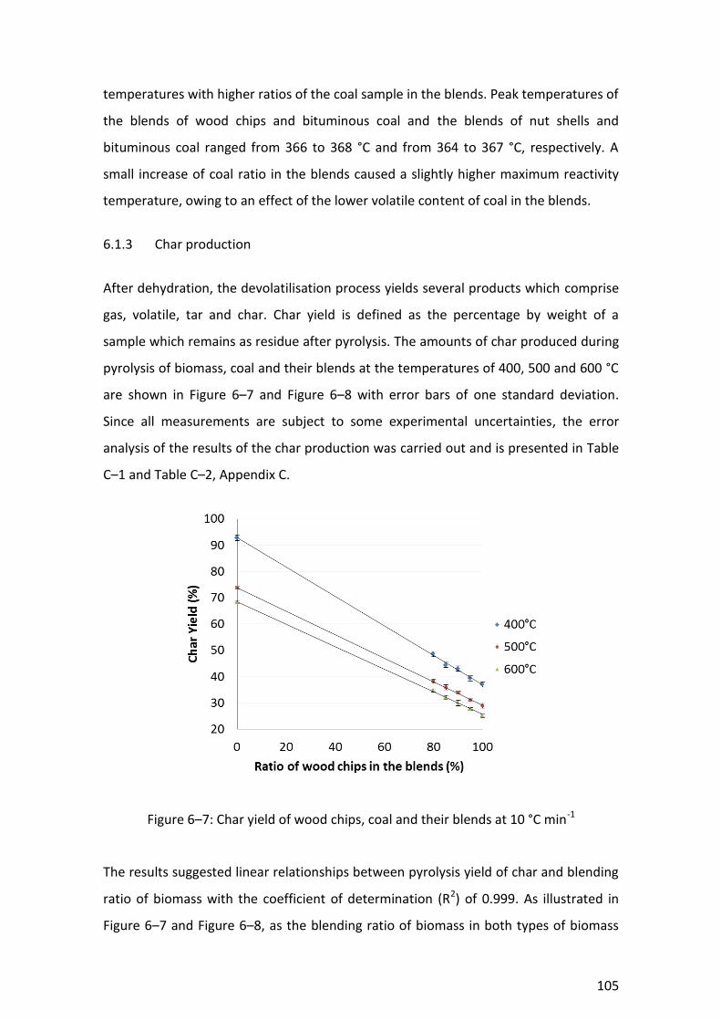
105

temperatures with higher ratios of the coal sample in the blends. Peak temperatures of

the blends of wood chips and bituminous coal and the blends of nut shells and

bituminous coal ranged from 366 to 368 °C and from 364 to 367 °C, respectively. A

small increase of coal ratio in the blends caused a slightly higher maximum reactivity

temperature, owing to an effect of the lower volatile content of coal in the blends.

6.1.3 Char production

After dehydration, the devolatilisation process yields several products which comprise

gas, volatile, tar and char. Char yield is defined as the percentage by weight of a

sample which remains as residue after pyrolysis. The amounts of char produced during

pyrolysis of biomass, coal and their blends at the temperatures of 400, 500 and 600 °C

are shown in Figure 6–7 and Figure 6–8 with error bars of one standard deviation.

Since all measurements are subject to some experimental uncertainties, the error

analysis of the results of the char production was carried out and is presented in Table

C–1 and Table C–2, Appendix C.

Figure 6–7: Char yield of wood chips, coal and their blends at 10 °C min-1

The results suggested linear relationships between pyrolysis yield of char and blending

ratio of biomass with the coefficient of determination (R2) of 0.999. As illustrated in

Figure 6–7 and Figure 6–8, as the blending ratio of biomass in both types of biomass

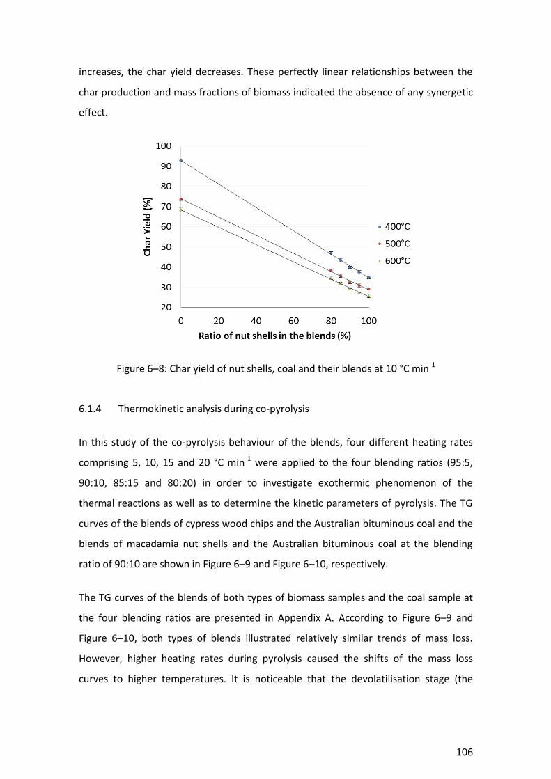
106

increases, the char yield decreases. These perfectly linear relationships between the

char production and mass fractions of biomass indicated the absence of any synergetic

effect.

Figure 6–8: Char yield of nut shells, coal and their blends at 10 °C min-1

6.1.4 Thermokinetic analysis during co-pyrolysis

In this study of the co-pyrolysis behaviour of the blends, four different heating rates

comprising 5, 10, 15 and 20 °C min-1 were applied to the four blending ratios (95:5,

90:10, 85:15 and 80:20) in order to investigate exothermic phenomenon of the

thermal reactions as well as to determine the kinetic parameters of pyrolysis. The TG

curves of the blends of cypress wood chips and the Australian bituminous coal and the

blends of macadamia nut shells and the Australian bituminous coal at the blending

ratio of 90:10 are shown in Figure 6–9 and Figure 6–10, respectively.

The TG curves of the blends of both types of biomass samples and the coal sample at

the four blending ratios are presented in Appendix A. According to Figure 6–9 and

Figure 6–10, both types of blends illustrated relatively similar trends of mass loss.

However, higher heating rates during pyrolysis caused the shifts of the mass loss

curves to higher temperatures. It is noticeable that the devolatilisation stage (the

107

second stage) was affected by the heating rates more than the dehydration stage and

the solid decomposition stage (the first and third stages).

Figure 6–9: TG curves of 90 % wood chips and 10% coal blends under N2

Figure 6–10: TG curves of 90 % nut shells and 10% coal blends under N2

The DTG curves of the blends of cypress wood chips and the Australian bituminous

coal and the blends of macadamia nut shells and the Australian bituminous coal at the

ratio of 90:10 at the heating rates of 5, 10, 15 and 20 min-1 are shown in Figure 6–11

and Figure 6–12, respectively. The DTG curves of the blends of cypress wood chips and

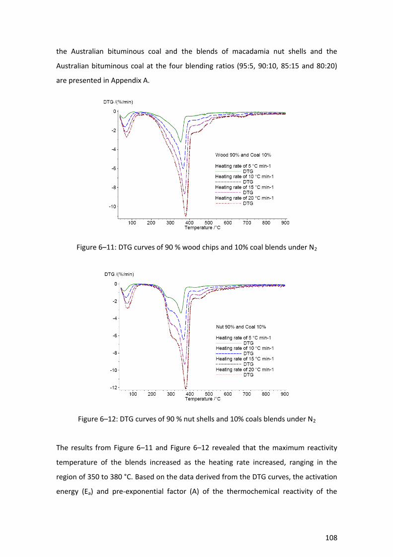
108

the Australian bituminous coal and the blends of macadamia nut shells and the

Australian bituminous coal at the four blending ratios (95:5, 90:10, 85:15 and 80:20)

are presented in Appendix A.

Figure 6–11: DTG curves of 90 % wood chips and 10% coal blends under N2

Figure 6–12: DTG curves of 90 % nut shells and 10% coals blends under N2

The results from Figure 6–11 and Figure 6–12 revealed that the maximum reactivity

temperature of the blends increased as the heating rate increased, ranging in the

region of 350 to 380 °C. Based on the data derived from the DTG curves, the activation

energy (Ea) and pre-exponential factor (A) of the thermochemical reactivity of the

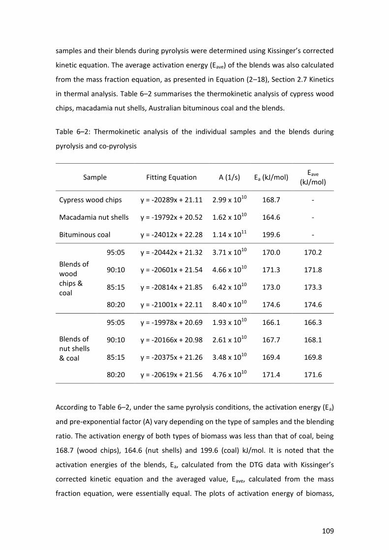
109

samples and their blends during pyrolysis were determined using Kissinger’s corrected

kinetic equation. The average activation energy (Eave) of the blends was also calculated

from the mass fraction equation, as presented in Equation (2–18), Section 2.7 Kinetics

in thermal analysis. Table 6–2 summarises the thermokinetic analysis of cypress wood

chips, macadamia nut shells, Australian bituminous coal and the blends.

Table 6–2: Thermokinetic analysis of the individual samples and the blends during

pyrolysis and co-pyrolysis

Sample Fitting Equation A (1/s) Ea (kJ/mol) Eave

(kJ/mol)

Cypress wood chips y = -20289x + 21.11 2.99 x 1010 168.7 -

Macadamia nut shells y = -19792x + 20.52 1.62 x 1010 164.6 -

Bituminous coal y = -24012x + 22.28 1.14 x 1011 199.6 -

Blends of wood chips & coal

95:05 y = -20442x + 21.32 3.71 x 1010 170.0 170.2

90:10 y = -20601x + 21.54 4.66 x 1010 171.3 171.8

85:15 y = -20814x + 21.85 6.42 x 1010 173.0 173.3

80:20 y = -21001x + 22.11 8.40 x 1010 174.6 174.6

Blends of nut shells & coal

95:05 y = -19978x + 20.69 1.93 x 1010 166.1 166.3

90:10 y = -20166x + 20.98 2.61 x 1010 167.7 168.1

85:15 y = -20375x + 21.26 3.48 x 1010 169.4 169.8

80:20 y = -20619x + 21.56 4.76 x 1010 171.4 171.6

According to Table 6–2, under the same pyrolysis conditions, the activation energy (Ea)

and pre-exponential factor (A) vary depending on the type of samples and the blending

ratio. The activation energy of both types of biomass was less than that of coal, being

168.7 (wood chips), 164.6 (nut shells) and 199.6 (coal) kJ/mol. It is noted that the

activation energies of the blends, Ea, calculated from the DTG data with Kissinger’s

corrected kinetic equation and the averaged value, Eave, calculated from the mass

fraction equation, were essentially equal. The plots of activation energy of biomass,

110

coal and their blends against blending ratio of biomass are presented with error bars

equal to the standard error of the estimate in Figures 6–13 and 6–14. Uncertainty

measures on slope and intercept of a least squares fit of activation energy of biomass,

coal and their blends during pyrolysis are summarised in Table C–3, Appendix C.

Figure 6–13: Activation energy of wood chips, coal and their blends during pyrolysis

Figure 6–14: Activation energy of nut shells, coal and their blends during pyrolysis

In the analysis of the kinetic parameters, the activation energy and pre-exponential

factor during co-pyrolysis increased with the addition of coal in the blends. The plots of

111

activation energy of the blends against the blending ratio of biomass also showed

linear relationships (R2 = 0.999). This also suggested no significant degree of

interaction between the blends during co-pyrolysis of biomass and coal. The finding of

no synergetic interaction of biomass and coal during co-pyrolysis in this study agrees

with the conclusions of previous studies (Chenand Wu, 2009; Idris et al., 2010; Meesri

and Moghtaderi 2002; Moghtaderi et al., 2004; Sadhukhan et al., 2008). Thermal

decomposition of biomass and coal appeared to take place independently as such co-

pyrolysis behaviour of the blends can be predicted from that of the individual samples.

The lack of synergy suggests that coal can be blended with biomass at any blending

ratio for use in pyrolysis energy conversion systems.

6.2 Combustion behaviour

Combustion is the oxidation process that converts fuels into energy with excess air. It

involves a series of heterogeneous and homogeneous reactions with extensive

interaction between thermal and mass fluxes. Combustion is a part of the gasification

process, producing carbon dioxide and water. The combustion process can be affected

by many factors such as the characteristics of fuels, operating temperature, heating

rate and reactor design. The study of thermochemical behaviour of cypress wood

chips, macadamia nut shells, Australian bituminous coal and their blends during

combustion and co-combustion was also carried out under an air environment using

thermogravimetric analysis.

6.2.1 Thermal decomposition of the individual samples during combustion

The TG curves of cypress wood chips, macadamia nut shells and Australian bituminous

coal during combustion at the heating rate of 10 °C min-1 are illustrated in Figure 6–15.

The TG curves of the three individual samples at the four heating rates (5, 10, 15 and

20 °C min-1) are presented in Appendix B.

Mass loss of the three samples during combustion regardless of their type can be

observed in three main stages comprising dehydration, devolatilisation and char

oxidation. The first stage, dehydration, was elimination of moisture which resulted in a

slight mass loss. In the second stage, devolatilisation was characterised by a significant

112

mass loss. Most of the volatile components were released in the second stage; this

caused the production of char. In the third stage, a significant loss of mass continued

as a result of oxidation of char produced in the second stage.

Figure 6–15: TG curves of the samples under air at 10 °C min-1

As illustrated in Figure 6–15, cypress wood chips and macadamia nut shells showed

relatively similar trends for the mass loss as a function of temperature, approximately

over 60% mass loss at 400 °C. The loss in the mass of the coal sample occurred at high

temperatures compared to biomass, resulting in only approximately 10% mass loss at

400 °C. Significant differences in the amount of volatile matter released between both

types of biomass and coal were found during combustion. The percentage of

cumulative mass loss of the three samples during combustion at temperatures of 200,

300, 400, 500 and 600 °C was observed and is summarised in Table 6–3.

Table 6–3: Cumulative mass loss of the samples during combustion, % of initial mass

Sample 200 °C 300 °C 400 °C 500 °C 600 °C

Cypress Wood Chips 9.7 25.2 62.0 92.1 93.9

Macadamia Nut Shells 8.9 27.5 68.8 96.0 96.5

Bituminous Coal 3.6 4.0 9.9 38.8 68.9

113

The first and second stages of mass loss (dehydration and devolatilisation) during

combustion appeared to be similar to those stages during pyrolysis, based on relatively

equal percentage of cumulative mass loss below 400 °C. However, the char oxidation

in the third stage of combustion caused a significant loss of mass while a slow loss of

mass continued in the third stage of pyrolysis as a result of slow decomposition of the

solid residue. As shown in Table 6–2 and Table 6–3, at temperature of 500 °C, the

percentage of cumulative mass loss of cypress wood chips, macadamia nut shells and

the Australian bituminous coal during combustion was 92.1, 96.0 and 38.8%

respectively, while the percentage of cumulative mass loss of the three samples during

pyrolysis was only 70.5, 70.0 and 25.6% respectively.

The DTG curves of cypress wood chips, macadamia nut shells and Australian

bituminous coal during combustion at the heating rate of 10 °C min-1 are shown in

Figure 6–16. The DTG curves of these three samples at the four heating rates are

presented in Appendix B.

Figure 6–16: DTG curves of the samples under air at 10 °C min-1

As shown in Figure 6–16, cypress wood chips and macadamia nut shells demonstrated

comparable trends for maximum reactivity temperature, with the peak at 335 and 328

°C, respectively. The maximum reactivity temperature of the coal was much higher

than that of biomass with the peak at 453 °C, due to its lower volatile content.

114

6.2.2 Thermal decomposition of the blends during co-combustion

The TG curves of the blends of cypress wood chips and the Australian bituminous coal

and the blends of macadamia nut shells and the coal during combustion at blending

ratios of 95:5, 90:10, 85:15 and 80:20 at the heating rate of 10 °C min-1 are illustrated

Figure 6–17 and Figure 6–18, respectively. The TG curves of these blends at the four

heating rates of 5, 10, 15 and 20 °C min-1 are presented in Appendix B.

Figure 6–17: TG curves of wood chips and coal blends under air at 10 °C min-1

Figure 6–18: TG curves of nut shells and coal blends under air at 10 °C min-1

115

It is noticeable that the mass loss curves of these blends are similar to that of the

biomass, except these curves are shifted slightly along the temperature axis. The

residual mass is higher. The percentage of cumulative mass loss of the blends of

cypress wood chips and the Australian bituminous coal at blending ratios of 95:5,

90:10, 85:15 and 80:20 during co-combustion at temperature of 400 °C was 60, 59, 56

and 52%, respectively. Similar trends of the percentage of cumulative mass loss of the

blends of macadamia nut shells and the coal were found, being 67, 64, 60 and 55%,

respectively. This indicated that even a small amount of the coal sample, which had

low volatile matter, had an effect on reducing the mass loss of the blends.

The DTG curves of the blends of cypress wood chips and the coal and the blends of

macadamia nut shells and the coal at blending ratios of 95:5, 90:10, 85:15 and 80:20 at

heating rate of 10 °C min-1 are shown in Figure 6–19 and Figure 6–20.

Figure 6–19: DTG curves of wood chips and coal blends under air at 10 °C min-1

The DTG curves of these two types of blends at the four heating rates are illustrated in

Appendix B. Corresponding to the TG curves of the blends, the DTG curves showed a

slight shift to higher temperatures with higher ratios of the coal sample in the blends.

Peak temperatures of the blends of cypress wood chips and the Australian bituminous

coal and the blends of macadamia nut shells and the Australian bituminous coal

ranged from 334 to 336 °C and from 328 to 331 °C, respectively.

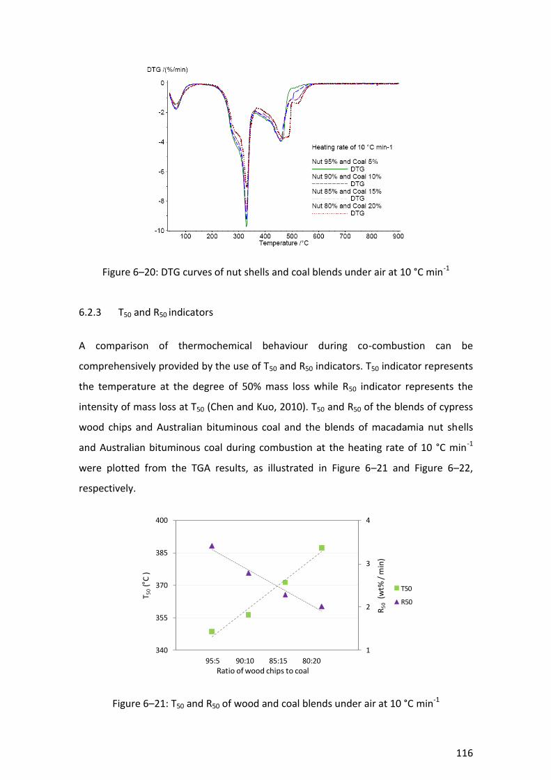
116

Figure 6–20: DTG curves of nut shells and coal blends under air at 10 °C min-1

6.2.3 T50 and R50 indicators

A comparison of thermochemical behaviour during co-combustion can be

comprehensively provided by the use of T50 and R50 indicators. T50 indicator represents

the temperature at the degree of 50% mass loss while R50 indicator represents the

intensity of mass loss at T50 (Chen and Kuo, 2010). T50 and R50 of the blends of cypress

wood chips and Australian bituminous coal and the blends of macadamia nut shells

and Australian bituminous coal during combustion at the heating rate of 10 °C min-1

were plotted from the TGA results, as illustrated in Figure 6–21 and Figure 6–22,

respectively.

Figure 6–21: T50 and R50 of wood and coal blends under air at 10 °C min-1

1

2

3

4

340

355

370

385

400

R5

0(w

t% /

min

)

T 50

( C

)

95:5 90:10 85:15 80:20Ratio of wood chips to coal

T50

R50

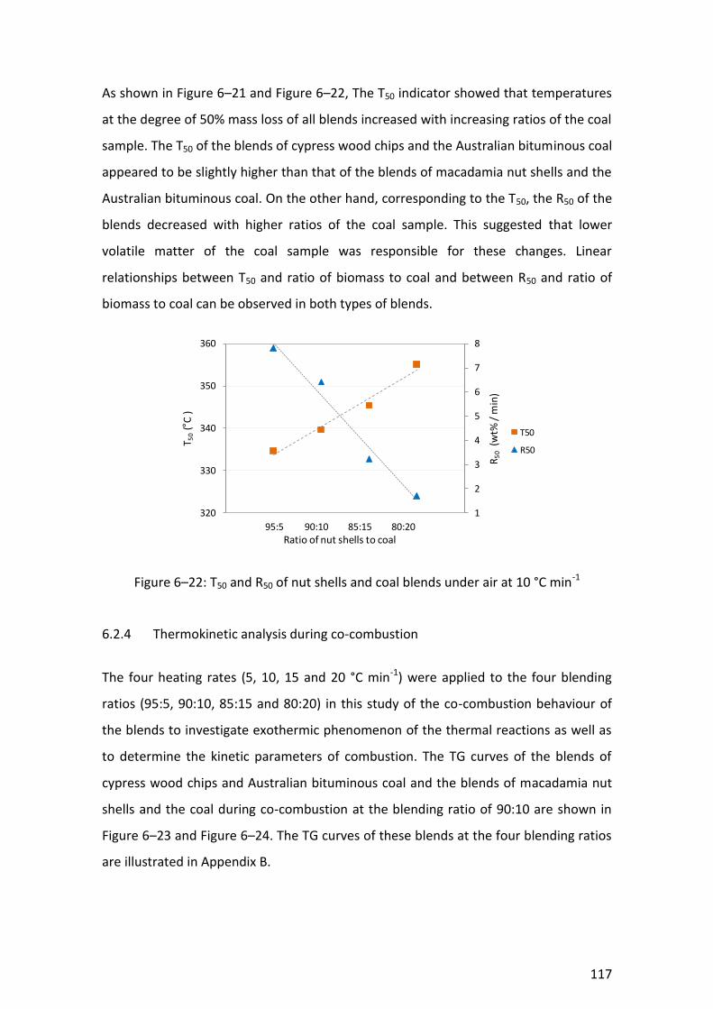
117

As shown in Figure 6–21 and Figure 6–22, The T50 indicator showed that temperatures

at the degree of 50% mass loss of all blends increased with increasing ratios of the coal

sample. The T50 of the blends of cypress wood chips and the Australian bituminous coal

appeared to be slightly higher than that of the blends of macadamia nut shells and the

Australian bituminous coal. On the other hand, corresponding to the T50, the R50 of the

blends decreased with higher ratios of the coal sample. This suggested that lower

volatile matter of the coal sample was responsible for these changes. Linear

relationships between T50 and ratio of biomass to coal and between R50 and ratio of

biomass to coal can be observed in both types of blends.

Figure 6–22: T50 and R50 of nut shells and coal blends under air at 10 °C min-1

6.2.4 Thermokinetic analysis during co-combustion

The four heating rates (5, 10, 15 and 20 °C min-1) were applied to the four blending

ratios (95:5, 90:10, 85:15 and 80:20) in this study of the co-combustion behaviour of

the blends to investigate exothermic phenomenon of the thermal reactions as well as

to determine the kinetic parameters of combustion. The TG curves of the blends of

cypress wood chips and Australian bituminous coal and the blends of macadamia nut

shells and the coal during co-combustion at the blending ratio of 90:10 are shown in

Figure 6–23 and Figure 6–24. The TG curves of these blends at the four blending ratios

are illustrated in Appendix B.

1

2

3

4

5

6

7

8

320

330

340

350

360

R5

0(w

t% /

min

)

T 50

( C

)

95:5 90:10 85:15 80:20Ratio of nut shells to coal

T50

R50

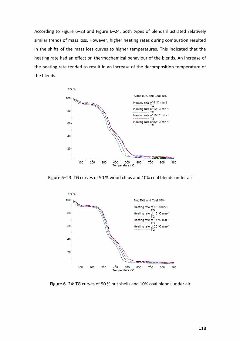
118

According to Figure 6–23 and Figure 6–24, both types of blends illustrated relatively

similar trends of mass loss. However, higher heating rates during combustion resulted

in the shifts of the mass loss curves to higher temperatures. This indicated that the

heating rate had an effect on thermochemical behaviour of the blends. An increase of

the heating rate tended to result in an increase of the decomposition temperature of

the blends.

Figure 6–23: TG curves of 90 % wood chips and 10% coal blends under air

Figure 6–24: TG curves of 90 % nut shells and 10% coal blends under air

119

The DTG curves of the blends of cypress wood chips and Australian bituminous coal

and the blends of macadamia nut shells and Australian bituminous coal during co-

combustion at blending ratios of 90:10 at heating rates of 5, 10, 15 and 20 °C min-1 are

shown in Figure 6–25 and Figure 6–26. The DTG curves of these blends at the four

blending ratios (95:5, 90:10, 85:15 and 80:20) are illustrated in Appendix B.

Figure 6–25: DTG curves of 90 % wood chips and 10% coal blends under air

Figure 6–26: DTG curves of 90 % nut shells and 10% coal blends under air

As illustrated in Figure 6–23 to Figure 6–26, the heating rate had had an effect on the

mass loss and the maximum reactivity temperature. Higher heating rates resulted in

120

the shifts of the TG and DTG curves to higher temperatures. The maximum reactivity

temperature of the blends increased as the heating rate increased, ranging in the

region of 315 to 350 °C. The conversions of the blends at higher heating rates occurred

at higher temperatures. This mainly resulted from limitation of heat transfer. The

limitation of heat transfer led to existence of temperature gradients in the blends.

Based on the data derived from the DTG curves, the activation energy (Ea) and pre-

exponential factor (A) of the thermochemical reactivity of the samples and their blends

during combustion and co-combustion were determined using Kissinger’s corrected

kinetic equation. The average activation energy (Eave) of the blends was also calculated

from the mass fraction equation, as mentioned above. Table 6–4 summarises the

thermokinetic analysis of cypress wood chips, macadamia nut shells, Australian

bituminous coal and the blends.

Table 6–4: Thermokinetic analysis of the samples and the blends during combustion

and co-combustion

Sample Fitting Equation A (1/s) Ea

(kJ/mol) Eave

(kJ/mol)

Cypress wood chips y = -16705x + 16.97 .392 x 109 138.9 -

Macadamia nut shells y = -16499x + 17.04 .492 x 109 147.4 -

Bituminous coal y = -21818x + 19.22 4.85 x 109 181.4 -

Blends of wood chips & coals

95:05 y = -16962x + 17.36 .578 x 109 141.0 141.0

90:10 y = -17255x + 17.82 .946 x 109 143.5 143.1

85:15 y = -17497x + 18.21 1.42 x 109 145.5 145.3

80:20 y = -17741x + 18.60 2.12 x 109 147.5 147.5

Blends of nut shells & coals

95:05 y = -16697x + 17.32 .597 x 109 149.3 149.1

90:10 y = -16892x + 17.61 .812 x 109 151.9 150.8

85:15 y = -17183x + 18.05 1.28 x 109 153.8 152.5

80:20 y = -17369x + 18.28 1.62 x 109 155.4 154.2

121

The trend of results from thermokinetic analysis during combustion was relatively

similar to those during pyrolysis. The activation energy of both types of biomass was

less than that of coal, being 138.9 (wood chips), 147.4 (nut shells) and 181.4 (coal)

kJ/mol. As presented in Table 6–4, the activation energies of the blends, Ea, calculated

with Kissinger’s corrected kinetic equation from the DTG data and the averaged

activation energies, Eave, calculated from the mass fraction equation, were essentially

equal. The plots of activation energy of the blends and blending ratio of biomass with

error bars equal to the standard error of the estimate are presented in Figure 6–27 and

Figure 6–28.

Figure 6–27: Activation energy of wood chips, coals and the blends during combustion

Figure 6–28: Activation energy of nut shells, coals and the blends during combustion

122

Uncertainty measures of the activation energy plots during combustion are

summarised in Table C–4, Appendix C. As illustrated in Figure 6–27 and Figure 6–28,

the plots of the activation energy of the blends and the blending ratio of biomass

showed linear relationships with R2 of 0.999 in the case of the blends of cypress wood

chips and Australian bituminous coal and R2 of 0.997 in the case of the blends of

macadamia nut shells and Australian bituminous coal. This suggested no significant

degree of interaction between the blends during co-combustion of biomass and coal.

The finding of no synergetic interaction of biomass and coal during co-combustion in

this study agrees with the conclusion of the previous study (Gil et al., 2010).

Thermochemical decomposition of biomass and coal appeared to take place

independently as such co-combustion behaviour of the blends can be predicted from

the measurements of the individual samples. The lack of synergy suggests that coal can

be blended with biomass at any blending ratio for use in combustion energy

conversion systems. However, in increasing coal proportion, it is necessary to take

consideration of limitation of combustion equipment.

6.3 Summary

Thermogravimetric analysis (TGA) was applied to investigate thermal decomposition

during pyrolysis and combustion of cypress wood chips, macadamia nut shells,

Australian bituminous coal and their blends. Kinetic parameters during pyrolysis and

combustion were determined through Kissinger’s corrected kinetic equation using the

TGA results.

Pyrolysis of the samples regardless of their type occurred in three stages comprising

dehydration, devolatilisation and solid decomposition. Combustion of the samples also

took place in three stages comprising dehydration, devolatilisation and char oxidation.

The TGA results revealed that thermal decomposition profiles of both types of biomass

showed similarity, predominantly due to similar composition in particular the volatile

content. However, biomass and coal were found to have substantially different

thermochemical behaviour during pyrolysis and combustion in terms of mass loss,

maximum reactivity temperature and end residue. Both types of biomass samples had

123

higher volatile components than the coal sample; as a result the stage of

devolatilisation played a larger part in the biomass samples than in the coal sample.

During co-pyrolysis and co-combustion, trends of the mass loss and maximum

reactivity temperature of the blends of cypress wood chips and Australian bituminous

coal and the blends of macadamia nut shells and Australian bituminous coal were

similar to those of the biomass samples, except slightly shifting to higher temperatures

with higher ratios of the coal sample in the blends. This implies that the low volatile

content of coal had an effect on reducing the mass loss and increasing the maximum

reactivity temperature. Moreover, the char production of the blends during pyrolysis

corresponded to the sum of the results for the individual biomass and the coal.

Measured TG data of co-pyrolysis indicated a linear relationship between char yield

and blending ratio of biomass in the blends.

Thermokinetic analysis of the individual samples and the blends was carried out using

the results from TGA. Activation energy (Ea) and pre-exponential factor (A) of the

thermochemical reactivity of the samples and their blends during pyrolysis and

combustion were determined using Kissinger’s corrected kinetic equation. Average

activation energy (Eave) of blends of biomass and coal based on their mass fraction

agreed closely with activation energy (Ea) derived from the TG data. No clear

synergetic effect or thermal interaction of biomass and coal during their co-pyrolysis

and co-combustion was observed in this study. The finding of no synergetic interaction

of biomass and coal during co-pyrolysis and co-combustion in this study agrees with

the conclusions of previous studies.

124

Chapter 7

Investigation of gasification and co-gasification in a downdraft gasifier

7.1 Gasification process and control

In this study, the gasification of biomass and coal blends was investigated in a

laboratory-scale downdraft fixed bed gasifier. The pre-treatment of the samples and

the gasifier operating conditions including air flow rate and residence time were

maintained as control variables. The sample blending ratio was the only condition that

was changed in the experiments reported here in order to investigate the influence of

these changes on the gasification results. Cypress wood chips, macadamia nut shells

and their blends with Australian bituminous coal were fed into the downdraft gasifier

unit at the top of the bed. The gasification and co-gasification experiments were run as

a batch-type process with the batch sizes of 3.00 ± 0.30 kg using air as a gasifying

agent. Air is commonly used in most biomass gasification systems because it is readily

available. The gasification process which occurs in the downdraft gasifier involves a

complex series of thermochemical reactions which can be characterised into four

distinct zones including drying, pyrolysis, combustion and gasification.

Each set of experiments was performed in triplicate. The experimental procedures are

provided in Section 4.4.2 operation of the gasification unit. The flame was initiated in

the gasifier at the top of the reduction bell in the area of the combustion zone. The

heat required for the endothermic reactions was supplied by partial oxidation of the

samples with air. The heat was transferred in the upward direction to the pyrolysis and

drying zones as well as in the downward direction to the gasification zone. In the

drying zone, the moisture content of the solid fuels and their blends was driven off.

During the pyrolysis process, the volatile components of the solid fuels and their

blends were vaporised at temperatures below 500°C. The volatile vapours comprised

hydrogen, carbon monoxide, carbon dioxide, hydrocarbon gases, water vapour (steam)

and tar. Char and ash, which were not vaporised, were by-products of the pyrolysis

process. In the combustion zone, the char and hydrogen reacted with oxygen from the

gasifying agent. The combustion reactions formed carbon dioxide and water. Then, in

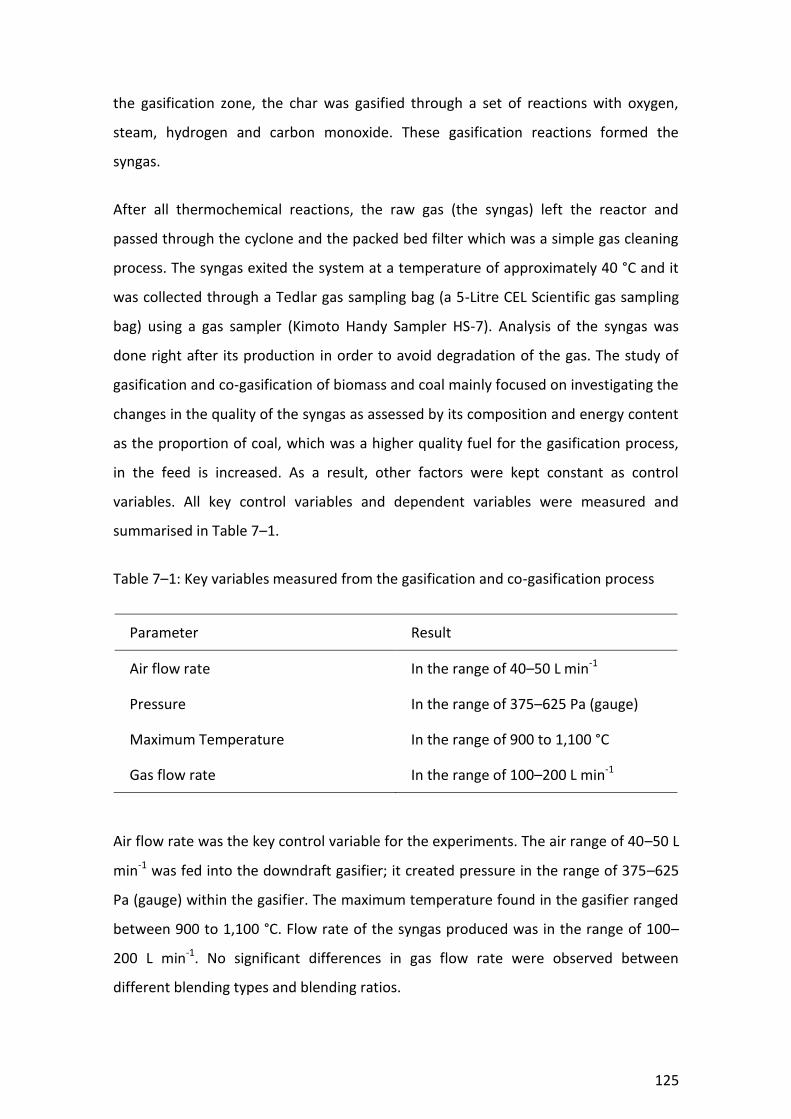
125

the gasification zone, the char was gasified through a set of reactions with oxygen,

steam, hydrogen and carbon monoxide. These gasification reactions formed the

syngas.

After all thermochemical reactions, the raw gas (the syngas) left the reactor and

passed through the cyclone and the packed bed filter which was a simple gas cleaning

process. The syngas exited the system at a temperature of approximately 40 °C and it

was collected through a Tedlar gas sampling bag (a 5-Litre CEL Scientific gas sampling

bag) using a gas sampler (Kimoto Handy Sampler HS-7). Analysis of the syngas was

done right after its production in order to avoid degradation of the gas. The study of

gasification and co-gasification of biomass and coal mainly focused on investigating the

changes in the quality of the syngas as assessed by its composition and energy content

as the proportion of coal, which was a higher quality fuel for the gasification process,

in the feed is increased. As a result, other factors were kept constant as control

variables. All key control variables and dependent variables were measured and

summarised in Table 7–1.

Table 7–1: Key variables measured from the gasification and co-gasification process

Parameter Result

Air flow rate In the range of 40–50 L min-1

Pressure In the range of 375–625 Pa (gauge)

Maximum Temperature In the range of 900 to 1,100 °C

Gas flow rate In the range of 100–200 L min-1

Air flow rate was the key control variable for the experiments. The air range of 40–50 L

min-1 was fed into the downdraft gasifier; it created pressure in the range of 375–625

Pa (gauge) within the gasifier. The maximum temperature found in the gasifier ranged

between 900 to 1,100 °C. Flow rate of the syngas produced was in the range of 100–

200 L min-1. No significant differences in gas flow rate were observed between

different blending types and blending ratios.

126

7.2 Gasification products

The gasification process converted cypress wood chips, macadamia nut shells and their

blends with Australian bituminous coal into syngas, volatiles, char and ash. Syngas,

which contains combustible components, is the key interest of the gasification

products. It can be further used in several applications depending on its quality.

However, there are a number of factors such as type of the fuel fed, type of the

gasifier used, type of the gasifying agent supplied, operating conditions and other

processing variables that have direct effects on the quality of the syngas produced. The

energy content of the syngas is also influenced by the method used to provide heat to

drive the gasification reactions. For example, a gasification system that is operated

with air as a gasifying agent often yields the syngas highly diluted with nitrogen.

Analysis of composition and quality of the syngas produced is therefore considered

necessary for its further utilisation.

7.3 Results of the syngas analysis

7.3.1 Composition of the syngas

In this study, the syngas composition was analysed using the GC/MS and MS

techniques. The GC/MS technique requires creating a calibration curve to determine

the concentration of an unknown substance while the MS technique, which forms ions

from molecules and analyses the ions according to their mass-to-charge ratio (m/z),

can directly measure the concentration of a component. CO concentration was

analysed using the GC/MS technique while concentrations of H2, CH4, CO2, H2O, O2 and

N2 were analysed using the MS technique. The results from the analysis of the carbon

monoxide standard solutions were used to create the carbon monoxide calibration

curve, as shown in Figure 7–1.

The plot of instrument response (corrected area) and analyte concentration (carbon

monoxide) showed a linear relationship with R2 of 0.997. The regression line equation

from the calibration curve (y = 0.214x + 5098) was used to calculate the concentration

of carbon monoxide in the syngas. Statistical analysis of the measurements was

conducted to analyse the uncertainties, as summarised in Table C–5, Appendix C.

127

Figure 7–1: The carbon monoxide calibration curve

The composition of the syngas produced from gasification of cypress wood chips and

macadamia nut shells and from co-gasification of their blends with bituminous coal

was measured, calculated and averaged, as summarised in Table 7–2 and Table 7–3.

Statistical analysis of the measurements of the composition of the syngas is shown in

Table C–6 and Table C–7, Appendix C while the detailed results from the analysis of the

composition of the syngas are listed in Appendix D.

Table 7–2: Average syngas composition from wood chips and their blends with coal, by

volume %

Wood chips to Coal

CO H2 CH4 CO2 H2O O2 N2 Total (%)

100:0 7.88 2.19 0.08 4.68 2.51 11.82 69.76 98.9

95:5 8.90 2.74 0.08 6.65 2.47 10.28 67.68 98.8

90:10 10.08 3.24 0.06 5.49 2.43 10.19 67.49 99.0

85:15 12.14 4.14 0.05 5.89 1.88 9.61 65.18 98.9

80:20 15.18 5.27 0.05 9.24 2.27 7.19 59.66 98.9

y = 0.214x + 5098R² = 0.997

0

50000

100000

150000

200000

250000

0 200000 400000 600000 800000 1000000

Co

rre

cte

d A

rea

Concentration (PPM)

Carbon Monoxide Calibration Curve

128

Table 7–3: Average syngas composition from nut shell and their blends with coal, by

volume %

Nut shells to Coal

CO H2 CH4 CO2 H2O O2 N2 Total (%)

100:0 8.30 2.27 0.06 5.71 2.25 11.01 69.26 98.9

95:5 9.84 2.67 0.06 6.02 2.32 10.72 67.18 98.8

90:10 11.85 3.64 0.05 8.08 2.80 8.48 64.15 99.1

85:15 12.75 4.52 0.05 9.25 2.85 6.63 62.86 98.9

80:20 15.09 5.34 0.05 10.07 2.93 4.88 60.58 98.9

The most important aspects of producing the syngas are that it should be high in

carbon content and hydrogen content as well as low in nitrogen content. Even though

the use of air (N2 of 78%) as the gasifying agent and other operation conditions set in

the experiments resulted in very high nitrogen content of the syngas, the focus of this

study was on investigating the effects of the use of coal on the syngas produced. The

influence of different ratios of the coal in the blends can be seen from the differences

in composition of the syngas, as shown in Table 7–2 and Table 7–3. It can be noticed

that both types of biomass samples gave relatively similar results, primarily due to the

similarity in their properties.

The gasification of biomass yielded the syngas with relatively high nitrogen content, at

an average of 69.8% in the case of cypress wood chips and 69.3% in the case of

macadamia nut shells. Average nitrogen content decreased with a higher blending

ratio of the coal sample. The co-gasification of biomass and coal at the blending ratio

of 80:20 produced the syngas with an average nitrogen content of 59.7% in the case of

cypress wood chips and coal blends and 60.6% in the case of macadamia nut shells

blending and coal blends. The average content of nitrogen in the syngas produced

from cypress wood chips, macadamia nut shells and four levels of their blends with

Australian bituminous coal was plotted with error bars of one standard deviation, as

presented in Figure 7–2.

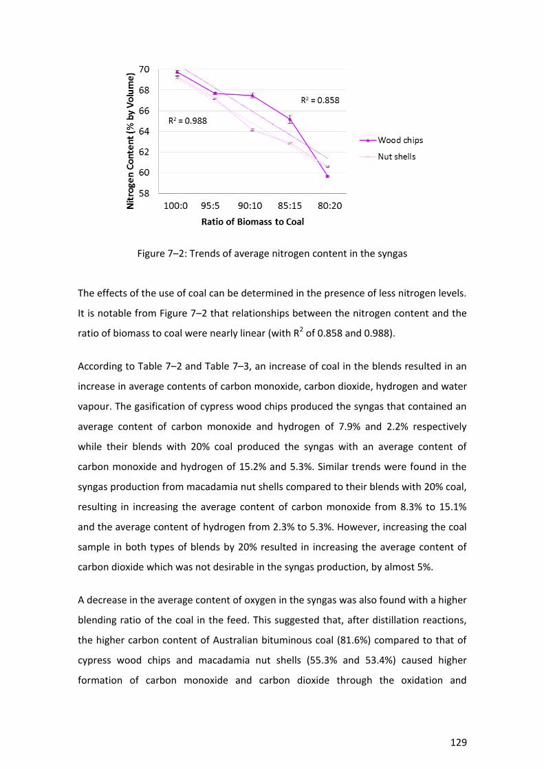
129

Figure 7–2: Trends of average nitrogen content in the syngas

The effects of the use of coal can be determined in the presence of less nitrogen levels.

It is notable from Figure 7–2 that relationships between the nitrogen content and the

ratio of biomass to coal were nearly linear (with R2 of 0.858 and 0.988).

According to Table 7–2 and Table 7–3, an increase of coal in the blends resulted in an

increase in average contents of carbon monoxide, carbon dioxide, hydrogen and water

vapour. The gasification of cypress wood chips produced the syngas that contained an

average content of carbon monoxide and hydrogen of 7.9% and 2.2% respectively

while their blends with 20% coal produced the syngas with an average content of

carbon monoxide and hydrogen of 15.2% and 5.3%. Similar trends were found in the

syngas production from macadamia nut shells compared to their blends with 20% coal,

resulting in increasing the average content of carbon monoxide from 8.3% to 15.1%

and the average content of hydrogen from 2.3% to 5.3%. However, increasing the coal

sample in both types of blends by 20% resulted in increasing the average content of

carbon dioxide which was not desirable in the syngas production, by almost 5%.

A decrease in the average content of oxygen in the syngas was also found with a higher

blending ratio of the coal in the feed. This suggested that, after distillation reactions,

the higher carbon content of Australian bituminous coal (81.6%) compared to that of

cypress wood chips and macadamia nut shells (55.3% and 53.4%) caused higher

formation of carbon monoxide and carbon dioxide through the oxidation and

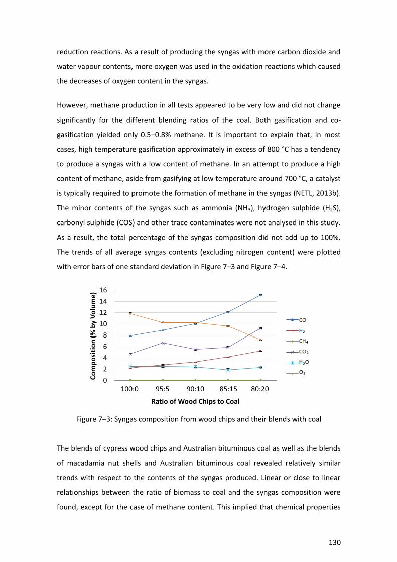
130

reduction reactions. As a result of producing the syngas with more carbon dioxide and

water vapour contents, more oxygen was used in the oxidation reactions which caused

the decreases of oxygen content in the syngas.

However, methane production in all tests appeared to be very low and did not change

significantly for the different blending ratios of the coal. Both gasification and co-

gasification yielded only 0.5–0.8% methane. It is important to explain that, in most

cases, high temperature gasification approximately in excess of 800 °C has a tendency

to produce a syngas with a low content of methane. In an attempt to produce a high

content of methane, aside from gasifying at low temperature around 700 °C, a catalyst

is typically required to promote the formation of methane in the syngas (NETL, 2013b).

The minor contents of the syngas such as ammonia (NH3), hydrogen sulphide (H2S),

carbonyl sulphide (COS) and other trace contaminates were not analysed in this study.

As a result, the total percentage of the syngas composition did not add up to 100%.

The trends of all average syngas contents (excluding nitrogen content) were plotted

with error bars of one standard deviation in Figure 7–3 and Figure 7–4.

Figure 7–3: Syngas composition from wood chips and their blends with coal

The blends of cypress wood chips and Australian bituminous coal as well as the blends

of macadamia nut shells and Australian bituminous coal revealed relatively similar

trends with respect to the contents of the syngas produced. Linear or close to linear

relationships between the ratio of biomass to coal and the syngas composition were

found, except for the case of methane content. This implied that chemical properties

0

2

4

6

8

10

12

14

16

100 95 90 85 80

Co

mp

osi

tio

n (

% b

y V

olu

me)

Ratio of Wood Chips to Coal

CO

H2

CH4

CO2

H2O

O2

100:0 95:5 90:10 85:15 80:20

131

of the samples fed to the system played an important part in the gasification process

and had a direct impact on the syngas composition.

Figure 7–4: Syngas composition from nut shells and their blends with coal

7.3.2 Quality of the syngas

The quality of the syngas can be assessed by the total combustible gas (TCG) in the

product gas and its heating value.

7.3.2.1 Total combustible gas (TCG) of the syngas

As indicated by Jaojaruek et al. (2011), to determine the quality of a syngas, total

combustible gas (TCG) can be used. It is basically defined as the mole fraction of all

combustible gases found in the syngas including carbon monoxide, hydrogen and

methane. So, the TCG can be calculated with Equation (7–1).

TCGsyngas = (YCO + YH2 + YCH4) x 100% (7–1)

where YCO, YH2 and YCH4 are mole fractions of carbon monoxide, hydrogen and

methane, respectively. However, for ideal gases, mole fraction is equivalent to the

volume fraction. Average total combustible gas of the syngas produced from

gasification of cypress wood chips, macadamia nut shells and four levels of their blends

with Australian bituminous coal were calculated with Equation (7–1), as presented in

Table 7–4.

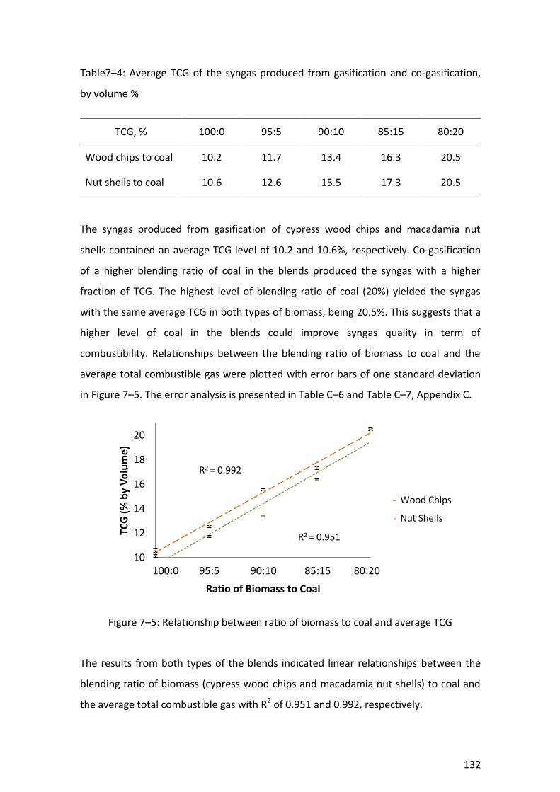
132

Table7–4: Average TCG of the syngas produced from gasification and co-gasification,

by volume %

TCG, % 100:0 95:5 90:10 85:15 80:20

Wood chips to coal 10.2 11.7 13.4 16.3 20.5

Nut shells to coal 10.6 12.6 15.5 17.3 20.5

The syngas produced from gasification of cypress wood chips and macadamia nut

shells contained an average TCG level of 10.2 and 10.6%, respectively. Co-gasification

of a higher blending ratio of coal in the blends produced the syngas with a higher

fraction of TCG. The highest level of blending ratio of coal (20%) yielded the syngas

with the same average TCG in both types of biomass, being 20.5%. This suggests that a

higher level of coal in the blends could improve syngas quality in term of

combustibility. Relationships between the blending ratio of biomass to coal and the

average total combustible gas were plotted with error bars of one standard deviation

in Figure 7–5. The error analysis is presented in Table C–6 and Table C–7, Appendix C.

Figure 7–5: Relationship between ratio of biomass to coal and average TCG

The results from both types of the blends indicated linear relationships between the

blending ratio of biomass (cypress wood chips and macadamia nut shells) to coal and

the average total combustible gas with R2 of 0.951 and 0.992, respectively.

10

12

14

16

18

20

0 5 10 15 20

TCG

(%

by

Vo

lum

e)

Ratio of Biomass to Coal

Wood Chips

Nut Shells

R2 = 0.992

R2 = 0.951

100:0 95:5 90:10 85:15 80:20

133

7.3.2.2 Heating value of the syngas

It becomes clear that the energy content of cypress wood chips and macadamia nut

shells was lower than that of Australian bituminous coal. As indicated in Chapter 5

Properties of fuels, the HHV of these three samples was 21,856, 20,714 and 27,061 kJ

per kg, respectively. For that reason, the HHV of the syngas which was the output of

the gasification process was expected to increase with an increasing ratio of coal in the

blends. Many formulae based on proximate and ultimate analyses are available for

computing heating values of solid fuels. Although heating values of gaseous fuels can

be also calculated by those formulae using ultimate and proximate analyses, this

approach which involves a separation of the constituent gases into elementary gases is

actually not simple and prone to result in arithmetical error.

The combustible composition of gaseous fuels is basically made up of carbon

monoxide, hydrogen and certain hydrocarbons. As a result, heating values of gaseous

fuels can be determined by separating their composition into constituent gases and

calculating the heating values from these constituents’ heating values. This method

appears to be much more convenient and less prone to error. Therefore, the heating

value of the syngas can be calculated from the heating value of the percentage

quantities of carbon monoxide, hydrogen and methane in the syngas, as presented in

Equation (7–2) and (7–3). The higher and lower heating values of these key constituent

gases are shown in Table 7–5.

HHVsyngas = YCOHHVCO + YH2HHVH2 + YCH4HHVCH4 (7–2)

LHVsyngas = YCOLHVCO + YH2LHVH2 + YCH4LHVCH4 (7–3)

Table 7–5: HHV and LHV of carbon dioxide, hydrogen and methane

Gas HHV (kJ/Nm3) LHV (kJ/Nm3)

Carbon Monoxide (CO) 13,100 13,100

Hydrogen (H2) 13,200 11,200

134

Gas HHV (kJ/Nm3) LHV (kJ/Nm3)

Methane (CH4) 41,200 37,100

Source: Jaojaruek et al. (2011)

Average HHV and LHV of the syngas produced from gasification of cypress wood chips,

macadamia nut shells and four levels of their blends with Australian bituminous coal,

which were calculated from Equation (7–2) based on the HHV and LHV of the

constituents presented in Table 7–5, are summarised in Table 7–6.

Table 7–6: Average HHV and LHV of the syngas produced from different ratios, kJ/Nm3

Ratio of Biomass to

Coal

HHV (kJ/Nm3) LHV (kJ/Nm3)

Wood chips Nut shells Wood chips Nut shells

100:0 1,354 1,412 1,307 1,364

95:5 1,561 1,666 1,502 1,610

90:10 1,773 2,053 1,706 1,979

85:15 2,157 2,287 2,073 2,195

80:20 2,705 2,702 2,597 2,593

According to Table 7–6, average heating values of the syngas increased with a higher

ratio of the coal in both types of biomass blends. Average HHV of the syngas produced

from cypress wood chips was 1,354 kJ per Nm3 while the blend of 80% cypress wood

chips and 20% Australian bituminous coal yielded the syngas with average HHV of

2,705 kJ per Nm3, an increase of 99.72%. Similar results were also found in macadamia

nut shells and their blends with Australian bituminous coal. The increase of the ratio of

the coal in the blends with macadamia nut shells from 0 to 20% caused the increase of

average heating value of the syngas from 1,412 to 2,702 kJ per Nm3, an increase of

91.42%. The LHV which were calculated from the HHV certainly illustrated the same

trends as the HHV. Relationships between the ratio of biomass (cypress wood chips

and macadamia nut shells) to coal and the average HHV and LHV of the syngas are

135

illustrated with error bars of one standard deviation in Figure 7–6 and Figure 7–7,

respectively. The error analysis is presented in Table C–8, Appendix C.

Figure 7–6: Relationship between ratio of biomass to coal and average HHV

Figure 7–7: Relationship between ratio of biomass to coal and average LHV

As illustrated in Figure 7–6 and 7–7, linear relationship between the blending ratio of

biomass to coal and the average HHV and LHV of the syngas appeared to be the same

as that between the blending ratio of biomass to coal and the average total

combustible gas, due to similar percentage quantities of constituents used to calculate

the TCG, HHV and LHV. The same R2 of 0.951 in the blends of cypress wood chips and

1,000

1,500

2,000

2,500

3,000

0 5 10 15 20

Ave

rage

HH

V (

kJ/N

m3)

Ratio of Biomass to Coal

Wood Chips

Nut Shells

100:0 95:5 90:10 85:15 80:20

y = 64.05x + 1383.7R² = 0.992

y = 65.958x + 1250.4R² = 0.951

1,000

1,500

2,000

2,500

0 5 10 15 20

Ave

rage

LH

V (

kJ/N

m3)

Ratio of Biomass to Coal

Wood Chips

Nut Shells

100:0 95:5 90:10 85:15 80:20

y = 63.007x + 1207R² = 0.951

y = 60.879x + 1339.4R² = 0.992

136

Australian bituminous coal and of 0.992 in blends of macadamia nut shells and

Australian bituminous coal were found.

7.4 Summary

The syngas was produced from gasification and co-gasification of cypress wood chips,

macadamia nut shells and four levels of their blends with Australian bituminous coal

using a laboratory-scale downdraft fixed bed gasifier under air as a gasifying agent.

Analysis of the quality of the syngas was performed in terms of its composition,

combustibility (TCG) and energy content (HHV and LHV). It was found that, due to the

similarity in chemical properties of cypress wood chips and macadamia nut shells,

gasification of both types of biomass samples yielded relatively similar composition of

the syngas, resulting in an average level of TCG of 10.2 and 10.6%, respectively.

Although the syngas produced in this study had a low average level of TCG and a high

average content of nitrogen owing to the use of air as the gasifying agent and other

operation conditions, this study only focused on investigating the effects of the

proportion of coal on the quality of the syngas produced. The blends of both types of

biomass samples with the coal sample produced the syngas with higher average

contents of carbon monoxide and hydrogen. The average TCG of both types of blends

at the highest ratio of coal (20%) increased to 20.5%. However, an average content of

carbon dioxide which was not desirable increased as the coal sample in the blends

increased.

The HHV and LHV of the syngas were moreover determined by calculating from the

heating value of the percentage quantities of carbon monoxide, hydrogen and

methane in the syngas. In the same manner, average HHV and LHV of the syngas

increased with a higher ratio of the coal sample in both types of blends. The average

HHV of the syngas produced from individual cypress wood chips was 1,354 kJ per Nm3

while the blend of 80% cypress wood chips and 20% Australian bituminous coal yielded

the syngas with the average HHV of 2,705 kJ per Nm3. Similar results were found in

individual macadamia nut shells and their blend with the coal sample, increasing the

average HHV from 1,412 to 2,702 kJ per Nm3. Linear relationships between the

blending ratio of biomass to coal and the syngas quality in terms of average TCG, HHV

137

and LHV were observed in both types of blends. This indicated that properties of a fuel,

especially its carbon content, have a direct effect on the composition of the final

product of the gasification process. The coal sample which had higher carbon content

than that of both types of biomass caused production of significantly higher carbon

monoxide in the syngas. It is concluded that the co-gasification of biomass as a primary

fuel and coal as a supplementary fuel could improve the syngas quality.

138

Chapter 8

Development of syngas production model using neural network

Considering the powerful potential of artificial neural networks, it is notable that little

research has been carried out in the field of neural network models for biomass

gasification applications. Availability of uncomplicated models for gasification

applications is expected to help the operation and optimisation of the process and

performance. Artificial neural networks, which have ability to organise highly non-

linear relationship, can be an effective means to predict gasification characteristics.

This study therefore aims to develop a neural network model that can predict quality

of the syngas produced from gasification and co-gasification of biomass and coal using

experimental data.

8.1 Selection of data

Selecting a proper set of variables for inclusion as input data and output (target) data is

considered as a very important phase of neural network model development. This is

because performance of the model developed depends highly on the input and output

variables used. Generally, a set of data has an impact on the reliability of the model.

Proper selection of the data set can also contribute to computational efficiency. If the

set of available data is dimensional, it becomes crucial to choose a subset of the

potential input variables with the purpose of decreasing the number of free

parameters in the model to facilitate good generalisation among finite data. Data

selection is certainly arduous since real systems are often complicated and related to

non-linear processes. Thus, the dependencies among the input and output data are

difficult to determine.

In this study, an extensive literature review was done in order to select a proper set of

variables for constructing a reliable neural network model. The input and output

variables were selected from the experimental results. The study principally focused

on the effects of the fuels and their blends on the syngas produced. For that reason,

the input data ought to contain important compositions of the fuels while the target

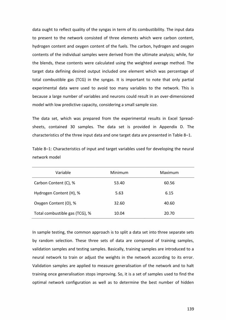
139

data ought to reflect quality of the syngas in term of its combustibility. The input data

to present to the network consisted of three elements which were carbon content,

hydrogen content and oxygen content of the fuels. The carbon, hydrogen and oxygen

contents of the individual samples were derived from the ultimate analysis; while, for

the blends, these contents were calculated using the weighted average method. The

target data defining desired output included one element which was percentage of

total combustible gas (TCG) in the syngas. It is important to note that only partial

experimental data were used to avoid too many variables to the network. This is

because a large number of variables and neurons could result in an over-dimensioned

model with low predictive capacity, considering a small sample size.

The data set, which was prepared from the experimental results in Excel Spread-

sheets, contained 30 samples. The data set is provided in Appendix D. The

characteristics of the three input data and one target data are presented in Table 8–1.

Table 8–1: Characteristics of input and target variables used for developing the neural

network model

Variable Minimum Maximum

Carbon Content (C), % 53.40 60.56

Hydrogen Content (H), % 5.63 6.15

Oxygen Content (O), % 32.60 40.60

Total combustible gas (TCG), % 10.04 20.70

In sample testing, the common approach is to split a data set into three separate sets

by random selection. These three sets of data are composed of training samples,

validation samples and testing samples. Basically, training samples are introduced to a

neural network to train or adjust the weights in the network according to its error.

Validation samples are applied to measure generalisation of the network and to halt

training once generalisation stops improving. So, it is a set of samples used to find the

optimal network configuration as well as to determine the best number of hidden

140

neurons. Testing samples are applied to evaluate the fully trained network. The testing

set provides an independent measure of neural network accuracy.

8.2 Design of the neural network model

The neural network model was constructed in MATLAB environment by the use of

Neural Network Toolbox. The network worked in unison to solve the specific problem

which was the quality of the syngas produced from gasification and co-gasification of

biomass and coal fuels using the experimental results.

8.2.1 Architecture of the neural network

The feed forward network which is the most common type of artificial neural network

architecture was used. Figure 8–1 illustrates the feed forward network which is

composed of three layers of processing elements, consisting of an input layer, hidden

layer and output layer. Each neuron in a particular layer is connected with all neurons

in the next layer, as shown in Figure 8–1.

Figure 8–1: Schematic diagram of the feed forward neural network

There is no explicit rule of determining the number of hidden layers for a neural

network. However, many studies mentioned that a single hidden layer with proper

number of hidden neurons is sufficient for the majority of problems. One hidden layer

is usually able to form any mapping required and approximate any function that has a

continuous mapping. It was reported that the situations in which performance of the

O

C

H TCG

OutputInput(pi)

Hidden

WeightsIWj,i

WeightsLWk,j

j = 1

j = 2

k = 1

b1j b2k

Biases

141

neural network with more than one hidden layer improves were very small. It is also

necessary to note that the neural network learns best with simplest mapping (Liu et

al., 2011; Priddy and Keller, 2005). As a consequence, this neural network was

designed to include only one hidden layer.

Likewise, there is no explicit rule of determining the number of neurons in each hidden

layer. Determining the number of hidden layers and the number of nodes in each of

those layers is however an essential part for overall neural network architecture. This

is because the number of hidden layers and the number of neurons in each of those

layers have a significant influence on the final results. Especially, the number of hidden

neurons has to be thoroughly considered. Experiments are typically adopted to obtain

the number of hidden neurons (Liu et al., 2011; Wunsch et al. 2003). As aforesaid, an

insufficient number of hidden neurons prevents the neural network from learning the

required function while an excessive number of hidden neurons leads the neural

network to overfit the training data which decreases its generalisation accuracy.

Therefore, to find the best number of hidden neurons, the trial and error method was

used by applying different numbers of hidden neurons in the range of 1–10. The best

solution was two hidden neurons which resulted in minimum mean squared error

(MSE). The results are presented in section 8.3.

8.2.2 Transfer functions in the neural network

In a feed forward neural network, almost every transfer functions can be used.

However, in order to apply the backpropagation training algorithm, the transfer

function has to be differentiable (Priddy and Keller, 2005). For this neural network, the

hyperbolic tangent sigmoid transfer function (tansig) was applied in the hidden layer

while the linear transfer function (purelin) was applied in the output layer. The

proposed neural network model is presented in Equation (8–1).

∑

(

( ( ∑ ( ) ))

) (8–1)

where p is input of the neuron; W is connection weight; b is bias value of the neuron.

142

8.2.3 Training algorithm for the neural network

After defining the problem, collecting and preparing the data, choosing the neural

network architecture, the network is ready to be trained. Training functions are

mathematical procedures to automatically adjust weights and biases of neural

networks, as aforementioned. It is important to find the training parameters that

produce the best performance, as indicated by performance of the network with

unseen data. This basically determines generalisation of the network. If the network is

overtrained; it normally either memorises the data in classification tasks or overfits the

data in estimation tasks. Thus, it becomes necessary to use the training data set that

was not used to train the network; since the purpose is to create the best network

performance on independent data (Liu et al., 2011; Priddy and Keller, 2005).

In this study, the neural network was trained using the Levenberg-Marquardt

backpropagation algorithm (trainlm). Trainlm in Neural Network Toolbox updates

values of weight and bias in accordance with Levenberg-Marquardt optimisation. The

Levenberg–Marquardt algorithm, independently created by Kenneth Levenberg and

Donald Marquardt, provides a mathematical solution to the problem of minimising a

function, typically nonlinear. It is an iterative technique that addresses the minimum of

a multivariate function expressed as the sum of squares of non-linear functions. The

algorithm can be regarded as a combination of the method of gradient descent and

the Gauss–Newton algorithm. The Levenberg–Marquardt algorithm is widely used as a

standard technique to solve non-linear least-squares problems. In Neural Network

Toolbox, trainlm is considered as the fastest backpropagation algorithm; so it is highly

recommended as a preferred choice of supervised algorithm (MathWorks, 2012;

Nelles, 2001; Yu and Wilamowski, 2011).

Furthermore, it is important to note that data splitting for training and testing is a vital

consideration during neural network development. Poor data splitting can lead to

inaccurate and inconsistent model performance (Priddy and Keller, 2005; MathWorks,

2012). As a result, multiples trials of different splits were carried out in this study. The

set of data was randomly divided into training samples, validation samples and testing

samples with 80/10/10, 70/15/15 and 60/20/20 splits to ensure optimum results.

143

8.3 Performance of the neural network model

The impact of composition (C, H and O) of the fuels on quality of the syngas in term of

TCG concentration is considered in this study. Neural Network Toolbox 7.0 in MATLAB

7.11.0 (R2010b) was used for developing the feed forward neural network model in

order to make predictions about the syngas. Carbon content, hydrogen content and

oxygen content were used as three input variables while percentage of TCG in the

syngas was uses as single output variable. The design of the network was chosen

through the trial and error method by applying three different sample splits and ten

different numbers of hidden neurons in the hidden layer. The number of hidden

neurons was increased from one to ten for each split. The entire process was repeated

and recorded. The network with the smallest number of hidden neurons and the

smallest error for validation was chosen. As many trials were conducted only results of

the network chosen were reported. Based on the experiment and analysis, the chosen

network consisted of two hidden neurons in the hidden layer with the sample split of

70/15/15. Figure 8–2 illustrates the proposed neural network diagram generated

through Neural Network Toolbox. The assessment and validation of a neural network

prediction model are based on a choice of one or more error metrics. Mean squared

error (MSE) is most commonly used as an error metric for neural network models that

perform a prediction task. The data set was randomly split into training samples (70%),

validation samples (15%) and testing samples (15%). The validation set was used to

validate the trained network while the true error of the network was estimated using

the testing set.

Figure 8–2: The neural network diagram generated from MATLAB

The tansig transfer function was applied for the hidden layer while the purelin transfer

function was applied for the output layer, as shown in Figure 8–2. During the training

144

process, the system automatically adjusted weights and biases of the neural network

according to the Levenberg–Marquardt algorithm which aimed to minimise errors

between the target output and the network output. It carried out 80 iterations. Each

iteration improved the weights slightly. The iteration loop stoped once no further

improvement was made. Screen capture of the neural network training is presented in

Figure 8–3.

Figure 8–3: The neural network training obtained from MATLAB

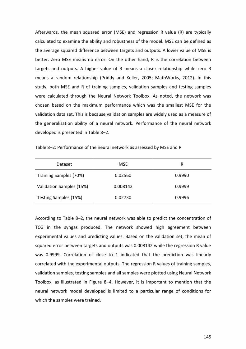
145

Afterwards, the mean squared error (MSE) and regression R value (R) are typically

calculated to examine the ability and robustness of the model. MSE can be defined as

the average squared difference between targets and outputs. A lower value of MSE is

better. Zero MSE means no error. On the other hand, R is the correlation between

targets and outputs. A higher value of R means a closer relationship while zero R

means a random relationship (Priddy and Keller, 2005; MathWorks, 2012). In this

study, both MSE and R of training samples, validation samples and testing samples

were calculated through the Neural Network Toolbox. As noted, the network was

chosen based on the maximum performance which was the smallest MSE for the

validation data set. This is because validation samples are widely used as a measure of

the generalisation ability of a neural network. Performance of the neural network

developed is presented in Table 8–2.

Table 8–2: Performance of the neural network as assessed by MSE and R

Dataset MSE R

Training Samples (70%) 0.02560 0.9990

Validation Samples (15%) 0.008142 0.9999

Testing Samples (15%) 0.02730 0.9996

According to Table 8–2, the neural network was able to predict the concentration of

TCG in the syngas produced. The network showed high agreement between

experimental values and predicting values. Based on the validation set, the mean of

squared error between targets and outputs was 0.008142 while the regression R value

was 0.9999. Correlation of close to 1 indicated that the prediction was linearly

correlated with the experimental outputs. The regression R values of training samples,

validation samples, testing samples and all samples were plotted using Neural Network

Toolbox, as illustrated in Figure 8–4. However, it is important to mention that the

neural network model developed is limited to a particular range of conditions for

which the samples were trained.

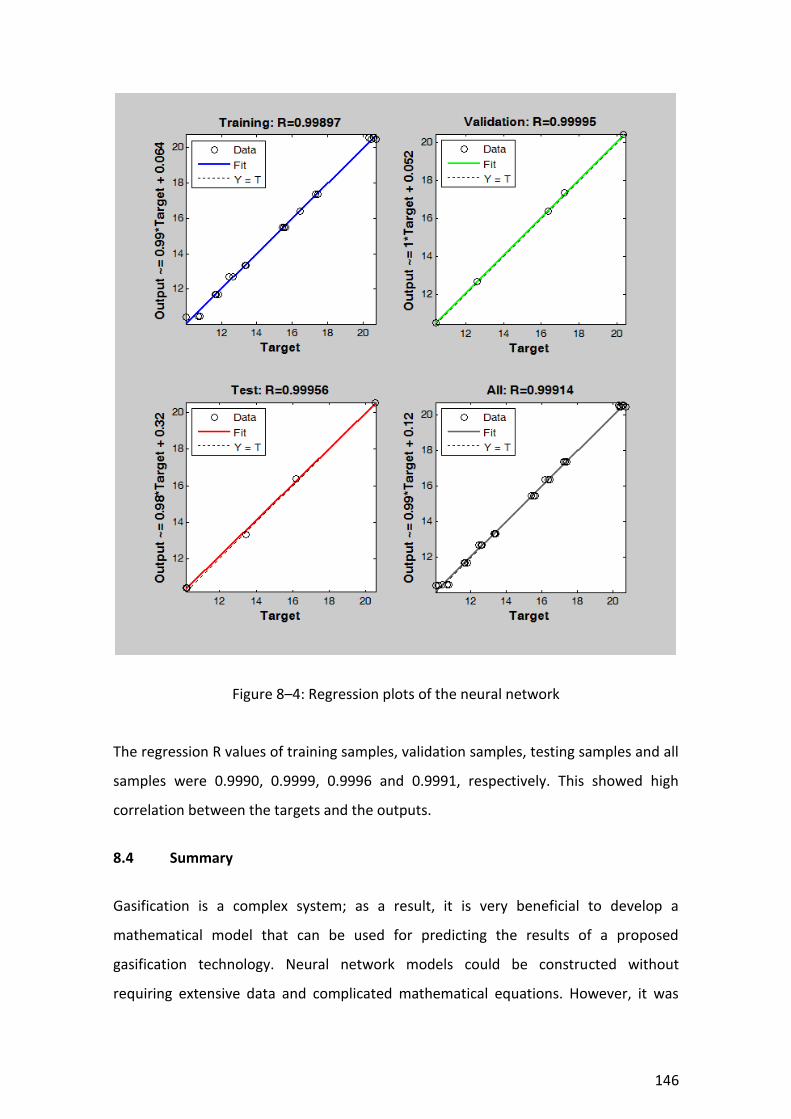
146

Figure 8–4: Regression plots of the neural network

The regression R values of training samples, validation samples, testing samples and all

samples were 0.9990, 0.9999, 0.9996 and 0.9991, respectively. This showed high

correlation between the targets and the outputs.

8.4 Summary

Gasification is a complex system; as a result, it is very beneficial to develop a

mathematical model that can be used for predicting the results of a proposed

gasification technology. Neural network models could be constructed without

requiring extensive data and complicated mathematical equations. However, it was

147

found that neural network modelling for biomass gasification application is still limited.

This study therefore developed a neural network model using experimental data in

order to predict the quality of the syngas produced from gasification and co-

gasification of biomass and coal. The neural network model was constructed in the

MATLAB environment by the use of Neural Network Toolbox. Key procedures applied

for developing the neural network consisted of problem identification, data

preparation, building the network, training the network and testing the network.

Only partial experimental results were selected to avoid too many variables to the

network which could result in an over-dimensioned model with low predictive

capacity, considering the small sample size. Since the research focuses on the effects

of the fuels and their blends on the syngas produced, the input data contained three

important compositions of the fuels (C, H and O) while the output data reflected the

quality of the syngas in the context of its combustibility (TCG). The trial and error

method was adopted to find the optimal solution for designing and training the neural

network model.

This study applied the feed forward neural network architecture which consisted of

three layers: an input layer, a hidden layer and an output layer. The training functions

included the hyperbolic tangent sigmoid transfer function (tansig) in the hidden layer

while the linear transfer function (purelin) in the output layer. The neural network was

trained by the Levenberg-Marquardt backpropagation algorithm (trainlm). The design

of the network was chosen through the trial and error method by applying ten

different numbers of hidden neurons in the hidden layer (1–10 neurons) and three

different sample splits (80/10/10, 70/15/15 and 60/20/20 splits) during training. The

neural network with two hidden neurons and the sample split of 70/15/15 resulted in

minimum mean squared error. The regression R value was 0.9999 which suggested

that the prediction was linearly correlated with the experimental outputs. So, the

neural network model developed was suitable for predicting the syngas quality

produced from the gasification process under these particular experimental

conditions.

148

Chapter 9

Financial analysis of two sizes of small scale gasification plants

Financial analysis plays a meaningful role to ensure that a technology can be achieved

in economic markets. It has been observed in practice that many technologies which

are technically feasible could not be deployed in commercial scales, mainly due to the

high cost of investment. In the investment analysis, two principal methods can be

applied to determine feasibility of a project including discount techniques and non-

discount techniques. In discount techniques, values from the capital are characterised

through cash inflow and outflow. The point of time, where cash is generated, is taken

into account among discount techniques. Non-discount techniques do not consider the

time value of money. Cash generated in the future is fundamentally assumed to have

equivalent value as years before. Key discount techniques include Net Present Value

(NPV) method and Internal Rate of Return (IRR) method while non-discount techniques

mainly consist of payback period (PB) method and Accounting Rate of Return (ARR)

method (Götze et al., 2007; Kapil, 2011; Röhrich, 2007).

9.1 Investment analysis

In this study, an investment analysis model for biomass gasification plants was

developed in Microsoft Excel worksheet. However, the data required for developing

the investment analysis model are usually confidential. The study was able to acquire

the data from Biomass Electricity Producer Company Limited, Thailand owing to a

previous relationship between this company and the researcher. The power plant was

designed to make use of several materials such as mango wood chips, saw dust and

rice husk. These raw materials have relatively similar properties to cypress wood chips

and macadamia nut shells which are widely available in Australia and could be readily

obtained for this study. The analysis was based on small scale biomass gasification

power plants with a 20-year project life.

The key methods adopted to develop the model are composed of the NPV method, the

IRR method and the payback period method. Net Present Value is the sum of the

149

present values of the annual cash flows minus the initial investment. Consequently, it

can be used to analyse the profitability of a project. The NPV method, as a valuable

indicator, can determine the value of an investment. A project that returns with a

positive NPV is feasible and attractive (Campbell and Brown, 2003; Götze et al., 2007;

Kapil, 2011). Internal Rate of Return is defined as the project discount rate at which the

NPV of a project is equal to zero. It means that the IRR is the rate of return that makes

the sum of present value of future cash flows and the final market value of a project

equal its current market value. A project will be attractive to invest in if the IRR is

greater than the rate of return that can be earned by alternative investments

(Campbell and Brown, 2003; Götze et al., 2007; Kapil, 2011).

The payback method principally calculates the time in years that takes to regain the

original capital outlay. Thus, payback period is the number of years that the cash

inflow is equal to the cash outflow from the cost of capital. An investment that has

longer payback period than the target payback period is to be rejected. In the case of

comparing several investment alternatives, those alternatives can be ranked by their

payback period and chosen by the shortest payback period. Although the payback

method appears to be effective for a quick analysis, it not only ignores the time value

of cash flows but also neglects a measurement of profitability (Götze et al., 2007; Kapil,

2011). Variables used for developing the investment analysis model were categorised

into investment, operation, finance and energy payment, as listed in Table 9–1. The

model developed was applied for assessing two different sizes of small scale biomass

gasification power plants, as presented in Appendix E.

Table 9–1: Variables used in the investment analysis model

Category Variable

Investment Activities Development Cost, Capital Expenditure and Total Investment

Operating Activities Revenues: Energy Payment, Capacity Payment and Total revenues

Operating Expenses: Administration, Operating Cost, Biomass Fuel, Maintenance, Insurance and Total

150

operating expenses

EBITDA: EBITDA (% of Revenues), Less Depreciation, Less Interest Expense and Less Corporate Tax

Net Income: Add Depreciation and Net Operating Cash Flow

Financing Activities Financing expenses (Fees), Debt Drawdown, Interest during construction, Debt Repayment, Net income bef. legal reserve, Legal Reserve Account and Net income bef. divided payment

Equity Financing: Capital Injection and Net Income

Energy Payment On-Peak Energy, Off-Peak Energy, Unit Prince for On-Peak Energy, Unit Prince for Off-Peak Energy and Fuel Adjustment Charge at the Given Time (Ft.)

Financial analysis of two sizes of small scale gasification plants including 600 and 1,200

kW were analysed and compared by the use of the investment analysis model

developed. From a study of the literature, the discount rate to calculate the NPV was

assumed at 5% which was above annual percentage rate (APR) of the interest rate for

the loan while the minimum acceptable rate of return (MARR) was assumed at 10%

(Doty and Turner, 2009; Newnan et al., 2004). The results from the investment analysis

model in terms of the NPV, IRR and payback period of the two sizes of biomass

gasification plants in Thailand are summarised in Table 9–2.

Table 9–2: Results of the investment analysis model for biomass gasification plants

Results from the model 600 kW 1,200 kW

NPV-Equity Cash Flow (5%), THB 14,518,312 42,471,273

Project IRR, % 13.6 19.6

Equity IRR, % 21.8 40.9

Payback period, yrs. 6.5 4.5

151

The results of the investment analysis, as presented in Table 9–2, indicated that both

sizes of the biomass gasification projects were financially feasible. However, the larger

project, a 1,200 kW plant, could achieve better financial performance compared to the

smaller project, a 600 kW plant. The NPV of the 1,200 kW plant was significantly higher

than that of the 600 kW plant. Similarly, the project IRR and equity IRR of the 1,200 kW

plant were higher compared to those of the 600 kW plant. The payback of the 1,200

kW plant was shorter than that of the 600 kW plant.

9.2 Sensitivity analysis

Sensitivity analysis, which determines the effect of different values of an independent

variable on a particular dependent variable under a set of assumptions, was also

carried out (Brigham and Ehrhardt, 2011). The analysis applied to both pessimistic and

optimistic views of three independent variables including capital cost, fuel cost and

energy payment in terms of the NPV, IRR and payback period for the 600 kW plant, as

summarised in Table 9–3.

Table 9–3: Results of the sensitivity analysis from both pessimistic and optimistic views

Pessimistic View Base Case Capital Cost

(+ 10%) Fuel Cost (+ 10%)

Energy Payment (– 10%)

NPV (THB.) 14,518,312 11,960,243 9,676,332 10,713,242

Project IRR 13.6% 11.8% 11.7% 12.1%

Equity IRR 21.8% 15.7% 16.7% 17.6%

Payback Period 6.5 yrs. 7 yrs. 7 yrs. 7 yrs.

Optimistic View Base Case Capital Cost

(– 10%) Fuel Cost (– 10%)

Energy Payment (+ 10%)

NPV (THB.) 14,518,312 17,076,381 19,360,293 18,323,382

Project IRR 13.6% 15.6% 15.3% 15.0%

Equity IRR 21.8% 34.2% 26.6% 25.0%

Payback Period 6.5 yrs. 5.5 yrs. 5.5 yrs. 5.5 yrs.

152

In sensitivity analysis, the key variables have been changed one at a time. The results

of the pessimistic scenario revealed that the fuel cost was the most sensitive variable

in the consideration of the NPV and IRR. As shown in Table 9–3, an increase in the fuel

cost by 10% caused the NPV to decrease by almost 5 million baht (33.4%) and the

project IRR to decrease by 1.87%. The payback period was not affected by the changes

in the three key variables, remaining around 7 years.

Similar trends of results of the optimistic scenario were also found. Basically, the

sensitivity analysis from both optimistic and pessimistic scenarios illustrated the same

changes compared to the base case but of opposite sign. The results suggested that

the fuel cost was the most critical factor affecting the financial performance of the

small scale biomass gasification plant under these particular assumptions.

9.3 Discussion on the investment opportunity

Various types of biomass have been used as traditional energy source in Thailand.

Available biomass fuels for gasification in the country are typically in the form of non-

plantation resources such as agricultural residues, wood residues and municipal solid

wastes (Garivait et al., 2006). Most biomass gasification plants in Thailand, including

Biomass Electricity Producer Company Limited, have utilised agricultural and wood

residues. Although the price of biomass varies by the season and area of operation, it

can be acquired a lower price per unit mass basis as compared to coal. In the

consideration of co-utilisation of biomass and coal to improve the gasification

performance, the fuels and blending ratios have to be carefully chosen to maintain a

financial viability of the system.

In Thailand, gasification technology and equipment are available from many

manufacturers, mostly in China, India and Japan as well as from in-house

manufacturers (Salam et al., 2010). Biomass Electricity Producer Company Limited and

several biomass gasification plants have acquired their gasification technology and

equipment from Chinese manufacturers because it requires less investment. It is also

important to note that, in Thailand, several policy instruments have been established

to promote the development and investment in renewable energy. For example, an

153

energy payment mechanism (called “adder”) which pays on top of the normal rate has

been used to compensate for external costs of biomass power generation. The Thai

Ministry of Energy has implemented a 15-year renewable energy plan from 2008 to

2022 which targets to increase energy supply from renewable energy sources to 20%

(Salam et al., 2010). So, with careful planning, an investment in a biomass gasification

plant in Thailand seems to be financially viable.

9.4 Summary

In this study, the financial analysis could facilitate decision-making in implementing

and utilising co-gasification technology in economic markets. This is because the

utilisation of coal in biomass based systems to improve the gasification performance

usually adds extra cost to the operations. The financial analysis of two sizes of small

scale gasification plants in Thailand was conducted to assess their investment

feasibility. An investment analysis model of biomass gasification with a 20-year project

life was developed in Microsoft Excel worksheet using the data from Biomass

Electricity Producer Company Limited, Thailand. The results indicated that investments

in the two sizes of small scale biomass gasification plants (600 and 1,200 kW), which

were assessed by the NPV, IRR and payback period, were financially feasible. However,

the larger project illustrated better financial performance compared to the smaller

project. This agreed with a study from the literature that economies of scale have a

direct impact on the economics of biomass gasification systems. The sensitivity

analysis which determined the effect of different values of the three variables (capital

cost, fuel cost and energy payment) on the NPV, IRR and payback period of the 600 kW

plant found that the fuel cost was the most sensitive variable. It had the most impact

on the financial performance of the biomass gasification plant under these particular

assumptions. In summary, the investment opportunity of a biomass gasification plant

in Thailand lies in the availability of biomass at a reasonable cost and the

establishment of policy instruments to promote renewable energy systems.

154

Chapter 10

Conclusions

Co-gasification of biomass as a primary fuel and coal as a supplementary fuel can be a

practical and cost effective method to improve quality of biomass gasification. This

research project investigated the influence of biomass and coal on the thermochemical

behaviour and the syngas production from the gasification process.

In the experiments, two types of biomass (cypress wood chips and macadamia nut

shells) and a type of coal (Australian bituminous coal) were selected. The results from

the proximate and ultimate analyses indicated that these two types biomass had

relatively similar approximate and absolute elemental composition. However, major

differences in properties (such as volatile matter, fixed carbon, carbon content and

oxygen content) between these two types of biomass and the Australian bituminous

coal were found.

Thermochemical behaviour of these two types biomass, the coal and their blends

during pyrolysis and combustion were observed using thermogravimetric analysis

(TGA) at the blending ratios of 95:5, 90:10, 85:15 and 80:20 at the heating rates of 5,

10, 15 and 20 °C min-1. Mass loss of the three samples during pyrolysis regardless of

their type occurred in three main stages comprising dehydration, devolatilisation and

solid decomposition. Devolatilisation appeared to be a dominant stage in pyrolysis; it

caused a significant mass loss from releasing at high rates.

The trends of mass loss of the two types of biomass samples and the coal sample were

found to be different. Mass loss of cypress wood chips and macadamia nut shells was

approximately over 60% at 400 °C while the loss in the mass of Australian bituminous

coal occurred at high temperatures compared to biomass, resulting in only 7% mass

loss at 400 °C. This was mainly due to the difference in volatile content.

During co-pyrolysis, the mass loss curves of the biomass and coal blends were similar

to that of the biomass, except these curves were shifted slightly along the temperature

155

axis. A small increase of the coal sample, which had low volatile matter, had an effect

on reducing the mass loss of the blends.

The analysis of char yield found a linear relationship between the yield of char and

blending ratio of biomass to coal with the R2 of 0.999.

In the thermokinetic analysis, the Ea of cypress wood chips and macadamia nut shells

was less than that of Australian bituminous coal, being 168.7, 164.6 and 199.6 kJ/mol,

respectively. The Ea of the blends of biomass and coal during co-pyrolysis followed that

of the weighted average of the individual samples in the blends.

Mass loss of the three samples during combustion could be also observed in three

main stages comprising dehydration, devolatilisation and char oxidation. The first and

second stages of mass loss (dehydration and devolatilisation) during combustion were

similar to those stages during pyrolysis, as indicated by relatively similar percentage of

cumulative mass loss below 400 °C.

However, the char oxidation in the third stage of combustion caused a significant loss

of mass (93.9%, 96.5% and 68.9% mass loss at 600 °C, respectively) while a slow loss of

mass continued in the third stage of pyrolysis as a result of slow decomposition of the

solid residue. Trends of mass loss during co-combustion were found to be similar to

that during co-pyrolysis.

The T50 indicator showed that temperatures at the degree of 50% mass loss of the

blends increased with increasing ratios of the coal sample while the R50 of the blends

which represent the intensity of mass loss at T50 decreased with higher ratios of the

coal sample. This suggested that lower volatile matter of the coal sample was

responsible for these changes.

During combustion, the Ea of cypress wood chips and macadamia nut shells was 138.9

and 147.4 kJ/mol, respectively while the Ea of Australian bituminous coal was 181.4

kJ/mol. The Ea of the blends of biomass and coal during co-combustion also followed

that of the weighted average of the individual samples in the blends.

156

No clear synergetic effects and thermochemical interaction between biomass and coal

were observed during co-pyrolysis and co-combustion. Thermochemical

decomposition of biomass and coal appeared to take place independently as such

thermokinetic parameters of the blends can be predicted from the measurements of

the individual samples using the weighted average method.

The biomass fuels (cypress wood chips, macadamia nut shells) and their blends with

the Australian bituminous coal at the four blending ratios were gasified using air as a

gasifying agent to investigate the effects of the fuels on the quality of the syngas as

assessed by its composition, combustibility (TCG) and energy content (HHV and LHV).

It was found that gasification of these two types of biomass yielded relatively similar

composition of the syngas, resulting in an average level of TCG of 10.2 and 10.6%,

respectively, mainly due to the similarity in their properties. Improvement in the

quality of the syngas was found in the co-gasification of the blends yielding the syngas

with the average TCG of 20.5% in both types of blends with the highest ratio of coal

(20%).

The HHV and LHV of the syngas were estimated by calculating from the heating value

of the percentage quantities of CO, H2 and CH4 in the syngas. Similar trends of results

of the HHV and LHV were found in comparison with the TCG. The average HHV of the

syngas of cypress wood chips and macadamia nut shells was 1,354 and 1,412 kJ/Nm3,

respectively while the blends of 80% biomass and 20% coal yielded the syngas with the

average HHV of 2,705 and 2,702 kJ per Nm3.

It could be concluded that, under these experimental conditions, the composition of

the syngas produced from the gasification system was directly influenced by properties

of the fuels fed. Even though thermochemical processes of the biomass and coal fuels

occurred individually, the co-gasification of these fuels (up to 20%) could linearly

enhance the quality of the syngas compared to the gasification of pure biomass.

A neural network model was developed to predict the quality of the syngas produced

from gasification and co-gasification of the biomass and coal fuels. The neural network

model was constructed in the MATLAB environment using carbon content, hydrogen

157

content and oxygen content of the fuels as the input data and the percentage of TCG in

the syngas as the target data. The feed forward backpropagation neural network

model developed was suitable for predicting the syngas quality produced from the

process with the regression R value was 0.9999 which suggested that the prediction

was linearly correlated with the experimental outputs.

The investment analysis model was developed to determine feasibility of two sizes of

small scale gasification plants (600 and 1,200 kW) in Thailand. Although both projects

were financially feasible, the results showed that the larger project could achieve

better financial performance compared to the smaller project with higher NPV and IRR

and shorter payback period. This agreed with the literature that economies of scale

have a direct impact on the economics of biomass gasification systems.

The sensitivity analysis of three key independent variables used in the model including

capital cost, fuel cost and energy payment suggested that the fuel cost was the most

critical factor affecting the financial performance of the system. Therefore, for the co-

gasification system, fuels and blending ratios have to be selected carefully to maintain

the financial viability of such system.

158

References

Abbas, T., Costen, P., Kandamby, N.H., Lockwood, F.C., & Ou, J.J. (1994). The influence

of burner injection mode on pulverized coal and biosolid co-fired flames. Combust

Flame, 99, 617-625.

Al-Mansour, F. & Zuwala, J. (2010). Evaluation of biomass co-firing in Europe. Biomass

and Bioenergy, 34(5), 620-629.

All Power Labs (2010). Gasifier Experimenters Kit. Retrieved from

http://gekgasifier.com/

ALT Inc. (2011). Pfeiffer Vacuum ThermoStar GSD 301 T3 Benchtop Mass Spectrometer.

Retrieved from www.usedlabequipment.com/lab_equipment/Pfeiffer+Vacuum%20

ThermoStar+GSD+301+T3+Benchtop+Mass+Spectrometer_19205.php?cPage=1&CatId

=110&SubCatId=934

Altman, A., & Hasegawa, P. M. (2011). Plant Biotechnology and Agriculture: Prospects

for the 21st Century. The United States: Elsevier Science.

Andersson, M. P., Abild-Pedersen, F., Remediakis, I. N., Bligaard, T., Jones, G., Engbæk,

J., Lytken, O., Horch, S., Nielsen, J.H., Sehested, J., Rostrup-Nielsen, J.R., Nørskov, J.K.,

Chorkendorff, I. (2008). Structure sensitivity of the methanation reaction: H2-induced

CO dissociation on nickel surfaces. Journal of Catalysis, 255(1), 6-19.

Anis, S., & Zainal, Z. A. (2011). Tar reduction in biomass producer gas via mechanical,

catalytic and thermal methods. A review. Renewable and Sustainable Energy Reviews,

15(5), 2355-2377.

Arbib, M. A. (2003). The Handbook of Brain Theory and Neural Networks, 2nd Edition.

The United States: Mit Press.

Arena, U., & Mastellone, M.L. (2006). Flugas - Fluidized Bed Gasifier for Alternative

Fuels. Retrieved from http://www.amracenter.com/doc/pubblicazioni/11i.Flugas.pdf

159

Ashizawa, M., Kajitani, S., Otaka M. & Watanabe, H. (2005). Development of

Performance Evaluation Techniques for Biomass Gasification Power Generation

System. Retrieved from http://criepi.denken.or.jp/en/publications/annual/2005/05

juten24.pdf

Babu, S.P. (2005) Observation on the current status of biomass gasification. Retrieved

from http://www.ieabioenergy.com/LibItem.aspx?id=184

Bain, R.L., Amos, W.A., Downing, M., & Perlack, R.L. (2003). Biopower Technical

Assessment: State of the Industry and Technology. National Renewable Energy

Laboratory, NREL/TP-510-33123

Balat, M., Balat, M., Kırtay, E. & Balat, H. (2009). Main routes for the thermo-

conversion of biomass into fuels and chemicals. Part 1: Gasification systems, Energy

Conversion and Management, 50 (12), pp. 3147-3157.

Bassam, N.E. (2010). Handbook of bioenergy crops: a complete reference to species,

development and applications. The United Kingdom: Earthscan.

Basu, P. (2006). Combustion and Gasification in Fluidized Beds. New York, The United

States: CRC Press.

Basu, P. (2010). Biomass Gasification and Pyrolysis: Practical Design and Theory. The

United States: Elsevier Science & Technology.

Baxter, L. (2005). Biomass–coal co-combustion: opportunity for affordable renewable

energy, Fuel, 84, 1295-1330

Bauen, A., Woods, J., & Hailes, R. (2004). Biopowerswitch!. The United Kingdom:

Imperial College London and E4tech (UK) Ltd.

Becker, J. (2008). Inorganic Mass Spectrometry: Principles and Applications. The United

States: Wiley

160

Berndesa, G., Hoogwijk, M., & van den Broek, R. (2003). The contribution of biomass in

the future global energy supply: a review of 17 studies. Biomass and Bioenergy. 25(1),

1-28.

Bingyan, X., Zengfan, L., Chungzhi, W., Haitao, H., & Xiguang, Z. (1994). Integrated

energy system in China - The cold north eastern region experience. Rome, Italy: Food

and Agriculture Organization of the United Nations (FAO).

Boerrigter, H. & Rauch, R. (2005) Review of applications of gases from biomass

gasification. Retrieved from http://www.ecn.nl/docs/library/report/2006/rx06066.pdf

Brammer, J.G. & Bridgwater, A.V. (1999). Drying technologies for an integrated

gasification bio-energy plant. Renewable and Sustainable Energy Reviews, 3, 243–289.

Brenes, M. D. (2006). Biomass and bioenergy: new research. The United States: Nova

Science Publishers.

Bridgwater, A.V. (1995). The technical and economic feasibility of biomass gasification

for power generation. Fuel, 14, 631–653.

Bridgwater, A.V. (2001). Progress in Thermochemical Biomass Conversion, Volume 2.

Oxford, UK: Blackwell Publishing.

Bridgwater, A.V. (2003). Renewable fuels and chemicals by thermal processing of

biomass, Chemical Engineering Journal, 91, 87–102

Bridgwater, A.V. (2008). Progress in Thermochemical Biomass Conversion. Great

Britain: John Wiley & Sons.

Bridgwater, A.V., Beenackers, A.A.C.M., & Sipila, K. (1999). An Assessment of the

Possibilities for Transfer of European Biomass Gasification Technology to China. The

United States: Office for Official Publications of the European Communities.

Brigham, E. F., & Ehrhardt, M. C. (2011). Financial Management: Theory and Practice.

The United States: South-Western Cengage Learning.

161

Brown, R. C., & Stevens, C. (2011). Thermochemical Processing of Biomass: Conversion

Into Fuels, Chemicals and Power. Great Britain: John Wiley & Sons.

Bryana, A.B., Warda, J., Hobbs, T. (2008). An assessment of the economic and

environmental potential of biomass production in an agricultural region. Land Use

Policy, 2008, 25(4), 533-549.

Callé, F.R. (2007). The biomass assessment handbook: bioenergy for a sustainable

environment. The United States: Earthscan

Campbell, H. F., & Brown, R. P. C. (2003). Benefit-Cost Analysis: Financial and Economic

Appraisal Using Spreadsheets. The United Kingdom: Cambridge University Press.

Carpentieri, M., Corti, A., & Lombardi, L. (2005). Life cycle assessment (LCA) of an

integrated biomass gasification combined cycle (IBGCC) with CO2 removal. Energy

Conversion and Management. 2005, 46(11-12), 1790-1808.

Celebi, O. C. (2012). Chapter 7 Neural Network. Retrieved from http://www.byclb.com/

TR/Tutorials/neural_networks/ch7_1.htm#c7

Chan, J. H., & Balke, S. T. (1997). The thermal degradation kinetics of polypropylene:

Part III. Thermogravimetric analyses. Polymer Degradation and Stability, 57(2), 135-

149.

Chasteen, T. G. (2000) Gas Chromatographic Injectors. Retrieved from

http://www.files.chem.vt.edu/chem-ed/sep/gc/gcinject.html

Chemistry World (2009). The biofuel future. Retrieved from http://www.rsc.org/

chemistry world/Issues/2009/April/Thebiofuelfuture.asp

Chen, D., Gao, X. & Dollimore, D. (1993). A generalized form of the Kissinger equation.

Thermochimica Acta, 215(26), 109-117.

Chen, D. & Fong, P.H. (1977). Evaluation of kinetic parameters from thermogravimetric

curves: Part I. Combined numerical method. Thermochimica Acta, 18(2), 161-170.

162

Chen, G., Andries, J., Luo, Z., & Spliethoff, H. (2003). Biomass pyrolysis/ gasification for

product gas production: the overall investigation of parametric effects. Energy

Conversion and Management, 44(11), 1875-1884.

Chen, W. & Kuo, P. (2010). A study on torrefaction of various biomass materials and its

impact on lignocellulosic structure simulated by a thermogravimetry. Energy, 35(6),

2580-2586.

Chen, W. & Wu, J. (2009). An evaluation on rice husks and pulverized coal blends using

a drop tube furnace and a thermogravimetric analyzer for application to a blast

furnace. Energy, 34(10): 1458–1466

Chopra, S., & Jain, A.K. (2003). A Review of Fixed Bed Gasification Systems for Biomass.

Agricultural Engineering International: CIGR Journal, 9, 1-23

Clarke, S., Preto, F. (2011). Biomass Densification for Energy Production. Retrieved

from http://www.omafra.gov.on.ca/english/engineer/facts/11-035.pdf

Colantoni S., Gatta S.D., de Prosperis R., Russo A., Fantozzi F., Desideri U. (2010). Gas

turbines fired with biomass pyrolysis syngas: analysis of the overheating of hot gas

path components, Journal of Engineering Gas Turbines Power, 132(6), 61401-61408

Collot, A. (2006). Matching gasification technologies to coal properties. International

Journal of Coal Geology, 65(3–4), 191-212.

Collot GA, Zhuo Y, Dugwell DR, Kandiyoti R. (1999). Co-pyrolysis and cogasification of

coal and biomass in bench-scale fixed-bed and fluidized bed reactors. Fuel, 78(6), 667-

679.

Concha, E., Turnes, M., Muniategui, S., Lopez, P., Fernandez, E., & Prada, D. (2002).

Optimisation of a programmed split-splitless injector in the gas chromatographic mass

spectrometric determination of organochlorine pesticides. Journal of Chromatography

A, 958(1-2), 17-24.

163

Costello, R. (1999). Biomass cofiring offers cleaner future for coal plants. Power

Engineering, 103(1), 45-48.

Corella, J., & Sanz, A. (2005). Modeling circulating fluidized bed biomass gasifiers. A

pseudo-rigorous model for stationary state. Fuel Processing Technology, 86(9), 1021–

1053.

CSIRO (2002). Biofuel Database. Retrieved from, http://www.det.csiro.au/science/

energy resources/biomass.htm

Culp, A.W. (1979). Principles of Energy Conversion. The United States of America:

McGraw-Hill Inc.

de Jong, W., Andries, J., Hein, K.R.G., (1999). Coal/biomass co-gasification in a

pressurised fluidised bed reactor, Renewable Energy, 16, 1110-1113.

de Klerk, A. (2011). Fischer-Tropsch Refining, 1st Edition. Singapore: Wiley-VCH Verlag

GmbH & Co. KGaA

de Souza, M.B., Nemer, L.C., Barreto, A.G. & Quitete. C.P.B (2012) Chapter 12 Neural

Network Based Modeling and Operational Optimization of Biomass Gasification

Processes. in Yun, Y. (Ed.), Gasification for Practical Applications. Rijeka, Croatia:

InTech

De, S. & Assadi, M. (2009). Impact of cofiring biomass with coal in power plants - A

techno-economic assessment, Biomass and Bioenergy, 33(2), 283-293.

Demirbas, A. (2003). Sustainable cofiring of biomass with coal. Energy Conversion and

Management, 44(9), 1465–1479.

Demirbas, A. (2004). Combustion characteristics of different biomass fuels. Progress in

Energy and Combustion Science, 30(2), 219-230.

Demirbas, A., & Demirbas I. (2007). Importance of rural bioenergy for developing

countries. Energy Conversion and Management, 48(8), 2386–2398.

164

Demirbas, M.F., Balat, M., & Balat, H. (2009). Potential contribution of biomass to the

sustainable energy development. Energy Conversion and Management, 50(7), 1746-

1760

Devi, L., Ptasinski, K.J., Janssen, F.J.J.G. (2003). A review of the primary measures for

tar elimination in biomass gasification processes. Biomass and Bioenergy, 24(2), 125-

140.

Devi, L., Ptasinski, K.J., Janssen, F.J.J.G., van Paasen, S.V.B., Bergman, P.C.A., & Kiel,

J.H.A. (2005). Catalytic decomposition of biomass tars: use of dolomite and untreated

olivine. Renewable Energy, 30(4), 565-587.

Dieck, R. H. (2007). Measurement Uncertainty: Methods and Applications, 4th Edition.

The United States: ISA.

Dong, C., Jin, B., Zhong, Z., & Lan, J. (2002). Tests on co-firing of municipal solid waste

and coal in a circulating fluidized bed. Energy Conversion and Management, 43(16),

2189-2199.

Dong, C., Jin, B., & Li, D. (2003). Predicting the heating value of MSW with a feed

forward neural network. Waste Management, 23(2), 103-106.

Doran, P. M. (2012). Bioprocess Engineering Principles, 2nd Edition. The United

Kingdom: Academic Press.

Dornburg, V. & Faaij, A.P.C. (2001). Efficiency and economy of wood-fired biomass

energy systems in relation to scale regarding heat and power generation using

combustion and gasification technologies. Biomass and Bioenergy, 21(2), 91-108.

Dorofki, M., Elshafie, A.H., Jaafar, O., Karim, O.A. & Mastura, S. (2012). Comparison of

Artificial Neural Network Transfer Functions Abilities to Simulate Extreme Runoff Data.

International Conference on Environment, Energy and Biotechnology IPCBEE, 33, 39-44.

Doty, S., & Turner, W. C. (2009). Energy management handbook. The United States:

Fairmont Press.

165

Ebeling, J.M., and Jenkins, B.M., (1985). Physical and chemical properties of biomass

fuels. Transactions of the ASABE, 28(3), 898-902.

EGAT (2011). Electricity Generation Authority of Thailand Annual Report 2011.

Thailand: Electricity Generating Authority of Thailand

Energy research Centre of the Netherlands (2012). Definitions used in Phyllis.

Retrieved from http://www.ecn.nl/phyllis/defs.asp

EPA (2000). Notice of Regulatory Determination on Wastes from the Combustion of

Fossil Fuels. Federal Register, 65(99), 32214-32237.

EREC (2007). Energy [r]evolution: A sustainable world energy outlook. The Netherlands:

Greenpeace International and EREC

Evans, A., Strezov, V., & Evans, T.J. (2010). Sustainability considerations for electricity

generation from biomass. Renewable and Sustainable Energy Reviews, 14(5), 1419-

1427.

FAO Forestry Department (1986). Wood gas as engine fuel. Roma, Italia: United

Nations (UN)

Fermoso, J., Arias, B., Plaza, M. G., Pevida, C., Rubiera, F., Pis, J. J., & Casero, P. (2009).

High-pressure co-gasification of coal with biomass and petroleum coke. Fuel Processing

Technology, 90(7–8), 926-932.

Franco, L., Elizondo, D.A., & Jerez, J.M. (2009). Constructive Neural Networks. Berlin,

Germany: Springer.

Fryda, L.E., Panopoulos, K.D., & Kakaras, E. (2008). Agglomeration in fluidised bed

gasification of biomass. Powder Technology, 181(3), 307-320.

Gabbott, P. (2008). Principles and applications of thermal analysis, Singapore:

Blackwell Publishing

166

Garcia, L., Salvador, M. L., Arauzo, J., & Bilbao, R. (2001). CO2 as a gasifying agent for

gas production from pine sawdust at low temperatures using a Ni/Al coprecipitated

catalyst. Fuel Processing Technology, 69(2), 157-174.

Garivait, S., Chaiyo, U., Patumsawad, S., & Deakhuntod, J. (2006). Physical and

Chemical Properties of Thai Biomass Fuels from Agricultural Residues. The 2nd Joint

International Conference on “Sustainable Energy and Environment (SEE 2006)”, 1-23

November 2006, Bangkok, Thailand

Geoscience Australia (2010). Coal. Retrieved from https://www.ga.gov.au/image_

cache/GA16878.pdf

Gil, J., Corella, J., Aznar, M.P., & Caballero, M.A. (1999). Biomass gasification in

atmospheric and bubbling fluidized bed: Effect of the type of gasifying agent on the

product distribution. Biomass and Bioenergy, 17(5), 389-403.

Gil, M. V., Casal, D., Pevida, C., Pis, J. J., & Rubiera, F. (2010). Thermal behaviour and

kinetics of coal/biomass blends during co-combustion. Bioresource Technology,

101(14), 5601-5608.

Gómez-Barea, A., Vilches, L.F., Leiva, C., Campoy, M., & Fernández-Pereira C. (2009).

Plant optimisation and ash recycling in fluidised bed waste gasification. Chemical

Engineering Journal, 146(2), 227–236.

Goswami, Y. (1986). Alternative Energy in Agriculture Vol. II. Florida, The United States:

CRC Press.

Götze, U., Northcott, D., & Schuster, P. (2007). Investment Appraisal: Methods and

Models. Germany: Springer.

Grammelis, P. (2010). Solid Biofuels for Energy: A Lower Greenhouse Gas Alternative.

London, Great Britain: Springer.

Grob, R. & Barry, E. (2004). Modern Practice of Gas Chromatography. The United

States: Wiley-Interscience.

167

Guo, B., Li, D., Cheng, C., Lu, Z., & Shen Y. (2001). Simulation of biomass gasification

with a hybrid neural network model. Bioresource Technology, 76(2), 77-83.

Hall, D.O.; House, J.I. (1995). Biomass: A modern and environmentally acceptable fuel.

Solar energy materials and solar cells, 38(1-4), 521-542.

Hall, D.O. Scrase, J.I. (1998). Will biomass be the environmentally friendly fuel of the

future? Biomass and Bioenergy, 15(4-5), 357-367.

Hansen, J.E. (2005). A slippery slope: How much global warming constitutes

“dangerous anthropogenic interference”? Climatic Change, 68, 269–279.

Hanrahan, G. (2011). Artificial Neural Networks in Biological and Environmental

Analysis. The United States: CRC Press.

Haq, Z. (2002). Biomass for electricity generation. Retrieved from www.eia.gov/oiaf/

analysispaper/biomass/pdf/biomass.pdf

Hartiniati, S.A. & Youvial, M. (1989). Performance of a pilot scale fluidized bed gasifier

fueled by rice husks, pyrolysis and gasification. In Proceedings of the International

Conference in Luxembourg, 23 –25 May 1989, 257–263.

Harvard University (2007). A Summary of Error Propagation. Retrieved from

http://ipl.physics.harvard.edu/wp-uploads/2013/03/PS3_Error_Propagation_sp13.pdf

Hastie, T., Tibshirani, R., & Friedman, J. (2009). The elements of statistical learning.

New York, The United States: Springer.

Haykiri-Açma, H., Ersoy-Meriçboyu, A. & Küçükbayrak, S. (2002). Combustion reactivity

of different rank coals. Energy Conversion and Management, 43(4), 459-465.

Hayter, S., Tanner, S., Comer, K., & Demeter, C. (2004). Biomass Cofiring in Coal–Fired

Boilers. Retrieved from www1.eere.energy.gov/femp/pdfs/fta_biomass_cofiring.pdf

Higman, C., & van der Burgt, M. (2008). Gasification, 2nd Edition, The United States:

Gulf Professional Publishing.

168

Hoffmann, E. & Stroobant, V. (2007). Mass Spectrometry: Principles and Applications.

The United States: Wiley-Interscience.

Hoogwijk, M., Faaij, A., van den Broek, R., Berndes, G., Gielen, D., Turkenburg, W.

(2003). Exploration of the ranges of the global potential of biomass for energy.

Biomass and Bioenergy, 25(2), 119-133.

Hoogwijk, M., Faaija, A., de Vriesb, B., Turkenburga, W. (2009). Exploration of regional

and global cost-supply curves of biomass energy from short-rotation crops at

abandoned cropland and rest land under four IPCC SRES land-use scenarios. Biomass

and Bioenergy, 33(1), 26-43.

IEA (2006). Key World Energy Statistics 2006. Paris, France: The International Energy

Agency

IEA (2007). Summary of Discussion at the Task 33 Workshop on Situation Analysis and

Role of Biomass Gasification (BMG) Technologies in Future Energy Needs. Retrieved

from www.ieatask33.org/app/webroot/files/file/publications/IEA_BRU_11-07.pdf

IEA (2010). Biomass for Heat and Power. Retrieved from http://www.iea-etsap.org

/web/E-TechDS/PDF/E05-Biomass%20for%20HP-GS-AD-gct.pdf

IEA (2011). Key World Energy Statistics 2011. Paris, France: The International Energy

Agency

Idris, S.S, Rahman, N.A., Ismail, K., Alias, A.Z., Rashid, Z.A. & Aris, M.J. (2010).

Investigation on thermochemical behaviour of low rank Malaysian coal, oil palm

biomass, and their blends during pyrolysis via thermogravimetric analysis (TGA).

Bioresource Technology, 101(12): 4584-4592.

Iliadis, L. S., & Jayne, C. (2011). Engineering Applications of Neural Networks, Part I,

India, Springer

Intelligent Energy Europe (2008). Eyes on the track, Mind on the horizon, From

inconvenient rapeseed to clean wood: A European road map for biofuels. Retrieved

169

from http://www.iee-library.eu/images/all_ieelibrary_docs/refuel_european_biofuel-

roadmap.pdf

IRENA (2012). Renewable Energy Technology: Cost Analysis Series, Biomass for Power

Generation, Germany: The International Renewable Energy Agency

Jaojaruek, K., Jarungthammachote, S., Gratuito, M., Wongsuwan, H. & Homhual, S.

(2011). Experimental study of wood downdraft gasification for an improved producer

gas quality through an innovative two-stage air and premixed air/gas supply approach.

Bioresource Technology, 102(7), 4834-4840.

Jenkins, B. M., Baxter, L. L., Miles Jr, T. R., & Miles, T. R. (1998). Combustion properties

of biomass. Fuel Processing Technology, 54(1–3), 17-46.

Jirjis, R. (2005). Effects of particle size and pile height on storage and fuel quality of

comminuted Salix viminalis. Biomass and Bioenergy, 28(2), 193–201.

Kalogirou, S. (2007). Artificial Intelligence in Energy and Renewable Energy Systems.

New York, USA: Nova Science Publishers.

Kamruzzaman, J., Begg, R., & Sarker, R. A. (2006). Artificial Neural Networks in Finance

and Manufacturing, USA, Idea Group Pub.

Kapil, S. (2011). Financial Management, Mumbai, India: Dorling Kindersley (India) Pvt.

Ltd.

Kastanaki, E., Vamvuka, D., Grammelis, P., & Kakaras, E. (2002). Thermogravimetric

studies of the behavior of lignite–biomass blends during devolatilisation. Fuel

Processing Technology, 78, 159- 166.

Khanal, S. K., Surampalli, R. Y., Zhang, T. C., Lamsal, B. P., Tyagi, R. D., & Kao, C. M.

(2010). Bioenergy and Biofuel from Biowastes and Biomass. The United States:

American Society of Civil Engineers.

170

Khandpur, R. S. (2006). Handbook of analytical instruments. India: Tata McGraw-Hill

Publising.

King, B. M., Rosopa, P. J., & Minium, E. W. (2011). Statistical Reasoning in the

Behavioral Sciences. The United States: John Wiley & Sons.

Kirkels, A.F., Verbong, G.P.J. (2011). Biomass gasification: Still promising? A 30-year

global overview. Renewable and Sustainable Energy Reviews, 15(1), pp. 471-481.

Kirkup, L., & Frenkel, B. (2006). An Introduction to Uncertainty in Measurement. The

United Kingdom: Cambridge University Press.

Kirubakaran, V., Sivaramakrishnanb, V., Nalinic, R., Sekard, T., Premalathae, M., &

Subramanian, P. (2009). A review on gasification of biomass. Renewable and

Sustainable Energy Reviews, 13(1), 179-186

Kitmondo (2013) Agilent Technologies 6890N, 5973N, 7683 Retrieved from

http://www.kitmondo.com/agilent-technologies-6890n,-5973n,-7683/ref457102

Klass, D. L. (1998). Biomass for Renewable Energy, Fuels, and Chemicals. The United

States: Academic Press.

Klimantos, P., Koukouzas, N., Katsiadakis, A. & Kakaras, E. (2009). Air-blown biomass

gasification combined cycles (BGCC): System analysis and economic assessment.

Energy, 34(5), 708-714.

Kotz, J.C., Treichel, R. & Townsend, J.R. (2009). Chemistry and chemical reactivity,

Volume 2, Canada: Cengage Learning.

Kreith, F., & Goswami, D. Y. (2011). Principles of Sustainable Energy. The United States:

Taylor & Francis Group.

Kumabe, K., Hanaoka T., Fujimoto, S., Minowa, T., & Sakanishi, K. (2007). Co-

gasification of woody biomass and coal with air and steam. Fuel, 86(5-6), 684-689.

171

Kurkela, E., Stahlberg, P., Laatikainen, J., & Simell, P. (1993). Development of Simplified

IGCC-Processes for Biofuels - Supporting Gasification Research at VTT. Bioresource

Technology, 46(1-2), 37-48.

Laster, E., Gong, M., & Thompson, A. (2007). A method for source apportionment in

biomass/coal blends using thermogravimetric analysis. Journal of Analytical and

Applied Pyrolysis, 80(1), 111-117.

Lee, J., Kim, D. & Kim, J. (2009). Reactivity study of combustion for coals and their chars

in relation to volatile content. Korean J. Chem. Eng., 26(2), 506-512

Lens, P., Westermann, P., Haberbauer, M. & Moreno, A. (2005). Biofuels for Fuel Cells:

Renewable Energy from Biomass Fermentation. Great Britain: Iwa Publishing

Leung, D.Y.C., Yin, X.L., & Wu, C.Z., (2004). A review on the development and

commercialization of biomass gasification technologies in China. Renewable and

Sustainable Energy Reviews, 8(6), 565-580.

Li, C., & Suzuki, K. (2009). Tar property, analysis, reforming mechanism and model for

biomass gasification - An overview. Renewable and Sustainable Energy Reviews, 13(3),

594-604.

Li, K., Zhang, R., and Bi, J. (2010). Experimental study on syngas production by co-

gasification of coal and biomass in a fluidized bed. International Journal of Hydrogen

Energy, 35(7), 2722-2726.

Lingireddy, S., & Brion, G. M., (2005). Artificial Neural Networks in Water Supply

Engineering. The United States: American Society of Civil Engineers.

Liu, D., Zhang, H., Polycarpou, M., Alippi, C., & He, H. (2011). Advances in Neural

Networks -- ISNN 2011. India: Springer.

Liu, F., Liu, X.N. & Wang, Q. (2009). Examination of Kissinger's equation for solid-state

transformation. Journal of Alloys and Compounds, 473(1-2), 152-156.

172

Llópiz, J., Romero, M.M., Jerez, A. & Laureiro, Y. (1995). Generalization of the kissinger

equation for several kinetic models, Thermochimica Acta, 256 (2), 205-211

López-Fonseca, R., Landa, I., Elizundia, U., Gutiérrez-Ortiz, M.A., González-Velasco, J.R.

(2006). Thermokinetic modeling of the combustion of carbonaceous particulate

matter. Combustion and Flame, 144(1-2), 398-406.

Lucas, C. (2004). Continuous High Temperature Air/steam Gasification (HTAG) of

Biomass. 6th Int. Conference on Science in Thermal and Chemical Biomass Conversion,

Victoria, Canada, 30 August -2 Septemper 2004

Lv, P., Yuan, Z., Wu, C., Ma, L., Chen, Y., & Tsubaki, N. (2007). Bio-syngas production

from biomass catalytic gasification. Energy Conversion and Management. 48(4), 1132–

1139.

Maciejewska, A., Veringa, H., Sanders, J., Peteves, S.D. (2006). Co-Firing of Biomass

with Coal: Constraints and Role of Biomass Pre-Treatment. The Netherlands: European

Commission

MathWorks (2012) MATLAB Functions in Neural Network Toolbox. Retrieved from

http://www.mathworks.com/help/nnet/functionlist.html

Maschio, G., Lucchesi, A. & Stoppato, G. (1994). Production of syngas from biomass.

Bioresource Technology, 48(2), 119-126.

McGowan, T. (2009). Biomass and alternate fuel systems: an engineering and economic

guide. The United States: John Wiley & Sons.

McKendry, P. (2002a). Energy production from biomass (Part1): Overview of biomass.

Bioresource Technology, 83(1), 37–46.

McKendry, P. (2002b). Energy production from biomass (Part2): Conversion

technologies. Bioresource Technology, 83(1), 47–54.

173

Meesri, C. & Moghtaderi, B. (2002) Lack of synergetic effects in the pyrolytic

characteristics of woody biomass=coal blends under low and high heating rate

regimes. Biomass and Bioenergy, 23, 55–66.

Miller, B. G., & Tillman, D. A. (2008). Combustion engineering issues for solid fuel

systems. The United States: Elsevier

Minchener, A. J. (2005). Coal gasification for advanced power generation. Fuel, 84(17),

2222-2235.

Mitchell, C.P., Bridgwater, A.V., Stevens, D.J., Toft, A.J. & Watters, M.P. (1995).

Technoeconomic assessment of biomass to energy. Biomass and Bioenergy, 9(1-5),

205-226.

Miyamoto, K. (1997). Renewable biological systems for alternative sustainable energy

production. Japan: Food & Agriculture Org.

Moghtaderi, B. (2007). Co-Combustion. In S. Van Loo & J. Koppejan (Eds.), Handbook of

Biomass Combustion and Co-Firing (pp. 203-248). The United Kingdom: Earthscan

Moghtaderi, B., Meesri, C., & Wall, T. F. (2004). Pyrolytic characteristics of blended coal

and woody biomass. Fuel, 83(6), 745-750.

Moghtaderi, B. & Ness, J. (2007). Coal-Biomass Cofiring Handbook, Australia:

Cooperative Research Centre for Coal in Sustainable Development

Mortimer, R. G. (2013). Mathematics for Physical Chemistry, 4th Edition. The United

States: Elsevier Science.

Sherren, K. (2006). Pillars of society: The historical context for sustainability and higher

education in Australia. In W. Filho & D. Carpenter (Eds.), Sustainability in the

Australasian university context (pp. 11-32). Frankfurt, Germany: Peter Lang.

Nagayoshi, H., Jun, H., & Hidemi, T. (2006). Low NOx Combustion Technique Using

Direct Injection into Strong Swirl Flow. IHI Eng Rev, 39(1), 33-39.

174

Nelles, O. (2001). Nonlinear System Identification: From Classical Approaches to Neural

Networks and Fuzzy Models. Germany: Springer.

Nemtsov, D., Zabaniotou, A. (2008). Mathematical modelling and simulation

approaches of agricultural residues air gasification in a bubbling fluidized bed reactor.

Chemical Engineering Journal, 143(1–3), 10-31.

NETL (2013a). Fischer-Tropsch Synthesis. Retrieved from http://www.netl.doe.gov/

technologies/coalpower/gasification/gasifipedia/5-support/5-11_ftsynthesis.html

NETL (2013b). Gasifipedia. Retrieved from http://www.netl.doe.gov/technologies/

coalpower/gasification/gasifipedia/4-gasifiers/4-2_physical-chem.html

Netzsch (2010). Operating Instructions: TG 209 F3 Tarsus. Germany: NETZSCH-

Gerätebau GmbH

Newnan, D. G., Eschenbach, T. G., & Lavelle, J. P. (2004). Engineering Economic

Analysis: Study Guide. The United States: Oxford University Press.

Niessen, W. (2001). Current Practice of Gas Chromatography-Mass Spectrometry. The

United States: CRC Press.

Nino, E.F. & Nino, T.G. (1997). Fuels and Combustion, Revised Edition. Philippines:

Publisher Rex Bookstore, Inc

Norton, G.A., (1993). A review of the derivative thermogravimetric technique (burning

profile) for fuel combustion studies, Thermochimica Acta, 214(2), 171-182

Nougues, J. M., Pan, Y. G., Velo, E., & Puigjaner, L. (2000). Identification of a pilot scale

fluidised-bed coal gasification unit by using neural networks. Applied Thermal

Engineering, 20(15–16), 1561-1575.

Obernberger, I., Brunner, T., Barnthaler, G. (2006). Chemical properties of solid

biofuels - significance and impact. Biomass and Bioenergy, 30(11), 973–982.

175

Paliwal, M., & Kumar, U. A. (2009). Neural networks and statistical techniques: A

review of applications. Expert Systems with Applications, 36(1), 2-17.

Pan, Y.G., Velo, E., Roca, X., Manya, J.J., & Puigjaner, L. (2000). Fluidized-bed co-

gasification of residual biomass/poor coal blends for fuel gas production. Fuel, 79(11),

1317-1326.

Parikka, M. (2004). Global biomass fuel resources. Biomass and Bioenergy, 27(6), 613-

620.

Park, D.K., Kim, S.D., Lee, S.H., & Lee, J.G. (2010). Co-pyrolysis characteristics of

sawdust and coal blend in TGA and a fixed bed reactor. Bioresource Technology,

101(15), 6151–6156

Parker, L.E. (2007). Notes on Multilayer, Feedforward Neural Networks. Retrieved from

http://web.eecs.utk.edu/~parker/Courses/CS594-fall07/handouts/

Patel, B. & Gami, B. (2012). Biomass Characterization and its Use as Solid Fuel for

Combustion. Iranica Journal of Energy & Environment, 3(2), 123-128

Paul, W.C. & Buchele, W.F. (1980). Development of a concentric vortex agri-residue

furnace. Agric Energy, 2, 349–356.

Prins, M.J., (2005). Thermodynamic analysis of biomass gasification and torrefaction.

Retrieved from http://alexandria.tue.nl/extra2/200510705.pdf

Priddy, K. L., & Keller, P. E. (2005). Artificial Neural Networks: An Introduction. The

United States: SPIE Press.

Prins, M.J., Ptasinski, K.J., Janssen, F.J.J.G. (2004). From coal to biomass gasification:

Comparison of thermodynamic efficiency. Energy, 32, 1248–1259.

Ptasinski, K.J, Prins, M.J., & Pierik, A. (2007). Exergetic evaluation of biomass

gasification, Energy, 32(4), 568-574.

176

Puig-Arnavat, M., Bruno, J. C., & Coronas, A. (2010). Review and analysis of biomass

gasification models. Renewable and Sustainable Energy Reviews, 14(9), 2841-2851.

Purohit, P. (2009). Economic potential of biomass gasification projects under clean

development mechanism in India. Journal of Cleaner Production, 17(2), 181-193.

Quaak, P., Knoef, H., & Stassen, H.E. (1999). Energy from Biomass: A Review of

Combustion and Gasification Technologies. World Bank Publications, 1-39.

Queensland Government (2010). Queensland’s coal - mines and advanced projects.

Retrieved from www.fof.org.au/uploads/media/Qld_coal_proj_2010.pdf

Queensland Government (2012a). White Cypress, Retrieved from www.dpi.qld.gov.au/

26_6834.htm

Queensland Government (2012b). Queensland macadamia industry, Retrieved from

www.dpi.qld.gov.au/16_15655.htm

Raja, A. K., & Srivastava, A. P. (2007). Power Plant Engineering. India: New Age

International

Redback Garden Centre (2012). Products, Retrieved from

www.redbacklandscaping.com.au

Reger, D.L., Goode, S.R. & Ball, D.W. (2009). Chemistry: Principles and Practice. Canada:

Cengage Learning.

Reich, L. & Stivala, S. (1978). Kinetic parameters from thermogravimetric curves.

Thermochimica Acta, 24(1), 9-16.

Reichel H., and Schirmer U., (1989). Waste incineration plants in the FRG: construction,

materials, investigation on cases of corrosion. Werkstoffe und Korrosion, 40(3), 135-

141.

177

Ricketts, B., Hotchkiss R., Livingston B. & Hall M. (2002). Technology Status Review of

Waste/Biomass Co-Gasification with Coal. In Proceedings of IChemE Fifth European

Gasification Conference in Noordwijk, The Netherlands, 8-10 April 2002

Rohrich, M. (2007). Fundamentals of Investment Appraisal: An Illustration Based on a

Case Study. Germany: Oldenbourg.

Rojas, R (1996). Neural Networks: A Systematic Introduction. Berlin, Germany:

Springer-Verlag.

Romesburg, H. C. (2009). Best Research Practices, How to gain reliable knowledge. The

United States: Lulu Enterprises.

Roos, A., Graham, R.L., Hektor, B., Rakos, C. (1999). Critical factors to bioenergy

implementation. Biomass and Bioenergy, 17(2), 113-126

Rosen, C. Mozaffari, M., Russelle, M. and Nater, E. (1997). Ash Evaluation: Minnesota

Agripower Project - Task III Research Report. Retrieved from http://www.osti.gov/

bridge/servlets/purl/ 623034/623034.pdf

Rural Industries Research and Development Corporation (2012) Macadamia. Retrieved

from www.rirdc.gov.au/programs/established-rural-industries/pollination/macadamia.

cfm

Sadhukhan, A.K., Gupta, P., Goyal, T., & Saha, R.K. (2008). Modelling of pyrolysis of

coal–biomass blends using thermogravimetric analysis. Bioresource Technology,

99(17), 8022-8026.

Sahu, S. G., Sarkar, P., Chakraborty, N., & Adak, A. K. (2010). Thermogravimetric

assessment of combustion characteristics of blends of a coal with different biomass

chars. Fuel Processing Technology, 91(3), 369-378.

Salam, P. A., Kumar, S. & Siriwardhana, M. (2010). Report on the Status of biomass

gasification in Thailand and Cambodia. Retrieved from http://www.eepmekong.org/_

downloads/Biomass_Gasification_report_final-submitted.pdf

178

Samarasinghe, S. (2007). Neural Networks for Applied Sciences and Engineering: From

Fundamentals to Complex Pattern Recognition. The United States: Auerbach.

Sami, M., Annamalai, K., & Wooldridge, M. (2001). Co-firing of coal and biomass fuel

blends. Progress in Energy and Combustion Science, 27(2), 171-214.

Satonsaowapak, J., Kulworawanichpong, T., Oonsivilai, R. & Oonsivilai, A. (2011).

Gasifier system identification for biomass power plants using response surface

method. World Academy of Science, Engineering and Technology, 60, 187-192.

Schalley, C. & Springer, A. (2009). Mass spectrometry and Gas Phase Chemistry of Non

Covalent Complexes. The United States: Wiley.

Schlamadinge, B., Spitzer, J., Kohkmaier, G.H., Deke, M.L. (1995). Carbon balance of

bioenergy from logging residue. Biomass and Bioenergy, 8(4), 221–234.

Schobert, H. H. (1995). Lignites of North America: Coal Science and Technology 23. The

Netherlands: Elsevier.

Seita, A., Shigeru, Y., Tooru, Y., & Kanji, K. (1999). Techniques for Low NOx Combustion

on Medium Speed Diesel Engine. Journal of the Japan Institution of Marine

Engineering, 34(2), 88-93.

Seo, D.K., Park, S.S., Hwang, J., Yu, T. (2010). Study of the pyrolysis of biomass using

thermo-gravimetric analysis (TGA) and concentration measurements of the evolved

species. Journal of Analytical and Applied Pyrolysis, 89 (1), 66-73.

Serageldin, M. A. & Pan, W. (1984). Coal analysis using thermogravimetry.

Thermochimica Acta, 76 (1-2), 145-160.

Shen, C.-H., Chen, W.-H., Hsu, H.-W., Sheu, J.-Y., & Hsieh, T.-H. (2012). Co-gasification

performance of coal and petroleum coke blends in a pilot-scale pressurized entrained-

flow gasifier. International Journal of Energy Research, 36(4), 499-508.

179

Sims, R. E. H. (2004). Bioenergy options for a cleaner environment in developed and

developing countries. The Netherlands: Elsevier.

Sivanandam, S.N., & Deepa, S. N. (2006). Introduction to Neural Networks Using

Matlab 6.0. India: Tata McGraw-Hill.

Sjostrom K., Chen G., Yu Q., Brage C., Rosén C. (1999). Promoted reactivity of char in

co-gasification of biomass and coal: synergies in the thermochemical process. Fuel,

78(10), 1189-1194.

Skoog, D.A., West, D.M., Holler, F.J. & Crouch, S.R. (2013). Fundamentals of Analytical

Chemistry. The United States: Cengage Learning

Sparkman, O., Penton, Z., Kitson, F. (2011). Gas Chromatography and Mass

Spectrometry: A Practical Guide. The United States: Academic Press.

Speight, J. G. (2005). Handbook of Coal Analysis. The United States of America: John

Wiley & Sons Inc.

Speight, J. G., Kelly, S., Balat, M., Demirbas, A., & Ghose, M. K. (2011). The Biofuels

Handbook. The United Kingdom: Royal Society of Chemistry.

Stracher, G. B., Prakash, A., & Sokol, E. V. (2011). Coal and Peat Fires: A Global

Perspective: Volume 1: Coal - Geology and Combustion. The United Kingdom: Elsevier

Science.

Sutcu, H. (2007). Pyrolysis by thermogravimetric analysis of blends of peat with coals of

different characteristics and biomass. Journal of the Chinese Institute of Chemical

Engineers, 38(3-4), 245-249.

Sutton, D., Kelleher, B., & Ross, J. R. H. (2001). Review of literature on catalysts for

biomass gasification. Fuel Processing Technology, 73(3), 155-173.

180

Svoboda, K., Pohořelý, M., Hartman, M., & Martinec, J. (2009). Pretreatment and

feeding of biomass for pressurized entrained flow gasification. Fuel Processing

Technology, 90(5), 629-635.

Timmons, D. & Mejía, C.V. (2010). Biomass energy from wood chips: Diesel fuel

dependence? Biomass and Bioenergy, 34 (9), 1419-1425.

Teislev, B. (2000). Wood-chips gasifier combined heat and power. Retrieved from

http://www.ieatask33.org/app/webroot/files/file/publications/WoodchipsGasifierCom

binedheatandPower.pdf

The Gymnosperm Database (2010). Callitris glaucophylla, Retrieved from

http://www.conifers.org/cu/Callitris_glaucophylla.php

Theodore, L., Ricci, F., & van Vliet, T. (2009). Thermodynamics for the Practicing

Engineer. Canada: John Wiley and Sons.

Thunman, H., Niklasson, F., Johnsson , F. & Leckner, B. (2001). Composition of Volatile

Gases and Thermochemical Properties of Wood for Modeling of Fixed or Fluidized

Beds. Energy Fuels, 15(6), 1488–1497.

Tillman, D.A. (2000). Biomass cofirng: the technology, the experience, the combustion

consequences. Biomass and Bioenergy, 19(6), 365-384.

Tinaut, F.V., Melgar, A., Pérez, J.F., & Horrillo, A. (2008). Effect of biomass particle size

and air superficial velocity on the gasification process in a downdraft fixed bed gasifier.

Fuel Processing Technology, 89(11), 1076-1089

Tomishige, K., Asadullah, M., & Kunimori, K. (2004). Syngas production by biomass

gasification using Rh/CeO2/SiO2 catalysts and fluidized bed reactor. Catalysis Today,

89(4), 389-403.

US Dept. of Energy (1997). Renewable Energy Technology Characterizations. The

United States: EPRI.

181

Uson, S., Valero, A., Correas, L., & Martínez, A. (2004). Co-Gasification of Coal and

Biomass in an IGCC Power Plant: Gasifier Modeling. International Journal of

Thermodynamics, 7(4), 165-172.

van Loo, S. & Koppejan, J. (2012) The handbook of biomass combustion and co-firing.

The United Kingdom: Earthscan.

Vuthaluru, H.B. (2003). Thermal behaviour of coal/biomass blends during co-pyrolysis.

Fuel Processing Technology, 85(2-3), 141-155.

van der Drift, A., van Doorn, J., Vermeulen, J.W. (2001). Ten residual biomass fuels for

circulating fluidized-bed gasification. Biomass and Bioenergy, 20(1), 45-56.

van Krevelen, D.W. (1993). Coal: Typology - Physics - Chemistry - Constitution. Canada:

Elsevier Science.

van Rossum, G., Potic, B., Kersten, S.R.A., & van Swaaij, W.P.M. (2009). Catalytic

gasification of dry and wet biomass. Catalysis Today, 145(1-2), 10-18.

Varol, M., Atimtay, A. T., Bay, B., & Olgun, H. (2010). Investigation of co-combustion

characteristics of low quality lignite coals and biomass with thermogravimetric

analysis. Thermochimica Acta, 510(1–2), 195-201.

Veijonen, K., Vainikka, P., Järvinen, T. and Alakangas, E. (2003). Biomass Co-firing: An

efficiency way to reduce greenhouse gas emission. Finland: European Bioenergy

Networks

Viswanathan, M. (2005). Measurement Error and Research Design. The United

Kingdom: SAGE Publications.

Wang, L., Weller, C. L., Jones, D. D., & Hanna, M. A. (2008). Contemporary issues in

thermal gasification of biomass and its application to electricity and fuel production.

Biomass and Bioenergy, 32(7), 573-581.

182

Warnecke, R. (2000). Gasification of biomass: comparison of fixed bed and Fluidized

bed gasifier. Biomass and Bioenergy, 18(6), 489-497.

Watson, J., & Sparkman, O. (2007). Introduction to Mass Spectrometry:

Instrumentation, Applications, and Strategies for Data Interpretation. The United

States: Wiley.

Watson, R.T. (2001). Climate Change 2001, Synthesis Report. The United States:

Intergovernmental Panel on Climate Change (IPCC).

Wiley-VCH (2003). Ullmann's Encyclopedia of Industrial Chemistry, 6th Edition.

Weinheim, Germany: Wiley-VCH.

Winslow, J.C., Smouse, S.M. & Ekmann, J.M. (1996). Cofiring of coal and waste.

London: IEA Coal Research.

World Coal Association (2011). Coal Statistics, Retrieved from www.worldcoal.org/

resources /coal-statistics/

Worldbank (2008). Biomass gasification technology forecast. Retrieved from

www.worldbank.org/html/fpd/em/biomass/igcc_appendix.pdf

Wright, L., Boundy, B., Perlack, B. Davis, S., Saulsbury, B. (2006). Biomass Energy Data

Book. The United States: Oak Ridge National Laboratory.

Wunsch, D.C., Hasselmo, M.E., & Venayagamoorthy, G.K. (2003). Advances in Neural

Network Research. Oxford, Great Britain: Pergamon.

Xiao, G., Ni, M.-j., Chi, Y., Jin, B.-s., Xiao, R., Zhong, Z.-p., & Huang, Y.-j. (2009).

Gasification characteristics of MSW and an ANN prediction model. Waste

Management, 29(1), 240-244.

Yadav, A.K. & Chandel, S.S. (2012). Artificial Neural Network based Prediction of Solar

Radiation for Indian Stations. International Journal of Computer Applications, 50, 1–4

183

Yang, W. (2003). Handbook of Fluidization and Fluid-particle Systems, 2nd Edition. The

United States: CRC Press.

Yi. C., Yanchun, L. & Yunlong, H. (2008). The correctional kinetic equation for the peak

temperature in the differential thermal analysis. Journal of Thermal Analysis and

Calorimetry, 93(1), 111-113.

Yu, H. & Wilamowski, B.M. (2011) Levenberg–Marquardt Training. Retrieved from

http://www.eng.auburn.edu/~wilambm/pap/2011/K10149_C012.pdf

Zhang, L., Xu, C. & Champagne, P. (2010). Overview of recent advances in thermo-

chemical conversion of biomass. Energy Conversion and Management, 51(5), 969-982.

Zhang, W. (2010). Computational Ecology: Artificial Neural Networks and their

Applications. Singapore: World Scientific.

Zulfiqar, M., Moghtaderi, B. & Wall, T.F. (2006). Flow properties of biomass and coal

blends. Fuel Processing Technology, 87(4), 281-288.

184

Appendix A – The TGA results during pyrolysis and co-pyrolysis

(a) (b)

(c) (d)

Figure 1: TG curves of the solid samples under N2 at (a) 5 (b) 10 (c) 15 (d) 20°C min-1

(a) (b)

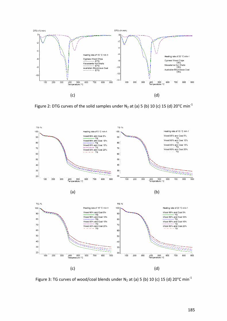
185

(c) (d)

Figure 2: DTG curves of the solid samples under N2 at (a) 5 (b) 10 (c) 15 (d) 20°C min-1

(a) (b)

(c) (d)

Figure 3: TG curves of wood/coal blends under N2 at (a) 5 (b) 10 (c) 15 (d) 20°C min-1

186

(a) (b)

(c) (d)

Figure 4: TG curves of nut/coal blends under N2 at (a) 5 (b) 10 (c) 15 (d) 20°C min-1

(a) (b)

187

(c) (d)

Figure 5: DTG curves of wood/coal blends under N2 at (a) 5 (b) 10 (c) 15 (d) 20°C min-1

(a) (b)

(c) (d)

Figure 6: DTG curves of nut/coal blends under N2 at (a) 5 (b) 10 (c) 15 (d) 20°C min-1

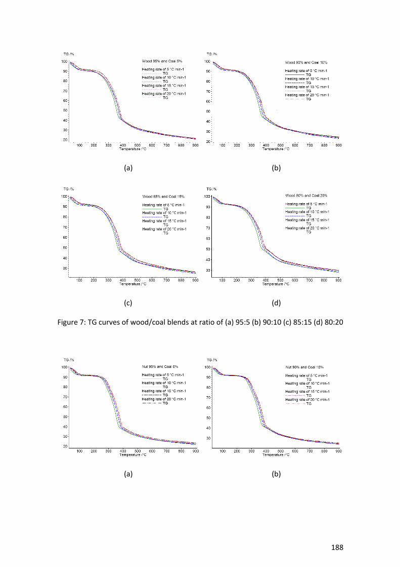
188

(a) (b)

(c) (d)

Figure 7: TG curves of wood/coal blends at ratio of (a) 95:5 (b) 90:10 (c) 85:15 (d) 80:20

(a) (b)

189

(c) (d)

Figure 8: TG curves of nut/coal blends at ratio of (a) 95:5 (b) 90:10 (c) 85:15 (d) 80:20

(a) (b)

(c) (d)

Figure 9: DTG curves of wood/coal blends at (a) 95:5 (b) 90:10 (c) 85:15 (d) 80:20

190

(a) (b)

(c) (d)

Figure 10: TG curves of nut/coal blends at ratio of (a) 95:5 (b) 90:10 (c) 85:15 (d) 80:20

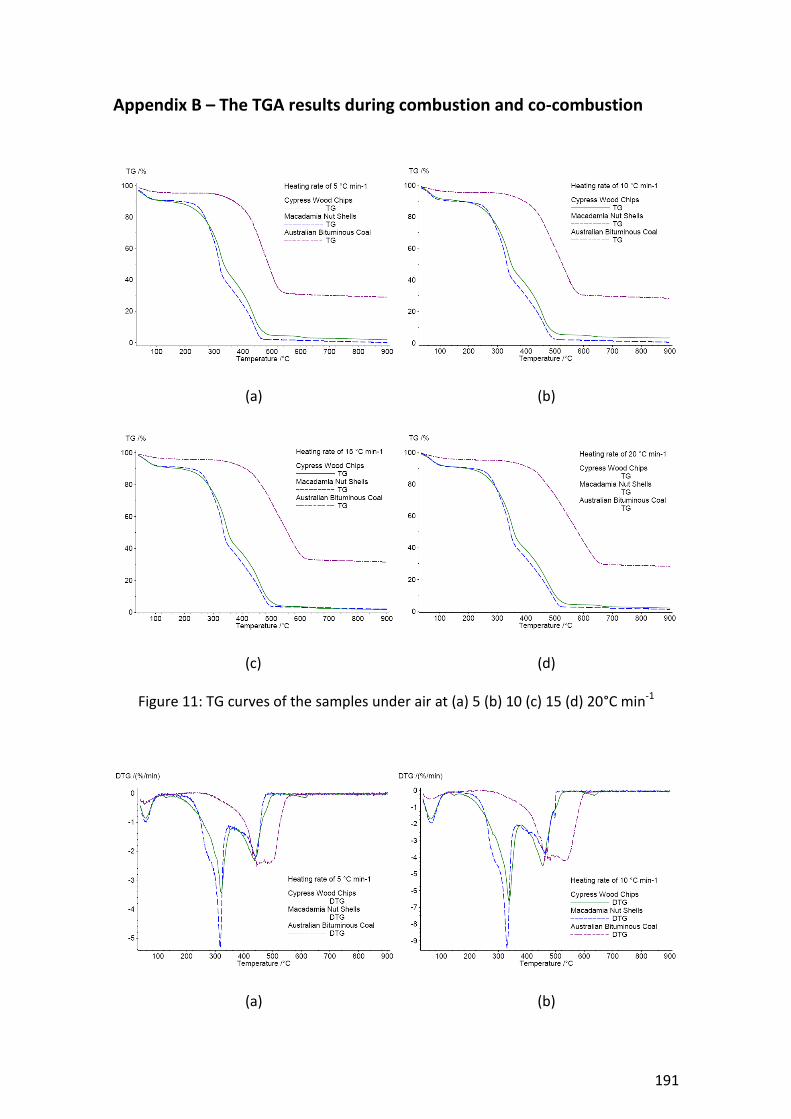
191

Appendix B – The TGA results during combustion and co-combustion

(a) (b)

(c) (d)

Figure 11: TG curves of the samples under air at (a) 5 (b) 10 (c) 15 (d) 20°C min-1

(a) (b)

192

(c) (d)

Figure 12: DTG curves of the samples under air at (a) 5 (b) 10 (c) 15 (d) 20°C min-1

(a) (b)

(c) (d)

Figure 13: TG curves of wood/coal blends under air at (a) 5 (b) 10 (c) 15 (d) 20°C min-1

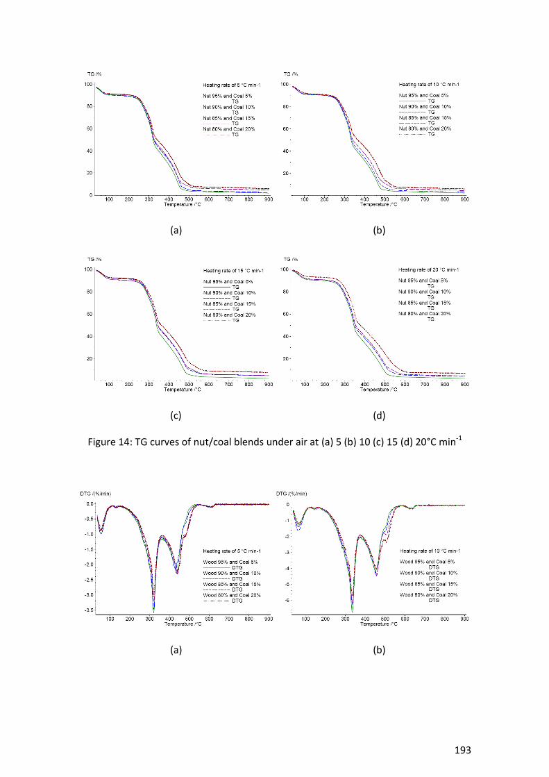
193

(a) (b)

(c) (d)

Figure 14: TG curves of nut/coal blends under air at (a) 5 (b) 10 (c) 15 (d) 20°C min-1

(a) (b)

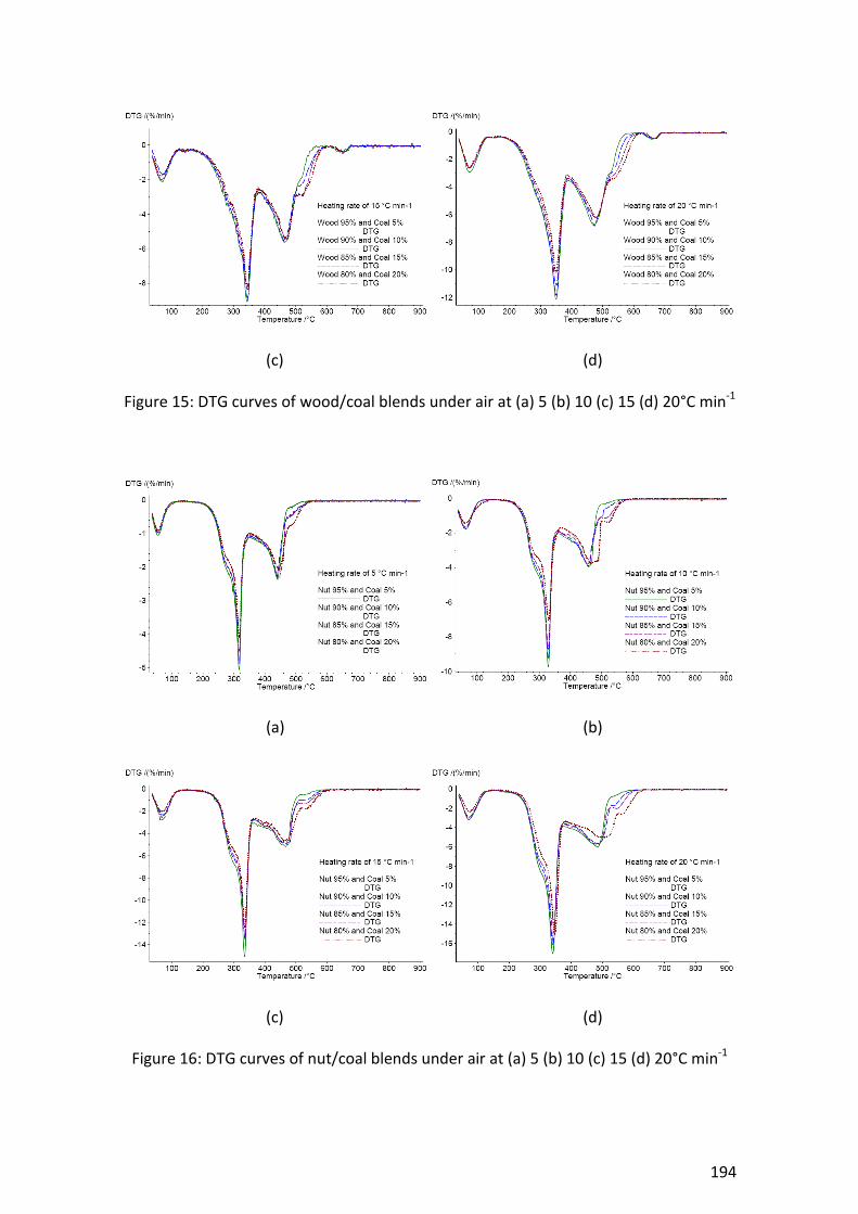
194

(c) (d)

Figure 15: DTG curves of wood/coal blends under air at (a) 5 (b) 10 (c) 15 (d) 20°C min-1

(a) (b)

(c) (d)

Figure 16: DTG curves of nut/coal blends under air at (a) 5 (b) 10 (c) 15 (d) 20°C min-1

195

(a) (b)

(c) (d)

Figure 17: TG curves of wood/coal blends at (a) 95:5 (b) 90:10 (c) 85:15 (d) 80:20

(a) (b)

196

(c) (d)

Figure 18: TG curves of nut/coal blends at ratio of (a) 95:5 (b) 90:10 (c) 85:15 (d) 80:20

(a) (b)

(c) (d)

Figure 19: DTG curves of wood/coal blends at (a) 95:5 (b) 90:10 (c) 85:15 (d) 80:20

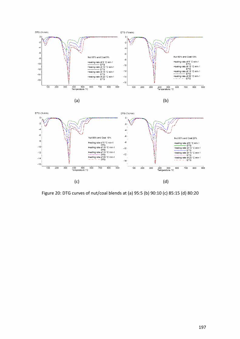
197

(a) (b)

(c) (d)

Figure 20: DTG curves of nut/coal blends at (a) 95:5 (b) 90:10 (c) 85:15 (d) 80:20

198

Appendix C – Experimental errors and error analysis

Uncertainties in scientific measurements always occur. Error analysis is an assessment

of uncertainty in a measurement. Instrumental, environmental and human limitations

can cause a measurement to deviate from the actual values of the quantities being

measured. There are two main types of measurement error: systematic error and

random error. Systematic errors are reproducible inaccuracies that consistently affect

all measurements in the same direction. This type of errors is commonly caused by the

measuring instruments. Systematic errors are difficult to identify and cannot be

analysed statistically. On the other hand, random errors arise from unknown and

unpredictable fluctuations in the measurements. Random errors are existent in most

of all data. This type of errors can be evaluated using statistical analysis and can be

decreased by averaging over several observations (Doran, 2012; Romesburg, 2009;

Viswanathan, 2005).

Measurements that are assumed to contains only random errors with free of

systematic errors can be analysed through statistical procedures. A practical estimate

of random uncertainties in scientific measurements can be achieved by several

methods. The most common method is to calculate the mean ( ) and the standard

deviation ( ) of a data set of repeated measurements of a given quantity. The

equations for the mean and the standard deviation are (Dieck, 2007; Doran, 2012):

∑

(C–1)

∑

(C–2)

where N is the number of measurement and is the result of the ith measurement. If

a measurement which is contains only random fluctuations is repeated several times,

approximately 68% of the measurements is subject to take values in the range

(Doran, 2012).

199

The use of measured values with standard deviations in a math operation increases

the magnitude of the subsequent standard deviation. In other words, the uncertainty

is propagated. To find the estimated uncertainty for a calculated result, it is required to

statistically combine the errors from multiple variables (Harvard University, 2007;

Skoog et al., 2003). Arithmetic calculations of error propagation used in this study are

listed below.

(C–3)

(C–4)

The standard error of the estimate (Syx) is a standard error statistic that is also

commonly used in experimental research. It is basically a measure of the dispersion in

the predicted values in a regression or the standard deviation of the prediction error.

Thus, the standard error of estimation can be interpreted the same as the standard

deviation which expresses the spread of a distribution of values in regard to the

distribution mean. The standard error of the estimate is calculated from Equation (C–

5) (King, et al., 2011).

√∑

(C–5)

where is estimated value of char yield, y is actual value of char yield and n is number

of observations.

The amounts of char produced during pyrolysis of biomass, coal and their blends at the

temperatures of 400, 500 and 600 °C and their uncertainties which were calculated

from Equation (C–1), Equation (C–2) and Equation (C–3) are presented in the following

table.

200

Table C–1: Results of the char production of cypress wood chips, coal and their blends,

the uncertainties and the standard error of the estimate

Ratio of wood chips to coal

400 °C 500 °C 600 °C

0:100 92.79 0.82 73.77 0.56 68.34 0.59

80:20 48.66 0.21 38.21 0.79 34.73 0.58

85:15 44.49 0.30 35.96 0.98 32.04 0.77

90:10 43.06 0.82 33.94 0.45 30.07 1.09

95:5 39.41 0.16 31.10 0.56 27.75 0.56

100:0 37.05 0.18 28.93 0.87 25.17 0.63

Standard error of the estimate (Syx)

0.59 0.26 0.37

Table C–2: Results of the char production of macadamia nut shells, coal and their

blends, the uncertainties and the standard error of the estimate

Ratio of nut shells to coal

400 °C 500 °C 600 °C

0:100 92.79 0.72 73.77 0.71 68.34 0.95

80:20 46.88 0.76 38.49 0.41 34.46 0.62

85:15 43.50 0.75 35.59 0.65 31.92 0.48

90:10 39.82 0.54 32.45 0.75 29.04 0.37

95:5 37.48 0.81 30.90 0.95 27.26 0.17

100:0 34.94 0.77 29.02 0.21 25.72 0.83

Standard error of the estimate (Syx)

0.47 0.56 0.46

201

In the use of graphical techniques to determine a quantity, it is important to determine

the uncertainty in slope and intercept of a least squares fit. If a quantity plotted on the

vertical axis is linearly influenced by a quantity plotted on the horizontal axis, these

plots would ideally fall on a straight line. The equation can be written as (Kirkup and

Frenkel, 2006; Morrison, 2013; Mortimer, 2013):

(C–6)

where m is the slope and b is the intercept of the least squares best fit line. The slope

and the intercept can be defined as (Morrison, 2013):

∑ ∑

∑

∑

∑

(C–7)

∑

∑

∑

∑

∑

∑

(C–8)

Standard deviation of slope or uncertainty in slope ( ) and standard deviation of

intercept or uncertainty in intercept ( ) are calculated from Equation (C–9) and

Equation (C–10), respectively (Morrison, 2013):

∑

(C–9)

∑

∑

(C–10)

The standard error of the estimate (Syx) or variance of y which is presented in Equation

(C–5) is commonly used for error bars of a least squares fit (Morrison, 2013).

202

Uncertainty measures on slope and intercept of a least squares fit of activation energy

of biomass, coal and their blends against ratio of biomass in the blend were calculated,

as summarised in Table 3 and Table 4.

Table C–3: Uncertainty measures on slope and intercept of a least squares fit of

activation energy of biomass, coal and their blends during pyrolysis

Measures Wood chips, coal and their blends

Nut shells, coal and their blends

Slope, m -0.3120 -0.3530

Intercept, b 199.6 199.6

Uncertainty in Slope, 0.0023 0.0022

Uncertainty in intercept, 0.1862 0.1825

Coefficient of determination, R2 0.9998 0.9998

Variance of y 0.1890 0.1853

Table C–4: Uncertainty measures on slope and intercept of a least squares fit of

activation energy of biomass, coal and their blends during combustion

Measures Wood chips, coal and their blends

Nut shells, coal and their blends

Slope, m -0.4240 -0.3344

Intercept, b 181.4 181.6

Uncertainty in Slope, 0.0017 0.0081

Uncertainty in intercept, 0.1393 0.6645

Coefficient of determination, R2 0.9999 0.9977

Variance of y 0.1414 0.6746

203

The error analysis of the results of carbon monoxide calibration curve was determined

using the calculations of the mean ( ) and the standard deviation ( ) of the data set

of three repeated measurements, as summarised in Table 5.

Table C–5: The error analysis of the results of carbon monoxide calibration curve

Concentration (PPM) Averaged Corrected Area Uncertainty ( )

1,000 588 4

5,000 2,722 32

10,000 5,301 73

20,000 9,558 37

50,000 19,250 78

100,000 32,890 90

150,000 38,903 72

200,000 47,541 56

The composition of the syngas produced from gasification of cypress wood chips,

macadamia nut shells and their blends with Australian bituminous coal was analysed

through statistical analysis. This includes the mean ( ) and the standard deviation ( )

of the data set of three repeated measurements as well as the standard error of the

estimate (Syx). The error analysis of the total combustible gas (TCG) is based on the

arithmetic calculation of error propagation, Equation (C–5).

Table C–6: The error analysis of the composition of the syngas and its total

combustible gas (TCG) from gasification of wood chips, coal and their blends

Ratio of biomass to coal

CO2 H2O O2 N2

100:0 4.68 0.12 2.51 0.08 11.82 0.20 69.76 0.14

204

95:5 6.65 0.38 2.47 0.12 10.28 0.06 67.68 0.11

90:10 5.49 0.14 2.43 0.14 10.19 0.13 67.49 0.24

85:15 5.89 0.13 1.88 0.20 9.61 0.06 65.18 0.37

80:20 9.24 0.09 2.27 0.04 7.19 0.04 59.66 0.89

Syx 1.32 0.23 0.70 1.69

Ratio of biomass CO H2 CH4 TCG

100:0 7.88 0.11 2.19 0.03 0.08 0.00 10.15 0.11

95:5 8.90 0.02 2.74 0.08 0.08 0.00 11.72 0.08

90:10 10.08 0.04 3.24 0.07 0.06 0.00 13.38 0.08

85:15 12.14 0.07 4.14 0.06 0.05 0.00 16.33 0.09

80:20 15.18 0.06 5.27 0.12 0.05 0.00 20.50 0.13

Syx 0.78 0.25 0.01 1.03

Table C–7: The error analysis of the composition of the syngas and its total

combustible gas (TCG) from gasification of nut shells, coal and their blends

Ratio of biomass to coal

CO2 H2O O2 N2

100:0 5.71 0.12 2.25 0.07 11.01 0.10 69.26 0.12

95:5 6.02 0.05 2.32 0.05 10.72 0.03 67.18 0.09

90:10 8.08 0.05 2.80 0.04 8.48 0.10 64.15 0.10

85:15 9.25 0.06 2.85 0.06 6.63 0.08 62.86 0.06

80:20 10.07 0.04 2.93 0.06 4.88 0.04 60.58 0.06

Syx 0.44 0.13 0.57 0.43

Ratio of biomass CO H2 CH4 TCG

100:0 8.30 2.27 0.06 0.00 10.63

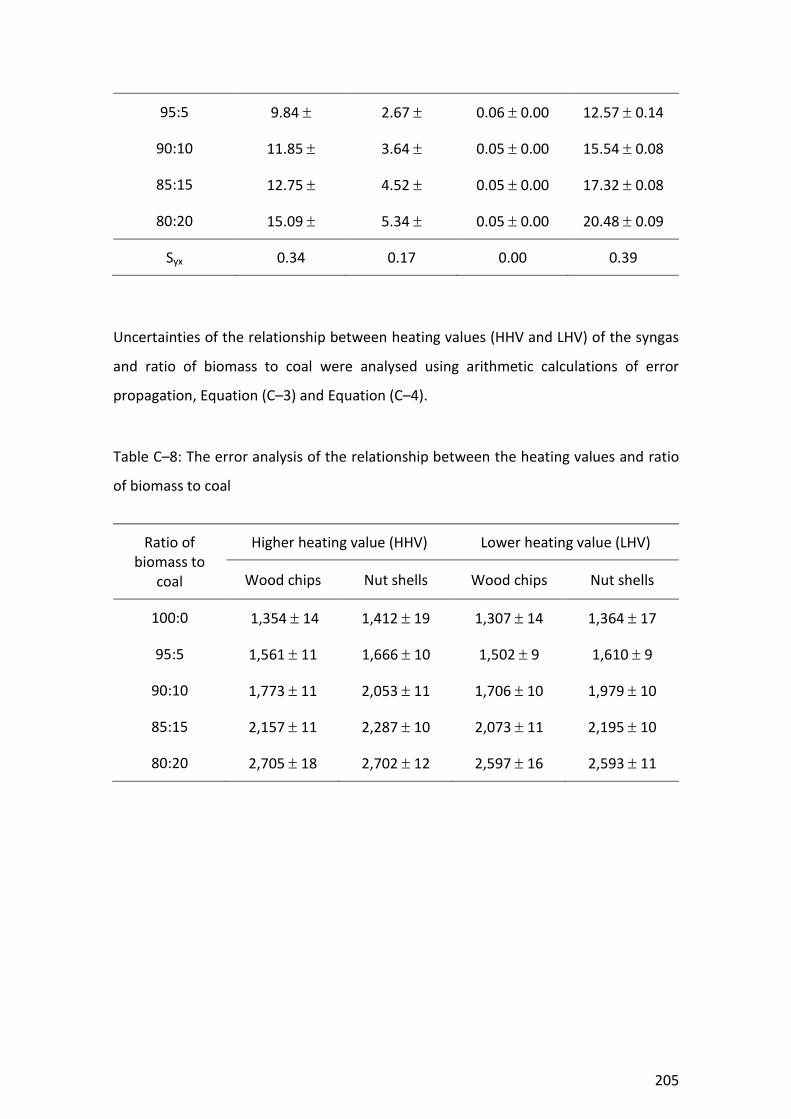
205

95:5 9.84 2.67 0.06 0.00 12.57 0.14

90:10 11.85 3.64 0.05 0.00 15.54 0.08

85:15 12.75 4.52 0.05 0.00 17.32 0.08

80:20 15.09 5.34 0.05 0.00 20.48 0.09

Syx 0.34 0.17 0.00 0.39

Uncertainties of the relationship between heating values (HHV and LHV) of the syngas

and ratio of biomass to coal were analysed using arithmetic calculations of error

propagation, Equation (C–3) and Equation (C–4).

Table C–8: The error analysis of the relationship between the heating values and ratio

of biomass to coal

Ratio of biomass to

coal

Higher heating value (HHV) Lower heating value (LHV)

Wood chips Nut shells Wood chips Nut shells

100:0 1,354 14 1,412 19 1,307 14 1,364 17

95:5 1,561 11 1,666 10 1,502 9 1,610 9

90:10 1,773 11 2,053 11 1,706 10 1,979 10

85:15 2,157 11 2,287 10 2,073 11 2,195 10

80:20 2,705 18 2,702 12 2,597 16 2,593 11

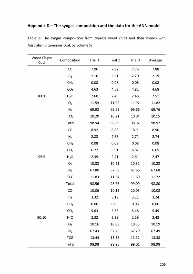
206

Appendix D – The syngas composition and the data for the ANN model

Table 1: The syngas composition from cypress wood chips and their blends with

Australian bituminous coal, by volume %

Wood Chips: Coal

Composition Trial 1 Trial 2 Trial 3 Average

100:0

CO 7.96 7.92 7.76 7.88

H2 2.16 2.21 2.20 2.19

CH4 0.08 0.08 0.08 0.08

CO2 4.63 4.59 4.82 4.68

H2O 2.60 2.45 2.48 2.51

O2 11.59 11.95 11.92 11.82

N2 69.92 69.69 69.66 69.76

TCG 10.20 10.21 10.04 10.15

Total 98.94 98.89 98.92 98.92

95:5

CO 8.92 8.88 8.9 8.90

H2 2.83 2.68 2.71 2.74

CH4 0.08 0.08 0.08 0.08

CO2 6.22 6.91 6.82 6.65

H2O 2.39 2.41 2.61 2.47

O2 10.32 10.21 10.31 10.28

N2 67.80 67.58 67.66 67.68

TCG 11.83 11.64 11.69 11.72

Total 98.56 98.75 99.09 98.80

90:10

CO 10.06 10.13 10.05 10.08

H2 3.32 3.19 3.21 3.24

CH4 0.06 0.06 0.06 0.06

CO2 5.63 5.36 5.48 5.49

H2O 2.32 2.38 2.59 2.43

O2 10.16 10.08 10.33 10.19

N2 67.43 67.75 67.29 67.49

TCG 13.44 13.38 13.32 13.38

Total 98.98 98.95 99.01 98.98

207

Wood Chips: Coal

Composition Trial 1 Trial 2 Trial 3 Average

85:15

CO 12.07 12.15 12.2 12.14

H2 4.08 4.15 4.19 4.14

CH4 0.05 0.05 0.05 0.05

CO2 5.76 6.01 5.9 5.89

H2O 1.65 2.04 1.95 1.88

O2 9.68 9.57 9.59 9.61

N2 65.61 64.98 64.95 65.18

TCG 16.20 16.35 16.44 16.33

Total 98.90 98.95 98.83 98.89

80:20

CO 15.24 15.13 15.17 15.18

H2 5.41 5.18 5.22 5.27

CH4 0.05 0.05 0.05 0.05

CO2 9.15 9.32 9.25 9.24

H2O 2.29 2.22 2.3 2.27

O2 7.15 7.22 7.2 7.19

N2 59.56 59.73 59.69 59.66

TCG 20.70 20.36 20.44 20.50

Total 98.85 98.85 98.88 98.86

Table 2: The syngas composition from macadamia nut shells and their blends with

Australian bituminous coal, by volume %

Nut Shells: Coal

Composition Trial 1 Trial 2 Trial 3 Average

100:0

CO 8.21 8.38 8.31 8.30

H2 2.14 2.33 2.34 2.27

CH4 0.06 0.06 0.06 0.06

CO2 5.84 5.62 5.67 5.71

H2O 2.30 2.28 2.17 2.25

O2 10.89 11.06 11.08 11.01

N2 69.38 69.15 69.25 69.26

TCG 10.41 10.77 10.71 10.63

Total 98.82 98.88 98.88 98.86

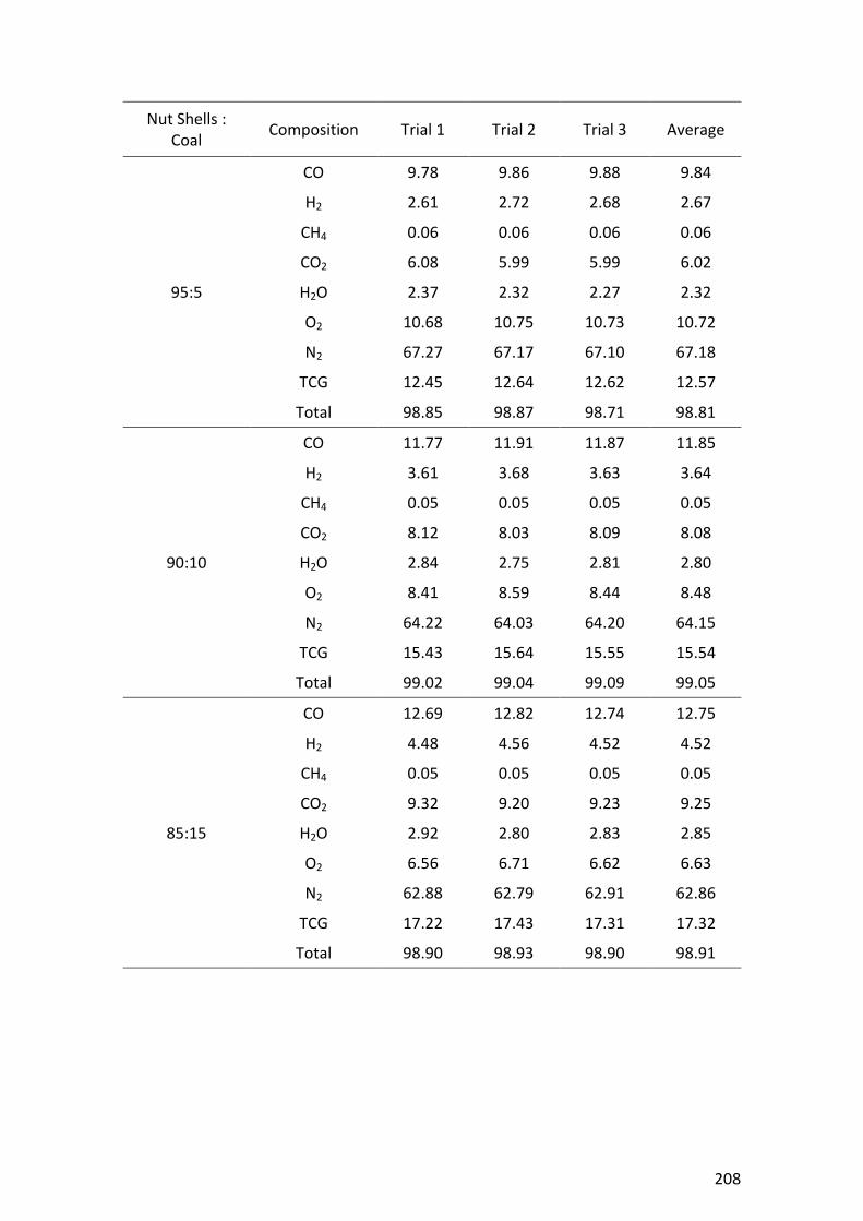
208

Nut Shells : Coal

Composition Trial 1 Trial 2 Trial 3 Average

95:5

CO 9.78 9.86 9.88 9.84

H2 2.61 2.72 2.68 2.67

CH4 0.06 0.06 0.06 0.06

CO2 6.08 5.99 5.99 6.02

H2O 2.37 2.32 2.27 2.32

O2 10.68 10.75 10.73 10.72

N2 67.27 67.17 67.10 67.18

TCG 12.45 12.64 12.62 12.57

Total 98.85 98.87 98.71 98.81

90:10

CO 11.77 11.91 11.87 11.85

H2 3.61 3.68 3.63 3.64

CH4 0.05 0.05 0.05 0.05

CO2 8.12 8.03 8.09 8.08

H2O 2.84 2.75 2.81 2.80

O2 8.41 8.59 8.44 8.48

N2 64.22 64.03 64.20 64.15

TCG 15.43 15.64 15.55 15.54

Total 99.02 99.04 99.09 99.05

85:15

CO 12.69 12.82 12.74 12.75

H2 4.48 4.56 4.52 4.52

CH4 0.05 0.05 0.05 0.05

CO2 9.32 9.20 9.23 9.25

H2O 2.92 2.80 2.83 2.85

O2 6.56 6.71 6.62 6.63

N2 62.88 62.79 62.91 62.86

TCG 17.22 17.43 17.31 17.32

Total 98.90 98.93 98.90 98.91

209

Nut Shells: Coal

Composition Trial 1 Trial 2 Trial 3 Average

80:20

CO 15.02 15.13 15.12 15.09

H2 5.26 5.40 5.36 5.34

CH4 0.05 0.05 0.04 0.05

CO2 10.11 10.04 10.06 10.07

H2O 2.99 2.87 2.93 2.93

O2 4.83 4.90 4.91 4.88

N2 60.63 60.51 60.60 60.58

TCG 20.33 20.58 20.52 20.48

Total 98.89 98.90 99.02 98.94

Table 3: Input variables and target variables used for developing the artificial neural

network model

Input Data Target Data

% C % H % O TCG

55.30 5.98 38.30 10.20

56.62 6.02 36.88 11.83

57.93 6.07 35.45 13.44

59.25 6.11 34.03 16.20

60.56 6.15 32.60 20.70

53.40 5.63 40.60 10.41

54.81 5.69 39.06 12.45

56.22 5.75 37.52 15.43

57.63 5.81 35.98 17.22

59.04 5.87 34.44 20.33

55.30 5.98 38.30 10.21

56.62 6.02 36.88 11.64

57.93 6.07 35.45 13.38

59.25 6.11 34.03 16.35

60.56 6.15 32.60 20.36

53.40 5.63 40.60 10.77

54.81 5.69 39.06 12.64

210

Input Data Target Data

% C % H % O TCG

56.22 5.75 37.52 15.64

57.63 5.81 35.98 17.43

59.04 5.87 34.44 20.58

55.30 5.98 38.30 10.04

56.62 6.02 36.88 11.69

57.93 6.07 35.45 13.32

59.25 6.11 34.03 16.44

60.56 6.15 32.60 20.44

53.40 5.63 40.60 10.71

54.81 5.69 39.06 12.62

56.22 5.75 37.52 15.55

57.63 5.81 35.98 17.31

59.04 5.87 34.44 20.52

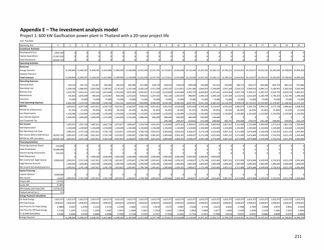
Appendix E – The investment analysis modelProject 1: 600 kW Gasification power plant in Thailand with a 20–year project life Unit: Thai Baht

Operating Year 0 1 2 3 4 5 6 7 8 9 10 11 12 13 14 15 16 17 18 19 20

Investment Activities

Development Cost -2,835,160 0 0 0 0 0 0 0 0 0 0 0 0 0 0 0 0 0 0 0 0

Capital Expenditure -25,367,550 0 0 0 0 0 0 0 0 0 0 0 0 0 0 0 0 0 0 0 0

Total Investment -28,202,710 0 0 0 0 0 0 0 0 0 0 0 0 0 0 0 0 0 0 0 0

Operating Activities

Revenues

Energy Payment 11,296,844 11,466,297 11,638,291 11,812,866 11,990,059 12,169,909 12,352,458 12,537,745 12,725,811 12,916,698 13,110,449 13,307,105 13,506,712 13,709,313 13,914,952 14,123,677 14,335,532 14,550,565 14,768,823 14,990,356

Capacity Payment - - - - - - - - - - - - - - - - - - - -

Total revenues 11,296,844 11,466,297 11,638,291 11,812,866 11,990,059 12,169,909 12,352,458 12,537,745 12,725,811 12,916,698 13,110,449 13,307,105 13,506,712 13,709,313 13,914,952 14,123,677 14,335,532 14,550,565 14,768,823 14,990,356

Operating Expenses

Administration -520,150 -535,755 -551,827 -568,382 -585,433 -602,996 -621,086 -639,719 -658,910 -678,678 -699,038 -720,009 -741,610 -763,858 -786,774 -810,377 -834,688 -859,729 -885,521 -912,086

Operating Cost -1,928,160 -1,986,005 -2,045,585 -2,106,952 -2,170,161 -2,235,266 -2,302,324 -2,371,394 -2,442,535 -2,515,811 -2,591,286 -2,669,024 -2,749,095 -2,831,568 -2,916,515 -3,004,010 -3,094,131 -3,186,955 -3,282,563 -3,381,040

Biomass Fuel -3,343,787 -3,444,101 -3,547,424 -3,653,846 -3,763,462 -3,876,366 -3,992,657 -4,112,436 -4,235,809 -4,362,884 -4,493,770 -4,628,583 -4,767,441 -4,910,464 -5,057,778 -5,209,511 -5,365,797 -5,526,770 -5,692,574 -5,863,351

Maintenance -735,832 -1,078,299 -780,644 -1,143,967 -828,185 -1,213,635 -878,622 -1,287,545 -932,130 -1,365,957 -988,897 -1,449,143 -1,049,120 -1,537,369 -1,113,012 -1,631,024 -1,180,794 -1,730,353 -1,252,705 -1,290,286

Insurance -75,000 -75,000 -75,000 -75,000 -75,000 -75,000 -75,000 -75,000 -75,000 -75,000 -75,000 -75,000 -75,000 -75,000 -75,000 -75,000 -75,000 -75,000 -75,000 -75,000

Total operating expenses -6,602,929 -7,119,159 -7,000,480 -7,548,148 -7,422,241 -8,003,263 -7,869,689 -8,486,094 -8,344,385 -8,998,330 -8,847,991 -9,541,760 -9,382,265 -10,118,259 -9,949,078 -10,729,922 -10,550,409 -11,378,807 -11,188,362 -11,521,763

EBITDA 4,693,915 4,347,138 4,637,811 4,264,718 4,567,817 4,166,647 4,482,769 4,051,651 4,381,426 3,918,368 4,262,458 3,765,346 4,124,447 3,591,054 3,965,874 3,393,754 3,785,123 3,171,758 3,580,461 3,468,593

EBITDA (% of Revenues) 41.55% 37.91% 39.85% 36.10% 38.10% 34.24% 36.29% 32.32% 34.43% 30.34% 32.51% 28.30% 30.54% 26.19% 28.50% 24.03% 26.40% 21.80% 24.24% 23.14%

Less Depreciation -1,150,000 -1,150,000 -1,150,000 -1,150,000 -1,150,000 -1,150,000 -1,150,000 -1,150,000 -1,150,000 -1,150,000 -1,150,000 -1,150,000 -1,150,000 -1,150,000 -1,150,000 -1,150,000 -1,150,000 -1,150,000 -1,150,000 -1,150,000

Less Interest Expense -1,600,000 -1,600,000 -1,600,000 -1,472,000 -1,344,000 -1,216,000 -1,088,000 -960,000 -800,000 -640,000 -480,000 -320,000 -160,000 0 0 0 0 0 0 0

Less Corporate Tax -295,760 -249,267 -323,831 -272,198 -348,982 -583,742 -693,968 -520,070 -635,184 -448,845 -569,091 -533,129

Net Income 1,943,915 1,597,138 1,887,811 1,642,718 2,073,817 1,800,647 2,244,769 1,941,651 2,135,666 1,879,101 2,308,627 2,023,148 2,465,465 1,857,312 2,121,906 1,723,684 1,999,939 1,572,913 1,861,370 1,785,464

Add Depreciation 1,150,000 1,150,000 1,150,000 1,150,000 1,150,000 1,150,000 1,150,000 1,150,000 1,150,000 1,150,000 1,150,000 1,150,000 1,150,000 1,150,000 1,150,000 1,150,000 1,150,000 1,150,000 1,150,000 1,150,000

Net Operating Cash Flow 3,093,915 2,747,138 3,037,811 2,792,718 3,223,817 2,950,647 3,394,769 3,091,651 3,285,666 3,029,101 3,458,627 3,173,148 3,615,465 3,007,312 3,271,906 2,873,684 3,149,939 2,722,913 3,011,370 2,935,464

Net Income Before Debt Service -28,202,710 3,093,915 2,747,138 3,037,811 2,792,718 3,223,817 2,950,647 3,394,769 3,091,651 3,285,666 3,029,101 3,458,627 3,173,148 3,615,465 3,007,312 3,271,906 2,873,684 3,149,939 2,722,913 3,011,370 2,935,464

EBTIDA for IRR Calculation -28,202,710 4,693,915 4,347,138 4,637,811 4,264,718 4,567,817 4,166,647 4,482,769 4,051,651 4,085,666 3,669,101 3,938,627 3,493,148 3,775,465 3,007,312 3,271,906 2,873,684 3,149,939 2,722,913 3,011,370 2,935,464

Financing Activities

Financing expenses (Fees) -250,000 0 0 0 0 0 0 0 0 0 0 0 0 0 0 0 0 0 0 0 0

Debt Drawndown 20,000,000 0 0 0 0 0 0 0 0 0 0 0 0 0 0 0 0 0 0 0 0

Interest during construction -533,333 0 0 0 0 0 0 0 0 0 0 0 0 0 0 0 0 0 0 0 0

Debt Repayment 0 0 -1,600,000 -1,600,000 -1,600,000 -1,600,000 -1,600,000 -2,000,000 -2,000,000 -2,000,000 -2,000,000 -2,000,000 -2,000,000

Net income bef. legal reserve -8,986,043 3,093,915 2,747,138 1,437,811 1,192,718 1,623,817 1,350,647 1,794,769 1,091,651 1,285,666 1,029,101 1,458,627 1,173,148 1,615,465 3,007,312 3,271,906 2,873,684 3,149,939 2,722,913 3,011,370 2,935,464

Legal Reserve Account 1,000,000 1,000,000 1,000,000 1,000,000 1,000,000 1,000,000 1,000,000 1,000,000 1,000,000 1,000,000 1,000,000 1,000,000 1,000,000 1,000,000 1,000,000 1,000,000 1,000,000 1,000,000 1,000,000 1,000,000

Net income bef divided payment 2,093,915 2,747,138 1,437,811 1,192,718 1,623,817 1,350,647 1,794,769 1,091,651 1,285,666 1,029,101 1,458,627 1,173,148 1,615,465 3,007,312 3,271,906 2,873,684 3,149,939 2,722,913 3,011,370 2,935,464

Equity Financing :

Capital Injection 9,000,000 0 0 0 0 0 0 0 0 0 0 0 0 0 0 0 0 0 0 0 0

Net Income 13,957 2,093,915 2,747,138 1,437,811 1,192,718 1,623,817 1,350,647 1,794,769 1,091,651 1,285,666 1,029,101 1,458,627 1,173,148 1,615,465 3,007,312 3,271,906 2,873,684 3,149,939 2,722,913 3,011,370 2,935,464

Project IRR 13.55%

Equlty IRR 21.80%

NPV-Equlty Cash Flow (5%) 14,518,312

Payback period (yrs.) 6.5

Energy Payment Calculation

On-Peak Energy 1,623,375 1,623,375 1,623,375 1,623,375 1,623,375 1,623,375 1,623,375 1,623,375 1,623,375 1,623,375 1,623,375 1,623,375 1,623,375 1,623,375 1,623,375 1,623,375 1,623,375 1,623,375 1,623,375 1,623,375 1,623,375

Off-Peak Energy 2,838,825 2,838,825 2,838,825 2,838,825 2,838,825 2,838,825 2,838,825 2,838,825 2,838,825 2,838,825 2,838,825 2,838,825 2,838,825 2,838,825 2,838,825 2,838,825 2,838,825 2,838,825 2,838,825 2,838,825 2,838,825

Unit Price for On-Peak Energy 2.9889 3.0337 3.0792 3.1254 3.1723 3.2199 3.2682 3.3172 3.3670 3.4175 3.4687 3.5208 3.5736 3.6272 3.6816 3.7368 3.7929 3.8498 3.9075 3.9661 4.0256

Unit Price for Off-Peak Energy 1.1765 1.1941 1.2121 1.2302 1.2487 1.2674 1.2864 1.3057 1.3253 1.3452 1.3654 1.3859 1.4066 1.4277 1.4492 1.4709 1.4930 1.5154 1.5381 1.5612 1.5846

Ft. (0.4683 Baht/kWh) 0.6584 0.6683 0.6783 0.6885 0.6988 0.7093 0.7199 0.7307 0.7417 0.7528 0.7641 0.7756 0.7872 0.7990 0.8110 0.8232 0.8355 0.8480 0.8608 0.8737 0.8868

Energy Payment 11,296,844 11,466,297 11,638,291 11,812,866 11,990,059 12,169,909 12,352,458 12,537,745 12,725,811 12,916,698 13,110,449 13,307,105 13,506,712 13,709,313 13,914,952 14,123,677 14,335,532 14,550,565 14,768,823 14,990,356

211

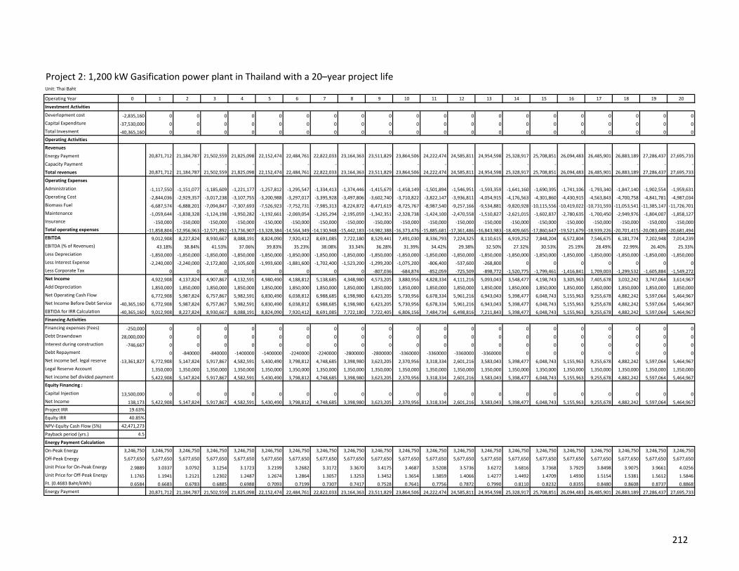
Project 2: 1,200 kW Gasification power plant in Thailand with a 20–year project life Unit: Thai Baht

Operating Year 0 1 2 3 4 5 6 7 8 9 10 11 12 13 14 15 16 17 18 19 20

Investment Activities

Deverlopment cost -2,835,160 0 0 0 0 0 0 0 0 0 0 0 0 0 0 0 0 0 0 0 0

Capital Expenditure -37,530,000 0 0 0 0 0 0 0 0 0 0 0 0 0 0 0 0 0 0 0 0

Total Invesment -40,365,160 0 0 0 0 0 0 0 0 0 0 0 0 0 0 0 0 0 0 0 0

Operating Activities

Revenues

Energy Payment 20,871,712 21,184,787 21,502,559 21,825,098 22,152,474 22,484,761 22,822,033 23,164,363 23,511,829 23,864,506 24,222,474 24,585,811 24,954,598 25,328,917 25,708,851 26,094,483 26,485,901 26,883,189 27,286,437 27,695,733

Capacity Payment - - - - - - - - - - - - - - - - - - - -

Total revenues 20,871,712 21,184,787 21,502,559 21,825,098 22,152,474 22,484,761 22,822,033 23,164,363 23,511,829 23,864,506 24,222,474 24,585,811 24,954,598 25,328,917 25,708,851 26,094,483 26,485,901 26,883,189 27,286,437 27,695,733

Operating Expenses

Administration -1,117,550 -1,151,077 -1,185,609 -1,221,177 -1,257,812 -1,295,547 -1,334,413 -1,374,446 -1,415,679 -1,458,149 -1,501,894 -1,546,951 -1,593,359 -1,641,160 -1,690,395 -1,741,106 -1,793,340 -1,847,140 -1,902,554 -1,959,631

Operating Cost -2,844,036 -2,929,357 -3,017,238 -3,107,755 -3,200,988 -3,297,017 -3,395,928 -3,497,806 -3,602,740 -3,710,822 -3,822,147 -3,936,811 -4,054,915 -4,176,563 -4,301,860 -4,430,915 -4,563,843 -4,700,758 -4,841,781 -4,987,034

Biomass Fuel -6,687,574 -6,888,201 -7,094,847 -7,307,693 -7,526,923 -7,752,731 -7,985,313 -8,224,872 -8,471,619 -8,725,767 -8,987,540 -9,257,166 -9,534,881 -9,820,928 -10,115,556 -10,419,022 -10,731,593 -11,053,541 -11,385,147 -11,726,701

Maintenance -1,059,644 -1,838,328 -1,124,198 -1,950,282 -1,192,661 -2,069,054 -1,265,294 -2,195,059 -1,342,351 -2,328,738 -1,424,100 -2,470,558 -1,510,827 -2,621,015 -1,602,837 -2,780,635 -1,700,450 -2,949,976 -1,804,007 -1,858,127

Insurance -150,000 -150,000 -150,000 -150,000 -150,000 -150,000 -150,000 -150,000 -150,000 -150,000 -150,000 -150,000 -150,000 -150,000 -150,000 -150,000 -150,000 -150,000 -150,000 -150,000

Total operating expenses -11,858,804 -12,956,963 -12,571,892 -13,736,907 -13,328,384 -14,564,349 -14,130,948 -15,442,183 -14,982,388 -16,373,476 -15,885,681 -17,361,486 -16,843,983 -18,409,665 -17,860,647 -19,521,679 -18,939,226 -20,701,415 -20,083,489 -20,681,494

EBITDA 9,012,908 8,227,824 8,930,667 8,088,191 8,824,090 7,920,412 8,691,085 7,722,180 8,529,441 7,491,030 8,336,793 7,224,325 8,110,615 6,919,252 7,848,204 6,572,804 7,546,675 6,181,774 7,202,948 7,014,239

EBITDA (% of Revenues) 43.18% 38.84% 41.53% 37.06% 39.83% 35.23% 38.08% 33.34% 36.28% 31.39% 34.42% 29.38% 32.50% 27.32% 30.53% 25.19% 28.49% 22.99% 26.40% 25.33%

Less Depreciation -1,850,000 -1,850,000 -1,850,000 -1,850,000 -1,850,000 -1,850,000 -1,850,000 -1,850,000 -1,850,000 -1,850,000 -1,850,000 -1,850,000 -1,850,000 -1,850,000 -1,850,000 -1,850,000 -1,850,000 -1,850,000 -1,850,000 -1,850,000

Less Interest Expense -2,240,000 -2,240,000 -2,172,800 -2,105,600 -1,993,600 -1,881,600 -1,702,400 -1,523,200 -1,299,200 -1,075,200 -806,400 -537,600 -268,800 0 0 0 0 0 0 0

Less Corporate Tax 0 0 0 0 0 0 0 0 -807,036 -684,874 -852,059 -725,509 -898,772 -1,520,775 -1,799,461 -1,416,841 1,709,003 -1,299,532 -1,605,884 -1,549,272

Net Income 4,922,908 4,137,824 4,907,867 4,132,591 4,980,490 4,188,812 5,138,685 4,348,980 4,573,205 3,880,956 4,828,334 4,111,216 5,093,043 3,548,477 4,198,743 3,305,963 7,405,678 3,032,242 3,747,064 3,614,967

Add Depreciation 1,850,000 1,850,000 1,850,000 1,850,000 1,850,000 1,850,000 1,850,000 1,850,000 1,850,000 1,850,000 1,850,000 1,850,000 1,850,000 1,850,000 1,850,000 1,850,000 1,850,000 1,850,000 1,850,000 1,850,000

Net Operating Cash Flow 6,772,908 5,987,824 6,757,867 5,982,591 6,830,490 6,038,812 6,988,685 6,198,980 6,423,205 5,730,956 6,678,334 5,961,216 6,943,043 5,398,477 6,048,743 5,155,963 9,255,678 4,882,242 5,597,064 5,464,967

Net Income Before Debt Service -40,365,160 6,772,908 5,987,824 6,757,867 5,982,591 6,830,490 6,038,812 6,988,685 6,198,980 6,423,205 5,730,956 6,678,334 5,961,216 6,943,043 5,398,477 6,048,743 5,155,963 9,255,678 4,882,242 5,597,064 5,464,967

EBTIDA for IRR Calculation -40,365,160 9,012,908 8,227,824 8,930,667 8,088,191 8,824,090 7,920,412 8,691,085 7,722,180 7,722,405 6,806,156 7,484,734 6,498,816 7,211,843 5,398,477 6,048,743 5,155,963 9,255,678 4,882,242 5,597,064 5,464,967

Financing Activities

Financing expenses (Fees) -250,000 0 0 0 0 0 0 0 0 0 0 0 0 0 0 0 0 0 0 0 0

Debt Drawndown 28,000,000 0 0 0 0 0 0 0 0 0 0 0 0 0 0 0 0 0 0 0 0

Interest during construction -746,667 0 0 0 0 0 0 0 0 0 0 0 0 0 0 0 0 0 0 0 0

Debt Repayment 0 -840000 -840000 -1400000 -1400000 -2240000 -2240000 -2800000 -2800000 -3360000 -3360000 -3360000 -3360000 0 0 0 0 0 0 0

Net income bef. legal reserve -13,361,827 6,772,908 5,147,824 5,917,867 4,582,591 5,430,490 3,798,812 4,748,685 3,398,980 3,623,205 2,370,956 3,318,334 2,601,216 3,583,043 5,398,477 6,048,743 5,155,963 9,255,678 4,882,242 5,597,064 5,464,967

Legal Reserve Account 1,350,000 1,350,000 1,350,000 1,350,000 1,350,000 1,350,000 1,350,000 1,350,000 1,350,000 1,350,000 1,350,000 1,350,000 1,350,000 1,350,000 1,350,000 1,350,000 1,350,000 1,350,000 1,350,000 1,350,000

Net income bef divided payment 5,422,908 5,147,824 5,917,867 4,582,591 5,430,490 3,798,812 4,748,685 3,398,980 3,623,205 2,370,956 3,318,334 2,601,216 3,583,043 5,398,477 6,048,743 5,155,963 9,255,678 4,882,242 5,597,064 5,464,967

Equity Financing :

Capital Injection 13,500,000 0 0 0 0 0 0 0 0 0 0 0 0 0 0 0 0 0 0 0 0

Net Income 138,173 5,422,908 5,147,824 5,917,867 4,582,591 5,430,490 3,798,812 4,748,685 3,398,980 3,623,205 2,370,956 3,318,334 2,601,216 3,583,043 5,398,477 6,048,743 5,155,963 9,255,678 4,882,242 5,597,064 5,464,967

Project IRR 19.63%

Equlty IRR 40.85%

NPV-Equlty Cash Flow (5%) 42,471,273

Payback period (yrs.) 4.5

Energy Payment Calculation

On-Peak Energy 3,246,750 3,246,750 3,246,750 3,246,750 3,246,750 3,246,750 3,246,750 3,246,750 3,246,750 3,246,750 3,246,750 3,246,750 3,246,750 3,246,750 3,246,750 3,246,750 3,246,750 3,246,750 3,246,750 3,246,750 3,246,750

Off-Peak Energy 5,677,650 5,677,650 5,677,650 5,677,650 5,677,650 5,677,650 5,677,650 5,677,650 5,677,650 5,677,650 5,677,650 5,677,650 5,677,650 5,677,650 5,677,650 5,677,650 5,677,650 5,677,650 5,677,650 5,677,650 5,677,650

Unit Price for On-Peak Energy 2.9889 3.0337 3.0792 3.1254 3.1723 3.2199 3.2682 3.3172 3.3670 3.4175 3.4687 3.5208 3.5736 3.6272 3.6816 3.7368 3.7929 3.8498 3.9075 3.9661 4.0256

Unit Price for Off-Peak Energy 1.1765 1.1941 1.2121 1.2302 1.2487 1.2674 1.2864 1.3057 1.3253 1.3452 1.3654 1.3859 1.4066 1.4277 1.4492 1.4709 1.4930 1.5154 1.5381 1.5612 1.5846

Ft. (0.4683 Baht/kWh) 0.6584 0.6683 0.6783 0.6885 0.6988 0.7093 0.7199 0.7307 0.7417 0.7528 0.7641 0.7756 0.7872 0.7990 0.8110 0.8232 0.8355 0.8480 0.8608 0.8737 0.8868

Energy Payment 20,871,712 21,184,787 21,502,559 21,825,098 22,152,474 22,484,761 22,822,033 23,164,363 23,511,829 23,864,506 24,222,474 24,585,811 24,954,598 25,328,917 25,708,851 26,094,483 26,485,901 26,883,189 27,286,437 27,695,733

212