The web of D-branes at singularities in compact Calabi-Yau manifolds

arX

iv:1

304.

2771

v1 [

hep-

th]

9 A

pr 2

013

DAMTP-2013-17

The Web of D-branes at Singularities

in Compact Calabi-Yau Manifolds

Michele Cicoli1,2,3, Sven Krippendorf4, Christoph Mayrhofer5,

Fernando Quevedo3,6, Roberto Valandro3,7

1 Dipartimento di Fisica e Astronomia, Università di Bologna,

via Irnerio 46, 40126 Bologna, Italy.

2 INFN, Sezione di Bologna, Italy.

3 ICTP, Strada Costiera 11, Trieste 34014, Italy.

4 Bethe Center for Theoretical Physics and Physikalisches Institut der

Universität Bonn, Nussallee 12, 53115 Bonn, Germany.

5 Institut für Theoretische Physik, Universität Heidelberg,

Philosophenweg 19, 69120 Heidelberg, Germany.

6 DAMTP, University of Cambridge, Wilberforce Road, Cambridge, CB3 0WA, UK.

7 INFN, Sezione di Trieste, Italy.

Abstract

We present novel continuous supersymmetric transitions which take place among

different chiral configurations of D3/D7 branes at singularities in the context of type

IIB Calabi-Yau compactifications. We find that distinct local models which admit

a consistent global embedding can actually be connected to each other along flat

directions by means of transitions of bulk-to-flavour branes. This has interesting

interpretations in terms of brane recombination/splitting and brane/anti-brane cre-

ation/annihilation. These transitions give rise to a large web of quiver gauge theories

parametrised by splitting/recombination modes of bulk branes which are not present

in the non-compact case. We illustrate our results in concrete global embeddings of

chiral models at a dP0 singularity.

Contents

1 Introduction and summary 1

2 D-branes at dP0 singularities 6

2.1 BPS D-branes . . . . . . . . . . . . . . . . . . . . . . . . . . . . . . . . . . . 6

2.2 Non-compact models . . . . . . . . . . . . . . . . . . . . . . . . . . . . . . . 8

2.3 Compact models . . . . . . . . . . . . . . . . . . . . . . . . . . . . . . . . . 9

3 Transitions among different quiver gauge theories 10

3.1 Kinematic conditions for the transitions . . . . . . . . . . . . . . . . . . . . . 12

3.2 F- and D-flatness conditions . . . . . . . . . . . . . . . . . . . . . . . . . . . 16

4 Transitions in an explicit dP0 example 17

4.1 Transitions of type I . . . . . . . . . . . . . . . . . . . . . . . . . . . . . . . 18

4.1.1 Transitions of type I with ∆n2 = −1 . . . . . . . . . . . . . . . . . . 19

4.1.2 Transitions of type I with ∆n0 = −1 . . . . . . . . . . . . . . . . . . 20

4.2 Transitions of type II . . . . . . . . . . . . . . . . . . . . . . . . . . . . . . . 21

4.3 Step by step transitions . . . . . . . . . . . . . . . . . . . . . . . . . . . . . 22

4.4 Local effective field theory description . . . . . . . . . . . . . . . . . . . . . . 24

5 Conclusions 26

A Fluxes from non-complete intersections 28

1 Introduction and summary

The moduli spaces of supersymmetric string constructions have proven to be far richer

than expected. In fact, there are several examples of string models which were initially

thought to be unrelated to each other but after a detailed investigation of their moduli

space turned out to be continuously connected. A primary example is given by Calabi-Yau

(CY) compactifications which are believed to be all connected to each other by topology

changing conifold transitions (for a review see for instance [1]).

Further examples have been discovered independently over the years. In [2, 3], working

in the context of heterotic orbifold compactifications, different chiral models obtained by

discrete Wilson lines were found to be actually connected by continuous Wilson lines which

lower the rank of the gauge group. The stringy nature of this phenomenon is manifested

1

by the impossibility to describe it in the effective field theory language in terms of a flat

direction in a single patch of field space.

Afterwards, Kachru and Silverstein showed that four-dimensionalN = 1 heterotic vacua

with different chiral content can be connected by phase transitions which can be described

in the Horava-Witten M-theory picture as M5-branes moving away from one E8 plane

[4]. Subsequently, Douglas and Zhou pointed out that vacua with different gauge group

and chiral spectrum are also connected at the classical level via continuous transitions

among different supersymmetric configurations [5]. They illustrated their general claims

in the case of heterotic compactifications on smooth CY three-folds where these chirality

changing transitions take place via deformations of the gauge bundle (parameterised by

charged bundle moduli) and in the case of type IIA CY orientifolds with D6-branes at angles

where continuous deformations of the three-cycles wrapped by the branes (parameterised

by open string moduli corresponding to splitting/recombination modes) drive transitions

between vacua with different gauge groups and chiral matter. Notice that these transitions

occur without going through a potential barrier since they connect two supersymmetric

configurations with the same central charge.

In this paper, we extend these results uncovering a novel transitions in which chirality

changing transitions can take place in the case of type IIB compactifications on CY orien-

tifolds, focusing on models with fractional branes at singularities. Following our previous

works on chiral local model building in explicit compact CY backgrounds [6,7], in a recent

paper [8] we provided a consistent global embedding of generic local models involving both

fractional D3- and ‘flavour’ D7-branes at singularities as well as bulk D7-branes wrapping

divisors which do not intersect the singularity. The analysis of [8] revealed that not all

models which can be built locally, admit a consistent global embedding. In this paper,

we shall complete this analysis, showing that those models which can be realised globally

are actually continuously connected to each other by supersymmetric transitions involving

D7-branes coming from the bulk. In this regard, models which appeared to be completely

disconnected from the local point of view, turn out to be all related from the global point

of view giving rise to a ‘web of quiver gauge theories’ parameterised by open string moduli

corresponding to splitting/recombination modes of bulk D7-branes.

Let us summarise the main features of these supersymmetric transitions focusing on the

case of branes at dP0 = P2 singularities, i.e. at C3/Z3 orbifold singularities. We start by

recalling that, in this case, there are three different kinds of fractional D3-branes, that we

call D30frac, D31frac and D32frac, with different D7-, D5- and D3-charges [9,10]. In the resolved

picture, when the dP0 divisor is blown up, the fractional branes can be seen as D7/D7

2

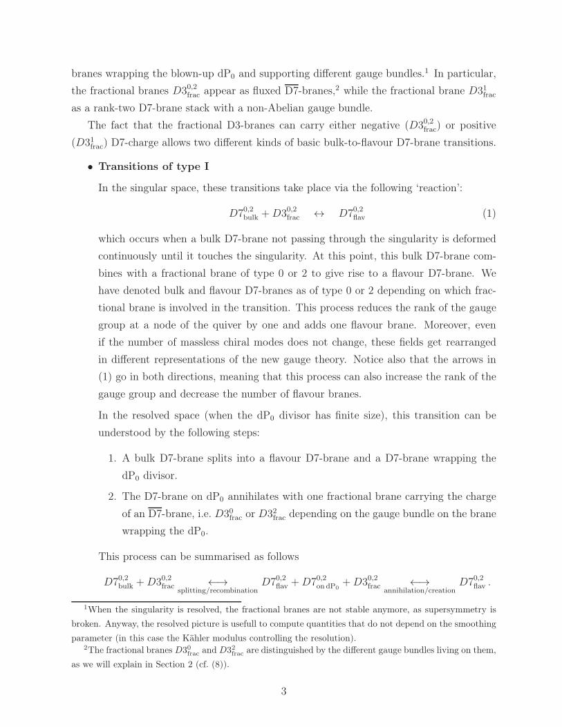
branes wrapping the blown-up dP0 and supporting different gauge bundles.1 In particular,

the fractional branes D30,2frac appear as fluxed D7-branes,2 while the fractional brane D31frac

as a rank-two D7-brane stack with a non-Abelian gauge bundle.

The fact that the fractional D3-branes can carry either negative (D30,2frac) or positive

(D31frac) D7-charge allows two different kinds of basic bulk-to-flavour D7-brane transitions.

• Transitions of type I

In the singular space, these transitions take place via the following ‘reaction’:

D70,2bulk +D30,2frac ↔ D70,2flav (1)

which occurs when a bulk D7-brane not passing through the singularity is deformed

continuously until it touches the singularity. At this point, this bulk D7-brane com-

bines with a fractional brane of type 0 or 2 to give rise to a flavour D7-brane. We

have denoted bulk and flavour D7-branes as of type 0 or 2 depending on which frac-

tional brane is involved in the transition. This process reduces the rank of the gauge

group at a node of the quiver by one and adds one flavour brane. Moreover, even

if the number of massless chiral modes does not change, these fields get rearranged

in different representations of the new gauge theory. Notice also that the arrows in

(1) go in both directions, meaning that this process can also increase the rank of the

gauge group and decrease the number of flavour branes.

In the resolved space (when the dP0 divisor has finite size), this transition can be

understood by the following steps:

1. A bulk D7-brane splits into a flavour D7-brane and a D7-brane wrapping the

dP0 divisor.

2. The D7-brane on dP0 annihilates with one fractional brane carrying the charge

of an D7-brane, i.e. D30frac or D32frac depending on the gauge bundle on the brane

wrapping the dP0.

This process can be summarised as follows

D70,2bulk +D30,2frac ←→splitting/recombination

D70,2flav +D70,2on dP0+D30,2frac ←→

annihilation/creationD70,2flav .

1When the singularity is resolved, the fractional branes are not stable anymore, as supersymmetry is

broken. Anyway, the resolved picture is usefull to compute quantities that do not depend on the smoothing

parameter (in this case the Kähler modulus controlling the resolution).2The fractional branes D30

fracand D32

fracare distinguished by the different gauge bundles living on them,

as we will explain in Section 2 (cf. (8)).

3

Notice that again the transition can take place in both directions through brane

splitting/recombination and brane annihilation/creation processes.

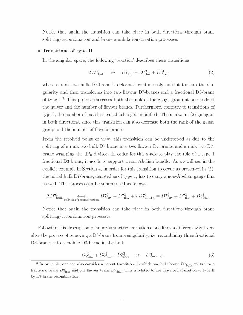
• Transitions of type II

In the singular space, the following ‘reaction’ describes these transitions

2D71bulk ↔ D70flav +D72flav +D31frac (2)

where a rank-two bulk D7-brane is deformed continuously until it touches the sin-

gularity and then transforms into two flavour D7-branes and a fractional D3-brane

of type 1.3 This process increases both the rank of the gauge group at one node of

the quiver and the number of flavour branes. Furthermore, contrary to transitions of

type I, the number of massless chiral fields gets modified. The arrows in (2) go again

in both directions, since this transition can also decrease both the rank of the gauge

group and the number of flavour branes.

From the resolved point of view, this transition can be understood as due to the

splitting of a rank-two bulk D7-brane into two flavour D7-branes and a rank-two D7-

brane wrapping the dP0 divisor. In order for this stack to play the rôle of a type 1

fractional D3-brane, it needs to support a non-Abelian bundle. As we will see in the

explicit example in Section 4, in order for this transition to occur as presented in (2),

the initial bulk D7-brane, denoted as of type 1, has to carry a non-Abelian gauge flux

as well. This process can be summarised as follows

2D71bulk ←→splitting/recombination

D70flav +D72flav + 2D71ondP0≡ D70flav +D72flav +D31frac .

Notice that again the transition can take place in both directions through brane

splitting/recombination processes.

Following this description of supersymmetric transitions, one finds a different way to re-

alise the process of removing a D3-brane from a singularity, i.e. recombining three fractional

D3-branes into a mobile D3-brane in the bulk

D30frac +D31frac +D32frac ↔ D3mobile . (3)

3 In principle, one can also consider a parent transition, in which one bulk brane D71bulk

splits into a

fractional brane D31frac

and one flavour brane D71flav

. This is related to the described transition of type II

by D7-brane recombination.

4

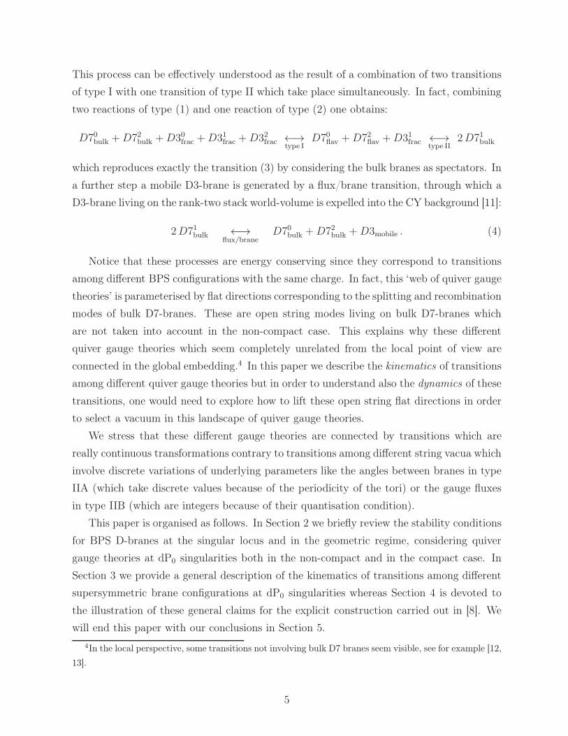
This process can be effectively understood as the result of a combination of two transitions

of type I with one transition of type II which take place simultaneously. In fact, combining

two reactions of type (1) and one reaction of type (2) one obtains:

D70bulk +D72bulk +D30frac +D31frac +D32frac ←→type I

D70flav +D72flav +D31frac ←→type II

2D71bulk

which reproduces exactly the transition (3) by considering the bulk branes as spectators. In

a further step a mobile D3-brane is generated by a flux/brane transition, through which a

D3-brane living on the rank-two stack world-volume is expelled into the CY background [11]:

2D71bulk ←→flux/brane

D70bulk +D72bulk +D3mobile . (4)

Notice that these processes are energy conserving since they correspond to transitions

among different BPS configurations with the same charge. In fact, this ‘web of quiver gauge

theories’ is parameterised by flat directions corresponding to the splitting and recombination

modes of bulk D7-branes. These are open string modes living on bulk D7-branes which

are not taken into account in the non-compact case. This explains why these different

quiver gauge theories which seem completely unrelated from the local point of view are

connected in the global embedding.4 In this paper we describe the kinematics of transitions

among different quiver gauge theories but in order to understand also the dynamics of these

transitions, one would need to explore how to lift these open string flat directions in order

to select a vacuum in this landscape of quiver gauge theories.

We stress that these different gauge theories are connected by transitions which are

really continuous transformations contrary to transitions among different string vacua which

involve discrete variations of underlying parameters like the angles between branes in type

IIA (which take discrete values because of the periodicity of the tori) or the gauge fluxes

in type IIB (which are integers because of their quantisation condition).

This paper is organised as follows. In Section 2 we briefly review the stability conditions

for BPS D-branes at the singular locus and in the geometric regime, considering quiver

gauge theories at dP0 singularities both in the non-compact and in the compact case. In

Section 3 we provide a general description of the kinematics of transitions among different

supersymmetric brane configurations at dP0 singularities whereas Section 4 is devoted to

the illustration of these general claims for the explicit construction carried out in [8]. We

will end this paper with our conclusions in Section 5.

4In the local perspective, some transitions not involving bulk D7 branes seem visible, see for example [12,

13].

5

2 D-branes at dP0 singularities

2.1 BPS D-branes

We consider type IIB string theory compactified on a CY three-fold. A Dp-brane is a (p+1)-

dimensional object which, when space-time filling, wraps a (p− 3)-cycle D of the compact

CY X and is characterised by the choice of the vector bundle E over D. A Dp-brane is

charged under the RR (p + 1)-potential. The RR charges of a D-brane are encoded in the

‘Mukai’ charge vector ΓE,D

ΓE,D = D ∧ ch(E) ∧

√

Td(TD)

Td(ND). (5)

D is the Poincaré dual form to the (p− 3)-cycle in X. Td(V ) = 1 + 12c1(V ) + 1

12(c1(V )2 +

c2(V )) + ... is the Todd class of the vector bundle V , TD is the tangent bundle of D and

ND the normal bundle of D in X while ch(E) is the Chern character of the vector bundle

E (or sheaf) living on the brane.5 The D9-charge is encoded in the zero-form component of

e−BΓE , the D7-charge in the two-form, the D5-charge in the four-form and the D3-charge

in the six-form.6

At large radius of the cycle D, the BPS condition on the D-brane is that the wrapped

cycle D is holomorphic and the vector bundle satisfies the Hermitian Yang-Mills equation,

or equivalently that it is a holomorphic and stable bundle. These are the F-flatness and

D-flatness conditions. The correct and most general mathematical definition for a (B-type)

BPS D-brane in type IIB string theory is that it is a Π-stable object in the derived category

of coherent sheaves on X [15]. The Π-stability condition [16] is a condition on the central

charge Z(E) of the D-brane: define the ‘grade’ of a D-brane as

ϕ(E) =1

πargZ(E) =

1

πIm logZ(E) .

The D-brane E is Π-stable if for all sub-objects E ′ ⊂ E one has ϕ(E ′) ≤ ϕ(E).

The central charge Z(E) of a (B-type) BPS D-brane depends purely on the complexified

Kähler form B + i J and it is independent of the complex structure moduli of X. When

5The charge vector can also be written in terms of the A-roof genus A, by shifting the sheaf E to the

sheaf W = E ⊗K1/2S whose first Chern class is identified with the gauge flux.

6These p-forms are actually the ‘push-forwards’ to the CY manifold X of forms on the D-brane (for

a review see [14]). For that reason, a two-form flux on a D7-brane, Poincaré dual to a curve C whose

push-forward is trivial on X but non-trivial on the D7-brane, will appear in the D3-charge (six-form) but

not in the D5-charge (four-form).

6

the D-brane wraps a large cycle the central charge is, up to quantum corrections,

Z(E) =

∫

X

e−B−iJΓE,D . (6)

From (6) we see that for a D3-brane at a generic point of X we have Z = −1.

The central charge and, consequently, the stability condition depend on the Kähler

moduli. When the D-brane wraps a large cycle, this reduces to the above conditions. In

particular, for a D7-brane with abelian flux the field strength of the line bundle has to be

of type (1, 1) and primitive, i.e.

F2,0 = 0 J ∧ F = 0 . (7)

The second one implies that the flux generated FI-term vanishes.

When the cycle shrinks to zero size, the stability condition changes. For dPn singu-

larities, i.e. point-like singularities arising when a dPn divisor in the compact manifold

shrinks to zero size, the set of exceptional sheaves corresponding to stable fractional branes

has been worked out [13, 17–20]. In this article, we are interested in fractional branes at

dP0 singularities. The corresponding sheaves have support on the shrinking dP0 and are

characterised by their Chern characters [9, 10]7

ch(F0) = −1 +H − 12H ∧H , ch(F1) = 2− H − 1

2H ∧H , ch(F2) = −1 , (8)

where H is the hyperplane class of dP0 = P2.

In this paper, we study transitions between BPS D-brane configurations with the same

total charge and, therefore, with the same total mass. Since these configurations are made

up by several BPS objects, they satisfy the BPS condition only if the involved objects

are mutually supersymmetric. The sum of two BPS objects remains BPS if the phases of

the central charges of the two objects are aligned. Supersymmetric transitions take place

among BPS configurations with the same charges and, therefore, the same mass/energy.

Hence, these transitions occur at zero energy cost, i.e. are flat directions.

As we have said, the set of stable BPS objects can change if we vary the geometric

(Kähler) moduli of the CY three-fold. Since we consider transitions among BPS states of

7Note that we use the opposite sign convention with respect to the literature on D3-branes at dPn

singularities. This is because in our convention a D7(anti-D7)-brane has charge +1(−1)D, where D is the

wrapped divisor. Note again that in this convention, the D3-charge is minus the integral of the six-form

component of ΓD7.

7

n2n0

n1

m1

m0m2

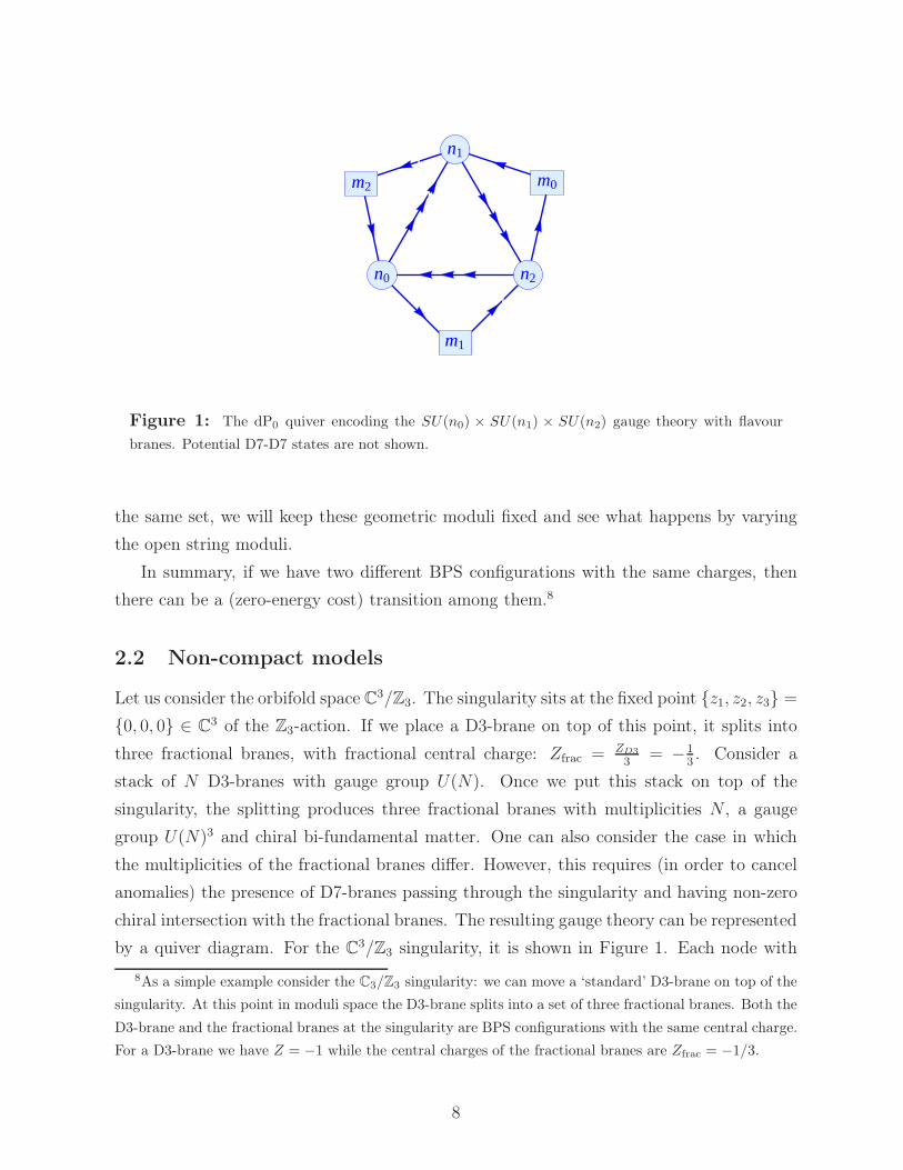
Figure 1: The dP0 quiver encoding the SU(n0) × SU(n1) × SU(n2) gauge theory with flavour

branes. Potential D7-D7 states are not shown.

the same set, we will keep these geometric moduli fixed and see what happens by varying

the open string moduli.

In summary, if we have two different BPS configurations with the same charges, then

there can be a (zero-energy cost) transition among them.8

2.2 Non-compact models

Let us consider the orbifold space C3/Z3. The singularity sits at the fixed point {z1, z2, z3} =

{0, 0, 0} ∈ C3 of the Z3-action. If we place a D3-brane on top of this point, it splits into

three fractional branes, with fractional central charge: Zfrac = ZD3

3= −1

3. Consider a

stack of N D3-branes with gauge group U(N). Once we put this stack on top of the

singularity, the splitting produces three fractional branes with multiplicities N , a gauge

group U(N)3 and chiral bi-fundamental matter. One can also consider the case in which

the multiplicities of the fractional branes differ. However, this requires (in order to cancel

anomalies) the presence of D7-branes passing through the singularity and having non-zero

chiral intersection with the fractional branes. The resulting gauge theory can be represented

by a quiver diagram. For the C3/Z3 singularity, it is shown in Figure 1. Each node with

8As a simple example consider the C3/Z3 singularity: we can move a ‘standard’ D3-brane on top of the

singularity. At this point in moduli space the D3-brane splits into a set of three fractional branes. Both the

D3-brane and the fractional branes at the singularity are BPS configurations with the same central charge.

For a D3-brane we have Z = −1 while the central charges of the fractional branes are Zfrac = −1/3.

8

label ni corresponds to a distinct fractional brane stack with gauge group U(ni). The

arrows indicate the bi-fundamental fields (ni, nj). Given a choice of ni, the flavour D7

brane multiplicities9 m0, m1, m2 are constrained by anomaly cancellation:

m0 = m+ 3(n1 − n0) , m1 = m , m2 = m+ 3(n1 − n2) . (9)

From a local point of view, models with different values of ni and m are not related to

each other, i.e. there seems to be no flat direction in moduli space which permits a change

of these numbers. In the following, we show that embedding these models in a globally

consistent string compactification allows such transitions.

2.3 Compact models

We now want to embed the local models at the C3/Z3 singularity in a compact CY manifold.

Therefore, we have to consider a CY three-fold X which admits such a singularity. This is

the case if X has a dP0 divisor DdP0; in the limit in which this divisor shrinks to zero size,

a C3/Z3 orbifold singularity is generated.

To embed the local D-brane model, we need the globally defined charge vectors of the

fractional and flavour branes which produces the quiver diagram in Figure 1, with a chosen

set of integers ni and m. In [8], we have seen that this imposes strong constraints on the

values of ni and m.

A fractional brane is a BPS brane with support on the shrinking dP0. There are three

types of mutually stable fractional branes for such a type of singularity. Their charge

vectors are determined by (5), with D = DdP0 (i.e. the shrinking divisor) and with ch(E)

given by (8):

ΓF0 = DdP0 ∧{

−1− 12DH −

14DH ∧DH

}

,

ΓF1 = DdP0 ∧{

2 + 2DH + 12DH ∧DH

}

, (10)

ΓF2 = DdP0 ∧{

−1− 32DH −

54DH ∧DH

}

.

DH is a two-form of the CY three-fold whose pullback lies in the class H of the dP0 divisor.10

9The numbers mi do not necessarily imply U(mi) gauge symmetries but can be, for instance, products

of U(1) gauge symmetries. Instead of one single arrow connecting the D3 and D7 branes, there may be

multiple arrows with reduced gauge symmetry. All this is encoded in the choice of the mi’s which are

themselves determined by anomaly cancellation.10There is an ambiguity in choosing DH , as we can add to it any two-form of X whose pullback onto the

dP0 is trivial.

9

The flavour D7-branes are BPS branes wrapping a large divisor Dflav which pass through

the singularity, i.e. in the resolved picture Dflav ∩ DdP0 6= ∅. Each of them will have an

associated charge vector

ΓEflav ,Dflav= Dflav ∧ ch(Eflav) ∧

√

Td(TDflav)

Td(NDflav), (11)

where Eflav is the vector bundle living on it. Since the flavour D7-brane extends in the

non-compact directions in the local model, its global charge vector is not fully determined

by the local data – in contrast to the fractional brane. The local ones, i.e. the pullback of

(11) to DdP0 , are given by:

ΓlocD7i≡ ΓEi

flav ,Diflav

∣

∣

∣

dP0

= aiH ∧ (1 + biH) with i = 0, 1, 2 , (12)

where the coefficient ai and bi are determined in [8]:

{a0, b0} = {m0,12} {a1, b1} = {−2m1, 1} {a2, b2} = {m2,

32} , (13)

with mi as in (9). Imposing that ΓlocD7i

come from globally defined and connected flavour

D7-branes gives the following constraints [8]:

0 ≤ −m ≤ 3(n1 −max{n0, n2}) . (14)

3 Transitions among different quiver gauge theories

In the local picture, quiver models with different multiplicities ni of fractional branes are

disconnected. As we now explain, this is not the case once one considers the full compacti-

fication with all the other branes needed to cancel the tadpoles. Due to bulk effects, there

are smooth transition between two brane configurations related to different quiver gauge

theories.

In the example studied in [8], we noticed that two different setups have the same D-brane

charges. The first one was n1 = 3, n0 = n2 = 2 and two flavour branes; the second one

was n0 = n1 = n2 = 3 and no flavour brane but with two bulk branes that do not intersect

the dP0 divisor and rest identical with the first configuration. The same charges can also

be realised by a configuration with n1 = n2 = 3, n0 = 2, one flavour brane and one bulk

brane. All three configurations are made up by mutually BPS D-branes. Hence, we have

evidence for a possible flat direction connecting the three D-brane formations. The basic

step is the following: starting from one D7-brane that does not touch the singularity, we

10

end up with one more flavour brane and one of the multiplicities ni of the nodes changed.

The transition occurs when the bulk brane touches the singularity.

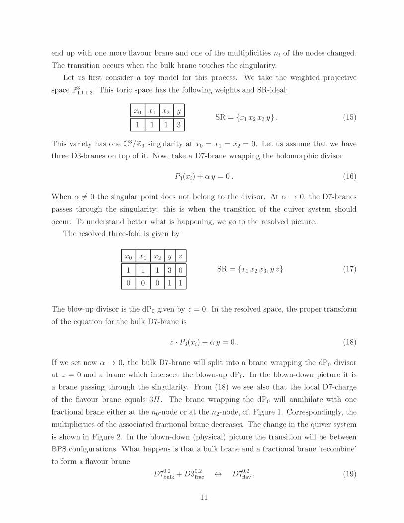
Let us first consider a toy model for this process. We take the weighted projective

space P31,1,1,3. This toric space has the following weights and SR-ideal:

x0 x1 x2 y

1 1 1 3SR = {x1 x2 x3 y} . (15)

This variety has one C3/Z3 singularity at x0 = x1 = x2 = 0. Let us assume that we have

three D3-branes on top of it. Now, take a D7-brane wrapping the holomorphic divisor

P3(xi) + α y = 0 . (16)

When α 6= 0 the singular point does not belong to the divisor. At α → 0, the D7-branes

passes through the singularity: this is when the transition of the quiver system should

occur. To understand better what is happening, we go to the resolved picture.

The resolved three-fold is given by

x0 x1 x2 y z

1 1 1 3 0

0 0 0 1 1

SR = {x1 x2 x3, y z} . (17)

The blow-up divisor is the dP0 given by z = 0. In the resolved space, the proper transform

of the equation for the bulk D7-brane is

z · P3(xi) + α y = 0 . (18)

If we set now α → 0, the bulk D7-brane will split into a brane wrapping the dP0 divisor

at z = 0 and a brane which intersect the blown-up dP0. In the blown-down picture it is

a brane passing through the singularity. From (18) we see also that the local D7-charge

of the flavour brane equals 3H . The brane wrapping the dP0 will annihilate with one

fractional brane either at the n0-node or at the n2-node, cf. Figure 1. Correspondingly, the

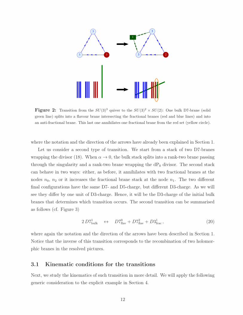
multiplicities of the associated fractional brane decreases. The change in the quiver system

is shown in Figure 2. In the blown-down (physical) picture the transition will be between

BPS configurations. What happens is that a bulk brane and a fractional brane ‘recombine’

to form a flavour brane

D70,2bulk +D30,2frac ↔ D70,2flav , (19)

11

3

33

3

23

1

Figure 2: Transition from the SU(3)3 quiver to the SU(3)2 × SU(2): One bulk D7-brane (solid

green line) splits into a flavour brane intersecting the fractional branes (red and blue lines) and into

an anti-fractional brane. This last one annihilates one fractional brane from the red set (yellow circle).

where the notation and the direction of the arrows have already been explained in Section 1.

Let us consider a second type of transition. We start from a stack of two D7-branes

wrapping the divisor (18). When α→ 0, the bulk stack splits into a rank-two brane passing

through the singularity and a rank-two brane wrapping the dP0 divisor. The second stack

can behave in two ways: either, as before, it annihilates with two fractional branes at the

nodes n0, n2 or it increases the fractional brane stack at the node n1. The two different

final configurations have the same D7- and D5-charge, but different D3-charge. As we will

see they differ by one unit of D3-charge. Hence, it will be the D3-charge of the initial bulk

branes that determines which transition occurs. The second transition can be summarised

as follows (cf. Figure 3)

2D71bulk ↔ D70flav +D72flav +D31frac , (20)

where again the notation and the direction of the arrows have been described in Section 1.

Notice that the inverse of this transition corresponds to the recombination of two holomor-

phic branes in the resolved pictures.

3.1 Kinematic conditions for the transitions

Next, we study the kinematics of such transition in more detail. We will apply the following

generic consideration to the explicit example in Section 4.

12

4

33

11

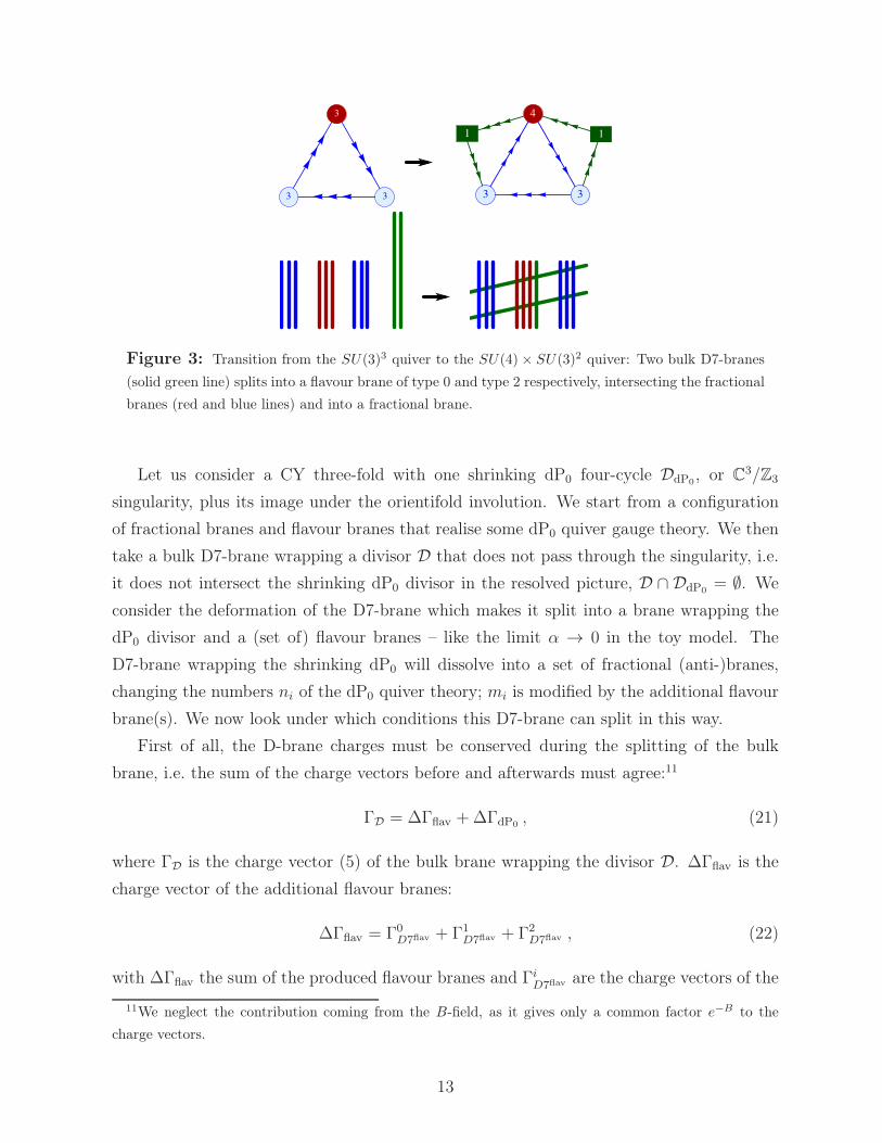
Figure 3: Transition from the SU(3)3 quiver to the SU(4)× SU(3)2 quiver: Two bulk D7-branes

(solid green line) splits into a flavour brane of type 0 and type 2 respectively, intersecting the fractional

branes (red and blue lines) and into a fractional brane.

Let us consider a CY three-fold with one shrinking dP0 four-cycle DdP0, or C3/Z3

singularity, plus its image under the orientifold involution. We start from a configuration

of fractional branes and flavour branes that realise some dP0 quiver gauge theory. We then

take a bulk D7-brane wrapping a divisor D that does not pass through the singularity, i.e.

it does not intersect the shrinking dP0 divisor in the resolved picture, D ∩ DdP0= ∅. We

consider the deformation of the D7-brane which makes it split into a brane wrapping the

dP0 divisor and a (set of) flavour branes – like the limit α → 0 in the toy model. The

D7-brane wrapping the shrinking dP0 will dissolve into a set of fractional (anti-)branes,

changing the numbers ni of the dP0 quiver theory; mi is modified by the additional flavour

brane(s). We now look under which conditions this D7-brane can split in this way.

First of all, the D-brane charges must be conserved during the splitting of the bulk

brane, i.e. the sum of the charge vectors before and afterwards must agree:11

ΓD = ∆Γflav +∆ΓdP0 , (21)

where ΓD is the charge vector (5) of the bulk brane wrapping the divisor D. ∆Γflav is the

charge vector of the additional flavour branes:

∆Γflav = Γ0D7flav + Γ1

D7flav + Γ2D7flav , (22)

with ∆Γflav the sum of the produced flavour branes and ΓiD7flav are the charge vectors of the

11We neglect the contribution coming from the B-field, as it gives only a common factor e−B to the

charge vectors.

13

three kinds of local flavour branes given in (12). ∆ΓdP0 is the shift in the fractional branes

∆ΓdP0 = DdP0 ∧ ch(E) ∧

√

Td(TDdP0)

Td(NDdP0)with ch(E) = r + nH + (1

2n2 − ℓ)H2 . (23)

Let us expand the condition (21). The D7-charge conservation implies the following

condition on the divisors wrapped by the branes:

D = rDdP0 +∑

i=0,1,2

D(i)flav . (24)

In order for the described transition to occur, we need that all the involved divisors classes

have holomorphic connected representatives – otherwise we would have a different splitting.

For instance, if there is no holomorphic smoothly connected divisor in the class Dflav =

D −DdP0, we cannot have the transition described in the toy model.

The D5-charge conservation constrains the gauge bundle:

D ∧ trF = DdP0 ∧(

n+ 32

)

H +∑

i=0,1,2

D(i)flav ∧ trF

(i)flav . (25)

The fluxes trFflav on the new flavour branes can be written as

trF(i)flav = F

(i)flav + β

(i)dP0DdP0

, with β(i)dP0∈ {−1

6,−1

3,−1

2} , (26)

and Fflav being a two-form orthogonal to DdP0on the D-brane world-volume. The coefficient

βdP0 is determined by the local D5-charge of the fractional branes (13). Moreover, if ∆mi

are the shifts of the flavour branes, their restriction on the dP0 is equal to D(i)flav|dP0

=

(∆m0 H,−2∆m1 H, ∆m2 H)i. Hence, we can rewrite the D5-charge conservation condition

as

D ∧ trF =∑

i=0,1,2

D(i)flav ∧ F

(i)flav +DdP0 ∧

(

n+ 32− 1

6∆m0 +

23∆m1 −

12∆m2

)

H .

We will see in a moment, equation (30), that the second term on the right hand side

vanishes, leading to the simple form:

D ∧ trF =∑

i=0,1,2

D(i)flav ∧ F

(i)flav . (27)

Finally one needs to check that the D3-charge is conserved. Given a certain gauge

bundle on the bulk brane wrapping D and requiring, for example, to have only abelian

fluxes on the flavour branes, the coefficient ℓ in (23) is determined.

14

So far we have analysed the condition for the bulk brane to split into a brane wrapping

the dP0 and a set of branes intersecting it – the flavour branes. After the splitting, the

D7-brane wrapping the dP0 has a charge vector equal to (23). For generic r, n and ℓ,

this brane is not a fractional brane but a combination of them. However, the only stable

branes on the shrinking dP0 are the fractional branes. Therefore the brane must dissolve

into them:

ch(E) = ∆n0 ch(F0) + ∆n1 ch(F1) + ∆n2 ch(F2) , (28)

where the Chern characters ch(Fi) of the fractional branes were given in (8). The mul-

tiplicities of the fractional branes after the transition are n′i = ni + ∆ni with i = 0, 1, 2.

Imposing the equality of (28) with the expression of ch(E) in (23), one obtains

∆n0 = −12n(n− 1) + ℓ ∆n1 = −

12n(n + 1) + ℓ ∆n2 = −

12n(n + 3)− r + ℓ . (29)

Notice that, since r > 0, for n ∈ Z we have ∆ni − ℓ ≤ 0 ∀i. A negative ∆ni means that

the splitting generates anti-fractional branes which annihilates −∆ni fractional branes of

type i in the initial quiver system. We also see that the ∆ni are all shifted by ℓ. Increasing

ℓ means to increase the D3-charge without modifying its D5- and D7-charges, cf. ch(E)

in (23). Hence, the transitions with equal ∆ni, up to an integer overall shift ℓ, differ by

absorption or ejection of |ℓ| D3-brane.

The splitting will also produce a number of new flavour branes, whose multiplicities are

given by

∆m0 = ∆m− 3n ∆m1 = ∆m ∆m2 = ∆m+ 3(n+ r) , (30)

where ∆m signals the arbitrariness in choosing which flavour branes are generated in the

transition. Since the restrictions of the flavour brane divisors on dP0 are:

D(0)flav|dP0 = ∆m0H D(1)

flav|dP0 = −2∆m1 H D(2)flav|dP0 = ∆m2 H , (31)

the following constraints on the values of ∆mi are imposed from the global embedding [8]:

∆m ≤ 0 − r − 13∆m ≤ n ≤ 1

3∆m . (32)

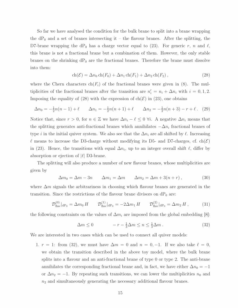
We are interested in two cases which can be used to connect all quiver models:

1. r = 1: from (32), we must have ∆m = 0 and n = 0,−1. If we also take ℓ = 0,

we obtain the transition described in the above toy model, where the bulk brane

splits into a flavour and an anti-fractional brane of type 0 or type 2. The anti-brane

annihilates the corresponding fractional brane and, in fact, we have either ∆n0 = −1

or ∆n2 = −1. By repeating such transitions, we can lower the multiplicities n0 and

n2 and simultaneously generating the necessary additional flavour branes.

15

2. r = 2: in this case −3 ≤ ∆m ≤ 0. We will be interested in ∆m = 0 and n = −1. If we

choose also ℓ = 1, we have ∆n1 = 1, ∆n0 = ∆n2 = 0, ∆m1 = 0 and ∆m0 = ∆m2 = 1.

Here the bulk D7-brane splits into the fractional brane at the n1 node (∆n1 = +1)

and into two flavour branes. In this case we have no annihilation.

We consider the case ∆m = 0 because the other possible values of ∆m correspond to a

recombination of a flavour brane of type 0 with a flavour brane of type 2 which gives a

flavour brane of type 1. Of course, whether this recombination is possible depends on the

gauge bundles on the two flavour branes.

We will illustrate these two classes of transitions in Section 4.

3.2 F- and D-flatness conditions

We consider transitions in which both the initial and the final states are supersymmet-

ric configurations. The F- and D-term vanishing conditions are realised by requiring the

stability conditions described in Section 2 (if the VEVs of the charged fields are zero).

The system of the fractional branes with Chern characters (8) is supersymmetric at the

singular point [10, 15]. The flavour branes and the bulk branes must wrap holomorphic

divisors D and have holomorphic field strength, i.e. F ∈ H1,1(D), where the generated

FI-terms vanish.

We will mostly consider D7-branes with abelian fluxes. In this case, the holomorphicity

condition on F is automatically satisfied if we take F to be a two-form pulled back from

the CY three-fold. When this is not the case, the holomorphicity condition may fix some

D7-brane deformation moduli. The transition can occur if the corresponding flat direction

is not lifted by the flux.

As regarding the D-terms, after taking the limit of shrinking dP0 (τDdP0→ 0), the FI-

terms of the fractional branes vanish. Furthermore, the sum of the FI-terms of the flavour

branes generated after the transition becomes equal to the FI-term of the initial bulk brane:

ξD

(0)flav

+ ξD

(1)flav

+ ξD

(2)flav

−→τD

dP0→0

ξD =1

V

∫

D

F ∧ J , (33)

where we used the D5-charge conservation condition. Consider the case when only one new

flavour brane is generated: if the starting bulk brane has zero FI-term, i.e. ξD = 0, then

the flavour brane will also have a vanishing FI-term.

16

4 Transitions in an explicit dP0 example

In this section we will apply the above considerations to an explicit example where we will

be able to describe in detail the transitions among different quiver gauge theories. We

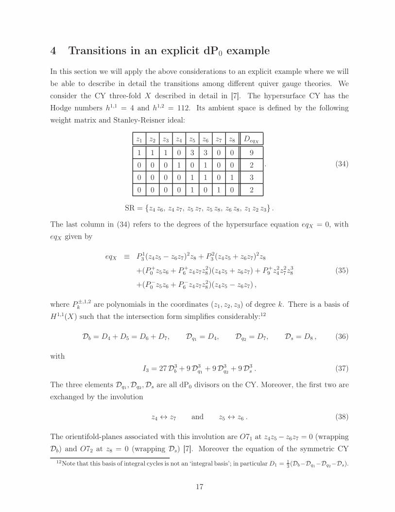
consider the CY three-fold X described in detail in [7]. The hypersurface CY has the

Hodge numbers h1,1 = 4 and h1,2 = 112. Its ambient space is defined by the following

weight matrix and Stanley-Reisner ideal:

z1 z2 z3 z4 z5 z6 z7 z8 DeqX

1 1 1 0 3 3 0 0 9

0 0 0 1 0 1 0 0 2

0 0 0 0 1 1 0 1 3

0 0 0 0 1 0 1 0 2

. (34)

SR = {z4 z6, z4 z7, z5 z7, z5 z8, z6 z8, z1 z2 z3} .

The last column in (34) refers to the degrees of the hypersurface equation eqX = 0, with

eqX given by

eqX ≡ P 13 (z4z5 − z6z7)

2z8 + P 23 (z4z5 + z6z7)

2z8

+(P+0 z5z6 + P+

6 z4z7z28)(z4z5 + z6z7) + P+

9 z24z27z

38 (35)

+(P−

0 z5z6 + P−

6 z4z7z28)(z4z5 − z6z7) ,

where P±,1,2k are polynomials in the coordinates (z1, z2, z3) of degree k. There is a basis of

H1,1(X) such that the intersection form simplifies considerably:12

Db = D4 +D5 = D6 +D7, Dq1 = D4, Dq2 = D7, Ds = D8 , (36)

with

I3 = 27D3b + 9D3

q1+ 9D3

q2+ 9D3

s . (37)

The three elements Dq1,Dq2,Ds are all dP0 divisors on the CY. Moreover, the first two are

exchanged by the involution

z4 ↔ z7 and z5 ↔ z6 . (38)

The orientifold-planes associated with this involution are O71 at z4z5− z6z7 = 0 (wrapping

Db) and O72 at z8 = 0 (wrapping Ds) [7]. Moreover the equation of the symmetric CY

12Note that this basis of integral cycles is not an ‘integral basis’; in particular D1 = 1

3(Db−Dq1−Dq2−Ds).

17

is now given by (35) with P−

k ≡ 0. In the following, we will consider dP0 quiver gauge

theories constructed ‘around’ the shrinking Dq1 divisor at z4 = 0 and its orientifold image

Dq2 at z7 = 0.

Let us consider the trinification SU(3)3 model described in [7] with four bulk D7-branes

plus their images wrapping the divisor Db to cancel the D7-tadpole generated by the O7-

plane O71. We will take the abelian flux Fb on the bulk branes to be of type (1, 1), i.e.

Fb ∈ H1,1(Db), and to have zero FI-term. The FI-term depends on the invariant combination

Fb = Fb −B: ξ ∝∫

DbJ ∧Fb. This is zero if the flux Fb is the Poincaré dual of a two-cycle

of Db which is trivial in the CY three-fold, even though not necessarily trivial on Db. In

this case, however, we might need to fix some D7-brane deformations to make the two-form

holomorphic. Moreover, Fb satisfy this condition only if the part of Fb proportional toc1(Db)

2= −Db

2(necessary to prevent a Freed-Witten anomaly [21, 22]) is cancelled by the

B-field. For this reason we take B = −Db

2− Ds

2.13 In principle one could obtain vanishing

FI-terms by fixing some combinations of Kähler moduli [6]; in the present case this can be

shown to be impossible, due to the simple intersection form (37) which in the literature has

been called ‘strong Swiss-cheese’ [23] .

4.1 Transitions of type I

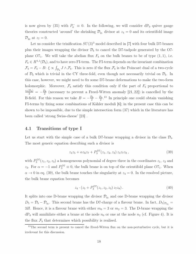
Let us start with the simple case of a bulk D7-brane wrapping a divisor in the class Db.

The most generic equation describing such a divisor is

z4z5 + αz6z7 + PD73 (z1, z2, z3) z4z7z8 , (39)

with PD73 (z1, z2, z3) a homogeneous polynomial of degree three in the coordinates z1, z2 and

z3. For α = −1 and PD73 ≡ 0, the bulk brane is on top of the orientifold plane O71. When

α→ 0 in eq. (39), the bulk brane touches the singularity at z4 = 0. In the resolved picture,

the bulk brane equation becomes

z4 · (z5 + PD73 (z1, z2, z3) z7z8) . (40)

It splits into one D-brane wrapping the divisor Dq1 and one D-brane wrapping the divisor

D5 = Db −Dq1. This second brane has the D7-charge of a flavour brane. In fact, D5|Dq1=

3H . Hence, it is a flavour brane with either m0 = 3 or m2 = 3. The D-brane wrapping the

dP0 will annihilate either a brane at the node n0 or one at the node n2 (cf. Figure 4). It is

the flux Fb that determines which possibility is realised.

13The second term is present to cancel the Freed-Witten flux on the non-perturbative cycle, but it is

irrelevant for this discussion.

18

3

33

3

23

1

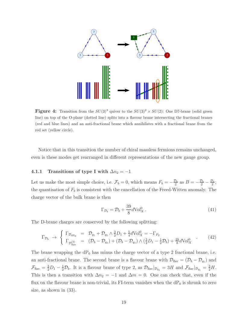
Figure 4: Transition from the SU(3)3 quiver to the SU(3)2 × SU(2): One D7-brane (solid green

line) on top of the O-plane (dotted line) splits into a flavour brane intersecting the fractional branes

(red and blue lines) and an anti-fractional brane which annihilates with a fractional brane from the

red set (yellow circle).

Notice that in this transition the number of chiral massless fermions remains unchanged,

even is these modes get rearranged in different representations of the new gauge group.

4.1.1 Transitions of type I with ∆n2 = −1

Let us make the most simple choice, i.e. Fb = 0, which means Fb = −Db

2as B = −Db

2− Ds

2;

the quantisation of Fb is consistent with the cancellation of the Freed-Witten anomaly. The

charge vector of the bulk brane is then

ΓDb= Db +

39

8dVol0X . (41)

The D-brane charges are conserved by the following splitting:

ΓDb→

{

ΓDdP0= Dq1 +Dq1 ∧

32D1 +

54dVol0X = −ΓF2

ΓD

(2)flav

= (Db −Dq1) + (Db −Dq1) ∧ (32D1 −

12Db) +

298dVol0X

. (42)

The brane wrapping the dP0 has minus the charge vector of a type 2 fractional brane, i.e.

an anti-fractional brane. The second brane is a flavour brane with Dflav = (Db − Dq1) and

Fflav = 32D1 −

12Db. It is a flavour brane of type 2, as Dflav|Dq1

= 3H and Fflav|Dq1= 3

2H .

This is then a transition with ∆n2 = −1 and ∆m = 0. One can check that, even if the

flux on the flavour brane is non-trivial, its FI-term vanishes when the dP0 is shrunk to zero

size, as shown in (33).

19

4.1.2 Transitions of type I with ∆n0 = −1

To obtain a transition with ∆n0 = −1, we need to choose a different flux on the bulk brane.

Since we still want a zero FI-term ξb = 0, the flux must be of the non-pullback type. If the

flux would be a pullback two-form, we would get ξb ∝ V1/3 which in turn would force the

CY to collapse.

In appendix A, we obtain such a flux Fb by defining a non-pullback two-form F C on Db.

After including the contribution from the B-field (B = −Db/2−Ds/2), we have:

Fb = ωC − ι∗D1 . (43)

The two-form Fb is non-trivial on Db. On the other hand, the push-forward of the Poincaré

dual curve is trivial inside the CY X. This means that we, again, have vanishing D5-charge

for the bulk brane and, therefore, zero FI-term. In appendix A, we also compute the square

of Fb:∫

Db

F2b = −12.

This allows us to write down the charge vector of the bulk brane:

ΓDb= Db −

9

8dVol0X . (44)

For the following transition the charges are conserved:

ΓDb→

{

ΓDdP0= Dq1 +Dq1 ∧

12D1 +

14dVol0X = −ΓF0

ΓD

(0)flav

= (Db −Dq1) + (Db −Dq1) ∧ (12D1 + ωC

flav −12Db)−

118dVol0X

. (45)

The brane wrapping the dP0 has minus the charge vector of a type 0 fractional brane, i.e.

an anti-fractional brane. The second brane is a flavour brane with Dflav = Db − Dq1 and

Fflav = ωCflav + 1

2ι∗D1 − ι∗B. Here ωC

flav is again a non-pullback two-form defined by the

curve C, as explained in appendix A. Since Dflav|Dq1= 3H and Fflav|Dq1

= 12H , the flavour

brane is of type 0. This last result depends on the fact that the defining curve C does not

intersect the dP0 divisor, and therefore ωCflav|Dq1

= 0.

In this transition, we have a different feature with respect to the previous one. This is

due to the presence of a flux that is not of the pullback type. Such flux is not necessarily

‘automatically’ holomorphic, and hence one may need to fix D7-brane deformations to

keep the two-form of (1, 1)-type. As explained in appendix A, switching on the flux (43)

on (39) can fix the deformation parameter encoded in the coefficient of the polynomial

PD73 (z1, z2, z3). In other words, varying PD7

3 can make the curve C non-holomorphic and

break supersymmetry. Regardless of this issue, α remains free to vary in a supersymmetric

20

4

33

11

Figure 5: Transition from the SU(3)3 quiver to the SU(4) × SU(3)2 quiver: A rank-two bulk

D7-brane (solid green line) splits into a fractional brane and two flavour branes (of type 0 and 2

respectively) intersecting the fractional branes (red and blue lines).

transition. This deformation is the one that we need to realise the transition to the flavour

brane wrapping z5+PD73 (z1, z2, z3) z7z8 = 0. Note that the flux Fflav present on the flavour

brane is constructed by using the curve C which still fixes the deformations in PD73 (z1, z2, z3).

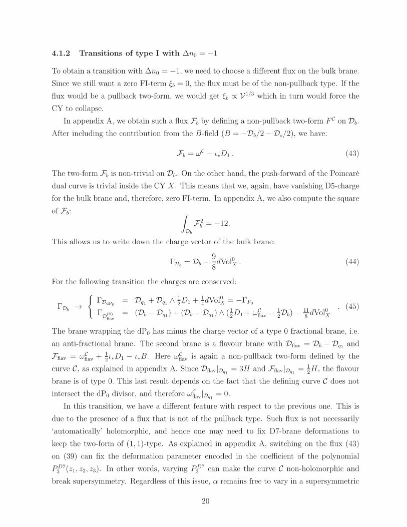
4.2 Transitions of type II

We start from a stack of two bulk D7-brane wrapping the divisor defined by equation (39).

This time, we can have a non-abelian flux, i.e. a non-trivial SU(2)-bundle. We still insist

that the first Chern class of the bundle has zero push-forward on the CY X, in order to

have a zero FI-term. On the other hand, we allow for a non-trivial second Chern class c2.

In particular, we choose a brane wrapping Db with a rank two vector bundle characterised

by the following Chern character

ch(Ebulk) = 2 + c1(Ebulk) +(

12c1(Ebulk)

2 − c2(Ebulk))

, (46)

with c1(Ebulk) = ωC− ι∗D1 and c2 = 1 · dVol0Db. Plugging this into (5), we obtain the charge

vector

ΓDb= 2Db +

11

4dVol0X . (47)

A charge conserving transition is given by:

ΓDb→

ΓDdP0= 2Dq1 + 2Dq1 ∧D1 +

12dVol0X = +ΓF1

ΓD

(0)flav

= (Db −Dq1) + (Db −Dq1) ∧ (12D1 + ωC

flav −12Db)−

118dVol0X

ΓD

(2)flav

= (Db −Dq1) + (Db −Dq1) ∧ (32D1 −

12Db) +

298dVol0X

, (48)

21

3

33

3

11

2 2

...

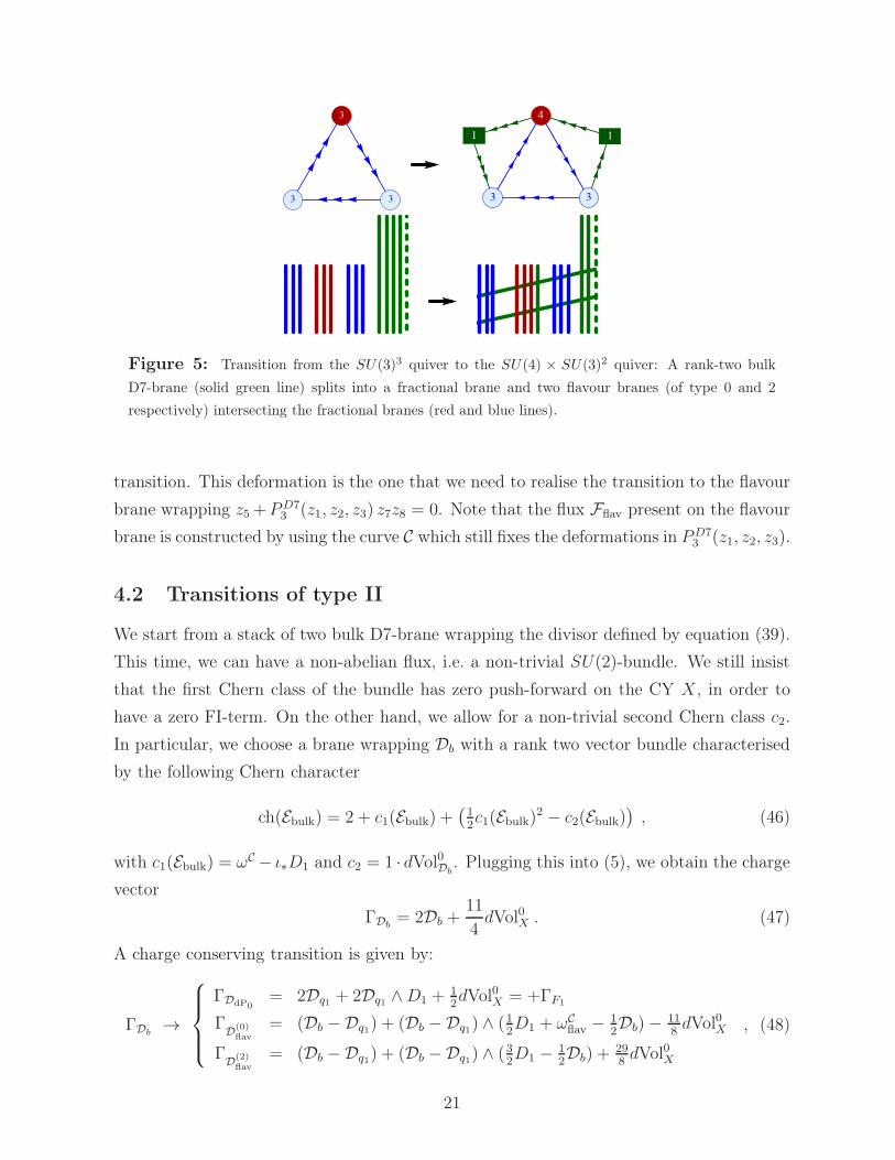
Figure 6: By repeating four times the transition described in Figure 4, we get four flavour branes

and no D7-brane on top of the O-plane.

We see that we generate both kinds of flavour branes which we obtained in the two type I

transitions. The D-brane wrapping the dP0 divisor is a fractional brane of type 1 and will

increase the multiplicity n1 in the quiver diagram (see Figure 5).

4.3 Step by step transitions

We can now use the transitions described above to connect different quiver gauge theories.

Take, for instance, the trinification model SU(3)3 and apply one transition of type I with

∆n0 = −1 and one of type I with ∆n2 = −1. In this way we reach the left-right symmetric

model with gauge group SU(3)×SU(2)2. In this process two bulk D7-branes wrapping the

divisor Db are transformed into the two needed flavour branes. Moreover, if one consider also

the D7-D7 states (between the two flavour branes), the total number of chiral modes remains

the same as in the SU(3)3 model (even if they are rearranged in different representations

of the new gauge group).14

One can do a step forward and apply another transition of type I. The final gauge group

on the fractional branes is the Standard Model, i.e. SU(3)×SU(2)×U(1), with the proper

structure of flavour branes. In our case one can, in principle, go one step further: on top of

the O7-plane wrapping Db there is still one more D7-brane. If this undergoes the transition

as well, either n0 or n2 are lowered by one, reaching the situation depicted in Figure 6.

Starting from the SU(3) × SU(2)2 model we can take another route. We may apply

the reverse of the type II transition: the two flavour branes recombine with the fractional

14This happens in the explicit example we have considered, where the only contribution to the flavour

brane fluxes comes from the local flux necessary to cancel the local D5-charge.

22

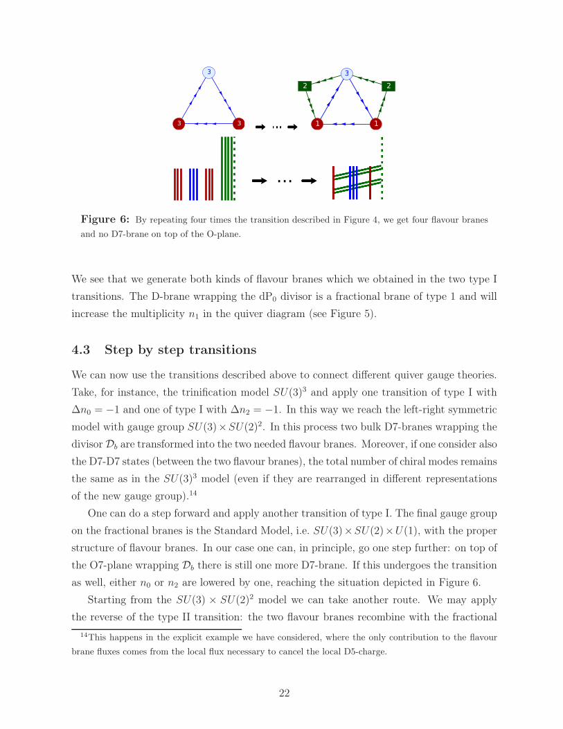
Figure 7: Part of the web of quiver gauge theories at a dP0 singularity. In particular we show the

gauge theories which have been shown to be in direct connection with the trinification SU(3)3 model.

Different levels in the web correspond to different D3-brane charges. Only some connections in the

web are shown.

brane of type 1:

ΓF1

ΓD

(0)flav

ΓD

(2)flav

→ Γn.a.D = 2Db +

114dVol0X = Db ∧ ch(Ebulk) ∧

√

TDb

NDb

, (49)

where ch(Ebulk) is given in (46). We see that we get a bulk brane wrapping the divisor Db,

with a bundle Ebulk of rank two and second Chern class such that∫

Dbc2(V ) = 1, i.e. we

have a brane-stack with an instanton-like background in the extra-dimension of Db with

instanton number equal to 1. The moduli space of the instanton-like solution has a flat

direction that is the size of the instanton. At the point in moduli space where the instanton

becomes point-like in the internal dimensions it is just a D3-brane and can be moved away

from the bulk D7-brane [11]. In this case, we end up with the SU(2)3 quiver model, a bulk

brane with charge vector (41) and a mobile D3-brane. If the D3-brane moves on top of the

singularity, we obtain the SU(3)3 quiver model and the bulk configuration we started with.

A summary of the different connected quiver gauge theories at the dP0 singularity is

shown in Figure 7.

23

4.4 Local effective field theory description

Having found a continuous connection between different quiver gauge theories, a natural

question to ask is if it is possible to describe this effect in terms of flat directions in field

theory space. In this section, we shall investigate only a possible local effective field theory

description focusing just on states between the D3- and flavour D7-branes. A proper full

understanding of these transitions would involve the inclusion of bulk D7 states but the

derivation of the global effective field theory (EFT) is beyond the scope of this paper.

Following our discussion of supersymmetric bulk-to-flavour brane transitions, we can

immediately infer three important facts:

• Transitions of type I involve brane creation/annihilation processes which are purely

stringy effects. This makes an EFT interpretation more involved.

• Transitions of type II proceed just through brane splitting/recombination processes,

corresponding to gauge enhancement/higgsing of the quiver gauge group. Thus we

expect to be able to find a local EFT description of these phenomena.

• Combinations of transitions of type I and II which reduce or increase the rank of the

gauge group can be interpreted in the local EFT by appropriate fields switching their

VEV on or off. However, given that some steps proceed via transitions of type I, the

interpretation of these processes is less clear.

Let us first show how a transition of purely type II can be interpreted in the local

EFT. As an example, we shall consider the transition from SU(3) × SU(2)2 × U(1)2 to

SU(2)3 which could be parameterised by the flat direction JII = A1B1C1 (in the absence

of superpotential couplings of the form W ⊃ A1B1C1 which would break the F-flatness

condition) with

A1 = (3, 1, 1)−0 , B1 = (3, 1, 1)0+ , C1 = (1, 1, 1)+− , (50)

where the subscripts represent the U(1)2 charges. Notice that A1 and B1 are D3-D7 states

whereas C1 is a D7-D7 state. The second ones are always present when the flux on the

flavour brane is such that it makes the FI-term vanish (for shrunk dP0).15

Let us now show how combinations of transitions of type I and II could also be described

in terms of flat directions in the local EFT. For example, the SU(3)2×SU(2)×U(1) model

can be connected to the SU(2)3 one by the combination of one transition of type I and

15Zero FI-term for the flavour branes means that the contribution on the flux from the bulk is suppressed.

24

another of type II. In this case the flat direction could be determined by the invariant

JI+II = X1U1W1 with (assuming again the correct superpotential couplings)

X1 = (3, 3, 1)0 , U1 = (3, 1, 1)+ , W1 = (1, 3, 1)− , (51)

where the subscripts represent again the U(1) charges. The flat direction 〈X1〉 = diag (0, 0, v3),

〈U1〉 = 〈W1〉 = (0, 0, v3) gives precisely the spectrum of the SU(2)3 quiver gauge theory.

Notice that X1 is a D3-D3 state whereas U1 and W1 are D3-D7 states.

As a second example, let us consider the process of removing one D3-brane from the

singularity (that can be seen as a combination of two transitions of type I with one transition

of type II). This will connect the SU(3)3 model to the SU(2)3 one. The flat directions can

be easily identified as follows. The original spectrum can be written as

Xi = (3, 3, 1) , Yi = (3, 1, 3) , Zi = (1, 3, 3) , (52)

where i = 1, 2, 3 is a family index. The flat directions can be taken to be 〈X1〉 = 〈Y1〉 =

〈Z1〉 = diag (v1, v2, v3). The existence of the gauge invariant JI+I+II = X1Y1Z1 guarantees

this configuration to be D-flat. It is also F-flat given the general structure of the dP0

superpotential W = ǫijkXiYjZk since 〈X2,3〉 = 〈Y2,3〉 = 〈Z2,3〉 = 0. For v1 = v2 = 0 the

SU(3)3 symmetry is broken to SU(2)3 with the massless spectrum matching precisely that

of the corresponding quiver.16 Similarly, v2, v3 6= 0 gives the U(1)3 quiver, and if also

v1 6= 0 the group is fully broken. These flat directions correspond to moving each set of

three fractional branes out of the singularity to become one bulk D3-brane.

Regarding transitions of purely type I, like the one connecting the SU(3)3 and the

SU(3)2×SU(2)×U(1) models, or the one relating the latter to the SU(3)×SU(2)2×U(1)2

quiver, we cannot interpret them as a simple Higgs mechanism as above since there are only

bi-fundamentals in the spectrum and both groups have the same rank. However one could

still find a local EFT description of these processes by ‘going through a loop’ in field space

considering different combinations of transitions of type I and II. For example, one could

connect SU(3)3 with SU(3)2 × SU(2)× U(1) by going first from SU(3)3 to SU(2)3 along

the flat direction (52) and then from SU(2)3 to SU(3)2 × SU(2)× U(1) along (51).

We finally point out that there are some similarities with the case found in heterotic

orbifolds [2,3] in which one discrete Wilson line breaks an SU(9) group to SU(3)3 ×U(1)2

while a continuous Wilson line connects both models by first breaking SU(9) to SU(3)3 and

16The 81 states in Xi, Yi, Zi split into the 36 states of the SU(2)3 quiver and 45 massive states. 15 of

these 45 states are eaten Goldstone modes from X1, Y1, Z1 while the other 30 states, corresponding to the

third row and column of the fields with zero VEVs, get a mass from the cubic superpotential.

25

then having a critical point in which the SU(3)3 symmetry gets enhanced to SU(3)3×U(1)2.

However, an EFT flat direction only captures the breaking of SU(9) to SU(3)3 missing

the enhanced symmetry point with the extra U(1)2 symmetry. Moreover, starting from

SU(3)3 × U(1)2 a flat direction gives rise to SU(3)3, implying that this model interpolates

between the two rank 8 enhanced symmetry points.

5 Conclusions

In this article we discovered new supersymmetric transitions which continuously connect at

the classical level four dimensional N = 1 string vacua with different gauge group and chiral

content. In particular, we found that quiver gauge theories arising from D3/D7-branes

at singularities which look completely independent from the non-compact point of view,

actually turn out to be all connected to each other by considering the global embedding

of these local models in compact CY manifolds. This ‘web of quiver gauge theories’ is

parameterised by splitting/recombination modes of bulk D7-branes since different gauge

theories are connected via bulk-to-flavour brane transitions.

We described two types of basic transitions that can be used as building blocks for all

the others:

• transitions of type I which occur when a bulk D7-brane not passing through the

singularity is deformed continuously until it touches the singularity and then combines

with a fractional D3-brane to give a flavour D7-brane;

• transitions of type II which take place when a bulk D7-brane touches the singularity

and then splits into a fractional D3-brane and two flavour D7-branes.

We stress that all these transitions are among different supersymmetric BPS configurations,

and so they take place without any energy cost. Moreover, there is an upper bound on the

number of possible transitions coming from the requirement of D7 tadpole cancellation

which fixes the number of bulk D7-branes available for the transitions.

We illustrated these general claims in a particular example taken from our previous

paper [8]. There, we constructed globally consistent chiral models with fractional D3-

branes and flavour D7-branes within a compact CY manifold with an orientifold action

that exchanges two dP0 singularities. Within this context, we showed that by applying

subsequently four transitions of type I, one can connect the SU(3)3 trinification model to

SU(3)2 × SU(2), then to the left-right symmetric gauge theory SU(3) × SU(2)2, to the

26

Standard Model SU(3)×SU(2)×U(1), and finally to SU(3)×U(1)2 where this is the last

possible transition since D7-charge cancellation allows for only four bulk D7-branes.

We then took another route in our web of quiver gauge theories, and starting from the

SU(3) × SU(2)2 model, we applied the inverse of a transition of type II which gives rise

to the SU(2)3 quiver with an additional bulk D7-brane supporting a non-Abelian flux. By

a subsequent flux/brane transition a mobile D3-brane can be expelled from this bulk D7-

brane into the whole CY manifold. From all this discussion, we learnt that the process of

removing a D3-brane from the dP0 singularity, for example going from SU(3)3 to SU(2)3,

can also be realised by applying a sequence of transitions, two of type I and finally one

of type II. We also tried to interpret these continuous transitions in the EFT language in

terms of VEVs of low-energy fields.

Our results open up several new avenues that would be interesting to explore in the

future:

• Besides understanding the kinematics of this web of quiver gauge theories, it would

be very interesting to unveil the full dynamics which governs these transitions. Given

that the flat directions of our web of quiver gauge theories are splitting/recombination

modes of bulk D7-branes, we expect this dynamics to be determined by the open

string potential within a moduli stabilisation setting similar to the one discussed

in [8]. In particular, these flat directions can possibly be lifted by supersymmetry

breaking effects. In this case, we would be able to understand the dynamics of these

transitions which is a crucial issue for addressing phenomenological questions such as

why there are three families or why we observe the Standard Model gauge group.

• Related to the previous issue, is the attempt to find a complete effective field theory

description of these transitions in terms of VEVs in field space. This might not be

entirely possible since some effects seem to be purely stringy, but a key question to

answer to have a clearer picture is what is the structure of D3-D7 couplings.

• An important further extension of our work is the study of these transitions in other

geometric backgrounds such as higher del Pezzo singularities. Moreover, it would

be interesting to analyse the interplay between bulk-to-flavour brane transitions in

a compact embedding and transitions among different del Pezzo surfaces [12] and

Seiberg/toric duality [24].

• On the cosmology side, having this richness of flat directions immediately suggests

potential applications for inflation after moduli stabilisation is properly implemented.

27

The fact that a brane/anti-brane annihilation interpretation enters in this scenario al-

ready within a supersymmetric setting may eventually be related to previous attempts

of brane/anti-brane inflation including post-inflationary effects like the generation of

topological defects such as cosmic strings at the end of inflation [25–28]. However,

this web of quiver gauge theories may also give rise to new inflationary scenarios. The

fact that the full structure of the flat directions is not properly captured by an EFT

description may open the possibility of a truly stringy scenario for inflation.

• A final interesting question to ask is to how these supersymmetric transitions can be

interpreted when up-lifting these constructions to F-theory [29–31]. Notice that so

far there has been little work regarding F-theory constructions with singularities on

the base since most of the work has been concentrated on singularities on the elliptic

fibration (see however Section 4.3 of [32] and [33]).

Acknowledgement

We would like to thank Andres Collinucci, Shanta de Alwis, Iñaki García-Etxebarria, Nop-

padol Mekareeya and Angel Uranga for useful discussions. The work of CM and SK was

supported by the DFG under TR33 “The Dark Universe”. SK was also supported by the

European Union 7th network program Unification in the LHC era (PITN-GA-2009-237920).

SK and CM would like to thank ICTP for hospitality.

A Fluxes from non-complete intersections

In this appendix, we construct an explicit two-form flux on the world-volume of the bulk

D7-branes D which is not the pullback of a two-form of the CY X. This means that the

Poincaré dual two-cycle in D is not described by one equation intersected with the D-brane

equation and the CY equation. Moreover, we want that this curve is algebraic, such that

the corresponding two-form flux is of type (1, 1). We follow the procedure outlined in [34].

To describe such curves we focus, for convenience, on one particular subset of the complex

structure moduli space of X: take the equation (35) defining the CY X, and make the

restriction P+9 = P3 · P6. Then we can rewrite the hypersurface equation of the CY as17

eqX ≡ z5 ·Q5 + z6 ·Q6 + P3 ·Q3 = 0 , (53)

17We have set P−

i ≡ 0 in order to obtain an orientifold invariant CY.

28

where Qi are polynomial of the coordinates different from z5 and z6. Consider now the

following curve in the ambient four-fold Y4

C : z5 = 0 ∩ z6 = 0 ∩ P3 = 0 . (54)

These three equations automatically solve the CY equation (53). Hence, the curve C is

inside X. Next, take the equation (39) defining the D-brane wrapping Db:

z4z5 + αz6z7 + PD73 z4z7z8 = 0 . (55)

If PD73 ≡ P3, then the curve C lies also on the D-brane world-volume; its Poincaré dual two

form ωC is holomorphic and is of the type we are looking for. If we deform the D-brane

equation by modifying PD73 , the curve will be modified too and it will not be represented by

the algebraic curve C anymore. Hence, it can develop (0, 2) components. Such a ‘deformed’

flux would break supersymmetry. The flux ωC fixes, therefore, the deformations which

would cause (0, 2) components.

Let us see what the homology class of the curve C in the ambient four-fold is:

[C] = D5 ·D6 · 3D1 = (D5 +D4) · (D6 +D7) ·13[X ] = 1

3Db · Db · [X ] = D1 · Db · [X ] . (56)

Hence, the two-cycle C −D1 ·Db is trivial on the CY three-fold,18 but the two-form ωC−D1

is non-trivial on the divisor Db.

Now we go to the limit α→ 0, when the D-brane splits into a brane wrapping the dP0

and one flavour brane with equation

z5 + PD73 z7z8 = 0 . (57)

If PD73 ≡ P3, the curve C is also inside the flavour D7-brane. The same consideration made

above are valid for the Poincaré dual two-form flux ωCflav.

To compute the D3-charge of the flux, we need to compute its square∫

DbωC ∧ωC. Since

its Poincaré dual two-cycle is not a complete intersection with the D-brane equations we

have to use the following relation:19

∫

Db

ωC ∧ ωC =

∫

C

ωC =

∫

C

c1(N |C⊂Db) . (58)

18In the example we are considering, the two cycles homologous in the ambient four-fold are homologous

on X as well.19See [35, 36] for applications of the same trick in an analogous context and for more details.

29

The last equality uses the fact that the Poincaré dual of a curve in a surface is equal to

the first Chern class of the normal bundle of that curve in the surface. From the following

exact sequence

0→ NC⊂Db→ NC⊂Y4 → NDb⊂Y4 → 0 , (59)

we find

c1(N |C⊂Db) = c1(N |C⊂Y4)− c1(N |Db⊂Y4)

= (D5 +D6 + 3D1)− (2D5 +D6 +D4 +D5 +D4)

= 3D1 − 2D5 − 2D4 . (60)

Hence,∫

Db

ωC ∧ ωC =

∫

C

c1(N |C⊂Db)

=

∫

Y4

D5 ·D6 · 3D1 · (3D1 − 2D5 − 2D4) = −9 . (61)

By using this result and the relation (56), which implies ωC · D1|Db= D1 · D1|Db

, we can

compute the square of Fb = ωC −D1:∫

Db

F2b =

∫

Db

(

ωC −D1

)2=

∫

Db

(

ωC)2−

∫

Db

D21 = −9− 3 = −12 (62)

We obtain the same results for the flux ωCflav, i.e.

∫

Db−Dq1ωCflav ∧ ωC

flav = −9. Moreover,

from the SR-ideal of Y4, one can see that C · Dq1 = 0.

References

[1] B. R. Greene, “String theory on Calabi-Yau manifolds,” arXiv:hep-th/9702155 [hep-th].

[2] L. E. Ibanez, H. P. Nilles, and F. Quevedo, “Reducing the Rank of the Gauge Group in Orbifold

Compactifications of the Heterotic String,” Phys.Lett. B192 (1987) 332.

[3] A. Font, L. E. Ibanez, H. P. Nilles, and F. Quevedo, “Degenerate Orbifolds,”

Nucl.Phys. B307 (1988) 109.

[4] S. Kachru and E. Silverstein, “Chirality changing phase transitions in 4-D string vacua,”

Nucl.Phys. B504 (1997) 272–284, arXiv:hep-th/9704185 [hep-th].

[5] M. R. Douglas and C. gang Zhou, “Chirality change in string theory,” JHEP 0406 (2004) 014,

arXiv:hep-th/0403018 [hep-th].

[6] M. Cicoli, C. Mayrhofer, and R. Valandro, “Moduli Stabilisation for Chiral Global Models,”

JHEP 02 (2012) 062, arXiv:1110.3333 [hep-th].

30

[7] M. Cicoli, S. Krippendorf, C. Mayrhofer, F. Quevedo, and R. Valandro, “D-Branes at del Pezzo

Singularities: Global Embedding and Moduli Stabilisation,” JHEP 1209 (2012) 019,

arXiv:1206.5237 [hep-th].

[8] M. Cicoli, S. Krippendorf, C. Mayrhofer, F. Quevedo, and R. Valandro, “D3/D7 Branes at

Singularities: Constraints from Global Embedding and Moduli Stabilisation,”

arXiv:1304.0022 [hep-th].

[9] D.-E. Diaconescu and J. Gomis, “Fractional branes and boundary states in orbifold theories,” JHEP

0010 (2000) 001, arXiv:hep-th/9906242 [hep-th].

[10] M. R. Douglas, B. Fiol, and C. Romelsberger, “The Spectrum of BPS branes on a noncompact

Calabi-Yau,” JHEP 0509 (2005) 057, arXiv:hep-th/0003263 [hep-th].

[11] M. R. Douglas, “Branes within branes,” arXiv:hep-th/9512077 [hep-th].

[12] B. Feng, S. Franco, A. Hanany, and Y.-H. He, “UnHiggsing the del Pezzo,” JHEP 0308 (2003) 058,

arXiv:hep-th/0209228 [hep-th].

[13] A. Hanany and A. Iqbal, “Quiver theories from D6 branes via mirror symmetry,” JHEP 0204 (2002)

009, arXiv:hep-th/0108137 [hep-th].

[14] P. S. Aspinwall, “D-branes on Calabi-Yau manifolds,” arXiv:hep-th/0403166 [hep-th].

[15] M. R. Douglas, “D-branes, categories and N=1 supersymmetry,” J.Math.Phys. 42 (2001) 2818–2843,

arXiv:hep-th/0011017 [hep-th].

[16] M. R. Douglas, B. Fiol, and C. Romelsberger, “Stability and BPS branes,” JHEP 09 (2005) 006,

arXiv:hep-th/0002037.

[17] D. R. Morrison and N. Seiberg, “Extremal transitions and five-dimensional supersymmetric field

theories,” Nucl.Phys. B483 (1997) 229–247, arXiv:hep-th/9609070 [hep-th].

[18] M. R. Douglas, S. H. Katz, and C. Vafa, “Small instantons, Del Pezzo surfaces and type I-prime

theory,” Nucl.Phys. B497 (1997) 155–172, arXiv:hep-th/9609071 [hep-th].

[19] K. A. Intriligator, D. R. Morrison, and N. Seiberg, “Five-dimensional supersymmetric gauge theories

and degenerations of Calabi-Yau spaces,” Nucl.Phys. B497 (1997) 56–100,

arXiv:hep-th/9702198 [hep-th].

[20] P. S. Aspinwall and I. V. Melnikov, “D-branes on vanishing del Pezzo surfaces,”

JHEP 12 (2004) 042, arXiv:hep-th/0405134.

[21] R. Minasian and G. W. Moore, “K theory and Ramond-Ramond charge,” JHEP 9711 (1997) 002,

arXiv:hep-th/9710230 [hep-th].

[22] D. S. Freed and E. Witten, “Anomalies in string theory with D-branes,” Asian J.Math 3 (1999) 819,

arXiv:hep-th/9907189 [hep-th].

[23] M. Cicoli, M. Kreuzer, and C. Mayrhofer, “Toric K3-Fibred Calabi-Yau Manifolds with del Pezzo

Divisors for String Compactifications,” JHEP 02 (2012) 002, arXiv:1107.0383 [hep-th].

31

[24] B. Feng, A. Hanany, Y.-H. He, and A. M. Uranga, “Toric duality as Seiberg duality and brane

diamonds,” JHEP 0112 (2001) 035, arXiv:hep-th/0109063 [hep-th].

[25] F. Quevedo, “Lectures on string/brane cosmology,” Class.Quant.Grav. 19 (2002) 5721–5779,

arXiv:hep-th/0210292 [hep-th].

[26] L. McAllister and E. Silverstein, “String Cosmology: A Review,” Gen.Rel.Grav. 40 (2008) 565–605,

arXiv:0710.2951 [hep-th].

[27] M. Cicoli and F. Quevedo, “String moduli inflation: An overview,”

Class.Quant.Grav. 28 (2011) 204001, arXiv:1108.2659 [hep-th].

[28] C. Burgess and L. McAllister, “Challenges for String Cosmology,”

Class.Quant.Grav. 28 (2011) 204002, arXiv:1108.2660 [hep-th].

[29] A. Collinucci, “New F-theory lifts,” JHEP 0908 (2009) 076, arXiv:0812.0175 [hep-th].

[30] A. Collinucci, “New F-theory lifts. II. Permutation orientifolds and enhanced singularities,”

JHEP 1004 (2010) 076, arXiv:0906.0003 [hep-th].

[31] R. Blumenhagen, T. W. Grimm, B. Jurke, and T. Weigand, “F-theory uplifts and GUTs,”

JHEP 0909 (2009) 053, arXiv:0906.0013 [hep-th].

[32] G. Aldazabal, L. E. Ibanez, F. Quevedo, and A. Uranga, “D-branes at singularities: A Bottom up

approach to the string embedding of the standard model,” JHEP 0008 (2000) 002,

arXiv:hep-th/0005067 [hep-th].

[33] V. Balasubramanian, P. Berglund, V. Braun, and I. Garcia-Etxebarria, “Global embeddings for

branes at toric singularities,” JHEP 1210 (2012) 132, arXiv:1201.5379 [hep-th].

[34] M. Bianchi, A. Collinucci, and L. Martucci, “Magnetized E3-brane instantons in F-theory,”

JHEP 1112 (2011) 045, arXiv:1107.3732 [hep-th].

[35] A. P. Braun, A. Collinucci, and R. Valandro, “G-flux in F-theory and algebraic cycles,”

Nucl. Phys. B856 (2012) 129–179, arXiv:1107.5337 [hep-th].

[36] J. Louis, M. Rummel, R. Valandro, and A. Westphal, “Building an explicit de Sitter,”

JHEP 1210 (2012) 163, arXiv:1208.3208 [hep-th].

32