Branes, black holes and topological strings on toric Calabi-Yau manifolds

arX

iv:h

ep-t

h/05

1224

5v1

19

Dec

200

5

hep-th/0512245HUTP-05/A0050UCB-PTH-05/42

Branes, Black Holes and Topological Stringson

Toric Calabi-Yau Manifolds

Mina Aganagic,1 Daniel Jafferis,2 Natalia Saulina,2

1 University of California, Berkeley, CA 94720, USA

2 Jefferson Physical Laboratory, Harvard University, Cambridge, MA 02138, USA

We develop means of computing exact degerenacies of BPS black holes on toric Calabi-

Yau manifolds. We show that the gauge theory on the D4 branes wrapping ample divisors

reduces to 2D q-deformed Yang-Mills theory on necklaces of P1’s. As explicit examples

we consider local P2, P1 × P1 and Ak type ALE space times C. At large N the D-brane

partition function factorizes as a sum over squares of chiral blocks, the leading one of

which is the topological closed string amplitude on the Calabi-Yau. This is in complete

agreement with the recent conjecture of Ooguri, Strominger and Vafa.

December, 2005

1. Introduction

Recently, Strominger, Ooguri and Vafa [1] made a remarkable conjecture relating four-

dimensional BPS black holes in type II string theory compactified on a Calabi-Yau manifold

X to the gas of topological strings on X . The conjecture states that the supersymmetric

partition function Zbrane of the large number N of D-branes making up the black hole, is

related to the topological string partition function Ztop as

Zbrane = |Ztop|2,

to all orders in ’t Hooft 1/N expansion. This provides an explicit proposal for what com-

putes the corrections to the macroscopic Bekenstein-Hawking entropy of d = 4, N = 2

black holes in type II string theory. Moreover, since the partition function Zbrane makes

sense for any N , this is providing the non-perturbative completion of the topological string

theory on X . A non-trivial test of the conjecture requires knowing topological string par-

tition functions at higher genus on the one hand, and on the other explicit computation of

D-brane partition functions. Since neither are known in general, some simplifying circum-

stances are needed.

Evidence that this conjecture holds was provided in [2][3] in a special class of local

Calabi-Yau manifolds which are a neighborhood of a Riemann surface Σ. The conjecture

for black holes preserving 4 supercharges was also tested to leading order in [4][5][6]. The

conjecture was found to have extensions to 1/2 BPS black holes in compactifications with

N = 4 supersymmetry [7][8][4][5]. In [9] the version of the conjecture for open topological

strings was formulated.

In this paper we consider black holes on local Calabi-Yau manifolds with torus sym-

metries. The local geometry with the branes should be thought of as an appropriate

decompactification limit of compact ones. While the Calabi-Yau manifold is non-compact,

by considering D4-branes which are also non-compact as in [2][3], one can keep the entropy

of the black hole finite. The non-compactness of the D4 branes turns out to also be the

necessary condition to get a large black hole in four dimensions. Because the D-branes

are noncompact, different choices of boundary conditions at infinity on the branes give

rise to different theories. In particular, in the present setting, a given D4 brane theory

cannot be dual to topological strings on all of X, but only to the topological string on

the local neighborhood of the D-brane in X . This constrains the class of models that can

1

have non-perturbative completion in terms of D4 branes and no D6 branes, but includes

examples such as neighborhood of a shrinking P2 or P1 × P1 in X .

The paper has the following organization. In section 2 we review the conjecture of

[1] focusing in particular to certain subtleties that are specific to the non-compact Calabi-

Yau manifolds. We describe brane configurations which should be dual to topological

strings on the Calabi-Yau. In section 3 we explain how to compute the corresponding

partition functions Zbrane. The D4 brane theory turns out to be described by qYM theory

on necklaces and chains of P1. Where the different P1’s intersect, one gets insertions

of certain observables corresponding to integrating out bifundamental matter from the

intersecting D4 branes. The qYM theory is solvable, and corresponding amplitudes can be

computed exactly. In section 4 we present our first example of local P2. We show that the

’t Hooft large N expansion of the D-brane amplitude is related to the topological strings

on the Calabi-Yau, and moreover and show that the version of the conjecture of [1] that

is natural for non-compact Calabi-Yau manifolds [3] is upheld. In section 5 we consider

an example of local P1 × P1. In section 6 we consider N D-branes on (a neighborhood of

an) Ak type ALE space. We show that at finite N our results coincide with that of H.

Nakajima for Euler characteristics of moduli spaces of U(N) instantons on ALE spaces,

while in the large N limit we find precise agreement with the conjecture of [1].

2. Black holes on Calabi-Yau manifolds

Consider IIA string theory compactified on a Calabi-Yau manifold X. The effective d =

4, N = 2 supersymmetric theory has BPS particles from D-branes wrapping holomorphic

cycles in X. We will turn off the D6 brane charge, and consider arbitrary D0, D2 and D4

brane charges.

2.1. D-brane theory

Pick a basis of 2-cycles [Ca] ∈ H2(X, Z), and a dual basis of 4-cycles [Da] ∈ H4(X, Z),

a = 1, . . . h1,1(X),

#(Da ∩ Cb) = δab.

This determines a basis for h1,1 U(1) vector fields in four dimensions, obtained by in-

tegrating the RR 3-form C3 on the 2-cycles Ca. Under these U(1)′s D2 branes in class

2

[C] ∈ H2(X, Z) and D4 branes in class [D] ∈ H4(X, Z) carry electric and magnetic charges

Q2 a and Q4b respectively:

[C] =∑

a

Q2 a [Ca], [D] =∑

a

Q4a [Da],

We also specify the D0 brane charge Q0. This couples to the one extra U(1) vector

multiplet which originates from RR 1-form.

The indexed degeneracy

Ω(Q4a, Q2a, Q0)

of BPS particles in spacetime with charges Q0, Q2,a, Qa4 can be computed by counting

BPS states in the Yang-Mills theory on the D4 brane [10]. This is computed by the

supersymmetric path integral of the four dimensional theory on D in the topological sector

with

Q0 =1

8π2

∫

D

trF ∧ F, Q2 a =1

2π

∫

Ca2

trF.

Since D is curved, this theory is topologically twisted, in fact it is the Vafa-Witten twist

of the maximally supersymetric N = 4 theory on D.

2.2. Gravity theory

When the corresponding supergravity solution exists, the massive BPS particles are

black holes in 4 dimensions, with horizon area given in terms of the charges

ABH =

√

1

3!Cabc Q4

aQ4bQ4

c|Q′0|

where Cabc are the triple intersection numbers of X, and Q′0 = Q0 − 1

2CabQ2aQ2b.1 The

Bekenstein-Hawking formula relates this to the entropy of the black hole

SBH =1

4ABH .

For large charges, the macroscopic entropy defined by area, was shown to agree with the

microscopic one [10][11] . The corrections to the entropy-area relation should be suppressed

by powers in 1/ABH (measured in plank units).

Following [12], Ooguri, Strominger and Vafa conjectured that, just as the leading

order microscopic entropy can be computed by the classical area of the horizon and genus

1 CabCbd = δad , Cab = CabcQ

c4

3

zero free energy F0 of A-model topological string on X , the string loop corrections to the

macroscopic entropy can be computed from higher genus topological string on X :

ZY M (Qa4 , ϕ

a, ϕ0) = |Ztop(ta, gs)|2 (2.1)

where

ZY M (Q4a, ϕa, ϕ0) =

∑

Q2 a,Q0

Ω(Qa4, Q2 a, Q0) exp

(

−Q0ϕ0 − Q2 aϕa

)

.

is the partition function of the N = 4 topological Yang-Mills with insertion of

exp(

−ϕ0

8π2

∫

trF ∧ F −∑

a

ϕa

2π

∫

ωa ∧ trF)

(2.2)

where we sum over all topological sectors.2 The Kahler moduli of Calabi-Yau,

ta =

∫

Ca

k + iB

and the topological string coupling constant gs are fixed by the attractor mechanism:

ta = (1

2Q4

a + iϕa) gs

gs = 4π/ϕ0

Moreover, since the loop corrections to the macroscopic entropy are suppressed by powers

of 1/N2 where N ∼ (CabcQa4Q

b4Q

c4)

1/3 [11] the duality in (2.1) should be a large N duality

in the Yang Mills theory.

2.3. D-branes for large black holes

Evidence that the conjecture (2.1) holds was provided in [2][3] for a very simple class

of Calabi-Yau manifolds. We show in this paper that this extends to a broader class,

provided that the classical area of the horizon is large. This imposes a constraint on the

divisor D, which is what we turn to next.

Recall that for every divisor D on X there is a line bundle L on X and a choice of a

section sD such that D is the locus where this section vanishes,

sD = 0.

2 Above, ωa are dual to Ca,∫

Ca ωb = δab.

4

Different choices of the section correspond to homologous divisors on X , so the choice of

[D] ∈ H4(X,Z) is the choice of the first Chern-class of L (this is just Poincare duality but

the present language will be somewhat more convenient for us) .

The classical entropy of the black hole is large when [D] is deep inside the Kahler cone

of X , [11] , i.e. [D] is a “very ample divisor”. Then, intersection of [D] with any 2-cycle

class on X is positive, which guarantees that

Cabctatbtc ≫ 0.

Moreover, the attractor values of the Kahler moduli are also large and positive

Re(ta) ≫ 0.

Interestingly, this coincides with the case when the corresponding twisted N = 4 theory is

simple. Namely, the condition that [D] is very ample is equivalent to

h2,0(D) > 0.

When this holds, [13],[14] , the Vafa-Witten theory can be solved through mass deforma-

tion. In contrast, when this condition is violated, the twisted N = 4 theory has lines of

marginal stability, where BPS states jump, and background dependence.3

In the next subsection, we will give an example of a toric Calabi-Yau manifold with

configurations of D4 branes satisfying the above condition.

2.4. An Example

Take X to be

X = O(−3) → P2.

This is a toric Calabi-Yau which has a d = 2 N = (2, 2) linear sigma model description

in terms of one U(1) vector multiplet and 4 chiral fields Xi, i = 0, . . .3 with charges

(−3, 1, 1, 1). The Calabi-Yau X is the Higgs branch of this theory obtained by setting the

D-term potential to zero,

|X1|2 + |X2|

2 + |X3|2 = 3|X0|

2 + rt

3 We thank C. Vafa for discussions which led to the statements here.

5

and modding out by the U(1) gauge symmetry. The Calabi-Yau is fibered by T3 tori,

corresponding to phases of the four X ’s modulo U(1). Above, rt > 0 is the Kahler modulus

of X , the real part of t =∫

Ctk + iB. The Kahler class [k] is a multiple of the integral class

[Dt] which generates H2(X, Z), [k] = rt [Dt].

Consider now divisors on X . A divisor in class

[D] = Q [Dt]

is given by zero locus of a homogenous polynomial in Xi of charge Q in the linear sigma

model:

D : sQD(X0, . . . , X3) = 0.

In fact sQD is a section of a line bundle over X of degree Q[Dt]. A generic such divisor

breaks the U(1)3 symmetry of X which comes from rotating the T 3 fibers. There are

special divisors which preserve these symmetries, obtained by setting Xi to zero,

Di : Xi = 0.

It follows that [D1,2,3] = [Dt], and that [D0] = −3[Dt]. The divisor D0 corresponds to the

P2 itself, which is the only compact holomorphic cycle in X .

= 0X 3

= 0X 2

= 0X 1

= 0X 0

Fig. 1. Local P2. We depicted the base of the T 3 fibration which is the interior of

the convex polygon in R3. The shaded planes are its faces.

As explained above, we are interested in D4 branes wrapping divisors whose

class [D] is positive, Q = Q4 > 0. Since the compact divisors have negative

classes, any divisor in this class is non-compact 4-cycle in X . The divisors have

a moduli space MQ, the moduli space of charge Q polynomials, which is very

large in this case since X is non-compact and the linear sigma model contains

6

a field X0 of negative degree. If D were compact, the theory on the D4 brane

would involve a sigma model on MQ. Since D is not compact, in formulating

the D4 brane theory we have to pick boundary conditions at infinity. This picks

a point in the moduli space MQ, which is a particular divisor D.

Now, consider the theory on the D4 brane on D. Away from the boundaries

of the moduli space MQ, the theory on the D4 brane should not depend on

the choice of the divisor, but only on the topology of D. In the interior of

the moduli space, D intersects the P2 along a curve Σ of degree Q, which is

generically an irreducible and smooth curve of genus g = (Q−1)(Q−2)/2, and

D is a line bundle over it. The theory on the brane is a Vafa-Witten twist of the

maximally supersymmetric N = 4 gauge theory with gauge group G = U(1).

At the boundaries of the moduli space, Σ and D can become reducible. For

example, Σ can collapse to a genus zero, degree Q curve by having sQ = XQ1 ,

corresponding to having D = Q ·D1. Then D is an O(−3) bundle over P1, and

the theory on the D4 brane wrapping D is the twisted N = 4 theory with gauge

group G = U(Q) with scalars valued in the normal bundle to D.

Both of these theories were studied recently in [3] in precisely this context.

In both cases, the theory on the D4 brane computes the numbers of BPS bound-

states of D0 and D2 brane with the D4 brane. Correspondingly, the topological

string which is dual to this in the 1/Q expansion describes only the maps

to X which fall in the neighborhood of D. In other words, the D4 brane

theory is computing the non-perturbative completion of the topological string

on XD where XD is the total space of the normal bundle to D in X . It is

not surprising that the YM theory on the (topologically) distinct divisors D

gives rise to different topological string theories – because D is non-compact,

different choices of the boundary conditions on D give rise to a-priori different

QFTs.

It is natural to ask if there is a choice of the divisor D for which we can

expect the YM theory theory to be dual to the topological string on X =

O(−3) → P2. Consider a toric divisor in the class [D] = Q[Dt] of the form

D = N1D1 + N2D2 + N3D3 (2.3)

where Q = N1 +N2 +N3 for Ni positive integers. The D4 brane on D will form

bound-states with D2 branes running around the edges of the toric base, and

7

arbitrary number of the D0 branes. Recall furthermore that, because X has

U(1) symmetries, the topological string on X localizes to maps fixed under the

torus actions, i.e. maps that in the base of the Calabi-Yau project to the edges.

It is now clear that the D4 branes on D in (2.3) are the natural candidate to

give the non-perturbative completion of the topological string on X . We will

see in the next sections that this expectation is indeed fully realized.

The considerations of this section suggest that of all the toric Calabi-Yau

manifolds, only a few are expected to have non-perturbative completions in

terms of D4 branes. The necessary condition translates into having at most

one compact 4-cycle in X , so that the topological string on the neighborhood

XD of an ample divisor can agree with the topological string on all of X . Even

so, the available examples have highly non-trivial topological string amplitudes,

providing a strong test of the conjecture.

3. The D-brane partition function

In the previous section we explained that D4-branes wrapping non-

compact, toric divisors should be dual to topological strings on the toric Calabi-

Yau threefold X . The divisor D in question are invariant under T 3 action on

X , and moreover generically reducible, as the local P2 case exemplifies. In this

section we want to understand what is the theory on the D4 brane wrapping

D.

Consider the local P2 with divisor D as in (2.3). Since D is reducible, the

theory on the branes is a topological N = 4 Yang-Mills with quiver gauge group

G = U(N1) × U(N2) × U(N3). The topology of each of the three irreducible

components is

Di : O(−3) → P1

In the presence of more than one divisor, there will be additional bifundamental

hypermultiplets localized along the intersections. Here, D1, D2 and D3 intersect

pairwise along three copies of a complex plane at Xi = 0 = Xj , i 6= j.

As shown in [2][3], the four-dimensional twisted N = 4 gauge theory on

O(−p) → P1

8

with (2.2) inserted is equivalent to a cousin of two dimensional Yang-Mills

theory on the base Σ = P1 with the action

S =1

gs

∫

Σ

tr Φ ∧ F +θ

gs

∫

Σ

tr Φ ∧ ωΣ −p

2gs

∫

Σ

tr Φ2 ∧ ωΣ (3.1)

where θ = ϕ1/2πgs. The four dimensional theory localizes to constant configu-

rations along the fiber. The field Φ(z) comes from the holonomy of the gauge

field around the circle at infinity:

∫

fiber

F (z) =

∮

S1z,∞

A(z) = Φ(z). (3.2)

Here the first integral is over the fiber above a point on the base Riemann

surface with coordinate z. The (3.1) is the action, in the Hamiltonian form, of

a 2d YM theory, where

Φ(z) = gs∂

∂A(z)

is the momentum conjugate to A. However, the theory is not the ordinary YM

theory in two dimensions. This is because the the field Φ is periodic. It is

periodic since it comes from the holonomy of the gauge field at infinity. This

affects the measure of the path integral for Φ is such that not Φ but exp(iΦ)

is a good variable. The effect of this is that the theory is a deformation of the

ordinary YM theory, the “quantum” YM theory [3].

Integrating out the bifundamental matter fields on the intersection should,

from the two dimensional perspective, correspond to inserting point observables

where the P1’s meet in the P2 base. We will argue in the following subsections,

that the point observable corresponds to

∑

R

TrR V −1(i) TrR V(i+1) (3.3)

where

V(i) = ei Φ(i)−i∮

A(i)

, V(i+1) = ei Φ(i+1)

The point observables Φ(i) and Φ(i+1) are inserted where the P1’s intersect, and

the integral is around a small loop on P1i arount the intersection point. The sum

is over all representations R that exist as representations of the gauge groups

9

on both P1i and P1

i+1. This means effectively one sums over the representations

of the gauge group of smaller rank.

By topological invariance of the YM theory, the interaction (3.3) depends

only on the geometry near the intersections of the divisors, and not on the

global topology. For intersecting non-compact toric divisors, this is universal,

independent of either D or X . In the following subsection we will derive this

result.

3.1. Intersecting D4 branes

In this subsection we will motivate the interaction (3.3) between D4-branes

on intersecting divisors. The interaction between the D4 branes comes from

the bifundamental matter at the intersection and, as explained above, since

the matter is localized and the theory topological, integrating it out should

correspond to universal contributions to path integral over DL and DR that are

independent of the global geometry. Therefore, we might as well take D’s, and

X itself to be particularly simple, and the simplest choice is two copies of the

complex 2-plane C2 in X = C3. We can think of the pair of divisors as line

bundles fibered over disks Ca and Cb. One might worry that something is lost

by replacing Σ by a non-compact Riemann surface, but this is not the case – as

was explained in [3] because the theory is topological, we can reconstruct the

theory on any X from simple basic pieces by gluing, and what we have at hand

is precisely one of these building blocks.

1S

1S

1S

a+b

ab

CC

C

C

D

b

a+b

a

D

L

R

Fig. 2. D4-branes are wrapped on the divisors DL,R = C2. The three boldfaced

lines in the figure on the left correspond to three disks Ca, Cb, Ca+b over which the

a, b and (a + b) 1-cycles of the lagrangian T 2×R fibration degenerate. The cycles of

the T 2 which are finite are depicted in the figure on right.

10

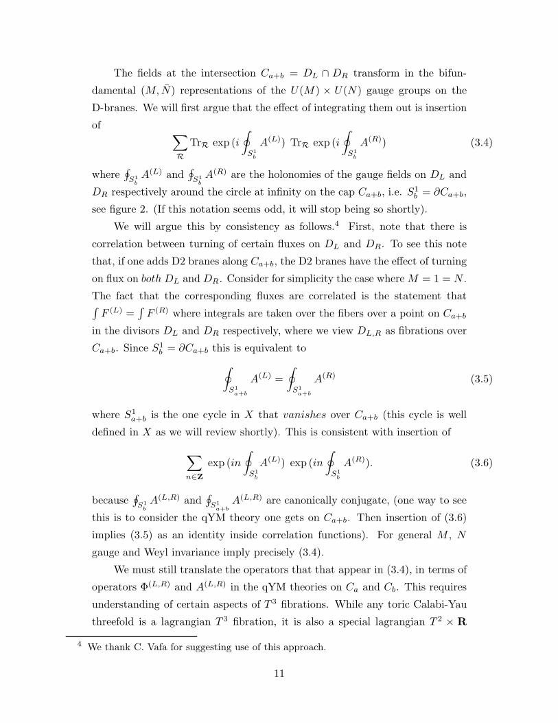
The fields at the intersection Ca+b = DL ∩ DR transform in the bifun-

damental (M, N) representations of the U(M) × U(N) gauge groups on the

D-branes. We will first argue that the effect of integrating them out is insertion

of∑

R

TrR exp (i

∮

S1b

A(L)) TrR exp (i

∮

S1b

A(R)) (3.4)

where∮

S1b

A(L) and∮

S1b

A(R) are the holonomies of the gauge fields on DL and

DR respectively around the circle at infinity on the cap Ca+b, i.e. S1b = ∂Ca+b,

see figure 2. (If this notation seems odd, it will stop being so shortly).

We will argue this by consistency as follows.4 First, note that there is

correlation between turning of certain fluxes on DL and DR. To see this note

that, if one adds D2 branes along Ca+b, the D2 branes have the effect of turning

on flux on both DL and DR. Consider for simplicity the case where M = 1 = N .

The fact that the corresponding fluxes are correlated is the statement that∫

F (L) =∫

F (R) where integrals are taken over the fibers over a point on Ca+b

in the divisors DL and DR respectively, where we view DL,R as fibrations over

Ca+b. Since S1b = ∂Ca+b this is equivalent to

∮

S1a+b

A(L) =

∮

S1a+b

A(R) (3.5)

where S1a+b is the one cycle in X that vanishes over Ca+b (this cycle is well

defined in X as we will review shortly). This is consistent with insertion of

∑

n∈Z

exp (in

∮

S1b

A(L)) exp (in

∮

S1b

A(R)). (3.6)

because∮

S1b

A(L,R) and∮

S1a+b

A(L,R) are canonically conjugate, (one way to see

this is to consider the qYM theory one gets on Ca+b. Then insertion of (3.6)

implies (3.5) as an identity inside correlation functions). For general M , N

gauge and Weyl invariance imply precisely (3.4).

We must still translate the operators that that appear in (3.4), in terms of

operators Φ(L,R) and A(L,R) in the qYM theories on Ca and Cb. This requires

understanding of certain aspects of T 3 fibrations. While any toric Calabi-Yau

threefold is a lagrangian T 3 fibration, it is also a special lagrangian T 2 × R

4 We thank C. Vafa for suggesting use of this approach.

11

fibration, where over each of the edges in the toric base a (p, q) cycle of the T 2

degenerates. The one-cycle which remains finite over the edge is ambiguous.

In the case of C3, we will choose a fixed basis of finite cycles (up to SL(2,Z)

transformations of the T 2 fiber), that will make the gluing rules particularly

simple.5 This is described in figure 2. In the figure, the 1-cycles of the T 2 that

vanish over Ca, Cb and Ca+b are S1a, S1

b , S1a+b, respectively. These determine

the point observables Φ’s in the qYM theories on the corresponding disk. We

have chosen a particular basis of the 1-cycles that remain finite. From the figure

it is easy to read off that

∮

S1b

A(L) =

∮

S1a+b

A(L) − Φ(L),

∮

S1b

A(R) = Φ(R),

which justifies (3.3). In the next subsection we will compute the qYM ampli-

tudes with these observables inserted.

3.2. Partition functions of qYM

Like ordinary two dimensional YM theory, the qYM theory is solvable

exactly [3]. In this subsection we will compute the YM partition functions with

the insertions of observables (3.3). In [3] it was shown that qYM partition

function Z(Σ) on an arbitrary Riemann surface Σ can be computed by means

of operatorial approach. Since the theory is invariant under area preserving

diffeomorphisms, knowing the amplitudes for Σ an annulus A, a pant P and a

cap C, completely solves the theory – amplitudes on any Σ can be obtained from

this by gluing. In the present case, we will only need the cap and the annulus

amplitudes, but with insertions of observables. Since the Riemann surfaces in

question are embedded in a Calabi-Yau, we are effectively sewing Calabi-Yau

manifolds, so one also has to keep track of the data of the fibration. The rules

of gluing a Calabi-Yau manifold out of C3 patches are explained in [15] and we

will only spell out their consequences in the language of 2d qYM.

In the previous subsection, the theory on divisors DL and DR in C3 was

equivalent to qYM theories on disks Ca and Cb, with some observable inser-

tions. These are Riemann surfaces with a boundary, so the corresponding path

5 In the language on next subsection, this corresponds to inserting precisely qpC2(R) to get

O(−p) line bundle

12

integrals define states in the Hilbert space of qYM theory on S1. Keeping the

holonomy U = Pei∮

A fixed on the boundary, the corresponding wave function

can be expressed in terms of characters of irreducible representations R of U(N)

as:

Z(U) =∑

R

ZR TrRU

The first thing we will answer is how to compute the corresponding states, and

then we will see how to glue them together. As we saw in the previous section,

the choice of the coordinate∮

S1 A on the boundary is ambiguous, as the choice

of the cycle which remains finite is ambiguous. This ambiguity is related to

the choice of the Chern class of a line bundle over a non-compact Riemann

surface, i.e. how the divisors DL,R are fibered over the corresponding disks.

The simplest choice is the one that gives trivial fibration, and this is the one

we made in figure 2 (this corresponds to picking the cycle that vanishes over

Ca+b).

The partition function on a disk with trivial bundle over it and no insertions

is

Z(C)(U) =∑

R∈U(N)

S0R eiθC1(R) TrRU, (3.7)

Above, C1(R) is the first casimir of the representation R, and SRP(N, gs) is a

relative of the S-matrix of the U(N) WZW model

SRQ(N, gs) =∑

w∈SN

ǫ(w)q−(R+ρN )·w(Q+ρN ), (3.8)

where

q = exp(−gs)

and SN is Weyl group of U(N) and ρN is the Weyl vector.6

Sewing ΣL and ΣR is done by

Z(ΣL ∪ ΣR) =

∫

dU Z(ΣL)(U) Z(ΣR)(U−1) =∑

R

ZR(ΣL)ZR(ΣR)

6 The normalization of the path integral is ambiguous. In our examples in sections 4-6 we will

choose it in such a way that the amplitudes agree with the topological string in the large N limit.

13

For example, the amplitude corresponding to Σ = P1 with O(−p) bundle over

it and no insertions can be obtained by gluing two disks and an annulus with

O(−p) bundle over it:

Z(A, p)(U1, U2) =∑

R∈U(N)

qpC2(R)/2 eiθC1(R) TrRU1 TrRU2 (3.9)

This gives

Z(P 1, p) =∑

R

(S0R)2qpC2(R)/2eiθC1(R) (3.10)

In addition we will need to know how to compute expectation values of

observables in this theory. As we will show in the appendix B, the amplitude

on a cap with a trivial line bundle and observable TrQ eiΦ−in

∮

S1A

inserted

equals

Z(C, TrQ eiΦ−in

∮

S1A)(U) =

∑

R

qn2 C2(Q)SQR(N, gs)TrRU. (3.11)

where U is the holonomy on the boundary.

It remains to compute the expectation value of the observables in (3.3) in

the two-dimensional theory on Ca and Cb. The amplitude on the intersecting

divisors DL, DR is

Z(V )(U (L), U (R)) =∑

Q∈U(M),P∈U(N)

VQP(M, N)TrQU (L)TrPU (R)

VQP(M, N) =∑

R∈U(M)

SQR(M, gs) q12C

(M)2 (R) SRP(N, gs)

(3.12)

In the above, U (L,R) is the holonomy at the boundary of Ca and Cb.

When M = N , there is a simpler expression for the vertex amplitude in

(3.12). Using the definition of SPR (3.8) and summing over R we have

VPQ = θN (q) q−12 C2(P) SPQq−

12 C2(Q) (3.13)

and where θ(q) =∑

m∈Zq

m2

2 . This is related to the familiar realization in WZW

models of the relation

STS = (TST )−1

between SL(2,Z) generators S and T in WZW models where

TRQ = q12 C2(R)δRQ, S−1

RP(gs, N) = SRP(−gs, N) = SRP(gs, N). (3.14)

The difference is that there is no quantization of the level k here. Even at a

non-integer level, this is more straightforward in the SU(N) case, where the

theta function in (3.13) would not have appeared.

14

3.3. Modular transformations

The partititon functions of D4 branes on various divisors with chemical

potentials

S4d =1

2gs

∫

trF ∧ F +θ

gs

∫

trF ∧ ω,

turned on, are computing degeneracies of bound-states of Q2 D2 branes and Q0

D0 branes with the D4 branes, where

Q0 =1

8π2

∫

trF ∧ F, Q2 =1

2π

∫

trF ∧ ω, (3.15)

so the YM amplitudes should have an expansion of the form

ZqYM =∑

q0,q1

Ω(Q0, Q2, Q4) exp

[

−4π2

gsQ0 −

2πθ

gsQ2

]

. (3.16)

The amplitudes we have given are not expansions in exp(−1/gs), but rather in

exp(−gs), so the existence of the (3.16) expansion is not apparent at all. The

underlying N = 4 theory however has S duality that relates strong and weak

coupling expansions, so we should be able to make contact with (3.16).

Since amplitudes on more complicated manifolds are obtained from the sim-

pler ones by gluing, it will suffice for us to show this for the propagators, vertices

and caps. Consider the annulus amplitude (3.9) Using the Weyl-denominator

form of the U(N) characters TrRU = ∆H(u)−1∑

w∈SN(−)ωeω(iu)·(R+ρN ) we

can rewrite Z(A, p) as

Z(A, p)(U, V ) = ∆H(u)−1∆H(v)−1∑

n∈ZN

∑

w∈SN

qp2 n2

en(iu−w(iv))

which is manifestly a modular form,7 which we can write

Z(A, p)(U, V ) = ∆H(u)−1∆H(v)−1(gsp

2π

)−N2

∑

m∈ZN

∑

w∈SN

q12p

(

m−u−w(v)

2π

)2

(3.17)

where in terms of q = e−4π2/gs . In the above, the eigenvalues Ui of U are

written as Ui = exp(iui), and ∆H(u) enters the Haar measure:

∫

dU =

∫

∏

i

dui∆H(u)2

7 Recall, θ(τ, u) = (−iτ)−12 e−iπ u2

τ θ(− 1τ, u

τ), where θ(τ, u) =

∑

n∈Zeiτn2

e2πiu.

15

Note that, in gluing, the determinant ∆H(u)2 factors cancel out, and simple

degeneracies will be left over.

Similarly, the vertex amplitude (3.12) corresponding to intersection of N

and M D4 branes can be written as (see appendix C for details):

Z(U, V ) = ∆H(u)−1∆H(v)−1θM (q)∑

m∈ZM

q−12m2

em·v∑

w∈SN

(−)w∑

n∈ZN

en(·w(iu)+iv−gs(ρN−ρM ))

(3.18)

where v, ρM are regarded as N dimensional vectors, the last N − M of whose

entries are zero. We see that Z(U, V ) is given in terms of theta functions, so it

is modular form, its modular transform given by

Z(U, V ) = ∆H(u)−1∆H(v)−1( gs

2π

)−M/2

θM (q)∑

m∈ZM

q−12 (m+iv/2π)2

∑

w∈SN

(−)w∑

n∈ZN

en(·w(iu)+iv−gs(ρN−ρM ))

(3.19)

In a given problem, it is often easier to compute the degeneracies of the BPS

states from the amplitude as a whole, rather than from the gluing the S-dual

amplitudes as in (3.19). Nevertheless, modularity at the level of vertices, prop-

agators and caps, demonstrates that the 1/gs expansion of our amplitudes does

exist in a general case.

4. Branes and black holes on local P2.

We will now use the results of the previous section to study black holes on

X = O(−3) → P2. As explained in section 2, to get large black holes on R3,1

we need to consider D4 branes wrapping very-ample divisors on X , which are

then necessarily non-compact. Moreover, the choice of divisor D that should

give rise to a dual of topological strings on X corresponds to

D = N1D1 + N2D2 + N3D3

where Di, i = 1, 2, 3 are the toric divisors of section 2.

Using the results of section 3, it is easy to compute the amplitudes corre-

sponding to the brane configuration. We have N1 ≥ N2 ≥ N3 D4 branes on

three divisors of topology Di = O(−3) → P1. From each, we get a copy of

16

quantum Yang Mills theory on P1 with p = 3, as discussed in section 3. From

the matter at the intersections, we get in addition, insertion of observables (3.3)

at two points in each P1.

N

N1

2 N 3

Fig. 3. Local P2, depicted as a toric web diagram. The numbers of D4 branes

wrapping the torus invariant non-compact 4-cycles are specified.

All together this gives:

ZqY M = α∑

Ri∈U(Ni)

VR2R1(N2, N1) VR3R2

(N3, N2) VR3R1(N3, N1)

3∏

j=1

q3C2(Ri)

2 eiθiC1(Ri)

(4.1)

Note that in the physical theory there should be only one chemical potential

for D2-branes, corresponding to the fact that H2(X,Z) is one dimensional. In

the theory of the D4 brane we H2(D,Z) is three dimensional, generated by the

3 P1’s in D – the three chemical potentials θi above couple to the D2 branes

wrapping these. While all of these D2 branes should correspond to BPS states

in the Yang-Mills theory, not all of them should correspond to BPS states once

the theory is embedded in the string theory. Because the three P1’s that the

D2 brane wrap are all homologous in H2(X,Z),

[P11] − [P1

3] ∼ 0, [P12] − [P1

3] ∼ 0

there will be D2 brane instantons that can cause those BPS states that carry

charges in H2(D,Z) to pair up into long multiplets. Decomposing H2(D,Z)

into a H2(D,Z)|| = H2(X,Z) and H2(D,Z)⊥, it is natural to turn off the the

chemical potentials for states with charges in H2(D,Z)⊥. This corresponds to

putting

θi = θ, i = 1, 2, 3.

17

For some part, we will keep the θ-angles different, but there is only one θ natural

in the theory.

The normalization α of the path integral is chosen in such a way that ZqY M

has chiral/anti-chiral factorization in the large Ni limit (see 4.6 and 4.10 below).

α = q−(ρ2N2

+N224 )q−2(ρ2

N3+

N324 ) e

(N1+N2+N3)θ2

6gs q(N1+N2+N3)3

72

The partition function simplifies significantly if we take equal numbers of

the D4 branes on each Di,

Ni = N, i = 1, 2, 3

since in this case, we can replace (3.12) form of the vertex amplitude with the

simpler (3.13), and the D-brane partition function becomes

ZqY M = α θ3N (q)∑

R1,R2,R3∈U(N)

SR1R2(gs, N) SR2R3

(gs, N) SR3R1(gs, N)

3∏

j=1

qC2(Ri)

2 eiθiC1(Ri)

(4.2)

In the following subsections we will first take the large Ni limit of ZqY M to

get the closed string dual of the system. We will then use modular properties

of the partition function to compute the degeneracies of the BPS states of D0-

D2-D4 branes.

4.1. Black holes from local P2

According to the conjecture of [1] (or more precisely, its version for the

non-compact Calabi-Yau manifolds proposed in [3]) the large N limit of the

D-brane partition function Zbrane, which in our case equals ZqY M , should be

given by

ZqY M (D, gs, θ) ≈∑

α

|Ztopα (t, gs)|

2

where

t =1

2(N1 + N2 + N3)gs − iθ

since [D] = (N1 + N2 + N3)[Dt] where [Dt] is dual to the class that generates

H2(X,Z). In the above, the two expressions should equal up to terms of order

18

O(exp(−1/gs)), hence the “approximate” sign. The sum over α is the sum over

chiral blocks which should correspond to the boundary conditions at infinity of

X . More precisely, the leading chiral block should correspond to including only

the normalizable modes of topological string on X , which count holomorphic

maps to P2, the higher ones containing fluctuation in the normal direction [3][9].

We will see below that this prediction is realized precisely.

The Hilbert space of the qYM theory, spanned by states labeled by repre-

sentations R of U(N), at large N splits into

HqY M ≈ ⊕ℓ H+ℓ ⊗H−

ℓ

where H+l and H−

l are spanned by representations R+ and R− with small

numbers of boxes as compared to N , and ℓ is the U(1) charge. Correspondingly,

the qYM partition function also splits as

ZqY M ≈∑

ℓ

Z+ℓ Z−

ℓ ,

where Z±ℓ are the chiral and anti-chiral partitions. We will now compute these,

and show that they are given by topological string amplitudes.

i. The Ni = N case.

We’ll now compute the large N limit of the D-brane partition function

(4.2) for Ni = N , i = 1, 2, 3. At large N , the U(N) Casimirs in representation

R = R+R−[ℓR] are given by

C2(R) = κR+ + κR− + N(|R+| + |R−|) + NℓR2 + 2ℓR(|R+| − |R−|),

C1(R) = NℓR + |R+| − |R−|(4.3)

where

κR =

N−1∑

i=1

Ri(Ri − 2i + 1)

and |R| is the number of boxes in R.

19

The S-matrix SRQ is at large N given in [9]

q−(ρ2+ N24 )SRQ(−gs, N) =M(q−1)η(q−1)N (−)|R+|+|R−|+|Q+|+|Q−|

×qNℓRℓQqℓQ(|R+|−|R−|)qℓR(|Q+|−|Q−|)qN(|R+|+|R−|+|Q+|+|Q−|)

2

×qκR+

+κR−2

∑

P

q−N|P |(−)|P |CQT+

R+P (q)CQT−

R−P T (q).

(4.4)

The amplitude CRPQ(q) is the topological vertex amplitude of [15].8 In (4.4)

M(q) and η(q) are MacMahon and Dedekind functions.

Putting this all together, let us now parameterize the integers ℓRias follows

3ℓ = ℓR1+ ℓR2

+ ℓR3, 3n = ℓR1

− ℓR3, 3k = ℓR2

− ℓR3.

It is easy to see that the sum over n and k gives delta functions: at large N

ZqY M (θi, gs) ∼ δ(

N(θ1 − θ3))

δ(

N(θ2 − θ3))

× ZfiniteqY M (θ, gs) (4.5)

where θi = θ in the finite piece. As we will show in Sec. 4.2 there is the same

δ-function singularity as in the partition function of the bound-states of N D4

branes. There it will be clear that it comes from summing over D2 branes with

charges in H2(X,D)⊥, as mentioned at the beginning of this section. The finite

piece in (4.5) is given by

ZfiniteqY M (N, θ, gs) =

∑

m∈Z

∑

P1,P2,P3

(−)∑

3

i=1|Pi|Z+

P1,P2,P3

(

t + mgs

)

Z+P T

1 ,P T2 ,P T

3

(

t−mgs

)

. (4.6)

The chiral block in (4.6) is the topological string amplitude on X = O(−3) →

P2,

Z+P1,P2,P3

(t) = Z0(gs, t)e−t0

∑

i|Pi|

∑

R1,R2,R3

e−t∑

i|Ri|q

∑

iκRi CRT

2 R1P T1

(q) CRT3 R2P T

2(q) CRT

1 R3P T3

(q)

(4.7)

where t0 = −12Ngs and the Kahler modulus t is (we will return to the meaning

of t0 shortly):

t =3Ngs

2− iθ.

8 The conventions of this paper and [15] differ, as here q = e−gs , but qthere = egs , con-

sequently the topological vertex amplitude CRP Q of [15] is related to the present one by

CRP Q(q) = CRP Q(q−1).

20

More precisely, the chiral block with trivial ghosts Pi = 0,

Z+0,0,0(t, gs) = Ztop(t, gs)

is exactly equal to the perturbative closed topological string partition function

for X = O(−3) → P2, as given in [15]. This exactly agrees with the prediction

of [1].

The prefactor Z0(gs, t) is given by

Z0(gs, t) = e− t3

18g2s M3(q−1)η

tgs (q−1)θ

tgs (q)

As explained in [3] the factor ηt

gs ∼ η3N2 comes from bound states of D0 and

D4 branes [14] without any D2 brane charge, and moreover, it has only genus

zero contribution perturbatively.

ηt

gs ∼ exp

(

−π2t

6g2s

)

+ (non − perturbative)

The factor θt

gs comes from the bound states of D4 branes with D2 branes along

each of three the non-compact toric legs in the normal direction to the P2, and

without any D0 branes. This gives no perturbative contributions

θt

gs ∼ 1 + (non − perturbative)

The subleading chiral blocks correspond to open topological string amplitudes

in X with D-branes along the fiber direction to the P2, which can be computed

using the topological vertex formalizm [15]. The appearance of D-branes was

explained in [9] where they were interpreted as non-normalizable modes of the

topological string amplitudes on X . The reinterpretation in terms of non-

normalizable modes of the topological string theory is a consequence of the

open-closed topological string duality on [16]. While this is a duality in the

topological string theory, in the physical string theory the open and closed

string theory are the same only provided we turn on Ramond-Ramond fluxes.

We cannot do this here however, since this would break supersymmetry, and

the only correct interpretation is the closed string one.

To make contact with this, define

Z+(U1, U2, U3) =∑

R1,R2,R3

Z+R1,R2,R3

TrR1U1 TrR2

U2 TrR3U3.

21

where Ui are unitary matrices. This could be viewed as an open topological

string amplitude with D-branes, or more physically, as the topological string

amplitude, with non-normalizable deformations turned on. These are not most

general non-normalizable deformations on X , but only those that preserve torus

symmetries – correspondingly they are localized along the non-compact toric

legs, just like the topological D-branes that are dual to them are. The non-

normalizable modes of the geometry can be identified with [16]

τni = gstr(U

ni )

where the trace is in the fundamental representation. We can then write (4.6)

as

Zfinite ∼

∫

dU1 dU2 dU3 |Z+(U1, U2, U3)|2

where we integrate over unitary matrices provided we shift

U → Ue−t0

where t0 = −12Ngs. This shift is the attractor mechanism for the non-

normalizable modes of the geometry [9]. In terms of the natural variables tni,

related by τni = exp(−tni ) to τ ’s we have

tni = nt0 (4.8)

This comes about as follows [9]. First note that size of any 2-cycle C in the

geometry should be fixed by the attractor mechanism to equal its intersection

with the 4-cycle class [D] of the D4 branes, in this case [D] = 3N [Dt]. The

relevant 2-cycle in this case is a disk C0 ending on the topological D-brane.

The real part of tni measures the size of an n-fold cover of this disk (there is no

chemical potential, i.e. t0 is real, since there is associated BPS state of finite

mass). Then (4.8) follows because

#(C0 ∩ D) = −N.

To see this note that in homology, the class 3N [Dt] could equally well be repre-

sented by −N D-branes on the base P2 and the latter has intersection number

22

1 with C0. The factor of n in (4.8) comes about since tn corresponds to the size

of the n-fold cover of the disk.

ii. The general Ni case.

The case N1 > N2 > N3 is substantially more involved, and in particular,

the large N limit of the amplitudes (3.12)(4.1) is not known. However, as we will

explain in the appendix D, turning off the U(1) factors of the gauge theory,

the large N limit can be computed, and we find a remarkable agreement with

the conjecture of [1].

Let us focus on the leading chiral block of the amplitude. The large N , M

limit of the interaction VQR(M, N) (more precisely, the modified version of it

to turn off the U(1) charges) is

VQR ∼ βM q(|Q+|+|Q−|)(N−M)

2 q(|R+|+|R−|)(M−N)

2

q−(κR+

+κR−+κQ+

+κQ−)

2 WQ+R+(q) WQ−R−

(q)

(4.9)

where

βM = q(ρ2M+ M

24 )M(q−1)ηM (q−1)θM(q)

In (4.9) the WPR is related to the topological vertex amplitude as

WPR(q) = (−)|P |+|R|C0P T R(q)qκR/2. It is easy to see that for N = M this

agrees with the large N limit of the simpler form of the VRQ amplitude in

(3.13). It is easy to see that that the leading chiral block of (4.1) is

ZqY M ∼ Z+0,0,0

(

t)

Z−0,0,0

(

t)

(4.10)

where Z+0,0,0(t) is

Z+0,0,0 = Z0

∑

R+,Q+,p+

WR+Q+(q)WQ+P+

(q)WP+R+(q)e−t(|R+|+|Q+|+|P+)

which is the closed topological string amplitude on X . In particular, this agrees

with the amplitude in (4.7). In the present context, the Kahler modulus t is

given by

t =1

2(N1 + N2 + N3)gs − iθ.

23

This is exactly as dictated by the attractor mechanism corresponding to the

divisor [D] = (N1 + N2 + N3)[Dt]!

The higher chiral blocks will naturally be more involved in this case. Some

of the intersection numbers fixing the attractor positions of ghost branes are

ambiguous, and correspondingly, far more complicated configurations of non-

normalizable modes are expected.

4.2. Branes on local P2

In this and subsequent section we will discuss the degeneracies of BPS

states that follow from (4.1). Using the results of (3.17) and (3.18) or by direct

computation, it is easy to see that ZqY M is a modular form. Its form however

is the simplest in the case

N1 = N2 = N3 = N,

so let us treat this first.

i. Degeneracies for Ni = N.

In this case, the form of the partition function written in (4.2) is more

convenient. By trading the sum over representations and over the Weyl-group,

as in (3.18), for sums over the weight lattices, the partition function of BPS

states is

ZqY M (N, θi, gs) = β∑

w∈SN

(−)w∑

n1,n2,n3∈ZN

q12

∑

3

i=1n2

i qw(n1)·n2+n2·n3+n3·n1 ei∑

3

i=1θie(N)·ni

(4.11)

where e(N) = (1, . . . , 1) and β = αθ3N(q). The amplitudes depend on the

permutations w only through their conjugacy classes, consequently we have:

ZqY M = β∑

~K

d( ~K) ZK1× . . .× ZKr

(4.12)

where ~K labels a partition of N into natural numbers N =∑r

a=1 Ka, and d( ~K)

is the number of elements in the conjugacy class of SN , the permutation group

of N elements, corresponding to having r cycles of length Ka, a = 1, . . . , r, and

ZK(θi, gs) = (−)wK

∑

n1,n2,n3∈ZK

q12

∑3

i=1n2

i qwK(n1)·n2+n2·n3+n3·n1 ei∑3

i=1θie(K)·ni (4.13)

24

Here wK stands for cyclic permutation of K elements. Note that the form of the

partition function (4.12) suggests that ZqY M is counting not only BPS bound

states, but also contains contribution from marginally bound states correspond-

ing to splitting of the U(N) to

U(N) → U(K1) × U(K2) × . . .× U(Kr)

In each of the sectors, the quadratic form is degenerate. The contribution of

bound states of N branes ZN diverges as

ZN (θi, gs) ∼∑

m1,m2∈Z

eiNm1(θ1−θ3)eiNm2(θ2−θ3) = δ(

N(θ1 − θ3))

δ(

N(θ2 − θ3))

This is exactly the type of the divergence we found at large N in the previous

subsection. This divergence should be related to summing over D2 branes with

charges in H2(D,Z)⊥ – these apparently completely decouple from the rest of

the theory.

More precisely, writing U(N) = U(1) × SU(N)/ZN , this will have a sum

over ’t Hooft fluxes which are correlated with the fluxes of the U(1). Then, ZN

is a sum over sectors of different N -ality,

ZN (θi, gs) = (−)wN

N−1∑

Li=0

∑

ℓi∈Z+LiN

qN2 (ℓ1+ℓ2+ℓ3)

2

eiN∑

iθiℓi

∑

m∈Z3(N−1)+~ξ(Li)

q12 mT MN m

where MN is a non-degenerate 3(N −1)×3(N −1) matrix with integer entries

and ~ξi is a shift of the weight lattice corresponding to turning on ’t Hooft flux.

Explicitly,

ξai =

N − a

NLi, i = 1, 2, 3 a = 0, . . .N − 1

where MN is 3(N − 1) × 3(N − 1) matrix

MN =

MN WN MN

WTN MN MN

MN MN MN

(4.14)

whose entries are

MN =

2 −1 0 . . . 0 0−1 2 −1 . . . 0 00 −1 2 . . . 0 0. . . . . . . .. . . . . . . .0 0 0 . . . −1 2

(4.15)

25

and

WN =

−1 2 −1 . . . 0 00 −1 2 . . . 0 00 0 −1 . . . . 0. . . . . . . .. . . . . . . .

−1 0 0 . . . 0 −1

(4.16)

We can express ZN in terms of Θ-functions

ZN (θi, gs) = (−)wN δ(

N(θ1 − θ3))

δ(

N(θ2 − θ3))

N−1∑

Li=0

Θ1[a(Li), b](τ) Θ3N−3[a(Li),b](τ)

where

Θk[a, b](τ) =∑

n∈Zk

eπiτ(n+a)2 e2πinb

and

τ =igs

2πN, τ =

igs

2πMN

a =L1 + L2 + L3

N, b =

N

2πθ, aL = ~ξ(L), b = 0,

The origin of the divergent factor we found is now clear: from the gauge theory

perspective it simply corresponds to a partition function of a U(1) ∈ U(N)

gauge theory on a 4−manifold whose intersection matrix is degenerate: #(Ci ∩

Cj) = 1, i, j = 1, 2, 3. More precisely, to define the intersection form of the

reducible four-cycle D, note that D is homologous to the (punctured) P2 in

the base, with precisely the intersection form at hand. The contribution of

marginally bound states with multiple U(1) factors have at first sight a worse

divergences, however these can be regularized by ζ-function regularization to

zero.9 This is a physical choice, since in these sectors we expect the partition

function to vanish due to extra fermion zero modes [14][17].

To extract the black hole degeneracies we use that the matrix MN is non-

degenerate and do modular S-transformation using

Θ[a, b](τ) = det(τ)−12 e2πiabΘ[b,−a](−τ−1)

9 For example, ZN−M(θi, gs)ZM(θi, gs) ∼ δ(

k(θ1 − θ3))

×∑

n∈Z1 × δ

(

k(θ2 − θ3))

×∑

n∈Z1.

where k is the least common divisor of N,M . Using ζ(2s) =∑

∞

n=11/n2s, where ζ(0) = −

12, we

can regularize∑

n∈Z1 = 0.

26

This brings ZN to the form

ZN (θi, gs) = δ(

N(θ1 − θ3))

δ(

N(θ2 − θ3))

(−)wN

(

2π

Ngs

)12

(

2π

gs

)

3(N−1)2

det−12MN

N−1∑

Li=0

∑

ℓ∈Z

e−2π2

Ngs(ℓ+ Nθ

2π)2e−

2πi(L1+L2+L3)

Nℓ

∑

m∈Z3(N−1)

e−2π2

gsmTM−1

Nme−2πim·ξ(Li)

where MN is the matrix in (4.14).

ii. Degeneracies for N1 > N2 > N3.

When the number of branes is not equal the partition sum ZqY M is sub-

stantially more complicated. By manipulations similar to the ones in appendix

B, ZqY M can be written as:

ZqY M = αθN2+2N3(q)∑

ν∈SN1

(−)ν∑

n1∈ZN1

∑

n2∈ZN2

∑

n3∈ZN3

q12 (n2

1−n23)qn2·ν(n1)+n3·n2+n3·n1

q−12 n1(ν−1PN1|N2

ν)n1q−12n2PN2|N3

n2q−12 n1PN1|N3

n1

q−ν(n1)·(ρN1−ρN2

)q−n2·(ρN2−ρN3

)q−n1·(ρN1−ρN3

)eiθ1e(N1)·n1+iθ2e(N2)·n2+iθ3e(N3)·n3

where operator PN|M projects N -dimensional vector on its first M components.

For example, consider N1 = 3, N2 = 2, N3 = 1. In this case there are six

terms in the sum

ν1 =

1 0 00 1 00 0 1

, ν2 =

0 1 01 0 00 0 1

, ν3 =

1 0 00 0 10 1 0

ν4 =

0 0 10 1 01 0 0

, ν5 =

0 1 00 0 11 0 0

, ν6 =

0 0 11 0 00 1 0

In this simple case ZqY M has the form

ZqY M = αθ4(q′)

(

π

gs

)2(

Z1 − Z2 − Z3 − Z4 + Z5 + Z6

)

q′ = e−π2

gs

where

Zi =

(

2π

gs

)3

det−12M(i)

∑

f∈Z6

e− 2π2

gs(f+Λ(i))

T M−1(i)

(f+Λ(i))

27

where non-degenerate matrices M(i) for i = 1, . . .6 are given by

M(1) =

1 0 0 0 0 00 −1 0 1 0 10 0 0 0 1 00 1 0 −1 0 10 0 1 0 0 00 1 0 1 0 −1

, M(2) =

1 0 0 0 0 00 −1 0 1 0 10 0 0 0 1 00 1 0 0 0 00 0 1 0 −1 10 1 0 0 1 −1

M(3) =

0 0 0 1 0 00 −1 0 0 1 10 0 1 0 0 01 0 0 0 0 00 1 0 0 −1 10 1 0 0 1 −1

, M(4) =

0 0 0 0 1 00 0 0 0 0 10 0 0 1 0 00 0 1 0 0 01 0 0 0 −1 10 1 0 0 1 −1

M(5) =

0 0 0 1 0 00 0 0 0 0 10 0 0 0 1 01 0 0 0 0 00 0 1 0 −1 10 1 0 0 1 −1

, M(6) =

0 0 0 0 1 00 −1 0 1 0 10 0 1 0 0 00 1 0 0 0 01 0 0 0 −1 10 1 0 0 1 −1

and vectors Λ(i) for i = 1, . . . , 6 have components

Λ(1) =1

2π(θ1, θ1, θ1, θ2, θ2, θ3) +

igs

2π(2,−

3

2,−

1

2,−

1

2,1

2, 0)

Λa(2) = Λa

(1), a = 1, . . . , 6

Λ1(3) =

1

2π(θ1, θ1, θ1, θ2, θ2, θ3) +

igs

2π(1

2,−

3

2, 1,

1

2,−

1

2, 0)

Λa(6) = Λa

(3), a = 1, . . . , 6

Λ1(4) =

1

2π(θ1, θ1, θ1, θ2, θ2, θ3) +

igs

2π(1

2, 0,−

1

2,1

2,−

1

2, 0)

Λa(5) = Λa

(4), a = 1, . . . , 6

28

5. Branes and black holes on local P1 ×P1

For our second example, we will take a noncompact Calabi-Yau threefold

X which is a total space of canonical line bundle K over the base B = P1B ×P1

F

X = K → P1B × P1

F

where K = O(−2,−2). The linear sigma model whose Higgs branch is X has

chiral fields Xi, i = 0, . . .4 and two U(1) gauge fields U(1)B and U(1)F un-

der which the chiral fields have charges (−2, 1, 0, 1, 0) and (−2, 0, 1, 0, 1). The

corresponding D-term potentials are

|X1|2 + |X3|

2 = 2|X0|2 + rB

|X2|2 + |X4|

2 = 2|X0|2 + rF

The H2(X, Z) is generated by two classes [DF ] and [DB ]. Correspondingly,

there are two complexified Kahler moduli tB and tF , tB = rB − iθB and tF =

rF − iθF . There are 4 ample divisors invariant under the T 3 torus actions

corresponding to setting

Di : Xi = 0, i = 1, 2, 3, 4

We have that [D1] = [D3] = [DB ] and [D2] = [D4] = [DF ]. We take N1 and N2

D4 branes on D1 and D3, and M1 and M2 D4 branes on D2 and D4 respectively,

corresponding to a divisor

D = N1D1 + M1D2 + N2D3 + M2D4

Since the topology of each Di is O(−2) → P1 we will get four copies of qYM

theory of P1 with ranks N1,2 and M1,2. In addition, from the matter at in-

tersection we get 4 sets of insertions of observables (3.3). All together, and

assuming N1,2 ≥ M1,2, we have

ZqY M = γ∑

R1,R2,Q1,Q2

VQ1R1VQ2R2

VR1Q2VR2Q1

q∑2

i=1C2(Ri)+C2(Qi)

eiθB,1C1(R1)+iθB,2C1(R2)eiθF,1C1(Q1)+iθF,2C1(Q2).

(5.1)

29

Above, R1,R2 are representationss of U(N1) and U(N2) and Q1,Q2 are repre-

sentations of U(M1) and U(M2), respectively.

N 2

M1 M

N 1

2

Fig. 4. The base of the local P1× P1. The numbers of D4 branes wrapping the

torus invariant non-compact 4-cycles are specified. This corresponds to qYM theory

on the neclace of 4 P1’s with ranks M1, N1, M2, and N2.

In principle, because dim(H2(D,Z)) = 4, there 4 different chemical po-

tentials that we can turn on for the D2 branes, corresponding to θB,i, θF,i.

In X however, there are only two independent classes, dim(H2(D,Z)) = 2, in

particular

[P1B,1] − [P1

B,2] = 0, [P1F,1] − [P1

F,2] = 0

We should turn off the chemical potentials for those states that can decay when

the YM theory is embedded in string theory, by putting

θB,1 = θB,2, θF,1 = θF,2. (5.2)

For the most part, we will keep the chemical potentials arbitrary, imposing (5.2)

at the end. The prefactor γ is

γ = q−(

2ρ2M1

+M112

)

q−(

2ρ2M2

+M212

)

q− 1

96

(

(N1+N2)3+(M1+M2)3−3(N1+N2)

2(M1+M2)−3(M1+M2)2(N1+N2)

)

× eθBθF (N1+N2+M1+M2)

4gs

In the next subsections we will first take the large N limit of the qYM parti-

tion function, and then consider the modular properties of the exact amplitude

to compute the degeneracies of the BPS bound states.

30

5.1. Black holes on local P1 × P1.

We will now take the large N limit of ZqY M in (5.1) and show that this is

related to the topological string on X in accordance with the [1] conjecture.

i. The N1 = N2 = N = M1 = M2 case.

In this case, we can use the simpler form of the vertex amplitude in (3.12)

to write the q-deformed Yang-Mills partition function as:

ZqY M = γ′∑

R1,2,Q1,2∈U(N)

SR1Q1(gs, N) SQ1R2

(gs, N) SR2Q2(gs, N) SQ2R1

(gs, N)

× ei∑

iθB,iC1(Ri)+iθF,iC1(Qi).

(5.3)

where γ′ = γθ4N(q). Using the large N expansion for S-matrix (4.4) and

parametrizing the U(1) charges ℓRiof the representations Ri as follows

2ℓB = ℓR1+ ℓR2

, 2ℓF = ℓQ1+ ℓQ2

, 2nB = ℓR1− ℓR2

, 2nF = ℓQ1− ℓQ2

, (5.4)

we find that the sum over nB,F gives delta functions

ZqY M (N, gs, θB,i, θF,i) ∼ δ(

N(θB,1 − θB,2))

δ(

N(θF,1 − θF,2))

ZfiniteqY M (N, gs, θB, θF )

where

ZfiniteqY M ∼

∑

mB,mF ∈Z

∑

P1,...,P4

(−)∑

4

i=1|Pi|Z+

P1,...,P4

(

tB + mBgs, tF + mF gs

)

Z+P T

1 ,...,P T4

(

tB − mBgs, tF − mF gs

)

(5.5)

In (5.5) the chiral block Z+P1,...,P4

(tB, tF ) is given by

Z+P1,...,P4

(tB , tF ) =Z0(gs, tB, tF )e−t0∑4

i=1|Pi|

∑

R1,R2,Q1,Q2

e−tB(|R1|+|R2|)e−tF (|Q1|+|Q2|)

× q12

∑

i=1,2κRi

+κQi CQT1 R1P1

(q) CRT2 Q1P2

(q) CQT2 R2P3

(q) CRT1 Q2P4

(q)

(5.6)

where Kahler moduli are

tB = gsN − iθB , tF = gsN − iθF .

31

The leading chiral block Z+0,...,0 is the closed topological string amplitude on X.

The Kahler moduli of the base P1B and the fiber P1

F are exactly the right values

fixed by the attractor mechanism: since the divisor D that the D4 brane wraps

is in the class [D] = 2N [DF ]+2N [DB ]. As we discussed in the previous section

in detail, the other chiral blocks (5.6) correspond to having torus invariant

non-normalizable modes excited along the four non-compact toric legs in the

normal directions to the base B. Moreover the associated Kahler parameters

should also be fixed by the attractor mechanism – as discussed in the previous

section, we can think of these as the open string moduli corresponding to the

ghost branes. The open string moduli are complexified sizes of holomorphic

disks ending on the ghost branes and these can be computed using the Kahler

form on X . Since the net D4 brane charge is the same as that of −N branes

wrapping the base, and the intersection number of the disks C0 ending on the

topological D-branes with the base is #(C0 ∩B) = 1, so the size of all the disks

ending on the branes should be t0 = −12Ngs, which is in accord with (5.6). The

prefactor in (5.6) is

Z0(gs, tB, tF ) = e1

24g2s

(

t3F +t3B−3t2F tB−3t2BtF

)

M4(q−1)ηtB+tF

gs (q−1)θtB+tF

gs (q)

As discussed before, the eta and theta function pieces contribute only to the

genus zero amplitude, and to the non-perturbative terms.

ii. The general N1,2, M1,2 case.

We will assume here Ni > Mj , i, j = 1, 2. Using the large N , M limit of

VRQ(N, M) with U(1) charges turned off (see Appendix D) we find that the

leading chiral block of the YM partition function is

ZqY M ∼ Z+0,...,0

(

tB , tF)

Z−0,...,0

(

tB , tF)

where Z+0,...,0

(

tB , tF)

is precisely the topological closed string partition function

on local P1 ×P1 [15] :

Z+0,...,0 = Z0

∑

Q+1 ,Q+

2 ,R+1 ,R+

2

WQ+1 R+

1(q)WQ+

1 R+2(q)WQ+

2 R+1(q)WQ+

2 R+2(q)e−tF (|Q+

1 |+|Q+2 |)e−tB(|R+

1 |+|R+2 |)

32

It is easy to see that this agrees with the amplitude given in (5.6). Moreover,

the Kahler parameters are exactly as predicted by the attractor mechanism

corresponding to having branes on a divisor class

[D] = (N1 + N2)[DB ] + (M1 + M2)[DF ].

Namely,

tB =1

2(M1 + M2)gs − iθB, tF =

1

2(N1 + N2)gs − iθF .

Note that the normal bundle to each of the divisor Di is trivial, so the size of

the corresponding P1 in Di = O(−2) → P1 is independent of the number of

branes on Di, but it does depend on the number of branes on the adjacent faces

which have intersection number 1 with the P1.

It would be interesting to study the structure of the higher chiral blocks.

In this case we expect the story to be more complicated, in particular because

some of the intersection numbers that compute the attractor values of the brane

moduli are now ambiguous.

5.2. Branes on local P1 ×P1

We will content ourselves with considering N1,2 = M1,2 = N case, the

more general case working in similar ways to the local P2 case. The partition

function (5.3) may be written as

ZqY M (N, θi, gs) = γ′∑

w∈SN

(−)w∑

n1,...,n4∈ZN

qw(n1)·n2+n2·n3+n3·n4+n4·n1 ei∑

4

i=1θie(N)·ni

(5.7)

where e(N) = (1, . . . , 1). As before in the case of local P2, the bound states

of N D4-branes are effectively counted by the ZN term, i.e. the term with

w = wN . Like in that case, ZN is again a sum over sectors of different N -ality,

ZN (θi, gs) = γ′ (−)wN

N−1∑

L1,...,L4=0

∑

ℓi∈Z+LiN

qN(ℓ1+ℓ3)(ℓ2+ℓ4)eiN∑4

i=1θiℓi

∑

m∈Z4(N−1)+~ξ(Li)

q12 mTMm

where M is a non-degenerate 4(N − 1) × 4(N − 1) matrix with integer entries

and ~ξi is a shift of the weight lattice corresponding to turning on ’t Hooft flux.

33

More explicitly,

ξai =

N − a

NLi, i = 1, . . . , 4 a = 0, . . .N − 1

M is 4(N − 1) × 4(N − 1) matrix

M =

0 WN 0 MN

WTN 0 MN 00 MN 0 MN

MN 0 MN 0

(5.8)

whose entries are (N − 1) × (N − 1) matrices

MN =

2 −1 0 0 . . . 0 0−1 2 −1 0 . . . 0 00 −1 2 −1 . . . 0 0. . . . . . . . .. . . . . . . . .0 0 0 0 . . . −1 2

(5.9)

and

WN =

−1 2 −1 0 . . . 0 00 −1 2 −1 . . . 0 00 0 −1 2 . . . . 0. . . . . . . . .. . . . . . . . .0 0 0 0 . . . −1 2

−1 0 0 0 . . . 0 −1

(5.10)

We can express ZN in terms of Θ-functions

ZN (θi, gs) =γ′ (−)wN δ(

N(θB,1 − θB,2))

δ(

N(θF,1 − θF,2))

N−1∑

L1,...,L4=0

Θ2[a(Li), b](τ) Θ4N−4[a(Li),b](τ)

where

Θk[a, b](τ) =∑

n∈Zk

eπiτ(n+a)2 e2πinb

and

τ =igs

2πN

(

0 11 0

)

, τ =igs

2πM

and

a =(L1 + L3

N,L2 + L4

N

)

, b =( N

2πθB,

N

2πθF

)

aL = ~ξ(L), b = 0,

34

To extract black hole degeneracies we use that matrix M is non-degenerate and

do modular S-transformation using

Θ[a, b](τ) = det(τ)−12 e2πiabΘ[b,−a](−τ−1)

After modular S-transformation ZN is brought to the form

ZN (θ, gs) =γ′ δ(

N(θB,1 − θB,2))

δ(

N(θF,1 − θF,2))

(−)wN

(

2π

Ngs

) (

2π

gs

)

4(N−1)2

det−12M

N−1∑

L1,...,L4=0

∑

ℓ,ℓ′∈Z

e−π2

Ngs(ℓ+

NθB2π

)(ℓ′+NθF2π

)e−2πi(L1+L3)

Nℓe−

2πi(L2+L4)N

ℓ′

∑

m∈Z4(N−1)

e−2π2

gsmT M−1me−2πim·ξ(Li)

6. Branes and black holes on Ak ALE space

Consider the local toric Calabi Yau X which is Ak ALE space times C.

This can be thought of as the limit of the usual ALE fibration over P1 as the

size of the base P1 goes to ∞. In this section we will consider black holes

obtained by wrapping N D4 branes on the ALE space.

kA

Fig. 5. N D4-branes are wrapped on Ak type ALE space in Ak ×C, for k = 3. The

D-brane partition function is computed by U(N) qYM theory on a chain of 3 P1’s.

35

This example will have a somewhat different flavor than the previous two,

so we will discuss the D4 brane gauge theory on a bit more detail. On the one

hand, the theory on the D4 brane is a topological U(N) Yang-Mills theory on

Ak ALE space which has been studied previously [18][14]. On the other hand,

the Ak ALE space has T 2 torus symmetries, so we should be able to obtain

the corresponding partition function by an appropriate computation in the two

dimensional qYM theory. We will start with the second perspective, and make

contact with [18][14] later.

As in [3] and in section 3, our strategy will be to cut the four manifold

into pieces where the theory is simple to solve, and then glue the pieces back

together. The Ak type ALE space can be obtained by gluing together k + 1

copies of C2. Correspondingly, we should be able to obtain YM amplitudes

on the ALE space by sewing together amplitudes on C2. Moreover, since the

C2 and the ALE space have T 2 isometries, the 4d gauge theory computations

should localize to fixed points of these isometries, and these are bundles with

second Chern class localized at the vertices, and first Chern class along the

edges.

Viewed as a manifold fibered by 2-tori T 2, C2 has contains two disks, say

Cbase and Cfiber that are fixed by torus action (see figure 2 by way of example).

Viewed as a line bundle over a disk Cbase as a base, the U(1) isometry of the

fiber allows us to do some gauge theory computations in the qYM theory on

Cbase. In particular, if the bundle is flat the qYM partition function on a disk

(3.7) with holonomy U = exp (i∮

A) fixed on the boundary of the Cbase fixed

and no insertions is10

Z(C)(U) =∑

R

eiθC1(R)S0R(N, gs)TrRU.

What is the four dimensional interpretation of this? The sum over R in the

above corresponds to summing over the four dimensional U(N) gauge fields

with∫

fiber

Fa = Ra gs, a = 1, . . .N, (6.1)

10 More precisely, as we explained in section 3, the coordinate U is ambiguous since the choice

of cycle which remains finite is ambiguous. This ambiguity relates to the choice of the normal

bundle to the disk, and the present choice corresponds to picking this bundle to be trivial, which

is implicit in the amplitude.

36

where Ra are the lengths of the rows in the Young tableau of R.11 This is

because on the one hand

S0R(N, gs) = 〈 TrR ei∮

A 〉. (6.2)

and on the other∮

Aa =∫

baseFa is conjugate to Φa =

∫

fiberFa, so inserting

(6.2) shifts F as in (6.1). The unusual normalization of F has to do with the

fact that qYM directly computes the magnetic, rather than the electric partition

function: In gluing two disks to get an P1 we sum over all R’s labelling the

bundles of the S-dual theory over the P1.

If we are to use 2d qYM theory to compute the N = 4 partition function

on ALE space, we must understand what in the 2d language is computing the

partition function on C2 with

∫

fiber

Fa = Ra gs,

∫

base

Fa = Qa gs, a = 1, . . .N, (6.3)

since clearly, what we call the “base” here versus the “fiber” is a matter of

convention. Using once more the fact that Φ and∮

A are conjugate, turning

on∫

baseFa = Qags corresponds to inserting TrQ e−iΦ at the point on Cbase

where it intersects Cfiber. Thus, turning on (6.3) corresponds to computing

〈TrQe−iΦ TrR ei∮

A 〉. This is an amplitude we already know:

SQR(N, gs) = 〈TrQe−iΦ TrRei∮

A 〉. (6.4)

Alternatively, the amplitude on C2 with arbitrary boundary conditions (6.3)

on the base and on the fiber is

∑

R,Q

SRQ(N, gs) TrRU TrQV (6.5)

We then glue the pieces together using the usual local rules. The only thing

we have to remember is that the normal bundle to each P1 is O(−2), and that

at the “ends” we should turn the fields off. In computing (6.4) we used the

coordinates in which C2 is a trivial fibration over both Cfiber and Cbase, and

therefore to get the first Chern class of the normal bundle to come out to be

11 To be more precise, Ra in (6.1) is shifted by 12(N + 1) − a.

37

−2, we must along each of them insert annuli with O(−2) bundle over them.

This gives:

Z =∑

R1...Rk

S0R(1)SR(1)R(2)

. . . SR(k)0 q∑

C2(R(j)) ei∑

θj |R(j)|, (6.6)

There is one independent θ angle for each P1 corresponding to the fact that they

are all independent in homology. These θ angles will get related to chemical

potentials for the D2 branes wrapping the corresponding 2-cycles.

6.1. Modularity

The S-duality of N = 4 Yang Mills acts on our partition function as gs →4π2

gs. By performing this modular transformation we will be able to read off the

degeneracies of the BPS bound states contributing to the entropy. First, using

the definition of the Chern Simons S-matrix, we find that

Z =∑

ω∈W

(−1)ω∑

n1,...nk∈ZN

qn21+...+n2

k−n1n2−...−nk−1nk eiθ1|n1|+...θk|nk|qρn1+nkω(ρ) (6.7)

Note the appearance of the intersection matrix of Ak ALE space. The fact

that the Cartan matrix appears gives the k vectors U(N) weight vectors nai

i = 1, . . . k, a = 1, . . .N an alternative interpretation as N SU(k) root vectors:

Z =∑

ω∈W

(−1)ωN∏

a=1

∑

na∈ΛRootSU(k)

q12 nana eiθnaq(ρ+ω(ρ))ana

where θ is a k-dimensional vector with entries θi. From the above, it is clear

that Z is a product of N SU(k) characters at level one. Recall that the level

one characters are

χ(1)λ (τ, u) =

θ(1)λ (τ, u)

ηk(τ)

where

θ(1)λ (τ, u) =

∑

n∈ΛRootSU(k)

eπiτ(n+λ)2+2πi(n+λ)u

To be concrete, our amplitude is given as follows:

Z = η(q)Nk∑

ω∈W

(−1)ωN∏

a=1

χ(1)0 (τ, ua(θ, ω))

38

Here,

τ =igs

2π, ua

i (θ, ω) =θi

2π+

igs

2π(ρ + ω(ρ))a

Modular transformations act on the space of level one characters as:

θ(1)η (−

1

τ,u

τ) = e−

uu2τ

∑

ω∈Wk

(−1)ω∑

λ

e2πik+1 ω(η+ρ)(λ+ρ)θ

(1)λ (τ, u),

consequently, the dual partition function also has an expansion in terms of N

level one characters. The product of N level one characters can be expanded

in terms of sums of level N characters, so this is consistent with the results

of H. Nakajima. The fact that the partition function is a sum over level N

characters, rather than a single one is natural given that we impose different

boundary conditions at the infinity of ALE space from [18].

6.2. The large N limit

In the ’t Hooft large N expansion, using (4.4), we find that the partition

function (6.7) can be written as follows:

ZALE =∑

P1,...,Pk+1

(−)|P1|+...|Pk+1|∑

m1,...,mk∈Z

Z+P1,..,Pk+1

(t1 + m1gs, . . . , tk + mkgs) Z+P T

1 ,..,P Tk+1

(t1 − m1gs, . . . , tk − mkgs),

where m’s are related to the U(1) charges of representations Ri as mi = 2ℓi −

ℓi−1 − ℓi+1, for i = 1, . . . , k (where ℓ0 = ℓk+1 = 0). The Kahler moduli are

tj = − i θj , j = 1, . . . , k,

which is what attractor mechanism predicts: Since ALE space has vanishing

first Chern class, the normal bundle of its embedding in a Calabi-Yau three-fold

is trivial, and consequently #[DAk∩C] = 0 where DAk

is (N times) the divisor

corresponding to the ALE space and C is any curve class in X .

The normalization constant αALE in (6.7) was determined by requiring the

large N limit factorizes in the appropriate way.

αALE = q(k+1)(ρ2+ N24 )e

N2gs

θT Aθ, (6.8)

where A is the inverse of the intersection matrix of ALE.

39

The chiral block in the chiral(anti-chiral) decomposition of ZALE has the

form

Z+P1,...,Pk+1

(t1, . . . , tk) = M(q)k+12 e

−t0 tT A t

2g2s

+π2(k+1)t0

6g2s e−t0

∑

k+1

d=1|Pd|×

×∑

R1...Rk

C0R1T P1

qκR1/2e−t1|R1|CR1R2

T P2qκR2

/2e−t2|R2| . . . CRk0Pk+1.

where

t0 =1

2Ngs. (6.9)

We see that the trivial chiral block Z+0,...,0(t1, . . . , tk) is exactly the topo-

logical string partition function on ALE, in agreement with the conjecture of

[1]. Moreover, the higher chiral blocks correspond to having k + 1 sets of topo-

logical “ghost“ branes in the C direction over the north and the south poles of

the P1’s. The associated moduli, i.e. the size of the holomorphic disks ending

on the topological ghost branes is also fixed by the attractor mechanism, to be

#(DAk∩Cdisk) = N . This is gives exactly (6.9) as the value of the correspond-

ing Kahler moduli t0, in agreement with the conjecture. As we discussed in

section 4, in the closed string language, these are the non-normalizable modes

in the topological string on X . The classical piece of the topological string

amplitude

1

2g2s

t0 tT At (6.10)

deserves a comment. Because X = Ak × C, taking only the compact coho-

mology the triple intersection numbers would unambiguously vanish. The non-

vanishing triple intersection numbers can be gotten only by a suitable regular-

ization of the C factor. This was already regularized, in terms of the Kahler

modulus t0 of the non-normalizable modes – which exactly give the measure of

the size of the disk, i.e. C, making (6.10) a natural answer.12

12 What is less natural is the appearance of the inverse intersection matrix of ALE. However,

one has to remember that this is a non-compact Calabi-Yau, where intersection numbers are

inherently ambiguous.

40

Acknowledgments

We are grateful to C. Vafa for many very valuable discussions, and collab-

oration on a related project. We also thank F. Denef, J. McGreevy, M. Marino,

A. Neitzke, T. Okuda, and H. Ooguri for useful discussions. M.A and N. S.

are grateful to the KITP program on the ”Mathematical Structures in String

Theory”, where part of this work was done. The research of M.A. is supported

in part by a DOI OJI Award, the Alfred P. Sloan Fellowship and the NSF grant

PHY-0457317. Research of N.S. and D.J. was supported in part by NSF grants

PHY-0244821 and DMS-0244464.

Appendix A. Conventions and useful formulas

The S matrix is given by

SRQ(N, gs) =∑

w∈SN

(−)wq−w(R+ρN )·(Q+ρN )

where q = exp(−gs), and ρaN = N−2a+1

2 , for a = 1, . . . , N. Note that while

the expression for SRQ looks like that for the S-matrix of the U(N) WZW

model, unlike in WZW case, gs is not quantized. Using Weyl denominator

formula TrRx =∏

i<j(xi − xj)∑

w∈SN(−)wxw(R+ρN ), the S-matrix can also

be written in terms of Schur functions sR(x1, . . . , xN ) = TrRx of N variables.

SRQ/S00(gs, N) = sR(q−ρN−Q)sQ(q−ρN ).

Above, x is an N by N matrix with eigenvalues xi, i = 1, . . .N , as

The S matrix has following important properties:

SRQ(N, gs) = SRQ(N,−gs) = S−1RQ(N, gs)

The first follows since (up to a sign that is +1 if N is odd and −1 if N is even),

Q+ρN = −ωN (Q+ρN ) where ωN is the permutation that maps a → N −a+1

for a = 1, . . . , N. The second is easily seen by computing∑

P

SRP(N,−gs)SPQ(N, gs) =∑

w∈SN

(−)w∑

n∈ZN

qw(ρN+R)·nq−n·(ρN +Q)

=∑

w∈SN

(−)wδ(N) (w(ρN + R) − (ρN + Q)) = δRQ.

41

where we absorbed one sum over the Weyl group into the unordered vector, n.

Note that (ρN + R)a and (ρN + Q)a are decreasing in a, so the delta function

can only be satisfied when w = 1.

The large N limit of the S matrix for coupled representations R =

R+R−[ℓR], Q = Q+Q−[ℓQ] is given in (4.4) in terms of the topological ver-

tex amplitude

CRQP (q) = CRQP (q−1), CRQP (q) = qκR2 sP (qρ)

∑

η

sRt/η(qP+ρ)sQ/η(qP t+ρ)

This has cyclic symmetry CPQR = CQRP , and using the properties of the Schur

functions under q → q−1: sR(qQ+ρ) = (−1)|R|sRT (q−QT −ρ) also a symmetry

under inversion: CRQP (q−1) = (−)|R|+|Q|+|P |CRtQtP t(q). The leading piece of

S in the large N limit is significantly simpler than (4.4). Since C0RQ(q) =

(−)|R|+|Q|WRT Q(q)q−12 κQ we have:

SRQ(gs, N) =(−)|R+|+|Q+|+|R−|+|Q−|q−NℓRℓQq−ℓR(|Q+|−|Q−|)q−ℓQ(|R+|−|R−|)

WR+Q+(q)WR−Q−

(q)q−N2 (|R+|+|R−|+|Q+|+|Q−|)

where

WRQ(q) = sR(qρ+Q)sQ(qρ)

where ρ = −a + 12 , for a = 1, . . . ,∞.

Appendix B. Quantum Yang-Mills amplitudes with observable inser-

tions

Consider the U(N) q-deformed YM path integral on the cap. As shown in

[3] this is given by

ZqYM(C)(U) =∑

R

S0RTrRU.

The Fourier transform to the Φ basis is given by the following path integral

over the boundary of the disk,

ZqYM(C)(U) =

∫

dHΦ e1

gsTrΦ

∮

A ZqYM(C)(Φ).

42

Since the qYM path integral localizes to configurations where Φ is covariantly

constant,so in particular Φ and A commute, integrating over the angles gives13

ZqYM(C)(~u) =

∫

∏

i

dφi∆H(φ)

∆H(u)e

1gs

∑

i~φ·~u ZqYM(C)(~φ),

where we defined a hermitian matrix u by U = eiu, and

∆H(φ) =∏

1≤i<j≤N

2sin[(φi − φj)/2] =∏

α>0

2 sin(~α · ~φ).

comes from the hermitian matrix measure over ~φ by adding images under ~φ →

~φ + 2π~n, to take into account the periodicity of Φ.

Now, in the Φ basis, the path integral on the disk with insertion of TrQeiΦ

is simply given by:

Z(C, TrQeiΦ)(Φ) = TrQeiΦ

since Φ is a multiplication operator in this basis. Transforming this to U -basis,

we use

TrQeiΦ := χQ(~φ) =

∑

ω∈SN(−1)ωeiω( ~Q+~ρ)·~φ

∑

ω∈SN(−1)ωeiω(~ρ)·~φ

,

where SN is the Weyl group and ~ρ is the Weyl vector. We also use the Weyl

denominator formula

∏

α>0

sin(~α · ~φ) =∑

ω∈SN

(−1)ωeiω(~ρ)·~φ.

Plugging this into the integral, and performing a sum over the weight lattice

we get

Z(C, TrQeiΦ)(U) =1

∆H(u)

∑

ω∈W

(−1)ωδ(~u + igsω(~ρ + ~Q))

13 There was an error in [3] where the denominator 1/∆H(u) was dropped. In that case this

only affected the definition of the wave function (whether one absorbs the determinant ∆H(φ)

into the wave function of φ or not), but here we need the correct expresion. This normalization

follows from [19] where the matrix model for a pair of commuting matrices with haar measure

was first discussed.

43

We can extract the coefficient of this in front of TrRU by computing an integral

∫

dUZ(C, TrQeiΦ)(U)TrRU−1

which easily gives

Z(C, TrQeiΦ)(U) =∑

R

SRQ(gs, N)TrRU.

where

SRQ(gs, N) =∑

ω

qω(Q+ρ)·(R+ρ)

in terms of q = e−gs .

Another expectation value we need is of

Z(C, TrQeiΦ−in∮

A)(U)

We can compute this by replacing Φ by Φ′ = Φ − n∮

A everywhere. The only

difference is that we must now transform from Φ − n∮

A basis (with∮

A as

a momentum) where the computations are simple to∮

A basis with Φ as a

momentum, and this is done by

Z2dYM(C)(U) =

∫

dΦ′ e1

gsTrΦ′u+ n

2gsTru2

Z2dYM(C)(Φ′).

This gives

Z(C, TrQeiΦ−in∮

A)(U) =∑

R

qn2 C2(Q)SQRTrRU

Appendix C. Modular transformations

C.1. The vertex amplitude

Consider the vertex amplitude corresponding to intersecting D4 branes:

Z(U, V ) =∑

R∈U(N), Q∈U(M)

VRQ(N, M)TrRUTrQV

where

VRQ =∑

P∈U(M)

qC

(M)2

(P)

2 SRP(gs, N) SPQ(−gs, M)

44

Using the definition (3.8) of SRQ and the Weyl-denominator form of the U(N)

characters Z(U, V ) becomes:

Z(U, V ) =1

∆H(u)∆H(v)

∑

w1,w3∈SN

∑

w′3,w2∈SM

(−)w1+w2+w3+w′3q

||P+ρM ||2

2

q(P+ρM )·w′3(Q+ρM )q−(P+ρN )·ω3(R+ρN )eiw1(R+ρN )·ue(Q+ρM )·w2(iv)

We can trade the sums over the Weyl groups, for sums over the full weight

lattices: Put

w2 = w−1Q , w′

3 = w−1P wQ,

this defines elements wP , wQ ∈ SM uniquely given w2, w′3. Then, we can always

find an element wR ∈ SN such that

w3 = w−1P wR,

for a given w3, by simply viewing wP as an element of SN acting on first M

entries of any N dimensional vector, leaving the others fixed. Finaly, find an

w ∈ SN such that

w1 = w−1wR,

Note now that

ωP (P + ρN ) = ωP (P + ρM ) + ρN − ρM

since ωP acts only on first M entries of a vector and the first M entries of

ρN − ρM are all equal, hence invariant under ωP . Using this and the fact that

now only permutations w are counted with alternating signs, we can combine

the sums ofer the weyl-groups with the sums over the lattices to write:

Z(U, V ) = ∆H(u)−1∆H(v)−1∑

w∈SN

(−)w∑

m,p∈ZM ; n∈ZN

qp2

2 qp·mq−(p+ρN−ρM )·nein·w(u)eim·v

Now split n = (n′, n′′) where n′ is the first M entries in n, n′′ the remaining

N − M , and similarly put ρN − ρM = (ρ′, ρ′′), where we have treated ρM as

N dinemsional vector first M entries of which is the standard Weyl vector of

45

U(M), the remaining being zero, and u = (u′, u′′). If one in addition defines

m′ = m − n′ above becomes

Z(U, V ) = θM (q)∆H(u)−1∆H(v)−1∑

w∈SN

(−)w∑

m′∈ZM

q−(m′)2

2 eim′·v

∑

n′∈ZM

∑

n′′∈ZN−M

q−ρ′·n′−ρ′′·n′′

en′(·w(iu′)+iv)+n′′·ω(iu′′)

where θ(q) =∑

n∈Zq

n2

2 is the usual theta function. We write n again as an

N−dimensional vector (n′, n′) = n to get our final expression

Z(U, V ) = θ(q)M∆H(u)−1∆H(v)−1∑

m′∈ZM

q−(m′)2

2 eim′·v∑

w∈SN

(−)wδ(iv+w(iu)+(ρN−ρM )gs)

where v, ρM are regarded as N dimensional vectors (v, 0N−M ), (ρM , 0N−M ).

Appendix D. Large N limit of the vertex amplitude

Here we find the large N, M limit of the interaction

VRQ =∑

P

SRP(N, gs) qC

(M)2

(P)

2 SPQ(M, gs)

(we’ve dropped an overall factor). Using TS−1 = θ(q)MS−1T−1S−1T−1 in the

U(M) factor, this can be done by computing first the large N, M limit of

∑

P

SRP(N, gs) SPA(M, gs)

and then using large M limit of (TST )−1AQ to get the full amplitude. In general,

either version of the problem is very difficult and at present unsolved. Things

simplify significantly if we turn off the U(1) charges all together. This means

we will effectively compute the SU(N) rather than U(N) version of interaction.

It will turn out that the crucial features that one expects from the amplitudes

assuming the conjecture holds, are unaffected by this. In this case, the repre-

sentations R are effectively labeled by Young tableaux’s.

46

From the free fermion description of the Y M amplitudes it follows easily

[20] that:

∑

P∈U(M)

SRP(gs, N)SPA(gs, M) → α−1N (q)α−1

M (q) S0(R+R−)(gs, N)S0(A+A−)(gs, M)

×∞∏

i,j=1

[ 12N − 1

2M + j − i]

[R+i − A+

j + 12N − 1

2M + j − i]

[ 12N − 1

2M + j − i]

[R−i − A−

j + 12N − 1

2M + j − i]

×∞∏

i,j=1

[ 12N + 12M − j − i + 1]

[R+i + A−

j + 12N + 1

2M − j − i + 1]

[ 12N + 12M − j − i + 1]

[R−i + A+

j + 12N + 1

2M − j − i + 1]

(D.1)

where the arrow indicates taking large N, M limit and where αN (q) =

q−(ρ2N + N

24 )M(q)ηN (q), and similarly for αM with M, N exchanged.

For simplicity, we will be are interested only in the leading chiral block of

the amplitude which determines the Calabi-Yau manifold that the YM theory

describes in the large N limit, and neglects the excitations of non-normalizable

modes. In this limit, the piece S0(R+R−)(gs)S0(A+A−)(gs) gives

αM (q)αN (q)WAT+

0(q)WAT−

0(q)WRT+

0(q)WRT−

0(q)q−

M(|A+|+|A−|)

2 q−N(|R+|+|R−|)

2

where WRP (q) = sR(qρ)sP (qR+ρ), and moreover WR0(q) = (−)|R|qkR/2WRT 0(q).

Of the infinite product terms, in the leading chiral block limit only the second

row in (D.1) contributes. This is because the interactions between the chiral

and anti-chiral part of the amplitude are supressed in this limit. Using

∏

i,j

1

xi − yj=

∏

i

x−1i

∑

R

sR(x−1)sR(y)

we get

const. ×∑

P+,P−

sP+(qR++ρ)sP+

(q−(A++ρ))sP−(qR−+ρ)sP−

(q−(A−+ρ))q(|P+|+|P−|) N−M2

The constant comes from regularizing the infinite products (see [20] for details)

and can be determined by computing the leading large N , M scaling

∏

(i,j)∈A+

[ 12N − 12M − j + i]

[−12N − 1

2M − j + i]

∏

(i,j)∈A−

[ 12N − 12M − j + i]

[−12N − 1

2M − j + i]

∏

(i,j)∈R+

[ 12N − 12M + j − i]

[ 12N + 12M + j − i]

∏

(i,j)∈R−

[ 12N − 12M + j − i]

[ 12N + 12M + j − i]

∼ qκA+

+κA−2 q

M(|R+|+|R−|+|A+|+|A−|)

2

47

where i goes over the rows and j over the columns. All together, this gives

∑

P∈U(M)

SRP(gs, N)SPA(gs, M) →(−)|R+|+|R−|q−N−M

2 (|R+|+|R−|)q−κR+

+κR−2 q

κA++κA−2

∑

P+

(−)|P+|WR+P+(q)WP T

+AT

+(q)q

N−M2 |P+|

∑

P−

(−)|P−|WR−P−(q)WP T

−AT

−(q)q

N−M2 |P−|

Next, recall that (see appendix A) the large M limit (more precisely, the leading

chiral block) of (TST )−1 is

(T−1S−1T−1)AQ = αM (q−1)WA+Q+(q)WA−Q−

(q)q−κA+

+κA−+κQ+

+κQ−2

To compute our final expression, we need to sum:

∑

P

SRP(N, gs) qC

(M)2

(P)

2 SPQ(M, gs) → αM (q−1)(−)|R+|+|R−|q−N−M

2 (|R+|+|R−|)

q−κR+

+κQ+2

∑

P+,A+

(−)|P+|WR+P+(q)WP T

+AT

+(q)WA+Q+

(q)qN−M

2 |P+|

q−κR−

+κQ−2

∑

P−,A−

(−)|P−|WR−P−(q)WP T

−AT

−(q)WA−Q−

(q)qN−M

2 |P−|.

Note that this contains an ill-defined expression

∑

A+

WP T+

AT+(q) WQ+A+

(q)∑

A−

WP T−

AT−(q) WQ−A−

(q) (D.2)

The physical interpretation of a finite version of this amplitude, with insertions

of e−t|A+| and e−t|A−| also suggests how to define (D.2). Namely, the finite

amplitude is the topological string amplitude (more precisely, two copies of it)

on O(−1) ⊕ O(−1) → P1 with D-branes as in the figure 6, where the size of

the P1 is t. In the limit t → 0 the P1 shrinks to zero size, and one can undergo

a conifold transition, to a small S3 of size ǫ. In this case, the only holomorphic

maps correspond to those with P+ = Q+, so that

∑

A+

WP T+

AT+(q) WQ+A+

(q) = δ(P+ − Q+),

48

and similarlty for the anti-chiral piece, which is independent of ǫ, as this is a

complex structure parameter.

P+

P+Q

P

Q

+

+ + =

t

Fig. 6. The figure on the left corresponds to O(−1) ⊕ O(−1) → P1 with P1 of size

t with two stacks of lagrangian D-branes. The representations P+ and Q+ label the

boundary conditions on open string maps. When t = 0 the Calabi-Yau is singular,

but can be desingularized by growing a small S3. The singular topological string

amplitudes can be regulated correspondingly, and with this regulator, they vanish

unless P+ = Q+. See [21] for more details.

Our final result is:

∑

P

SRP(N, gs) qC

(M)2

(P)

2 SPQ(M, gs) → αM (q−1) θM(q) (−)|R+|+|R−|+|Q+|+|Q−|

q−N−M

2 (|R+|+|R−|)qN−M

2 (|Q+|+|Q−|)q−κR+

+κR−2 q−

κQ++κQ−2 WR+Q+

(q)WR−Q−(q)

(D.3)

49

References

[1] H. Ooguri, A.Strominger, C. Vafa, “Black Hole Attractors and the Topo-

logical String”, hep-th/0405146.

[2] C. Vafa, “Two dimensional Yang-Mills, Black Holes and Topological

Strings”, hep-th/0406058.

[3] M. Aganagic, H. Ooguri, N. Saulina, C. Vafa, “Black Holes, q-Deformed

2d Yang-Mills and Non-perturbative Topological Strings”, hep-th/0411280,

Nucl.Phys. B715 (2005) 304-348.

[4] A. Dabholkar, F. Denef, G. Moore, B. Pioline, “Exact and Asymptotic

Degeneracies of Small Black Holes”, hep-th/0502157, JHEP 0508 (2005)

021

[5] A. Dabholkar, F. Denef, G. Moore, B. Pioline, “Precision Counting of Small

Black Holes”, hep-th/0507014, JHEP 0510 (2005) 096

[6] D. Shih, X. Yin, “Exact Black Hole Degeneracies and the Topological

String”, hep-th/0508174.

[7] A. Dabholkar, “Exact counting of black hole microstates”, hep-th/0409148.

[8] A. Sen, “Black holes, elementary strings and holomorphic anomaly”, hep-

th/0502126; “Black-holes and the spectrum of half-BPS states in N=4 su-

persymmetric string theory”, hep-th/0504005.

[9] M. Aganagic, A. Neitzke, C. Vafa, “BPS Microstates and the Open Topo-

logical String Wave Function”, hep-th/0504054.

[10] C. Vafa, “Instantons on D-branes”, hep-th/9512078, Nucl.Phys. B463

(1996) 435-442.

[11] J. Maldacena, A. Strominger, E. Witten, “Black Hole Entropy in M-

Theory”, hep-th/9711053, JHEP 9712 (1997) 002

[12] G. Lopez Cardoso, B. de Wit, T. Mohaupt, “Corrections to macro-

scopic supersymmetric black-hole entropy”, Phys. Lett.B 451,(309)1999,

hep-th/9812082; “Deviations from the area law for supersymmetric black

holes”, Fortsch.Phys.48, 49(2000), hep-th/9904005; “Macroscopic entropy

formulae and non-holomorphic corrections for supersymmetric black holes”,

Nucl. Phys. B 567, 87(2000), hep-th/9906094.

[13] E. Witten, “Supersymmetric Yang-Mills Theory On A Four-Manifold”,

hep-th/9403195, J.Math.Phys. 35 (1994) 5101-5135.

[14] C. Vafa, E. Witten, “A strong coupling test of S-duality”, Nucl. Phys. B

431: 3-77, 1994, hep-th/9408074.

[15] M. Aganagic, A. Klemm, M. Marino and C. Vafa, “The topological vertex,”

arXiv:hep-th/0305132.

50

[16] M. Aganagic, R. Dijkgraaf, A. Klemm, M. Marino and C. Vafa, “Topolog-

ical strings and integrable hierarchies,” arXiv:hep-th/0312085.

[17] J. A. Minahan, D. Nemeschansky, C. Vafa, N. P. Warner, “E-Strings and

N=4 Topological Yang-Mills Theories” hep-th/9802168, Nucl.Phys. B527

(1998) 581-623.

[18] H. Nakajima, “Instantons on ALE spaces, quiver varieties and Kac-Moody

algebras”, Tohoku Univ. preprint 1993.

[19] M. Aganagic, A. Klemm, M. Marino and C. Vafa, “Matrix model as a

mirror of Chern-Simons theory,” JHEP 0402, 010 (2004), hep-th/0211098.

[20] M. Aganagic, H. Ooguri, T. Okuda, to appear.

[21] M. Aganagic, M. Marino and C. Vafa, “All loop topological string ampli-

tudes from Chern-Simons theory,” Commun. Math. Phys. 247, 467 (2004)

[arXiv:hep-th/0206164].

51