The Use of Structural Equation Modeling (SEM) in Built ... · structural equation modeling (SEM) in marketing and consumer research while Choi (2011) explored potential psychological

Research on Humanities and Social Sciences www.iiste.org

ISSN (Paper)2224-5766 ISSN (Online)2225-0484 (Online)

Vol.6, No.6, 2016

109

The Use of Structural Equation Modeling (SEM) in Built

Environment Disciplines

Babatunde Femi Akinyode*

Faculty of Built Environment, Universiti Teknologi Malaysia, and Faculty of Environmental Sciences,

Ladoke Akintola University of Technology, Nigeria.

Abstract

The use of Structural Equation Modeling (SEM) in research has increased in various field of disciplines and

becoming of greater interest among researchers in built environment. However, there is little awareness about the

attributes, application and importance of this approach in data analysis. This has consequently led to difficulties

encountered in the use, explanation and/or drawing appropriate interpretations from SEM analyses. This article

therefore aims at offering rudimentary knowledge of SEM approach in data analysis, unveiling its attributes,

application and importance as well as giving examples in testing associations amongst variables and constructs.

The article employed thirty-eight literatures review after winnowing through relevant published materials. The

understanding of this analytical tool is expected to help in analysing data when considering more complex

research questions and testing multivariate models in a single study. This paper will serve as eye opener to the

researchers to have better understanding of SEM analytical techniques.

Keywords: Confirmatory Factor Analysis, Data Cleaning, Exploratory Factor Analysis, Measurement Model,

Model Modifications, Structural Equation Modeling.

1. Introduction

The use of Structural Equation Modeling (SEM) in research has increased in various field of disciplines and

becoming of greater interest among researchers in built environment disciplines. Various scholars explained

SEM in various ways (Carvalho & Chima, 2014; Davčik, 2013; Hox & Bechger, 2014; Hoyle, 1995, 2012; Kline,

2011; Nachtigall, Kroehne, Funke, & Steyer, 2003; Schumacker & Lomax, 2010; Timothy Teo, Tsai, & Yang,

2013). It is a statistical technique that can be used to test hypotheses about the relationships among observed and

latent variables (Hoyle, 1995, 2012). (Hoyle, 1995). Ashill (2011) and Bagozzi and Yi (1988) referred to it as

‘causal Modeling’ which has become a popular tool in the methodological approach among researchers. It is a

technique that represents, estimates and test a theoretical network of linear relationship among observable or

unobservable variables. This is a second generation statistical analysis procedure that is established to analyse

the inter-relationships between multiple variables in a model (Awang, 2014) which could be stated in a chains of

single and multiple regression equations. The technique is capable of efficiently estimating correlation and

covariance in a model, analysing the path analysis with multiple dependents, running of CFA, analysing of

multiple regression models at the same time and analysing regressions with multi-collinearity problems as well

as modelling the inter-relationships among the variable in the model. This is mainly to test the relationship

between constructs/variables of interest in the study.

Schumacker and Lomax (2010) and Hoyle (2012) categorised variables into two major types which include

latent variables and observed variables. Latent variables are termed as constructs or factors (Awang, 2014; Hoyle,

2012; Schumacker & Lomax, 2010) that are not directly observable or measured but indirectly observed or

measured. These are inferred from respondents’ response (observed variables) towards a set of items within the

questionnaire through tests, surveys, and so on. On the other hand, the observed, measured or indicator variables

are a set of variables that being used to describe or deduce the latent variable or construct (Awang, 2014;

Schumacker & Lomax, 2010) that are directly measured. Variables can either be dependent or independent

variables. The SEM therefore consists of observed variables and latent variables, whether independent or

dependent. There are varieties of softwares that are available to analyse SEM and these include AMOS, LISREL,

SEPATH, PRELIS, SIMPLIS, MPLUS, EQS and SAS which have contributed to the various practise of SEM

(Timothy Teo et al., 2013). The LISREL program was the first SEM software program to be developed before

other software programs were developed in the mid-1980s (Byrne, 2010; Kline, 2011; Schumacker & Lomax,

2004, 2010). However, this study is limited to the use of AMOS software as a result of its greater advantage over



Vol.6, No.6, 2016

110

other softwares in terms of its graphic presentation of the model. It does not necessitates writing of instructions

through computer program like some other softwares.

Various scholars employed AMOS graphic to model and analyse research problems in various disciplines such as

psychological, tourism, medical and healthcare, social science, education, academic, market and institutional

(Awang, 2014; Baumgartner & Homburg, 1996; Choi, 2011; Dyer, Gursoy, Sharma, & Carter, 2007; Nair, Kumar,

& Ramalu, 2015; Timothy Teo et al., 2013). Baumgartner and Homburg (1996) reviewed the applications of

structural equation modeling (SEM) in marketing and consumer research while Choi (2011) explored potential

psychological processes that mediate the effects of various individual and contextual variables on the creative

performance of individuals. The application of items on a measurement scale was made by Dyer et al. (2007) to

develop a structural model to describe the tourism impact perceptions of the residents and how these perceptions

affect their support for tourism development. Nair, Nair et al. (2015) in their study developed constructs and

factors influencing Organizational Health within the context of the system theory to create a measurement model

that can be used to measure business performance with Organizational changes whereas Timothy Teo et al. (2013)

introduced researchers in education to the appllication of structural equation modeling (SEM) in educational

research.

Awang (2014) summarised the engagement of Amos graphic in various disciplines. According to him, Amos

graphic could be engaged in modelling and evaluating the role of medical counselling in helping the healing

process of patients undergoing treatment in a hospital, defining of the impact of communal image of drugs

producers and medicine price on the doctors’ readiness to practice hereditary drugs to their patients, determining

the effects of interviewees’ socio-economic status on their stress and health situation. Others include evaluation

of the influence of infrastructure facilities, academic facilities, academic instructors and program schedule on

students’ performance in an institution, assessing how students’ satisfaction mediates the relationship between

university reputation and the loyalty of outgoing undergraduates to continue into postgraduate study, the effects

of firm’s corporate reputation on the competitiveness of its products in the market and lastly, the significance of

the organisational climate in a workplace as a moderator in the relationship between employees’ job satisfaction

and their work commitment can also be studied with the aid of Amos graphic.

The use of AMOS also has the benefits of specifying, estimating, assessing and presenting the model in a causal

path diagram to show the hypothesised relationships among the constructs of interest (Arbuckle, 2013; Bian,

2011). Where the model is not fit to the data when the empirical model is tested against the hypothesised model

for the goodness of fit, it gives room for the modification for the purpose of improving the model. Though, SEM

continues to be applied and get popular among various disciplines but with little awareness amongst built

environment disciplines. This article therefore aims at offering rudimentary knowledge of structural equation

modelling (SEM) approach in data analysis, unveiling its attributes, application and importance as well as

applying it to the built environment research by giving examples of testing associations amongst variables and

constructs.

2. Overview of SEM Approach

The growth and attractiveness of SEM was generally accredited to the development of software such as AMOS,

LISREL, SEPATH, PRELIS, SIMPLIS, MPLUS, EQS and SAS. Many researchers are finding the use of SEM to

be more appropriate to address variety of research questions (A P Nair, Kumar, & Sri Ramalu, 2014; Dyer et al.,

2007; Manafi & Subramaniam, 2015; Syme, Shao, Po, & Campbell, 2004). This is resulted from the improved

interfaces of these various softwares and combination of different methodological techniques within the SEM

techniques (Timothy Teo et al., 2013). SEM is the combination of a measurement model and a structural model.

The measurement model defines the relationships between observed variables and latent (unobserved) variables.

The latent (unobserved) variables are hypothesized to be measured within the measurement model. The

measurement model allows the researcher through confirmatory factor analysis (CFA) to evaluate how well the

observed variables combine to identify underlying hypothesized constructs. The latent variables are to be

represented by at least three measured variables called indicators as shown in Figure 1. Bollen (1989)

discourages testing models that include constructs with single indicator in order to guarantee the reliability of the

observed indicators and to ensure that the models contain little error. This will enable the latent variables to be

better represented. The researcher decides on the observed indicators to define the latent factors in the

measurement model. The extent to which a latent variable is accurately defined depends on how strongly related

the observed indicators are. Model misspecification in the hypothesized relationships among variables occurred



Vol.6, No.6, 2016

111

when an indicator is weakly related to other indicators and this resulted in a poor definition of the latent variable

(Timothy Teo et al., 2013).

Figure 1. Example of Measurement Model

According to the figure 1, there are five latent factors named D to H being estimated by different number of

observed variables. The observed variables are represented by rectangles shape named with different codes while

the latent variables are represented by the oval shape. The straight line with an arrow at the end represents a

hypothesized effect one variable has on another. The ovals shape indicators on the right hand side of each

observed variables represent the measurement errors (residuals) indicated with e1 to e21. On the other hand, the

structural model deals with the nature and magnitude of the interrelationships among constructs (Hair, Black,

Babin, & Anderson, 2010). This is the interrelationship between the latent variables which are the hypothesized

to be measured.

3. Methodology

In order to apply the use of SEM in built environment research, relevant literature reviews were conducted

through published researched journal articles, books, conference proceedings, unpublished thesis and

monographs. This aimed at identifying issues relating to the application of the SEM. This paper essentially

employed an extensive relevant literature reviews that centred on the subject through Search Engines such as

Google scholar, Library of congress, LISTA (EBSCO) and Web of Science core collection (Thompson Reuters).

Many articles were consulted through each of these search engines but after winnowing, only thirty-eight articles

were used and quoted in this paper. The selected thirty-eight articles were based on their contents’ relevancy to

the subject of discussion in this paper. Those that were not directly relevant to the subject were discarded. The

application of content analysis techniques were employed for the analysis and explanation. This involved reading,

skimming and interpreting the documents that were necessary in the materials to be analysed. The literature

review aimed at examining and synthesizing issues as relate to the underlying subject.

The significant issues as contained in this paper were viewed as the process of understanding the attributes,

application and importance of SEM in built environment research as the techniques of data analysis. The paper

offered rudimentary knowledge of the approach for testing associations between variables and constructs. These

are expected to be of assistance for analysing complex research questions and test multivariate models in a single

study of built environment research. The paper will serve as eye opener to the researcher in built environment

disciplines to have better understanding of research analytical techniques through which other researchers can

build upon.



Vol.6, No.6, 2016

112

4. SEM in Built Environment Research

There are six steps to be carried out in SEM for the purpose of testing a model and these include data collection,

specification, identification, estimation, evaluation, and modification (Haenlein & Kaplan, 2004; Hoyle, 1995;

Kline, 2011, 2013; Schumacker & Lomax, 2004, 2010; Weston & Gore-Jr, 2006). Researcher specifies the

hypothesized relationships in existence between observed and latent variables in model specification. Many

researchers saw Model identification as complex concept to understand and treated it as a condition that must be

considered preceding analysis of data (Timothy Teo et al., 2013; Weston & Gore-Jr, 2006). Estimation followed

data collection, specification and identification. It encompasses defining the significance of the unknown

parameters and the error associated with the estimated value. The estimation include the regression in terms of

standardised and unstandardised estimates, correlation, covariances, variances coefficients and so on. These are

generated through the use of AMOS software package in SEM (Arbuckle, 2013). There are varieties of

estimation procedures which must be selected before the conduct of the analysis and these include Maximum

Likelihood (ML), Least Squares (LS), unweighted LS, generalized LS, and asymptotic distribution free (ADF)

(Arbuckle, 2013; Kline, 2013; Weston & Gore-Jr, 2006).

CFA is used to test the measurement model before estimating the full structural model (Gerbing & Anderson,

1992). This tests and determines if indicators load on specific latent variables as proposed and if any indicators

do not load as expected. The indicators may load on multiple factors instead of loading on a single factor and

may fail to load significantly on the expected factor. This is followed by testing of the full structural model to

estimate relationships among unobserved variables showed with unidirectional arrows. Weston and Gore-Jr

(2006) specified four-phases of SEM to include:

• Estimation of exploratory factor analysis (EFA) to allow the researcher greater precision in determining

potential problems with the measurement model;

• Testing of the confirmatory factor analysis (CFA);

• Simultaneous testing of the measurement and structural equations model and

• Lastly testing of preceding hypotheses on specified parameters.

Fitness of the model to the data has to be evaluated after the estimation, aimed at determining if there is

relationships between measured and latent variables in the estimated model as indicated by a varieties of model

fitness indices such as goodness-of-fit index (Jöreskog & Sörbom, 1996), chi-square χ2 (Bollen, 1989),

Comparative Fit Index (CFI) (Bentler & Chou, 1987), Steiger’s Root Mean Square Error of Approximation

(RMSEA) (Steiger, 1998), Standardized Root Mean Square Residual (SRMR) (Bentler & Chou, 1987).

Recommendations were made by various scholars for model fitness. For example, Bentler and Chou (1987)

suggested nonsignificant χ2 for acceptable fit and CFI greater than 0.90, RMSEA should be less than 0.10

according to the suggestion of Browne, Cudeck, Bollen, and Long (1993) while SRMR should be less than 0.10.

(Bentler & Chou, 1987).

The last step to be carried out in SEM for the purpose of testing a model is model modification. This is an

important step and a process of ensuring that the specified model fit well to the data. Modification may therefore

be needed when the proposed model is not fit to the data. This entails altering the estimated model by correlating

or deleting the variables that redundant in the model.

5. Data Cleaning and screening in SEM

The importance of data cleaning and screening in SEM cannot be over-emphasised. Several issues have to be

taken into consideration in the course of cleaning and screening the data to be used in SEM. Firstly, data sampled

size has to be considered. However, there is no consensus as regards what should be the sample size that is

adequate in SEM. For example, Kline (2011) suggest a sample size of 10 to 20 respondents per estimated

parameter to be sufficient sample size. However, a sample size of less than 100 households, sample size between

100 and 200 households and sample size that is greater than 200 households are considered as small sample size,

medium sample size and large sample size respectively for structural equation modeling (SEM) analysis (Kline,

2011) . Weston and Gore-Jr (2006) in his own opinion suggests a sample size of 200 to be adequate when

researcher forestalls no difficulties with data such as missing data or non-normal distributions. Multicollinearity

is another thing that is important to be considered in data cleaning and screening. This refers to situations where

extremely associated observed variables are basically redundant. It is also imperative for researchers scrutinise

univariate and multivariate outliers. Response of the respondents characterise a univariate outlier when the

responses are extreme on only one variable. This could either be changed or amended to the next utmost extreme



Vol.6, No.6, 2016

113

response depends on the normality of the data.

Multivariate outliers occur when respondents have two or more extreme responses or an uncommon

configuration of responses. Recoding or removing of multivariate outliers could solve the problem of

multivariate outliers. Multivariate distribution of statistics is expected to be normally distributed in SEM. Thus,

non-normality will affect the correctness of statistical tests and become problematic in the model. Testing a

model with non-normally distributed data may results to incorrect model. The model may assumed a good fit to

the data when the model is a poor fit to the data and the model may assumed a poor fit to the data when the

model is a good fit to the data. Examination of the skewness and kurtosis distribution of each observed variable

is used to determine univariate normality. Transformation of data and deleting or transforming univariate or

multivariate outliers enhances multivariate normality and increase data normality. Missing data denotes a

systematic loss of data and it is very important in the data cleaning and screening. It is important to address

missing data before the researcher proceed in the data analysis through SEM. This can be resolved by running

the descriptive analysis through the SPSS packaged and taking note of the extent of the problem. Whenever a

missing data is discovered, it advisable for the researcher to go back to the raw data and find out the exact

questionnaire for the purpose of inciting the missing data.

6. Built Environment Research Analysis through SEM

In built environment research, latent constructs being measured by a set of items in a questionnaire are being

dealt with in most cases. The first generation statistical analysis technique in research could not entertain latent

constructs and this necessitates the use of SEM that allows the relationship among the constructs to be modelled

with their respective item variables and for simultaneous analysis. SEM is an hybrid of factor analysis and path

analysis to provide a summary of the interrelationships among variables (Weston & Gore-Jr, 2006). The

researches in built environment disciplines are often complex and multidimensional in nature which necessitates

complex research questions to be answered. The first generation statistical analysis techniques of handling built

environment research may not be able to cope with the task of the complex and multidimensional nature of the

study. This is because first generation statistical analysis techniques of statistics did not easily allow for testing of

multivariate models with latent variables. SEM is a family of statistical techniques that allows for the testing of

such models. SEM makes provision for interrelationships summary between variables and the hypothesized

relationships between constructs can also be tested by the researcher. The ability of the SEM in estimating and

testing the relationships among constructs is of great advantage over the first generation statistical analysis

techniques.

The use of SEM in built environment disciplines gives room for the conduct of numerous different multiple

regression models and modifying through identification and removal of the weaknesses in the model until the

model is found to be fitted to the data. The analysis and presentation of the revised model as if it were the

originally hypothesized model are made through the SEM. The use of multiple measures in SEM to represent

constructs allows for the establishment of construct validity of factors unlike in general linear models where

constructs may be represented with only one measure. SEM takes into consideration measurement errors

whereas these are not taking into consideration in the general linear models in first generation statistical analysis

techniques.

7. Application of SEM to Analyse Built Environment Research

The example to be used here is taken from an analysis of a research work on housing affordability dilemmas in

consumer decision making on housing demand in Nigerian urban centres. The emphasis here is on the

application of SEM in built environment research, rather than process of analysis and the content of the

interpretation. However, as it is easier to understand the SEM background, its features and application in built

environment research, it is helpful to have better understanding of the analytical tool and statistical procedures of

considering more complex research questions and test multivariate models in a single study.

The application of confirmatory factor analysis (CFA) and structural equation modeling (SEM) with the aid of

AMOS (Analysis of Moment Structures) were applied to establish the relationship among the consumers’

evaluation factors and the effects of consumers’ evaluation on housing affordability. Modifications were made to

the model in form of elimination of those items that did not contribute to a particular variable scale (Bian, 2011).

Correlation among items that have the same direction towards contributing to a particular variable scale (Choi,

2004; Schumacker & Lomax, 2004, 2010) was also made to modify the model. However, consideration was



Vol.6, No.6, 2016

114

given to the modifications that made sense or justified on theoretical grounds (Arbuckle, 2013; Loehlin, 2004) to

enhance genuine improvement in the measurement in the course of modifying the model.

7.1 Example: CFA to Establish the Relationship among the Consumers’ Evaluation Factors

CFA was performed to establish the relationship and strength of the factors within the measurement model. CFA

technique was applied to evaluate the factor structures within a measurement model in order to ascertain how

well the measurement model fits to the data. The variables in consumers’ evaluation aspect of the questionnaire

were converged as an unobserved latent factors to measure each factor according to the exploratory factor

analysis (EFA) result.

CFA was performed on consumers’ evaluation factors in order to validate and confirm the variables that measure

the factors. AMOS was used to accomplish this task taking into consideration sequence of iterative procedures

suggested by different scholars. Modifications to the measurement models were made to get the model fitted

well to the data. Content validity of particular variables that converged to each of the factors were tested for

internal consistency with the aid of SPSS in the early stage of the study. The Cronbach’s Alpha of the

measurement model was carried out to indicate that the items identified for each factor had good internal

consistency and capable of confidently measuring the degree of consumers’ evaluation accurately. Discriminant

analysis of the consumers’ evaluation was carried in order to ensure all variables that are capable of measuring

the construct/factor. Discriminant validity is assessed to determine the extent to which independent measured

variables are correlated. This is obtained through varieties of investigation that necessitates unobserved

constructs/factors to be correlated to each other. Several indicators on maximum likelihood estimates such as

assessment of the normality, regression weights, standardized regression weights, squared multiple correlations

and standardized residual covariances of modified discriminant validity of consumers’ evaluation were examined

to ascertain that none of these estimates revealed a problematic variable in the construct. This aimed at achieving

a better model fitness.

7.2 Example: SEM to Establish the Effects of Consumers’ Evaluation on Housing Affordability

Structural equation model (SEM) was applied to analyse and validate the confirmatory research model. This is to

demonstrate the influence and degree of consumers’ evaluation on housing affordability. This entails statistical

approaches such as path analysis, regression and square multiple correlation (R2) to determine the effects and

degree of consumers’ evaluation on housing affordability. A sequence of procedure was strictly followed in order

to achieve this through the structural equation model. Four factors were considered according to CFA. The

theoretical structural equation model of assessing the effects of exogenous latent variables consumers’ evaluation

factors on endogenous latent variable housing affordability as shown in the Figure 2 were tested. The rectangle is

representing the manifest variable while the oval shaped represents the list of endogenous latent variables.

Figure 2. Theoretical structural equation model of the effects of consumers’ evaluation factors with their

indicators on housing affordability (I)



Vol.6, No.6, 2016

115

Schumacker and Lomax (2010) explain latent variables (constructs or factors) as the variables that are not

directly observable or measured but indirectly observed or measured while the observed, measured, or indicator

variables are the set of variables that are used to define or infer the latent variable or construct. Latent variables

in SEM generally correspond to hypothetical constructs or factors, which are explanatory variables presumed to

reflect a continuum that is not directly observable but an observed or manifest variables used as indirect measure

of a construct referred to as indicators (Kline, 2011). The initial structural model was tested using the sampled

data with the aid of AMOS software. At a start, the measurement model was tested without correlation among

the factors as shown in Figure 3 and later tested with the factors being correlated as shown in Figure 4.

Figure 3: The initial structural equation model to illustrate the effects of the consumers’ evaluation factors on

housing affordability (I)

This is in accordance to the suggestion of Anderson and Gerbing (1992) and Kline (2013). To determine the

good model fit at this stage, model fit indices were limited to the commonly accepted model indices and these

include Ratio, goodness of fit index-GFI, adjusted goodness of fit index-AGFI and Comparative Fit index-CFI as

well as the root mean square error of approximation (RMSEA). However, the initial structural equation model

was re-adjusted or modified by correlating the factors as shown in Figure 4 in order to confirm if a better and

acceptable model fit can be achieved.

Figure 4. The structural equation model to illustrate the effects of the consumers’ evaluation on housing

affordability.

Various indicators such as assessment of normality, standardized regression weights, variance, correlations,

covariance, squared multiple correlations (R2) and outliers were considered for investigation to be sure that no

variable is problematic in the model. The path analysis estimate between the consumers’ evaluation and housing

affordability were measured to ascertain their significant influence on housing affordability. Value of variance



Vol.6, No.6, 2016

116

cannot be negative, hence it means the model is wrong (Jöreskog & Sörbom, 1996). This is to determine if all the

variables within the construct can measure the consumers’ evaluation within the structural equation model and

ascertain the significant level of consumers’ evaluation influence on housing affordability.

8. Model Modifications and Fitness

The fitness aimed at determining how well the model fit well to the sample data. This is to compare the predicted

model covariance of the specified model with the sample covariance matrix of the sampled data. Modifications

need to be made to the model in order for the model to be fitted to the sample data. There are three approaches in

modifying a model and this can be in form of elimination of those items that did not contribute to a particular

variable scale, has low theoretical importance or a low communality (Bian, 2011). The second approach centres

on the correlation among items that have the same direction towards contributing to a particular variable scale

because some common unmeasured latent variable is influencing both of them (Choi, 2004; Schumacker &

Lomax, 2004, 2010) and thirdly, combination of the two approaches (Arbuckle, 2013; Choi, 2004; Huang, 2011;

Loehlin, 2004) to improve model fitness to data. However, any modification to be adopted must make sense or

be justified on theoretical grounds (Arbuckle, 2013; Loehlin, 2004) to enhance genuine improvement in

measurement or theory.

In modifying the model, decision on which and how many of the variables need to be eliminated from the

measurement model or which variables are to be correlated demand for iterative sequences for the purpose of

achieving model that complies and fits well to the data at p = .05. Indicators such as assessment of normality,

standardized regression weighs, square multiple correlation (R2), variance, residual covariance, correlations,

covariance, outliers and modification indices have to be taken into consideration. They have to be investigated

and use for the modification for the purpose of achieving a measurement model that is well fitted to the data. For

the purpose of achieving a better model fit, several indicators on maximum likelihood estimates such as

regression weights, standardized regression weights, squared multiple correlations and standardized residual

covariances of modified discriminant validity of consumers’ evaluation were to be examined and ascertain that

none of these estimates revealed a problematic variable to be eliminated from the construct.

In addition, modification indices (MI) provided by SEM programs gives the value of modification index. This

depict the amount that the chi-square value is expected to decrease if the corresponding parameter is freed which

is expected to improve the fitness of the model. Though the SEM software will suggest all changes that will

improve model fit, changes to be made must make sense or be justified on theoretical grounds (Arbuckle, 2013;

Loehlin, 2004). This is to develop unpretentious improvement in measurement or theory. The researcher must

always be guided by theory and avoid making adjustments, no matter how well they may improve model fit

(Timothy Teo et al., 2013).

Various indicators indices have been agreed among the researchers to measure the fitness of the model

(A.Marcoulides & E.Schumacker, 2009; Browne et al., 1993; Schumacker & Lomax, 2010). These can be

categorised into four categories and these include Absolute Fit Measures, Incremental Fit Measures,

Parsimonious Fit Measures and Other Fit indices as shown in the Table 1. Chi-square and Chi-square/df is the

test of model discrepancy that indicates the extent to which the data (sample covariances) is incompatible with

the hypothesis (implied covariances). Data with a better fit with the model gives small chi-square values and chi-

square/df ratio with value 5 or less. In other words, the more the implied and sample covariances differ, the

bigger the chi-square statistics, and the stronger the evidence against the null hypothesis that the data fits the

model. X2 = (O – E)/E.



Vol.6, No.6, 2016

117

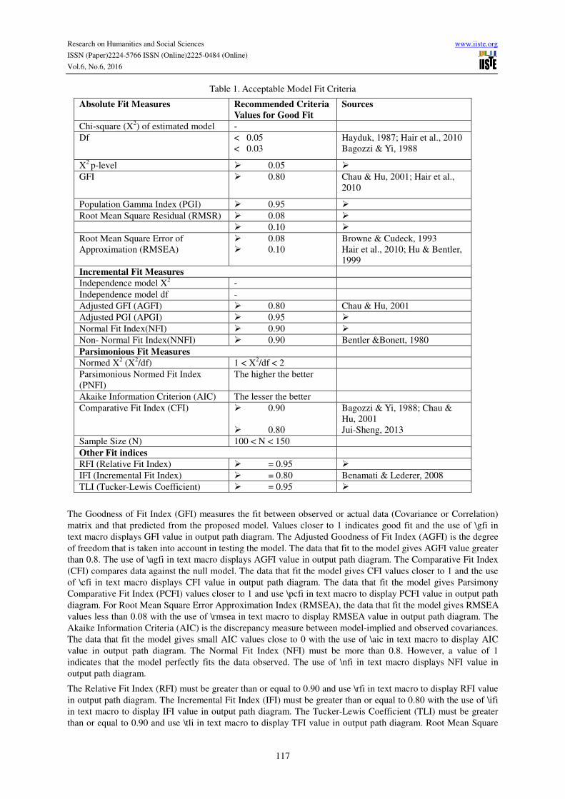
Table 1. Acceptable Model Fit Criteria

Absolute Fit Measures Recommended Criteria

Values for Good Fit

Sources

Chi-square (X2) of estimated model -

Df < 0.05

< 0.03

Hayduk, 1987; Hair et al., 2010

Bagozzi & Yi, 1988

X2

p-level � 0.05 �

GFI � 0.80

Chau & Hu, 2001; Hair et al.,

2010

Population Gamma Index (PGI) � 0.95 �

Root Mean Square Residual (RMSR) � 0.08 �

� 0.10 �

Root Mean Square Error of

Approximation (RMSEA)

� 0.08

� 0.10

Browne & Cudeck, 1993

Hair et al., 2010; Hu & Bentler,

1999

Incremental Fit Measures

Independence model X2 -

Independence model df -

Adjusted GFI (AGFI) � 0.80 Chau & Hu, 2001

Adjusted PGI (APGI) � 0.95 �

Normal Fit Index(NFI) � 0.90 �

Non- Normal Fit Index(NNFI) � 0.90 Bentler &Bonett, 1980

Parsimonious Fit Measures

Normed X2 (X

2/df) 1 < X

2/df < 2

Parsimonious Normed Fit Index

(PNFI)

The higher the better

Akaike Information Criterion (AIC) The lesser the better

Comparative Fit Index (CFI) � 0.90

� 0.80

Bagozzi & Yi, 1988; Chau &

Hu, 2001

Jui-Sheng, 2013

Sample Size (N) 100 < N < 150

Other Fit indices

RFI (Relative Fit Index) � = 0.95 �

IFI (Incremental Fit Index) � = 0.80 Benamati & Lederer, 2008

TLI (Tucker-Lewis Coefficient) � = 0.95 �

The Goodness of Fit Index (GFI) measures the fit between observed or actual data (Covariance or Correlation)

matrix and that predicted from the proposed model. Values closer to 1 indicates good fit and the use of \gfi in

text macro displays GFI value in output path diagram. The Adjusted Goodness of Fit Index (AGFI) is the degree

of freedom that is taken into account in testing the model. The data that fit to the model gives AGFI value greater

than 0.8. The use of \agfi in text macro displays AGFI value in output path diagram. The Comparative Fit Index

(CFI) compares data against the null model. The data that fit the model gives CFI values closer to 1 and the use

of \cfi in text macro displays CFI value in output path diagram. The data that fit the model gives Parsimony

Comparative Fit Index (PCFI) values closer to 1 and use \pcfi in text macro to display PCFI value in output path

diagram. For Root Mean Square Error Approximation Index (RMSEA), the data that fit the model gives RMSEA

values less than 0.08 with the use of \rmsea in text macro to display RMSEA value in output path diagram. The

Akaike Information Criteria (AIC) is the discrepancy measure between model-implied and observed covariances.

The data that fit the model gives small AIC values close to 0 with the use of \aic in text macro to display AIC

value in output path diagram. The Normal Fit Index (NFI) must be more than 0.8. However, a value of 1

indicates that the model perfectly fits the data observed. The use of \nfi in text macro displays NFI value in

output path diagram.

The Relative Fit Index (RFI) must be greater than or equal to 0.90 and use \rfi in text macro to display RFI value

in output path diagram. The Incremental Fit Index (IFI) must be greater than or equal to 0.80 with the use of \ifi

in text macro to display IFI value in output path diagram. The Tucker-Lewis Coefficient (TLI) must be greater

than or equal to 0.90 and use \tli in text macro to display TFI value in output path diagram. Root Mean Square



Vol.6, No.6, 2016

118

Residual (RMR or RMSR) is the square root of the average squared amount by which the sample variances and

covariance differ from the root estimates obtained from the model assuming the model is correct and it must be

smaller than 0.08. The use of \rmr in text macro displays RMR value in output path diagram.

9. Benefits and Limitation of SEM Application

The constraint of Ordinary Least Square (OLS) in dealing with latent constructs gave birth to the development of

SEM which is the second generation multivariate analysis technique with many benefits. The employment of

SEM in research aids the researcher in keeping pace with the latest growth in research methodology. The

simultaneous computation of multiple equations of inter-relationships in a model is of great advantage in the use

of SEM (Weston & Gore-Jr, 2006). AMOS (Analysis of Moment Structures) is the software developed for SEM

to effectively, efficiently and accurately model and analyse the inter-relationships among latent constructs

(Awang, 2014; Schumacker & Lomax, 2010; Weston & Gore-Jr, 2006). Through the employment of AMOS

graphic interface, path diagrams can be created in place of writing of equations or typing of commands, the use

of CFA to validate the measurement model of a latent construct that leads to the modelling of SEM and aids

speed, efficient and accuracy of analysis and testing of the theory through AMOS. SEM is seen as a hybrid of

factor analysis and path analysis to provide a parsimonious summary of the interrelationships between variables

like in factor analysis and through which researchers can test hypothesized associations amongst constructs as in

path analysis (Weston & Gore-Jr, 2006).

Awang (2014) see SEM as the most efficient technique in handling CFA for measurement models, analysing the

causal relationships among the latent constructs in a structural model, estimating their variance and covariance

and testing of the hypothesis for mediators and moderators in a model. AMOS itself is user friendly which

makes the process of hypothesis testing easier in SEM (Schumacker & Lomax, 2010). The fitness of the data

to the multiple models can be achieved through the use of AMOS graphic in a single analysis. The use of AMOS

through examination of every pair of the models to identify and either constrain or delete redundant items in a

measurement model that endanger model fitness is of great benefit.

Byrne (2010) summarised the importance of SEM and compares it with other multivariate techniques with its

four exclusive attributes as followed:

• SEM takes a confirmatory approach to data analysis by stipulating the associations between variables.

Other multivariate techniques are descriptive by nature such as exploratory factor analysis so that

hypothesis testing is rather difficult to do.

• SEM offers explicit estimates of error variance parameters while other multivariate techniques are not

capable of either assessing or correcting for measurement error. For example, a regression analysis

ignores the potential error in all the independent (explanatory) variables included in a model and this

raises the possibility of incorrect conclusions due to misleading regression estimates.

• SEM procedures incorporate unobserved (latent) and observed variables together but other multivariate

techniques are based on observed measurements only.

• SEM is capable of modeling multivariate relations, and estimating direct and indirect effects of

variables under study but other multivariate techniques are capable of performing the task.

However, with all the benefits of the SEM, there are various challenges in employing it in data analysis. SEM

requires large sample size. Parameter estimation on variances, regression coefficients and covariances is based

by Maximum Likelihood (ML) and assumes normality among the variables that requires large sample size.

Model that is based on a small sample size is assumed to exhibits estimation problems and unreliable results.

Built environment research that will apply SEM will require minimum sample size of 100 sample size in order to

meet the assumption of maximum likelihood estimation (Kline, 2011). Besides this, the process of SEM is

somehow technical, complicated and can be frustrating which can lead the researcher to misuse the technique in

developing a “fit index tunnel vision” (Kline, 2011). Consideration of multiple fit indices and residuals can be

ignored by the researcher in testing fitness of the model to the data but only consider a single indices like CFI

thereby avoid modification of the model.

10. Conclusion

Efforts have been made in this paper to explain what SEM is and its application in built environment research

with examples. It is evidence that SEM can be of advantage in built environment research by considering more



Vol.6, No.6, 2016

119

complex research questions and test multivariate models in a single study. The use of SEM involves the interplay

of statistical procedures and theoretical understanding in built environment study. Despite various benefits of the

SEM, the paper also highlighted some of its shortcomings. This paper will serve as eye opener to the researcher

in built environment disciplines to have better understanding of research analytical techniques over the first

generation statistical analysis technique. It is however suggested that researchers in built environment disciplines

should be encouraged to make more consultation to some of the references and other textbooks for better

understanding of the SEM and its various softwares. This paper is limited to brief introduction to the background,

features of the SEM and its application in built environment research. Further study is needed to examine the

methodological approach to facilitate analysis in built environment research through SEM. There is a need for

greater disclosure to give details technique for conducting SEM analysis presenting a step-by-step guide of the

analytic procedure with the aid of an empirical example.

References

A P Nair, H., Kumar, D., & Sri Ramalu, S. (2014). Organizational Health: Delineation, Constructs and

Development of a Measurement Model. Asian Social Science, 10(14). doi: 10.5539/ass.v10n14p145

A.Marcoulides, G., & E.Schumacker, R. (2009). New Developments and Techniques in Structural Equation

Modeling (Taylor & Francis e-Library ed.). London: Lawrence Erlbaum Associates, Inc.,.

Anderson, J. C., & Gerbing, D. W. (1992). Assumptions and Comparative Strengths of the Two-Step Approach-

Comment on Fornell and Yi. Sociological Methods & Research, 20(3), 321-333.

Arbuckle, J. L. (2013). Amos 22 User Guide: Amos Development Corporation.

Ashill, N. J. (2011). An Introduction to Structural Equation Modeling (SEM) and the Partial Least Squares (PLS)

Methodology. 110-129. doi: 10.4018/978-1-60960-615-2.ch006

Awang, Z. (2014). A Handbook on Structural equation Modeling. Malaysia: MPWS Rich Resources.

Bagozzi, R. P., & Yi, Y. (1988). On the Evaluation of Structural Equation Models. Journal of the Academy of

Marketing Science, 16(1), 74-94. doi: 0744)940092-0703/88 / 1601-0074

Baumgartner, H., & Homburg, C. (1996). Applications of structural equation modeling in marketing and

consumer research: A review. International Journal of Research in Marketing, 13(2), 139-161.

Bentler, P. M., & Chou, C.-P. (1987). Practical issues in structural modeling. Sociological Methods & Research,

16(1), 78-117.

Bian, H. (2011). Structural Equation Modelling with AMOS II.

Bollen, K. A. (1989). Structural Equations with latent Variables. New York: Willey.: New York: Willey.

Browne, M. W., Cudeck, R., Bollen, K. A., & Long, J. S. (1993). Alternative ways of assessing model fit. Sage

Focus Editions, 154, 136-136.

Byrne, B. M. (2010). Structural Equation Modeling with AMOS: Basic Concepts, Applications, and

Programming (Second edition ed.). United States of America: Taylor and Francis Group, LLC.

Carvalho, J. d., & Chima, F. O. (2014). Applications of Structural Equation Modeling in Social Sciences

Research. American International Journal of Contemporary Research, 4(1), 6-11.

Choi, J. N. (2004). Individual and Contextual Predictors of Creative Performance: The Mediating Role of

Psychological Processes. Creativity Research Journal, 16(2 & 3), 187-199.

Choi, J. N. (2011). Individual and contextual predictors of creative performance: The mediating role of

psychological processes. Creativity Research Journal, 16(2-3), 187-199.

Davčik, N. S. (2013). The Use And Misuse Of Structural Equation Modeling In Management Research:

University Institute of Lisbon (ISCTE-IUL).

Dyer, P., Gursoy, D., Sharma, B., & Carter, J. (2007). Structural modeling of resident perceptions of tourism and

associated development on the Sunshine Coast, Australia. Tourism Management, 28(2), 409-422.

Gerbing, D. W., & Anderson, J. C. (1992). Monte Carlo Evaluations of Goodness of Fit Indices for Structural

Equation Models. Sociological Methods and Research, 21(2), 132-160.

Haenlein, M., & Kaplan, A. M. (2004). A Beginner’s Guide to Partial Least Squares Analysis. Understanding

Statistics, 3(4), 283–297.



Vol.6, No.6, 2016

120

Hair, J. F., Black, W. C., Babin, B. J., & Anderson, R. E. (2010). Multivariate Data Analysis: Overview of

Multivariate Methods (Seventh Edition ed.). Pearson Prentice Hall: Upper Saddle River, New Jersey: Pearson

Education International.

Hox, J. J., & Bechger, T. M. (2014). An Introduction to Structural Equation Modeling. Family Science Review,

11, 354-373.

Hoyle, R. H. (1995). Structural Equation Modelling: Concepts, Issues and Applications. London: Sage

Publications.

Hoyle, R. H. (2012). Handbook of Structural Equation Modelling. New York, London: The Guilford Press: A

Division of Guilford Publications, Inc.

Huang, H.-C. (2011). Factors Influencing Intention to Move into Senior Housing. Journal of Applied

Gerontology, 31(4), 488-509. doi: 10.1177/0733464810392225

Jöreskog, K. G., & Sörbom, D. (1996). LISREL 8 user's reference guide: Scientific Software International.

Kline, R. B. (2011). Principles and Practice of Structural Equation Modeling (D. A. Kenny & T. D. Little Eds.

Third ed.). New York, London: THE GUILFORD PRESS: A Division of Guilford Publications, Inc.

Kline, R. B. (2013). Assessing statistical aspects of test fairness with structural equation modelling. Educational

Research and Evaluation: An International Journal on Theory and Practice, 19(2-3), 204-222. doi:

10.1080/13803611.2013.767624

Loehlin, J. C. (2004). Latent Variable Models: An Introduction to Factor, Path, and Structural Equation

Analysis (Fourth Edition ed.). London: Lawrence Erlbaum Associates, Publishers Mahwah, New Jersey.

Manafi, M., & Subramaniam, I. D. (2015). The Role of the Perceived Justice in the Relationship between Human

Resource Management Practices and Knowledge Sharing: A Study of Malaysian Universities Lecturers. Asian

Social Science, 11(12). doi: 10.5539/ass.v11n12p131

Nachtigall, C., Kroehne, U., Funke, F., & Steyer, R. (2003). Why Should We Use SEM-Pros and Cons of

Structural Equation Modelling. Methods of Psychological Research Online, 8(2), 1-22.

Nair, H. A. P., Kumar, D., & Ramalu, S. S. (2015). Instrument Development for Organisational Health. Asian

Social Science, 11(12). doi: 10.5539/ass.v11n12p200

Schumacker, R. E., & Lomax, R. G. (2004). A Beginner's Guide to Structural Equation Modeling (D. Riegert

Ed. Second Edition ed.). London: Lawrence Erlbaum Associates, Inc.

Schumacker, R. E., & Lomax, R. G. (2010). A Beginner’s Guide to Structural Equation Modeling (3rd Edition

ed.). New York: Routledge Taylor and Francis Group, LLC.

Steiger, J. H. (1998). A note on multiple sample extensions of the RMSEA fit index.

Syme, G. J., Shao, Q., Po, M., & Campbell, E. (2004). Predicting and understanding home garden water use.

Landscape and Urban Planning, 68, 121–128. doi: 10.1016/j.landurbplan.2003.08.002

Timothy Teo, Tsai, L. T., & Yang, C.-C. (2013). Applying Structural Equation Modeling (SEM) in Educational

Research: An Introduction. In M. S. Khine (Ed.), Application of Structural Equation Modelling in Educational

Research and Practice. Rotterdam/ Boston / Taipei: Sense Publishers.

Weston, R., & Gore-Jr, P. A. (2006). A Brief Guide to Structural Equation Modeling. The Counseling

Psychologist, 34(5), 719-751. doi: 10.1177/0011000006286345

The Use of Structural Equation Modeling (SEM) in Built ... · structural equation modeling (SEM) in marketing and consumer research while Choi (2011) explored potential psychological

Documents