Introduction to Structural Equation Modeling Paul D. Allison, Ph.D. Upcoming Seminar: August 16-17, 2019, Vancouver

Welcome message from author
This document is posted to help you gain knowledge. Please leave a comment to let me know what you think about it! Share it to your friends and learn new things together.
Transcript
Introduction to Structural Equation Modeling Paul D. Allison, Ph.D.
Upcoming Seminar: August 16-17, 2019, Vancouver

1/20/2017
1
Introduction toStructural Equation Modeling
Structural Equation Models
What is SEM good for?
SEM
Preview: A Latent Variable SEM
Latent Variable Model (cont.)
Cautions
Outline
Software for SEMs
Favorite Textbook
Linear Regression in SEM
GSS2014 Example
Regression with Mplus
Mplus Output
Linear Regression with Stata
Linear Regression with SAS
Linear Regression with lavaan
FIML for Missing Data
Further Reading
Assumptions
FIML in SAS
FIML in Stata
FIML in lavaan
FIML in Mplus
Mplus “Problem”
Path Diagram from Mplus
Path Analysis of Observed Variables
Some Rules and Definitions
Three Predictor Variables
1
2
3
4
5
6
7
8
9
10
11
12
13
14
15
16
17
18
19
20
21
22
23
24
25
26
27
28
29
2
3
4
5
6
7
8
9
10
11
12
13
14
15
16
17
18
19
20
21
22
23
24
25
26
27
28
29

1/20/2017
2
Two-Equation System
Why combine the two equations?
Calculation of Indirect Effect
A More Complex Model
Decomposition of Direct & Indirect Effects
Standardized Coefficients
Numerical Examples
More Complex Example
Decomposition of Effects
Illness Data
Summary Data
Illness Regression - Mplus
Covariance Matrix
Covariance Matrix for Illness Data
Mplus Results – Goodness of Fit
Counting Moments & Parameters
Mplus Results - Unstandardized
Mplus Results - Standardized
Illness Regression - Stata
Illness Regression - SAS
Illness Regression - lavaan
Illness Model with Indirect Effects
Mplus Model Diagram
Other Packages
Path Diagrams in Other Packages
Mplus GOF
Identification Status of the Model
Improving the Model
GOF for Improved Model
30
31
32
33
34
35
36
37
38
39
40
41
42
43
44
45
46
47
48
49
50
51
52
53
54
55
56
57
58
30
31
32
33
34
35
36
37
38
39
40
41
42
43
44
45
46
47
48
49
50
51
52
53
54
55
56
57
58

1/20/2017
3
Estimates for Improved Model
Indirect Effects
Indirect Estimates
Indirect Effects in SAS
Specific Indirect Effects with PARMS
Indirect Effects in Stata
Specific Indirect Effects in Stata
Indirect Effects in lavaan
Indirect Estimates from lavaan
Partial Correlations
Partial Correlations (cont.)
Maruyama (1998) Data
Partial Correlations in Mplus
Results with Partial Correlation
Results (cont.)
Partial Correlations in SAS
Partial Correlations in Stata
Partial Correlations in lavaan
Causal Ordering
How to Decide
Nonrecursive Systems
Identification Problem in Nonrecursive Models
Identification Problem (cont.)
A Just-Identified Model
Reduced Form Equations
Solutions for Structural Parameters
Sufficient Condition for Identification
Varieties of Identification
Problems with Instrumental Variables
59
60
61
62
63
64
65
66
67
68
69
70
71
72
73
74
75
76
77
78
79
80
81
82
83
84
85
86
87
59
60
61
62
63
64
65
66
67
68
69
70
71
72
73
74
75
76
77
78
79
80
81
82
83
84
85
86
87

1/20/2017
4
Example of a Nonrecursive Model
Nonrecursive Example (cont.)
Nonrecursive Mplus Program
Nonrecursive Results
Nonrecursive Results (cont.)
SAS Code for Nonrecursive Model
Stata Code for Nonrecursive Model
lavaan Code for Nonrecursive Model
Latent Variable Models
Roadmap for Latent Variables
Classical Test Theory
Random Measurement Error
Reliability
Parallel Measures
Tau-Equivalent Measures
Tau-Equivalance: Example
Tau-Equivalence in Mplus
Tau-Equivalence in SAS
Tau-Equivalence in Stata
Tau-Equivalence in lavaan
Congeneric Tests
Three Congeneric Tests
Three Congeneric Measures (cont.)
Identification in General
Standardized Version
Digression: Tracing Rule for Correlations
Tracing Rule (cont.)
Tracing Rule (cont.)
Standardized Version of 3 Congenerics (cont.)
88
89
90
91
92
93
94
95
96
97
98
99
100
101
102
103
104
105
106
107
108
109
110
111
112
113
114
115
116
88
89
90
91
92
93
94
95
96
97
98
99
100
101
102
103
104
105
106
107
108
109
110
111
112
113
114
115
116

1/20/2017
5
Three Congenerics: Example
Three Congenerics: Mplus
Three Congenerics: SAS
Three Congenerics: Stata
Three Congenerics: lavaan
Four Congeneric Measures
Overidentification with 4 Congeneric Measures
Four Congeneric Measures with Mplus
Four Congeneric Measures with SAS
Four Congeneric Measures with Stata
Four Congeneric Measures with lavaan
Mplus Results for Four Congenerics
Alternative Model for 4 Congeneric Measures
Mplus for Alternative Model
Results for Alternative Model
Results (cont.)
Heywood Case
Other Code for Alternative Model
lavaan code for Alternative Model
Factor Models
Factor Models (cont.)
Identification (Standardized)
Identification (cont.)
Two Approaches to Identification Problem
Identification (Unstandardized)
Determining Identification
Normalizing Constraints
Normalizing Constraints
ML Estimation of CFA Models
117
118
119
120
121
122
123
124
125
126
127
128
129
130
131
132
133
134
135
136
137
138
139
140
141
142
143
144
145
117
118
119
120
121
122
123
124
125
126
127
128
129
130
131
132
133
134
135
136
137
138
139
140
141
142
143
144
145

1/20/2017
6
Multivariate Normality
ML Details
Chi-Square Test
Self-Concept Example: Mplus Code
Self Concept Path Diagram
SAS Code for Self Concept
Stata Code for Self Concept
lavaan Code for Self Concept
Self Concept: Mplus Results
Self Concept Results
Global Goodness of Fit Measures
Other Global Measures
Other Global Measures (cont.)
Specific Goodness of Fit Measures
Standardized Residuals for Self-Concept Model
Residuals in SAS
Residuals in Stata and lavaan
Modification Indices
Mod Indices for Self-Concept
Freeing Up Parameters
Results from Freeing 1 Parameter
Selected Results (cont.)
Correlated Errors
Two Correlated Errors
A Five-Indicator Model
A Two-Factor Model
Example: Self-Concept Data
Selected Results
The General Structural Equation Model
146
147
148
149
150
151
152
153
154
155
156
157
158
159
160
161
162
163
164
165
166
167
168
169
170
171
172
173
174
146
147
148
149
150
151
152
153
154
155
156
157
158
159
160
161
162
163
164
165
166
167
168
169
170
171
172
173
174

1/20/2017
7
GSS2014 Example: Mplus Code
GSS2014 Example: Mplus Results
GSS2014: Mplus Standardized Results
GSS2014: Code for Other Packages
Farm Manager Example (Rock et al. 1977)
Farm Managers Path Diagram
Data and Mplus Code
SAS Code for Farm Managers
lavaan Code for Farm Managers
Stata Code for Farm Managers
Farm Managers: Selected Mplus Results
Selected Results (cont.)
Identification in SEM Models
An Identified SEM
Alternative Estimation Methods
GLS Example
GLS Results
What to Do If Endogenous Variables Aren’t Normal
Example: NLSY Data
ML Results for NLSY Data
Both Variables Highly Skewed
Other ESTIMATOR Options
Satorra-Bentler Robust SE’s
Weighted Least Squares
WLS in Mplus for NLSY Data
WLS Output
Multiple Group Analysis
Subjective Class Example
Subjective Class Data
175
176
177
178
179
180
181
182
183
184
185
186
187
188
189
190
191
192
193
194
195
196
197
198
199
200
201
202
203
175
176
177
178
179
180
181
182
183
184
185
186
187
188
189
190
191
192
193
194
195
196
197
198
199
200
201
202
203

1/20/2017
8
Subjective Class Models
Mplus Code for Model 1
Mplus Code (cont.)
Model 4 Code
Tests for Comparing the Groups
SAS Code to Read Data
SAS Code – Model 1
SAS Code – Model 2
SAS Code – Model 3
SAS Code – Model 4
Reading in the Data in Stata
Stata Code for 2-Group Models
Stata Code (cont.)
Interactions and Non-Linearities
Interactions with Latent Variables
Interactions with Latent Variables
Ordinal and Binary Data
Special Correlations
Special Correlations
Specialized Models
Mplus for MIMIC Model with Binary Data
Diagram for Probit MIMIC Model
Stata for MIMIC Model with Binary Data
Probit Results with WLSMV Method
Probit Results (cont.)
Other Features of Mplus
Cautions About SEMs
Examples I Don’t Like
Examples I Like
204
205
206
207
208
209
210
211
212
213
214
215
216
217
218
219
220
221
222
223
224
225
226
227
228
229
230
231
232
204
205
206
207
208
209
210
211
212
213
214
215
216
217
218
219
220
221
222
223
224
225
226
227
228
229
230
231
232

1/20/2017
9
SEMs and Causality
Exemplary Article
233
234
233
234
Introduction toStructural Equation Modeling
Paul D. Allison, InstructorJanuary 2017
www.StatisticalHorizons.com
1
Copyright © 2017 Paul Allison
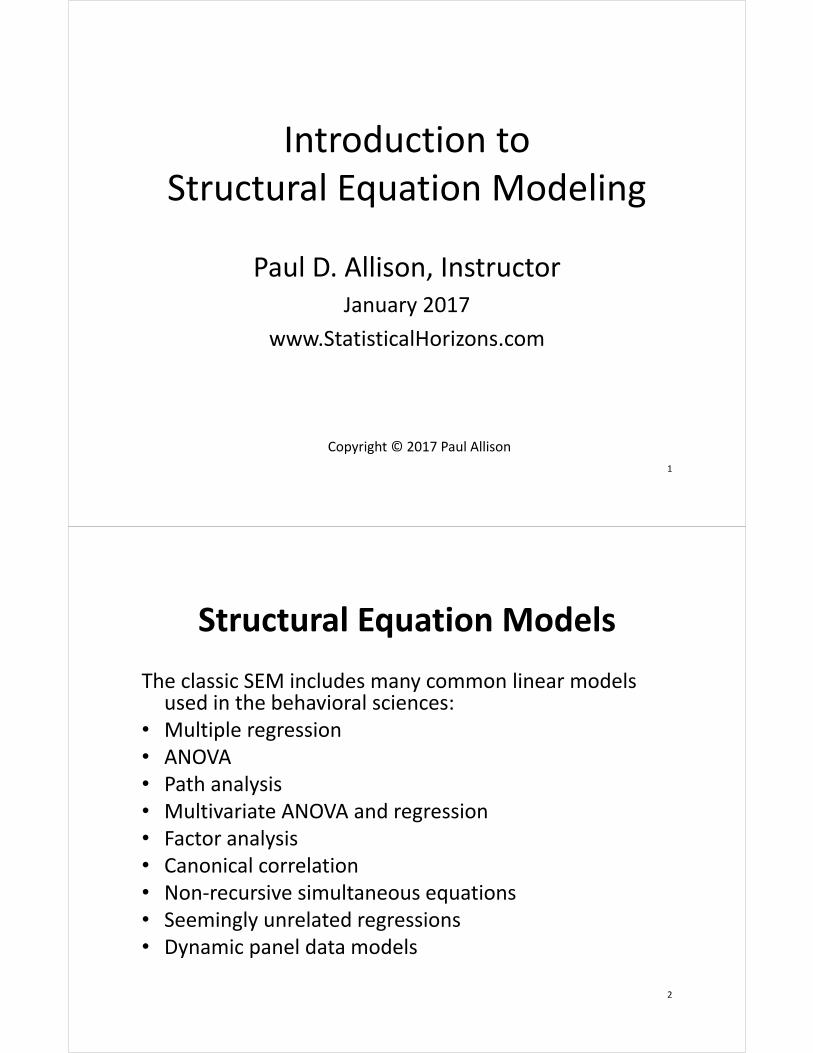
Structural Equation ModelsThe classic SEM includes many common linear models
used in the behavioral sciences:• Multiple regression• ANOVA• Path analysis• Multivariate ANOVA and regression• Factor analysis• Canonical correlation• Non-recursive simultaneous equations• Seemingly unrelated regressions• Dynamic panel data models
2
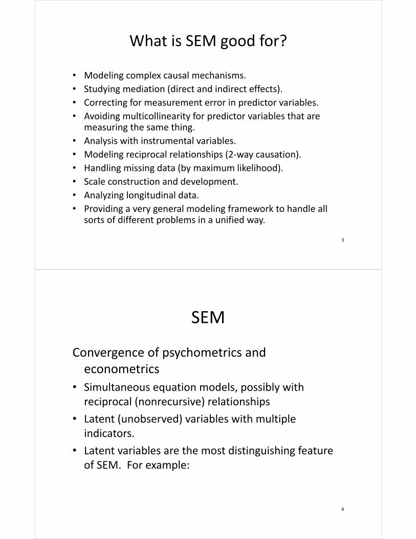
What is SEM good for?
• Modeling complex causal mechanisms.• Studying mediation (direct and indirect effects).• Correcting for measurement error in predictor variables.• Avoiding multicollinearity for predictor variables that are
measuring the same thing.• Analysis with instrumental variables.• Modeling reciprocal relationships (2-way causation).• Handling missing data (by maximum likelihood).• Scale construction and development.• Analyzing longitudinal data.• Providing a very general modeling framework to handle all
sorts of different problems in a unified way.
3
SEM
Convergence of psychometrics and econometrics
• Simultaneous equation models, possibly with reciprocal (nonrecursive) relationships
• Latent (unobserved) variables with multiple indicators.
• Latent variables are the most distinguishing feature of SEM. For example:
4
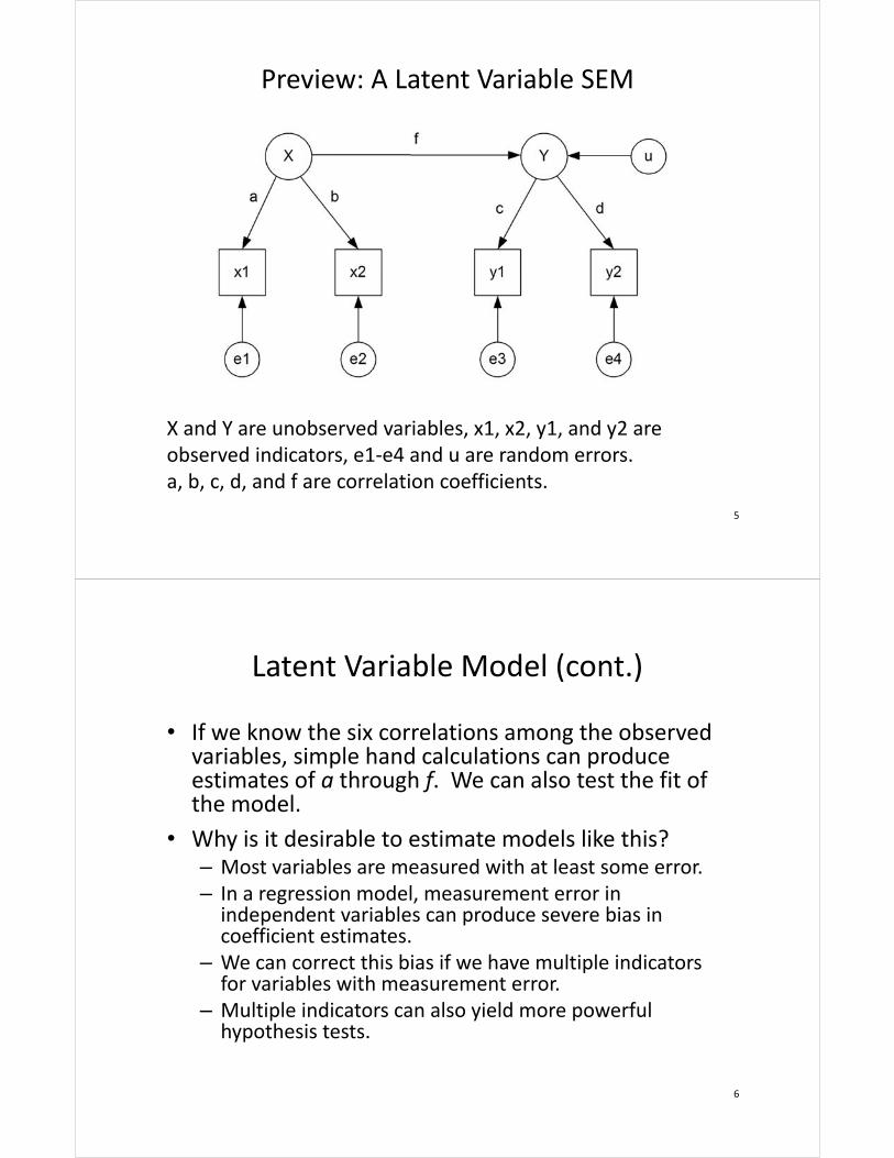
X and Y are unobserved variables, x1, x2, y1, and y2 are observed indicators, e1-e4 and u are random errors. a, b, c, d, and f are correlation coefficients.
Preview: A Latent Variable SEM
5
Latent Variable Model (cont.)
6
• If we know the six correlations among the observed variables, simple hand calculations can produce estimates of a through f. We can also test the fit of the model.
• Why is it desirable to estimate models like this? – Most variables are measured with at least some error. – In a regression model, measurement error in
independent variables can produce severe bias in coefficient estimates.
– We can correct this bias if we have multiple indicators for variables with measurement error.
– Multiple indicators can also yield more powerful hypothesis tests.
Cautions
• Although SEM’s can be very useful, the methodology is often used badly and indiscriminately.– Often applied to data where it’s inappropriate.– Can sometimes obscure rather than illuminate. – Easy to get sucked into overly complex modeling.
7
Outline1. Introduction to SEM2. Linear regression with missing data3. Path analysis of observed variables4. Direct and indirect effects5. Identification problem in nonrecursive models6. Reliability: parallel and tau-equivalent measures7. Multiple indicators of latent variables8. Confirmatory factor analysis9. Goodness of fit measures10. Structural relations among latent variables11. Alternative estimation methods.12. Multiple group analysis13. Models for ordinal and nominal data
8

Software for SEMsLISREL – Karl Jöreskog and Dag SörbomEQS – Peter BentlerPROC CALIS (SAS) – W. Hartmann, Yiu-Fai YungAmos – James ArbuckleMplus – Bengt Muthénsem, gsem (Stata)Packages for R:
OpenMX – Michael Nealesem – John Foxlavaan – Yves Rosseel
9
Favorite Textbook
10
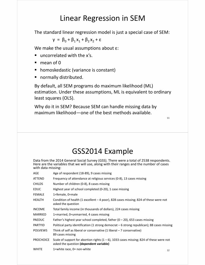
Linear Regression in SEMThe standard linear regression model is just a special case of SEM:
y = β0 + β1 x1 + β2 x2 + ε
We make the usual assumptions about ε: uncorrelated with the x’s. mean of 0 homoskedastic (variance is constant) normally distributed.
By default, all SEM programs do maximum likelihood (ML) estimation. Under these assumptions, ML is equivalent to ordinary least squares (OLS).
Why do it in SEM? Because SEM can handle missing data by maximum likelihood—one of the best methods available.
11
GSS2014 ExampleData from the 2014 General Social Survey (GSS). There were a total of 2538 respondents. Here are the variables that we will use, along with their ranges and the number of cases with data missing: AGE Age of respondent (18-89), 9 cases missingATTEND Frequency of attendance at religious services (0-8), 13 cases missingCHILDS Number of children (0-8), 8 cases missingEDUC Highest year of school completed (0-20), 1 case missingFEMALE 1=female, 0=maleHEALTH Condition of health (1 excellent – 4 poor), 828 cases missing; 824 of these were not
asked the questionINCOME Total family income (in thousands of dollars), 224 cases missingMARRIED 1=married, 0=unmarried, 4 cases missingPAEDUC Father’s highest year school completed, father (0 – 20), 653 cases missingPARTYID Political party identification (1 strong democrat – 6 strong republican); 88 cases missingPOLVIEWS Think of self as liberal or conservative (1 liberal – 7 conservative)
89 cases missingPROCHOICE Scale of support for abortion rights (1 – 6), 1033 cases missing; 824 of these were not
asked the question (dependent variable)WHITE 1=white race, 0= non-white 12
Related Documents

![Estimating and interpreting structural equation models … · Estimating and interpreting structural equation models in Stata 12 ... and Var [ǫ] = Σ sem (y1 ... Structural equation](https://static.cupdf.com/doc/110x72/5b286e167f8b9ae8108b4592/estimating-and-interpreting-structural-equation-models-estimating-and-interpreting.jpg)