THE USE OF MULTIPLE ANTENNA TECHNIQUES FOR UWB WIRELESS PERSONAL AREA NETWORKS (UWB-MIMO WPANs) Mr. Mason Adam Submitted in Partial Fulfilment of the Requirements of the Degree of Doctor of Philosophy, October 2014

Welcome message from author
This document is posted to help you gain knowledge. Please leave a comment to let me know what you think about it! Share it to your friends and learn new things together.
Transcript

THE USE OF MULTIPLE ANTENNA TECHNIQUES
FOR UWB WIRELESS PERSONAL AREA
NETWORKS (UWB-MIMO WPANs)
Mr. Mason Adam
Submitted in Partial Fulfilment of the Requirements of the Degree of Doctor of Philosophy, October
2014

ii
Contents
Contents ……..……………………………………………………………..…………..………II
List of Figures……………………………………………………………………………..….VIII
List of Tables………………………………………………………………………………….X
Abbreviations………………………………………………………………..…………….XI
Abstract……………………………………………………………………………………..XIII
1 Introduction……….…………………………………………….……………………1
1.1. Overview............................................................................................................................................ 1
1.2. Resarch aim and objectives ........................................................................................................ 5
iii
1.3. Thesis Contributions .................................................................................................................... 9
1.4. MIMO Design implmentation ................................................................................................. 10
1.5. Modeling challneges of physical channel .......................................................................... 11
1.6. Resarch limitations .................................................................................................................... 13
1.7. The proposed structure of the Thesis ................................................................................ 17
1.8. Research Methodology ............................................................................................................ 20
2 Background………………………………………………………………………24
2.1. ECMA-368 Specifications ........................................................................................................ 24
2.2. MIMO System ............................................................................................................................... 30
2.2.1. Alamouti Scheme Space-Time Block Code (STBC) ........ ………………………35
2.3. The Physical channel ................................................................................................................ 38
2.4. MIMO-OFDM Wireless system block model ................................................................... 42
2.5. Convolutional Coding ............................................................................................................... 44
2.6. Viterbi Decoding ......................................................................................................................... 48
2.7. BCJR algorithm and its challenges ...................................................................................... 51
2.8. Turbo code and its cost of implementation .................................................................... 57
2.9. Modulation Schemes ................................................................................................................ 59

iv
2.9.1. Quadrature Phase Shift Keying ......................................... ………………………59
2.9.2. Dual Carrier Modulation ................................................... ………………………62
2.9.3. Dual Circular 32-QAM ..................................................... ………………………66
3 Design ...........................................................................................................…... 71
3.1. Introduction ................................................................................................................................. 71
3.2. Design Overview ........................................................................................................................ 72
3.3. Design Method ............................................................................................................................ 76
3.3.1. The Transmitting Model Design ....................................... ………………………76
3.3.2. The Receiving Model Design ........................................... ………………………83
3.3.3. Modification to the Receiving Model Design ................... ………………………88
3.4. Mathematical Analysis ............................................................................................................. 90
3.4.1. Analysis of Avarge Probablity of Error ............................. ………………………91
3.4.2. Error Performance Measure based on the noise static ...... ………………………98
3.4.3. Numerical Evaluation of PEP ......................................... ………………………102
3.4. Concluding Remarks .............................................................................................................. 115
v
4 Implementation…………………………………………………………………...116
4.1. Introduction .............................................................................................................................. 116
4.2. Implementation on transmitters ...................................................................................... 117
4.3. Modulation of symbols ......................................................................................................... 119
4.4. IFFT OFDM implementation on the MIMO configuration ...................................... 124
4.5. The implementad channel model ..................................................................................... 129
4.6. Receivers Implmentation ..................................................................................................... 138
4.7. Optimisation for the decoding method (LLR) .................................................................. 151
4.8. Conclusion ................................................................................................................................. 155
5 Simulation Result………………………….…………………………………..156

vi
5.1. Introduction .............................................................................................................................. 156
5.2. Overview of simulation ......................................................................................................... 157
5.3. Simulation functions ............................................................................................................... 158
5.4. Specifications of the simulation process ........................................................................ 159
5.5. Time-Frequency Implementation ..................................................................................... 161
5.6. Smiulation using coded modulation with hard decoding evulation ................... 168
5.7. Smiulation verification based on LLR implementation ............................................ 170
5.8. Evaluation based on Comparsion between ML & LLR methods ........................... 173
5.9. Evaluation and verification of the spatial hypothesis ............................................... 176
5.10. Evaluation based on CSI distortion ................................................................................ 178
5.11. Performance variation based on spatial configuration ......................................... 180
5.12. Comparative analysis based on increase in the order of modulation .............. 182
5.13. Comparative analysis based on analytical upper bound error probablity .... 184
5.14. Analysis of wireless range evaluation .......................................................................... 186
5.15. Conclusion ................................................................................................................................ 189
6 Conclusions.....................................................................................................…...191
vii
6.1. The acheviment of this research ........................................................................................ 191
6.2. Observation about the research process ........................................................................ 195
6.3. Review of the complete proposed model ....................................................................... 199
6.4. Future research recommendation .................................................................................... 202
6.5. Concluding Remarks .............................................................................................................. 206
References….……………………………….…………207
Bibliogrphy….……………………………………….…213
Appendix………………………………………………215

viii
LIST OF FIGURES
Figure (1): Research methodology
Figure (2.1.1): Spectrum division into band groups
Figure (2.1.2) PPDU and PLCP structure
Figure (2.1.3): Modulated symbol interleaving over three bands with ZPS Figure (2.4.1): MIMO wireless block model system Figure (2.5.1): Block diagram of main components in convolutional encoder
Figure (2.5.2): The trellis Diagram structures in discrete intervals
Figure (2.6.1): The survivor paths of a trellis diagram based on Viterbi Decoding
Figure (2.7.1): The BCJR algorithm parameters in the trellis Figure (2.8.1): The encoding structure of the Turbo scheme
Figure (2.8.2): Block diagram structure of the Turbo Decoder
Figure (2.9.1): Quadrature Phase Shift Keying Mapping Figure (2.9.2): Constellation mapping of DCM: (A1) = S [N]; (A2) = S[N+50]
Figure (2.9.3): Constellation mapping of DC 32-QAM: (B1) = S [K]; (B2) = S[K+50]
Figure (3.1): Scheme of the Design development
Figure (3.2): The formation of the modulation across the dual complex symbols
Figure (3.3): The two distance metrics across the 8 signal constellation points
Figure (3.4): The constellation maps used for the dual 8-ary PSK symbols
Figure (3.5): The transmitting configuration design across the two antennas
Figure (3.6): The design scheme of the dual receivers Figure (3.7): The design scheme for the modified dual receivers
Figure (4.1): Space Frequency division within an OFDM block
ix
Figure (4.2): Time window for discretisation Figure (4.3): Comparison between IEEE803.15.3a model and its modified version
Figure (4.4): Time and frequency channel response Figure (4.5): The decoding regions for the MSB of the PSK symbols
Figure (4.6): Expression of the metric length position
Figure (4.7): The proposed model
Figure (5.5.1): BER Simulation of MIMO DC32QAM vs SISO DC32QAM
Figure (5.5.2): BER Simulation of MIMO DCM vs SISO DCM Figure (5.5.3): BER Comparison between DCM, DC32QAM and MIMO model
Figure (5.5.4): Impulse response with its time response and impulse realisation
Figure (5.5.5): Comparison between analytical Rayleigh and Simulation models
Figure (5.5.6): BER results of DC32QAM, Analytical and MIMO models Figure (5.5.7): Comparion of the models error peromances using hard decoding
Figure (5.5.8): BER comparison of the model using LLR de-mapping method Figure (5.5.9): Comparison of BER performance between ML soft and LLR de-
mapping methods
Figure (5.5.10): BER performance comparison for soft decoding at low SNR
Figure (5.5.11): SISO DC32QAM vs MIMO DC32QAM BER evaluation
Figure (5.5.12): Models comparison with impairments in the CSI
Figure (5.5.13): Spatial orthognality effect on BER of the proposed model Figure (5.5.14): BER model performance based on rearranged constellation maps
Figure (5.5.15): Analytical upper bound error probability comparison
Figure (5.5.16): BER comparison between the proposed models
Figure (5.5.17): Performance comparison of the models over coverage area
Figure (5.5.18): File data collecting the SNRs and BER values between the models.

x
List of Tables
Table (2.1): The defined data rates and modulation parameters in ECMA standard
Table (2.9.2): The DCM mapping signal across the constellation maps
Table (4.1): Frequency transformation parameters
Table (4.2): Transmitting parameters
Table (4.3): Paramteters of Matlab viterbi function
Table (5.1): summery of specific simulation settings used in the simulation
xi
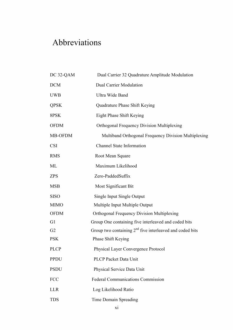
Abbreviations
DC 32-QAM Dual Carrier 32 Quadrature Amplitude Modulation
DCM Dual Carrier Modulation
UWB Ultra Wide Band
QPSK Quadrature Phase Shift Keying
8PSK Eight Phase Shift Keying
OFDM Orthogonal Frequency Division Multiplexing
MB-OFDM Multiband Orthogonal Frequency Division Multiplexing
CSI Channel State Information
RMS Root Mean Square
ML Maximum Likelihood
ZPS Zero-PaddedSuffix
MSB Most Significant Bit
SISO Single Input Single Output
MIMO Multiple Input Multiple Output
OFDM Orthogonal Frequency Division Multiplexing
G1 Group One containing five interleaved and coded bits
G2 Group two containing 2nd
five interleaved and coded bits
PSK Phase Shift Keying
PLCP Physical Layer Convergence Protocol
PPDU PLCP Packet Data Unit
PSDU Physical Service Data Unit
FCC Federal Communications Commission
LLR Log Likelihood Ratio
TDS Time Domain Spreading

xii
FDS Frequency Domain Spreading
TFI Time Frequency Interleaving
FFI Fix Frequency Interleaving
TFC Time Frequency Coding
FFT Fast Fourier Transform
FEC Forward Error Correction
STBC Space-Time Block Code
STTC Space-Time Trellis Codes
AWGN Additive White Gaussian Noise
IEEE Institute of Electrical and Electronics Engineers
IEEE 802.15 Working Group of IEEE
IFFT Inverse Fast Fourier Transform
BCJR Bahl Cocke Jelinek and Raviv algorithm
Log-MAP Logrithmic Maximum A Posteriori decoding
SOVA Soft Output Viterbi Algorithm
ECMA-368 ECMA international Standard for UWB technology
PER Packet Error Rate
LOS Line Of Sight propagation
BER Bit Error Rate
NLOS Non Line Of Sight propagation
SNR Signal to Noise Ratio

xiii
Abstract
The research activities over the three years were presented in this thesis. The work
centred on the use of multiple spatial elements for Ultra wide band wireless system
in order to increase the throughput, and for wireless range requirement applications,
increases the coverage area. The challenges and problems of this type of
implementation are identified and analysed when considered at the physical layer.
The study presents a model design that integrates the multiple antenna configurations
on the short range wireless communication systems. As the demand for capacity
increases in Wireless Personal Area Networks (WPAN); to address this issue, the
framework of the Wi-Media Ultra Wide Band (UWB) standard has been
implemented in many WPAN systems. However, challenging issues still remain in
terms of increasing throughput, as well as extending cellular coverage range.
Multiple Input Multiple Output (MIMO) technology is a well-established antenna
technology that can increase system capacity and extend the link coverage area for
wireless communication systems. The work started by carrying out an investigation
into integrated MIMO technology for WPANs based on the Wi-Media framework
using Multi-band Orthogonal Frequency Division Multiplexing (MB-OFDM). It
considered an extensive review of applicable research, the potential problems posed
by some approaches and some novel approaches to resolve these issues. The
proposed ECMA-368 standard was considered, and a UWB system with a multiple
antenna configuration was undertaken as a basis for the analysis. A novel scheme
incorporating Dual Circular 32 - QAM was proposed for MB-OFDM based systems
in order to enhance overall throughput, and could be modified to increase the
xiv
coverage area at compromise of the data rate. The scheme was incorporated into a
spatial multiplexing model with measured computational complexity and practical
design issues. This way the capacity could be increased to twice the theoretical
levels, which could pay the way to high speed multi-media wireless indoor
communication between devices. Furthermore, the range of the indoor wireless
network could be increased in practical wireless sensor networks. The inherent
presence of spatial and frequency diversity that is associated with this multiple
radiators configuration enlarge the signal space, by introducing additional degrees of
freedom that provide a linear increase in the system capacity, for the same available
spectrum. By incorporating the spatial elements with a Dual Circular modulation that
is specified within the standard, it can be shown that a substantial gain in spectral
efficiency could be possible. A performance analysis of this system and the use of
spatial multiplexing for potential data rates above Gigabit per second transmission
were considered. In this work, a model design was constructed that increases the
throughput of indoor wireless network systems with the use of dual radiating
elements at the both transmitter and receiver. A simulation model had been
developed that encapsulate the proposed design. Tests were carried out which
investigate the performance characteristics of various spatial and modulation
proposals and identifies the challenges surrounding their deployments. Results
analysis based on various simulation tests including the IEEE802.15.3a UWB
channel model had shown a lower error rate performance in the implementation of
the model. The proposed model can be integrated in commercial indoor wireless
networks and devices with relatively low implementation cost. Further, the design
used in future work to address the current challenges in this field and provides a
framework for future systems development.

1
1Introduction
1.1 Overview
The Wireless Personal Area Network (WPAN) is a short range communication
system that interconnects various applications in the home and office environments.
WPAN networking technology has grown considerably in the last few years, partly
because of the advances in the underlying technology and partly due to its
commercial merits penetrating the consumer market. Nevertheless, since the Federal
Communication Commission’s (FCCs) decision to allow unlicensed UWB operation
in the 3.1-10.6GHz spectrum with power restrictions [1], there has been a surge in
the number of commercially available short range wireless portable products. There
has also been a growing interest in the technology from the academic community due
to the potential benefits of wireless short range communications. There are currently
various wireless communication networks that includes cellular, GPS, Military,
Emergency and public services all of which had been assigned to a particular part of
the frequency spectrum. The decision to allow unlicensed WPANs in the UWB
spectrum has presented at the same time an opportunity and a challenge for RF
designers. In a design approach, the flexibility over the physical layer has meant that
different protocols at different layers could be implemented based on specific
2
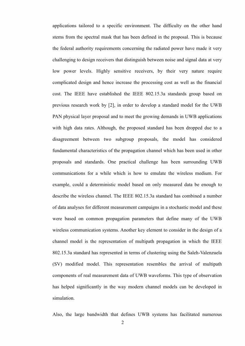
applications tailored to a specific environment. The difficulty on the other hand
stems from the spectral mask that has been defined in the proposal. This is because
the federal authority requirements concerning the radiated power have made it very
challenging to design receivers that distinguish between noise and signal data at very
low power levels. Highly sensitive receivers, by their very nature require
complicated design and hence increase the processing cost as well as the financial
cost. The IEEE have established the IEEE 802.15.3a standards group based on
previous research work by [2], in order to develop a standard model for the UWB
PAN physical layer proposal and to meet the growing demands in UWB applications
with high data rates. Although, the proposed standard has been dropped due to a
disagreement between two subgroup proposals, the model has considered
fundamental characteristics of the propagation channel which has been used in other
proposals and standards. One practical challenge has been surrounding UWB
communications for a while which is how to emulate the wireless medium. For
example, could a deterministic model based on only measured data be enough to
describe the wireless channel. The IEEE 802.15.3a standard has combined a number
of data analyses for different measurement campaigns in a stochastic model and these
were based on common propagation parameters that define many of the UWB
wireless communication systems. Another key element to consider in the design of a
channel model is the representation of multipath propagation in which the IEEE
802.15.3a standard has represented in terms of clustering using the Saleh-Valenzuela
(SV) modified model. This representation resembles the arrival of multipath
components of real measurement data of UWB waveforms. This type of observation
has helped significantly in the way modern channel models can be developed in
simulation.
Also, the large bandwidth that defines UWB systems has facilitated numerous

3
approaches to utilising the spectrum for short range wireless data communication.
One classic approach had used all the available spectrum of the signal at very low
power with very with very short duration to transmit information, where additional
capacity could be obtained by incorporating a pseudo random spreading sequence
with the signal pulse. Such approach makes use of the spatial property of these pulses
in combating signal fading. Furthermore, there is no need for a carrier signal in this
method as it tends to consume power and spectrum both of which are very scarce.
Although this type of transmission scheme has been the traditional approach, the
single band nature of its communication has remained a point of discussion in
industry and research communities. In [3], a discussion regarding the physical layer
has highlighted the concept behind the multiband design. Here, the model has been
one which divides the large spectrum into sub-bands of 500 MHz or more and
modulating the signal information using Orthogonal Frequency Division
Multiplexing (OFDM). OFDM has been used for many years in conventional RF
communications and has proved its effectiveness. Moreover, the underlying technical
knowledge has been familiar to designers and researches alike, and hence made more
sense for the scheme to be considered in research studies. Nevertheless, there is a
major difference between OFDM in the narrowband and ultra wideband applications.
In narrowband systems, OFDM symbols are transmitted over a single band, while in
UWB domains, the symbols are interleaved over different bands. This inevitably
requires reconsideration of the physical layer protocol, and should take into account
coding and transmission design procedures.
The Multiband OFDM Alliance Special Interest Group (MBOA-SIG) of industrial
consortia had supported the Multiband OFDM transmission scheme for UWB
4
applications. The industrial backing of this scheme has shaped consumer electronics
in the UWB domains and has resulted in its integration on the Universal Serial Bus
(USB) and Bluetooth-SIG systems. In addition, the publication of the ECMA-368
standard [4] by the Wi-Media Alliance has forwarded the technology into the
commercial market and facilitated worldwide recognition. The ECMA-368 standard
defines the physical layer and Medium Access Control (MAC) sub layer interface for
short range wireless high speed communications. It was very important to
standardise the free license in order to push the technology developments forward.
When considering antenna technology for UWB systems a combination of frequency
division and Multiple Input Multiple Output (MIMO) antenna schemes could be used
in WPANs. The benefits of implementing MIMO technology in wireless
communications have been well proven and documented for narrow band systems.
The rapid increase in indoor multimedia networked applications from high-definition
television (HDTV) to fully integrated home and office devices that rely on short
range wireless links have highlighted the need for the multiple antenna technology in
the UWB domain. If MIMO had been incorporated in the physical layer, then the
received power could be enhanced as well as the range without violating the low
emission levels imposed by the regulation authorities. Due to the large bandwidth
available in UWB systems, frequency diversity tends to exists in such configuration
which could be used in the information coding process to increase the rate of
transmission. Although MIMO technology seems to represent an obvious solution for
increasing the capacity of UWB applications, there has been a slow progress in its
integration in commercial products. One of the key challenges for the technology has
been the increase in the complexity and cost to the front end RF modules as well as
the signal processing algorithms. On the one hand wireless portable devices for
personal communications tend to be small in size and require minimum embedded
5
complexity. On the other hand, multiple antennas need special transmission coding
and demodulation, and that increases the processing in the transmitter and receiver.
Nevertheless, the rapid demand for WPAN in the last few years has raised the
technology profile in the commercial world, and that has fostered more research in
PANs. However, and more importantly, MIMO systems and their implementation
have moved a long way in the last decade with the developments of more advanced
signal processing algorithms. These developments have in turn enabled RF
engineers to pursue very complex wireless link designs and introduce novel concepts
in the transmission layer protocols.
1.2 Research aim and Objectives
The aim of this research was to propose a multiple spatial simulation model at the
physical layer that operate in the Ultra wide band domain for Wireless personal Area
Networks to enable an increase in the transmission rate to a maximum of dual the
current available rate without an increase in the transmission power, or a reduction in
the error performance. In addition, it facilitates an improvement in the data rate for
capacity sensitive applications, and becomes configurable in order to enable an
6
increase in the wireless communication link for wireless range sensitive applications.
For these applications, it was possible to increase the transmission range at the
expense of the available data rate by a modification to the receiving algorithm. The
proposed model would have the ability to vary the information rate in the link
depending on the status of the channel. The scheme makes use of the channel
diversity to reduce the fading correlation factors and improve the error performance
of the wireless model. This research deals with the standard model that had been
implemented in real commercial and consumer electronics. Due to the strong backing
by various industrial consortia, the ECMA-368 standard had been developed and
adapted in many commercial products. Hence, the intended model considers the
ECMA-368 standard physical layer requirements and conditions in the implantation
process. In particular, a method of integrating MIMO with MB-OFDM transmission
was developed. Although developments in MIMO technology for narrow band
systems had produced a large number of research papers in the literature, the volume
of literature containing these techniques in application to UWB remain very scarce.
The area of concern governs this research manifest itself in the design and
implementation of MIMO model with orthogonal frequency division modulation that
fits within the WPAN-UWB systems. The model would be tested against an
appropriate channel model test-bed in order to validate this proposed work. Hence,
the model was evaluated using the defined standard channel model proposed by the
Institute of Electrical and Electronics Engineers namely the IEEE 802.15.3a
7
standard, as well as stochastic channel model. The standard model produced by the
IEEE was well suited to simulation and there were useful properties that would assist
in finalising the models design. Statistical models aim to analyse certain channel
parameters that describe the propagation mechanism. The use of multiple antennas in
WPANs would be evaluated and an implementation process would be developed
reflect the other area of concern. Spatial multiplexing would be explored and a novel
method that optimises the multiple antenna schemes for the system would be
developed. The MB-OFDM scheme enables symbol modulation in the frequency
domain using spectral multiplexing, and incorporating the independent fading across
different spectrum. Therefore, the spreading of the transmitted data into different
frequencies optimises the cross correlation between spectrum tone signatures leading
to improvement in the system performance, and allows efficiency in increasing the
information rate. In addition, by combining the spatial and frequency domains, the
signal space would significantly enlarge, and that would provide a foundation for
rich media content transmission eventually approaching gigabit rates. Furthermore,
an evaluation of the encoding on the signal data using spatial multiplexing as well as
spatial and frequency diversity would be carried out to maximise the transmission
range, and optimising the system capacity. This takes into account the introduction of
spatial degree of freedom in the signal space, as a result of multiple antennas
introduction in the physical space. The design would cultivate the multi-radiating
elements advantages across the multiple dimensions coding in the physical layer
protocol. The model requirements encapsulate a design that is practically feasible and
able to adapt to different system design specifications. It would contain a scalability
function that allows future requirements to be incorporated in the system design.
8
The specific objectives of the proposed model in this research were to induce an
algorithm that combines multi-antenna with multiband UWB WPAN systems. It
should produce a suitable MIMO technique for the operation in Wireless personal
area network communication systems. The new concept had to be conformed to the
ECMA-368 standard and the multiple spatial configuration should be integrated at
the physical layer of the standard. The design should facilitate a readjustment in the
model structure to enable increase in the wireless coverage area by encapsulating the
communication range requirement in wireless sensor networks. Therefore, it was a
requirement to produce a simulation model that covers the design requirements, and
enabling verification of this proposed concept. This evaluation should be carried out
against an approved industrially recognised model.
9
1.3 Thesis Contributions
The contribution to knowledge from this research is anticipated to be presented at the
physical layer and focusing in two specific areas. The first is integrating MIMO
technique with DC-32QAM in WPAN. The model design would contribute to the
available capacity by increasing the theoretical throughput without increasing the
spectrum of operation for UWB-WPAN systems. The second would be facilitating
adjustment to the model in order to increase the transmission range of the
communication with the specified transmission power available for legacy wireless
system devices and single radiating element within wireless networks intended for
indoor applications. This increase in the coverage area would be specific to wireless
sensor network application where the range is more critical than the throughput.

10
1.4 MIMO Design Implementation
The naturally inherent dense environment that exists for indoor wireless
communication presents a solid platform to explore the spatial, temporal and
frequency diversities. MIMO technology has been proven to increase the system data
rate for intensive media applications, and further enhance the available
communications range. Furthermore, the technology has been used in narrow band
systems and single band transmission processes. In this research, multiple antenna
techniques will be implemented for UWB applications with a multiband OFDM
transmission scheme. Firstly, the modulation of the signal information will be
optimised to enable fast coding processes and transmission rates. The data frames
will be spread across the antenna elements and then radiated at the same time which
will increase the system efficiency considerably. This is an important contribution to
WPAN systems in which a multi-antenna algorithm has been embedded in a
multiband spectrum to enhance the overall capacity. Increasing the models capacity
will have a direct impact on all forms of short range wireless communications. For
example, a multimedia transmission between a set box and a television could be
enabled without degrading the quality or increasing the compression coding.
Alternatively, a network of several portable devices could be launched where devices
perform different operations all at the same time. It could also further extended to the
automotive industry where inboard entertainment systems could be facilitated, and
more applications and functions could be realised. The implication of MIMO
technology on home and office wireless systems is a robust communication link
11
between peripheral devices at very high data rates.
1.5 Modelling challenges of physical channel
UWB spectrum is very board and due to that, there is a variation in the frequency
response of the system operating in these frequency bands. This challenge makes it
very hard for RF designers to develop a channel model that satisfies the whole
spectrum of the transmission link. Therefore, UWB applications have been designed
based on a predefined model that specified for that particular wireless link system
and its defined spectrum band of operation. This was then applied across the channel
domain, and therefore the modelling of the channel had combined stochastic
approach as well as actual channel measurements. Short range wireless portable
devices operating on this channel should be designed so as to operate across the
frequency bands, and should overcome the channel fading signatures differences
between high and low end of the spectrum. In order to give an accurate account for
the proposed design, the final concept in this project should deliver good
performance across different channel models. The work proposed in this research
would tackle this channel propagation challenge; and it is anticipated that accuracy in
12
identifying the multiple paths in indoor environments would have to be enhanced and
optimised. In particular how the scattering signals could be reflected in the multipath
model and the impulse response of the channel. Furthermore, how this response
could be interpreted in the receiver block and how to create a novel design that
represents this physical property. The stochastic model representation would be
reviewed in order to have a better representation of the signal delay spread, and how
the received power of these waves is disturbed. In existing literature, the statistical
analysis so far has been hampered by very narrow studies of the propagation
mechanism in ultra wideband domains.
However, this work would be widening the boundary of the study to include different
environmental scenarios. Therefore, the modelling would consider diffraction,
reflection and scattering effects in the evaluation process. In addition, it is intended
that this research will present a novel model that encapsulate different propagation
scenarios, and will bridge the physical layer design barrier that limit Ultra wide band
devices within severely and hostile indoor channel propagations. The enhancement
of the proposed concept should allow the integration of several WPAN peripheral
devices resulting in an optimisation to the technology as well as reducing design
costs. Further, it opens opportunities for future research into new applications other
than the current office and home based applications. It is common knowledge that
there are new short range wireless applications becoming available across different
technology fields, each of which has a special interest in replacing wired
communication links between devices in ever more crowded networks. Hence, the
work proposed in the physical channel would contribute to various forms of future
13
wireless propagation.
1.6 Research limitations
The research into the physical layer of UWB communication systems has reached a
level of maturity over the last decade, but nevertheless, there are a number of open
research questions that needed to be addressed. The physical layer encompasses the
encoding of data, the RF modules that enable the transmission and reception of data,
and the generic generation of wireless signals. Research into the first layer of the
UWB communications link had been bounded by the limited number of available
measurements obtained from the environment. The work here takes this into account,
and will therefore attempt to analyse the available experimental data that exists for
indoor wireless links. Although the modelling and simulation proposed in this
research handles various multipath channels that reflect certain geometric
configurations in home and office environments, there are some additional
observations that needed to be addressed. Firstly, the limited research in this field
makes it very challenging to obtain a comprehensive approach to the problems at the
physical layer. Secondly, the narrow focused nature of previous research into the
14
spectrum had limited the available results to specific frequencies and not across the
entire spectrum. In some commercial applications, the research into wireless links
had focused on the lower bands of the UWB spectrum, and this reflected in the
development of much specialised models. Channel propagation is a physical
phenomenon that depends on objects scattering signals in all directions and this
creates an infinite number of dimensional representations.
However, research into the electromagnetic waves propagation, and the energy
distribution of the channel paths was very difficult. Modelling of the propagation
physical phenomenon and its representation for wireless indoor and office
environment is particularly challenging. All the currently available models based on
measurements and statistical representation included a data base of different types of
building furniture and decoration material etc. However, all of these representations
are still limited and do not account for every scenario. More importantly, because of
the relatively small wavelength that characterise UWB applications, scattering from
some materials tends to create a different frequency response when interacting with
these objects. This in turn, makes it very hard to design a simulation process that
absorbs these effects, and hence limit the accuracy of the design model.
A further limitation is that the MIMO configuration we aim to adopt relates to the
physical layer transmission scheme that operates on narrow band spectrum. Due to
the widespread use of the ECMA-368 standard in commercial applications, the
15
multi-antenna system proposed in this research has been designed to comply with
this particular standard. Therefore, the proposed MIMO algorithm would require
further modification and optimisation in the case of a new standard's requirement.
This is because the standard uses the MB-OFDM scheme for the transmission
process and hence all the research work has been based on this type of spectrum
segmentation.
Advanced in information theory in the last decade had introduced a very high class
performance codes in the field of forward error correction class of codes. Due to the
high data rates required by this research, and the limitation in the complexity
requirements at low power wireless personal area network systems, the available
coding methods and coding rate had to be in consistent with the standard
specification. As such, iterative decoding algorithms that required feedbacks would
not be used in this research. These types of codes that required additional cost in
transmitter and receiver structures would limit the research objectives in introducing
these types of codes. A review of the advanced available methods as the turbo
decoding would be highlighted but not taken to optimise the coding process. Forward
error correction coding would be the used as the source of coding algorithm in
conformance with the standard.
Also, the ultra-wideband system generally requires very high speed clocks, and this
requires advanced digital signal processing. This presents a very practical challenge
as there are limitations in the model design and simulation that have to be

16
considered. Designing pulses with very short periods operating at low energy level
presents a challenging software and hardware prerequisite. In addition, the cost of
developing hardware electronics for this type of application increases rapidly. In
order to maintain higher data transmission, proper decoding of the received symbols
should be realised which in turns requires complex processing units. Accurate
synchronisation is also very important for the digital signal processing block,
however the cost factor should be considered in these applications. Furthermore,
another key challenge is the interference that is created in this type of
communications link. On the one hand, there are power constraints on the
transmitted signals that tend to adversely reflect on the signal to noise ratio. On the
other hand, the error margin increases considerably as the information rate of the
system increases. In this research, some effort will be made to address all of the
above challenges and come up with useful solutions. Although, it is intended that the
resulting outcome will accomplished these prerequisites, there are observations that
will need to be identified.
17
1.7 The proposed structure of the thesis
The contents of the proposed thesis will be divided into chapters that identify specific
topics. A summary of these chapters has been provided in the following:
Chapter two will provide a review of the past and current literature of the various
concepts that underpin WPAN. It will analyse current research work in the UWB
channels and experimental studies into specific environments. A review of previous
channel propagation models will be summarised to identify certain results that are of
key interest to this work. Published studies into the area of multiple antenna
technology will be reviewed and relevant results to this project will be highlighted.
The design methodologies behind channel modelling and multiple antenna
techniques will also been outlined in the assessment. A review of the modulation
methods would be provided along with their implementation.
Chapter three presents the design concept used in this work. The proposed model
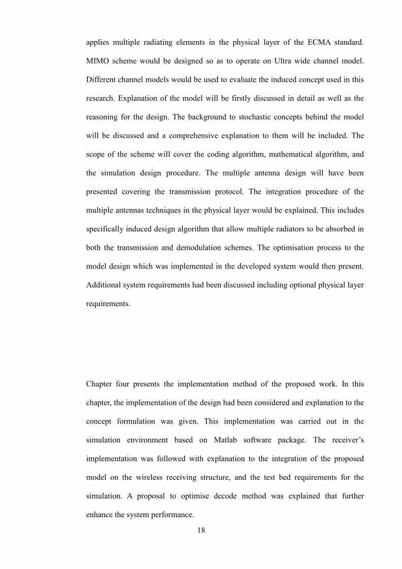
18
applies multiple radiating elements in the physical layer of the ECMA standard.
MIMO scheme would be designed so as to operate on Ultra wide channel model.
Different channel models would be used to evaluate the induced concept used in this
research. Explanation of the model will be firstly discussed in detail as well as the
reasoning for the design. The background to stochastic concepts behind the model
will be discussed and a comprehensive explanation to them will be included. The
scope of the scheme will cover the coding algorithm, mathematical algorithm, and
the simulation design procedure. The multiple antenna design will have been
presented covering the transmission protocol. The integration procedure of the
multiple antennas techniques in the physical layer would be explained. This includes
specifically induced design algorithm that allow multiple radiators to be absorbed in
both the transmission and demodulation schemes. The optimisation process to the
model design which was implemented in the developed system would then present.
Additional system requirements had been discussed including optional physical layer
requirements.
Chapter four presents the implementation method of the proposed work. In this
chapter, the implementation of the design had been considered and explanation to the
concept formulation was given. This implementation was carried out in the
simulation environment based on Matlab software package. The receiver’s
implementation was followed with explanation to the integration of the proposed
model on the wireless receiving structure, and the test bed requirements for the
simulation. A proposal to optimise decode method was explained that further
enhance the system performance.

19
The final chapter will provide a conclusion to the research project by highlighting the
obtained results from the system model. It will outline the contribution of this work
for the short range WPAN technology and how it can be integrated in future research.
It will also identify areas in the research which could be incorporated in future
studies in PANs. A review of the validation process for the multiple antenna system
would be discussed along with comparative tests with existing approved practical
models. A detail analysis will be discussed to project the merits of the design model.
A review of standardised models will also be carried on to identify a viable test
method.

20
1.8 Research methodology
The purpose of this section is to outline the research methodology used in the
production of multiple antennas model for Ultra wide band system used in the
Wireless Personal Area Network systems. It describes six phases including
identification, designing model, implementation, Optimisation, testing and
verification of the proposed model that was presented in this project. The adopted
research methodology for this work had been illustrated graphically in the following
figure.

21
Phase 1: Literature Review
Phase 2: Identify and analysis the challenges in the
Implementation of MIMO in UWB systems
Phase 3: Designing a prototype of a physical layer
wireless communication system
Phase 4: Implementation of MIMO configuration on the
model design
Phase 5: System model optimisation and improvements
Phase 6: System testing and evaluation
Figure 1: Research methodology
22
Six phases approach were identified in defining an appropriate research
program structure. These are as follows
Phase 1 (Literature Review): This phase covers previous works on the
implementation of MIMO techniques on Ultra wide band wireless systems.
The focus would be on identifying the main problems and challenges that
encapsulate the technology. Various concepts would be looked at and explored
to facilitate new design models.
Phase 2 (Identifying related problems): In this section, the emphasis would
be on identifying tangible problems in the design and implementation of
spatial elements in hostile indoor environments. Challenging channel
behaviours and problems would be induced and considered for research work.
Phase 3 (Designing a prototype of a physical layer Wireless
communication system): In this stage, a prototype design model would be
constructed to enable the linking of the various physical layer blocks of the
wireless system and producing a functional and operational design model. This
interconnection allows for observation of the blocks parameters and the system
performance.
23
Phase 4 (Implementation of MIMO configuration on the model design):
MIMO construction would take place in this section and would be integrated
in the simulation model. The algorithm for implementation would be tested to
verify the system performance. The design concept would be implemented to
infer the theoretical analysis.
Phase 5 (System model optimisation and improvements): The modelling
design would be improved and optimised. Further analysis would be carried
out to improve the performance and reduce the complexity involves.
Phase 6 (System testing and evaluation): In this step, the various scenarios
would be tested and the model would be observed to finalise the design.
Evaluation would be performed on each block within the simulation model and
all the results would be documented.

24
2 Background Research
2.1 ECMA-368 Specifications
The ECMA standard specifies OFDM modulation with multiple bands in
which the spectrum had been segmented into a collection of lower frequency
bands. It divides the unlicensed spectrum into sub-bands each of which
consists of a 528MHz bandwidth, and combines a tuple of bands in Band
Groups (BG1 – BG5) except for the last two bands [5], and figure (2.1.1) gives
a description of this spectrum division. A flexible feature of the model is the
variable transmission rate in which the standard supports data rates of 53.3, 80,
106.7, 160, 200, 320, 400, 480 Mb/s. The MB-OFDM scheme has been used in
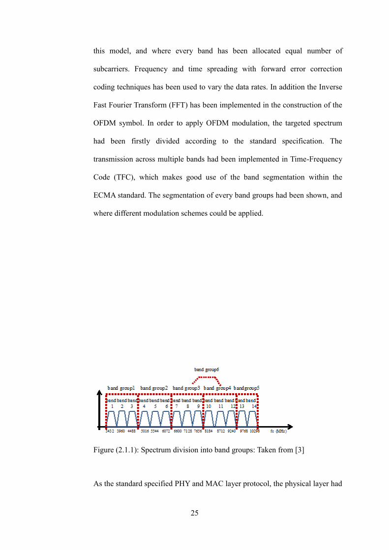
25
this model, and where every band has been allocated equal number of
subcarriers. Frequency and time spreading with forward error correction
coding techniques has been used to vary the data rates. In addition the Inverse
Fast Fourier Transform (FFT) has been implemented in the construction of the
OFDM symbol. In order to apply OFDM modulation, the targeted spectrum
had been firstly divided according to the standard specification. The
transmission across multiple bands had been implemented in Time-Frequency
Code (TFC), which makes good use of the band segmentation within the
ECMA standard. The segmentation of every band groups had been shown, and
where different modulation schemes could be applied.
Figure (2.1.1): Spectrum division into band groups: Taken from [3]
As the standard specified PHY and MAC layer protocol, the physical layer had

26
defined Physical Layer Convergence Protocol (PLCP) sub-layer to interface
between this layer and the upper MAC counterpart [6]. This sub-layer
provides a method for converting PHY Service Data Unit (PSDU) into PLCP
Packet Data Unit (PPDU). The PPDU structure consists of the PLCP preamble
that includes the Channel Estimation and Packet synchronisation sequences,
the PLCP header, and the PSDU. Further error detection and correction were
added to improve the wireless communication links.
Figure (2.1.2) PPDU and PLCP structure: Taken from [4]
The process of transmission consists of collect a number of packets (or frames)
in which a predefined number of modulated OFDM symbols forming the
message packet. As it had been stated, frequency domain spreading, time
domain spreading and Forward Error Correction (FEC) are used to vary the
data rate. There are three specified types of TFC, the first one is where the

27
coded information is interleaved over three bands and that termed as Time-
Frequency Interleaving (TFI) [7]. The second coding is where the coded
information is interleaved over two bands, and this referred to as TF12. The
third one in which the transmission was done over signal band where the term
Fix Frequency Interleaving (FFI) was used for this type of coding. Four time-
frequency codes within the first four and six bands group make use of TFI, and
three time-frequency codes uses TFI2 and FFI coding, giving support of ten
channels in each band group. In the case of the fifth band group, two time-
frequency codes uses FFI and one uses TFI2. On the other hand in the six band
group, FFI channels and one of the TFI2 channels overlap with the channels in
the third and fourth band groups. In order to allow range regularity and radio
coexistence within the standard, a mechanism for nulling the OFDM
subcarriers in the TFC operations had been provided. Frequency Domain
Spreading (FDS), and Time Domain Spreading (TDS) were been facilitated in
order to expand the bandwidth for the modulation schemes. Further, the
various coding rates were assigned to different coding and modulations
depending on the applications. Table (2.1) gives description of the different
coding, Data rates, and modulation in the PSDU.
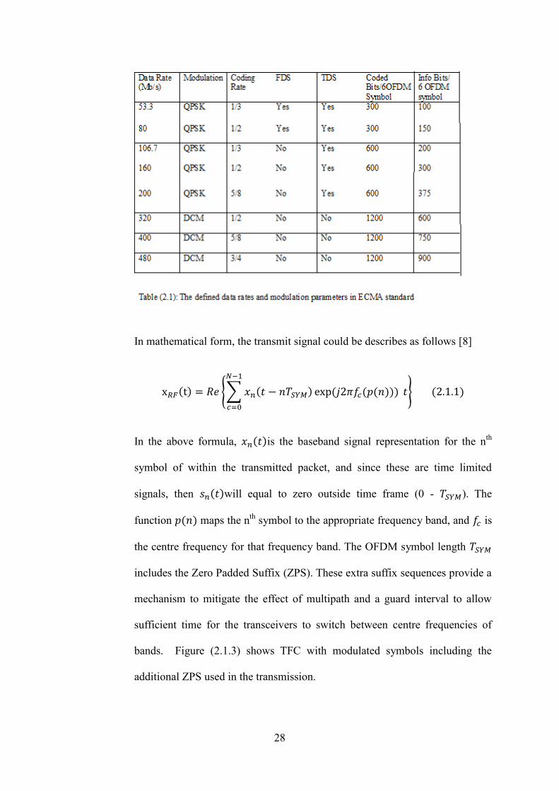
28
In mathematical form, the transmit signal could be describes as follows [8]
x𝑅𝐹(t) = 𝑅𝑒 {∑ 𝑥𝑛(𝑡 − 𝑛𝑇𝑆𝑌𝑀) exp(𝑗2𝜋𝑓𝑐(𝑝(𝑛)))
𝑁−1
𝑐=0
𝑡} (2.1.1)
In the above formula, 𝑥𝑛(𝑡)is the baseband signal representation for the nth
symbol of within the transmitted packet, and since these are time limited
signals, then 𝑠𝑛(𝑡)will equal to zero outside time frame (0 - 𝑇𝑆𝑌𝑀). The
function 𝑝(𝑛) maps the nth
symbol to the appropriate frequency band, and 𝑓𝑐 is
the centre frequency for that frequency band. The OFDM symbol length 𝑇𝑆𝑌𝑀
includes the Zero Padded Suffix (ZPS). These extra suffix sequences provide a
mechanism to mitigate the effect of multipath and a guard interval to allow
sufficient time for the transceivers to switch between centre frequencies of
bands. Figure (2.1.3) shows TFC with modulated symbols including the
additional ZPS used in the transmission.
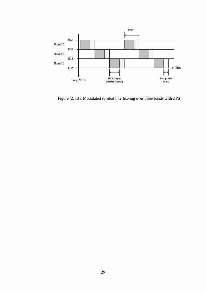
29
Figure (2.1.3): Modulated symbol interleaving over three bands with ZPS

30
2.2 MIMO System
Multiple Input Multiple Output (MIMO) techniques consist of using multiple
antennas at both ends of the communication channel to exploit spatial diversity
and add another degree of freedom to the system capacity [9], [10]. The
technique combines the temporal, spatial and frequency diversities in the
transmission scheme to increase the link throughput. MIMO enables the
transmission of data over multiple channels and hence increases the available
data rate of the system [11]. This in turn produces a linear increase in capacity
without the need for bandwidth expenditure [12]. Furthermore, it doesn't
require additional transmission power and this single factor makes it very
attractive for short range wireless communication networks [13]. This is
because of the astringent power regulation imposed by federal regulators (e.g.
the FCC in the USA).
The spectrum allocation in MIMO multiband systems has been constructed by
supplying each user a sub band (with a minimum bandwidth of 500 MHz) and
all the transmitting antennas operate in the same band for each user at that
particular time duration. The encoding process has been applied across all of
the antennas, the number of subcarriers within one symbol and the number of
OFDM symbols that forms blocks or frames for transmission. This way, each
complex symbol could be identified by the subcarriers of the particular

31
spectrum at the specified antenna element during a known OFDM period of a
marked frame. Due to the encoding format, a matrix representation is used in
multi-spatial systems to simplify its mathematical representation. The
sequences allocated to each user and for each antenna were designed such that
they were orthogonal to each other or the correlation factor is zero between
them [14]. This independent property ensures the formulation of a diagonal
matrix which simplifies the detection process at the receiver side and reducing
the hardware and complexity costs. The transmitted based band signal (d)
represented by each symbol to be transmitted on antenna z has been
interpreted mathematically as follows [15].
𝑑𝑧(𝑡) = √𝐸
𝐴 ∑𝑏𝑧(𝑠) 𝑒
−𝑗2𝜋𝑠∆𝑓
𝑆−1
𝑠=0
(𝑡 − 𝑇𝐴𝑃) (2.1.2)
Where E, A , b, T and f represent the total energy, the total number of antennas,
the complex symbol, the duration of the added prefix (this could be Cyclic
prefix or Zero-padding) and the sub frequency spacing between two
subcarriers. The energy of all the transmitted signals has been normalised to
eliminate the number of radiating elements, and in addition satisfying the
spectrum mask regulations [16]. A total number of Z blocks consisting of
OFDM symbols are transmitted from all the antennas forming a code word

32
matrix B and for each radiating element a number of symbols have been
allocated. That is for the 𝑎𝑡ℎ antenna, a number of complex code weights
forms a matrix X𝑎representing the duration of the OFDM symbol for the
particular block z. Furthermore, there were A antennas forming a matrix U of
all the blocks and the complex symbols. Within the symbol duration, a total of
S subcarriers are used to modulate the symbol. The channel operates across all
the subcarriers of the symbol, all symbols within the block and across all the
antennas forming a matrix CH. For every receiving antenna, a channel vector
CH𝑖of dimension ZSA x 1 has been formed consisting of a superposition to the
physical link response weights from the spatial elements [17], [18].
B = [B0 , B1 , … B(Z−1) ] (2.1.3)
𝑋𝑎𝑧 = [𝑋𝑎
𝑧 (0), 𝑋𝑎𝑧 (1) , … 𝑋𝑎
𝑧 (𝑆 − 1) ] (2.1.4)
CH = [CH1 , CH2 , … CHU ] (2.1.5)
CH𝑖 = [CHi1 , CHi2 , … CHiA ] (2.1.6)
The sub channel weights of the radiating elements in CH can be represented
statistically as a random variable with a magnitude having the form of the log
normal or Nakagami distribution [19]. The convolution process between the
transmitted signal and the channel results in a received signal that is
33
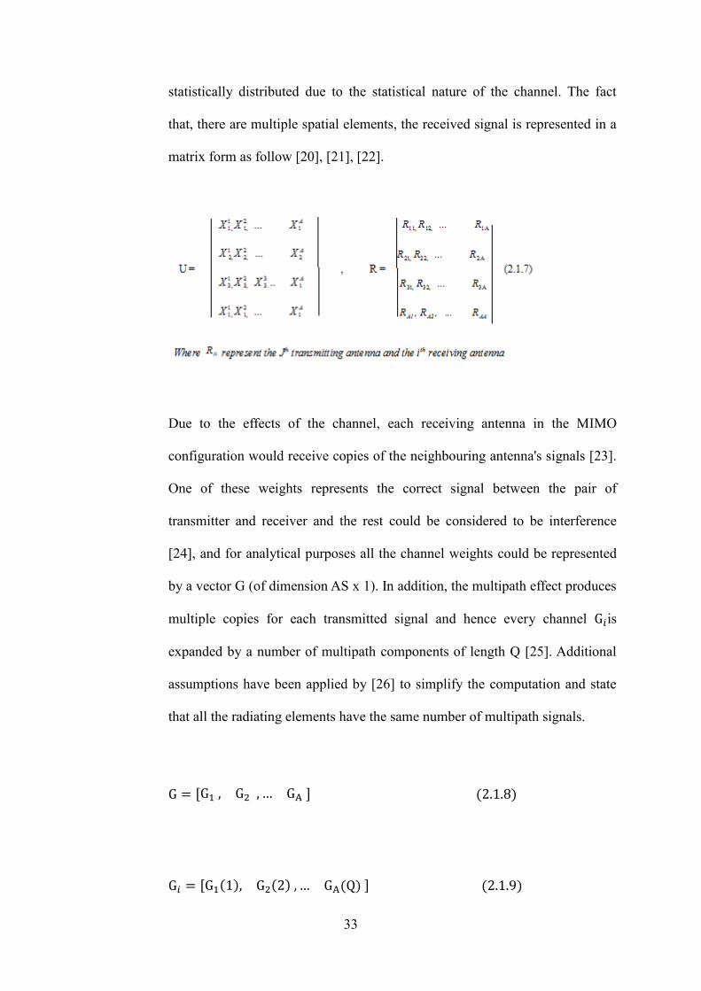
statistically distributed due to the statistical nature of the channel. The fact
that, there are multiple spatial elements, the received signal is represented in a
matrix form as follow [20], [21], [22].
Due to the effects of the channel, each receiving antenna in the MIMO
configuration would receive copies of the neighbouring antenna's signals [23].
One of these weights represents the correct signal between the pair of
transmitter and receiver and the rest could be considered to be interference
[24], and for analytical purposes all the channel weights could be represented
by a vector G (of dimension AS x 1). In addition, the multipath effect produces
multiple copies for each transmitted signal and hence every channel G𝑖is
expanded by a number of multipath components of length Q [25]. Additional
assumptions have been applied by [26] to simplify the computation and state
that all the radiating elements have the same number of multipath signals.
G = [G1 , G2 , … GA ] (2.1.8)
G𝑖 = [G1(1), G2(2) , … GA(Q) ] (2.1.9)
34
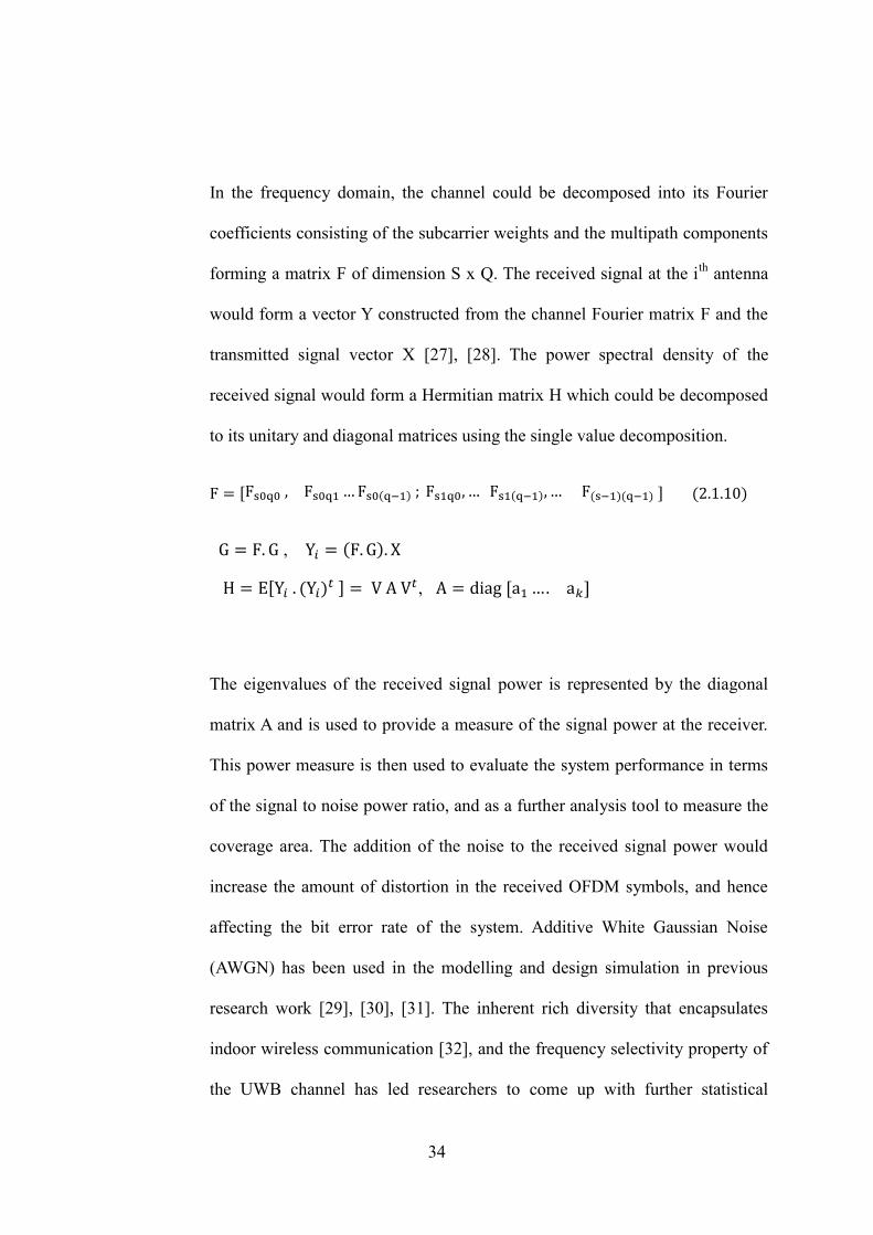
In the frequency domain, the channel could be decomposed into its Fourier
coefficients consisting of the subcarrier weights and the multipath components
forming a matrix F of dimension S x Q. The received signal at the ith
antenna
would form a vector Y constructed from the channel Fourier matrix F and the
transmitted signal vector X [27], [28]. The power spectral density of the
received signal would form a Hermitian matrix H which could be decomposed
to its unitary and diagonal matrices using the single value decomposition.
F = [Fs0q0 , Fs0q1…Fs0(q−1) ; Fs1q0, … Fs1(q−1), … F(s−1)(q−1) ] (2.1.10)
G = F. G , Y𝑖 = (F. G). X
H = E[Y𝑖 . (Y𝑖)𝑡 ] = V A V𝑡, A = diag [a1…. a𝑘]
The eigenvalues of the received signal power is represented by the diagonal
matrix A and is used to provide a measure of the signal power at the receiver.
This power measure is then used to evaluate the system performance in terms
of the signal to noise power ratio, and as a further analysis tool to measure the
coverage area. The addition of the noise to the received signal power would
increase the amount of distortion in the received OFDM symbols, and hence
affecting the bit error rate of the system. Additive White Gaussian Noise
(AWGN) has been used in the modelling and design simulation in previous
research work [29], [30], [31]. The inherent rich diversity that encapsulates
indoor wireless communication [32], and the frequency selectivity property of
the UWB channel has led researchers to come up with further statistical

35
assumptions [33]. These have assumed that the spectrum of each sub band that
the symbol hops across was independent of each other and were not correlated.
Implementing this assumption for the evaluation of the MIMO model
performance, has shown that using the multiband approach with symbol
hopping increases the system performance and provides an additional degree
of freedom in the frequency domain. Nevertheless, further research is needed
to be carried out concerning the operation of multiband transmission plans in
the UWB systems. This includes determining more accurate statistical models
for the MIMO capacity in the physical medium, and the spectrum power for
each of the sub bands across each band group.
2.2.1Alamouti Scheme Space-Time Block Code (STBC)
The growing demand for more channel capacity had led to research in the
spatial domain to add an extra degree of freedom to the capacity. The break
through that was captured by Alamouti scheme [34], which had opened a new
area of research into the MIMO techniques.
36
The scheme uses two transmit antennas, two time intervals, and a novel
complex orthogonal principle that uses space-time technique to increase the
performance without increasing the signal power. A code-word matrix was
formed from two consecutive symbols (s1,s2), and their complex conjugate
counterparts in a dual time pins as follows
𝑿 = [𝑠1 −𝑠2∗
𝑠2 𝑠1∗] (2.2.1)
The scheme using two symbol periods to transmit the dual symbols from two
antennas, and therefore in essence the original content information would be
transmitted twice across the time intervals. The original principle was
formation of the matrix𝑿, which is a complex orthogonal matrix as
𝑿 𝑿𝐻 = [|𝑠1|2 + |𝑠2|2 0
0 |𝑠1|2 + |𝑠2|2]
= |𝑠1|2 + |𝑠2|2 ∗ 𝑰2 (2.2.2)
This orthognality of the matrix of rank two gives the Alamouti code a diversity
gain of 2. The diversity analysis was based on the Maximum likelihood
detection. Nevertheless, there is a critical condition that fading should remain
invariant of the two consecutive symbol periods for every spatial code.
[𝑦1𝑦2∗] = [
ℎ1 ℎ2ℎ2∗ −ℎ1
∗] [𝑥1𝑥2] + [
𝑛1𝑛2∗] (2.2.3)

37
At the receiver, estimating the channel coefficients will lead to multiplying the
received noisy signal vector with the channel matrix will lead to the following
[ℎ1∗ ℎ2ℎ2∗ −ℎ1
] [𝑦1𝑦2∗] = [
ℎ1∗ ℎ2ℎ2∗ −ℎ1
] [ℎ1 ℎ2ℎ2∗ −ℎ1
∗] [𝑥1𝑥2] + [
ℎ1∗ ℎ2ℎ2∗ −ℎ1
] [𝑛1𝑛2∗]
[��1��2∗] = [|ℎ1|
2 + |ℎ2|2] [
𝑥1𝑥2] + [
ℎ1∗𝑛1 + ℎ2𝑛2
∗ ℎ2∗𝑛1 + ℎ1𝑛2
∗ ] (2.2.4)
Due to the orthognality of Alamouti code, simple ML receiver would estimate
the transmitted symbol as follows
��𝑗 = 𝐸𝑟𝑟𝑜𝑟 𝑓𝑢𝑛𝑐𝑡𝑖𝑜𝑛 (��𝑗
|ℎ1|2+|ℎ2|2) = 𝑄 (
��𝑗
|ℎ1|2+|ℎ2|2) (2.2.5)
It is important to note that, the two main objectives in using orthogonal space-
time code were to increase the diversity order, and reducing the complexity of
symbols detection at the receivers. Further, the complex orthogonal codes
would not exists for a number of spatial elements that is greater than two with
the defined objective goals mentioned before. STBC could be further
improved in terms of its coding gain by using convolutional encoders as in
what is termed as Space-Time Trellis Codes (STTC).

38
2.3 The Physical Channel
There has been a significant amount of research concerning the channel
measurements for Ultra-wide band applications stemming from the practical
and theoretical difficulties these systems present. The measurement approach
has been carried out based on two distinctive domains, the time domain
approach which evaluates and measures the impulse response of the medium;
whereas the frequency domain methods deals with the channel transfer
function based on spectrum evaluation. In the time domain, channel sounders
have been implemented by using either short or high energy pulses, or more
robust methods using correlative channel sounders [35]. The latter uses wide
band signal with low Signal to Noise Ratio (SNR) to avoid interfering with the
surrounding wireless systems (e.g. narrowband applications). At the other end,
a PN sequence is used in the correlation process where the original transmitted
signal is then induced. In order to extract the channel parameters, different
measurement procedures have been performed. Two high resolution algorithm
methods that have been used in practice and have been highlighted in research
papers [36]. The first is the CLEAN algorithm which is based on an iteration
process. Received pulses are first correlated with a known pulse shape in order
to extract the strongest pulse and then iteratively extract the following
dominant pulse components until a threshold of energy level is reached. The
39
SAGE algorithm [37] is the other method which uses a maximum likelihood
estimate using the parameters applied with iteration process. The Vector
Network Analyser (VNA) technique is a widely used measurement method in
the frequency domain [38]. It uses a frequency sweep of sinusoidal waveform
to excite the channel and then measure its transfer function. The inherent
averaging makes it less affected by noise and interference and can perform
large band width measurements. However, due to the slow operation of
frequency stepping, this process can take a long time for dynamic channels.
Furthermore, the wiring issues tend to limit the measurements to short area
ranges. Scalar Network Analyser is a modified method that measures only the
magnitude of the transfer function and hence reduces the operation time that
VNA takes.
Measured data has shown that for the indoor channel, the scattered objects
tend to be distributed in the form of clusters between the transmitters and
receivers [39]. Furthermore, within each cluster the arrival ray tends to be non-
uniformly distributed. One important implication of the clustering assumption
is the Saleh-Valenzuela (SV) model in which multipath components follow a
Poisson distribution with inter arrival times that is exponentially distributed
[40]. Moreover, the model has a cluster and ray arrival times as well as a decay
factor value for each of them and hence provides a great flexibility in
modelling different scenarios.
The IEEE has established various standardisation groups to develop standard
40
models each of which covers certain applications under common specifications
of its physical layer proposal. These models have been developed based on
measured data and the simulation of identifiable prerequisite requirements for
system design. These were common primary characteristics of the multipath
channel such as the power delay profile, RMS delay and the number of
multipath components, and data that requires an agreement between the
measured data and the standardised models realisations.
In this section, two models that frequently mentioned in research papers are
highlighted (namely the IEEE 802.15.3.a and IEEE 802.15.4a).
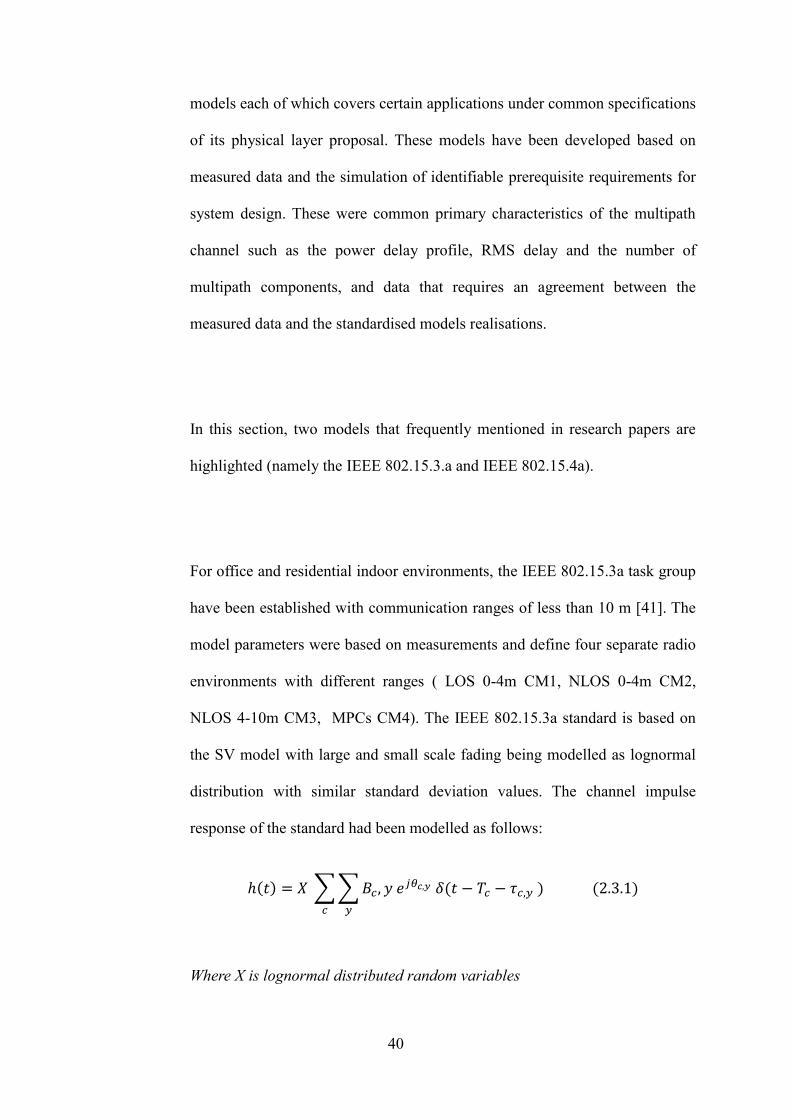
For office and residential indoor environments, the IEEE 802.15.3a task group
have been established with communication ranges of less than 10 m [41]. The
model parameters were based on measurements and define four separate radio
environments with different ranges ( LOS 0-4m CM1, NLOS 0-4m CM2,
NLOS 4-10m CM3, MPCs CM4). The IEEE 802.15.3a standard is based on
the SV model with large and small scale fading being modelled as lognormal
distribution with similar standard deviation values. The channel impulse
response of the standard had been modelled as follows:
ℎ(𝑡) = 𝑋 ∑∑𝐵𝑐, 𝑦 𝑒𝑗𝜃𝑐,𝑦 𝛿(𝑡 − 𝑇𝑐 − 𝜏𝑐,𝑦 )
𝑦𝑐
(2.3.1)
Where X is lognormal distributed random variables
41
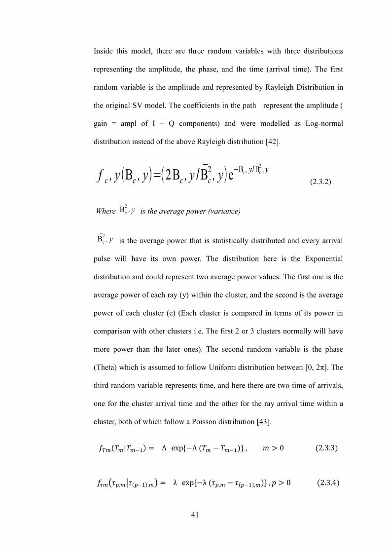
Inside this model, there are three random variables with three distributions
representing the amplitude, the phase, and the time (arrival time). The first
random variable is the amplitude and represented by Rayleigh Distribution in
the original SV model. The coefficients in the path represent the amplitude (
gain = ampl of I + Q components) and were modelled as Log-normal
distribution instead of the above Rayleigh distribution [42].
f c , y(Βc , y)=(2Βc , y /Βc
2, y)e
−Βc , y/ Βc
2, y
(2.3.2)
Where Βc
2, y is the average power (variance)
Βc
2, y is the average power that is statistically distributed and every arrival
pulse will have its own power. The distribution here is the Exponential
distribution and could represent two average power values. The first one is the
average power of each ray (y) within the cluster, and the second is the average
power of each cluster (c) (Each cluster is compared in terms of its power in
comparison with other clusters i.e. The first 2 or 3 clusters normally will have
more power than the later ones). The second random variable is the phase
(Theta) which is assumed to follow Uniform distribution between [0, 2π]. The
third random variable represents time, and here there are two time of arrivals,
one for the cluster arrival time and the other for the ray arrival time within a
cluster, both of which follow a Poisson distribution [43].
𝑓𝑇𝑚(𝑇𝑚|𝑇𝑚−1) = Λ exp{−Λ (𝑇𝑚 − 𝑇𝑚−1)} , 𝑚 > 0 (2.3.3)
𝑓𝜏𝑚(𝜏𝑝,𝑚|𝜏(𝑝−1),𝑚) = λ exp{−λ (𝜏𝑝,𝑚 − 𝜏(𝑝−1),𝑚)} , 𝑝 > 0 (2.3.4)

42
Although these results have been used in existing research and have gained
acceptance in the academic community, there are still very limited
measurements that have been taken to date when considering the free spectrum
channel. Hence, further investigation is needed before these assumptions could
be taken as a realistic representation of the channel behaviour. In this research,
the above channel model would be used as basis for modelling the physical
medium and further analysis would be carried out to investigate the channel
parameters that have been identified in the literature.
2.4 MIMO-OFDM wireless system block model
As engineering designers was able to implement multicarrier in the discrete
time domain using inverse fast Fourier transform acting as modulator and its
corresponding fast Fourier projection in the frequency domain representing the

43
demodulation, block representation becomes a useful representation tool in the
design and implementation of complex wireless system. Representing the
model into a number of interconnected blocks allows for systematic design,
implementation and evaluation of wireless projects. MIMO wireless model
consists of a number of integrated blocks at the transmitting and receiving
sides [44]. These are the coding module which provides Forward error
correction codes that helps reducing the channel noise distortion, and the
modulation block where the desired signal was mapped across the
constellation. This constellation was associated with the specified modulation
scheme. The resulted complex symbols was then modulated and translated in
the time domain using frequency transform according to the IFFT, and then
passed to Digital to Analogue conversion (D/A). At the receiving block, the
opposite operation was carried out, by estimating the original wireless signal
using the decoding and demodulation blocks. Figure (2.4.1) gives a description
of the multiple antennas wireless model used in the design and modelling of
real wireless systems.

44
Figure (2.4.1): MIMO wireless block model system: Taken from [33]
2.5 Convolutional Coding
There are considerable performance improvements in using coded transmitted
signals over un-coded signals in wireless communication system. The
Convolutional coding process produces coded signal out of un-coded message
sequence, and uses parity bits computed from message bits. Convolutional
code is specified by the number of input bits (i), the number of output bits (o),
45
and the number of memory registers (o, i, m) [45]. Since there are a number of
parity bits, the code rate (r) of the encoder is (i / o), and this quantity
represents the efficiency of the code. The number of inputs and outputs
normally range from 1 to 8 in practical application, whereas the number of
registers takes values ranging from 2 to 10. Convolutional encoder contained
core quantities, and these are the constraint length, and the generator
polynomials. The constraint length (L) represents the number of bits in the
encoder memory that effect the output coded signal. Increasing the constraint
length would increase the resilience to bit errors. Although the downside is that
it takes longer time to decode. The numbers of generator polynomials are
equal to the number of parity bits in every sliding window. The convolutional
code is generated by convolving the desired message signal with the generator
polynomial. The output code normally specified by constraint length and the
code rate as (r*L). Convolutional encoders sometimes defined as systematic
and non-systematic encoders. Systematic encoders are very easy to implement
in hardware and have simple look up table. Further, the errors in these
encoders dose not propagate catastrophically. On the other hand, in the case of
non-systematic encoders, the output symbols do not include the input data. A
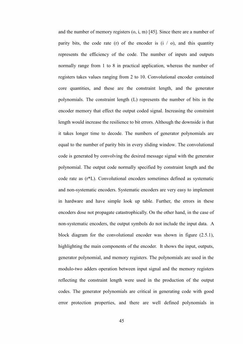
block diagram for the convolutional encoder was shown in figure (2.5.1),
highlighting the main components of the encoder. It shows the input, outputs,
generator polynomial, and memory registers. The polynomials are used in the
modulo-two adders operation between input signal and the memory registers
reflecting the constraint length were used in the production of the output
codes. The generator polynomials are critical in generating code with good
error protection properties, and there are well defined polynomials in
46
standardised real time wireless application.
Figure (2.5.1): Block diagram of main components in convolutional encoder
The code rate of the encoder could be altered by the use of Puncturing.
Puncturing uses dummy bits in the encoding and decoding process. The
advantage of using Puncturing is that the coding rate could be changed
dynamically in a flexible way depending on the channel condition, which
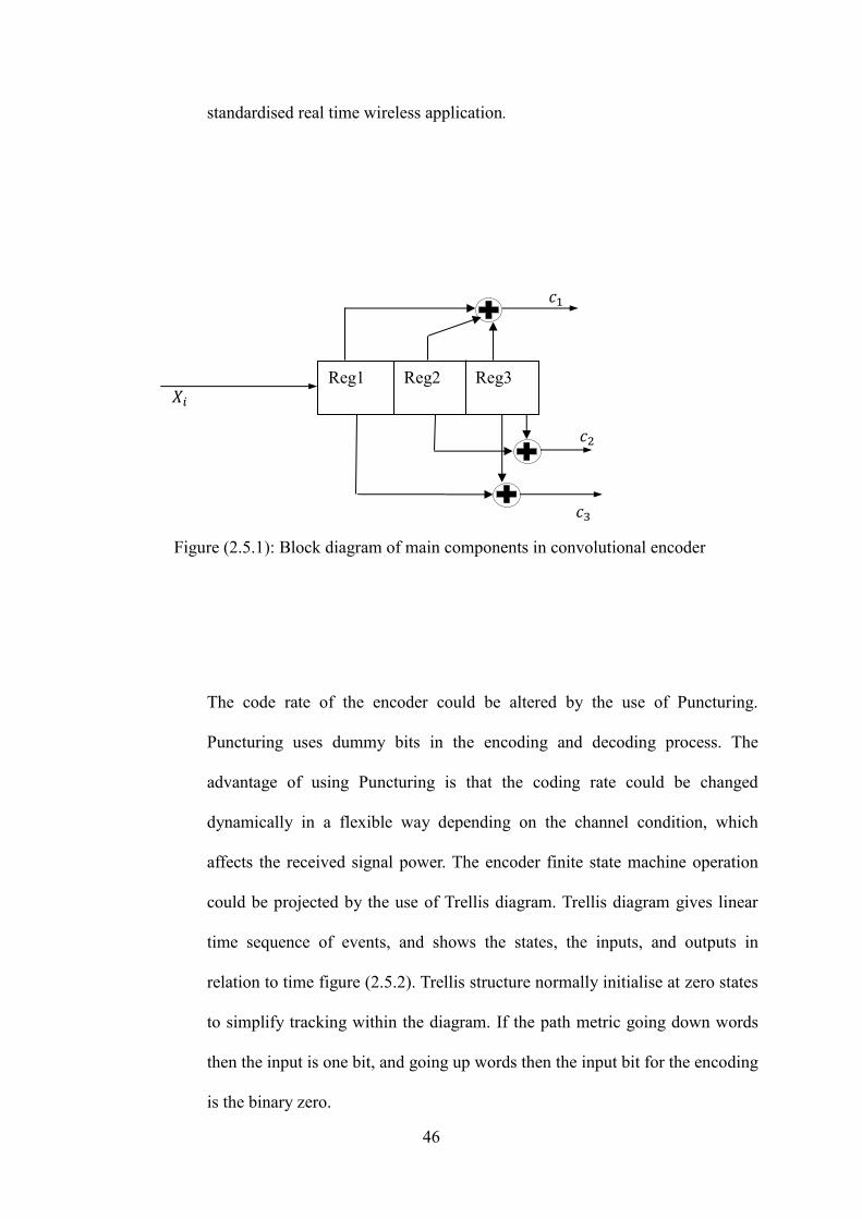
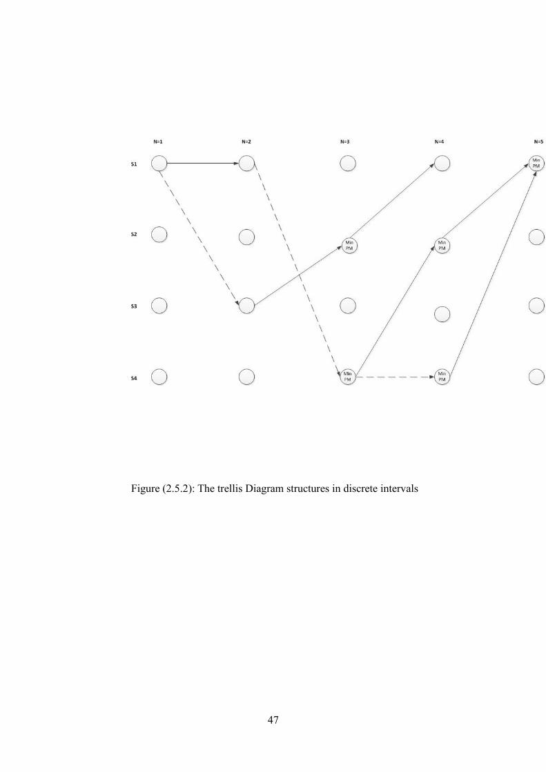
affects the received signal power. The encoder finite state machine operation
could be projected by the use of Trellis diagram. Trellis diagram gives linear
time sequence of events, and shows the states, the inputs, and outputs in
relation to time figure (2.5.2). Trellis structure normally initialise at zero states
to simplify tracking within the diagram. If the path metric going down words
then the input is one bit, and going up words then the input bit for the encoding
is the binary zero.
𝑐1
Reg1 Reg2 Reg3 𝑋𝑖
𝑐2
𝑐3
47
Figure (2.5.2): The trellis Diagram structures in discrete intervals
48
2.6 Viterbi Decoding
Viterbi decoder is a powerful and widely applicable algorithm that uses soft
Maximum likelihood decoding on the trellis structure [46]. The decoding
algorithm maximising the probability condition of the received symbol given
the transmitted signal, by choosing the nearest symbol based on minimisation
of the Euclidean metric. The Viterbi algorithm have two sequential phases, the
first includes calculation of the trellis metrics (the branch metric, path metric,
and decision bits), and the second represents the trace-back in time to identify
the most likely sequence of symbols. Look up table are generated and used by
the decoding algorithm across the trellis structure, therefore there are memory
limitation for the traceback that control Viterbi process. The Branch Metric
(BM) calculates and stores the output difference between the observed parity
bits, and the estimated parity bits (this estimated output bits depend on the
input to the encoder and the current state of the encoder). The Path Metric
(PM) represents a value on the state node indicating the path weight at that
particular node and particular time ( a node may have many path coming to it,
but the one with the highest value, represents the weight of that node at that
particular time). This weight value project the number of bit errors detected
when comparing observed and the most likely message up to that particular
time. However, when traversing through the trellis to estimate the most likely

49
path, at any particular time interval, the decision would be picking the node at
that particular time with the smallest path metric among the entire node within
that time index. Traversing in the forward direction could have multipath with
the equal PM, and therefore the backward process enables to find the most
likely path. The backward process starts at the last time interval, and chooses
the node with lowest PM, and then traverses backward from that states. This
way, all the multiple paths are removed and only the survive path would be left
representing the most likely sequence. Figure (2.6.1) below shows the survivor
path based on the implementation of the Viterbi algorithm.
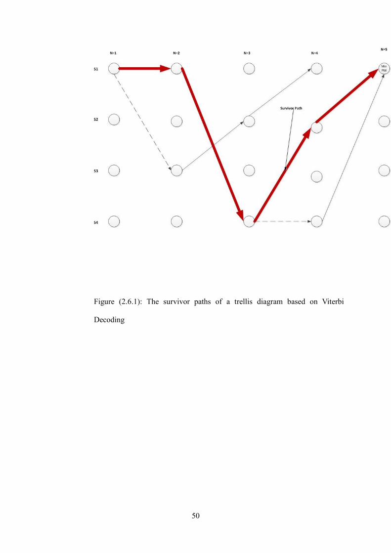
50
Figure (2.6.1): The survivor paths of a trellis diagram based on Viterbi
Decoding
51
2.7 BCJR algorithm and its challenges
This algorithm was proposed by Bahl Jelinek Cocke and Raviv (BCJR) to
maximise the posterior decoding defined on the trellis structure of the
convolutional code [47]. This is an iterative decoder based on the forward
error correction code, and principally is a soft output algorithm used for
Markov chain based structure. It is important to note that, convolutional code
exhibits Markov chain since it’s a finite state machine. In Viterbi algorithm,
the error probability is minimised between the transmitted and received code-
word, while the aim in BCJR method is to minimise the bit error probability. It
is very clear that, the latter algorithm gives better performance in terms of the
error performance. The two vectors for the encoders are the input sequence
signal to the encoder𝑋_𝑖, and the output signal sequence from the encoder𝑋_𝑜.
Considering the states of the encoder, there are a number of states for every
encoder based on the memory registers of that particular encoder. While
transmitting, the encoder transit from one state to another with every instant of
time project three main states𝑆𝑝𝑟𝑒𝑣,𝑆𝑐𝑢𝑟, and 𝑆𝑛𝑒𝑥 (𝑆𝑝𝑟𝑒𝑣indicating the
previous state, 𝑆𝑐𝑢𝑟refer to the current state, and 𝑆𝑛𝑒𝑥indicating the next state
for the encoder). The encoder moves (jump) between states depending on the
input source information sequence (the original voice or data sequence
required for transmission). The posterior log likelihood ratio of the input signal

52
depending on observed finite and limited received signal could be defined as
flows
𝐿(𝑥_𝑖) = log {𝑃(𝑥_𝑖 = 1|𝑌)
𝑃(𝑥_𝑖 = 0|𝑌) } (2.7.1)
Therefore, the scheme could also be referred to as Maximum Posteriori
Probability (MAP) decoder. However, since there is a convolutional encoder
that applied to the input signal, then the output transmitted signal (x) will
depends on the input signal and the states of the encoder. Including these states
in the conditional formula would be as flow
𝐿(𝑥_𝑖) = log {∑ 𝑃(𝑆𝑘−1 = 𝑢, 𝑆𝑘 = 𝑝|𝑌)𝑢,𝑝;𝑥_𝑖=1
∑ 𝑃(𝑆𝑘−1 = 𝑢, 𝑆𝑘 = 𝑝|𝑌)𝑢,𝑝;𝑥_𝑖=0 } (2.7.2)
In the transition between the previous state (𝑆𝑘−1) and the current state (𝑆𝑘), all
the paths through the branches as result of an input one (𝑥_𝑖 = 1) would be
summed together in the numerator expression for the posterior likelihood (eq.
2.7.2), while all the state transitions from (u to p) as result of an input zero to
the convolutional encoder (𝑥_𝑖 = 0) would be summed in the denominator.
Furthemore, the observed sequency (Y), could be divided into three segments,
the past, current and the future (𝑌𝑦<𝑘, 𝑌𝑦=𝑘, and𝑌𝑦>𝑘,). The likelihood
expression could be segmented based on its probability components relating
the encoder states. In the use of Bay’s theorem and Markov property, the

53
individual probabilities forming the expression could be expressed by certain
quantities that needed to be calculated within the iterative process.
𝑃(𝑆𝑘−1 = 𝑢, 𝑆𝑘 = 𝑝|��1,𝑘)
= 𝑃(𝑆𝑘−1 = 𝑢|��1,𝑘−1)𝑃(𝑆𝑘 = 𝑘, ��𝑘|𝑆𝑘−1 = 𝑢)𝑃(��𝑘+1,𝑘|𝑆𝑘 = 𝑝)
𝑃(𝑆𝑘−1 = 𝑢, 𝑆𝑘 = 𝑝, ��1,𝑘) = 𝑃(𝑆𝑘−1= 𝑢, ��1,𝑘−1) 𝑃(𝑆𝑘 = 𝑘, ��𝑘|𝑆𝑘−1 = 𝑢)𝑃(��𝑘+1,𝑘|𝑆𝑘 = 𝑝)
𝑃(𝑆𝑘−1 = 𝑢, 𝑆𝑘 = 𝑝, ��1,𝑘) = 𝛼𝑘−1(𝑢) 𝛾𝑘(𝑢, 𝑝) 𝛽𝑘(𝑝) (2.7.3)
𝛼𝑘−1(𝑢) = 𝑃(𝑆𝑘−1 = 𝑢, ��1,𝑘−1) (2.7.4)
𝛾𝑘(𝑢, 𝑝) = 𝑃(𝑆𝑘 = 𝑝, ��𝑘|𝑆𝑘−1 = 𝑢) (2.7.5)
𝛽𝑘(𝑝) = 𝑃(��𝑘+1,𝑘|𝑆𝑘 = 𝑝) (2.7.6)
The forward calculation starting from the initial sate to the end involves (𝛼),
and the backward path calculation involves (𝛽), while the transition between
states related to (𝛾) labelled in figure (2.7.1). It is important to note, the
reverse path (backward) only calculated recursively after the whole Y
sequence had been received.
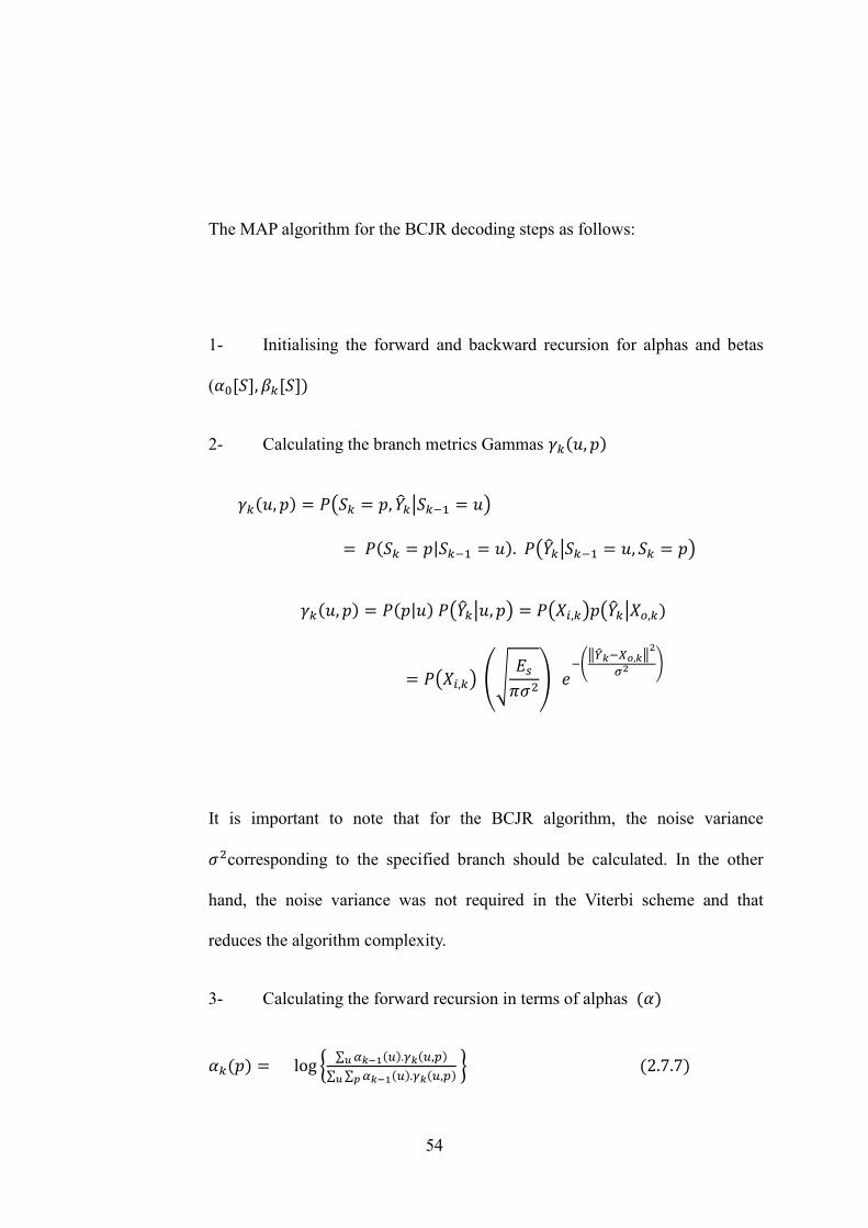
54
The MAP algorithm for the BCJR decoding steps as follows:
1- Initialising the forward and backward recursion for alphas and betas
(𝛼0[𝑆], 𝛽𝑘[𝑆])
2- Calculating the branch metrics Gammas 𝛾𝑘(𝑢, 𝑝)
𝛾𝑘(𝑢, 𝑝) = 𝑃(𝑆𝑘 = 𝑝, ��𝑘|𝑆𝑘−1 = 𝑢)
= 𝑃(𝑆𝑘 = 𝑝|𝑆𝑘−1 = 𝑢). 𝑃(��𝑘|𝑆𝑘−1 = 𝑢, 𝑆𝑘 = 𝑝)
𝛾𝑘(𝑢, 𝑝) = 𝑃(𝑝|𝑢) 𝑃(��𝑘|𝑢, 𝑝) = 𝑃(𝑋𝑖,𝑘)𝑝(��𝑘|𝑋𝑜,𝑘)
= 𝑃(𝑋𝑖,𝑘) (√𝐸𝑠𝜋𝜎2
) 𝑒−(‖��𝑘−𝑋𝑜,𝑘‖
2
𝜎2)
It is important to note that for the BCJR algorithm, the noise variance
𝜎2corresponding to the specified branch should be calculated. In the other
hand, the noise variance was not required in the Viterbi scheme and that
reduces the algorithm complexity.
3- Calculating the forward recursion in terms of alphas (𝛼)
𝛼𝑘(𝑝) = log {∑ 𝛼𝑘−1(𝑢).𝛾𝑘(𝑢,𝑝)𝑢
∑ ∑ 𝛼𝑘−1(𝑢).𝛾𝑘(𝑢,𝑝)𝑝𝑢 } (2.7.7)
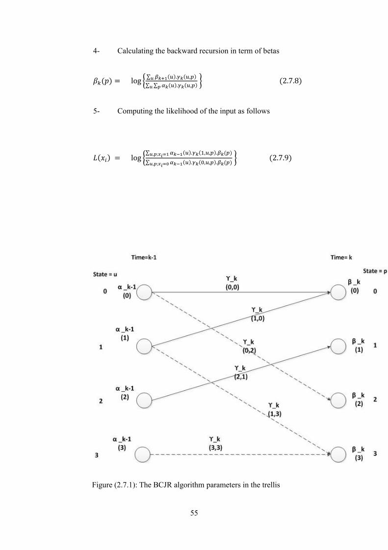
55
4- Calculating the backward recursion in term of betas
𝛽𝑘(𝑝) = log {∑ 𝛽𝑘+1(𝑢).𝛾𝑘(𝑢,𝑝)𝑢
∑ ∑ 𝛼𝑘(𝑢).𝛾𝑘(𝑢,𝑝)𝑝𝑢 } (2.7.8)
5- Computing the likelihood of the input as follows
𝐿(𝑥𝑖) = log {∑ 𝛼𝑘−1(𝑢).𝛾𝑘(1,𝑢,𝑝).𝑢,𝑝;𝑥𝑖=1
𝛽𝑘(𝑝)
∑ 𝛼𝑘−1(𝑢).𝛾𝑘(0,𝑢,𝑝).𝑢,𝑝;𝑥𝑖=0𝛽𝑘(𝑝)
} (2.7.9)
Figure (2.7.1): The BCJR algorithm parameters in the trellis

56
Further approximation could be used to the BCJR algorithm in the name of
Log-MAP and Max-Log-MAP, which make use of the logarithmic property to
give an efficient implementation. The Max algorithm gives further reduction in
the complexity by removing the exponential term in the Log-MAP method.
Therefore, the latter algorithm gives an optimal computational performance in
comparison to the original scheme. In conclusion, BCJR algorithm works in a
recursion process by depending on joint events (previous, current, and
expected future events), and therefore has a complexity issue as well as
overhead cost. This is one of the major challenges in applying these non-linear
algorithms in low cost wireless applications. This is because, for every
observed received signal vector, there would a multiple computations
regarding the states of the encoder with evaluation to the relation between the
input signal vector, and the estimated trellis states. The numerical instability of
underflow and overflow due to design errors in the iteration process makes this
algorithm less favourable to be implemented in wireless indoor application.
57
2.8 Turbo code and its cost of implementation
Turbo have a convolutional structure with two encoders applied for every input
sequence (original information signal), separated by an inter-leaver [48]. These
are recursive systematic convolutional encoders (figure 2.8.1). At the receiving
side, there are two Soft-Input Soft-Output (SISO) decoders separated by inter-
leaver to reformat the second encoder at the transmitter. Figure (2.82) gives a
description of the decoding structure used in the turbo algorithm. The
implementation of SISO algorithm could be based on SOVA or the more
optimise but involved MAP method, with passing extrinsic information in the
implementation. The turbo algorithm is an iterative decoder, and therefore it’s
critical to determine the number of iteration for every cycle within the method.
Choosing a large number of iteration would increase the cost exponentially,
and if there is no threshold limit, the algorithm will run to infinite loop and
would result in failures. This particular problem of iteration is one of the main
disadvantages in applying this algorithm in WPAN systems.

58
Figure (2.8.1): The encoding structure of the Turbo scheme
Figure (2.8.2): Block diagram structure of the Turbo Decoder
𝑋𝑛𝑐
Punct &
P/S
Encoder 1
Encoder 2
Int
𝑋𝑛𝑜1
𝑋𝑛𝑜2
𝑋𝑖
Decoder 1
𝐿𝑒21 DeInt
Decoder2 Int
Int
Hard
Decison
DeInt 𝑌𝑛𝑜2
𝑌𝑛𝑐 𝐿𝑒12
𝑌𝑛𝑜1
��𝑖

59
2.9. Modulation Schemes
The modulation schemes that have been used in the UWB Multiband wireless
communications standards were based on Quadrature Phase Shift Keying
(QPSK) and Quadrature Amplitude modulation (QAM) including 16-QAM &
32-QAM. The ECMA-368 standard has defined Quadrature Phase Shift
Keying (QPSK) modulation for up to 200 Mbps and Dual Carrier Modulation
(DCM) for the higher rate schemes [49], [50]. The various modulation
schemes that have been proposed in the literature and undertaken in previous
research work are summarised in this section.
2.9.1. Quadrature Phase Shift Keying
This scheme had been assigned for control signals at the packet header and for
the lower transmitting rate less than 320 Mb/s (53.3 Mb/s, 80 Mb/s, 106.7
Mb/s, 160 Mb/s, and 200 Mb/s). QPSK modulation has been accomplished by
dividing the coded bit sequences into groups of 2 bits forming a complex
number that have In-phase and Quadrature components (figure 2.9.1), and uses
the normalisation factor (𝑀 = 1
√2) expressed as follow.
𝑠[𝑘] = 𝑀 × [(2 × 𝑏[2𝑘] − 1) + 𝑗(2 × 𝑏[2𝑘 + 1] − 1) ] (2.9.1.1)
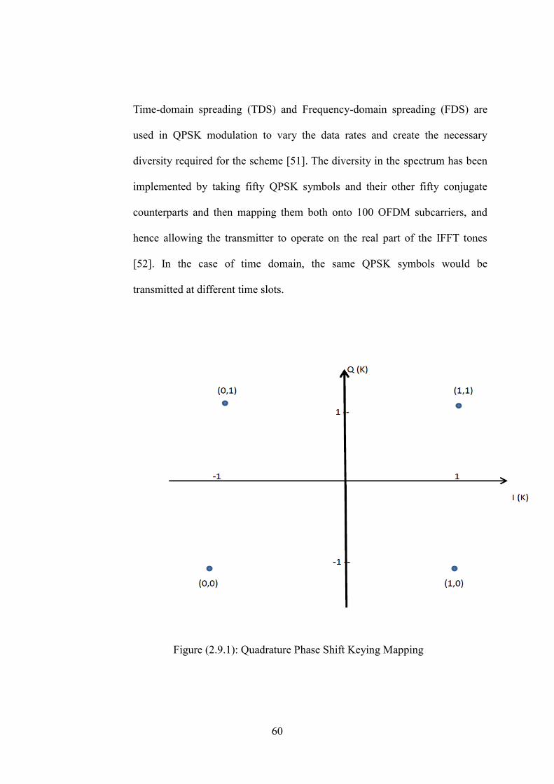
60
Time-domain spreading (TDS) and Frequency-domain spreading (FDS) are
used in QPSK modulation to vary the data rates and create the necessary
diversity required for the scheme [51]. The diversity in the spectrum has been
implemented by taking fifty QPSK symbols and their other fifty conjugate
counterparts and then mapping them both onto 100 OFDM subcarriers, and
hence allowing the transmitter to operate on the real part of the IFFT tones
[52]. In the case of time domain, the same QPSK symbols would be
transmitted at different time slots.
Figure (2.9.1): Quadrature Phase Shift Keying Mapping
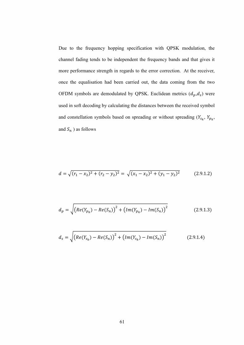
61
Due to the frequency hopping specification with QPSK modulation, the
channel fading tends to be independent the frequency bands and that gives it
more performance strength in regards to the error correction. At the receiver,
once the equalisation had been carried out, the data coming from the two
OFDM symbols are demodulated by QPSK. Euclidean metrics (𝑑𝑝,𝑑𝑠) were
used in soft decoding by calculating the distances between the received symbol
and constellation symbols based on spreading or without spreading (𝑌𝑠𝑘 , 𝑌𝑝𝑘,
and 𝑆𝑛 ) as follows
𝑑 = √(𝑟1 − 𝑥2)2 + (𝑟2 − 𝑦2)2 = √(𝑥1 − 𝑥2)2 + (𝑦1 − 𝑦2)2 (2.9.1.2)
𝑑𝑝 = √(𝑅𝑒(𝑌𝑝𝑘) − 𝑅𝑒(𝑆𝑛))2+ (𝐼𝑚(𝑌𝑝𝑘) − 𝐼𝑚(𝑆𝑛))
2 (2.9.1.3)
𝑑𝑠 = √(𝑅𝑒(𝑌𝑠𝑘) − 𝑅𝑒(𝑆𝑛))2+ (𝐼𝑚(𝑌𝑠𝑘) − 𝐼𝑚(𝑆𝑛))
2 (2.9.1.4)
62
2.9.2. Dual Carrier Modulation
DCM has been suggested by [53] to accommodate the need for higher data rate
applications as part of the ECMA standard. It uses frequency diversity by
allocating the DCM symbol (which consists of four bits) to two separate
subcarriers separated by 200 MHz The idea behind DCM is to use frequency
diversity in a large symbol bandwidth by transmitting the same information in
parallel and with 50 tones separation within the same symbol. If one subcarrier
experiences a deep fade, the probability of another subcarrier carrying the
same information but separated by relatively large bandwidth to experience the
same deep fade is realistically very small. A total number of 100 complex
symbols are mapped to 100 IFFT subcarriers in the transmitter block before
transmission [54]. This method groups the bits in two sections each having a
length of 50 with 100 bits. It then takes a subgroup of 2 bits as (b[g(k)], b[g(k)
+ 50]) and (b[g(k) +1], b[g(k) + 51]). These groups of 4 bits are then
converted to 2 QPSK symbols (table 2.9.2). A pair of 16-QAM constellation
maps was used to perform the dual modulation and transform each pair of
symbols into a DCM symbol (figure 2.9.2).

63
(A1): S [K] = [I (K), Q (K)]
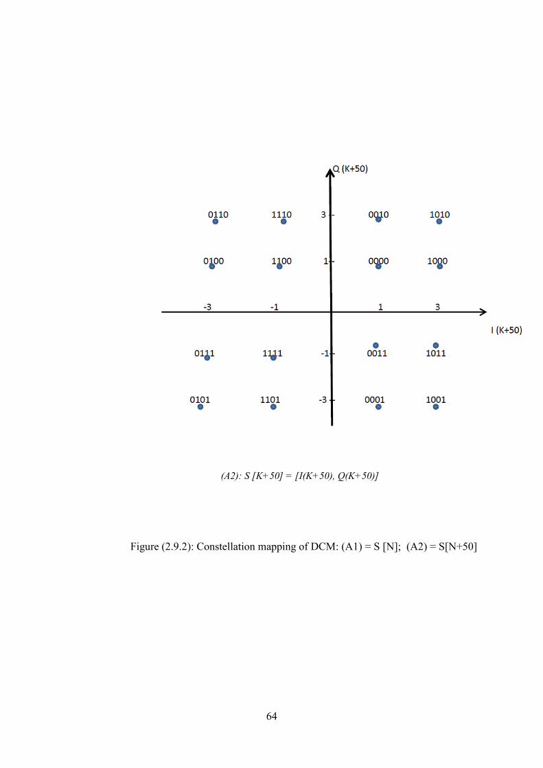
64
(A2): S [K+50] = [I(K+50), Q(K+50)]
Figure (2.9.2): Constellation mapping of DCM: (A1) = S [N]; (A2) = S[N+50]

65
Table (2.9.2): The DCM mapping signal across the constellation maps
The de-mapping process at the receiver uses the two constellation maps and
combines the subcarriers that represent the same symbol. Each two subcarrier
containing the I and Q quadrature components of the particular symbol had
been separated by 50 FFT tones, and hence this diversity produces two
different signals with various power strength for the symbol [55]. When
combining these signals, one constellation map would be required to represent
the two bits, and the other one would identify the next two bits. Originally,

66
each subcarrier represents four bits that had been mapped in such way so as to
make the linear combination of two subcarriers would produce only two bits in
each constellation branch. The starting point was the combining of two
subcarriers with total of 8 bits in each constellation, and then after the
combining process, each output of a constellation branch ending with two bits.
The top branch would contain the first and third bits (b1,b3), and the lower
branch would represent (b2,b4) as [56].
2.9.3. Dual Circular 32-QAM
Although ECMA-368 standard offers 480 Mb/s transmission rate, it is difficult
to achieve this data rate in real life due to poor channel conditions which
causes drop packets. This in turns results in lower throughputs and
retransmission was needed in this instance. Furthermore, although this rate
could be adequate for data and voice communications, for intensive media,
video conferencing and live streaming contents, a higher transmission rate

67
would be needed to enable successful communication for these types of
applications. The DC 32-QAM scheme had been proposed in order to increase
the system throughput by mapping more information on each subcarrier of the
100 IFFT data tones [57]. The scheme takes 1500 interleaved and coded bits
and then divides them into 250 bits, then further division is carried out by
forming 50 groups of 5 reordered bits (b_g(k), b_g(k )+ 50, b_g(k ) + 51,
b_g(k) + 100, b_g(k) + 101 ) to be mapped over two symbols using 2 8-ary
PSK constellations (figure 2.9.3). The first four bits are mapped to two QPSK
symbol similar to the DCM, while the fifth bit is used to conform the mapping
to two 8-ary PSK-like constellations. To further enhance the interleaving
process, the first and the hundredth bits are combined together and the same
process for the second bit from the first fifty pair with the second forming the
next fifth pair as follow
(2 b_g(k) + 50 – 1) + j ( 2 b_g(k) + 100 - 1 )
(2 b_g(k) + 51 – 1) + j ( 2 b_g(k) + 101 - 1)
Due to the nature of 8-ary PSK constellation, all the constellation points have
equal amplitude which adds another advantage to DC 32-QAM in comparison
to the 2 16-QAM DCM scheme in terms of constant power ratio. Furthermore,
this type of modulation conforms to the specification of ECMA-368 and have
the same DCM frequency planning by using two individual OFDM data
carriers separated by 50 tonnes (subcarriers) with 200 separation for the
diversity purposes, and each subcarrier have 4 bandwidth standard
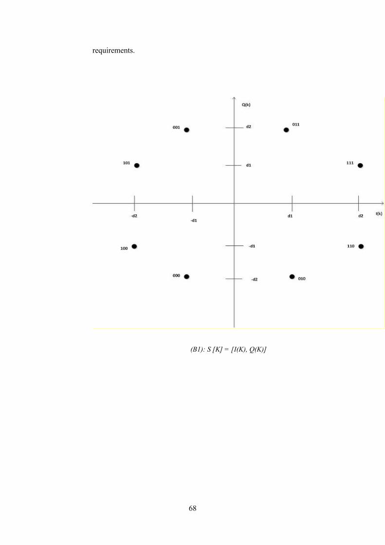
68
requirements.
(B1): S [K] = [I(K), Q(K)]

69
(B2): S [K+50] = [I(K+50), Q(K+50)]
Figure (2.9.3): Constellation mapping of DC 32-QAM: (B1) = S [K]; (B2) = S[K+50]
In the demodulation process, a soft bit de-mapping has been proposed for I &
Q components that had been transmitted on two different subcarriers. Each
70
subcarrier represented by a symbol consisting of the four bits that formed the 2
QPSK symbols, plus the fifth bit which de-mapped according to each of the
two DC 32-QAM symbols ( S(k) , S(k + 50) ). In the case of the S(k)
constellation, the fifth bit is considered zero valued if the received symbol is
close to the constellation point along the Q axis, else it takes a value of one if
it’s close to the I axis. For the constellation of S(k + 50) the opposite is
applied, that is the fifth bit is considered to be a one if the received symbol is
close to the constellation point along the Q axis, otherwise its zero. Channel
State Information (CSI) had been used to further improve the decoding
process. System simulation for both DCM and DC 32-QAM has shown that
the latter outperforms the DCM in terms of both throughput and transmission
range. The results of these previous researches will be used in the
developments of the design model and further work will be carried out to
develop a more optimised modulation scheme.

71
3. Design
3.1 Introduction
In this chapter, the designs of the proposed MIMO model have been described
including the development phases. An overview of the design scheme is then
summarised in the first part. In the second section, the transmitting design
scheme was then explained and instructions to the design steps taken had been
highlighted. The modulation scheme is analysed from a design prospective and
a detail methodology to the principle concept is then given. The receiving
model design was then followed on the next section, where a description to
this phase was undertaken. The design principle was explained and schematic
analysis was then produced. A configuration for receiver structures that allows
the model to increase the coverage area was shown. This construction provided
conformation of the model to wireless range demand applications. The last
section gives a mathematical analysis the performance of the proposed model.
In this part, a mathematical treatment to the concept of the design was given
including performance metric measures. Concluding remarks is then
summarising the design work.
72
3.2 Design Overview
The model design of a physical layer MIMO-UWB wireless communication
system operating in the free spectrum requires a number of interconnected
modules representing the transmitter, receiver and the physical channel. The
project had been divided into layers and each one has its own requirements and
operational functions. The design tasks have been spread across these layers
with various degrees of complexity. The structure involves the transmitting
module, the physical channel model and the receiver part, and this
arrangement was embedded in the design. Encompassing this design structure,
it is ability of backward compatibility for legacy systems with lower
transmission rate. The scheme uses the inherent spatial and frequency
diversities to boost the system performance by increasing the capacity, and
facilitates higher throughput that dynamically varies to accommodate both the
physical conditions and the type of wireless transmissions (data, videos, etc.).
The first layer of the design framework includes a transmitting module
consisting of two spatial elements with initial design requirements. The second
part of this phase constitutes a multipath fading channel model designed to test
and evaluate the system performance in terms of the spatial and frequency
73
diversity presence. This in turn introduces more channels for the transmitted
signal, and so improving the link budget. The receiving module represents the
last sub-system within this layer, and includes the decoding and estimation
algorithms, as well as objects link requirements. The aim design for this layer
was to evaluate the proposed concept and how to develop theoretical
algorithms into working wireless systems. Therefore, a predefined metrics
conditions was evaluated at the output of the receivers. In the case of not
satisfying the test requirements, the design is then readjusted and modified
until certain conditions are satisfied. This method enables the development in
stages with ascending order in term of complexity forming a bottom up
hierarchy.
Once this phase was completed, the next layer would include an advanced
MIMO transmitting and receiving sub-systems. An additional Standardised
IEEE802.15.3a channel model would be included. The transmitting block
includes the objects within the pervious developed transmitting block, as well
as stringent modulation and spatial requirements. The receiving block in this
phase would include an optimised decoding and equalisation algorithms that
meet the desired requirements. The validation of the research hypotheses
would be met at this stage, and hence an iterative approach would be applied.
The results error performance was then compared with previous work and
identified pre-set levels in the signal power. System optimisation was the third
phase and covers the improvements to the model design and performance. The
packet error rate (PER) for the communication link of both LOS and NLOS
was further reduced in this sub-system. The complexities in the receiver were
studied to make further improvement, and the overall design complexity was
74
optimised. Testing of the application included verification of particular
conditions, by the simulation of hypothesised scenarios in order to test the
fitness of the model. Additional requirements had been embedded into the
model and then examined for approval purposes. Further development to the
design was carried out in this stage so as to ensure practical feasibility of the
system in real time environments.
The evaluation phase involves multiple tests of various indoor scenarios in
order to full fill all the design requirements. Experimental analysis was applied
to the final version of the developed design in order to validate the simulated
design model against standardised and recognised approved models.
Predefined parameters had been used to test various fitness tests and systems
requirements such as the time delay, bit error rate (BER), the signal to noise
ratio (SNR) and the power profile. The necessity for this step was to match the
system requirements with the achieved results and approves theoretical
concepts. These results approved the design concept in increasing the link
capacity, by the use of spatial element and contribute to the knowledge in this
field. Figure 3.1 below gives an overview to the design framework.

75
Figure (3.1): Scheme of the Design development
76
3.3 Design Method
3.3.1 The Transmitting Model Design
The design architecture of the modulation scheme consists of two branches,
each of which contains dual QPSK constellations that convert the input stream
into two sequences of complex symbols. Then, the pair of symbols within
every branch was reordered by interchanging the In-phase components of this
complex numbers. This transformation expands the fading diversity across the
modulated symbols within the code-word, and improves the performance
across the spatial and frequency domains. This form of implementation
enforces frequency selectivity and fading variation across the desired signal
components. The next stage in this transmitting design was to increase the
spectral efficiency (bps/Hz) of the modulation scheme. For this purpose, a
method for achieving high end wireless link with large modulation scheme that
convert the two bits symbol into a large dimension symbol was developed.
Incorporation of dual circular 8 points constellation maps in the name of 8-ary
PSK modulation would results in an increase the modulation dimension and
facilitates high data rate transmission. The equal decision region for symbol
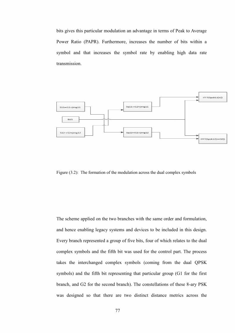
77
bits gives this particular modulation an advantage in terms of Peak to Average
Power Ratio (PAPR). Furthermore, increases the number of bits within a
symbol and that increases the symbol rate by enabling high data rate
transmission.
Figure (3.2): The formation of the modulation across the dual complex symbols
The scheme applied on the two branches with the same order and formulation,
and hence enabling legacy systems and devices to be included in this design.
Every branch represented a group of five bits, four of which relates to the dual
complex symbols and the fifth bit was used for the control part. The process
takes the interchanged complex symbols (coming from the dual QPSK
symbols) and the fifth bit representing that particular group (G1 for the first
branch, and G2 for the second branch). The constellations of these 8-ary PSK
was designed so that there are two distinct distance metrics across the

78
orthogonal In-phase and Quadrature domains on the four quadrants scatter
diagram. The eight signal points were distributed across the two orthogonal
domains based on these dual Euclidean metrics.
Figure (3.3): The two distance metrics across the 8 signal constellation points
In this 8-ary PSK modulation with constant amplitude modulation, the
positions of symbols were rotated around the circle by 𝑗2𝜋
16 (22.2 degrees), so as
to ensure that only two distance metrics (d1, d2) from the origin across the real
and imaginary axes in the complex plane contains the constellation points.
79
These metric locations was used to position the four QPSK complex signals
using the driving bit (b5) located in each of the two sub groups(G1,G2) . For
the first branch, the two output complex symbols from the four point
modulation (QPSK modulation) was multiplied by the distance metrics so as to
be transformed into PSK complex symbols ready to be distributed across the
eight point maps. The first complex symbol was assigned to the first PSK
constellation, while the second symbol representing the third and fourth bits
within G1 was a located to the second constellation. The binary value of the
fifth bit represents the most significant bit of the PSK symbol (three bits
symbol), and was used as a reference to identify the particular signal point on
the map in which these symbols represents. In a similar manner, these steps
were applied across the second branch in parallel to achieve the spectral
efficiency of the system. The original four quadrature symbols represented as
follows
s𝑞𝑝𝑠𝑘1𝐺1 = 𝑥𝐺1𝑐(𝑛) + 𝑗𝑥
𝐺1𝑐(𝑛)+50 (3.1)
s𝑞𝑝𝑠𝑘2𝐺1 = 𝑥𝐺1𝑐(𝑛)+1 + 𝑗𝑥𝐺1𝑐(𝑛)+51 (3.2)
s𝑞𝑝𝑠𝑘1𝐺2 = 𝑥𝐺2𝑐(𝑛) + 𝑗𝑥
𝐺2𝑐(𝑛)+50 (3.3)
s𝑞𝑝𝑠𝑘2𝐺2 = 𝑥𝐺2𝑐(𝑛)+1 + 𝑗𝑥
𝐺2𝑐(𝑛)+51 (3.4)

80
Where 𝑐(𝑛) = {2𝑛 𝑛 ∈ {0… .24}
2𝑛 + 50 𝑛 ∈ {25… .49}
The metrics d1 and d2 were interchanged between the symbols based on b5
binary value. In the case of the first group, the following operation was done
on the dual constellations.
For the first constellation
If b5 == 0
s𝑝𝑠𝑘1𝑔1(m) = 𝑑1 ∗ 𝑟𝑒𝑎𝑙 (s𝑞𝑝𝑠𝑘1
𝑔1) + 𝑑2 ∗ 𝑖𝑚𝑎𝑔 (s𝑞𝑝𝑠𝑘1𝑔1)
Else
s𝑝𝑠𝑘1𝑔1(m) = 𝑑2 ∗ 𝑟𝑒𝑎𝑙 (s𝑞𝑝𝑠𝑘1
𝑔1) + 𝑑1 ∗ 𝑖𝑚𝑎𝑔 (s𝑞𝑝𝑠𝑘1𝑔1)
For the second constellation
If b5 == 0
s𝑝𝑠𝑘2𝑔1(m) = 𝑑2 ∗ 𝑟𝑒𝑎𝑙 (s
𝑞𝑝𝑠𝑘2𝑔1) + 𝑑1 ∗ 𝑖𝑚𝑎𝑔(s
𝑞𝑝𝑠𝑘2𝑔1)

81
Else
s𝑝𝑠𝑘2𝑔1(m) = 𝑑1 ∗ 𝑟𝑒𝑎𝑙 (s
𝑞𝑝𝑠𝑘2𝑔1) + 𝑑2 ∗ 𝑖𝑚𝑎𝑔(s
𝑞𝑝𝑠𝑘2𝑔1)
End
Figure (3.4): The constellation maps used for the dual 8-ary PSK symbols
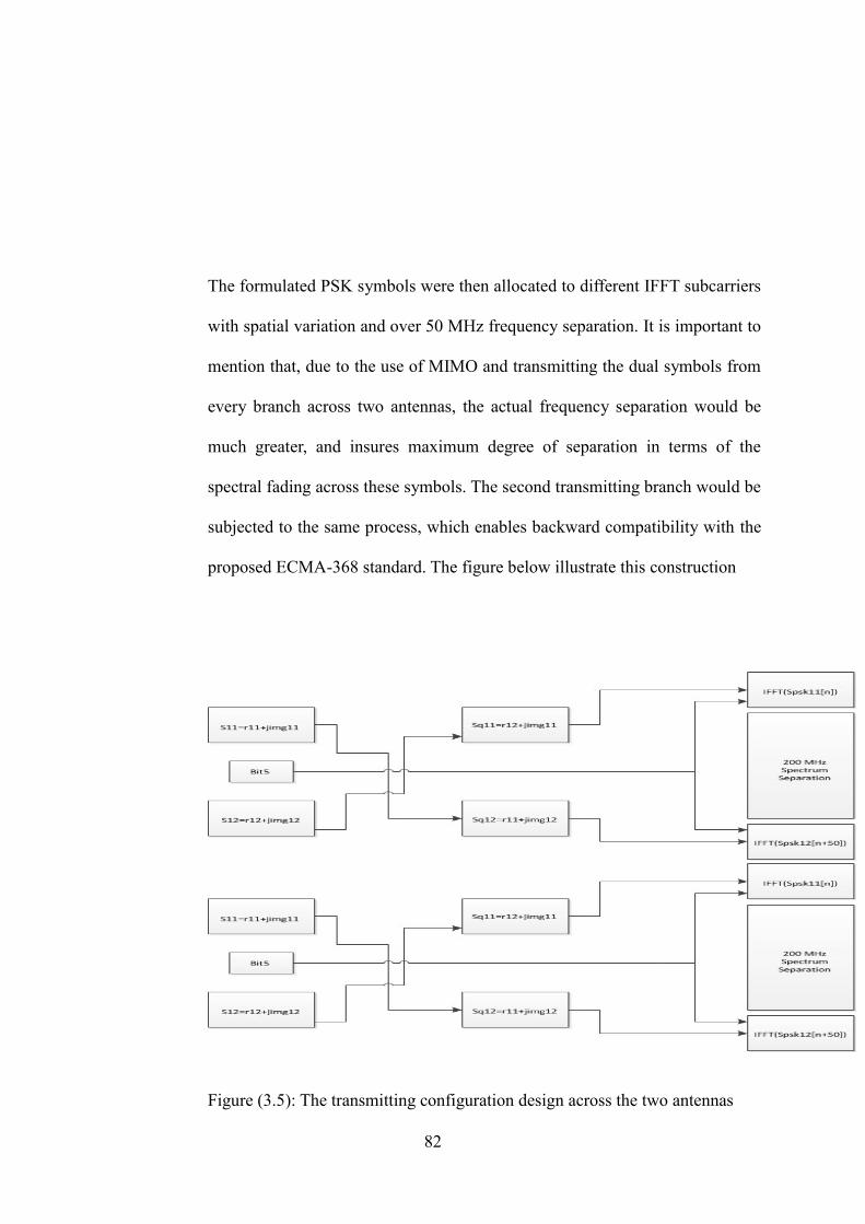
82
The formulated PSK symbols were then allocated to different IFFT subcarriers
with spatial variation and over 50 MHz frequency separation. It is important to
mention that, due to the use of MIMO and transmitting the dual symbols from
every branch across two antennas, the actual frequency separation would be
much greater, and insures maximum degree of separation in terms of the
spectral fading across these symbols. The second transmitting branch would be
subjected to the same process, which enables backward compatibility with the
proposed ECMA-368 standard. The figure below illustrate this construction
Figure (3.5): The transmitting configuration design across the two antennas

83
3.3.2 The Receiving model Design
The receiver architecture consists of two branches, and there are dual 8-PSK
constellations in every branch. A cross interchanging was applied to the In-
phase components with the four received complex symbols. This process was
undertaken by taking the real amplitude of the first complex symbol within the
second branch, and inserted in place of the In-phase component of the first
symbol within the first receiver branch. In the same time, the amplitude of the
first symbol within the first branch replaces the amplitude of the first complex
symbol within the second receiving branch. In a similar process, the second
received 8-PSK symbol within the first receiving branch was readjusted by
replacing its real amplitude with its counterpart of the second symbol within
the second receiving block. In across exchange, the second received 8-ary PSK
complex symbol was modified by inserting the In-phase of the second symbol
of the first branch in place of its real amplitude. Therefore, all the received
signals carried by the four complex symbols were readjusted in this process,
and figure (6) describes this design scheme. The recived signals at both dual
receivers had been expressed by the following received symobls.

84
𝑅𝑘(𝑛)
𝑝𝑠𝑘1𝐴1
(m) = 𝐻𝑘(𝑛)𝐴1 𝑆
𝑘(𝑛)
𝑝𝑠𝑘1𝐴1
(m)+ z𝑘(𝑛)𝐴1 (3.3.1)
𝑅𝑘(𝑛+50)
𝑝𝑠𝑘2𝐴1
(m) = 𝐻𝑘(𝑛+50)𝐴1 𝑆
𝑘(𝑛+50)
𝑝𝑠𝑘2𝐴1
(m)+ z𝑘(𝑛+50)𝐴1 (3.3.2)
𝑅𝑘(𝑛)
𝑝𝑠𝑘1𝐴2
(m) = 𝐻𝑘(𝑛)𝐴2
𝑆𝑘(𝑛)
𝑝𝑠𝑘1𝐴2
(m)+ z𝑘(𝑛)𝐴2 (3.3.3)
𝑅𝑘(𝑛+50)
𝑝𝑠𝑘2𝐴2
(m) = 𝐻𝑘(𝑛+50)𝐴2 𝑆
𝑘(𝑛+50)
𝑝𝑠𝑘2𝐴2
(m)+ z𝑘(𝑛+50)𝐴2 (3.3.4)
Where 𝐻𝑘(𝑛)𝑖 and 𝐻𝑘(𝑛+50)
𝑖 were the channel spectrums for the first anad
second sections of the ith receiver.
Channel equlaisation was carried out to remove the specturm distrubance
caused by the filtring effect of the medium. This channel fading minmisation is
a critical step for the system performance, and a good channel estimater
implementation is an essential requirment in mulitple antennas wirelss model.
In the presence of channel weights estimaters 𝑊𝑖𝑗 , the following formulas
was enduced.
��𝑘(𝑛)
𝑝𝑠𝑘1𝐴1
(m) = 𝑊𝑛𝐴1 𝑅
𝑘(𝑛)
𝑝𝑠𝑘1𝐴1
(m) (3.3.5)

85
��𝑘(𝑛+50)
𝑝𝑠𝑘2𝐴1
(m) =𝑊𝑘(𝑛+50)𝐴1 𝑅
𝑘(𝑛+50)
𝑝𝑠𝑘2𝐴1
(m) (3.3.6)
��𝑘(𝑛)
𝑝𝑠𝑘1𝐴2
(m) =𝑊𝑛𝐴2 𝑅
𝑘(𝑛)
𝑝𝑠𝑘1𝐴2
(m) (3.3.7)
��𝑘(𝑛+50)
𝑝𝑠𝑘2𝐴2
(m) =𝑊𝑘(𝑛+50)𝐴2 𝑅
𝑘(𝑛+50)
𝑝𝑠𝑘2𝐴2
(m) (3.3.8)
The noise term z was assumed to be AWGN reprsenting the recivers’ entiteis
such as thermol noise, and therefore multiplication by the channel estimator
would not change the statiscal propoty of this term. Taking this into account,
the noise power determine the practical snr for a useble error rate performance.
To elaporate on the mathematics, one could assume the noise power to be
amargenlaised quantity by ignoring the additional z term from the received
symbol formula. It is important to mension here, this assummtion was done to
highlight the channel effect at this junction. In reality, the noise term always
exists and there is no way to completely remove the nosie from the system. All
the availabe alogrithms would minimise the noise term, but will not remove
the noise completely. These process would be repeated across the the dual
antennas and then the transmitted symbols could be estimated. It is sufficient
to mention the estimation process within one radiating element. Hence, the
estimated transmitted symobl for one of the receiving antennas ��𝑖𝑗 could be
86
recoverd in the presence of frequency and spatial divresities with the follwing
formula.
��𝑘(𝑛)
𝑝𝑠𝑘1𝐴1
(m) = (ℎ∗𝑛𝐴1ℎ𝑛𝐴1)−1
. ��𝑘(𝑛)
𝑝𝑠𝑘1𝐴1
(m) (3.3.9)
��𝑘(𝑛+50)
𝑝𝑠𝑘2𝐴1
(m) = (ℎ∗𝑘(𝑛+50)𝐴1
ℎ𝑘(𝑛+50)𝐴1
)−1
��𝑘(𝑛+50)
𝑝𝑠𝑘2𝐴1
(m) (3.3.10)
It was clear that, each of the received symbol had bits coming from different
channel spectrum. The differences in the channel fading signatures were due to
the two degrees of freedom in the diversity presence that were located in UWB
channels. If only the inherent of diversity effect had been constraind to the
frequency domain as it was the case for classical DC modulation, then induced
correlation between the channel coffeicints presented in the medium specturm
would effect the dual received signals of the same symbol. The additional
degree of freedom encapsulated by the spatial diveristy would minmise this
correlation factor, and results had shown the advanteges of this additional
degree of freedom in the diversity to the overall system performance.

87
Figure (3.6): The design scheme of the dual receivers
88
3.3.3 Modification to the Receiving model Design
In wireless applications where the coverage area is a critical requirement, the
model could be configured to full-fill this criteria. In wireless sensor networks,
the wireless range demand plays a crucial component for system validation,
and its eclipses the throughput requirement. In this context, the model could
be configured to replace the multiplexing technique by a full use of diversity
across the spatial and frequency domains. This modification allows for
increase in the signal power without a violation to the FFC regulation, or an
increase in the radiation power. The transmitting structure remains the same,
but the receiving model would be readjusted by adding a combiner module to
combine the received symbols from the dual receiving antennas. This increase
in the coverage area comes at expense of the throughput, which gives an
optimum performance for wireless range sensitivity systems. Figure (3.7)
gives a block description of the receiving configuration. The rest of the de-
mapping and decoding algorithm remains the same.

89
Figure (3.7): The design scheme for the modified dual receivers

90
3.4 Mathematical Analysis
One of the main aims in using MIMO system is to improve the data rate
through the introduction of Spatial Multiplexing Gain (SMG). In this analysis,
a numerical derivation of the error performance for the proposed model was
presented. Analytical formulation was carried out to drive the performance of
the scheme in the presence of noise and fading channel effects. The first
section drives an average probability of error in multipath environment with
direct and non-line of sight channel coefficients. In the second section, the
distribution of the noise was used to measure the model performance and drive
a mathematical expression for the error bound based on this observation. A
numerical derivation of the Pair-wise Error Probability PEP was driven based
on the probability density of the pairwise distance metric between symbol pair
combination. This method enables to formulate an error measure metric that
could be applied to different channel fading properties.

91
3.4.1 Analysis of Average Probability of Error
Although the coding and mapping of the symbols would affect the error
detection in the receiving process, it adds further complexity to induce a close
form analytical formula for the probability of error. This could be noticed if
Gray coding for example had been considered, where the probability of
detection decreases significantly when shifting away from neighbouring
symbols in the constellation map. Therefore, assumption of equal symbol error
condition in the constellation map would be observed here. The average error
performance would dependent on the fading parameter in the SNR and
governs its probability density𝑃𝑐ℎ(𝑐ℎ). In this work, the Nakagmi-n model
consisting of (𝛾, 𝑛, 𝜎) as channel parameters, and with 𝑃𝑁𝑐ℎ(𝛾; 𝑛, 𝜎) as it its
probability density function would be used to describes a scenario with a
combination of line of sight and non-line of sight multipath fading
components. Therefore, the average probability of error 𝑃(𝐸) could be
redefind in the following form
𝑃(𝐸)
= ∫ ∞
0
𝑃𝑒|𝐻𝑖 𝑃𝑁𝑐ℎ(𝛾; 𝑛, 𝜎) 𝑑𝛾 (3.4.1)

92
Considering the conditional error probability and with the conditional
approximation formula would lead to
𝑃𝑒|𝐻𝑖
=1
𝜋∫ ∏𝑒
−(��𝑟
sin2 𝜃)
𝑅
𝑟=1
𝜋2
0
𝑑𝜃 (3.4.2)
𝑃(𝐸)
= ∫ ∞
0
1
𝜋∫ ∏𝑒
−(��𝑟
sin2 𝜃)
𝑅
𝑟=1
𝜋2
0
𝛾
𝜎2 𝑒
−(𝛾2+𝑛2
2𝜎2) 𝐼0 (
𝛾𝑛
𝜎2) 𝑑𝛾 (3.4.3)
Let the SNR ��𝑟
��𝑟 = 𝛾
Introducing the MGF 𝑓(𝑏, 𝜌) would lead to the follwing
𝑓(𝑏, 𝜌) = ∫ ∞
0
𝑃𝜌(𝜌)𝑒𝑏𝜌 𝑑𝜌 (3.4.4)
𝑃(𝐸) =1
𝜋 ∫ ∏𝑓𝑅𝑎𝑐 (− (
𝑘
sin2 𝜃) , ��𝑟)
𝑅
𝑟=1
𝑑𝜃 (3.4.5)
𝜋2
0
𝑓𝑅𝑎𝑐 (−(𝑘
sin2 𝜃) , ��𝑟) = ∫
∞
0
𝑃��𝑟(��𝑟)𝑒𝑘
sin2 𝜃��𝑟 𝑑��𝑟 (3.4.6)
𝑓𝑅𝑎𝑐 (−𝑘
2 sin2 𝜃, ��𝑟)
=(1 + 𝑛2) sin 𝜃2
(1 + 𝑛2) sin 𝜃2 + 𝑘 ��𝑟 𝑒(−
𝑛2𝑘 ��𝑟(1+𝑛2)2 sin2 𝜃+𝑘 ��𝑟
) (3.4.7)
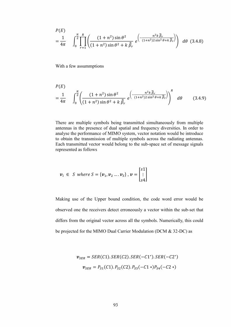
93
𝑃(𝐸)
=1
4𝜋 ∫ ∏(
(1 + 𝑛2) sin 𝜃2
(1 + 𝑛2) sin 𝜃2 + 𝑘 ��𝑟 𝑒(−
𝑛2𝑘 ��𝑟(1+𝑛2)2 sin2 𝜃+𝑘 ��𝑟
))
𝑅
𝑟=1
𝑑𝜃 (3.4.8)
𝜋2
0
With a few assummptions
𝑃(𝐸)
=1
4𝜋 ∫ (
(1 + 𝑛2) sin 𝜃2
(1 + 𝑛2) sin 𝜃2 + 𝑘 ��𝑟 𝑒(−
𝑛2𝑘 ��𝑟(1+𝑛2)2 sin2 𝜃+𝑘 ��𝑟
))
𝑅
𝑑𝜃 (3.4.9)
𝜋2
0
There are multiple symbols being transmitted simultaneously from multiple
antennas in the presence of dual spatial and frequency diversities. In order to
analyse the performance of MIMO system, vector notation would be introduce
to obtain the transmission of multiple symbols across the radiating antennas.
Each transmitted vector would belong to the sub-space set of message signals
represented as follows
𝒗𝑖 ∈ 𝑆 𝑤ℎ𝑒𝑟𝑒 𝑆 = {𝒗1, 𝒗2… . 𝒗𝑆} , 𝒗 = [𝑠1⋮𝑠4]
Making use of the Upper bound condition, the code word error would be
observed one the receivers detect erroneously a vector within the sub-set that
differs from the original vector across all the symbols. Numerically, this could
be projected for the MIMO Dual Carrier Modulation (DCM & 32-DC) as
𝒗𝑆𝐸𝑅 = 𝑆𝐸𝑅(𝐶1). 𝑆𝐸𝑅(𝐶2). 𝑆𝐸𝑅(−𝐶1∗). 𝑆𝐸𝑅(−𝐶2∗)
𝒗𝑆𝐸𝑅 = 𝑃𝑆1(𝐶1). 𝑃𝑆2(𝐶2). 𝑃𝑆3(−𝐶1 ∗)𝑃𝑆4(−𝐶2 ∗)
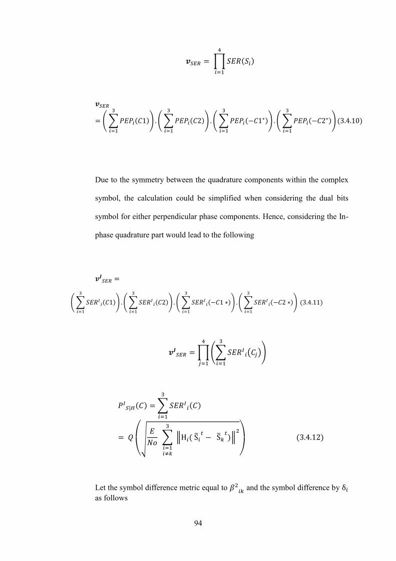
94
𝒗𝑆𝐸𝑅 = ∏𝑆𝐸𝑅(𝑆𝑖)
4
𝑖=1
𝒗𝑆𝐸𝑅
= ( ∑𝑃𝐸𝑃𝑖(𝐶1)
3
𝑖=1
) . ( ∑𝑃𝐸𝑃𝑖(𝐶2)
3
𝑖=1
) . ( ∑𝑃𝐸𝑃𝑖(−𝐶1∗)
3
𝑖=1
) . ( ∑𝑃𝐸𝑃𝑖(−𝐶2∗)
3
𝑖=1
)(3.4.10)
Due to the symmetry between the quadrature components within the complex
symbol, the calculation could be simplified when considering the dual bits
symbol for either perpendicular phase components. Hence, considering the In-
phase quadrature part would lead to the following
𝒗𝑰𝑆𝐸𝑅 =
( ∑𝑆𝐸𝑅𝐼𝑖(𝐶1)
3
𝑖=1
) . ( ∑𝑆𝐸𝑅𝐼𝑖(𝐶2)
3
𝑖=1
) . ( ∑𝑆𝐸𝑅𝐼𝑖(−𝐶1 ∗)
3
𝑖=1
) . ( ∑𝑆𝐸𝑅𝐼𝑖(−𝐶2 ∗)
3
𝑖=1
) (3.4.11)
𝒗𝑰𝑆𝐸𝑅 =∏(∑𝑆𝐸𝑅𝐼𝑖(𝐶𝑗)
3
𝑖=1
)
4
𝑗=1
𝑃𝐼𝑆|𝐻(𝐶) =∑𝑆𝐸𝑅𝐼𝑖(𝐶)
3
𝑖=1
= 𝑄
(
√𝐸
𝑁𝑜 ∑ ‖H𝑖( S𝑖
𝑡− S𝑘
𝑡)‖
23
𝑖=1𝑖≠𝑘 )
(3.4.12)
Let the symbol difference metric equal to 𝛽2𝑖𝑘
and the symbol difference by δ𝑖
as follows
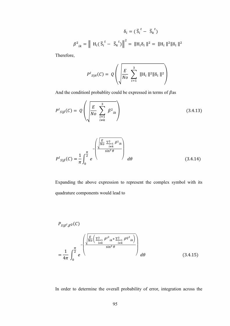
95
δ𝑖 = ( S𝑖𝑡− S𝑘
𝑡)
𝛽2𝑖𝑘= ‖ H𝑖( S𝑖
𝑡− S𝑘
𝑡)‖
2
= ‖H𝑖δ𝑖 ‖2 = ‖H𝑖 ‖
2‖δ𝑖 ‖2
Therefore,
𝑃𝐼𝑆|𝐻(𝐶) = 𝑄
(
√𝐸
𝑁𝑜 ∑
3
𝑖=1
‖H𝑖 ‖2‖δ𝑖 ‖2
)
And the conditionl probablity could be expressed in terms of 𝛽as
𝑃𝐼𝑆|𝛽(𝐶) = 𝑄
(
√𝐸
𝑁𝑜 ∑
3
𝑖=1𝑖≠𝑘
𝛽2𝑖𝑘
)
(3.4.13)
𝑃𝐼𝑆|𝛽(𝐶) =1
𝜋∫ 𝑒
−
(
√
𝐸𝑁𝑜
∑ 3𝑖=1𝑖≠𝑘
𝛽2𝑖𝑘
sin2 𝜃
)
𝜋2
0
𝑑𝜃 (3.4.14)
Expanding the above expression to represent the complex symbol with its
quadrature components would lead to
𝑃𝑆|𝛽𝐼,𝛽𝑄(𝐶)
=1
4𝜋 ∫ 𝑒
−
(
√
𝐸𝑁𝑜 ( ∑ 3
𝑖=1𝑖≠𝑘
𝛽𝐼2𝑖𝑘+ ∑ 3
𝑖=1𝑖≠𝑘
𝛽𝑄2𝑖𝑘)
sin2 𝜃
)
𝜋2
0
𝑑𝜃 (3.4.15)
In order to determine the overall probability of error, integration across the

96
distributions of SNR is required as the following.
𝑃𝑆(𝐸) = ∫ ∞
0
∫ 𝑃𝑆|𝛽𝐼,𝛽𝑄(𝐶) 𝑃𝛽𝐼(𝛽𝐼) 𝑃𝛽𝑄(𝛽
𝑄) 𝑑𝛽𝐼 𝑑𝛽𝑄∞
0
(3.4.16)
The squared magnitude of the channel ‖H ‖2 would determine the exhibited
distribution of 𝛽2, and hence the squred magnitude summation of independent
ecludian metric resemples the distribution as the weights of its channel where
‖H ‖2 = (|ℎ1|2 + |ℎ2|
2 + … . +|ℎ𝐿|2)
And ‖H𝑖 ‖2 that was considered to be a CHI-SQUARED random variable with
2L degree of freedom. The density function of this distribution had been
defined as
𝑃𝛽(𝛽) =1
(𝐿 − 1)! 𝛽𝐿−1 𝑒−𝛽 (3.4.17)
Let
��𝑧 = √𝐸
𝑁𝑜 ( ∑ 3
𝑖=1𝑖≠𝑘
𝛽𝑧2𝑖𝑘) , 𝑎𝑛𝑑 𝑧 = 𝐼, 𝑄, 𝑘 =
2(𝑀−1)
3log (𝑀) , 𝑀 = 16 ,32
Then, the average probability of error would be defined as
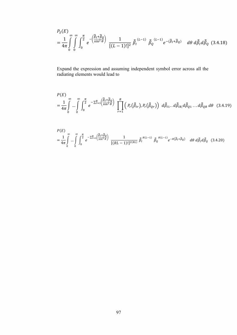
97
𝑃𝑆(𝐸)
=1
4𝜋∫ ∫ ∫ 𝑒
−(��𝐼+��𝑄sin2 𝜃
)𝜋2
0
∞
0
1
[(𝐿 − 1)!]2 ��𝐼
(𝐿−1) ��𝑄
(𝐿−1)𝑒−(��𝐼+��𝑄) 𝑑𝜃 𝑑��𝐼𝑑��𝑄
∞
0
(3.4.18)
Expand the expression and assuming independent symbol error across all the
radiating elements would lead to
𝑃(𝐸)
=1
4𝜋∫ …∫ ∫ 𝑒
−∑ (��𝐼+��𝑄sin2 𝜃
)𝑅𝑟=1
𝜋2
0
∞
0
∏( 𝑃𝑟(��𝐼𝑟), 𝑃𝑟(��𝑄𝑟))
𝑅
𝑟=1
𝑑��𝐼1. . 𝑑��𝐼𝑅,𝑑��𝑄1 . . . 𝑑��𝑄𝑅 𝑑𝜃 (3.4.19)
∞
0
𝑃(𝐸)
=1
4𝜋∫ …∫ ∫ 𝑒
−∑ (��𝐼+��𝑄sin2 𝜃
)𝑅𝑟=1
𝜋2
0
∞
0
1
[(𝑅𝐿 − 1)!]2(𝑅𝐿) ��𝐼
𝑅(𝐿−1) ��𝑄
𝑅(𝐿−1)𝑒−𝑅(��𝐼+��𝑄) 𝑑𝜃 𝑑��𝐼𝑑��𝑄 (3.4.20)
∞
0

98
3.4.2 Error performance measure based on the noise statistic
In order to validate a wireless model, it is importunate to envisage its response
to different transmitted signals and this condition could not fulfilled by a
deterministic wireless signal. Therefore its well-known to transmit stochastic
signals for the analysis proposes. Based on this observation, the transmitted
signal X was a random variable, and given that the channel H was assumed to
be statistically distributed according to the specific environment, then the
received signal Y would also be a random variable. The joint entropy H(X,Y)
would be
𝐻(𝑋, 𝑌) = ∑ ∑ 𝑃(𝑥, 𝑦). log1
𝑃(𝑥,𝑦)𝑦𝑥 (3.4.21)
=∑∑𝑃(𝑥, 𝑦). log1
𝑃(𝑥, 𝑦)𝑦𝑥
= −∑∑𝑃(𝑥, 𝑦). log 𝑃(𝑥)
𝑦𝑥
− ∑∑𝑃(𝑥, 𝑦). log(𝑦|𝑥)
𝑦𝑥
= −∑𝑃(𝑥). log 𝑃(𝑥) + 𝐻(𝑌|𝑋)
𝑥
= 𝐻(𝑋) + 𝐻(𝑌|𝑋) (3.4.22)
99
The mutual information I(X; Y) is
𝐼(𝑋; 𝑌) = 𝐻(𝑋) − 𝐻(𝑋|𝑌) = 𝐻(𝑌) − 𝐻(𝑌|𝑋)
And
𝑓(𝑦) = 𝑓(𝑋;𝐻) + 𝑓(𝑁)
𝑓(𝑦) − 𝑓(𝑋;𝐻) = 𝑓(𝑌|𝑋, 𝐻) = 𝑓(𝑁)
Where f(Y), f(Y|X,H) and f(N) is the Probability Density Function (PDF) of
the received signal vector, the conditional PDF of the received signal and the
PDF of the noise respectively.
The conditional pdf of the received signal vector given the joint channel and
the transmitted signal vectors would be as
𝑓(𝑌|𝑋, 𝐻) = 𝑓(𝑁) = ∏∏1
𝜋
𝑅
𝑟
𝑇
𝑡
exp(−|𝑁𝑡𝑟|2)
= 1
𝜋𝑅 𝑇 exp(−∑∑|𝑁𝑡
𝑟|2𝑅
𝑟
𝑇
𝑡
) (3.4.23)
Where R are the number of receiving antennas, T the number of transmitting
antennas
Hence,

100
𝑓(𝑌|𝑋, 𝐻) = 1
𝜋𝑅 𝑇 exp(− 𝑡𝑟 (𝑁 𝑁𝐻)) (3.4.24)
Maximising the above conditional PDF would result in the Maximum
likelihood (ML) of 𝐶𝑀𝐿 (the transmitted code word), and reduces the error
probability of the system as follow
𝐶𝑀𝐿 = argmax𝑥𝑓(𝑌|𝑋,𝐻)
𝐶𝑀𝐿 = argmax𝑥
1
𝜋𝑅 𝑇 exp
(
− 𝑡𝑟
(
(𝑌 − √
𝐸𝑥𝑁0𝑁𝑡
𝐻𝑋)
. (𝑌 − √𝐸𝑥𝑁0𝑁𝑡
𝐻𝑋)
𝐻
)
)
(3.4.25)
𝐶𝑀𝐿 = argmin𝑥𝑡𝑟
(
(𝑌 − √
𝐸𝑥𝑁0𝑁𝑡
𝐻𝑋) .
(𝑌 − √𝐸𝑥𝑁0𝑁𝑡
𝐻𝑋)
𝐻
)
(3.4.26)
The probability of symbol error would be obtained where difference metric of
the predicted erroneous code word �� would be higher than the metric of the
transmitted code word X. In a mathematical form, the above observation could
be expressed as follows
101
𝑡𝑟 (𝑁.𝑁𝐻) = 𝑡𝑟
(
(𝑌 − √
𝐸𝑥𝑁0𝑁𝑡
𝐻��) .
(𝑌 − √𝐸𝑥𝑁0𝑁𝑡
𝐻��)
𝐻
)
≥ 𝑡𝑟
(
(𝑌 − √
𝐸𝑥𝑁0𝑁𝑡
𝐻𝑋) .
(𝑌 − √𝐸𝑥𝑁0𝑁𝑡
𝐻𝑋)
𝐻
)
(3.4.27)
And the noise could be related to the probability of error and the Euclidean
metric.
𝑡𝑟 (𝑁.𝑁𝐻) ∝ 𝑃(𝐸) ∝ 𝑡𝑟
(
(𝑌 − √
𝐸𝑥𝑁0𝑁𝑡
𝐻��) .
(𝑌 − √𝐸𝑥𝑁0𝑁𝑡
𝐻��)
𝐻
)
Since Y represents the correct received word, the expression could be
combined as follows
𝑡𝑟 (𝑁.𝑁𝐻) = 𝑡𝑟
(
(√
𝐸𝑥𝑁0𝑁𝑡
ℎ𝑥 + 𝑁 − √𝐸𝑥𝑁0𝑁𝑡
ℎ��)
. (√𝐸𝑥𝑁0𝑁𝑡
ℎ𝑥 + 𝑁 −√𝐸𝑥𝑁0𝑁𝑡
ℎ��)
𝐻
)
102
𝑡𝑟 (𝑁.𝑁𝐻) = 𝑡𝑟
(
( √
𝐸𝑥𝑁0𝑁𝑡
(ℎ�� − ℎ𝑥) + 𝑁)
. ( √𝐸𝑥𝑁0𝑁𝑡
(ℎ�� − ℎ𝑥 ) + 𝑁)
𝐻
)
(3.4.28)
3.4.3 Numerical Evaluation of PEP
As there were variable coding methods, the weights of error probabilities
normally varies and tends to be effected by the particular coding scheme. In
the case of Gray coding, the weight of error estimation decreases sharply as
the distance between the received and the estimated symbol increases. This is
because nearby symbols would have high probability errors, and to get one bit
of error in each symbol would require small amount of energy. In order to get
more bits within a specific symbol, then high energy would be required to a

103
achieve that. The high energy of errors would accommodate outer symbols in
the decoding sphere on the scatter diagram. The energy of errors and the
probability of errors have an inverse relationship when quantifying the
decoding algorithm. In addition to this observation, the various modulation
schemes spread the symbols on the constellation diagram with different energy
separation. That is to say, for Quadrature amplitude type modulation, the
energy between the symbols and the origin point on the constellation map had
variables values. While, the Phase Shift keying method, have an equal energy
values between the symbols and the origin of the scatter diagram. For a single
symbol s transmitted from antenna t, the error would result in detecting one the
M-1 neighbouring symbols (7 for 8-PSK) within the constellation. It could be
noticed that the larger the sphere decoding the more neighbouring symbols to
choose from, and therefore there were more erroneous symbols available for
selection. This in turns increases the probability of error and reduces the
system performance. On the other hand the small radius that could be
envisaged in the second smaller sphere contained small number of erroneous
symbols. That leads to a small percentage in the probability of error, which
lead to a more optimised system with good error performance property. A
point to mention here that, the term erroneous symbols was used to indicate
the process of estimating wrongly transmitted symbols in a map with only
correct symbol in a collection of noisy received symbols.
In the current proposal, a dual antennas configuration using Dual Carrier based
on Circular and Quadrature modulation (in the form of 8-ary PSK

104
constellations) were used in the PEP derivation. The probability of error was
derived based on Maximum Likelihood (ML) metric symbol estimation.
Initially the symbols across the constellation had been assumed to have equally
likelihood probability with maximum a posteriori (MAP) detection. Therefore,
from a transmitting point of view and with blind prior knowledge of the user
signal, it was reasonable to assume equate the symbol probabilities within the
constellation. As the desired signal was a random variable based on a
stochastic process, there should be an equal probability weights across all the
signal points. Introducing the Union bound principle for this evaluation and
having the number of points within a specific scatter diagram as M, and then
the probability of error 𝑃𝑠(𝐸) for a single transmitted symbol would be
𝑃𝑆 (⋃𝑃𝑠
𝑆
𝑠=1
) ≤ 𝑃𝑠=𝑠1(𝐸) + 𝑃𝑠=𝑠2(𝐸)… . . +𝑃𝑠=𝑆(𝐸)
𝑃𝑆(𝐸) ≤ ∑𝑃𝑠(𝐸)
𝑆
𝑠=1
(3.4.29)
As there were M number of symbols across a particular constellation map, and
with equal transmitting probability, then the symbol error probability could be
obtained based on the bound formulation as
𝑃𝑆(𝐸) ≤ 1
𝑀 ∑𝑃𝑖(𝐸)
𝑀
𝑖=1
(3.4.30)

105
Having obtained M symbols for transmission, then by introducing pairwise
symbol error which could interpreted by 𝑃(𝑠, 𝑒), then having send the symbol
s as one of the signal within the M map, then an erroneous detection of symbol
e as an element of this map would correspond to this pair error combination.
The joint Probability of erroneous symbols would translated as
𝑃𝑆(𝐸) ≤ 1
𝑀 ∑∑𝑃(𝑠, 𝑒)
𝑠≠𝑒
𝑀
𝑠=1
(3.4.31)
In the case of upper bound on the Probability error at the receiver, there would
be M.M combination of pair error probability, therefore
𝑃𝑆(𝐸) ≤ 1
𝑀.𝑀 ∑ ∑𝑃(𝑠, 𝑒)
𝑀
𝑠=1𝑠≠𝑒
𝑀
𝑒=1
(3.4.32)
Having defined multiple symbols across the radiating element within a
multiple spatial configuration, the error performance could be bounded for this
multi-dimensional modulation. Expanding the above expression for the case of
multiple antennas, then the probability of symbol error across all the radiating
elements would be
𝑃𝑆(𝐸) ≤ 1
𝑇.𝑀.𝑀 ∑∑ ∑𝑃𝑡(𝑠, 𝑒)
𝑀
𝑠=1𝑠≠𝑒
𝑀
𝑒=1
𝑇
𝑡=1
(3.4.33)
106
In order to evaluate the proposed model in term of the pairwise error
performance, it was critical to analysis the probability of error within the
received signal. In the presence of channel Information CI metric (it is variable
entity which could exhibits distortions due to noisy coefficients) that determine
the equalisation process at the receiver, and given a well-known prior
knowledge of the state channel, the receiving signals would be processed. This
could be done by investigating the statistical behaviour of the received signal
components. As it was more involve getting a close form equation for the
error measures, a practical approximation was needed to induce a systematic
pairwise error probability formula. Hence, an error bound had been introduce
by assuming that all the receiving symbols vectors were in an error, and all the
symbols were independent from each other. This assumption was a realistic
measure as the transmitted signal and the noise both of which were
independent and identically distributed entities. This leads to the following
PEP formula
𝑃(𝐸) = ∏ ∏∏𝑃𝑛,𝑠𝑝 (𝐸)
𝑀
𝑠=1
𝑁
𝑛=1
𝐴1,𝐴2
𝑝=1
(3.4.34)
Introducing the upper bound principle in order to evaluate the PEP for the
system model would give a maximisation limit for the error performance.
Therefore, the upper bound pairwise error probability across all the symbols
within the MIMO configuration could be defined in terms of the Euclidean
energy metric 𝐷(𝑠, 𝑒)between the transmitted s and the erroonus detected e
symbols as

107
𝑃(𝐸) ≤ ∏ ∏∏ exp− (𝐷𝑠,𝑛𝑝 (𝑠, 𝑒))
𝑀
𝑠=1
𝑁
𝑛=1
𝐴1,𝐴2
𝑝=1
(3.4.35)
In the case of erroneous detection of all the N symbols that spans the OFDM
block across the pairwise construction within the T and R antennas, would
define the PEP metric within the following condition
𝐷(𝑠, 𝑒) = ∑∑‖∑ℎ𝑡,𝑛𝑟 ∆𝑛
𝑟 (𝑠, 𝑒)
𝑇
𝑡=1
‖
𝐹
𝑁
𝑛=1
𝑅
𝑟=1
𝐷(𝑠, 𝑒) = ∑∑(∑ (ℎ𝑟,𝑛𝑡2 ∆𝑛
𝑡2(𝑠, 𝑒))†
𝑇
𝑡2=1
∑ ℎ𝑟,𝑛𝑡1 ∆𝑛
𝑡1(𝑠, 𝑒)
𝑇
𝑡1=1
)
𝑁
𝑛=1
𝑅
𝑟=1
(3.4.36)
Where ∆ ≡ 𝑡ℎ𝑒 𝑒𝑟𝑟𝑜𝑟 𝑚𝑎𝑔𝑛𝑖𝑡𝑢𝑑𝑒 𝑚𝑒𝑡𝑟𝑖𝑐 𝑏𝑒𝑡𝑤𝑒𝑒𝑛 𝑐 &𝑒
Assumming that the channel fading remain constant over the N symbols that
spanning an OFDM block. Then, the formula could be readjusted as
𝐷(𝑠, 𝑒) = ∑∑ (∑(ℎ𝑟𝑡2)
†ℎ𝑟 𝑡1
𝑇
𝑡1=1
∑ (∆𝑛𝑡2(𝑠, 𝑒))
𝐻
∆𝑛𝑡1(𝑠, 𝑒)
𝑁
𝑛=1
)
𝑇
𝑡2=1
𝑅
𝑟=1
𝐷(𝑠, 𝑒)
= ∑∑ ∑(ℎ𝑟𝑡2)
†ℎ𝑟 𝑡1
𝑇
𝑡1=1
∑ (∆𝑛𝑡2(𝑠, 𝑒))
𝐻
𝑑𝑛𝑡1(𝑠, 𝑒)
𝑁
𝑛=1
(3.4.37)
𝑇
𝑡2=1
𝑅
𝑟=1

108
Manipulating the channel fading coefficients within the summations would
reproduce the following term
𝐻𝑟 = ∑ ℎ𝑡2 𝑞
𝑇
𝑡2=1
Considering the pairwise distance energy between the transmitted symbol and
the erroneous estimated symbols which represented the second term in the
exponential part of 𝐷(𝑠, 𝑒) in a matrix form (K) that consisting of all the pair
combinations that maximises the error qunity. Then, a single row matrix would
be defined as
𝐾𝑡2,𝑡1 = ∑ (∆𝑛𝑡2(𝑠, 𝑒))
†
∆𝑛𝑡1(𝑠, 𝑒)
𝑁
𝑛=1
Since the power of the pairwise distance forms a nonnegative definite matrix
and the components were independent and identically distributed, then the
square matrix K that contained the pair distances of symbols across all the
radiating elements would exhibit a Harmitian property and the square root of
this matrix could be expressed as
𝐾1/2 =
[ ∆11 ∆2
1 … ∆𝑁1
∆12
⋮∆22 …⋮ ⋱
∆𝑁2
⋮∆1𝑇 ∆2
2 … ∆𝑁𝑇 ]
(3.4.38)

109
Applying matrix decomposition on the matrix K, then a formation of unitary
matrices A and its conjugate such that multiplication by its conjugate results in
an identity matrix (AA*=I) contained on its columns the eigenvectors of the
symbol pairs difference matrix, and a diagonal matrix Σ would be induced to
describe the original complex entity matrix. The power of the matrix K was
governed by the non-negative diagonal matrix Σ containing its eginvlues
𝜆𝑡, {𝑡 = 1, …𝑇} on its diagonal positions. This operation transfer the pair-wise
combination into the following form
𝐾 = 𝐴† Σ 𝐴 , 𝑎𝑛𝑑 Σ = ∑𝜆𝑡
𝑇
𝑡=1
Therefore, D(s,e) was redefined as
𝐷(𝑠, 𝑒) = ∑ (𝐻𝑟)†𝐾 𝐻𝑟 = ∑ (𝐻𝑟)
†𝐴† Σ 𝐴 𝐻𝑟
𝑅
𝑟=1
𝑅
𝑟=1
(3.4.39)
The fading coefficeints h was a random variable that been governed by the
statiscal property of the the medium in which the wireless system operates. An
imporatant observation to mention was that, the stochatical behaviour of the
random variable parameter encapsulate the probablity density of any other
term was multiplied with it (ie: H* A). Thefore, introducing another paramter
𝜙 that reprents the multiplication of the unitry matrix A with the channel
coefficients.
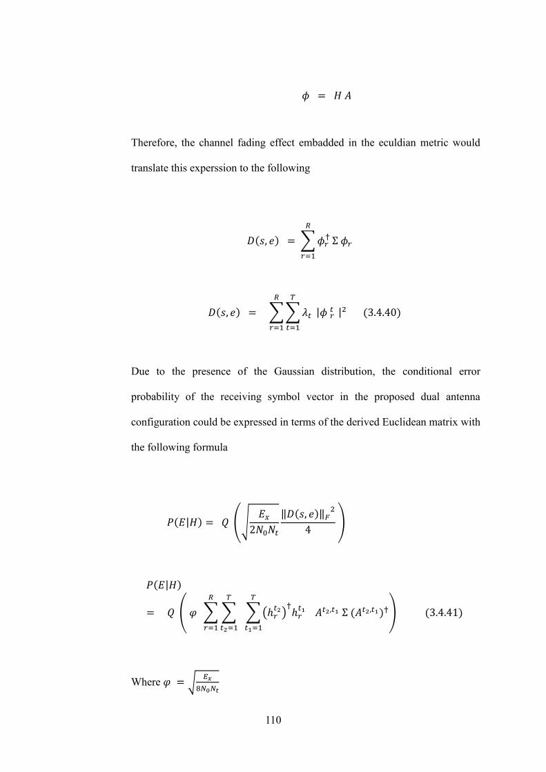
110
𝜙 = 𝐻 𝐴
Therefore, the channel fading effect embadded in the eculdian metric would
translate this experssion to the following
𝐷(𝑠, 𝑒) = ∑𝜙𝑟†
𝑅
𝑟=1
Σ 𝜙𝑟
𝐷(𝑠, 𝑒) = ∑∑𝜆𝑡
𝑇
𝑡=1
|𝜙 𝑟 𝑡 |2
𝑅
𝑟=1
(3.4.40)
Due to the presence of the Gaussian distribution, the conditional error
probability of the receiving symbol vector in the proposed dual antenna
configuration could be expressed in terms of the derived Euclidean matrix with
the following formula
𝑃(𝐸|𝐻) = 𝑄 (√𝐸𝑥
2𝑁0𝑁𝑡
‖𝐷(𝑠, 𝑒)‖𝐹2
4 )
𝑃(𝐸|𝐻)
= 𝑄 ( 𝜑 ∑∑ ∑(ℎ𝑟𝑡2)
†ℎ𝑟 𝑡1
𝑇
𝑡1=1
𝐴𝑡2,𝑡1 Σ (𝐴𝑡2,𝑡1)†𝑇
𝑡2=1
𝑅
𝑟=1
) (3.4.41)
Where 𝜑 = √𝐸𝑥
8𝑁0𝑁𝑡
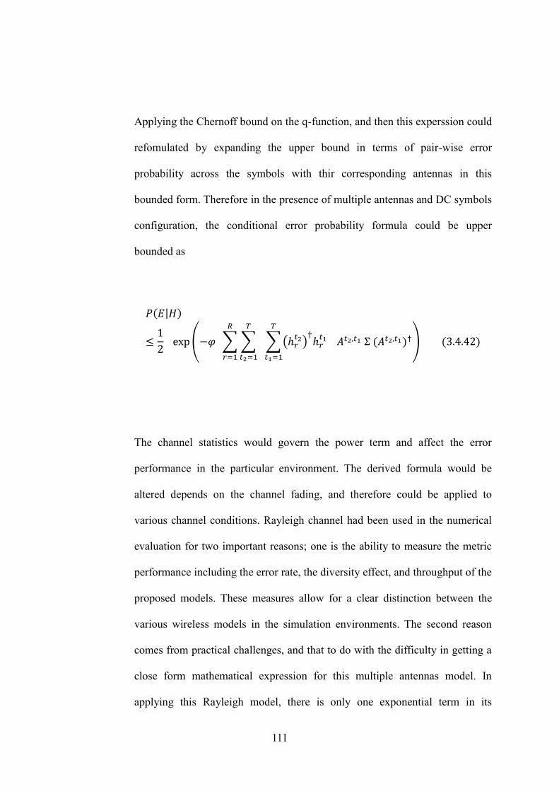
111
Applying the Chernoff bound on the q-function, and then this experssion could
refomulated by expanding the upper bound in terms of pair-wise error
probability across the symbols with thir corresponding antennas in this
bounded form. Therefore in the presence of multiple antennas and DC symbols
configuration, the conditional error probability formula could be upper
bounded as
𝑃(𝐸|𝐻)
≤1
2 exp(−𝜑 ∑∑ ∑(ℎ𝑟
𝑡2)†ℎ𝑟 𝑡1
𝑇
𝑡1=1
𝐴𝑡2,𝑡1 Σ (𝐴𝑡2,𝑡1)†𝑇
𝑡2=1
𝑅
𝑟=1
) (3.4.42)
The channel statistics would govern the power term and affect the error
performance in the particular environment. The derived formula would be
altered depends on the channel fading, and therefore could be applied to
various channel conditions. Rayleigh channel had been used in the numerical
evaluation for two important reasons; one is the ability to measure the metric
performance including the error rate, the diversity effect, and throughput of the
proposed models. These measures allow for a clear distinction between the
various wireless models in the simulation environments. The second reason
comes from practical challenges, and that to do with the difficulty in getting a
close form mathematical expression for this multiple antennas model. In
applying this Rayleigh model, there is only one exponential term in its

112
probability density function and that reduces the complexity burden of the
software and hardware running environment. As the effect of channel remain
constant when the same channel fading was used across wireless systems, then
an accurate comparison had been performed between this proposed model with
pervious proposed wireless model. Including the channel distribution within
the error formula and taking the average probability to remove the uncertainty
introduced by the random variable within the expression would translate the
derived conditional equation to the following
𝑃(𝐸) ≤ ∫ 𝑃(𝐸|𝐻) 𝑃(𝐻)
∞
0
𝑃(𝐸)
≤ ∫|H| exp( 𝜑 ∑∑ ∑(ℎ𝑟𝑡2)
𝐻ℎ𝑟 𝑡1
𝑇
𝑡1=1
𝐴𝑡2,𝑡1 Σ (𝐴𝑡2,𝑡1)∗𝑇
𝑡2=1
𝑅
𝑟=1
)exp(−|𝐻|2) 𝑑𝐻
∞
0
(3.4. 43)
Where the pdf of the channel was
𝑃(𝐻) = 2 |𝐻| 𝑒(−|𝐻|2)
𝑃(𝐸) ≤ ∫ |H| exp( 𝜑 ∑∑𝜆𝑡
𝑇
𝑡=1
ϕ𝑡𝑟
𝑅
𝑟=1
) exp(−|𝐻|2) 𝑑𝐻
∞
0
( 3.4.44)
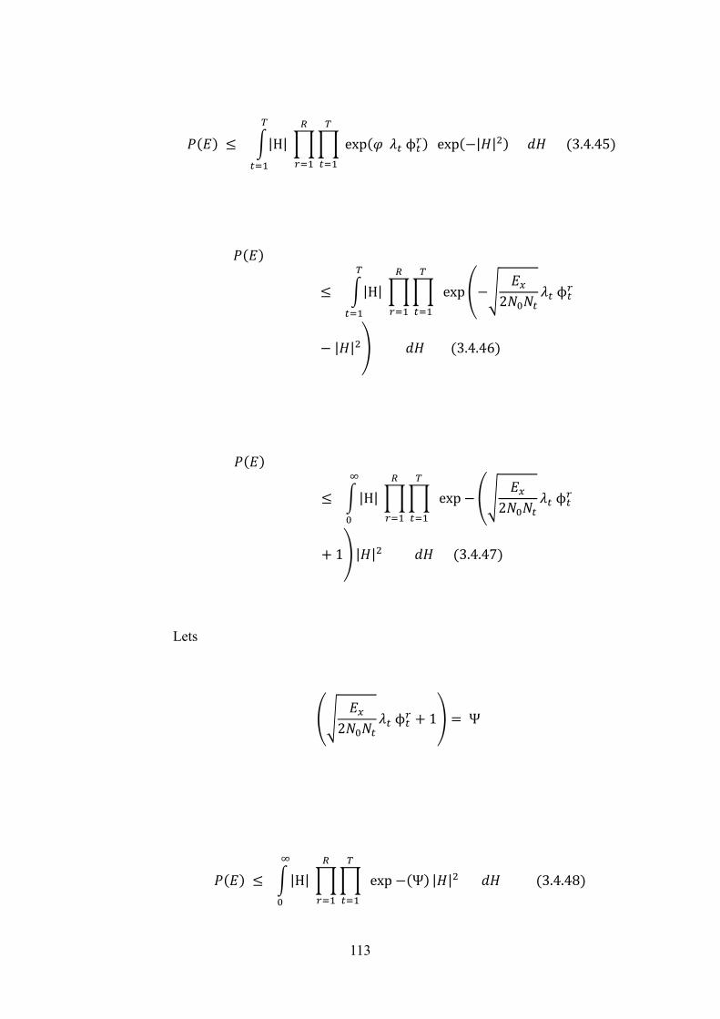
113
𝑃(𝐸) ≤ ∫|H| ∏∏ exp(𝜑 𝜆𝑡 ϕ𝑡𝑟)
𝑇
𝑡=1
𝑅
𝑟=1
𝑇
𝑡=1
exp(−|𝐻|2) 𝑑𝐻 (3.4.45)
𝑃(𝐸)
≤ ∫|H| ∏∏ exp(−√𝐸𝑥
2𝑁0𝑁𝑡𝜆𝑡 ϕ𝑡
𝑟
𝑇
𝑡=1
𝑅
𝑟=1
𝑇
𝑡=1
− |𝐻|2) 𝑑𝐻 (3.4.46)
𝑃(𝐸)
≤ ∫|H| ∏∏ exp −(√𝐸𝑥
2𝑁0𝑁𝑡𝜆𝑡 ϕ𝑡
𝑟
𝑇
𝑡=1
𝑅
𝑟=1
∞
0
+ 1) |𝐻|2 𝑑𝐻 (3.4.47)
Lets
(√𝐸𝑥
2𝑁0𝑁𝑡𝜆𝑡 ϕ𝑡
𝑟 + 1) = Ψ
𝑃(𝐸) ≤ ∫|H| ∏∏ exp −(Ψ)
𝑇
𝑡=1
𝑅
𝑟=1
∞
0
|𝐻|2 𝑑𝐻 (3.4.48)

114
Introducing the following Laplace transform expression into the above
equation would lead to the next expression for the average error
∫ 𝑒𝑥𝑝−𝑠𝑦∞
0
𝑑𝑦 = 1
𝑠 , 𝑠 > 0
𝑃(𝐸) = ∏∏
𝑇
𝑡=1
𝑅
𝑟=1
1
Ψ = ∏∏
1
(√𝐸𝑥
2𝑁0𝑁𝑡𝜆𝑡 ϕ𝑡
𝑟 + 1)
𝑇
𝑡=1
𝑅
𝑟=1
(3.4.49)
115
3.5 Concluding Remarks
In this chapter, the design steps taken to produce this novel model was
explained and described in details. A flowchart to the design plan was given
with an overview description the scheme was highlighted. The transmitting
and receiving models for the design were reviewed, explained, prepared and
issued. A configuration to the receivers was shown that allows the model to
increase the coverage at the expense of the through put for wireless range
demand applications. A mathematical analysis of the proposed model was then
developed in terms of the error performance. The next chapter would cover the
implementation of this design, and gives the instructions required to execute
the various algorithms across the design flowchart. The implementation of
OFDM with MIMO within UWB wireless system would be performed and
analysed. The finalisation of the channel model that simulated the rich
multipath environment would be covered.

116
4. Implementation
4.1 Introduction
In this chapter, the implementation of the design had been considered along
with an explanation to the concept formulation. This implementation was
carried out in the simulation environment based on Matlab software package.
The physical layer setting was conducted and conformed based on the ECMA-
368 standard. The chapter was divided into sections, where the second section
considered the construction of the transmitters. This included the coding and
modulation for the desired signals. The next section had considered the model
channel that was used to infer the indoor distortion that attach with wireless
signals in this close environment. The receiver’s implementation was followed
with explanation to the integration of the proposed model on the wireless
receiving structure, and the test bed requirements for the simulation. A
proposal to optimise decode method was explained that further enhance the
system performance in the next section. Concluding remarks is then
summarised this chapter.
117
4.2 Implementation on transmitters
In this proposal, modulation was carried out across two antennas with two
frames containing 1500 coded and interleaved bits each. In the presence of
frequency diversity, these frames were divided into six blocks at every branch
spreading across the dual radiating elements. In this scheme, spatial diversity
was used to further enhance the system performance and reduces the effect of
fading. The implementation of the scheme was based on parallel formulation,
so as to ensure backward compatibility, and reduces the cost and complexity of
high speed hardware clocks at a slight expense of the extra RF modules. In
every branch, a block of 250 codded and interleaved signal bits were divided
into 50 groups, and every group contains 5 bits. The spreading of every group
exhibit multiplexing and diversity properties in sub-optimum manner, and
hence the dual 8-ary PSK symbols on every radiating elements forms two
separate OFDM frames separated by 50 MHz spectrum, and spatial separation
that adds another degree of freedom. The 100 signal subcarriers were used to
modulate an equal number of 8PSK symbols, and hence there were a
118
distinction between the DCM modulation where the dual OFDM symbol
frames within a branch carry exactly the same signal information, in this
scheme the frames were independent and carried different parts of the bit’s
group information. Therefore, the formation of the frames project signals
multiplexing. Encoding was added to the standard in order to limit the signal
errors at receivers. Convolutional coding with 7 registers, 2 inputs, and 3
outputs was implemented. As the coding rate could be varied by the use of
dummy zeroes as part of the puncturing process, the defined rate had been
achieved by the use of this method. The puncturing pattern [1 1 1 0 0 1] was
used to retransform the original encoder rate to the specified rate for this
model. The generated data was then passed to a convolutional encoder of a rate
¾, with a constraint length of 7 coming from the memory registers (with each
memory holding 1 bit used to perform the convolutional algorithm). A data
generation file was created to produce three vectors of bits sequence with
length 450, 450, and 225 bits. These bits were then passed to half rate
convolutional encoder resulted in producing new vectors with length 900, 900,
and 450 bits. These vectors were then passed to the above puncturing process
resulting in the required vectors with 600, 600, and 300 sequence bits.
Modulo-2 adders with the corresponding polynomial generators were used to
produce the output encoded information data. These generated codes had been
projected based on specified trellis structure. The trellis structure represents an
important parameter in the optimisation of coding and therefore this structure
had to be specified in a predefined format. The predefined standard Matlab
library function Poly2trellis had been used to define the trellis structure based
on this model design, and therefore its entries had to be adjusted for this
119
proposal. The encoded information data were then passed to an interleaving
procedure, as to strength the robustness against deep fade distortion.
4.3 Modulation of symbols
The incoming bits streams were mapped into modulated symbols, and that
involved a number of processes in the implementation phase. The serial data
stream was converted into truncated vectors of parallel sequences of equal
size, and then passed to a Fourier transform functions for time domain
translation. The interleaved signal information bits were initially segmented
into super frames, and there were F number of frames. The frame contained D
data symbols, and this sequence was encoded into a codeword matrix by
dividing it into B OFDM blocks and every block has a length of K subcarriers.
Then, these blocks were mapped across the A transmitting elements forming a
matrix of BK x A.
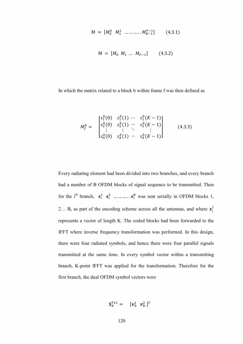
120
M = [𝑀00 𝑀1
1 ……… . .𝑀𝐵−1𝐹−1] (4.3.1)
M = [𝑀0 𝑀1 … 𝑀𝐹−1] (4.3.2)
In which the matrix related to a block b within frame f was then defined as
𝑀𝑓𝑏 =
[ 𝑠1𝑏(0) 𝑠1
𝑏(1)
𝑠2𝑏(0)⋮
𝑠𝐴𝑏(0)
𝑠2𝑏(1)⋮
𝑠𝐴𝑏(1)
⋯ 𝑠1𝑏(𝐾 − 1)
…⋱…
𝑠2𝑏(𝐾 − 1)
⋮𝑠𝐴𝑏(𝐾 − 1)]
(4.3.3)
Every radiating element had been divided into two branches, and every branch
had a number of B OFDM blocks of signal sequence to be transmitted. Then
for the ith
branch, 𝒔𝑖1 𝒔𝑖
2 ……… . . 𝒔𝑖𝐵 was sent serially in OFDM blocks 1,
2… B, as part of the encoding scheme across all the antennas, and where 𝒔𝑖𝑗
represents a vector of length K. The coded blocks had been forwarded to the
IFFT where inverse frequency transformation was performed. In this design,
there were four radiated symbols, and hence there were four parallel signals
transmitted at the same time. In every symbol vector within a transmitting
branch, K-point IFFT was applied for the transformation. Therefore for the
first branch, the dual OFDM symbol vectors were
𝑺𝑏𝑇𝑥1 = [𝒗𝑏
1 𝒗𝑏2 ]𝑇

121
𝑺𝑏𝑇𝑥1 = [
𝑠𝑏1(0) 𝑠𝑏
1(1) … 𝑠𝑏1(𝐾 − 1)
𝑠𝑏2(0) 𝑠𝑏
2(1) … 𝑠𝑏2(𝐾 − 1)
] (4.3.4)
For the second branch,
𝑺𝑏𝑇𝑥2 = [𝒗𝑏
3 𝒗𝑏4 ]𝑇
𝑺𝑏𝑇𝑥2 = [
𝑠𝑏3(0) 𝑠𝑏
3(1) … 𝑠𝑏3(𝐾 − 1)
𝑠𝑏4(0) 𝑠𝑏
4(1) … 𝑠𝑏4(𝐾 − 1)
] (4.3.5)
The space frequency coding that had been proposed in the implementation
scheme for this configuration was described in the figure (1). At the t instant of
time, the fours 8-ary PSK symbols 𝑠𝑏1(𝑡), 𝑠𝑏
3(𝑡)), (𝑠𝑏2(𝑡), 𝑠𝑏
4(𝑡)) was assigned
to the f(k), and f(k+50) subcarriers within the b block across both transmitting
antennas.
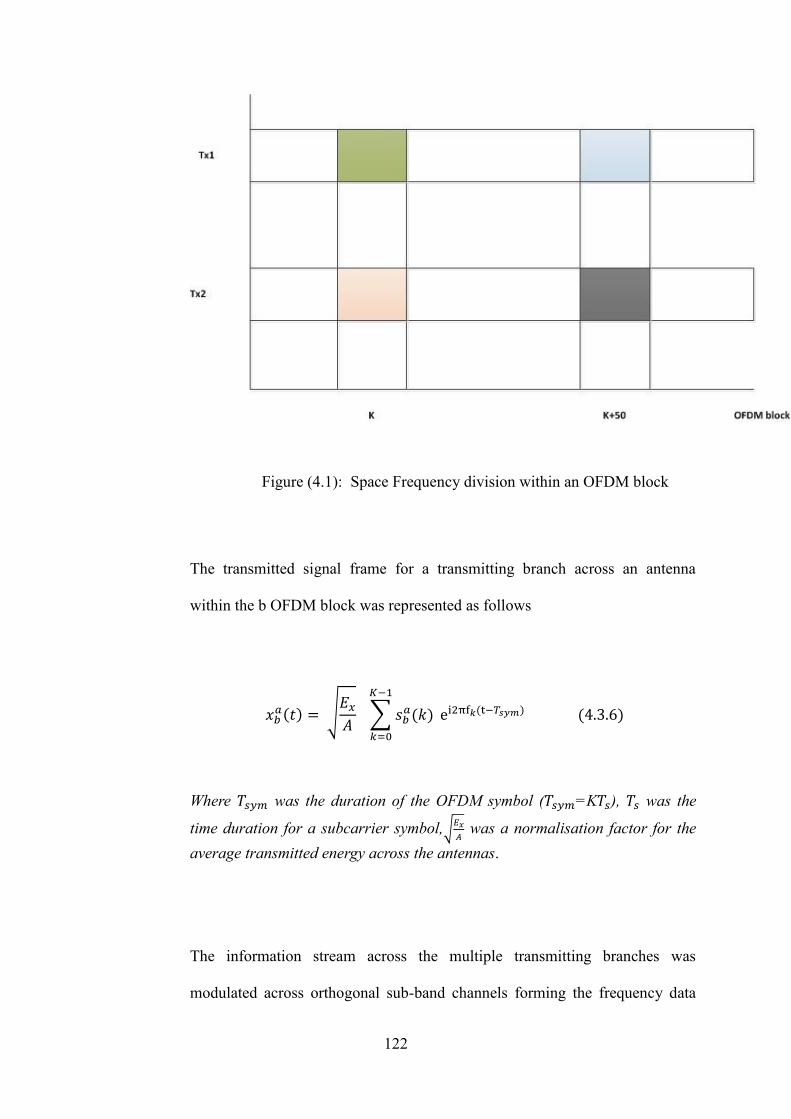
122
Figure (4.1): Space Frequency division within an OFDM block
The transmitted signal frame for a transmitting branch across an antenna
within the b OFDM block was represented as follows
𝑥𝑏𝑎(𝑡) = √
𝐸𝑥𝐴 ∑ 𝑠𝑏
𝑎(𝑘)
𝐾−1
𝑘=0
ei2πf𝑘(t−𝑇𝑠𝑦𝑚) (4.3.6)
Where 𝑇𝑠𝑦𝑚 was the duration of the OFDM symbol (𝑇𝑠𝑦𝑚=K𝑇𝑠), 𝑇𝑠 was the
time duration for a subcarrier symbol,√𝐸𝑥
𝐴 was a normalisation factor for the
average transmitted energy across the antennas.
The information stream across the multiple transmitting branches was
modulated across orthogonal sub-band channels forming the frequency data
123
subcarriers of the OFDM symbols. The samples data was developed in the
frequency domain, and therefore the signal spectrum had to be transformed to
the time domain through the inverse frequency transform using IFFT. OFDM
process is easily implemented in the digital domain. OFDM was bandwidth
efficient since the spectrum was divided into narrow bands for transmitting
more information data. In addition, it overcomes fading selectivity by the
formation of these narrow band channels. Guard intervals within OFDM make
it more robust to the effect of ISI, and this parallel formation of sub-channels
makes it less susceptible to impulse noise. Furthermore, when using parallel
transmission as a pose to serial counterpart, that makes this scheme more
dynamics in terms of resource allocation, and hence the data rate could be
varied by transmitting at different sub-channels with variable fading. In the
second stage of modulation, the transmitted signal was shifted up in the
frequency domain to the carrier spectrum by filtering and up-conversion. The
OFDM carrier frequencies consist of orthogonal functions, each of which was
used to carry a complex symbol representing an information signal. OFDM
overlaps the subcarriers and that make use of the available spectrum in an
efficient way. It could be noted that the transmitted formula for the symbol
have two parts, one is the information part and the second represents the
carrier function. This process results in a new pass-band signal as follows
𝑥𝑏𝑎(𝑡) = ∑ 𝑅𝑒(𝑥𝑏
𝑎(𝑡))
𝐾−1
𝑘=0
ei2πf𝑘(t−𝑇𝑠𝑦𝑚) (4.3.7)

124
4.4 IFFT OFDM implementation on the MIMO
configuration
In the implementation scheme, there were dual transmitting and receiving
antennas, with an OFDM modulation that consists of 128 subcarriers in which
100 tonnes (Ds) were used to carry the information signals. These modulation
carries was designed and arranged to accommodate the serial to parallel (S/P)
converted and encoded message samples. It was useful to note that, ifft
function folds the signal across the origin, and hence shifting the signals before
the Fourier transformation was necessary. Therefore, the samples were
readjusted in a developed function (SigShift) that fold these signals and add
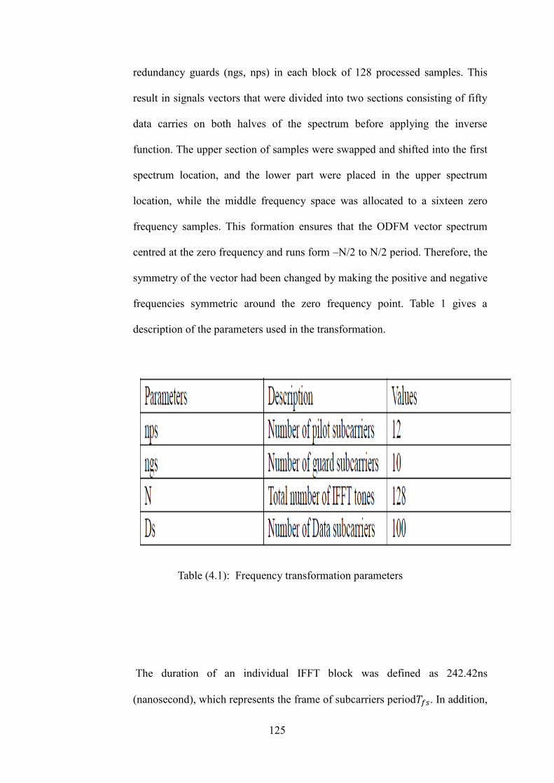
125
redundancy guards (ngs, nps) in each block of 128 processed samples. This
result in signals vectors that were divided into two sections consisting of fifty
data carries on both halves of the spectrum before applying the inverse
function. The upper section of samples were swapped and shifted into the first
spectrum location, and the lower part were placed in the upper spectrum
location, while the middle frequency space was allocated to a sixteen zero
frequency samples. This formation ensures that the ODFM vector spectrum
centred at the zero frequency and runs form –N/2 to N/2 period. Therefore, the
symmetry of the vector had been changed by making the positive and negative
frequencies symmetric around the zero frequency point. Table 1 gives a
description of the parameters used in the transformation.
Table (4.1): Frequency transformation parameters
The duration of an individual IFFT block was defined as 242.42ns
(nanosecond), which represents the frame of subcarriers period𝑇𝑓𝑠. In addition,
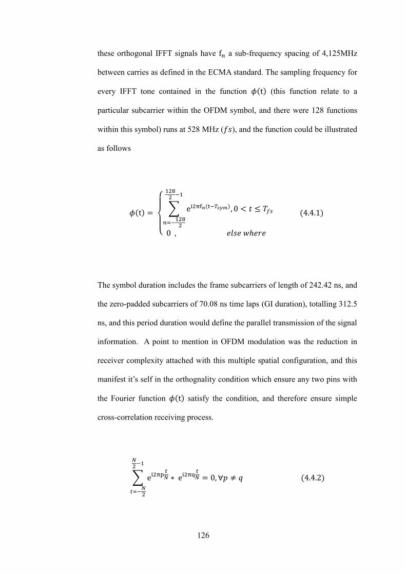
126
these orthogonal IFFT signals have f𝑛 a sub-frequency spacing of 4,125MHz
between carries as defined in the ECMA standard. The sampling frequency for
every IFFT tone contained in the function 𝜙(t) (this function relate to a
particular subcarrier within the OFDM symbol, and there were 128 functions
within this symbol) runs at 528 MHz (𝑓𝑠), and the function could be illustrated
as follows
𝜙(t) =
{
∑ ei2πf𝑛(t−𝑇𝑠𝑦𝑚), 0 < 𝑡 ≤ 𝑇𝑓𝑠
1282−1
𝑛=−1282
0 , 𝑒𝑙𝑠𝑒 𝑤ℎ𝑒𝑟𝑒
(4.4.1)
The symbol duration includes the frame subcarriers of length of 242.42 ns, and
the zero-padded subcarriers of 70.08 ns time laps (GI duration), totalling 312.5
ns, and this period duration would define the parallel transmission of the signal
information. A point to mention in OFDM modulation was the reduction in
receiver complexity attached with this multiple spatial configuration, and this
manifest it’s self in the orthognality condition which ensure any two pins with
the Fourier function 𝜙(t) satisfy the condition, and therefore ensure simple
cross-correlation receiving process.
∑ ei2πp𝑡𝑁
𝑁2−1
𝑡=−𝑁2
∗ ei2πq𝑡𝑁 = 0, ∀𝑝 ≠ 𝑞 (4.4.2)
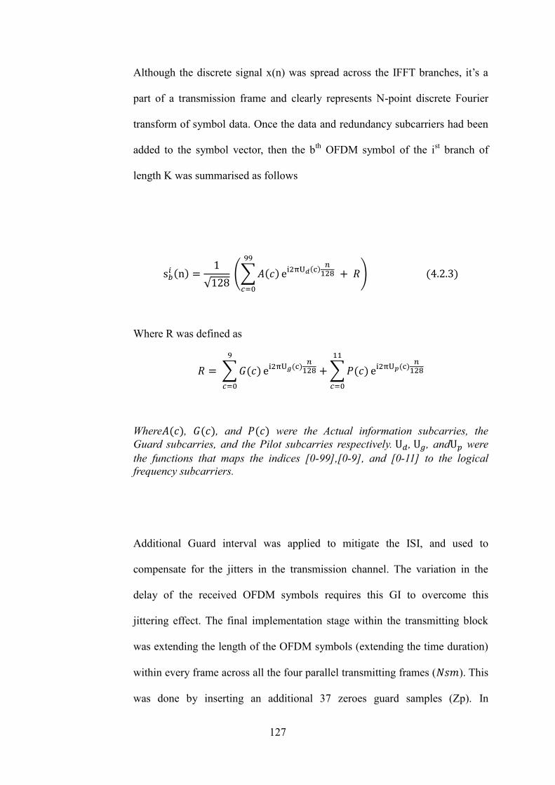
127
Although the discrete signal x(n) was spread across the IFFT branches, it’s a
part of a transmission frame and clearly represents N-point discrete Fourier
transform of symbol data. Once the data and redundancy subcarriers had been
added to the symbol vector, then the bth
OFDM symbol of the ist branch of
length K was summarised as follows
s𝑏𝑖 (n) =
1
√128 (∑𝐴(𝑐)
99
𝑐=0
ei2πU𝑑(c)
𝑛128 + 𝑅) (4.2.3)
Where R was defined as
𝑅 = ∑𝐺(𝑐)
9
𝑐=0
ei2πU𝑔(c)𝑛128 +∑𝑃(𝑐)
11
𝑐=0
ei2πU𝑝(c)𝑛128
Where𝐴(𝑐), 𝐺(𝑐), and 𝑃(𝑐) were the Actual information subcarries, the
Guard subcarries, and the Pilot subcarries respectively. U𝑑, U𝑔, andU𝑝 were
the functions that maps the indices [0-99],[0-9], and [0-11] to the logical
frequency subcarriers.
Additional Guard interval was applied to mitigate the ISI, and used to
compensate for the jitters in the transmission channel. The variation in the
delay of the received OFDM symbols requires this GI to overcome this
jittering effect. The final implementation stage within the transmitting block
was extending the length of the OFDM symbols (extending the time duration)
within every frame across all the four parallel transmitting frames (𝑁𝑠𝑚). This
was done by inserting an additional 37 zeroes guard samples (Zp). In
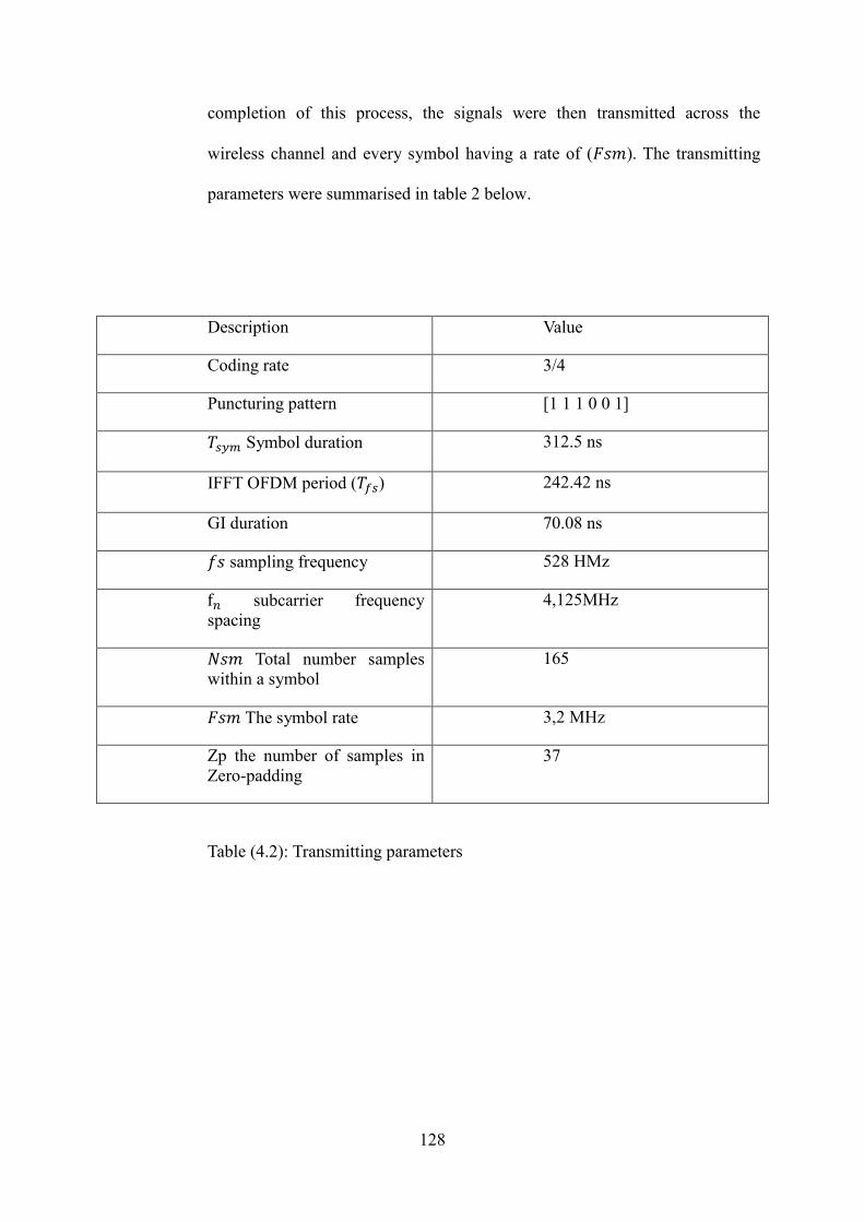
128
completion of this process, the signals were then transmitted across the
wireless channel and every symbol having a rate of (𝐹𝑠𝑚). The transmitting
parameters were summarised in table 2 below.
Description Value
Coding rate 3/4
Puncturing pattern [1 1 1 0 0 1]
𝑇𝑠𝑦𝑚 Symbol duration 312.5 ns
IFFT OFDM period (𝑇𝑓𝑠) 242.42 ns
GI duration 70.08 ns
𝑓𝑠 sampling frequency 528 HMz
f𝑛 subcarrier frequency
spacing
4,125MHz
𝑁𝑠𝑚 Total number samples
within a symbol
165
𝐹𝑠𝑚 The symbol rate 3,2 MHz
Zp the number of samples in
Zero-padding
37
Table (4.2): Transmitting parameters

129
4.5 The implemented Channel model
In this implementation, different hypothesis were considered to test the fitness
of the proposed multi-antennas wireless model. In order to propose a wireless
model, it was necessary to define and implement a channel model that
emulates the specific environment in which this designed concept operate on.
The choice of the channel model in this design was very important to ensure a
reliable simulation that was based on a recognised and verified UWB channel
model. Specific scenarios were covered to ensure the practical feasibility of
the design. Additional verifications were used to test the proposed design. A
standardised channel model was used to infer the performance merits of the
system. The model has been used to simulate the physical channel effects on
the wireless signal. In this section, the channel model was implemented to
satisfy the indoor medium characteristics. Previous measurements had shown
that Indoor Ultra wide band channel impulse response behaves in clustering
manners. The observation had shown that log normal distribution fits the
measurement data for the UWB channel amplitudes. Furthermore, the phase
components of the impulse response were considered to be redundant as they
were rotated within the absolute of 90 degrees.

130
In order to validate any work, it had to be subjected to a well-known and
verified standard model. As result, the proposed DC-32QAM had been
subjected to the IEEE803.15.3a model for validation and verification. .
Modelling channel behaviour in the time domain deals with continuous time
events. As it was the case, these continuous time events needed to be discretise
in the simulation process, and therefore it was imperative to define this
discretisation stage where the UWB transmission have high temporal
resolution. One of the challenges in a simulation work was how to validate a
particular novel design while clarifying very clearly the very distinct
contributions in simulation environment. To this end, the well approved
standardised channel model was used in the verification, and then modified
based on a proposal concept. In the development stage, the simulation was
carried out using the first two propagation scenarios of the model, namely line
of sight and non-line of sight for short ranges (ch1, ch2). It had been useful to
consider the transmitted signals as a time limited event and the channel
response as multipath cloud with various power coefficients spanning different
time resolution. These events needed to be transferred from its continuous time
domain to the discrete version for the modelling purposes. The specified
channel uses very small sampling times for the discretisation process of the
UWB continuous channel, in order to convert it to discrete sample model.
Furthermore, Nyquist theorem states that for a successful sampling operation,
the sampling frequency has to be twice the largest frequency in the signal, and
hence to capture of the spectrum content within the targeted signal, the
sampling frequency should be chosen to be much greater than the maximum
frequency. This in turn reduces the sampling resolution window and increases
131
the number of samples. Taking these notes into account, adjustment for the
IEEE model was needed to absorb the requirements of this work. This was
reflected in the reduction of the simulation time and a reduction in complexity
of the algorithm by focusing on the behaviour of a limited number of multipath
channel coefficients without losing the bulk of the spectrum content. The
amplitudes of the multipath fading in the SG3a UWB model reflect the signal
distribution at the receivers, resulting from the filtering effect by the channel.
The characteristic of the received signal cloud was obtained by actual
measurements and stochastic analysis for the indoor environment in the
standard. This standardised model uses a sampling period of 0.167 ns
(nanosecond) for the discretisation process of the UWB channel response,
translating this continuous response into discrete samples model. It was
important to keep the channel characteristic of the model the same by keeping
all the main channel parameters to its original values. The cluster arrival rate,
ray arrival rate, cluster attenuation constant, ray attenuation constant, The
overall standard deviation of the multipath shadowing with a lognormal
distribution, standard deviation of lognormal shadowing for the clusters,
standard deviation of lognormal shadowing for the rays within a particular
cluster, the mean excess delay, the number of significant paths within 10dB of
peak power (NP_10dB), the Power Delay Profile (PDP), and the RMS delay
spread should all be consistent with the standard requirements.
The specified model produces impulse response consisting of 100 channel

132
realisations, each of which had a multipath cloud containing over 600 paths.
The first step here was to average these multipath channels across each time
pin to form an average channel, that encapsulate the medium behaviour. As
this was time varying channel, this averaging gave more accurate response
than a single channel response representation. Noting that, the UWB channel
response of the standard was discretised version with equal time pins across
the entire channel, and hence averaging will not change the time index. In the
discretisation stage, a search for the maximum delayed coefficient (ch(t_max))
was firstly obtained. It was noted that different scatters and indoor structures
resulted in various time delay pins, and hence a number of significant pins was
identified by combination of measurements and stochastic process. This
ensures that all other weights occurred within this time window, as these
events were not periodic and have specified time resolution. Next, a sampling
time (ts) was chosen which facilitate capturing the core content of the
multipath amplitudes. The sampling time was very critical for indoor wireless
transmission due to the unlimited bandwidth, resulted from the randomness
property of the arrival times. This governs the signal wave’s propagation and
results in high resolution signals. From simulation analysis, it was found that
the sampling time for these models should be at least smaller than four times
the significant path that represented the smallest time duration. In addition,
finding suitable sampling window would depends on the user requirements as
well as the software and hardware limitations, but the smaller the value, the
more accurate the signalling process analysis. To illustrate this operation,
consider h1 (the first channel coefficient) with a maximum time delay tm, then
the sampling time (ts) was chosen much smaller that tm by at least half of its

133
value (Figure 4.2). Then, in order to discretise h1, the length of h1 was
expanded in the discrete domain based on the following syntax
h1 = 1+ floor ( tm / ts )
h1 samples at k times its frequency f(h1) ==> fs = k*f(h1) , so N = k
ch = 100 ( there were 100 channels),
np = NP (for each ch there were a number of multipath NP)
To discretise path(n)_time_cont , then
Ch=n , np(ch=n)= NP paths , path(n)_time_cont = L ns (L nano-seconds)
Now, storing these discrete time indices in an array( t_Nfs) as
t_Nfs = 1 + floor (Path_time_discrete)
The above expression, could expanded to store all the discrete samples
corresponds to all continuous time array ( path(1:end)_time_cont) as follows
t_Nfs = 1 + floor( path(1:end)_time_cont / ts)
Figure (4.2): Time window for discretisation

134
A vector of equally space discrete samples with a maximum length
corresponding to the largest path delay was then created to allocate all the time
pins within the temporal cloud. Then, each continuous time instance of a
significant path had a corresponding discrete sampling value within this vector
encapsulating its duration in the discrete domain. An array of channel
amplitudes with the same time vector length was then created and populated
with weights corresponding to these time pins. Thus, the largest delay path had
its amplitude allocated at the last index in the array and hence preserving the
distribution of the impulse response. These large spectrum content UWB
channel response was passed through filtering operation in order to down
sample it to a workable band limited spectrum by using a resample function.
Although, some frequency response parts were eliminated and the spectrum
shape had a marginal alteration, the core of channel behaviour was still
persevered. The graphs below (Figure 4.3) provide a comparison of the two
models, where it could be seen that the overall density and the statistical shape
had been preserved.

135
Figure (4.3): Comparison between IEEE803.15.3a model and its modified version
For simulation purposes, a down conversion with filtering and resampling was
0 20 40 60 80 100 120-2.5
-2
-1.5
-1
-0.5
0
0.5
1
1.5Impulse response realizations of IEEE 802.15.3a model
Time[ns]
0 20 40 60 80 100 120-4
-3
-2
-1
0
1
2
3Impulse response realizations of the modified model
Time[ns]
136
undertaken by readjusting the sampling period. Hence, the implementation was
performed by applying down sampling conversion with the aid of resampling
using a time resolution of 3.006 ns. Resampling had produced a sampling
period of 2.672 ns (0.167 * 16), which resulted from multiplying the sampling
index by sixteen. This sampling time increases the resolution window sixteen
times the original sampling index and reducing the sampling frequency by the
same amount. Quantisation for the continuous time response was lead to
formatting the desired resolution ts and a decimating factor of N. The value of
N was an even quantity that was chosen to be a next power of two integers in
the discretisation process. Similar responses with the same time index was
added together, with transmit pulse filtering and band pass or low pass down
conversion to fit the simulation requirements of the particular system (down
conversion for this system). The resampling adjustment had to ensure the
mitigation of the aliasing effect before the decimation by considering code
with anti-aliasing filtering or complex down conversion. It was important to
mention that, the sampling pins tend to store multipath coefficients and it was
not practically feasible to store the entire continuous time multipath. In gernal,
changing an event that elapse a very small period would mean oversampling
with higher number of samples proportional to its spectrum in simulation test-
beds. This in turns leads to a large number of weight coefficients in the
convolution stage, and increases the costs of processing and memory
requirements attached with the implementation. Furthermore, the proposed
ECMA-368 standard specifies FFT size of 128 tones with 100 subcarriers for
the transmitted signal at both transmitters and receivers sides.
As mentioned before, the resulting impulse response had over six hundred

137
paths which needed to be resampled in order to limit the simulation and
facilitated the 128 fft frequency transformation. This domain translation had to
match the transmitted signal transformation in the simulation. Fifty symbols
were required for the signal in each subsection of the transmitter with 50 MHz
spectrum separation between the two sections, and hence a maximum of fifty
channel samples was required in the convolution process. Knowing that the
FFT is periodic and symmetric in nature, there was a limitation in UWB
channel samples available for DSP processing within the sampling
environment. This was then justified the proposed sampling period expressed
for this channel model. Figure 4.4 below show the channel impulse response in
the time and frequency domains.
Figure (4.4): Time and frequency channel response
0 20 40 60 80 100 120-0.4
-0.2
0
0.2
0.4
0.6
0.8
1
1.2
1.4Impulse response realizations of IEEE 802.15.3a model with ts of 2.672 ns
Time[ns]
Impu
lse re
spon
se
0 0.02 0.04 0.06 0.08 0.1 0.12 0.14 0.16 0.18 0.20
0.02
0.04
0.06
0.08
0.1
0.12
0.14Single-Sided Amplitude Spectrum of the channel
Frequency
|CH(f)|

138
4.6 Receiver Implementation
The received noisy and distorted symbols had an additional length of Guard
signal that did not contain information data, and had been used to reduce the
ISI (Inter Symbol Interference). Therefore, the first step was to remove these
redundancies from the OFDM symbol frame.
The guard intervals was copied and added to the header of the symbol frame in
repetitive manner across the symbols, and therefore a specific function was
implemented at the receive branches to remove these redundancies by
reordering the received frames. The operation was done by initially creating a
frame that consists of two vectors, one represents the last 37 samples of the
particular received symbol, and the second part consists of 91 zero samples,
and then 128 length vector was added to the first received 128 sample of the
original frame.
The re-adjustment procedure had the following format
Y1 = Y0 (1:128)
Y2 = Y0 (128:165)
139
Y3 = zeros (1:91)
Y = Y1 + [Y2 Y3]
Once these additional guard intervals was removed from OFDM symbols, then
Fast Fourier Transform FFT operation was performed across the symbols and
the frame to translate the received signals into the frequency domain. The
translation was performed on a noisy and corrupted symbols and expressed
mathematically as follows
Y(q) = 𝑓𝑓𝑡(𝑦) =1
𝑁∑(∑ Y𝑙,𝐷1,2
𝐴𝑎 (p)
𝑁−1
𝑝=0
e−i2πpn/N + 𝑧)
𝑁−1
𝑛=0
ei2πnq/N (4.6.1)
Y(q) = 𝑌(𝑞)𝐻(𝑞) + 𝑍(𝑞) , 𝑞 = 0,2…127 (4.6.2)
The process used 128 FFT bin size that was specified within the ECMA
standard, and hence this implementation gives practical advantage in terms of
hardware complexity. Equalisation had been followed for these frequency
domain samples across symbol vectors and packet frames. In order to carry the
equalisation process, accurate channel estimation in the name of CSI was
critical. Hence in this part, two model scenarios was implemented one which
had assumed perfect channel estimation procedure, and the other had
140
considered partial channel estimation (equalisation errors). Frequency
transformation had to be applied for the channel coefficients, so as to carry out
frequency domain equalisation. Since symmetrical frequency domains channel
samples was required, a shift and swap between the upper and lower channel
spectrum had been carried out. This ensures synchronisation with the received
signal samples in the frequency domain, and avoids distortion in the
equalisation. The implementation steps for the channel frequency transform
were summarised as follows
hf = fft ([h 𝑧𝑒𝑜𝑟𝑠(128 − 𝑙𝑒𝑛𝑔𝑡ℎ(ℎ))], 128)
hf = [ ℎ𝑓(128: 49) ℎ𝑓(2: 51) ]
A critical equalisation task was removing the channel spectrum distortion from
the received signal components. In this case, received symbols were divided
by the channel spectrum to eliminate the channel effect. Zero Forcing equaliser
have a problem of noise enhancement for low SNR, and while a formulation
for the model had used to constrain the complexity associated with MIMO
implementation, it was imperative to address this shortfall within the
simulation environment. The reconstruction had been conducted by
transformation, in which the first PSK symbol within the second antenna was
allocated in the first radiating element, and replacing the first slot of the
second receiving branch by the corrosponding second symbol within the first
antenna. Then, as the design proposal had stated that, the dual 8-ary PSK
symbols across the two radiating elements had to be combined. This
141
tranformation induces new received symbols contained fading distrotions with
additonal degree of freedom encapsuated from the spatial and frequency
domain configration. Then a matlab file function (ReTransformConcept) were
created to take the dual symbols across the 1500 symbols frame on every
branch of the receiving antennas. The real components of the dual receiving
branches were interchanged inducing modified symbols as result of the
transformation. Then following this process, the resulting complex symbols in
every branch across the dual radiating elements were divided with the
magnitude of the quadrature components of its corroposnding symbols. These
ulterd symbols were then soft decoded to infer the orignal transmitted QPSK
symbols.
𝑦𝑘(𝑛)𝑝𝑠𝑘1
𝑅1
= 𝑑1𝑝𝑠𝑘1
𝑅1
+ 𝑗𝑑2𝑝𝑠𝑘1
𝑅1
(4.6.3)
𝑦𝑘(𝑛+50)𝑝𝑠𝑘2
𝑅2
= 𝑑1𝑝𝑠𝑘2
𝑅2
+ 𝑗𝑑2𝑝𝑠𝑘2
𝑅2
(4.6.4)
𝑦𝑘(𝑛+50)𝑝𝑠𝑘2
𝑅1
= 𝑑1𝑝𝑠𝑘2
𝑅1
+ 𝑗𝑑2𝑝𝑠𝑘2
𝑅1
(4.6.5)
𝑦𝑘(𝑛)𝑝𝑠𝑘1
𝑅2
= 𝑑1𝑝𝑠𝑘1
𝑅2
+ 𝑗𝑑2𝑝𝑠𝑘1
𝑅2
(4.6.6)
Applied cross insertion, the new complex symbols were then became
��𝑘(𝑛)𝑝𝑠𝑘1
𝑅1
= Real (𝑦𝑘(𝑛+50)𝑝𝑠𝑘2
𝑅2
) + 𝑗𝑑2𝑝𝑠𝑘1
𝑅1
= 𝑑1𝑝𝑠𝑘2
𝑅2
+ 𝑗𝑑2𝑝𝑠𝑘1
𝑅1
(4.4.7)
142
��𝑘(𝑛+50)𝑝𝑠𝑘2
𝑅2
= Real (𝑦𝑘(𝑛)𝑝𝑠𝑘1
𝑅1
) + 𝑗𝑑2𝑝𝑠𝑘2
𝑅2
= 𝑑1𝑝𝑠𝑘2
𝑅2
+ 𝑗𝑑2𝑝𝑠𝑘2
𝑅2
(4.4.8)
��𝑘(𝑛+50)𝑝𝑠𝑘2
𝑅1
= Real (𝑦𝑘(𝑛)𝑝𝑠𝑘1
𝑅2
) + 𝑗𝑑2𝑝𝑠𝑘2
𝑅1
= 𝑑1𝑝𝑠𝑘2
𝑅2
+ 𝑗𝑑2𝑝𝑠𝑘2
𝑅1
(4.4.9)
��𝑘(𝑛)𝑝𝑠𝑘1
𝑅2
= Real (𝑦𝑘(𝑛+50)𝑝𝑠𝑘2
𝑅1
) + 𝑗𝑑2𝑝𝑠𝑘1
𝑅2
= 𝑑1𝑝𝑠𝑘2
𝑅2
+ 𝑗𝑑2𝑝𝑠𝑘1
𝑅2
(4.4.10)
The orignal QPSK symbols were then determined as
y𝑞𝑝𝑠𝑘1𝑔1
=(��𝑘(𝑛)
𝑝𝑠𝑘1𝑅1
)
|𝑑2𝑝𝑠𝑘1
𝑅1
|= 𝑟𝑔1𝑐(𝑛) + 𝑗𝑟
𝑔1𝑐(𝑛)+50 (4.4.11)
y𝑞𝑝𝑠𝑘2𝑔1
=(��𝑘(𝑛+50)
𝑝𝑠𝑘2𝑅2
)
|𝑑2𝑝𝑠𝑘2
𝑅2
|= 𝑟𝑔1𝑐(𝑛)+1 + 𝑗𝑟
𝑔1𝑐(𝑛)+51 (4.4.12)
y𝑞𝑝𝑠𝑘1𝑔2
=(��𝑘(𝑛+50)
𝑝𝑠𝑘2𝑅1
)
|𝑑2𝑝𝑠𝑘2
𝑅1
|= 𝑟𝑔2𝑐(𝑛) + 𝑗𝑟
𝑔2𝑐(𝑛)+50 (4.4.13)
y𝑞𝑝𝑠𝑘2𝑔2
=(��𝑘(𝑛)
𝑝𝑠𝑘1𝑅2
)
|𝑑2𝑝𝑠𝑘1
𝑅2
|= 𝑟𝑔2𝑐(𝑛)+1 + 𝑗𝑟
𝑔2𝑐(𝑛)+51 (4.4.14)
The searching subspace of the paths metrics for the soft decoding alogirhm
had been reduced by this receving design, and the transformation process
results in lowering the signal constellation to four points scatter map. For
143
every received symbol, the In-phase and Qudarature components coming from
different indenpent channels, and the demodulation were perfomed by
examming these distance metrics to obatin the orignal two dimenstional (two
bits symbol) transmitted symbols. These induced distorted complex numbers
were then passed to a measure function (RecAntenDCMSoft_QPSK) which
have the task of measuring the recovred actual eculidean distances on the two
In-phase and quarduature orthognal domains. These actual noisy measurment
were then used in the ML searching alogrithm to reconstruct the orignal
signals. Its imporatn to mension here that, these two measurment values
correposnds to the Second Most Significant bit (SMB) and the Least
Significant Bit (LSB) of the 8-ary PSK symobls. The eculdian metrics
evulation was done independnetly across the orthongal dimensions of the
mdoified complex symbols. These metrics were then used in the demodulation
process as soft decoding inputs to the Vierbi decoder. This reduction in the
signal alphabate reduces combutation within the viterbi alogrithm. The
reduction of the finite eculidean metric sets that spans the signal constellation,
optimise the ML solution which was refltected in the number of paths metrics
within the trellis. In the ML scheme, finding the minmum distance across a
large set of signals was NP-hard optimisation problem and therefore a smaller
set of path mertics makes this deocding alogirthm releasiable in paractical
applications. A reduction in the complexity was observed by reducing the
searching graph subspace for the demapper. This was then repeated for the 50
complex symbols across the receiveing branches. In mathematical form, the
above process would be expersssed as follows
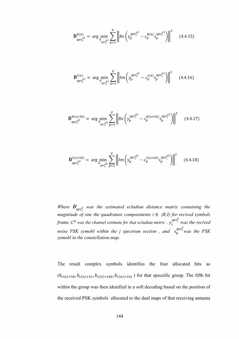
144
��𝑞𝑝𝑠𝑟
𝑔1𝑅(𝑛)
= arg min𝑑𝑞𝑝𝑠𝑟
𝑔1∑‖𝑅𝑒(𝑦𝑝
𝑞𝑝𝑠𝑟𝑔1
− 𝑐𝑝𝑅(𝑛)
𝑠𝑝𝑞𝑝𝑠𝑟
𝑔1
)‖
2𝑃
𝑝=1
(4.4.15)
��𝑞𝑝𝑠𝑟
𝑔1𝐼(𝑛)
= arg min𝑑𝑞𝑝𝑠𝑟
𝑔1∑‖𝐼𝑚(𝑦𝑝
𝑞𝑝𝑠𝑟𝑔1
− 𝑐𝑝𝐼(𝑛)
𝑠𝑝𝑞𝑝𝑠𝑟
𝑔1
)‖
2𝑃
𝑝=1
(4.4.16)
��𝑞𝑝𝑠𝑟
𝑔2𝑅(𝑛+50)
= arg min𝑑𝑞𝑝𝑠𝑟
𝑔2∑‖𝑅𝑒(𝑦𝑝
𝑞𝑝𝑠𝑟𝑔2
− 𝑐𝑝𝑅(𝑛+50)
𝑠𝑝𝑞𝑝𝑠𝑟
𝑔2
)‖
2𝑃
𝑝=1
(4.4.17)
��𝑞𝑝𝑠𝑟
𝑔2𝐼(𝑛+50)
= arg min𝑑𝑞𝑝𝑠𝑟
𝑔2∑‖𝐼𝑚(𝑦𝑝
𝑞𝑝𝑠𝑟𝑔2
− 𝑐𝑝𝐼(𝑛+50)
𝑠𝑝𝑞𝑝𝑠𝑟
𝑔2
)‖
2𝑃
𝑝=1
(4.4.18)
Where ��𝑞𝑝𝑠𝑟
𝑔𝑖 was the estimated ecludian distance matrix containing the
magntiude of one the quadrature compoentents i ∈ (R,I) for recived symbols
frame, 𝐶𝑑 was the channel estimate for that ecludian metric . 𝑦𝑗
𝑞𝑝𝑠𝑟𝑔
was the recived
noise PSK symobl within the j spectrum section , and 𝑠𝑝𝑞𝑝𝑠𝑟
𝑔
was the PSK
symobl in the constellation map.
The result complex symbols identifies the four allocated bits as
(𝑏𝑐(𝑛)+50, 𝑏𝑐(𝑛)+51, 𝑏𝑐(𝑛)+100, 𝑏𝑐(𝑛)+101 ) for that speceific group. The fifth bit
within the group was then idenified in a soft decoding based on the position of
the received PSK symbols allocated to the dual maps of that receiving antanna
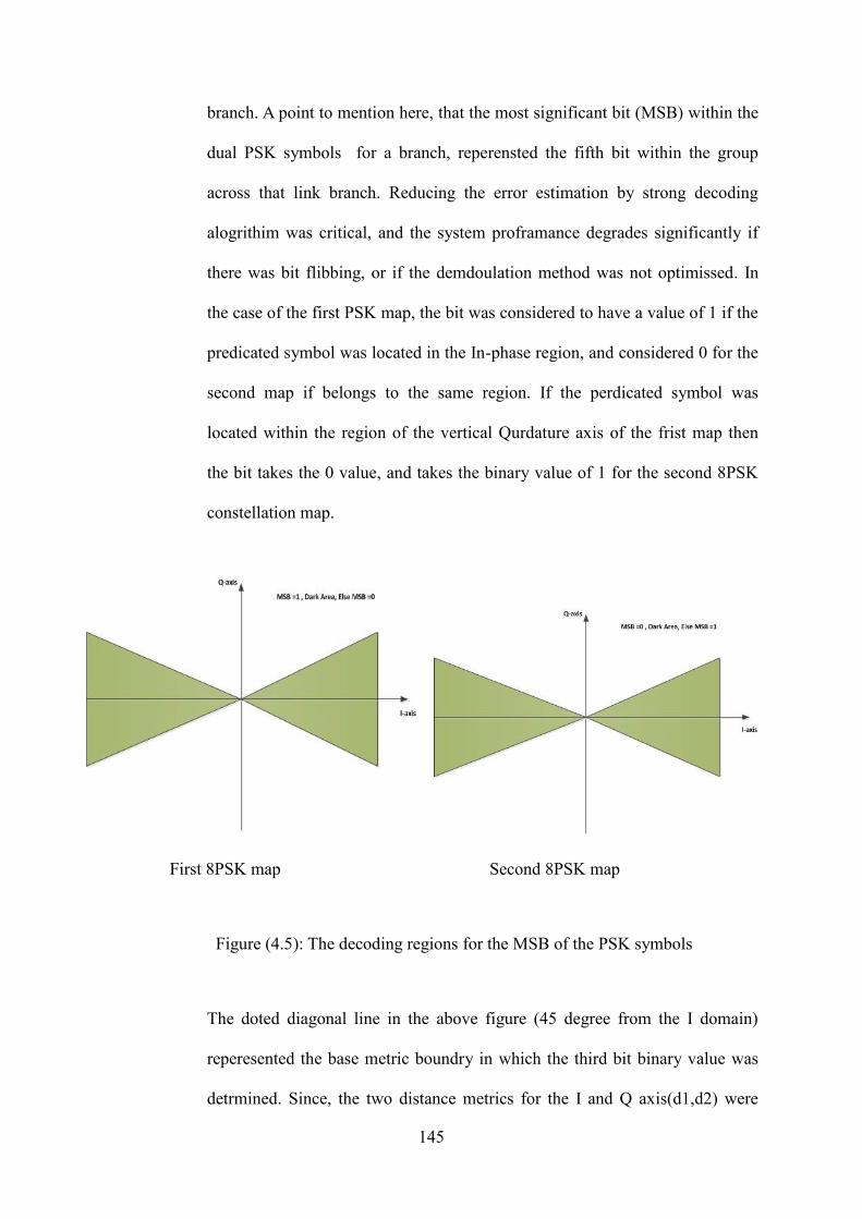
145
branch. A point to mention here, that the most significant bit (MSB) within the
dual PSK symbols for a branch, reperensted the fifth bit within the group
across that link branch. Reducing the error estimation by strong decoding
alogrithim was critical, and the system proframance degrades significantly if
there was bit flibbing, or if the demdoulation method was not optimissed. In
the case of the first PSK map, the bit was considered to have a value of 1 if the
predicated symbol was located in the In-phase region, and considered 0 for the
second map if belongs to the same region. If the perdicated symbol was
located within the region of the vertical Qurdature axis of the frist map then
the bit takes the 0 value, and takes the binary value of 1 for the second 8PSK
constellation map.
First 8PSK map Second 8PSK map
Figure (4.5): The decoding regions for the MSB of the PSK symbols
The doted diagonal line in the above figure (45 degree from the I domain)
reperesented the base metric boundry in which the third bit binary value was
detrmined. Since, the two distance metrics for the I and Q axis(d1,d2) were

146
equal across both orthognal domains. Then, a simple substraction of the
received complex symbol real and imagnry parts from the 𝐼𝑑1𝑝𝑠𝑘1
𝑎
(d1), and
𝐼𝑑2𝑝𝑠𝑘1
𝑎
(d2) determined the positon of the symbol within the above regions.
Therefore, upon receiving the two symbols within each reciving
block(𝑦𝑘(𝑛)𝑝𝑠𝑘1
𝑎
, 𝑦𝑘(𝑛+50)𝑝𝑠𝑘2
𝑎
), the follwing metrics used to infer the 3rd
bit.
In the case of b3 = 0
The conditon for the first 8PSK map was
P1 = √[𝑅𝑒𝑎𝑙 |𝑦𝑘(𝑛)
𝑝𝑠𝑘1𝑎
| − 𝐼𝑑1𝑝𝑠𝑘1
𝑎
]2
+ [𝐼𝑚𝑎𝑔 |𝑦𝑘(𝑛)
𝑝𝑠𝑘1𝑎
| − 𝐼𝑑2𝑝𝑠𝑘1
𝑎
]2
(4.4.19)
P2 = √[𝑅𝑒𝑎𝑙 |𝑦𝑘(𝑛)
𝑝𝑠𝑘1𝑎
| − 𝐼𝑑2𝑝𝑠𝑘1
𝑎
]2
+ [𝐼𝑚𝑎𝑔 |𝑦𝑘(𝑛)
𝑝𝑠𝑘1𝑎
| − 𝐼𝑑1𝑝𝑠𝑘1
𝑎
]2
(4.4.20)
P1 < P2
The condtion for the second 8PSK map
P1 = √[𝑅𝑒𝑎𝑙 |𝑦𝑘(𝑛+50)
𝑝𝑠𝑘2𝑎
| − 𝐼𝑑1𝑝𝑠𝑘2
𝑎
]2
+ [𝐼𝑚𝑎𝑔 |𝑦𝑘(𝑛+50)
𝑝𝑠𝑘2𝑎
| − 𝐼𝑑2𝑝𝑠𝑘2
𝑎
]2
(4.4.21)
P2 = √[𝑅𝑒𝑎𝑙 |𝑦𝑘(𝑛+50)
𝑝𝑠𝑘2𝑎
| − 𝐼𝑑2𝑝𝑠𝑘2
𝑎
]2
+ [𝐼𝑚𝑎𝑔 |𝑦𝑘(𝑛+50)
𝑝𝑠𝑘2𝑎
| − 𝐼𝑑1𝑝𝑠𝑘2
𝑎
]2
(4.4.22)
147
P1 > P2
In the other case of b3 = 1
The conditon for the first 8PSK map was
P1 = √[𝑅𝑒𝑎𝑙 |𝑦𝑘(𝑛)
𝑝𝑠𝑘1𝑎
| − 𝐼𝑑1𝑝𝑠𝑘1
𝑎
]2
+ [𝐼𝑚𝑎𝑔 |𝑦𝑘(𝑛)
𝑝𝑠𝑘1𝑎
| − 𝐼𝑑2𝑝𝑠𝑘1
𝑎
]2
(4.4.23)
P2 = √[𝑅𝑒𝑎𝑙 |𝑦𝑘(𝑛)
𝑝𝑠𝑘1𝑎
| − 𝐼𝑑2𝑝𝑠𝑘1
𝑎
]2
+ [𝐼𝑚𝑎𝑔 |𝑦𝑘(𝑛)
𝑝𝑠𝑘1𝑎
| − 𝐼𝑑1𝑝𝑠𝑘1
𝑎
]2
(4.4.24)
P1 > P2
The condtion for the second 8PSK map
P1 = √[𝑅𝑒𝑎𝑙 |𝑦𝑘(𝑛+50)
𝑝𝑠𝑘2𝑎
| − 𝐼𝑑1𝑝𝑠𝑘2
𝑎
]2
+ [𝐼𝑚𝑎𝑔 |𝑦𝑘(𝑛+50)
𝑝𝑠𝑘2𝑎
| − 𝐼𝑑2𝑝𝑠𝑘2
𝑎
]2
(4.4.25)
P2 = √[𝑅𝑒𝑎𝑙 |𝑦𝑘(𝑛+50)
𝑝𝑠𝑘2𝑎
| − 𝐼𝑑2𝑝𝑠𝑘2
𝑎
]2
+ [𝐼𝑚𝑎𝑔 |𝑦𝑘(𝑛+50)
𝑝𝑠𝑘2𝑎
| − 𝐼𝑑1𝑝𝑠𝑘2
𝑎
]2
(4.4.26)
P1 < P2

148
Figure (4.6): Expression of the metric length position
The viterbi alogrithm was undertaken by using a predfined function within a
software backage ( vitdec function within the Matlab library). The
implementation had required to specify the input parameters for the function
was based on the modulation method used on the transmitted symbols. These
paramters were then used in the decoding process to estimate the binary
singnal information. The trace back length through the trellis was set to 100,
and the structure of the trellis was consistant with the transmitter convolutional
structure. The use of unquant mode was applied to infer the soft decoding
based on the actual calculated ecludian entries. This function itself had been
used with the system paramters defined in table 3.
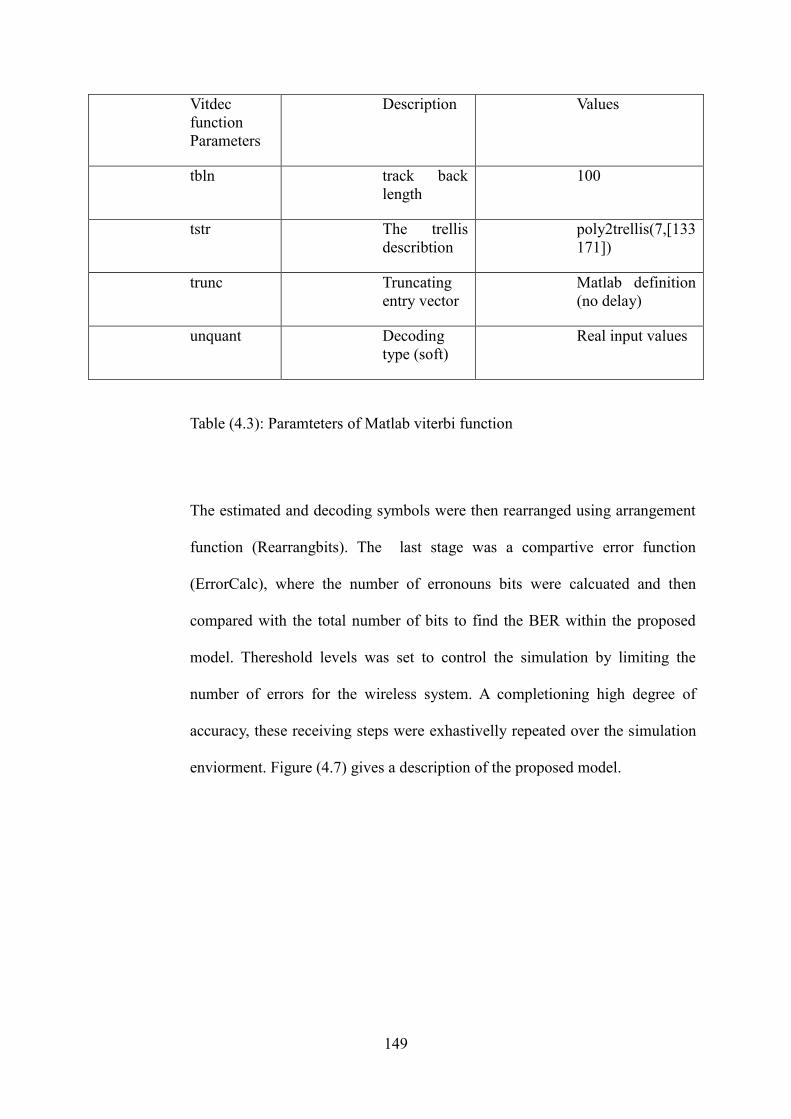
149
Vitdec
function
Parameters
Description Values
tbln track back
length
100
tstr The trellis
describtion
poly2trellis(7,[133
171])
trunc Truncating
entry vector
Matlab definition
(no delay)
unquant Decoding
type (soft)
Real input values
Table (4.3): Paramteters of Matlab viterbi function
The estimated and decoding symbols were then rearranged using arrangement
function (Rearrangbits). The last stage was a compartive error function
(ErrorCalc), where the number of erronouns bits were calcuated and then
compared with the total number of bits to find the BER within the proposed
model. Thereshold levels was set to control the simulation by limiting the
number of errors for the wireless system. A completioning high degree of
accuracy, these receiving steps were exhastivelly repeated over the simulation
enviorment. Figure (4.7) gives a description of the proposed model.
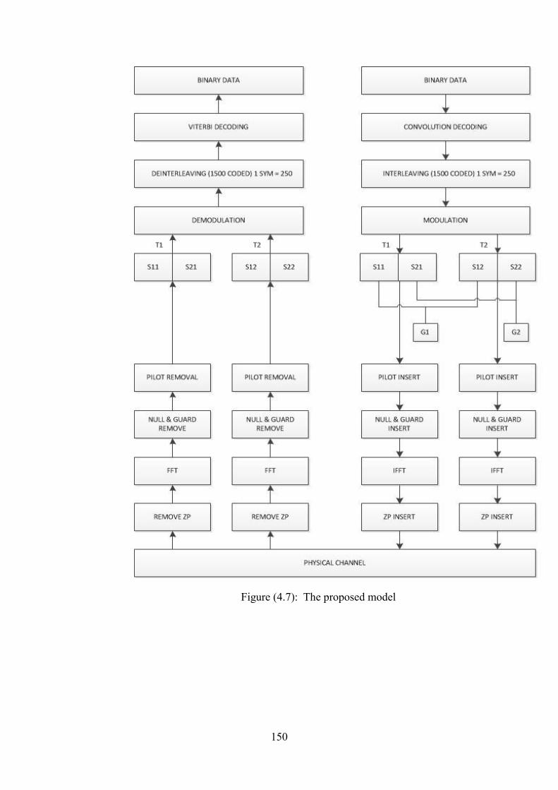
150
Figure (4.7): The proposed model

151
4.7 Optimisation for the Decoding method (LLR)
Introducing the LLR approach to optimise the soft decoding approach by
ensuring the entry to the viterbi decoder had more certanty to the entry metric.
Given the observed received symbols, the conditional probablity of the
transmitted symbols could be used to infer the LLR formula. In the aid of
Payes’Rule and with logrithmic tranformation, the LLR could be summerised
as follows
𝐿(𝑥|𝑦) = 𝐿(𝑦|𝑥) 𝐿(𝑥) /𝐿(𝑦)
Since y was observed (known quanity), then
𝐿(𝑥|𝑦) = 𝐿(𝑦|𝑥) 𝐿(𝑥)
𝐿(𝑥|𝑦) = 𝐿(𝑦|𝑥) + 𝐿(𝑥)
The LLR represents a method for for identfying the most probable transmitted
bits within a noisy received symbols that would be passed to the Vitrebi
decoder. In the dual carrier configuration for each decoding block, there were

152
two receivd symobls( 𝑦𝑘(𝑛)𝑖 , 𝑦𝑘(𝑛+50)
𝑖 ) corrpupted by different channel fadings
according to the inherent frequency and spatial diversities within the UWB
channels. Hence, the error performance for each of these received distotred
symbols was different from each other, and this had been as a result of
multivarite fading in the channel specturm that convloved with that particular
symbol signal. Demapping of the control bit would follow the same process as
the ML method, and the second copies of the received symbols would be
passed to the tranfomration operation.The transformation concept at the
receiving reduces the constellation dimension (down convert the eight points
map to four points scatter). This process gives an important advanatages
interms of the complexity reduction in the demapping and decoding
alogrithms. Therefore, implmenting LLR demapping resulted in two soft
quntities, MSB 𝑏1(the Most Significant Bit), and LSB 𝑏0(the Least Significant
Bit). What is critical here was that, the MSB was related to the soft input to the
decoder follwing the transformation and not related to the orignal received
qunitiy. The constellation map was divided into regions related to each binary
value carried by these symbol bits. A subset of values were located to a
particular region corrosponding to one the significant bit value. The LLR
demapping process across the first received transformed symbol 𝑦𝑘(𝑛)𝑖 one of
the dual reciving block was carried out in the follwing equations.
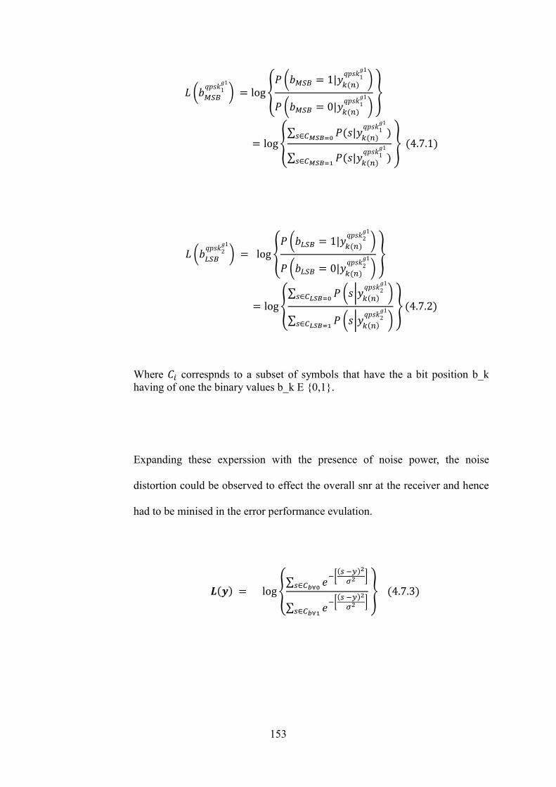
153
𝐿 (𝑏𝑀𝑆𝐵𝑞𝑝𝑠𝑘1
𝑔1
) = log{𝑃 (𝑏𝑀𝑆𝐵 = 1|𝑦𝑘(𝑛)
𝑞𝑝𝑠𝑘1𝑔1
)
𝑃 (𝑏𝑀𝑆𝐵 = 0|𝑦𝑘(𝑛)𝑞𝑝𝑠𝑘1
𝑔1
)
}
= log{∑ 𝑃(𝑠|𝑦
𝑘(𝑛)
𝑞𝑝𝑠𝑘1𝑔1
)𝑠∈𝐶𝑀𝑆𝐵=0
∑ 𝑃(𝑠|𝑦𝑘(𝑛)
𝑞𝑝𝑠𝑘1𝑔1
)𝑠∈𝐶𝑀𝑆𝐵=1
} (4.7.1)
𝐿 (𝑏𝐿𝑆𝐵𝑞𝑝𝑠𝑘2
𝑔1
) = log {𝑃 (𝑏𝐿𝑆𝐵 = 1|𝑦
𝑘(𝑛)
𝑞𝑝𝑠𝑘2𝑔1
)
𝑃 (𝑏𝐿𝑆𝐵 = 0|𝑦𝑘(𝑛)
𝑞𝑝𝑠𝑘2𝑔1
)
}
= log{∑ 𝑃 (𝑠|𝑦
𝑘(𝑛)
𝑞𝑝𝑠𝑘2𝑔1
)𝑠∈𝐶𝐿𝑆𝐵=0
∑ 𝑃 (𝑠|𝑦𝑘(𝑛)
𝑞𝑝𝑠𝑘2𝑔1
)𝑠∈𝐶𝐿𝑆𝐵=1
} (4.7.2)
Where 𝐶𝑖 correspnds to a subset of symbols that have the a bit position b_k
having of one the binary values b_k E {0,1}.
Expanding these experssion with the presence of noise power, the noise
distortion could be observed to effect the overall snr at the receiver and hence
had to be minised in the error performance evulation.
𝑳(𝒚) = log {∑ 𝑒
−[(𝑠 −𝑦)2
𝜎2]
𝑠∈𝐶𝑏∀0
∑ 𝑒−[(𝑠 −𝑦)2
𝜎2]
𝑠∈𝐶𝑏∀1
} (4.7.3)
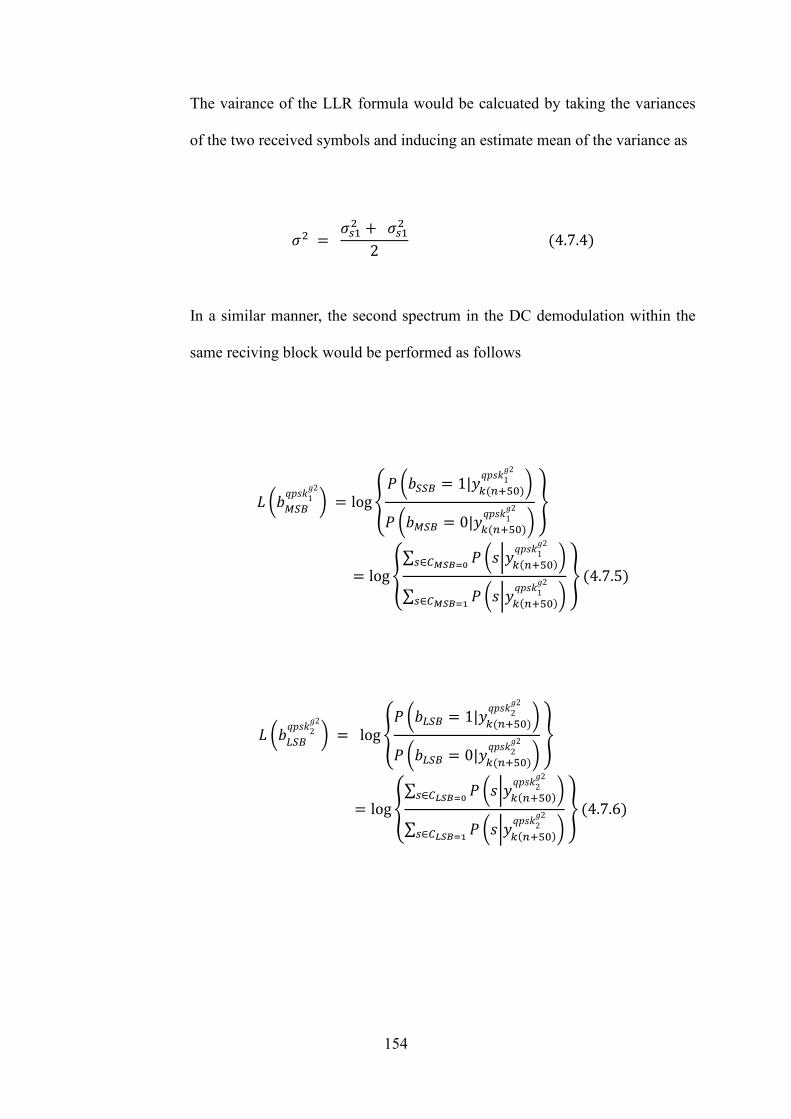
154
The vairance of the LLR formula would be calcuated by taking the variances
of the two received symbols and inducing an estimate mean of the variance as
𝜎2 = 𝜎𝑠12 + 𝜎𝑠1
2
2 (4.7.4)
In a similar manner, the second spectrum in the DC demodulation within the
same reciving block would be performed as follows
𝐿 (𝑏𝑀𝑆𝐵𝑞𝑝𝑠𝑘1
𝑔2
) = log{𝑃 (𝑏𝑆𝑆𝐵 = 1|𝑦
𝑘(𝑛+50)
𝑞𝑝𝑠𝑘1𝑔2
)
𝑃 (𝑏𝑀𝑆𝐵 = 0|𝑦𝑘(𝑛+50)
𝑞𝑝𝑠𝑘1𝑔2
)
}
= log{∑ 𝑃 (𝑠|𝑦
𝑘(𝑛+50)
𝑞𝑝𝑠𝑘1𝑔2
)𝑠∈𝐶𝑀𝑆𝐵=0
∑ 𝑃 (𝑠|𝑦𝑘(𝑛+50)
𝑞𝑝𝑠𝑘1𝑔2
)𝑠∈𝐶𝑀𝑆𝐵=1
} (4.7.5)
𝐿 (𝑏𝐿𝑆𝐵𝑞𝑝𝑠𝑘
2𝑔2
) = log {𝑃 (𝑏𝐿𝑆𝐵 = 1|𝑦
𝑘(𝑛+50)
𝑞𝑝𝑠𝑘2𝑔2
)
𝑃 (𝑏𝐿𝑆𝐵 = 0|𝑦𝑘(𝑛+50)
𝑞𝑝𝑠𝑘2𝑔2
)
}
= log{∑ 𝑃 (𝑠|𝑦
𝑘(𝑛+50)
𝑞𝑝𝑠𝑘2𝑔2
)𝑠∈𝐶𝐿𝑆𝐵=0
∑ 𝑃 (𝑠|𝑦𝑘(𝑛+50)
𝑞𝑝𝑠𝑘2𝑔2
)𝑠∈𝐶𝐿𝑆𝐵=1
} (4.7.6)

155
4.8 Conclusion
In this chapter, the implementation for the proposed simulation model had
been considered. The transmitting, and receiving structures were given, and
their implementation in a simulated environment had been explained. The
channel that emulates the real indoor fading and distortion was considered, and
implemented in the running program. A proposal to improve the demodulation
and estimation of symbols was given, and the formation of this model within
the physical layer standard had been highlighted.
156
5. Simulation
5.1 Introduction
In this chapter, the simulation of the proposed design was carried out to
envisage the hypothesis of the scheme. In order to perform the different tasks
and the required tests, a software application had to be considered which
satisfied the research hypothecs. Matlab software application had been
identified for this implementation. Matlab is software package that allows
mathematical manipulation of various algorithms and functions. The
communication toolbox within Matlab provides a laboratory environment
where wireless communication system could be design, simulated and then
evaluated in a controllable platform. The chapter covers a definition of the
functions used in the simulation, specification of the wireless model scenario,
implementation and result observations of the work. A conclusion notes on
these results was given with future remarks on suggested work.

157
5.2 Overview of the simulation
The design and simulation process of the model had predicted the response of
MIMO WPAN system to the inherent distortions, noise impairments and real-
indoor wireless environment disturbances by quantitative and analytical
measures. The proposed model design had to be evaluated in a simulation
environment to induce the requirement hypothesis. Therefore, in this work a
form of test-bed like environment were constructed to emulate the real life
operational conditions. There were a number of parameters that had to be
identified within the framework of the design. The actual measureable
parameter in real time WPAN system is the ratio between the signal power and
the noise power referred to as SNR. Thermal noise and other form of noise
would be combined in AWAGN model. In this simulation design, the power
spectral of the noise had been assigned in the algorithm in relation to the SNR.
The second parameter was the channel coefficient related to each path within
the ultra-wide band channel model. These had been generated randomly so as
to represent the indoor medium condition. Hence, a stochastic model in the

158
form of Gaussian distribution had been used in the mathematical evaluation.
The delay within the channel clusters had to be identified in the model
parameters. Non direct line of sight paths in the multipath model, had incur
time delay and hence these delay interval had been set up in the process. The
followed result figures had been undertaken in multiple simulation conditions
with various requirements.
5.3 Simulation functions
In order to facilitated and emulate this wireless model, a simulation test bed
was required to be designed and created in which the requirements and
specifications of this WPAN application was satisfied. In fulfilling these
requirements, several functions and multiple elapsing methods had been
created using similar principle to encapsulation in object oriented
programming. This was achieved by separate various design and
implementation methods and algorithms into separate functions, and all being
called in one main object body. This allows optimisation, correction and
modification while developing the model.
159
5.4 Specifications of the simulation process
Monte Carlo simulation had been considered in this evaluation method with
analyses of the various degrees of freedom corresponding to the spatial,
frequency and time domains included in the proposed design. The number of
packet frames had been set to 2000 and the bit stream had been set with large
sequential intervals so as to formulate a confidence margin in the accuracy of
the simulation results. The source signal was generated from a pseudo random
sequence generator. The frame length consists of 1500 interleaved and coded
bits corresponding to DC32-QAM with additional length variability. The
simulation setting had been carried based on two main distinct principles. The
first uses interchanged simulation analysis between time and frequency
domains on the transmitting and receiving structure. The second setting uses
primarily frequency domain analysis to infer the design and implementation
hypothesis. Specific simulation settings was summarised in the following table
in accordance with specification requirements that was defined in the
implementation chapter.
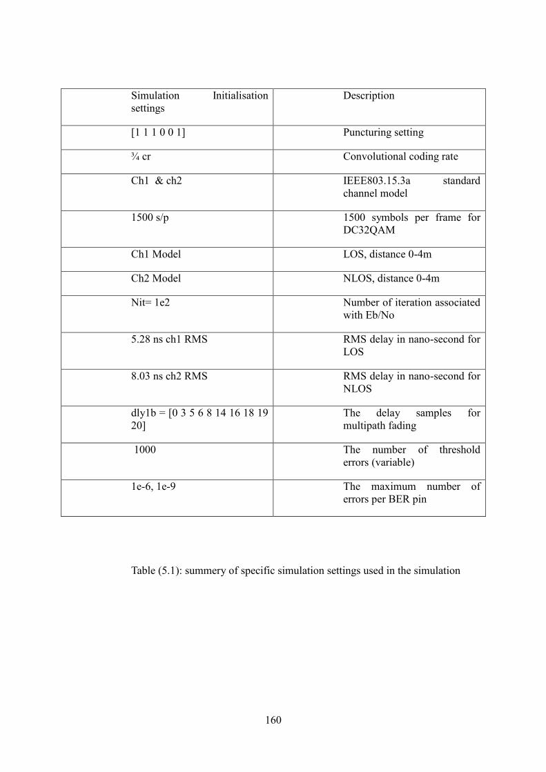
160
Simulation Initialisation
settings
Description
[1 1 1 0 0 1] Puncturing setting
¾ cr Convolutional coding rate
Ch1 & ch2 IEEE803.15.3a standard
channel model
1500 s/p 1500 symbols per frame for
DC32QAM
Ch1 Model LOS, distance 0-4m
Ch2 Model NLOS, distance 0-4m
Nit= 1e2 Number of iteration associated
with Eb/No
5.28 ns ch1 RMS RMS delay in nano-second for
LOS
8.03 ns ch2 RMS RMS delay in nano-second for
NLOS
dly1b = [0 3 5 6 8 14 16 18 19
20]
The delay samples for
multipath fading
1000 The number of threshold
errors (variable)
1e-6, 1e-9 The maximum number of
errors per BER pin
Table (5.1): summery of specific simulation settings used in the simulation
161
5.5 Time-frequency implementation
In this section, the work was focused on implementing the proposed method in
the frequency domain and then transferred to the time domain at the channel
stage and finally translated the received signal component to the frequency
domain at the receiver. Therefore, the transmitted symbol had been constructed
as an OFDM symbol contains 100 IFFT frequency tones for the message
signal and the additional 28 subcarriers were assigned for the standard
requirements (10 guard carries, 12 pilots subcarriers and 6 nulling tones). To
reduce ISI, addition padded zero had been used based on the requirement
specification. The modulated symbols were then passed to128 standard inverse
fast Fourier transform function defined in Matlab tool box with a known
algorithm. The following figures (5.5.1, 1.5. 2) show the performance of dual
antennas based on DCM and DC-32QAM, and then compared them to
standard single antenna configuration. The model was developed based on the
pervious functions along with a number of standard Matlab functions. The
results for the system BER had been presented in the following graphs. The
results show comparisons between dual antennas configuration and single
transmitter systems. During simulation two channel models were applied,
namely, the LOS CM1 model and NLOS CM2 model both of which are
available from the IEEE 802.15.3a channel model standard. This standardised

162
model was applied because it captures the physical link behaviour in the UWB
domain. Figure 5.5.1 shows that the MIMO model provides 8dB of
improvement at 10−2 BER in comparison to the SISO DC 32-QAM.
Furthermore, the BER curve for the SISO model diverges when reducing the
BER threshold and moving at the upper region of the SNR which further
highlights the increased signal strength that the MIMO configuration provides.
The error rate performance tends to vary marginally at very low SNR in figure
5.5.2 with slight improvement when crossing the 14 dB level in the SNR for
the DCM, although the increase remains very small.
Figure (5.5.1): BER Simulation of MIMO DC32QAM vs SISO DC32QAM
0 5 10 15 20 25 3010
-4
10-3
10-2
10-1
100
EbN0[dB]
BE
R
SISO DC32QAM simulation
MIMO DC32QAM model simulation
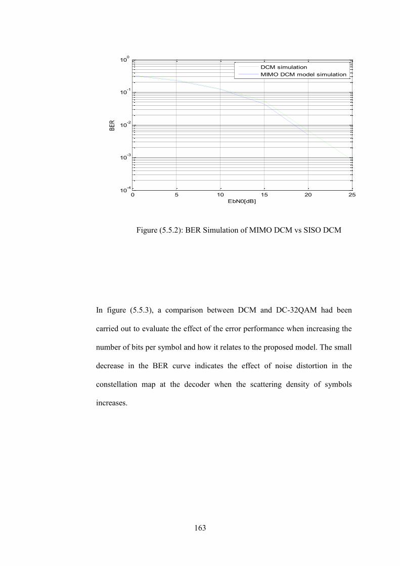
163
Figure (5.5.2): BER Simulation of MIMO DCM vs SISO DCM
In figure (5.5.3), a comparison between DCM and DC-32QAM had been
carried out to evaluate the effect of the error performance when increasing the
number of bits per symbol and how it relates to the proposed model. The small
decrease in the BER curve indicates the effect of noise distortion in the
constellation map at the decoder when the scattering density of symbols
increases.
0 5 10 15 20 2510
-4
10-3
10-2
10-1
100
EbN0[dB]
BE
R
DCM simulation
MIMO DCM model simulation
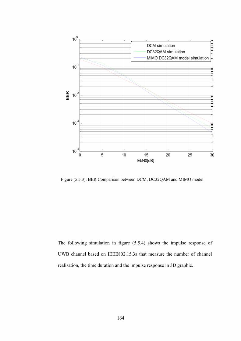
164
Figure (5.5.3): BER Comparison between DCM, DC32QAM and MIMO model
The following simulation in figure (5.5.4) shows the impulse response of
UWB channel based on IEEE802.15.3a that measure the number of channel
realisation, the time duration and the impulse response in 3D graphic.
0 5 10 15 20 25 3010
-4
10-3
10-2
10-1
100
EbN0[dB]
BE
R
DCM simulation
DC32QAM simulation
MIMO DC32QAM model simulation
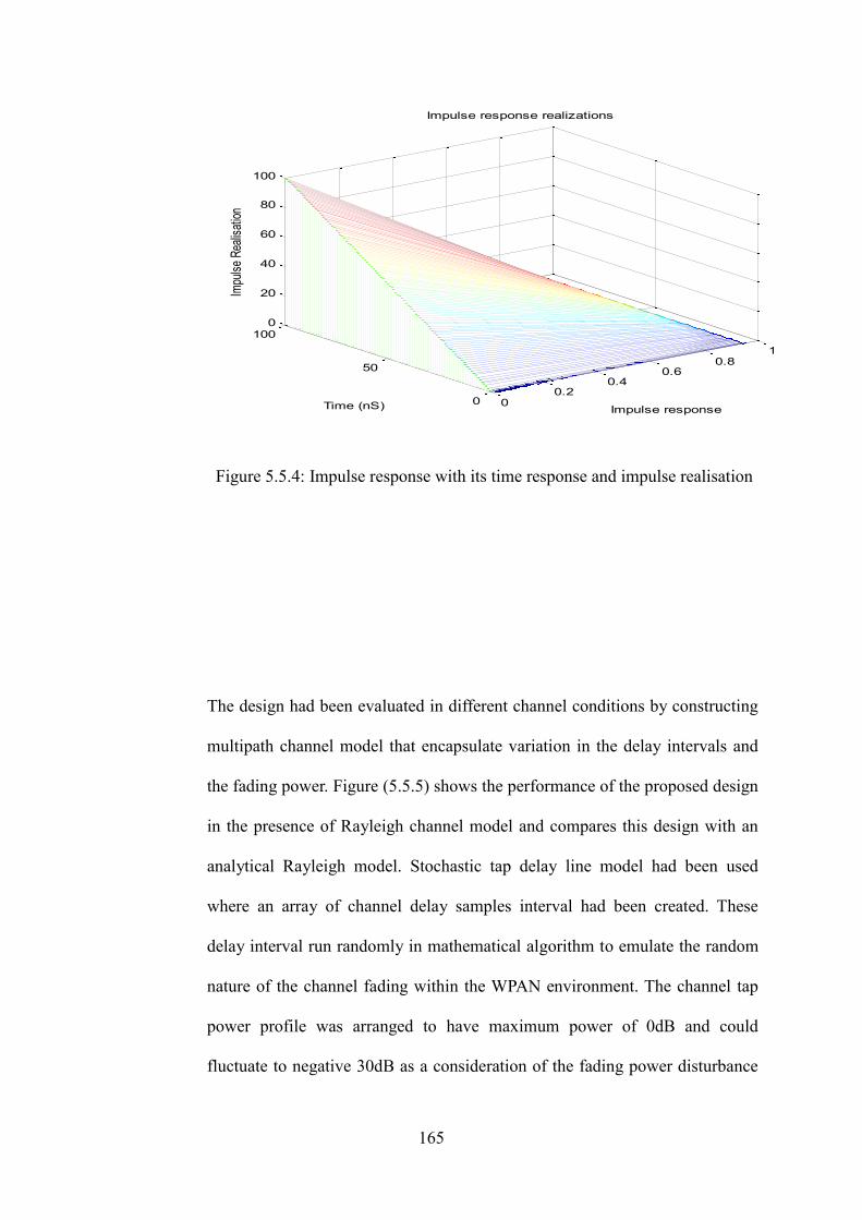
165
Figure 5.5.4: Impulse response with its time response and impulse realisation
The design had been evaluated in different channel conditions by constructing
multipath channel model that encapsulate variation in the delay intervals and
the fading power. Figure (5.5.5) shows the performance of the proposed design
in the presence of Rayleigh channel model and compares this design with an
analytical Rayleigh model. Stochastic tap delay line model had been used
where an array of channel delay samples interval had been created. These
delay interval run randomly in mathematical algorithm to emulate the random
nature of the channel fading within the WPAN environment. The channel tap
power profile was arranged to have maximum power of 0dB and could
fluctuate to negative 30dB as a consideration of the fading power disturbance
00.2
0.40.6
0.81
0
50
1000
20
40
60
80
100
Impulse response
Impulse response realizations
Time (nS)
Impu
lse
Rea
lisat
ion

166
that governs this hostile environment. The error performance had been
compared in figure (5.5.6) where analytical and simulation models as well as
DC 32-QAM had all been tested, and the results show close approximation
between the analytical and simulation models.
Figure (5.5.5): Comparison between analytical Rayleigh and Simulation models
0 5 10 15 20 25 3010
-6
10-5
10-4
10-3
10-2
10-1
100
Eb/N0[dB]
BER
Analytic Rayleigh fading
Simulation

167
Figure (5.5.6): BER results of DC32QAM, Analytical and MIMO models
0 5 10 15 20 25 3010
-3
10-2
10-1
100
EbN0[dB]
BE
R
Analytical
DC32QAM simulation
MIMO DC32QAM model simulation
168
5.6 Simulation using coded modulation with hard
decoding evaluation
In the evaluation process, it was important to cover different decoding
algorithms and measure the response of the model in different implementation
settings, and how its error performance compared. In particulare, if the model
was used in a wireless application where the demodualtion at the receivers was
based on hard alogrithm implemenation, how this model works in this setting.
In this test, a test bench was developed to measure the model behaviour when
decoding based on hard algorithm de-mapping. In the same setting, multipath
fading based on complex and randomly distributed channel amplitude fading
coefficients were generated to emulate the channel distortion. After which, the
transmitted signals were convolved with the channel coefficients in the time
domain, and then converted in the frequency domain where the receiving
process had been performed. Figure (5.5.7) shows the results of the simulation
of DC32-QAM-B-8PSK, MIMO-DC32QAM, and the new proposed concept
of MIMO-DC-32QAM. As the SNR increases, the number of bits in errors
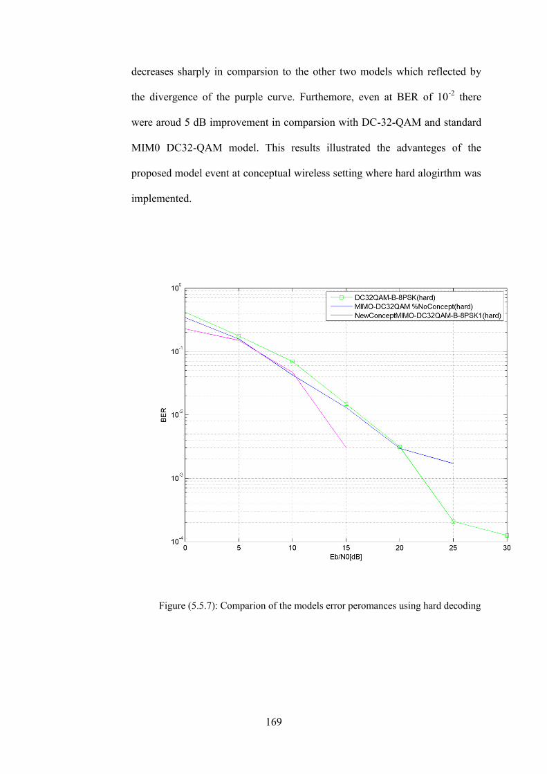
169
decreases sharply in comparsion to the other two models which reflected by
the divergence of the purple curve. Furthemore, even at BER of 10-2
there
were aroud 5 dB improvement in comparsion with DC-32-QAM and standard
MIM0 DC32-QAM model. This results illustrated the advanteges of the
proposed model event at conceptual wireless setting where hard alogirthm was
implemented.
Figure (5.5.7): Comparion of the models error peromances using hard decoding
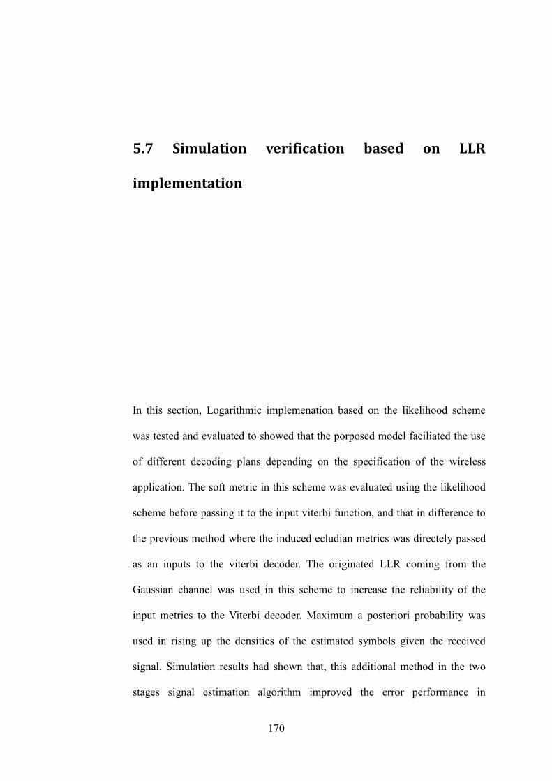
170
5.7 Simulation verification based on LLR
implementation
In this section, Logarithmic implemenation based on the likelihood scheme
was tested and evaluated to showed that the porposed model faciliated the use
of different decoding plans depending on the specification of the wireless
application. The soft metric in this scheme was evaluated using the likelihood
scheme before passing it to the input viterbi function, and that in difference to
the previous method where the induced ecludian metrics was directely passed
as an inputs to the viterbi decoder. The originated LLR coming from the
Gaussian channel was used in this scheme to increase the reliability of the
input metrics to the Viterbi decoder. Maximum a posteriori probability was
used in rising up the densities of the estimated symbols given the received
signal. Simulation results had shown that, this additional method in the two
stages signal estimation algorithm improved the error performance in

171
comparison to standard decoding scheme. In addition, since the design and
implementation of the proposed model had resulted in a reduced signal
constellation (map with four symbol points), the attached LLR complexity was
significantly reduced. The likelihood metric in this simulation had two
quantities that were forwarded to the vitedec decoder function. The first was
the sign of the LLR indicating the binary decision, and the other represented
the magnitude of the metric which reflected the confidence in the likelihood
for the soft decoding algorithm. The variance used in the LLR expression was
calculated from the variances coming from the two branches across the two
receiving antennas. Since every input to the de-mapper (the new modified
received symbol) had originally coming from two branches across the two
radiating elements. The additional advantages of this likelihood scheme had
been measured in the resulted error performance comparison shown by the
BER curve in figure (5.5.8), where a measurable improvements had be shown
as steps of SNR levels. The figure also highlighted the way the proposed
scheme formulate the regions which the received symbols had been estimated,
and this planning reduces the number of erroneous bits which reflected in
steepens of the error curve. As the proposed de-mapping scheme had
considered an approximation to the Likelihood formula in the consideration of
noise, it was important to measure the significant of this approximation on the
error performance. Monte Carlo simulation had shown that this modified
Likelihood formula gives a good error performance and the approximation had
relatively small degradation in the error curve.
172
Figure (5.5.8): BER comparison of the model using LLR de-mapping method
173
5.8 Evaluation based on Comparison between ML &
LLR methods
There are a number of soft decoding algorithms, and different wireless systems
and applications had been declared based on these algorithms. What was
important for any novel concept was to satisfy these systems by providing
good error performance in all the available settings. Therefore, it was
imperative to carry out an evaluation test based on well-known soft de-
mapping methods that used in WLAN applications. In this simulation setting, a
comparative in the model performance when applying ML soft metric and
LLR de-mapping methods was conducted and evaluated. Simulation results
had shown that the model performance equally when applying these soft
decoding algorithm, and this clearly illustrate the advantages of implementing
the proposed model on Indoor wireless systems. In figure (5.5.9), the single
DC32-QAM-B-8PSK (green curve), stnadard MIMO-DC32QAM(blue
curve), the proposed model with the ML soft demapping and its implemnation
based on LLR demapping were shown. In the graph, the new proposed concept
of MIMO-DC-32QAM LLR (cyan curve) using LLR method and the proposed

174
concept of MIMO-DC-32QAM Soft (blue-circle curve) with ML soft
demapping showed a compariable resluts indicating the strength of the noval
model. Additonal test had been carried out envisage the error performance at
lower SNR between modulation models, and once again figure (5.5.10)
showed that the prposed model gives good BER performance in comparsion
with single dual carrier configuration model.
Figure (5.5.9): Comparison of BER performance between ML soft and LLR
demapping methods
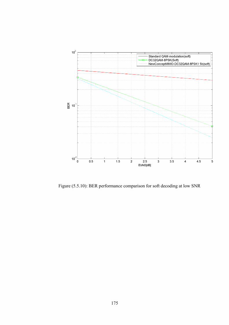
175
Figure (5.5.10): BER performance comparison for soft decoding at low SNR
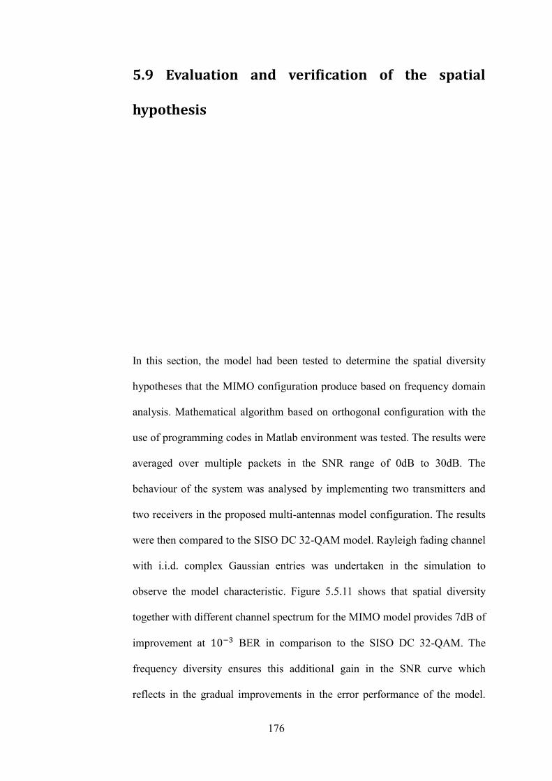
176
5.9 Evaluation and verification of the spatial
hypothesis
In this section, the model had been tested to determine the spatial diversity
hypotheses that the MIMO configuration produce based on frequency domain
analysis. Mathematical algorithm based on orthogonal configuration with the
use of programming codes in Matlab environment was tested. The results were
averaged over multiple packets in the SNR range of 0dB to 30dB. The
behaviour of the system was analysed by implementing two transmitters and
two receivers in the proposed multi-antennas model configuration. The results
were then compared to the SISO DC 32-QAM model. Rayleigh fading channel
with i.i.d. complex Gaussian entries was undertaken in the simulation to
observe the model characteristic. Figure 5.5.11 shows that spatial diversity
together with different channel spectrum for the MIMO model provides 7dB of
improvement at 10−3 BER in comparison to the SISO DC 32-QAM. The
frequency diversity ensures this additional gain in the SNR curve which
reflects in the gradual improvements in the error performance of the model.
177
Furthermore, the BER curve for the SISO model diverges when reducing the
BER threshold and moving at the upper region of the SNR which further
highlights the increased signal strength that the MIMO configuration provides.
Figure (5.5.11): SISO DC32QAM vs MIMO DC32QAM BER evaluation
0 5 10 15 20 25 3010
-6
10-5
10-4
10-3
10-2
10-1
100
Eb/No[dB]
BE
R
SISO DC32QAM simulation
MIMO DC32QAM model simulation

178
5.10 Evaluation based on CSI distortions
Figure (5.5.12) shows the case where the Channel State Information at the
received is being corrupted and how the system perform in this circumstances.
The CSI disturbance could be due to the nature of the dynamic environment in
the indoor case scenario which normally very hostile, or could be due to the
type of receiver being implemented. Furthermore, the mathematical algorithm
being considered at the decoder would deviates the weight channel coefficients
resulting in error estimation at the decoding process. At 10−3BER, an
improvement of 9dB could be observed when the decoder has enough
knowledge of the pilot symbols for the model compared with noisy model.
Regardless of the real implementing environment, the model had to show
successful operation at all these scenario, hence the following graph indicate
the performance of the design.

179
Figure (5.5.12): Models comparison with impairments in the CSI
0 5 10 15 20 25 3010
-6
10-5
10-4
10-3
10-2
10-1
100
Eb/No[dB]
BE
R
DC32QAM with partial CI
MIMO DC32QAM with partial CI
DC32QAM SISO
MIMO DC32QAM model
180
5.11 Performance variation based on spatial
configuration
The next figure (5.5.13), a test had been carried out to investigate the effect of
the symbol conjugation on the model performance. In this simulation, two
configurations had been taken, one with alternate conjugation in the complex
plane. In the second configuration, the symbol pair transmitted from both
antennas was omitted from the negative conjugation in the spatial domain. It
could be noticed very clearly that the red curve representing the second
configuration deviate deeply as the SNR increases and performance deteriorate
rapidly. Moreover, the error rate figures increases and overshoot the standard
DCM model with single radiating element.
.
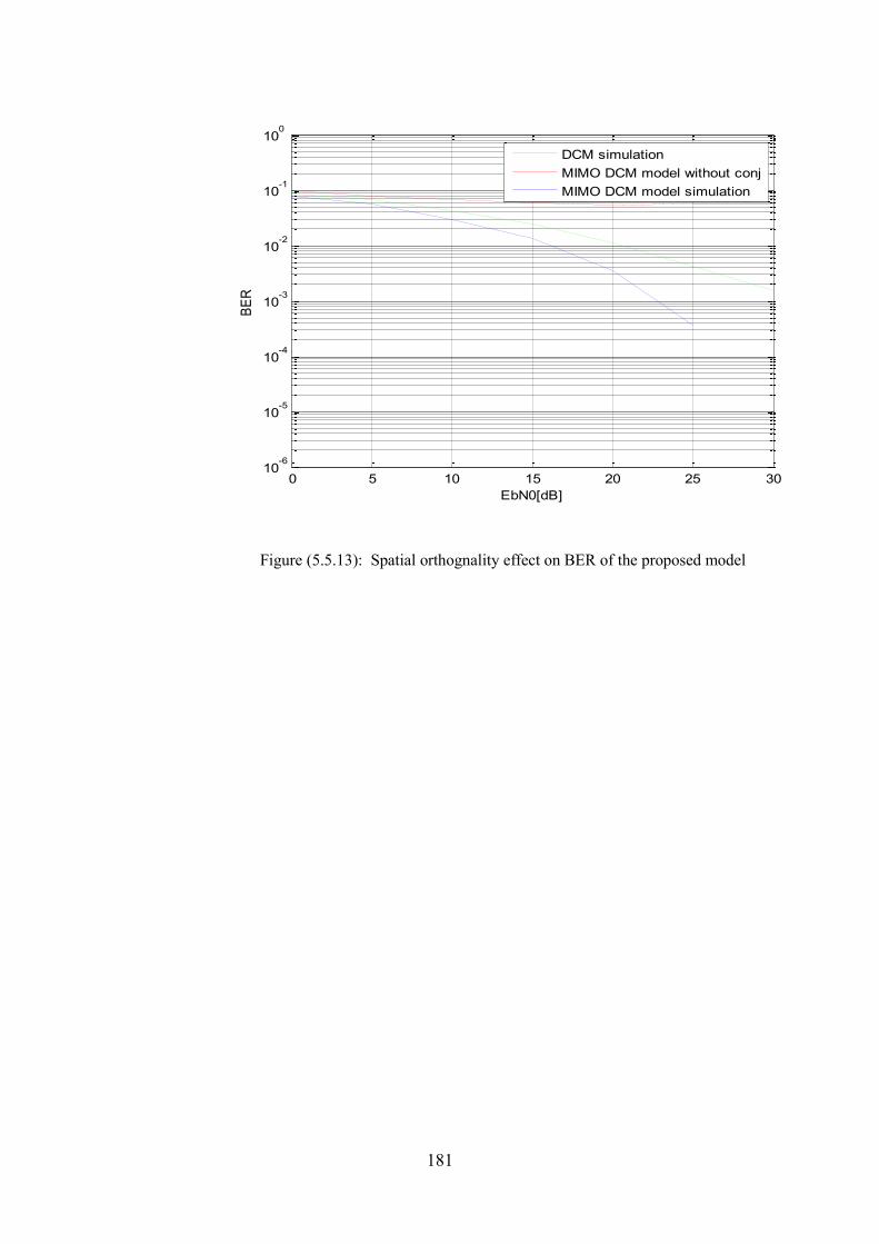
181
Figure (5.5.13): Spatial orthognality effect on BER of the proposed model
0 5 10 15 20 25 3010
-6
10-5
10-4
10-3
10-2
10-1
100
EbN0[dB]
BE
R
DCM simulation
MIMO DCM model without conj
MIMO DCM model simulation

182
5.12 Comparative analyse based on increase in the
order of modulation
In the following figure (5.5.14), another test had been carried out in order to
investigate if increasing the number of bits in the modulation symbol and
rearranging the constellation map would affect the model performance, and if
so by how much and is there any explanation for that. The result had indicated
clearly that the way the symbols had been scattered in the constellation
diagram on the dual mapping would change the error rate performance in the
models. The curves had shown that the SNR values increase slightly if the
Euclidean distance between the same symbols across the two maps were
further apart.

183
Figure (5.5.14): BER model performance based on rearranged constellation maps
0 5 10 15 20 25 3010
-6
10-5
10-4
10-3
10-2
10-1
100
Eb/No[dB]
BE
R
DC32QAM
16QAM-DCM
MIMO DC32QAM model
MIMO DCM model

184
5.13 Comparative analyse based on Analytical
upper bound error probability
It is important to measure analytical the error performance between dual
antenna system and classical single antenna structure. In this work, the upper
bound error probability was evaluated in an analytical manner. The derived
formula used in the design chapter was used in this simulation to evaluate
mathematically the system performance in comparison with single antenna
model. This evaluation was only based on numerical derivation, and statistical
concepts were used to derive an upper bound on the error probability. Figure
(5.5.15) shows the upper bound probability based on equation (3.4.49) in the
design chapter.
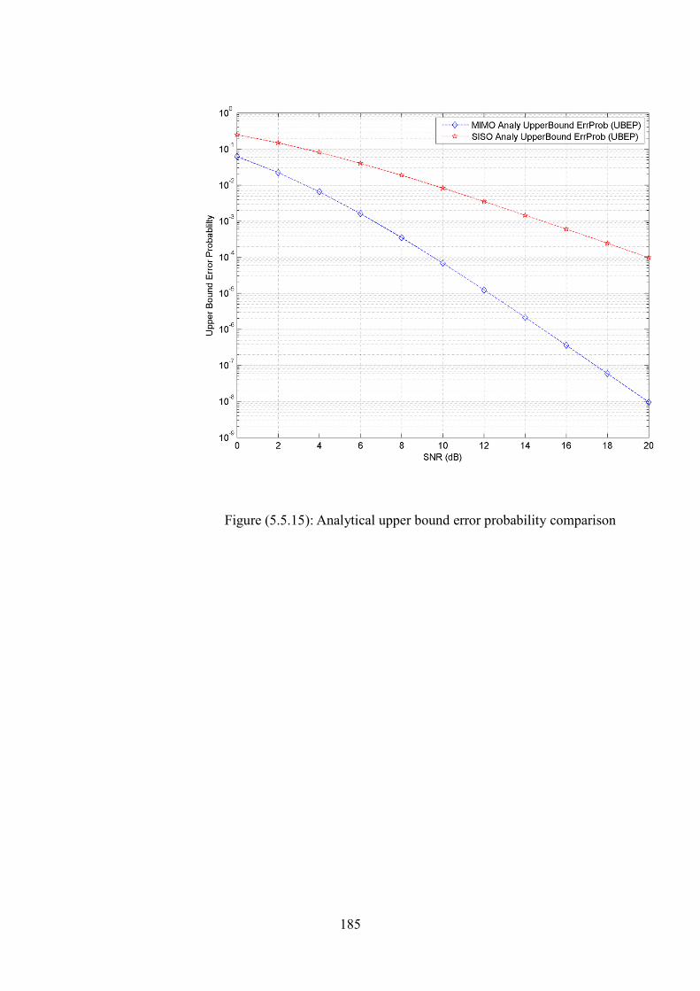
185
Figure (5.5.15): Analytical upper bound error probability comparison

186
5.14 Analysis of wireless range Evaluation
In this part, the modification of the model was evaluated to configure how the
full frequency and spatial diversities was used to increase the coverage area.
As the proposed aim here was to increase the receiving signal energy, and over
shadowing the throughput. Therefore, the model had replaced the multiplexing
technique with the use of diversity to strengthen the SNR at the receivers. The
first figure (5.5.16) shows an error performance comparison between the
modified model, the original designed model, and the previously proposed
model (legacy model). The figure clearly shows the performance improvement
the modified model achieved in comparison to the other concepts. Figure
(5.5.17) on the other hand, shows the relation between the coverage area and
packet error rate, and indicates the increase in the wireless range with the
modification to the model that had shown in the design chapter. The calculated
and simulated file data (figure 5.5.18) for the SNRs and BER values between
the models were shown below.

187
Figure (5.5.16): BER comparison between the proposed models
Figure (5.5.17): Performance comparison of the models over coverage area

188
EbN0 = 0[dB], BER_for_DC32QAM-Based8PSK = 4.649e-001,
NOE_for_DC32QAM-Based8PSK = 550
------------------------------------------------------------
-----------
EbN0 = 0[dB], BER_for_NewConpMIMO_DC32QAM-Based8PSK =
4.691e-001, NOE_for_NewConpMIMO_DC32QAM-Based8PSK = 575
------------------------------------------------------------
-----------
EbN0 = 5[dB], BER_for_DC32QAM-Based8PSK = 4.603e-001,
NOE_for_DC32QAM-Based8PSK = 543
------------------------------------------------------------
-----------
EbN0 = 5[dB], BER_for_NewConpMIMO_DC32QAM-Based8PSK =
4.593e-001, NOE_for_NewConpMIMO_DC32QAM-Based8PSK = 522
------------------------------------------------------------
-----------
EbN0 = 10[dB], BER_for_DC32QAM-Based8PSK = 3.837e-001,
NOE_for_DC32QAM-Based8PSK = 367
------------------------------------------------------------
-----------
EbN0 = 10[dB], BER_for_NewConpMIMO_DC32QAM-Based8PSK =
4.008e-001, NOE_for_NewConpMIMO_DC32QAM-Based8PSK = 536
------------------------------------------------------------
-----------
EbN0 = 15[dB], BER_for_DC32QAM-Based8PSK = 9.850e-002,
NOE_for_DC32QAM-Based8PSK = 56
------------------------------------------------------------
-----------
EbN0 = 15[dB], BER_for_NewConpMIMO_DC32QAM-Based8PSK =
1.283e-001, NOE_for_NewConpMIMO_DC32QAM-Based8PSK = 53
------------------------------------------------------------
-----------
EbN0 = 20[dB], BER_for_DC32QAM-Based8PSK = 1.167e-002,
NOE_for_DC32QAM-Based8PSK = 4
------------------------------------------------------------
-----------
EbN0 = 20[dB], BER_for_NewConpMIMO_DC32QAM-Based8PSK =
1.125e-002, NOE_for_NewConpMIMO_DC32QAM-Based8PSK = 2
------------------------------------------------------------
-----------
EbN0 = 25[dB], BER_for_DC32QAM-Based8PSK = 1.333e-003,
NOE_for_DC32QAM-Based8PSK = 0
------------------------------------------------------------
-----------
EbN0 = 25[dB], BER_for_NewConpMIMO_DC32QAM-Based8PSK =
1.167e-003, NOE_for_NewConpMIMO_DC32QAM-Based8PSK = 0
------------------------------------------------------------
-----------
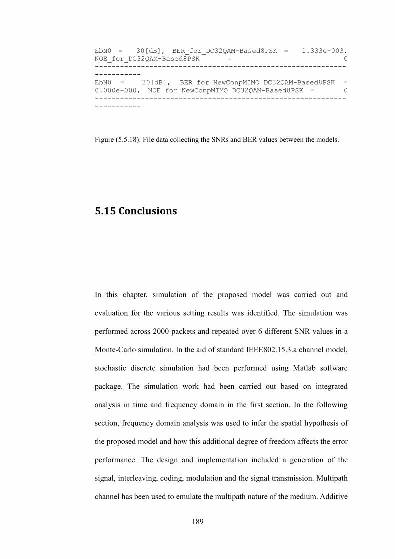
189
EbN0 = 30[dB], BER_for_DC32QAM-Based8PSK = 1.333e-003,
NOE_for_DC32QAM-Based8PSK = 0
------------------------------------------------------------
-----------
EbN0 = 30[dB], BER_for_NewConpMIMO_DC32QAM-Based8PSK =
0.000e+000, NOE_for_NewConpMIMO_DC32QAM-Based8PSK = 0
------------------------------------------------------------
-----------
Figure (5.5.18): File data collecting the SNRs and BER values between the models.
5.15 Conclusions
In this chapter, simulation of the proposed model was carried out and
evaluation for the various setting results was identified. The simulation was
performed across 2000 packets and repeated over 6 different SNR values in a
Monte-Carlo simulation. In the aid of standard IEEE802.15.3.a channel model,
stochastic discrete simulation had been performed using Matlab software
package. The simulation work had been carried out based on integrated
analysis in time and frequency domain in the first section. In the following
section, frequency domain analysis was used to infer the spatial hypothesis of
the proposed model and how this additional degree of freedom affects the error
performance. The design and implementation included a generation of the
signal, interleaving, coding, modulation and the signal transmission. Multipath
channel has been used to emulate the multipath nature of the medium. Additive

190
White Gaussian Noise (AWGN) has been added to account for the additional
distortion that includes equipment’s (receiver and transmitter) and signal
amplifications. The receiving block has been accomplished, and the design
performance has been analysed by testing the system with predefined SNR
values. The output has shown the results of the BER for the model and
compared to theoretical values. In this work, MIMO techniques have been
investigated in order to envisage a novel conceptual design that could be
implemented in systems operating in free spectrum. The hostile indoor channel
environments make these types of systems very challenging and very costly to
build. Investigations of the core problems affecting the integration of multiple
spatial elements has been undertaken in this work. Simulation results show the
strength of the proposed model, and its operation in different Wireless and
application settings with good error performance in comparison to pervious
works. The proposed model design could be used as a basis for future work to
address the current challenges in this field and provides a framework for future
systems development

191
6. Conclusion
The aim of this chapter is to provide a summary of the presented results that
had shown in the previous chapter, and gives a description of the proposed
design along with the research objectives. A conclusion to the work, and
recommendation for further research was then provided.
6.1 The research achievement
The design and implementation of the proposed multiple antennas concept
applicable for WPAN applications had achieved the objectives set out in the
first chapter. The model provided an increase in the transmission rate by twice
the amount without the need to increase the radiating power or a decrease in
the error rate performance. A successful transmission was observed with low
192
bit error rate, which could be used at the physical layer in low power
requirement indoor wireless communication systems. In addition the model
had facilitated the option of increasing the coverage area for special wireless
sensor network application by making some modification to the wireless link
structure.
All key objectives were achieved. A design model was developed that allows
the integration of multi-antennas technique with orthogonal frequency division
modulation in UWB-WPAN systems. The proposed project was designed to
ensure that the goals and objectives completed by implementing low cost
algorithms and digital components across at the transmitting and receiving
blocks. In this aspect, the implementation had achieved its set up requirements.
A conceptual algorithm was developed that allows the implementation of dual
radiating elements including the modulation, coding, de-mapping, and
detection at receivers that optimise the system performance in comparison
with previously proposed models. The induced concept was conformed to the
ECMA-368 wireless communication standard as stated in the objectives of
research. In this context, the model design was based on this standard that
specifies the physical and medium access control layers. The model had shown
that changing the modulation scheme and the mapping method along with an
optimisation to the receiving structures would result in an increase in
throughput in an optimal performance. The concept used frequency diversity
in the spectrum and spatial dimensions to increase the robustness of the
system. The frequency diversity achieved by separating the transmitted
193
symbols by a large bandwidth spectrum (50 subcarriers with 206.25 MHz),
taking advantage of the inherently rich multipath fading spectrum that span
the UWB systems.
The Dual carrier 32QAM symbols were allocated into two individual OFDM
data subcarriers with wide frequency separation ensured that deep channel
fades in part of the spectrum would not affect the other used frequency band.
This mapping method ensured an effective process in recovering the original
signal information bits. This modulation scheme provided an increase in the
transmission rate by doubling the throughputs, and this leaps enabled free
license spectrum wireless link to have beyond Gigabit capability. The concept
structure fits within the standard configuration without modification or
changing to the transmitting and receiving modules requirements.
The coding scheme was designed to fit into the Physical Layer Service Data
Unit encoding process. Phase shift keying was used in the high dimension
mapping due to its unified symbol energy which reduces the noise
disturbances between symbols in the signal to noise ratio. The signal points
were allocated in circular loci across the constellation providing power
constant for this modulation. Further, this scheme provides equal decision
region for complex symbols across the map, which ensure equal energy
distribution between the signal points. Allocating different signal power across
the scatter diagram for modulation schemes results in variation in the
probability of symbol error rates at the detection process, and that reduces the
194
overall error performance in the modulation schemes. This observation made
the 8PSK modulation scheme an ideal candidate for the high dimension
mapping, and that was observed in the performance of the model. On the other
hand, higher order Quadrature amplitude modulations do not have fixed
amplitude. Therefore these modulation plans tend to worsen the peak to
average power ratio of the OFDM signals, and that reflected in the digital to
analogue converters and the gain control mechanism.
Verification for the design was carried out with a number of tests including the
IEEE802.15.3a UWB channel model standard to induce the objectives and the
hypothesis requirements. The reviewing and inspection had shown that the
model enables to overcome the poor radio channel condition and delivered
error performance in an optimal manner in comparison to the lower rate signal
that associated with single radiating element system. The model could increase
the wireless coverage area by a modification to the receiving structure. The
concept had achieved increased in the data rate, and system improvement
while effectively maintaining low cost implementation in terms of the low
power and high performance scheme. Due to the stringent power requirements
set for wireless application operating at the free license spectrum (FCC
regulation), this model represented a good fit that allow high rate transmission
without the need to violate the standard requirements in terms of RF
regulation. The design achieved good performance without an additional
overhead to the ECMA standard. The contribution of this research enables
multiple antennas configuration within the UWB technology within the

195
physical layer enabling increase in the through put, and facilitating its usability
in modern indoor wireless applications.
6.2 Observation about the research process
The research and development of this project was accomplished by a number
of interconnected modules. The model design of a physical layer MIMO-UWB
wireless communication system operating in the free spectrum was achieved
by concatenation of the transmitters, receivers and the physical channel
models. The project was divided into layers and each one had its own
196
requirements and operational functions. The design tasks were spread across
these layers with various degrees of complexity. The structure involved the
transmitting module, the physical channel model and the receiver part, and this
arrangement was embedded in the design. Encompassing this design structure,
it is ability of backward compatibility for legacy systems with lower
transmission rate. . The scheme used the inherent spatial and frequency
diversities to boost the system performance by increasing the capacity, and
facilitates higher throughput that dynamically varies to accommodate both the
physical conditions and the type of wireless transmissions (data, videos, etc.).
The first layer of the design framework included transmitting module
consisting of two spatial elements with initial design requirements. The second
part of this phase constituted a multipath fading channel model designed to test
and evaluates the system performance in terms of the spatial and frequency
diversity presence. This in turn introduced more channels for the transmitted
signal, and so improving the link budget. The receiving module represented
the last sub-system within this layer, and included the decoding and estimation
algorithms, as well as objects link requirements. The aim design for this layer
was to evaluate the proposed concept and how to develop theoretical
algorithms into working wireless systems. Therefore, a predefined metrics
conditions was evaluated at the output of the receivers. In the case of not
satisfying the test requirements, the design was then readjusted and modified
until certain conditions are satisfied. This method enabled the development in
stages with ascending order in term of complexity forming a bottom up

197
hierarchy.
Once this phase was completed, the next layer had included an advanced
MIMO transmitting and receiving sub-systems. An additional Standardised
IEEE802.15.3a channel model was included. The transmitting block included
the objects within the pervious developed transmitting block, as well as
stringent modulation and spatial requirements. The receiving block in this
phase had included an optimised decoding and equalisation algorithms that
met the desired requirements. The validation of the research hypotheses was
met at this stage, and hence an iterative approach was applied. The results
error performance was then compared with previous work and identified pre-
set levels in the signal power. System optimisation was the third phase and
covered the improvements to the model design and performance. The packet
error rate (PER) for the communication link of both LOS and NLOS was
further reduced in this sub-system. The complexities in the receiver were
studied to make further improvement, and the overall design complexity was
optimised.
Testing of the application included verification of particular conditions, by the
simulation of hypothesised scenarios in order to test the fitness of the model.
Additional requirements had been embedded into the model and then
examined for approval purposes. Further development to the design was
carried out in this stage so as to ensure practical feasibility of the system in
real time environments.
The evaluation phase involved multiple tests of various indoor scenarios in
198
order to fulfil all the design requirements. Experimental analysis was applied
to the final version of the developed design in order to validate the simulated
design model against standardised and recognised approved models.
Predefined parameters was used to test various fitness tests and systems
requirements such as the time delay, bit error rate (BER), the signal to noise
ratio (SNR) and the power profile. The necessity for this step was to match the
system requirements with the achieved results and approves theoretical
concepts. These results approved the design concept in increasing the link
capacity, by the use of spatial element and contribute to the knowledge in this
field.
The signal to noise power ratio in decibels was implemented in the simulation
as know quantities. A defined vector was used to store the power ratio values
in descending order. The noise power was changed based on alteration to the
noise variance through the standard deviation in conjugation with the
predefined SNR. The power spectral density of the AWGN was then limited by
the limitation of the signal power at every time interval in the simulation.
Expressing the standard deviation in terms of the SNR per transmitted signal
had resulted in controlling the noise distortion on the received signals in the
simulation environments.
199
6.3 Review of the complete proposed model
Previous work had shown that capacity could be improved by the use of
multiple antenna system, and based on these researches the induced work had
focused on increasing the performance with the use of dual radiating elements
for WPAN. The work used multiplexing technique based on orthogonal
division in the spectrum with OFDM modulation. OFDM technique gives
immunity to inter-symbol interference, can be implemented at lower
complexity FFT as it divides the spectrum, and could easily shape the
spectrum. This scheme gave considerable improvement in the throughput and
substantial increase in the SNR at the receiving end without increasing the
transmission power. In this context, the work had used this proven theory to
develop the concept which applicable for use in the UWB wireless indoor
communication. MIMO technique strength comes in two folds, for capacity
requirements systems it increases the data rate. For coverage area applications
as wireless sensor network, it increases the signal power term of the snr at
receivers without increasing the transmission power. This enabled increase in
the coverage area for wireless systems. It is important to note that, backward
compatibility is essential in developing new wireless models.
Multiple radiating elements with a pair of Dual Circular 32-QAM transmitting
four complex symbols with a total of ten bits have the ability to deliver 1.2

200
Gb/s. The dual 8PSK symbols comes from lower dimension QPSK symbols.
The most significant bit of every symbol represented the fifth bit within the
original group (5 bits), and its bipolarity was used to deliver the two QPSK
symbols into the upper constellation maps (8ary-PSKs). Diversity was
observed in the fifth bit across both complex symbols. The scheme took a dual
of 500 coded and interleaved bits across two radiating elements, and
conforming to backward compatibility by spreading the mapping with 250
coded bits across every branch. The design used the defined convolutional
encoder specified for the higher data rate within the standard, along with fast
Fourier transform with only 128 frequency tones that is applicable for low cost
analogue to digital convertors. The finalised concept provided high bit-rate
wireless communication between devices which could be suitable for
streaming high definition video between consumer products, without
consuming high frequency clock rates.
The structure of the receivers was designed in order to translate the dimension
of the received symbols according to a novel transformation process. The
received symbols coming to the receivers had different channel state
information reflected in the equalisation process within every group bits (a
symbol has 5 bits). The proposed concept transfers the 8PSK symbols to
QPSK symbols which gives a number of advantages. Firstly, this translation
reduces the decoding searching subspace, and widens the de-mapping
constellation. Dense constellation with high number of points tends to have
large symbol error rate in comparison to the less dense constellation

201
modulation systems. The difference in dimension creates differences in the
Euclidean powers required for the noise powers, in order to shift the received
symbol to one of its neighbouring symbol’s region. Error in the decoding
occurs if the received symbol was shifted into another symbol’s region. The
larger the Euclidian distance between neighbouring symbols, the larger the
noise power requirement needed to force symbol error detection the
transmission. The larger the constellation dimensions with more complex
symbols, the lower the Euclidian metric between constellation points.
Therefore, the idea of this proposed model concept was to transfer the received
symbol to a lower constellation dimension, and then performs the decoding
process. This way, the Euclidean metric between symbols was increased before
the de-mapping, and hence reducing the overall symbol and bit error of the
system. The novelty here was increasing the error performance without
increasing the receiver complexity which adds to software, hardware and
overhead costs. Further, the induced method reduces the internal of the digital
logic in the IFFT and FFT, and the precision of the ADC and DAC. The QPSK
gives a large sub-carrier spacing in comparison to the more dense 8 points
constellation, and this reflected on the noise requirement in the carrier
synthesis, and improves the system robustness to synchronisation errors.

202
6.4 Future research recommendation
In consideration to the proposed concept, there are areas that could be taken in
further research. This physical layer model was intended for a single standard,
and additional work could be carried out in order to allow the multiple
antennas model to be applicable with other international standards. The cross
standards compatibility could make it more commercially viable, and improve
the market potential for this physical layer configuration.
The framework for developing models for UWB-WPAN in the PHY centred
around a low complexity and implementation cost. On the other hand, there
are powerful coding schemes that give good code performance that is close to
the Shannon theory limit, but have complexity and cost attached to them.
Implementing an advance receiving algorithm would have cost attached to
that, and therefore further research in obtaining cost effective receiving
203
structure is very critical in the progression of this technology. The coding
algorithm could be optimised by researching a new novel concept in
integrating more advanced Forward error correction methods. In this context, a
further research in obtaining an optimised algorithm that reduces the
complexity requirements of these strong coding methods to fit in the Wireless
personal area network systems. One such scheme is the turbo code, where it
represented an advanced algorithm that produces strong forward error
correction code. This method improves the coding gain which is critical in
optimising the error performance. The corresponding decoding process for
this method requires more accurate equalisers. Therefore, additional work
needed to reduce the computational complexity involves in constructing an
optimised equalisers for multiple antennas systems that fits within wireless
portable devices. Channel state information aided de-mapping scheme could
be improved to further optimise the channel knowledge to strengthen the
received signal. One way is to induce stronger algorithm at the receivers for
systems with receivers only CSI configuration (No feedback CSI at
transmitters). In conjunction with this, further research could be carried out to
enable the use of differential modulation method that works between
consecutive codes in order to overcome the channel estate information errors
that results in decoding errors at receivers, and error performance degradation.
One more option could be introducing feedback with the formation of
transmitter side CSI, which distribute the transmitting signal power according
to the channel condition
204
The hardware is another area that requires further research. Hardware
implementation solutions for clock rates to accommodate the ever increasing
data rates, and fast wireless connection would be a challenge in low cost and
low sizes indoor wireless systems and portable devices. Architecture and logic
design on circuit boards would be problem in low budget devices, and further
research in these areas is essential to ensure the success of the technology. The
wireless applications using this technology have size and power limitation, and
therefore further research in the hardware architecture could further improved
the implementation of the model in the physical layer. The challenges of the
wireless portable devices that operate in the free license spectrum are the size
limitation, limited research in the area, and the financial cost requirements
(high silicon cost, and high electrical power)). In order to make high data rate
transmission available in the market at affordable prices, investment in the
research for improving the system clock rate, and its integration at FPGA is
essential. To this end, further advanced in signal processing could enable high
frequency clock to be integrated in the physical structure. The high frequency
rate enables the implementation of large dimension FFT that could be fit
within the PHY and MAC layer standard. Increasing the number of frequency
index modulation allows the use of frequency diversity with this model across
all modulated symbol bits. This in turns gives the model additional coverage
area without reduction in the throughput.
205
The radio channel condition represents a critical parameter in degrading the
performance of the wireless link in the free license spectrum. The limited
current research in the area of UWB propagation makes it very challenging to
obtain a physical wireless link model that operate in this large spectrum, and
fully depends on existing channel models. The channel response behaviour and
peculiarities are not fully defined in statistical and current measurement model
and that requiring further research in order to accurately define its impulse
response across the spectrum. In this context, further research in the UWB
channel response particularly at upper spectrum was needed in order to test
MIMO configuration model at the physical layer. As there are limited current
researches in the channel behaviour, it would be useful to carry out more
measurement campaign across the free licences spectrum.

206
6.5 Concluding Remarks
In this work, a model design was constructed that increases the throughput of
indoor wireless network systems with the use of dual radiating elements at the
both transmitter and receiver. A simulation model was developed that
encapsulate the proposed design. Furthermore, the range of the indoor wireless
network could be increased in practical wireless sensor networks. The model
allows the wireless range to be extended by the use of diversity across the
spatial and frequency domains, based on adjustment to the receiver structure.
The outcome of the work is summarised in a MIMO model design that fits
within the ECMA-368 Standard. The design enables a transmission rate of
1200 Mbps at the physical layer. In addition, the coverage area could be
increased at a compromise in throughput for wireless range applications. Tests
had been carried out which investigate the performance characteristics of
various spatial and modulation proposals and identifies the challenges
surrounding their deployments. Results analysis based on various simulation
tests including the IEEE802.15.3a UWB channel model had shown a lower
error rate performance in the implementation of the model. The proposed
model can be integrated in commercial indoor wireless networks and devices
with relatively low implementation cost. Further, the design could be used in
future work to address the current challenges in this field and provides a
framework for future systems development.
207
REFERENCES
1) “First report and order, revision of part 15 of the commission’s rules
regarding ultra
-wideband transmission systems,” FCC, ET Docket 98-153, Feb. 14, 2002.
2) Batra, A.; Balakrishnan, J.; Dabak, A.; , "Multi-band OFDM: a new
approach for UWB ,"Circuits and Systems, ISCAS '04. Proceedings of the
2004 International Symposium on,vol.5, no., pp. V-365- V-368 Vol.5, 23-26
May 2004.
3) Wylie-Green, M.P.; Ranta, P.A.; Salokannel, J.; , "Multi-band OFDM
UWB solution for IEEE 802.15.3a WPANs," Advances in Wired and Wireless
Communication, IEEE/Sarnoff Symposium on , vol., no., pp.102-105, 18-19
April 2005.
4) “Standard ECMA-368: High rate ultra wideband PHY and MAC
standard,” ECMA, First Edition, Dec. 2005.
5) R. S. Sherratt, "Design issues toward a cost effective physical layer for
multiband OFDM (ECMA-368) in consumer products," Consumer
Electronics, IEEE Transactions on, vol.52, pp. 1179-1183, 2006.
6) R. S. Sherratt, "Design Considerations for the Multiband OFDM
Physical Layer in Consumer Electronic Products," in Consumer Electronics,
2006. ISCE '06. 2006 IEEE Tenth International Symposium on, 2006, pp. 1-5.
7) T. Lunttila; S. Iraji; H. Berg; , "Advanced Coding schemes for a
Multiband OFDM Ultrawideband System towards 1 Gbps ," IEEE CCNC
2006.
8) J. G. Proakis , “ Digial communications”, Fourth Edition, McGraw-
Hill, International Edition, 2001.
9) B. A. Cetiner, E. Akay, E. Sengul, and E. Ayanoglu, "A MIMO System
With Multifunctional Reconfigurable Antennas," Antennas and Wireless
Propagation Letters, IEEE, vol. 5, pp. 463-466, 2006.
10) L. Junsheng, M. Ghavami, C. Xiaoli, B. Allen, and W. Malik,
"Diversity Analysis of Multi-Antenna UWB Impulse Radio Systems with
Correlated Propagation Channels," in Wireless Communications and
Networking Conference, 2007.WCNC 2007. IEEE, 2007, pp. 1593-1598.
11) A. Stephan, J. F. Helard, and B. Uguen, "MIMO UWB Systems Based

208
on Linear Precoded OFDM for Home Gigabit Applications," in Global
Telecommunications Conference, 2008. IEEE GLOBECOM 2008. IEEE,
2008, pp. 1-6.
12) J. Paulraj, D. A. Gore, R. U. Nabar, and H. Bolcskei, "An overview of
MIMO communications - a key to gigabit wireless," Proceedings of the IEEE,
vol. 92, pp. 198-218, 2004.
13) L. Zhiwei, P. Xiaoming, F. Chin, and P. Khiam Boon, "Enhanced MB-
OFDM UWB system with multiple transmit and receive antennas," in Ultra-
Wideband, 2009. ICUWB 2009. IEEE International Conference on, 2009, pp.
793-797.
14) K. Su-Nam, U. Chul-Yong, K. Dong-Wook, and K. Ki-Doo, "A study
on the wireless MIMO-UWB transceiving techniques for WPAN," in
Consumer Electronics, 2005. ICCE. 2005 Digest of Technical Papers.
International Conference on, 2005, pp. 91-92.
15) W. P. Siriwongpairat, W. Su, M. Olfat, and K. J. R. Liu, "Space-time-
frequency coded multiband UWB communication systems," in Wireless
Communications and Networking Conference, 2005 IEEE, 2005, pp. 426-431
Vol. 1.
16) H. Jia and L. Moon Ho, "UWB MIMO System with Cooperative
Multi-path Diversity, " in Intelligent Pervasive Computing, 2007. IPC. The
2007 International Conference on 2007, pp. 128-131.
17) H. Xu and S. Dharmendra, "Behaviors of MIMO UWB-IR Transceiver
with Statistical Models," International MultiConference of Engineers &
Computer Scientists 2009, pp.440-444, 2009.
18) A. Jinyoung and K. Sangchoon, "Performance of UWB MIMO
Systems with Rake Receive Processing," in Communication Software and
Networks, 2010. ICCSN '10.Second International Conference on, 2010, pp.
165-168.
19) Y. Cho, J. Kim, W.Yang,C. Kang , “ MIMO-OFDM Wireless
Communications with Matlab”, John Wiley and Sons, 2010.
20) T. Koike-Akino, "Bit-Flipping Equalizer and ML Search-Space
Analysis in Ultra-Wideband MIMO Channels," in Global Telecommunications
Conference, 2008. IEEE GLOBECOM 2008. IEEE, 2008, pp. 1-5.
21) Z. Lin, B. Premkumar, and A. S. Madhukumar, "MMSE detection for
high data rate UWB MIMO systems," in Vehicular Technology Conference,
2004. VTC2004-Fall. 2004 IEEE 60th, 2004, pp. 1463-1467 Vol. 2.
22) N. Malhouroux-Gaffet, P. Pajusco, and E. Haddad, "Effect of
propagation phenomena on MIMO capacity of wireless systems between 3 and
10 GHz," in Antennas and Propagation (EuCAP), 2010 Proceedings of the
Fourth European Conference on, 2010,pp. 1-5.
209
23) J. Chusing, L. Wuttisittikulkij, and S. Segkhoontod, "Achieving Rate
Two Space-Time-Frequency Codes for Multiband UWB-MIMO
Communication Systems Using Rotated Multidimensional Modulation," in
Communication Networks and Services Research,2007. CNSR '07. Fifth
Annual Conference on, 2007, pp. 294-301.
24) J. Adeane, W. Q. Malik, I. J. Wassell, and D. J. Edwards, "Simple
correlated channel model for ultrawideband multiple-input multiple-output
systems," Microwaves, Antennas & Propagation, IET, vol. 1, pp. 1177-1181,
2007.
25) M. Borgmann and H. Bolcskei, "On the capacity of noncoherent
wideband MIMO-OFDM systems," in Information Theory, 2005. ISIT 2005.
Proceedings. International Symposium on, 2005, pp. 651-655.
26) T. Kaiser, Z. Feng, and E. Dimitrov, "An Overview of Ultra-Wide-
Band Systems With MIMO," Proceedings of the IEEE, vol. 97, pp. 285-312,
2009.
27) T. Kaiser and M. El Hadidy, "A Signal Processing Framework for
MIMO UWB Channels with Real Antennas in Real Environments," in Ultra-
Wideband, 2007. ICUWB 2007. IEEE International Conference on, 2007, pp.
111-116.
28) Iqbal, S. M. Riazul Islam, and K. S. Kwak, "Minimum mean square
error-ordered successive interference cancellation (MMSEOSIC) in UWB-
MIMO systems," in Information and Communication Technology
Convergence (ICTC), 2010 International Conference on, 2010, pp. 53-54.
29) M. Jaekyun, J. Hui, J. Taehyun, and L. Sok-Kyu, "Channel estimation
for MIMO-OFDM systems employing spatial multiplexing," in Vehicular
Technology Conference, 2004.VTC2004-Fall. 2004 IEEE 60th, 2004, pp.
3649-3654 Vol. 5.
30) G. J. R. Kumar and K. S. Shaji, "Low complexity algorithm for
channel estimation of UWB MIMO-OFDM wireless fading channels," in
Emerging Trends in Robotics and Communication Technologies
(INTERACT), 2010 International Conference on, 2010, pp. 125-128.
31) H. Jia and L. Moon Ho, "M-ary Signals in UWB MIMO System Using
Orthogonal Space Time Block Codes," in Communication Technology, 2006.
ICCT '06. International Conference on, 2006, pp. 1-4.
32) G. L. Stuber, J. R. Barry, S. W. McLaughlin, L. Ye, M. A. Ingram, and
T. G. Pratt, "Broadband MIMO-OFDM wireless communications,"
Proceedings of the IEEE, vol. 92,pp. 271-294, 2004.
33) W. P. Siriwongpairat, S. Weifeng, M. Olfat, and K. J. R. Liu,
"Multiband-OFDM MIMO coding framework for UWB communication
systems," Signal Processing, IEEE Transactions on, vol. 54, pp. 214-224,
2006.
210
34) Alamounti, S.M. (1998) A simple transmit diversity scheme for wireless
communications. IEEE J. Select. Areas Commun., 16(8), 1451–1458.
35) F. Molisch, "Ultra-Wide-Band Propagation Channels," Proceedings of
the IEEE, vol. 97, pp. 353-371, 2009.
36) R. J. M. Cramer, R. A. Scholtz, and M. Z. Win, "Evaluation of an ultra-
wide-band propagation channel," Antennas and Propagation, IEEE
Transactions on, vol. 50, pp. 561-570, 2002.
37) F. Molisch, "Ultrawideband propagation channels-theory,
measurement, and modeling," Vehicular Technology, IEEE Transactions on,
vol. 54, pp. 1528-1545, 2005.
38) V. P. Tran and A. Sibille, "UWB Spatial Multiplexing by Multiple
Antennas and RAKE Decorrelation," in Wireless Communication Systems,
2005. 2nd International Symposium on, 2005, pp. 272-276.
39) L. Zhiwei, P. Xiaoming, P. Khiam Boon, and F. Chin, "Kronecker
Modelling for Correlated Shadowing in UWB MIMO Channels," in Wireless
Communications and Networking Conference, 2007.WCNC 2007. IEEE,
2007, pp. 1583-1587.
40) F. Molisch, K. Balakrishnan, D. Cassioli, C. Chia-Chin, S. Emami, A.
Fort, J. Karedal, J. Kunisch, H. Schantz, and K. Siwiak, "A comprehensive
model for ultrawideband propagation channels," in Global
Telecommunications Conference, 2005. GLOBECOM '05. IEEE, 2005, pp. 6
pp.-3653.
41) F. Molisch, J. R. Foerster, and M. Pendergrass, "Channel models for
ultrawideband personal area networks," Wireless Communications, IEEE, vol.
10, pp. 14-21, 2003.
42) Y. Jun, A. Seyedi, D. Birru, and W. Dong, "Design and Performance of
Multi-Band OFDM UWB System with Multiple Antennas," in Personal,
Indoor and Mobile Radio Communications, 2007. PIMRC 2007. IEEE 18th
International Symposium on, 2007, pp.1-5.
43) Batra, J. Balakrishnan, G. R. Aiello, J. R. Foerster, and A. Dabak,
"Design of a multiband OFDM system for realistic UWB channel
environments," Microwave Theory and Techniques, IEEE Transactions on,
vol. 52, pp. 2123-2138, 2004.
44) W.Zhang,X.Xia , and K.Letaief, "Space-Time/Frequency coding for
MIMO-OFDM in next generation broadband wireless system", IEEE Wireless
Communications, June 2007.
45) Shu Lin, Daniel J.Costello, Error Conrtol Coding: Fundamentals and
Applications ", Prentice Hall, 1983.
46) Viterbi AJ (April 1967). "Error bounds for convolutional codes and an
asymptotically optimum decoding algorithm". IEEE Transactions on
211
Information Theory 13 (2): 260–269.
47) L.Bahl, J.Cocke, F.Jelinek, and J.Raviv, "Optimal Decoding of Linear
Codes for minimizing symbol error rate", IEEE Transactions on Information
Theory, vol. IT-20(2), pp.284-287, March 1974.
48) Jakob Dahl Andersen, “Turbo Codes Extended with Outer BCH
Code”, Electronics letters, vol. 32 No. 22, Oct. 1996.
49) C. Soobum and P. Sang Kyu, "PAPR performance of dual carrier
modulation using improved data allocation scheme," in Advanced
Communication Technology (ICACT), 2011 13th International Conference on,
2011, pp. 115-118.
50) L. C. Tran and A. Mertins, "Differential Space-Time-Frequency Codes
for MB-OFDM UWB with Dual Carrier Modulation," in Communications,
2009. ICC '09. IEEE International Conference on, 2009, pp. 1-5.
51) R. S. Sherratt and R. Yang, "A Dual QPSK Soft-demapper for ECMA-
368 Exploiting Time-Domain Spreading and Guard Interval Diversity," in
Consumer Electronics, 2007.ICCE 2007. Digest of Technical Papers.
International Conference on, 2007, pp. 1-2.
52) Neogy, T. S. Chakraborty, and S. Chakrabarti, "Algorithm selection
and hardware implementation for channel equalization in MB-OFDM Based
UWB communications for indoor WPAN applications," in Ultra Modern
Telecommunications and Control Systems and Workshops (ICUMT), 2010
International Congress on, 2010, pp. 888-895.
53) Batra and J. Balakrishnan, "Improvements to the multi-band ofdm
physical layer," in Consumer Communications and Networking Conference,
2006. CCNC 2006. 3rd IEEE,2006, pp. 701-705.
54) R. Hyun-Seok, L. Jun-Seok, and C. G. Kang, "BER analysis of dual-
carrier modulation (DCM) over Rayleigh fading channel," in Ultra Modern
Telecommunications and Control Systems and Workshops (ICUMT), 2010
International Congress on, 2010, pp. 717-721.
55) T. H. Nguyen, T. H. Nguyen, V. T. Tran, B. G. Truong Vu, and V. D.
Nguyen, "A scheme of Dual Carrier Modulation with Soft-decoding for MB-
OFDM MIMO systems," in Advanced Technologies for Communications
(ATC), 2011 International Conference on, 2011, pp. 220-223.
56) M. Vestias, H. Santos, and H. Sarmento, "DCM demapper for MB-
OFDM on FPGA," in Consumer Electronics (ICCE), 2010 Digest of Technical
Papers International Conference on, 2010, pp. 125-126.
57) Y. Runfeng and R. Sherratt, "Enhancing MB-OFDM throughput with
dual circular 32-QAM," Consumer Electronics, IEEE Transactions on, vol. 54,
pp. 1640-1646, 2008.
58) Z. Feng and T. Kaiser, "On the Evaluation of ChannelCapacity of
212
UWB Indoor Wireless Systems," Signal Processing, IEEE Transactions on,
vol. 56, pp. 6106-6113, 2008.
59) B. Ray, P. K. Venkataraghavan, and B. Sriram, "Equalization for
Multiband OFDM based UWB Systems," in Vehicular Technology Conference,
2007. VTC2007-Spring. IEEE 65th, 2007, pp. 3081-3085.
60) Parag A. Dighe, Ranjan K. Mallik, " Analysis of Transmit–Receive
Diversity in Rayleigh Fading," IEEE TRANSACTIONS ON
COMMUNICATIONS, VOL. 51, NO. 4, APRIL 2003.
61) M. Torabi, D. Haccoun, W. Ajib, " BER Performance Analysis of
Multiuser Diversity with Antenna Selection in MRC MIMO Systems," IEEE
Communications Society publication in the IEEE "GLOBECOM" 2009
proceedings.
213
Bibliography
“Digital communication over fading channels”(second edition) by Marvin
Kenneth Simon 1939- Mohamed-Slim Alouini. Hoboken, N.J. : Wiley-
Interscience. ISBN 0471715239
“Principles of digital communication systems and computer networks” by
K.V.Prasad. Hingham Mass.: Charles River Media. ISBN 1584503297
“Wireless personal and local area networks” by Axel Sikora. Chichester :
Wiley. ISBN 0470851104
“Wireless communications and networking” by Vijay Kumar Garg.
Amsterdam ; Boston : Elsevier Morgan Kaufmann. ISBN 9780123735805
“Wireless networks : from the physical layer to communication, computing,
sensing, and control” by Giorgio Franceschetti; Sabatino Stornelli.
Burlington, MA : Academic Press. ISBN 9780080481791
“Digital Communications”(fourth edition) by John. Proakis. McGraw-Hill.
ISBN 0072321113
“Error Control Coding: Fundamentals and Applications” by Shu Lin, Daniel J.
Costello. Prentic-Hall. ISBN 013283796X

214
“MIMO-OFDM wireless communications with MATLAB” by Y. Cho, J.
Kim, W. Yang, C. Kang. John Wiley & Sons (Asia) Pte Ltd, 2 Clementi Loop,
# 02-01. ISBN 978-0-470-82561-7
“Space-Time Coding for Broadband Wireless Communications” by Georgios
B. Giannakis, Zhiqiang Liu, Xiaoli Ma, Shengli Zhou. John Wiley & Sons.
ISBN 047146287X

215
Appendix
A summary of specified functions from the main design and implementation
folders had been shown below
constellation8psk1: Generate the first 8PSK map in the
DC32QAM
constellation8psk2: Generate the second 8PSK map in the
DC32QAM
constellation1: Generate the first 16QAM map in the
DCM
constellation2: Generate the second 16QAM map in
the DCM
constellationqpsk1: Generate the QPSK map in the
modulation
constellation32: Generate the first DC based on 32QAM
constellation
constellation32_Qray_A: Generate the second DC based on
32QAM constellation
TransAntennas2Tx: Map two DCM symbols into four
216
subcarrier tones within dual antennas configuration across twice the dual
constellation maps (constellation1 & constellation2).
TransDCM: Map the DCM symbol into two
subcarrier tones within single antenna configuration across the dual
constellation maps (constellation1 & constellation2).
TransAntennas32: Map the DC 32-QAM symbol into two
subcarrier tones within single antenna configuration across the dual
constellation maps (constellation32 & constellation32_Qray_A).
TransAntennas2Tx_DC32QAM: Map two DC 32-QAM symbols into four
subcarrier tones within dual antennas configuration across twice the dual
constellation maps (constellation32 & constellation32_Qray_A).
Mapping: Map the four bits symbol into two dimensional
complex number representing a DCM symbol.
Mapping32: Map the five bits symbol into two dimensional
complex number representing a DC 32-QAM symbol.
MappingD8psk1: maps the QPSK complex symbols based on the
value of fifth bit to the higher PSK constellation map (the 1st 8PSK map)
MappingD8psk1: maps the QPSK complex symbols based on the
value of fifth bit to the higher PSK constellation map (the 2nd 8PSK map).
tranmatrix: Applies the DCM matrix across the two complex
number to produce the two DCM symbols.
tranmatrix2Tx: Applies a pair of DCM matrix across four complex
numbers to produce two pair of DCM symbols.

217
Channlisation: Multiply the transmitted signal with the channel
coeffients in the frequency domain and then adding AWGN to the end product.
Noise: Generate additive white guassin noise with a predefined
power spectral density.
Decodmatrix: Reproducing the original symbol by applying the
reverse DCM matrix across the dual DCM symbols and combining them.
Decodmatrix2Rx2: Reproducing the two original symbols by applying the
reverse DCM matrix across the pair of the dual DCM symbols and combining
them.
DataGen: This function generate the transmitted signals based on
pseudo random generation method using built in algorithm stored in the library
functions.
MRC_Mod_cal: Return the estimated symbol (constellation points) based
on calculation of the distance metrics of each received signal from all the
constellation points. Then, it finds the min distance from these metrics, and
returns the constellation complex symbol with the min dis.
Channlisation: performs the frequency domain convolution by multiplying
the signal with the channel confinements.
TransformConcept: Applies transformation across the dual qpsk symbols
to introduce the new dual complex symbols for transmition within the MIMO
configuration.
ReTransformConcept: This function readjusts the received psk symbols in
order to reproduce the original qpsk symbols.
Redemap8psktoqpsk1: Remaps the 8PSK symbol to the QPSK complex
218
symbol based on the value of the third bit
SoftLLRDemappingqpsk: performs calculation for the Euclidean metrics
used in the Log likelihood ratio method.
SoftDemappingqpsk: performs calculation for the Euclidean metrics used
in in the input Viterbi function as pure metrics.
RecAntenDCMLLRSoft_QPSK: This function performs Soft Demapping
using log likelihood ratio method
RecAntenDCMSoft_QPSK: This function performs Soft Demapping that
used as input to the Viterbi decoder as pure soft Euclidean metrics.
RecAntennasSoft32psk1: This function performs Soft Demapping based
on the DC32QAM using the first 8PSK constellation.
RecAntennasSoft32psk2: This function performs Soft Demapping based
on the DC32QAM using the second 8PSK constellation.
DemappingSoft8psk1: This function performs Soft Demapping on the
Euclidean metrics of the complex symbols related to the first 8PSK
constellation.
DemappingSoft8psk2: This function performs Soft Demapping on the
Euclidean metrics of the complex symbols related to the second 8PSK
constellation.
MainSoftLLRRayleighNewConceptComparsion: The main body where
the LLR decoding method was applied on the model with comparison to
previous models based on multipath fading channel.
MainSoftIndoorNewConceptComparsion: The main body where the soft

219
decoding method was applied on the model with comparison to previous
models based on standard IEEE channel for indoor wireless communication.
MainHardRayleighNewConceptComparsion: The main body where the
hard decoding method was applied on the model with comparison to previous
models models based on multipath fading channel with different settings.
MainSoftLLRRayleighNewConceptComparsion3: The main body where
the LLR decoding method was applied on the model with comparison to
previous models based on multipath fading channel with different settings.
MainSoft_LLRComparsionIndoor: The main body where the LLR and
ML soft decoding methods were applied and compared on the model with
comparison to previous models based on standard IEEE channel for indoor
wireless communication.
MainHardIndoorNewConceptComparsion: The main body where the
hard decoding method was applied on the model with comparison to previous
models based on standard IEEE channel for indoor wireless communication.
MRC_calculation: Perform Maximum Ratio combining technique at the
receiver.
SigShift: segment the data subcarriers into two folds and then
insert the guard and pilot carries to the end of the segments, followed by
reverse both sections for the IFFT operation.
ErrorCalculation: Calculate the number of errors by comparing the
received samples with the transmitted samples.
ErrorPlot: Plot the error performance curve in a graphical form
comparing the performance of the system as the signal to noise power in dB
increases in discrete interval.
220
========================================================
==========
clear all
% main_UWB1
%======================================================
========================================================
================================================
%Initial parameters
N_tx = 2;
Nrm = sqrt(10); % DCM_QPSK Normlisation
Nrmqpsk= sqrt(6.175); % DC32-8PSK Normlisation
Nrmf32 = sqrt(210/8);%MIMO-DC32-QAM-Flip Normalisation
%Nrmf32 = sqrt(62/3);%MIMO-DC32-QAM-Flip Normalisation
frame_length = 1200;frame_length2 = 1500;
sgpsk1=0;sgpsk2=0;sgf1a=0;sgf1b=0;sgf2a=0;sgf2b=0;sgnew1a=0;sgnew1b=
0;% signal power
sgpp1=0;sgpp2=0; sgz1a=0; sgz1b=0; sgz2a=0;
sgz2b=0;sgnew2a=0;sgnew2b=0; % signal power
ThresholdErros = 1000;
Chanl = 'Multipath channel';
nfs=300; % Number of symobles

221
%PdB=[0 -5 -11 -13 -17 -19 -21 -25 -30 -45];
PdB=[0 -8 -17 -21 -25];
%dly = [0 3 5 6 8 9 10 11 12 13];
dly = [0 3 5 6 8];
dly1b = [0 3 5 6 8 14 16 18 19 20];
dly2a = [4 12 15 17 21];
%dly2a = [4 12 15 17 21 30 32 34 36 38];
DSM=[3.5 3 2.5 2 1.5 1 0.5];% Distance in meters
npc = 5;
powr =10.^(PdB/10);
tt=0:5:30;
fber = zeros(1,length(tt));
fEn = zeros(1,length(tt));
% Opening file
file_name=['Main_CodedUncoded_Ber_file' Chanl '_' 'Numder of Antennas'
num2str(N_tx) '_' 'Frame Length' num2str(frame_length2) '.dat'];
myfileid=fopen(file_name, 'w+');
Nit = 10; % The number of iteration
%Nit = 1000; % The number of iteration
%======================================================
========================================================
================================================
EBN=[0:5:30]; % EbN0 (Energy per bit to noise power ratio)
%EBN=[0:2:30]; % EbN0 (Energy per bit to noise power ratio)
for jj=1:length(EBN)
ebn = EBN(jj);
sd= sqrt(0.5/(10^(ebn/10))); % The standard deviation

222
nvr = sd^2;
zfqpsk1 = zeros(1,6*165+37); zfqpsk2 = zeros(1,6*165+37);% DC32-8PSK
%--------------------------------------------------------------------------------------------
------------------
znewpsk1a = zeros(1,6*165+37); znewpsk1b = zeros(1,6*165+37);% New
Concept-MIMO-DC32-8PSK (Tx1)
znewpsk2a = zeros(1,6*165+37); znewpsk2b = zeros(1,6*165+37);% New
Concept-MIMO-DC32-8PSK (Tx2)
%--------------------------------------------------------------------------------------------
------------------
zfd1bb = zeros(1,6*165+37); zfd2bb = zeros(1,6*165+37); % DCM1_QPSK
%--------------------------------------------------------------------------------------------
------------------
zfqpsk1a = zeros(1,6*165+37);zfqpsk1b = zeros(1,6*165+37);% MIMO
DC32-Based on Dual 8PSK(Tx1)
zfqpsk2a = zeros(1,6*165+37); zfqpsk2b = zeros(1,6*165+37);% MIMO
DC32-Based on Dual 8PSK(Tx2)
%--------------------------------------------------------------------------------------------
------------------
zdrf1a = zeros(1,6*165+37); zrqf1b = zeros(1,6*165+37);% MIMO-DC32-
QAM-Flip (Tx1)
zdrf2a = zeros(1,6*165+37); zrqf2b = zeros(1,6*165+37);% MIMO-DC32-
QAM-Flip (Tx2)
%--------------------------------------------------------------------------------------------
------------------
nebb=0;neSDC8a=0;nedc1=0;nedtst=0; nefdyx1 = 0; nefdyx2=0; nencm1a=0;
nencm1atst=0;nemimo8psk=0;
randn('state',0); rand('state',0); % rand('state',0) ensures fixed random number
gen(fixed pesudo sequence)
for jj2=1:Nit % Start of second loop
%======================================================
========================================================
223
================================================
[codqpsk1t,codqpsk2t,codb5t] = DataGen(); % The Inforamtion data
generation
[codqpsk1bt,codqpsk2bt,codb5bt] = DataGen(); % The second generation
concering MIMO configration
[cod1at]=Rearrangbits(codqpsk1t,codqpsk2t,codb5t);
[cod2t]=Rearrangbits(codqpsk1bt,codqpsk2bt,codb5bt);
[cod1bt]=RearrangDCMbits(codqpsk1t,codqpsk2t); % Proposed DCM-QAM
[cod2bt]=RearrangDCMbits(codqpsk1bt,codqpsk2bt);% Proposed DCM-
QAM conscering MIMO configuration
%======================================================
========================================================
================================================
% Convoulational coding implementation
tstr = poly2trellis(7,[133 171]);
codqpsk1 =convenc(codqpsk1t,tstr,[1 1 1 0 0 1]); % For QPSK symbols
codqpsk2 =convenc(codqpsk2t,tstr,[1 1 1 0 0 1]); % For QPSK symbols
codqpsk1b =convenc(codqpsk1bt,tstr,[1 1 1 0 0 1]); % For QPSK symbols
codqpsk2b =convenc(codqpsk2bt,tstr,[1 1 1 0 0 1]); % For QPSK symbols
codb5 =convenc(codb5t,tstr,[1 1 1 0 0 1]); % For B5 code
codb5b =convenc(codb5bt,tstr,[1 1 1 0 0 1]); % For B5 code
cod1a =convenc(cod1at,tstr,[1 1 1 0 0 1]); % For DC-32QAM & MIMO-
DC32QAM modulation with five bits group(G=5bits)
cod2 =convenc(cod2t,tstr,[1 1 1 0 0 1]); % For DC-32QAM & MIMO-
DC32QAM modulation with five bits group(G=5bits)
%======================================================
========================================================
================================================
%Constellation DC32-QAM
[signal11,bit11]=constellation32();
[signal22,bit22]=constellation32_Qray_A();

224
[signal1b,bit1b]=constellation1();
[signal2b,bit2b]=constellation2();
% Constellation QPSK
[signalqpsk1,bitqpsk1]=constellationqpsk1();
[signalqpsk2,bitqpsk2]=constellationqpsk2();
%Constellation MIMO_DC32-QAM
[signal1,bit1]=constellation32();
[signal2,bit2]=constellation32_Qray_A();
%Constellation of 8psk
[signal3,bit3]= constellation8psk1a();
[signal3b,bit3b]= constellation8psk1b();
%--------------------------------------------------------------------------------------------
----------
% % Transforming QPSK Data for DC32-Based on Dual 8PSK & DCM based
on QPSKs
[ycpsk1,ycpsk2]=TransformationQpsk(codqpsk1,codqpsk2,signalqpsk1,signal
qpsk1,bitqpsk1,bitqpsk1);
%--------------------------------------------------------------------------------------------
----------
% Transforming QPSK Data for Proposed NewConcept-MIMO-DC32-Based
on Dual 8PSK & New Concept MIMO-New DC32-Based on Dual 8PSK
[ycpsk1a,ycpsk1b]=TransformationQpsk(codqpsk1,codqpsk2,signalqpsk1,sign
alqpsk1,bitqpsk1,bitqpsk1);%Tx1
[ycpsk2a,ycpsk2b]=TransformationQpsk(codqpsk1b,codqpsk2b,signalqpsk1,si
gnalqpsk1,bitqpsk1,bitqpsk1);%Tx2
%--------------------------------------------------------------------------------------------
----------
% Transforming of Proposed NewConcept-MIMO-DC32-Based on Dual
8PSK & New Concept MIMO-New DC32-Based on Dual 8PSK
[qpnew11,qpnew12]=TransformConcept(ycpsk1a,ycpsk1b); % Generate the
new qpsk symbols coming from g1

225
[qpnew21,qpnew22]=TransformConcept(ycpsk2a,ycpsk2b); % Generate the
new qpsk symbols coming from g2
%======================================================
========================================================
================================================
%TransAnennas on MIMO-DC32-QAM-Flip
[Rf1a] = DC32SymbolCreation(cod1a,signal11,bit11,frame_length2); %
group1 g1 bits
%Rf1b = conj(Rf1a);
[Rf2a] = DC32SymbolCreation(cod2,signal11,bit11,frame_length2); % group2
g2 bits
%Rf2b = -conj(Rf2a);
%--------------------------------------------------------------------------------------------
------------
%TransAnennas DC32-Based on Dual 8PSK
[R1qpsk1,R2qpsk2] =
TransAntennasD8psk(ycpsk1,ycpsk2,signal3,signal3b,bit3,bit3b,codb5);
%--------------------------------------------------------------------------------------------
-------------
%TransAnennas of Proposed NewConcept-MIMO-DC32-Based on Dual
8PSK & New Concept MIMO-New DC32-Based on Dual 8PSK
[ynewpsk1a,ynewpsk1b] =
TransAntennasD8psk(qpnew11,qpnew12,signal3,signal3b,bit3,bit3b,codb5);
% G1-8PSK
[ynewpsk2a,ynewpsk2b] =
TransAntennasD8psk(qpnew21,qpnew22,signal3,signal3b,bit3,bit3b,codb5);
% G2-8PSK
%--------------------------------------------------------------------------------------------
-------------
%TransAnennas on MIMO DC32-Based on Dual 8PSK
[R1qpsk1a,R2qpsk1b] =
TransAntennasD8psk(ycpsk1a,ycpsk1b,signal3,signal3b,bit3,bit3b,codb5); %
Tx1
[R1qpsk2a,R2qpsk2b] =
TransAntennasD8psk(ycpsk2a,ycpsk2b,signal3,signal3b,bit3,bit3b,codb5b); %

226
Tx2
%======================================================
========================================================
================================================
% Normalisation DC32QAM-basd 8PSK
Rqpsk1 = R1qpsk1/Nrmqpsk; Rqpsk2 = R2qpsk2/Nrmqpsk;
%-------------------------------------------------------------------------------
% Normalisation of Proposed NewConcept-MIMO-DC32-Based on Dual
8PSK & New Concept MIMO-New DC32-Based on Dual 8PSK
Rnewpsk1a = ynewpsk1a/Nrmqpsk; Rnewpsk1b = ynewpsk1b/Nrmqpsk; %
Rnewpsk2a = ynewpsk2a/Nrmqpsk; Rnewpsk2b = ynewpsk2b/Nrmqpsk; %
%-------------------------------------------------------------------------------
% Normalisation MIMO DC32-Based on Dual 8PSK
Rqpsk1a = R1qpsk1a/Nrmqpsk; Rqpsk1b = R2qpsk1b/Nrmqpsk; % Tx1
Rqpsk2a = R1qpsk2a/Nrmqpsk; Rqpsk2b = R2qpsk2b/Nrmqpsk; % Tx2
%------------------------------------------------------------------------------
% % Normalisation MIMO-DC32-QAM-Flip
Rf1a = Rf1a/Nrmf32; %Rf1b = Rf1b/Nrmf32; % 1s Branch
Rf2a = Rf2a/Nrmf32; %Rf2b = Rf2b/Nrmf32; % 2nd Branch
%======================================================
========================================================
================================================
% Channel
[hf1,hf2,hf] = Channel(nfs,2); % The operating channel
% [hf1] = IndChannelLS(Rnewpsk1a);
% [hf2] = IndChannelNLS(Rnewpsk1a);
%======================================================
========================================================
================================================
% Spatial_Channlisation- DC32QAM-basd 8PSK
227
[y8psk1,y8psk2,Y8psk] =
Channlisation2(hf1,hf1,Rqpsk1,Rqpsk2,sd,nfs,Nrmqpsk,hf);% DC32QAM-
basd 8PSK
%--------------------------------------------------------------------------------------------
--------------------------------------------------------------
% Spatial_Channlisation- MIMO DC32-Based on Dual 8PSK
[ym8psk1a,ym8psk1b,Ym8psk1] =
Channlisation2(hf1,hf2,Rqpsk1a,Rqpsk1b,sd,nfs,Nrm,hf);%MIMO DC32-
Based on Dual8PSK Tx1
[ym8psk2a,ym8psk2b,Ym8psk2] =
Channlisation2(hf1,hf2,Rqpsk2a,Rqpsk2b,sd,nfs,Nrm,hf);%MIMO DC32-
Based on Dual8PSK Tx2
%--------------------------------------------------------------------------------------------
--------------------------------------------------------------
%///////////////////////////////////////////////////////////////////////////////////////////////////////////////
//////////////////////////////////////////
% Spatial_Channlisation- New Concept-MIMO-DC32-Based on Dual 8PSK
[ymnpsk1a,ymnpsk1b,Ymnpsk1] =
Channlisation2(hf1,hf2,Rnewpsk1a,Rnewpsk1b,sd,nfs,Nrmqpsk,hf);%New
Concept-MIMO-DC32-Based on Dual 8PSK
[ymnpsk2a,ymnpsk2b,Ymnpsk2] =
Channlisation2(hf1,hf2,Rnewpsk2a,Rnewpsk2b,sd,nfs,Nrmqpsk,hf);%New
Concept-MIMO-DC32-Based on Dual 8PSK
%///////////////////////////////////////////////////////////////////////////////////////////////////////////////
//////////////////////////////////////////
%///////////////////////////////////////////////////////////////////////////////////////////////////////////////
//////////////////////////////////////////
% Spatial_Channlisation- Modification for SensApp
[ysensp1a,ysensp1b,ysensp1] =
Channlisation2(hf1,hf2,Rnewpsk1a,Rnewpsk1b,sd,nfs,Nrmqpsk,hf);%Modific
ation for SensApp
[ysensp2a,ysensp2b,ysensp2] =
Channlisation2(hf1,hf2,Rnewpsk1b,Rnewpsk1a,sd,nfs,Nrmqpsk,hf);%Modific
ation for SensApp
%///////////////////////////////////////////////////////////////////////////////////////////////////////////////
//////////////////////////////////////////

228
%======================================================
========================================================
================================================
% Readjust Normalisation
%--------------------------------------------------------------------------------------------
------------------------
% Readjust Normalisation DC32QAM-basd 8PSK
y8psk1 = y8psk1*Nrmqpsk; y8psk2 = y8psk2*Nrmqpsk; Y8psk =
Y8psk*Nrmqpsk;
%--------------------------------------------------------------------------------------------
-----------------------
% Readjust Normalisation of Proposed NewConcept-MIMO-DC32-Based on
Dual 8PSK & New Concept MIMO-New DC32-Based on Dual 8PSK
%///////////////////////////////////////////////////////////////////////////////////////////////////////////////
//////////////////////////////////////////
ymnpsk1a = ymnpsk1a*Nrmqpsk; ymnpsk1b = ymnpsk1b*Nrmqpsk;
Ymnpsk1 = Ymnpsk1*Nrmqpsk;% 1st part from the 2x2
ymnpsk2a = ymnpsk2a*Nrmqpsk; ymnpsk2b = ymnpsk2b*Nrmqpsk;
Ymnpsk2 = Ymnpsk2*Nrmqpsk;% 2nd part from the 2x2
%///////////////////////////////////////////////////////////////////////////////////////////////////////////////
//////////////////////////////////////////
% Readjust Normalisation Modification for SensApp
ysensp1a = ysensp1a*Nrmqpsk; ysensp1b = ysensp1b*Nrmqpsk; ysensp1 =
ysensp1*Nrmqpsk;% Modification for SensApp
ysensp2a = ysensp2a*Nrmqpsk; ysensp2b = ysensp2b*Nrmqpsk; ysensp2 =
ysensp2*Nrmqpsk;% Modification for SensApp
%///////////////////////////////////////////////////////////////////////////////////////////////////////////////
//////////////////////////////////////////
%--------------------------------------------------------------------------------------------
----------------------------------------------------------------
% Readjust Normalisation MIMO DC32-Based on Dual 8PSK
ym8psk1a = ym8psk1a*Nrmqpsk; ym8psk1b = ym8psk1b*Nrmqpsk;
Ym8psk1 = Ym8psk1*Nrmqpsk;% 1st part
ym8psk2a = ym8psk2a*Nrmqpsk; ym8psk2b = ym8psk2b*Nrmqpsk;
229
Ym8psk2 = Ym8psk2*Nrmqpsk;% 2nd part
%======================================================
========================================================
================================================
y8psk1 = y8psk1; y8psk2 = y8psk2; % DC32-Based on Dual8PSK
%======================================================
========================================================
================================================
%
Receiver:+++++++++++++++++++++++++++++++++++++++++++++++++
++++++++++++++++++++++++++++++++++++++++++++++++++++++++
++++++++++++++++++++++++++++++++++++++++++
%--------------------------------------------------------------------------------------------
------------------------------------------------------------------
% Adjustment and rearrgement of Decoding DC32QAM-basd 8PSK
%y8psk1 = (y8psk1).*conj(hf1); y8psk2 = (y8psk2).* conj(hf1);%
DC32QAM-basd 8PSK
y8psk1 = (y8psk1)./(hf1); y8psk2 = (y8psk2)./(hf1);% DC32QAM-basd 8PSK
%y8psk1 = (y8psk1)./(hf1); y8psk2 = (y8psk2)./(hf2);% DC32QAM-basd
8PSK
%--------------------------------------------------------------------------------------------
------------------------------------------------------------------
% Adjustment and rearrgement of Decoding MIMO DC32-Based on Dual
8PSK
%ym8psk1a = (ym8psk1a).*conj(hf1); ym8psk1b = (ym8psk1b).* conj(hf2);%
MIMO DC32-Based on Dual 8PSK Rx1
%ym8psk2a = (ym8psk2a).*conj(hf1); ym8psk2b = (ym8psk2b).*conj(hf2);%
MIMO DC32-Based on Dual 8PSK Rx2
ym8psk1a = (ym8psk1a)./(hf1); ym8psk1b = (ym8psk1b)./(hf2);% MIMO
DC32-Based on Dual 8PSK Rx1
ym8psk2a = (ym8psk2a)./(hf1); ym8psk2b = (ym8psk2b)./(hf2);% MIMO
DC32-Based on Dual 8PSK Rx2
%///////////////////////////////////////////////////////////////////////////////////////////////////////////////
///////////////////////////////////////////
% Adjustment and rearrgement of Decoding for Modification for SensApp

230
ysensp1a = (ysensp1a)./(hf1); ysensp1b = (ysensp1b)./(hf2);% Modification
for SensApp
ysensp2a = (ysensp2a)./(hf1); ysensp2b = (ysensp2b)./(hf2);% Modification
for SensApp
%======================================================
========================================================
=============================================
%--------------------------------------------------------------------------------------------
------------------------------------------------------------------
%///////////////////////////////////////////////////////////////////////////////////////////////////////////////
///////////////////////////////////////////
% Adjustment and rearrgement of Decoding of New Concept-MIMO-DC32-
Based on Dual 8PSK
%ymnpsk1a = (ymnpsk1a).*conj(hf1); ymnpsk1b = (ymnpsk1b).* conj(hf2);%
Concept-MIMO-DC32-Based on Dual 8PSK Rx1
ymnpsk1a = (ymnpsk1a)./(hf1); ymnpsk1b = (ymnpsk1b)./(hf2);% Concept-
MIMO-DC32-Based on Dual 8PSK Rx1
ymnpsk2a = (ymnpsk2a)./(hf1); ymnpsk2b = (ymnpsk2b)./(hf2);% Concept-
MIMO-DC32-Based on Dual 8PSK Rx2
%++++++++++++++++++++++++++++++++++++++++++++++++++++++
++++++++++++++++++++++++++++++++++++++++++++++++++++++
%[b5nps1]=Bit5SoftPrevDecoding(ymnpsk1a,ymnpsk1b,signal3(8));%
NewConcepMIMO-DC32QAM-B-8PSK with bit 5(g1)
%[b5nps2]=Bit5SoftPrevDecoding(ymnpsk2a,ymnpsk2b,signal3(8));%
NewConcepMIMO-DC32QAM-B-8PSK with bit 5(g2)
%///////////////////////////////////////////////////////////////////////////////////////////////////////////////
///////////////////////////////////////////
%======================================================
========================================================
===============================================
% Strengthen the received through combining through process
[ysenpsk1,ysenpsk2] =
SymbCombing(ysensp1a,ysensp2b,ysensp1b,ysensp2a); % Combining at the
receviers for MIMO
%======================================================
========================================================
231
===============================================
%///////////////////////////////////////////////////////////////////////////////////////////////////////////////
/////////////////////////////////////////////
% Applying symbols adjustment at the receivers before applying for
Modification for SensApp
[ysenqpsk1,ysenqpsk2]=ReTransformConcept(ysenpsk1,ysenpsk2);%
Modification for SensApp
%--------------------------------------------------------------------------------------------
-----------------------------------------------------------
[ysenbit1]=Bit5SoftPrevDecoding(ysenpsk1,ysenpsk2,signal3(8));%
Modification for SensApp
%--------------------------------------------------------------------------------------------
-----------------------------------------------------------
[yysenqpsk1,yysenqpsk2] =
RecAntenDCMLLRSoft_QPSK(ysenqpsk1,ysenqpsk2,signalqpsk1,bitqpsk1,si
gnalqpsk1,bitqpsk1,nvr);% Modification for SensApp
%======================================================
========================================================
==============================================
% Applying symbols adjustment at the receivers before applying Soft
Decoding for New Concept-MIMO-DC32-Based on Dual 8PSK
%///////////////////////////////////////////////////////////////////////////////////////////////////////////////
///////////////////////////////////////////
[Yqpnew1a,Yqpnew1b]=ReTransformConcept(ymnpsk1a,ymnpsk1b);%
NewConcepMIMO-DC32QAM-B-8PSK(g1)
[Yqpnew2a,Yqpnew2b]=ReTransformConcept(ymnpsk2a,ymnpsk2b);%
NewConcepMIMO-DC32QAM-B-8PSK(g2)
%++++++++++++++++++++++++++++++++++++++++++++++++++++++
++++++++++++++++++++++++++++++++++++++++++++++++++++++++
+++++++++++++++++++++++++++++++++++++++++++++++
[bnpk1as]=Bit5SoftPrevDecoding(ymnpsk1a,ymnpsk1b,signal3(8));%
NewConcepMIMO-DC32QAM-B-8PSK with bit 5(g1)
[bnpk2as]=Bit5SoftPrevDecoding(ymnpsk2a,ymnpsk2b,signal3(8));%
NewConcepMIMO-DC32QAM-B-8PSK with bit 5(g2)
%...........................................................................................................................
................................
232
[YYnp1tas,YYnp1tbs] =
RecAntenDCMSoft_QPSK(Yqpnew1a,Yqpnew1b,signalqpsk1,bitqpsk1,signal
qpsk1,bitqpsk1);% NewConcepMIMO-DC32QAM-B-8PSK(g1)b5
[YYnp2tas,YYnp2tbs] =
RecAntenDCMSoft_QPSK(Yqpnew2a,Yqpnew2b,signalqpsk1,bitqpsk1,signal
qpsk1,bitqpsk1);% NewConcepMIMO-DC32QAM-B-8PSK(g2)b5
% [YYnp1tas,YYnp1tbs] =
RecAntenDCMLLRSoft_QPSK(Yqpnew1a,Yqpnew1b,signalqpsk1,bitqpsk1,si
gnalqpsk1,bitqpsk1,nvr);% NewConcepMIMO-DC32QAM-B-8PSK(g1)b5
% [YYnp2tas,YYnp2tbs] =
RecAntenDCMLLRSoft_QPSK(Yqpnew2a,Yqpnew2b,signalqpsk1,bitqpsk1,si
gnalqpsk1,bitqpsk1,nvr);% NewConcepMIMO-DC32QAM-B-8PSK(g2)b5
%...........................................................................................................................
.......................
[YYnp1tastst,YYnp1tbstst] =
RecAntenDCMLLRSoft_QPSKtst(Yqpnew1a,Yqpnew1b,signalqpsk1,bitqpsk1
,signalqpsk1,bitqpsk1,nvr);% NewConcepMIMO-DC32QAM-B-8PSK(g1)b5
[YYnp2tastst,YYnp2tbstst] =
RecAntenDCMLLRSoft_QPSKtst(Yqpnew2a,Yqpnew2b,signalqpsk1,bitqpsk1
,signalqpsk1,bitqpsk1,nvr);% NewConcepMIMO-DC32QAM-B-8PSK(g2)b5
%///////////////////////////////////////////////////////////////////////////////////////////////////////////////
///////////////////////////////////////////
%--------------------------------------------------------------------------------------------
--------------------------------------------------------------
% Applying symbols adjustment at the receivers before applying Soft
Decoding for DC32-Based on Dual 8PSK
[b5s8psk]=Bit5SoftPrevDecoding(y8psk1,y8psk2,signal3(8));% DC32QAM-
B-8PSK with bit 5 of the Group
%...........................................................................................................................
................................
[Ytqpsk1] = RecAntennasSoft32psk1(y8psk1,signal3,bit3,y8psk2,signal3(8));
% 1st 8PSK (soft)
[Ytqpsk2] =
RecAntennasSoft32psk2(y8psk2,signal3b,bit3b,y8psk1,signal3(8));% 2nd
8PSK (soft)
%--------------------------------------------------------------------------------------------
233
-----------------------------------------------------------------
% Applying symbols adjustment of Decoding MIMO DC32-Based on Dual
8PSK
[Yk8p1a] =
RecAntennasSoft32psk1(ym8psk1a,signal3,bit3,ym8psk1b,signal3(8));%
MIMO-DC32QAM-8PSK(Rx1a)
[Yk8p1b] =
RecAntennasSoft32psk2(ym8psk1b,signal3b,bit3b,ym8psk1a,signal3(8));%
MIMO-DC32QAM-8PSK(Rx1b)
[b5Ykm1]=Bit5SoftPrevDecoding(ym8psk1a,ym8psk1b,signal3(8)); %
MIMO-DC32QAM-8PSK(g1)
%
[Yk8p2a] =
RecAntennasSoft32psk1(ym8psk2a,signal3,bit3,ym8psk2b,signal3(8));%
MIMO-DC32QAM-8PSK(Rx2a)
[Yk8p2b] =
RecAntennasSoft32psk2(ym8psk2b,signal3b,bit3b,ym8psk2a,signal3(8));%
MIMO-DC32QAM-8PSK(Rx2b)
[b5Ykm2]=Bit5SoftPrevDecoding(ym8psk2a,ym8psk2b,signal3(8)); %
MIMO-DC32QAM-8PSK(g2)
%======================================================
========================================================
================================================
% Applying symbols adjustment at the receivers before applying Decoding for
the Almounti Scheme
hb = sum(abs(hf).^2,2);
%======================================================
========================================================
================================================
% ML soft Decoding using Viterbi Decoding for New Concept-MIMO-DC32-
Based on Dual 8PSK (ML Soft)
%///////////////////////////////////////////////////////////////////////////////////////////////////////////////
///////////////////////////////////////////
YYnp11tats =vitdec(YYnp1tas,tstr,100,'trunc','unquant',[1 1 1 0 0 1]);%
NewConcept-MIMO-DC32QAM-B-8PSK(Rx1)
YYnp12tbts =vitdec(YYnp1tbs,tstr,100,'trunc','unquant',[1 1 1 0 0 1]);%

234
NewConcept-MIMO-DC32QAM-B-8PSK(Rx1)
bnpk1ats =vitdec(bnpk1as,tstr,100,'trunc','unquant',[1 1 1 0 0 1]);%
NewConcept-MIMO-DC32QAM-B-8PSK(Rx1) b5 of g1
%...........................................................................................................................
...............................
YYnp21tats =vitdec(YYnp2tas,tstr,100,'trunc','unquant',[1 1 1 0 0 1]);%
NewConcept-MIMO-DC32QAM-B-8PSK(Rx1)
YYnp22tbts =vitdec(YYnp2tbs,tstr,100,'trunc','unquant',[1 1 1 0 0 1]);%
NewConcept-MIMO-DC32QAM-B-8PSK(Rx1)
bnpk2ats =vitdec(bnpk2as,tstr,100,'trunc','unquant',[1 1 1 0 0 1]);%
NewConcept-MIMO-DC32QAM-B-8PSK(Rx1) b5 of g2
%~~~~~~~~~~~~~~~~~~~~~~~~~~~~~~~~~~~~~~~~~~~~~~~~~~~~~~~~~
~~~~~~~~~~~~~~~~~~~~~~~~~~~~~~~~~~~~~~~~~~~~~~~~~~~~~~~~~~
~~~~~~~~~~~~~~~~~~~~~~~~~~~~~~~~~~~~~~~
YYnp11tatstst =vitdec(YYnp1tastst,tstr,100,'trunc','unquant',[1 1 1 0 0 1]);%
NewConcept-MIMO-DC32QAM-B-8PSK(Rx1)
YYnp12tbtstst =vitdec(YYnp1tbstst,tstr,100,'trunc','unquant',[1 1 1 0 0 1]);%
NewConcept-MIMO-DC32QAM-B-8PSK(Rx1)
bnpk1atstst =vitdec(bnpk1as,tstr,100,'trunc','unquant',[1 1 1 0 0 1]);%
NewConcept-MIMO-DC32QAM-B-8PSK(Rx1) b5 of g1
%...........................................................................................................................
...............................
YYnp21tatstst=vitdec(YYnp2tastst,tstr,100,'trunc','unquant',[1 1 1 0 0 1]);%
NewConcept-MIMO-DC32QAM-B-8PSK(Rx1)
YYnp22tbtstst =vitdec(YYnp2tbstst,tstr,100,'trunc','unquant',[1 1 1 0 0 1]);%
NewConcept-MIMO-DC32QAM-B-8PSK(Rx1)
bnpk2atstst =vitdec(bnpk2as,tstr,100,'trunc','unquant',[1 1 1 0 0 1]);%
NewConcept-MIMO-DC32QAM-B-8PSK(Rx1) b5 of g2
%///////////////////////////////////////////////////////////////////////////////////////////////////////////////
///////////////////////////////////////////
%--------------------------------------------------------------------------------------------
--------------------------------------------------------------
% ML soft Decoding using Viterbi Decoding for DC32-Based on Dual 8PSK
(ML Soft)
Ytqpsk1t =vitdec(Ytqpsk1,tstr,100,'trunc','unquant',[1 1 1 0 0 1]);%
235
DC32QAM-B-8PSK (soft)
Ytqpsk2t =vitdec(Ytqpsk2,tstr,100,'trunc','unquant',[1 1 1 0 0 1]);%
DC32QAM-B-8PSK (soft)
b1psk1t =vitdec(b5s8psk,tstr,100,'trunc','unquant',[1 1 1 0 0 1]);% DC32QAM-
B-8PSK (soft)
%--------------------------------------------------------------------------------------------
--------------------------------------------------------------
% Decoding using Viterbi of Decoding MIMO DC32-Based on Dual 8PSK
Yk8p1avd =vitdec(Yk8p1a,tstr,100,'trunc','unquant',[1 1 1 0 0 1]);% MIMO-
DC32QAM-B-8PSK (soft)
Yk8p1bvd =vitdec(Yk8p1b,tstr,100,'trunc','unquant',[1 1 1 0 0 1]);% MIMO-
DC32QAM-B-8PSK (soft)
b5Ykm1vd =vitdec(b5Ykm1,tstr,100,'trunc','unquant',[1 1 1 0 0 1]);% MIMO-
DC32QAM-B-8PSK (soft)
%''''''''''''''''''''''''''''''''''''''''''''''''''''''''''''''''''''''''''''''''''''''''''''''''''''''''''''''''''''''''''''''''''''''''''''''''''''''''''''
Yk8p2avd =vitdec(Yk8p2a,tstr,100,'trunc','unquant',[1 1 1 0 0 1]);% MIMO-
DC32QAM-B-8PSK (soft)
Yk8p2bvd =vitdec(Yk8p2b,tstr,100,'trunc','unquant',[1 1 1 0 0 1]);% MIMO-
DC32QAM-B-8PSK (soft)
b5Ykm2vd =vitdec(b5Ykm2,tstr,100,'trunc','unquant',[1 1 1 0 0 1]);% MIMO-
DC32QAM-B-8PSK (soft)
%======================================================
========================================================
============================================
% ML soft Decoding using Viterbi Decoding for Modification for SensApp
yysenbitsqpsk1 =vitdec(yysenqpsk1,tstr,100,'trunc','unquant',[1 1 1 0 0 1]);%
Modification for SensApp
yysenbitsqpsk2 =vitdec(yysenqpsk2,tstr,100,'trunc','unquant',[1 1 1 0 0 1]);%
Modification for SensApp
ysenbits1 =vitdec(ysenbit1,tstr,100,'trunc','unquant',[1 1 1 0 0 1]);%
Modification for SensApp
%*************************************************************
***************************************************************
****************************

236
%///////////////////////////////////////////////////////////////////////////////////////////////////////////////
///////////////////////////////////////////
%======================================================
========================================================
===============================================
% Rearrangment the recievd bits for New Concept-MIMO-DC32-Based on
Dual 8PSK
%///////////////////////////////////////////////////////////////////////////////////////////////////////////////
///////////////////////////////////////////
[Ynpsk1ts]=Rearrangbits(YYnp11tats,YYnp12tbts,bnpk1ats); %%
NewConcept-MIMO-DC32QAM-B-8PSK (the 5 bits of G1)
%~~~~~~~~~~~~~~~~~~~~~~~~~~~~~~~~~~~~~~~~~~~~~~~~~~~~~~~~~
~~~~~~~~~~~~~~~~~~~~~~~~~~~~~~~~~~~~~~~~~~~~~~~~~~~~~~~~~~
~~~~~~~~~~~~~~~~~~~~~~~~~~~~~~~~~~~~~~
[Ynpsk1tstst]=Rearrangbits(YYnp11tatstst,YYnp12tbtstst,bnpk1atstst); %%
NewConcept-MIMO-DC32QAM-B-8PSK (the 5 bits of G1)
%///////////////////////////////////////////////////////////////////////////////////////////////////////////////
///////////////////////////////////////////
%--------------------------------------------------------------------------------------------
--------------------------------------------------------------
% Rearrangment the recievd bits for DC32-Based on Dual 8PSK
[Ytxa2t]=Rearrangbits(Ytqpsk1t,Ytqpsk2t,b1psk1t); %% DC32QAM-B-8PSK
(the 5 bits of the Group)
%--------------------------------------------------------------------------------------------
--------------------------------------------------------------
% Rearrangment the recievd bits for MIMO-DC32QAM-B-8PSK Based on
Dual 8PSK
[Yk8p2avdg1]=Rearrangbits(Yk8p2avd,Yk8p2bvd,b5Ykm2vd); %MIMO-
DC32QAM-B-8PSK (the 5 bits of the Group)
%======================================================
========================================================
============================================
% Rearrangment the recievd bits for Modification for SensApp
[Ysensg1]=Rearrangbits(yysenbitsqpsk1,yysenbitsqpsk2,ysenbits1); %
Modification for SensApp

237
%--------------------------------------------------------------------------------------------
--------------------------------------------------------------
%======================================================
========================================================
===============================================
% Error Calculation for New Concept-MIMO-DC32-Based on Dual 8PSK
%///////////////////////////////////////////////////////////////////////////////////////////////////////////////
//////////////////////////////////////
% check the way the loop (jj2) works on nencm1a on both sides n(jj2) != n
[nencm1a(jj2)] = ErrorCalculation(Ynpsk1ts,cod1at); % Error calculation for
New Concept of MIMO-DC32QAM-B-8PSK
%~~~~~~~~~~~~~~~~~~~~~~~~~~~~~~~~~~~~~~~~~~~~~~~~~~~~~~~~~
~~~~~~~~~~~~~~~~~~~~~~~~~~~~~~~~~~~~~~~~~~~~~~~~~~~~~~~~~~
~~~~~~~~~~~~~~~~~~~~~~~~~~~~~~~~~
[nencm1atst(jj2)] = ErrorCalculation(Ynpsk1tstst,cod1at); % Error calculation
for New Concept of MIMO-DC32QAM-B-8PSK
%///////////////////////////////////////////////////////////////////////////////////////////////////////////////
//////////////////////////////////////
%--------------------------------------------------------------------------------------------
--------------------------------------------------------------
% Error Calculation for New DC32-Based on Dual 8PSK
[neSDC8a(jj2)] = ErrorCalculation(Ytxa2t,cod1at);% Error calculation for
DC32QAM-B-8PSK
%--------------------------------------------------------------------------------------------
--------------------------------------------------------------
% Error Calculation for MIMO-DC32QAM-B-8PSK Based on Dual 8PSK
[nemimo8psk(jj2)] = ErrorCalculation(Yk8p2avdg1,cod1at);% Error
calculation for DC32QAM-B-8PSK
%--------------------------------------------------------------------------------------------
--------------------------------------------------------------
%======================================================
========================================================
============================================
% Error Calculation for Modification for SensApp
238
[nensens(jj2)] = ErrorCalculation(Ysensg1,cod1at); % Error calculation for
Modification for SensApp
%///////////////////////////////////////////////////////////////////////////////////////////////////////////////
//////////////////////////////////////
end % End of the second loop
jj2..........................................................................................................................
.....
%
%======================================================
========================================================
==============================================
% Ber Calculation
%--------------------------------------------------------------------------------------------
-----------------------------------------------------------
%Ber for DC32-Based on Dual 8PSK
fberdc81(jj) = sum(neSDC8a)/(nfs*4*Nit);% for DC32-Based on Dual 8PSK
PERfberdc81(jj) = 1 - power((1- fberdc81(jj)),Nit);
%--------------------------------------------------------------------------------------------
-----------------------------------------------------------
%///////////////////////////////////////////////////////////////////////////////////////////////////////////////
//////////////////////////////////////////
% Ber for proposed NewConcept MIMO-DC32-Based on Dual 8PSK
[Berncm1a(jj)] = sum(nencm1a)/(nfs*4*Nit); % 1st part in g1
PERBerncm1a(jj) = 1 - power((1- Berncm1a(jj)),Nit);
%~~~~~~~~~~~~~~~~~~~~~~~~~~~~~~~~~~~~~~~~~~~~~~~~~~~~~~~~~
~~~~~~~~~~~~~~~~~~~~~~~~~~~~~~~~~~~~~~~~~~~~~~~~~~~~~~~~~~
~~~~~~~~~~~~~~~~~~~~~~~~~~~~~~~~~~~~~
[Berncm1atst(jj)] = sum(nencm1atst)/(nfs*4*Nit); % 1st part in g1
%///////////////////////////////////////////////////////////////////////////////////////////////////////////////
//////////////////////////////////////////
%--------------------------------------------------------------------------------------------
-------------------------------------------------------------
%Ber for MIMO-DC32QAM-B-8PSK Based on Dual 8PSK
bermimo8psk1(jj) = sum(nemimo8psk)/(nfs*4*Nit);% for DC32-Based on

239
Dual 8PSK
%--------------------------------------------------------------------------------------------
--------------------------------------------------------------
[Bersens(jj)] = sum(nensens)/(nfs*4*Nit); % for Modification for SensApp
PERBersens(jj) = 1 - power((1- Bersens(jj)),Nit);
%///////////////////////////////////////////////////////////////////////////////////////////////////////////////
//////////////////////////////////////////
%--------------------------------------------------------------------------------------------
--------------------------------------------------------------
%% Priniting out
%fprintf('EbN0 = %3d[dB], BER = %11.3e, Number_of_Err_for_DC32QAM
= %4d\n', EBN(jj), Ber1(jj),nedc1(jj));
fprintf('EbN0 = %3d[dB], BER_for_DC32QAM-Based8PSK = %11.3e,
NOE_for_DC32QAM-Based8PSK = %4d\n', EBN(jj), fberdc81(jj),
neSDC8a(jj));
fprintf('--------------------------------------------------------------------------------------
--------------\n');
fprintf('EbN0 = %3d[dB], BER_for_NewConpMIMO_DC32QAM-
Based8PSK = %11.3e, NOE_for_NewConpMIMO_DC32QAM-Based8PSK =
%4d\n', EBN(jj),Berncm1a(jj), nencm1a(jj));
fprintf('--------------------------------------------------------------------------------------
--------------\n');
fprintf(myfileid, 'EbN0 = %3d[dB], BER_for_DC32QAM-Based8PSK =
%11.3e, NOE_for_DC32QAM-Based8PSK = %4d\n', EBN(jj), fberdc81(jj),
neSDC8a(jj)); % Popluate exfile
fprintf(myfileid,'-----------------------------------------------------------------------
\n');
fprintf(myfileid, 'EbN0 = %3d[dB], BER_for_NewConpMIMO_DC32QAM-
Based8PSK = %11.3e, NOE_for_NewConpMIMO_DC32QAM-Based8PSK =
%4d\n', EBN(jj),Berncm1a(jj), nencm1a(jj));
fprintf(myfileid,'-----------------------------------------------------------------------
\n');
%--------------------------------------------------------------------------------------------
-------------------------------------------------------
%%%if Ber2bb<1e-6, break; end % careful: Determine the EBN range

240
%%%end % End of loop refering to power of the signal
sgpsk1,sgpsk2,sgnew1a,sgnew2a,and sgnew2b
end %--------------End of first loop jj---------------------------------------------------
----------------------------------------------------------------
if (myfileid~=0), fclose(myfileid); end
%======================================================
========================================================
============================================
%Berncm1a_valuesssss = Berncm1a
figure(1),
%-----------------------------------------------------------------------------
semilogy(EBN,fberdc81,'g--^'),hold on;
%-----------------------------------------------------------------------------
semilogy(EBN,Berncm1a,'b--o'),hold on;
%-----------------------------------------------------------------------------
%semilogy(EBN,Berncm1atst,'k--<'),grid on;
%-----------------------------------------------------------------------------
semilogy(EBN,Bersens,'m-h'),grid on; % for Modification for SensApp
%-----------------------------------------------------------------------------
%legend('DC32QAM-based on 8PSK','NewConcept MIMO-DC32-Based on
Dual 8PSK','NewConcept Test MIMO-DC32-Based on Dual 8PSK','MIMO-
DC32QAM-B-8PSK');
legend('DC32QAM-based on 8PSK','NewConcept MIMO-DC32-Based on
Dual 8PSK','MIMO Modification for SensApp');
%legend('DC32QAM-based on 8PSK','NewConcept MIMO-DC32-Based on
Dual 8PSK');
xlabel('EbN0[dB]'), ylabel('BER');
%======================================================
========================================================
============================================
figure(2),
%-----------------------------------------------------------------------------

241
semilogy(DSM,fberdc81,'g--^'),hold on;
%-----------------------------------------------------------------------------
%semilogy(DSM,Berncm1a,'b--p'),hold on;
%-----------------------------------------------------------------------------
semilogy(DSM,Bersens,'m--*'),grid on;
%-----------------------------------------------------------------------------
%legend('DC32QAM-based on 8PSK','NewConcept MIMO-DC32-Based on
Dual 8PSK','MIMO Modification for SensApp');
legend('DC32QAM-based on 8PSK','MIMO Modification for SensApp');
xlabel('Distance (meters)'), ylabel('Error Rate');
%======================================================
========================================================
============================================
figure(3),
%-----------------------------------------------------------------------------
semilogy(DSM,PERfberdc81,'g--^'),hold on;
%-----------------------------------------------------------------------------
%semilogy(DSM,PERBerncm1a,'b--p'),hold on;
%-----------------------------------------------------------------------------
semilogy(DSM,PERBersens,'m--*'),grid on;
%-----------------------------------------------------------------------------
%legend('DC32QAM-based on 8PSK','NewConcept MIMO-DC32-Based on
Dual 8PSK','MIMO Modification for SensApp');
legend('DC32QAM-based on 8PSK','MIMO Modification for SensApp');
xlabel('Distance (meters)'), ylabel('Error Rate');
%======================================================
========================================================
========================================================
===============================
========================================================
==========
242
%%%%%%%%%%%%%%%%%%%%%%%%%%%%%%%%%%%%%%
%%%%%%
clear all
% main_UWB1
%======================================================
========================================================
================================================
%Initial parameters
N_tx = 2;
Nrm = sqrt(10); % DCM_QPSK Normlisation
Nrmqpsk= sqrt(6.175); % DC32-8PSK Normlisation
Nrmf32 = sqrt(210/8);%MIMO-DC32-QAM-Flip Normalisation
%Nrmf32 = sqrt(62/3);%MIMO-DC32-QAM-Flip Normalisation
frame_length = 1200;frame_length2 = 1500;
sgpsk1=0;sgpsk2=0;sgf1a=0;sgf1b=0;sgf2a=0;sgf2b=0;sgnew1a=0;sgnew1b=
0;% signal power
sgpp1=0;sgpp2=0; sgz1a=0; sgz1b=0; sgz2a=0;
sgz2b=0;sgnew2a=0;sgnew2b=0; % signal power
ThresholdErros = 1000;
%ThresholdErros = 500;
%PdB=[0 -5 -11 -13 -17 -19 -21 -25 -30 -45];
PdB=[0 -8 -17 -21 -25];
%dly = [0 3 5 6 8 9 10 11 12 13];
dly = [0 3 5 6 8];
dly1b = [0 3 5 6 8 14 16 18 19 20];
dly2a = [4 12 15 17 21];
%dly2a = [4 12 15 17 21 30 32 34 36 38];
npc = 5;

243
powr =10.^(PdB/10);
tt=0:5:30;
fber = zeros(1,length(tt));
fEn = zeros(1,length(tt));
Nit =10; % The number of iteration
%Nit = 1000; % The number of iteration
%======================================================
========================================================
================================================
EBN=[0:5:30]; % EbN0 (Energy per bit to noise power ratio)
for jj=0:length(EBN)
zfqpsk1 = zeros(1,6*165+37); zfqpsk2 = zeros(1,6*165+37);% DC32-8PSK
%--------------------------------------------------------------------------------------------
------------------
znewpsk1a = zeros(1,6*165+37); znewpsk1b = zeros(1,6*165+37);% New
Concept-MIMO-DC32-8PSK (Tx1)
znewpsk2a = zeros(1,6*165+37); znewpsk2b = zeros(1,6*165+37);% New
Concept-MIMO-DC32-8PSK (Tx2)
%--------------------------------------------------------------------------------------------
------------------
zfd1bb = zeros(1,6*165+37); zfd2bb = zeros(1,6*165+37); % DCM1_QPSK
%--------------------------------------------------------------------------------------------
------------------
zfqpsk1a = zeros(1,6*165+37);zfqpsk1b = zeros(1,6*165+37);% MIMO
DC32-Based on Dual 8PSK(Tx1)
zfqpsk2a = zeros(1,6*165+37); zfqpsk2b = zeros(1,6*165+37);% MIMO
DC32-Based on Dual 8PSK(Tx2)
%--------------------------------------------------------------------------------------------
------------------
zdrf1a = zeros(1,6*165+37); zrqf1b = zeros(1,6*165+37);% MIMO-DC32-
QAM-Flip (Tx1)
244
zdrf2a = zeros(1,6*165+37); zrqf2b = zeros(1,6*165+37);% MIMO-DC32-
QAM-Flip (Tx2)
%--------------------------------------------------------------------------------------------
------------------
nea2=0;tnea2=0;tnebb=0;nebb=0; ne8p1=0;tn8p1=0; ne32d1=0;tn32d1=0;
new1a=0;tnew1a=0; tnew1ta=0;new1ta=0;
tnew1tas=0;new1tas=0;tnew1as=0;new1as=0;tnebbs=0;nebbs=0;
randn('state',0); rand('state',0); % rand('state',0) ensures fixed random number
gen(fixed pesudo sequence)
for jj2=1:Nit % Start of second loop
%======================================================
========================================================
================================================
[codqpsk1t,codqpsk2t,codb5t] = DataGen(); % The Inforamtion data
generation
[codqpsk1bt,codqpsk2bt,codb5bt] = DataGen(); % The second generation
concering MIMO configration
[cod1at]=Rearrangbits(codqpsk1t,codqpsk2t,codb5t);
[cod2t]=Rearrangbits(codqpsk1bt,codqpsk2bt,codb5bt);
[cod1bt]=RearrangDCMbits(codqpsk1t,codqpsk2t); % Proposed DCM-QAM
[cod2bt]=RearrangDCMbits(codqpsk1bt,codqpsk2bt);% Proposed DCM-
QAM conscering MIMO configuration
%======================================================
========================================================
================================================
% Convoulational coding implementation
tstr = poly2trellis(7,[133 171]);
codqpsk1 =convenc(codqpsk1t,tstr,[1 1 1 0 0 1]); % For QPSK symbols
codqpsk2 =convenc(codqpsk2t,tstr,[1 1 1 0 0 1]); % For QPSK symbols
codqpsk1b =convenc(codqpsk1bt,tstr,[1 1 1 0 0 1]); % For QPSK symbols
245
codqpsk2b =convenc(codqpsk2bt,tstr,[1 1 1 0 0 1]); % For QPSK symbols
codb5 =convenc(codb5t,tstr,[1 1 1 0 0 1]); % For B5 code
codb5b =convenc(codb5bt,tstr,[1 1 1 0 0 1]); % For B5 code
cod1a =convenc(cod1at,tstr,[1 1 1 0 0 1]); % For DC-32QAM & MIMO-
DC32QAM modulation with five bits group(G=5bits)
cod2 =convenc(cod2t,tstr,[1 1 1 0 0 1]); % For DC-32QAM & MIMO-
DC32QAM modulation with five bits group(G=5bits)
cod1bb =convenc(cod1bt,tstr,[1 1 1 0 0 1]); % For DCM
%======================================================
========================================================
================================================
%Constellation DC32-QAM
%[signal11,bit11]=constellation32();
[signal11,bit11]=constellation32_NoGray();
%%%[signal11,bit11]=constellation();
[signal22,bit22]=constellation32_Qray_A();
[signal1b,bit1b]=constellation1();
[signal2b,bit2b]=constellation2();
% Constellation QPSK
[signalqpsk1,bitqpsk1]=constellationqpsk1();
[signalqpsk2,bitqpsk2]=constellationqpsk2();
%Constellation MIMO_DC32-QAM
[signal1,bit1]=constellation32();
[signal2,bit2]=constellation32_Qray_A();
%Constellation of 8psk
[signal3,bit3]= constellation8psk1a();
[signal3b,bit3b]= constellation8psk1b();
%--------------------------------------------------------------------------------------------
----------

246
% Transforming QPSK Data for DC32-Based on Dual 8PSK & DCM based on
QPSKs
[ycpsk1,ycpsk2]=TransformationQpsk(codqpsk1,codqpsk2,signalqpsk1,signal
qpsk1,bitqpsk1,bitqpsk1);
%--------------------------------------------------------------------------------------------
----------
% Transforming QPSK Data for MIMO DC32-Based on Dual 8PSK & New
Concept MIMO-New DC32-Based on Dual 8PSK
[ycpsk1a,ycpsk1b]=TransformationQpsk(codqpsk1,codqpsk2,signalqpsk1,sign
alqpsk1,bitqpsk1,bitqpsk1);%Tx1
[ycpsk2a,ycpsk2b]=TransformationQpsk(codqpsk1b,codqpsk2b,signalqpsk1,si
gnalqpsk1,bitqpsk1,bitqpsk1);%Tx2
%[ycpsk2a,ycpsk2b]=TransformationQpsk(codqpsk1b,codqpsk2b,signalqpsk2
,signalqpsk2,bitqpsk2,bitqpsk2);%Tx2
%--------------------------------------------------------------------------------------------
----------
% Transforming New Proposed Concept on MIMO-New DC32-Based on Dual
8PSK
[qpnew11,qpnew12]=TransformConcept(ycpsk1a,ycpsk1b); % Generate the
new qpsk symbols coming from g1
[qpnew21,qpnew22]=TransformConcept(ycpsk2a,ycpsk2b); % Generate the
new qpsk symbols coming from g2
%======================================================
========================================================
================================================
%TransAnennas on MIMO-DC32-QAM-Flip
[Rf1a] = DC32SymbolCreation(cod1a,signal11,bit11,frame_length2); %
group1 g1 bits
%[Rf1a] = DC32SymbolCreation(cod1bb,signal11,bit11,frame_length2); %
group1 g1 bits cod1bb
Rf1b = conj(Rf1a);
[Rf2a] = DC32SymbolCreation(cod2,signal11,bit11,frame_length2); % group2
g2 bits
%[Rf2a] = DC32SymbolCreation(cod2,signal11,bit11,frame_length2); %
group2 g2 bits
247
Rf2b = -conj(Rf2a);
%--------------------------------------------------------------------------------------------
-----------
%TransAnennas DCM based on QPSKs
[s1b,s2b]=tranmatrix_DCM(ycpsk1,ycpsk2);
[sx1,sx2] = TransDCM_QPSK(s1b,s2b,signal1b,signal2b,bit1b,bit2b);
%--------------------------------------------------------------------------------------------
------------
%TransAnennas DC32-Based on Dual 8PSK
[R1qpsk1,R2qpsk2] =
TransAntennasD8psk(ycpsk1,ycpsk2,signal3,signal3b,bit3,bit3b,codb5);
%--------------------------------------------------------------------------------------------
-------------
%TransAnennas of NewConcept of MIMO DC32-Based on Dual 8PSK
[ynewpsk1a,ynewpsk1b] =
TransAntennasD8psk(qpnew11,qpnew12,signal3,signal3b,bit3,bit3b,codb5);
% G1-8PSK
[ynewpsk2a,ynewpsk2b] =
TransAntennasD8psk(qpnew21,qpnew22,signal3,signal3b,bit3,bit3b,codb5);
% G2-8PSK
%--------------------------------------------------------------------------------------------
-------------
%TransAnennas on MIMO DC32-Based on Dual 8PSK (Without the new
concept transfomation)
[R1qpsk1a,R2qpsk1b] =
TransAntennasD8psk(ycpsk1a,ycpsk1b,signal3,signal3b,bit3,bit3b,codb5); %
Tx1
[R1qpsk2a,R2qpsk2b] =
TransAntennasD8psk(ycpsk2a,ycpsk2b,signal3,signal3b,bit3,bit3b,codb5b); %
Tx2
%======================================================
========================================================
================================================
%figure(1),
248
%[re,im] = const_map(ynewpsk1a);
% Normalisation DC32QAM-basd 8PSK
Rqpsk1 = R1qpsk1/Nrmqpsk; Rqpsk2 = R2qpsk2/Nrmqpsk;
%-------------------------------------------------------------------------------
% Normalisation New Cocept on MIMO DC32QAM-basd 8PSK
Rnewpsk1a = ynewpsk1a/Nrmqpsk; Rnewpsk1b = ynewpsk1b/Nrmqpsk; %
G1
Rnewpsk2a = ynewpsk2a/Nrmqpsk; Rnewpsk2b = ynewpsk2b/Nrmqpsk; %
G2
%-------------------------------------------------------------------------------
% Normalisation MIMO DC32-Based on Dual 8PSK (Without the new
concept transfomation)
Rqpsk1a = R1qpsk1a/Nrmqpsk; Rqpsk1b = R2qpsk1b/Nrmqpsk; % Tx1
Rqpsk2a = R1qpsk2a/Nrmqpsk; Rqpsk2b = R2qpsk2b/Nrmqpsk; % Tx2
%-----------------------------------------------------------------------------
% Normalisation DCM_QPSK
RR1b = sx1/Nrm; RR2b = sx2/Nrm; % DCM_QPSK
%------------------------------------------------------------------------------
% Normalisation MIMO-DC32-QAM-Flip
Rf1a = Rf1a/Nrmf32; Rf1b = Rf1b/Nrmf32; % 1s Branch
Rf2a = Rf2a/Nrmf32; Rf2b = Rf2b/Nrmf32; % 2nd Branch
%======================================================
========================================================
==================
% Applying conjugatetion
%d1 = conj(d1);d2 = conj(d2);
% Constellation map
%figure(1),
249
%[re,im] = const_map(Rqpsk1a);
%======================================================
========================================================
=================
%First Branch
f1=1:128; f2=128;f3 =37+[1:100]; f4=100; y1=zeros(1,640);
ff1 = 1:100; ff2=100; n1=1:50;n2=51:100;k1=1:165;k2=165;
for i=1:3
[dqpsk1(f1)] = SigShift(Rqpsk1(ff1),28,n2,n1); % DC32-8PSK1
[dqpsk2(f1)] = SigShift(Rqpsk2(ff1),28,n2,n1); % DC32-8PSK2
%-------------------------------------------------------------------------------------
[dnewpsk1a(f1)] = SigShift(Rnewpsk1a(ff1),28,n2,n1); % New Concept-
MIMO-DC32-8PSK1(Tx1a)
[dnewpsk1b(f1)] = SigShift(Rnewpsk2a(ff1),28,n2,n1); % New Concept-
MIMO-DC32-8PSK2(Tx1b)
%[dnewpsk1b(f1)] = SigShift(Rnewpsk1b(ff1),28,n2,n1); % New Concept-
MIMO-DC32-8PSK2(Tx1b)
%-------------------------------------------------------------------------------------
[dqpsk1a(f1)] = SigShift(Rqpsk1a(ff1),28,n2,n1);%MIMO DC32-Based on
Dual 8PSK(Tx1a) (without concept)
[dqpsk1b(f1)] = SigShift(Rqpsk1b(ff1),28,n2,n1);%MIMO DC32-Based on
Dual 8PSK(Tx1b) (without concept)
%-------------------------------------------------------------------------------------
[dx1bb(f1)] = SigShift(RR1b(ff1),28,n2,n1); % DCM1_QPSK
[dx2bb(f1)] = SigShift(RR2b(ff1),28,n2,n1); % DCM2_QPSK
%-------------------------------------------------------------------------------------
[drf1a(f1)] = SigShift(Rf1a(ff1),28,n2,n1); % MIMO-DC32-QAM-Flip (Tx1a)
%[drf1b(f1)] = SigShift(Rf2a(ff1),28,n2,n1); % MIMO-DC32-QAM-Flip
(Tx1b)
250
[drf1b(f1)] = SigShift(Rf2b(ff1),28,n2,n1); % MIMO-DC32-QAM-Flip
(Tx1b)
%-------------------------------------------------------------------------------------
dfqpsk1(f1) = ifft(dqpsk1(f1),128);% % DC32-8PSK1
dfqpsk2(f1) = ifft(dqpsk2(f1),128);% % DC32-8PSK2
%------------------------------------------------------------------------------------
dfnewpsk1a(f1) = ifft(dnewpsk1a(f1),128);% New Concept-MIMO-DC32-
8PSK1(Tx1a)
dfnewpsk1b(f1) = ifft(dnewpsk1b(f1),128);% New Concept-MIMO-DC32-
8PSK1(Tx1b)
%------------------------------------------------------------------------------------
dfqpsk1a(f1) = ifft(dqpsk1a(f1),128);%MIMO DC32-Based on Dual
8PSK(Tx1a)(without concpet)
dfqpsk1b(f1) = ifft(dqpsk1b(f1),128);%MIMO DC32-Based on Dual
8PSK(Tx1b)(without concept)
%------------------------------------------------------------------------------------
dfx1bb(f1) = ifft(dx1bb(f1),128);% DCM1_QPSK
dfx2bb(f1) = ifft(dx2bb(f1),128);% DCM2_QPSK
%------------------------------------------------------------------------------------
drqf1a(f1) = ifft(drf1a(f1),128);% MIMO-DC32-QAM-Flip (Tx1a)
drqf1b(f1) = ifft(drf1b(f1),128);% MIMO-DC32-QAM-Flip (Tx1b)
%------------------------------------------------------------------------------------
zfqpsk1(k1) = ZeroPad(dfqpsk1(f1),37); % DC32-8PSK1
zfqpsk2(k1) = ZeroPad(dfqpsk2(f1),37); % DC32-8PSK2
%------------------------------------------------------------------------------------
znewpsk1a(k1) = ZeroPad(dfnewpsk1a(f1),37);% New Concept-MIMO-
DC32-8PSK1(Tx1a)
znewpsk1b(k1) = ZeroPad(dfnewpsk1b(f1),37);% New Concept-MIMO-
DC32-8PSK1(Tx1b)
%------------------------------------------------------------------------------------

251
zfqpsk1a(k1) = ZeroPad(dfqpsk1a(f1),37);%MIMO DC32-Based on Dual
8PSK(Tx1a)(without concept)
zfqpsk1b(k1) = ZeroPad(dfqpsk1b(f1),37);%MIMO DC32-Based on Dual
8PSK(Tx1b)(without concept)
%------------------------------------------------------------------------------------
zfd1bb(k1) = ZeroPad(dfx1bb(f1),37); % DCM1_QPSK
zfd2bb(k1) = ZeroPad(dfx2bb(f1),37); % DCM2_QPSK
%------------------------------------------------------------------------------------
zdrf1a(k1) = ZeroPad(drqf1a(f1),37);% MIMO-DC32-QAM-Flip (Tx1a)
zrqf1b(k1) = ZeroPad(drqf1b(f1),37);% MIMO-DC32-QAM-Flip (Tx1b)
%++++++++++++++++++++++++++++++++++++++++++++++++++++++
+++++++++++++++++++++++++++++++++++++
%Second Branch
%-------------------------------------------------------------------------------------
[dqpsk2a(f1)] = SigShift(Rqpsk2a(ff1),28,n2,n1);%MIMO DC32-Based on
Dual 8PSK(Tx2a)
[dqpsk2b(f1)] = SigShift(Rqpsk2b(ff1),28,n2,n1);%MIMO DC32-Based on
Dual 8PSK(Tx2b)
%-------------------------------------------------------------------------------------
%[dnewpsk2a(f1)] = SigShift(Rnewpsk2a(ff1),28,n2,n1); % New Concept-
MIMO-DC32-8PSK1(Tx2a)
[dnewpsk2a(f1)] = SigShift(Rnewpsk1b(ff1),28,n2,n1); % New Concept-
MIMO-DC32-8PSK1(Tx2a)
[dnewpsk2b(f1)] = SigShift(Rnewpsk2b(ff1),28,n2,n1); % New Concept-
MIMO-DC32-8PSK2(Tx2b)
%-------------------------------------------------------------------------------------
%[drf2a(f1)] = SigShift(Rf1b(ff1),28,n2,n1); % MIMO-DC32-QAM-Flip
(Tx2a)
[drf2a(f1)] = SigShift(Rf2a(ff1),28,n2,n1); % MIMO-DC32-QAM-Flip (Tx2a)
[drf2b(f1)] = SigShift(Rf1b(ff1),28,n2,n1); % MIMO-DC32-QAM-Flip
(Tx2b)
%-------------------------------------------------------------------------------------

252
dfqpsk2a(f1) = ifft(dqpsk2a(f1),128);%MIMO DC32-Based on Dual
8PSK(Tx2a)
dfqpsk2b(f1) = ifft(dqpsk2b(f1),128);%MIMO DC32-Based on Dual
8PSK(Tx2b)
%------------------------------------------------------------------------------------
dfdnewpsk2a(f1) = ifft(dnewpsk2a(f1),128);% New Concept-MIMO-DC32-
8PSK1(Tx2a)
dfdnewpsk2b(f1) = ifft(dnewpsk2b(f1),128);% New Concept-MIMO-DC32-
8PSK1(Tx2b)
%------------------------------------------------------------------------------------
drqf2a(f1) = ifft(drf2a(f1),128);% MIMO-DC32-QAM-Flip (Tx2a)
drqf2b(f1) = ifft(drf2b(f1),128);% MIMO-DC32-QAM-Flip (Tx2b)
%------------------------------------------------------------------------------------
znewpsk2a(k1) = ZeroPad(dfdnewpsk2a(f1),37);% New Concept-MIMO-
DC32-8PSK1(Tx2a)
znewpsk2b(k1) = ZeroPad(dfdnewpsk2b(f1),37);% New Concept-MIMO-
DC32-8PSK1(Tx2b)
%------------------------------------------------------------------------------------
zfqpsk2a(k1) = ZeroPad(dfqpsk2a(f1),37);%MIMO DC32-Based on Dual
8PSK(Tx2a)
zfqpsk2b(k1) = ZeroPad(dfqpsk2b(f1),37);%MIMO DC32-Based on Dual
8PSK(Tx2b)
%------------------------------------------------------------------------------------
zdrf2a(k1) = ZeroPad(drqf2a(f1),37);% MIMO-DC32-QAM-Flip (Tx2a)
zrqf2b(k1) = ZeroPad(drqf2b(f1),37);% MIMO-DC32-QAM-Flip (Tx2b)
%----------------------------------------------------------------------------------
f1=f1+f2;f3=f3+f4;ff1=ff1+ff2;k1=k1+k2;
end
%======================================================
========================================================
===============================================
%%% channel implementation
253
% DC32QAM-based-on-8PSK with channel effect
% [xh1qpsk1,h1a,hf1qska,hIqsk1,tqsk1] = Channel2a(zfqpsk1);
% [xh2qpsk2,h21a,hf2qska,hIqsk2,tqsk2] = Channel2a(zfqpsk2);
[xh1qpsk1,h1a,hf1qska,hIqsk1,tqsk1]=
RayleighChannelA1_a(zfqpsk1,dly,npc,powr);
[xh2qpsk2,h21a,hf2qska,hIqsk2,tqsk2]=
RayleighChannelA1_a(zfqpsk2,dly,npc,powr);
%%%[xh2a,h21a,hf21a,hImp2a,t22a] =
RayleighChannelA1_bb(zfd2a,2,10,powr,hImp1a);
%--------------------------------------------------------------------------------------------
-----------
% New Concept of MIMO-DC32QAM-based-on-8PSK with channel effect
%[xhnpk1a,hnew1a,hfnewpsk1a,hInewqsk1a,tnewpsk1a] =
Channel1a(znewpsk1a);%New Concept MIMO-DC32QAM-b8PSK(Tx1a)
[xhnpk1a,hnew1a,hfnewpsk1a,hInewqsk1a,tnewpsk1a] =
RayleighChannelA1_a(znewpsk1a,dly,npc,powr);%New Concept MIMO-
DC32QAM-b8PSK(Tx1a)
%[xhnpk1b,hnew1b,hfnewpsk1b,hInewqsk1b,tnewpsk1b] =
Channel2a(znewpsk1b);%New Concept MIMO-DC32QAM-b8PSK(Tx1b)
[xhnpk1b,hnew1b,hfnewpsk1b,hInewqsk1b,tnewpsk1b] =
RayleighChannelA1_a(znewpsk1b,dly,npc,powr);%New Concept MIMO-
DC32QAM-b8PSK(Tx1b)
%[xhnpk2a,hnew2a,hfnewpsk2a,hInewqsk2a,tnewpsk2a] =
Channel1a(znewpsk2a);%New Concept MIMO-DC32QAM-b8PSK(Tx2a)
[xhnpk2a,hnew2a,hfnewpsk2a,hInewqsk2a,tnewpsk2a] =
RayleighChannelA2_b(znewpsk2a,dly2a,npc,powr);%New Concept MIMO-
DC32QAM-b8PSK(Tx2a)
%[xhnpk2b,hnew2b,hfnewpsk2b,hInewqsk2b,tnewpsk2b] =
Channel2a(znewpsk2b);%New Concept MIMO-DC32QAM-b8PSK(Tx2b)
[xhnpk2b,hnew2b,hfnewpsk2b,hInewqsk2b,tnewpsk2b] =
RayleighChannelA2_b(znewpsk2b,dly2a,npc,powr);%New Concept MIMO-
DC32QAM-b8PSK(Tx2b)
%--------------------------------------------------------------------------------------------
-----------
% %MIMO DC32-Based on Dual 8PSK with channel effect
254
%[xh1qpsk1a,hq1a,hf1qska1a,hIq1a,tq1a] = Channel1a(zfqpsk1a);% MIMO
DC32-Based on Dual 8PSK(Tx1a)
[xh1qpsk1a,hq1a,hf1qska1a,hIq1a,tq1a] =
RayleighChannelA1_a(zfqpsk1a,dly,npc,powr);% MIMO DC32-Based on
Dual 8PSK(Tx1a)(without concept)
%[xh1qpsk1b,hq1b,hf1qska1b,hIq1b,tq1b] = Channel1a(zfqpsk1b); % MIMO
DC32-Based on Dual 8PSK(Tx2a)<<<<<<<<<<<<<<
[xh1qpsk1b,hq1b,hf1qska1b,hIq1b,tq1b] =
RayleighChannelA1_a(zfqpsk1b,dly,npc,powr); % MIMO DC32-Based on
Dual 8PSK(Tx2a)(without concept)
%[xh1qpsk2a,hq2a,hf1qska2a,hIq2a,tq2a] = Channel2a(zfqpsk2a);% MIMO
DC32-Based on Dual 8PSK(Tx1b)<<<<<<<<<<<<
[xh1qpsk2a,hq2a,hf1qska2a,hIq2a,tq2a] =
RayleighChannelA2_b(zfqpsk2a,dly2a,npc,powr);% MIMO DC32-Based on
Dual 8PSK(Tx1b)<<<<<<<<<<<<
%[xh1qpsk2b,hq2b,hf1qska2b,hIq2b,tq2b] = Channel2a(zfqpsk2b); % MIMO
DC32-Based on Dual 8PSK(Tx2b)
[xh1qpsk2b,hq2b,hf1qska2b,hIq2b,tq2b] =
RayleighChannelA2_b(zfqpsk2b,dly2a,npc,powr); % MIMO DC32-Based on
Dual 8PSK(Tx2b)
%--------------------------------------------------------------------------------------------
-----------
% DCM1_QPSK with channel effect
%[xh1bb,h1bb,hf11bb,hImp1bb,t11bb] = Channel1a(zfd1bb); %
DCM1_QPSK
[xh1bb,h1bb,hf11bb,hImp1bb,t11bb] =
RayleighChannelA1_a(zfd1bb,dly,npc,powr); % DCM1_QPSK
%[xh2bb,h21bb,hf21bb,hImp2bb,t22bb] = Channel1a(zfd2bb); %
DCM2_QPSK
[xh2bb,h21bb,hf21bb,hImp2bb,t22bb] =
RayleighChannelA1_a(zfd2bb,dly,npc,powr); % DCM2_QPSK
%--------------------------------------------------------------------------------------------
-----------
% MIMO-DC32-QAM-Flip with channel effect
%[xhzf1a,hqf1a,hfz1a,hIf1a,tf1a] = Channel1a(zdrf1a);% MIMO-DC32-
QAM-Flip (Tx1a)
255
[xhzf1a,hqf1a,hfz1a,hIf1a,tf1a] =
RayleighChannelA1_a(zdrf1a,dly,npc,powr);% MIMO-DC32-QAM-Flip
(Tx1a)
%[xhzf1b,hqf1b,hfz1b,hIf1b,tf1b] = Channel1a(zrqf1b); % MIMO-DC32-
QAM-Flip (Tx1b)
[xhzf1b,hqf1b,hfz1b,hIf1b,tf1b] =
RayleighChannelA1_a(zrqf1b,dly,npc,powr); % MIMO-DC32-QAM-Flip
(Tx1b)
%[xhzf2a,hqf2a,hfz2a,hIf2a,tf2a] = Channel2a(zdrf2a);% MIMO-DC32-
QAM-Flip (Tx2a)
[xhzf2a,hqf2a,hfz2a,hIf2a,tf2a] =
RayleighChannelA2_b(zdrf2a,dly2a,npc,powr);% MIMO-DC32-QAM-Flip
(Tx2a)
%[xhzf2b,hqf2b,hfz2b,hIf2b,tf2b] = Channel2a(zrqf2b); % MIMO-DC32-
QAM-Flip (Tx2b)
[xhzf2b,hqf2b,hfz2b,hIf2b,tf2b] =
RayleighChannelA2_b(zrqf2b,dly2a,npc,powr); % MIMO-DC32-QAM-Flip
(Tx2b)
%======================================================
========================================================
==============================================
% Noise Part
if jj == 0 % Measuring the signal power so as to add the noise
xx11 = xh1bb(1:length(zfd1bb));xx22 =xh2bb(1:length(zfd2bb));sgpp1 =
sgpp1 + xx11*xx11';sgpp2 = sgpp2 + xx22*xx22'; % DCM_QPSK
%--------------------------------------------------------------------------------------------
------------------------------------
xx1qsk = xh1qpsk1(1:length(zfqpsk1));xx2qsk =
xh2qpsk2(1:length(zfqpsk2));sgpsk1 = sgpsk1 + xx1qsk*xx1qsk';sgpsk2 =
sgpsk2 + xx2qsk*xx2qsk'; % DC32QAM-8PSK
%--------------------------------------------------------------------------------------------
------------------------------------
xxn1a=xhnpk1a(1:length(znewpsk1a));xxn1b=xhnpk1b(1:length(znewpsk1b))
;sgnew1a=sgnew1a+xxn1a*xxn1a';sgnew1b=sgnew1b+xxn1b*xxn1b';%New
ConMIMODC32QAM-8PSK(Tx1)
xxn2a=xhnpk2a(1:length(znewpsk2a));xxn2b=xhnpk2b(1:length(znewpsk2b))
;sgnew2a=sgnew2a+xxn2a*xxn2a';sgnew2b=sgnew2b+xxn2b*xxn2b';%New
256
ConMIMODC32QAM-8PSK(Tx2)
%--------------------------------------------------------------------------------------------
------------------------------------
xq8f1a=xh1qpsk1a(1:length(zfqpsk1a));xq8f1b=xh1qpsk1b(1:length(zfqpsk1b
));sgf1a=sgf1a+xq8f1a*xq8f1a';sgf1b=sgf1b+xq8f1b*xq8f1b';%MIMO-
DC32QAM-8PSK(Tx1)
xq8f2a=xh1qpsk2a(1:length(zfqpsk2a));xq8f2b=xh1qpsk2b(1:length(zfqpsk2b
));sgf2a=sgf2a+xq8f2a*xq8f2a';sgf2b=sgf2b+xq8f2b*xq8f2b';%MIMO-
DC32QAM-8PSK(Tx2)
%--------------------------------------------------------------------------------------------
------------------------------------
xzf1a=xhzf1a(1:length(zdrf1a));xzf1b=xhzf1b(1:length(zrqf1b));sgz1a=sgz1a
+xzf1a*xzf1a';sgz1b=sgz1b+xzf1b*xzf1b';%MIMO-DC32-QAM-Flip(Tx1)
xzf2a=xhzf2a(1:length(zdrf2a));xzf2b=xhzf2b(1:length(zrqf2b));sgz2a=sgz2a
+xzf2a*xzf2a';sgz2b=sgz2b+xzf2b*xzf2b';continue;%MIMO-DC32-QAM-
Flip(Tx2)
end
%======================================================
========================================================
================================================
Nu = 100; % The nubmer of used fft frequency tones
N = 128; % The number of fft frequency tones
Nbps = 4; % The number of bits per sympol
snr = EBN(jj) +10*log10(Nbps*(Nu/N));
snr2 = EBN(jj) +10*log10(Nbps*(Nu/N));
%--------------------------------------------------------------------------------------------
--------
% Noise DC32QAM_Based on 8PSK
noise_mag1psk = sqrt((10.^(-snr/10))*sgpsk1/2);
noise_mag2psk = sqrt((10.^(-snr2/10))*sgpsk2/2);
%--------------------------------------------------------------------------------------------
--------
yr1apsk = xh1qpsk1 +
1*noise_mag1psk*(randn(size(xh1qpsk1))+1j*randn(size(xh1qpsk1)));

257
yr2apsk = xh2qpsk2
+1*noise_mag2psk*(randn(size(xh2qpsk2))+1j*randn(size(xh2qpsk2)));
% yr1apsk = xh1qpsk1;
% yr2apsk = xh2qpsk2;
%======================================================
========================================================
================================================
% Noise New Concept of MIMO-DC32QAM_Based on 8PSK
noise_magsgnew1a = sqrt((10.^(-snr/10))*sgnew1a/2);
noise_magsgnew1b = sqrt((10.^(-snr2/10))*sgnew1b/2);
noise_magsgnew2a = sqrt((10.^(-snr/10))*sgnew2a/2);
noise_magsgnew2b = sqrt((10.^(-snr2/10))*sgnew2b/2);
%--------------------------------------------------------------------------------------------
--------
yrnewpsk1a = xhnpk1a
+1*noise_magsgnew1a*(randn(size(xhnpk1a))+1j*randn(size(xhnpk1a)));
yrnewpsk1b = xhnpk1b
+1*noise_magsgnew1b*(randn(size(xhnpk1b))+1j*randn(size(xhnpk1b)));
yrnewpsk2a = xhnpk2a
+1*noise_magsgnew2a*(randn(size(xhnpk2a))+1j*randn(size(xhnpk2a)));
yrnewpsk2b = xhnpk2b
+1*noise_magsgnew2b*(randn(size(xhnpk2b))+1j*randn(size(xhnpk2b)));
% yrnewpsk1a = xhnpk1a;
% yrnewpsk1b = xhnpk1b;
% yrnewpsk2a = xhnpk2a;
% yrnewpsk2b = xhnpk2b;
%======================================================
========================================================
================================================
% Noise DCM_QPSK
noise_mag1bb = sqrt((10.^(-snr/10))*sgpp1/2); % DCM1_QPSK

258
noise_mag2bb = sqrt((10.^(-snr2/10))*sgpp2/2);% DCM2_QPSK
%--------------------------------------------------------------------------------------------
-------
yr1bb = xh1bb
+1*noise_mag1bb*(randn(size(xh1bb))+1j*randn(size(xh1bb)));
yr2bb = xh2bb
+1*noise_mag2bb*(randn(size(xh2bb))+1j*randn(size(xh2bb)));
%yr1bb = xh1bb;
%yr2bb = xh2bb;
%======================================================
========================================================
================================================
% Noise MIMO-DC32QAM-8PSK (Without the new concept transfomation)
noise_mag = sqrt((10.^(-snr/10))*sgf1a/2);
noise_mag2 = sqrt((10.^(-snr2/10))*sgf1b/2);
noise_mag221 = sqrt((10.^(-snr/10))*sgf2a/2);
noise_mag222 = sqrt((10.^(-snr2/10))*sgf2b/2);
%--------------------------------------------------------------------------------------------
------------
y8p1a=xh1qpsk1a+1*noise_mag*(randn(size(xh1qpsk1a))+1j*randn(size(xh1
qpsk1a)));%MIMO-DC32QAM-8PSK (Tx1a)(without concept)
y8p1b=xh1qpsk1b+1*noise_mag2*(randn(size(xh1qpsk1b))+1j*randn(size(xh
1qpsk1b)));%MIMO-DC32QAM-8PSK (Tx1b)(without concept)
%--------------------------------------------------------------------------------------------
------------
y8p2a=xh1qpsk2a+1*noise_mag221*(randn(size(xh1qpsk2a))+1j*randn(size(
xh1qpsk2a)));%MIMO-DC32QAM-8PSK (Tx2a)
y8p2b=xh1qpsk2b+1*noise_mag222*(randn(size(xh1qpsk2b))+1j*randn(size(
xh1qpsk2b)));%MIMO-DC32QAM-8PSK (Tx2b)
% y8p1a=xh1qpsk1a;
% y8p1b=xh1qpsk1b;

259
% y8p2a=xh1qpsk2a;
% y8p2b=xh1qpsk2b;
%======================================================
========================================================
================================================
% Noise MIMO-DC32-QAM-Flip
noise_mag1a = sqrt((10.^(-snr/10))*sgz1a/2);
noise_mag1b = sqrt((10.^(-snr2/10))*sgz1b/2);
noise_mag2a = sqrt((10.^(-snr/10))*sgz2a/2);
noise_mag2b = sqrt((10.^(-snr2/10))*sgz2b/2);
%--------------------------------------------------------------------------------------------
------------
yqf1aa=xhzf1a+1*noise_mag1a*(randn(size(xhzf1a))+1j*randn(size(xhzf1a)))
;% MIMO-DC32-QAM-Flip (Tx1a)
yqf1bb=xhzf1b+1*noise_mag1b*(randn(size(xhzf1b))+1j*randn(size(xhzf1b))
);% MIMO-DC32-QAM-Flip(Tx1b)
%%%--------------------------------------------------------------------------------------
------------------
yqf2aa=xhzf2a+1*noise_mag2a*(randn(size(xhzf2a))+1j*randn(size(xhzf2a)))
;% MIMO-DC32-QAM-Flip (Tx2a)
yqf2bb=xhzf2b+1*noise_mag2b*(randn(size(xhzf2b))+1j*randn(size(xhzf2b))
);% MIMO-DC32-QAM-Flip (Tx2b)
% yqf1aa=xhzf1a;
% yqf1bb=xhzf1b;
% yqf2aa=xhzf2a;
% yqf2bb=xhzf2b;
%======================================================
========================================================
===============================================

260
% Receiver
t1 = 37+[1:165];t2=1:128;t3=1:100;n15=79:128; n14=2:51;e4=1:200;
for ss1=1:3
% First Branch
kt1apsk(t2) = GuardElimn(yr1apsk(t1),37,165);% DC32QAM_B_8PSK1
kt2apsk(t2) = GuardElimn(yr2apsk(t1),37,165);% DC32QAM_B_8PSK2
%----------------------------------------------------------------------------
knewpsk1a(t2) = GuardElimn(yrnewpsk1a(t1),37,165);% NewConceptMIMO-
DC32QAM_B_8PSK(Tx1a)
knewpsk1b(t2) = GuardElimn(yrnewpsk1b(t1),37,165);%
NewConceptMIMO-DC32QAM_B_8PSK(Tx1b)
%----------------------------------------------------------------------------
ky8p1a(t2) = GuardElimn(y8p1a(t1),37,165);% MIMO-DC32QAM-8PSK
(Tx1a)(without concept)
ky8p1b(t2) = GuardElimn(y8p1b(t1),37,165);% MIMO-DC32QAM-8PSK
(Tx1b)(without concept)
%----------------------------------------------------------------------------
kyqf1a(t2) = GuardElimn(yqf1aa(t1),37,165);% MIMO-DC32-QAM-Flip
(Tx1a)
kyqf1b(t2) = GuardElimn(yqf1bb(t1),37,165);% MIMO-DC32-QAM-Flip
(Tx1b)
%----------------------------------------------------------------------------
kt1bb(t2) = GuardElimn(yr1bb(t1),37,165);% DCM1_QPSK
kt2bb(t2) = GuardElimn(yr2bb(t1),37,165);% DCM2_QPSK
%----------------------------------------------------------------------------
y1apsk(t2) = fft(kt1apsk(t2),128); % DC32QAM_B_8PSK1
y2apsk(t2) = fft(kt2apsk(t2),128); % DC32QAM_B_8PSK2
%----------------------------------------------------------------------------
yknewpsk1a(t2) = fft(knewpsk1a(t2),128); % NewConceptMIMO-
DC32QAM_B_8PSK(Tx1a)

261
yknewpsk1b(t2) = fft(knewpsk1b(t2),128); % NewConceptMIMO-
DC32QAM_B_8PSK(Tx1b)
%----------------------------------------------------------------------------
yky8p1a(t2) = fft(ky8p1a(t2),128); % MIMO-DC32QAM-8PSK
(Tx1a)(without concept)
yky8p1b(t2) = fft(ky8p1b(t2),128); % MIMO-DC32QAM-8PSK
(Tx1b)(without concept)
%----------------------------------------------------------------------------
ykyqf1a(t2) = fft(kyqf1a(t2),128); % MIMO-DC32-QAM-Flip (Tx1a)
ykyqf1b(t2) = fft(kyqf1b(t2),128); % MIMO-DC32-QAM-Flip (Tx1b)
%----------------------------------------------------------------------------
y1bb(t2) = fft(kt1bb(t2),128); % DCM1_QPSK
y2bb(t2) = fft(kt2bb(t2),128); % DCM2_QPSK
%----------------------------------------------------------------------------
y11apsk(t3) =[y1apsk(n15) y1apsk(n14)];% DC32QAM_B_8PSK1
y22apsk(t3) =[y2apsk(n15) y2apsk(n14)];% DC32QAM_B_8PSK2
%----------------------------------------------------------------------------
yyknpsk1a(t3) =[yknewpsk1a(n15) yknewpsk1a(n14)];% NewConceptMIMO-
DC32QAM_B_8PSK(Tx1a)
yyknpsk1b(t3) =[yknewpsk1b(n15) yknewpsk1b(n14)];%
NewConceptMIMO-DC32QAM_B_8PSK(Tx1b)
%----------------------------------------------------------------------------
yyky8p1a(t3) =[yky8p1a(n15) yky8p1a(n14)];% MIMO-DC32QAM-8PSK
(Tx1a)(without concept)
yyky8p1b(t3) =[yky8p1b(n15) yky8p1b(n14)];% MIMO-DC32QAM-8PSK
(Tx1b)(without concept)
%----------------------------------------------------------------------------
yykyqf1a(t3) =[ykyqf1a(n15) ykyqf1a(n14)];% MIMO-DC32-QAM-Flip
(Tx1a)
yykyqf1b(t3) =[ykyqf1b(n15) ykyqf1b(n14)];% MIMO-DC32-QAM-Flip
(Tx1b)

262
%----------------------------------------------------------------------------
y11bb(t3) =[y1bb(n15) y1bb(n14)];% DCM1_QPSK
y22bb(t3) =[y2bb(n15) y2bb(n14)];% DCM2_QPSK
%---------------------------------------------------------------------------
yq1apsk(t3) = y11apsk(t3)./hf1qska; % DC32QAM_B_8PSK1
yq2apsk(t3) = y22apsk(t3)./hf2qska; % DC32QAM_B_8PSK2
%---------------------------------------------------------------------------
yqnewpsk1a(t3) = yyknpsk1a(t3)./hfnewpsk1a; % NewConceptMIMO-
DC32QAM_B_8PSK(Tx1a)
yqnewpsk1b(t3) = yyknpsk1b(t3)./hfnewpsk1b; % NewConceptMIMO-
DC32QAM_B_8PSK(Tx1b)
%---------------------------------------------------------------------------
yqkp8p1a(t3) = yyky8p1a(t3)./hf1qska1a; % MIMO-DC32QAM-8PSK
(Tx1a)(without cncept)
yqkp8p1b(t3) = yyky8p1b(t3)./hf1qska1b; % MIMO-DC32QAM-8PSK
(Tx1b)(without concept)
%---------------------------------------------------------------------------
yqyf1a(t3) = yykyqf1a(t3)./hfz1a; % MIMO-DC32-QAM-Flip (Tx1a)
yqyf1b(t3) = yykyqf1b(t3)./hfz1b; % MIMO-DC32-QAM-Flip (Tx1b)
%---------------------------------------------------------------------------
yq1bb(t3) = y11bb(t3)./hf11bb; % DCM1_QPSK
yq2bb(t3) = y22bb(t3)./hf21bb; % DCM2_QPSK
%++++++++++++++++++++++++++++++++++++++++++++++++++++++
++++++++++++++++++++++++++++++++++++++++++++++++++
% Second Branch
ky8p2a(t2) = GuardElimn(y8p2a(t1),37,165);% MIMO-DC32QAM-8PSK
(Tx2a)
ky8p2b(t2) = GuardElimn(y8p2b(t1),37,165);% MIMO-DC32QAM-8PSK
(Tx2b)
263
%----------------------------------------------------------------------------
knewpsk2a(t2) = GuardElimn(yrnewpsk2a(t1),37,165);% NewConceptMIMO-
DC32QAM_B_8PSK(Tx2a)
knewpsk2b(t2) = GuardElimn(yrnewpsk2b(t1),37,165);%
NewConceptMIMO-DC32QAM_B_8PSK(Tx2b)
%----------------------------------------------------------------------------
kyqf2a(t2) = GuardElimn(yqf2aa(t1),37,165);% MIMO-DC32-QAM-Flip
(Tx2a)
kyqf2b(t2) = GuardElimn(yqf2bb(t1),37,165);% MIMO-DC32-QAM-Flip
(Tx2b)
%----------------------------------------------------------------------------
yky8p2a(t2) = fft(ky8p2a(t2),128); % MIMO-DC32QAM-8PSK (Tx2a)
yky8p2b(t2) = fft(ky8p2b(t2),128); % MIMO-DC32QAM-8PSK (Tx2b)
%----------------------------------------------------------------------------
yknewpsk2a(t2) = fft(knewpsk2a(t2),128); % NewConceptMIMO-
DC32QAM_B_8PSK(Tx2a)
yknewpsk2b(t2) = fft(knewpsk2b(t2),128); % NewConceptMIMO-
DC32QAM_B_8PSK(Tx2b)
%----------------------------------------------------------------------------
ykyqf2a(t2) = fft(kyqf2a(t2),128); % MIMO-DC32-QAM-Flip (Tx2a)
ykyqf2b(t2) = fft(kyqf2b(t2),128); % MIMO-DC32-QAM-Flip (Tx2b)
%----------------------------------------------------------------------------
yyky8p2a(t3) =[yky8p2a(n15) yky8p2a(n14)];% MIMO-DC32QAM-8PSK
(Tx2a)
yyky8p2b(t3) =[yky8p2b(n15) yky8p2b(n14)];% MIMO-DC32QAM-8PSK
(Tx2b)
%----------------------------------------------------------------------------
yyknpsk2a(t3) =[yknewpsk2a(n15) yknewpsk2a(n14)];% NewConceptMIMO-
DC32QAM_B_8PSK(Tx2a)
yyknpsk2b(t3) =[yknewpsk2b(n15) yknewpsk2b(n14)];%
NewConceptMIMO-DC32QAM_B_8PSK(Tx2b)
%----------------------------------------------------------------------------
264
yykyqf2a(t3) =[ykyqf2a(n15) ykyqf2a(n14)];% MIMO-DC32-QAM-Flip
(Tx2a)
yykyqf2b(t3) =[ykyqf2b(n15) ykyqf2b(n14)];% MIMO-DC32-QAM-Flip
(Tx2b)
%----------------------------------------------------------------------------
yqkp8p2a(t3) = yyky8p2a(t3)./hf1qska2a; % MIMO-DC32QAM-8PSK (Tx2a)
yqkp8p2b(t3) = yyky8p2b(t3)./hf1qska2b; % MIMO-DC32QAM-8PSK
(Tx2b)
%---------------------------------------------------------------------------
yqnewpsk2a(t3) = yyknpsk2a(t3)./hfnewpsk2a; % NewConceptMIMO-
DC32QAM_B_8PSK(Tx2a)
yqnewpsk2b(t3) = yyknpsk2b(t3)./hfnewpsk2b; % NewConceptMIMO-
DC32QAM_B_8PSK(Tx2b)
%---------------------------------------------------------------------------
yqyf2a(t3) = yykyqf2a(t3)./hfz2a; % MIMO-DC32-QAM-Flip (Tx2a)
yqyf2b(t3) = yykyqf2b(t3)./hfz2b; % MIMO-DC32-QAM-Flip (Tx2b)
%---------------------------------------------------------------------------
t1=t1+165;t2=t2+128;n14=n14+128;n15=n15+128;t3=t3+100;
end
%======================================================
========================================================
===============================================
% Removing Conjucation
%======================================================
========================================================
===============================================
% Applying Spatial concept
%[yqkp8p1aa,yqkp8p1bb] =
SpatialConcept(hf1qska1a,hf1qska2a,yqkp8p1a,yqkp8p1b);
%======================================================
========================================================
===============================================

265
% Readjust Normlisation for DC32QAM-B-8PSK
yq1apsk = yq1apsk*Nrmqpsk; yq2apsk = yq2apsk*Nrmqpsk;
%--------------------------------------------------------------------------------
% Readjust Normlisation for New Concept MIMO-DC32QAM-B-8PSK
yqnewpsk1a=yqnewpsk1a*Nrmqpsk;yqnewpsk1b=yqnewpsk1b*Nrmqpsk; %
NewConcepDC32QAM-B-8PSK(Rx1)
yqnewpsk2a=yqnewpsk2a*Nrmqpsk;yqnewpsk2b=yqnewpsk2b*Nrmqpsk; %
NewConcepDC32QAM-B-8PSK(Rx2)
%--------------------------------------------------------------------------------
% Readjust Normlisation for MIMO-DC32QAM-8PSK (Without the new
concept transfomation)
yqkp8p1a=yqkp8p1a*Nrmqpsk; yqkp8p1b=yqkp8p1b*Nrmqpsk;%MIMO-
DC32QAM-8PSK (Tx1)
yqkp8p2a=yqkp8p2a*Nrmqpsk; yqkp8p2b=yqkp8p2b*Nrmqpsk;%MIMO-
DC32QAM-8PSK (Tx2)
%--------------------------------------------------------------------------------
% Readjust Normlisation for MIMO-DC32-QAM-Flip
yqyf1a=yqyf1a*Nrmf32; yqyf1b=yqyf1b*Nrmf32;%MIMO-DC32-QAM-
Flip (Tx1)
yqyf2a=yqyf2a*Nrmf32; yqyf2b=yqyf2b*Nrmf32;%MIMO-DC32-QAM-
Flip (Tx2)
%--------------------------------------------------------------------------------
% Readjust Normlisation for DCM_QPSK
yq1bb = yq1bb * Nrm; yq2bb = yq2bb * Nrm;
%======================================================
========================================================
================================================
%%% Constellation map
%figure(1),
%[re2,im2] = const_map(yq1bb);
266
%======================================================
========================================================
================================================
% Removing conjugatetion
%======================================================
========================================================
================================================
% Decodmatrix for DCM_QPSK
[ys1bb,ys2bb]=Decodmatrix(yq1bb,yq2bb);
%======================================================
========================================================
================================================
% Division for DCM_QPSK
ys1bbf = ys1bb./5; ys2bbf = ys2bb./5;
%======================================================
========================================================
================================================
% RecAntennas for DC32QAM-B-8PSK LLR method
[Ytqpsk1] =
RecAntennasSoft32psk1(yq1apsk,signal3,bit3,yq2apsk,signal3(8)); % 1st
8PSK (soft)
[Ytqpsk2] =
RecAntennasSoft32psk2(yq2apsk,signal3b,bit3b,yq1apsk,signal3(8));% 2nd
8PSK (soft)
[b5s8psk]=Bit5SoftPrevDecoding(yq1apsk,yq2apsk,signal3(8)); % b5 of the
gorup
%--------------------------------------------------------------------------------------------
----------------------------------------------------
% RecAntennas for New Concept of MIMO-DC32QAM-B-8PSK ( with New
5bit idea) LLR method
nnn2a = noise_magsgnew2a;nnn1a=noise_magsgnew1a;nnn1b =
noise_magsgnew1b; nnn2b = noise_magsgnew2b;
[b5nps1]=Bit5SoftPrevDecoding(yqnewpsk1a,yqnewpsk2a,signal3(8));%
NewConcepMIMO-DC32QAM-B-8PSK with bit 5(g1)

267
[b5nps2]=Bit5SoftPrevDecoding(yqnewpsk1b,yqnewpsk2b,signal3(8));%
NewConcepMIMO-DC32QAM-B-8PSK with bit 5(g2)
%.............................................................................................
[Yqpnew1a,Yqpnew1b]=ReTransformConcept(yqnewpsk1a,yqnewpsk2a); %
New concept for g1 with b5
[Yqpnew2a,Yqpnew2b]=ReTransformConcept(yqnewpsk1b,yqnewpsk2b); %
New concept for g2 with b5
%.............................................................................................
[YYqpnew1a,YYqpnew1b] =
RecAntenDCMLLRSoft_QPSK(Yqpnew1a,Yqpnew1b,signalqpsk1,bitqpsk1,si
gnalqpsk1,bitqpsk1,nnn1a,nnn2a);% NewConcepMIMO-DC32QAM-B-
8PSK(g1)b5
[YYqpnew2a,YYqpnew2b] =
RecAntenDCMLLRSoft_QPSK(Yqpnew2a,Yqpnew2b,signalqpsk1,bitqpsk1,si
gnalqpsk1,bitqpsk1,nnn1b,nnn2b);% NewConcepMIMO-DC32QAM-B-
8PSK(g2)b5
%--------------------------------------------------------------------------------------------
--------------------------------------------------------------
% RecAntennas for New Concept of MIMO-DC32QAM-B-8PSK LLR
method
[bnpk1a]=Bit5SoftPrevDecoding(yqnewpsk1a, yqnewpsk2a,signal3(8));%
NewConcepMIMO-DC32QAM-B-8PSK (g1)
[bnpk1b]=Bit5SoftPrevDecoding(yqnewpsk1b,yqnewpsk2b,signal3(8));%
NewConcepMIMO-DC32QAM-B-8PSK (g2)
%.......................................................................................................
[Yqpnew1ta,Yqpnew1tb]=ReTransformConcept(yqnewpsk1a,yqnewpsk2a);%
NewConcepMIMO-DC32QAM-B-8PSK (g1)
[Yqpnew2ta,Yqpnew2tb]=ReTransformConcept(yqnewpsk1b,yqnewpsk2b);%
NewConcepMIMO-DC32QAM-B-8PSK (g2)
%.......................................................................................................
[YYnp1ta,YYnp1tb] =
RecAntenDCMLLRSoft_QPSK(Yqpnew1ta,Yqpnew1tb,signalqpsk1,bitqpsk1,
signalqpsk1,bitqpsk1,nnn1a,nnn2a);% NewConcepMIMO-DC32QAM-B-
8PSK (g1)
[YYnp2ta,YYnp2tb] =
RecAntenDCMLLRSoft_QPSK(Yqpnew2ta,Yqpnew2tb,signalqpsk1,bitqpsk1,
268
signalqpsk1,bitqpsk1,nnn1b,nnn2b);% NewConcepMIMO-DC32QAM-B-
8PSK (g2)
%--------------------------------------------------------------------------------------------
---------------------------------------------------------------
% RecAntennas for MIMO-DC32QAM-8PSK (Without the new concept
transfomation) LLR method
[Yk8p1a] =
RecAntennasSoft32psk1(yqkp8p1a,signal3,bit3,yqkp8p1b,signal3(8));%
MIMO-DC32QAM-8PSK(Rx1a)
[Yk8p1b] =
RecAntennasSoft32psk2(yqkp8p1b,signal3b,bit3b,yqkp8p1a,signal3(8));%
MIMO-DC32QAM-8PSK(Rx1b)
[b5Ykm1]=Bit5SoftPrevDecoding(yqkp8p1a,yqkp8p1b,signal3(8)); %
MIMO-DC32QAM-8PSK(g1)
%
[Yk8p2a] =
RecAntennasSoft32psk1(yqkp8p2a,signal3,bit3,yqkp8p2b,signal3(8));%
MIMO-DC32QAM-8PSK(Rx2a)
[Yk8p2b] =
RecAntennasSoft32psk2(yqkp8p2b,signal3b,bit3b,yqkp8p2a,signal3(8));%
MIMO-DC32QAM-8PSK(Rx2b)
[b5Ykm2]=Bit5SoftPrevDecoding(yqkp8p2a,yqkp8p2b,signal3(8)); %
MIMO-DC32QAM-8PSK(g2)
%--------------------------------------------------------------------------------------------
--------
% RecAntennas for DCM_QPSK LLR method
[Ytx1bb,Ytx2bb] =
RecAntenDCMLLRSoft_QPSK(ys1bbf,ys2bbf,signalqpsk1,bitqpsk1,signalqps
k1,bitqpsk1,nnn1a,nnn2a);
%--------------------------------------------------------------------------------------------
--------
% Readjusting the received symbol for %MIMO-DC32-QAM-Flip LLR
method
ydcf1a = conj(yqyf2b);
ydcf2a = -conj(yqyf1b);
269
[y32dc1] = SymbolsCombining(yqyf1a,ydcf1a); % getting back group 1 g1
[y32dc2] = SymbolsCombining(yqyf2a,ydcf2a); % getting back group 2 g2
%--------------------------------------------------------------------------------------------
---------
%RecAntennas for %MIMO-DC32-QAM-Flip LLR method
[Yx32dc1] = RecAntennas32(y32dc1,frame_length2,signal11,bit11); % First
estimated symbol
[Yx32dc2] = RecAntennas32(y32dc2,frame_length2,signal11,bit11); %
Second estimated symbol
%======================================================
========================================================
================================================
%///////////////////////////////////////////////////////////////////////////////////////////////////////////////
//////////////////////////////////////
%======================================================
========================================================
================================================
% RecAntennas for New Concept of MIMO-DC32QAM-B-8PSK ( with New
5bit idea)
[b5nps1s]=Bit5SoftPrevDecoding(yqnewpsk1a,yqnewpsk2a,signal3(8));%
NewConcepMIMO-DC32QAM-B-8PSK with bit 5(g1)
[b5nps2s]=Bit5SoftPrevDecoding(yqnewpsk1b,yqnewpsk2b,signal3(8));%
NewConcepMIMO-DC32QAM-B-8PSK with bit 5(g2)
%.............................................................................................
[Yqpnew1as,Yqpnew1bs]=ReTransformConcept(yqnewpsk1a,yqnewpsk2a); %
New concept for g1 with b5
[Yqpnew2as,Yqpnew2bs]=ReTransformConcept(yqnewpsk1b,yqnewpsk2b);
% New concept for g2 with b5
%.............................................................................................
[YYqpnew1as,YYqpnew1bs] =
RecAntenDCMSoft_QPSK(Yqpnew1as,Yqpnew1bs,signalqpsk1,bitqpsk1,sign
alqpsk1,bitqpsk1);% NewConcepMIMODC32QAMB-8PSK(g1)b5
[YYqpnew2as,YYqpnew2bs] =
RecAntenDCMSoft_QPSK(Yqpnew2as,Yqpnew2bs,signalqpsk1,bitqpsk1,sign
alqpsk1,bitqpsk1);% NewConcepMIMODC32QAMB-8PSK(g2)b5
270
%--------------------------------------------------------------------------------------------
--------------------------------------------------------------
% RecAntennas for New Concept of MIMO-DC32QAM-B-8PSK
[bnpk1as]=Bit5SoftPrevDecoding(yqnewpsk1a, yqnewpsk2a,signal3(8));%
NewConcepMIMO-DC32QAM-B-8PSK (g1)
[bnpk1bs]=Bit5SoftPrevDecoding(yqnewpsk1b,yqnewpsk2b,signal3(8));%
NewConcepMIMO-DC32QAM-B-8PSK (g2)
%.......................................................................................................
[Yqpnew1tas,Yqpnew1tbs]=ReTransformConcept(yqnewpsk1a,yqnewpsk2a);
% NewConcepMIMO-DC32QAM-B-8PSK (g1)
[Yqpnew2tas,Yqpnew2tbs]=ReTransformConcept(yqnewpsk1b,yqnewpsk2b);
% NewConcepMIMO-DC32QAM-B-8PSK (g2)
%.......................................................................................................
[YYnp1tas,YYnp1tbs] =
RecAntenDCMSoft_QPSK(Yqpnew1tas,Yqpnew1tbs,signalqpsk1,bitqpsk1,sig
nalqpsk1,bitqpsk1);% NewConcepMIMO-DC32QAM-B-8PSK (g1)
[YYnp2tas,YYnp2tbs] =
RecAntenDCMSoft_QPSK(Yqpnew2tas,Yqpnew2tbs,signalqpsk1,bitqpsk1,sig
nalqpsk1,bitqpsk1);% NewConcepMIMO-DC32QAM-B-8PSK (g2)
%--------------------------------------------------------------------------------------------
---------------------------------------------------------------
% RecAntennas for MIMO-DC32QAM-8PSK (Without the new concept
transfomation)
[Yk8p1a] =
RecAntennasSoft32psk1(yqkp8p1a,signal3,bit3,yqkp8p1b,signal3(8));%
MIMO-DC32QAM-8PSK(Rx1a)
[Yk8p1b] =
RecAntennasSoft32psk2(yqkp8p1b,signal3b,bit3b,yqkp8p1a,signal3(8));%
MIMO-DC32QAM-8PSK(Rx1b)
[b5Ykm1]=Bit5SoftPrevDecoding(yqkp8p1a,yqkp8p1b,signal3(8)); %
MIMO-DC32QAM-8PSK(g1)
%
[Yk8p2a] =
RecAntennasSoft32psk1(yqkp8p2a,signal3,bit3,yqkp8p2b,signal3(8));%
MIMO-DC32QAM-8PSK(Rx2a)

271
[Yk8p2b] =
RecAntennasSoft32psk2(yqkp8p2b,signal3b,bit3b,yqkp8p2a,signal3(8));%
MIMO-DC32QAM-8PSK(Rx2b)
[b5Ykm2]=Bit5SoftPrevDecoding(yqkp8p2a,yqkp8p2b,signal3(8)); %
MIMO-DC32QAM-8PSK(g2)
%--------------------------------------------------------------------------------------------
--------
% RecAntennas for DCM_QPSK
[Ytx1bbs,Ytx2bbs] =
RecAntenDCMSoft_QPSK(ys1bbf,ys2bbf,signalqpsk1,bitqpsk1,signalqpsk1,b
itqpsk1);
%--------------------------------------------------------------------------------------------
--------
% Readjusting the received symbol for %MIMO-DC32-QAM-Flip
ydcf1a = conj(yqyf2b);
ydcf2a = -conj(yqyf1b);
[y32dc1] = SymbolsCombining(yqyf1a,ydcf1a); % getting back group 1 g1
[y32dc2] = SymbolsCombining(yqyf2a,ydcf2a); % getting back group 2 g2
%--------------------------------------------------------------------------------------------
---------
%RecAntennas for %MIMO-DC32-QAM-Flip
[Yx32dc1] = RecAntennas32(y32dc1,frame_length2,signal11,bit11); % First
estimated symbol
[Yx32dc2] = RecAntennas32(y32dc2,frame_length2,signal11,bit11); %
Second estimated symbol
%======================================================
========================================================
================================================
% Viterbi decoding for DC32QAM-B-8PSK (soft) LLR method
Ytqpsk1t =vitdec(Ytqpsk1,tstr,100,'trunc','unquant',[1 1 1 0 0 1]);%
DC32QAM-B-8PSK (soft)
Ytqpsk2t =vitdec(Ytqpsk2,tstr,100,'trunc','unquant',[1 1 1 0 0 1]);%
DC32QAM-B-8PSK (soft)
b1psk1t =vitdec(b5s8psk,tstr,100,'trunc','unquant',[1 1 1 0 0 1]);% DC32QAM-
272
B-8PSK (soft)
%--------------------------------------------------------------------------------------------
-------
% Viterbi decoding MIMO-DC32QAM-8PSK (soft) (Without the new concept
transfomation) LLR method
Ytk8p1at =vitdec(Yk8p1a,tstr,100,'trunc','unquant',[1 1 1 0 0 1]);% MIMO-
DC32QAM-8PSK(Rx1) (soft)
Ytk8p1bt =vitdec(Yk8p1b,tstr,100,'trunc','unquant',[1 1 1 0 0 1]);% MIMO-
DC32QAM-8PSK(Rx1) (soft)
b1psk1at =vitdec(b5Ykm1,tstr,100,'trunc','unquant',[1 1 1 0 0 1]);% MIMO-
DC32QAM-8PSK(Rx1) (soft)
%
Ytk8p2at =vitdec(Yk8p2a,tstr,100,'trunc','unquant',[1 1 1 0 0 1]);% MIMO-
DC32QAM-8PSK(Rx2) (soft)
Ytk8p2bt =vitdec(Yk8p2b,tstr,100,'trunc','unquant',[1 1 1 0 0 1]);% MIMO-
DC32QAM-8PSK(Rx2) (soft)
b1psk2at =vitdec(b5Ykm2,tstr,100,'trunc','unquant',[1 1 1 0 0 1]);% MIMO-
DC32QAM-8PSK(Rx2) (soft)
%--------------------------------------------------------------------------------------------
------------------------------------
% Viterbi decoding for NewConcept-MIMO-DC32QAM-B-8PSK (soft) (
with New 5bit idea) LLR method
YYnp1at =vitdec(YYqpnew1a,tstr,100,'trunc','unquant',[1 1 1 0 0 1]);%
NewConcept-MIMO-DC32QAM-B-8PSK with b5(Rx1)
YYnp1bt =vitdec(YYqpnew1b,tstr,100,'trunc','unquant',[1 1 1 0 0 1]);%
NewConcept-MIMO-DC32QAM-B-8PSK with b5(Rx1)
b5nps1t =vitdec(b5nps1,tstr,100,'trunc','unquant',[1 1 1 0 0 1]);%
NewConcept-MIMO-DC32QAM-B-8PSK with b5(Rx1)
YYnp2aaat =vitdec(YYqpnew2a,tstr,100,'trunc','unquant',[1 1 1 0 0 1]);%
NewConcept-MIMO-DC32QAM-B-8PSK with b5(Rx2)
YYnp2bbt =vitdec(YYqpnew2b,tstr,100,'trunc','unquant',[1 1 1 0 0 1]);%
NewConcept-MIMO-DC32QAM-B-8PSK with b5(Rx2)
b5nps22t =vitdec(b5nps2,tstr,100,'trunc','unquant',[1 1 1 0 0 1]);%

273
NewConcept-MIMO-DC32QAM-B-8PSK with b5(Rx2)
%--------------------------------------------------------------------------------------------
------------------------------------
% Viterbi decoding for NewConcept-MIMO-DC32QAM-B-8PSK (soft)
LLR method
YYnp1tat =vitdec(YYnp1ta,tstr,100,'trunc','unquant',[1 1 1 0 0 1]);%
NewConcept-MIMO-DC32QAM-B-8PSK(Rx1)
YYnp1tbt =vitdec(YYnp1tb,tstr,100,'trunc','unquant',[1 1 1 0 0 1]);%
NewConcept-MIMO-DC32QAM-B-8PSK(Rx1)
bnpk1at =vitdec(bnpk1a,tstr,100,'trunc','unquant',[1 1 1 0 0 1]);%
NewConcept-MIMO-DC32QAM-B-8PSK(Rx1)
%--------------------------------------------------------------------------------------------
------------------------------------
% Viterbi decoding for DCM_QPSK (soft) LLR method
% Ytx1bbt =vitdec(Ytx1bb,tstr,96,'trunc','unquant',[1 1 1 0 0 1],erasures);%
DCM_QPSK
Ytx1bbt =vitdec(Ytx1bb,tstr,100,'trunc','unquant',[1 1 1 0 0 1]);%
DCM_QPSK
Ytx2bbt =vitdec(Ytx2bb,tstr,100,'trunc','unquant',[1 1 1 0 0 1]);%
DCM_QPSK
%--------------------------------------------------------------------------------------------
------------------------------------
% Viterbi Decoding for MIMO-DC32-QAM-Flip LLR method
Yx32dc1 =vitdec(Yx32dc1,tstr,100,'trunc','hard',[1 1 1 0 0 1]);% MIMO-
DC32-QAM-Flip (Rx1)
Yx32dc2 =vitdec(Yx32dc2,tstr,100,'trunc','hard',[1 1 1 0 0 1]);% MIMO-
DC32-QAM-Flip (Rx1)
%--------------------------------------------------------------------------------------------
------------------------------------
% Vetribi decoding implementation (Soft bit decoding) LLR method
%decoded = vitdec(code,trellis,tblen,opmode,'soft',nsdec);
%======================================================
========================================================
================================================
274
%///////////////////////////////////////////////////////////////////////////////////////////////////////////////
//////////////////////////////////////
%======================================================
========================================================
================================================
% Viterbi decoding for NewConcept-MIMO-DC32QAM-B-8PSK (soft) (
with New 5bit idea)
YYnp1ats =vitdec(YYqpnew1as,tstr,100,'trunc','unquant',[1 1 1 0 0 1]);%
NewConcept-MIMO-DC32QAM-B-8PSK with b5(Rx1)
YYnp1bts =vitdec(YYqpnew1bs,tstr,100,'trunc','unquant',[1 1 1 0 0 1]);%
NewConcept-MIMO-DC32QAM-B-8PSK with b5(Rx1)
b5nps1ts =vitdec(b5nps1s,tstr,100,'trunc','unquant',[1 1 1 0 0 1]);%
NewConcept-MIMO-DC32QAM-B-8PSK with b5(Rx1)
YYnp2aaats =vitdec(YYqpnew2as,tstr,100,'trunc','unquant',[1 1 1 0 0 1]);%
NewConcept-MIMO-DC32QAM-B-8PSK with b5(Rx2)
YYnp2bbts =vitdec(YYqpnew2bs,tstr,100,'trunc','unquant',[1 1 1 0 0 1]);%
NewConcept-MIMO-DC32QAM-B-8PSK with b5(Rx2)
b5nps22ts =vitdec(b5nps2s,tstr,100,'trunc','unquant',[1 1 1 0 0 1]);%
NewConcept-MIMO-DC32QAM-B-8PSK with b5(Rx2)
%--------------------------------------------------------------------------------------------
------------------------------------
% Viterbi decoding for NewConcept-MIMO-DC32QAM-B-8PSK (soft)
YYnp1tats =vitdec(YYnp1tas,tstr,100,'trunc','unquant',[1 1 1 0 0 1]);%
NewConcept-MIMO-DC32QAM-B-8PSK(Rx1)
YYnp1tbts =vitdec(YYnp1tbs,tstr,100,'trunc','unquant',[1 1 1 0 0 1]);%
NewConcept-MIMO-DC32QAM-B-8PSK(Rx1)
bnpk1ats =vitdec(bnpk1as,tstr,100,'trunc','unquant',[1 1 1 0 0 1]);%
NewConcept-MIMO-DC32QAM-B-8PSK(Rx1)
%--------------------------------------------------------------------------------------------
------------------------------------
% Viterbi decoding for DCM_QPSK (soft)
% Ytx1bbt =vitdec(Ytx1bb,tstr,96,'trunc','unquant',[1 1 1 0 0 1],erasures);%
DCM_QPSK

275
Ytx1bbts =vitdec(Ytx1bbs,tstr,100,'trunc','unquant',[1 1 1 0 0 1]);%
DCM_QPSK
Ytx2bbts =vitdec(Ytx2bbs,tstr,100,'trunc','unquant',[1 1 1 0 0 1]);%
DCM_QPSK
%======================================================
========================================================
================================================
% Rearrangments
[Ytxa2t]=Rearrangbits(Ytqpsk1t,Ytqpsk2t,b1psk1t); % for DC32QAM-B-
8PSK LLR method
%%------------------------------------------------------------------------------------------
------------------------
[Ym8p1]=Rearrangbits(Ytk8p1at,Ytk8p1bt,b1psk1at); %MIMO-DC32QAM-
8PSK(Rx1)(Without the new concept transfomation) LLR method
[Ym8p2]=Rearrangbits(Ytk8p2at,Ytk8p2bt,b1psk2at); %MIMO-DC32QAM-
8PSK(Rx2)(Without the new concept transfomation) LLR method
%%------------------------------------------------------------------------------------------
------------------------
[ydcmqpsk1]=RearrangDCMbits(Ytx1bbt,Ytx2bbt); % Proposed DCM-QAM
(Soft Decoding) LLR method
%%------------------------------------------------------------------------------------------
------------------------
[Ynpsk1]=Rearrangbits(YYnp1at,YYnp1bt,b5nps1t); % NewConcept-MIMO-
DC32QAM-B-8PSK with b5(G1)(With new bit5 idea) LLR method
%%------------------------------------------------------------------------------------------
------------------------
[Ynpsk1t]=Rearrangbits(YYnp1tat,YYnp1tbt,bnpk1at); %% NewConcept-
MIMO-DC32QAM-B-8PSK (G1) LLR method
%======================================================
========================================================
================================================
%///////////////////////////////////////////////////////////////////////////////////////////////////////////////
//////////////////////////////////////
%%=====================================================
========================================================
================================================

276
[ydcmqpsk1s]=RearrangDCMbits(Ytx1bbts,Ytx2bbts); % Proposed DCM-
QAM (Soft Decoding)
%%------------------------------------------------------------------------------------------
------------------------
[Ynpsk1s]=Rearrangbits(YYnp1ats,YYnp1bts,b5nps1ts); % NewConcept-
MIMO-DC32QAM-B-8PSK with b5(G1)(With new bit5 idea)
%%------------------------------------------------------------------------------------------
------------------------
[Ynpsk1ts]=Rearrangbits(YYnp1tats,YYnp1tbts,bnpk1ats); %% NewConcept-
MIMO-DC32QAM-B-8PSK (G1)
%======================================================
========================================================
===============================================
% Error calculation for DC32QAM-B-8PSK LLR method
%%%[tnea2,nea2] = ErrorCalc(b1psk1t,codb5t,nea2,tnea2); % Test for bit5
[tnea2,nea2] = ErrorCalc(Ytxa2t,cod1at,nea2,tnea2);
%---------------------------------------------------------------------------------------
% Error calculation for New Concept of MIMO-DC32QAM-B-8PSK LLR
method
[tnew1ta,new1ta] = ErrorCalc(Ynpsk1t,cod1at,new1ta,tnew1ta);
%[tnew1a,new1a] = ErrorCalc(b5nps1t,codb5t,new1a,tnew1a); % Bit 5
decoding test
%--------------------------------------------------------------------------------------
% Error calculation for New Concept of MIMO-DC32QAM-B-8PSK (With
new bit5 idea) LLR method
[tnew1a,new1a] = ErrorCalc(Ynpsk1,cod1at,new1a,tnew1a); % New 5bit idea
%%%[tnew1a,new1a] = ErrorCalc(Ynpsk1,cod1bt,new1a,tnew1a); % 4 bits
(2QPSK) test
%--------------------------------------------------------------------------------------
% Error calculation for MIMO-DC32QAM-8PSK (Without the new concept
transfomation) LLR method
[tn8p1,ne8p1] = ErrorCalc(Ym8p1,cod1at,ne8p1,tn8p1); % Rx1
%--------------------------------------------------------------------------------------

277
% Error calculation for MIMO-DC32-QAM-Flip LLR method
[tn32d1,ne32d1] = ErrorCalc(Yx32dc1,cod1at,ne32d1,tn32d1); % Rx1
%--------------------------------------------------------------------------------------
% Error calculation for DCM_QPSK LLR method
[tnebb,nebb] = ErrorCalc(ydcmqpsk1,cod1bt,nebb,tnebb);
%======================================================
========================================================
================================================
%///////////////////////////////////////////////////////////////////////////////////////////////////////////////
//////////////////////////////////////
%%=====================================================
========================================================
================================================
% Error calculation for New Concept of MIMO-DC32QAM-B-8PSK
[tnew1tas,new1tas] = ErrorCalc(Ynpsk1ts,cod1at,new1tas,tnew1tas);
%[tnew1as,new1as] = ErrorCalc(b5nps1ts,codb5t,new1as,tnew1as); % Bit 5
decoding test
%--------------------------------------------------------------------------------------
% Error calculation for New Concept of MIMO-DC32QAM-B-8PSK (With
new bit5 idea)
[tnew1as,new1as] = ErrorCalc(Ynpsk1s,cod1at,new1as,tnew1as); % New 5bit
idea
%%%[tnew1as,new1as] = ErrorCalc(Ynpsk1s,cod1bt,new1as,tnew1as); % 4
bits (2QPSK) test
%--------------------------------------------------------------------------------------
% Error calculation for DCM_QPSK
[tnebbs,nebbs] = ErrorCalc(ydcmqpsk1s,cod1bt,nebbs,tnebbs);
%======================================================
========================================================
===============================================
%Comparison
if ne8p1>ThresholdErros, break; end % BER for MIMO-DC32QAM-
8PSK(Without the new concept transfomation)
278
if nebb>ThresholdErros, break; end % BER for DCM_QPSK
if new1ta>ThresholdErros, break; end % BER for New Concept of MIMO-
DC32QAM-B-8PSK
if new1a>ThresholdErros, break; end % BER for New Concept of MIMO-
DC32QAM-B-8PSK (New 5bit idea)
if nea2>ThresholdErros, break; end % BER for DC32QAM-B-8PSK
if ne32d1>ThresholdErros, break; end % BER for MIMO-DC32-QAM-Flip %
Carfull for the use of ne32d1
end % jj2 close of the second loop (generate the randomisation in noise & ch
100 times)
%======================================================
========================================================
==============================================
if jj==0, sgpp1= sgpp1/165/3/Nit;sgpp2=sgpp2/165/3/Nit; % for
DCM_QPSK
sgpsk1= sgpsk1/165/3/Nit; sgpsk2= sgpsk2/165/3/Nit; % for
DC32QAM-8PSK
sgz1a= sgz1a/165/3/Nit; sgz1b= sgz1b/165/3/Nit; % for MIMO-
DC32-QAM-Flip(Tx1)
sgz2a= sgz2a/165/3/Nit; sgz2b= sgz2b/165/3/Nit; % for MIMO-
DC32-QAM-Flip(Tx2)
sgf1a= sgf1a/165/3/Nit; sgf1b= sgf1b/165/3/Nit; % for MIMO-
DC32QAM-8PSK (Without the new concept transfomation)
sgf2a= sgf2a/165/3/Nit; sgf2b= sgf2b/165/3/Nit; % for MIMO-
DC32QAM-8PSK (Without the new concept transfomation)(Tx2)
sgnew1a= sgnew1a/165/3/Nit; sgnew1b= sgnew1b/165/3/Nit; % for
New Concept of MIMO-DC32QAM_Based on 8PSK (Tx1)
sgnew2a= sgnew2a/165/3/Nit; sgnew2b= sgnew2b/165/3/Nit; % for
New Concept of MIMO-DC32QAM_Based on 8PSK (Tx2)
else
%======================================================
========================================================
================================================

279
% BER for DC32QAM-B-8PSK LLR method
Ber22 = nea2/tnea2; %
fber22(jj) = Ber22;
fEn2(jj) = EBN(jj);
%--------------------------------------------------------------------------------------------
-----------------------
% BER for New Concept of MIMO-DC32QAM-B-8PSK LLR method
Bernew1ta = new1ta/tnew1ta; %
fbernew1ta(jj) = Bernew1ta;
%--------------------------------------------------------------------------------------------
-----------------------
% BER for New Concept of MIMO-DC32QAM-B-8PSK ( with New 5bit
idea) LLR method
Bernew1a = new1a/tnew1a; % New 5bit idea
fbernew1a(jj) = Bernew1a;% New 5bit idea
%--------------------------------------------------------------------------------------------
-----------------------
% BER for MIMO-DC32QAM-8PSK(Without the new concept transfomation)
LLR method
Ber8p1 = ne8p1/tn8p1; % MIMO-DC32QAM-8PSK (Rx1)
fBer8p1(jj) = Ber8p1;
%--------------------------------------------------------------------------------------------
-----------------------
% BER for MIMO-DC32-QAM-Flip LLR method
Ber32d1 = ne32d1/tn32d1; % MIMO-DC32-QAM-Flip (Rx1)
fBer32d1(jj) = Ber32d1;
%--------------------------------------------------------------------------------------------
-----------------------
% BER for DCM_QPSK LLR method
Ber2bb = nebb/tnebb; %

280
fber2bb(jj) = Ber2bb;
%======================================================
========================================================
================================================
%///////////////////////////////////////////////////////////////////////////////////////////////////////////////
//////////////////////////////////////
%%=====================================================
========================================================
================================================
% BER for New Concept of MIMO-DC32QAM-B-8PSK
Bernew1tas = new1tas/tnew1tas; %
fbernew1tas(jj) = Bernew1tas;
%--------------------------------------------------------------------------------------------
-----------------------
% BER for New Concept of MIMO-DC32QAM-B-8PSK ( with New 5bit
idea)
Bernew1as = new1as/tnew1as; % New 5bit idea
fbernew1as(jj) = Bernew1as;% New 5bit idea
%--------------------------------------------------------------------------------------------
-----------------------
% BER for DCM_QPSK
Ber2bbs = nebbs/tnebbs; %
fber2bbs(jj) = Ber2bbs;
%======================================================
========================================================
================================================
fprintf('EbN0=%3d[dB], BER=%4d/%8d =%11.3e\n',
EBN(jj),nea2,tnea2,Ber22);
if Ber2bb<1e-6, break; end % careful: Determine the EBN range
end
end % jj loop % ----End of the first loop------------------------------
%======================================================
========================================================
281
================================================
%%%figure(2),
semilogy(fEn2,fber22,'gs-'); hold on % DC32QAM-B-8PSK
%%%---------------------------------------------------------------------------------------
-----------------------
semilogy(fEn2,fBer8p1,'b'); hold on % MIMO-DC32QAM-8PSK
(Rx1)(Without the new concept transfomation)
% %%%------------------------------------------------------------------------------------
------------------------
semilogy(fEn2,fBer32d1,'r'); hold on % MIMO-DC32-QAM-Flip (Rx1)
% %%%------------------------------------------------------------------------------------
------------------------
%%% semilogy(fEn2,fbernew1ta,'m*'); hold on % New Concept of MIMO-
DC32QAM-B-8PSK LLR method
% %%%------------------------------------------------------------------------------------
------------------------
% semilogy(fEn2,fber2bb,'k'); hold on % BER for DCM_QPSK LLR method
%%%---------------------------------------------------------------------------------------
-----------------------
semilogy(fEn2,fbernew1a,'c--'); grid on % New Concept of MIMO-
DC32QAM-B-8PSK with New 5bit idea LLR method
%======================================================
========================================================
================================================
%///////////////////////////////////////////////////////////////////////////////////////////////////////////////
//////////////////////////////////////
%%=====================================================
========================================================
================================================
%semilogy(fEn2,fbernew1tas,'y*'); hold on % New Concept of MIMO-
DC32QAM-B-8PSK
% %%%------------------------------------------------------------------------------------
------------------------
% semilogy(fEn2,fber2bbs,'ks'); hold on % BER for DCM_QPSK

282
%%%---------------------------------------------------------------------------------------
-----------------------
semilogy(fEn2,fbernew1as,'b--o'); grid on % New Concept of MIMO-
DC32QAM-B-8PSK with New 5bit
%%=====================================================
========================================================
================================================
%%%legend('DC32QAM-B-8PSK(soft)','MIMO-DC32-QAM-Flip','BER for
DCM-QPSK LLR','NewConceptMIMO-DC32QAM-8PSK1 5b(soft)with
LLR');
%legend('DC32QAM-B-8PSK(soft)','MIMO-DC32QAM
(Soft)','NewConceptMIMO-DC32QAM-8PSK1 5b(soft)with LLR');
legend('DC32QAM-B-8PSK(soft)','MIMO-DC32QAM (Soft)','MIMO-DC32-
QAM-Flip','NewConceptMIMO-DC32QAM-8PSK1 5b with
LLR','NewConceptMIMO-DC32QAM-8PSK1 5b(soft)');
xlabel('Eb/N0[dB]'), ylabel('BER');
%%%===================================================
========================================================
=================================================
========================================================
==========
Related Documents