The Two Sides of Envy - auapps.american.edu

The Two Sides of Envy∗

Boris Gershman†

American University

July 2014

Abstract

The two sides of envy, destructive and constructive, give rise to qualitatively different equi-

libria, depending on the economic, institutional, and cultural environment. If investment

opportunities are scarce, inequality is high, property rights are not secure, and social com-

parisons are strong, society is likely to be in the “fear equilibrium,” in which better endowed

agents underinvest in order to avoid destructive envy of the relatively poor. Otherwise, the

standard “keeping up with the Joneses” competition arises, and envy is satisfied through sub-

optimally high efforts. Economic growth expands the production possibilities frontier and

triggers an endogenous transition from one equilibrium to the other causing a qualitative

shift in the relationship between envy and economic performance: envy-avoidance behavior

with its adverse effect on investment paves the way to creative emulation. From a welfare

perspective, better institutions and wealth redistribution that move the society away from

the low-output fear equilibrium need not be Pareto improving in the short run, as they un-

leash the negative consumption externality. In the long run, such policies contribute to an

increase in social welfare due to enhanced productivity growth.

Keywords: Culture, Economic growth, Envy, Inequality, Institutions, Redistribution

JEL Classification Numbers: D31, D62, D74, O15, O43, Z13

∗I am grateful to the Editor, Oded Galor, and two anonymous referees for their advice. Quamrul

Ashraf, Pedro Dal Bo, Carl-Johan Dalgaard, Geoffroy de Clippel, Peter Howitt, Mark Koyama, Nippe

Lagerlof, Ross Levine, Glenn Loury, Stelios Michalopoulos, Michael Ostrovsky, Jean-Philippe Platteau,

Louis Putterman, Eytan Sheshinski, Enrico Spolaore, Ilya Strebulaev, Holger Strulik, David Weil, and

Peyton Young provided valuable comments. I also thank seminar and conference participants at American

University, Brown University, George Mason University, Gettysburg College, Higher School of Economics,

Fall 2011 Midwest economic theory meetings at Vanderbilt University, Moscow State University, 2011

NEUDC conference at Yale University, 2013 ASREC conference in Arlington, 2013 EEA-ESEM congress

in Gothenburg, New Economic School, SEA 80th annual conference in Atlanta, University of Copenhagen,

University of Namur, University of Oxford, University of South Carolina, and Williams College.†Department of Economics, American University, 4400 Massachusetts Avenue NW, Washington, DC

20016-8029 (e-mail: [email protected]).

Destructive egalitarian envy dictates the darkest pages of history;

hierarchical and creative emulation narrates its splendor.

Gonzalo Fernandez de la Mora (1987)

Egalitarian Envy: The Political Foundations of Social Justice

1 Introduction

The interplay between culture and economic activity has recently become the centerpiece of

a vibrant interdisciplinary research agenda.1 Trust, religion, family ties, and risk attitudes

are among the attributes argued to have profound effects on economic outcomes.2 Although

concern for relative standing, envy for short, is widely recognized as a salient feature of

individuals interacting in a society, there is no agreement on how it affects the economy,

either directly, through its impact on incentives to work and invest, or indirectly, through

its connection to institutions and social norms.3 In some parts of the world people engage

in conspicuous consumption and overwork, driven by competition for status, while in others

they hide their wealth and underinvest, constrained by the fear of malicious envy.

This paper develops a unified framework capturing qualitatively different equilibria that

emerge in the presence of envy, depending on the economic, institutional, and cultural

environment. It sheds new light on the implications of envy for economic performance and

social welfare and examines its changing role in the process of development.

Throughout the paper envy is taken to be a characteristic of preferences that makes

people care about how their own consumption level compares to that of their reference

group. This operational definition implies that envy can be satisfied in two major ways: by

increasing own outcome (constructive envy) and by decreasing the outcome of the reference

1The term “culture” refers to features of preferences, beliefs, and social norms (Fernandez, 2011).2For a state-of-the-art overview see various chapters in Benhabib et al. (2011). A different strand of li-

terature looks at the endogenous formation of preferences in the context of long-run economic development,

with recent examples including Doepke and Zilibotti (2008) on patience and work ethic and Galor and

Michalopoulos (2012) on risk aversion.3A number of evolutionary theoretic explanations have been proposed for why people care about rel-

ative standing, see Hopkins (2008, section 3) and Robson and Samuelson (2011, section 4.2). Evidence

documenting people’s concern for relative standing is abundant and comes from empirical happiness re-

search (Luttmer, 2005), job satisfaction studies (Card et al., 2012), experimental economics (Zizzo, 2003;

Rustichini, 2008), neuroscience (Fliessbach et al., 2007), and surveys (Solnick and Hemenway, 2005; Clark

and Senik, 2010); see Clark et al. (2008, section 3) and Frank and Heffetz (2011, section 3) for an overview.

1

group (destructive envy).4 Given the two sides of envy, individuals face a fundamental

trade-off. On the one hand, they strive for higher relative standing. On the other hand,

they want to avoid the destructive envy of those falling behind. The way this trade-off is

resolved shapes the role of envy in society.

The basic theory is set up as a simple two-stage dynamic “envy game” between two

social groups or individuals who are each other’s reference points. In the first stage of the

game each individual may choose to allocate part of his time to productive investment that,

combined with initial endowment, raises his future productivity. In the second stage the

available time is split between own production and the disruption of the other individual’s

production process. The optimal allocation of time between productive and destructive

activities in this setup depends on the scope of available investment opportunities, disparity

of investment outcomes, and tolerance for inequality, the latter endogenously determined

by the level of property rights protection (effectiveness of destructive technology) and the

strength of social comparisons. The unique equilibrium of the game belongs to one of three

qualitatively different classes whose features are broadly consistent with the conflicting

evidence on the role of envy across societies.

If the initial inequality is low, tolerance for inequality is high, and peaceful investment

opportunities are abundant, the familiar “keeping up with the Joneses” (KUJ) equilibrium

arises. In this case individuals compete peacefully for their relative standing, and the

consumption externality leads to high effort and output. These are typical characteristics

of a consumer society prominently documented for the U.S. by Schor (1991) and Matt

(2003).

Higher inequality, lower tolerance for inequality, and scarce investment opportunities

lead to the “fear equilibrium,” in which the better endowed individual anticipates destruc-

tive envy and prevents it by restricting his effort. Such envy-avoidance behavior is typical

for traditional agricultural communities in developing economies, where the fear of inciting

envy discourages production (Foster, 1979; Dow, 1981). It is also characteristic for the

emerging markets, where potential entrepreneurs are reluctant to start new business that

can provoke envious retaliation of others (Mui, 1995).

4An alternative option is to drop out of competition for status (Banerjee, 1990; Barnett et al., 2010).

Yet another possibility is to redefine the reference group, see Falk and Knell (2004) for a model with

endogenous formation of reference standards.

2

Finally, if the distribution of endowments is highly unequal, and tolerance for inequality

is very low, as is investment productivity, a “destructive equilibrium” arises, in which actual

conflict takes place and time is wasted to satisfy envy.5

The qualitatively different nature of these equilibria leads to opposite effects of envy

on aggregate economic performance. In the KUJ equilibrium stronger envy increases effort

and output by intensifying status competition, while in the fear equilibrium it reinforces

the envy-avoidance behavior further discouraging investment.

To explore the endogenous evolution of the role of envy in the process of economic

development, the basic model is embedded in an endogenous growth framework, in which

productivity rises due to learning-by-doing and knowledge spillovers. Rising productivity

expands investment opportunities and the society experiences an endogenous transition

from the fear of envy to the KUJ equilibrium: envy-avoidance behavior, dictated by the

destructive side of envy, eventually paves the way to emulation, driven by its constructive

side. Over the course of this fundamental transition envy feeds back into productivity

growth by constraining or spurring investment, depending on the type of equilibrium.

In the dynamic setting, inequality and tolerance parameters not only affect economic

outcomes at a given point in time but also determine the division of the transition pro-

cess into alternative “envy regimes” and the overall long-run trajectory of the economy.

The transition from fear to competition can be delayed or accelerated by various factors

affecting the strength of social comparisons and the relative attractiveness of productive

and destructive effort, such as religion, political ideology, institutions, and exogenous pro-

ductivity spillovers.

The striking difference between alternative equilibria is also reflected in a comparative

welfare analysis. While better institutions and wealth redistribution can move the society

from the low-output fear equilibrium to the high-output KUJ equilibrium, such change

need not be welfare enhancing if it triggers the “rat race” competition. That is, individuals

may be happier in the fear equilibrium, since the threat of destructive envy constrains the

suboptimally high efforts that would have been induced in the KUJ equilibrium. However,

in the long-run, from the viewpoint of future generations, such policies that shift the society

to a KUJ trajectory contribute to improving social welfare due to additional productivity

growth.

5Allowing for transfers replaces destructive activities of the poor with “voluntary” sharing of the rich,

reflecting the evidence on the fear-of-envy-motivated redistribution in peasant societies of Latin America

(Cancian, 1965), Southeast Asia (Scott, 1976), and Africa (Platteau, 2000). This possibility is examined

in Gershman (2012).

3

The rest of the paper is organized as follows. Section 2 summarizes the evidence on

the two sides of envy. Section 3 lays out the basic model and examines comparative

statics. Section 4 looks at the long-run dynamics. Section 5 conducts the welfare analysis.

Section 6 concludes. The Appendix contains the detailed versions of some key results.

Supplementary materials available online include the detailed proofs of all statements and

an extension of the model that incorporates bequest dynamics.

2 Evidence on the two sides of envy

The affluence of the rich excites the indignation of

the poor, who are often both driven by want, and

prompted by envy, to invade his possessions.

Adam Smith (1776)

The Wealth of Nations

As wealth increases, the continued stimulus of em-

ulation would make each man strive to surpass, or

at least not fall below, his neighbours, in this.

Richard Whately (1831)

Introductory Lectures on Political Economy

As exemplified by the quotations above, the distinction between constructive and de-

structive sides of envy goes back to classical economics. Since then, this dichotomy has

been discussed extensively by anthropologists (Foster, 1972), philosophers (D’Arms and

Kerr, 2008), political scientists (Fernandez de la Mora, 1987), psychologists (Smith and

Kim, 2007), sociologists (Schoeck, 1969; Clanton, 2006), and recently got a renewed inter-

est from economists (Elster, 1991; Zizzo, 2008; Mitsopoulos, 2009).6

2.1 Destructive envy and the fear of it

Evidence on the destructive potential of envy comes primarily from the developing world.

For instance, recent data from the Afrobarometer surveys indicate that envy is perceived

as an important source of conflict.7 Respondents were asked the following question: “Over

what sort of problems do violent conflicts most often arise between different groups in

this country?” They were offered to choose three most important problems from a list of

several dozens of possible answers (such as religion, ethnic differences, economic issues).

Remarkably, in nine countries, where the list featured “envy/gossip” as a potential source of

violent conflict, an average of over 9% of respondents put it among the top three problems.

6Certain psychological approaches treat “benign” and “malicious” envy as two separate emotions

(van de Ven et al., 2009). The present theory is crucially different in that the emotion, envy, is the

same, but its manifestation is an equilibrium outcome.7Second round, 2002–2003; raw data available at http://www.afrobarometer.org.

4

The threat of destructive envy naturally causes a rational fear of it which motivates

envy-avoidance behavior. Numerous examples of such behavior come from anthropological

research on small-scale agricultural communities around the world. According to Foster

(1972), in peasant societies “a man fears being envied for what he has, and wishes to

protect himself from the consequences of the envy of others” (p. 166). People are reluctant

to exert effort or innovate since they expect sanctions in the form of plain destruction,

forced redistribution, or envy-driven supernatural punishment.8

In Amatenango, a Mayan village in Mexico, “the fear of exciting envy acts as a brake

on productive activity and the enjoyment of improved consumption resulting from wealth”

(Nash, 1970, p. 95). Similarly, the “envious hostility of neighbors” discourages the villagers

of Northern Sierra de Puebla, also in Mexico, to produce food beyond subsistence (Dow,

1981). In peasant communities of Southeast Asia people work “in large measure through

the abrasive force of gossip and envy and the knowledge that the abandoned poor are likely

to be a real and present danger to better-off villagers” (Scott, 1976, p. 5).

The fear of destructive envy is not an exclusive feature of simple agricultural societies.

Mui (1995) focuses on the large industrial economies, Russia and China, in the process of

transition to the free market. He brings up evidence on emerging cooperative restaurants

and shops in the Soviet Union being regularly attacked by people resenting the success of

those new businesses. Mui then tells a similar story of a Chinese peasant whose successful

entrepreneurship provoked the envious neighbors to steal timber for his new house and kill

his farm animals. “I dare not work too hard to get rich again” was his comment to the press.

The fear of envy may be a particularly serious issue in societies with socialist experience

marked by the ideology of material egalitarianism and neglect of private property rights,

both of which reduce the tolerance for inequality.

2.2 Constructive envy and keeping up with the Joneses

A very different strand of evidence comes from developed economies, in which the construc-

tive side of envy is predominant while the fear of destructive envy is virtually non-existent.

As observed with dismay by the Christian Advocate newspaper in 1926, consumer soci-

eties obey a new version of the tenth commandment: “Thou shalt not be outdone by thy

neighbor’s house, thou shalt not be outdone by thy neighbor’s wife, nor his manservant,

8The rational fear of envy becomes curiously embedded in cultural beliefs. The term “institutionalized

envy” coined by Wolf (1955) summarizes the set of cultural control mechanisms related to the fear of envy

including gossip, the fear of witchcraft, and the evil eye belief. See Gershman (2014) for more details.

5

nor his car, nor anything – irrespective of its price or thine own ability – anything that is

thy neighbor’s” (cited in Matt, 2003, p. 4).

Under “keeping up with the Joneses” envy acts as an additional incentive to work hard

to be able to match the consumption pattern of the reference group. According to Schor

(1991), the steady increase in work hours in the U.S. since the early 1970s is primarily due

to the competitive effects of social comparisons. The positive association between concern

for relative standing and labor supply in developed economies is also found in rigorous

empirical research. Neumark and Postlewaite (1998) study the employment decisions of

women using data from the U.S. National Longitudinal Survey of Youth and find evidence

that those are partly driven by relative income (see also Park, 2010). Bowles and Park

(2005) use aggregate data from ten OECD countries over the period 1963–1998 to show

that greater earnings inequality is associated with longer work hours. They attribute this

finding to the “Veblen effect” of the consumption of the rich on the less wealthy, that is,

emulation. Perez-Asenjo (2011) examines the data from the U.S. General Social Survey

and reports that individuals work longer hours if their income falls relative to that of their

respective reference groups.

Overworking caused by constructive envy and the welfare consequences of the KUJ-

type competition have become the subject of recent research in the field of happiness

economics (Graham, 2010). In particular, concern for relative standing is one of the keys

to understanding why happiness and material well-being might not always go together. In

the words of Schor (1991, p. 124), those caught in a race for relative standing “would be

better off with more free time; but without cooperation, they will stick to the long hours,

high consumption choice.”9

2.3 From fear to competition: The case of Tzintzuntzan

As hinted in the previous discussion, the destructive side of envy and the fear of it dom-

inate in developing communities with limited investment opportunities and poor institu-

tional environment, while the constructive side of envy is prevalent in advanced consumer

9Some have argued that, in addition to its stimulating effect on labor supply, “wasteful” conspicuous

consumption may hurt savings and, hence, economic growth (Frank, 2007). Cozzi (2004) argues instead

that status competition can lead to increased capital accumulation. Corneo and Jeanne (1998) show

that the effect of status competition on savings depends crucially on the assumption about the timing of

“contests for status” over the life cycle. Moav and Neeman (2012) develop a model in which both human

capital and conspicuous consumption serve as signals for income and show that in this setup concern for

status can generate a poverty trap due to increasing marginal propensity to save.

6

economies. Thus, it is tempting to surmise that the role of envy evolves in the process

of economic development. While such time-series evidence is difficult to obtain, one case

study is particularly illuminating.

The Mexican village of Tzintzuntzan became famous all over the world due to the

fieldwork of anthropologist George Foster who documented the life in this community for

more than half a century. Part of his work represents an extensive case study on the

evolution of envy-related behavior and culture over time.

During the first twenty years of Foster’s fieldwork that started in 1944 Tzintzuntzan

represented an isolated peasant community, marked by low productivity in agriculture,

pottery, and a few other activities that shaped the economic basis of the village. One of

the striking phenomena described by Foster is that villagers were reluctant to fully use

even those limited opportunities that were available to them due the fear of envy-driven

hostility of their neighbors. To pick one example, a relatively wealthy peasant refused to lay

a cement or tile floor or cut windows in his rooms since he was “frankly afraid people will

envy him” (Foster, 1979, p. 154). Such fear was a major obstacle to economic development

and innovation exacerbating the vicious cycle between meager investment opportunities

and destructive envy. Tzintzuntzan of those decades is not a unique case, but rather a

typical representative of similar communities across the globe, as illustrated in section 2.1.

What is particularly interesting about Tzintzuntzan is the documented history of its

remarkable transformation. As Foster describes in the epilogue of his book, the rise in

economic opportunities came both from within the village and as a spillover from Mexico’s

impressive economic growth manifested in extensive infrastructure investment including

new roads, electrification, expansion of health and educational facilities, and stimulation

of tourism. As the villagers have become convinced of the reality of new opportunities,

“they have shown ingenuity in responding to them” (Foster, 1979, p. 375).

These new opportunities deeply affected the envy-related behavior in the community:

an increasing number of people seemed “no longer worried by the fear of negative sanctions

if they spend conspicuously” (pp. 380–381). Generation by generation, the village was

making a fundamental transition to a true consumer society: “Fearing envy, a few older

people still hesitate to improve their houses, but most families routinely remodel old homes

or build new ones, complete with gas stove, television set, expensive hi-fi radio-phonograph

combinations, hot water shower baths, and other products of a commercial age” (p. 383).10

10This is in line with evidence cited by Moav and Neeman (2012) and others that even in poor economies

some people engage in conspicuous consumption. The theory that follows identifies the conditions that

facilitate a transition from the fear of envy to peaceful status competition in developing societies.

7

The transformation in the material life of the society brought about a deep change in the

envy-related culture. Beliefs in the destructive force of envy, the “zero-sum thinking,” and

cognitive orientation that Foster dubbed the “image of limited good” eventually paved the

way to consumer culture with open competition in “dress, hair styles, in weddings and

baptisms, and in ‘knowing city ways’ ” (p. 383).

It would be misleading to view such evolution of the role of envy as an idiosyncratic fea-

ture of small-scale peasant communities on their path to integration into larger economies.

Elements of this fundamental transition are observed at different times in various societies.

According to Matt (2003), the American society experienced an impressive transition of

similar sort towards the beginning of the twentieth century: “Envy, which thirty years

earlier had been considered a grave sin, was now regarded as a beneficial force for social

progress and individual advancement” (p. 2). She attributes such transformation in values

and behavior to the growing abundance of goods due to mass production which channeled

envy into emulation rather than conflict, hostility, and strife.11

The controversial evidence on the role of envy in society poses a number of questions.

How does the same feature, concern for relative standing, give rise to these qualitatively

different cases? Under what conditions do the fear of envy or the KUJ competition emerge?

What are the implications of social comparisons for economic performance and welfare?

How do they change in the process of development? The first step towards thinking about

these issues is to construct a unified framework reconciling the above evidence.

3 The basic model

3.1 Environment

Consider an economy populated by a sequence of non-overlapping generations, indexed by

t > 0. Time is discrete, each generation lives for one period and consists of two equal-sized

homogeneous groups of people. They differ only in the amount of broadly defined initial

endowments, Ki, i = 1, 2. In particular,

K1 = λK, K2 = (1− λ)K, (1)

where K is the total endowment in the economy and λ ∈ (0, 1/2) captures the degree of

initial inequality: group 1 is “poor” and group 2 is “rich.” Assume for simplicity that

11For a similar perspective on envy, the rise of consumer culture, and the transition from envy-avoidance

to “envy-provocation” see Belk (1995, chapter 1).

8

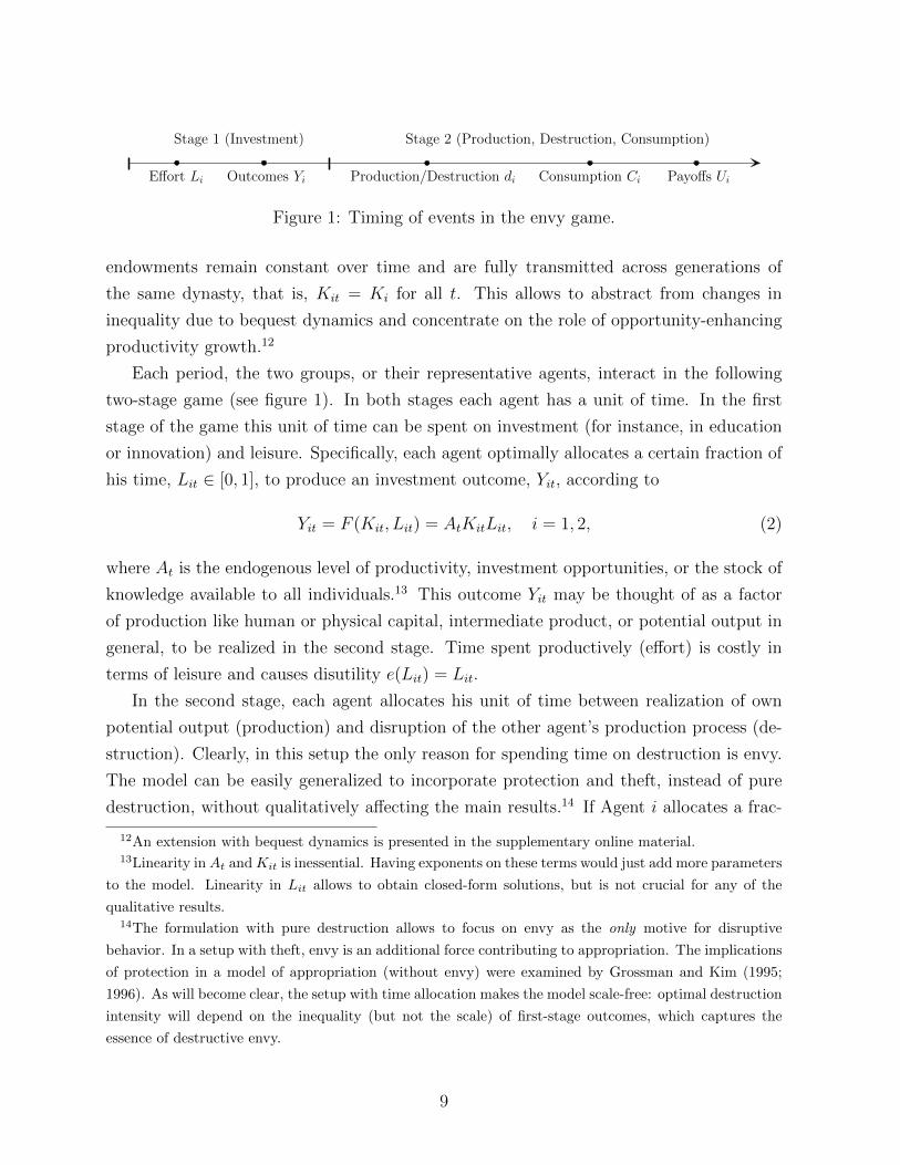
Effort Li Outcomes Yi

Stage 1 (Investment) Stage 2 (Production, Destruction, Consumption)

Production/Destruction di Consumption Ci Payoffs Ui

Figure 1: Timing of events in the envy game.

endowments remain constant over time and are fully transmitted across generations of

the same dynasty, that is, Kit = Ki for all t. This allows to abstract from changes in

inequality due to bequest dynamics and concentrate on the role of opportunity-enhancing

productivity growth.12

Each period, the two groups, or their representative agents, interact in the following

two-stage game (see figure 1). In both stages each agent has a unit of time. In the first

stage of the game this unit of time can be spent on investment (for instance, in education

or innovation) and leisure. Specifically, each agent optimally allocates a certain fraction of

his time, Lit ∈ [0, 1], to produce an investment outcome, Yit, according to

Yit = F (Kit, Lit) = AtKitLit, i = 1, 2, (2)

where At is the endogenous level of productivity, investment opportunities, or the stock of

knowledge available to all individuals.13 This outcome Yit may be thought of as a factor

of production like human or physical capital, intermediate product, or potential output in

general, to be realized in the second stage. Time spent productively (effort) is costly in

terms of leisure and causes disutility e(Lit) = Lit.

In the second stage, each agent allocates his unit of time between realization of own

potential output (production) and disruption of the other agent’s production process (de-

struction). Clearly, in this setup the only reason for spending time on destruction is envy.

The model can be easily generalized to incorporate protection and theft, instead of pure

destruction, without qualitatively affecting the main results.14 If Agent i allocates a frac-

12An extension with bequest dynamics is presented in the supplementary online material.13Linearity in At andKit is inessential. Having exponents on these terms would just add more parameters

to the model. Linearity in Lit allows to obtain closed-form solutions, but is not crucial for any of the

qualitative results.14The formulation with pure destruction allows to focus on envy as the only motive for disruptive

behavior. In a setup with theft, envy is an additional force contributing to appropriation. The implications

of protection in a model of appropriation (without envy) were examined by Grossman and Kim (1995;

1996). As will become clear, the setup with time allocation makes the model scale-free: optimal destruction

intensity will depend on the inequality (but not the scale) of first-stage outcomes, which captures the

essence of destructive envy.

9

tion dit ∈ [0, 1] of his time to disrupt the productive activity of Agent j, the latter retains

only a fraction pjt of his final output, where

pjt = p(dit) =1

1 + τdit, i, j = 1, 2, i 6= j. (3)

The function p(dit) has standard properties: it is bounded, with p(0) = 1, decreasing,

and convex (Grossman and Kim, 1995). Parameter τ > 0 measures the effectiveness of

destructive technology and may reflect the overall level of private property rights protection.

In particular, property rights are secure if τ is low.

Time 1− dit is spent on the realization of potential output Yit yielding the final output

(1 − dit)Yit. Since only a fraction p(djt) of this output is retained, the consumption level

of Agent i is given by

Cit = (1− dit)p(djt)Yit, i, j = 1, 2, i 6= j. (4)

Finally, payoffs are generated. The utility function takes the following form:

Uit = U(Cit, Cjt, Lit) = v(Cit − θCjt)− e(Lit) =(Cit − θCjt)1−σ

1− σ− Lit, (5)

where i, j = 1, 2, i 6= j, σ > 1, and θ ∈ (0, 1).15 It is increasing in own consumption

and decreasing in the other agent’s consumption, as well as own effort. Agents are each

other’s reference points, which is natural in the setup with two individuals (groups), and

parameter θ captures the strength of concern for relative standing (social comparisons).

This utility function features additive comparison which is one of the two most popular

ways to model envy, the other being ratio comparison.16 Overall, the form of the utility

function is identical to that in Ljungqvist and Uhlig (2000), except that in their model

the reference point of each agent is the average consumption in the population. The

latter assumption implies that each individual agent is too small to affect the reference

consumption level, a common approach in models with interdependent preferences that

15Assume for simplicity that Uit = −∞ whenever Cit 6 θCjt. Under the assumption (10) below, this

will never be the case in equilibrium. The assumption on the elasticity of marginal utility with respect

to relative consumption, σ, is a convenient regularity condition that guarantees concavity of equilibrium

outputs in endowments (see section 3.3). Linearity in effort is assumed for analytical tractability. For

simplicity, we also abstract from leisure in stage 2.16Additive comparison was assumed, among others, by Knell (1999) and Ljungqvist and Uhlig (2000).

Boskin and Sheshinski (1978) and Carroll et al. (1997) are examples of models with ratio comparison.

Clark and Oswald (1998) examine the properties of both formulations. The model in Gershman (2014)

shows that the qualitative results of this section can be obtained in a framework with ratio comparison.

10

basically rules out the possibility of destructive envy. The present setup is thus different

since groups (agents) are able to affect each other’s outcomes.17

A crucial property of the utility function (5) is complementarity between own and ref-

erence consumption that leads to the “keeping up with the Joneses” kind of behavior,

or emulation.18 Clark and Oswald (1998) call such a function a “comparison-concave”

utility (since v is concave). Intuitively, individuals are willing to match an increase in

consumption of their reference group. The reason is that a rise in Cj reduces the rela-

tive consumption (status) of individual i which, under concave comparisons, increases the

marginal utility of his own consumption. The payoff function (5) also implies that con-

sumption is a “positional” good, while leisure (disutility of effort) is not. This view has

been consistently advocated by Frank (1985; 2007) and finds support in the data (Solnick

and Hemenway, 2005).

To complete the model, we need to define intergenerational linkages. In the basic

version of the model generations are connected solely through the dynamics of investment

opportunities, or productivity.19 Specifically, productivity is driven by learning-by-doing

and knowledge spillovers: the higher is the total investment outcome (potential output)

in the society in a given period, the greater will be the stock of knowledge available for

the next generation. That is, individual learning-by-doing affects future productivity of

everyone in the economy. The simplest formulation capturing such dynamics, borrowed

from Aghion et al. (1999), is

At = A(Yt−1) = (Y1t−1 + Y2t−1)α, (6)

where α ∈ (0, 1) is the degree of intergenerational knowledge spillover.20 To account for

external shocks to productivity, such as exogenous positive spillovers from a larger economy

17It is not uncommon in political economy literature to model group interaction in the context of two-

agent games (Grossman and Kim, 1995). The implicit assumption is that groups are able to solve the

collective action problem and act in a coordinated way.18Dupor and Liu (2003) make a distinction between jealousy (envy) and KUJ behavior (emulation). The

former is defined as ∂Uit/∂Cjt < 0, while the latter is defined as ∂2Uit/∂Cjt∂Cit > 0. Interestingly, for a

class of utility functions including (5) these two notions are equivalent.19In the extension of the model available in the supplementary online material generations are linked

through bequests.20Aghion et al. (1999) assume that α = 1. Here, α < 1 in order to capture the possibility of a low

productivity steady state, as will become clear from the analysis of section 4. If α = 1 or At evolves

according to a Romer-style “ideas production function,” the society never gets stuck in a “bad” long-run

equilibrium, but all the main qualitative results still carry through. We also assume for simplicity that the

new knowledge is only available to the next generation, that is, there is no contemporary spillover effect.

11

described for the case of Tzintzuntzan in section 2.3, one could introduce an additional

component in equation (6). For example, if At = ζ · Y αt−1, a jump in ζ > 0 might be

interpreted as a shock to the process of knowledge creation.

3.2 Equilibria of the envy game

We start by analyzing the envy game for a given generation t. In what follows the time

index t is omitted whenever this does not cause confusion. Given the dynamic structure

of the game, we are looking for the subgame perfect equilibria. Hence, the model is solved

backwards, starting at stage 2.

Second-stage equilibrium. Given the outcomes of the investment stage, Y1 and Y2,

Agent i chooses the intensity of destruction, di, to maximize his payoff:

maxdi

v((1− di)p(dj)Yi − θ(1− dj)p(di)Yj) s.t. 0 6 di 6 1, (7)

where i, j = 1, 2, i 6= j. This yields the optimal second-stage response:21

d∗i =

0, if Yi/Yj > τθ(1− dj)(1 + τdj);

1τ·(√

τθYjYi

(1− dj)(1 + τdj)− 1), if Yi/Yj < τθ(1− dj)(1 + τdj).

(8)

Several features of this expression are of interest. First, without envy (θ = 0) there is

no destruction. If envy is present, the decision to engage in destruction depends on the

inequality of investment outcomes, Yi/Yj. If Yi is high enough relative to Yj, Agent i finds it

optimal to refrain from destruction. Otherwise, he allocates part of his time to destruction

and its intensity is increasing in ex-post inequality, effectiveness of destructive technology,

and the strength of envy. As such, this result reflects the trade-off between using the

available unit of time productively and destructively to improve relative standing.

The product τθ is an endogenous (inverse) measure of tolerance for inequality. Given

the ratio of investment outcomes, destructive envy is more likely to be activated if social

comparisons are strong (large θ) and property rights are poorly protected (large τ). Hence,

large τθ means low tolerance for inequality. If dj = 0, the product τθ is the critical level of

ex-post inequality, beyond which Agent i chooses to engage in destruction. Assume from

now on that τθ < 1, that is, if dj = 0, there is some tolerance for inequality and d∗i = 0 for

Yi > Yj. Given this “non-zero tolerance for inequality” assumption, the agent with higher

21As shown in the proofs of the main results available online, the assumptions of the model guarantee

that Ci−θCj > 0 in equilibrium for d∗i < 1. Hence, d∗i = 1 is never optimal and this case is not considered.

12

investment outcome will never attack in the second-stage equilibrium, as established in the

following lemma.22

Lemma 1. (Second-stage equilibrium). Let Y2 > Y1. Then, in the second-stage equilib-

rium d∗2 = 0 and

d∗1 =

0, if Y1/Y2 > τθ;

1τ·(√

τθ Y2Y1− 1), if Y1/Y2 < τθ.

(9)

Hence, Agent 2 retains a fraction p∗2 = p(d∗1) = min{√Y1/τθY2, 1} of his final output which

is strictly decreasing in τ , θ, and Y2/Y1, if destruction takes place.

For expositional simplicity, we proceed as if there is a “predator and prey” type relation-

ship (Grossman and Kim, 1996) between Agent 1 and Agent 2 from the outset, so that only

the initially poor agent is allowed to engage in destruction at stage 2. Such assumption is

made without loss of generality and underlines the asymmetric equilibrium roles played by

the agents in the general formulation of the model. Specifically, proposition 1 will confirm

that in the unique subgame perfect equilibrium of the game the initially better endowed

agent always has a higher investment outcome and so, given lemma 1, would never spend

time on destructive activities, even if permitted.

Note also that for Agent 1 to be able to avoid the negatively infinite utility, his choice

of d∗1 < 1 has to yield positive relative consumption. This is secured by assuming that

K1

K2

≡ k > k ≡ 4τθ

(1 + τ)2(10)

which imposes an upper bound on the level of initial inequality (or, equivalently, certain

restrictions on parameters θ and τ) and makes the necessary “catching up” feasible, as

formally demonstrated in the proof of lemma 3.

First-stage best responses. Agents are forward-looking and anticipate the optimal

second-stage actions when making their first-stage decisions. Although Agent 2 is passive

at stage 2, he is perfectly aware of how his investment outcome affects d∗1 and takes this

into account at stage 1:

maxY2

U2 = v(p(d∗1)Y2 − θ(1− d∗1)Y1)− Y2/AK2 s.t. 0 6 Y2 6 AK2. (11)

22This assumption rules out the case in which the agent with higher investment outcome engages in

destructive activities to improve his relative position even further. While such behavior is a theoreti-

cal possibility, the case considered here is more intuitive and consistent with the anecdotal evidence on

destructive envy in section 2.

13

For technical reasons, it is easier to analyze the best responses (BRs) of both agents in

terms of their consumption levels, Ci, rather than the first-stage outcomes Yi. Note that

these are different only if destruction actually takes place. In the latter case there is a

one-to-one mapping between Yi and Ci, as shown formally in the proof of lemma 2.23

Lemma 2. (BR of Agent 2). Denote the following productivity thresholds:

A21 ≡(

1

1− τθ2

) σσ−1

, A22 ≡ A21 ·(

1 + θ2

2

) 1σ−1

, A23 ≡ (1 + τ) ·(

1 + θ2

2

) 1σ−1

.

Assume further that A22 > A23 and AK2 > A23.24 Then, the best-response of Agent 2,

BR2 ≡ C∗2(C1), is a piecewise function of the following form:

C∗2(C1) =

min{AK2, θC1 + (AK2)1/σ, C1/τθ}, if C1 > C1;

min{Cd2 (C1), C

d2 (C1)}, if C1 < C1,

(12)

where Cd2 (C1) and Cd

2 (C1) are strictly increasing and concave. The definitions of Cd2 (C1),

Cd2 (C1), and the threshold level C1, as well as the detailed form of (12), are given in the

Appendix.

The threshold in expression (12) separates the cases in which Agent 2 allows second-

stage destruction (C1 < C1) from those in which he does not (C1 > C1). In the former set

of cases, the only difference between Cd2 (C1) and Cd

2 (C1) is whether Agent 2 invests “part

time” (L2 < 1) or “full time” (L2 = 1) in stage 1. In the latter, more interesting set of cases,

the best response of Agent 2 can be of three kinds: 1) invest full time (C∗2 = AK2) hitting

the resource constraint, 2) invest part time while displaying the KUJ behavior (C∗2 = θC1+

(AK2)1/σ) and not being subject to destructive envy of the poor agent, 3) invest part time

and produce the maximum output that rules out destructive envy (C∗2 = C1/τθ). Note that

if destruction were not allowed (under perfect property rights protection), as in standard

models of keeping up with the Joneses, and the resource constraint did not exist, the

unique best response of Agent 2 would always be C∗2 = θC1 + (AK2)1/σ. Thus, expression

(12) highlights the additional constraints that Agent 2 faces: the resource (investment

opportunities) constraint which must be satisfied and the “fear of envy constraint” which

may or may not be binding.

23Technically, these consumption-based best responses correspond to the best responses in terms of first-

stage investment outcomes adjusted for the second-stage destructive activity. Such transformation focuses

on final outputs and makes it easier to analyze the destructive equilibria.24The former assumption is made to cover all possible configurations of the best-response function. The

latter imposes a lower bound on productivity which simplifies derivations.

14

C15

BR2

C2C2

C1

AK2

C14

C2 = C1/τθ

(a) A23 < AK2 < A22

BR2

C14

AK2

C13

C2C2

C1

C2 = C1/τθ

(b) A22 6 AK2 < A21

BR2

C11

AK2

C12C13

C1

C2

C2 = C1/τθ

(c) AK2 > A21

Figure 2: Best response of Agent 2.

Figure 2 depicts the alternative configurations of the second agent’s best response.25

The differences observed at various productivity levels deliver part of the intuition behind

the upcoming main results. Specifically, the number of segments of the best-response

function increases once AK2 surpasses respective thresholds, opening qualitatively new

possibilities.

For low levels of AK2, as in figure 2(a), the optimal response is to invest full time, if

C1 > C15, and consume either all of the output or the part that is left after destruction. For

C1 < C15, it is optimal to invest part time in stage 1 while still being subject to destruction

in stage 2. Note that for C1 < C14 it is never optimal to completely avoid destruction, even

though it is always feasible. The intuition is that in this case full envy-avoidance would

yield the level of relative consumption that is too low to be compensated by additional

leisure time.26

Yet, as A increases, full envy-avoidance behavior becomes viable for C1 ∈ [C13, C14), as

depicted in figure 2(b). For such values of C1 it is not worth allowing destruction at all:

the gain in leisure is sufficient to compensate the reduction in relative consumption due

to envy-avoidance. Clearly, if destructive activities on part of Agent 1 were not allowed,

25The values of thresholds C11, C12, C13, C14, and C15 shown in figure 2 are specified in the detailed

form of lemma 2 in the Appendix.26In fact, for levels of C1 between C15 and C14 Agent 2 would be willing to produce more than AK2 to

improve his relative position, but is constrained by the available resources.

15

Agent 2 would want to produce more than C1/τθ, but imminent destruction for C2 above

this threshold reduces the marginal benefit of investment and leads to self-restraint. Note

also that for C1 > C14 Agent 2 wants to produce more than AK2 but is constrained by the

available time and investment opportunities.

Finally, for AK2 > A21 we observe all four possible actions of Agent 2. The new

segment in figure 2(c) is the KUJ response for C1 ∈ [C12, C11), in which case destructive

envy is not binding and Agent 2 can produce as much as he really wants (absent the

hazard of destruction) without crossing the C1/τθ threshold. For C1 > C11 his envy-driven

constructive behavior is constrained by the available resources.

Agent 1 is also forward-looking and knows his own optimal second-stage behavior when

optimizing at the investment stage:

maxY1

U1 = v((1− d∗1)Y1 − θp(d∗1)Y2)− Y1/AK1 s.t. 0 6 Y1 6 AK1. (13)

Lemma 3. (BR of Agent 1). Denote the following productivity thresholds:

A11 ≡(

τ

τ − 1

) σσ−1

, A12 ≡ 1. (14)

The best-response of Agent 1, BR1 ≡ C∗1(C2), is a piecewise function of the following form:

C∗1(C2) =

min{Cd1 (C2), C

d1 (C2)}, if C2 > C2;

min{AK1, θC2 + (AK1)1/σ}, if C2 < C2,

(15)

where Cd1 (C2) is strictly increasing and convex and Cd

1 (C2) is linearly decreasing. The

definitions of Cd1 (C2), C

d1 (C2), and the threshold level C2, as well as the detailed form of

(15), are given in the Appendix.

The threshold in expression (15) separates the cases in which Agent 1 engages in envy-

motivated destruction (C2 > C2) from those in which he does not (C2 < C2). As in the

case of Agent 2, the only difference between Cd1 (C2) and Cd

1 (C2) is whether Agent 1 hits the

resource constraint or not. If Agent 1 does not engage in destruction and chooses instead

to catch up peacefully, his best response is C1 = θC2 + (AK1)1/σ unless such KUJ-type

behavior is constrained by the available investment opportunities AK1.

As depicted in figure 3, the best response of Agent 1 becomes more “diverse” as pro-

ductivity rises.27 For low A, the best response is just to do as much as possible by investing

full time. For C2 < C24, the output AK1 is large enough to place ex-post inequality within

27The values of thresholds C21, C22, C23, and C24 shown in figure 3 are specified in the detailed version

of lemma 3 in the Appendix.

16

BR1

AK1

C24

C2

C1

C2 = C1/τθ

(a) AK1 < A12

BR1

AK1

C23

C24

C1

C2

C2 = C1/τθ

(b) A12 6 AK1 < A11

BR1

C2

C21

C22

C1AK1

C2 = C1/τθ

(c) AK1 > A11

Figure 3: Best response of Agent 1.

the tolerance limit, but beyond that threshold it becomes optimal to engage in destruction

in stage 2. For intermediate values of A we observe the emergence of the KUJ segment cor-

responding to C2 < C23: envy is satisfied through peaceful effort which is not constrained

by the available resources. Yet, as C2 increases, so does the desired level of C1 until it

hits the investment opportunities upper bound. Note that higher C2 also increases the

marginal benefit of second-stage destruction. For AK1 > A11 all three segments become

apparent. The opportunities for peaceful catching up allow the KUJ segment to extend all

the way to the C2 = C1/τθ border, beyond which Agent 1 produces below the tolerance

threshold and engages in destruction in stage 2. Finally, at C2 = C22 the production level

hits the capacity constraint and remains there for higher values of C2.

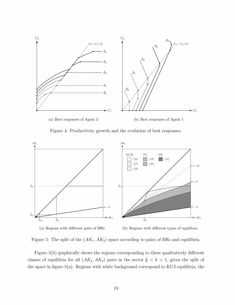
Figure 4 shows the evolution of best responses driven by productivity growth from

A = A0 to A = A4. The tendency for both functions is to become more “segmented” as

investment opportunities increase and allow for a wider range of actions. For Agent 2,

as figure 4(a) demonstrates, rising A leads to the emergence and subsequent expansion of

the fear and KUJ segments. For Agent 1, as shown in figure 4(b), the main consequence

of productivity growth is the emergence and extension of the KUJ segment. Thus, rising

economic opportunities make the envy game more interesting: the latent regions of both

best responses come into play potentially giving rise to new equilibrium outcomes. This

dynamics is explored in detail in section 4.

17

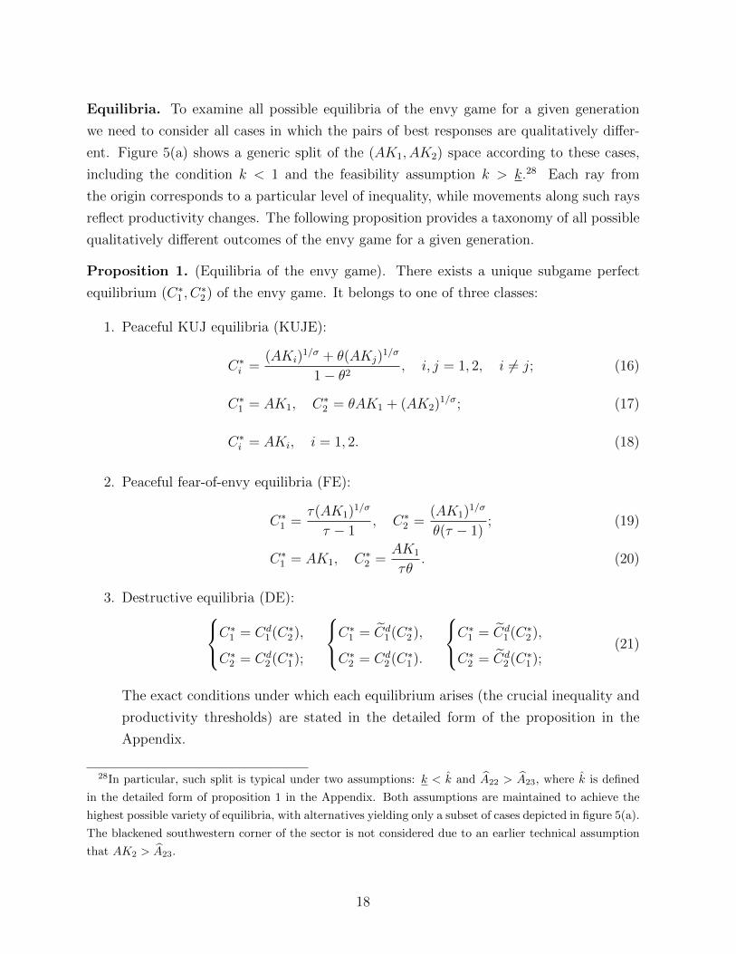
Equilibria. To examine all possible equilibria of the envy game for a given generation

we need to consider all cases in which the pairs of best responses are qualitatively differ-

ent. Figure 5(a) shows a generic split of the (AK1, AK2) space according to these cases,

including the condition k < 1 and the feasibility assumption k > k.28 Each ray from

the origin corresponds to a particular level of inequality, while movements along such rays

reflect productivity changes. The following proposition provides a taxonomy of all possible

qualitatively different outcomes of the envy game for a given generation.

Proposition 1. (Equilibria of the envy game). There exists a unique subgame perfect

equilibrium (C∗1 , C∗2) of the envy game. It belongs to one of three classes:

1. Peaceful KUJ equilibria (KUJE):

C∗i =(AKi)

1/σ + θ(AKj)1/σ

1− θ2, i, j = 1, 2, i 6= j; (16)

C∗1 = AK1, C∗2 = θAK1 + (AK2)1/σ; (17)

C∗i = AKi, i = 1, 2. (18)

2. Peaceful fear-of-envy equilibria (FE):

C∗1 =τ(AK1)

1/σ

τ − 1, C∗2 =

(AK1)1/σ

θ(τ − 1); (19)

C∗1 = AK1, C∗2 =AK1

τθ. (20)

3. Destructive equilibria (DE):C∗1 = Cd1 (C∗2),

C∗2 = Cd2 (C∗1);

C∗1 = Cd1 (C∗2),

C∗2 = Cd2 (C∗1).

C∗1 = Cd1 (C∗2),

C∗2 = Cd2 (C∗1);

(21)

The exact conditions under which each equilibrium arises (the crucial inequality and

productivity thresholds) are stated in the detailed form of the proposition in the

Appendix.

28In particular, such split is typical under two assumptions: k < k and A22 > A23, where k is defined

in the detailed form of proposition 1 in the Appendix. Both assumptions are maintained to achieve the

highest possible variety of equilibria, with alternatives yielding only a subset of cases depicted in figure 5(a).

The blackened southwestern corner of the sector is not considered due to an earlier technical assumption

that AK2 > A23.

18

A0

C1

C2

A1

A2

A3

A4

C2 = C1/τθ

(a) Best responses of Agent 2

A0

C1

C2

A1

A2

A3

A4C2 = C1/τθ

(b) Best responses of Agent 1

Figure 4: Productivity growth and the evolution of best responses.

AK2

AK1

A12

A11

A22 A21

k = k

(a) Regions with different pairs of BRs

k = k

k = k

A21

(16)

(17)

(18)

KUJE

(19)

(20)

FE

(21)

DE

k = τθ

A11

AK2

AK1

(b) Regions with different types of equilibria

Figure 5: The split of the (AK1, AK2) space according to pairs of BRs and equilibria.

Figure 5(b) graphically shows the regions corresponding to these qualitatively different

classes of equilibria for all (AK1, AK2) pairs in the sector k < k < 1, given the split of

the space in figure 5(a). Regions with white background correspond to KUJ equilibria, the

19

light gray area represents the fear-of-envy equilibria, and the dark gray color marks the

destructive region. Figure 6 shows examples of equilibria for different levels of productivity.

In the first class of equilibria only constructive envy is present and both agents compete

peacefully by undertaking productive investment in the first stage of the game, possibly

hitting the resource constraint.29 The features of a standard “keeping-up-with-the-Joneses”

equilibrium (16) are well-known from previous literature and have been formally analyzed

by Frank (1985) and Hopkins and Kornienko (2004), among others.30 In particular, envy

encourages additional investment effort which leads to “overworking” (see section 5).

In the second class of equilibria the better endowed agent is constrained by the threat

of envy-motivated destruction and invests the maximum possible amount of time that does

not trigger aggression. There is no actual destruction in such equilibrium, but there is the

“fear” of it that constrains the effort of Agent 2. This equilibrium resembles the fear of

envy documented in many developing societies, as discussed in section 2.31 In the third

class of equilibria there is actual destruction and part of the time is used unproductively by

Agent 1 to satisfy envy. As a consequence, part of the second agent’s output is destroyed.

The intuition for when each kind of equilibrium emerges is simple. Given the level of

productivity, a KUJ equilibrium is more likely vis-a-vis the fear or destructive outcomes

if inequality is low and/or tolerance for inequality is high, that is, property rights are

well-protected and social comparisons are weak. Otherwise, destructive envy is activated

resulting in output loss due to underinvestment or outright destruction. The relation to

inequality is obvious in figure 5(b): darker regions corresponding to cases in which de-

structive envy is either binding or present lie further away from the 45-degree line marking

perfect equality. It is important to emphasize that, for a given level of productivity, three

parameters (not counting σ) jointly determine the type of equilibrium. For instance, just

29We include the full-time investment case (18) in the group of KUJ-type equilibria, since it does

not feature either destructive envy or the fear of it. One caveat, however, is that at very low levels of

productivity working full time is unrelated to KUJ-type incentives. With this in mind, by default we refer

to case (18) as the one in which it is the catching-up behavior that is limited by the available resources.30Note that (16) would always be the unique equilibrium of the envy game in the absence of destructive

technology (under perfect property rights protection) and the resource constraint.31Mui (1995) constructs a theoretical framework in which (costless) technological innovation may not be

adopted in anticipation of envious retaliation. The intuition of the fear equilibrium in the present theory

is similar, except that here the fear of envy operates on the intensive margin by discouraging (costly)

investment. Furthermore, in Mui’s framework retaliation reduces envy directly by assumption rather than

through the improvement of the relative standing of the envier. Finally, his paper ignores constructive

envy and thus, focuses on one side of the big picture.

20

BR2

C1

C2

BR1 BR2

C1

C2

BR1

(a) AK1 > A11, AK2 > A21: KUJE (left) and FE (right)

BR1

C2

C1

BR2BR2

BR1

C2

C1

(b) AK1 < A11, AK2 > A21: KUJE

BR2

C2

C1

BR1 BR2BR1

C2

C1

(c) AK1 < A11, AK2 < A21: FE (left) and DE (right)

Figure 6: Equilibria of the game for different productivity levels.

21

having low inequality is not enough to be in the KUJE. If at the same time institutions are

very weak (destructive technology is efficient) and/or relative standing concerns are very

strong, the society may still end up in a fear or even destructive equilibrium.

A question of special interest is how endogenously rising productivity can affect the

type of equilibrium, given the level of inequality and tolerance parameters. First, as fol-

lows from the detailed form of proposition 1 in the Appendix, once A gets large enough,

the type of equilibrium is determined only by k, τ , and θ. Thus, rising productivity need

not automatically turn destructive envy into constructive if there is persistently high in-

equality or low tolerance for inequality. For example, for k < k any level of productivity

yields either fear-type or destructive equilibrium.32 Conversely, if k > τθ, the equilibrium

outcome is always a KUJ-type competition, and growing A just takes the society from a

full-time equilibrium, in which individuals are constrained by the available resources, to

a conventional KUJE with positively sloped best responses, as in the left panel of figure

6(a).

The most interesting case is the one with intermediate levels of inequality (or tolerance

for inequality), that is k < k < τθ. For such parameter values, productivity growth

can lead the society through all envy regimes, from destructive equilibrium through the

fear of envy and to the KUJ competition, consistent with the evidence on such transition

presented in section 2.3.33 As will become clear from the analysis of section 4, even when

productivity matters for determination of the equilibrium type, inequality and tolerance

parameters play a key role in guiding the long-run dynamics of the society. Before looking

at the evolving role of envy in the process of development, it is instructive to first consider

comparative statics for each particular equilibrium type.

3.3 Comparative statics

Consider the impact of four parameters of interest, λ, θ, τ , and A, on economic performance

as measured by final outputs. The qualitative effects are similar within the three groups

of equilibria identified above.

As follows from proposition 1, total outputs in the KUJ-type equilibria (16), (17),

and (18) are given by Y = (λ1/σ + (1 − λ)1/σ) · (AK)1/σ/(1 − θ), Y = (1 + θ)λAK +

32This is due to the assumption that k < k. If, on the other hand, k > k, a high enough level of

productivity guarantees a peaceful KUJ equilibrium. The thresholds k and k are given by (28).33A shift towards this sector from higher starting levels of inequality may happen endogenously due to

bequest dynamics, see the online supplementary material.

22

(1 − λ)1/σ(AK)1/σ, and Y = AK, respectively. Clearly, economic performance in these

cases does not depend on τ since destructive envy is not binding. The effect of θ is

straightforward: increasing the strength of relative concerns acts as additional incentive to

work, which leads to higher levels of effort and output in the conventional KUJ equilibrium

(16). In the “partial” KUJ equilibrium (17) we observe a similar effect only for Agent 2,

while Agent 1 is working at the capacity constraint and cannot respond to rising θ. Finally,

in case (18) both agents invest at their capacity levels and the incentivizing marginal effect

of envy is absent.

The effect of raising λ (increasing equality) on economic activity depends crucially

on σ, with the exception of the full-time equilibrium (18), in which redistribution alters

individual investment levels, but not aggregate output. Under the baseline assumption

σ > 1, outputs in the conventional KUJ equilibrium are strictly concave and increasing

functions of λ which is more natural than a kind of nondecreasing returns to scale that

would emerge under σ 6 1. The total effect of redistribution on private outputs in (16)

consists of two parts: wealth effects and comparison effects. Wealth effects are just the

direct effects of making one agent poorer and the other richer. In case of increasing λ the

wealth effect is positive for Agent 1 and negative for Agent 2. The total wealth effect on

output is positive since the poor agent is more productive on the margin under concave

output functions.34 Comparison effects reflect the fact that the reference group becomes

poorer for Agent 1 and richer for Agent 2. Consequently, comparison effect is negative

for Agent 1 and positive for Agent 2. The total comparison effect has the same sign as

the total wealth effect. In particular, under σ > 1, the negative comparison effect on the

output of the poor is outweighed by the positive comparison effect on the output of the

rich. In the partial KUJ equilibrium (17) Agent 2 experiences both wealth and comparison

effects, while Agent 1 is investing at full capacity. As shown in the proof of proposition

2, the effect of λ on aggregate output is always positive in this case, that is, the negative

wealth effect on the rich is always dominated by the incentivizing effect of redistribution.

Next, consider the fear-type equilibria (19) and (20) in which total output is given,

respectively, by Y = (1 + τθ)(λAK)1/σ/(θ(τ − 1)) and Y = (1 + τθ)λAK/(τθ). In both

cases the output of Agent 2 is “tied” to that of Agent 1 with the coefficient of tolerance

1/τθ. Raising τ (reducing the quality of institutions) decreases the tolerance of Agent

1 for inequality and aggravates the “fear constraint” of Agent 2. This means that with

34This “opportunity-enhancing” effect of redistribution under diminishing returns to individual endow-

ments and imperfect capital markets is well-known in the literature, see, for example, Aghion et al. (1999,

section 2.2).

23

higher τ Agent 2 has to produce less to avoid destructive envy, which leads to lower

individual and total outputs. The effect of raising θ is similar since it, too, decreases the

tolerance for inequality. This is in stark contrast with the role of envy in the KUJ-type

equilibria. In the latter case envy acts as additional incentive to work, while in the fear

equilibria it constrains productive effort by increasing the hazard of destructive envy. On

the other hand, the effect of raising equality in the fear equilibria is unambiguously positive.

Increasing λ enhances the output of Agent 1 which “trickles up” into the higher output of

Agent 2. That is, redistribution from the rich to the poor increases investment and final

output by alleviating the fear of envy constraint.

Destructive equilibria are harder to examine analytically. Multiple effects are at work

which makes the aggregate comparative statics with respect to θ ambiguous for the first

case in (21). If inequality is high or tolerance for inequality is low, stronger envy leads to

substantial destruction which may lower the consumption of Agent 2, as well as the total

final output, C. In contrast, if the destructive environment is not severe (or σ, the catching-

up propensity, is high), the stimulating effect of envy dominates. Thus, comparative statics

in the DE combines the features of the FE and the KUJE. At the same time, higher τ and

lower λ unambiguously decrease total consumption.

Finally, rising productivity of investment, A, has a positive impact on aggregate eco-

nomic performance, regardless of the equilibrium type. The following proposition summa-

rizes the comparative statics results discussed above.

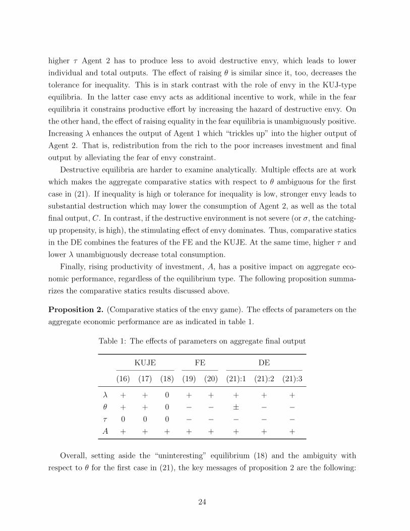
Proposition 2. (Comparative statics of the envy game). The effects of parameters on the

aggregate economic performance are as indicated in table 1.

Table 1: The effects of parameters on aggregate final output

KUJE FE DE

(16) (17) (18) (19) (20) (21):1 (21):2 (21):3

λ + + 0 + + + + +

θ + + 0 − − ± − −τ 0 0 0 − − − − −A + + + + + + + +

Overall, setting aside the “uninteresting” equilibrium (18) and the ambiguity with

respect to θ for the first case in (21), the key messages of proposition 2 are the following:

24

1) equality and higher productivity increase aggregate final output; 2) the strength of

envy enhances output when society is in the unconstrained KUJ-type competition and

has a detrimental effect whenever destructive envy and the fear of it are active; 3) better

property rights enhance economic activity when they matter, that is, when destructive

envy is binding.

4 Envy and the growth process

Now that we established how incentives respond to changes in parameters in each equilib-

rium, we turn to the analysis of dynamics implied by proposition 1 together with equation

(6), that is, transitions from one equilibrium type to another driven by endogenous produc-

tivity growth. Specifically, focus on the sector defined by k ∈ (k, τθ), in which such growth

can trigger qualitative changes. Clearly, at each point in time the dynamics is determined

by the region of the phase plane 5(b) in which the society is located.

Assume that the initial level of productivity A0 is large enough, so that the society is

already past the destructive region and starts in the fear-type equilibrium (20).35 Then,

the dynamics of productivity is given by

At =

[(1 + 1/τθ)K1]

α · Aαt−1, if At−1 < A;

[(1 + θ)At−1K1 + (At−1K2)1/σ]α, if A 6 At−1 < A;

[(K1/σ1 +K

1/σ2 )/(1− θ)]α · Aα/σt−1 , if At−1 > A,

(22)

where the productivity thresholds are

A ≡

[τθ

1− τθ2· K

1/σ2

K1

] σσ−1

, A ≡

[K

1/σ1 + θK

1/σ2

(1− θ2)K1

] σσ−1

,

as follows directly from proposition 1. In the long run, the society will settle in one of the

three regions, as established in the following proposition.

35Another reason for why the economy might start in the fear-type equilibrium is if it has redistributive

mechanisms in place. A variation of the basic model in Gershman (2012) shows how in the presence of

preemptive transfers destructive equilibrium can be replaced by a “fear equilibrium with transfers.”

25

Proposition 3. (Long-run steady state.) Assume that k ∈ (k, τθ) and A0 ∈ (A, A).36

Then

limt→∞

At =

A∗1 ≡ [(1 + 1/τθ)K1]

α1−α , if α < α;

A∗2, if α 6 α < α;

A∗3 ≡ [(K1/σ1 +K

1/σ2 )/(1− θ)]

ασσ−α , if α > α,

(23)

whereA∗2 is implicitly defined by equation (A∗2)1/α = (1+θ)A∗2K1+(A∗2K2)

1/σ, the thresholds

α and α are implicitly defined by equations A∗1 = A and A∗2 = A, respectively. Furthermore,

αθ > 0, αλ < 0, ατ > 0, and αθ > 0, αλ < 0, ατ = 0.

Proposition 3 implies that lower inequality and higher tolerance for inequality are likely

to put the society on a trajectory that leads to the long-run KUJ equilibrium marked by

high productivity level. In contrast, under high fundamental inequality and low tolerance

the society is likely to get stuck in the fear of envy region with low productivity in the

steady state. The comparative statics of long-run levels of productivity clearly replicate

those in proposition 2.

Figure 7 demonstrates how endogenous productivity growth can take the society away

from the initial fear equilibrium to the long-run KUJE. The left panel shows such transition

on the (AK1, AK2) plane, while the right panel shows the evolution of best responses

and the equilibrium type following productivity growth. Initially, peaceful investment

opportunities are scarce locating the society in the fear equilibrium. Yet, the growth

process expands investment opportunities, and envy-avoidance behavior, dictated by the

destructive side of envy, paves the way to constructive emulation. Note also that ex-post

inequality of outputs reduces as a result of this transition.37 If, however, the society starts

off closer to the k = k line, it is likely to stay in the same fear region where it started,

as the lower trajectory in figure 7(a) illustrates. In such cases, the fear of envy does

not let investment opportunities grow big enough to enable full-fledged constructive KUJ

competition. Apart from inequality and tolerance parameters, the development trajectory

of the society might be affected by an external shock to investment opportunities of the

type discussed in section 2.3 or a change in the strength of knowledge spillover α.

Importantly, depending on the current regime, envy affects economic growth in opposite

ways. In the fear-type equilibrium it discourages investment and growth, while in the

KUJ-type equilibria the effect is the opposite. The same is true for the long-run levels of

36The lower bound on initial productivity is A ≡ [τθ/((1− τθ2)K1)]σ/(σ−1) · [(1 + θ2)K2/2]1/(σ−1).37Specifically, as follows directly from proposition 1, ex-post inequality is equal to C1/C2 = τθ in the

fear region, then monotonically decreases to (k1/σ + θ)/(1 + θk1/σ) and stays at that level thereafter.

26

AK1

AK2A∗1K2

k = k

k = τθ

A∗3K1

k = 1

(a) Alternative growth trajectories

C1

C2

C2 = C1/τθ

(b) Dynamics of best responses

Figure 7: Productivity-driven transition from FE to KUJE.

productivity. A number of factors, such as religion and ideology in general, can plausibly

affect the intensity of social comparisons.38 In the context of the model, religious and

moral teachings condemning envy cause downward pressure on θ. In the fear region, such

teachings enhance growth because the fear constraint of the rich is alleviated permitting

higher effort. Moreover, a fall in θ lowers the thresholds A and A contributing to a faster

transition from FE to KUJE. As the economy enters the KUJ region, destructive envy

turns into emulation, and θ has the opposite impact on economic performance. In the

KUJ region the same factors that drive the society out of the fear equilibrium have a

negative effect on output.

An example of ideology positively affecting θ is that of material egalitarianism. The

concept of everyone being equal and the neglect of private property rights are effective in

fostering social comparisons and lowering tolerance for inequality. Hence, this ideology op-

erates in favor of destructive envy in the fear region and delays the transition to the KUJE,

38All major world religions denounce envy. In Judeo-Christian tradition envy is one of the deadly sins

and features prominently in the tenth commandment. Schoeck (1969, p. 160) goes as far as to say that “a

society from which all cause of envy had disappeared would not need the moral message of Christianity.”

27

At

At−1A AA′ A′

45◦

(a) Dynamic effects of a rise in θ

At

At−1A AA′

45◦

(b) Dynamic effects of a rise in τ

Figure 8: Envy, property rights, and productivity dynamics.

as shown in figure 8(a).39 Yet, upon entering the KUJ region, intense social comparisons

are channeled into productive activity and boost economic growth.

Similarly, one could examine the dynamic effects of a shock in τ that could be due to

various reasons, from changes in technologies of destruction and protection to reforms of

legal institutions. Better property rights encourage productivity growth in the fear region

and have no effect on either the dynamics or the steady state in the KUJ region. In contrast,

an increase in τ would endogenously prolong the presence of the economy in the fear region,

as shown in figure 8(b), while at the same time making the FE more egalitarian, since the

erosion of institutions decreases tolerance for inequality and exacerbates the fear constraint.

This may explain the persistence of the fear of envy, along with such characteristics as

poorly protected private property rights and relatively low inequality.

5 Welfare, property rights, and inequality

As shown in the previous section, the initial level of inequality and the two tolerance

parameters jointly determine the growth trajectory of the economy, potentially resulting

in qualitatively different long-run equilibria. Yet, in principle, societies might have the

39Figure 8 ignores for simplicity that for low enough A the dynamics is governed by the outcomes of

destructive equilibria.

28

ability to challenge the underlying institutional and distributional status quo if this leads

to welfare improvements. This section examines the incentives to undertake such changes.

Specifically, assume that k ∈ [k, k) and the society is in the long-run fear equilibrium

with the steady-state productivity level AF given by

AF =

[1 + τθ

θ(τ − 1)K

1/σ1

] ασσ−α

, (24)

where, in addition, AFK1 > A11 and AFK2 > A21.40 Given this starting point, when

will both social groups want to move away from the fear of envy equilibrium to a KUJ

trajectory by adopting better institutions (lower τ) or redistributing the initial wealth from

the rich to the poor (higher k)? In answering this question we consider both the incentives

of the current generation (short run) and the welfare consequences for future generations

of both dynasties upon convergence to the new long-run KUJE.41 In that steady state the

level of productivity is given by

AKUJ =

[K

1/σ1 +K

1/σ2

1− θ

] ασσ−α

, (25)

which is always greater than AF. Note that only future generations will be able to reap

the full benefit of technological advancement prompted by institutional or distributional

change.

The two thought experiments are illustrated in figure 9. Figure 9(a) shows a switch

to KUJ dynamics via the adoption of better institutions: a lower value of τ changes the

split of the phase plane, as a result of which the society finds itself in the KUJ region and

starts growing towards the new long-run steady state. Figure 9(b) shows the consequences

of an ex-ante redistribution of endowments: a jump from k to k′ does not affect the split

of the phase plane into sectors but puts the society onto a more equal growth path in the

KUJ region leading to a higher long-run productivity level. We examine the details of both

scenarios in turn.

40That is, for concreteness we focus on case 19, although similar intuition would clearly hold for (20).

The expression for AF follows from equations (6) and (19).41An alternative, but similar way to think about it would be to consider a benevolent utilitarian social

planner maximizing the (discounted) welfare of current and all future generations of the society. A more

involved option would be to incorporate Barro-style dynastic preferences in the analysis. In any case the

crucial point will be the differential welfare effect on current versus future generations.

29

AK1

AK2AFK2

k′

k

k′

k

AKUJK2

k

k = 1

(a) Institutional change: a decrease in τ

AK1

AK2AFK2

k

k

k

k′

AKUJ′K ′2

k = 1

(b) Redistribution: an increase in k

Figure 9: From fear of envy to keeping up with the Joneses.

5.1 Institutional change

The connection between institutions and externalities was famously drawn by Demsetz

(1967) who considered the emergence of property rights to be a way to cope with cer-

tain externality problems. In the present theory, two types of externalities make institu-

tions matter: a negative consumption externality (envy) and a positive intergenerational

learning-by-doing externality (knowledge spillover). As established in the following propo-

sition, on the one hand, weaker property rights protection may internalize the negative

consumption externality. On the other hand, stronger property rights allow future gener-

ations to benefit from the positive knowledge spillover which has a positive effect on social

welfare in the long run. Thus, it is the relative strength of the two types of externalities

that determines the long-run welfare effect of an institutional change.

Proposition 4. (Welfare and institutional change.) Assume that k ∈ [k, k) and the society

is in the long-run FE. Then,

I. Short run (current generation). ∃! θ ∈ (0, 1) such that: 1) If θ > θ, a shift to the

KUJE via better institutions is a Pareto worsening; 2) If θ 6 θ, ∃! k1 ∈ [k, k) such

that this shift is a Pareto worsening if and only if k > k1.

II. Long run (future generations). ∃! α ∈ (0, 1) such that: 1) If α < α, the long-run

KUJE is never a Pareto improvement over the initial fear equilibrium; 2) If α > α,

30

∃! k2 ∈ [k, k], such that the long-run KUJE is a Pareto improvement over the initial

fear equilibrium if and only if k > k2.

Consider the short-run part first. The intuition for this result revolves around the

negative effect of the consumption externality on social welfare. As follows from the proof

of proposition 4, Agent 1 (the poor) always prefers the FE: he enjoys the same level of

relative consumption as in the KUJE, but exerts less effort. Agent 2 (the rich) always

benefits from higher relative consumption in the KUJE, but at a cost of increased effort,

and thus, faces a trade-off. It turns out that he prefers to stay in the FE if only if in the

alternative KUJE he would have to work too hard to support his high relative standing, or,

in other words, if a rise in social status does not compensate for the cost of foregone leisure.

That would be the case if either social comparisons are strong (θ is large) or inequality

is low (k is large). Under these conditions the FE is Pareto dominant since the fear of

destructive envy restrains effort and curbs the consumption externality that otherwise

leads to overworking in the KUJE. Thus, weaker property rights protection corrects the

distortion caused by envy.42

As follows from proposition 2, regardless of welfare effects, outputs of both agents will

always be higher in the KUJE compared to the initial FE. The result that both agents

can be better off in an equilibrium with lower consumption is reminiscent of what Gra-

ham (2010) calls the “paradox of happy peasants and miserable millionaires” and related

research in happiness economics (Clark et al., 2008).

It is also instructive to read the short-run part of proposition 4 in the “reverse” order,

assuming that the society is initially in the KUJE. Then, it implies that, under strong

enough consumption externality, weaker property rights protection (higher τ) causing a

switch to the fear equilibrium might constitute a Pareto improvement. For low values of

θ, such shift would be favored by the rich if and only if the distribution of endowments

is relatively equal. Such reading of this result can be viewed as a formalization of a more

than a century-old argument raised by Veblen (1891) in an attempt to explain the support

for socialist movement and the abolition of private property rights. In particular, Veblen

argued that the “ground of the unrest with which we are concerned is, very largely, jealousy,

– envy, if you choose: and the ground of this particular form of jealousy that makes for

socialism, is to be found in the institution of private property.”

42Curiously, this is akin to the effects of Pareto improving redistributive taxation in the presence of

concern for relative standing, see Boskin and Sheshinski (1978), Oswald (1983), and Frank (1985).

31

Veblen goes on to describe what in the language of the present theory represents a

transition from the KUJE (“keep up appearances”) to the FE (“socialism”): “The ultimate

ground of this struggle to keep up appearances by otherwise unnecessary expenditure, is the

institution of private property. . . With the abolition of private property, the characteristic

of human nature which now finds its exercise in this form of emulation, should logically

find exercise in other, perhaps nobler and socially more serviceable, activities.” Elimination

of the KUJ competition, in Veblen’s view, would lessen the amount of labor and output

required to support the economy. This is similar to what happens upon transition to the

fear equilibrium under conditions stated above: output and labor supply fall, individuals

enjoy more leisure and are, at least in the short run, happier with less output. As discussed

above, the rich may prefer well-protected property rights if inequality is high enough, since

moving to the FE would mean losing too much in terms of relative standing. Thus, in a

KUJE with relatively high inequality there is likely to be a conflict of interests with regard

to institutional quality.

While intuitive in the short run, the negative impact of better institutions on social

welfare need not hold for future generations of both dynasties. This is where the second,

positive externality comes in. As follows from part 2 of proposition 4, if the spillover

effect (α) is strong enough, the long-run KUJE will Pareto dominate the initial FE. The

intuition for such reversal of the short-run result is simple. Better institutions make people

exert more effort due to constructive envy, which causes productivity growth and raises

investment opportunities of future generations. This growth eventually allows everyone

to increase relative consumption and decrease effort compared to the initial jump.43 Note

that the long-run Pareto improvement result holds in an equal enough society, as stated in

proposition 4. Otherwise, the shift is too costly for the poor dynasty in terms of foregone

leisure despite the increase in relative consumption.44

To summarize the message of proposition 4, while a strong consumption externality

unleashed by better institutions might lead to lower welfare in the short run, a strong

spillover effect can more than make up for it in the long run. Such scenario is shown in

figure 10.

43Clearly, an increase in C1 and C2 by the same factor due to rising productivity makes everyone better

off since own consumption is valued more than reference consumption (θ < 1).44Note also that in the short run a Pareto improvement is more likely to happen in an unequal society,

while in the long run it is the other way round. The reason is that in the former case it is the rich agent

who is critical and his preference is to maintain higher inequality, while in the latter case the poor agent

is critical and he prefers equality. See the proof of proposition 4 for details.

32

7173

7577

Rel

ativ

e co

nsum

ptio

n (C

1-q C

2)

-.62

-.61

-.6

-.59

Wel

fare

(U

1)

0 1 2 3 4 5 6 7 8 9 10

Generation since the adoption of better institutions

(a) Welfare of the poor

110

120

130

140

Rel

ativ

e co

nsum

ptio

n (C

2-qC

1)

-.37

-.36

-.35

Wel

fare

(U

2)

0 1 2 3 4 5 6 7 8 9 10

Generation since the adoption of better institutions

(b) Welfare of the rich71

7375

77

Rel

ativ

e co

nsum

ptio

n (C

1-qC

2)

.35

.36

.37

.38

Eff

ort (

L1)

0 1 2 3 4 5 6 7 8 9 10

Generation since the adoption of better institutions

Effort Relative consumption

(c) Effort and relative consumption of the poor

110

120

130

140

Rel

ativ

e co

nsum

ptio

n (C

2-qC

1)

.16

.17

.18

.19

Eff

ort(

L2)

0 1 2 3 4 5 6 7 8 9 10

Generation since the adoption of better institutions

Effort Relative consumption

(d) Effort and relative consumption of the rich

Figure 10: From FE to KUJE via better institutions.

5.2 Redistribution

As follows from proposition 1, another way to abandon the fear equilibrium and enable KUJ

competition is to make the distribution of endowments more equal. Is there a scope for

Pareto-improving redistribution in the short and the long run? The following proposition

holds.

Proposition 5. (Welfare and redistribution.) Assume that k ∈ [k, k) and the society is in

the long-run FE. Then,

I. Short run (current generation). ∃! ¯θ ∈ (0, 1) such that: 1) If θ > ¯θ, redistribution

shifting the society to a KUJE is never a Pareto improvement; 2) If θ 6 ¯θ, ∃!

33

¯k ∈ [k, k), such that Pareto-improving shift to a KUJE is feasible for k ∈ [k, ¯k].

However, the optimal level of inequality from the viewpoint of Agent 2, k∗, always

lies in the fear region, that is, k∗ ∈ [k, k).

II. Long run (future generations). For small enough θ or τ , ∃! ¯α ∈ (0, 1) such that, if

α > ¯α: 1) Pareto-improving redistribution shifting the society to a KUJE is feasible

for all k ∈ [k, k]; 2) The optimal level of inequality from the viewpoint of the rich

dynasty in the long-run KUJE, k∗, is strictly less than 1, that is, k∗ ∈ [k, 1).

Clearly, the poor agent is always in favor of redistribution, both in the short and the

long run. It increases the marginal product of his effort while at the same time decreasing

that of the rich. From the point of view of the rich agent, redistribution can only be

beneficial under certain conditions and only to a certain extent. Specifically, his preferred

level of initial inequality is never in the KUJ region in the short run. If comparisons are

important (θ is high), it is never optimal to give up the initial wealth advantage and then

work hard to compete peacefully with an “enriched” rival. For weak relative standing

concerns, however, the boost in own output following the relaxation of the fear constraint

might be worth transferring part of the endowment to the poor.

In the long run, redistribution leads to a rise in the effort-saving productivity growth,

similar to the effect of better property rights protection. This additional gain raises the

welfare of future generations compared to the current one. In fact, if the knowledge spillover

effect is strong enough (α is high), Pareto-improving redistribution to the KUJ region is

always feasible, regardless of the starting point. The optimal level of initial inequality in

the long-run is always in the KUJ region, although it is never a perfect equality. In sum,

even if the dynasty of the rich experiences a short-term loss, in the long-run both dynasties

can be better off.

Figure 11 shows possible development scenarios for the case in which the rich are worse

off in the short run. As figure 11(b) demonstrates, depending on the degree of redistribution

(captured by the value of k′ > k), the rich may be better or worse off in the long run relative

to the initial fear-of-envy steady state. Specifically, too much sharing leads to a drastic

increase in effort that is not compensated enough by a rise in relative consumption, see

figures 11(c) and 11(d). Still, moderate redistribution brings about a Pareto improvement

in the long run.

Overall, the results of this section supplement the growth implications of the two sides

of envy with welfare analysis. Specifically, as long as the knowledge spillover effect is strong

enough, the long-run growth and welfare results are aligned: destructive envy and the fear

34

-1-.

9-.

8-.

7-.

6

-1-.

9-.

8-.

7-.

6

Wel

fare

of

the

poor

(U

1)

0 1 2 3 4 5 6 7 8 9 10

Generation since redistribution of initial endowments

Low k' Medium k' k'=1

(a) Welfare of the poor

-.7

-.65

-.6

-.55

-.5

-.7

-.65

-.6

-.55

-.5

Wel

fare

of

the

rich

(U

2)

0 1 2 3 4 5 6 7 8 9 10

Generation since redistribution of initial endowments

Low k' Medium k' k'=1

(b) Welfare of the rich

.25

.3.3

5.4

.45

.1.2

.3.4

.5

L1 (

blac

k) a

nd L

2 (gr

ay)

0 1 2 3 4 5 6 7 8 9 10

Generation since redistribution of initial endowments

Low k' Medium k' k'=1

(c) Efforts

2025

3035

40

1020

3040

C1-

qC2 (

blac

k) a

nd C

2-qC

1 (gr

ay)

0 1 2 3 4 5 6 7 8 9 10

Generation since redistribution of initial endowments

Low k' Medium k' k'=1

(d) Relative consumption

Figure 11: From FE to KUJE via redistribution.

of it contribute to stagnation, while constructive envy leads to productivity growth and

higher social welfare, as stated in the epigraph to this paper.

6 Concluding remarks

This paper develops a unified framework for the economic analysis of envy by capturing

its two main forces, destructive and constructive. The dominant role of envy in the so-

ciety is determined in equilibrium by the available investment opportunities, the level of

fundamental inequality, and the endogenous degree of tolerance for inequality shaped by

institutions and culture.

35

The qualitatively different equilibria that arise in this framework are broadly consistent

with evidence on the implications of envy for economic performance and its changing role

in the process of development. The “keeping up with the Joneses” equilibrium roughly

corresponds to modern advanced economies, in which emulation is an important driver

of economic activity. The “fear equilibrium” resembles the adverse effects of envy in de-

veloping economies, in which the anticipation of envious retaliation prevents productive

investment and retards progress. The different nature of these equilibria yields contrasting

comparative statics. In the KUJ equilibrium, envy enhances investment by intensifying em-

ulation, while in the fear equilibrium it reduces output by reinforcing the envy-avoidance

behavior. As rising productivity expands investment opportunities, the society experi-

ences an endogenous transition from the fear equilibrium to the KUJ equilibrium causing

a qualitative change in the relationship between envy and economic performance.

From a welfare perspective, better institutions and wealth redistribution that move

the society away from the low-output fear equilibrium and put it on a KUJ trajectory

need not be Pareto improving in the short run, as they unleash the negative consumption

externality. In the long run, such policies will increase social welfare due to enhanced

productivity growth if the knowledge spillover effect is sufficiently strong.

One important direction for future research is the study of envy-related cultural beliefs

and institutions from the perspective of the proposed unified framework. Another interest-

ing subject for further investigation is the interaction between the process of development,

inequality, and the endogenous formation of preferences featuring envy.

36

Appendix

Detailed Form of Lemma 2. The detailed version of equation (12) is:

1. If AK2 > A21, then

C∗2(C1) =

AK2, if C1 > C11;

θC1 + (AK2)1/σ, if C12 6 C1 < C11;

C1 · 1τθ, if C13 6 C1 < C12;

Cd2 (C1), if C1 < C13,

where

C11 ≡AK2 − (AK2)

1/σ

θ, C12 ≡

τθ(AK2)1/σ

1− τθ2, C13 ≡

τθ

1− τθ2

(1 + θ2

2AK2

)1/σ

,

and Cd2 (C1) is implicitly given by

C2 − θC1 = φ ·(C1 + θC2

C2

)1/σ

, φ ≡(

1 + θ2

2θ(1 + τ)AK2

)1/σ

. (26)

2. If AK2 ∈ [A22, A21), then

C∗2(C1) =

AK2, if C1 > C14;

C1 · 1τθ, if C13 6 C1 < C14;

Cd2 (C1), if C1 < C13,

where C14 ≡ τθAK2.

3. If AK2 ∈ (A23, A22), then

C∗2(C1) =

AK2, if C1 > C14;

Cd2 (C1), if C15 6 C1 < C14;

Cd2 (C1), if C1 < C15,

where Cd2 (C1) is implicitly given by

C1 = θC2 ·(

1 + τ

AK2

· C2 − 1

)and C15 solves Cd

2 (C15) = Cd2 (C15).

37

The threshold C1 from lemma 2 is defined as C1 ≡ min{C13, C14}.

Detailed Form of Lemma 3. The detailed version of equation (15) is:

1. If AK1 > A11, then

C∗1(C2) =

Cd

1 (C2), if C2 > C22;

Cd1 (C2), if C21 6 C2 < C22;

θC2 + (AK1)1/σ, if C2 < C21,

where

Cd1 (C2) ≡

1 + τ

τAK1 − θC2, C21 ≡

(AK1)1/σ

θ(τ − 1),

the function Cd1 (C2) is implicitly given by

C1 − θC2 = ψ ·(

C1

C1 + θC2

)1/σ

, ψ ≡(

1 + τ

τAK1

)1/σ

, (27)

and C22 solves Cd1 (C22) = Cd

1 (C22).

2. If AK1 ∈ [A12, A11), then

C∗1(C2) =

Cd

1 (C2), if C2 > C24;

AK1, if C23 6 C2 < C24;

θC2 + (AK1)1/σ, if C2 < C23,

where

C23 ≡AK1 − (AK1)

1/σ

θ, C24 ≡

AK1

τθ.

3. If AK1 < A12, then

C∗1(C2) =

Cd1 (C2), if C2 > C24;

AK1, if C2 < C24.

The threshold C2 from lemma 3 is defined as C2 ≡ min{C21, C24}.

Detailed Form of Proposition 1. The unique subgame perfect equilibrium (C∗1 , C∗2) of

the envy game is determined as follows.

1. If AK1 > A11 and AK2 > A21, then:

38

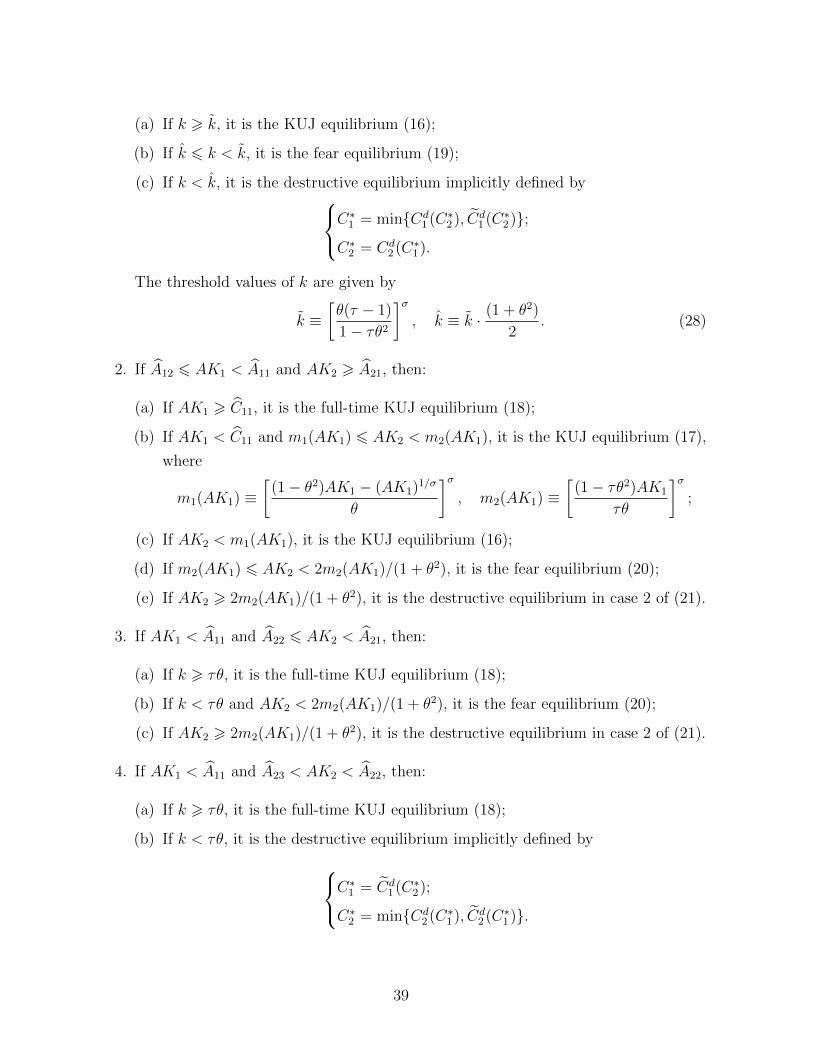
(a) If k > k, it is the KUJ equilibrium (16);

(b) If k 6 k < k, it is the fear equilibrium (19);

(c) If k < k, it is the destructive equilibrium implicitly defined byC∗1 = min{Cd1 (C∗2), Cd

1 (C∗2)};

C∗2 = Cd2 (C∗1).

The threshold values of k are given by

k ≡[θ(τ − 1)

1− τθ2

]σ, k ≡ k · (1 + θ2)

2. (28)

2. If A12 6 AK1 < A11 and AK2 > A21, then:

(a) If AK1 > C11, it is the full-time KUJ equilibrium (18);

(b) If AK1 < C11 and m1(AK1) 6 AK2 < m2(AK1), it is the KUJ equilibrium (17),

where

m1(AK1) ≡[

(1− θ2)AK1 − (AK1)1/σ

θ

]σ, m2(AK1) ≡

[(1− τθ2)AK1

τθ

]σ;

(c) If AK2 < m1(AK1), it is the KUJ equilibrium (16);

(d) If m2(AK1) 6 AK2 < 2m2(AK1)/(1 + θ2), it is the fear equilibrium (20);

(e) If AK2 > 2m2(AK1)/(1 + θ2), it is the destructive equilibrium in case 2 of (21).

3. If AK1 < A11 and A22 6 AK2 < A21, then:

(a) If k > τθ, it is the full-time KUJ equilibrium (18);

(b) If k < τθ and AK2 < 2m2(AK1)/(1 + θ2), it is the fear equilibrium (20);

(c) If AK2 > 2m2(AK1)/(1 + θ2), it is the destructive equilibrium in case 2 of (21).

4. If AK1 < A11 and A23 < AK2 < A22, then:

(a) If k > τθ, it is the full-time KUJ equilibrium (18);

(b) If k < τθ, it is the destructive equilibrium implicitly defined byC∗1 = Cd1 (C∗2);

C∗2 = min{Cd2 (C∗1), Cd

2 (C∗1)}.

39

References

Aghion, Philippe, Eve Caroli, and Cecilia Garcıa-Penalosa, “Inequality and Eco-

nomic Growth: The Perspective of the New Growth Theories,” Journal of Economic

Literature, December 1999, 37 (4), 1615–1660.

Banerjee, Abhijit, “Envy,” in Bhaskar Dutta, Shubhashis Gangopadhyay, Debraj Ray,

and Dilip Mookherjee, eds., Economic Theory and Policy: Essays in Honour of Dipak

Banerjee, New York: Oxford University Press, 1990, pp. 91–111.

Barnett, Richard C., Joydeep Bhattacharya, and Helle Bunzel, “Choosing to

Keep up with the Joneses and Income Inequality,” Economic Theory, December 2010,

45 (3), 469–496.

Belk, Russell W., Collecting in a Consumer Society, London: Routledge, 1995.

Benhabib, Jess, Alberto Bisin, and Matthew Jackson, eds, Handbook of Social

Economics, Vol. 1, Elsevier, 2011.

Boskin, Michael J. and Eytan Sheshinski, “Optimal Redistributive Taxation when

Individual Welfare Depends upon Relative Income,” Quarterly Journal of Economics,

November 1978, 92 (4), 589–601.

Bowles, Samuel and Yongjin Park, “Emulation, Inequality, and Work Hours: Was

Thorsten Veblen Right?,” Economic Journal, November 2005, 115 (507), F397–F412.

Cancian, Frank, Economics and Prestige in a Maya Community, Stanford, CA: Stanford

University Press, 1965.

Card, David, Alexandre Mas, Enrico Moretti, and Emmanuel Saez, “Inequality

at Work: The Effect of Peer Salaries on Job Satisfaction,” American Economic Review,

October 2012, 102 (6), 2981–3003.

Carroll, Christopher D., Jody R. Overland, and David N. Weil, “Comparison

Utility in a Growth Model,” Journal of Economic Growth, December 1997, 2 (4),

339–367.

Clanton, Gordon, “Jealousy and Envy,” in Jan E. Stets and Jonathan H. Turner, eds.,

Handbook of the Sociology of Emotions, Berlin: Springer, 2006, chapter 18, pp. 410–

442.

40

Clark, Andrew E. and Claudia Senik, “Who Compares to Whom? The Anatomy of

Income Comparisons in Europe,” Economic Journal, May 2010, 120, 573–594.

, Paul Frijters, and Michael Shields, “Relative Income, Happiness and Utility:

An Explanation for the Easterlin Paradox and Other Puzzles,” Journal of Economic

Literature, June 2008, 46 (1), 95–144.

Clark, Anrew E. and Andrew J. Oswald, “Comparison-Concave Utility and Following

Behaviour in Social and Economic Settings,” Journal of Public Economics, October

1998, 70 (1), 133–155.

Corneo, Giacomo and Olivier Jeanne, “Social Organization, Status, and Savings

Behavior,” Journal of Public Economics, October 1998, 70 (1), 37–51.

Cozzi, Guido, “Rat Race, Redistribution, and Growth,” Review of Economic Dynamics,

October 2004, 7 (4), 900–915.

D’Arms, Justin and Alison Duncan Kerr, “Envy in the Philosophical Tradition,” in

Richard H. Smith, ed., Envy: Theory and Research, Oxford University Press, 2008,

chapter 3, pp. 39–59.

Demsetz, Harold, “Toward a Theory of Property Rights,” American Economic Review,

May 1967, 57 (2), 347–359.

Doepke, Matthias and Fabrizio Zilibotti, “Occupational Choice and the Spirit of

Capitalism,” Quarterly Journal of Economics, May 2008, 123 (2), 747–793.

Dow, James, “The Image of Limited Production: Envy and the Domestic Mode of Pro-

duction in Peasant Society,” Human Organization, Winter 1981, 40 (4), 360–363.

Dupor, Bill and Wen-Fang Liu, “Jealousy and Equilibrium Overconsumption,” Amer-

ican Economic Review, March 2003, 93 (1), 423–428.

Elster, Jon, “Envy in Social Life,” in Richard J. Zeckhauser, ed., Strategy and Choice,

Cambridge, MA: MIT Press, 1991, chapter 3, pp. 49–82.

Falk, Armin and Markus Knell, “Choosing the Joneses: Endogenous Goals and Refer-

ence Standards,” Scandinavian Journal of Economics, October 2004, 106 (3), 417–435.

Fernandez de la Mora, Gonzalo, Egalitarian Envy: The Political Foundations of Social

Justice, New York: Paragon House Publishers, 1987.

41

Fernandez, Raquel, “Does Culture Matter?,” in Jess Benhabib, Alberto Bisin, and

Matthew Jackson, eds., Handbook of Social Economics, Vol. 1, Elsevier, 2011, chap-

ter 11, pp. 481–510.

Fliessbach, K., B. Weber, P. Trautner, T. Dohmen, U. Sunde, C.E. Elger, and

A. Falk, “Social Comparison Affects Reward-Related Brain Activity in the Human

Ventral Striatum,” Science, 2007, 318 (5854), 1305–1308.

Foster, George, “The Anatomy of Envy: A Study in Symbolic Behavior,” Current An-

thropology, April 1972, 13 (2), 165–202.

, Tzintzuntzan: Mexican Peasants in a Changing World, New York: Elsevier, 1979.

Frank, Robert H., “The Demand for Unobservable and Other Nonpositional Goods,”

American Economic Review, March 1985, 75 (1), 101–116.

, Falling Behind: How Rising Inequality Harms the Middle Class, Berkeley: University

of California Press, 2007.

and Ori Heffetz, “Preferences for Status: Evidence and Economic Implications,”

in Jess Benhabib, Alberto Bisin, and Matthew Jackson, eds., Handbook of Social

Economics, New York: Elsevier, 2011, chapter 3.

Galor, Oded and Stelios Michalopoulos, “Evolution and the Growth Process: Natural

Selection of Entrepreneurial Traits,” Journal of Economic Theory, 2012, 147, 759–780.

Gershman, Boris, “Economic Development, Institutions, and Culture Through the Lens

of Envy.” PhD dissertation, Brown University 2012.

, “The Economic Origins of the Evil Eye Belief,” June 2014. Working Paper, American

University.

Graham, Carol, Happiness Around the World. The Paradox of Happy Peasants and

Miserable Millionaires, Oxford University Press, 2010.

Grossman, Herschel I. and Minseong Kim, “Swords or Plowshares? A Theory of the

Security of Claims to Property,” Journal of Political Economy, December 1995, 103

(6), 1275–88.

42

and , “Predation and Production,” in Michelle R. Garfinkel and Stergios Skaper-

das, eds., The Political Economy of Conflict and Appropriation, Cambridge, MA:

Cambridge University Press, 1996, chapter 4, pp. 57–72.

Hopkins, Ed, “Inequality, Happiness and Relative Concerns: What Actually is Their

Relationship?,” Journal of Economic Inequality, December 2008, 6 (4), 351–372.

and Tatiana Kornienko, “Running to Keep in the Same Place: Consumer Choice

as a Game of Status,” American Economic Review, September 2004, 94 (4), 1085–

1107.

Knell, Markus, “Social Comparisons, Inequality, and Growth,” Journal of Institutional

and Theoretical Economics, December 1999, 155 (4), 664–695.

Ljungqvist, Lars and Harald Uhlig, “Tax Policy and Aggregate Demand Management

under Catching Up with the Joneses,” American Economic Review, June 2000, 90 (3),

356–366.

Luttmer, Erzo F., “Neighbors as Negatives: Relative Earnings and Well-Being,” Quar-

terly Journal of Economics, August 2005, 120 (3), 963–1002.

Matt, Susan J., Keeping Up with the Joneses: Envy in American Consumer Society,

1890–1930, Philadelphia: University of Pennsylvania Press, 2003.

Mitsopoulos, Michael, “Envy, Institutions and Growth,” Bulletin of Economic Research,

July 2009, 61 (3), 201–222.

Moav, Omer and Zvika Neeman, “Saving Rates and Poverty: The Role of Conspicuous

Consumption and Human Capital,” Economic Journal, September 2012, 122 (563),

933–956.

Mui, Vai-Lam, “The Economics of Envy,” Journal of Economic Behavior & Organization,

May 1995, 26 (3), 311–336.

Nash, June, In the Eyes of the Ancestors: Belief and Behavior in a Maya Community,

New Haven: Yale University Press, 1970.

Neumark, David and Andrew Postlewaite, “Relative Income Concerns and the Rise

in Married Women’s Employment,” Journal of Public Economics, October 1998, 70

(1), 157–183.

43

Oswald, Andrew J., “Altruism, Jealousy and the Theory of Optimal Non-Linear Taxa-

tion,” Journal of Public Economics, February 1983, 20 (1), 77–87.

Park, Yongjin, “The Second Paycheck to Keep Up With the Joneses: Relative Income

Concerns and Labor Market Decisions of Married Women,” Eastern Economic Jour-

nal, Spring 2010, 36, 255–276.

Perez-Asenjo, Eduardo, “If Happiness is Relative, Against Whom Do We Compare Our-

selves? Implications for Labour Supply,” Journal of Population Economics, October

2011, 24 (4), 1411–1442.

Platteau, Jean-Philippe, Institutions, Social Norms, and Economic Development, Har-

wood Academic Publishers, 2000.

Robson, Arthur J. and Larry Samuelson, “The Evolutionary Foundations of Pref-

erences,” in Jess Benhabib, Alberto Bisin, and Matthew Jackson, eds., Handbook of

Social Economics, New York: Elsevier, 2011, chapter 4.

Rustichini, Aldo, “Dominance and Competition,” Journal of the European Economic

Association, April–May 2008, 6 (2–3), 647–656.

Schoeck, Helmut, Envy: A Theory of Social Behavior, New York: Harcourt, Brace, and

World, 1969.

Schor, Juliet B., The Overworked American: The Unexpected Decline of Leisure, New

York: Basic Books, 1991.

Scott, James C., The Moral Economy of the Peasant: Rebellion and Subsistence in

Southeast Asia, New Haven, CT: Yale University Press, 1976.

Smith, Richard H. and Sung H. Kim, “Comprehending Envy,” Psychological Bulletin,

January 2007, 133 (1), 46–64.

Solnick, Sara J. and David Hemenway, “Are Positional Concerns Stronger in Some

Domains than in Others?,” American Economic Review Papers and Proceedings, May

2005, 95 (2), 147–151.

van de Ven, Niels, Marcel Zeelenberg, and Rik Pieters, “Leveling Up and Down:

The Experiences of Benign and Malicious Envy,” Emotion, June 2009, 9 (3), 419–429.

44

Veblen, Thorstein B., “Some Neglected Points in the Theory of Socialism,” Annals of

the American Academy of Political and Social Science, November 1891, 2 (3), 57–74.

Wolf, Eric R., “Types of Latin American Peasantry: A Preliminary Discussion,” Amer-

ican Anthropologist, June 1955, 57 (3, Part 1), 452–471.

Zizzo, Daniel J., “Money Burning and Rank Egalitarianism with Random Dictators,”

Economics Letters, November 2003, 81 (2), 263–266.

, “The Cognitive and Behavioral Economics of Envy,” in Richard H. Smith, ed., Envy:

Theory and Research, Oxford University Press, 2008, chapter 11, pp. 190–210.

45

Supplementary Appendix A

“The Two Sides of Envy”

Journal of Economic Growth

Boris Gershman∗

This appendix contains the proofs of all statements from “The Two Sides of Envy.”

A Proofs

Proof of Lemma 1. As follows from (8), d∗2 = 0 iff Y2/Y1 > τθ(1 − d1)(1 + τd1). This clearly holds, if

d1 = 0, since τθ < 1 and Y2 > Y1. If d1 = (√τθY2/Y1 − 1)/τ > 0, the above inequality is equivalent to√Y2Y1

>θ(1 + τ)

√τθ

1 + τθ2.

Since Y2 > Y1, this would always hold if the right-hand side is less or equal than unity, that is, θ√τθ 6

(1+τθ2)/(1+τ). Since τ < 1/θ, sup{θ√τθ} = inf{(1+τθ2)/(1+τ)} = θ. Hence, θ

√τθ 6 (1+τθ2)/(1+τ),

given that τθ < 1 and Y2 > Y1, and lemma 1 gives the unique second-stage equilibrium.

Proof of Lemma 2. Agent 2 is solving (11) subject to (9). First, consider the case Y2 6 Y1/τθ, in which

d∗1 = 0 and

U2 =(Y2 − θY1)1−σ

1− σ− Y2AK2

is strictly concave in Y2. Since Y2 6 AK2, there are two subcases.

1) If Y1 6 τθAK2, the first-order conditions yield

Y2 =

θY1 + (AK2)1/σ, if Y1 > C12;

Y1 · 1τθ , if Y1 < C12.

(A.1)

Since in this subcase Y1 6 τθAK2, for AK2 > A21 the best response of Agent 2 is given by (A.1), while

for AK2 < A21 it is just Y2 = Y1/τθ.

2) If Y1 > τθAK2, the first-order conditions yield

Y2 =

AK2, if Y1 > C11;

θY1 + (AK2)1/σ, if Y1 < C11.(A.2)

Since in this subcase Y1 > τθAK2, for AK2 > A21 the best response of Agent 2 is given by (A.2), while

for AK2 < A21 it is just Y2 = AK2.

∗Department of Economics, American University, 4400 Massachusetts Avenue NW, Washington, DC

20016-8029 (e-mail: [email protected]).

1

Putting the two subcases together we obtain the best-response function for the case Y2 6 Y1/τθ:

Y2 =

AK2, if Y1 > C11;

θY1 + (AK2)1/σ, if C12 6 Y1 < C11;

Y1 · 1τθ , if Y1 < C12,

for AK2 > A21;

AK2, if Y1 > C14;

Y1 · 1τθ , if Y1 < C14,

for AK2 < A21.

(A.3)

Now consider the destructive case, Y2 > Y1/τθ, in which

U2 =1

1− σ·

(√Y1Y2τθ· (1 + θ2)− θ(τ + 1)

τY1

)1−σ

− Y2AK2

is strictly concave in Y2. Since Y2 6 AK2, the only relevant case to consider is when Y1 < τθAK2. The

interior optimum, Y d2 (Y1), is uniquely defined by the first-order condition

ω2(Y1, Y2) ≡

(√Y1Y2τθ· (1 + θ2)− θ(τ + 1)

τY1

)−σ·

(1 + θ2

2√τθ·√Y1Y2

)− 1

AK2= 0. (A.4)

The right derivative of U2 at point Y2 = Y1/τθ is positive (negative) iff Y1 < C13 (Y1 > C13). Furthermore,

C13 < τθAK2 iff AK2 > A22, and C13 < C12, since θ ∈ (0, 1).

Next, consider the right derivative of U2 at point Y2 = AK2, that is, ω2(Y1, AK2). Equation (9) implies

that for Y2 = AK2 the minimal Y1 that can guarantee that d∗1 6 1 is equal to Y1 ≡ τθAK2/(1 + τ)2 which

corresponds to C1 = 0. Since consumption of Agent 1 will always be positive in equilibrium, we focus on

the analysis of ω2(Y1, AK2) for Y1 ∈ [Y1, τθAK2]. It is straightforward to show that: a) ω2(Y1, AK2) < 0

iff AK2 > A23; b) ω′2(Y ∗1 , AK2) = 0, where

Y ∗1 ≡[σ − 1

σ − 1/2· 1 + θ2

2θ2(1 + τ)

]2· τθAK2;

c) ω2(τθAK2, AK2) > 0 iff AK2 < A22. It follows from these properties and the intermediate value

theorem that on the segment [Y1, τθAK2] the function ω2(Y1, AK2) has a unique root Y15, if AK2 6 A22,

and no roots, if AK2 > A22, in which case ω2(Y1, AK2) is negative on the whole segment.

The preceding analysis implies that for the case Y2 > Y1/τθ the best response function is

Y2 =

Y1 · 1τθ , if C13 6 Y1 < τθAK2;

Y d2 (Y1), if Y1 < Y1 < C13,for AK2 > A22;AK2, if Y15 6 Y1 < τθAK2;

Y d2 (Y1), if Y1 < Y1 < Y15,for A23 < AK2 < A22.

(A.5)

To express (A.5) in terms of consumption, as stated in lemma 2, note that if destruction takes placeC1 = (1− d∗1)Y1 =

1 + τ

τY1 −

√θ

τY1Y2;

C2 = p∗2Y2 =

√Y1Y2τθ

.

=⇒

Y1 =

τ

1 + τ(C1 + θC2);

Y2 = θ(1 + τ) · C22

C1 + θC2.

(A.6)

2

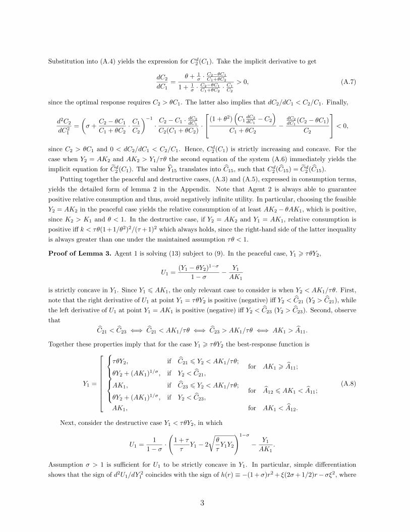
Substitution into (A.4) yields the expression for Cd2 (C1). Take the implicit derivative to get

dC2

dC1=

θ + 1σ ·

C2−θC1

C1+θC2

1 + 1σ ·

C2−θC1

C1+θC2· C1

C2

> 0, (A.7)

since the optimal response requires C2 > θC1. The latter also implies that dC2/dC1 < C2/C1. Finally,

d2C2

dC21

=

(σ +

C2 − θC1

C1 + θC2· C1

C2

)−1·C2 − C1 · dC2

dC1

C2(C1 + θC2)·

(1 + θ2)(C1

dC2

dC1− C2

)C1 + θC2

−dC2

dC1(C2 − θC1)

C2

< 0,

since C2 > θC1 and 0 < dC2/dC1 < C2/C1. Hence, Cd2 (C1) is strictly increasing and concave. For the

case when Y2 = AK2 and AK2 > Y1/τθ the second equation of the system (A.6) immediately yields the

implicit equation for Cd2 (C1). The value Y15 translates into C15, such that Cd2 (C15) = Cd2 (C15).

Putting together the peaceful and destructive cases, (A.3) and (A.5), expressed in consumption terms,

yields the detailed form of lemma 2 in the Appendix. Note that Agent 2 is always able to guarantee

positive relative consumption and thus, avoid negatively infinite utility. In particular, choosing the feasible

Y2 = AK2 in the peaceful case yields the relative consumption of at least AK2 − θAK1, which is positive,

since K2 > K1 and θ < 1. In the destructive case, if Y2 = AK2 and Y1 = AK1, relative consumption is

positive iff k < τθ(1+1/θ2)2/(τ +1)2 which always holds, since the right-hand side of the latter inequality

is always greater than one under the maintained assumption τθ < 1.

Proof of Lemma 3. Agent 1 is solving (13) subject to (9). In the peaceful case, Y1 > τθY2,

U1 =(Y1 − θY2)1−σ

1− σ− Y1AK1

is strictly concave in Y1. Since Y1 6 AK1, the only relevant case to consider is when Y2 < AK1/τθ. First,

note that the right derivative of U1 at point Y1 = τθY2 is positive (negative) iff Y2 < C21 (Y2 > C21), while

the left derivative of U1 at point Y1 = AK1 is positive (negative) iff Y2 < C23 (Y2 > C23). Second, observe

that

C21 < C23 ⇐⇒ C21 < AK1/τθ ⇐⇒ C23 > AK1/τθ ⇐⇒ AK1 > A11.

Together these properties imply that for the case Y1 > τθY2 the best-response function is

Y1 =

τθY2, if C21 6 Y2 < AK1/τθ;

θY2 + (AK1)1/σ, if Y2 < C21,for AK1 > A11;AK1, if C23 6 Y2 < AK1/τθ;

θY2 + (AK1)1/σ, if Y2 < C23,for A12 6 AK1 < A11;

AK1, for AK1 < A12.

(A.8)

Next, consider the destructive case Y1 < τθY2, in which

U1 =1

1− σ·

(1 + τ

τY1 − 2

√θ

τY1Y2

)1−σ

− Y1AK1

.

Assumption σ > 1 is sufficient for U1 to be strictly concave in Y1. In particular, simple differentiation

shows that the sign of d2U1/dY21 coincides with the sign of h(r) ≡ −(1 +σ)r2 + ξ(2σ+ 1/2)r−σξ2, where

3

r ≡√θY2/τY1 and ξ ≡ (τ + 1)/τ . It is easy to show that the maximum value of h is proportional to

1 − 8σ < 0 and so, U1 is concave under σ > 1. The interior optimum, Y d1 (Y2), is given by the first-order

condition:

ω1(Y2, Y1) ≡

(1 + τ

τY1 − 2

√θ

τY1Y2

)−σ·

(1 + τ

τ−√θ

τ· Y2Y1

)− 1

AK1= 0. (A.9)

Since Y1 6 AK1 there are two subcases.

1) Consider the subcase Y2 > AK1/τθ. Consider the left derivative of U1 at point Y1 = AK1, that is,

ω1(Y2, AK1). Under assumption (10) the following properties hold: a) ω1(AK1/τθ,AK1) > 0 iff AK1 <

A11; b) ω′1(Y2, AK1) > 0 for Y2 > AK1/τθ; c) limY2→Y2ω1(Y2, AK1) = +∞, where Y2 ≡ (1+τ)2AK1/4τθ.

Hence, by the intermediate value theorem, for AK1 > A11 there exists a unique value Y22 such that

ω1(Y22, AK1) = 0. Altogether for this subcase the best response of Agent 1 is Y1 = AK1 for AK1 < A11,

while for AK1 > A11 it is Y1 = AK1, if Y2 > Y22, and Y d1 (Y2), otherwise.

2) Now consider the subcase Y2 6 AK1/τθ. Note that the right derivative of U1 at point Y1 = τθY2

is positive iff Y2 < C21. Hence, for AK1 > A11 the best response is Y1 = τθY2, if Y2 < C21, and Y d1 (Y2),

otherwise. For AK1 < A11 the best response is Y1 = τθY2 for any Y2 6 AK1/τθ.

Putting the two subcases together we obtain the best-response function for the case Y1 < τθY2:

Y1 =

AK1, if Y2 > Y22;

Y d1 (Y2), if C21 6 Y2 < Y22;

τθY2, if Y2 < C21,

for AK1 > A11;

AK1, if Y2 > AK1/τθ;

τθY2, if Y2 < AK1/τθ,for AK1 < A11.

(A.10)

Substitute of (A.6) into (A.9) yields the expression for Cd1 (C2). Take the implicit derivative to get

dC1

dC2=

θ − θσ ·

C1−θC2

C1+θC2

1− θσ ·

C1−θC2

C1+θC2· C2

C1

> 0, (A.11)

since σ > 1 and the optimal response requires C1 > θC2. The latter also implies that dC1/dC2 < C1/C2.

Finally,

d2C1

dC22

=θ

σ

(1− θ

σ· C1 − θC2

C1 + θC2· C2

C1

)−1 θ(dC1

dC2· C2

C1− 1)2

C1 + θC2+

(C1 − θC2)(dC1

dC2+ θ)(

1− dC1

dC2· C2

C1

)(C1 + θC2)2

> 0,

since σ > 1, C1 > θC2, and dC1/dC2 < C1/C2. Hence, Cd1 (C2) is strictly increasing and convex. For the

case when Y1 = AK1 and AK1 < τθY2 the top equation in (A.6) immediately yields the expression for

Cd1 (C2). The value for Y22 translates into C22, such that Cd1 (C22) = Cd1 (C22). Putting together the peaceful

and destructive cases, (A.8) and (A.10), expressed in consumption terms, yields the detailed statement of

lemma 3 in the Appendix. Note that Agent 1 is always able to guarantee positive relative consumption

and thus, avoid negatively infinite utility. In particular, choosing the feasible Y1 = AK1 in the peaceful

case yields the relative consumption of at least AK1 − θAK2 which is positive, since the condition for the

peaceful case K1 > τθK2 and τ > 1 imply that K1 > θK2. In the destructive case, if Y1 = AK1 and

Y2 = AK2, relative consumption is positive iff k > 4τθ/(1 + τ)2 which holds by assumption (10).

4

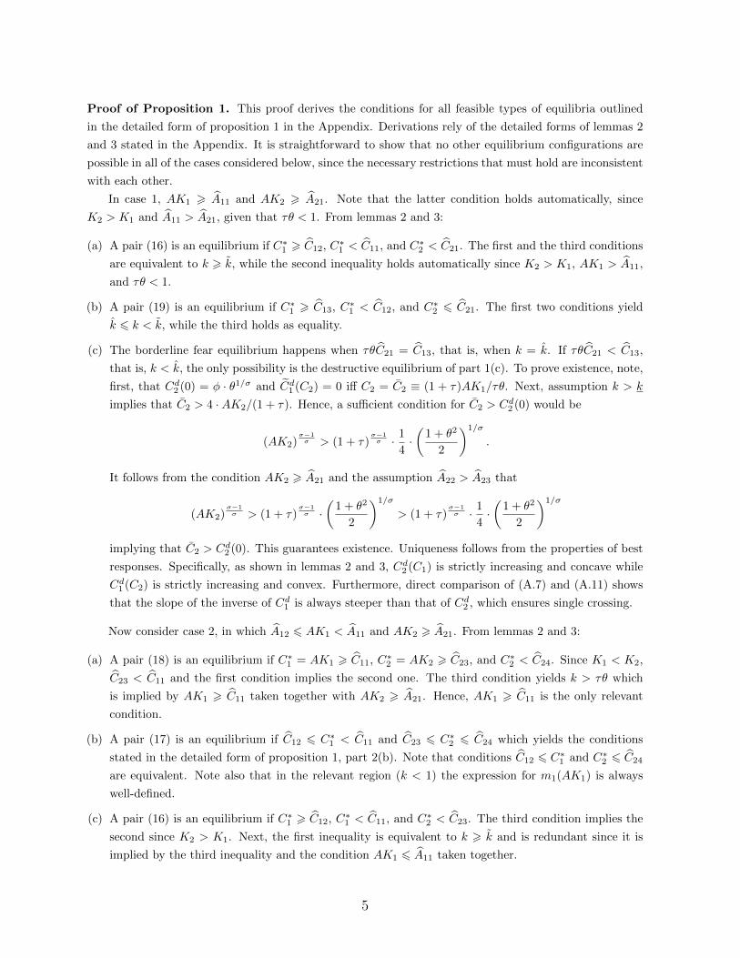
Proof of Proposition 1. This proof derives the conditions for all feasible types of equilibria outlined

in the detailed form of proposition 1 in the Appendix. Derivations rely of the detailed forms of lemmas 2

and 3 stated in the Appendix. It is straightforward to show that no other equilibrium configurations are

possible in all of the cases considered below, since the necessary restrictions that must hold are inconsistent

with each other.

In case 1, AK1 > A11 and AK2 > A21. Note that the latter condition holds automatically, since

K2 > K1 and A11 > A21, given that τθ < 1. From lemmas 2 and 3:

(a) A pair (16) is an equilibrium if C∗1 > C12, C∗1 < C11, and C∗2 < C21. The first and the third conditions

are equivalent to k > k, while the second inequality holds automatically since K2 > K1, AK1 > A11,

and τθ < 1.

(b) A pair (19) is an equilibrium if C∗1 > C13, C∗1 < C12, and C∗2 6 C21. The first two conditions yield

k 6 k < k, while the third holds as equality.

(c) The borderline fear equilibrium happens when τθC21 = C13, that is, when k = k. If τθC21 < C13,

that is, k < k, the only possibility is the destructive equilibrium of part 1(c). To prove existence, note,

first, that Cd2 (0) = φ · θ1/σ and Cd1 (C2) = 0 iff C2 = C2 ≡ (1 + τ)AK1/τθ. Next, assumption k > k

implies that C2 > 4 ·AK2/(1 + τ). Hence, a sufficient condition for C2 > Cd2 (0) would be

(AK2)σ−1σ > (1 + τ)

σ−1σ · 1

4·(

1 + θ2

2

)1/σ

.

It follows from the condition AK2 > A21 and the assumption A22 > A23 that

(AK2)σ−1σ > (1 + τ)

σ−1σ ·

(1 + θ2

2

)1/σ

> (1 + τ)σ−1σ · 1

4·(

1 + θ2

2

)1/σ

implying that C2 > Cd2 (0). This guarantees existence. Uniqueness follows from the properties of best

responses. Specifically, as shown in lemmas 2 and 3, Cd2 (C1) is strictly increasing and concave while

Cd1 (C2) is strictly increasing and convex. Furthermore, direct comparison of (A.7) and (A.11) shows

that the slope of the inverse of Cd1 is always steeper than that of Cd2 , which ensures single crossing.

Now consider case 2, in which A12 6 AK1 < A11 and AK2 > A21. From lemmas 2 and 3:

(a) A pair (18) is an equilibrium if C∗1 = AK1 > C11, C∗2 = AK2 > C23, and C∗2 < C24. Since K1 < K2,

C23 < C11 and the first condition implies the second one. The third condition yields k > τθ which

is implied by AK1 > C11 taken together with AK2 > A21. Hence, AK1 > C11 is the only relevant

condition.

(b) A pair (17) is an equilibrium if C12 6 C∗1 < C11 and C23 6 C∗2 6 C24 which yields the conditions

stated in the detailed form of proposition 1, part 2(b). Note that conditions C12 6 C∗1 and C∗2 6 C24

are equivalent. Note also that in the relevant region (k < 1) the expression for m1(AK1) is always

well-defined.

(c) A pair (16) is an equilibrium if C∗1 > C12, C∗1 < C11, and C∗2 < C23. The third condition implies the

second since K2 > K1. Next, the first inequality is equivalent to k > k and is redundant since it is

implied by the third inequality and the condition AK1 6 A11 taken together.

5

(d) A pair (20) is an equilibrium if C13 6 C∗1 < C12, C∗2 6 C24, and C∗2 > C23. The first two inequalities

yield the conditions stated in the detailed form of proposition 1, part 2(d). The third condition holds

as equality, while the last one is equivalent to AK1 6 A11 presumed to hold for this case.

(e) The borderline fear equilibrium happens when AK1 = C13. If AK1 < C13, the only possibility is the

destructive equilibrium from part 2(e). For the proof of existence see case 1(c); uniqueness follows

immediately from the properties of Cd1 (C2) and Cd2 (C1).

Consider case 3, in which AK1 < A11 and A22 6 AK2 < A21. Technically, this case covers two

subcases depending on how AK1 compares to A12. However, they yield the same results. Note also that

the subregion in which AK1 < A12 exists iff A12 > k · A22. From lemmas 2 and 3:

(a) If AK1 > A12, a pair (18) is an equilibrium if C∗1 > C14, C∗2 > C23, and C∗2 6 C24. The first and the

third inequalities are equivalent to k > τθ, while the second inequality is implied by K2 > K1 together

with the conditions AK2 < A21 and τθ < 1. If AK1 < A12, the only two conditions are C∗1 > C14 and

C∗2 < C24 yielding again k > τθ.

(b) If AK1 > A12, a pair (20) is an equilibrium if C13 6 C∗1 < C14, C∗2 > C23 and C∗2 6 C24. The last

inequality holds as equality, while the third one is implied by AK1 < A11. The first two conditions yield

those stated in the detailed form of proposition 1, part 3(b). If AK1 < A12, the relevant conditions

are C13 6 C∗1 < C14 and C∗2 6 C24 yielding the same set of restrictions as for AK1 > A12.

(c) See the proof for case 2(e) above.

Finally, consider case 4, in which AK1 < A11 and A23 < AK2 < A22. Technically, this case covers

two subcases depending on how AK1 compares to A12. However, they yield the same results. Note also

that the subregion in which AK1 < A12 exists iff A12 > k · A23, and the other subregion only exists iff

A12 < A22. From lemmas 2 and 3:

(a) See the proof for case 3(a) above.

(b) The borderline case happens when k = τθ. If k < τθ, the only possibility is the destructive equilibrium

from part 4(b). For the proof of existence see case 1(c); uniqueness follows immediately from the

properties of Cd1 (C2), Cd2 (C1), and Cd2 (C1).

Proof of Proposition 2. The results for cases (16), (19), (18) and (20) follow immediately from the

expressions for individual outputs. For case (17) the effects of θ, τ , and A are straightforward, while for λ

we have ∂C1/∂λ = AK > 0 and∂C2

∂λ=

(θ − 1

σ(AK2)

1−σσ

)AK

which is positive iff AK2 > (σθ)σ

1−σ . It follows that ∂C/∂λ > 0 iff AK2 > [σ(1 + θ)]σ

1−σ which always

holds since for this case AK2 > A21 > 1 and [σ(1 + θ)]σ

1−σ < 1.

For the first case in (21), consider the system defining the equilibrium:{f1 ≡ C1 − θC2 − ψ[C1/(C1 + θC2)]1/σ = 0;

f2 ≡ C2 − θC1 − φ[(C1 + θC2)/C2]1/σ = 0.

6

Using the equilibrium conditions, it can be shown that

[DCf ]−1 =

1

∆1

[1 + 1

σ ·C2−θC1

C1+θC2· C1

C2θ − θ

σ ·C1−θC2

C1+θC2

θ + 1σ ·

C2−θC1

C1+θC21− θ

σ ·C1−θC2

C1+θC2· C2

C1

],

where C is the vector of consumption levels, f is the vector of f1 and f2, and

∆1 ≡ det(DCf) = 1− θ2 +(C1 − θC2)2(C2 − θC1)

σ(C1 + θC2)C1C2> 0.

It follows from this expression that all elements of [DCf ]−1 are positive since σ > 1 and θC1 < C2 < C1/θ

in equilibrium.

For the effects of λ, note that, by the implicit function theorem, DλC = −[DCf ]−1 ·Dλf and

Dλf = −

[ψλψ (C1 − θC2)φλφ (C2 − θC1)

]=

1

σ

[− 1λ (C1 − θC2)1

1−λ (C2 − θC1)

].

It follows that the sign of ∂C1/∂λ coincides with the sign of[1 +

1

σ· C2 − θC1

C1 + θC2· C1

C2

]· (C1 − θC2)− θλ

1− λ·[1− 1

σ· C1 − θC2

C1 + θC2

]· (C2 − θC1).

Dividing (26) by (27) and denoting x ≡ C1/C2 ∈ (θ, 1), in equilibrium we have

λ

1− λ=

(x− θ1− θx

)σ· τ(1 + θ2)

2θ(1 + τ)2· (x+ θ)2

x.

Plugging this expression for λ/(1− λ) in the previous equation and making transformations, we get

σ(θ + x) + x(1− θx)

σ(θ + x)− (x− θ)− τ(1 + θ2)

2(1 + τ)2·(x− θ1− θx

)σ−1· (x+ θ)2

x.

The first term is always greater than 1. The second term is increasing in x and at x = 1 simplifies to

[τ(1 + θ2)(1 + θ)2]/[2(1 + τ)2]. Since τ > 1, the supremum of the latter expression is equal to [(1 + θ2)(1 +

θ)2/4] 6 1 for all θ ∈ (0, 1). Hence, the second term is always less than 1 and ∂C1/∂λ > 0.

Although the sign of ∂C2/∂λ is ambiguous, the sign of ∂C/∂λ is not, as it coincides with that of

σ(1 + θ)(x+ θ) + (1− θx)(1 + x)

σ(1 + θ)(x+ θ)− θ(x− θ)(1 + 1/x)− τ(1 + θ2)

2(1 + τ)2·(x− θ1− θx

)σ−1· (x+ θ)2

x.

As above, the first term of this expression is always greater than 1, while the second is always less than 1.

Hence, ∂C/∂λ > 0.

For the effects of θ, note that DθC = −[DCf ]−1 ·Dθf and

Dθf =

C2 ·(

1σ ·

C1−θC2

C1+θC2− 1)

−C1 + 1σ ·

C2−θC1

C1+θC2· (1−θ

2)C1−2θ3C2

θ(1+θ2)

.It follows that the sign of ∂C1/∂θ is determined by the sign of

C2 + θC1 −1

σ

C2 − θC1

C1 + θC2·(

(1− θ2)C1 − 2θ3C2

1 + θ2− C1

).

7

Since (1− θ2)C1 − 2θ3C2 − (1 + θ2)C1 = −2θ2C1 − 2θ3C2 < 0, it is clear that ∂C1/∂θ > 0. As discussed

in the main text, the sign of ∂C2/∂θ is generally ambiguous.

For the effects of τ and A, note that DτC = −[DCf ]−1 ·Dτ f , DAC = −[DAf ]

−1 ·DAf , where

Dτ f = −

[ψτψ (C1 − θC2)φτφ (C2 − θC1)

], DAf = −

[ψAψ (C1 − θC2)φAφ (C2 − θC1)

].

Both elements of Dτ f are positive, since ψτ < 0 and φτ < 0. It follows that the elements of DτC are

negative, that is, both C1 and C2 are decreasing in τ . Both elements of DAf negative, since ψA > 0 and

φA > 0. It follows that the elements of DAC are positive, that is, both C1 and C2 are increasing in A.

For the second case of (21), consider the system defining this destructive equilibrium:{f1 ≡ C1 + θC2 − (1 + τ)AK1/τ = 0;

f2 ≡ C2 − θC1 − φ[(C1 + θC2)/C2]1/σ = 0.

Using the equilibrium conditions, it can be shown that

[DCf ]−1 =

1

∆2

[1 + 1

σ ·C2−θC1

C1+θC2· C1

C2−θ

θ + 1σ ·

C2−θC1

C1+θC21

],

where C is the vector of consumption levels, f is the vector of f1 and f2, and ∆2 ≡ det(DCf) = 1 + θ2 +

(C2 − θC1)/(σC2) > 0.

For the effects of λ, note that, by the implicit function theorem, DλC = −[DCf ]−1 ·Dλf and

Dλf =

[− 1λ (C1 + θC2)1

(1−λ)σ (C2 − θC1)

].

It follows immediately that ∂C1/∂λ > 0. Given that λ < 1/2, the sign of ∂C2/∂λ coincides with

θ

λ· (C1 + θC2) +

1

σ· (C2 − θC1) ·

(1

λ− 1

1− λ

)> 0.

For the effects of θ, note that DθC = −[DCf ]−1 ·Dθ f and

Dθ f =

[C2

−C1 + 1σ ·

C2−θC1

C1+θC2· (1−θ

2)C1−2θ3C2

θ(1+θ2)

].

It follows that the sign of ∂C1/∂θ coincides with that of

−θC1 − C2 −1

σ· C2 − θC1

C1 + θC2· 2θ2(1 + θC2)

1 + θ2< 0.

Next, although the sign of ∂C2/∂θ is ambiguous, ∂C/∂θ < 0, since

C1 − C2 − θ(C1 + C2)− 1

σ· C2 − θC1

C1 + θC2·(

1 +2θ3 + 2θ4C2 + (1− θ2)C1 − 2θ3C2

θ(1 + θ2)

)< 0,

where C1 < C2 in equilibrium and 2θ4C2 + (1 − θ2)C1 − 2θ3C2 > θC2(1 − 3θ2 + 2θ3) > 0, as C1 > θC2

and θ ∈ (0, 1).

8

For the effects of τ , note that DτC = −[DCf ]−1 ·Dτ f and

Dτ f =1

1 + τ·

[1τ (C1 + θC2)1σ (C2 − θC1)

].

This immediately implies that ∂C2/∂τ < 0. Although the sign of ∂C1/∂τ is ambiguous, the sign of ∂C/∂τ

coincides with that of

−C1 + θC2

τ(1 + τ)·[1 + θ +

1

σ· C2 − θC1

C1 + θC2·(C1

C2+ 1

)]− 1− θ

σ· C2 − θC1

1 + τ< 0.

Finally, for the effects of A, note that DAC = −[DCf ]−1 ·DAf and

DAf = − 1

A·

[C1 + θC2

1σ (C2 − θC1)

].

It follows immediately that ∂C2/∂A > 0. The sign of ∂C1/∂A coincides with that of

1

A·[C1 + θC2 +

C2 − θC1

σ·(C1

C2− θ)]

> 0.

For the thirds case of (21), the equilibrium individual and total consumption levels are given by

C1 = A ·

(1 + τ

τ·K1 −

√θ

τ·K1K2

), C2 = A ·

√K1K2

τθ, C = A ·

(1 + τ

τ·K1 + (1− θ) ·

√K1K2

τθ

).

The positive effect of A and the negative effect of θ on both C1 and C2 are obvious. While τ negatively

affects both C2 and C, its effect on C1 is ambiguous. Specifically, ∂C1/∂τ < 0 iff k > τθ/4. Similarly,

higher λ positively affects both C2 and C, but its effect on C1 is ambiguous.

Proof of Proposition 3. The steady-state levels of A follow immediately from (22). The economy gets

stuck in the fear region iff A∗1 < A which yields

α

1− α<

σ

σ − 1· ln

(τθ

1− τθ2· K

1/σ2

K1

)· 1

ln((1 + 1/τθ)K1)

defining the α threshold. It is straightforward to show that the right-hand side of this inequality is

increasing in τ and θ and decreasing in λ, that is, αθ > 0, αλ < 0, ατ > 0.

If A∗1 > A, then the economy is stuck in the KUJ-type region iff A∗2 < A which yields

α

1− α<

σ

σ − 1· ln

(K

1/σ1 + θK

1/σ2

(1− θ2)K1

)·

(ln

((1 + θ)K1(K

1/σ1 +K

1/σ2 )

K1/σ1 + θK

1/σ2

))−1defining the α threshold. First, note that the right-hand side of the above inequality is independent of

τ , that is, ατ = 0. Next, for the effect of θ, note that the numerator of the right-hand side is increasing

in θ while the denominator is decreasing in θ, since the sign of the respective derivative coincides with

that of K1/σ1 −K1/σ

2 < 0. Hence, αθ > 0. For the effect of λ, note that the numerator of the right-hand

side is decreasing in λ, while the denominator is increasing in λ since the sign of the respective derivative

coincides with that of(λ

1− λ

) 1σ

− 1− σθσ

· λ

1− λ+σ − 1

σ·

(1 +

θ

λ

(1− λλ

) 1−σσ

)+ θ ·

(σ + 1

σ+

(1− λλ

) 1σ

)> 0.

9

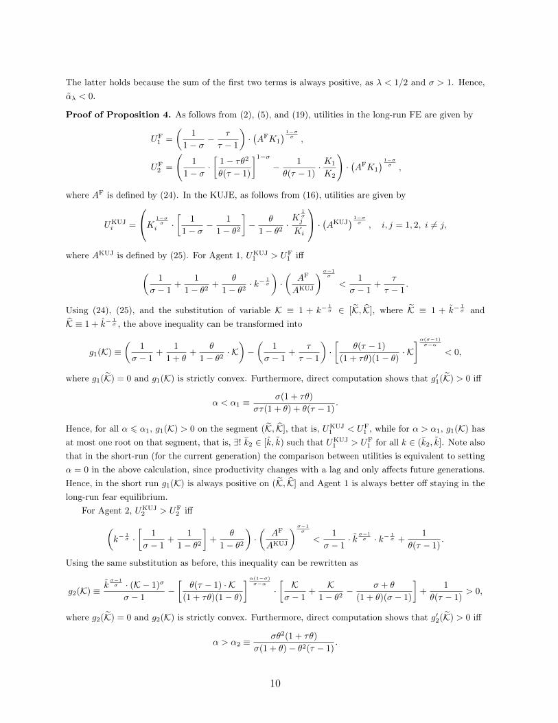
The latter holds because the sum of the first two terms is always positive, as λ < 1/2 and σ > 1. Hence,

αλ < 0.

Proof of Proposition 4. As follows from (2), (5), and (19), utilities in the long-run FE are given by

UF1 =

(1

1− σ− τ

τ − 1

)·(AFK1

) 1−σσ ,

UF2 =

(1

1− σ·[

1− τθ2

θ(τ − 1)

]1−σ− 1

θ(τ − 1)· K1

K2

)·(AFK1

) 1−σσ ,

where AF is defined by (24). In the KUJE, as follows from (16), utilities are given by

UKUJi =

K 1−σσ

i ·[

1

1− σ− 1

1− θ2

]− θ

1− θ2·K

1σj

Ki

· (AKUJ) 1−σ

σ , i, j = 1, 2, i 6= j,

where AKUJ is defined by (25). For Agent 1, UKUJ1 > UF

1 iff(1

σ − 1+

1

1− θ2+

θ

1− θ2· k− 1

σ

)·(

AF

AKUJ

)σ−1σ

<1

σ − 1+

τ

τ − 1.

Using (24), (25), and the substitution of variable K ≡ 1 + k−1σ ∈ [K, K], where K ≡ 1 + k−

1σ and

K ≡ 1 + k−1σ , the above inequality can be transformed into

g1(K) ≡(

1

σ − 1+

1

1 + θ+

θ

1− θ2· K)−(

1

σ − 1+

τ

τ − 1

)·[

θ(τ − 1)

(1 + τθ)(1− θ)· K]α(σ−1)

σ−α

< 0,

where g1(K) = 0 and g1(K) is strictly convex. Furthermore, direct computation shows that g′1(K) > 0 iff

α < α1 ≡σ(1 + τθ)

στ(1 + θ) + θ(τ − 1).

Hence, for all α 6 α1, g1(K) > 0 on the segment (K, K], that is, UKUJ1 < UF

1 , while for α > α1, g1(K) has

at most one root on that segment, that is, ∃! k2 ∈ [k, k) such that UKUJ1 > UF

1 for all k ∈ (k2, k]. Note also

that in the short-run (for the current generation) the comparison between utilities is equivalent to setting

α = 0 in the above calculation, since productivity changes with a lag and only affects future generations.

Hence, in the short run g1(K) is always positive on (K, K] and Agent 1 is always better off staying in the

long-run fear equilibrium.

For Agent 2, UKUJ2 > UF

2 iff(k−

1σ ·[

1

σ − 1+

1

1− θ2

]+

θ

1− θ2

)·(

AF

AKUJ

)σ−1σ

<1

σ − 1· k

σ−1σ · k− 1

σ +1

θ(τ − 1).

Using the same substitution as before, this inequality can be rewritten as

g2(K) ≡ kσ−1σ · (K − 1)σ

σ − 1−[

θ(τ − 1) · K(1 + τθ)(1− θ)

]α(1−σ)σ−α

·[K

σ − 1+

K1− θ2

− σ + θ

(1 + θ)(σ − 1)

]+

1

θ(τ − 1)> 0,

where g2(K) = 0 and g2(K) is strictly convex. Furthermore, direct computation shows that g′2(K) > 0 iff

α > α2 ≡σθ2(1 + τθ)

σ(1 + θ)− θ2(τ − 1).

10

Hence, for all α > α2, g2(K) > 0 on the segment (K, K], that is, UKUJ2 > UF

2 , while for α < α2, g2(K)

has at most one root on that segment. Since θ ∈ (0, 1) and τθ < 1, we also know that α1 > α2 which leads

to the final statement of the long-run part of the proposition, where α ≡ α1. To complete the statement

of the short-run part of the proposition, note that, for α = 0, g′2(K) < 0 and g2(K) < 0 iff(1

1− θ2+

1

σ − 1

)·(

1 + θ2

2

)σ−1σ

− 1

σ − 1− 1 + θ2

2(1− θ2)> 0.

Let q ≡ (1 + θ2)/2 ∈ (1/2, 1) and s ≡ (σ− 1)/σ ∈ (0, 1). After re-arranging, the above inequality becomes

ϑ(q) ≡ [s+ 2(1− s)(1− q)]qs + (2− 3s)q − 2(1− s) > 0.

Note that: 1) ϑ(1/2) = (1/2)s + s/2 − 1 < 0 since it is strictly convex in s on the (0, 1) interval and is

equal to zero at its endpoints, 2) ϑ(1) = 0, 3) ϑ′(1) = s(s−1) < 0, and 4) ϑ′′(q) < 0. Hence ∃! q ∈ (1/2, 1),

such that ϑ(q) > 0 iff q > q. This implies that ∃! θ ∈ (0, 1), such that g2(K) < 0 (and thus, UKUJ2 < UF

2

in the short run) ∀k ∈ (k, k) iff θ > θ. If θ < θ, ∃! k1 ∈ (k, k), such that UKUJ2 < UF

2 in the short run iff

k > k1. This, along with the fact that Agent 1 is always better off in the FE under α = 0, completes the

proof of the short-run part of the proposition.

Proof of Proposition 5. First, note that both UF1 and UKUJ

1 are strictly increasing in k for Agent 1,

that is, he is always supportive of redistribution. The critical role is thus played by Agent 2. To examine

UF2 and UKUJ

2 as functions of k rewrite the equilibrium utilities as

UF2 (k) =

(1

1− σ· k

σ−1σ − 1

θ(τ − 1)· k)·(

k

1 + k·K) 1−σσ−α

·[

1 + τθ

θ(τ − 1)

] α(1−σ)σ(σ−α)

,

UKUJ2 (k) =

(1

1− σ− 1

1− θ2− θ

1− θ2· k 1

σ

)·(

1

1 + k·K) 1−σσ−α

·

(k

1σ

1− θ

)α(1−σ)σ−α

.

Consider first the behavior of UF2 (k). Direct calculations show that dUF

2 (k)/dk < 0 iff

h1(k) ≡ −(σ − α)k2 − (1− α)k + δ < 0, δ ≡ θ(τ − 1)kσ−1σ .

The short-run part of the proposition corresponds to the case α = 0. In this case, in particular, it is

straightforward to show that h1(k) < 0, that is, the maximum value of h1(k) on [k, k] is strictly less that k.

Furthermore, if h1(k) > 0, h1(k) < 0 (hence, dUF2 (k)/dk < 0) ∀k ∈ [k, k], in which case redistribution to

Agent 1 is never optimal in the fear equilibrium from the viewpoint of Agent 2 (that is, Pareto improving

redistribution towards KUJE is not feasible). If h1(k) > 0, h1(k) has one positive root k∗ =√

1 + 4σδ/(2σ)

falling in the interval [k, k] which is the global maximum of UF2 (k) on that interval. Note that in this latter

case redistribution to KUJE might be Pareto improving for some range of initial k (incidentally, UKUJ2 (k)

is strictly decreasing in k in the short-run case α = 0). Specifically, such range will be non-empty iff

UF2 (k) < UF

2 (k). This inequality is equivalent to

(1 + θ2

2· 1 + k

1 + k

)σ−1σ

<σ + 1 + θ2(σ − 1− 2τ)

2(σ − τθ2). (A.12)

11

Denote the left-hand side of this expression as L1(θ) and the right-hand side of it as R1(θ). First note

that L(0)−R1(0) = (1/2)(σ−1)/σ − 1/(2σ)− 1/2 < 0 since σ > 1. In addition,

L1(1/τ)−R1(1/τ) =

[2(1 + τ2)

1 + 3τ2

]σ−1σ

− 2τ(τ − 1) + (σ − 1)(1 + τ2)

2τ(στ − 1),

which is a strictly increasing function of σ with inf{L1(1/τ)−R1(1/τ)} = 0. Furthermore, simple differen-

tiation shows that R1(θ) is strictly increasing and convex if and only if σ > τ , and it is strictly decreasing

and concave if and only if σ < τ . The left-hand side L1(θ) is strictly increasing. Hence, in the case when

σ < τ there is a unique ¯θ such that L1(¯θ) = R1(¯θ). For the case σ > τ , rewrite (A.12) as

1 + θ2

2· (1 + k) < R1(θ)

σσ−1 · (1 + k).

Both sides of this inequality are strictly increasing and convex in θ as products of strictly increasing positive

convex functions. Given that L1(0) < R1(0) and L1(1/τ) > R1(1/τ), this implies a single intersection, as

in the case with σ < τ . Putting together the two cases yields the short-run part of the proposition.

Now examine the long-run equilibrium value of UKUJ2 (k). Direct calculations show that the sign of

dUKUJ2 (k)/dk coincides with that of h2(k) ≡ L2(k)−R2(k), where

L2(k) ≡ ρ2 ·ρ3 − ρ4k

1σ

1 + k1σ

, R2(k) ≡ σρ1 ·ρ3k

σ−1σ − ρ4k

1 + k+ ρ4,

and

ρ1 ≡1− σσ − α

< 0, ρ2 ≡α(1− σ)

σ − α< 0, ρ3 ≡

1

1− σ− 1

1− θ2< 0, ρ4 ≡

θ

1− θ2> 0.

Direct calculation also shows that h2(1) = −(σ − θ)/[2(1− θ)]− θ/(1− θ2) < 0, that is, redistribution up

to perfect equality (k = 1) is never optimal for Agent 2. Next,

dL2(k)

dk= −ρ2(ρ3 + ρ4)

σ· k

1−σσ

(1 + k1σ )2

< 0,

since ρ2 < 0 and ρ3 + ρ4 < 0. Furthermore, d2L2(k)/dk2 > 0, that is, L2(k) is a strictly decreasing convex

function of k. On the other hand,

dR2(k)

dk= ρ1 ·

ρ3(σ − 1)k−1σ − ρ3k

σ−1σ − σρ4

(1 + k)2= 0 ⇐⇒ k

1σ =

ρ3σρ4· (σ − 1− k).

The latter equation can have at most one root on the interval [k, 1). Hence, R2(k) is either strictly

increasing or has a unique interior global maximum on [k, 1). It follows that L2(k) and R2(k) have a

unique intersection on [k, 1) iff L2(k) > R2(k). The latter holds iff

α > ¯α ≡ σ · θ(1 + σk) + (σ − θ2)kσ−1σ

θ(1 + σk1σ ) + σ − θ2

· 1 + k1σ

1 + k.

Note that ¯α = 0 for θ = 0 and ¯α = σ > 1 for θ = 1/τ . Hence, by continuity, there is a region of small

enough values of θ such that ¯α < 1. Similarly, ¯α = σθ/(σ+θ−θ2) < 1 for τ = 1 and ¯α = σ > 1 for τ = 1/θ.

Hence, by continuity, there is a region of small enough values of τ such that ¯α < 1. This concludes the

proof of the long-run part of proposition 5.

12

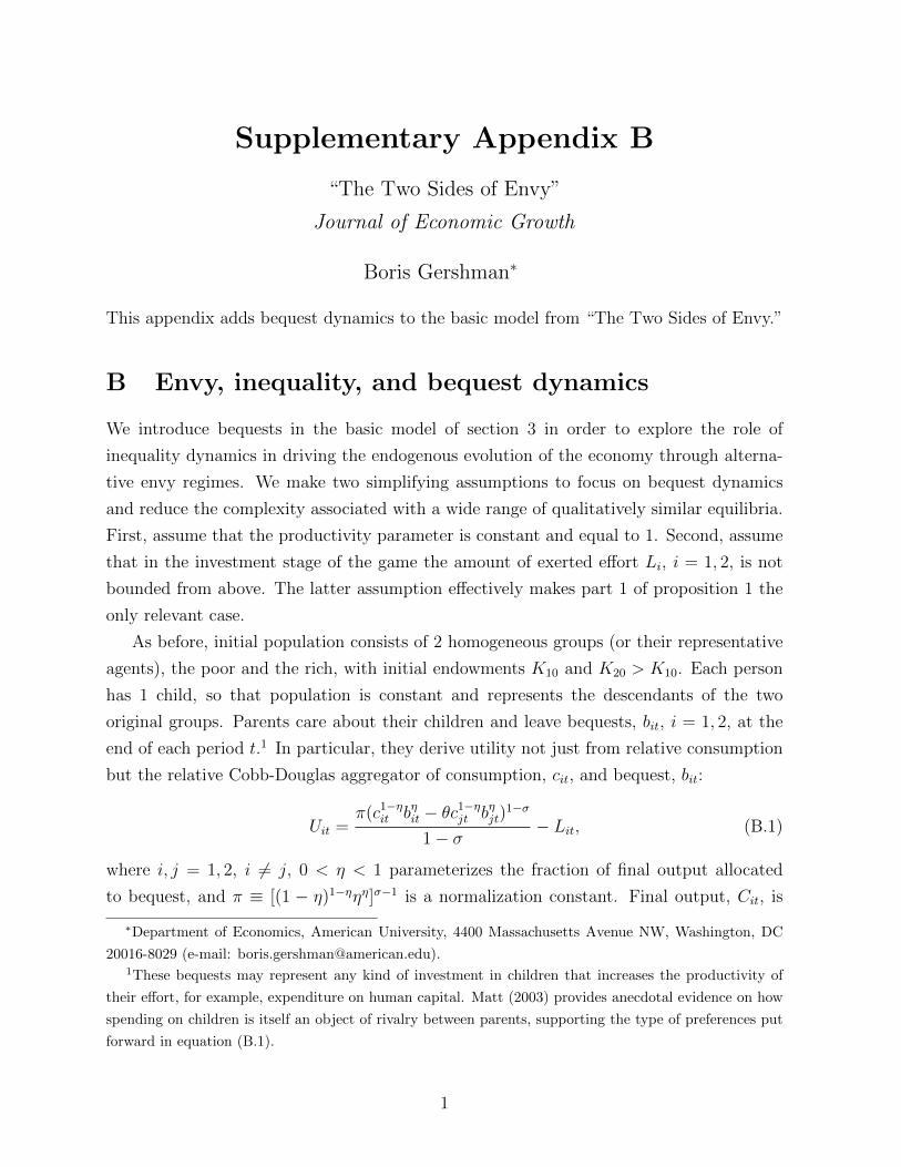
Supplementary Appendix B

“The Two Sides of Envy”

Journal of Economic Growth

Boris Gershman∗

This appendix adds bequest dynamics to the basic model from “The Two Sides of Envy.”

B Envy, inequality, and bequest dynamics

We introduce bequests in the basic model of section 3 in order to explore the role of

inequality dynamics in driving the endogenous evolution of the economy through alterna-

tive envy regimes. We make two simplifying assumptions to focus on bequest dynamics

and reduce the complexity associated with a wide range of qualitatively similar equilibria.

First, assume that the productivity parameter is constant and equal to 1. Second, assume

that in the investment stage of the game the amount of exerted effort Li, i = 1, 2, is not

bounded from above. The latter assumption effectively makes part 1 of proposition 1 the

only relevant case.

As before, initial population consists of 2 homogeneous groups (or their representative

agents), the poor and the rich, with initial endowments K10 and K20 > K10. Each person

has 1 child, so that population is constant and represents the descendants of the two

original groups. Parents care about their children and leave bequests, bit, i = 1, 2, at the

end of each period t.1 In particular, they derive utility not just from relative consumption

but the relative Cobb-Douglas aggregator of consumption, cit, and bequest, bit:

Uit =π(c1−ηit bηit − θc

1−ηjt bηjt)

1−σ

1− σ− Lit, (B.1)

where i, j = 1, 2, i 6= j, 0 < η < 1 parameterizes the fraction of final output allocated

to bequest, and π ≡ [(1 − η)1−ηηη]σ−1 is a normalization constant. Final output, Cit, is

∗Department of Economics, American University, 4400 Massachusetts Avenue NW, Washington, DC

20016-8029 (e-mail: [email protected]).1These bequests may represent any kind of investment in children that increases the productivity of

their effort, for example, expenditure on human capital. Matt (2003) provides anecdotal evidence on how

spending on children is itself an object of rivalry between parents, supporting the type of preferences put

forward in equation (B.1).

1

split between consumption and bequest, that is, bit + cit = Cit. This formulation leaves the

workings of the basic model from section 3 intact while introducing dynamic linkages.

The initial endowment of generation t+ 1, Kit+1, is assumed to depend on the parents’

endowment and their investment in children:

Kit+1 = Kβitbit = Kβ

itηCit, (B.2)

where i = 1, 2, and 0 < 1 − β < 1 is the rate of geometric depreciation of parental

endowment.2 Note that part 1 of proposition 1 holds in each period, and the level of initial

inequality in period t+ 1 is determined endogenously by the difference equation

kt+1 ≡K1t+1

K2t+1

= kβt ·C1t

C2t

, (B.3)

given the initial condition k0 ∈ (0, 1). The joint dynamics of K1t and K2t depends on the

type of equilibrium, in which the economy resides, and the equilibrium next period is, in

turn, determined by the economic outcomes of the current period. Lemma B.1 characterizes

this dynamical system and follows directly from proposition 1 and the law of motion (B.2).

Lemma B.1. (Dynamics of endowments). The two-dimensional dynamical system for K1t

and K2t is given by

[K1t+1

K2t+1

]=

η

1−θ2 [Kβ1t(K

1/σ1t + θK

1/σ2t ), Kβ

2t(K1/σ2t + θK

1/σ1t )], if kt > k;

ηθ(τ−1) [τθK

1/σ+β1t , Kβ

2tK1/σ1t ], if k 6 kt < k;

η[Kβ1t · C∗1(K1t, K2t), K

β2t · C∗2(K1t, K2t)], if kt < k,

(B.4)

where C∗1(K1t, K2t) and C∗2(K1t, K2t) are the final outputs in the DE corresponding to the

first case of (21) and the thresholds k and k are defined in (28).

The thresholds k and k divide the (K1t, K2t) phase plane into three regions according

to the types of equilibria (see figures B1 and B2): KUJE, FE, and DE. In each of these

regions the motion is governed by the corresponding part of the dynamical system (B.4).

To rule out explosive dynamics it is assumed throughout this section that σ(1 − β) > 1

which also implies that the results of all previous sections hold, since σ > 1.

It is useful to examine the companion one-dimensional difference equation (B.3) driving

the dynamics of inequality. Its properties are established in the following lemma.

2Persistence of endowments is introduced to make the dynamics more realistic. If β = 0, the qualitative

results remain unchanged, but the economy will not stay in the fear equilibrium for more than one period.

2

Lemma B.2. (Dynamics of inequality). The dynamics of kt is given by

kt+1 =

g1(kt) ≡ [k

1/σ+βt + θkβt ]/[1 + θk

1/σt ], if kt > k;

g2(kt) ≡ τθkβt , if k 6 kt < k;

g3(kt), if kt < k,

(B.5)

where g3(kt) is implicitly given by

kt =τ(1 + θ2)

2θ(1 + τ)2· (zt+1 + θ)2

zt+1

·(zt+1 − θ1− θzt+1

)σ, zt+1 ≡ kt+1/k

βt . (B.6)

Moreover, kt+1 > kt for all kt ∈ (0, 1).

Further analysis focuses on the dynamics of the system in the fear region and the KUJ

region. The two lemmas below provide its characterization.

Lemma B.3. (KUJ region dynamics). The system converges to a unique stable “equal”

long-run steady state KKUJ1 = KKUJ

2 = K = [η/(1− θ)]σ

σ(1−β)−1 . The steady-state levels of

output are equal to Y KUJ1 = Y KUJ

2 = Y = K1/σ/(1 − θ). The evolution of endowments is

determined by the loci

∆Ki ≡ Kit+1 −Kit = 0 : K1/σit + θK

1/σjt = K1−β

it · (1− θ2)/η, i, j = 1, 2, i 6= j,

where dKit/dKjt > 0 and d2Kit/dK2jt < 0.

Figure B1(a) shows the dynamics in the KUJ region. The descendants of the initially

poor eventually catch up with the rich dynasty, and in the steady state both have the same

endowments and consumption levels.

Lemma B.4. (Fear region dynamics). In the fear region the system moves towards the

unique stable “unequal” long-run steady state K1 = [ητ/(τ−1)]σ

σ(1−β)−1 , K2 = K1 ·(τθ)1

β−1 .

The corresponding levels of output are Y1 = [τ/(τ − 1)]K1/σ1 and Y2 = K

1/σ1 /[θ(τ − 1)].

This steady state is, however, unattainable, since it is located in the KUJ region, that is,

the system enters the KUJ region before reaching the fear steady state. The evolution of

endowments is determined by the loci

∆K1 = 0 : K1t = K1 = [ητ/(τ − 1)]σ

σ(1−β)−1 ;

∆K2 = 0 : K1t = Kσ(1−β)2t · [θ(τ − 1)/η]σ.

3

K1t

k

k

∆K2 = 0

∆K1 = 0

KUJE

FE

DE

S

K2t

45◦

(a) The KUJ region

K2t

K1t

k

k∆K2 = 0

∆K1 = 0

KUJE

FE

DE

K1S ′

45◦

τθ

(b) The fear of envy region

Figure B1: Dynamics of bequests and the steady states.

Figure B1(b) shows the dynamics in the fear region. It is instructive to look at the

comparative statics of the long-run levels of output with respect to τ and θ. They resemble

the results of the static model: in the KUJ steady state, outputs are increasing in θ

and independent of τ ; in the (unattainable) fear steady state, the output of group 1 is

independent of θ and decreasing in τ , while the output of group 2 is decreasing in θ and

τ . Note also that, despite their qualitatively different nature, as τθ → 1, the two long-run

equilibria get closer and coincide in the limit.

Given lemmas B.2–B.4, it is easy to establish how the possible trajectories look. The

long-run convergence result is stated in proposition B.1 and illustrated in figure B2.

Proposition B.1. (Long-run convergence). Given the initial conditions {K10, K20}, such

that k0 ∈ (0, 1), the endowments converge to a unique stable long-run “equal” steady state

of the KUJ region, K. Inequality decreases monotonically along the transition path.

Thus, if the economy starts off, say, in the destructive region, it experiences a transition

to the KUJ steady state, possibly passing through the fear region and staying there for a

while. Initially, destructive envy and the fear of it reduce original inequality of endowments

by discouraging productive effort of the rich or destroying part of their output. This leads to

more equal investment opportunities for future generations who eventually find it optimal

to compete productively.

The changes in tolerance parameters τ and θ can delay or accelerate the transition

between alternative envy regimes. For instance, a decrease in θ due to the diffusion of

4

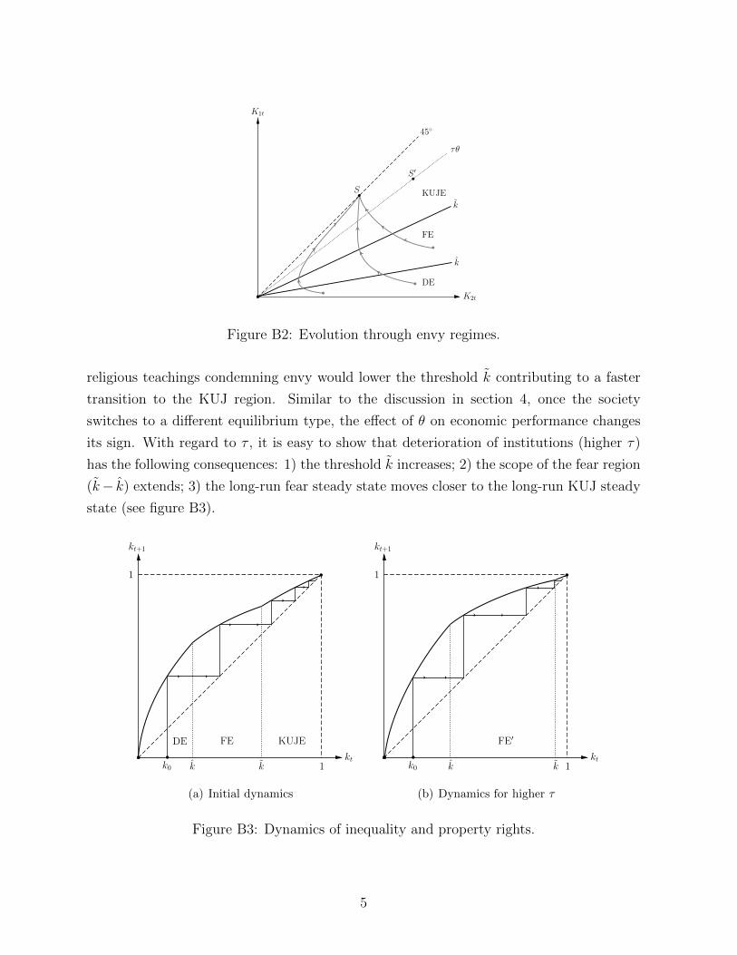
K1t

k

k

KUJE

FE

DE

S ′

S

K2t

45◦

τθ

Figure B2: Evolution through envy regimes.

religious teachings condemning envy would lower the threshold k contributing to a faster

transition to the KUJ region. Similar to the discussion in section 4, once the society

switches to a different equilibrium type, the effect of θ on economic performance changes

its sign. With regard to τ , it is easy to show that deterioration of institutions (higher τ)

has the following consequences: 1) the threshold k increases; 2) the scope of the fear region

(k− k) extends; 3) the long-run fear steady state moves closer to the long-run KUJ steady

state (see figure B3).

kt

kt+1

1

1

k0

DE FE KUJE

k k

(a) Initial dynamics

kt+1

1

1

FE′

kk0 kkt

(b) Dynamics for higher τ

Figure B3: Dynamics of inequality and property rights.

5

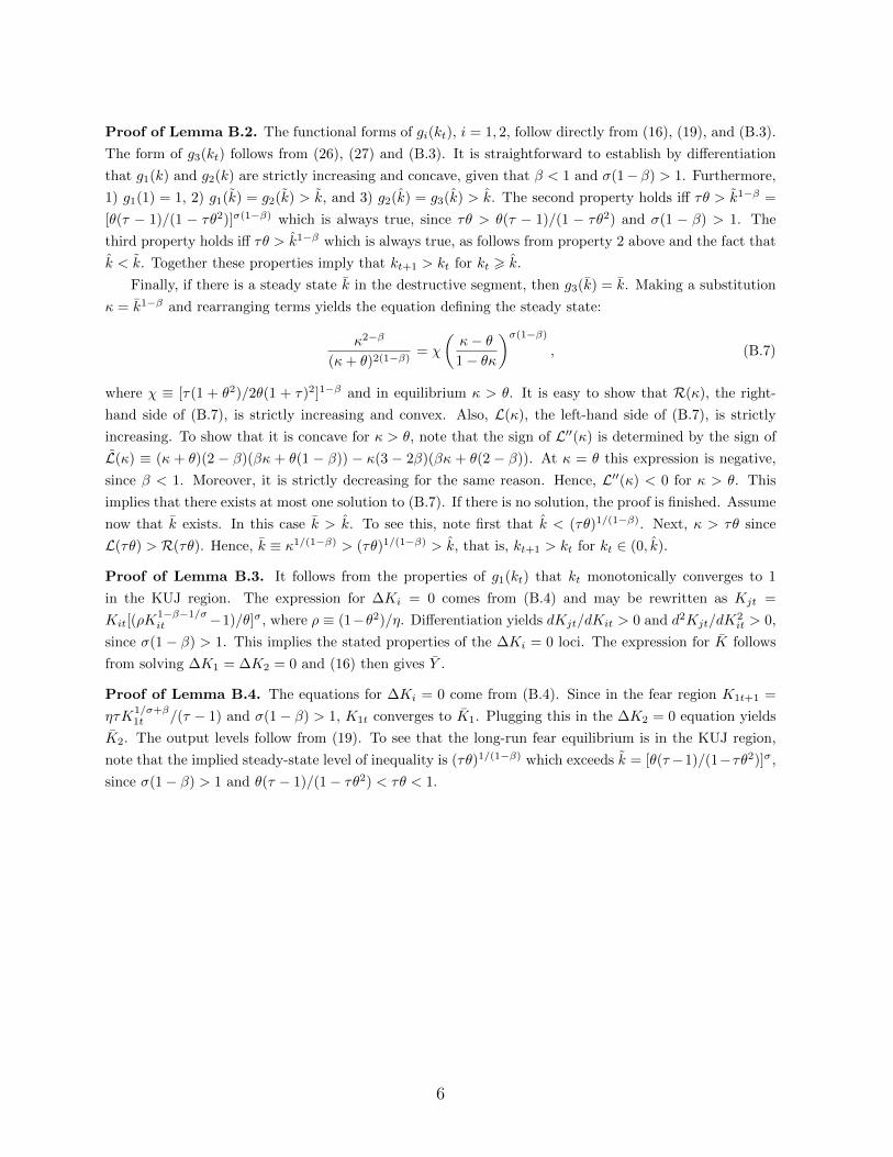
Proof of Lemma B.2. The functional forms of gi(kt), i = 1, 2, follow directly from (16), (19), and (B.3).

The form of g3(kt) follows from (26), (27) and (B.3). It is straightforward to establish by differentiation

that g1(k) and g2(k) are strictly increasing and concave, given that β < 1 and σ(1− β) > 1. Furthermore,

1) g1(1) = 1, 2) g1(k) = g2(k) > k, and 3) g2(k) = g3(k) > k. The second property holds iff τθ > k1−β =

[θ(τ − 1)/(1 − τθ2)]σ(1−β) which is always true, since τθ > θ(τ − 1)/(1 − τθ2) and σ(1 − β) > 1. The

third property holds iff τθ > k1−β which is always true, as follows from property 2 above and the fact that

k < k. Together these properties imply that kt+1 > kt for kt > k.

Finally, if there is a steady state k in the destructive segment, then g3(k) = k. Making a substitution

κ = k1−β and rearranging terms yields the equation defining the steady state:

κ2−β

(κ+ θ)2(1−β)= χ

(κ− θ1− θκ

)σ(1−β), (B.7)

where χ ≡ [τ(1 + θ2)/2θ(1 + τ)2]1−β and in equilibrium κ > θ. It is easy to show that R(κ), the right-

hand side of (B.7), is strictly increasing and convex. Also, L(κ), the left-hand side of (B.7), is strictly

increasing. To show that it is concave for κ > θ, note that the sign of L′′(κ) is determined by the sign of

L(κ) ≡ (κ + θ)(2 − β)(βκ + θ(1 − β)) − κ(3 − 2β)(βκ + θ(2 − β)). At κ = θ this expression is negative,

since β < 1. Moreover, it is strictly decreasing for the same reason. Hence, L′′(κ) < 0 for κ > θ. This

implies that there exists at most one solution to (B.7). If there is no solution, the proof is finished. Assume

now that k exists. In this case k > k. To see this, note first that k < (τθ)1/(1−β). Next, κ > τθ since

L(τθ) > R(τθ). Hence, k ≡ κ1/(1−β) > (τθ)1/(1−β) > k, that is, kt+1 > kt for kt ∈ (0, k).

Proof of Lemma B.3. It follows from the properties of g1(kt) that kt monotonically converges to 1

in the KUJ region. The expression for ∆Ki = 0 comes from (B.4) and may be rewritten as Kjt =

Kit[(ρK1−β−1/σit −1)/θ]σ, where ρ ≡ (1−θ2)/η. Differentiation yields dKjt/dKit > 0 and d2Kjt/dK

2it > 0,

since σ(1− β) > 1. This implies the stated properties of the ∆Ki = 0 loci. The expression for K follows

from solving ∆K1 = ∆K2 = 0 and (16) then gives Y .

Proof of Lemma B.4. The equations for ∆Ki = 0 come from (B.4). Since in the fear region K1t+1 =

ητK1/σ+β1t /(τ − 1) and σ(1− β) > 1, K1t converges to K1. Plugging this in the ∆K2 = 0 equation yields

K2. The output levels follow from (19). To see that the long-run fear equilibrium is in the KUJ region,

note that the implied steady-state level of inequality is (τθ)1/(1−β) which exceeds k = [θ(τ−1)/(1−τθ2)]σ,

since σ(1− β) > 1 and θ(τ − 1)/(1− τθ2) < τθ < 1.

6