The Tip of the Iceberg: a Quantitative Framework for ...The Tip of the Iceberg: A Quantitative Framework for Estimating Trade Costs ∗ Alfonso Irarrazabal†,AndreasMoxnes ‡, and

working papers

25 | 2011

September 2011

The analyses, opinions and fi ndings of these papers

represent the views of the authors, they are not necessarily

those of the Banco de Portugal or the Eurosystem

THE TIP OF THE ICEBERG: A QUANTITATIVE FRAMEWORK FOR ESTIMATING TRADE COSTS

Alfonso Irarrazabal

Andreas Moxnes

Luca David Opromolla

Please address correspondence to

Luca David Opromolla

Banco de Portugal, Economics and Research Department

Av. Almirante Reis 71, 1150-012 Lisboa, Portugal;

Tel.: 351 21 313 8153, email: [email protected]

BANCO DE PORTUGAL

Av. Almirante Reis, 71

1150-012 Lisboa

www.bportugal.pt

Edition

Economics and Research Department

Pre-press and Distribution

Administrative Services Department

Documentation, Editing and Museum Division

Editing and Publishing Unit

Printing

Administrative Services Department

Logistics Division

Lisbon, September 2011

Number of copies

80

ISBN 978-989-678-105-7

ISSN 0870-0117 (print)

ISSN 2182-0422 (online)

Legal Deposit no. 3664/83

The Tip of the Iceberg: A Quantitative Framework for

Estimating Trade Costs∗

Alfonso Irarrazabal†, Andreas Moxnes‡, and Luca David Opromolla§

September 20, 2011

AbstractInternational economics has overwhelmingly relied on Samuelson’s (1954) assump-

tion that trade costs are proportional to value. We develop a quantitative analytical

framework that features both additive and multiplicative (iceberg) trade costs, building

on a model of international trade with heterogeneous firms and demand heterogene-

ity. We structurally estimate the magnitude of additive trade costs, for every product

and destination available in our firm-level data of Norwegian exporters. Identification

is aided by the theoretical finding that the elasticity of demand to producer price is

dampened, in absolute value, when prices are low, and this mechanism is magnified

when additive trade costs are high. This magnification mechanism becomes useful in

the subsequent econometric analysis. Estimated additive trade costs are substantial.

On average, additive costs are 33 percent, expressed relative to the median price. This

leads us to reject the pure iceberg cost assumption. We assess the importance of these

costs in shaping global trade flows. Our micro estimates of additive trade costs explain

most of the geographical variation in aggregate trade. An implication of our work is

that inferring trade costs from standard gravity models suffers from specification bias,

since these models assume away the role of additive trade costs.

JEL Classification: F10 Keywords: Trade Costs, Heterogeneous Firms, Exports.

∗This is a substantia lly revised version of "The T ip of the Iceb erg: M odeling Trade Costs and Implications for Intra-Industry

Reallo cation". Acknow ledgements: We would like to thank Costas Arkolakis, G regory Corcos, Don Davis, Rob Johnson, Samuel

Kortum , Ralph Ossa, Arvid Raknerud , Andrés Rodríguez-C lare, A lexandre Sk iba, Karen Helene U lltveit-Moe, and K jetil Storesletten

for their helpfu l suggestions, as well as sem inar partic ipants at Banco de Portugal, Dartmouth, D IME-ISGEP Workshop, IIES Sto ckholm ,

ITSG -Bocconi Workshop, LMDG Workshop, LSE , NBER Summer Institute ITI2010, Norwegian School of M anagem ent, University of

O slo , and Yale. We thank Statistics Norway for data preparation and clarifi cations. We thank the pro ject “Europ ean F irm s in a G lobal

Economy: Internal Policies for External Competitiveness” (EFIGE) for financia l support. A lfonso Irarrazabal thanks the hospita lity

of the Chicago Booth School of Business where part of th is research was conducted. Luca David Opromolla acknow ledges financia l

support from national funds by FCT (Fundação para a C iência e a Tecnologia). Th is artic le is part of the Strategic Pro ject: PEst-

OE/EGE/UI0436/2011. The analysis, opin ions, and findings represent the views of the authors, they are not necessarily those of Banco

de Portugal.

†Norges Bank, [email protected].

‡Dartmouth College, Department of Econom ics, andreas.m [email protected].

§Banco de Portugal, Research Departm ent and Research Unit on Complexity and Econom ics (UECE), [email protected].

1

1 Introduction

The costs of international trade are the costs associated with the exchange of goods and

services across borders. Trade costs impede international economic integration and may

also explain a great number of empirical puzzles in international macroeconomics (Obstfeld

and Rogoff 2000). Since Samuelson (1954), economists usually model and estimate variable

trade costs as iceberg (i.e. multiplicative) costs, implying that pricier goods are costlier to

trade. Trade costs change the relative price of domestic to foreign goods and therefore alter

the worldwide allocation of production and consumption. Gains from trade typically occur

because freer trade allows prices across markets to converge.

In this paper we take a different approach. We depart from Samuelson’s framework,

modeling variable trade costs as comprising both a multiplicative (iceberg) and an additive

part.1 Multiplicative costs are defined as a constant percentage of the producer price per

unit traded, while additive costs are defined as a constant monetary cost per unit traded

(conditional on a product type, e.g. shoes).2 Even though more expensive varieties of a

given product may be costlier to export, those costs are presumably not proportional to the

product price. For example, a $200 pair of shoes will typically face much lower multiplicative

costs (i.e. cost relative to producer price) than a $20 pair of shoes.3 A number of trade policy

instruments also act like additive trade costs. According to the World Trade Organization

(WTO), 19 percent of U.S. non-agricultural imports are subject to additive tariffs.4 Quotas

1Trade costs are broadly defined to include “...all costs incurred in getting a good to a final user other than

the production cost of the good itself” (Anderson and van Wincoop, 2004). This includes transportation

costs, policy barriers, information costs, contract enforement costs, costs associated with the use of different

currencies, legal and regulatory costs, and local distribution costs.2We use the terminology additive costs throughout the paper. Per-unit or specific trade costs are also

terms frequently used in the literature.3According to UPS rates at the time of writing, a fee of $125 is charged for shipping a one kilo package

from Oslo to New York (UPS Standard). They charge an additional 1% of the declared value for full

insurance. Supposing that each pair of shoes weighs 02 kg, the multiplicative shipping costs are in this case

126 ((25+0.01*20)/20) and 135 ((25+0.01*200)/200) percent for the $20 and $200 pair of shoes respectively.42006 data from the WTO are presented in Table 6. We discuss the data in more detail in the appendix.

Until the 1950’s, two-thirds of dutiable U.S. imports were subject to additive tariffs. This proportion fell to

less than 40 percent by the early 1970’s (Irwin, 1998).

2

(through the imposition of a quota license price) also act like a additive tariff.5 In the

U.S. and the European Union, 95 and 151 percent of the Harmonized System (HS) six-

digit subheadings in the schedule of agricultural concessions are covered by tariff quotas.

Distribution costs are also partly additive costs (e.g. Corsetti and Dedola, 2005).

The presence of additive trade costs has important consequences when firms charge

different prices. First, when trade costs are incurred additively, trade costs not only alter

relative prices across markets but also relative prices within markets. For example, the

$200 pair of shoes becomes cheaper relative to the $20 pair in the presence of a additive

tariff. As a consequence, and as shown by Alchian and Allen (1964), additive costs alter

relative consumption patterns both within and across markets. Second, falling prices in

the manufacturing sector (e.g. due to productivity growth) increase effective trade costs, if

not accompanied by falling prices in the transport sector (or falling nominal tariffs). This

illustrates the simple point that it is real trade costs, and not nominal ones, that determine

the extent of economic integration. Third, the elasticity of demand to producer (f.o.b., free

on board) price is dampened, in absolute value, when prices are low, and this mechanism

is magnified when additive trade costs are high. This magnification mechanism becomes

useful in the subsequent econometric analysis.

The first contribution of this paper is therefore to present a model of international

trade with heterogeneous firms, building on Melitz (2003), Chaney (2008) and Eaton et al.

(2010), but that features both iceberg costs and additive variable trade costs, as well as

fixed entry costs, and to explore the economic implications of such a model. Our model

and quantitative framework are robust to heterogeneity in demand shocks (quality) across

producers within a narrowly defined sector. The second contribution is to document new

firm-level facts about the relationship between f.o.b. prices and the volume of exports across

markets, consistent with the presence of additive trade costs. The third contribution is to

develop a quantitative framework, derived from a subset of the model, that allows us to

estimate the magnitude of additive trade costs, for every product and destination in our

5Demidova et al. (2009) use a trade model with heterogeneous firms to analyze the behavior of

Bangladeshi garments exporters selling their products to the EU and to the U.S. and facing quotas as

well as other types of barriers. Khandelwal, Schott and Wei (2011) investigate the impact of quota removal

on aggregate productivity in China.

3

firm-level data of Norwegian exporters. The methodology is reminiscent of a difference-in-

differences approach, where trade costs are identified by comparing the difference in the

elasticity of sales to f.o.b. price between low- and high price firms, for a particular product,

across destinations.

Several strong results emerge from the empirical analysis. First of all, additive costs

are pervasive. The weighted mean of additive trade costs, expressed relative to the median

price, is 33 percent. Our estimates are strongly positively correlated with observable proxies

of trade costs, such as distance and product weight per value.6 The pure iceberg model

is therefore rejected. Second, we show that our micro estimates of additive trade costs

can explain a substantial share of the geographical variation in world aggregate trade flows.

Specifically, in our framework additive trade costs alone can explain between 40 to 70 percent

of the elasticity of aggregate trade to distance. This suggests that the role of multiplicative

(iceberg) trade costs is limited. An implication of our work is that inferring trade costs from

standard gravity models suffers from specification bias, since these models assume away the

role of additive trade costs.

1.1 Previous Literature

More flexible modeling of trade costs is not new in international economics. Alchian and

Allen (1964) pointed out that additive costs imply that the relative price of two varieties

of some good will depend on the level of trade costs, and that relative demand for the high

quality good increases with trade costs (“shipping the good apples out”). More recently,

Hummels and Skiba (2004) found strong empirical support for the Alchian-Allen hypothesis.

Specifically, the elasticity of freight rates with respect to price was estimated to be well below

the unitary elasticity implied by the iceberg assumption. Also, their estimates implied

that doubling freight costs increases average free on board (f.o.b.) export prices by 80 −141 percent, consistent with high quality goods being sold in markets with high freight

costs. However, the authors could not identify the magnitude of additive costs, as we

do here. Furthermore, our methodology identifies all kinds of trade costs, whereas their

paper is concerned with shipping costs exclusively. Lugovskyy and Skiba (2009) introduce

6Hummels and Skiba (2004) find that distance has a positive and significant impact on freight costs.

4

a generalized iceberg transportation cost into a representative firm model with endogenous

quality choice, showing that in equilibrium the export share and the quality of exports

decrease in the exporter country size.

Our work also relates to a recent paper by Berman, Martin, and Mayer (2011). They

also introduce a model with heterogeneous firms and additive costs, but in their model the

additive component is interpreted as local distribution costs that are independent of firm

productivity. Their research question is very different, however, as their paper analyzes

pricing to market and the reaction of exporters to exchange rate changes. They show that,

in response to currency depreciation, high productivity firms optimally raise their markup

rather than the volume, while low productivity firms choose the opposite strategy.

Our work also connects to the papers that quantify trade costs. Anderson and van

Wincoop (2004) provides an overview of the literature, and recent contributions are Ander-

son and van Wincoop (2003), Eaton and Kortum (2002), Head and Ries (2001), Hummels

(2007), and Jacks, Meissner, and Novy (2008). This strand of the literature either compiles

direct measures of trade costs from various data sources, or infers a theory-consistent index

of trade costs by fitting models to cross-country trade data.7 Our approach of using the

within-market relationship between f.o.b. prices and exports is conceptually different and

provides an complimentary approach to inferring trade barriers from data. This is possible

thanks to the recent availability of detailed firm-level data. Furthermore, whereas the tra-

ditional approach can only identify iceberg trade costs relative to some benchmark, usually

domestic trade costs, our method identifies the absolute level of (additive) trade costs.

The rest of the paper is organized as follows. Section 2 presents the model and summarize

its implications. Since the subsequent empirical framework is formulated conditional on a

set of general equilbrium variables, we present only the features of the model that is relevant

to the empirical work, and choose to close the model later in the paper. In Section 3 we

describe the data and present some empirical patterns that are suggestive of the presence of

additive trade costs. Section 4 lays out the econometric strategy and presents the baseline

estimates as well as robustness checks. In Section 5 we complete the theory and describe

7Helpman, Melitz and Rubinstein (2008) develop a gravity model that controls both for firm heterogeneity

and fixed costs of exporting and make predictions about the response of trade to changes in trade costs.

5

the full equilibrium. In Section 6 we calibrate the model and evaluate the importance of

additive trade costs in shaping world trade flows. Finally, Section 7 concludes.

2 The Model

In this section, we present a stylized model of heterogeneous firms and international trade

that features both iceberg and additive trade costs. We keep the model as parsimonious

as possible with the purpose of showing that this simple modification has important conse-

quences when firms are heterogeneous. In Section 2.4 we summarize a number of important

implications of the model, among them that variation in f.o.b. prices translates into less

variation in exports when additive trade costs are high. These properties of the model will

become useful in the subsequent empirical analysis. Since calculating the general equilib-

rium of the model is not necessary for the empirical analysis, we choose to close the model

later in the paper (see Section 5).

Compared to the previous literature (e.g. Melitz, 2003, Chaney, 2008 and Eaton, Kor-

tum and Kramarz 2010), the model has two innovations. First, we introduce additive trade

costs. Second, we have two layers of heterogeneity, demand shocks and productivity, that

are potentially correlated.8 Heterogeneity in demand shocks can be interpreted as hetero-

geneity in quality: higher values of the demand shock, resulting in higher demand for a

given price, can be interpreted as being associated with higher quality (Khandelwal, 2011,

Sutton, 1991). By allowing for a (positive) correlation between demand shocks and prices,

we can account for the possibility that the largest exporters are not necessarily the lowest

price firms.

2.1 The Basic Environment

We consider a world economy comprising asymmetric countries. Each country is

populated by a measure of workers. The economy consists of a differentiated goods

8 In Eaton, Kortum and Kramarz (2010), demand shocks are uncorrelated with the productivity draws.

We do not introduce entry shocks in the model, in contrast to Eaton, Kortum and Kramarz (2010), since

the extensive margin is largely irrelevant for the identification of trade costs (see Section 4).

6

sector and a transport services sector (described in the next section). For expositional ease

we do not label sectors, and present the model for a generic unspecified sector.9

Preferences across varieties of the differentiated product have the standard CES form

with an elasticity of substitution 1. Each variety enters the utility function with its own

exogenous country-specific weight . These weights represent firm- and destination-specific

demand shocks. These preferences generate a demand function ()1− in country

for a variety with price and demand shock . The demand level ≡ −1 is

exogenous from the point of view of the individual supplier and depends on total expenditure

and the consumption-based price index .

Finally, we assume that workers are immobile across countries, but mobile across sectors

and that market structure in the differentiated sector is monopolistic competition.

2.2 Variable Trade Costs

Unlike much of the earlier trade literature, firms also have to incur an additive cost , per

unit output, in order to transfer a good from to market . In other words, technology is

assumed to be Leontief, so additive trade costs are proportional to the quantity produced

(not proportional to value).10 In Section 5, we model how wages and are determined

and assign a numeraire. For now it suffices to take as given the matrix of trade costs across

countries. Additionally, the economic environment consists of a standard iceberg cost ,

so that units of the final good must be shipped in order for one unit to arrive. The

presence of iceberg costs ensures that any positive correlation between product value and

shipping costs is captured by the model.11

9 In the econometric section, a sector is interpreted as a product group according to the harmonized

system (HS) nomenclature, at the 8 digit level (HS8). A differentiated good within a sector is interpreted

as a firm observation within an HS8 code.10This is similar to Burstein, Neves and Rebelo (2003) and Corsetti and Dedola (2005), who assume that

production and retailing are complements.11Hummels, Lugovskyy, and Skiba (2009) find evidence for market power in international shipping. An

extension of our model with increasing returns in shipping could generate lower additive trade costs for more

efficient firms. In other words, additive trade costs would become more like iceberg costs, since they would

be correlated with the price of the good shipped.

7

2.3 Prices

Firms are heterogeneous in terms of both their technology, associated with productivity

, and their set of destination-specific demand shocks =1 . A firm in country

can access market only after paying a destination-specific fixed cost , in units of the

numéraire. Given labor costs and the variable trade costs and , profits are12

[ − − ]−

where = −1 − is the quantity demanded. Given market structure and preferences,

a firm with efficiency maximizes profits by setting its consumer price as a constant markup

over total marginal production cost,

=

− 1³

+

´ (1)

Exploiting the relationship between consumer prices, , and producer (f.o.b.) prices,

,

= + (2)

the producer price can be written as

=

− 1µ

+

¶

Note that the markup over production costs is no longer constant. All else equal, a more

efficient firm will charge a higher markup, since the perceived elasticity of demand that such

a firm faces is lower. In other words, the markup is higher for more efficient firms since,

due to the presence of additive trade costs, a larger share of the consumer price does not

depend on the producer price.

2.4 Model Implications

In this Section, we summarize a few properties of the theoretical framework. Among these,

Proposition 1 will become particularly useful in the subsequent empirical analysis. The

first two propositions describe the relationship between demand and producer prices and

demand and additive trade costs. The last two propositions describe how relative prices

across and within markets are affected by additive trade costs.

12As a convention, we assume that additive trade costs are paid on the "melted" output.

8

Proposition 1 The (absolute value of the) elasticity of demand, with respect to the f.o.b.

price, , is dampened when additive trade costs constitute a large share of the price. More-

over, the elasticity is dampened more among low-price firms than high price firms as additive

trade costs increase.

The first part of the proposition can be seen analytically from

=

¯ ln

ln e¯=

¯ ln

ln

ln

ln e¯=

¡1 + e¢−1

where e ≡

Due to CES preferences, the first elasticity is ln ln = −. Due to the relationshipbetween the consumer and producer prices, = + (equation 2), the second

elasticity is ln ln e = ¡1 + e¢−1. Without additive trade costs, the second

elasticity is one. With positive additive trade costs, the elasticity is decreasing in e.In other words, if additive trade costs constitute a large share of the price ( relative to

e), the demand elasticity with respect to the f.o.b. price is low. The economic intuitionis that, since additive trade costs constitute a larger share of the consumer price for low-

price goods, a given percentage increase in the producer price translates into a smaller

percentage increase in the consumer price and consequently a smaller percentage decrease

in consumption.

The second part of the proposition can be seen analytically from

e = − ¡1 + ¢−1

0

holding producer prices constant.13 In other words, the elasticity falls as e rises, and thedecline is larger when f.o.b. prices are low. The economic intuition is that, for high price

firms, a marginal increase in e has a small impact on the consumer price (see Proposition2) and the impact on the elasticity is therefore small. In the empirical Section below we

identify the magnitude of additive trade costs by exploiting this mechanism.

13Allowing producer prices to change in response to a rise in additive trade costs (due to en-

dogenous markups) does not change this conclusion. Specifically, we get =

− 1− ( − 1)−1 1 + −1 , which, after inserting the optimal , also turns outto be negative.

9

Proposition 2 The (absolute value of the) elasticity of demand with respect to additive

trade costs is higher for low price than high price firms.

Analytically, we see this from¯ ln

lne¯=

¯ ln

ln

ln

lne¯=

¡1 + e¢−1

holding producer prices constant.14 The second elasticity is now ln lne = ¡1 + e¢−1.Hence, if additive trade costs constitute a large share of the price (which will be the case

when prices are low), a percentage increase in additive trade costs has a big negative per-

centage impact on quantity sold. The economic intuition is simply that an increase in

additive trade costs translates into a larger percentage increase in the consumer price for

low price firms.

Proposition 3 Relative consumer prices within a market are distorted in the presence of

additive trade costs, but not in the presence of iceberg costs.

Consider two different varieties with producer prices 0 sold in market . Then

0=

+ e0 + e 1

and, holding producer prices constant,

0

e = − − 0¡0 + e¢2 0

In other words, an increase in reduces the consumer price of the high price variety

relative to the low price variety. Under some regularity conditions about demand (see e.g.

Hummels and Skiba, 2004), an increase in raises relative consumption of the high price

variety relative to the low price variety. This is the well-known Alchian-Allen effect. On the

contrary, if = 0 and 0, relative consumer prices equals relative producer prices,

0 =

0, so that changes in iceberg costs do not affect relative demand.

14Allowing producer prices to change in response to a rise in additive trade costs (due to en-

dogenous markups) does not change this conclusion. Specifically, we get ln ln =

2 ( − 1) 1 + −1.

10

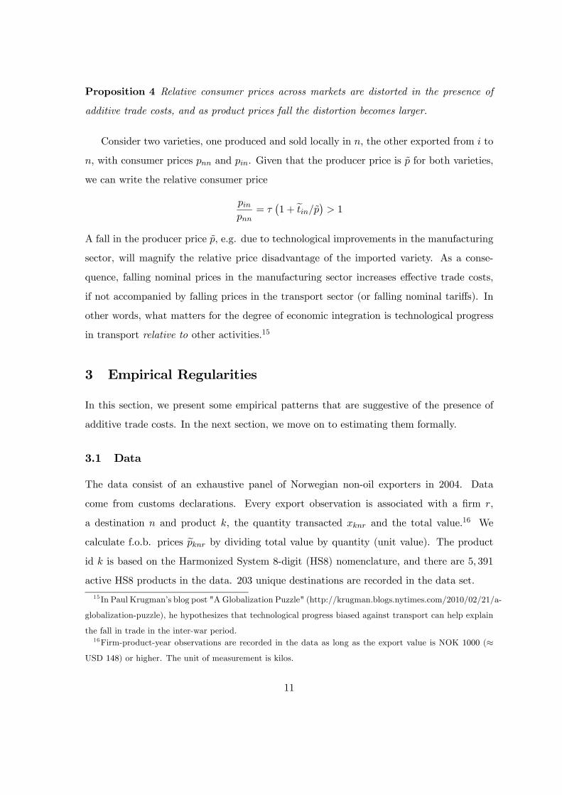
Proposition 4 Relative consumer prices across markets are distorted in the presence of

additive trade costs, and as product prices fall the distortion becomes larger.

Consider two varieties, one produced and sold locally in , the other exported from to

, with consumer prices and . Given that the producer price is for both varieties,

we can write the relative consumer price

=

¡1 + e¢ 1

A fall in the producer price , e.g. due to technological improvements in the manufacturing

sector, will magnify the relative price disadvantage of the imported variety. As a conse-

quence, falling nominal prices in the manufacturing sector increases effective trade costs,

if not accompanied by falling prices in the transport sector (or falling nominal tariffs). In

other words, what matters for the degree of economic integration is technological progress

in transport relative to other activities.15

3 Empirical Regularities

In this section, we present some empirical patterns that are suggestive of the presence of

additive trade costs. In the next section, we move on to estimating them formally.

3.1 Data

The data consist of an exhaustive panel of Norwegian non-oil exporters in 2004. Data

come from customs declarations. Every export observation is associated with a firm ,

a destination and product , the quantity transacted and the total value.16 We

calculate f.o.b. prices e by dividing total value by quantity (unit value). The productid is based on the Harmonized System 8-digit (HS8) nomenclature, and there are 5 391

active HS8 products in the data. 203 unique destinations are recorded in the data set.

15 In Paul Krugman’s blog post "A Globalization Puzzle" (http://krugman.blogs.nytimes.com/2010/02/21/a-

globalization-puzzle), he hypothesizes that technological progress biased against transport can help explain

the fall in trade in the inter-war period.16Firm-product-year observations are recorded in the data as long as the export value is NOK 1000 (≈

USD 148) or higher. The unit of measurement is kilos.

11

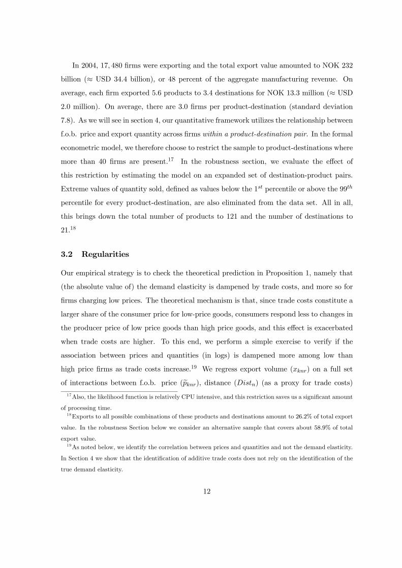
In 2004, 17 480 firms were exporting and the total export value amounted to NOK 232

billion (≈ USD 344 billion), or 48 percent of the aggregate manufacturing revenue. On

average, each firm exported 56 products to 34 destinations for NOK 133 million (≈ USD20 million). On average, there are 30 firms per product-destination (standard deviation

78). As we will see in section 4, our quantitative framework utilizes the relationship between

f.o.b. price and export quantity across firms within a product-destination pair. In the formal

econometric model, we therefore choose to restrict the sample to product-destinations where

more than 40 firms are present.17 In the robustness section, we evaluate the effect of

this restriction by estimating the model on an expanded set of destination-product pairs.

Extreme values of quantity sold, defined as values below the 1 percentile or above the 99

percentile for every product-destination, are also eliminated from the data set. All in all,

this brings down the total number of products to 121 and the number of destinations to

21.18

3.2 Regularities

Our empirical strategy is to check the theoretical prediction in Proposition 1, namely that

(the absolute value of) the demand elasticity is dampened by trade costs, and more so for

firms charging low prices. The theoretical mechanism is that, since trade costs constitute a

larger share of the consumer price for low-price goods, consumers respond less to changes in

the producer price of low price goods than high price goods, and this effect is exacerbated

when trade costs are higher. To this end, we perform a simple exercise to verify if the

association between prices and quantities (in logs) is dampened more among low than

high price firms as trade costs increase.19 We regress export volume () on a full set

of interactions between f.o.b. price (e), distance () (as a proxy for trade costs)

17Also, the likelihood function is relatively CPU intensive, and this restriction saves us a significant amount

of processing time.18Exports to all possible combinations of these products and destinations amount to 262% of total export

value. In the robustness Section below we consider an alternative sample that covers about 589% of total

export value.19As noted below, we identify the correlation between prices and quantities and not the demand elasticity.

In Section 4 we show that the identification of additive trade costs does not rely on the identification of the

true demand elasticity.

12

and a dummy equal to one if the price is above the product-destination median, ≡1 [e (e)],

ln = + [ln e ×× ln ××] +

where ×× denotes the full set of interactions and is the vector of coefficients. The

relationship between f.o.b. price and quantity exported is

ln

ln e = 1 + 2 ln + 3 + 4 (ln ×)

which is allowed to vary depending on distance from Norway (2), between low- and high

price firms (3), and the interaction between the two (4). The important coefficient is

the triple interaction term 4 (ln e × ln ×), since this captures whether the

change in elasticity as distance is increasing (2 ln ln e ln, the empirical

counterpart to e from Proposition 1) is different between low- and high price firms.

Given that ln ln e 0, our theory suggests that 4 0, so that (the absolute

value of) the elasticity is dampened more among low-price firms than high price firms as

trade costs increase (recall that = 1 denotes high price firms). We review the results

for the triple interaction term in Table 1.20

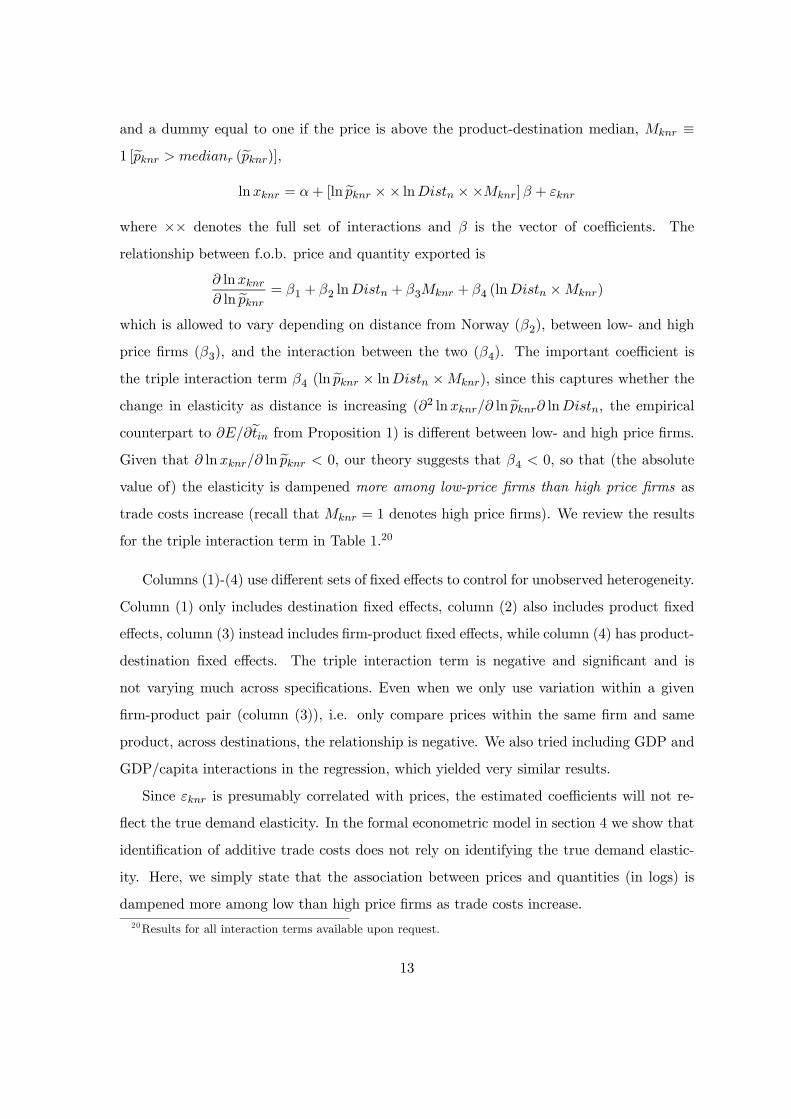
Columns (1)-(4) use different sets of fixed effects to control for unobserved heterogeneity.

Column (1) only includes destination fixed effects, column (2) also includes product fixed

effects, column (3) instead includes firm-product fixed effects, while column (4) has product-

destination fixed effects. The triple interaction term is negative and significant and is

not varying much across specifications. Even when we only use variation within a given

firm-product pair (column (3)), i.e. only compare prices within the same firm and same

product, across destinations, the relationship is negative. We also tried including GDP and

GDP/capita interactions in the regression, which yielded very similar results.

Since is presumably correlated with prices, the estimated coefficients will not re-

flect the true demand elasticity. In the formal econometric model in section 4 we show that

identification of additive trade costs does not rely on identifying the true demand elastic-

ity. Here, we simply state that the association between prices and quantities (in logs) is

dampened more among low than high price firms as trade costs increase.

20Results for all interaction terms available upon request.

13

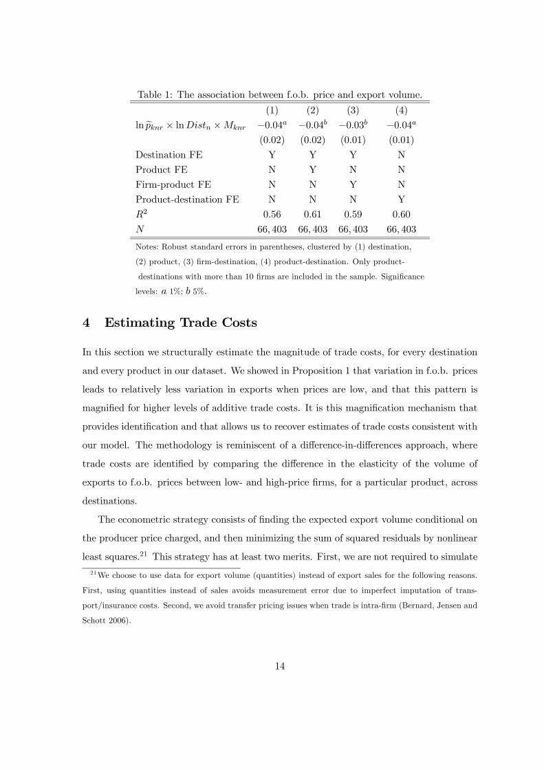
Table 1: The association between f.o.b. price and export volume.

(1) (2) (3) (4)

ln e × ln × −004 −004 −003 −004(002) (002) (001) (001)

Destination FE Y Y Y N

Product FE N Y N N

Firm-product FE N N Y N

Product-destination FE N N N Y

2 056 061 059 060

66 403 66 403 66 403 66 403

Notes: Robust standard errors in parentheses, clustered by (1) destination,

(2) product, (3) firm-destination, (4) product-destination. Only product-

destinations with more than 10 firms are included in the sample. Significance

levels: 1%; 5%

4 Estimating Trade Costs

In this section we structurally estimate the magnitude of trade costs, for every destination

and every product in our dataset. We showed in Proposition 1 that variation in f.o.b. prices

leads to relatively less variation in exports when prices are low, and that this pattern is

magnified for higher levels of additive trade costs. It is this magnification mechanism that

provides identification and that allows us to recover estimates of trade costs consistent with

our model. The methodology is reminiscent of a difference-in-differences approach, where

trade costs are identified by comparing the difference in the elasticity of the volume of

exports to f.o.b. prices between low- and high-price firms, for a particular product, across

destinations.

The econometric strategy consists of finding the expected export volume conditional on

the producer price charged, and then minimizing the sum of squared residuals by nonlinear

least squares.21 This strategy has at least two merits. First, we are not required to simulate

21We choose to use data for export volume (quantities) instead of export sales for the following reasons.

First, using quantities instead of sales avoids measurement error due to imperfect imputation of trans-

port/insurance costs. Second, we avoid transfer pricing issues when trade is intra-firm (Bernard, Jensen and

Schott 2006).

14

the full general equilibrium in order to obtain estimates of trade costs. Second, our estimator

is more general than our theory. In particular, in the model, our assumption about CES

preferences implies that mark-ups are constant. In the econometrics, however, there is no

constraint on the mark-ups, since we always condition on observed f.o.b. prices.

Our methodology for estimating trade costs is very different from the earlier literature.22

First, most studies model trade costs as iceberg exclusively, omitting the presence of additive

costs. A notable exception is Hummels and Skiba (2004), who distinguish between them and

find evidence for the presence of additive shipping costs.23 However, they are not able to

identify the magnitude of additive shipping costs. Also, compared to our work, they study

freight costs exclusively, whereas we consider all types of international trade costs. Second,

our methodology utilizes within product-destination, across firms, variation in exports and

f.o.b. prices to achieve identification, whereas earlier studies typically utilize cross-country

variation in aggregate (or product-level) trade. Third, whereas the traditional approach

can only identify trade costs relative to some benchmark, usually domestic trade costs, our

method identifies the absolute level of trade costs.24

4.1 Estimation

We employ a simple nonlinear least squares (NLS) estimator where the objective is to

minimize the squared difference between expected export volume and actual export volume

(in logs). We use the volume of exports instead of sales because using sales complicates

the estimating equation considerably.25 Export volume in the model is = −1 − .

Taking this to the data, we modify the expression in two ways. First, since the data is

differentiated by products , we make the demand shifter product-destination-specific

and the elasticity of substitution product-specific. Second, we allow for deviations from

log linearity in the demand function by introducing a squared price term. The reason for

22Anderson and van Wincoop (2004) provide a comprehensive summary of the literature.23They find an elasticity of freight rates with respect to price around 06, well below the unitary elasticity

implied by the iceberg assumption on shipping costs.24As will become clear below, we identify . Our preferred measure of additive trade costs is

relative to the observed median f.o.b. price.25This occurs because f.o.b. sales are =

−1 − .

15

doing so will become clear in Section 4.2. The export volume expression then becomes

ln = + 1 ln + 2 (ln )2 + lne (3)

where 1 and 2 denote the polynomial price coefficients.26 Subscripts , , and denote

HS-8 product, destination and firm, respectively (subscript is dropped since Norway is

always the source country). The demand shifter captures total expenditure and the

price index of product in market . The demand shocks e ≡ ( − 1) can besystematically correlated with prices, as discussed in the theory section. We assume that

this relationship is also approximated by a second order polynomial (in logs) plus statistical

noise ,

lne = + 1 ln + 2 (ln )2 + (4)

In sectors with a high degree of quality heterogeneity, we expect lne ln 0,

so that high-price firms on average get better demand shocks. We can then rewrite the

demand equation as

ln = + + (1 + 1) ln + (2 + 2) (ln )2 + (5)

The c.i.f. price is unobserved, but the f.o.b. price e is observable in our data. Wetherefore substitute with e using = e + . We also employ the ap-

proximation ln (1 + ) ≈ , which is reasonably accurate for ee ∈ [0 12] (recall thate ≡ ). This allows us to difference out the product-destination specific intercept

term.27 Removing this nuisance parameter is important since the cost of minimizing the

objective function, in terms of processing time, is prohibitive when nuisance parameters are

present.28 The resulting estimating equation is

dln = e1 ³\ln e + ede−1´+ e2 ∙ \(ln e)2 + 2e \e−1 ln e + e2de−2¸+b (6)

26 In the model, we had 1 = − and 2 = 0.27The constant term is + + (1 + 1) ln + (2 + 2) (ln )

2

28As we show in the robustness section, the log approximation is also useful because the estimating equation

encompasses the case where demand shocks are a function of c.i.f. prices (as in the baseline model), and the

case where demand shocks are a function of f.o.b. prices.

16

where e is our coefficient of interest, e1 = 1+1+2e2 ln , e2 = 2+2 and hats

denote each variable’s deviation from its mean. e.g. dln = ln − (1)P

ln

with being the number of exporters in product-destination pair .

Finally, we decompose e into product- and destination-specific fixed effects, e = ,

and normalize 1 = 1.2930 This decomposition enables us to identify trade costs that are

due to product and market characteristics, respectively. We then minimize the sum of

squared residuals

(Ψ) =X

X∈1

X∈2

b2where 1 is the set of destinations present for product and

2 is the set of firms exporting

to product-destination pair . The coefficient vector is thenΨ =³

e1 e2´, in total3 + − 1 parameters.

A potential concern is that prices and quantities are determined simultaneously, so

that the error term is correlated with the explanatory variables. Our estimator for e is,however, robust to any supply side mechanisms that make e endogenous. For example,assume that firms facing favorable demand shocks (s) also charge higher prices. We

could approximate this with the polynomial = 1 ln + 2 (ln )2 + where

is an error term. In that case, the estimating equation would be similar to equation

(6), the only difference being the interpretation of the slope parameters, which would take

the form e1 + 1 ande2 + 2 In sum, even though the interpretation of the slope

parameters would change, the estimate of e would not. Intuitively, the slope coefficientsare a mixture of various structural supply and demand side parameters and any particular

element is not separately identified (e.g. 1). Identification of the trade cost coefficient is

instead based on systematic nonlinear deviations from this equilibrium relationship between

29The normalization is similar to the one adopted in the estimation of two-way fixed effects in the employer-

employee literature (Abowd, Creecy, and Kramarz 2002). Note that even though is estimated relative to

some normalization, the estimate of is invariant to the choice of normalization. We also need to ensurethat all products and destinations belong to the same mobility group. The intuition is that if a given product

is sold only in a destination where no other products are sold, then one cannot separate the product from

the destination effect.30 In the robustness Section below we check whether our estimates are sensitive to the trade cost decom-

position = . by estimating directly for all possible product-destination pairs.17

price and quantity.

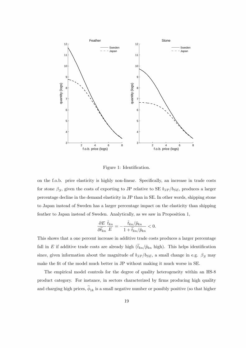
4.2 Identification of trade costs

The intuition behind identification can be explained by the following example. Assume that

we have two products, feather (F) and stone (S) sold in two different destinations, Sweden

(SE) and Japan (JP). Figure 1 shows f.o.b. prices and quantities for one particular numerical

example.31 e1 and e2 are identified by fitting the empirical model to the data (for eachproduct) among high-price firms. For high-price firms, the slopes are roughly similar in

both markets, as additive trade costs constitute a negligible share of their c.i.f. price. In

other words, we get information about e1 and e2 by looking at high-price intervals wherethe slopes are fairly similar across markets.32

The product and destination fixed effects and are identified by the differences

in the slopes for low-price firms across products (comparing F and S) and across markets

(comparing SE and JP). For a given product (e.g. S), the elasticity may be nonconstant

across the price interval for reasons other than trade costs (i.e. e2 6= 0).33 But, as we

move to more remote markets, any dampening of the elasticity that is specific to low-price

firms will be attributed to trade costs. The methodology is therefore reminiscent of a

difference-in-differences approach, where trade costs are identified from the change in the

difference in elasticities between low- and high price firms, as we move to more remote

destinations. Defining the absolute value of the elasticity with respect to the f.o.b.

price, for product-destination and for = igh or ow, we can express this double

difference as −

−¡0 −

0¢for destinations and 0.

In addition, identification is helped by the fact that the impact of additive trade costs

31We used the following values for the parameters: 1 = 1, 2 = 01, = 10, = 5.32This can be easily seen by letting −→ 0 in equation (6),

ln = 1 \ln + 2 \(ln )2+33Note that the inclusion of 2 in the empirical model is important in order to allow non-constant slope

coefficients. Without 2, any deviation from log-linearity among low price firms would be attributed to

additive trade costs. In practice though, the estimates of trade costs are fairly similar when estimating under

the restriction that 2 = 0.18

2 4 6 83

4

5

6

7

8

9

10

11

12

quan

tity

(logs

)

f.o.b. price (logs)

Feather

2 4 6 83

4

5

6

7

8

9

10

11

12

quan

tity

(logs

)

f.o.b. price (logs)

Stone

SwedenJapan

SwedenJapan

Figure 1: Identification.

on the f.o.b. price elasticity is highly non-linear. Specifically, an increase in trade costs

for stone , given the costs of exporting to JP relative to SE , produces a larger

percentage decline in the demand elasticity in JP than in SE. In other words, shipping stone

to Japan instead of Sweden has a larger percentage impact on the elasticity than shipping

feather to Japan instead of Sweden. Analytically, as we saw in Proposition 1,

e = −

1 + e 0

This shows that a one percent increase in additive trade costs produces a larger percentage

fall in if additive trade costs are already high (e high). This helps identificationsince, given information about the magnitude of , a small change in e.g. may

make the fit of the model much better in JP without making it much worse in SE.

The empirical model controls for the degree of quality heterogeneity within an HS-8

product category. For instance, in sectors characterized by firms producing high quality

and charging high prices, e1 is a small negative number or possibly positive (so that higher19

prices are associated with more sales). As long as we control for differences in e1 and e2across products, our estimate of e is unbiased.

The essential identifying assumption is that the parameters governing the intersection

between supply and demand (e1 and e2) are product specific and not product-destinationspecific (but the intercepts are allowed to be product-destination specific). Even though

these two assumptions are not directly testable, it is difficult to explain the findings in this

paper by product-destination specific variation in e1 and e2 exclusively. In particular, al-ternative theoretical explanations, e.g. demand side explanations, would need to reproduce

the empirical finding that the f.o.b. price elasticity for low price firms falls faster than the

elasticity for high price firms as trade costs (as proxied by distance) increases.

Furthermore, a model with firms varying their level of quality across markets (for a given

product), perhaps due to country income differences such as in Verhoogen (2008), would

not be able to reproduce the findings in this paper. In our framework, quality differences

across markets would be captured by the constant term in the demand shock equation (4),

which is differenced out in the estimating equation (6).

We also emphasize that, although our e is assumed to be constant within an HS-8product, across firms (e.g. same $20 trade cost for all pairs of shoes exported to the U.S.),

our framework allows for varying total trade costs across firms, within a product-destination

pair. Recall that iceberg costs is controlled for (subsumed into the intercept terms),

even though not separately identified. Hence, any mechanism that would make e varysystematically with product value would be subsumed into the intercept terms. This just

shows that the e that we identify is, by definition, the cost that is constant across all firmswithin a product-destination pair.

Finally, a comment about the interpretation of the results. Our methodology only allows

identification of e ≡ (and not ). When commenting on the magnitude of

additive trade costs in Section 4.3, we divide the estimates of e by the observed medianf.o.b. price in product-destination , i.e. = () e =

³e´. In

other words, we measure additive trade costs relative to the f.o.b. price multiplied by the

iceberg cost. As a consequence, our estimates of additive trade costs would be higher if we

were to report e (and had information about ).20

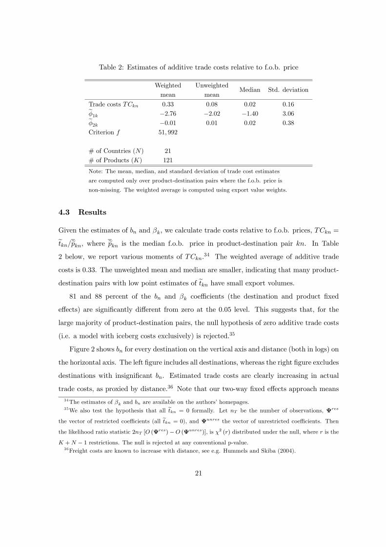
Table 2: Estimates of additive trade costs relative to f.o.b. price

Weighted

mean

Unweighted

meanMedian Std. deviation

Trade costs 033 008 002 016e1 −276 −202 −140 306e2 −001 001 002 038

Criterion 51 992

# of Countries () 21

# of Products () 121

Note: The mean, median, and standard deviation of trade cost estimates

are computed only over product-destination pairs where the f.o.b. price is

non-missing. The weighted average is computed using export value weights.

4.3 Results

Given the estimates of and , we calculate trade costs relative to f.o.b. prices, =ee, where e is the median f.o.b. price in product-destination pair . In Table2 below, we report various moments of .

34 The weighted average of additive trade

costs is 033. The unweighted mean and median are smaller, indicating that many product-

destination pairs with low point estimates of e have small export volumes.81 and 88 percent of the and coefficients (the destination and product fixed

effects) are significantly different from zero at the 005 level. This suggests that, for the

large majority of product-destination pairs, the null hypothesis of zero additive trade costs

(i.e. a model with iceberg costs exclusively) is rejected.35

Figure 2 shows for every destination on the vertical axis and distance (both in logs) on

the horizontal axis. The left figure includes all destinations, whereas the right figure excludes

destinations with insignificant . Estimated trade costs are clearly increasing in actual

trade costs, as proxied by distance.36 Note that our two-way fixed effects approach means

34The estimates of and are available on the authors’ homepages.35We also test the hypothesis that all = 0 formally. Let be the number of observations, Ψ

the vector of restricted coefficients (all = 0), and Ψ the vector of unrestricted coefficients. Then

the likelihood ratio statistic 2 [ (Ψ)− (Ψ)], is 2 () distributed under the null, where is the

+ − 1 restrictions. The null is rejected at any conventional p-value.36Freight costs are known to increase with distance, see e.g. Hummels and Skiba (2004).

21

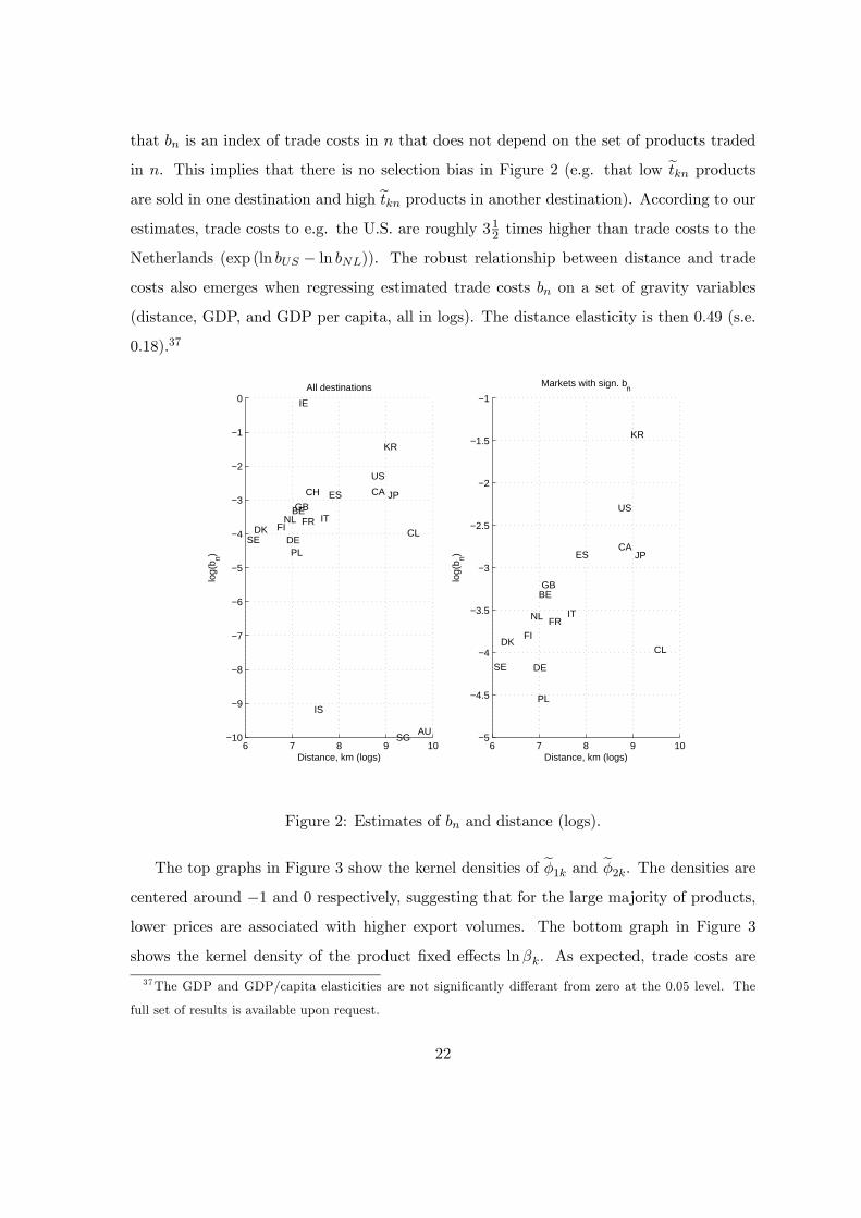
that is an index of trade costs in that does not depend on the set of products traded

in . This implies that there is no selection bias in Figure 2 (e.g. that low e productsare sold in one destination and high e products in another destination). According to ourestimates, trade costs to e.g. the U.S. are roughly 31

2times higher than trade costs to the

Netherlands (exp (ln − ln )). The robust relationship between distance and trade

costs also emerges when regressing estimated trade costs on a set of gravity variables

(distance, GDP, and GDP per capita, all in logs). The distance elasticity is then 049 (s.e.

018).37

6 7 8 9 10−10

−9

−8

−7

−6

−5

−4

−3

−2

−1

0

AU

BE

CACH

CLDE

DK

ES

FIFR

GB

IE

IS

IT

JP

KR

NL

PLSE

SG

US

Distance, km (logs)

log(

b n)

All destinations

6 7 8 9 10−5

−4.5

−4

−3.5

−3

−2.5

−2

−1.5

−1

BE

CA

CL

DE

DK

ES

FI

FR

GB

IT

JP

KR

NL

PL

SE

US

Distance, km (logs)

log(

b n)

Markets with sign. bn

Figure 2: Estimates of and distance (logs).

The top graphs in Figure 3 show the kernel densities of e1 and e2. The densities arecentered around −1 and 0 respectively, suggesting that for the large majority of products,lower prices are associated with higher export volumes. The bottom graph in Figure 3

shows the kernel density of the product fixed effects ln. As expected, trade costs are

37The GDP and GDP/capita elasticities are not significantly differant from zero at the 0.05 level. The

full set of results is available upon request.

22

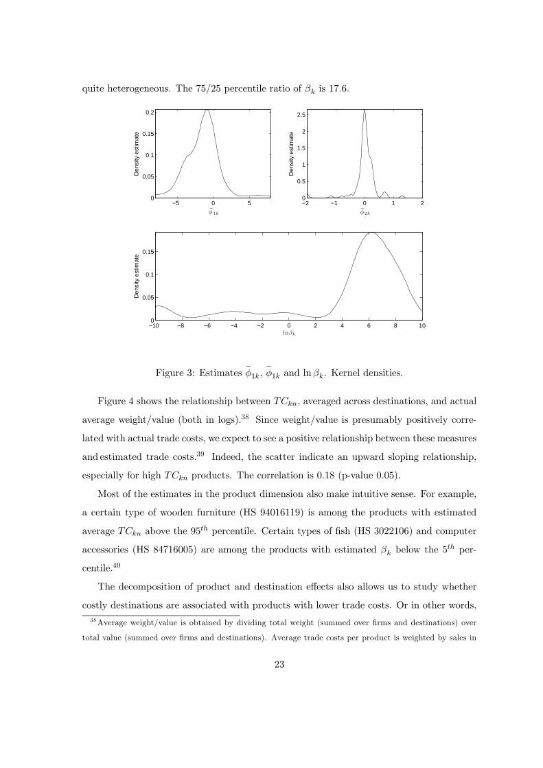
quite heterogeneous. The 7525 percentile ratio of is 176.

−5 0 50

0.05

0.1

0.15

0.2

˜φ 1k

Den

sity

est

imat

e

−2 −1 0 1 20

0.5

1

1.5

2

2.5

˜φ 2k

Den

sity

est

imat

e

−10 −8 −6 −4 −2 0 2 4 6 8 100

0.05

0.1

0.15

lnβk

Den

sity

est

imat

e

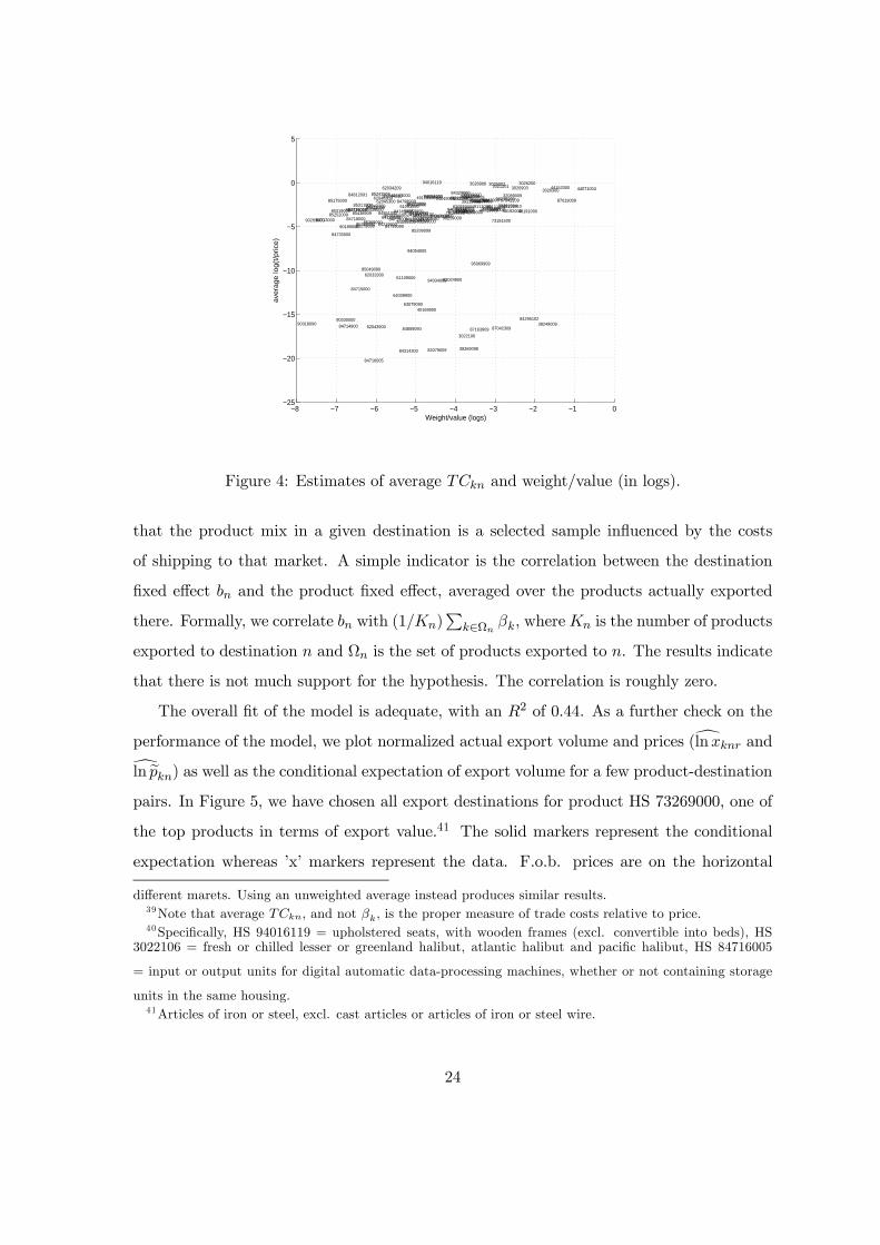
Figure 3: Estimates e1, e1 and ln. Kernel densities.Figure 4 shows the relationship between , averaged across destinations, and actual

average weight/value (both in logs).38 Since weight/value is presumably positively corre-

lated with actual trade costs, we expect to see a positive relationship between these measures

and estimated trade costs.39 Indeed, the scatter indicate an upward sloping relationship,

especially for high products. The correlation is 018 (p-value 005).

Most of the estimates in the product dimension also make intuitive sense. For example,

a certain type of wooden furniture (HS 94016119) is among the products with estimated

average above the 95 percentile. Certain types of fish (HS 3022106) and computer

accessories (HS 84716005) are among the products with estimated below the 5 per-

centile.40

The decomposition of product and destination effects also allows us to study whether

costly destinations are associated with products with lower trade costs. Or in other words,

38Average weight/value is obtained by dividing total weight (summed over firms and destinations) over

total value (summed over firms and destinations). Average trade costs per product is weighted by sales in

23

−8 −7 −6 −5 −4 −3 −2 −1 0−25

−20

−15

−10

−5

0

5

3021201

3022106

3025002 3026200

3026300 3026903 3026906

21069090

32089009

38249009

3923100439231006

3923500039239006

39259009

39269098

40169300

40169900

4407100444152000

44219009

4819100048192009

48211000 49011009

49019909491110104911109149111099

49119190

4911990961091000

61103000

6110900062033300

62034209

62043300

62043900

6204530062046309

63079090

64039900

73079900

73089008

73181500

73182900

73269000

76042900

761090097616990082055900

82079009

83024900

8310000084099909

8413810084139100

84149000

84219900

84295102

84314190

84314300

84314990

84329000

84713000

84714900

84715000

84716005

84716008

84718000 84719009

84733000

84798909

84799090

84812091

8481909084851002

84859090

85030000

85044010

85044099

85049090

85169009

85175000

85179099

8524320085243901

85243906

85252009

85299099

8531100085319000

85366900

85369090

85371009

85389090

8543890985439000

8701900987042209

87042309

8708409087089990

87163909

9018900090269000

9031809090330000

94016119

94019009

9403200994033009

94034009

94036099

940390009404900694051000

94054000

94059900

95039000

95069909

Weight/value (logs)

ave

rage lo

g(t

/price

)

Figure 4: Estimates of average and weight/value (in logs).

that the product mix in a given destination is a selected sample influenced by the costs

of shipping to that market. A simple indicator is the correlation between the destination

fixed effect and the product fixed effect, averaged over the products actually exported

there. Formally, we correlate with (1)P

∈Ω , where is the number of products

exported to destination and Ω is the set of products exported to . The results indicate

that there is not much support for the hypothesis. The correlation is roughly zero.

The overall fit of the model is adequate, with an 2 of 044. As a further check on the

performance of the model, we plot normalized actual export volume and prices (dln anddln e) as well as the conditional expectation of export volume for a few product-destinationpairs. In Figure 5, we have chosen all export destinations for product HS 73269000, one of

the top products in terms of export value.41 The solid markers represent the conditional

expectation whereas ’x’ markers represent the data. F.o.b. prices are on the horizontal

different marets. Using an unweighted average instead produces similar results.39Note that average , and not , is the proper measure of trade costs relative to price.40Specifically, HS 94016119 = upholstered seats, with wooden frames (excl. convertible into beds), HS

3022106 = fresh or chilled lesser or greenland halibut, atlantic halibut and pacific halibut, HS 84716005

= input or output units for digital automatic data-processing machines, whether or not containing storage

units in the same housing.41Articles of iron or steel, excl. cast articles or articles of iron or steel wire.

24

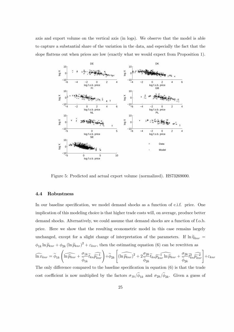
axis and export volume on the vertical axis (in logs). We observe that the model is able

to capture a substantial share of the variation in the data, and especially the fact that the

slope flattens out when prices are low (exactly what we would expect from Proposition 1).

−6 −4 −2 0 2 4−10

0

10

log f.o.b. price

log

X

DE

−4 −2 0 2 4 6−10

0

10

log f.o.b. price

log

X

DK

−4 −2 0 2 4 6−10

0

10

log f.o.b. price

log

X

FI

−6 −4 −2 0 2 4−10

0

10

log f.o.b. price

log

X

GB

−5 0 5−10

0

10

log f.o.b. price

log

X

NL

−6 −4 −2 0 2 4−10

0

10

log f.o.b. price

log

X

PL

−5 0 5 10−10

0

10

log f.o.b. price

log

X

SE

Data

Model

Figure 5: Predicted and actual export volume (normalized). HS73269000.

4.4 Robustness

In our baseline specification, we model demand shocks as a function of c.i.f. price. One

implication of this modeling choice is that higher trade costs will, on average, produce better

demand shocks. Alternatively, we could assume that demand shocks are a function of f.o.b.

price. Here we show that the resulting econometric model in this case remains largely

unchanged, except for a slight change of interpretation of the parameters. If lne =1 ln e + 2 (ln e)2 + , then the estimating equation (6) can be rewritten as

dln = e1Ã\ln e + 1e1ede−1

!+e2

"\

(ln e)2 + 22e2e \e−1 ln e + 2e2e2de−2#+

The only difference compared to the baseline specification in equation (6) is that the trade

cost coefficient is now multiplied by the factors 1e1 and 2e2. Given a guess of25

1, and assuming that 1e1 = 2e2, we can easily recalculate average trade costsby multiplying our baseline estimate with e11. In Table 3, column R1, we report themean, median and standard deviation of trade costs under 1 = −4 for all . Weightedaverage trade costs are in this case 42 percent of the median f.o.b. price. Decreasing 1

to −8 lowers the average to 21 percent. The relative magnitude of trade costs (i.e. acrossdestinations or products) is not affected by this change of the model.

In the next columns of Table 3 we present some re-estimations of the model that address

several issues. First, we check whether our estimates are sensitive to the trade cost decom-

position e = . We instead estimate e directly for all possible product-destinationpairs. Since there are no longer any interlinkages between different products, we minimize

the objective function product by product. As shown in column R2, the results are fairly

similar compared to the baseline case.

We also investigate whether the choice of truncating the data set to only product-

destinations with more than 40 firms affects the results. We choose product-destinations

with more than 20 firms present, resulting in 33 destinations and 378 products.42 The

increase in product-destination pairs now makes joint estimation infeasible, so we proceed

by estimating product by product, as above. The estimate of average weighted trade costs

increases to 66 percent, as shown in column (R3). The unweighted average increases more

moderately from 12 to 25 percent.

Finally, firms are not randomly entering into different product-destinations and this can

create a correlation between prices and the error term. We hypothesize that the correlation

is positive, since firms with both bad demand shocks and high prices are not exporting.

Analogous to the case with endogenous prices, described in the identification section, such

a selection effect would only affect the slope parameters e1 and e2, and not the estimatesof trade costs. We refer the reader to the appendix for further details.

42Exports to all possible combinations of these products and destinations amount to 589% of total export

value.

26

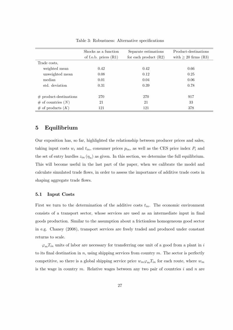
Table 3: Robustness: Alternative specifications

Shocks as a function

of f.o.b. prices (R1)

Separate estimations

for each product (R2)

Product-destinations

with ≥ 20 firms (R3)Trade costs,

weighted mean 042 042 066

unweighted mean 008 012 025

median 001 004 006

std. deviation 031 039 078

# product-destinations 270 270 917

# of countries () 21 21 33

# of products () 121 121 378

5 Equilibrium

Our exposition has, so far, highlighted the relationship between producer prices and sales,

taking input costs and , consumer prices , as well as the CES price index and

the set of entry hurdles () as given. In this section, we determine the full equilibrium.

This will become useful in the last part of the paper, when we calibrate the model and

calculate simulated trade flows, in order to assess the importance of additive trade costs in

shaping aggregate trade flows.

5.1 Input Costs

First we turn to the determination of the additive costs . The economic environment

consists of a transport sector, whose services are used as an intermediate input in final

goods production. Similar to the assumption about a frictionless homogeneous good sector

in e.g. Chaney (2008), transport services are freely traded and produced under constant

returns to scale.

units of labor are necessary for transferring one unit of a good from a plant in

to its final destination in , using shipping services from country . The sector is perfectly

competitive, so there is a global shipping service price for each route, where

is the wage in country . Relative wages between any two pair of countries and are

27

then pinned down in all markets, as long as each country produces the shipping service,

and are equal to = . By normalizing the price on a particular shipping route

to one, say from to , all nominal wages are pinned down. The additive trade cost is then

defined as ≡ = ∀ (i.e. same cost irrespective of the nationality

of the shipping supplier).

5.2 Entry and Cutoffs

We assume that the total mass of potential entrants in country is so that larger and

wealthier countries have more entrants.43 This assumption, as in Chaney (2008), greatly

simplifies the analysis and it is similar to Eaton and Kortum (2002), where the set of goods

is exogenously given. Without a free entry condition, firms generate net profits that have

to be redistributed. Following Chaney, we assume that each consumer owns shares of

a totally diversified global fund and that profits are redistributed to them in units of the

numéraire good. The total income spent by workers in country is the sum of their

labor income and of the dividends they earn from their portfolio , where is

the dividend per share of the global mutual fund.

Firms will enter market only if they can earn positive profits there. Some low pro-

ductivity firms may not generate sufficient revenue to cover their fixed costs. We define

the productivity threshold () from ( ) = 0, as the lowest possible productivity

level consistent with non-negative profits in export markets, conditional on a demand draw

,

() =

⎧⎪⎪⎨⎪⎪⎩

∙1

³

´1(1−) −

¸−1if

∞ if 1

(7)

with = 1 [ ()]1(1−) , and 1 a constant.

44

In the presence of finite additive trade costs, even the most productive firm receives finite

revenues that may not be sufficient to cover the entry cost in market . Therefore, under

some parameter values, the entry hurdle can be infinite, opening up the possibility of zero

trade flows between country-pairs. Note that, unlike in Helpman, Melitz, and Rubinstein

43 0 is a proportionality constant.

44Specifically, 1 = ()1

1− ( − 1) .

28

(2008), zero trade flows will emerge without imposing an upper bound on productivity

levels. Also note that, unlike Eaton, Kortum, and Sotelo (2011), zero trade flows will

emerge without assuming a finite integer number of firms.

5.3 Price Levels

Productivity and demand shocks in market are drawn from a joint distribution with

density ( ). We do not impose any particular assumptions on () now. E.g. and

may be negatively correlated, so that high cost firms (low firms) on average draw better

demand shocks.45 The price index is then

1− =X

Z Z ∞

()

( () )1− ( ) (8)

We can summarize an equilibrium with the following set of equations:

= ( ) ∀

= (1 )

The first equation states that the price index is a function of itself (since () is a function

of ) and the dividend share (since () is a function of which is a function of

). The second equation states that the dividend share is a function of itself and all price

indices. We show why this is so in the Appendix.

6 Implications for Aggregate Trade Flows

In this section, we ask what our trade cost estimates imply for aggregate trade flows.

Specifically, we ask to what extent our micro-level estimates are able to explain the macro

trade elasticity, i.e. the aggregate impact of trade barriers on trade flows. This enables us

to assess the importance of additive trade costs in shaping aggregate trade flows. Moreover,

we can quantify the relative importance of additive versus multiplicative (iceberg) trade

costs in shaping trade flows. For instance, if the macro trade elasticity is fully explained by

45Baldwin and Harrigan (2011) and Johnson (2010) find evidence for a positive correlation between costs

and demand shocks.

29

our micro-level estimates of additive trade costs, then the role of multiplicative trade costs

in explaining the trade elasticity must be limited.

Our methodology is as follows. First, from aggregate trade data, we calculate the actual

elasticity of trade flows with respect to variable trade barriers (proxied by distance). Second,

we calculate the general equilibrium from our model, given a set of parameters (some to be

calibrated, others based on our micro-level estimates as well as on the previous literature).

Third, we estimate the elasticity of simulated trade flows with respect to variable trade

barriers. Our objective is to match the simulated and actual trade elasticity.

We make one simplification compared to the more general model, by assuming, as in

Baldwin and Harrigan (2008) and Johnson (2010), that demand shocks are related to prices

according to = . By linking demand shocks and prices in this manner, we can account

for the possibility that the largest exporters are not necessarily the lowest price firms.46 The

function is simply intended to reflect a reduced form relationship that is observable in the

data, and we show in the next paragraph how we can infer from our micro estimates.47

The model is then effectively recast to one dimension of heterogeneity (productivity), and

we follow the literature and assume that productivities are distributed Pareto, with shape

parameter and support [1;+∞). In the appendix, we derive the expressions for the priceindex, cutoffs and quantity sold under the restriction that =

.

Next, we choose some baseline parameters from our micro estimates and from the pre-

vious literature. The parameters are summarized in Table 5. Specifically, the Pareto shape

coefficient relative to the elasticity of substitution, ( − 1), is 246, as in Eaton, Kortumand Kramarz (2010). Fixed costs are $700 000 in 2004-prices, as in Das, Roberts and

Tybout (2008). In the baseline specification, we simulate the model under three different

values of the elasticity of substitution = 5 7 9. From our micro estimates of Section

4, we have ³e1´ = −202 and

³e2´ ≈ 0 (see Table 2). In the model, the

elasticity of quantity sold with respect to c.i.f. prices is ( − 1) − (see the Appen-

46Additive trade costs have a larger negative impact on sales for low price firms. If low price firms have

the largest market share, then variation in additive trade costs will have a larger impact on aggregate trade

flows compared to when low price firms have a smaller market share.47 I.e. we do not model the possibility of firms choosing higher quality subject to a cost, but =

may be a reduced form outcome of such a process.

30

dix). Since e1 (in Section 4) is the micro estimate of this elasticity, the average is then = ((e1)+) ( − 1).48 Finally, we assume that productivity in the transport sec-tor −1 is identical across countries, so that wages are also identical, normalized to 1. This

assumption will have a negligible impact on our results, since all country-specific variation

will be controlled for by country fixed effects (see below).

We follow the literature (e.g. Anderson and van Wincoop, 2004), and let = 1 ,

where 1 is a parameter to be estimated and is distance in kilometers from to ,

normalized relative to min ().49 Our micro estimates suggest that the elasticity of

with respect to distance is 2 = 049, with GDP and GDP/capita insignificant (see

Section 4.3). We therefore let = 2 ⇐⇒ =

1+2 , where is a

parameter that we will calibrate. Finally, the simulation relies on data on income , as

proxied by PPP-based GDP from Penn World Table 6.2, and data on distance, from CEPII

(2008). We denote the set of fixed parameters Θ = 2.Before calibrating the model, we estimate the actual trade elasticity, from a standard

gravity equation with exporter and importer fixed effects,

ln = + + ln + (9)

where is aggregate trade from to in 2004. We estimate (and simulate the model) on

the same set of 22 countries that our micro estimates are based on. Trade data are gathered

from CEPII (2008). The estimated is −092 (s.e. 005), close to what is typicallyfound in the literature (e.g. Anderson and van Wincoop, 2003).

Finally, we calibrate the model. There are three unknown variables, (the constant

determining the number of potential entrants), (the constant determining the level of

additive trade costs), and 1 (the elasticity of with respect to distance). Calibration

proceeds as follows:

1. Given Θ, choose some initial¡0 01

0¢and pin down the matrix of additive and

multiplicative trade costs using = 1+2 and =

1. Then simulate

481 is defined as 1 + 1 +22 ln . Given 2 = 0, we get 1 = 1 + 1, which is the elasticity

with respect to c.i.f. price (see equation 5).49As is usual in gravity models, only the relative magnitude of can be identified, not the absolute

magnitude. We therefore choose the normalization that = 1 for the country pair with min().

31

the full general equilibrium.

2. Calculate the simulated counterpart to the average trade cost estimate from

Section 4.3. Specifically, the equilibrium unweighted average additive trade costs

(divided by ) relative to the simulated median f.o.b. price for Norwegian exporters,

=

1

− 1X

6=

¡e

¢The median f.o.b. price in is the simulated median f.o.b. price charged by Norwegian

firms entering export market .

3. Calculate the simulated trade elasticity by estimating equation (9) on simulated

trade data ln .

4. Iterate (index ) over ( 1 ) until

=

= 008 (see Table 2), =

= 092, and min () = 1.50

The results are summarized in Table 4. Under = 5, the calibrated value of 1 is

0055, suggesting that a doubling of distance increases by only 55 percent. This stands

in sharp contrast to conventional gravity studies, where 1 ( − 1) is typically around 10(Anderson and van Wincoop, 2004), giving 1 = 025 when = 5 In other words, our

results suggest that the impact of distance on multiplicative trade costs is roughly one fifth

of what conventional estimates suggest. Increasing the elasticity of substitution to 7

lowers 1 even more, and when = 9 our estimates show that 1 is only about one tenth

of the magnitude found in conventional gravity studies (0013(18)).

We also calibrate the model under the assumption that 1 = 0 =⇒ = 1 for all

country pairs, and stop matching the trade elasticity moment (but keep the other two

moments). The goal is to understand to what extent additive trade costs alone can explain

the macro trade elasticity. The results are shown in row 4 of Table 4. The actual trade

elasticity is −092, while the simulated trade elasticity is in the range of −035 to −064,depending on the choice of the elasticity of substitution. This means that additive trade

50 will affect the matrix since more potential entrants reduce the price index and increase the entry

hurdles. The requirement that min () = 1 ensures that the extensive margin will be active in all markets

(if 1, changes in trade costs will not necessarily change the number of entrants).

32

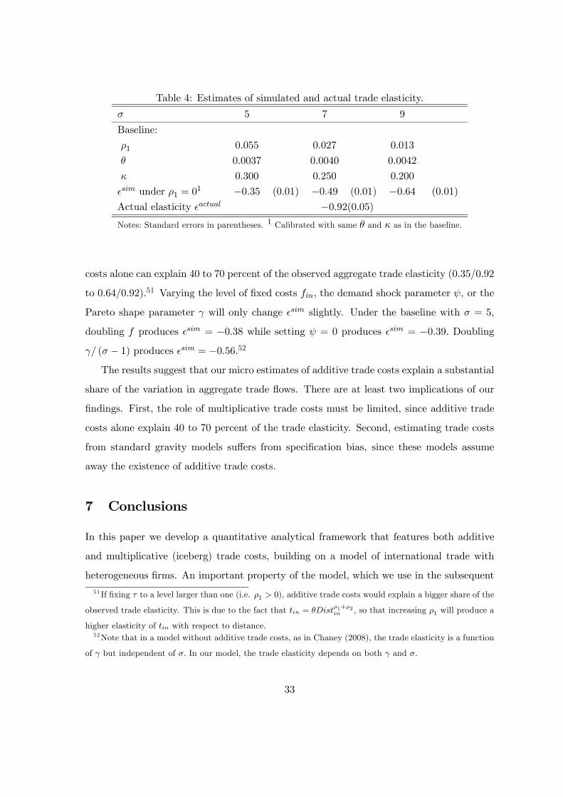
Table 4: Estimates of simulated and actual trade elasticity.

5 7 9

Baseline:

1 0055 0027 0013

00037 00040 00042

0300 0250 0200

under 1 = 01 −035 (001) −049 (001) −064 (001)

Actual elasticity −092(005)Notes: Standard errors in parentheses. 1 Calibrated with same and as in the baseline.

costs alone can explain 40 to 70 percent of the observed aggregate trade elasticity (035092

to 064092).51 Varying the level of fixed costs , the demand shock parameter , or the

Pareto shape parameter will only change slightly. Under the baseline with = 5,

doubling produces = −038 while setting = 0 produces = −039 Doubling ( − 1) produces = −056.52

The results suggest that our micro estimates of additive trade costs explain a substantial

share of the variation in aggregate trade flows. There are at least two implications of our

findings. First, the role of multiplicative trade costs must be limited, since additive trade

costs alone explain 40 to 70 percent of the trade elasticity. Second, estimating trade costs

from standard gravity models suffers from specification bias, since these models assume

away the existence of additive trade costs.

7 Conclusions

In this paper we develop a quantitative analytical framework that features both additive

and multiplicative (iceberg) trade costs, building on a model of international trade with

heterogeneous firms. An important property of the model, which we use in the subsequent

51 If fixing to a level larger than one (i.e. 1 0), additive trade costs would explain a bigger share of the

observed trade elasticity. This is due to the fact that = 1+2 , so that increasing 1 will produce a

higher elasticity of with respect to distance.52Note that in a model without additive trade costs, as in Chaney (2008), the trade elasticity is a function

of but independent of In our model, the trade elasticity depends on both and

33

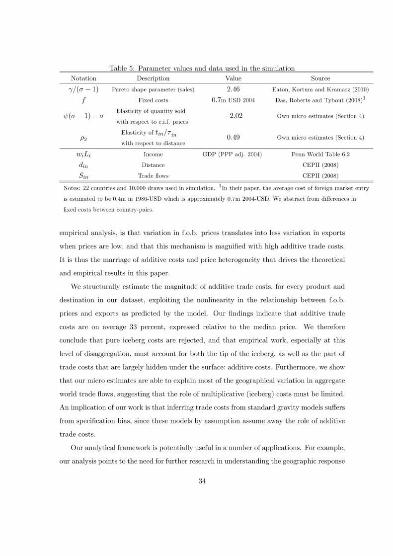
Table 5: Parameter values and data used in the simulation

Notation Description Value Source

( − 1) Pareto shape parameter (sales) 246 Eaton, Kortum and Kramarz (2010)

Fixed costs 07m USD 2004 Das, Roberts and Tybout (2008)1

( − 1)− Elasticity of quantity sold

with respect to c.i.f. prices−202 Own micro estimates (Section 4)

2Elasticity of

with respect to distance049 Own micro estimates (Section 4)

Income GDP (PPP adj. 2004) Penn World Table 6.2

Distance CEPII (2008)

Trade flows CEPII (2008)

Notes: 22 countries and 10,000 draws used in simulation. 1In their paper, the average cost of foreign market entry

is estimated to be 0.4m in 1986-USD which is approximately 0.7m 2004-USD. We abstract from differences in

fixed costs between country-pairs.

empirical analysis, is that variation in f.o.b. prices translates into less variation in exports

when prices are low, and that this mechanism is magnified with high additive trade costs.

It is thus the marriage of additive costs and price heterogeneity that drives the theoretical

and empirical results in this paper.

We structurally estimate the magnitude of additive trade costs, for every product and

destination in our dataset, exploiting the nonlinearity in the relationship between f.o.b.

prices and exports as predicted by the model. Our findings indicate that additive trade

costs are on average 33 percent, expressed relative to the median price. We therefore

conclude that pure iceberg costs are rejected, and that empirical work, especially at this

level of disaggregation, must account for both the tip of the iceberg, as well as the part of

trade costs that are largely hidden under the surface: additive costs. Furthermore, we show

that our micro estimates are able to explain most of the geographical variation in aggregate

world trade flows, suggesting that the role of multiplicative (iceberg) costs must be limited.

An implication of our work is that inferring trade costs from standard gravity models suffers

from specification bias, since these models by assumption assume away the role of additive

trade costs.

Our analytical framework is potentially useful in a number of applications. For example,

our analysis points to the need for further research in understanding the geographic response

34

of aggregate trade flows to additive trade costs. Furthermore, our theoretical finding that

uneven productivity growth in the manufacturing versus the transport sector may in fact

dampen economic integration, suggests that modeling additive trade costs may enhance our

understanding of the growth of trade. Finally, we saw that additive trade costs not only

distorts prices across markets, but also within markets. Hence, investigating the welfare

consequences of additive barriers (which may be very different from the standard case

in Arkolakis, Costinot and Rodriguez-Clare, 2010) might be a fruitful avenue for future

research.

References

[1] Abowd, John M., Robert H. Creecy, and Francis Kramarz, “Computing Person and

Firm Effects Using Linked Longitudinal Employer-Employee Data,” Cornell University

Working Paper, 2002.

[2] Alchian, Armen A., and William R. Allen, University Economics (Belmont, CA:

Wadsworth Publishing Company, 1964).

[3] Altonji, Joseph G., and Lewis M. Segal, “Small-Sample Bias in GMM Estimation of

Covariance Structures,” Journal of Business & Economic Statistics, 3 (1996), 353-366.

[4] Anderson, James E., and Eric van Wincoop, “Gravity with Gravitas: A Solution to

the Border Puzzle,” American Economic Review, 1 (2003), 170-192.

[5] Anderson, James E., and Eric van Wincoop, “Trade Costs,” Journal of Economic

Literature, 3 (2004), 691-751.

[6] Arkolakis, Konstantinos, “Market Penetration Costs and the New Consumers Margin

in International Trade,” NBER working paper No. 14214, 2008.

[7] Arkolakis, Konstantinos, Arnaud Costinot, and A. Rodríguez-Clare, “New Trade Mod-

els, Same Old Gains?,” mimeo, 2010.

35

[8] Arkolakis, Konstantinos, Arnaud Costinot, and A. Rodríguez-Clare, "Gains From

Trade under Monopolistic Competition: A Simple Example with Translog Expendi-

ture Functions and Pareto Distributions of Firm-Level Productivity", mimeo, 2010.

[9] Baldwin, Richard and James Harrigan, “Zeros, Quality and Space: Trade Theory and

Trade Evidence,” NBER Working Paper No. 13214, 2007.

[10] Berman, Nicolas, Philippe Martin, and Thierry Mayer, ‘´How Do Different Exporters

React to Exchange Rate Changes? Theory, Empirics and Aggregate Implications,”

Forthcoming in the Quarterly Journal of Economics, 2011.

[11] Bernard, Andrew B., Jonathan Eaton, Bradford J. Jensen, and Samuel Kortum,

“Plants and Productivity in International Trade,” American Economic Review,

4(2003), 1268-1290.

[12] Bernard, Andrew, Bradford J. Jensen, and Peter Schott, “Transfer Pricing by US-Based

Multinational Firms,” NBER Working Paper 12493, 2006.

[13] Broda, Christian, and David Weinstein, “Globalization and the Gains from Variety,”

Quarterly Journal of Economics, 2 (2006), 541-585.

[14] Burstein, A. and João C. Neves and Sergio Rebelo, "Distribution costs and real ex-

change rate dynamics during exchange-rate-based stabilizations", Journal of Monetary

Economics, 2003.

[15] Cameron A. Colin, and Pravin K. Trivedi, Microeconometrics: Methods and Applica-

tions, (New York, NY: Cambridge University Press, 2005).

[16] Chaney, Thomas, “Distorted Gravity: The Intensive and Extensive Margins of Inter-

national Trade,” American Economic Review, 98 (2008), 1707—1721.

[17] Corsetti, Giancarlo and Dedola, Luca, 2005. "A macroeconomic model of international

price discrimination," Journal of International Economics, Elsevier, vol. 67(1), pages

129-155, September.

[18] Delipalla, Sofia and Keen, Michael (1992), "The Comparison between Ad Valorem and

Specific Taxation under Imperfect Competition", Journal of Public Economics.

36

[19] Demidova, Svetlana, Hiau Looi Kee, and Kala Krishna, “Do Trade Policy Dixoerences

Induce Sorting? Theory and Evidence From Bangladeshi Apparel Exporters,” mimeo,

2009.

[20] Eaton, Jonathan, and Samuel Kortum, “Technology, Geography, and Trade,” Econo-

metrica, 70 (2002), 1741-1779.

[21] Eaton, Jonathan, Samuel Kortum, and Francis Kramarz, “An Anatomy of Interna-

tional Trade: Evidence from French Firms," working paper, 2010.

[22] Keith Head, and John Ries, “Increasing Returns versus National Product Differenti-

ation as an Explanation for the Pattern of U.S.-Canada Trade,” American Economic

Review, 4 (2001), 858-876.

[23] Helpman, Elhanan, Marc J. Melitz, and Yona Rubinstein. 2008. “Estimating Trade

Flows: Trading Partners and Trading Volumes.” Q.J.E., 123 (May): 441-487.

[24] Hummels, David, “Transportation Costs and International Trade in the Second Era of

Globalization,” Journal of Economic Perspectives, 21 (2007), 131-154.

[25] Hummels, David, and Alexandre Skiba, “Shipping the Good Apples Out? An Empirical

Confirmation of the Alchian-Allen Conjecture,” Journal of Political Economy, 6(2004),

1384-1402.

[26] Hummels, David and Peter J. Klenow, “The Variety and Quality of a Nation’s Ex-

ports,” American Economic Review, 3 (2005), 704-723.

[27] Hummels, David, Volodymyr Lugovskyy, and Alexandre Skiba, “The Trade Reduc-

ing Effects of Market Power in International Shipping,” Journal of Development Eco-

nomics, 1 (2009), 84-97.

[28] Irarrazabal, Alfonso, Moxnes Andreas, and Luca David Opromolla, “The Margins of

Multinational Production and the Role of Intra-firm Trade,” CEPR Discussion Paper

7145, 2008.

[29] Irwin, Douglas A. "Changes in U.S. Tariffs: The Role of Import Prices and Commercial

Policies," American Economic Review, 4 (1998), 1015-1026.

37

[30] Jacks, David S., Christopher M. Meissner, and Dennis Novy, “Trade Costs, 1870—2000,”

American Economic Review Papers & Proceedings, 2 (2008), 529—534.

[31] Johnson, Robert C., “Trade and Prices with Heterogeneous Firms,” mimeo, 2009.

[32] Kehoe, Timothy J., and Kim J. Ruhl, “How Important is the New Goods Margin in

International Trade?,” Federal Reserve Bank of Minneapolis Staff Report 324, 2009.

[33] Khandelwal, Amit K., "The Long and Short (of) Quality Ladders", Review of Economic

Studies, 77(4), 1450-1476, 2010.

[34] Khandelwal, Amit K., Schott, Peter K. and Wei, Shang-Jin, "Trade Liberalization and

Embedded Institutional Reform: Evidence from Chinese Exporters," mimeo, 2011.

[35] Klenow, Pete, and Andrés Rodríguez-Clare, “Quantifying variety gains from trade

liberalization,” mimeo, 1997.

[36] Lugovskyy, Volodymyr, and Alexandre Skiba, “Quality Choice: Effects of Trade, Trans-

portation Cost, and Relative Country Size,” mimeo, 2009.

[37] Luttmer, Erzo G. J., “Selection, Growth, and the Size Distribution of Firms,” The

Quarterly Journal of Economics, 3 (2007), 1103-1144.

[38] Manova, Kalina, and Zhiwei Zhang, “Quality Heterogeneity across Firms and Export

Destinations,” NBER Working Paper 15342, 2009.

[39] Martins, Pedro S., and Luca David Opromolla, “Exports, Imports and Wages: Evi-

dence from Matched Firm-Worker-Product Panels,” IZA Discussion Papers 4646, 2009.

[40] Melitz, Mark J., “The Impact of Trade on Intra-Industry Reallocations and Aggregate

Industry Productivity,” Econometrica, 71(2003), 1695-1725.

[41] Melitz, Mark J., and Giammarco Ottaviano, “Market Size, Trade, and Productivity,”

Review of Economic Studies 1(2008), 295-316.

[42] Obstfeld, Maurice, and Kenneth Rogoff, “The Six Major Puzzles in International

Macroeconomics: Is There a Common Cause?,” NBER Macroeconomics Annual, 15

(2000), 339-390.

38

[43] Ottaviano, Giammarco, Takatoshi Tabuchi and Jacques-François Thisse, “Agglomera-

tion and Trade Revisited,” International Economic Review, 43(2002), 409-435.

[44] Rauch, James E., “Networks versus markets in international trade,” Journal of Inter-

national Economics, 1(1999), 7-35.

[45] Romer, Paul, “New Goods, Old Theory, and the Welfare Costs of Trade Restrictions,”

Journal of Development Economics, XLIII(1994), 5—38.

[46] Samuelson, Paul A., “The Transfer Problem and the Transport Costs II: Analysis of Ef-

fects of Trade Impediments,” The Economic Journal, June 1954, 64, 264-89; reprinted

in Joseph Stiglitz, ed., Collected Scientific Papers of Paul A. Samuelson, Vol. 2, Cam-

bridge, Mass., ch. 75.

[47] Suits, D.B. and Musgrave, R.A. (1953), "Ad Valorem and Unit Taxes Compared",

Quarterly Journal of Economics, Vol. 67, pp 598-604.

[48] Sutton, J. (1991). Price Competition, Advertising, and the Evolution of Concentration.

Cambridge: The MIT Press.

[49] WTO "World Tariff Profiles 2006," WTO Secretariat.

A Appendix

A.1 Simulating the Model

A.1.1 Numerical approximation

In this subsection we show how to simulate the model numerically. The numerical approx-

imation of the equilibrium consists of the following steps.

1. Choose a starting value of the the dividend share and the price indices 0 and 0 .53

53Superscripts denote the round of iteration.

39

2. For = 1, solve the the system of +1 equations and +1 unknowns characterized

by

=

³ −1 −1

´∀

= ³−1 −1

1 −1

´as shown in the main text. This involves solving the equilibrium cutoffs (7) and the

expression for the price index (8).

3. Iterate over 2. When¯ − −1

¯and | − −1| are sufficiently small, the equilib-

rium³=1

´is found.

Since the price index does not have a closed-form solution, we approximate it with Monte

Carlo methods. Specifically, we take = 1+ 5 random draws and from the density

( ). An integral of the formZ Z ∞

()

( ) ( )

for an arbitrary function () is approximated by taking the mean of ( ) over ( )

draws that satisfy (), and adjusting by multiplying with the share of observations

that satisfy (),

[ ( ) | ()] ×# where ()

A.1.2 Global Profits

Following Chaney (2008), we assume that each worker owns shares of a global fund. The

fund collects global profits Π from all firms and redistributes them in units of the numéraire

good to its shareholders. Dividend per share in the economy is defined as = ΠP

,

and total labor income is = (1 + ). Profits for country firms selling to market

are

=

−

40

where denotes total sales from to , is the number of entrants, and is the entry

cost. Global profits are then

Π =X

X

µ

−

¶=

X

−X

X

Note thatP

is simply Dividend per share is then:

=ΠP

=(1)

P −

P

P P

=() (1 + )

P −

P

P P

Solving for yields

= −

1−

Note that since =

R R()

( ) , is only a function of the entry

hurdle function (). Replacing () with the entry hurdle expression (7), becomes

a function of itself and the price indices, = ( 1 ) (suppressing all exogenous

variables).

A.1.3 Demand shocks and prices

In Section 6, we simulate the model under the restriction that = . The price index

then becomes

1− =X

Z ∞

()(1−)(1−) ()

where () is the marginal pdf, assumed to be Pareto with shape parameter and support

[1;+∞).54

Quantity demanded can now be re-expressed as

() = ()(−1)− −1

54Unlike in earlier models, we do not need to impose the condition − 1 for the size distribution offirms to have a finite mean, as long as additive trade costs are positive. The reason is that even the most

productive firms have finite revenue.

41

The entry hurdle to access market becomes

=

⎧⎪⎪⎨⎪⎪⎩

∙e1 ³ ´1[(−1)(−1)] 1(1−) −

¸−1if

∞ if 1

(10)

where ≡ e1 ³ ´1[(−1)(−1)] 1(1−) and

e1 = − 1

µ

¶1[(−1)(−1)]

A.2 Selection bias

Firms are not randomly entering into different product-destinations and this can create a

correlation between prices and the error term. In this section, we show that selection may

bias the incidental slope coefficients, but not the trade costs coefficients.

According to the model, a firm with a demand shock enters market if its’ pro-

ductivity is above the theshold (), i.e. (). Alternatively, we can

re-express the entry hurle in terms of the highest price the firm can charge, conditional on

a demand shock, (). Assuming we find a suitable log-linear approximation

of the inequality, we write the entry condition as

ln + () + ln 0

Export volume is, from equation (3),

ln = + 1 ln + 2 (ln )2 + ln

Since ln determines both entry and sales, the error term is correlated with the price

ln . Using standard methods, and assuming that ln is normal, we find the expec-

tation of the error term in the export volume equation,

[ln | ln + () + ln 0] = [ln + ()]

where is the Mills ratio, () = () Φ (). Heckman’s two step procedure suggest the

following regression,

ln = + 1 ln + 2 (ln )2 + [ln + ()] +

42

Approximating the Mills ratio with the polynomial [ln + ()] = + ln +

(ln )2, we get

ln = + + (1 + ) ln + (2 + ) (ln )2 +

Hence, the incidental slope coefficients may suffer from selection bias, but the the parameter

of interest e remains unchanged.A.3 The prevalence of non-ad valorem duties (NAVs)

A significant share of duties are non-ad valorem (NAVs). According to the WTO World

Tariff Profiles (2006), “NAVs are applied by 68 out of the 151 countries shown in this

publication including several LDCs...” Table 6 reports, for a set of countries, the share

of Harmonized System six-digit subheadings (both for agricultural and non-agricultural

products) subject to non-ad valorem duties. The share of products subject to NAVs is

usually higher in the case of agricultural products but is also important for non-agricultural

products. For example, in the United States, the 3.4% of non-agricultural products that are

subject to NAVs account for 18.9% of imports. Still according to the WTO World Tariff

Profiles (2006) “One of the peculiarities of NAVs resides in the fact that even if they are

applied to a limited number of tariff lines, the products concerned are often classified as

sensitive, either because governments collect significant tariff revenues, e.g. cigarettes and

alcoholic drinks, or for protecting domestic products against lower priced imports. These

highlight the importance of analysing NAVs.”

43

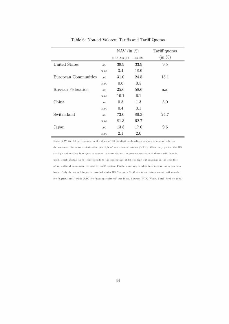
Table 6: Non-ad Valorem Tariffs and Tariff Quotas

NAV (in %) Tariff quotas

MFN Applied Imports (in %)

United States AG 39.9 33.9 9.5

NAG 3.4 18.9

European Communities AG 31.0 24.5 15.1

NAG 0.6 0.5

Russian Federation AG 25.6 58.6 n.a.

NAG 10.1 6.1

China AG 0.3 1.3 5.0

NAG 0.4 0.1

Switzerland AG 73.0 80.3 24.7

NAG 81.3 62.7

Japan AG 13.8 17.0 9.5

NAG 2.1 2.0

Note: NAV (in % ) corresp onds to the share of HS six-dig it subheadings sub ject to non-ad valorem

duties under the non-discrim ination princip le of m ost-favored nation (MFN). When only part of the HS

six-dig it subheading is sub ject to non-ad valorem duties, the p ercentage share of these tariff lines is

used. Tariff quotas (in % ) corresponds to the p ercentage of HS six-dig it subheadings in the schedule

of agricultural concession covered by tariff quotas. Partia l coverage is taken into account on a pro rata

basis. Only duties and imports recorded under HS Chapters 01-97 are taken into account. AG stands

for "agricu ltural" while NAG for "non-agricultural" products. Source: WTO World Tariff Profi les 2006.

44

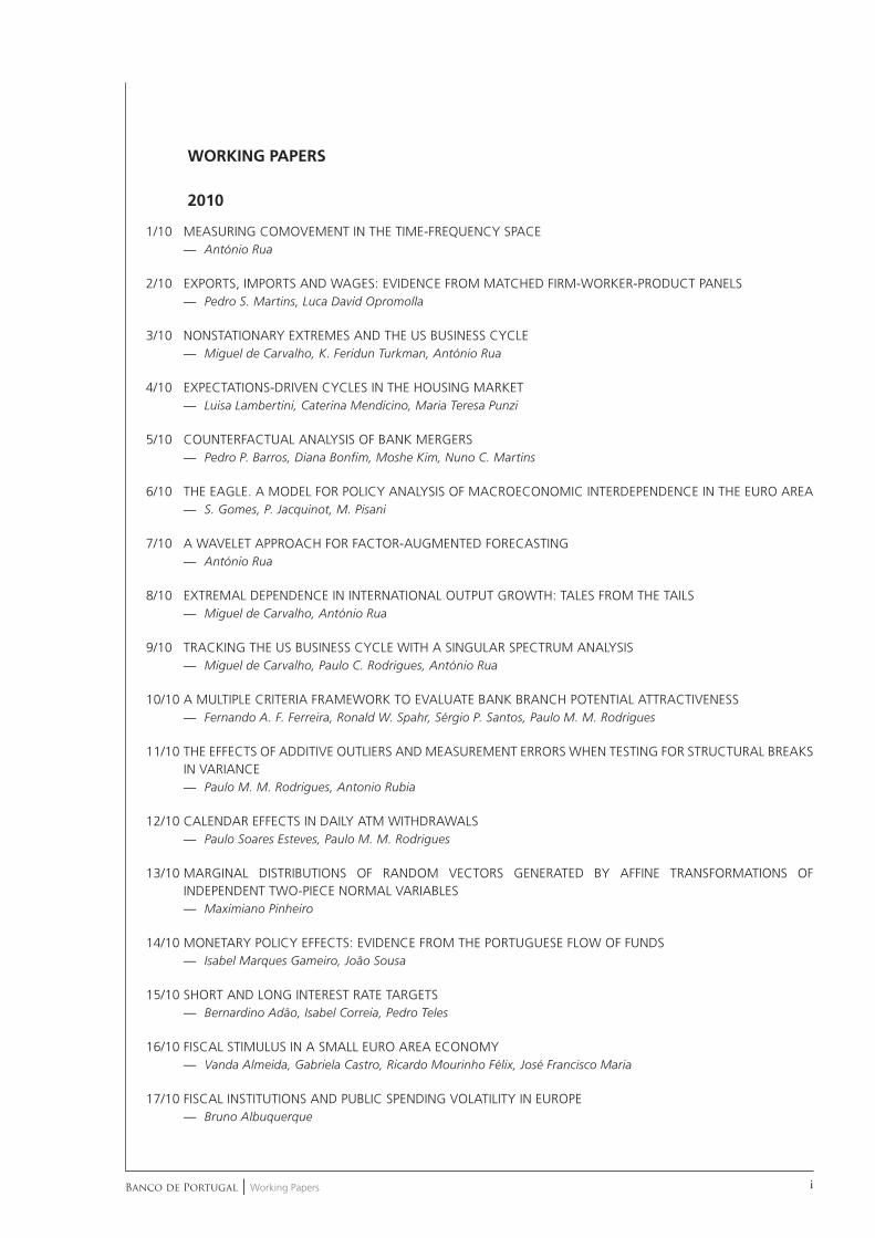
Banco de Portugal | Working Papers i

WORKING PAPERS

2010

1/10 MEASURING COMOVEMENT IN THE TIME-FREQUENCY SPACE

— António Rua

2/10 EXPORTS, IMPORTS AND WAGES: EVIDENCE FROM MATCHED FIRM-WORKER-PRODUCT PANELS

— Pedro S. Martins, Luca David Opromolla

3/10 NONSTATIONARY EXTREMES AND THE US BUSINESS CYCLE

— Miguel de Carvalho, K. Feridun Turkman, António Rua

4/10 EXPECTATIONS-DRIVEN CYCLES IN THE HOUSING MARKET

— Luisa Lambertini, Caterina Mendicino, Maria Teresa Punzi

5/10 COUNTERFACTUAL ANALYSIS OF BANK MERGERS

— Pedro P. Barros, Diana Bonfi m, Moshe Kim, Nuno C. Martins

6/10 THE EAGLE. A MODEL FOR POLICY ANALYSIS OF MACROECONOMIC INTERDEPENDENCE IN THE EURO AREA

— S. Gomes, P. Jacquinot, M. Pisani

7/10 A WAVELET APPROACH FOR FACTOR-AUGMENTED FORECASTING

— António Rua

8/10 EXTREMAL DEPENDENCE IN INTERNATIONAL OUTPUT GROWTH: TALES FROM THE TAILS

— Miguel de Carvalho, António Rua

9/10 TRACKING THE US BUSINESS CYCLE WITH A SINGULAR SPECTRUM ANALYSIS

— Miguel de Carvalho, Paulo C. Rodrigues, António Rua

10/10 A MULTIPLE CRITERIA FRAMEWORK TO EVALUATE BANK BRANCH POTENTIAL ATTRACTIVENESS

— Fernando A. F. Ferreira, Ronald W. Spahr, Sérgio P. Santos, Paulo M. M. Rodrigues

11/10 THE EFFECTS OF ADDITIVE OUTLIERS AND MEASUREMENT ERRORS WHEN TESTING FOR STRUCTURAL BREAKS

IN VARIANCE

— Paulo M. M. Rodrigues, Antonio Rubia

12/10 CALENDAR EFFECTS IN DAILY ATM WITHDRAWALS

— Paulo Soares Esteves, Paulo M. M. Rodrigues

13/10 MARGINAL DISTRIBUTIONS OF RANDOM VECTORS GENERATED BY AFFINE TRANSFORMATIONS OF

INDEPENDENT TWO-PIECE NORMAL VARIABLES

— Maximiano Pinheiro

14/10 MONETARY POLICY EFFECTS: EVIDENCE FROM THE PORTUGUESE FLOW OF FUNDS

— Isabel Marques Gameiro, João Sousa

15/10 SHORT AND LONG INTEREST RATE TARGETS

— Bernardino Adão, Isabel Correia, Pedro Teles

16/10 FISCAL STIMULUS IN A SMALL EURO AREA ECONOMY

— Vanda Almeida, Gabriela Castro, Ricardo Mourinho Félix, José Francisco Maria

17/10 FISCAL INSTITUTIONS AND PUBLIC SPENDING VOLATILITY IN EUROPE

— Bruno Albuquerque

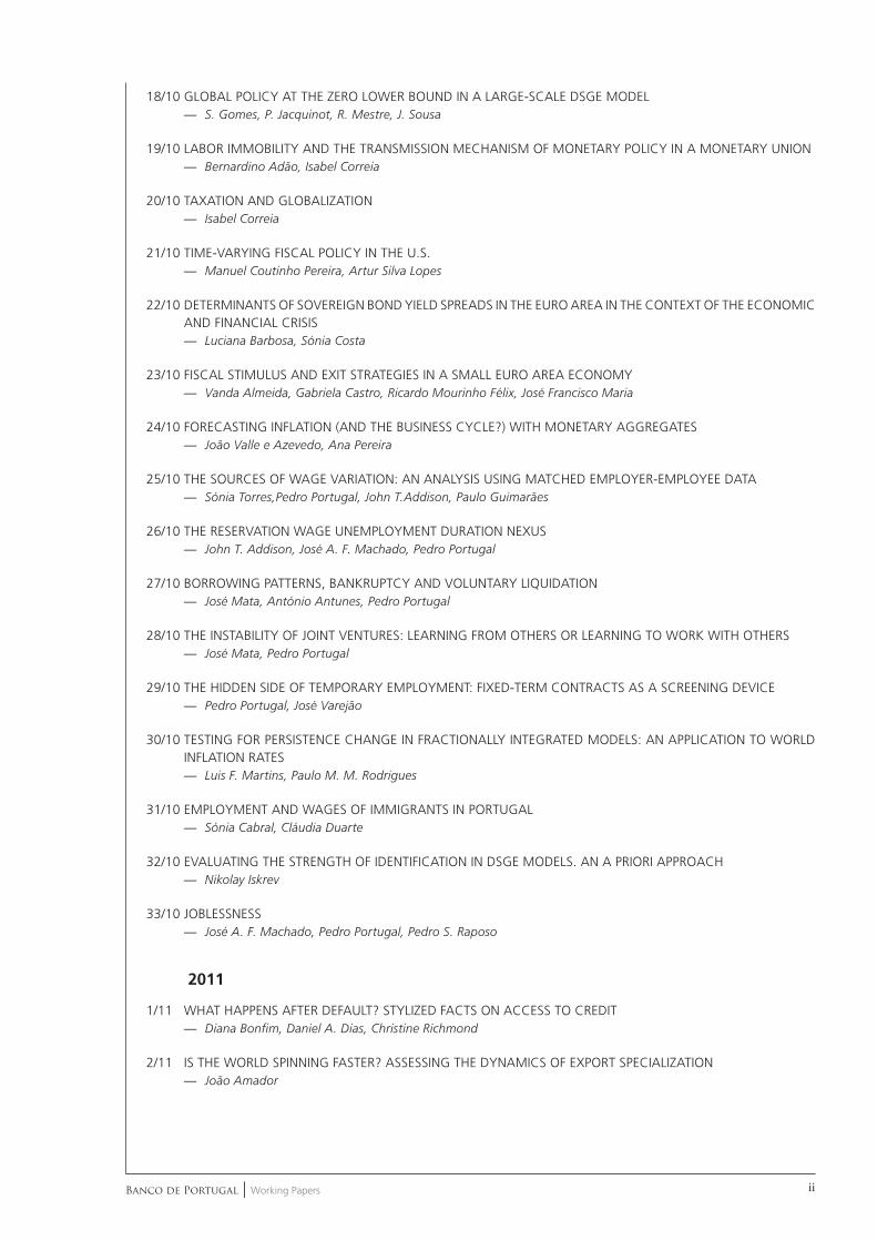
Banco de Portugal | Working Papers ii

18/10 GLOBAL POLICY AT THE ZERO LOWER BOUND IN A LARGE-SCALE DSGE MODEL

— S. Gomes, P. Jacquinot, R. Mestre, J. Sousa

19/10 LABOR IMMOBILITY AND THE TRANSMISSION MECHANISM OF MONETARY POLICY IN A MONETARY UNION

— Bernardino Adão, Isabel Correia

20/10 TAXATION AND GLOBALIZATION

— Isabel Correia

21/10 TIME-VARYING FISCAL POLICY IN THE U.S.

— Manuel Coutinho Pereira, Artur Silva Lopes

22/10 DETERMINANTS OF SOVEREIGN BOND YIELD SPREADS IN THE EURO AREA IN THE CONTEXT OF THE ECONOMIC

AND FINANCIAL CRISIS

— Luciana Barbosa, Sónia Costa

23/10 FISCAL STIMULUS AND EXIT STRATEGIES IN A SMALL EURO AREA ECONOMY

— Vanda Almeida, Gabriela Castro, Ricardo Mourinho Félix, José Francisco Maria

24/10 FORECASTING INFLATION (AND THE BUSINESS CYCLE?) WITH MONETARY AGGREGATES

— João Valle e Azevedo, Ana Pereira

25/10 THE SOURCES OF WAGE VARIATION: AN ANALYSIS USING MATCHED EMPLOYER-EMPLOYEE DATA

— Sónia Torres,Pedro Portugal, John T.Addison, Paulo Guimarães

26/10 THE RESERVATION WAGE UNEMPLOYMENT DURATION NEXUS

— John T. Addison, José A. F. Machado, Pedro Portugal

27/10 BORROWING PATTERNS, BANKRUPTCY AND VOLUNTARY LIQUIDATION

— José Mata, António Antunes, Pedro Portugal

28/10 THE INSTABILITY OF JOINT VENTURES: LEARNING FROM OTHERS OR LEARNING TO WORK WITH OTHERS

— José Mata, Pedro Portugal

29/10 THE HIDDEN SIDE OF TEMPORARY EMPLOYMENT: FIXED-TERM CONTRACTS AS A SCREENING DEVICE

— Pedro Portugal, José Varejão

30/10 TESTING FOR PERSISTENCE CHANGE IN FRACTIONALLY INTEGRATED MODELS: AN APPLICATION TO WORLD

INFLATION RATES

— Luis F. Martins, Paulo M. M. Rodrigues

31/10 EMPLOYMENT AND WAGES OF IMMIGRANTS IN PORTUGAL

— Sónia Cabral, Cláudia Duarte

32/10 EVALUATING THE STRENGTH OF IDENTIFICATION IN DSGE MODELS. AN A PRIORI APPROACH

— Nikolay Iskrev

33/10 JOBLESSNESS

— José A. F. Machado, Pedro Portugal, Pedro S. Raposo

2011

1/11 WHAT HAPPENS AFTER DEFAULT? STYLIZED FACTS ON ACCESS TO CREDIT

— Diana Bonfi m, Daniel A. Dias, Christine Richmond

2/11 IS THE WORLD SPINNING FASTER? ASSESSING THE DYNAMICS OF EXPORT SPECIALIZATION

— João Amador

Banco de Portugal | Working Papers iii

3/11 UNCONVENTIONAL FISCAL POLICY AT THE ZERO BOUND

— Isabel Correia, Emmanuel Farhi, Juan Pablo Nicolini, Pedro Teles

4/11 MANAGERS’ MOBILITY, TRADE STATUS, AND WAGES

— Giordano Mion, Luca David Opromolla

5/11 FISCAL CONSOLIDATION IN A SMALL EURO AREA ECONOMY

— Vanda Almeida, Gabriela Castro, Ricardo Mourinho Félix, José Francisco Maria

6/11 CHOOSING BETWEEN TIME AND STATE DEPENDENCE: MICRO EVIDENCE ON FIRMS’ PRICE-REVIEWING

STRATEGIES

— Daniel A. Dias, Carlos Robalo Marques, Fernando Martins

7/11 WHY ARE SOME PRICES STICKIER THAN OTHERS? FIRM-DATA EVIDENCE ON PRICE ADJUSTMENT LAGS

— Daniel A. Dias, Carlos Robalo Marques, Fernando Martins, J. M. C. Santos Silva

8/11 LEANING AGAINST BOOM-BUST CYCLES IN CREDIT AND HOUSING PRICES

— Luisa Lambertini, Caterina Mendicino, Maria Teresa Punzi

9/11 PRICE AND WAGE SETTING IN PORTUGAL LEARNING BY ASKING

— Fernando Martins

10/11 ENERGY CONTENT IN MANUFACTURING EXPORTS: A CROSS-COUNTRY ANALYSIS

— João Amador

11/11 ASSESSING MONETARY POLICY IN THE EURO AREA: A FACTOR-AUGMENTED VAR APPROACH

— Rita Soares

12/11 DETERMINANTS OF THE EONIA SPREAD AND THE FINANCIAL CRISIS

— Carla Soares, Paulo M. M. Rodrigues

13/11 STRUCTURAL REFORMS AND MACROECONOMIC PERFORMANCE IN THE EURO AREA COUNTRIES: A MODEL-

BASED ASSESSMENT

— S. Gomes, P. Jacquinot, M. Mohr, M. Pisani

14/11 RATIONAL VS. PROFESSIONAL FORECASTS

— João Valle e Azevedo, João Tovar Jalles

15/11 ON THE AMPLIFICATION ROLE OF COLLATERAL CONSTRAINTS

— Caterina Mendicino

16/11 MOMENT CONDITIONS MODEL AVERAGING WITH AN APPLICATION TO A FORWARD-LOOKING MONETARY

POLICY REACTION FUNCTION

— Luis F. Martins

17/11 BANKS’ CORPORATE CONTROL AND RELATIONSHIP LENDING: EVIDENCE FROM RETAIL LOANS

— Paula Antão, Miguel A. Ferreira, Ana Lacerda

18/11 MONEY IS AN EXPERIENCE GOOD: COMPETITION AND TRUST IN THE PRIVATE PROVISION OF MONEY

— Ramon Marimon, Juan Pablo Nicolini, Pedro Teles

19/11 ASSET RETURNS UNDER MODEL UNCERTAINTY: EVIDENCE FROM THE EURO AREA, THE U.K. AND THE U.S.

— João Sousa, Ricardo M. Sousa

20/11 INTERNATIONAL ORGANISATIONS’ VS. PRIVATE ANALYSTS’ FORECASTS: AN EVALUATION

— Ildeberta Abreu

21/11 HOUSING MARKET DYNAMICS: ANY NEWS?

— Sandra Gomes, Caterina Mendicino

Banco de Portugal | Working Papers iv

22/11 MONEY GROWTH AND INFLATION IN THE EURO AREA: A TIME-FREQUENCY VIEW

— António Rua

23/11 WHY EX(IM)PORTERS PAY MORE: EVIDENCE FROM MATCHED FIRM-WORKER PANELS

— Pedro S. Martins, Luca David Opromolla

24/11 THE IMPACT OF PERSISTENT CYCLES ON ZERO FREQUENCY UNIT ROOT TESTS

— Tomás del Barrio Castro, Paulo M.M. Rodrigues, A.M. Robert Taylor

25/11 THE TIP OF THE ICEBERG: A QUANTITATIVE FRAMEWORK FOR ESTIMATING TRADE COSTS

— Alfonso Irarrazabal, Andreas Moxnes, Luca David Opromolla