The Quantum Focussing Conjecture and Quantum Null Energy Condition by Jason Koeller A dissertation submitted in partial satisfaction of the requirements for the degree of Doctor of Philosophy in Physics in the Graduate Division of the University of California, Berkeley Committee in charge: Professor Raphael Bousso, Chair Professor Yasunori Nomura Professor Nicolai Reshetikhin Summer 2017

Welcome message from author
This document is posted to help you gain knowledge. Please leave a comment to let me know what you think about it! Share it to your friends and learn new things together.
Transcript

The Quantum Focussing Conjecture and Quantum Null Energy Condition
by
Jason Koeller
A dissertation submitted in partial satisfaction of the
requirements for the degree of
Doctor of Philosophy
in
Physics
in the
Graduate Division
of the
University of California, Berkeley
Committee in charge:
Professor Raphael Bousso, ChairProfessor Yasunori Nomura
Professor Nicolai Reshetikhin
Summer 2017

The Quantum Focussing Conjecture and Quantum Null Energy Condition
Copyright 2017by
Jason Koeller

1
Abstract
The Quantum Focussing Conjecture and Quantum Null Energy Condition
by
Jason Koeller
Doctor of Philosophy in Physics
University of California, Berkeley
Professor Raphael Bousso, Chair
Evidence has been gathering over the decades that spacetime and gravity are best under-stood as emergent phenomenon, especially in the context of a unified description of quan-tum mechanics and gravity. The Quantum Focussing Conjecture (QFC) and Quantum NullEnergy Condition (QNEC) are two recently-proposed relationships between entropy andgeometry, and energy and entropy, respectively, which further strengthen this idea.
In this thesis, we study the QFC and the QNEC. We prove the QNEC in a variety ofcontexts, including free field theories on Killing horizons, holographic theories on Killinghorizons, and in more general curved spacetimes. We also consider the implications of theQFC and QNEC in asymptotically flat space, where they constrain the information contentof gravitational radiation arriving at null infinity, and in AdS/CFT, where they are related toother semiclassical inequalities and properties of boundary-anchored extremal area surfaces.It is shown that the assumption of validity and vacuum-state saturation of the QNEC forregions of flat space defined by smooth cuts of null planes implies a local formula for themodular Hamiltonian of these regions. We also demonstrate that the QFC as originallyconjectured can be violated in generic theories in d ≥ 5, which led the way to an improvedformulation subsequently suggested by Stefan Leichenauer.

i
Contents
Contents i
List of Figures iii
List of Tables vi
1 Introduction 1
2 Proof of the Quantum Null Energy Condition 42.1 Introduction . . . . . . . . . . . . . . . . . . . . . . . . . . . . . . . . . . . . 42.2 Statement of the Quantum Null Energy Condition . . . . . . . . . . . . . . . 82.3 Reduction to a 1+1 CFT and Auxiliary System . . . . . . . . . . . . . . . . 92.4 Calculation of the Entropy . . . . . . . . . . . . . . . . . . . . . . . . . . . . 142.5 Extension to D = 2, Higher Spin, and Interactions . . . . . . . . . . . . . . . 25
3 Holographic Proof of the Quantum Null Energy Condition 283.1 Introduction . . . . . . . . . . . . . . . . . . . . . . . . . . . . . . . . . . . . 283.2 Statement of the QNEC . . . . . . . . . . . . . . . . . . . . . . . . . . . . . 303.3 Proof of the QNEC . . . . . . . . . . . . . . . . . . . . . . . . . . . . . . . . 333.4 Discussion . . . . . . . . . . . . . . . . . . . . . . . . . . . . . . . . . . . . . 44
4 Information Content of Gravitational Radiation and the Vacuum 494.1 Introduction . . . . . . . . . . . . . . . . . . . . . . . . . . . . . . . . . . . . 494.2 Asymptotic Entropy Bounds and Bondi News . . . . . . . . . . . . . . . . . 534.3 Implications of the Equivalence Principle . . . . . . . . . . . . . . . . . . . . 584.4 Entropy Bounds on Gravitational Wave Bursts and the Vacuum . . . . . . . 64
5 Geometric Constraints from Subregion Duality Beyond the ClassicalRegime 665.1 Introduction . . . . . . . . . . . . . . . . . . . . . . . . . . . . . . . . . . . . 665.2 Glossary . . . . . . . . . . . . . . . . . . . . . . . . . . . . . . . . . . . . . . 695.3 Relationships Between Entropy and Energy Inequalities . . . . . . . . . . . . 76

ii
5.4 Relationships Between Entropy and Energy Inequalities and Geometric Con-straints . . . . . . . . . . . . . . . . . . . . . . . . . . . . . . . . . . . . . . . 77
5.5 Discussion . . . . . . . . . . . . . . . . . . . . . . . . . . . . . . . . . . . . . 90
6 Local Modular Hamiltonians from the Quantum Null Energy Condition 936.1 Introduction and Summary . . . . . . . . . . . . . . . . . . . . . . . . . . . . 936.2 Main Argument . . . . . . . . . . . . . . . . . . . . . . . . . . . . . . . . . . 956.3 Holographic Calculation . . . . . . . . . . . . . . . . . . . . . . . . . . . . . 986.4 Discussion . . . . . . . . . . . . . . . . . . . . . . . . . . . . . . . . . . . . . 100
7 Violating the Quantum Focusing Conjecture and Quantum CovariantEntropy Bound in d ≥ 5 dimensions 1037.1 Introduction . . . . . . . . . . . . . . . . . . . . . . . . . . . . . . . . . . . . 1037.2 Violating the QFC in Gauss-Bonnet Gravity . . . . . . . . . . . . . . . . . . 1057.3 Violating the Generalized Covariant Entropy Bound . . . . . . . . . . . . . . 1097.4 Discussion . . . . . . . . . . . . . . . . . . . . . . . . . . . . . . . . . . . . . 110
8 The Quantum Null Energy Condition in Curved Space 1128.1 Introduction and Summary . . . . . . . . . . . . . . . . . . . . . . . . . . . . 1128.2 Scheme-(in)dependence of the QNEC . . . . . . . . . . . . . . . . . . . . . . 1148.3 Holographic Proofs of the QNEC . . . . . . . . . . . . . . . . . . . . . . . . 1218.4 Discussion . . . . . . . . . . . . . . . . . . . . . . . . . . . . . . . . . . . . . 129
A Appendices 132A.1 Correlation Functions . . . . . . . . . . . . . . . . . . . . . . . . . . . . . . . 132A.2 Details of the Asymptotic Expansions . . . . . . . . . . . . . . . . . . . . . . 134A.3 KRS Bound . . . . . . . . . . . . . . . . . . . . . . . . . . . . . . . . . . . . 135A.4 Single Graviton Wavepacket . . . . . . . . . . . . . . . . . . . . . . . . . . . 138A.5 Non-Expanding Horizons and Weakly Isolated Horizons . . . . . . . . . . . . 143A.6 Scheme Independence of the QNEC . . . . . . . . . . . . . . . . . . . . . . . 145
Bibliography 152

iii
List of Figures
2.1 The spatial surface Σ splits a Cauchy surface, one side of which is shown in yellow.The generalized entropy Sgen is the area of Σ plus the von Neumann entropy Sout
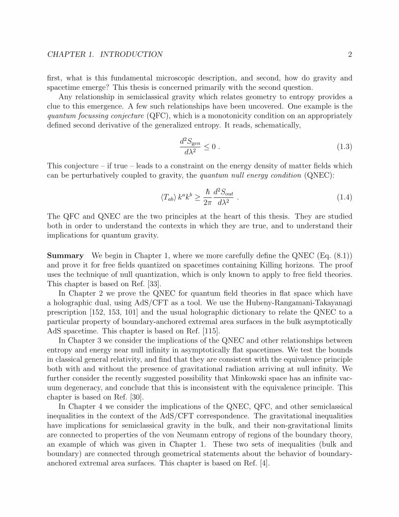
of the yellow region. The quantum expansion Θ at one point of Σ is the rate atwhich Sgen changes under a small variation dλ of Σ, per cross-sectional area Aof the variation. The Quantum Focussing Conjecture states that the quantumexpansion cannot increase under a second variation in the same direction. If theclassical expansion and shear vanish (as they do for the green null surface in thefigure), the Quantum Null Energy Condition is implied as a limiting case. Ourproof involves quantization on the null surface; the entropy of the state on theyellow spacelike slice is related to the entropy of the null quantized state on thefuture (brighter green) part of the null surface. . . . . . . . . . . . . . . . . . . . 6
2.2 The state of the CFT on x > λ can be defined by insertions of ∂Φ on the Euclideanplane. The red lines denote a branch cut where the state is defined. . . . . . . . 11
2.3 Sample plots of the imaginary part (the real part is qualitatively identical) ofthe naıve bracketed digamma expression in (2.74) and the one in (2.78) obtainedfrom analytic continuation with z = −m − iαij for m = 3 and various valuesof αij. The oscillating curves are (2.74), while the smooth curves are the resultof applying the specified analytic continuation prescription to that expression,resulting in (2.78). . . . . . . . . . . . . . . . . . . . . . . . . . . . . . . . . . . 23
3.1 Here we show the region R (shaded cyan) and the boundary Σ (black border)before and after the null deformation. The arrow indicates the direction ki, and〈Tkk〉 is being evaluated at the location of the deformation. The dashed lineindicates the support of the deformation. . . . . . . . . . . . . . . . . . . . . . . 30
3.2 The surface M in the bulk (shaded green) is the union of all of the extremalsurfaces anchored to the boundary that are generated as we deform the entan-gling surface. The null vector ki (solid arrow) on the boundary determines thedeformation, and the spacelike vector sµ (dashed arrow) tangent toM is the onewe construct in our proof. The QNEC arises from the inequality sµsµ ≥ 0. . . . 38
iv
4.1 Penrose diagram of an asymptotic flat spacetime. Gravitational radiation (i.e.,Bondi news) arrives on a bounded portion of I+ (red). The asymptotic regionsbefore and after this burst (blue) are Riemann flat. The equivalence principlerequires that observers with access only to the flat regions cannot extract classicalinformation; however, an observer with access to the Bondi news can receiveinformation (see Sec. 4.3). We find in Sec. 4.4 that the asymptotic entropy boundsof Sec. 4.2 are consistent with these conclusions. . . . . . . . . . . . . . . . . . . 50
5.1 The logical relationships between the constraints discussed in this paper. Theleft column contains semi-classical quantum gravity statements in the bulk. Themiddle column is composed of constraints on bulk geometry. In the right columnis quantum field theory constraints on the boundary CFT. All implications aretrue to all orders in G~ ∼ 1/N . We have used dashed implication signs for thosethat were proven to all orders before this paper. . . . . . . . . . . . . . . . . . . 68
5.2 The causal relationship between e(A) and D(A) is pictured in an example space-time that violates C ⊆ E . The boundary of A’s entanglement wedge is shaded.Notably, in C ⊆ E violating spacetimes, there is necessarily a portion of D(A)that is timelike related to e(A). Extremal surfaces of boundary regions from thisportion of D(A) are necessarily timelike related to e(A), which violates EWN. . 78
5.3 The boundary of a BCC-violating spacetime is depicted, which gives rise to aviolation of C ⊆ E . The points p and q are connected by a null geodesic throughthe bulk. The boundary of p’s lightcone with respect to the AdS boundary causalstructure is depicted with solid black lines. Part of the boundary of q’s lightconeis shown with dashed lines. The disconnected region A is defined to have part ofits boundary in the timelike future of q while also satisfying p ∈ D(A). It followsthat e(A) will be timelike related to D(A) through the bulk, violating C ⊆ E . . . 79
5.4 The surface M and N are shown touching at a point p. In this case, θM < θN . Thearrows illustrate the projection of the null orthogonal vectors onto the Cauchysurface. . . . . . . . . . . . . . . . . . . . . . . . . . . . . . . . . . . . . . . . . 82
5.5 This picture shows the various vectors defined in the proof. It depicts a cross-section of the extremal surface at constant z. e(A)vac denotes the extremal surfacein the vacuum. For flat cuts of a null plane on the boundary, they agree. Forwiggly cuts, they will differ by some multiple of ki. . . . . . . . . . . . . . . . . 88
6.1 This image depicts a section of the plane u = t− x = 0. The region R is definedto be one side of a Cauchy surface split by the codimension-two entangling surface∂R = (u = 0, v = V (y), y). The dashed line corresponds to a flat cut of thenull plane. . . . . . . . . . . . . . . . . . . . . . . . . . . . . . . . . . . . . . . . 94
A.1 A short observation (green shaded rectangle) cannot distinguished the reducedgraviton state from the vacuum reduced to the same region. The graviton deliversno information to this observer. . . . . . . . . . . . . . . . . . . . . . . . . . . . 139
v
A.2 A long observation (green shaded rectangle) can distinguish the reduced gravitonstate from the reduced vacuum. The graviton carries information to this observer. 141
A.3 A graviton conveys O(1) information as long as it has appreciable support in theregion of observation. . . . . . . . . . . . . . . . . . . . . . . . . . . . . . . . . . 142
vi
List of Tables
8.1 Scheme-independence of QNEC for all four-derivative counter-terms ∆L from(8.16) when (8.17) and (8.18) hold.119
8.2 Scheme-independence of QNEC for the six-derivative counter-terms ∆L builtfrom polynomial contractions of the Riemann tensor when the null congruenceN is a weakly isolated horizon. However, as shown in the main text, scheme-independence can fail for counter-terms involving derivatives of the Riemanntensor.120

vii
Acknowledgments
I have had the pleasure of working with and learning from many people throughout thisprocess. I would like to thank my advisor, Raphael Bousso, for his support, guidance, inspi-ration and example. I am grateful to Stefan Leichenauer for patiently answering countlessquestions and for our fruitful collaboration. I would also like to thank Don Marolf for hisadvice and collaboration.
I would like to thank all of my other collaborators – Aron Wall, Zach Fisher, Illan Halpern,Chris Akers, Adam Levine, Arvin Shahbazi Moghaddam, and Zicao Fu – for all that I’velearned from them.
I would also like to recognize all of the others in the Berkeley Center for Theoreti-cal Physics who made it such an enjoyable and intellectually stimulating place, especiallyVenkatesh Chandrasekaran, Sean Weinbeg, Fabio Sanches, Mudassir Moosa, and YasunoriNomura.

1
Chapter 1
Introduction
Quantum gravity remains the final frontier of fundamental physics. Attempts to quantize thegravitational field directly lead to inconsistencies away from the regime in which perturbationtheory provides a good approximation.
There is increasing evidence that a fundamentally different approach is needed. One suchapproach is to take seriously the possibility that spacetime and gravity are not fundamental,but instead emerge from a microscopic description which is quantum mechanical but notgravitational. The celebrated AdS/CFT correspondence provides an explicit example ofthis for the case of spacetimes with asymptotically negative curvature. In more generalspacetimes we must rely on less direct evidence.
A hint comes from thought experiments involving black holes. In classical general rela-tivity, the dynamics of black holes can naturally be recast in a form which resembles the lawsof thermodynamics, in which the entropy is the area of the event horizon in Planck units:
SBH =A
4G~. (1.1)
This association of a thermodynamical entropy with a geometrical quantity was historicallythe first hint that gravity and spacetime might be an emergent phenomenon, in the same waythermodynamics emerges from statistical mechanics. When quantum effects are included inthe description, black holes become able to radiate and evaporate. Hence the similarity tothermodynamics becomes more than just mathematical analogy, provided that one includethe entropy of both black holes and matter (including the radiation):
Sgen = SBH + Sout , (1.2)
where Sout is the entropy of matter outside of the black hole. This generalized entropy isreally just the total entropy including the entropy of black holes and matter, but is referredto as the generalized entropy for historical reasons.
If gravity and spacetime are in some sense a reorganization of the degrees of freedom ofa more fundamental microscopic description, two immediate questions present themselves:
CHAPTER 1. INTRODUCTION 2
first, what is this fundamental microscopic description, and second, how do gravity andspacetime emerge? This thesis is concerned primarily with the second question.
Any relationship in semiclassical gravity which relates geometry to entropy provides aclue to this emergence. A few such relationships have been uncovered. One example is thequantum focussing conjecture (QFC), which is a monotonicity condition on an appropriatelydefined second derivative of the generalized entropy. It reads, schematically,
d2Sgen
dλ2≤ 0 . (1.3)
This conjecture – if true – leads to a constraint on the energy density of matter fields whichcan be perturbatively coupled to gravity, the quantum null energy condition (QNEC):
〈Tab〉 kakb ≥~2π
d2Sout
dλ2. (1.4)
The QFC and QNEC are the two principles at the heart of this thesis. They are studiedboth in order to understand the contexts in which they are true, and to understand theirimplications for quantum gravity.
Summary We begin in Chapter 1, where we more carefully define the QNEC (Eq. (8.1))and prove it for free fields quantized on spacetimes containing Killing horizons. The proofuses the technique of null quantization, which is only known to apply to free field theories.This chapter is based on Ref. [33].
In Chapter 2 we prove the QNEC for quantum field theories in flat space which havea holographic dual, using AdS/CFT as a tool. We use the Hubeny-Rangamani-Takayanagiprescription [152, 153, 101] and the usual holographic dictionary to relate the QNEC to aparticular property of boundary-anchored extremal area surfaces in the bulk asymptoticallyAdS spacetime. This chapter is based on Ref. [115].
In Chapter 3 we consider the implications of the QNEC and other relationships betweenentropy and energy near null infinity in asymptotically flat spacetimes. We test the boundsin classical general relativity, and find that they are consistent with the equivalence principleboth with and without the presence of gravitational radiation arriving at null infinity. Wefurther consider the recently suggested possibility that Minkowski space has an infinite vac-uum degeneracy, and conclude that this is inconsistent with the equivalence principle. Thischapter is based on Ref. [30].
In Chapter 4 we consider the implications of the QNEC, QFC, and other semiclassicalinequalities in the context of the AdS/CFT correspondence. The gravitational inequalitieshave implications for semiclassical gravity in the bulk, and their non-gravitational limitsare connected to properties of the von Neumann entropy of regions of the boundary theory,an example of which was given in Chapter 1. These two sets of inequalities (bulk andboundary) are connected through geometrical statements about the behavior of boundary-anchored extremal area surfaces. This chapter is based on Ref. [4].
CHAPTER 1. INTRODUCTION 3
In Chapter 5 we use the QNEC to derive a local expression for the modular Hamiltonianof a region bounded by a smooth cut of a null plane, generalizing the class of regions forwhich such an expression is known. The result holds in any theory in which the QNEC isboth true and saturated in the vacuum state. We discuss the validity of these assumptionsin free theories and holographic theories to all orders in 1/N . This chapter is based onRef. [116].
In Chapter 6 we point out that the QFC as explicitly conjectured in Ref. [34] can beviolated in theories containing a perturbative Gauss-Bonnet gravitational coupling – as anygeneric effective field theory of gravity will – in dimensions d ≥ 5. This chapter is basedon Ref. [81]. This work led to an improved formulation of the QFC which avoids this issue[123].
Finally, in Chapter 7 we conclude by discussing the status of the QNEC in holographictheories in curved spacetimes. We identify a set of sufficient restrictions on the spacetimegeometry and surface for the QNEC to hold in d ≤ 5. In d ≥ 6, we find that these conditionsare not sufficient. This chapter is based on Ref. [80].

4
Chapter 2
Proof of the Quantum Null EnergyCondition
2.1 Introduction
The null energy condition (NEC) states that Tkk ≡ Tabkakb ≥ 0, where Tab is the stress tensor
and ka is a null vector. This condition is satisfied by most reasonable classical matter fields.In Einstein’s equation, it ensures that light-rays are focussed, never repelled, by matter. TheNEC underlies the area theorems [91, 28] and singularity theorems [146, 93, 172], and manyother results in general relativity [135, 79, 66, 167, 92, 144, 171, 145, 84].
However, quantum fields violate all local energy conditions, including the NEC [65]. Theenergy density 〈Tkk〉 at any point can be made negative, with magnitude as large as we wish,by an appropriate choice of quantum state. In a stable theory, any negative energy must beaccompanied by positive energy elsewhere. Thus, positive-definite quantities linear in thestress tensor that are bounded below may exist, but must be nonlocal. For example, a totalenergy may be obtained by integrating an energy density over all of space; an “averagednull energy” is defined by integrating 〈Tkk〉 along a null geodesic [22, 173, 114, 169, 87, 98].In some field theories, “quantum energy inequalities” have also been shown, in which anintegral of the stress-tensor need not be positive, but is bounded below [76].
In this article, we will consider a new type of lower bound on 〈Tkk〉 at a single pointp. Here the bound itself is computed from a nonlocal object: the von Neumann entropySout[Σ] ≡ −Tr(ρ ln ρ) of the quantum fields restricted to some finite or infinite spatial regionwhose boundary Σ contains p, is normal to ka, and has vanishing null expansion at p. (Thereare infinitely many ways of choosing such Σ for any (p, ka).) Then a lower bound is givenby the second derivative of Sout, under deformations of an infinitesimal area element A of Σin the ka direction at p (see Figure 2.1):
〈Tkk〉 ≥~
2πAS′′out[Σ] . (2.1)
We call (2.1) the Quantum Null Energy Condition (QNEC) [34]. The quantity Sout is
CHAPTER 2. PROOF OF THE QUANTUM NULL ENERGY CONDITION 5
divergent but its derivatives are finite. (A more rigorous formulation in terms of functionalderivatives will be given in the main text.) Note that the right hand side can have any sign.If it is positive, then the QNEC is stronger than the NEC; but since it can be negative, it canaccommodate situations where the NEC would fail. By integrating the QNEC along a nullgenerator, we can obtain the ANEC, in situations where the boundary term S ′out vanishes atearly and late times.
Intriguingly, the QNEC—an intrinsically field theoretic statement—was recognized bystudying conjectured properties of the generalized entropy,
Sgen[Σ] =A[Σ]
4G~+ Sout[Σ] , (2.2)
a key concept arising in quantum gravity [13, 14, 15]. Here Σ is a codimension-2 surfacewhich divides a Cauchy surface in two, A[Σ] is its area and Sout is the von Neumann entropyof the matter fields on one side of Σ.
The generalized second law (GSL) is the conjecture [13] that the generalized entropycannot decrease as Σ is moved up along a causal horizon. Equation (2.1) first appeared as asufficient condition for the GSL, satisfied by a nontrivial class of states of a 1+1 dimensionalCFT [179]. The QNEC emerged as a general constraint on quantum field theories when itwas noted that the Quantum Focussing Conjecture (QFC) implies (2.1) in an appropriatelimit [34]. We will briefly describe the QFC and outline how the QNEC arises from it.
A generalized entropy can be ascribed not only to horizon slices, but to any surfacethat splits a Cauchy surface [180, 64, 19, 136, 69]. Moreover, one can define a quantumexpansion Θ[Σ; y1], the rate (per unit area) at which the generalized entropy changes whenthe infinitesimal area element of ν at a point y1 is deformed in one of its future orthogonalnull directions [34] (see Fig. 2.1). This quantity limits to the classical (geometric) expansionas ~→ 0. The QFC states that the quantum expansion Θ[Σ; y1] will not increase under anysecond variation of Σ along the same future congruence, be it at y1 or at some other pointy2 [34].
The QFC, in turn, was proposed as a quantum version of the covariant entropy bound(Bousso bound) [23, 25, 72], a quantum gravity conjecture which bounds the entropy ona nonexpanding null surface in terms of the difference between its initial and final area.The QFC implies the Bousso bound; but because the generalized entropy appears to beinsensitive to the UV cutoff [165, 105, 161], the QFC remains well-defined in more generalsettings. (The QFC is distinct from the quantum Bousso bound of [32, 31], which definesthe entropy by vacuum subtraction [45], a procedure applicable if the gravitational effects ofmatter are negligible.)
In the case where y1 6= y2, it can be shown [34] that the QFC follows from strongsubadditivity, an entropy inequality which all quantum systems must obey.1 For y1 = y2,
1Some recent articles [17, 121] considered a different type of second derivative of the entropy in 1+1field theory. These inequalities involve varying the two endpoints of an interval independently, and thereforefollow from strong subadditivity alone, without making reference to the stress-tensor.

CHAPTER 2. PROOF OF THE QUANTUM NULL ENERGY CONDITION 6
A|z
Sout()
d
Figure 2.1: The spatial surface Σ splits a Cauchy surface, one side of which is shown inyellow. The generalized entropy Sgen is the area of Σ plus the von Neumann entropy Sout
of the yellow region. The quantum expansion Θ at one point of Σ is the rate at which Sgen
changes under a small variation dλ of Σ, per cross-sectional area A of the variation. TheQuantum Focussing Conjecture states that the quantum expansion cannot increase under asecond variation in the same direction. If the classical expansion and shear vanish (as theydo for the green null surface in the figure), the Quantum Null Energy Condition is impliedas a limiting case. Our proof involves quantization on the null surface; the entropy of thestate on the yellow spacelike slice is related to the entropy of the null quantized state on thefuture (brighter green) part of the null surface.
the QFC remains a conjecture in general, but in special cases it can be proven. The QFCconstrains a combination of “geometric” terms proportional to G−1 that stem from theclassical expansion, as well as “matter entropy” terms that stem from Sout and do notinvolve Newton’s constant. The classical expansion is governed by Raychaudhuri’s equation,θ′ = −θ2/2 − σ2 − 8πG〈Tkk〉.2 If the expansion θ and the shear σ vanish at y1, then therate of change of the expansion is governed by a term proportional to G. In this case, allG’s cancel in the terms of the QFC, and (2.1) emerges as an apparently nongravitationalstatement.
Outline In this paper, we will prove the QNEC in a broad arena. Our proof applies tofree or superrenormalizable, massive or massless bosonic fields, in all cases where the surfaceΣ lies on a stationary null hypersurface (one with everywhere vanishing expansion). Themost important example is Minkowski space, with Σ lying on a Rindler horizon. Such ahorizon exists at every point p, with every orientation ka, so the QNEC constrains all nullcomponents of the stress tensor everywhere in Minkowski space.
A similar situation arises in a de Sitter background, where p and ka specify a de Sitterhorizon, and in Anti-de Sitter space, where they specify a Poincare horizon. Other examples
2Raychaudhuri’s equation immediately implies that, in cases where the classical geometrical terms dom-inate, the QFC is true iff the classical spacetime obeys the null curvature condition.

CHAPTER 2. PROOF OF THE QUANTUM NULL ENERGY CONDITION 7
include an eternal Schwarzschild or Kerr black hole, but in this case our proof applies onlyto points on the horizon, with ka tangent to the horizon generators. These should all beviewed as fixed background spacetimes with no dynamical gravity; our proof establishes thatfree scalar field theory on these backgrounds satisfies (2.1).
We give a brief review of the formal statement of the QNEC in Sec. 2.2. We then setup the calculation of all relevant terms in Sec. 2.3. In Sec. 2.3, we review the null surfacequantization of the theory, on the particular null surface N that is orthogonal to Σ withtangent vector ka. Null quantization has the remarkable feature that the vacuum statefactorizes in the transverse spatial directions. This reduces any purely kinematic problem(such as ours) to the analysis of a large number of copies of the free chiral scalar CFT in1+1 dimensions. We then restrict attention to the particular chiral CFT on the infinitesimalpencil that passes through the point p where Σ is varied. The state on this pencil is entangledwith an auxiliary quantum system which contains both the information crossing the othergenerators of N , and the information that does not fall across N at all.
In the 1+1 chiral CFT, the pencil state is very close to the vacuum, but not so close thatthe QNEC would be trivially saturated by application of the first law of the entanglemententropy. To constrain the second order variations of Sout (the Fisher information), we mustkeep track of the deviation of the pencil state from the vacuum to second order. We discussthe appropriate expansion of the overall state in Sec. 2.3. We write the state in terms ofoperators inserted on the Euclidean plane corresponding to the pencil and expand in a basisof the auxiliary system. Then in Sec. 2.3, we expand the entropy and identify the parts ofour expnsion enter into the second derivative.
In Sec. 2.4, we compute the sign of 〈Tkk〉− ~2πAS
′′out. In Sec. 2.4 we review the replica trick
for computing the von Neumann entropy by the analytic continuation of Renyi entropies. Weextract two terms relevant to the QNEC, which are computed in Sec. 2.4 and 2.4 respectively.The most subtle part of the calculation is the analytic continuation of the second of theseterms, in Sec. 2.4. In Sec. 2.4, we combine the terms and conclude that the QNEC holds forall states.
In Sec. 2.5, we extend our result to establish the QNEC also for superrenormalizablescalar fields, and for bosonic fields of higher spin. We also discuss the extension to interactingtheories. We expect that the proof we have given can be extended to fermionic fields, butwe leave this task for the future.
Discussion Our result establishes a new and surprising link between quantum informationand a more familiar physical quantity, the stress tensor. The QNEC identifies the “accel-eration” of information transfer as a lower bound on the energy density. Equivalently, thestress tensor can be viewed as imposing a constraint on the second derivative of the vonNeumann entropy. The latter can be difficult to calculate but plays an important role inquantum information theory, condensed matter, and high energy physics.
Our proof of the QNEC requires no assumptions beyond the known properties of freequantum fields, but it is quite lengthy and somewhat involved. Yet, the QNEC follows

CHAPTER 2. PROOF OF THE QUANTUM NULL ENERGY CONDITION 8
almost trivially from a statement involving gravity, the Quantum Focussing Conjecture. Thisperplexing situation is somewhat reminiscent of the proof of the quantum Bousso bound [32],particularly in the interacting case [31]. It is intriguing that the study of quantum gravitycan lead us to simple conjectures such as (2.1) which can be proven entirely within thenongravitational sector, where they are far from obvious—so far, indeed, that they had notbeen recognized until they emerged as implications of holographic entropy bounds or ofproperties of the generalized entropy.
It is becoming clear that the structure of known quantum field theories carries a deep im-print of causal and information theoretic properties ultimately dictated by quantum gravity.This adds to the evidence that “quantizing gravity” has nothing to do with the inclusion ofone last force in a quantization program. It would be interesting to try to formulate modelsof quantum gravity in which focussing of the entropy occurs naturally.
Remarkably, the QNEC does not seem to follow from any of the standard identitiesthat apply purely at the level of quantum information. Our proof did involve additionalstructure supplied by quantum field theory. The QNEC is related to the relative entropyS(ρ|σ) = Tr(ρ ln ρ) − Tr(ρ lnσ), which equals −Sgen (up to a constant) when σ is taken tobe the vacuum state. The relative entropy satisfies positivity, which guarantees that Sgen(ρ)is less than in the vacuum state. It also enjoys monotonicity, which implies that Sgen isincreasing under restrictions; this constrains the first derivative, which is the GSL [174]. Itmay appear that the QNEC can be proven using properties of the relative entropy. But theQNEC is a statement about the second derivative of the generalized entropy. It is possiblethat the QNEC hints at more general quantum information inequalities, which are yet tobe discovered. It is interesting that a recently proposed new GSL, which applies in stronglygravitating regions such as cosmology, also can be shown to follow from the QFC [27].
2.2 Statement of the Quantum Null Energy Condition
The statement of the QNEC involves the choice of a point p a null vector ka at p, and asmooth codimension-2 surface Σ orthogonal to ka at p such that Σ splits a Cauchy surfaceinto two portions. The null vector ka is a member of a vector field orthogonal to Σ definedin a neighborhood of p, ka(y). Here and below we use y as a coordinate label on Σ, alsocalled the “transverse direction.” We can consider a family of surfaces Σ[λ(y)] obtained bydeforming Σ along the null geodesics generated by ka(y) by the affine parameters λ(y).
The deformed surfaces will also be Cauchy-splitting [29]. This allows us to define a familyof entropies Sout[λ(y)], which are the von Neumann entropies of the quantum fields restrictedto the Cauchy surface on one side of Σ[λ(y)]. The choice of Cauchy surface is unimportant,since by unitarity the entropy will be independent of that choice. The choice of side ofΣ[λ(y)] also does not matter, because the QNEC is symmetric with respect to ka → −ka.
Once we have defined Sout[λ(y)], we can consider its functional derivatives. In general, thesecond functional derivative will contain diagonal and off-diagonal terms (present becauseSout is a non-local functional), and the diagonal terms will be proportional to a δ-function.

CHAPTER 2. PROOF OF THE QUANTUM NULL ENERGY CONDITION 9
We define the second functional derivative at coincident points by factoring out that δ-function:
δ2Sout
δλ(y)δλ(y′)=δ2Sout
δλ(y)2δ(y − y′) + off-diagonal. (2.3)
Then if the expansion and the shear of ka(y) vanish at p, we have the general conjecture
〈Tkk(p)〉 ≥~
2π√h(p)
δ2Sout
δλ(p)2
∣∣∣λ(y)=0
, (2.4)
where h is the determinant of the induced metric on Σ and Tkk ≡ Tabkakb. We will find it
convenient below to work with a discretized version of the functional derivative, obtained bydividing Σ into regions of small area A and considering variations locally constant in thoseregions. Then (2.4) reduces to the form advertised in (2.1):
〈Tkk〉 ≥~
2πAS′′out . (2.5)
2.3 Reduction to a 1+1 CFT and Auxiliary System
Null Quantization
The proof that follows applies when Σ is a section of a general stationary null surface N inD > 2 (the case D = 2 will be treated separately, in section 2.5). We consider deformationsof Σ along N toward the future, so the deformation vector ka is future-directed, and wechoose to take the “outside” direction to be the side towards which ka points. As mentionedabove, a proof of this case automatically implies a proof for the opposite choice of outside.By unitary time evolution of the spacelike Cauchy data, we can consider the state to bedefined on the portion of N in the future of Σ together with a portion of future null infinity.
We rely on null quantization on N , which requires that N be stationary [174]. Nullquantization is simplest if we first discretize N along the transverse direction into regions ofsmall transverse area A. These regions, which are fully extended in the null direction, arecalled pencils. Ultimately we will take the continuum limit A → 0, and the QNEC will beshown to hold in this limit. At intermediate stages, A acts as a small expansion parameter.3
This is the reason why we are restricting ourselves to D > 2 spacetime dimensions for now:without a transverse direction to discretize, there would be no small expansion parameter.Also, while logically independent from the discretization used to define the QNEC in (2.1),we will take these two discretizations to be the same. That is, we will consider deformationsof the surface Σ which are localized to the same regions of size A that define the discretizednull quantization.
3The dimensionless expansion parameter is A in units of a characteristic length scale of the state we areinterested in, e.g., the wavelength of typical excitations. The state remains fixed as A → 0.

CHAPTER 2. PROOF OF THE QUANTUM NULL ENERGY CONDITION 10
There is a distinguished pencil that contains the point p; this is the pencil on which wewill perform our deformations. The total Hilbert space of the system can be decomposedas H = Hpen ⊗ Haux, where Hpen refers to the fields on the distinguished pencil and Haux
is everything else. “Everything else” includes both the remaining pencils on N restricted tothe future of Σ, as well as the relevant portion of null infinity. We do not have to be specificabout the exact structure of the auxiliary system; our proof does not assume anything aboutit other than what is implied by quantum mechanics. Beginning with a density matrix onH, we obtain a one-parameter family of density matrices ρ(λ) by tracing out the part of thepencil in the past of affine parameter λ. When λ → −∞ the pencil is fully extended, andwhen λ→ +∞ the entire pencil has been traced out. λ = 0 corresponds to no deformationof the original surface.
When restricted to N , the theory decomposes into a product of 1+1-dimensional freechiral CFTs, with one CFT associated to each pencil of N . In particular, this means thatthe vacuum state factorizes with respect to the pencil decomposition of N [174].
Crucially, when A is small, the state of the pencil is near the vacuum. This can be seenas follows. For a region of small size A, the amplitude to have n particles on the pencilscales like An/2 (so the probability is appropriately extensive), and therefore the coefficientof |n〉〈m| in the pencil Fock basis expansion of the state scales like A(n+m)/2. Hence for smallA we can write the state as
ρ(λ) = ρ(0)pen(λ)⊗ ρ(0)
aux + σ(λ) , (2.6)
where ρ(0)pen(λ) is the vacuum state density matrix on the part of the pencil with affine
parameter greater than λ, ρ(0)aux is some state in the auxiliary system (not necessarily the
vacuum), and the perturbation σ(λ) is small: the largest terms are obtained by taking thepartial trace of |0〉〈1| and |1〉〈0| in the pencil Fock basis, and these terms have coefficientswhich scale like A1/2. Entanglement between the pencil and the auxiliary system is alsopresent in σ; we will explore the form of σ in more detail in the following section.
Expansion of the State
As discussed above, the pencil state can be described in terms of a 1+1-dimensional free chiralCFT, with fields that depend only on the coordinate z = x+ t. In this notation, translationsalong the Rindler horizon in the 1+1 CFT are translations in z, and are generated by ∂ ≡ ∂
∂z.
In a chiral theory, this is equivalent to translations in the spatial coordinate x. Therefore theshift in affine parameter λ of the previous section can be replaced by a shift in the spatialcoordinate for the purposes of the CFT calculation. In addition, quantization on a surfaceof constant Euclidean time τ = it = 0 in a chiral theory is equivalent to quantization on theRindler horizon. Thus when we construct the state we can use standard Euclidean methodsfor two-dimensional CFTs.

CHAPTER 2. PROOF OF THE QUANTUM NULL ENERGY CONDITION 11
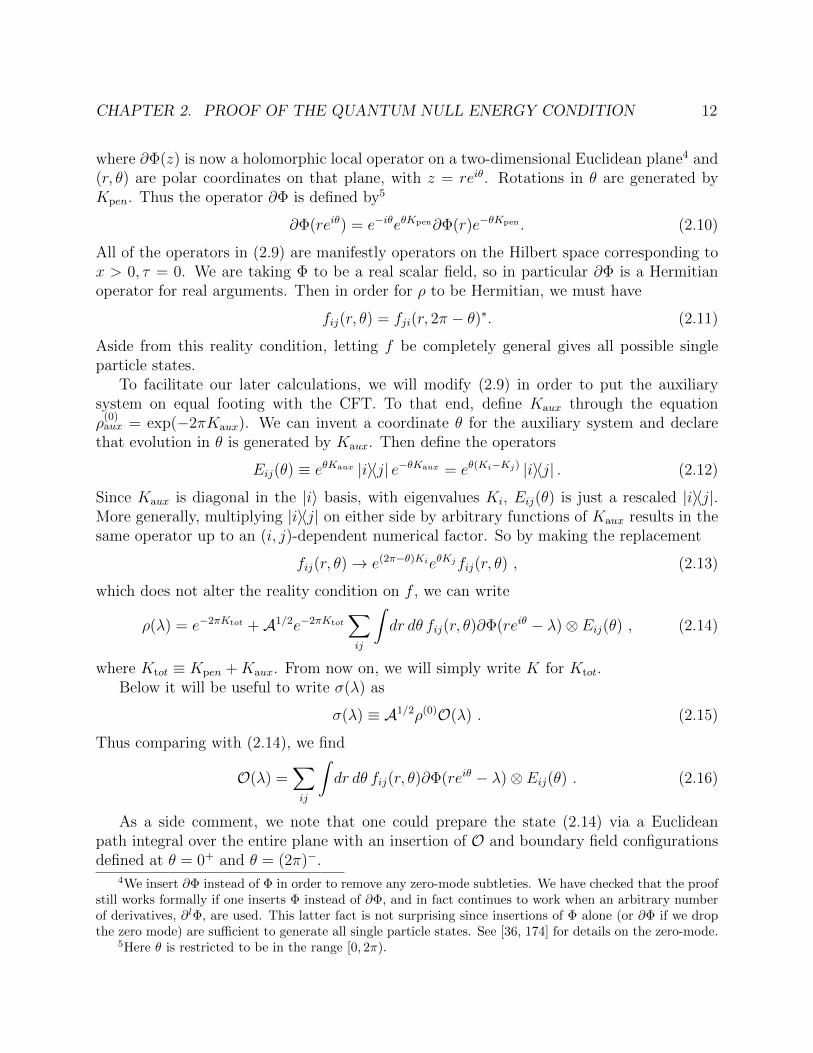
x
@
1
Figure 2.2: The state of the CFT on x > λ can be defined by insertions of ∂Φ on theEuclidean plane. The red lines denote a branch cut where the state is defined.
We have argued that, at order A1/2, the perturbation σ on the full pencil must be of theschematic form |0〉〈1| (plus Hermitian conjugate). So on the full pencil, we have the state
ρ = ρ(−∞) = |0〉〈0| ⊗ ρ(0)aux +A1/2
∑
ij
(|0〉〈ψij|+ |ψji〉〈0|)⊗ |i〉〈j|+ · · · , (2.7)
where |i〉〈j| is a basis of operators in the auxiliary system and “· · · ” denotes terms whichvanish more quickly as A → 0. We will argue in Sec. 2.3 that those terms are not relevant forthe QNEC, and so we will ignore them from now on. For later convenience, we will take thebasis |i〉 in the auxiliary system to be the one in which ρ
(0)aux is diagonal. The states |ψij〉 are
single-particle states in the CFT, and we have ensured that the state is Hermitian. The CFTpart of the state can be constructed by acting on the vacuum with a single copy of the fieldoperator. In a Euclidean path integral picture, we can get the most general single-particlestate by allowing arbitrary single-field insertions on the Euclidean plane. This is shown inFig. 2.2.
To obtain the state at a finite value of λ, we need to take the trace of (2.7) over theregion x < λ. Alternatively, we can hold fixed the inaccessible region, x < 0, but translatethe field operators used to construct the state by λ. From this point of view the vacuum isindependent of λ and we write it as
ρ(0)pen = e−2πKpen , (2.8)
where, up to an additive constant, the modular Hamiltonian Kpen coincides with the Rindlerboost generator for the CFT [168, 20]. Specializing to the case of a single chiral scalar field(extensions will be discussed in Sec. 2.5), the trace of (2.7) becomes
ρ(λ) = e−2πKpen ⊗ ρ(0)aux +A1/2
∑
ij
(e−2πKpen
∫drdθ fij(r, θ)∂Φ(reiθ − λ)
)⊗ |i〉〈j| , (2.9)
CHAPTER 2. PROOF OF THE QUANTUM NULL ENERGY CONDITION 12
where ∂Φ(z) is now a holomorphic local operator on a two-dimensional Euclidean plane4 and(r, θ) are polar coordinates on that plane, with z = reiθ. Rotations in θ are generated byKpen. Thus the operator ∂Φ is defined by5
∂Φ(reiθ) = e−iθeθKpen∂Φ(r)e−θKpen . (2.10)
All of the operators in (2.9) are manifestly operators on the Hilbert space corresponding tox > 0, τ = 0. We are taking Φ to be a real scalar field, so in particular ∂Φ is a Hermitianoperator for real arguments. Then in order for ρ to be Hermitian, we must have
fij(r, θ) = fji(r, 2π − θ)∗. (2.11)
Aside from this reality condition, letting f be completely general gives all possible singleparticle states.
To facilitate our later calculations, we will modify (2.9) in order to put the auxiliarysystem on equal footing with the CFT. To that end, define Kaux through the equationρ
(0)aux = exp(−2πKaux). We can invent a coordinate θ for the auxiliary system and declare
that evolution in θ is generated by Kaux. Then define the operators
Eij(θ) ≡ eθKaux |i〉〈j| e−θKaux = eθ(Ki−Kj) |i〉〈j| . (2.12)
Since Kaux is diagonal in the |i〉 basis, with eigenvalues Ki, Eij(θ) is just a rescaled |i〉〈j|.More generally, multiplying |i〉〈j| on either side by arbitrary functions of Kaux results in thesame operator up to an (i, j)-dependent numerical factor. So by making the replacement
fij(r, θ)→ e(2π−θ)KieθKjfij(r, θ) , (2.13)
which does not alter the reality condition on f , we can write
ρ(λ) = e−2πKtot +A1/2e−2πKtot∑
ij
∫dr dθ fij(r, θ)∂Φ(reiθ − λ)⊗ Eij(θ) , (2.14)
where Ktot ≡ Kpen +Kaux. From now on, we will simply write K for Ktot.Below it will be useful to write σ(λ) as
σ(λ) ≡ A1/2ρ(0)O(λ) . (2.15)
Thus comparing with (2.14), we find
O(λ) =∑
ij
∫dr dθ fij(r, θ)∂Φ(reiθ − λ)⊗ Eij(θ) . (2.16)
As a side comment, we note that one could prepare the state (2.14) via a Euclideanpath integral over the entire plane with an insertion of O and boundary field configurationsdefined at θ = 0+ and θ = (2π)−.
4We insert ∂Φ instead of Φ in order to remove any zero-mode subtleties. We have checked that the proofstill works formally if one inserts Φ instead of ∂Φ, and in fact continues to work when an arbitrary numberof derivatives, ∂lΦ, are used. This latter fact is not surprising since insertions of Φ alone (or ∂Φ if we dropthe zero mode) are sufficient to generate all single particle states. See [36, 174] for details on the zero-mode.
5Here θ is restricted to be in the range [0, 2π).

CHAPTER 2. PROOF OF THE QUANTUM NULL ENERGY CONDITION 13
Expansion of the Entropy
In the previous sections we saw that null quantization gives us a state of the form
ρ(λ) = ρ(0)pen(λ)⊗ ρ(0)
aux + σ(λ), (2.17)
where ρ(0)pen(λ) is the vacuum state reduced density matrix on the part of the pencil with
affine parameter greater than λ, ρ(0)aux is an arbitrary state in the auxiliary system, and the
perturbation σ is proportional to the small parameter A1/2. In this section, we will expandthe entropy perturbatively in σ and show that the QNEC reduces to a statement about thecontributions of σ to the entropy. We will assume that both ρ(λ) and ρ(0)(λ) ≡ ρ
(0)pen(λ)⊗ρ(0)
aux
are properly normalized density matrices, so Tr(σ) = 0.The von Neumann entropy of ρ(λ) is Sout(λ). We will expand it as a perturbation series
in σ(λ):Sout(λ) = S(0)(λ) + S(1)(λ) + S(2)(λ) + · · · (2.18)
where S(n)(λ) contains n powers of σ(λ). At zeroth order, since ρ(0) is a product state, wehave
S(0)(λ) = −Tr[ρ(0)(λ) log ρ(0)(λ)
]= −Tr
[ρ(0)
pen(λ) log ρ(0)pen(λ)
]− Tr
[ρ(0)
aux log ρ(0)aux
]. (2.19)
The first term on the right-hand side is independent of λ because of null translation invarianceof the vacuum: all half-pencils have the same vacuum entropy. The second term is manifestlyindependent of λ. So S(0) is λ-independent and does not play a role in the QNEC.
Now we turn to S(1)(λ):
S(1)(λ) = −Tr[σ(λ) log ρ(0)(λ)
]= −Tr
[σ(λ) log ρ(0)
pen(λ)]− Tr
[σ(λ) log ρ(0)
aux
]. (2.20)
Once again, the second term is λ-independent, which we can see by evaluating the trace overthe pencil subsystem:
Tr[σ(λ) log ρ(0)
aux
]= Traux
[[Trpen σ(λ)] log ρ(0)
aux
]= Traux
[σ(∞) log ρ(0)
aux
]. (2.21)
To evaluate the first term, we use the fact that ρ(0)pen(λ) is thermal with respect to the boost
operator on the pencil. Then we have
−Tr[σ(λ) log ρ(0)
pen(λ)]
=2πA~
∫ ∞
λ
dλ′ (λ′ − λ)〈Tkk(λ′)〉, (2.22)
where the integral is along the generator which defines the pencil and the expectation valueis taken in the excited state. This is the first λ-dependent term we have in the perturbativeexpansion of S(λ). Taking two derivatives and evaluating at λ = 0 gives the identity
(S(0) + S(1)
)′′=
2πA~〈Tkk〉. (2.23)

CHAPTER 2. PROOF OF THE QUANTUM NULL ENERGY CONDITION 14
Subtracting S ′′out from both sides of this equation shows that
~2πAS
′′out − 〈Tkk〉 =
~2πA
(Sout − S(0) − S(1)
)′′=
~2πAS
(2)′′ + · · · , (2.24)
where “· · · ” contains terms higher than quadratic order in σ. The QNEC (equation (2.1))is the statement that this quantity is negative in the limit A → 0. Earlier we showed thatσ was proportional to A1/2. Then S(2) is proportional to A, and we must check that S(2)′′
is negative. However, the higher order terms S(`) for ` > 2 vanish more quickly with A andtherefore drop out in the limit A → 0.
We have shown that the QNEC reduces to the statement that S(2)′′ ≤ 0 for perturbationsfrom the vacuum. In fact, we have shown something a little stronger. In general, theperturbation σ will have terms proportional to An/2 for all n ≥ 1. Our arguments showthat only the term proportional to A1/2 matters for the QNEC, and furthermore that thisterm is off-diagonal in the single-particle/vacuum subspace. So we can simplify matters byconsidering states which contain only such a term proportional to A1/2 and no higher powersof A. In other words, we can take the state to be of the form in (2.7) with the unwritten“· · · ” terms set equal to zero. Now we only need to show that S(2)′′ ≤ 0 for such states.
2.4 Calculation of the Entropy
The Replica Trick
The replica trick prescription is to use the following formula for the von Neumann en-tropy [38]:
Sout = −Tr[ρ log ρ] = (1− n∂n) log Tr[ρn]∣∣∣n=1
. (2.25)
This can be written as
Sout = D log Zn (2.26)
where Zn ≡ Tr[ρn]6 and the operator D is defined by
Df(n) ≡ (1− n∂n)f(n)∣∣n=1
(2.27)
where f(n) is some function of n. Since Zn is only defined for integer values of n, we firstmust analytically continue to real n > 0 in order to apply the D operator. The analyticcontinuation step is in general quite tricky, and will require care in our calculation. (Ouranalytic continuation is performed in Section 2.4.)
6In the replica trick one often works with the partition function Zn, in terms of which Zn = Zn/(Z1)n.Choosing Zn over Zn is equivalent to choosing a different normalization for ρ, but we find it convenient tokeep Tr ρ = 1.

CHAPTER 2. PROOF OF THE QUANTUM NULL ENERGY CONDITION 15
On general grounds discussed above, we must study the second-order term in a per-turbative expansion of the entropy about the state ρ(0). Suppressing all λ dependence, wehave
Zn = Tr[(ρ(0) + σ)n
]. (2.28)
Expanding Zn to quadratic order to isolate S(2)′′, we have
Zn = Tr[(ρ(0))n
]+ nTr
[σ(ρ(0))n−1
]+n
2
n−2∑
k=0
Tr[(ρ(0))kσ(ρ(0))n−k−2σ
]+ · · · . (2.29)
Using the notation introduced in (2.15) we can write
Zn = Tr[(ρ(0))n
]+ nTr
[O(ρ(0))n
]+n
2
n−1∑
k=1
Tr[(ρ(0))−kO(ρ(0))kO(ρ(0))n
]+ · · · . (2.30)
We denote by O(k) the operator O conjugated by (ρ(0))k:
O(k) ≡ (ρ(0))−kO(ρ(0))k (2.31)
= e2πkKOe−2πkK . (2.32)
This is equivalent to a Heisenberg evolution of O in the angle θ by an amount 2πk. Since Ois the integral of operators with angles 0 ≤ θ < 2π, it follows that O(k) will be an integralover operators with angles 2πk < θ < 2π(k + 1).7 Furthermore, since rotations by 2πkcommute with translations by λ, we can obtain O(k) from O simply by letting the range ofintegration that defines O shift from [0, 2π] to [2πk, 2π(k + 1)], as long as we define fij(r, θ)to be periodic in θ with period 2π.
It will also be convenient to introduce an angle-ordered expectation value, defined as
〈. . .〉n ≡Tr[(ρ(0))nT [. . . ]]
Tr[(ρ(0))n], (2.33)
where T [. . . ] is θ-ordering. Then (2.30) can be written
Zn = Tr[(ρ(0))n
](
1 + n 〈O〉n +n
2
n−1∑
k=1
⟨O(k)O
⟩n
)+ · · · . (2.34)
Taking the logarithm of Zn and extracting the part quadratic in σ gives
log Zn ⊃n
2
n−1∑
k=1
⟨O(k)O
⟩n− n2
2〈O〉2n , (2.35)
7One could worry that the phase factor in (2.10) spoils this relation, but notice that the phase has period2π in θ and so does not appear when shifting by 2πk.

CHAPTER 2. PROOF OF THE QUANTUM NULL ENERGY CONDITION 16
where we have kept only the part quadratic in O. The contribution of the second termto the entanglement entropy will be proportional to 〈O〉, which vanishes because of thetracelessness of σ. Therefore we only need to consider the first term.
Since we are considering angle-ordered expectation values, we have the identity
⟨(n−1∑
k=0
O(k)
)2⟩
n
= nn−1∑
k=0
⟨O(k)O
⟩n, (2.36)
and so from the first term in (2.35) the relevant part of log Zn can be written as
log Zn ⊃ −n
2〈OO〉n +
1
2
⟨(n−1∑
k=0
O(k)
)2⟩
n
. (2.37)
Restoring the λ dependence and taking λ derivatives gives
S(2)′′ =∂2
∂λ2
∣∣∣∣λ=0
D log Zn(λ) (2.38)
= D −n2〈OO〉′′n +D 1
2
⟨(n−1∑
k=0
O(k)
)2⟩′′
n
. (2.39)
The 〈. . .〉′′n notation means take two λ derivatives and then set λ = 0. In the followingsections we will compute these two terms separately.
We note that the two terms in (2.39) are analogous to δS(1)EE and δS
(2)EE of Ref. [67], where
a similar perturbative computation of the entropy was performed. Though the details ofthe two calculations differ (in particular we have an auxiliary system as well as a CFT), itwould be interesting to explore further the connection between our present work and that ofRef. [67].
Evaluation of Same-Sheet Correlator
In this section we consider the term 〈OO〉′′n appearing in (2.39). The analytic continuationof this term in n is straightforward. We first apply D:
D−n2〈OO〉n = D −n
2
Tr[e−2πnKT [OO]
]
Tr[e−2πnK ](2.40)
= −π 〈OO∆K〉 (2.41)
where ∆K ≡ K−〈K〉 is the vacuum-subtracted modular Hamiltonian. When an expectationvalue 〈. . .〉 appears without a subscript it is understood to refer to the normalized expectationvalue 〈. . .〉n with n = 1, i.e., the angle-ordered expectation value with respect to ρ(0). Also
CHAPTER 2. PROOF OF THE QUANTUM NULL ENERGY CONDITION 17
note that K appears outside of the angle-ordering in the trace form of the expectation value,which is formally equivalent to being inserted at θ = 0.
We now consider the λ dependence. Recall that K is defined to be λ-independent, andthe λ-dependence of O enters through a shift in the coordinate insertion of ∂Φ (see (2.16)).We first split ∆K into ∆Kpen and ∆Kaux. The expectation value involving ∆Kaux will beindependent of λ because of translation invariance of the CFT, and so can be ignored. SinceKpen is the CFT boost generator on the half-line x > 0, ∆Kpen has a well-known expressionin terms of the energy-momentum tensor of the CFT [168, 20]:
∆Kpen = A∫ ∞
0
dx xTkk(x) = − 1
2π
∫ ∞
0
dx xT (x) . (2.42)
Therefore the correlation function (2.41) is expressed in terms of the correlation functions〈∂Φ(z − λ)∂Φ(w − λ)T (x)〉, which are the same as 〈∂Φ(z)∂Φ(w)T (x+ λ)〉 by translationinvariance. This makes the λ-derivatives easy to evaluate. We find
D−n2〈OO〉′′n =
1
2〈OOT (0)〉 . (2.43)
Inserting the explicit form of O gives
〈OOT (0)〉 =1
(2π)2
∑
i,j,i′j′
m,m′
∫dr dr′ dθ dθ′
(f
(m)ij (r)f
(m′)i′j′ (r′)e−imθe−im
′θ′
× 〈∂Φ(reiθ)∂Φ(r′eiθ′)T (0)〉 〈Eij(θ)Ei′j′(θ′)〉
),
(2.44)
where we have introduced Fourier representations of fij(r, θ) defined by
fij(r, θ) =1
2π
∞∑
m=−∞
f(m)ij (r)e−imθ . (2.45)
The correlation functions we need are evaluated in the appendix. Plugging equation (A.12)with n = 1 and equation (A.6) into equation (2.44) yields
〈OOT (0)〉
=−2
(2π)3
∑
i,j,pm,m′
∫dr dr′ dθ dθ′
(rr′)2f
(m)ij (r)f
(m′)ji (r′)e−π(Ki+Kj) sinhπαij
ip+ αijeiθ(−p−m−2)eiθ
′(p−m′−2)
=1
π
∑
i,j,m
∫dr dr′
(rr′)2f
(m−2)ij (r)f
(−m−2)ji (r′)e−π(Ki+Kj) sinh παij
im− αij, (2.46)
where we used the Kronecker deltas coming from the θ integration and redefined the dummyvariable m → m − 2, and αij ≡ Ki −Kj is the difference between two eigenvalues of Kaux.

CHAPTER 2. PROOF OF THE QUANTUM NULL ENERGY CONDITION 18
Note that we reserve the letters p and q throughout to denote integers divided by n, but inthis case n = 1 and so p ranges over the integers. Substituting equation (2.46) into equation(2.43), we find
D−n2〈OO〉′′n =
1
2π
∑
i,j,m
∫dr dr′
(rr′)2f
(m−2)ij (r)f
(−m−2)ji (r′)e−π(Ki+Kj) sinhπαij
im− αij. (2.47)
Evaluation of Multi-Sheet Correlator
We now turn to the second term in (2.39),
1
2D⟨(
n−1∑
k=0
O(k)
)2⟩′′
n
. (2.48)
The analytic continuation of this term to real n will turn out to be much more challengingthan that of the first term of (2.39), because n appears in the upper summation limit.
Using (2.16), can write the sum over replicas in (2.48) as follows:
⟨(n−1∑
k=0
O(k)
)2⟩
n
=
⟨(∑
i,j
∫ 2πn
0
dr dθ fij(r, θ)∂Φ(r, θ;λ)⊗ Eij(θ))2⟩
n
. (2.49)
This equality comes from interpreting O(k) as O inserted on the (k + 1)th replica sheet (see(2.31)). Summing over sheets and integrating θ ∈ [0, 2π] on each one is equivalent to justintegrating θ ∈ [0, 2πn], which covers the entire replicated manifold. The definition of ∂Φfor angles greater than 2π is given by the the Heisenberg evolution rule, the right hand sideof (2.10). The field is still holomorphic, but it would be misleading to write it as a functionof reiθ since it is not periodic in θ with period 2π.
Because the fij(r, θ) are not dynamical, they should be identical on each sheet. In theFourier representation as in (2.45), this means keeping the Fourier coefficients fixed andkeeping the m parameters integer. Thus we have
1
2D⟨(
n−1∑
k=0
O(k)
)2⟩′′
n
= D 1
2(2π)2
∑
i,j,i′,j′
m,m′
∫dr dr′ dθ dθ′ f
(m)ij (r)f
(m′)i′j′ (r′)e−imθe−im
′θ′
× 〈∂Φ(r, θ)∂Φ(r′, θ′)〉′′n 〈Eij(θ)Ei′j′(θ′)〉n . (2.50)
The CFT two point function is calculated in Appendix A.1:
〈∂Φ(z)∂Φ(w)〉′′n =1
n(zw)2
∑
|q|<1
sign(q)q(q2 − 1)(wz
)q(2.51)
=1
n(rr′)2
∑
|q|<1
sign(q)P (q, r, r′)eiθ(−q−2)eiθ′(q−2) (2.52)

CHAPTER 2. PROOF OF THE QUANTUM NULL ENERGY CONDITION 19
where q takes values in the integers divided by n, and
P (q, r, r′) ≡ q(q2 − 1)
(r′
r
)q. (2.53)
When n = 1 there are no nonzero terms in the sum, but when n > 1 the answer is nonzero.For future convenience, we separated the parts which depend on θ from those that do not.
The auxiliary system two point function is calculated in Appendix A.1:
〈Eij(θ)Ei′j′(θ′)〉n = δij′δji′e−2πnKi
1
πnZauxn
∑
p
e−ip(θ−θ′) sinhnπαijip+ αij
enπαij , (2.54)
where p is also an integer divided by n and Zauxn ≡ Tr
[e−2πnK
(0)aux
]is a normalization factor.
Substituting this equation as well as (2.52) into (2.50) gives
D 1
n2(2π)3Zauxn
∑
i,j,pm,m′
∫dr dr′ dθ dθ′
(rr′)2f
(m)ij (r)f
(m′)ji (r′)eiθ(−q−p−2−m)eiθ
′(q+p−2−m′)
×sinhπnαijip+ αij
e−πn(Ki+Kj)∑
|q|<1
sign(q)P (q, r, r′) . (2.55)
The angle integrations give Kronecker deltas multiplied by 2πn. The result is
D i
2πZauxn
∑
i,j,m
∫dr dr′
(rr′)2f
(m−2)ij (r)f
(−m−2)ji (r′) sinhπnαije
−πn(Ki+Kj)
∑
|q|<1
sign(q)P (q, r, r′)
q +m+ iαij
=i
2π
∑
i,j,m
∫dr dr′
(rr′)2f
(m−2)ij (r)f
(−m−2)ji (r′) sinhπαije
−π(Ki+Kj) D
∑
|q|<1
sign(q)P (q, r, r′)
q +m+ iαij
.
(2.56)
In going to the last line, we used the fact that the sum in brackets vanishes when n = 1and that, for any two functions f(n), g(n) such that f(1) and
[ddnf(n)
]n=1
are finite andg(1) = 0, the following relation holds:
D (f(n)g(n)) = f(1)Dg(n) . (2.57)
We now turn to the analytic continuation and application of D on the term in bracketsin (2.56). We will take care of the awkward sign(q) by writing the q-dependent part of thesum as two sums with positive argument. We will suppress the (r, r′) dependence for therest of the calculation:
∑
|q|<1
sign(q)P (q)
q +m+ iαij=∑
0<q<1
P (q)
q +m+ iαij+
P (−q)q −m− iαij
. (2.58)

CHAPTER 2. PROOF OF THE QUANTUM NULL ENERGY CONDITION 20
Now we write q = k/n to turn this into a sum over integers:
∑
0<q<1
(P (q)
q +m+ iαij+
P (−q)q −m− iαij
)=
n−1∑
k=1
(P ( k
n)
kn
+m+ iαij+
P (− kn)
kn−m− iαij
). (2.59)
In the next section we will see how to evaluate and analytically continue such sums quitegenerally.
Analytic Continuation
We need to evaluate
Dn−1∑
k=1
(P ( k
n)
kn− z +
P (− kn)
kn
+ z
), (2.60)
where P (z) is given by (2.52). However, for the remainder of this section, we will considerP (z) to be an arbitrary analytic function whose functional form is independent of n. Wewill specialize to the form given by (2.52) in section 2.4.
We start by writing the sum in (2.60) as
Dn−1∑
k=1
(P ( k
n)− P (z)kn− z +
P (− kn)− P (z)
kn
+ z
)+D
n−1∑
k=1
(P (z)kn− z +
P (z)kn
+ z
)(2.61)
and then we evaluate the terms separately. Consider the first term in the first set of paren-thesis. Because P (z) is analytic, we can expand it in a power series with positive powers ofz: P (z) =
∑∞r=0 arz
r. This gives
Dn−1∑
k=1
∞∑
r=1
ar( kn)r − zrkn− z . (2.62)
We can simplify the fraction using polynomial division; for r ≥ 1,
( kn)r − zrkn− z =
r−1∑
s=0
zr−s−1
(k
n
)s, (2.63)
which means the first term in the first set of parenthesis in (2.61) is
Dn−1∑
k=1
P ( kn)− P (z)kn− z =
∞∑
r=1
r−1∑
s=0
arzr−s−1D
n−1∑
k=1
(k
n
)s. (2.64)
The advantage of writing it this way is that it isolates the n dependence into somethingwhich can be easily analytically continued. First, recall that overall factors of powers of n

CHAPTER 2. PROOF OF THE QUANTUM NULL ENERGY CONDITION 21
don’t matter if the expression they multiply vanishes at n = 1, as in (2.57). Next, note thatthe resulting expression is actually a polynomial in n. It can be expressed this way usingFaulhaber’s formula:
n−1∑
k=1
ks =1
s+ 1
s∑
j=0
(−1)j(s+ 1
j
)Bj(n− 1)s−j+1 , (2.65)
where Bs is the j-th Bernoulli number in the convention that B1 = −1/2. This makesapplication of D straightforward:
Dn−1∑
k=1
(k
n
)s= D
n−1∑
k=1
ks = −(−1)sBs . (2.66)
Thus for the first term in (2.61) we have
Dn−1∑
k=1
P ( kn)− P (z)kn− z = −
∞∑
r=1
r−1∑
s=0
arzr−s−1(−1)sBs . (2.67)
The second term follows completely analogously:
Dn−1∑
k=1
P (− kn)− P (z)
kn
+ z=∞∑
r=1
r−1∑
s=0
arzr−s−1Bs . (2.68)
Combining these results, the first set of large parenthesis in (2.61) is
−∞∑
r=1
r−1∑
s=0
arzr−s−1Bs [(−1)s − 1] . (2.69)
For even s this is zero. For odd s > 1, Bs = 0, and so only s = 1 can contribute. SubstitutingB1 = −1/2 gives
−P (z)
z2+a1
z+a0
z2. (2.70)
We now turn to the second set of parenthesis in (2.61). These two terms can be evaluatedsimultaneously. First, we can multiply through by n/n to give an overall factor of n (whichis irrelevant) and convert the denominators to k− zn and k+ zn. We also pull P (z) throughD because it is independent of n:
P (z)Dn−1∑
k=1
(1
k − zn +1
k + zn
). (2.71)

CHAPTER 2. PROOF OF THE QUANTUM NULL ENERGY CONDITION 22
This sum can be evaluated in terms of the digamma function ψ(0)(w), which is defined interms of the Gamma function Γ(w):
ψ(0)(w) ≡ Γ′(w)
Γ(w)= −γ +
∞∑
k=0
(1
k + 1− 1
k + w
). (2.72)
By manipulating the sum, one can show
n−1∑
k=1
1
k − w = ψ(0)(n− w)− ψ(0)(1− w) . (2.73)
Thus the second set of parenthesis in (2.61) is equal to
P (z)D[ψ(0)(n− zn)− ψ(0)(1− zn) + ψ(0)(n+ zn)− ψ(0)(1 + zn)
]. (2.74)
We cannot naively apply D yet. We first have to select the correct analytic continuationto real positive n from the many possible analytic continuations of integer n data. Thisis known to be a challenging problem in general.8 Nevertheless, in our context the correctanalytic continuation prescription is clear.
The digamma function has poles in the complex plane at zero and all negative realintegers. Recall that we are ultimately interested in plugging in zm ≡ −m − iαij. Thus ifwe are not careful, for certain values of m, the digamma functions in (2.74) will blow upwhen αij → 0 near n = 1. On the other hand, on physical grounds we expect our result tobe perfectly well-behaved when αij → 0, which simply corresponds to a degeneracy in theauxiliary system. The way we avoid the poles of the digamma function near n = 1 whenαij → 0 is by using the reflection formula
ψ(0)(1− w) = ψ(0)(w) + π cot πw , (2.75)
which produces different analytic continuations given the same integer data. These obser-vations lead to the following prescription: for each value of m, use the reflection formula(2.75) to avoid the poles of the digamma function near n = 1 as αij → 0.
As an example, consider the term ψ(0)(1− zmn) = ψ(0)(1 +mn+ αijn) in (2.74). Whenαij = 0, this has a pole when nm ≤ 1. Thus for a given m ≤ 1, we cannot expect to have asmooth n-derivative at n = 1. The resolution is to use (2.75) to get
ψ(0)(1 +mn+ αijn) = ψ(0)(−mn− αij)− π cotπ(mn+ αij) (2.76)
= ψ(0)(−mn− αij)− π cotπαij , (2.77)
8See Ref. [67] for a recent discussion of the difficulties of the analytic continuation. Ref. [67] also containsanother method for computing the entropy perturbatively that does not rely on the replica trick. Such amethod avoids the need to analytically continue, and applying it to the present calculation would serve as acheck of our analytic continuation prescription. We leave that check to future work.

CHAPTER 2. PROOF OF THE QUANTUM NULL ENERGY CONDITION 23
1 2 3n
Αij = 1
1 2 3n
Αij = 0.5
1 2 3n
Αij = 0.1
Figure 2.3: Sample plots of the imaginary part (the real part is qualitatively identical) of thenaıve bracketed digamma expression in (2.74) and the one in (2.78) obtained from analyticcontinuation with z = −m − iαij for m = 3 and various values of αij. The oscillatingcurves are (2.74), while the smooth curves are the result of applying the specified analyticcontinuation prescription to that expression, resulting in (2.78).
where the last equality is only true for integer n. The remaining digamma term is now freeof poles for mn ≤ 1, which is precisely when there was a problem before the applicationof the reflection formula, and D can now be easily applied. This example illustrates howthe correct analytic continuation depends on the value of m. We must apply this reasoningseparately to each term in (2.74). After applying this procedure to each digamma functionas needed to avoid the poles, it will turn out that all of the extra cotangent terms cancelagainst each other.
There is another way to motivate this prescription. Even for small but finite αij, theanalytic continuations picked out by our prescription can be seen to be qualitatively betterthan the one obtained by using (2.74) directly, as illustrated in Figure 2.3. Notice that whileboth curves match for integer n, the curve obtained by applying the prescription outlinedabove is the only one which smoothly interpolates between the integers. The oscillations ofthe “wrong” curves get larger and larger as αij is reduced or m is increased.
Applying our prescription to (2.74), there are three expressions depending on the valueof m. We are focussing on the quantity in brackets in (2.74):
ψ(0)(1− n− nzm)− ψ(0)(−nzm) + ψ(0)(n− nzm)− ψ(0)(1− nzm) m > 0
ψ(0)(n+ nzm)− ψ(0)(1 + nzm) + ψ(0)(n− nzm)− ψ(0)(1− nzm) m = 0
ψ(0)(n+ nzm)− ψ(0)(1 + nzm) + ψ(0)(1− n+ nzm)− ψ(0)(nzm) m < 0
(2.78)
Now we are ready to apply D. The digammas ψ(0)(w) will turn into polygammas ψ(1)(w) ≡ddwψ(0)(w), which obey the recurrence relation
ψ(1)(w + 1) = ψ(1)(w)− 1
w2. (2.79)

CHAPTER 2. PROOF OF THE QUANTUM NULL ENERGY CONDITION 24
This recurrence relation simplifies the result for m > 0 and m < 0 while the recurrencerelation along with the reflection formula simplifies the result for m = 0. The result for thesecond set of parenthesis in (2.61) with z = zm is
P (zm)
z2m
+ δ(m)P (zm)π2
sinh2 παij. (2.80)
We are now ready to give the final expression for (2.60). Adding (2.70) with z = zm and(2.80) we find
Dn−1∑
k=1
(P ( k
n)
kn− zm
+P (− k
n)
kn
+ zm
)=a1
zm+a0
z2m
+ δ(m)P (−iαij)π2
sinh2 παij(2.81)
for arbitrary analytic P (zm).
Completing the Proof
Now we specialize to the form of P (z) needed for our calculation which came from theparticular 〈∂Φ∂Φ〉′′ two-point function we were computing ((2.52) and (2.53)):
P (z) = z(z2 − 1)ez log (r′/r) . (2.82)
Thus a0 = 0, and a1 = −1. Using (2.81) gives
Dn−1∑
k=1
(P ( k
n)
kn− zm
+P (− k
n)
kn
+ zm
)=
i
im− αij+ δ(m)
iπ2
sinh2 παijαij(α
2ij + 1)
(r′
r
)−iαij
. (2.83)
Plugging this into (2.56) and plugging that into (2.49) gives the term from (2.39) that wehave been focussing on in this section:
D1
2
⟨(n−1∑
k=0
O(k)
)2⟩′′
n
=−1
2π
∑
i,j,m
∫drdr′
(rr′)2f
(m−2)ij (r)f
(−m−2)ji (r′) sinhπαije
−π(Ki+Kj)
×[
1
im− αij+ δ(m)
αij
sinh2 παijπ2(α2
ij + 1)
(r′
r
)−iαij
]. (2.84)
Notice that the first term in this expression exactly cancels the contribution to S(2)′′
coming from the first term in (2.39), presented in (2.47). We now consider the second term,and define the manifestly positive quantity Mij ≡ e−π(Ki+Kj)π2(α2
ij + 1) to clean up thenotation. Then we have
S(2)′′ =−1
2π
∑
i,j
∫drdr′
(rr′)2f
(−2)ij (r)f
(−2)ji (r′)
(r′
r
)−iαij αijsinhπαij
Mij . (2.85)

CHAPTER 2. PROOF OF THE QUANTUM NULL ENERGY CONDITION 25
The integrals over r, r′ factorize, giving
S(2)′′ =−1
2π
∑
i,j
[∫ ∞
0
dr riαij−1f(−2)ij (r)
] [∫ ∞
0
dr r−iαij−1f(−2)ji (r)
]αij
sinhπαijMij . (2.86)
Recall the constraint on the test functions derived previously by requiring the density matrixbe Hermitian (equation (2.11)): fij(r, θ) = fji(r, 2π − θ)∗. In Fourier space, this implies
f(m)ji (r) = f
(m)ij (r)∗. Inserting this into (2.86) we see that the factors in brackets are complex-
conjugates of each other. Furthermore, because sinhπαij always has the same sign as αij,the overall sign of the entire term is negative and so we find
S(2)′′ ≤ 0 . (2.87)
As discussed after (2.24), this proves the QNEC.
2.5 Extension to D = 2, Higher Spin, and Interactions
In D = 2, there are no transverse directions, and so it is not possible to use the fact that thestate is very close to the vacuum. Nevertheless, once one has proven the QNEC for a freescalar field in D > 2, one can use dimensional reduction to prove it for free scalar fields inD = 2. Let Φ(z, y) be the chiral scalar on N in D > 2, where y labels the D − 2 transversecoordinates. One can isolate a single transverse mode by integrating Φ(z, y) against a realtransverse wavefunction, and this defines an effective two-dimensional field:
Φ2D(z) ≡∫dy ψ(y)Φ(z, y) , (2.88)
where ψ is normalized such that∫ψ2 = 1. Correlation functions of Φ2D and its derivatives
exactly match those of a two-dimensional chiral scalar, and so our dimensional reduction isdefined by the subspace of the D-dimensional theory obtained by acting on the vacuum withΦ2D. In any such state, one can integrate the D-dimensional QNEC along the transversedirection to find ∫
dy 〈Tkk(y)〉 ≥ 1
2π
∫dy
δ2Sout
δλ(y)2. (2.89)
Here we have suppressed the value of the affine parameter as a function of the transversedirection. The effective two-dimensional change in the entropy is defined by considering atotal variation in all of the generators which is uniform in the transverse direction. For sucha variation we have
S ′′2D =
∫dy dy′
δ2Sout
δλ(y)δλ(y′)≤∫dy
δ2Sout
δλ(y)2, (2.90)
where the the inequality comes from applying strong subadditivity to the off-diagonal secondderivatives [34]. The two-dimensional energy momentum tensor is defined in terms of the

CHAPTER 2. PROOF OF THE QUANTUM NULL ENERGY CONDITION 26
normal ordered product of the two-dimensional fields, T2D =: ∂Φ2D∂Φ2D :. However, usingWick’s theorem one can easily check that T2D acts on the dimensionally reduced theory inthe same way as the integrated D-dimensional Tkk:
〈T2D(w)Φ2D(z1) · · ·Φ2D(zn)〉 =
∫dy 〈Tkk(w, y)Φ2D(z1) · · ·Φ2D(zn)〉 . (2.91)
Therefore the QNEC holds for a free scalar field in two dimensions:
〈T2D〉 =
∫dy 〈Tkk(y)〉 ≥ 1
2π
∫dy
δ2Sout
δλ(y)2≥ 1
2πS ′′2D. (2.92)
The extension to bosonic fields with spin is trivial, as these simply reduce onN to multiplecopies of the 1+1 chiral scalar CFT, one for each polarization. These facts are reviewed in[174]. Similarly, fermionic fields reduce to the chiral 1+1 fermion CFT; we expect that thereis a similar proof in this case.
Astute readers may have noticed that the mass term of the higher dimensional field the-ory plays no role in our analysis. Since it does not contribute to the commutation relationson N or to Tkk, it plays no role in our analysis. Regardless of whether the D dimensionaltheory has a mass, the 1 + 1 chiral theory is massless. In a sense, null surface quantizationis a UV limit of the field theory. One might therefore expect that the addition of inter-actions with positive mass dimension (superrenormalizable couplings) will also not changethe algebra of observables on N . So long as this is the case, the extension to theories withsuperrenormalizable interactions is trivial.
One argument that superrenormalizable interactions are innocuous proceeds in two stages[174]. First, one considers the direct effects of adding interaction terms to the Lagrangian; forexample a scalar field potential V (φ). So long as these interaction terms contain no deriva-tives (or are Yang-Mills couplings), they do not contribute to the commutation relations offields restricted to the null surface, or to Tkk. (So far, the interaction could be of any scalingdimension, so long as one avoids derivative couplings.)
Next, one considers loop corrections due to renormalization. In the case of a marginallyrenormalizable, or nonrenormalizable theory, these loop corrections normally require the ad-dition of counterterms containing derivatives (for example, field strength renormalization),spoiling the null surface formulation. On the other hand, in a superrenormalizable theory,only couplings with positive mass dimension require counterterms. For a standard QFT con-sisting of scalars, spinors, and/or gauge fields, none of these superrenormalizable interactionsinclude the possibility derivative couplings. Thus one expects that loop corrections do notspoil the algebra of observables on the null surface. However, superrenormalizable theoriesare difficult to construct except when D < 4. (For example, the φ3 theory is superenormal-izable in D < 6, but is unstable.)
It is an open question whether the QNEC is valid for non-Gaussian D = 2 CFT’s instates besides conformal vacua, or more generally for QFT’s in any dimension which flow

CHAPTER 2. PROOF OF THE QUANTUM NULL ENERGY CONDITION 27
to a nontrivial UV fixed point.9 Nor have we carefully considered the effects of making thescalar field noncompact. QCD in D = 4 is a borderline case; the coupling flows to zero,but slowly enough that there is an infinite field strength renormalization. Strictly speakingthis makes null surface quantization invalid, yet it is still a useful numerical technique forstudying hadron physics [36]. However, we conjecture that the QNEC will be true in everyQFT satisfying reasonable axioms.
9In more than 2 dimensions, interacting CFTs appear to have no nontrivial observables on the hori-zon[174, 31], so the current proof cannot be extended to this situation.

28
Chapter 3
Holographic Proof of the QuantumNull Energy Condition
3.1 Introduction
The Null Energy Condition (NEC), Tkk ≡ Tijkikj ≥ 0, is ubiquitous in classical physics as
a signature of stable field theories. In General Relativity it underlies many results, such asthe singularity theorems [146, 93, 172] and area theorems [91, 28]. In AdS/CFT, imposingthe NEC in the bulk has several consequences for the field theory at leading order in large-N , including the holographic c-theorems [137, 138, 77] and Strong Subadditivity of thecovariant holographic entanglement entropy [177]. Yet ultimately the NEC, interpreted as alocal bound on the expectation value 〈Tkk〉, is known to fail in quantum field theory [65].
The Quantum Null Energy Condition (QNEC) was proposed in [34] as a correction theNEC which holds true in quantum field theory. In the QNEC, 〈Tkk〉 at a point p is boundedfrom below by a nonlocal quantity constructed from the von Neumann entropy of a region.Suppose we divide space into two regions, one of which we callR, with the dividing boundaryΣ passing through p. We compute the entropy of R, and consider the second variation ofthe entropy as Σ is deformed in the null direction ki at p. Call this second variation S ′′ (amore careful construction of S ′′ is given in below in Section 3.2). Then the QNEC statesthat
〈Tkk〉 ≥~
2π√hS ′′, (3.1)
where√h is the determinant of the induced metric on Σ at the location p.1 The QNEC
has its origins in quantum gravity: it arose as a consequence of the Quantum FocussingConjecture (QFC), proposed in [34], but is itself a statement about quantum field theoryalone.
1In general, there may be ambiguities in the definition of Tkk because of “improvement terms.” It isplausible that a similar ambiguity in the definition of S leaves the QNEC unaffected by these issues [49, 3,97, 122].

CHAPTER 3. HOLOGRAPHIC PROOF OF THE QUANTUM NULL ENERGYCONDITION 29
In [33], the QNEC was proved for the special case of free (or superrenormalizable) bosonicfield theories for certain surfaces Σ. Here we will prove the QNEC for a completely differentclass of field theories, namely those which have a good gravity dual, at leading order in thelarge-N expansion. We will consider any theory obtained from such a large-N UV CFT by ascalar relevant deformation. We will also assume that the bulk theory is an Einstein gravitytheory, so that the leading order part of the entropy is given by the area of an extremalsurface in the bulk in Planck units:
S =A(m)
4GN~, (3.2)
where A(m) is the area of a bulk codimension-two surface m which is homologous toR and isan extremum of the area functional in the bulk [152, 153, 101]. Computing that change in theextremal area as the surface Σ is deformed is then a simple task in the calculus of variations.2
A key property is that the change in area of an extremal surface under deformations is dueentirely to the near-boundary asymptotic region, where a general analytic computation ispossible.
Our proof method involves tracking the motion ofm as Σ is deformed. The “entanglementwedge” proposal for the bulk region dual to R, together with bulk causality, suggests thatm should move in a spacelike way as we deform Σ in our chosen null direction [53, 96], and atheorem of Wall [177] shows that this is, in fact, correct.3 We construct a bulk vector sµ inthe asymptotic bulk region which points in the direction of the deformation of m, and sincesµ is spacelike we have sµsµ ≥ 0. Holographically, 〈Tkk〉 is encoded in the near-boundaryexpansion of the bulk metric, and therefore enters into the expression for sµsµ. We will seethat the inequality sµsµ ≥ 0 is precisely the QNEC.4
The remainder of the paper is organized as follows. In Section 3.2 we will give a carefulaccount of the construction of S ′′ and the statement of the QNEC. In Section 3.3 we prove theQNEC at leading order in large-N using holography. In Section 3.3 we recall the asymptoticexpansions of the bulk metric and extremal surface embedding functions that we will usefor the rest of our proof. In Section 3.3 we discuss the fact that null deformations of Σ onthe boundary induce spacelike deformations of m in the bulk and define the spacelike vectorsµ. In Section 3.3 we construct sµ in the asymptotic region and calculate its norm, therebyproving the QNEC. Then in Section 3.3 we specialize to CFTs and examine the QNEC in
2There can be phase transitions in the holographic entanglement entropy where S′ is discontinuous atleading order in N . This happens when there are two extremal surfaces with areas that become equal atthe phase transition. Since we are instructed to use the minimum of the two areas to compute the entropy,the entropy function is always concave in the vicinity of the phase transition. Therefore S′′ = −∞ formally,so the QNEC is satisfied. Thus it is sufficient to assume that no phase transitions are encountered in theremainder of the paper.
3We would like to thank Zachary Fisher, Mudassir Moosa, and Raphael Bousso for discussions aboutthe spacelike nature of these deformations, as well as bringing the theorem of [177] to our attention.
4Relations between the boundary energy-momentum tensor and a coarse-grained entropy were studiedusing holography in [35]. The entropy we consider in this paper is the fine-grained von Neumann entropy.

CHAPTER 3. HOLOGRAPHIC PROOF OF THE QUANTUM NULL ENERGYCONDITION 30
Figure 3.1: Here we show the region R (shaded cyan) and the boundary Σ (black border)before and after the null deformation. The arrow indicates the direction ki, and 〈Tkk〉 isbeing evaluated at the location of the deformation. The dashed line indicates the supportof the deformation.
different conformal frames. Finally, in Section 3.4 we discuss the outlook on extensions ofthe proof and its ideas, as well as possible applications of the QNEC.
Notation Our conventions follow those described in footnote 5 of [103]. Letters from thesecond half of the Greek alphabet (µ, ν, ρ, . . .) label directions in the bulk geometry. Lettersfrom the second half of the Latin alphabet (i, j, k, . . .) label directions in the boundary.Entangling surface directions in the boundary (or on a cutoff surface) are denoted by lettersfrom the beginning of the Latin alphabet (a, b, c, . . .), while directions along the correspondingbulk extremal surface are labeled with the beginning of the Greek alphabet (α, β, γ, . . .).We will often put an overbar on bulk quantities to distinguish them from their boundarycounterparts, e.g., h(z = 0) = h. We neglect the expectation value brackets when we refer tothe expectation value of the boundary stress tensor, i.e. Tij ≡ 〈Tij〉. Boundary latin indicesi, j, k, . . . are raised and lowered with the boundary metric ηij. Outside of the Introductionwe set ~ = 1.
3.2 Statement of the QNEC
In this section we will give a careful statement of the QNEC. Consider an arbitrary quantumfield theory in d-dimensional Minkowski space. The QNEC is a pointwise lower bound onthe expectation value of the null-null component of the energy-momentum tensor, Tkk ≡〈Tij〉kikj, in any given state. Let us choose a codimension-2 surface Σ which contains thepoint of interest, is orthogonal to ki, and divides a Cauchy surface into two regions. Wecan assign density matrices to the two regions of the Cauchy surface and compute their vonNeumann entropies. In a pure state these two entropies will be identical, but we do notnecessarily have to restrict ourselves to pure states. So choose one of the two regions, whichwe will call R for future reference, and compute its entropy S. If we parameterize the surface

CHAPTER 3. HOLOGRAPHIC PROOF OF THE QUANTUM NULL ENERGYCONDITION 31
Σ by a set of embedding functions X i(y) (where y represents d − 2 internal coordinates),then we can think of the entropy as a functional S = S[X i(y)].
Our analysis is centered around how the functional S[X i(y)] changes as the surface Σ(and region R) is deformed.5 Introducing a deformation δX i(y), we can define variationalderivatives of S through the equation
∆S =
∫dy
δS
δX i(y)δX i(y) +
1
2
∫dydy′
δ2S
δX i(y)δXj(y′)δX i(y)δXj(y′) + · · · . (3.3)
One might worry that the functional derivatives δS/δX i(y), δ2S/δX i(y)δXj(y′), and soon are unphysical by themselves because we cannot reasonably consider deformations ofthe surface on arbitrarily fine scales. But the functional derivatives are a useful tool forcompactly writing the QNEC, and we can always integrate our expressions over some smallregion in order to get a physically well-defined statement. Below we will do precisely thatto obtain the global version of the QNEC from the local version.
The QNEC relates Tkk to the second functional derivative of the entropy under nulldeformations, i.e., the second term in (3.3) in the case where δX i(y) = ki(y) is an orthogonalnull vector field on Σ. Let λ be an affine parameter along the geodesics generated by ki(y);it will serve as our deformation parameter. Then we can isolate the second variation of theentropy by taking two derivatives with respect to λ: 6
D2S
Dλ2=
∫dydy′
δ2S
δX i(y)δXj(y′)ki(y)kj(y′). (3.4)
It is important that ki(y) also satisfies a global monotonicity condition: the domain ofdependence of R must be either shrinking or growing under the deformation. In other words,the domain of dependence of the deformed region must either contain or be contained in thedomain of dependence of the original region. By exchanging the role played by R and itscomplement, we can always assume that the domain of dependence is shrinking. In thiscase the deformation has a nice interpretation in the Hilbert space in terms of a continuoustracing out of degrees of freedom. Then consider the following decomposition of the secondvariation of S into a “diagonal” part, proportional to a δ-function, and an “off-diagonal”part:
δ2S
δX i(y)δXj(y′)ki(y)kj(y′) = S ′′(y)δ(y − y′) + (off-diagonal). (3.5)
Our notation for the diagonal part, S ′′(y), suppresses its dependence on the surface Σ, butit is still a complicated non-local functional of the X i. Because of the global monotonicityproperty of ki(y), one can show using Strong Subadditivity of the entropy that the “off-diagonal” terms are non-positive [34]. We will make use of this property below to transitionfrom the local to the global version of the QNEC.
5Deformations of Σ induce appropriate deformations of R [28].6We use capital-D for ordinary derivatives to avoid any possible confusion with the S′′ notation. D-
derivatives are defined by (3.4), while S′′ is defined by (3.5).
CHAPTER 3. HOLOGRAPHIC PROOF OF THE QUANTUM NULL ENERGYCONDITION 32
For a generic point on a generic surface, S ′′ will contain cutoff-dependent divergent terms.It is easy to see why: the cutoff-dependent terms in the entropy are proportional to localgeometric integrals on the entangling surface, and the second variation of such terms ispresent in S ′′.7 By restricting the class of entangling surfaces we consider, we can guaranteethat the cutoff-dependent parts of the entropy have vanishing second derivative. In thecourse of our proof (see section 3.3), we will find that a sufficient condition to eliminate allcutoff-dependence in S ′′ is that kiK
iab = 0 in a neighborhood of the location where we wish
to bound Tkk, where Kiab is the extrinsic curvature tensor of Σ (also known as the second
fundamental form).8 The locality of this statement should be emphasized: away from thepoint where we wish to bound Tkk, Σ can be arbitrary.
Finally, we can state the QNEC. When ki(y) satisfies the global monotonicity constraintand kiK
iab = 0 in a neighborhood of y = y0, we have
Tkk ≥1
2π√hS ′′ (3.6)
where√h is the surface volume element of Σ and all terms are evaluated at y = y0. A few
remarks are in order. In d = 2, the requirement kiKiab = 0 is trivial. In that case we are also
able to prove the stronger inequality
Tkk ≥1
2π
[S ′′ +
6
c(S ′)
2
]. (3.7)
Here S ′ ≡ kiδS/δX i and c is the central charge of the UV fixed point of the theory. Thisstronger inequality in d = 2 is actually implied by the weaker one in the special case of a CFTby making use of the conformal transformation properties of the entropy [179], though herewe will prove it even when the theory contains a relevant deformation. One can use similarlogic in d > 2 to generalize the statement of the QNEC when applied to a CFT. By Weyltransformation, we can transform a surface that has kiK
iab = 0 to one where kiK
iabh
ab 6= 0,though the trace-free part still vanishes. In that case, we will find
Tkk −A(T )kk ≥
1
2π√h
[(Sfin −A(S)
)′′+
2θ
d− 2
(Sfin −A(S)
)′](3.8)
for CFTs in d > 2, where θ ≡ −kiKiabh
ab is the expansion in the ki direction, and A(T )kk and
A(S) are anomalous shifts in Tkk and S, respectively [86]. The two anomalies are both zero in
odd dimensions, and A(T )kk is zero for global conformal transformations in Minkowski space.
A(S) is a local geometric functional of Σ, and may be non-zero even when A(T )kk vanishes.
The finite part of the entropy appears in this equation because we are starting with the
7Although it is the case that all of the cutoff-dependence in the second variation of the entropy iscontained in the diagonal part, which we have called S′′, it is still true that S′′ contains finite terms as well.If it did not, the QNEC would be the same as the NEC.
8Kiab is defined as DaDbX
i, where Da is the induced covariant derivative on Σ.
CHAPTER 3. HOLOGRAPHIC PROOF OF THE QUANTUM NULL ENERGYCONDITION 33
finite inequality (3.6). The Weyl-transformed surface violates the condition kiKiab = 0, so
the divergent parts of the variation of S do not automatically vanish. We will discuss thisinequality in more detail in Section 3.3.
Before continuing on with the proof of the QNEC, we should discuss briefly the integratedversion. Suppose that kiK
iab = 0 on all of Σ (which we can always enforce by setting ki = 0
on some parts of Σ). Then we can integrate (3.6) to obtain
2π
∫dy√h Tkk ≥
D2S
Dλ2. (3.9)
Here we made use of (3.4) and (3.5), and also the fact that the “off-diagonal” terms in (3.5)are non-positive [34]. This is a global version of the QNEC, but it is actually equivalentto the local version. By considering the limiting case of a vector field ki(y) with supportconcentrated around y = y0, we can obtain (3.6) from (3.9).
3.3 Proof of the QNEC
Setup: Asymptotic Expansions
Our proof of the QNEC relies on the form of the bulk metric and extremal surface near theAdS boundary. In this section, we review the Fefferman-Graham expansion of the bulk metricand the analogous expansion of the extremal embedding functions, recalling the relevantproperties of each.
Metric Expansion We are only interested in QFTs formulated on d-dimensional Minkowskispace. Through order zd, the asymptotic expansion of the metric near the AdS boundarytakes the form
ds2 =L2
z2
(dz2 +
[f(z)ηij +
16πGN
dLd−1zdtij
]dxidxj + o(zd)
)= Gµνdx
µdxν . (3.10)
Here L is the AdS length, f(z) only contains powers of z less than d (and possibly a termproportional to zd log z) and satisfies f(0) = 1. The exact form of f(z) will depend on thetheory; in a CFT f(z) = 1 but we are free to turn on relevant deformations which can modifyit. We are assuming that only Poincare-invariant theories are being considered; this is whyηij is the only tensor appearing up to order zd.
The tensor tij, defined by its appearance in (3.10) as the coefficient of zd, is not necessarilythe same as Tij. In a CFT on Minkowski space they are equal, but in the presence of arelevant deformation one has to carefully define the renormalized energy-momentum tensorof the new theory.9 In particular, tij may not vanish in the vacuum state of the deformed
9See [89] for example.

CHAPTER 3. HOLOGRAPHIC PROOF OF THE QUANTUM NULL ENERGYCONDITION 34
theory. However, the difference Tij − tij is proportional to ηij.10 Therefore tkk = Tkk, which
is all we will need.The (d+1)-dimensional bulk metric is denoted by Gµν , but we will also find it convenient
to define the rescaled metric
gµν ≡z2
L2Gµν . (3.11)
Embedding Functions The embedding of the (d − 1)-dimensional extremal surface min the (d + 1)-dimensional bulk can be described by specifying the bulk coordinates as afunction of z and (d − 2) intrinsic coordinates ya, Xµ = Xµ(ya, z). These functions arecalled the “embedding functions.”11 The induced metric on m is given by
Hαβ ≡ ∂αXµ∂βX
νGµν [X], (3.12)
where Gµν is the bulk metric. Instead of Hαβ, it is often more convenient to use a rescaledsurface metric:
hαβ ≡ ∂αXµ∂βX
νgµν [X] =z2
L2Hαβ, (3.13)
where gµν = (z2/L2)Gµν as defined above. Our internal coordinates for the surface are chosenso that Haz = haz = 0 and Xz = z [158].
The embedding functions satisfy an equation of motion coming from extremizing thetotal area. In terms of this induced metric, this can be written as [103]
1√H∂α
(√HHαβ∂βX
µ)
+ HαβΓµνσ∂αXν∂βX
σ = 0, (3.14)
where Γµνσ is the bulk Christoffel symbol constructed with the bulk metric (3.10) and H ≡det Hαβ. The embedding functions have an asymptotic expansion near the boundary witha structure very similar to that of the bulk metric. There are two solutions, with the state-independent solution containing lower powers of z than the state-dependent solution. Thestate-independent solution only contains terms of lower order than zd, and only depends onthe state-independent part of the bulk metric (3.10). If we only include the terms in (3.14)relevant for the terms of lower order than zd, we find
zd−1∂z
(z1−d
√hhzzf∂zX
i)
+ ∂a
(f√hhab∂bX
i)
= 0. (3.15)
where h ≡ det hab. The solution to this equation can be found algebraically order-by-orderin z up to zd. The expansion reads
X i(ya, z) = X i(ya) +1
2(d− 2)z2Ki(ya) + · · ·+ 1
dzd(V i(ya) +W i(ya) log z
)+ o(zd). (3.16)
10The difference should be proportional to the relevant coupling φ0, and dimensional analysis dictatesthat the only possibility is φ0Oηij where O is the relevant operator.
11Our index conventions are described at the end of the Introduction.

CHAPTER 3. HOLOGRAPHIC PROOF OF THE QUANTUM NULL ENERGYCONDITION 35
Here Ki is the trace of the extrinsic curvature tensor of the entangling surface Σ. Since thebackground geometry is flat, this can be written as
Ki =1√h∂a
(√hhab∂bX
i). (3.17)
The omitted terms “· · · ” contain powers of z between 2 and d. In a CFT there wouldbe only even powers, but with a relevant deformation odd or fractional powers are alloweddepending the dimension of the relevant operator. These terms, as well as the logarithmicterm W i, are all state-independent,12 and are local functions of geometric invariants of theentangling surface [103]. These geometric invariants are formed from contractions of theextrinsic curvature and its derivatives, and will vanish if the surface is flat: if Ki vanishes insome neighborhood on the surface, then X i = X i + V izd/d satisfies the equation of motionup to that order in z. The logarithmic coefficient W i is only present in when d is evenfor a CFT, but it may also show up in odd dimensions if relevant operators of particulardimensions are turned on.
The state-dependent part of the solution starts at order zd, and the only term we haveshown in (3.16) is V i. We will find below that this term encodes the variation of the entropythat enters into the QNEC.
Extremal Surface Area Asymptotic Expansion With Hαβ = ∂αXµ∂βX
νGµν the in-duced metric on the extremal surface, the area functional is
A =
∫dzdd−2y
√H[X]. (3.18)
We are interested in variations of the extremal area when the entangling surface Σ is de-formed. That is, when the boundary embedding functions X i are varied. The variation ofthe area is not guaranteed to be finite: divergences will be regulated by a cutoff surface atz = ε. A straightforward exercise in the calculus of variations shows that
δA = −Ld−1
zd−1
∫dd−2y
√h
gij∂zXi
√1 + glm∂zX l∂zXm
δXj
∣∣∣∣∣z=ε
. (3.19)
Each factor in this expression (including δXj) should be expanded in powers of z and eval-uated at z = ε. Making use of (3.10) and (3.16), we find
1
Ld−1√h
δA
δX i= − 1
(d− 2)εd−2Ki + (power law)−Wi log ε− Vi + (finite state-independent).
(3.20)
12They are only state-independent if there are no scalar operators of dimension ∆ < d/2. For the case ofoperators with d/2 > ∆ > (d− 2)/2, see Appendix A.2.
CHAPTER 3. HOLOGRAPHIC PROOF OF THE QUANTUM NULL ENERGYCONDITION 36
The most divergent term goes like ε2−d, and is the variation of the usual area-law termexpected in any quantum field theory. The logarithmically divergent term is directly de-termined in terms of the logarithmic term in the expansion of the embedding functions in(3.16). The remaining terms, including both the lower-order power law divergences and thestate-independent finite terms, are determined in terms of the “· · · ” of (3.16). Their preciseform is not important, but our analysis later will depend on the fact that they are built outof local geometric data on Σ, and that they vanish when Ki
ab = 0 locally. That is, if Kiab and
its derivatives vanish at a point y, then these terms are zero at that point.
Elimination of Divergences Now we will illustrate that the condition kiKiab = 0 in the
neighborhood of a point is enough to remove divergences in S ′′.13 First we note that thecondition kiK
iab = 0 is robust under null deformations in the ki direction. That is, if it is
satisfied initially then it remains satisfied for all values of λ. To see this, we use the identity14
kiKiab = ki∂a∂bX
i = −∂aki∂bX i (3.21)
and take a λ-derivative to get
∂λ(kiKiab) = −∂aki∂bki = −(kiK
iac)h
cd(kjKjdb). (3.22)
For the last equality we used the fact that ki∂aki = 0, so the inner product could be evaluated
by first projecting onto the tangent space of Σ. This shows that kiKiab remains zero if it is
initially zero, and so all of our remaining results hold even as we deform Σ.We claim when kiK
iab = 0 locally, the expansion (3.16) reduces to
X i(y, z) = X i(y) +B(y, z)ki(y) +1
dV i(y)zd + o(zd). (3.23)
Here B(y, z) is a function which vanishes at z = 0 and contains powers of z less than d,and possibly a term proportional to zd log z. The nontrivial claim here is that the leading zterms up to zd are all proportional to ki. We will now prove this claim.
We know from the equations of motion that the terms of in the embedding functionexpansion at orders lower than zd are determined locally in terms of the geometry of theentangling surface. This means they can only depend on ηij, ∂aX
i, Kiab, and finitely many
derivatives of Kiab in the directions tangent to Σ. If Ki
ab is proportional to ki, the same istrue for its derivatives. To see this, we only need to show that ∂ak
i is proportional to ki.Since ki is null, we have ki∂ak
i = 0. Therefore ∂aki does not have any components in the null
direction opposite to ki (which we will call li below). We can also compute its componentsin the tangent directions:
∂bXi∂aki = −ki∂a∂bX i = −kiKi
ab = 0. (3.24)
13In the remainder of proof we assume ki(y) 6= 0. That is, we are only considering regions of the entanglingsurface which are actually being deformed.
14The extrinsic curvature is often defined as Kiab = ∂aX
l∂bXm∇lh i
m. “Differentiating by parts” andrestricting to Minkowski space gives the first equality of equation (3.21).

CHAPTER 3. HOLOGRAPHIC PROOF OF THE QUANTUM NULL ENERGYCONDITION 37
Hence ∂aki ∝ ki, and so all of the tangent derivatives of Ki
ab are proportional to ki.Now, one can check that if Ki
ab and all of its derivatives are zero then (3.23) with B = 0solves the equation of motion up to order zd. This means that at least one power of Ki
ab (orits derivatives) must appear in each of the terms in the expansion of X i of lower order thanzd beyond zeroth order. But this means that at least one power of ki appears, and there areno tensors available to give nonzero contractions with ki. Hence each of these terms mustbe proportional to ki, and this is the claim of (3.23). We emphasize that this expansion isvalid in any state of the theory, even in the presence of a relevant deformation.
An analogous result holds for the expansion of the entropy variation, which means that(3.20) reduces to
δA
δX i(y)= C(y, ε)ki(y)− Ld−1
√h(y) Vi(y), (3.25)
where C(y, ε)ki(y) represents the local terms (both divergent and finite) in (3.20). But nowwe see that all divergent terms are absent in null variations of the area: by contracting (3.25)with ki we see that the only non-zero contribution is the finite state-dependent term kiVi.
Proof Strategy: Extremal Surfaces are Not Causally Related
The QNEC involves the change in the von Neumann entropy of a region R under the localtransport of a portion of the entangling surface Σ along null geodesics (see Figure 3.1). Theentropy S(R) is computed as the area of the extremal surface m(R) in the bulk, and sowe need to analyze the behavior of extremal surfaces under boundary deformations. Ouranalysis is rooted in the following Fact: for any two boundary regions A and B with domainof dependence D(A) and D(B) such that D(A) ⊂ D(B), m(B) is spacelike- or null-separatedfrom m(A). This result is proved as theorem 17 in [177] and relies on the null curvaturecondition in the bulk, which in Einstein gravity is equivalent to the bulk (classical) NEC.15
Even though this Fact can be proved based on properties of extremal area surfaces, it isuseful to understand the intuition behind why it should be true. The idea, first advocatedin [53], is that associated to the domain of dependence D(A) of any region A in the fieldtheory should be a region w(A) of the bulk, which in [96] was dubbed the “entanglementwedge.” The extremal surface m(A) is the boundary of the entanglement wedge. Considertwo regions A and B satisfying D(A) ⊂ D(B), and consider also the complement of region B,B. Assume for simplicity that m(B) = m(B). If some part of m(A) were timelike-seperatedfrom some part of m(B), then that part of m(A) would also be timelike-separated fromw(B). But the entanglement wedge proposal dictates that (unitary) field theory operatorsacting in B can influence the bulk state anywhere in w(B), and so by bulk causality couldinfluence the extremal surface m(A) and thereby alter the entropy S(A). But a unitary
15Strictly speaking, theorem 17 in [177] concludes that m(A) and m(B) are spacelike-separated, becausethe bulk null generic condition is assumed. However, special regions and special states will have null separa-tion. For example, in the vacuum any region in d = 2 as well as spherical regions and half-spaces in arbitrarydimension have this property. This observation is used for spherical regions in section 3.3

CHAPTER 3. HOLOGRAPHIC PROOF OF THE QUANTUM NULL ENERGYCONDITION 38
Figure 3.2: The surfaceM in the bulk (shaded green) is the union of all of the extremal sur-faces anchored to the boundary that are generated as we deform the entangling surface. Thenull vector ki (solid arrow) on the boundary determines the deformation, and the spacelikevector sµ (dashed arrow) tangent to M is the one we construct in our proof. The QNECarises from the inequality sµsµ ≥ 0.
operator acting on B leaves the density matrix of B invariant, and therefore also the densitymatrix of A, and therefore also S(A).
Based on this heuristic argument, one expects that a similar spacelike-separation prop-erty should exist for the boundaries of the entanglement wedges of D(A) and D(B) in anyholographic theory, not just one where those boundaries are given by extremal area surfaces.For this reason, we are optimistic about the prospects for proving the QNEC using thepresent method beyond Einstein gravity, though we leave the details for future work.
Let Σ be the boundary of the region R. We consider deformations of Σ by transportingit along orthogonal null geodesics generated by the orthogonal vector field ki on Σ, thusgiving us a one-parameter family of entangling surfaces Σ(λ) which bound the regions R(λ),where λ is an affine parameter of the deformation. We also obtain a one-parameter familyof extremal surfaces m(R(λ)) in the bulk whose areas compute the entropies of the regions.Recall the global monotonicity constraint on ki: we demand that the domain of dependenceof R(λ) is either shrinking or growing as a function of λ. In other words, we have eitherD(R(λ1)) ⊂ D(R(λ2)) or D(R(λ2)) ⊂ D(R(λ1)) for every λ1 < λ2. Then, by the Factquoted above, the union M of all of the m(R(λ)) is an achronal hypersurface in the bulk(see Figure 3.2). That is, all tangent vectors on M are either spacelike or null.16 We willsee that the QNEC is simply the non-negativity of the norm of a certain vector sµ tangentto M: gµνs
µsν ≥ 0.Since M is constructed as a one-parameter family of extremal surfaces (indexed by λ),
we can take as a basis for its tangents space the vectors ∂aXµ, ∂zX
µ, and ∂λXµ. The first
16Part of theorem 17 in [177] is that the extremal surfaces associated to all the R(λ) lie on a single bulkCauchy surface. M is just a portion of that Cauchy surface.

CHAPTER 3. HOLOGRAPHIC PROOF OF THE QUANTUM NULL ENERGYCONDITION 39
two are tangent to the extremal surface at each value of λ, while the third points in thedirection of the deformation. One can check that the optimal inequality is given by choosingsµ to be normal to the extremal surface m(R). Thus we can simply define sµ as the normalpart of ∂λX
µ.It turns out to be algebraically simplest to construct a null basis of vectors normal to the
extremal surface at fixed λ and then find the linear combination of them which is tangentto M. We begin with the null vectors ki, li on the boundary which are orthogonal to theentangling surface. ki is the null vector which generates our deformation, and li is the otherlinearly-independent orthogonal null vector, normalized so that liki = 1. We now define thenull vectors kµ and lµ in the bulk which are orthogonal to the extremal surface and limitto ki and li, respecticely, as z → 0. kµ and lµ can be expanded in z just like Xµ, and theexpansion coefficients for kµ and lµ can be solved for in terms of those for Xµ. We willperform this expansion explicitly in the next section.
Once we have constructed kµ and lµ, we write
sµ = αkµ + βlµ. (3.26)
The coefficients α and β are determined by the requirement that sµ be tangent toM. Thisis achieved by setting
α = gµν lµ∂λX
ν , β = gµν kµ∂λX
ν . (3.27)
Then the inequality gµνsµsν ≥ 0 becomes
αβ ≥ 0. (3.28)
Now, ∂λXµ → δµi k
i as z → 0, which implies that α → 1 and β → 0 in that limit. Thismeans that the coefficient of the most slowly-decaying term of β is non-negative. Below wewill compute gµν k
µ∂λXν perturbatively in z to derive the QNEC.
Derivation of the QNEC
In this section we derive the QNEC by explicitly constructing a perturbative expansion forthe null vector field kµ orthogonal to the extremal surface and compute gµν k
µ∂λXν . This
requires knowledge of the asymptotic expansion of the embedding functions Xµ(y, z) andthe metric gµν up to the order zd. Using the assumption kiK
iab = 0, which we imposed to
eliminate divergences in the entropy, we have the simple expression (3.23) for X i, which wereproduce here,
X i(y, z) = X i(y) +B(y, z)ki(y) +1
dV i(y)zd + o(zd), (3.29)
it is straightforward to construct the vector kµ. We use the ansatz
kµ(ya, z) = δµz kz(ya, z) + δµi
(ki(ya) + zd∆ki(ya)
), (3.30)

CHAPTER 3. HOLOGRAPHIC PROOF OF THE QUANTUM NULL ENERGYCONDITION 40
where
(kz)2 +
(16πGN
dLd−1Tkk + 2ki∆k
i
)zd = o(zd) (3.31)
ensures that kµ is null to the required order. We demand that kµ is orthogonal to both ∂aXµ
and ∂zXµ, which for d > 2 results in the two conditions
0 = ∂aXi∆ki +
1
dki∂aV
i +16πGN
dLd−1tij∂aX
ikj, (3.32)
0 = ki∆ki +
8πGN
dLd−1Tkk. (3.33)
For d = 2 we instead have
0 = ki∆ki +
1
2(kiV
i)2 +4πGN
LTkk. (3.34)
Together these equations determine ∆ki up to the addition of a term proportional to ki. Thisfreedom in ∆ki is an expected consequence of the non-uniqueness of kµ, but the inequalitywe derive is independent of this freedom. Notice that the function B plays no role in definingkµ. This is because we are only ever evaluating our expressions up to order zd, and since ki
is null and orthogonal to Σ there are no available vectors at low enough order to contractwith Bki which could give a nonzero contribution.
Now we take the inner product of kµ with ∂λXµ to get
gµν kµ∂λX
ν =
(ki∆k
i +1
dki∂λV
i +16πGN
dLd−1Tkk
)zd + o(zd). (3.35)
Here we used the geodesic equation, ∂λki = 0, in order to find once more that the Bki term
in (3.29) drops out. Using our constraint on ∆ki and the inequality (3.28) gives us theinequality
8πGN
Ld−1Tkk ≥ −ki∂λV i (3.36)
for d > 2 and the inequality
8πGN
LTkk ≥ −ki∂λV i + (kiV
i)2 (3.37)
for d = 2.The RHS of these equations can be related to variations of the entropy using (3.25),
which we reproduce here:
δA
δX i(y)= C(y, ε)ki(y)− Ld−1
√h(y) Vi(y).

CHAPTER 3. HOLOGRAPHIC PROOF OF THE QUANTUM NULL ENERGYCONDITION 41
To convert from extremal surface area to the entropy we only need to divide by 4GN . Thenapplying (3.25) to (3.36) and (3.37) immediately yields
Tkk ≥1
2π√hkiD
Dλ
δS
δX i(3.38)
for d > 2 and
Tkk ≥1
2π
[kiD
Dλ
δS
δX i+
4GN
L
(kiδS
δX i
)2]
(3.39)
for d = 2. The explicit factor 4GN/L should be re-interpreted in the field theory languagein terms of the number of degrees of freedom. For a CFT, we have 4GN/L = 6/c. Whena relevant deformation is turned on, we have to use the central charge associated with theultraviolet fixed point, cUV . This is the appropriate quantity because our derivation takesplace in the asymptotic near-boundary geometry, which is dual to the UV of the theory. Inother words, L here refers to the effective AdS length in the near-boundary region.
To complete the proof, we can simply restrict the support of ki to an infinitesimal neigh-borhood of the point y, in which case we have
ki(y)D
Dλ
δS
δX i(y)→ S ′′(y), (3.40)
where we recall the definition (3.5) of S ′′. Then (3.38) and (3.39) imply the advertised formsof the QNEC, (3.6):
Tkk ≥1
2π√hS ′′
in d > 2 and (3.7):
Tkk ≥1
2π
[S ′′ +
6
c(S ′)
2
]
in d = 2 dimensions. Following the arguments given in Section 3.2, we also have the inte-grated form of the QNEC, (3.9):
2π
∫dy√h Tkk ≥
∫dy S ′′ ≥ D2S
Dλ2,
as well as the analogous integrated version of (3.7).
Generalizations for CFTs
In this section we turn off our relevant deformation, restricting to a CFT in d > 2. Supposewe perform a Weyl transformation, sending ηij → gij = e2Υηij. To find a new inequalityvalid for the new conformal frame, we can simply take the QNEC, (3.6),
Tkk ≥1
2π√hS ′′,
CHAPTER 3. HOLOGRAPHIC PROOF OF THE QUANTUM NULL ENERGYCONDITION 42
and apply the Weyl transformation laws to Tkk and S ′′.The effect of the Weyl transformation on Tij is well-known. In odd dimensions, it trans-
forms covariantly with weight d−2, while in even dimensions there is an anomalous additiveshift for Weyl transformations that are not part of the global conformal group. In generalthen
Tij = e(d−2)Υ(Tij −A(T )
ij
), (3.41)
where A(T )ij is the anomaly which depends on Υ [42].
The effect of the Weyl transformation on the entropy is entirely encoded in the cutoffdependence of the divergent terms. This is especially clear in the holographic context: aWeyl transformation is simply a change of coordinates in the bulk, so the extremal surface mis the same before and after. The only difference is that we now regulate the IR divergencesby terminating the surface on z = ε with a new coordinate z. Graham and Witten consideredthe transformation of such surface variables under Weyl transformations [86]. The divergentparts all transform with different weights (and shifts), so the transformation of S as a wholeis complicated. But the QNEC already isolates the finite part of the entropy, Sfin, so we needonly ask how it transforms. Graham and Witten have shown that Sfin is invariant when d isodd and has an anomalous shift when d is even [86]:
Sfin = Sfin −A(S). (3.42)
The anomalous shift A(S) depends on the surface Σ as well as Υ, and will generically benonzero even when A(T )
ij vanishes. For a surface with kiKiab = 0 prior to the Weyl transfor-
mation, the anomaly is [86]
A(S) =1
8
∫dy√h[KiKi + 2∂aΥ∂
aΥ]. (3.43)
Finally, we must say how S ′′fin transforms. These derivatives are with respect to the affineparameter λ which labels the flow along the geodesics generated by ki. The vector tangentto the same geodesic but affinely-parametrized with respect to the new metric is ki = e−2Υki.Acting on a scalar function S, the second derivative operator becomes
ki∂i(kj∂jS
)= e2Υki∂i
(e2Υkj∂jS
)= e4Υ
(ki∂i
(kj∂jS
)+ 2(ki∂iΥ)(kj∂jS)
)(3.44)
Then we have, in total,
S ′′fin = e4Υ[(Sfin −A(S))′′ + 2(ki∂iΥ)(Sfin −A(S))′
], (3.45)
where on the right-hand side we are careful to compute derivatives using the correctly-normalized ki. We also note that the expansion in the ki direction is no longer zero afterWeyl transformation, and is instead given by
θ = ki∂i log√h = (d− 2)ki∂iΥ. (3.46)

CHAPTER 3. HOLOGRAPHIC PROOF OF THE QUANTUM NULL ENERGYCONDITION 43
Putting these equations together, and dropping hats on the variables, we find that for metricsof the form e2Υηij we have a “conformal QNEC”:
Tkk −A(T )kk =
1
2π√h
[(Sfin −A(S))′′ +
2
d− 2θ(Sfin −A(S))′
]. (3.47)
This is a local inequality that applies to all surfaces Σ which are shearless in the ki direc-tion. This bound can of course be integrated to yield an inequality corresponding to finitedeformations.
Special case: spherical entangling regions
The entanglement entropy across spheres has special properties compared to regions with lesssymmetry. Spheres minimize the entanglement entropy among all continuously-connectedshapes with the same entangling surface area [9, 5], which has led to the entropy of a spherebeing used as a c-function [47, 137, 46, 118]. Spheres also play a special role because theform of their modular Hamiltonian is known explicitly [48, 106, 70]
Spheres are special in the context of our analysis as well. Consider the integrated versionof the conformal QNEC (3.47) specialized to the case where Σ is a sphere in flat space. Thiscan be obtained by a special conformal transformation from a planar entangling region (so
A(T )kk = 0). We will also choose ki to be uniform and directed radially inward around the
sphere, so that θ = −(d− 2)/R, where R is the sphere radius. Then we have the inequality
2πRd−2
∫dΩTkk(Ω) ≥ D2
Dλ2(Sfin −A(S))− 2
R
D
Dλ(Sfin −A(S)) (3.48)
For this setup, we also know that the QNEC should be exactly saturated in the vacuumstate. This is because the extremal surface corresponding to a sphere on the boundary invacuum AdS is just the boundary of the causal wedge, and uniformly transporting the sphereinward in a null direction just transports the extremal surface along the causal wedge. Inother words, we know that sµ is null, implying saturation of the inequality (3.48):17
0 =D2
Dλ2(Sfin,vac −A(S))− 2
R
D
Dλ(Sfin,vac −A(S)), (3.49)
where we used Tkk = 0 in the vacuum. We could use this to compute A(S) given the knownresult for Sfin,vac. But we could just as easily subtract this equation from the previousinequality to obtain
2πRd−2
∫dΩTkk(Ω) ≥ D2
Dλ2(S − Svac)−
2
R
D
Dλ(S − Svac), (3.50)
17If the QNEC is saturated for a particular entangling surface, the conformal QNEC will be saturatedfor the conformally transformed surface. We can always think of this transformation as a passive Weyltransformation, which doesn’t change the bulk geometry; sµsµ is the same in all boundary conformal frames.So saturation of the conformal QNEC for a sphere in the vacuum is equivalent to saturation of the QNECfor a plane in the vacuum.

CHAPTER 3. HOLOGRAPHIC PROOF OF THE QUANTUM NULL ENERGYCONDITION 44
which is an inequality involving the vacuum-subtracted entropy of a sphere in an excitedstate of a CFT. Note that we no longer have to specify the finite piece of S because thevacuum subtraction automatically cancels the divergent pieces.
3.4 Discussion
Potential Extensions
The structure of our proof was very simple, and we expect that a similar proof could extendthe results beyond the regime of validity presented here. Let us review the key ingredients:
• It was important that the entropy was computable in terms of a surface observablewhich was an extremal value, in this case the area. This allowed us to focus on thenear-boundary behavior of the surfaces as we made deformations of Σ, which is theonly way we were able to have analytic control of the problem.
• We had to know that the extremal surfaces moved in a spacelike way in the bulk as Σwas deformed. In our specific case, theorem 17 of [177] provided the rigorous proof ofthis fact, but as discussed in Section 3.3 this is should be a general property of the bulkentanglement wedge that is enforced by causality. Thus we expect that an analogoustheorem can be proved in other contexts.
• When we performed our near-boundary expansions of sµ and S, we needed to findthe appropriate cancellations down to order zd, where the energy-momentum tensorof the field theory appeared. This cancellation was enforced by a simple geometricrequirement on Σ, namely kiK
iab = 0. It may have seemed miraculous that this hap-
pened in our holographic calculation, since it seemed to rely on special properties of theasymptotic expansions of the bulk metric and embedding functions. But cancellationof this type was expected and predicted from field theory arguments alone. Namely,these lower-order terms are the ones that determine the divergent parts of the entropy,and in general the divergent parts of the entropy are local geometric functionals whichare state-independent. This means that a local geometric condition on Σ should beenough to eliminate them, and all of the “miraculous” properties we found stemmedfrom that.
Higher-Curvature Theories The proof given in this paper was set in the context ofboundary theories dual to Einstein gravity. From the boundary theory point of view there isnothing particularly special about these theories, and thus if the QNEC is at all universal onewould expect that the current proof could be modified to include higher-curvature theoriesin the bulk.
Of the three points discussed above, the first is the most troubling. It is not knownin general if the field theory entropy in an arbitrary higher-derivative theory of gravity is

CHAPTER 3. HOLOGRAPHIC PROOF OF THE QUANTUM NULL ENERGYCONDITION 45
obtained by extremization of a local functional on a surface, though it has been shown forLovelock and four-derivative gravity theories [54]. If this is not the case in general, then theproof of the QNEC would have to change dramatically for these other theories.
Next Order in 1/N It will likely be much more difficult to extend the proof to includefinite-N corrections. Finite-N corresponds to quantum effects in the bulk. At the next order,N0, the inclusion of quantum effects require the addition of the bulk entanglement entropyacross the extremal area surface m to the area of m when computing the boundary entropy[69]. It has been suggested that the correct procedure to all orders is to extremize the bulkgeneralized entropy (A + Sbulk) instead of the area [64], but for the first correction we cancontinue to determine m by extremizing the area alone.
The difficulty in extending our proof to the next order is that, while the surface m isstill determined by extremizing a local functional, the entropy itself is not given by the valueof that functional. So while we still have (3.36), which is an inequality involving V i, thecoefficient of the zd term in the expansion of the embedding functions, we cannot identifyV i with the variation of the entropy. Instead, the variation of the entropy is given by
kiδS
δX i=
1
4GN
kiδA
δX i+ ki
δSbulk
δX i=
√h
4GN
kiVi + kiδSbulk
δX i. (3.51)
Applying this result to (3.36), we find that a sufficient (but not necessary) condition for theQNEC to hold at order N0 is
D
Dλ
δSbulk
δX iki ≤ 0. (3.52)
Intriguingly, this is almost the QNEC applied in the bulk, except for two things. Notice thatthe variation δSbulk/δX
i is a global variation of Sbulk, not a local one. We could re-expand itin terms of a local variation integrated over all of m. But the variation of m is spacelike overmost of the surface, even though it becomes null at infinity. The integrated QNEC does notapply when the variation is spacelike in some places. We would also expect that the bulkstress tensor should play some role in any bulk entropy inequality.
Curved Backgrounds A straightforward generalization of this proof is the extension tofield theories on a curved background. The main problem is that the state-independent termsin the asymptotic metric expansion would not be proportional to the metric and thus wouldnot vanish when contracted with the deforming null vector ki. For example, for arbitrarybulk gravity theories dual to d = 4 CFTs the first two terms in the metric expansion read[104]
gij(x, z) = g(0)ij +z2
2
[Rij −
1
2(d− 1)R g(0)ij
]+ · · · , (3.53)
CHAPTER 3. HOLOGRAPHIC PROOF OF THE QUANTUM NULL ENERGYCONDITION 46
where g(0)ij is the boundary metric. The Rij term will interfere with the proof if Rkk 6= 0.But there is another aspect of the curved-background setup which may help: the geometricalcondition we have to impose on Σ to eliminate divergences is not just kiK
i = 0. The secondvariation of the area law term in the entropy, for instance, is proportional to the derivativeof the geometric expansion of a null geodesic congruence, θ, and by Raychaudhuri’s equationthis depends on Rkk. So it may be that the condition which guarantees the absence ofdivergences in the QNEC in a curved-background is also strong enough to deal with all thebackground geometric terms which can show up to ruin the proof. 18
Quantum Focussing Conjecture We have discussed at length the restriction to surfacessatisfying kiK
iab = 0 as a way to eliminate divergences in the variation of the von Neumann
entropy. But the original motivation for the QNEC, the Quantum Focussing Conjecture(QFC), was made in the context of quantum gravity, where the von Neumann entropy is finite(and is usually referred to as the generalized entropy). Instead of an area law divergence, thegeneralized entropy contains a term A/4GN , and instead of subleading divergences there areterms involving (properly renormalized) higher curvature couplings. The QFC is an analogueof the QNEC for the generalized entropy, and simply states S ′′gen ≤ 0. When applied to asurface satisfying kiK
iab = 0 it reduces to the QNEC, but when applied to a surface where
kiKiab 6= 0, it has additional terms involving the gravitational coupling constants of the
theory.Using out present method of proof, we could potentially study these additional gravita-
tional terms, and hence prove some version of the QFC. The idea is to consider an inducedgravity setup in AdS/CFT, where the field theory lives not on the asymptotic boundary buton a brane located at some finite position. As is well-known, the CFT becomes coupled toa d-dimensional graviton in this setup [149, 148]. Furthermore, it has been shown that thearea of an extremal surface anchored to the brane and extending into the bulk computesSgen for the CFT+gravity theory on the brane [19, 136].
For a brane which is close to the boundary, we can essentially apply all of the methodologyof our current proof to this situation. The only difference is that, since we are not takingz → 0, we do not have to worry about setting kiK
iab = 0 to kill the divergences. And when
we compute sµsµ without the condition kiK
iab = 0, there will be additional terms that would
have dominated in the z → 0 limit. Schematically, we will have
0 ≤ sµsµ = z2(non-vanishing when kiK
iab 6= 0
)+ · · ·+ zd (Tkk − S ′′) . (3.54)
Since z is left finite and is related to the finite gravitational constant of the braneworldgravity, these terms have exactly the expected form of terms in the QFC. It remains to beseen if the QFC as conjectured is correct, or if there are other corrections to it. This methodshould tell us the answer either way, and we will investigate it in future work.
18Update in version 2: Using a generalization of the method used in this paper, one can show that theQNEC holds when applied to Killing horizons of boundary theories living on arbitrary curved geometries[80].

CHAPTER 3. HOLOGRAPHIC PROOF OF THE QUANTUM NULL ENERGYCONDITION 47
Connections to Other Work
Relation to studies of shape-dependence of entanglement entropy The shape-dependence of entanglement entropy in the vacuum state of a quantum field theory hasrecently been an active area of research.19 Recent studies have focused on the explicitcalculation of the “off-diagonal” parts of the second variation of the entropy, sometimesknown as the “entanglement density” [141, 142, 17]. These terms play no role in the localversion of the QNEC, which only involves the diagonal part. For an integrated version of theQNEC, it is sufficient that the off-diagonal terms are negative, a result which can be provenvia strong subadditivity alone, as discussed above [34, 17]. It would be interesting to see ifany of the methods applied to the study of the entanglement density could be applied to thediagonal part of the second variation to study the QNEC for interacting theories withoutusing holography.
Other energy conditions A number of non-local conditions on the stress tensor in quan-tum field theory have been suggested over the years, some more exotic than others. Theseinclude the average null energy condition (ANEC) [93], as well as the more recent “quantuminequalities” (QIs) [74, 75] which imply the “quantum interest conjecture” [76]. The motiva-tion for non-local energy conditions in quantum field theory naturally comes from the factthat quantum fields violate all local energy conditions defined at a single point [65].
It would be interesting to understand the relation between these inequalities, and to seewhich ones imply or are implied by the others. It was pointed out in [74] that the QIs implythe ANEC in Minkowski space, and by integrating the QNEC along a null generator onecan obtain the ANEC in situations where the boundary term S ′ vanishes at early and latetimes [33]. But does the QNEC imply a null limit of the QI?20 Or can the QI be shown toimply the QNEC? One might expect that the QNEC should be the more general statement,simply because of the huge freedom in the choice of region used to define the entropy.
Semiclassical generalizations of classical proofs from NEC → QNEC Many proofsof theorems in classical gravity rely on the assumption of the Null Energy Condition (NEC)[91, 28, 146, 93, 172, 135, 79, 66, 167, 92, 144, 171, 145, 84]. In the context of AdS/CFT,the large-N limit of the boundary theory is dual to classical gravity in the bulk, and thusthe NEC can be used to derive theorems about the AdS/CFT correspondence in this regime(e.g. [177, 84, 137, 138, 96, 35], as well as many others). One wonders about the fate ofthese results away from the strictly classical limit, because the NEC is known to be violatedby quantum fields [65].
As shown in this paper and [33], the QNEC is a generalization of the NEC which holds inseveral nontrivial examples of fully quantum theories. It would be interesting to try to replacethe assumption of the NEC with the assumption of the QNEC to generalize classical proofs
19See e.g. [150, 151, 44, 68, 5].20In [74] it is mentioned that a QI can be derived for null geodesics for 1+1-dimensional Minkowski space,
but that it is not known if an analogous statement holds in higher dimensions.

CHAPTER 3. HOLOGRAPHIC PROOF OF THE QUANTUM NULL ENERGYCONDITION 48
in gravity to the semi-classical regime. While the introduction of entropy into gravitationaltheorems may be a non-trivial modification, a similar program of replacing the NEC withthe GSL for causal horizons [14, 174] has already had success in various cases [180, 64].Replacing the NEC with the QNEC could potentially be even more powerful, as the QNECholds at any point in spacetime without the need for a causal horizon.

49
Chapter 4
Information Content of GravitationalRadiation and the Vacuum
4.1 Introduction
Entropy bounds control the information flow through any light-sheet [23], in terms of thearea difference between two cuts σ1, σ2 of the light-sheet:
S ≤ A[σ1]− A[σ2]
4G~. (4.1)
A light-sheet is a null hypersurface consisting of null geodesics orthogonal to σ1 that arenowhere expanding. A cut is a spatial cross-section of the light-sheet.
In simple settings, one can take S to be the thermodynamic entropy of isolated systemscrossing the light-sheet. More generally, the definition of S is subtle, because in field theorythere are divergent contributions from vacuum entanglement across σ1 and σ2. Precisedefinitions of S were found only recently, leading to rigorous proofs of two different fieldtheory limits (G → 0) of Eq. (4.1). The proofs apply to free [32, 33] and interacting [31]scalar fields. Entropy bounds have also been verified [31] or proven [115] holographically forinteracting gauge fields with a gravity dual.
Gravitational waves heat water, so they can be used to send information. In general, itis challenging to distinguish between gravitational waves and a curved spacetime. This canbe done approximately in a setting where the wavelength of the radiation is small comparedto other curvature radii in the geometry. A more rigorous notion of gravitational radiationis the “Bondi news,” which is defined in terms of an asymptotic expansion of the metric ofasymptotically flat spacetimes [21, 154].
The Bondi news corresponds to gravitational radiation that reaches distant regions (seeFig. 4.1). It has been observed by monitoring test masses far from the source [1, 2]. Itsdefinition contains a rescaling by a factor of the radius, so that it remains finite as theradiation is diluted and weakened. Ultimately, it can be thought of as a spin-2 degree offreedom on future null infinity, I+.
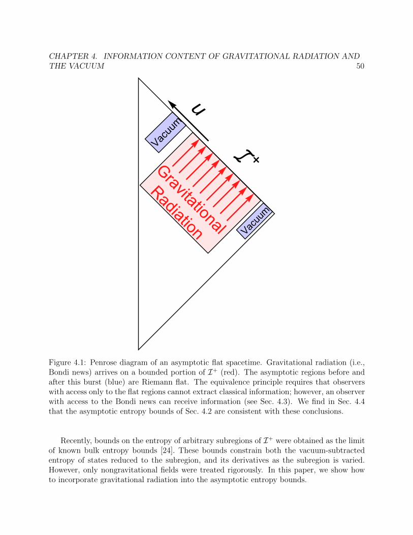
CHAPTER 4. INFORMATION CONTENT OF GRAVITATIONAL RADIATION ANDTHE VACUUM 50
Gravitational
Radiation
u
ℐ +Vacuum
Vacuum
Figure 4.1: Penrose diagram of an asymptotic flat spacetime. Gravitational radiation (i.e.,Bondi news) arrives on a bounded portion of I+ (red). The asymptotic regions before andafter this burst (blue) are Riemann flat. The equivalence principle requires that observerswith access only to the flat regions cannot extract classical information; however, an observerwith access to the Bondi news can receive information (see Sec. 4.3). We find in Sec. 4.4that the asymptotic entropy bounds of Sec. 4.2 are consistent with these conclusions.
Recently, bounds on the entropy of arbitrary subregions of I+ were obtained as the limitof known bulk entropy bounds [24]. These bounds constrain both the vacuum-subtractedentropy of states reduced to the subregion, and its derivatives as the subregion is varied.However, only nongravitational fields were treated rigorously. In this paper, we show howto incorporate gravitational radiation into the asymptotic entropy bounds.
CHAPTER 4. INFORMATION CONTENT OF GRAVITATIONAL RADIATION ANDTHE VACUUM 51
The bulk entropy bounds that formed the starting point of Ref. [24] have been proven forcertain fields [174, 32, 31, 33, 115]. Unless there is a discontinuity in the asymptotic limit,we expect these proofs to apply to the asymptotic bounds as well. Explicit proofs have notyet been given for a spin-2 field, however. To be conservative, the asymptotic bounds ongravitational radiation should be regarded as a conjecture.
Therefore, we will perform a simple consistency check: we ask whether the bounds arecompatible with the equivalence principle. We take this principle to be the statement that anempty, Riemann-flat spacetime region contains no classical information. (By this we meana subset of Minkowski space, not of a Riemann-flat spacetime with nontrivial topology. Inthis paper, “flat” will always mean Riemann-flat and devoid of matter.) In particular, theclassical information of the spacetime geometry is contained only in its Riemann curvature,and not, for example, in the choice of coordinates.
The simplest setting is empty Minkowski space. In any subregion of I+, our upper boundsvanish, implying that the vacuum-subtracted entropy is nonpositive and independent of thesubregion. (In particular, the upper bounds do not depend on a “choice of vacuum” ofMinkowski space.) This is consistent with the equivalence principle, which tells us that noclassical information is present.
The asymptotic metric of Minkowski space, written in Bondi coordinates, is not uniquelyfixed by fall-off conditions. One can freely choose the 1/r correction to the shape of spheresspecified by setting the coordinates u and r to constants. (Note that this correction describesthe shape of an embedded surface, whose location is determined by an arbitrary coordinatechoice. Its shape is not indicative of any actual curvature of Minkowski space, which ismanifestly Riemann-flat.) The freedom corresponds to a choice of a single real function c(Ω)of the coordinates on the sphere.
Recently, this degeneracy in the choice of Bondi coordinates has been interpreted as adegeneracy of the actual vacuum state of Minkowski space [162, 94]. We take no positionon the formal convenience of elevating a classical coordinate choice to a degeneracy of thevacuum.
However, the equivalence principle rules out the possibility that a coordinate choice inMinkowski space has any measurable consequences. Therefore, c(Ω) must be unobservable.This is consistent with the fact that our bounds are insensitive to c(Ω) and vanish identicallyin Minkowski space.
We also consider a classical gravitational wavepacket with finite support, which arrivesat I+ as Bondi news. In portions of I+ where the news has no support, our upper boundsvanish. This is consistent with the absence of classical information according to the equiv-alence principle: distant regions without gravitational radiation are Riemann-flat, so theirgeometry cannot be distinguished from Minkowski space.
In Bondi coordinates, the Bondi news does change the function c(Ω), by an integral ofthe news [162, 164, 94]. Since the news can be measured, this integral can be measured; forexample, it results in a permanent displacement of physical detectors. Thus, in a nonvacuumspacetime, c(Ω) is a coordinate choice only in that it can be picked freely either before orafter the burst. The difference—the gravitational memory—is invariant and physical. The

CHAPTER 4. INFORMATION CONTENT OF GRAVITATIONAL RADIATION ANDTHE VACUUM 52
equivalence principle, and our bounds, constrain how the memory can be observed: namely,only by recording the news with physical detectors (which must be present during the burst).The memory cannot be measured by merely probing the asymptotic vacuum regions beforeand after the burst.
Outline In Sec. 4.2, we review the derivation of asymptotic entropy bounds of Ref. [24](Sec. 4.2), and we show that they respond to gravitational radiation through the square ofthe Bondi news (Sec. 4.2).
In Sec. 4.3, we discuss implications of the equivalence principle. In Sec. 4.3, we con-sider the term CAB(∞) that appears in the asymptotic (Bondi) metric of asymptotically flatspacetimes. This term can be nonvanishing even in Minkowski space and has been inter-preted as labelling degenerate vacua [162, 7, 94]. Since it corresponds to a coordinate choicein Minkowski space, the equivalence principle demands that CAB be unobservable in anyexperiment. In Sec. 4.3, we consider gravitational memory (the integral of Bondi news).The equivalence principle implies that the memory can only be measured by an observeror apparatus that has access to all the Bondi news that produces the memory. In Sec. 4.3,we discuss “soft” gravitons and gravitational waves, by which we mean waves with longwavelength compared to some other time scale in the process that produces them. Givenenough time, such excitations can be distinguished from the vacuum and so their informationcontent is unconstrained by the equivalence principle.
In Sec. 4.4, we discuss implications of the entropy bounds of Sec. 4.2, in the same settingsconsidered in Sec. 4.3. In Minkowski space, there is no news, and all our upper boundsvanish. We also consider a classical probabilistic ensemble (i.e., a mixed state) of classicalgravitational wave bursts. We find that our bounds permit an observer to distinguish betweendifferent classical messages if and only if the observer has access to the news. Thus theimplications of our entropy bounds are consistent with the conclusions we draw from theequivalence principle in Sec. 4.3.
In Appendix A.3, we discuss an asymptotic entropy bound proposed by Kapec et al. [110].We focus on the case of empty Minkowski space. Whether this bound differs from (a specialcase of) ours depends on the definition of the entropy, which was not fully specified inRef. [110]. We argue that consistency with the equivalence principle requires a choice underwhich the bounds agree. We clarify that the extra term in the upper bound of Ref. [110]originates from a difference in how the relevant null surfaces are constructed before theasymptotic limit is taken.
In Appendix A.4, we apply the bounds of Sec. 4.2 to a single graviton wavepacket. Thiscase is not obviously constrained by the equivalence principle and so lies outside the mainline of argument pursued here. We find that our bounds have implications similar to thosederived for the classical Bondi news in Sec. 4.4.
CHAPTER 4. INFORMATION CONTENT OF GRAVITATIONAL RADIATION ANDTHE VACUUM 53
4.2 Asymptotic Entropy Bounds and Bondi News
In Ref. [24], entropy bounds were applied to a distant planar light-sheet. The bounds canbe expressed in terms of the stress tensor of matter crossing the light-sheet, and the squareof the shear of the light-sheet. It was shown that the matter contribution is independent ofthe orientation of the light-sheet in the asymptotic limit. However this was not proven forthe contribution from the shear. Here we fill this gap by demonstrating that the shear termcontributes to the upper bounds as the square of the Bondi news. Thus it is associated withgravitational radiation reaching the boundary. In particular, this implies that the asymptoticbounds of Ref. [24] are fully independent of the orientation of the light-sheets used to derivethem.
Asymptotic Entropy Bounds
In this subsection we briefly review the derivation and formulation of the asymptotic entropybounds of Ref. [24]. Expectation value brackets are left implicit throughout.
We consider entropy bounds [23, 72, 34] in the general form of Eq. (4.1). In the weak-gravity limit, Newton’s constant G is taken to become small, and a light-sheet is chosenthat consists of initially parallel light-rays (θ0 = 0). An example of this is a null planet− z = const in Minkowski space. The effects of matter on the light-sheet are computed toleading nontrivial order in G, from the focussing equation [172]
− dθdw
= 8πGTabkakb + ςabς
ab . (4.2)
Here Tab is the matter stress tensor, ka is the tangent vector to the light-rays that comprise thelight-sheet, w is an affine parameter and ς is the shear (defined by Eq. 4.20). The expansionθ is the logarithmic derivative of the area of a cross-section spanned by infinitesimally nearbylight-rays.
By Eq. (4.1), the upper bound is given by the total area loss between two cross-sectionsof the light-sheet. It can be computed by integrating Eq. (4.2) twice along the light-rays, andthen across the transverse directions. If the shear scales as G1/2, the area loss will scale asG, so Newton’s constant drops out in Eq. (4.1). The resulting bound involves only Planck’sconstant ~, so it can be viewed as a pure field theory statement.
Near the boundary of an asymptotically flat spacetime, the matter stress tensor falls offas r−2 and the shear associated with gravitational radiation falls of as r−1, so the aboveargument can be carried out at finite G, as an expansion in G/r2. In particular, one canwork on a Minkowski background,
ds2 = −du2 − 2du dr + r2dΩ2 , (4.3)
and compute area differences at order G/r2, by integrating the focussing equation (4.2).Keeping the radiation under consideration fixed, the area of the radiation front increases
in the asymptotic limit as the local stress tensor decreases. It is convenient to rescale

CHAPTER 4. INFORMATION CONTENT OF GRAVITATIONAL RADIATION ANDTHE VACUUM 54
both [24], and formulate asymptotic entropy bounds directly in terms of finite quantities onI+. The asymptotic energy flux is the energy arriving on I+ per unit advanced time andunit solid angle:1
T = Tuu + ςabςab , (4.4)
The first term is the energy flux of nongravitational radiation,
Tuu = limr→∞
r2Tuu , (4.5)
The second term is set by the shear of the light-sheet and will be defined in Sec. 4.2. It willbe shown to correspond to the energy delivered by gravitational waves.
In Ref. [24], the basic tool for deriving the asymptotic entropy bounds is the notion of adistant planar light-sheet. Let p ∈ I+ be a point at affine time up and angle ϑp = π. LetH(up) be the boundary of the past of p:
H(up) ≡ I−(p) , p ∈ I+ . (4.6)
As discussed in Ref. [24], H(up) is a null hypersurface. At O(G/u2p)
0, it is the null planet + z = up in Minkowski space, with affine parameter w ≡ t − z and tangent vector kµ =dxµ/dw. In the u, r, ϑ, φ coordinates, kµ has components
ku = cos2(ϑ/2) (4.7)
kr = −(cosϑ)/2 (4.8)
kϑ = sinϑ cos2(ϑ/2)/(up − u) (4.9)
kφ = 0 . (4.10)
In Ref. [24] it was shown that a number of known weak-gravity entropy bounds apply onH(up). Cuts on different H(up) were identified for different up by using the same functionu(Ω) to define each cut; this function also defines a cut on I+. Bulk entropy bounds wereapplied to subregions defined by the cuts. The limit as up → ∞ was taken and the bulk
entropy bounds were re-expressed in terms of the asymptotic energy flux T . We will nowlist these results; see Ref. [24] for details.
From the Quantum Null Energy Condition [34, 33] (QNEC) on H(up), one obtains theBoundary QNEC,
1
δΩ
d2
du2Sout[σ,Ω] ≤ 2π
~T . (4.11)
Here δΩ is a small solid angle element near a null geodesic at angle Ω on I+. The secondderivative is computed as this element is pushed to larger u, starting a given cut σ of I+.The limit as δΩ→ 0 is implicit. The entropy Sout is the von Neumann entropy of the stateof the subregion of I+ above the cut. That is,
Sout ≡ −tr>σ ρ log ρ . (4.12)
1We will generally refer to boundary versions of bulk quantities by adding a hat.
CHAPTER 4. INFORMATION CONTENT OF GRAVITATIONAL RADIATION ANDTHE VACUUM 55
The reduced state in the region above the cut σ is defined by
ρ = tr<σ ρg , (4.13)
where ρg is the global state on I+. We need not include future timelike infinite since weassume that all matter decays to radiation at sufficiently late times. Note that all cuts of I+
have the same intrinsic and extrinsic geometry. Therefore, divergent terms in Sout drop outwhen differences are computed, or when derivatives are taken (also below). With the abovedefinition, the QNEC has been proven for free scalar fields, and also for interacting gaugefields with a gravity dual [115].
From the differential, weak gravity Generalized Second Law (GSL) on H(up) [13, 174],or by integrating Eq. (4.11), one obtains the Boundary GSL in differential form
− 1
δΩ
d
duSout[σ; Ω] ≤ 2π
~
∫ ∞
σ
du T . (4.14)
From the integrated weak-gravity GSL on H(up), or by integrating Eq. (4.14), one obtainsthe Boundary GSL in integral form,
Sout[σ2]− Sout[∞] ≤ 2π
~
∫ ∞
σ2
d2Ω du [u− u2(Ω)] T , (4.15)
where Sout[∞] is to be understood in a limiting sense.Finally, from the Quantum Bousso Bound (QBB) [32, 31] on finite “slabs” of H(up) one
obtains a Boundary QBB,
SC [σ1, σ2] ≤ 2π
~
∫ σ1
σ2
d2Ω du g(u) T (u,Ω) . (4.16)
The weighting function g is different for free and interacting bulk fields [32, 31]. Since fieldsbecome free asymptotically, we expect that it is given by the free field expression g(u) =(u1 − u)(u− u2)/(u1 − u2).
In Eq. (4.16), SC is the vacuum-subtracted entropy [129, 45] of a finite affine interval onI+. It is defined directly on the finite portion of the light-sheet between σ1 and σ2, as thedifference of two von Neumann entropies
SC [σ1, σ2] = −tr ρ log ρ+ trχ logχ . (4.17)
Here the density operator ρ is obtained from the global quantum state ρg by tracing outthe exterior of the region between σ1 and σ2; and χ is similarly obtained from the globalvacuum state.2 The ultraviolet contributions from vacuum entanglement are the same in
2As discussed in the introduction, the equivalence principle requires that the reduced vacuum state isunique, so it implies that the definition of the vacuum-subtracted entropy is unambiguous. We return tothis point in App. A.3.

CHAPTER 4. INFORMATION CONTENT OF GRAVITATIONAL RADIATION ANDTHE VACUUM 56
both reduced states, so they cancel out [129, 45, 32]. With this definition, the QBB has beenproven both for free and interacting scalar fields. It has also been verified for gauge fieldswith gravity duals [31].
For free theories, the algebra of operators factorizes over the null geodesics that generatethe light-sheet [174]. We expect that this case applies to I+. Then the von Neumann entropyof the vacuum state restricted to the semi-infinite region above a cut σ is independent of thecut. Therefore, we have
Sout[σ2]− Sout[σ1] = SC [σ2]− SC [σ1] , (4.18)
where SC [σ] is now computed on the semi-infinite regions above σ1 and σ2. Thus we canalso express other bounds, Eqs. (4.11) and (4.14), in terms of derivatives and differences ofthe manifestly finite quantity SC , instead of Sout.
In particular, we can write the integrated Boundary GSL, Eq. (4.15), as
SC [σ2] ≤ 2π
~
∫ ∞
σ2
d2Ω du [u− u2(Ω)] T . (4.19)
We have used the fact that the reduced density matrix of any physical state above a cut atsufficiently large u is that of the vacuum restricted to the same region, and thus SC [∞] = 0.We will use this form of the integrated Boundary GSL in Sec. 4.4.
Bondi News as Shear on Distant Light-Sheets
Let ςab be the shear tensor on H(up), defined as the tracefree part of the extrinsic curvature:
ςab = Bab −1
2θqab , (4.20)
where Bab = q ca q
db ∇ckd, and qab is the metric on the cuts w = const. One could choose
different cuts, but some foliation of H(up) into cuts has to be chosen in order to discuss theevolution of the shear. The shear tensor has only transverse components, so its informationis fully captured by the lower-dimensional tensor
ςAB ≡ ςabeaAe
bB . (4.21)
The D − 2 orthonormal vectors eaA
are tangent to the cut. Below we will denote anyprojection with the ea
Aby capital indices placed on higher-dimensional tensors.
The evolution equation for the shear is [172, 147]
d
dwςAB = WAB − θ ςAB , (4.22)
whereWAB = −CabcdeaAkbecBkd ≡ −CAbBdkbkd (4.23)

CHAPTER 4. INFORMATION CONTENT OF GRAVITATIONAL RADIATION ANDTHE VACUUM 57
and Cabcd is the Weyl tensor. We now recall that at fixed (u,Ω) there is no difference betweenexpansions in inverse powers of up and r, since [24]
r =up − u
2 cos2(ϑ/2). (4.24)
The asymptotic behavior of the Weyl tensor is [73]
CAuBϑ ∼ O(r−1) , (4.25)
CAuBr ∼ O(r−3) , (4.26)
CArBr ∼ O(r−4) , (4.27)
CArBϑ ∼ O(r−3) , (4.28)
CAϑBϑ ∼ O(r−1) ; (4.29)
and from Eqs. (4.9) and (4.10)
kϑ ∼ O(r−1) , kφ = 0 . (4.30)
Hence we haveWAB = −CAuBu(ku)2 +O(u−2
p ) . (4.31)
These Weyl components are related to the Bondi news, NAB [73]:
CAuBu = − 1
2r
d
duNAB +O(r−2) . (4.32)
We have introduced an unbarred basis defined by eaA = reaA
, with the feature that in thisbasis boundary quantities such as CAB and NAB are independent of r. Unbarred capitalindices will be raised and lowered with the unit two sphere metric, hAB.
Since the expansion of H(up) is of order G/r2, the θ ςAB term in Eq. (4.22) is alwayssubleading in our analysis. Because the Bondi news and the shear of H(up) both vanish inthe far future, Eq. (4.22) implies
ςAB =1
2rNAB cos2(ϑ/2) +O(r−2) , (4.33)
where we have used d2u/dw2 ∼ O(r−1).On the other hand, the “boundary shear tensor” appearing in Eq. (4.4) was defined in
Ref. [24] as
ςab(u, ϑ, φ) ≡ 1√8πG
limr→∞
rςab(u, r, ϑ, φ)
cos2(ϑ/2). (4.34)
Comparing the previous two equations and using Eq. (4.21), we recognize that the bound-ary shear is the Bondi news, up to an O(1) rescaling:3
ςAB =NAB√32πG
. (4.35)
3In the Newman-Penrose formalism, the Bondi news is commonly identified with the u-derivative of theshear of the family of outgoing null congruences specified by u = const [139]. Here we relate the news to theshear of ingoing null congruences.

CHAPTER 4. INFORMATION CONTENT OF GRAVITATIONAL RADIATION ANDTHE VACUUM 58
The factor of G−1/2 ensures that ς2 has the dimension of an energy flux.Returning to the definition of the total asymptotic energy flux, Eq. (4.4), we can now
write T in terms of the Bondi news:
T = Tuu +1
32πGNABN
AB , (4.36)
Note that the definition of the boundary shear ςAB was tied to a family of null planes H(up)whose orientation picks out a special point on the sphere. Since the Bondi news admitsan independent definition that does not require us to pick such a point, it follows that theasymptotic bounds derived in Ref. [24] are independent of the orientation of the H(up).
In the remainder of this paper, we will specialize to the case where all outgoing radiationis gravitational. Then Tuu = 0 and T = NABN
AB/32πG. We see that the square of theBondi news controls the entropy flux of gravitational radiation.
4.3 Implications of the Equivalence Principle
In this section, we consider classical aspects of gravitational radiation. We derive conse-quences of the equivalence principle: the hypothesis that no subset of Minkowski spacecontains any measurable classical information. Since we use the notion of classical infor-mation throughout this and the following sections, we begin with a simple example of suchinformation and its description, in Sec. 4.3.
It is possible to find nonvacuum quantum states whose effective stress tensor (analogousto Eq. (4.36)) vanishes in a bounded region. The geometry in this region could be Riemann-flat, yet the region could contain quantum information. Here we only assume the absenceof classical information in Minkowski space. In particular we assume that no observable isassociated with a coordinate choice in Minkowski space.
The geometry of Minkowski space is trivial, but of course the coordinates are arbitrary.So the matrix of metric components can take many different forms, both generally and in theasymptotic region. Restricting to Bondi coordinates does not fully fix this ambiguity. Theequivalence principle implies that any parameters of the Bondi metric that are not unique inMinkowski space must be unobservable, or else that parameter would constitute measurableinformation. There is no ~ in the metric of Minkowski space in any Bondi gauge, so thecorresponding coordinate information would be classical information.
This includes in particular a parameter CAB (defined below) that has been interpreted [7,162, 94] as labelling degenerate vacua (Sec. 4.3). Indeed, no observation of this parameterhas yet been made, and we are not aware of a proposal for how it could be measured.
A key consequence of the equivalence principle is that the gravitational memory createdby Bondi news can be measured only by recording the news. It cannot be measured byprobing the vacuum before and after the news (Sec. 4.3). Finally, we note that the equivalenceprinciple does not preclude soft gravitational radiation from carrying information, if “soft”is understood in the physically relevant sense of a small expansion parameter (Sec. 4.3).

CHAPTER 4. INFORMATION CONTENT OF GRAVITATIONAL RADIATION ANDTHE VACUUM 59
These conclusions are in harmony with our findings in Sec. 4.4, where we apply thebounds of Sec. 4.2 to constrain the information content of gravitons and of the vacuum.
Classical Information
A simple example is a classical n-bit message written by Alice and delivered to Bob, sayas a sequence of red and blue balls shot across space. Before Bob looks at the balls, he isignorant of their state. Thus he can describe it as a density operator in a 2n dimensionalHilbert space, which is diagonal in the red, bluen basis, with equal probability 2−n foreach possible message. The Shannon and von Neumann entropies are both
−2n∑
i=1
pi log pi = −Trρ log ρ = n log 2 . (4.37)
This is an incoherent superposition, or classical probabilistic ensemble (not to be confusedwith a coherent quantum superposition of ball sequences).
By looking at the balls, Bob learns Alice’s message. Alice cannot send Bob more infor-mation than the maximum entropy of the system that carries the message. Since we canexpress Bob’s initial ignorance as a density operator, quantum entropy bounds limit classicalcommunication, as a special case.
Of course, the full quantum Hilbert space is much larger due to the internal degrees offreedom of the balls. And even in the tiny subfactor spanned by red, bluen, more generalstates are possible at the quantum level, which are not product states of the individual balls.
But for classical messages represented by a quantum density operator ρi, the ensembleinterpretation [140] implies that the full density operator can be written as
ρ =2n∑
i=1
ρi . (4.38)
Since the ρi are classically distinguishable—and therefore mutually orthogonal—states, thereis an irreducible uncertainty in the von Neumann entropy: the entropy cannot be paramet-rically less than the classical value, n log 2. At the field theory level, this will remain truefor the vacuum-subtracted von Neumann entropy: it must be parametrically at least n log 2(assuming the region contains all balls), since the vacuum entanglement is an ultravioletquantum property shared by all the classical states.
In this paper we often consider the equivalence principle: the statement that Minkowskispace, and any subset of it, contain no classical information. It is worth reflecting on what itwould mean if empty Riemann flat space did contain measurable information. In that caseit could be used by Alice to communicate a message to Bob.
To be concrete, consider an arbitrarily large patch of flat space (say, the interior of a fallingelevator, or a large void in our universe). For it to contain information in an operationallymeaningful sense, Alice would have to be capable of “preparing” this region, perhaps by

CHAPTER 4. INFORMATION CONTENT OF GRAVITATIONAL RADIATION ANDTHE VACUUM 60
sending a certain sequence of gravitational waves through it. Later, long after those waveshave left the region and it is again empty and Riemann-flat, Bob would have to be capableof reading out the message that Alice “left behind”, by examining only this patch.
Specifically, if c(Ω) was observable, then independent observers with access only to theflat space region, would all come to the same conclusion as to which coordinates shouldbe used to label its spacetime points. More precisely, up to corrections subleading in 1/r,such observers would uniquely identify topological spheres on which the Bondi coordinatesu and r must be constant, thus partially fixing the chart. This would indeed be a textbookviolation of the equivalence principle.
Empty Space Has No Classical Information
Let us consider the asymptotic metric of an asymptotically flat spacetime, in standard re-tarded Bondi coordinates (see, e.g., [21, 154, 7, 162, 164, 73]):
ds2 = −(
1− 2mB(u,Ω)
r
)du2 − 2 du dr
+ r2
(hAB +
CAB(u,Ω)
r
)×
×(dϑA +
DCCAC
2r2du
)(dϑB +
DCCCB
2r2du
)
+ . . . (4.39)
where mB is the Bondi mass aspect, and the ellipses indicate terms subleading in r. Here,CAB(u,Ω) appears as the 1/r correction to the round two-sphere metric hAB. It satisfieshABCAB = 0 and CAB = CBA. The Bondi news is defined by
NAB = ∂uCAB . (4.40)
In Minkowski space, the news vanishes. However, the asymptotic metric of Minkowskispace can be written in the form of Eq. (4.39), with mB ≡ 0 and any u-independent choiceof a tracefree symmetric CAB(Ω) satisfying
CAB = (2DADB − hABDCDC) c(Ω) (4.41)
for some function c on the sphere. But of course, the geometry is always the same, no matterhow we label its points. There is no curvature of any kind, whatever value we choose forc(Ω). By the equivalence principle, this implies that c and CAB cannot be measured.
CAB does transform nontrivially under large diffeomorphisms of the asymptotic met-ric [162, 12, 11, 73]; indeed, this is one way to see that it is non-unique in Minkowski space.Under a BMS supertranslation, u→ u+ f(Ω), one has
CAB → CAB +(2DADB − hABDCDC
)f(Ω) (4.42)
CHAPTER 4. INFORMATION CONTENT OF GRAVITATIONAL RADIATION ANDTHE VACUUM 61
in regions where NAB = 0. This corresponds to a well-defined change in the shape of a largecoordinate sphere at constant u, r. It affects all such spheres equally; for example CAB(∞)and CAB(−∞) will change by the same amount under a supertranslation. Of course, thisdoes not imply that CAB is observable. A coordinate sphere is not a physical object buta collection of spacetime points. Its initial shape before the transformation is set by acoordinate choice.
The transformation properties of CAB under supertranslations have been interpreted asan infinite “vacuum degeneracy” of Minkowski space [162, 7, 94]. Each “vacuum” is labeledby the function c(Ω) in Eq. (4.41). We conclude that the equivalence principle precludes anyobservable consequences of this degeneracy.4 (Refs. [10, 62] give an argument that the vacuaare indistinguishable starting from different assumptions.)
Gravitational Memory
In nonvacuum spacetimes, CAB need not be constant in u, and differences between CAB atdifferent cuts are observable as “gravitational memory.” However, the value of CAB at anyone cut (or its zero-mode) must be unobservable in any asymptotically flat spacetime, orelse the equivalence principle would be violated in regions where no news arrives. We willnow discuss this.
Suppose that some process (a binary inspiral, say) produces gravitational radiation, andthat the corresponding Bondi news arrives entirely between the cuts σ1 and σ2 of I+. Theintegral of the news along the null direction is called the gravitational memory produced bythe process,
∆CAB(Ω) ≡∫ σ2
σ1
duNAB(u,Ω) (4.43)
By Eq. (4.43), the production of memory requires nonzero flux of radiation, NAB. Hencememory production occurs only in excited states, not in the vacuum. For example, a gravitonwavepacket can produce memory; but then the global state is not the vacuum, but a one-particle state. This qualitative fact continues to hold invariantly in the “soft limit,” as thewavepacket is taken to have arbitrarily large wavelength.
What is the physical manifestation of ∆CAB, or equivalently, how can it be measured?In Sec. 4.2, we showed that NAB is proportional to the shear of a planar null congruenceH(up) near I+. Hence the gravitational memory is related to the integrated shear, i.e., theresulting strain of the congruence. The displacement vector ηA of two infinitesimally nearbynull geodesics will change by
∆ηA = ∆CAB
ηB
2r(4.44)
4Note that the equivalence principle only precludes diffeomorphisms from transforming the classicalvacuum into a physically distinct configuration. The equivalence principle does not imply that large diffeo-morphisms always act trivially. When acting on an excited state, a supertranslation generically producesa distinct excited state, for example with a different relative timing of the Bondi news arriving at differentangles.
CHAPTER 4. INFORMATION CONTENT OF GRAVITATIONAL RADIATION ANDTHE VACUUM 62
between σ1 and σ2. This can be measured by setting up (before σ1) a collection of physical,massless particles propagating along the null geodesics that constitute H(up), and observingtheir transverse location on a screen that they hit after σ2. ∆CAB can also be measuredusing an array of timelike detectors distributed over a large sphere. The displacement of anytwo detectors similarly suffers an overall change given by Eq. (4.44).
In general, the memory captures only a small fraction of the information that arrives indistant regions: the integral of the Bondi news. It would certainly be nice to measure thiscomponent using gravitational wave detectors [50, 99]. Such a measurement would not takeinfinite time, and it would not be conceptually distinct from any other measurement of theoutgoing radiation.
By Eq. (4.40) we can write the gravitational memory, Eq. (4.43), as a difference of themetric quantity CAB evaluated at the two cuts,
∆CAB(Ω) = CAB[σ2]− CAB[σ1] . (4.45)
If CAB is interpreted as labelling a vacuum, the creation of gravitational memory by newscould be described as a “transition” between two such vacua. However, according to theequivalence principle this language is misleading, because CAB cannot be observed at alocal cut. A “vacuum” in the above sense is a coordinate label that contains no physicalinformation.
Only the difference ∆CAB is invariant (up to Lorentz transformations [73]) and so canbe observed. ∆CAB is nonzero only in global states which are not the vacuum, and it isfully determined by the integral of the Bondi news. So the function CAB(u,Ω) containsno physical information beyond what is already in its u-derivative, the news NAB. Theobservable memory, ∆CAB, captures a subset of the information in the news.
By the equivalence principle, ∆CAB can only be measured by an observer who has ac-cess to the entire region in which news arrives. For example, if physical test particles areintroduced into the asymptotic region, and their initial position at σ1 is recorded, then thememory ∆CAB can be measured at σ2 by observing the new location of these physical ob-jects. This is an integrated measurement of the Bondi news, with the dynamics of the testmasses doing the integration.
Formally, it can be convenient to consider the “zero mode” of the news,
CAB(Ω,∞)− CAB(Ω,−∞) ≡∫ ∞
−∞duNAB(Ω, u) . (4.46)
This quantity represents the total amount of memory produced in an asymptotically flatspacetime. As written, it is not observable, since no experiment began in the infinite pastand will end in the infinite future. Fortunately, in any physical process or sequence ofprocesses, the production of news will have a beginning and an end. So one can record theentire memory in a finite-duration experiment, corresponding to a sufficiently large finiterange of integration.
To summarize both this and the previous subsection, the value of CAB at any one cut canbe changed by a global change of coordinates. By the equivalence principle, CAB cannot be

CHAPTER 4. INFORMATION CONTENT OF GRAVITATIONAL RADIATION ANDTHE VACUUM 63
observed and contains no physical information. Therefore, in particular, we cannot measurethe gravitational memory, ∆CAB by observing CAB locally at σ1 and σ2 and computing thedifference. Rather, physical test masses are essential for recording the news and integratingit to obtain ∆CAB between the two cuts. If we forgot to introduce real test masses at σ1,we cannot look at empty space at σ2 and learn anything from it.
Soft Gravitons
A soft particle is an excitation of a massless field whose characteristic wavelength, or inversefrequency, is large compared to some dynamical timescale that otherwise characterizes aproblem. For example, consider a binary system composed of neutron stars or black holes.They orbit each other with some frequency ω, which varies slowly as they approach, untilthey eventually merge. The system will emit “hard” gravitational waves with frequencyof order ω. The overall duration of the inspiral process is much greater than ω−1; it ischaracterized by a second time scale τ ω−1. Or consider a black hole emitting Hawkingradiation. The wavelength of the “hard part” of the radiation is of order the black holeradius, ω−1 ∼ O(R), which changes slowly. Nonetheless, the overall process takes a muchlonger time, τ ∼ O(R3/G~).
Because the emission of “hard” radiation slowly transports gravitating energy from thecenter to distant regions, the gravitational field will vary not only with characteristic fre-quency ω, but also over the timescale τ . Therefore, signals with characteristic frequencyas low as τ−1 are produced in the above processes. Such signals are referred to as “soft”.(Often the term “soft graviton” is used, even when the signal is classical.)
This terminology is convenient when we wish to distinguish particles associated withdifferent timescales in a given problem. Useful results can be obtained by expanding inratios of such timescales [182]. It can also be convenient to idealize soft particles by takinga τ → ∞ limit, for the purposes of making such expansions sharp. It is worth stressing,however, that infinite-duration experiments are not actually needed to produce and measurea soft particle. (If they were, soft particles would have no physical relevance.) The largertime scale τ is necessarily finite in any physical process.
Moreover, the production of observable radiation comes at a nonzero energy cost. If asoft graviton were added to the vacuum, one would obtain an excited state orthogonal to thevacuum, not a new vacuum. This is a qualitative statement, and independent of τ . Thus,there is no fundamental difference between soft particles and any other form of radiationthat arrives in distant regions.
Correspondingly, when we apply the boundary entropy bounds of Sec. 4.2 in Sec. 4.4,all Bondi news can be treated on the same footing. For example, if the interval underconsideration in Eq. (4.19) or Eq. (4.16) is large enough to contain a news wavepacket (hardor soft), we will find that this graviton will contribute to the energy side, and genericallyalso to the entropy side of the inequality.

CHAPTER 4. INFORMATION CONTENT OF GRAVITATIONAL RADIATION ANDTHE VACUUM 64
4.4 Entropy Bounds on Gravitational Wave Bursts
and the Vacuum
In this section, we compute the upper bounds of Sec. 4.2 in simple asymptotically flatspacetimes: Minkowski space, and a burst of Bondi news that creates gravitational memory.We show that the upper bounds are consistent with constraints derived in the previoussection from the equivalence principle.
Vacuum
Let us apply the bounds of Sec. 4.2 to empty Minkowski space: the Boundary QNEC,Eq. (4.11); the Boundary GSL in integrated and differential form, Eqs. (4.14) and (4.19);and the Boundary QBB, Eq. (4.16). All of these bounds are linear in the boundary stresstensor T , i.e., quadratic in the Bondi news. Since T = 0 in Minkowski space, the upperbounds all vanish.
The Boundary QBB implies that the vacuum-subtracted entropy is nonpositive in anyfinite subregion of I+. The Boundary GSL implies that it is nonpositive for any semi-infinite region above a cut, and independent of the choice of region or deformations of thecut. The Boundary QFC implies (redundantly with the above) that the second derivativeunder deformations also vanishes.
These upper bounds are consistent with all implications of the equivalence principledescribed in the previous section: no subset of Minkowski space contains any classical infor-mation. Moreover, both the bounds and the equivalence principle are consistent with thesimplest possibility for the quantum description of Minkowski space: that the ground stateis unique, and that the vacuum-subtracted entropy precisely vanishes on any subregion ofI+.
Classical Bondi News
For simplicity, we will consider a single wave packet of gravitational radiation, of character-istic wavelength λ in the u-direction. The wave packet is roughly centered on u = 0 anddelocalized on the sphere. The wave packet can be used to send a message to an observerat I+, for example by encoding it in its polarization, its shape, its direction (the angle Ω atwhich it arrives), or the time of arrival, within a finite discrete set of N possible choices.
For concreteness, let us encode the information in the energy of the wavepacket. We takethe energy to be of order E for any message, but with a grading into N different values.A single graviton has energy of order ~/λ. Since we wish to work in the classical regime,the grading must be much coarser than that, so the number of distinct classical states willsatisfy
N Eλ
~, (4.47)

CHAPTER 4. INFORMATION CONTENT OF GRAVITATIONAL RADIATION ANDTHE VACUUM 65
We assume that any of the distinct classical signals arrives with equal probability 1/N . Theclassical Shannon entropy is thus logN .
If we apply the Boundary QBB, Eq. (4.16), or the Boundary GSL, Eq. (4.19), to theregion occupied by the wavepacket, we obtain
SC .Eλ
~(4.48)
This is consistent: in our example, the vacuum-subtracted entropy need not be much greaterthan the Shannon entropy logN , which is much smaller than N and hence, by Eq. (4.47),much smaller than the upper bound. Thus, the asymptotic bounds of Sec. 4.2 easily accom-modate the classical information contained in the Bondi news.
On the other hand, if we apply the same bounds to a region that fails to overlap withthe wavepacket, then the upper bound vanishes:
SC ≤ 0 . (4.49)
This is consistent with the absence of classical information in asymptotic regions that do notcontain news, as required by the equivalence principle.
In particular, the bounds are consistent with our conclusion in Sec. 4.3 that gravitationalmemory can only be measured by an observer who has access to the news that creates thememory. In our present example, the news is featureless but for its overall energy. So itsintegral, the memory, contains the same amount of information as the news, logN . [Wehave T ∼ NABN
AB/G ∼ E/λ, so the memory will be of order ∆CAB ∼ NABλ ∼ (GEλ)1/2.]By Eq. (4.49), this information is unavailable to an observer who cannot access the news.

66
Chapter 5
Geometric Constraints fromSubregion Duality Beyond theClassical Regime
5.1 Introduction
AdS/CFT implies constraints on quantum gravity from properties of quantum field theory.For example, field theory causality requires that null geodesics through the bulk are delayedrelative to those on the boundary. Such constraints on the bulk geometry can often beunderstood as coming from energy conditions on the bulk fields. In this case, bulk nullgeodesics will always be delayed as long as there is no negative null energy flux [84].
In this paper, we examine two constraints on the bulk geometry that are required by theconsistency of the AdS/CFT duality. The starting point is the idea of subregion duality,which is the idea that the state of the boundary field theory reduced to a subregion A is itselfdual to a subregion of the bulk. The relevant bulk region is called the entanglement wedge,E(A), and consists of all points spacelike related to the extremal surface anchored on ∂A, onthe side towards A [53, 96]. The validity of subregion duality was argued [55, 88] to followfrom the Ryu-Takayanagi-FLM formula [152, 153, 101, 69, 126, 56], and the consistency ofsubregion duality immediately implies two constraints on the bulk geometry.
The first constraint, which we call Entanglement Wedge Nesting (EWN), is that if aregion A is contained in a region B on the boundary (or more generally, if the domainof dependence of A is contained in the domain of dependence of B), then E(A) must becontained in E(B). This condition was previously discussed in [53, 177].
The second constraint is that the set of bulk points I−(D(A)) ∩ I+(D(A)), called thecausal wedge C(A), is completely contained in the entanglement wedge E(A). We call thisC ⊆ E . See [53, 177, 64, 100, 96] for previous discussion of C ⊆ E .
We refer to the delay of null geodesics passing through the bulk relative to their bound-ary counterparts [84] as the Boundary Causality Condition (BCC), as in [63]. These three
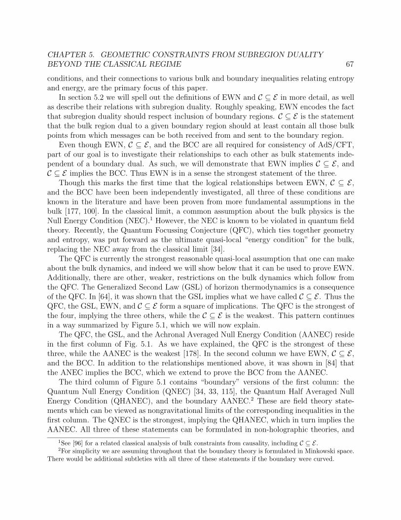
CHAPTER 5. GEOMETRIC CONSTRAINTS FROM SUBREGION DUALITYBEYOND THE CLASSICAL REGIME 67
conditions, and their connections to various bulk and boundary inequalities relating entropyand energy, are the primary focus of this paper.
In section 5.2 we will spell out the definitions of EWN and C ⊆ E in more detail, as wellas describe their relations with subregion duality. Roughly speaking, EWN encodes the factthat subregion duality should respect inclusion of boundary regions. C ⊆ E is the statementthat the bulk region dual to a given boundary region should at least contain all those bulkpoints from which messages can be both received from and sent to the boundary region.
Even though EWN, C ⊆ E , and the BCC are all required for consistency of AdS/CFT,part of our goal is to investigate their relationships to each other as bulk statements inde-pendent of a boundary dual. As such, we will demonstrate that EWN implies C ⊆ E , andC ⊆ E implies the BCC. Thus EWN is in a sense the strongest statement of the three.
Though this marks the first time that the logical relationships between EWN, C ⊆ E ,and the BCC have been been independently investigated, all three of these conditions areknown in the literature and have been proven from more fundamental assumptions in thebulk [177, 100]. In the classical limit, a common assumption about the bulk physics is theNull Energy Condition (NEC).1 However, the NEC is known to be violated in quantum fieldtheory. Recently, the Quantum Focussing Conjecture (QFC), which ties together geometryand entropy, was put forward as the ultimate quasi-local “energy condition” for the bulk,replacing the NEC away from the classical limit [34].
The QFC is currently the strongest reasonable quasi-local assumption that one can makeabout the bulk dynamics, and indeed we will show below that it can be used to prove EWN.Additionally, there are other, weaker, restrictions on the bulk dynamics which follow fromthe QFC. The Generalized Second Law (GSL) of horizon thermodynamics is a consequenceof the QFC. In [64], it was shown that the GSL implies what we have called C ⊆ E . Thus theQFC, the GSL, EWN, and C ⊆ E form a square of implications. The QFC is the strongest ofthe four, implying the three others, while the C ⊆ E is the weakest. This pattern continuesin a way summarized by Figure 5.1, which we will now explain.
The QFC, the GSL, and the Achronal Averaged Null Energy Condition (AANEC) residein the first column of Fig. 5.1. As we have explained, the QFC is the strongest of thesethree, while the AANEC is the weakest [178]. In the second column we have EWN, C ⊆ E ,and the BCC. In addition to the relationships mentioned above, it was shown in [84] thatthe ANEC implies the BCC, which we extend to prove the BCC from the AANEC.
The third column of Figure 5.1 contains “boundary” versions of the first column: theQuantum Null Energy Condition (QNEC) [34, 33, 115], the Quantum Half Averaged NullEnergy Condition (QHANEC), and the boundary AANEC.2 These are field theory state-ments which can be viewed as nongravitational limits of the corresponding inequalities in thefirst column. The QNEC is the strongest, implying the QHANEC, which in turn implies theAANEC. All three of these statements can be formulated in non-holographic theories, and
1See [96] for a related classical analysis of bulk constraints from causality, including C ⊆ E .2For simplicity we are assuming throughout that the boundary theory is formulated in Minkowski space.
There would be additional subtleties with all three of these statements if the boundary were curved.

CHAPTER 5. GEOMETRIC CONSTRAINTS FROM SUBREGION DUALITYBEYOND THE CLASSICAL REGIME 68
GSL
AANEC
QFC Ent. Wedge Nesting (EWN)
BCC
QNEC
Quantum Half-ANEC
(QHANEC)
AANECFigure 5.1: The logical relationships between the constraints discussed in this paper. The leftcolumn contains semi-classical quantum gravity statements in the bulk. The middle columnis composed of constraints on bulk geometry. In the right column is quantum field theoryconstraints on the boundary CFT. All implications are true to all orders in G~ ∼ 1/N . Wehave used dashed implication signs for those that were proven to all orders before this paper.
all three are conjectured to be true generally. (The AANEC was recently proven in [71] as aconsequence of monotonicity of relative entropy and in [90] as a consequence of causality.)
In the case of a holographic theory, it was shown in [115] that EWN in the bulk impliesthe QNEC for the boundary theory to leading order in G~ ∼ 1/N . We demonstrate that thisrelationship continues to hold with bulk quantum corrections. Moreover, in [112] the BCCin the bulk was shown to imply the boundary AANEC. Here we will complete the patternof implications by showing that C ⊆ E implies the boundary QHANEC.
In the classical regime, the entanglement wedge is defined in terms of a codimension-2surface with extremal area [101, 69, 96, 56]. It has been suggested that the correct quantumgeneralization should be defined in terms of the “quantum extremal surface”: a Cauchy-splitting surface which extremizes the generalized entropy to one side [64]. Indeed, we findthat the logical structure of Fig. 5.1 persists to all orders in perturbation theory in G~ ∼ 1/N
CHAPTER 5. GEOMETRIC CONSTRAINTS FROM SUBREGION DUALITYBEYOND THE CLASSICAL REGIME 69
if and only if the entanglement wedge is defined in terms of the quantum extremal surface.This observation provides considerable evidence for prescription of [64].
The remainder of this paper is organized as follows. In Section 5.2 we will define all of thestatements we set out to prove, as well as establish notation. Then in Sections 5.3 and 5.4 wewill prove the logical structure encapsulated in Figure 5.1. Several of these implications arealready established in the literature, but for completeness we will briefly review the relevantarguments. We conclude with a discussion in Section 8.4.
5.2 Glossary
Regime of Validity Quantum gravity is a tricky subject. We work in a semiclassical(large-N) regime, where the dynamical fields can be expanded perturbatively in G~ ∼ 1/Nabout a classical background [174].3 For example, the metric has the form
gab = g0ab + g
1/2ab + g1
ab +O((G~)3/2) , (5.1)
where the superscripts denote powers of G~. In the semi-classical limit — defined as G~→ 0— the validity of the various inequalities we consider will be dominated by their leading non-vanishing terms. We assume that the classical O((G~)0) part of the metric satisfies the nullenergy condition (NEC), without assuming anything about the quantum corrections. Formore details on this type of expansion, see Wall [178].
We primarily consider the case where the bulk theory can be approximated as Einsteingravity with minimally coupled matter fields. In the semiclassical regime, bulk loops willgenerate Planck-suppressed higher derivative corrections to the gravitational theory and thegravitational entropy.4 We will comment on the effects of these corrections throughout.
We consider a boundary theory on flat space, possibly deformed by relevant operators.When appropriate, we will assume the null generic condition, which guarantees that everynull geodesic encounters matter or gravitational radiation.
Geometrical Constraints
There are a number of known properties of the AdS bulk causal structure and extremalsurfaces. At the classical level (i.e. at leading order in G~ ∼ 1/N), the NEC is the standardassumption made about the bulk which ensures that these properties are true [177]. However,some of these are so fundamental to subregion duality that it is sensible to demand them
3The demensionless expansion parameter would be G~/`D−2, where ` is a typical length scale in whateverstate we are considering. We will leave factors of ` implicit.
4Such corrections are also necessary for the generalized entropy to be finite. See Appendix A of [34] fordetails and references. Other terms can be generated from, for example, stringy effects, but these will besuppressed by the string length `s. For simplicity, we will not separately track the `s expansion. This shouldbe valid as long as the string scale is not much different from the Planck scale.

CHAPTER 5. GEOMETRIC CONSTRAINTS FROM SUBREGION DUALITYBEYOND THE CLASSICAL REGIME 70
and to ask what constraints in the bulk might ensure that these properties hold, even underquantum corrections. Answering this question is one key focus of this paper.
In this section, we review three necessary geometrical constraints. In addition to definingeach of them and stating their logical relationships (see Figure 5.1), we explain how each iscritical for subregion duality.
Boundary Causality Condition (BCC)
A standard notion of causality in asymptotically-AdS spacetimes is the condition that thebulk cannot be used for superluminal communication relative to the causal structure of theboundary. More precisely, any causal bulk curve emanating from a boundary point p andarriving back on the boundary must do so to the future of p as determined by the boundarycausal structure.
This condition, termed “BCC” in [63], is known to follow from the averaged null curvaturecondition (ANCC) [84]. Engelhardt and Fischetti have derived an equivalent formulationin terms of an integral inequality for the metric perturbation in the context of linearizedperturbations to the vacuum [63].
Microcausality in the boundary theory requires that the BCC hold. If the BCC wereviolated, a bulk excitation could propagate between two spacelike-separated points on theboundary leading to nonvanishing commutators of local fields at those points. In Sec. 5.4we will show that BCC is implied by C ⊆ E . Thus BCC is the weakest notion of causalityin holography that we consider.
C ⊆ E
Consider the domain of dependence D(A) of a boundary region A. Let us define the causalwedge of a boundary region A to be C(A) ≡ I−(D(A)) ∩ I+(D(A)).5
By the Ryu-Takayanagi-FLM formula, the entropy of the quantum state restricted toA is given by the area of the extremal area bulk surface homologous to A plus the bulkentropy in the region between that surface and the boundary [152, 153, 101, 69, 126, 56].This formula was shown to hold at O((1/N)0) in the large-N expansion. In [64], Engelhardtand Wall proposed that the all-orders modification of this formula is to replace the extremalarea surface with the Quantum Extremal Surface (QES), which is defined as the surfacewhich extremizes the generalized entropy: the surface area plus the entropy in the regionbetween the surface and A. Though the Engelhardt-Wall prescription remains unproven, wewill assume that it is the correct all-orders prescription for computing the boundary entropyof A. We denote the QES of A as e(A).
The entanglement wedge E(A) is the bulk region spacelike-related to e(A) on the A sideof the surface. This is the bulk region believed to be dual to A in subregion duality [53].
5I±(S) represent respectively the chronological future and past of the set S. The causal wedge wasoriginally defined in [96] in terms of the causal future and past, J±(S), but for our purposes the chronologicalfuture and past are more convenient.

CHAPTER 5. GEOMETRIC CONSTRAINTS FROM SUBREGION DUALITYBEYOND THE CLASSICAL REGIME 71
Dong, Harlow and Wall have argued that this is the case using the formalism of quantumerror correction [55, 88].C ⊆ E is the property that the entanglement wedge E(A) associated to a boundary region
A completely contains the causal wedge C(A) associated to A. C ⊆ E can equivalently beformulated as stating that e(A) is out of causal contact with D(A), i.e. e(A) ∩ (I+(D(A) ∪I−(D(A)) = ∅. In our proofs below we will use this latter characterization.
Subregion duality requires C ⊆ E because the bulk region dual to a boundary region Ashould at least include all of the points that can both send and receive causal signals to andfrom D(A). Moreover, if C ⊆ E were false then it would be possible to use local unitaryoperators in D(A) to send a bulk signal to e(A) and thus change the entropy associated tothe region [53, 177, 64, 96]. That is, of course, not acceptable, as the von Neumann entropyis invariant under unitary transformations.
This condition has been discussed at the classical level in [96, 177]. In the semiclassicalregime, Engelhardt and Wall [64] have shown that it follows from the generalized secondlaw (GSL) of causal horizons. We will show in Sec. 5.4 that C ⊆ E is also implied byEntanglement Wedge Nesting.
Entanglement Wedge Nesting (EWN)
The strongest of the geometrical constraints we consider is EWN. In the framework of sub-region duality, EWN is the property that a strictly larger boundary region should be dualto a strictly larger bulk region. More precisely, for any two boundary regions A and B withdomain of dependence D(A) and D(B) such that D(A) ⊂ D(B), we have E(A) ⊂ E(B).
This property was identified as important for subregion duality and entanglement wedgereconstruction in [53, 177], and was proven by Wall at leading order in G~ assuming thenull curvature condition [177]. We we will show in Sec. 5.4 that the Quantum FocussingConjecture (QFC) [34] implies EWN in the semiclassical regime assuming the generalizationof HRT advocated in [64].
Constraints on Semiclassical Quantum Gravity
Reasonable theories of matter are often assumed to satisfy various energy conditions. Theleast restrictive of the classical energy conditions is the null energy condition (NEC), whichstates that
Tkk ≡ Tab kakb ≥ 0 , (5.2)
for all null vectors ka. This condition is sufficient to prove many results in classical gravity.In particular, many proofs hinge on the classical focussing theorem [172], which followsfrom the NEC and ensures that light-rays are focussed whenever they encounter matter orgravitational radiation:
θ′ ≡ d
dλθ ≤ 0 , (5.3)

CHAPTER 5. GEOMETRIC CONSTRAINTS FROM SUBREGION DUALITYBEYOND THE CLASSICAL REGIME 72
where θ is the expansion of a null hypersurface and λ is an affine parameter.Quantum fields are known to violate the NEC, and therefore are not guaranteed to focus
light-rays. It is desirable to understand what (if any) restrictions on sensible theories existin quantum gravity, and which of the theorems which rule out pathological phenomenon inthe classical regime have quantum generalizations. In the context of AdS/CFT, the NECguarantees that the bulk dual is consistent with boundary microcausality [84] and holographicentanglement entropy [177, 37, 95, 96], among many other things.
In this subsection, we outline three statements in semiclassical quantum gravity whichhave been used to prove interesting results when the NEC fails. They are presented in orderof increasing strength. We will find in sections 5.3 and 5.4 that each of them has a uniquerole to play in the proper functioning of the bulk-boundary duality.
Achronal Averaged Null Energy Condition
The achronal averaged null energy condition (AANEC) [173] states that
∫Tkk dλ ≥ 0 , (5.4)
where the integral is along a complete achronal null curve (often called a “null line”). Localnegative energy density is tolerated as long as it is accompanied by enough positive energydensity elsewhere. The achronal qualifier is essential for the AANEC to hold in curvedspacetimes. For example, the Casimir effect as well as quantum fields on a Schwarzschildbackground can both violate the ANEC [114, 170] for chronal null geodesics. An interestingrecent example of violation of the ANEC for chronal geodesics in the context of AdS/CFTwas studied in [83].
The AANEC is fundamentally a statement about quantum field theory formulated incurved backgrounds containing complete achronal null geodesics. It has been proven forQFTs in flat space from monotonicity of relative entropy [71], as well as causality [90].Roughly speaking, the AANEC ensures that when the backreaction of the quantum fields isincluded it will focus null geodesics and lead to time delay. This will be made more precisein Sec. 5.4 when we discuss a proof of the boundary causality condition (BCC) from theAANEC.
Generalized Second Law
The generalized second law (GSL) of horizon thermodynamics states that the generalizedentropy (defined below) of a causal horizon cannot decrease in time.
Let Σ denote a Cauchy surface and let σ denote some (possibly non-compact) codimension-2 surface dividing Σ into two distinct regions. We can compute the von Neumann entropy of

CHAPTER 5. GEOMETRIC CONSTRAINTS FROM SUBREGION DUALITYBEYOND THE CLASSICAL REGIME 73
the quantum fields on the region outside of σ, which we will denote Sout6. The generalized
entropy of this region is defined to be
Sgen = Sgrav + Sout (5.5)
where Sgrav is the geometrical/gravitational entropy which depends on the theory of gravity.For Einstein gravity, it is the familiar Bekenstein-Hawking entropy. There will also bePlanck-scale suppressed corrections7, denoted Q, such that it has the general form
Sgrav =A
4G~+Q (5.6)
There is mounting evidence that the generalized entropy is finite and well-defined in per-turbative quantum gravity, even though the split between matter and gravitational entropydepends on renormalization scale. See the appendix of [34] for details and references.
The quantum expansion Θ can be defined (as a generalization of the classical expansion θ)as the functional derivative per unit area of the generalized entropy along a null congruence[34]:
Θ[σ(y); y] ≡ 4G~√h
δSgen
δσ(y)(5.7)
= θ +4G~√h
δQ
δσ(y)+
4G~√h
δSout
δσ(y)(5.8)
where√h denotes the determinant of the induced metric on σ, which is parametrized by y.
These functional derivatives denote the infinitesimal change in a quantity under deformationsof the surface at coordinate location y along the chosen null congruence. To lighten thenotation, we will often omit the argument of Θ.
A future (past) causal horizon is the boundary of the past (future) of any future-infinite(past-infinite) causal curve [108]. For example, in an asymptotically AdS spacetime anycollection of points on the conformal boundary defines a future and past causal horizon inthe bulk. The generalized second law (GSL) is the statement that the quantum expansionis always nonnegative towards the future on any future causal horizon
Θ ≥ 0 , (5.9)
with an analogous statement for a past causal horizon.
6The choice of “outside” is arbitrary. In a globally pure state both sides will have the same entropy, soit will not matter which is the “outside.” In a mixed state the entropies on the two sides will not be thesame, and thus there will be two generalized entropies associated to the same surface. The GSL, and allother properties of generalized entropy, should apply equally well to both.
7There will also be stringy corrections suppressed by α′. As long as we are away from the stringy regime,these corrections will be suppressed in a way that is similar to the Planck-suppressed ones, and so we willnot separately track them.
CHAPTER 5. GEOMETRIC CONSTRAINTS FROM SUBREGION DUALITYBEYOND THE CLASSICAL REGIME 74
In the semiclassical G~ → 0 limit, Eq. (5.7) reduces to the classical expansion θ if it isnonzero, and the GSL becomes the Hawking area theorem [91]. The area theorem followsfrom the NEC.
Assuming the validity of the GSL allows one to prove a number of important results insemiclassical quantum gravity [180, 64]. In particular, Wall has shown that it implies theAANEC [178], as we will review in Section 5.3, and C ⊆ E [64], reviewed in Section 5.4 (seeFig. 5.1).
Quantum Focussing Conjecture
The Quantum Focussing Conjecture (QFC) was conjectured in [34] as a quantum general-ization of the classical focussing theorem, which unifies the Bousso Bound and the GSL. TheQFC states that the functional derivative of the quantum expansion along a null congruenceis nowhere increasing:
δΘ[σ(y1); y1]
δσ(y2)≤ 0 . (5.10)
In this equation, y1 and y2 are arbitrary. When y1 6= y2, only the Sout part contributes, andthe QFC follows from strong subadditivity of entropy [34]. For notational convenience, wewill often denote the “local” part of the QFC, where y1 = y2, as8
Θ′[σ(y); y] ≤ 0. (5.11)
Note that while the GSL is a statement only about causal horizons, the QFC is conjecturedto hold on any cut of any null hypersurface.
If true, the QFC has several non-trivial consequences which can be teased apart byapplying it to different null surfaces [34, 27, 64]. In Sec. 5.4 we will see that EWN can beadded to this list.
Quantum Null Energy Condition
When applied to a locally stationary null congruence, the QFC leads to the Quantum NullEnergy Condition (QNEC) [34, 115]. Applying the Raychaudhuri equation and Eqs. (5.5),(5.7) to the statement of the QFC (5.10), we find
0 ≥ Θ′ = − θ2
D − 2− σ2 − 8πGTkk +
4G~√h
(S ′′out − S ′outθ) (5.12)
where S ′′out is the local functional derivative of the matter entropy to one side of the cut. If weconsider a locally stationary null hypersurface satisfying θ2 = σ2 = 0 in a small neighborhood,
8Strictly speaking, we should factor out a delta function δ(y1− y2) when discussing the local part of theQFC [33, 115]. Since the details of this definition are not important for us, we will omit this in our notation.
CHAPTER 5. GEOMETRIC CONSTRAINTS FROM SUBREGION DUALITYBEYOND THE CLASSICAL REGIME 75
this inequality reduces to the statement of the Quantum Null Energy Condition (QNEC)[34]:
Tkk ≥~
2π√hS ′′out (5.13)
It is important to notice that the gravitational coupling G has dropped out of this equation.The QNEC is a statement purely in quantum field theory which can be proven or disprovenusing QFT techniques. It has been proven for both free fields [33] and holographic field the-ories at leading order in G~ [115].9 In Section 5.4 of this paper, we generalize the holographicproof to all orders in G~. These proofs strongly suggest that the QNEC is a true property ofgeneral quantum field theories.10 In the classical ~→ 0 limit, the QNEC becomes the NEC.
Quantum Half-Averaged Null Energy Condition
The quantum half-averaged energy condition (QHANEC) is an inequality involving the in-tegrated stress tensor and the first null derivative of the entropy on one side of any locally-stationary Cauchy-splitting surface subject to a causality condition (described below):
∫ ∞
λ
Tkk dλ ≥ −~
2π√hS ′(λ), (5.14)
Here ka generates a null congruence with vanishing expansion and shear in a neighborhoodof the geodesic and λ is the affine paramter along the geodesic. The geodesic thus must be ofinfinite extent and have Rabk
akb = Cabcdkakc = 0 everywhere along it. The aforementioned
causality condition is that the Cauchy-splitting surfaces used to define S(λ) should not betimelike-related to the half of the null geodesic Tkk is integrated over. Equivalently, S(λ)should be well-defined for all λ from the starting point of integration all the way to λ =∞.
The causality condition and the stipulation that the null geodesic in (5.14) be containedin a locally stationary congruence ensures that the QHANEC follows immediately fromintegrating the QNEC (Eq. (5.13)) from infinity (as long as the entropy isn’t evolving atinfinite affine parameter, i.e., S ′(∞) = 0). Because the causality condition is a restriction onthe global shape of the surface, there will be situations where the QNEC holds locally butwe cannot integrate to arrive at a QHANEC.
The QHANEC appears to have a very close relationship to monotonicity of relativeentropy. Suppose that the modular Hamiltonian of the portion of a null plane above anarbitrary cut u = σ(y) (where u is a null coordinate) is given by
K[σ(y)] =
∫dd−2y
∫ ∞
σ(y)
dλ (λ− σ(y))Tkk (5.15)
9There is also evidence [82] that the QNEC holds in holographic theories where the entropy is taken tobe the casual holographic information [100], instead of the von Neumann entropy.
10The free-field proof of [33] was for arbitrary cuts of Killing horizons. The holographic proof of [115](generalized in this paper) showed the QNEC for a locally stationary (θ = σ = 0) portion of any Cauchy-splitting null hypersurface in flat space.

CHAPTER 5. GEOMETRIC CONSTRAINTS FROM SUBREGION DUALITYBEYOND THE CLASSICAL REGIME 76
Then (5.45) becomes monotonicity of relative entropy. As of yet, there is no known generalproof in the literature of (5.15), though for free theories it follows from the enhanced sym-metries of null surface quantization [174]. Eq. (5.15) can be also be derived for holographicfield theories [116]. It has also been shown that linearized backreaction from quantum fieldsobeying the QHANEC will lead to a spacetime satisfying the GSL [174].11
In Sec. 5.4, we will find that C ⊆ E implies the QHANEC on the boundary.
5.3 Relationships Between Entropy and Energy
Inequalities
The inequalities discussed in the previous section are not all independent. In this section wediscuss the logical relationships between them.
GSL implies AANEC
Wall has shown [178] that the GSL implies the AANEC in spacetimes which are linearizedperturbations of classical backgrounds, where the classical background obeys the null energycondition (NEC). Here, we point out that this proof is sufficient to prove the AANEC fromthe GSL in the semi-classical regime, to all orders in G~ (see Sec. 5.2).
Because the AANEC is an inequality, in the semi-classical G~ → 0 limit its validity isdetermined by the leading non-zero term in the G~ expansion. Suppose that this term isorder (G~)m. Suppose also that at order (G~)m−1 the metric contains a complete achronalnull geodesic γ, i.e. a null geodesic without a pair of conjugate points. (If at this order no suchgeodesics exist, the AANEC holds trivially at this order as well as all higher orders, as higher-order contributions to the metric cannot make a chronal geodesic achronal.) Achronalityguarantees that γ lies in both a future and past causal horizon, H±.
Wall’s proof required that, in the background spacetime, the expansion and shear vanishalong γ in both H+ and H−. Wall used the NEC in the background spacetime to derivethis, but here we note that the NEC is not necessary given our other assumptions. The“background” for us is the O((G~)m−1) part of the metric. Consider first the past causalhorizon,H−, which must satisfy the boundary condition θ(−∞)→ 0. Since γ is achronal, theexpansion θ of H− cannot blow up to −∞ anywhere along γ. As λ→∞, θ can either remainfinite or blow up in the limit. Suppose first that θ asymptotes to a finite constant as λ→∞.Then limλ→∞ θ
′ = 0. Assuming the matter stress tensor dies off at infinity (as it must for theAANEC to be well-defined), Raychaudhuri’s equation gives limλ→∞ θ
′ = −θ2/(D − 2)− σ2,
11It has been shown [35] that holographic theories also obey the QHANEC when the causal holographicinformation [100] is used, instead of the von Neumann entropy. This implies a second law for the causalholographic information in holographic theories.

CHAPTER 5. GEOMETRIC CONSTRAINTS FROM SUBREGION DUALITYBEYOND THE CLASSICAL REGIME 77
the only solution to which is12
limλ→∞
θ = limλ→∞
σ = 0 . (5.16)
Similar arguments apply to H+. This also implies that H+ = H−. The rest of the prooffollows [178]. This proves the AANEC at order (G~)m.
The alternative case is that |θ| → ∞ as λ → ∞. But if Tkk dies off at infinity, then forlarge enough λ we have θ′ < −θ2/(D− 2) + ε for some ε. Then a simple modification of thestandard focussing argument shows that θ goes to −∞ at finite affine parameter, which is acontradiction.
QFC implies GSL
In a manner exactly analogous to the proof of the area theorem from classical focusing, theQFC can be applied to a causal horizon to derive the GSL. Consider integrating Eq. 5.10from future infinity along a generator of a past causal horizon:
∫dd−2y
√h
∫ ∞
λ
dλΘ′[σ(y, λ); y] ≤ 0 (5.17)
Along a future causal horizon, θ → 0 as λ → ∞, and it is reasonable to expect the matterentropy Sout to stop evolving as well. Thus Θ→ 0 as λ→∞, and the integrated QFC thentrivially becomes
Θ[σ(y); y] ≥ 0 (5.18)
which is the GSL.
QHANEC implies AANEC
In flat space, all achronal null geodesics lie on a null plane. Applying the QHANEC to cutsof this null plane taking λ→ −∞ produces the AANEC, Eq. (5.4).
5.4 Relationships Between Entropy and Energy
Inequalities and Geometric Constraints
In this section, we discuss how the bulk generalized entropy conditions reviewed in Sec. 5.2imply the geometric conditions EWN, C ⊆ E and BCC (described in Sec. 5.2). We alsoexplain how these geometric conditions imply the boundary QNEC, QHANEC and AANEC.

CHAPTER 5. GEOMETRIC CONSTRAINTS FROM SUBREGION DUALITYBEYOND THE CLASSICAL REGIME 78
Figure 5.2: The causal relationship between e(A) and D(A) is pictured in an example space-time that violates C ⊆ E . The boundary of A’s entanglement wedge is shaded. Notably, inC ⊆ E violating spacetimes, there is necessarily a portion of D(A) that is timelike relatedto e(A). Extremal surfaces of boundary regions from this portion of D(A) are necessarilytimelike related to e(A), which violates EWN.
EWN implies C ⊆ E implies the BCC
EWN implies C ⊆ EThe C ⊆ E and EWN conditions were defined in Sec. 5.2. There, we noted that C ⊆ Ecan be phrased as the condition that the extremal surface e(A) for some boundary region Alies outside of timelike contact with D(A). We will now prove that EWN implies C ⊆ E byproving the contrapositive: we will show that if C ⊆ E is violated, there exist two boundaryregions A,B with nested domains of dependence, but whose entanglement wedges are notnested.
Consider an arbitrary region A on the boundary. C ⊆ E is violated if and only if thereexists at least one point p ∈ e(A) such that p ∈ I+(D(A))∪I−(D(A)), where I+ (I−) denotesthe chronological future (past). Then violation of C ⊆ E is equivalent to the exisence of atimelike curve connecting e(A) to D(A). Because I+ and I− are open sets, there exists anopen neighborhood O ⊂ D(A) such that every point of O is timelike related to e(A) (seeFigure 5.2). Consider a new boundary region B ⊂ O. Again by the openness of I+ andI−, the corresponding entanglement wedge E(B) also necessarily contains points that aretimelike related to e(A). Since E(A) is defined to be all points spacelike-related to e(A) onthe side towards A, E(B) * E(A). But by construction D(B) ⊆ D(A), and thus EWN is
12We absorb the graviton contribution to the shear into the stress tensor.

CHAPTER 5. GEOMETRIC CONSTRAINTS FROM SUBREGION DUALITYBEYOND THE CLASSICAL REGIME 79
Figure 5.3: The boundary of a BCC-violating spacetime is depicted, which gives rise to aviolation of C ⊆ E . The points p and q are connected by a null geodesic through the bulk.The boundary of p’s lightcone with respect to the AdS boundary causal structure is depictedwith solid black lines. Part of the boundary of q’s lightcone is shown with dashed lines. Thedisconnected region A is defined to have part of its boundary in the timelike future of q whilealso satisfying p ∈ D(A). It follows that e(A) will be timelike related to D(A) through thebulk, violating C ⊆ E .
violated.In light of this argument, we have an additional characterization of the condition C ⊆ E :
C ⊆ E is what guarantees that E(A) containsD(A), which is certainly required for consistencyof bulk reconstruction.
C ⊆ E implies the BCC
We prove the contrapositive. If the BCC is violated, then there exists a bulk null geodesicfrom some boundary point p that returns to the boundary at a point q not to the future ofp with respect to the boundary causal structure. Therefore there exist points in the timelikefuture of q that are also not to the future of p.
If q is not causally related to p with respect to the boundary causal structure, we derivea contradiction as follows. Define a boundary subregion A with two disconnected parts:one that lies entirely within the timelike future of q but outside the future of p, and onecomposed of all the points in the future lightcone of p on a boundary timeslice sufficientlyclose to p such that A is completely achronal. By construction, p ∈ D(A). Moreover, because∂A includes points timelike related to q, e(A) includes points timelike related to q and by

CHAPTER 5. GEOMETRIC CONSTRAINTS FROM SUBREGION DUALITYBEYOND THE CLASSICAL REGIME 80
extension p. Therefore A is an achronal boundary subregion whose extremal surface containspoints that are timelike related to D(A). See Figure 5.3.
If q is in the past of p, then a contradiction is reached more easily. Define a boundarysubregion A as the intersection of p’s future lightcone with any constant time slice sufficientlyclose to p, chosen so that e(A) is not empty. Then p is in D(A) and q is in I−(A) accordingto the boundary causal structure (though according to the bulk causal structure it is inJ+(p)). Hence e(A) is timelike related to D(A) in the bulk causal structure, which is thesought-after contradiction.
Semiclassical Quantum Gravity Constraints Imply GeometricConstraints
Quantum Focussing implies Entanglement Wedge Nesting
Consider a boundary region A associated with boundary domain of dependence D(A). Asabove, we denote the quantum extremal surface anchored to ∂A as e(A). For any otherboundary region, B, such that D(B) ⊂ D(A), we will show that E(B) ⊂ E(A), assumingthe QFC.
Since we are treating quantum corrections perturbatively, every quantum extremal sur-face is located near a classical extremal area surface.13 Wall proved in [177] that E(B) ⊂ E(A)is true at the classical level if we assume classical focussing. Thus to prove the quantumstatement within perturbation theory we only need to consider those (nongeneric) caseswhere e(B) happens to intersect the boundary of E(A) classically.14 In such a case, onemight worry that a perturbative quantum correction could cause e(B) to exit E(A). We willnow argue that this does not happen.15
First, deform the region B slightly to a new region B′ ⊂ A such that e(B′) lies withinE(A) classically. Then, since perturbative corrections cannot change this fact, we will haveE(B′) ⊂ E(A) even at the quantum level. Now, following [64], we show that in deforming B′
back to B we maintain EWN.The QFC implies that the null congruence generating the boundary of I±(e(A)) satisfies
Θ ≤ 0. Combined with Θ = 0 at e(A) (from the definition of quantum extremal surface), thisimplies that every point on the boundary of E(A) satisfies Θ ≤ 0. Therefore the boundary ofE(A) is a quantum extremal barrier as defined in [64], and so no continuous family of quantumextremal surfaces can cross the boundary of E(A). Thus, as we deform B′ back into B, thequantum extremal surface is forbidden from exiting E(A). Therefore e(B) ⊂ E(A), and byextension E(B) ⊂ E(A).
13Another possibility is that quantum extremal surfaces which exist at finite G~ move off to infinity asG~→ 0. In that case there would be no associated classical extremal surface. If we believe that the classicallimit is well-behaved, then these surfaces must always be subdominant in the small G~ limit, and so we cansafely ignore them.
14The only example of this that we are aware of is in vacuum AdS where A is the interior of a sphere onthe boundary and B is obtained by deforming a portion of the sphere in an orthogonal null direction.
15For now we ignore the possibility of phase transitions. They will be treated separately below.
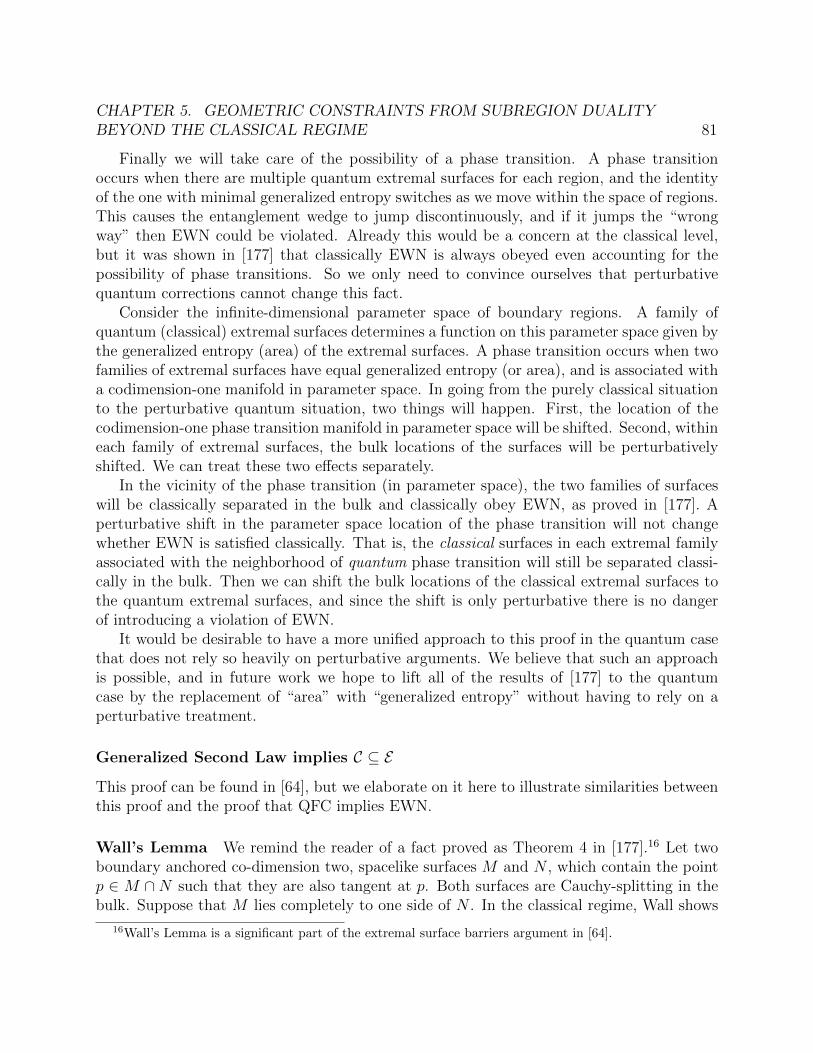
CHAPTER 5. GEOMETRIC CONSTRAINTS FROM SUBREGION DUALITYBEYOND THE CLASSICAL REGIME 81
Finally we will take care of the possibility of a phase transition. A phase transitionoccurs when there are multiple quantum extremal surfaces for each region, and the identityof the one with minimal generalized entropy switches as we move within the space of regions.This causes the entanglement wedge to jump discontinuously, and if it jumps the “wrongway” then EWN could be violated. Already this would be a concern at the classical level,but it was shown in [177] that classically EWN is always obeyed even accounting for thepossibility of phase transitions. So we only need to convince ourselves that perturbativequantum corrections cannot change this fact.
Consider the infinite-dimensional parameter space of boundary regions. A family ofquantum (classical) extremal surfaces determines a function on this parameter space given bythe generalized entropy (area) of the extremal surfaces. A phase transition occurs when twofamilies of extremal surfaces have equal generalized entropy (or area), and is associated witha codimension-one manifold in parameter space. In going from the purely classical situationto the perturbative quantum situation, two things will happen. First, the location of thecodimension-one phase transition manifold in parameter space will be shifted. Second, withineach family of extremal surfaces, the bulk locations of the surfaces will be perturbativelyshifted. We can treat these two effects separately.
In the vicinity of the phase transition (in parameter space), the two families of surfaceswill be classically separated in the bulk and classically obey EWN, as proved in [177]. Aperturbative shift in the parameter space location of the phase transition will not changewhether EWN is satisfied classically. That is, the classical surfaces in each extremal familyassociated with the neighborhood of quantum phase transition will still be separated classi-cally in the bulk. Then we can shift the bulk locations of the classical extremal surfaces tothe quantum extremal surfaces, and since the shift is only perturbative there is no dangerof introducing a violation of EWN.
It would be desirable to have a more unified approach to this proof in the quantum casethat does not rely so heavily on perturbative arguments. We believe that such an approachis possible, and in future work we hope to lift all of the results of [177] to the quantumcase by the replacement of “area” with “generalized entropy” without having to rely on aperturbative treatment.
Generalized Second Law implies C ⊆ EThis proof can be found in [64], but we elaborate on it here to illustrate similarities betweenthis proof and the proof that QFC implies EWN.
Wall’s Lemma We remind the reader of a fact proved as Theorem 4 in [177].16 Let twoboundary anchored co-dimension two, spacelike surfaces M and N , which contain the pointp ∈ M ∩N such that they are also tangent at p. Both surfaces are Cauchy-splitting in thebulk. Suppose that M lies completely to one side of N . In the classical regime, Wall shows
16Wall’s Lemma is a significant part of the extremal surface barriers argument in [64].
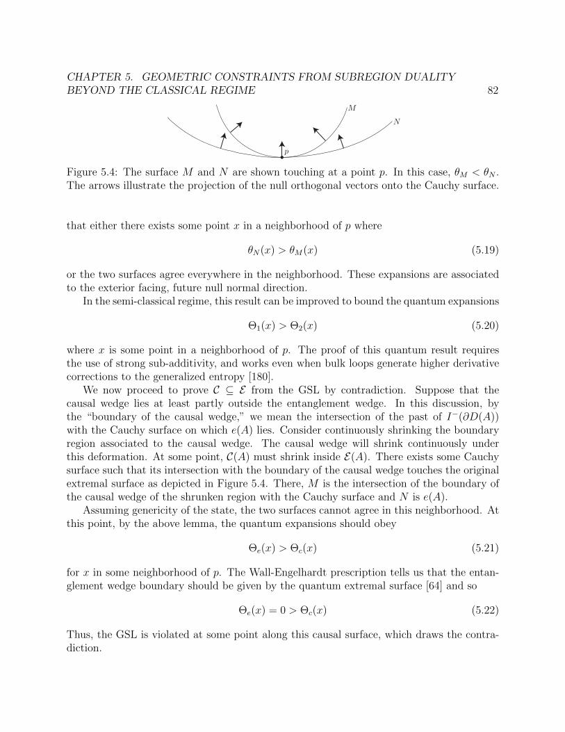
CHAPTER 5. GEOMETRIC CONSTRAINTS FROM SUBREGION DUALITYBEYOND THE CLASSICAL REGIME 82
Figure 5.4: The surface M and N are shown touching at a point p. In this case, θM < θN .The arrows illustrate the projection of the null orthogonal vectors onto the Cauchy surface.
that either there exists some point x in a neighborhood of p where
θN(x) > θM(x) (5.19)
or the two surfaces agree everywhere in the neighborhood. These expansions are associatedto the exterior facing, future null normal direction.
In the semi-classical regime, this result can be improved to bound the quantum expansions
Θ1(x) > Θ2(x) (5.20)
where x is some point in a neighborhood of p. The proof of this quantum result requiresthe use of strong sub-additivity, and works even when bulk loops generate higher derivativecorrections to the generalized entropy [180].
We now proceed to prove C ⊆ E from the GSL by contradiction. Suppose that thecausal wedge lies at least partly outside the entanglement wedge. In this discussion, bythe “boundary of the causal wedge,” we mean the intersection of the past of I−(∂D(A))with the Cauchy surface on which e(A) lies. Consider continuously shrinking the boundaryregion associated to the causal wedge. The causal wedge will shrink continuously underthis deformation. At some point, C(A) must shrink inside E(A). There exists some Cauchysurface such that its intersection with the boundary of the causal wedge touches the originalextremal surface as depicted in Figure 5.4. There, M is the intersection of the boundary ofthe causal wedge of the shrunken region with the Cauchy surface and N is e(A).
Assuming genericity of the state, the two surfaces cannot agree in this neighborhood. Atthis point, by the above lemma, the quantum expansions should obey
Θe(x) > Θc(x) (5.21)
for x in some neighborhood of p. The Wall-Engelhardt prescription tells us that the entan-glement wedge boundary should be given by the quantum extremal surface [64] and so
Θe(x) = 0 > Θc(x) (5.22)
Thus, the GSL is violated at some point along this causal surface, which draws the contra-diction.

CHAPTER 5. GEOMETRIC CONSTRAINTS FROM SUBREGION DUALITYBEYOND THE CLASSICAL REGIME 83
AANEC implies Boundary Causality Condition
The Gao-Wald:1984rg proof of the BCC [84] uses the fact — which follows from their as-sumptions of the NEC and null generic condition (discussed below) — that all complete nullgeodesics through the bulk contain a pair of conjugate points.17 Here, we sketch a slightmodification of the proof which instead assumes the achronal averaged null energy condition(AANEC).
We prove that the AANEC implies BCC by contradiction. Let the spacetime satisfy thenull generic condition [172], so that each null geodesic encounters at least some matter orgravitational radiation.18 Violation of the BCC implies that the ”fastest” null geodesic γbetween two boundary points p and q lies in the bulk. Such a null geodesic is necessarilycomplete and achronal, as p and q are not timelike related. As explained in Sec. 5.3, anachronal null geodesic in an AANEC satisfying spacetime is contained in a congruence thatis both a past and future causal horizon. Integrating Raychaudhuri’s equation along theentire geodesic then gives 0 ≤ −
∫(θ2 + σ2), which implies θ = σ = 0 everywhere along the
geodesic, and hence θ′ = 0. Raychaudhuri’s equation then says θ′ = −Tkk = 0 everywhere,which contradicts the generic condition.
Geometric Constraints Imply Field Theory Constraints
The geometrical constraints EWN, C ⊆ E , and BCC have non-trivial implications for theboundary theory. We derive them in this section, which proves the three implications con-necting columns two and three of Fig. 5.1. The key idea behind all three proofs is the same:express the geometrical constraints in terms of bulk quantities near the asymptotic bound-ary, and then use near-boundary expansions of the metric and extremal surfaces to convertthem into field theory statements.
Entanglement Wedge Nesting implies the Boundary QNEC
At leading order in G~ ∼ 1/N , this proof is the central result of [115]. There the boundaryentropy was assumed to be given by the RT formula without the bulk entropy corrections.We give a proof here of how the 1/N corrections can be incorporated naturally. We will nowshow, in a manner exactly analogous to that laid out in [115], that EWN implies the boundaryQNEC. In what follows, we will notice that in order to recover the boundary QNEC, we mustuse the quantum extremal surface, not just the RT surface with FLM corrections [64].
The quantum extremal surface (QES) prescription, as first introduced in [64], is thefollowing. To find the entropy of a region A in the boundary theory, first find the minimalcodimension-2 bulk surface homologous to A, e(A), that extremizes the bulk generalized
17Intuitively speaking, points p and q along a geodesic γ are conjugate if an infinitesimally nearby geodesicintersects γ at both p and q. This can be shown to be equivalent to the statement that the expansion of acongruence through p approaches −∞ at q. See e.g. [172] for details.
18Mathematically, each complete null geodesic should contain a point where kakbk[cRd]ab[ekf ] 6= 0.

CHAPTER 5. GEOMETRIC CONSTRAINTS FROM SUBREGION DUALITYBEYOND THE CLASSICAL REGIME 84
entropy on the side of A. The entropy of A is then given by
SA = Sgen(e(A)) =AQES
4G~+ Sbulk (5.23)
Entanglement Wedge Nesting then becomes a statement about how the quantum extremalsurface moves under deformations of the boundary region. In particular, for null deformationsof the boundary region, EWN states that e(A) moves in a spacelike (or null) fashion.
To state this more precisely, we can set up a null orthogonal basis about e(A). Let kµ bethe inward-facing, future null orthogonal vector along the quantum extremal surface. Let `µ
be its past facing partner with ` · k = 1. Following the prescrition in [115], we denote thelocally orthogonal deviation vector of the quantum extremal surface by sµ. This vector canbe expanded in the local null basis as
s = αk + β` (5.24)
The statement of entanglement wedge nesting then just becomes the statement that β ≥ 0.In order to find how β relates to the boundary QNEC, we would like to find its relation
to the entropy. We start by examining the expansion of the extremal surface solution inFefferman-Graham coordinates. Note that the quantum extremal surface obeys an equationof motion including the bulk entropy term as a source
Kµ = −4G~√H
δSbulk
δXµ(5.25)
Here, Kµ = θk`µ+θ`k
µ is the extrinsic curvature of the QES. As discussed in [115], solutionsto (5.25) without the bulk source take the form
X iHRT (ya, z) = X i(ya) +
1
2(d− 2)z2Ki(ya) + ...+
zd
d(V i(ya) +W i(ya) log z) + o(zd) (5.26)
We now claim that the terms lower order than zd are unaffected by the presence of thesource. More precisely
X iQES(ya, z) = X i(ya) +
1
2(d− 2)z2Ki(ya) + ...+
zd
d(V i
QES +W i(ya) log z) + o(zd) (5.27)
This expansion is found by examining the leading order pieces of the extremal surfaceequation. First, expand (5.25) to derive
zd−1∂z
(z1−df
√hhzz∂zX
i)
+ ∂a
(√habh
abf∂bXi)
= −zd−14G~fδSbulkδXj
gji (5.28)
Here we are parameterizing the near-boundary AdS metric in Fefferman-Graham coordinatesby
ds2 =1
z2
(dz2 + gijdx
idxj)
(5.29)
=1
z2
(dz2 +
[f(z)ηij +
16πGN
dzdtij
]dxidxj + o(zd)
). (5.30)

CHAPTER 5. GEOMETRIC CONSTRAINTS FROM SUBREGION DUALITYBEYOND THE CLASSICAL REGIME 85
The function f(z) encodes the possibility of relevant deformations in the field theory whichwould cause the vacuum state to differ from pure AdS. Here we have set LAdS = 1.
One then plugs in (5.27) to (5.28) to see that the terms lower order than zd remainunaffected by the presence of the bulk entropy source as long as δSbulk/δX
i remains finiteat z = 0. We discuss the plausibility of this boundary condition at the end of this section.
For null deformations to locally stationary surfaces on the boundary, one can show using(5.27) that the leading order piece of β in the Fefferman-Graham expansion is order zd−2.Writing the coordinates of the boundary entangling surface as a function of some deformationparameter - X i(λ) - we find that [115],
β ∝ zd−2
(Tkk +
1
8πGN
ki∂λVi
QES
). (5.31)
We will now show that V iQES is proportional to the variation in Sgen at all orders in 1/N ,
as long as one uses the quantum extremal surface and assumes mild conditions on derivativesof the bulk entropy. The key will be to leverage the fact that Sgen is extremized on the QES.Thus, its variation will come from pure boundary terms. At leading order in z, we willidentify these boundary terms with the vector VQES.
We start by varying the generalized entropy with respect to a boundary deformation
δSgen =
∫
QES
δSgenδX i
δX idzdd−2y −∫
z=ε
(∂Sgen
∂(∂zX i)+ ...
)δX idd−2y (5.32)
where the boundary term comes from integrating by parts when deriving the Euler-Lagrangeequations for the functional Sgen[X]. The ellipsis denotes terms involving derivatives of Sgen
with respect to higher derivatives of the embedding functions (∂Sgen/∂(∂2X), . . .) Theseboundary terms will include two types of terms: one involving derivatives of the surface areaand one involving derivatives of the bulk entropy.
The first area term was already calculated in [115]. There it was found that
∂A
∂(∂zX i)= − 1
zd−1
∫dd−2y
√h
gij∂zXi
√1 + glm∂zX l∂zXm
δXj|z=ε (5.33)
One can use (5.27) to expand this equation in powers ε, and then contract with the nullvector k on the boundary in order to isolate the variation with respect to null deformations.For boundary surfaces which are locally stationary at some point y, one finds that all termslower order than zd vanish at y. In fact, it was shown in [115] that the right hand side of(5.33), after contracting with ki, is just kiVi at first non-vanishing order. Finally, we assumethat that all such derivatives of the bulk entropy in (5.32) vanish as z → 0. This is similar tothe reasonable assumption that entropy variations vanish at infinity, which should be true ina state with finite bulk entropy. It would be interesting to classify the pathologies of stateswhich violate this assumption. Thus, the final result is that
kiV QESi = − 1√
hkiδSgen
δX i. (5.34)
CHAPTER 5. GEOMETRIC CONSTRAINTS FROM SUBREGION DUALITYBEYOND THE CLASSICAL REGIME 86
The quantum extremal surface prescription says that the boundary field theory entropyis equal to the generalized entropy of the QES [64]. Setting Sgen = Sbdry in (5.34) andcombining that with (5.31) shows that the condition β ≥ 0 is equivalent to the QNEC. SinceEWN guarantees that β ≥ 0, the proof is complete.
We briefly comment about the assumptions used to derive (5.34). The bulk entropyshould - for generic states - not depend on the precise form of the region near the boundary.The intuition is clear in the thermodynamic limit where bulk entropy is extensive. As longas we assume strong enough fall-off conditions on bulk matter, the change in the entropywill have to vanish as z → 0.
Note here the importance of using the quantum extremal surface. Had we naively con-tinued to use the extremal area prescription, but still assumed SA = Sbulk(e(A)) + A
4G~ , wewould have discovered a correction to the boundary QNEC from the bulk entropy. Thevariation of the bulk extremal surface area would be given by a pure boundary term, butthe QNEC would take the erroneous form
Tkk ≥1
2π√h
(S ′′A − S ′′bulk(e(A))) . (5.35)
In other words, if one wants to preserve the logical connections put forth in Figure 5.1 whileaccounting for 1/N corrections, the use of quantum extremal surfaces is necessary.
We discuss the effects of higher derivative terms in the gravitational action coming fromloop corrections at the end of this section.
C ⊆ E implies the QHANEC
We now examine the boundary implication of C ⊆ E . As before, this proof will hold to allorders in G~, again assuming proper fall-off conditions on derivatives of the bulk entropy.
The basic idea will be to realize that general states in AdS/CFT can be treated asperturbations to the vacuum in the limit of small z. Again, we will consider the general casewhere the boundary field theory includes relevant deformations. Then, near the boundary,the metric can be written
ds2 =1
z2
(dz2 +
[f(z)ηij +
16πGN
dzdtij
]dxidxj + o(zd)
), (5.36)
where f(z) encodes the effects of the relevant deformations. In this proof we take theviewpoint that the order zd piece of this expansion is a perturbation on top of the vacuum.In other words
gab = gvacab + δgab. (5.37)
Of course, this statement is highly coordinate dependent. In the following calculations, wetreat the metric as a field on top of fixed coordinates. We will have to verify the gauge-independence of the final result, and do so below.
For this proof we are interested in regions A of the boundary such that ∂A is a cut ofa null plane. In null coordinates, that would look like ∂A = (u = U0(y), v = 0). These

CHAPTER 5. GEOMETRIC CONSTRAINTS FROM SUBREGION DUALITYBEYOND THE CLASSICAL REGIME 87
regions are special because in the vacuum state e(A) lies on the past causal horizon generatedby bulk geodesics coming from (u =∞, v = 0). This can be shown using Lorentz symmetryas follows:
An arbitrary cut of a null plane can be deformed back to a flat cut by action with aninfinite boost (since boosts act by rescalings of u and v). Such a transformation preservesthe vacuum, and so the bulk geometry possesses an associated Killing vector. The pastcausal horizon from (u = ∞, v = 0) is a Killing horizon for this boost, and by symmetrythe quantum extremal surface associated to the flat cut will be the bifurcation surface ofthe Killing horizon. Had e(A) for the arbitrary cut left the horizon, then it would have beentaken off to infinity by the boost and not ended up on the bifurcation surface.19
We can construct an orthogonal null coordinate system around e(A) in the vacuum. Wedenote the null orthogonal vectors by k and ` where kz = 0 = `z and kx = kt = 1 so thatk · ` = 1. Then the statement of C ⊆ E becomes20
k · (η − XSD) ≥ 0 (5.38)
Here we use η, XSD to denote the perturbation of the causal horizon and quantum extremalsurface from their vacuum position, respectively. The notation of XSD is used to denote thestate-dependent piece of the embedding functions for the extremal surface. Over-bars willdenote bulk embedding functions of e(A) surface and Xa will denote boundary coordinates.The set up is illustrated in Figure 5.5.
Just as in the previous section, for a locally stationary surface (such as a cut of a nullplane), one can write the embedding coordinates of e(A), X, as an expansion in z [115]:
X i(ya, z) = X i(ya) +1
2(d− 2)z2Ki(ya) + ...+
zd
d(V i +W i(ya) log z) + o(zd) (5.39)
where V i is some local “velocity” function that denotes the rate at which the entanglingsurface diverges from its boundary position and represents the leading term in the state-dependent part of the embedding functions. The state-independent terms of lower order inz are all proportional to ki. In vacuum, we also have V i ∝ ki, and so for non-vacuum statesk · XSD = 1
dV · kzd + o(zd).
19It is also worth noting that EWN together with C ⊆ E can also be used to construct an argument.Suppose we start with a flat cut of a null plane, for which e(A) is also a flat cut of a null plane in thevacuum (the bifurcation surface for the boost Killing horizon). We then deform this cut on the boundary toan arbitrary cut of the null plane in its future. In the bulk, EWN states that e(A) would have to move in aspace-like or null fashion, but if it moves in a space-like way, then C ⊆ E is violated.
20The issue of gauge invariance for this proof should not be overlooked. On their own, each term in (5.38)is not gauge invariant under a general diffeomorphism. The sum of the two, on the other hand, does nottransform under coordinate change:
gµν → gµν +∇(µξν)
Plugging this into the formula for k · η shows that δ(k · η) = −(k · ξ), which is precisely the same as thechange in position of the extremal surface δ(k · XSD) = −(k · ξ).

CHAPTER 5. GEOMETRIC CONSTRAINTS FROM SUBREGION DUALITYBEYOND THE CLASSICAL REGIME 88
Figure 5.5: This picture shows the various vectors defined in the proof. It depicts a cross-section of the extremal surface at constant z. e(A)vac denotes the extremal surface in thevacuum. For flat cuts of a null plane on the boundary, they agree. For wiggly cuts, they willdiffer by some multiple of ki.
Equation (5.34) tells us that XSD is proportional to boundary variations of the CFTentropy. Thus, equation (5.39) together with (5.34) tells us the simple result that
k · XSD = −4GN
d√hS ′Az
d−2. (5.40)
Now we explore the η deformation, where η is the vector denoting the shift in the positionof the causal horizon. This discussion follows much of the formalism found in [63]. At aspecific value of (z, y), the null generator of the causal surface, k′, is related to the vacuumvector k by
k′ = k + δk = k + ka∇aη (5.41)
In the perturbed metric, k′ must be null to leading order in η = O(zd). Imposing thiscondition we find that
kb∇b(η · k) = −1
2δgabk
akb (5.42)
Here δgab is simply the differece between the excited state metric and the vacuum metric,which can be treated as a perturbation since we are in the near-boudnary limit. This equationcan be integrated back along the original null geodesic, with the boundary condition imposedthat η(∞) = 0. Thus, we find the simple relation
(k · η)(λ) =1
2
∫ ∞
λ
δgkk dλ. (5.43)
The holographic dictionary tells us how to relate δgkk to boundary quantities. Namely,to leading order in z, the expression above can be recast in terms of the CFT stress tensor
k · η =1
2
∫ ∞
λ
16πGN
dzd−2Tkk dλ. (5.44)
CHAPTER 5. GEOMETRIC CONSTRAINTS FROM SUBREGION DUALITYBEYOND THE CLASSICAL REGIME 89
Plugging all of this back in to (5.38), we finally arrive at the basic inequality
∫ ∞
λ
Tkk dλ+~
2π√hS ′A ≥ 0. (5.45)
Note that all the factors ofGN have dropped out and we have obtained a purely field-theoreticQHANEC.
Loop corrections Here we will briefly comment on how bulk loop corrections affect theargument. Quantum effects do not just require that we add Sout to A; higher derivativeterms suppressed by the Planck-scale will be generated in the gravitational action which willmodify the gravitational entropy functional. With Planck-scale suppressed higher derivativecorrections, derivatives of the boundary entropy of a region have the form
S ′ =A′
4G~+Q′ + S ′out (5.46)
where Q′ are the corrections which start at O((G~)0). The key point is that Q′ is alwaysone order behind A′ in the G~ perturbation theory. As G~ → 0, Q′ can only possibly berelevant in situations where A′ = 0 at O((G~)0). In this case, V i ∼ ki, and the bulk quantumextremal surface in the vacuum state is a cut of a bulk Killing horizon. But then Q′ mustbe at least O(G~), since Q′ = 0 on a Killing horizon for any higher derivative theory. Thuswe find Eq. (5.34) is unchanged at the leading nontrivial order in G~.
Higher derivative terms in the bulk action will also modify the definition of the boundarystress tensor. The appearance of the stress tensor in the QNEC and QHANEC proofscomes from the fact that it appears at O(zd) in the near-boundary expansion of the bulkmetric [115]. Higher derivative terms will modify the coefficient of Tij in this expansion, andtherefore in the QNEC and QHANEC. (They will not affect the structure of lower-orderterms in the asymptotic metric expansion because there aren’t any tensors of appropriateweight besides the flat metric ηij [115]). But the new coefficient will differ from the one inEinstein gravity by the addition of terms containing the higher derivative couplings, whichare 1/N -suppressed relative to the Einstein gravity term, and will thus only contribute tothe sub-leading parts of the QNEC and QHANEC. Thus the validity of the inequalities atsmall G~ is unaffected.
Boundary Causality Condition implies the AANEC
The proof of this statement was first described in [112]. We direct interested readers tothat paper for more detail. Here we will sketch the proof and note some similarities to theprevious two subsections.
As discussed above, the BCC states that no bulk null curve can connect boundary pointsthat are not connected by a boundary causal curve. In the same way that we took a boundarylimit of C ⊆ E to prove the QHANEC, the strategy here is to look at nearly null time-like

CHAPTER 5. GEOMETRIC CONSTRAINTS FROM SUBREGION DUALITYBEYOND THE CLASSICAL REGIME 90
curves that hug the boundary. These curves will come asymptotically close to beating theboundary null geodesic and so in some sense derive the most stringent condition on thegeometry.
Expanding the near boundary metric in powers of z, we use holographic renormalizationto identify pieces of the metric as the stress tensor
gµνdxµdxν =
dz2 + ηijdxidxj + zdγij(z, x
i)dxidxj
z2(5.47)
where γij(0, xi) = 16πGN
d〈Tij〉. Using null coordinates on the boundary, we can parameterize
the example bulk curve by u 7→ (u, V (u), Z(u), yi = 0). One constructs a nearly null, time-like curve that starts and ends on the boundary and imposes time delay. If Z(−L) = Z(L) =0, then the BCC enforces that V (L)− V (−L) ≥ 0. For the curve used in [112], the L→∞limit turns this inequality directly into the boundary AANEC.
5.5 Discussion
We have identified two constraints on the bulk geometry, entanglement wedge nesting (EWN)and the C ⊆ E , coming directly from the consistency of subregion duality and entanglementwedge reconstruction. The former implies the latter, and the latter implies the boundarycausality condition (BCC). Additionally, EWN can be understood as a consequence of thequantum focussing conjecture, and C ⊆ E follows from the generalized second law. Bothstatements in turn have implications for the strongly-coupled large-N theory living on theboundary: the QNEC and QHANEC, respectively. In this section, we list possible general-izations and extensions to this work.
Unsuppressed higher derivative corrections There is no guarantee that higher deriva-tive terms with un-suppressed coefficients are consistent with our conclusions. In fact, in[39] it was observed that Gauss-Bonnett gravity in AdS with an intermediate-scale couplingviolates the BCC, and this fact was used to place constraints on the theory. We have seenthat the geometrical conditions EWN and C ⊆ E are fundamental to the proper functioningof the bulk/boundary duality. If it turns out that a higher derivative theory invalidates someof our conclusions, it seems more likely that this would be point to a particular pathologyof that theory rather than an inconsistency of our results. It would be interesting if EWNand C ⊆ E could be used to place constraints on higher derivative couplings, in the spirit of[39]. We leave this interesting possibility to future work.
A further constraint from subregion duality Entanglement wedge reconstruction im-plies an additional property that we have not mentioned. Given two boundary regions Aand B that are spacelike separated, E(A) is spacelike separated from E(B). This propertyis actually equivalent to EWN for pure states, but is a separate statement for mixed states.

CHAPTER 5. GEOMETRIC CONSTRAINTS FROM SUBREGION DUALITYBEYOND THE CLASSICAL REGIME 91
In the latter case, it would be interesting to explore the logical relationships of this propertyto the constraints in Fig. 5.1.
Beyond AdS In this paper we have only discussed holography in asymptotically AdSspacetimes. While the QFC, QNEC, and GSL make no reference to asymptotically AdSspacetimes, EWN and C ⊆ E currently only have meaning in this context. One couldimagine however that a holographic correspondence with subregion duality makes sense inmore general spacetimes — perhaps formulated in terms of a “theory” living on a holographicscreen [25, 28, 29]. In this case, we expect analogues of EWN and C ⊆ E . For some initialsteps in this direction, see [155].
Quantum generalizations of other bulk facts from generalized entropy A keylesson of this paper is that classical results in AdS/CFT relying on the null energy condition(NEC) can often be made semiclassical by appealing to powerful properties of the generalizedentropy: the quantum focussing conjecture and the generalized second law. We expect thisto be more general than the semiclassical proofs of EWN and C ⊆ E presented here. Indeed,Wall has shown that the generalized second law implies semiclassical generalizations of manycelebrated results in classical general relativity, including the singularity theorem [180]. Itwould be illuminating to see how general this pattern is, both in and out of AdS/CFT. Asan example, it is known that strong subadditivity of holographic entanglement entropy canbe violated in spacetimes which don’t obey the NEC [37]. It seems likely that the QFC canbe used to derive strong subadditivity in cases where the NEC is violated due to quantumeffects in the bulk.
Gravitational inequalities from field theory inequalities We have seen that thebulk QFC and GSL, which are semi-classical quantum gravity inequalities, imply their non-gravitational limits on the boundary, the QNEC and QHANEC. But we can regard thebulk as an effective field theory of perturbative quantum gravity coupled to matter, andcan consider the QNEC and QHANEC for the bulk matter sector. At least when includinglinearized backreaction of fields quantized on top of a Killing horizon, the QHANEC impliesthe GSL [174], and the QNEC implies the QFC [34]. In some sense, this “completes” thelogical relations of Fig. 5.1.
Support for the quantum extremal surfaces conjecture The logical structure un-covered in this paper relies heavily on the conjecture that the entanglement wedge should bedefined in terms of the surface which extremizes the generalized entropy to one side [64] (asopposed to the area). Perhaps similar arguments could be used to prove this conjecture, orat least find an explicit example where extremizing the area is inconsistent with subregionduality, as in [83].
CHAPTER 5. GEOMETRIC CONSTRAINTS FROM SUBREGION DUALITYBEYOND THE CLASSICAL REGIME 92
Connections to Recent Proofs of the AANEC Recent proofs of the AANEC haveilluminated the origin of this statement within field theory [71, 90]. In one proof, the engineof the inequality came from microcausality and reflection positivity. In the other, the proofrelied on montonoicity of relative entropy for half spaces. A natural next question would behow these two proofs are related, if at all. Our paper seems to offer at least a partial answerfor holographic CFTs. Both the monotonicity of relative entropy and microcausality - inour case the QHANEC and BCC, respectively - are implied by the same thing in the bulk:C ⊆ E . In 5.2, we gave a motivation for this geometric constraint from subregion duality. Itwould be interesting to see how the statement of C ⊆ E in a purely field theoretic languageis connected to both the QHANEC and causality.
93
Chapter 6
Local Modular Hamiltonians from theQuantum Null Energy Condition
6.1 Introduction and Summary
The reduced density operator ρ for a region in quantum field theory encodes all of theinformation about observables localized to that region. Given any ρ, one can define themodular Hamiltonian K by
ρ = e−K . (6.1)
Knowledge of this operator is equivalent to knowledge of ρ, but the modular Hamiltonianfrequently appears in calculations involving entanglement entropy. In general, i.e. for arbi-trary states reduced to arbitrary regions, K is a complicated non-local operator. However,in certain cases it is known to simplify.
The most basic example where K simplifies is the vacuum state of a QFT in Rindlerspace, i.e. the half-space t = 0, x ≥ 0. The Bisognano–Wichmann theorem [20] states thatin this case the modular Hamiltonian is
∆K =2π
~
∫dd−2y
∫ ∞
0
xTtt dx (6.2)
where ∆K ≡ K − 〈K〉vac defines the vacuum-subtracted modular Hamiltonian, and y ared − 2 coordinates parametrizing the transverse directions. The vacuum subtraction gen-erally removes regulator-dependent UV-divergences in K. Other cases where the modularHamiltonian is known to simplify to an integral of local operators are obtained via conformaltransformation of Eq. (6.2), including spherical regions in CFTs [48], regions in a thermalstate of 1+1 CFTs [43], and null slabs [32, 32].
Using conservation of the energy-momentum tensor, one can easily re-express the Rindlermodular Hamiltonian in Eq. (6.2) as an integral over the future Rindler horizon u ≡ t−x = 0
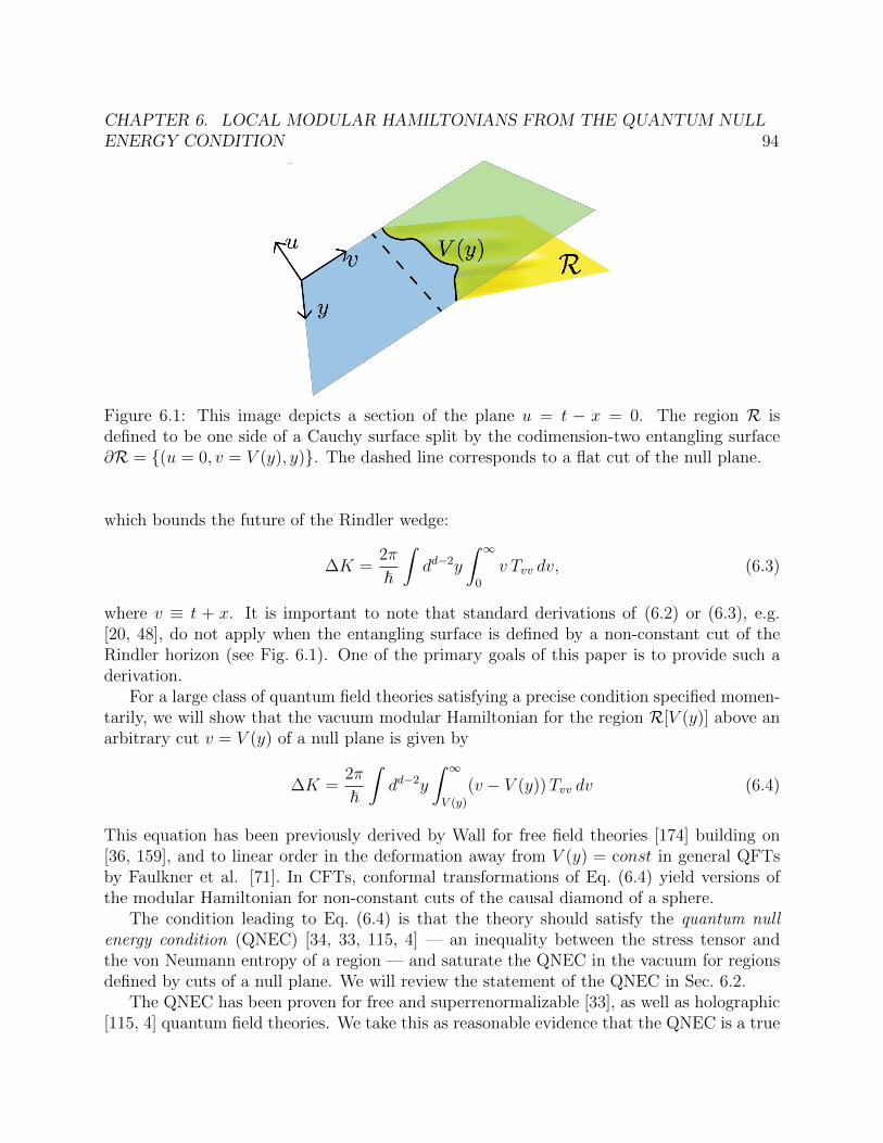
CHAPTER 6. LOCAL MODULAR HAMILTONIANS FROM THE QUANTUM NULLENERGY CONDITION 94
Figure 6.1: This image depicts a section of the plane u = t − x = 0. The region R isdefined to be one side of a Cauchy surface split by the codimension-two entangling surface∂R = (u = 0, v = V (y), y). The dashed line corresponds to a flat cut of the null plane.
which bounds the future of the Rindler wedge:
∆K =2π
~
∫dd−2y
∫ ∞
0
v Tvv dv, (6.3)
where v ≡ t + x. It is important to note that standard derivations of (6.2) or (6.3), e.g.[20, 48], do not apply when the entangling surface is defined by a non-constant cut of theRindler horizon (see Fig. 6.1). One of the primary goals of this paper is to provide such aderivation.
For a large class of quantum field theories satisfying a precise condition specified momen-tarily, we will show that the vacuum modular Hamiltonian for the region R[V (y)] above anarbitrary cut v = V (y) of a null plane is given by
∆K =2π
~
∫dd−2y
∫ ∞
V (y)
(v − V (y))Tvv dv (6.4)
This equation has been previously derived by Wall for free field theories [174] building on[36, 159], and to linear order in the deformation away from V (y) = const in general QFTsby Faulkner et al. [71]. In CFTs, conformal transformations of Eq. (6.4) yield versions ofthe modular Hamiltonian for non-constant cuts of the causal diamond of a sphere.
The condition leading to Eq. (6.4) is that the theory should satisfy the quantum nullenergy condition (QNEC) [34, 33, 115, 4] — an inequality between the stress tensor andthe von Neumann entropy of a region — and saturate the QNEC in the vacuum for regionsdefined by cuts of a null plane. We will review the statement of the QNEC in Sec. 6.2.
The QNEC has been proven for free and superrenormalizable [33], as well as holographic[115, 4] quantum field theories. We take this as reasonable evidence that the QNEC is a true

CHAPTER 6. LOCAL MODULAR HAMILTONIANS FROM THE QUANTUM NULLENERGY CONDITION 95
fact about relativistic quantum field theories in general, and for the purposes of this papertake it as an assumption. In Sec. 6.2 we will show how saturation of the QNEC in a givenstate leads to an operator equality relating certain derivatives of the modular Hamiltonian ofthat state to the energy-momentum tensor. Applied to the case outlined above, this operatorequality will be integrated to give Eq. (6.4).
Given the argument in Sec. 6.2, the only remaining question is whether the QNEC is infact saturated in the vacuum state for entangling surfaces which are cuts of a null plane.This has been shown for free theories in [33]. In Sec. 6.3, we prove that this is the casefor holographic theories to all orders in 1/N . We emphasize that Eq. (6.4) holds purely asa consequence of the validity of the QNEC and the saturation in the vacuum for R, twofacts which are potentially true in quantum field theories much more generally than free andholographic theories.
Finally, in Sec. 6.4 we will conclude with a discussion of possible extensions to curvedbackgrounds and more general regions, connections between the relative entropy and theQNEC, and relations to other work.
6.2 Main Argument
Review of QNEC
The von Neumann entropy of a region in quantum field theory can be regarded as a functionalof the entangling surface. We will primarily be interested in regions to one side of a cut ofa null plane in flat space, for which the entangling surface can be specified by a functionV (y) which indicates the v-coordinate of the cut as a function of the transverse coordinates,collectively denoted y. See Fig. 6.1 for the basic setup. Each cut V (y) defines a half-space,namely the region to one side of the cut. We will pick the side towards the future of the nullplane. For the purposes of this section we are free to consider the more general situationwhere the entangling surface is only locally given by a cut of a null plane. Thus the vonNeumann entropy can be considered as a functional of a profile V (y) which defines the shapeof the entangling surface, at least locally.
Suppose we define a one-parameter family of cuts V (y;λ) ≡ V (y; 0)+λV (y), with V (y) >0 to ensure that R(λ1) ⊂ R(λ2) if λ1 > λ2. If S(λ) is the entropy of region R(λ), then theQNEC in integrated form states that
∫dd−2y 〈Tvv(y)〉 V (y)2 ≥ ~
2π
d2S
dλ2. (6.5)
In general there would be a√h induced metric factor weighting the integral, but here and
in the rest of the paper we will assume that the y coordinates have been chosen such that√h = 1.
By taking advantage of the arbitrariness of V (y) we can derive from this the local formof the QNEC. If we take a limit where V (y′)2 → δ(y − y′), then the l.h.s. reduces to 〈Tvv〉.
CHAPTER 6. LOCAL MODULAR HAMILTONIANS FROM THE QUANTUM NULLENERGY CONDITION 96
We define S ′′(y) as the limit of d2S/dλ2 in the same situation:
d2S
dλ2→ S ′′(y) when V (y′)2 → δ(y − y′). (6.6)
Taking the limit of the nonlocal QNEC then gives the local one:
〈Tvv〉 ≥~2πS ′′. (6.7)
The local QNEC together with strong subadditivity can likewise be used to go backwardand derive the nonlocal QNEC [34, 33, 115]. The details of that argument are not importanthere. In the next section we will discuss the consequences of the saturation of the QNEC,and will have to distinguish whether we mean saturation of the nonlocal inequality Eq. (6.5)or the local inequality Eq. (6.7), the latter condition being weaker.
The QNEC under state perturbations
In this section we consider how the QNEC behaves under small deformations of the state.We begin with a reference state σ and consider the deformed state ρ = σ + δρ, with δρtraceless but otherwise arbitrary.
Consider a one-parameter family of regions R(λ) as in the previous section. Define R(λ)to be the complement of R(λ) within a Cauchy surface. The reduced density operator forany given region R(λ) given by
ρ(λ) = σ(λ) + δρ(λ) = TrR(λ)σ + TrR(λ)δρ. (6.8)
By the First Law of entanglement entropy, the entropy of ρ(λ) is given by
S(ρ(λ)) = S(σ(λ))− TrR(λ)δρ(λ) log σ(λ) + o(δρ2). (6.9)
The second term can be written in a more useful way be defining the modular HamiltonianKσ(λ) as
Kσ(λ) ≡ −1R(λ) ⊗ log σ(λ). (6.10)
Defining Kσ(λ) this way makes it a global operator, which makes taking derivatives withrespect to λ formally simpler. Using this definition, we can write Eq. (6.9) as
S(ρ(λ)) = S(σ(λ)) + Tr δρKσ(λ) + o(δρ2). (6.11)
Now in the second term the trace is over the global Hilbert space, and the λ-dependence hasbeen isolated to the operator Kσ(λ). Taking two derivatives, and simplifying the notationslightly, we find
d2S
dλ2(ρ) =
d2S
dλ2(σ) + Tr δρ
d2Kσ
dλ2+ o(δρ2). (6.12)
CHAPTER 6. LOCAL MODULAR HAMILTONIANS FROM THE QUANTUM NULLENERGY CONDITION 97
Suppose that the nonlocal QNEC, Eq. (6.5), is saturated in the state σ for all profilesV (y). Then, using Eq. (6.12), the nonlocal QNEC for the state ρ can be written as
∫dd−2y (Tr δρ Tvv) V
2 ≥ ~2π
Tr δρd2Kσ
dλ2+ o(δρ2). (6.13)
The operator δρ was arbitrary, and in particular could be replaced by −δρ. Then the onlyway that Eq. 6.13 can hold is if we have the operator equality
d2Kσ
dλ2= C +
2π
~
∫dd−2y TvvV
2. (6.14)
Here C is a number that we cannot fix using this method that is present because of thetracelessness of δρ.
Eq. (6.14) can be integrated to derive the full modular Hamiltonian Kσ if we have ap-propriate boundary conditions. Up until now we have only made use of local properties ofthe entangling surface, but in order to provide boundary conditions for the integration ofEq. (6.14) we will assume that the entangling surface is globally given by a cut of a nullplane, and that V (y;λ = 0) = 0. We will also make σ the vacuum state. In that situation itis known that the QNEC is saturated for free theories, and in the next section we will showthat this is also true for holographic theories at all orders in the large-N expansion.
Our first boundary condition is at λ = ∞.1 Since we expect that Kσ(λ) should have afinite expectation value in any state as λ → ∞, it must be that dKσ/dλ → 0 as λ → ∞.Then integrating Eq. (6.14) gives
dKσ
dλ= −2π
~
∫dd−2y
∫ ∞
V (y;λ)
dv TvvV . (6.15)
Note that this equation implies that the vacuum expectation value 〈Kσ(λ)〉vac is actuallyλ-independent, which makes vacuum subtraction easy.
Our second boundary condition is Eq. (6.3), valid at λ = 0 when V (y;λ) = 0. Integratingonce morenand making use of this boundary condition, we find
∆Kσ(λ) =2π
~
∫dd−2y
∫ ∞
V (y;λ)
(v − V (y;λ))Tvv dv (6.16)
which is Eq. (6.4). Note that the l.h.s. of this equation is now the vacuum-subtractedmodular Hamiltonian.
1It is not always possible to consider the λ → ∞ limit of a null perturbation to an entangling surfacebecause parts of the entangling surface may become timelike related to each other at some finite value of λ,at which point the surface is no longer the boundary of a region on a Cauchy surface. However, when theentangling surface is globally equal to a cut of a null plane this is not an issue.

CHAPTER 6. LOCAL MODULAR HAMILTONIANS FROM THE QUANTUM NULLENERGY CONDITION 98
Before moving on, we will briefly comment on the situation where the local QNEC,Eq. (6.7), is saturated but the nonlocal QNEC, Eq. (6.5), is not. Then, analogously to S ′′
in Eq. (6.6), one may define a local second derivative of Kσ:
d2Kσ
dλ2→ K ′′σ(y) when V (y′)2 → δ(y − y′). (6.17)
Very similar manipulations then show that saturation of the local QNEC implies the equality
K ′′σ =2π
~Tvv. (6.18)
This equation is weaker than Eq. (6.14), which is meant to be true for arbitrary profilesof V (y), but it may have a greater regime of validity. We will comment on this further inSec. 6.4.
6.3 Holographic Calculation
In the previous section we argued that the form of the modular Hamiltonian could be deducedfrom saturation of the QNEC. In this section we will use the holographic entanglemententropy formula [153, 152, 101, 69] to show that the QNEC is saturated in vacuum forentangling surfaces defined by arbitrary cuts v = V (y) of the null plane u = 0 in holographictheories. Our argument applies to any holographic theory defined by a relevant deformationto a holographic CFT, and will be at all orders in the large-N expansion. To reach arbitraryorder in 1/N we will assume that the all-orders prescription for von Neumann entropy isgiven by the quantum extremal surface proposal of Engelhardt and Wall [64]. This is thesame context in which the holographic proof of the QNEC was extended to all orders in1/N [4].2
As before, the entangling surface in the field theory is given by the set of points ∂R =(u, v, y) : v = V (y), u = 0 with null coordinates u = t−x and v = t+x, and the regionR ischosen to lie in the u < 0 portion of spacetime. Here y represents d−2 transverse coordinates.The bulk quantum extremal surface anchored to this entangling surface is parameterized bythe functions V (y, z) and U(y, z). It was shown in [115, 4] that if we let the profile V (y)depend on a deformation parameter λ, then the second derivative of the entropy is given by
d2S
dλ2= − d
4G~
∫dd−2y
dU(d)
dλ, (6.19)
to all orders in 1/N , where U(d)(y) is the coefficient of zd in the small-z expansion of U(z, y).We will show that U = 0 identically for any profile V (y), which then implies that d2S/dλ2 =0, which is the statement of QNEC saturation in the vacuum.
2It is crucial that we demonstrate saturation beyond leading order in large-N . The argument in theprevious section used exact saturation, and an error that is naıvely subleading when evaluated in certainstates may become very large in others.
CHAPTER 6. LOCAL MODULAR HAMILTONIANS FROM THE QUANTUM NULLENERGY CONDITION 99
One way to show that U vanishes is to demonstrate that U = 0 solves the quantumextremal surface equations of motion in the bulk geometry dual to the vacuum state of theboundary theory. The quantum extremal surface is defined by having the sum of the areaplus the bulk entropy on one side be stationary with respect to first-order variations of itsposition. One can show that U = 0 is a solution to the equations of motion if any only if
δSbulk
δV (y, z)= 0 (6.20)
in the vacuum everywhere along the extremal surface. This would follow from null quanti-zation if the bulk fields were free [33], but that would only allow us to prove the result atorder-one in the 1/N expansion.
For an all-orders argument, we opt for a more indirect approach using subregion dual-ity, or entanglement wedge reonstruction [53, 96, 55, 88].3 A version of this argument firstappeared in [4], and we elaborate on it here.
Entanglement wedge reconstruction requires two important consistency conditions inthe form of constraints on the bulk geometry which must hold at all orders in 1/N : Thefirst constraint, entanglement wedge nesting (EWN), states that if one boundary region iscontained inside the domain of dependence of another, then the quantum extremal surfaceassociated to the first boundary region must be contained within the entanglement wedgeof the second boundary region [53, 177]. The second constraint, C ⊆ E , demands that thecausal wedge of a boundary region be contained inside the entanglement wedge of that region[53, 96, 177, 64, 100]. Equivalently, it says that no part of the quantum extremal surface ofa given boundary region can be timelike-related to the (boundary) domain of dependence ofthat boundary region. It was shown in [4] that C ⊆ E follows from EWN, and EWN itself issimply the statement that a boundary region should contain all of the information about anyof its subregions. We will now explain the consequences of these two constraints for U(y, z).
Without loss of generality, suppose the region R is defined by a coordinate profile whichis positive, V (y) > 0. Consider a second region R0 which has an entangling surface atv = u = 0 and whose domain of dependence (i.e., Rindler space) contains R. The quantumextremal surface associated to R0 is given by U0 = V0 = 0. This essentially follows fromsymmetry.4 The entanglement wedge of R0 is then a bulk extension of the boundary Rindlerspace, namely the set of bulk points satisfying u ≤ 0 and v ≥ 0. Then EWN implies thatU ≤ 0 and V ≥ 0.
The only additional constraint we need from C ⊆ E is the requirement that the quantumextremal surface for R not be in the past of the domain of dependence of R. From thedefinition of R, it is clear that a bulk point is in the past of the domain of dependence of Rif and only if it is in the past of the region u < 0 on the boundary, which is the same as the
3The entanglement wedge of a boundary region is the set of bulk points which are spacelike- or null-related to that region’s quantum extremal surface on the same side of the quantum extremal surface as theboundary region itself.
4One might worry that the quantum extremal surface equations display spontaneous symmetry breakingin the vacuum, but this can be ruled out using C ⊆ E with an argument similar to the one we present here.

CHAPTER 6. LOCAL MODULAR HAMILTONIANS FROM THE QUANTUM NULLENERGY CONDITION 100
region u < 0 in the bulk. Therefore it must be that U ≥ 0. Combined with the constraintfrom EWN above, we then conclude that the only possibility is U = 0. This completes theproof that the QNEC is saturated to all orders in 1/N .
6.4 Discussion
We conclude by discussing the generality of our analysis, some implications and future di-rections, and connections with previous work.
Generalizations and Future Directions
General Killing horizons Though we restricted to cuts of Rindler horizons in flat spacefor simplicity, all of our results continue to hold for cuts of bifurcate Killing horizons forQFTs defined in arbitrary spacetimes, assuming the QNEC is true and saturated in thevacuum in this context. In particular, Eq. (6.4) holds with v a coordinate along the horizon.For holographic theories, entanglement wedge nesting (EWN) and the entanglement wedgebeing outside of the causal wedge (C ⊆ E) continue to prove saturation of the QNEC. To seethis, note that a Killing horizon on the boundary implies a corresponding Killing horizonin the bulk. Now take the reference region R0 satisfying V (y) = U(y) = 0 to be theboundary bifurcation surface. By symmetry, the associated quantum extremal surface lieson the bifurcation surface of the bulk Killing horizon. Then the quantum extremal surfaceof the region R defined by V (y) ≥ 0 must lie in the entanglement wedge of R0 — insidethe bulk horizon — by entanglement wedge nesting, but must also lie on or outside of thebulk horizon by C ⊆ E . Thus it lies on the bulk horizon, U = 0, and the QNEC remainssaturated by Eq. (6.19).
Future work In this work, we have only established the form of KR for regionsR boundedby arbitrary cuts of a null plane. A natural next direction would be to understand if andhow we can extend Eq. (6.18) to more general entangling surfaces. As discussed above,the QNEC was shown to hold for locally flat entangling surfaces in holographic, free andsuper-renormalizable field theories [33, 115, 4]. Thus, if we could prove saturation, i.e. thatS ′′vac = 0 at all orders in 1/N , then we would establish (6.18) for all regions with a locallyflat boundary.
One technique to probe this question is to perturb the entangling surface away from a flatcut and compute the contributions to the QNEC order-by-order in a perturbation parameterε. Preliminary calculations [124] have revealed that for holographic theories at leading orderin large N , S ′′vac = 0 at all orders in ε.
Another interesting problem is to show that in a general QFT vacuum, null derivatives ofentanglement entropy across arbitrary cuts of null planes vanish. That, along with a generalproof of QNEC will establish (18) as a consequence. We will leave this to future work.

CHAPTER 6. LOCAL MODULAR HAMILTONIANS FROM THE QUANTUM NULLENERGY CONDITION 101
The QNEC as S(ρ‖σ)′′ ≥ 0
There is a connection between the QNEC and relative entropy, first pointed out in [4], thatwe elaborate on here. The relative entropy S(ρ‖σ) between two states ρ and σ is defined as
S(ρ‖σ) = Tr ρ log ρ− Tr ρ log σ (6.21)
and provides a measure of distinguishability between the two states [140]. Substituting thedefinition of K, Eq. (6.1), into Eq. (6.21) provides a useful alternate presentation:
S(ρ‖σ) = 〈Kσ〉ρ − S(ρ). (6.22)
If Eq. (6.4) is valid, then taking two derivatives with respect to a deformation parameter, asin the main text, shows that the nonlocal QNEC, Eq. (6.5), is equivalent to
∂2λS(ρ(λ)‖σ(λ)) ≥ 0. (6.23)
For comparison, monotonicity of relative entropy for the types of regions and deformationswe have been discussing can be written as
∂λS(ρ(λ)‖σ(λ)) ≤ 0. (6.24)
Eq. (6.23) is a sort of “convexity” of relative entropy.5 Unlike monotonicity of relativeentropy, which says that the first derivative is non-positive, there is no general information-theoretic reason for the second derivative to be non-negative. In the event that Eq. (6.18)holds but not Eq. (6.4), we would still have
S(ρ‖σ)′′ ≥ 0. (6.25)
where the ′′ notation denotes a local deformation as in Sec. 6.2.It would be extremely interesting to characterize what about quantum field theory and
null planes makes (6.23) true. We can model the null deformation as a non-unitary timeevolution in the space of states, with the vacuum state serving as an equilibrium statefor this evolution. Then an arbitrary finite-energy state will relax toward the equilibriumstate, with the relative entropy S(ρ‖σ) characterizing the free energy as a function of time.Monotonicity of relative entropy is then nothing more than the statement that free energydecreases, i.e. the second law of thermodynamics. The second derivative statement givesmore information about the approach to equilibrium. If that approach is of the form ofexponential decay, then all successive derivatives would alternate in sign. However, for nulldeformations in quantum field theory we do not expect to have a general bound on thebehavior of derivatives of the energy-momentum tensor, meaning that the third derivative ofthe free energy should not have a definite sign.6 Perhaps there is some way of characterizingthe approach to equilibrium we have here, which is in some sense smoother than the mostgeneral possibility but not so constrained as to force exponential behavior.
5This is distinct from the well-known convexity of relative entropy, which says that S(tρ1 +(1−t)ρ2‖σ) ≤tS(ρ1‖σ) + (1− t)S(ρ2‖σ).
6We thank Aron Wall for a discussion of this point.

CHAPTER 6. LOCAL MODULAR HAMILTONIANS FROM THE QUANTUM NULLENERGY CONDITION 102
Relation to previous work
Faulkner, Leigh, Parrikar and Wang [71] have discussed results very similar to the onespresented here. They demonstrated that for first-order null deformations δV (y) to a flat cutof a null plane, the perturbation to the modular Hamiltonian takes the form
〈KR〉ψ − 〈KR0〉ψ = −2π
~
∫dd−2y
∫
V (y)
dv Tvv(y) δV (y) (6.26)
This is precisely the form expected from our equation (6.4). Faulkner et al. went on tosuggest that the natural generalization of the modular Hamiltonian to finite deformationsaway from a flat cut takes the form of Eq. (6.4). In the context of holography they showedthat this conclusion applied both on the boundary and in the bulk is consistent with JLMS[109]. In the present paper, we have shown that Eq. (6.4) holds for theories which obeythe QNEC, and for which the QNEC is saturated in the vacuum. A non-perturbative, fieldtheoretic proof of these assumptions remains a primary goal of future work.

103
Chapter 7
Violating the Quantum FocusingConjecture and Quantum CovariantEntropy Bound in d ≥ 5 dimensions
7.1 Introduction
The gravitational focussing theorem plays a key role in the modern understanding of GeneralRelativity. This key results states (see e.g. [172]) that the expansion of null congruencescannot increase toward the future in any solution to Einstein-Hilbert gravity sourced bymatter satisfying the Null Energy Condition (NEC). It leads to the second law of blackhole thermodynamics [91], singularity theorems [146, 93], the chronology protection theorem[92], topological censorship [79], and other fundamental results. It also guarantees essentialproperties of holographic entanglement entropy [177, 96] in the context of gauge/gravityduality.
However, the null energy condition is known to be violated by quantum effects [65].This then raises the question of whether quantum corrections might enable fundamentallynew and perhaps pathological gravitational phenomena. Indeed, it was recently establishedthat traversable wormholes can be constructed in this way [83]. On the other hand, theconjectured Generalized Second Law of thermodynamics (GSL) would both limit the utilityof traversable wormholes and prohibit even more troubling exotic physics [180].
Motivated in part by the GSL, and also in part by the covariant entropy conjecture [23],it was suggested in [34] that a generalization of the focussing theorem might continue tohold at the quantum level. Known as the Quantum Focussing Conjecture (QFC), it wouldimply both the GSL (for any causal horizon) and a form [34] of the covariant entropy boundof [23] related to the version discussed by Strominger and Thompson [163].
The QFC is formulated by noting that the expansion θ of any null congruence can beexpressed as a first functional derivative of the area of cuts of the congruence, and thatEinstein-Hilbert gravity associates a Bekenstein-Hawking entropy SBH = A/4G with many

CHAPTER 7. VIOLATING THE QUANTUM FOCUSING CONJECTURE ANDQUANTUM COVARIANT ENTROPY BOUND IN D ≥ 5 DIMENSIONS 104
surfaces of area A. In particular, given a region R with boundary Σ = ∂R in some Cauchysurface, and also given a null congruence N orthogonal to Σ, we have
θ[Σ, y] =4G√h
δSBH
δΣ(y), (7.1)
where y labels the space of null generators, δΣ(y) is an infinitesimal displacement of thesurface along the null generator y, and h denotes the determinant of the transverse metricin the y-coordinate system on the null congruence N . For semi-classical gravity (and inparticular where the metric itself may be treated classically), ref. [34] then defines thegeneralized expansion Θ[σ, y] by replacing SBH = A/4G in (7.1) with the generalized entropyfunctional
Sgen = Sgrav + Sout. (7.2)
Here Sgrav is an appropriate gravitational entropy functional (say, from [54, 134, 57, 175],which coincides with that of [107] for the case studied here) and Sout is a von Neumannentropy for quantum fields outside the null congruence.1 Finally, the statement of the QFCis simply that Θ is semi-classically non-decreasing as we push the surface Σ toward the futureor, in other words, that a corresponding second derivative of Sgen is negative or zero:
1√h(y)
δ
δΣ (y2)Θ [Σ; y1] ≤ 0. (7.3)
While (7.3) is divergent for y1 = y2, and in particular the contribution of the Einstein-Hilbertterm to (7.3) is θδ(y1 − y2) where θ = ka∇aθ, the quantity (7.3) remains meaningful whentreated as a distribution.
As evidence for the QFC, one may recall [34] that in Einstein-Hilbert gravity, taking aweakly-gravitating (G → 0) limit implies quantum fields satisfy a so-called Quantum NullEnergy Condition (QNEC) generalizing the classical NEC, and that this QNEC has nowbeen established in a variety of contexts [33, 115]. In such cases, an associated QFC followsimmediately at first order in the coupling G of such theories to Einstein-Hilbert gravity.
However, we argue here that for d ≥ 5 spacetime dimensions the QFC generally fails. Todo so, we recall that integrating out massive fields typically induces a Gauss-Bonnet termin the gravitational effective action; see e.g. [160]. Classical Einstein-Hilbert-Gauss-Bonnetgravity is analyzed in section 7.2, and is shown to violate the QFC at weak curvature ford ≥ 5.2 The form of this violation shows that similar issues arise at the quantum level,and also in the presence of arbitrary higher derivative terms controlled by a single lengthscale so long as the coefficient of the Gauss-Bonnet term is non-zero. The QFC is thus
1Sout presumably includes an appropriate set of boundary terms for gauge fields as in e.g. [58, 59, 85, 6,60, 61].
2Causality violations implying pathologies for non-stringy theories with large Gauss-Bonnet couplingswere found in [39]. By contrast, we emphasize that the QFC violation found in this paper is present for theless restrictive class of theories containing even a small effective field theory Gauss-Bonnet term.

CHAPTER 7. VIOLATING THE QUANTUM FOCUSING CONJECTURE ANDQUANTUM COVARIANT ENTROPY BOUND IN D ≥ 5 DIMENSIONS 105
violated in generic d ≥ 5 theories of semi-classical gravity coupled to massive quantumfields, and presumably in the presence of massless quantum fields as well. Our example alsoleads in section 7.3 to violations of the generalized covariant entropy bound (also called thequantum Bousso bound) conjectured in [34].3 We close in section 7.4 with further discussionemphasizing future directions and the possibility that a reformulated QFC and quantumBousso bound may nevertheless hold.
7.2 Violating the QFC in Gauss-Bonnet Gravity
Consider the the Einstein-Hilbert-Gauss-Bonnet action
I =1
16πG
∫ddx√−gR + γ
∫ddx√−g
(RabcdR
abcd − 4RabRab +R2
). (7.4)
As noted above, we will first treat this theory classically and identify violations of theassociated QFC (7.3). We will then note that explicit quantum corrections are sub-leadingin a long-wavelength expansion so our classical violation extends directly to the quantumlevel.
We work in the weak curvature limit, taking the Weyl tensor to be first order in somesmall quantity ε:
Cabcd = O (ε) . (7.5)
In this limit, iteratively solving the equation of motion yields
Rab =16πGγ
d− 2CcdefC
cdefgab − 32πGγCacdeCcdeb +O
(ε3). (7.6)
Note that since the right-hand side is non-zero only due to contributions to the equations ofmotion from the variation of the Gauss-Bonnet term, the Gauss-Bonnet theorem requires itto vanish for d = 4. It also vanishes for d < 4 where the Weyl tensor is identically zero.
Now consider a null hypersurface N generated by a hypersurface-orthognal null normalvector field ka. For simplicity, we choose both the expansion θ and the shear σab of N tovanish at some point p, or equivalently that the extrinsic curvature along k vanishes therefor any cut Σ of N through p; i.e.,
K(k)ab |p := (h c
a hdb ∇ckd)|p = 0, (7.7)
where h ca is the projector onto Σ. As in e.g. [41], we will use the notation K
(X)ab :=
h ca h
db ∇cXd below for any vector field Xd orthogonal to Σ. Note that (7.7) does not re-
strict the spacetime at p in any way; given any p in any spacetime, we may choose Σ andthen define the orthogonal null congruence N so that the above conditions are satisfied. Weuse indices a, b, c, d, . . . to denote coordinates in spacetime and indices α, β, γ, δ, . . . todenote coordinates on Σ.
3This conjecture is closely related to the Strominger-Thompson proposal [163].
CHAPTER 7. VIOLATING THE QUANTUM FOCUSING CONJECTURE ANDQUANTUM COVARIANT ENTROPY BOUND IN D ≥ 5 DIMENSIONS 106
It is convenient to also introduce an auxiliary null vector field la orthogonal to Σ andsatisfying gabk
alb = −1. The spacetime metric can then be written
gab = hab − kalb − lakb, (7.8)
where the transverse part hab = h ca gcb is the induced metric on Σ. We will reserve k and l
“indices” to denote contractions with ka and la, as in e.g. Akl := Aabkalb. Substituting (7.8)
into equation (7.6) and noticing that Cklkα = −C βkβα for all d, the Raychaudhuri equation
θ = − θ2
d−2−σabσab−Rabk
akb for hypersurface-orthogonal null congruences satisfying equation(7.7) yields
θ|p = −Rabkakb = 32πGγCacdeC
cdeb kakb +O
(ε3)
= 32πGγ(CkαβγC
αβγk − 2C β
kβα Cαγ
kγ − 4CkαkβCα βk l
)+O
(ε3).
(7.9)
As noted above, (7.9) vanishes for d = 4. One may see this explicitly by using thed = 4 identity CkαβγC
αβγk = 2C β
kβα Cαγ
kγ from [52] so that the first two terms cancel in(7.9). To deal with the final term we again use the d = 4 results from [52] to write Ckαlβ asCkαlβ = −1
4Ahαβ + 1
2Bεαβ where εαβ is the area element of Σ and A and B are independent
scalars; in particular, there is no traceless symmetric term. The final term in (7.9) thenvanishes since C α
kαk = 0 = Ckαkβεαβ identically for all d.
To study the QFC, recall [54, 40] that the entropy functional associated with the Gauss-Bonnet term is
SGB = −8πγ
∫
Σ
dd−2y√hR, (7.10)
where R is the scalar curvature of the induced metric hαβ. Let us introduce a deformationvector field Xa = fka on N , where f is a scalar function of the null generators y. Takingf = δ(y − yp), when Σ is is deformed along Xa the first derivative of entropy (7.10) is
δXSGB = −8πγ
∫
Σ
dd−2y√h
(Rab − 1
2Rhab
)δX hab
= −16πγ
∫
Σ
dd−2y√h
(Rab − 1
2Rhab
)K
(X)ab
= −16πγ√h
(Rab − 1
2Rhab
)K
(k)ab .
(7.11)
Here, to obtain the second line, we used δX hab = 2K(X)ab (i.e. equation (3.10) of [41]).
We now introduce another vector field Z = δ(y − yZ)ka. Recalling that K(k)ab vanishes at
p, we find the second derivative
δZ
(1√hδXSGB
)= −16πγ
(Rab − 1
2Rhab
)(δZK
(k)ab )|p. (7.12)

CHAPTER 7. VIOLATING THE QUANTUM FOCUSING CONJECTURE ANDQUANTUM COVARIANT ENTROPY BOUND IN D ≥ 5 DIMENSIONS 107
Since K(k)ab |p = 0 and Za = δ(y− yZ)ka, the derivative of K
(k)ab at p takes the simple form [41]
(δZK(k)ab )|p = (−h c
a hdb Z
ekfRecfd)|p (7.13)
and (7.12) becomes δZ
(1√hδXSGB
)= δ(yp − yZ)S ′′GB for
S ′′GB = 16πγ
(Rab − 1
2Rhab
)Rkakb. (7.14)
Since we treat the theory classically, we save for the end of this section consideration of anyexplicit Sout term in equation (7.2) associated with the entropy of gravitons and thus find
δ
δΣ (yZ)Θ [Σ; yp] =
√hQδ(yp − yZ) (7.15)
forQ = θ + 4GS ′′GB. (7.16)
Since K(k)ab |p = 0, the Gauss equation (i.e. equation (2.14) of [41]) at p is simply
(Rabcd)|p = (h ea h
fb h
gc h
hd Refgh)|p, (7.17)
and expression (7.14) becomes
S ′′GB = 16πγ
(Rcedf h
cdhaehbf − 1
2Rcedf h
cdhef hab)Rkakb. (7.18)
In the weak curvature limit, we may use (7.5) and (7.6) to further write
S ′′GB = 16πγ
(Ccedf h
cdhaehbf − 1
2Ccedf h
cdhef hab)Ckakb +O
(ε3)
= 32πγCkαkβCα βk l +O
(ε3),
(7.19)
where in the last step we have used habCkakb = Ckkkl + Cklkk which vanishes since the Weyltensor is anti-symmetric in pairs of indices (Cabcd = −Cbacd = −Cabdc). Combining (7.9) and(7.19) with the definition (7.16) yields
Q = 32πGγ(CkαβγC
αβγk − 2C β
kβα Cαγ
kγ
)+O
(ε3). (7.20)
As with (7.9), expression (7.20) vanishes for d = 4. To show that it generally doesnot vanish for d = 5, we use further results from [52] to write it in terms of independentcomponents of the Weyl tensor; the Weyl tensor at a point is constrained by its symmetries,

CHAPTER 7. VIOLATING THE QUANTUM FOCUSING CONJECTURE ANDQUANTUM COVARIANT ENTROPY BOUND IN D ≥ 5 DIMENSIONS 108
tracelessness, and the algebraic Bianchi identity. The block Ckαβγ, which has boost weight−1, can be written in terms of 8 independent components as
Ckαβγ = hαβvγ − hαγvβ + ε δβγ nδα, for d = 5, (7.21)
where εαβγ is the area element of Σ, vγ is a vector containing 3 independent components andnδα is a traceless symmetric matrix containing 5 independent components. Thus,
Q = 64πGγ(nαβn
αβ − 2vγvγ)
+O(ε3)
, for d = 5. (7.22)
Furthermore, for d > 5 we may again use [52] to take the block Ckαβγ to be of the form (7.21),although (7.21) is no longer the most general form for Ckαβγ and of course the number ofcomponents of each object above increases with the spacetime dimension d.
It is clear from (7.22) that (7.20) is generally non-zero for d ≥ 5. Furthermore, while theQFC requires Q to be non-positive, for γ > 0 it can be made positive by setting vγ = 0 andtaking nαβ 6= 0, and for γ < 0 we can make Q positive by taking nαβ = 0 with vγ 6= 0.
Violations of the QFC thus occur for either sign of the Gauss-Bonnet coupling γ andthe QFC generally fails for classical d ≥ 5 Einstein-Hilbert-Gauss-Bonnet gravity. We mayimmediately extend this result to the quantum level by noting that graviton contributions tothe Sout term of equation (7.2) are of order G while our violation above is of order Gγ. Thekey point here is that γ has dimensions (Length)−(d−4) so that the Gγ term is more importantat large length scales than the G term in Sout. In other words, the classical contributions to(7.2) will dominate in the long-distance limit.
Let us now consider more general (perhaps, effective) theories of gravity with higherderivative terms. First, it is trivial to add a cosmological constant Λ to the action (7.4).Noticing that C α
kαk = 0 identically for all d, one finds no change to equation (7.19). Next,recall that at the four-derivative level, up to total derivatives there are only two furtherindependent terms that we may add to the action, and we may choose to write both interms of the square of the Ricci tensor (so that they do not depend on the Weyl tensor).Thus Ricci-flat metrics continue to solve the theory with γ = 0, and there continue to besolutions of the form (7.6) in the presence of such terms, and in such cases we again find(7.20) (up to additional corrections that are also of order ε2 but involve additional derivativesand so remains smaller in the long-distance limit). Finally, so long as they are controlled bya common length scale, in a long-distance expansion any terms in the action with more thanfour derivatives can be ignored relative to those already discussed so that (7.6) continues tohold in that regime.
The key point, however, is the associated implication for generic quantum theories ofmassive fields when coupled to semi-classical gravity. Since integrating out massive fieldsgives an effective action of the above type, so long as the resulting Gauss-Bonnet coefficient4
4The final Gauss-Bonnet coefficient is of course formally the sum of the Gauss-Bonnet coefficient inthe gravitational action and the coefficient induced by integrating out the matter. For d ≥ 5 the latter isgenerally divergent, so the former must be as well if the effective action is to be finite. In this sense, as usual,there is generally no meaning to attempting to couple the massive field theory to Einstein-Hilbert gravityalone.
CHAPTER 7. VIOLATING THE QUANTUM FOCUSING CONJECTURE ANDQUANTUM COVARIANT ENTROPY BOUND IN D ≥ 5 DIMENSIONS 109
is non-zero the theory will violate the associated QFC.
7.3 Violating the Generalized Covariant Entropy
Bound
Bousso’s original covariant entropy bound [23] involved the concept of “entropy flux througha non-expanding null surface” and conjectured this to be bounded by ( 1
4Gtimes) the area
of the largest cut. There has been much discussion of how this concept might be properlydefined, with one seemingly-natural choice involving entropy defined directly on the nullsurface. This version was proven for free and interacting theories in the G → 0 limit fromthe monotonicity property of the relative entropy [32, 31]. Alternatively, Strominger andThompson [163] suggested focussing on the case where any cut of the null surface N isclosed and bounds a spacelike surface. One may then discuss the von Neumann entropy SvNof the region enclosed, and replace the “flux of entropy across N” with the change in SvNbetween the initial and final surfaces.
As noted in [34], this choice gives rise to a putative (generalized) covariant entropybound which is intrinsically finite and does not require renormalization. The conjecture of[34] states that if some set of null generators has non-positive quantum expansion (Θ ≤ 0)on some cut Cinitial of N , then any cut Cfinal obtained by moving Cinitial to the future alongthese generators will have smaller or equal generalized entropy Sgen so long as no caustic liesbetween Cinitial and Cfinal. The non-increase of Sgen is equivalent to the claim
∆S ≤ ∆A/4G, (7.23)
which is a generalized covariant entropy bound of the form first discussed in [72]. Note,however, that the condition Θ|Cinitial
≤ 0 under which this was conjectured in [34] differsfrom the assumption used in [23, 72] which requires the classical expansion θ to be non-positive on all intermediate cuts. Furthermore, equation (7.23) follows directly from theQFC in cases where the latter is valid [34].
However, it turns out the QFC violation constructed above is also a counterexample tothe generalized covariant entropy bound (i.e. the quantum Bousso bound) of [34]. The keypoint is that the Gauss-Bonnet contribution (7.11) to the the quantum expansion vanishes
at p since K(X)ab = 0. But since θ|p = 0 as well, the full quantum expansion Θ also vanishes
at p.From here we need only note that we can then achieve Θ ≤ 0 near p on Cinitial by taking
the classical expansion θ sufficiently negative near p; i.e., by simply choosing Cinitial to havelarge enough extrinsic curvature of the appropriate sign. We then find that later cuts Cfinal
differing from Cinitial only very near p and by small affine parameter distance along the QFC-violating generators must have larger generalized entropy Sgen, violating the conjecture of[34]. Indeed, in the appropriate limit the increase of Sgen is determined by (£kΘ) |p > 0.
CHAPTER 7. VIOLATING THE QUANTUM FOCUSING CONJECTURE ANDQUANTUM COVARIANT ENTROPY BOUND IN D ≥ 5 DIMENSIONS 110
7.4 Discussion
Using an explicit calculation for classical Einstein-Hilbert-Gauss-Bonnet gravity, we arguedthat the QFC of [34] is violated in generic d ≥ 5 theories of gravity coupled to massivequantum fields. The key point is that integrating out the massive fields generically inducesa Gauss-Bonnet term which, at least for a certain class of solutions, dominates in the long-distance limit. There we may use the explicit Einstein-Hilbert-Gauss-Bonnet calculation ofsection 7.2. We expect similar violations to continue to arise when massless quantum fieldsare included as well. Our construction also provides a counterexample to the generalizedcovariant entropy bound (i.e. the quantum Bousso bound) conjectured in [34]. It remainsan open question whether the QFC and covariant entropy bound could hold for d ≤ 4,and it would be interesting to investigate the affect of Ricci-squared terms in this context.As mentioned in the introduction, the QFC is closely related to the Quantum Null EnergyCondition (QNEC). Indeed, when a matter theory satisfying the Quantum Null EnergyCondition is coupled to Einstein-Hilbert gravity, the QFC will hold at least to first order inthe gravitational coupling G. The reader may thus ask whether our results are in tensionwith the QNEC proofs in [33] and [115]. The answer is no, as those results prove the QNEConly for congruences N through p that form bifurcate Killing horizons at G = 0. And ona bifurcate Killing horizon components of the Weyl tensor with non-zero boost weight mustvanish. This would then force Ckαβγ = 0 and thus Q = 0 in (7.20), reproducing the expectedresult that the QFC hold at first order in Gγ for such cases.5
Conversely, taking the limit Gγ → 0 of our results shows that for d ≥ 5 the renormalizedQNEC must generally fail6 for surfaces Σ defining null congruences N that are only locallystationary at p; i.e., which satisfy θ = σab = Rabk
akb = 0 in the background spacetime.However, one may ask if the QNEC can hold at locally stationary points of null congruencesfor d < 5 or where further conditions are satisfied. The forthcoming work [80] will provideresults of this kind, including a proof for d ≤ 3 holographic theories at locally stationarypoints.
It is natural to ask if our QFC violation also provides a perturbative counterexample tothe GSL. While Einstein-Hilbert-Gauss-Bonnet gravity is known to violate the GSL at thenon-perturbative level [107, 127, 157], these are of lesser interest as higher derivative the-ories of gravity are expected [39] to approximate UV-complete theories only when treatedperturbatively as an effective field theory valid at lengths longer than some cutoff scale `c.And indeed, as in section 7.3, one can certainly find cases where the generalized entropyinside the horizon increases and thus that outside decreases. But the GSL is naturally con-jectured to hold at most for causal horizons (see e.g. [108], [174]), and determining whether
5Indeed, a result of [117] shows that the QFC holds for any Lovelock theory of gravity (a class whichincludes the Einstein-Hilbert-Gauss-Bonnet gravity) when evaluated at first order in G about a Killinghorizon. This result was then generalized in [156] and extended to arbitrary higher-derivative theories ofgravity in [175].
6As will be discussed in more detail in [80], the QNEC may still hold in some sense for appropriate barequantities. But finite renormalized quantities cannot satisfy a QNEC-like bound.
CHAPTER 7. VIOLATING THE QUANTUM FOCUSING CONJECTURE ANDQUANTUM COVARIANT ENTROPY BOUND IN D ≥ 5 DIMENSIONS 111
a given null N is a causal horizon requires understanding the very far future. Analyzing theconstraints on N , thus requires going well beyond the local approximations used here, andthus beyond the scope of this work, though see [175, 16, 18] for further work on the GSL forhigher derivative gravity and more thorough reviews.
Finally, one may ask if some version of the QFC or quantum Bousso bound might yetbe salvaged for general d ≥ 5 theories. In particular, we recall again that higher derivativegravity should be treated as an effective field theory with a cutoff `c. But the QFC, and inparticular our construction of a counterexample, requires the choice of a null congruence Nthat is taken to be arbitrarily well localized in the transverse directions. Furthermore, sincethe Gauss-Bonnet term should be treated as perturbatively small, correspondingly smallchanges in N can make θ, σab non zero at p so that θ = − θ2
d−2− σabσab − Rabk
akb becomessufficiently negative at p that Q < 0 for the new surface. In other words, perturbatively closeto any compact QFC-violating null congruence N lies a QFC-respecting null congruence N ′.If this can be interpreted as a distinction finer than the cutoff scale `c, there is room for theformulation of an effective QFC valid only at larger scales.7 But such an interpretation isnot immediately clear as the above mentioned deformation from N to N ′ involves addingextrinsic curvature of a particular sign; it is not just a transverse smearing of the surface.And while it is attractive from many perspectives to conjecture that a QFC-like inequalitymay hold in an appropriately cutoff sense, both the form that this effective QFC mighttake and how in practice it would be used to restrict possible pathologies of NEC-violatingspacetimes remain open questions for future investigation.
Note added in v2. After the appearance of our paper on the arXiv, it was pointed outin [123] that the violation described above is removed by restricting the QFC to apply onlyto variations of the entropy defined by surfaces that are smooth on the scale set by Gγ,and which is presumably associated with the cut-off that defines the effective theory. Thisemphasizes the importance of studying the effect of RabR
ab terms in the action, which mightcontribute a different class of terms to the QFC.
7We thank Aron Wall for this suggestion.

112
Chapter 8
The Quantum Null Energy Conditionin Curved Space
8.1 Introduction and Summary
Energy conditions are indispensable in understanding classical and quantum gravity. Theweakest but most commonly used of the standard energy conditions is the null energy condi-tion (NEC), which states that Tkk ≡ Tabk
akb ≥ 0 where Tab is the stress tensor of the mattercoupled to gravity and ka is any null vector. It is sufficiently weak to be satisfied by familiarclassical field theories, yet strong enough to prove the second law of black hole thermodynam-ics [91], singularity theorems [146, 93], the chronology protection theorem [92], topologicalcensorship [79], and other fundamental results. It also guarantees essential properties ofholographic entanglement entropy [177, 96] in the context of gauge/gravity duality.
On the other hand, it has long been known that the NEC is violated even in free quan-tum field theories [65]. Several quantum replacements for the NEC have been suggested —such as the averaged null energy condition (ANEC) [173, 87, 119, 120, 112] and “quantuminequalities” [74, 75, 76, 125] — which involve integrating 〈Tkk〉 over a region of spacetime,and others [133, 132, 131, 130]. In this paper we study the quantum null energy condition(QNEC) [34, 33, 115, 4],
〈Tkk〉 ≥1
2πS ′′ , (8.1)
which places a bound on the renormalized 〈Tkk〉 at a point p in terms of a particular secondderivative of the renormalized von Neumann entropy of a region touching p with respect todeformations of the region at p.1 In (8.1) we have set ~ = 1. Although shown in (8.1), wewill often omit the expectation value brackets below.
1The same inequality has been investigated [82] with the “causal holographic information” of [100, 78,102, 111, 35] playing the role of S instead of the von Neumann entropy. Another variant was studied in thehydrodynamic approximation in [72].

CHAPTER 8. THE QUANTUM NULL ENERGY CONDITION IN CURVED SPACE113
The conjecture of [34] states that (8.1) holds when ka generates a locally stationaryhorizon through p; i.e., it generates a hypersurface-orthogonal null congruence with vanishingshear σab at p and expansion θ at p vanishing to second order along the generator (σab|p =θ|p = θ|p = 0). Below, we restrict to backgrounds satisfying the null convergence conditionRabk
akb ≥ 0, so the Raychaudhuri equation
θ = − θ2
d− 2− σabσab −Rabk
akb (8.2)
then requires Rabkakb = 0 at p.
This conjecture was motivated in [34] by taking a non-gravitating (G → 0) limit of a“quantum focussing conjecture” (QFC), which was in turn motivated by the generalizedsecond law (GSL) of thermodynamics [14] and the proposed covariant entropy bound [23].Such conjectures suffice to preserve the most fundamental of the above results even in thepresence of quantum corrections [180, 34]. For example, although quantum corrections allowthe formation of traversable wormholes, the GSL severely limits their utility [83].
The QNEC has been proven for deformations along bifurcate Killing horizons in freebosonic theories [33] using the techniques of null quantization, and it was also shown to holdfor holographic theories formulated in flat space in [115]. In the holographic case, the Ryu-Takayanagi-Hubeny-Rangamani formula [101] was used to translate the QNEC (applied inthe boundary theory) at leading order in 1/N into a statement about how boundary-anchoredextremal surfaces in AdS move when the anchoring region is deformed. The relevant con-dition is that when the boundary region is deformed within its domain of dependence, thecorresponding extremal surface should move in a spacelike way, at least near the boundary.This condition — called “entanglement wedge nesting” in [4] — is automatically true as-suming entanglement wedge reconstruction [53, 96], and can also be proven directly fromthe NEC applied in the bulk [177]. It was shown in [4] that the QNEC continues to holdat all orders in 1/N , assuming the entanglement wedge nesting property and the quantumextremal surfaces prescription of [64] (building on [69]).
And as we note in section 8.3 below, the Koeller-Leichenauer holographic argument [115]admits a straightforward extension to arbitrary backgrounds. However, the quantities towhich the resulting inequality applies are naturally divergent. One might expect that theinequality takes the form of a QNEC for the “bare” quantities that have not been fullyrenormalized. Though even this remains to be shown, it is nevertheless of central interest tounderstand when local counter-terms contribute to (8.1) – or, more specifically, when theycontribute to the difference between the left- and right-hand sides. In such cases, a QNECfor renormalized quantities would also depend on the choice of renormalization scheme, assuch choices induce finite shifts in naively-divergent couplings. We therefore refer to thisphenomenon as scheme-dependence.
A result of [175] shows the QNEC to be scheme-independent when the null congruenceN lies on a bifurcate Killing horizon (see [117] and [156] for precursors in special cases),but the more general setting is studied in section 8.2 below. For d ≤ 3 we find that this

CHAPTER 8. THE QUANTUM NULL ENERGY CONDITION IN CURVED SPACE114
extends2 to locally stationary null congruences N , and for d = 4, 5 it holds when someadditional derivatives of the shear σab and expansion θ also vanish at p. For d ≥ 6 we showthat scheme-independence generally fails even for weakly isolated horizons [8] satisfyingthe dominant energy condition. The qualitative difference between the above cases is thatin d ≤ 5, finite counter-terms can only depend algebraically on the Riemann tensor bydimensional analysis, while in d ≥ 6 derivatives of the Riemann tensor become allowed. InSec. 8.2 we show explicitly that the QNEC fails to be invariant under the addition of thesimplest possible such counter-term,
∫d6x√−g(∇aR)(∇aR).
In all cases where we find the QNEC to be scheme-independent, we show in section 8.3that a renormalized QNEC can be proven for the universal sector of holographic theoriesusing the method of [115]. This in particular establishes the QNEC for holographic theorieson arbitrary backgrounds when the null congruence N lies on a bifurcate Killing horizon.
We close with some final discussion in section 8.4. In particular, we note that a corollaryto our work is a general proof of the QFC and GSL for holographic quantum field theoriesin d ≤ 3 at leading order in both 1/N and the coupling G to gravity3, and for these theorieson weakly-isolated horizons in d ≤ 5. This is the first proof of the GSL in the semi-classicalregime which does not require the quantum fields to be perturbations to a Killing horizon.
8.2 Scheme-(in)dependence of the QNEC
As discussed above, a crucial question is whether local counter-terms affect (8.1). To answerthis question, it is useful to be more precise about how the various terms in (8.1) are to becomputed. We briefly review such recipes in section 8.2 and then consider the effect of localcounter-terms in 8.2.
2 A semantic subtlety is that [34] did not spell out in detail the set of backgrounds in which the QNECshould hold. In particular, although the focussing theorem applies only to spacetimes satisfying the nullconvergence condition Rabk
akb ≥ 0 for null vectors ka, the utility of this theorem in Einstein-Hilbert gravity(where Rabk
akb = 8πTabkakb) stems from the fact that reasonable matter theories satisfy the null energy
condition (NEC) Tabkakb ≥ 0. Thus the focussing theorem holds on solutions to reasonable theories. The
derivation [34] of the QNEC from the QFC suggests the former to hold on backgrounds that solve reasonabletheories of gravity and indeed the discussion in [34] assumed that the QNEC was to be studied on an Einsteinspace. In contrast, the idea that the QNEC is an intrinsically field-theoretic property (having nothing to dowith coupling to gravity) suggests that – like the classical NEC for reasonable matter theories – it should infact hold on any background spacetime. We will focus on the latter perspective for several reasons: First,the results of [33, 115] hold on any bifurcate Killing horizon without other restrictions on the background.Second, as explained in footnote 5 below, the results of [81] imply for d ≥ 5 that the QNEC is scheme-dependent on general null congruences even for standard scalar field theories on Ricci-flat backgrounds.Third, the result below that the QNEC holds on any null congruence N in an arbitrary d ≤ 3 background.
3I.e., this is the “boundary” Newton constant, not the bulk Newton constant of the gravitational dual.
CHAPTER 8. THE QUANTUM NULL ENERGY CONDITION IN CURVED SPACE115
Preliminaries
We consider states |Ψ〉 that are pure on a sufficiently enlarged spacetime (with metric gab)and which are defined by a path integral with arbitrary operator insertions O[Φ] and sources(included in the action I):
|Ψ〉 =
∫ τ=0
τ=−∞[DΦ]O[Φ]e−I[Φ,gab] (8.3)
We use Euclidean notation for familiarity, though the integration contour may also includeLorentzian or complex pieces of spacetime (as in e.g. the discussion of entropy in [56]).
The partition function Z = Tr [|Ψ〉 〈Ψ|] for such a state is computed by sewing togethertwo copies of (8.3) to form the path integral
Z[gab] =
∫[DΦ]O[Φ]e−I[Φ,gab]. (8.4)
As usual, (8.4) is a functional of the background geometry gab. We take the definitions of[DΦ] and I[Φ, gab] to include appropriate renormalizations to make Z[gab] well-defined. Therenormalized effective action W is defined by
Z[gab] = e−W [gab]. (8.5)
Both Tkk and S ′′ are to be computed from W [gab]. The expectation value of the renor-malized gravitational stress tensor in |Ψ〉 is defined by
〈Tab〉 ≡ −2√−g
δW
δgab. (8.6)
Given a region R with boundary Σ = ∂R, we take the renormalized S to be computedfrom W [gab] via the replica trick, as the response of W [gab] to a conical singularity at Σ(henceforth called the entangling surface):
S = −Trρ log ρ = (1− ∂n) log Trρn. (8.7)
The density matrix can be written in terms of the path integral, ρn =Z[g(n)ab]
Zn[g(1)ab], where
g(n)ab denotes the geometry with n replicas of the original geometry, glued together at theentangling surface. Thus S can be expressed in terms of W [g(n)ab] as
S = W(1) − ∂nW(n)
∣∣n=1
, (8.8)
with W(n) ≡ W [g(n)ab].It then remains to compute S ′′. Given a null congruenceN orthogonal to Σ (by convention
taken outgoing relative to the region R), we may vary Σ by displacing it along the null

CHAPTER 8. THE QUANTUM NULL ENERGY CONDITION IN CURVED SPACE116
generators of N . This defines an associated deformation of R, and thus a change of S. Thequantity S ′′ is well-defined at p when the second such variation takes the form
δ
δΣ (y1)
[1√h
δ
δΣ (yp)S
]=√h S ′′(yp)δ(y1 − yp) + f(yp, y1) (8.9)
for smooth functions S ′′(yp), f(yp, y1). Here y labels the generators of the null congruenceN , yp is the null generator through p, and h denotes the determinant of the metric on Σ inthe y-coordinate system.4
The QNEC and local counter-terms
The renormalized effective actionW depends on the choice of renormalization scheme, thoughany two schemes will differ only by adding finite local counter-terms; i.e., by the additionto W of integrals of marginal or relevant operators built from background curvatures of gaband/or matter fields. Such terms might in principle affect either side of (8.1). Below, wecalculate the net effect on the QNEC quantity
Q := Tabkakb − 1
2πS ′′ (8.10)
at points p where kc generates a locally stationary null congruence in a background satisfyingthe null convergence condition Rabk
akb ≥ 0. In particular, as noted in the introduction wemust have
(Rabkakb)|p = 0 (8.11)
at all such points.We consider a theory that approaches a (unitary) conformal fixed point in the UV. The
possible terms thus depend on the spacetime dimension d. We will assume in all cases thatthere are no scalar operators saturating the unitarity bound ∆ = d−2
2, so the addition to W of
kinetic terms like∫ddx√−g(∂φ)2 are not allowed. For simplicity, for d = 2 we also neglect
conserved currents as in this case they would require special treatment. Apart from thisone case, in the absence of non-metric sources combining covariance with unitarity boundsforbids the appearance of terms in W involving CFT operators with spin j ≥ 1. For lateruse in section 8.3 we note that, using an argument like that in footnote 5 below, a result of[175] thus shows that the QNEC is scheme-independent on any bifurcate Killing horizon.
d ≤ 3
For d ≤ 3, the terms one may add to W are only∫ddx√−gφ1,
∫ddx√−g Rφ2, (8.12)
4In general, one might expect even more singular terms (involving e.g. derivatives of delta-functions) toappear in (8.9). In such cases a QNEC of the form (8.1) cannot hold.

CHAPTER 8. THE QUANTUM NULL ENERGY CONDITION IN CURVED SPACE117
for scalar operators φ1, φ2 of dimensions ∆1,∆2 with ∆1 ≤ d and ∆2 ≤ d − 2. Note thatthis includes the case φ2 = 1. The contribution of the first term to Tab is proportional to gaband thus vanishes when contracted with kakb for null kc. Its explicit contribution to S alsovanishes, so it does not affect the QNEC.
For terms of the second form in (8.12) one finds
∆S = 4π
∫
CB
dd−2y√hφ2, (8.13)
∆Tab = 2(∇a∇b − gab∇2
)φ2 − 2
(Rab −
1
2gabR
)φ2. (8.14)
Using (8.11) and the fact that kc is null, direct computation then gives
∆Q = −2φ2
(θ +Rabk
akb)− 4θφ2 = 2φ2
(θ2
d− 2+ σabσ
ab
)− 4θφ2, (8.15)
where the final step uses (8.2). Both terms vanish on a locally stationary horizon, and infact σab vanishes identically for d = 3. So under the above conditions the QNEC is scheme-independent for d ≤ 3. In fact, we see that it is really only necessary to impose θ = 0.
d = 4, 5
Increasing d leads to additional terms. The allowed terms for d = 4, 5 are those in (8.12)together with
∫ddx√−g RabR
ab,
∫ddx√−gRabcdR
abcd. (8.16)
Since scalar operators φ have dimensions larger than d−22≥ 1, for d = 4, 5 they cannot
be inserted into the terms (8.16). Note that terms like∫ddx√−gR2 can be written as the
second term in (8.12) by taking φ2 to involve R, so such terms were already considered above.The contributions of (8.16) to the QNEC quantity Q are complicated and do not appear
to vanish at the desired points p. Indeed, for d ≥ 5 the results of [81] show that the particularcombination of the terms in (8.16) with
∫ddx√−gR2 that defines the Gauss-Bonnet term
contributes ∆Q 6= 0 even on Ricci-flat backgrounds5, though the Gauss-Bonnet contributionto Q vanishes for d = 4.
The fact that terms in (8.16) are four-derivative counter-terms suggests that their con-tributions to ∆Tabk
akb and ∆S ′′ contain fourth derivatives of the horizon generator ka. It isthus natural to ask if we can force ∆Q = 0 for (8.16) by setting the first, second, and third
5 Ref. [81] considered a perturbative computation of QQFC := θ+ 4GS′′GB, where θ is affine derivative ofthe expansion of N . The computation was done at first order in the Gauss-Bonnet coupling γ about a Ricci-flat background. From the Raychauduri equation (8.2), the first order change in θ is precisely −∆Tabk
akb
where ∆Tab is the Gauss-Bonnet term’s contribution to Tab. Thus QQFC = −4GQ with Q defined by (8.10).
CHAPTER 8. THE QUANTUM NULL ENERGY CONDITION IN CURVED SPACE118
derivatives of the expansion θ and shear σαβ to zero, where here and from now on, we useindices α, β, . . . to indicate coordinates on Σ. It turns out that this is the case. For d = 4, 5we impose the conditions
θ|p = (Daθ)|p = (DbDaθ)|p = (DcDbDaθ)|p = 0,
σαβ|p = (Daσαβ)|p = (DbDaσαβ)|p = (DcDbDaσαβ)|p = 0,(8.17)
where Da is the covariant derivative along the congruence N . We will show below that (whencombined with a positive energy condition) these requirements suffice to show ∆Q = 0,though the question remains open which conditions are precisely necessary.
A final condition we impose is that the background solve the Einstein equations with asource respecting the dominant energy condition (DEC) up to a term proportional to themetric.6 This is equivalent to requiring Rab to be of the form
Rab = R(DEC)ab + αgab, (8.18)
for some scalar field α, where for any future-pointing causal (either timelike or null) vectorfield va, the vector field −Ra
b(DEC)vb must also be both future-pointing and causal. A short
argument (see appendix A.5) using (8.17) then shows that on the null generator through pwe have
Rabkb = fka +O(λ3), (8.19)
for some scalar function f and that
Rabcdkbkd = ζkakc +O(λ3), (8.20)
for some scalar function ζ. Since (8.17) implies that equation (A.42) holds at point p, thecontracted Bianchi identity implies that equation (A.58) holds at point p, namely
(ka∂af)|p = (1
2ka∂aR)|p = (−ka∂aζ)|p. (8.21)
The expressions for ∆S for the counter-terms (8.16) can be found in [54] and the expres-sions for ∆Tab for these counter-terms can be calculated by using the definition (8.6). Theseexpressions are simplified greatly by using conditions (8.17) and (8.18). After such simpli-fications it is straightforward (see appendix A.6) to compute ∆S ′′ and, as shown in table8.1, the above conditions suffice to force ∆Q = 0 for both terms (8.16) in all dimensions. Intable 8.1 we have used the notation ∂k := ka∂a, which we continue to use elsewhere below.
As a final comment, we note that a careful analysis of the calculation shows that althoughfor d = 5 we require the full list of conditions (8.17) show ∆Q = 0, for d = 4 it sufficesto use only a subset of the conditions. The reason is that for d = 4 we may choose tostudy the Gauss-Bonnet term RabcdR
abcd − 4RabRab +R2 (instead of RabcdR
abcd). This termis topological and so contributes to neither Tab nor S ′′, and to guarantee ∆Q = 0 for theonly remaining counter-term RabR
ab we need only (8.18) and conditions on the first line of(8.17).
6This condition is motivated by the discussion of weakly isolated horizons proposed in [8].

CHAPTER 8. THE QUANTUM NULL ENERGY CONDITION IN CURVED SPACE119
Table 8.1: Scheme-independence of QNEC for all four-derivative counter-terms ∆L from(8.16) when (8.17) and (8.18) hold.
∆L ∆Tabkakb ∆S ∆Q
R2 4∂2kR 8πR 0
RabRab 4∂2kf 8πf 0
RabcdRabcd −8∂2kζ −16πζ 0
d ≥ 6
In six dimensions, six-derivative counter-terms become allowed. Based on the results above,one might hope to maintain scheme-independence of the QNEC in this case by requiringeven more derivatives of the extrinsic curvature to vanish. However, we now show that ford ≥ 6 the contribution ∆Q is generally non-zero even on weakly isolated horizons (whereθ, σαβ vanish identically on N [8]) in backgrounds satisfying (8.18).
Since all derivatives of θ, σαβ vanish, the results (8.19), (8.20), and (8.21) now exactly holdon a finite neighborhood of point p on the horizon. Furthermore, we show in appendix A.5that on weakly isolated horizons the Riemann tensor Rabck can be written as Rabck = kcAab+k[aBb]c, where Aab is antisymmetric and satisfies kaAab ∝ kb and Bab satisfies kaBab ∝ kband kbBab ∝ ka. This allows one to write down additional relations also listed in appendixA.5. Together, they allow one to show the QNEC to be unchanged by adding six-derivativecounter-terms built from polynomial contractions of the Riemann tensor. The computationsare presented in appendix A.6 and the results are summarized in table 8.2.
However, we will shortly see that scheme-independence of the QNEC can fail even onweakly isolated horizons for counter-tems that contain derivatives of the Riemann tensor.There are four such counter-terms, (∇aR)(∇aR), (∇aRbc)(∇aRbc), (∇eRabcd)(∇eRabcd), and(∇aRbc)(∇bRac). Neglecting total derivatives of the action, these counter-terms are notlinearly independent and one can write the last two previous counter-terms in terms of theother ten [143].
We will show this failure for the term (∇aR)(∇aR). From [143] we have
∆Tkk = kakb∆Tab
= −4kakb∇a∇b(∇e∇eR)− 2(ka∇aR)(kb∇bR)
= −4∂2k(∇a∇aR)− 2(∂kR)2.
(8.22)
The formula used to calculate the change in the entropy is given in [134], where it was writtenas
∆S = ∆SG-Wald:1984rg + ∆SAnomaly. (8.23)

CHAPTER 8. THE QUANTUM NULL ENERGY CONDITION IN CURVED SPACE120
Table 8.2: Scheme-independence of QNEC for the six-derivative counter-terms ∆L built frompolynomial contractions of the Riemann tensor when the null congruence N is a weaklyisolated horizon. However, as shown in the main text, scheme-independence can fail forcounter-terms involving derivatives of the Riemann tensor.
∆L ∆Tabkakb ∆S ∆Q
R3 6∂2k(R
2) 12πR2 0
RRabRab 2∂2k(R
abRab) + 4∂2k(Rf) 4πRabRab + 8πRf 0
RabRbcRca 6∂2
k(f2) 12πf 2 0
RabcdRacRbd 2∂2k(f
2)− 4∂2k(RakclR
ac) 4πf 2 − 8πRakclRac 0
RRabcdRabcd 2∂2k(R
abcdRabcd)− 8∂2k(Rζ) 4πRabcdRabcd − 16πRζ 0
RabcdRcdbeRea −8∂2
k(ζf)− 2∂2k(R
bcdk Rcdbl) −16πζf − 4πR bcd
k Rcdbl 0
RabcdR
cebfR
dfae −6∂2
k(Rf
kel Re
lfk ) + 6∂2k(ζ
2) −12πR fkel R
elfk + 12πζ2 0
RabcdRcdefRefab −12∂2
k(ReflkReflk) −24πRef
lkReflk 0
On weakly isolated horizons, the “generalized Wald:1984rg entropy” term in (8.23) reducesto the ordinary Wald:1984rg entropy and is given by
∆SG-Wald:1984rg = ∆SWald:1984rg = −2π × (−2∇a∇aR)× (−2) = −8π∇a∇aR. (8.24)
On weakly isolated horizons, by applying equation (A.12) of [134], one finds that the “entropyanomaly” term in (8.23) vanishes for counter-term (∇aR)(∇aR). Thus,
∆SAnomaly = 0. (8.25)
Finally, we obtain
∆Q = ∆Tkk −1
2π∆S ′′ = −2(∂kR)2. (8.26)
This quantity does not vanish generally, although it vanishes on Ricci-flat background.It is not hard to find an explicit geometry in which this counter-term spoils the scheme-
independence of the QNEC. Consider the spacetime metric
ds2 = −dudv − dvdu− cu2v2du2 +∑
α
(dyα)2, (8.27)
where c is a positive constant which is not assumed to be small. In this spacetime, there isa non-expanding null surface v = 0. Its Ricci tensor is
Rab = c2u4v2(du)a(du)b + cu2(du)a(dv)b + cu2(dv)a(du)b = −cu2g⊥ab, (8.28)

CHAPTER 8. THE QUANTUM NULL ENERGY CONDITION IN CURVED SPACE121
where g a⊥ b is the projector onto the u-v plane. Since this plane is timelike, for any future-
pointing causal vector vb the vector −Rabvb = cu2g a
⊥ bvb is again future-pointing and causal
and the Ricci tensor (8.28) satisfies (8.18) with α = 0. Thus the plane v = 0 is a weaklyisolated horizon. But from (8.28) we find scalar curvature R = −2cu2, hence
∆Q = −32c2u2 6= 0 (8.29)
and the QNEC fails to be scheme-independent.
8.3 Holographic Proofs of the QNEC
The QNEC was proven to hold in [115] for leading-order holographic field theories on flatspacetimes. We review this derivation in section 8.3 below and show that the argument ad-mits a straightforward generalization to arbitrary curved backgrounds; i.e., to the case wherethe boundary of the asymptotically locally AdS bulk is arbitrary. However, the resultinginequality is generally divergent, and we expect it to yield a finite renormalized QNEC onlyin the contexts where the QNEC is scheme-independent. For the scheme-independent casesdescribed in section 8.2, we will indeed be able to derive such a finite renormalized QNECbelow.
Since all the proofs in this section are provided in the context of AdS/CFT correspon-dence, we change our index notation to make it more suitable for this context. In this section,we use indices µ, ν, . . . to indicate the d+1 coordinates on the bulk spacetime and use indicesi, j, . . . to indicate the d coordinates on the boundary spacetime.
Outline of holographic proofs
The central idea of [115] is to reformulate both Tkk and S ′′ in terms of quantities in thedual bulk asymptotically AdS spacetime, and to use a fact about extremal surfaces knownas “entanglement wedge nesting” (EWN) [53, 177, 4] to provide the desired inequality. Tobegin, consider two regions A,B on the asymptotically AdS boundary. Entanglement wedgenesting states that if these boundary regions are nested in the sense that D(B) ⊆ D(A) thentheir extremal surfaces e(A), e(B) must also be nested, i.e. everywhere spacelike related.Here D(A) is the domain of dependence of A in the asymptotically AdS boundary.
Now consider a family of boundary regions A(λ) with entangling surfaces ∂A(λ), whichdiffer by localized deformations along a single null generator ki(y) of a null hypersurface shotout from the initial surface A(0). The derivatives of the entropy used in the QNEC are thenderivatives with respect to this particular λ, which we can take to be an affine parameterfor ki. Consider the codimension-1 bulk surface M foliated by the (smallest for each A(λ))extremal surfaces e(λ) ≡ e(A(λ)),
M := ∪λe(λ) (8.30)
EWN for A(λ) implies that M is a spacelike surface.

CHAPTER 8. THE QUANTUM NULL ENERGY CONDITION IN CURVED SPACE122
The surfaceM can be parametrized by λ and the d−1 coordinates yα = z, ya associatedwith each e(λ). The coordinate basis for the tangent space ofM then consists of ∂λX
µ andthe d− 1 coordinate basis tangent vectors of the extremal surfaces, ∂αX
µ. By EWN, each ofthese vectors has positive norm. The norm of ∂λX
µ can be expanded in z near the boundary,and will involve the near-boundary expansion of both the metric and the extremal surfaceembedding functions. EWN implies in particular that as z → 0 the most dominant term inthis expansion is positive. In [115] it was shown that for locally-stationary surfaces (satisfyingθ|p = σab|p = 0 at a point p) in flat space one has7
0 ≤ Gµν∂λXµ∂λX
ν =16πG
dzd−2
(Tkk −
1
2πS ′′), (8.31)
where the quantities on the right-hand side are have been renormalized.8 Thus for thesesurfaces in flat space, EWN implies the renormalized QNEC.
As indicated in equation (8.31), the renormalized quantities in the QNEC appear in theEWN inequality at O(zd−2). So in order to derive the renormalized QNEC, the terms in thez-expansion of (∂λX
µ)2 must vanish at all lower orders. This condition provides restrictionson the surfaces and space-times. In flat space, it is sufficient to have local stationarity, i.e.θ|p = 0, σαβ|p = 0 at a point p [115]. More generally the condition may be more complicated.To compute (8.31) explicitly, we set `AdS = 1 and use Fefferman-Graham-style coordinatesto introduce the near-boundary expansion of the bulk metric Gµν :
Gzz(xµ) =
1
z2, Gzi = 0,
Gij(xµ) ≡ 1
z2gij =
1
z2
(g(0)ij + g(2)ij + . . .+ g(dl)ij + g(d)ij +
16πG
dzdTij
),
(8.32)
and the embedding functions of the extremal surfaces
Xz(yα) = z,
X i(yα) = X i(0) +X i
(2) + . . .+X i(dl) −
4G
dzdgij(0)S
′i + X i
(d),(8.33)
where
S ′i ≡1√h(0)
δSren
δX i(0)
(8.34)
7Any vector tangent to M has positive norm. The original proof of [115] used sµ ≡ tµν∂λXν , where tµνprojects onto the 2-dimensional subspace orthogonal to e(λ), instead of ∂λX
µ itself. Both work equally wellto derive the QNEC in d ≥ 3. We restrict to d ≥ 3 and use ∂λX
µ for simplicity. Note that for d = 2 by achange of conformal frame one may always choose to work on a flat background.
8In flat space, the local stationarity condition makes the renormalization trivial; Tkk and S′′ are finiteto begin with [115]. This is not guaranteed if the boundary spacetime is curved.
CHAPTER 8. THE QUANTUM NULL ENERGY CONDITION IN CURVED SPACE123
is the renormalized entropy directional derivative per unit area and subscripts denote powersof z, e.g. X i
(m) is O(zm), while g(dl)ij is a log term of order zd log z. As a result, ∂λXµ involves
S ′′ = ∂λ(kiSi′). The terms g(d)ij and X i
(d) refer to the geometric parts of the O(zd−2) and
O(zd) parts of the metric and embedding functions, respectively. For more details, see [103,115, 158] for the extremal surface expansion, and e.g. [89, 103] for the metric.
The key point is that S ′ ≡ ki(0)S′i and Tijk
i(0)k
i(0) appear at O(zd−2). This is why plugging
these expansions into (∂λXµ)2 gives the QNEC at O(zd−2), as in (8.31). That the CFT stress
tensor appears at O(zd−2) in the near-boundary expansion for the metric is well known. Wenow derive the appearance of S ′i in equation (8.33).
In Einstein-Hilbert gravity, the HRT prescription [101] is
S(λ) =A(e(λ))
4G=
1
4G
∫dzdd−2y
√H[X], (8.35)
where H[X] is the determinant of the induced metric on e(λ) written as a functional of X.Varying the on-shell area functional with respect to X i gives a boundary term evaluated ata cutoff surface z = const. This produces the regulated entropy variation
1√h
δSreg
δX i= − 1
4Gz1−d gij∂zX
j
√1 + gnm∂zXn∂zXm
∣∣∣∣∣z=const
, (8.36)
where h is the determinant of the induced metric. Everything in equation (8.36) (includingδX i) is to be expanded in z and evaluated at a cutoff surface at z = const. In general, therewill be terms that diverge as z → 0.
The entropy can be renormalized using in a manner similar to that used for the on-shellaction (see e.g. [89]). Indeed, the two are intimately related [166]. Adding local, geometrical,covariant counter-terms gives the renormalized entropy via
Sren = limz→0
(Sreg + Sct) . (8.37)
With an arbitrary choice of renormalization scheme, Sct can contain finite counter-termsin addition to those required to cancel divergences. Expanding (8.36) and removing thedivergences, we have the finite renormalized entropy variation given in general by
1√h(0)
δSren
δX i(0)
= − d
4Gzdg(0)ijX
j(d) + . . . (8.38)
where h(0) is the determinant of the metric induced on Σ by g(0)ij, Xj(d) denotes the O(zd)
part of Xj, and the “. . .” denotes finite, local, geometric terms, which include both finite con-tributions to equation (8.36) from products of lower-order terms in the embedding functions,as well as possible finite counter-terms from Sct. Re-arranging for X i
(d) gives
X i(d) = −4G
dzdgij(0)
1√h(0)
δSren
δXj(0)
+ X i(d) (8.39)

CHAPTER 8. THE QUANTUM NULL ENERGY CONDITION IN CURVED SPACE124
In this expression, X i(d) contains the contribution from the “. . .” of equation (8.38). Plugging
(8.39) into the expansion of X i yields equation (8.33), as promised.The geometric restrictions on the surface and geometry which guarantee that the lower-
order terms in expression (8.31) vanish can in principle be determined by solving the relevantequations, though we will not carry out an exhaustive analysis here.
We show in section 8.3 below that the above argument leads to a finite renormalizedscheme-independent QNEC for d ≤ 3 at points p where the expansion θ vanishes for thechosen null congruence N . We then show in 8.3 and 8.3 below that for d = 4, 5 it leads to afinite renormalized scheme-independent QNEC at points p where the chosen null congruenceN satisfies the conditions on the first line of (8.17) on backgrounds satisfying (8.18). Fromthe results of section 8.2 and the fact [89] that – for Einstein-Hilbert gravity in the bulk– holographic renormalization requires only counter-terms that can be built from the Riccitensor, it is no surprise that we do not require the full list of conditions (8.17). Finally,in section 8.3 we provide a finite renormalized scheme-independent QNEC for holographictheories on Killing horizons in arbitrary backgrounds.
Proof of the d ≤ 3 holographic QNEC
For d = 3 the asymptotic metric expansion (8.32) and the asymptotic embedding functionexpansion (8.33) take the form
gij(x, z) = g(0)ij + g(2)ij + g(3)ij + . . . , (8.40)
X i(x, z) = X i(0) +X i
(2) +X i(3) + . . . . (8.41)
The causal property of extremal surfaces then implies
0 ≤ gij(∂λXi)(∂λX
j)
= g(0)ijkikj + g(2)ijk
ikj + 2g(0)ij(∇λXi(2))k
j + g(3)ijkikj + 2g(0)ij(∇λX
i(3))k
j.(8.42)
One can easily check that the Einstein equations and extremal surface equation at secondorder in z give
g(2)ij =z2
d− 2
(Rij −
1
2(d− 1)Rg(0)ij
), X i
2 =1
2(d− 2)z2Ki , (8.43)
in terms of the (traced) extrinsic curvature Ki := gjk(0)Kijk of the (boundary) codimension-2
surface ∂A with conventions given by (A.44). Since ki is null, θ = ∇λ(g(0)ijKikj) and that
ki satisfies the geodesic equation ∇λki := kj∇jk
i = 0, the terms on the second line of (8.42)combine to give
z2
d− 2
(Rijk
ikj + θ)
= − z2
d− 2
(θ2
d− 2+ σijσij
), (8.44)
CHAPTER 8. THE QUANTUM NULL ENERGY CONDITION IN CURVED SPACE125
where in the last step we have used (8.2). Both terms vanish on a locally stationary horizon,and in fact σij vanishes identically for d = 3. The terms on the third line of (8.42) then givethe renormalized QNEC (8.31).
The d = 2 argument is identical in form. Though terms at order z2 are not divergent forz = 2, there are then divergent terms at order z2 log z which are structurally the same asthe z2 terms for d = 3.
Proof of the d = 4 holographic QNEC
For the case of four dimensional boundary, the asymptotic metric expansion (8.32) and theasymptotic embedding function expansion (8.33) take the form
gij(x, z) = g(0)ij + g(2)ij + g(4l)ij + g(4)ij + . . . , (8.45)
X i(x, z) = X i(0) +X i
(2) +X i(4l) +X i
(4) + . . . . (8.46)
The causal property of extremal surfaces provides us the inequality in QNEC. We have
0 ≤ gij(∂λXi)(∂λX
j)
= g(0)ijkikj + g(2)ijk
ikj + 2g(0)ij(∇λXi(2))k
j
+ g(4l)ijkikj + 2g(0)ij(∇λX
i(4l))k
j + g(4)ijkikj + 2g(0)ij(∇λX
i(4))k
j.
(8.47)
Terms on the second line of (8.47) vanish just as in section 8.3. From [89, 128] we have
g(4l)ijkikj = −z
4 log z
24∂2kR, (8.48)
g(4)ijkikj = z4
(4πGTkk +
1
32∂2kR
), (8.49)
which may be used to calculate the third line of equation (8.47). Here and below we freelyuse equation (A.42) which follows from the first line of (8.17). We will first show that thelog terms cancel each other, and then show that the O(z4) terms produce the QNEC.
We introduce the standard notation
Aren = Areg + Act. (8.50)
The entropy counter-terms Act generically contain a finite part which we must extract.This comes from the requirement that the counter-terms are covariant functionals of thegeometric quantities on the cutoff surface. The counter-term Act, O(log z) which cancels thelog divergence has an explicit log z, and consequently has no finite part. The finite partAct, finite of the counter-terms comes from the counter-term which cancels the leading area-law divergence. This is [166]
Act, A = − 1
d− 2
∫
z=ε
dd−2y√γ = −1
2
∫
z=ε
dd−2y√γ(0)
1
z2
[1 +
1
2g||ijg(2)ij + . . .
], (8.51)

CHAPTER 8. THE QUANTUM NULL ENERGY CONDITION IN CURVED SPACE126
where√γ is the induced metric on the intersection of the HRT surface with the cutoff surface,
and g‖ij is the part of the boundary metric parallel to the entangling surface. Using the firstequality of (8.21), the finite part of the counter-term can be written
Act, finite = −1
4
∫dd−2y
√γ(0)
(gij − g⊥ij
)(−1
2Rij +
1
12Rgij
)
= −1
4
∫dd−2y
√γ(0)
(f − R
3
).
(8.52)
Thus we find
A′ct, finite = − 1
24∂kR. (8.53)
From Eq. (8.36) we have
A′reg = − 1
zd−1gij(∂zX
i)(∂λXj). (8.54)
Expanding the above equation and using equation (8.43), we find that the non-trivial con-tributions are at the same order as in (8.47), which are
A′reg = − 1
z3
[g(0)ij(∇zX
i(4l))k
j|z3 log z + g(0)ij(∇zXi(4l))k
j|z3 + g(0)ij(∇zXi(4))k
j]. (8.55)
The first term on right-hand side is the logarithmic divergence of the first derivative of theentropy, which can be computed as [136]
A′reg, O(log z) = −1
2(log z)∂k
(f − R
3
)= − 1
12(log z)∂kR (8.56)
From this, we can infer that
g(0)ij(∇zXi(4l))k
j|z3 log z =1
12z3(log z)∂kR, (8.57)
g(0)ijXi(4l)k
j =1
48z4(log z)∂kR, (8.58)
g(0)ij(∇zXi(4l))k
j|z3 =1
48z3∂kR, (8.59)
g(0)ij(∇λXi(4l))k
j =1
48z4(log z)∂2
kR. (8.60)
As expected, the O (z4 log z) terms in equation (8.47) cancel:
g(4l)ijkikj + 2g(0)ij(∇λX
i(4l))k
j = 0. (8.61)
And since the rate of change of the renormalized area is
A′ren = A′reg, finite + A′ct, finite = − 1
z3
[1
48z3∂kR + g(0)ij(∂zX
i(4))k
j
]− 1
24∂kR, (8.62)
CHAPTER 8. THE QUANTUM NULL ENERGY CONDITION IN CURVED SPACE127
we obtain
g(0)ij(∇zXi(4))k
j =z3
(−A′ren −
1
16∂kR
), (8.63)
g(0)ijXi(4)k
j =z4
4
(−A′ren −
1
16∂kR
), (8.64)
g(0)ij(∇λXi(4))k
j =z4
(−A
′′ren
4− 1
64∂2kR
). (8.65)
We now have all we need to evaluate the rest of the final line of equation (8.47) and derivethe QNEC. Plugging (8.65) and equation (8.49) into equation (8.47), we obtain the QNEC
0 ≤ Tkk −A′′ren
8πG. (8.66)
Proof of the d = 5 holographic QNEC
The d = 5 case is similar. We find
0 ≤ gij(∂λXi)(∂λX
i)
= g(0)ijkikj + g(2)ijk
ikj + 2g(0)ij(∇λXi(2))k
j
+ g(4)ijkikj + 2g(0)ij(∇λX
i(4))k
j + g(5)ijkikj + 2g(0)ij(∇λX
i(5))k
j,
(8.67)
with terms on the second line vanishing just as in section 8.3. As before, we will freely useequation (A.42) which follows from (8.17). For d = 5 we find [89, 128]
g(4)ijkikj =
z4
32∂2kR, (8.68)
g(5)ijkikj = z5 16πG
5Tkk. (8.69)
We again consider (8.50). Because the boundary dimension is odd, the counter-term
Act, A = − 1
d− 2
∫
z=ε
dd−2y√γ = −1
3
∫
z=ε
dd−2y√γ(0)
1
z3
[1 +
1
2g||ijg(2)ij + . . .
]. (8.70)
contributes no finite part to the renormalized entropy;
Act, finite = 0. (8.71)
From Eq. (8.36) we have
A′reg = − 1
zd−1gij(∂zX
i)(∂λXj). (8.72)

CHAPTER 8. THE QUANTUM NULL ENERGY CONDITION IN CURVED SPACE128
Expanding the above equation, we find that the non-trivial contributions are at the sameorder as above, which are
A′reg = − 1
z4g(0)ij(∇zX
i(4))k
j − 1
z4g(0)ij(∇zX
i(5))k
j. (8.73)
The first term on right-hand side is a divergence which must be canceled by the counter-term and the second term on right-hand side is the finite part. We introduce the followingnotations:
A′reg, O(z−1) = − 1
z4g(0)ij(∇zX
i(4))k
j, (8.74)
A′reg, finite = − 1
z4g(0)ij(∇zX
i(5))k
j. (8.75)
Using (8.19), the O(z−1) divergent part of the regulated area can be computed as [136]
Areg, O(z−1) =
∫dd−2y
√γ(0)
1
2z
(1
3Rijg
⊥ij − 5
24R
)
=
∫dd−2y
√γ(0)
1
2z
(2
3f − 5
24R
).
(8.76)
Together with the first equality in (8.21), this further implies
A′reg, O(z−1) =1
16z∂kR. (8.77)
Therefore we have
g(0)ij(∇zXi(4))k
j = − z3
16∂kR, (8.78)
g(0)ijXi(4)k
j = − z4
64∂kR, (8.79)
g(0)ij(∇λXi(4))k
j = − z4
64∂2kR. (8.80)
Plugging equation (8.80) and (8.68) into (8.67), we find as expected that the O(z4) termscancel:
g(4)ijkikj + 2g(0)ij(∇λX
i(4))k
j = 0. (8.81)
Combining the above results yields
A′ren =A′reg, finite + A′ct, finite = − 1
z4g(0)ij(∇zX
i(5))k
j + 0, (8.82)
which implies
g(0)ijXi(5)k
j = −z5
5A′ren. (8.83)
Using (8.67), (8.69), (8.81), (8.83), we thus obtain the renormalized QNEC
0 ≤ Tkk −1
8πGA′′ren. (8.84)

CHAPTER 8. THE QUANTUM NULL ENERGY CONDITION IN CURVED SPACE129
Killing horizons
As noted in section 8.2, a result of [175] implies the QNEC to be scheme-independent onany bifurcate Killing horizon. So for any d we would expect the holographic argument toyield a finite renormalized QNEC in this case as well.
In particular, we consider a boundary metric g(0)ij with a bifurcate Killing horizon H(0)
generated by the Killing vector ξi(0), i.e.
Lξg(0)ij = 0 (8.85)
We evaluate the QNEC for deformations generated by ki ∝ ξi(0) acting on a cut ∂A of H(0).
The critical fact is that, as explained above, the possible (finite or divergent) correctionsto (8.31) are of the form Zijk
ikj for some smooth (covariant) geometric tensor Zij built fromthe spacetime metric g(0)ij, the extrinsic curvature Ki
jk, the projector h(0)ij onto ∂A, and
their derivatives. Since ξi(0) generates a symmetry, the quantity Zijξi(0)ξ
j(0) is some constant
C along the flow generated by ξi(0), and thus along each generator. But ξi(0) = fki for some
scalar function f that vanishes on the bifurcation surface. The fact that Zijkikj = f−2C
must be smooth and thus finite at the bifurcation surface then forces C = 0, so all possiblecorrections to (8.31) in fact vanish. Note that this argument relies only on the general form ofthe Fefferman-Graham expansion and not on the detailed equations of motion. In particular,it continues to hold in the presence of bulk higher-derivative corrections.
8.4 Discussion
We have investigated the QNEC in curved space by analyzing the scheme-independence of theQNEC and its validity in holographic field theories. For d ≤ 3, for arbitrary backgroud metricwe found that the QNEC (8.1) is naturally finite and independent of renormalization schemefor points p and null congruences N for which the expansion θ vanishes at p. It is interestingthat this condition is weaker than the local stationarity assumption (θ|p = θ|p = 0, σab|p = 0)under which the QNEC was previously proposed to hold, and it is in particular weaker thanthe conditions under which it can be derived from the quantum focusing conjecture [34]. Butfor d = 4, 5 we require local stationarity as well as the vanishing of additional derivativesas in (8.17), as well as a dominant energy condition (8.18). Under the above conditions,we also showed the universal sector of leading-order holographic theories to satisfy a finiterenormalized QNEC.
The success of this derivation for d ≤ 3 (using only θ = 0) suggests that the QNECmay hold for general field theories in contexts where it cannot be derived from the quantumfocusing conjecture (QFC). If so, it would be incorrect to think of the QFC as being morefundamental than the QNEC; the QNEC seems to have a life of its own.
For d ≥ 6 we argued these properties to generally fail even for weakly isolated horizons(where all derivatives of θ, σab vanish) satisfying the dominant energy condition, thoughthey do hold on Killing horizons. The issue in d = 6 is that finite counter-terms in the
CHAPTER 8. THE QUANTUM NULL ENERGY CONDITION IN CURVED SPACE130
effective action can contain derivatives of the Riemann tensor, and that these terms changethe definition of the entropy and stress tensor in such a way that the combination enteringthe QNEC is not invariant.
Our d = 5 argument for scheme-independence required the conditions (8.17) and (8.18),while for d = 4 we need only (8.18) and the first line of (8.17). It certainly appears thatlocal stationarity is not itself sufficient for the four-derivative counter-terms in (8.16), thishas been shown (using [81] and in footnote 5) only for d ≥ 5 in the case of the Gauss-Bonnetterm. For d = 4 the Gauss-Bonnet term gives ∆Q = 0. Terms involving only the scalarcurvature (i.e., the R2 term) are easily handled by changing conformal frame to write thetheory as Einstein-Hilbert gravity coupled to a scalar field [181]. So if the QNEC is invariantunder the remaining RabR
ab term, one would expect a useful QNEC (and thus perhaps alsoa useful quantum focussing condition (QFC)) to hold in d = 4 as well.
As explained in [34], the QNEC implies the perturbative semi-classical generalized secondlaw (GSL) of thermodynamics at first non-trivial order in the gravitational coupling G. Aconsequence of our work is a thus proof of the (first-order) semi-classical GSL on causalhorizons satisfying the conditions above, and in particular on general causal horizons ford ≤ 3. Even at this order, this is the first GSL proof valid when the null congruence N doesnot reduce to a Killing horizon in the background.
Now, as described in footnote 5, it was recently shown in [81] that for d ≥ 5 the QNECgenerally fails to be scheme-independent when the change of renormalization scheme entailsthe addition of a Gauss-Bonnet term to the action, and furthermore that the associatedchange ∆Q can have either sign. It then follows that (for theories that require a Gauss-Bonnet counter-term) a renormalized QNEC cannot hold in general renormalization schemesas, if one finds a finite Q ≥ 0 with some scheme, we may always change the scheme to adda Gauss-Bonnet term so that Qmodified = Q+ ∆QGB < 0.
In a rather different direction, it was recently noted [4, 116] that on Killing horizonsthe quantum null energy condition is related to a property of the relative entropy S(ρ||σ)between an arbitrary state ρ and the vacuum state σ:
0 ≤ Tkk −~2πS ′′ = S(ρ||σ)′′ (8.86)
In this equation, the derivatives of the relative entropy are the same type of local derivativeswith respect to null deformations of the region that appear in S ′′. (This “concavity” propertyis about the second derivative, while the well-known monotonicity of relative entropy boundsthe f irst derivative, S(ρ||σ)′ ≤ 0.) While we have seen that the QNEC is not always welldefined or true in curved space, the relative entropy is known to be scheme-independent.It would thus be interesting to understand if an inequality of the form S(ρ||σ)′′ ≥ 0 forappropriate σ might hold more generally, perhaps even in cases where the QNEC fails. Onemight also investigate whether, without introducing any smearing, this could lead to a newconjecture for theories with dynamical gravity that could replace the quantum focussingcondition [34] and which might hold even when the original QFC is violated [81].
CHAPTER 8. THE QUANTUM NULL ENERGY CONDITION IN CURVED SPACE131
Finally, we comment on the relation of the QNEC to the observation of [123] that at leastthe QFC violation of [81] can be avoided by taking the QFC to apply only to suitably smoothvariations of the generalized entropy. One might then ask if such a “smeared QFC” could leadto a suitably smeared version of the QNEC that would hold even when the original QNECfails. However, the original QFC reduces to the QNEC only at locally stationary pointswhere θ|p = θ|p = σab|p = 0. And the point of the averaging in [123] is precisely that, whend > 3 and kah b
e hcf h
dg Rabcd 6= 0 (where ka and ha
b are respectively the null normal vector andthe projector onto the chosen cut of the null congruence N), the locally stationary conditioncan hold only a set of measure zero. Dimensional analysis then shows that smearing out theQFC on scales long compared to the cutoff leads manifestly non-positive QFC contributionsfrom violations of local stationarity to swamp those from failures of the QNEC. In otherwords, any QNEC-like inequality is irrelevant to the smeared QFC of [123] unless
d ≤ 3 or kah be h
cf h
dg Rabcd = 0, (8.87)
so that only under one of these conditions could any QNEC be derived from this smearedQFC. We therefore suspect that these are the most general conditions under which anyQNEC could possibly hold, and the analysis of section 8.2 suggests that further conditionsare likely required at least for d ≥ 6. Indeed, as shown in appendix A.5, the condition (8.87)follows from (8.17), and (8.18), and then from [81] one sees that it suffices to avoid the d ≥ 5QNEC violation associated with the Gauss-Bonnet term. However, it remains to furtherinvestigate the effect of the RabR
ab counter-term for both d = 4, 5 because (8.87) does notappear to guarantee the existence of a null congruence N satisfying the sufficient conditionswhich we used in this paper. Similar comments must also apply to the proposed “quantumdominant energy condition” of [176], which reduces to the QNEC when considering pairs ofvariations that act in the same null direction.
Acknowledgements
It is a pleasure to thank Chris Akers, Raphael Bousso, Venkatesh Chandrasekaran, Xi Dong,Stefan Leichenauer, Adam Levine, Rong-Xin Miao and Arvin Moghaddam for discussions.JK would especially like to thank Stefan Leichenauer for many useful discussions on relatedideas. ZF and DM were supported in part by the Simons Foundation and by funds from theUniversity of California. JK was supported in part by the Berkeley Center for TheoreticalPhysics, by the National Science Foundation (award numbers 1521446, and 1316783), byFQXi, and by the US Department of Energy under contract DE-AC02-05CH11231.

132
Appendix A
Appendices
A.1 Correlation Functions
Scalar Field
The chiral scalar operator ∂Φ(z) is a conformal primary of dimension (h, h) = (1, 0). Itstwo point function on the Euclidean plane is fixed by conformal symmetry up to an overallconstant. We will take the following normalization:
〈∂Φ(z)∂Φ(w)〉 =−1
(z − w)2. (A.1)
The two point function on the n-sheeted replicated manifold is obtained by application ofthe conformal transformation z → zn:
〈∂Φ(z)∂Φ(w)〉n =−1
n2zw
(zw)1/n
(z1/n − w1/n)2. (A.2)
The second-derivative of this two point function under translations of the holomorphiccoordinate, evaluated at λ = 0, is defined by
〈∂Φ(z − λ)∂Φ(w − λ)〉′′n = 〈∂3Φ(z)∂Φ(w)〉n + 〈∂Φ(z)∂3Φ(w)〉n + 2 〈∂2Φ(z)∂2Φ(w)〉n .(A.3)
One can show that this combination of correlation functions can be written as
1
n(zw)2
∑
|q|<1
sign(q)q(q2 − 1)(wz
)q, (A.4)
where q is an integer divided by n. Notice that this implies that the sum vanishes for n = 1,as required by translation invariance.

APPENDIX A. APPENDICES 133
Our convention for the only nonzero component of the stress tensor for the holomorphicsector of the theory is
T (z) = −2πTzz(z) = −1
2: ∂Φ(z)∂Φ(z) : , (A.5)
where : AB : denotes the normal-ordered product. Thus using Wick’s theorem we have
〈∂Φ(z)∂Φ(w)T (0)〉 =−1
(zw)2. (A.6)
Auxiliary System
In this appendix we will evaluate the θ-ordered correlation functions of the auxiliary system,
〈Eij(θ)Ei′j′(θ′)〉n =Tr[e−2πnKauxT [Eij(θ)Ei′j′(θ
′)]]
Tr [e−2πnKaux ]. (A.7)
First, consider the case θ > θ′:
Tr[e−2πnKauxEij(θ)Ei′j′(θ
′)]
= e−2πnKie(θ−θ′)αijδij′δji′ , (A.8)
where αij ≡ Ki −Kj is the difference in two of the eigenvalues of Kaux. For θ < θ′, we havethe opposite ordering inside the expectation value, which gives
Tr[e−2πnKauxEi′j′(θ
′)Eij(θ)]
= e−2πnKie(θ−θ′+2πn)αijδij′δji′ (A.9)
We will find it convenient to use the following complex exponential representation of e(θ−θ′)αij ,valid for θ − θ′ ∈ (0, 2πn):
e(θ−θ′)αij =1
πn
∑
p
e−ip(θ−θ′) sinhnπαijip+ αij
enπαij . (A.10)
Here p is being summed over all rational numbers which are integers divided by n. This canbe substituted directly into (A.8). For the expectation value when θ < θ′ given by (A.9),we can take θ − θ′ + 2πn as our Fourier series variable instead of θ − θ′, which also lies in(0, 2πn) in this case. This means we can substitute this into (A.10), giving the same complexexponential representation:
e(θ−θ′+2πn)αij =1
πn
∑
p
e−ip(θ−θ′) sinhnπαijip+ αij
enπαij . (A.11)
Collecting these results, the θ-ordered correlation function in the auxiliary system is simply
〈Eij(θ)Ei′j′(θ′)〉n = δij′δji′e−2πnKi
1
πnZauxn
∑
p
e−ip(θ−θ′) sinhnπαijip+ αij
enπαij , (A.12)
whereZauxn ≡ Tr
[e−2πnKaux
]. (A.13)
Note that Zaux1 = 1.

APPENDIX A. APPENDICES 134
A.2 Details of the Asymptotic Expansions
In this appendix we will provide a few more details about the asymptotic expansions ap-pearing in section 3.3. Consider an Einstein-scalar field system where the scalar field Φ hasmass m2 = ∆(∆ − d), and ∆ is the dimension of the relevant boundary operator O. It isuseful to also define α = d −∆. Let us assume first that ∆ ≥ d/2, so that α < ∆. This isthe case for the standard quantization of the scalar field. Near z = 0, the leading part of thefield is then Φ ∼ φ0z
α, where φ0 is a constant which is proportional to the coupling constantof the relevant operator. Then the Einstein equations have a solution of the form given by(3.10),
ds2 =L2
z2
(dz2 +
[f(z)ηij +
16πGN
dLd−1zdtij
]dxidxj + o(zd)
), (A.14)
where f(z) is state-independent and has an expansion
f(z) = 1 +
mα≤d∑
m=2
f(mα)zmα. (A.15)
Here f(mα) is proportional to φm0 . The minimal value m = 2 corresponds to the fact that, inEinstein gravity, the metric couples quadratically to Φ.
It is important for the this proof that all terms in the expansion of the metric andembedding functions of lower order than zd are proportional to ηij and ki, respectively. Forthe metric, we can see this immediately from (A.14) for operators with ∆ ≥ d/2. One has tobe more careful in the case where d/2 > ∆ > (d−2)/2. The lower bound here represents theunitarity bound. Treatment of this case requires the alternative quantization, which meansthat the roles of α and ∆ are switched [113]. In particular, it means that when we solveEinstein’s equations there will be terms of order less than zd which are state-dependent:
ds2 =L2
z2
(dz2 +
[(ηij +
2n+m∆≤d∑
m=2,n=0
g(2n+m∆)ij z2n+m∆
)+
16πGN
dLd−1zdtij
]dxidxj + o(zd)
).
(A.16)
Here the g(2n+mα)ij are built out of the expectation value of the relevant operator, 〈O〉, rather
than its coupling constant. However, all is not lost. Because ∆ > (d − 2)/2, only thecoefficients with n = 0 actually appear in this sum because the others are o(zd).1 But
g(m∆)ij depends only on 〈O〉m and not any of its derivatives (this follows from a scaling
argument [103]). So g(m∆)ij ∝ ηij, which is what we need for the argument in the main text.
We also have to make sure that derivatives of 〈O〉 do not contaminate the expansion ofthe embedding functions X i. From the equation of motion, we see that the lowest order atwhich ∂a〈O〉 enters the expansion of X i is z2+2∆, but 2 + 2∆ > d for ∆ > (d− 2)/2.
1We are excluding operators which saturate the unitarity bound, ∆ = (d − 2)/2, because those areexpected to be free scalars not coupled to the rest of the system.

APPENDIX A. APPENDICES 135
A.3 KRS Bound
Ultimately the equivalence principle is a hypothesis, supported by a certain amount of ev-idence. Indeed, Strominger [162] (building on earlier work of Ashtekar [7] and others) hasargued that the vacuum of asymptotically flat spacetimes, Minkowski space, is infinitelydegenerate, i.e., that it corresponds to an infinite number of distinct quantum states labeledby the quantity CAB in Eq. (4.39).
If these states could be distinguished by any observation, empty space would contain aninfinite amount of information. This would constitute a violation of the equivalence principlein its usual, classical sense: in a basis where Minkowski-like states are labeled by CAB, theycan be naturally identified with a choice of coordinates, so coordinates would be measurable.Kapec, Raclariu, and Strominger [110] (KRS) recently proposed an entropy bound thatcontains an extra term (denoted XKRS below), designed to account for this possibility.
A precise definition of the relevant entropy was not yet given in Ref. [110]. More impor-tantly, no measurement protocol has been suggested for extracting the information containedin empty space. Such a measurement would rule out the equivalence principle experimen-tally. Conversely, absent experimental evidence to the contrary, we would argue that theequivalence principle should be retained: we should not consider Minkowski space writtenwith different coordinate parameters CAB to be physically distinct spacetimes.
In order to facilitate further study, we will summarize our understanding of the differencesbetween our bounds and the KRS bound. We will offer a geometric interpretation of theextra term XKRS. We will explain why it appears in their derivation of an asymptoticbound but not in ours. We will also describe how the presence of this term conflicts withthe equivalence principle.
KRS considered the asymptotic limit of bulk null hypersurfaces with approximately spher-ical cross-sections. This simplifies the approach to I+ in spherical Bondi coordinates, com-pared to our use of planar light-sheets. Unlike the planar null surfaces H(up) used above,however, existing bulk entropy bounds become divergent and hence trivial in the asymptoticlimit of spherical null surfaces. Hence they cannot be used as a starting point if one wishesto work with spherical cross-sections. A new subtraction method was proposed to cancel thedivergence [110]. The KRS bound is
SKRS0 [σ2] ≤ ∆K[σ2] +XKRS[σ2;CAB(∞)] (A.17)
where u2(Ω) defines the position of the cut.2 A full definition of SKRS0 was left to future
work, but we will argue below that the choice is tightly constrained by coordinate invariance.Let us first consider the r.h.s. of Eq. (A.17). The first term is given by
∆K[σ2] ≡ 2π
~
∫ ∞
σ2
d2Ω du [u− u2(Ω)] T . (A.18)
2In the notation of Ref. [110], our σ2 is their Σ; our ∆K is −AΣF /4G~; and our XKRS is (−AΣ
0 +AΣF )/4G~.

APPENDIX A. APPENDICES 136
This is precisely the r.h.s. of our integrated Boundary GSL, Eq. (4.19):
SC [σ2] ≤ ∆K[σ2] . (A.19)
However the r.h.s. of the KRS bound contains the extra term
XKRS ≡ − 1
8G~
∫d2Ω DAu2(Ω) DBC
AB (A.20)
=1
8G~
∫d2Ω u2(Ω) DADBC
AB (A.21)
whereCAB ≡ CAB(∞)− CAB
0 . (A.22)
Here CAB0 refers to a fiducial choice of Bondi coordinates (or of a “late-time vacuum” in
the sense of Ref. [162]) at u → ∞, whereas CAB refers to the “actual” Bondi coordinates(or “late-time vacuum”) that will be attained as u → ∞. Because DADBC
AB is a totalderivative, its average on the cut σ2 vanishes, so unless it vanishes identically, it will haveindefinite sign on the sphere. It also follows that XKRS = 0 if u2 = const, so the extra termonly contributes if the cut has nontrivial angular dependence in the chosen coordinates.
In the bulk, DADBCAB arises geometrically from a nonvanishing expansion of the null
hypersurfaces at late times, which remains after the KRS regularization. Namely, the nullexpansion orthogonal to a surface of constant u, r in Minkowski space in the metric ofEq. (4.39) is
θ[CAB] = −1
r− 1
2r2DADBCAB , (A.23)
so the difference between two choices CAB, CAB0 yields
θ(Ω) = − 1
2r2DADBCAB . (A.24)
Substituting this result in Eq. (A.21), the term XKRS can thus be understood as an extraarea difference accumulated due to a nonzero regulated expansion θ of the KRS null surfaceat late times.
The extra term XKRS was motivated in Ref. [110] by covariance of their geometric con-struction under BMS transformations, so it is worth explaining its absence in Eq. (A.19)and our other bounds. KRS consider a coordinate sphere at fixed u, r at late times, andconstruct a null hypersurface orthogonal to it. BMS transformations act nontrivially by de-forming the geometry of this coordinate sphere and changing its null expansion as a functionof angle. This change propagates along the entire null hypersurface and leads to an extraarea difference XKRS as described above.
A bulk BMS supertranslation of a given late-time cross-section of the null plane H(up)would yield a similar term. The null surface H(up) orthogonal to the new cross-sectionwould be neither a light-sheet nor a causal horizon, because the expansion at late times has

APPENDIX A. APPENDICES 137
the wrong sign on some generators. From this perspective, the KRS conjecture involves amodification of the nonexpansion condition of the covariant entropy bound, such that thepermitted range of the (regulated) expansion depends on the late-time Bondi frame.
However, with our definition of H(up), BMS supertranslations do not act in this way.We defined H(up) not in terms of a given bulk cross-section, but as the boundary of thepast of a point p on I+ [24]. BMS supertranslations can only move this point along thenull geodesic generator on which it lies. The boundary of the past of any point on I+ hasvanishing late-time expansion and is a causal horizon. Thus, supertranslations map the setof all H(up) to itself. Therefore they have no effect when the limit as up →∞ is taken, andthey leave no imprint in our asymptotic entropy bounds.
We now turn to the l.h.s. of Eq. (A.17). The indefinite sign of DADBCAB(∞) on the
sphere constrains possible definitions of SKRS0 . It implies that SKRS
0 [σ2] cannot be unique inMinkowski space, for any nonconstant cut σ2. In particular, it is not possible for SKRS
0 toalways vanish for arbitrary subregions of the boundary of Minkowski space regardless of thechoice of coordinates.
To see this, choose asymptotic coordinates such that CAB = βCAB where CAB is nonva-nishing and satisfies Eq. (4.41), and β is a constant. By Eq. (A.20), XKRS is linear in β soit can be made negative and arbitrarily large in magnitude by an appropriate choice of β.This would violate the KRS bound so SKRS
0 [σ2] must depend on CAB.The above considerations also imply that SKRS
0 cannot be bounded from below bythe Shannon entropy—not even approximately—in the case where classical Bondi news ispresent.
Indeed, KRS advocate that SKRS0 should not be unique in Minkowski space. Rather it
should contain a “soft term” that depends on CAB in some way, so that the KRS bound issatisfied independently of the choice of the “reference vacuum” CAB
0 .Here we note that the only definition consistent with the equivalence principle is
SKRS0 ≡ SC +XKRS , (A.25)
where SC has no dependence on CAB. With this choice, the XKRS terms would cancel, andthus, all dependence on CAB would drop out. Then Eq. (A.17) would reduce to Eq. (A.19).With any inequivalent definition, the physical content of Eq. (A.17) would depend on acoordinate choice.
This is becauseXKRS depends on the quantity CAB defined in Eq. (A.22). We have arguedin Sec. 4.3 that CAB(∞) can be changed by changing the coordinate choice. Therefore,neither CAB(∞) nor its difference from a fiducial value, CAB, can be observable, if theequivalence principle is valid. [Note that the fiducial value CAB
0 need not correspond to thevalue of CAB at any cut on I+. If it did, CAB could be measured, and it would originatewith physical radiation whose information content satisfies Eq. (A.19).]
In particular, if SKRS0 could be constructed entirely from observable quantities, then
Eq. (A.17) could be used to constrain CAB, thus making it accessible to observation. Thiswould be a problem: CAB must remain unobservable by the equivalence principle, becauseit corresponds to a coordinate choice in Minkowski space.
APPENDIX A. APPENDICES 138
In closing, we stress again that by the equivalence principle we mean the statement thatempty Riemann-flat space contains no classical information. In Sec. 4.4 we showed that thebounds of Sec. 4.2 are consistent with this principle. In this appendix we have argued thatthe KRS bound is not consistent with it, except for a particular choice of definition of entropyunder which it would reduce to Eq. (4.19). We make no claims about the compatibility ofthe KRS bound with any other formulation of the equivalence principle.
A.4 Single Graviton Wavepacket
In this appendix, we study the implications of asymptotic bounds in a quantum setting; wewill find that in some cases they restrict the entropy more strongly than the equivalenceprinciple did for classical waves.
We consider a classical probabilistic ensemble of single graviton wave packets, of charac-teristic wavelength λ in the u-direction. Like the classical gravitational wave of Sec. 4.4, thewave packets shall be roughly centered on u = 0, and delocalized on the sphere. This is aglobal quantum state, defined on all of I+.
Any such state is orthogonal to the vacuum. Here we shall take the global state ρg to bea mixed state with global von Neumann entropy of order unity:
Sg = −tr ρg log ρg ∼ O(1) . (A.26)
For example, ρg could be an incoherent superposition of the graviton wavepacket in twodifferent polarization states. Alice could encode a message about the weather in the choiceof polarization, and Bob could decode this message if he is able to measure the polarization.
In the region occupied by the wave packet, we have
NABNAB ∼ O
(l2Pλ2
), (A.27)
T ∼ O
(~λ2
), (A.28)
NAB ∼ O
(lpλ
), (A.29)
where expectation value brackets are left implicit. The gravitational memory created by thewavepacket is
∆C∞AB =
∫ ∞
−∞NAB du ≈
∫ λ
−λNAB du ∼ O(lP ) , (A.30)
wherelP ≡
√G~ (A.31)
is the Planck length. Note that the memory is independent of λ and so remains finite as λis taken large.
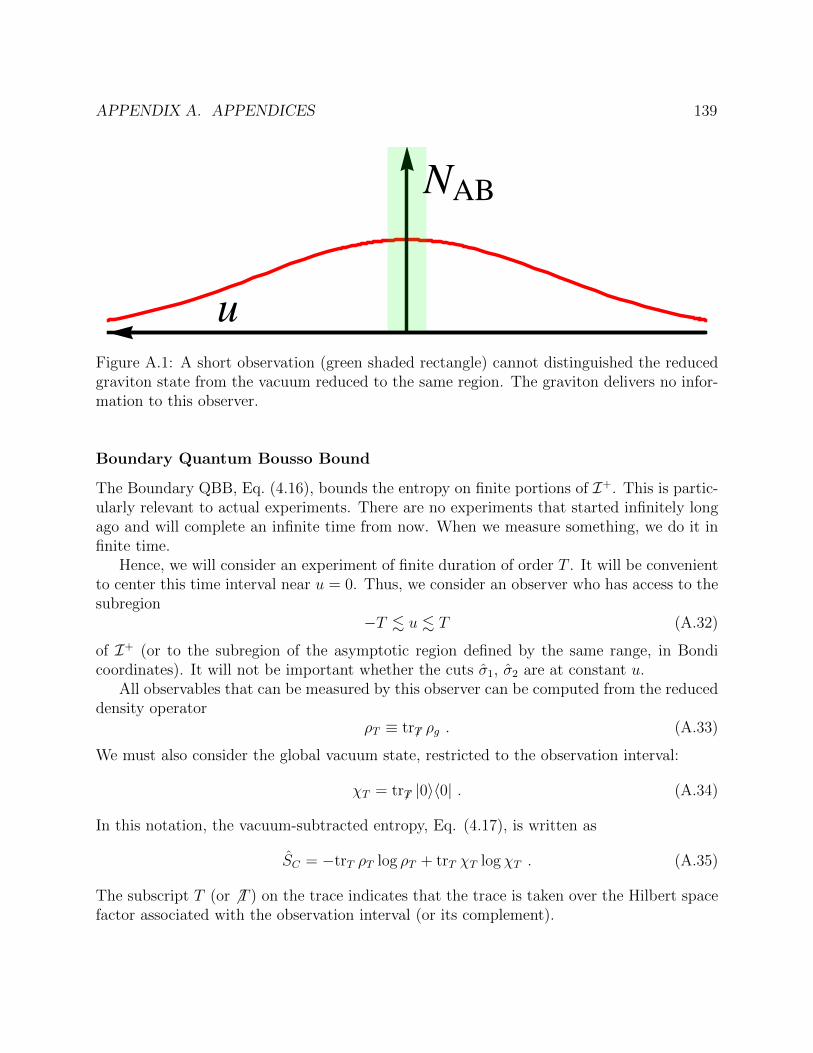
APPENDIX A. APPENDICES 139
u
NAB
Figure A.1: A short observation (green shaded rectangle) cannot distinguished the reducedgraviton state from the vacuum reduced to the same region. The graviton delivers no infor-mation to this observer.
Boundary Quantum Bousso Bound
The Boundary QBB, Eq. (4.16), bounds the entropy on finite portions of I+. This is partic-ularly relevant to actual experiments. There are no experiments that started infinitely longago and will complete an infinite time from now. When we measure something, we do it infinite time.
Hence, we will consider an experiment of finite duration of order T . It will be convenientto center this time interval near u = 0. Thus, we consider an observer who has access to thesubregion
−T . u . T (A.32)
of I+ (or to the subregion of the asymptotic region defined by the same range, in Bondicoordinates). It will not be important whether the cuts σ1, σ2 are at constant u.
All observables that can be measured by this observer can be computed from the reduceddensity operator
ρT ≡ tr6T ρg . (A.33)
We must also consider the global vacuum state, restricted to the observation interval:
χT = tr6T |0〉〈0| . (A.34)
In this notation, the vacuum-subtracted entropy, Eq. (4.17), is written as
SC = −trT ρT log ρT + trT χT logχT . (A.35)
The subscript T (or 6 T ) on the trace indicates that the trace is taken over the Hilbert spacefactor associated with the observation interval (or its complement).

APPENDIX A. APPENDICES 140
Short Observation Regime We begin by considering the case where λ T . In thisregime, the observer has access to a region occupied by the graviton wavepacket, but muchsmaller than the wavepacket (Fig. A.1). The Boundary QBB implies
SC . O(T T 2/~) ∼ O(T 2/λ2) , (A.36)
so the upper bound vanishes quadratically with T/λ.To understand this result, it is instructive to return to the bulk and consider the case of a
scalar field wavepacket passing through H(up). In this setting, the entropy can be computedexplicitly; and the bound has been proven [32, 31]. A beautiful explanation of the vanishingof the information content was given by Casini [45], building on pioneering work of Marolf,Minic, and Ross [129].
To an observer with access to a finite or semi-infinite region, the vacuum (restricted tothis region) is a noisy state. For example, in the simplest case of a semi-infinite region(Rindler space), the restricted vacuum is a thermal state. Further restrictions only make thefluctuations larger. This means that the global vacuum restricted to the interval (−T, T )is a state in which thermal-like excitations with energy up to order ~/T are unsuppressed.This energy is larger, by a huge factor λ2/T 2, than the total energy of the graviton in thisregion. This is the physical origin of Eq. (A.36): because of thermal noise, states with andwithout the graviton wavepacket cannot be distinguished by an observer with access to asmall subregion of the wavepacket. In short, the vacuum-subtracted entropy is a physicalquantity that correctly captures how much information can be gained by a given observer.
We can also shift the observation interval so that it fails to overlap with the graviton.This is analogous to a case of classical Bondi news studied in Sec. 4.4, and it gives the sameresult: In this case it does not matter how long or short the observation is; if it does notoverlap with the news, then upper bound vanishes.
Long Observation Regime Next, let us consider the case where the observer has accessto a region that includes the whole wavepacket: T λ (Fig. A.2). In the long-observationregime, the experiment begins well before the graviton starts arriving, and ends well after.From Eq. (A.28) we see that the energy density T scales as λ−2. The Boundary QBB,Eq. (4.16), evaluates to
SC . O(T Tλ/~) ∼ O
(T
λ
), (A.37)
as the integral has support only only on the central interval of size O(λ) where g ∼ O(T ).Since we have T λ, Eq. (A.37) is consistent with the ability of the observer to extractinformation from the graviton.
We may specify a “soft limit” of the long-observation regime as follows: Let T = αλ,with α 1 fixed. Then we take λ to become as large as we like, while the experiment alwayslasts longer than the wavepacket. We note that the upper bound remains fixed in this limit,at O(α) 1. We can tighten the upper bound to O(1) while remaining marginally withinthe long-observation regime by taking α ∼ 1.

APPENDIX A. APPENDICES 141
u
NAB
Figure A.2: A long observation (green shaded rectangle) can distinguish the reduced gravitonstate from the reduced vacuum. The graviton carries information to this observer.
We can gain further intuition by returning to the bulk and considering the same gravitonas it crosses a planar light-sheet H(up). It induces focussing as dθ/dw ∼ O(G~/(Aλ2)), wereA is the transverse area on which the wavepacket has support. Integrating twice along thelight-rays and once transversally, we see that the area loss between the two ends of the wavepacket is of order the Planck area for α ∼ 1. Thus, a single quantum induces loss of abouta Planck area in planar light-sheets, independently of wavelength [26]. Hence the bound onits entropy is of order unity.
We will not try to compute the entropy of the graviton directly, but we expect it tobe of order unity. To see this, let us again consider instead a scalar field wavepacket, forwhich the QBB has been proven [32, 31]. We understand the presence of nonzero entropy:the experiment can access the whole wavepacket, and the excitation can be distinguishedreasonably well from the thermal noise that pollutes any finite-duration measurements [129,45]. Thus as α ∼ 1, the bound becomes approximately saturated at the order-of-magnitudelevel.
Boundary Generalized Second Law
Finally, let us consider an observer with access to a semi-infinite region above some cut σ2
of I+. The bound that applies to this case is the integrated Boundary GSL, Eq. (4.19):
SC [σ2] ≤ ∆K[σ2] , (A.38)
where
∆K[σ2] ≡ 2π
~
∫ ∞
σ2
d2Ω du [u− u2(Ω)] T (A.39)

APPENDIX A. APPENDICES 142
is the modular Hamiltonian.We stressed earlier that all real experiments are finite. Nevertheless, the above bound is
a useful approximation for long but finite observations: first specify the global state, whichmust obey fall-off conditions [51] on the news. Then restrict to an interval (u2, T ) such thatT lies far inside the future region with essentially no news, and consider the QBB for thisinterval. Since the slope of g is unity near the lower end of the interval, and since SC willno longer depend on T in this regime, the Boundary QBB reduces to Eq. (A.38).
u
NAB
Figure A.3: A graviton conveys O(1) information as long as it has appreciable support inthe region of observation.
Let us apply Eq. (A.38) to a graviton wavepacket with support in the region (−λ, λ).First suppose that the cut σ2 lies, say, around the center of the wavepacket, as depicted inFig. A.3. By the previous paragraph, the results will be the same as for the QBB in theregime α ∼ 1: the asymptotic geometry can be distinguished from Minkowski space, andthe upper bound will be of order unity. On the other hand, if we shift the wavepacket so asto lie entirely prior to σ2, then the upper bound vanishes.
We can also consider the differential version of the Boundary GSL, which can be writtenas
− 1
δΩ
d
duSC [σ2; Ω] ≤ 2π
~
∫ ∞
σ2
du T . (A.40)
This vanishes if the news has no support in the region above the cut σ2. Thus, for the case ofnews that arrives entirely prior to σ, the upper bounds on the entropy, and on its variationunder deformations of σ, both vanish. This is the same behavior we encountered for theclassical case in Sec. 4.4.
In the case where a graviton wavepacket lies partially or entirely above the cut (Fig. A.3),we see that the derivative of SC is bounded by the energy of the wavepacket. This is

APPENDIX A. APPENDICES 143
nonzero for any finite λ. We note that the upper bound depends on the energy, not onthe gravitational memory created by the wavepacket. Therefore, the upper bound on thederivative of SC vanishes in the soft limit as λ becomes large, even though ∆CAB remainsfixed in this limit. Thus, the differential Boundary GSL implies that the variation in entropyof the region above a cut σ, under fixed length deformations of σ, is insensitive to the additionof gravitons of much greater wavelength.
A.5 Non-Expanding Horizons and Weakly Isolated
Horizons
In this appendix, we study properties of non-expanding horizons and weakly isolated hori-zons. First, we provide geometric identities for non-expanding null surfaces. We use ka
to indicate the generator of a null surface which satisfies the null condition kaka = 0 and
the geodesic equation kb∇bka = 0. We introduce an auxiliary null vector field la satisfying
lala = 0, kal
a = −1, and £kla = 0. The transverse metric of the null surface is given by
hab = gab + kalb + lakb. To make the notation more precise, we use the sign “ = ” to denote“equal on the horizon” in this appendix and in appendix A.6.
A non-expanding null surface is defined by
h ca h
db ∇ckd = 0. (A.41)
Substituting the definition of hab into the above equation, we obtain
∇akb = Lakb + kaRb +Bkakb, (A.42)
where La ≡ −ld∇akd, Rb ≡ −lc∇ckb, and B ≡ −lcld∇ckd. La, Ra and B satisfy relationsLak
a = 0, Rbkb = 0, and Lal
a = B = Rblb. Furthermore, there is
∇aka = 0. (A.43)
The extrinsic curvature, defined by
Kcab := −h d
a heb ∇dh
ce , (A.44)
of a non-expanding null surface can always be written as
Kcab = kcAab, (A.45)
where Aab ≡ −h da ∇dlb + Lalb +Bkalb.
On a non-expanding null surface, the Riemann tensor contracting with a ka can be writtenin terms of La, Ra, and B as
Rabck ≡ 2∇[a∇b]kc
= 2kc∇[aLb] + 2Rck[aRb] + 2k[b∇a]Rc + 2kck[b∇a]B + 2Bkck[aRb] + 2Bk[bLa]kc.(A.46)

APPENDIX A. APPENDICES 144
From the above equation, one immediately obtains
Rakck = − LbkckaRb − kbkc∇bLa − kbka∇bRc − kbkcka∇bB, (A.47)
Rbk = ka∇aLb + kb∇aRa + kbL
aRa + kb∂kB, (A.48)
Rkk = 0. (A.49)
The above results are for non-expanding horizons in general. By further imposing thedominant energy condition (8.18), one observes special properties of weakly isolated horizons.First, by noticing that equation (A.49) implies that vector Ra
bkb must be a vector tangent
to the horizon and equation (8.18) implies that Rabkb can be written as a term proportional
to ka plus a causal vector, one concludes that for weakly isolated horizons there is
Rabkb = fka. (A.50)
Second, we argue that on weakly isolated horizons the Weyl tensor is Petrov type II. Toprove this, we only need to show that for weakly isolated horizons there is
Cabcdkakchbeh
df = 0, (A.51)
Cabcdkahbeh
cfh
dg = 0. (A.52)
Equation (A.50) and equation
Rabcd = Cabcd +2
d− 2
(ga[cRd]b − gb[cRd]a
)− 2
(d− 1) (d− 2)Rga[cgd]b (A.53)
together imply that
Cabcdkakchbeh
df = Rabcdk
akchbehdf , (A.54)
Cabcdkahbeh
cfh
dg = Rabcdk
ahbehcfh
dg. (A.55)
Equation (A.46) implies that the right-hand side of equation (A.55) vanishes and equation(A.47) implies that the right-hand side of equation (A.54) vanishes. Therefore, equations(A.51) and (A.52) do hold and the Wyel tensor is indeed Petrov type II on weakly isolatedhorizons. This leads us to conclude that on weakly isolated horizons we have
Cabcdkbkd = ζkakc, (A.56)
which, together with (A.53) and (A.50), further leads to
Rabcdkbkd = ζkakc. (A.57)
The contracted Bianchi identity ∇aRa
bcd +∇bRcd−∇cRbd = 0 provides a relationship amongζ, f , and the spacetime scalar curvature R:
1
2∂kR = ∂kf = − ∂kζ. (A.58)

APPENDIX A. APPENDICES 145
These features guide one to conclude ka∇aLb ∝ kb and kb∇bRc ∝ kc. Therefore, onweakly isolated horizons, the Riemann tensor Rabck can be written as Rabck = kcAab+k[aBb]c,
where Aab is antisymmetric and satisfies kaAab ∝ kb and Bab satisfies kaBab ∝ kb and kbBab ∝ka. This guarantees more proportionl relations, including RacRabck ∝ kb, R
bcdk Rcdbe ∝ ke,
R fkec R
eafk ∝ kakc, and Rab
ckRabdk ∝ kckd.These relations are crucial to the scheme-independence of QNEC for d = 4, 5. However, in
those cases we do not require them to hold on the entire horizon, but only to the appropriateorder in λ about the point p. As a result, it suffices to impose only (8.17).
A.6 Scheme Independence of the QNEC
In this appendix, we derive the scheme independence of the QNEC for four-derivativecounter-terms and six-derivative counter-terms built from arbitrary polynomial contractionsof the Riemann tensor. Equations (A.42), (A.50), and (A.57) are our three inputs. As wehave mentioned at the end of appendix A.5, with these three assumptions the Riemann ten-sor Rabck can be written in the form Rabck = kcAab + k[aBb]c, where Aab is antisymmetric and
satisfies kaAab ∝ kb and Bab satisfies kaBab ∝ kb and kbBab ∝ ka. Moreover, the contractedBianchi identity implies that equation (A.58) holds on the horizon. We introduce notationsg⊥ab ≡ −kalb− lakb and εab ≡ −kalb + lakb, where the meaning of la has been explained at thebeginning of appendix A.5.
In principle, to calculate the gravitational entropy associated with the type of counter-terms considered in this appendix, we need to use Dong’s entropy formula [54]. However,it is easy to see that the S ′ct from Dong’s entropy formula reduces to that computed fromWald:1984rg’s formula when (8.17) and (8.18) hold. Therefore, in this appendix, we computethe gravitational entropy from the formula
S ′ct = ∂k
(−2πεabεcd
∂Lct
∂Rabcd
). (A.59)
Furthermore, the kk-component of the stress tensor associated with these counter-terms isgiven by the standard functional derivative formula
Tkk, ct = kbkd−2√−g
δIct
δgbd. (A.60)
The change of the QNEC associated with these counter-terms is thus given by
Qct = Tkk, ct −1
2πS ′′ct. (A.61)
Four-derivative counter-terms
We now consider the three possible four-derivative counter-terms,
I1 =
∫ddx√−gRabcdRabcd, I2 =
∫ddx√−gRabRab, and I3 =
∫ddx√−gR2. (A.62)
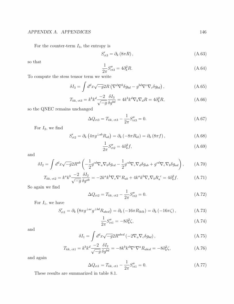
APPENDIX A. APPENDICES 146
For the counter-term I3, the entropy is
S ′ct3 = ∂k (8πR) , (A.63)
so that1
2πS ′′ct3 = 4∂2
kR. (A.64)
To compute the stess tensor term we write
δI3 =
∫ddx√−g2R
(∇d∇bδgbd − gbd∇c∇cδgbd
), (A.65)
Tkk, ct3 = kbkd−2√−g
δI3
δgbd= 4kbkd∇b∇dR = 4∂2
kR, (A.66)
so the QNEC remains unchanged
∆Qct3 = Tkk, ct3 −1
2πS ′′ct3 = 0. (A.67)
For I2, we find
S ′ct2 = ∂k(4πg⊥abRab
)= ∂k (−8πRkl) = ∂k (8πf) , (A.68)
1
2πS ′′ct2 = 4∂2
kf, (A.69)
and
δI2 =
∫ddx√−g2Rab
(−1
2gcd∇a∇bδgcd −
1
2gcd∇c∇dδgab + gcd∇c∇bδgad
), (A.70)
Tkk, ct2 = kakb−2√−g
δI2
δgab= −2kakb∇c∇cRab + 4kakb∇c∇bR
ca = 4∂2
kf. (A.71)
So again we find
∆Qct2 = Tkk, ct2 −1
2πS ′′ct2 = 0. (A.72)
For I1, we have
S ′ct1 = ∂k(8πg⊥acg⊥bdRabcd
)= ∂k (−16πRlklk) = ∂k (−16πζ) , (A.73)
1
2πS ′′ct1 = −8∂2
kζ, (A.74)
and
δI1 =
∫ddx√−g2Rabcd (−2∇a∇cδgbd) , (A.75)
Tkk, ct1 = kbkd−2√−g
δI2
δgbd= −8kbkd∇c∇aRabcd = −8∂2
kζ, (A.76)
and again
∆Qct1 = Tkk, ct1 −1
2πS ′′ct1 = 0. (A.77)
These results are summarized in table 8.1.
APPENDIX A. APPENDICES 147
Six-derivative counter-terms
We now consider six-derivative counter-terms built from arbitrary polynomial contractionsof the Riemann tensor. These terms are listed in [143]. They are
I1 =
∫ddx√−gRabcdRcdefR
efab, I2 =
∫ddx√−gRab
cdRcebfR
dfae,
I3 =
∫ddx√−gRabcdRcdbeR
ea, I4 =
∫ddx√−gRRabcdRabcd,
I5 =
∫ddx√−gRabcdRacRbd, I6 =
∫ddx√−gRabRbcR
ca,
I7 =
∫ddx√−gRRabRab, I8 =
∫ddx√−gR3.
(A.78)
For I8, we findS ′ct8 = ∂k
(12πR2
), (A.79)
1
2πS ′′ct8 = 6∂2
kR2, (A.80)
and
δI8 =
∫ddx√−g3R2
(∇d∇bδgbd − gbd∇c∇cδgbd
), (A.81)
Tkk, ct8 = kbkd−2√−g
δI3
δgbd= kbkd(6)∇b∇dR
2 = 6∂2kR
2, (A.82)
and thus
∆Qct8 = Tkk, ct8 −1
2πS ′′ct8 = 0. (A.83)
For I7, we findS ′ct7 = ∂k
[−2π
(−2RabRab − 4fR
)], (A.84)
1
2πS ′′ct7 = 2∂2
k
(RabRab
)+ 4∂2
k (fR) , (A.85)
and
δI7 =
∫ddx√−gRabRab
(∇d∇cδgcd − gcd∇e∇eδgcd
)
+
∫ddx√−g2RRab
(−1
2gcd∇a∇bδgcd −
1
2gcd∇c∇dδgab + gcd∇c∇bδgad
),
(A.86)
Tkk, ct7 = kckd−2√−g
δI7
δgcd
= 2kckd∇c∇d
(RabRab
)− 2kckd∇e∇e (RRcd) + 4kckd∇b∇d
(RR b
c
)
= 2∂2k
(RabRab
)+ 4∂2
k (Rf) ,
(A.87)

APPENDIX A. APPENDICES 148
and thus
∆Qct7 = Tkk, ct7 −1
2πS ′′ct7 = 0. (A.88)
For I6, we have
S ′ct6 = ∂k(6πRbcR
cag⊥ab) = −∂k (12πRkcR
cl) = ∂k
(12πf 2
), (A.89)
1
2πS ′′ct6 = 6∂2
k
(f 2), (A.90)
and
δI6 =
∫ddx√−g3RbeR a
e
(−1
2gcd∇a∇bδgcd −
1
2∇c∇cδgab +∇d∇bδgad
), (A.91)
Tkk, ct6 = kakb−2√−g
δI6
δgab
= −3kakb∇c∇c (RbeRea) + 6kakb∇c∇b (RceRea)
= 6∂2k
(f 2),
(A.92)
and so
∆Qct6 = Tkk, ct6 −1
2πS ′′ct6 = 0. (A.93)
To deal with counter-term I5, not first that Rkb = fkb implies RacRabck = fkb and thatcontracting both sides with lb then gives the function f = −RacRalck. Thus we find
RacRabck = − kbRacRalck. (A.94)
We may now compute
S ′ct5 = ∂k(2πg⊥[a|c|g
⊥b]dR
acRbd + 4πg⊥bdRabcdRac
)
= ∂k(4πf 2 − 8πRakclRac
),
(A.95)
1
2πS ′′ct5 = 2∂2
k
(f 2)− 4∂2
k
(RakclRac
), (A.96)
and
δI5 =
∫ddx√−gRa[cR|b|d] (−2∇a∇cδgbd)
+
∫ddx√−gRabcd2Rac
(−1
2gef∇b∇dδgef −
1
2∇e∇eδgbd +∇f∇dδgbf
),
(A.97)
Tkk, ct5 =kbkd−2√−g
δI5
δgbd
=− 4kbkd∇c∇aRa[cR|b|d] − 2kbkd∇e∇e (RabcdRac) + 4kbkf∇d∇f (RabcdR
ac)
=2kbkd∇c∇aRadRbc + 4kbkf∇d∇f (RabcdRac)
=2∂2k
(f 2)− 4∂2
k (RakclRac) ,
(A.98)

APPENDIX A. APPENDICES 149
which together imply
∆Qct5 = Tkk, ct5 −1
2πS ′′ct5 = 0. (A.99)
For I4, we findS ′ct4 = ∂k
[−2π
(−2RabcdRabcd + 8ζR
)], (A.100)
1
2πS ′′ct4 = 2∂2
k
(RabcdRabcd
)− 8∂2
k (ζR) , (A.101)
and
δI4 =
∫ddx√−gRabcdRabcd
(∇f∇eδgef − gef∇g∇gδgef
)
+
∫ddx√−g2RRabcd (−2∇a∇cδgbd) ,
(A.102)
Tkk, ct4 = kbkd−2√−g
δI4
δgbd
= 2kekf∇e∇f
(RabcdRabcd
)− 8kbkd∇c∇a (RRabcd)
= 2∂2k
(RabcdRabcd
)− 8∂2
k (Rζ) ,
(A.103)
so that
∆Qct4 = Tkk, ct4 −1
2πS ′′ct4 = 0. (A.104)
For counter-term I3, note that Rakck = ζkakc implies R bcdk Rcdbe = ζke. Contracting both
sides with le then gives the function ζ = −R bcdk Rcdbl. Thus we find
R bcdk Rcdbe = −keR bcd
k Rcdbl. (A.105)
We may now compute
S ′ct3 =∂k(−8πRcdbeR a
e g⊥[a|c|g
⊥b]d + 2πRabcdR e
cdb g⊥ea
)
=∂k(−16πRlkleR
ek − 4πR bcd
k Rcdbl
)
=∂k(−16πζf − 4πR bcd
k Rcdbl
),
(A.106)
1
2πS ′′ct3 = −8∂2
k (ζf)− 2∂2k
(R bcdk Rcdbl
), (A.107)
and
δI3 =
∫ddx√−g2RcdbeR a
e (−2∇a∇cδgbd)
+
∫ddx√−gRabcdR e
cdb
(−1
2gfg∇a∇eδgfg −
1
2∇f∇fδgea +∇f∇eδgaf
),
(A.108)

APPENDIX A. APPENDICES 150
Tkk, ct3 =kbkd−2√−g
δI3
δgbd
=− 8kbkd∇c∇a
(RcdbeR a
e
)− keka∇f∇f
(RabcdRcdbe
)
2kakf∇e∇f
(RabcdRcdbe
)
=− 8∂2k (ζf)− 2∂2
k
(R bcdk Rcdbl
).
(A.109)
Putting these together yields
∆Qct3 = Tkk, ct3 −1
2πS ′′ct3 = 0. (A.110)
For counter-term I2, notice that Rakck = ζkakc implies ReafkR
fec k = ζkakc. Contracting
both sides with lalc gives the function ζ = RelfkR
fel k. One then finds
ReafkR
fec k = kakcR
elfkR
fel k. (A.111)
With this in hand, we calculate
S ′ct2 =∂k
(−12πg⊥[a
cg⊥b]
dRcebfR
dfae
)
=∂k
[−12π
(R fkel R
elfk −R f
lel Re
kfk
)]
=∂k
[−12π
(R fkel R
elfk − ζ2
)],
(A.112)
1
2πS ′′ct2 = −6∂2
k
(R fkel R
elfk − ζ2
), (A.113)
and
δI2 =
∫ddx√−g3R
[cegfR
d]faeggb (−2∇a∇cδgbd) , (A.114)
Tkk, ct2 =kbkd−2√−g
δI2
δgbd
=− 12kbkd∇c∇a
(R
[cebfR
d]fae)
=− 6kbkd∇c∇a
(RcebfR
faed −RdebfR
faec
)
=− 6∇c∇a
(RcekfR
faek − ζ2kck
a)
=− 6∇c∇a(Re
cfkRf
ea k
)+ 6∂2
k
(ζ2)
=− 6∂2k
(Re
lfkRf
el k
)+ 6∂2
k
(ζ2).
(A.115)
The result is then
∆Qct2 = Tkk, ct2 −1
2πS ′′ct2 = 0. (A.116)
APPENDIX A. APPENDICES 151
For the final counter-term I1, notice that Rakck = ζkakc implies RabckRabdk = ςkckd.
Contracting both sides with lcld gives the function ς = RablkRablk. Thus we find
RabckRabdk = kckdR
ablkRablk. (A.117)
This givesS ′ct1 =∂k
(−12πRcdefR ab
ef g⊥[a|c|g⊥b]d
)
=∂k
(−24πRef
lkReflk
),
(A.118)
1
2πS ′′ct1 = −12∂2
k
(Ref
lkReflk
), (A.119)
and
δI1 =
∫ddx√−g3RcdefR ab
ef (−2∇a∇cδgbd) , (A.120)
Tkk, ct1 =kbkd−2√−g
δI1
δgbd
=− 12kbkd∇c∇a
(RcdefR ab
ef
)
=− 12∇c∇a(Ref
ckRefak
)
=− 12∂2k
(Ref
lkReflk
).
(A.121)
The result is then once again that
∆Qct1 = Tkk, ct1 −1
2πS ′′ct1 = 0. (A.122)
The above results are summarized in table 8.2.

152
Bibliography
[1] B. P. Abbott et al. “Observation of Gravitational Waves from a Binary Black HoleMerger”. In: Phys. Rev. Lett. 116.6 (2016), p. 061102. doi: 10.1103/PhysRevLett.116.061102. arXiv:1602.03837 [gr-qc].
[2] B.P. Abbott et al. “GW151226: Observation of Gravitational Waves from a 22-Solar-Mass Binary Black Hole Coalescence”. In: Phys. Rev. Lett. 116.24 (2016), p. 241103.doi: 10.1103/PhysRevLett.116.241103. arXiv:1606.04855 [gr-qc].
[3] Chris Akers et al. “Entanglement and RG in the O(N) vector model”. In: (2015).arXiv:1512.00791 [hep-th].
[4] Chris Akers et al. “Geometric Constraints from Subregion Duality Beyond the Clas-sical Regime”. In: (2016). arXiv:1610.08968 [hep-th].
[5] Andrea Allais and Mark Mezei. “Some results on the shape dependence of entan-glement and Renyi entropies”. In: Phys. Rev. D91.4 (2015), p. 046002. doi: 10.1103/PhysRevD.91.046002. arXiv:1407.7249 [hep-th].
[6] Sinya Aoki et al. “On the definition of entanglement entropy in lattice gauge theories”.In: JHEP 06 (2015), p. 187. doi: 10.1007/JHEP06(2015)187. arXiv:1502.04267[hep-th].
[7] A. Ashtekar. “Asymptotic Quantization of the Gravitational Field”. In: Phys. Rev.Lett. 46 (1981), pp. 573–576. doi: 10.1103/PhysRevLett.46.573.
[8] Abhay Ashtekar, Christopher Beetle, and Jerzy Lewandowski. “Geometry of genericisolated horizons”. In: Class. Quant. Grav. 19 (2002), pp. 1195–1225. doi: 10.1088/0264-9381/19/6/311. arXiv:gr-qc/0111067 [gr-qc].
[9] Amin Faraji Astaneh, Gary Gibbons, and Sergey N. Solodukhin. “What SurfaceMaximizes Entanglement Entropy?” In: Phys. Rev. D90.8 (2014), p. 085021. doi:10.1103/PhysRevD.90.085021. arXiv:1407.4719 [hep-th].
[10] Artem Averin et al. “Goldstone origin of black hole hair from supertranslations andcriticality”. In: (2016). arXiv:1606.06260 [hep-th].
[11] Glenn Barnich and Cedric Troessaert. “Aspects of the BMS/CFT correspondence”.In: JHEP 05 (2010), p. 062. doi: 10.1007/JHEP05(2010)062. arXiv:1001.1541[hep-th].

BIBLIOGRAPHY 153
[12] Glenn Barnich and Cedric Troessaert. “Symmetries of asymptotically flat 4 dimen-sional spacetimes at null infinity revisited”. In: Phys. Rev. Lett. 105 (2010), p. 111103.doi: 10.1103/PhysRevLett.105.111103. arXiv:0909.2617 [gr-qc].
[13] J. D. Bekenstein. “Black holes and the second law”. In: Nuovo Cim. Lett. 4 (1972),pp. 737–740.
[14] Jacob D. Bekenstein. “Black Holes and Entropy”. In: Phys. Rev. D7 (1973), pp. 2333–2346. doi: 10.1103/PhysRevD.7.2333.
[15] Jacob D. Bekenstein. “Generalized second law of thermodynamics in black hole physics”.In: Phys. Rev. D 9 (1974), p. 3292.
[16] Srijit Bhattacharjee et al. “Entropy functionals and c-theorems from the second law”.In: Phys. Rev. D93.10 (2016), p. 104045. doi: 10.1103/PhysRevD.93.104045. arXiv:1508.01658 [hep-th].
[17] Jyotirmoy Bhattacharya et al. “Entanglement Density and Gravitational Thermody-namics”. In: Phys. Rev. D91.10 (2015), p. 106009. doi: 10.1103/PhysRevD.91.106009. arXiv:1412.5472 [hep-th].
[18] Sayantani Bhattacharyya et al. “Towards a second law for Lovelock theories”. In:JHEP 03 (2017), p. 065. doi: 10 . 1007 / JHEP03(2017 ) 065. arXiv:1612 . 04024[hep-th].
[19] Eugenio Bianchi and Robert C. Myers. “On the Architecture of Spacetime Geometry”.In: Class. Quant. Grav. 31 (2014), p. 214002. doi: 10.1088/0264-9381/31/21/214002. arXiv:1212.5183 [hep-th].
[20] J. J Bisognano and E. H. Wichmann. “On the Duality Condition for Quantum Fields”.In: J. Math. Phys. 17 (1976), pp. 303–321. doi: 10.1063/1.522898.
[21] H. Bondi, M. G. J. van der Burg, and A. W. K. Metzner. “Gravitational waves ingeneral relativity. 7. Waves from axisymmetric isolated systems”. In: Proc. Roy. Soc.Lond. A269 (1962), pp. 21–52. doi: 10.1098/rspa.1962.0161.
[22] Arvind Borde. “Geodesic focusing, energy conditions and singularities”. In: Class.Quant. Grav. 4 (1987), pp. 343–356. doi: 10.1088/0264-9381/4/2/015.
[23] Raphael Bousso. “A Covariant entropy conjecture”. In: JHEP 07 (1999), p. 004. doi:10.1088/1126-6708/1999/07/004. arXiv:hep-th/9905177 [hep-th].
[24] Raphael Bousso. “Asymptotic Entropy Bounds”. In: (2016). arXiv:1606.02297 [hep-th].
[25] Raphael Bousso. “Holography in general space-times”. In: JHEP 06 (1999), p. 028.doi: 10.1088/1126-6708/1999/06/028. arXiv:hep-th/9906022 [hep-th].
[26] Raphael Bousso. “Light-sheets and Bekenstein’s bound”. In: Phys. Rev. Lett. 90(2003), p. 121302. eprint: hep-th/0210295.
[27] Raphael Bousso and Netta Engelhardt. “Generalized Second Law for Cosmology”.In: Phys. Rev. D93.2 (2016), p. 024025. doi: 10.1103/PhysRevD.93.024025. arXiv:1510.02099 [hep-th].
BIBLIOGRAPHY 154
[28] Raphael Bousso and Netta Engelhardt. “New Area Law in General Relativity”. In:Phys. Rev. Lett. 115.8 (2015), p. 081301. doi: 10.1103/PhysRevLett.115.081301.arXiv:1504.07627 [hep-th].
[29] Raphael Bousso and Netta Engelhardt. “Proof of a New Area Law in General Rela-tivity”. In: Phys. Rev. D92.4 (2015), p. 044031. doi: 10.1103/PhysRevD.92.044031.arXiv:1504.07660 [gr-qc].
[30] Raphael Bousso, Illan Halpern, and Jason Koeller. “Information Content of Gravita-tional Radiation and the Vacuum”. In: (2016). arXiv:1607.03122 [hep-th].
[31] Raphael Bousso et al. “Entropy on a null surface for interacting quantum field theoriesand the Bousso bound”. In: Phys. Rev. D91.8 (2015), p. 084030. doi: 10.1103/PhysRevD.91.084030. arXiv:1406.4545 [hep-th].
[32] Raphael Bousso et al. “Proof of a Quantum Bousso Bound”. In: Phys. Rev. D90.4(2014), p. 044002. doi: 10.1103/PhysRevD.90.044002. arXiv:1404.5635 [hep-th].
[33] Raphael Bousso et al. “Proof of the Quantum Null Energy Condition”. In: Phys. Rev.D93.2 (2016), p. 024017. doi: 10.1103/PhysRevD.93.024017. arXiv:1509.02542[hep-th].
[34] Raphael Bousso et al. “Quantum focusing conjecture”. In: Phys. Rev. D93.6 (2016),p. 064044. doi: 10.1103/PhysRevD.93.064044. arXiv:1506.02669 [hep-th].
[35] William Bunting, Zicao Fu, and Donald Marolf. “A coarse-grained generalized secondlaw for holographic conformal field theories”. In: Class. Quant. Grav. 33.5 (2016),p. 055008. doi: 10.1088/0264-9381/33/5/055008. arXiv:1509.00074 [hep-th].
[36] Matthias Burkardt. “Light front quantization”. In: Adv. Nucl. Phys. 23 (1996), pp. 1–74. doi: 10.1007/0-306-47067-5_1. arXiv:hep-ph/9505259 [hep-ph].
[37] Robert Callan, Jian-Yang He, and Matthew Headrick. “Strong subadditivity and thecovariant holographic entanglement entropy formula”. In: JHEP 06 (2012), p. 081.doi: 10.1007/JHEP06(2012)081. arXiv:1204.2309 [hep-th].
[38] Curtis G. Callan Jr. and Frank Wilczek. “On geometric entropy”. In: Phys.Lett. B333(1994), pp. 55–61. doi: 10.1016/0370-2693(94)91007-3. arXiv:hep-th/9401072[hep-th].
[39] Xian O. Camanho et al. “Causality Constraints on Corrections to the Graviton Three-Point Coupling”. In: JHEP 02 (2016), p. 020. doi: 10.1007/JHEP02(2016)020.arXiv:1407.5597 [hep-th].
[40] Joan Camps. “Generalized Entropy and Higher Derivative Gravity”. In: JHEP 03(2014), p. 070. doi: 10.1007/JHEP03(2014)070. arXiv:1310.6659 [hep-th].
[41] Li-Ming Cao. “Deformation of Codimension-2 Surface and Horizon Thermodynam-ics”. In: JHEP 03 (2011), p. 112. doi: 10.1007/JHEP03(2011)112. arXiv:1009.4540[gr-qc].

BIBLIOGRAPHY 155
[42] Andrea Cappelli and Antoine Coste. “On the Stress Tensor of Conformal Field The-ories in Higher Dimensions”. In: Nucl. Phys. B314 (1989), p. 707. doi: 10.1016/0550-3213(89)90414-8.
[43] John Cardy and Erik Tonni. “Entanglement hamiltonians in two-dimensional confor-mal field theory”. In: J. Stat. Mech. 1612.12 (2016), p. 123103. doi: 10.1088/1742-5468/2016/12/123103. arXiv:1608.01283 [cond-mat.stat-mech].
[44] Dean Carmi. “On the Shape Dependence of Entanglement Entropy”. In: (2015).arXiv:1506.07528 [hep-th].
[45] H. Casini. “Relative entropy and the Bekenstein bound”. In: Class.Quant.Grav. 25(2008), p. 205021. doi: 10.1088/0264- 9381/25/20/205021. arXiv:0804.2182[hep-th].
[46] H. Casini and M. Huerta. “A Finite Entanglement Entropy and the C-Theorem”. In:Phys. Lett. B600 (2004), pp. 142–150. doi: 10.1016/j.physletb.2004.08.072.arXiv:hep-th/0405111 [hep-th].
[47] H. Casini and Marina Huerta. “On the RG Running of the Entanglement Entropy ofa Circle”. In: Phys. Rev. D85 (2012), p. 125016. doi: 10.1103/PhysRevD.85.125016.arXiv:1202.5650 [hep-th].
[48] Horacio Casini, Marina Huerta, and Robert C. Myers. “Towards a Derivation of Holo-graphic Entanglement Entropy”. In: JHEP 05 (2011), p. 036. doi: 10.1007/JHEP05(2011)036. arXiv:1102.0440 [hep-th].
[49] Horacio Casini, F. D. Mazzitelli, and Eduardo Teste. “Area terms in entanglemententropy”. In: Phys. Rev. D91.10 (2015), p. 104035. doi: 10.1103/PhysRevD.91.104035. arXiv:1412.6522 [hep-th].
[50] D. Christodoulou. “Nonlinear nature of gravitation and gravitational wave experi-ments”. In: Phys. Rev. Lett. 67 (1991), pp. 1486–1489. doi: 10.1103/PhysRevLett.67.1486.
[51] D. Christodoulou and S. Klainerman. The Global nonlinear stability of the Minkowskispace. Princeton: Princeton University Press, 1993.
[52] Alan Coley and Sigbjorn Hervik. “Higher dimensional bivectors and classification ofthe Weyl operator”. In: Class. Quant. Grav. 27 (2010), p. 015002. doi: 10.1088/0264-9381/27/1/015002. arXiv:0909.1160 [gr-qc].
[53] Bartlomiej Czech et al. “The Gravity Dual of a Density Matrix”. In: Class. Quant.Grav. 29 (2012), p. 155009. doi: 10.1088/0264-9381/29/15/155009. arXiv:1204.1330 [hep-th].
[54] Xi Dong. “Holographic Entanglement Entropy for General Higher Derivative Grav-ity”. In: JHEP 01 (2014), p. 044. doi: 10.1007/JHEP01(2014)044. arXiv:1310.5713[hep-th].

BIBLIOGRAPHY 156
[55] Xi Dong, Daniel Harlow, and Aron C. Wall. “Reconstruction of Bulk Operatorswithin the Entanglement Wedge in Gauge-Gravity Duality”. In: Phys. Rev. Lett.117.2 (2016), p. 021601. doi: 10.1103/PhysRevLett.117.021601. arXiv:1601.05416[hep-th].
[56] Xi Dong, Aitor Lewkowycz, and Mukund Rangamani. “Deriving covariant holographicentanglement”. In: JHEP 11 (2016), p. 028. doi: 10.1007/JHEP11(2016)028. arXiv:1607.07506 [hep-th].
[57] Xi Dong and Rong-Xin Miao. “Generalized Gravitational Entropy from Total Deriva-tive Action”. In: JHEP 12 (2015), p. 100. doi: 10.1007/JHEP12(2015)100. arXiv:1510.04273 [hep-th].
[58] William Donnelly. “Decomposition of entanglement entropy in lattice gauge theory”.In: Phys. Rev. D85 (2012), p. 085004. doi: 10.1103/PhysRevD.85.085004. arXiv:1109.0036 [hep-th].
[59] William Donnelly. “Entanglement entropy and nonabelian gauge symmetry”. In:Class. Quant. Grav. 31.21 (2014), p. 214003. doi: 10.1088/0264- 9381/31/21/
214003. arXiv:1406.7304 [hep-th].
[60] William Donnelly and Aron C. Wall. “Entanglement entropy of electromagnetic edgemodes”. In: Phys. Rev. Lett. 114.11 (2015), p. 111603. doi: 10.1103/PhysRevLett.114.111603. arXiv:1412.1895 [hep-th].
[61] William Donnelly and Aron C. Wall. “Geometric entropy and edge modes of theelectromagnetic field”. In: Phys. Rev. D94.10 (2016), p. 104053. doi: 10.1103/PhysRevD.94.104053. arXiv:1506.05792 [hep-th].
[62] Gia Dvali, Cesar Gomez, and Dieter Lust. “Classical Limit of Black Hole QuantumN-Portrait and BMS Symmetry”. In: Phys. Lett. B753 (2016), pp. 173–177. doi:10.1016/j.physletb.2015.11.073. arXiv:1509.02114 [hep-th].
[63] Netta Engelhardt and Sebastian Fischetti. “The Gravity Dual of Boundary Causal-ity”. In: (2016). arXiv:1604.03944 [hep-th].
[64] Netta Engelhardt and Aron C. Wall. “Quantum Extremal Surfaces: Holographic En-tanglement Entropy Beyond the Classical Regime”. In: JHEP 01 (2015), p. 073. doi:10.1007/JHEP01(2015)073. arXiv:1408.3203 [hep-th].
[65] H. Epstein, V. Glaser, and A. Jaffe. “Nonpositivity of Energy Density in QuantizedField Theories”. In: Nuovo Cim. 36 (1965), p. 1016. doi: 10.1007/BF02749799.
[66] Edward Farhi and Alan H. Guth. “An Obstacle to Creating a Universe in the Labo-ratory”. In: Phys. Lett. B183 (1987), p. 149. doi: 10.1016/0370-2693(87)90429-1.
[67] Thomas Faulkner. “Bulk Emergence and the RG Flow of Entanglement Entropy”.In: JHEP 05 (2015), p. 033. doi: 10.1007/JHEP05(2015)033. arXiv:1412.5648[hep-th].

BIBLIOGRAPHY 157
[68] Thomas Faulkner, Robert G. Leigh, and Onkar Parrikar. “Shape Dependence of En-tanglement Entropy in Conformal Field Theories”. In: (2015). arXiv:1511.05179[hep-th].
[69] Thomas Faulkner, Aitor Lewkowycz, and Juan Maldacena. “Quantum Correctionsto Holographic Entanglement Entropy”. In: JHEP 11 (2013), p. 074. doi: 10.1007/JHEP11(2013)074. arXiv:1307.2892 [hep-th].
[70] Thomas Faulkner et al. “Gravitation from Entanglement in Holographic CFTs”.In: JHEP 03 (2014), p. 051. doi: 10.1007/JHEP03(2014)051. arXiv:1312.7856[hep-th].
[71] Thomas Faulkner et al. “Modular Hamiltonians for Deformed Half-Spaces and theAveraged Null Energy Condition”. In: (2016). arXiv:1605.08072 [hep-th].
[72] Eanna E. Flanagan, Donald Marolf, and Robert M. Wald. “Proof of classical versionsof the Bousso entropy bound and of the generalized second law”. In: Phys. Rev. D62(2000), p. 084035. doi: 10.1103/PhysRevD.62.084035. arXiv:hep- th/9908070[hep-th].
[73] Eanna E. Flanagan and David A. Nichols. “Conserved charges of the extended Bondi-Metzner-Sachs algebra”. In: (2015). arXiv:1510.03386 [hep-th].
[74] L. H. Ford and Thomas A. Roman. “Averaged Energy Conditions and QuantumInequalities”. In: Phys. Rev. D51 (1995), pp. 4277–4286. doi: 10.1103/PhysRevD.51.4277. arXiv:gr-qc/9410043 [gr-qc].
[75] L. H. Ford and Thomas A. Roman. “Restrictions on Negative Energy Density in FlatSpace-Time”. In: Phys. Rev. D55 (1997), pp. 2082–2089. doi: 10.1103/PhysRevD.55.2082. arXiv:gr-qc/9607003 [gr-qc].
[76] L. H. Ford and Thomas A. Roman. “The Quantum Interest Conjecture”. In: Phys.Rev. D60 (1999), p. 104018. doi: 10.1103/PhysRevD.60.104018. arXiv:gr-qc/9901074 [gr-qc].
[77] D. Z. Freedman et al. “Renormalization group flows from holography supersymmetryand a c theorem”. In: Adv. Theor. Math. Phys. 3 (1999), pp. 363–417. arXiv:hep-th/9904017 [hep-th].
[78] Ben Freivogel and Benjamin Mosk. “Properties of Causal Holographic Information”.In: JHEP 09 (2013), p. 100. doi: 10.1007/JHEP09(2013)100. arXiv:1304.7229[hep-th].
[79] John L. Friedman, Kristin Schleich, and Donald M. Witt. “Topological censorship”.In: Phys. Rev. Lett. 71 (1993). [Erratum: Phys. Rev. Lett.75,1872(1995)], pp. 1486–1489. doi: 10.1103/PhysRevLett.71.1486. arXiv:gr-qc/9305017 [gr-qc].
[80] Zicao Fu, Jason Koeller, and Donald Marolf. “The Quantum Null Energy Conditionin Curved Space”. In: (2017). arXiv:1706.01572 [hep-th].

BIBLIOGRAPHY 158
[81] Zicao Fu, Jason Koeller, and Donald Marolf. “Violating the Quantum Focusing Con-jecture and Quantum Covariant Entropy Bound in d ≥ 5 dimensions”. In: (2017).arXiv:1705.03161 [hep-th].
[82] Zicao Fu and Donald Marolf. “Does horizon entropy satisfy a Quantum Null EnergyConjecture?” In: Class. Quant. Grav. 33.24 (2016), p. 245011. doi: 10.1088/0264-9381/33/24/245011. arXiv:1606.04713 [hep-th].
[83] Ping Gao, Daniel Louis Jafferis, and Aron Wall. “Traversable Wormholes via a DoubleTrace Deformation”. In: (2016). arXiv:1608.05687 [hep-th].
[84] Sijie Gao and Robert M. Wald. “Theorems on Gravitational Time Delay and RelatedIssues”. In: Class. Quant. Grav. 17 (2000), pp. 4999–5008. doi: 10.1088/0264-9381/17/24/305. arXiv:gr-qc/0007021 [gr-qc].
[85] Sudip Ghosh, Ronak M Soni, and Sandip P. Trivedi. “On The Entanglement EntropyFor Gauge Theories”. In: JHEP 09 (2015), p. 069. doi: 10.1007/JHEP09(2015)069.arXiv:1501.02593 [hep-th].
[86] C. Robin Graham and Edward Witten. “Conformal Anomaly of Submanifold Observ-ables in AdS / CFT Correspondence”. In: Nucl. Phys. B546 (1999), pp. 52–64. doi:10.1016/S0550-3213(99)00055-3. arXiv:hep-th/9901021 [hep-th].
[87] Noah Graham and Ken D. Olum. “Achronal averaged null energy condition”. In: Phys.Rev. D76 (2007), p. 064001. doi: 10.1103/PhysRevD.76.064001. arXiv:0705.3193[gr-qc].
[88] Daniel Harlow. “The Ryu-Takayanagi Formula from Quantum Error Correction”. In:(2016). arXiv:1607.03901 [hep-th].
[89] Sebastian de Haro, Sergey N. Solodukhin, and Kostas Skenderis. “Holographic re-construction of space-time and renormalization in the AdS / CFT correspondence”.In: Commun. Math. Phys. 217 (2001), pp. 595–622. doi: 10.1007/s002200100381.arXiv:hep-th/0002230 [hep-th].
[90] Thomas Hartman, Sandipan Kundu, and Amirhossein Tajdini. “Averaged Null En-ergy Condition from Causality”. In: (2016). arXiv:1610.05308 [hep-th].
[91] S. W. Hawking. “Gravitational Radiation from Colliding Black Holes”. In: Phys. Rev.Lett. 26 (1971), pp. 1344–1346. doi: 10.1103/PhysRevLett.26.1344.
[92] S. W. Hawking. “The Chronology Protection Conjecture”. In: Phys. Rev. D46 (1992),pp. 603–611. doi: 10.1103/PhysRevD.46.603.
[93] S. W. Hawking and G. F. R. Ellis. The Large Scale Structure of Space-Time. Cam-bridge University Press, 1973.
[94] Temple He et al. “BMS supertranslations and Weinberg’s soft graviton theorem”.In: JHEP 05 (2015), p. 151. doi: 10.1007/JHEP05(2015)151. arXiv:1401.7026[hep-th].

BIBLIOGRAPHY 159
[95] Matthew Headrick. “General properties of holographic entanglement entropy”. In:JHEP 03 (2014), p. 085. doi: 10.1007/JHEP03(2014)085. arXiv:1312.6717 [hep-th].
[96] Matthew Headrick et al. “Causality & Holographic Entanglement Entropy”. In: JHEP12 (2014), p. 162. doi: 10.1007/JHEP12(2014)162. arXiv:1408.6300 [hep-th].
[97] Christopher P. Herzog. “Universal Thermal Corrections to Entanglement Entropy forConformal Field Theories on Spheres”. In: JHEP 10 (2014), p. 28. doi: 10.1007/JHEP10(2014)028. arXiv:1407.1358 [hep-th].
[98] Diego M. Hofman. “Higher Derivative Gravity, Causality and Positivity of Energyin a UV complete QFT”. In: Nucl. Phys. B823 (2009), pp. 174–194. doi: 10.1016/j.nuclphysb.2009.08.001. arXiv:0907.1625 [hep-th].
[99] Gerard ’t Hooft. “The black hole horizon as a quantum surface”. In: Phys. ScriptaT36 (1991), pp. 247–252.
[100] Veronika E. Hubeny and Mukund Rangamani. “Causal Holographic Information”.In: JHEP 06 (2012), p. 114. doi: 10.1007/JHEP06(2012)114. arXiv:1204.1698[hep-th].
[101] Veronika E. Hubeny, Mukund Rangamani, and Tadashi Takayanagi. “A Covariantholographic entanglement entropy proposal”. In: JHEP 07 (2007), p. 062. doi: 10.1088/1126-6708/2007/07/062. arXiv:0705.0016 [hep-th].
[102] Veronika E. Hubeny, Mukund Rangamani, and Erik Tonni. “Thermalization of CausalHolographic Information”. In: JHEP 05 (2013), p. 136. doi: 10.1007/JHEP05(2013)136. arXiv:1302.0853 [hep-th].
[103] Ling-Yan Hung, Robert C. Myers, and Michael Smolkin. “Some Calculable Contri-butions to Holographic Entanglement Entropy”. In: JHEP 08 (2011), p. 039. doi:10.1007/JHEP08(2011)039. arXiv:1105.6055 [hep-th].
[104] C. Imbimbo et al. “Diffeomorphisms and Holographic Anomalies”. In: Class. Quant.Grav. 17 (2000), pp. 1129–1138. doi: 10.1088/0264-9381/17/5/322. arXiv:hep-th/9910267 [hep-th].
[105] Ted Jacobson. “Black Hole Entropy and Induced Gravity”. In: (1994). arXiv:gr-qc/9404039 [gr-qc].
[106] Ted Jacobson. “Entanglement Equilibrium and the Einstein Equation”. In: (2015).arXiv:1505.04753 [gr-qc].
[107] Ted Jacobson and Robert C. Myers. “Black hole entropy and higher curvature inter-actions”. In: Phys. Rev. Lett. 70 (1993), pp. 3684–3687. doi: 10.1103/PhysRevLett.70.3684. arXiv:hep-th/9305016 [hep-th].
[108] Ted Jacobson and Renaud Parentani. “Horizon entropy”. In: Found. Phys. 33 (2003),pp. 323–348. doi: 10.1023/A:1023785123428. arXiv:gr-qc/0302099 [gr-qc].
[109] Daniel L. Jafferis et al. “Relative entropy equals bulk relative entropy”. In: JHEP 06(2016), p. 004. doi: 10.1007/JHEP06(2016)004. arXiv:1512.06431 [hep-th].

BIBLIOGRAPHY 160
[110] Daniel Kapec, Ana-Maria Raclariu, and Andrew Strominger. “Area, EntanglementEntropy and Supertranslations at Null Infinity”. In: (2016). arXiv:1603.07706 [hep-th].
[111] William R. Kelly and Aron C. Wall. “Coarse-grained entropy and causal holographicinformation in AdS/CFT”. In: JHEP 03 (2014), p. 118. doi: 10.1007/JHEP03(2014)118. arXiv:1309.3610 [hep-th].
[112] William R. Kelly and Aron C. Wall. “Holographic proof of the averaged null energycondition”. In: Phys. Rev. D90.10 (2014). [Erratum: Phys. Rev.D91,no.6,069902(2015)],p. 106003. doi: 10.1103/PhysRevD.90.106003,10.1103/PhysRevD.91.069902.arXiv:1408.3566 [gr-qc].
[113] Igor R. Klebanov and Edward Witten. “AdS / CFT correspondence and symmetrybreaking”. In: Nucl. Phys. B556 (1999), pp. 89–114. doi: 10.1016/S0550-3213(99)00387-9. arXiv:hep-th/9905104 [hep-th].
[114] G. Klinkhammer. “Averaged energy conditions for free scalar fields in flat space-times”. In: Phys. Rev. D43 (1991), pp. 2542–2548. doi: 10.1103/PhysRevD.43.2542.
[115] Jason Koeller and Stefan Leichenauer. “Holographic Proof of the Quantum Null En-ergy Condition”. In: Phys. Rev. D94.2 (2016), p. 024026. doi: 10.1103/PhysRevD.94.024026. arXiv:1512.06109 [hep-th].
[116] Jason Koeller et al. “Local Modular Hamiltonians from the Quantum Null EnergyCondition”. In: (2017). arXiv:1702.00412 [hep-th].
[117] Sanved Kolekar, T. Padmanabhan, and Sudipta Sarkar. “Entropy Increase duringPhysical Processes for Black Holes in Lanczos-Lovelock Gravity”. In: Phys. Rev. D86(2012), p. 021501. doi: 10.1103/PhysRevD.86.021501. arXiv:1201.2947 [gr-qc].
[118] Zohar Komargodski and Adam Schwimmer. “On Renormalization Group Flows inFour Dimensions”. In: JHEP 12 (2011), p. 099. doi: 10.1007/JHEP12(2011)099.arXiv:1107.3987 [hep-th].
[119] Eleni-Alexandra Kontou and Ken D. Olum. “Averaged null energy condition in aclassical curved background”. In: Phys. Rev. D87.6 (2013), p. 064009. doi: 10.1103/PhysRevD.87.064009. arXiv:1212.2290 [gr-qc].
[120] Eleni-Alexandra Kontou and Ken D. Olum. “Proof of the averaged null energy con-dition in a classical curved spacetime using a null-projected quantum inequality”. In:Phys. Rev. D92 (2015), p. 124009. doi: 10.1103/PhysRevD.92.124009. arXiv:1507.00297 [gr-qc].
[121] Nima Lashkari et al. “Inviolable Energy Conditions from Entanglement Inequalities”.In: JHEP 06 (2015), p. 067. doi: 10.1007/JHEP06(2015)067. arXiv:1412.3514[hep-th].
[122] Jeongseog Lee et al. “Rnyi entropy, stationarity, and entanglement of the conformalscalar”. In: JHEP 03 (2015), p. 075. doi: 10.1007/JHEP03(2015)075. arXiv:1407.7816 [hep-th].
BIBLIOGRAPHY 161
[123] Stefan Leichenauer. “The Quantum Focusing Conjecture Has Not Been Violated”.In: (2017). arXiv:1705.05469 [hep-th].
[124] Stefan Leichenauer, Adam Levine, and Arvin Shahbazi Moghaddam. “In Progress”.In: (2017).
[125] Adam R. Levine. “A Holographic Dual of the Quantum Inequalities”. In: (2016).arXiv:1605.05751 [gr-qc].
[126] Aitor Lewkowycz and Juan Maldacena. “Generalized Gravitational Entropy”. In:JHEP 08 (2013), p. 090. doi: 10.1007/JHEP08(2013)090. arXiv:1304.4926 [hep-th].
[127] Tomas Liko. “Topological deformation of isolated horizons”. In: Phys. Rev. D77(2008), p. 064004. doi: 10.1103/PhysRevD.77.064004. arXiv:0705.1518 [gr-qc].
[128] Donald Marolf, William Kelly, and Sebastian Fischetti. “Conserved Charges in Asymp-totically (Locally) AdS Spacetimes”. In: Springer Handbook of Spacetime. Ed. by Ab-hay Ashtekar and Vesselin Petkov. 2014, pp. 381–407. doi: 10.1007/978-3-642-41992-8_19. arXiv:1211.6347 [gr-qc]. url: http://inspirehep.net/record/1204437/files/arXiv:1211.6347.pdf.
[129] Donald Marolf, Djordje Minic, and Simon F. Ross. “Notes on space-time thermody-namics and the observer dependence of entropy”. In: Phys.Rev. D69 (2004), p. 064006.doi: 10.1103/PhysRevD.69.064006. arXiv:hep-th/0310022 [hep-th].
[130] Prado Martin-Moruno and Matt Visser. “Classical and semi-classical energy condi-tions”. In: Fundam. Theor. Phys. 189 (2017), pp. 193–213. doi: 10.1007/978-3-319-55182-1_9. arXiv:1702.05915 [gr-qc].
[131] Prado Martin-Moruno and Matt Visser. “Semi-classical and nonlinear energy con-ditions”. In: 14th Marcel Grossmann Meeting on Recent Developments in Theoreti-cal and Experimental General Relativity, Astrophysics, and Relativistic Field Theo-ries (MG14) Rome, Italy, July 12-18, 2015. 2015. arXiv:1510.00158 [gr-qc]. url:https://inspirehep.net/record/1395606/files/arXiv:1510.00158.pdf.
[132] Prado Martin-Moruno and Matt Visser. “Semiclassical energy conditions for quantumvacuum states”. In: JHEP 09 (2013), p. 050. doi: 10 . 1007 / JHEP09(2013 ) 050.arXiv:1306.2076 [gr-qc].
[133] Prado Martn-Moruno and Matt Visser. “Classical and quantum flux energy conditionsfor quantum vacuum states”. In: Phys. Rev. D88.6 (2013), p. 061701. doi: 10.1103/PhysRevD.88.061701. arXiv:1305.1993 [gr-qc].
[134] Rong-Xin Miao and Wu-zhong Guo. “Holographic Entanglement Entropy for the MostGeneral Higher Derivative Gravity”. In: JHEP 08 (2015), p. 031. doi: 10.1007/JHEP08(2015)031. arXiv:1411.5579 [hep-th].
[135] M. S. Morris, K. S. Thorne, and U. Yurtsever. “Wormholes, Time Machines, andthe Weak Energy Condition”. In: Phys. Rev. Lett. 61 (1988), pp. 1446–1449. doi:10.1103/PhysRevLett.61.1446.

BIBLIOGRAPHY 162
[136] Robert C. Myers, Razieh Pourhasan, and Michael Smolkin. “On Spacetime Entan-glement”. In: JHEP 06 (2013), p. 013. doi: 10.1007/JHEP06(2013)013. arXiv:1304.2030 [hep-th].
[137] Robert C. Myers and Aninda Sinha. “Holographic C-Theorems in Arbitrary Dimen-sions”. In: JHEP 01 (2011), p. 125. doi: 10.1007/JHEP01(2011)125. arXiv:1011.5819 [hep-th].
[138] Robert C. Myers and Aninda Sinha. “Seeing a C-Theorem with Holography”. In:Phys. Rev. D82 (2010), p. 046006. doi: 10.1103/PhysRevD.82.046006. arXiv:1006.1263 [hep-th].
[139] E. T. Newman and R. Penrose. “Note on the Bondi-Metzner-Sachs group”. In: J.Math. Phys. 7 (1966), pp. 863–870. doi: 10.1063/1.1931221.
[140] Michael A. Nielsen and Isaac L. Chuang. Quantum Computation and Quantum Infor-mation: 10th Anniversary Edition. 10th. New York, NY, USA: Cambridge UniversityPress, 2011. isbn: 1107002176, 9781107002173.
[141] Masahiro Nozaki, Tokiro Numasawa, and Tadashi Takayanagi. “Holographic LocalQuenches and Entanglement Density”. In: JHEP 05 (2013), p. 080. doi: 10.100
7/JHEP05(2013)080. arXiv:1302.5703 [hep-th].
[142] Masahiro Nozaki et al. “Dynamics of Entanglement Entropy from Einstein Equation”.In: Phys. Rev. D88.2 (2013), p. 026012. doi: 10.1103/PhysRevD.88.026012. arXiv:1304.7100 [hep-th].
[143] Julio Oliva and Sourya Ray. “Classification of Six Derivative Lagrangians of Gravityand Static Spherically Symmetric Solutions”. In: Phys. Rev. D82 (2010), p. 124030.doi: 10.1103/PhysRevD.82.124030. arXiv:1004.0737 [gr-qc].
[144] Ken D. Olum. “Superluminal Travel Requires Negative Energies”. In: Phys. Rev. Lett.81 (1998), pp. 3567–3570. doi: 10.1103/PhysRevLett.81.3567. arXiv:gr-qc/9805003 [gr-qc].
[145] R. Penrose, R. D. Sorkin, and E. Woolgar. “A Positive Mass Theorem Based onthe Focusing and Retardation of Null Geodesics”. In: (1993). arXiv:gr-qc/9301015[gr-qc].
[146] Roger Penrose. “Gravitational Collapse and Space-Time Singularities”. In: Phys. Rev.Lett. 14 (1965), pp. 57–59. doi: 10.1103/PhysRevLett.14.57.
[147] Eric Poisson. A Relativist’s Toolkit. Cambridge, UK: Cambridge Univ. Pr., 2004.
[148] Lisa Randall and Raman Sundrum. “A Large mass hierarchy from a small extradimension”. In: Phys. Rev. Lett. 83 (1999), pp. 3370–3373. doi: 10.1103/PhysRevLett.83.3370. arXiv:hep-ph/9905221 [hep-ph].
[149] Lisa Randall and Raman Sundrum. “An Alternative to compactification”. In: Phys.Rev. Lett. 83 (1999), pp. 4690–4693. doi: 10.1103/PhysRevLett.83.4690. arXiv:hep-th/9906064 [hep-th].

BIBLIOGRAPHY 163
[150] Vladimir Rosenhaus and Michael Smolkin. “Entanglement Entropy: a PerturbativeCalculation”. In: JHEP 12 (2014), p. 179. doi: 10.1007/JHEP12(2014)179. arXiv:1403.3733 [hep-th].
[151] Vladimir Rosenhaus and Michael Smolkin. “Entanglement Entropy for Relevant andGeometric Perturbations”. In: JHEP 02 (2015), p. 015. doi: 10.1007/JHEP02(2015)015. arXiv:1410.6530 [hep-th].
[152] Shinsei Ryu and Tadashi Takayanagi. “Aspects of Holographic Entanglement En-tropy”. In: JHEP 08 (2006), p. 045. doi: 10.1088/1126- 6708/2006/08/045.arXiv:hep-th/0605073 [hep-th].
[153] Shinsei Ryu and Tadashi Takayanagi. “Holographic derivation of entanglement en-tropy from AdS/CFT”. In: Phys. Rev. Lett. 96 (2006), p. 181602. doi: 10 . 110
3/PhysRevLett.96.181602. arXiv:hep-th/0603001 [hep-th].
[154] R. K. Sachs. “Gravitational waves in general relativity. 8. Waves in asymptoticallyflat space-times”. In: Proc. Roy. Soc. Lond. A270 (1962), pp. 103–126. doi: 10.1098/rspa.1962.0206.
[155] Fabio Sanches and Sean J. Weinberg. “A Holographic Entanglement Entropy Con-jecture for General Spacetimes”. In: (Mar. 2016). eprint: 1603.05250. url: https://arxiv.org/abs/1603.05250.
[156] Sudipta Sarkar and Aron C. Wall. “Generalized second law at linear order for actionsthat are functions of Lovelock densities”. In: Phys. Rev. D88 (2013), p. 044017. doi:10.1103/PhysRevD.88.044017. arXiv:1306.1623 [gr-qc].
[157] Sudipta Sarkar and Aron C. Wall. “Second Law Violations in Lovelock Gravity forBlack Hole Mergers”. In: Phys. Rev. D83 (2011), p. 124048. doi: 10.1103/PhysRevD.83.124048. arXiv:1011.4988 [gr-qc].
[158] A. Schwimmer and S. Theisen. “Entanglement Entropy, Trace Anomalies and Holog-raphy”. In: Nucl. Phys. B801 (2008), pp. 1–24. doi: 10.1016/j.nuclphysb.2008.04.015. arXiv:0802.1017 [hep-th].
[159] Geoffrey L. Sewell. “Quantum fields on manifolds: PCT and gravitationally inducedthermal states”. In: Annals Phys. 141 (1982), pp. 201–224. doi: 10.1016/0003-4916(82)90285-8.
[160] Ilya L. Shapiro. “Effective Action of Vacuum: Semiclassical Approach”. In: Class.Quant. Grav. 25 (2008), p. 103001. doi: 10 . 1088 / 0264 - 9381 / 25 / 10 / 103001.arXiv:0801.0216 [gr-qc].
[161] Sergei N. Solodukhin. “The Conical singularity and quantum corrections to entropy ofblack hole”. In: Phys.Rev. D51 (1995), pp. 609–617. doi: 10.1103/PhysRevD.51.609.arXiv:hep-th/9407001 [hep-th].
[162] Andrew Strominger. “On BMS Invariance of Gravitational Scattering”. In: JHEP 07(2014), p. 152. doi: 10.1007/JHEP07(2014)152. arXiv:1312.2229 [hep-th].
BIBLIOGRAPHY 164
[163] Andrew Strominger and David Mattoon Thompson. “A Quantum Bousso bound”.In: Phys. Rev. D70 (2004), p. 044007. doi: 10.1103/PhysRevD.70.044007. arXiv:hep-th/0303067 [hep-th].
[164] Andrew Strominger and Alexander Zhiboedov. “Gravitational Memory, BMS Super-translations and Soft Theorems”. In: JHEP 01 (2016), p. 086. doi: 10.1007/JHEP01(2016)086. arXiv:1411.5745 [hep-th].
[165] Leonard Susskind and John Uglum. “Black Hole Entropy in Canonical QuantumGravity and Superstring Theory”. In: Phys. Rev. D50 (1994), pp. 2700–2711. doi:10.1103/PhysRevD.50.2700. arXiv:hep-th/9401070 [hep-th].
[166] Marika Taylor and William Woodhead. “Renormalized entanglement entropy”. In:JHEP 08 (2016), p. 165. doi: 10 . 1007 / JHEP08(2016 ) 165. arXiv:1604 . 06808[hep-th].
[167] Frank J. Tipler. “Causality Violation in Asymptotically Flat Space-Times”. In: Phys.Rev. Lett. 37 (1976), pp. 879–882. doi: 10.1103/PhysRevLett.37.879.
[168] W. G. Unruh. “Notes on black hole evaporation”. In: Phys. Rev. D 14 (1976), p. 870.
[169] R. Verch. “The averaged null energy condition for general quantum field theories intwo dimensions”. In: Journal of Mathematical Physics 41 (Jan. 2000), pp. 206–217.doi: 10.1063/1.533130. eprint: math-ph/9904036.
[170] Matt Visser. “Gravitational vacuum polarization. 2: Energy conditions in the Boul-ware vacuum”. In: Phys. Rev. D54 (1996), pp. 5116–5122. doi: 10.1103/PhysRevD.54.5116. arXiv:gr-qc/9604008 [gr-qc].
[171] Matt Visser, Bruce Bassett, and Stefano Liberati. “Superluminal Censorship”. In:Nucl. Phys. Proc. Suppl. 88 (2000), pp. 267–270. doi: 10.1016/S0920-5632(00)00782-9. arXiv:gr-qc/9810026 [gr-qc].
[172] Robert M. Wald. General Relativity. University of Chicago Press, 1984.
[173] Robert M. Wald and U. Yurtsever. “General proof of the averaged null energy condi-tion for a massless scalar field in two-dimensional curved space-time”. In: Phys. Rev.D44 (1991), pp. 403–416. doi: 10.1103/PhysRevD.44.403.
[174] Aron C. Wall. “A proof of the generalized second law for rapidly changing fields andarbitrary horizon slices”. In: Phys. Rev. D85 (2012). [Erratum: Phys. Rev.D87,no.6,069904(2013)],p. 104049. doi: 10.1103/PhysRevD.87.069904,10.1103/PhysRevD.85.104049.arXiv:1105.3445 [gr-qc].
[175] Aron C. Wall. “A Second Law for Higher Curvature Gravity”. In: Int. J. Mod. Phys.D24.12 (2015), p. 1544014. doi: 10.1142/S0218271815440149. arXiv:1504.08040[gr-qc].
[176] Aron C. Wall. “Lower Bound on the Energy Density in Classical and Quantum FieldTheories”. In: Phys. Rev. Lett. 118.15 (2017), p. 151601. doi: 10.1103/PhysRevLett.118.151601. arXiv:1701.03196 [hep-th].
BIBLIOGRAPHY 165
[177] Aron C. Wall. “Maximin Surfaces, and the Strong Subadditivity of the CovariantHolographic Entanglement Entropy”. In: Class. Quant. Grav. 31.22 (2014), p. 225007.doi: 10.1088/0264-9381/31/22/225007. arXiv:1211.3494 [hep-th].
[178] Aron C. Wall. “Proving the Achronal Averaged Null Energy Condition from theGeneralized Second Law”. In: Phys. Rev. D81 (2010), p. 024038. doi: 10.1103/PhysRevD.81.024038. arXiv:0910.5751 [gr-qc].
[179] Aron C. Wall. “Testing the Generalized Second Law in 1+1 Dimensional ConformalVacua: an Argument for the Causal Horizon”. In: Phys. Rev. D85 (2012), p. 024015.doi: 10.1103/PhysRevD.85.024015. arXiv:1105.3520 [gr-qc].
[180] Aron C. Wall. “The Generalized Second Law implies a Quantum Singularity Theo-rem”. In: Class. Quant. Grav. 30 (2013). [Erratum: Class. Quant. Grav.30,199501(2013)],p. 165003. doi: 10.1088/0264-9381/30/19/199501,10.1088/0264-9381/30/16/165003. arXiv:1010.5513 [gr-qc].
[181] David Wands. “Extended gravity theories and the Einstein-Hilbert action”. In: Class.Quant. Grav. 11 (1994), pp. 269–280. doi: 10.1088/0264-9381/11/1/025. arXiv:gr-qc/9307034 [gr-qc].
[182] Steven Weinberg. “Infrared photons and gravitons”. In: Phys. Rev. 140 (1965), B516–B524. doi: 10.1103/PhysRev.140.B516.
Related Documents