The Poverty and Income Inequality Impacts of South Asian Trade Liberalisation on the Sri Lankan Economy Sumudu Perera 1 School of Business, Economics and Public Policy, University of New England The impacts of South Asian trade liberalisation on poverty and income inequality in the Sri Lankan economy are examined using a multi-country computable general equilibrium (CGE) model. A non-parametric extended representative household-agent approach is used to estimate the income inequality and poverty effects using micro household survey data. Two trade liberalisation policy simulations are investigated (i) the formation of the South Asian Free Trade Agreement (SAFTA) and (ii) unilateral trade liberalisation in South Asia. Poverty in Sri Lanka is predominantly rural and the findings suggest that poverty and income inequality is reduced in the urban, rural and estates sectors in Sri Lanka under both trade liberalisation policies. Keywords: Trade liberalisation, Poverty, Multi-Country Computable General Equilibrium (CGE) model, Non-Parametric Method, Extended Representative Agent Approach JEL Classifications: F15, F 13, F47, H31, H60 1. Introduction Sri Lanka, the pioneer of economic liberalisation in South Asia has introduced market oriented policy reforms in 1977. Prior to economic liberalisation, the industrial sector was promoted through protectionists measures such as tariffs, quotas and reservation of certain manufacturing activities to small industries. The post-1977 reforms placed a special emphasis on the role of foreign direct foreign investment in promoting export oriented industrialisation (Dias, 1991). 1 Correspondence: PhD Candidate, School of Business, Economics and Public Policy, University of New England, Armidale, NSW 2351, Australia. E-mail: [email protected]

Welcome message from author
This document is posted to help you gain knowledge. Please leave a comment to let me know what you think about it! Share it to your friends and learn new things together.
Transcript

The Poverty and Income Inequality Impacts of South Asian Trade Liberalisation on the Sri Lankan Economy
Sumudu Perera1
School of Business, Economics and Public Policy, University of New England
The impacts of South Asian trade liberalisation on poverty and income inequality in the
Sri Lankan economy are examined using a multi-country computable general equilibrium (CGE)
model. A non-parametric extended representative household-agent approach is used to
estimate the income inequality and poverty effects using micro household survey data. Two
trade liberalisation policy simulations are investigated (i) the formation of the South Asian Free
Trade Agreement (SAFTA) and (ii) unilateral trade liberalisation in South Asia. Poverty in Sri
Lanka is predominantly rural and the findings suggest that poverty and income inequality is
reduced in the urban, rural and estates sectors in Sri Lanka under both trade liberalisation
policies.
Keywords: Trade liberalisation, Poverty, Multi-Country Computable General Equilibrium (CGE)
model, Non-Parametric Method, Extended Representative Agent Approach
JEL Classifications: F15, F 13, F47, H31, H60
1. Introduction
Sri Lanka, the pioneer of economic liberalisation in South Asia has introduced market
oriented policy reforms in 1977. Prior to economic liberalisation, the industrial sector was
promoted through protectionists measures such as tariffs, quotas and reservation of certain
manufacturing activities to small industries. The post-1977 reforms placed a special emphasis on
the role of foreign direct foreign investment in promoting export oriented industrialisation (Dias,
1991).
1 Correspondence: PhD Candidate, School of Business, Economics and Public Policy, University of New England, Armidale, NSW 2351, Australia. E-mail: [email protected]

Sri Lanka is a lower middle income developing country according to the World Bank
classification with per capita income in 2010 estimated at US$ 2400 (Central Bank Sri Lanka,
2010). Similar to most of the other South Asian economies, by 2008, Sri Lanka’s total trade
equivalent to 54.5 per cent of the GDP and had an average growth rate of 6 per cent during the
period of 2004-2008 (Central Bank, 2010). The service sector is the dominant sector in the
economy accounting for about 59.5 per cent of GDP and 41 per cent of employment in 2008.
The industrial sector accounted for 28.4 percent of GDP and 26.3 per cent of employment while
the agricultural sector accounted for 12.1 of GDP and 32.7 per cent of employment in 2008
(Central Bank, 2010). Moreover, it has achieved a high level of human development due to the
heavy investments in social infrastructure by successive governments.
Sri Lanka is an original member of the World Trade Organisation and also entered into a
number of regional trading agreements (e.g. Bangkok Agreement in 1975, BIMSTEC in 1997). For
the past decade, Sri Lanka’s trade policy has focused on negotiating a number of bilateral and
regional trade agreements to increase its market access to the region (Wijayasiri 2007;
WTO,2004; Bouët et al., 2010). Economic integration in the South Asian region commenced with
the establishment of the South Asian Association for Regional Co-operation (SAARC) in 1985 by
the seven South Asian countries: Bangladesh, Bhutan, India, Maldives, Nepal, Pakistan, and Sri
Lanka. In 1995 and these economies instigated a framework for region wide integration under
the South Asian Preferential Trading Agreement (SAPTA). Subsequently, the member countries
agreed that SAPTA would commence the transformation into a South Asian Free Trade Area
(SAFTA) by the beginning of 2006, with full implementation completed by December 31, 2015.
Also it is worth noting that unlike some other South Asian economies Sri Lanka has executed a
series of unilateral tariff reductions and also significantly reduce non-tariff barriers (Siriwardana,
2001). Hence, Sri Lanka is relatively low tariff country in comparison to her South Asian regional
trading partners.
There is ample theoretical and empirical evidence to support the view that open trade
regimes lead to faster growth and poverty reduction in developing countries (Bourguignon and
Morisson 1990, Barro, 2000 and Dollar and Kraay, 2004). However, in contrast Annabi et al.
(2005), Khondker and Raihan (2004) stated that trade liberalisation produces welfare loss and
thereby increases poverty in developing countries.
Although Sri Lanka has achieved substantial economic progress after introducing
economic reforms, about 20-30 percent of its population was living below the poverty line over
the last decade (i.e. between 1990-2000) (Jayanetti & Tilakaratna, 2005). Hence, there is
growing concern among policy makers of Sri Lanka about income distribution and the poverty
implications of trade reforms. As per the Official Poverty Line (OPL) for Sri Lanka2, using the
Household Income and Expenditure Survey (HIES) of the Department of Census and Statistics
(DCS), the poverty Head Count Index (HCI) for Sri Lanka in 2009/10 was 8.9 percent which means
1.8 million people were identified as poor. The figures in Table 1 show a decline in aggregate
poverty levels during the period of 1990-2010. The fall in poverty is significant in both the urban
and the rural sectors. In particular, the percentage of poor has more than halved in the urban
sector during the last decade. It also reveals a two third drop of poverty in estates sector3
which
all most equal to the poverty head count ratio reported in the rural sector.
Table 1 Poverty Headcount Index in Sri Lanka from 1990/91 to 2009/10
Furthermore, from Figure 1 it could be noted that despite the declining trend in poverty
in Sri Lanka, poverty is predominantly a rural phenomenon.
2 The Department of Census and Statistics (DCS) introduced the Official Poverty Line (OPL) for Sri Lanka in June 2004. The year 2002 value of the OPL, which was Rs. 1423 real total expenditure per person per month, is updated for the inflation of prices through the Colombo Consumer Price Index (CCPI) calculated monthly by the DCS. According to price index values 3176 in 2002 and 4983 in 2006/07 as reported by the CCPI the value of the OPL for 2006/07 is Rs. 2233 real total expenditure per person per month.
3 The estate sector is considered to be part of the rural sector. Large plantations growing tea, rubber and coconut were introduced in Sri Lanka during the British colonial period and labour was imported from South India to work on these plantations. These are included in the estate sector, which comprises 5 per cent of the total population in Sri Lanka (World Bank, 2009).
Sector Survey Period 1990-91 (%) 1995-96 (%) 2002 (%) 2009/10(%)
Sri Lanka 26.1 28.8 22.7 8.9 Urban 16.3 14.0 7.9 5.3 Rural 29.5 30.9 24.7 9.4 Estate 20.5 38.4 30.0 11.4 Source: Department of Census and Statistics (DCS), estimates based on HIES 1990-91, 1995-96, 2002 and 2009-10.

Figure 1 Contribution to Poverty (percentage) by Sector: 2009/10
Source: Department of Census and Statistics (DCS), estimates based on HIES 2009-2010.
Against this background, it is important to investigate in detail, whether trade
liberalisation in South Asia and in Sri Lanka itself would result in an improvement in welfare of
all parties or only benefit a few groups in society. The aim of this paper is therefore to
investigate the impact of two trade liberalisation policies (SAFTA and unilateral trade
liberalisation) on income inequality and poverty of different household groups in urban, rural
and estate sectors in Sri Lanka. The structure of the paper is as follows. Section 2 reviews the
existing CGE studies relating to trade liberalisation and poverty. The methodology of the study is
presented in Section 3. The method of Kernel income distribution, poverty and income
distribution measures are outlined in Section 4. The results of the analysis are discussed in
Section 5. Concluding comments are provided in Section 6.
2. Trade Liberalisation and Poverty : A Survey of Literature
It is acknowledged that sustained economic growth brings about poverty reduction4
4 Bourguignon and Morisson (1990); Li, Squire and Zou (1998); Barro (2000); Dollar and Kraay (2002, 2004) and Lundberg and Squire (2003)
.
However, this in itself is inadequate without understanding the nexus between trade
liberalisation, poverty and income distribution. One reason is that trade reforms affect
individuals in diverse ways including employment, redistribution of resources, change in prices
Urban 9%
Rural 85%
Estate 6%

of consumer goods, and changes in government revenues and expenditure (Winters, 2004).
Trade liberalisation affects income distribution and poverty in a country through two main
transmission channels: changes in the relative prices of factors of production (labor and capital)
and commodities. These changes will lead to some households gaining while others will lose.
The link between trade liberalisation and poverty and inequality is important for two reasons:
firstly, social scientists, economists and society in general all are concerned about the equality,
as inequality can lead to social and political tensions and eventually the reversal of trade policy
reforms, secondly, increases in poverty and inequality might cause lower economic growth
(Aghion et al., 1999, Azaridis et at., 2005).
The evolution of income inequality due to the process of economic development has been
dominated by the Kuznets hypothesis. The Kuznet’s hypothesis claims that faster GDP growth
facilitates reduction of economic inequality in liberalised economies in the long-run. This
hypothesis is popularly known as an "inverted U-shaped pattern of income inequality", the
inequality first increasing and then decreasing with development. On the other hand, the
Hechscher-Ohlin-Samuelson theorem (H-O-S) posits that as less developed countries liberalise
their economies, they tend to specialise in the production of goods for which they hold a
comparative advantage, namely low skilled labour intensive goods. Consequently, the wages of
low skilled workers relative to that of high skilled workers tend to rise due to trade
liberalisation. By using the skilled-unskilled wage ratio as a proxy for inequality, therefore, it is
expected that inequality should decline in less developed countries in the long run.
To investigate these links economists have employed different theoretical and empirical
methodologies such as cross-country or single country case studies, which may also have their
own limitations. These limitations point to the need for undertaking in-depth analyses within
individual countries over time (Athukorala et al., 2009). Apart from the fact that many different
empirical approaches have been used to analyse the impact of trade liberalisation on household
income distribution and poverty, Computable General Equilibrium (CGE) modelling is by far the
most recognised analytical tool to address the policy issues (Bandara, 1991). This is because
these models are able to incorporate various channels through which trade reforms affect
different groups in society.
CGE models are generally based on neoclassical theories where households, firms and
the other economic agents behave optimally to achieve equilibrium in the economy. For
instance, the models can be built as single country or multi-country models, based on a
geographical focus (global or regional), sectoral focus (single sector/multiple sectors) and can be
static (counterfactual analysis) or dynamic (models that allow the determination of a time path
by which a new equilibrium is reached). Models can also be built according to the level of
household disaggregation required for analysis.
Filho and Horridge (2004) and Savard (2005) provide useful applications and discussions
on income distribution and poverty within a CGE modelling framework. Applications of CGE
models in poverty analysis can be classified into three main categories, depending on how
households are integrated into the CGE model (Sothea, 2009). They are; the standard
Representative Household (RH) approach, the Extended Representative Household approach
(ERH), and the Micro-Simulation (MS) approach.
CGE models with RH approach are designed by disaggregating the household sector into
several groups assuming that a representative agent from a particular group will constitute the
behaviour of the whole group (Naranpanawa, 2005). Accordingly, in the RH approach, poverty
analysis is undertaken by using the fluctuations in expenditure or income levels of the RH, which
are generated by the model in conjunction with the household survey data. Sothea (2009)
pointed out that the RH approach is a traditional method and easy to implement. However, the
main limitation of this model for income distribution and poverty analysis is that there are no
intra-group income distribution changes because of the single-representative household
aggregation.
According to the ERH approach, distributive impacts are easily captured by extending
the disaggregation of the representative households in order to identify as many household
categories as possible corresponding to different socio-economic groups. In this method, the
data that have been directly drawn from a household survey can be used to represent the size
distribution of economic welfare, which is consistent with the micro-simulation approach. The
main advantage of using this approach is that it provides information on inter-group income
distributions (Ravallion et al., 2004 and Bourguignon et al., 2003). Therefore, this method is
better able to capture absolute poverty impacts in comparison to the first approach.

For the past 20 years, MS models have been increasingly applied in qualitative and
quantitative analyses of economic policies. Bourguignon and Spadaro (2006) point out that the
MS technique is useful in analysing economic policies in two ways. Firstly this method fully
takes into account the heterogeneity of the economic behaviour agents (e.g. households)
observed in micro data unlike RH or ERH methods which only work with typical households
(actual/real households) or typical economic agents. Dixon et al. (1995) and Meagher (1996)
incorporated a MS model with a partial equilibrium framework in the 1980s and others have
subsequently attempted to use MS models by fully integrating households into a CGE model
(Cogneau et al., 2001; Decaluwé et al., 1999; Cockburn, 2001; Savard, 2004; Bourguignon and
Spadaro, 2006).
Naranpanawa (2005) formulated a poverty focused CGE model for the Sri Lankan
economy to investigate link between globalisation and poverty. In order to estimate both intra
group income distribution and inter group income distribution, income distribution functional
forms for different household groups have been empirically estimated and linked to the CGE
model in 'top down' approach. The results revealed that in the short-run, liberalisation of
manufacturing industries promote economic growth and reduce absolute poverty in low-income
household groups in Sri Lanka. In addition, it was noted that in the long-run, trade liberalisation
reduces absolute poverty in substantial proportion in all groups. It further indicates that, in the
long-run, liberalisation of the manufacturing industries is more pro poor than that of the
agricultural industries. Therefore, the overall simulation results suggest that trade reforms may
widen the income distribution gap between the rich and the poor, thus promoting relative
poverty.
The majority of multi-country CGE models have used well known databases and modelling
software for developing global multilateral general equilibrium trade models through the GTAP.
However, the GTAP database is limited to one representative household and therefore its use
for poverty impact analysis is crucially dependent on the quality of the database extension for
such analysis (Evans, 2001). Gilbert and Oladi (2010) formulated a CGE model to assess the
potential impact of trade reforms under the Doha Development Agenda on the economies of
South Asia, and compared the results with a potential regional trade agreement (SAFTA). The
structure of the model they built is similar in many respects to the GTAP model. The results

suggest that the distributional impacts of trade reforms in South Asia are not likely to be biased
against the rural poor in many of the economies.
In this paper, the focus is on a multi country framework rather than single country as has
been used widely by many other CGE modellers (e.g. Naranpanawa, 2005, Sothea, 2009) to
address the impact of trade reforms on household income distribution and poverty. This is
because these types of models offer a complete structure in which to simulate the general
impact of trade liberalisation on a national economy in both the short run and long run
perspectives. These models are also more suitable for analysing the impacts of multilateral trade
liberalisation, or the formation of custom unions etc., on a particular country as the model can
link major trading partners with the rest of the world (Naranpanawa, 2005). Hence, multi-
country models are able to provide a more realistic assessment of the impacts of trade
liberalisation than single country models. Therefore, a multi-country CGE model for South Asia
(SAMGEM) is formulated, based on the GTAP model and by disaggregating the household sector
in the South Asian economies; hence, the model follows the Extended Representative Agent
(ERA) approach in poverty analysis. The model is also formulated by endogenising the monetary
poverty line, based on cost of basic needs approach5
, to capture the poverty impacts of trade
reforms in South Asia. A non-parametric representative household agent approach is used to
estimate the income inequality and poverty effects of trade liberalisation in South Asia on
households in Sri Lanka by using the micro household survey data in the DAD (Distributive
Analysis) programme.
3. Methodology
3.1 Data
Data used in this paper are drawn primarily from the Consumer Finances and Socio
Economic Survey (CFS) in 2003/2004 (The Central Bank of Sri Lanka, 2003/2004) which was
conducted by the Central Bank of Sri Lanka. The CFS 2003/2004 covered a sample of 11,722
households representing all districts, provinces and sectors (urban, rural and estate) in the
5 Decaluwé et at. (1999), Decaluwé, Savard and Thorbecke (2005) and Naranpanawa (2005)

country excluding only Killinochchi, Mannar and Mullaitivu districts in the Northern Province6
.
The sample population totaled 50,545 individuals comprising 26,503 females and 24,042 males
in the 11,722 households.
The CFS contains information on income and consumption at a household level.
Cockburn (2005) noted that household consumption data are preferred to household income for
distributive analysis as it tends to be more stable and reliable. Hence, household consumption
data were converted into per capita level by taking into account the household size in
conducting the poverty and income distribution analysis which will be discussed in Section 4.
Table 2 Allocation of Sample Proportionate to Housing Units in Population Frame
Province Population of Household Sample of Households Sample Allocation by Sector
No. Percentage No. Percentage Urban Rural Estate
Western 1,289,446 27.5 3,224 27.4 856 2,344 24
Central 612,368 13.1 1,536 13.1 120 1,104 312
North Western 603,840 12.9 1,512 12.6 56 1,448 8
Southern 599,765 12.8 1,512 12.8 104 1,376 32
Sabaragamuwa 485,237 10.4 1,216 10.3 40 1,064 112
Eastern 339,341 7.2 856 7.3 168 688 0
Uva 310,139 6.6 784 6.7 32 640 112
North Central 304,569 6.5 768 6.5 32 736 0
Northern 142,452 3.0 360 3.1 80 280 0
Total 1,687,157 100.00 11,768 100.00 1,488 9,680 600
Source: Central Bank of Sri Lanka, 2003/2004
Table 2 indicates the coverage of the sample size and the surveyed population. The
highest number of households (82.26 percent) was from rural areas whilst the lowest sample
size and the surveyed population were from the estate sector (5.09 percent). On the other hand
the urban sector covers only 12.65 percent of the sample size and the surveyed population. The
sample size was designed according to the total population in respective sectors in Sri Lanka.
In conducting income distribution and poverty analysis, the households in Table 2 in
urban, rural and estate sectors were divided into 10 groups based on the monthly per capita
expenditure. Table 3 indicates the monthly per capita household expenditure by expenditure
decile and by sector. 6 These three districts in the Northern Province were excluded due to the prevailing security situation at that time.

The CFS in 2003/2004 reports that the per capita expenditure per one month in the
urban, rural and estate sectors were Rs. 6,383, Rs.3,651 and Rs. 2,367 respectively or in terms of
US dollars: US$ 65, US$ 37 and US$ 24 at 2004 exchange rate respectively. However, Sri Lanka
used several poverty lines based on different survey data, until her acceptance of the poverty
line established for Sri Lanka in June 2004. This was based on the year 2002 Household Income
and Expenditure Survey (HIES) data by the Department of Census and Statistics (DCS). The
Official Poverty Line (OPL) is an absolute poverty line which is fixed at a specific welfare level in
order to compare over time with household food and non-food consumption expenditure. The
cost of basic needs approach was used to the value of the OPL (DSC, Sri Lanka, 2006).
Accordingly, for the year 2002, the value of the OPL in Sri Lanka was Rs. 1,423 per person per
month (just under US$ 15 at 2002 exchange rate), based on the spending needed to obtain
minimum basic needs. The DCS updated this value using Colombo Consumer Price Index (CCPI)
and the value of OPL for 2006/07 was reported to the Rs. 2,233 (under US$ 22 at 2007 exchange
rate).
Table 3 Average Monthly Household Expenditure, by Monthly Per capita Expenditure Deciles – 2003/04
Decile Group
Urban Rural Estate
Per capital household
expenditure Range (Rs.)
Mean Household
expenditure
(Rs.)
Per capital household
expenditure Range (Rs.)
Mean Household
expenditure
(Rs.)
Per capital household
expenditure Range (Rs.)
Mean Household
expenditure
(Rs.) All Groups 6383.35 3650.71 2367.05
1
Less than 1960
1517.56
Less than 1400
1040.43 Less than 1250
1013.90
2 1961-2550 2249.34 1401-1780 1611.87 1251-1475 1382.67
3 2551-3130 2841.10 1781-2110 1945.04 1476-1650 1573.62
4 3131-3850 3507.59 2111-2448 2278.51 1651-1835 1741.74
5 3851-4640 4236.78 2448-2830 2634.16 1836-2065 1937.95
6 4641-5650 5162.20 2831-3300 3059.68 2066-2300 2175.86
7 5651-7030 6256.70 3301-3910 3593.80 2301-2684 2488.48
8 7031-9460 8114.71 3911-4875 4351.82 2685-3173 2903.78
9 9461-14600 11329.87 4876-9600 5704.90 3174-4120 3598.02
10 More than 14660
25728.37 More than 9600
12960.10 More than 4120
6347.30
Source: Author’s calculations from the CFS, 2003/2004

Furthermore, from the aforesaid monthly per capita expenditure reported in the
2003/2004 CFS for urban, rural and estate sectors, the cost of living in urban areas are
comparatively higher than that of rural and estate sectors. Therefore, it is more realistic to use
different poverty lines for urban, rural and estate sectors in calculating poverty indices as cost of
basic needs can be different in different geographical areas in the country.
Gunetilleke and Senanayake (2004) estimated the poverty line for Sri Lanka for the year
2004, using the CCPI on the 2002 poverty line, as Rs. 1526 per month (approximately US$ 16 at
2004 exchange rates). Hence, in calculating national poverty indices, Rs. 1526 will be taken as
the national poverty line. Furthermore, DSC estimated different poverty lines for various
districts in Sri Lanka in the HIES in 2002. For the present study these values have been updated
by using CCPI for determining poverty lines for urban, rural and estate sectors in Sri Lanka.
Accordingly for the year 2004, the poverty line7
for urban sector is estimated as Rs. 1767
(approximately US$ 18 at 2004 exchange rate), for rural sector Rs. 1652 (approximately US$ 17
at 2004 exchange rate) and for the estate sector as Rs.1570 (approximately US$ 16 at 2004
exchange rate).
3.2 Incorporation of the CGE Model Results in Income Distribution and Poverty Analysis
The SAMGEM has been formulated by incorporating the multi-household framework.
Therefore, the model can capture the impact of trade liberalisation on the consumer price index
for each household group included in the model (see Table A.1 in Appendix). Changes in
consumer price index for different household groups in the urban, rural and estate sectors
under the SAFTA and unilateral trade liberalisation have been used to generate the new per
capita expenditure. Then the base year and the post simulation per capita expenditure will be
used to perform poverty and income distribution analysis in DAD. Further, SAMGEM has been
formulated by endogenising poverty lines into the model by selecting a basic commodity
bundles8
7 These amounts present the minimum expenditure that a person needs to spend to satisfy basic needs during a one month.
for urban, rural and estate sector households in Sri Lanka. Hence, changes in these
poverty lines will be applied to calculate the poverty indices for urban, rural and estate sectors
as a result of implementing the selected trade policy options.
8 As recommended by Ravallion and Sen (1996) these commodity bundles include the necessities of the respective sectors to satisfy their basic requirements.

4. The Non-parametric or Kernel Method of Income Distribution
As the data on individual income and per capita household consumption levels for Sri
Lankan households are available, one can estimate the income distribution by specifying a
parametric functional form such as a lognormal or beta distribution. A disadvantage of the
parametric method is the need to assume that actual income density needs to be lognormal or
other such functions (e.g. beta distribution), which may not always be true (Dhongde, 2004). For
instance, Minhas et al. (1987) applied lognormal distribution to analyse income distribution in
India, however, Kakwani and Subbarao (1990) mentioned that this lognormal distribution tends
to overcorrect the positive skewness of the income distribution and, thus, fits poorly to the
actual data. Hence, the non-parametric approach instead estimates distribution directly from
the given data, without assuming any particular form. Boccanfuso and Savard (2001) also noted
that the parametric approach is particularly useful when the primary household or individual
level data are unavailable. The present study employs the non-parametric method or Kernel
method as the individual household data are available and therefore, this data can be used
directly for poverty and income distribution analysis without assuming any particular functional
form for the true distribution.
The Kernel method is the most mathematically studied and commonly used non-
parametric density estimation method (Boccanfuso and Savard, 2001). These authors
mentioned that the Kernel function (K) is generally a unimodal, symmetric, bounded density
function. The Rosenblatt-Parzen Kernel method of nonparametric probability density estimation
( )xf∧
is given by (Parzen, 1962; Rosenblatt, 1956):
−
= ∑=
∧
hxx
KhN
xf iN
i 1
11)(
In the Kernel density function h is the smoothing parameter and N is the sample size.
When using this estimator, each observation will provide a ‘bump’ to the density estimation of
( )xf∧
, consequently the shape and the width of the density function depends on the shape of K
and the size of h respectively. Once all these ‘bumps’ are summed the distribution of all data
points will be obtained. In this case K and h affect the accuracy of the density function,

essentially the smoothing parameter (h), which means, the smaller the value of h, the less
smooth will be the density estimates whereas, the larger the value of h, the estimated density
function will be too smooth. The poverty head count ratio is obtained by summing all the
estimated densities, until the poverty line income is reached. In performing non-parametric
method or Kernel estimation, DAD software will be used. DAD9
which stands for ‘Distributive
Analysis/Analyse Distributive’ is specially designed to facilitate the analysis and the comparisons
of social welfare, inequality and poverty using micro data.
4.1 Poverty and Inequality Measures
It is important to note that although there is some relationship between poverty and
income inequality, they are two different concepts (Borraz et al., 2012). Armstrong et at., (2009)
explained that poverty measures fall under two broad categories: absolute poverty, which
measures the number of people below a certain income threshold, that is unable to afford
certain basic goods and services, and relative poverty that compares household income and
spending patterns of groups or individuals with the income and expenditure patterns of the
population.
On the other hand, Haughton and Khandker (2009) describes that inequality is a broader
concept than poverty and it is defined over the entire population and does not only focus on the
poor. Inequality measurements generally sort the population from poorest to richest and exhibit
the percentage of expenditure (or income) attributable to each fifth (quintile) or tenth (decile)
of the population. In the literature there are various measures of poverty and income inequality
such as Sen Index (Sen, 1976), Watts Index (Zheng, 1993), S-Gini coefficient (Kakwani, 1980),
Theil Index (Champernowne, 1974) and Atkinson Index (1970). The present study uses the
measurements described in the following section to analyse the impact of trade liberalisation on
household income distribution and poverty in the Sri Lankan economy.
9 DAD or Distributive Analysis/Analyse Distributive software (Duclos, Araar and Fortin, 2002) was specifically developed to undertake poverty and income distribution analysis. It is freely distributed and available at www.mimap.ecn.ulaval.ca

4.1.1 Poverty Measures
The present study employs the Foster, Greer and Thorbecke (FGT) indices to evaluate
poverty for a base year and after simulation for each household group with an endogenous
poverty line in the SAMGEM. The FGT index renders the properties such as monotonicity,
flexibility and distributional sensitivity axiom and therefore, it is by far the most frequently used
poverty index (Foster, Greer and Thorbecke, 1984). In addition to the aforesaid characteristics,
the FGT measure can also be applied to various sub-groups in a given population. Accordingly,
this attribute will be applied in Section 7.5 to estimate poverty across various sub-groups of
urban, rural and estate sectors in Sri Lanka.
Cockburn (2005, p.2) explains the FGT index as follows:
[ ]α
αα ∑=
−=J
jjyz
NzP
1
1
In the above formula, j is the sub-group of individuals with income below the poverty
line (z). N is the total number of individuals in the sample, yj is the income of individual j and α is
the parameter which allows the analysis to distinguish between alternative FGT indices.
Therefore, by allowing the poverty parameter α to vary, it makes it possible to investigate
different aspects of poverty. As explained by Cockburn (2005), when α is equal to 0 the above
expression simplifies to NJ
and this measures the poverty head count ratio, which indicates the
incidence of poverty. Similarly, poverty depth is measured by poverty gap, which can be
obtained when α is equal to one and the poverty severity is measured by setting α is equal to
two.
4.1.2 Inequality Measurements
While FGT indices are used to measure poverty, Lorenz curve and S-Gini index are
widely and commonly used measures of income inequality. With households in rising order of
income, the Lorenz curve expresses the cumulative percentage of population on the x-axis (the
p-values) and the cumulative percentage of income or expenditure on the y-axis
(Cockburn,2005). Figure 2 below illustrates the graphical representation of a typical Lorenz
curve.

Figure 2 Lorenz Curve
As shown in the figure, the curvature of the Lorenz curve summarizes inequality: if
everyone had the same income/expenditure (the perfect equality case), the Lorenz curve would
lie along a 450 ray from the origin and, if all income/expenditure were held by just one person
(complete inequality), and the curve would lie along the horizontal axis.
The Gini coefficient is a measure of income inequality which provides a compact version
of the Lorenz curve ( Kakwani, 1980, Kakwani, 1986, Villasenor and Arnold, 1989, Basmann et
al., 1990, Ryu and Slottje, 1996). This can be calculated as the ratio of area enclosed by the
Lorenz curve and the perfect equality line to the total area below that line, which means that
the Gini coefficient is defined as A/(A + B), where A and B are the areas shown in Figure 2. If A is
equal to 0, the Gini coefficient becomes 0, which means perfect equality, whereas if B is equal to
0, the Gini coefficient becomes 1, which means complete inequality. Haughton and Khandker
(2009) consider that inequality may be broken down by population groups or income sources or
in other dimensions. However, they mentioned that the Gini index is not easily decomposable or
additive across groups and therefore, the total Gini of the society is not equal to the sum of the
Gini coefficients of its sub groups.
0
B 450
A
Cum
ulat
ive
Perc
enta
ge o
f Exp
endi
ture
Cumulative Percentage of Population
100
100

5. Discussion of Results
5.1 Income Inequality in Sri Lanka
As previously noted, the Lorenz curve and the Gini coefficient are the most commonly
used indicators of inequality. Hence, the present study will estimate Lorenz curves for Sri Lanka
at national level as well as for different sectors (urban, rural and estate) by using the household
survey data of CFS 2003/04. Moreover, S-Gini coefficients will also be calculated for different
sectors and different household groups, so that it will enable to decide the extent to which trade
liberalisation helps to reduce inequality between different groups in such sectors.
Figure 3 illustrates the estimated Lorenz curves for Sri Lanka at national level as well as
for different sectors based on the monthly per capita expenditure obtained from the CFS,
2003/04.
Figure 3 Lorenz Curves for Sri Lanka
Source: Author’s estimation from the CFS 2003/04
A comparison of the sectoral Lorenz curves for the base year shows that the urban
sector Lorenz curves dominates the rural sector, which in turn dominates the estate sector
-0.20
0.00
0.20
0.40
0.60
0.80
1.00
0.00 0.10 0.20 0.30 0.40 0.50 0.60 0.70 0.80 0.90 1.00
Cum
ulat
ive
% o
f mon
thly
per
cap
ita
expe
ndit
ure
Cumulative % of households
Line of Perfect Equality Urban Rural Estate Sri Lanka

Lorenz curve. Hence, it is clear that the inequality is the lowest in the estate sector and the
highest in the urban sector with the rural sector occupying a position in between.
Given these base year scenarios, it is interesting to determine whether SAFTA and
unilateral trade liberalisation would reduce inequality in different sectors in Sri Lanka. Under
these trade policy options, it appears that only very slight movement occurs in the Lorenz curve
in all three sectors, so that there is no wider gap between Lorenz curves for two income
distributions, i.e. between base year and after liberalisation. Araar and Duclos (2006) explained
that when the gap between two Lorenz curves is marginal, it is appropriate to estimate the
difference between two Lorenz curves. Hence, Figures 4 and 5 present such a plot for
differences (i.e. the difference between base year and after trade liberalisation) in Lorenz curves
under the SAFTA and unilateral trade liberalisation in the short run and long run in the urban
sector. In estimating the difference between Lorenz curves, a new vector containing post
liberalisation per capita expenditure for each household were obtained by applying the price
changes generated by the SAMGEM under the policy options analysed.
Figure 4 Difference between the Lorenz Curves in Urban Sector: SAFTA and Base Year
Source: Author’s estimation from the CFS 2003/04 and Results from SAMGEM
The vertical axis of the graph depicts the difference between base year and post trade
liberalisation income distributions and the horizontal axis represents the household deciles. It is
noted that the curves under the SAFTA and unilateral trade liberalisation both in the short run
-0.0007
-0.0006
-0.0005
-0.0004
-0.0003
-0.0002
-0.0001
0 0.00 0.10 0.20 0.30 0.40 0.50 0.60 0.70 0.80 0.90 1.00
Diff
eren
ce (%
)
Cumulative % of population
Base Year-SAFTA_SR Base Year-SAFTA_LR

and long run show a U shape, indicating that there is a reduction in inequality, however, the
reduction is higher in the long-run in comparison to the short-run under both policy options.
Moreover, the reduction of inequality is more pronounced under the unilateral trade
liberalisation than under the SAFTA.
Figure 5 Differences between the Lorenz Curves in Urban Sector: Unilateral Trade
Liberalisation and Base Year
Source: Author’s estimation from the CFS 2003/04 and Results from SAMGEM
It is also apparent that the extent of redistribution of income is largest in the middle
income group compared with the lowest and the highest income groups. For instance, transition
from base scenario to SAFTA at the fifth decile, there is a redistribution of 0.03 percent and 0.05
percent of total income in the short-run and long-run respectively from the rich to poor
households. Under the unilateral trade liberalisation, it is apparent that at the fifth decile the
inequality will further reduce from 0.10 percent in the short-run to 0.15percent in the long-run.
This will further reduce at the seventh decile where reduction of inequality 0.12 percent and
0.18 percent in short run and long run respectively.
Figures 6 and 7 illustrate the difference between Lorenz curves of the two trade policies
by comparing with the base scenario in the rural sector.
-0.002
-0.0015
-0.001
-0.0005
0 0.00 0.10 0.20 0.30 0.40 0.50 0.60 0.70 0.80 0.90 1.00
Diff
eren
ce(%
)
Cumulative % of population
Base Year-Unilateral_SR Base Year-Unilateral_LR

Figure 6 Difference between the Lorenz Curves in Rural Sector: SAFTA and Base Year
Source: Author’s estimation from the CFS 2003/04 and Results from SAMGEM
The difference between Lorenz curves for two income distributions, under the SAFTA
and unilateral trade liberalisation in the rural sector is also reveal a U shape both in the short
and long run. Hence, it is apparent that inequality in the rural sector will also reduce under both
policy options. Although under the unilateral trade liberalisation the reduction in income
inequality is higher than that of SAFTA, there is no wider gap between the short-run and the
long-run. It is also clear that the reduction in income inequality is higher in the middle income
groups than that of lowest and the highest income groups. Consequently, in the rural sector also
there is a redistribution of income from the richer household groups to the middle income
household groups due to trade liberalisation.
Figure 7 Differences between the Lorenz Curves in Rural Sector:
Unilateral Trade Liberalisation and Base Year
Source: Author’s estimation from the CFS 2003/04 and Results from SAMGEM
-0.0007
-0.0006
-0.0005
-0.0004
-0.0003
-0.0002
-0.0001
0
0.0001
0.00 0.10 0.20 0.30 0.40 0.50 0.60 0.70 0.80 0.90 1.00
Diff
eren
ce(%
)
Cumulative % of population
Base Year-SAFTA_SR Base Year-SAFTA_LR
-0.0014
-0.0012
-0.001
-0.0008
-0.0006
-0.0004
-0.0002
0
0.0002
0.00 0.10 0.20 0.30 0.40 0.50 0.60 0.70 0.80 0.90 1.00
Diff
eren
ce(%
)
Cumulative % of population
Base Year-Unilateral_SR Base Year-Unilateral_LR

Figures 8 and 9 illustrate the difference between Lorenz curves under SAFTA and
unilateral trade liberalisation in the estate sector in short-run and long-run.
Figure 8 Difference between the Lorenz Curves in Estate Sector: SAFTA and Base Year
Source: Author’s estimation from the CFS 2003/04 and Results from SAMGEM
Figure 9 Difference between the Lorenz Curves in Estate Sector: Unilateral Trade
Liberalisation and Base Year
Source: Author’s estimation from the CFS 2003/04 and Results from SAMGEM
The above figures indicate that, similar to the urban and rural sectors, there is a notable
reduction in income inequality in the estate sector middle income household groups under both
policy options. In the case of unilateral trade liberalisation, it appears that the reduction in
income inequality is higher than that of SAFTA. There is a redistribution of income from rich to
poor households under both the policy options.
-0.00045
-0.0004
-0.00035
-0.0003
-0.00025
-0.0002
-0.00015
-0.0001
-0.00005
0 0.00 0.10 0.20 0.30 0.40 0.50 0.60 0.70 0.80 0.90 1.00
Diff
eren
ce (%
)
Cumulative % of population
Base Year-SAFTA_SR Base Year-SAFTA_LR
-0.0012
-0.001
-0.0008
-0.0006
-0.0004
-0.0002
0 0.00 0.10 0.20 0.30 0.40 0.50 0.60 0.70 0.80 0.90 1.00
Diff
eren
ce (%
)
Cumulative % of population
Base Year-Unilateral_SR Base Year-Unilateral_LR

The Lorenz curve provides useful ways of showing the complete pattern of income
distribution. However, the S-Gini index is the most commonly applied inequality measure in the
literature, probably because of its link to the Lorenz curves which provide an intuitive and
graphical representation of inequality (Ourti and Clarke, 2008). Table 4 illustrates the Gini
coefficients for Sri Lanka at national level during different survey periods based on the monthly
per capita expenditure.
Table 4 Gini-Coefficient of Household Expenditure for Sri Lanka
Survey Period 2002 2003/04* 2005 2006/07 2009/10
Gini coefficient of household expenditure at national level
0.41 0.43 0.40 0.41 0.37
Source: Household Income and Expenditure Survey Reports, Various Issues, Department of Census and
Statistics, Sri Lanka.
* Author’s estimation from the CFS 2003/04
According to Table 4, the Gini index at national level in 2002 was 0.41 and the estimated
results demonstrate that this increased to 0.43 in 2003/04. The Gini coefficient of Sri Lanka has
increased at an annual rate of 4.87 percent in 2003/2004. The reason for the rise in inequality in
these periods was due to the Asian tsunami which brought huge economic losses and increased
the vulnerability of coastal communities in Sri Lanka. Furthermore, political unrest and civil war
which prevailed in Sri Lanka for more than two decades hindered the country’s development
process and disrupted the normalcy of the growth process. Hence, these factors also adversely
affected to different socio economic -groups in Sri Lanka, thereby raising inequality. However, it
is apparent that by 2009/10 inequality drops by 10.8 percent compared to 2006/07 as a result of
improved political and economic stability in the country.
On the other hand, it is apparent that, per capita consumption between sectors (urban,
rural and estate) was uneven according to the household expenditure data of CFS, 2003/04 (see
Table 3). Hence, it is interesting to determine the inequality in different sectors in Sri Lanka
before and after trade liberalisation. The DAD programme provides the facility to decompose
the S-Gini index by different household groups. Hence, the S-Gini index has been calculated to
illustrate the extent of inequality between different household groups. This is particularly useful
to demonstrate how trade policies may alter the income distribution of richer households and

poorer households in different sectors in Sri Lanka. Tables 5-7 present the S-Gini coefficients for
urban, rural and estate sectors in Sri Lanka under the base year, SAFTA and unilateral trade
liberalisation.
Tables 5-7 indicate that the estimated S-Gini coefficient of household per capital
expenditure for urban, rural and estate sectors are 0.4659, 0.4040 and 0.2991 respectively. This
means that the income disparity between households is highest in the urban sector and the
lowest in the estate sector in the base year, which indicates that there was a greater
homogeneous consumption pattern among the households in the estate sector than the other
two sectors.
In the urban sector, 5.24 percent of the total consumption expenditure is spent by those
of the poorest two deciles, while 52.95 percent of the total expenditure is spent by those in the
richest two deciles in the base year. At the rural level, the corresponding figures are 6.72
percent and 47.72 respectively. On the other hand in the estate sector poorest two deciles
spend 9.46 percent whereas the richest two deciles spent 40.25 percent of the total expenditure
in the base year. This further explains that the inequality is higher in the urban sector in
comparison to the other two sectors in Sri Lanka.
When examining the post liberalisation inequality under the SAFTA, it is apparent that in
the urban sector inequality will decrease overall in the short-run (0.4655) and this further
reduces in the long-run (0.4652). Table 5 illustrates the estimated S-Gini coefficients as 0.4646
and 0.4638 respectively under the unilateral trade liberalisation, which indicates that inequality
further reduces in the urban sector in the long-run. Moreover, it is apparent that in the urban
sector the share of the expenditure that the poorest two deciles will be able to spend increases
up to 5.26 percent and in the richest two deciles reduces to 52.46 percent in the long-run under
the SAFTA. Additionally, under the unilateral trade liberalisation the share of total expenditure
being spent by the poorest two deciles increases up to 5.28 percent and the same in the richest
two deciles reduces up to 52.79 percent in comparison to the base year. This indicates that
there is a redistribution of income from the rich to the poor households in the long-run due to
trade liberalisation in the urban sector.

Table 5 Decomposition of inequality by group using the S-Gini Index: Urban Sector
Source: Author’s estimation from the CFS 2003/04 and Results from SAMGEM
Note: The respective standard errors are reported in parenthesis at 95% confidence limit Expend- Per capita expenditure
Group Population Share (%)
Base Year SAFTA Unilateral Trade Liberalisation
Expend (%)
S-Gini Short-Run Long-Run Short-Run Long-Run Expend
(%) S-Gini Expend
(%) S-Gini Expend
(%) S-Gini Expend
(%) S-Gini
Total 100 100 0.4659 (0.0134)
100 0.4655 (0.0135)
100 0.4652 (0.0134)
100 0.4646 (0.013)
100 0.4638 (0.0135)
Between Groups
0.4525 (0.0135)
0.4522 (0.0137)
0.4518 (0.0133)
0.4513 (0.0136)
0.4505 (0.0134)
S-Gini by groups Decile 1
10 2.12 0.1227 (0.008)
2.13 0.1226 ( 0.009)
2.13 0.1225 (0.008)
2.13 0.1225 (0.008)
2.14 0.1224 (0.008)
Decile 2 10 3.12
0.0436 (0.001)
3.12 0.0435 (0.002)
3.13 0.0434 (0.001)
3.13 0.0434 (0.002)
3.14 0.0433
(0.0015) Decile 3
10 3.95 0.0321 (0.001)
3.94 0.0320 (0.002)
3.95 0.0320 (0.001)
3.95 0.0320 (0.001)
3.95 0.0321
(0.0012) Decile 4
10 4.84 0.0340 (0.001)
4.85 0.0339 (0.001)
4.86 0.0339 (0.003)
4.87 0.0339 (0.001)
4.88 0.0339
(0.0013) Decile 5
10 5.89 0.0321 (0.001)
5.89 0.0320 (0.001)
5.90 0.0320 (0.001)
5.91 0.0320 (0.001)
5.94 0.0320
(0.0011) Decile 6
10 7.16 0.0332 (0.001)
7.15 0.0331 (0.001)
7.60 0.0331 (0.001)
7.15 0.0331 (0.001)
7.17 0.0330
(0.0011) Decile 7
10 8.69 0.0383 (0.004)
8.70 0.0382 (0.002)
8.70 0.0382 (0.001)
8.71 0.0382 (0.001)
8.72 0.0381
(0.0014) Decile 8
10 11.28 0.0491 (0.002)
11.28 0.0490 (0.002)
11.27 0.0490 (0.002)
11.26 0.0490 (0.001)
11.27 0.0490
(0.0018) Decile 9
10 15.78 0.0679 (0.003)
15.78 0.0678 (0.003)
15.44 0.0678 (0.003)
15.78 0.0678 (0.002)
15.77 0.0677
(0.0029) Decile 10
10 37.17 0.2738 (0.032)
37.16 0.2737 (0.033)
37.02 0.2736 (0.032)
37.11 0.2736 (0.032)
37.02 0.2735
(0.0321)

Table 6 Decomposition of inequality by group using the S-Gini Index: Rural Sector
Source: Author’s estimation from the CFS 2003/04 and Results from SAMGEM
Note: The respective standard errors are reported in parenthesis at 95% confidence limit Expend- Per capita expenditure
Group Population Share (%)
Base Year SAFTA Unilateral Trade Liberalisation
Expend (%)
S-Gini Short-Run Long-Run Short-Run Long-Run Expend
(%) S-Gini Expend
(%) S-Gini Expend
(%) S-Gini Expend
(%) S-Gini
Total 100 100 0.4040 (0.0070)
100 0.4033 (0.0070)
100 0.4032 (0.0071)
100 0.4026 (0.0073)
100 0.4025 (0.0072)
Between Groups 0.3911 (0.0061)
0.3904 (0.0062)
0.3904 (0.0061)
0.3898 (0.0067)
0.3897 (0.0066)
S-Gini by groups Decile 1
10 2.60 0.2584
(0.0672) 2.58
0.2583 (0.0672)
2.58 0.2582
(0.0672) 2.58
0.2581 (0.0672) 2.60
0.2580 (0.0673)
Decile 2 10 4.12
0.0363 (0.0005)
4.14 0.0363
(0.0005) 4.15
0.0363 (0.0005)
4.14 0.0362
(0.0056) 4.14
0.0361 (0.0005)
Decile 3 10 4.96
0.0276 (0.0004)
4.98 0.0275
(0.0004) 4.98
0.0275 (0.0004)
4.98 0.0274
(0.0004) 4.99
0.0273 (0.0004)
Decile 4 10 5.81
0.0247 (0.0003)
5.83 0.0246
(0.0003) 5.82
0.0246 (0.0003)
5.84 0.0245
(0.0003) 5.84
0.0244 (0.0003)
Decile 5 10 6.71
0.0245 (0.0003)
6.72 0.0244
(0.0003) 6.73
0.0244 (0.0003)
6.73 0.0243
(0.0003) 6.73
0.0242 (0.0003)
Decile 6 10 7.81
0.0264 (0.0004)
7.82 0.0263
(0.0003) 7.82
0.0263 (0.0004)
7.83 0.0262
(0.0004) 7.83
0.0262 (0.0003)
Decile 7 10 9.17
0.0283 (0.0004)
9.17 0.0283
(0.0004) 9.18
0.0283 (0.0004)
9.18 0.0283
(0.0004) 9.18
0.0282 (0.0004)
Decile 8 10 11.10
0.0365 (0.0005)
11.11 0.0365
(0.0005) 11.10
0.0364 (0.0005)
11.11 0.0363
(0.0005) 11.11
0.0363 (0.0005)
Decile 9 10 14.58
0.0560 (0.0009)
14.57 0.0559
(0.0008) 14.57
0.0558 (0.0008)
14.57 0.0557
(0.0008) 14.56
0.0557 (0.0008)
Decile 10 10 33.14
0.3025 (0.0178)
33.08 0.3026
(0.0178) 33.07
0.3025 (0.0178)
33.04 0.3024
(0.0178) 33.02
0.3024 (0.0178)
The S-Gini coefficient in the rural sector under the SAFTA will also reduce to 0.4033 and
0.4032 in the short-run and long-run respectively. It is also noticed that there is a greater
reduction in inequality occur under the unilateral trade liberalisation in which case the
estimated S-Gini coefficient in the short-run 0.4026 and in the long-run 0.4025. It is seen that
under the SAFTA, the share of expenditure that will be spent by the poorest two deciles
increases to 6.73 percent while in the richest two deciles the share reduces to 47.65 percent in
the long-run. Under the unilateral trade liberalisation it also appears that there is a
redistribution of income from rich to poor household groups in the rural sector as the share of
expenditure that the poorest two deciles can spend will increase to 6.74 percent and the same
in the richest households reduces to 47.58 percent in the long-run.
The estimated Gini coefficients in the estate sector under the SAFTA shows a slight
decrease in the inequality from 0.2986 in the short-run to 0.2985 in the long-run. In the case of
unilateral trade liberalisation the estimated Gini coefficients in the short-run (0.2980) and long-
run (0.2978) indicate that the income disparity in the estate sector will further narrow in the
long-run as a result of trade liberalisation.
When examining the estimated S-Gini coefficients between household groups it is
apparent that there is a reduction in inequality between household groups under the two trade
policies in all three sectors. Hence, it is clear that income disparities may narrow down between
the household groups due to trade liberalisation. As explained before, there is lower inequality
between household groups in the estate sector than that of urban and rural sectors in Sri Lanka.
Changes in the S-Gini coefficients under the SAFTA and unilateral trade liberalisation
confirm that inequality in urban, rural and estate sectors will reduce especially in the long-run.
The standard deviations reported in the parentheses were used to calculate “t” values for
respective S-Gini coefficients. These values are reported in Appendix A.5. Since, there are a large
number of observations, the critical “t” value when α=0.025 takes 1.95. This has been compared
with the calculated “t” values to determine the significance of the above results provided in
Tables 5 -7. The “t” test indicated that the calculated S-Gini-coefficients are significant at five
percent significance level (95 percent confidence limit).

Table 7 Decomposition of inequality by group using the S-Gini Index: Estate Sector
Source: Author’s estimation from the CFS 2003/04 and Results from SAMGEM
Note: The respective standard errors are reported in parenthesis at 95% confidence limit Expend- Per capita expenditure
Group Population Share (%)
Base Year SAFTA Unilateral Trade Liberalisation
Expend (%)
S-Gini Short-Run Long-Run Short-Run Long-Run Expend
(%) S-Gini Expend
(%) S-Gini Expend
(%) S-Gini Expend
(%) S-Gini
Total 100 100 0.2991 (0.0134)
100 0.2986 (0.0134)
100 0.2985 (0.0134)
100 0.2980 (0.0134)
100 0.2978 (0.0134)
Between Groups 0.2915 (0.0135)
0.2912 (0.0136)
0.2911 (0.0135)
0.2905 (0.0136)
0.2904 (0.0135)
S-Gini by groups Decile 1
10 4.02 0.1054
(0.0209) 4.03
0.1053 (0.0209)
4.03 0.1052
(0.0209) 4.03
0.1051 (0.0209)
4.03 0.1050
(0.0209) Decile 2
10 5.44 0.0279
(0.0014) 5.45
0.0279 (0.0014)
5.44 0.0279
(0.0014) 5.43
0.0279 (0.0014)
5.43 0.0279
(0.0014) Decile 3
10 6.16 0.0188
(0.0011) 6.17
0.0188 (0.0011)
6.17 0.0188
(0.0011) 6.18
0.0188 (0.0011)
6.18 0.0188
(0.0011) Decile 4
10 6.94 0.0166
(0.0009) 6.94
0.0166 (0.0009)
6.95 0.0166
(0.0009) 6.95
0.0166 (0.0009)
6.96 0.0166
(0.0009) Decile 5
10 7.60 0.0220
(0.0011) 7.60
0.0220 (0.0011)
7.60 0.0220
(0.0011) 7.61
0.0220 (0.0011)
7.62 0.0220
(0.0011) Decile 6
10 8.53 0.0188
(0.0011) 8.53
0.0188 (0.0011)
8.53 0.0188
(0.0011) 8.54
0.0188 (0.0011)
8.54 0.0188
(0.0011) Decile 7
10 9.75 0.0272
(0.0015) 9.76
0.0272 (0.0015)
9.76 0.0272
(0.0015) 9.76
0.0272 (0.0015)
9.76 0.0272
(0.0015) Decile 8
10 11.31 0.0263
(0.0017) 11.30
0.0263 (0.0017)
11.30 0.0263
(0.0017) 11.31
0.0262 (0.0017)
11.31 0.0262
(0.0017) Decile 9
10 14.12 0.0399
(0.0027) 14.12
0.0399 (0.0027)
14.12 0.0399
(0.0027) 14.14
0.0398 (0.0027)
14.15 0.0398
(0.0027) Decile 10
10 26.13 0.1923
(0.0305) 26.10
0.1923 (0.0305)
26.10 0.1923
(0.0305) 26.05
0.1923 (0.0305)
26.02 0.1923
(0.0305)

The estimated Lorenz curves and the Gini coefficients suggest that inequality in
households in urban, rural and estates sectors is expected to fall under the SAFTA and unilateral
trade liberalisation both in the short run and long run. Hence, it appears that this long term
effects of trade liberalisation are consistent with the H-O-S theorem. Furthermore, the U shape
difference between Lorenz curves (base year and after trade liberalisation) indicate that there is
redistribution of income from rich to poor households under both the trade policy options.
5.2 Non-parametric Estimation of Poverty in Sri Lanka
The aim of the present section is to investigate the impact of trade liberalisation on
poverty of different household groups in urban, rural and estate sectors in Sri Lanka. Poverty
indicators are estimated for the base year and after liberalisation, namely: under the SAFTA and
unilateral trade liberalisation, which determine the extent to which trade liberalisation affect
poverty in Sri Lanka.
As mentioned in Section 4.1.1, Foster-Greer-Thorbecke (FGT) index is used to analysis
the poverty in urban, rural and estate sectors in Sri Lanka. The poverty head-count ratio (α=0), is
the most commonly used indicator of poverty as it gives the proportion of population earning
income less than or equal to the poverty line income level. In analysing poverty other poverty
measures are estimated such as the poverty gap (α=1), which measures the extent to which
individuals fall below the poverty line and poverty severity (α=2) which averages the squares of
the poverty gaps relative to the poverty line.
In order to estimate the poverty head count ratio, one needs to estimate the
distribution of income (Dhongde, 2004). Hence, the present study estimates the income
distribution functions for urban, rural and estate sectors in Sri Lanka by employing the non-
parametric technique, as the non-parametric method estimates income distribution directly
without assuming any particular functional form for the true distribution.
• Urban Sector Density Function
Figures 10-12 illustrate the Kernel Density Function of per capita expenditure for urban,
rural and estate sector household groups in Sri Lanka in the base year. The vertical axis presents

the y value which is an estimate of the probability density at value of x (monthly per capita
expenditure). The vertical line is the poverty line in: urban sector Rs. 1767, rural sector Rs. 1652
and estate sector Rs. 1570 in the base year respectively.
Figure 10 Urban Sector Density Function: Base Year 2003/04
Source: Author’s estimation from CFS, 2003/04
Figure 11 Rural Sector Density Function: Base Year 2003/04
Source: Author’s estimation from CFS, 2003/04
0
0.00002
0.00004
0.00006
0.00008
0.0001
0.00012
0.00014
0.00016
500 4400 8300 12200 16100 20000
F(y)
Monthly per capita expenditure (Rs.)
Urabn Sector_Density Function
0
0.00005
0.0001
0.00015
0.0002
0.00025
0.0003
0.00035
300 1270 2240 3210 4180 5150 6120 7090 8060 9030 10000
F(y)
Monthly per capita expenditure (Rs.)
Rural Sector_Density Fuction
Poverty Line (z)=Rs. 1652
Poverty Line (z)=Rs. 1767

Figure 12 Estate Sector Density Function: Base Year 2003/04
Source: Author’s estimation from CFS, 2003/04
Dhongde (2004) explained that according to the Kernel method, the poverty head count
ratio is calculated by taking the sum of the estimated densities until the poverty line of income
(per capita expenditure) level is reached. From the above estimated density functions it is clear
the urban sector has the smallest proportion of households living below the poverty line and in
contrast the highest in the estate sector, while the rural sector records the higher level of
poverty than the urban sector and lower than that of the estate sector in the base year. The
reasons for poverty differences in urban, rural and estate sector poverty will be discussed in the
latter part of this section.
Given the base year scenario, it is interesting to examine the impact of SAFTA and
unilateral trade liberalisation on poverty in urban, rural and estate sectors in Sri Lanka. As noted
in Section 3.2, SAMGEM has been formulated by incorporating monetary poverty lines for
urban, rural and estate sectors in Sri Lanka. These changes in monetary poverty lines will be
taken into account in calculating FGT indices for different trade policy scenarios, namely: SAFTA
and unilateral trade liberalisation. Table 8 illustrates the percentage changes in average poverty
line for urban, rural and estates sectors in Sri Lanka under SAFTA and unilateral trade
liberalisation.
0
0.0001
0.0002
0.0003
0.0004
0.0005
0.0006
200 1180 2160 3140 4120 5100 6080 7060 8040 9020 10000
F(y)
Monthly per capita expenditure (Rs.)
Estate Sector_Density Function
Poverty Line (z)=Rs. 1570

Table 8 Percentage Change in Poverty Lines in Different Sectors in Sri Lanka
Sector
SAFTA Unilateral Trade Liberalisation Short-Run Long-Run Short-Run Long-Run
Urban -0.3370 -0.5601 -3.3387 -3.4669 Rural -0.6391 -1.0624 -3.9818 -4.5568 Estate -0.6903 -1.1150 -4.2033 -4.7778
Source: Simulation Results from SAMGEM
Table 8 shows that the poverty line declines for all three sectors under both trade
liberalisation options although the magnitude of the decrease in values are higher in the long-
run. Further, it is apparent that there is larger reduction in monetary poverty lines under
unilateral trade liberalisation due to non discriminatory trade liberalisation. Additionally, one
can observe that reduction in prices of a basic commodity bundle is larger for rural and estate
sectors households than the urban sector as the basic commodity bundle mainly includes food
items for which the rural and estate sector have a higher demand. As a result of the removal of
tariffs under the two trade policy options, the prices of basic goods become cheaper in
comparison to manufacturing and industrial goods. The estimated values of per capita
expenditure and new prices generated under the trade policy options were used in calculating
FGT indices to ascertain the post simulation poverty profiles in urban, rural and estate sectors in
Sri Lanka.
In order to understand how poverty profiles change in urban, rural and estate sectors as
a result of implementing the two trade policies, it is useful to estimate the density functions
incorporating post simulation results with new per capita income and new poverty line. The
Density function for per capita expenditure illustrates the percentage of individuals with a given
per capita expenditure. However, the estimated post liberalisation density functions overlap the
above illustrated density functions demonstrated from Figures 10 -12 since simulated post shock
values are comparatively smaller. Hence, under such circumstances, Araar and Duclos (2006)
suggest that it is appropriate to estimate difference between two density functions, namely;
difference between base year values and post simulation values.

Appendix A.2 to A.4 explain the difference between density functions (i.e. the difference
between the base year values and the post simulation values) under the SAFTA and unilateral
trade liberalisation for urban, rural and estate sectors respectively. Figure A.2.1 and A.2.2
estimate the difference between density function under SAFTA and unilateral trade
liberalisation in the urban sector. Figure A.2.1 shows that, in the short–run, there is a tendency
that number of households whose monthly per capita expenditure between Rs.500-3000 will
decrease marginally and there is a greater decline in the number of household who falls
between this range in the long-run. There is a higher probability of decline in the number of
households whose monthly per capital expenditure ranges from Rs500-4400 under the
unilateral trade liberalisation.
Similar explanation can be seen in Figure A.3.1 and Figure A.3.2 under the rural sector
with a difference in monthly household per capita expenditure between Rs300-2250 under the
SAFTA and unilateral trade liberalisation between Rs300- 2270. There is a higher probability of
decline in poverty in the rural sector than there is in the urban sector as the consequence of
trade liberalisation. In Figure A.4.1 and Figure A.4.2 there is even higher probability of poverty
decline in the estate sector with the implementation of SAFTA and unilateral trade liberalisation.
There is a trend of moving from lower to a higher monthly per capita expenditure level in all the
three sectors under both policy options. Further elucidation is followed in the FGT poverty
indices illustrated in Tables 9 -11 for urban, rural and estate sectors in Sri Lanka.

Table 9 FGT Poverty Indices under the Base Year and Different Trade Policy Options: Urban Sector
Household
Group
Population
Share (%)
Base Year
(z=Rs. 1767)
SAFTA Unilateral Trade Liberalisation
Short-Run
(z=Rs.1761)
Long-Run
(z=Rs.1757)
Short-Run
(z=Rs.1707)
Long-Run
(z=Rs.1705)
α =0 α =1 α =2 α =0 α =1 α =2 α =0 α =1 α =2 α =0 α =1 α =2 α =0 α =1 α =2
(%) (%) (%) (%) (%) (%) (%) (%) (%) (%) (%) (%) (%) (%) (%)
Total 100.00 7.32 (0.006)
1.50 (0.001)
0.53 (0.000)
7.12 (0.006)
1.46 (0.002)
0.51 (0.000)
6.90 (0.006)
1.43 (0.001)
0.50 (0.000)
5.01 (0.005)
1.16 (0.001)
0.41 (0.000)
4.87 (0.005)
1.15 (0.001)
0.40 (0.000)
Decile 1 10 72.92 (0.036)
15.01 (0.014)
5.30 (0.007)
70.94 (0.037)
14.62 (0.014)
5.16 (0.007)
69.59 (0.038)
14.31 (0.014)
5.08 (0.007)
50.00 (0.041)
11.60 (0.013)
4.10 (0.006)
48.64 (0.041)
11.49 (0.013)
4.06 (0.006)
Decile 2 10 0.0 (0.00)
0.0 (0.00)
0.0 (0.00)
0.0 (0.00)
0.0 (0.00)
0.0 (0.00)
0.0 (0.00)
0.0 (0.00)
0.0 (0.00)
0.0 (0.00)
0.0 (0.00)
0.0 (0.00)
0.0 (0.00)
0.0 (0.00)
0.0 (0.00)
Decile 3 10 0.0 (0.00)
0.0 (0.00)
0.0 (0.00)
0.0 (0.00)
0.0 (0.00)
0.0 (0.00)
0.0 (0.00)
0.0 (0.00)
0.0 (0.00)
0.0 (0.00)
0.0 (0.00)
0.0 (0.00)
0.0 (0.00)
0.0 (0.00)
0.0 (0.00)
Decile 4 10 0.0 (0.00)
0.0 (0.00)
0.0 (0.00)
0.0 (0.00)
0.0 (0.00)
0.0 (0.00)
0.0 (0.00)
0.0 (0.00)
0.0 (0.00)
0.0 (0.00)
0.0 (0.00)
0.0 (0.00)
0.0 (0.00)
0.0 (0.00)
0.0 (0.00)
Decile 5 10 0.0 (0.00)
0.0 (0.00)
0.0 (0.00)
0.0 (0.00)
0.0 (0.00)
0.0 (0.00)
0.0 (0.00)
0.0 (0.00)
0.0 (0.00)
0.0 (0.00)
0.0 (0.00)
0.0 (0.00)
0.0 (0.00)
0.0 (0.00)
0.0 (0.00)
Decile 6 10 0.0 (0.00)
0.0 (0.00)
0.0 (0.00)
0.0 (0.00)
0.0 (0.00)
0.0 (0.00)
0.0 (0.00)
0.0 (0.00)
0.0 (0.00)
0.0 (0.00)
0.0 (0.00)
0.0 (0.00)
0.0 (0.00)
0.0 (0.00)
0.0 (0.00)
Decile 7 10 0.0 (0.00)
0.0 (0.00)
0.0 (0.00)
0.0 (0.00)
0.0 (0.00)
0.0 (0.00)
0.0 (0.00)
0.0 (0.00)
0.0 (0.00)
0.0 (0.00)
0.0 (0.00)
0.0 (0.00)
0.0 (0.00)
0.0 (0.00)
0.0 (0.00)
Decile 8 10 0.0 (0.00)
0.0 (0.00)
0.0 (0.00)
0.0 (0.00)
0.0 (0.00)
0.0 (0.00)
0.0 (0.00)
0.0 (0.00)
0.0 (0.00)
0.0 (0.00)
0.0 (0.00)
0.0 (0.00)
0.0 (0.00)
0.0 (0.00)
0.0 (0.00)
Decile 9 10 0.0 (0.00)
0.0 (0.00)
0.0 (0.00)
0.0 (0.00)
0.0 (0.00)
0.0 (0.00)
0.0 (0.00)
0.0 (0.00)
0.0 (0.00)
0.0 (0.00)
0.0 (0.00)
0.0 (0.00)
0.0 (0.00)
0.0 (0.00)
0.0 (0.00)
Decile 10 10 0.0 (0.00)
0.0 (0.00)
0.0 (0.00)
0.0 (0.00)
0.0 (0.00)
0.0 (0.00)
0.0 (0.00)
0.0 (0.00)
0.0 (0.00)
0.0 (0.00)
0.0 (0.00)
0.0 (0.00)
0.0 (0.00)
0.0 (0.00)
0.0 (0.00)
Source: Author’s estimation from the CFS 2003/04 and Results from SAMGEM
Note: z= Poverty Line The respective standard errors are reported in parenthesis at 95% confidence limit

According to Table 9, it is apparent that poverty head count ratio (P0), poverty gap (P1)
and poverty severity (P2) in the urban sector is 7.32 percent, 1.5 percent and 0.53 percent
respectively. As shown in Table 9, the urban sector poverty is expected to decline under the
SAFTA and unilateral trade liberalisation both in the short run and long run. Further, it is noted
that poverty reduction in the urban sector is higher under the unilateral trade liberalisation in
comparison to the SAFTA outcome due to non-discriminatory trade liberalisation. Moreover,
decomposition of FGT indices based on household groups indicate that, only households
belonging to the first decile fall below the poverty line in the base year, under SAFTA and
unilateral trade liberalisation. For instance, in the base year 72.92 percent of the households in
the first decile fall below the poverty line and in the short-run the same will be reduced to 70.94
percent and 50 percent under the SAFTA and unilateral trade liberalisation respectively. As
indicated from the estimated results this is expected to further decline in the long run under the
above mentioned trade policy options.
As illustrated in Table 10, it is noted that poverty is higher in the rural sector in
comparison to the urban sector. For instance, in the base year poverty head count ratio (P0),
poverty gap (P1) and poverty severity (P2) in the rural sector is 16.02 percent, 4.27 percent and
1.07 percent respectively. Similar to the urban sector, poverty is expected to be reduced in the
rural sector under the aforesaid trade policy scenarios both in the short run and in the long run.
FGT decomposition by household groups indicate that, in the rural sector almost all the
households belonging to the first decile and 60.14 percent of the households in the second
decile fall below the poverty line in the base year. However, in the short-run, under the SAFTA
all households in the first decile and 53.11 percent of the households in the second decile will
fall below the poverty line. Under the unilateral trade liberalisation scenario this is expected to
further reduce as figures indicate that all households in the first decile and 22.15 percent of the
households belonging to the second decile will fall below the poverty line. Similar to the urban
sector, poverty is expected to be reduced further in the long-run under these trade policy
options in the said household groups.

Table 10 FGT Poverty Indices under the Base Year and Different Trade Policy Options: Rural Sector
Household Group
Population Share (%)
Base Year (z=Rs. 1652)
SAFTA Unilateral Trade Liberalisation
Short-Run (z=Rs.1641)
Long-Run (z=Rs.1634)
Short-Run (z=Rs.1586)
Long-Run (z=Rs.1576)
α =0 α =1 α =2 α =0 α =1 α =2 α =0 α =1 α =2 α =0 α =1 α =2 α =0 α =1 α =2
(%) (%) (%) (%) (%) (%) (%) (%) (%) (%) (%) (%) (%) (%) (%)
Total 100.00 16.02 (0.003)
4.27 (0.003)
1.07 (0.004)
15.31 (0.004)
4.10 (0.003)
1.01 (0.001)
14.95 (0.003)
4.01 (0.003)
0.97
(0.001)
12.21 (0.003)
3.41 (0.003)
0.74 (0.003)
11.08 (0.003)
3.30 (0.003)
0.71 (0.003)
Decile 1 10 100 (0.000)
38.86 (0.033)
10.55 (0.003)
100 (0.000)
37.96 (0.033)
9.99 (0.003)
100 (0.000)
37.43 (0.033)
9.67 (0.003)
100 (0.000)
33.48 (0.036)
7.54 (0.002)
100 (0.000)
32.65 (0.036)
7.51 (0.002)
Decile 2 10 60.14 (0.015)
3.88 (0.001)
0.34 (0.001)
53.11 (0.016)
3.11 (0.001)
0.24 (0.001)
49.48 (0.017)
2.68 (0.001)
0.20 (0.001)
22.15 (0.013)
0.64 (0.000)
0.025 (0.000)
18.01 (0.012)
0.40 (0.000)
0.012 (0.000)
Decile 3 10 0.0 (0.00)
0.0 (0.00)
0.0 (0.00)
0.0 (0.00)
0.0 (0.00)
0.0 (0.00)
0.0 (0.00)
0.0 (0.00)
0.0 (0.00)
0.0 (0.00)
0.0 (0.00)
0.0 (0.00)
0.0 (0.00)
0.0 (0.00)
0.0 (0.00)
Decile 4 10 0.0 (0.00)
0.0 (0.00)
0.0 (0.00)
0.0 (0.00)
0.0 (0.00)
0.0 (0.00)
0.0 (0.00)
0.0 (0.00)
0.0 (0.00)
0.0 (0.00)
0.0 (0.00)
0.0 (0.00)
0.0 (0.00)
0.0 (0.00)
0.0 (0.00)
Decile 5 10 0.0 (0.00)
0.0 (0.00)
0.0 (0.00)
0.0 (0.00)
0.0 (0.00)
0.0 (0.00)
0.0 (0.00)
0.0 (0.00)
0.0 (0.00)
0.0 (0.00)
0.0 (0.00)
0.0 (0.00)
0.0 (0.00)
0.0 (0.00)
0.0 (0.00)
Decile 6 10 0.0 (0.00)
0.0 (0.00)
0.0 (0.00)
0.0 (0.00)
0.0 (0.00)
0.0 (0.00)
0.0 (0.00)
0.0 (0.00)
0.0 (0.00)
0.0 (0.00)
0.0 (0.00)
0.0 (0.00)
0.0 (0.00)
0.0 (0.00)
0.0 (0.00)
Decile 7 10 0.0 (0.00)
0.0 (0.00)
0.0 (0.00)
0.0 (0.00)
0.0 (0.00)
0.0 (0.00)
0.0 (0.00)
0.0 (0.00)
0.0 (0.00)
0.0 (0.00)
0.0 (0.00)
0.0 (0.00)
0.0 (0.00)
0.0 (0.00)
0.0 (0.00)
Decile 8 10 0.0 (0.00)
0.0 (0.00)
0.0 (0.00)
0.0 (0.00)
0.0 (0.00)
0.0 (0.00)
0.0 (0.00)
0.0 (0.00)
0.0 (0.00)
0.0 (0.00)
0.0 (0.00)
0.0 (0.00)
0.0 (0.00)
0.0 (0.00)
0.0 (0.00)
Decile 9 10 0.0 (0.00)
0.0 (0.00)
0.0 (0.00)
0.0 (0.00)
0.0 (0.00)
0.0 (0.00)
0.0 (0.00)
0.0 (0.00)
0.0 (0.00)
0.0 (0.00)
0.0 (0.00)
0.0 (0.00)
0.0 (0.00)
0.0 (0.00)
0.0 (0.00)
Decile 10 10 0.0 (0.00)
0.0 (0.00)
0.0 (0.00)
0.0 (0.00)
0.0 (0.00)
0.0 (0.00)
0.0 (0.00)
0.0 (0.00)
0.0 (0.00)
0.0 (0.00)
0.0 (0.00)
0.0 (0.00)
0.0 (0.00)
0.0 (0.00)
0.0 (0.00)
Source: Author’s estimation from the CFS 2003/04 and Results from SAMGEM
Source: Author’s estimation from the CFS 2003/04 and Results from SAMGEM
Note: z = Poverty Line The respective standard errors are reported in parenthesis at 95% confidence limit

Table 11 FGT Poverty Indices under the Base Year and Different Trade Policy Options: Estate Sector
Household Group
Population Share (%)
Base Year (z=Rs. 1570)
SAFTA Unilateral Trade Liberalisation
Short-Run (z=Rs.1560)
Long-Run (z=Rs.1552)
Short-Run (z=Rs.1504)
Long-Run (z=Rs.1494)
α =0 α =1 α =2 α =0 α =1 α =2 α =0 α =1 α =2 α =0 α =1 α =2 α =0 α =1 α =2
(%) (%) (%) (%) (%) (%) (%) (%) (%) (%) (%) (%) (%) (%) (%)
Total 100.00 24.20 (0.017)
4.93 (0.004)
1.65 (0.002)
23.36 (0.017)
4.66 (0.004)
1.56 (0.002)
23.02 (0.017)
4.48 (0.004)
1.50 (0.002)
17.31 (0.015)
3.44 (0.004)
1.17 (0.002)
16.30 (0.015)
3.27 (0.004)
1.11 (0.002)
Decile 1 10 100 (0.00)
35.73 (0.018)
14.74 (0.019)
100 (0.00)
34.76 (0.018)
14.12 (0.019)
100 (0.00)
34.14 (0.018)
13.73 (0.019)
100 (0.00)
29.81 (0.019)
11.24 (0.019)
100 (0.00)
28.91 (0.020)
10.78 (0.019)
Decile 2 10 100 (0.00)
12.09 (0.005)
1.64 (0.001)
100 (0.00)
10.85 (0.005)
1.36 (0.001)
100 (0.00)
9.98 (0.005)
1.18 (0.001)
72.88 (0.057)
4.44 (0.005)
0.37 (0.005)
62.71 (0.063)
3.59 (0.004)
0.27 (0.001)
Decile 3 10 42.37 (0.064)
1.36 (0.002)
0.05 (0.000)
33.89 (0.061)
0.82 (0.002)
0.02 (0.000)
30.05 (0.059)
0.52 (0.001)
0.01 (0.000)
0.0 (0.00)
0.0 (0.00)
0.0 (0.00)
0.0 (0.00)
0.0 (0.00)
0.0 (0.00)
Decile 4 10 0.0 (0.00)
0.0 (0.00)
0.0 (0.00)
0.0 (0.00)
0.0 (0.00)
0.0 (0.00)
0.0 (0.00)
0.0 (0.00)
0.0 (0.00)
0.0 (0.00)
0.0 (0.00)
0.0 (0.00)
0.0 (0.00)
0.0 (0.00)
0.0 (0.00)
Decile 5 10 0.0 (0.00)
0.0 (0.00)
0.0 (0.00)
0.0 (0.00)
0.0 (0.00)
0.0 (0.00)
0.0 (0.00)
0.0 (0.00)
0.0 (0.00)
0.0 (0.00)
0.0 (0.00)
0.0 (0.00)
0.0 (0.00)
0.0 (0.00)
0.0 (0.00)
Decile 6 10 0.0 (0.00)
0.0 (0.00)
0.0 (0.00)
0.0 (0.00)
0.0 (0.00)
0.0 (0.00)
0.0 (0.00)
0.0 (0.00)
0.0 (0.00)
0.0 (0.00)
0.0 (0.00)
0.0 (0.00)
0.0 (0.00)
0.0 (0.00)
0.0 (0.00)
Decile 7 10 0.0 (0.00)
0.0 (0.00)
0.0 (0.00)
0.0 (0.00)
0.0 (0.00)
0.0 (0.00)
0.0 (0.00)
0.0 (0.00)
0.0 (0.00)
0.0 (0.00)
0.0 (0.00)
0.0 (0.00)
0.0 (0.00)
0.0 (0.00)
0.0 (0.00)
Decile 8 10 0.0 (0.00)
0.0 (0.00)
0.0 (0.00)
0.0 (0.00)
0.0 (0.00)
0.0 (0.00)
0.0 (0.00)
0.0 (0.00)
0.0 (0.00)
0.0 (0.00)
0.0 (0.00)
0.0 (0.00)
0.0 (0.00)
0.0 (0.00)
0.0 (0.00)
Decile 9 10 0.0 (0.00)
0.0 (0.00)
0.0 (0.00)
0.0 (0.00)
0.0 (0.00)
0.0 (0.00)
0.0 (0.00)
0.0 (0.00)
0.0 (0.00)
0.0 (0.00)
0.0 (0.00)
0.0 (0.00)
0.0 (0.00)
0.0 (0.00)
0.0 (0.00)
Decile 10 10 0.0 (0.00)
0.0 (0.00)
0.0 (0.00)
0.0 (0.00)
0.0 (0.00)
0.0 (0.00)
0.0 (0.00)
0.0 (0.00)
0.0 (0.00)
0.0 (0.00)
0.0 (0.00)
0.0 (0.00)
0.0 (0.00)
0.0 (0.00)
0.0 (0.00)
Source: Author’s estimation from the CFS 2003/04 and Results from SAMGEM
Note: z = Poverty Line The respective standard errors are reported in parenthesis at 95% confidence limit

Table 11 illustrates the poverty profile in the estate sector in Sri Lanka. From the
estimated results, it is seen that in the base year poverty head count ratio (P0), poverty gap (P1)
and poverty severity (P2) in the estate sector is 24.20 percent, 4.93 percent and 1.65 percent
respectively. From this it is clear that the highest poverty is recorded in the estate sector in
comparison to the urban and rural sectors in Sri Lanka as indicated by the Kernel density
functions illustrated form Figures 10 -12.
As can be seen in the other two sectors with the implementation of the two trade
policies, poverty is expected to decline in the estate sector as well. The decomposition of FGT
indices by household groups indicates that the households belonging to the first three deciles
fall below the poverty line in the base year, which means that 100 percent of households in the
first two deciles and 42.37 percent of the households in the third deciles fall below the poverty
line. Under the SAFTA, it is apparent that, in the short-run, the same situation prevails in the
first two deciles, however, there is a fall in poverty in households belonging to the third deciles
up to 33.89 percent. Nevertheless, under the unilateral trade liberalisation, it can be noted that
poverty prevails only among the households in the first two deciles and all households in the
third deciles fall above the poverty line.
By examining the base year (2003/04) poverty profiles in Sri Lanka it can be seen that,
the poverty in terms of head count ratio (P0) in the urban sector is the lowest (7.32 percent) and
estate sector is the highest (24.2 percent) while in rural sector it records 16.02 percent. DCS
(2006/07) noted that the rural population consists of 82 percent of the total population,
reflecting its highest population share, thus the highest number of poor persons is recorded
from the rural sector. This is also clear from the sample size indicated in Table 2, as the sample
size has been selected according to the population size of the respective sectors. As noted in
Table 11, although the poverty in the estate sector is the highest among all three sectors, estate
sector population consists of less than 5 percent of the total population in Sri Lanka. Hence, it is
revealed that, in overall there is a higher incidence of poverty in rural provinces (including estate
sector) and the rural sector of Western province in Sri Lanka.
Economic growth in Sri Lanka after trade liberalisation in 1977 has largely been limited
to the urban manufacturing and services sector located in the country’s Western province
where capital city is located, leaving agricultural households, especially those in remote
provinces with little or no growth in consumption and income. According to the Central Bank
Annual Report of Sri Lanka (2004), the composition of GDP originating from agriculture has
declined during the last two decades and its contribution to GDP is just over 17 percent, the
share of the industry has been steady at 27-28 percent while the service sector is the dominant
sector which contributes about 54 percent as a share of GDP. Further, the Central Bank Report
explained that, the share of employment in agriculture, industry and services was 30.2 percent,
25 percent and 44.8 percent respectively in 2004. By comparing the output and employment
structures it is clear that the labour productivity is very low in agriculture, where nearly a one
third of the workers are engaged in producing just one-sixth of the country’s value added.
Hence, agricultural productivity growth is fundamental for a reduction in poverty levels
especially in rural and estate sectors in Sri Lanka as nearly 90 percent of the poor live in the rural
agricultural economy.
The World Bank (2007) noted that the estate sector households suffered from
disadvantages similar to the rural poor households. These include remoteness, poor
infrastructural facilities, low level and poor quality education and dependence on agriculture for
livelihoods. The only difference between rural poor and estate sector households is in access to
public health services, which is worse in the estate sector. Hence, it is apparent that one of the
main reasons for the high incidence of poverty in the estate sector is associated with lack of
mainstream economic infrastructure in such areas in the country.
All countries in the world, including Sri Lanka, have committed themselves to attaining
the targets embodied in the Millennium Declaration Goals by 2015. Eradicating extreme poverty
and hunger constitutes the first MDG. For this reason, it is worthwhile to investigate the poverty
level over the period 1990-2004 and examine the prospects of Sri Lanka attaining the first MDG
of halving the incidence of consumption poverty between 1990 and 2015. Table 12 illustrates
the poverty trend by sectors and also under different trade policy options as indicated by the
poverty head count ratio. In calculating poverty head count ratio at the national level minimum
monthly per capita expenditure Rs. 1526 (see Section 3.1) is taken as the poverty line and this is
adjusted by changing the consumer price index for Sri Lanka in calculating poverty head count
index under the SAFTA and unilateral trade liberalisation at the national level. According to the

results obtained from SAMGEM, under the SAFTA, the estimated national poverty line in the
short run and long run would be Rs.1517 and Rs. 1512 respectively and under the unilateral
trade liberalisation, the poverty line in the short-run is estimated as Rs.1467 and the same in the
long-run is Rs.1461.
Table 12 Poverty Trends by Sectors from 1990-2004 and under Different Trade Policy Options
Sector 1990/91
(%)
2003/04* (Base Year)
(%)
SAFTA* Unilateral Trade Liberalisation*
Target in 2015
(%)
SR (%)
LR (%)
SR (%)
LR (%)
National 26.1 18.3 17.7 17.4 14.3 14.2 13.1
Urban 16.1 7.3 7.1 6.9 5.0 4.8 8.1
Rural 29.4 16.2 15.3 14.9 12.2 11.1 14.7
Estate 20.5 24.2 23.4 23.0 17.3 16.3 10.2
Source: Department of Census and Statistics (DCS), based on HIES 1990-91 *Note: Author’s estimation from the CFS 2003/04 and Results from SAMGEM
As indicated in Table 12, it is evident that the poverty head count ratio in Sri Lanka has
declined from 26.1 percent in 1990/91 to 18.3 percent in 2004 and this is expected to further
decline under the SAFTA and unilateral trade liberalisation. As can be seen from Table 1, Sri Lanka
has already achieved these targets by 2009/10 except in the estate sector. Hence, it can be seen
that Sri Lanka has made a significant progress towards poverty reduction.
The calculated poverty indices (see Tables 10-12) under the SAFTA and unilateral trade
liberalisation suggest that there is a reduction in poverty in urban, rural and estate sectors in Sri
Lanka. In order to test the significance of the results indicated in Tables 10 -12, a “t” test has been
used by calculating the “t” values taking the standard deviations reported in parenthesis for
respective poverty indices. These values are reported in Appendix A.6. The critical “t” value, when
α=0.025 from the “t” table is indicated as 1.96. As the calculated ‘t” values are greater than this
critical “t” value it can be concluded that the poverty indices reported in Tables 10 -12 are
significant at five percent significance level (95 percent confidence limit).

6. Concluding Remarks
It is widely accepted that trade liberalisation accelerates economic growth which would
lead to poverty reduction in developing countries. Sri Lanka has achieved positive economic
growth rates over the period of 1995-2009 except in 2001 due to the terrorist attacks on Sri
Lanka’s international airport and military targets in the USA on September 11 and their
aftermath. It is clear that there is a significant reduction in poverty of Sri Lanka over the period
of 1990/91 and 2009/10. In applying the results obtained from the SAMGEM to analyse income
inequality using S-Gini co-efficients in the DAD programme, the results suggest that the
inequality in urban, rural and estates sectors in Sri Lanka, is reduced in overall as well as
between different household groups under the SAFTA and unilateral trade liberalisation. It is
also suggested that the inequality is highest in the urban and lowest estate sector while rural
sector falls between the two. Furthermore, estimated FGT indices indicated that poverty is
highest in the estate sector followed by the rural sector and urban sector. It is also expected
that the poverty in all three sectors decline under the two trade policies and the poverty
reduction is higher under the unilateral trade liberalisation than under the SAFTA. Hence, it is
obvious that Sri Lanka is progressing towards achieving the first MDG by 2015. For this reason, it
can be concluded that trade liberalisation in Sri Lanka per se has a positive impact both in theory
and practice.
It is the duty of the Sri Lankan government and policy makers of the country to transfer
the benefits of trade liberalisation to the less developed and economically backward regions in
rural and estate sectors (Central, Sabaragamuwa, Uva and Southern provinces) where most of
the poor people are living in the country. Moreover, clear and focused initiatives are needed to
enhance productivity in the agricultural sector accompanied by infrastructure development,
which is especially important in provinces in the rural and estate sector provinces.
Another important issue to be concerned is that whether such growth benefits are
equitably distributed among all sectors in the country. In this case policy makers need to make a
clear focus on the question of equity vs. efficiency i.e. the tradeoff between investing scare
resources in projects to uplift remote areas or investing in more profitable projects in urban
growth centers. McCulloch Winters and Cirera (2001) explained that in order to yield stronger

results from an open trade regime, such policies must be accompanied by appropriate
complementary policies, such as education, security well being, infrastructure, financial and
macroeconomic policies. They also described that the precise mix of trade and other policies
which are needed will depend on specific circumstances of each country. Hence, it is important
that policy makers in Sri Lanka focus on the detailed pathways through which trade liberalisation
can have positive impact on poor people and also distribute benefits from trade liberalisation
more fairly among all parities in the country to alleviate inequality and poverty in Sri Lanka.
Acknowledgments I am grateful to Professor Mahinda Siriwardana (principal supervisor) and Dr. Stuart Mounter
(co-supervisor) for their helpful advices and comments on this paper. A special word of gratitude
is due to Dr. Abdelkrim Araar at the Laval University in Canada for responding to my e-mail
queries on how to use the DAD software for the income distribution analysis.

Appendix A.1
Percentage change in CPI under the SAFTA
Percentage change in CPI under the unilateral trade liberalisation
Source: Simulation results derived from SAMGEM
Note: SR-Short-Run LR-Long-Run
SR1-SR10 – Rural Household Groups SU1-SU10 – Urban Household Groups
SE1-SE10 – Estate Sector Household Groups
SR1 SR2 SR3 SR4 SR5 SR6 SR7 SR8 SR9 SR10
SR -0.513 -0.417 -0.561 -0.562 -0.533 -0.423 -0.449 -0.394 -0.345 -0.331
LR -0.763 -0.703 -0.852 -0.839 -0.800 -0.649 -0.679 -0.590 -0.513 -0.443
SU1 SU2 SU3 SU4 SU5 SU6 SU7 SU8 SU9 SU10
SR -0.359 -0.415 -0.451 -0.468 -0.393 -0.239 -0.315 -0.277 -0.270 -0.222
LR -0.610 -0.714 -0.753 -0.697 -0.673 -0.465 -0.535 -0.361 -0.418 -0.313
SE1 SE2 SE3 SE4 SE5 SE6 SE7 SE8 SE9 SE10
SR -0.457 -0.658 -0.492 -0.607 -0.613 -0.276 -0.424 -0.262 -0.258 -0.234
LR -0.761 -1.005 -0.793 -0.906 -0.924 -0.545 -0.665 -0.529 -0.306 -0.298
SR1 SR2 SR3 SR4 SR5 SR6 SR7 SR8 SR9 SR10
SR -3.640 -3.434 -3.855 -3.824 -3.809 -3.503 -3.577 -3.477 -3.320 -3.250
LR -3.762 -3.631 -4.094 -4.030 -3.992 -3.581 -3.678 -3.495 -3.265 -3.068
SU1 SU2 SU3 SU4 SU5 SU6 SU7 SU8 SU9 SU10
SR -3.490 -3.663 -3.580 -3.748 -3.600 -3.148 -3.390 -2.961 -3.154 -2.991
LR -3.633 -3.930 -3.866 -3.841 -3.828 -3.222 -3.451 -2.922 -3.056 -2.749
SE1 SE2 SE3 SE4 SE5 SE6 SE7 SE8 SE9 SE10
SR -3.572 -4.251 -3.779 -4.054 -4.106 -3.278 -3.781 -3.291 -3.143 -3.054
LR -3.824 -4.640 -4.035 -4.328 -4.414 -3.441 -3.923 -3.462 -3.387 -3.217

Appendix A.2
Figure A.2.1 Difference between Density Functions under SAFTA: Urban Sector
Source: Author’s estimation from CFS, 2003/04
Figure A.2.2 Difference between Density Functions under Unilateral Trade Liberalisation: Urban Sector
Source: Author’s estimation from CFS, 2003/04
-0.00001
-0.000008
-0.000006
-0.000004
-0.000002
0
0.000002
0.000004
500 2450 4400 6350 8300 10250 12200 14150 16100 18050 20000
Diff
eren
ce(%
)
Monthly per capita expenditure (Rs.)
Unilateral_SR Unilateral_LR
-0.000002
-1.5E-06
-0.000001
-5E-07
0
0.0000005
0.000001
500 2450 4400 6350 8300 10250 12200 14150 16100 18050 20000
Diff
ernc
e(%
)
Monthly per capita expenditure (Rs.)
SAFTA_SR SAFTA_LR

Appendix A.3
Figure A.3.1 Difference between Density Functions under SAFTA: Rural Sector
Source: Author’s estimation from CFS, 2003/04
Figure A.3.2 Difference between Density Functions under Unilateral Trade Liberalisation: Urban Sector
Source: Author’s estimation from CFS, 2003/04
-0.000008
-0.000006
-0.000004
-0.000002
0
0.000002
0.000004
300 1270 2240 3210 4180 5150 6120 7090 8060 9030 10000
Diff
eren
ce(%
)
Monthly per capita expenditure (Rs.)
SAFTA_SR SAFTA_LR
-0.00003
-0.000025
-0.00002
-0.000015
-0.00001
-0.000005
0
0.000005
0.00001
0.000015
300 1270 2240 3210 4180 5150 6120 7090 8060 9030 10000
Diff
eren
ce(%
)
Monthly per capita expenditure (Rs.)
Unilateral_SR Unilateral_LR

Appendix A.4
Figure A.4.1 Difference between Density Functions under SAFTA: Estate Sector
Source: Author’s estimation from CFS, 2003/04
Figure A.4.2 Difference between Density Functions under Unilateral Trade Liberalisation: Estate Sector
Source: Author’s estimation from CFS, 2003/04
-0.00006
-0.00005
-0.00004
-0.00003
-0.00002
-0.00001
0
0.00001
0.00002
0.00003
200 1180 2160 3140 4120 5100 6080 7060 8040 9020 10000
Diff
eren
ce(%
)
Monthly per capita expenditure (Rs.)
Unilateral_SR Unilateral_LR
-0.000014
-0.000012
-0.00001
-0.000008
-0.000006
-0.000004
-0.000002
0
0.000002
0.000004
0.000006
0.000008
200 1180 2160 3140 4120 5100 6080 7060 8040 9020 10000
Diff
eren
ce(%
)
Monthly per capita expenditure (Rs.)
SAFTA_SR SAFTA_LR
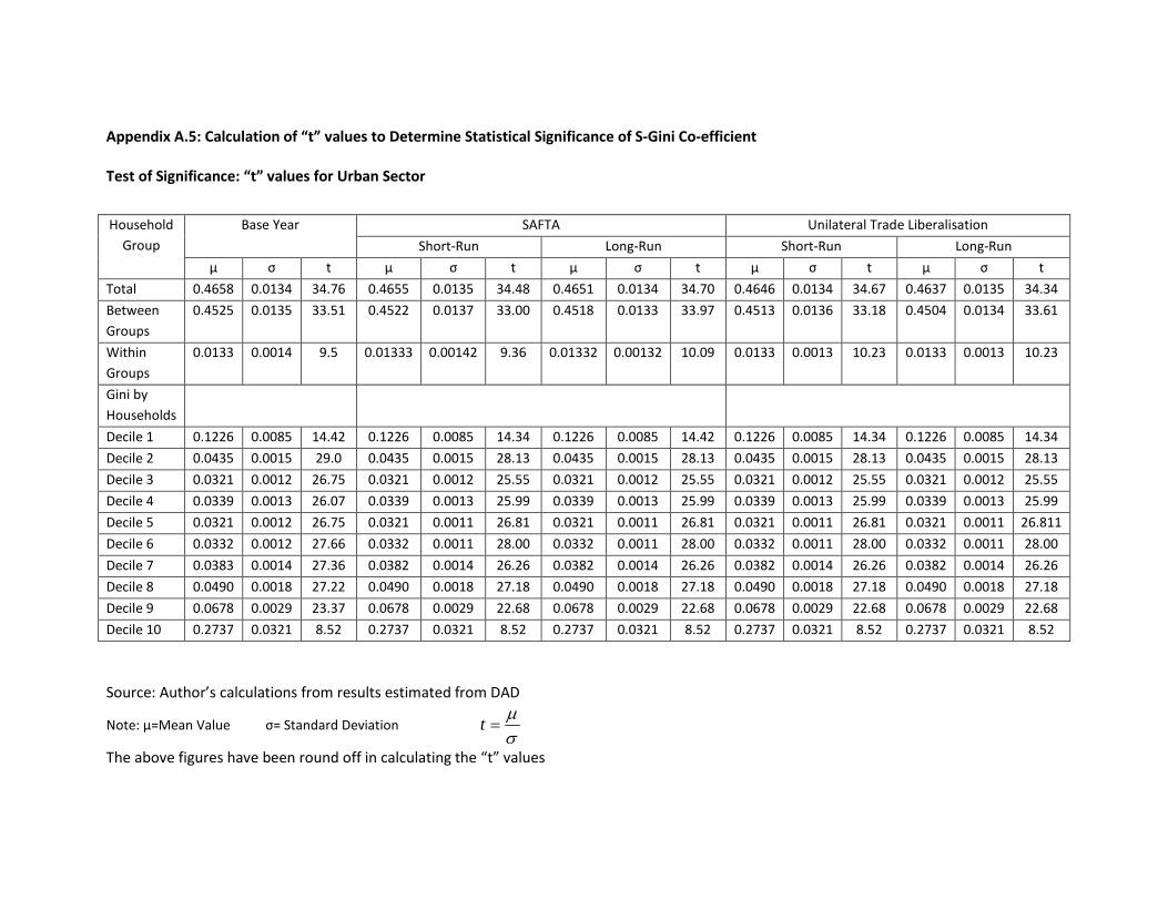
Appendix A.5: Calculation of “t” values to Determine Statistical Significance of S-Gini Co-efficient
Test of Significance: “t” values for Urban Sector
Source: Author’s calculations from results estimated from DAD
Note: µ=Mean Value σ= Standard Deviation σµ
=t
The above figures have been round off in calculating the “t” values
Household Group
Base Year SAFTA Unilateral Trade Liberalisation
Short-Run Long-Run Short-Run Long-Run
µ σ t µ σ t µ σ t µ σ t µ σ t
Total 0.4658 0.0134 34.76 0.4655 0.0135 34.48 0.4651 0.0134 34.70 0.4646 0.0134 34.67 0.4637 0.0135 34.34
Between Groups
0.4525 0.0135 33.51 0.4522 0.0137 33.00 0.4518 0.0133 33.97 0.4513 0.0136 33.18 0.4504 0.0134 33.61
Within Groups
0.0133 0.0014 9.5 0.01333 0.00142 9.36 0.01332 0.00132 10.09 0.0133 0.0013 10.23 0.0133 0.0013 10.23
Gini by Households
Decile 1 0.1226 0.0085 14.42 0.1226 0.0085 14.34 0.1226 0.0085 14.42 0.1226 0.0085 14.34 0.1226 0.0085 14.34
Decile 2 0.0435 0.0015 29.0 0.0435 0.0015 28.13 0.0435 0.0015 28.13 0.0435 0.0015 28.13 0.0435 0.0015 28.13
Decile 3 0.0321 0.0012 26.75 0.0321 0.0012 25.55 0.0321 0.0012 25.55 0.0321 0.0012 25.55 0.0321 0.0012 25.55
Decile 4 0.0339 0.0013 26.07 0.0339 0.0013 25.99 0.0339 0.0013 25.99 0.0339 0.0013 25.99 0.0339 0.0013 25.99
Decile 5 0.0321 0.0012 26.75 0.0321 0.0011 26.81 0.0321 0.0011 26.81 0.0321 0.0011 26.81 0.0321 0.0011 26.811
Decile 6 0.0332 0.0012 27.66 0.0332 0.0011 28.00 0.0332 0.0011 28.00 0.0332 0.0011 28.00 0.0332 0.0011 28.00
Decile 7 0.0383 0.0014 27.36 0.0382 0.0014 26.26 0.0382 0.0014 26.26 0.0382 0.0014 26.26 0.0382 0.0014 26.26
Decile 8 0.0490 0.0018 27.22 0.0490 0.0018 27.18 0.0490 0.0018 27.18 0.0490 0.0018 27.18 0.0490 0.0018 27.18
Decile 9 0.0678 0.0029 23.37 0.0678 0.0029 22.68 0.0678 0.0029 22.68 0.0678 0.0029 22.68 0.0678 0.0029 22.68
Decile 10 0.2737 0.0321 8.52 0.2737 0.0321 8.52 0.2737 0.0321 8.52 0.2737 0.0321 8.52 0.2737 0.0321 8.52

Test of Significance: “t” values for Rural Sector
Source: Author’s calculations from results estimated from DAD
Note: µ=Mean Value σ= Standard Deviation σµ
=t
The above figures have been round off in calculating the “t” values
Household Group
Base Year SAFTA Unilateral Trade Liberalisation
Short-Run Long-Run Short-Run Long-Run
µ σ t µ σ t µ σ t µ σ t µ σ t
Total 0.4040 0.007 57.17 0.4033 0.007 57.61 0.4032 0.007 57.6 0.4026 0.007 57.51 0.4025 0.007 57.5
Between Groups
0.3911 0.006 65.18 0.3904 0.006 65.06 0.3903 0.006 65.05 0.38977 0.006 64.96 0.38970 0.006 64.95
Within Groups
0.01289 0.0001 128.9 0.01288 0.0005 25.76 0.01287 0.0004 32.17 0.01286 0.0006 21.43 0.01286 0.0005 25.72
Gini by Households
Decile 1 0.2584 0.0672 3.84 0.2584 0.0672 3.84 0.2584 0.0672 3.84 0.2584 0.0672 3.84 0.2584 0.0672 3.84
Decile 2 0.0363 0.0005 64.77 0.0363 0.0005 64.77 0.0363 0.0005 64.77 0.0363 0.0005 64.77 0.0363 0.0005 64.77
Decile 3 0.0275 0.0004 66.41 0.0275 0.0004 66.41 0.0275 0.0004 66.41 0.0275 0.0004 66.41 0.0275 0.0004 66.41
Decile 4 0.0246 0.0003 69.21 0.0246 0.0003 69.21 0.0246 0.0003 69.21 0.0246 0.0003 69.21 0.0246 0.0003 69.21
Decile 5 0.0244 0.0003 69.94 0.0244 0.0003 69.93 0.0244 0.0003 69.93 0.0244 0.0003 69.93 0.0244 0.0003 69.93
Decile 6 0.0263 0.0003 69.62 0.0263 0.0003 69.63 0.0263 0.0003 69.63 0.0263 0.0003 69.63 0.0263 0.0003 69.63
Decile 7 0.0283 0.0004 70.85 0.0283 0.0004 70.85 0.0283 0.0004 70.85 0.0283 0.0004 70.85 0.0283 0.0004 70.85
Decile 8 0.0365 0.0005 69.06 0.0365 0.0005 69.06 0.0365 0.0005 69.06 0.0365 0.0005 69.06 0.0365 0.0005 69.06
Decile 9 0.0559 0.0008 64.98 0.0559 0.0008 64.98 0.0559 0.0008 64.98 0.0559 0.0008 64.98 0.0559 0.0008 64.98
Decile 10 0.3025 0.0178 16.94 0.3025 0.0178 16.94 0.3025 0.0178 16.94 0.3025 0.0178 16.94 0.3025 0.0178 16.94

Test of Significance: “t” values for Estate Sector
Source: Author’s calculations from results estimated from DAD
Note: µ=Mean Value σ= Standard Deviation σµ
=t
The above figures have been round off in calculating the “t” values
Household Group
Base Year SAFTA Unilateral Trade Liberalisation
Short-Run Long-Run Short-Run Long-Run
µ σ t µ σ t µ σ t µ σ t µ σ t
Total 0.2990 0.0134 22.31 0.29866 0.0134 22.28 0.29860 0.0134 22.28 0.29801 0.0134 22.23 0.29787 0.0134 22.22
Between Groups
0.2915 0.0135 21.59 0.29119 0.0136 21.41 0.29111 0.0135 21.56 0.29053 0.0136 21.36 0.29040 0.0135 21.51
Within Groups
0.0074 0.0001 74.0 0.0074 0.00013 56.92 0.0074 0.00013 56.92 0.0074 0.0001 74.0 0.0074 0.0001 74.0
Gini by Households
Decile 1 0.1053 0.02093 5.034 0.1053 0.02093 5.034 0.1053 0.02093 5.034 0.1053 0.02093 5.034 0.1053 0.02093 5.034
Decile 2 0.02791 0.0014 19.17 0.02791 0.0014 19.17 0.02791 0.0014 19.17 0.02791 0.0014 19.17 0.02791 0.0014 19.17
Decile 3 0.01882 0.0011 15.74 0.01882 0.0011 15.74 0.01882 0.0011 15.74 0.01882 0.0011 15.74 0.01882 0.0011 15.74
Decile 4 0.0166 0.0009 17.05 0.0166 0.0009 17.05 0.0166 0.0009 17.05 0.0166 0.0009 17.05 0.0166 0.0009 17.05
Decile 5 0.0220 0.0011 19.19 0.0220 0.0011 19.19 0.0220 0.0011 19.19 0.0220 0.0011 19.19 0.0220 0.0011 19.19
Decile 6 0.0188 0.0011 16.92 0.0188 0.0011 16.92 0.0188 0.0011 16.92 0.0188 0.0011 16.92 0.0188 0.0011 16.92
Decile 7 0.0272 0.0015 17.53 0.0272 0.0015 17.53 0.0272 0.0015 17.53 0.0272 0.0015 17.53 0.0272 0.0015 17.53
Decile 8 0.02631 0.0017 15.11 0.02631 0.0017 15.11 0.02631 0.0017 15.11 0.02631 0.0017 15.11 0.02631 0.0017 15.11
Decile 9 0.0399 0.0027 14.34 0.0399 0.0027 14.34 0.0399 0.0027 14.34 0.0399 0.0027 14.34 0.0399 0.0027 14.34
Decile 10 0.1923 0.0305 6.28 0.1923 0.0305 6.28 0.1923 0.0305 6.28 0.1923 0.0305 6.28 0.1923 0.0305 6.28

Appendix A.6: Calculation of “t” values to Determine Statistical Significance of FGT indices
Test of Significance: “t” values for Urban Sector
Source: Author’s calculations from results estimated from DAD
Note: µ=Mean Value σ= Standard Deviation σµ
=t
The above figures have been round off in calculating the “t” values
Household Group
Base Year SAFTA Unilateral Trade Liberalisation
Short-Run Long-Run Short-Run Long-Run
µ σ t µ σ t µ σ t µ σ t µ σ t
Total α =0 7.32 0.006 1220 7.12 0.006 1186 6.9 0.006 1150 5.01 0.005 1002 4.87 0.005 974
α =1 1.5 0.001 1500 1.46 0.002 730 1.43 0.001 1430 1.16 0.001 1160 1.15 0.001 1150
α =2 0.53 0.000 infinity 0.51 0.000 infinity 0.5 0.000 infinity 0.41 0.000 infinity 0.4 0.000 infinity
Gini by Households
Decile 1 α =0 72.92 0.036 2025 70.94 0.037 1917 69.59 0.038 1831 50 0.041 1219 48.64 0.041 1186
α =1 15.01 0.014 1072 14.62 0.014 1044 14.31 0.014 1022 11.6 0.013 892 11.49 0.013 883
α =2 5.3 0.007 752 5.16 0.007 737 5.08 0.007 725 4.1 0.006 683 4.06 0.006 676
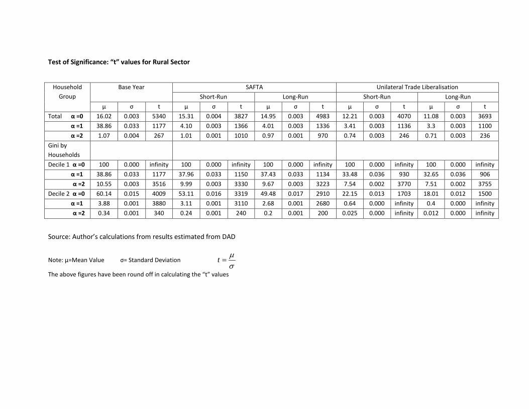
Test of Significance: “t” values for Rural Sector
Source: Author’s calculations from results estimated from DAD
Note: µ=Mean Value σ= Standard Deviation σµ
=t
The above figures have been round off in calculating the “t” values
Household Group
Base Year SAFTA Unilateral Trade Liberalisation
Short-Run Long-Run Short-Run Long-Run
µ σ t µ σ t µ σ t µ σ t µ σ t
Total α =0 16.02 0.003 5340 15.31 0.004 3827 14.95 0.003 4983 12.21 0.003 4070 11.08 0.003 3693
α =1 38.86 0.033 1177 4.10 0.003 1366 4.01 0.003 1336 3.41 0.003 1136 3.3 0.003 1100
α =2 1.07 0.004 267 1.01 0.001 1010 0.97 0.001 970 0.74 0.003 246 0.71 0.003 236
Gini by Households
Decile 1 α =0 100 0.000 infinity 100 0.000 infinity 100 0.000 infinity 100 0.000 infinity 100 0.000 infinity
α =1 38.86 0.033 1177 37.96 0.033 1150 37.43 0.033 1134 33.48 0.036 930 32.65 0.036 906
α =2 10.55 0.003 3516 9.99 0.003 3330 9.67 0.003 3223 7.54 0.002 3770 7.51 0.002 3755
Decile 2 α =0 60.14 0.015 4009 53.11 0.016 3319 49.48 0.017 2910 22.15 0.013 1703 18.01 0.012 1500
α =1 3.88 0.001 3880 3.11 0.001 3110 2.68 0.001 2680 0.64 0.000 infinity 0.4 0.000 infinity
α =2 0.34 0.001 340 0.24 0.001 240 0.2 0.001 200 0.025 0.000 infinity 0.012 0.000 infinity

Test of Significance: “t” values for Estate Sector
Source: Author’s calculations from results estimated from DAD
Note: µ=Mean Value σ= Standard Deviation σµ
=t
The above figures have been round off in calculating the “t” values
Household Group
Base Year SAFTA Unilateral Trade Liberalisation
Short-Run Long-Run Short-Run Long-Run
µ σ t µ σ t µ σ t µ σ t µ σ t
Total α =0 24.2 0.017 1423 23.36 0.017 1374 23.02 0.017 1354 17.31 0.015 1154 16.3 0.015 1086
α =1 4.93 0.004 1232 4.66 0.004 1165 4.48 0.004 1120 3.44 0.004 860 3.27 0.004 817
α =2 1.65 0.002 825 1.56 0.002 780 1.5 0.002 750 1.17 0.002 585 1.11 0.002 555
Gini by Households
Decile 1 α =0 100 0.000 infinity 100 0.000 infinity 100 0.000 infinity 100 0.000 infinity 100 0.000 infinity
α =1 35.73 0.018 1985 34.76 0.018 1931 34.14 0.018 1896 29.81 0.019 1568 28.91 0.02 1445
α =2 14.74 0.019 775 14.12 0.019 743 13.73 0.019 722 11.24 0.019 591 10.78 0.019 567
Decile 2 α =0 100 0.000 infinity 100 0.000 infinity 100 0.000 infinity 72.88 0.057 1278 62.71 0.063 995
α =1 12.09 0.005 2418 10.85 0.005 2170 9.98 0.005 1996 4.44 0.005 888 3.59 0.004 897
α =2 1.64 0.001 1640 1.36 0.001 1360 1.18 0.001 1180 0.37 0.005 74 0.27 0.001 270
Decile 3 α =0 42.37 0.064 662 33.89 0.061 555 30.05 0.059 509 - - - - - -
α =1 1.36 0.002 680 0.82 0.002 410 0.52 0.001 520 - - - - - -
α =2 0.05 0.000 infinity 0.02 0.000 infinity 0.01 0.000 infinity - - - - - -
References
Aghion, P., Caroli, E., & Garcia-Penalosa, C. (1999). Inequality and economic growth: the perspective of the new growth theories. Journal of Economic Literature, 37(4), 1615-1660.
Annabi, N., Cisse, F., & Cockburn, J. (2005). Trade Liberalisation, Growth and Poverty in Senegal: A Dynamic
Microsimulation CGE Model Analysis (CIRPEE Working Paper 05-12,). Retrieved from http://www.cirpee.org/fileadmin/documents/Cahiers_2005/CIRPEE05-12.pdf
Armstrong, P., & Burger, C. (2009). Poverty, inequality and the role of social grants: An analysis using decomposition techniques. Working Papers.
Athukorala, P. (2009). Trade liberalisation and poverty in south asia (series: routledge studies in the growth economies of asia). Recherche, 67, 02.
Atkinson, A. B. (1970). On the Measurement of Inequality. Journal of Economic Theory, 2, 244-263. Azariadis, C., & Stachurski, J. (2005). Poverty traps. Handbook of economic growth, 1, 295-384.
Bandara, J. (1991). Computable General Equilibrium Models for Developing Policy Analysis in Less Developed Countries. Journal of Economic Surveys, 5(1), 3-68.
Barro, R. J. (2000). Inequality and Growth in a Panel of Countries. Journal of Economic Growth, 5(1), 5-32.
Basmann, R. L., Hayes, K. J., Slottje, D., & Johnson, J. (1990). A general functional form for approximating the Lorenz curve. Journal of econometrics, 43(1), 77-90.
Boccanfuso, D., & Savard, L. (2001). A methodological note on computing FGT indicators from CGE models: Citeseer.
Borraz, F., Ferrés, D., & Rossi, M. (2012). Assessment of the distributive impact of national trade reforms in Brazil. Journal of Economic Inequality, 1-21.
Bouët, A., Mevel, S., & Thomas, M. (2010). Is SAFTA Trade Creating or Trade Diverting?
Bourguignon, F., & Morrison, C. (1990). Income Distribution, Development and Foreign Trade: A Cross-sectional Analysis. European Economic Review, 34(6), 1113-1132.
Bourguignon, F., Robilliard, A. S., & Robinson, S. (2003). Representative versus real households in the macroeconomic modelling of inequality Retrieved from http://dial.prd.fr/dial_publications/PDF/Doc_travail/2003-10.pdf
Bourguignon, F., & Spadaro, A. (2006). Microsimulation as a Tool for Evaluating Redistribution Policies: Society for the Study of Economic Inequility.
Champernowne, D. G. (1974). A comparison of measures of inequality of income distribution. The Economic Journal, 84(336), 787-816.
Cockburn, J. (2001). Trade Liberalisation and Poverty in Nepal A Computable General Equilibrium Micro Simulation Analysis. Retrieved from http://www.crefa.ecn.ulaval.ca/cahier/0118.pdf
Cockburn, J. (2005). Procedure for Conducting Poverty /Ditribution Analysis of CGE Simulation Results with DAD. Retrieved from http://www.pep-net.org/fileadmin/medias/pdf/non-parametric.pdf
Cogneau, D., & Robilliard, A.-S. (2001). Growth, Distribution and Poverty in Madagascar: Learning from a Microsimulation Model in a General Equilibrium Framework.

Decaluwé, B., Dumont, J. C., & Savard, L. (1999). Measuring Poverty and Inequality in a Computable General Equilibrium Model. Québec, Canada: Université Laval.
Decaluwé, B., Savard, L., & Thorbecke, E. (2005). General equilibrium approach for poverty analysis: with an application to Cameroon. African Development Review, 17(2), 213-243.
Department of Census and Statistics. (1990-91, 1995-96, 2002 and 2006-07,2009-10). Household Income and Expenditure Survey (HIES). Colombo, Sri Lanka: Department of Census and Statistics
Dhongde, S., & Research, W. I. f. D. E. (2004). Decomposing spatial differences in poverty in Índia: United nations university. World institute for development economics research (UNU-WIDER).
Dias, S. (1991). Economic Liberalization and the Development of Manufacturing in Sri Lanka. Asian Survey, 31(7), 613-629.
Dixon, P., Malakellis, M., & Meagher, T. (1995). A Microsimulation/Applied General Equilibrium Approach to Analysing Income Distribution in Australia: Plans and Preliminary Illustration. Paper presented at the The Industry Commission Conference on Equity, Efficiency and Welfare, Melbourne.
Dollar, D., & Kraay, A. (2002). Growth Is Good for the Poor. Journal of Economic Growth, 7(3), 195-225.
Dollar, D., & Kraay, A. (2004). Trade,Growth and Poverty. The Economic Journal 114(493), F22–F49.
Duclos, J., Araar, A. E. F. C., & Fortin, C. (2002). DAD: Distributive analysis/Analyse Distributive, User's Manual. Université Laval.[Links].
Duclos, J. Y., & Araar, A. (2006). Poverty and equity: measurement, policy and estimation with DAD (Vol. 2): Springer Verlag.
Evans, D. ( 2001). Identifying Winners and Losers in Southern Africa from Global Trade Policy Reform: Integrating Findings from GTAP and Poverty Case Studies. Paper presented at the Fourth Annual Conference on Global Economic Analysis, Purdue University, West Lafayette.
Filho, J. B., & Horridge, J. M. (2004). Economic integration, Poverty and Regional Inequality in Brazil: Centre of Policy Studies, Monash University.
Foster, J., Greer, J., & Thorbecke, E. (1984). A class of decomposable poverty measures. Econometrica: Journal of the Econometric Society, 761-766.
Gilbert, J., & Oladi, R. (2010). Regional Trade Reform Under SAFTA and Income Distribution in South Asia. Retrieved from https://www.gtap.agecon.purdue.edu/resources/download/4988.pdf
Gunetilleke, N., & Senanayake, D. (2004). Monetary Poverty Estimates in Sri Lanka: Selected Issues. Asian Development Bank: Asian Development Bank.
Haughton, J. H., & Khandker, S. R. (2009). Handbook on poverty and inequality: World Bank Publications.
Jayanetti, S., & Tilakaratna, G. (2005). Impact of Trade Liberalization on Poverty and Houehold Welfare in Sri Lanka Research Studies: Poverty and Social Welfare Series Colombo: Institute of Policy Studies.
Kakwani, N. (1980). On a Class of Poverty Measures. Econometrica, 48(2), 437–446.
Kakwani, N. (1986). Analyzing redistribution policies: a study using Australian data: Cambridge Univ Pr.
Kakwani, N., & Subbarao, K. (1990). Rural Poverty and Its Alleviation in India. Economic and Political Weekly, 31(March), A2-A16.

Khondker, B. H., & Raihan, S. (2004). Welfare and poverty impacts of policy reforms in Bangladesh: A general equilibrium approach.
Li, H., Squire, L., & Zou, H. (1998). Explaining International and Intertemporal Variations in Income Inequality. Review of Development Economics, 2(3), 318-334.
Lundberg, M., & Squire, L. (2003). The Simultaneous Evolution of Growth and Inequality. Economic Journal, 113(4), 326-344.
McCulloch, N., Winters, A., & Cirera, X. (2001). Trade liberalization and poverty: A handbook: Cambridge Univ Press.
Meagher, G. A. (1996). Forecasting changes in the distribution of income: an applied general equilibrium approach’, in Harding, A. . Microsimulation and Public Policy, 361–384.
Minhas, B., Jain, L., Kansal, S., & Saluja, S. (1987). On the Choice of Appropriate Consumer Price Indices and Datasets for Estimating the Incidence Of Poverty in India. Indian Economic Review, 12, 19-49.
Naranpanawa, R. M. A. K. B. (2005). Trade Liberalisation and Poverty In a Computable General Equilibrium Model: The Sri Lankan Case. (PhD), Griffith University. Retrieved from http://www4.gu.edu.au:8080/adt-root/uploads/approved/adt-QGU20070130.165943/public/02Whole.pdf
Parzen, E. (1962). On the Estimation of Probability Density and Model. Annals of Mathematical Statistics, 27, 1065-1076.
Ravallion, Martin, & Lokshin, M. (2004). Gainers and Losers from Trade Reform in Morocco. Paper presented at the Seventh Annual Conference on Global Economic Analysis, Washington, DC.
Ravallion, M., & Sen, B. (1996). When method matters: Monitoring poverty in Bangladesh. Economic Development and Cultural Change, 44(4), 761-792.
Rosenblatt, M. (1956). Remarks on Some Nonparametric Estimates of the Density Function. Annals of Mathematical Statistics, 27, 832-837.
Ryu, H. K., & Slottje, D. J. (1996). Two flexible functional form approaches for approximating the Lorenz curve. Journal of econometrics, 72(1), 251-274.
Savard, L. (2004). Poverty and Inequality Analysis within a CGE Framework: a Comparative Analysis of the Representative Agent and Micro-Simulation Approaches. Retrieved from http://www.cirpee.org/fileadmin/documents/Cahiers_2004/CIRPEE04-12.pdf
Savard, L. (2005). Poverty and Inequality Analysis within a CGE Framework: A Comparative Analysis of the Representative Agent and Microsimulation Approaches. Development Policy Review, 23(3), 313-331.
Sen, A. K. (1976). Poverty: An Ordinal Approach to Measurement Econometrica, 44, 219-231.
Siriwardana, M. (2001). Looking Beyond SAARC: Some Trade Liberalisation Options for Sri Lanka. Asian Studies Review, 25(4), 453-477.
Sothea, O. (2009). Income Distribution and Poverty in a CGE Framework : A Proposed Methodology. (PhD), Monash University,, Melbourne, Australia.
The Central Bank of Sri Lanka. (2003/2004). Consumer Finance and Socio-Economic Survey Colombo: The Central Bank of Sri Lanka.
The Central Bank of Sri Lanka. (2010). Annual Report. Colombo, Sri Lanka: The Central Bank of Sri Lanka.
The World Bank. (2007). Sri Lanka Poverty Assessment. World Bank, Washington D.C.
Van Ourti, T., & Clarke, P. (2008). The bias of the Gini coefficient due to grouping: revisiting first-order corrections: Tinbergen Institute.
Villasenor, J. A., & Arnold, B. C. (1989). Elliptical lorenz curves. Journal of econometrics, 40(2), 327-338.
Wijayasiri, J., & Studies, I. o. P. (2007). Utilization of Preferential Trade Arrangements: Sri Lanka's Experience with the EU and US GSP Scheme: Institute of Policy Studies.
Winters, A. L. (2004). Trade Liberalisation and Economic Performance: An Overview. The EconomicJ ournal, 114, F 4-F21.
World Trade Organisation. (2004). Sri Lanka Trade Policy Review (Vol. Report by the Secretariat. WT/TPR/S/128. Geneva: WTO).
Zheng, B. (1993). An Axiomatic Characterization of the Watts Index. Economics Letters, 42, 81-86.
Related Documents