The Influence and Role of Arts on Community Well-being by HeeKyung Sung A Dissertation Presented in Partial Fulfillment of the Requirements for the Degree Doctor of Philosophy Approved December 2015 by the Graduate Supervisory Committee: Mark A. Hager, Chair Roland Kushner Woojin Lee Rhonda Phillips ARIZONA STATE UNIVERSITY May 2016

Welcome message from author
This document is posted to help you gain knowledge. Please leave a comment to let me know what you think about it! Share it to your friends and learn new things together.
Transcript

The Influence and Role of Arts on Community Well-being
by
HeeKyung Sung
A Dissertation Presented in Partial Fulfillment of the Requirements for the Degree
Doctor of Philosophy
Approved December 2015 by the Graduate Supervisory Committee:
Mark A. Hager, Chair
Roland Kushner Woojin Lee
Rhonda Phillips
ARIZONA STATE UNIVERSITY
May 2016

i
ABSTRACT
Arts and culture function as indispensable parts of humans’ lives. Numerous
studies have examined the impact and value of arts and culture, from individual quality of
life to overall community health. However, research has been less focused on identifying
the influence of crucial dimensions of arts and culture on overall community well-being,
and contributing to understanding the intertwining connection between these elements
and community well-being. To explore the dimensions of arts and cultural resources and
community well-being, and in turn, to present the relationship between them in a
community, this dissertation was based on three subsequent studies. A total of 518
counties were included in the analysis. Specifically, this study is unique in that it sought
evidence based on county-level data drawn on the Local Arts Index (LAI) from
Americans for the Arts (AFA) and County Health Rankings & Roadmaps (CHRR)
variables to provide an arts-community measurement system suggesting critical and
meaningful variables among a wide range of existing data. The results revealed the
positive impacts of arts and cultural resources on community well-being. Each arts and
cultural domain also has critical relationships with community individual, social, and
economic well-being. Specifically, the ‘arts business’ domain was considerably
associated with community individual well-being and comprehensive community well-
being. The ‘arts consumption’ domain showed synthetically significant associations with
community’s individual and economic well-being, and by extension, influenced
comprehensive community well-being. Lastly, the ‘arts nonprofits’ domain was related to
all the components of community well-being. In conclusion, residents’ arts consumption
and the existence of arts and cultural/creative industries, including arts nonprofits, are

ii
constantly suggested as key to improving county-level community well-being. This study
centers on presenting a more realistic vision of how arts and cultural resources are
associated with community well-being components. Recognizing the power of arts and
cultural resources in society and bolstering them to promote community well-being is a
global issue of the utmost pertinence. Thus, research utilizing a longitudinal data-driven
approach is likely to continue measuring the impact of arts and culture, and examining
how they are related to and can strengthen community well-being.

iii
DEDICATION
This dissertation is dedicated to my husband June, and my loving parents.

iv
ACKNOWLEDGMENTS
I would like to sincerely thank Dr. Mark A. Hager, my committee chair and advisor, for
his guidance and great support through my PhD journey. Dr. Hager’s advice and
knowledge not only influenced the development of my dissertation, but also led me to
become a better scholar.
I would also like to express my appreciation to my committee members, Dr. Woojin Lee,
Dr. Rhonda Phillips, and Dr. Roland Kushner. Their valuable suggestions and
encouragement led me to successfully complete my dissertation and made this experience
a wonderful opportunity for my personal growth as a researcher. My journey would not
have been possible without their help and support. Also, I would like to acknowledge and
thank American for the Arts for providing me with the opportunity to conduct this
research using the Local Arts Indicators.
I am so thankful to my family for their unending support, love, and prayers. Especially, I
am so grateful to my husband, June for his continuous care and encouragement. Without
his wholehearted support, it would have been impossible to reach the end of this long
journey. I dedicate this work to them.
Above all else, I thank God for being with me along the way.

v
TABLE OF CONTENTS
Page
LIST OF TABLES ............................................................................................................. ix
LIST OF FIGURES .......................................................................................................... xii
CHAPTER
1 INTRODUCTION ................................................................................................... 1
2 VALUE OF THE ARTS .......................................................................................... 7
Arts and Culture as Cultural Capital ................................................................... 8
Impact of the Arts on Individuals ..................................................................... 12
Impact of the Arts on Society ........................................................................... 15
Impact of the Arts on Economic Prosperity ...................................................... 20
Measurement of Arts Impact ............................................................................. 23
How Art Works System Map ............................................................................ 30
3 THE DATA: THE LOCAL ARTS INDEX (LAI) ................................................ 33
Background ....................................................................................................... 33
Conceptual Dimensions of CAVM ................................................................... 35
Arts Activity................................................................................................. 36
Cultural Participation ............................................................................. 36
Cultural Programming ........................................................................... 36
Arts Resources ............................................................................................. 37
Consumer Expenditure........................................................................... 38
Nonprofit Arts Revenue ......................................................................... 39
Government Support .............................................................................. 40

vi
CHAPTER Page
Local Connection to National Organizations ......................................... 40
Artists and Arts Businesses .................................................................... 41
Arts Nonprofits ...................................................................................... 42
Arts Competitiveness ................................................................................... 44
Establishments, Employees, and Payroll ............................................... 45
Support of the Arts ................................................................................. 46
Local Culture Character ............................................................................... 47
Institutional and Entrepreneurial Arts .................................................... 47
Local and Global Representation ........................................................... 48
Professional Arts Training ..................................................................... 49
Discussion of the Community Arts Vitality Model (CAVM) ........................... 50
4 EMPIRICAL DIMENSIONS OF COMMUNITY ARTS ..................................... 52
Methodology ..................................................................................................... 52
The Research Parameters and Procedure ..................................................... 53
Steps in Exploratory Factor Analysis .......................................................... 56
Results ............................................................................................................... 58
The Exploratory Factor Analysis (EFA): Underlying Dimensions of
Community Arts........................................................................................... 58
Data Preparation..................................................................................... 58
Factor Extraction and Rotation .............................................................. 70
Interpretation of Factor Results ............................................................. 74
Discussion ......................................................................................................... 83

vii
CHAPTER Page
5 ARTS AND COMMUNITY WELL-BEING ........................................................ 87
A General Concept of Community Well-Being ................................................ 87
Measuring Community Well-Being .................................................................. 94
Approach to Conceptualization of Arts and Culture on Community
Well-Being ....................................................................................................... 99
Arts and Community Well-Being Model ........................................................ 104
Summary ......................................................................................................... 108
6 EMPIRICAL DIMENSIONS OF COMMUNITY WELL-BEING .................... 110
Data: Community Well-Being ........................................................................ 110
The County Health Rankings And Roadmaps (CHRR) ............................ 110
Community Well-Being Variables ............................................................ 112
Individual Well-Being ......................................................................... 112
Social Well-Being ................................................................................ 113
Economic Well-Being .......................................................................... 115
Methodology ................................................................................................... 117
The Research Parameters and Procedure ................................................... 118
The results ....................................................................................................... 122
Principal Component Analysis .................................................................. 122
Factor Score ............................................................................................... 132
Higher-Order Factor Analysis .................................................................... 134
Summary ......................................................................................................... 136
7 ANALYSIS: ARTS IMPACT ON COMMUNITY WELL-BEING ................... 139

viii
CHAPTER Page
Data Preparation .............................................................................................. 140
Overall Sample Description ....................................................................... 140
Variable Definition .................................................................................... 142
Multiple Regression Analysis ......................................................................... 144
Research Findings ........................................................................................... 148
8 CONCLUSION & DISCUSSION ....................................................................... 185
Conclusion ...................................................................................................... 186
Contribution .................................................................................................... 199
Limitations and Future Research .................................................................... 203
REFERENCES ............................................................................................................... 208
APPENDIX
A NTEE CODES FOR ARTS NONPROFIT ORGANIZATIONS IN THE LAI .. 225
B THE ITEMS EXCLUDED FOR EXPLORATORY FACTOR ANALYSIS......228

ix
LIST OF TABLES
Table Page
1. Economic Impact of Arts and Culture Industry ............................................................ 22
2. A Summary of Selected Studies on Measurement of Arts Impact ............................... 25
3. Indicators of Arts Activities .......................................................................................... 37
4. Indicators of Arts Resources ......................................................................................... 43
5. Indicators of Arts Competitiveness ............................................................................... 46
6. Indicators of Local Cultural Character ......................................................................... 50
7. Potential Arts and Cultural Variables ........................................................................... 55
8. Descriptive Statistics for Local Arts and Culture Items ............................................... 60
9. Descriptive Statistics of Variables with Data Transformation ..................................... 63
10. KMO and Bartlett’s Test of Sphericity ....................................................................... 69
11. Factor Correlation Matrix ........................................................................................... 73
12. KMO and Bartlett’s Test of Sphericity ....................................................................... 75
13. Correlations, Measures for Sampling Adequacy, and Partial Correlations ................ 76
14. Results for the Extraction of Common Factors........................................................... 78
15. Pattern/Structure Matrix Coefficients and Communalities (h2) .................................. 80
16. The Comparison between CAVM and ABCN............................................................ 85
17. Summary of Studies related to Community Well-Being (CWB) Measurement ......... 94
18. Summary of Arts and Cultural Impact Related to Community Well-Being ............. 101
19. Prediction of Variables Loading for Individual Well-Being Factor ......................... 113
20. Prediction of Variables Loading for Social Well-Being Factor ................................ 115
21. Prediction of Each Variables Loading for Economic Well-Being Factor ................ 116

x
Table Page
22. Descriptive Statistics for Community Well-Being Variables ................................... 118
23. Community Well-Being Variables Loaded for Each Factor ..................................... 124
24. KMO and Bartlett’s Test of Sphericity ..................................................................... 125
25. Correlations, Measures for Sampling Adequacy, and Partial Correlations; Indicators
of CWB ................................................................................................................... 126
26. Results for the Extraction of Principal Component Analysis ................................... 128
27. Pattern/Structure Matrix Coefficients and Communalities (h2) ................................ 130
28. Component Correlation Matrix ................................................................................. 132
29. Factor Score Coefficient Matrix ............................................................................... 134
30. Correlation of Primary Factors, Higher-order Factor Loadings, and Reliability ...... 136
31. Distrubution of County Populations in 2010 ............................................................ 140
32. Median Households Income 2005-2009 ................................................................... 141
33. Independent Variables and Dependent Variables ..................................................... 143
34. Pearson Correlation among the Six Arts Business Variables ................................... 146
35. Pearson Correlation among the Six Arts Consumption Variables ............................ 147
36. Pearson Correlation among the Six Arts Nonprofit Variables .................................. 147
37. Model 1: Arts Business Variables on Community Individual Well-Being .............. 152
38. Model 2: Arts Consumption Variables on Community Individual Well-Being ....... 153
39. Model 3: Arts Nonprofit Variables on Community Individual Well-Being ............. 155
40. Model 4: Arts Business Variables on Community Social Well-Being ..................... 157
41. Model 5: Arts Consumption Variables on Community Social Well-Being ............. 160
42. Model 6: Arts Nonprofit Variables on Community Social Well-Being ................... 161

xi
Table Page
43. Model 7: Arts Business Variables on Community Economic Well-Being............... 164
44. Model 8: Arts Consumption Variables on Community Economic Well-Being ....... 166
45. Model 9: Arts Nonprofit Variables on Community Economic Well-Being ............. 168
46. Model 10: Arts Business Variables on Overall Community Well-Being ................. 170
47. Model 11: Arts Consumption Variables on Overall Community Well-Being ......... 172
48. Model 12: Arts Nonprofit Variables on Overall Community Well-Being ............... 174
49. Multiple Regression Models Predicting Community Individual Well-Being .......... 177
50. Multiple Regression Models Predicting Community Social Well-Being ................. 179
51. Multiple Regression Models Predicting Community Economic Well-Being........... 181
52. Multiple Regression Models Predicting Overall Community Well-being ............... 183
53. Summary of Constant Significant Variables across Models..................................... 195

xii
LIST OF FIGURES
Figure Page
1. “ How Art Works” Illustrated by Iyengar et al. (2012, P. 17) ..................................... 31
2. Four Dimensions of CAVM (Source From Cohen, Cohen, & Kushner, 2012)............ 35
3. Scatterplot Matrix of Variables ..................................................................................... 65
4. Scree Plot Produced by Principal Components Extraction ........................................... 72
5. The Mandala of Wellbeing Adapted from Michalos et al. (2010, P. 7) ....................... 93
6. A Diagram of the Evidence of Arts and Cultural Contribution to CWB .................... 102
7. Arts and Community Well-Being Excerpted and Modified from “How Art Works”
Illustrated by Iyengar and Colleagues (2012, P. 17) ............................................... 103
8. The Relationship between Arts and Community ........................................................ 105
9. The Model of Arts and Community Well-Being. ....................................................... 105
10. An Expanded Model of Arts and Community Well-Being ...................................... 107
11. Bivariate Scatterplots ................................................................................................ 120
12. The Scree Plot of the PCA for Community Well-Being Components ..................... 123
13. Structure and Loading of Community Well-Being Items on Second Order Factors 137
14. Analyses of Standardized Residuals ......................................................................... 145
15. An Expanded Model of Arts and Community Individual Well-Being ..................... 149
16. An Expanded Model of Arts and Community Social Well-Being ........................... 156
17. An Expanded Model of Arts and Community Economic Well-Being ..................... 163
18. An Expanded Model of Arts and Overall Community Well-Being ......................... 169
19. Diagram Of Arts And Cultural Contribution To CWB ............................................ 192

1
CHAPTER 1
INTRODUCTION
In recent years, the value of arts and culture and its impact on communities has
drawn attention from both academia and practitioners. It has been strongly argued that
arts and cultural facilities, strategies, productions, and consumptions are important for
community revitalization, which contains processes and outcomes that enhance social,
cultural, and economic development (Blessi, Tremblay, Sandri, & Pilati, 2012; Grodach,
2010; Grodach & Loukaitou-Sideris, 2007; Pratt, 2010). The exploration of arts and
cultural resources has spawned many community projects. In turn, attempts to examine
connections between arts and community have placed the arts and culture within the
broader concept of well-being, which embraces from individual quality of life to overall
community health.
More recently, academic accomplishments dedicated to understanding and
determining the benefits of arts and culture have surfaced in the quality of life and well-
being literature. Given a growing body of literature, sound arts infrastructure and various
arts and cultural activities seem to provide promising opportunities for enhancing
community health and the quality of life of residents. For example, Grodach and
Loukaitou-Sideris (2007) argued that improving the quality of life of all citizens is the
most essential benefit of cultural activities. A body of studies by the Victorian Health
Promotion Foundation (VicHealth) emphasized community-based cultural events and
networks as one way of development of community health and well-being (Eckersley,
Wierenga, & Wyn, 2005; VicHealth, 2006, 2013). By extension, much research of the
Arts Council England emphasized not only values of arts and culture on people’s health

2
and well-being, but also a wider impact on their society and economy (Arts Council
England, 2015a, 2015b; Reeves, 2002; Tuck & Dickinson, 2015).
Traditionally, arts have functioned as indispensable parts of humans’ lives. Arts
were considered as one virtue of a good person which stood for a wealth of cultural,
intellectual, and aesthetic value in ancient Athens. Furthermore, philosophers such as
Plato, Aristotle, and Locke claimed the influence of arts education on children’s value
and behaviors (Mark & Charles, 1992). The significance of arts and culture to American
life was given attention to after the Revolutionary War in the 18th century. Americans
began to pursue intellectual, artistic, and creative activities in the form of literature,
music, and poetry to enhance their intellectual enjoyment in leisure and quality of life.
Furthermore, the City Beautiful Movement in the late 19th century emerged as a societal
function of arts, beautifying communities and increasing quality of life for residents
(Phillips, 2004). Since the 1980s, arts and culture, as a characteristic of distinctive
competitiveness against other places, have been used as important economic resources for
community development, and in turn, have become a crucial industry for many
communities (Ginsburgh & Throsby, 2006).
Supportively, empirical evidence for the impacts and values of the arts has been
reviewed by numerous studies. These have ranged from studies on health (Stuckey &
Nobel, 2010) and well-being (South, 2006), quality of life (Michalos & Kahlke, 2010),
helping at-risk youth (Rapp-Paglicci, Ersing, & Rowe, 2006), education (Ruppert, 2006),
social networks (Greaves & Farbus, 2006), social inclusion (Goodlad, Hamilton, &
Taylor, 2002a, 2002b), social identity (McClinchey, 2008), community engagement
(Johnson & Stanley, 2007), community economic development (Borrup, 2006; Stern and

3
Seifert, 2010), and regeneration (Grodach & Loukautou-Sideris, 2007). Following this
lead, researchers and advocacy agents have used arts and cultural assessment to support
their claims that arts and cultural prosperity has a strong correlation with regional
economies and social health (Borgonovi, 2004; Jackson, Houghton, Russell, & Triandos,
2005; Lowe, 2000; Markusen & Gadwa, 2010b; Matarasso & Chell, 1998).
Along with attention to assessment of the impact of arts and cultural value on
community, some studies, however, have acknowledged its methodological challenges
(Evans, 2005; Galloway, 2009, Guetzkow, 2002; Newman, Curtis, & Stephens, 2003).
One of the most commonly presented issues is that much research relies heavily on self-
reported evidence collected by selective arts programs and projects (Galloway, 2009;
Guetzkow, 2002; Merli, 2002; Mulligan, Humphery, James, Scanlon, Smith & Welch,
2006). Thus, it might expect to some degree to inflate results, while not every interaction
results in a positive and long-term community-wide impact.
Furthermore, Guetzkow (2002) and Hoynes (2003) note that the use of the
existing data is somewhat limited by a lack of sample size, regularity, and development
of standard measures. For example, most research into the benefits and impacts of arts
and culture has been based on case studies focusing on specific arts events, cities, or
regions. Also, even though communities create arts and cultural indicators, different
communities are apt to collect different kinds of data, complicating efforts to construct a
clear concept having internal validity. Leaving the issues of arts’ aesthetic or instrumental
values for society aside, research is less focused on identifying the influence of crucial
dimensions of arts and culture on overall community well-being, and understanding the
intertwining connection between these elements and community well-being. It is still not

4
clear that indeed arts and culture cause community well-being. Although some cases
show a robust connection between arts and community development (Blessi et al., 2012;
Lavanga, 2006; Markusen & Gadwa, 2010a; Strom, 1999), they cannot be generalized
because different cities capitalize on arts and culture in different ways.
Therefore, I propose a dissertation about the influence and role of arts and culture
on communities, building a clear conceptual framework that links arts and culture to
broader community well-being and deepening the understanding of the quality of life in
communities. Instead of making overstated claims about and unconditional supports of
the potential of the values and impacts of arts and culture on peoples’ lives and
communities, a more realistic vision of how arts and cultural resources influence
community needs to be substantiated beyond following the self-referential, anecdotal
evidences. The initial intention of this research was to identify arts and cultural resources
in a community and examine the relationship between these resources and overall
community well-being outcomes. Developing a new set of indicators for assessing
community well-being outcome of the arts and cultural resources was not the aim of this
study; rather, I placed the value in using publicly available arts and community data.
Specifically, in pursuit of a methodologically sound approach, this study has sought
evidence based on county level data drawn on the Local Arts Index (LAI) from American
for the Arts (AFA) and County Health Rankings & Roadmaps (CHRR) variables since
county level data could be adequate to not only embrace distinct community
characteristics but also make possible the comparison of community results.
To help advance research in arts and community, this study 1) gathers crucial and
key evidence connected to arts-based community development from previous literature,

5
2) organizes themes and concepts related to arts and community in order to provide an
arts-community measurement system suggesting critical and meaningful variables among
a wide range of existing data, and 3) presents findings that emerged from these variables
and the relationship between the arts and community at the county level.
This dissertation takes the How Arts Works System Map developed by the
National Endowment for the Arts (NEA) as its starting point. This system map is an
overarching theoretical background to investigate various arts and cultural resources on
different community outcomes. The study is divided into three parts. The first part
(chapters 2, 3, and 4) reviews the impacts of arts in community based on previous
literature, and explains several conceptual dimensions of arts and cultural factors drawn
from the Local Arts Index (LAI) from American for the Arts. After reviewing the
literature on arts and cultural resources in community, chapter 4 identifies and organizes
representative factors which play an important role in communities.
The second part (chapters 5 and 6) develops community well-being concepts
related to arts and cultural activities. After reviewing the literature on community well-
being and its related concept, based on the How Arts Works System Map (Iyengar et al.,
2012) as a theoretical framework, chapter 5 proposes a comprehensive model of arts and
community well-being and hypotheses for this study. In chapter 6, drawing on CHRR
variables, the study explores how these variables are classified within the three different
aspects of community well-being, that is individual, social, and economic community
well-being.
The last part (chapter 7) combines the previous two sections to examine the
hypotheses and conceptual framework for this study, and expounds the overall arts and

6
cultural tendency on community well-being issues. It demonstrates the current state of
relationship between factors of arts and cultural assets (e.g., arts and cultural participation,
resources, and commodities) and community – individual, social, and economic –
outcomes such as state of health, level of education, crime rate, income levels, and
employment rate. The presentations on the findings in this chapter help to bolster a
theoretical framework presenting a full and detailed picture of the ongoing relationship
between arts and community well-being with an eye to examining both empirical and
objective evidence that is collected from public data. Finally, chapter 8 includes a
summary of the findings of the three sections of the paper, along with discussions and
implications to the study of arts management and community well-being.

7
CHAPTER 2
VALUE OF THE ARTS
Since John Dewey (1934) declared in his book Arts as Experience that the value
of the arts has to be incorporated into social relationships systems, the impact of this
value on individuals and society has been discussed in various academic fields, as well as
among arts practitioners and policymakers. Setting the “art for its own sake” versus “art
for social value” argument aside, much research has provided empirical evidence of the
impact and value of the arts as autotelic experience, to the arts as an instrumental way of
sustaining society. In 1965, The National Foundation for the Arts and Humanities Act
was adopted; reflecting the importance of arts and culture in the United States (Hoynes,
2003). Local government entities including arts boards and arts councils were established
as a result and began to reflect on arts-based community development within public
policy. They focused on public understanding of, and appreciation for, the positive
impact of the arts on developing and expressing individual creativity, providing a tool for
economic growth, and connecting people across cultural boundaries in order to enrich
community life (Moore & Moore, 2005).
Since then, community prosperity through arts-based development has been
somewhat taken for granted by communities, residents, policy-makers, and even
academics. Beyond the expression of individual creativity and artistic appreciation, the
arts and culture of a community are regarded as an important asset for creating an
economic niche within the community and generating a distinctive community identity
(Florida, 2002a, 2002b; Foster, 2009; Markusen & Schrock, 2006; Richards, 2011). Thus,
this chapter focuses on previous literature on arts and cultural functions as forms of

8
community capital, and then discusses their role and impact on communities. Lastly, a
comprehensive arts and cultural system map developed by Iyengar and colleagues (2012)
is reviewed as a basis for exploring the value and impact of the arts.
2.1 Arts and Culture as Cultural Capital
Culture, in narrow usage, may connote peoples’ tastes in the arts. From this
perspective, it could be knowledgement of and participation in high culture (DiMaggio &
Useem, 1982). However, the term culture can be defined more broadly, embracing a way
of viewing the world, traditions, and languages. Culture is a crucial element for fostering
cohesive and sustainable communities (Jeannotte, 2003). In this vein, the term ‘cultural
capital’ encompasses arts and cultural products and is explained as any cultural resources
or assets communities own, whether they are tangible or intangible. Although the scope
of cultural capital varies by research context, it can be consumed, invested in, and
exchanged within society so as to promote the well-being of communities (Berkes &
Folke, 1994; Bourdieu, 1986; Jacobs, 2007; Jeannotte, 2003; Throsby, 1999).
Flora and colleagues describe cultural capital as “the shared products of society”
(Flora et al., 1992, p. 58). According to the Community Capitals Framework (CCF)
developed by Flora and colleagues, there are seven diverse community assets for
analyzing how communities work. These include natural, human, cultural, social,
financial, built, and political capital (Emery & Flora, 2006; Flora, Flora, & Fey, 2007;
Gutierrez-Montes, Emery, & Fernandez-Baca, 2009). In the CCF, cultural capital is
described as representing each community’s distinctive character–which is inherent in the
language, shared identity, attitude, and heritage of community members–and influencing

9
how creativity and innovation emerge in a community (Emery & Flora, 2006; Jacobs,
2007). As one way of expressing a community’s distinctiveness, festivals, celebrations,
and events are a part of cultural capital. Others include community stories, food, and
tradition, which affect the everyday lives of community members. In a community
system, cultural capital has significant value in helping create a flow of other assets so as
to sustain a community.
In a similar manner, Berkes and Folke (1992) posit that cultural capital is a
vehicle for sustainability. They define cultural capital as “factors that provide human
societies with the means and adaptations to deal with the natural environment and to
actively modify it” (Berkes & Folke, 1994, p. 130). They stress the importance of cultural
capital as an interface between natural capital and human-made capital (e.g., economic
activity) (Berkes & Folke, 1992, 1994). In this regard, cultural capital is thought to attract
people to visit a community and indeed may influence not only the economic prosperity
of a community but also its social capital, human capital, and overall infrastructures
(Jacobs, 2007).
On the other hand, Bourdieu identified the concept of cultural capital at the
individual level. It may help to form an individual’s character and guide their actions and
tastes. Bourdieu defined cultural capital as “the form of long-lasting dispositions of the
mind and body [and] the form of cultural goods” (Bourdieu, 1986, p.243). Also, in the
way of cultural expression, cultural capital includes material objects such as paintings,
written works, dances, and music, as well as a symbolic legacy that is transferable
through generations. The transmission of cultural capital makes a group of people enable
the reproduction of social structure and maintain their social status. Furthermore,

10
Bourdieu suggests that cultural capital in the form of academic qualifications establishes
the value of the holder of a given qualification (Bourdieu, 1986; Jeannotte, 2003).
Recently, studies demonstrate that an investment of cultural capital provides benefits in
academic performance, physical and psychological fitness, and social relationships
(Daykin, Viggiani, Pilkington, & Moriatry, 2013; Dooris, 2005; Kinder & Harland, 2004;
Lobo & Winsler, 2006; Schwarz & Tait, 2007; Spandler, Secker, Kent, Hacking, &
Shenton, 2007).
On the one hand, Jeannotte (2003) describes the role of cultural capital for the
collective well-being of society. She argues that cultural capital is created by peoples’
engagement in arts, cultural, and heritage activities. Also, being involved in arts projects
helps encourage intercultural connection and understanding of others. Community
cultural organizations and local arts agencies play an important role in strengthening
social ties and community spirit. Thus, cultural capital here is a crucial input for the
formation of institutions, norms, and shared meanings in a community (Jeannotte, 2003).
On the other hand, by incorporating cultural capital into economic value, much
research highlights growing cultural consumption as an essential economic resource for
local development (Florida, 2002b; Lavanga, 2006). As an approach to the economic
concept of cultural capital, Throsby (1999) defined cultural capital as “the stock of
cultural value embodied in an asset” (p. 6). This asset can be used in the production of
goods and services. As people consume these goods and services, cultural value
facilitates economic value. Tangible cultural capital is embodied in artworks, artifacts,
heritage buildings, and structures. On the other hand, intangible cultural capital comes in
the form of ideas, beliefs, traditions, and languages. Moreover, as a part of the arts,

11
intangible cultural capital instigates a “flow of services” of tangible cultural capital,
which can boost both economic value and cultural value itself (Throsby, 1999, p.7).
Phillips and Shockley (2010) propose that cultural capital is essential for asset-
based community development (ABCD), which is “a planned effort to produce assets that
increase the capacity of residents to improve their quality of life” (Green & Haines, 2007,
p. vii). Cultural capital as “forces of creativity and innovation” (Phillips & Shockley,
2010, p. 98) promotes interactions among people, which, in turn, spur a synergistic effect
on community development. Supporting community culture and infrastructures, as well
as encouraging cultural participation among community residents, is germane to
community sustainability (i.e., community health, public housing, ecological
preservation, and rural revitalization). Such sustainability is commonly recognized as a
way of enhancing community well-being.
Collectively, arts and culture in the term ‘cultural capital’ are crucially related to
individuals’ lives and hold much potential to impact the broad sphere of community.
Given that, the following section will focus more on three aspects of arts and cultural
impacts–benefit of the arts to individuals, benefit to society and communities, and the
economic benefit of the arts. Even though the following section focuses on three main
categories that emerged from a review of existing literature, each category is not
insulated from the other category. Rather, they overlap in the context of the value and
impact of arts and culture.

12
2.2 Impact of the Arts on Individuals
With an emphasis on arts impacts on individual, previous research stresses not
only its hedonic pleasure (Nicholson & Pearce, 2001; Van Zyl & Botha, 2004), but also
instrumental value of arts–improving individuals’ ability and skills, and enhancing their
physical and psychological well-being (Lowe, 2000; Macnaughton, White & Stacy, 2005;
South, 2006). Various actions within the arts, such as public art, murals, festivals and
fairs, museums, and performances provide people a chance to enjoy themselves and
participate in the arts. A desire for an escape from one’s daily routine is fulfilled through
arts experiences, while having fun, feeling free, and taking a rest (Nicholson & Pearce,
2001; Van Zyl & Botha, 2004). However, adding to hedonic pleasure or aesthetic
appreciation, arts and cultural activities provide further benefits to participants in the way
of self-expression, learning new skills, or even promoting their health and well-being
(Daykin et al., 2013; Dooris, 2005; Eversole, 2005; Matarasso, 1997). A desire for
novelty and uniqueness are important motivations for arts participation (Nicholson &
Pearce, 2001; Van Zyl & Botha, 2004). Participating in the arts allows people to
experience new and different arts products, seek a unique cultural experience, and satisfy
their curiosity. Hall and Robertson (2001) state that acquisition of new arts skills is one of
the benefits of public arts. Also, through arts projects, individuals develop artistic
knowledge, appreciation of art forms, as well as enhanced creativity and skills (Kay,
2000; Shaw, 2003). Hence, an individual can fulfill his/her personal goals, whether they
might be to be entertained or to improve their quality of life (Michalos, 2005; Prebensen,
2010).

13
Given growing interest in the relationship between art and health, many studies
argue that the arts have a contribution to make in improving health and well-being
(Macnaughton, White & Stacy, 2005; South, 2006). A study by Matarasso (1997) found
that participation in the arts makes people feel better or healthier. Further, Stuckey and
Nobel (2010) argued that adults’ artistic engagement, in music or visual arts therapy, has
significant positive effects on wellness and healing. Michalos and Kahlke (2010)
highlighted that participating in arts activities, such as playing an instrument,
significantly correlates with satisfaction with one’s quality of life and happiness.
Although the production of art had a more immediate effect on satisfaction compared to
consuming art, 83 percent of respondents surveyed agreed or strongly agreed that the arts
assume the role of self-health enhancers.
The arts do not only help participants feel better and healthier but they can also
improve self-confidence, self-identity, and self-esteem (Matarasso , 1997; Michalos &
Kahlke, 2010; Kay, 2000). For example, Daykin and colleagues (2008) reviewed 14
studies exploring the impact of the arts on young people. The findings demonstrated the
positive impacts of participation in the arts, including development of self-confidence,
improvement in social skill and empowerment, and enhanced peer interaction and co-
operation. Greaves and Farbus (2006) show that engaging the aging population in
creative activities increases their sense of self-worth, improves their social networks, and
influences their physical and psychological well-being. A study by White (2006) shows
that providing arts spaces and introducing the process of creating arts promote health in
the following ways: by bringing people together, promoting positive feelings, and
building artistic skill and confidence.

14
Furthermore, engagement in the arts increases an individuals’ development by
helping build their skills and increasing motivation. It allows individuals to discover new
ways of seeing and doing things. Varied interpretations and meanings enable people to
imagine and consider other perspectives, cultivate creative self-expressions, as well as
evoke feelings and emotions (Lowe, 2000). Also, arts education encourages student
success and achievement (Catterall, 2012; Respress, & Lutfi, 2006; Ruppert, 2006;
Walker, 1995). Ruppert (2006) indicates that learning about the arts is of benefit to
students. For instance, students who take more arts classes have higher SAT scores. Arts
learning also enhances student motivation to learn, improves critical thinking and social
skills, and increases reading and language skills (Ruppert, 2006). Walker (1995)
mentioned that participation in the fine arts leads to academic success, resulting in higher
grade point averages and a greater commitment to school attendance. More interestingly,
the cultural arts have been used as a delinquency prevention program. Findings from
numerous studies found that arts programs, which improve academic performance, as
well as coping and conflict resolution skills, have an impact on reducing youth
delinquency and making at-risk youth more engaged in their school activities (Rapp-
Paglicci, Ersing, & Rowe, 2007; Rapp-Paglicci, Stewart, & Rowe, 2011; Respress &
Lutfi, 2006).
In sum, the arts enhance the physical and psychological well-being of individuals,
as well as the public health of communities. A review of literature indicates that art-
related activities can be instrumental to enhancing individuals’ ability to express their
feelings and emotions, develop new skills, and increase their confidence and
interpersonal skills. Further, some studies show that these activities are highly related to

15
greater civic engagement and an increase in social capital (Catterall, 2012; Dooris, 2005;
Matarasso, 1997). Given that, the following section gives attention to the social benefit of
arts and culture, focusing more on community arts.
2.3 Impact of the Arts on Society
Matarasso (1997) discuss the fifty distinct forms of social impact of the arts,
although not all of these impacts were clearly measured in his research. The study
covered sixty projects in varied settings (such as rural or urban) and collected a self-
administered survey from 513 respondents. The findings were categorized into six
themes: personal development, social cohesion, community empowerment and self-
determination, local image and identity, imagination and vision, and health and well-
being. In line with Matarasso (1997), the research stresses that participations in arts and
cultural activities helps build social relationships and networks that strengthen social
capital, enhance the civic engagement of residents, and develop social identity and
community cohesion (Catterall, 2012; Derrett, 2003; Dooris, 2005; Small, 2007; Stuiver,
Jagt, Erven, & Hoving, 2012).
Pickernell et al. (2007) mention that the value of social capital is that it
strengthens aspects of human relationships like trust and reciprocity, and improves social
interaction. Derrett (2003) mentions that social capital entails interpersonal and
organizational trust, reciprocity, and collective action. In the context of arts and culture,
much evidence has revealed that building social capital is one of the important social
benefits of involvement in arts and culture (Buch, Milne, & Dickon, 2011; Reid, 2007;
Rogers & Anastasiadou, 2011; Small, 2007; Van Zyl & Botha, 2004; Wood, 2005). For

16
example, Saleh and Wood (1998) investigated the motivations of volunteers at the
Saskatoon Folkfest in Canada, and found that they were motivated by social reasons such
as spending time with friends, sharing their culture with others, and meeting people.
According to youth behavior studies, young people, whether they are at risk or not,
experience and develop peer interaction, interpersonal relationships, and social skills
through arts programs (Daykin et al., 2012; Daykin, Orme, Evans, Salmon, McEachran,
& Brain, 2008).
Conversely, social capital reflects collective and collaborative aspects when it
comes to communities. Developing a social network, social contact and encouragement
of a community group’s collaboration are important features of social capital in the arts
and culture context (Derrett, 2003; Rogers & Anastasiadou, 2011; Show, 2003; Small,
2007). In this sense, the phenomena of community engagement and cooperation with
others reflect the social capital of a community. Goodlad, Hamilton, & Taylor (2002a,
2002b) examined arts projects in Scotland, and discovered that arts programs buffer
social inclusion in deprived areas. Buch, Milne, and Dickon (2011) investigated the
perspective of different stakeholders from a cultural festival in New Zealand. In this
study, the Auckland City Council, a representative of the policy level, stressed that social
interaction, building stronger community networks, and collaboration with other
organizations are all essential for the development of social capital. McCarthy (2006)
argues that public arts within cultural quarters boost the corporation (business) area,
which aims to work in partnership with all people concerned as a whole. Cultural
quarters, here, mean spatially distinct areas that comprise more cultural facilities than
other areas. Through public arts in cultural quarters, all stakeholders can develop their

17
interpersonal links to co-operate and enlarge networks for business or future investment
(Hall & Robertson, 2001; McCarthy, 2006).
Moreover, Catterall (2012) indicates that students with intensive arts experiences
are more likely to display civic-minded behavior such as high levels of volunteering,
voting, and engagement with local or school politics. According to Kopczynski and
Hager (2004), people who attend performing arts are likely to be involved in other
community and volunteer activities. Further, a report by the National Endowment for the
Arts (NEA) (2006) indicates that arts participants are more than twice as likely to
volunteer or do charity work than non-attendees in their community. This clearly
demonstrates that beyond an increase in the attendance rate of performing arts, attending
arts performances boosts civic engagement or civic-mined behavior.
In a similar way, Dooris (2005) affirms that the arts promote health and well-
being by enabling communication, building social capital, and engaging communities. He
also points out the value of community arts for individuals’ health and well-being.
Johnson and Stanley (2007) and South (2006) stressed the importance of community arts
as a method for engaging individuals at the community level. According to Barraket
(2005), “community arts” is an approach to creative activity that utilizes the arts as a
means of expression and development (p.3). Lowe (2000) illustrated that community art
is distinct in its collaborative nature, involving individuals in a collective and creative
process, and enriching group experiences (p. 364). In her findings, community arts
participants improved their group solidarity and collective identity. Arts and cultural
participation is a way to increase social identity in a community by fostering a feeling of
belonging and a connection to a particular culture or group among community members.

18
Social identity can be defined as “a perception of oneness with a group of persons”
(Ashforth & Mael, 1989, p.20). McClinchey (2008) reveals that cultural festivals,
especially ethnic festivals, instill a sense of place or belonging for community
membership. Also, celebrating culture and identity is conducive to the preservation or
recovery of culture in a community. Essentially, it represents cultural authenticity and
neighborhood distinctiveness (Crespi-Vallbona & Richards, 2007; McClinchey, 2008).
Additionally, arts and cultural participation helps individuals not only have
positive self-identification and a sense of pride for their culture, but it also provides an
awareness of their local or civic identity (Crespi-Vallbona & Richards, 2007; De Bres &
Davis, 2001; Spiropoulos, Gargalianos, & Sotiriadou, 2006). Small (2007) conducted a
case study in order to investigate the social impacts of community-based festivals in
Australia. According to Small (2007), community identity and cohesion include a sense
of identity, connectedness, a feeling of togetherness, a sense of ownership of the festival
and a feeling of pride. Sharp, Pollock, and Paddison (2005), and Hall and Robertson
(2001) argue that the benefits of public art are to instill civic pride and a sense of
community, as well as to enhance local distinctiveness. Likewise, the arts support social
values and identities of community members, who in turn take on critical roles for social
change (Stuiver et al., 2012). The creation of various forms of the arts, no matter if the
creator is an amateur or a professional, enables people to express their voices and
communicate with each other (McDonald, Catalani, & Minkler, 2012). A case study by
Stuiver and colleagues (2012) provided insight into art as an empowerment tool within a
community. Artistic intervention (in this study, site-specific performance) gave a voice to
underrepresented groups and generated community trust and belief. Addressing

19
community needs and giving voice to community stakeholders supports capacity building
in the way of understanding community problems, facilitating solutions, and encouraging
community empowerment (Hall & Robertson, 2001; McCarthy, 2006).
As noted earlier, strengthening community identity and pride is germane to
building group trust. Likewise, increasing trust in a community helps people feel safe
from crime (Shaw, 2003). Along with that, Quinn (2005) argues that arts participation
helps people share their common interest so as to challenge community problems. Many
works of art and art programs in areas of social deprivation help cities become
revitalized, while gathering community members’ collective abilities to address social
problems and increase their community resilience (Bailey, Miles, & Stark, 2004;
Lavanga, 2006). Strong investment in the cultural sector might contribute to an
improvement of community image. For example, about 25 years ago, a museum park and
new festivals were created in Rotterdam–a postindustrial city–so as to improve the city’s
image. Now the city is one of several cities that exude the multi-ethnic character of the
Netherlands (Lavanga, 2006). As the city used arts and culture as a tool for urban
development, it gained not only substantial social benefits but economic benefits as well.
Arts and cultural assets can be used as tools for community regeneration, which
subsequently revitalizes the community environment and impacts economic
development.

20
2.4 Impact of the Arts on Economic Prosperity
It has become common for communities to use arts and cultural activities and
resources to attract tourism, to promote a city’s image, and to foster economic
development. About one decade ago, the CEO of Americans for the Arts, Robert L.
Lynch, contended that it is important to articulate the economic contributions of the arts,
while acknowledging their intrinsic value to society (as cited in Cohen, Schaffer, &
Davidson, 2003, p. 31). Arts as cultural and creative industries are essential resources for
the economic growth of communities (Grodach, 2011; Hayter & Pierce, 2009; Lavanga,
2006; Markusen & Gadwa, 2010a; Phillips, 2004; Welch, Plosila, & Clarke, 2004).
Throsby (1994) described comprehensive reflections of arts as forms of production and
consumption in the context of cultural economics. Phillips (2004) argues that upward
arts-based community development programs are a powerful contributor in the economic
sphere, and claims that comprehensive approaches (e.g., art business incubators, artists’
cooperatives, tourism venue development) are imperative. In a similar manner, Grodach
(2010, 2011) focused on the economic development potential of “arts spaces,” including
artists’ cooperatives, arts incubators, ethnic-specific art spaces, and community arts.
In line with previous works, some have argued that governments should take the
lead in promoting artistic and cultural environments (Markusen & Schrock, 2006;
Grodach & Loukautou-Sideris, 2007). Grodach and Loukautou-Sideris (2007) mention
that as a strategy for urban revitalization, municipal governments endeavor to develop
arts and cultural activities, events, and facilities. Furthermore, their findings also indicate
that these arts and cultural resources attract visitors, strengthen the competitive advantage
of cities, create employment opportunities, and support local businesses and services. For

21
example, in Tampa, Florida, the Department of Cultural Affairs developed an artist
village to revitalize the place and to benefit local artists (Grodach & Loukautou-Sideris,
2007).
On the other hand, there are some studies that focus more on community-based
arts activities as a source of community economic development. According to this thread,
arts production and consumption generate businesses and jobs, which in turn provide
support for local economic improvement (Borrup, 2006; Stern and Seifert, 2010).
Furthermore, given the growth of arts occupations in the U.S., researchers have
emphasized the value of artists as economic actors in society (Markusen & King, 2003;
Markusen, Schrock, & Cameron, 2004; Markusen, 2006). Markusen and colleagues, in
particular, mention that artists amplify their economic contribution to a community in
several ways: by generating artwork, providing arts activities to other people, supporting
local businesses, and community development.
More generally, Hayter and Pierce (2009) highlight how art and culture as an
industry stimulate state economic development. In their study, arts and culture-related
industries included from creative individuals (e.g., artists) to nonprofit organizations and
facilities, and from individual entrepreneurs to cultural sectors. Specifically, they ensured
that arts nonprofits involved in the arts took a role as productive economic contributors.
For instance, in the inner city of Cleveland, Ohio, Gorden Square Arts District–which
three nonprofit organizations developed together–improved nearby streetscapes, created
jobs, promoted new businesses, and generated half a billion dollars in income for the
community (Markusen & Gadwa, 2010a).

22
According to Arts and Economic Prosperity IV (2013), the nonprofit arts and
culture industry generates $135.2 billion in economic activity, including $74.1 billion in
audience spending. In terms of government revenue, it contributes $22.3 billion (See
Table 1).
Table 1. Economic Impact of Arts and Culture Industry
Note. Sources from Arts & Economic Prosperity IV by Americans for the Arts (p. 3)
This line of works affirms that cultural activities and facilities, along with successful arts
production, help stir economic activity by attracting people from both within and outside
the community. For example, arts-related activities yield arts products, create more jobs
related to the arts, and subsequently promote arts consumption. Furthermore, affluent arts
organizations such as studios, galleries, theaters, and other cultural spaces make a place
more attractive to residents, artists, businessmen and women, and other visitors (Welch et
al, 2004). Markusen (2006) mentions that greater visibility of artistic activity in a region
makes the population patronize artists and art events. Meanwhile, a high rate of arts
participation and funding leads to a relatively high concentration of artists in a region.
Area of Impact Organizations Audiences Total
Total Direct Expenditures $61.12 Billion $74.08 Billion $135.20 Billion
Full-Time Equivalent Jobs $2.24 Million $1.89 Million $4.13 Million
Resident Household Income $47.53 Billion $39.15 Billion $86.68 Billion
Local Government Revenue $2.24 Billion $3.83 Billion $6.07 Billion
State Government Revenue $2.75 Billion $3.92 Billion $6.67 Billion
Federal Income Tax Revenue $5.26 Billion $4.33 Billion $9.59 Billion

23
As discussed in the last three sections, much research has provided empirical
evidence that a combination of local amenities, regional support for the arts, artists, and
arts-related industries plays a significant role in amplifying the impact that the arts have
on a community. Given a growing attention on arts and culture as essential assets for
society, it has become imperative to determine how to measure the value of the arts using
more realistic, tangible, and practical methods. The following section will focus more on
the aspect of measuring the impact of the arts as it is presented in the current literature.
2.5 Measurement of Arts Impact
Measuring the impact and value of the arts has been discussed in previous studies,
although some studies stress its methodological challenges (Galloway, 2009, Guetzkow,
2002; Meril, 2002; Newman, Curtis, & Stephens, 2003). Over the last few decades,
researchers have brought attention to realistic evaluations of the impact of the arts and
culture on our lives and society, instead of the general assumption that the arts and
culture lead to positive personal, social, and economic changes. Given that, studies on the
impact of the arts are widely implemented in relation to the role or contribution of arts
participation and assets to society.
Much of the literature has drawn on empirical studies that attempt to measure the
effect of arts and culture on individuals in areas such as health, education, and social
inclusion (Goodlad, Hamilton, & Taylor, 2002a; Ruppert, 2006; Stuckey & Nobel, 2010).
As with increased interest in arts as a method for engaging individuals and communities,
many researchers have investigated community arts projects in order to provide evidence
that the arts are effective at getting individuals and communities to interact and to

24
increase social value and community cohesion (Johnson & Stanley, 2007). Furthermore,
the empirical evidence for the economic impact of the arts has been reviewed by
numerous studies (Borrup, 2006; Grodach & Loukautou-Sideris, 2007; Stern and Seifert,
2010). Table 2 provides an overview of some notable arts impact studies.

25
Table 2. A Summary of Selected Studies on Measurement of Arts Impact
Methods
Authors Topic Research Strategy Techniques Observations
Johns (1988) Positive impact of community arts project
Analysis of community arts from state arts agency and local household
Interview, observation, documentation, and household survey
• Impacts identified by: - Develop strong personal relationships
and artistic techniques - Increase community capacities - Increase arts exposure leading to
support for arts participation - Enhance collective action and sense
of community
Matarasso (1997)
Social impacts of arts participation
Case studies of 90 arts projects, including a variety of locations Reviews findings based on literature review
Interview, discussion group, observation, and participants survey
• Evidence supported by: - Personal development - Social cohesion - Community empowerment - Local identity - Imagination and vision - Health and well-being
Williams (1997)
Impacts of community-based arts projects
Survey of community participants from 89 community-based arts projects
Survey, descriptive analyses
• Economic impacts - Generate employment - Increase audiences for art work - Attract further community resources
• Social impacts - Improve communication skills - Understand different cultures - Social cohesion - Community identity - Public awareness and actual action
on a social issue

26
Table 2. continued
Methods
Authors Topic Research Strategy Techniques Observations
Matarasso & Chell (1998)
Mapping community arts
Analysis of community arts in Belfast
Telephone interview with local arts organization, discussion group, documentation, and participants survey
• Economic impacts - Create new jobs - Help training new skills and get work
• Social impacts - Develop new friendships - Understand different cultures - Raise awareness of community issues - Increase community cooperation
Matarasso (1999)
Local culture index
Develop a local culture index to measure the cultural vitality of communities
Review of previous studies
Total 55 indicators were established:
• Input indicators - Infrastructure and investment - Access and distribution
• Output indicators - Activity and participation - Diversity - Education and training - Commercial creative activity
• Outcome indicators - Personal development - Community development
Lowe (2000) Creating community arts
Investigate two community arts projects, focusing on participants and artists
Observation, focus groups and evaluation reports
• Social impacts - Develop new relationships and
networks between participants - Increase sense of place - Increase neighborhood identity and
reduce isolation - Raise awareness of common
community concerns

27
Table 2. continued
Methods
Authors Topic Research Strategy Techniques Observations
Keating (2002) Community arts and Community well-being
Provide a tool guide for evaluating community arts projects
Interviews with key informants
• Define key elements to be evaluated: participants, project, community, process, impact, and outcome
• Suggest six stages of evaluation - Setting project aims - Planning the evaluation - Determining evaluation indicators - Collecting and analyzing the data - Reporting the data and improving on
current practice
Borgonovi (2004)
Influential factors of performing arts attendance
Analysis of 2002 Public Participation in the Arts (SPPA) survey
Secondary data, logistic regression
• Define factors that influence arts attendance
Jackson, Houghton, Russell, & Triandos (2005)
Economic impact of regional festivals
Case studies of seven regional festival in Victoria, Australia Provide a tool kit to assess the economic impacts
Survey of organizers and attendees, interview with key informants
• Whether regional or metropolitan festivals, economic multiplier impact is almost the same
Grodach & Loukaitou-Sideris (2007)
Cultural strategies and urban revitalization
Survey of the Department of Cultural Affairs, targeted managers/directors in 49 U.S cities
Survey, descriptive analyses
• Indicate type and scope of municipal cultural strategies
• Examine important impacts of cultural activities and facilities
• Flagship cultural projects

28
Table 2. continued
Source: Partially adapted and modified from Galloway, Table 1 (2009, p. 134); Newman et al., Table 1 (2003, p. 317); with more studies added
Methods
Authors Topic Research Strategy Techniques Observations
Michalos & Kahlke (2010)
Arts and perceived quality of life (QoL)
Survey of 1,027 adults in British Columbia regarding arts-related activities, health, and quality of life
Survey, descriptive analyses, correlations, and multiple regression
• Measure the impact of arts-related activities on the perceived quality of life
• Arts motivation identified by: - Arts as self-health enhancers - Arts as self-developing activities - Arts as community builder - Arts-related activities itself
• Significant correlation between arts-related activities, satisfaction with QoL, and general health
Americans for the Arts (Cohen, Cohen, & Kushner, 2012)
Local Arts Index
Analysis of 81 county-level arts and culture activity indicators from 2010 to 2012
Secondary data from multiple sources such as government, research organization, and arts nonprofits
• Understanding of the cultural vitality
• Indicators identified by four dimensions: - Arts activity - Arts resources - Arts competiveness - Local cultural character
Americans for the Arts (Kushner, & Cohen, 2014)
National Arts Index
Analysis of 81 national-level arts and culture activity indicators from 2001 to 2012
Secondary data from multiple sources such as government, research organization, and arts nonprofits
• Arts and culture activity measured by the 81 indicators
• Indicators identified by four dimensions: - Financial flow - Capacity and infrastructure - Arts participation - Competitiveness
• Provide index score (97.3), with 2003 as a benchmark year

29
The review demonstrated that various methodologies were employed to research
ways of measuring the impact of the arts. The majority of studies focused on arts projects
and festivals (arts production itself) to understand the values and impacts of the arts
(Jackson, Houghton, Russell, & Triandos, 2005; Johns, 1988; Lowe, 2000; Matarasso,
1997; Matarasso & Chell, 1998; Williams, 1997). Evidence-based research has
dominated the field of arts and culture, but simultaneously researchers have identified
numerous measurement issues with evidence-based arts studies as well (Belfiore, 2006;
Galloway 2009; Guetzkow, 2002; Meril, 2002). One of the issues that has been raised is
reliability. Reliance on anecdotal evidence and subjective accounts of people involved in
the arts as participants or organizers might make the claim weak, although anecdotes, to
some extent, demonstrate evidence (Guetzkow, 2002). Following that, Meril (2002)
raises concern that arts research methodology has a lack of internal validity since the
method of measurement is not thoroughly observable, nor reliable. Furthermore, the
contribution of arts and cultural participation could vary depending on community
characteristics and individuals’ interests or concerns (Galloway, 2006).
Given that, another strain of research has focused on developing a measurement
system to further the possibility of generalizing study findings (Cohen, Cohen, &
Kushner, 2012; Keating, 2002; Kushner & Cohen, 2014; Matarasso, 1999). As an
example, a comprehensive framework of ‘how art works’ (Iyengar et al., 2012) suggests a
robust research methodology with respect to the values of the arts as a significant
component in our society. The following section describes how this system map is
constructed and operationalized.

30
2.6 ‘How Art Works’ System Map
The ‘how art works’ system map is a framework that has been developed to
visualize components related to the arts as a system and display the conceptual
relationship between arts engagement and its impact on individuals and communities
(Iyengar et al., 2012). This framework helps to create a clearer understanding of the value
and impact of the arts, and each node in this map is supported by relevant studies and
datasets. Arts infrastructure (e.g., arts venues, arts organizations, financial and volunteer
support, and public policy) and arts-related education and training inspire arts creation
(e.g., creating artifacts and producing arts performances) and participation. These arts-
related inputs influence people’s actions (i.e., in cognitive, behavioral, emotional, and
physiological ways), direct and indirect economic outputs through arts consumptions and
related businesses, and society and communities, encouraging a sense of place, sense of
belonging, and overall cultural vitality. Further, whole processes can induce a more
prosperous societal capacity of communities/individuals to innovate and create new
ideas, applications, and products. The result of these processes affects arts-related input
so as to create a loop in a community system (Iyengar et al., 2012).
The system map is divided into four constructs–arts input, art, quality of life
outcomes, and broader societal impact–and subsequent structures. The variables reflected
in this system map are as follows (Iyengar et al., 2012, p. 18):
• Arts Input o Arts infrastructure includes physical spaces, organizations, associations, and formal and informal social support system that help arts creation and consumption. o Education and training refer to formal and informal arts-related education, practices, and skills that support artistic expression and consumption.

31
• Intervening variables o Arts creation covers professional and non-professional artists from musicians and dancers to writers, architects, and designers. o Arts participation includes artistic acts through performance, interpretation, and
experience, and the consumption of arts products.
• Quality of life outcomes o Direct and indirect economic benefits of art include not only arts-related
expenditure (direct benefits) but also travel and lodging expenditures (indirect benefits)
o Benefit of art to individuals refers to the cognitive, emotional, and physical benefits that arts participation and experience can provide.
o Benefit of art to society and communities embraces the values and impacts of arts engagement for communities, encouraging cultural vitality, social cohesion, and community improvement.
• Broader societal impact o Societal capacities to innovate and to express ideas refer to the individual and
collective competencies of community members in order to innovate and to express ideas, systems, and products.
To understand the key variables within the construct, the system map of “how art works”
is presented in Figure 1:
Figure 1. “ How art works” illustrated by Iyengar et al. (2012, p. 17)

32
In the context of arts and cultural studies, while there is little doubt that subjective
points of view of participants are critical, the objective of research to examine the value
and impact of the arts on people and society should not be cast aside. Fortunately,
valuable data collected by governments or research organizations exists in many areas of
arts and culture. For example, as a longitudinal study, the National Arts Index and Local
Arts Index provide extensive indicators based on conceptual frameworks (Cohen, Cohen,
& Kushner, 2012; Kushner & Cohen, 2014; “Local arts index”, n. d.; “National arts
index”, n. d.), although internal validity of these indicators were put aside. Given that, an
aim of the present study was to overcome these limitations and offer a way forward for
providing both evidence and verifying internal validity, contributing to future arts impact
assessment studies.
The next chapter will introduce the data employed in this study in detail.
Following Lee and Lingo’s (2011) emphasis on the importance of regional or city level
research, the Local Arts Index (LAI) was used in examining local arts and cultural
vitality. Also, this data was used as the basis for monitoring and gauging community
well-being, which is discussed in a later chapter.

33
CHAPTER 3
THE DATA: THE LOCAL ARTS INDEX (LAI)
Given their importance to society, it is imperative to understand not only the
benefit of arts and culture through a narrative and subjective point of view but also arts
and cultural vitality through objectively measurable indicators. The Local Arts Index
(LAI) was developed to examine local arts and cultural vitality, along with efforts to use
this data as the basis for monitoring and gauging community well-being. Although the
data for this current study was collected and combined with Americans for the Arts and
other publicly available sources, this chapter focuses heavily on the data from Americans
for the Arts (Cohen, Cohen, & Kushner, 2012; Kushner & Cohen, 2014; “Local arts
index”, n. d.; “National arts index”, n. d.).
3.1 Background
The Local Arts Index (LAI) was developed in 2012 as a tool for providing a
comprehensive understanding of the cultural vitality of individuals and communities.
These indicators are used to capture the state of arts and culture in a community. In 2010,
Americans for the Arts launched the National Arts Index (NAI) to measure the health and
vitality of arts and culture in the United States. As of 2014, the NAI is comprised of 81
indicators. This index provides evidence-based data regarding arts and culture-related
nonprofits and commercial organizations, artists, consumer spending, arts participation,
support of the arts, arts education, and more (“National arts index”, n. d.). The NAI
embodies the diverse characteristics of arts and culture through national-level indicators,
which came from regularly published sources. Overall, the NAI has helped cultivate an

34
understanding of how arts thrive and are sustained, as well as how they impact the lives
of Americans at the national level. However, its usefulness for examining local arts and
culture is limited, resulting in a need for a scaled-down version of the index that is
appropriate for use at the community level. In response to the growing demand for such
an index at the community level, the Local Arts Index (LAI) was developed to examine
the status of local arts and cultural prosperity and to provide comparative information on
arts and culture at the community level (“Local arts index”, n. d.).
Cohen, Cohen and Kushner (2012) introduced the Local Arts Index and
Community Arts Vitality Model (CAVM) in their initial report as a project of Americans
for the Arts. They gathered data regarding arts and culture which reflected various
aspects of the arts at the county level. The most current LAI includes 53 local arts and
cultural measures, drawing from a variety of secondary sources such as the Bureau of
Labor Statistics, Bureau of the Census, and the Internal Revenue Service, as well as
commercial data providers such as Scarborough Research, and Dun & Bradstreet. At the
county level, each county has its own FIPS code, which is regarded as the unit of
analysis. In total, there are 3,143 counties including the District of Columbia.
Communities can capitalize on arts and culture in order to achieve sustainability
and development. Thus, measuring the vitality of arts and culture, which affect its own
industry and a community, is imperative for sustaining communities and helping them to
thrive in the future. As an effort to reflect various aspects of the arts and cultural
conditions at the local level, the Community Arts Vitality Model (CAVM) focuses
largely on arts activity, resources, competitiveness, and local cultural character.

35
3.2 Conceptual Dimensions of CAVM
Local arts and cultural participation, nonprofit arts organizations, arts and cultural
programs, employment in the arts and culture industry, and support of the arts can
contribute to the vitality of arts and culture at the local level. As stated earlier, these
factors are categorized under broader concepts such as arts activity, arts resources, arts
competitiveness, and local cultural character in the Community Arts Vitality Model
(CAVM) (Cohen, Cohen, & Kushner, 2012). CAVM used in the LAI was originally
modeled on the Arts and Culture Balanced Scorecard1 in the NAI reports (Kushner &
Cohen, 2014). The figure below presents the four conceptual dimensions which make up
the Community Arts Vitality Model (CAVM).
Figure 2. Four dimensions of CAVM (source from Cohen, Cohen, & Kushner, 2012)
1 The 81 NAI indicators are organized into the Arts and Culture Balanced Scorecard which provides four key dimensions of the arts ecology: financial flows, capacity, arts participation, and competitiveness.
Community Arts Vitality Model
I. Arts Activity
� Cultural participation � Cultural programming
II. Arts Resources � Consumer expenditures � Nonprofit arts revenues � Government Support � Local connection to national org. � Artists and arts businesses � Arts nonprofits
IV. Local Character
� Institutional and entrepreneurial arts � Local and global representation � Professional arts training
III. Competitiveness
� Establishments, employments and payroll � Support of the arts

36
3.2.1 Arts Activity
‘Arts activity’ consists of the number of people attending arts-related activities
and events as well as cultural programs provided by arts and culture organizations. It
covers a wide range of cultural participation from attending performing arts and cultural
events to attending movies and purchasing music online. Further, arts and cultural
programming are also essential for encouraging people’s participation and their
engagement in arts and culture (Cohen, Cohen, & Kushner, 2012; “Local arts index”,
n.d.). Thus, this dimension of the CAVM considers arts and cultural programs as a way
of increasing people’s participation in arts activity. Through participation in various arts
and cultural programs, people can enjoy experiences of their own, gaining various social
benefits.
3.2.1.1 Cultural participation
The cultural participation factor consists of seven indicators, which measure the
extent of participation in arts and culture activities. The indicators are represented by the
percentage of the local population engaged in a specific cultural activity, including arts
and culture events, movie theaters, zoos, and on-line purchases of music. This data is
drawn from Scarborough Research, which gathered consumer behavior information from
1,643 counties in 2009-2011.
3.2.1.2 Cultural programming
The cultural programs provided by local arts and culture nonprofit organizations
are closely related to arts and cultural activities that local residents are engaged in. The
LAI treats ‘total nonprofit arts expenditure per capita’ as an indicator of this dimension of
the CAVM. This indicator also tries to show how much money the arts nonprofit

37
organizations are spending on their programs. Data for this indicator is obtained from the
National Center for Charitable Statistics (NCCS) Core Files and is converted to a per
capita measure, scaled to every 100,000 people in the county.
Table 3. Indicators of Arts Activities
Cultural participation
Adult population share attending popular entertainment
Adult population share attending live performing arts
Adult population share visiting art museums
Adult population share visiting zoos
Adult population share purchasing music media or online
Adult population share attending movies
Overall participation in arts and culture activities*
Cultural programming
Total nonprofit arts expenditure per capita
Note. * denotes that this variable is calculated based on other cultural participation variables.
3.2.2 Arts Resources
Building and strengthening community capacity is the cornerstone of community
development. As community arts and cultural assets, arts resources include consumer
expenditures on various cultural activities, which translate into the revenue of arts
organizations, as well as public funds supported by municipal, state, and federal
governments (Cohen, Cohen, & Kushner, 2012). Also, the number of artists is an
indication of the status of the arts in a community. Furthermore, a tendency for having
higher memberships within national arts-related organizations reflects a connection to the
broader national arts scene. In turn, community arts resources can become more plentiful
by becoming incorporated within national level organizations (Cohen, Cohen, &
Kushner, 2012).

38
In addition, the number of arts nonprofits in a community mirrors the arts
resources a community has. For example, how accessible arts nonprofits are to residents
can be a key proxy for determining whether community arts resources are bountiful or
lacking. Lastly, beyond consideration of arts nonprofits, commercial arts-centric
businesses such as record stores, private galleries, and even bookstores are also
responsive to arts resources of a community. The following six factors, which represent
‘Arts Resources’ dimensions focus on the economic influence of arts and culture at the
local level, showing the number of arts-centric nonprofits/businesses and their revenue
flows from consumer expenditure and government support.
3.2.2.1 Consumer expenditure
Within every community, there are a variety of arts-related activities for residents
to enjoy. People consume various forms of local arts and culture, and in turn, their
consumptions can provide financial returns to the arts nonprofits/businesses.
Furthermore, consumer expenditures make it possible to estimate the breadth and scope
of the arts-related market at the local level. Indicators for this factor focus specifically on
how much money people spend on a variety of arts-related activities such as
entertainment admission, purchase of books, musical instruments, and photographic
equipment, as well as use of recorded media (music and DVDs). This data came from
Claritas Research from 2009, and all six of the indicators were converted to a per capita
estimate of dollars spent by county residents.

39
3.2.2.2 Nonprofit arts revenue
Nonprofit arts organizations include arts centers, theatres, museums, orchestras,
and more, as identified by the National Taxonomy of Exempt Entities (NTEE)2. The LAI
chose 43 NTEE codes as the domains for nonprofit arts. Its revenues are resources for
arts nonprofits to use in production of arts and cultural programs and services to their
communities. Overall, revenue can come from the expenses of attendees and audiences,
grants from the government, private contributions/donations, and other subsidies. Of all
of the various revenue streams, here nonprofit arts revenue mainly focuses on program
and contributed revenues which have the greatest impact on nonprofit arts revenue. First,
program revenue usually covers ticket, subscription, admission, and other fees paid by
consumers. The ‘nonprofit arts program revenue’ indicator measures program revenue
per capita in each county for all arts and culture nonprofit organizations. This indicates
the average earnings of these organizations for every 100,000 people in each county.
The ‘nonprofit arts contributions revenue’ indicator represents total private giving
to arts and culture organizations per capita in each county. In parallel with the program
revenue indicator, this indicator shows the capacity of local arts organizations to obtain
revenue from donors. While program revenue mostly comes from individuals who
consume program services, contributed revenues might come from either individuals or
institutions such as foundations and businesses. Lastly, the ‘total nonprofit arts revenue’
indicator covers all other revenue sources, such as memberships and rents that can be
brought in by local arts and culture organizations.
2 The National Taxonomy of Exempt Entities (NTEE) system is used by the IRS and NCCS to classify nonprofit organizations. This system divides the universe of nonprofit organizations into 26 major groups under 10 broad categories; arts, culture, and humanities are categorized into a single major group.

40
This indicator also provides information about revenue per capita for each county,
although further detail beyond that is lacking. Data for this section is drawn from the
National Center for Charitable Statistics (NCCS) Core Files and converted to a per capita
measure, which is scaled to every 100,000 people in a county.
3.2.2.3 Government support
Through various funding programs, governments support local arts and culture in
order to enhance public access to the arts and enhance community benefit from a thriving
arts and cultural industry. For example, all 50 states have state arts agencies (such as the
Arizona Commission on the Arts), which are financially supported by state legislatures,
the National Endowment for the Arts (NEA), and other government agencies. Public
funds from governments can be critical resources for local arts and cultural organizations,
artists, and arts institutions. To trace government support of local arts scenes, two
indicators are introduced to explain arts funding over multiple years to grantees in each
county by the NEA and state arts agencies. The data is obtained from the NEA and the
National Assembly of State Arts Agencies (NASAA).
3.2.2.4 Local connection to national organizations
Connections to nationally well-known organizations can be an avenue for
stimulating local arts and culture, whereby community art resources can become more
plentiful. Therefore, measuring the presence of members of national arts service
organizations by county might be an applicable proxy. The indicators used for this factor
include the number of accredited museums, the sum of national arts service organization
members, and the sum of national arts education organization members. Accredited
museums refer to those museums that have been certified by the American Association of

41
Museums (AAM) accreditation program. According to the LAI, national arts service
organizations include:
• Americans for the Arts
• American Association for State and Local History
• Chorus America
• League of American Orchestras
• League of Historic American Theaters
• National Guild of Community Schools of the Arts
• Opera America
• Theatre Communications Group
Lastly, measuring national arts education association members can be a good proxy for
finding the number of educated arts professionals in a community. Thus, this indicator
incorporates membership data of representative arts education associations such as the
Educational Theater Association, National Art Education Association, National
association for Music Education, and the National Dance Education Organization. All the
indicators for this factor are also scaled to every 100,000 county residents.
3.2.2.5 Artists and arts businesses
Three indicators for this factor illuminate the commercial capacity of the arts by
presenting the number of artists and businesses. The arts are quite the economic force in
the United States. According to Kushner and Cohen’s national arts index report (2014), in
2012, there were 91,000 nonprofit art organizations and 800,000 more arts businesses,
2.1 million artists active in the workforce, 749,000 self-employed artists, and $151 billion
in consumer spending. Given the growing number of arts businesses and independent
artists, their contribution to driving arts and cultural prosperity is as important as that of
nonprofit arts organizations or government agencies. First of all, the presence of solo
artists can be regarded as an indication of the capacity of a community to deliver the arts.

42
Furthermore, they are valuable assets for enlivening a community and evidence of a
thriving arts industry. This indicator measures solo artists per 100,000 people in a county
with data drawn from the Bureau of the Census and the NAI.
In addition, arts-centric businesses are important arts resources in a community.
This factor, termed ‘Creative Industries,’ is described using 644 codes in the Standard
Industrial Classification (SIC) system from Americans for the Arts. This indicator
measures the number of businesses that fall within the category of ‘Creative Industries’ in
each county for every 100,000 people. It can be a suitable proxy of not only how
available arts-centric businesses are in a community, but also how many arts-related
options are available to residents. The data for this factor is provided by Dun &
Bradstreet. Similar to the previous indicator, County Business Patterns under the Bureau
of the Census provides a comparable resource, using the North American Industrial
Classification System (NAICS) which is the standard used by Federal statistical agencies
in classifying business establishments. This indicator measures the number of arts and
culture establishments as defined in 44 codes from the NAICS system for every 100,000
residents in each county. It covers some of the same ground as the ‘Creative Industries’
category, but uses a broader and publicly available classification system.
3.2.2.6 Arts nonprofits
How broadly arts nonprofits are accessible to residents can be a key proxy of
whether community arts resources are bountiful or depleted. In this regard, the nonprofit
arts are a central character in the cultural vitality of American communities. Indicators in
this factor reflect the nonprofit arts sector as a whole, and are comprised of eight types as
follows:

43
• Arts education nonprofit organizations
• Collections-based nonprofit organizations
• Humanities and heritage nonprofit organizations
• Media arts nonprofit organizations
• Performing arts nonprofit organizations
• Field service arts nonprofit organizations
• Visual arts nonprofit organizations
• Other arts education nonprofit organizations
All the indicators measure the number of arts nonprofit organizations based on the NTEE
codes which are assigned a specific type of organization and are scaled to every 100,000
county residents. In addition, all the data for this factor come from the Core Files of the
National Center for Charitable Statistics (NCCS). More detailed information, which the
specific NTEE codes include, will be shown in Appendix 1. The indicators (a total of 26)
representing ‘Arts resources’ factors are as follows:
Table 4. Indicators of Arts Resources
Consumer expenditures
Expenditure on entertainment admission fees per capita
Expenditure on recorded media per capita
Expenditure on musical instruments per capita
Expenditure on photographic equipment and supplies per capita
Expenditure on reading materials per capita
Total consumer expenditures on selected categories per capita
Nonprofit arts revenues
Nonprofit arts program revenue per capita
Nonprofit arts contributions revenue per capita
Total nonprofit arts revenue per capita
Government support
NEA grants per 10,000 population
State arts agency grants per capita
Local connection to
national organizations
AAM accredited museums per 100,000 population
National arts service organization members per 100,000 population
National arts education organization members per 100,000 population

44
Artists and arts
businesses
Solo artists per 100,000 population
“Creative Industries” businesses per 100,000 population
Arts and culture establishments per 100,000 population
Arts nonprofits
Total nonprofit arts organization per 100,000 population
Arts education nonprofit organizations per 100,000 population
Collections-based nonprofit organizations per 100,000 population
Humanities and heritage nonprofit organizations per 100,000 population
Media arts nonprofit organizations per 100,000 population
Performing arts nonprofit organizations per 100,000 population
Field service arts nonprofit organizations per 100,000 population
Visual arts nonprofit organizations per 100,000 population
Other arts nonprofit organizations per 100,000 population
3.2.3 Arts Competitiveness
Based on the concept of the LAI (2012), ‘Arts competitiveness’ reflects how arts
capital competes in the local market. The labor market can be important in arts
competitiveness. For example, a high level of employment and payroll in arts-centric
businesses leads to a healthy arts economy. Also, a high number of arts-related
occupations could be seen as a part of community economic development. Arts-related
businesses look for various community resources such as workspaces, community
support, employment, and artists. Therefore, this may indicate that the higher
employment in the arts industry is the more community resources there are for support,
and the more competitive arts are in a community. Obtaining arts grants can be a mark of
success in competitive circumstances, as demands for funding outnumber the actual
number of funding resources available in communities. In addition to receiving arts
grants, understanding how people and households support arts nonprofits might also

45
buffer the competitiveness of the arts sector. In this dimension, there are two factors–
‘Establishments, employees and payroll’ and ‘Support of the arts’–which indicate arts’
share in a county’s economy and the robustness of philanthropy for the arts.
3.2.3.1 Establishments, employees, and payroll
Knowing the arts’ share of all business activity and the labor market helps in
understanding how arts-centric businesses are competing in the local market. Indicators
in this factor reflect the ability to compete in the local economic context based on arts
establishments, employees, and payroll. This factor includes five indicators. First,
‘Creative Industries’ share of all businesses helps to explain the weight of the arts sector
in a community’s overall business environment. The percentage of arts-centric businesses
among all businesses in a community can demonstrate how competitive the arts are in the
business sector of that community. Furthermore, ‘Creative industries’ share of all
employees indicates the influence of the arts sector in a community’s overall labor
market. It also refers to the percentage of all employees in each county who work in arts
businesses. These two indicators are obtained from Dun & Bradstreet; as mentioned in
the previous section, ‘Creative Industries’ are defined as the number of businesses by the
644 codes in the Standard Industrial Classification (SIC) system by Americans for the
Arts. The remaining three indicators also show an important attribute of the arts economy
in the context of businesses, following the NAICS system. These indicators measure arts
and culture industry’s share of all establishments, employees, and their payroll. The same
44 NAICS codes are used to estimate the number of establishments, employees, and
payroll. All the data are drawn from County Business Patterns of the Bureau of the
Census.

46
3.2.3.2 Support of the arts
Local arts organizations are not only able to receive funds from various sources,
but they also raise funds from individual donors. These activities are related to the market
competitiveness of the arts industry. Two indicators are included in this factor: ‘State arts
grant success rate’ and ‘Household share donating to public broadcasting or arts.’ The
‘State arts grant success rate’ indicator shows how successfully arts organizations in a
community obtain state arts grants. For example, a county value of 100 percent means
that the amount awarded equals the amount requested by the organizations in a
community. The data are collected from the National Assembly of State Arts Agencies
(NASAA). On the other hand, a community’s collective willingness to support the arts is
undoubtedly a part of arts competitiveness. This helps capture local philanthropic activity
related to the arts. Scarborough Research data provides insight into private contributions,
such as people’s donations to arts nonprofits. The indicator ‘Household share donating to
public broadcasting or arts’ measures the three-year average percentage of respondents
whose households supported arts and culture organizations, including public
broadcasting.
Table 5. Indicators of Arts Competitiveness
Establishments, employees and
payroll
‘Creative Industries’ share of all businesses
‘Creative Industries’ share of all employees
Arts and culture share of all establishments
Arts and culture share of all employees
Arts and culture share of all payroll
Support of the arts
State arts grant success rate
Household share donating to public broadcasting or arts

47
3.2.4 Local Culture Character
Kushner (2014) argues that local environments are crucially conducive to arts
entrepreneurship. Similarly, the character of arts organizations and arts businesses helps
create distinctive characteristics of a community. The community atmosphere (such as
whether or not arts organizations are new or old, commercial or nonprofit, and what kinds
of arts organizations and businesses are mainstream) forms important local arts market
conditions (Cohen, Cohen, & Kushner, 2012). Also, the presence of higher arts education
institutions such as arts degrees and professional arts training programs promote the
image and character of local culture.
Furthermore, arts activities organized or promoted by local ethnic organizations
also help to mold a community’s unique identity. Also, local historical sites reflect the
characteristics of the community. When it comes to arts and culture as amenities, these
cultural entities attract visitors and tourists. In this sense, arts and culture can represent a
local community’s character and image. There are three factors included in this
dimension: ‘Institutional and Entrepreneurial Arts,’ ‘Local and Global Representation,’
and ‘Professional Arts Training.’ Together, they show some of the unique characteristics
that are distinct from one place to another.
3.2.4.1 Institutional and entrepreneurial arts
Each community has a distinctive mix of arts organizations, including different
programs, operating style, size, and age of establishments. The indicators for this factor
focus on a blend of different kinds of arts organizations in each county as a matter of
distinct character. The first two indicators measure the percentage of all nonprofits that
are ‘millennial’ and their revenue share. The ‘millennial’ organizations are those that are

48
relatively new arts organizations, with an IRS ruling date of January 2000 or later (c.f.,
Kushner, 2014). In addition, the ‘Competitive environment for the nonprofit arts’
indicator looks at the mix of different-sized organizations. This indicator measures the
share of total expenditure made by the four largest arts organizations in the market. How
much of the arts are delivered by those top four arts organizations can be used as a proxy
for the concentration of the arts market environment of each county.
In the LAI report by Cohen, Cohen, and Kushner (2012), on average the four big
arts organization occupied 58 percent of expenditures in the market. The result presented
that comparatively higher value of concentration suggested the less competitive arts
market environment in a county. Lastly, depending on the characteristics of a community,
there may be a mix of commercial and nonprofit organizations. Thus the last indicator
measures the arts nonprofits’ share of all arts establishments to examine how arts
nonprofit and business blend together. All of this data is obtained from the NCCS and
Dun & Bradstreet.
3.2.4.2 Local and global representation
Local cultural expressions, traditions, and culture influence community cultural
characteristics, and how they are displayed regionally, nationally, and even globally
affect the uniqueness and distinctiveness of a particular community’s characteristics in
the global arts scene. Among organizations that are identified using the NTEE, one of the
codes (A23) refers to ‘cultural and ethnic awareness organizations’ that support the
cultural life of particular ethnic groups in a community. This indicator measures the
number of such organizations for every 100,000 residents as an aspect of a community’s
particular cultural character, especially when viewed in the context of both the language

49
diversity and ethnic diversity of the population. In addition, historical sites serve as an
important element in the cultural and educational life of a community. Heritage sites
provide a sense of a community so as to make the community culturally unique. The
indicator measures the number of places per 100,000 people included in the National
Register of Historic Places.
3.2.4.3 Professional arts training
Active arts education can enhance the cultural atmosphere within the local
community in several ways. Sometimes schools could be considered as arts and cultural
venues for audiences. Also, arts students can be the most vigorous arts and culture
consumers. Thus, two education-related indicators are presented to gauge how these
institutions develop and promote the image of communities. The ‘Accredited degree
granting programs’ indicator shows the number of accredited schools for every 100,000
residents in each county using the FIPs code. This indicator includes schools of music,
theatre, and dance, as well as art and design.
In addition, the ‘Visual and performing arts degrees’ indicator measures the
number of visual and performing arts degrees issued by degree-granting institutions,
including associate’s, bachelor’s, master’s, and doctoral degrees. It is also scaled to every
100,000 residents in a county. The data comes from the National Center for Education
Statistics in the federal Department of Education and is aggregated in counties for these
indictors by the LAI.

50
Table 6. Indicators of Local Cultural Character
3.3 Discussion of the Community Arts Vitality Model (CAVM)
The Local Arts Index (LAI) is deemed as having very useful indicators that allow
one to examine various aspects of arts and cultural resources and arts vitality of each
county. Correspondingly, the CAVM draws on four dimensions of arts and culture based
on the findings in the LAI. This conceptual model has practical use. For example, one can
find a series of indicators related to the arts for a county, as well as track and compare its
arts industry to those of other counties. However, there is little explanation as to why it is
divided into four dimensions. Since this model is not derived from evidence-based
approaches, further examination to determine whether this model indeed represents local
arts and cultural assets is necessary. Furthermore, when researchers and observers sift
through each of the indicators, some indicators might seem similar, and thus, redundant.
Therefore, dimensions of the model might overlap with each other. Given that, it is
worthwhile to see whether there is a more efficient way to interpret local arts and cultural
assets, by finding a parsimonious model based on statistical analyses.
As stated earlier, most indicators cover fewer counties due to their uneven
population distribution and density, although the data heavily draw on information from
Institutional and
Entrepreneurial Arts
Millennial share of all arts nonprofits
Revenue share of millennial arts nonprofits
Competitive environment for the nonprofit arts
Nonprofit share of arts establishments
Local and Global
Representation
Cultural and ethnic awareness nonprofits per 100,000 population
National register of historic places sites per 100,000 population
Professional Arts Training
Accredited degree granting programs
Visual and performing arts degrees per 100,000 population

51
the federal government and national companies. Thus, from a statistical point of view,
this might cause missing value issues when analyses are conducted. Also, several arts
indicators are combined into one indicator. For example, the indicator ‘Overall
participation in arts and culture activities’ is compiled from each cultural participation
indicator, including popular entertainment, performing art, arts museum, etc. Also,
variables such as ‘Arts and culture share of all establishments,’ ‘Nonprofit share of arts
establishments,’ and ‘Millennial share of all arts nonprofits’ are calculated based on a set
of NAICS and NTEE codes selected as the representation of arts and culture. This
implies that same raw information is provided in more than one way (Meloun et al., 2002,
p.443), and collinearity issues are also of concern.
Furthermore, after scanning all the indicators, the author found that there was
overlap between indicators. For instance, the NTEE code for the ‘Cultural and ethnic
awareness nonprofits’ indicator of the ‘Local character’ dimension is also included in the
‘Humanities and heritage nonprofit organizations’ indicator of the ‘Arts resources’
dimension. This raises questions of statistical overlap in categories. In regard to this
matter, a thorough data screening process was conducted for further analysis in order to
resolve issues within the data. The following chapter describes the research method
utilized to reach an enhanced understanding of the arts and cultural dimensions drawn
from the LAI. To that end, the subsequent sections discuss sample collection, screening
procedures, and data analysis techniques used in this study, followed by the results.

52
CHAPTER 4
EMPIRICAL DIMENSIONS OF COMMUNITY ARTS
The purpose of this study is to explore the underlying dimensions of the Local
Arts Indicators (LAI), and demonstrate the relationship between factors of arts and
cultural assets (i.e., arts and cultural participation, resources, and commodities) and
community well-being outcomes (i.e., individual, social and economic well-being). As a
first step, this chapter explores dimensions of the LAI using a factor analysis to simplify
the original Community Arts Vitality Model (CAVM) into a more interpretable, smaller
number of factors.
4.1 Methodology
The general goal of this chapter is to examine the LAI in order to show applicable
variables for a comprehensive understanding of the dimensions of arts and culture in a
community. Specifically, the purpose of this chapter is to explore the underlying
dimensions generated from a statistical approach. The research challenges the CAVM
model as outlined in the previous chapter by using an exploratory factor analysis (EFA)
to empirically derive dimensions of arts and cultural resources to measure community
arts vitality. Factor analytic techniques help select a representative subset of variables and
construct new or composite dimensions from the original ones, while it retains their
original character (Hair, Anderson, Tatham, & Black, 1998; Tabachnick & Fidell, 2007).
Thus, factor analysis (FA) derives underlying dimensions, summarizing patterns of
correlations among observed variables in order to reduce a large set of data to a smaller
number of factors. There are two major types of factor analysis: exploratory factor

53
analysis (EFA) and confirmatory factor analysis (CFA). The word ‘exploratory’ in this
context connotes that it can start with relatively few preconceived ideas or little
knowledge regarding the factor structures as compared with than CFA (Joliffe & Morgan,
1992). Thus, EFA is usually performed in the early stages of research to provide a tool
for consolidating variables. This study employs EFA to determine the underlying factors,
looking for the most parsimonious number of factors. As mentioned earlier, individual
U.S. counties are the unit of analysis, and all the data utilized for this EFA are drawn
from Americans for the Arts’ Local Arts Index. Specific details are provided in the
following sections.
4.1.1 The Research Parameters and Procedure
The decision for selecting variables and samples to perform the EFA involves
satisfaction of several basic conditions. First, this study screens the variables carefully to
avoid multicollinearity or singularity issues. If an indicator is developed by its subscales,
total score is from combining subscale scores. As mentioned earlier, since cultural
participation indicators such as popular entertainment, performing art, and arts museum
are included separately in the data set, the ‘Overall participation in arts and culture
activities’ indicator, which is compiled from such individual cultural participation
indicators, is excluded from the data set. Also, based on preliminary correlations
screening among variables, in order to meet an assumption of the factorability, variables,
which do not show at least some correlations greater than 0.3 among the variables to
identify coherent factors, are excluded for further analytic processes (Tabachnick &
Fidell, 2007). For example, the ‘millennial’-related indicators, which mean the indicators
included by only nonprofit arts organizations established after January 2000 (Cohen,

54
Cohen, & Kushner, 2012; Kushner, 2014), are excluded in this study because, from a
statistical point of view, the correlation matrix does not reflect sufficiently high
correlations. Most correlation coefficients among the variables present less than 0.1; thus,
factor analysis, including these variables, is probably questionable.
Next, several indicators are aggregated if the same data were collected in
subsequent years. For example, variables such as ‘Total nonprofit arts revenue per capita
2009 (SNTRVPC09)’ and ‘Total nonprofit arts revenue per capita 2010 (SNTRVPC10)’
were combined into one variable ‘SNTRVPC.’ It could give a better sense of nonprofit
arts revenue flow over time rather than just single-year revenue. In addition, although
historic sites provide a sense of a community as well as makes the community culturally
unique, the data are collected from the register’s web pages on the National Park Service
site. The researcher considered national parks service as beyond a common perception of
arts and culture, and excluded it for further analytic processes.
Furthermore, if the variable has greater than 50 percent of its data missing, or the
case has greater than 90 percent of its data missing, the researcher can consider removing
it from the data set prior to a factor analysis (Small, 2007). After the first phase of data
screening process for the analysis, 32 local arts indicators with 518 counties are
tentatively select for analysis. Among 3,144 counties in the U.S, 518 county data cover
more than 68 percent of the U.S. population (Cohen, Cohen, & Kushner, 2012).
Finally, it satisfies the adequate sample size which is at least 300 cases for factor
analysis, or a minimum ratio of five cases to every variables, with preferable 10 to 20
cases per variable (Hair et al., 1998; Tabachnick & Fidell, 2007). Possible variables that
are used for this study are listed in Table 7.

55
Table 7. Potential Arts and Cultural Variables
No. Arts and cultural variables
1 SSCAPOP Adult population share attending popular entertainment, 2009-2011
2 SSCAMUS Adult population share visiting art museums, 2009-2011
3 SSCALPA Population share attending live performing arts, 2009-2011
4 SSCAZOO Adult population share visiting zoos, 2009-2011
5 SSCAMED Adult population share purchasing music online, 2009-2011
6 SSCAMOV Adult population share attending movies, 2009-2011
7 SNEXPPC Total nonprofit arts expenditures per capita, 2009-2010
8 SCLAFEE Expenditures on entertainment admission fees per capita, 2009
9 SCLAMED Expenditures on recorded media per capita, 2009
10 SCLAMUS Expenditures on musical instruments per capita, 2009
11 SCLAPHO Expenditures on photographic equipment and supplies per capita, 2009
12 SCLABOK Expenditures on reading materials per capita, 2009
13 SNTRVPC Total nonprofit arts revenue per capita, 2005-2010
14 SSAGPEC State arts agency grants per capita, 2003-2009
15 SARTSOLO Solo artists per 100,000 population, 2009
16 SCIBSPC Creative Industries businesses per 100,000 population, 2011
17 SCPBSPC Arts and culture establishments per 100,000 population, 2011
18 SNPOEDU Arts education nonprofit organizations per 100,000 population, 2011
19 SNPOCOL Collections-based nonprofit organizations per 100,000 population, 2009-2010
20 SNPOHUM Humanities and heritage nonprofit organizations per 100,000 population, 2009-2010
21 SNPOMED Media arts nonprofit organizations per 100,000 population, 2009-2010
22 SNPOLPA Performing arts and events nonprofit organizations per 100,000 population, 2009-2010
23 SNPOSRV Field service arts nonprofit organizations per 100,000 population, 2009-2010
24 SNPOVIS Visual arts nonprofit organizations services per 100,000 population, 2009-2010
25 SNPOOTH Other arts nonprofit organizations per100000 population, 2009-2010
26 SCIBUSSH Creative Industries share of all businesses, 2011
27 SCIEMPSH Creative Industries share of all employees, 2011
28 SCBETSH Arts and culture share of all establishments, 2011
29 SCBEMSH Arts and culture share of all employees, 2011
30 SCBPYSH Arts and culture share of all payroll, 2011
31 SVPADEG Visual and performing arts degrees 2003-2009
32 SSCADON Household share donating to public broadcasting or arts and culture, 2009-2011

56
4.1.2 Steps in Exploratory Factor Analysis
Factor analysis consists of the following steps: 1) selecting and measuring a set of
variables; 2) determining whether the data is appropriate for the factor analysis; 3)
extracting a set of initial factors from the correlation matrix; 4) determining the number
of factors; 5) rotating the factors to make factors more interpretable; and 6) interpreting
the results (Tabachnick & Fidell, 2007, p. 608).
Before proceeding with the data analysis, all variables were screened for possible
missing values and outliers. Outliers were identified using z-scores and Mahalanobis D
(Bandalos & Finney, 2006), and the distributions of the 32 variables were assessed by
skew, kurtosis, and various graphical methods (Tabachnick & Fidell, 2007). Furthermore,
if the skewness statistic was greater than |3|, and/or the kurtosis statistic was greater than
|10|, it was considered as ‘extreme’ non-normality, and transformation of data was
performed (Kline, 2005).
In order for the factor analysis to be considered appropriate, the Kaiser-Meyer-
Olkin (KMO) measure of sampling adequacy (at least 0.6 as the minimum value for a
good factor analysis) and Bartlett’s test of sphericity were tested (Tabachnick & Fidell,
2007). A significant (p< .001) result would indicate that there is adequate correlation
between the variables to execute factor analysis. By using Kaiser’s criterion (eigenvalue
greater than 1) and the scree test, as well as experiments with numbers of factors, the
suitable number of factors was extracted. Principal axis factoring was performed to
obtain a solution, followed by promax rotation. Principal axis factoring is the most
commonly used extraction method (Tabachnick & Fidell, 2007). Furthermore, the
research assumed that the arts and cultural factors using secondary data are expected to

57
correlate to a certain degree. Hence, promax, which is a common oblique rotation
procedure, was used because it allowed correlation between factors (Finch, 2006). After
examining and comparing each of the different factor solutions with consideration of a
combination of decision rules, a final dimensionality was identified. Lastly, an internal
reliability analysis of the variables that loaded on each factor was also performed. It will
be explained in more detail in the next section with reference to the results generated in
this study.
In sum, an exploratory factor analysis (EFA) was conducted using the data drawn
from Americans for the Arts’ Local Arts Index. The objective of this analysis was
exploration of the underlying factors. Although the CAVM model suggested four
dimensions (Arts activity, Arts resources, Arts competitiveness, and Local arts character),
no further analysis was conducted by Kushner and colleagues to examine whether each
factor was appropriately presented by the variables. Thus, the current analysis seeks to
understand whether the factors explain the variables based on the statistical analytic
approach. I seek to explore underlying dimensions and reduce a large set of variables to a
smaller number of factors, while retaining the character of the original variables. For the
analysis, 32 local arts indicators were chosen with 518 counties, representing more than
68 percent of the U.S. population (Cohen, Cohen, & Kushner, 2012). Also, it satisfied the
adequate sample size (Hair et al., 1998; Tabachnick & Fidell, 2007), and the county was
regarded as a unit of analysis.

58
4.2 Results
This section reports exploration of the arts and cultural factors based on the
original LAI’s Community Arts Vitality Model (CAVM) and included variables. Each
step of the exploratory factor analysis (EFA) is explained followed by results of the EFA
using SPSS 22.0.
4.2.1 The Exploratory Factor Analysis (EFA): Underlying Dimensions of
Community Arts
Factor analysis can identify the structure of a set of variables as well as implement
a process of data reduction. In this study, local arts and cultural characteristics from the
LAI are examined to understand if these variables can be grouped, and provide a smaller
number of empirically distinct factors. All the variables are metric data and appropriate
for factor analysis. Regarding the adequacy of the sample size, there is approximately a
15-to-1 ratio of cases to variables, which falls into acceptable range (Hair et al., 1998;
Tabachnick & Fidell, 2007). The analysis follows the steps mentioned in the earlier
section: 1) selecting and measuring a set of variables; 2) preparing the correlation matrix
to determine whether the data is appropriate for the factor analysis; 3) extracting a set of
initial factors from the correlation matrix; 4) determining the number of factors; 5)
rotating the factors to make factors more interpretable; and 6) interpreting the results
(Tabachnick & Fidell, 2007, p. 608).
4.2.1.1 Data Preparation
Descriptions of variable distributions is a fundamental part of any quantitative
research. As an initial step for this analysis, descriptive statistics of all variables were
calculated; the results are presented in Table 11 including valid N, mean, standard

59
deviation, skewness, and kurtosis. Linearity is examined by the inspection of scatterplots.
Furthermore, outliers are inspected using z-scores and Mahalanobis Distance (Bandalos
& Finney, 2006) followed by examining collinearity issues. If necessary, data
transformations are applied.
If a factor analysis is used descriptively, then assumptions about normality are not
essential, but it enhances the solution (Tabachnick & Fidell, 2007). According to Kim
(2013), there is no one standard method to assess normal distribution, but the formal
normality tests such as the Kolmogorov-Smirnov test may be unreliable for large samples
(e.g., n > 300). Therefore, the researcher checked normality based on skewness and
kurtosis, and conducted visual inspection.
Also, linearity is an implicit assumption of multivariate techniques based on the
measure of correlational relationships such as factor analysis and multiple regression
analysis. It assumes that relationships among variables are linear, and nonlinear effects
are not represented in the correlation value (Hair et al., 1998; Tabachnick & Fidell,
2007). Therefore, when linearity fails, it impacts actual strength of the relationship. The
common way to inspect linearity is to examine bivariate scatterplots and to identify
nonlinear pattern thereby. Screening all possible pairs might not be effective when there
are numerous variables. Hair et al. (1998) suggests screening only pairs that are likely to
show nonlinear pattern based on their skewness. Also, the differences in skewness for
variables imply the possibility of curvilinearity as evidence of a nonlinear relationship
(Tabachnick & Fidell, 2007).

60
Table 8. Descriptive Statistics for Local Arts and Culture Items
Items N Mean Std. Deviation Skewness Kurtosis
Attending popular entertainment [SSCAPOP] 518 0.20 0.05 -0.04 0.37
Visiting art museums [SSCAMUS] 518 0.13 0.07 1.77 5.43
Attending live performance [SSCALPA] 518 0.25 0.09 0.60 0.56
Visiting zoos [SSCAZOO] 518 0.25 0.11 0.59 -0.15
Music purchase online [SSCAMED] 518 0.13 0.04 0.70 1.87
Attending movies [SSCAMOV] 518 0.49 0.08 -0.22 0.21
Entertainment admission fees [SCLAFEE] 518 24.45 5.08 0.19 0.48
Recorded media expenditures [SCLAMED] 518 57.82 11.39 0.62 0.58
Musical instruments expenditures [SCLAMUS] 518 11.91 5.60 0.25 -0.01
Photo equipment expenditures [SCLAPHO] 518 41.22 8.57 0.19 0.05
Reading materials expenditures [SCLABOK] 518 164.73 33.53 0.08 0.68
Arts education nonprofits [SNPOEDU] 518 0.64 0.77 2.49 10.99
Collections based nonprofits [SNPOCOL] 518 2.49 2.65 2.22 5.90
Humanities/heritage nonprofits [SNPOHUM] 518 2.46 2.27 2.38 8.60
Media arts nonprofits [SNPOMED] 518 0.88 1.26 4.00 24.94
Performing/events nonprofits [SNPOLPA] 518 3.80 3.62 4.25 38.91
Field service arts nonprofits [SNPOSRV] 518 1.80 2.02 4.06 27.42

61
Note. For all variables, standard error of skewness = 0.11; standard error of kurtosis = 0.21.
Table 8. continued
Items N Mean Std. Deviation Skewness Kurtosis
Visual arts nonprofits [SNPOVIS] 518 0.48 0.65 2.48 8.75
Other arts nonprofits [SNPOOTH] 518 0.72 1.03 3.89 24.77
Total nonprofit arts expenditures [SNEXPPC] 518 87.31 296.96 12.01 168.35
Total nonprofit arts revenue [SNTRVPC] 518 88.18 295.15 12.12 172.74
State arts agency grants [SSAGPEC] 514 5.66 9.08 5.01 37.86
Solo artists [SARTSOLO] 516 199.46 142.59 4.62 38.35
Creative industry (CI) businesses [SCIBSPC] 518 273.05 125.29 2.37 12.74
Arts/cultural (AC) establishments [SCPBSPC] 518 54.07 41.91 6.81 85.43
AC share of all establishments [SCBETSH] 518 0.02 0.01 2.82 15.81
AC share of all employees [SCBEMSH] 518 0.01 0.01 3.61 22.53
AC share of all payroll [SCBPYSH] 518 0.01 0.01 3.61 23.71
CI share of all businesses [SCIBUSSH] 518 0.04 0.01 1.14 4.02
CI share of all employees [SCIEMPSH] 518 0.02 0.01 2.53 17.14
Visual/performing arts degrees [SVPADEG] 518 227.56 376.08 3.72 18.79
Donation to arts and culture/pubic broadcasting [SSCADON]
518 0.19 0.06 0.90 2.02
Valid N (listwise) 512

62
In this study, with 32 variables, examination of all bivariate scatterplots is
impossible. Therefore, the researcher examines several pairs of scatterplot expected to
reflect the least linear relationship based on the differences in skewness. The scatterplot
matrix of original variables is displayed in the left section of Figure 3. Although the plot
might not display strong linear relationships as well as show the possibility of outliers,
there is no evidence of curved set of points, which would denote a nonlinear relationship
(see Figure 3). However, transformation of the variables is considered to achieve more
strong linearity.
Following a suggestion by Kline (2005), if the skewness statistic was greater than
|3|, and/or the kurtosis statistic is greater than |10|, it was considered as “extreme” non-
normality and transformation of data was performed. The researcher executed an Arcsine
transformation on a variable if it was expressed as a proportion (Kirk, 2013); otherwise,
natural logarithm, in which the constant e (2.7182818) is the base, is performed
(Osborne, 2002). In brief, arcsine transformation is used to normalize data when data are
proportion between 0 and 1 or percentage between 0 percent and 100 percent.
Furthermore, the logarithm is commonly used for reducing right skewness in distribution
shape. As the logarithm of any negative or number less than one cannot be applied, a
constant must be added to in order to move the minimum value of the distribution if a
variable contains value less than one (Osborne, 2002). In this study, Ln[variable name]
denotes natural logarithm transformation; T[variable name] denotes Arcsine
transformation (see Table 9).

63
Table 9. Descriptive Statistics of Variables with Data Transformation
Items N Mean Std.
Deviation Skewness Kurtosis
Attending popular entertainment [SSCAPOP] 518 0.20 0.05 -0.04 0.37
Visiting art museums [SSCAMUS] 518 0.13 0.07 1.77 5.43
Attending live performance [SSCALPA] 518 0.25 0.09 0.60 0.57
Visiting zoos [SSCAZOO] 518 0.25 0.11 0.59 -0.15
Music purchase online [SSCAMED] 518 0.13 0.04 0.70 1.87
Attending movies [SSCAMOV] 518 0.49 0.08 -0.22 0.21
Entertainment admission fees [SCLAFEE] 518 24.45 5.08 0.19 0.48
Recorded media expenditures [SCLAMED] 518 57.82 11.39 0.62 0.58
Musical instruments expenditures [SCLAMUS] 518 11.91 5.60 0.25 -0.01
Photo equipment expenditures [SCLAPHO] 518 41.22 8.57 0.19 0.05
Reading materials expenditures [SCALBOK] 518 164.73 33.53 0.08 0.68
Arts education nonprofits [LnSNPOEDU] 518 0.41 0.39 0.83 0.44
Collections based nonprofits [LnSNPOCOL] 518 1.04 0.63 0.36 -0.09
Humanities/heritage nonprofits [LnSNPOHUM] 518 1.08 0.57 0.19 0.08
Media arts nonprofits [LnSNPOMED] 518 0.50 0.47 0.99 1.31
Performing/events nonprofits [LnSNPOLPA] 518 1.36 0.67 -0.23 0.14
Field service arts nonprofits [LnSNPOSRV] 518 0.86 0.56 0.31 0.42

64
Note. Ln[variable] denotes natural logarithm transformation; T[variable] denotes Arcsine Transformation
Table 9. Continued.
Items N Mean Std.
Deviation Skewness Kurtosis
Visual arts nonprofits [LnSNPOVIS] 518 0.32 0.35 1.15 1.16
Other arts nonprofits [LnSNPOOTH] 518 0.44 0.43 0.99 1.22
Total nonprofit arts expenditures [LnSNEXPPC] 518 3.47 1.34 0.11 0.12
Total nonprofit arts revenue [LnSNTRVPC] 518 3.51 1.32 0.08 0.21
State arts agency grants [LnSSAGPEC] 514 1.41 0.93 0.50 -0.32
Solo artists [LnSARTSOLO] 516 5.14 0.54 0.22 1.54
Creative industry share of all businesses
[SCIBUSSH] 518 0.04 0.01 1.14 4.02
Creative industry (CI) businesses [LnSCIBSPC] 518 5.53 0.42 -0.03 0.87
Arts/cultural (AC) establishments [LnSCPBSPC] 518 3.84 0.55 0.16 1.26
AC share of all establishments [TSCBETSH] 518 0.29 0.06 1.33 5.15
AC share of all employees [TSCBEMSH] 518 0.16 0.09 0.33 1.57
AC share of all payroll [TSCBPYSH] 518 0.16 0.09 0.63 1.95
CI share of all employees [TSCIEMPSH] 518 0.26 0.06 0.87 3.55
Visual/performing arts degrees [LnSVPADEG] 518 3.74 2.48 -0.53 -1.19
Donation to arts and culture/pubic broadcasting
[SSCADON] 518 0.19 0.06 0.90 2.02
Valid N (listwise) 512

65
After the transformation of variables, the researcher re-checked the data to ensure
that the transformation improved the distribution of the data. For example, as shown in
Table 8, the item ‘SNTRVPC (Total nonprofit arts revenue per capita)’ demonstrates
severe positive skewness (γ1=12.12) and kurtosis (γ2=172.74). After performing the
natural logarithm, the new obtained log transformed scores indicated normalized
distribution, showing skewness (γ1=0.78), kurtosis (γ2=0.21) and normality
(Kolmogorov-Smirnov test: D = .031, p = .200).
Furthermore, linearity is examined again using the transformed variables in order
to inspect whether they show oval-shaped organization of points as evidence of linear
relationship (Tabachnick & Fidell, 2007). As expected, the scatterplot matrix using
transformed variables, which is shown in the right side of Figure 3, displays a relatively
balanced spread of scores, indicating oval-shaped pattern of points along with a straight
line. Therefore, it verifies a linear relationship between each pair of variables.
Figure 3. Scatterplot matrix of variables

66
The 518 cases, with transformation applied to variables, are screened for
univariate and multivariate outliers. Cases that fall at the outer ranges of the distribution
are regarded as potential outliers. If the sample sizes are larger than 80, univariate outliers
can be detected when the threshold value of standard (z score) is ranged from 3 to 4
(p < .001, two-tailed test) (Hair et al., 1998, p. 65). On the other hand, Mahalanobis
Distance can be used for the multivariate outliers. It measures the distance from the mean
center of the cases in multidimensional space of each case. It is suggested as a very
conservative probability estimate for a case being an outlier (p < .001 for the x2 value)
(Hair et al., 1998; Tabachnick & Fidell, 2007). However, the researcher has to cautiously
decide the retention or deletion of each outlier. Even though the potential outliers have
been identified, they should be retained unless there is demonstrable proof that they are
truly aberrant and not representatives of cases in the population (Hair et al., 1998, p. 66).
Also, case deletion might be limited on its generalizability. In this study, some counties
might have much higher arts and cultural assets than others, and it is obvious when a
county includes a city that is famous for its arts. Although some outliers were identified
using z-scores and Mahalanobis Distance (Bandalos & Finney, 2006), in consideration of
the context of this research, outliers were left in the data.
Muticollinearity is a problem that occurs when there is high correlation (.90 and
above) between two variables; singularity occurs when one of the variables is a
combination of two or more of the other variables (Tabachnick & Fidell, 2007).
However, Hair et al. (1998) state that some degree of multicollinearity is desirable when
factor analysis is performed since the purpose of this analysis is to identify interrelated
sets of variables (p. 99). That said, multicollinearity and singularity often cause statistical

67
instability. Hence, screening steps should be taken to reduce the multicollinearity and
singularity. As mentioned previously, if an indicator is developed by its subscales, the
variable is regarded as a redundant variable, and excluded from the set of the data so as to
avoid singularity. Also, if a bivariate correlation is 0.9 above, it suspects multicollinearity
and one of the two variables is not included in the same analysis (Tabachnick & Fidell,
2007). After checking a correlation matrix, two strong positive correlations between
variables are identified; these are SNEXPPC (Total nonprofit arts expenditures) and
SNTRVPC (Total nonprofit arts revenue), presenting r = 0.99, n = 518, p < 0.001, and
SCPBSPC (Arts/cultural (AC) establishments) and SCBETSH (AC share of all
establishments), presenting r = 0.93, n = 518, p < 0.001. Therefore, after several EFA
trials, SNEXPPC and SCBETSH are excluded from analysis.
Also, checking the squared multiple correlation (SMC) of a variable helps
investigate multicollinearity. High SMC indicates that the variable is highly related to the
others, suggesting multicollinearity (Tabachnick & Fidell, 2007). SPSS provides SMCs
(1- Tolerance) as a collinearity statistics table, along with condition index and variance
proportions. Furthermore, Belsely, Kuh, and Welsch (1980) suggest a condition index
and variance proportions as other criteria for multicollinearty. If the condition index is
greater than 30 and a given dimension has at least two or more variables along with large
variance proportions (> 0.5), it indicates muticollinearity problems and a researcher
might delete the variable with the highest variance proportion (Tabachnick & Fidell,
2007). As a result of SMCs and condition index, SCLABOK (Reading materials
expenditures) is excluded from the final set of the data.

68
Lastly, factorability is the assumption that there are at least some correlations
amongst the variables to identify coherent factors. In order for the factor analysis to be
considered appropriate, the data matrix must reflect sufficiently high correlations. If no
correlation exceeds 0.3, factor analysis is probably inappropriate. A visual examination of
the correlations helped identify those which were statistically significant. The results
revealed that most correlations were significant at p < 0.01 level and provided a basis for
examining the Bartlett’s test and Kaiser-Meyer-Olkin (KMO) Measure of Sampling
Adequacy.
The Bartlett’s test of sphericity measures the presence of correlations among the
variables. It tests the hypothesis that the correlations in a correlation matrix are zero.
Therefore, if the null hypothesis is rejected at the significant level, it can conclude that
the correlation matrix has significant correlations among at least some of the variables
and is appropriate for factor analysis (Hair et al., 1998). In addition, Kaiser-Meyer-Olkin
(KMO) Measure of Sampling Adequacy also quantifies the degree of inter-correlations
among the variables. It compares a ratio of the sum of squared correlations to the sum of
squared correlations plus sum of squared partial correlations. The Measure of Sampling
Adequacy for individual variables is examined first through the Anti-image Correlation
Matrix, and variables falling below 0.5 ranges are removed in the variable set. In the
same manner, the overall KMO is evaluated to decide whether the set of variables are
appropriate for factor analysis. The index ranges from 0 to 1. Kaiser (1970, 1974) has
described MSAs (Measure of Sampling Adequacy) above 0.9 as marvelous; above 0.8 as
meritorious; above 0.7 as middling; above 0.6 as mediocre; above 0.5 as miserable; and
below 0.5 as unacceptable (Hair et al., 1998).

69
As shown in Table 10, Kaiser-Meyer-Olkin (KMO) Measure of Sampling
Adequacy was 0.934, exceeding the recommended value of 0.5 (Kaiser, 1970, 1974).
Barlett’s test of sphericity (χ2 (406) = 11749.804) reached statistical significance
(p < .001). Also, there is no individual variable falling into unacceptable MSA values.
Therefore, the result supports the factorability of the correlation matrix, and the
remaining variables are correlated enough to be appropriate for factor analysis.
In sum, prior to the factor analysis, variables were examined through SPSS for
missing values, normal distributions and the assumptions of multivariate analysis such as
linearity and multicollinearity. In this stage, three more variables (i.e., SNEXPPC,
SCBETSH and SCLABOK) were excluded from analysis in order to avoid
multicollinearity. To reduce the extreme skewness and kurtosis, some variables are
transformed using arcsine transformation and natural Logarithm. By using Mahalanobis
Distance with p < 0.001 χ2(33) = 63.870, approximately five percent (27) of cases were
identified as multivariate outliers. However, in consideration of the context of this
research, all 518 cases were retained for the factor analysis. Lastly, the factorability of the
correlation matrix was assessed to determine whether the variables are adequate for the
factor analysis. The results of The Bartlett’s test of sphericity and Kaiser-Meyer-Olkin
(KMO) Measure of Sampling Adequacy showed that the variables collectively meet the
fundamental requirements for factor analysis.
Table 10. KMO and Bartlett’s Test of Sphericity
Kaiser-Meyer-Olkin Measure of Sampling Adequacy .934
Bartlett's Test of Sphericity Approx. Chi-Square 11749.804
df 406
Sig. .000

70
4.2.1.2 Factor Extraction and Rotation
In consideration of all the criteria mentioned above, an exploratory factor analysis
(EFA) was applied to the arts and cultural variables in order to gain an understanding of
the dimensions of arts and cultural resources. To determine the number of underlying
dimensions, the principal axis factoring method was chosen. As noted earlier, principal
axis factoring is the most commonly used extraction method (Tabachnick & Fidell,
2007). Contrary to the principal component analysis which uses total variance to reduce
the original information to a minimum number of the factors, factor analysis primarily
focuses on identifying underlying dimensions based on the common variance, excluding
error and unique variance (Hair et al., 1998). Common variance is defined as the variance
in a variable that is shared with all other variables in the analysis. This shared variance is
estimated by communalities. In other words, communalities give information about how
much of the variance in each item is accounted for by factors. Thus, low values (less than
.30) indicate that the variable does not fit well with the other variables (Pallant, 2010).
Given that, if an item had a communality of less than 0.3, it is regarded as an ineligible
item and dropped out of the final models. By removing ineligible items, overall
communality and variance can be increased.
Hair et al. (1998) noted that factor loadings greater than 0.3 are considered to be
adequate; factor loadings of 0.4 are considered important. Furthermore, if factor loadings
are 0.5 or greater, they are considered practically significant. In a similar manner,
Costello and Osborne (2005) mentioned that the premise of the ‘cleanest’ factor structure
has the best fit to the data with item loadings above 0.3, no or few item cross-loadings,
and no factors with fewer than three items. Tabachnick and Fidell (2007) supported a

71
0.32 criterion as a minimum threshold. On the other hand, Stevens (2002) suggested a
loading criterion above 0.4 as the threshold in order to interpret the factor. Adding to that,
Gänswein (2011) argued that it is necessary that not only loadings more than 0.4 on the
expected factor but also cross-loadings less than 0.4 on the other factors in order to
provide distinct differentiation between factors. Hair et al. (1998) noted that factor
loadings are influenced by sample size and significance. Sample sizes of 250 require
minimum factor loadings of 0.35 for significance at p < 0.05, whereas, sample sizes of
350 require minimum factor loadings of 0.3 for significance at p < 0.05.
First, by using Kaiser’s criterion (eigenvalue > 1) and the scree test, the suitable
number of factors was examined (Henson & Roberts, 2006) (see Figure 4). As an initial
run to estimate possible number of factors, principal components extraction with varimax
rotation was performed. The maximum number of factors with eigenvalues larger than
1.0 was five. However, the scree plot indicated there was a clear break between the third
and the fourth factors. In addition, the fifth factor has only one variable. Since only one
variable on a factor implied a poor fit of the factor to the analysis (Hair et al., 1998), the
variable ‘ LnSNPOEDU (Arts education nonprofits)’ was eliminated.
Second, a common factor analysis extraction (e.g., principal axis factoring),
eliminating unique and error variance from each variable, was used to find a final
solution. In particular, principal axis factoring (PAF) extraction was run to specify the
optimal number of factors. The trial PAF run with four factors was performed, and
eliminated four more variables which communalities are less than 0.3 (Pallant, 2010) (see
Appendix 2). Furthermore, as the eigenvalue for the fourth factor was less than 1.0 (The
Kaiser criterion), three factors with eigenvalues over 1.0 were chosen for follow-up runs.

72
Figure 4. Scree plot produced by principal components extraction
In addition, the complexity of the variables was considered as well. Factor
loadings and cross-loadings for each individual variable were examined. If the variable
showed severe cross-loadings across the factors, it was considered to be excluded for the
next run because it might have little contribution to identifying the underlying dimension
(Hair et al., 1998). For example, ‘SSCADON’ (Household donations to arts and culture)
showed a severe cross-loading pattern across the all three factors: 0.46 for factor 1; 0.41
for factor 2; and 0.31 for factor 3. Thus, this variable was eliminated from further
analysis because it was not likely to uniquely contribute to any of the underlying
dimensions. More detailed information regarding items excluded in this analysis will be
shown in Appendix 2. In consideration of the rule-of thumb suggested by previous
literature (Costello & Osborne, 2005; Hair et al., 1998; Pallant, 2010; Stevens, 2002), the
researcher computed several additional trial solutions, and finally 17 variables were
selected as the best representation of the data.

73
The next step was the decision regarding a rotation method. The decision was
based on the result of the factor correlation matrix. Tabachnick and Fidell (2007)
suggested that if correlations exceed 0.32, oblique rotation method is adequate.
Correlations exceeding 0.32 means approximately more than 10 percent overlap in
variance among factors. Thus, it supports the oblique rotation procedure which allows
correlation between factors. The researcher used promax rotation, which is a common
oblique rotation procedure based on varimax, along with the value of Kappa 2 (k=2).
Promax takes the rotated matrix provided by varimax, and the orthogonal loadings are
raised to a stated power, Kappa (k) (Tataryn, Wood, & Gorsuch, 1999). As a result,
values for the smaller loadings become much smaller with the promax solution, while the
larger loadings are not reduced as much. Promax has an advantage of reaching a simple
structure, particularly for larger data sets (Finch, 2006). Hedrickson and White (1964)
described that lower k value is acceptable even though the optimal value for k is 4. The
rules-of-thumb for the value of k suggested by Tataryn, Wood, & Gorsuch (1999) is 2, 3,
or 4. Table 14 shows the correlation between factor 1 and 2 (0.357), and factor 1 and 3
(0.391) are larger than Hair’s suggestion 0.32. Therefore, principal axis factoring
extraction with promax (k=2) rotation was used to interpret the final analytic solution.
Table 11. Factor Correlation Matrix
Factor 1 2 3
1 1.000
2 .357 1.000
3 .391 .180 1.000
Note. Extraction method: Principal Axis Factoring; Rotation method: Promax with Kaiser Normalization

74
4.2.1.3 Interpretation of Factor Results
Principal axis factoring (PAF) extraction with promax (k=2) rotation was
performed in order to estimate a generated number of factors and variables with
consideration of a combination of decision rules from previous studies (Hair et al., 1998;
Henson & Roberts, 2006; Kaiser, 1970, 1974; Pallant, 2010; Tabachnick & Fidell, 2007;
Tataryn, Wood, & Gorsuch, 1999). Finally, the analysis identified three underlying
structures for the 17 variables. As noted earlier, PAF considers only the common
variance associated with a set of variables, and the estimates of communality (squared
multiple correlations) are in the diagonal of the observed correlation matrix (Hair et al.,
1998; Tabachnick & Fidell, 2007). Also, promax rotation needs the value of k (kappa).
This is the power to which the loadings are raised, so higher value of k leads to higher
correlation among factors and simpler structure of the loadings. For this study, promax
rotation (k=2) was employed as rotated solution which revealed the presence of a simple
structure.
In addition, the Kaiser-Meyer-Olkin (KMO) Measure of Sampling Adequacy also
quantifies the degree of inter-correlations among the variables. As shown in Table 12 and
13, the Kaiser-Meyer-Olkin index of sampling adequacy (0.908), as well as the anti-
image correlation matrix for individual variables exceeded the recommended value of 0.5
(Kaiser, 1970, 1974). Barlett’s test of sphericity indicated (χ2 (136) = 7469.278) reached
statistical significance (p < .001). Therefore, it indicated that the set of correlations in the
correlation matrix was significantly different from zero and appropriate for factor
analysis. Also, communalities were examined for the 17 variables and the range noted.
The initial communalities ranged from 0.43 to 0.86, exceeding the cut-off value of 0.3.

75
Extraction of communalities ranged from 0.30 to 0.92, indicating the amount of variance
in a variable that is accounted for by the three factors taken together (See Table 15). As
noted earlier, based on the Kaiser’s criterion (eigenvalue > 1) and the scree test, a three-
factor solution was extracted.
Table 12. KMO and Bartlett’s Test of Sphericity
Kaiser-Meyer-Olkin Measure of Sampling Adequacy .908
Bartlett's Test of Sphericity Approx. Chi-Square 7469.278
df 136
Sig. .000

76
Table 13. Correlations, Measures for Sampling Adequacy, and Partial Correlations
1 2 3 4 5 6 7 8 9
1. SSCALPA Attending live performance
.945 .540 .641 .355 .460 .674 .487 .324 .663
2. SSCAMED Online music purchase
-0.11 .969 .517 .433 .421 .569 .257 .054 .504
3. SCLAFEE Entertainment admission fees
-0.05 -0.06 .847 .423 .254 .802 .324 .136 .576
4. SCLAMED Recorded media expenditures
0.13 -0.06 -0.024 .864 .507 .554 .162 -.146 .391
5. SCALMUS Musical instruments expenditures
-0.12 -0.13 0.386 -0.318 .794 .501 .215 .136 .391
6. SCLAPHO Photo equipment expenditures
-0.35 -0.10 -0.647 -0.136 -0.353 .800 .200 .012 .486
7.LnSNTRVPC Total nonprofit arts revenue
-0.04 0.01 -0.028 -0.064 0.034 0.07 .941 .621 .632
8.LnSSAGPEC State arts agency grants
-0.08 0.10 -0.066 0.322 -0.144 0.096 -0.286 .875 .424
9.LnSARTSOLO Solo artists -0.13 -0.13 -0.153 0.013 -0.101 0.135 0.016 -0.063 .948
10.LnSCPBSPC Arts/cultural establishments
-0.05 0.04 0.025 -0.019 -0.132 -0.017 -0.03 -0.164 -0.107
11.LnSNPOCOL Collections-based nonprofits
-0.05 -0.01 0.037 0.152 0.01 0.058 -0.213 0.018 -0.092
12.LnSNPOHUM Humanities/ heritage nonprofits
0.04 0.00 -0.036 -0.058 0.05 -0.124 -0.121 -0.1 -0.036
13.LnSNPOLPA Performing/events nonprofits
-0.11 -0.03 0.058 -0.139 0.055 0.009 -0.291 -0.088 -0.153
14.TSCBEMSH Arts/cultural share of all employees
-0.12 -0.05 -0.09 0.008 -0.035 0.06 -0.103 0.07 0.134
15.TSCBPYSH Arts/cultural share of all payroll
0.04 0.03 0.005 -0.009 -0.011 0.136 -0.039 -0.073 -0.10
16.TSCIEMPSH Creative industry share of all employees
-0.13 -0.04 -0.036 0.015 0.067 0.054 -0.142 0.077 -0.184
17.LnSCIBSPC Creative industry businesses
0.12 0.01 -0.021 -0.128 0.12 -0.196 0.003 0.102 -0.345

77
Table 13. continued
Note. Diagonal values in bold are MSAs for individual variables; correlations are above diagonal; and partial correlations are below the diagonal.
10 11 12 13 14 15 16 17
1. SSCALPA Attending live performance
.636 .239 .351 .569 .507 .500 .569 .630
2. SSCAMED Online music purchase .433 .071 .198 .364 .329 .314 .418 .499
3. SCLAFEE Entertainment admission fees
.515 .080 .291 .411 .369 .352 .488 .616
4. SCLAMED Recorded media expenditures
.384 -.089 .138 .311 .239 .240 .335 .490
5. SCALMUS Musical instruments expenditures
.413 .055 .178 .306 .267 .274 .273 .386
6. SCLAPHO Photo equipment expenditures
.448 .009 .266 .349 .237 .209 .379 .571
7.LnSNTRVPC Total nonprofit arts revenue
.689 .521 .520 .739 .608 .660 .558 .567
8.LnSSAGPEC State arts agency grants .495 .430 .428 .516 .394 .476 .305 .305
9.LnSARTSOLO Solo artists .838 .318 .406 .717 .621 .711 .751 .850
10.LnSCPBSPC Arts/cultural establishments
.935 .346 .443 .737 .724 .812 .737 .865
11.LnSNPOCOL Collections-based nonprofits
-0.074 .866 .546 .471 .250 .277 .137 .196
12.LnSNPOHUM Humanities/heritage nonprofits
-0.128 -0.317 .899 .550 .246 .302 .203 .317
13.LnSNPOLPA Performing/events nonprofits
-0.074 -0.114 -0.179 .957 .567 .627 .553 .662
14.TSCBEMSH Arts/cultural share of all employees
-0.011 -0.037 0.092 -0.015 .894 .870 .666 .635
15.TSCBPYSH Arts/cultural share of all payroll
-0.317 0.07 -0.007 -0.008 -0.648 .886 .738 .696
16.TSCIEMPSH Creative industry share of all employees
0.025 0.122 0.106 0.07 -0.004 -0.234 .951 .774
17.LnSCIBSPC Creative industry businesses
-0.483 0.061 0.123 -0.084 -0.037 0.065 -0.247 .914

78
Table 14 explains the information regarding the number of factors selected based
on the latent root criterion (eigenvalue > 1). The three-factor solution explained a total of
65.9% of the variance of the 17 variables--with factor 1 contributing 47.7%, factor 2
contributing 12.2%, and factor 3 contributing 6.1%, while the remaining 15 factors each
explained a relatively trivial amount of information. Therefore, the first three factors were
retained for further analysis. In social sciences, factor solutions that account for 60
percent of the total variance are considered as satisfactory (Hair et al, 1998). Thus, the
three-factor solution met the satisfactory condition.
Table 14. Results for the Extraction of Common Factors
Factor Initial Eigenvalues Extraction Sums of Squared Loadings
Total
Percent of Variance
Cumulative Percent
Total Percent of Variance
Cumulative Percent
1 8.38 49.30 49.30 8.10 47.65 47.65
2 2.45 14.41 63.72 2.07 12.18 59.83
3 1.35 7.96 71.68 1.03 6.05 65.88
4 0.87 5.09 76.77
5 0.67 3.94 80.71
6 0.56 3.30 84.01
7 0.45 2.66 86.67
8 0.42 2.49 89.16
9 0.37 2.16 91.32
10 0.32 1.86 93.17
11 0.27 1.59 94.76
12 0.24 1.43 96.20
13 0.19 1.11 97.31
14 0.16 0.94 98.25
15 0.12 0.69 98.94
16 0.10 0.61 99.55
17 0.08 0.45 100.00
Note. Extraction method: principal axis factoring; rotation method: promax with Kaiser normalization.

79
Rotations of factors simplify the factor structure and make its interpretation
clearer. It is obtained by rotating the primary axes for the data plot so as to redistribute
the variance to achieve a more meaningful factor pattern. For example, the sums of
squared loadings before rotation were 8.10, 2.07, and 1.02 respectively. At rotation, the
sums of squared loadings increased to 6.40, 5.04, and 3.83. It indicated that the variance
in each variable accounted for by each factor was redistributed, so that the second and
third factor could account for much increased variance. Furthermore, while orthogonal
rotation should maintain the 90 degrees axes rotation, the new axes in oblique rotations
are free to take any position, allowing correlations among factors (Abdi, 2003; Hair et al.,
1998). Hair et al. (1998) noted that the oblique solution represents more accurate variable
clusters because each rotated factor axis can be close to the respective group of variables.
To aid in the interpretation of these three factors, promax oblique rotation with
k=2 was performed. Table 15 contains the pattern and structure matrices with the factor
loadings for each variable on each factor greater than 0.40 (Bandalos & Finney, 2010;
Gänswein, 2011; Stevens, 2002). The structure matrix is the factor loading matrix,
representing the variance in a measured variable explained by a factor on both a unique
and common contribution. Simply put, it represents the correlations between the variables
and the factors. In contrast, the pattern matrix contains loadings that represent the unique
contribution of each variable to the factor.

80
Table 15. Pattern/Structure Matrix Coefficients and Communalities (h2)
Pattern Matrix Structure Matrix
Variables 1 2 3
1 2 3 h2
Arts/cultural share of all payroll
0.93
0.94
0.41 0.88
Arts/cultural share of all employees
0.82
0.84
0.70
Creative industry share of all employees
0.78
0.82 0.48
0.72
Arts/cultural establishments
0.69
0.87 0.56 0.54 0.87
Creative industry businesses
0.64 0.45
0.80 0.68
0.82
Solo artists 0.59
0.80 0.62 0.49 0.80
Photographic equipment expenditures
0.99
0.95
0.92
Entertainment admission fees
0.71
0.40 0.76
0.60
Recorded media expenditures
0.62
0.64
0.44
Online music purchase
0.60
0.66
0.45
Attending live performance
0.58
0.55 0.71 0.41 0.64
Musical instruments expenditures
0.49
0.54
0.30
Collections-based nonprofits
0.74
0.72 0.53
Humanities/heritage nonprofits
0.73
0.73 0.56
State arts agency grants
0.57
0.47
0.66 0.51
Total nonprofit arts revenue
0.48
0.56
0.70
0.74 0.74
Performing/events nonprofits
0.51
0.67 0.45 0.70 0.72
Note. Extraction method: principal axis factoring; rotation method: promax with Kaiser normalization; 6 iterations required; all values less than .40 were omitted; communality values (h2) are not equal to the sum of the squared loadings due to the correlation of the factors.

81
First of all, in interpreting factors, assessing statistical significance of factor
loadings is necessary to consider whether the variable is enough to account for the
expected underlying factor. With the use of a 0.05 significance level, if sample size is
greater than 350, loadings of 0.3 has practical significance which denotes approximately
10 percent of explanation by the factor (Hair et al., 1998). As shown in Table 15, all the
variables loaded significantly on at least one factor. For this study, a loading criterion
above 0.4 suggested by Stevens (2002) was used to interpret the factor.
For the first factor, pattern coefficients ranged from 0.59 to 0.93, including six
variables: Arts/cultural share of all payroll; arts/cultural share of all employees; creative
industry share of all employees; arts/cultural establishments; creative industry businesses;
and solo artists. Arts and cultural business related variables tended to have high loadings
(coefficients) on this factor followed by creative industry related variables. Also, the solo
artists variable was included in this factor. The presence of artists might show a
flourishing local arts scene and, in turn, it usually links to the capacity of local arts
business. To sum, these six variables showed the level of arts businesses; thus, factor 1
could be named as ‘arts business,’ and help understand that arts economy as arts
businesses are related to a direct economic impact on arts and cultures.
On the other hand, the second factor reflects the consumption of arts and cultural
facilities and resources. The pattern coefficients ranged from 0.49 to 0.99, including six
variables: Photographic equipment expenditures; entertainment admission fees; recorded
media expenditures; online music purchase; attending live performance; and musical
instruments expenditures. All the variables presented in this factor indicated arts-related
consumptions such as expenditures and arts-related activity participation. Hence, this

82
factor could be named as ‘arts consumption,’ and help estimate the number of people
engaged in and how much money people spend on art-related activities. Furthermore, it
provides insight into the scope of the arts and cultural market through participation and
expenditures by the local population.
The third factor derived from the result of the EFA covered the overall scope of
the nonprofit arts sectors in a community. The pattern coefficients ranged from 0.51 to
0.74, including five variables: Collections-based nonprofits; humanities/heritage
nonprofits; state arts agency grants; total nonprofit arts revenue; and performing/events
nonprofits. Given that many arts and cultural facilities and programs are run by nonprofit
organization, total nonprofit arts revenue per capita can capture how broadly nonprofit
arts organizations are available for the people. In addition, humanities and heritage
nonprofit organization includes ethnic and historical organizations, while performing arts
and events cover music, theatre, dance, other arts performance, and fairs and festival.
Collections-based nonprofits cover a variety of museums such as arts, history, and
science museums. Furthermore, obtaining state arts grants can be a sign of the
competence of these local arts nonprofits. Therefore, it could be named as ‘arts
nonprofit,’ and provides insight into the prosperity of the arts and cultural market in a
community.
Lastly, internal consistency describes the extent to which all the variables in a
factor measure the same concept. One of the most commonly used types of internal
consistency reliability is Cronbach’s coefficient alpha, which applies to the consistency
among the variables in a factor (Tavakol & Dennick, 2011). Cronbach’s coefficient alpha
ranges between 0 and 1; the closer Cronbach’s coefficient alpha is to 1.0, the greater the

83
internal consistency of the items in the scale. Although Schmitt (1996) argued that there
is no sacred level of acceptable or unacceptable level of alpha (p.353), general rule-of-
thumb for the acceptable value of ranged from 0.70 to 0.95 (DeVellis, 2003; Nunnally &
Bernstein, 1994; Tavakol & Dennick, 2011), and even above 0.60 in exploratory research
(Hair et al, 1998). Low estimates of internal consistency are more likely to have an
unstable factor solution with relatively weak relationships (Bandalos & Finney, 2010).
To assess the internal consistency and reliability for each of three factors, Crobach’s
alpha was employed. The alpha based on standardized items is calculated from the
correlations matrix, so it is useful in cases where the variables use different measurement
unit (Falk & Savalei, 2011). In this study, the standardized Cronbach’s alpha of all three
factors ranged from 0.85 to 0.95. Specifically, the reliability for the six variables in ‘arts
business’ (n = 516) resulted in an alpha of 0.948. Also, the reliability for the six variables
in ‘arts consumption’ (n = 518) indicated an alpha of 0.863. With regard to the factor
‘arts nonprofit,’ Cronbach’s coefficient alpha based on 514 cases was 0.853. Thus, the
results show each of variables in that factor was measuring the same concept.
4.3 Discussion
An exploratory factor analysis was conducted based on the LAI. As a result of the
factor analysis, arts business, consumption, and nonprofit (ABCN) dimensions were
identified, while CAVM originally supported four dimensions (i.e., arts activity, arts
resources, competitiveness, and local character). These three dimensions encompassed
most parts of arts activity, arts resources, and competitiveness in the CAVM, although
three dimensions did not include any variables from the fourth factor of CAVM (i.e.,

84
local character). These variables did not meet the general rules-of-thumb and were
eliminated during factor analysis.
Using principal axis factoring extraction with promax (k =2) rotation, the results
indicated that the presence of three independent factors accounted for a total of 65.9% of
the variance of the 17 variables–with ‘arts business’ contributing 47.7%, ‘arts
consumption’ contributing 12.2%, and ‘arts nonprofit’ contributing 6.1%. Furthermore,
Cronbach’s alpha was calculated to assess the internal consistency and reliability for each
of three factors. Standardized Cronbach’s alpha of all three factors ranged from 0.85 to
0.95, falling into the acceptable range (DeVillis, 2003; Hair et al., 1998; Nunnally &
Bernstein, 1994; Tavakol & Dennick, 2011).
In comparison to the CAVM, the first factor covers ‘arts business’ related
activities, including six variables with respect to arts and cultural businesses, employees,
payroll, and number of artists. In other words, the ‘arts business’ factor puts ‘arts
resources’ and ‘competitiveness’ factors from CAVM together (see Table 16). As
mentioned previously, arts businesses, their employments and payroll, and solo artists are
related each other, so it might be more legitimate if these are accounted for under the one
factor. Given that, the factor ‘arts business’ will help represent the local arts economy in
that arts businesses are related to a direct economic impact on arts and cultures.
Next, the ‘arts consumption’ factor includes six variables regarding people’s
participation and expenditures of arts and culture. In CAVM, participation and
expenditure are presented in ‘arts activity’ and ‘arts resources’ respectively. However, all
the variables can be broadly construed as peoples’ arts consumption. Furthermore,
according to the LAI, there is no specific reason that participation and expenditure

85
variables should be separately presented. Therefore, as shown in Table 16, arts and
cultural participation and expenditures account for ‘arts consumption’ as a result of the
factor analysis. As individuals’ spending time and money on arts and cultural activities
show the vitality of the arts in a community, its presence can be a key marker of a local
arts scene. Also, this factor helps estimate the scope of the arts and cultural market
through participation and expenditure by the local population.
Table 16. The comparison between CAVM and ABCN
Note. ‘Local character’ dimension is not accounted for by ABCN factors.
Lastly, ‘arts nonprofits’ with five variables encompasses overall scope of the
nonprofit arts sector in a community. For example, the number of nonprofit arts in a
community that are accessible to people might provide insight into the prosperity of the
arts nonprofit sector. Moreover, government support, such as state arts agency grants and
nonprofit arts revenue, are important to estimate their income streams which indicate the
prosperity of arts nonprofit sector in a community as well. As shown in Table 16, all
variables in this factor are originally in the CAVM ‘arts resources’ category. The ‘Arts
business’ factor overlaps somewhat the ‘arts nonprofits’ since the ‘arts business’ factor
can cover both commercial and nonprofit arts and cultural businesses. However, as a
CAVM Categories of Variables ABCN
Arts activity Cultural participation Arts consumption
Arts resources
Consumer expenditures
Nonprofit arts revenues
Arts nonprofit Government support
Arts nonprofits
Artists and arts businesses Arts business
Competitiveness Establishments, employments, and payroll

86
basis for the U.S arts and culture, it would be worthwhile to focus on ‘arts nonprofit’
alone to understand overall scope of the nonprofit arts sector in a community.
In sum, the three-factor solution successfully implements a process of data
reduction, identifying the meaningful underlying factors. Arts businesses and nonprofits
are becoming involved more and more in distributing arts and cultural benefits to
communities. Given circumstances, people have more chances to spend their time and
money on arts activities as well as benefit from them. Furthermore, arts-related activities
may result in the economic impact, strengthen social cohesion, and encourage quality of
life. In this sense, as a crucial part of a community, the state of arts and cultural assets can
be consistent predictors of community well-being. For a further analysis, identification of
the underlying dimensions with respect to arts and cultural assets is important to utilize in
examining the relationship between arts and cultural factors, and community well-being,
which will be discussed the following chapter.

87
CHAPTER 5
ARTS AND COMMUNITY WELL-BEING
This chapter reviews a broad array of community well-being literature and then
specifies the dimensions of community well-being (i.e., individual, social, and economic
well-being). Also, the notion of arts and cultural impacts within community well-being
dimensions is discussed in light of discussions in chapter 2 and 4. Lastly, based on the
literature, this chapter proposes a conceptual model of arts and community well-being
and propositions which are used to examine the relationship between arts and cultural
assets and community well-being outcomes. Specifically, the next section provides an
overview of the general concept of community well-being. A number of components that
influence community well-being are then discussed followed by an introduction to a
measurement system of community well-being.
5.1 A general concept of community well-being
When we envision a concept of community well-being, people may agree that
community well-being is reflected by a wide range of economic, social, environmental,
cultural, human, and political forces. Also, the well-being of a community is reflected in
personal life and a resident’s satisfaction. Residents, especially at the local level, play an
essential role in determining the economic, social and cultural prosperity (Insch & Florek,
2008) and collective outcomes of residents regarding various economic, social, and
physical statuses that can be considered evidence of community well-being.
To put it another way, community well-being can encompass residents’ quality of
life and related community conditions. From the community perspective, while there is

88
no one universal definition, the premise of the well-being of a community is “enhancing,
creating or recreating healthy and viable communities” (Christakopoulou, Dawson, &
Gari, 2001, p. 321). Much literature defines community well-being within similar
boundaries. For example, the Local Government Community Services Association of
Australia (lGCSAA) defines community well-being as “qualities for developing healthy
and sustainable communities” (Derrett, 2003, p. 53). Also, Wiseman and Brasher (2008)
describe community well-being as “the combination of social, economic, environmental,
cultural, and political conditions identified by individuals and their communities as
essential for them to flourish and fulfill their potential” (p. 358).
Some researchers consider community well-being as subjective resident
satisfaction regarding a local place. Whorton and Moore (1984) argued that collective
and subjective information serve as reasonable indicators for community satisfaction, and
then discussed six core community satisfaction concepts included concern for crime,
concern for the availability of jobs, concern for access to adequate health care, concern
for available housing, satisfaction with public education, and satisfaction with community
(p. 299). Forjaz and colleagues (2011) suggested that satisfaction with the local place of
residence entails the social and physical environment, community services and facilities,
and attachment to community. They claimed that community well-being is an important
indicator to gauge the impact of local community on peoples’ health and general well-
being, and develop a community well-being index that included eleven items.
On the other hand, Wills (2001) posited that the ultimate goal of community well-
being is to make a community successful in balancing between environmental
sustainability, economic prosperity, and outcomes such as livability, equity, vitality,

89
sustainability, and prosperity. Furthermore, she held that in order for a community to
achieve the state of wellness, good governance is essential. Following this, Cuthill (2004)
claimed, “community well-being is the ultimate goal of all democratic governance
including that delivered by local government” (p. 9). He emphasized that building human
and social capital achieved by citizen participation is critical as a basis for community
well-being. In a similar manner, a research study conducted by Finlay and colleagues
(2010) posited that social factors (e.g., education, employment and working conditions,
health care services, housing, social safety, communications, and special factors based on
community context) are essential for understanding community wellness. According to
their research, these factors are related to community health outcomes, especially in a
distressed community, and improvements of these factors influence the rebuilding of a
community which is embodied in community well-being.
Another approach focusing on social factors can be found in the study of Maybery
and colleagues (2009). Specifically they approach community well-being as community
resilience of residents coping with their stressful circumstances. In this study, key
ecological factors that influence resilient communities are social assets, service assets that
support community action and behavior, neighborhood and economic resources, and
community risk factors such as levels of crime. As a result of a survey of small inland
rural communities in Australia, it demonstrates that social assets are the most valued in
the community as a way to build community well-being. Again, it supports the claim that
social connectedness and social ties are critical determinants for community resilience
and well-being.

90
Furthermore, the burgeoning literature in Australia seeks to provide an integrated
understanding of local community well-being (Cox, Frere, West, & Wiseman, 2010;
Davern, West, Bodenham, & Wiseman, 2011; Miles, Greer, Kraatz, & Kinnear, 2008;
Wills, 2001; Wiseman, Heine, Langworthy, McLean, Pyke, Raysmith, & Salvaris, 2006;
Wiseman & Brasher, 2008). Their focus goes beyond individual and collective well-
being and moves on to the circumstances and outcomes of the broader community. Wills
(2001) proposed three community domains (i.e., social, economic, and environmental
domains) linked to seven community well-being outcomes, including livability, equity,
conviviality, vitality, adequate prosperity, sustainability, and viability. Furthermore,
Miles et al. (2008) developed a model to measure community well-being. The model is
referred to as the six-by-six community well-being model. It is comprised of six
dimensions featuring 36 indicators, with each dimension consisting of six indicators to
cover economic, social, and environmental well-being in a community. The six
dimensions include: 1) wealth and affordability, 2) safety and public health, 3) personal
health and fitness, 4) diversity and learning, 5) community and governance, and 6)
environment and infrastructure. Based on these six dimensions, they suggested that
community well-being indicators could reflect a community’s health and its basic quality
of life, and be used as a tool for better understanding of status quo of the community in
relation to other communities.
Similarly, Wiseman and Brasher (2008), Cox et al., (2010), and Davern et al,
(2011), presented the Community Indicators Victoria (CIV) commissioned by the
Victorian Health Promotion Foundation (VicHealth) as a tool for measuring well-being
of a local community. The CIV provides a broad picture of progress and well-being of

91
community, combining not only subjective measures but also objective ones in five
overarching domains:
• Health, safe and inclusive communities
• Dynamic, resilient economies
• Sustainable built and natural environment
• Culturally rich and vibrant communities
• Democratic and engaged communities
More interestingly, CIV regarded arts and cultural activities, sporting and recreational
activities, and cultural diversity as important components for community well-being.
These indicators are included in the domain titled ‘culturally rich and vibrant
communities.’
There are several other instruments that are broadly linked to community well-
being, although these are established to measure the state of cities and communities from
the perspective of well-being and sustainability. The City Monitor was initiated by the
Department of Urban Policy of the central Flemish administrative organization in
Belgium (Van Asseche, Block, & Reynaert, 2010).
They agitated that indicators simplify the representation of societal problems, and
in this manner, they proposed a sustainability framework (The City Monitor) to map
livable signs of Flemish cities. The City Monitor is based on the concept of sustainability,
focusing on economic, social, physical-ecological, and institutional principles; these
sustainability principles interrelate eight activity domains that can take place in the city
such as living, education, working, safety, social welfare, culture, environment, and
mobility. As community indicators, the implementation of the City Monitor helped

92
analyze the quality of life in Flemish communities (Van Asseche, Block, & Reynaert,
2010).
On the other hand, Michalos and colleagues (2011) offer a different take on the
well-being concept by suggesting a Canadian Index of Wellbeing (CIW). Even though
their primary goal was to measure a composite index of well-being, they posited that
most of the phenomena relevant to well-being at the present time could be conceptualized
in eight domains. As shown in Figure 5, each domain of the CIW system is symbolized in
three resources (i.e., personal, public, and ecosystem resources). For example, the
personal resources for well-being includes resources in order to achieve personal well-
being; that is, healthy populations, time use, and education. The second concentric circle
presents public resources that encompass living standards, demographic engagement,
community vitality, and leisure and culture. As an ecosystem resource, the environment
affects all of the domains. The authors noted that the CIW system illustrates the general
shape of domains and interaction among all the circles occurs to sustain well-being.
Lastly, the County Health Ranking and Roadmaps (CHRR) was developed as a
collaborative work between the Robert Wood Johnson Foundation and the University of
Wisconsin Population Health Institute to measure community vital health factors in
nearly every county in the United States (“County health ranking and roadmaps
(CHRR)”, n. d.). It provides a reliable, sustainable source of local data to communities to
help them identify opportunities to improve their community health. The health factors
emphasized were divided into health behaviors and clinical care (e.g., diet and exercise,
smoking, and access to physicians), social and economic factors (e.g., education, crime
rate, and employment), and physical environment (e.g., air and water quality, housing,

93
and transit); these factor influence a multi-dimensional concept of quality of life that
includes domains related to physical, mental, emotional, and social functioning.
Figure 5. The Mandala of Wellbeing adapted from Michalos et al. (2010, p. 7)
Given the above rationale, it is recognized that the concept of community well-
being is grounded in not only the residents’ perceptions and satisfaction to the
community but also on community conditions, qualities, and assets. The aforementioned
studies focusing on identifying components that were comprehensive and consistent
across the communities also offered intriguing insights into how community indicators
are developed and used to gauge current community well-being. Thus, the following
section shows how a range of aspects affecting the state of a local community are
categorized under the community well-being studies, focusing more on various
community well-being dimensions and subsequent measurements.

94
5.2 Measuring Community Well-Being
As a framework for community assessment, community well-being should be
reflected by a range of aspects affecting the state of a local community. A number of
studies suggested a range of community well-being indicators with multidimensional
aspects of well-being as a viable proxy for community. These are summarized below in
Table 17.
Table 17. Summary of Studies related to Community Well-being (CWB) Measurement
Authors CWB Domains Subsequent Measurement
Whorton & Moore (1984)
• Concern for crime
• Availability of jobs
• Concern for health care
• Concern for housing
• Satisfaction with public education
• Satisfaction with community
Subjective
• Total 24 items to present six core factors, with each factor comprising four items
Chistakopoulou, Dawson, & Gari (2001)
• Place to live a) Satisfaction with built
environment b) Service and facilities c) Environmental quality d) Personal safety
• Social community a) Community spirit b) Informal interaction
• Economic community a) Income sufficiency
• Political community a) Decision making process
• Personal space a) Place attachment
• Part of the city
Subjective and objective
• Total 45 items to present nine sub-domains
• ‘Part of the city’ was not measured in this study
Wills (2001)
• Social/physical well-being
• Economic well-being
• Environmental well-being
• Economic development
• Environmental sustainability
• Public/environmental health
• Community safety
• Housing
• Physical, emotional social and spiritual development
• Social determinants of health

95
Authors CWB Domains Subsequent Measurement
Cuthill (2004)
• Social capital
• Human capital
• Physical capital
• Financial capital
• Natural capital
• The cohesiveness of people and societies
• The status of individuals
• Local infrastructure including education, housing, and health services
• Stocks of money, savings, and pensions
• Nature’s goods and services
Wiseman et al. (2006); Cox et al. (2010); Davern et al. (2011)
Community Indicator Victoria
• Healthy, safe, and inclusive communities
• Dynamic, resilient and fair economies
• Sustainable built and natural environments
• Culturally rich and vibrant communities
• Democratic and active citizenship
Subjective and objective
• Multi-item scales in terms of 23 sub-domains and 72 indicators
Miles et al. (2008)
• Wealth and Affordability
• Safety and Public Heath
• Personal health and Fitness
• Diversity and Learning
• Community and Governance
• Environment and Infrastructure
Subjective and objective
• Total 36 items to present six core factors, with each factor comprising six items
Maybery et al. (2009)
• Social assets
• Service agency assets
• Neighborhood and economic resources
• Community risks
Subjective
• Total 20 items–17 asset typed items and 3 items of common risk types of community

96
Authors CWB Domains Subsequent Measurement
Finlay et al. (2010)
Emphasis on northern First Nations in Canada
• Social determinants of health
• Factors with respect to the northern context, including First Nations cultural perspectives
Subjective
• 13 sub-domains of social determinants of health (e.g., education, employment, food security, health care services, social safety, etc.)
• 8 factors regarding First Nations context (e.g., colonization, territory, poverty, cultural continuity, etc.)
Van Assche, Block, & Reynaert (2010)
The city monitor 1) Eight activity domains
• Living
• Learning and education
• Care and welfare
• Culture and leisure
• Working and enterprise
• Safety and protection
• Transportation and mobility
• Nature and environment 2) Four sustainable principles
• Economic principles
• Social principles
• Physical-ecological principles
• Institutional principles
• 200 indicators from statistics, registrations, surveys, and other data sources
Sirgy et al. (2010)
• Social well-being
• Leisure well-being
• Health well-being
• Safety well-being
• Family and home well-being
• Political well-being
• Spiritual well-being
• Neighborhood well-being
• Environmental well-being
• Transportation well-being
• Education well-being
• Work well-being
• Financial well-being
• Consumer well-being
Subjective
• 87 multi-items based on 14 domains

97
Authors CWB Domains Subsequent Measurement
White (2010) • The material
• The social The human
Subjective and objective
• Practical welfare and standards of living
• Social relations and public goods
• Capabilities, values and attitudes
Michalos, et al. (2011)
Canadian Index of Wellbeing 1) Personal resources
• Healthy populations
• Time use
• Education 2) Public resources
• Living standards
• Community vitality
• Democratic engagement
• Leisure and culture 3) Ecosystem resources
• Environment
• Total 64 items to present eight core factors, with each factor comprising eight items
Forjaz et al. (2011)
• Community services
• Community attachment
• Physical and social environment
Subjective
• Support to families
• Social services
• Leisure
• Health services
• Security
• Belonging
• Trust in people
• Social conditions
• Economic situation
• Environment
Prilleltensky et al. (2015)
• Community well-being as one of well-being components of ICOPPE Scale, including six domains
• Satisfaction with ones’ community
County Health Rankings and Roadmaps (n.d.)
• Health outcomes
• Health behaviors
• Clinical care
• Social and economic factors
• Physical environment
• Total 36 items under the 16 sub-domains of determinants of community health (e.g., education, employment, diet and exercise, safety, social support, etc.)

98
As in the community well-being literature, empirical investigations of community
well-being have examined the effects of several objective and subjective items.
Community well-being can be driven by residents’ subjective quality of life in that if
people are satisfied with their living conditions in a community, the community will be
more likely to reach a status of well-being. On the other hand, if the community
endeavors to develop infrastructure and community systems, this can also influence the
quality of life of residents, and in turn, impact community well-being. Overall, the
community well-being assessment was built on a mix of indicators such as personal
physical and mental health, education, poverty, unemployment, and crime. In other
words, potential data assessing community well-being can be derived from not only
peoples’ perceived evaluation of their life circumstances, but also from objective indices
which are publicly collected in the communities. Also, while there is some dispute in the
literature regarding the definition and operationalization of community well-being, as
well as the construction of its system, domains and a variety of characteristics can be
classified into more general dimensions. Taken the studies illustrated in the above table
as a whole, important components for community well-being can be parsed in physical
(human), economic, social, and environmental contexts. The following offers four
distinct ways of characterizing community well-being:
• Physical (individual) community well-being refers to the well-being of personal health and nutrition associated with the state of physical and mental health. With respect to characteristics, indicators could be physical activity, smoking and drug use, obesity, and mental and physical health of residents.
• Social community well-being refers to the well-being outcome derived from relation-dynamics in a community. It includes social networks, inclusion, safety, and community formation indicators such as voting rate, crime rate, education attainment, and volunteering rate.

99
• Economic community well-being encompasses the economic state of the community. Economic well-being is reflected in income levels, housing quality, employment, and investment and spending patterns.
• Environmental community well-being embraces nature-related dimensions of community infrastructures. Furthermore, it also covers overall living environments associated with physical, social, and economic well-being components in a community.
It is difficult to find and measure all the constituents and determinants that impact
community well-being system. Also, the function of each community well-being
dimension based on the above literature can overlap and interact with each other. In many
discussions of community well-being, there is not enough attention paid to the role of arts
and cultural assets, while much literature from arts and cultural industry fields claims arts
impact on residents’ and community quality of life (See chapter 2). To see a broad, as
well as detailed image of the relationship between community well-being and arts and
cultural capacity, the next section focuses more on synthesizing arts and cultural values
and impacts within community well-being context. While there are many other variables
that influence community well-being, it is necessary in the context of this research to
focus on art-community well-being relationship which are highlighted in chapter two and
four.
5.3 Approach to Conceptualization of Arts and Culture on Community Well-being
Community well-being is grounded in community conditions, qualities, and assets
that are derived from community characteristics. Previously, chapter 2 described how arts
and culture are embodied in, or at least related to, human and community life. It seems
that arts and cultural assets and residents’ consumptions of these are linked to community

100
well-being, despite the lack of attention on the impacts of arts and culture in community
well-being studies. A few studies related to community indicators emphasized the values
of arts and culture in community well-being (Besleme, Maser, Silverstein, 1999; Cox et
al., 2010; Davern et al., 2011). Besleme, Maser, and Silverstein (1999) introduced two
local community indicators from Jacksonville, FL and Truckee Meadows region, NV.
Jacksonville indicators discuss culture and recreation as one of the ten elements of quality
of life in Jacksonville, while Truckee Meadows indicators more specifically point out arts
as one of the ten elements of community quality of life. Another approach can be found
in Community Indicators Victoria (CIV). It evaluated cultural viability–arts and cultural
activities, sporting and recreational activities, and cultural diversity–as important
components for community well-being (Cox et al., 2010; Davern et al., 2011).
Supportively, based on reviewing literature in chapter 2, although they did not quote
community well-being directly, it was found that much research has examined the
relationship between arts and various well-being components of a community such as
residents’ health, social networks, civic engagement, and economic prosperity (Catterall,
2012; Daykin et al., 2012; Grodach, 2011; Hayter & Pierce, 2009; Michalos & Kahlke,
2010; Rogers & Anastasiadou, 2011). Table 18 summarizes a wide range of arts and
cultural benefits related to community well-being (CWB).

101
Table 18. Summary of Arts and Cultural Impact Related to Community Well-being
Physical (individual) well-being
Social well-being Economic well-being
• Achieve hedonic pleasure or aesthetic appreciation
• Build artistic skills
• Promote physical and psychological health
• Cultivate self expression
• Improve self confidence and self esteem
• Increase creativity
• Reduce youth delinquency
• Build social relationships and networks
• Enhance civic engagement
• Develop community cohesion
• Support social inclusion
• Improve community cooperation
• Understand local identity and culture
• Encourage community empowerment
• Generate employment
• Yield arts products
• Promote arts consumption
• Forster artists and arts industries
• Promote a city’s image
• Foster local businesses and services
• Support nonprofit organizations and facilities
In this sense, promoting artistic and cultural environments synthetically influence
overall community well-being. Furthermore, as a result of the factor analysis in chapter
four, the ABCN framework was indicated that arts business, arts consumption, and arts
nonprofit could be essential components to measure the vitality of arts and culture in a
community. Given that, accordance with the ABCN and community well-being
components, Figure 6 illustrates how arts and cultural resources are synthesized in the
context of community well-being.

102
CWB
ABCN
Physical WB Social WB Economic WB
Arts
Business
Arts
Consumption
Arts
Nonprofit
Figure 6. A diagram of the evidence of arts and cultural contribution to CWB
This diagram demonstrates how diverse factors of arts and culture are related to, and have
potential to make a contribution toward community well-being. The detailed arts and
cultural indicators of each domain are presented in chapter four.
In addition, as shown in chapter two, the “how art works” system map constructed
by Iyengar and colleagues (2012) shows a clear vision with respect to arts-related inputs
and direct and indirect community outcomes. In particular, focusing on art inputs and
quality of life outcomes in this system (see Figure 7), arts infrastructure and arts-related
Solo artists
Arts and cultural establishment
Employment
and payroll
Cultural participation
Consumer expenditure
Government
support
Arts revenue
Arts nonprofits

103
education and training invigorate arts creation and participation, and in turn, these arts-
related inputs influence individuals, society, and communities, and direct and indirect
economic outputs. Therefore, in consideration of aforementioned discussions in this
chapter, it could be concluded that interactions between arts and each well-being
dimension influence overall community well-being environment.
Figure 7. Arts and community well-being excerpted and modified from “how art works” illustrated by Iyengar and colleagues (2012, p. 17)
However, to operationalize the above conceptual framework, there are some gaps
in previous empirical studies. For example, arts infrastructure, and arts education and
training influence primarily arts participation rather than other community outcomes.
Although their claim that arts infrastructure and education impact arts participation and
Quality of Life Outcomes
Arts-related Input
Arts Infrastructure
Education and Training
Economic Benefits
Society & Community
Benefits
Individual Benefits
Arts Participation
and Creation

104
creation is obvious, others argue that arts infrastructure such as arts organizations and arts
venue also can be used as a tool for community economic development (Grodach, 2010,
2011; Hayter & Pierce, 2009; Lavanga, 2006; Makusen & Gadwa, 2010a).
Also, arts education and training influence not only the likelihood of arts
participation and creation, but also, as an independent factor, are related to the individual
and social benefits. Ruppert (2006) and others (Catterall, 2012; Respress, & Lutfi, 2006;
Walker, 1995) indicate that arts learning is of benefit to students, supporting their
academic success and reducing youth delinquency. Furthermore, Bailey and colleagues
(2004) examine how art works and programs in areas of social deprivation support
community revitalization, gathering the collective ability to relieve social problems and
increase capacity. Lastly, based on the result of factor analysis described in chapter four,
it was identified that arts business, arts consumption, and arts nonprofit domains
encompass the essential attributes of arts and culture in the context of community
environment. Therefore, on the basis of all things considered in this chapter, a model for
investigating the relationship between the arts and community well-being can be laid out.
5.4 Arts and Community Well-Being Model
The purpose of this study is to investigate the relationship between key domains
of arts and culture and community outcomes in the context of community well-being. The
conceptual model for this study was initiated by drawing a simple relationship (see
Figure 8). As mentioned earlier, determination and construction of key variables with
consistent and interpretable data are imperative to understand comprehensive phenomena
regarding arts and community. Previous community well-being literature and Local Arts

105
Index (LAI) reports helped construct a concrete model to gauge arts’ value and impact on
the lives of individuals and communities.
Figure 8. The relationship between arts and community
As a next step, to measure arts and cultural resources, categorizing these into key
factors was important. In chapter four, the result of the factor analysis, drawing on the
Local Arts Index identified three underlying dimensions of arts and culture: arts business
(e.g., artists, arts and cultural establishment, employee, and payroll), arts consumption
(e.g., arts participation and consumption), and arts nonprofit (e.g., nonprofit arts revenues
and government support). Given that, Figure 9 suggests that the core dimensions with
supporting indicators were suggested in the left box. Furthermore, outcome of
community well-being are dependent variables in this study. From the previous literature,
community well-being is accounted by the multicultural character of communities (see
Table 17). However, with consideration for the notable well-being domains related to arts
and culture, this study covers individual, social, and economic well-being variables.
Figure 9. The model of arts and community well-being
Community arts and
cultural resources
• Arts Business • Arts Consumption • Arts Nonprofit
Outcomes of community
well-being
• Individual well-being • Social well-being • Economic well-being
Arts and cultural
Resources
Outcomes of
community well-being

106
In effect, this model will investigate a more complicated relationship between arts
and cultural resources and outcomes of community well-being. Based upon an
understanding of the impact of arts and culture on community, this study argues that each
arts and cultural dimension influences outcomes of community well-being. Furthermore,
these might selectively support specific dimensions of community well-being. For
example, arts business might be related to economic community well-being outcome
rather than individual well-being. On the other hand, arts consumption might broadly
influence all three dimensions of community well-being. Given that, the present research
considers whether or not arts and cultural resources of local communities positively affect
community human, social, economic outcomes, and, by extension, collective well-being
which combines above three well-being components at the county level, examining my
broadest research question “if a community has more abundant arts and cultural resources
and activities, does it have better community well-being?” Therefore, the expanded
model and propositions are as follows (see Figure 10 below):

107
Figure 10. An expanded model of arts and community well-being
Proposition 1: With an abundant presence of arts and cultural assets within a community,
community individual well-being will be positively enhanced.
Proposition 1a: With an abundant presence of arts and cultural business factors within a community, community individual well-being will be positively enhanced. Proposition 1b: Peoples’ arts and cultural consumptions and experiences have a positive impact on community individual well-being outcomes. Proposition 1c: With an abundant presence of arts and cultural nonprofit factors within a community, community individual well-being will be positively enhanced.
Proposition 2: With an abundant presence of arts and cultural assets within a community,
community social well-being will be positively enhanced.
Proposition 2a: With an abundant presence of arts and cultural business factors within a community, community social well-being will be positively enhanced. Proposition 2b: Peoples’ arts and cultural consumptions and experiences have a positive impact on community social well-being outcomes. Proposition 2c: With an abundant presence of arts and cultural nonprofit factors within a community, community social well-being will be positively enhanced.
P1a P4a
P4b
P2a
P3a
P1b P2b
P3b
P4c
P1c P2c
P3c
Arts
Business
Arts Consumption
Arts Nonprofit
Community
Well-being
Social Well-being
Individual Well-being
Economic Well-being

108
Proposition 3: With an abundant presence of arts and cultural assets within a community,
community economic well-being will be positively enhanced.
Proposition 3a: With an abundant presence of arts and cultural business factors within a community, community economic well-being will be positively enhanced. Proposition 3b: Peoples’ arts and cultural consumptions and experiences have a positive impact on community economic well-being outcomes. Proposition 3c: With an abundant presence of arts and cultural nonprofit factors within a community, community economic well-being will be positively enhanced.
Proposition 4: With an abundant presence of arts and cultural assets within a community,
overall community well-being will be positively enhanced.
Proposition 4a: With an abundant presence of arts and cultural business factors within a community, overall community well-being will be positively enhanced. Proposition 4b: Peoples’ arts and cultural consumptions and experiences have a positive impact on overall community well-being outcomes. Proposition 4c: With an abundant presence of arts and cultural nonprofit factors within a community, overall community well-being will be positively enhanced.
5.5 Summary
This chapter reviewed a broad array of community well-being literature and the
dimensions of community well-being (i.e., individual, social, and economic well-being)
and their measurement system was discussed. Also, this chapter proposed a
conceptualization of the arts and community well-being model. It included a number of
propositions that focus on the impact of the arts and cultural resource dimensions in a
community on the individual, social, and economic outcomes within a county level.
Specifically, in line with the result of the factor analysis drawn from the Local Arts Index

109
(see Chapter 4 for details), it is postulated that arts and cultural business, consumption,
and nonprofit factors influence local individual, social, and economic outcomes, which
reflect different dimensions of community well-being. To examine propositions
postulated in this chapter, the following chapter will discuss the research methodology
with respect to community well-being: how this study simplifies community well-being
data, and develops the measurement and statistical analysis.

110
CHAPTER 6
EMPIRICAL DIMENSIONS OF COMMUNITY WELL-BEING
The preceding chapter addressed the literature that was relevant to community
well-being and its relationship with arts and cultural prosperity in a community.
Furthermore, several propositions were proposed in light of that review, along with a
conceptual model (see Figure 10). The purpose of this chapter is to describe the research
methodology utilized and results in order to 1) reach an enhanced understanding of
community well-being variables; 2) simplify a set of community well-being data into a
more interpretable, three-factor solutions (i.e., individual well-being, social well-being,
and economic well-being); 3) create factor scores to incorporate factor information in
subsequent analyses; and 4) examine the validity of community well-being constructs as
a general construct using higher-order factor analysis.
As a first step, variables and data, drawing on the County Health Rankings and
Roadmaps (CHRR) are explained. Given the data was gathered from the County Health
Rankings and Roadmaps (CHRR), community well-being variables rely heavily on
several CHRR sources (“CHRR”, n. d.; “Trends data”, 2014). To that end, the subsequent
sections discuss the methodology, data analysis, and interpretation of the results.
6.1 Data: Community well-being
6.1.1 The County Health Rankings and Roadmaps (CHRR)
The CHRR was originally developed by collaboration between the Robert Wood
Johnson Foundation (RWJF) and University of Wisconsin Population Health Institute for
American’s healthier lives in a diverse society. The major goal of the CHRR is to

111
measure and report a variety of health factors using county level as a unit of analysis, and
rank them within the same state (“CHRR”, n. d.). It helps raise an understanding of many
health features that influence a community, and shows the current status of community
health compared to other counties in the same state. In addition, it provides tools to
understand data and assists communities to make changes toward healthy communities.
The original data are synthesized from a variety of national data sources such as
the Behavioral Risk Factor Surveillance System (BRFSS) and the National Center for
Health Statistics (NCHS). The set of data was comprised of several categories such as
quality of life, health behaviors, clinical care, social and economic factors, and physical
environment. Each category is broken down into a number of sub-components. Even
though the ranking system was based on the summary composite scores weighted by its
sub-components, CHRR clearly states that there is no one accurate formula that is
perfectly exemplified in order to indicate community health (“CHRR”, n. d.). Therefore,
given that the community well-being variables are drawn on the data set of the County
Health Rankings and Roadmaps (CHRR), this study specifically focuses on individual,
social, and economic well-being so as to explain overall community well-being.
Based on a review of existing literature (see chapter 2 and 5), the researcher
determined possible 17 variables from the CHRR to identify three dimensions of
community well-being outcomes (i.e., individual well-being, social well-being, and
economic well-being), and further to investigate the relationship between arts and culture,
and community well-being. With an effort to reflect various aspects of community well-
being at a local level, specific variables chosen for this study will be discussed in more
detail in the next section.

112
6.1.2 Community well-being variables
As stated in the previous chapter, the model for this study was developed to
analyze the statistical relationship between the three assets of arts and culture in a
community and three dimensions of community well-being (see Figure 10). The
dependent variable for this study is county-level community well-being. Therefore, it is
necessary to not only explain potential community well-being variables but also
understand expected well-being dimensions. As noted earlier, the researcher used CHRR
variables in examining county-level community well-being. To clarify the variables, this
section relies heavily on several sources from CHRR (“CHRR”, n. d.; “Trends data”,
2014).
6.1.1.1 Individual well-being
Individual well-being consists of human health-related indicators that measure
people’s overall health (PFHEALTH), physical and mental health (PPHD and PMHD),
smoking and obesity rate (ASMOK and AOBESY), and physical activity (PINACT). As
shown in Table 19, the first three indicators are related to health related quality of life of
a population. The data are based on self-reported health in contrast with other well-being
indicators, so it can be more subjective than others. However, self-reported health
indicators have been the most frequently used in health research (“CHRR”, n. d). Thus, it
is judicious to include three self-reported health indicators to know the individual well-
being of a county population.
Also, health behaviors such as smoking, obesity, and exercise are also critical for
the individual well-being of a county. According to the Centers for Disease Control and
Prevention (2014), cigarette smoking is a fatal cause of disease such as cancer and stroke,

113
and secondhand smoke exposure is pernicious as well. Thus, it could be an influential
indicator to check individual well-being. In a similar manner, adult obesity and physical
exercise can reflect the status of healthy life. Obesity is a chronic disease in the U.S,
increasing many health problems such as type 2 diabetes (“CHRR”, n. d). Therefore,
knowing the county-level obesity rate might reflect the individual well-being of a county.
Furthermore, since physical activities such as regular exercise are an essential element to
assess individual well-being, physical inactivity percentage is included as well. It is
calculated based on the amount of time people spend participating in various physical
activities (“CHRR”, n. d). The data of six variables in this category were obtained from
the Behavioral Risk Factor Surveillance System (BRFSS) and National Center for
Chronic Disease Prevention and Health Promotion (NCCDPHP).
Table 19. Prediction of Variables Loading for Individual Well-being Factor
Potential Individual well-being variables Predicted factor
loaded
PFHEALTH Percent of adults reporting fair or poor health
Individual Well-being
PPHD Physically unhealthy days per month PMHD Mentally unhealthy days per month ASMOK Percent of current adult smoker AOBESY Percent of adults that report a BMI ≥ 30 PINACT Percent of adults reporting physical inactivity
6.1.1.2 Social well-being
The concept of social well-being is derived from interpersonal dynamics
(Wilkinson, 1979), including socioeconomic security, community formation, and family
and social support. In this view, six variables were chosen from the CHRR (see Table
20). The rate of pregnant teens (TNBIRTH) is associate with social well-being in a
community in that they are more likely to involve other risky behaviors such as drug use,

114
alcohol use, and delinquency. Also, teen moms would likely rely on public assistance for
their child support, and be less likely to complete high school (38%) compared to their
peers (Ng & Kaye, 2012). On the other hand, higher level of education leads to control
over one’s life, which is connected to healthier lifestyle and increased social supports
(“CHRR”, n. d). Thus, tracking high school graduation rate (HSGRAD) obtained from
the National Center for Education Statistics is appropriate to monitor the social well-
being in a community.
Furthermore, family and social support helps live in neighborhoods with healthier
influences. Communities with a greater social support increase social capital, which is
referred to as interpersonal trust and civic engagement (“CHRR”, n. d). In this study,
children in single-parent households (CHSIGPA), percent of children eligible for free
lunch (CHFLUN), and percent of adults without social support (SOSUPT) were used as
proxy measures of support. In the way that people who have a job with higher income get
greater social supports than those with less income (“CHRR”, n. d), SOSUPT variable
expects to reflect economic well-being to an extent. These data came from BRFSS and
the American Community Survey. Lastly, unsafe neighborhoods affect directly and
indirectly community health as well as social disadvantage (Egerter, Barclay, Grossman-
Kahn, and Braveman, 2011). Thus, community safety was measured using the levels of
violence (VICRIME) and injuries (INDEATH) experienced by the population. Violent
crime is defined to include murder and non-negligent manslaughter, forcible rape,
robbery, and aggravated assault (The FBI’s Uniform Crime Report, 2013). According to
the Centers for Disease Control and Prevention (CDC), injury mortality includes car
accidents, poisoning, suicide, and other accidents (“CDC”, n.d.).

115
Table 20. Prediction of Variables Loading for Social Well-being Factor
Potential social well-being variables Predicted factor
loaded TNBIRTH Birth rate per 1,000 female populations ages 15-19
Social Well-being
HSGRAD Rate of high school graduation
SOSUPT Percent of adults that report not getting emotional/social support
CHSIGPA Percent of children in single-parent households VICRIME Violent crime rate per 100,000 population INDEATH Injury mortality rate per 100,000 population CHFLUN Percent of children eligible for free lunch
6.1.1.3 Economic well-being
The economic state of the community such as income and employment level is
correlated with health and other community circumstances like sense of community,
neighborhood stability, social exclusion (Christakopoulou, Dawson, & Gari, 2001) and
community health (“CHRR”, n. d). As shown in Table 21, four indicators show an
important attribute of the economic well-being in a community. The annual average
unemployment rate, which indicates the total unemployed persons as a percent of the
labor force ages 16 and older (UNEMPT) is used to assess economic well-being.
Unemployment rate could be an effective indicator that obviously shows community
economic conditions. In a similar manner, the rate of people having insurance can be a
barometer of economic conditions in a community. According to a report by the Henry J.
Kaiser Family Foundation (2014), the number of uninsured people increased during
recessionary periods when people lost their jobs. Also, most of the uninsured are in low-
income family and about 60% of the uninsured have family income below 200% of
poverty. Thus, measuring the percent of the population younger than age 65 without
health insurance (UNINSURE) can explain the status of economic well-being in a

116
community. The data for this measure come from the Census Bureau’s Small Area Health
Insurance Estimates (SAHIE).
Along with variables reflecting job situations, measuring a rate of poverty in a
community can mirror the economic conditions in a community. Specially, CHRR
measures the percentage of children living in poverty (CHPOVT) based on data from the
Census’ Small Area Income and Poverty Estimates (SAIPE). Challenges associated with
poverty have an impact on people’s housing options. Housing also reflects the largest
single monthly expenditure for many individuals and families and a significant source of
wealth. Quality housing is not affordable for everyone, and those with lower incomes are
most likely to live in unhealthy, overcrowded, or unsafe housing conditions (Braveman,
Dekker, Egerter, & Sadegh-Nobari, 2011). Given that, measuring the percentage of the
population living with severe housing problems (HOPROBM) can signify the overall
economic situations in a community. Based on the variables chosen for community well-
being, the rest of this chapter will focus on a determination and interpretation of the
community well-being components and subcomponent variables.
Table 21. Prediction of Each Variables Loading for Economic Well-being Factor
Potential economic well-being variables Predicted factor
loaded
UNINSURE Percent of population under age 65 without health insurance
Economic Well-being
UNEMPT Percent of population age 16+ unemployed CHPOVT Percent of children under age 18 in poverty
HOPROBM Percent of households with severe housing problems

117
6.2 Methodology
The objective of this section is 1) to summarize most of the original information
in three factors and 2) to create composite scores in order to incorporate factor
information as part of a regression analysis in Chapter 7; and 3) to define a broader
construct that encompasses all factors identified. Thus, in consideration of all the criteria
outlined by chapter 4 (Hair et al., 1998; Tabachnick & Fidell, 2007), a principal
component analysis (PCA) with promax rotation was conducted. A principal component
analysis and factor analysis are very close in that it allows a researcher to identify the
structure of relationships among variables by examining the correlations between
variables. However, a principal component analysis considers total variance (i.e.,
common, specific, and error variance taken together) to extract factors, while a factor
analysis uses only common variance. The primary goal of the PCA derives the minimum
number of factors in order to account for as much of the variance represented in the set of
variables as possible (Hair et al., 1998).
Similar to the chapter 4, the following steps were taken: 1) selecting and
measuring a set of variables; 2) determining whether the data is appropriate for the PCA;
3) extracting a set of initial factors from the correlation matrix; 4) determining the
number of factors; 5) rotating the factors to make components more interpretable; and 6)
interpreting the results (Tabachnick & Fidell, 2007, p. 608). In addition, to enhance
interpretability of community well-being, a higher-order factor analysis is conducted. In
other words, the correlations among the original factors are used as the correlations for a
higher-order factor analysis (Gorsuch, 1997). The processes and results of the PCA will
be elaborated upon in the next section, and the data were analyzed with SPSS 22.0.

118
6.2.1 The Research Parameters and Procedure
As an initial step for this PCA, descriptive statistics of all variables were
performed and the results are displayed in Table 22, including valid N, mean, standard
deviation, skewness, and kurtosis. Even though Tabachnick and Fidell (2007) stated
assumptions about normality are not necessary as long as PCA are used to summarize the
relationships in a large set of observed variables, normal distribution enhances the
solution. However, since variables do not reflect “extreme” non-normality variable
(Kline, 2005), transformation of data was not considered.
Table 22. Descriptive Statistics for Community Well-being Variables
Variables (N=486) N Mean Std.
Deviation Skewness Kurtosis
PFHEALTH Percent of adults overall fair or poor health
515 0.15 0.05 0.98 1.71
PPHD Physical unhealthy days per month
516 3.57 0.78 1.31 3.71
PMHD Mental unhealthy days per month
515 3.51 0.71 0.89 2.56
ASMOK Percent of adults currently smoking
499 0.19 0.05 0.47 0.27
AOBESY Percent of adults BMI more than 30
518 0.28 0.05 -0.21 0.20
PINACT Percent of adults no leisure physical activity
518 0.24 0.05 0.16 0.05
TNBIRTH Birth rate age 15-19 518 34.98 15.66 0.57 0.30
HSGRAD* Percent of not graduated high school
516 0.19 0.09 1.02 2.74

119
Variables (N=486) N Mean Std.
Deviation Skewness Kurtosis
SOSUPT Percent of adults no social emotional support
513 0.19 0.04 0.38 0.20
CHSIGPA Percent of children in single family
518 0.31 0.09 0.88 1.85
CHFLUN Percent of children for free Lunch
518 0.37 0.15 0.42 -0.03
VICRIME Violent crime per 100,000 514 344.34 244.20 2.03 7.31
INDEATH Injury mortality rate per 100,000
518 59.75 17.50 0.72 0.89
UNINSURE Percent of younger than 65 no health insurance
518 0.15 0.05 0.69 0.86
UNEMPT Percent of the unemployed age 16+
518 0.08 0.02 1.09 2.37
CHPOVT Percent of children living in poverty
518 0.20 0.08 0.55 0.34
HOPROBM Percentage of household with severe housing problem
518 0.16 0.05 1.13 1.30
Note. For all variables, standard error of skewness = 0.11; standard error of kurtosis = 0.22; * denotes the variable was reversed. Also, to inspect linearity, the researcher examined bivariate scatterplots to identify
nonlinear patterns. Following the suggestion by Hair et al. (1998), only pairs that are
likely to show nonlinear patterns based on their skewness were screened. Therefore, to
check linearity, bivariate scatterplots for AOBESY (γ1= -0.21) and VICRIME (γ1=2.03),
and PPHD (γ1=1.31) and AOBESY (γ1= -0.21) were conducted. As shown in Figure 11,
the plot of AOBESY and PPHD displayed an oval-shaped organization of points,

120
although it suggested some possible outliers. Furthermore, compared to the plot of
AOBESY and PPHD, even though the plot of VICRIME and AOBESY might not be a
pleasing strong relationship, there was no evidence of curvilinearity as evidence of a
nonlinear relationship (Tabachnick & Fidell, 2007).
Figure 11. Bivariate Scatterplots
The 518 cases are screened for univariate and multivariate outliers. Cases, which
fall at the outer ranges of the distribution, are regarded as potential outliers. To detect
univariate outliers, the threshold value of standard (z score) is ranged from 3 to 4 (p <
.001, two-tailed test) when the sample sizes are larger (Hair et al., 1998). On the other
hand, Mahalanobis Distance can be used for the multivariate outliers. As described in
Chapter 4, it is suggested a very conservative probability estimate for a case being an
outlier (p < .001 for the x2 value) (Hair et al., 1998; Tabachnick & Fidell, 2007). In this
study, if Mahalanobis Distance is greater than 40.790 (χ2 (17) = 40.790, p < .001), the
case could be estimated as an outlier. Approximately 4.9 percent (24) of cases were

121
identified as potential multivariate outliers. However, even though the potential outliers
have been identified, they should be retained unless there is demonstrable proof that they
are truly aberrant and not representatives of any cases in the population (Hair et al., 1998,
p. 66). Also, case deletion might be limited on its generalizability. In consideration of the
context of this research, there was no evidence that the cases were not in the population,
so outliers were kept in the data.
The statistical problem created by singularity and multicollinearity occurs when a
matrix inversion is used in the analysis. A PCA does not need to invert a matrix, so
multicollinearity is not a problem (Tabachnick & Fidell, 2007). Furthermore, there is no
evidence that indicates much higher correlations (0.90 and higher) between variables.
Therefore, multicollinearity is not a threat to the dimensions of the dependent variable. In
addition, the correlation matrix revealed that there were numerous correlations among the
17 variables, exceeding r = .30 (Hair et al., 1998; Tabachnick & Fidell, 2007). Therefore,
the data matrix has sufficient correlations and it is appropriate for the further PCA.
Lastly, the factorability of the correlation matrix assessed whether the variables
are adequate for the factor analysis. Kaiser-Meyer-Olkin (KMO) Measure of Sampling
Adequacy (MSA) was 0.897, exceeding the recommended value of 0.5 (Kaiser, 1970,
1974). Furthermore, MSA values of individual variables were acceptable, presenting
from 0.76 to 0.95; most of the values in the anti-image correlation matrix were small. The
results of The Bartlett’s test of sphericity (χ2 (136) = 7183.695) reached statistical
significance (p < 0.001). Therefore, the result supported the factorability of the
correlation matrix, and the variables collectively met the fundamental requirements for
component analysis.

122
6.3 The Results
To review the study, the purpose of this chapter was 1) to simplify a large set if
data to a smaller number of factors, retaining their original character, and 2) to discover a
set of variables that are correlated with each other as factors; 3) to create composite
scores in order to incorporate factor information as part of a regression analysis in chapter
7; and 4) to define a broader construct that encompasses all factors identified using higher
order factor analysis. As an initial step, a principal component analysis was employed.
6.3.1 Principal Component Analysis
Principal component analysis with promax rotation was performed with a sample
of 518 counties and 17 variables. For this analysis, promax rotation (k=4) was employed,
which revealed the presence of a simple structure (Tataryn, Wood, & Gorsuch, 1999). As
pointed out earlier, the aim of PCA is to extract maximum variance from the data set with
each factor. Thus, PCA analyzed all the variance in the observed variables. In other
words, all the variance is distributed to factors, including error and unique variance for
each observed variable. Contrary to the EFA, factors are simply aggregates of correlated
variables, so there is no underlying theory, while they are empirically associated
(Tabachnick & Fidell, 2007). Furthermore, the first extracted factor accounts for the
largest possible amount of variance, and the last factor has the least variance.
To estimate the possible number of components, Kaiser’s criterion (eigenvalue
greater than 1) and the scree test were used. The number of components which
eigenvalue is larger than one was three, explaining 72.4% of total variance. As shown in
Figure 12, the scree plot showed that the curve flattened after the first three components.
It also supported a three-component solution. Communalities were inspected in order to

123
see that the variables are well-explained by the solution. Communalities represent the
proportion of the variance in the original variables that is accounted for by the component
solution (Tabachnick & Fidell, 2007). Since all variables exceeded the cut-off value of
0.3 (Pallant, 2010), the analysis proceeded to the next stage.
Figure 12. The Scree plot of the PCA for community well-being components
Next, factor loadings and cross-loadings for each individual variable were
examined. If a variable showed severe cross loadings across the factors, it was considered
to be excluded for next run (Hair et al., 1998). Also, any variable that loaded above 0.40
was considered for the further analysis (Stevens, 2002). In consideration of the rules-of
thumb suggested by previous literature (Costello & Osborne, 2005; Hair et al., 1998;
Pallant, 2010; Stevens, 2002; Tataryn, Wood, & Gorsuch, 1999) (c.f., chapter 4), the
researcher computed several additional trial solutions, and 14 variables were finalized.
For example, percent of adults reporting fair or poor health (PFHEALTH), injury
mortality rate per 100,000 population (INDEATH), and percent of children under age 18
in poverty (CHPOVT) were excluded after several PCA trials due to low loadings or

124
cross-loadings. Specially, contrary to the expectation, the result of PCA showed that
percent of adults without social support (SOSUPT) was finally included in the factor
‘economic well-being.’ Noting that people with higher income get greater social supports
than those with less income (“CHRR”, n. d), SOSUPT can show the extent to which it is
related to people’s income, and it can be included in the economic well-being factor (See
Table 23).
Table 23. Community Well-being Variables Loaded for Each Factor
Community well-being variables Factor loaded
PPHD Physically unhealthy days per month
Individual Well-being
PMHD Mentally unhealthy days per month ASMOK Percent of adults that reported currently smoking AOBESY Percent of adults that report a BMI ≥ 30 PINACT Percent of adults reporting no leisure-time physical activity
TNBIRTH Birth rate per 1,000 female populations ages 15-19
Social Well-being
HSGRAD Rate of high school graduation CHSIGPA Percent of children in single-parent households VICRIME Violent crime rate per 100,000 population CHFLUN Percent of children eligible for free lunch
UNINSURE Percent of population under age 65 without health insurance
Economic Well-being
UNEMPT Percent of population age 16+ unemployed
SOSUPT Percent of adults that report not getting emotional/social support
HOPROBM Percent of households with severe housing problems

125
As with the original set of variables, the Kaiser-Meyer-Olkin index of sampling
adequacy (0.897) as well as the Barlett’s test of sphericity indicated (χ2 (136) = 7183.695,
p < .001) satisfied the recommended value (Hair et al., 1998; Kaiser, 1970, 1974). As
shown in Table 24, the reduced set of 14 variables also collectively met the necessary
MSA value of 0.6 and the Bartlett’s test of sphericity indicated that nonzero correlations
existed at the significance level of .0001.
Table 24. KMO and Bartlett’s Test of Sphericity
Kaiser-Meyer-Olkin Measure of Sampling Adequacy .855
Bartlett's Test of Sphericity Approx. Chi-Square 4949.874
df 91
Sig. .000
Table 25 contained the correlation matrix along with the MSAs for individual
variables and their partial correlations. As indicated in the table, there were many
medium to large correlations (r > 0.30) in this matrix. Measures of sampling adequacy for
each variable also exceeded the threshold value of 0.6, presenting 0.73 to 0.91. Also,
most partial correlations were legitimately low. Thus, it showed that the set of 14
variables was appropriate for principal component analysis. Communalities were
examined for the 14 variables and extraction of communalities ranged from 0.5 to 0.85,
indicating the amount of variance in a variable that is accounted for by the three factors
taken together (See Table 27).

126
Table 25. Correlations, Measures for Sampling Adequacy, and Partial Correlations;
Indicators of CWB
1 2 3 4 5 6 7
1. PPHD Physical unhealthy days per month
0.861 0.613 0.466 0.594 0.749 0.228 0.322
2. ASMOK Percent of adults currently smoking
-0.116 0.883 0.605 0.702 0.592 0.203 0.313
3. AOBESY Percent of adults BMI more than 30
0.03 -0.051 0.866 0.73 0.399 0.083 0.298
4. PINACT Percent of adults no leisure physical activity
-0.21 -0.31 -0.417 0.811 0.496 0.085 0.309
5. PMHD Mental unhealthy days per month
-0.516 -0.231 -0.026 0.035 0.861 0.32 0.363
6. HSGRAD* Percent of not graduated high school
0.048 -0.146 0.063 0.197 -0.122 0.879 0.631
7.CHSIGPA Percent of children in single family
0.101 -0.127 -0.111 -0.053 0.014 -0.225 0.875
8.CHFLUN Percent of children for free Lunch
-0.03 0.05 -0.067 -0.163 -0.072 -0.317 -0.28
9.VICRIME Violent crime per 100,000
0.112 0.107 0.046 -0.076 -0.004 -0.094 -0.42
10.TNBIRTH Birth rate age 15-19 -0.251 -0.112 -0.162 0.136 0.145 0.099 -0.141
11.UNINSURE Percent of younger than 65 no health insurance
0.023 0.098 0.105 -0.085 -0.038 -0.159 0.241
12.UNEMPT Percent of the unemployed age 16+
-0.096 -0.097 -0.06 0.123 -0.082 0.103 -0.064
13.HOPROBM Household with severe housing problem
-0.049 0.212 0.203 0.227 0.042 0.019 -0.162
14.SOSUPT Percent of adults no social emotional support
-0.037 0.026 0.028 -0.215 -0.141 0.069 -0.102

127
Table 25. continued
Not Note. Diagonal values in bold are MSAs for individual variables; correlations are above diagonal; partial correlations are below the diagonal; and * denotes the variable reversed.
8 9 10 11 12 13 14
1. PPHD Physical unhealthy days per month
0.463 0.151 0.574 0.371 0.343 -0.009 0.41
2. ASMOK Percent of adults currently smoking
0.328 0.111 0.453 0.141 0.15 -0.303 0.195
3. AOBESY Percent of adults BMI more than 30
0.309 0.138 0.443 0.101 0.067 -0.346 0.139
4. PINACT Percent of adults no leisure physical activity
0.356 0.153 0.449 0.163 0.078 -0.304 0.252
5. PMHD Mental unhealthy days per month
0.463 0.196 0.464 0.32 0.352 0.05 0.428
6. HSGRAD* Percent of not graduated high school
0.676 0.536 0.474 0.463 0.251 0.38 0.355
7.CHSIGPA Percent of children in single family
0.771 0.749 0.618 0.388 0.4 0.429 0.554
8.CHFLUN Percent of children for free Lunch
0.91 0.629 0.753 0.641 0.423 0.447 0.572
9.VICRIME Violent crime per 100,000
-0.054 0.872 0.51 0.32 0.288 0.433 0.438
10.TNBIRTH Birth rate age 15-19 -0.267 -0.225 0.829 0.692 0.366 0.173 0.491
11.UNINSURE Percent of younger than 65 no health insurance
-0.191 0.167 -0.556 0.794 0.348 0.403 0.437
12.UNEMPT Percent of the unemployed age 16+
0.006 0.055 -0.066 0.008 0.902 0.489 0.544
13.HOPROBM Household with severe housing problem
-0.229 -0.134 0.3 -0.252 -0.272 0.731 0.568
14.SOSUPT Percent of adults no social emotional support
0.033 0.016 -0.138 0.033 -0.167 -0.432 0.886

128
As seen in Table 26, based on the Kaiser’s criterion (eigenvalue > 1) and the scree
test, a three-component solution was extracted. Factor 1 explained 43.3% of the variance
in the variables, while factor 2 accounted for 20.4%, and factor 3 accounted for 8.5% of
the variance in the variables. Therefore, the three-extracted factor explained a total of
72.2% of the variance with 14 variables. In addition, factor rotations with promax helped
redistribute the variance to make a clearer, more meaningful pattern. For example, the
sum of squared loadings before rotation were 6.07, 2.86, and 1.18 respectively. At
rotation, the sums of squared loadings were changed to 4.21, 4.88, and 4.31. While a total
of 72.2% of the variance was explained by the three factors, the variance in each variable
accounted for by each factor was redistributed.
Table 26. Results for the Extraction of Principal Component Analysis
Variables Initial Eigenvalues Extraction Sums of Squared Loadings
Total
Percent of Variance
Cumulative Percent
Total Percent of Variance
Cumulative Percent
1 6.07 43.32 43.32 6.07 43.32 43.32
2 2.86 20.43 63.75 2.86 20.43 63.75
3 1.18 8.45 72.20 1.18 8.45 72.20
4 0.85 6.05 78.25
5 0.67 4.77 83.02
6 0.48 3.44 86.46
7 0.39 2.77 89.23
8 0.32 2.31 91.54
9 0.26 1.82 93.37
10 0.24 1.69 95.06
11 0.23 1.62 96.68
12 0.20 1.40 98.08
13 0.15 1.08 99.16
14 0.12 0.84 100.00
Note. Extraction method: Principal Component Analysis.

129
As noted earlier, communalities indicate the amount of variance in a variable
accounted for by these three components. The communalities of the 14 variables are
presented from 0.5 to 0.85, exceeding the cut-off value of 0.3 (Pallant, 2010). Table 27
displays the variables and factor loadings for the rotated factors, with loadings less than
0.4 (16% of variance) omitted to improve clarity (Stevens, 2002). Factor loadings
indicate the correlation between the factor and the original variables. Moreover, squaring
the factor loadings provides information about how much variance in a variable is
explained by the factor. The higher factor loading a variable has, the more important that
variable is to the factor. To aid in the interpretation of these three factors, promax oblique
rotation with k=4 was performed. The structure matrix is the factor loading matrix,
representing the correlations between the variables and the factors. In contrast, the pattern
matrix contains loadings that represent the unique contribution of each variable to the
factor. As shown in Table 27, variables are ordered and grouped by size of loading to
interpret three-extracted factors.

130
Table 27. Pattern/Structure Matrix Coefficients and Communalities (h2)
Note. Extraction method: principal component analysis; rotation method: promax with Kaiser normalization; all values less than 0.4 were omitted; rotation converged in
Pattern Matrix
Structure Matrix
Variables 1 2 3
1 2 3 h2
Percent of adults no leisure physical activity 0.89
0.88
0.78
Percent of adults currently smoking 0.86
0.86
0.75
Percent of adults BMI more than 30 0.84
0.81
0.71
Physical unhealthy days per month 0.70
0.51
0.78
0.58 0.79
Mental unhealthy days per month 0.61 0.53 0.71 0.60 0.70
Violent crime per 100,000
0.94
0.89 0.53 0.73
Percent of children in single family
0.86
0.41 0.89 0.66 0.82
Percent of not graduated high school
0.82
0.84
0.63
Percent of children for free Lunch
0.72
0.79 0.43 0.85
Birth rate age 15-19 0.41 0.53 0.58 0.73 0.58 0.72
Percent of the unemployed age 16+
0.88
0.57 0.81 0.65
Percent of adults no social emotional support
0.72
0.80 0.67
Percent of younger than 65 no health insurance -0.62
0.66
0.52 0.68 0.50
Household with severe housing problem
0.44
0.60 0.64 0.84

131
As seen in Table 27, it is concluded that the first factor included five variables,
displaying pattern coefficients from 0.61 to 0.88. These five variables included adults’
inactivity, smoking, obesity, and physical and mental health. Thus, this factor collectively
explained individual well-being in the community. On the other hand, the second factor
covered social well-being variables. It included five variables regarding violent crime,
children in single family, children eligible for free lunch, teen birth rate, and non-
graduates from high school. The factor loadings ranged from 0.53 to 0.94, and showed a
clear pattern. Lastly, the third component explained the percent of unemployment, no
insurance, no social support, and severe housing problems in a community. The factor
loadings ranged from 0.44 to 0.88. This factor reflected the economic conditions of a
community through the status of peoples’ employment, insurances, and social support.
Furthermore, households who cannot afford to fix their housing problems might live in
poorer economic well-being circumstances. Hence, this component could be named as
community economic well-being. The variables with negative definitions had their data
values reversed when calculates factor scores later.
As displayed in Table 28, the correlations between these three factors were
identified, ranging from 0.25 to 0.57. The correlation coefficient between ‘individual
well-being (IW)’ and ‘social well-being (SW)’ was 0.25. Also, the correlation coefficient
between ‘individual well-being (IW)’ and ‘economic well-being (EW)’ was 0.26. On the
other hand, ‘social well-being (SW)’ and ‘economic well-being (EW)’ were highly inter-
correlated, presenting r = 0.57. As previously noted, as correlations exceed 0.32, oblique
method with promax rotation was employed for the data.
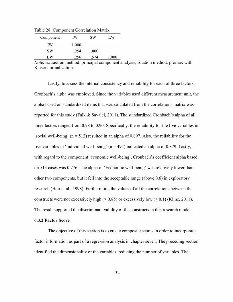
132
Table 28. Component Correlation Matrix
Component IW SW EW
IW 1.000
SW .254 1.000
EW .256 .574 1.000
Note. Extraction method: principal component analysis; rotation method: promax with Kaiser normalization. Lastly, to assess the internal consistency and reliability for each of three factors,
Cronbach’s alpha was employed. Since the variables used different measurement unit, the
alpha based on standardized items that was calculated from the correlations matrix was
reported for this study (Falk & Savalei, 2011). The standardized Cronbach’s alpha of all
three factors ranged from 0.78 to 0.90. Specifically, the reliability for the five variables in
‘social well-being’ (n = 512) resulted in an alpha of 0.897. Also, the reliability for the
five variables in ‘individual well-being’ (n = 494) indicated an alpha of 0.879. Lastly,
with regard to the component ‘economic well-being’, Cronbach’s coefficient alpha based
on 513 cases was 0.776. The alpha of ‘Economic well-being’ was relatively lower than
other two components, but it fell into the acceptable range (above 0.6) in exploratory
research (Hair et al., 1998). Furthermore, the values of all the correlations between the
constructs were not excessively high (> 0.85) or excessively low (< 0.1) (Kline, 2011).
The result supported the discriminant validity of the constructs in this research model.
6.3.2 Factor Score
The objective of this section is to create composite scores in order to incorporate
factor information as part of a regression analysis in chapter seven. The preceding section
identified the dimensionality of the variables, reducing the number of variables. The

133
dimensionality was supported by the interpretation of each factor, showing high factor
loadings of each variable on one factor. Thus, in order to substitute for the original 14
variables, three new variables (factor score for factor 1 to 3) were created based on the
result of the PCA. Factor scores are composite variables that provide information about
each observation’s placement on the factors (Distefano, Shu, & Mîndrilă, 2009), and it is
determined by using factor score coefficients. Before calculating factor scores for each of
the three factors, the variables with negative definitions had their data values reversed.
For example, if the scale was 0 to 30 (e.g., per month data), the value of the variable was
reversed by subtracting the original value from 30. PPHD (physically unhealthy days per
month) was changed to physically healthy days per month (30 - PPHD). Likewise, all the
scores of the variables, except the variable ‘HSGRAD (rate of high school graduation),’
were reversed. These processes did not influence the aforementioned factor results but
make factor scores reverse, retaining all distributional characteristics.
Since regression-based factor scores have been regarded as common practice in
the factor analysis literature (Distefano, Zhu, & Mîndrilă, 2009; Gorsuch, 1983), this
study used the regression approach to estimating factor scores through the SPSS program.
As noted earlier, regression factor scores estimate the location of each individual on the
factor, and the computed factor scores are standardized to a mean of zero and a standard
deviation of one via principal component analysis. Table 29 shows the coefficients used
to calculate the factor scores. Using the coefficients for factor 1, the method of creating
factor scores is equivalent to using the equations.
F1 = 0.191 x the standardized form of the variable PPHD (zPPHD) + 0.235 x
zASMOK + … + 0.004 x zSOSUPT

134
This method helps maximize validity of estimates in that it amplifies the correlation
between factor scores and the corresponding factor (Distefano, Zhu, & Mîndrilă, 2009).
Table 29. Factor Score Coefficient Matrix
Factor
1 2 3
PPHD Physical unhealthy days per month* 0.191 -0.076 0.199
ASMOK Percent of adults currently smoking* 0.235 -0.007 -0.009
AOBESY Percent of adults BMI more than 30* 0.226 0.047 -0.111
PINACT Percent of adults no leisure physical activity* 0.24 0.013 -0.046
PMHD Mental unhealthy days per month* 0.167 -0.062 0.203
HSGRAD Percent of graduated high school -0.022 0.24 -0.03
CHSIGPA Percent of children in single family* 0.018 0.249 -0.017
CHFLUN Percent of children for free Lunch* 0.037 0.205 0.06
VICRIME Violent crime per 100,000* -0.036 0.28 -0.073
TNBIRTH Birth rate age 15-19* 0.102 0.146 0.053
UNINSURE Percent of younger than 65 no health insurance* 0.003 0.091 0.158
UNEMPT Percent of the unemployed age 16+* -0.012 -0.056 0.338
HOPROBM Household with severe housing problem* -0.173 0.081 0.246
SOSUPT Percent of adults no social emotional support* 0.004 0.028 0.269
Note. Extraction method: principal component analysis; rotation method: promax with Kaiser normalization; *denotes the variable reversed to estimate factor scores.
Factor scores are new data for a follow-up analysis. In this study, these three new
variables will be used in the multiple regression analyses to investigate the relationship
with arts and cultural variables identified in Chapter 4. Data screening processes are
needed in order to use factor scores in subsequence analyses. This will be discussed in
more detail in the Chapter 7.
6.3.3 Higher-order Factor Analysis
The aim of higher-order factor analysis in this study was to determine whether a
higher-order factor could explain a broader construct that encompasses the primary three

135
factors. Simply put, higher-order factor analysis is a factor analysis based on factor
correlations, obtaining a more parsimonious structure. The original factors (first order
factors) become the variables for the second factor analysis. In other words, the
correlations among the rotated first order factors, which are obtained from the original
variables, are used as the correlations for a second factor analysis (Gorsuch, 1997; Wind,
Green, & Jain, 1973; Wolff & Preising, 2005). In the way that if factors are inter-
correlated, it can be factored with the higher order factors, this procedure may be
repeated until a general factor or multiple uncorrelated factors are obtained (Wind, Green,
& Jain, 1973; Wolff & Preising, 2005).
So, to enhance interpretability of community well-being, a higher-order factor
analysis was employed. In this study, it was necessary that individual, social, and
economic well-being factors derive a general factor of ‘community well-being’ for
further analyses in Chapter 7. It was expected that community well-being factor as a
second order factor could provide a more parsimonious explanation of the primary three
factors. To perform a higher-order factor analysis with principal component extraction,
the estimation criteria for extraction of factors were consistent with the criteria of PCA.
First, Kaiser’s criterion (eigenvalue > 1) test supported one factor, explaining
58.3% of total variance. The Kaiser-Meyer-Olkin index of sampling adequacy (0.579)
barely fell into the acceptable range above 0.5 guided by Kaiser (1970, 1974), but the
Barlett’s test of sphericity indicated χ2 (3) = 234.9909, p < .0001 satisfying the
recommended value (Hair et al., 1998; Kaiser, 1970, 1974). Furthermore, communalities
were inspected in order to see if the primary factors–IW, SW, and EW–are well explained
by the solution. Even though IW (0.33) is slightly lower than SW (0.71) and EW (0.71),

136
all variables exceeded the cut-off value 0.3 (Pallant, 2010). Next, factor loadings were
examined. Since one factor solution was sustained, there were no cross loadings. As seen
in Table 30, all three primary factors were loaded by the high order factor, showing factor
loadings of 0.57, 0.84, and 0.84. Also, to assess the reliability, Cronbach’s alpha was
employed. With regard to the second order factor ‘community well-being,’ Cronbach’s
coefficient alpha based on 487 cases was 0.629, presenting above the lower limit of 0.6 in
exploratory research (Hair et al, 1998). Thus, it was concluded that these primary factors
correlated, and a general construct ‘community well-being’ could be extracted.
Table 30. Correlation of Primary Factors, Higher-order Factor Loadings, and Reliability
Factor
Primary
IW SW EW Higher-order
Cronbach’s alpha
Primary factor
Individual well-being [IW] 1.00 0.25 0.26 0.57 .629
Social well-being [SW] 0.25 1.00 0.57 0.84
Economic well-being [EW] 0.26 0.57 1.00 0.84
Note. Extraction method: principal component analysis; 1 components extracted.
6.4 Summary
Principal component analysis (PCA) was conducted based on the various well-
being variables, drawn from the County Health Rankings and Roadmaps (CHRR). As a
result of PCA, individual well-being, social well-being, and economic well-being were
identified. Using principal component extraction with promax (k =4) rotation, the results
indicated the presence of three factors accounted for a total of 72.2% of the variance of
the 14 variables–with ‘individual well-being’ contributing 43.3%, ‘social well-being’

137
contributing 20.4%, and ‘economic well-being’ contributing 8.5%. Furthermore,
Cronbach’s alpha was calculated to assess the internal consistency and reliability for each
of the three factors. Standardized Cronbach’s alpha of all three factors ranged from 0.78
to 0.90, falling into the acceptable range (DeVillis, 2003; Hair et al., 1998; Nunnally &
Bernstein, 1994; Tavakol & Dennick, 2011).
Based on the result of the PCA, three composite scores were created in order to
incorporate factor information as part of a regression analysis for the following chapter.
Furthermore, It was expected that a community well-being factor as a second order factor
could provide a more parsimonious explanation of the primary three factors. Thus, to
enhance the interpretability of community well-being, a higher-order factor analysis was
employed.
Figure 13. Structure and loading of community well-being items on first and second
order factors

138
As shown in Figure 13, results supported one general factor, ‘community well-
being,’ explaining 58.3% of total variance. Three primary factors were loaded by the
higher-order factor, showing factor loadings of 0.57 (IW), 0.84 (SW), and 0.84 (EW).
Also, Cronbach’s coefficient alpha based on 487 cases was 0.629, presenting above the
lower limit of 0.60 for exploratory research (Hair et al, 1998). Thus, it was concluded that
a general construct of ‘community well-being’ could be used for a parsimony explanation
of ‘individual,’ ‘social,’ and ‘economic’ well-being.
The following chapter will focus more on explaining the relationship between arts
and cultural dimensions (see chapter 4), and community well-being. The analysis turns to
the central research question: whether the state of arts and cultural assets at the county
level can be a consistent predictor of community well-being.

139
CHAPTER 7
ANALYSIS: ARTS IMPACT ON COMMUNITY WELL-BEING
This chapter presents the result of analyses using main data sets drawing on Local
Arts Index and County Health Rankings and Roadmaps as described in previous chapters.
This study was originally designed to examine whether arts and cultural assets within a
community enhances various dimensions of community well-being. The results of the
factor analyses employed in the preceding chapters helped develop the variables as basic
constructs, and, in turn, combining these arts and community outcome variables allows
this study to present a broad but detailed picture of arts and cultural impact on
community well-being. Given that, the purpose of this chapter is to demonstrate the
relationship between ABCN (i.e., arts business, consumption and nonprofit) and
community well-being outcomes (i.e., individual, social and economic well-being). The
statistical procedure applied in this chapter is a multiple regression analysis to examine
the proposed model and propositions. Before conducting a multiple regression analysis,
an overall sample description with regard to community demographic and economic data
is explained. Also, the variables used for this study are briefly introduced for readers’
convenience (see details in Chapter 4 and 6). Following these analyses, this chapter
explains the result of hypothesized relationship among three dimensions of arts and
cultural resources and individual, social, economic, and overall community well-being.

140
7.1 Data Preparation
7.1.1 Overall Sample Description
To get a full picture of community arts and cultural vitality, it is necessary to scan
the overall context of counties that are selected as cases. It includes demographic and
economic characteristics, and is listed in the table below. To precisely show the
approximate size and population of the counties, the data are divided into seven groups
from ‘less than 50,000 to ‘over 2 million.’ As shown in the Table 31, among 518
counties, 35 counties are in the range of less than 50,000 residents, and 94 counties are in
the population between 50,000 to 100,000. In particular, 161 counties between 100,000 to
250,000 residents account for over one-third of the cases, while only 12 counties are in
the range of over 2 million. Besides, Table 31 shows 101 counties in the population range
of 250,000 to 500,000; 88 counties, between 500,000 to 1milion; and 27 counties,
between 1 million to 2 million.
Table 31. Distrubution of County Populations in 2010
Ranges Frequency Percent Cumulative
Percent
Less than 50,000 35 6.8 6.8
50,000 - 100,000 94 18.1 24.9
100,000 - 250,000 161 31.1 56.0
250,000 - 500,000 101 19.5 75.5
500,000 - 1 million 88 17.0 92.5
1 million - 2 million 27 5.2 97.7
Over 2 million 12 2.3 100.0
Total 518 100.0
Source. Local Arts Index 2012 (Cohen, Cohen, & Kushner, 2012).

141
Additionally, median households income in this data set covers multiple years
ranging from 2005 to 2009. Based on the LAI, household income was divided into ten
decile groups from the smallest ten percent (low income) to the largest ten percent (high
income). The lowest tenth of these cases were in the first decile group, while the highest
ten percent of the cases were in the tenth decile group. Originally, since some counties
had same value and were included in the boundaries between deciles, approximately 314
counties (uneven size of groups), which were 10 percent of total number of counties in
the U.S, were included in each decile groups (Cohen, Cohen, & Kushner, 2012). The
table below shows the median households income of counties based on the selected 518
counties among 3,143 counties in the U.S.
Table 32. Median Households Income 2005-2009
Note. Source from Local Arts Index 2012 (Cohen, Cohen, & Kushner, 2012); Decile grouping presents 10 percent of 3,143 counties in rank order; Decile group 1 means the lowest 10 percent of the median household income.
Decile Grouping Frequency Percent Cumulative
Percent
1 5 1.0 1.0
2 10 1.9 2.9
3 15 2.9 5.8
4 14 2.7 8.5
5 18 3.5 12.0
6 37 7.1 19.1
7 53 10.2 29.3
8 72 13.9 43.2
9 106 20.5 63.7
10 188 36.3 100.0
Total 518 100.0

142
As shown in Table 32 above, the two high-income groups (group 9 and 10)
account for over 50 percent of the counties. On the other hand, the number of counties in
relatively low-income groups from 1 to 3 presents less than 10 percent of the data set.
The result might be related to what the study is looking for. Through the first phase of the
data screening process, the researcher removed counties which have a lot of missing
values. Low-income counties might have insufficient arts and cultural resources and
peoples’ participation, so many arts-related data might not be available to collect in those
regions. Therefore, missing data likely eliminates more relatively low economic level
counties than high-income counties.
In this section, overall context of counties is presented. Communities can vary in
their location, population, and income. Although the 518 counties selected were not
distributed evenly across the country, it would not be a problem to conduct a further
analysis since they represent more than 68% of the U.S. population (Cohen, Cohen, &
Kushner, 2012). In the following section, ABCN variables as independent variables, and
community well-being variables as dependent variables are briefly re-introduced.
7.1.2 Variable definition
To employ multiple regression analysis, a set of independent variables (IV) and
dependent variables (DV) are constructed based on the result of factor analyses in the
preceding chapters (See Table 33). Independent variables represent arts and cultural
participation, nonprofit arts organization, arts and cultural programing and employment,
and support of the arts, which measure a wide range of the vitality of arts and culture at
the local level. On the other hand, community well-being factors that reflect a range of
aspects affecting the state of a local community take a role as a dependent variable. Arts

143
and cultural assets and residents’ consumptions of these assets are embodied in
community life, which in turn are linked to community well-being. Therefore, it is
expected that this research demonstrates a comprehensive, as well as detailed, illustration
of the relationship between community well-being and arts and cultural capacity.
Table 33. Independent Variables and Dependent Variables
ABCN Variables (IVs) Community Well-being Variables (DVs)
Arts Businesses Individual Well-being
Arts/cultural share of all payroll Percent of adults no leisure physical activity
Arts/cultural share of all employees Percent of adults currently smoking
Creative industry share of all employees Percent of adults BMI more than 30
Arts/cultural establishments Physical unhealthy days per month
Creative industry businesses Mental unhealthy days per month
Solo artists Percent of adults no leisure physical activity
Arts Consumption Social Well-being
Photographic equipment expenditures Violent crime per 100,000
Entertainment admission fees Percent of children in single family
Recorded media expenditures Percent of not graduated high school
Online music purchase Percent of children for free Lunch
Attending live performance Birth rate age 15-19
Musical instruments expenditures
Arts Nonprofits Economic Well-being
Collections-based nonprofits Percent of the unemployed age 16+
Humanities/heritage nonprofits Percent of adults no social emotional support
State arts agency grants Percent of younger than 65 no health insurance
Total nonprofit arts revenue Household with severe housing problem
Performing/events nonprofits
In the following section, these 518 counties are subjected to multiple regression
analysis in order to investigate the relationship between ABCN and community well-
being outcomes.

144
7.2 Multiple Regression Analysis
Multiple regression analysis, as a form of general linear modeling, reveals the
relationship between a single dependent variable (DV) and a set of independent variables
(IV). The degree and character of independent variables are objectively assessed in order
to examine their individual contribution to the variation of the dependent variable. Also,
in addition to producing the optimal prediction, multiple regression analysis provides the
magnitude and positive or negative relationship of each independent variable toward the
dependent variable. The simultaneous assessment of each independent variable and the
dependent variable determines the relative importance of each independent variable (Hair
et al., 2005).
Green (1991) suggested rules of thumbs for the size of the sample; N ≥ 50 + 8×IV
(the number of independent variables) are required to test the multiple correlation, and N
≥ 104 + IV are necessary to test individual predictors. In applying to the current study,
the maximum number of independent variables from all ABCN factors could be 17.
Therefore, the size of sample for the multiple regression analysis needs at least 186. The
sample of this study is over 500, so it satisfies the minimum requirement.
Also, in the previous chapter, regression diagnostics were tested to meet the
practical issues in multiple regression analysis such as outliers, linearity, and
multicollinearity (Hair et al., 1998; Tabachnick & Fidell, 2007) (see chapter 4 for
details). More specifically, an examination of residual plots was performed to identify the
possibility of non-linear relationships and heteroscedasticity, which indicates that the
variance of errors differs at different values of the independent variables (Osborne &
Waters, 2002). In multiple regression analysis, the variance of errors is expected to be the
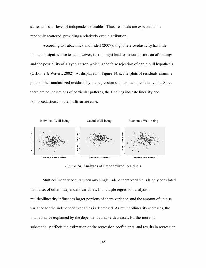
145
same across all level of independent variables. Thus, residuals are expected to be
randomly scattered, providing a relatively even distribution.
According to Tabachnick and Fidell (2007), slight heterosedasticity has little
impact on significance tests; however, it still might lead to serious distortion of findings
and the possibility of a Type I error, which is the false rejection of a true null hypothesis
(Osborne & Waters, 2002). As displayed in Figure 14, scatterplots of residuals examine
plots of the standardized residuals by the regression standardized predicted value. Since
there are no indications of particular patterns, the findings indicate linearity and
homoscedasticity in the multivariate case.
Figure 14. Analyses of Standardized Residuals
Multicollinearity occurs when any single independent variable is highly correlated
with a set of other independent variables. In multiple regression analysis,
multicollinearity influences larger portions of share variance, and the amount of unique
variance for the independent variables is decreased. As multicollinearity increases, the
total variance explained by the dependent variable decreases. Furthermore, it
substantially affects the estimation of the regression coefficients, and results in regression
Individual Well-being Social Well-being Economic Well-being

146
coefficients being incorrectly estimated (Hair et al., 1998). Thus, in chapter 4, variables
having high correlations (generally 0.90 and above) were removed as the first indication
of substantial collinearity.
Table 34 shows correlation values between the six arts business variables.
Simkiss, Ebrahim, & Waterston (2009) note the possibility of collinearity should be
considered when several variables’ correlations exceeded 0.80. However, since these
variables were derived from the result of the factor analysis in chapter 4, a certain degree
of share variance is expected. Also, Tabachinick and Fidell (2007) stated that “The
statistical problems created by singularity and multicollinearity occur at much higher
correlations (0.90 and higher)” (p. 90). Given that all correlation values falls within
acceptable levels of less than 0.90, there is limited concern of collinearity in the
regression model at least among the arts business variables.
Table 34. Pearson Correlation among the Six Arts Business Variables
1 2 3 4 5
1. Solo artists 1
2. Arts/cultural share of all establishments
.84*** 1
3. Arts/cultural share of all employees
.62*** .72*** 1
4. Arts/cultural share of all payroll
.71*** .81*** .87*** 1
5. Creative industry share of all employees
.75*** .74*** .66*** .74*** 1
6. Creative industry businesses .85*** .87*** .63*** .70*** .78***
Note. Listwise N = 516; *p <.05; **p <.01; ***p <.001

147
Table 35. Pearson Correlation among the Six Arts Consumption Variables
1 2 3 4 5
1. Attending live performance 1
2. Online/music media purchase .54*** 1
3. Entertainment admission fees .64*** .52*** 1
4. Recorded media expenditures .36*** .43*** .43*** 1
5. Musical instruments expenditures
.46*** .42*** .26*** .51*** 1
6. Photographic equipment expenditures
.68*** .57*** .80*** .56*** .50***
Note. Listwise N = 518; *p <.05; **p <.01; ***p <.001
Table 36. Pearson Correlation among the Six Arts Nonprofit Variables
1 2 3 4
1. Total nonprofit arts revenue 1
2. State arts agency grants .62*** 1
3. Collections-based nonprofits .53*** .44*** 1
4. Humanities/heritage nonprofits .52*** .43*** .55*** 1
5. Performing/events nonprofits .74*** .52*** .48*** .55***
Note. Listwise N = 514; *p <.05; **p <.01; ***p <.001
As shown in Table 35, although there is a little concern about the magnitude of
association between entertainment admission fees and photographic equipment
expenditures (r = .80), correlation values indicate acceptable levels of less than 0.90
(Simkiss, Ebrahim, & Waterston, 2009; Tabachinick & Fidell, 2007). Also, Table 36
shows that all correlation values are in the acceptable ranges. Thus, based on these
correlation results, current analysis has no substantial collinearity among independent

148
variables in the regression model. Furthermore, as a result of the inspection of correlation
values of all 17 variables, all correlation values are in the acceptable ranges.
In addition to the correlation check, VIF (Variance Inflation Factor) and tolerance
values were calculated to check potential multicollinearity between independent variables
in the regression model based on the cut-off value of VIF < 10.0 (Chatterjee, Hadi, &
Price, 2000; Hair et al., 1998). The VIF is a measure of the degree to which each
independent variable is explained by the other independent variables in the analysis; it
directly affects the variance of the regression coefficient related to the independent
variable (Hair et al., 1998; O’Brien, 2007). On the other hand, tolerance (tolerance =
1/VIF) is the amount of variability of the independent variable that is not explained by
the other independent variables. Therefore, extremely small tolerance values indicate
high collinearity. As a result of an evaluation of VIF and tolerance, all VIF are below 10
which corresponds to a tolerance value above 0.10 in the regression model.
7.3 Research Findings
The purpose of this section is to report the results of empirical tests of the
propositions. After checking the above regression diagnostics, a standard multiple
regression was conducted to test propositions and illustrate the degree to which each arts
and cultural variable explains community well-being. The first analysis concerned
Proposition 1: With an abundant presence of arts and cultural assets within a community,
community individual well-being will be positively enhanced (see Figure 15).

149
Figure 15. An expanded model of arts and community individual well-being
The three regression models proposed below were statistically significant, indicating that
arts business, arts consumption, and arts nonprofit respectively influence community
individual well-being. The following propositions further concern whether specific
variables within these arts business, arts consumption, and arts nonprofit factors could
explain community individual well-being.
Proposition 1a: With an abundant presence of arts and cultural business factors within a community, community individual well-being will be positively enhanced.
Concerning proposition 1a, a standard multiple regression was performed between
community individual well-being as the dependent variable and solo artist, arts/cultural
establishments, arts/cultural share of all employees, arts/cultural share of all payroll,
creative industry share of all employees, and creative industry businesses as independent
variables. The result indicates that the multiple correlation coefficient (R), using all the
variables simultaneously is 0.73, and adjusted R2 is 0.52 which means that 52% of the
Community
Well-being
Social Well-being
Individual Well-being
Economic Well-being
Arts
Business
Arts Consumption
Arts Nonprofit
P1a
P1b
P1c

150
variance in community individual well-being can be explained from six arts business-
related variables. Also, the combination of these variables significantly predicts the
community individual well-being, indicating F(6,478) = 88.68, p < .001. Furthermore, as
presented in Table 37, solo artists, arts/cultural share of all employees, arts/cultural share
of all payroll, and creative industry businesses are significantly contributing to the
prediction when all variables are entered. More specifically, the analysis revealed that the
number of solo artists variable (β = 0.45, t = 6.75, p = 0.00) and the number of creative
industry businesses (β = 0.37, t = 4.95, p = 0.00) were the influential variables, showing a
positive relationship with community individual well-being.
In addition, individual well-being outcomes are likely to increase when a portion
of employees in the arts/cultural field is increased. However, the ratio of arts and cultural
payroll to all payrolls shows a negative relationship with individual well-being outcomes.
In spite of increasing arts employment, 34 percent of artists are self-employed (“NEA
Announces”, 2011). Furthermore, according to the Bureau of Labor Statistics (BLS) 2014
data, even though arts-related occupations’ median wages ($45,180) are higher than the
median for the whole labor force ($35,540), arts-related occupations as a whole earn far
less than the median wage of the professional category such as educational, legal, and
engineering-related occupations ($70,487), to which they can belong. In this sense, larger
arts and cultural share of all payroll might imply that a community has relatively smaller
portion of payroll from other workforces, which might earn higher wage, or might be
directly related to community individual well-being.
Calculating semipartial correlations (sr2) provides insight in assessing the relative
importance of independent variables (Nathans, Oswald, & Nimon, 2012). In a semipartial

151
correlation, the contribution of other independent variables is taken out of only the
independent variable. Thus, it tells us a unique contribution of an independent variable to
R2 (Tabachnick & Fidell, 2007). Specifically, it indicates how much R2 decreases if that
variable is removed from the regression equation. This statistic is also termed ‘unique
effects’ of commonality coefficients. Commonality coefficients explain how independent
variables operate together in a given regression model. Furthermore, it helps identifying
the relative importance of independent variables with regard to the dependent variable
(Nathans, Oswald, & Nimon, 2012; Nimon & Oswald, 2013). Thus, rather than heavy
reliance on beta weights to interpret regression results, semipartial correlations (sr2) of
significant variables are valuable to see the detailed picture about how independent
variables uniquely contribute to the regression model.
As indicated by the squared semipartial correlations in Table 37, it is noted that
the sum for the four significant IVs (0.045 + 0.014 + 0.007 + 0.024 = 0.90), which
uniquely contribute to R2 is 0.09, while shared variability represents 0.43, which means
the variance that all variables jointly contribute to R2. Additionally, arts/cultural
establishments (r = 0.61) and creative industry share of all employees (r = 0.56) show
relatively high correlation with community individual well-being, but do not contribute
significantly to county’s individual well-being. In this sense, the relationship might be
mediated by the relationship between the dependent variable and other independent
variables in the regression model, although the bivariate correlation between community
individual well-being and the above two variables were statistically different from zero
using a post hoc test suggested by Tabachnick and Fidell (2007), presenting F(6,478) =
47.71, p < .01, and F(6,478) = 35.46, p < .01.

152
Table 37. Model 1: Arts Business Variables on Community Individual Well-being
Arts Business Variable (N=485) IW (r)
B β sr2
(unique)
Solo artists .70 .85 0.45*** .045
Arts/cultural share of all establishments .61 -.16 -0.09
Arts/cultural share of all employees .50 2.65 0.25*** .014
Arts/cultural share of all payroll .50 -2.41 -0.21** .007
Creative industry share of all employees .56 -.16 -0.01
Creative industry businesses .68 .92 0.37*** .024
Constant -8.80
Multiple R .73
R2 .52
Adjusted R2 .52
F test statistic, significance F(6,478) = 88.68 p < .001
Note: r denotes correlation coefficient between each IVs and DV; B denotes unstandardized coefficients; β (Beta) denotes standardized coefficients; sr2 denotes unique contribution to the DV; *p < .05; **p < .01; ***p < .001.
Proposition 1b: Peoples’ arts and cultural consumptions and experiences have a positive impact on community individual well-being outcomes.
Concerning proposition 1b, a standard multiple regression was tested to illustrate
the relationship between community individual well-being as the dependent variable and
six independent variables with respect to peoples’ arts consumption such as adult
population share of attending live performing arts and expenditure on entertainment
admission fees. Among independent variables, there were no interrelations in excess of
.90, and all VIF were less than the cut-off value of 10. Thus, there is no evidence of
multicollinearity. The result indicates that the multiple correlation coefficient (R), using
all the variables simultaneously is 0.75, and adjusted R2 is 0.56 with F(6,480) = 104.80,

153
p < .001. In other words, 56% of the variance in community individual well-being can be
explained from six arts consumption-related variables when these are entered
simultaneously in the regression model. This analysis summarizes that attending live
performance, online music purchase, expenditure on entertainment admission fees and
recorded media contribute significantly to predicting positive community individual well-
being.
Table 38. Model 2: Arts Consumption Variables on Community Individual Well-being
Arts Consumption Variable (N=487) IW (r)
B β sr2
(unique)
Attending live performance .66 5.08 0.43*** .086
Online/music media purchase .51 3.02 0.12** .009
Entertainment admission fees .59 .05 0.24*** .018
Recorded media expenditures .51 .03 0.28*** .048
Musical instruments expenditures .37 .00 0.01
Photographic equipment expenditures .58 -.01 -0.11
Constant -3.74
Multiple R .75
R2 .57
Adjusted R2 .56
F test statistic, significance F(6,480) = 104.80 p < .001
Note: r denotes correlation coefficient between each IVs and DV; B denotes unstandardized coefficients; β (Beta) denotes standardized coefficients; sr2 denotes unique contribution to the DV; *p < .05; **p < .01; ***p < .001. More specifically, the beta weights, presented in Table 38, suggest that adults’
population share of attending live performance contributes most to explaining community
individual well-being, indicating β = 0.43, t = 9.78, p = 0.00, and that purchasing online

154
and music media, expenditures on entertainment admission fees, and recorded media
expenditures also positively contribute to the prediction of community individual well-
being. Also, it is noted that the sum for the four significant independent variables which
uniquely contribute to R2 is 0.16, while shared variability of the six independent variables
in combination represents 0.41. Although expenditures on photographic equipment (r =
.58) show relatively high correlation with community individual well-being, but do not
present statistical significance when all other independent variables are held constant.
The overall result provides a considerable support for the proposition 1b.
Proposition 1c: With an abundant presence of arts and cultural nonprofit factors within a community, community individual well-being will be positively enhanced.
The result reveals that this combination of arts nonprofit variables–total nonprofit
arts revenue, state arts agency grants, collection-based nonprofits, humanities/heritage
nonprofits, and performing/events nonprofits–significantly predict community individual
well-being, F(5,477) = 63.83, p < .001, with four of five variables showing statistically
significant contribution to regression. The multiple correlation coefficient (R), using all
the variables simultaneously, is 0.63, and adjusted R2 is 0.40. Thus, 40% of the variance
in community individual well-being can be predicted from the five arts nonprofit
variables when these are entered simultaneously.

155
Table 39. Model 3: Arts Nonprofit Variables on Community Individual Well-being
Arts Nonprofit Variable (N=483) IW (r)
B β sr2
(unique)
Total nonprofit arts revenue .46 .21 0.28*** .027
State arts agency grants .13 -.33 -0.31*** .056
Collections-based nonprofits .18 -.28 -0.17*** .017
Humanities/heritage nonprofits .31 .12 0.07
Performing/events nonprofits .57 .87 0.57*** .125
Constant -1.30
Multiple R .63
R2 .40
Adjusted R2 .40
F test statistic, significance F(5,477) = 63.83 p < .001
Note: r denotes correlation coefficient between each IVs and DV; B denotes unstandardized coefficients; β (Beta) denotes standardized coefficients; sr2 denotes unique contribution to the DV; *p < .05; **p < .01; ***p < .001. As shown in Table 39, the analysis revealed that the number of performing/events
nonprofits variable (β = 0.57, t = 9.99, p = 0.00) was the most influential variable,
showing a positive relationship with community individual well-being. Also, as total
nonprofit arts revenue increases (β = 0.28, t = 4.64, p = 0.00), community individual
well-being increases. Between these two variables, however, the number of
performing/events nonprofits is relatively important to increasing the community
individual well-being outcome, as indicated by the squared semipartial correlations (sr2).
Contrary to my expectation, even though state arts agency grants and collection-based
nonprofits variables are statistically influential as predictors in the regression model
(β = -0.31, t = -6.65, p = .00, and β = -0.17, t = -3.73, p = 0.00.), they have a negative
relationship with community individual well-being. However, these two variables exhibit

156
lower correlation (r = .13, and r = .18) with the community individual well-being than
other variables. Given this low correlation with the dependent variable, it might be
unlikely to contribute meaningfully to the result.
Next, concerning Proposition 2: With an abundant presence of arts and cultural
assets within a community, community social well-being will be positively enhanced (see
Figure 16), three regression models proposed below were statistically significant,
indicating that arts business, arts consumption, and arts nonprofit respectively influence
community social well-being. The following propositions further explain whether
specific variables within these arts business, arts consumption, and arts nonprofit factors
contribute to community social well-being.
Figure 16. An expanded model of arts and community social well-being
Proposition 2a: With an abundant presence of arts and cultural business factors within a community, community social well-being will be positively enhanced.
The result reveals that this combination of the six arts business variables
significantly predict community social well-being, F(6,478) = 16.01, p < .001, but only
P2a
P2b
P2c
Arts
Business
Arts Consumption
Arts Nonprofit
Community
Well-being
Social Well-being
Individual Well-being
Economic Well-being

157
three variables–arts/cultural establishments, arts/cultural share of all payroll, and creative
industry share of all employees–show statistically significant contribution to regression
respectively. The multiple correlation coefficient (R), using all the variables
simultaneously, is 0.41, and adjusted R2 is 0.16. In other words, 16% of the variance in
community social well-being can be predicted from the six arts business related variables
when entered simultaneously.
Table 40. Model 4: Arts Business Variables on Community Social Well-being
Arts Business Variable (N=485) SW (r)
B β sr2
(unique)
Solo artists -.00 .05 0.03
Arts/cultural share of all establishments .01 .84 0.45*** .031
Arts/cultural share of all employees -.14 1.67 0.15
Arts/cultural share of all payroll -.22 -8.15 -0.71*** .082
Creative industry share of all employees -.13 -3.46 -0.19* .011
Creative industry businesses .04 .40 0.16
Constant -4.90
Multiple R .41
R2 .17
Adjusted R2 .16
F test statistic, significance F(6,478) = 16.01 p < .001
Note: r denotes correlation coefficient between each IVs and DV; B denotes unstandardized coefficients; β (Beta) denotes standardized coefficients; sr2 denotes unique contribution to the DV; *p < .05; **p < .01; ***p < .001.
As shown in Table 40, the analysis reveals that the proportion of arts and cultural
industries of all establishments in a county (β = 0.45, t = 4.19, p = 0.00) positively
influences the community social well-being outcome. It means that if a community has
relatively many arts and cultural industries, it would likely enhance community social

158
well-being. On the other hand, creative industry share of all employees (β = -0.19,
t = -2.54, p < 0.05) and arts/cultural share of all payroll (β = -0.71, t = -6.91, p = 0.00) are
statistically influential as predictors in the regression model, but showing a negative
relationship with community social well-being.
Similar to the result of Model 1 (Arts businesses on community individual well-
being), it can be understood that many people working in arts-centric businesses are self-
employed with relatively low wages. Thus, a community with enhanced social well-being
outcome might entail more portions of employees and payroll which are not related to
arts and culture. Furthermore, contrary to the result of community individual well-being,
the solo artists variable is barely contributing to community social well-being. As
mentioned before, the squared semipartial correlation indicates how much variance an
independent variable contributes to a regression equation that is not shared with other
independent variables. As a result, it is noted that arts/cultural share of all payroll variable
contributes the most uniquely to R2 (sr2 =.08), and the sum of unique effects on
community social well-being of three significant independent variables is 0.12. Given
that, it can be concluded that the findings do not support the proposition that arts and
cultural businesses are associated positively with community social well-being.
Proposition 2b: Peoples’ arts and cultural consumptions and experiences have a positive impact on community social well-being outcomes.
Concerning proposition 2b, the result illustrates the relationship between
community social well-being as the dependent variable and six independent variables
with respect to peoples’ arts consumption. The multiple correlation coefficient (R), using
all the variables simultaneously, is 0.63, and adjusted R2 is 0.39 which indicates 39% of

159
the variance in community social well-being can be predicted from six arts consumption
related variables when these are entered simultaneously in the regression. R for
regression is significantly different from zero, showing F(6,480) = 53.01, p < 0.001. This
analysis summarizes that expenditure on photographic equipment contributes
significantly to predicting community social well-being (See Table 41).
More specifically, the beta weights, presented in Table 41, suggest that
expenditures on photographic equipment contributes most to explaining community
social well-being (β = 0.94, t = 13.62, p = 0.00), and indicate adults population share of
attending live performance, and expenditures on entertainment admission negatively
contribute to the prediction of community social well-being. However, as shown Table
41, it is noted that unique variances of adult population share of attending live
performance, and expenditures on entertainment admission, are relatively small, while
expenditures on photographic equipment uniquely explains 23% of the R-squared value.
Thus, although it can be concluded that the result partially supports the proposition,
expenditures on photographic equipment is the most influential variable, which shows a
strongly positive association with community social well-being.

160
Table 41. Model 5: Arts Consumption Variables on Community Social Well-being
Arts Consumption Variable (N=487) SW (r)
B β sr2
(unique)
Attending live performance .25 -2.45 -0.21*** .020
Online/music media purchase .27 .34 0.01
Entertainment admission fees .34 -.05 -0.24*** .019
Recorded media expenditures .28 -.01 -0.06
Musical instruments expenditures .26 .00 -0.02
Photographic equipment expenditures .58 .12 0.94*** .232
Constant -2.57
Multiple R .63
R2 .39
Adjusted R2 .39
F test statistic, significance F(6,480) = 53.01 p < .001
Note: r denotes correlation coefficient between each IVs and DV; B denotes unstandardized coefficients; β (Beta) denotes standardized coefficients; sr2 denotes unique contribution to the DV; *p < .05; **p < .01; ***p < .001.
Proposition 2c: With an abundant presence of arts and cultural nonprofit factors within a community, community social well-being will be positively enhanced.
The result of the model 6 reveals that this combination of arts nonprofit variables
significantly predict community social well-being, F (5,477) = 32.70, p < 0.001, with all
five variables showing statistically significant contributions to the regression model. The
multiple correlation coefficient (R), using all the variables simultaneously, is 0.51, and
adjusted R2 is 0.25. It means that 25% of the variance in community social well-being
can be predicted from the five arts nonprofit variables when other variables are held
constant. As presented in Table 42, the analysis revealed that as variables related to
number of arts and culture-centric nonprofits increases, community social well-being

161
outcomes are positively enhanced. The number of humanities/heritage nonprofits (β =
0.37, t = 7.04, p = 0.00) is the relatively more important variable, which shows a positive
relationship with community social well-being. Also, performing/events nonprofits (β =
0.19, t = 3.02, p < 0.01) and collections-based nonprofits (β = 0.11, t = 2.20, p < 0.05) are
positively associated with community social well-being.
Table 42. Model 6: Arts Nonprofit Variables on Community Social Well-being
Arts Nonprofit Variable (N=483) SW (r)
B β sr2
(unique)
Total nonprofit arts revenue -.22 -.30 -0.39*** .052
State arts agency grants -.29 -.39 -0.36*** .076
Collections-based nonprofits .05 .18 0.11* .008
Humanities/heritage nonprofits .17 .66 0.37*** .077
Performing/events nonprofits -.03 .30 0.19** .014
Constant .30
Multiple R .51
R2 .26
Adjusted R2 .25
F test statistic, significance F(5,477) = 32.70 p < .001
Note: r denotes correlation coefficient between each IVs and DV; B denotes unstandardized coefficients; β (Beta) denotes standardized coefficients; sr2 denotes unique contribution to the DV; *p < .05; **p < .01; ***p < .001.
However, contrary to my assumption that arts revenue and state arts agency grants
will have a positive impact on community social well-being, these two variables indicate
statistically significant negative relationship with community social well-being,
presenting β = -0.39, t = -5.76, p = 0.00, and β = -0.36, t = -6.95, p = 0.00. It can be
understood that even though abundant nonprofit organizations in a county help increase

162
community social well-being, arts revenue per capita is relatively low in a county that has
a high level of social well-being. Also, state arts agency grants might be frequently
allocated when a community has relatively low chance to find financial resources serving
their residents. In this regard, arts revenue and grants, paradoxically, are not positively
related to social community well-being in this model. Furthermore, the squared
semipartial correlations in Table 42 show that the sum for the five significant
independent variables, which uniquely contribute to R2 is 0.23, while shared variability
represents 0.03. It suggests that these variables contribute more to a regression effect
when functioning independently rather than operating in combination with other
variables.
Concerning Proposition 3: With an abundant presence of arts and cultural assets
within a community, community economic well-being will be positively enhanced (see
Figure 17), three regression models proposed below were statistically significant,
indicating that arts business, arts consumption, and arts nonprofits respectively influence
community economic well-being. The following propositions further explain how
individual variables within these arts business, arts consumption, and arts nonprofit
factors could predict community economic well-being.

163
Figure 17. An expanded model of arts and community economic well-being
Proposition 3a: With an abundant presence of arts and cultural business factors within a community, community economic well-being will be positively enhanced.
Concerning proposition 3a, the result illustrates the relationship between
community economic well-being as the dependent variable and six independent variables
with respect to arts business. The multiple correlation coefficient (R), using all the
variables simultaneously, is 0.45, and adjusted R2 is 0.19 which indicates 19% of the
variance in community economic well-being can be predicted from six arts business-
related variables when these are entered simultaneously in the regression. R for
regression is significantly different from zero, showing F (6,478) = 19.85, p < 0.001.
Overall, this analysis summarizes that solo artists, arts/cultural establishments, and
creative industries businesses contribute significantly to predicting positive community
economic well-being. However, the variable arts/cultural share of all payroll shows the
negative relationship with community economic well-being, while it is most influential as
a predictor in the regression model (See Table 43).
P3a
P3b
P3c
Arts
Business
Arts Consumption
Arts Nonprofit
Community
Well-being
Social Well-being
Individual Well-being
Economic Well-being

164
Table 43. Model 7: Arts Business Variables on Community Economic Well-being
Arts Business Variable (N=485) EW (r)
B β sr2
(unique)
Solo artists .22 .36 0.19* .008
Arts/cultural share of all establishments .19 .72 0.38*** .022
Arts/cultural share of all employees -.03 .11 0.01
Arts/cultural share of all payroll -.06 -6.72 -0.58*** .057
Creative industry share of all employees .06 -2.43 -0.13
Creative industry businesses .24 .60 0.24* .010
Constant -6.22
Multiple R .45
R2 .20
Adjusted R2 .19
F test statistic, significance F(6,478) = 19.85 p < .001
Note: r denotes correlation coefficient between each IVs and DV; B denotes unstandardized coefficients; β (Beta) denotes standardized coefficients; sr2 denotes unique contribution to the DV; *p < .05; **p < .01; ***p < .001.
More specifically, the analysis revealed that arts/cultural share of all
establishments (β = 0.38, t = 3.67, p = 0.00) is the most positive influential variable,
followed by creative industry businesses (β = 0.24, t = 2.49, p < 0.05) and the number of
solo artists (β = 0.19, t = 2.21, p < 0.05). Furthermore, arts/cultural share of all payroll is
statistically influential as a predictor in the regression model, presenting β = -0.58,
t = -5.81, p = 0.00, although its negative relationship with community economic well-
being does not support the proposition. Similar to the proposition 1a (Arts businesses on
individual well-being), it might be a reason that many people in arts and culture-centric
businesses are self-employed and earn far less than the wage of other professional jobs.
Furthermore, this variable seems to be the most influential variable in this model.

165
However, it shows very low correlation (r = -0.06) compared with the other community
economic well-being variables. Given these low correlations with the dependent variable,
it might be unlikely to contribute meaningfully to the result. In this regard, it can be
concluded that the result mostly supports the proposition that community economic well-
being is positively enhanced when arts and cultural business factors are abundant in a
community.
Proposition 3b: Peoples’ arts and cultural consumptions and experiences have a positive impact on community economic well-being outcomes.
Concerning proposition 3b, the regression model demonstrates the relationship
between community economic well-being as the dependent variable and six independent
variables with respect to peoples’ arts consumption. The result indicates that the multiple
correlation coefficient (R), using all the variables simultaneously, is 0.74, and adjusted R2
is 0.54 with F (6,480) = 95.86, p < 0.001. In other words, 54% of the variance in
community economic well-being can be explained from six arts consumption-related
variables when these are entered simultaneously in the regression. This analysis
summarizes that all the six variables contribute significantly to predicting community
economic well-being (See Table 44).
More specifically, as shown in Table 44, the standardized coefficients indicate
that expenditures on photographic equipment contributes most to explaining community
economic well-being, presenting β = 1.01, t = 16.78, p = 0.00, and that purchasing online
and music media (β = 0.11, t = 2.88, p = 0.00), and expenditures on musical instruments
(β = 0.17, t = 4.20, p = 0.00) also positively contribute to the prediction of community
economic well-being. On the other hand, adult population share of attending live

166
performances (β = -0.21, t = -4.67, p = 0.00), expenditures on entertainment admission
(β = -0.37, t = -6.75, p = 0.00), as well as expenditures on recorded media (β = -0.14, t = -
3.60, p = 0.00) are not positively associated with community economic well-being. An
interesting point here is that all three variables that are positively related with community
economic well-being may be viewed as hobbies that need at least more active
involvement and engagement in arts and culture than buying tickets to theatres and other
events. Given that, this model implies that if active involvements in arts and culture are
associated with peoples’ daily basic activities such as playing musical instruments and
taking a picture, peoples’ consumptions and expenditures on arts and culture can enhance
community economic well-being.
Table 44. Model 8: Arts Consumption Variables on Community Economic Well-being
Arts Consumption Variable (N=487) EW (r)
B β sr2
(unique)
Attending live performance .31 -2.48 -0.21*** .021
Online/music media purchase .37 2.71 0.11** .008
Entertainment admission fees .32 -.08 -0.37*** .043
Recorded media expenditures .32 -.01 -0.14*** .012
Musical instruments expenditures .45 .03 0.17*** .017
Photographic equipment expenditures .65 .12 1.01*** .267
Constant -2.57
Multiple R .74
R2 .55
Adjusted R2 .54
F test statistic, significance F(6,480) = 95.86 p < .001
Note: r denotes correlation coefficient between each IVs and DV; B denotes unstandardized coefficients; β (Beta) denotes standardized coefficients; sr2 denotes unique contribution to the DV; *p < .05; **p < .01; ***p < .001.

167
In addition, the six significant independent variables which uniquely contribute to
R2 is 0.37, and among them expenditures on photographic equipment variable is the most
important predictor, contributing uniquely to 27% of variance of the community
economic well-being accounted for by R-squared. In sum, the result partially supports the
proposition that community economic well-being is positively enhanced when arts and
cultural business factors are abundant in a community.
Proposition 3c: With an abundant presence of arts and cultural nonprofit factors within a community, community economic well-being will be positively enhanced.
The result indicates that this combination of arts nonprofit variables significantly
predicts community economic well-being, F (5,477) = 11.56, p < 0.001, showing similar
patterns with proposition 1c (Arts nonprofits on individual well-being) and proposition 2c
(Arts nonprofits on social well-being). The multiple correlation coefficient (R), using all
the variables simultaneously, is 0.33, and adjusted R2 is 0.10. In other words, 10% of the
variance in community economic well-being can be predicted from the five arts nonprofit
variables when these are entered simultaneously. Table 45 reveals that as variables
related to the number of arts-centric nonprofits increases, community economic well-
being outcomes are positively enhanced. The number of humanities/heritage nonprofits
(β = 0.29, t = 5.01, p = 0.00) is more important, followed by performing/events
nonprofits (β = 0.25, t = 3.58, p = 0.00).

168
Table 45. Model 9: Arts Nonprofit Variables on Community Economic Well-being
Arts Nonprofit Variable (N=483) EW (r)
B β sr2
(unique)
Total nonprofit arts revenue .03 -.14 -0.18* .011
State arts agency grants -.05 -.19 -0.18** .018
Collections-based nonprofits .08 -.06 -0.04
Humanities/heritage nonprofits .23 .66 0.29*** .027
Performing/events nonprofits .16 .30 0.25*** .024
Constant -.25
Multiple R .33
R2 .11
Adjusted R2 .10
F test statistic, significance F(5,477) = 11.56 p < .001
Note: r denotes correlation coefficient between each IVs and DV; B denotes unstandardized coefficients; β (Beta) denotes standardized coefficients; sr2 denotes unique contribution to the DV; *p < .05; **p < .01; ***p < .001. Consistent with previous results, arts revenue and state arts agency grants indicate
statistically significant negative relationship with the community economic well-being
outcomes, presenting β = -0.18, t = -2.48, p < 0.05, and β = -0.18, t = -3.08, p < 0.01.
However, it might be unlikely to contribute meaningfully to the result, since these two
variables show virtually very low correlation (r = 0.03, and r = -0.05) with the
community economic well-being. Furthermore, as presented in Table 45, the sum for the
four significant independent variables, which uniquely contribute to R2 is 0.10. Hence,
this suggests that these variables contribute more to a regression effect when functioning
independently rather than operating in combination with other variables.

169
The last analysis concerns Proposition 4: With an abundant presence of arts and
cultural assets within a community, overall community well-being will be positively
enhanced (see Figure 18). Overall, three regression models proposed below were
statistically significant, indicating that arts business, arts consumption, and arts nonprofits
respectively influence overall community well-being. The following propositions further
explore whether specific variables within these arts business, arts consumption, and arts
nonprofit factors explain overall community well-being.
Figure 18. An expanded model of arts and overall community well-being
Proposition 4a: With an abundant presence of arts and cultural business factors within a community, overall community well-being will be positively enhanced.
Overall, the result reveal that this combination of arts business variables
significantly predict overall community well-being, F (6,478) = 30.60, p < 0.001, with all
six variables showing statistically significant contribution to the regression model. The
multiple correlation coefficient (R), using all the variables simultaneously, is 0.53, and
Social Well-being
Individual Well-being
Community
Well-being
Arts
Business
Arts Consumption
Arts Nonprofit
P4a
P4b
P4c
Economic Well-being

170
adjusted R2 is 0.27 which means 27% of the variance in overall community well-being
can be predicted from the six arts business variables when these are entered
simultaneously.
As displayed in Table 46, the analysis reveals that four of six variables positively
influence the overall community well-being outcome. More specifically, overall
community well-being is enhanced as the four variables increase: the proportion of
arts/cultural industries of all establishments (β = 0.37, t = 3.74, p = 0.00), creative
industry businesses (β = 0.32, t = 3.41, p < 0.01), arts/cultural share of all employees
(β = 0.16, t = 2.04, p < 0.05), and solo artists (β = 0.25, t = 3.07, p < 0.01).
Table 46. Model 10: Arts Business Variables on Overall Community Well-being
Arts Business Variable (N=485) CW (r)
B β sr2
(unique)
Solo artists .33 .48 0.25** .014
Arts/cultural share of all establishments .30 .70 0.37*** .021
Arts/cultural share of all employees .09 1.73 0.16* .006
Arts/cultural share of all payroll .03 -7.96 -0.69*** .079
Creative industry share of all employees .15 -2.89 -0.16* .008
Creative industry businesses .36 .78 0.32** .018
Constant -7.69
Multiple R .53
R2 .28
Adjusted R2 .27
F test statistic, significance F(6,478) = 30.60 p < .001
Note: r denotes correlation coefficient between each IVs and DV; B denotes unstandardized coefficients; β (Beta) denotes standardized coefficients; sr2 denotes unique contribution to the DV; *p < .05; **p < .01; ***p < .001.

171
On the other hand, arts/cultural share of all payroll (β = -0.69, t = -7.24, p = 0.00),
and creative industry share of all employees (β = -0.16, t = -2.27, p < 0.05) show negative
relationships with overall community well-being. Even though arts/cultural share of all
payroll variable is a statistically influential predictor in the regression model, this variable
shows very low correlation (r = 0.03) with the overall community well-being. Given its
low correlation with the dependent variable, it is unlikely to contribute meaningfully to
the prediction of community well-being. All things considered, the result mostly supports
the proposition that overall community well-being is positively enhanced with abundant
arts businesses in a community.
Proposition 4b: Peoples’ arts and cultural consumptions and experiences have a positive impact on overall community well-being outcomes.
Concerning proposition 4b, the regression model demonstrates the relationship
between overall community well-being and six independent variables with respect to
peoples’ arts consumption. The result indicates that the multiple correlation coefficient
(R), using all the variables simultaneously, is 0.81, and adjusted R2 is 0.65 with F (6,480)
= 148.73, p < 0.001. In other words, 65% of the variance in overall community well-
being can be explained from six arts consumption related variables when variables are
held constant in the regression.
As shown in Table 47, the standardized coefficients indicate that expenditures on
photographic equipment contributes most to explaining overall community well-being,
presenting β = 0.91, t = 17.17, p = 0.00, and that purchasing online and music media
(β = 0.10, t = 2.99, p < 0.01), and expenditures on musical instruments (β = 0.08, t = 2.11,
p < 0.05) also positively contribute to the prediction of overall community well-being. On

172
the other hand, expenditures on entertainment admission negatively contribute to the
prediction of overall community well-being (β = -0.22, t = -4.54, p = 0.00). It can be
understood that arts and cultural consumption related to people’s daily basis such as
purchases of music and photographic equipment help enhance overall community well-
being.
Table 47. Model 11: Arts Consumption Variables on Overall Community Well-being
Arts Consumption Variable (N=487) CW (r)
B β sr2
(unique)
Attending live performance .49 -.71 -0.06
Online/music media purchase .47 2.47 0.10** .007
Entertainment admission fees .51 -.05 -0.22*** .015
Recorded media expenditures .45 .00 -0.01
Musical instruments expenditures .46 .01 0.08* .003
Photographic equipment expenditures .78 .91 0.91*** .214
Constant -3.70
Multiple R .81
R2 .65
Adjusted R2 .65
F test statistic, significance F(6,480) = 148.73 p < .001
Note: r denotes correlation coefficient between each IVs and DV; B denotes unstandardized coefficients; β (Beta) denotes standardized coefficients; sr2 denotes unique contribution to the DV; *p < .05; **p < .01; ***p < .001.
Also, similar to the result of Proposition 3b (Model 8: Arts consumptions on
community economic well-being), among the six variables, expenditures on photographic
equipment variable is the most important predictor, contributing uniquely to 21 percent of
variance of community economic well-being. Even though expenditures on the

173
entertainment admission variable show statistically significant difference from zero, its
unique contribution to the overall community well-being is less than 2 percent. Given
that, the relationship might be mediated by the relationship between community well-
being and other variables in the regression model. Taken together, it can be concluded
that the result mostly supports the proposition that community arts consumptions are
positively related with overall community well-being.
Proposition 4c: With an abundant presence of arts and cultural nonprofit factors within a community, overall community well-being will be positively enhanced.
Lastly, proposition 4c explains how arts and cultural nonprofit resources in a
community impact overall community well-being. Overall, the result reveals that this
combination of arts nonprofit variables significantly predict overall community well-
being, F (5,477) = 28.86, p < 0.001, showing similar patterns with Proposition 3c (Model
9: Arts nonprofits on community economic well-being). The multiple correlation
coefficient (R), using all the variables simultaneously, is 0.48, and adjusted R2 is 0.22
which indicates 22% of the variance in overall community well-being can be predicted
from the five arts nonprofit variables when these are entered simultaneously.
As displayed in Table 48, the result indicates that as variables related to number
of arts and culture-related nonprofits increases, overall community well-being is
positively enhanced. Unlike the result of arts nonprofits on community economic well-
being, in this output the number of performing/events nonprofits (β = 0.40, t = 6.19,
p = 0.00) is more influential, followed by humanities/heritage nonprofits (β = 0.34,
t = 6.39, p = 0.00). Arts revenue and state arts agency grants indicate statistically
significant negative relationship with the overall community well-being (β = -0.14,

174
t = -2.69, p < 0.01, and β = -0.39, t = -6.84, p < 0.001). However, it might be unlikely to
contribute meaningfully to the result, since these two variables show relatively very low
correlation (r = 0.06, and r = -0.12) with the community well-being.
Table 48. Model 12: Arts Nonprofit Variables on Overall Community Well-being
Arts Nonprofit Variable (N=483) EW (r)
B β sr2
(unique)
Total nonprofit arts revenue .06 -.14 -0.18** .012
State arts agency grants -.12 -.39 -0.36*** .075
Collections-based nonprofits .12 -.03 -0.02
Humanities/heritage nonprofits .30 .60 0.34*** .066
Performing/events nonprofits .25 .61 0.40*** .062
Constant -.40
Multiple R .48
R2 .23
Adjusted R2 .22
F test statistic, significance F(5,477) = 28.86 p < .001
Note: r denotes correlation coefficient between each IVs and DV; B denotes unstandardized coefficients; β (Beta) denotes standardized coefficients; sr2 denotes unique contribution to the DV; *p < .05; **p < .01; ***p < .001.
In sum, this pattern is shown steadily through the previous models (Model 6 and
9). It shows a clear relationship that abundant nonprofit organizations in a community are
germane to enhancing community well-being. However, regardless of their abundance,
overall community well-being might show not much differences depending on arts
revenue per capita. Furthermore, state arts agency grants per capita could be relatively
low if arts and cultural nonprofit organizations have or find fruitful financial resources to
invest in arts and culture within a community. All things considered, it can be concluded

175
that overall community well-being is positively enhanced with an abundant presence of
arts and cultural nonprofits, but is not much related to arts revenue and state arts agency
grants that the community earns.
As a result of the above 12 multiple regression models, the current study reported
the extent to which the given 17 independent variables related to arts business, arts
consumption, and arts nonprofit factor vary with individual, social, economic, and overall
community well-being. Additionally, the discussion of my research question suggested
that abundant arts and cultural resources would be more likely to engage in the
improvement of community well-being. Given that, it would be interesting to see
relatively influential variables among arts and cultural resources in the data set when all
17 independent variables are considered at once. Thus, the following section examines
the relationship between all 17 arts and cultural variables and each of individual, social,
economic, and community well-being.
First, as presented in Table 49, this last analysis explores the overall relationship
between arts and cultural capacity and community individual well-being. The first three
models indicate results of previous regression models under propositions (Proposition 1a,
2a, and 3a). Additionally, Model 13 (M13) is introduced to show the result when all
variables are entered simultaneously. Also, the section summarizes significant results
which have consistency of effects across the models.
Model 1 (M1) presents results for the arts business variables tested for proposition
1a (Arts business on community individual well-being). Two of six variables in this
factor show consistency of significant effect across the models. Number of solo artists is
positively related to community individual well-being, presenting β = 0.28 with

176
significance level of p = 0.00 in Model 13. Creative industry businesses is positively
related to community individual well-being, but the significance level dropps to p < 0.05
when other variables are controlled in Model 13. Model 2 (M2) indicates results of
proposition 1b, which considered the arts consumption variables. Two of six variables in
this section show consistency of significant effect in Model 13. Attending live
performance and expenditures on recorded media are likely to improve community
individual well-being, showing p < 0.001 significant level.
Model 3 (M3) presents results for the arts nonprofit variables tested for
proposition 1c (Arts nonprofits on community individual well-being). Two of six
variables in this factor also present consistency of significant effects across the model.
State arts agency grants per capita is also related to community individual well-being,
presenting β = -.19 with significance level p = 0.00 in Model 13, when all independent
variables are entered at once. As noted previously, state arts agency funding serving each
county resident might be larger when a county has relative low individual well-being.
Performing/events nonprofits is positively related to the community individual well-
being, but significance level drops to p < 0.05 level when other variables are controlled in
Model 13.
In sum, the result reveals that this combination of all the variables significantly
predict community individual well-being, F (17,463) = 50.93, p < 0.001. The multiple
correlation coefficient (R), using all the variables simultaneously, is 0.81, and adjusted R2
is 0.64 which means 64% of the variance in community individual well-being can be
predicted from the 17 arts and cultural variables when these are entered simultaneously.
More specifically Model 13 suggests that community individual well-being is positively

177
influenced by solo artists, creative industry businesses, attending live performance,
expenditures on recorded media, and performing/events nonprofits, while state arts
agency funding maintains a negative relationship with community individual well-being.
Table 49. Multiple Regression Models Predicting Community Individual Well-being
Individual Well-being
M1 M2 M3 M13 Summary
Arts business
Solo artists 0.45***
0.28*** +
Arts/cultural share of all establishments
-0.09
-0.11
Arts/cultural share of all employees 0.25***
0.10
Arts/cultural share of all payroll -0.21**
0.01
Creative industry share of all employees
-0.01
-0.06
Creative industry businesses 0.37*** 0.16* +
Arts consumption
Attending live performance
0.43***
0.26*** +
Online/music media purchase
0.12**
0.05
Entertainment admission fees
0.24***
0.09
Recorded media expenditures
0.28***
0.15*** +
Musical instruments expenditures
0.01
-0.01
Photographic equipment expenditures -0.11 0.01
Arts nonprofits
Total nonprofit arts revenue
0.28*** 0.08
State arts agency grants
-0.31*** -0.19*** -
Collections-based nonprofits
-0.17*** 0.00
Humanities/heritage nonprofits
0.07 0.00
Performing/events nonprofits
0.57*** 0.11* +
Constant -8.80 -3.74 -1.30 -6.21
Multiple R 0.73 0.75 0.63 0.81
Adjusted R2 0.52 0.56 0.40 0.64
F test statistic, significance
F(6,478) = 88.68 p < .001
F(6,480) = 104.80 p < .001
F(5,477) = 63.83 p < .001
F(17,463) = 50.93 p < .001
Note: *p < .05; **p < .01; ***p < .001.

178
Next, Table 50 reveals the comprehensive results regarding arts and cultural
capacity and community social well-being. Consistent with the previous table, the first
three models indicate results of previous regression models for propositions 2a, 2b, and
2c. Model 14 (M14) shows how arts and cultural variables affect community social well-
being when all 17 variables are entered simultaneously. The final summary suggests a
direction of significant results if it has consistency of effects across the models. Overall,
the result of Model 14 reveals that this combination of all the variables significantly
predict community social well-being, F (17,463) = 44.32, p < 0.001. The multiple
correlation coefficient (R), using all the variables simultaneously, is 0.79, and adjusted R2
is 0.61 which means 61% of the variance in community social well-being can be
predicted from the 17 arts and cultural variables when these are entered simultaneously.
More specifically, the result reveals that arts nonprofits play a strong role in
community social well-being. As presented in Model 14, collection-based nonprofits such
as museums and humanities/heritage nonprofits, including racial heritage organizations,
are positively related to social well-being. Also, consistent with previous analyses across
the models, nonprofit arts revenue and state arts agency grants are not positively
associated with social well-being. In the arts business factor, two of six variables show
consistency of significant effect, but Model 14 presents mixed results. The proportion of
arts/cultural establishments in a county is positively related with social well-being,
showing β = 0.40 with significant level p < 0.001. Also, the magnitude of the coefficient
of arts/cultural share of all payroll drops markedly, presenting β = -0.17 with significance
level p < 0.05. On the other hand, in Model 4 creative industry business was not initially

179
significant, but when controlling for the highly significant effect of arts nonprofits
variables in model four, the direction and magnitude of the coefficient was changed, with
β = -0.27 at p < 0.01 level. Furthermore, except one variable, photographic equipment
expenditure, which still shows strong positive relationship with social well-being
(β = 0.65, p < .001), most of variables in the arts consumption seem not to significantly
impact social well-being when all the variables are considered together.
Table 50. Multiple Regression Models Predicting Community Social Well-being
Social Well-being
M4 M5 M6 M14 Summary
Arts business
Solo artists 0.03
-0.11
Arts/cultural share of all establishments
0.45***
0.40*** +
Arts/cultural share of all employees 0.15
0.05
Arts/cultural share of all payroll -0.71***
-0.17* -
Creative industry share of all employees
-0.19*
-0.10
Creative industry businesses 0.16 -0.27***
Arts consumption
Attending live performance
-0.21***
0.02
Online/music media purchase 0.01
0.04
Entertainment admission fees
-0.24***
0.00
Recorded media expenditures
-0.06
-0.02
Musical instruments expenditures
-0.02
0.04
Photographic equipment expenditures 0.94*** 0.65*** +
Arts nonprofits
Total nonprofit arts revenue
-0.39*** -0.32*** -
State arts agency grants
-0.36*** -0.24*** -
Collections-based nonprofits
0.11* 0.23*** +
Humanities/heritage nonprofits
0.37*** 0.15*** +
Performing/events nonprofits
0.19** -0.01
Constant -4.90 -2.57 0.30 -0.22 Multiple R 0.41 0.63 0.51 0.79
Adjusted R2 0.16 0.39 0.25 0.61
F test statistic, significance
F(6,478) = 16.01 p < .001
F(6,480) = 53.01 p < .001
F(5,477) = 32.70 p < .001
F(17,463) = 44.32 p < .001

180
Note: *p < .05; **p < .01; ***p < .001. Table 51 displays the relationship between arts and cultural variables and
community economic well-being. The first three models indicate results of previous
regression models under propositions 3a, 3b, and 3c. Model 15 shows the result when all
variables are entered simultaneously. The final summary suggests a direction of
significant results which have consistency of effects across the models. Overall, Model
15 reveals that this combination of all the variables significantly predicts community
economic well-being, F (17,463) = 38.29, p < 0.001. The multiple correlation coefficient
(R), using all the variables simultaneously, is 0.76, and adjusted R2 is 0.57 which means
57% of the variance in community economic well-being can be predicted from the 17 arts
and cultural variables when these are entered simultaneously. Consistent with proposition
3b (M8), the beta weight indicates that photographic equipment expenditure contributes
most to explaining community economic well-being (β = 0.93, p < .001). Purchasing
online and music media, and expenditures on musical instruments also positively
contribute to the prediction of community economic well-being. On the other hand, adult
population share of attending live performance, expenditures on entertainment admission,
as well as expenditures on recorded media negatively contribute to the prediction of
community economic well-being. It might be concluded that taking a picture, playing an
instrument, or listening to music which might lead to continuous participation in arts and
culture through peoples’ everyday lives as pastime are positively related to community
economic well-being.
When all the variables are considered simultaneously in Model 15, the proportion
of arts/cultural payroll in all businesses still shows a negative impact on economic well-

181
being, although the magnitude and significance of the coefficient drop markedly,
presenting β = -0.19 with significant level p < 0.05. Also, in Model 9, collection-based
nonprofits such as museums was not initially significant, but when controlling for the
highly significant effect of arts consumption variables in Model 8, the direction and
magnitude of the coefficient was changed with β = 0.09 at 0.05 significance level.
Table 51. Multiple Regression Models Predicting Community Economic Well-being
Economic Well-being
M7 M8 M9 M15 Summary
Arts business
Solo artists 0.19*
0.05
Arts/cultural share of all establishments
0.38***
0.15
Arts/cultural share of all employees 0.01
-0.03
Arts/cultural share of all payroll -0.58***
-0.19* - Creative industry share of all employees
-0.13
-0.03
Creative industry businesses 0.24* -0.03
Arts consumption
Attending live performance
-0.21***
-0.21*** -
Online/music media purchase
0.11**
0.11** +
Entertainment admission fees
-0.37***
-0.33*** -
Recorded media expenditures
-0.14***
-0.12** -
Musical instruments expenditures
0.17***
0.17*** + Photographic equipment expenditures 1.01*** 0.93*** +
Arts nonprofits
Total nonprofit arts revenue
-0.18* -0.05
State arts agency grants
-0.18** -0.02
Collections-based nonprofits
-0.04 0.09*
Humanities/heritage nonprofits
0.29***
0.08
Performing/events nonprofits
0.25***
0.04
Constant -6.22 -2.57 -0.25 -3.27
Multiple R 0.45 0.74 0.33 0.76
Adjusted R2 0.19 0.54 0.10 0.57
F test statistic, significance
F(6,478) = 19.85 p < .001
F(6,480) = 95.86 p < .001
F(5,477) = 11.56 p < .001
F(17,463) = 38.29 p < .001

182
Note: *p < .05; **p < .01; ***p < .001. Table 52 suggests the results of relationships between arts and cultural variables
and overall community well-being which amalgamates with individual, social, and
economic well-being. The result reveals that this combination of all the variables
significantly predict overall community well-being, F (17,463) = 73.26, p < 0.001. The
multiple correlation coefficient (R), using all the variables simultaneously, is 0.85, and
adjusted R2 is 0.72 which means 72 % of the variance in community well-being can be
predicted when 17 arts and cultural variables are considered together in one model.
As presented in Model 16 of Table 52, total 10 variables in 17 display statistically
significant impacts on community well-being. The photographic equipment expenditure
variable is the most influential one (β = 0.77, p < 0.001), followed by arts/cultural share
of all establishments (β = 0.23, p < 0.001). Unlike the result of Model 12 that evaluates
proposition 4c, the magnitude and significance of coefficient of the performing/events
nonprofits drops markedly. On the other hand, consistent with the results of economic
well-being in Table 51, although collection-based nonprofits was not initially significant
in Model 12, the direction and magnitude of the coefficient was changed to β = 0.15 at
the 0.001 significance level when controlling for arts business and consumption variables
in Model 16. It shows that collection-based nonprofits such as museums are an important
part of arts businesses, and in turn, lead to enhanced community well-being.
Also, consistent with proposition 4c (Model 12 in this table), arts revenue and
state arts agency grants statistically indicate significant negative relationships with
overall community well-being, presenting β = -0.16, t = -3.40, p < 0.01, and β = -0.19,
t = -5.20, p < 0.001. It might imply that arts revenue per capita and state arts agency

183
grants per capita is relatively low in community with high overall well-being, although
abundant nonprofit organizations in a community are germane to enhancing community
well-being.
Table 52. Multiple Regression Models Predicting Overall Community Well-being
Community Well-being
M10 M11 M12 M16 Summary
Arts business
Solo artists 0.25**
0.06
Arts/cultural share of all establishments
0.37***
0.23** +
Arts/cultural share of all employees 0.16*
0.04
Arts/cultural share of all payroll -0.69***
-0.17** -
Creative industry share of all employees
-0.16*
-0.08
Creative industry businesses 0.32** -0.10
Arts consumption
Attending live performance
-0.06
-0.01
Online/music media purchase
0.10**
0.09** +
Entertainment admission fees
-0.22***
-0.13** -
Recorded media expenditures
-0.01
-0.02
Musical instruments expenditures
0.08*
0.10** +
Photographic equipment expenditures 0.91*** 0.77*** +
Arts nonprofits
Total nonprofit arts revenue
-0.18** -0.16** -
State arts agency grants
-0.36*** -0.19*** -
Collections-based nonprofits
-0.02 0.15***
Humanities/heritage nonprofits
0.34*** 0.11** +
Performing/events nonprofits
0.40*** 0.05
Constant -7.69 -3.70 -0.40 -3.72 Multiple R 0.53 0.81 0.48 0.85
Adjusted R2 0.27 0.65 0.22 0.72
F test statistic, significance
F(6,478) = 30.60 p < .001
F(6,480) = 148.73 p < .001
F(5,477) = 28.86 p < .001
F(17,463) = 73.26 p < .001
Note: *p < .05; **p < .01; ***p < .001.
Across the models, arts and cultural impacts on community well-being is dynamic
and complicated. In this vein, the current study illustrates broad phenomena focusing on

184
how arts and cultural variables are associated with community individual, social, and
economic well-being rather than simple yes and no conclusions. Especially, the full
models (Model 13 to 16) embrace the characteristics of the original individuals models
(Models 1 to 12) to demonstrate how arts and cultural capacity are related to community
well-being, although the magnitude of the coefficients differ across models. The
following chapter includes a summary of the findings and observations emerging from
the analyses, along with discussion and implications of the study.

185
CHAPTER 8
CONCLUSION & DISCUSSION
When considering community health and well-being, arts and cultural facilities
and activities play essential roles in providing promising opportunities for improving the
quality of life for residents and communities. A number of studies focus on documenting
the empirical evidence for the impacts and values of arts and culture (Grodach &
Loukautou-Sideris, 2007; Michalos & Kahlke, 2010; Packer & Ballantyne, 2011; South,
2006). However, methodological challenges emerged as an issue in that existing data is
somewhat limited since it relies heavily on self-reported evidence and idiosyncratic case
studies (Galloway, 2009; Guetzkow, 2002; Hoynes, 2003). Despite the emergence of arts
and culture within the broader concept of well-being, relatively little systematic research
has been conducted to explore the relationships between arts and cultural resources and
community well-being.
In order to better understand how arts and cultural resources influence community,
this study identified crucial factors of arts and cultural resources in a community and
examined the relationship between these resources and overall community well-being
outcomes. Using the How Arts Works System Map (Iyengar et., 2012) as a theoretical
framework, this study developed an arts-community measurement system drawing on
meaningful variables among a wide range of existing data, and explained findings
emerging from these variables and the relationship between the arts and community at the
county level. The following sections provide detailed discussion of the findings. Also, the
contribution of the study along with limitations and avenues for future study are
discussed.

186
8.1 Conclusion
This research expands on collective as well as complex traits of arts and cultural
resources that are related to community well-being at the county level. To study the
dimensions of arts and cultural resources and community well-being, and in turn, to
present the relationship between them in a community, this dissertation was based on
three subsequent studies. Study I identified the critical dimensions of arts and culture
which employed by an exploratory factor analysis. Study II parsed community well-being
components related to arts and cultural dimensions by a principal component analyses.
Study III drew on the previous two studies, and investigated what arts and cultural factors
and subsequent variables affect community individual, social, and economic well-being,
and, by extension, overall community well-being.
First, Study I explored the dimensions of arts and cultural assets, drawing on the
Local Arts Index (LAI), using a factor analysis. Conceptually, LAI indicators were
originally categorized in four factors based on the Community Arts Vitality Model
(Cohen, Cohen, & Kushner, 2012). However, this model is not derived from evidence-
driven approaches, and indicators overlap each other. Thus, to present a parsimonious
number of arts and cultural variables that can be clearly interpreted in a community, an
exploratory factor analysis was conducted. Using principal axis factoring extraction with
promax (k =2) rotation, the results indicated that the presence of three independent factors
accounted for a total of 65.9 percent of the variance of the 17 variables--with ‘arts
business’ contributing 47.7 percent, ‘arts consumption’ contributing 12.2 percent, and
‘arts nonprofit’ contributing 6.1 percent.

187
The first factor covered arts business-related activities, including six variables
with respect to arts and cultural businesses, employees, payroll, and number of artists.
Next, six arts and cultural participations and expenditures variables accounted for an ‘arts
consumption’ dimension as a result of the factor analysis. Lastly, ‘arts nonprofits’ factor
with five variables encompassed overall scope of the nonprofit arts sector, and indicated
their prosperity in a community. Furthermore, the standardized Cronbach’s alpha of all
three factors was ranged from 0.85 to 0.95, falling into the acceptable range (Hair et al.,
1998). In sum, the three-factor solution successfully implemented a process of data
reduction, identifying the meaningful underlying factors. Also, simplification of the
original CAVM into a more interpretable, smaller number of factors added to our
understanding of the use of ABCN (Arts businesses, consumptions, and nonprofits) in
examining their influence on community well-being.
Study II explored the dimensions of community well-being, which are especially
germane to arts and cultural resources in community-based studies. In particular, Study II
focused on presenting how the study simplifies community well-being data, and develops
the measurement and statistical analysis. Variables and data, drawing on the County
Health Rankings and Roadmaps (CHRR) were used to construct arts and culture-related
community well-being dimensions. A principal component analysis (PCA) with promax
rotation was performed to uncover a set of variables that are correlated with each other as
factors, and created composite scores in order to incorporate factor information as part of
a regression analysis in Study III.
The results indicated the presence of three factors accounting for a total of 72.2
percent of the variance of the 14 variables: ‘individual well-being’ (43.3 percent), ‘social

188
well-being’ (20.4 percent), and ‘economic well-being’ (8.5 percent). Also, the
standardized Cronbach’s alpha of all three factors ranged from 0.78 to 0.90, falling into
the acceptable range (Hair et al., 1998). Furthermore, higher-order factor analysis
determined that the primary three factors are explained by a broader construct called
‘community well-being.’ It enhanced the interpretability of community well-being in
explaining the relationship between arts and cultural dimensions, and community well-
being in Study III.
Study III extended existing literature, examining the relationship between arts and
various well-being components of a community (Besleme, Maser, Silverstein, 1999;
Catterall, 2012; Cox et al., 2010; Daykin et al., 2012; Davern et al., 2011; Grodach, 2011;
Hayter & Pierce, 2009; Michalos & Kahlke, 2010; Rogers & Anastasiadou, 2011) by
employing multiple regression analysis. In general, the results revealed the positive
impact of arts and cultural resources on community well-being. Each arts and cultural
domain also has critical relationships with community individual, social, and economic
well-being. When considering each of the arts and cultural domains specifically, the ‘arts
business’ domain was considerably associated with community individual well-being and
comprehensive community well-being. Contrary to the diagram (Figure 6), the ‘solo
artists’ variable was the most influential variable predicting community individual well-
being, but was not associated with community social well-being. Also, the ‘arts/cultural
employees’ variable followed a similar pattern with the ‘solo artists’ variable. On the
other hand, just as Grodach and Loukaitou-Sideris (2007) argued that cities nurture the
economic potential of the arts by developing creative industries, ‘arts/cultural
establishment’ and ‘creative industry businesses’ had a strong positive relationship with

189
community economic well-being rather than community individual well-being, showing
beta weights of 0.38 and 0.24 respectively. As aforementioned, an interesting point
addressed in this domain is that regardless of the increase of arts and cultural employees
in a county, the ‘arts/cultural payroll’ variable shows a constant negative relationship
with community individual, social, and economic well-being. Even though the physical
density of cultural and creative assets promotes the economic prosperity for the local
area, this supported the claim that a high wage structure is not a function of arts-related
occupational density in a city (Hoyman & Faricy, 2009).
Overall, the ‘arts consumption’ domain showed synthetically significant
associations with community individual and economic well-being, and by extension,
influenced comprehensive community well-being. As with many of the previous studies
(Michalos & Kahlke, 2010; Packer & Ballantyne, 2011), overall arts and cultural
participation (e.g., attending live performances, entertainment expenditure, recorded
and/or online music purchases) were positively related to community individual well-
being. However, contrary to the argument that attendance can contribute to personal and
social well-being (Michalos & Kahlke, 2010; Packer & Ballantyne, 2011), in this study,
attending live performances and entertainment did not contribute to community social
well-being outcomes. The results of community economic well-being presented more
interesting aspects, in that they showed a different facet depending on the characteristics
of consumption. Michalos and Kahlke (2010) mentioned that arts-related activity could
be divided into producing arts and consuming arts. They also highlighted that producing
arts such as playing a musical instrument is more highly correlated with peoples’
satisfaction with perceived quality of life. Similarly, in an attempt to better understand

190
peoples’ arts and cultural consumption, some studies classified arts and cultural activities
depending on their characteristics such as cultural activity in venues and artistic activity
(“How the arts”, n.d.), out-of-home events, and in-home consumption (DiMaggio &
Mukhtar, 2004). Consistent with empirical evidence in previous studies, this study
demonstrated that only variables that require continuous participation such as purchase,
rental, and repair of musical instruments and photographic equipment (i.e., artistic
activity, or in-home consumption) were positively associated with community economic
well-being, whereas attending live performance, and expenditures on entertainment and
recorded media (i.e., cultural activity in venues, or out-of-home events) showed negative
relationships with community economic well-being. In particular, ‘photographic
equipment expenditure’ was the most positively influential variable to explain
community social, economic, and comprehensive community well-being.
Lastly, the ‘arts nonprofits’ domain was related to all components of community
well-being across-the-board. It was not surprising that performing events nonprofits are a
positive enhancer of community well-being followed by humanities/heritage nonprofits.
Also, collection-based nonprofits such as museums and libraries especially show a
significant positive association with community social well-being. However, contrary to
the diagram (Figure 6) which explained the positive impact of arts revenue and
government support on community economic well-being, the results indicated that the
‘arts revenue’ and ‘state arts grants’ variables constantly had a negative relationship with
community well-being. This can be explained that arts revenue is more likely to rely on
nonprofits performance. Even though revenue can be boosted by peoples’ attendance
and/or levels of artists living in the community (“What drives”, n.d.), Matarasso (1999)

191
argues that ‘the level of inputs does not automatically reflect levels of quality or impact’
(p. 9). Furthermore, arts and cultural nonprofits are sometimes built by its existence and
altruistic value rather than focusing on its revenue. In this sense, the results answer the
call that their existence in a community is more important for enhancing community
well-being than an emphasis on creating more profits. Also, with the belief that cultural
facilities play a significant role in developing communities, most facilities were annually
funded by local and state governments (Grodach & Loukaitou-Sideris, 2007). However,
even though they are important supporters of arts and culture, state arts funding is related
to the economy. According to the National Arts Index (Kushner & Cohen, 2014), state
support dropped remarkably through 2004, which is a 23 percent decline compared to
2003, and fell to below $1.00 per capita in 2010. Thus, state arts agency grants per capita
might show little difference across counties, and if it differs, state arts agency grants per
capita could be relatively low when the community has fruitful resources to invest in arts
and culture.
In consideration of the observations emerging from the analyses, a new diagram is
suggested to present arts and cultural contributions to community well-being (See Figure
19). Given that, accordance with the ABCN and community well-being components, and
overall community well-being, Figure 19 illustrates how arts and cultural resources are
synthesized in the context of community well-being, drawing on the result of multiple
regression analysis. For example, the ‘solo artists’ variable influences community
individual, economic, and overall community well-being, but is not related to community
social well-being. This diagram reveals how diverse arts and cultural resources are
related to, and have potential to make a contribution to community well-being.

192
CWB
ABCN
Individual WB Social WB Economic WB Community
WB
Arts
Business
Arts
Consumption
Arts
Nonprofit
Figure 19. Diagram of arts and cultural contribution to CWB
In addition, taking together the variables from the regression models (Model 13,
14, 15, and 16), this study illustrates a more comprehensive picture of how arts and
cultural resources are associated with community individual, social, and economic well-
being. It also addresses some critical observations emerging from data-driven evidence.
From the community individual well-being perspective, findings in this study echo
previous research that argues that producing arts or participating in arts activities makes
people feel better or healthier, and has a positive effect on wellness and healing
Overall arts and
cultural
participation
Arts and culture-related activities
Arts revenue
Arts nonprofits
Solo artists
Arts and cultural/ creative industry establishment
Employment
Solo artists

193
(Matarasso, 1997; Michalos & Kahlke, 2010; Stuckey & Novel, 2010). For example,
leaving the issue of state arts agency grants (which constantly shows a negative
relationship with components of community well-being) aside, the abundant presence of
solo artists who identify as independent performers and artists, active arts participation
(i.e., attending live performances), and thriving performing events nonprofits faithfully
carry out their duties to enhance community individual well-being. In this regard, the
representative appearances that affect community individual well-being could be
connected to arts performance-centered settings.
On the other hand, social well-being encompasses the phenomena of community
engagement and cooperation with others, reflecting social capital in the community. As
noted earlier, arts work and programs help people share their common interest so as to
challenge community problems such as social deprivation and crime, and in turn, induce
social change (Bailey, Miles, & Stark, 2004; Lavanga, 2006; Quinn, 2005; Stuiver et al.,
2012). Given that, if a community has plentiful arts and cultural establishments, this helps
people access arts projects and programs more easily. Also, museums and libraries,
including heritage ethnic organizations, usually provide arts programs and they are open
to the public. In this sense, the result that abundant presence of museums and libraries are
strongly associated with community social well-being confirms the previous literature.
Supportively, as an aggregated domain, ‘arts nonprofits’ was the most influential to
envisage community social well-being.
In incorporating cultural capital into economic value, Florida (2002b) and
Lavanga (2006) stress cultural consumption as an essential economic resource for local
development. In other words, as people consume these goods and services, cultural value

194
facilitates economic value, and in turn, boosted economic value could affect community
economic well-being. Following the argument above, the result of this study
demonstrated that arts consumption-related variables take roles as predictors of
community economic well-being. However, as aforementioned, only variables that
require continuous consumptions such as purchase, rental, and repair of musical
instruments, and purchase of photographic equipment and supplies have a positive
contribution to community economic well-being. Meanwhile, in this study, buying tickets
to attend live performances and other entertainments shows a negative relationship with
community economic well-being. However, a report by the National Endowment for the
Arts (NEA) (2010) indicates that most outdoor arts festival are free of charge (59 %) or
charge less than $15 per ticket. So these populations might not likely be reflected in the
original data set. Furthermore, although Hayter and Pierce (2009) highlighted that arts
nonprofit took a role as productive economic contributors, when all arts and cultural
variables are considered at once, the current study found that only collections-based
nonprofits (i.e., museum, and library) support their argument, presenting a positive
relationship between arts nonprofits and community economic well-being.
From the overall community well-being point of view, the result notes that a large
ratio of arts and cultural establishments to all establishments has a positive value and
impact on community well-being. Also, community well-being is strongly influenced by
peoples’ vigorous and constant arts consumptions to spend their time such as buying
musical instruments and photographic equipment. The current study found that arts
consumption and nonprofits play more significant roles as proxies of overall community
well-being compared to arts businesses in a community. In other words, it can be said

195
that communities that invigorate vibrant arts and cultural institutions with active
consumers would be more likely to improve their community well-being outcomes.
Table 53 displays the directions of significant variables, predicting community
well-being components. For instance, the sign ‘+’ indicates a significant positive
relationship with each of community well-being components. Conversely, the sign ‘-’
indicates that the variable is not positively associated with a community well-being
outcome. It provides a more effective graphic for visualizing these relationships at a
glance. Using this table, the pattern of arts and cultural resources is clearly shown, as well
as helps detect several interesting observations which are explained next.
Table 53. Summary of Constant Significant Variables Across Models
IW SW EW CW
Arts business
Solo artists +
Arts/cultural establishments
+ + +
Arts/cultural share of all employees
Arts/cultural share of all payroll
- - -
Creative industry share of all employees
Creative industry businesses +
Arts consumption
Attending live performance +
-
Online/music media purchase
+ +
Entertainment admission fees
- -
Recorded media expenditures +
-
Musical instruments expenditures
+ +
Photographic equipment expenditures + + +
Arts nonprofits
Total nonprofit arts revenue
-
-
State arts agency grants - -
-
Collections-based nonprofits
+
Humanities/heritage nonprofits
+ + +
Performing/events nonprofits +

196
Lastly, as discussed above, some critical observations emerge from the study.
I. Arts/cultural share of all payroll was not positively related to individual, social,
economic, or overall community well-being.
This observation was constantly revealed across the models discussed earlier. The
following points could be a key to better understand the circumstance. As noted earlier,
34 percent of artists are self-employed among arts employees (“NEA Announces”, 2011)
with relatively lower wages than other professionals (The Bureau of Labor Statistics
(BLS), 2014). Thus, following Hoyman and Faricy (2009), capturing a large arts and
cultural share of all payroll does not account for high wages; conversely, it implies that
the average wage of a community is not competitive against other communities. Unlikely
a portion of arts and culture-related payroll, arts/cultural and creative industry
establishments have positive values and impacts on community well-being components.
A report by Arts Council England (2013) pointed out that expenditure on the arts and
culture causes the arts and cultural industry’s increases. Furthermore, in providing their
services, the arts and cultural industries generate an increase in employment and profit,
which impact household income throughout the economy. Although the causal
relationships between individual variables were not considered in this study, when it
comes to community well-being, the current study is consistent with the report above,
showing that arts and cultural consumptions, art and cultural establishment, and arts
nonprofits have a positive influence on community well-being. Given that, rather than
focusing on the portion of arts and cultural payroll, the volume of arts and cultural
businesses–both commercial and nonprofits–and people’s arts and cultural consumption
in a community are more applicable to examining community well-being.

197
II. Producing arts is distinct from consuming arts in examining the impact on community
economic well-being.
This study shows a clear distinction depending on the pattern of consumption.
Variables that are positively related to community economic well-being may be viewed
as hobbies that need at least more active involvement and engagement in arts and culture
than buying tickets to performing arts, and other events. Given that, this study implies
that if active involvements in arts and culture are associated with peoples’ daily basic
activities such as playing musical instruments and taking a picture, people’s
consumptions and expenditures on arts and culture can enhance community economic
well-being. It might be concluded that taking a picture, playing an instrument, or listening
to music which might lead to continuous participation in arts and culture through
people’s everyday lives as pastime are positively related to community economic well-
being.
III. Nonprofit arts revenue and state arts agency grants are not positively related to
social, economic, or overall community well-being.
As discussed before, even though abundant nonprofit organizations in a
community help increase the state of community well-being, this does not always account
for the higher return on investment (Matarasso, 1999) because they value more its
existence or altruistic purpose than making a profit. In addition, arts revenue is more
likely to rely on nonprofits’ yearly performance; moreover, total arts revenue per capita
might be more sensitive to the population of a community rather than showing a
measurable standard of how much nonprofits earn for a fiscal year. Thus, even though the
‘arts revenue’ variable was identified as a reliable variable for explaining arts nonprofits

198
in a community, it was hard to find its positive association with community well-being
outcomes. Also, in accordance with a report by the National Assembly of State Arts
Agencies (NASAA) (2014), overall state arts agency grants rely heavily on their
legislative appropriations, constituting 75.8 percent of aggregate income in fiscal year
2014. Furthermore, legislative appropriations to state arts agencies are controlled by
states, and it is related to the economy. Since the economic recession in 2007, state arts
funding steadily declined with state budget cuts, and have not fully recovered yet.
According to the National Assembly of State Arts Agencies (NASAA) (2014), state arts
funding per capita, which is projected in fiscal year 2015, is $1.15, while the District of
Columbia alone shows an exceptional performance ($25.46). Thus, state arts agency
grants per capita might show little difference across counties except Washington, D. C.
Also, state arts agency grants per capita could be relatively low when a
community has fruitful resources to invest in arts and culture. For example, in 2010, the
State of California ranked the lowest in state arts funding per capita ($0.12) (State
Ranked, n.d). Since then, California increased their funding every year, and in 2015 the
state planed to spend almost $9 million. However, even though one in ten (approximately
1,447,100) jobs is related to the creative industry (Kleinhenz et al., 2015), state arts
funding per capita is still much lower than average ($0.23), and ranked 44th place among
50 states in the United States (NASAA, 2014). Moreover, since state arts agencies are
controlled by states, it might be hard to see a clear comparison across the county-level.
In this regard, arts revenue and grants, ironically, are not positively related to community
well-being outcomes from this data-driven perspective. However, the LAI data used in
this analysis were gathered when the economic recession had hit across the country.

199
Therefore, multi-year average of data will be necessary to present the validity of the
research findings and interpretations in the future.
8.2 Contribution
The results of this study underpin previous arts and cultural impact on community
studies in developing a framework of arts and community well-being (Figure 10). The
framework includes multiple facets of influence of arts and cultural resources on
community well-being. Thus, this study focuses on gaining an understanding of broad
arts and cultural phenomena in a community and explaining their ecological relationship
with well-being, rather than placing an emphasis on statistical tests of propositions.
Furthermore, a strength of this study is the presentation of a more realistic vision of how
arts and cultural resources are associated with community well-being components.
The first two studies (see chapter 4 and chapter 6) contribute to its methodological
analysis. These two studies approach attempt to develop the measurement of arts and
cultural capacity, as a way to help predict community well-being. The aggregation
method that simplifies a large set of data into a smaller number of factors, retaining their
original character, supports the conceptual framework used in this study. First, Study I
contributes a parsimonious list of LAI indicators covering the arts and cultural resources
in a community and their constituent categories (arts business, consumption, and
nonprofits) as broadly as possible, while minimizing the number of indicators retained.
Even though the original LAI model was not derived from evidence-driven approaches,
this study, integrating LAI’s four dimensions of the Community Arts Vitality Model,
successfully identified the meaningful underlying factors based on a factor analysis along

200
with a parsimonious number of arts and cultural variables that can be clearly interpreted
in a community. It is evidenced by Study I, which successfully validated the
measurement, that arts business, arts consumption, and arts nonprofit domains embrace
the essential attributes of arts and culture in the context of community environments.
Study II contributes to exploring dimensions of community well-being, which are
especially related to arts and cultural resources in community-based studies (see Chapter
5). Based on previous studies, thematic aggregation could group a set of community well-
being indicators; however, few studies have so far developed a community well-being
structure related to arts and culture. Given that, confirming the findings of previous
studies that arts and cultural resources are crucial elements for individual, social, and
economic well-being, this study contributes to identifying individual, social and
economic well-being dimensions based on a data-driven approach. Based on a factor
analysis, it attests to the validity and reliability of these dimensions.
Particularly, Study II simplifies well-being-related variables and data, drawing on
the County Health Rankings and Roadmaps (CHRR) so as to construct arts and culture-
related community well-being dimensions along with a parsimonious number of
community well-being variables, but with broad coverage. To explain how the primary
three factors are a part of one broader ‘community well-being’ concept, higher-order
factor analysis was performed. The result of higher-order factor analysis contributes to
demonstrating that the individual, social, and economic well-being factors, which are
determined by the factor analysis, can build a county-level well-being construct (see
Figure 13).

201
In addition, Study III is the first known attempt to examine how the presence of
arts and culture within a community is associated with community individual, social, and
economic well-being forces by analyzing county-level data, drawing on publicly
available secondary sources. Much previous research discussed in the literature review
has been carried using case studies, ad-hoc, and/or small-scale way in order to advocate
the positive impact of arts and culture on peoples’ lives and community. However, these
are sometimes not sufficient evidence to generalize the arts and cultural impacts on
community. In contrast, this study into the community well-being impact of arts and
cultural resources provides a chance to look over the relatively objective arts and cultural
phenomena through county-level data, and discovers substantial evidence, explaining
their relationships with community well-being.
Iyengar and colleagues (2012) emphasize that arts participation and creation give
economic, individual, and community benefits; however, even though they developed
measurement structure and a research agenda based on the theory-based system, they did
not actually measure their claims. Hence, this study represents the first study to
theoretically and empirically examine the constructs. The result as substantial evidence
satisfies the ‘How art works’ framework illustrated by Iyengar and colleagues (2012) (see
Figure 1). Furthermore, using ‘how art works’ as a platform, this study generates and
tests specific measurement models related to arts and community well-being (see Figure
9). The results generally support the proposed hypotheses. In all three areas of arts and
cultural resources observed here, there are clear indications that community arts and
cultural capacity are significantly associated with community individual, social, and
economic well-being. Specifically, vivid evidence through multiple regression analyses

202
reveals that the abundant presence of arts and cultural establishments, including
nonprofits, and peoples’ active engagement in arts and cultural activities can be
influential predictors of positive community individual, social, and economic well-being.
In addition, separate from the investigation of each hypotheses suggested in this
study, the body of work helps open my eyes to the current status of arts and culture in a
community and face up to the details. Also, it provides important insight into how
policymakers, practitioners, and arts advocates approach issues related to arts and
community. For example, findings in this study indicate that arts revenue and state arts
funding are less associated with community well-being outcome than the conventional
wisdom pictures them. On the other hand, residents’ arts consumption and the existence
of arts and cultural/creative industries, including arts nonprofits, are constantly suggested
as key points for improving county-level community well-being. However, this is not to
say that arts revenue and state arts funding are not important to community well-being.
Rather, this study encourages multidisciplinary research collaboration among
policymakers, practitioners, and researchers to figure out complex resource allocation
requirements.
This study has committed to secondary data sources in studying arts and cultural
impact and value. The advent of available public datasets helps researchers inspect a
broader circumstance, and leads to a greater reflection beyond the studies based on self-
referential, and anecdotal evidence. Furthermore, the data usually have a stack of a series
of years, so long-term measurement is possible to not only trace the change or sustained
impacts, but also induce more generalized conclusions throughout the years. In this
regard, the findings help inform health and arts practitioners, marketers, and

203
policymakers in exploring the possibilities of arts and cultural resources and in
developing management strategies.
8.3 Limitations and Future Research
Following the recommendation by Newman et al. (2003) that the evidence of arts
and cultural impacts needs to not only be considered at the individual level, but also
reflect on the communities in which individuals live, the current study discovered that
arts and cultural resources positively embodied with individual, social, and economic
well-being, thereby resulting in enhancing overall community well-being. However,
several limitations to this study exist. First, some methodological problems are inherent
as independent variables are highly correlated. When employing the multiple regression
analysis in Study III, arts and cultural variables, which were derived from the result of the
factor analysis in Study I, were used as independent variables. Thus, there is some
concern about the magnitude of association (r ≥ 0.80) between several variables within a
same factor, although all the relationships were less than 0.90 and had no
multicollinearity problem (c.f., Tabachinick & Fidell, 2007). This might also influence
the decrease of the total variance explained by the dependent variable. Taken these
concerns together, future research is needed to resolve multicollinearity by combining the
highly correlated variables through principal component analysis, or omitting a variable
from the analysis. More rigorous measurement that can avoid highly correlated variables
should be developed.
More specifically, in the dataset, per capita and per 100,000 populations were
used as a unit of measurement. Per capita or per 100,000 populations represent per unit of

204
population (i.e., the total divided by the county total population/100,000 county residents)
(NASAA, 2014). Use of per capita variables might cloud comparison across the county-
level based on their demographic characteristics. Alternatively, instead of per capita
variables, future study can use total number of arts nonprofits, or total number of arts and
culture establishments in each county. Subsequently, demographic variables can be used
as control variables. This will allow researchers to examine more robust models in
multiple regression in that the study examines the influence of arts and cultural resources
on community well-being, adjusting for the impact of county population (e.g., size of the
county). This study chose 518 counties among over 3,000 counties in the U.S based on
statistical screening processes. Thus, the results are not necessarily representative of the
entire counties, but reflect some notable features across the county. Future study could
develop substitute measurement models to enhance the external validity of the study.
Particularly, the LAI provides various county-focused demographic variables such as
racial and language diversity. If these variations in demographic characteristics are
considered as control variables, it will lead people to understand how their community
arts scenes differ depending on the various local demographic diversity, and help develop
more practical strategies to improve the arts-community well-being relationship.
In addition, since Study I and Study II simplify a large set of data into a more
parsimonious number of variables, this study has some limitations to indicate the
relationship between arts and cultural variables and specific well-being characteristics.
Especially, in this study, individual, social, and economic well-being were created as
composite variables, retaining the characteristics of variables included in each factor.
Thus, it is empirically challenging to support previous literature, although the current

205
study covers the part of the claims of previous literature. For example, McClinchey
(2008) posited that arts and cultural participation increases social identity in
communities. Based on his claim, the current study analyzed the relationship between arts
and cultural participation and social well-being. However, the result showed that
photographic equipment expenditures increase community social well-being; it is
somewhat unclear whether this supports the claim by McClinchey (2008), even though
photographic equipment expenditure belongs in the arts consumption factor in this study.
This problem of uncertainty rather suggests the need for refinement of measurement with
more relevant and meaningful secondary or primary data sources.
Similarly, among the LAI, some arts and cultural variables, which did not meet
the criteria of factor analysis, were excluded for further EFA processes. For example, the
‘millennial’-related indicators might show a distinctive community character in arts and
cultural scene (Cohen, Cohen, & Kushner, 2012; Kushner, 2014). In the LAI, these
variables are used as proxies for the concentration of the arts market environment of each
county. However, the ‘millennial’-related indicators were excluded in this study because,
from a statistical point of view, the correlation matrix did not reflect sufficient correlation
coefficients among the variables. Thus, it did not meet the assumption of factorability.
However, it should not be overlooked that these variables could still reflect important
local cultural character, and it does not mean these variables are less important to
examine the relationship between arts and cultural resources, and community well-being.
This study was the first step in examining the use of county-level secondary data to
explore the relationship between arts and community well-being. Future study could
construct substitute measurement models to support and strengthen this line of research.

206
Although the proposed model was developed based on a deliberative review of
literature and with a sound conceptual foundation, the cross-sectional data still limit
strong causal inferences to explain the influence and role of arts on community well-
being. Furthermore, the specific findings of this study signify that the relationship
between arts and culture and community well-being does not easily lead to a simple
acceptance or rejection of propositions. Even though the primary goal was to illustrate a
detailed picture of what each regression model demonstrates, this limitation might
potentially restrain the interpretation of hypotheses. Notwithstanding some limitations,
various regression models in this study verified its greatest ability to describe how
combinations of arts and cultural resources, as they might be configured in real
community lives, reflect community individual, social, and economic well-being.
A recent report from Tom Fleming (2015) captures spillover effects of the arts,
culture, and creative industries to the economy and society in Europe. Based on research
documents from 17 European countries, the report demonstrates three broad types of
spillovers such as knowledge spillover (i.e., impact of creativity), industry spillover (i.e.,
culture-led generation), and network spillover (i.e., cultural activity and perceived life
satisfaction, and social cohesion) (Fleming, 2015). Likewise, greater awareness of arts
and cultural resources in society and understanding of how to encourage and facilitate
them are a global issue. Future study is necessary to continue measuring the impact of
arts and culture, and examining how they are adapted and related to community well-
being.
The current study centers on quantitative methods used to certify the relationship
between arts and culture and community well-being. However, quantitative evidence

207
alone will not deliver a robust inference representing the real world. Developing
methodologies enables future researchers to better understand the value of arts and
culture in community. Thus, future study that is to relate the quantitative approaches to
qualitative aspects around arts and culture will provide more vivid understanding, as a
way to help interpret arts and community well-being. This study seems to be a very
beginning of the game that requires an effort to put the complicated pieces of puzzle
together in one board. However, along with that, continued research via a longitudinal
data-driven approach is likely to resolve the limitations of this study and to continue push
forward thinking on the relationships of arts, culture, and community well-being.

208
REFERENCES
Abdi, H. (2003). Factor rotations in factor analyses. In Lewis-Beck, M., A. Bryman, & T. Futing (Eds.), Encyclopedia of social sciences research methods. Thousand Oaks: Sage.
Americans for the Arts. (2013). Arts & Economic Prosperity IV. Washington, DC: Americans for the Arts.
Arts Council England (2013). Contribution of the arts and culture industry to the
national economy. London, UK: Arts Council England.
Arts Council England (2015a). The value of arts and culture to people and society: An
evidence review. London, UK: Arts Council England.
Arts Council England (2015b). Contribution of the arts and culture industry to the
national economy. London, UK: Arts Council England.
Ashforth, B. E., & Mael, F. (1989). Social identity theory and the organization. Academy
of management review, 14(1), 20-39.
Bailey, C., Miles, S., & Stark, P. (2004). Culture‐led urban regeneration and the revitalisation of identities in Newcastle, Gateshead and the North East of England. International journal of cultural policy, 10(1), 47-65.
Bandalos, D. L., & Finney, S. J. (2006). Factor analysis. In Hancock, G. R., & R. O. Mueller (Eds.), The review’s guide to quantitative methods in the social science (pp. 93-114). NY: Routledge.
Barraket, J. (2005). Putting people in the picture? The role of the arts in social inclusion. Social Policy Working Paper No. 4. Melbourne: Brotherhood of St Laurence and University of Melbourne Centre for Public Policy.
Belfiore, E. (2006). The social impacts of the arts--myth or reality? In M. Mirza (Ed.), Culture vultures: Is UK arts policy damaging the arts? (pp. 20-37). London, UK: Policy Exchange.
Belsley, D. A., Kuh, E., & Welsch, R. E. (1980). Regression diagnostics: Identifying
influential data and sources of collinearity. New York: John Wiley & Sons.
Berkes, F., & Folke, C. (1992). A systems perspective on the interrelations between natural, human-made and cultural capital. Ecological Economics, 5, 1-8.

209
Berkes, F., & Folke, C. (1994). Investing in cultural capital for sustainable use of natural capital. In Jansson, A. (Ed.), Investing in natural capital: the ecological
economics approach to sustainability (pp. 128-150). Washington DC: Island Press.
Besleme, K., Maser, E., & Silverstein, J. (1999). A community indicators case study:
Addressing the quality of life in two communities. San Francisco, CA: Redefining Progress.
Blessi, G. T., Tremblay, D., Sandri, M., & Pilati, T. (2012). New trajectories in urban regeneration processes: Cultural capital as source of human and social capital accumulation - Evidence from the case of Tohu in Montreal. Cities, 29, 397-409.
Borgonovi, F. (2004). Performing arts attendance: an economic approach. Applied
Economics, 36(17), 1871-1885.
Borrup, T. (2006). The creative community builder’s handbook: How to transform
communities using local assets, art, and culture. Saint Paul, MN: Fieldstone Alliance.
Bourdieu, P. (1986). The forms of capital. In Richardson, J. (Ed.), Handbook of theory
and research for the sociology of education (pp. 241-258). Westport, CT: Greenwood press.
Braveman, p., Dekker, M., Egerter, S., & Sadegh-Nobari, t. (2011). Housing and health. Exploring the Social Determinants of Health Issue Brief No. 7. Princeton: Robert Wood Johnson Foundation (RWJF). Retrieved from http://www.rwjf.org/ content/dam/farm/reports/issue_briefs/2011/rwjf70451
Bureau of Labor Statistics (2014). Occupational employment statistics. [Data file]. Retrieved from http://www.bls.gov/oes/#data
Buch, T., Milne, S., & Dickson, G. (2011). Multiple stakeholder perspectives on cultural events: Auckland's Pasifika festival. Journal of Hospitality Marketing &
Management, 20(3-4), 311-328.
Catterall, J. S. (2012). The arts and achievement in at-risk youth: Findings from four
longitudinal studies Research Report# 55. Washington, DC: National Endowment for the Arts.
Centers for Disease Control and Prevention (2014). Smoking & Tobacco. Retrieved from http://www.cdc.gov/tobacco/data_statistics/fact_sheets/fast_facts/index.htm#toll.

210
Chatterjee, S., Hadi, A., & Price, B. (2000). The use of regression analysis by example. New York, NY: John Wiley & Sons.
Christakopoulou, S., Dawson, J., & Gari, A. (2001). The community well-being questionnaire: Theoretical context and initial assessment of its reliability and validity. Social Indicators Research, 56, 321-351.
Cohen, M., Cohen, R., & Kushner, R. J. (2012). Local Arts Index: A project of Americans
for the Arts. Arlington, VA: Americans for the Arts.
Cohen, R., Schaffer, W., & Davidson, B. (2003) Arts and economic prosperity: The economic impact of nonprofit arts organizations and their audiences. The Journal
of Arts Management, Law, and Society, 33(1), 17-31.
Costello, A. B., & Osborne, J. W. (2005). Best practice in exploratory factor analysis: Four recommendations for getting the most from your analysis. Practical
Assessment, Research & Evaluation, 10(7), 1-9.
County Health Rankings and Roadmaps. (n.d.). County health rankings and roadmaps. Retrieved from http://www.countyhealthrankings.org/about-project
County Health Rankings & Roadmaps. (2014). 2014 county health rankings national
data [Data file]. Retrieved from http://www.countyhealthrankings.org/ rankings/data.
Cox, D., Frere, M., West, S., & Wiseman, J. (2010). Developing and using local community wellbeing indicators: Learning from the experience of community indicators Victoria. Australian Journal of Social Issues, 45(1), 71-88.
Crespi-Vallbona, M., & Richards, G. (2007). The meaning of cultural festivals: Stakeholder perspectives in Catalunya. International Journal of Cultural Policy,
13(1), 103-122.
Cuthill, M. (2004). Community well-being: The ultimate goal of democratic governance. Queensland Planner, 44(2), 8-11
Davern, M. T., West, S., Bodenham, S., & Wiseman, J. (2011). Community inddicators in Action: Using indicators as a tool for planning and evaluating the health and wellbeing of a community. In M.J. Sirgy, R. Phillips, and D. Rahtz (Eds.), Community quality-of -life indicators; Best cases V (pp. 319-338). New York: Springer Science+Business Media.

211
Daykin, N., Orme, J., Evans, D., Salmon, D., McEachran, M., & Brain, S. (2008). The impact of participation in performing arts on adolescent health and behaviour a systematic review of the literature. Journal of health psychology, 13(2), 251-264.
Daykin, N., Viggiani, N. D., Pilkington, P., & Moriatry, Y. (2013). Music making for health, well-being and behavior change in youth justice settings: A systematic review. Health Promotion International, 28(2), 197-210.
De Bres, K., & Davis, J. (2001). Celebrating group and place identity: A case study of a new regional festival. Tourism Geographies, 3(3), 326-337.
Derrett, R. (2003). Festivals and regional destinations: How festivals demonstrate a sense of community and place. Rural Society, 13(1), 35-53.
Dewey, J. (1934). Art as experience. New York, NY: Minton, Balch & Company.
DeVellis, R. (2003). Scale development: theory and applications. In Bickman, L & D. J. Rog (Eds.). Applied social research methods. Thousand Oaks: Sage.
DiMaggio, P., & Mukhtar, T. (2004). Arts participation as cultural capital in the United States, 1982–2002: Signs of decline?. Poetics, 32(2), 169-194.
DiMaggio, P., & Useem, M. (1982). The arts in class reproduction. In Apple, M. C. (Ed.), Cultural and economic reproduction in education:Essays on class, ideology
and the State (pp. 181-201). London, UK: Routledge & Kegan Paul Ltd.
DiStefano, C., Zhu, M., Mîndrilă, D. (2009), Understanding and using factor scores: Considerations for the applied research, Practical Assessment Research &
Evaluation, 14(20),1-11.
Dooris, M. (2005). A qualitative review of Walsall arts into health partnership. Health
Education. 105(5), 355-373.
Eckersley, R., Wierenga, A., & Wyn, J. (2005). Flashpoints & signposts: Pathways to
success and wellbeing for Australia’s young people. Retrieved from https://www.vichealth.vic.gov.au/media-and-resources/publications/flashpoints-and-signposts
Egerter S, Barclay C, Grossman-Kahn R, & Braveman P. (2011). Violence, social disadvantage and health. Exploring the Social Determinants of Health Issue Brief,
10, 1-19.
Emery, M., & Flora, C. (2006). Spiraling-up: Mapping community transformation with community capitals framework. Community Development, 37(1), 19-35.

212
Evans, G. (2005). Measure for measure: Evaluating the evidence of culture's contribution to regeneration. Urban studies, 42(5-6), 959-983.
Eversole, R. (2005). Challenging the creative class: Innovation, ‘creative regions’ and community development. Australasian Journal of Regional Studies, 11(3), 351-360.
Falk, C. F., & Savalei, V. (2011). The relationship between unstandardized and standardized alpha, true reliability, and the underlying measurement model. Journal of Personality Assessment, 93(5), 445-453.
FBI’s Uniform Crime Report (2013). Violent crime. Retrieved from http://www.fbi.gov/about-us/cjis/ucr/crime-in-the-u.s/2013/crime-in-the-u.s.-2013/violent-crime/violent-crime-topic-page/violentcrimemain_final.
Finch, H. (2006). Comparison of the performance of varimax and promax rotations: Factor structure recovery for dichotomous items. Journal of Educational
Measurement, 43(1), 39-52.
Finlay, J., Hardy, M., Morris, D., & Nagy, A. (2010). Mamow Ki-ken-da-ma-win: A partnership approach to Child, Youth, Family and Community wellbeing. International Journal of Mental Health Addiction, 8, 245-257.
Fleming, T. (2015). Cultural and creative spillovers in Europe: Report on a preliminary
evidence review. Retrieved from http://ccspillovers.wikispaces.com/ Results+and+report.
Flora, C., Flora, J., & Fey, S. (2007). Community capitals framework. Biosecurity
Bilingual Monograph, Learning Communities: International Journal of Learning
in Social Contexts (Australia), & Kritis: Journal of interdisciplinary development
studies (Indonesia). 30-39.
Flora, C., Flora J., Spears, J. D., Swanson, L. E., Lapping, M. B., & Weinberg, M. L. (1992). Community and Culture. In Rural Communities: Legacy & change
(pp.57-78). Boulder, CO: Westview Press.
Florida, R. L. (2002a). Bohemia and economic geography. Journal of Economic
Geography, 2(1), 55-71.
Florida, R. L. (2002b). The rise of the creative class: and how it's transforming work,
leisure, community and everyday life. New York, NY: Basic Books.

213
Forjaz, M. J., Prieto-Flores, M. E., Ayala, A., Rodriguez-Blazquez, C., Fernandez-Mayoralas, G., Rojo-perez, F., & Martinez-Martin, P. (2011). Measurement properties of the community wellbeing index in older adults. Quality Life
Research, 20, 733-743.
Foster, D. (2009). The value of the arts and creativity. Cultural Trends, 18(3), 257-261.
Galloway, S. (2006). Cultural participation and individual quality of life: A review of research findings. Applied Research in Quality of Life, 1(3-4), 323-342.
Galloway, S. (2009). Theory-based evaluations and the social impact of the arts. Cultural
Trends, 18, 125-148.
Gänswein, W. (2011). Effectiveness Of Information Use For Strategic Decision Making. Wiesbaden, Germany: Gabler Verlag.
Ginsburgh, V. A., & Throsby, D. (2006). Handbook of the economics of art and culture. Amsterdam, The Netherlands: North-Holland.
Goodlad, R., Hamilton, C., & Taylor, P. (2002b). Not just a treat: Issues in evaluating arts programmes to secure social inclusion. In UK Evaluation Society Conference:
The Art of Evaluation: artistry, discipline and delivery. London.
Goodlad, R., Hamilton, C., & Taylor, P. (2002a). Not just a treat: Arts and social inclusion. Glasgow, UK: the Scottish Arts Council.
Gorsuch, R. L. (1983). Factor analysis (2nd ed.). Hillsdale, NJ: Erlbaum.
Gorsuch, R. L. (1997). Exploratory factor analysis: Its role in item analysis. Journal of
Personality Assessment, 68(3), 532-560.
Greaves, C. J., & Farbus, L. (2006). Effects of creative and social activity on the health and well-being of socially isolated older people: outcomes from a multi-method observational study. The Journal of the Royal Society for the Promotion of
Health, 126(3), 134-142.
Green, G. P., & Haines, A. (2007). Asset building and community development (2nd ed.). Thousand Oaks, CA: Sage Publications.
Green, S. B. (1991). How many subjects does it take to do a regression analysis. Multivariate behavioral research, 26(3), 499-510.
Grodach, C. (2010). Art spaces, public space, and the link to community development. Community Development Journal, 45(4), 474-493.

214
Grodach, C. (2011). Art spaces in community and economic development: Connections to neighborhoods, artists, and the cultural economy. Journal of Planning
Education and Research, 31(1), 74-85.
Grodach, C., & Loukaitou‐Sideris, A. (2007). Cultural development strategies and urban revitalization: A survey of US cities. International journal of cultural policy, 13(4), 349-370.
Guetzkow, J. (2002). How the arts impact communities: An introduction to the literature
in arts impact studies. Princeton, NJ: Princeton University Center for Arts and Cultural Policy Studies.
Gutierrez-Montes, I., Emery, M., & Fernandez-Baca, E. (2009). The sustainable livelihoods approach and the community capitals framework: The importance of system-level approaches to community change efforts, Journal of the Community
Development Society, 40(2), 106-113.
Hair, J. F., Anderson, R. E., Tatham, R. L., & Black, W. C. (1998). Multivariate Data
Analysis (5th ed.) New Jersey: Prentice Hall.
Hall, T., & Robertson, I. (2001). Public art and urban regeneration: Advocacy, claims and critical debates. Landscape Research, 26(1), 5-26.
Hayter, C., & Pierce, S. C. (2009). Arts & the economy: Using arts and culture to stimulate state economic development. Washington D.C: NGA Center for Best Practices.
Henson, R. K., & Roberts, J. K. (2006). Use of exploratory factor analysis in published research common errors and some comment on improved practice. Educational
and Psychological Measurement, 66(3), 393-416.
Hendrickson, A. E., & White, P. O. (1964). Promax: A quick method for rotation to oblique simple structure. British Journal of Statistical Psychology, 17(1), 65-70.
Henry J. Kaiser Family Foundation (2014). Key facts about the uninsured population. Retrieved from http://kff.org/uninsured/fact-sheet/key-facts-about-the-uninsured-population/
How the arts. (n.d.). How the arts and culture sector catalyzes economic vitality. American Planning Association. Retrieved from https://www.planning.org/ research/arts/briefingpapers/vitality.htm
Hoyman, M., & Faricy, C. (2009). It takes a village a test of the creative class, social capital, and human capital theories. Urban Affairs Review, 44(3), 311-333.

215
Hoynes, W. (2003). The Arts, Social Health, and the Development of Cultural Indicators. International Journal of Public Administration, 26(7), 773-788.
Insch, A., & Florek, M. (2008). A great place to live, work and play: Conceptualising place satisfaction in the case of a city's residents. Journal of Place Management
and Development, 1(2), 138-149.
Iyengar, S., Grantham, E., Heeman, R., Ivanchenko, R., Nichols, B., Shingler, T., Shewfelt, S., & Woronkowicz, J. (2012). How art works: The National
Endowment for the Arts’ five-year research agenda, with a system map and
measurement model. Washington, DC: National Endowment for the Arts.
Jackson, J., Houghton, M., Russell, R., & Triandos, P. (2005). Innovations in measuring economic impacts of regional festivals: A do-it-yourself kit. Journal of Travel
Research, 43(4), 360-367.
Jacobs, C. (2007). Measuring success in communities: Understanding the community capitals framework. Extension Extra: Community Capitals Series # 1. Retrieved from http://pascalobservatory.org/sites/default/files/CapitalsExtension%20
Jeannotte, M. S. (2003). Singing alone? The contribution of cultural capital to social cohesion and sustainable communities. The International Journal of Cultural
Policy, 9(1), 35-49.
Johns, B. (1988). The community artist as a community development catalyst: An evaluation of a pilot project. Journal of the Community Development Society of
America, 19(1), 37-50.
Johnson, V., & Stanley, J. (2007). Capturing the contribution of community arts to health and well-being. International Journal of Mental Health Promotion, 9(2), 28-35.
Joliffe, I. T., & Morgan, B. J. T. (1992). Principal component analysis and exploratory factor analysis. Statistical Methods in Medical Research, 1(1), 69-95.
Kaiser, H. F. (1970). A second-generation Little Jiffy. Psychometrika, 35, 401-415.
Kaiser, H. F. (1974). An index of factorial simplicity. Psychometrika, 39, 31-36.
Kay, A. (2000). Art and community development: the role the arts have in regenerating communities. Community Development Journal, 35(4), 414-424.
Keating, C. (2002). Evaluating community arts and community well-being: An evaluation guide for community arts practitioners. Retrieved from http://www.effectivechange.com.au/Documents/PDFGuide.pdf

216
Kim, H. Y. (2013). Statistical notes for clinical researchers: assessing normal distribution (2) using skewness and kurtosis. Restorative Dentistry & Endodontics, 38(1), 52-54.
Kinder, K. & Harland, J. (2004). The arts and social inclusion: What’s the evidence? Support for Learning, 19(2), 52-56.
Kirk, R. E. (2013). Experimental Design - Procedures for the Behavioral Sciences (4th ed.). Los Angeles: Sage. ISBN 978-1-4129-7445-5
Kleinhenz, R. A., Ritter-Martinez, K., Entis, G., & Cooper, C. (2015). 2014 Otis report on the creative economy of California. Retrieved from http://www.otis.edu/sites/ default/files/2015_Otis_Report_on_the_Creative_Economy_CA.pdf
Kline, R. B. (2005). Principles and practice of structural equation modeling (2nd ed.). New York: Guilford Press.
Kline, R. B. (2011). Principles and practice of structural equation modeling (3rd ed.). New York: Guilford Press.
Kopczynski, M., & Hager, M. (2004). The value of the performing arts in five
communities 2. Washington, DC: Performing Arts Research Coalition.
Kushner, R. J. (2014). Cultural enterprise formation and cultural participation in America’s counties. In Rushton, M. (Ed.), Creative communities (pp. 144-165). Washington, D. C: Brookings Institution Press.
Kushner, R. J., & Cohen, R. (2014). National Arts Index 2014: An annual measure of the
vitality of arts and culture in the United States. Washington, D. C: American for the Arts.
Lavanga, M. (2006). The contribution of cultural and creative industries to a more sustainable urban development: The case studies of Rotterdam and Tampere. Paper for the ACEI: Association of cultural Economics International conference. Vienna, Austria, July 6-9, 2006.
Lee, C. W., & Lingo, E. L. (2011). The “Got Art?” paradox: Questioning the value of art in collective action. Poetics, 39(4), 316-335.
Lobo, Y. B., & Winsler, A. (2006). The effects of a creative dance and movement program on the social competence of Head Start preschoolers. Social
Development, 15(3), 501-519.
Local arts index (n.d.). Local arts index - where I live. Retrieved from http://www.artsindexusa.org/where-i-live.

217
Lowe, S. S. (2000). Creating community: Art for community development. Journal of
Contemporary Ethnography, 29(3), 357-386.
Macnaughton, J., White, M., & Stacy, R. (2005). Researching the benefits of arts in health. Health Education, 105(5), 332-339.
Mark, M. L., & Charles, L. G. (1992). A history of American music education. New York, NY: Schirmer Books.
Markusen, A. (2006). Urban development and the politics of a creative class: Evidence from a study of artists. Environment and Planning A, 38(10), 1921-1940.
Markusen, A., & Gadwa, A. (2010a). Creative placemaking. Washington DC: National Endowment for the Arts.
Markusen, A., & Gadwa, A. (2010b). Arts and culture in urban or regional planning: A review and research agenda. Journal of Planning Education and Research, 29(3), 379-391.
Markusen, A., & King, D. (2003). The artistic dividend: The arts' hidden contributions to
regional development. Minneapolis, MN: University of Minnesota.
Markusen, A., & Schrock, G. (2006). The artistic dividend: Urban artistic specialisation and economic development implications. Urban Studies, 43(10), 1661-1686.
Markusen, A., Schrock, G., & Cameron, M. (2004). The artistic dividend revisited. Minneapolis, MN: University of Minnesota.
Matarasso, F. (1997). Use or ornament? The social impact of participation in the arts. . Gloucester, UK: Comedia
Matarasso, F. (1999). Towards a local culture index: Measuring the cultural vitality of
communities. Gloucester, UK: Comedia.
Matarasso, F., & Chell, J. (1998). Vital Signs: mapping community arts in Belfast. . Gloucester, UK: Comedia.
Maybery, D., Pope, R., Hodgins, G., Hitchenor, Y., & Shepherd, A. (2009). Resilience and well-being of small inland communities: community assets as key determinants. Rural Society, 19(4), 326-339
McCarthy, J. (2006). Regeneration of cultural quarters: public art for place image or place identity? Journal of Urban Design, 11(2), 243-262.

218
McClinchey, K. A. (2008). Urban ethnic festivals, neighborhoods, and the multiple realities of marketing place. Journal of travel & tourism marketing, 25(3-4), 251-264.
Mcdonald, M., Ctalani, C., & Minkler, M. (2012). Using the arts and new media in community organizing and community building: An overview and case study from post-Katrina New Orleans. In Meredith Minkler (Ed.), Community
organizing and community building for health and welfare. NY: Rutgers University Press.
Meloun, M., Militký, J., Hill, M., & Brereton, R. G. (2002). Crucial problems in regression modelling and their solutions. Analyst, 127(4), 433-450.
Merli, P. (2002). Evaluating the social impact of participation in arts activities: A critical review of Francois Matarasso’s Use or Ornament? The International Journal of
Cultural Policy, 8(1), 107-118.
Michalos, A. C. (2005). Arts and the quality of life: An exploratory study. In the
International Conference on Quality of Life in Global World (pp. 11-59). The Netherlands: Springer..
Michalos, A. C., & Kahlke, P. M. (2010). Arts and the perceived quality of life in British Columbia. Social Indicators Research, 96,1-39.
Michalos, A.C., Smale, B., Labonté, R., Muharjarine, N., Scott, K., Moore, K., Swystun, L., Holden, B., Bernardin, H., Dunning, B., Graham, P., Guhn, M., Gadermann, A.M., Zumbo, B.D., Morgan, A., Brooker, A.-S., & Hyman, I. (2011). The
Canadian Index of Wellbeing. Technical Report 1.0. Waterloo, ON: Canadian Index of Wellbeing and University of Waterloo.
Miles, R. L., Greer, L., Kraatz. D., Kinnear, S. (2008). Measuring community wellbeing: A central Queensland case study. Australasian Journal of Regional Studies, 14(1), 73-93.
Moore, M. H., & Moore, G. W. (2005). Creating public value through state arts
agencies. Minneapolis, MN: Arts Midwest.
Mulligan, M., Humphery, K., James, P., Scanlon, C., Smith, P., & Welch, N. (2006). Creating community: Celebrations, arts and wellbeing within and across local
communties. Melbourne, Australia: Globalism Institute.
Nathans, L. L., Oswald, F. L., & Nimon, K. (2012). Interpreting multiple linear regression: A guidebook of variable importance. Practical Assessment, Research
& Evaluation, 17(9), 1-19.

219
National Assembly of State Arts Agencies (2014). State arts agency legislative
appropriations preview fiscal year 2015. Retrieved from http://www.nasaa-arts.org/Research/Funding/NASAAFY2015SAALegAppropPreview.pdf
National arts index (n.d.). 2014 National arts index. Retrieved from http://www.artsindexusa.org/2014-national-arts-index.
National Endowment for the Arts (NEA) (2006). The arts and civic engagement:
Involved in arts, involved in life. Retrieved from http://arts.gov/publications/arts-and-civic-engagement-involved-arts-involved-life-0
National Endowment for the Arts (NEA) (2010). Live from your neighborhood: A
national study of outdoor arts festival. Retrieved from https://www.arts.gov/sites/default/files/Festivals-Executive-Summary.pdf
National Center for Charitable Statistics. (n.d.). National taxonomy of exempt entities. Retrieved from http://www.nccs.urban.org/classification/NTEE.cfm
NEA Announces, (2011). NEA announces new research note on artists in the workforce. Retrieved from http://arts.gov/news/2011/nea-announces-new-research-note-artists-workforce
Newman, T., Curtis, K., & Stephens, J. (2003). Do community‐based arts projects result in social gains? A review of the literature. Community Development Journal, 38(4), 310-322.
Ng, A. S., & Kaye, K. (2012). Why It Matters: Teen Childbearing, Education, and
Economic Wellbeing. Washington, D. C: The National Campaign to Prevent Teen and Unplanned Pregnancy.
Nicholson, R. E., & Pearce, D. G. (2001). Why do people attend events: A comparative analysis of visitor motivations at four South Island events. Journal of Travel
Research, 39(4), 449-460.
Nimon, K. F., & Oswald, F. L. (2013). Understanding the results of multiple linear regression beyond standardized regression coefficients. Organizational Research
Methods, 16(4), 650-674.
Nunnally, J. C., 7 Bernstein, I. H. (1994). Psychometric theory (3rd ed.). New York: McGraw‐Hill.
O’Brien, R. M. (2007). A caution regarding rules of thumb for variance inflation factors. Quality & Quantity, 41(5), 673-690.

220
Osborne, J. (2002). Notes on the use of data transformations. Practical Assessment,
Research & Evaluation, 8(6). Retrieved November 12, 2014 from http://PAREonline.net/getvn.asp?v=8&n=6.
Osborne, J. W., & Waters, E. (2002). Multiple Regression Assumptions. ERIC Digest. Retrieved from http://files.eric.ed.gov/fulltext/ED470205.pdf
Packer, J., & Ballantyne, J. (2011). The impact of music festival attendance on young people's psychological and social well-being. Psychology of Music, 39(2), 164-181.
Pallant, J. (2010). SPSS survival manual: A step by step guide to data analysis using
SPSS. UK: Open University Press.
Phillips, R. (2004). Artful business: Using the arts for community economic development. Community Development Journal, 39(2), 112-122.
Phillips, R., & Shockley, G. (2010). Linking cultural capital conceptions to asset-based community development. In Green, G. P. & A. Goetting (Eds.), Mobilizing
communities: Asset building as a community development strategy (pp. 92-111). Philadelphia, PA: Temple University Press.
Pickernell, D., O'Sullivan, D., Senyard, J. M., & Keast, R. L. (2007). Social Capital and Network Building for Enterprise in Rural Areas: Can Festivals and Special Events Contribute? In Proceedings 30th Institute for Small Business and
Entrepreneurship Conference (pp. 1-18), Glasgow, Scotland, United Kingdom
Pratt, A. C. (2010). Creative cities: Tensions within and between social, cultural and economic development: A critical reading of the UK experience. City, Culture
and Society, 1(1), 13-20.
Prebensen, N. K. (2010). Value creation through stakeholder participation: A case study of an event in the High North. Event Management, 14(1), 37-52.
Prilleltensky, I., & Prilleltensky, O. (2012). Webs of well-being: The interdependence of personal, relational, organizational and community well-being. In J. Haworth & G. Hart (Eds.), Well-being: individual, community and social perspectives. New York, NY: Palgrave Macmillan.
Quinn, B. (2005). Arts festivals and the city. Urban studies, 42(5-6), 927-943.
Rapp-Paglicci, L. A., Ersing, R., & Rowe, W. (2007). The effects of cultural arts programs on at-risk youth: Are there more than anecdotes and promises? Journal
of Social Service Research, 33(2), 51-56.

221
Rapp-Paglicci, L., Stewart, C., & Rowe, W. (2011). Can a Self-Regulation Skills and Cultural Arts Program Promote Positive Outcomes in Mental Health Symptoms and Academic Achievement for At-Risk Youth?. Journal of Social Service Research, 37(3), 309-319.
Reeves, M. (2002). Measuring the economic and social impact of the arts: A review. London, UK: Arts Council England.
Reid, S. (2007). Identifying social consequences of rural events. Event Management, 11(1-2), 89-98.
Respress, T., & Lutfi, G. (2006). Whole brain learning: The fine arts with students at risk. Reclaiming children and youth, 15(1), 24-31.
Richards, G. (2011). Creativity and tourism: The state of the art. Annals of Tourism
Research, 38(4), 1225-1253.
Rogers, P., & Anastasiadou, C. (2011). Community involvement in festivals: Exploring ways of increasing local participation. Event Management, 15(4), 387-399.
Ruppert, S. S. (2006). Critical evidence: How the arts benefit student achievement. Washington, D. C: National Assembly of State Arts Agencies.
Saleh, F., & Wood, C. (1998). Motives of volunteers in multicultural events: The case of Saskatoon Folkfest. Festival Management and Event Tourism, 5(1-2), 59-70.
Schmitt, N. (1996). Uses and abuses of coefficient alpha. Psychological Assessment, 8(4), 350-353.
Schwarz, E. C., & Tait, R. (2007). Recreation, arts, events and festivals: Their contribution to a sense of community in the Colac-Otway Shire of country Victoria. Rural Society, 17(2), 125-138.
Sharp, J., Pollock, V., & Paddison, R. (2005). Just art for a just city: public art and social inclusion in urban regeneration. Urban Studies, 42(5-6), 1001-1023.
Shaw, P. (2003). What’s art got to do with it? Briefing paper on the role of the arts in
neighborhood renewal. UK: arts council of England.
Simkiss, D., Ebrahim, G.J., & Waterston, A.J.R. (2011). Chapter 5: Regression
diagnostics. Retrieved from http://www.oxfordjournals.org.ezproxy1.lib.asu.edu/
our_journals/tropej/online/ma_chap5.pdf

222
Sirgy, M. J., Widgery, R. N., Lee, D., & Yu, G. B. (2010). Developing a measure of community well-being based on perceptions of impact in various life domains. Social Indicators Research, 96(2), 295-311.
Small, K. (2007). Social dimensions of community festivals: An application of factor analysis in the development of the social impact perception scale. Event Management, 11, 45-55.
South, J. (2006). Community arts for health: An evaluation of a district programme. Health Education, 106(2), 155-168.
Spandler, H., Secker, J., Kent, L., Hacking, S., & Shenton, J. (2007). Catching life: the contribution of arts initiatives to recovery approaches in mental health. Journal of
Psychiatric and Mental Health Nursing, 14(8), 791-799.
Spiropoulos, S., Gargalianos, D., & Sotiriadou, K. (2006). The 20th Greek Festival of Sydney: A stakeholder analysis. Event Management, 9, 169-183.
States Ranked. (n.d.). Sates ranked by funding for the arts. Retrieved from http://artbistro. monster.com/careers/articles/9960-states-ranked-by-funding-for-the-arts?page=5
Stern, M. J., & Seifert, S. C. (2010). Cultural clusters: The implications of cultural assets agglomeration for neighborhood revitalization. Journal of Planning Education
and Research 29(3), 262-279.
Stevens, J. P. (2002). Applied multivariate statistics for the social sciences (4th ed.). New Jersey: Lawrence Erlbaum Associates, Publishers.
Strom, E. (1999). Let's put on a show! Performing arts and urban revitalization in Newark, New Jersey. Journal of Urban Affairs, 21(4), 423-435.
Stuckey, H. L., & Nobel, J. (2010). The connection between art, healing, and public health: A review of current literature. American Journal of Public Health, 100(2), 254-263.
Stuiver, M., van der Jagt, P., van Erven, E., & Hoving, I. (2013). The potentials of art to involve citizens in regional transitions: exploring a site-specific performance in Haarzuilens, the Netherlands. Community Development Journal, 48(2), 298-312.
Tabachnick, B. G., & Fidell, L. S. (2007). Using multivariate statistics (5th ed.). Boston, NJ: Pearson Education.
Tataryn, D. J., Wood, J. M., & Gorsuch, R. L. (1999). Setting the value of k in promax: A Monte Carlo study. Educational and Psychological Measurement, 59(3), 384-391.

223
Tavakol, M., & Dennick, R. (2011). Making sense of Cronbach's alpha. International
Journal of Medical Education, 2, 53-55.
Throsby, D. (1994). The production and consumption of the arts: A view of cultural economics. Journal of Economic Literature, 32(1), 1-29.
Trends data (2014). 2014 Trends data documentation. Retrieved from http://www.countyhealthrankings.org/sites/default/files/2014%20CHR%20trends%20data%20documentation.pdf.
Tuck, F., & Dickinson, S. (2015). The economic impact of museums in England. London, UK: Arts Council England.
Van Assche, J., Block, T., & Reynaert, H. (2010). Can community indicators live up to their expectations? The case of the Flemish city monitor for livable and sustainable urban development. Applied Research in Quality of Life, 5(4), 341-352.
Van Zyl, C., & Botha, C. (2004). Motivational factors of local residents to attend the Aardklop National Arts Festival. Event Management, 8(4), 213-222.
Victorian Health Promotion Foundation (2006). Creating community: Celebrations, arts
and wellbeing, within & across local communities. Melbourne, Victoria: VicHealth and the Global Institute, RMIT.
Victorian Health Promotion Foundation (2013). Making art with communities: A work
guide. Retrieved from https://www.vichealth.vic.gov.au/media-and-resources/publications/making-art-with-communities-a-work-guide
Walker, D. M. (1995). Connecting right and left brain: Increasing academic
performance of African American students through the arts ED 390 857.
Welch, N., Plosila, W., & Clarke, M. (2004). Vibrant culture-thriving economy: Arts , culture, and prosperity in Arizona’s valley of the sun. AZ: Morrison Institute for Public Policy.
What Drives. (n.d.). What drives performance? A look into community characteristics. National Center for Arts Research. Retrieved from http://mcs.smu.edu/ artsresearch2014/reports/what-drives-performance-look-community-characteristics-2
White, M. (2006). Establishing common ground in community-based arts in health. The
Journal of the Royal Society for the Promotion of Health, 126(3), 128-133.

224
White, S. C. (2010). Analysing wellbeing: A framework for developing practice. Development in Practice, 20(2), 158-172.
Whorton, J. W., & Moore, A. B. (1984). Summative scales for measuring community satisfaction. Social Indicators Research, 15(3), 297-307.
Williams, D. (1997). How the arts measure up: Australian research into the social impart of the arts, Social Impact of the Arts Working Paper 8, Stroud, UK: Comedia.
Wills, J. (2001). Measuring community well being: A framework for the development of community indicators. Local Government Community Services Association of
Australia (LGCSAA) 8th Biennial National Conference, Perth, Australia.
Wind, Y., Green, P. E., & Jain, A. K. (1973). Higher order factor analysis in the classification of psychographic variables. Journal of the Market Research Society, 15(4), 105-109.
Wiseman, J. & Brasher, K. (2008). Community wellbeing in an unwell world: Trends, challenges, and possibilities. Journal of Public Health Policy, 29, 353-366.
Wiseman, J., Heine, W., Langworthy, A., McLean, N., Pyke, J., Raysmith, H., & Salvaris, M. (2006). Measuring wellbeing: Engaging communities. Victoria, Australia: VicHealth.
Wolff, H. G., & Preising, K. (2005). Exploring item and higher order factor structure with the Schmid-Leiman solution: Syntax codes for SPSS and SAS. Behavior
Research Methods, 37(1), 48-58.
Wood, E.H. (2005). Measuring the economic and social impacts of local authority events, International Journal of Public Sector Management, 18 (1) 37-53

225
APPENDIX A
NTEE CODES FOR ARTS NONPROFIT ORGANIZATIONS IN THE LAI

226
The National Taxonomy of Exempt Entities (NTEE) system is used to classify the
organizations based on descriptive data in the organizations' applications for recognition
of tax-exempt status (Forms 1023 and 1024). The NTEE classification system divides
nonprofit organizations into 10 broad categories with 26 major groups. Among 10
categories, arts and culture-related nonprofits are included in the group A in category 1.
The LAI use 43 codes to gather nonprofit data, and some codes are drawn from education
(e.g., libraries), environmental and animals (e.g., botanical gardens and arboreta, zoos
and aquariums), human services (e.g., arts fair and festivals). The 43 codes used in this
study as follows:
Code Type of Nonprofit Organizations Code Type of Nonprofit Organizations
A01 Alliance/Advocacy Organizations A57 Science & Technology Museum
A02 Management & Technical Assistance A60 Performing Arts
A03 Professional Societies & Associations A61 Performing Arts Centers
A05 Professional Institute/Public policy Analysis
A62 Dance
A11 Single Organization Support A63 Ballet
A12 Fundraising /Fund Distribution A65 Theater
A19 Nonmonetary Support (not elsewhere classified)
A68 Music
A20 Arts, Cultural Organizations A69 Symphony Orchestras
A23 Cultural/Ethnic Awareness A6A Opera
A25 Arts Education/Schools A6B Singing Choral
A26 Arts Council/Agency A6C Music Groups, Bands, Ensembles
A30 Media, Communications Organizations A6E Performing Arts Schools
A31 Film, Video A70 Humanities Organizations
A32 Television A80 Historical Societies and Related Activities
A33 Printing, Publishing A84 Commemorative Events
A34 Radio A90 Arts Service Activities/Organizations
A40 Visual Arts Organizations A99 Other Arts, Culture, Humanities Organizations (not elsewhere classified)
A50 Museums & Museum Activities B70 Libraries
A51 Art Museums C41 Botanical Gardens and Arboreta
A52 Children’s Museums D50 Zoos and Aquariums
A54 History Museums N52 County/Street/Civic/Multi-Arts Fairs and Festivals
A56 Natural History, Natural Science Museums

227
APPENDIX B
THE LAI VARIABLES EXCLUDED FOR AN EXPLORATORY FACTOR
ANALYSIS

228
Total nonprofit arts expenditures [LnSNEXPPC]
High correlation coefficient
AC share of all establishments [TSCBETSH]
Creative industry share of all businesses [SCIBUSSH]
Reading materials expenditures [SCALBOK] High squared multiple correlation
Arts education nonprofits [LnSNPOEDU] A poor fit of the factor to the analysis Other arts nonprofits [LnSNPOOTH]
Attending movies [SSCAMOV]
Communality less than 0.3
Attending popular entertainment [SSCAPOP]
Visiting zoos [SSCAZOO]
Visual/performing arts degrees [LnSVPADEG]
Visual arts nonprofits [LnSNPOVIS]
Donation to arts and culture/pubic broadcasting [SSCADON]
A severe cross-loading pattern
Media arts nonprofits [LnSNPOMED]
Visiting art museums [SSCAMUS]
Attending movies [SSCAMOV]
Field service arts nonprofits [LnSNPOSRV]
Related Documents