arXiv:1701.03089v1 [math.AG] 11 Jan 2017 The Hilbert scheme of 11 points in A 3 is irreducible Theodosios Douvropoulos, Joachim Jelisiejew, Bernt Ivar Utstøl Nødland, and Zach Teitler Abstract We prove that the Hilbert scheme of 11 points on a smooth threefold is irreducible. In the course of the proof, we present several known and new techniques for producing curves on the Hilbert scheme. 1 Introduction Let X be a smooth connected quasi-projective variety. The Hilbert scheme of d points in X is the scheme parametrizing finite subschemes of X of degree d . There are ample introductory readings on the Hilbert scheme of points available, includ- ing [16, 17, 19, 26, 30, 37, 38]. The Hilbert scheme of points is quasi-projective (projective iff X is) and con- nected [16, 17, 23]. Moreover, Fogarty [17] proved that for dim X ≤ 2 it is smooth of dimension d · (dim X ). For higher-dimensional X , much less is known. The questions of irreducibility of the Hilbert scheme of points is especially interesting, because it ensures that all finite schemes are limits of reduced ones; see [4] for an application. This question is local and only depends on the dimension of X : the answer for n- dimensional X will be the same as for A n , see [1, p. 4] or [10, Lemma 2.2]. We Theodosios Douvropoulos School of Mathematics, University of Minnesota, Minneapolis, e-mail: [email protected] Joachim Jelisiejew Faculty of Mathematics, Informatics and Mechanics, University of Warsaw, Poland e-mail: [email protected] Bernt Ivar Utstøl Nødland Department of Mathematics, University of Oslo, Norway. e-mail: [email protected] Zach Teitler Boise State University, Department of Mathematics, 1910 University Drive, Boise, Idaho 83725- 1555, USA. e-mail: [email protected] 1

Welcome message from author
This document is posted to help you gain knowledge. Please leave a comment to let me know what you think about it! Share it to your friends and learn new things together.
Transcript
arX
iv:1
701.
0308
9v1
[mat
h.A
G]
11 J
an 2
017
The Hilbert scheme of11 points in A3 is
irreducible
Theodosios Douvropoulos, Joachim Jelisiejew, Bernt Ivar Utstøl Nødland, andZach Teitler
Abstract We prove that the Hilbert scheme of 11 points on a smooth threefold isirreducible. In the course of the proof, we present several known and new techniquesfor producing curves on the Hilbert scheme.
1 Introduction
Let X be a smooth connected quasi-projective variety. The Hilbert scheme ofdpoints inX is the scheme parametrizing finite subschemes ofX of degreed. Thereare ample introductory readings on the Hilbert scheme of points available, includ-ing [16, 17, 19, 26, 30, 37, 38].
The Hilbert scheme of points is quasi-projective (projective iff X is) and con-nected [16, 17, 23]. Moreover, Fogarty [17] proved that for dimX≤ 2 it is smooth ofdimensiond ·(dimX). For higher-dimensionalX, much less is known. The questionsof irreducibility of the Hilbert scheme of points is especially interesting, because itensures that all finite schemes are limits of reduced ones; see [4] for an application.This question is local and only depends on the dimension ofX: the answer forn-dimensionalX will be the same as forAn, see [1, p. 4] or [10, Lemma 2.2]. We
Theodosios DouvropoulosSchool of Mathematics, University of Minnesota, Minneapolis, e-mail:[email protected]
Joachim JelisiejewFaculty of Mathematics, Informatics and Mechanics, University of Warsaw, Poland e-mail:[email protected]
Bernt Ivar Utstøl NødlandDepartment of Mathematics, University of Oslo, Norway. e-mail: [email protected]
Zach TeitlerBoise State University, Department of Mathematics, 1910 University Drive, Boise, Idaho 83725-1555, USA. e-mail:[email protected]
1
2 T. Douvropoulos, J. Jelisiejew, B.I. U. Nødland, Z. Teitler
denote the Hilbert scheme ofd points inAn by Hdn . Our motivating question is the
following:
For which pairs(n,d) is the Hilbert scheme Hdn irreducible?
By Fogarty’s results, allHd2 are irreducible. Mazzola [36] proved irreducibility of
Hdn for all n andd ≤ 7. Iarrobino [27, 28] showed that for everyn≥ 3 andd≥ 78
the schemeHdn is reducible. Emsalem and Iarrobino proved thatHd
n is reduciblefor d ≥ 8 andn≥ 4, see [29, Section 2.2, p. 158] and also [8]. Borges dos Santos,Henni, and Jardim [2] showed thatH9
3 andH103 are irreducible by comparing them
with appropriate spaces of commuting matrices and using theresults ofSivic [40,Theorems 26, 32]. Thus, the reducibility ofHd
n was unknown only for the valuesn= 3 and 11≤ d≤ 77. Here we improve the lower bound.
Theorem 1.1.The Hilbert scheme of11 points in a smooth irreducible threefold isirreducible of dimension33.
We prove Theorem 1.1 in Section 4. We review background information in Sec-tion 2. In Section 3 we give an overview of strategy, gather general results that willbe used in the proof of the above theorem, and demonstrate howto useMacaulay2[21] for some computations.
In Section 5 we discuss a special class of subschemes, which appeared in theearliest example of reducibleHd
3 , due to Iarrobino [27]. Namely, letm be the idealof the origin ofA3. Fix d and consider the idealsms ⊂ I ⊂ m
s+1 such thatV(I)has degreed; thens is uniquely determined. Call such idealsvery compressedanddenote byH max,d their family. LetRd
3 denote the closure inHd3 of the open set of
smooth subschemes. The componentRd3 is called thesmoothable component. It has
dimension 3d. The result of [27] is that ford≥ 96 we have dimH max,d ≥ 3d and,thus, a general very compressed ideal does not lie in the smoothable component. Weshow that ford≤ 95 the familyH max,d is in fact contained inRd
3.
Proposition 1.2.The familyH d,max of very compressed ideals is contained in thesmoothable component if and only if d≤ 95.
The key points of the proof are the use of smoothings by degenerating to initialideals and aMacaulay2calculation, see Section 5.
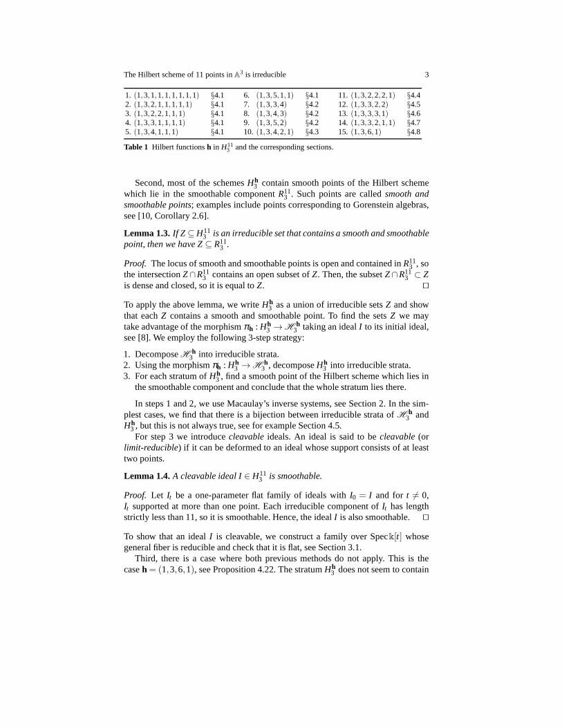
We now explain our approach to the proof of Theorem 1.1. We build upon thestrategy of [8]. As explained there, questions about smoothability of a specified idealI are easily reduced to the case whereI is local and has full embedding dimension 3.There are fifteen possible Hilbert functions ofI , see Table 1. For each Hilbert func-tion h, the schemeHh
3 parameterizes local ideals with fixed Hilbert functionh andthe standard graded Hilbert schemeH h
3 parameterizes homogeneous ideals withfixed Hilbert functionh. We apply three different strategies to show that for eachHilbert functionh in our list, we haveHh
3 ⊂ R113 .
First, for some cases the knowledge about the Hilbert function of an idealI isenough to produce a deformation (viaray familiesintroduced in [9]) whose specialfiber isI and general fiber is reducible. By Lemma 1.4, such anI is smoothable, seeSection 4.1.
The Hilbert scheme of 11 points inA3 is irreducible 3
1. (1,3,1,1,1,1,1,1,1) §4.1 6. (1,3,5,1,1) §4.1 11.(1,3,2,2,2,1) §4.42. (1,3,2,1,1,1,1,1) §4.1 7. (1,3,3,4) §4.2 12.(1,3,3,2,2) §4.53. (1,3,2,2,1,1,1) §4.1 8. (1,3,4,3) §4.2 13.(1,3,3,3,1) §4.64. (1,3,3,1,1,1,1) §4.1 9. (1,3,5,2) §4.2 14.(1,3,3,2,1,1) §4.75. (1,3,4,1,1,1) §4.1 10.(1,3,4,2,1) §4.3 15.(1,3,6,1) §4.8
Table 1 Hilbert functionsh in H113 and the corresponding sections.
Second, most of the schemesHh3 contain smooth points of the Hilbert scheme
which lie in the smoothable componentR113 . Such points are calledsmooth and
smoothable points; examples include points corresponding to Gorenstein algebras,see [10, Corollary 2.6].
Lemma 1.3.If Z ⊆H113 is an irreducible set that contains a smooth and smoothable
point, then we have Z⊆ R113 .
Proof. The locus of smooth and smoothable points is open and contained inR113 , so
the intersectionZ∩R113 contains an open subset ofZ. Then, the subsetZ∩R11
3 ⊂ Zis dense and closed, so it is equal toZ. ⊓⊔
To apply the above lemma, we writeHh3 as a union of irreducible setsZ and show
that eachZ contains a smooth and smoothable point. To find the setsZ we maytake advantage of the morphismπh : Hh
3 →H h3 taking an idealI to its initial ideal,
see [8]. We employ the following 3-step strategy:
1. DecomposeH h3 into irreducible strata.
2. Using the morphismπh : Hh3 →H h
3 , decomposeHh3 into irreducible strata.
3. For each stratum ofHh3 , find a smooth point of the Hilbert scheme which lies in
the smoothable component and conclude that the whole stratum lies there.
In steps 1 and 2, we use Macaulay’s inverse systems, see Section 2. In the sim-plest cases, we find that there is a bijection between irreducible strata ofH h
3 andHh
3 , but this is not always true, see for example Section 4.5.For step 3 we introducecleavableideals. An ideal is said to becleavable(or
limit-reducible) if it can be deformed to an ideal whose support consists of atleasttwo points.
Lemma 1.4.A cleavable ideal I∈ H113 is smoothable.
Proof. Let It be a one-parameter flat family of ideals withI0 = I and for t 6= 0,It supported at more than one point. Each irreducible component of It has lengthstrictly less than 11, so it is smoothable. Hence, the idealI is also smoothable. ⊓⊔
To show that an idealI is cleavable, we construct a family over Speck[t] whosegeneral fiber is reducible and check that it is flat, see Section 3.1.
Third, there is a case where both previous methods do not apply. This is thecaseh = (1,3,6,1), see Proposition 4.22. The stratumHh
3 does not seem to contain
4 T. Douvropoulos, J. Jelisiejew, B.I. U. Nødland, Z. Teitler
smooth points. However, the stratum is irreducible and we can describe what gen-eral points look like. We build a deformation showing that such general points aresmoothable, hence, by irreducibility, the entire stratum has to be smoothable.
We work over an algebraically closed fieldk of characteristic zero.
2 Prerequisites
Hilbert schemes and smoothability. The Hilbert scheme Hdn parameterizes sub-schemes ofAn of dimension zero and degreed. More formally,Hd
n represents thefunctor which assigns to eachk-schemeX the set of subschemes ofAn×X whichare flat overX and for which all fibers are finite of degreed, see [26, Chapter 1].Equivalently, lettingT = k[α1,α2, . . . ,αn], the schemeHd
n parameterizes idealsI forwhich T/I is a vector space of dimensiond. In other words,Hd
n also represents thefunctor which assigns to eachk-algebraA the set of idealsI in T⊗A such that thequotientsT⊗A/I are locally freeA-modules of rankd.
The Zariski tangent space toHdn at the point representingI is the T-module
Hom(I ,T/I), see [26, Theorem 1.1]. UsingMacaulay2[21], we can compute thedimension of this tangent space. We stress that a point is smooth if and only if thepoint lies on only one irreducible component of the scheme and the dimension ofthe tangent space at that point equals the dimension of the component of the schemecontaining the point. The dimension of the tangent space increases at singular points.
On Hdn , there is a distinguished component corresponding to smooth schemes.
Indeed, a slightly perturbed tuple ofd closed points inAn is just another such tuple.Thus, the set of tuples of points is open in the Hilbert schemeand their closureis a component. It is called thesmoothable componentof Hd
n and denoted byRdn.
Clearly,Rdn is generically smooth of dimensionnd. SinceHd
2 is smooth, we haveRd
2 = Hd2 .
A point of Rdn is said to besmoothable. Thus, an idealI is smoothable if and only
if it can be deformed to an ideal ofd distinct points. This means that one can builda one-parameter flat family of schemes over a discrete valuation ring for which thegeneral member consists ofd distinct points and the special fiber isT/I , see [6, 8]for details. In particular, a disjoint union of smoothable schemes is smoothable anda limit of smoothable schemes is smoothable.
Hilbert functions. In analyzing the Hilbert schemeHdn , it is useful to use work
with an invariant that refines the degreed. There are two closely-related notions ofHilbert function:
• For a gradedT-moduleM, its Hilbert function is defined byh(i) = dim(Mi). Inparticular, given a homogeneous idealI ⊂ T, we consider the Hilbert function ofthe quotient ringT/I .
• For a filteredT-moduleM with descending filtrationM = M0⊇M1 ⊇M2 ⊇ ·· · ,the Hilbert functionh is defined byh(i) = dim(Mi/Mi+1). In particular, if thescheme associated to an idealI ⊂ T is supported at a point, thenT/I is a local
The Hilbert scheme of 11 points inA3 is irreducible 5
ring (A,m), and the Hilbert functionh with respect to the filtration by powers ofm is defined to beh(i) = dim(mi/mi+1). If I is homogeneous andT/I is local,the two notions coincide.
We writeh as a vector(h(0),h(1), . . . ), trimming it after the last positive entry.Let A= T/I whereT = k[α1,α2, . . . ,αn] is a polynomial ring with its standard
grading andI is a homogeneous ideal. Assume thatI contains no linear forms. Wecall such an algebrastandard graded.
Macaulay’s bound is an upper bound for the growth of Hilbert functions of stan-dard graded algebras, defined as follows. First, for positive integersh andd, thereexist uniquely determined integersδ ≥ 1 andkd > kd−1 > · · ·> kδ ≥ δ such that
h=
(
kd
d
)
+
(
kd−1
d−1
)
+ · · ·+
(
kδδ
)
.
This expression is called thed-binomial expansionof h and denotedh(d). Thed-binomial expansion ofh can be found greedily: letkd be the greatest integer suchthat
(kdd
)
≤ h, then find the(d− 1)-binomial expansion ofh−(kd
d
)
. Now h〈d〉 is
defined as follows. Ifh(d) =(kd
d
)
+(kd−1
d−1
)
+ · · ·+(kδ
δ)
then we define
h〈d〉 :=
(
kd +1d+1
)
+ · · ·+
(
kδ +1δ +1
)
.
Example 2.1.We have 5(2) =(3
2
)
+(2
1
)
, so 5〈2〉 =(4
3
)
+(3
2
)
= 7. Similarly, we have
4(2) =(3
2
)
+(1
1
)
, so 4〈2〉 =(4
3
)
+(2
2
)
= 5.
Example 2.2.If h≤ d then we haveh(d) =(d
d
)
+(d−1
d−1
)
+ · · ·+(d−h+1
d−h+1
)
andh〈d〉 = h.
Theorem 2.3 (Macaulay’s bound, [34] or [3, Theorem 4.2.10]). Let A be a stan-dard gradedk-algebra with Hilbert functionh. For every non-negative integer d,we haveh(d+1)≤ h(d)〈d〉.
Corollary 2.4. Let A be a standard gradedk-algebra with Hilbert functionh. Ifd≥ 0 is such thath(d)≤ d, then we haveh(d)≥ h(d+1)≥ h(d+2)≥ ·· · .
Once the Macaulay bound is attained then it will also be attained for all higherdegrees provided that no new generators of the ideal appear:
Theorem 2.5 (Gotzmann’s Persistence Theorem, [20] or [3, Theorem 4.3.3]).Let A= T/I be a standard graded algebra with Hilbert functionh. If d ≥ 0 is aninteger such thath(d+1) = h(d)〈d〉 and I is generated in degrees≤ d, then we haveh(k+1) = h(k)〈k〉 for all k ≥ d.
Apolarity and inverse systems. A key tool in the analysis of finite schemes is thetechnique ofMacaulay’s inverse systems, also known as apolarity. General refer-ences include [15, 18], [30, Section 1.3, Chapter 5], [39].
Let S= k[x1,x2, . . . ,xn] andT = k[α1,α2, . . . ,αn] be polynomial rings with thestandard grading. Whenn≤ 3, we instead use variablesx,y,z andα,β ,γ. We write
6 T. Douvropoulos, J. Jelisiejew, B.I. U. Nødland, Z. Teitler
S≤d for⊕d
k=0Sk, and similarlyT≤d. The polynomial ringT acts onSby lettingαi
act as partial differentiation byxi . This is called theapolarityaction. We denote thisaction by , so thatαi F = ∂F
∂xifor F ∈ S. This gives bilinear mapsTd×Se→ Se−d
for all d,e. In particular, for eachd the pairingTd×Sd→S0 = k is a perfect pairing.
Definition 2.6. For any subsetJ⊂ S theapolar ideal, or annihilating ideal J⊥ ⊂ Tis the ideal of elementsΘ ∈ T such thatΘ F = 0 for all F ∈ J. ForF ∈ Swe writeF⊥ for ({F})⊥.
WhenJ is spanned by homogeneous elements, the apolar ideal is homogeneous.WhenJ consists of a single elementF , then the idealF⊥ is Gorenstein, see [12,Section 21.2].
Example 2.7.If F = xa11 xa2
2 · · ·xann , then we claim thatF⊥ = (αa1+1
1 , . . . ,αan+1n ). In-
deed, it is easy to see that eachαai+1i ∈ F⊥. Conversely, ifΘ ∈ T has a term
αb11 αb2
2 · · ·αbnn with eachbi ≤ ai, then the apolar pairing of this term withF is a
monomial that determines thebi , meaning that it cannot be cancelled by the otherterms ofΘ . Hence, ifΘ ∈ F⊥, then each term ofΘ must lie in the indicated ideal.
The linear mapT→ Sgiven byΘ 7→Θ F provides a simple approach to com-putingF⊥. The apolar idealF⊥ is the kernel of this map. We can computeJ⊥ byintersecting the idealsF⊥ for F in J. If J is ak-vector space, then it is sufficient toconsiderF in a basis forJ.
Example 2.8.ForF = x3+ yz, we haveF⊥ = (α3−6β γ,αβ ,αγ,β 2,γ2).
Example 2.9.ForF = x2y+ y2z, we haveF⊥ = (γ2,αγ,α2−β γ,β 3,αβ 2).
Definition 2.10.A Macaulay inverse system, or simply inverse system, is aT-sub-module ofS. That is, an inverse system is ak-vector subspaceJ⊆Swhich is closedunder differentiation: ifF ∈ J, then all of the derivativesα1 F , . . . ,αn F lie in J.
The inverse system generated bya subsetf1, . . . , fs of S is 〈 f1, f2, . . . , fs〉 =T f1 + T f2 + · · ·+ T fs, that is, the vector space spanned by thefi together withall higher partial derivatives. Clearly, we have〈 f1, . . . , fs〉⊥ =
⋂si=1〈 fi〉
⊥ =⋂s
i=1 f⊥i .An inverse system ishomogeneousif it is generated by homogeneous elements.
Remark 2.11.The mappingJ 7→ J⊥ sends finite-dimensional inverse systems to lo-cal ideals supported at the origin, that is,m-primary ideals wherem is the ideal ofthe origin. The mapping is one-to-one, sinceJ may be computed fromJ⊥ similarlyto the discussion above. In fact it is a bijection, as shown byMacaulay [35], orsee for example [15, Corollaire 2]. WhenI is a local ideal, we will writeI⊥ for itsinverse system.
Recall thatHhn andH h
n consist of all homogeneous and local ideals, respectively,with Hilbert function h. On the other handHd
n , consists of all zero-dimensionalschemes of lengthd in A
n, not only local ones or ones supported at the origin.
Proposition 2.12 ([18, Remark after Proposition 2.5]).If J is a homogeneous in-verse system then, J is isomorphic as a gradedk-vector space to T/J⊥.
The Hilbert scheme of 11 points inA3 is irreducible 7
Proposition 2.13 ([15, Proposition 2(a)]).For a finite-dimensional inverse systemJ, we havedimk J = dimkT/J⊥.
Proof. Let d be large enough so thatJ⊆S≤d. It follows that the mapT≤d→T/J⊥ issurjective. Hence, both of the dimensions are equal to the codimension ofJ⊥∩T≤d
in T≤d. ⊓⊔
Remark 2.14.For an inverse systemJ, for each integerk, J≤k denotes the vectorspace of polynomials of degree at mostk in J. These form an increasing filtration,J≤0⊆ J≤1⊆ ·· · . The inverse systemJ is a filteredT-module, so its Hilbert functionh is given byh(k) = dimJ≤k− dimJ≤k−1 for eachk and∑h(i) = dimk J. If J ishomogeneous, thenh(k) = dimJk.
Proposition 2.15 ([30, Lemma 2.12]).Let f ∈ S be a homogeneous form of degreed. If h is the Hilbert function of the inverse system〈 f 〉, thenh = (h(0), . . . ,h(d)) issymmetric:h(i) = h(d− i) for all i.
Proposition 2.16 ([7]).Suppose that f∈ S is a homogeneous form of degree d. Leth be the Hilbert function of〈 f 〉. If h(d−1) = k, that ish= (. . . ,k,1), then there areindependent linear functionsℓ1, ℓ2, . . . , ℓk ∈ S1 and a homogeneous form g such thatf = g(ℓ1, ℓ2, . . . , ℓk). Equivalently, there is a linear change of coordinates so that fdepends only on the variables x1, . . . ,xk, not on xk+1, . . . ,xn.
Remark 2.17.Using the above proposition, one can show that if〈 f 〉 has Hilbertfunction(. . . ,1,1), then f = ℓd for some linear functionℓ and〈 f 〉 has Hilbert func-tion (1,1, . . . ,1,1). If h(d−2)= h(d−1)= 2, then eitherf = ℓd+md or f = ℓd−1mfor some independent linear functionsℓ,m∈S1, and either way〈 f 〉 has Hilbert func-tion (1,2,2, . . . ,2,2,1). For proof see for example [30, Theorem 1.44]: in their no-tation,s= 2, andf⊥ has a quadratic generator, which up to a change of coordinatesis eitherαβ or β 2.
Dealing with nonhomogeneous inverse systems is much harderthan workingwith homogeneous ones. Fortunately, each inverse systemJ has an associated ho-mogeneous inverse system lead(J).
Definition 2.18.The leading formof a polynomial is its highest degree homoge-neous part. This may not be a monomial. For an inverse systemJ ⊂ S, the inversesystem of leading forms ofJ, denoted lead(J), is the vector subspace ofSspannedby leading forms of all the elements ofJ.
For example, the inverse system〈x3+ y2〉= span{x3+ y2,x2,x,y,1} has
lead(〈x3+ y2〉) = span{x3,x2,x,y,1} = 〈x3,y〉.
There is a tight connection between a systemJ and lead(J).
Proposition 2.19.The Hilbert functions of J andlead(J) are equal.
8 T. Douvropoulos, J. Jelisiejew, B.I. U. Nødland, Z. Teitler
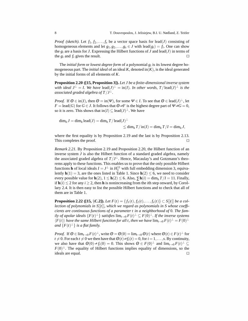
Proof (sketch).Let f1, f2, . . . , fs be a vector space basis for lead(J) consisting ofhomogeneous elements and letg1,g2, . . . ,gs ∈ J with lead(gi) = fi . One can showthegi are a basis forJ. Expressing the Hilbert functions ofJ and lead(J) in terms ofthegi and fi gives the result. ⊓⊔
Theinitial form or lowest degree formof a polynomialgi is its lowest degree ho-mogeneous part. Theinitial ideal of an idealK, denoted in(K), is the ideal generatedby the initial forms of all elements ofK.
Proposition 2.20 ([15, Proposition 3]).Let J be a finite-dimensional inverse systemwith ideal J⊥ = I. We havelead(J)⊥ = in(I). In other words, T/ lead(J)⊥ is theassociated graded algebra of T/J⊥.
Proof. If Θ ∈ in(I), thenΘ = in(Ψ ), for someΨ ∈ I . To see thatΘ ∈ lead(J)⊥, letF = lead(G) for G∈ J. It follows thatΘ F is the highest degree part ofΨ G= 0,so it is zero. This shows that in(I)⊆ lead(J)⊥. We have
dimk J = dimk lead(J) = dimkT/ lead(J)⊥
≤ dimk T/ in(I) = dimk T/I = dimk J,
where the first equality is by Proposition 2.19 and the last isby Proposition 2.13.This completes the proof. ⊓⊔
Remark 2.21.By Proposition 2.19 and Proposition 2.20, the Hilbert function of aninverse systemJ is also the Hilbert function of a standard graded algebra, namelythe associated graded algebra ofT/J⊥. Hence, Macaulay’s and Gotzmann’s theo-rems apply to these functions. This enables us to prove that the only possible Hilbertfunctionsh of local idealsI = J⊥ in H11
3 with full embedding dimension 3, equiva-lently h(1) = 3, are the ones listed in Table 1. Sinceh(2)≤ 6, we need to considerevery possible value forh(2), 1≤ h(2)≤ 6. Also,∑h(i) = dimkT/I = 11. Finally,if h(i)≤ 2 for anyi ≥ 2, thenh is nonincreasing from theith step onward, by Corol-lary 2.4. It is then easy to list the possible Hilbert functions and to check that all ofthem are in Table 1.
Proposition 2.22 ([15,§C.2]). Let F(t) = { f1(t), f2(t), . . . , fs(t)} ⊂ S[[t]] be a col-lection of polynomials in S[[t]], which we regard as polynomials in S whose coeffi-cients are continuous functions of a parameter t in a neighborhood of0. The fam-ily of apolar ideals{F(t)⊥} satisfieslimt→0 F(t)⊥ ⊆ F(0)⊥. If the inverse systems〈F(t)〉 have the same Hilbert function for all t, then we havelimt→0 F(t)⊥ = F(0)⊥
and{F(t)⊥} is a flat family.
Proof. If Θ ∈ limt→0 F(t)⊥, writeΘ =Θ(0) = limt→0Θ(t) whereΘ(t)∈ F(t)⊥ fort 6= 0. For eacht 6= 0 we then have thatΘ(t) fi(t) = 0, for i = 1, . . . ,s. By continuity,we also have thatΘ(0) fi(0) = 0. This showsΘ ∈ F(0)⊥ and limt→0 F(t)⊥ ⊆F(0)⊥. The equality of Hilbert functions implies equality of dimensions, so theideals are equal. ⊓⊔
The Hilbert scheme of 11 points inA3 is irreducible 9
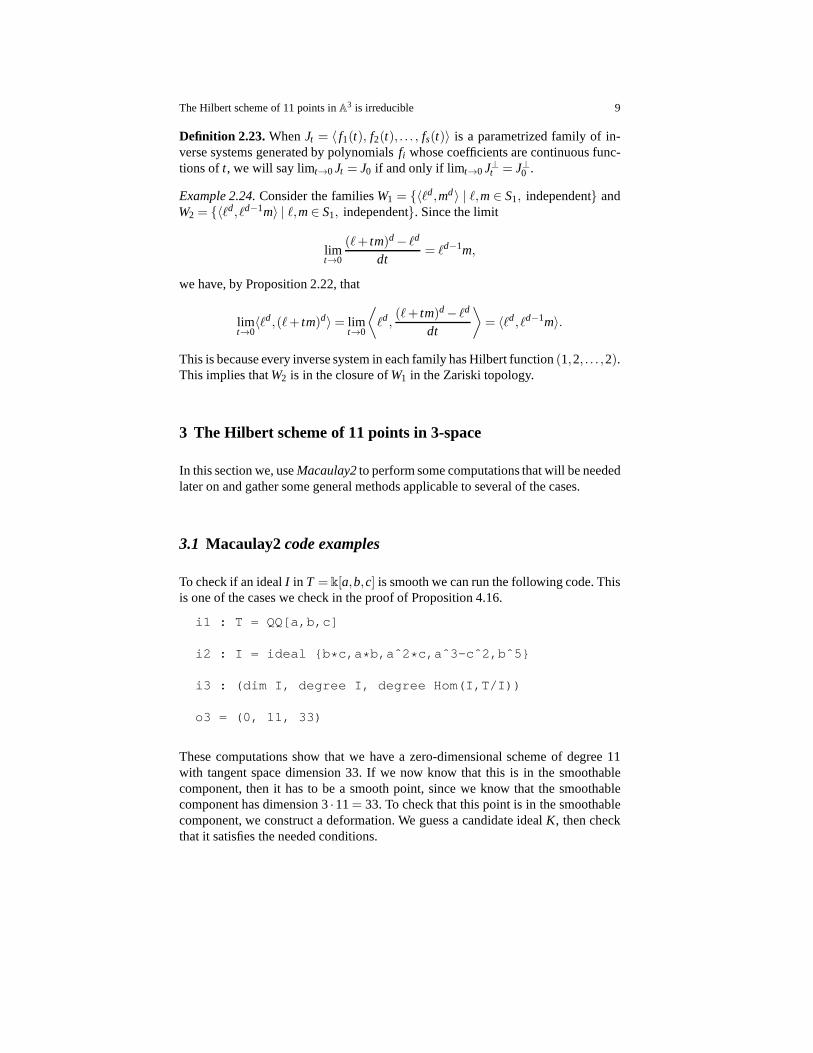
Definition 2.23.WhenJt = 〈 f1(t), f2(t), . . . , fs(t)〉 is a parametrized family of in-verse systems generated by polynomialsfi whose coefficients are continuous func-tions oft, we will say limt→0 Jt = J0 if and only if limt→0 J⊥t = J⊥0 .
Example 2.24.Consider the familiesW1 = {〈ℓd,md〉 | ℓ,m∈ S1, independent} and
W2 = {〈ℓd, ℓd−1m〉 | ℓ,m∈ S1, independent}. Since the limit
limt→0
(ℓ+ tm)d− ℓd
dt= ℓd−1m,
we have, by Proposition 2.22, that
limt→0〈ℓd,(ℓ+ tm)d〉= lim
t→0
⟨
ℓd,(ℓ+ tm)d− ℓd
dt
⟩
= 〈ℓd, ℓd−1m〉.
This is because every inverse system in each family has Hilbert function(1,2, . . . ,2).This implies thatW2 is in the closure ofW1 in the Zariski topology.
3 The Hilbert scheme of 11 points in 3-space
In this section we, useMacaulay2to perform some computations that will be neededlater on and gather some general methods applicable to several of the cases.
3.1 Macaulay2code examples
To check if an idealI in T = k[a,b,c] is smooth we can run the following code. Thisis one of the cases we check in the proof of Proposition 4.16.
i1 : T = QQ[a,b,c]
i2 : I = ideal {b * c,a * b,aˆ2 * c,aˆ3-cˆ2,bˆ5}
i3 : (dim I, degree I, degree Hom(I,T/I))
o3 = (0, 11, 33)
These computations show that we have a zero-dimensional scheme of degree 11with tangent space dimension 33. If we now know that this is inthe smoothablecomponent, then it has to be a smooth point, since we know thatthe smoothablecomponent has dimension 3·11= 33. To check that this point is in the smoothablecomponent, we construct a deformation. We guess a candidateidealK, then checkthat it satisfies the needed conditions.
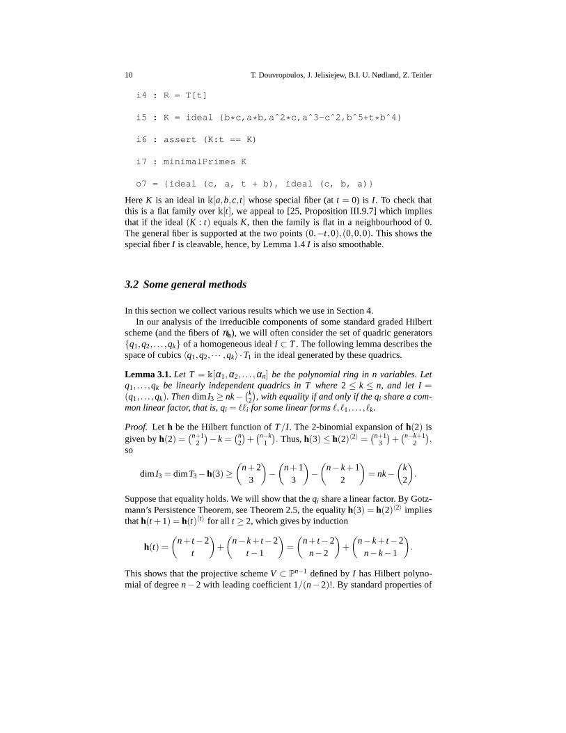
10 T. Douvropoulos, J. Jelisiejew, B.I. U. Nødland, Z. Teitler
i4 : R = T[t]
i5 : K = ideal {b * c,a * b,aˆ2 * c,aˆ3-cˆ2,bˆ5+t * bˆ4}
i6 : assert (K:t == K)
i7 : minimalPrimes K
o7 = {ideal (c, a, t + b), ideal (c, b, a)}
HereK is an ideal ink[a,b,c, t] whose special fiber (att = 0) is I . To check thatthis is a flat family overk[t], we appeal to [25, Proposition III.9.7] which impliesthat if the ideal(K : t) equalsK, then the family is flat in a neighbourhood of 0.The general fiber is supported at the two points(0,−t,0),(0,0,0). This shows thespecial fiberI is cleavable, hence, by Lemma 1.4I is also smoothable.
3.2 Some general methods
In this section we collect various results which we use in Section 4.In our analysis of the irreducible components of some standard graded Hilbert
scheme (and the fibers ofπh), we will often consider the set of quadric generators{q1,q2, . . . ,qk} of a homogeneous idealI ⊂ T. The following lemma describes thespace of cubics〈q1,q2, · · · ,qk〉 ·T1 in the ideal generated by these quadrics.
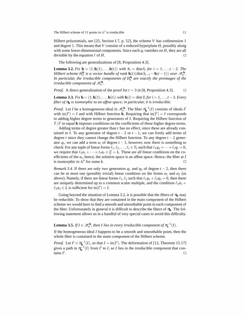
Lemma 3.1.Let T = k[α1,α2, . . . ,αn] be the polynomial ring in n variables. Letq1, . . . ,qk be linearly independent quadrics in T where2 ≤ k ≤ n, and let I=(q1, . . . ,qk). ThendimI3 ≥ nk−
(k2
)
, with equality if and only if the qi share a com-mon linear factor, that is, qi = ℓℓi for some linear formsℓ,ℓ1, . . . , ℓk.
Proof. Let h be the Hilbert function ofT/I . The 2-binomial expansion ofh(2) isgiven byh(2) =
(n+12
)
− k =(n
2
)
+(n−k
1
)
. Thus,h(3) ≤ h(2)〈2〉 =(n+1
3
)
+(n−k+1
2
)
,so
dimI3 = dimT3−h(3)≥(
n+23
)
−
(
n+13
)
−
(
n− k+12
)
= nk−
(
k2
)
.
Suppose that equality holds. We will show that theqi share a linear factor. By Gotz-mann’s Persistence Theorem, see Theorem 2.5, the equalityh(3) = h(2)〈2〉 impliesthath(t +1) = h(t)〈t〉 for all t ≥ 2, which gives by induction
h(t) =(
n+ t−2t
)
+
(
n− k+ t−2t−1
)
=
(
n+ t−2n−2
)
+
(
n− k+ t−2n− k−1
)
.
This shows that the projective schemeV ⊂ Pn−1 defined byI has Hilbert polyno-
mial of degreen−2 with leading coefficient 1/(n−2)!. By standard properties of
The Hilbert scheme of 11 points inA3 is irreducible 11
Hilbert polynomials, see [25, Section I.7, p. 52], the schemeV has codimension 1and degree 1. This means thatV consists of a reduced hyperplaneH, possibly alongwith some lower-dimensional components. Since eachqi vanishes onH, they are alldivisible by the equationℓ of H. ⊓⊔
The following are generalizations of [8, Proposition 4.3].
Lemma 3.2.Fix h = (1,h(1), . . . ,h(t)) with hi = dimSi for i = 1, . . . , t − 2. TheHilbert scheme Hhn is a vector bundle of rankh(t)(dimSt−1−h(t−1)) overH h
n .In particular, the irreducible components of Hh
n are exactly the preimages of theirreducible components ofH h
n .
Proof. A direct generalization of the proof fort = 3 in [8, Proposition 4.3]. ⊓⊔
Lemma 3.3.Fix h = (1,h(1), . . . ,h(t)) with h(i) = dimTi for i = 1, . . . , t−3. Everyfiber ofπh is isomorphic to an affine space; in particular, it is irreducible.
Proof. Let I be a homogeneous ideal inH hn . The fiberπ−1
h (I) consists of idealsI ′
with in(I ′) = I and with Hilbert functionh. Requiring that in(I ′) = I correspondsto adding higher degree terms to generators ofI . Requiring the Hilbert function ofT/I ′ to equalh imposes conditions on the coefficients of these higher degree terms.
Adding terms of degree greater thant has no effect, since these are already con-tained inI . To any generator of degreet −2 or t −1, we can freely add terms ofdegreet since they cannot change the Hilbert function. To any degreet−2 gener-ator qi , we can add a termai of degreet − 1, however, now there is something tocheck: For any tuple of linear formsℓ1, ℓ2, . . . , ℓr ∈ T1 such thatℓ1q1+ · · ·+ℓrqr = 0,we require thatℓ1a1+ · · ·+ ℓrar ∈ I ′t = It . These are all linear conditions on the co-efficients of theai , hence, the solution space is an affine space. Hence, the fiberat Iis isomorphic toAk for somek. ⊓⊔
Remark 3.4.If there are only two generatorsq1 andq2 of degreet − 2, then therecan be at most one (possibly trivial) linear condition on theforms a1 anda2 (asabove). Namely, if there are linear formsℓ1, ℓ2 such thatℓ1q1+ ℓ2q2 = 0, then theseare uniquely determined up to a common scalar multiple, and the conditionℓ1a1+ℓ2a2 ∈ It is sufficient for in(I ′) = I .
Going beyond the situation of Lemma 3.2, it is possible that the fibers ofπh maybe reducible. To show that they are contained in the main component of the Hilbertscheme we would have to find a smooth and smoothable point in each component ofthe fiber. Unfortunately in general it is difficult to describe the fibers ofπh. The fol-lowing statement allows us in a handful of very special casesto avoid this difficulty.
Lemma 3.5.If I ∈H hn , then I lies in every irreducible component ofπ−1
h (I).
If the homogeneous idealI happens to be a smooth and smoothable point, then thewhole fiber is contained in the main component of the Hilbert scheme.
Proof. Let I ′ ∈ π−1h (I), so thatI = in(I ′). The deformation of [12, Theorem 15.17]
gives a path inπ−1h (I) from I ′ to I , so I lies in the irreducible component that con-
tainsI ′. ⊓⊔
12 T. Douvropoulos, J. Jelisiejew, B.I. U. Nødland, Z. Teitler
3.3 Non-linear changes of coordinates
We recall the technique of non-linear changes of coordinates as in [9, 14] and [31,Section 2.2]. Assume we have a zero-dimensional quotientA= T/I = k[α,β ,γ]/Isupported at the origin. The algebraA can also be viewed as a quotient of thepower series ringR= k[[α,β ,γ]]. The power series ring has a much larger auto-morphism group than the polynomial ring. Denote the maximalideal of R by m.For anyσ1,σ2,σ3 ∈m whose images spanm/m2, there is an automorphismφ of Rdefined byφ(α) = σ1, φ(β ) = σ2, andφ(γ) = σ3.
Let J= 〈 f1, f2, . . . , fr〉 be the associated inverse system ofI . By [31, Section 2.2],the inverse system ofφ−1(I) is generated byφ∨( fi) whereφ∨ is defined as follows.Let Dα = φ(α)−α, Dβ = φ(β )−β , andDγ = φ(γ)− γ. Then we have
φ∨( f ) = ∑(k,m,n)∈Z3
≥0
xkymzn
k!m!n!·(
DkαDm
β Dnγ f
)
.
Example 3.6.Let J = 〈 f 〉 for f = x4+ y4+g where degg≤ 3. By subtracting mul-tiples ofα f andα2 f from f , we may assume the monomialsx3 andx2 do notappear ing. We will perform a non-linear change of coordinates so that there are nomonomials ing divisible byx2. This will be needed in the proof of Lemma 4.8.
Let B be the coefficient ofx2y in g and letC be the coefficient ofx2z. Let φ(α) =α, φ(β ) = β − B
12α2, andφ(γ) = γ − C12α2. We haveDα = 0, Dβ = − B
12α2, andDγ =−
C12α2, so
φ∨(x4) = x4+ yDβ (x4)+ zDγ(x
4)+ · · ·= x4− yBx2− zCx2+ · · · ,
where we have omitted terms of degree less than 3. Similarlyφ∨(y4) = y4 andφ∨(g)is equal tog, modulo terms of degree less than 3. Alsoφ∨( f ) will have no termsdivisible byx2.
3.4 An explicit construction of flat families
The section is adapted from [9, Section 5], where more general results were provedfor Gorenstein schemes. Fix a zero-dimensional schemeR. In this section, undercertain mild assumptions onR, we construct a family with special fiberRand generalfiber reducible, so thatR becomes cleavable.
Proposition 3.7.Let R⊂ An be a finite scheme supported at the origin. Let C⊂ A
n
be a smooth curve passing through the origin. Let H= (x = 0) be a hyperplaneintersecting C transversely. Let r≥ 1 be such that the ideal of intersection R∩C inC is (xr) and let Hr−1 = (xr−1 = 0) denote the thick hyperplane. If R⊂C∪Hr−1 asschemes, then R is cleavable.
The Hilbert scheme of 11 points inA3 is irreducible 13
Proof. SinceR∩C is cut out ofC by xr , we can choose anF ∈ I(R) whose imagein k[C] = k[An]/I(C) is xr . Then we haveq := xr −F ∈ I(C). Now the image ink[C] of any i ∈ I(R) is gxr , for someg. Write i = g(xr −q)+ j, for somej. We seethat j ∈ I(R)∩ I(C) which implies thatI(R) = (xr −q)+ I(R∪C), hence,R is cutout of R∪C by the equationxr −q. There is a deformation ofR⊂ R∪C given bydeforming this equation, namely
V(xr − txr−1−q)⊂ (R∪C)×A1, (1)
with t being the local parameter onA1.To prove the flatness of the family (1) it is enough to prove that every polynomial
f ∈ k[t] is not a zero-divisor in the coordinate ring ofV =V(xr−txr−1−q). Supposethere is anf ∈ k[t] and a functiong on V such thatf g is zero. We will show thatg vanishes onV ∩ (C×A1) and onV ∩ (Hr−1×A1). SinceR∪C⊂C∪Hr−1, thisimplies thatg vanishes on the whole ofV, so that it is zero.
First let us restrict toC, i.e. consider the familyV ∩ (C×A1). It is given bythe equationxr − txr−1, thus, it is flat. Therefore,f (t) is not a zero-divisor, hence,g restricts to zero onC×A1. Next let us restrict toHr−1, i.e. consider the familyV∩ (Hr−1×A1). It is given by the equationxr −q, which does not involvet. Hence,this family is constant, thus, flat. Hence,g restricts to zero onHr−1×A1, whichconcludes the proof of flatness. The fiber of the family (1) over t 6= 0 is supportedon at least two points: the origin and(t,0, . . . ,0), thus, reducible. Therefore,R iscleavable. ⊓⊔
Corollary 3.8. Let R⊂ An be a finite scheme supported at the origin. Let I= I(R)be its ideal. Choose coordinatesα1,α2, . . . ,αn on An. Assume that c is such thatαc
1 ·α j ∈ I(R) for all j 6= 1. Assume moreover thatαc1 /∈ I +(α2,α3, . . . ,αn). Then R
is cleavable.
Proof. This follows from Proposition 3.7 above if we takeC = V(α2,α3, . . . ,αn),H = (α1). Then r is defined byR∩C = (α r
1) and by assumptionr > c, so thatR⊂C∪Hr−1. ⊓⊔
Corollary 3.9. Suppose that R⊂ A3 is a scheme of length11. Let I⊂ k[α,β ,γ] beits ideal and suppose thatαβ ,αγ ∈ I. Then the ideal I is smoothable.
Proof. If R is reducible, it is smoothable because all its components are. SupposeRis irreducible supported at the origin. If any order one element lies inI , then aftera non-linear coordinate changeR is contained in anA2 and so is smoothable. If noorder one element lies inI , then Corollary 3.8 applied toc = 1 implies thatR iscleavable. Therefore, it is smoothable by Lemma 1.4. ⊓⊔
14 T. Douvropoulos, J. Jelisiejew, B.I. U. Nødland, Z. Teitler
4 Proof of main theorem
In this section, we prove Theorem 1.1 by proving for each possible Hilbert functionthat algebras with that Hilbert function are smoothable. For reference, Table 1 showsin which section each Hilbert function is treated.
In this section we fixn= 3, S= k[x,y,z], andT = k[α,β ,γ].
4.1 Cases with long tails of ones
Proposition 4.1.Let h be one of these Hilbert functions:(1,3,1,1,1,1,1,1,1),(1,3,2,1,1,1,1,1), (1,3,2,2,1,1,1), (1,3,3,1,1,1,1), (1,3,4,1,1,1), (1,3,5,1,1).Then we have Hh3 ⊂ R11
3 .
Proof. Let I ∈Hh3 be an ideal with Hilbert functionh. By Proposition 4.2, the ideal
I is cleavable. By Lemma 1.4, the idealI is smoothable. SoI ∈R113 . ⊓⊔
Proposition 4.2.Let R= SpecA⊂ An be an irreducible subscheme andh be theHilbert function of the local algebra A. Supposeh=(1,h(1), . . . ,h(c),1, . . . ,1) withat least c trailing ones, that is, letting s be the greatest value such thath(s) 6= 0, weassume thath(k) = 1 for c+1≤ k≤ s, and s≥ 2c. Then the scheme R is cleavable.
The proof follows the Gorenstein case of [9, Example 5.15].
Proof. Let I be the ideal ofR and letJ be the inverse system ofI . Consider a mini-mal generating set ofJ. It has a unique generatorf of degrees. As explained in Sec-tion 3.3, we can perform a non-linear coordinate change to assume thatf = xs
1+g,for someg such thatαc
1 g= 0. All other generators ofJ are of degree at mostc.By subtracting some partials off , we may assume that they are also annihilated byαc
1. Thus,αc1α j lies in I for all j 6= 1.
It remains to check thatαc1 /∈ I +(α2,α3, . . . ,αn). Take anyq∈ (α2,α3, . . . ,αn).
Then(αc1−q) f = s!
(s−c)! xs−c1 −q g. We claim this is nonzero. Note thats−c≥ c
by assumption on the number of trailing ones. Therefore,αs−c1 annihilatesg. So
αs−c1
(
s!(s− c)!
xs−c1 −q g
)
= s!x01−q (αs−c
1 g) = s! 6= 0.
This shows(αc1 − q) f 6= 0, as claimed, soαc
1 − q /∈ I . Therefore,αc1 /∈ I +
(α2,α3, . . . ,αn). Thus, by Corollary 3.8 the subschemeR is cleavable. ⊓⊔
4.2 Cases with short Hilbert functions
For the three casesh= (1,3,3,4), h= (1,3,4,3), andh= (1,3,5,2), the analysis ofthe irreducible components of their standard graded Hilbert schemes completely de-
The Hilbert scheme of 11 points inA3 is irreducible 15
termines the corresponding strata in the (not graded) Hilbert schemeHh3 . Explicitly,
in each of these casesHh3 is a vector bundle overH h
3 by Lemma 3.2, so the irre-ducible components ofHh
3 are exactly the preimages of the irreducible componentsof H h
3 .In each of the three cases, we will first coverH h
3 by a collection of irreduciblesets (which are not necessarily components) and produce a smooth and smoothableideal for each set. By Lemma 3.2 and Lemma 1.3, this is enough to guarantee thatall algebras inHh
3 are smoothable.
Proposition 4.3.Let h = (1,3,3,4). Then Hh3 ⊂ R11
3 .
Proof. Let I ⊂ T, I ∈H h3 be a homogeneous ideal such thatA= T/I has Hilbert
function h. Then dimI2 = dimT2− h(2) = 3. Let I ′ = (I2) be the ideal gener-ated by the quadrics inI . By Lemma 3.1, dimI ′3 ≥ 3 · 3−
(32
)
= 6, but dimI ′3 ≤dimI3 = dimT3−h(3) = 6. SoI3 = I ′3, equality holds in the dimension bound, andby Lemma 3.1, the quadrics inI2 must share a common linear factorℓ.
ThenI2 is spanned byℓα, ℓβ , ℓγ. That is, the standard graded Hilbert schemeH h
3 is parametrized by the lineℓ. It is, therefore, isomorphic to the GrassmannianGr(1,3)∼= P
2 and, hence, irreducible. By Lemma 3.2,Hh3 is also irreducible.
It is sufficient to find one smooth and smoothable point inHh3 . Consider the
ideal L = (αβ ,αγ,α2 + β 3,β 2γ2,β γ3,γ4). It is smoothable by Corollary 3.9 andwe check computationally thatL is smooth. ⊓⊔
Proposition 4.4.Let h = (1,3,4,3). Then Hh3 ⊂ R11
3 .
Proof. The standard graded Hilbert schemeH h3 is a union of two irreducible sets.
We will provide a smooth and smoothable point in each of them.Let I ⊂ T, I ∈ H h
3 be a homogeneous ideal such thatA = T/I has Hilbertfunctionh. Then dimI2 = 2. By Lemma 3.1, the space of cubics generated by thequadrics inI2 can have dimension either 6 or 5, and the latter occurs exactly whenthe quadrics share a linear factor. LetP⊂H h
3 be the set of idealsI whose quadricsgenerate a 6-dimensional space of cubics and letQ⊂ H h
3 be the set of idealsIwhose quadrics generate a 5-dimensional space of cubics. ThenH h
3 = P∪Q. Weclaim that each ofP andQ is irreducible.
The subsetP is parametrized by pairs of spaces(K,M), where K is a 2-dimensional subspace ofT2, not of the form span{ℓ · ℓ1, ℓ · ℓ2}, and M is a 7-dimensional subspace ofT3 that containsK ·T1, equivalently a line inT3/K ·T1.Thus,P is realized as a projective bundle with fiberP(T3/K ·T1) over an open sub-set of Gr(2,T2). In particular,P is irreducible.
In the subsetQ, the quadricsq1,q2 that spanI2 have the formq1 = ℓ ·ℓ1 andq2 =ℓ · ℓ2 for some linesℓ,ℓ1, ℓ2. This component is parametrized by a triple(ℓ,L,N),whereℓ∈ T1 is the common line,L = (ℓ1, ℓ2)⊂ T1 is the space spanned by the othertwo lines, andN is a 7-dimensional space ofT3 that contains the 5-dimensional spaceℓ ·L ·T1. SoQ is isomorphic to a Grassmannian bundle with fiber Gr(7−5,T3/ℓ ·L ·T1), over a base Gr(1,T1)×Gr(2,T1); it is, therefore, irreducible.
Now Hh3 = π−1
h (P)∪ π−1h (Q), and by Lemma 3.2 these are irreducible sets as
well. To complete this case, we provide a smooth and smoothable ideal for each set.
16 T. Douvropoulos, J. Jelisiejew, B.I. U. Nødland, Z. Teitler
The idealI = (α2,β 2,γ3,αβ γ2) lies inP and, hence, also inπ−1h (P). It is monomial,
hence, smoothable by [8, Proposition 4.15] and it is easy to check computationallythat it is a smooth point. Forπ−1
h (Q) let I = (αβ ,αγ,α3+ γ3,β γ2,β 3γ,β 4). ThenI is smoothable by Corollary 3.9 and once again a smooth point. ⊓⊔
Proposition 4.5.Let h = (1,3,5,2). Then Hh3 ⊂ R11
3 .
Proof. Let I ⊂ T, I ∈H h3 be a homogeneous ideal such thatA= T/I has Hilbert
functionh. Then dimI2 = 1 and dimI3 = dimT3− h(3) = 8. The standard gradedHilbert schemeH 3
h is parametrized by pairs(L,M), whereL is some 1-dimensionalsubspace ofT2 and M is an 8-dimensional subspace ofT3 that contains the 3-dimensional subspaceL ·T1. This parametrization realizes an isomorphism ofH h
3to a Grassmannian bundle with basePT2 and fiber Gr(8−3,T3/L ·T1), proving thatH h
3 is irreducible. By Lemma 3.2,Hh3 is irreducible as well.
Now let I = (αβ ,α3,β 3,γ3,αγ2,α2γ +β γ2). One can check thatI ∈Hh3 . Since
αβ 2,αγ2 ∈ I andα2 /∈ I +(β ,γ), Corollary 3.8 withc= 2 impliesI is smoothable.Finally one can check computationally thatI is a smooth point. ⊓⊔
4.3 Caseh = (1,3,4,2,1)
Proposition 4.6.Let h = (1,3,4,2,1). Then Hh3 ⊂ R11
3 .
Proof. Let I ∈H h3 be a homogeneous ideal with inverse systemJ. Let f ∈ J4 and let
h f be the Hilbert function of〈 f 〉. Since〈 f 〉 ⊂ J we haveh f ≤ h. By Proposition 2.15and Macaulay’s bound (Theorem 2.3),h f must be(1,2,3,2,1), (1,2,2,2,1), or(1,1,1,1,1).
If h f = (1,2,3,2,1) see Lemma 4.7. Ifh f = (1,2,2,2,1) then by Remark 2.17we can choose coordinates so thatf = x4+y4 or f = x3y. For f = x4+y4 see Lemma4.8 and forf = x3y see Lemma 4.9. Ifh f = (1,1,1,1,1) see Lemma 4.10. ⊓⊔
Lemma 4.7.Let h = (1,3,4,2,1) and let I∈ H h3 be a homogeneous ideal with
inverse system J. Suppose that the degree4 generator f of J is such that the Hilbertfunction of〈 f 〉 is (1,2,3,2,1). Thenπ−1
h (I)⊂ R113 .
Proof. Let I ′ ∈ π−1h (I) with inverse systemJ′. Let F be the degree 4 generator of
J′, so thatf is the leading form ofF . We will construct a familyJ′t so thatJ′1 = J′
andJ′0 is 〈x2y2,z2〉, 〈x2y2,zx〉, or 〈x2y2,z(x+ y)〉. First change coordinates so thatf ∈ k[x,y]. Thenx2,xy,y2 ∈ 〈 f 〉2 ⊂ J′, soJ′≤2 is spanned by{x2,xy,y2,Q,S≤1} fora quadratic formQ ∈ k[x,y,z]. Write Q = cxz+ dyz+ ez2. If e 6= 0 then changingcoordinates by replacingz with a suitable linear combination ofx,y,z to completethe square eliminates thexz andyz terms and takesQ to z2 modulox2,xy,y2. SoeitherJ′ = 〈F,z2〉 or J′ = 〈F,z(cx+dy)〉.
Write F = f + g, degg≤ 3. By well-known facts about binary forms (see forexample, [30, Theorem 1.43]), we havef = ℓ4
1+ ℓ42+ ℓ4
3 for some nonproportionallinear formsℓi ∈ k[x,y]. Observe that 18x2y2 = (x+ y)4 +ω(x+ωy)4 +ω2(x+
The Hilbert scheme of 11 points inA3 is irreducible 17
ω2y)4 whereω is a cube root of unity. We change coordinates ink[x,y] so thatℓ1 = x+y andℓ2 = ω1/4(x+ωy). Let ft = ℓ4
1+ ℓ42+(tℓ3+(1− t)ω1/2(x+ω2y))4,
Ft = ft + tg, andJ′t = 〈Ft ,Q〉.It is easy to check thatF1 = F , F0 = 18x2y2, and for all but finitely many
t, 〈 ft 〉 has Hilbert function(1,2,3,2,1) and J′t has Hilbert function(1,3,4,2,1).Then limJ′t = J′0 = 〈18x2y2,Q〉 = 〈x2y2,Q〉, as in Definition 2.23. Rescalingx andy and interchanging if necessary,Q is one ofz2, zx, or z(x+ y). Now 〈x2y2,z2〉⊥
and 〈x2y2,zx〉⊥ are monomial ideals, hence, smoothable. The family(γ2,αγ −β γ,β 2γ,β 3,α3+ tα2) shows that〈x2y2,z(x+ y)〉⊥ = (γ2,αγ −β γ,β 2γ,β 3,α3) issmoothable. So all three points are smoothable and it is easyto check that each oneis a smooth point. Hence, the irreducible (one-dimensional) family {(J′t )
⊥} ⊂ R113 ,
in particularI ′ = (J′1)⊥ ∈ R11
3 . ⊓⊔
Lemma 4.8.Let h = (1,3,4,2,1) and let I∈ H h3 be a homogeneous ideal with
inverse system J. Suppose that the degree4 generator of J is of the formℓ4+m4 forsome independent linear formsℓ,m∈ S1. Thenπ−1
h (I)⊂ R113 .
Proof. Assumeℓ = x,m= y. Let I ′ ∈ π−1h (I) with inverse systemJ′. We will ap-
ply Corollary 3.8. Consider the degree four generatorF = x4+ y4+g∈ J′, wheredegg≤ 3. Sincex2 ∈ J we can subtract thex2 term out ofg. Then the only terms ofg divisible byx2 are possiblyx3, x2y, x2z. After a non-linear coordinate change asin Example 3.6 we may assume that there are no such terms. Thenα2 F = 12x2,soα2 6∈ F⊥+(β ,γ). Moreoverα2β andα2γ annihilateF and so its partials, hence,lie in I ′. Therefore, the assumptions of Corollary 3.8 forc= 2 are satisfied andI ′ iscleavable. By Lemma 1.4, it is smoothable. ⊓⊔
Lemma 4.9.Let h = (1,3,4,2,1) and let I∈ H h3 be a homogeneous ideal with
inverse system J. Suppose that the degree4 generator of J is of the formℓ3m forsome independent linear formsℓ,m∈ S1. Thenπ−1
h (I)⊂ R113 .
Proof. Assumeℓ = x, m= y, so thatJ = 〈x3y,Q1,Q2〉 for some quadratic formsQ1,Q2. Let I ′ ∈ π−1
h (I) with inverse systemJ′. We will show I ′ is smoothable bywriting it as a limit of smoothable points. Note,J′ = 〈x3y+g3+g2,Q1,Q2〉 wheregi is a form of degreei for i = 2,3. We introduce a parametert and letyt = x+ ty.Observe that limt→0(y4
t −x4)/4t = x3y. For generalt we will define a formg3(t) sothatJ′t = 〈(y
4t − x4)/4t +g3(t)+g2,Q1,Q2〉 → J′ in the sense of Definition 2.23.
To defineg3(t), first note thatγ g3 ∈ J2 = span{x2,xy,Q1,Q2}. For i = 1,2let Q♯
i =∫
Qi dz be a homogeneous form of degree 3 so thatγ Q♯i = Qi . Write
g3 = ax2z+ bxyz+ cQ♯1 + dQ♯
2 + e(x,y) for some scalarsa,b,c,d and a 3-forme.
Now we defineg3(t) = ax2z+(b/2t)(y2t − x2)z+ cQ♯
1+dQ♯2+e(x,y).
Now γ g3(t) ∈ span{x2,y2t ,Q1,Q2}, hence, lead(J′t ) = 〈y
4t − x4,Q1,Q2〉. Since
dimJ2 = 4 we havexy 6∈ span{x2,Q1,Q2}. Sincexy = limt→0(y2t − x2)/(2t) we
also havey2t 6∈ span{x2,Q1,Q2} for generalt. For sucht the space(lead(J′t ))2
has dimension 4, which means that lead(J′t ) andJ′t have Hilbert functionh. Alsolimt→0 g3(t) = g3. Therefore, limt→0 J′t = J′, as desired. By Lemma 4.8, each(J′t )
⊥
with t 6= 0 is smoothable, which impliesI ′ = lim(J′t )⊥ is smoothable as well. ⊓⊔
18 T. Douvropoulos, J. Jelisiejew, B.I. U. Nødland, Z. Teitler
Lemma 4.10.Let h = (1,3,4,2,1) and let I∈H h3 be a homogeneous ideal with
inverse system J. Suppose that the degree4 generator f of J is such that the Hilbertfunction of〈 f 〉 is (1,1,1,1,1). Thenπ−1
h (I)⊂ R113 .
Proof. By Remark 2.17, we can choose coordinates so thatf = z4. LetV ⊂H h3 be
the set of idealsI satisfying the hypothesis, that is,V = {I ∈H h3 | I ⊂ (z4)⊥}. For
I ∈V, dimI2 =2 and dimI3 =8. By Lemma 3.1, dimT1 · I2 is either 5 or 6. LetV1⊂Vbe the set ofI such that dimT1 · I2 = 6, equivalently the quadrics inI2 have no com-mon factor. LetV2⊂V be the set ofI such that dimT1 · I2 = 5 andI2 = span{ℓℓ1, ℓℓ2}for some linear formsℓ,ℓ1, ℓ2 such that span{ℓ1, ℓ2} ⊆ z⊥ = span{α,β} (neces-sarily equality must hold). And letV3 ⊂ V be the remainder, the set ofI suchthat dimT1 · I2 = 5 andI2 = span{ℓℓ1, ℓℓ2} for some linear formsℓ,ℓ1, ℓ2 such thatspan{ℓ1, ℓ2} 6⊂ z⊥. We will show that eachVi and eachπ−1
h (Vi) is irreducible, andgive a smooth and smoothable point on eachπ−1
h (Vi).First, every idealI ∈ V is determined by(I2, I3). SupposeI ∈ V1. The subspace
I2 ⊂ (z2)⊥ is parametrized by an open subset of Gr(2,(z2)⊥) = Gr(2,5). And thenI3⊂ (z3)⊥ is such thatT1 · I2⊂ I3. The quotientI3/T1 · I2 is a 2-dimensional subspaceof (z3)⊥/T1 · I2. So for each choice ofI2, I3 may be chosen from Gr(8−6,(z3)⊥/T1 ·I2) = Gr(2,3). This showsV1 is a Grassmannian bundle over an open subset of aGrassmannian, in particular irreducible. LetI2 = span{q1,q2}. SinceI ∈ V1, thereare no linesℓ1, ℓ2 such thatℓ1q1+ℓ2q2 = 0. By Lemma 3.3 and Remark 3.4, the fiberπ−1
h (I) is a certain product of affine spaces. Explicitly it isT23 ×T4
4 , correspondingto cubic terms that may be added to the quadric generators ofI and quartic termsthat may be added to the quadric and cubic generators ofI . This makesπ−1
h (V1) a(trivial!) vector bundle overV1, hence, irreducible. A smooth and smoothable pointin π−1
h (V1) is given by〈yz,x2y,z4〉⊥ = (αγ,β 2,β γ2,α3,γ5). It is smoothable be-cause it is a monomial ideal and we check computationally that it is a smooth point.This shows thatπ−1
h (V1)⊂ R113 .
If I ∈ V2 then I2 = ℓ · span{α,β} for some linear formℓ, so I2 is determinedby the choice of[ℓ] ∈ PT1. As before, for each choice ofℓ, I3 may be chosen fromGr(8−5,(z3)⊥/T1 · I2) =Gr(3,4). Again this makesV2 a Grassmannian bundle overan irreducible base, soV2 is irreducible. By Remark 3.4,π−1
h (V2) is a trivial subbun-dle of a trivial vector bundle overV2, namelyπ−1
h (V2) ⊂V2× (T23 ×T5
4 ) is definedby βa1−αa2 ∈ I4 = (z4)⊥, wherea1,a2 are the cubic terms added to the quadricgeneratorsℓα, ℓβ . Hence,π−1
h (V2) is irreducible. A smooth and smoothable pointin this set is given by the limit of the flat family(αγ,β γ,β 3+ γ4,α3− t ·α2,α2β ).
If I ∈ V3 then, writingI2 = span{ℓℓ1, ℓℓ2}, we must haveℓ z= 0, since for atleast one ofi = 1,2 we haveℓi z 6= 0, butℓℓi z2 = 0. Nowℓ may be chosen fromz⊥
and span{ℓ1, ℓ2} may be chosen to be any 2-dimensional subspace ofT1 other thanz⊥. So the choice ofI2 is parametrized by an open subset ofP(z⊥)×Gr(2,T1).Once again, for each choice ofI2, I3 may be chosen from the GrassmannianGr(8− 5,(z3)⊥/T1 · I2) = Gr(3,4). Hence,V3 is a Grassmannian bundle over anirreducible base, in particular irreducible. By Remark 3.4, π−1
h (V3) is a (nontrivial)subbundle of a trivial vector bundle overV2, namelyπ−1
h (V3) ⊂V3× (T23 ×T5
4 ) isdefined byℓ2a1− ℓ1a2 ∈ I4 = (z4)⊥ where, as before,a1,a2 are the cubic terms
The Hilbert scheme of 11 points inA3 is irreducible 19
added to the quadric generatorsℓℓ1, ℓℓ2. Hence,π−1h (V3) is irreducible. The ideal
(β 2,β γ,α3,α2γ,αγ2,γ5) ∈V3 is smoothable because it is monomial and we checkcomputationally that it is smooth. ⊓⊔
4.4 Caseh = (1,3,2,2,2,1)
Lemma 4.11.Let h = (1,h(1), . . . ,h(k),2, . . . ,2,1) such thath(i) = dimSi for alli ≤ k, then has at least two2s and a1 in the last position. Then the standardgraded Hilbert schemeH h
n is irreducible. Each ideal I∈H hn is the apolar ideal
J⊥ of an inverse system J of one of the following forms:〈ℓd +md,Sk〉, 〈ℓd−1m,Sk〉,〈ℓd,md−1,Sk〉, 〈ℓd, ℓd−2m,Sk〉 for some linear formsℓ,m.
Proof. Say the last 1 is in degreed, let J be a homogeneous inverse system withHilbert functionh, and let f ∈ J be thed-form that appears. Either〈 f 〉 has Hilbertfunction(. . . ,2,2,1) or (. . . ,1,1,1). In the first casef = ℓd+md or f = ℓd−1m, andJ is generated byf together withSk. The second type is a limit of the first type,similarly to Example 2.24.
In the second casef = ℓd and there is a generatorg of degreed−1. Noteg has atmost 2 first derivatives since〈g〉d−2⊆ Jd−2. So〈g〉 has Hilbert function(. . . ,2,1,0)or (. . . ,1,1,0). If it is (. . . ,1,1,0) theng= md−1 for a linear formm independentfrom ℓ. If the Hilbert function ofg is (. . . ,2,1,0) thenℓd−2 ∈ 〈g〉d−2, sog= ℓd−2mfor a linear formm independent fromℓ.
So eitherg = ℓd−2m or g = md−1. Correspondingly, eitherJ = 〈ℓd, ℓd−2m,Sk〉or J = 〈ℓd,md−1,Sk〉. Both of these can be obtained as limits of inverse sys-tems of the first two forms in appropriate ways, using Proposition 2.22. Explic-itly, 〈ℓd, ℓd−2m,Sk〉 = limt→0〈ℓ
d−1(ℓ+ tm),Sk〉 and 〈ℓd,md−1,Sk〉 = limt→0〈ℓd +
tmd,Sk〉. ⊓⊔
Proposition 4.12.Let h = (1,3,2,2,2,1). Then Hh3 ⊂ R11
3 .
Proof. By Lemma 4.11, every homogeneous ideal inH h3 is the apolar ideal of
an inverse system which is isomorphic to one of the following: J1 = 〈x5 + y5,z〉,J2 = 〈x4y,z〉, J3 = 〈x5,y4,z〉, or J4 = 〈x5,x3y,z〉. We may dispose of the first twocases easily. We computeI2 = J⊥2 = (α5,β 2,αγ,β γ,γ2). Then I2 is smoothablebecause it is a monomial ideal and one can easily check computationally that it isa smooth point. By Lemma 3.5, the smooth and smoothable pointI2 lies in everycomponent of the fiberπ−1
h (I2), which shows that each irreducible component ofthe fiber is contained inR11
3 .Similarly, I1 = J⊥1 = (α5− β 5,αβ ,αγ,β γ,γ2) is smooth and it is smoothable
by Corollary 3.9. Using Lemma 3.5 again, this smooth and smoothable point lies ineach irreducible component of the fiber, so each irreduciblecomponent of the fiberis contained inR11
3 .Now we consider the last two cases, where one finds that the homogeneous ideals
J⊥3 , J⊥4 are not smooth points (although they are monomial, hence, smoothable). So
20 T. Douvropoulos, J. Jelisiejew, B.I. U. Nødland, Z. Teitler
we need to develop a more detailed description of the fibers inthese cases. In Lemma4.13 we show that the fiberπ−1
h (J⊥3 ) is contained inR113 and in Lemma 4.14 we do
the same forJ4. ⊓⊔
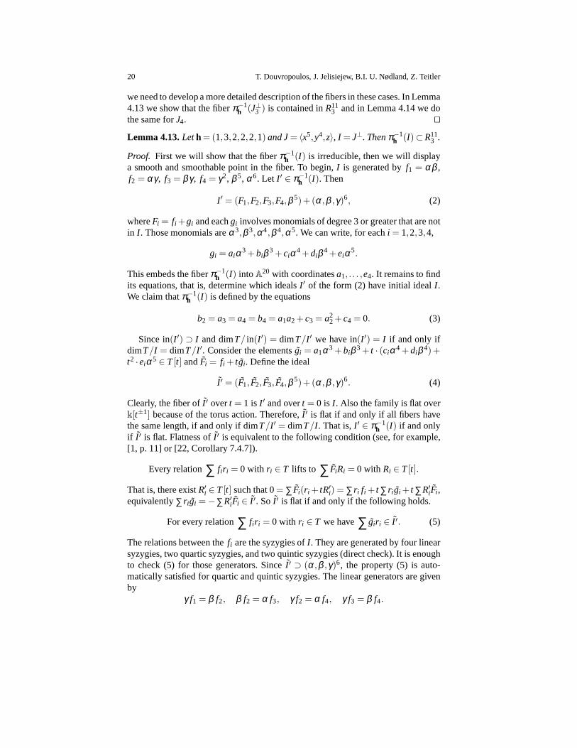
Lemma 4.13.Leth= (1,3,2,2,2,1) and J= 〈x5,y4,z〉, I = J⊥. Thenπ−1h (I)⊂R11
3 .
Proof. First we will show that the fiberπ−1h (I) is irreducible, then we will display
a smooth and smoothable point in the fiber. To begin,I is generated byf1 = αβ ,f2 = αγ, f3 = β γ, f4 = γ2, β 5, α6. Let I ′ ∈ π−1
h (I). Then
I ′ = (F1,F2,F3,F4,β 5)+ (α,β ,γ)6, (2)
whereFi = fi +gi and eachgi involves monomials of degree 3 or greater that are notin I . Those monomials areα3,β 3,α4,β 4,α5. We can write, for eachi = 1,2,3,4,
gi = aiα3+biβ 3+ ciα4+diβ 4+eiα5.
This embeds the fiberπ−1h (I) intoA
20 with coordinatesa1, . . . ,e4. It remains to findits equations, that is, determine which idealsI ′ of the form (2) have initial idealI .We claim thatπ−1
h (I) is defined by the equations
b2 = a3 = a4 = b4 = a1a2+ c3 = a22+ c4 = 0. (3)
Since in(I ′) ⊃ I and dimT/ in(I ′) = dimT/I ′ we have in(I ′) = I if and only ifdimT/I = dimT/I ′. Consider the elements ˜gi = a1α3+biβ 3+ t · (ciα4+diβ 4)+t2 ·eiα5 ∈ T[t] andFi = fi + tgi. Define the ideal
I ′ = (F1, F2, F3, F4,β 5)+ (α,β ,γ)6. (4)
Clearly, the fiber ofI ′ overt = 1 is I ′ and overt = 0 is I . Also the family is flat overk[t±1] because of the torus action. Therefore,I ′ is flat if and only if all fibers havethe same length, if and only if dimT/I ′ = dimT/I . That is,I ′ ∈ π−1
h (I) if and onlyif I ′ is flat. Flatness ofI ′ is equivalent to the following condition (see, for example,[1, p. 11] or [22, Corollary 7.4.7]).
Every relation∑ fir i = 0 with r i ∈ T lifts to ∑ FiRi = 0 with Ri ∈ T[t].
That is, there existR′i ∈ T[t] such that 0= ∑ Fi(r i + tR′i) = ∑ r i fi + t ∑ r i gi + t ∑R′iFi ,equivalently∑ r i gi =−∑R′iFi ∈ I ′. So I ′ is flat if and only if the following holds.
For every relation∑ fi r i = 0 with r i ∈ T we have∑ gir i ∈ I ′. (5)
The relations between thefi are the syzygies ofI . They are generated by four linearsyzygies, two quartic syzygies, and two quintic syzygies (direct check). It is enoughto check (5) for those generators. SinceI ′ ⊃ (α,β ,γ)6, the property (5) is auto-matically satisfied for quartic and quintic syzygies. The linear generators are givenby
γ f1 = β f2, β f2 = α f3, γ f2 = α f4, γ f3 = β f4.
The Hilbert scheme of 11 points inA3 is irreducible 21
By (5), the fiber is cut out by the conditions
γg1−β g2 ∈ I ′, β g2−αg3 ∈ I ′, γg2−αg4 ∈ I ′, γg3−β g4 ∈ I ′.
We now check that they unfold into (3). Consider an idealI ′ ∈ π−1h (I). The element
γg1−β g2 lies in I ′ by (5). Since
γg1−β g2 = a1α3γ +b1β 3γ−a2α3β −b2β 4
+ t(c1α4γ +d1β 4γ− c2α4β −d2β 5)+ t2(e1α5γ−e2α5β )
lies in I ′, its initial form lies in I , which impliesb2 = 0. Similarly, by consideringthe initial forms ofγg1−αg3 ∈ I ′ we deduce thata3 = 0; from γg2−αg4 ∈ I ′ wegeta4 = 0; from γg3−β g4 ∈ I ′ we getb4 = 0. Note the following relations:
α3β ≡−a1tα5, α3γ ≡−a2tα5, β 3γ ≡−b3tβ 5 (mod I ′).
Using these relations, together withb2 = a3 = a4 = b4 = 0, we check that
β g2−αg3≡−t(a1a2+ c3)α5 (mod I ′).
This implies that−t(a1a2 + c3)α5 ∈ I ′, so by evaluating att = 1 we get(a1a2+c3)α5 ∈ I ′. Hence, the leading form(a1a2+ c3)α5 is in I . Therefore,a1a2+ c3 =0. Similarly, γg2−αg4 ≡ −(a2
2+ c4)α5 (mod I ′) which gives the conditiona22+
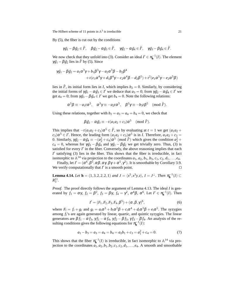
c4 = 0, whereas forγg3− β g4 and γg1− β g2 we get trivially zero. Thus, (3) issatisfied for everyI ′ in the fiber. Conversely, the above reasoning implies that eachI ′ satisfying (3) lies in the fiber. This shows that the fiber is irreducible, in factisomorphic toA14 via projection to the coordinatesa1, a2, b1, b3, c1, c2, d1, . . . ,e4.
Finally, let I ′ = (α6,β 5,αβ ,αγ,β γ +α5,γ2). It is smoothable by Corollary 3.9.We verify computationally thatI ′ is a smooth point. ⊓⊔
Lemma 4.14.Let h = (1,3,2,2,2,1) and J= 〈x5,x3y,z〉, I = J⊥. Thenπ−1h (I) ⊂
R113 .
Proof. The proof directly follows the argument of Lemma 4.13. The ideal I is gen-erated byf1 = αγ, f2 = β 2, f3 = β γ, f4 = γ2, α4β , α6. Let I ′ ∈ π−1
h (I). Then
I ′ = (F1,F2,F3,F4,β 5)+ (α,β ,γ)6, (6)
whereFi = fi + gi and gi = aiα3 + biα2β + ciα4 + diα3β + eiα5. The syzygiesamong fi ’s are again generated by linear, quartic, and quintic syzygies. The lineargenerators areβ f1−α f3, γ f1−α f4, γ f2−β f3, γ f3−β f4. An analysis of the re-sulting conditions gives the following equations forπ−1
h (I):
a1−b3 = a3 = a4 = b4 = a2b1+ c3 = a21+ c4 = 0. (7)
This shows that the fiberπ−1h (I) is irreducible, in fact isomorphic toA14 via pro-
jection to the coordinatesa1,a2,b1,b2,c1,c2,d1, . . . ,e4. A smooth and smoothable
22 T. Douvropoulos, J. Jelisiejew, B.I. U. Nødland, Z. Teitler
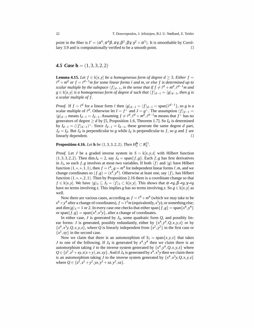
point in the fiber isI ′ = (α6,α4β ,αγ,β 2,β γ,γ2+α5). It is smoothable by Corol-lary 3.9 and is computationally verified to be a smooth point. ⊓⊔
4.5 Caseh = (1,3,3,2,2)
Lemma 4.15.Let f ∈ k[x,y] be a homogeneous form of degree d≥ 3. Either f =ℓd +md or f = ℓd−1m for some linear formsℓ and m, or else f is determined up toscalar multiple by the subspace〈 f 〉d−1, in the sense that if f6= ℓd +md, ℓd−1m andg∈ k[x,y] is a homogeneous form of degree d such that〈 f 〉d−1 = 〈g〉d−1, then g isa scalar multiple of f .
Proof. If f = ℓd for a linear formℓ then〈g〉d−1 = 〈 f 〉d−1 = span{ℓd−1}, sog is ascalar multiple ofℓd. Otherwise letI = f⊥ andJ = g⊥. The assumption〈 f 〉d−1 =〈g〉d−1 meansId−1 = Jd−1. Assumingf 6= ℓd, ℓd +md, ℓd−1m means thatf⊥ has nogenerators of degree≥ d by [5, Proposition 1.6, Theorem 1.7]. SoId is determinedby Id−1 = (〈 f 〉d−1)
⊥. SinceJd−1 = Id−1, these generate the same degreed part,Jd = Id. But Jd is perpendicular tog while Id is perpendicular tof , sog and f arelinearly dependent. ⊓⊔
Proposition 4.16.Let h be(1,3,3,2,2). Then Hh3 ⊂ R11
3 .
Proof. Let J be a graded inverse system inS= k[x,y,z] with Hilbert function(1,3,3,2,2). Then dimJ4 = 2, sayJ4 = span{ f ,g}. Each f ,g has first derivativesin J3, so eachf ,g involves at most two variables. If both〈 f 〉 and〈g〉 have Hilbertfunction(1,∗,∗,1,1), then f = ℓ4, g= m4 for independent linear formsℓ,m, and wechange coordinates so( f ,g) = (x4,y4). Otherwise at least one, say〈 f 〉, has Hilbertfunction(1,∗,∗,2,1). Then by Proposition 2.16 there is a coordinate change so thatf ∈ k[x,y]. We have〈g〉3 ⊆ J3 = 〈 f 〉3 ⊂ k[x,y]. This shows thatα g,β g,γ ghave no terms involvingz. This impliesg has no terms involvingz. Sog∈ k[x,y] aswell.
Now there are various cases, according asf = ℓ4+m4 (which we may take to bex4+y4 after a change of coordinates),f = ℓ3m(equivalently,x3y), or something else;and dim〈g〉3 = 1 or 2. In every case one checks that either span{ f ,g}= span{x4,y4}or span{ f ,g}= span{x4,x3y}, after a change of coordinates.
In either case,J is generated byJ4, some quadratic formQ, and possibly lin-ear forms:J is generated, possibly redundantly, either by{x4,y4,Q,x,y,z} or by{x4,x3y,Q,x,y,z}, whereQ is linearly independent from{x2,y2} in the first case or{x2,xy} in the second case.
Now we claim that there is an automorphism ofS1 = span{x,y,z} that takesJ to one of the following. IfJ4 is generated byx4,y4 then we claim there is anautomorphism takingJ to the inverse system generated by{x4,y4,Q,x,y,z} whereQ∈{z2,z2+xy,z(x+y),zx,xy}. And if J4 is generated byx4,x3y then we claim thereis an automorphism takingJ to the inverse system generated by{x4,x3y,Q,x,y,z}whereQ∈ {z2,z2+ y2,yz,y2+ xz,y2,xz}.
The Hilbert scheme of 11 points inA3 is irreducible 23
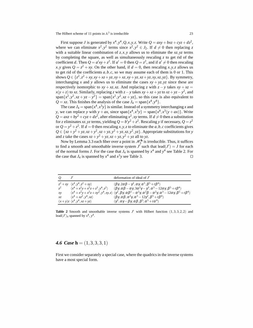
First supposeJ is generated byx4,y4,Q,x,y,z. Write Q= axy+bxz+ cyz+dz2,where we can eliminatex2,y2 terms sincex2,y2 ∈ J2. If d 6= 0 then replacingzwith a suitable linear combination ofz,x,y allows us to eliminate thexz,yz termsby completing the square, as well as simultaneously rescaling z to get rid of thecoefficientd. ThenQ= a′xy+z2. If a′ = 0 thenQ= z2, and ifa′ 6= 0 then rescalingx,y givesQ = z2 + xy. On the other hand, ifd = 0, then rescalingx,y,z allows usto get rid of the coefficientsa,b,c, so we may assume each of them is 0 or 1. ThisshowsQ∈ {z2,z2+xy,xy+xz+yz,xy+xz,xy+yz,xz+yz,xy,xz,yz}. By symmetry,interchangingx andy allows us to eliminate the casesxy+ yz,yz since these arerespectively isomorphic toxy+ xz,xz. And replacingz with z− y takesxy+ xz=x(y+z) to xz. Similarly, replacingzwith z−y takesxy+xz+yzto xz+yz−y2, andspan{x2,y2,xz+ yz− y2} = span{x2,y2,xz+ yz}, so this case is also equivalent toQ= xz. This finishes the analysis of the caseJ4 = span{x4,y4}.
The caseJ4 = span{x4,x3y} is similar. Instead of a symmetry interchangingx andy, we can replacey with y+ax, since span{x4,x3y} = span{x4,x3(y+ax)}. WriteQ= axz+by2+cyz+dz2, after eliminatingx2,xy terms. Ifd 6= 0 then a substitutionfor zeliminatesxz,yzterms, yieldingQ= b′y2+z2. Rescalingy if necessary,Q= z2
or Q= y2+z2. If d = 0 then rescalingx,y,z to eliminate thea,b,c coefficients givesQ∈ {xz+y2+yz,xz+y2,xz+yz,y2+yz,xz,y2,yz}. Appropriate substitutions foryandz take the casesxz+ y2+ yz,xz+ yz,y2+ yzall to yz.
Now by Lemma 3.3 each fiber over a point inH h3 is irreducible. Thus, it suffices
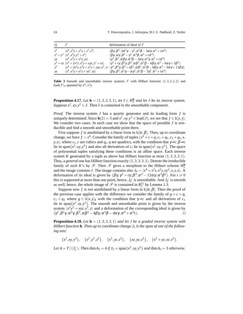
to find a smooth and smoothable inverse systemJ′ such that lead(J′) = J for eachof the normal formsJ. For the case thatJ4 is spanned byx4 andy4 see Table 2. Forthe case thatJ4 is spanned byx4 andx3y see Table 3. ⊓⊔
Q J′ deformation of ideal ofJ′
z2+xy 〈x4,y4,z2+xy〉 (β γ ,2αβ − γ2,αγ ,α5,β 5+ tβ 4)z2 〈x4+x2y+x2z+z3,y4,z2〉 (β γ ,αβ −αγ ,3α2γ− γ3,α3−12αγ ,β 5+ tβ 4)xy 〈x4+x2y+x2z+xy2,y4,xy,z〉 (γ2,β γ ,αβ 2−α2γ ,α2β −α2γ ,α3−12αγ ,β 5+ tβ 4)xz 〈x4+xz2,y4,xz〉 (β γ ,αβ ,α2γ ,α3−12γ2,β 5+ tβ 4)(x+y)z 〈x4,y4,xz+yz〉 (γ2,αγ−β γ ,αβ ,β 5,α5+ tα4)
Table 2 Smooth and smoothable inverse systemsJ′ with Hilbert function (1,3,3,2,2) andlead(J′)4 spanned byx4, y4.
4.6 Caseh = (1,3,3,3,1)
First we consider separately a special case, where the quadrics in the inverse systemshave a most special form.
24 T. Douvropoulos, J. Jelisiejew, B.I. U. Nødland, Z. Teitler
Q J′ deformation of ideal ofJ′
z2 〈x4,x3y+x2z+z3,z2〉 (β γ ,β 2,3α2γ− γ3,α2β −3αγ ,α5+ tα4)z2+y2 〈x4,x3y,y2+z2〉 (β γ ,αγ ,β 2− γ2,α4β ,α5+ tα4)yz 〈x4,x3y+x2z,yz〉 (γ2,β 2,αβ γ ,α2β −3αγ ,α3γ ,α5+ tα4)y2+xz 〈x4+2x2z,x3y+xyz,y2+xz〉 (γ2+ tγ ,β 2γ ,β 3,αβ 2,α2β −6β γ ,α3−6αγ +3β 2)y2 〈x4+2x2z,x3y+x2z+xyz,y2,z〉 (γ2,β 2γ ,β 3+ tβ 2,αβ 2,α2β −6β γ ,α3−6αγ +12β γ)xz 〈x4,x3y+x2z+xz2,xz〉 (β γ ,β 2,α2γ−αγ2,α2β −3γ2,α5+ tα4)
Table 3 Smooth and smoothable inverse systemsJ′ with Hilbert function (1,3,3,2,2) andlead(J′)4 spanned byx4, x3y.
Proposition 4.17.Let h = (1,3,3,3,1), let I ∈ Hh3 and let J be its inverse system.
Suppose x2,xy,y2 ∈ J. Then I is contained in the smoothable component.
Proof. The inverse systemJ has a quartic generator and its leading formf isuniquely determined. Sinceh(2) = 3 andx2,xy,y2 ∈ lead(J), we see thatf ∈ k[x,y].We consider two cases. In each case we show that the space of possibleJ is irre-ducible and find a smooth and smoothable point there.
First supposef is annihilated by a linear form ink[α,β ]. Then, up to coordinatechange, we havef = x4. Consider the family of tuples(x4+c+q,c1+q1,c2+q2,x,y,z), whereci , c are cubics andqi, q are quadrics, with the condition thatγ c,β clie in span{x2,xy,y2} and also all derivatives ofci lie in span{x2,xy,y2}. The spaceof polynomial tuples satisfying these conditions is an affine space. Each inversesystemK generated by a tuple as above has Hilbert function at most(1,3,3,3,1).Thus, ageneralone has Hilbert function exactly(1,3,3,3,1). Denote the irreduciblefamily of suchK’s by F . ThenF gives a morphism to the Hilbert schemeHh
3and the image containsJ. The image contains alsoJ0 = 〈x4+x2z,x2y,xy2,x,y,z〉. Adeformation of its ideal is given by(β γ,γ2 + tγ,β 3,α3−12αγ,α2β 2). For t 6= 0this is supported at more than one point, hence,J⊥0 is smoothable. AndJ⊥0 is smoothas well, hence, the whole image ofF is contained inR11
3 by Lemma 1.3.Suppose nowf is not annihilated by a linear form ink[α,β ]. Then the proof of
the previous case applies with the difference we consider the family of g+ c+ q,c1 + q1 whereg ∈ k[x,y]4 with the condition thatγ c and all derivatives ofc1
lie in span{x2,xy,y2}. The smooth and smoothable point is given by the inversesystem〈x2y2+ xyz,x3,z〉 and a deformation of the corresponding ideal is given by(γ2,β 2γ,α2γ,β 3,αβ 2−4β γ,α2β −4αγ,α4+α3t). ⊓⊔
Proposition 4.18.Let h = (1,3,3,3,1) and let J be a graded inverse system withHilbert functionh. Then up to coordinate change J2 is the span of one of the follow-ing sets:
{x2,xy,y2}, {x2,y2,z2}, {x2,yz,z2}, {xz,yz,z2}, {x2+ yz,xz,z2}.
Let A= T/(J⊥2 ). ThendimA3 = 4 if J2 = span{x2,xy,y2} anddimA3 = 3 otherwise.
The Hilbert scheme of 11 points inA3 is irreducible 25
Proof. Let I = (J⊥2 ). By Macaulay’s bound, dimA3 ≤ (dimA2)〈2〉 = 3〈2〉 = 4. If
dimA3 = 4, then by Lemma 3.1 the quadrics inI2 share a common linear factor.After a change of coordinates,I2 is spanned by{γ2,β γ,αγ}. ThenJ contains thequadricsx2,xy,y2.
So we reduce to the case dimA3 = 3, equivalently dimI3 = 7. We start with theclaim that, whenI = (I2) is generated by 3 quadrics and dimI3 = 7, thenI is thesaturated ideal of a zero-dimensional degree3 scheme inP2. The spaceT1⊗ I2 hasdimension 9 and maps by multiplication surjectively toT1⊗ I2→ I3, so the kernelhas dimension 2, which means there are 2 linear syzygies among the quadrics inI2.The minimal free resolution ofA= T/I is equal to
0← T← T(−2)⊕3← T(−3)⊕2⊕T(−4)⊕q⊕F ′← T(−4)⊕p⊕F ′′← 0,
whereF ′,F ′′ are sums ofT(−i) with i > 4. We will show thatp= q= 0. First, ifp= β3,4(I) 6= 0 thenI contains the idealℓ(α,β ,γ) for some linear formℓ, by [13,discussion following Theorem 8.15, p. 162]. But this is the case dimA3 = 4 whichwe have already treated. Since we are now assuming dimA3 = 3, then we must havep= 0. Next, we compute dimA4 by considering the free resolution above:
dimA4 = dimT4−3dimT2+(2dimT1+qdimT0)−0,
where the final 0 reflectsp= 0. This gives dimA4 = 15−3·6+2·3+q= 3+q. Atthe same time, 3+q= dimA4≤ (dimA3)
〈3〉 = 3〈3〉 = 3. Soq= 0.Now I is generated in degree 2 and dimA4 = (dimA3)
〈3〉 = 3. By Gotzmann’sPersistence Theorem, dimAk = 3 for all k≥ 3. This showsZ = ProjA has Hilbertpolynomial 3, soZ = V(I) ⊂ P
2 is zero-dimensional and has degree 3. To see thatI is saturated, letI ′ be the saturation ofI . Since the quadrics inI share no commonlinear factor,Z is not contained in any line, soI ′ contains no linear forms. Thendim(T/I ′)1 = 3. The Hilbert function of a saturated ideal is nondecreasing, so foreveryk≥ 1, 3= dim(T/I ′)1 ≤ dim(T/I ′)k ≤ dim(T/I)k = 3, which showsI ′ = I .This completes the proof of the claim thatI is the saturated ideal of a degree 3zero-dimensional schemeZ in P
2.SinceZ is cut out by quadrics, the intersection ofZ with any line has degree at
most 2. ThenZ is one of the following.
1. Z may be a disjoint union of three non-collinear reduced points. We change coor-dinates so thatZ = {[1 : 0 : 0], [0 : 1 : 0], [0 : 0 : 1]}. ThenI2 = span{αβ ,αγ,β γ}.
2. Z may be the union of a reduced point with a zero-dimensional scheme of degree2. We choose coordinates so that the reduced point is[1 : 0 : 0] and the scheme ofdegree 2 is supported at[0 : 0 : 1] and is contained in the line spanned by[0 : 0 : 1]and[0 : 1 : 0]. ThenI2 = span{αβ ,αγ,β 2}.
3. Z may be a scheme of degree 3 supported at a point which we may take to be[0 : 0 : 1]. Then after a change of coordinates eitherI2 = span{α2,αβ ,β 2} orI2 = span{α2−β γ,αβ ,β 2}.
To see the last claim, first note that ifq= ℓ1ℓ2 ∈ I2 is a reducible quadric then bothcomponentsℓ1, ℓ2 pass through[0 : 0 : 1], becauseZ is not contained in any single
26 T. Douvropoulos, J. Jelisiejew, B.I. U. Nødland, Z. Teitler
line. If every quadric inI2 is reducible thenI2 = span{α2,αβ ,β 2} consists of allthe quadrics that are singular at[0 : 0 : 1]. Otherwise, there is a smooth quadric inI2and we can choose coordinates so that it isq= α2−β γ. A quadricq′ ∈ I2 intersectsq in Z plus one more point. If the extra point is also[0 : 0 : 1] thenq′ = β 2+λq forsome scalarλ . Otherwiseq′ = ℓβ +λq whereℓ is the line through[0 : 0 : 1] and theextra point. SoI2 is spanned byq, αβ , andβ 2. Now, having the normal forms ofZ,we calculateJ2 asI⊥2 , obtaining the list above. ⊓⊔
Lemma 4.19.Fix a three dimensional space of quadrics Q and a subspace A⊂〈α,β ,γ〉. Suppose that the derivatives of Q span〈x,y,z〉. Consider the setJ (Q,A)of inverse systems J such that
1. J has Hilbert function(1,3,3,3,1),2. Q equals J2,3. A is equal to the space of linear forms annihilating the quartic in lead(J).
ThenJ (Q,A) is irreducible or empty.
Proof. SupposeJ (Q,A) is non-empty. LetI = Q⊥. Let h be the Hilbert functionof T/I . By Proposition 4.18, we have eitherQ = span{x2,xy,y2} up to coordinatechange orh(3) = 3. The equalityQ = span{x2,xy,y2} is impossible, since deriva-tives ofQ spanx,y,z. Thus,h(3) = 3. The remaining part of the proof resembles theproof of Proposition 4.17. Leta= dimA. Consider the setF of tuples of polyno-mials
f + c+q, c1+q1, . . . ,ca+qa ∈ S, (8)
such that
1. f is homogeneous of degree four and annihilated byA (and possibly other linearforms),
2. all ci andc are homogeneous of degree three,3. all qi andq are homogeneous of degree two,4. both f and allci are annihilated byI ,5. the spaceA c is contained inQ.
All given conditions are linear in coefficients of polynomials, thus,F is an affinespace. Consider an open (possibly empty) subsetF0⊂F consisting of tuples wheref is annihilated exactly byA and such thatci are linearly independent and span{ci}is disjoint from the space of partial derivatives off . ThenF0 is irreducible as anopen set in affine space.
Consider an inverse systemJ generated by all linear forms and a tuple inF0.We now prove that its Hilbert functionh is at most(1,3,3,3,1) position-wise. ByProposition 2.19, it is enough to show that the Hilbert function of lead(J) is atmost(1,3,3,3,1). It is clear thath(0) = h(4) = 1 andh(1) ≤ 3. All cubic termsin lead(J) are leading forms of combinations ofci and partials off . Thus, they areannihilated byI . The space of cubics annihilated byI is h(3) = 3-dimensional, thus,h(3) ≤ 3. Consider now the quadrics in lead(J). They are combinations of leadingforms of partials off , of ci and also ofA c. All those forms lie inQ, thus,h(2)≤ 3.Therefore,h≤ (1,3,3,3,1) position-wise.
The Hilbert scheme of 11 points inA3 is irreducible 27
Since(1,3,3,3,1) is the maximal possible value ofh, the setFgen⊂F0 consist-ing of systems with Hilbert function(1,3,3,3,1) is open, thus, irreducible. It gives amap to the Hilbert scheme whose image isJ (Q,A), which is, therefore, irreducibleas well. ⊓⊔
Proposition 4.20.Let h be(1,3,3,3,1). Then Hh3 ⊂ R11
3 .
Proof. Let J be a graded inverse system inS= k[x,y,z] with Hilbert functionh = (1,3,3,3,1). It has a unique degree 4 generatorf . We will subdivide the casesaccording to the Hilbert function of the inverse systemK generated byf . The Hilbertfunction is symmetric. Using Macaulay’s bound, we find that there are four dif-ferent cases for the Hilbert function ofK: (1,1,1,1,1), (1,2,2,2,1), (1,2,3,2,1),(1,3,3,3,1).
Case(1,3,3,3,1): f generates the entire module, hence,J is Gorenstein. And ev-eryJ′ in the fiberπ−1
h (J) is also Gorenstein. By [33, Proposition 2.2] or [32, Corol-lary 4.3], any Gorenstein subscheme ofA3 is smoothable, hence, all such pointsJ′
lie in the smoothable component ofH113 .
Case(1,2,3,2,1): Since f has two independent first derivatives, we know it de-pends on only two variables, sayx,y. Since it spans a three-dimensional set of sec-ond derivatives, this will have to be〈x2,xy,y2〉, so we are done by Proposition 4.17.
Case(1,2,2,2,1): Let Q be the space of quadrics insideJ. By Proposition 4.17,we may assume thatQ 6= span{x2,xy,y2} up to coordinate change, so that deriva-tives of Q spanx,y,z. Then by Proposition 4.18 and Lemma 4.19 we see that theirreducible strata are determined byQ equal to
span{x2,y2,z2}, span{x2,yz,z2}, span{xz,yz,z2}, span{x2+ yz,xz,z2}(9)
and the linear forms annihilatingf (up to simultaneous coordinate change). It re-mains to check which annihilators are possible for eachQ. Let A = T/Q⊥. Bythe proof of Proposition 4.18, this is a homogeneous coordinate ring of a zero-dimensional subscheme of ProjT. Note that if a linear formσ annihilatesf , thenthe intersection of ProjA with the projective line(σ = 0) has degree at least two.Wedirectly check that for the four cases in (9) we get the following possible annihila-tors.
1. α or β or γ for Q= span{x2,y2,z2},2. α or β for Q= span{x2,yz,z2},3. λ1α +λ2β with λi ∈ k arbitrary forQ= span{xz,yz,z2},4. β for Q= span{x2+ yz,xz,z2}.
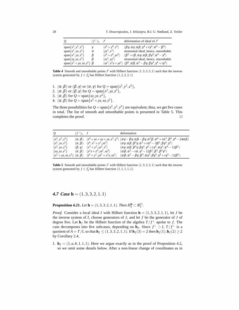
Note that for first, third and fourth case there is a unique choice up to coordinatechange. Therefore, we have five distinct cases in total. The corresponding smoothand smoothable points are presented in Table 4.
Case(1,1,1,1,1): the argument is completely analogous to the previous case upto the point where we determine possible( f⊥)1 depending onQ. As before, letA=T/Q⊥. Note that an annihilator(σ1,σ2) is possible if and only ifl4∈ J, equivalently[l ] ∈ ProjA, wherel is the linear form annihilated by(σ1,σ2) and[l ] ∈ ProjT is itsclass.Based on this observation, the possible annihilators in the four cases in (9) are
28 T. Douvropoulos, J. Jelisiejew, B.I. U. Nødland, Z. Teitler
Q ( f⊥)1 J′ deformation of ideal ofJ′
span{x2,y2,z2} γ 〈x4+y4,z3〉 (β γ ,αγ ,αβ ,γ4+ tγ3,α4−β 4)span{x2,yz,z2} α 〈yz3,x3〉 monomial ideal, hence, smoothablespan{x2,yz,z2} β 〈x4+z4,yz2〉 (β 2+ tβ ,αγ ,αβ ,β γ3,α4− γ4)span{xz,yz,z2} β 〈xz3,yz2〉 monomial ideal, hence, smoothablespan{x2+yz,xz,z2} β 〈xz3,x2z+yz2〉 (β 2,αβ ,α2−β γ ,β γ3,γ4+ tγ3)
Table 4 Smooth and smoothable pointsJ′ with Hilbert function(1,3,3,3,1) such that the inversesystem generated byf ∈ J′4 has Hilbert function(1,2,2,2,1)
1. (α,β ) or (β ,γ) or (α,γ) for Q= span{x2,y2,z2},2. (α,β ) or (β ,γ) for Q= span{x2,yz,z2},3. (α,β ) for Q= span{xz,yz,z2},4. (α,β ) for Q= span{x2+ yz,xz,z2}.
The three possibilities forQ= span{x2,y2,z2} are equivalent, thus, we get five casesin total. The list of smooth and smoothable points is presented in Table 5. Thiscompletes the proof. ⊓⊔
Q ( f⊥)1 J deformation
{x2,y2,z2} (α ,β ) 〈z4+xz+xy+yz,x3,y3〉 (αγ−β γ ,αβ−β γ ,α2β ,α4+ tα3,β 4,γ4−24αβ ){x2,yz,z2} (α ,β ) 〈z4,x3+y2,yz2〉 (αγ ,αβ ,β 2γ ,α3+ tα2−3β 2,β γ3,γ5){x2,yz,z2} (β ,γ) 〈x4+y2,yz2,z3〉 (αγ ,αβ ,β 2γ ,β γ3,γ4+ tγ3,αγ3,α4−12β 2){xz,yz,z2} (α ,β ) 〈y2z+z4,yz2,xz2〉 (αβ ,α2− tα ,γ3−12β 2,β 3,β 2γ2){x2+yz,xz,z2} (α ,β ) 〈z4+y2,yz2+x2z,xz2〉 (αβ ,α2−β γ ,β 3,αγ3,β γ3,γ4+ tγ3−12β 2)
Table 5 Smooth and smoothable pointsJ′ with Hilbert function(1,3,3,3,1) such that the inversesystem generated byf ∈ J′4 has Hilbert function(1,1,1,1,1).
4.7 Caseh = (1,3,3,2,1,1)
Proposition 4.21.Let h = (1,3,3,2,1,1). Then Hh3 ⊂ R11
3 .
Proof. Consider a local idealI with Hilbert functionh = (1,3,3,2,1,1), let J bethe inverse system ofI , choose generators ofJ, and let f be the generator ofJ ofdegree five. Leth f be the Hilbert function of the algebraT/ f⊥ apolar to f . Thecase decomposes into five subcases, depending onh f . Since f⊥ ⊃ I , T/ f⊥ is aquotient ofA= T/I , so thath f ≤ (1,3,3,2,1,1). If h f (3) = 2 thenh f (1),h f (2)≥ 2by Corollary 2.4.
1. h f = (1,a,b,1,1,1). Here we argue exactly as in the proof of Proposition 4.2,so we omit some details below. After a non-linear change of coordinates as in

The Hilbert scheme of 11 points inA3 is irreducible 29
Section 3.3, we may assumef = x5+g with α2 g= 0. SinceJ is generated byf together with elements of degree 3 or less,α3β andα3γ annihilate all ofJ. Ifq∈ (β ,γ) is such thatαc−q annihilatesf , thenc≥ 4; hence,α3 /∈ I +(β ,γ).Now Corollary 3.8 proves that the element is cleavable, hence, smoothable byLemma 1.4.
2. h f = (1,3,3,2,1,1). In this caseI = f⊥ and soA is Gorenstein, hence, smooth-able by [33, Proposition 2.2] or [32, Corollary 4.3].
3. h f = (1,2,3,2,1,1). After changing coordinates so thatf ∈ k[x,y] we haveJ =〈 f ,z〉, soA is smoothable by Corollary 3.9.
4. h f = (1,3,2,2,1,1). In this case after a non-linear change of coordinates we havef = g+ z2 for g ∈ k[x,y] with Hilbert function(1,2,2,2,1,1), see [9, Proposi-tion 4.5, Example 4.6]. The set of thoseg is irreducible by a result of Iarrobino [9,Proposition 4.8]. Thus, the set off is also irreducible.J is generated byf anda quadricq which may be chosen arbitrarily, modulo〈 f 〉2, thus, the set of pairs( f ,q) is irreducible. It is now enough to find a smooth, smoothable point. Sucha point is given by the idealI = 〈x5+ y4+ z2,xz〉⊥ = limt→0(β γ,αβ ,αβ 2,α2β ,β 4+ tβ 3−12γ2,α5−60γ2).
5. h f = (1,2,2,2,1,1). As in the previous case, after a nonlinear change of coor-dinates we getf ∈ k[x,y] and the set off ∈ k[x,y] is irreducible by [9, Propo-sition 4.8].J is generated byf and a quadricq with no relations. For generalqafter adding a multiple ofq to f we get fnew with h fnew = (1,3,2,2,1,1) and,thus, reduce to the previous case. ⊓⊔
4.8 Caseh = (1,3,6,1)
Proposition 4.22.Let h = (1,3,6,1). Then Hh3 ⊂ R11
3 .
This case is in contrast with previous ones. First, it is easyto check thatHh
3 = H h3 , that is, every local ideal with Hilbert functionh is homogeneous. And
second, it is also easy to check thatH h3 is irreducible, in fact aP9 = Gr(9,10). The
isomorphism is given by sending an ideal to all its cubic equations. However, in thisset there seem to be no smooth points. We argue by showing thatgeneral points inH h
3 are smoothable, then by irreducibility so are all points.
Proof. Let I ∈Hh3 with inverse systemJ. NecessarilyI andJ are homogeneous. Let
f ∈ J be the cubic generator, which is unique up to scalar. We see thatHh3 = H h
3 isparametrized by the point[ f ] in the projective space of cubics in three variables, aP
9, so once againHh3 is irreducible.
The cubicf is the equation of a plane cubic curve. Assume it is a smooth curve.Then we may change coordinates so thatf is in Hesse normal form, that isf =x3+ y3+ z3+6hxyzfor someh, see for example [11, Section 3.1.2].
Now J = 〈 f ,S2〉. We may directly compute
I = J⊥ = (αβ 2,α2β ,αγ2,α2γ,β γ2,β 2γ,α3−β 3,α3− γ3,αβ γ−hγ3).
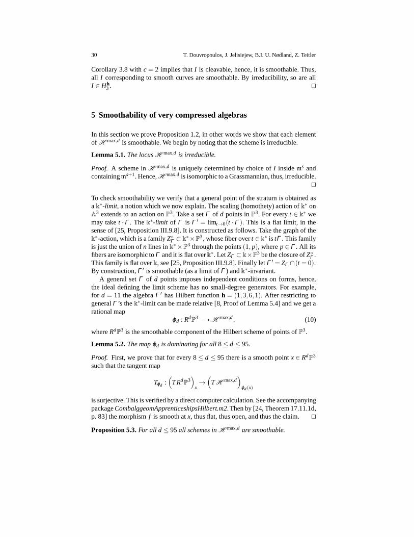
30 T. Douvropoulos, J. Jelisiejew, B.I. U. Nødland, Z. Teitler
Corollary 3.8 withc= 2 implies thatI is cleavable, hence, it is smoothable. Thus,all I corresponding to smooth curves are smoothable. By irreducibility, so are allI ∈ Hh
3 . ⊓⊔
5 Smoothability of very compressed algebras
In this section we prove Proposition 1.2, in other words we show that each elementof H max,d is smoothable. We begin by noting that the scheme is irreducible.
Lemma 5.1.The locusH max,d is irreducible.
Proof. A scheme inH max,d is uniquely determined by choice ofI insidems andcontainingms+1. Hence,H max,d is isomorphic to a Grassmannian, thus, irreducible.
⊓⊔
To check smoothability we verify that a general point of the stratum is obtained asak∗-limit, a notion which we now explain. The scaling (homothety) action ofk∗ onA
3 extends to an action onP3. Take a setΓ of d points inP3. For everyt ∈ k∗ we
may taket ·Γ . Thek∗-limit of Γ is Γ ′ = limt→0(t ·Γ ). This is a flat limit, in thesense of [25, Proposition III.9.8]. It is constructed as follows. Take the graph of thek∗-action, which is a familyZ◦Γ ⊂ k
∗×P3, whose fiber overt ∈ k∗ is tΓ . This family
is just the union ofn lines ink∗×P3 through the points(1, p), wherep∈ Γ . All its
fibers are isomorphic toΓ and it is flat overk∗. LetZΓ ⊂ k×P3 be the closure ofZ◦Γ .
This family is flat overk, see [25, Proposition III.9.8]. Finally letΓ ′ = ZΓ ∩ (t = 0).By construction,Γ ′ is smoothable (as a limit ofΓ ) andk∗-invariant.
A general setΓ of d points imposes independent conditions on forms, hence,the ideal defining the limit scheme has no small-degree generators. For example,for d = 11 the algebraΓ ′ has Hilbert functionh = (1,3,6,1). After restricting togeneralΓ ’s thek∗-limit can be made relative [8, Proof of Lemma 5.4] and we get arational map
ϕd : RdP
399K H max,d, (10)
whereRdP
3 is the smoothable component of the Hilbert scheme of points of P3.
Lemma 5.2.The mapϕd is dominating for all8≤ d≤ 95.
Proof. First, we prove that for every 8≤ d ≤ 95 there is a smooth pointx∈ RdP
3
such that the tangent map
Tϕd :(
TRdP
3)
x→
(
TH max,d)
ϕd(x)
is surjective. This is verified by a direct computer calculation. See the accompanyingpackageCombalggeomApprenticeshipsHilbert.m2. Then by [24, Theorem 17.11.1d,p. 83] the morphismf is smooth atx, thus flat, thus open, and thus the claim.⊓⊔
Proposition 5.3.For all d ≤ 95all schemes inH max,d are smoothable.
The Hilbert scheme of 11 points inA3 is irreducible 31
Proof. By Lemma 5.1, the locusH max,d is irreducible. Ford < 8 all schemes aresmoothable by [8]. Assumed ≥ 8. By Lemma 5.2, the mapϕd from (10) is domi-nating. Hence, a general element ofH max,d is smoothable. But smoothability is aclosed property, thus, all elements ofH max,d are smoothable. ⊓⊔
Proof (Proof of Proposition 1.2).Whend ≤ 95 the claim follows from Proposi-tion 5.3. Whend≥ 96 the claim follows by dimension count, as in [27]. ⊓⊔
Remark 5.4 (Comparison with the case of8 points in A4). From the cased = 96onwards we do not get a surjective tangent map and, indeed, the dimension of the
family H max,96=H(1,3,6,10,20,35,21)
3 is equal to 3·96, thus, a general member of thisfamily cannot be smoothable for dimensional reasons. (Points in H max,96 defineschemes supported at a single point, soH max,96 would have to be contained in theboundary ofR96
3 .) This was the original example of [27]. Our methods show thatH max,d is smoothable for alld ≤ 95, hence, the boundd = 96 obtained in [27] issharp for this method. Note that in [28] another, only partially related, method wasused to prove thatHd
3 is reducible ford ≥ 78. It is currently unclear whether thisother method can yield irreducible components ford≤ 77.
Even thoughTϕd is not surjective ford ≥ 96, we conjecture that the mapsTϕd are of maximal rank. This is no longer true forA4: in fact Tϕ8A
4 has 20-dimensional image in the 21-dimensional Grassmannian Gr(3,10), which accountsfor the fact that there are nonsmoothable ideals of degree 8 in A
4, as proven in [8].An explicit example of such a scheme inA4 = Speck[α,β ,γ,δ ] is given by theideal(α2,αβ ,β 2,αδ +β γ,γ2,γδ ,δ 2) = 〈xz,xw,yz,yw,xy− zw〉⊥, see [8, Proposi-tion 5.1]. This scheme gives an answer to [41, Problem 3 on Parameters and Mod-uli].
Acknowledgements This article was initiated during the Apprenticeship Weeks(22 August–2 September 2016), led by Bernd Sturmfels, as part of the Combinatorial Algebraic GeometrySemester at the Fields Institute. The authors wish to thank the Fields Institute, the organizers ofthe Thematic Program on Combinatorial Algebraic Geometry in Fall 2016, and the organizers ofthe Apprenticeship Weeks which took place during the program. We are very grateful to MarkHuibregtse, Anthony Iarrobino, Gary Kennedy, Greg Smith, Bernd Sturmfels, and several anony-mous referees for numerous helpful comments. This work was supported by a grant from theSimons Foundation (#354574, Zach Teitler). JJ was supported by Polish National Science Center,project 2014/13/N/ST1/02640. BIUN was supported by NRC project 144013.
References
1. Michael Artin.Deformations of singularities. Notes by C.S. Seshadri and Allen Tannenbaum.Tata Institute of Fundamental Research, Bombay, India, 1976.
2. Patricia Borges dos Santos, Abdelmoubine Amar Henni, andMarcos Jardim. Commutingmatrices and the Hilbert scheme of points on affine spaces.arXiv:1304.3028 , 2013.
3. Winfried Bruns and Jurgen Herzog.Cohen-Macaulay rings, volume 39 ofCambridge Studiesin Advanced Mathematics. Cambridge University Press, Cambridge, 1993.
32 T. Douvropoulos, J. Jelisiejew, B.I. U. Nødland, Z. Teitler
4. Weronika Buczynska and Jarosław Buczynski. Secant varieties to high degree Veronese reem-beddings, catalecticant matrices and smoothable Gorenstein schemes.J. Algebraic Geom.,23:63–90, 2014.
5. Weronika Buczynska, Jarosław Buczynski, Johannes Kleppe, and Zach Teitler. Apolarity anddirect sum decomposability of polynomials.Michigan Math. J., 64(4):675–719, 2015.
6. Jarosław Buczynski and Joachim Jelisiejew. On smoothability. In preparation.7. Enrico Carlini. Reducing the number of variables of a polynomial. InAlgebraic geometry and
geometric modeling, Math. Vis., pages 237–247. Springer, Berlin, 2006.8. Dustin A. Cartwright, Daniel Erman, Mauricio Velasco, and Bianca Viray. Hilbert schemes of
8 points.Algebra Number Theory, 3(7):763–795, 2009.9. Gianfranco Casnati, Joachim Jelisiejew, and Roberto Notari. Irreducibility of the Gorenstein
loci of Hilbert schemes via ray families.Algebra Number Theory, 9(7):1525–1570, 2015.10. Gianfranco Casnati and Roberto Notari. On the Gorenstein locus of some punctual Hilbert
schemes.J. Pure Appl. Algebra, 213(11):2055–2074, 2009.11. Igor V. Dolgachev. Classical algebraic geometry. A modern view. Cambridge University
Press, Cambridge, 2012.12. David Eisenbud. Commutative algebra, volume 150 ofGraduate Texts in Mathematics.
Springer-Verlag, New York, 1995. With a view toward algebraic geometry.13. David Eisenbud.The geometry of syzygies, volume 229 ofGraduate Texts in Mathematics.
Springer-Verlag, New York, 2005. A second course in commutative algebra and algebraicgeometry.
14. Joan Elias and Maria Evelina Rossi. Analytic isomorphisms of compressed local algebras.Proc. Amer. Math. Soc., 143(3):973–987, 2015.
15. Jacques Emsalem. Geometrie des points epais.Bull. Soc. Math. France, 106(4):399–416,1978.
16. Barbara Fantechi, Lothar Gottsche, Luc Illusie, Steven L. Kleiman, Nitin Nitsure, and An-gelo Vistoli. Fundamental algebraic geometry, volume 123 ofMathematical Surveys andMonographs. American Mathematical Society, Providence, RI, 2005. Grothendieck’s FGAexplained.
17. John Fogarty. Algebraic families on an algebraic surface. Amer. J. Math, 90:511–521, 1968.18. Anthony V. Geramita. Inverse systems of fat points: Waring’s problem, secant varieties of
Veronese varieties and parameter spaces for Gorenstein ideals. In The Curves Seminar atQueen’s, Vol. X (Kingston, ON, 1995), volume 102 ofQueen’s Papers in Pure and Appl.Math., pages 2–114. Queen’s Univ., Kingston, ON, 1996.
19. Lothar Gottsche.Hilbert schemes of zero-dimensional subschemes of smooth varieties, vol-ume 1572 ofLecture Notes in Mathematics. Springer-Verlag, Berlin, 1994.
20. Gerd Gotzmann. Eine Bedingung fur die Flachheit und dasHilbertpolynom eines graduiertenRinges.Math. Z., 158(1):61–70, 1978.
21. Daniel R. Grayson and Michael E. Stillman. Macaulay2, a software system for research inalgebraic geometry. Available athttp://www.math.uiuc.edu/Macaulay2/ .
22. Gert-Martin Greuel and Gerhard Pfister.A Singular introduction to commutative algebra.Springer, Berlin, extended edition, 2008. With contributions by Olaf Bachmann, ChristophLossen and Hans Schonemann, With 1 CD-ROM (Windows, Macintosh and UNIX).
23. Alexander Grothendieck.Fondements de la geometrie algebrique. [Extraits du SeminaireBourbaki, 1957–1962.]. Secretariat mathematique, Paris, 1962.
24. Alexander Grothendieck.Elements de geometrie algebrique. IV.Etude locale des schemas etdes morphismes de schemas IV.Inst. HautesEtudes Sci. Publ. Math., (32):361, 1967.
25. Robin Hartshorne.Algebraic geometry. Springer-Verlag, New York, 1977. Graduate Texts inMathematics, No. 52.
26. Robin Hartshorne. Deformation theory, volume 257 ofGraduate Texts in Mathematics.Springer, New York, 2010.
27. Anthony Iarrobino. Reducibility of the families of 0-dimensional schemes on a variety.Invent.Math., 15:72–77, 1972.
28. Anthony Iarrobino. Compressed algebras: Artin algebras having given socle degrees and max-imal length.Trans. Amer. Math. Soc., 285(1):337–378, 1984.
The Hilbert scheme of 11 points inA3 is irreducible 33
29. Anthony Iarrobino and Jacques Emsalem. Some zero-dimensional generic singularities; finitealgebras having small tangent space.Compositio Math., 36(2):145–188, 1978.
30. Anthony Iarrobino and Vassil Kanev.Power sums, Gorenstein algebras, and determinantalloci, volume 1721 ofLecture Notes in Mathematics. Springer-Verlag, Berlin, 1999. AppendixC by Anthony Iarrobino and Steven L. Kleiman.
31. Joachim Jelisiejew. Classifying local artinian gorenstein algebras.Collectanea Mathematica,68(1):101–127, 2017.
32. Hans Kleppe. Deformation of schemes defined by vanishingof Pfaffians. J. Algebra,53(1):84–92, 1978.
33. Jan O. Kleppe and Rosa M. Miro-Roig. The dimension of theHilbert scheme of Gorensteincodimension 3 subschemes.J. Pure Appl. Algebra, 127(1):73–82, 1998.
34. Francis S. Macaulay. Some properties of enumeration in theory of modular systems.Proc.London Math. Soc., 25:531–555, 1927.
35. Francis S. Macaulay.The algebraic theory of modular systems. Cambridge MathematicalLibrary. Cambridge University Press, Cambridge, 1994. Revised reprint of the 1916 original,With an introduction by Paul Roberts.
36. Guerino Mazzola. Generic finite schemes and Hochschild cocycles. Comment. Math. Helv.,55(2):267–293, 1980.
37. Ezra Miller and Bernd Sturmfels.Combinatorial commutative algebra, volume 227 ofGrad-uate Texts in Mathematics. Springer-Verlag, New York, 2005.
38. Hiraku Nakajima.Lectures on Hilbert schemes of points on surfaces, volume 18 ofUniversityLecture Series. American Mathematical Society, Providence, RI, 1999.
39. Kristian Ranestad and Frank-Olaf Schreyer. Varieties of sums of powers.J. Reine Angew.Math., 525:147–181, 2000.
40. KlemenSivic. On varieties of commuting triples III.Linear Algebra Appl., 437(2):393–460,2012.
41. Bernd Sturmfels. Fitness, Apprenticeship, and Polynomials. In Gregory G. Smith and BerndSturmfels, editors,Combinatorial Algebraic Geometry. Springer, to appear.arXiv:1612.03539 .
Related Documents