The Fundamentals of Stell ar Ast rophys ics George W. Collins, II Copyright 2003: All sections of this book may be reproduced as long as proper attribution is given.

Welcome message from author
This document is posted to help you gain knowledge. Please leave a comment to let me know what you think about it! Share it to your friends and learn new things together.
Transcript
7/18/2019 The Fundamentals of Stellar Astrophysics - Collins G. W.
http://slidepdf.com/reader/full/the-fundamentals-of-stellar-astrophysics-collins-g-w 1/524
7/18/2019 The Fundamentals of Stellar Astrophysics - Collins G. W.
http://slidepdf.com/reader/full/the-fundamentals-of-stellar-astrophysics-collins-g-w 2/524
Contents
. . .
Page
Preface to the Internet Edition
Preface to the W. H. Freeman Edition
xiv
xv
Part I Stellar InteriorsChapter 1
Introduction and Fundamental Principles
1.1 Stationary or “Steady” Properties of matter
a Phase Space and Phase Density b Macrostates and Microstates.
c Probability and Statistical Equilibrium
d Quantum Statistics
e Statistical Equilibrium for a Gas
f Thermodynamic Equilibrium – Strict and
Local
1.2 Transport Phenomena
a. Boltzmann Transport Equation
b. Homogeneous Boltzmann Transport Equation
and Liouville’s Theorem
c. Moments of the Boltzmann Transport Equation
and Conservation Laws
1.3 Equation of State for the Ideal Gas and Degenerate
Matter
Problems
References and Supplemental Reading
3
5
5
6
6
9
11
15
15
15
17
18
26
32
33
ii
7/18/2019 The Fundamentals of Stellar Astrophysics - Collins G. W.
http://slidepdf.com/reader/full/the-fundamentals-of-stellar-astrophysics-collins-g-w 3/524
Chapter 2
Basic Assumptions, Theorems, and Polytropes
2.1 Basic Assumptions
2.2 Integral Theorems from Hydrostatic Equilibrium
a Limits of State Variables
b β * Theorem and Effects of Radiation
Pressure2.3 Homology Transformations
2.4 Polytropes
a Polytropic Change and the Lane-Emden
Equation
b Mass-Radius Relationship for Polytropes
c Homology Invariants
d Isothermal Spheree Fitting Polytropes Together
Problems
References and Supplemental Reading
Chapter 3
Sources and Sinks of Energy
3.1 "Energies" of Stars
a Gravitational Energy
b Rotational Energyc Nuclear Energy
3.2 Time Scales
a Dynamical Time Scale
b Kelvin-Helmholtz (Thermal) Time Scale
c Nuclear (Evolutionary) Time Scale
3.3 Generation of Nuclear Energy
a General Properties of the Nucleus
b The Bohr Picture of Nuclear Reactions
c Nuclear Reaction Cross Sections
d Nuclear Reaction Ratese Specific Nuclear Reactions
Problems
References and Supplemental Reading
34
34
36
36
38
40
42
43
46
47
4951
53
54
56
57
57
59
60
61
61
62
63
64
65
66
68
7072
75
75
iii
7/18/2019 The Fundamentals of Stellar Astrophysics - Collins G. W.
http://slidepdf.com/reader/full/the-fundamentals-of-stellar-astrophysics-collins-g-w 4/524
Chapter 4
Flow of Energy through the Star and Construction of Stellar
Models
4.1 The Ionization, Abundances, and Opacity of
Stellar Material
a Ionization and the Mean Molecular Weight
b Opacity
4.2 Radiative Transport and the Radiative Temperature
Gradient
a Radiative Equilibrium
b Thermodynamic Equilibrium and Net Flux
c Photon Transport and the Radiative Gradient
d Conservation of Energy and the Luminosity4.3 Convective Energy Transport
a Adiabatic Temperature Gradient
b Energy Carried by Convection
4.4 Energy Transport by Conduction
a Mean Free Path
b Heat Flow
4.5 Convective Stability
a Efficiency of Transport Mechanisms
b Schwarzschild Stability Criterion
4.6 Equations of Stellar Structure
4.7 Construction of a Model Stellar Interior
a Boundary Conditions
b Schwarzschild Variables and Method
c Henyey Relaxation Method for Construction of
Stellar Models
Problems
References and Supplemental Reading
77
78
78
80
86
86
86
87
8990
90
91
94
94
95
96
96
97
100
101
102
102
105
109
110
iv
7/18/2019 The Fundamentals of Stellar Astrophysics - Collins G. W.
http://slidepdf.com/reader/full/the-fundamentals-of-stellar-astrophysics-collins-g-w 5/524
Chapter 5
Theory of Stellar Evolution
5.1 The Ranges of Stellar Masses, Radii, and
Luminosity
5.2 Evolution onto the Main Sequence
a Problems concerning the Formation of
Stars
b Contraction out of the Interstellar Medium
c Contraction onto the Main Sequence
5.3 The Structure and Evolution of Main Sequence Stars
a Lower Main Sequence Stars
b Upper Main Sequence Stars
5.4 Post Main Sequence Evolution
a Evolution off the Lower Main Sequence
b Evolution away from the Upper Main Sequencec The Effect of Mass-loss on the Evolution of Stars
5.5 Summary and Recapitulation
a Core Contraction - Envelope Expansion: Simple
Reasons
b Calculated Evolution of a 5 M ⊙ star
Problems
References and Supplemental Reading
Chapter 6Relativistic Stellar Structure
6.1 Field Equations of the General Theory of Relativity
6.2 Oppenheimer-Volkoff Equation of Hydrostatic
Equilibrium
a Schwarzschild Metric
b Gravitational Potential and Hydrostatic
Equilibrium
6.3 Equations of Relativistic Stellar Structure and
Their Solutions
a A Comparison of Structure Equations
b A Simple Model
c Neutron Star Structure
112
113
114
114
116
119
125
126
128
129
129
136138
139
140
143
144
145
149
150
152
152
154
154
155156
158
v
7/18/2019 The Fundamentals of Stellar Astrophysics - Collins G. W.
http://slidepdf.com/reader/full/the-fundamentals-of-stellar-astrophysics-collins-g-w 6/524
6.4 Relativistic Polytrope of Index 3
a Virial Theorem for Relativistic Stars
b Minimum Radius for White Dwarfs
c Minimum Radius for Super-massive Stars
6.5 Fate of Super-massive Stars
a Eddington Luminosity
b Equilibrium Mass-Radius Relation
c Limiting Masses for Super-massive Stars
Problems
References and Supplemental Reading
Chapter 7
Structure of Distorted Stars
7.1 Classical Distortion: The Structure Equations
a A Comparison of Structure Equationsb Structure Equations for Cylindrical Symmetry
7.2 Solution of Structure Equations for a Perturbing
Force
a Perturbed Equation of Hydrostatic Equilibrium
b Number of Perturbative Equations versus Number
of Unknowns
7.3 Von Zeipel's Theorem and Eddington-Sweet
Circulation Currents
a Von Zeipel's Theorem
b Eddington-Sweet Circulation Currents
7.4 Rotational Stability and Mixing
a Shear Instabilities
b Chemical Composition Gradient and Suppression
of Mixing
c Additional Types of Instabilities
Problems
References and Supplemental Reading
Chapter 8Stellar Pulsation and Oscillation
8.1 Linear Adiabatic Radial Oscillations
a Stellar Oscillations and the Variational Virial
theorem
161
161
164
165
167
167
168
168
172
173
175
176
176177
184
185
186
187
187
190
195
195
196
198
199
199
201
202
203
vi

7/18/2019 The Fundamentals of Stellar Astrophysics - Collins G. W.
http://slidepdf.com/reader/full/the-fundamentals-of-stellar-astrophysics-collins-g-w 7/524
7/18/2019 The Fundamentals of Stellar Astrophysics - Collins G. W.
http://slidepdf.com/reader/full/the-fundamentals-of-stellar-astrophysics-collins-g-w 8/524
d Physical Meaning of the Source Function 240
e Special Forms of the Redistribution Function 241
9.3 Moments of the Radiation Field 243
a Mean Intensity 244
b Flux 244c Radiation Pressure 245
9.4 Moments of the Equation of Radiative Transfer
a Radiative Equilibrium and Zeroth Moment of the
Equation of Radiative Transfer
b First Moment of the Equation of Radiative
Transfer and the Diffusion Approximation
247
248
248
c Eddington Approximation 249
Problems 251
Supplemental Reading 252
Chapter 10
Solution of the Equation of Radiative Transfer 253
10.1 Classical Solution to the Equation of Radiative Transfer
and Integral Equations for the Source Function 254
a Classical Solution of the Equation of Transfer for
the Plane-Parallel Atmosphere 254
b Schwarzschild-Milne Integral Equations 257
c Limb-darkening in a Stellar Atmosphere 260
10.2 Gray Atmosphere 263a Solution of Schwarzschild-Milne Equations for
the Gray Atmosphere 265
b Solutions for the Gray Atmosphere Utilizing the
Eddington Approximation 266
c Solution by Discrete Ordinates: Wick-
Chandrasekhar Method 268
10.3 Nongray Radiative Transfer 274
a Solutions of the Nongray Integral Equation for the
Source Function 275
b Differential Equation Approach: The Feautrier
Method 276
10.4 Radiative Transport in a Spherical Atmosphere 279
viii
7/18/2019 The Fundamentals of Stellar Astrophysics - Collins G. W.
http://slidepdf.com/reader/full/the-fundamentals-of-stellar-astrophysics-collins-g-w 9/524
a Equation of Radiative Transport in Spherical
Coordinates
280
b An Approach to Solution of the Spherical Radiative
Transfer Problem 283
Problems 287
References and Supplemental Reading 289
Chapter 11
Environment of the Radiation Field 291
11.1 Statistics of the Gas and the Equation of State 292
a Boltzmann Excitation Formula 292
b Saha Ionization Equilibrium Equation 293
11.2 Continuous Opacity 296
a Hydrogenlike Opacity 296
b Neutral Helium 297c Quasi-atomic and Molecular States 297
d Important Sources of Continuous Opacity for
Main Sequence Stars 299
11.3 Einstein Coefficients and Stimulated Emission 300
a Relations among Einstein Coefficients 301
b Correction of the Mass Absorption Coefficient for
Stimulated Emission 302
11.4 Definitions and Origins of Mean Opacities 303
a Flux-Weighted (Chandrasekhar) Mean Opacity 304
b Rosseland Mean Opacity 304
c Planck Mean Opacity 306
11.5 Hydrostatic Equilibrium and the Stellar Atmosphere 307
Problems 308
References 309
Chapter 12
The Construction of a Model Stellar Atmosphere 310
12.1 Statement of the Basic Problem 31012.2 Structure of the Atmosphere, Given the Radiation Field 312
a Choice of the Independent Variable of
Atmospheric Depth 314
ix
7/18/2019 The Fundamentals of Stellar Astrophysics - Collins G. W.
http://slidepdf.com/reader/full/the-fundamentals-of-stellar-astrophysics-collins-g-w 10/524
b Assumption of Temperature Dependence with
Depth 314
c Solution of the Equation of Hydrostatic
Equilibrium 314
12.3 Calculation of the Radiation Field of the Atmosphere 316
12.4 Correction of the Temperature Distribution and Radiative
Equilibrium 318
a Lambda Iteration Scheme 318
b Avrett-Krook Temperature Correction Scheme 319
12.5 Recapitulation 325
Problems 326
References and Supplemental Reading 328
Chapter 13
Formation of Spectral Lines 33013.1 Terms and Definitions Relating to Spectral Lines 331
a Residual Intensity, Residual Flux, and
Equivalent Width 331
b Selective (True) Absorption and Resonance
Scattering 333
c Equation of Radiative Transfer for Spectral
Line Radiation 335
13.2 Transfer of Line Radiation through the Atmosphere 336
a Schuster-Schwarzschild Model Atmosphere for
Scattering Lines 336
b Milne-Eddington Model Atmosphere for the
Formation of Spectral Lines 339
Problems 346
Supplemental Reading 347
Chapter 14
Shape of Spectral Lines 348
14.1 Relation between the Einstein, Mass Absorption, and
Atomic Absorption Coefficients 34914.2 Natural or Radiation Broadening 350
a Classical Radiation Damping 351
x

7/18/2019 The Fundamentals of Stellar Astrophysics - Collins G. W.
http://slidepdf.com/reader/full/the-fundamentals-of-stellar-astrophysics-collins-g-w 11/524
b Quantum Mechanical Description of Radiation
Damping 354
c Ladenburg f-value 355
14.3 Doppler Broadening of Spectral Lines 357
a Microscopic Doppler Broadening 358
b Macroscopic Doppler Broadening 364
14.4 Collisional Broadening 369
a Impact Phase-Shift Theory 370
b Static (Statistical) Broadening Theory 378
14.5 Curve of Growth of the Equivalent Width 385
a Schuster-Schwarzschild Curve of Growth 385
b More Advanced Models for the Curve of Growth 389
c Uses of the Curve of Growth 390
Problems 392
References and Supplemental Reading 395
Chapter 15
Breakdown of Local Thermodynamic Equilibrium 398
15.1 Phenomena Which Produce Departures from Local
Thermodynamic Equilibrium 400
a Principle of Detailed Balancing 400
b Interlocking 401
c Collisional versus Photoionization 402
15.2 Rate Equations for Statistical Equilibrium 403
a Two-Level Atom 403
b Two-Level Atom plus Continuum 407
c Multilevel Atom 409
d Thermalization Length 410
15.3 Non-LTE Transfer of Radiation and the Redistribution
Function 411
a Complete Redistribution 412
b Hummer Redistribution Functions 413
15.4 Line Blanketing and Its Inclusion in the construction of
Model Stellar Atmospheres and Its Inclusion in the
Construction of Model Stellar Atmospheres 425
a Opacity Sampling 426
xi
7/18/2019 The Fundamentals of Stellar Astrophysics - Collins G. W.
http://slidepdf.com/reader/full/the-fundamentals-of-stellar-astrophysics-collins-g-w 12/524
b Opacity Distribution Functions 427
Problems 429
References and Supplemental Reading 430
Chapter 16
Beyond the Normal Stellar Atmosphere 432
16.1 Illuminated Stellar Atmospheres 434
a Effects of Incident Radiation on the Atmospheric
Structure 434
b Effects of Incident Radiation on the Stellar Spectra 439
16.2 Transfer of Polarized Radiation 440
a Representation of a Beam of Polarized Light and
the Stokes Parameters 440
b Equations of Transfer for the Stokes 445
c Solution of the Equations of Radiative Transfer for Polarized Light . 454
d Approximate Formulas for the Degree of
Emergent Polarization 457
e Implications of the Transfer of Polarization for
Stellar Atmospheres 465
16.3 Extended Atmospheres and the Formation of Stellar
Winds 469
a Interaction of the Radiation Field with the Stellar
Wind 470
b Flow of Radiation and the Stellar Wind 474
Problems 477
References and Supplemental Reading 478
Epilog 480
Index 483
Errata to the W. H. Freeman edition. 495
xii

7/18/2019 The Fundamentals of Stellar Astrophysics - Collins G. W.
http://slidepdf.com/reader/full/the-fundamentals-of-stellar-astrophysics-collins-g-w 13/524
PrefaceTo the (2003) WEB Edition
One may justifiability wonder why anyone would take the time to put a decade-old book on astrophysics on the WEB. Several events of the past few months have led
me to believe that may well be some who wish to learn about the basics of stellar
structure. Since the fundamentals of stellar astrophysics have changed little in the pastdecade and as this book has been out of print for nearly that long, I felt that some may
still find it useful for learning the basics. The task was somewhat facilitated by mydiscovery of some old machine-readable disks that contained a version of the book
including some of the corrections to the published version. With considerable help from
Charles Knox, I was able to retrieve the information from the out-dated format andtransfer the text to a contemporary word processor. However, the equations were lost in
the process so that their inclusion in this edition had to take another form. This was
accomplished by scanning the originals from the book and correcting those with errorsin a variety of ways. This accounts for the fonts of the equations being somewhat at
variance with that of the text. However, I believe that difference does not detract
significantly from the understandability of the material. The most common form of
correction was to simply re-set them with an equation editor embedded in the WORD processor. Equations look somewhat different from the others. However, the ability to
correct errors that arose in the published edition seemed to out weigh any visual
inconvenience.
The reader will notice that all the recommended reading is to books published
prior to 1987. Some of this is a result of a predilection of mine to cite initial references,
but most of it is a result of my failure to update the references to contemporary times.There have been a number of books and many articles during the past decade or so
which would greatly enlighten the reader, but to include them would be a major part of anew book and lies beyond the scope of this effort.
While I have been able to correct the errors resulting from the first production of
the book, I am sure new ones have materialized during its regeneration. Since specialcharacter and all the Greek alphabet letters did not convert correctly during the recovery
it is likely that some have escaped my attempts to replace them. For this and any other
errors that may have occurred I apologize in advance. In addition, I have simply copiedthe index for the W. H. Freeman edition so that the page numbers may not correspond to
the values presented here. However, the pagination at the beginning and end of eachchapter does correspond to the W. H. Freeman edition so that the error within anychapter is likely to be less than a page or so. This was felt to be sufficiently close so that
much of the value of an index would be preserved. Finally, I have included errata to the
W. H. Freeman edition as the final part of the book. It was initially prepared in 1991,
but the publisher refused to permit it to accompany the first printing. However, I have
xiii
7/18/2019 The Fundamentals of Stellar Astrophysics - Collins G. W.
http://slidepdf.com/reader/full/the-fundamentals-of-stellar-astrophysics-collins-g-w 14/524
always felt the value of any text book was materially enhanced by knowing the errors
incurred during its preparation. While it is not considered to be complete, I feel that mostof the substantive errors are covered. They, and others, have been corrected in the WEB
edition.
I have resisted the temptation to update the material since that would have been amonumental task approaching the original generation of the book itself with little
increase in the reader’s depth of understanding. In the original version of this text I
included only that astrophysics that one could be reasonably confident was correct andwould pass the test of time. Thus there were several subject sketchily addressed due to
lack of knowledge. Sadly few of the “skeletons” that reside in the “closet” of stellar
astrophysics have been properly buried in the past decade. Stellar evolution beyond thehelium-flash in low mass stars still is a bit murky. While the evolution of massive stars
toward their final demise is clearer than a decade ago, models of the final collapse to a
Type II supernova remain unsatisfactory. The role of rotation in the evolution of starsonto the Main Sequence, while clearly important also seems poorly understood.
However, I am confidant that application of the fundamental physics of stellarastrophysics along with the explosive expansion of computing power will lead to the
solutions of these problems in the present century.
While the copyright for ISBN# 7176-1993-2) was returned to me by W.H.
Freeman in May of 1997 when the book went out of print, I have no real desirefinancially profit from its further distribution. As others can readily attest, one doesn’t
get rich writing graduate texts in astronomy. I will find payment enough should others
find it helpful in understanding stars. However, should anyone find its contents helpfuland wish to cite them, I would appreciate that proper attribution be made.
Finally, in addition to being indebted to Charlie Knox for his help in rescuing the
text from an old computer-readable form, I am beholden to John Martin for helping me
get these sections ready for the Internet.
George W. Collins, II
Case Western Reserve University
January 2003
xiv

7/18/2019 The Fundamentals of Stellar Astrophysics - Collins G. W.
http://slidepdf.com/reader/full/the-fundamentals-of-stellar-astrophysics-collins-g-w 15/524
Preface
To the (1989) W.H. Freeman Edition
Since I began studying the subject some 30 years ago, its development
has continued at a slow steady pace. There have been few of the breakthroughs of leapsforward that characterize the early development of a discipline. Perhaps that is because
the foundations of the understanding of stars were provided by the generations that preceded mine. Names like Eddington, Milne, Schuster, Schwarzschild, Cowling,
Chandrasekhar, and many others echo down through the history of this subject as the
definers and elucidators of stellar structure. The outline of the theory of the structure andevolution of th stars clearly has belonged to the first half of the twentieth century. In the
second half of this century, we have seen that outline filled in so that there are very few
aspects of either a star’s structure or life history for which our understanding is
incomplete. Certainly the advent of pulsars, black holes and the other unusual objectsthat are often called stars has necessitated broadening the scope of the theory of stellar
astrophysics. Then there are areas concerning both the birth and death of stars that
largely elude our understanding. But the overall picture of the structure and evolution ofmost stars now seem, in the main, to be well understood.
When I say that “the overall picture of the structure and evolution of most starsnow seem, in the main, to be well understood,” I do not imply that there is not much to
be learned. Nothing should humble a theorist more than supernova 1987A, whose
progenitor was a blue supergiant, when conventional wisdom said it should be a red
supergiant. Theorists instantly explained such a result with the benefit of perfecthindsight, but the event should give us pause for thought. It was indeed a massive star
that exploded, and contemporary models firmly rooted in the physics described in this
text and elsewhere describe the event qualitatively quite well. Even with such anunexpected event the basic picture has been confirmed, but as time passes, the picture
will become clearer. It is even likely that the outliners of the picture defined in the
twentieth century may be resolved in a unanticipated manner in the twenty first. But thefundamentals of that picture are unlikely to change.
I suspect that there are few astronomers alive who would not be astounded ifwe found that stars do ”not• form from the interstellar medium, burn hydrogen as
main sequence stars for 90 percent of their life and undergo complex, but
understandable changes during the last moments of their life. It is in this sense that thefoundations of stellar astrophysics are understood. I am convinced that there willcontinually be surprises as we probe more carefully into the role of rotation, magnetic
fields, and companion- induced distortion on the structure and evolution of stars. But
the understanding of these issues will be built on the foundation of spherical stars that
xv

7/18/2019 The Fundamentals of Stellar Astrophysics - Collins G. W.
http://slidepdf.com/reader/full/the-fundamentals-of-stellar-astrophysics-collins-g-w 16/524
I have attempted to present in this book, and it is this foundation that must be
understood before one can move on to the more complicated problems.
The general speculation and excitement that encompassed the growing theory
of stellar structure 50 years ago has moved on to the poorly understood realm of the
galaxies and cosmology. The theoretical foundations of galactic structure seem to bein a state akin to that of stellar structure in the early part of this century, while recent
developments in cosmology may actually have elevated that discipline to the status of
a science. The pressure exerted by the burgeoning information from these areas ongraduate curricula has provided a substantial squeeze on the more traditional aspects
of an astronomer's education.
This is as it should be. If a discipline does not develop and expand, it will
stagnate. Change is the hallmark of any vital intellectual enterprise. Few graduate
programs in the United States now offer courses in celestial mechanics. Yet, half acentury ago, no one would have been called an astronomer who could not determine
planetary positions from the orbital elements or determine those elements from severalindependent observations. However, we all know where to look for that information if
we ever actually have to perform such a task. Such is the evolution of that subjectmatter we call astronomy. It is a time-dependent thing, for one individual can only
hold so much information in mind at one time. Thus a course of study in stellar
astrophysics that used to cover 2 years is now condensed into 1 year or less and this pressure can only increase. I have always felt that in addition to discovering "new"
things about the universe, it is important to "sift and winnow" the old in order to save
that which will be important for the understanding of the new. This is a responsibilitythat all academicians have, and it must be assumed if the next generation is to have the
limited room of their minds filled with the essentials of the old that is required so thatthey may continue the development of the new. Such is the basic motivation for this
book.
Over the years, a number of books have been written about various aspects ofstellar astrophysics, and many have deservedly become classics. It is not my intention
to compete with these classics; indeed, the reader will find them referenced often, and
it is my sincere hope that the reader will take the time to read and learn from them. A
major purpose of this effort is to make, in some cases, that reading a little easier. Thusthe primary aim of this book differs from others used as graduate texts in astronomy.
Traditionally, they have taken a discipline as far as it could be developed at the time
and in some cases beyond. That is not my intent. Instead, I present the basic materialrequired to advance to the understanding of contemporary research in a wide variety
of areas related to the study of stars. For example, it would be fruitless to attempt to
grapple with contemporary work in the theory of non-radial oscillations withoutunderstanding the basis for pulsation theory such as is given in Chapter 8.
xvi

7/18/2019 The Fundamentals of Stellar Astrophysics - Collins G. W.
http://slidepdf.com/reader/full/the-fundamentals-of-stellar-astrophysics-collins-g-w 17/524
As stellar astrophysics has developed, attention has increasingly become
focused on the details and refinements that make the current models of stars soquantitatively accurate. While this accuracy is important for the advancement of the
subject, it can form a barrier to the understanding of its foundations. Thus, I have left
many of these details to others in the hopes that the student interested in advancing the
understanding of stellar astrophysics will search them out. Some will observe that Ihave not sifted and winnowed enough and that too many of the blind alleys and
unproductive directions of development have been included. This may be so, for it is
difficult to shrug off those formalisms with which one has struggled and foundrewarding in youth. I leave further sifting to the next generation. Suffice it to say that I
have included in this book what I feel is either necessary or at least enjoyable for the
understanding of stars.
This book is aimed at first year graduate students or the very advanced
undergraduates. I assume throughout that the readers have considerable factualknowledge of stars and astronomy. Readers should be acquainted with the
Hertzsprung-Russell diagram and know something of the ranges of the parameters thatdefine stars. The student who wants to make a contribution to astronomy, must
understand how this knowledge about stars was gained from observation. Only thencan the accuracy of that knowledge be assessed, and without such an assessment,
deception of self and perhaps others is guaranteed.
Given such a background, I shall attempt to describe the development of a
nearly axiomatic theory of stellar structure that is consistent with what we know about
stars. This theory is incomplete for there is much that we still do not know about stars.The terminal phases of stellar evolution are treated schematically. The structure of
distorted stars is barely touched, and the theory of the evolution of close binaries isignored entirely. The decision to downplay or ignore this material does not arise from
a disdain of these subjects on my part, but is simply a question of time and space. It is
my sincere hope that the student upon finishing this book will seize some of theseareas for future research and being interested and prepared, pick up the gauntlet and
advance the subject. At the end of the sections on stellar interiors and atmospheres I
have included several topics that represent logical extensions of the traditional theory
of stellar structure. These should not be considered as either complete or exhaustive, but merely illustrative for the selection of the subjects was dictated by personal
interest as opposed to fundamental importance. In a curriculum pressed for time, some
can be safely ignored.
The relatively complete foundation of the theory of stellar structure has one
minor psychological drawback that results from a contemporary penchant in some ofthe physical sciences. The rapid development of astronomy into new areas of research
during the past two decades has tended to produce research papers that emphasize
only the most contemporary work. Thus papers and books that reference older workare likely to be regarded as out of date. In this instance, this view is exacerbated by my
xvii
7/18/2019 The Fundamentals of Stellar Astrophysics - Collins G. W.
http://slidepdf.com/reader/full/the-fundamentals-of-stellar-astrophysics-collins-g-w 18/524
tendency to give original references wherever possible. Thus the reader may find that
many of the references date to the middle part of this century or earlier. Hopefully thereader will forgive this tendency of mine and remember that this book is about the
fundementals of stellar astrophysics and not intended to bring the reader to the current
state of research effort in stellar astronomy. To answer the need of the student who
wishes to go beyond an introduction, I have included some additional references at theend of some chapters that represent reviews of a few more contemporary concerns of
stellar structure.
Some will inevitably feel that more problems in stellar structure and atmospheres
should be discussed. I can only counter by saying that it is easy to add, but difficult to
take away. For any topic that you might add, find one that you would remove withoutendangering the basic understanding of the student. Regrettably, only a finite amount
of time and space can be devoted to the teaching of this subject, devoted to the
teaching of this subject, and the hard choices are not what to include, but what to leaveout. With the exception of a few topics that I included purely for my own enjoyment, I
regard the vast majority of this book as fundamental to the understanding of stars.
To those that would say, "Yes models are well understood, but models are notstars", I would shout "Amen!" I have spent most of my professional career modeling
the outer layers of distorted stars, and I am acutely aware of the limitations of such
models. Nevertheless, modeling as a model for understanding nature is becoming acompletely acceptable method. For stellar astrophysics, it has been an extremely
productive approach. When combined critically with observation, modeling can
provide an excellent avenue toward the understanding of how things work. Indeed, if pressed in a thoughtful way, most would find that virtually any comparison of theory
with observation or experiment involves the modeling of some aspect of the physicalworld. Thus while one must be ever mindful of the distinction between models of the
real world and the world itself, one cannot use that distinction as an excuse for failing
to try to describe the world.
For the student who feels that it is unnecessary to understand all this theory
simply to observe the stars, ask yourself how you will decide what you will observe. If
that does not appear to be a significant question, then consider another line ofendeavor. For those who suffer through this material on their way to what they
perceive as the more challenging and interesting subjects of galaxies and cosmology,
consider the following argument.
While the fascinating areas of galactic and extragalactic astronomy deservedly fill
larger and larger parts of the graduate curricula, let us not forget that galaxies aremade of stars and ultimately our conception of the whole can be no better than our
understanding of the parts. In addition, the physical principles that govern stars are at
work throughout the universe. Stars are the basic building blocks from which ourlarger world is made and remain the fundamental probes with which we test our
xviii

7/18/2019 The Fundamentals of Stellar Astrophysics - Collins G. W.
http://slidepdf.com/reader/full/the-fundamentals-of-stellar-astrophysics-collins-g-w 19/524
theories of that world. The understanding of stars and the physical principles that rule
their existence is, and I believe will remain, central to our understanding of theuniverse.
Do not take this argument as an apology for the study of stars. The opposite is
true for I feel some of the most difficult problems in astronomy involve the detailedunderstanding of stars. Consider the following example. Thomas Gold described the
basic picture and arguments for believing that pulsars are spinning magnetic neutron
stars nearly 25 years ago. In the main, he was correct although many details of his picture have been changed. However, we do not yet have a fully selfªconsistent picture
of pulsars in spite of the efforts of a substantial number of astronomers. Such a self-
consistent and complete picture is very difficult to formulate. Without it, ourunderstanding of pulsars will not be complete, but that is not to say that the basic
picture of a pulsar as a spinning magnetic neutron star is wrong. Rather it is simply
incomplete.
A considerable number of the problems of stellar astrophysics are of this type.They are not to be undertaken by the timid for they are demanding in the extreme. Nor
should these problems be regarded as merely filing in details. This is the excuse of thedilettante who would be well advised to follow Isaac Newton's admonition:
“To explain all nature is too difficult a task for any manor even for any one age. 'Tis much better to do a little
with certainty, and leave the rest for others that come after you
than to explain all things”_
I believe that many astronomers will choose, as I have chosen, to spend themajority of their professional careers involved in the study of stars themselves. It is
my hope that they will recognize the fundamental nature of the material in this book
and use it to attack the harder problems of today and the future.
I cannot conclude this preface without some acknowledgment of those who
made this effort possible. Anyone who sets out to codify some body of knowledge
which he or she has spent the greater part of life acquiring, cannot expect to achieveany measure of success unless he or she is surrounded by an understanding family and
colleagues. Particular thanks are extended to the students of stellar interiors and
atmospheres at The Ohio State University who used this book in its earliest form andfound and eliminated numerous errors. Many more were reveled by the core of
reviewers who scrutinized the text. My thanks to Richard Boyd, Joe Cassinelli,
George Field, Arne Henden, John Mathis, Peter Mϑsz<ros, Dimitri Mihalas, DonaldOsterbrock, Michael Sitko, and Sydney Wolf for being members of that core. Their
comments and constructive criticism were most helpful in shaping this book. Theremaining shortcomings, mistakes, and blunders are mine and mine alone.
xix

7/18/2019 The Fundamentals of Stellar Astrophysics - Collins G. W.
http://slidepdf.com/reader/full/the-fundamentals-of-stellar-astrophysics-collins-g-w 20/524
xx
Certainly little of the knowledge contained here originated from my own
efforts. I have merely chewed and digested material fed to me by mentors dedicated tothe search and preservation of that body of knowledge known as astronomy. To name
them all would require considerable space, possibly be construed as self-serving, and
perhaps be embarrassing to some of them. Nevertheless, they have my undying
admiration and gratitude for passing on some of what they know and sharing with methat most precious of commodities; their knowledge, wisdom, and mostly their time.
George W. Collins, IIThe Ohio State University
(1988)

7/18/2019 The Fundamentals of Stellar Astrophysics - Collins G. W.
http://slidepdf.com/reader/full/the-fundamentals-of-stellar-astrophysics-collins-g-w 21/524
Part I
Stellar Interiors
1

7/18/2019 The Fundamentals of Stellar Astrophysics - Collins G. W.
http://slidepdf.com/reader/full/the-fundamentals-of-stellar-astrophysics-collins-g-w 22/524
2
1 Stellar Interiors Copyright (2003) George W. Collins, II
1
Introduction andFundamental Principles
. . .
The development of a relatively
complete picture of the structure and evolution of the stars has been one of the great
conceptual accomplishments of the twentieth century. While questions still exist
concerning the details of the birth and death of stars, scientists now understand over
90% of a star's life. Furthermore, our understanding of stellar structure has
progressed to the point where it can be studied within an axiomatic framework
comparable to those of other branches of Physics. It is within this axiomatic
framework that we will study stellar structure stellar spectra - the traditional source
of virtually all information about stars.
7/18/2019 The Fundamentals of Stellar Astrophysics - Collins G. W.
http://slidepdf.com/reader/full/the-fundamentals-of-stellar-astrophysics-collins-g-w 23/524
1. Introduction and Fundamental Principles
3
This book is divided into two parts: stellar interiors and stellar atmospheres.
While the division between the two is fairly arbitrary, it is a traditional division
separating regimes where different axioms apply. A similar distinction exists
between the continuum and lines of a stellar spectrum. These distinctions represent a
transition zone where one physical process dominates over another. The transition in
nature is never abrupt and represents a difference in degree rather than in kind.
We assume that the readers know what stars are, that is, have a working
knowledge of the Hertzsprung-Russell diagram and of how the vast wealth of
knowledge contained in it has been acquired. Readers should understand that most
stars are basically spherical and should know something about the ranges of masses,
radii, and luminosities appropriate for the majority of stars. The relative size and
accuracy of the stellar sample upon which this information is based must be
understood before a theoretical description of stars can be believed. However, themore we learn about stars, the more the fundamentals of our theoretical descriptions
are confirmed. The history of stellar astrophysics in the twentieth century can be
likened to that of a photographer steadily sharpening the focus of the camera to
capture the basic nature of stars.
In this book, the basic problem of stellar structure under consideration is the
determination of the run of physical variables that describe the local properties of
stellar material with position in the star. In general, the position in the star is the
independent variable(s) in the problem, and other parameters such as the pressure P,
temperature T, and density ρ are the dependent variables. Since these parameters
describe the state of the material, they are often referred to as state variables. Part I ofthis book discusses these parameters alone. In Part II, when we arrive near the
surface of the star, we shall also be interested in the detailed distribution of the
photons, particularly as they leave the star.
Although there are some excursions into the study of nonspherical stars, the
main thrust of this book is to provide a basis for understanding the structure of
spherical stars. Although the proof is not a simple one, it would be interesting to
show that the equilibrium configuration of a gas cloud confined solely by gravity is
that of a sphere. However, instead of beginning this book with a lengthy proof, we
simply take the result as an axiom that all stars dominated by gravity alone are
spherical.
We describe these remarkably stable structures in terms of microphysics,
involving particles and photons which are largely in equilibrium. Statistical
mechanics is the general area of physics that deals with this subject and contains the
axioms that form the basis for stellar astrophysics. Our discussion of stellar structure
centers on the interaction of light with matter. We must first describe the properties
7/18/2019 The Fundamentals of Stellar Astrophysics - Collins G. W.
http://slidepdf.com/reader/full/the-fundamentals-of-stellar-astrophysics-collins-g-w 24/524
4
1 Stellar Interiors
of the space in which the interaction will take place. It is not the normal Euclidean
three-dimensional space of intuition, but a higher-dimension space. This higher-
dimension space, called phase space, includes the momentum distribution of the
particles which make up the star as well as their physical location.
1.1 Stationary or "Steady" Properties of Matter
a. Phase Space and Phase Density
Consider a volume of physical space that is small compared to the
physical system in question, but still large enough to contain a statistically significant
number of particles. The range of physical space in which this small volume is
embedded may be infinite or finite as long as it is significantly larger than the small
volume. First let a set of three Cartesian coordinates x1, x2, and x3 represent the
spatial part of the volume. Then allow the additional three Cartesian coordinates v1,
v2, and v3 represent the components of the velocity of the particles. Coordinates v1,v2, and v3 are orthogonal to the spatial coordinates. This simply indicates that the
velocity and position are assumed to be uncorrelated. It also provides for a six-
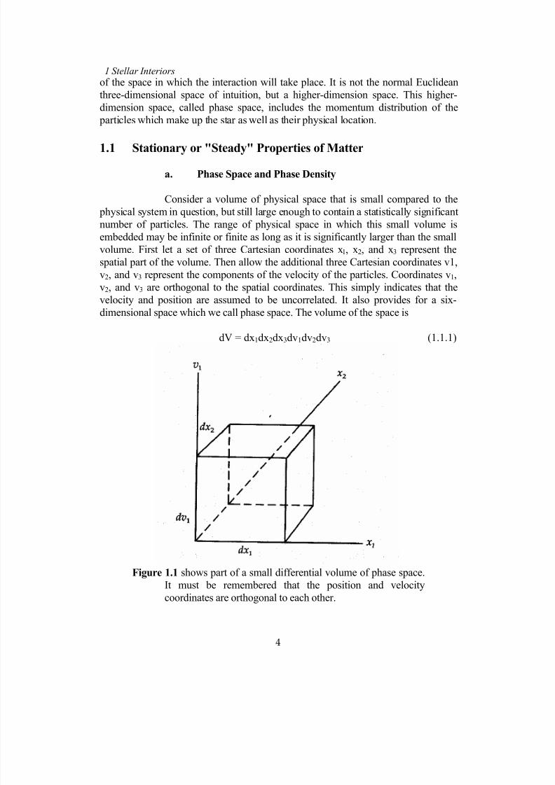
dimensional space which we call phase space. The volume of the space is
dV = dx1dx2dx3dv1dv2dv3 (1.1.1)
Figure 1.1 shows part of a small differential volume of phase space.
It must be remembered that the position and velocity
coordinates are orthogonal to each other.

7/18/2019 The Fundamentals of Stellar Astrophysics - Collins G. W.
http://slidepdf.com/reader/full/the-fundamentals-of-stellar-astrophysics-collins-g-w 25/524
7/18/2019 The Fundamentals of Stellar Astrophysics - Collins G. W.
http://slidepdf.com/reader/full/the-fundamentals-of-stellar-astrophysics-collins-g-w 26/524
6
1 Stellar Interiors
an ordinary room of gas, is this any more unlikely than each particle to returning to
that specific position with the same velocity? The answer is no. Thus, if each
microstate is equally probable, then the associated macrostates are not equally
probable and it makes sense to search for the most probable macrostate of a system.
In a system which is continually rearranging itself by collisions, the most probablemacrostate becomes the most likely state in which to find the system. A system
which is in its most probable macrostate is said to be in statistical equilibrium.
Many things can determine the most probable macrostate. Certainly the total
number of particles allowed in each microstate and the total number of particles
available to distribute will be important in determining the total number of
microstates in a given macrostate. In addition, quantum mechanics places some
conditions on our ability to distinguish particles and even limits how many of certain
kinds of particles can be placed in a given volume of phase space. But, for the
moment, let us put aside these considerations and concentrate on calculating the
number of microstates in a particular macrostate.
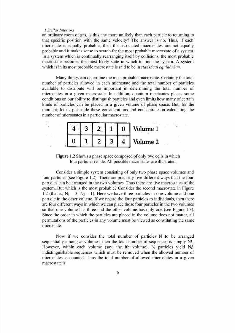
Figure 1.2 Shows a phase space composed of only two cells in which
four particles reside. All possible macrostates are illustrated.
Consider a simple system consisting of only two phase space volumes and
four particles (see Figure 1.2). There are precisely five different ways that the four
particles can be arranged in the two volumes. Thus there are five macrostates of the
system. But which is the most probable? Consider the second macrostate in Figure
1.2 (that is, N1 = 3, N2 = 1). Here we have three particles in one volume and one
particle in the other volume. If we regard the four particles as individuals, then there
are four different ways in which we can place those four particles in the two volumes
so that one volume has three and the other volume has only one (see Figure 1.3).
Since the order in which the particles are placed in the volume does not matter, all
permutations of the particles in any volume must be viewed as constituting the same
microstate.
Now if we consider the total number of particles N to be arranged
sequentially among m volumes, then the total number of sequences is simply N!.
However, within each volume (say, the ith volume), Ni particles yield Ni!
indistinguishable sequences which must be removed when the allowed number of
microstates is counted. Thus the total number of allowed microstates in a given
macrostate is
7/18/2019 The Fundamentals of Stellar Astrophysics - Collins G. W.
http://slidepdf.com/reader/full/the-fundamentals-of-stellar-astrophysics-collins-g-w 27/524
1. Introduction and Fundamental Principles
7
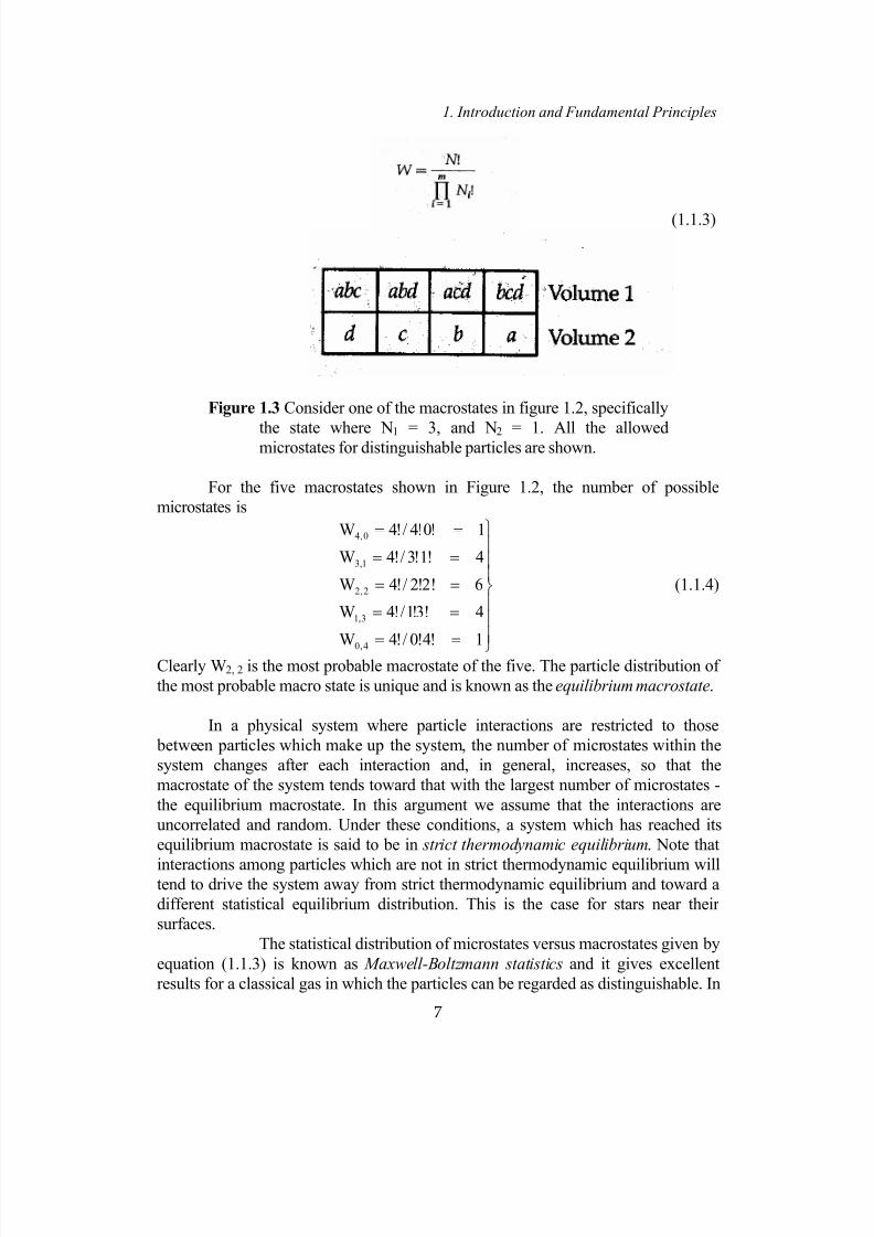
(1.1.3)
Figure 1.3 Consider one of the macrostates in figure 1.2, specifically
the state where N1 = 3, and N2 = 1. All the allowedmicrostates for distinguishable particles are shown.
For the five macrostates shown in Figure 1.2, the number of possible
microstates is
==
==
==
==
==
1!4!0/!4W
4!3!1/!4W
6!2!2/!4W
4!1!3/!4W
1!0!4/!4W
4,0
3,1
2,2
1,3
0,4
(1.1.4)
Clearly W2, 2 is the most probable macrostate of the five. The particle distribution of
the most probable macro state is unique and is known as the equilibrium macrostate.
In a physical system where particle interactions are restricted to those
between particles which make up the system, the number of microstates within the
system changes after each interaction and, in general, increases, so that the
macrostate of the system tends toward that with the largest number of microstates -
the equilibrium macrostate. In this argument we assume that the interactions are
uncorrelated and random. Under these conditions, a system which has reached its
equilibrium macrostate is said to be in strict thermodynamic equilibrium. Note that
interactions among particles which are not in strict thermodynamic equilibrium willtend to drive the system away from strict thermodynamic equilibrium and toward a
different statistical equilibrium distribution. This is the case for stars near their
surfaces.
The statistical distribution of microstates versus macrostates given by
equation (1.1.3) is known as Maxwell-Boltzmann statistics and it gives excellent
results for a classical gas in which the particles can be regarded as distinguishable. In

7/18/2019 The Fundamentals of Stellar Astrophysics - Collins G. W.
http://slidepdf.com/reader/full/the-fundamentals-of-stellar-astrophysics-collins-g-w 28/524
8
1 Stellar Interiors
a classical world, the position and momentum of a particle are sufficient to make it
distinguishable from all other particles. However, the quantum mechanical picture of
the physical world is quite different. So far, we have neglected both the Heisenberg
uncertainty principle and the Pauli Exclusion Principle.
d. Quantum Statistics
Within the realm of classical physics, a particle occupies a point in
phase space, and in some sense all particle are distinguishable by their positions and
velocities. The phase space volumes are indeed differential and arbitrarily small.
However, in the quantum mechanical view of the physical world, there is a limit to
how well the position and momentum (velocity, if the mass is known) of any particle
can be determined. Within that phase space volume, particles are indistinguishable.
This limit is known as the Heisenberg uncertainty principle and it is stated as
follows:
∆ p∆x ≥ h/2π ≡ h ( 1.1.5)
Thus the minimum phase space volume which quantum mechanics allows is of the
order of h3. To return to our analogy with Maxwell-Boltzmann statistics, let us
subdivide the differential cell volumes into compartments of size h3 so that the total
number of compartments is
n = dx1dx2dx3dp1dp2dp3 / h3 (1.1.6)
Let us redraw the example in Figure 1.3 so that each cell in phase space is subdividedinto four compartments within which the particles are indistinguishable. Figure 1.4
shows the arrangement for the four particles for the W3,1 macrostate for which there
were only four allowed microstates under Maxwell-Boltzmann Statistics. Since the
particles are now distinguishable within a cell, there are 20 separate ways to arrange
the three particles in volume 1 and 4 ways to arrange the single particle in volume 2.
The total number of allowed microstates for W3,1 is 20×4, or 80. Under these
conditions the total number of microstates per macrostate is
W = ∏ Wi , (1.1.7)
i
where Wi is the number of microstates per cell of phase space, which can beexpressed in terms of the number of particles Ni in that cell.

7/18/2019 The Fundamentals of Stellar Astrophysics - Collins G. W.
http://slidepdf.com/reader/full/the-fundamentals-of-stellar-astrophysics-collins-g-w 29/524
1. Introduction and Fundamental Principles
9
Figure 1.4 The same macrostate as figure 1.3 only now the cells of
phase space are subdivided into four compartments withinwhich particles are indistinguishable. All of the possible
microstates are shown for the four particles.
Let us assume that there are n compartments in the ith cell which contains N i
particles. Now we have to arrange a sequence of n + Ni objects, since we have to
consider both the particles and the compartments into which they can be placed.
However, not all sequences are possible since we must always start a sequence with
a compartment. After all we have to put the particle somewhere! Thus there are n
sequences with Ni + n-1 items to be further arranged. So there are n[Ni + n-1]!
different ways to arrange the particles and compartments. We must eliminate all the
permutations of the compartments because they reside within a cell and thereforerepresent the same microstate. But there are just n! of these. Similarly, the order in
which the particles are added to the cell volume is just as irrelevant to the final
microstate as it was under Maxwell-Boltzmann statistics. And so we must eliminate
all the permutations of the Ni particles, which is just Ni!. Thus the number of
microstates allowed for a given macrostate becomes
7/18/2019 The Fundamentals of Stellar Astrophysics - Collins G. W.
http://slidepdf.com/reader/full/the-fundamentals-of-stellar-astrophysics-collins-g-w 30/524
10
1 Stellar Interiors
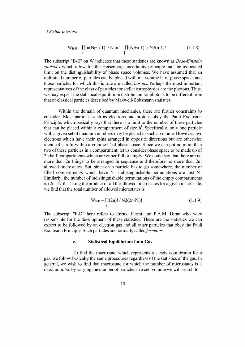
WB-E = ∏ n(Ni+n-1)! / Ni!n! = ∏(Ni+n-1)! / Ni!(n-1)! (1.1.8)
i i
The subscript "B-E" on W indicates that these statistics are known as Bose-Einstein statistics which allow for the Heisenberg uncertainty principle and the associated
limit on the distinguishability of phase space volumes. We have assumed that an
unlimited number of particles can be placed within a volume h3 of phase space, and
those particles for which this is true are called bosons. Perhaps the most important
representatives of the class of particles for stellar astrophysics are the photons. Thus,
we may expect the statistical equilibrium distribution for photons to be different from
that of classical particles described by Maxwell-Boltzmann statistics.
Within the domain of quantum mechanics, there are further constraints to
consider. Most particles such as electrons and protons obey the Pauli Exclusion
Principle, which basically says that there is a limit to the number of these particlesthat can be placed within a compartment of size h
3. Specifically, only one particle
with a given set of quantum numbers may be placed in such a volume. However, two
electrons which have their spins arranged in opposite directions but are otherwise
identical can fit within a volume h3 of phase space. Since we can put no more than
two of these particles in a compartment, let us consider phase space to be made up of
2n half-compartments which are either full or empty. We could say that there are no
more than 2n things to be arranged in sequence and therefore no more than 2n!
allowed microstates. But, since each particle has to go somewhere, the number of
filled compartments which have Ni! indistinguishable permutations are just Ni.
Similarly, the number of indistinguishable permutations of the empty compartments
is (2n - Ni)!. Taking the product of all the allowed microstates for a given macrostate,we find that the total number of allowed microstates is
WF-D = ∏(2n)! / Ni!(2n-Ni)! (1.1.9)
i
The subscript "F-D" here refers to Enrico Fermi and P.A.M. Dirac who were
responsible for the development of these statistics. These are the statistics we can
expect to be followed by an electron gas and all other particles that obey the Pauli
Exclusion Principle. Such particles are normally called fermions.
e. Statistical Equilibrium for a Gas
To find the macrostate which represents a steady equilibrium for a
gas, we follow basically the same procedures regardless of the statistics of the gas. In
general, we wish to find that macrostate for which the number of microstates is a
maximum. So by varying the number of particles in a cell volume we will search for

7/18/2019 The Fundamentals of Stellar Astrophysics - Collins G. W.
http://slidepdf.com/reader/full/the-fundamentals-of-stellar-astrophysics-collins-g-w 31/524
1. Introduction and Fundamental Principles
11
dW = 0. Since lnW is a monotonic function of W, any maximum of lnW is a
maximum of W. Thus we use the logarithm of equations (1.1.7) through (1.1.9) to
search for the most probable macrostate of the distribution functions. These are
ln W (1.1.10)
Σ=
+Σ=
Σ=
!lnN-)! N-ln(2n-ln(2n)!ln W
1)!-ln(n-!lnN-1)!- Nln(n
)! Nln(- N!lnln W
iii
D-F
iii
E-B
ii
B-M
The use of logarithms also makes it easier to deal with the factorials through the use
of Stirling's formula for the logarithm of a factorial of a large number.
lnN! ≈ N lnN – N (1.1.11)
For a given volume of gas, dN = dn = 0. The variations of equations (1.1.10) become
δln WM-B = ΣlnNidNi = 0
i
δln WB-E = Σln[(n+Ni)/Ni]dNi = 0 (1.1.12)
i
δln WF-D = Σln[(2n-Ni)/Ni]dNi = 0
i
These are the equations of condition for the most probable macrostate for thethree statistics which must be solved for the particle distribution Ni. We have
additional constraints, which arise from the conservation of the particle number and
energy, on the system which have not been directly incorporated into the equations
of condition. These can be stated as follows:
δ[ Σ Ni ] = δ N = 0 , δ [ Σwi Ni ] = Σ wiδ Ni = 0 , (1.1.13)
i i i
where wi is the energy of an individual particle. Since these additional constraints
represent new information about the system, we must find a way to incorporate them
into the equations of condition. A standard method for doing this is known as themethod of Lagrange multipliers. Since equations (1.1.13) represent quantities which
are zero we can multiply them by arbitrary constants and add them to equations
(1.1.12) to get

7/18/2019 The Fundamentals of Stellar Astrophysics - Collins G. W.
http://slidepdf.com/reader/full/the-fundamentals-of-stellar-astrophysics-collins-g-w 32/524

7/18/2019 The Fundamentals of Stellar Astrophysics - Collins G. W.
http://slidepdf.com/reader/full/the-fundamentals-of-stellar-astrophysics-collins-g-w 33/524
1. Introduction and Fundamental Principles
13
For a free particle like that found in a monatomic gas, the partition function1 is (see
also section 11.1b)
Vh
)mkT2()T(U3
2
3
π= , (1.1.19)
where V is the specific volume of the gas, m is the mass of the particle, and T is the
kinetic temperature. Replacing dlnU/dlnT in equation (1.1.18) by its value obtained
from equation (1.1.19), we get the familiar relation
NkT2
3E = , (1.1.20)
which is only correct if T is the kinetic temperature. Thus we arrive at a self-
consistent solution if the parameter T is to be identified with the kinetic temperature.
The situation for a photon gas in the presence of material matter is somewhat
simpler because the matter acts as a source and sinks for photons. Now we can no
longer apply the constraint dN = 0. This is equivalent to adding lnα2= 0 (i.e., α2 = 1)
to the equations of condition. If we let β2 = 1/(kT) as we did with the Maxwell-
Boltzmann statistics, then the appropriate solution to the Bose-Einstein formula
[equation (1.1.15)] becomes
1e
1
n
N
)kT(h
i
−= ν , (1.1.21)
where the photon energy wi has been replaced by hν. Since two photons in a volume
h3 can be distinguished by their state of polarization, the number of phase space
compartments is
n = (2/h3)dx1dx2dx3dp1dp2dp3 (1.1.22)
We can replace the rectangular form of the momentum volume dp1dp2dp3, by
its spherical counterpart 4π p2dp and remembering that the momentum of a photon is
hν/c, we get
ν−
πν= ν d
1e
1
c
8
V
dN
)kT(h3
2
. (1.1.23)
Here we have replaced Ni with dN. This assumes that the number of particles in any
phase space volume is small compared to the total number of particles. Since the
energy per unit volume dEν is just hν dN/V, we get the relation known as Planck's
law or sometimes as the blackbody law:
7/18/2019 The Fundamentals of Stellar Astrophysics - Collins G. W.
http://slidepdf.com/reader/full/the-fundamentals-of-stellar-astrophysics-collins-g-w 34/524
14
1 Stellar Interiors
)T(Bc
4d
1ec
h8dE
)kT(h
3
3 ννν
π≡ν
−
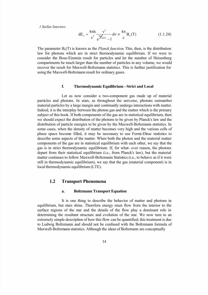
νπ= (1.1.24)
The parameter Bν(T) is known as the Planck function. This, then, is the distribution
law for photons which are in strict thermodynamic equilibrium. If we were to
consider the Bose-Einstein result for particles and let the number of Heisenberg
compartments be much larger than the number of particles in any volume, we would
recover the result for Maxwell-Boltzmann statistics. This is further justification for
using the Maxwell-Boltzmann result for ordinary gases.
f. Thermodynamic Equilibrium - Strict and Local
Let us now consider a two-component gas made up of material
particles and photons. In stars, as throughout the universe, photons outnumber
material particles by a large margin and continually undergo interactions with matter.
Indeed, it is the interplay between the photon gas and the matter which is the primary
subject of this book. If both components of the gas are in statistical equilibrium, then
we should expect the distribution of the photons to be given by Planck's law and the
distribution of particle energies to be given by the Maxwell-Boltzmann statistics. In
some cases, when the density of matter becomes very high and the various cells of
phase space become filled, it may be necessary to use Fermi-Dirac statistics to
describe some aspects of the matter. When both the photon and the material matter
components of the gas are in statistical equilibrium with each other, we say that the
gas is in strict thermodynamic equilibrium. If, for what- ever reason, the photons
depart from their statistical equilibrium (i.e., from Planck's law), but the material
matter continues to follow Maxwell-Boltzmann Statistics (i.e., to behave as if it were
still in thermodynamic equilibrium), we say that the gas (material component) is in
local thermodynamic equilibrium (LTE).
1.2 Transport Phenomena
a. Boltzmann Transport Equation
It is one thing to describe the behavior of matter and photons in
equilibrium, but stars shine. Therefore energy must flow from the interior to thesurface regions of the star and the details of the flow play a dominant role in
determining the resultant structure and evolution of the star. We now turn to an
extremely simple description of how this flow can be quantified; this treatment is due
to Ludwig Boltzmann and should not be confused with the Boltzmann formula of
Maxwell-Boltzmann statistics. Although the ideas of Boltzmann are conceptually
7/18/2019 The Fundamentals of Stellar Astrophysics - Collins G. W.
http://slidepdf.com/reader/full/the-fundamentals-of-stellar-astrophysics-collins-g-w 35/524
1. Introduction and Fundamental Principles
15
simple, many of the most fundamental equations of theoretical physics are obtained
from them.
Basically the Boltzmann transport equation arises from considering what can
happen to a collection of particles as they flow through a volume of phase space. Our
prototypical volume of phase space was a six-dimensional "cube", which implies that
it has five-dimensional "faces". The Boltzmann transport equation basically
expresses the change in the phase density within a differential volume, in terms of
the flow through these faces, and the creation or destruction of particles within that
volume.
For the moment, let us call the six coordinates of this space xi remembering
that the first three refer to the spatial coordinates and the last three refer to the
momentum coordinates. If the "area" of one of the five-dimensional "faces" is A, the
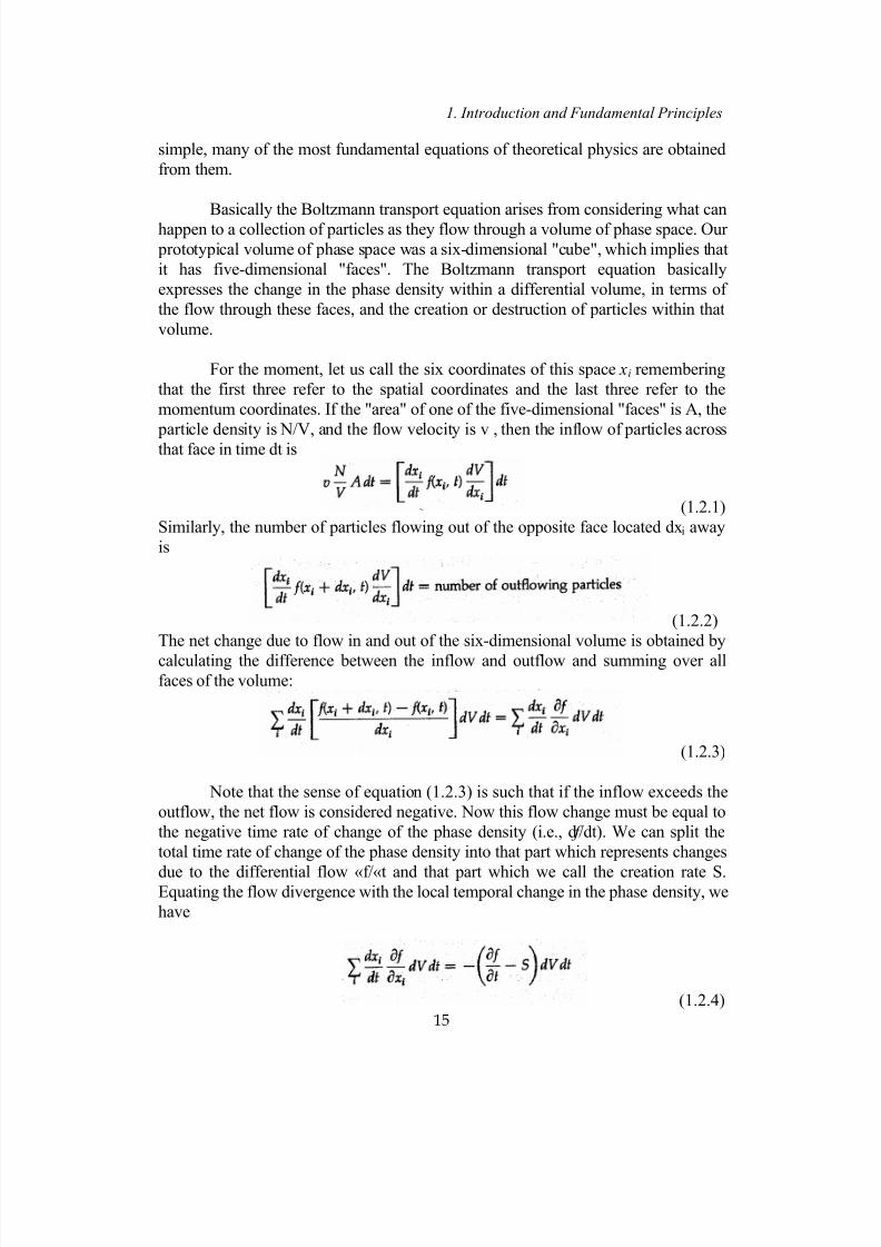
particle density is N/V, and the flow velocity is v , then the inflow of particles acrossthat face in time dt is
(1.2.1)
Similarly, the number of particles flowing out of the opposite face located dx i away
is
(1.2.2)
The net change due to flow in and out of the six-dimensional volume is obtained by
calculating the difference between the inflow and outflow and summing over allfaces of the volume:
(1.2.3)
Note that the sense of equation (1.2.3) is such that if the inflow exceeds the
outflow, the net flow is considered negative. Now this flow change must be equal to
the negative time rate of change of the phase density (i.e., d f /dt). We can split the
total time rate of change of the phase density into that part which represents changes
due to the differential flow «f/«t and that part which we call the creation rate S.Equating the flow divergence with the local temporal change in the phase density, we
have
(1.2.4)
7/18/2019 The Fundamentals of Stellar Astrophysics - Collins G. W.
http://slidepdf.com/reader/full/the-fundamentals-of-stellar-astrophysics-collins-g-w 36/524
16
1 Stellar Interiors
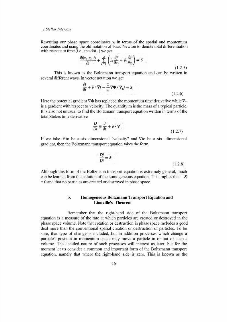
Rewriting our phase space coordinates xi in terms of the spatial and momentumcoordinates and using the old notation of Isaac Newton to denote total differentiationwith respect to time (i.e., the dot .) we get
(1.2.5)
This is known as the Boltzmann transport equation and can be written in
several different ways. In vector notation we get
(1.2.6)
Here the potential gradient ∇Φ has replaced the momentum time derivative while ∇v
is a gradient with respect to velocity. The quantity m is the mass of a typical particle.
It is also not unusual to find the Boltzmann transport equation written in terms of thetotal Stokes time derivative
(1.2.7)
If we take to be a six dimensional "velocity" and ∇to be a six- dimensional
gradient, then the Boltzmann transport equation takes the form
vr
(1.2.8)
Although this form of the Boltzmann transport equation is extremely general, much
can be learned from the solution of the homogeneous equation. This implies that S
= 0 and that no particles are created or destroyed in phase space.
b. Homogeneous Boltzmann Transport Equation and
Liouville's Theorem
Remember that the right-hand side of the Boltzmann transport
equation is a measure of the rate at which particles are created or destroyed in the
phase space volume. Note that creation or destruction in phase space includes a good
deal more than the conventional spatial creation or destruction of particles. To be
sure, that type of change is included, but in addition processes which change a
particle's position in momentum space may move a particle in or out of such a
volume. The detailed nature of such processes will interest us later, but for the
moment let us consider a common and important form of the Boltzmann transport
equation, namely that where the right-hand side is zero. This is known as the
7/18/2019 The Fundamentals of Stellar Astrophysics - Collins G. W.
http://slidepdf.com/reader/full/the-fundamentals-of-stellar-astrophysics-collins-g-w 37/524
1. Introduction and Fundamental Principles
17
homogeneous Boltzmann transport equation. It is also better known as Liouville's
theorem of statistical mechanics. In the literature of stellar dynamics, it is also
occasionally referred to as Jeans' theorem2 for Sir James Jeans was the first to
explore its implications for stellar systems. By setting the right-hand side of theBoltzmann transport equation to zero, we have removed the effects of collisions from
the system, with the result that the density of points in phase space is constant.
Liouville's theorem is usually generalized to include sets or ensembles of particles.
For this generalization phase space is expanded to 6N dimensions, so that each
particle of an ensemble has six position and momentum coordinates which are
linearly independent of the coordinates of every other particle. This space is often
called configuration space, since the entire ensemble of particles is represented by a
point and its temporal history by a curve in this 6N-dimensional space. Liouville's
theorem holds here and implies that the density of points (ensembles) in
configuration space is constant. This, in turn, can be used to demonstrate the
determinism and uniqueness of Newtonian mechanics. If the configuration density isconstant, it is impossible for two ensemble paths to cross, for to do so, one path
would have to cross a volume element surrounding a point on the other path, thereby
changing the density. If no two paths can cross, then it is impossible for any two
ensembles to ever have exactly the same values of position and momentum for all
their particles. Equivalently, the initial conditions of an ensemble of particles
uniquely specify its path in configuration space. This is not offered as a rigorous
proof, only as a plausibility argument. More rigorous proofs can be found in most
good books on classical mechanics3,4
. Since Liouville’s theorem deals with
configuration space, it is sometimes considered more fundamental than the
Boltzmann transport equation; but for our purposes the expression containing the
creation rate S will be required and therefore will prove more useful.
c. Moments of the Boltzmann Transport Equation and
Conservation Laws
By the moment of a function we mean the integral of some property
of interest, weighted by its distribution function, over the space for which the
distribution function is defined. Common examples of such moments can be found in
statistics. The mean of a distribution function is simply the first moment of the
distribution function, and the variance can be simply related to the second moment.
In general, if the distribution function is analytic, all the information contained in thefunction is also contained in the moments of that function.
The complete solution to the Boltzmann transport equation is, in general,
extremely difficult and usually would contain much more information about the
system than we wish to know. The process of integrating the function over its
defined space to obtain a specific moment removes or averages out much of the
7/18/2019 The Fundamentals of Stellar Astrophysics - Collins G. W.
http://slidepdf.com/reader/full/the-fundamentals-of-stellar-astrophysics-collins-g-w 38/524
18
1 Stellar Interiors
information about the function. However, this process also usually yields equations
which are much easier to solve. Thus we trade off information for the ability to solve
the resulting equations, and we obtain some explicit properties of the system of
interest. This is a standard "trick" of mathematical physics and one which isemployed over and over throughout this book. Almost every instance of this type
carries with it the name of some distinguished scientist or is identified with some
fundamental conservation law, but the process of its formulation and its origin are
basically the same.
We define the nth moment of a function f as
∫= dx)x(f x)]x(f [M n
n . (1.2.9)
By multiplying the Boltzmann equation by powers of the position and velocity and
integrating over the appropriate dimensions of phase space, we can generate
equations relating the various moments of the phase density )v,x(f rr . In general, such
a process always generates two moments of different order n, so that a succession of
moment taking always generates one more moment than is contained in the resulting
equations. Some additional property of the system will have to be invoked to relate
the last generated higher moment to one of lower order, in order to close the system
of equations and allow for a solution. To demonstrate this process, we show how the
equation of continuity, the Euler-Lagrange equations of hydrodynamic flow, and the
virial theorem can all be obtained from moments of the Boltzmann transport
equation.
Continuity Equation and the Zeroth Velocity Moment Although most
moments, particularly in statistics, are normalized by the integral of the distribution
function itself, we have chosen not to do so here because the integral of the phase
density f over all velocity space has a particularly important physical meaning,
namely, the local spatial density.
(1.2.10)
By we mean that the integration is to be carried out over all three velocity
coordinates v
vdr
1, v2, and v3. A pedant might correctly observe that the velocity
integrals should only range from -c to +c, but for our purposes the Newtonian view
will suffice. Integration over momentum space will properly preserve the limits.
Now let us integrate the component form of equation (1.2.5) over all velocity space
to generate an equation for the local density. Thus,
7/18/2019 The Fundamentals of Stellar Astrophysics - Collins G. W.
http://slidepdf.com/reader/full/the-fundamentals-of-stellar-astrophysics-collins-g-w 39/524
1. Introduction and Fundamental Principles
19
(1.2.11)
Since the velocity and space coordinates are linearly independent, all timeand space operators are independent of the velocity integrals. The integral of the
creation rate S over all velocity space becomes simply the creation rate for particles
in physical space, which we call . By noting that the two summations in equation
(1.2.11) are essentially scalar products, we can rewrite that moment and get
(1.2.12)
It is clear from the definition of ρ that the first term is the partial derivative of the
local particle density. The second term can be modified by use of the vector identity
(1.2.13)r
and by noting that ∇ , since space and velocity coordinates are independent.
If the particles move in response, to a central force, then we may relate their
accelerations to the gradient of a potential which depends on only position and not
velocity. The last term then takes the form
0v =•
v&r
∫∇•Φ•∇ vd)v(f )m/ v( r
. If we further
require that f(v) be bounded (i.e., that there be no particles with infinite velocity),
then since the integral and gradient operators basically undo each other, the integral
and hence the last term of equation (1.2.12) vanish, leaving
(1.2.14)
The second term in equation (1.2.14) is the first velocity moment of the phase
density and illustrates the manner by which higher moments are always generated by
the moment analysis of the Boltzmann transport equation. However, the physical
interpretation of this moment is clear. Except for a normalization scalar, the second
term is a measure of the mean flow rate of the material. Thus, we can define a mean
flow velocity u r
(1.2.15)which, upon multiplying by the particle mass, enables us to obtain the familiar form
of the equation of continuity:
(1.2.16)

7/18/2019 The Fundamentals of Stellar Astrophysics - Collins G. W.
http://slidepdf.com/reader/full/the-fundamentals-of-stellar-astrophysics-collins-g-w 40/524
20
1 Stellar Interiors
This equation basically says that the explicit time variation of the density plus
density changes resulting from the divergence of the flow is equal to the local
creation or destruction of material .
Euler-Lagrange Equations of Hydrodynamic Flow and the First Velocity
Moment of the Boltzmann Transport Equation The zeroth moment of the transport
equation provided insight into the way in which matter is conserved in a flowing
medium. Multiplying the Boltzmann transport equation by the velocity and
integrating over all velocity space will produce momentum-like moments, and so we
might expect that such operations will also produce an expression of the conservation
of momentum. This is indeed the case. However, keep in mind that the velocity is a
vector quantity, and so the moment analysis will produce a vector equation rather
than the scalar equation, as was the case with the equation of continuity. Multiplying
the Boltzmann transport equation by the local particle velocity v
r
, we get
(1.2.17)
We can make use of most of the tricks that were used in the derivation of the
continuity equation (1.2.16). The first term can be expressed in terms of the mean
flow velocity [equation (1.2.15)] while the second term can be expressed as
(1.2.18)
by using the vector identity given by equation (1.2.13). Since the quantity in
parentheses of the third term in equation (1.2.17) is a scalar and since the particleaccelerations depend on position only, we can move them and the vector scalar
product outside the velocity integral and re-express them in terms of a potential, so
the third term becomes
(1.2.19)
The integrand of equation (1.2.19) is not a simple scalar or vector, but is the
vector outer, or tensor, product of the velocity gradient of f with the vector velocityvr
itself. However, the vector identity given by equation (1.2.13) still applies if the
scalar product is replaced with the vector outer product, so that the integrand inequation (1.2.19) becomes
(1.2.20)
The quantity 1 is the unit tensor and has elements of the Kronecker delta δi j whose
7/18/2019 The Fundamentals of Stellar Astrophysics - Collins G. W.
http://slidepdf.com/reader/full/the-fundamentals-of-stellar-astrophysics-collins-g-w 41/524
1. Introduction and Fundamental Principles
21
elements are zero when i ≠ j and 1 when i = j. Again, as long as f is bounded, the
integral over all velocity space involving the velocity gradient of f will be zero, and
the first velocity moment of the Boltzmann transport equation becomes
(1.2.21)
Differentiating the first term and using the continuity equation (1.2.14) to eliminate
t/n ∂∂ , we get
(1.2.22)
Since ∇ is zero and the velocity and space coordinates are independent, we may
rewrite the third term in terms of a velocity tensor defined asv
r•
(1.2.23)
Some rearranging and the use of a few vector identities lead to
(1.2.24)
The quantity in brackets of the third term is sometimes called the pressuretensor. A density ρ times a velocity squared is an energy density, which has the units
of pressure. We can rewrite that term so it has the form
(1.2.25)
which shows the form of a moment of f. In this instance the moment is a tensor that
more or less describes the difference between the local flow indicated byr
and the
mean flow . The form of the moment is that of a variance, and the tensor, in
general, consists of nine components. Each component measures the net momentumtransfer (or contribution to the local energy density) across a surface associated with
that coordinate which results from the net flow coming from another coordinate.
Thus the third term is simply the divergence of the pressure tensor which is a vector
quantity, and the first velocity moment of the Boltzmann transport equation becomes
v
ur
7/18/2019 The Fundamentals of Stellar Astrophysics - Collins G. W.
http://slidepdf.com/reader/full/the-fundamentals-of-stellar-astrophysics-collins-g-w 42/524
22
1 Stellar Interiors
. (1.2.26)
This set of vector equations is known as the Euler-Lagrange equations of
hydrodynamic flow and they are derived here in their most general form.
It is common to make some further assumptions concerning the flow tofurther simplify these flow equations. If we consider the common physical situationwhere there are many collisions in the gas, then there is a tendency to randomize thelocal velocity field
r and thus to makev )v(f )v(f
rr−= . Under these conditions, the
pressure tensor becomes diagonal, all elements are equal, and its divergence can bewritten as the gradient of some scalar which we call the pressure P . In addition, thecreation rate S in equation (1.2.26) which involves the effects of collisions will also become symmetric in velocity, which means that the entire integral over velocityspace will vanish. This single assumption leads to the simpler and more familiarexpression for hydrodynamic flow, namely
(1.2.27)
This assumption is necessary to close the moment analysis in that it provides a
relationship between the pressure tensor and the scalar pressure P . From the
definition of the pressure tensor, under the assumption of a nearly isotropic velocity
field, P will be P (ρ) and an expression known as an equation of state will exist. It is
this additional equation that will complete the closure of the hydrodynamic flow
equations and will allow for solutions. It is also worth remembering that if the mean
flow velocity is very large compared to the velocities produced by collisions, then
the above assumption is invalid, no scalar equation of state will exist, and the full-
blown equations of hydrodynamic flow given by equation (1.2.26) must be solved. Inaddition, a good deal of additional information about the system must be known so
that a tensor equation of state can be found and the creation term can be evaluated.
ur
It is worth making one further assumption regarding the flow equations.
Consider the case where the flow is zero and the material is quiescent. The entire
left-hand side of equation (1.2.27) is now zero, and the assumption of an isotropic
velocity field produced by random collisions holds exactly. The Euler-Lagrange
equations of hydrodynamic flow now take the particularly simple form
(1.2.28)which is known as the equation of hydrostatic equilibrium. This equation is usually
cited as an expression of the conservation of linear momentum.Thus the zeroth
moment of the Boltzmann transport equation results in the conservation of matter,
whereas the first velocity moment yields equations which represent the conservation
of linear momentum. You should not be surprised that the second velocity moment
will produce an expression for the conservation of energy. So far we have considered
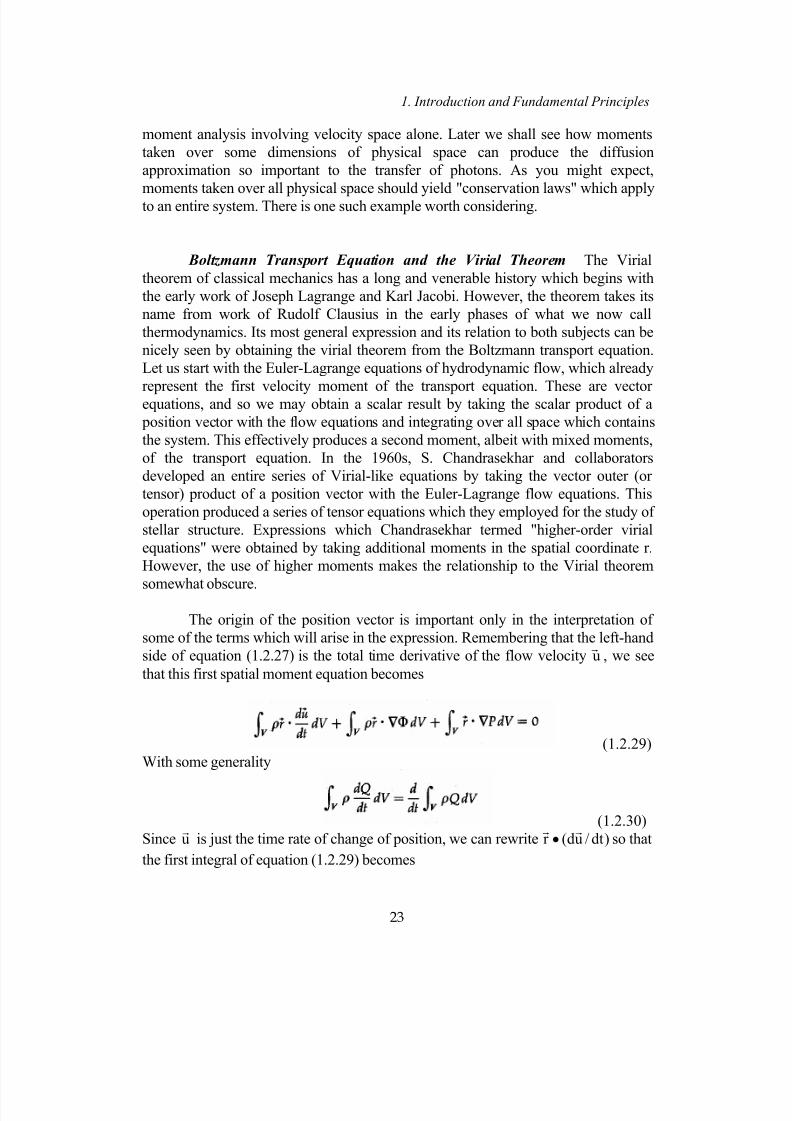
7/18/2019 The Fundamentals of Stellar Astrophysics - Collins G. W.
http://slidepdf.com/reader/full/the-fundamentals-of-stellar-astrophysics-collins-g-w 43/524
1. Introduction and Fundamental Principles
23
moment analysis involving velocity space alone. Later we shall see how moments
taken over some dimensions of physical space can produce the diffusion
approximation so important to the transfer of photons. As you might expect,
moments taken over all physical space should yield "conservation laws" which apply
to an entire system. There is one such example worth considering.
Boltzmann Transport Equation and the Virial Theorem The Virial
theorem of classical mechanics has a long and venerable history which begins with
the early work of Joseph Lagrange and Karl Jacobi. However, the theorem takes its
name from work of Rudolf Clausius in the early phases of what we now call
thermodynamics. Its most general expression and its relation to both subjects can be
nicely seen by obtaining the virial theorem from the Boltzmann transport equation.
Let us start with the Euler-Lagrange equations of hydrodynamic flow, which already
represent the first velocity moment of the transport equation. These are vectorequations, and so we may obtain a scalar result by taking the scalar product of a
position vector with the flow equations and integrating over all space which contains
the system. This effectively produces a second moment, albeit with mixed moments,
of the transport equation. In the 1960s, S. Chandrasekhar and collaborators
developed an entire series of Virial-like equations by taking the vector outer (or
tensor) product of a position vector with the Euler-Lagrange flow equations. This
operation produced a series of tensor equations which they employed for the study of
stellar structure. Expressions which Chandrasekhar termed "higher-order virial
equations" were obtained by taking additional moments in the spatial coordinate r.
However, the use of higher moments makes the relationship to the Virial theorem
somewhat obscure.
The origin of the position vector is important only in the interpretation of
some of the terms which will arise in the expression. Remembering that the left-hand
side of equation (1.2.27) is the total time derivative of the flow velocity u , we see
that this first spatial moment equation becomes
r
(1.2.29)
With some generality
(1.2.30)r
Since is just the time rate of change of position, we can rewriteur
)dt/ud(r r
• so that
the first integral of equation (1.2.29) becomes
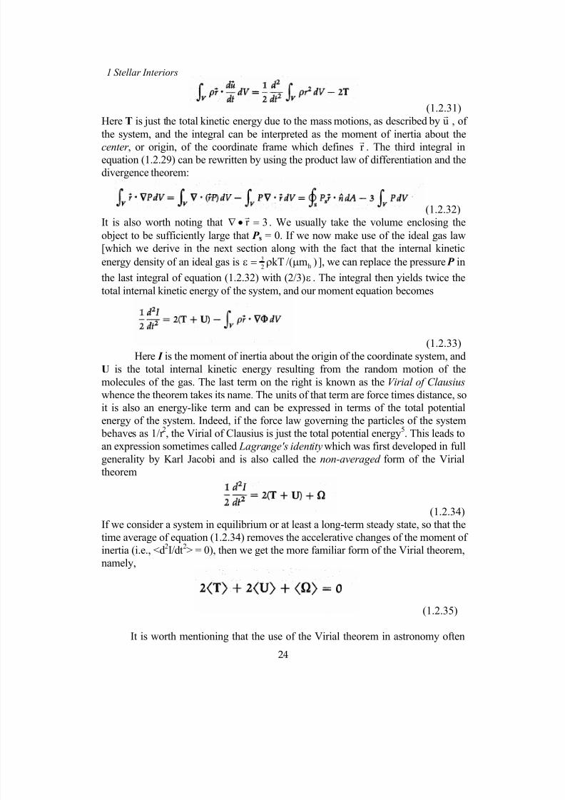
7/18/2019 The Fundamentals of Stellar Astrophysics - Collins G. W.
http://slidepdf.com/reader/full/the-fundamentals-of-stellar-astrophysics-collins-g-w 44/524
24
1 Stellar Interiors
(1.2.31)
Here T is just the total kinetic energy due to the mass motions, as described by , of
the system, and the integral can be interpreted as the moment of inertia about the
center , or origin, of the coordinate frame which defines
ur
r r . The third integral in
equation (1.2.29) can be rewritten by using the product law of differentiation and the
divergence theorem:
(1.2.32)r
It is also worth noting that 3r =•∇ . We usually take the volume enclosing the
object to be sufficiently large that P s = 0. If we now make use of the ideal gas law
[which we derive in the next section along with the fact that the internal kinetic
energy density of an ideal gas is )m/(kT h2
3 µρ=ε ], we can replace the pressure P in
the last integral of equation (1.2.32) with (2/3)ε . The integral then yields twice thetotal internal kinetic energy of the system, and our moment equation becomes
(1.2.33)
Here I is the moment of inertia about the origin of the coordinate system, and
U is the total internal kinetic energy resulting from the random motion of the
molecules of the gas. The last term on the right is known as the Virial of Clausius
whence the theorem takes its name. The units of that term are force times distance, so
it is also an energy-like term and can be expressed in terms of the total potential
energy of the system. Indeed, if the force law governing the particles of the system behaves as 1/r
2, the Virial of Clausius is just the total potential energy
5. This leads to
an expression sometimes called Lagrange's identity which was first developed in full
generality by Karl Jacobi and is also called the non-averaged form of the Virial
theorem
(1.2.34)
If we consider a system in equilibrium or at least a long-term steady state, so that the
time average of equation (1.2.34) removes the accelerative changes of the moment of
inertia (i.e., <d2I/dt
2> = 0), then we get the more familiar form of the Virial theorem,
namely,
(1.2.35)
It is worth mentioning that the use of the Virial theorem in astronomy often

7/18/2019 The Fundamentals of Stellar Astrophysics - Collins G. W.
http://slidepdf.com/reader/full/the-fundamentals-of-stellar-astrophysics-collins-g-w 45/524
1. Introduction and Fundamental Principles
25
replaces the time averages with ensemble averages over all available phase space.
The theorem which permits this is known as the Ergodic theorem, and all of
thermodynamics rests on it. Although such a replacement is legitimate for large
systems consisting of many particles, such as a star, considerable care must be
exercised in applying it to stellar or extra-galactic systems having only a few
members. However, the Virial theorem itself has basically the form and origin of a
conservation law, and when the conditions of the theorem's derivation hold, it must
apply.
1.3 Equation of State for an Ideal Gas and Degenerate Matter
Formulation of the Boltzmann transport equation also provides an
ideal setting for the formulation of the equation of state for a gas under wide-ranging
conditions. The statistical distribution functions developed in Section 1.1 give us the
distribution functions for particles which depend largely on how filled phase spacehappens to be. Those functions relate the particle energy and the kinetic temperature
to the distribution of particles in phase space. This is exactly what is meant by f )v(r
.
Thus we can calculate the expected relationship between the pressure as given by the
pressure tensor and the state variables of the distribution function. The result is
known as the equation of state.
As given in equation (1.2.24), the pressure tensor is p( ut
uurr
− ). If )v(f r
is
symmetric in , then u must be zero (or there must exist an inertial coordinate
system in whichr
is zero), and the divergence of the pressure tensor can be replaced
by the gradient of a scalar, which we call the gas pressure, and will be given by
vr r
u
(1.3.1)
From Maxwell-Boltzmann statistics, the distribution function of particles, in terms of
their velocity, was given by equation (1.1.16). If we regard the number of cells of
phase space to be very large, we can replace Ni by dN and consider equation (1.1.16)
to give the distribution function f )v(r
, so that
(1.3.2)
Now, in general,
(1.3.3)
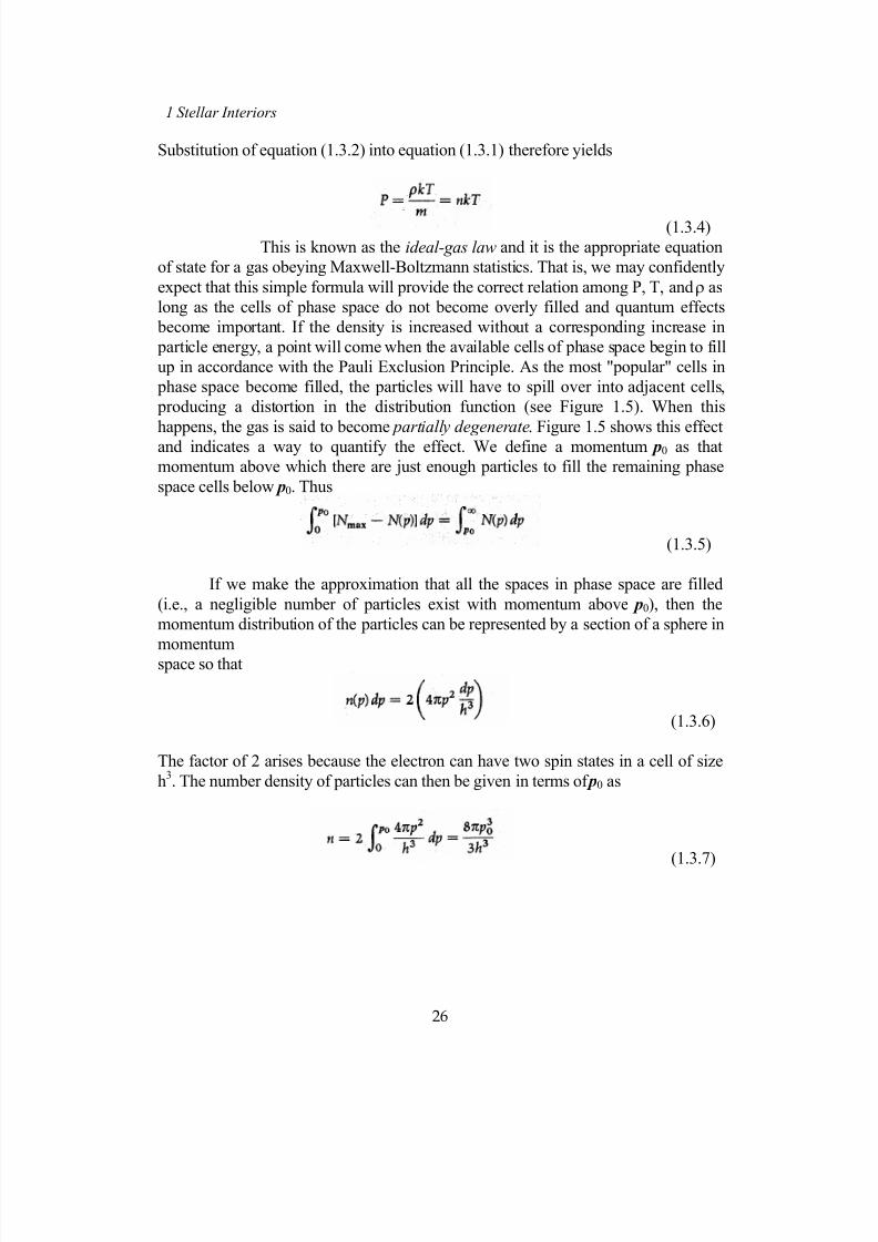
7/18/2019 The Fundamentals of Stellar Astrophysics - Collins G. W.
http://slidepdf.com/reader/full/the-fundamentals-of-stellar-astrophysics-collins-g-w 46/524
26
1 Stellar Interiors
Substitution of equation (1.3.2) into equation (1.3.1) therefore yields
(1.3.4)
This is known as the ideal-gas law and it is the appropriate equation
of state for a gas obeying Maxwell-Boltzmann statistics. That is, we may confidently
expect that this simple formula will provide the correct relation among P, T, and ρ as
long as the cells of phase space do not become overly filled and quantum effects
become important. If the density is increased without a corresponding increase in
particle energy, a point will come when the available cells of phase space begin to fill
up in accordance with the Pauli Exclusion Principle. As the most "popular" cells in
phase space become filled, the particles will have to spill over into adjacent cells,
producing a distortion in the distribution function (see Figure 1.5). When this
happens, the gas is said to become partially degenerate. Figure 1.5 shows this effectand indicates a way to quantify the effect. We define a momentum p0 as that
momentum above which there are just enough particles to fill the remaining phase
space cells below p0. Thus
(1.3.5)
If we make the approximation that all the spaces in phase space are filled
(i.e., a negligible number of particles exist with momentum above p0), then the
momentum distribution of the particles can be represented by a section of a sphere in
momentumspace so that
(1.3.6)
The factor of 2 arises because the electron can have two spin states in a cell of size
h3. The number density of particles can then be given in terms of p0 as
(1.3.7)
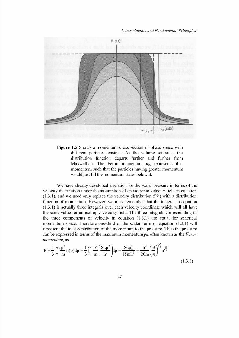
7/18/2019 The Fundamentals of Stellar Astrophysics - Collins G. W.
http://slidepdf.com/reader/full/the-fundamentals-of-stellar-astrophysics-collins-g-w 47/524
1. Introduction and Fundamental Principles
27
Figure 1.5 Shows a momentum cross section of phase space with
different particle densities. As the volume saturates, the
distribution function departs further and further from
Maxwellian. The Fermi momentum p0, represents that
momentum such that the particles having greater momentum
would just fill the momentum states below it.
We have already developed a relation for the scalar pressure in terms of the
velocity distribution under the assumption of an isotropic velocity field in equation
(1.3.1), and we need only replace the velocity distribution f( vr
) with a distribution
function of momentum. However, we must remember that the integral in equation
(1.3.1) is actually three integrals over each velocity coordinate which will all have
the same value for an isotropic velocity field. The three integrals corresponding to
the three components of velocity in equation (1.3.1) are equal for spherical
momentum space. Therefore one-third of the scalar form of equation (1.3.1) will
represent the total contribution of the momentum to the pressure. Thus the pressure
can be expressed in terms of the maximum momentum p0, often known as the Fermi
momentum, as
353
22
3
5
0 p
0 3
22 p
0
2
n3
m20
h
mh15
p8dp
h
p8
m
p
3
1dp) p(n
m
p
3
1P
00
π
=π
=
π== ∫∫
(1.3.8)
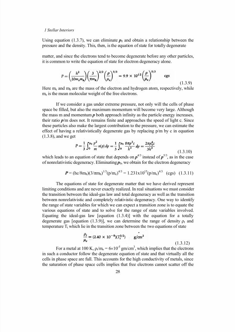
7/18/2019 The Fundamentals of Stellar Astrophysics - Collins G. W.
http://slidepdf.com/reader/full/the-fundamentals-of-stellar-astrophysics-collins-g-w 48/524
28
1 Stellar Interiors
Using equation (1.3.7), we can eliminate p0 and obtain a relationship between the
pressure and the density. This, then, is the equation of state for totally degenerate
matter, and since the electrons tend to become degenerate before any other particles,it is common to write the equation of state for electron degeneracy alone.
(1.3.9)
Here me and mh are the mass of the electron and hydrogen atom, respectively, while
me is the mean molecular weight of the free electrons.
If we consider a gas under extreme pressure, not only will the cells of phase
space be filled, but also the maximum momentum will become very large. Although
the mass m and momentum p both approach infinity as the particle energy increases,their ratio p/m does not. It remains finite and approaches the speed of light c. Since
these particles also make the largest contribution to the pressure, we can estimate the
effect of having a relativistically degenerate gas by replacing p/m by c in equation
(1.3.8), and we get
(1.3.10)
which leads to an equation of state that depends on p4/3
instead of p5/3
, as in the case
of nonrelativistic degeneracy. Eliminating p0, we obtain for the electron degeneracy
P = (hc/8mh)(3/πmh)
1/3
(p/me)
4/3
= 1.231x10
15
(p/me)
4/3
(cgs) (1.3.11)
The equations of state for degenerate matter that we have derived represent
limiting conditions and are never exactly realized. In real situations we must consider
the transition between the ideal-gas law and total degeneracy as well as the transition
between nonrelativistic and completely relativistic degeneracy. One way to identify
the range of state variables for which we can expect a transition zone is to equate the
various equations of state and to solve for the range of state variables involved.
Equating the ideal-gas law [equation (1.3.4)] with the equation for a totally
degenerate gas [equation (1.3.9)], we can determine the range of density ρt and
temperature Tt which lie in the transition zone between the two equations of state
(1.3.12)
For a metal at 100 K, ρt/me = 6×10⁻⁵
gm/cm3, which implies that the electrons
in such a conductor follow the degenerate equation of state and that virtually all the
cells in phase space are full. This accounts for the high conductivity of metals, since
the saturation of phase space cells implies that free electrons cannot scatter off the

7/18/2019 The Fundamentals of Stellar Astrophysics - Collins G. W.
http://slidepdf.com/reader/full/the-fundamentals-of-stellar-astrophysics-collins-g-w 49/524
1. Introduction and Fundamental Principles
29
other particles in the metal (for in doing so they would have to move to a new cell in
phase space, which is more than likely filled). Thus, they travel relatively unhindered
through the conductor. In general, a totally degenerate gas proves to be an excellent
conductor.
For temperatures on the order of 107 K which prevail in the center of the sun,
the transition densities occur at about 8×10² g/cm
3 which is significantly higher than
we find in the sun. Thus, we may be assured that the ideal-gas law will be
appropriate throughout the interior of the sun and most stars. However, white dwarfs
do exceed the transition density for the temperatures we may expect in these stars.
Therefore, we can expect a transition from the ideal-gas law which will prevail in the
surface regions to total degeneracy in the interior. In this transition region the
equation of state becomes more complex. A complete discussion of this region can
be found in Cox and Giuli6 and Chandrasekhar
7. The basic philosophy is to write the
equation of state in parametric form in terms of a degeneracy parameter y, wherethe equation of state becomes the ideal-gas law when y << 0 and the equation of
state approaches the totally degenerate equation of state if y >> 0 . This parametric
form can be written as
(1.3.13)
In the transition zone between nonrelativistic and relativistic degeneracy,
S. Chandrasekhar 7 also gives a parametric equation of state in terms of the
"maximum" momentum p0 of the Fermi sea:
(1.3.14)
As x approaches zero, the nonrelativistic equation of state is obtained
whereas as x approaches infinity, the fully relativistic limit is obtained. In the rare
case where the gas occupies both transition regions at the same time, the equation of
state becomes quite complicated. Refer to Cox and Giuli for a detailed description of
this situation8.
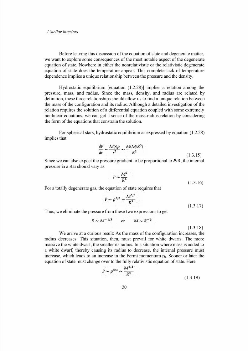
7/18/2019 The Fundamentals of Stellar Astrophysics - Collins G. W.
http://slidepdf.com/reader/full/the-fundamentals-of-stellar-astrophysics-collins-g-w 50/524
30
1 Stellar Interiors
Before leaving this discussion of the equation of state and degenerate matter,
we want to explore some consequences of the most notable aspect of the degenerateequation of state. Nowhere in either the nonrelativistic or the relativistic degenerate
equation of state does the temperature appear. This complete lack of temperature
dependence implies a unique relationship between the pressure and the density.
Hydrostatic equilibrium [equation (1.2.28)] implies a relation among the
pressure, mass, and radius. Since the mass, density, and radius are related by
definition, these three relationships should allow us to find a unique relation between
the mass of the configuration and its radius. Although a detailed investigation of the
relation requires the solution of a differential equation coupled with some extremely
nonlinear equations, we can get a sense of the mass-radius relation by considering
the form of the equations that constrain the solution.
For spherical stars, hydrostatic equilibrium as expressed by equation (1.2.28)
implies that
(1.3.15)
Since we can also expect the pressure gradient to be proportional to P /R, the internal
pressure in a star should vary as
(1.3.16)For a totally degenerate gas, the equation of state requires that
(1.3.17)
Thus, we eliminate the pressure from these two expressions to get
(1.3.18)
We arrive at a curious result: As the mass of the configuration increases, the
radius decreases. This situation, then, must prevail for white dwarfs. The more
massive the white dwarf, the smaller its radius. In a situation where mass is added toa white dwarf, thereby causing its radius to decrease, the internal pressure must
increase, which leads to an increase in the Fermi momentum p0. Sooner or later the
equation of state must change over to the fully relativistic equation of state. Here
(1.3.19)

7/18/2019 The Fundamentals of Stellar Astrophysics - Collins G. W.
http://slidepdf.com/reader/full/the-fundamentals-of-stellar-astrophysics-collins-g-w 51/524
1. Introduction and Fundamental Principles
31
If we again eliminate the pressure by using equation (1.3.16), then the radius also
disappears and
M (1.3.20).constant~
Thus, for a fully relativistic degenerate gas, there is a unique mass for whichthe configuration is stable. Should mass be added beyond this point, the star would be forced into a state of unrestrained gravitational collapse. Much later we shall seethat a further change in the equation of state, which occurs when the densityapproaches that of nuclear matter, can halt the collapse, allowing the formation of aneutron star. But for "normal" matter a limit is set by quantum mechanics, and this prevents the formation of white dwarfs with masses greater than about 1.4 M⊙ . Thisis the limit found by S. Chandrasekhar in the late 1930s and for which he receivedthe Nobel Prize in 1983. The configuration described by the fully relativisticallydegenerate equation of state is a strange one indeed, and we shall explore it in somedetail later. For now, let us turn to the most basic assumptions that must be made forthe study of stellar structure and to what they imply about the nature of stars.
Problems
1. Consider a standard deck of 52 playing cards dealt into four hands of 13
cards each. If a given suit distribution within a hand represents a macrostate
while a specific set of cards within a suit represents a microstate, find
a the number of possible macrostates for each hand,
b the number of microstates allowed for each macrostate, and
c the most probable macrostate.
2 Consider a space with three cells of size 2h3, and nine particles. Find the total
number of macrostates, the total number of microstates, and the most probable macrostate, assuming the particles are
a "Maxwellons",
b fermions, and
c bosons.
3. Given that
and that w = ( px2 + p
2y + p
2z)/m, find an expression for B in terms of N for the
cases where φ = 0, ±1.
4. Derive the equation of state for a Fermi gas from first principles.
5. Given that f ( x) is an analytic function in the interval 0 ≤ x ≤ 4 , show that f ( x)
can be represented in terms of the moments of the function M i [ f ( x)], where
7/18/2019 The Fundamentals of Stellar Astrophysics - Collins G. W.
http://slidepdf.com/reader/full/the-fundamentals-of-stellar-astrophysics-collins-g-w 52/524
32
1 Stellar Interiors
6. If the pressure tensor P has the form specified by equation (1.2.25), show that
it can be rewritten as it appears in equation (1.2.24) (i.e., as the tensor
operated on by the divergence operator in the third term on the left-hand
side).
7. Show that the Virial theorem holds in the form given by equation (1.2.35)
even if the forces of interaction include velocity dependent terms (i.e., such
as Lorentz forces or viscous drag forces).
8. Show that the second velocity moment of the Boltzmann transport equation
leads to an equation describing the conservation of energy.
References and Supplemental Reading
1. Aller, L.H., The Atmospheres of the Sun and Stars, 2d ed., Ronald Press,
New York, 1963, pp. 104, 108.
2. Ogorodnikov,K.F., Dynamics of Stellar Systems, Trans: J.B.Sykes,
Ed. A.Beer, Macmillan, New York, 1965, p. 143.
3. Goldstein, H., Classical Mechanics, Addison-Wesley, Reading, Mass.,1959,
p. 266.
4. Landau,L.D., and Lifshitz, E.M., Mechanics, Trans: J.B.Sykes and J.S.Bell,
Addison- Wesley, Reading, Mass., 1960, p. 147.
5. Collins,G.W.,II, The Virial Theorem in Stellar Astrophysics, Pachart
Publishing House, Tucson Ariz., 1978, p. 14.
6. Cox,J.P.,and Giuli, R.T., Principles of Stellar Structure, Gordon and Breach,
New York, 1968, p. 781.
7. Chandrasekhar, S., An Introduction to Stellar Structure, Dover, New York,1957, p. 401.
8. _______________,ibid., p. 360.
9. Cox, J.P., and Giuli, R.T. Principles of Stellar Structure Gordon and Breach,
New York, 1968, p. 812.
7/18/2019 The Fundamentals of Stellar Astrophysics - Collins G. W.
http://slidepdf.com/reader/full/the-fundamentals-of-stellar-astrophysics-collins-g-w 53/524
1. Introduction and Fundamental Principles
33
The reader may wish to consult a number of supplemental references to
further understand the material in this chapter. Since the approach is basically that of
statistical mechanics, any good book on that subject should enhance the readers
understanding. Some examples are:
Reif, F., Statistical Physics, McGraw-Hill, New York, 1967.
Akhiezer, A.I., and Peletminskii, S.V.: Methods of Statistical Physics,
Pergamon, New York, 1981.
Anderws, F.C., Equilibrium Statistical Mechanics, Wiley, New York, 1975.
Mayer, J.E., and Mayer, G.M. Statistical Mechanics, Wiley, New York,
1977.
7/18/2019 The Fundamentals of Stellar Astrophysics - Collins G. W.
http://slidepdf.com/reader/full/the-fundamentals-of-stellar-astrophysics-collins-g-w 54/524

7/18/2019 The Fundamentals of Stellar Astrophysics - Collins G. W.
http://slidepdf.com/reader/full/the-fundamentals-of-stellar-astrophysics-collins-g-w 55/524
2⋅ Basic Assumptions, Theorems, and Polytropes
However, it is a result which we shall use throughout most of this book. A less
obvious axiom, but one which is essential for the construction of the stellar interior,
is that the density is a monotonically decreasing function of the radius.
Mathematically, this can be expressed as
ρ(r) ≤ <ρ>(r) for r > 0 , (2.1.1)
where
<ρ>(r) / M(r)/[4πr 3/3] , (2.1.2)
and M(r) is the mass interior to a sphere of radius r and is just 4 π r 2 ρ dr. In
addition, we assume as a working hypothesis that the appropriate equation of state is
the ideal-gas law. Although this is expressed here as an assumption, we shall shortly
see that it is possible to estimate the conditions which exist inside a star and that they
are fully compatible with the assumption.
It is a fairly simple matter to see that the free-fall time for a particle on the
surface of the sun is about 20 min. This is roughly equivalent to the dynamical time
scale which is the time scale on which the sun will respond to departures from
hydrostatic equilibrium. Most stars have dynamical time scales ranging from
fractions of a second to several months, but in all cases this time is a small fraction of
the typical evolutionary time scale. Thus, the assumption of hydrostatic equilibrium
is an excellent one for virtually all aspects of stellar structure. In Chapter 1 we
developed an expression for hydrostatic equilibrium [(equation (1.2.28)], where the
pressure gradient is proportional to the potential gradient and the local constant of
proportionality is the density. For spherical stars, we may take advantage of thesimple form of the gradient operator and the source equation for the gravitational
potential to obtain a single expression relating the pressure gradient to M(r) and ρ.
The source equation for the gravitational potential field is also known as
Poisson's equation and in general it is
∇2Ω = 4πGρ , (2.1.3)
which in spherical coordinates becomes
(2.1.4)
Integrating this over r, we get
(2.1.5)
35
7/18/2019 The Fundamentals of Stellar Astrophysics - Collins G. W.
http://slidepdf.com/reader/full/the-fundamentals-of-stellar-astrophysics-collins-g-w 56/524
1. Stellar Interiors
Replacing the potential gradient from equation (1.2.28), we have
(2.1.6)
This is the equation of hydrostatic equilibrium for spherical stars. Because of its
generality and the fact that virtually no assumptions are required to obtain it, we can
use its integral to place fairly narrow limits on the conditions that must prevail inside
a star.
In equation (2.1.2), we introduced a new variable M(r). Note that its
invocation is equivalent to invoking a conservation law. The conservation of mass
basically requires that the total mass interior to r be accounted for by summing over
the density interior to r. Thus,
(2.1.7)
or its differential form
(2.1.8)
2.2 Integral Theorems from Hydrostatic Equilibrium
a Limits on State Variables
Following Chandrasekhar,1we wish to define a quantity I σ,ν(r) which
is effectively the σth moment of the mass distribution further weighted by r −ν .
Specifically
(2.2.1)
There are quite a variety of physical quantities which can be related to I σ,ν. For
example,
(2.2.2)
is just the absolute value of the total gravitational energy of the star.
We can use this integral quantity to place limits on physical quantities of
interest if we replace ρ by <ρ> as defined by equation (2.1.2). Since
36

7/18/2019 The Fundamentals of Stellar Astrophysics - Collins G. W.
http://slidepdf.com/reader/full/the-fundamentals-of-stellar-astrophysics-collins-g-w 57/524
2⋅ Basic Assumptions, Theorems, and Polytropes
(2.2.3)
we may rewrite I σ,ν as
(2.2.4)
Now since our assumption of the monotonicity of ρ requires ρc ≥ <ρ>(r) ≥
ρ(r), we can obtain an inequality to set limits on I σ,ν. Namely,
)3/1(
)r (M)r (
3
4
4
G)r (I
)3/1(
)r (M
3
4
4
G 3/1
33
,
3/1
3c
3
ν−+σ>ρ<
ππ
≥≥ν−+σ
ρ
ππ
ν−+σνν
νσ
ν−+σνν
(2.2.5)
Now let us relate < P >, <T >, and < g > to I σ,ν , where these quantities are defined as
(2.2.6)
Making use of the result that the surface pressure and temperature are
effectively zero compared to their internal values, we can eliminate the temperature
by using the ideal-gas law, integrate the first two members of equations (2.2.6) by
parts and eliminate the pressure gradient by utilizing hydrostatic equilibrium. We
obtain
(2.2.7)
The last of these expressions comes immediately from the definition of g . Applying
the inequality [(equation (2.2.5)], we can immediately obtain lower limits for these
37
7/18/2019 The Fundamentals of Stellar Astrophysics - Collins G. W.
http://slidepdf.com/reader/full/the-fundamentals-of-stellar-astrophysics-collins-g-w 58/524
1. Stellar Interiors
quantities of
(2.2.8)
Since these theorems apply for any gas sphere in hydrostatic equilibrium where the
ideal-gas law applies, we can use them for establishing the range of values to be
expected in stars in general. In addition, it is possible to use the other half of the
inequality to place upper limits on the values of these quantities at the center of the
star.
b * Theorem and Effects of Radiation Pressure
We have consistently neglected radiation pressure throughout this
discussion and a skeptic could validly claim that this affects the results concerning
the temperature limits. However, there is an additional theorem, also due to
Chandrasekhar 1 (p.73), which places limits on the effects of radiation pressure. This
theorem is generally known as the β* theorem. Let us define β as the ratio of the gas
pressure to the total pressure which includes the radiation pressure. The radiation
pressure for a photon gas in equilibrium is just Pr = aT4/3. Combining these
definitions with the ideal-gas law, we can write
(2.2.9)
Using the integral theorems to place an upper limit on the central pressure, we get
(2.2.10)
Equation (2.2.10), when combined with the last of equations (2.2.9) and solved for
M , yields
38

7/18/2019 The Fundamentals of Stellar Astrophysics - Collins G. W.
http://slidepdf.com/reader/full/the-fundamentals-of-stellar-astrophysics-collins-g-w 59/524
2⋅ Basic Assumptions, Theorems, and Polytropes
(2.2.11)
Now we define β* to be the value of β which makes Equation (2.2.11) an
equality, and then we obtain the standard result that
(2.2.12)
Since (1-β)/β4 is a monotone increasing function of (1-β),
(2.2.13)
Equation (2.2.11) can be solved directly for M in terms of β* and thus it places limits
on the ratio of radiation pressure to total pressure for stars of a given mass.Chandrasekhar 1 (p.75) provides the brief table of values shown in Table 2.1.
As we shall see later, m is typically of the order of unity (for example µ is ½
for pure hydrogen and 2 for pure iron). It is clear from Table 2.1, that by the time that
radiation pressure accounts for half of the total pressure, we are dealing with a verymassive star indeed. However, it is equally clear that the effects of radiation pressure
must be included, and they can be expected to have a significant effect on the
structure of massive stars.
39

7/18/2019 The Fundamentals of Stellar Astrophysics - Collins G. W.
http://slidepdf.com/reader/full/the-fundamentals-of-stellar-astrophysics-collins-g-w 60/524
1. Stellar Interiors
2.3 Homology Transformations
The term homology has a wide usage, but in general it means "proportional to" and isdenoted by the symbol ~ . One set is said to be homologous to another if the two can
be put into a one-to-one correspondence. If every element of one set, say zi, can be
identified with every element of another set, say z'i, then z i ~ z'i and the two sets are
homologous. Thus a homology transformation is a mapping which relates the
elements of one set to those of another. In astronomy, the term homology has been
used almost exclusively to relate one stellar structure to another in a special way.
One can characterize the structure of a star by means of the five variables
P(r), T(r), M (r), µ(r), and ρ(r) which are all dependent on the position coordinate r. In
our development so far, we have produced three constraints on these variables, the
ideal-gas law, hydrostatic equilibrium, and the definition of M (r). Thus specifyingthe transformation of any two of the five dependent variables and of the independent
variable r specifies the remaining three. If the transformations can be written as
simple proportionalities, then the two stars are said to be homologous to each other.
For example, if
(2.3.1)
then
(2.3.2)where ξ, ζ, η, and χ stand for any of the remaining structure variables. However,
because of the constraints mentioned above, C4, C5, and C6 are not linearly
independent but are specified in terms of the remaining C's. Consider the definition
of M (r) and a homology transformation from r → r'. Then
(2.3.3)
In a similar manner, we can employ the equation of hydrostatic equilibriumto find the homology transformation for the pressure P, since
40
(2.3.4)

7/18/2019 The Fundamentals of Stellar Astrophysics - Collins G. W.
http://slidepdf.com/reader/full/the-fundamentals-of-stellar-astrophysics-collins-g-w 61/524
2⋅ Basic Assumptions, Theorems, and Polytropes
If we take µ to be the chemical composition m, then the remaining structure variable
is the temperature whose homology transformation is specified by the ideal-gas law
as
(2.3.5)
so that
(2.3.6)
Should we take ξ to be T, then the homology transform for µ is specified and is
(2.3.7)
We can use the constraints specified by equations (2.3.3), (2.3.4), and (2.3.6)
and the initial homology relations [equation (2.3.1)] to find how the structure
variables transform in terms of observables such as the total mass M and radius R.
Thus,
(2.3.8)
Since homology transformations essentially represent a linear scaling from one
structure to another, it is not surprising that the dependence on mass and radius is the
same as implied by the integral theorems [equations (2.2.8)].
The primary utility of homology transformations is that they provide a "feel"
for how the physical structure variables change given a simple change in the defining
parameters of the star, "all other things being equal." An intuitive feel for the
behavior of the state variables P, T, and p which result from the scaling of the mass
and radius is essential if one is to understand stellar evolution. Consider the
homologous contraction of a homogeneous uniform density mass configuration.
Here the total mass and composition remain constant, and we obtain a very specific
homology transformation
41
7/18/2019 The Fundamentals of Stellar Astrophysics - Collins G. W.
http://slidepdf.com/reader/full/the-fundamentals-of-stellar-astrophysics-collins-g-w 62/524
1. Stellar Interiors
(2.3.9)
which is known as Lane's Law1 (p.47) and has been thought to play a role in star
formation. In addition, certain phases of stellar collapse have been shown to behave
homologously. In these instances, the behavior of the state variables is predictable by
simple homology transformations in spite of the complicated detailed physics
surrounding these events.
2.4 Polytropes
We have progressed about as far as we can in setting conditions for stellar structure
with the assumptions that we made. It is now necessary to add a constraint on the
structure. Physically, the logical arenas to search for such constraints are energy production and energy flow, and we shall do so in later chapters. However, before
we enter those somewhat complicated domains, consider the impact of a somewhat
ad hoc relationship between the pressure and the density. This relationship has its
origins in thermodynamics and results from the notion of polytropic change. This
gives rise to the polytropic equation of state
P(r) = K ρ(r)(n+1)/n
(2.4.1)
where n is called the polytropic index. Clearly, an equation of state of this form,
when coupled with the equation of hydrostatic equilibrium, will provide a single
relation for the run of pressure or density with position. The solution of this equation
basically solves the fundamental problem of stellar structure insofar as the equation
of state correctly represents the behavior of the stellar gas. Such solutions are called
polytropes of a particular index n.
Many astrophysicists feel that the study of polytropes is of historical
interest only. While it is true that the study of polytropes did develop early in the
history of stellar structure, this is so because polytropes provide significant insight
into the structure and evolution of stars. The motivation comes from the observation
that ideal gases behave in a certain way when they change in an adiabatic manner. It
is a generalization of this behavior which is characterized by the polytropic equation
of state. Later we shall see that when convection is established in the interior of a
star, it is so efficient that the resultant temperature gradient is that of an adiabatic gas
responding to hydrostatic equilibrium. Such a configuration is a polytrope. We have
already seen that the degenerate equations of state have the same form as the
polytropic equation of state, and so we might properly expect that degenerate
configurations will be well represented by polytropes. In addition, we shall find that
in massive stars where the pressure is dominated by the pressure of radiation, the
42

7/18/2019 The Fundamentals of Stellar Astrophysics - Collins G. W.
http://slidepdf.com/reader/full/the-fundamentals-of-stellar-astrophysics-collins-g-w 63/524
2⋅ Basic Assumptions, Theorems, and Polytropes
equation of state is essentially that of a photon gas in statistical equilibrium and that
equation of state is also polytropic. The simple nature of polytropic structure and its
correspondence to many physical stars provides a basis for incorporating additional
effects (such as rotation) in a semi-analytical manner and thereby offers insight intothe nature of the effects in real stars. Thus, for providing insight into the structure and
behavior of real stars, an understanding of polytropes is essential. However, even
beyond the domain of stellar astrophysics, polytropes find many applications. Certain
problems in stellar dynamics and galactic structure can be described by polytropes,
and the polytropic equation of state has even been used to represent the density
distribution of dark matter surrounding galaxies. But with the applications to stars in
mind, let us consider the motivation for the polytropic equation of state.
a Polytropic Change and the Lane-Emden Equation
From basic thermodynamics we learn that the infinitesimal change inthe heat of a gas Q can be related to the change in the internal energy dU and the
work done on the gas so that
(2.4.2)
The strange-looking derivative is known as a Pfaffian derivative, and its most
prominent property is that it is not an exact differential. A complete discussion of the
mathematical properties is given by Chandrasekhar 1 (p.17). The ideal-gas law can be
stated in its earliest form as PV = RT, which leads to
PdV+VdP = RdT (2.4.3)
where R is the gas constant and V is the specific volume (i.e., the volume per unit
mass). Now let us define the specific heat at constant a Cα as
(2.4.4)
Here, the differentiation is done in such a way that α remains constant. Thus
(dU/dT)V is the specific heat, CV, at constant volume. Using equation (2.4.3) to
eliminate PdV in equation (2.4.2) we get
CP = CV + R (2.4.5)where CP is the specific heat at constant pressure.
With this notion that ( Q/dT)α is the specific heat at constant α , we make
the generalized definition of polytropic change to be
43

7/18/2019 The Fundamentals of Stellar Astrophysics - Collins G. W.
http://slidepdf.com/reader/full/the-fundamentals-of-stellar-astrophysics-collins-g-w 64/524
1. Stellar Interiors
(2.4.6)
where C is some constant. Using equations (2.4.2), and (2.4.3) and the definition ofC we can write
(2.4.7)
Now for an ordinary gas it is common to define the ratio of specific heats (CP/CV) as
γ. In that same spirit, we can define a polytropic gamma as
(2.4.8)By use of the ideal-gas law, we can write
(2.4.9)
Thus, we can relate the specific heat C associated with polytropic change to the
polytropic index n to be found in the polytropic equation of state [equation (2.4.1)].
So
n = 1/(γ'-1) (2.4.10)
If C = 0, then the general relation describes where the change in the internal energy is
equal to the work done on the gas [see equation (2.4.2)], which means the gas
behaves adiabatically. If C = 4, then the gas is isothermal.
The polytropic equation of state provides us with a highly specific
relationship between P and ρ. However, hydrostatic equilibrium also provides us
with a specific relationship between P and ρ, and we may use the two to eliminate
the pressure P, thereby obtaining an equation in ρ alone which describes the run of
density throughout the configuration. Differentiating equation (2.1.6) with respect to
r and eliminating P by means of the polytropic equation of state, we get
(2.4.11)
This nonlinear second-order differential equation for the density distribution is
subject to the boundary conditions ρ(0) = ρc and ρ(R) = 0. Or to put it another way,
the radius of the configuration is defined to be that value of r for which ρ = 0. The
44

7/18/2019 The Fundamentals of Stellar Astrophysics - Collins G. W.
http://slidepdf.com/reader/full/the-fundamentals-of-stellar-astrophysics-collins-g-w 65/524
2⋅ Basic Assumptions, Theorems, and Polytropes
only free parameters in the equation are the polytropic index (n) and the parameter K
and any solution to such an equation is called a polytrope. The parameter K is related
to the total mass of the configuration. In addition, the equation is generally known as
the Lane-Emden Equation. However, in this case, we have written it in physicalvariables. During the nineteenth and early twentieth century, a considerable effort
was expended in the solution of this equation for various values of the polytropic
index (n). If one is going to investigate the general solution-set of any equation, it is
usually a good idea to express the equation in a dimensionless form. This can be
done to equation (2.4.11) by transformation to the so-called Emden variables given
by
(2.4.12)
where,
(2.4.13)
Here λ is just a scaling parameter useful for keeping track of the units of ρ and plays
no role in the resulting equation. It is clear that ξ is just a scaled, dimensionless
radius while θ '’s meaning is rather more obscure. While θ is dimensionless by virtue
of using λ to absorb the units of ρ, it does vary as ρ(1/n) and is the normalized ratio of
P/ρ. If we make the substitutions indicated by equation (2.4.12) we obtain the more
familiar form of the Lane-Emden equation
(2.4.14)
By picking K and n we can transform any solutions of eq (2.4.14) and obtain the
solution for the polytrope of a given mass M and index n in terms of the run of
physical density with position. The non-linear nature of the transformation has had
the advantage that the boundary conditions of the physical equation can easily be
written as initial conditions at ξ = 0. The utility of λ now becomes clear as we can
scale θ (0) to be 1 so that
(2.4.15)The last initial condition comes from hydrostatic equilibrium. As r → 0, M(r) → 0
as r 3 and ρ → ρc. Thus it is clear from equation (2.1.6) that dP/dr → 0 as well. This
implies that dθ /dξ → 0 as ξ → 0.
In principle, we are now prepared to solve the Lane-Emden Equation for any
polytropic index n. Unfortunately, only three analytic solutions exist, and they are for
45

7/18/2019 The Fundamentals of Stellar Astrophysics - Collins G. W.
http://slidepdf.com/reader/full/the-fundamentals-of-stellar-astrophysics-collins-g-w 66/524
1. Stellar Interiors
n = 0, 1, and 5. None of these correspond to particularly interesting physical
situations, but in the hopes of learning something about the general behavior of
polytropic solutions we give them:
(2.4.16)
For n = 0, we see that the solution is monotonically decreasing toward the surface
which is physically reasonable. This is also true for n = 1, and n = 5 although the rate
of decline is slower. Indeed, the n = 5 case only, θ asymptotically approaches zero
from arbitrarily large ξ. If we denote the value of ξ for which θ goes to zero as ξ1,then
(2.4.17)
The value of r which corresponds to ξ1 is clearly the radius R of the configuration.
For other values of the polytropic index n it is possible to develop a series solution
which is useful for starting many numerical methods for the solution. The first few
terms in the solution are
(2.4.18)
b Mass-Radius Relationship for Polytropes
For these solutions to be of any use to us, we must be able to relate
them to a configuration having a specific mass and radius. We have already indicated
how the radius is related to ξ1 and α, which really means that the mass is related to n
and K . Now let us turn to the relationship between the mass of the configuration and
the parameters of the polytrope. By using the definition of M(r) and the Lane-Emdenequation, (2.4.14), to eliminate θ n, we can write
(2.4.19)
46

7/18/2019 The Fundamentals of Stellar Astrophysics - Collins G. W.
http://slidepdf.com/reader/full/the-fundamentals-of-stellar-astrophysics-collins-g-w 67/524
2⋅ Basic Assumptions, Theorems, and Polytropes
for the total mass. Using R = αξ1 to eliminate α for the expression for M, we can
obtain a mass-radius relation for any polytrope.
n
)1n(
)1n()1n(
1n
1n
)n3(n
)1n(
1
d
d)4()1n(K R GM
−
ξ
−+−−−
ξθ
ξ
π+−= (2.4.20)
For a given configuration, equation (2.4.20) can be used to determine K since
everything else on the right-hand side depends on only the polytropic index n. Thus,
for a collection of polytropic model stars we can write the mass-radius relation as
M(n
-1)/n
R (3
-n)/n
= (const)(n) . (2.4.21)
c Homology Invariants
We can apply what we have learned about homology transformations to
polytropes. In general, if θ n(ξ) is a solution of the Lane-Emden equation,
then )A(A n
)1n(2
ξθ− is also a solution (for a proof see Chandrasekhar 6). Here A is an
arbitrary constant, so Aξ is clearly a homology transformation of ξ. This produces an
entire family of solutions to the Lane-Emden equation, and it would be useful if we
could obtain a set of solutions which contained all the homology solutions. To do
this, we must find a set of variables which are invariant to homology transformations.
Chandrasekhar 1(p.105) suggests the following variables
ξθ
ξθ+−=µ
+=−≡+
ξθξθ−=
>ρ<ρ=≡
−
d
d)1n(
]m/kT)[(
]r /)r (GM[
2
3
r lnd
)]r (Pln[dv)1n(
dd)r (
)r (3
r lnd
)]r (Mln[du
1
h23
n
(2.4.22)
as representing a suitable set of variables which are invariant to homology
transformations. The physical interpretation of u is that it is 3 times the ratio of the
local density to the local mean density, while (n+1)v is simply 1.5 times the ratio of
the local gravitational energy to the local internal energy. In general, these quantitieswill remain invariant to any change in the structure which can be described by a
homology transformation. We can use these variables to rewrite the Lane Emden
equation so as to obtain all solutions which are homologous to each other.
47

7/18/2019 The Fundamentals of Stellar Astrophysics - Collins G. W.
http://slidepdf.com/reader/full/the-fundamentals-of-stellar-astrophysics-collins-g-w 68/524
1. Stellar Interiors
(2.4.23)
Not all solutions to this equation are physically reasonable. For instance, at
ξ = 0 we must require that θ (ξ) remain finite. One can show by substituting into
hydrostatic equilibrium as expressed in Emden variables, that dθ /dξ = 0 at ξ = 0.
This requires that at the center of the polytrope the values [u=3, v=0] set the initial
conditions for the unique solution meeting the minimal requirements for being a
physical solution. These solutions are known as the E-solutions and we have already
given a series expansion for the θ E solution in equation (2.4.18). By substituting this
series into the equations for u and v, and expanding by the binomial theorem we
obtain the following series solutions for u and v:
(2.4.24)
Figure 2.1 shows the solution for two common polytropes with physical
interpretations. The solid lines represent the E-solutions which satisfy
hydrostatic equilibrium at the origin. The dashed and dotted lines depict
samples of the F- and M- solutions respectively. While these solutions
do not satisfy the condition of hydrostatic equilibrium at the center of the
polytrope, they may represent valid solutions for stars composed ofmultiple polytropes joined in the interior. The solution reaching the
center must always be an E-solution. The polytrope with n = 1.5
represents the solution for a star in convective equilibrium, while the n =
3 polytrope solution is what is expected for a star dominated by radiation
pressure.
48
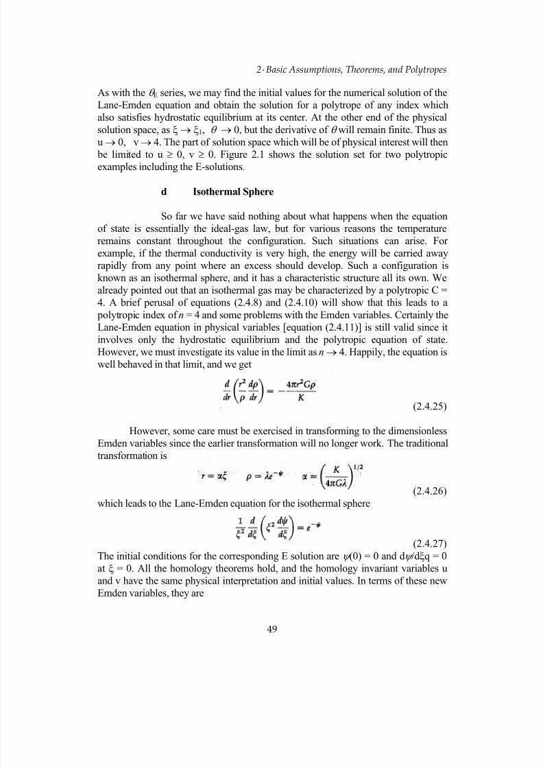
7/18/2019 The Fundamentals of Stellar Astrophysics - Collins G. W.
http://slidepdf.com/reader/full/the-fundamentals-of-stellar-astrophysics-collins-g-w 69/524
2⋅ Basic Assumptions, Theorems, and Polytropes
As with the θ E series, we may find the initial values for the numerical solution of the
Lane-Emden equation and obtain the solution for a polytrope of any index which
also satisfies hydrostatic equilibrium at its center. At the other end of the physical
solution space, as ξ → ξ1, θ → 0, but the derivative of θ will remain finite. Thus asu → 0, v → 4. The part of solution space which will be of physical interest will then
be limited to u ≥ 0, v ≥ 0. Figure 2.1 shows the solution set for two polytropic
examples including the E-solutions.
d Isothermal Sphere
So far we have said nothing about what happens when the equation
of state is essentially the ideal-gas law, but for various reasons the temperature
remains constant throughout the configuration. Such situations can arise. For
example, if the thermal conductivity is very high, the energy will be carried away
rapidly from any point where an excess should develop. Such a configuration isknown as an isothermal sphere, and it has a characteristic structure all its own. We
already pointed out that an isothermal gas may be characterized by a polytropic C =
4. A brief perusal of equations (2.4.8) and (2.4.10) will show that this leads to a
polytropic index of n = 4 and some problems with the Emden variables. Certainly the
Lane-Emden equation in physical variables [equation (2.4.11)] is still valid since it
involves only the hydrostatic equilibrium and the polytropic equation of state.
However, we must investigate its value in the limit as n → 4. Happily, the equation is
well behaved in that limit, and we get
(2.4.25)
However, some care must be exercised in transforming to the dimensionless
Emden variables since the earlier transformation will no longer work. The traditional
transformation is
(2.4.26)
which leads to the Lane-Emden equation for the isothermal sphere
(2.4.27)
The initial conditions for the corresponding E solution are ψ (0) = 0 and dψ /dξq = 0
at ξ = 0. All the homology theorems hold, and the homology invariant variables u
and v have the same physical interpretation and initial values. In terms of these new
Emden variables, they are
49
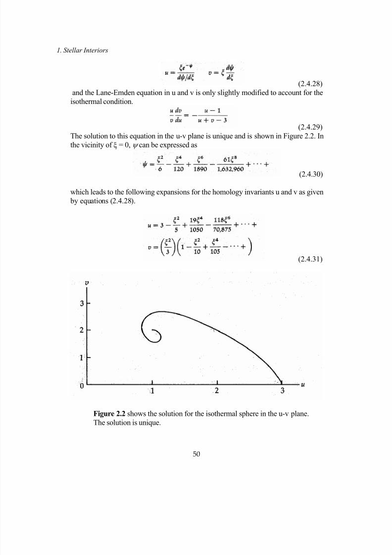
7/18/2019 The Fundamentals of Stellar Astrophysics - Collins G. W.
http://slidepdf.com/reader/full/the-fundamentals-of-stellar-astrophysics-collins-g-w 70/524
1. Stellar Interiors
(2.4.28)
and the Lane-Emden equation in u and v is only slightly modified to account for the
isothermal condition.
(2.4.29)
The solution to this equation in the u-v plane is unique and is shown in Figure 2.2. In
the vicinity of ξ = 0, ψ can be expressed as
(2.4.30)
which leads to the following expansions for the homology invariants u and v as given by equations (2.4.28).
(2.4.31)
Figure 2.2 shows the solution for the isothermal sphere in the u-v plane.
The solution is unique.
50
7/18/2019 The Fundamentals of Stellar Astrophysics - Collins G. W.
http://slidepdf.com/reader/full/the-fundamentals-of-stellar-astrophysics-collins-g-w 71/524
2⋅ Basic Assumptions, Theorems, and Polytropes
The physical importance of the isothermal sphere is widespread having
applications from stellar cores to galaxy structure. So it is worthwhile to emphasize
one curious aspect of the structure. Direct substitution of a density dependence with
the form ρ(r) ~ r
-2
into equation (2.4.25) shows that such a density law will satisfyhydrostatic equilibrium at all points within an isothermal sphere. Thus, ρ(r) ~ r -2
is
often used to describe the radial density variation in spherically symmetric regions
which are assumed to be isothermal.
e Fitting Polytropes Together
As we shall see later, many stars, including those on the main
sequence, can be reasonably represented by a combination of polytropes where the
local value of the polytropic index is chosen to reflect the physical constraints placed
on the star by the mode of energy transport or possibly the equation of state. Thus, itis useful to understand what conditions must hold where the polytropes meet. Let us
consider a simple star composed of a core and an envelope having different
polytropic indices (see Figure 2.3).
Now let q be the fraction of the total mass in the core, n the polytropic index
of the core, and m the total mass of the core. Physically, we must require that the
pressure and density be continuous across the boundary. This implies that u and v are
continuous across the boundary between the two polytropes. Since the initial
conditions at the center of the core must be u = 3, v = 0, the core solution must be an
E solution for the core index n. The envelope solution will not, in general, be an E
solution; but as long as the central point (u=3, v=0) is not encountered, there is noviolation of hydrostatic equilibrium by such a solution. Thus one can construct a
reasonable model by proceeding outward along the core solution until the mass of
the core is reached. This defines the fitting point in the u-v plane. One then searches
the F or M solutions which meet the core solution at the fitting point, to ensure
continuity of P and ρ across the boundary. There will be many solutions
corresponding to different values of the polytropic index of the envelope. Picking
one such solution, one continues with this solution until ξ1 is reached, at which point
M(ξ1) should equal m/q. If it does not, then there is no solution for that value of the
polytropic index of the envelope and another solution at the fitting point should be
chosen.
51

7/18/2019 The Fundamentals of Stellar Astrophysics - Collins G. W.
http://slidepdf.com/reader/full/the-fundamentals-of-stellar-astrophysics-collins-g-w 72/524
1. Stellar Interiors
Figure 2.3 represents a model star composed of two polytropes. The
outer convective hydrogen envelope can be represented by a
polytrope of index n = 1.5, while the helium core is isothermal. The
discontinuous change in u and v resulting from the change in
chemical composition can be seen as a jump from the isothermal core
solution toward the origin and the appropriate M-solution for the
envelope. Such a model can be expected to qualitatively represent the
evolved phase of a red giant.
The techniques of J.L. Lagrange known as variation of parameters can be utilized to
convert an error on the mass at ξ1, dm(ξ1), to a correction in the polytropic index δne
of the envelope solution. Any solution which satisfies the continuity conditions and
the constraints set by the core mass and mass fraction is unique. In addition, it is possible to allow for a discontinuity in the chemical composition at the boundary by
permitting a discontinuity in the density such that momentum conservation is
maintained across the boundary. That is, pressure equilibrium must be maintained
across the boundary. From the ideal-gas law, the ratio of the density in the envelope
to that of the core is
52

7/18/2019 The Fundamentals of Stellar Astrophysics - Collins G. W.
http://slidepdf.com/reader/full/the-fundamentals-of-stellar-astrophysics-collins-g-w 73/524
2⋅ Basic Assumptions, Theorems, and Polytropes
(2.4.32)
This is equivalent to specifying a jump in u and (n + 1)v by the ratio of the mean
molecular weights of the core and envelope. Thus the fitting point, when it is
reached, is displaced toward the origin in u and (n + 1)v by the ratio of the mean
molecular weights of the envelope and core. This displaced point in the u-v plane is
the new point from which the solution is to be continued (see Figure 2.3). The
solution is then completed as in the previous instance.
By making use of polytropic solutions, it is possible to represent stars with
convective cores and radiative envelopes with some accuracy and to get a rough idea
of the run of pressure, density, and temperature throughout the star. Polytropes are
useful in determining the effects of the buildup of chemical discontinuities as a result
of nuclear burning. As mentioned earlier, very massive stars are radiation-dominated
and are quite accurately represented by polytropes of index n = 3 (γ' = 4/3).
Polytropes often can be used as an initial model which is then perturbed to
approximate a given physical situation. For relatively little effort, polytropic models
can provide substantial insight into the behavior of stars in response to various
changes in physical conditions. We obtain this insight at a relatively low cost. To do
significantly better, we must do much more. We will have to know, in some detail,
how energy is transported throughout the star. But before we can do that, we must
understand the detailed structure of the gas so that we can understand the properties
which impede that flow of energy.
Problems
1. Use the integral theorems of Chandrasekhar to place limits on the central
temperature of a star of given mass M.
2. Estimate the mass of a white dwarf at which the relativistic degenerate
equation of state becomes essential for representing its structure.
3. Prove that all solutions to the Lane-Emden equation which remain finite at
the origin (ξ = 0), must, of necessity, have
53

7/18/2019 The Fundamentals of Stellar Astrophysics - Collins G. W.
http://slidepdf.com/reader/full/the-fundamentals-of-stellar-astrophysics-collins-g-w 74/524
1. Stellar Interiors
4. Show that the mass interior to ξ [that is, M(ξ)] in an isothermal sphere is
given by
5. Find a series solution for the Lane-Emden Equation in the vicinity of ξ = 0,
subject to the boundary condition that (dθ /dξ)ξ=0 be zero. This solution
should have an accuracy of O(ξ12).
6. Find a series solution for the isothermal sphere subject to the same conditions
that are given in Problem 5.
7. Use the series solutions from Problems 5 and 6 to obtain corresponding series
solutions for the homology invariants u and v.
8. Calculate a value for the free-fall time for an object on the surface of the sun
to arrive at the center of the sun.
9. Show that the results of equation (2.3.8) are indeed correct. State clearly all
assumptions you make during your derivation.
References and Supplemental Reading
1. Chandrasekhar S.: An Introduction to the Study of Stellar Structure Dover,
New York, 1957 p. 77.
For those who are interested in a further discussion of the integral theorems, some
excellent articles are:
Chandrasekhar, S.: An Integral Theorem on the Equilibrium of a Star
Ap. J. 87, 1938, pp. 535 - 552;
________________ The Opacity in the Interior of a Star Ap. J. 86, 1937,
pp. 78 - 83;
________________ The Pressure in the Interior of a Star Ap. J. 85, 1937,
pp. 372 - 379; ________________ The Pressure in the Interior of a Star. Mon. Not. R.
astr. Soc. 96, 1936, pp. 644 - 647.
Milne, E.A.: The Pressure in the Interior of a Star Mon. Not. R. astr. Soc. 96,
1936, pp. 179 - 184.
54
7/18/2019 The Fundamentals of Stellar Astrophysics - Collins G. W.
http://slidepdf.com/reader/full/the-fundamentals-of-stellar-astrophysics-collins-g-w 75/524
2⋅ Basic Assumptions, Theorems, and Polytropes
55
For a complete discussion of polytropes and isothermal spheres see any of these:
Chandrasekhar S.: An Introduction to the Study of Stellar Structure Dover,
New York, 1957, chap. 4, p. 84.
Eddington, A.S.: The Internal Constitution of the Stars Dover, New York,
1959, chap. 4, p. 79.
Cox, J. P., and Giuli, R. T.: Principles of Stellar Structure Gordon & Breach,
New York, 1968, Chap. 12, p. 257.
An interesting example of the use of polytropes to explore the more complicated
phenomenon of rotation can be found in
Limber, D. N., and Roberts, P.H. : On Highly Rotating Polytropes V , Ap. J.141, 1965, pp.1439-1442.
Geroyannis, V.S., and Valvi, F. N. : Numerical Implementation of a
Perturbation Theory Up to Third Order for Rotating Polytropic Stars:
Parameters Under Differential Rotation, Ap.J. 312, 1987, pp. 219-226.
A brief but useful account of the physical nature of polytropes may be found in
Clayton, D. D.: Principles of Stellar Evolution and Nucleosynthesis,
McGraw-Hill, New York, 1968, pp. 155-158.

7/18/2019 The Fundamentals of Stellar Astrophysics - Collins G. W.
http://slidepdf.com/reader/full/the-fundamentals-of-stellar-astrophysics-collins-g-w 76/524
1 ⋅ Stellar Interiors
Copyright (2003) George W. Collins, II
3
Sources and Sinks of Energy
. . .
We have come to that place in the study of stellar structure where we must be
mindful of the flow of energy through the star. After all, stars do shine. So far, we
have been able to learn much about the equilibrium structure of a star withoutconsidering that it is really a structure in a steady state, rather than one in perfect
strict equilibrium. The basic reason that we have been able to ignore the flow of
energy through the star is that, during a dynamical time, a very small fraction of the
stored energy in the star escapes from the star. Although a star is not, strictly
speaking, an equilibrium structure, it comes closer to being one than most any other
object in the universe.
56

7/18/2019 The Fundamentals of Stellar Astrophysics - Collins G. W.
http://slidepdf.com/reader/full/the-fundamentals-of-stellar-astrophysics-collins-g-w 77/524
3 ⋅ Sources and Sinks of Energy
However, before delving into the actual movement of energy within the star,
we must first identify the sources of that energy as well as the processes which
impede its flow. This will also give us the chance to discuss the stores of energy
within the star since these certainly represent a potential supply of flowing energywith which to generate the stellar luminosity.
3.1 "Energies" of Stars
One of the great mysteries of the late nineteenth and early twentieth centuries was
the source of the energy required to sustain the luminosity of the sun. By then, the
defining solar parameters of mass, radius, and luminosity were known with sufficient
precision to attempt to relate them. For instance, it was clear that if the sun derived
its energy from chemical processes typically yielding less that 1012
erg/g, it could
shine no longer than about 10,000 years at its current luminosity. It is said that Lord
Kelvin, in noting that the liberation of gravitational energy could only keep the sunshining for about 10 million years, found it necessary to reject Charles Darwin's
theory of evolution because there would have been insufficient time for natural
selection to provide the observed diversity of species.
a Gravitational Energy
It is generally conceded that the sun has shone at roughly its present
luminosity for at least the past 2 billion years and has been in existence for nearly 5
billion years. With this in mind, let us begin our study of the sources of stellar energy
with an inventory of the stores of energy available to the sun. Perhaps the most
obvious source of energy is that suggested by Lord Kelvin, namely gravitation. Fromthe integral theorems of Chapter 2, we may place a limit on the gravitational energy
of the sun by remembering that I1,1(R) is related to the total gravitational potential
energy. Thus, from equations (2.2.2) and (2.2.5)
(3.1.1)
The right-hand side of the inequality is the gravitational potential energy for a
uniform density sphere, which provides a sensible upper limit for the energy.
Remember that the gravitational energy is considered negative by convention; arather larger magnitude of energy may be available for a star that is more centrally
concentrated than a uniform- density sphere. We may acquire a better estimate of the
gravitational potential energy by using the results for a polytrope. Chandrasekhar 1
obtains the following result, due to Betti and Ritter, for the gravitational potential
energy of a polytrope:
57

7/18/2019 The Fundamentals of Stellar Astrophysics - Collins G. W.
http://slidepdf.com/reader/full/the-fundamentals-of-stellar-astrophysics-collins-g-w 78/524
1 ⋅ Stellar Interiors
(3.1.2)
For a star in convective equilibrium (that is, n = 3/2) the factor multiplying GM2/R
becomes 6/7 or nearly unity. Note that for a polytrope of index 5, Ω → -∞ implying
an infinite central concentration of material. This is also one of the polytropes for
which there exists an analytic solution and ξ1 = ∞. Thus, one has the picture of a
mass point surrounded by a massless envelope of infinite extent. Equation (3.1.2)
also tells us that as the polytropic index increases, so does the central concentration.
It is not at all obvious that the total gravitational energy would be available to
permit the star to shine. Some energy must be provided in the form of heat, to
provide the pressure which supports the star. We may use the Virial theorem
[equation (1.2.35)] to estimate how much of the gravitational energy can be utilized
by the luminosity. Consider a star with no mass motions, so that the macroscopickinetic energy T in equation (1.2.35) is zero. Let us also assume that the equilibrium
state is good enough that we can replace the time averages by the instantaneous
values. Then the Virial theorem becomes
2U + Ω = 0 (3.1.3)
Remember that U is the total internal kinetic energy of the gas which
includes all motions of the particles making up the gas. Now we know from
thermodynamics that not all the internal kinetic energy is available to do work, and it
is therefore not counted in the internal energy of the gas. The internal kinetic energy
density of a differential mass element of the gas is
dU = (3/2)RTdm = (3/2)(CP-CV)Tdm (3.1.4)
where the relationship of the gas constant R to the specific heats was given in
Chapter 2 [equation (2.4.5)]. However, from the definition of specific heats [equation
(2.4.4)], the internal heat energy of a differential mass element is
dU = CVTdm (3.1.5)
Eliminating Tdm from equations (3.1.4) and (3.1.5) and integrating the energy
densities of the entire star, we getU = (3/2) <γ - 1> U (3.1.6)
where U is the total internal heat energy or just the total internal energy. The quantity
<γ - 1> is the value of γ - 1 averaged over the star. For simplicity, let us assume that γ
is constant through out the star. Then the Virial theorem becomes
58
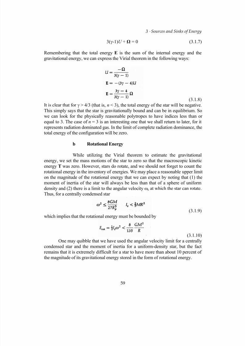
7/18/2019 The Fundamentals of Stellar Astrophysics - Collins G. W.
http://slidepdf.com/reader/full/the-fundamentals-of-stellar-astrophysics-collins-g-w 79/524
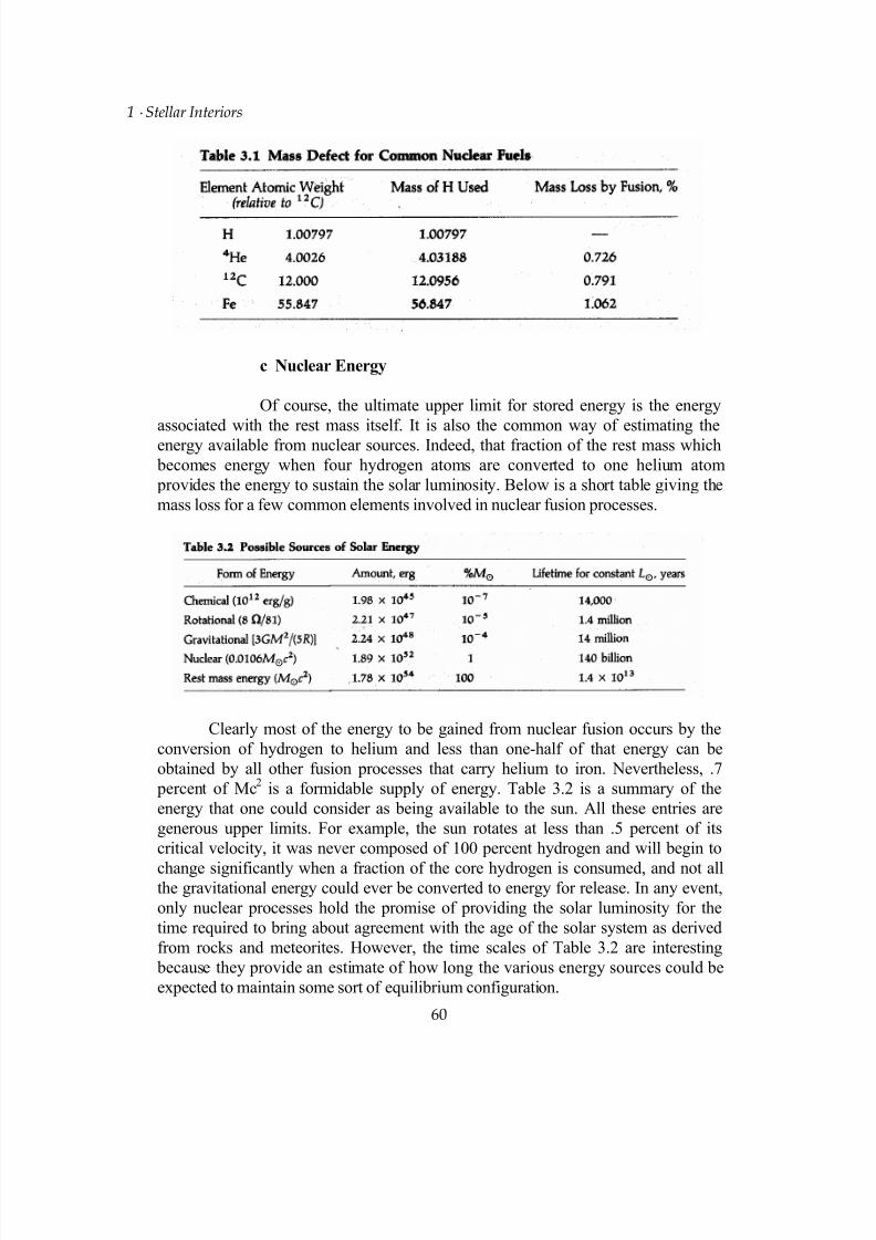
7/18/2019 The Fundamentals of Stellar Astrophysics - Collins G. W.
http://slidepdf.com/reader/full/the-fundamentals-of-stellar-astrophysics-collins-g-w 80/524
1 ⋅ Stellar Interiors
c Nuclear Energy
Of course, the ultimate upper limit for stored energy is the energy
associated with the rest mass itself. It is also the common way of estimating the
energy available from nuclear sources. Indeed, that fraction of the rest mass which
becomes energy when four hydrogen atoms are converted to one helium atom
provides the energy to sustain the solar luminosity. Below is a short table giving the
mass loss for a few common elements involved in nuclear fusion processes.
Clearly most of the energy to be gained from nuclear fusion occurs by the
conversion of hydrogen to helium and less than one-half of that energy can be
obtained by all other fusion processes that carry helium to iron. Nevertheless, .7
percent of Mc2 is a formidable supply of energy. Table 3.2 is a summary of the
energy that one could consider as being available to the sun. All these entries are
generous upper limits. For example, the sun rotates at less than .5 percent of its
critical velocity, it was never composed of 100 percent hydrogen and will begin to
change significantly when a fraction of the core hydrogen is consumed, and not allthe gravitational energy could ever be converted to energy for release. In any event,
only nuclear processes hold the promise of providing the solar luminosity for the
time required to bring about agreement with the age of the solar system as derived
from rocks and meteorites. However, the time scales of Table 3.2 are interesting
because they provide an estimate of how long the various energy sources could be
expected to maintain some sort of equilibrium configuration.
60
7/18/2019 The Fundamentals of Stellar Astrophysics - Collins G. W.
http://slidepdf.com/reader/full/the-fundamentals-of-stellar-astrophysics-collins-g-w 81/524
3 ⋅ Sources and Sinks of Energy
3.2 Time Scales
One of the most useful notions in stellar astrophysics for establishing an intuitive feel
for the significance of various physical processes is the time required for those processes to make a significant change in the structure of the star. To enable us to
estimate the relative importance of these processes, we shall estimate the time scales
for several of them. In Chapter 2 we used the free-fall time of the sun to establish the
fact that the sun can be considered to be in hydrostatic equilibrium. The statement
was made that this time scale was essentially the same as the dynamical time scale.
So let us now turn to estimating the time required for dynamical forces to change a
star.
a Dynamical Time Scale
The Virial theorem of Chapter 1 [equation (1.2.34)] provides us witha ready way of estimating the dynamical time scale, for in the form given, it must
hold for all 1/r 2 forces. Consider a star which is not in equilibrium because the
internal energy is too low. As it enters the non-equilibrium condition, the star's
kinetic energy will also be small. Thus, the Virial theorem would require
(3.2.1)
implying a rapid collapse. If we take as an average value for the accelerative change
in the moment of inertia
(3.2.2)
where td is the dynamical time by definition, then we get
(3.2.3)
or
(3.2.4)
Now we compare this to the free-fall time obtained by direct integration of
(3.2.5)
remembering that, since the star is "free-falling", M(r) will always be the mass
interior to r. Thus, a surface point will always be affected by the total mass M. With
some attention to the boundary conditions [see equations (5.2.12) through (5.2.17)],
direct integration yields a free-fall time of
61
7/18/2019 The Fundamentals of Stellar Astrophysics - Collins G. W.
http://slidepdf.com/reader/full/the-fundamentals-of-stellar-astrophysics-collins-g-w 82/524
1 ⋅ Stellar Interiors
(3.2.6)
which is essentially the same (within about a factor of 1.4) as the dynamical time.
Although we considered a star having zero pressure in order to derive both
those time scales, the situation would not be significantly different if some pressure
did exist. While a collapse will cause an increase in the pressure, the Virial theorem
assures us that the gravitational energy will always exceed the internal energy of the
gas unless there is a change in the equation of state resulting in a sudden increase in
the internal energy. However, for the interior of the star to adjust to the collapse, it is
necessary for information regarding the collapse to be communicated throughout the
star. This will be accomplished by pressure waves which travel at the speed of sound.
The sound crossing time is
(3.2.7)
For a monatomic gas γ = 5/3. Hence
(3.2.8)
We may estimate the mean temperature for a uniform density sphere from the
integral theorems [equations (2.2.4) and (2.2.7)] and obtain
(3.2.9)
Although the sound crossing time is somewhat larger than the free-fall and
dynamical time scales, they are all of the same order of magnitude, ( )GMR 3 . This is
about 27 min for the sun. The similar magnitude for these times is to be expected
since they have a common origin in dynamical phenomena. So we have finally
justified our statement in Chapter 2 that any departure from hydrostatic equilibrium
will be resolved in about 20 min. This short time scale is characteristic of the
dynamical time scale; it is generally the shortest of all the time scales of importance
in stars.
b Kelvin-Helmholtz (Thermal) Time Scale
Now we turn to some of considerations that led Lord Kelvin to reject
the Darwinian theory of evolution. These involve the gravitational heating of the sun.
If you imagine the early phases of a star's existence, when the internal temperature is
insufficient to ignite nuclear fusion, then you will have the physical picture of a
cloud of gas which is slowly contracting and is thereby being heated. Ultimately
62

7/18/2019 The Fundamentals of Stellar Astrophysics - Collins G. W.
http://slidepdf.com/reader/full/the-fundamentals-of-stellar-astrophysics-collins-g-w 83/524
3 ⋅ Sources and Sinks of Energy
some of the energy generated by this contraction will be released from the stellar
surface in the form of photons. As long as the process is slow compared to the
dynamical time scale for the object, the Virial theorem in the form of equation
(1.2.35) will hold and <T> ≈ 0. Thus
½<Ω> = - <U> (3.2.10)
which implies that one-half of the change in the gravitational energy will go into
raising the internal kinetic energy of the gas. The other half is available to be radiated
away. This was the mechanism that Lord Kelvin proposed was responsible for
providing the solar luminosity and he suggested a lifetime for such a mechanism to
be simply the time required for the luminosity to result in a loss of energy equal to
the present gravitational energy. If we estimate the latter by assuming that the star of
interest is of uniform density, then
(3.2.11)
This is known as the Kelvin-Helmholtz gravitational contraction time, and it
is the same as the lifetime obtained from the gravitational energy given in the
previous section. Since the star is simply cooling off and having its internal energy
re-supplied by gravitational contraction, some authors refer to this time scale as the
thermal time scale. More properly, one could define the thermal time scale tth as the
time required for the luminosity to result in an energy loss equal to the internal heat
energy, and then one could relate that to the Kelvin-Helmholtz time by means of the
Virial theorem. That is,
(3.2.12)
Thus, we see that the two time scales are of the same order of magnitude differing
only by a factor of 2 for a monatomic gas. For the sun, both time scales are of the
order of 1011
times longer than the dynamical time. In general the thermal time scale
is very much longer than the dynamical time scale. The thermal time scale is the time
over which thermal instabilities will be resolved, and so they are always less
important than dynamical instabilities.
c Nuclear (Evolutionary) Time Scale
In the beginning of this section we estimated the lifetime of the sun
which could result from the dissipation of various sources of stored energy. By far
the most successful at providing a long life was nuclear energy. The conversion of
hydrogen to iron provided for a lifetime of some 140 billion years. However, in
practice, when about 10 percent of the hydrogen is converted to helium in stars like
63
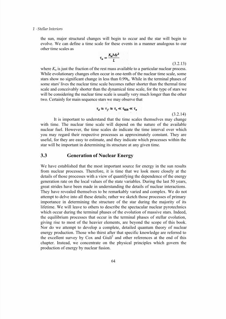
7/18/2019 The Fundamentals of Stellar Astrophysics - Collins G. W.
http://slidepdf.com/reader/full/the-fundamentals-of-stellar-astrophysics-collins-g-w 84/524
1 ⋅ Stellar Interiors
the sun, major structural changes will begin to occur and the star will begin to
evolve. We can define a time scale for these events in a manner analogous to our
other time scales as
(3.2.13)
where K n is just the fraction of the rest mass available to a particular nuclear process.
While evolutionary changes often occur in one-tenth of the nuclear time scale, some
stars show no significant change in less than 0.99tn. While in the terminal phases of
some stars' lives the nuclear time scale becomes rather shorter than the thermal time
scale and conceivably shorter than the dynamical time scale, for the type of stars we
will be considering the nuclear time scale is usually very much longer than the other
two. Certainly for main sequence stars we may observe that
(3.2.14)
It is important to understand that the time scales themselves may change
with time. The nuclear time scale will depend on the nature of the available
nuclear fuel. However, the time scales do indicate the time interval over which
you may regard their respective processes as approximately constant. They are
useful, for they are easy to estimate, and they indicate which processes within the
star will be important in determining its structure at any given time.
3.3 Generation of Nuclear Energy
We have established that the most important source for energy in the sun resultsfrom nuclear processes. Therefore, it is time that we look more closely at the
details of those processes with a view of quantifying the dependence of the energy
generation rate on the local values of the state variables. During the last 50 years,
great strides have been made in understanding the details of nuclear interactions.
They have revealed themselves to be remarkably varied and complex. We do not
attempt to delve into all these details; rather we sketch those processes of primary
importance in determining the structure of the star during the majority of its
lifetime. We will leave to others to describe the spectacular nuclear pyrotechnics
which occur during the terminal phases of the evolution of massive stars. Indeed,
the equilibrium processes that occur in the terminal phases of stellar evolution,
giving rise to most of the heavier elements, are beyond the scope of this book. Nor do we attempt to develop a complete, detailed quantum theory of nuclear
energy production. Those who thirst after that specific knowledge are referred to
the excellent survey by Cox and Giuli2 and other references at the end of this
chapter. Instead, we concentrate on the physical principles which govern the
production of energy by nuclear fusion.
64

7/18/2019 The Fundamentals of Stellar Astrophysics - Collins G. W.
http://slidepdf.com/reader/full/the-fundamentals-of-stellar-astrophysics-collins-g-w 85/524
3 ⋅ Sources and Sinks of Energy
a General Properties of the Nucleus
The notion that the atom can be viewed as being composed of a
nucleus surrounded by a cloud of electrons which are confined to shells led to avery successful theory of atomic spectra. A very similar picture can be postulated
for the nucleus itself, namely, that nucleons are arranged in shells within the
nucleus and undergo transitions from one excited state (shell) to another subject
to the same sort of selection rules that govern atomic transitions. The origin of the
shell structure of any nucleus is that nucleons are fermions and therefore must
obey the Pauli Exclusion Principle, just as the atomic electrons do. Thus, only two
protons or two neutrons may occupy a specific cell in phase space (protons and
neutrons have the same spin as electrons, so each species can have two of its kind
in a quantum state characterized by the spatial quantum numbers).
However, the nucleons are much more tightly bound in the nucleus thanthe electrons in the atom. Whereas the typical ionization energy of an atom can be
measured in tens to thousands of electron volts, the typical binding energy of a
nucleon in the nucleus is several million electron volts. This large binding energy
and the Pauli Exclusion Principle can be used to explain the stability of the
neutron in nuclei. Although free neutrons beta-decay to protons (and an electron
and an electron antineutrino) with a half-life of about 10 min, neutrons appear to
be stable when they are in nuclei. If neutrons did decay, the resulting proton
would have to occupy one of the least tightly bound proton shells, which
frequently costs more energy than is liberated by the beta decay of the neutron.
Thus, unless the neutron decay can provide sufficient energy for the decay
products to be ejected from the nucleus, the neutron must remain in the nucleus asa stable entity.
In general, for a nucleus to be stable, its mass must be less than the sum of
the masses of any possible combination of its constituents. Thus, Li5 is not stable,
whereas He4 is. A more detailed explanation of the reasons for the stability or
instability of a particular nucleus requires a considerably more detailed discussion
of nuclear interactions and nuclear structure than is consistent with the scope of
this book. However, note that the instability of mass-5 nuclei posed one of the
greatest barriers of the century to the understanding of the evolution of stars. The
nuclear evolution beyond mass 5 was finally solved by Fred Hoyle, who showed
that the triple-a process, which we consider later, could actually initiate synthesisof all the nuclei heavier than mass 12.
Before we turn to the specifics of nuclear energy production, it is worth
saying something about notation. Consider the reaction where a particle a hits a
nucleus X , producing a nucleus ϒ and other particle(s) b. In other words,
65

7/18/2019 The Fundamentals of Stellar Astrophysics - Collins G. W.
http://slidepdf.com/reader/full/the-fundamentals-of-stellar-astrophysics-collins-g-w 86/524
1 ⋅ Stellar Interiors
(3.3.1)
Such a reaction can be written X (a,b) ϒ. Usually for such a reaction to happen, it
must be exothermic. That is, the rest energy of the initial constituents of the
reaction must exceed that of the products.
(3.3.2)
b The Bohr Picture of Nuclear Reactions
Although quantum mechanics formally describes the transition from
the initial to the final state, it is convenient to break down the process and to say that
a compound nucleus is formed by the collision and subsequently decays to the
reaction products. With this assumption, a reaction can be viewed as consisting of
two steps
(3.3.3)
where C* is the compound nucleus and the asterisk indicates that it is in an excited
state. The compound nucleus can decay by various modes which have these
convenient physical interpretations:
(3.3.4)
Elastic scattering simply involves a particle "bouncing off" the nucleus in
such a manner that the momentum and kinetic energy of both the constituents are
conserved. However, inelastic scattering results in the nucleus being left in an
excited state at the expense of the kinetic energy of the reactants. Particle emission is
the process most often associated with nuclear reactions. The results of the
interaction leave both reactants changed. Under certain conditions, the Bohr picture
fails for these interactions since they proceed directly to the final state without the
formation of a compound nucleus. In radiative capture, the compound nucleus
decays from the excited state to a stable state by the emission of a photon.
The validity of this two-stage process, due to Neils Bohr, depends on the
lifetime of the compound nucleus C*. The duration of a nuclear collision can be
66
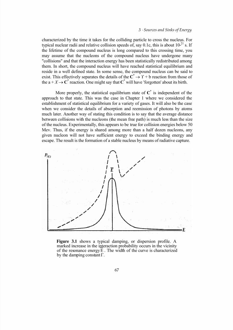
7/18/2019 The Fundamentals of Stellar Astrophysics - Collins G. W.
http://slidepdf.com/reader/full/the-fundamentals-of-stellar-astrophysics-collins-g-w 87/524
3 ⋅ Sources and Sinks of Energy
characterized by the time it takes for the colliding particle to cross the nucleus. For
typical nuclear radii and relative collision speeds of, say 0.1c, this is about 10-21
s. If
the lifetime of the compound nucleus is long compared to this crossing time, you
may assume that the nucleons of the compound nucleus have undergone many"collisions" and that the interaction energy has been statistically redistributed among
them. In short, the compound nucleus will have reached statistical equilibrium and
reside in a well defined state. In some sense, the compound nucleus can be said to
exist. This effectively separates the details of the C*→ ϒ + b reaction from those of
the a + X → C* reaction. One might say that C
* will have 'forgotten' about its birth.
More properly, the statistical equilibrium state of C* is independent of the
approach to that state. This was the case in Chapter 1 where we considered the
establishment of statistical equilibrium for a variety of gases. It will also be the case
when we consider the details of absorption and reemission of photons by atoms
much later. Another way of stating this condition is to say that the average distance between collisions with the nucleons (the mean free path) is much less than the size
of the nucleus. Experimentally, this appears to be true for collision energies below 50
Mev. Thus, if the energy is shared among more than a half dozen nucleons, any
given nucleon will not have sufficient energy to exceed the binding energy and
escape. The result is the formation of a stable nucleus by means of radiative capture.
Figure 3.1 shows a typical damping, or dispersion profile. Amarked increase in the interaction probability occurs in the vicinityof the resonance energyE . The width of the curve is characterized by the damping constant Γ.
67
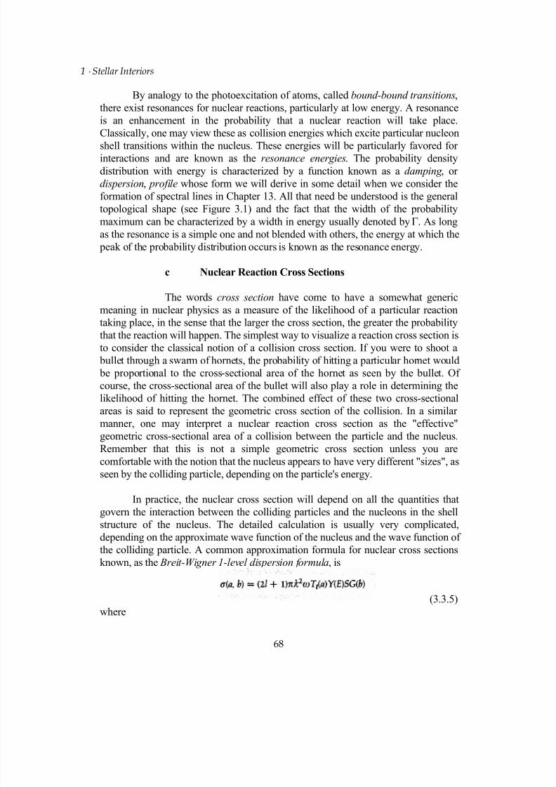
7/18/2019 The Fundamentals of Stellar Astrophysics - Collins G. W.
http://slidepdf.com/reader/full/the-fundamentals-of-stellar-astrophysics-collins-g-w 88/524
1 ⋅ Stellar Interiors
By analogy to the photoexcitation of atoms, called bound-bound transitions,
there exist resonances for nuclear reactions, particularly at low energy. A resonance
is an enhancement in the probability that a nuclear reaction will take place.
Classically, one may view these as collision energies which excite particular nucleonshell transitions within the nucleus. These energies will be particularly favored for
interactions and are known as the resonance energies. The probability density
distribution with energy is characterized by a function known as a damping , or
dispersion, profile whose form we will derive in some detail when we consider the
formation of spectral lines in Chapter 13. All that need be understood is the general
topological shape (see Figure 3.1) and the fact that the width of the probability
maximum can be characterized by a width in energy usually denoted by Γ. As long
as the resonance is a simple one and not blended with others, the energy at which the
peak of the probability distribution occurs is known as the resonance energy.
c Nuclear Reaction Cross Sections
The words cross section have come to have a somewhat generic
meaning in nuclear physics as a measure of the likelihood of a particular reaction
taking place, in the sense that the larger the cross section, the greater the probability
that the reaction will happen. The simplest way to visualize a reaction cross section is
to consider the classical notion of a collision cross section. If you were to shoot a
bullet through a swarm of hornets, the probability of hitting a particular hornet would
be proportional to the cross-sectional area of the hornet as seen by the bullet. Of
course, the cross-sectional area of the bullet will also play a role in determining the
likelihood of hitting the hornet. The combined effect of these two cross-sectional
areas is said to represent the geometric cross section of the collision. In a similarmanner, one may interpret a nuclear reaction cross section as the "effective"
geometric cross-sectional area of a collision between the particle and the nucleus.
Remember that this is not a simple geometric cross section unless you are
comfortable with the notion that the nucleus appears to have very different "sizes", as
seen by the colliding particle, depending on the particle's energy.
In practice, the nuclear cross section will depend on all the quantities that
govern the interaction between the colliding particles and the nucleons in the shell
structure of the nucleus. The detailed calculation is usually very complicated,
depending on the approximate wave function of the nucleus and the wave function of
the colliding particle. A common approximation formula for nuclear cross sectionsknown, as the Breit-Wigner 1-level dispersion formula, is
(3.3.5)
where
68

7/18/2019 The Fundamentals of Stellar Astrophysics - Collins G. W.
http://slidepdf.com/reader/full/the-fundamentals-of-stellar-astrophysics-collins-g-w 89/524
3 ⋅ Sources and Sinks of Energy
(3.3.6)
We will make no attempt to derive this result. However, we do try to show
that the result at least contains the right sort of terms and is reasonable. The term
is essentially the geometric cross section of the colliding particle as it is related
to the particle's de Broglie wavelength. The angular momentum term (2 +1) is a
measure of the impact parameter and the energy. As l increases, so does the impact
parameter. For constant angular momentum, an increasing impact parameter will
mean a decreasing collision energy, implying a net increase of the collision
probability. However, as the impact parameter increases and the collision energy
drops, the probability that the colliding particle will be able to overcome the coulomb
barrier decreases drastically. Thus, we need be concerned only with = 0, or 1. The
term transmission function of particle a includes the probability that the particle will
penetrate the coulomb barrier of the nucleus. The parameter ω allows for the spin-
spin interactions of the nucleus and the particle and is of the order unity. Function
ϒ(E) includes the effects of resonances and from the dispersion curve in Figure 3.1
can clearly be a very strong function of collision energy E. The spin degeneracy
parameter S is generally 1 except when a and X are the same kind of particle and
also have zero spin; then S = 2. Finally, G(b) is a measure of the probability that
particle b will be created from the compound nucleus as opposed to some other
possibility. Now that we have the nuclear reaction cross sections, we have to
2Dπ
l
l
69

7/18/2019 The Fundamentals of Stellar Astrophysics - Collins G. W.
http://slidepdf.com/reader/full/the-fundamentals-of-stellar-astrophysics-collins-g-w 90/524
1 ⋅ Stellar Interiors
determine the rate at which collisions will occur. Then we will be able to find the
energy produced by stellar material.
d Nuclear Reaction Rates
The reaction cross section of the previous section can be measured as a
function of the collision energy (and some atomic constants) alone and therefore can
be written as a function of the particle's velocity v relative to the target. By
resurrecting the geometric interpretation of the cross section, the number of particles
crossing an area (colliding with the target) per unit time is just Nσ(v)v where N is the
density of colliding particles (see Figure 3.2)
Consider collisions between two different kinds of particles with a number
density in phase space of dN1 and dN2. To obtain the number of collisions per second
per unit volume, we must integrate over all available velocity space. That is, we mustsum over the collisions between particles so that the collision rate r is
(3.3.7)
Figure 3.2 is a schematic representation of a collision between particle a
and a target with a geometrical cross section σ.
Let us assume that the velocity distributions of both kinds of particles are given by
maxwellian velocity distributions
(3.3.8)
so that equation (3.3.7) becomes
(3.3.9)
If we transform to the center-of-mass coordinate system, assuming the velocity field
is isotropic so that the triple integrals of equation (3.3.9) can be written as spherical
70
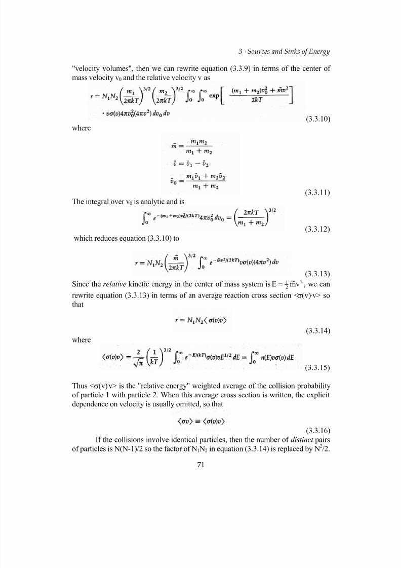
7/18/2019 The Fundamentals of Stellar Astrophysics - Collins G. W.
http://slidepdf.com/reader/full/the-fundamentals-of-stellar-astrophysics-collins-g-w 91/524
3 ⋅ Sources and Sinks of Energy
"velocity volumes", then we can rewrite equation (3.3.9) in terms of the center of
mass velocity v0 and the relative velocity v as
(3.3.10)
where
(3.3.11)
The integral over v0 is analytic and is
(3.3.12)
which reduces equation (3.3.10) to
(3.3.13)
Since the relative kinetic energy in the center of mass system is 2
21 vm~E = , we can
rewrite equation (3.3.13) in terms of an average reaction cross section <σ(v) v> sothat
(3.3.14)
where
(3.3.15)
Thus <σ(v).v> is the "relative energy" weighted average of the collision probability
of particle 1 with particle 2. When this average cross section is written, the explicitdependence on velocity is usually omitted, so that
(3.3.16)
If the collisions involve identical particles, then the number of distinct pairs
of particles is N(N-1)/2 so the factor of N1 N2 in equation (3.3.14) is replaced by N2/2.
71

7/18/2019 The Fundamentals of Stellar Astrophysics - Collins G. W.
http://slidepdf.com/reader/full/the-fundamentals-of-stellar-astrophysics-collins-g-w 92/524
1 ⋅ Stellar Interiors
If we call the energy produced per reaction Q, we can write the energy produced per
gram of stellar material as
(3.3.17)
The number densities can be replaced with the more common fractional abundances
by mass to get
(3.3.18)
where N0 is Avogadro's number. Since <σv> is a complicated function of
temperature and must be obtained numerically, equation (3.3.18) is usually
approximated numerically as
(3.3.19)
where
(3.3.20)
Here ν itself is very weakly dependent on the temperature. Most of the
important energy production mechanisms have this form. Equation (3.3.19)
expresses the energy generated for a specific energy generation mechanism in terms
of the state variables T and p. This is what we were after. Formulas such as these,
where ε0 has been determined, will enable us to determine the energy producedthroughout the star in terms of the state variables. Before turning to the description of
processes which impede the flow of this energy, let us consider a few of the specific
nuclear reactions for which we have expressions of the type given by equation
(3.3.20.)
e Specific Nuclear Reactions
The nuclear reactions that provide the energy for main sequence stars
all revolve on the conversion of hydrogen to helium. However, this is accomplished
by a variety of ways. We may divide these ways into two groups. The first is known
as the proton-proton cycle (p-p cycle) and it begins with the conversion of twohydrogen atoms to deuterium. Several possibilities occur on the way to the
production of4He. These alternate options are known as P2-P6 cycles. In addition to
the proton-proton cycle, a series of nuclear reactions involving carbon, nitrogen, and
oxygen also can lead to the conversion of hydrogen to helium with no net change in
the abundance of C, N, and O. For this reason, it is known as the CNO cycle. These
reactions and their side chains as given by Cox and Giuli2 are given in Table 3.3
72
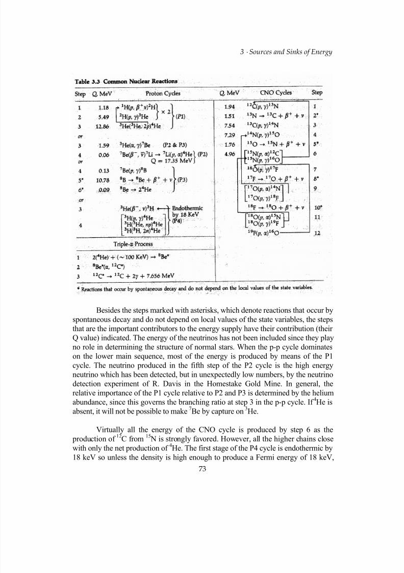
7/18/2019 The Fundamentals of Stellar Astrophysics - Collins G. W.
http://slidepdf.com/reader/full/the-fundamentals-of-stellar-astrophysics-collins-g-w 93/524
3 ⋅ Sources and Sinks of Energy
Besides the steps marked with asterisks, which denote reactions that occur by
spontaneous decay and do not depend on local values of the state variables, the steps
that are the important contributors to the energy supply have their contribution (their
Q value) indicated. The energy of the neutrinos has not been included since they play
no role in determining the structure of normal stars. When the p-p cycle dominates
on the lower main sequence, most of the energy is produced by means of the P1
cycle. The neutrino produced in the fifth step of the P2 cycle is the high energy
neutrino which has been detected, but in unexpectedly low numbers, by the neutrino
detection experiment of R. Davis in the Homestake Gold Mine. In general, the
relative importance of the P1 cycle relative to P2 and P3 is determined by the helium
abundance, since this governs the branching ratio at step 3 in the p-p cycle. If 4He isabsent, it will not be possible to make
7Be by capture on
3He.
Virtually all the energy of the CNO cycle is produced by step 6 as the
production of12
C from15 N is strongly favored. However, all the higher chains close
with only the net production of4He. The first stage of the P4 cycle is endothermic by
18 keV so unless the density is high enough to produce a Fermi energy of 18 keV,
73
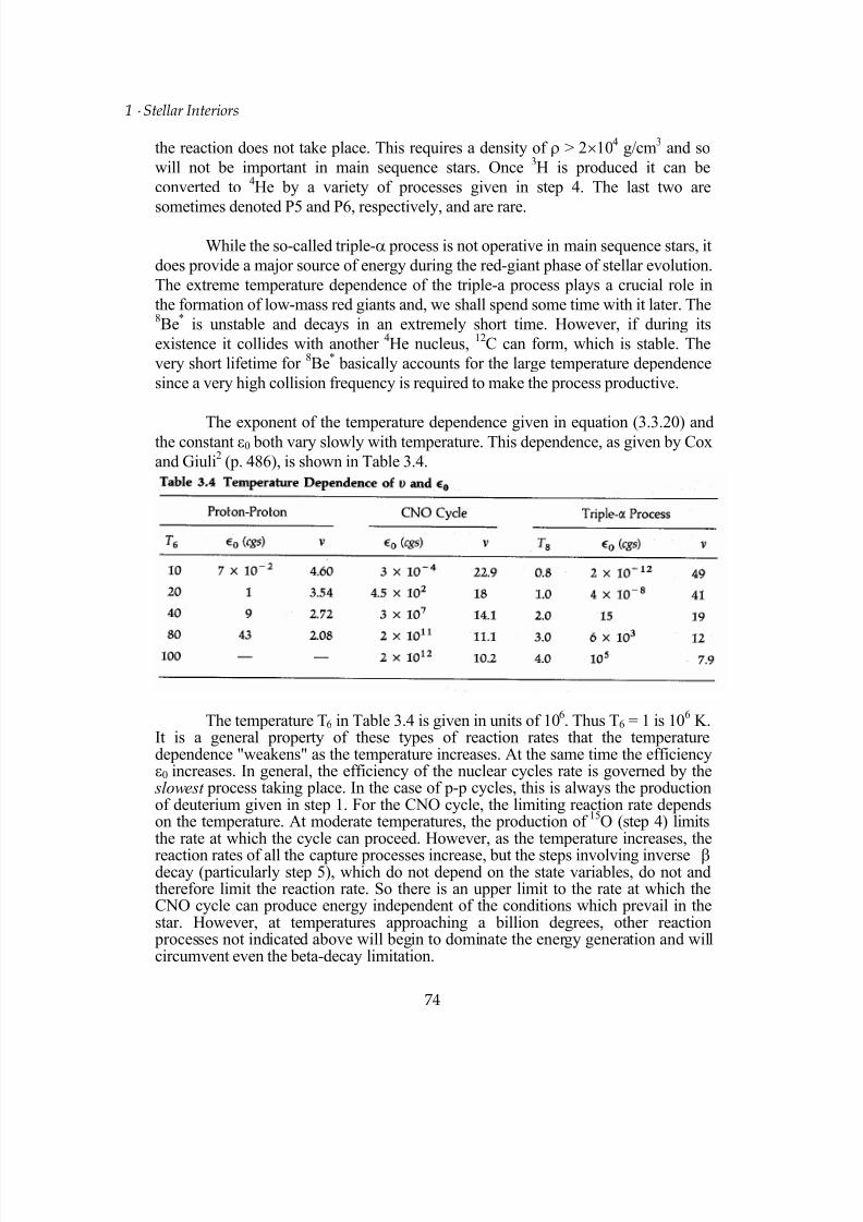
7/18/2019 The Fundamentals of Stellar Astrophysics - Collins G. W.
http://slidepdf.com/reader/full/the-fundamentals-of-stellar-astrophysics-collins-g-w 94/524
1 ⋅ Stellar Interiors
the reaction does not take place. This requires a density of ρ > 2×10⁴ g/cm
3 and so
will not be important in main sequence stars. Once3H is produced it can be
converted to4He by a variety of processes given in step 4. The last two are
sometimes denoted P5 and P6, respectively, and are rare.
While the so-called triple-α process is not operative in main sequence stars, it
does provide a major source of energy during the red-giant phase of stellar evolution.
The extreme temperature dependence of the triple-a process plays a crucial role in
the formation of low-mass red giants and, we shall spend some time with it later. The8Be
* is unstable and decays in an extremely short time. However, if during its
existence it collides with another4He nucleus,
12C can form, which is stable. The
very short lifetime for8Be
* basically accounts for the large temperature dependence
since a very high collision frequency is required to make the process productive.
The exponent of the temperature dependence given in equation (3.3.20) andthe constant ε0 both vary slowly with temperature. This dependence, as given by Cox
and Giuli2 (p. 486), is shown in Table 3.4.
The temperature T6 in Table 3.4 is given in units of 106. Thus T6 = 1 is 10
6 K.
It is a general property of these types of reaction rates that the temperaturedependence "weakens" as the temperature increases. At the same time the efficiencyε0 increases. In general, the efficiency of the nuclear cycles rate is governed by the slowest process taking place. In the case of p-p cycles, this is always the productionof deuterium given in step 1. For the CNO cycle, the limiting reaction rate dependson the temperature. At moderate temperatures, the production of
15O (step 4) limits
the rate at which the cycle can proceed. However, as the temperature increases, the
reaction rates of all the capture processes increase, but the steps involving inverse β decay (particularly step 5), which do not depend on the state variables, do not andtherefore limit the reaction rate. So there is an upper limit to the rate at which theCNO cycle can produce energy independent of the conditions which prevail in thestar. However, at temperatures approaching a billion degrees, other reaction processes not indicated above will begin to dominate the energy generation and willcircumvent even the beta-decay limitation.
74

7/18/2019 The Fundamentals of Stellar Astrophysics - Collins G. W.
http://slidepdf.com/reader/full/the-fundamentals-of-stellar-astrophysics-collins-g-w 95/524

7/18/2019 The Fundamentals of Stellar Astrophysics - Collins G. W.
http://slidepdf.com/reader/full/the-fundamentals-of-stellar-astrophysics-collins-g-w 96/524
76
1 ⋅ Stellar Interiors
I have provided the bare minimum information regarding nuclear energy generation
in this chapter. Further reading should be done in:
Clayton, D. D.: Principles of Stellar Evolution and Nucleosynthesis,McGraw- Hill, New York, 1968 Chaps. 4, 5, pp. 283-606.
Rolfs, C., and Rodney, W. S.: Cauldrons in the Cosmos, University of
Chicago Press, Chicago, 1986.
Rolfs, C., and Trautvetter, H. P.: “Experimental Nuclear Astrophysics” Ann.
Rev. Nucl. Part. Sci. 28, 1978, pp.115-159.
Bahcall, J. N., Huebner, W. F., Lubia, S. H., Parker, P. D., and Ulrich, R. K.:
Rev. Mod. Phy. 54, 1982, p. 767.
In addition, a good overview to the way in which the rates of energy generation
interface with the equations of stellar structure is found in
Schwarzschild, M.: The Structure and Evolution of the Stars Princeton
University Press, Princeton N.J., 1958, pp. 73-88.

7/18/2019 The Fundamentals of Stellar Astrophysics - Collins G. W.
http://slidepdf.com/reader/full/the-fundamentals-of-stellar-astrophysics-collins-g-w 97/524
4 ⋅ Flow of Energy through the Star and Construction of Models
Copyright (2003) George W. Collins, II
4
Flow of Energy through the Star and Construction of Stellar Models
. . .
That the central temperatures of stars are higher than their surface
temperatures can no longer be in doubt. The laws of thermodynamics thus ensure
that energy will flow from the center of stars to their surfaces. The physical processesthat accomplish this will basically establish the temperature gradient within the star.
This is the remaining relationship required for us to link the interior structure with
that of the surface. The temperature gradient and along with the conservation laws of
mass and energy provide the three independent relationships necessary to relate the
three state variables to the values they must have at the boundaries of the star.
77

7/18/2019 The Fundamentals of Stellar Astrophysics - Collins G. W.
http://slidepdf.com/reader/full/the-fundamentals-of-stellar-astrophysics-collins-g-w 98/524
1 ⋅ Stellar Interiors
Energy can move through a medium by essentially three ways, and they can
each be characterized by the gas particles which carry the energy and the forces
which resist these efforts. These mechanisms are radiative transfer, convective
transport, and conductive transfer , of energy. The efficiency of these processes isdetermined primarily by the amount of energy that can be carried by the particles,
their number and their speed. These variables set an upper limit to the rate of energy
transport. In addition, the "opacity" of the material to the motion of the energy-
carrying particles will also affect the efficiency. In the case of radiation, we have
characterized this opacity by a collision cross section and the density. Another way
to visualize this is via the notion of a mean free path. This is just the average distance
between collisions experienced by the particles. In undergoing a collision, the
particle will give up some of its energy thereby losing its efficiency as a transporter
of energy. We will see that, in general, there are large differences in the mean free
paths for the particles that carry energy by these three mechanisms, and so one
mechanism will usually dominate in the transfer of energy.
Before we can describe the radiative flow of energy, we must understand
how the presence of matter impedes that flow. Thus we shall begin our discussion of
the transport of energy by determining how the local radiative opacity depends on
local values of the state variables. From the assumption of strict thermodynamic
equilibrium (STE) we know that any impediment to the flow can be described in
terms of a parameter that depends only on the temperature. However, to calculate
that parameter, we have to investigate the detailed dependence of the opacity on
frequency.
4.1 The Ionization, Abundances, and Opacity of Stellar Material
We have now described the manner in which nuclear energy is produced in most
stars, but before we can turn to the methods by which it flows out of the star, we
must quantitatively discuss the processes which impede that flow. Each constituent
of the gas will interact with the photons of the radiation field in a way that is
characterized by the unique state of that particle. Thus, the type of atom, its state of
ionization, and excitation will determine which photons it can absorb and emit. It is
the combination of all the atoms, acting in consort that produces the opacity of the
gas. The details which make up this combination can be extremely complicated.
However, several of the assumptions we have made, and justified, will make the task
easier and certainly the principles involved can be demonstrated by a few examples.
a Ionization and the Mean Molecular Weight
Our first task is to ascertain how many of the different kinds of
particles that make up the gas are present. To answer this question, we need to know
not only the chemical makeup of the gas, but also the state of ionization of the atoms.
78
7/18/2019 The Fundamentals of Stellar Astrophysics - Collins G. W.
http://slidepdf.com/reader/full/the-fundamentals-of-stellar-astrophysics-collins-g-w 99/524
4 ⋅ Flow of Energy through the Star and Construction of Models
We have already established that the temperatures encountered in the stellar interior
are very high, so we might expect that most of the atoms will be fully ionized. While
this is not exactly true, we will assume that it is the case. A more precise treatment of
this problem will be given later when we consider the state of the gas in the stellar
atmosphere where, the characteristic temperature is measured in thousands of
degrees as opposed to the millions of degrees encountered in the interior.
We will find it convenient to divide the composition of the stellar material
into three categories.
(4.1.1)
It is common in astronomy to refer to everything which is not hydrogen or helium as
"metals". For complete ionization, the number of particles contributed to the gas perelement is just
(4.1.2)
where Zi is the atomic number and Ai is the atomic weight of the element. Thus, the
number of particles contributed by hydrogen will just be twice the hydrogen
abundance, and for helium, three-fourths times the helium abundance. In general,
(4.1.3)
The limit of equation (4.1.3) for the heavy metals is ½. However, even at 107 K theinner shells of the heavy metals will not be completely ionized and so ½ will be an
overestimate of the contribution to the particle number. This error is somewhat
compensated by the 1 in the numerator of equation (4.1.3) for the light elements
where it provides an underestimate of the particle contribution. Thus we take the
total number of particles contributed by the metals to be ½ Z. The total number of
particles in the gas from all sources is then
(4.1.4)
Since everything in the star is classed as either hydrogen, helium, or metals,
X + Y + Z = 1 and we may eliminate the metal abundance from our count of the
total number of particles, to get
(4.1.5)
Throughout the book we have introduced the symbol m as the mean
79
7/18/2019 The Fundamentals of Stellar Astrophysics - Collins G. W.
http://slidepdf.com/reader/full/the-fundamentals-of-stellar-astrophysics-collins-g-w 100/524
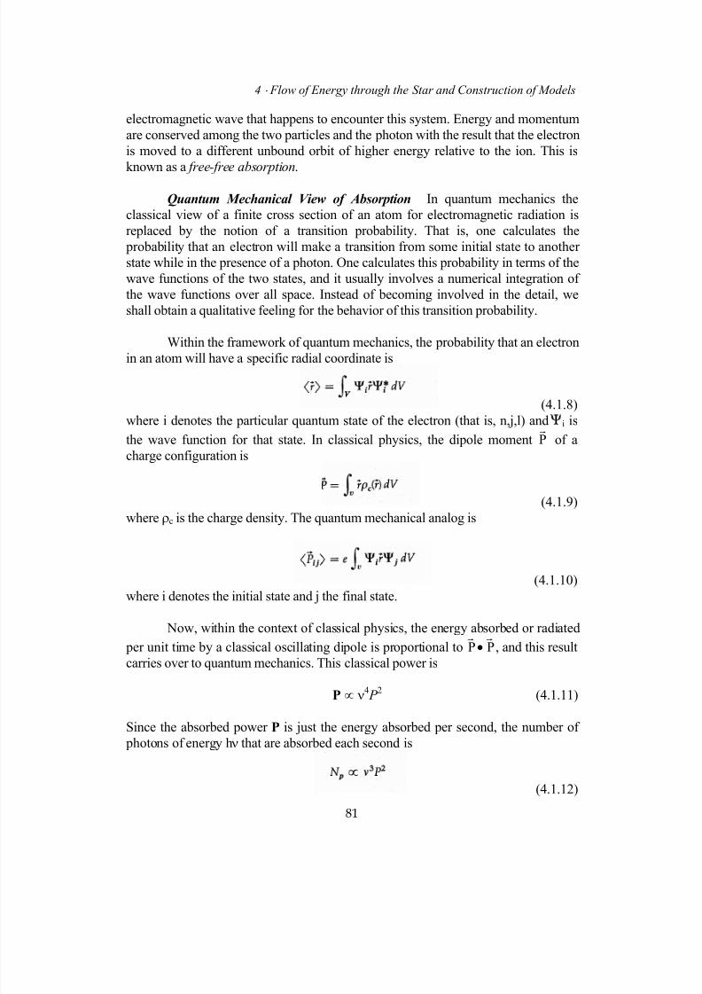
7/18/2019 The Fundamentals of Stellar Astrophysics - Collins G. W.
http://slidepdf.com/reader/full/the-fundamentals-of-stellar-astrophysics-collins-g-w 101/524
4 ⋅ Flow of Energy through the Star and Construction of Models
electromagnetic wave that happens to encounter this system. Energy and momentum
are conserved among the two particles and the photon with the result that the electron
is moved to a different unbound orbit of higher energy relative to the ion. This is
known as a free-free absorption.
Quantum Mechanical View of Absorption In quantum mechanics the
classical view of a finite cross section of an atom for electromagnetic radiation is
replaced by the notion of a transition probability. That is, one calculates the
probability that an electron will make a transition from some initial state to another
state while in the presence of a photon. One calculates this probability in terms of the
wave functions of the two states, and it usually involves a numerical integration of
the wave functions over all space. Instead of becoming involved in the detail, we
shall obtain a qualitative feeling for the behavior of this transition probability.
Within the framework of quantum mechanics, the probability that an electronin an atom will have a specific radial coordinate is
(4.1.8)
where i denotes the particular quantum state of the electron (that is, n,j,l) and i is
the wave function for that state. In classical physics, the dipole moment Pr
of a
charge configuration is
(4.1.9)
where ρc is the charge density. The quantum mechanical analog is
(4.1.10)
where i denotes the initial state and j the final state.
Now, within the context of classical physics, the energy absorbed or radiated
per unit time by a classical oscillating dipole is proportional to P Prr
• , and this result
carries over to quantum mechanics. This classical power is
P ∝ ν4
P 2
(4.1.11)
Since the absorbed power P is just the energy absorbed per second, the number of
photons of energy hν that are absorbed each second is
(4.1.12)
81
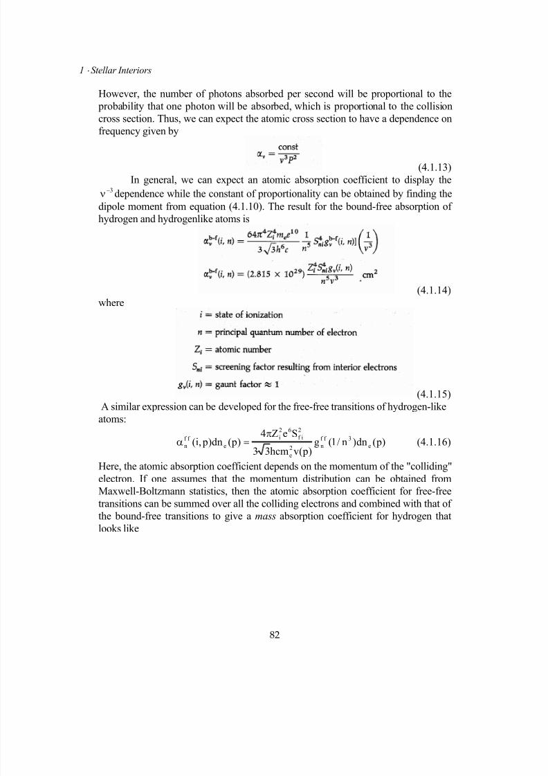
7/18/2019 The Fundamentals of Stellar Astrophysics - Collins G. W.
http://slidepdf.com/reader/full/the-fundamentals-of-stellar-astrophysics-collins-g-w 102/524
1 ⋅ Stellar Interiors
However, the number of photons absorbed per second will be proportional to the
probability that one photon will be absorbed, which is proportional to the collision
cross section. Thus, we can expect the atomic cross section to have a dependence on
frequency given by
(4.1.13)
In general, we can expect an atomic absorption coefficient to display the
dependence while the constant of proportionality can be obtained by finding the
dipole moment from equation (4.1.10). The result for the bound-free absorption of
hydrogen and hydrogenlike atoms is
3−ν
(4.1.14)
where
(4.1.15)
A similar expression can be developed for the free-free transitions of hydrogen-likeatoms:
) p(dn)n/1(g) p(vhcm33
SeZ4) p(dn) p,i( e
3f f
n2
e
2
if
62
i
e
f f
n
π=α (4.1.16)
Here, the atomic absorption coefficient depends on the momentum of the "colliding"
electron. If one assumes that the momentum distribution can be obtained from
Maxwell-Boltzmann statistics, then the atomic absorption coefficient for free-free
transitions can be summed over all the colliding electrons and combined with that of
the bound-free transitions to give a mass absorption coefficient for hydrogen that
looks like
82
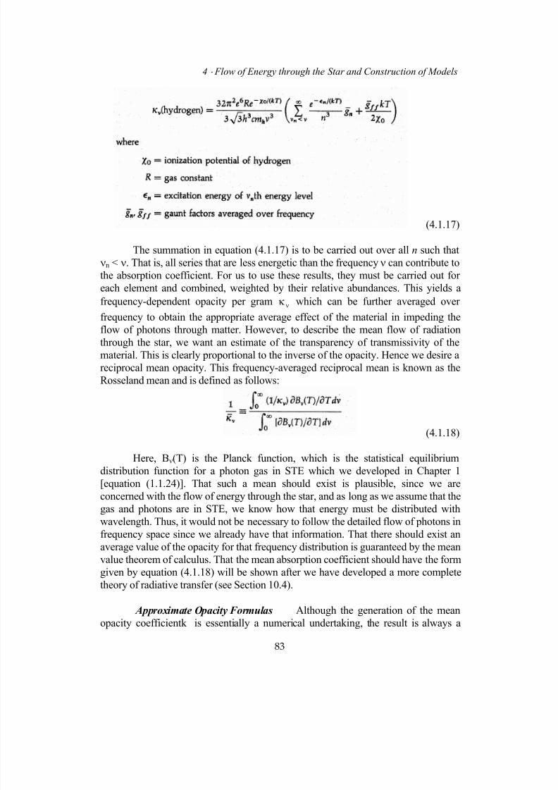
7/18/2019 The Fundamentals of Stellar Astrophysics - Collins G. W.
http://slidepdf.com/reader/full/the-fundamentals-of-stellar-astrophysics-collins-g-w 103/524
4 ⋅ Flow of Energy through the Star and Construction of Models
(4.1.17)
The summation in equation (4.1.17) is to be carried out over all n such that
νn < ν. That is, all series that are less energetic than the frequency ν can contribute to
the absorption coefficient. For us to use these results, they must be carried out foreach element and combined, weighted by their relative abundances. This yields a
frequency-dependent opacity per gram νκ which can be further averaged over
frequency to obtain the appropriate average effect of the material in impeding the
flow of photons through matter. However, to describe the mean flow of radiation
through the star, we want an estimate of the transparency of transmissivity of the
material. This is clearly proportional to the inverse of the opacity. Hence we desire a
reciprocal mean opacity. This frequency-averaged reciprocal mean is known as the
Rosseland mean and is defined as follows:
(4.1.18)
Here, Bν(T) is the Planck function, which is the statistical equilibrium
distribution function for a photon gas in STE which we developed in Chapter 1
[equation (1.1.24)]. That such a mean should exist is plausible, since we are
concerned with the flow of energy through the star, and as long as we assume that the
gas and photons are in STE, we know how that energy must be distributed with
wavelength. Thus, it would not be necessary to follow the detailed flow of photons in
frequency space since we already have that information. That there should exist an
average value of the opacity for that frequency distribution is guaranteed by the mean
value theorem of calculus. That the mean absorption coefficient should have the form
given by equation (4.1.18) will be shown after we have developed a more complete
theory of radiative transfer (see Section 10.4).
Approximate Opacity Formulas Although the generation of the mean
opacity coefficientk is essentially a numerical undertaking, the result is always a
83
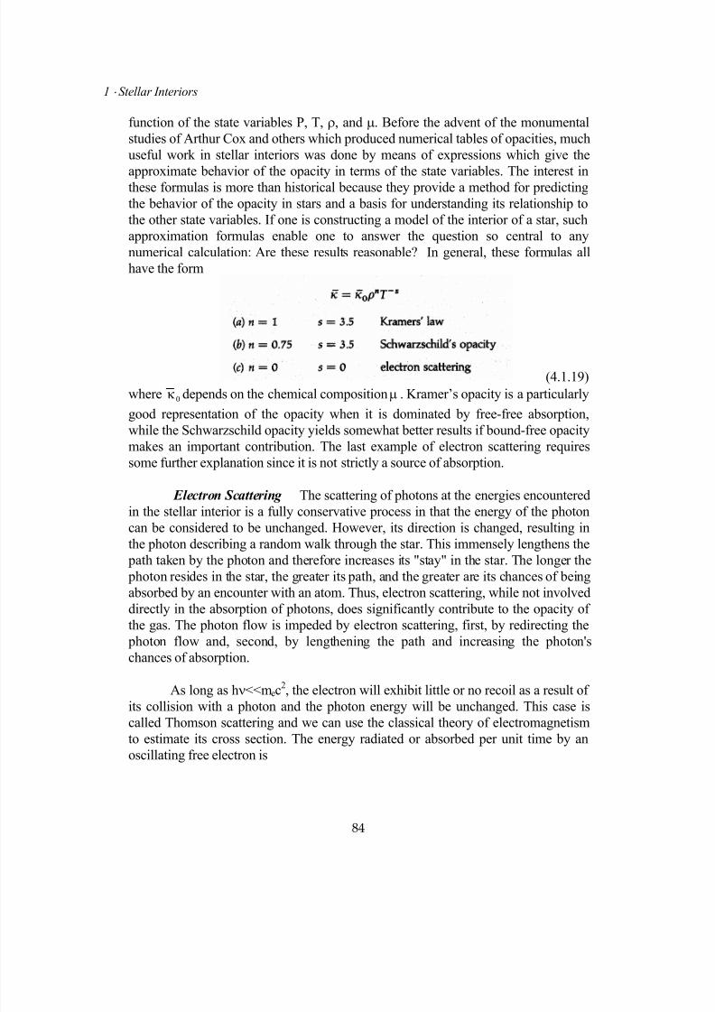
7/18/2019 The Fundamentals of Stellar Astrophysics - Collins G. W.
http://slidepdf.com/reader/full/the-fundamentals-of-stellar-astrophysics-collins-g-w 104/524
1 ⋅ Stellar Interiors
function of the state variables P, T, ρ, and µ. Before the advent of the monumental
studies of Arthur Cox and others which produced numerical tables of opacities, much
useful work in stellar interiors was done by means of expressions which give the
approximate behavior of the opacity in terms of the state variables. The interest inthese formulas is more than historical because they provide a method for predicting
the behavior of the opacity in stars and a basis for understanding its relationship to
the other state variables. If one is constructing a model of the interior of a star, such
approximation formulas enable one to answer the question so central to any
numerical calculation: Are these results reasonable? In general, these formulas all
have the form
(4.1.19)
where 0κ depends on the chemical composition µ . Kramer’s opacity is a particularly
good representation of the opacity when it is dominated by free-free absorption,
while the Schwarzschild opacity yields somewhat better results if bound-free opacity
makes an important contribution. The last example of electron scattering requires
some further explanation since it is not strictly a source of absorption.
Electron Scattering The scattering of photons at the energies encountered
in the stellar interior is a fully conservative process in that the energy of the photon
can be considered to be unchanged. However, its direction is changed, resulting inthe photon describing a random walk through the star. This immensely lengthens the
path taken by the photon and therefore increases its "stay" in the star. The longer the
photon resides in the star, the greater its path, and the greater are its chances of being
absorbed by an encounter with an atom. Thus, electron scattering, while not involved
directly in the absorption of photons, does significantly contribute to the opacity of
the gas. The photon flow is impeded by electron scattering, first, by redirecting the
photon flow and, second, by lengthening the path and increasing the photon's
chances of absorption.
As long as hν<<mec2, the electron will exhibit little or no recoil as a result of
its collision with a photon and the photon energy will be unchanged. This case iscalled Thomson scattering and we can use the classical theory of electromagnetism
to estimate its cross section. The energy radiated or absorbed per unit time by an
oscillating free electron is
84
7/18/2019 The Fundamentals of Stellar Astrophysics - Collins G. W.
http://slidepdf.com/reader/full/the-fundamentals-of-stellar-astrophysics-collins-g-w 105/524

7/18/2019 The Fundamentals of Stellar Astrophysics - Collins G. W.
http://slidepdf.com/reader/full/the-fundamentals-of-stellar-astrophysics-collins-g-w 106/524
1 ⋅ Stellar Interiors
the twentieth century. What we have seen is some of the major physical principles
which affect the outcome of such efforts. For the details of the modern values of
these functions, you should consult the current literature as refinements continue.
Nevertheless, from now on, we may assume that we have functions of the form
(4.1.26)
at our disposal. Now we turn to the problem of describing the flow of energy through
the star.
4.2 Radiative Transport and the Radiative Temperature
Gradient
Although all forms of energy transport may be present at any given place in a star,we will see that their relative efficiency is such that generally only one form will be
important for describing the flow of energy. The transport of energy by radiation is
essentially the radiative diffusion of photons through the stellar material. It is the
opacity of the material that opposes this flow. To establish the interplay between
thermodynamics and radiative opacity, we assume that all the energy is flowing by
this process.
a Radiative Equilibrium
Since we are assuming that all the energy is flowing outward by
means of radiative diffusion, the entire energy produced by the star within a sphereof radius r can be characterized by a local luminosity L(r) which is entirely made up
of photons. When this is the case, we may describe this flow of photons locally by
defining the radiative flux as
F(r) = L(r)/4πr 2
(4.2.1)
When these conditions prevail, the entire flow of energy is carried by photons and
the star is said to be in radiative equilibrium.
b Thermodynamic Equilibrium and Net Flux
In Chapter 1 we developed an elegant formalism to describe the flowof particles through space. In a later chapter we shall use this to produce an
extremely general equation of radiative transfer which describes the flow in
momentum space as well as physical space. But at this point, we are dealing with a
gas in STE, and that fixes many properties of the gas. For example, we know that the
phase density f that appears in the Boltzmann transport equation will be the Planck
function since we have shown that to be the equilibrium distribution function for
86
7/18/2019 The Fundamentals of Stellar Astrophysics - Collins G. W.
http://slidepdf.com/reader/full/the-fundamentals-of-stellar-astrophysics-collins-g-w 107/524
4 ⋅ Flow of Energy through the Star and Construction of Models
photons in STE. We also know that while there is a net flow of photons, the energy
involved in that flow must be small compared to the local energy density; otherwise,
the photon gas could not be considered in equilibrium.
Another way of visualizing this is to observe that any system said to be in
thermodynamic equilibrium cannot have temperature gradients. If it did, there would
be a flow of energy driven by the temperature gradient. In a star we must have such a
flow, or the star will not shine. What is important is the relative size of the
temperature radiant through some volume for which the system is to be considered in
equilibrium. In the case of the sun, this typical length would be the distance a photon
travels before it encounters an atom. From the opacity calculations of Chapter 3 and
our knowledge of the conditions within the sun, we would calculate that the mean
free path for a photon in the center of the sun is less than a centimeter. Thus, as a
measure of the extent to which STE is met in the sun, let us calculate
(4.2.2)
In other words, the change in the local temperature over a scale length appropriate
for the photon gas is about 1 part in 1011
. There are few gaseous structures in the
universe where the conditions for STE are met better than this. Small as this relative
temperature gradient is, it drives the luminous flux of the sun, and so we must
estimate its dependence on the state variables.
c Photon Transport and the Radiative Gradient
Since we know so much about the nature of the photons in the star,we need not resort to the basic Boltzmann transport equation in order to describe
how photons flow. Instead, consider the Euler-Lagrange equations of hydrodynamic
flow. Since they were derived under fairly general conditions, they should be
adequate to describe the flow of photons. Equation (1.2.27) provides a reasonably
simple description of this process. But we are interested in a steady-state description,
so all explicit time dependence in that equation must vanish. Thus, equation (1.2.27)
becomes
(4.2.3)
However, in deriving equation (1.2.27), we averaged the local particle phase
density over velocity space. For photons traveling at the velocity of light, this does
not make much sense. Instead, the moment generation which led to the Euler-
Lagrange equations of hydrodynamic flow should be carried out over momentum
space, or photon frequency. Since this expression is for photons, P is the local
radiation pressure due to photons and ur
is the mean flow velocity, or diffusion
87
7/18/2019 The Fundamentals of Stellar Astrophysics - Collins G. W.
http://slidepdf.com/reader/full/the-fundamentals-of-stellar-astrophysics-collins-g-w 108/524
1 ⋅ Stellar Interiors
velocity of those photons. However, in equation (1.2.27), p is the local mass density.
For photons, this translates to the local energy density. In addition, the influence of
gravity on the photons throughout the star can be estimated by the gravitational red
shift that photons will experience which is
(4.2.4)
Since the change in the photon energy resulting from moving through the
gravitational potential is about 1 part in a million, we may safely neglect the
influence of ∇ . In spherical coordinates, all spatial operators in equation (4.2.3)
simply become derivatives with respect to the radial coordinate, so that equation
(4.2.3) becomes
(4.2.5)where
(4.2.6)r
Here <hν> is the average photon energy, and dp indicates integration over all
momentum coordinates which, in the absence of a strong potential gradient, can
be represented by the differential spherical momentum volume 4π
p
2
dp. We canthen write equation (4.2.5) as
(4.2.7)
The first term on the right-hand side represents the net flow of momentum and
can be related to the flow of radiant energy by
(4.2.8)
and equation (4.2.7) becomes
(4.2.9)
The quantity [ F (r)/cρe] is the fraction of photons which are participating in
the net flow of energy. Thus the radial derivative represents the change in the
88

7/18/2019 The Fundamentals of Stellar Astrophysics - Collins G. W.
http://slidepdf.com/reader/full/the-fundamentals-of-stellar-astrophysics-collins-g-w 109/524
4 ⋅ Flow of Energy through the Star and Construction of Models
fraction with r. The only reason for this fraction to change is the interaction of the
flowing photons with matter. If we define the volume absorption coefficient αv, to be
the "collision" cross section per unit volume, then the probability per unit length that
a photon will be absorbed in passing through that volume is just αv. However, the
probability that one photon will be absorbed per unit length is equal to the fraction of
n photons that will be absorbed in that same unit length. Thus, the second term on the
right hand side of equation (4.2.9) becomes
(4.2.10)
The radiation pressure gradient is now
(4.2.11)But in STE the radiation pressure depends on only a single parameter and is given by
(4.2.12)
This implies we can write the radiation pressure gradient in terms of the temperature
as
(4.2.13)
Equating this to the magnitude of the radiation pressure gradient from equation
(4.2.11), we finally obtain an expression for the radiative temperature gradient:
(4.2.14)
This relationship specifies how the temperature must change if the energy is being
carried by radiative diffusion and the specification is made in terms of the state
variables and parameters that we have already determined characterize the problem.
d Conservation of Energy and the Luminosity
With the advent of the radiant flux F(r), we have introduced a new
variable into the problem. Relating the flux to the total luminosity [equation (4.2.1)]only transfers the source of the problem to the luminosity L(r). That such a parameter
is important should surprise no one, for the luminosity of a star is perhaps its most
obvious characteristic. However, it is only with the transport of energy that we are
faced with the internal energy, stored or produced, arriving at the surface and leaking
into space. As far as the structure of the star is concerned, this is a "second-order"
effect. It is only a small part of the internal energy that is lost during a dynamical
89

7/18/2019 The Fundamentals of Stellar Astrophysics - Collins G. W.
http://slidepdf.com/reader/full/the-fundamentals-of-stellar-astrophysics-collins-g-w 110/524
1 ⋅ Stellar Interiors
time interval. However, for the proper understanding of the star as an object in steady
state, it is a central condition which must be met, for in steady state the energy lost
must be matched by the energy produced.
Fortunately, we have an additional fundamental constraint that must be met
by any physical system which we have not yet imposed - the conservation of energy.
This is completely analogous to the conservation of mass which we invoked in
Chapter 2 [equations (2.1.7) and (2.1.8)] only now it is the total energy interior to r
which must pass through r per unit time is called L(r). Thus,
(4.2.15)
The corresponding differential form is
(4.2.16)
4.3 Convective Energy Transport
Our approach to the transport of energy by convection will be somewhat different
from that for radiation. For radiation, we knew how much energy there was to
carry −[L(r)/4πr 2], and we set about finding the temperature gradient required to
carry it. For convection, we will anticipate the answer by calculating the amount of
energy that a super-adiabatic temperature gradient will carry. For a wide range of
parameters thought to prevail in the stellar interior, we shall discover that theadiabatic gradient is adequate to carry all the required energy. But first we must
determine the adiabatic temperature gradient.
a Adiabatic Temperature Gradient
In Chapter 2 [equation (2.4.6)] we defined polytropic change in terms
of a specific heat-like quantity C which is equal to the change in heat with respect to
temperature. For an adiabatic change, the gas does no work on the surrounding
medium, so that C = 0. The polytropic γ' as defined by equation (2.4.8 ) is
(4.3.1)
Using equation (2.4.5 ) and the ideal-gas law, we have
(4.3.2)
90

7/18/2019 The Fundamentals of Stellar Astrophysics - Collins G. W.
http://slidepdf.com/reader/full/the-fundamentals-of-stellar-astrophysics-collins-g-w 111/524
4 ⋅ Flow of Energy through the Star and Construction of Models
or
(4.3.3)
where n is the appropriate polytropic index for an adiabatic gas.
Now the polytropic equation of state [equation (2.4.1)] and the ideal-gas law
guarantee that
(4.3.4)
Forming the logarithmic derivative of P and T with respect to ρ we get
(4.3.5)
Dividing these two equations yields
(4.3.6)
which is known as the polytropic temperature gradient and for an adiabatic gas is
just
(4.3.7)
b Energy Carried by Convection
Imagine a small element of matter rising as a result of being
somewhat hotter than its surroundings (see Figure 4.1). We can express the
temperature difference between the gas element and its surroundings in terms of the
external temperature gradient and the internal temperature gradient experienced by
the small element as it rises. We assume that the element is behaving adiabatically,
and so this internal gradient is the adiabatic gradient and the temperature difference
is
(4.3.8)
91
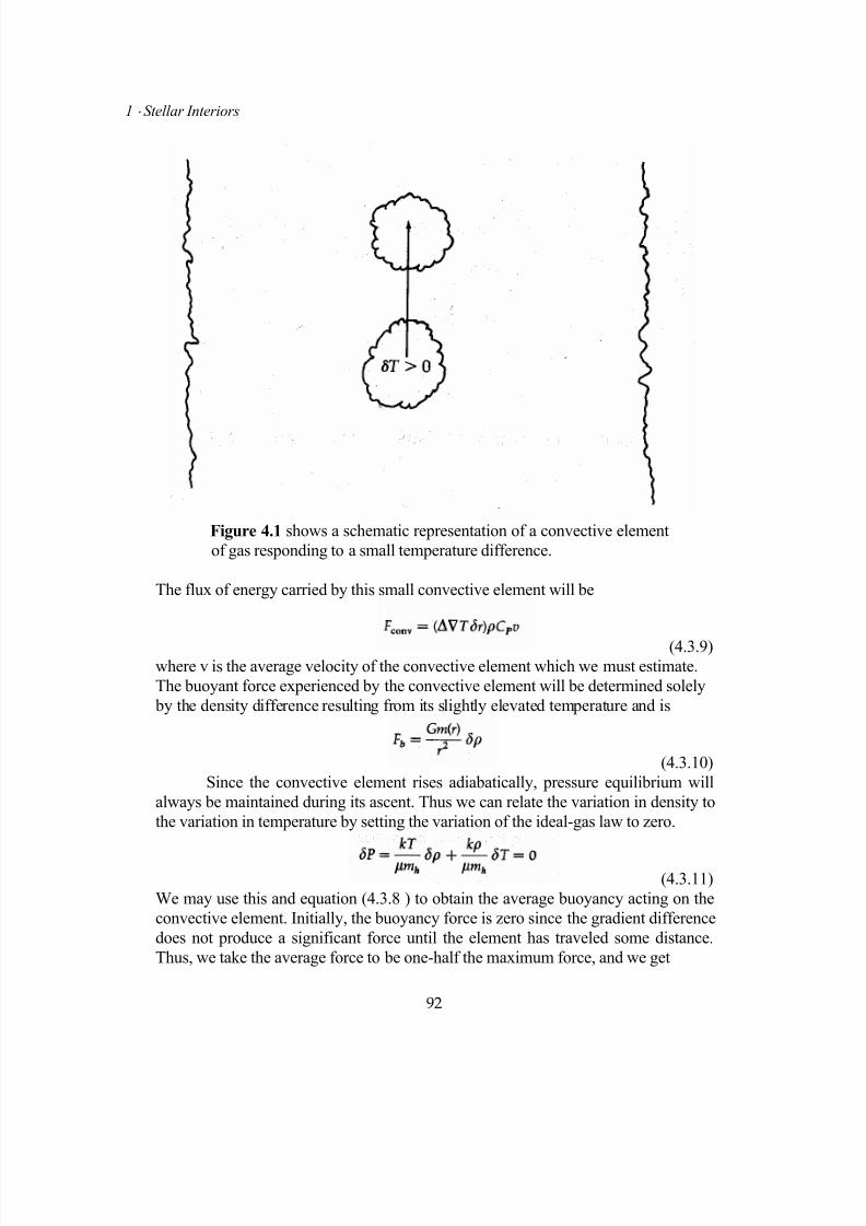
7/18/2019 The Fundamentals of Stellar Astrophysics - Collins G. W.
http://slidepdf.com/reader/full/the-fundamentals-of-stellar-astrophysics-collins-g-w 112/524
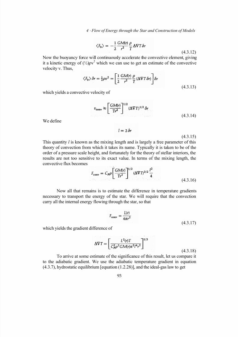
7/18/2019 The Fundamentals of Stellar Astrophysics - Collins G. W.
http://slidepdf.com/reader/full/the-fundamentals-of-stellar-astrophysics-collins-g-w 113/524
4 ⋅ Flow of Energy through the Star and Construction of Models
(4.3.12)
Now the buoyancy force will continuously accelerate the convective element, givingit a kinetic energy of (½)ρv
2 which we can use to get an estimate of the convective
velocity v. Thus,
(4.3.13)
which yields a convective velocity of
(4.3.14)
We define
(4.3.15)
This quantity l is known as the mixing length and is largely a free parameter of this
theory of convection from which it takes its name. Typically it is taken to be of the
order of a pressure scale height, and fortunately for the theory of stellar interiors, the
results are not too sensitive to its exact value. In terms of the mixing length, the
convective flux becomes
(4.3.16)
Now all that remains is to estimate the difference in temperature gradients
necessary to transport the energy of the star. We will require that the convection
carry all the internal energy flowing through the star, so that
(4.3.17)
which yields the gradient difference of
(4.3.18)
To arrive at some estimate of the significance of this result, let us compare it
to the adiabatic gradient. We use the adiabatic temperature gradient in equation
(4.3.7), hydrostatic equilibrium [equation (1.2.28)], and the ideal-gas law to get
93
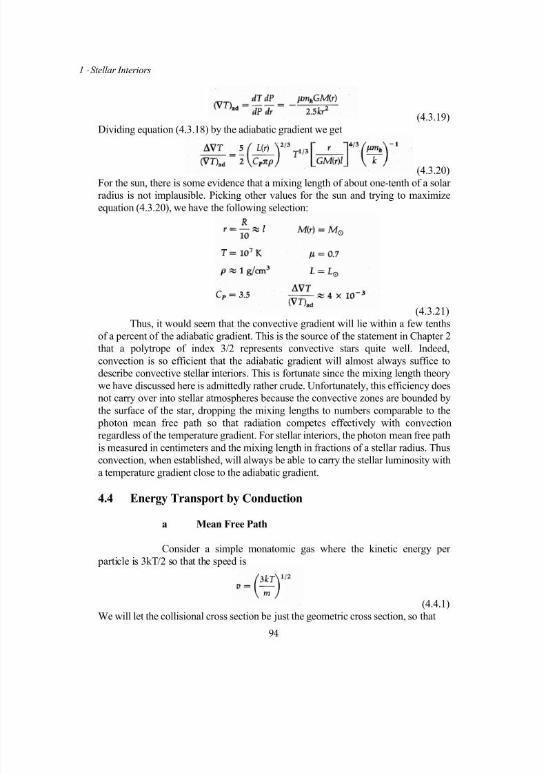
7/18/2019 The Fundamentals of Stellar Astrophysics - Collins G. W.
http://slidepdf.com/reader/full/the-fundamentals-of-stellar-astrophysics-collins-g-w 114/524
1 ⋅ Stellar Interiors
(4.3.19)
Dividing equation (4.3.18) by the adiabatic gradient we get
(4.3.20)
For the sun, there is some evidence that a mixing length of about one-tenth of a solar
radius is not implausible. Picking other values for the sun and trying to maximize
equation (4.3.20), we have the following selection:
(4.3.21)
Thus, it would seem that the convective gradient will lie within a few tenths
of a percent of the adiabatic gradient. This is the source of the statement in Chapter 2
that a polytrope of index 3/2 represents convective stars quite well. Indeed,
convection is so efficient that the adiabatic gradient will almost always suffice to
describe convective stellar interiors. This is fortunate since the mixing length theory
we have discussed here is admittedly rather crude. Unfortunately, this efficiency does
not carry over into stellar atmospheres because the convective zones are bounded by
the surface of the star, dropping the mixing lengths to numbers comparable to the photon mean free path so that radiation competes effectively with convection
regardless of the temperature gradient. For stellar interiors, the photon mean free path
is measured in centimeters and the mixing length in fractions of a stellar radius. Thus
convection, when established, will always be able to carry the stellar luminosity with
a temperature gradient close to the adiabatic gradient.
4.4 Energy Transport by Conduction
a Mean Free Path
Consider a simple monatomic gas where the kinetic energy per
particle is 3kT/2 so that the speed is
(4.4.1)
We will let the collisional cross section be just the geometric cross section, so that
94
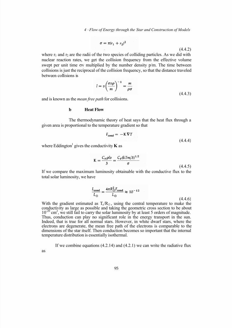
7/18/2019 The Fundamentals of Stellar Astrophysics - Collins G. W.
http://slidepdf.com/reader/full/the-fundamentals-of-stellar-astrophysics-collins-g-w 115/524
4 ⋅ Flow of Energy through the Star and Construction of Models
(4.4.2)
where r 1 and r 2 are the radii of the two species of colliding particles. As we did with
nuclear reaction rates, we get the collision frequency from the effective volume
swept per unit time σv multiplied by the number density p/m. The time between
collisions is just the reciprocal of the collision frequency, so that the distance traveled
between collisions is
(4.4.3)
and is known as the mean free path for collisions.
b Heat Flow
The thermodynamic theory of heat says that the heat flux through a
given area is proportional to the temperature gradient so that
(4.4.4)
where Eddington1 gives the conductivity K as
(4.4.5)
If we compare the maximum luminosity obtainable with the conductive flux to thetotal solar luminosity, we have
(4.4.6)With the gradient estimated as Tc/R ⊙ , using the central temperature to make theconductivity as large as possible and taking the geometric cross section to be about10
-20 cm
2, we still fail to carry the solar luminosity by at least 5 orders of magnitude.
Thus, conduction can play no significant role in the energy transport in the sun.Indeed, that is true for all normal stars. However, in white dwarf stars, where theelectrons are degenerate, the mean free path of the electrons is comparable to the
dimensions of the star itself. Then conduction becomes so important that the internaltemperature distribution is essentially isothermal.
If we combine equations (4.2.14) and (4.2.1) we can write the radiative flux
as
95
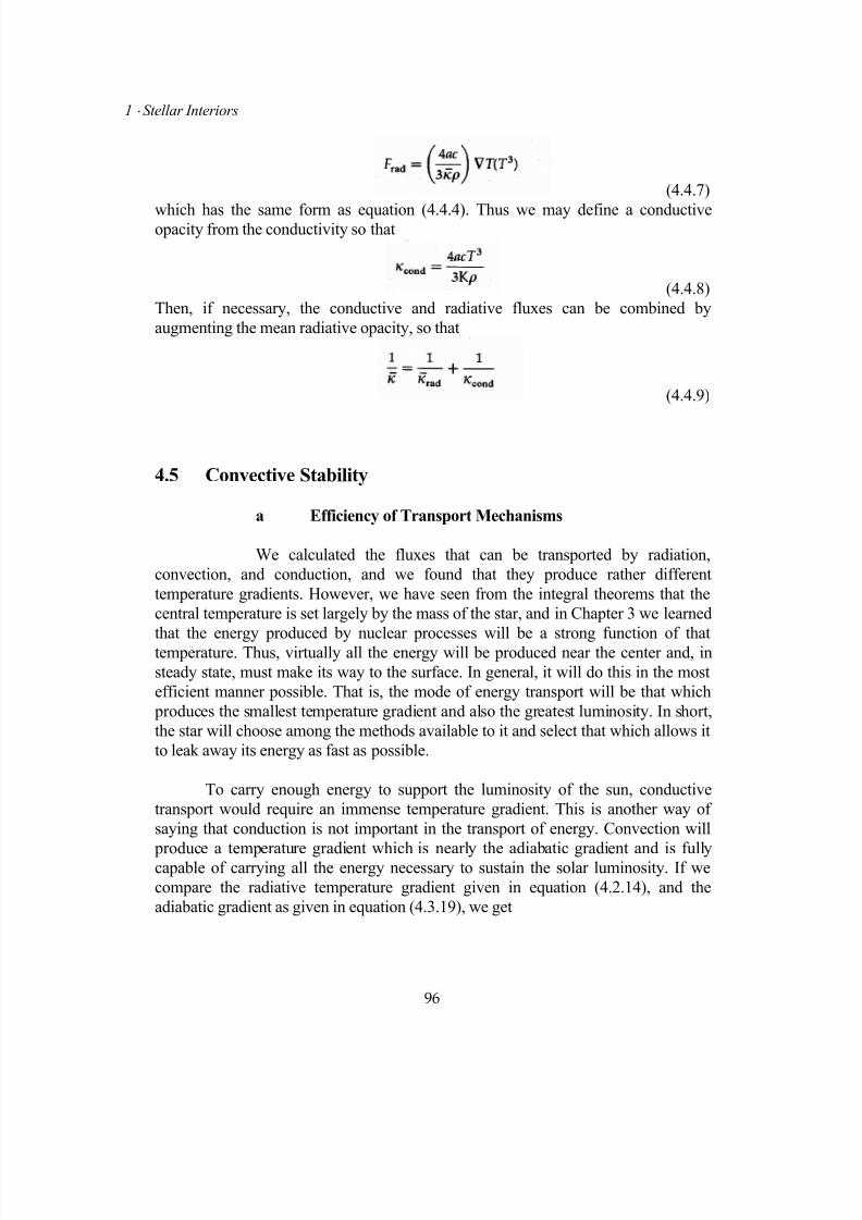
7/18/2019 The Fundamentals of Stellar Astrophysics - Collins G. W.
http://slidepdf.com/reader/full/the-fundamentals-of-stellar-astrophysics-collins-g-w 116/524
1 ⋅ Stellar Interiors
(4.4.7)
which has the same form as equation (4.4.4). Thus we may define a conductiveopacity from the conductivity so that
(4.4.8)
Then, if necessary, the conductive and radiative fluxes can be combined by
augmenting the mean radiative opacity, so that
(4.4.9)
4.5 Convective Stability
a Efficiency of Transport Mechanisms
We calculated the fluxes that can be transported by radiation,
convection, and conduction, and we found that they produce rather different
temperature gradients. However, we have seen from the integral theorems that the
central temperature is set largely by the mass of the star, and in Chapter 3 we learned
that the energy produced by nuclear processes will be a strong function of thattemperature. Thus, virtually all the energy will be produced near the center and, in
steady state, must make its way to the surface. In general, it will do this in the most
efficient manner possible. That is, the mode of energy transport will be that which
produces the smallest temperature gradient and also the greatest luminosity. In short,
the star will choose among the methods available to it and select that which allows it
to leak away its energy as fast as possible.
To carry enough energy to support the luminosity of the sun, conductive
transport would require an immense temperature gradient. This is another way of
saying that conduction is not important in the transport of energy. Convection will
produce a temperature gradient which is nearly the adiabatic gradient and is fullycapable of carrying all the energy necessary to sustain the solar luminosity. If we
compare the radiative temperature gradient given in equation (4.2.14), and the
adiabatic gradient as given in equation (4.3.19), we get
96
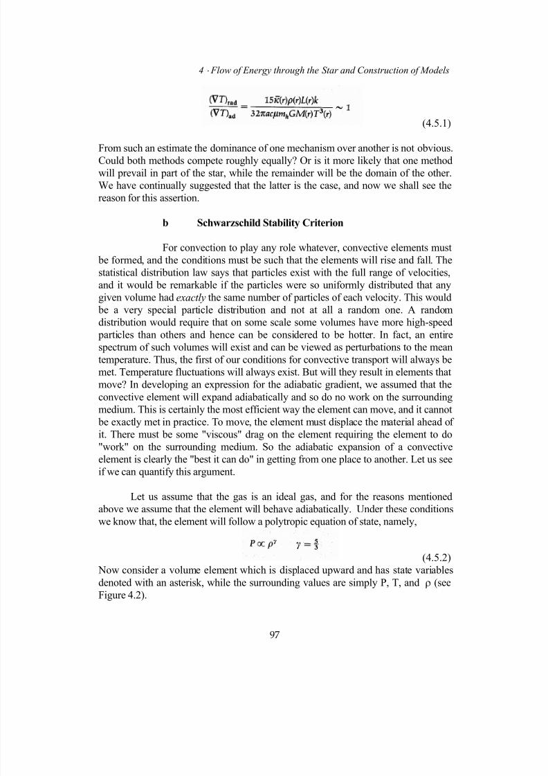
7/18/2019 The Fundamentals of Stellar Astrophysics - Collins G. W.
http://slidepdf.com/reader/full/the-fundamentals-of-stellar-astrophysics-collins-g-w 117/524
4 ⋅ Flow of Energy through the Star and Construction of Models
(4.5.1)
From such an estimate the dominance of one mechanism over another is not obvious.
Could both methods compete roughly equally? Or is it more likely that one method
will prevail in part of the star, while the remainder will be the domain of the other.
We have continually suggested that the latter is the case, and now we shall see the
reason for this assertion.
b Schwarzschild Stability Criterion
For convection to play any role whatever, convective elements must
be formed, and the conditions must be such that the elements will rise and fall. The
statistical distribution law says that particles exist with the full range of velocities,and it would be remarkable if the particles were so uniformly distributed that any
given volume had exactly the same number of particles of each velocity. This would
be a very special particle distribution and not at all a random one. A random
distribution would require that on some scale some volumes have more high-speed
particles than others and hence can be considered to be hotter. In fact, an entire
spectrum of such volumes will exist and can be viewed as perturbations to the mean
temperature. Thus, the first of our conditions for convective transport will always be
met. Temperature fluctuations will always exist. But will they result in elements that
move? In developing an expression for the adiabatic gradient, we assumed that the
convective element will expand adiabatically and so do no work on the surrounding
medium. This is certainly the most efficient way the element can move, and it cannot be exactly met in practice. To move, the element must displace the material ahead of
it. There must be some "viscous" drag on the element requiring the element to do
"work" on the surrounding medium. So the adiabatic expansion of a convective
element is clearly the "best it can do" in getting from one place to another. Let us see
if we can quantify this argument.
Let us assume that the gas is an ideal gas, and for the reasons mentioned
above we assume that the element will behave adiabatically. Under these conditions
we know that, the element will follow a polytropic equation of state, namely,
(4.5.2)
Now consider a volume element which is displaced upward and has state variables
denoted with an asterisk, while the surrounding values are simply P, T, and ρ (see
Figure 4.2).
97
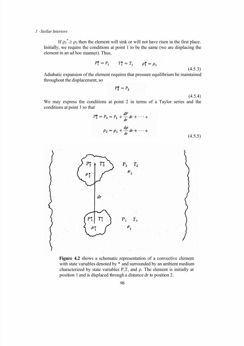
7/18/2019 The Fundamentals of Stellar Astrophysics - Collins G. W.
http://slidepdf.com/reader/full/the-fundamentals-of-stellar-astrophysics-collins-g-w 118/524
1 ⋅ Stellar Interiors
If ρ2* ≥ ρ2 then the element will sink or will not have risen in the first place.
Initially, we require the conditions at point 1 to be the same (we are displacing the
element in an ad hoc manner). Thus,
(4.5.3)
Adiabatic expansion of the element requires that pressure equilibrium be maintained
throughout the displacement, so
(4.5.4)
We may express the conditions at point 2 in terms of a Taylor series and the
conditions at point 1 so that
(4.5.5)
Figure 4.2 shows a schematic representation of a convective element
with state variables denoted by * and surrounded by an ambient medium
characterized by state variables P,T, and ρ. The element is initially at
position 1 and is displaced through a distance dr to position 2.
98

7/18/2019 The Fundamentals of Stellar Astrophysics - Collins G. W.
http://slidepdf.com/reader/full/the-fundamentals-of-stellar-astrophysics-collins-g-w 119/524
4 ⋅ Flow of Energy through the Star and Construction of Models
Using the equation of state, we may write
(4.5.6)
If we take ρ2* ≥ ρ2 to be a condition for stability (i.e., the element will return to its
initial position if displaced), then equations (4.5.5), and (4.5.6) require that
(4.5.7)
The ideal-gas law requires that
(4.5.8)
which can be used to replace the density gradient in inequality (4.5.7) to get
(4.5.9)
Dividing by dT/dr, we obtain the Schwarzschild stability criterion for a polytropic
gas
(4.5.10)
which for a monatomic gas with a γ = 5/3 is just
(4.5.11)
Thus, if the logarithmic derivative of pressure with respect to temperature is
greater than or equal to 2.5, convection will not occur. In other words, if the actual
temperature gradient is less than the adiabatic gradient, convection will not occur.
This, then, is our means for deciding whether convection or radiation will be the
99

7/18/2019 The Fundamentals of Stellar Astrophysics - Collins G. W.
http://slidepdf.com/reader/full/the-fundamentals-of-stellar-astrophysics-collins-g-w 120/524
1 ⋅ Stellar Interiors
dominant mode of energy transport. Should radiation be able to transport the energy
with a temperature gradient less than the adiabatic gradient, no energy will be carried
by convection, for the gas is stable against the thermal perturbations which must
exist. However, if this is not the case, convection will be established; and it is so veryefficient that it is capable of carrying all the energy with a temperature gradient that
is just slightly super-adiabatic. For most of stellar structure, we may regard energy
transport as being bimodal; either radiation or convection will transport the energy,
with the decision being made by equation (4.5.10). The Schwarzschild stability
criterion has been shown to be quite general and will hold under the most varied of
conditions, including those stars where general relativity must be included to
describe their structure.
4.6 Equations of Stellar Structure
Having settled the mode of energy transport, we are in a position to describe thestructure of a star in a steady-state condition. This is a good time to review briefly
what we have done. The equations of stellar structure arise from conservation laws
and relationships developed from the local microphysics. In Chapter 1, we posed the
basic problem of stellar interiors to be the description of the variation of state
variables P, T, and γ with position in the star. For spherical stars, this amounts to
indicating their dependence on the radial coordinate r. In developing that description,
we introduced additional variables and their relation to the state variables so that by
now our list of parameters has grown to nine members, P(r), T(r), p(r), M(r), L(r),
ε(r), κ (r), γ(r),and µ(r). To specify these parameters, we have at our disposal three
conservation laws and a transport equation in addition to three functional
relationships derived from the microphysics. The function γ(r) can also be specified by microphysics and is usually given by its adiabatic value. Only the variation ofµ(r)
needs to be specified ab initio. When we move to the stage of evolving the stellar
models, the chemical composition will need to be specified for the initial model since
the processes of nuclear energy generation will tell us how the composition changes
with time. However, we must, at least initially, specify both the composition of the
star and how it varies throughout the entire star. The use of a convective theory of
transport which attempts to improve on the adiabatic gradient will also introduce
another parameter, known as the mixing length, which must also be specified ab
initio.
The constraints posed by the conservation laws take the form of differentialequations whose solution is subject to a set of boundary conditions. Below is a
summary of these differential equations and their origin:
100
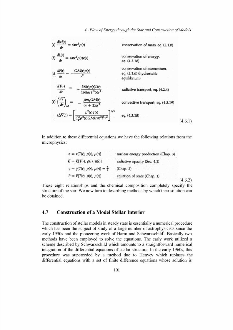
7/18/2019 The Fundamentals of Stellar Astrophysics - Collins G. W.
http://slidepdf.com/reader/full/the-fundamentals-of-stellar-astrophysics-collins-g-w 121/524
4 ⋅ Flow of Energy through the Star and Construction of Models
(4.6.1)
In addition to these differential equations we have the following relations from the
microphysics:
(4.6.2)
These eight relationships and the chemical composition completely specify the
structure of the star. We now turn to describing methods by which their solution can
be obtained.
4.7 Construction of a Model Stellar Interior
The construction of stellar models in steady state is essentially a numerical procedure
which has been the subject of study of a large number of astrophysicists since the
early 1950s and the pioneering work of Harm and Schwarzschild2. Basically two
methods have been employed to solve the equations. The early work utilized a
scheme described by Schwarzschild which amounts to a straightforward numerical
integration of the differential equations of stellar structure. In the early 1960s, this
procedure was superceded by a method due to Henyey which replaces the
differential equations with a set of finite difference equations whose solution is
101

7/18/2019 The Fundamentals of Stellar Astrophysics - Collins G. W.
http://slidepdf.com/reader/full/the-fundamentals-of-stellar-astrophysics-collins-g-w 122/524
1 ⋅ Stellar Interiors
carried out globally and enables one to include time-dependent phenomena in a
natural way. However, since this method requires an initial solution which is usually
obtained by the Schwarzschild procedure, we describe both methods.
a Boundary Conditions
Using the functional relations given by equations (4.6.2), we may
reduce the problem of solving the structure equations to one of finding solutions for
the four differential equations given in equations (4.6.1). These constitute a set of
four nonlinear first-order differential equations in four unknowns. In general, such a
system will have four constants of integration which must be specified to guarantee a
solution. In principle, two of these constants are specified by requiring that the model
be physically reasonable. These are
(4.7.1)
At the other end of the range of the independent variable,
(4.7.2)
However, five constants are specified by equations (4.7.1), and (4.7.2), if R *
is included as a parameter. Only four of these can be linearly independent. Thus, if
one specifies M* and R *, the solution will specify L*. Another aspect of the problemis that the constants are not all specified at the same boundary, and so it is not
possible to treat the problem as an initial-value problem and to solve by
straightforward numerical integration. Such problems are known as two-point
boundary-value problems, and one must essentially guess the missing integration
constants at one boundary, obtain the numerical solution complete to the other
boundary, and adjust the guesses until the specified integration constants at the far
boundary are obtained. A further problem arises from the fact that the equations of
hydrostatic equilibrium and energy transport are numerically unstable as r → 0
because the derivatives require the calculation of "0/0" at the origin. However, the
problem can be recast as a double-eigenvalue problem with the fitting (solution
adjustment) taking place in the interior but away from the boundary. This isessentially the Schwarzschild approach.
b Schwarzschild Variables and Method
When one is searching for the numerical solution to a physical
problem, it is convenient to re-express the problem in terms of a set of dimensionless
102
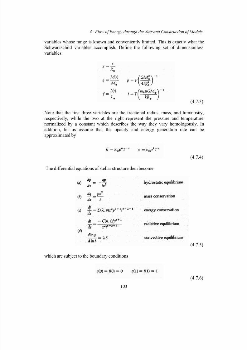
7/18/2019 The Fundamentals of Stellar Astrophysics - Collins G. W.
http://slidepdf.com/reader/full/the-fundamentals-of-stellar-astrophysics-collins-g-w 123/524
4 ⋅ Flow of Energy through the Star and Construction of Models
variables whose range is known and conveniently limited. This is exactly what the
Schwarzschild variables accomplish. Define the following set of dimensionless
variables:
(4.7.3)
Note that the first three variables are the fractional radius, mass, and luminosity,
respectively, while the two at the right represent the pressure and temperature
normalized by a constant which describes the way they vary homologously. Inaddition, let us assume that the opacity and energy generation rate can be
approximated by
(4.7.4)
The differential equations of stellar structure then become
(4.7.5)
which are subject to the boundary conditions
(4.7.6)
103

7/18/2019 The Fundamentals of Stellar Astrophysics - Collins G. W.
http://slidepdf.com/reader/full/the-fundamentals-of-stellar-astrophysics-collins-g-w 124/524
1 ⋅ Stellar Interiors
The parameters C(n,s) and D(λ,ν) are the eigenvalues of the problem, and
these values specify the type of star being considered. In physical variables they are
(4.7.7)
Note that the ideal-gas law has been used to eliminate the density from the
problem, and this may cause some problems with the solution at the surface where
the pressure and temperature essentially go to zero, in addition to the numerical
problems at the center when x → 0. However, Schwarzschild shows that near the
surface one may approximate the dimensionless pressure p and dimensionlesstemperature t by
(4.7.8)
If the star has a convective core, then all the energy is produced in a region
where the structure is essentially specified by the adiabatic gradient and so the
energy conservation equation [equation (4.7.5c)] is redundant. This means that the
eigenvalue D(λ,ν) is unspecified and the problem will be solved by determining
C(n,s) alone. Such a model is known as a Cowling model . The additional constraints
on the solution are specified by the mass and size of the convective core (qc and xc).
These are determined by the value of x for which d(ln p)/d(ln t) < 2.5, and the star
becomes subject to the radiative temperature gradient. The stellar luminosity is then
L = Lc and for the envelope f = 1. While such a scheme works well for models with
convective cores, numerical problems will generally occur at the center should it be
in radiative equilibrium and the solution obtained numerically. However, a slightly
different set of dimensionless variables can be defined where the pressure and
temperature are scaled by their values at the center of the star. The differentialequations of stellar structure become stable at r = 0 since the dimensionless pressure
and temperature are both unity at the center by definition. One then, integrates
outward from the center with Pc and Tc as eigenvalues. The stellar mass, luminosity,
and radius can be related to these new eigenvalues. That there are two distinct
eigenvalues is demonstrated by the surface boundary condition that both the surface
pressure and surface temperature must vanish at the same value of x.
104

7/18/2019 The Fundamentals of Stellar Astrophysics - Collins G. W.
http://slidepdf.com/reader/full/the-fundamentals-of-stellar-astrophysics-collins-g-w 125/524
4 ⋅ Flow of Energy through the Star and Construction of Models
Unfortunately the equations of stellar structure become numerically unstable near the
surface for the same reasons that required the approximation of the solutions of
equations (4.7.5) by equation (4.7.8). Although the errors in the model can be made
small with the aid of modern computers, it is bad practice to numerically solve
equations which are inherently unstable. For that reason, the usual procedure is to
integrate from both the outside and the inside and to make the fit at the boundary
between the core and envelope. The approximations near the surface are still present,
but their effect on the solution is minimized. In actual practice, the fitting can be
accomplished in the U-V plane where the solutions are homologously invariant. The
fitting procedure is similar to that described in Chapter 2.
Since Schwarzschild introduced this method of solution of the equations of
stellar structure in the 1950s, many variants have been used by numerous
investigators. In one form or another, all variants suffer from problems similar to
those that plague the Schwarzschild procedure. In general, this approach to thenumerical solution of two-point nonlinear boundary-value problems always suffers
from the propagation of errors from one boundary to the other. The most serious of
these errors are usually the truncation errors associated with the numerical
integration scheme which tend to be systematic. However, this approach enabled the
generation of stellar models which represented the steady-state aspect of stars for the
first time. Although qualitative information about stellar evolution can be gained
from polytropes (and we do so in Chapter 5), specific and detailed descriptions of
stellar evolution require the generation of steady-state models. However, some
aspects of stellar evolution happen on time scales which are very short compared to
the thermal time scale, and in some instances short compared to the dynamical time
scale. Often, substantive changes occur to the internal structure which produces onlysmall changes at the surface. Thus, minor changes in the surface boundary conditions
can reflect monumental changes in the internal structure of the star. In addition, we
must include the time-dependent terms in the equations describing the conservation
of momentum and energy. Specifically, if some of the generated energy does work
on the star, causing it to expand as energy is liberated by contraction, then this
energy must be included in the energy conservation equation relating the stellar
luminosity to the sources of energy. This is usually accomplished by keeping track of
the time rate of change of the entropy. The direct integration scheme does not
readily lend itself to the inclusion of such terms. Such models are no longer merely
steady-state models, and we will require more sophisticated tools to deal with them.
c Henyey Relaxation Method for Construction of Stellar Models
To overcome some of the numerical instability problems described in
the previous section, Louis Henyey et al3. developed a superior numerical scheme in
the early 1960s. This method is the foundation for all modern stellar-model
calculations. His approach was to transform the problem to a set of variables in
105
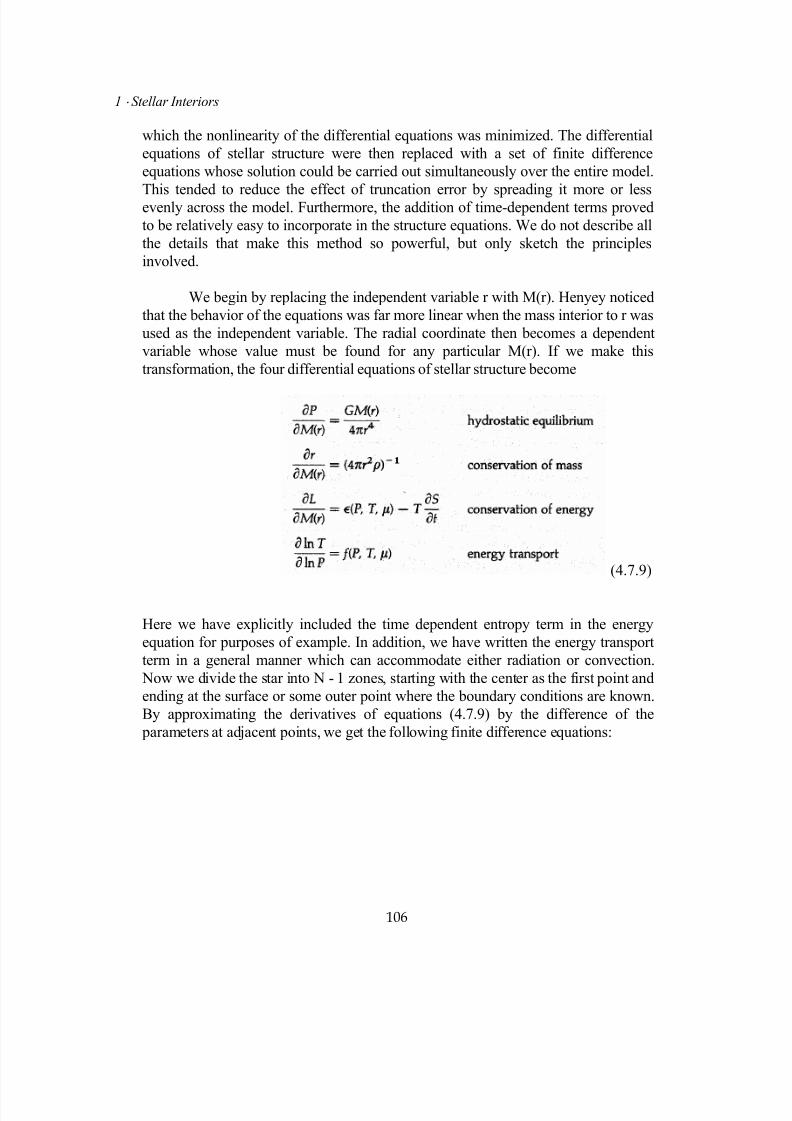
7/18/2019 The Fundamentals of Stellar Astrophysics - Collins G. W.
http://slidepdf.com/reader/full/the-fundamentals-of-stellar-astrophysics-collins-g-w 126/524
1 ⋅ Stellar Interiors
which the nonlinearity of the differential equations was minimized. The differential
equations of stellar structure were then replaced with a set of finite difference
equations whose solution could be carried out simultaneously over the entire model.
This tended to reduce the effect of truncation error by spreading it more or lessevenly across the model. Furthermore, the addition of time-dependent terms proved
to be relatively easy to incorporate in the structure equations. We do not describe all
the details that make this method so powerful, but only sketch the principles
involved.
We begin by replacing the independent variable r with M(r). Henyey noticed
that the behavior of the equations was far more linear when the mass interior to r was
used as the independent variable. The radial coordinate then becomes a dependent
variable whose value must be found for any particular M(r). If we make this
transformation, the four differential equations of stellar structure become
(4.7.9)
Here we have explicitly included the time dependent entropy term in the energy
equation for purposes of example. In addition, we have written the energy transport
term in a general manner which can accommodate either radiation or convection.
Now we divide the star into N - 1 zones, starting with the center as the first point and
ending at the surface or some outer point where the boundary conditions are known.
By approximating the derivatives of equations (4.7.9) by the difference of the
parameters at adjacent points, we get the following finite difference equations:
106

7/18/2019 The Fundamentals of Stellar Astrophysics - Collins G. W.
http://slidepdf.com/reader/full/the-fundamentals-of-stellar-astrophysics-collins-g-w 127/524
4 ⋅ Flow of Energy through the Star and Construction of Models
)M,T,P(f P
T
PP
TT
t
ST
MM
LL
P)r 4(MMr r
r 4
GM
MM
PP
21i
21i
21i
21i
21i
i1i
i1i
21i
21i
21i
i1i
i1i
1
21i
12
21i
i1i
i1i
4
21i
21i
i1i
i1i
+++
+
+
+
+
+
+++
+
−
+
−
++
+
+
+
+
+
=−
−
∂
∂−ε=
−
−
π=−−
π=
−
−
(4.7.10)
The subscript i + ½ is used exclusively on the right-hand side of equations
(4.7.10) to indicate that the value to be used is intermediate between the values at iand i + 1. It will turn out that we must have an initial guess of the model's structure in
order to solve the finite difference equations. It is this guess which may supply the
initial information for evaluating the parameters at the points i + ½. Since the mass
points Mi represent the independent variable of this problem, the four equations
given in equations (4.7.10) contain eight unknowns. However, we have N - 1
systems of such equations with considerable overlap in unknowns among them. The
situation at the outer zone will be handled somewhat differently since there is no N +
1 point. Thus if we count the total number of equations we have 4N - 4. But at each
point there are only four unknowns, making the total number of unknowns of 4N.
The remaining four constraints are essentially the boundary conditions of the
problem. By analogy to the Schwarzschild problem, let us take the central boundaryconditions to be r 1 = L1 = 0, which removes two of the additional unknowns. Now if
we choose two of the remaining unknowns at the surface, such as r N and L N, the
problem is completely specified. Indeed, if we choose the surface pressure to be zero,
then choosing a star of a particular mass and radius (and distribution of chemical
composition) will specify the stellar configuration. One of the motivating notions
that led Henyey to this type of technique was the ability to match a stellar interior to
a model of the stellar atmosphere. This technique is ideally suited to do this. One
simply takes as the outer zone that point where the physical parameters are known as
the result of a separate study. In the second part of this book, we present a theory of
stellar atmospheres which provides far more accurate surface boundary conditions
than those of early investigators. In addition to improving the manner in which thesurface boundary conditions are handled, it may be advisable to ignore the point at
the center. A Taylor series expansion can be used to express the values of P2, T2, L2,
and r 2 in terms of the central temperature Tc and Pc. Because the system of equations
is strongly diagonal, the solution is easier to come by if the central boundary
conditions are expressed in this manner.
107

7/18/2019 The Fundamentals of Stellar Astrophysics - Collins G. W.
http://slidepdf.com/reader/full/the-fundamentals-of-stellar-astrophysics-collins-g-w 128/524
1 ⋅ Stellar Interiors
The Henyey approach shown in equations (4.7.10) represents the derivative
of the structure equations by first-order finite differences. Thus the errors of the
approximation are second order in those derivatives. This necessitates the use of the
large number of zones to accurately represent the model, and it is this large numberof zones that represents the primary computational burden in the construction of the
model. Although increasing the order of the finite difference equations would
improve the stability, it would also increase the density (i.e., the number of terms) of
the resulting linear algebraic equations, slowing their solution and decreasing their
stability. Budge4 has shown that an improvement in the accuracy of the
approximation can be achieved by using a Runge-Kutta fourth-order approximation
for the derivatives without increasing the resulting linear equation density. Although
there is some increase in the computational burden for obtaining the coefficients, this
is more than offset by being able to reduce the number of zones in the model.
We still must solve these linear equations. It is not uncommon in the standardHenyey scheme to choose up to 500 zones in the star, which will yield some 2000
nonlinear equations in as many unknowns. Now it is clear why we need an initial
solution. If we have a solution which is close to the correct one, we may express the
correct solution in terms of the initial solution and a small linear correction to that
solution. This will reduce the system of nonlinear equations to a linear system where
the corrections are the unknowns. Such a scheme is known as a Newton-Raphson
iteration scheme. Since the system is sparse (each equation contains only 8 of the
2000 unknowns) and the independent variable was chosen so as to make the
equations somewhat linear, the iteration scheme is usually stable. However, the
stability also depends on the quality of the initial solution. This is normally obtained
by means of a Schwarzschild-type integration or a previously determined model.
It is clear that the Henyey method lends itself naturally to the problem of
stellar evolution. In this case the initial model is a model calculated for an earlier
time. Thus the procedure would be to start at some initial time with a Schwarzschild
model, allow a small interval of time for the model to pass by, calculate the changes
in the chemical composition resulting from nuclear processes, and modify the model
accordingly. This serves as the initial first guess for the Henyey scheme, and a new
model is produced. The effects of time are again allowed for, and the next Henyey
model is constructed, etc. In this way an entire sequence of stellar models
representing the life history of the star can be constructed. One generally starts the
sequence when the star is well represented by a steady-state model, and theSchwarzschild solution gives an accurate description of the stellar structure. Such a
time is the arrival on the main sequence and the accompanying onset of hydrogen
burning. The resulting life history of the star is as good as the microphysics which
goes into the solution and the quality of the computer and the associated numerical
techniques used to obtain the solution.
108
7/18/2019 The Fundamentals of Stellar Astrophysics - Collins G. W.
http://slidepdf.com/reader/full/the-fundamentals-of-stellar-astrophysics-collins-g-w 129/524
4 ⋅ Flow of Energy through the Star and Construction of Models
At this point, we have covered the fundamentals required to construct a
model of the interior of a star. However, we should not leave the impression that
such a model would reflect the accuracy of contemporary stellar interior models.
There are many complications and refinements which should be treated and included
to produce a model with modern sophistication. We have said nothing about the
small departures of the equation of state from the ideal-gas law which occur at quite
modest densities due to electron screening. Nor have we dealt with many of the
vagaries of the theory of convection, such as semi-convection, convective overshoot,
or mixing-length determination. These result largely from the primitive nature of the
existing theory of convection, and while they do pose significant problems at certain
points in a star's evolution, they do not affect the conceptual picture of stellar
structure. It seems almost criminal not to devote more attention to the efforts of those
who have labored to provide improved opacities and nuclear energy generation rates.
But again, while these improve the details of the models and enhance our confidence
in the predictions based on them, they do not conceptually change the basic physicsupon which the models rest. While we have outlined the numerical procedures
necessary to actually solve the structure equations, there is much cleverness and
imaginative numerical analysis required to translate what we outlined to a computer
program which will execute to completion in an acceptable time. Do not forget that
the early models of Schwarzschild and Harm were calculated basically by hand,
aided only by a desk calculator whose capabilities are far exceeded by even the
cheapest pocket calculator of the present. It is no accident that the rapid advance of
our knowledge of stellar structure parallels the explosive advance in our ability to
carry out numerical calculations.
An understanding of the refinements of contemporary models is essential forany who would choose to do meaningful research in stellar interiors. It is not
essential for those who would understand the results and their physical motivation,
and it is to those people that this book is addressed. With the knowledge of the
physical processes that determine the structure of stars, let us now turn to the
crowning achievement of the study of stellar structure - the theory of stellar
evolution.
Problems
1. Assume that there is a star in which the energy is generated uniformly
throughout the star (that is, ε = constant). In addition, the opacity is constant(i.e., electron scattering). Further assume that the star is in radiative and
hydrostatic equilibrium. Show that 1-β is constant throughout the star and
that it is a polytrope of index n = 3.
109
7/18/2019 The Fundamentals of Stellar Astrophysics - Collins G. W.
http://slidepdf.com/reader/full/the-fundamentals-of-stellar-astrophysics-collins-g-w 130/524
1 ⋅ Stellar Interiors
2. Suppose that in a star, the only source of energy generation is radioactive
decay, so the energy production per unit mass is constant and independent of
density and temperature. Further suppose that the opacity is given by
Kramer’s' law. Show that the structure of the star is described by a polytrope,and find the value of the polytropic index n.
3. Compare the local value of the radiative gradient with the adiabatic gradient
throughout the sun. Describe the regions of radiative and convective
equilibrium in light of your results. What would you expect to be the effect
on the radiative and convective zones of replacing 50 percent of the solar
luminosity with an energy generation source which was more efficient?
4. For a sphere in radiative equilibrium and STE, show that the radiation
pressure is one third the energy density.
5. Since the convective temperature gradient differs systematically from the
adiabatic gradient, it is possible that the cumulative effect is significant when
it is integrated over the entire convective zone. Examine this effect in the sun
and decide whether it is significant.
6. Use a stellar interiors code or existing models to find the variation of the
fractional ionization of hydrogen and helium with depth in the sun.
7. Use a stellar interiors code, or existing models to find the fraction by mass
and radius within which (a) 20 percent, (b) 50 percent, (c) 90 percent, and
(d) 99 percent of the sun's energy is generated.8. Repeat Problem 7 for a star of 10M⊙ .
9. Repeat problem 7 but with Z = 10-8.
10. Determine the relative importance of bound-bound transitions, bound-free
transitions, and electron scattering as opacity sources in the sun.
References and Supplemental Reading
1. Eddington, A.S.: The Internal Constitution of the Stars, Dover, New York,1959, p.276.
2. Harm, R., and Schwarzschild, M.: Numerical Integrations for the Stellar
Interior , Ap.J. Supp. No. 1., 1955, pp. 319-430.
110

7/18/2019 The Fundamentals of Stellar Astrophysics - Collins G. W.
http://slidepdf.com/reader/full/the-fundamentals-of-stellar-astrophysics-collins-g-w 131/524
4 ⋅ Flow of Energy through the Star and Construction of Models
111
3. Henyey, L.G., Wilets, L., Bohm, K.H., Lelevier, R., and Levee, R.D.:
A Method for Automatic Computation of Stellar Evolution, Ap. J. 129, 1959,
pp.628-636.
4. Budge, K.G.: An Improved Method for Calculating Stellar Models, Ap.J.
312, 1987, pp.217-218.
In addition to a very clear exposition of convection and the mixing-length theory, the
clearest description of Schwarzschild variables and the Schwarzschild
integration scheme can be found in
Schwarzschild, M.: Structure and Evolution of the Stars, Princeton
University Press, Princeton N.J., 1958, chap. 3, p. 96.
An exceptionally clear description of the Henyey method of integration of the
equations of stellar structure is given by
Kippenhahn, R., Weigert, A., and Hofmeister, E.: "Methods for Calculating
Stellar Evolution", Methods in Computational Physics, vol. 7 (Eds.: B. Adler,
S. Fernbach, and M. Rotenberg), Academic, New York, 1967, p. 129 - 190.

7/18/2019 The Fundamentals of Stellar Astrophysics - Collins G. W.
http://slidepdf.com/reader/full/the-fundamentals-of-stellar-astrophysics-collins-g-w 132/524
1 ⋅ Stellar Interiors
Copyright (2003) George W. Collins, II
5
Theory of Stellar Evolution
. . .
One of the great triumphs of the twentieth century has been the
detailed description of the life history of a star. We now understand with someconfidence more than 90 percent of that life history. Problems still exist for the very
early phases and the terminal phases of a star's life. These phases are very short, and
the problems arise as much from the lack of observational data as from the
difficulties encountered in the theoretical description. Nevertheless, continual
progress is being made, and it would not be surprising if even these remaining
problems are solved by the end of the century.
112

7/18/2019 The Fundamentals of Stellar Astrophysics - Collins G. W.
http://slidepdf.com/reader/full/the-fundamentals-of-stellar-astrophysics-collins-g-w 133/524
5 ⋅ Theory of Stellar Evolution
To avoid vagaries and descriptions which may later prove inaccurate, we
concentrate on what is known with some certainty. Thus, we assume that stars can
contract out of the interstellar medium, and generally we avoid most of the detailed
description of the final, fatal collapse of massive stars. In addition, the fascinating
field of the evolution of close binary stars, where the evolution of one member of the
system influences the evolution of the other through mass exchange, will be left for
another time. The evolution of so-called normal stars is our central concern.
Although the details of the theory of stellar evolution are complex, it is
possible to gain some insight into the results expected of these calculations from
some simple considerations. We have developed all the formalisms for calculating
steady-state stellar models. However, those models could often be accurately
represented by an equilibrium model composed of a polytrope or combinations of
polytropes. We should then expect that the evolutionary history of a star could beapproximately represented by a series of polytropic models. What is needed is to find
the physical processes relating one of these models to another thereby generating a
sequence. Such a description is no replacement for model calculation for without the
details, important aspects of stellar evolution such as lifetimes remain hidden. In
addition, there are branching points in the life history of a star where the path taken
depends on results of model calculations so specific that no general considerations
will be able to anticipate them. However, a surprising amount of stellar evolution can
be understood in terms of sequences of equilibrium models connected by some rather
general notions concerning the efficiency of energy transfer. Descriptions of these
models, and their relationship to one another, form the outline upon which we can
hang the details of the model calculations.
In general, we trace the evolution of a star in terms of a model of that star's
changing position on the Hertzsprung-Russell diagram. With that in mind, let us
briefly review the range of parameters which define the internal structure of a star.
5.1 The Ranges of Stellar Masses, Radii, and Luminosity
113
In Section 2.2 b, we used the β* theorem to show that as the mass of a star increases,
the ratio of radiation pressure to total pressure also increases so that by the time onereaches about 100M⊙ approximately 80 percent of the pressure will be supplied bythe photons themselves. Although it is not obvious, at about this mass the outerlayers can no longer remain in stable equilibrium, and the star will begin to shed itsmass. Very few stars with masses above 100M⊙ are known to exist, and those thatdo show instabilities in their outer layers. At the other end of the mass scale, a massof about 0.1M⊙ is required to produce core temperatures and densities sufficient to provide a significant amount of energy from nuclear processes. Thus, we can take therange of stellar masses to span roughly 3 powers of 10 with the sun somewhat belowthe geometric mean.
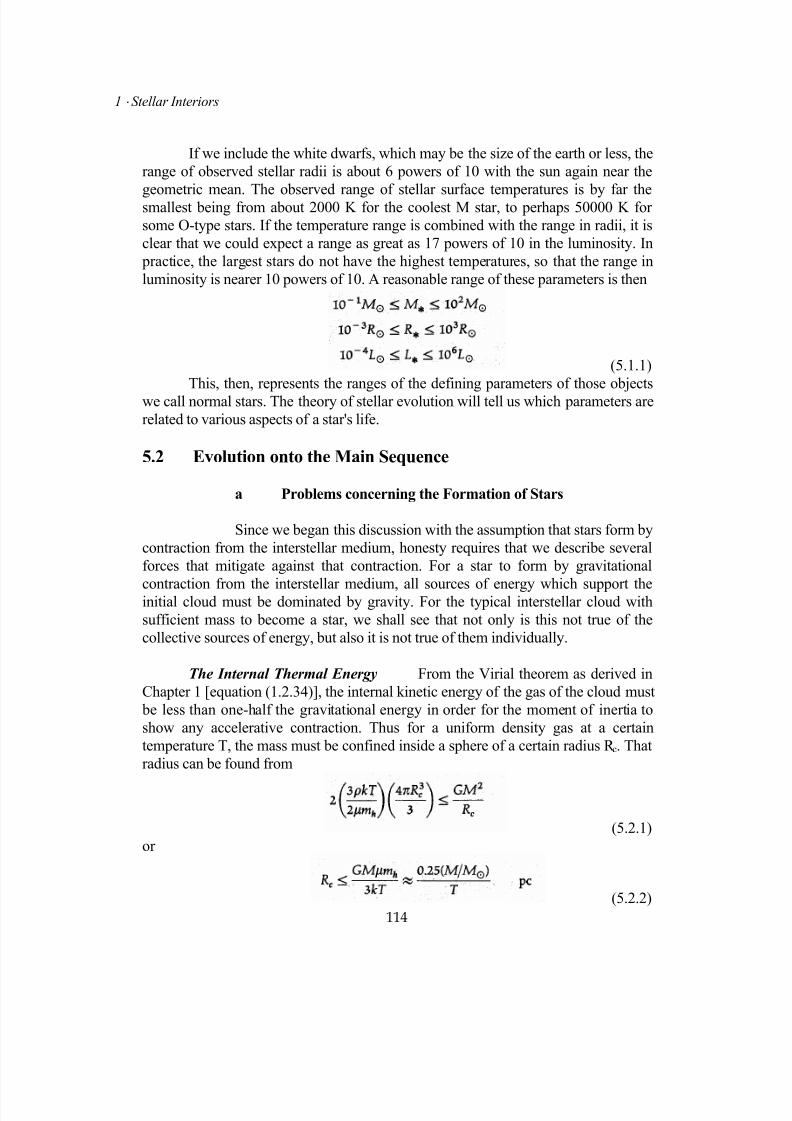
7/18/2019 The Fundamentals of Stellar Astrophysics - Collins G. W.
http://slidepdf.com/reader/full/the-fundamentals-of-stellar-astrophysics-collins-g-w 134/524
7/18/2019 The Fundamentals of Stellar Astrophysics - Collins G. W.
http://slidepdf.com/reader/full/the-fundamentals-of-stellar-astrophysics-collins-g-w 135/524
5 ⋅ Theory of Stellar Evolution
This distance is sometimes known as the Jeans length, for it is the distance below
which a gas cloud becomes gravitationally unstable to small fluctuations in density.
For a solar mass of material with a typical interstellar temperature of 50 K, the cloud
would have to be smaller than about 5×10⁻³
pc with a mean density of about 108
particles per cubic centimeter . This is many orders of magnitude greater than that
found in the typical interstellar cloud, so it would seem unlikely that such stars
should form.
The Rotational Energy The Virial theorem can also be used to determine
the effects of rotation on a collapsing cloud. Again, from Chapter 1, the rotational
kinetic energy must be less than one-half the gravitational potential energy in order
for the cloud to collapse. So
(5.2.3)
which for a sphere of uniform density and constant angular velocity gives
(5.2.4)
The differential rotation of the galaxy implies that there must be a shear or velocity
gradient which would impart a certain amount of rotation to any dynamical entity
forming from the interstellar medium. For an Oort constant, A = 16 km/s/kpc, this
implies that
(5.2.5)
Thus, it would seem that to quell rotation, the initial mass of the sun must have been
confined within a sphere of about 0.7 pc.
Magnetic Energy A similar argument concerning the magnetic energy
density M, where
(5.2.6)
can be made by appealing to the Virial theorem with the result that
(5.2.7)
For a value of the ambient interstellar galactic magnetic field of 5 microgauss we get
115
7/18/2019 The Fundamentals of Stellar Astrophysics - Collins G. W.
http://slidepdf.com/reader/full/the-fundamentals-of-stellar-astrophysics-collins-g-w 136/524
1 ⋅ Stellar Interiors
(5.2.8)
How are we to reconcile these impediments to gravitational contraction with
the fact that stars exits? One can use the rotational and magnetic energies against one
another. A moderate magnetic field of a spinning object will cause a great deal of
angular momentum per unit mass to be lost by a star through the centripetal
acceleration of a stellar wind. The resulting spin-down of the star will weaken the
internal sources of the stellar magnetic field itself. Observations of extremely slow
rotation among the magnetic A p seem to suggest that this mechanism actually occurs.
Clouds can be cooled by the formation of dust grains and molecules, as long as the
material is shielded from the light of stars by other parts of the cloud. The high
densities and low temperatures observed for some molecular clouds imply that this
cooling, too, is occurring in the interstellar medium. However, unless some sort of
phase transition occurs in the material, the thermal cooling time is so long that it isunlikely that the cloud will remain undisturbed for a sufficient time for the Jeans'
condition to be reached. Thus it seems unlikely that the Jeans' condition can be met
for low-mass clouds.
It is clear from equation (5.2.2) that ρ/T~R c , so for a given temperaturethe Jeans' length increases with decreasing density. However, the Jean's massincreases as the cube of the Jeans' length. Thus, for a cloud of typical interstellardensity to collapse, it must be of the order of 10
4 M⊙ . It is thought that the
contraction of these large clouds creates the conditions enabling smallercondensations within them to form protostars. The pressure that the large contractingcloud exerts on smaller internal perturbations of greater density may squeeze themdown to within the Jeans' length after which these internal condensations unstablycontract to form the protostars of moderate mass. These are some of the argumentsused to establish the conditions for gravitational contraction upon which all stellarformation depends, and since stars do form, something of this sort must happen.
b Contraction out of the Interstellar Medium
Since we have given some justification for the assumption that stars
will form out of clouds of interstellar matter which have become unstable to
gravitational collapse, let us consider the future of such a cloud.
Homologous Collapse For simplicity, consider the cloud to bespherical and of uniform density. The equation of motion for a unit mass of material
somewhere within the cloud is
(5.2.9)
If we assume that the material at the center doesn't move [that is, v(0) = 0], then the
116
7/18/2019 The Fundamentals of Stellar Astrophysics - Collins G. W.
http://slidepdf.com/reader/full/the-fundamentals-of-stellar-astrophysics-collins-g-w 137/524
5 ⋅ Theory of Stellar Evolution
first integral of the equations of motion yields
(5.2.10)or
v ∝ r (5.2.11)
This says that at any time the velocity of collapse is proportional to the radial
coordinate. This is a self-similar velocity law like the Hubble law for the expansion
of the universe, only in reverse. Thus, at any instant the cloud will look similar to the
cloud at any other point in time, only smaller and with a higher density ρ0. Thus, the
density will remain constant throughout the cloud but steadily increase with time.
Since the velocity is proportional to r, the collapse is homologous and we obtain
Lane's law of Chapter 2 [equation (2.3.9)] which completely specifies the internal
structure throughout the collapse.
One should not be left with the impression that this homologous collapse is
uniform in time. It is not; rather, it proceeds in an accelerative fashion, resulting in a
rapid compaction of the cloud. When the density increases to the point that internal
collisions between particles produce a pressure sufficient to oppose gravity, the
equations of motion become more complicated. Some of the energy produced by the
collapse leaks away in the form of radiation from the surface of the cloud and a
temperature gradient is established. These processes destroy the self-similar, or
homologous, nature of the collapse, and so we must include them in the equations of
motion.
However simple and appealing this solution may be, it is a bit of a swindle.The mathematics is correct, and the assumption that v(0) = 0 may be quite
reasonable. However, it is unlikely that most clouds are spherically symmetric and of
uniform density. Density fluctuations must exist and without the pressures of
hydrostatic equilibrium to oppose the central force of gravity, there is no a priori
reason to assume spherical symmetry. Normally this would seem like unnecessary
quibbling with an otherwise elegant solution. Unfortunately, these perturbations are
amplified by the collapse itself and destroy any possibility of the cloud maintaining a
uniform density.
Non-Homologous Collapse Let us consider the same equations of motion
as before so that the first integral is given by
(5.2.12)
Now we wish to follow the history of a point within which the mass is constant so
that M(r) is constant and
117
7/18/2019 The Fundamentals of Stellar Astrophysics - Collins G. W.
http://slidepdf.com/reader/full/the-fundamentals-of-stellar-astrophysics-collins-g-w 138/524
1 ⋅ Stellar Interiors
(5.2.13)
The variable R has replaced r, and this introduces a minus sign into equation(5.2.13), since for a collapse dr = -dR. Equation (5.2.13) is just the energy integral, so
there are no surprises here. Now we change variables so that
(5.2.14)
If we take the initial velocity of the cloud to be zero and the initial value of x to be 1,
then equation (5.2.13) becomes
(5.2.15)
which can be integrated over time to give
(5.2.16)
Now a can be related to the mean density, so that we can rewrite equation (5.2.16) as
(5.2.17)
If <ρi(R i)> is constant and not a function of R i, then we recover the homologous
contraction which is clearly not uniform in time. However, if the initial mean densityis a decreasing function of R i, then the collapse time of a sphere of material M(R i) is
an increasing function of R i. This means that initial concentrations of material will
become more concentrated and any inhomogeneities in the density will grow
unstably with time.
This is essentially the result found by Larson1 in 1969. If the cloud is
gravitationally confined within a sphere of the Jeans' length, the cloud willexperience rapid core collapse until it becomes optically thick. If the outer regionscontain dust, they will absorb the radiation produced by the core contraction andreradiate it in the infrared part of the spectrum. After the initial free-fall collapse of a1M⊙ cloud, the inner core will be about 5 AU surrounded by an outer envelope
about 20000 AU When the core temperature reaches about 2000 K, the H2 moleculesdissociate, thereby absorbing a significant amount of the internal energy. The loss ofthis energy initiates a second core collapse of about 10 percent of the mass with theremainder following as a "heavy rain". After a time, sufficient matter has rained outof the cloud, and the cloud becomes relatively transparent to radiation and falls freelyto the surface, producing a fully convective star. While this scenario seems relativelysecure for low mass stars (i.e., around 1M⊙ ), difficulties are encountered with themore massive stars. Opacities in the range of 1500 to 3000 K make the evolutionary
118
7/18/2019 The Fundamentals of Stellar Astrophysics - Collins G. W.
http://slidepdf.com/reader/full/the-fundamentals-of-stellar-astrophysics-collins-g-w 139/524
5 ⋅ Theory of Stellar Evolution
tracks somewhat uncertain. Indeed, there are some indications that massive starsfollow a more homologous and orderly contraction to the state where they becomefully convective.
Although this is the prevailing picture for the early phases of the evolutionfor low-mass protostars, there are some difficulties with it. Such stars would be
shielded from observation by the in-falling rain of material until quite late in their
formation. Since the entire configuration including the rain is hardly in a state of
hydrostatic equilibrium, the arguments given below would not pertain until quite late
in the star's formation, by which time the star may well have reached the main
sequence. There seems to be little support in observation for this point of view, and
the entire subject is still somewhat controversial.
Michael Disney2 has pointed out that the details of the collapse from the
interstellar medium depend critically on the ratio of the sound travel time to the free-
fall time in the contracting protostar. Although this ratio is typically unity [equations(3.2.4), (3.2.6), and (3.2.9)], small departures from unity appear to matter. The free-
fall time is basically the time during which the collapse takes place, and the sound
travel time is the time required for the interior to sense the effects of pressure
disturbances initiated at the boundary. Thus, if τs/τf > 1, the interior tends to be
unaffected by the boundary pressure during the collapse. Any external pressure will
then tend to compress the matter in the outer part of the collapsing cloud without
affecting the interior regions, removing any density gradients that may exist in the
perturbation and forcing the collapse to be more nearly homologous. This would
reduce the effect of the rain and cause the protostar to collapse more as a unit. Any
initial velocity resulting from of the homologous collapse of the large cloud will only
exacerbate the situation by significantly shortening the time required for the collapse.Thus the initial phases of star formation remain in some doubt and probably depend
critically on the circumstances surrounding the initial conditions of the collapse of
the larger cloud.
c Contraction onto the Main Sequence
Once the protostar has become opaque to radiation, the energy
liberated by the gravitational collapse of the cloud cannot escape to interstellar space.
The collapse will slow down dramatically and the future contraction will be limited
by the star's ability to transport and radiate the energy away into space. Initially, it
was thought that such stars would be in radiative equilibrium and that the future of
the star would be dictated by the process of radiative diffusion in the central regions
of the star. Indeed, for most stars this is true for the phases just prior to nuclear
ignition. However, Hayashi3 showed that there would be a period after the central
regions became opaque to radiation during which the star would be in convective
equilibrium.
119

7/18/2019 The Fundamentals of Stellar Astrophysics - Collins G. W.
http://slidepdf.com/reader/full/the-fundamentals-of-stellar-astrophysics-collins-g-w 140/524
1 ⋅ Stellar Interiors
Hayashi Evolutionary Tracks In Chapter 4 we found that once convection
is established, it is incredibly efficient at transporting energy. Thus, as long as there
are no sources of energy other than gravitation, the future contraction will be limited
by the star's ability to radiate energy into space rather than by its ability to transportenergy to the surface. We have also learned that the structure of a fully convective
star will essentially be that of a polytrope of index n = 1.5. We may combine these
two properties of the star to approximately trace the path it must take on the
Hertzsprung-Russell diagram.
With gravitation as the only source of energy and the contraction taking place
on a time scale much longer than the dynamical time, the Virial theorem allows one-
half of the change in gravitational energy to appear as the luminosity and be radiated
away into space. The other half will go into the internal energy of the star increasing
the internal temperature. Thus,
(5.2.18)
Since the luminosity is positive, dR/dt must be negative which ensures that the star
will contract. Since the luminosity is related to the surface parameters by
(5.2.19)
the change in the luminosity with respect to the radius will be
(5.2.20)Equation (5.2.19) is essentially a definition of what we mean by the effective
temperature. As long as the star remains in convective equilibrium, it will be a
polytrope and the contraction will be a self-similar, and thus homologous,
contraction.
Since the rate of stellar collapse is dictated by the photosphere's ability to
radiate energy, we should expect the photospheric conditions to dictate the details of
the collapse. Indeed, as we shall see in the last half of this book, the eigenvalues that
determine the structure of a stellar atmosphere are the surface gravity and the
effective temperature. So as long as the stellar luminosity is determined solely by the
change in gravity, and the energy loss is dictated by the atmosphere, we might expectthat the independent variable Te to remain unchanged. However, it is necessary to
show that such a sequence of models actually forms an evolutionary sequence. The
extent to which this will be true depends on the radiative efficiency of the
photosphere. This is largely determined by the opacity. At low temperatures the
opacity will increase rapidly with temperature owing to the ionization of hydrogen.
This implies that any homological increase of the polytropic boundary temperature at
120

7/18/2019 The Fundamentals of Stellar Astrophysics - Collins G. W.
http://slidepdf.com/reader/full/the-fundamentals-of-stellar-astrophysics-collins-g-w 141/524
5 ⋅ Theory of Stellar Evolution
the base of the atmosphere will be met by an increase in the radiative opacity and a
steepening of the resultant radiative gradient. This increase in the radiative opacity
also forces the radiating surface farther away from the inner boundary, causing the
effective temperature to remain unchanged. A much more sophisticated argument
demonstrating this is given by Cox and Giuli4.
The star can effectively be viewed as a polytrope wrapped in a radiative
blanket, with the changing size of the polytrope being dictated by the leakage
through the blanket. The blanket is endowed with a positive feedback mechanism
through its radiative opacity, so that the effective temperature remains essentially
constant. The validity of this argument rests on the ability of convection to deliver
the energy generated by the gravitational contraction efficiently to the photosphere to
be radiated away. With this assumption, we should expect the effective temperature
to remain very nearly constant as the star contracts. Thus dTe/dR * in equation
(5.2.20) will be approximately zero, and we expect the star to move vertically downthe Hertzsprung-Russell (H-R) diagram with the luminosity changing roughly as R *2
until the internal conditions within the star change. Thus for the Hayashi tracks
(5.2.21)
While the location of a specific track will depend on the atomic physics of
the photosphere, the relative location of these tracks for stars of differing mass will
be determined by the fact that the underlying star is a polytrope of index n = 3/2.
From the polytropic mass-radius relation developed in Chapter 2 [equation (2.4.21)]
we see that
M
1/3
R = constant (5.2.22)and that
(5.2.23)
Equations (5.2.19), and (5.2.20) also imply that
(5.2.24)
If we inquire as to the spacing of the vertical Hayashi tracks in the H-R
diagram, then we can look for the effective temperatures for stars of different mass
but at the same luminosity. Thus, we can take the left-hand side of equation (5.2.24)to be zero and combine the right-hand side with equation (5.2.23) to get
(5.2.25)
This extremely weak dependence of the effective temperature on mass means that we
121
7/18/2019 The Fundamentals of Stellar Astrophysics - Collins G. W.
http://slidepdf.com/reader/full/the-fundamentals-of-stellar-astrophysics-collins-g-w 142/524
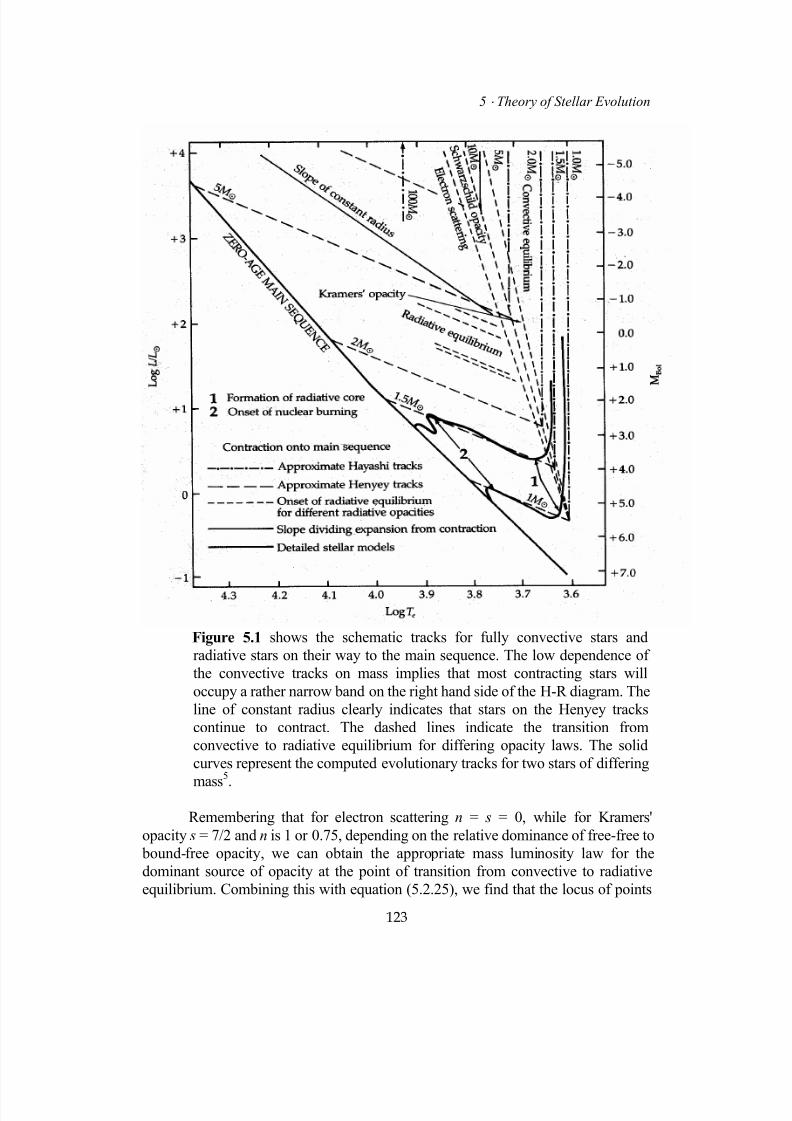
7/18/2019 The Fundamentals of Stellar Astrophysics - Collins G. W.
http://slidepdf.com/reader/full/the-fundamentals-of-stellar-astrophysics-collins-g-w 143/524
5 ⋅ Theory of Stellar Evolution
Figure 5.1 shows the schematic tracks for fully convective stars and
radiative stars on their way to the main sequence. The low dependence of
the convective tracks on mass implies that most contracting stars will
occupy a rather narrow band on the right hand side of the H-R diagram. The
line of constant radius clearly indicates that stars on the Henyey tracks
continue to contract. The dashed lines indicate the transition from
convective to radiative equilibrium for differing opacity laws. The solid
curves represent the computed evolutionary tracks for two stars of differing
mass5
.
Remembering that for electron scattering n = s = 0, while for Kramers'
opacity s = 7/2 and n is 1 or 0.75, depending on the relative dominance of free-free to
bound-free opacity, we can obtain the appropriate mass luminosity law for the
dominant source of opacity at the point of transition from convective to radiative
equilibrium. Combining this with equation (5.2.25), we find that the locus of points
123

7/18/2019 The Fundamentals of Stellar Astrophysics - Collins G. W.
http://slidepdf.com/reader/full/the-fundamentals-of-stellar-astrophysics-collins-g-w 144/524
1 ⋅ Stellar Interiors
in the H-R diagram will be described by
(5.2.29)
For the very massive stars, radiation pressure may play an important role toward theend of the Hayashi contraction phase, so that the onset of radiative equilibriumoccurs sooner, increasing the value on the right-hand side of equation (5.2.28)slightly. But for stars with a mass less than about 3M⊙ equations (5.2.25), and(5.2.29) will describe their relative position on the H-R diagram with some accuracy.
Henyey Evolutionary Tracks After sufficient time has passed for the
adiabatic gradient to exceed the radiative gradient, convection ceases and the main barrier to energy loss is no longer the ability of the photosphere to radiate energy into
space. Rather the radiative opacity of the core slows the leakage of energy generated
by gravitational contraction, and the atmosphere no longer provides the primary
barrier to the loss of energy. Further contraction now proceeds on the Kelvin-
Helmholtz time scale. As the star continues to shine, the gravitational energy
continues to become more negative, and to balance it, in accord with the Virial
theorem, the internal energy continues to rise. This results in a slow but steady
increase in the temperature gradient which results in a steady increase in the
luminosity as the radiative flux increases. This increased luminosity combined with
the ever-declining radius produces a sharply rising surface temperature as the
photosphere attempts to accommodate the increased luminosity. This will yieldtracks on the H-R diagram which move sharply to the left while rising slightly (see
Figure 5.1). For the reasons mentioned above, the beginning of these tracks will be
along a series of points which move upward and to the left for stars of greater mass.
We may quantify this by asking how the luminosity changes in time. We
differentiate equation (5.2.18) and obtain
(5.2.30)
The parameter a is simply a measure of the central condensation of the model, whichwe require to be independent of time. This requirement is satisfied if the contraction
is homologous. If we further invoke the Virial theorem and require that the
contraction proceed so as to keep the second derivative of the moment of inertia
equal to zero, then
124

7/18/2019 The Fundamentals of Stellar Astrophysics - Collins G. W.
http://slidepdf.com/reader/full/the-fundamentals-of-stellar-astrophysics-collins-g-w 145/524

7/18/2019 The Fundamentals of Stellar Astrophysics - Collins G. W.
http://slidepdf.com/reader/full/the-fundamentals-of-stellar-astrophysics-collins-g-w 146/524
1 ⋅ Stellar Interiors
reside on or very near the main sequence and so must be involved in the utilization of
their most prolific and efficient source of energy − the fusion of hydrogen into
helium. So we may take the intersection of the Henyey track with the main sequence
as an indication that hydrogen ignition has begun in the stellar core.
Actually nuclear processes begin somewhat before the main sequence is
encountered. The first constituents of the star to undergo nuclear fusion are
deuterium and lithium which require conditions substantially below that of hydrogen
for their ignition. However, their abundance is sufficiently low so that they provide
little more than a stabilizing effect on the star as it proceeds along its Henyey track,
causing the star to hook on to the main sequence.
For the sun, about a million years is required for the equilibrium abundances
of the proton-proton cycle to be established with sufficient accuracy for their use in
the energy generation schemes. At this point, the star can be said to have arrived atthe zero-Age main sequence. As the name implies, this is generally taken as the
beginning point of stellar evolution calculations, as the onset of nuclear burning
makes the details of the prior evolution largely irrelevant to the subsequent evolution.
In some real sense, the star forgets where it came from. Since it is fairly obvious that
the effects of stellar evolution during the main sequence phase will result in little
movement on the H-R diagram, we need to understand more of the structure of the
interior to appreciate these effects. Therefore, we begin by describing the structure to
be expected for the hydrogen burning models that describe the main sequence. The
structure of main sequence stars can be readily broken into two distinct groups: those
that occupy the upper half of the main sequence, and those that occupy the lower
main sequence.
a Lower Main Sequence Stars
We define the lower main sequence to be those stars with masses lessthan about 2 solar masses. For these stars, after the trace elements with low ignitiontemperatures have been exhausted and hydrogen fusion has begun, the equilibriumstructure is established in about a million years. The mass of these stars is insufficientto produce a central temperature high enough to initiate the CNO cycle, so the primary source of energy is the proton-proton cycle. Models indicate that in the sun,98 percent of the energy is supplied by the proton-proton cycle. The relatively lowdependence on temperature of the proton-proton cycle implies that the energy
generation will be less concentrated toward the center than would be the case withthe CNO cycle. This and the modest central temperature imply that a temperaturegradient less than the adiabatic gradient is all that is required to carry the energy produced by the p-p cycle. Thus, these stars have a central core which is in radiativeequilibrium. However, in the sun, the adiabatic gradient is never far from the actualtemperature gradient, and it would take a very little increase in the temperaturegradient to cause the core to become unstable to convection. Indeed, the conditionsfor convective instability are met in the outer regions of these stars resulting in the
126
7/18/2019 The Fundamentals of Stellar Astrophysics - Collins G. W.
http://slidepdf.com/reader/full/the-fundamentals-of-stellar-astrophysics-collins-g-w 147/524
5 ⋅ Theory of Stellar Evolution
formation of a convective envelope. In the sun, this point is reached at about 0.75R ⊙ ,so that about 98.8 percent of the mass is included in the radiative core. Ultimately,the situation is reversed near the surface, as it must be, for the energy leaves thesurface of the star by radiation.
The existence of the radiative core in stars of the lower main sequence has a
significant effect on the subsequent evolution of the star. The4He, which is the end
product of hydrogen burning, remains in the locale in which it is produced. However,
since the production rate is strongly dependent on temperature, the helium abundance
increases more rapidly as one approaches the center of the star. The helium must be
supported against its own gravity while it contributes nothing to the support of the
remainder of the star. As a result, the internal temperature will increase to maintain
the luminosity in the face of decreasing hydrogen abundance and the increasing mass
of the particles (i.e. the4He). This is why the temperature scales with the mean
molecular weight m, [see equation (2.3.8)]. Thus, we should expect stars like the sun
to slowly increase in brightness, as the internal temperature rises, during their mainsequence lifetime. Indeed, the standard solar model indicates that the solar
luminosity has increased by about 40 percent since its arrival on the zero age main
sequence.
Toward the end of the star's main sequence life, the helium abundance will
rise to the point where a core of helium, surrounded by a hydrogen burning shell, will
form in the center of the star. The support of this isothermal helium core is eventually
helped by the Pauli Exclusion Principle. In Chapter 1, we outlined the equation of
state to be expected for a gas where all the available h3 volumes of phase space were
filled. Because of their lower mass, this condition will be experienced first by the
electrons. The degenerate equation of state does not contain the temperature andtherefore permits the existence of an electron pressure capable of assisting in the
support of the helium core; this equation is independent of the conditions existing in
the hydrogen-burning shell. Thus as the core builds, we could expect its structure to
shift from that of an isothermal sphere, described in Chapter 2, to that of a polytrope
with a γ= 5/3, as would be dictated by the electron pressure of a fully degenerate gas.
This change from an isothermal sphere to a polytrope will dictate the mass
distribution, for the pressure of the ions becomes small compared to that of the
electrons. However, because of the high conductivity of a degenerate gas, the
configuration will remain isothermal since any energy surplus can immediately be
transported to a region of energy deficit by electron conduction. Thus, the region is
still known as the isothermal helium core, even though the pressure equilibrium isdictated by the electron pressure behaving as a polytropic gas with a γ of 5/3.
Therefore, the main sequence lifetime of a low mass star consists of a steady
energy output from hydrogen burning in an environment of steadily increasing
helium. On a nuclear time scale, the helium abundance increases preferentially in the
most central regions causing the temperature to rise which results in a slow increase
127

7/18/2019 The Fundamentals of Stellar Astrophysics - Collins G. W.
http://slidepdf.com/reader/full/the-fundamentals-of-stellar-astrophysics-collins-g-w 148/524
1 ⋅ Stellar Interiors
in the luminosity throughout the main sequence lifetime of the star. After about 10
percent of the radiative core mass has been consumed, an isothermal helium core
begins to form and structural changes begin to occur very rapidly. This signals the
end of the main sequence lifetime.
b Upper Main Sequence Stars
The situation regarding the stellar structure for stars of more than 2
solar masses is nearly reversed from that of the lower main sequence. For stars on the
main sequence, the observed mass-radius relation is approximately
M ∝ R 4/3
(5.3.1)
However, from the homology relations in Chapter 2 [equations (2.3.8)], we knowthat
T ∝ M/R (5.3.2)
Therefore, for stars along the main sequence, we expect the central temperature to
increase slowly as we proceed up the main sequence in accord with
Tc ∝ R 1/3
∝ M1/4
(5.3.3)
This slow rise in the central temperature will result in a greater fraction of the
energy being produced by the more temperature-sensitive CNO cycle. Thus, by the
time one reaches stars of greater than about 2 solar masses, the CNO cycle will bethe dominant source of energy production. The much larger temperature sensitivity
of the CNO cycle as compared to the p-p cycle means that the region of energy
production will be rather more centrally concentrated than in stars of less mass. This,
in turn, requires a steeper temperature gradient in order to transport the energy to the
outer parts of the star. Since in the sun the radiative gradient was already quite close
to the adiabatic gradient, this small increase is sufficient to cause the inner regions to
become convectively unstable, and a substantial convective core will be established.
However, in the outer parts of the star, the declining density causes the product of
ρκ , which appears in the radiative gradient [equation (4.2.14)], to reduce the
radiative gradient below that of the adiabatic gradient, and so convection stops. Thus,
we have a star composed of a convective core surrounded by an envelope in radiativeequilibrium. This role reversal for the core and envelope has a profound effect on the
evolution of the star.
The presence of a convective core ensures that the inner regions of the star
will be well mixed. As helium is produced from the burning of hydrogen, it is mixed
thoroughly throughout the entire core. Thus, we do not have a buildup of a helium
128

7/18/2019 The Fundamentals of Stellar Astrophysics - Collins G. W.
http://slidepdf.com/reader/full/the-fundamentals-of-stellar-astrophysics-collins-g-w 149/524
5 ⋅ Theory of Stellar Evolution
core that increases in helium abundance toward the center in these stars. Instead, the
entire convective core is available as a fuel source for energy production at the center
of the star. For this reason, energy production is remarkably steady in these stars until
the entire convective core is nearly exhausted of hydrogen. Even as exhaustion
approaches, the extreme temperature dependence of the CNO cycle implies that
deficits produced by the declining availability of hydrogen fuel can be made up by
modest increases in the temperature and hence minor changes in the structure of the
star. Indeed, it is not until more than 99 percent of the convective core mass has been
converted to helium that truly significant changes occur in the structure of the star
and the star can be said to be leaving the main sequence.
5.4 Post Main Sequence Evolution
The evolution of stars off the main sequence represents the response of the star to a
depletion of the available fuel supply, and it can be qualitatively understood byexamining the response of the core and envelope to the attempts of the nuclear
burning regions to adjust to the diminution of the available hydrogen. In stars of the
lower main sequence, the hydrogen-burning shell begins to move into a region of
declining density resulting in a decrease in available hydrogen. For stars of the upper
main sequence, the situation is somewhat different. The convective nature of the core
ensures the existence of mass motions, which continue to bring hydrogen into the
central regions for hydrogen burning until the entire core is depleted. These two
rather different approaches to hydrogen exhaustion produce somewhat different
evolutionary futures for the two kinds of stars, so we examine them separately.
a Evolution off the Lower Main Sequence
The development of a helium core, which signals the onset of post
main sequence evolution, is surrounded by a thin hydrogen-burning shell. The
hydrogen burning continues in a shell around the helium core which steadily grows
outward, in mass, through the star. However, the helium core must be supported
against its own gravity as well as support the weight of the remaining star, and its
energy sources are all on the outside. As a result, it is impossible for the hydrogen-
burning shell to establish a temperature gradient within the helium core. Only
gravitational contraction of the core will result in the release of energy inside the
helium core, and except for this source of energy the helium core must be isothermal,
with its temperature set by the burning of hydrogen surrounding it. But the rate ofhydrogen burning is dictated largely by the mass of material lying above the burning
zone, because this is the material that must kept in equilibrium. As the mass of the
isothermal helium core increases, the equilibrium temperature of the core will also
rise and this demand can be met only by a slow contraction of the helium core. The
slow increase in the core temperature triggers a steady increase in the stellar
luminosity.
129
7/18/2019 The Fundamentals of Stellar Astrophysics - Collins G. W.
http://slidepdf.com/reader/full/the-fundamentals-of-stellar-astrophysics-collins-g-w 150/524
1 ⋅ Stellar Interiors
As the isothermal core grows through the addition of He from the hydrogen-
burning shell, the core temperature must rise in order for it to remain in equilibriumand support the outer layers of the star. Since an isothermal sphere is a unique
polytropic configuration, it seems reasonable that there would be a limit to the
amount of overlying material that such an isothermal core could support. This limit is
known as the Chandrasekhar-Schönberg (C-S) limit . The limit will depend solely on
the mass fraction of the isothermal core and the mean molecular weights of the core
and envelope. Should the core exceed this limiting mass fraction, it must contract to
provide the temperature and pressure gradients necessary to support the remainder of
the star as well as itself.
Chandrasekhar-Schönberg Limit A detailed evaluation of the
Chandrasekhar-Schönberg limit requires matching the isothermal core solution to the pressure required to support the overlying stellar mass. The maximum mass fraction
that an isothermal core can have is
(5.4.1)
where µo and µi are the mean molecular weight of the outer region and core
respectively. Although the specific calculation of qc-s requires detailed consideration
of the isothermal core solution, we can provide an argument for the plausibility of
such a limit by considering the Virial theorem for the core alone.
(5.4.2)
where
(5.4.2a)
and r c is the radius of the isothermal core. The third term on the left-hand side arises
because we cannot take the volume integrals, which yield the global theorem, over a
surface where the pressure is zero. Thus, we must include a "surface" term which iseffectively the surface pressure times the enclosed volume of the core. We may solve
this expression for the pressure at the boundary of the core and obtain
(5.4.3)
130
7/18/2019 The Fundamentals of Stellar Astrophysics - Collins G. W.
http://slidepdf.com/reader/full/the-fundamentals-of-stellar-astrophysics-collins-g-w 151/524
5 ⋅ Theory of Stellar Evolution
Now we wish to find the maximum core radius which will provide sufficient
pressure to support the remaining star. We can find a maximum pressure by
differentiating equation (5.4.3) with respect to r c and finding that value of r c for
which the pressure gradient is zero. Certainly any core which yields a zero surface
pressure gradient is the largest physically reasonable core. This calculation results in
a maximum r c given by
(5.4.4)
Substitution into equation (5.4.3) yields the maximum surface pressure attainable at
the surface of the core.
(5.4.5)
Remember that the homologous behavior of the temperature allows us to write
(5.4.6)
so we can eliminate the temperature from 5.4.5 and express the result with a term
which is homologous to the pressure of the envelope. Thus,
(5.4.7)
The term M2/R
4 is homologous to the pressure of the envelope at the surface of the
core. The ratio of this to the maximum attainable core pressure must be less than
unity for the core to be able to support the envelope,
(5.4.8)
where the constant is the same as in equation (5.4.1) . Thus, we see that the
isothermal core can, at most, support about 37 percent of the mass of the star, but if
the core is primarily helium, this limit is reduced to about 10 percent.
131
7/18/2019 The Fundamentals of Stellar Astrophysics - Collins G. W.
http://slidepdf.com/reader/full/the-fundamentals-of-stellar-astrophysics-collins-g-w 152/524
1 ⋅ Stellar Interiors
Degenerate Core Only for stars near the upper end of our range(i.e. M ≈ M⊙ ) will the mass of the core approach the Chandrasekhar-Schönberg limitwithout becoming degenerate and the core undergoing further gravitational
contraction. For stars with masses M ≤ 1.3M⊙ the slowly developing isothermalcore will be degenerate from a point in its development when the core mass is well below the Chandrasekhar-Schönberg limit. Under these conditions, that limit doesnot apply because the added pressure of the degenerate electron gas is sufficient tosupport nearly any additional mass. Thus, the isothermal helium cores of lower mainsequence stars can increase to virtually any mass below the Chandrasekhardegeneracy limit. As mass is added to the core, we can expect the core to contractaccording to the mass-radius law for degenerate configurations that we derived inChapter 1 [equation (1.3.18)]. This law, following differentiation with respect totime, indicates that the core will shrink on the same time scale that mass is added toit, and that is the nuclear time scale.
Progress to the Red Giant Phase In terms of its physical size, thisisothermal degenerate helium core is never very large. Thus the post main sequence
evolution of a low-mass star can be viewed as the processing of stellar material
through the burning zone, with the resultant helium being packed into a very small
volume of systematically higher mean molecular weight. The declining density just
above the helium core will lead to an increase in temperature, in order for the nuclear
energy generation mechanisms to supply the energy required to support the star.
However, an increase in the central temperature would lead to an increase in the
temperature gradient and an increase in the luminosity. The increased luminosity, in
turn, causes the outer envelope of the star to expand, decreasing the temperature
gradient. Equilibrium is established at a higher shell temperature and somewhat
greater luminosity and temperature gradient. The result is that the star moves upwardand very slightly to the right on the H-R diagram. The process continues until the
temperature gradient exceeds the adiabatic gradient. Then the entire outer envelope
becomes convective. The increase in physical size of the envelope lowers the surface
temperature and thereby increases the radiative opacity in the outer layers. This
further decreases the efficiency of radiative transport and hastens the formation of the
outer convection zone. The outer envelope is now well approximated by a polytrope
of index n = 1.5, and the conditions for the Hayashi tracks become operative.
The star now approximately follows the track of a fully convective star only
now in reverse. The continual decline of the available hydrogen supply in the shell
burning region, which becomes extremely thin, leads to a steady increase in the shelltemperature and accompanying rise in the luminosity. With the outer convection
zone behaving as a good polytrope and efficiently carrying the energy to the surface,
the energy loss is again limited by the photosphere and the star expands rapidly to
accommodate the increased energy flow. The star now moves nearly vertically up the
giant branch as a red giant.
132
7/18/2019 The Fundamentals of Stellar Astrophysics - Collins G. W.
http://slidepdf.com/reader/full/the-fundamentals-of-stellar-astrophysics-collins-g-w 153/524
5 ⋅ Theory of Stellar Evolution
Helium Flash As the temperature of the hydrogen-burning shell
increases and the degenerate core builds in mass; the temperature eventually reaches
approximately 108 K. This is about the ignition temperature of helium via the triple-α
processes. Under normal conditions, the burning of helium could begin in ameasured way which would allow for an orderly transition of nuclear energy
generation processes. However, the core is degenerate, so the electron pressure is
only weakly dependent on temperature. Indeed, the limiting equation of state for total
degeneracy does not contain the temperature at all. Thus helium burning sets in with
unrelenting ferocity. With its extreme dependence on temperature, the triple-α
process initiates a thermal runaway which is limited only by the eventual removal of
the degeneracy from the core. The complete equation of state for a partially
degenerate gas does indeed, contain the temperature and at a sufficiently high
temperature the equation of state will revert to the ideal-gas law. When this occurs,
the core rapidly expands, cools, and reaches equilibrium, with helium continuing to
burn to carbon in its center. The response of the core to this entire process is so swiftthat the total energy produced is a small fraction of the stored energy of the star. In
addition, the site for the production of the energy is sufficiently far removed from the
outer boundary that energy is diffused smoothly throughout the star and never makes
a noticeable change in the stars appearance.
The duration of the flash, is so much shorter time than the dynamical time
scale for the entire star that one would expect that all manifestation of the flash
would be damped out by the overlying star and remain hidden from the observer.
However, detailed hydrodynamical calculations7 indicate that the pressure pulse
resulting from the rapid expansion of the core arrives at the surface with a velocity
well in excess of the escape velocity. This may well result in a one-time mass loss ofthe order of 30 percent which would affect the subsequent evolution.
Terminal Phases of Low Mass Evolution Initially, after helium ignition,
the hydrogen burning shell continues to supply about 90 percent of the required
support energy. However, now an orderly transition of energy mechanisms can take
place, resulting in the transfer from hydrogen burning to helium burning over an
extended time. The star will move somewhat down the giant branch and out on the
horizontal branch, from near the peak of the giant branch where the helium flash took
place. Meanwhile the helium core is in convective equilibrium, with the convection
zone extending almost to the hydrogen shell. The re-expansion of the core is
responsible for the contraction of the outer envelope, causing the star to move outonto the horizontal branch. It appears likely, that after helium burning has ceased and
the resultant carbon core is contracting, the outer envelope becomes unstable to
radiation pressure and lifts off the star, forming a planetary nebula and leaving the
hot core, which now relieved of its outer burden, simply cools. If the mass is below
the Chandrasekhar limiting mass for carbon white dwarfs, the star continues to cool
to the virtually immortal state of a white dwarf.
133
7/18/2019 The Fundamentals of Stellar Astrophysics - Collins G. W.
http://slidepdf.com/reader/full/the-fundamentals-of-stellar-astrophysics-collins-g-w 154/524
1 ⋅ Stellar Interiors
Structure and Evolution of White Dwarfs We have already discussed
much that is relevant to the description of this abundant stellar component of the
galaxy, and we will return to the subject in Section 6.4. In Section 1.3 we derived the
equation of state appropriate for a relativistic and a nonrelativistic degenerate gas andfound them to be polytropic. In Section 2.4 we developed the mass-radius relation for
polytropes in general, which provides the approximate results appropriate for white
dwarfs. In Chapter 6 we will see how the relativistic equation of state and the theory
of general relativity lead to an upper limit of the mass that one can expect to find for
white dwarfs. However, some description of the white dwarfs formed by the
evolution of low-mass stars and their subsequent fate is appropriate.
There are basically two approaches to the theory of white dwarfs. The first is
to observe that a relativistically degenerate gas will behave as a polytrope and to
explore the implications of that result. The second is to investigate the detailed
physics that specifies the equation of state and to create models based on the results.Cox and Giuli8 and references therein provide an excellent example of the latter. Our
approach will be much nearer the former.
The ejection of a planetary nebula during the later phases of the evolution of
a low-mass star leaves a hot degenerate core of carbon and oxygen exposed to the
interstellar medium. While such a core may range in mass from about 0.1 of a solar
mass to more than a solar mass, its future will be remarkably independent of its mass.
While the actual run of the state variables will pass through regions of degeneracy
through partial degeneracy to a nondegenerate surface layer, the basic properties of
the star can be understood by treating the stars as polytropes.
From observation we know that the white dwarf remains of stellar evolution
are about a solar mass confined to a volume of planetary dimensions and thus will
have a density of the order of ρ = 106 g/cm
3. If we assume that the gas is fully
ionized, then the typical energy of an electron will be about 0.1 MeV for a fully
degenerate gas. If the stellar core were at a temperature of 107ΕK, the typical ion
would have an energy of about 1 keV. Since energy densities are like pressures, even
if the number densities were the same for the electrons and ions, the pressure of the
electrons would dominate. In fact, since the typical ion produces many electrons, the
dominance of the electron pressure, is even greater. Thus the structure will be largely
determined by the electron pressure and the ions may be largely ignored. However,
Hamada and Salpeter 9
have shown that at densities around 108
g/cm3
the Fermienergy of the electron "sea" becomes so high that inverse beta decay becomes likely
and some of the electrons disappear into the protons of the nuclei, causing the
limiting mass to be somewhat reduced over what would be expected for a purely
degenerate gas. Also, the thermal energy of the ions is lost, permitting the star to
shine.
134

7/18/2019 The Fundamentals of Stellar Astrophysics - Collins G. W.
http://slidepdf.com/reader/full/the-fundamentals-of-stellar-astrophysics-collins-g-w 155/524
5 ⋅ Theory of Stellar Evolution
Since these stars are largely degenerate, most of the momentum states in
phase space are full, and an electron that is perturbed from its place in phase space
has to travel quite a distance before it can find an empty place. This implies that the
mean free path of electrons will be very long in spite of the high densities. Such
electrons play essentially the same role as the conduction electrons of a conductor so
that the electrical and thermal conductivity will be very high in a degenerate gas.
This crowding of the states in phase space also results in the reduction in radiative
opacity since it is difficult for a photon to move an electron from one state to another.
As a result, it is very difficult for temperature gradients to exist within a fully
degenerate configuration. However, in the outer regions of the white dwarf where the
gas becomes partially degenerate, the opacity rapidly rises and the conductivity
drops, giving rise to a steep temperature gradient with the result that the energy flow
to the surface is seriously impeded. Thus Aller has likened a white dwarf to a metal
ball wrapped in an insulating blanket. Since the structure of a polytrope is stable and
independent of the temperature, the evolutionary history of a white dwarf largelyrevolves on the details of its cooling.
In 1952, Leon Mestel10
took basically this classical approach to the cooling
of white dwarfs and found that the cooling curve [dln(L)/dln(t)] was approximately
constant and independent of time. Iben and Tutukov11
, using a much more detailed
analysis and equation of state, found virtually the same result which they regarded as
occurring through a series of accidents. Their results give [dln(L)/dln(t) ≈ (-1.4, -
1.6)] for 5 < log(tyrs.) < 9.4. It is true that a considerable number of effects
complicate the simple picture of a polytrope wrapped in a blanket.
For example, while we may neglect the ions for an excellent approximationof the description of the white dwarf structure, the contribution of the ion pressure
will make the star slightly larger than one would expect from the polytropic
approximation. Because of the extreme concentration of the star, a small contraction
produces a considerable release of gravitational energy, which is then to be radiated
away. This extends the cooling time significantly over that which would be expected
simply for a cooling polytrope. Toward the end of the cooling curve a series of odd
things happen to the equation of state for the white dwarf. As the interior regions
cool, they undergo a series of phase transitions first to a liquid state and then to a
crystalline phase. Each of these transitions results in a "heat of liquefaction or
crystallization" being released and increasing the luminosity temporarily. Problems
of the final cooling remain in the understanding of the low-temperature high-densityopacities that will determine the flow of radiation in this final descent of the white
dwarf to a cool cinder, called a black dwarf in thermal equilibrium with the ambient
radiation field of the galaxy. The question is of considerable interest since such
objects could be detected only by their gravitational effect and could bear on the
question of the "missing mass".
135
7/18/2019 The Fundamentals of Stellar Astrophysics - Collins G. W.
http://slidepdf.com/reader/full/the-fundamentals-of-stellar-astrophysics-collins-g-w 156/524
1 ⋅ Stellar Interiors
b Evolution away from the Upper Main Sequence
The evolution of the more massive stars that inhabit the upper main
sequence is driven by the same processes that govern the evolution of the lower mainsequence, namely, the exhaustion of hydrogen fuel. However, the processes are quite
different. The exhaustion of the convective core leads to the production of a helium
center, as in the lower main sequence stars, but now the core will have to contend
with the Chandrasekhar-Schönberg limit.
Nature of the Massive Helium Core In massive stars, as the hydrogen isdepleted in the helium core, the temperature rises rapidly, to produce the energynecessary to accommodate the demands of stellar structure. For stars with massesgreater than about 7 M⊙ , the resulting helium core will be greater than theChandrasekhar-Schönberg limit; and to make up for the energy deficit caused by thefailing hydrogen burning, the core will have to contract. Since the contraction must
maintain a temperature gradient, the contraction will proceed rather faster than would be expected for an isothermal core. However, the steep temperature gradientestablished by the terminal phases of core hydrogen burning will be relaxed becausethe energy generated by gravitational contraction will not be as centrallyconcentrated as it was from hydrogen burning. This drop in temperature gradient willcause convection to cease, yielding a core in radiative equilibrium supplying therequired stellar energy by contraction.
The contraction of virtually any polytrope will result in an increase in
internal temperature. This is really a consequence of the Virial theorem. However,
the cessation of hydrogen burning in the core and the resultant decrease in the
temperature gradient imply a change in the overall structure of the core, and thus the
polytropic analogy is somewhat strained. The decline in the temperature gradientactually implies that the core will suffer a reduction of its internal energy while the
boundary temperature increases. This loss of internal energy goes into the support of
the outer envelope. Thus, both this energy and the energy generated by contraction
are available for the support of the outer layers of the star.
The increase in the boundary temperature of the core will result in a slow
expansion and cooling of the radiative envelope for the same reason described for
low-mass stars. After a suitable rise in the boundary temperature, hydrogen is
reignited in a shell surrounding the helium core. This results in a marked change in
the temperature gradient of the hydrogen-burning shell at the core boundary. The
localization of the energy production in such a small region steepens the temperaturegradient to the point where the temperature gradient exceeds the adiabatic gradient,
driving the entire envelope into convection. The outer envelope now rapidly transfers
the energy to the surface, which again becomes the limiting barrier to its escape. The
star moves rapidly toward the giant branch as a star with a helium core surrounded
by a hydrogen-burning shell and covered with a deep convective envelope. This
envelope is so deep that it reaches into the region where nuclear processing has taken
136

7/18/2019 The Fundamentals of Stellar Astrophysics - Collins G. W.
http://slidepdf.com/reader/full/the-fundamentals-of-stellar-astrophysics-collins-g-w 157/524
5 ⋅ Theory of Stellar Evolution
place, dredging up some of this material to the surface. The result of this process is
evident in the atmospheric spectra of some late-type supergiants.
Stars with masses less than about 5M⊙ will end their hydrogen burning witha helium core below that of the Chandrasekhar-Schönberg limit and will contendwith a slowly contracting isothermal core right through the ignition of a hydrogen- burning shell. The future of such a star is mirrored in the behavior of lower-massstars except that helium ignition takes place before the core becomes significantlydegenerate. The result is that these stars experience no helium flash, and thetransition to helium burning is orderly.
Ignition of the Massive Helium Core In both cases described above,
the contraction of the helium core proceeds while the hydrogen shell is burning. In
the more massive stars, where the core is above the Chandrasekhar-Schönberg limit,
the star must do so to maintain a temperature gradient for its own support. In the less
massive case, the core grows slowly as a result of the processing of the hydrogen inthe energy-generating shell. The added mass results in a slow core contraction. In
both instances, the decreasing density in the hydrogen-burning shell necessitates a
rise in the temperature required for energy generation. After the increasing
temperature gradient caused by this increasing shell temperature has forced the
envelope to become fully convective, the convective envelope continues to expand,
for the energy escape is again limited by the radiative efficiency of the photosphere.
Eventually the central temperature reaches 108 K, and helium ignition takes
place. The ignition has a dramatic effect on the core but does not exhibit the
explosive nature of the helium flash. The core undergoes a rapid expansion and,
because of the huge temperature dependence of the triple-a process, becomesunstable to convection. This produces an expanded convective helium core
surrounded by a hydrogen-burning shell. This shell supplies more than 90 percent of
the energy required to maintain the luminosity. The rapid core expansion is
accompanied by a contraction of the outer envelope with a corresponding increase in
the surface temperature. The star moves off to the left in the H-R diagram,
maintaining about the same total luminosity. The hydrogen burning shell continues
to supply the majority of the energy throughout the helium burning phase which
proceeds in much the same manner as the main sequence core hydrogen-burning
phase, but on a much shorter time scale.
Terminal Phases of Evolution of Massive Stars The end phase of the
evolution of massive stars is still somewhat murky and the subject of active research.
Initially, the helium burning continues in the core until the core becomes largely
carbon. At the point of helium exhaustion, the core again gravitationally contracts,
rising in temperature, until helium is ignited in a shell source around the core. For
stars with a mass between 3 and 7 solar masses, there is some evidence that the
137
7/18/2019 The Fundamentals of Stellar Astrophysics - Collins G. W.
http://slidepdf.com/reader/full/the-fundamentals-of-stellar-astrophysics-collins-g-w 158/524
1 ⋅ Stellar Interiors
carbon core which develops is degenerate and that ignition, when it occurs, occurs
explosively, perhaps producing a supernova. For stars of more than 10 solar masses,
carbon burning can take place in a nonviolent manner, producing cores of neon,
oxygen, and finally silicon, each surrounded by a shell source of the previous corematerial which continues to provide some energy to the star. The results of silicon
burning yield elements of the iron group for which further nuclear reactions are
endothermic, and so this burning will not only fail to contribute energy for the
support of the star but also rob it of energy. In addition, the densities become high
enough that the electrons are forced into the protons of the nuclei by means of
inverse b decay. This effect has been called neutronization of the core. Both
mechanisms produce a significant number of neutrinos which also do not take part in
the support of the star against gravity and can be viewed as "cooling" mechanisms
for the core.
This rapid cooling precipitates a rapid collapse of the core followed by theentire star. The in-fall velocity soon exceeds the speed of sound, resulting in the
formation of a shock wave, and interior densities may become large enough for the
material to become opaque to neutrinos. Under some conditions the endothermic
nuclear reactions may bring about the disintegration of the iron-group elements into4He. Which process dominates for stars of which mass is not at all clear. The shock
wave formed by the in-fall may "bounce", or the increased neutrino opacity may
provide sufficient energy and momentum to ensure that a large fraction of the star
will be blown into the interstellar medium.
The remnants, if any, could be a neutron star or a black hole. Although the
details of the terminal phases of massive stars remain somewhat unclear, it isvirtually certain that these phases are likely to end with the production of a
supernova and the subsequent enrichment of the interstellar medium by heavy
elements.
c The Effect of Mass-loss on the Evolution of Stars
Throughout our discussion of stellar evolution we have assumed thatthe mass of the evolving star remains essentially constant. Certainly there is areduction in mass from the nuclear production of energy, but this can never exceed0.7 percent and therefore can be safely neglected. However, as we shall see in section16.3, stars may exhibit rather large winds emanating from their atmospheres. In some
cases these winds may result in mass loss rates exceeding 10-5
M⊙ per year and socould lead to a significant reduction in the mass of the star during its nuclear lifetime.
Ever since the observation by Armin Deutch12
that the red supergiantα Herculis was losing mass faster than about 10
-8M⊙ per year, interest in the
effects of mass loss on the evolution of a star has been high. Generally one wouldexpect that a star slowly losing mass would follow the classical evolutionary trackrepresented by models of stars having successively lower and lower mass. Thus for a
138
7/18/2019 The Fundamentals of Stellar Astrophysics - Collins G. W.
http://slidepdf.com/reader/full/the-fundamentals-of-stellar-astrophysics-collins-g-w 159/524
5 ⋅ Theory of Stellar Evolution
main sequence star that is losing mass at a significant rate the evolutionary track onthe HR diagram would not rise like the constant mass models, but move steadily tothe right and perhaps down until the asymptotic giant branch is reached. In addition,the lifetime would be significantly enhanced as a result of the reduced stellar mass.
Such were the conclusion reached by Massevitch13
and collaboraters14
in the late1950's. However, the evolutionary tracks of 1-2M⊙ failed to fit the HR diagrams ofglobular clusters and in the absence of evidence for mass loss from main sequencestars, their work was largely ignored. However, during the 1960s and 70s it becameclear that virtually all early type stars exhibited significant stellar winds and it waslikely that their evolution from the main sequence was affected
13,14. In general, the
more massive the star, the greater the fractional mass loss rate will be. This wouldexplain why stars in the range of a few solar masses where unaffected and theconstant mass models fit the globular cluster HR diagrams relatively well. However,from studies of the ratio of blue to red supergiants in the Milky Way and othergalaxies Humphreys and Davidson
15 concluded that stars more massive than 50M⊙
never made it to the red supergiant phase but remained confined to the left hand sideof the HR diagram throughout their lives. Lamers
16 found that this did not appear to
be the case for stars in our galaxy concluding that a 100M⊙ could only loose 15 percent of its mass during it main sequence lifetime.
The impact of such mass loss on the subsequent evolution of the star seemsto depend on an accurate knowledge of the mass loss rate during the the evolutionwhich in turn rests on the specifics of the origin of stellar winds. Using anempirically inspired mass loss rate, Brunish and Truran
17 found that mass loss
affected the evolution of stars less than 30M⊙ more than the massive stars. However,Sreenivasan and Wilson
18,19 found including rotation and a theoretically motivated
origin for the mass loss rate resulted in a much more complicated evolutionaryhistory. By adjusting the amount of rotation present in the initial star they are able tomatch most of the observations. However, it is fair to say that as of the present much
remains poorly understood about the specific role played by mass loss in the massivestars. It also appears that a proper understanding will require models that correctlycouple the atmosphere to the interior and include rotation in a physically selfconsistent way.
5.5 Summary and Recapitulation
139
In this chapter we have sketched the evolution of normal stars from their contractionout of the interstellar medium to their probable fate. We have not discussed manytopics and details which are important to the detailed understanding of stellarevolution and some important problems remain unsolved. For the evolution ofindividual stars, an area of singular importance that was acknowledged only in passing concerns the origin of the elements. The production of the elements throughnuculosynthesis was suggested by Burbidge, Burbidge, Fowler and Hoyle20 and theearly view of the important processes are reviewed by Bashkin
21. The manifestation
of these elements in the outer layers of the star and the internal processes by whichthey got there are covered by Wallerstein
22. In addition, we have said nothing about
the fascinating topic of the evolution of close binary stars where the futures of thecomponents are linked through the process of mass exchange. We have said nothingabout the mass loss from massive stars that may alter the evolution of these stars. Norhave we touched on the tricky processes by which a white dwarf cools off. We also

7/18/2019 The Fundamentals of Stellar Astrophysics - Collins G. W.
http://slidepdf.com/reader/full/the-fundamentals-of-stellar-astrophysics-collins-g-w 160/524
1 ⋅ Stellar Interiors
avoided the effects of rotation and magnetic fields on the evolution of stars alongwith the details of the dynamic collapse of stars, and these should be regarded asfertile areas for research. However, we did delineate major events in the lives ofnormal stars. Specifically, we used the efficiency of energy transport, the temperature
sensitivity of the nuclear reactions, and the radiative ability of the photosphere toindicate the probable direction that the evolution of stars will take. Simple argumentsof efficiency lead to a remarkably accurate description of the early phases of stellarevolution to the main sequence. Post main sequence evolution is made morecomplicated by the zonal nature of the star, complications to the equation of state,and the existence of multiple energy sources. Nevertheless, we can see the basicconservation laws of physics at work during the latter phases of stellar evolution andcan get a feel for the important processes at work. We close this discussion withanother view of the interplay between the core and outer envelope along with adetailed look at the evolution of a 5M⊙ star.
a Core Contraction - Envelope Expansion: Simple Reasons
For years there has been some debate over why the envelope of an
evolving star expands when the core contracts, for many people find the result
counterintuitive. A number of explanations have been suggested and objections have
been made to almost all, of being simplistic or incomplete. Some have regarded the
question as being so complicated that it is not useful to search for a single cause, and
in response to the question of envelope expansion they simply say, "It happens
because my computer tells me it does." This is no answer at all, for it offers no
insight into the physical phenomena that result in the particular behavior exhibited by
the star. Certainly the physical situation which leads to the expansion of the envelope
during core contraction is complicated and simple answers, in some sense, willalways be incomplete. However, we should make the effort to identify the important
processes at work which dominate the result.
It would be useful if we could clarify the question a little. A star goes through
several different phases as it evolves from the main sequence to the giant branch of
the H-R diagram, and all result in an expansion of the envelope accompanying some
contraction of the core. However, the structure of the core and that of the envelope
differ widely in these various phases as do the magnitude and time scale for the
resulting core contraction-envelope expansion. We attempted to make plausible the
expansion of the convective envelope which accompanies the temperature increase
of the hydrogen-burning shell, resulting from the contraction of the radiative helium-rich core, by appealing to the behavior of convective polytropes. Although such
envelopes will not be the complete polytropes of the Hayashi tracks, it seems
reasonable that the stars will approach the tracks in their general behavior, for the
same principles that result in the Hayashi tracks are operative in the expansion of the
convective envelope. However, in envelope expansion, the processes are reversed
and less perfectly followed, since only the envelope is involved. The general
140
7/18/2019 The Fundamentals of Stellar Astrophysics - Collins G. W.
http://slidepdf.com/reader/full/the-fundamentals-of-stellar-astrophysics-collins-g-w 161/524

7/18/2019 The Fundamentals of Stellar Astrophysics - Collins G. W.
http://slidepdf.com/reader/full/the-fundamentals-of-stellar-astrophysics-collins-g-w 162/524
1 ⋅ Stellar Interiors
Now, for upper main sequence stars, the mass of the core substantially
exceeds that of the envelope,
Ω . GMc2/R c + GMcMe/R * (5.5.5)
If, for simplicity, we further hold the masses of the core and envelope constant
during the core contraction, we have
(5.5.6)
The sign of equation (5.5.6) indicates that we should expect the observed radius of
the star to increase for any decrease in the core radius, and the magnitude of the
right-hand side implies that a very large amplification of the change in core size
would be seen in the stellar radius. One can argue that the assumptions are onlyapproximately true or that the time scales involved occasionally approach the
Kelvin-Helmholtz time, but that will affect only the degree of the change, not the
sign. Indeed, detailed evolutionary model calculations throughout the period of
evolution from the main sequence to the giant branch indicate that the total
gravitational and internal energy is indeed constant to about 10 percent. The
accuracy for shorter times is considerably better. For lower main sequence stars, the
mass of the core is less than that of the envelope. Nevertheless, a result similar to
equation (5.5.6), with the same sign, is obtained although the magnitude of the
derivative is not as large.
The nature of this argument is so general that we may expect any action ofthe core to be oppositely reflected in the behavior of the envelope regardless of the
relative structure. Thus, we can understand the global response of the star to the
initial contraction of the core when the overlying layers are in radiative equilibrium
as well as the subsequent rapid expansion to and up the giant branch when the outer
envelope is fully convective. In addition, contraction of the stellar envelope
following the core expansion accompanying the helium flash, which leads to its
position on the horizontal branch, can also be qualitatively understood. In general,
whenever the core contracts, we may expect the envelope to expand and vice versa.
Detailed model calculations confirm that this is the case.
142

7/18/2019 The Fundamentals of Stellar Astrophysics - Collins G. W.
http://slidepdf.com/reader/full/the-fundamentals-of-stellar-astrophysics-collins-g-w 163/524
5 ⋅ Theory of Stellar Evolution
b Calculated Evolution of a 5 M star
In this final section we look at the specific track on the H-R diagram made by a 5M⊙
star as determined by models made by Icko Iben. This is best presented in the form
of a figure and is therefore shown in Figure 5.2 above. Similar calculations have
been done for representative stellar masses all along the main sequence so the
evolutionary tracks of all stars on the main sequence are well known. The basic
nature of the theory of stellar evolution can be confirmed by comparing the locationof a collection of stars of differing mass but similar physical age with the H-R
diagrams of clusters of stars formed about the same time. A reasonable picture is
obtained for a large variety of clusters with widely ranging ages. It would be
presumptuous to attribute this picture to chance. While much remains to be done to
illuminate the details of certain aspects of the theory of stellar evolution, the basic
picture seems secure.
143

7/18/2019 The Fundamentals of Stellar Astrophysics - Collins G. W.
http://slidepdf.com/reader/full/the-fundamentals-of-stellar-astrophysics-collins-g-w 164/524
1 ⋅ Stellar Interiors
Figure 5.2 delineates the evolution of a 5M⊙ star from its arrival onthe main sequence through its demise at the onset on carbon burning
23.
The labeled points are points of interest discussed in the chapter andtheir duration, place in the stellar lifetime, and the significant physical process taking place are given in Table 5.1.
Problems
1. Find the fraction by mass and radius inside of which 20 percent, 50 percent,
and 99 percent of the sun's energy is generated. Compare the results with a
star of the same chemical composition but with 10 times the mass.
2. Determine the mass for which stars with the chemical composition of the sun
derive equal amounts of energy from the CNO and p-p Cycles.
144
7/18/2019 The Fundamentals of Stellar Astrophysics - Collins G. W.
http://slidepdf.com/reader/full/the-fundamentals-of-stellar-astrophysics-collins-g-w 165/524
5 ⋅ Theory of Stellar Evolution
3. Determine the relative importance of free-free and bound-free absorption and
electron scattering as opacity sources in the sun.
4. Calculate the evolutionary tracks for a 1M⊙ star and 10M⊙ star.5. Choose a representative set of models from the evolutionary calculations in
Problem 4, (a) Calculate the moment of inertia, gravitational and internal
energies of the core and envelope, and the total energy of the star (b)
Determine the extent to which the conditions in Section 5.5a are met during
the evolution of the star.
6. Compute the Henyey track for a 1M⊙ star, and compare it with that of a
polytrope of index n = 3. Would you recommend that the comparison be
made with a polytrope of some different index? If so, why?
7. Compute the evolutionary track for the sun from early on the Hayashi trackas far as you can. At what point do you feel the models no longer represent
the actual future of the sun, and why?
8. Discuss the evolution of a 5M⊙ star as it leaves the main sequence. Detail
specifically the conditions that exist immediately before and after the onset of
hydrogen-shell burning.
9. Consider a star composed of an isothermal helium core and a convective
hydrogen envelope. Suppose that the mass in the core remains constant with
time but that the core contracts. By constructing a model of appropriate
polytropes, show what happens to the envelope and comment on the externalappearance of the star.
References and Supplemental Reading
1. Larson, R.B.: The Dynamics of a Collapsing Proto-star , Mon. Not. R. astr.
Soc. 45, 1969, pp. 271-295.
2. Disney, M.J.: Boundary and Initial Conditions in Protostar Calculations,
Mon. Not R. astr. Soc. 175, 1976, pp. 323-333.
3. Hayashi, C.: Evolution of Protostars, Ann. Rev. Astr. and Astrophys. 4,
1966, pp. 171-192.
4. Cox, J.P., and Giuli, R.T.: Principles of Stellar Structure, Gordon and
Breach, New York, 1968, chap. 26, pp. 743-750.
145
7/18/2019 The Fundamentals of Stellar Astrophysics - Collins G. W.
http://slidepdf.com/reader/full/the-fundamentals-of-stellar-astrophysics-collins-g-w 166/524
1 ⋅ Stellar Interiors
5. Iben,Jr., I."Normal Stellar Evolution", Stellar Evolution, (Eds.: H-Y Chiu
and A. Muriel), M.I.T. Press, Cambridge, Mass., 1972, pp. 44 - 53.
6. Harris, II, D.L., Strand, K., Aa., and Worley, C.E. "Empirical Data on Stellar
Masses, Luminosities, and Radii", Basic Astronomical Data (Ed.: K.Aa.
Strand), Stars and Stellar Systems, vol. 3, University of Chicago Press,
Chicago, 1963, p. 285.
7. Deupree, R.G.,and Cole, P.W.: Mass Loss During the Core Helium Flash,
Ap.J. 249, 1981, pp. L35 - L38.
8. Cox, J.P., and Guili, R.T.: Principles of Stellar Structure, Gordon and
Breach, New York, 1968, chap. 26, pp. 874 - 943.
9. Hamada, T. and Salpeter, E.E.: Models for Zero Temperature Stars, Ap.J.
134, 1961, pp. 683 - 698.
10. Mestel, L.: On the Theory of White Dwarf Stars I The Energy Sources of
White Dwarfs, Mon. Not. R. astr. Soc. 112, 1952, pp. 583 - 597, Particularly
see sec. 4, "The Rate of Cooling of a White Dwarf" pp.590 - 593.
11. Iben Jr.,I., and Tutukov, A.V.: Cooling of Low-Mass Carbon-Oxygen
Dwarfs from the Planetary Nucleus Stage through the Crystallization Stage,
Ap.J. 282, 1984, pp. 615 - 630.
12. Deutch, A.J.: The Circumstellar Envelope of Alpha Herculis, Ap.J. 123,
1956, pp. 210 -227.
13. Massevitch, A.G.: The Evolution of Stars in the h and χ Persei Double
Cluster , Soviet Astronomy 1, 1957, pp. 177 - 182.
14. Ruben, G., and Massevitch, A.G.: An Investigation of Evolutionary Paths
for a Homogeneous Stellar Model with a Convective Core,
Soviet Astronomy 1, 1957, pp. 705 - 718.
15. Humphreys, R.M., and Davidson, K.: Studies of Luminous Stars in NearbyGalaxies.III. Comments on the Most Massive Stars in the Milky Way and
The Large Magellanic Cloud , Ap.J. 232, 1979, pp. 409 - 420.
16. Lamers, H.J.G.L.M.: Mass Loss from O and B Stars, Ap.J. 245, 1981,
pp. 593 -608.
146
7/18/2019 The Fundamentals of Stellar Astrophysics - Collins G. W.
http://slidepdf.com/reader/full/the-fundamentals-of-stellar-astrophysics-collins-g-w 167/524
5 ⋅ Theory of Stellar Evolution
17. Brunish, W.M., and Truran, J.W.: The Evolution of Massive Stars I. The
Influence of Mass Loss on Population I Stars, Ap.J. 256, 1982,
pp. 247 - 258.
18. Sreenivasan, S.R., and Wilson, W.J.F.: The Evolution of Massive Stars
Losing Mass and Angular Momentum: Supergiants, Ap.J. 290, 1985,
pp. 653 - 659.
19. Sreenivasan, S.R., and Wilson, W.J.F.: The Evolution of Massive Stars
Losing Mass and Angular Momentum: Rotational Mixing in Early-Type
Stars, Ap.J. 292, 1985, pp. 506 - 510.
20. Burbidge, E.M., Burbidge, G.R., Fowler, W.A., and Hoyle, F.: Synthesis
of the Elements in Stars, Rev. of Mod. Phy., 29, 1957, pp. 547 - 650.
21. Bashkin, S. "The Orgin of the Elements", Stellar Structure,
(Ed.: L.H.Aller and D.B. McLaughlin), University of Chicago
Press, Chicago, 1965, pp. 1 - 60.
22. Wallerstein, G.: Mixing in Stars, Sci. 240, 1988, pp. 1743-1750.
23. Iben,Jr., I.: Stellar Evolution Within and Off the Main-Sequence, Ann Rev.
Astr. and Astrophys. 5, 1967, pp. 571 - 626.
A review of the 'traditional' collapse can be found in:
• Hayashi, C.: Evolution of Protostars, (1966) Ann. Rev. Astr. and Astrophys.
4, pp171-192.
A comprehensive review of the problems involved in non-homologous collapse can
be found in:
• Larson, R.: Processes in Collapsing Interstellar clouds, Ann Rev Astr.
Astrophys. Annual Reviews Inc. Palo Alto (1973) 11, Ed: L.Goldberg, D.
Layzer, and J.Phillips pp219-238.
An excellent classical description of the early phases of the contraction of protostars
can be found in:
• Bodenheimer, P.: Stellar Evolution Toward the Main Sequence, Rep. Prog.
Phys. (1972) 35, pp1-54.
147
7/18/2019 The Fundamentals of Stellar Astrophysics - Collins G. W.
http://slidepdf.com/reader/full/the-fundamentals-of-stellar-astrophysics-collins-g-w 168/524
148
1 ⋅ Stellar Interiors
A more recent description of the hydrodynamic problems of collapsing stars is
contained in:
• Tohline, J.E.: Hydrodynamic Collapse Fund. Cosmic Phys. (1982) 8,
pp1-82.
One of the best physical reviews of main-sequence evolution and the phases leading
up to the red giant phases is still:
• Schwarzschild, M.: Structure and Evolution of the Stars, Princeton
University Press (1958) Chapters V,VI pp165-227.
For the evolution of a normal 5Mυ star, the description by:
• Iben,Jr., I.: Stellar Evolution Within and Off the Main-Sequence
(1967) Ann Rev. Astr. and Astrophys. 5,pp.571-626,
or
• Iben,Jr., I.: "Normal Stellar Evolution" Stellar Evolution (1972)
Ed: H-Y Chiu and A. Muriel MIT Press Cambridge and London pp1-106.
is still regarded as basically correct. However, the broadest based and most
contemporary survey of the results of stellar evolution calculations remains:
• Cox, J.P., and Giuli, R.T.: Principles of Stellar Structure, (1968) Gordonand Breach, Science Pub., New York, London, Paris, Chapter 26 pp944-
1028.
An extremely literate presentation of the early theory of white dwarfs can be found in
this fine review article by:
• Mestel, L.: "The Theory of White Dwarfs", Stellar Structure (1965) (Ed.
L.H. Aller and D.B. Mclaughlin) Stars and Stellar Systems vol. 5 (Gen. Ed:
G.P.Kuiper and B.M. Middlehurst), University of Chicago Press, Chicago,
London pp297-325.

7/18/2019 The Fundamentals of Stellar Astrophysics - Collins G. W.
http://slidepdf.com/reader/full/the-fundamentals-of-stellar-astrophysics-collins-g-w 169/524
6 ⋅ Relativistic Stellar Structure
149
Copyright (2003) George W. Collins, II
6
Relativistic Stellar
Structure
. . .
In the next two chapters we consider some specific problems which
lie outside the realm of normal stellar structure. In the past several decades, it has
become increasingly clear that a large number of stars require some further subtletiesof physics for their proper description. Two areas that we shall consider involve the
initial assumption of spherical symmetry and the assumption that the gravitational
field can be described by the Newtonian theory of gravity with sufficient accuracy to
properly represent the star. In this chapter, we investigate some of the ramifications
of the general theory of relativity for highly condensed objects and super-massive
stars.

7/18/2019 The Fundamentals of Stellar Astrophysics - Collins G. W.
http://slidepdf.com/reader/full/the-fundamentals-of-stellar-astrophysics-collins-g-w 170/524
1 ⋅ Stellar Interiors
150
Although the application of the general theory of relativity to astronomical
problems has a long and venerable history dating back to Einstein himself, it was not
until the discovery of pulsars in the 1960s that a great deal of interest was directed
toward the impact of the theory on stellar structure. To be sure, the pioneering
theoretical work was done 30 years earlier and can be traced back to Landau1 in
1932. The fundamental work of Oppenheimer 2,3
and collaborators still provides the
fundamental basis for most models requiring general relativity for their
representation. But it was the discovery that neutron stars actually existed and were
probably the result of the dynamical collapse of a supernova that led to the
construction of modern models that represent our contemporary view of these
objects.
It is not my intent to provide a complete description of the general theory of
relativity in order that the reader is able to understand all the ramifications for stellarstructure implied by that theory. For that, the reader is referred to “Gravitation” by
Misner, Thorne, and Wheeler 4. Rather, let us outline the origin of the fundamental
equations of relativistic stellar structure and the results of their applications to some
simple objects, without the rigors of their complete derivation. The intent here is to
provide some physical insight into the role played by general relativity in a variety of
objects for which that role is important.
6.1 Field Equations of the General Theory of Relativity
The general theory of relativity is a classical field theory of gravitation in which all
variables are assumed to be continuous and are uniquely specified. Thus, theHeisenberg uncertainty principle and quantum mechanics play no direct role in the
theory. Although it is traditional to present general relativity in a system of units
where c = h = G = 1, we adopt the nontraditional notion of generally maintaining the
physical constants in the expressions in the hopes that the physical interpretation of
the various terms may be clearer to the readers. However, we adopt the Einstein
summation convention where repeated indices are summation indices for this
section, to avoid the host of summation signs that would otherwise accompany the
tensor calculus.
The basic philosophy of general relativity is to relate the geometry of space-
time, which determines the motion of matter, to the density of matter-energy, knownas the stress energy tensor . This relation is accomplished through the Einstein field
equations. The geometry of space-time is dictated by the metric tensor which defines
the properties of that geometry and basically describes how travel in one coordinate
involves another coordinate, so that
7/18/2019 The Fundamentals of Stellar Astrophysics - Collins G. W.
http://slidepdf.com/reader/full/the-fundamentals-of-stellar-astrophysics-collins-g-w 171/524
6 ⋅ Relativistic Stellar Structure
151
(6.1.1)
The elements of the metric tensor are dimensionless; for ordinary Euclidean
space they are all unity if µ = ν and zero otherwise. If one were doing geometry on adeformed rubber sheet, this would not necessarily be true. In general, the distance
traveled, expressed in terms of any set of local coordinates, will depend on the
orientation of those coordinates on the rubber sheet. The coefficients that "weight"
the role played by each coordinate in determining the distance according to equation
(6.1.1), for all directions traveled, are the elements of the metric tensor. Now the field
equations relate second derivatives of the metric tensor to the properties of the local
matter-energy density expressed in terms of the stress-energy tensor. Specifically the
Einstein field equations are
(6.1.2)Here Gµ ν is known as the Einstein tensor and Tµ ν is the stress energy tensor in
physical units (say grams per cubic centimeter). The quantity G/c2 is a very small
number in any common system of units, which shows that the departure from
Euclidean space is small unless the stress-energy is exceptionally large. The specific
relation of the metric tensor to the Einstein tensor is extremely complicated and for
completeness is given below.
Define
(6.1.3)
and
(6.1.4)
where gαβ is the matrix inverse of gαβ. The symbol β µ ν is known as the Christoffel
symbol . The Christoffel symbols and their derivatives can be combined to produce
the Riemann curvature tensor
(6.1.5)which when summed over two of its indices produces the Ricci tensor
(6.1.6)
This can be further summed (contracted) over the remaining two indices to yield a
quantity known as the scalar curvature
7/18/2019 The Fundamentals of Stellar Astrophysics - Collins G. W.
http://slidepdf.com/reader/full/the-fundamentals-of-stellar-astrophysics-collins-g-w 172/524
1 ⋅ Stellar Interiors
152
(6.1.7)
Finally, the Einstein tensor can be expressed in terms of the Ricci tensor, the scalar
curvature, and the metric tensor itself as
(6.1.8)
For a given arbitrary metric, the calculations implied by equations (6.1.4)
through (6.1.8) are extremely tedious, but conceptually simple. Since the metric
tensor depends on only the geometry, and since the operations described in forming
the Riemann and Ricci tensors, and scalar curvature are essentially geometric,
nothing but geometry appears in the Einstein tensor. Hence the saying, "the left-hand
side of the Einstein field equations is geometry, while the right-hand side is physics".
6.2 Oppenheimer-Volkoff Equation of Hydrostatic Equilibrium
a Schwarzschild Metric
For reasons that are obvious by now, much of the initial progress in
general relativity was made by considering highly symmetric metrics which simplify
the Einstein tensor. So let us consider the most general metric which exhibits
spherical symmetry. This is certainly consistent with our original assumption of
spherical stars. If we take the usual spherical coordinates r, θ, φ, and let t represent
the time coordinate, then the distance between two points in this spherical metric can
be written as
(6.2.1)
where λ(r) and α(r) are arbitrary functions of the radial coordinate r. We must also
make some assumptions about the physics of the star in question. This amounts to
specifying the stress energy tensor.
Consistent with our assumption of spherical symmetry, let us assume that the
material of the star has an equation of state which exhibits no transverse strains, so
that all the off-diagonal elements of the stress energy tensor are zero and the first
three spatial elements are equal to the matter equivalent of the energy density. Thefourth diagonal component is just the matter density so

7/18/2019 The Fundamentals of Stellar Astrophysics - Collins G. W.
http://slidepdf.com/reader/full/the-fundamentals-of-stellar-astrophysics-collins-g-w 173/524
6 ⋅ Relativistic Stellar Structure
153
(6.2.2)
This is equivalent to saying that the equation of state has the familiar form
P = P( ρ ) (6.2.3)
Now if we take the metric tensor specified by equation (6.2.1), and go
through the operations specified by equations (6.1.2) through (6.1.8), and sum over
the three spatial indices because of the spherical symmetry, then the Einstein field
equations become
(6.2.4)Here the prime denotes differentiation with respect to the radial coordinate r. This
solution must hold through all space, including that outside the star where P = ρ = 0.
If we take the boundary of the star to be where r = R, then for r > R we get the
Schwarzschild metric equations
(6.2.5)
which have solutions
(6.2.6)
where A and B are arbitrary constants of integration for the differential equations and
are to be determined from the boundary conditions. At large values of r, we require
that the metric go over to the spherical metric of Euclidean flat space, so that
(6.2.7)
and B = 1. A line integral around the object must yield a temporal period anddistance consistent with Kepler's third law, meaning that A is related to the
Newtonian mass of the object. Specifically,
(6.2.8)
which has the units of a length and is known as the Schwarzschild radius.

7/18/2019 The Fundamentals of Stellar Astrophysics - Collins G. W.
http://slidepdf.com/reader/full/the-fundamentals-of-stellar-astrophysics-collins-g-w 174/524
1 ⋅ Stellar Interiors
154
b Gravitational Potential and Hydrostatic Equilibrium
Since
(6.2.9)
we know that
(6.2.10)
whereΩ is the Newtonian potential at large distances. The parameter α(r) then plays
the role of a potential throughout the entire Schwarzschild metric. So we can solve
the first of equations (6.2.4) for its spatial derivative and get
(6.2.11)
This is quite reminiscent of the Newtonian potential gradient, except (1) that
the mass has been augmented by a term representing the local "mass" density
attributable to the kinetic energy of the matter producing the pressure and (2) that the
radial coordinate has been modified to account for the space curvature. Now even in
a non-Euclidean metric we have the reasonable result
(6.2.12)
where ρ~ is the total local mass density so that the matter density, ρ, must be
increased by P /c2 to include the mass of the kinetic energy of the gas. [For a rigorous
proof of this see Misner, Thorne, and Wheeler 4 (p601)]. Combining equations
(6.2.11) and (6.2.12), we get
(6.2.13)
This is known as the Oppenheimer-Volkoff equation of hydrostatic equilibrium, and
along with the equation of state it determines the structure of a relativistic star.
6.3 Equations of Relativistic Stellar Structure and Their
Solutions
In many respects the construction of stellar models for relativistic stars is easier than
that for Newtonian models. The reasons can be found in the very conditions which
7/18/2019 The Fundamentals of Stellar Astrophysics - Collins G. W.
http://slidepdf.com/reader/full/the-fundamentals-of-stellar-astrophysics-collins-g-w 175/524
6 ⋅ Relativistic Stellar Structure
155
make consideration of general relativity important. Except in the case of super-
massive stars, when gravity has been able to compress matter to such an extent that
general relativity is necessary to describe the metric of the space occupied by the
star, all forms of energy generation which might provide opposition to gravity have
ceased. Because of the high degree of compaction, the material generally has a highconductivity and is isothermal, so its cooling rate is limited only by the ability of the
surface to radiate energy. In addition, the high density leads to equations of state in
which the kinetic energy of the gas is relatively unimportant in determining the state
of the gas. The pressure is determined by inter-nuclear forces and thus depends on
only the density. In a way, the messy detailed physics of low-density gas, which
depends on its chemical composition and internal energy, has been "squeezed" out of
it and replaced by a simpler environment where gravity rules supreme. To be sure,
the equation of state of nuclear matter is still an area of intense research interest. But
progress in this area is limited as much by our inability to test the results of
theoretical predictions as by the theoretical difficulties themselves.
a A Comparison of Structure Equations
To see the sort of simplification that results from the effects of
extreme gravity, let us compare the equations of stellar structure in the Newtonian
limit, and the relativistic limit.
(6.3.1)
For relativistic stellar models, we need only solve equations (6.3.1a) through
(6.3.1c) and (6.3.1e) subject to certain boundary conditions. Combining equations
(6.3.1b) and (6.3.1c), we have just three equations in three unknowns − M(r), P, and
ρ . Two of the equations are first-order differential equation requiring two constants
of integration. One additional eigenvalue of the problem is required because we must
7/18/2019 The Fundamentals of Stellar Astrophysics - Collins G. W.
http://slidepdf.com/reader/full/the-fundamentals-of-stellar-astrophysics-collins-g-w 176/524
1 ⋅ Stellar Interiors
156
specify the type (mass) of star we wish to make.
Thus,
(6.3.2)
For the eigenvalue, we might just as well have specified the central pressure for that
would lead to a specific star and would make the problem an initial value problem.
We can gain some insight into the effects of general relativity by looking at a
concrete example.
b A Simple Model
The reduction of the equation of state to the form P = P( ρ ) is
reminiscent of the polytropic equation of state. For polytropes, the combination of
the equation of state with hydrostatic equilibrium led to the Lane-Emden equation
which specified the entire structure of the star subject to certain reasonable boundary
conditions. To be sure, we could write a similar "relativistic" Lane-Emden equation
for relativistic polytropes, but instead we take a different approach. Let us consider a
situation where the constraint presented by the equation of state is replaced by a
direct constraint on the density. While this does not result in a polytropic equation of
state, it is illustrative and analytic, allowing for the solution to be obtained in closed
form. Assume the density to be constant, so that
(6.3.3)
The first of the two remaining equations of stellar structure then has the direct
solution
(6.3.4)
while the Oppenheimer-Volkoff equation of hydrostatic equilibrium becomes
(6.3.5)
This equation has an analytic solution which can be obtained by
direct, albeit somewhat messy, integration. We can facilitate the integration by
introducing the variables

7/18/2019 The Fundamentals of Stellar Astrophysics - Collins G. W.
http://slidepdf.com/reader/full/the-fundamentals-of-stellar-astrophysics-collins-g-w 177/524
6 ⋅ Relativistic Stellar Structure
157
(6.3.6)
and rewrite the equation for hydrostatic equilibrium as
(6.3.7)
which is subject to the boundary condition y(R) = 0. With zero as a value for the
surface pressure, the solution of equation (6.3.7) is
(6.3.8)
in terms of physical variables this is
(6.3.9)
Now we evaluate equation (6.3.9) for the central pressure by letting r go to
zero. Then
(6.3.10)
As the central pressure rises, the star will shrink, reflecting the larger effects ofgravity so that
(6.3.11)
where R s is the Schwarzschild radius. This implies that the smallest stable radius for
such an object would be slightly larger than its Schwarzschild radius. A more
reasonable limit on the central pressure would be to limit the speed of sound to be
less than or equal to the speed of light. A sound speed in excess of the speed of light
would suggest conditions where the gas would violate the principle of causality.
Namely, sound waves could propagate signals faster than the velocity of light. SinceP/ p0 is the square of the local sound speed, consider
(6.3.12)
This lower value for the central pressure yields a somewhat larger minimum radius.
Since any reasonable equation of state will require that the density monotonically

7/18/2019 The Fundamentals of Stellar Astrophysics - Collins G. W.
http://slidepdf.com/reader/full/the-fundamentals-of-stellar-astrophysics-collins-g-w 178/524
1 ⋅ Stellar Interiors
158
decrease outward and since causality will always dictate that the sound speed be less
than the speed of light, we conclude that any stable star must have a radius R such
that
(6.3.13)
In reality, this is an extreme lower limit, and neutron stars tend to be rather larger and
of the order of 4 or 5 Schwarzschild radii. Nevertheless, neutron stars still represent
stellar configurations in which the general theory of relativity plays a dominant role.
c Neutron Star Structure
The larger size of actual neutron stars, compared to the above limit,
results from detailed consideration of the physics that specifies the actual equation of
state. Although this is still an active area of research and is likely to be so for some
time, we will consider the results of an early equation of state given by Salpeter 5,6.
He shows that we can write a parametric equation of state in the following way:
(6.3.14)
where
(6.3.15)
and is the maximum Fermi momentum and may depend weakly on the
temperature. The relationship between the mass and central density is shown in
Figure 6.1. If one includes the energy losses from neutrinos due to inverse beta
decay, there exists a local maximum for the mass at around 1 solar mass.
ρ
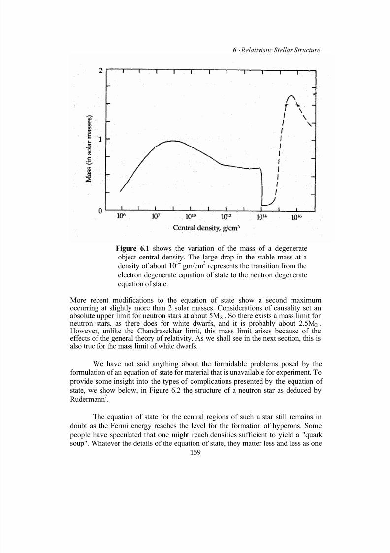
7/18/2019 The Fundamentals of Stellar Astrophysics - Collins G. W.
http://slidepdf.com/reader/full/the-fundamentals-of-stellar-astrophysics-collins-g-w 179/524
6 ⋅ Relativistic Stellar Structure
159
Figure 6.1 shows the variation of the mass of a degenerate
object central density. The large drop in the stable mass at a
density of about 1014
gm/cm3 represents the transition from the
electron degenerate equation of state to the neutron degenerate
equation of state.
More recent modifications to the equation of state show a second maximumoccurring at slightly more than 2 solar masses. Considerations of causality set anabsolute upper limit for neutron stars at about 5M⊙ . So there exists a mass limit forneutron stars, as there does for white dwarfs, and it is probably about 2.5M⊙ .However, unlike the Chandrasekhar limit, this mass limit arises because of theeffects of the general theory of relativity. As we shall see in the next section, this isalso true for the mass limit of white dwarfs.
We have not said anything about the formidable problems posed by the
formulation of an equation of state for material that is unavailable for experiment. To
provide some insight into the types of complications presented by the equation of
state, we show below, in Figure 6.2 the structure of a neutron star as deduced byRudermann
7.
The equation of state for the central regions of such a star still remains in
doubt as the Fermi energy reaches the level for the formation of hyperons. Some
people have speculated that one might reach densities sufficient to yield a "quark
soup". Whatever the details of the equation of state, they matter less and less as one
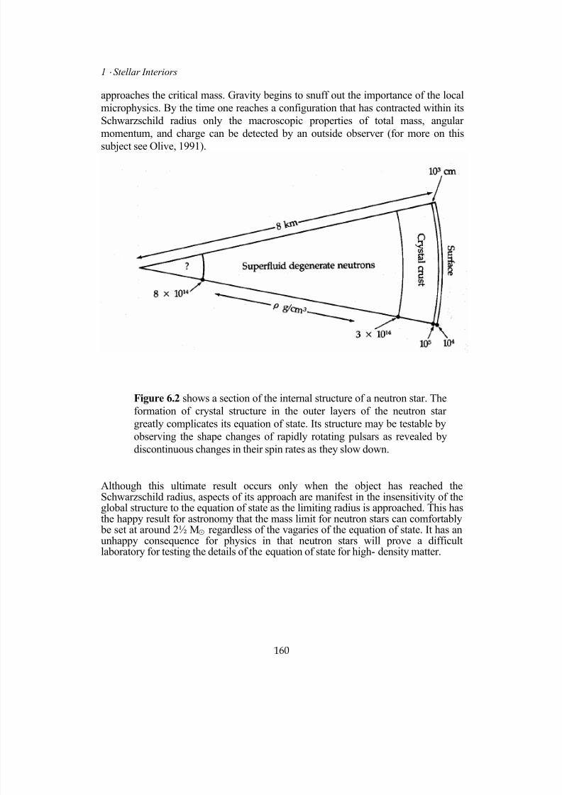
7/18/2019 The Fundamentals of Stellar Astrophysics - Collins G. W.
http://slidepdf.com/reader/full/the-fundamentals-of-stellar-astrophysics-collins-g-w 180/524
1 ⋅ Stellar Interiors
160
approaches the critical mass. Gravity begins to snuff out the importance of the local
microphysics. By the time one reaches a configuration that has contracted within its
Schwarzschild radius only the macroscopic properties of total mass, angular
momentum, and charge can be detected by an outside observer (for more on this
subject see Olive, 1991).
Figure 6.2 shows a section of the internal structure of a neutron star. The
formation of crystal structure in the outer layers of the neutron star
greatly complicates its equation of state. Its structure may be testable by
observing the shape changes of rapidly rotating pulsars as revealed by
discontinuous changes in their spin rates as they slow down.
Although this ultimate result occurs only when the object has reached theSchwarzschild radius, aspects of its approach are manifest in the insensitivity of theglobal structure to the equation of state as the limiting radius is approached. This hasthe happy result for astronomy that the mass limit for neutron stars can comfortably be set at around 2½ M⊙ regardless of the vagaries of the equation of state. It has anunhappy consequence for physics in that neutron stars will prove a difficult
laboratory for testing the details of the equation of state for high- density matter.
7/18/2019 The Fundamentals of Stellar Astrophysics - Collins G. W.
http://slidepdf.com/reader/full/the-fundamentals-of-stellar-astrophysics-collins-g-w 181/524
6 ⋅ Relativistic Stellar Structure
161
6.4 Relativistic Polytrope of Index 3
In Chapter 2, we remarked that the equation of state for a totally relativistic
degenerate gas was a polytrope of index 3. In addition, we noted that an objectdominated by radiation pressure would also be a polytrope of index n = 3. In the first
category we find the extreme white dwarfs, those nearing the Chandrasekhar
degeneracy limit. In the second category we find stars of very great mass where,
from the β* theorem, we can expect the total pressure to be very nearly that of the
pressure from photons. It is somewhat curious that such different types of stars
should have their structures given by the same equilibrium model. However, both
types are dominated by relativistic (in the sense of the special theory of relativity)
particles, and this aspect of the gas is characterized by a polytrope of index n = 3.
Our approach to the study of these objects will be a little different from our
previous discussions of stellar structure. Rather than concentrate on the internal properties and physics of these objects, we consider only their global properties, such
as mass, radius, and internal energy. This will be sufficient to understand their
stability and evolutionary history. The ideal vehicle for such an investigation is the
Virial theorem.
a Virial Theorem for Relativistic Stars
The Virial theorem for relativistic particles differs somewhat from
that derived in Chapter 1. The effect of special relativity on the "mass" or momentum
of such particles increases the gravitational energy required to confine the particles
as the internal energy increases (see Collins8
). Thus, for stable configurations, insteadof
2T + Ω = 0 (6.4.1)
we get
T + Ω = 0 (6.4.2)
which specifies the total energy of the configuration as
E = T + Ω = 0 (6.4.3)
This is sometimes called the binding energy because it is the energy required to
disperse the configuration throughout space. Thus polytropes of index n = 3 are
neutrally stable since it would take no work at all to disperse them and as such these
polytropes represent a limiting condition that can never be reached. To investigatethe fate of objects approaching such a limit, it is necessary to look at the behavior of
those conditions that lead to small departures from the limit. One of those conditions
is the distortion of the metric of space caused by the matter-energy itself and so well
described by the general theory of relativity.
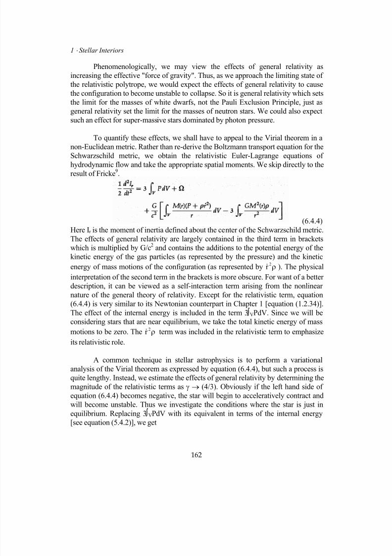
7/18/2019 The Fundamentals of Stellar Astrophysics - Collins G. W.
http://slidepdf.com/reader/full/the-fundamentals-of-stellar-astrophysics-collins-g-w 182/524
1 ⋅ Stellar Interiors
162
Phenomenologically, we may view the effects of general relativity as
increasing the effective "force of gravity". Thus, as we approach the limiting state of
the relativistic polytrope, we would expect the effects of general relativity to cause
the configuration to become unstable to collapse. So it is general relativity which sets
the limit for the masses of white dwarfs, not the Pauli Exclusion Principle, just as
general relativity set the limit for the masses of neutron stars. We could also expect
such an effect for super-massive stars dominated by photon pressure.
To quantify these effects, we shall have to appeal to the Virial theorem in a
non-Euclidean metric. Rather than re-derive the Boltzmann transport equation for the
Schwarzschild metric, we obtain the relativistic Euler-Lagrange equations of
hydrodynamic flow and take the appropriate spatial moments. We skip directly to the
result of Fricke9.
(6.4.4)
Here Ir is the moment of inertia defined about the center of the Schwarzschild metric.
The effects of general relativity are largely contained in the third term in brackets
which is multiplied by G/c2 and contains the additions to the potential energy of the
kinetic energy of the gas particles (as represented by the pressure) and the kinetic
energy of mass motions of the configuration (as represented by ). The physical
interpretation of the second term in the brackets is more obscure. For want of a better
description, it can be viewed as a self-interaction term arising from the nonlinear
nature of the general theory of relativity. Except for the relativistic term, equation(6.4.4) is very similar to its Newtonian counterpart in Chapter 1 [equation (1.2.34)].
The effect of the internal energy is included in the term 3
ρ2r &
VPdV. Since we will be
considering stars that are near equilibrium, we take the total kinetic energy of mass
motions to be zero. The term was included in the relativistic term to emphasize
its relativistic role.
ρ2r &
A common technique in stellar astrophysics is to perform a variational
analysis of the Virial theorem as expressed by equation (6.4.4), but such a process is
quite lengthy. Instead, we estimate the effects of general relativity by determining the
magnitude of the relativistic terms as γ → (4/3). Obviously if the left hand side ofequation (6.4.4) becomes negative, the star will begin to acceleratively contract and
will become unstable. Thus we investigate the conditions where the star is just in
equilibrium. Replacing 3 VPdV with its equivalent in terms of the internal energy
[see equation (5.4.2)], we get
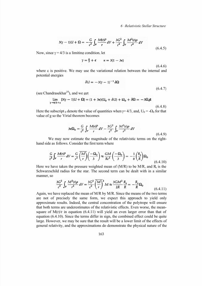
7/18/2019 The Fundamentals of Stellar Astrophysics - Collins G. W.
http://slidepdf.com/reader/full/the-fundamentals-of-stellar-astrophysics-collins-g-w 183/524
6 ⋅ Relativistic Stellar Structure
163
(6.4.5) Now, since γ = 4/3 is a limiting condition, let
(6.4.6)
where ε is positive. We may use the variational relation between the internal and
potential energies
(6.4.7)
(see Chandrasekhar 10
), and we get
(6.4.8)
Here the subscript 0 denote the value of quantities when γ= 4/3, and, U0 = -Ω0 for that
value of g so the Virial theorem becomes
(6.4.9)
We may now estimate the magnitude of the relativistic terms on the right-
hand side as follows. Consider the first term where
(6.4.10)
Here we have taken the pressure weighted mean of (M/R) to be M/R, and R s is the
Schwarzschild radius for the star. The second term can be dealt with in a similar
manner, so
(6.4.11)
Again, we have replaced the mean of M/R by M/R. Since the means of the two terms
are not of precisely the same form, we expect this approach to yield only
approximate results. Indeed, the central concentration of the polytrope will ensure
that both terms are underestimates of the relativistic effects. Even worse, the mean-
square of M(r)/r in equation (6.4.11) will yield an even larger error than that of
equation (6.4.10). Since the terms differ in sign, the combined effect could be quite
large. However, we may be sure that the result will be a lower limit of the effects of
general relativity, and the approximations do demonstrate the physical nature of the
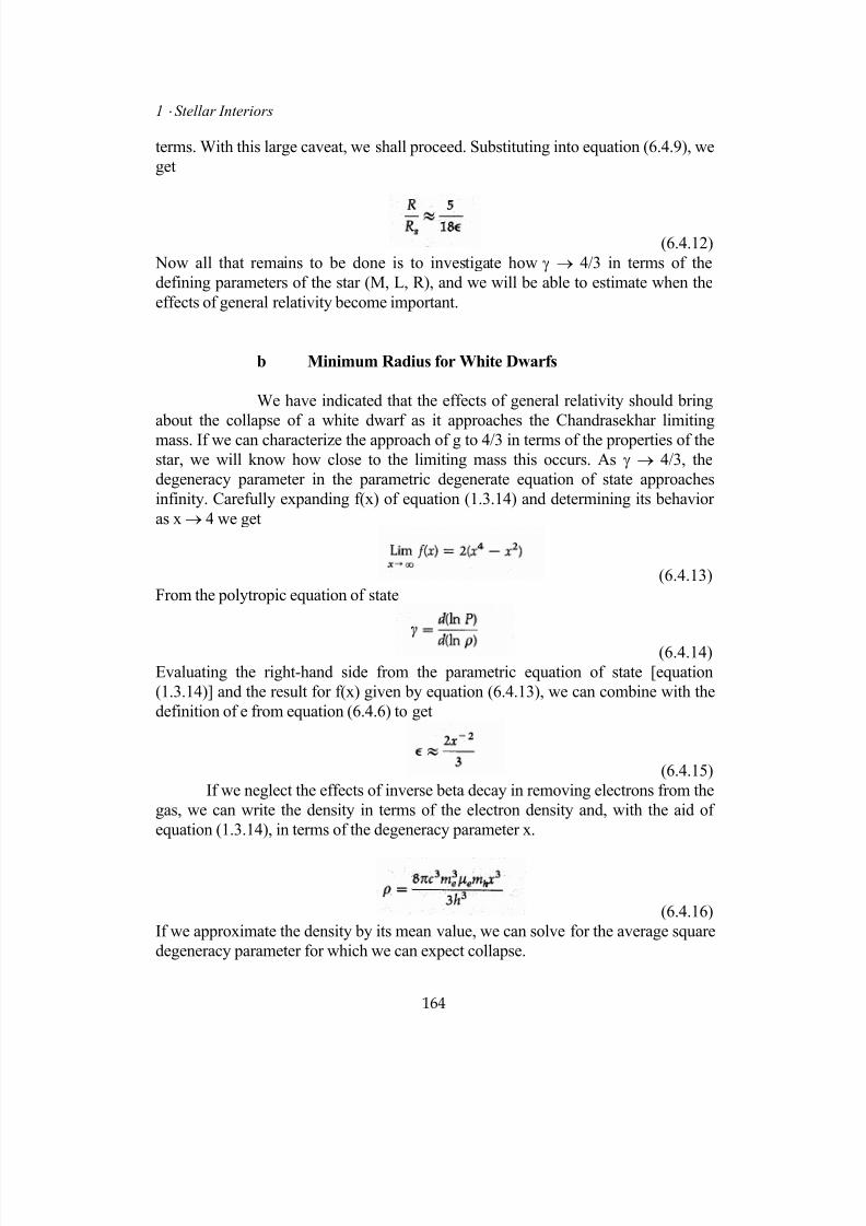
7/18/2019 The Fundamentals of Stellar Astrophysics - Collins G. W.
http://slidepdf.com/reader/full/the-fundamentals-of-stellar-astrophysics-collins-g-w 184/524
1 ⋅ Stellar Interiors
164
terms. With this large caveat, we shall proceed. Substituting into equation (6.4.9), we
get
(6.4.12)
Now all that remains to be done is to investigate how γ → 4/3 in terms of the
defining parameters of the star (M, L, R), and we will be able to estimate when the
effects of general relativity become important.
b Minimum Radius for White Dwarfs
We have indicated that the effects of general relativity should bring
about the collapse of a white dwarf as it approaches the Chandrasekhar limiting
mass. If we can characterize the approach of g to 4/3 in terms of the properties of the
star, we will know how close to the limiting mass this occurs. As γ → 4/3, the
degeneracy parameter in the parametric degenerate equation of state approaches
infinity. Carefully expanding f(x) of equation (1.3.14) and determining its behavior
as x → 4 we get
(6.4.13)
From the polytropic equation of state
(6.4.14)
Evaluating the right-hand side from the parametric equation of state [equation
(1.3.14)] and the result for f(x) given by equation (6.4.13), we can combine with the
definition of e from equation (6.4.6) to get
(6.4.15)
If we neglect the effects of inverse beta decay in removing electrons from the
gas, we can write the density in terms of the electron density and, with the aid of
equation (1.3.14), in terms of the degeneracy parameter x.
(6.4.16)
If we approximate the density by its mean value, we can solve for the average square
degeneracy parameter for which we can expect collapse.
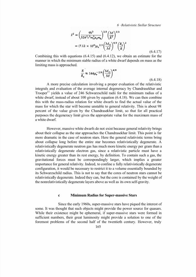
7/18/2019 The Fundamentals of Stellar Astrophysics - Collins G. W.
http://slidepdf.com/reader/full/the-fundamentals-of-stellar-astrophysics-collins-g-w 185/524
6 ⋅ Relativistic Stellar Structure
165
(6.4.17)
Combining this with equations (6.4.15) and (6.4.12), we obtain an estimate for the
manner in which the minimum stable radius of a white dwarf depends on mass as the
limiting mass is approached.
(6.4.18)
A more precise calculation involving a proper evaluation of the relativistic
integrals and evaluation of the average internal degeneracy by Chandrasekhar and
Trooper 11
yields a value of 246 Schwarzschild radii for the minimum radius of a
white dwarf, instead of about 100 given by equation (6.4.18). We can then combinethis with the mass-radius relation for white dwarfs to find the actual value of the
mass for which the star will become unstable to general relativity. This is about 98
percent of the value given by the Chandrasekhar limit, so that for all practical
purposes the degeneracy limit gives the appropriate value for the maximum mass of
a white dwarf.
However, massive white dwarfs do not exist because general relativity brings
about their collapse as the star approaches the Chandrasekhar limit. This point is far
more dramatic in the case of neutron stars. Here the general relativistic terms bring
about collapse long before the entire star becomes relativistically degenerate. A
relativistically degenerate neutron gas has much more kinetic energy per gram than arelativistically degenerate electron gas, since a relativistic particle must have a
kinetic energy greater than its rest energy, by definition. To contain such a gas, the
gravitational forces must be correspondingly larger, which implies a greater
importance for general relativity. Indeed, to confine a fully relativistically degenerate
configuration, it would be necessary to restrict it to a volume essentially bounded by
its Schwarzschild radius. This is not to say that the cores of neutron stars cannot be
relativistically degenerate. Indeed they can, but the core is contained by the weight of
the nonrelativistically degenerate layers above as well as its own self-gravity.
c Minimum Radius for Super-massive Stars
Since the early 1960s, super-massive stars have piqued the interest of
some. It was thought that such objects might provide the power source for quasars.
While their existence might be ephemeral, if super-massive stars were formed in
sufficient numbers, their great luminosity might provide a solution to one of the
foremost problems of the second half of the twentieth century. However, truly
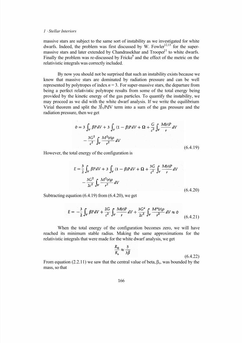
7/18/2019 The Fundamentals of Stellar Astrophysics - Collins G. W.
http://slidepdf.com/reader/full/the-fundamentals-of-stellar-astrophysics-collins-g-w 186/524
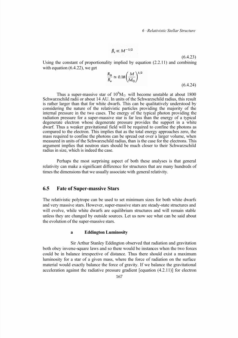
7/18/2019 The Fundamentals of Stellar Astrophysics - Collins G. W.
http://slidepdf.com/reader/full/the-fundamentals-of-stellar-astrophysics-collins-g-w 187/524
6 ⋅ Relativistic Stellar Structure
167
(6.4.23)Using the constant of proportionality implied by equation (2.2.11) and combining
with equation (6.4.22), we get
(6.4.24)
Thus a super-massive star of 108M⊙ will become unstable at about 1800
Schwarzschild radii or about 14 AU. In units of the Schwarzschild radius, this resultis rather larger than that for white dwarfs. This can be qualitatively understood byconsidering the nature of the relativistic particles providing the majority of theinternal pressure in the two cases. The energy of the typical photon providing the
radiation pressure for a super-massive star is far less than the energy of a typicaldegenerate electron whose degenerate pressure provides the support in a whitedwarf. Thus a weaker gravitational field will be required to confine the photons ascompared to the electron. This implies that as the total energy approaches zero, themass required to confine the photons can be spread out over a larger volume, whenmeasured in units of the Schwarzschild radius, than is the case for the electrons. Thisargument implies that neutron stars should be much closer to their Schwarzschildradius in size, which is indeed the case.
Perhaps the most surprising aspect of both these analyses is that general
relativity can make a significant difference for structures that are many hundreds of
times the dimensions that we usually associate with general relativity.
6.5 Fate of Super-massive Stars
The relativistic polytrope can be used to set minimum sizes for both white dwarfs
and very massive stars. However, super-massive stars are steady-state structures and
will evolve, while white dwarfs are equilibrium structures and will remain stable
unless they are changed by outside sources. Let us now see what can be said about
the evolution of the super-massive stars.
a Eddington Luminosity
Sir Arthur Stanley Eddington observed that radiation and gravitation
both obey inverse-square laws and so there would be instances when the two forces
could be in balance irrespective of distance. Thus there should exist a maximum
luminosity for a star of a given mass, where the force of radiation on the surface
material would exactly balance the force of gravity. If we balance the gravitational
acceleration against the radiative pressure gradient [equation (4.2.11)] for electron

7/18/2019 The Fundamentals of Stellar Astrophysics - Collins G. W.
http://slidepdf.com/reader/full/the-fundamentals-of-stellar-astrophysics-collins-g-w 188/524
1 ⋅ Stellar Interiors
168
scattering, we can write
(6.5.1)
Therefore, any object that has a luminosity greater than
(6.5.2)
will be forced into instability by its own radiation pressure. This effectively provides
a mass-luminosity relationship for super-massive stars since these radiation-
dominated configurations will radiate near their limit.
b Equilibrium Mass-Radius Relation
If we now assume that the star can reach a steady-state, that
represents a near-equilibrium state on a dynamical time, then the energy production
must equal the energy lost through the luminosity. Eugene Capriotti14
has evaluated
the luminosity integral and gets
(6.5.3)
We can assume that massive stars will derive the nuclear energy needed to maintain
their equilibrium from the CNO cycle, can evaluate e as indicated in Chapter 3
[equation (3.3.19)], and can evaluate the central term of equation (6.5.3) to obtain the
approximate relation on the right. Assuming that the stars will indeed radiate at the
Eddington luminosity, we can use equation (6.5.2) to find
(6.5.4)
Thus we have a relation between the mass and radius for any super-massive star that
would reach equilibrium through the production of nuclear energy. However, we
have yet to show that the star can reach that equilibrium state.
c Limiting Masses for Super-massive Stars
Let us add equations (6.4.19) and (6.4.20) taking care to express the relativistic
integrals as dimensionless integrals by making use of the homology relations for
pressure and density, and get for the total energy:
∫∫
−
ρρ
+Ωβ−=
1
0
2
22
32c
c
1
022
32
M
)r (dM
r M
R )r (M
cR 2
MG9
M
)r (dM
P
P
r M
R )r (M
cR
MG2
2
1E
(6.5.5)
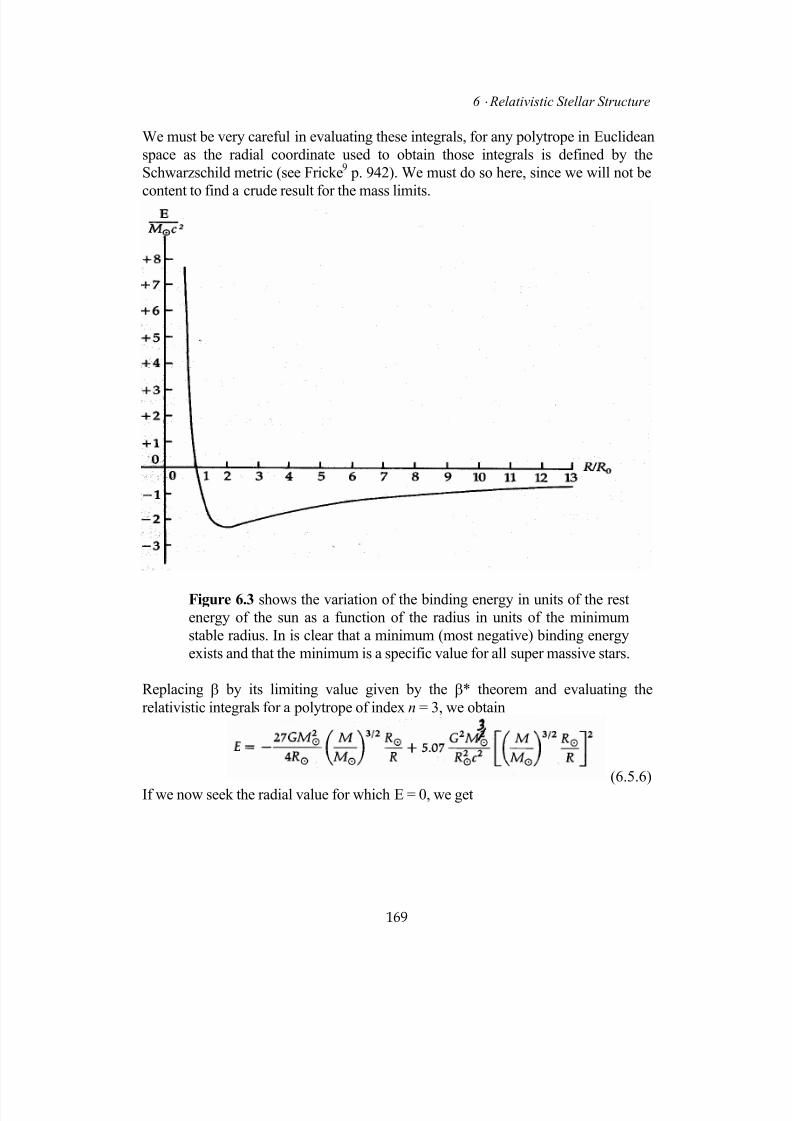
7/18/2019 The Fundamentals of Stellar Astrophysics - Collins G. W.
http://slidepdf.com/reader/full/the-fundamentals-of-stellar-astrophysics-collins-g-w 189/524
6 ⋅ Relativistic Stellar Structure
169
We must be very careful in evaluating these integrals, for any polytrope in Euclidean
space as the radial coordinate used to obtain those integrals is defined by the
Schwarzschild metric (see Fricke9 p. 942). We must do so here, since we will not be
content to find a crude result for the mass limits.
Figure 6.3 shows the variation of the binding energy in units of the rest
energy of the sun as a function of the radius in units of the minimum
stable radius. In is clear that a minimum (most negative) binding energy
exists and that the minimum is a specific value for all super massive stars.
Replacing β by its limiting value given by the β* theorem and evaluating the
relativistic integrals for a polytrope of index n = 3, we obtain
(6.5.6)
If we now seek the radial value for which E = 0, we get
7/18/2019 The Fundamentals of Stellar Astrophysics - Collins G. W.
http://slidepdf.com/reader/full/the-fundamentals-of-stellar-astrophysics-collins-g-w 190/524
7/18/2019 The Fundamentals of Stellar Astrophysics - Collins G. W.
http://slidepdf.com/reader/full/the-fundamentals-of-stellar-astrophysics-collins-g-w 191/524
6 ⋅ Relativistic Stellar Structure
171
If the nuclear energy produced is sufficient to bring the total energy above
the binding energy curve, the star will explode. However, should the energy not be
produced at a rate sufficient to catch the binding energy that is rising due to the
relativistic collapse, the star will continue an unrestrained collapse to theSchwarzschild radius and become a black hole. Which scenario is played out will
depend on the star's mass. For these stars, the temperature gradient will be above the
adiabatic gradient, so convection will exist. However, the only energy transportable
by convection is the kinetic energy of the gas, which is an insignificant fraction of
the internal energy. Therefore, unlike normal main sequence stars, although it is
present, convection will be a very inefficient vehicle for the transport of energy. This
is why the star remains with a structure of a polytrope of index n = 3 in the presence
of convection. The pressure support that determines the density distribution comes
entirely from radiation and is not governed by the mode of energy transport. We saw
a similar situation for degenerate white dwarfs. The equation of state indicated that
their structure would be that of a polytrope of index n= 1.5 (for nonrelativisticdegeneracy) and yet the star would be isothermal due to the long mean free path of
the degenerate electrons. However, the structure is not that of an isothermal sphere
since the pressure support came almost entirely from the degenerate electron gas and
is largely independent of the energy and temperature distribution of the ions.
The star will radiate at the Eddington luminosity, and that will set the time
scale for collapse. Remember that the total energy of these stars is small compared to
the gravitational energy. So most of the energy derived from gravitational
contraction must go into supporting the star, and very little is available to supply the
Eddington luminosity. This can be seen from the relativistic Virial theorem [equation
(6.4.2)], which indicates that any change in the gravitational energy is taken up bythe kinetic energy. Relativistic particles (in this case, photons) are much more
difficult to bind by gravitation than ordinary matter; thus little of the gravitational
energy resulting from collapse will be available to let the star shine. The collapse will
proceed very quickly on a time scale that is much nearer to the dynamical time scale
than the Kelvin-Helmholtz time scale. The onset of nuclear reactions will slow the
collapse, but will not stop it for the massive stars.
A dynamical analysis by Appenzeller and Fricke15,16
(see also Fricke9) shows
that stars more massive than about 7.5 × 10⁵M⊙ will undergo collapse to a black
hole. Here the collapse proceeds so quickly and the gravity is so powerful that thenuclear reactions, being limited by β decay at the resulting high temperatures, do nothave the time to produce sufficient energy to arrest the collapse. For less massivestars, this is not the case. Stars in the narrow range of 5×10
5M⊙ # M # 7.5×10
5M⊙
will undergo explosive nuclear energy generation resulting in the probabledestruction of the star.
Nothing has been said about the role of chemical composition in the
evolution of these stars. Clearly, if there is no carbon present, the CNO cycle is not
7/18/2019 The Fundamentals of Stellar Astrophysics - Collins G. W.
http://slidepdf.com/reader/full/the-fundamentals-of-stellar-astrophysics-collins-g-w 192/524
1 ⋅ Stellar Interiors
172
available for the stabilization of the star. Model calculations show that the triple-a
process cannot stop the collapse. For stars with low metal abundance, only the
proton-proton cycle is available as an energy source. This has the effect of lowering
the value of the maximum stable mass. Surprisingly, there is no range at which an
explosion occurs. If the star cannot stabilize before reaching R m, it will continue in a
state of unrestrained gravitational collapse to a black hole. Thus, it seems unlikely
that stars more massive than about a half million solar masses could exist. In
addition, it seems unlikely that black holes exist with masses greater than a few solar
masses and less than half a million solar masses. If they do, they must form by
accretion and not as a single entity.
Problems
1. Describe the physical conditions that correspond to polytropes of different
indices, and discuss which stars meet these conditions.
2. What modifications must be made to the classical equation of hydrostatic
equilibrium to obtain the Oppenheimer-Volkoff equation of hydrostatic
equilibrium?
3. Find the mass-radius law for super-massive stars generating energy by means
of the proton-proton cycle. Assume that the metal abundance is very small.
4. Determine the mass corresponding to a white dwarf at the limit of stability togeneral relativity.
5. Evaluate the relativistic integrals in equation (6.4.4) for a polytrope of index
n = 3. Be careful for the Euclidean metric appropriate for the polytropic
tables is not the same as the Schwarzschild metric of the equation (see Fricke9
p. 941).
6. Use the results of Problem 5 to reevaluate the minimum radius for white
dwarfs.
7. Assuming that a neutron star can be represented by a polytrope with γ = 3/2,find the minimum radius for a neutron star for which it is stable against
general relativity. To what mass does this correspond?
7/18/2019 The Fundamentals of Stellar Astrophysics - Collins G. W.
http://slidepdf.com/reader/full/the-fundamentals-of-stellar-astrophysics-collins-g-w 193/524
6 ⋅ Relativistic Stellar Structure
173
References and Supplemental Reading
1. Landau, L.: On the Theory of Stars, Physik Zeitz. Sowjetunion 1, 1932, pp.
285 - 288.
2. Oppenheimer, J.R., and Snyder, H.: On Continued Gravitational
Contraction, Phys. Rev. 56, 1939, pp. 455 - 459.
3. Oppenheimer, J.R., and Volkoff, G.: On Massive Neutron Cores, Phys. Rev.
55, 1939, pp. 374 - 381.
4. Misner, C.W., Throne, K.S., and Wheeler, J.A.: Gravitation, W.H. Freeman,
New York, 1970
5. Salpeter, E.E.: Matter at High Densities, Ann. Rev. Phys. 11, 1960, pp. 393 - 417.
6. ______________ Energy and Pressure of a Zero Temperature Plasma,
Ap.J. 134, 1961, pp. 683 - 698.
7. Rudermann, M.: Pulsars: Structure and Dynamics, Ann. Rev. Astron. and
Astrophys. 10, 1972, pp. 427 - 476.
8. Collins, G.W.,II,: The Virial Theorem in Stellar Astrophysics, Pachart
Pubishing House, 1978, pp. 34 -37.
9. Fricke, K.J.: Dynamical Phases of Supermassive Stars, Ap. J. 183, 1973,
pp. 941 - 958.
10. Chandrasekhar S.: An Introduction to the Study of Stellar Structure, Dover,
New York, 1957, p.53 eq. (102).
11. Chandrasekhar,S., and Trooper, R.F.: The Dynamical Instability of the White-
Dwarf Configuration approaching the Limiting Mass, Ap. J. 139, 1964,
pp.1396 -1397.
12. Fowler, W.A.: Massive Stars, Relativistic Polytropes, and Gravitational Radiation, Rev. Mod. Phys., 36, 1964, pp. 545 - 555, p.1104 Errata,
13. Fowler, W.A.: The Stability of Supermassive Stars, Ap.J. 144, 1966,
pp.180 -200.
14. Capriotti, E.R. private communication, 1986.
7/18/2019 The Fundamentals of Stellar Astrophysics - Collins G. W.
http://slidepdf.com/reader/full/the-fundamentals-of-stellar-astrophysics-collins-g-w 194/524
1 ⋅ Stellar Interiors
174
15. Appenzeller, I., and Fricke, K.: Hydrodynamic Model Calculations forSupermassive Stars I: The Collapse of a Nonrotating 0.75 × 10
6 M ⊙ Star ,
Astr. and Ap. 18, 1972, pp. 10 - 15.
16. Appenzeller, I., and Fricke, K.: Hydrodynamic Model Calculations forSupermassive Stars II: The Collapse and Explosion of a Nonrotating
5.2× 10⁵ M ⊙ Star , Astr. and Ap. 21, 1972, pp. 285 - 290.
For a more detailed view of the internal structure of neutron stars, one should
see:
Baym,G., Bethe, H., and Pethick,C.J.: Neutron Star Matter , Nuc. Phys. A
175, 1971, pp. 225 - 271.
No introduction to the structure of degenerate objects would be complete without areading of
Hamada,T. and Salpeter,E.E.: Models for Zero-Temperature Stars, Ap.J.
134, 1961, pp. 683 - 698.
I am indebted to E. R. Capriotti for introducing me to the finer points of super-
massive stars, and most of the material in Sections 6.4b, 6.5b, and 6.5c was
developed directly from his notes of the subject. Those interested in the historical
development of Super-massive stars should read:
Hoyle, F., and Fowler, W.A.: On the Nature of Strong Radio Sources,Mon. Not. R. astr. Soc. 125, 1963, pp. 169 - 176,
Faulkner, J., and Gribbin, J.R.: Stability and Radial Vibrational Periods of
the Hamada Salpeter White Dwarf Models, Nature 218, 1966, pp.734 - 736.
While there are many other contributions to the subject that I have not included,
these will acquaint the readers with the important topics and the flavor of the
subject.
After the initial edition published by W.H. Freeman in 1989 there have been
numerous additions to the literature in this area. One of the most notable dealing withthe structure of Neutron Stars and the Quark-Hadron phase transition is:
Olive, K., 1991, Science, 251, pp. 1197-1198.
7/18/2019 The Fundamentals of Stellar Astrophysics - Collins G. W.
http://slidepdf.com/reader/full/the-fundamentals-of-stellar-astrophysics-collins-g-w 195/524
7 ⋅ Structure of Distorted Stars
Copyright (2003) George W. Collins, II
7
Structure of Distorted Stars
. . .
Throughout this book we have assumed that stars are spherical. This reduces the
problem of stellar structure to one dimension, greatly simplifying its description.
Unfortunately, many stars are not spherical, but are distorted by their own rotation or
the presence of a nearby companion. Not only does this add geometric complications
to the mathematical representation of the equations of stellar structure, but also new
physical phenomena, such as global circulation currents, may result. Major problemsare created for the observational comparison with theory in that the appearance of a
star will now depend on its orientation with respect to the observer. Some quantities,
such as the total luminosity and the stellar effective temperature, are no longer
accessible to observation. With these problems in mind, we consider some
approaches to developing a theoretical framework for the structure of distorted stars.
175
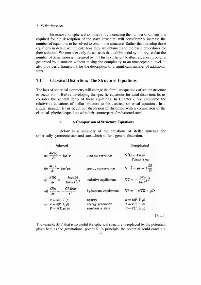
7/18/2019 The Fundamentals of Stellar Astrophysics - Collins G. W.
http://slidepdf.com/reader/full/the-fundamentals-of-stellar-astrophysics-collins-g-w 196/524
1 ⋅ Stellar Interiors
The removal of spherical symmetry, by increasing the number of dimensions
required for the description of the star's structure, will considerably increase the
number of equations to be solved to obtain that structure. Rather than develop those
equations in detail, we indicate how they are obtained and the basic procedures fortheir solution. We consider only those cases that exhibit axial symmetry so that the
number of dimensions is increased by 1. This is sufficient to illustrate most problems
generated by distortion without raising the complexity to an unacceptable level. It
also provides a framework for the description of a significant number of additional
stars.
7.1 Classical Distortion: The Structure Equations
The loss of spherical symmetry will change the familiar equations of stellar structure
to vector form. Before developing the specific equations for axial distortion, let us
consider the general form of these equations. In Chapter 6 we compared therelativistic equations of stellar structure to the classical spherical equations. In a
similar manner, let us begin our discussion of distortion with a comparison of the
classical spherical equations with their counterparts for distorted stars.
a A Comparison of Structure Equations
Below is a summary of the equations of stellar structure for
spherically symmetric stars and stars which suffer a general distortion.
(7.1.1)
176
The variable M (r) that is so useful for spherical structure is replaced by the potential,
given here as the gravitational potential. In principle, the potential could contain a
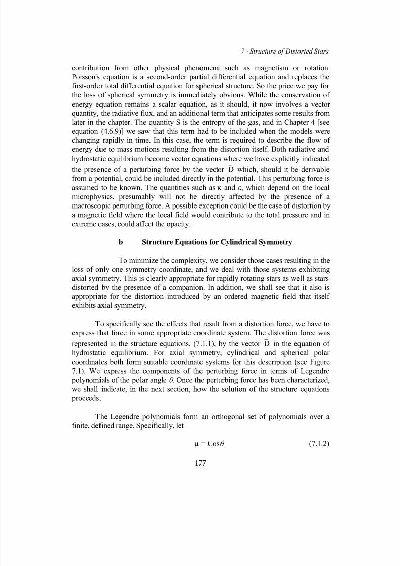
7/18/2019 The Fundamentals of Stellar Astrophysics - Collins G. W.
http://slidepdf.com/reader/full/the-fundamentals-of-stellar-astrophysics-collins-g-w 197/524
7 ⋅ Structure of Distorted Stars
contribution from other physical phenomena such as magnetism or rotation.
Poisson's equation is a second-order partial differential equation and replaces the
first-order total differential equation for spherical structure. So the price we pay for
the loss of spherical symmetry is immediately obvious. While the conservation of
energy equation remains a scalar equation, as it should, it now involves a vector
quantity, the radiative flux, and an additional term that anticipates some results from
later in the chapter. The quantity S is the entropy of the gas, and in Chapter 4 [see
equation (4.6.9)] we saw that this term had to be included when the models were
changing rapidly in time. In this case, the term is required to describe the flow of
energy due to mass motions resulting from the distortion itself. Both radiative and
hydrostatic equilibrium become vector equations where we have explicitly indicated
the presence of a perturbing force by the vector Dr
which, should it be derivable
from a potential, could be included directly in the potential. This perturbing force is
assumed to be known. The quantities such as κ and ε, which depend on the local
microphysics, presumably will not be directly affected by the presence of amacroscopic perturbing force. A possible exception could be the case of distortion by
a magnetic field where the local field would contribute to the total pressure and in
extreme cases, could affect the opacity.
b Structure Equations for Cylindrical Symmetry
To minimize the complexity, we consider those cases resulting in the
loss of only one symmetry coordinate, and we deal with those systems exhibiting
axial symmetry. This is clearly appropriate for rapidly rotating stars as well as stars
distorted by the presence of a companion. In addition, we shall see that it also is
appropriate for the distortion introduced by an ordered magnetic field that itselfexhibits axial symmetry.
To specifically see the effects that result from a distortion force, we have to
express that force in some appropriate coordinate system. The distortion force was
represented in the structure equations, (7.1.1), by the vector Dr
in the equation of
hydrostatic equilibrium. For axial symmetry, cylindrical and spherical polar
coordinates both form suitable coordinate systems for this description (see Figure
7.1). We express the components of the perturbing force in terms of Legendre
polynomials of the polar angle θ . Once the perturbing force has been characterized,
we shall indicate, in the next section, how the solution of the structure equations
proceeds.
The Legendre polynomials form an orthogonal set of polynomials over a
finite, defined range. Specifically, let
µ = Cosθ (7.1.2)
177
7/18/2019 The Fundamentals of Stellar Astrophysics - Collins G. W.
http://slidepdf.com/reader/full/the-fundamentals-of-stellar-astrophysics-collins-g-w 198/524
1 ⋅ Stellar Interiors
Figure 7.1 shows suitable coordinate systems to describe an axially
symmetric perturbing force Dr
with components Dr and Dθ . We have
chosen to illustrate rotational distortion so that Z represents the spin
axis. However, we could have illustrated gravitational distortion by an
external object in which case Z would lie along the line of centers ofthe system and D
r
would point to the center of the other object.
Then the Legendre polynomials form an orthonormal set in the interval
subject to the normalization condition11 +≤µ≤−
(7.1.3)
Here δm,n is the Kronecker delta which is 1 if m = n and 0 otherwise. Various
members of the set of Legendre polynomials can be generated from the recursion
relation
(7.1.4)
where the first three members of the set are
178
7/18/2019 The Fundamentals of Stellar Astrophysics - Collins G. W.
http://slidepdf.com/reader/full/the-fundamentals-of-stellar-astrophysics-collins-g-w 199/524
7 ⋅ Structure of Distorted Stars
(7.1.5)
Before we can specify the effects of the perturbing force in detail, we must
indicate its nature. So let us turn to some simple examples of distorting forces and
their effects on the structure equations.
Rigid Rotation For our first example, we consider the case where the
star is rotating as a rigid body. This yields a simple expression for the magnitude of
the distorting force produced by the local centripetal acceleration, which is
(7.1.6)
where ω is the angular velocity of the star and is assumed to be constant. The
components of the acceleration are then
(7.1.7)
which can be expressed in terms of Legendre polynomials and their derivatives as
(7.1.8)
Due to the axial symmetry, Dφ = 0 and it is a simple matter to show that the curl of D,r
, is 0 so that DD×∇ r
is derivable from a scalar potential by
Λ−∇=Dr
(7.1.9)
where
(7.1.10)
Thus, the components of the perturbing force and the rotational potential can be
expressed in terms of the Legendre polynomials as
(7.1.11)
179
7/18/2019 The Fundamentals of Stellar Astrophysics - Collins G. W.
http://slidepdf.com/reader/full/the-fundamentals-of-stellar-astrophysics-collins-g-w 200/524
1 ⋅ Stellar Interiors
Although the above relations are correct for ω = constant, it is worth
considering the functional dependence of ω for which it is true in general. Consider
the nature of centripetal acceleration in a cylindrical coordinate system where the
radial coordinate is denoted by s. The components of D
r
aresD,0DD 2
sz ω=== φ (7.1.12)
In order for the rotational force to be derivable from a scalar potential, its curl must
be zero. The cylindrical components of the curl are
(7.1.13)
The radial component is identically zero, so we may suspect that if the object
exhibits axial symmetry, ω cannot be a function of φ . In this case, the z component of
the curl would also be zero. Thus, the condition that the rotational force be derivable
from a scalar potential boils down to the φ component of the curl being zero, so that
(7.1.14)
Thus,
(7.1.15)
so the angular velocity must be constant on cylinders. It can be shown, that if the
perturbing force is not derivable from a potential, then no equilibrium solution of the
structure equations exists. This is sometimes called the Taylor-Proudman theorem1
and it basically guarantees that if the star has reached an equilibrium angular
momentum distribution, the angular velocity will be constant on cylinders.
Gravitational Distortion by an External Point Mass Now let us return
to the spherical polar coordinates that we used to obtain the components of the
rotational force. The force will be directed toward an external point mass locatedalong the z axis at a distance d from the center of the star (see Figure 7.2).
180
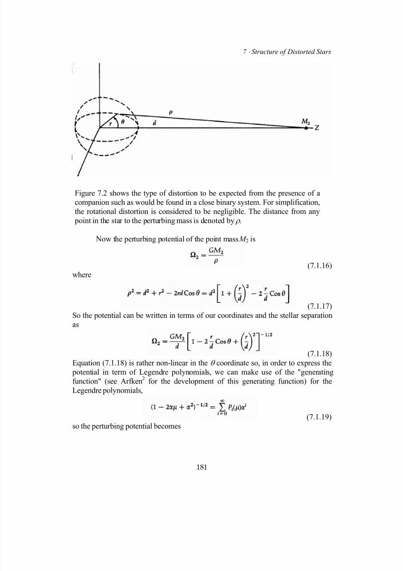
7/18/2019 The Fundamentals of Stellar Astrophysics - Collins G. W.
http://slidepdf.com/reader/full/the-fundamentals-of-stellar-astrophysics-collins-g-w 201/524
7 ⋅ Structure of Distorted Stars
Figure 7.2 shows the type of distortion to be expected from the presence of a
companion such as would be found in a close binary system. For simplification,the rotational distortion is considered to be negligible. The distance from any
point in the star to the perturbing mass is denoted by ρ .
Now the perturbing potential of the point mass M 2 is
(7.1.16)
where
(7.1.17)
So the potential can be written in terms of our coordinates and the stellar separation
as
(7.1.18)
Equation (7.1.18) is rather non-linear in the θ coordinate so, in order to express the
potential in term of Legendre polynomials, we can make use of the "generating
function" (see Arfken2 for the development of this generating function) for the
Legendre polynomials,
(7.1.19)
so the perturbing potential becomes
181
7/18/2019 The Fundamentals of Stellar Astrophysics - Collins G. W.
http://slidepdf.com/reader/full/the-fundamentals-of-stellar-astrophysics-collins-g-w 202/524
1 ⋅ Stellar Interiors
(7.1.20)
Since the perturbing force is conservative, we may obtain it from
(7.1.21)
which has components
(7.1.22)
So far, the only approximation that we have made is that the perturbing
potential is that of a point mass. To simplify the remaining discussion, we assume
that the point mass is distant compared to the size of the object so that
(7.1.23)
Note that the zeroth order terms of the components can be added vectorially to give
(7.1.24)
This is just the gravitational force that is balanced by the acceleration resulting from
the orbital motion of the system, and so this force can be made to vanish by going to
a rotating coordinate system. In such a system, the components of the perturbing
force will just be the first-order terms, so that
(7.1.25)
These components of the perturbing force have the same form as those of rotation[see equation (7.1.11)], and any method which is applicable to the solution of the
structure equations for rotational distortion will also be applicable to the problem of
gravitational distortion.
182

7/18/2019 The Fundamentals of Stellar Astrophysics - Collins G. W.
http://slidepdf.com/reader/full/the-fundamentals-of-stellar-astrophysics-collins-g-w 203/524
7 ⋅ Structure of Distorted Stars
Distortion Resulting from a Toroidal Magnetic Field Consider the Lorentz
force of an internal magnetic field on the material of the star:
(7.1.26)
The perturbing acceleration due to this force will be
(7.1.27)
Now assume a special, but not implausible, geometry for the internal stellar magnetic
field. Specifically, let us choose a toroidal field that exhibits pure axial symmetry so
that
(7.1.28)where ψ (r) contains the arbitrary, but presumed known, variation of the field with the
radial coordinate r. Since the field only has a φ component, the vector part of
equation (7.1.27) is
(7.1.29)r
The θ and r components of the curl of B are
(7.1.30)
which yields for the vector components of the perturbing field
θ∂
θ∂=
θ∂
θ∂ψπρ=
θ+=θ
∂ψ∂
ψ+ψ
πρ=
−θ
−
)Cos(P)r (C
~)Cos(P
r
)r ()c4((D
)Cos(P)r (B~
)r (A~
Sinr
)r (r
)r ()c4(D
22
21
2
22
1
r
(7.1.31)
Again, these components have the same form as those of rotational distortion.
Thus we can expect to be able to solve a wide variety of distortion problems
by considering the single case of an axis-symmetric perturbing force of the form
given in equations (7.1.11), (7.1.25), and (7.1.31). We now consider some aspects of
the solution of such problems.
183
7/18/2019 The Fundamentals of Stellar Astrophysics - Collins G. W.
http://slidepdf.com/reader/full/the-fundamentals-of-stellar-astrophysics-collins-g-w 204/524
1 ⋅ Stellar Interiors
7.2 Solution of Structure Equations for a Perturbing Force
The equations given by equations (7.1.1), and which arise from the perturbations
discussed in Section 7.1, are partial differential equations and must be solved
numerically. The numerical solution of partial differential equations constitutes a
major area of study in its own right and is beyond the scope of this book. So we leave
the numerical methods required for the actual solution to others and another time.
Instead, we concentrate on the conditions required for the equations to have a
solution and some of the implications of those solutions.
Since the perturbing forces derived in Section 7.1 are all conservative forces
(that is, ∇ ×Dr
= 0), they are all derivable from some scalar potential which we can
call . This can be added to the gravitational potential so that we have a generalized potential to enter into the structure equations which we can call
(7.2.1)
Since all the forces exhibited axial symmetry, there will be no explicit dependence of
the generalized potential on φ . There will be sets of values of θ and r, for whichΦ is
constant. For the unperturbed gravitational potential alone these would be spheres of
a given radius. For the generalized potential, they will be surfaces that exhibit axial
symmetry. Such surfaces are known as level surfaces since a particle placed on one
would feel no forces that would move it along the surface. Thus, if represents a
normal to such a surface, the gradient of the potential can be expressed as
n
(7.2.2)
As long as the chemical composition is constant, the state variables will be
constant on level surfaces. This is sometimes known as Poincare's theorem which
we prove for rotation in the next section. However, the result is entirely reasonable.
The values of the state variables change in response to forces acting on the gas. Since
the potential is constant on a level surface and its gradient is always normal to the
surface, there are no forces along the surface to produce such differences.
If we take the state variables to be constant along level surfaces of constant potential, we can expect the variables to have the same functional dependence on the
coordinates as the potential itself. Thus, from the form of given by equation
(7.1.11), the state variables, and those parameters that depend directly on them, can
be written as
184
7/18/2019 The Fundamentals of Stellar Astrophysics - Collins G. W.
http://slidepdf.com/reader/full/the-fundamentals-of-stellar-astrophysics-collins-g-w 205/524
7 ⋅ Structure of Distorted Stars
(7.2.3)
The gravitational potential must also be written with a θ dependence, because the
perturbing force will rearrange the matter density so that the potential is no longer
spherically symmetric.
We now regard equations (7.2.3) as perturbative equations in the traditional
sense in that the terms with subscript 2 will be considered to be small compared to
the terms with subscript 0.
a Perturbed Equation of Hydrostatic Equilibrium
Substituting the perturbed form of the structure variables given by
equation (7.2.3), into the equation of hydrostatic equilibrium [equation (7.1.1 d)], we
get
(7.2.4)
The terms on the last line of equation (7.2.4) are small "second-order" terms by
comparison to the other terms, so, in the tradition of perturbative analysis, we will
ignore them. Since the equations must hold for all values of θ , the r component of the
gradient yields two distinct equations and the θ component yields one equation.
These are basically the zeroth and second-order equations from the two components
of the gradient. However, in general, there will be no zeroth-order θ equation, since
the unperturbed state is spherically symmetric. Remembering the form for Dr
from
equation (7.1.11), we see that the partial differential equations for hydrostatic
equilibrium are
185
7/18/2019 The Fundamentals of Stellar Astrophysics - Collins G. W.
http://slidepdf.com/reader/full/the-fundamentals-of-stellar-astrophysics-collins-g-w 206/524
1 ⋅ Stellar Interiors
r /)r (C)r ()r ()r ()r (P
)r (B)r (r
)r ()r (
r
)r ()r (
r
)r (P
)r (A)r (r
)r (
r
)r (P
0202
0
0
2
2
0
2
0
0
0
0
ρ+Ωρ−=
ρ+∂
Ω∂ρ+
∂
Ω∂ρ−=
∂
∂
ρ+∂
Ω∂ρ−=
∂
∂
(7.2.5)
b Number of Perturbative Equations versus Number of
Unknowns
The number of independent partial differential equations generated
by the vector equation of hydrostatic equilibrium is 3. In general, the vector
equations of stellar structure will yield three such independent equations while the
scalar equations will produce only two, since there is no θ component. In Table 7.1
we summarize the number of equations we can expect from each of the structureequations.
Each of the perturbed variables P, T, and Ω will produce a first- and second-
order unknown function of r for a total of six unknowns. The perturbations in the
density ρ are not linearly independent since they are related to those of P and T by
the equation of state. A similar situation exists for the opacity κ and energy
generation ε. However the radiative flux is a vector quantity and will yield two
unknown perturbed quantities, F0r and F2r , from the r-component and one, F1θ, from
the θ component. Thus the total number of unknowns in the problem is 9 and the
problem is over determined and has no solution. This implies that we have left some
physics out of the problem.
In counting the unknowns resulting from perturbing equations (7.1.1), we
implicitly assumed that there were no mass motions present in the star, with the
result that ∂ S /∂t in equation (7.1.1b) was taken to be zero. If we assume that a
stationary state exists, then we can represent the local time rate of change of entropy
by a velocity times an entropy gradient, so equation (7.1.1b) becomes
(7.2.6)
Thus, we have added a velocity with three components each of which willhave two perturbed parameters. However, in general 0vr
will be zero, since we
assume no circulation currents in the unperturbed model. In addition, S will exhibit
axial symmetry and have no φ component. Thus the v2φ perturbed parameter will be
orthogonal to S and not appear in the final equations. This leaves us with 11
unknowns and 10 equations. However, we have not included the fact that mass
conservation must be involved with any transport of matter, and modifying the
186
7/18/2019 The Fundamentals of Stellar Astrophysics - Collins G. W.
http://slidepdf.com/reader/full/the-fundamentals-of-stellar-astrophysics-collins-g-w 207/524
7 ⋅ Structure of Distorted Stars
conservation of mass equation to include mass motions will provide one more
equation, completing the specification of the problem.
7.3 Von Zeipel's Theorem and Eddington-Sweet Circulation
Currents
For a solution to exist for the structure of a distorted star, we had to invoke mass
motions in the star itself. This result was essentially obtained by von Zeipel3 in the
middle 1920s. At that time, the source of stellar energy was unknown, and von
Zeipel set about to place constraints on the energy generation within a distorted star
and in so doing produced one of the most misunderstood theorems of stellar
astrophysics. The theorem is essentially a proof by contradiction that stars cannot
simultaneously satisfy radiative and hydrostatic equilibrium if the stars are distorted.
The normal version of the theorem is given for rigidly rotating stars and this is theversion quoted by Eddington
4. However, in the original publication, the version
developed for rigid rotation is followed immediately by a version appropriate for
tidally distorted stars5. Thus, clearly the theorem results from the induced distortion
itself and is independent of the details that produce the distortion. We describe the
version for rotation here, but keep in mind that is it the distortion that is important,
not the mechanism by which that distortion is generated.
a Von Zeipel's Theorem
As originally stated by von Zeipel3 in 1924, this theorem says that for
a rigidly rotating star in hydrostatic and radiative equilibrium, the rate of energygeneration is given by
(7.3.1)
187
7/18/2019 The Fundamentals of Stellar Astrophysics - Collins G. W.
http://slidepdf.com/reader/full/the-fundamentals-of-stellar-astrophysics-collins-g-w 208/524
1 ⋅ Stellar Interiors
In light of what we now know about stars, this is an absurd result, because it requires
that the energy generation rate become negative near the surface as the density goes
to zero. As is the case when any theorem yields an absurd result, one must challenge
the assumptions. To see where the trouble is likely to be, let us sketch von Zeipel'sargument.
The equation of hydrostatic equilibrium
(7.3.2)
indicates that the potential gradient is related to the pressure gradient by the scalar
density ρ . Hence, both vectors point in the same direction, and we can describe the
change in pressure as a proportional change in potential so that
(7.3.3)
From this it is clear, that the pressure must be constant on a level surface where
dΦ = 0. This is equivalent to saying that the pressure can be written as a function of
the potential Φ alone. If the pressure is a function of Φ alone, then the scalar ρ ,
relating the potential and pressure gradients, must also be a function of Φ alone. Or
(7.3.4)
As long as the chemical composition µ is constant or at least not varying over an
equipotential (level) surface, the ideal-gas law guarantees that the temperature will
also be a function of Φ alone:
(7.3.5)
This is what we stated in Section 7.2 to be Poincare's theorem.
Now the radiative temperature gradient which arises from radiative
equilibrium requires that
(7.3.6)which, expressed in terms of the potential gradient, becomes
(7.3.7)
188
However, since κ , ρ , and T are all state variables or functions of them, they are all
functions ofΦ alone and

7/18/2019 The Fundamentals of Stellar Astrophysics - Collins G. W.
http://slidepdf.com/reader/full/the-fundamentals-of-stellar-astrophysics-collins-g-w 209/524
7 ⋅ Structure of Distorted Stars
(7.3.8)
But Φ is just the local gravity, and it is most certainly not a function of the
potential alone or constant on level surfaces. Indeed, for a critically rotating star, the
gravity varies from the mass gravity at the pole to zero at the equator, where the mass
gravity is balanced by the centripetal acceleration. Thus, equation (7.3.8) basically
says that in the presence of the radiative temperature gradient
(7.3.9)
which is sometimes known as von Zeipel's law of gravity darkening .
If we further consider radiative equilibrium in the absence of mass motions,
we can write
(7.3.10)
For a star in rigid rotation,2Φ will depend on only the density and some constants
and so will be a function of Φ alone. The left-hand side of equation (7.3.10) will
depend on only the state variables and must also be a function ofΦ alone. But, again,
the gravity Φ is not a function of Φ alone, so
(7.3.11)
Therefore, evaluating2Φ by means of equations (7.1.10) and (7.2.1), we get
(7.3.12)
189
The absurdity of equation (7.3.12) results primarily from the assumption that
the effects of mass motions are not present in equation (7.3.10). The addition of mass
motions removes the exclusive dependence of radiative equilibrium on the potential
and the remainder of the argument falls apart releasing the constraint on ε. The
gradient of f(Φ) is no longer zero and allows for the variation of ε with radius that
we know must exist. However, as we shall see, small amounts of energy are all that
is required to be carried by the currents of the mass motions. Thus the radiative
gradient will still be basically the temperature gradient that is operative in the
radiative zones of the star. The result given in equation (7.3.9) will still be largely
correct, and we may expect the radiative flux to be redistributed in accordance with
the local value of the gravity. Therefore, particularly for the rapidly rotating upper
main sequence stars with radiative envelopes, we may expect that their surface will
not be uniformly bright, but will become darker with decreasing local gravity. While

7/18/2019 The Fundamentals of Stellar Astrophysics - Collins G. W.
http://slidepdf.com/reader/full/the-fundamentals-of-stellar-astrophysics-collins-g-w 210/524
1 ⋅ Stellar Interiors
it is true that the conditions of radiative equilibrium become rather different in the
stellar atmosphere as the photons begin to escape into outer space, the thickness of
the atmosphere compared to the depth of the radiative envelope is minuscule and
whatever variation of radiative flux has been established at the base of theatmosphere will be largely reflected in the flux emerging from the star. So von
Zeipel's theorem, while telling us nothing about the energy generation within the star,
does tell us quite a lot about the manner in which the radiation leaves the star.
b Eddington-Sweet Circulation Currents
We have seen that radiative and hydrostatic equilibrium cannot be
simultaneously satisfied in a distorted star and that the failure of these conditions
results in the mass motion of material carrying energy to make up the deficit
produced by the departure from spherical geometry. That the energy transfer is
accomplished by means of the physical motion of material seems ensured. Theresimply is no other mechanism to effect the transfer. Radiation has been accounted
for, conduction is ineffective and the environment is stable against classical
convection. These arguments persuaded Eddington4
(p. 286) to suggest the existence
of such currents which were later quantified by Sweet6. Let us now estimate the
speed of these currents and determine the amount of energy they may carry. The
currents will be quite slow since, even in the most distorted of stars the local
departure of the energy flux from spherical symmetry is quite small. Even so, any
mass motion could be important if it transports material throughout the star on a
nuclear time scale. The possibility would then exist for a resupply of nuclear fuel,
and that could upset some of our stellar evolution calculations.
Conservation of Energy and Circulation Velocity The distortion of a star
will force a departure from radiative equilibrium and a change in the divergence of
the radiative flux from that expected for spherical stars. We argued earlier that the
change in the divergence will be brought about by the additional nonradial transport
of energy by mass motions, as expressed by the second term on the right-hand side of
equation (7.2.6). Thus, to estimate the velocity of those motions, we must estimate
the entropy gradient that distortion will establish.
From thermodynamics remember that the entropy can be expressed in terms
of the state variables of an ideal gas as
(7.3.13)
Therefore, the general energy source term in equations (7.1.1b) can be written as
190
7/18/2019 The Fundamentals of Stellar Astrophysics - Collins G. W.
http://slidepdf.com/reader/full/the-fundamentals-of-stellar-astrophysics-collins-g-w 211/524
7 ⋅ Structure of Distorted Stars
(7.3.14)
and the entropy gradient of equation (7.2.6) becomes
(7.3.15)
Now the temperature and pressure gradients are both normal to equipotential
surfaces, so the vector nature of equation (7.3.15) is unimportant and it must hold for
the magnitude of the individual terms. Therefore,
(7.3.16)
Equation (7.3.16), when combined with the ideal-gas law and the fact that the
temperature and pressure gradients point in the same direction, enables equation(7.3.15) to be written as
(7.3.17)
Now the adiabatic gradient can be expressed as
(7.3.18)
Since for the zeroth-order values of these gradients
(7.3.19)
we can write the zeroth-order value for the entropy gradient as
(7.3.20)
In the equilibrium model, there are no mass motions; the velocity in equation
(7.2.6) is already a first-order term and so to estimate its value we need only keep
zeroth-order terms in the entropy gradient. The zeroth-order pressure gradient is just
(7.3.21)
Combining this with equations (7.2.6) and (7.3.20), we can write the perturbed
191
7/18/2019 The Fundamentals of Stellar Astrophysics - Collins G. W.
http://slidepdf.com/reader/full/the-fundamentals-of-stellar-astrophysics-collins-g-w 212/524
1 ⋅ Stellar Interiors
equation for energy conservation as
(7.3.22)
Now, from von Zeipel's gravity darkening law [equations (7.3.6) and (7.3.7)]
we have
(7.3.23)
which means that we can write the divergence of the flux as
(7.3.24)
But, since the radiative flux and gravity are vectors pointing in the same direction,
(7.3.25)For rotation we can obtain the generalized potential from equations (7.1.1a)
and (7.1.10). Expressing the rotational potential in cylindrical coordinates, we get
(7.3.26)
Equation (7.3.24) for the perturbed flux divergence can be broken into its perturbed
components so that
(7.3.27)
Since the zeroth-order flux-to-gravity ratio can be written as
192
7/18/2019 The Fundamentals of Stellar Astrophysics - Collins G. W.
http://slidepdf.com/reader/full/the-fundamentals-of-stellar-astrophysics-collins-g-w 213/524
7 ⋅ Structure of Distorted Stars
(7.3.28)
its derivative with respect to the generalized potential is
(7.3.29)
The luminosity can be written in terms of an average energy generation ratee
and M (r) so that
(7.3.30)which yields
(7.3.31)
If we further assume that the distortion is small so that g2/g0 << 1, then equation
(7.3.31) can be combined with equation (7.3.22) to give the velocity for the induced
circulation currents as
(7.3.32)
Eddington-Sweet Time Scale and Mixing If we take reasonable values
for the parameters in equation (7.3.32), namely,
(7.3.33)
then we can rewrite the circulation velocity as
(7.3.34)
Here we have introduced the fractional angular rotational velocity w, which is just ω
normalized by the critical angular velocity, ωc, where the effective equatorial gravity
is zero for a centrally condensed star (Roche model). In addition, if we introduce a
time scale such as the Kelvin-Helmholtz time scale [equation (3.2.11)], we can
193

7/18/2019 The Fundamentals of Stellar Astrophysics - Collins G. W.
http://slidepdf.com/reader/full/the-fundamentals-of-stellar-astrophysics-collins-g-w 214/524

7/18/2019 The Fundamentals of Stellar Astrophysics - Collins G. W.
http://slidepdf.com/reader/full/the-fundamentals-of-stellar-astrophysics-collins-g-w 215/524
7 ⋅ Structure of Distorted Stars
On the basis of this analysis we would have to conclude that there is an
excellent possibility that rapidly rotating stars on the upper main sequence may be
mixed thoroughly throughout and their main sequence life times may be prolonged.
However, we have not dealt with the formation of the helium core itself and the
effects caused by the change in chemical composition.
7.4 Rotational Stability and Mixing
A complete discussion of the stability of a rotating star is quite complicated and
beyond the scope of this book. However, we consider some of the important effects
on the stability of rotating stars. The usual approach to the subject of stability
involves finding the spectrum of perturbations for which the equations of motion are
stable (i.e., the perturbations will damp out with time). A related approach is to usethe Virial theorem
7, which after all is just a spatial moment of the equations of
motion. Various physical processes may occur and give rise to an instability:
1. Buoyancy forces that result from thermal stratification
2. Perturbations that may grow in the presence of an angular momentum
gradient
3. Instabilities in the presence of a magnetic field
4. Shear instabilities producing flows both parallel and perpendicular to the
local gravity field
5. Failure of the equipotential surfaces being surfaces of constant temperature
and pressure [that is, ω ≠ ω(s)]6. Development of a molecular weight gradient as a result of nuclear evolution
7 Diffusion of heat, angular momentum, and the mean molecular weight
Of all these effects, probably the most important for the stability of rotating stars is
the various shear instabilities.
a Shear Instabilities
The existence of a velocity gradient implies the presence of particle
interactions resulting from changes in the macroscopic velocity field. These
interactions result from the collisions that are the product of the differential streammotion of the gas, and the severity of these collisions is usually characterized by the
viscosity n of the material. The viscosity will try to remove the velocity gradient.
However, if the shear is too great, the velocity field will break up into turbulent flow.
The conditions of the flow can be characterized by a dimensionless number known
as the Reynolds number Re, which for rotating stars is
195
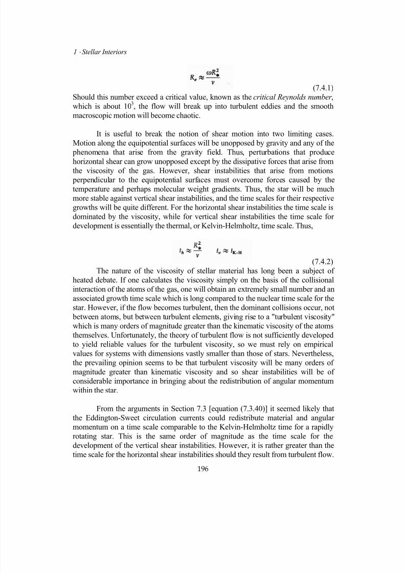
7/18/2019 The Fundamentals of Stellar Astrophysics - Collins G. W.
http://slidepdf.com/reader/full/the-fundamentals-of-stellar-astrophysics-collins-g-w 216/524
1 ⋅ Stellar Interiors
(7.4.1)
Should this number exceed a critical value, known as the critical Reynolds number ,which is about 103, the flow will break up into turbulent eddies and the smooth
macroscopic motion will become chaotic.
It is useful to break the notion of shear motion into two limiting cases.
Motion along the equipotential surfaces will be unopposed by gravity and any of the
phenomena that arise from the gravity field. Thus, perturbations that produce
horizontal shear can grow unopposed except by the dissipative forces that arise from
the viscosity of the gas. However, shear instabilities that arise from motions
perpendicular to the equipotential surfaces must overcome forces caused by the
temperature and perhaps molecular weight gradients. Thus, the star will be much
more stable against vertical shear instabilities, and the time scales for their respectivegrowths will be quite different. For the horizontal shear instabilities the time scale is
dominated by the viscosity, while for vertical shear instabilities the time scale for
development is essentially the thermal, or Kelvin-Helmholtz, time scale. Thus,
(7.4.2)
The nature of the viscosity of stellar material has long been a subject of
heated debate. If one calculates the viscosity simply on the basis of the collisional
interaction of the atoms of the gas, one will obtain an extremely small number and an
associated growth time scale which is long compared to the nuclear time scale for thestar. However, if the flow becomes turbulent, then the dominant collisions occur, not
between atoms, but between turbulent elements, giving rise to a "turbulent viscosity"
which is many orders of magnitude greater than the kinematic viscosity of the atoms
themselves. Unfortunately, the theory of turbulent flow is not sufficiently developed
to yield reliable values for the turbulent viscosity, so we must rely on empirical
values for systems with dimensions vastly smaller than those of stars. Nevertheless,
the prevailing opinion seems to be that turbulent viscosity will be many orders of
magnitude greater than kinematic viscosity and so shear instabilities will be of
considerable importance in bringing about the redistribution of angular momentum
within the star.
From the arguments in Section 7.3 [equation (7.3.40)] it seemed likely that
the Eddington-Sweet circulation currents could redistribute material and angular
momentum on a time scale comparable to the Kelvin-Helmholtz time for a rapidly
rotating star. This is the same order of magnitude as the time scale for the
development of the vertical shear instabilities. However, it is rather greater than the
time scale for the horizontal shear instabilities should they result from turbulent flow.
196
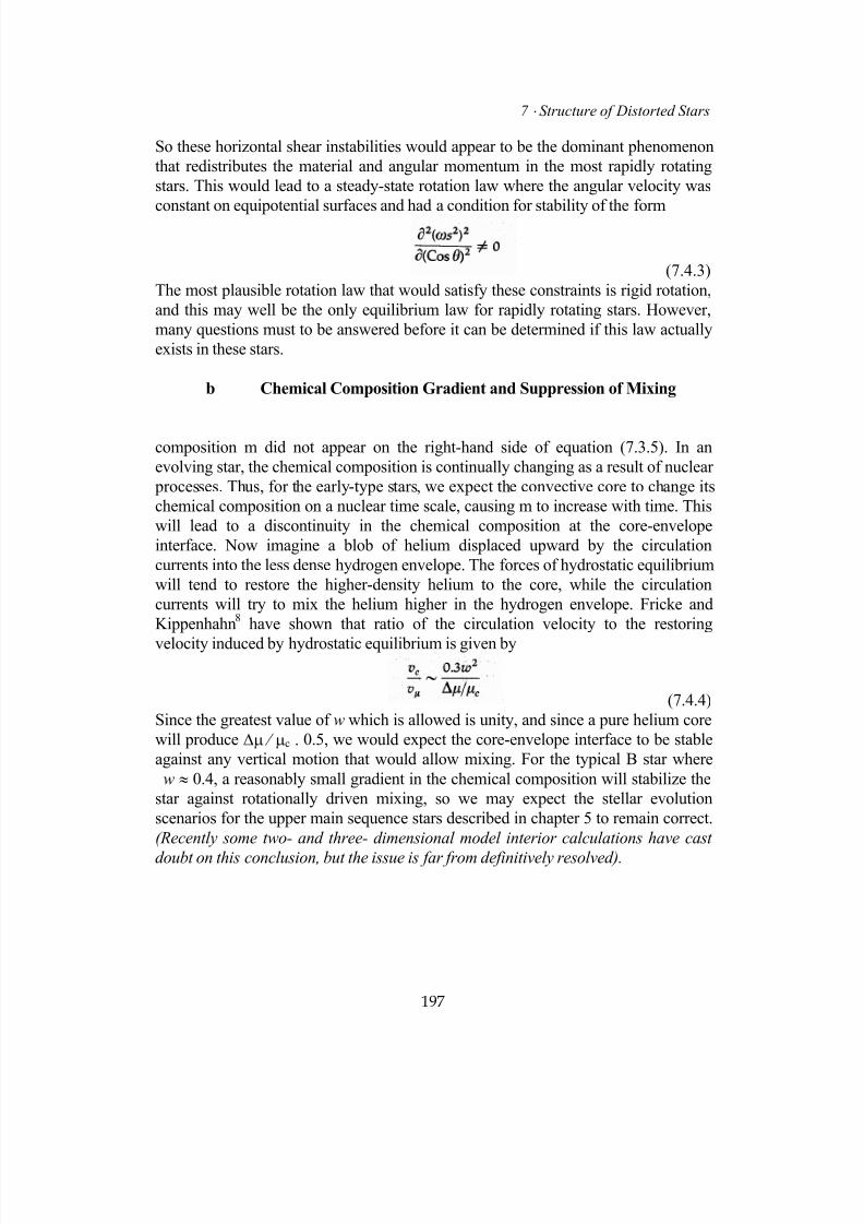
7/18/2019 The Fundamentals of Stellar Astrophysics - Collins G. W.
http://slidepdf.com/reader/full/the-fundamentals-of-stellar-astrophysics-collins-g-w 217/524
7 ⋅ Structure of Distorted Stars
So these horizontal shear instabilities would appear to be the dominant phenomenon
that redistributes the material and angular momentum in the most rapidly rotating
stars. This would lead to a steady-state rotation law where the angular velocity was
constant on equipotential surfaces and had a condition for stability of the form
(7.4.3)
The most plausible rotation law that would satisfy these constraints is rigid rotation,
and this may well be the only equilibrium law for rapidly rotating stars. However,
many questions must to be answered before it can be determined if this law actually
exists in these stars.
b Chemical Composition Gradient and Suppression of Mixing
composition m did not appear on the right-hand side of equation (7.3.5). In an
evolving star, the chemical composition is continually changing as a result of nuclear
processes. Thus, for the early-type stars, we expect the convective core to change its
chemical composition on a nuclear time scale, causing m to increase with time. This
will lead to a discontinuity in the chemical composition at the core-envelope
interface. Now imagine a blob of helium displaced upward by the circulation
currents into the less dense hydrogen envelope. The forces of hydrostatic equilibrium
will tend to restore the higher-density helium to the core, while the circulation
currents will try to mix the helium higher in the hydrogen envelope. Fricke and
Kippenhahn8 have shown that ratio of the circulation velocity to the restoring
velocity induced by hydrostatic equilibrium is given by
(7.4.4)
Since the greatest value of w which is allowed is unity, and since a pure helium core
will produce ∆µ ⁄ µc . 0.5, we would expect the core-envelope interface to be stable
against any vertical motion that would allow mixing. For the typical B star where
w ≈ 0.4, a reasonably small gradient in the chemical composition will stabilize the
star against rotationally driven mixing, so we may expect the stellar evolution
scenarios for the upper main sequence stars described in chapter 5 to remain correct.
(Recently some two- and three- dimensional model interior calculations have cast
doubt on this conclusion, but the issue is far from definitively resolved).
197
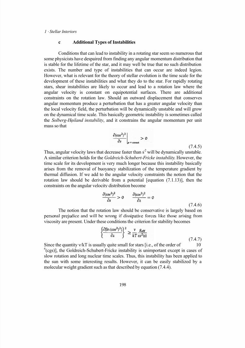
7/18/2019 The Fundamentals of Stellar Astrophysics - Collins G. W.
http://slidepdf.com/reader/full/the-fundamentals-of-stellar-astrophysics-collins-g-w 218/524
1 ⋅ Stellar Interiors
c Additional Types of Instabilities
Conditions that can lead to instability in a rotating star seem so numerous that
some physicists have despaired from finding any angular momentum distribution thatis stable for the lifetime of the star, and it may well be true that no such distribution
exists. The number and type of instabilities that can occur are indeed legion.
However, what is relevant for the theory of stellar evolution is the time scale for the
development of these instabilities and what they do to the star. For rapidly rotating
stars, shear instabilities are likely to occur and lead to a rotation law where the
angular velocity is constant on equipotential surfaces. There are additional
constraints on the rotation law. Should an outward displacement that conserves
angular momentum produce a perturbation that has a greater angular velocity than
the local velocity field, the perturbation will be dynamically unstable and will grow
on the dynamical time scale. This basically geometric instability is sometimes called
the Solberg-H φiland instability, and it constrains the angular momentum per unitmass so that
(7.4.5)
Thus, angular velocity laws that decrease faster than s-2
will be dynamically unstable.
A similar criterion holds for the Goldreich-Schubert-Fricke instability. However, the
time scale for its development is very much longer because this instability basically
arises from the removal of buoyancy stabilization of the temperature gradient by
thermal diffusion. If we add to the angular velocity constraints the notion that the
rotation law should be derivable from a potential [equation (7.1.13)], then the
constraints on the angular velocity distribution become
(7.4.6)
The notion that the rotation law should be conservative is largely based on
personal prejudice and will be wrong if dissipative forces like those arising from
viscosity are present. Under these conditions the criterion for stability becomes
(7.4.7)
Since the quantity ν/kT is usually quite small for stars [i.e., of the order of 10-6(cgs)], the Goldreich-Schubert-Fricke instability is unimportant except in cases of
slow rotation and long nuclear time scales. Thus, this instability has been applied to
the sun with some interesting results. However, it can be easily stabilized by a
molecular weight gradient such as that described by equation (7.4.4).
198
7/18/2019 The Fundamentals of Stellar Astrophysics - Collins G. W.
http://slidepdf.com/reader/full/the-fundamentals-of-stellar-astrophysics-collins-g-w 219/524
7 ⋅ Structure of Distorted Stars
Under conditions of rapid rotation, one might expect non-axis symmetric
motions to occur that can separate surfaces of constant pressure from equipotential
surfaces. Instabilities resulting from such situations are generally referred to as
baroclinic instabilities. These and other types of diffusive instabilities we leave to
others to discuss.
Problems
1. Discuss the problems you would encounter in describing the structure of a
very rapidly rotating magnetic neutron star. Specifically discuss how you
would propose calculating a model of the structure, and list the assumptions
you would make.
2. Show that
and clearly state the assumptions you would make.
3. Indicate how the conservation of mass equation should be modified to
accommodate the flow of matter resulting from the Eddington-Sweet
currents.
References and Supplemental Reading
1. Lamb, H.: Hydrodynamics, 5th ed. Cambridge University Press, NewYork,
1924, pp.216-217.
2 Arfken, G.: Mathematical Methods for Physicists, Academic, New York,
1970, pp534-538.
3. von Zeipel, H.,: The Radiative Equilibrium of a Rotating System of
Gaseous Masses", Mon. Not. R. astr. Soc. 84, 1924, pp.665-701
4. Eddington, A.S.: The Internal Constitution of the Stars, Dover Pub. Inc.,
New York, 1926, pp.282-283, 1959.
5. von Zeipel, H.: The Radiative Equilibrium of a Double-Star System with
Nearly Spherical Components, Mon. Not. R. astr. Soc. 84, 1924, pp.702-
199
7/18/2019 The Fundamentals of Stellar Astrophysics - Collins G. W.
http://slidepdf.com/reader/full/the-fundamentals-of-stellar-astrophysics-collins-g-w 220/524
200
1 ⋅ Stellar Interiors
719.
6 Sweet, P.A.: The Importance of Rotation in Stellar Evolution, Mon. Not.R. astr. Soc. 110, 1950, pp.548-558.
7. Collins, G.W.,II: The Virial Theorem in Stellar Astrophysics, Pachart,
Tucson, Ariz., chap.3, 1978, pp.61-102.
8. Fricke, K.J., and Kippenhahn, R.: Evolution of Rotating Stars, Annual
Review of Astronomy and Astrophysics, Annual Review, Palo AltoCalif.
1972, Ed: L. Goldberg Vol. 10, pp45-72.
During the last quarter of a century, much has been done regarding the
structure of distorted stars. A useful historical review through the early 1970's can be found in
Roxburgh, I.W.:" Rotation and Stellar Interiors" Stellar Rotation, Ed: A.
Slettebak,D. Reidel Pub. Co.,Dordrecht-Holland, 1970, p9-19.
However, the most comprehensive review of the problems relating to the structure
of rotating stars is
Toussel, J.L.: The Theory of Rotating Stars Princeton University Press,
Princeton N.J., 1978.
For the fundamental literature on distorted polytropes, see
Chandrasekhar, S.: The Equilibrium of Distorted Polytropes I (The
Rotational Problem), Mon. Not R. ast. Soc. 93, 1933, pp.390-405.
Chandrasekhar, S.: The Equilibrium of Distorted Polytropes II (The Tidal
Problem), Mon. Not. R. astr. Soc. 93, 1933, pp.449-471.
More recent work on this subject can be found in Limber and Roberts (1965) and
Geroyannis and Valvi (1987) (see References and Supplemental Reading in
Chapter 2).
7/18/2019 The Fundamentals of Stellar Astrophysics - Collins G. W.
http://slidepdf.com/reader/full/the-fundamentals-of-stellar-astrophysics-collins-g-w 221/524
8 ⋅ Stellar Pulsation and Oscillation
Copyright (2003) George W. Collins, II
8
Stellar Pulsation
and Oscillation
. . .
201
That some stars vary in brightness has been known from time immemorial.That this variation is the result of intrinsic changes in the star itself has been known
for less than 100 years and the causes of those variations have been understood for
less than 30 years. It is not a simple matter to distinguish the light variations resulting
from eclipses by a companion from those caused by physical changes in the star
itself. However, for the cepheid variables (named for the prototype example δ
Cepheii), the treatment of the light variations as if they resulted from eclipses by a
companion leads to some absurd results. If this were the case, the orbit of the
companion would have to be highly elliptical with the semimajor axes pointed
toward the earth. This somewhat Ptolemaic view suggests that the binary hypothesis
is incorrect but is far from conclusive. Further analysis shows that the sum of the
radii for the two hypothetical stars would exceed their separation. Such a situation is
even less likely. However, the coup degrace is administered to the binary hypothesis
when one considers the radial velocity curve produced by the star throughout a
period of light variation. Here one finds that maximum radial velocity occurs near
minimum light, which is nearly the reverse of that required by the binary hypothesis.
Thus, one is left with almost no other option than to conclude that this class of stars
is intrinsically varying.

7/18/2019 The Fundamentals of Stellar Astrophysics - Collins G. W.
http://slidepdf.com/reader/full/the-fundamentals-of-stellar-astrophysics-collins-g-w 222/524

7/18/2019 The Fundamentals of Stellar Astrophysics - Collins G. W.
http://slidepdf.com/reader/full/the-fundamentals-of-stellar-astrophysics-collins-g-w 223/524
8 ⋅ Stellar Pulsation and Oscillation
should take place on the hydrodynamic time scale roughly equal to the sound
crossing time. Let us now consider how we may quantify this notion.
Begin by assuming that the pulsations take place in an adiabatic manner. By
this we mean that the energy associated with the motion of the pulsation does no net
work on the gas of the star and is therefore conserved from one oscillation to the
next. Thus an adiabatic oscillation can proceed forever once it is established. This
lack of sharing of energy with the star means that driving and damping terms that
must be present in any real situation are assumed to be negligible. Thus we cannot
hope to determine anything about the evolutionary history of such oscillations in real
stars. The origin or fundamental cause of such oscillations will not be found by such
analysis. However, we can learn something about the eigenfrequencies for those
oscillations and the stellar parameters upon which they depend.
The history of the theory of stellar pulsation can be traced to Eddington
1, 2
, but a conceptually simple picture was introduced by Ledoux3 and is nicely described
by Ledoux and Walraven4. This approach involves the Virial theorem and so focuses
on the global properties of the stars and their relation to the periods of pulsation. This
approach was developed by Chandrasekhar 5 to deal with some extremely
complicated problems and is summarized by Collins6.
a Stellar Oscillations and the Variational Virial theorem
Consider a spherical star in equilibrium. Now allow the moment of
inertia, the internal energy, and the gravitational potential energy to vary in such a
manner that the Virial theorem always holds. Then the Virial theorem as given byequation (1.2.34) can be written as
(8.1.1)
The conservation of mass requires that the mass interior to some radial distance r
remain constant throughout the oscillation, so that
(8.1.2)
This is virtually a definition of what is meant by M(r). The variations of the moment
of inertia and gravitational potential energy can simply be calculated from theirdefinitions as
(8.1.3)
To calculate the effect of the oscillations on the total internal energy, we have to
consider how the gas responds to the radial motion of material. In terms of the state
203

7/18/2019 The Fundamentals of Stellar Astrophysics - Collins G. W.
http://slidepdf.com/reader/full/the-fundamentals-of-stellar-astrophysics-collins-g-w 224/524
1 ⋅ Stellar Interiors
variables, the total internal energy is
(8.1.4)
For adiabatic pulsations
(8.1.5)
Now let us assume that the pulsations can be characterized by
(8.1.6)
and make the sensible requirement that ξ remain finite at the origin.
The conservation of mass [equation (8.1.2)] requires that
∫ ∫ ∫ δρπ+δρπ+ρδπ==r
0
r
0
r
00
2
00
2
00 )r (dr 4dr r 4rdr r 80)]r (M[d (8.1.7)
while the definition of ξ requires
(8.1.8)
Assuming the variations are small and by keeping only the first-order terms, we get
(8.1.9)
Since this integral must hold for all values of r, the integrands must be equal, or
(8.1.10)
When this is combined with equation (8.1.5), the variation of the internal energy as
given by equation (8.1.4) becomes
(8.1.11)
This may be combined with equations (8.1.1) and (8.1.3 to give the constraint on
radial oscillations implied by the Virial theorem. However, to arrive at some sensible
result, we have to make some further assumption about the nature of the oscillation.
Let us assume that the amplitude variation is linear with position, so that the
pulsation varies homologously within the star and is simply periodic in time and
204
7/18/2019 The Fundamentals of Stellar Astrophysics - Collins G. W.
http://slidepdf.com/reader/full/the-fundamentals-of-stellar-astrophysics-collins-g-w 225/524
8 ⋅ Stellar Pulsation and Oscillation
(8.1.12)
Substitution of this form of the variation into the variational forms of the moment of
inertia, internal and potential energies, and subsequently into the variational Virial
theorem [equation (8.1.1)] gives
(8.1.13)
where <γ> is an average throughout the star weighted by the gravitational potential.
For a homogeneous uniform star that behaves as a perfect gas throughout, this
becomes
(8.1.14)
If we compare this to the free-fall time given by equation (3.2.6), we see that the
pulsation period, which is just 2π/σ, is of the same order. Specifically
(8.1.15)
Since pulsation is a dynamic phenomenon, we should not be surprised that it takes
place on a dynamical time scale and its period is slightly longer than the free-fall
time. For Cepheid variables, observationally determined values for the mean density
(that is, 10-3
gm/cm3 > p > 10
-6gm/cm
3) imply that the characteristic pulsation periods
should lie in the interval 0.3d < P p < 90d which, conveniently, is observed for these
stars. Thus these stars can be understood as undergoing radial oscillations.
b Effect of Magnetic Fields and Rotation on Radial Oscillations
The impact of rotational motion or the presence of a strong magnetic
field can be significant to the characteristic periods of pulsation for a star. Detailed
predictions are difficult, for they depend on knowledge of the internal angular
momentum and magnetic field distribution. However, the Virial theorem gives us
some insight into the nature of such effects. We need only calculate the variational
behavior for the magnetic energy density and angular momentum (see Collins6) to
find that the pulsational frequency, under the assumptions made in obtaining
equation (8.1.13), is
000
2 35)M(43[ ω>γ−<+−Ω>−γ<−=σ L0 ]/I0 (8.1.16)
Here M0 is the total internal magnetic energy of the equilibrium configuration while
L0 is the total angular momentum. It is clear that the effect of rotation on stars where
4/3 < γ < 5/3 will cause a decrease in the pulsational period, while the presence of a
strong magnetic field will cause the period to increase.
205

7/18/2019 The Fundamentals of Stellar Astrophysics - Collins G. W.
http://slidepdf.com/reader/full/the-fundamentals-of-stellar-astrophysics-collins-g-w 226/524
1 ⋅ Stellar Interiors
c Stability and the Variational Virial Theorem
If we eliminate the total internal energy in favor of the total energy E,the Virial theorem for static stars as given by equation (1.2.34) can be written as
(8.1.17)
Thus, if the total energy of any configuration is greater than zero, the moment of
inertia will increase without bound and the system can be said to be dynamically
unstable. This condition is sometimes called Jacobi's stability criterion and as stated
is a sufficient condition for a system to be dynamically unstable. We may extend this
condition to the variational Virial theorem by noting that if σ2 < 0, then the
perturbations have the form
(8.1.18)
Since we may expect the full spectrum of perturbations to be present in any
configuration, the ∀ sign does not matter, for some perturbation will grow
exponentially without bound and the object will be unstable. A quick inspection of
equations (8.1.13) and (8.1.16) shows that they represent a set of sufficient
conditions for a star to be dynamically unstable. In the absence of magnetic fields
and rotation, equation (8.1.13) shows that a necessary condition for a star to be stable
is that γ > 4/3, which is consistent with what we learned in Chapter 6 about the
relativistic polytrope. In the absence of rotation, equation (8.1.16) implies that themagnitude of the gravitational energy must exceed that of the magnetic energy if the
star is to remain stable. In chapter 7 we saw that the presence of a magnetic field
would tend to distort the star and this would seem to be a destabilizing process. This
is not necessarily the case for rotation since equation (8.1.16) indicates that, for 4/3 <
γ < 5/3, rotation actually seems to help stabilize the star. This occurs because as an
oscillation takes place in a rotating star, it is necessary for the pulsating material to
conserve angular momentum. For reasonable values of γ, this removes energy from
the gas, thereby enhancing the stability of the motion of the perturbation.
The oscillations described so far represent only the fundamental or lowest
frequency of oscillation that one could expect. It is this fundamental mode that islimited by the global characteristics of the star. However, it is possible for the star to
oscillate at higher frequencies. Under these conditions, the oscillations will take the
form of standing waves, with nodes at the surface and the center of the star and
possibly elsewhere. However, to show this, it is necessary to consider the internal
structure in greater detail than that afforded by the Virial theorem.
206

7/18/2019 The Fundamentals of Stellar Astrophysics - Collins G. W.
http://slidepdf.com/reader/full/the-fundamentals-of-stellar-astrophysics-collins-g-w 227/524
8 ⋅ Stellar Pulsation and Oscillation
d Linear Adiabatic Wave Equation
To find higher-order modes of oscillation, it is necessary to track the
motion of the gas within the star. This can be done by considering the equations of
motion for the gas. In Chapter 1 we developed the Euler-Lagrange equations of
hydrodynamic flow [equation (1.2.27)]. These can be use to develop equations of
motion for small-amplitude oscillations. Remember that
(8.1.19)
Since represents the motion of the gas during the pulsation, we can assume it to be
small. Under these conditions, the second term of equation (8.1.19) will be second-
order, and we may write the equations of motion as
ur
(8.1.20)
where
(8.1.21)
The subscript 0 refers to the equilibrium configuration, so hydrostatic equilibrium
requires that ρ∇Ω0 = -∇ P 0. The variational form of the equations of motion becomes
(8.1.22)
Assuming that the variation has the form given by equation (8.1.12) and that the
variation of the density is given by equation (8.1.10), we can use the fact that
(8.1.23)
and some algebra to write
(8.1.24)
207
This is known as the linear adiabatic wave equation for ξ(r) (see Cox7);
since all the coefficients are real, σ2 must also be real, and pure standing waves are
possible. Clearly this is a linear homogeneous second-order differential equation in
the displacement ξ0, so we can expect some ambiguity in the solution. This

7/18/2019 The Fundamentals of Stellar Astrophysics - Collins G. W.
http://slidepdf.com/reader/full/the-fundamentals-of-stellar-astrophysics-collins-g-w 228/524
1 ⋅ Stellar Interiors
ambiguity takes the form of an amplitude that can be scaled. That is, if ξ0(r)
represents a solution to the wave equation, so does Aξ0(r). Since the spatial variation
must vanish at the origin, the boundary condition at the center is
(8.1.25)
The appropriate boundary condition for the surface is rather more difficult to obtain
and is given by Cox7 (pp. 77-80) as
(8.1.26)
These conditions provide the two constants required for the integration of the
wave equation, but the actual solution takes the form of a two-point boundary-value
problem. Actually with the equilibrium structure known from models, the problem is
to find the eigenvalue σ2 which satisfies the wave equation subject to the boundary
conditions. Thus, in principle, we can find the entire spectrum of allowed adiabatic
oscillations for a particular star. Since the solutions are pure standing waves, the state
variables oscillate locally about the equilibrium values passing through them twice
each cycle. However, to understand the origin of these oscillations, we must describe
the nonadiabatic processes which drive and damp them.
8.2 Linear Nonadiabatic Radial Oscillations
The nonadiabatic processes that give rise to stellar pulsations are basically
thermodynamic, so we should expect the time scale for their development to be
roughly the thermal or Kelvin time scale. Since this is generally much longer than
dynamical time scale of the resonant oscillation period, we might anticipate the
energies involved in the nonadiabatic processes to be significantly less than those of
the pulsational motions themselves. Small as these effects are, they are responsible
for the origin of the pulsations.
Throughout the book we have generally treated the gas in stars as an idealgas. Its thermodynamic properties could thus be represented by the parameter γ,
which is just the ratio of the specific heats of the gas. Now that we will be dealing
with nonadiabatic processes, we should provide a more complete description of how
a gas behaves when it departs from being an ideal gas.
208

7/18/2019 The Fundamentals of Stellar Astrophysics - Collins G. W.
http://slidepdf.com/reader/full/the-fundamentals-of-stellar-astrophysics-collins-g-w 229/524
8 ⋅ Stellar Pulsation and Oscillation
a Adiabatic Exponents
We will define several quantities that describe the change of the state
variables of the gas with respect to one another when the gas is subject to an
adiabatic change. It may seem a little odd that an adiabatic change is used to
characterize the nonadiabatic behavior of a gas, but for the defined parameters to
properly describe the behavior of the gas alone, it is necessary to separate the
external environment of the gas from the gas itself. Hence we consider externally
imposed changes to the gas that do no net work on the gas. If the gas is an ideal gas
then the single parameter γ is sufficient to describe all the changes of the state
variables with respect to each other. If the gas is not an ideal gas, then it is necessary
to describe the change of each state variable with respect to the others. Thus we
define
(8.2.1)
Since there are three state variables, there can be only two linearly independent
changes of one with respect to another. That is clear from the definition of 2. Since
the 's are defined in terms of logarithmic derivatives, they appear as exponents in
the actual relations between the state variables themselves. Since the 's describe the
response of the gas to an adiabatic change, they are known as the adiabatic
exponents of the gas. Under the conditions where the thermodynamic pressure is
entirely due to an ideal gas, 1 = γ.
As one proceeds inward through the outer envelopes of stars there exist
regions where the dominant elements that make up the star (i.e., hydrogen andhelium) change from being largely neutral to being largely ionized. This change
usually makes for a relatively small change in temperature and so is physically a
relatively narrow zone in the envelope. A gas that undergoes a change in its
ionization state in response to a small change in temperature finds itself with more
degrees of freedom than an ideal gas. This can be described as a change in the values
of the adiabatic exponents, and it will play an important role in understanding stellar
pulsation.
b Nonadiabatic Effects and Pulsational Stability
209
In Section 8.1 we investigated the dynamical stability of a star tosmall pulsation. However, even where stable adiabatic pulsations are possible, the
presence of nonadiabatic terms may force oscillations to grow or damp out in time.
Thus we must investigate how the presence of nonadiabatic effects will affect the
stability of stellar oscillations. We know that the thermodynamic nature of the
nonadiabatic terms will cause them to effect the oscillations on a thermal time scale,
but it would be useful to have a method of estimating what that time scale might be

7/18/2019 The Fundamentals of Stellar Astrophysics - Collins G. W.
http://slidepdf.com/reader/full/the-fundamentals-of-stellar-astrophysics-collins-g-w 230/524
1 ⋅ Stellar Interiors
and to know whether the oscillations will grow or die out. To do this, we estimate the
rate at which energy is transferred from the kinetic and potential energies associated
with the oscillatory motion to the stellar gas by the nonadiabatic processes.
Let us begin by defining the nature of the perturbation to have the form
(8.2.2)
The pulsational frequency is complex so as to represent the dissipational losses
through the quantity η as well as the pure oscillatory motion having a frequency σ.
The linear analysis of a simple harmonic oscillator shows that
(8.2.3)where W is the total work done on the oscillator by the restoring forces over a
complete cycle while is the total oscillation energy (potential and kinetic). We
may rewrite this for η and replace W / P p by the average rate of energy loss <dW /dt>.
We get
(8.2.4)
The instantaneous work done on the star by the oscillation can be represented as the
sum of the gravitational and pressure forces times a differential displacement divided
by a differential time and integrated over the entire mass of the star, so
(8.2.5)
Integrating the second term on the right by parts and using the condition that the
surface pressure is zero, we get
(8.2.6) Now, by averaging over one full pulsational period, the gravitational forces vanish
since they are fully conservative, so that
(8.2.7)
However, since the heat increase over a complete cycle of the pulsation can be
210

7/18/2019 The Fundamentals of Stellar Astrophysics - Collins G. W.
http://slidepdf.com/reader/full/the-fundamentals-of-stellar-astrophysics-collins-g-w 231/524
8 ⋅ Stellar Pulsation and Oscillation
expressed in terms of the pressure and density changes,
(8.2.8)which means that the average energy transfer can be written as
(8.2.9)
Since the pulsation represents a closed cycle the star, behaves as if it were a Carnot
engine. If <dW /dt> > 0, then the pressure forces are doing positive work on the star
and some source of that work must be found. Indeed, each mass shell may be treated
separately by calculating the ∫ PdV forces for that shell. So the star may be viewed
as a sum of Carnot engines, some of which feed energy into the pulsation and others
which remove it. If the sum of all the Carnot engines produce <dW /dt> > 0, the staris unstable and the oscillations will grow on a thermal time scale τth [see equation
(3.2.12)] which we can estimate from the inverse of η. Thus
(8.2.10)
Cox7 (see p. 117) finds that τth/P p ranges from the order of 1 to about 1000 for
common variables extending from the Mira variables to the RR Lyrae stars,
respectively. This would imply that the pulsations in these stars ought to damp out in
less than 1000 periods due to thermal losses. Since this is clearly not the case, we
must find some sort of driving mechanism.
c Constructing Pulsational Models
While it is possible to develop a nonadiabatic wave equation (see
Cox7, pp. 72, 73) similar to equation (8.1.24), we forgo doing so here. Instead let us
consider a few aspects of the actual construction of a pulsating model. In principle,
one has a complete equilibrium model which provides the run of state variables
throughout the stars at equilibrium. It is against this background that one formulates
the problem of how those state variables will vary with position and time. By
assuming a variation of the form given in equation (8.2.2) for each of the state
variables, one has the four dependent variables δr/r 0, δ ρ / ρ 0, ρT/T0, and δL/L0, with
M (r) as the independent variable. The situation is similar to that encountered in
Chapter 4 when we arranged the variables in the same manner to utilize the Henyey
scheme for the construction of equilibrium models. Just as the construction of those
models involved the solution of a two-point boundary-value problem for a particular
eigenvalue, so this problem involves finding the complex eigenfrequency ω.
211
7/18/2019 The Fundamentals of Stellar Astrophysics - Collins G. W.
http://slidepdf.com/reader/full/the-fundamentals-of-stellar-astrophysics-collins-g-w 232/524
1 ⋅ Stellar Interiors
It is clear that unlike the linear adiabatic wave equation, the linear
nonadiabatic wave equation will be complex. Hence the four dependent variables
will be complex, with the real part describing the oscillatory motion and theimaginary part describing the damping of the solution. The central boundary
conditions can make use of the fact that all variations must vanish at the center.
Indeed, many early models8, 9
simply required the solution to go over to the adiabatic
solution in the deep interior of the star. However, the surface boundary conditions are
rather trickier. Perhaps the simplest condition that can be employed at the surface is
the radiative condition
(8.2.11)
In addition to the difficulties of posing the correct boundary conditions, significant
numerical problems are encountered in the actual solution. These problems wereovercome by Castor
10 and Iben
11 so that reliable pulsational models can now be
obtained.
d Pulsational Behavior of Stars
We have already indicated that the helium and hydrogen ionization
zones might be expected to play a significant role in determining the actual nature of
pulsating stars, since they represent zones where the value of 3 varies with position.
However, such zones exist in all stars, but not all stars exhibit radial oscillations.
Indeed, further thought about the role of ionization zones would lead one to believe
that the destabilizing effect on a radial oscillation entering the ionization zone from
below brought about by the rapidly declining value of 3 would be offset by the
damping effect of a rising 3 at the top of the zone. For the majority of stars this
appears to be the case. Something else must be operative, and to understand its
nature, we must consider the nature of nonadiabatic forces near the surface of the
star.
Consider the part of the stellar envelope that is relatively near the surface.
This region is what Cox7 (pp. 140, 141) has called the transition zone. As one moves
up through the stellar envelope toward the surface, the thermal cooling time steadily
decreases. The nearer one is to the surface, the less time is required for energy to
diffuse to the surface and escape. Thus the nonadiabatic effects will be more
pronounced since pulsational energy that appears as thermal energy will be quickly
radiated away. Changes in the luminosity generated deeper in the star will become
"frozen in" the star and not travel with the wave. When this transition zone coincides
with an ionization zone, the potential exists for the nonadiabatic effects of ionization
to also be "frozen in". Thus, if the ionization zone lies at the right depth, the driving
212

7/18/2019 The Fundamentals of Stellar Astrophysics - Collins G. W.
http://slidepdf.com/reader/full/the-fundamentals-of-stellar-astrophysics-collins-g-w 233/524
8 ⋅ Stellar Pulsation and Oscillation
effects caused by the decline in Γ3 upon entering the zone will not be reversed upon
leaving, because the luminosity changes so induced become "frozen in".
Since the conditions for ionization are set by atomic physics, we should
expect that stars with the appropriate effective temperatures and gravities to produce
an ionization zone at the correct diffusion depth corresponding to the transition zone
will exhibit radial pulsations. There is indeed a region on the H-R diagram known as
the instability strip which encompasses the Cepheid variables, W Virginis stars, δ
Scuti stars, RR-Lyrae stars, and Dwarf Cepheids where this condition appears to be
met for the He II ionization zone. The He II ionization zone seems to be the
dominant zone for most of the common variable stars. The H and He I ionization
zones lie so close together that they may be virtually considered as one. They
invariably lie above the He II ionization zone in a region where the luminosity
changes have already been frozen in and so play little role in the hot stars. However,
this zone is suspected of introducing a phase shift between the luminosity variationsand the radial velocity variation from that which is expected. Normally one would
expect the time of maximum compression to be the time of maximum luminosity.
However, the luminosity maximum lags somewhat, and this may result from its
being delayed in the hydrogen ionization zone. In late-type variables where the He II
zone is so deep as to be below the transition zone, the hydrogen ionization zone may
be the primary driver of the pulsations. However, for these stars the situation
becomes complicated by the large geometric extent of the atmosphere and the
complex nature of the opacity.
We have seen how the onset of He II ionization at the appropriate place in the
star can cause conditions to exist that will drive pulsations simply by a rapid declineof 3. This cause of pulsation is called the γ -mechanism. However, there is another
contributor to the destabilizing effect of ionization. In most of the stellar interior, an
increase in temperature is accompanied by a decline in opacity. Certainly Kramer’s
law [equation (4.1.19)] implies this. Thus any temperature increase accompanying
the compression of a passing pulsational perturbation would cause a decline in the
local opacity and a release of the radiation trapped there. This would tend to stabilize
the region against pulsations by removing the pulsational energy in the form of
radiation. However, at low temperatures a rise in temperature results in an increase in
opacity. This effect was largely responsible for the nearly vertical tracks of
collapsing convective protostars (see Section 5.2c). If the opacity increases with
increasing temperature, the opacity will tend to trap the energy at that point and prevent the energy from diffusing away. This is a destabilizing effect that tends to
feed the pulsations, and it has been called the κ mechanism. Of these two, the γ
mechanism seems to be the more important for the pulsation of Cepheid variables.
When the oscillations become large, the linear theory we have been
213

7/18/2019 The Fundamentals of Stellar Astrophysics - Collins G. W.
http://slidepdf.com/reader/full/the-fundamentals-of-stellar-astrophysics-collins-g-w 234/524
1 ⋅ Stellar Interiors
describing becomes invalid. However, the complications introduced by these
nonlinearities are well beyond the scope of this book, and we leave them to others to
discuss.
8.3 Nonradial Oscillations
So far we have considered only those oscillations that involve the radial coordinate
only. While these oscillations seem sufficient to explain the majority of known
pulsating stars, other less dramatic phenomena result from more complicated
oscillations. Indeed, one would expect that most pulsational energy would appear in
the fundamental radial mode of oscillation, and it is precisely those modes involving
the modulation of the greatest amount of energy that can be most easily detected.
However, the detection of short-period oscillations of low amplitude in the sunsuggests that more complicated types of oscillations can occur. Their importance to
the structural models of the sun and their probable detection in some early-type stars
require that we spend a little time discussing them. However, the subject is too broad
and many of the results are too uncertain to do more than sketch the nature of the
problem. To give the greatest insight into the nature of the problem, I will
concentrate on the adiabatic oscillations. The true cause of the oscillations lies in
nonadiabatic theory, as it did for radial oscillations, and the results are still rather
uncertain. In addition, the theory for oscillations among stars that are not spherically
symmetric is still in its infancy. It was clear from Chapter 6 that the loss of spherical
symmetry resulted in a substantial increase in the complexity of the theoretical
description. No less is to be expected from pulsation theory. From the small amountof energy involved in the present cases of nonradial oscillations, it will be
appropriate to use perturbation theory and to assume that the amplitudes of the
oscillations are small.
a Nature and Form of Oscillations
Just as there exists a wave equation for radial oscillations, so there is
a wave equation for nonradial oscillations. However, instead of being a scalar
equation in the radial coordinate r alone, it will be a vector equation whose solution
will represent the behavior of the displacement vector r r
δ and the associated
variations of the state variables in the various dimensions that define the star. Sinceour problem will be an adiabatic one, the solutions will be undamped waves
propagating not only along the radial coordinate but also over the surface
coordinates. In Chapter 7 we saw that it was possible to represent the polar angle
variation in terms of a series of Legendre polynomials. This was a special case of a
much more general representation of the angular variation of solutions to a wide
range of important physical equations. Laplace's equation, the Schrödinger equation,
214
7/18/2019 The Fundamentals of Stellar Astrophysics - Collins G. W.
http://slidepdf.com/reader/full/the-fundamentals-of-stellar-astrophysics-collins-g-w 235/524
7/18/2019 The Fundamentals of Stellar Astrophysics - Collins G. W.
http://slidepdf.com/reader/full/the-fundamentals-of-stellar-astrophysics-collins-g-w 236/524
1 ⋅ Stellar Interiors
(8.3.4)
and cs is just the local speed of sound. This is simply the equation for a simple
harmonic oscillator; here K is the local wave number and in this instance is related to
the frequency of oscillation ω, scale height h, and local gravity g by
(8.3.5)
where
(8.3.5a)Thus we may expect that the general solution for the equations of motion will
consist of a complicated interplay of waves propagating in all three coordinates. Also
the specific nature of these waves will depend on the structure of the star, with the
low-frequency wave anchored deep in the interior and the high-frequency waves
determined largely by the local structure of the star nearer the surface. To try to bring
some order to the multiplicity of oscillations that may be present in stars, let us
consider an idealized case.
b Homogeneous Model and Classification of Modes
Consider a homogeneous star of uniform density. Admittedly this isan unrealistic case in the real world, but it has the virtue that the eigenfrequencies of
the equations of motion can be found and have a particularly simple form. Cowling15
found that the eigenfrequencies could be organized into several groups based on the
physical mechanisms primarily responsible for their propagation. These modes all
have their counterparts in the solutions of more realistic models, and so Cowling's
classification scheme provides a useful basis for identifying the types of modes to be
expected in real stars. Following Cox7 (p. 235), we can define a dimensionless
frequency
(8.3.6)The radial oscillation modes are then given by
(8.3.7)
216
7/18/2019 The Fundamentals of Stellar Astrophysics - Collins G. W.
http://slidepdf.com/reader/full/the-fundamentals-of-stellar-astrophysics-collins-g-w 237/524
8 ⋅ Stellar Pulsation and Oscillation
which for large n are approximately given by
(8.3.8)
The negative root in equation (8.3.7) and its asymptotic counterpart in the g modes of
equations (8.3.8) imply that ƒ2ln < 0. So the star is dynamically unstable, and this is a
result of the homogeneous model's being unstable to convection. In real stars this is
not generally the case, and the g modes can be real.
The terminology has its roots in the nature of the oscillations corresponding
to each of the modes. The p modes are known as pressure modes; they can be viewed
as pressure or acoustic waves and are characterized by relatively large radial pressure
disturbances. For n = 0 they correspond to the radial oscillations studied in the
previous two sections. Thus, as n increases, the p modes can be roughly viewed as
radial standing waves having n nodes. It would be reasonable to call them
longitudinal waves. On the other hand, stable oscillations characterized by the g
modes can be viewed as transverse waves. They are also known as gravity waves
(not to be confused with gravitational waves, which are a phenomenon of the general
theory of relativity); because the primary force acting as a restoring force for the
oscillation is the local gravity. These waves are characterized by relatively small
pressure and density variations and are largely transverse in their physical
displacement. The most common analogy to these waves is water waves where the
restoring force is clearly that of gravity and virtually no pressure or density changes
are involved. Curiously the case for n = l and n >> 1 leads to
(8.3.9)
and a characteristic frequency that is independent of the order n. Physically such a
condition would correspond to small blobs of material having a typical size much
less than the stellar dimension, moving radially, and exhibiting small pressure and
density changes. This is a fairly good description of a convective element and is
often taken as a basis for describing the expected spectrum for convective blobs in a
region unstable to convection. Thus the presence of g modes in a region stable
against convection may be the result of excitation by a lower-lying convective
region. The actual frequencies of oscillation for the g modes are always less thanthose for the corresponding p mode (see Figure 8.1).
Lying between these two classes of modes is a solitary mode called the f
mode. This mode is generally attributed to Lord Kelvin and is characterized by ∇ ⋅
δr = 0 for the homogeneous model. This implies that both δ P and δρ are zero as for
an incompressible fluid. However, this is not true for stellar models in general, and
217
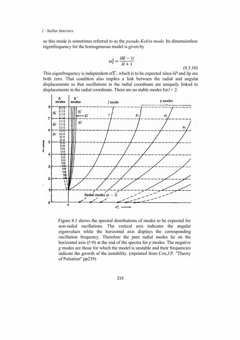
7/18/2019 The Fundamentals of Stellar Astrophysics - Collins G. W.
http://slidepdf.com/reader/full/the-fundamentals-of-stellar-astrophysics-collins-g-w 238/524

7/18/2019 The Fundamentals of Stellar Astrophysics - Collins G. W.
http://slidepdf.com/reader/full/the-fundamentals-of-stellar-astrophysics-collins-g-w 239/524
8 ⋅ Stellar Pulsation and Oscillation
c Toroidal Oscillations
There remains one last class of oscillations that we have not
considered. So far we have been faithful to our assumption of spherical symmetry
and discussed no modes that have a dependence on the azimuthal angle φ so that m =
0. To have included cases where m ≠ 0 would have been to admit the existence of a
preferred plane and thereby violate the assumption of spherical symmetry. Thus the
modes described so far will present surface phenomena that are independent of the
orientation of the star. This will not be the case for m ≠ 0. However, there is no a
priori reason why azimuthal modes cannot exist. Indeed, for each value of l there are
2l + 1 allowed values of m (that is, m = 0, ∀1, ∀2, ∀ ⋅ ⋅ ⋅ ∀l) which represent waves
that propagate in the ∀ φ direction. Of course for a nonrotating star there is no
preferred direction of propagation, so these modes are degenerate and there are only l
+ 1 distinct possibilities.
Papaloizou and Pringle16
have shown that for rotation, this degeneracy is
broken and the resulting modes correspond to traveling waves around the rotational
axis of the star similar to Rossby waves in the earth's atmosphere, so they designated
them r modes. These waves travel with a characteristic velocity that is approximately
1/m times the rotational period of the star. Thus such a wave would be seen by an
observer to be moving at a rate that is slightly faster (+m) and slightly slower (-m)
than the rotational speed of the star. Any comprehensive analysis of the effects of
rotation must deal with the effects of angular momentum conservation as well as
shape distortion and is therefore quite difficult. However, there can be little doubt
that rotation will influence the values for the eigenfrequencies for the p and g modes.Although the overall effects of rotation are extremely complicated, there is some
evidence from nonadiabatic studies that the prograde modes are somewhat less stable
and therefore more likely to be excited, than the retrograde modes.
It is possible to have such modes in a star for which the total angular
momentum is zero. In the case where l = 1 such modes represent uniform rotation of
the object. For l > 1 the modes would represent torsional oscillations. In the simplest
case where l = 2, one hemisphere would rotate, say clockwise, while the other
hemisphere rotated counterclockwise. Unfortunately, to stabilize such an oscillation,
some sort of shear would have to be sustained by the stellar material. Such restoring
shears are simply absent in normal stars. However, in white dwarfs and neutron stars,at least part of the star is expected to be in a crystalline phase and this matter could
perhaps sustain such oscillations.
219
7/18/2019 The Fundamentals of Stellar Astrophysics - Collins G. W.
http://slidepdf.com/reader/full/the-fundamentals-of-stellar-astrophysics-collins-g-w 240/524
7/18/2019 The Fundamentals of Stellar Astrophysics - Collins G. W.
http://slidepdf.com/reader/full/the-fundamentals-of-stellar-astrophysics-collins-g-w 241/524
8 ⋅ Stellar Pulsation and Oscillation
There are strong indications that nonradial modes have been detected in other
stars. β Cephei stars are suspected to exhibit the effects of traveling waves on their
surfaces in their spectra. Papaloizou and Pringle16
explain the short period
oscillations seen in some cataclysmic variables to the r modes of surface traveling
waves. In addition18, 19
sharp absorption features that move through the broad
absorption lines of some rapidly rotating stars have been interpreted as representing
nonradial oscillations. If this is proves to be the case, then the observations indicate
the existence of a phenomenon for which there is no clear theoretical description. For
reasons already mentioned, pulsation theory in the presence of extreme rotation is
extremely difficult and far from well developed. However, should nonradial
oscillations be unambiguously measured for these stars, the potential for detailed
understanding of their internal structure is considerable. Given the uncertainties
regarding the effects of rotation on the internal structure of these stars, every effort
should be made to explore these observations as a probe of the stellar interior.
Problems
1. Show how equations (8.3.8) and (8.3.9) can be obtained from equation
(8.3.7).
2. Use the Virial theorem to find the fundamental radial pulsation period for a
homogeneous star where the equation of state is
3. Compute the lowest-order mode for polytropes with indices n of 1.5, 2.5, and3 for stellar masses M = 1.5M⊙ and 30M⊙ .
4. Assuming that the shear forces resulting from the crystalline structure of a
white dwarf near the Chandrasekhar limit were sufficient to permit torsional
oscillations, estimate the frequency of the lowest-order mode.
5. Show how the wave equation [equation (8.1.24)] is obtained from the
equations of motion [equation (8.1.19)].
References and Supplemental Reading
1. Eddington, A.S.: On the Pulsations of a Gaseous Star and the Problem of the
Cepheid Variables. Part I , Mon. Not. R. astr. Soc., 79, 1918,
pp. 2 - 22.
221
7/18/2019 The Fundamentals of Stellar Astrophysics - Collins G. W.
http://slidepdf.com/reader/full/the-fundamentals-of-stellar-astrophysics-collins-g-w 242/524
1 ⋅ Stellar Interiors
2. Eddington, A.S.: The Internal Constitution of the Stars, Dover, New York,
1959, chap. 8.
3. Ledoux, P.: On the Radial Pulsation of Stars", Ap.J. 102, 1945,
pp.143 - 153
4. Ledoux, P., and Walraven, Th.: "Variable Stars", Handb. d. Phys., Vol. 51,
Springer-Verlag Berlin, 1958, pp.353 - 601.
5. Chandrasekhar, S.: Hydrodynamic and Hydromagnetic Stability, Oxford
University Press, London, 1961.
6. Collins, G.W.,II: The Virial Theorem in Stellar Astrophysics, Pachart Press,
Tucson, Ariz., 1978.
7. Cox, J.P.: Theory of Stellar Pulsation, Princeton University Press, Princeton
N.J., 1980.
8. Baker,N., and Kippenhahn, R.:The Pulsations of Models of δ Cephei Stars",
z. f. Astrophys. 54, 1962, pp.114 - 151.
9. Cox, J.P.: On Second Helium Ionization as a Cause of Pulsational Instability
in Stars, Ap.J. 138, 1963, pp.487 - 536.
10. Castor, J.I.: On the Calculation of Linear, Nonadiabatic Pulsations of Stellar Models, Ap.J. 166, 1971, pp.109 - 129.
11. Iben, I., Jr.: On the Specification of the Blue Edge Of The RR Lyrae
Instability Strip, Ap.J. 166, 1971, pp.131 - 151.
12. Arfken, G.: Mathematical Methods for Physicists, 2nd. ed. Academic, New
York, 1970, pp.569 - 572.
13. Deubner, F.-L., and Gough, D. "Helioseismology: Oscillations as a
Diagnostic of the Solar Interior", Annual Reviews of Astronomy and
Astrophysics, vol. 22, Annual Reviews, Palo Alto, Calif., 1984, pp.593 - 619.
14. Lamb, H.: Hydrodynamics 5th.ed., Cambridge University Press, New York,
1924, pp.467 - 484.
15. Cowling, T.G.: The Non-radial Oscillations of Polytropic Stars, Mon. Not.
R. astr. Soc., 101, 1941, pp.367 - 373.
222
7/18/2019 The Fundamentals of Stellar Astrophysics - Collins G. W.
http://slidepdf.com/reader/full/the-fundamentals-of-stellar-astrophysics-collins-g-w 243/524

7/18/2019 The Fundamentals of Stellar Astrophysics - Collins G. W.
http://slidepdf.com/reader/full/the-fundamentals-of-stellar-astrophysics-collins-g-w 244/524
224
1 ⋅ Stellar Interiors
Epilogue to Part I: Stellar Interiors
We have presented the study of stellar interiors as a subject that builds from a
minimal base of assumptions to the description of some of the most exotic objects in
the universe. To describe the structure of most stars in a qualitative manner, we need
only construct equilibrium models which follow a polytropic law. To improve that
description and to understand the evolution of stars, it is necessary to add a
substantial amount of physics and to construct steady-state models. We illustrated the
nature of the physics to be added, but many more details need to be included to
create models of contemporary accuracy. We did not examine in detail those
instances for which steady-state models fail because of rapid evolution whichrequires hydrodynamic equilibrium to be invoked. However, we did sketch some
consequences of this rapid evolution.
We saw that it is possible to understand all the stellar evolution that takes
place on a time scale longer than the dynamical time in light of a sequence of
equilibrium models linked by estimates of the dominant mode of energy transport
required for the construction of steady-state models. This approach yields a good
qualitative picture of stellar evolution from pre-main sequence contraction through
the helium-burning phases. Finally, we investigated some problems that lie outside
the normal theory of stellar structure and evolution primarily to indicate the direction
in which research in these areas has been proceeding.
The one axiom that has dominated Part I of the book is STE. This enabled us
to characterize the stellar gas and radiation field entirely in terms of the state
variables P, T, and ρ. This was possible because the mean free path for particles and
photons was much smaller than the characteristic size of the star. As the boundary is
approached, systematic differences from the statistical energy distribution expected
from STE will appear, but by the time this begins to happen, the structure of the star
will usually be determined. However, to know what the star will look like, we have
to consider this region in greater detail. Such an investigation is the aim of Part II.

7/18/2019 The Fundamentals of Stellar Astrophysics - Collins G. W.
http://slidepdf.com/reader/full/the-fundamentals-of-stellar-astrophysics-collins-g-w 245/524
Part II
Stellar Atmospheres
7/18/2019 The Fundamentals of Stellar Astrophysics - Collins G. W.
http://slidepdf.com/reader/full/the-fundamentals-of-stellar-astrophysics-collins-g-w 246/524
II Stellar Atmospheres
226
7/18/2019 The Fundamentals of Stellar Astrophysics - Collins G. W.
http://slidepdf.com/reader/full/the-fundamentals-of-stellar-astrophysics-collins-g-w 247/524

7/18/2019 The Fundamentals of Stellar Astrophysics - Collins G. W.
http://slidepdf.com/reader/full/the-fundamentals-of-stellar-astrophysics-collins-g-w 248/524
II Stellar Atmospheres
There is a tendency to think of the difference between the interior and the
atmosphere of a star as distinct, as it is with earth. To be sure, the relative extent of the
solar atmosphere compared to the interior is similar to that of earth, but the similarity
ends there. There is no sharp interface between stellar atmospheres and interiors as
commonly exist with planets. There is no material phase change at the interface.
Indeed, for stars, the distinction between atmospheres and interiors is denoted by the
failure of certain assumptions used in the study of stellar interiors.
The solution of the problem posed by the surface layers of a star is similar to
that for the interior. We have to describe the behavior of the state variables P, T, and ρ
with position in the star. However, an additional problem is posed by the atmosphere.
We have to describe the energy distribution of photons as they leave the star, for this
specifies the appearance of the star which is the fundamental tie with observation. Only
if this description of the stellar spectrum agrees with that which is observed can we saythat we have provided a successful description of the star.
The approach to finding the structure of the atmosphere can be largely divided
into two parts. First, one determines the flow of radiation through the atmosphere,
given the structure of the atmosphere. Second, having determined the radiation field
throughout the surface layers, one corrects the atmospheric structure so that energy is
conserved at all levels of the atmosphere. Since most of the energy is carried by
radiation, the second condition usually amounts to the imposition of radiative
equilibrium throughout the atmosphere. One then uses the improved structure to
correct the radiation field and repeats the process until a self-consistent model is found.
To carry out this procedure it is necessary to make some assumptions about theconditions that prevail in this transition zone between the interior and the space
surrounding the star.
9.1 Basic Assumptions for the Stellar Atmosphere
a Breakdown of Strict Thermodynamic Equilibrium
The description of the energy distribution of the photons in the stellar
interior was made particularly simple by the assumption that all constituents of the gas
that made up the star were in their most probable macrostate, resulting from random or
uncorrelated collisions. That is, they were in thermodynamic equilibrium. All aspectsof such a gas can then be characterized by a single parameter, the temperature, which
specifies the mean energy of the gas. All other aspects of the distribution function of
the gas particles are described by the equilibrium distribution function for the
respective kinds of particles.
228
7/18/2019 The Fundamentals of Stellar Astrophysics - Collins G. W.
http://slidepdf.com/reader/full/the-fundamentals-of-stellar-astrophysics-collins-g-w 249/524
9 Flow of Radiation through the Atmosphere
The validity of this assumption relied on the fact that various components of
the gas would undergo randomizing collisions within a volume where the state
variables (specifically the temperature) could be considered constant. Within the deepinterior of a star, these conditions are met as well as anywhere in the universe.
However, any configuration must have a boundary, and it is there that we should
expect this assumption to fail. Such is the case for stars. However, the manner of that
failure has a peculiar characteristic in that the particles that make up a star are of two
distinctly different types. The photons that make up such an important component of
the gas behave quite differently from the particles that have a material rest mass. These
photons follow different quantum statistics so that their equilibrium distribution
functions are different − Bose-Einstein for the photons and generally maxwellian for
everything else. In addition, the mean free path between collisions for material
particles is very much less than that for photons. Thus, we would expect that the
photons would be the first species of particles to be affected by the presence of a boundary, and this is indeed the case. As one moves outward through a star, the
presence of the surface begins to affect the state of the gas when photons first begin to
escape directly into space and fail to interact any longer with the material particles of
the gas. Since the probability that a specific photon will escape depends on the atomic
physics of the opacity corresponding to the photon's energy, we should not expect all
photons to escape with equal facility. Thus, the photon distribution will depart
progressively from that of the Planck's law as one approaches the boundary and our
notion of STE will have broken down.
The increase in the photon mean free path brought about by the decreasing
density introduces another problem not unrelated to that posed by the boundary. Thevariation of the state variables over a "typical" photon mean free path will become a
significant fraction of the value of the variables themselves. Thus, the radiation field at
any point near the boundary will be made up of photons originating in rather different
physical environments. Thus, the characteristics of the radiation field will no longer be
determined by the local values of the state variables, but will depend on the structure
solution of the entire atmosphere. This global aspect of the properties of the local
radiation field completely changes the mathematical formalism that describes the flow
of radiation from that used in the interior.
b Assumption of Local Thermodynamic Equilibrium
It is a happy consequence of the difference between photons and
particles with material rest mass that the mean free path for photons is generally very
much greater than that for other particles. Thus, while the photons may sense the
boundary, there is a substantial region where the material particles do not. The material
particles continue to undergo collisions with other material particles and photons, the
majority of which still represent their thermodynamic equilibrium distribution. Thus,
229
7/18/2019 The Fundamentals of Stellar Astrophysics - Collins G. W.
http://slidepdf.com/reader/full/the-fundamentals-of-stellar-astrophysics-collins-g-w 250/524
II Stellar Atmospheres
the material particles of the gas will continue to behave as if they were in
thermodynamic equilibrium as one approaches the boundary. Certainly, the point will
be reached when collisions between material particles and other constituents of the gas
will become sufficiently infrequent that the nonequilibrium photons of the gas will
force departures from the Maxwell-Boltzmann energy distribution expected for
particles in thermodynamic equilibrium. But by this point in the atmosphere (in many
stars), the majority of the photons will have escaped, much of the stellar spectrum will
have been established, and the atmospheric structure below this point will be
determined. Thus, the notion that the distribution function for the material particles
remains that obtained from the local values of the state variables in thermodynamic
equilibrium, while the photon distribution does not, is a useful notion. It is called local
thermodynamic equilibrium (LTE) and it is one of the central assumptions for much of
the remainder of this book. To understand the physical situation that prevails when
LTE fails, one must first understand the solution to the problems for which LTE is
valid.
The effect of the boundary upon particles that lie within a mean free path of the
boundary extends to convective blobs. In the stellar interior, we were able to make do
with the crude mixing-length theory because the differences between the adiabatic
gradient and that predicted by the mixing-length theory were so small that large errors
in this difference became rather small errors in the actual gradient. This was due to the
large size of the mixing length, which implied great efficiency for convective transport.
This will no longer be the case in the stellar atmosphere, for it is not possible to have a
mixing length greater than the local distance to the boundary, and that is the order of a
photon mean free path. Thus, convection, should it even occur in the deeper sections of
the atmosphere, will be nowhere as efficient as it was in the interior. The mixing-length theory, while crude, can be used to estimate the impact of convection on the
atmospheric structure. Fortunately, radiation dominates, by definition, in the outer
sections of the atmosphere, and so convection will not be a major concern.
c Continuum and Spectral Lines
In describing the spectral energy distribution of the photons emerging
from a star, it is traditional to distinguish between the smooth distribution of photons
and the dark interruptions, or lack of photons, called spectral absorption lines. These
features arise because the opacity of atomic bound-bound transitions is so large
compared to that of bound-free and free-free processes that photons with energiescorresponding to those bound-bound transitions do not sense the boundary until they
are relatively near it. At this point in the atmosphere, the temperature has declined to
the point where the emitted radiation is less intense than that originating deeper in the
atmosphere. Thus, there will be fewer photons at the frequencies corresponding to the
bound-bound transitions, giving rise to the absorption lines of stellar spectra.
230

7/18/2019 The Fundamentals of Stellar Astrophysics - Collins G. W.
http://slidepdf.com/reader/full/the-fundamentals-of-stellar-astrophysics-collins-g-w 251/524
9 Flow of Radiation through the Atmosphere
Remember that the distinction between continuum and line is largely artificial,
and often the continuum is shot through with myriads of weak lines. The utility of the
concept persists, and we are careful to explain exactly what is meant by the distinction.
Since a large section of this book is be devoted to the processes that give rise tospectral lines (and throughout that section we assume that the structure of the
atmosphere is known), we assume that continuum processes and photons involved in
those processes are the photons that determine the structure of the atmosphere.
d Additional Assumptions of Normal Stellar Atmospheres
Although some of the development of the theory of stellar atmospheres
is presented in great generality, the basic focus of this book is on the theory of
"normal" stars. This development is appropriate for most of the stars on the main
sequence and some others. We indicate where the assumptions fail in the description ofthe atmospheres of other stars and what can be done about them, but for now we adopt
the traditional assumptions of stellar atmospheres.
In addition to the assumption of LTE, we assume that the thickness of the
atmosphere is small compared to the radius of the star. Under these conditions, the
surface geometry may be assumed to be that of a plane- parallel slab of infinite
thickness possessing a surface extending to infinity in all directions (see Figure 9.1).
Since most of the stellar mass will reside inside the atmosphere, it is consistent with the
plane-parallel atmosphere approximation to assume that the surface gravity is constant.
Thus, the notion of hydrostatic equilibrium given in equation (2.1.6) simplifies to
(9.1.1)
Furthermore, since no sources of energy are likely to be present in the stellar
atmosphere and we need not worry about time dependent entropy terms, the
conservation of energy [equation (7.1.1)] becomes
(9.1.2)
If all the energy is to be carried by radiation, equation (9.1.2) ensures that the radiant
flux in the atmosphere will be constant.
231
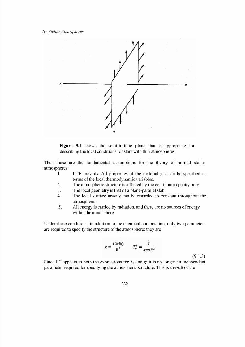
7/18/2019 The Fundamentals of Stellar Astrophysics - Collins G. W.
http://slidepdf.com/reader/full/the-fundamentals-of-stellar-astrophysics-collins-g-w 252/524
II Stellar Atmospheres
Figure 9.1 shows the semi-infinite plane that is appropriate for
describing the local conditions for stars with thin atmospheres.
Thus these are the fundamental assumptions for the theory of normal stellar
atmospheres:
1. LTE prevails. All properties of the material gas can be specified in
terms of the local thermodynamic variables.
2. The atmospheric structure is affected by the continuum opacity only.
3. The local geometry is that of a plane-parallel slab.
4. The local surface gravity can be regarded as constant throughout the
atmosphere.
5. All energy is carried by radiation, and there are no sources of energy
within the atmosphere.
Under these conditions, in addition to the chemical composition, only two parameters
are required to specify the structure of the atmosphere: they are
(9.1.3)
Since R -2
appears in both the expressions for T e and g ; it is no longer an independent
parameter required for specifying the atmospheric structure. This is a result of the
232
7/18/2019 The Fundamentals of Stellar Astrophysics - Collins G. W.
http://slidepdf.com/reader/full/the-fundamentals-of-stellar-astrophysics-collins-g-w 253/524
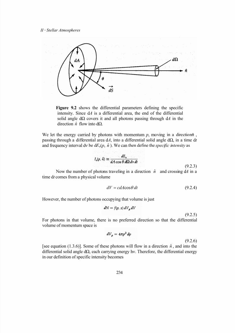
7/18/2019 The Fundamentals of Stellar Astrophysics - Collins G. W.
http://slidepdf.com/reader/full/the-fundamentals-of-stellar-astrophysics-collins-g-w 254/524
II Stellar Atmospheres
Figure 9.2 shows the differential parameters defining the specific
intensity. Since d A is a differential area, the end of the differential
solid angle dΩ covers it and all photons passing through d A in the
direction flow into dΩ.n
We let the energy carried by photons with momentum p, moving in a directionn ,
passing through a differential area d A, into a differential solid angle dΩ, in a time dt
and frequency interval dν be d E ν( p, ). We can then define the specific intensity asn
(9.2.3)
Now the number of photons traveling in a direction and crossing d A in a
time dt comes from a physical volume
n
dt cdAdV θ cos= (9.2.4)
However, the number of photons occupying that volume is just
(9.2.5)
For photons in that volume, there is no preferred direction so that the differential
volume of momentum space is
(9.2.6)
[see equation (1.3.6)]. Some of these photons will flow in a direction n , and into the
differential solid angle dΩ, each carrying energy hν. Therefore, the differential energy
in our definition of specific intensity becomes
ˆ
234
7/18/2019 The Fundamentals of Stellar Astrophysics - Collins G. W.
http://slidepdf.com/reader/full/the-fundamentals-of-stellar-astrophysics-collins-g-w 255/524
9 Flow of Radiation through the Atmosphere
(9.2.7)
Combining equations (9.2.2) through (9.2.7), we can relate the specific intensity to the
phase space density of photons
(9.2.8)
b General Equation of Radiative Transfer
Now let us rewrite equation (9.2.1) in vector form:
(9.2.9)
If we assume that the photons are moving under the influence of a strong potential
gradient Φ, then we can write for photons that
(9.2.10)
Substitution of equations (9.2.10) and (9.2.8) into equation (9.2.9) yields an extremely
general form of the equation of radiative transfer:
(9.2.11)
This equation gives the correct description of the transfer of radiation in an arbitrary
coordinate system, even if the boundary conditions are changing on a time scale
comparable to the photon diffusion time. It is even correct if the photons are subject to
energy loss by virtue of their moving through a strong gravitational field, although
some care must be exercised in the choice of coordinates. However, if the propagation
takes place in a dispersive medium, then r & must be replaced by
(9.2.12)
235
7/18/2019 The Fundamentals of Stellar Astrophysics - Collins G. W.
http://slidepdf.com/reader/full/the-fundamentals-of-stellar-astrophysics-collins-g-w 256/524
II Stellar Atmospheres
and the unit of length is changed by n, where n is the index of refraction of the
medium, as well.
Fortunately, in normal stellar atmospheres, the radiation field is time-
independent, and the gravitational potential gradient is usually negligible so that
equation (9.2.11) becomes
(9.2.13)
The assumption of plane parallelism will simplify this even further, but first let us turn
to the "creation" rate S .
c "Creation" Rate and the Source Function
The "creation" rate S is just a measure of the rate at which photons that
contribute to the flow through d A into dΩ are lost to the volume dV dV p. Any
absorption process that takes place in that phase space volume will result in the loss of
a photon. However, photons can be "lost" from the volume without being destroyed.
Any scattering process that changes the momentum of the photon can remove the
photon from the volume. Thus, we can write the number lost to the differential volume
as
(9.2.14)
where α is just the fraction of particles present that are lost due to scattering and
absorption. Particles may also "appear" in the volume or be "created" by thermal
emission or scattering processes. We assume that the thermal emission processes are
isotropic so that the number gained in the volume and radiated into a unit solid angle is
(9.2.15)
where ε is the thermal emission per unit volume of phase space.
The situation for scattering is somewhat more complicated. Photons may
appear in the volume and be scattered by matter in the volume into direction with
the appropriate momentum. These photons appear to be created just as surely as the
thermal photons do, but with a difference. The thermal emission rate depends only on
the thermodynamic characteristics of the material gas, whereas the scattered photons
have their origin directly in the radiation field. This dependence of the "creation" rate,
and hence the specific intensity, on the radiation field itself is one of the hallmarks of
radiative transfer in stellar atmospheres. It is through the scattering process that the
local value of the radiation field depends on the values of the radiation field throughout
the medium. This coupling of the local radiation field to the global radiation field
n
236
7/18/2019 The Fundamentals of Stellar Astrophysics - Collins G. W.
http://slidepdf.com/reader/full/the-fundamentals-of-stellar-astrophysics-collins-g-w 257/524
7/18/2019 The Fundamentals of Stellar Astrophysics - Collins G. W.
http://slidepdf.com/reader/full/the-fundamentals-of-stellar-astrophysics-collins-g-w 258/524
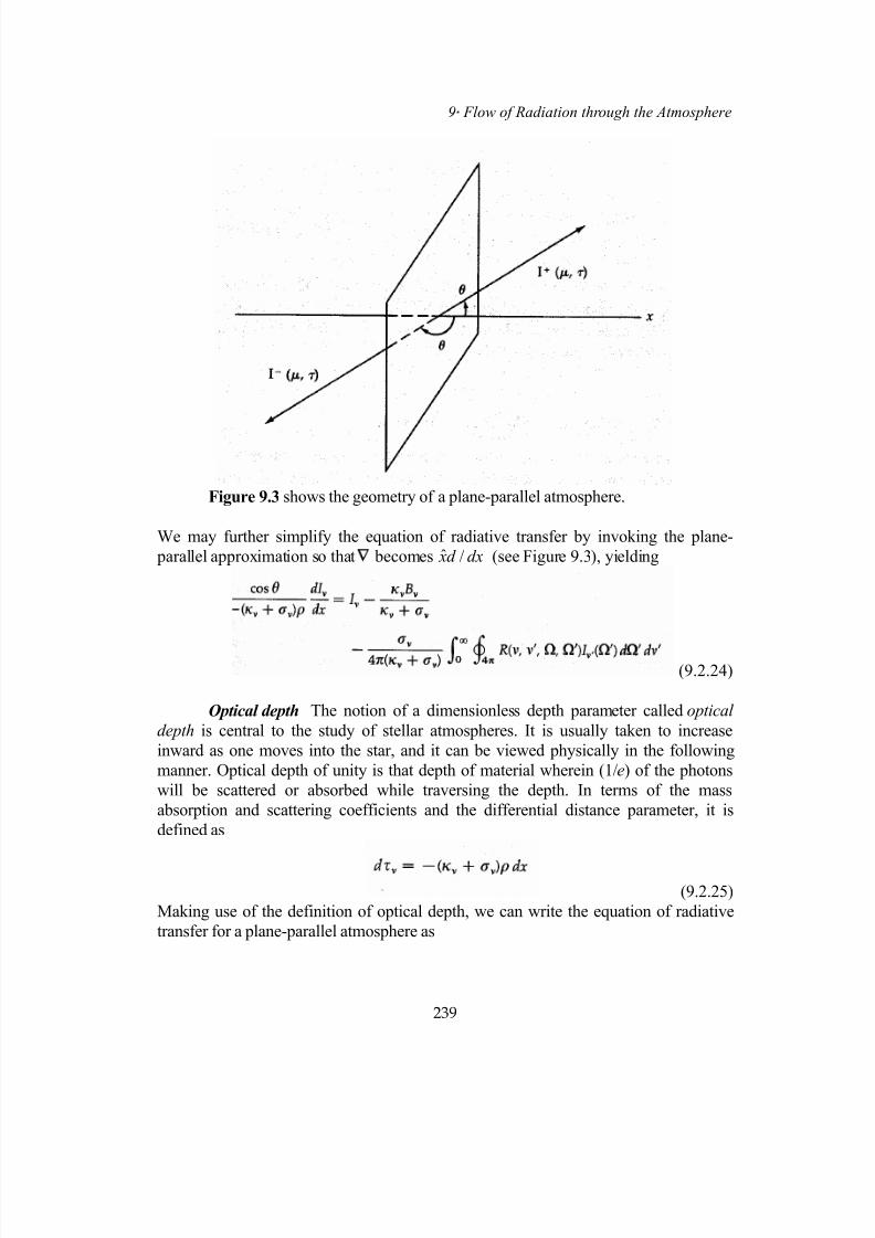
7/18/2019 The Fundamentals of Stellar Astrophysics - Collins G. W.
http://slidepdf.com/reader/full/the-fundamentals-of-stellar-astrophysics-collins-g-w 259/524
9 Flow of Radiation through the Atmosphere
Figure 9.3 shows the geometry of a plane-parallel atmosphere.
We may further simplify the equation of radiative transfer by invoking the plane-
parallel approximation so that becomes (see Figure 9.3), yieldingdxd x /ˆ
(9.2.24)
Optical depth The notion of a dimensionless depth parameter called optical
depth is central to the study of stellar atmospheres. It is usually taken to increase
inward as one moves into the star, and it can be viewed physically in the following
manner. Optical depth of unity is that depth of material wherein (1/e) of the photons
will be scattered or absorbed while traversing the depth. In terms of the mass
absorption and scattering coefficients and the differential distance parameter, it is
defined as
(9.2.25)
Making use of the definition of optical depth, we can write the equation of radiative
transfer for a plane-parallel atmosphere as
239

7/18/2019 The Fundamentals of Stellar Astrophysics - Collins G. W.
http://slidepdf.com/reader/full/the-fundamentals-of-stellar-astrophysics-collins-g-w 260/524
II Stellar Atmospheres
(9.2.26)
where
(9.2.27)
The parameter S ν is known as the source function of the radiation field. Since the
quantity (κν+σν) appears so frequently, it is customary to call it the mass extinction
coefficient . The name is reasonable as it is, indeed, a measure of the total ability of
material to attenuate the flow of photons.
d Physical Meaning of the Source Function
The source function is one of the most important concepts in the theory
of radiative transfer, and it is important to have a good intuitive feeling for its meaning.
As the name implies, the source function represents the local contribution to the
radiation field. It is a measure of the energy contributed to the radiation field by
physical processes taking place at a particular spot in the atmosphere. Consider the
case where scattering is unimportant so that σν = 0. Under these conditions the
expression for the source function [equation (9.2.27)] becomes
(9.2.28)
and all photons locally contributed to the radiation field can be characterized by thePlanck function since they arise from thermal processes. This is a consequence of the
assumption of LTE which enabled us to use Kirchhoff's law to characterize the local
emissivity of the gas in terms of its absorptivity. Some authors take this as a definition
of LTE, but as such, it would be unduly restrictive. The presence of scattering, say by
electrons will require a more complicated source function such as that given by
equation (9.2.27), but the excitation and ionization characteristics of the gas may still
be those expected for a gas in thermodynamic equilibrium. Thus, S ν = Bν is normally a
sufficient condition for the existence of LTE, but not a necessary one.
Now consider the case when pure absorption processes are negligible and
virtually all the opacity of the material arises from scattering processes. Then
(9.2.29)
Here the source function depends only on the incident radiation field. Since the
redistribution function is normalized to unity, the integral in equation (9.2.29) simply
240

7/18/2019 The Fundamentals of Stellar Astrophysics - Collins G. W.
http://slidepdf.com/reader/full/the-fundamentals-of-stellar-astrophysics-collins-g-w 261/524
9 Flow of Radiation through the Atmosphere
represents some sort of average of the local specific intensity over all frequencies and
angles. The factor of 1/4π then represents that part of the average that is scattered into
the differential solid angle appropriate for Iν.
Thus, under the conditions of pure scattering, the source function becomes
totally independent of the local physical conditions and is completely determined by
the local radiation field. If this condition were to prevail throughout the atmosphere,
one would have the curious result that the radiation field would be independent of the
local values of the state variables (P, T, and ρ) and depend only on the ability of
particles to scatter photons and the details of how the particles do it. In some real sense,
the radiation field would become decoupled from the physical properties of the gas.
Indeed, one can learn little about the physical conditions that prevail in a fog by
observing the light transmitted through it from say an automobile headlight. This
independence of the radiation field from the state variables of the gas enables one to
solve the entire problem of radiative transfer for pure scattering without knowinganything about the gas other than the redistribution function. We use this property later
to discuss methods of solving the equation of radiative transfer. However, as the case
of the fog illustrates, this is a two edged sword. The decoupling of the radiation field
from the state variables of the gas, in the case of pure scattering, means that we can not
use the radiation field to determine the run of state variables with depth.
e Special Forms of the Redistribution Function
Since the redistribution function plays such an important role in
specifying the nature of scattering in the source function, we examine some common
physical situations and the corresponding redistribution functions.
Coherent Scattering The term coherent scattering refers to the case where
photons are scattered in direction but not in frequency. Thomson scattering by
electrons is of this form. Such processes are generally known as conservative
processes because no energy is exchanged between the radiation field and the particles.
While this is never strictly true, in many cases it is an excellent approximation. This is
certainly true for the scattering of optical photons by the electrons present in a stellar
atmosphere. Under these conditions we can write the redistribution function as
(9.2.30)
where δ(ν-ν') is the Dirac delta function. The delta function on frequency causes the
frequency integral in equation (9.2.27) to collapse, simplifying the source function
considerably.
241
7/18/2019 The Fundamentals of Stellar Astrophysics - Collins G. W.
http://slidepdf.com/reader/full/the-fundamentals-of-stellar-astrophysics-collins-g-w 262/524
II Stellar Atmospheres
Noncoherent Scattering This phrase has come to mean considerably more than
the opposite of coherent scattering. For fully noncoherent scattering, the frequency of a
scattered photon is completely uncorrelated with the frequency of the incident photon.
In some sense, the photon "forgets" its prior frequency. Like coherent scattering, thiscase also represents an approximation. Clearly, if the situation were to apply to the
entire frequency range from zero to infinity, the value of the redistribution function at
any specific value of ν would have to be arbitrarily small. Thus, the common use of the
approximation is confined to a finite frequency range such as a spectral line. As we
shall see later, very strong spectral lines often possess the property that an electron in
the upper state is so perturbed by interactions with other particles of the gas that the
specific value of the absorbed energy is irrelevant in determining the energy of the
photon that will be emitted in the subsequent transition. Thus, over a finite frequency
interval, the wavelength of the emitted photon will be totally uncorrelated with the
wavelength of the absorbed photon. Under these conditions, the frequency simply does
not appear in the redistribution function and
(9.2.31)
Redistribution functions of this form are often called complete redistribution functions.
Isotropic Scattering As with complete redistribution, the photon undergoing
isotropic scattering suffers from "amnesia". The direction of the scattered photon is
completely uncorrelated with the direction of the incident photon. Thus, the angular
dependence of the redistribution function vanishes and
(9.2.32)
This also considerably simplifies the source function in equation (9.2.27). If the
radiation field were isotropic, the integral over the solid angle merely produces a factor
of 4π, which cancels the corresponding factor in front of the integral. In general, this is
also an approximation. Although it is far from obvious, we shall see that it is an
excellent approximation for electron scattering of optical photons in a stellar
atmosphere. So great is the simplification introduced by the assumption of isotropic
scattering that there is a tendency to invoke it even when it is totally inappropriate.
Later, we shall see what sorts of methods can be used to incorporate the full
redistribution function in the solution of the equation of radiative transfer. Such cases
are often called partially coherent anisotropic scattering , and their solution poses oneof the most difficult problems in radiative transfer. However, before we consider these
formidable problems, we must understand how to approach the solution of more basic
problems. The dominant form of scattering in normal stellar atmospheres is Thomson
scattering by electrons, and for purposes of determining the atmospheric structure it is
an excellent approximation to assume that such scattering is isotropic. Under the
assumption of coherent isotropic scattering, the source function given by equation
242
7/18/2019 The Fundamentals of Stellar Astrophysics - Collins G. W.
http://slidepdf.com/reader/full/the-fundamentals-of-stellar-astrophysics-collins-g-w 263/524
9 Flow of Radiation through the Atmosphere
(9.2.27) becomes
(9.2.33)
9.3 Moments of the Radiation Field
In Chapter 1 we saw that a good deal of information was gleaned and simplification
achieved by taking moments of the phase density of the particles that made up the gas
in question. By such methods we were able to obtain equations for the continuity of
matter and momentum and eventually to develop expressions for the hydrodynamic
flow of a gas and hydrostatic equilibrium. The basic approach was to throw away
information contained in the phase density by averaging it over some appropriate part
of the phase space volume. That part of the volume was generally taken to be described
by coordinates for which we did not require specific knowledge of the phase density.Since we were to invoke STE for the gas, we knew that the details of the velocity
distribution could be ignored since in thermodynamic systems the velocity
distributions are specified by a single parameter (the temperature) which is related to
the mean velocity. Thus, averaging the phase density over velocity or momentum
space made good sense.
We may expect the same sort of benefits by taking moments of the radiation
field and particularly the specific intensity, for there is a simple relation [equation
(9.2.8)] between the specific intensity and the phase density of photons. However, here
we must be careful because it is the momentum distribution of photons in which we are
interested so that averaging over momentum space would remove the very informationwe seek. We must look to other coordinates of phase space to find those which can be
considered unimportant.
One of our initial assumptions is the atmosphere is well approximated by a
plane-parallel slab. By symmetry, the radiation flow through such a slab will be
isotropic about the normal to the slab. Hence, no important information will be
contained in the azimuthal coordinate (see Figure 9.3). In addition, we might expect
that information in the polar angle θ will not play a central role in the interaction of the
radiation field with matter. It is this interaction that determines the emergent spectrum
and the atmospheric structure. For these reasons, we can expect that the angular
coordinates of phase space may prove expendable and that averages of the radiationfield over these coordinates could prove useful in describing the flow of radiation
through the atmosphere. Thus, we shall average over two of the three spatial
coordinates, choosing the third to represent the direction of net energy flow. In the case
of the plane-parallel atmosphere, this clearly is the direction of the atmosphere normal.
Also, because of the simple transformation between the specific intensity and the
photon phase density, the quantity to be averaged should be the specific intensity itself.
243

7/18/2019 The Fundamentals of Stellar Astrophysics - Collins G. W.
http://slidepdf.com/reader/full/the-fundamentals-of-stellar-astrophysics-collins-g-w 264/524
II Stellar Atmospheres
In addition, the higher-order moments should involve the spatial coordinates just as the
higher moments in Chapter 1 involved the velocity itself. Such angular moments will
then describe various aspects of the net flow of energy.
a Mean Intensity
Averaging over the angular coordinates described in Figure 9.3 is
equivalent to averaging over all solid angles, so with some generality we can define the
lowest-order moment of the radiation field as
(9.3.1)
For a plane-parallel atmosphere, where the intensity has no φ dependence and cosθ isreplaced by µ, equation (9.3.1) is equivalent to
(9.3.2)
This quantity, known as the mean intensity, is analogous to the particle density of
Chapter 1 and differs from the photon energy density by a factor of 4π/c.
b Flux
The next-highest-order moment is related to the net flow of energy in a
specific direction , and it is defined, in a manner analogous to that for the meanintensity J
nν, as follows:
(9.3.3)
If we break into its components, then for the axis-symmetric case of a plane parallel
atmosphere, this becomes
n
(9.3.4)
where points along the normal to the atmosphere. Indeed, it is fair to describe the
flux as an intensity-weighted unit vector pointing in the direction of the flow of energy.
Although the flux as defined here is a vector quantity, it is common to drop the vector
properties since they are generally obvious from the geometry of the atmosphere.
However, the vector nature does point to the similarity with the moments of defined in
n
244

7/18/2019 The Fundamentals of Stellar Astrophysics - Collins G. W.
http://slidepdf.com/reader/full/the-fundamentals-of-stellar-astrophysics-collins-g-w 265/524
9 Flow of Radiation through the Atmosphere
Chapter 1 where the first moment of the phase density was the mean flow velocity.
This definition of the first moment of the radiation field is sometimes known as the
Harvard flux because it is heavily employed by the ATLAS atmosphere computer code
developed at Harvard University, where the analogy to the mean intensity was deemedmore important than the physical interpretation.
The actual energy crossing a differential area d A in the direction n isˆ
(9.3.5)
The quantity Fν is often called the physical flux because it represents the actual flow of
energy. For a plane-parallel atmosphere this reduces to
(9.3.6)
The quantity π appears so regularly that many early authors, who were primarily
concerned with plane-parallel atmospheres, defined a third form of the flux as
(9.3.7)
This has become known as the radiative flux and it neither represents a physical
quantity directly nor is analogous to the mean intensity. However, it is the most widely
used definition of the first moment of the radiation field, so the student is to be warned
to determine which definition of the flux a particular author is using or else all sorts of
confusion may result. Throughout this book, we use all three definitions, but we try to
be quite clear as to which is which and why a specific choice is made.
c Radiation Pressure
The analogy between this moment and the pressure tensor in Chapter 1
is very close, and the formal definition has the same normalization properties as Jν. So
(9.3.8)
In a manner similar to the physical flux Fν, K ν can be regarded as an intensity-
weighted unit dyadic (not to be confused with the unit tensor 1 that has components
δij). Now K ν is known as the radiation pressure tensor and is completely analogous to
the pressure tensor P that we obtained in Chapter 1 [equation (1.2.25)]. The meaning of
the unit dyadic (in this case the vector outer product of a unit vector with itself) can be
245

7/18/2019 The Fundamentals of Stellar Astrophysics - Collins G. W.
http://slidepdf.com/reader/full/the-fundamentals-of-stellar-astrophysics-collins-g-w 266/524
II Stellar Atmospheres
seen by writing out the various Cartesian components of K ν in spherical coordinates:
φθθτ×
θφθθφθθ
φθθφθφφθ
φθθφφθφθ
π=
νν
π π
ν
∫ ∫d d
ii
sin)(I
cosk ˆk ˆ sincossin jk ˆ coscossinik ˆ
sincossink ˆ j sinsin j j cossinsini j
coscossink ˆi sincossin ji cossinˆˆ
4
1K
0
2
02
22
222
(9.39)
For the axis-symmetric case this becomes
(9.3.10)
or
(9.3.11)
Now consider the case where the radiation field is nearly isotropic so that we
may expand Iν(τν , µ) in a rapidly converging series as
(9.3.12)
where the lead term I0(τν) is the dominant term. The components of the radiation
pressure tensor then become
(9.3.13)
Define the scalar moment K ν(τν) so that
(9.3.14)
The identity of this moment to the magnitude of the radiation pressure tensor in the
case of near isotropy ensures that
246

7/18/2019 The Fundamentals of Stellar Astrophysics - Collins G. W.
http://slidepdf.com/reader/full/the-fundamentals-of-stellar-astrophysics-collins-g-w 267/524
9 Flow of Radiation through the Atmosphere
(9.3.15)
The isotropy condition was required in Chapter 1 in order for the divergence of the
pressure tensor to be replaced by the gradient of the scalar pressure. Thus, in every
sense of the word K ν(τν) may be considered to be related to the pressure of radiation.
There remains only the problem of units. Since P represents the transfer of momentum
across a surface, the exact relationship is
(9.3.16)
Although these expressions give the correct formulation of the radiation pressure in
terms of moments of the radiation field, it is important to remember that the radiation
pressure is not identical to the force per unit area exerted by photons. That will involve
the opacity, for to exert a force the photon must interact with the matter. In the stellarinterior, this was no problem because the mean free path was so short as to guarantee
that all photons would interact in a short distance. However, in a stellar atmosphere,
this is no longer true for some of the photons escape. We return to this point when we
consider the forces acting on the gas.
9.4 Moments of the Equation of Radiative Transfer
In Chapter 1 we saw that much useful information could be obtained about the
gas by taking moments of the Boltzmann transport equation. The process always
generated moments of phase density that were of one order higher than that used to
generate the equation itself. Thus, to be useful, a relation between the higher-ordermoment and one of lower order had to be found. If this could be done, a self-consistent
set of moment equations could be found and solved, yielding the values of those
moments throughout the configuration. A similar set of circumstances will exist for the
equation of radiative transfer.
To maintain a high level of generality, let us consider the general equation of
radiative transfer given by equation (9.2.11) but with the "creation rate" replaced by
the source function and the potential gradient taken to be zero. Thus
(9.4.1)
Furthermore, assume that the scattering is isotropic and coherent so that the source
function in equation (9.2.27) becomes
(9.4.2)
247
7/18/2019 The Fundamentals of Stellar Astrophysics - Collins G. W.
http://slidepdf.com/reader/full/the-fundamentals-of-stellar-astrophysics-collins-g-w 268/524
II Stellar Atmospheres
Now we integrate equation (9.4.1) over all solid angles, using the form of the source
function given by equation (9.4.2), and get
(9.4.3)
This is the equation of radiative equilibrium and describes how the radiative flux flows
through the atmosphere. Note that the effects of scattering have disappeared from this
equation. This is an expression of the conservative nature of scattering. Since no
energy is gained or lost in each individual scattering event, the average can contribute
nothing to the energy balance for the radiative flux and so all scattering terms must
vanish.
a Radiative Equilibrium and Zeroth Moment of the Equation of
Radiative Transfer
Consider the right-hand side of equation (9.4.3). This is essentially the
right-hand side of the Boltzmann transport equation, which denotes the creation and
destruction of particles in phase space, suitably averaged over direction. Thus, if there
is no net production of photons in the atmosphere, this term, integrated over frequency,
must be zero. Therefore, integrating equation (9.4.3) over all frequencies, we get
(9.4.4)
This is a very general statement of radiative equilibrium, and either side of this
equation is an equivalent statement of it. If we let , then for a static plane-
parallel atmosphere∫∞=
0dv F F ν
(9.4.5)
This will serve as a definition of the local effective temperature T e.
b First Moment of the Equation of Radiative Transfer and the
Diffusion Approximation
We multiply equation (9.4.1) [with the source function of equation
(9.4.2) replacing the "creation rate"] by a unit vector n pointing in the direction of
flow of radiant energy and integrate over all solid angles to obtain
ˆ
(9.4.6)
248
7/18/2019 The Fundamentals of Stellar Astrophysics - Collins G. W.
http://slidepdf.com/reader/full/the-fundamentals-of-stellar-astrophysics-collins-g-w 269/524
9 Flow of Radiation through the Atmosphere
Now we make the approximation of near isotropy for the radiation field that was
done in equation (9.3.12) and evaluate J ν(τν) from its definition [equation (9.3.1)] to
get
(9.4.7)
We have already shown that under similar assumptions K ν(τν) = I0/3, so for conditions
of near isotropy
(9.4.8)
This is known as the diffusion approximation and it can be used to close the
moment equation (9.4.6), yielding
(9.4.9)
Now equations (9.4.3) and (9.4.9) can be combined, by utilizing radiative equilibrium
[equation (9.4.4)], to produce a "wave equation" for the radiative flux F
(9.4.10)
which has all the properties of the usual wave equation. Such an equation is useful in
solving problems in radiative transfer when the boundary conditions change on a time
scale comparable to the photon diffusion time through the medium. Such situations
may occur in some nebulae, novae and supernovae, or possibly quasars. For stellar
atmospheres, the time-independent solutions will generally be sufficient. For a plane-
parallel atmosphere in which the radiation field can be viewed as static, equations
(9.4.3) and (9.4.9) become, respectively,
(9.4.11)
That the static equations will be appropriate for normal stellar atmospheres becomes
apparent when we consider that the diffusion time for a photon through a stellar
atmosphere is only a few orders of magnitude times the light travel time. An
atmosphere is a place from which photons escape after perhaps a few dozeninteractions. Normal stars do not change on so short a time scale.
c Eddington Approximation
249
Although the diffusion approximation provides a method for closing the
moment equations of the equation of radiative transfer, it does not allow the complete

7/18/2019 The Fundamentals of Stellar Astrophysics - Collins G. W.
http://slidepdf.com/reader/full/the-fundamentals-of-stellar-astrophysics-collins-g-w 270/524
II Stellar Atmospheres
solution of the problem. The moment equations are, after all, differential equations and
are subject to boundary conditions. Specification of these boundary conditions will
provide a complete and unique solution for the radiation field. Sir Arthur Stanley
Eddington suggested an additional approximation, inspired by the diffusion
approximation that allows for the sufficient specification of boundary conditions to
permit the solution of equations (9.4.11).
We consider the situation at the surface, and we assume the emergent radiation
field to be isotropic. Since there is generally no incident radiation at the surface of a
star, and using the condition of near isotropy given by equation (9.3.12) we get
(9.4.12)Hence,
(9.4.13)
This and the condition of radiative equilibrium given by equation (9.4.4) provide the
two additional constraints necessary to solve equations (9.4.11). For the case of the
gray atmosphere (see Section 10.2) a particularly simple solution is given by equation
(10.2.15). Although the emergent radiation field is only approximately isotropic, it is
the genius of this approximation that the errors introduced by the surface
approximation are somewhat offset by the errors incurred by the assumption of thediffusion approximation. Thus, as we shall see later, the Eddington approximation
produces solutions for the radiation field that are usually accurate to about 10 percent.
As a result, the Eddington approximation is frequently used to solve problems in
radiative transfer. To do better, we shall have to do a great deal more.
We have seen that it is possible to describe the flow of radiation through a
stellar atmosphere. The derivation involves the same formalisms that we developed in
Chapter 1 to describe the flow of matter. The resulting description of this flow is
known as the equation of radiative transfer and it differs significantly from the simple
result developed for the study of stellar interiors. The differences point up one of the
central differences between stellar interiors and stellar atmospheres. Deep inside a star,the structure of the gas and radiation field is fully determined by the local values of the
state variables of the gas. This is not the case in the stellar atmosphere. At any given
point in the atmosphere, the local radiation field is composed of photons which
originated in an environment that differed significantly from the local environment.
Thus, the solution for the equation of radiative transfer locally will depend on the
solution everywhere. This global nature of radiative transfer in a stellar atmosphere is
250
7/18/2019 The Fundamentals of Stellar Astrophysics - Collins G. W.
http://slidepdf.com/reader/full/the-fundamentals-of-stellar-astrophysics-collins-g-w 271/524
9 Flow of Radiation through the Atmosphere
one of the central differences between the interior and the outer layers of a star. We
now turn our attention to solving the equation of radiative transfer.
Problems
1. Show that the specific intensity along a ray in empty space is constant.
2. Compute the specific intensity and the radiative flux at a distance r on the axis
of an emitting disk having radius ρ and temperature Te. Assume the disk to be
located at r = 0.
3. Derive the equation of radiative transfer that is appropriate for spherical
geometry. List carefully all the assumptions that you make.
4. Derive the plane-parallel equation of radiative transfer appropriate for adispersive medium with an index of refraction n which is different from unity
and which may vary with position.
5. Show that for any diagonal tensor A, in spherical coordinates,
6. Use the above equation to show that if K is a diagonal tensor with all elements
equal to K, then
Here K, J , and K have their usual meanings for radiative transfer [see equations (9.3.1),
(9.3.8), and (9.3.14)].
7. Derive equation (9.2.11) from equations (9.2.8) through (9.2.10). Show all
your work.
8. Derive equation (9.2.18) from equations (9.2.2), (9.2.8), (9.2.14), (9.2.15),
(9.2.17). Show all your work.
9. Derive equation (9.4.10) from first principles and axioms. Clearly list all
assumptions that you make.
251
7/18/2019 The Fundamentals of Stellar Astrophysics - Collins G. W.
http://slidepdf.com/reader/full/the-fundamentals-of-stellar-astrophysics-collins-g-w 272/524
II Stellar Atmospheres
252
Supplemental Reading
A number of books provide an excellent description of the processes taking
place in a stellar atmosphere. For excellent, clear, and correct definitions of thequantities that appear in the theory of radiative transfer see
Mihalas, D.: Stellar Atmospheres, 2d ed. W.H. Freeman, San Francisco, 1978, Chap.
1, pp. 1-18.
Strong insight into problems posed by scattering can be found in
Sobolev, V.V.: A Treatise on Radiative Transfer , (Trans.: S. I. Gaposchkin), D.Van
Nostrand, Princeton N.J., 1963 Chap. 1, pp. 1 - 37.
An excellent overall statement of the problem can be found in
Mustel, E.R.: Theoretical Astrophysics, (Ed.: V.A. Ambartsumyan, trans. J.B.
Sykes), Pergamon, New York, 1958, pp. 1-8.
To have some feeling for just how long people have been worrying about problems
like these and to sample the physical insight of one of the most insightful men of the
twentieth century, read
Eddington, A.S.: On the Radiative Equilibrium of the Stars, Mon. Not. R. astr. Soc.,
77, 1916, pp. 16 - 35.

7/18/2019 The Fundamentals of Stellar Astrophysics - Collins G. W.
http://slidepdf.com/reader/full/the-fundamentals-of-stellar-astrophysics-collins-g-w 273/524
10 ⋅ So
Copyright (2003) George W. Collins, II lution of the Equation of Radiative Transfer
253
10
Solution of the Equation of Radiative Transfer
. . .
One-half of the general problem of stellar atmospheres revolves around the
solution of the equation of radiative transfer. Although equation (9.2.11) represents a
very general formulation of radiative transfer, clearly the specific nature of the
equation of transfer will depend on the geometry and physical environment of the
medium through which the radiation flows. The nature of the physical medium will
also influence the details of the source function so that the source function may
depend on the radiation field itself. Thus, the mode of solution may be expected to be
different for the different conditions that exist. However, the notion of plane
parallelism is common to so many stars and other physical situations that we spend a
significant amount of effort investigating the solution of the equation of transfer for
plane-parallel atmospheres.

7/18/2019 The Fundamentals of Stellar Astrophysics - Collins G. W.
http://slidepdf.com/reader/full/the-fundamentals-of-stellar-astrophysics-collins-g-w 274/524
II ⋅ Stellar Atmospheres
10.1 Classical Solution to the Equation of Radiative Transfer and
Integral Equations for the Source Function
There are basically two schools of approach to the solution of the
equation of transfer. One involves the solution of an integral equation for the source
function, while the other deals directly with the differential equation of transfer. Both
have their merits and drawbacks. Since both are widely used, we give examples of
each. Both involve the classical solution, so that we begin the discussion with that
solution.
a Classical Solution of the Equation of Transfer for the Plane-
Parallel Atmosphere
The equation of transfer is a linear differential equation, whichimplies that a formal solution exists for the radiation field in terms of the source
function. This linear property is a marked difference from the situation in stellar
interiors where the structure equations were all highly nonlinear. Although under
some conditions the solution [i.e., Iν(τν,µ)] itself is involved in the source function,
this involvement is still linear. Let us consider a fairly general equation of radiative
transfer for a plane-parallel atmosphere, but one where we may neglect time-
dependent effects and the presence of the potential gradient on the radiation field.
(10.1.1)
Since this equation is linear in Iν(τν,µ), we may write the complete solution as thesum of the solution to the homogeneous equation plus any particular solution. So let
us choose as homogeneous and particular solutions
(10.1.2)
Substitution into the equation of transfer places constraints on c1 and f '’(τν), namely
(10.1.3)
While we have assumed that the geometry of the atmosphere is plane-
parallel, we have not yet specified the extent of the atmosphere. For the moment, letus assume that the atmosphere consists of a finite slab of thickness τ0 (see Figure
10.1). The general classical solution for the plane-parallel slab is then
(10.1.4)
254
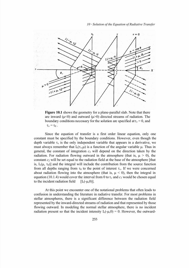
7/18/2019 The Fundamentals of Stellar Astrophysics - Collins G. W.
http://slidepdf.com/reader/full/the-fundamentals-of-stellar-astrophysics-collins-g-w 275/524
10 ⋅ Solution of the Equation of Radiative Transfer
Figure 10.1 shows the geometry for a plane-parallel slab. Note that there
are inward (µ<0) and outward (µ>0) directed streams of radiation. The
boundary conditions necessary for the solution are specified at τν = 0, and
τν = τ0 .
Since the equation of transfer is a first order linear equation, only one
constant must be specified by the boundary conditions. However, even though the
depth variable τν is the only independent variable that appears in a derivative, we
must always remember that Iν(τν,µ) is a function of the angular variable µ. Thus in
general, the constant of integration c2 will depend on the direction taken by the
radiation. For radiation flowing outward in the atmosphere (that is, µ > 0), the
constant c2 will be set equal to the radiation field at the base of the atmosphere [that
is, Iν(µ, τ0)] and the integral will include the contribution from the source function
from all depths ranging from τ0 to the point of interest τν. If we were concerned
about radiation flowing into the atmosphere (that is, µ < 0), then the integral in
equation (10.1.4) would cover the interval from 0 to τν and c2 would be chosen equal
to the incident radiation field [Iν(-µ,0)].
At this point we encounter one of the notational problems that often leads to
confusion in understanding the literature in radiative transfer. For most problems in
stellar atmospheres, there is a significant difference between the radiation field
represented by the inward-directed streams of radiation and that represented by those
flowing outward. In modeling the normal stellar atmosphere, there is no incident
radiation present so that the incident intensity Iν(-µ,0) = 0. However, the outward-
255
7/18/2019 The Fundamentals of Stellar Astrophysics - Collins G. W.
http://slidepdf.com/reader/full/the-fundamentals-of-stellar-astrophysics-collins-g-w 276/524
II ⋅ Stellar Atmospheres
directed streams always result from a lower boundary condition which is nonzero.
Thus it is useful to distinguish between the inward- and outward-directed streams in
some notational way. We have already used a standard method of indicating this
difference; namely, we explicitly labeled the inward-directed streams by -µ. Thus,
we usually regard the angular variable m as an intrinsically positive quantity that is
bounded by 0 < µ < 1. The sign of m must then be explicitly indicated, and we do
this when we use this convention. Thus, to gain a physical understanding of the
meaning of any solution for the radiation field, one must always keep in mind which
streams of radiation are being considered.
The general classical solution for the two streams can then be written as
(10.1.5)
While τν represents the vertical depth in the atmosphere increasing inward, τν/µ is
the actual path along the direction taken by the radiation. In general, extinction by
scattering or absorption will exponentially diminish the strength of the intensity by
. Since the source function represents the local source of photons from all
processes, and since it is attenuated by the optical distance along the path of the
radiation, the integrand of the integral represents the local contribution of the source
function to the value of the intensity at τ
µ τ /-e
ν. The remaining term simply represents the
local contribution to the specific intensity of the attenuated incident radiation.
One further complication must be dealt with before we can use thisdescription of a stellar atmosphere. In general, stellar atmospheres can be regarded as
being infinitely thick. Since the influence of the lower boundary diminishes as e ,
and since this optical depth will exceed several hundred within a few thousand
kilometers of the surface for main sequence stars, we can take it to be infinity. In
addition, we should require the radiative flux to be finite everywhere. This will force
the constant c
0-τ τ
2 in equation (10.1.4) to vanish. Furthermore, the surface is generally
unilluminated. So we can write the classical solution for the semi-infinite plane-
parallel atmosphere as
(10.1.6)
256
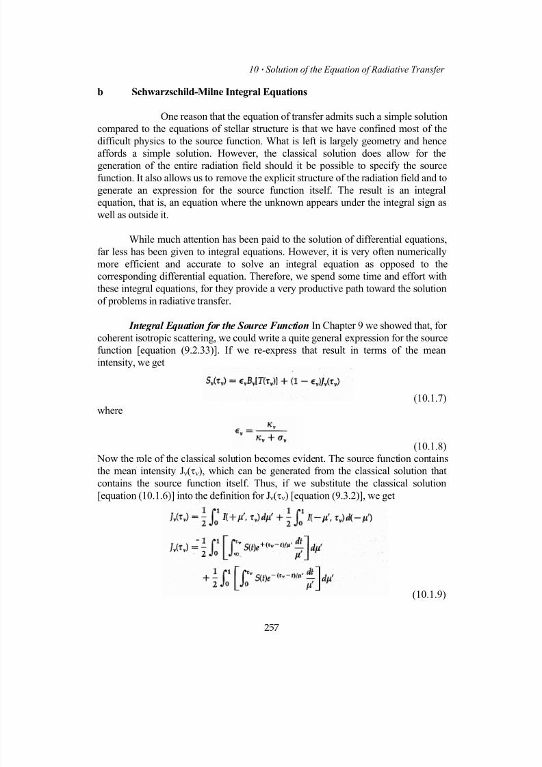
7/18/2019 The Fundamentals of Stellar Astrophysics - Collins G. W.
http://slidepdf.com/reader/full/the-fundamentals-of-stellar-astrophysics-collins-g-w 277/524
10 ⋅ Solution of the Equation of Radiative Transfer
b Schwarzschild-Milne Integral Equations
One reason that the equation of transfer admits such a simple solution
compared to the equations of stellar structure is that we have confined most of the
difficult physics to the source function. What is left is largely geometry and hence
affords a simple solution. However, the classical solution does allow for the
generation of the entire radiation field should it be possible to specify the source
function. It also allows us to remove the explicit structure of the radiation field and to
generate an expression for the source function itself. The result is an integral
equation, that is, an equation where the unknown appears under the integral sign as
well as outside it.
While much attention has been paid to the solution of differential equations,
far less has been given to integral equations. However, it is very often numerically
more efficient and accurate to solve an integral equation as opposed to thecorresponding differential equation. Therefore, we spend some time and effort with
these integral equations, for they provide a very productive path toward the solution
of problems in radiative transfer.
Integral Equation for the Source Function In Chapter 9 we showed that, for
coherent isotropic scattering, we could write a quite general expression for the source
function [equation (9.2.33)]. If we re-express that result in terms of the mean
intensity, we get
(10.1.7)where
(10.1.8)
Now the role of the classical solution becomes evident. The source function contains
the mean intensity Jν(τν), which can be generated from the classical solution that
contains the source function itself. Thus, if we substitute the classical solution
[equation (10.1.6)] into the definition for Jν(τν) [equation (9.3.2)], we get
(10.1.9)
257
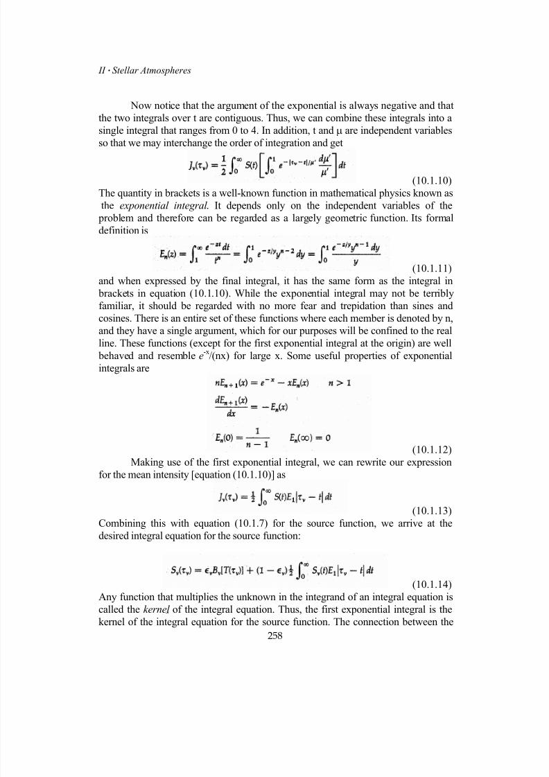
7/18/2019 The Fundamentals of Stellar Astrophysics - Collins G. W.
http://slidepdf.com/reader/full/the-fundamentals-of-stellar-astrophysics-collins-g-w 278/524
II ⋅ Stellar Atmospheres
Now notice that the argument of the exponential is always negative and that
the two integrals over t are contiguous. Thus, we can combine these integrals into a
single integral that ranges from 0 to 4. In addition, t and µ are independent variables
so that we may interchange the order of integration and get
(10.1.10)
The quantity in brackets is a well-known function in mathematical physics known as
the exponential integral . It depends only on the independent variables of the
problem and therefore can be regarded as a largely geometric function. Its formal
definition is
(10.1.11)and when expressed by the final integral, it has the same form as the integral in
brackets in equation (10.1.10). While the exponential integral may not be terribly
familiar, it should be regarded with no more fear and trepidation than sines and
cosines. There is an entire set of these functions where each member is denoted by n,
and they have a single argument, which for our purposes will be confined to the real
line. These functions (except for the first exponential integral at the origin) are well
behaved and resemble e-x
/(nx) for large x. Some useful properties of exponential
integrals are
(10.1.12)
Making use of the first exponential integral, we can rewrite our expression
for the mean intensity [equation (10.1.10)] as
(10.1.13)
Combining this with equation (10.1.7) for the source function, we arrive at the
desired integral equation for the source function:
(10.1.14)
Any function that multiplies the unknown in the integrand of an integral equation is
called the kernel of the integral equation. Thus, the first exponential integral is the
kernel of the integral equation for the source function. The connection between the
258
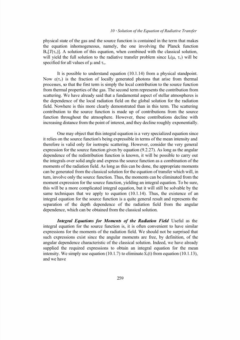
7/18/2019 The Fundamentals of Stellar Astrophysics - Collins G. W.
http://slidepdf.com/reader/full/the-fundamentals-of-stellar-astrophysics-collins-g-w 279/524
10 ⋅ Solution of the Equation of Radiative Transfer
physical state of the gas and the source function is contained in the term that makes
the equation inhomogeneous, namely, the one involving the Planck function
Bν[T (τν)]. A solution of this equation, when combined with the classical solution,
will yield the full solution to the radiative transfer problem since Iν(µ, τν) will bespecified for all values of µ and τν.
It is possible to understand equation (10.1.14) from a physical standpoint.
Now ε(τν) is the fraction of locally generated photons that arise from thermal
processes, so that the first term is simply the local contribution to the source function
from thermal properties of the gas. The second term represents the contribution from
scattering. We have already said that a fundamental aspect of stellar atmospheres is
the dependence of the local radiation field on the global solution for the radiation
field. Nowhere is this more clearly demonstrated than in this term. The scattering
contribution to the source function is made up of contributions from the source
function throughout the atmosphere. However, these contributions decline withincreasing distance from the point of interest, and they decline roughly exponentially.
One may object that this integral equation is a very specialized equation since
it relies on the source function's being expressible in terms of the mean intensity and
therefore is valid only for isotropic scattering. However, consider the very general
expression for the source function given by equation (9.2.27). As long as the angular
dependence of the redistribution function is known, it will be possible to carry out
the integrals over solid angle and express the source function as a combination of the
moments of the radiation field. As long as this can be done, the appropriate moments
can be generated from the classical solution for the equation of transfer which will, in
turn, involve only the source function. Thus, the moments can be eliminated from themoment expression for the source function, yielding an integral equation. To be sure,
this will be a more complicated integral equation, but it will still be solvable by the
same techniques that we apply to equation (10.1.14). Thus, the existence of an
integral equation for the source function is a quite general result and represents the
separation of the depth dependence of the radiation field from the angular
dependence, which can be obtained from the classical solution.
Integral Equations for Moments of the Radiation Field Useful as the
integral equation for the source function is, it is often convenient to have similar
expressions for the moments of the radiation field. We should not be surprised that
such expressions exist since the angular moments are free, by definition, of theangular dependence characteristic of the classical solution. Indeed, we have already
supplied the required expressions to obtain an integral equation for the mean
intensity. We simply use equation (10.1.7) to eliminate S ν(t) from equation (10.1.13),
and we have
259
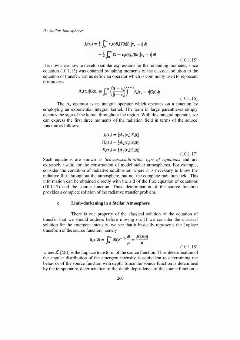
7/18/2019 The Fundamentals of Stellar Astrophysics - Collins G. W.
http://slidepdf.com/reader/full/the-fundamentals-of-stellar-astrophysics-collins-g-w 280/524
II ⋅ Stellar Atmospheres
(10.1.15)It is now clear how to develop similar expressions for the remaining moments, since
equation (10.1.13) was obtained by taking moments of the classical solution to the
equation of transfer. Let us define an operator which is commonly used to represent
this process.
(10.1.16)
The Λn operator is an integral operator which operates on a function by
employing an exponential integral kernel. The term in large parentheses simply
denotes the sign of the kernel throughout the region. With this integral operator, we
can express the first three moments of the radiation field in terms of the sourcefunction as follows:
(10.1.17)
Such equations are known as Schwarzschild-Milne type of equations and are
extremely useful for the construction of model stellar atmospheres. For example,
consider the condition of radiative equilibrium where it is necessary to know the
radiative flux throughout the atmosphere, but not the complete radiation field. This
information can be obtained directly with the aid of the flux equation of equations
(10.1.17) and the source function. Thus, determination of the source function
provides a complete solution of the radiative transfer problem.
c Limb-darkening in a Stellar Atmosphere
There is one property of the classical solution of the equation of
transfer that we should address before moving on. If we consider the classical
solution for the emergent intensity, we see that it basically represents the Laplace
transform of the source function, namely
(10.1.18)
where [S (t)] is the Laplace transform of the source function. Thus determination of
the angular distribution of the emergent intensity is equivalent to determining the
behavior of the source function with depth. Since the source function is determined
by the temperature, determination of the depth dependence of the source function is
260

7/18/2019 The Fundamentals of Stellar Astrophysics - Collins G. W.
http://slidepdf.com/reader/full/the-fundamentals-of-stellar-astrophysics-collins-g-w 281/524
10 ⋅ Solution of the Equation of Radiative Transfer
equivalent to determining the depth dependence of the temperature. This is of
considerable significance for stars where this dependence can be measured directly
for it provides a direct observational check on the models of those stellar
atmospheres.
If we anticipate some later results and assume that the source function can be
approximated by
(10.1.19)
then
(10.1.20)
Thus, the coefficient a that multiplies the angular parameter µ in the emergent
intensity is a direct measure of the source function gradient, while the constant term
b denotes the value of the source function at the boundary. The decrease in
brightness as one approaches the limb of the apparent stellar disk implied by
equation (10.1.20) is called limb-darkening. Since for spherical stars the variation
across the apparent disk is the same as the local angular dependence of the emergent
intensity, measurement of the limb-darkening coefficient a yields a measurement of
the source function gradient. This is of particular interest for the sun where such
measurements are possible. Unfortunately, the poorest theoretical representation of
the model atmosphere occurs near the surface, and this corresponds to just that
region of the stellar disk (i.e., near the limb where µ → 0) where confirmatory
measurements are most difficult to make. Although we have made an approximation
to the depth dependence of the source function in equation (10.1.19), the
approximation is unnecessary and more rigorous studies of this depth dependence
would deal directly with the Laplace transform itself as given by equation (10.1.18).
We have now compiled methods by which we can theoretically relate the emergent
intensity to the source function and provided a potential observational method to
verify our result. However, before discussing methods for the solution for the
integral equation for the source function [equation (10.1.14)] we consider the
solutions to a somewhat simpler problem, in order to gain an appreciation for the
behavior of these solutions.
Empirical Determination of T( τ
) for the Sun In the sun and someeclipsing binary stars, it is possible to determine the variation of the specific intensity
across the apparent disk. If we approximate that variation by
(10.1.21)
we can use equation (10.1.18) to obtain a power series representation of the source
261

7/18/2019 The Fundamentals of Stellar Astrophysics - Collins G. W.
http://slidepdf.com/reader/full/the-fundamentals-of-stellar-astrophysics-collins-g-w 282/524
II ⋅ Stellar Atmospheres
function with optical depth. Let us further assume that the source function can be
represented by the Planck function, which in turn can be expanded in a power series
in the optical depth so that
(10.1.22)
Then the substitution of this power series representation into equation (10.1.18)
yields
(10.1.23)
Since for the sun, the ai's and Iν(0,1) may be determined from observation, the bi's
may be regarded as known. Thus, the temperature variation with monochromatic
optical depth may be recovered from
10.1.24)
In the sun, the assumption that S ν(τν)= Bν(τν) is a particularly good one, so that for
the sun the optical depth variation of the temperature can be determined with the
same sort of accuracy that attends the determination of the limb-darkening.
Empirical Determination of ( τ1 ) / ( τ2 ) for the Sun This type of analysis
can be continued under the above assumptions to obtain the variation with optical
depth of the ratio of two monochromatic absorption coefficients. Since by definition
(10.1.25)
the ratio of two monochromatic optical depths is
(10.1.26)
Differentiating equation (10.1.22) with respect to temperature and substituting the
result into equation (10.1.26), we get
(10.1.27)
Thus it is possible to determine the approximate wavelength dependence of the
opacity for stars like the sun from the observed limb-darkening. Such observations
provide a valuable check on the theory of stellar atmospheres.
262

7/18/2019 The Fundamentals of Stellar Astrophysics - Collins G. W.
http://slidepdf.com/reader/full/the-fundamentals-of-stellar-astrophysics-collins-g-w 283/524
10 ⋅ Solution of the Equation of Radiative Transfer
10.2 Gray Atmosphere
For the better part of this century, theoretical astrophysicists have been
concerned with the solution to an idealized radiative transfer problem known as the
gray atmosphere. Although it is an idealized situation, it has some counterparts in
nature. In addition, this problem possesses the virtue that a complete solution can be
obtained for the radiation field without recourse to the physical details of the
atmosphere. In this regard, the gray atmosphere model is rather like polytropic
models for stellar interiors. As was the case for polytropes and stellar interiors, we
may expect to gain significant insight into the properties of stellar atmospheres by
understanding the solution to the gray atmosphere problem. The additional
assumption required to turn our study of radiative transfer into that of a gray
atmosphere is simple. Assume that the opacity, whether it is absorption or scattering,is independent of frequency. Thus, any frequency can be treated as any other
frequency, as far as the radiative transfer is concerned. This independence of the
radiative transfer from frequency has the interesting consequence that the
mathematical solution to the equation of transfer for any frequency will be the
solution for all frequencies, and thus must be the solution for the sum of all
frequencies. Hence, the aspect of the solution that specifies the radiative flux also
refers to the total flux, making the condition of radiative equilibrium relatively
simple to apply. Since all aspects of the mathematical description are independent of
frequency, we drop the subscript n for the balance of this discussion.
Knowing what we do about the physical processes of absorption, it isreasonable to ask if the gray atmosphere is anything more than an interesting
mathematical exercise. Certainly bound-bound transitions are anything but gray.
However, there are some bound-free transitions that exhibit only weak frequency
dependence over substantial regions of the spectrum. If those regions of the spectrum
correspond to that part of the spectrum containing most of the radiant flux, then the
atmosphere will be very similar to a gray atmosphere. Absorption due to the H-minus
ion is relatively frequency-independent throughout the visible part of the spectrum
and in some stars is the dominant source of opacity. However, the premier example
of a gray opacity source is electron scattering. Thomson scattering by free electrons
is frequency-independent by definition, and for stars hotter than about 25,000 K, it is
the dominant source of opacity throughout the range of wavelengths encompassingthe maximum flow of energy. Thus, the early O and B stars have atmospheres that, to
a very high degree, may be regarded as gray.
Since frequency dependence has been removed from the problem, we may
write the equation of radiative transfer for a plane-parallel static atmosphere as
263

7/18/2019 The Fundamentals of Stellar Astrophysics - Collins G. W.
http://slidepdf.com/reader/full/the-fundamentals-of-stellar-astrophysics-collins-g-w 284/524
II ⋅ Stellar Atmospheres
(10.2.1)
where, for isotropic coherent scattering, the source function is
(10.2.2)
Now the independence of the opacity on frequency makes the condition of radiative
equilibrium given by equation (9.4.4) particularly simple.
(10.2.3)
or simply
(10.2.4)
Substitution of this result into equation (10.2.2) yields
(10.2.5)
The fact that the mean intensity is equal to the Planck function and that either can be
taken to be the source function has the interesting result that the solution to the gray
atmosphere is independent of the relative roles of scattering and absorption. Thus,
the radiation field for a pure absorbing gray atmosphere, where the source function is
clearly the Planck function, will be indistinguishable from the radiation field of a pure scattering gray atmosphere. In addition, since there is a general independence
on frequency, the spectral energy distribution will be that resulting from a gray
atmosphere where the source function is the Planck function.
The gray atmosphere implies that all the development of Chapters 9 and 10
will apply at each frequency. This is indeed the easiest way to obtain equations
(10.2.1) through (10.2.4). But there is much more. The integral equation for the
source function [equation (10.1.14)] and that for the moments of the radiation field
[equations (10.1.17)] become
(10.2.6)
Solution of these equations, combined with the classical solution to the equation of
264
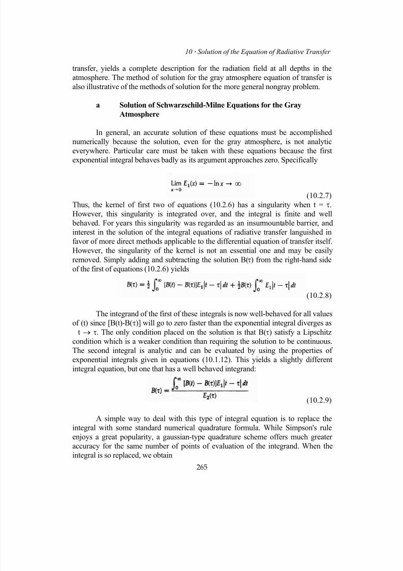
7/18/2019 The Fundamentals of Stellar Astrophysics - Collins G. W.
http://slidepdf.com/reader/full/the-fundamentals-of-stellar-astrophysics-collins-g-w 285/524
10 ⋅ Solution of the Equation of Radiative Transfer
transfer, yields a complete description for the radiation field at all depths in the
atmosphere. The method of solution for the gray atmosphere equation of transfer is
also illustrative of the methods of solution for the more general nongray problem.
a Solution of Schwarzschild-Milne Equations for the Gray
Atmosphere
In general, an accurate solution of these equations must be accomplished
numerically because the solution, even for the gray atmosphere, is not analytic
everywhere. Particular care must be taken with these equations because the first
exponential integral behaves badly as its argument approaches zero. Specifically
(10.2.7)
Thus, the kernel of first two of equations (10.2.6) has a singularity when t = τ.
However, this singularity is integrated over, and the integral is finite and well
behaved. For years this singularity was regarded as an insurmountable barrier, and
interest in the solution of the integral equations of radiative transfer languished in
favor of more direct methods applicable to the differential equation of transfer itself.
However, the singularity of the kernel is not an essential one and may be easily
removed. Simply adding and subtracting the solution B(τ) from the right-hand side
of the first of equations (10.2.6) yields
(10.2.8)
The integrand of the first of these integrals is now well-behaved for all values
of (t) since [B(t)-B(τ)] will go to zero faster than the exponential integral diverges as
t → τ. The only condition placed on the solution is that B(τ) satisfy a Lipschitz
condition which is a weaker condition than requiring the solution to be continuous.
The second integral is analytic and can be evaluated by using the properties of
exponential integrals given in equations (10.1.12). This yields a slightly different
integral equation, but one that has a well behaved integrand:
(10.2.9)
A simple way to deal with this type of integral equation is to replace the
integral with some standard numerical quadrature formula. While Simpson's rule
enjoys a great popularity, a gaussian-type quadrature scheme offers much greater
accuracy for the same number of points of evaluation of the integrand. When the
integral is so replaced, we obtain
265
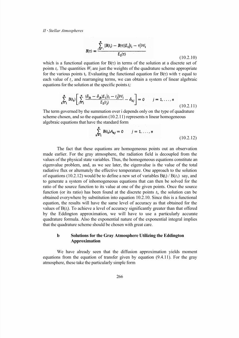
7/18/2019 The Fundamentals of Stellar Astrophysics - Collins G. W.
http://slidepdf.com/reader/full/the-fundamentals-of-stellar-astrophysics-collins-g-w 286/524
II ⋅ Stellar Atmospheres
(10.2.10)which is a functional equation for B(τ) in terms of the solution at a discrete set of
points t i. The quantities W i are just the weights of the quadrature scheme appropriate
for the various points ti. Evaluating the functional equation for B(τ) with τ equal to
each value of t j, and rearranging terms, we can obtain a system of linear algebraic
equations for the solution at the specific points t i:
(10.2.11)
The term governed by the summation over i depends only on the type of quadrature
scheme chosen, and so the equation (10.2.11) represents n linear homogeneousalgebraic equations that have the standard form
(10.2.12)
The fact that these equations are homogeneous points out an observation
made earlier. For the gray atmosphere, the radiation field is decoupled from the
values of the physical state variables. Thus, the homogeneous equations constitute an
eigenvalue problem, and, as we see later, the eigenvalue is the value of the total
radiative flux or alternately the effective temperature. One approach to the solution
of equations (10.2.12) would be to define a new set of variables B(t i) / B(t 1) say, andto generate a system of inhomogeneous equations that can then be solved for the
ratio of the source function to its value at one of the given points. Once the source
function (or its ratio) has been found at the discrete points t i, the solution can be
obtained everywhere by substitution into equation 10.2.10. Since this is a functional
equation, the results will have the same level of accuracy as that obtained for the
values of B(t i). To achieve a level of accuracy significantly greater than that offered
by the Eddington approximation, we will have to use a particularly accurate
quadrature formula. Also the exponential nature of the exponential integral implies
that the quadrature scheme should be chosen with great care.
b Solutions for the Gray Atmosphere Utilizing the EddingtonApproximation
We have already seen that the diffusion approximation yields moment
equations from the equation of transfer given by equation (9.4.11). For the gray
atmosphere, these take the particularly simple form
266
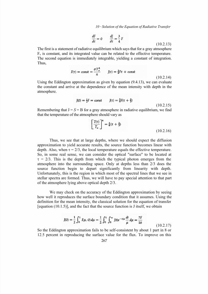
7/18/2019 The Fundamentals of Stellar Astrophysics - Collins G. W.
http://slidepdf.com/reader/full/the-fundamentals-of-stellar-astrophysics-collins-g-w 287/524
10 ⋅ Solution of the Equation of Radiative Transfer
(10.2.13)
The first is a statement of radiative equilibrium which says that for a gray atmosphere
Fν is constant, and its integrated value can be related to the effective temperature.
The second equation is immediately integrable, yielding a constant of integration.
Thus,
(10.2.14)
Using the Eddington approximation as given by equation (9.4.13), we can evaluate
the constant and arrive at the dependence of the mean intensity with depth in the
atmosphere.
(10.2.15)
Remembering that J = S = B for a gray atmosphere in radiative equilibrium, we find
that the temperature of the atmosphere should vary as
(10.2.16)
Thus, we see that at large depths, where we should expect the diffusion
approximation to yield accurate results, the source function becomes linear with
depth. Also, when τ = 2/3, the local temperature equals the effective temperature.
So, in some real sense, we can consider the optical "surface" to be located atτ = 2/3. This is the depth from which the typical photon emerges from the
atmosphere into the surrounding space. Only at depths less than 2/3 does the
source function begin to depart significantly from linearity with depth.
Unfortunately, this is the region in which most of the spectral lines that we see in
stellar spectra are formed. Thus, we will have to pay special attention to that part
of the atmosphere lying above optical depth 2/3.
We may check on the accuracy of the Eddington approximation by seeing
how well it reproduces the surface boundary condition that it assumes. Using the
definition for the mean intensity, the classical solution for the equation of transfer
[equation (10.1.5)], and the fact that the source function is J itself, we obtain
(10.2.17)
So the Eddington approximation fails to be self-consistent by about 1 part in 8 or
12.5 percent in reproducing the surface value for the flux. To improve on this
267
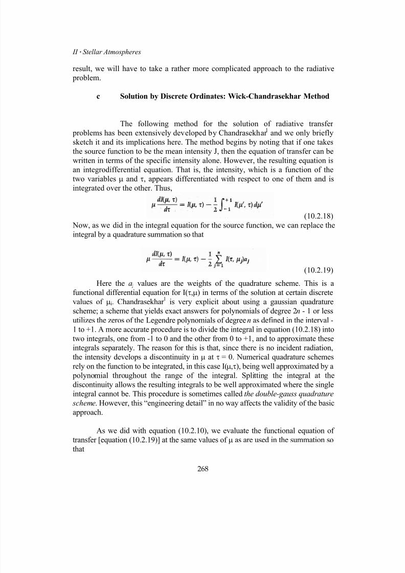
7/18/2019 The Fundamentals of Stellar Astrophysics - Collins G. W.
http://slidepdf.com/reader/full/the-fundamentals-of-stellar-astrophysics-collins-g-w 288/524
II ⋅ Stellar Atmospheres
result, we will have to take a rather more complicated approach to the radiative
problem.
c Solution by Discrete Ordinates: Wick-Chandrasekhar Method
The following method for the solution of radiative transfer
problems has been extensively developed by Chandrasekhar 1 and we only briefly
sketch it and its implications here. The method begins by noting that if one takes
the source function to be the mean intensity J, then the equation of transfer can be
written in terms of the specific intensity alone. However, the resulting equation is
an integrodifferential equation. That is, the intensity, which is a function of the
two variables µ and τ, appears differentiated with respect to one of them and is
integrated over the other. Thus,
(10.2.18)
Now, as we did in the integral equation for the source function, we can replace the
integral by a quadrature summation so that
(10.2.19)
Here the a j values are the weights of the quadrature scheme. This is a
functional differential equation for I(τ,µ) in terms of the solution at certain discrete
values of µi. Chandrasekhar 1 is very explicit about using a gaussian quadraturescheme; a scheme that yields exact answers for polynomials of degree 2n - 1 or less
utilizes the zeros of the Legendre polynomials of degree n as defined in the interval -
1 to +1. A more accurate procedure is to divide the integral in equation (10.2.18) into
two integrals, one from -1 to 0 and the other from 0 to +1, and to approximate these
integrals separately. The reason for this is that, since there is no incident radiation,
the intensity develops a discontinuity in µ at τ = 0. Numerical quadrature schemes
rely on the function to be integrated, in this case I(µ,τ), being well approximated by a
polynomial throughout the range of the integral. Splitting the integral at the
discontinuity allows the resulting integrals to be well approximated where the single
integral cannot be. This procedure is sometimes called the double-gauss quadrature
scheme. However, this “engineering detail” in no way affects the validity of the basicapproach.
As we did with equation (10.2.10), we evaluate the functional equation of
transfer [equation (10.2.19)] at the same values of µ as are used in the summation so
that
268

7/18/2019 The Fundamentals of Stellar Astrophysics - Collins G. W.
http://slidepdf.com/reader/full/the-fundamentals-of-stellar-astrophysics-collins-g-w 289/524
10 ⋅ Solution of the Equation of Radiative Transfer
(10.2.20)
We now have a system of n homogeneous linear differential equations for the
functions I(τ,µi). Each of these functions represents the specific intensity along a
particular direction specified by the value of µi. Since the value µi=0 represents the
point of discontinuity in I(µ,τ) at the surface, this value should be avoided. Thus,
there will normally be as many negative values of µi as positive ones. To solve the
problem, we must find n constants of integration for the n first-order differential
equations.
Inspired by the general exponential attenuation of a beam of photons passing
through a medium, let us assume a solution of the form
(10.2.21)
Substitution of this form into this set of linear differential equations (10.2.20), will
satisfy the equations if
(10.2.22)
and k satisfies the eigenvalue equation
(10.2.23)Thus equation (10.2.22) provides a constant of integration for every distinct value
of k . Since in all quadrature schemes the sum of the weights must equal the
interval, k 2 = 0 will satisfy equation (10.2.23). Thus, since equation (10.2.23) is
essentially polynomic in form there will be n/2 - 1 distinct nonzero values of k 2
and thus n - 2 distinct nonzero values of k which we denote as ±k α. When these
are combined with the value k = 0, we are still missing one constant of
integration. Wick, inspired by the Eddington approximation, suggested a solution
of the form
(10.2.24)Substitution of this form into equations (10.2.20) also satisfies the equation of
transfer provided that
(10.2.25)
The product constant bQ can be identified with the constant obtained from k 2=0 so it
269
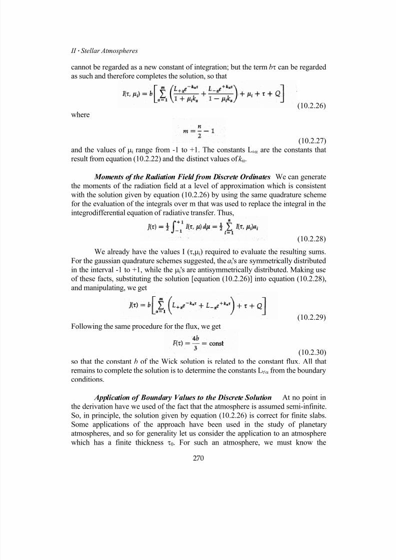
7/18/2019 The Fundamentals of Stellar Astrophysics - Collins G. W.
http://slidepdf.com/reader/full/the-fundamentals-of-stellar-astrophysics-collins-g-w 290/524
II ⋅ Stellar Atmospheres
cannot be regarded as a new constant of integration; but the term bτ can be regarded
as such and therefore completes the solution, so that
(10.2.26)
where
(10.2.27)
and the values of µi range from -1 to +1. The constants L±α are the constants that
result from equation (10.2.22) and the distinct values of k α.
Moments of the Radiation Field from Discrete Ordinates We can generate
the moments of the radiation field at a level of approximation which is consistent
with the solution given by equation (10.2.26) by using the same quadrature schemefor the evaluation of the integrals over m that was used to replace the integral in the
integrodifferential equation of radiative transfer. Thus,
(10.2.28)
We already have the values I (τ,µi) required to evaluate the resulting sums.
For the gaussian quadrature schemes suggested, the ai's are symmetrically distributed
in the interval -1 to +1, while the µi's are antisymmetrically distributed. Making use
of these facts, substituting the solution [equation (10.2.26)] into equation (10.2.28),
and manipulating, we get
(10.2.29)
Following the same procedure for the flux, we get
(10.2.30)
so that the constant b of the Wick solution is related to the constant flux. All that
remains to complete the solution is to determine the constants L∀α from the boundary
conditions.
Application of Boundary Values to the Discrete Solution At no point in
the derivation have we used of the fact that the atmosphere is assumed semi-infinite.
So, in principle, the solution given by equation (10.2.26) is correct for finite slabs.
Some applications of the approach have been used in the study of planetary
atmospheres, and so for generality let us consider the application to an atmosphere
which has a finite thickness τ0. For such an atmosphere, we must know the
270
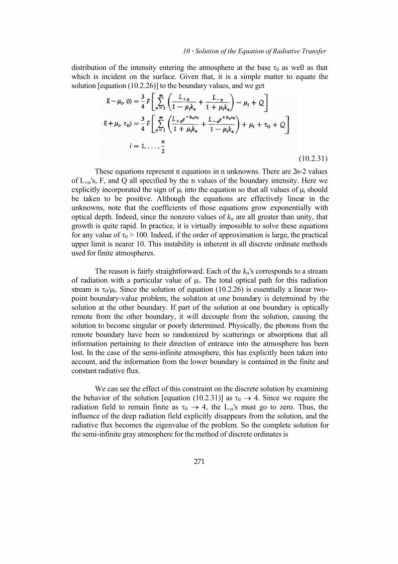
7/18/2019 The Fundamentals of Stellar Astrophysics - Collins G. W.
http://slidepdf.com/reader/full/the-fundamentals-of-stellar-astrophysics-collins-g-w 291/524
10 ⋅ Solution of the Equation of Radiative Transfer
distribution of the intensity entering the atmosphere at the base τ0 as well as that
which is incident on the surface. Given that, it is a simple matter to equate the
solution [equation (10.2.26)] to the boundary values, and we get
(10.2.31)
These equations represent n equations in n unknowns. There are 2n-2 values
of L±α's, F, and Q all specified by the n values of the boundary intensity. Here we
explicitly incorporated the sign of µi into the equation so that all values of µi should
be taken to be positive. Although the equations are effectively linear in theunknowns, note that the coefficients of those equations grow exponentially with
optical depth. Indeed, since the nonzero values of k α are all greater than unity, that
growth is quite rapid. In practice, it is virtually impossible to solve these equations
for any value of τ0 > 100. Indeed, if the order of approximation is large, the practical
upper limit is nearer 10. This instability is inherent in all discrete ordinate methods
used for finite atmospheres.
The reason is fairly straightforward. Each of the k α's corresponds to a stream
of radiation with a particular value of µi. The total optical path for this radiation
stream is τ0/µi. Since the solution of equation (10.2.26) is essentially a linear two-
point boundary-value problem, the solution at one boundary is determined by thesolution at the other boundary. If part of the solution at one boundary is optically
remote from the other boundary, it will decouple from the solution, causing the
solution to become singular or poorly determined. Physically, the photons from the
remote boundary have been so randomized by scatterings or absorptions that all
information pertaining to their direction of entrance into the atmosphere has been
lost. In the case of the semi-infinite atmosphere, this has explicitly been taken into
account, and the information from the lower boundary is contained in the finite and
constant radiative flux.
We can see the effect of this constraint on the discrete solution by examining
the behavior of the solution [equation (10.2.31)] as τ0 → 4. Since we require theradiation field to remain finite as τ0 → 4, the L-α's must go to zero. Thus, the
influence of the deep radiation field explicitly disappears from the solution, and the
radiative flux becomes the eigenvalue of the problem. So the complete solution for
the semi-infinite gray atmosphere for the method of discrete ordinates is
271

7/18/2019 The Fundamentals of Stellar Astrophysics - Collins G. W.
http://slidepdf.com/reader/full/the-fundamentals-of-stellar-astrophysics-collins-g-w 292/524
II ⋅ Stellar Atmospheres
(10.2.32)
Table 10.1 contains some values of L+α, k α, and Q for various orders of
approximation for the semi-infinite gray atmosphere for the single-gauss quadrature
scheme. By analogy to the Eddington approximation, the source function is
sometimes written as
(10.2.33)
where
(10.2.34)
is known as the Hopf function. It is clear that for the Eddington approximation the
appropriate Hopf function would be q(τ) = 2/3. The Eddington approximation also
avoids the problem of the solution's becoming unstable with increasing depth, by the
use of the diffusion approximation, which basically assumes that the radiation field
has been directionally randomized.
Nonconservative Gray Atmospheres The notion of a nonconservative gray
atmosphere may sound like a contradiction in terms, and if it were meant to apply to
all frequencies, it would be. However, consider the case where the opacity is
essentially gray over the part of the spectrum containing most of the emergent
radiation, but radiative equilibrium does not apply because some energy is lost from
the radiation field to perhaps convection. Or consider an atmosphere where the
dominant opacity source is the scattering of light from a hot external source, but the
atmosphere itself is so cold that the thermal emission can be neglected. Planetary
atmospheres often fit into this category.
272
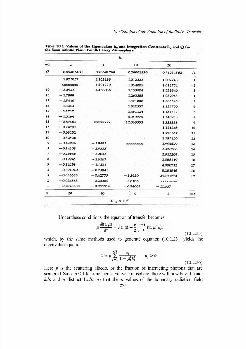
7/18/2019 The Fundamentals of Stellar Astrophysics - Collins G. W.
http://slidepdf.com/reader/full/the-fundamentals-of-stellar-astrophysics-collins-g-w 293/524
10 ⋅ Solution of the Equation of Radiative Transfer
Under these conditions, the equation of transfer becomes
(10.2.35)
which, by the same methods used to generate equation (10.2.23), yields the
eigenvalue equation
(10.2.36)
Here p is the scattering albedo, or the fraction of interacting photons that are
scattered. Since p < 1 for a nonconservative atmosphere, there will now be n distinct
k α's and n distinct L±α's, so that the n values of the boundary radiation field
273

7/18/2019 The Fundamentals of Stellar Astrophysics - Collins G. W.
http://slidepdf.com/reader/full/the-fundamentals-of-stellar-astrophysics-collins-g-w 294/524
II ⋅ Stellar Atmospheres
completely specify the solution. The L∀α’s are specified by the boundary equations
(10.2.37)
and the source function for the atmosphere is given by
(10.2.38)
We need not consider the unilluminated semi-infinite atmosphere since all
radiation moving up through a nonconservative semi-infinite atmosphere willeventually be lost before it emerges. Thus, only the finite slab or an illuminated semi-
infinite nonconservative atmosphere will yield anything other than the trivial
solution.
10.3 Nongray Radiative Transfer
While the elimination of the assumption of a gray opacity removes the easy
incorporation of radiative equilibrium into the solution of the equation of radiative
transfer, most methods described in Section 10.2 can be used for the nongray case. In
spite of the diversity of methods available to the researcher for the solution of
radiative transfer problems (there are more than are described here), most practical
approaches can be divided into two categories: the solution of the integral equation
for the source function and methods based on the solution of the differential
equations for the radiation field. The solution of the integral equation for the source
function is highly efficient, since no more information is generated than is necessary
for the solution of the problem, and has also proved effective in dealing with
problems of polarization, where complex redistribution functions are required (see
Chapter 16). The differential equation approach is perhaps more widely used because
a highly efficient algorithm has been developed which enables the investigator to
utilize existing and proven mathematical packages for much of the numerical work.
In addition, the differential equation approach has proved effective where geometries
other than plane-parallel ones are required, and lends itself naturally to the
incorporation of time-dependent and hydrodynamic terms when they may be needed.
Of the myriads of specific applications, we will be concerned with only two.
274
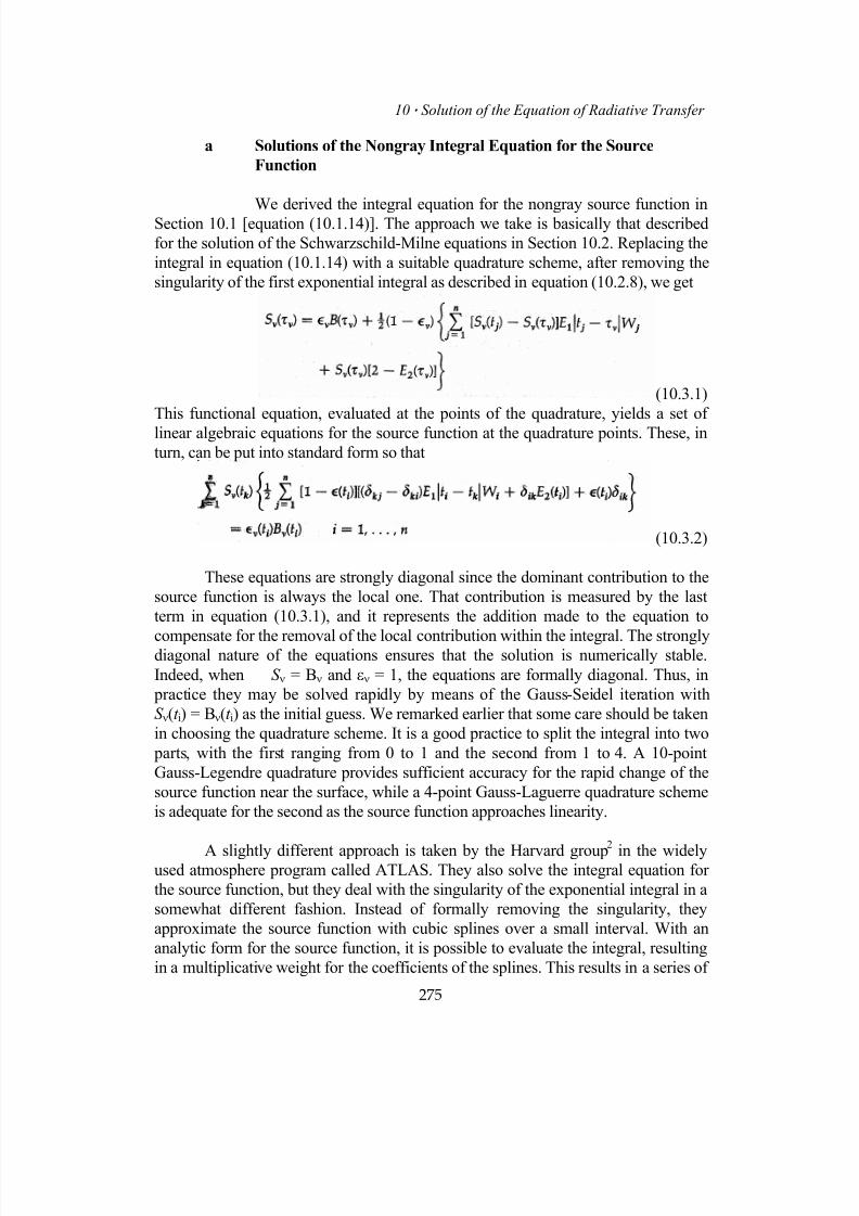
7/18/2019 The Fundamentals of Stellar Astrophysics - Collins G. W.
http://slidepdf.com/reader/full/the-fundamentals-of-stellar-astrophysics-collins-g-w 295/524
10 ⋅ Solution of the Equation of Radiative Transfer
a Solutions of the Nongray Integral Equation for the Source
Function
We derived the integral equation for the nongray source function in
Section 10.1 [equation (10.1.14)]. The approach we take is basically that described
for the solution of the Schwarzschild-Milne equations in Section 10.2. Replacing the
integral in equation (10.1.14) with a suitable quadrature scheme, after removing the
singularity of the first exponential integral as described in equation (10.2.8), we get
(10.3.1)
This functional equation, evaluated at the points of the quadrature, yields a set of
linear algebraic equations for the source function at the quadrature points. These, in
turn, can be put into standard form so that
(10.3.2)
These equations are strongly diagonal since the dominant contribution to the
source function is always the local one. That contribution is measured by the last
term in equation (10.3.1), and it represents the addition made to the equation to
compensate for the removal of the local contribution within the integral. The stronglydiagonal nature of the equations ensures that the solution is numerically stable.
Indeed, when S ν = Bν and εν = 1, the equations are formally diagonal. Thus, in
practice they may be solved rapidly by means of the Gauss-Seidel iteration with
S ν(t i) = Bν(t i) as the initial guess. We remarked earlier that some care should be taken
in choosing the quadrature scheme. It is a good practice to split the integral into two
parts, with the first ranging from 0 to 1 and the second from 1 to 4. A 10-point
Gauss-Legendre quadrature provides sufficient accuracy for the rapid change of the
source function near the surface, while a 4-point Gauss-Laguerre quadrature scheme
is adequate for the second as the source function approaches linearity.
A slightly different approach is taken by the Harvard group2
in the widelyused atmosphere program called ATLAS. They also solve the integral equation for
the source function, but they deal with the singularity of the exponential integral in a
somewhat different fashion. Instead of formally removing the singularity, they
approximate the source function with cubic splines over a small interval. With an
analytic form for the source function, it is possible to evaluate the integral, resulting
in a multiplicative weight for the coefficients of the splines. This results in a series of
275

7/18/2019 The Fundamentals of Stellar Astrophysics - Collins G. W.
http://slidepdf.com/reader/full/the-fundamentals-of-stellar-astrophysics-collins-g-w 296/524
II ⋅ Stellar Atmospheres
weights which are numerically very similar to those present in equation (10.3.2).
Again, a set of linear algebraic equations is produced for the source function at a
discrete set of optical depths. The results of the two methods are nearly identical,
with the gaussian quadrature scheme being somewhat more efficient.
b Differential Equation Approach: The Feautrier Method
This method replaces the differential equations of radiative transfer
with a set of finite difference equations for parameters related to the specific intensity
at a discrete set of values for the angular variable mi. However, the choice of values
of mi is irrelevant to understanding the method, so we leave that choice arbitrary for
the moment. Instead of solving the equation of transfer for the specific intensity, we
write equations of transfer for combinations of inward- and outward-directed
streams.
Feautrier Equations Consider the variables
(10.3.3)
Here we have paired the outward directed stream I(+µ,τ) with its inward -directed
counterpart I(-µ,τ) into quantities that resemble a "mean" intensity u and a "flux" v.
One of the benefits of the linearity of the equation of transfer is that we can add or
subtract such equations and still get a linear equation. Thus, by adding an equation
for a +µ stream to one for a -µ stream we get
(10.3.4)
Similarly, by subtracting one from the other, we get
(10.3.5)
Using this result to eliminate v from equation (10.3.4), we have
(10.3.6)
This is a second-order linear differential equation, so we will need two
constraints or constants of integration. At the surface I(-µ,0) = 0, so v(0) = u(0), and
from equation (10.3.5) we have
(10.3.7)
276
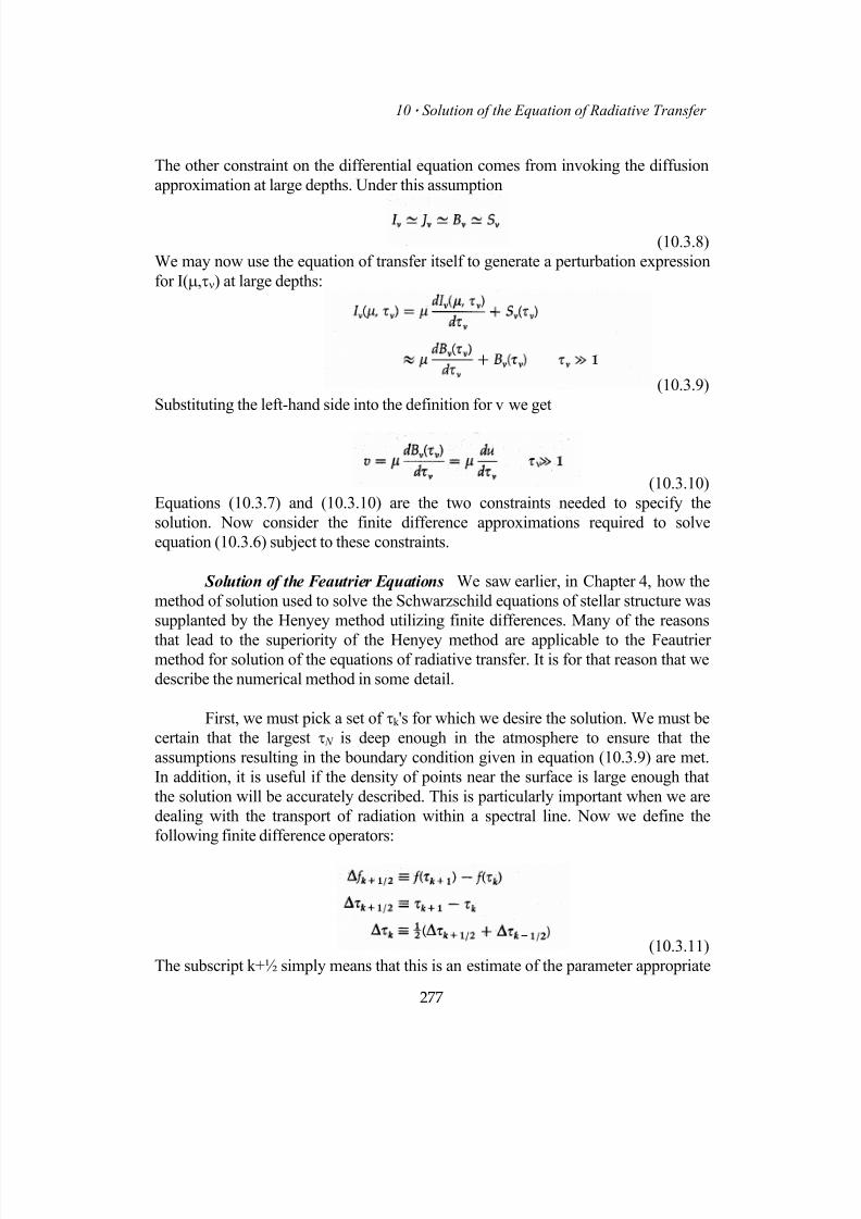
7/18/2019 The Fundamentals of Stellar Astrophysics - Collins G. W.
http://slidepdf.com/reader/full/the-fundamentals-of-stellar-astrophysics-collins-g-w 297/524
10 ⋅ Solution of the Equation of Radiative Transfer
The other constraint on the differential equation comes from invoking the diffusion
approximation at large depths. Under this assumption
(10.3.8)
We may now use the equation of transfer itself to generate a perturbation expression
for I(µ,τν) at large depths:
(10.3.9)
Substituting the left-hand side into the definition for v we get
(10.3.10)
Equations (10.3.7) and (10.3.10) are the two constraints needed to specify the
solution. Now consider the finite difference approximations required to solve
equation (10.3.6) subject to these constraints.
Solution of the Feautrier Equations We saw earlier, in Chapter 4, how the
method of solution used to solve the Schwarzschild equations of stellar structure was
supplanted by the Henyey method utilizing finite differences. Many of the reasons
that lead to the superiority of the Henyey method are applicable to the Feautriermethod for solution of the equations of radiative transfer. It is for that reason that we
describe the numerical method in some detail.
First, we must pick a set of τk 's for which we desire the solution. We must be
certain that the largest τ N is deep enough in the atmosphere to ensure that the
assumptions resulting in the boundary condition given in equation (10.3.9) are met.
In addition, it is useful if the density of points near the surface is large enough that
the solution will be accurately described. This is particularly important when we are
dealing with the transport of radiation within a spectral line. Now we define the
following finite difference operators:
(10.3.11)
The subscript k+½ simply means that this is an estimate of the parameter appropriate
277
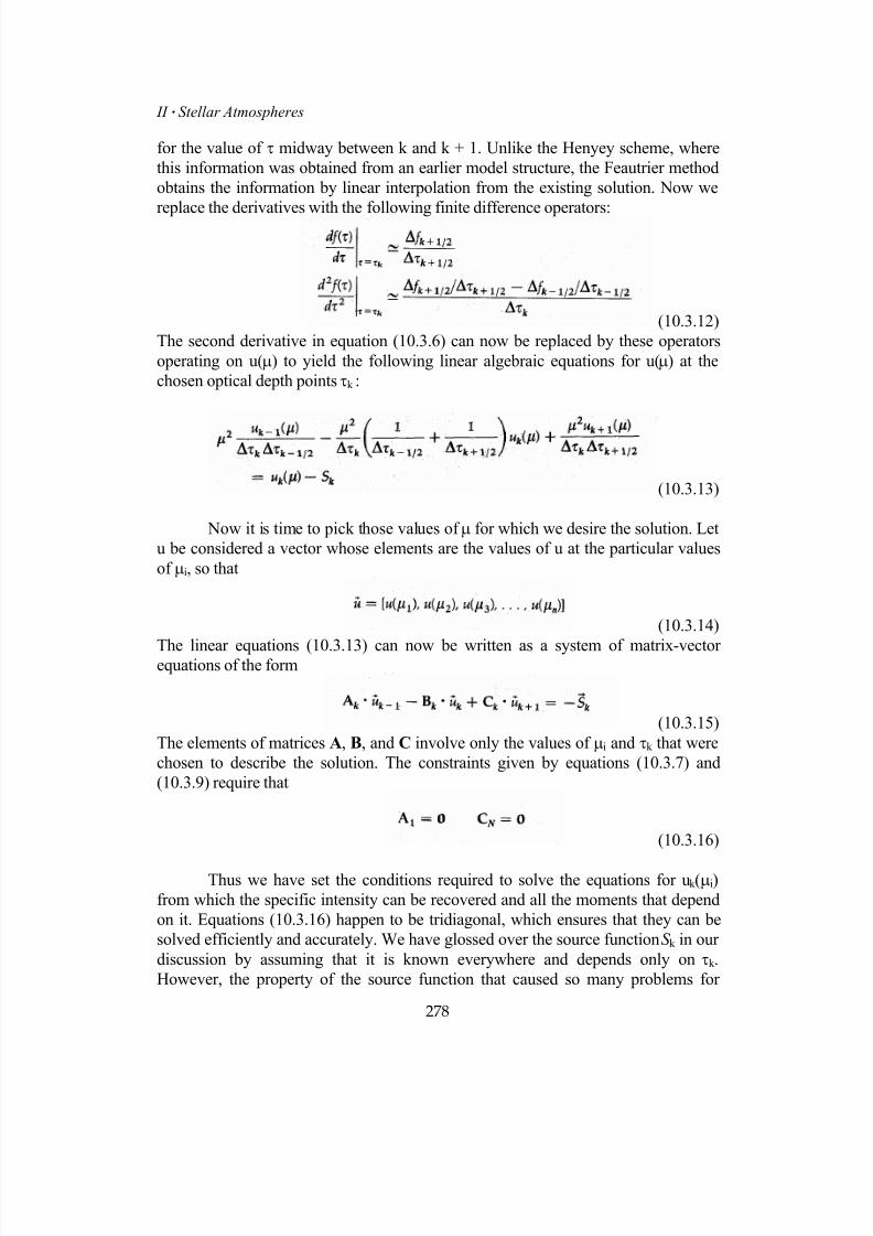
7/18/2019 The Fundamentals of Stellar Astrophysics - Collins G. W.
http://slidepdf.com/reader/full/the-fundamentals-of-stellar-astrophysics-collins-g-w 298/524
II ⋅ Stellar Atmospheres
for the value of τ midway between k and k + 1. Unlike the Henyey scheme, where
this information was obtained from an earlier model structure, the Feautrier method
obtains the information by linear interpolation from the existing solution. Now we
replace the derivatives with the following finite difference operators:
(10.3.12)
The second derivative in equation (10.3.6) can now be replaced by these operators
operating on u(µ) to yield the following linear algebraic equations for u(µ) at the
chosen optical depth points τk :
(10.3.13)
Now it is time to pick those values of µ for which we desire the solution. Let
u be considered a vector whose elements are the values of u at the particular values
of µi, so that
(10.3.14)
The linear equations (10.3.13) can now be written as a system of matrix-vectorequations of the form
(10.3.15)
The elements of matrices A, B, and C involve only the values of µi and τk that were
chosen to describe the solution. The constraints given by equations (10.3.7) and
(10.3.9) require that
(10.3.16)
Thus we have set the conditions required to solve the equations for uk (µi)
from which the specific intensity can be recovered and all the moments that depend
on it. Equations (10.3.16) happen to be tridiagonal, which ensures that they can be
solved efficiently and accurately. We have glossed over the source function S k in our
discussion by assuming that it is known everywhere and depends only on τk .
However, the property of the source function that caused so many problems for
278
7/18/2019 The Fundamentals of Stellar Astrophysics - Collins G. W.
http://slidepdf.com/reader/full/the-fundamentals-of-stellar-astrophysics-collins-g-w 299/524
10 ⋅ Solution of the Equation of Radiative Transfer
earlier methods (and, indeed, resulted in the integral equations in the first place) is
that the source function usually depends on the intensity itself. However, for
scattering, the source function does depend on the intensity in a linear manner.
Therefore, it is possible to represent the source function in terms of the unknowns uk
and vk and include them in the equations, still preserving their tridiagonal form.
There is one caveat to this. The Feautrier method imposes a certain symmetry
on the solution to the radiative transfer problem by combining inward- and outward-
directed streams. If the redistribution function does not share this symmetry, it will
not be possible to represent the scattering in terms of the functions u(µ) and v(µ).
Thus, for some problems involving anisotropic scattering, the Feautrier method may
not be applicable. In addition, when the redistribution function involves
redistribution in frequency, the optical depth points must be chosen so that the
deepest point will satisfy the assumptions required for the approximation given in
equation (10.3.9) for all frequencies. If this is not done, errors incurred at thosefrequencies for which the assumptions fail can propagate in an insidious manner
throughout the entire solution.
The Feautrier method does not suffer from the exponential instabilities
described for the discrete ordinate method, because it invokes the diffusion
approximation at large depths (specifically the inner boundary). The diffusion
approximation basically contains the information that the radiation field has been
randomized in direction and thereby stabilizes the solution in the same manner as it
stabilizes the Eddington solution. As we see in Chapter 11, knowledge of the mean
intensity, the radiative flux, and occasionally the radiation pressure is usually
sufficient to calculate the structure of the atmosphere. The Feautrier method findsmore information than that and therefore is not as efficient as it might be. However,
the numerical methods for solving the resulting linear equations are so fast that the
overall efficiency of the method is quite good, and it provides an excellent method of
solution for most problems of radiative transfer in stellar atmospheres. Remember
that, like any numerical method, the Feautrier method should be used with great care
and only on those problems for which it is suited.
10.4 Radiative Transport in a Spherical Atmosphere
Any discussion of the solution of radiative transfer problems would be
incomplete without some mention of the problem introduced by a departure from thesimplifying assumption of plane-parallel geometry. In addition, there are stars for
which the plane-parallel approximation is inappropriate, and we would like to model
these stars as well as the main sequence stars for which the plane-parallel
approximation is generally adequate. The density in the outer regions of red
supergiants is so low that the atmosphere will occupy the outer 30 percent to 40
percent of what we would like to call the radius of the star. Here, the plane-parallel
279
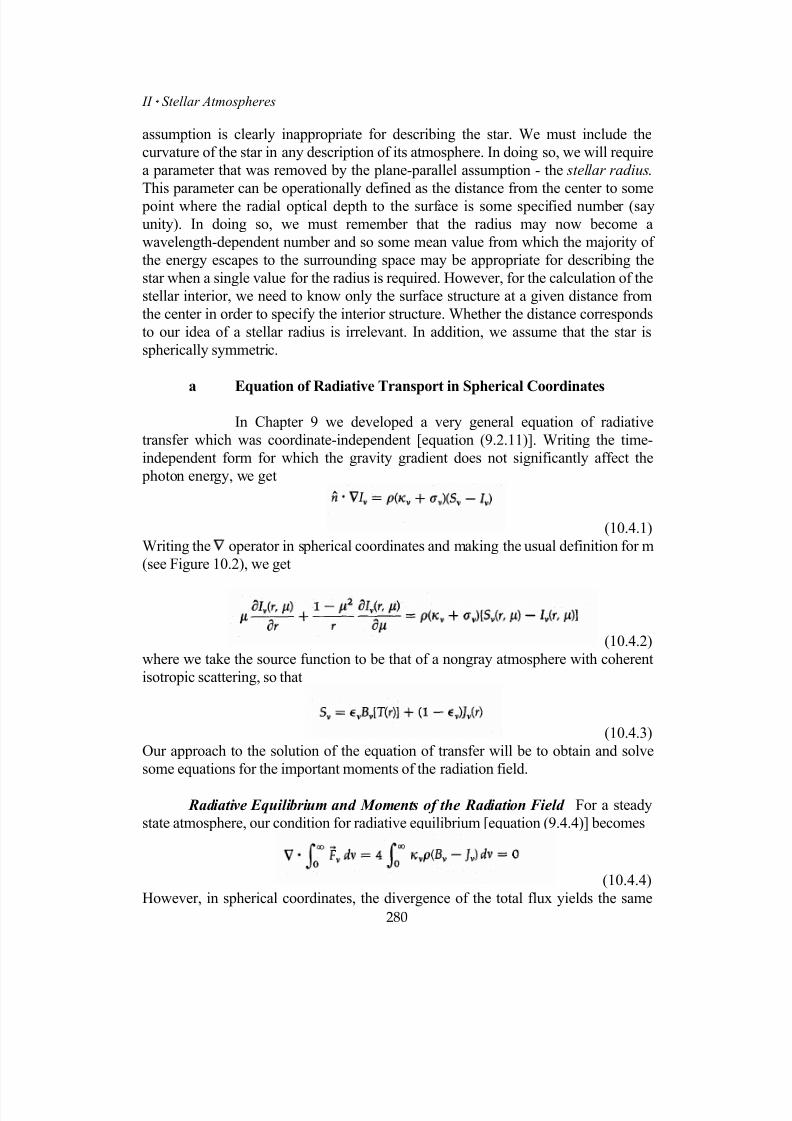
7/18/2019 The Fundamentals of Stellar Astrophysics - Collins G. W.
http://slidepdf.com/reader/full/the-fundamentals-of-stellar-astrophysics-collins-g-w 300/524
II ⋅ Stellar Atmospheres
assumption is clearly inappropriate for describing the star. We must include the
curvature of the star in any description of its atmosphere. In doing so, we will require
a parameter that was removed by the plane-parallel assumption - the stellar radius.
This parameter can be operationally defined as the distance from the center to some
point where the radial optical depth to the surface is some specified number (say
unity). In doing so, we must remember that the radius may now become a
wavelength-dependent number and so some mean value from which the majority of
the energy escapes to the surrounding space may be appropriate for describing the
star when a single value for the radius is required. However, for the calculation of the
stellar interior, we need to know only the surface structure at a given distance from
the center in order to specify the interior structure. Whether the distance corresponds
to our idea of a stellar radius is irrelevant. In addition, we assume that the star is
spherically symmetric.
a Equation of Radiative Transport in Spherical Coordinates
In Chapter 9 we developed a very general equation of radiative
transfer which was coordinate-independent [equation (9.2.11)]. Writing the time-
independent form for which the gravity gradient does not significantly affect the
photon energy, we get
(10.4.1)
Writing the operator in spherical coordinates and making the usual definition for m
(see Figure 10.2), we get
(10.4.2)
where we take the source function to be that of a nongray atmosphere with coherent
isotropic scattering, so that
(10.4.3)
Our approach to the solution of the equation of transfer will be to obtain and solve
some equations for the important moments of the radiation field.
Radiative Equilibrium and Moments of the Radiation Field For a steady
state atmosphere, our condition for radiative equilibrium [equation (9.4.4)] becomes
(10.4.4)
280
However, in spherical coordinates, the divergence of the total flux yields the same
7/18/2019 The Fundamentals of Stellar Astrophysics - Collins G. W.
http://slidepdf.com/reader/full/the-fundamentals-of-stellar-astrophysics-collins-g-w 301/524
10 ⋅ Solution of the Equation of Radiative Transfer
condition that we obtained for stellar interiors [equation (4.2.1)]:
(10.4.5) Now the condition of radiative equilibrium is obtained from the zeroth moment of
the equation of transfer [equation (9.4.3)], while the first moment of the equation of
transfer [equation (9.4.6)] yields an expression for the radiation pressure tensor. For
an atmosphere with no time-dependent processes, these moment equations become
(10.4.6)
Noting that there is no net flow of radiation in either the θ or φ coordinates for a
spherically symmetric atmosphere, we see that the divergence of the flux in spherical
coordinates becomes
(10.4.7)
If we make the assumption that the radiation field is nearly isotropic, then K ν
becomes K ν where K ν is the scalar moment that we have identified with the
radiation pressure [see equations (9.3.14) through (9.3.16)]. Perhaps the easiest way
to find the representation of equation (10.4.6) in spherical coordinates is to multiply
equation (10.4.2) by m and integrate over all m. This yields the second of the
required moment equations,
(10.4.8)
281

7/18/2019 The Fundamentals of Stellar Astrophysics - Collins G. W.
http://slidepdf.com/reader/full/the-fundamentals-of-stellar-astrophysics-collins-g-w 302/524
II ⋅ Stellar Atmospheres
Figure 10.2 shows the geometry assumed for the Spherical Equations
of radiative transfer. The angle θ for which µ = cosθ is defined with
respect to the radius vector. Unlike the plane-parallel approximation
the depth variable is the radius and increases outward.
Closing the Moment Equations and the Eddington Factor In Chapter 9 we
observed [equation (9.4.8)] that under conditions of near isotropy K ν = Jν/3. This was
the moment approximation needed to close the moment equations, and it is known as
the diffusion approximation. However, such conditions do not prevail throughout the
atmosphere, so it is common to assume that the two moments can be related by a
scale factor, which has come to be known as the Eddington factor, defined as
(10.4.9)
We can replace the radiation pressure by the Eddington factor and obtain
(10.4.10)
for the second moment equation.
Equation (10.4.10) combined with equation (10.4.7) form a complete system
for Fν and Jν subject to the appropriate boundary conditions. Of course, we have not
fundamentally changed the problem since the Eddington factor is unknown and
282

7/18/2019 The Fundamentals of Stellar Astrophysics - Collins G. W.
http://slidepdf.com/reader/full/the-fundamentals-of-stellar-astrophysics-collins-g-w 303/524
10 ⋅ Solution of the Equation of Radiative Transfer
presumably a function of depth. It must be found so that any atmosphere produced is
self-consistent under the constraint of radiative equilibrium. The Eddington factor
basically measures the isotropy of the radiation field, since for isotropic radiation it is
1/3. Imagine a radiation field entirely directed along µ = ±1. For such a field f ν = 1,
while for a radiation field confined to a plane that is normal to this direction, f ν = 0. If
we consider the normal radiation field emerging from a star, the temperature gradient
normally produces limb-darkening, implying that the radiation field near the surface
becomes more strongly directed along the normal to the atmosphere. Thus, we
should expect the Eddington factor to increase as the surface approaches. This effect
should be enhanced for stars with large spherical atmospheres. Thus, for normal
stellar atmospheres
(10.4.11)
b An Approach to Solution of the Spherical Radiative Transfer
Problem
Sphericality Factor This factor is introduced purely for mathematical
convenience and as such has no major physical importance. However, it does tend to
make the spherical moment equations resemble their plane-parallel counterparts. We
define
(10.4.12)
so that
(10.4.13)
The parameter r c is the deepest radius for which the problem is to be solved. Given
Fν, we can find the sphericality factor qν by numerically integrating equation
(10.4.12). Using this definition of qν, we may rewrite the second moment equation
(10.4.10), as
(10.4.14)
This form is suitable for combining with the first moment equation (10.4.7), to
eliminate Fν and get
(10.4.15)
where
283
7/18/2019 The Fundamentals of Stellar Astrophysics - Collins G. W.
http://slidepdf.com/reader/full/the-fundamentals-of-stellar-astrophysics-collins-g-w 304/524
II ⋅ Stellar Atmospheres
(10.4.16)
and εν has the same meaning as before [see equation (10.1.8)]. We have now
generated a second order differential equation for Jν that is similar to the one
obtained for the Feautrier method, and we solve it in a similar manner.
Boundary Conditions The boundary conditions are determined in
much the same manner as for the Feautrier method. For the lower boundary we make
the same assumptions of isotropy as were made for equation (10.3.9). Indeed, we
multiply equation (10.3.9) by µ and integrate over all µ, to get
(10.4.17)
This and equation (10.4.14) allow us to specify the derivative of Jν at the lower
boundary as
(10.4.18)
Again r c is the deepest point for which the solution is desired. Equation (10.4.14) also
sets the upper boundary condition at R as
(10.4.19)
so that we again have a two-point boundary-value problem and a second-orderdifferential equation for Jν which we can solve by the same finite difference
techniques that were used for the Feautrier method [see equations (10.3.11) through
(10.3.16)].
The problem can now be solved, assuming we know the behavior of the
Eddington factor with depth in the atmosphere. Unfortunately, to find this, we must
know the angular distribution of the radiation field at all depths. Normally, we could
appeal to the classical solution, for knowledge of Jν would provide all the
information needed to calculate the source function. But the classical solution was
appropriate for only the plane-parallel approximation. To find the analog for
spherical coordinates, we have to use the symmetry of a spherical atmosphere and perform still another coordinate transformation.
Impact Space and Formal Solution for the Spherical Equation of Radiative
Transfer Consider a coordinate frame attached to the star so that the z axis
points in the direction of the observer and passes through the center of the star (see
Figure 10.3). Coordinates z and p designate all places within the star with p playing
284
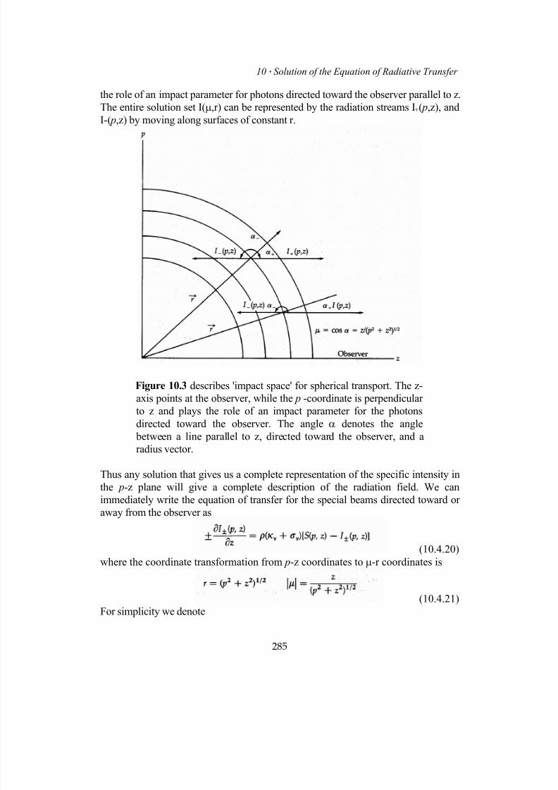
7/18/2019 The Fundamentals of Stellar Astrophysics - Collins G. W.
http://slidepdf.com/reader/full/the-fundamentals-of-stellar-astrophysics-collins-g-w 305/524
10 ⋅ Solution of the Equation of Radiative Transfer
the role of an impact parameter for photons directed toward the observer parallel to z.
The entire solution set I(µ,r) can be represented by the radiation streams I+( p,z), and
I-( p,z) by moving along surfaces of constant r.
Figure 10.3 describes 'impact space' for spherical transport. The z-
axis points at the observer, while the p -coordinate is perpendicular
to z and plays the role of an impact parameter for the photonsdirected toward the observer. The angle α denotes the angle
between a line parallel to z, directed toward the observer, and a
radius vector.
Thus any solution that gives us a complete representation of the specific intensity in
the p-z plane will give a complete description of the radiation field. We can
immediately write the equation of transfer for the special beams directed toward or
away from the observer as
(10.4.20)where the coordinate transformation from p-z coordinates to µ-r coordinates is
(10.4.21)
For simplicity we denote
285

7/18/2019 The Fundamentals of Stellar Astrophysics - Collins G. W.
http://slidepdf.com/reader/full/the-fundamentals-of-stellar-astrophysics-collins-g-w 306/524
II ⋅ Stellar Atmospheres
(10.4.22)
Equation (10.4.20) is a linear first order equation that has a classical solution
of
(10.4.23)
While this is a complicated expression, it can be evaluated numerically as long as
one has a representation of the source function. Thus, it is now possible to solve for
the entire radiation field and recalculate the variable Eddington factor f ν. Equation
(10.4.15) is then solved again for a new value of Jν and hence S ν. The entire procedure is repeated until a self-consistent solution is found. Rather than carry out
the admittedly messy numerical integration, Mihalas3 describes a Feautrier-like
method to calculate the intensities directly.
A method proposed by Schmid-Burgk 4 assumes that the source function can
be locally represented by a polynomial in the optical depth. This analytic function is
then substituted into the formal solution in impact space so that the radiation field
can be represented in terms of the undetermined coefficients of the source function's
approximating polynomials. The moments of the radiation field can then be
generated which depend only on these same coefficients. Thus, if one starts with an
initial atmospheric structure and a guess for the source function, one can fit thatsource function to the local polynomial and thereby determine the approximating
coefficients. These, in turn, can be used to generate the moments of the radiation
field upon which an improved version of the source function rests. An excellent
initial guess for the source function is S ν = Bν, and unless scattering completely
dominates the opacity, the iteration process converges very rapidly.
It is clear that the spherical atmosphere poses significant difficulties over and
above those found in the plane-parallel atmosphere. However, there are very few
differences that are fundamental in nature. All present methods rely on the global
symmetry of spherical stars, and it seems likely that those stars with atmospheres
sufficiently extended to require the spherical treatment will also be subject to otherforces, such as rotation, that further distort the atmospheres so that even this global
symmetry is lost. However, such studies can offer insight into the severity of the
effects that we can expect from the geometry.
We have only skimmed the surface of the methods and techniques devised to
solve the equation of radiative transfer. The methods discussed merely comprise
286
7/18/2019 The Fundamentals of Stellar Astrophysics - Collins G. W.
http://slidepdf.com/reader/full/the-fundamentals-of-stellar-astrophysics-collins-g-w 307/524
10 ⋅ Solution of the Equation of Radiative Transfer
some of the more popular and successful methods currently in use. We have left to
the studious reader the entire area of the "exact approximation" and the H-functions
of Chandrasekhar 1 (pp. 105 to 126). No mention has been made of invariant
embedding and the voluminous literature written for Linear two-point boundary-
value problems. Many of these techniques have proved useful in solving specific
radiative transfer problems, and those who would count themselves experts in this
area should avail themselves of that literature. There is an entire field of study
surrounding the transfer of radiation within spectral lines, some of which will be
discussed later, but much of which will not be. This material is important for anyone
interested in problems requiring line-transfer solutions. However, the methods
presented here suffice for providing the solution to half of the task of constructing a
normal stellar atmosphere, and next we turn to the solution of the other half of the
problem.
Problems
1. Find the general expression for
2. Find the eigenvalues k α and L+α for the discrete ordinate solution to the semi-
infinite plane-parallel gray atmosphere for n = 8.
3. Repeat Problem 2 for the double-gauss quadrature scheme for n = 8.
4.
If there is an arbitrary iterative functionΦ
( x) such that
then an iterative sequence defined by Φ( xk ) will converge to a fixed point x0
if and only if
Use this theorem to prove that any fixed-point iteration scheme will provide a
solution for
5. Find a general interpolative scheme for I(τ,µ) when µ < 0 for the discrete
ordinate approximation. The interpolative formula should have the same
degree of precision as the quadrature scheme used in the discrete ordinate
solution.
287
7/18/2019 The Fundamentals of Stellar Astrophysics - Collins G. W.
http://slidepdf.com/reader/full/the-fundamentals-of-stellar-astrophysics-collins-g-w 308/524
II ⋅ Stellar Atmospheres
6. Consider a pure scattering plane-parallel gray atmosphere of optical depth t0,
illuminated from below by I(τ0,+µ) = I0. Further assume that the surface is not
illuminated [that is, I(0,-µ) = 0. Use the Eddington approximation to find F(τ),J(τ), and I(0,+µ) in terms of I0 and τ0.
7. Show that in a gray atmosphere
8. Use the first of the Schwarzschild-Milne integral equations for the source
function in a gray atmosphere [equation (10.2.6)] to derive an integral
equation for the Hopf function q(τ).
9. Show that no self-consistent solution to the equation of radiative transfer
exists for a pure absorbing plane-parallel gray atmosphere in radiative
equilibrium where the source function has the form
10. Show that the equation of transfer in spherical coordinates
transforms to
in impact space where r 2 = ( p
2+z
2), and µ = z/r.
11. Derive an integral equation for the mean intensity Jν(τν) when the source
function is given by
12. Numerically obtain a solution for the Schwarzschild-Milne integral equation
for the source function in a gray atmosphere by solving equation (10.2.11) forthe ratio of the source function at eight points in the atmosphere to its value at
one point. Describe why you picked the points as you did, and compare your
result with that obtained from the Eddington approximation.
13. Using equation (10.2.21), show that equations (10.2.22) and (10.2.23) follow
from the discrete ordinate equation of transfer [equation (10.2.20)].
288

7/18/2019 The Fundamentals of Stellar Astrophysics - Collins G. W.
http://slidepdf.com/reader/full/the-fundamentals-of-stellar-astrophysics-collins-g-w 309/524

7/18/2019 The Fundamentals of Stellar Astrophysics - Collins G. W.
http://slidepdf.com/reader/full/the-fundamentals-of-stellar-astrophysics-collins-g-w 310/524
II ⋅ Stellar Atmospheres
290
both editions of his book on stellar atmospheres, but of the two, I prefer the first
edition;
Mihalas, D.:Stellar Atmospheres, 1st ed., W.H.Freeman, San Francisco,
1970, pp.34 -66.
For a lucid discussion of the relative merits of solutions to the integral
equations of radiative transfer, see
Kalkofen, W. A Comparison of Differential and Integral Equations of
Radiative Transfer , J. Quant. Spectrosc. & Rad. Trans. 14, 1974,
pp. 309 - 316.
For a general background of the subject as considered by some of the finest minds of
the twentieth century, everyone should spend some time eading Selected Papers onthe Transfer of Radiation, edited by D. H. Menzel (Dover, New York, 1966). All
these papers are of landmark quality, but I found this one to be most rewarding and
somewhat humbling:
Schuster, A.: Radiation through a Foggy Atmosphere, Ap.J. 21, 1905 pp.1 - 22,
It is clear that Arthur Schuster identified and understood most of the important
aspects of scattering theory in radiative transfer without the benefit of the work of the
rest of the twentieth century that is available to the contemporary student of physics.
Much of the work on neutron diffusion theory deals with the same mathematical
formalisms that serve radiative transfer theory, and we should be ever mindful of the physics literature on that subject if we are to appreciate the full breadth of the nature
of the problems posed by the flow of radiation through the outer layers of stars.
Finally, it would be a mistake to ignore the substantial contribution from the Russian
school of radiative transfer theory. Perhaps the finest example of their efforts can be
found in
Sobolev, V. V.: A Treatise on Radiative Transfer ,(Trans. S. I. Gaposchkin), Van
Nostrand, Princeton, N.J., 1963.
The approaches described in this book are insightful, novel, and particularly useful in
dealing with some of the more advanced problems of radiative transfer.
7/18/2019 The Fundamentals of Stellar Astrophysics - Collins G. W.
http://slidepdf.com/reader/full/the-fundamentals-of-stellar-astrophysics-collins-g-w 311/524
11 Environment of the Radiation Field
Copyright (2003) Geroge W. Collins, II
11
Environment of the Radiation Field
. . .
Thus far, we have said little or nothing about the gas through which the radiation isflowing. This constitutes the second half of the problem of constructing a model forthe atmosphere of a star. To get the solutions for the radiation field described inChapter 10, we must know the opacity, − and not just the mean opacity that wasrequired for stellar interiors, but the frequency-dependent opacity that determineswhich photons will escape from the star and from what location. We must understandenough of the physics of the gas for that opacity to be determined. Given that, we cancalculate the emergent stellar spectrum by solving the equation of radiative transfer.
This seems like a small requirement, but as we look more closely at the details of theopacity, the more specific knowledge of the state of the gas is required. For theconstruction of a model of the atmospheric structure, a little more is required. Wemust know how the particles that make up the gas interact with each other as well aswith photons. Fortunately, with the aid of the assumption of local thermodynamicequilibrium (LTE), much of our task has already been accomplished.
291
7/18/2019 The Fundamentals of Stellar Astrophysics - Collins G. W.
http://slidepdf.com/reader/full/the-fundamentals-of-stellar-astrophysics-collins-g-w 312/524
II Stellar Atmospheres
11.1 Statistics of the Gas and the Equation of State
For normal stellar atmospheres, the effective temperatures range from a few
thousand degrees to perhaps 50,000 K. The pressures are such as to permit theexistence of spectral lines and so the densities cannot be great enough to causedepartures from the ideal-gas law. The assumption of LTE implies that the materialcomponents of the gas making up the stellar atmosphere behave as if they were inthermodynamic equilibrium characterized by the local value of the kinetictemperature. In Chapter 1 [equations (1.1.16) and (1.1.17)] we found that as long asthe density of available cells in phase space is much greater than the particle phasedensity, such a gas should obey Maxwell-Boltzmann statistics. If this is true, thefraction of particles that have a certain kinetic energy wi is
(11.1.1)Since the pressure is the second velocity moment of the density, the Maxwell-Boltzmann distribution formula [equation (11.1.1)] leads to the ideal-gas law[equation (1.3.4)], namely,
(11.1.2)Later [equation (4.1.6)] we found it convenient to represent the total number of particles in terms of the density and the corresponding mass of hydrogen atoms µmh that would yield the required number of particles, so that
(11.1.3)The parameter µ is called the mean molecular weight .
a Boltzmann Excitation Formula
Under the assumption of LTE, the energy distribution of all particlesrepresents the most probable macrostate for the system. This state is arrived atthrough random collisions between the gas particles themselves. Such a gas is said to be collisionally relaxed and is in stationary equilibrium. This means that all aspectsof the gas will exhibit the same energy distribution, including those energy aspects of
the gas which do not allow for a continuum distribution of energy states − specifically those states described by the orbital electrons. Thus, an ensemble ofatoms will exhibit a distribution of states of electronic excitation that follows theMaxwell-Boltzmann distribution law. Were the energy not shared between theexcitation energy and the kinetic energy of the particles, collisions would ensure thatenergy differences were made up in the deficit population at the expense of the population that had the relative surplus.
292
7/18/2019 The Fundamentals of Stellar Astrophysics - Collins G. W.
http://slidepdf.com/reader/full/the-fundamentals-of-stellar-astrophysics-collins-g-w 313/524
11 Environment of the Radiation Field
Such a situation would not represent a time-independent distribution untilequilibrium between the two populations was established and therefore would not bethe most probable macrostate. Since the various states of atomic excitation will bedistributed according to the Maxwell-Boltzmann distribution law, the number of particles in any particular state of excitation will be
(11.1.4)Here, g j is the statistical weight, and it has the same meaning as it did in Chapter 1[equation (1.1.17)]. The parameter ε j is the excitation energy above the ground state,and U(T) is the partition function. U(T) is nothing more than a normalization parameter that reflects the total number of particles available for distribution amongthe various energy states. It also has the same meaning as it did for the continuumdistribution of energies discussed in Chapter 1, but now will be determined from thesum over the discrete states of excitation. Its role as a normalization parameter of thedistribution is most clearly demonstrated by summing equation (11.1.4) over all particles and their energy states so that the left-hand side is unity. This then confirmsthe form of the partition function as
(11.1.5)
b Saha Ionization Equilibrium Equation
A completely rigorous derivation of the Saha equation from first principles is long and not particularly illuminating. So instead of performing such aderivation, we appeal to arguments similar to those for the Boltzmann excitationformula. The object now is to find the equilibrium distribution formula for thedistribution of the various states of ionization for a collection of atoms. Again, weassume that a time-independent equilibrium exists between the electrons and theions. However, now the electron population will depend on the equilibriumestablished for all elements, which appears to make this case quite different from theBoltzmann excitation formula. However, we proceed in a manner similar to that forthe Boltzmann excitation formula. Let us try to find the probability of excitation, not
for a bound state, but of a state in the continuum where the electron can be regardedas a free particle.
Consider an atom in a particular state of ionization, and denote the number ofsuch atoms in a particular state of excitation, say the ground state, by the quantity n00.The number of these atoms excited to the ionized state where the electron can beregarded as a free particle is then given by the Boltzmann excitation formula as
293
7/18/2019 The Fundamentals of Stellar Astrophysics - Collins G. W.
http://slidepdf.com/reader/full/the-fundamentals-of-stellar-astrophysics-collins-g-w 314/524
II Stellar Atmospheres
(11.1.6)Here g f is the statistical weight of the final state of the ionized atom, and χ0 is theionization potential of the atom in question. The second term in the exponential issimply the energy of the electron that has been elevated to the continuum. Now wecan relate the total number of ionized atoms in the ground state to the total number ofionized atoms through the repeated use of the Boltzmann excitation formula and the partition function as
(11.1.7)where Ni is the total number of atoms in the ith state of ionization. However, sincethe resultant ionized atoms we are considering are in their ground state, ε0 is zero by
definition. In addition, the statistical weight of the final state g f , can be written as the product of the statistical weight of the ground state of the ionized atom and that of afree electron. We may now use this result and equation (11.1.6) to write
(11.1.8)which simplifies to
(11.1.9)
Although we picked a specific state of excitation − the ground state − to arrive atequation (11.1.9), that choice was in no way required. It only provided us with a wayto use the Boltzmann excitation formula for atoms in two differing states ofionization.
The statistical weight of a free electron is really nothing more than the probability of finding a given electron in a specific cell of phase space, so that
(11.1.10)
Again, for electrons, the familiar factor of 2 arises because the spin of an electron can be either "up" or "down". Assuming that the microscopic velocity field is isotropic,we can replace the "momentum volume" by its spherical counterpart and express it interms of the velocity:
(11.1.11)
294
7/18/2019 The Fundamentals of Stellar Astrophysics - Collins G. W.
http://slidepdf.com/reader/full/the-fundamentals-of-stellar-astrophysics-collins-g-w 315/524
11 Environment of the Radiation Field
The "space volume" of phase space occupied by the electron can be expressed interms of the inverse of the electron number density, so that the statistical weight of anelectron becomes
(11.1.12)and equation (11.1.9) can be written as
(11.1.13)
So far we have assumed that the ionization produced an electron in a specific
free state, that is, with a specific velocity in the energy continuum. However, we areinterested in only the total number of ionizations, so we must integrate equation(11.1.13) over all allowed velocities for the electrons that result from the ionization process. Thus,
(11.1.14)For convenience, we also assumed that the states of ionization of interest were theneutral and first states of ionization. However, the argument is correct for any twoadjacent states of ionization so we can write with some generality
(11.1.15)This expression is often written in terms of the electron pressure as
(11.1.16)Both expressions [equations (11.1.15) and (11.1.16)] are known as the Saha
ionization equation. Its validity rests on the Boltzmann excitation formula and the
velocity distribution of the electrons produced by the ionization being described bythe Boltzmann distribution formula. Both these conditions are met under theconditions of LTE. Indeed, many authors take the validity of the Saha andBoltzmann formulas as a definition for LTE.
The Boltzmann excitation equation and the Saha ionization equation can becombined to yield the fraction of atoms in a particular state of ionization and
295

7/18/2019 The Fundamentals of Stellar Astrophysics - Collins G. W.
http://slidepdf.com/reader/full/the-fundamentals-of-stellar-astrophysics-collins-g-w 316/524
II Stellar Atmospheres
excitation. Knowing that fraction, we are in a position to describe the extent to whichthose atoms will impede the flow of photons through the gas.
11.2 Continuous Opacity In Section 4.1b we discussed the way in which a gas can absorb photons, and
we calculated the continuous opacity due to an atom of hydrogen. The calculation ofthe opacity of other individual species of atoms follows the same type of argument,and so we do not deal with them in detail here since these details can be found inother elsewhere1. However, in the stellar interior, we were able to characterize theopacity of the stellar material by a single parameter known as the Rosseland mean
opacity. This resulted from the fact that the radiation field was itself inthermodynamic equilibrium and therefore depended on the temperature alone.Therefore, all parameters that arise from the interaction of the radiation field and the
gas, which is also in thermodynamic equilibrium, must be described in terms of thestate variables alone. Unfortunately, in the stellar atmosphere, although the gas canstill be considered to be in thermodynamic equilibrium (LTE), the radiation field isnot. Thus, the opacity must be determined for each frequency for which a significantamount of radiant energy is flowing through the gas.
Traditionally, the dominant source of opacity has been considered to be thatarising from bound-free atomic transitions which are called "continuous" opacitysources. However, contributions to the total opacity that result from bound-boundatomic transitions have been found to play an important role in forming the structureof the atmosphere in a wide variety of stars. Since we will deal with the formation of
spectral lines arising from bound-bound transitions in considerable detail later, wedefer the discussion of bound-bound opacity until then. It is sufficient to know thatthe total opacity can be calculated for each frequency of importance and to explicitlyconsider some of the important sources.
a Hydrogenlike Opacity
Any atom which has a single electron in its outer shell will absorb photons in a manner similar to that for hydrogen, so we should expect the opacity tohave a form similar to that of equation (4.1.17). Indeed the expression differs fromthat of hydrogen by only a factor involving the atomic weight and the atomic
constants appropriate for the particular atom. Thus, the opacity per gram of theionized species is
(11.2.1)
296

7/18/2019 The Fundamentals of Stellar Astrophysics - Collins G. W.
http://slidepdf.com/reader/full/the-fundamentals-of-stellar-astrophysics-collins-g-w 317/524
11 Environment of the Radiation Field
where R is the Rydberg constant. For ionized helium, Z = 2. Since hydrogen andhelium are by far the most abundant elements in stars, neutral hydrogen and ionizedhelium must be considered major sources of opacity.
b Neutral Helium
Again, because of the large abundance of neutral helium it long beenregarded as an important source of stellar opacity. However, since neutral helium hastwo electrons in the outer shell, the atomic absorption coefficient is much moredifficult to calculate. Approximate values for the opacity of neutral helium were firstgiven by Ueno et al.2 in 1954. Later Stewart and Webb3 calculated the opacity arisingfrom the ground state, and in general the contributions from the first two excitedstates must be treated separately. For states of excitation greater than 2, the
approximate solutions will generally suffice.
c Quasi-atomic and Molecular States
Although molecular opacity plays an important role in the later-typestars (and will be dealt with later), one might think that molecular opacity isunimportant at temperatures greater than those corresponding to the disassociationenergies of the molecules. However, some molecules and atomic states may form fora short time and absorb photons before they disassociate. If the abundance of theatomic species that give rise to these quasi-states is great, they may provide asignificant source of opacity. The prototypical example of a short lived or quasi-state
is the H-minus ion.
Classically, the existence of the H-minus ion can be inferred from theincomplete screening of the proton by the orbiting electron of Hydrogen (see figure11.1). Although the orbiting electron is "on one side" of the proton, it is possible to bind an additional electron to the atom for a short time. During this time, theadditional electron can undergo bound-free transitions. Quantum mechanically, thereexists a single weakly bound state for an electron near a neutral hydrogen atom. Thisstate is weakly bound since the dipole moment of the hydrogen atom is small. Thenegatively charged configuration is called the H-minus ion and is important in starsonly because of the great abundance of hydrogen and electrons at certain
temperatures and densities. The Saha equation for the abundance of such ions will besomewhat different from that for normal atoms as the existence of the ion willdepend on the availability of electrons as well as hydrogen atoms. Thus the Sahaequation for the H-minus ion would have the form
297

7/18/2019 The Fundamentals of Stellar Astrophysics - Collins G. W.
http://slidepdf.com/reader/full/the-fundamentals-of-stellar-astrophysics-collins-g-w 318/524
II Stellar Atmospheres
(11.2.2)
The parameter Φ(T ) involves partition functions and the like, but depends ononly the temperature. Since the Saha equation for neutral hydrogen implies that theratio of ionized to neutral hydrogen will also be proportional to the electron pressure,the abundance of the H-minus ion will depend quadratically on the electron pressure.Thus, the relative importance of H-minus to hydrogen opacity will decrease withdecreasing pressure. So H-minus is less important than hydrogen as an opacitysource for giants than for main sequence dwarfs of the same spectraltype.
Figure 11.1 shows a classical representation of a Bohr Hydrogen atomwith an additional electron bound temporarily so as to form an H-minus ion.
The opacity of a single H-minus ion has been calculated by a number of people over the past 40 years and is not a simple quantum mechanical calculation.The weak binding of the additional electron allows for the existence of a single
298
7/18/2019 The Fundamentals of Stellar Astrophysics - Collins G. W.
http://slidepdf.com/reader/full/the-fundamentals-of-stellar-astrophysics-collins-g-w 319/524
11 Environment of the Radiation Field
bound state from which bound-free transitions make contributions to the continuousopacity. The contribution from the bound-free transitions has a peak at about 0.8micrometers (µm) and is roughly bell-shaped in frequency with a half width of about
1 µm. The free-free contribution rises steadily into the infrared, becoming equal tothe bound-free absorption at about 1.45 µm.
d Important Sources of Continuous Opacity for Main Sequence
Stars
OB Stars For the hottest stars on the main sequence (the O stars), most ofthe hydrogen is ionized along with a substantial amount of the helium. The largestsource of continuous opacity is therefore due to electron scattering. From spectraltype B2 to O, neutral helium joins electron scattering as an important opacity source.In the early-type stars later than B2, hydrogen becomes a significant opacity source
which increases in importance as one considers later B-type stars. In these stars, theopacity due to bound-bound (see Section 15.4) and bound-free transitions in themetals becomes increasingly important for the ultraviolet part of the spectrum.
Stars of Spectral Type A0 to F5 At spectral type A0, neutral hydrogen isthe dominant source of continuous opacity. As one moves to later spectral types, H-minus opacity increases in importance and dominates the opacity in the late A typeand F stars. For stars of spectral type F, another molecule emerges as an importantopacity source. Although the H2 molecule cannot exist for long at these temperatures,enough does exist at any instant so that the once ionized form, H2
+, provides up to 10 percent of the continuous opacity. The H-minus opacity continues to grow in
importance throughout this range of spectral type.
Stars of Spectral Type F5 to G In this range H-minus continues to provide more than 60 percent of the continuous opacity. However, other moleculesare not of particular importance until one gets to spectral types later than G. Thecontinuous opacity of metals is particularly important in the ultraviolet range below3000Å. The opacity due to atomic hydrogen diminishes steadily into the G stars, butis still of major importance.
Late Spectral-Type K to M Stars Very little of the spectral energydistribution of these stars can be considered to result from continuum processes -
particularly in the later spectral types. The absorption from the myriads of discretetransitions of molecules so dominates the spectrum of the late-type stars that little isapparent except the large molecular absorption bands. However, insofar ascontinuum processes still take place, Rayleigh scattering from H2 molecules is themost important source. Absorption arising from the disassociation of molecules also provides an important source of continuous opacity, particularly in the infraredregion of the spectrum.
299
7/18/2019 The Fundamentals of Stellar Astrophysics - Collins G. W.
http://slidepdf.com/reader/full/the-fundamentals-of-stellar-astrophysics-collins-g-w 320/524
II Stellar Atmospheres
11.3 Einstein Coefficients and Stimulated Emission
An extremely useful way to view the processes of absorption is to consider thespecific types of interactions between a photon and an atom. This view will becomethe preferred one when we consider problems where we cannot assume LTE. Inquantum mechanics, it is customary to think of the probability of the occurrence of aspecific event rather than the classical picture of the frequency with which the eventoccurs. These are really opposite sides of the same coin, but they yield somewhat philosophically different pictures of the processes in question. In considering thetransition of an atom from one excited state to another, Einstein defined a set ofcoefficients that denote the probability of specific transitions taking place. These areknown as the Einstein coefficients. All radiative processes and the equation ofradiative transfer itself may be formulated in terms of these coefficients. The
coefficients are determined by the wave functions of the atom alone and thus do notdepend in any way on the environment of the atom. (As with most rules, there is anexception. If the density is sufficiently high that the presence of other atoms distortsthe wave functions of the atom of interest, then the Einstein coefficients of that atomcan be modified.)
Consider an atomic transition which takes an atom from a lower-energy stateof excitation n' to a higher-energy state n (or vice versa). The upper state n may be a bound or continuum state, and the transition will involve the absorption or emissionof a photon. The number of transitions that will occur in a given time interval for anensemble of atoms will then depend on the probability that one transition will occur
times the number of atoms available to make the transition. There types of transitionscan occur:
1. Spontaneous emission, where the electron spontaneously makes adownward transition with the accompanying emission of a photon.
2. Stimulated absorption, where a passing photon is absorbed, producing the resulting transition.
3. Stimulated emission, where the electron makes a downward transitionwith the accompanying emission of a photon. If this occurs in the
presence of a photon of the same type as that emitted by thetransition, the probability of the event is greatly enhanced.
The symmetric process of spontaneous absorption simply cannot occur because onecannot absorb what is not there.
300
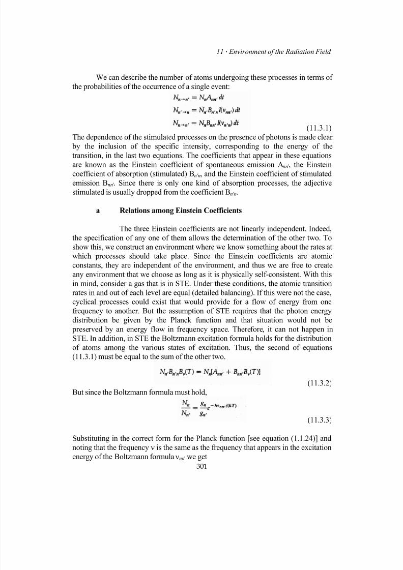
7/18/2019 The Fundamentals of Stellar Astrophysics - Collins G. W.
http://slidepdf.com/reader/full/the-fundamentals-of-stellar-astrophysics-collins-g-w 321/524
11 Environment of the Radiation Field
We can describe the number of atoms undergoing these processes in terms ofthe probabilities of the occurrence of a single event:
(11.3.1)The dependence of the stimulated processes on the presence of photons is made clear by the inclusion of the specific intensity, corresponding to the energy of thetransition, in the last two equations. The coefficients that appear in these equationsare known as the Einstein coefficient of spontaneous emission Ann', the Einsteincoefficient of absorption (stimulated) Bn'n, and the Einstein coefficient of stimulatedemission Bnn'. Since there is only one kind of absorption processes, the adjectivestimulated is usually dropped from the coefficient Bn'n.
a Relations among Einstein Coefficients
The three Einstein coefficients are not linearly independent. Indeed,the specification of any one of them allows the determination of the other two. Toshow this, we construct an environment where we know something about the rates atwhich processes should take place. Since the Einstein coefficients are atomicconstants, they are independent of the environment, and thus we are free to createany environment that we choose as long as it is physically self-consistent. With thisin mind, consider a gas that is in STE. Under these conditions, the atomic transitionrates in and out of each level are equal (detailed balancing). If this were not the case,
cyclical processes could exist that would provide for a flow of energy from onefrequency to another. But the assumption of STE requires that the photon energydistribution be given by the Planck function and that situation would not be preserved by an energy flow in frequency space. Therefore, it can not happen inSTE. In addition, in STE the Boltzmann excitation formula holds for the distributionof atoms among the various states of excitation. Thus, the second of equations(11.3.1) must be equal to the sum of the other two.
(11.3.2)But since the Boltzmann formula must hold,
(11.3.3)
301
Substituting in the correct form for the Planck function [see equation (1.1.24)] andnoting that the frequency ν is the same as the frequency that appears in the excitationenergy of the Boltzmann formula νnn' we get
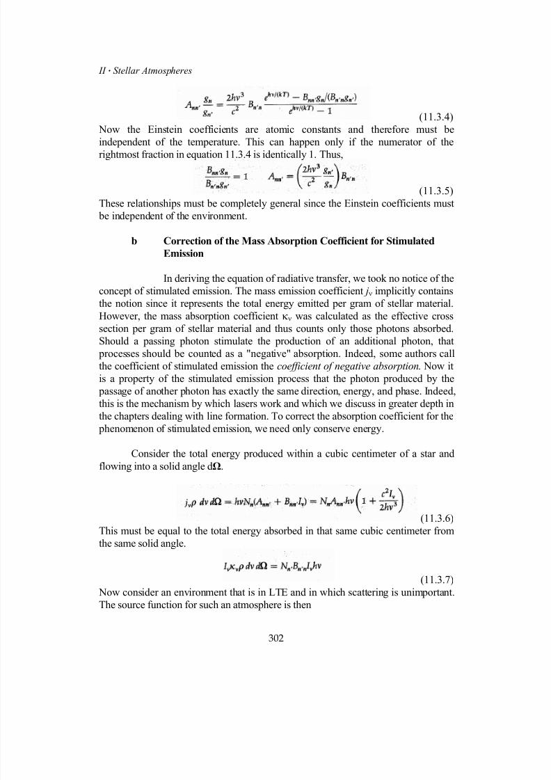
7/18/2019 The Fundamentals of Stellar Astrophysics - Collins G. W.
http://slidepdf.com/reader/full/the-fundamentals-of-stellar-astrophysics-collins-g-w 322/524
II Stellar Atmospheres
(11.3.4) Now the Einstein coefficients are atomic constants and therefore must beindependent of the temperature. This can happen only if the numerator of therightmost fraction in equation 11.3.4 is identically 1. Thus,
(11.3.5)These relationships must be completely general since the Einstein coefficients must be independent of the environment.
b Correction of the Mass Absorption Coefficient for Stimulated
Emission
In deriving the equation of radiative transfer, we took no notice of theconcept of stimulated emission. The mass emission coefficient jν implicitly containsthe notion since it represents the total energy emitted per gram of stellar material.However, the mass absorption coefficient κν was calculated as the effective crosssection per gram of stellar material and thus counts only those photons absorbed.Should a passing photon stimulate the production of an additional photon, that processes should be counted as a "negative" absorption. Indeed, some authors callthe coefficient of stimulated emission the coefficient of negative absorption. Now itis a property of the stimulated emission process that the photon produced by the passage of another photon has exactly the same direction, energy, and phase. Indeed,this is the mechanism by which lasers work and which we discuss in greater depth inthe chapters dealing with line formation. To correct the absorption coefficient for the phenomenon of stimulated emission, we need only conserve energy.
Consider the total energy produced within a cubic centimeter of a star andflowing into a solid angle dΩ.
(11.3.6)This must be equal to the total energy absorbed in that same cubic centimeter from
the same solid angle.
(11.3.7) Now consider an environment that is in LTE and in which scattering is unimportant.The source function for such an atmosphere is then
302
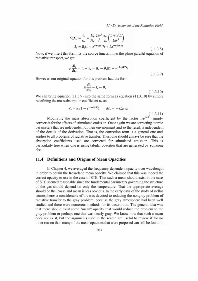
7/18/2019 The Fundamentals of Stellar Astrophysics - Collins G. W.
http://slidepdf.com/reader/full/the-fundamentals-of-stellar-astrophysics-collins-g-w 323/524
11 Environment of the Radiation Field
(11.3.8) Now, if we insert this form for the source function into the plane-parallel equation ofradiative transport, we get
(11.3.9)However, our original equation for this problem had the form
(11.3.10)We can bring equation (11.3.9) into the same form as equation (11.3.10) by simplyredefining the mass absorption coefficient κν as
(11.3.11)Modifying the mass absorption coefficient by the factor 1-ehν/kT simply
corrects it for the effects of stimulated emission. Once again we are correcting atomic parameters that are independent of their environment and so the result is independentof the details of the derivation. That is, the correction term is a general one andapplies to all problems of radiative transfer. Thus, one should always be sure that theabsorption coefficients used are corrected for stimulated emission. This is particularly true when one is using tabular opacities that are generated by someoneelse.
11.4 Definitions and Origins of Mean Opacities
In Chapter 4, we averaged the frequency-dependent opacity over wavelengthin order to obtain the Rosseland mean opacity. We claimed that this was indeed thecorrect opacity to use in the case of STE. That such a mean should exist in the caseof STE seemed reasonable since the fundamental parameters governing the structureof the gas should depend on only the temperature. That the appropriate averageshould be the Rosseland mean is less obvious. In the early days of the study of stellar
atmospheres a considerable effort was devoted to reducing the nongray problem ofradiative transfer to the gray problem, because the gray atmosphere had been wellstudied and there were numerous methods for its description. The general idea wasthat there should exist some "mean" opacity that would reduce the problem to thegray problem or perhaps one that was nearly gray. We know now that such a meandoes not exist, but the arguments used in the search are useful to review if for noother reason than many of the mean opacities that were proposed can still be found in
303
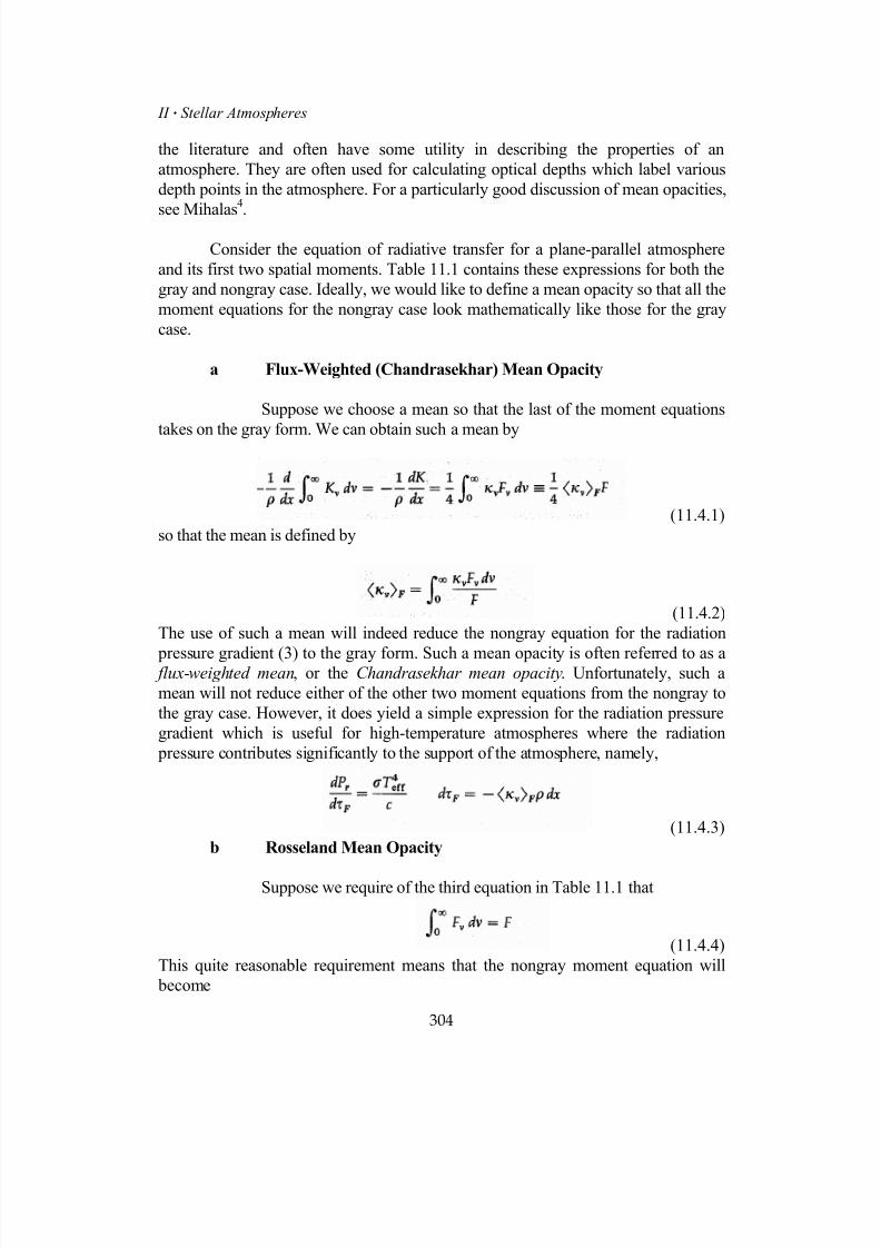
7/18/2019 The Fundamentals of Stellar Astrophysics - Collins G. W.
http://slidepdf.com/reader/full/the-fundamentals-of-stellar-astrophysics-collins-g-w 324/524
II Stellar Atmospheres
the literature and often have some utility in describing the properties of anatmosphere. They are often used for calculating optical depths which label variousdepth points in the atmosphere. For a particularly good discussion of mean opacities,see Mihalas4.
Consider the equation of radiative transfer for a plane-parallel atmosphereand its first two spatial moments. Table 11.1 contains these expressions for both thegray and nongray case. Ideally, we would like to define a mean opacity so that all themoment equations for the nongray case look mathematically like those for the graycase.
a Flux-Weighted (Chandrasekhar) Mean Opacity
Suppose we choose a mean so that the last of the moment equations
takes on the gray form. We can obtain such a mean by
(11.4.1)so that the mean is defined by
(11.4.2)The use of such a mean will indeed reduce the nongray equation for the radiation
pressure gradient (3) to the gray form. Such a mean opacity is often referred to as a flux-weighted mean, or the Chandrasekhar mean opacity. Unfortunately, such amean will not reduce either of the other two moment equations from the nongray tothe gray case. However, it does yield a simple expression for the radiation pressuregradient which is useful for high-temperature atmospheres where the radiation pressure contributes significantly to the support of the atmosphere, namely,
(11.4.3)b Rosseland Mean Opacity
Suppose we require of the third equation in Table 11.1 that
(11.4.4)This quite reasonable requirement means that the nongray moment equation will become
304
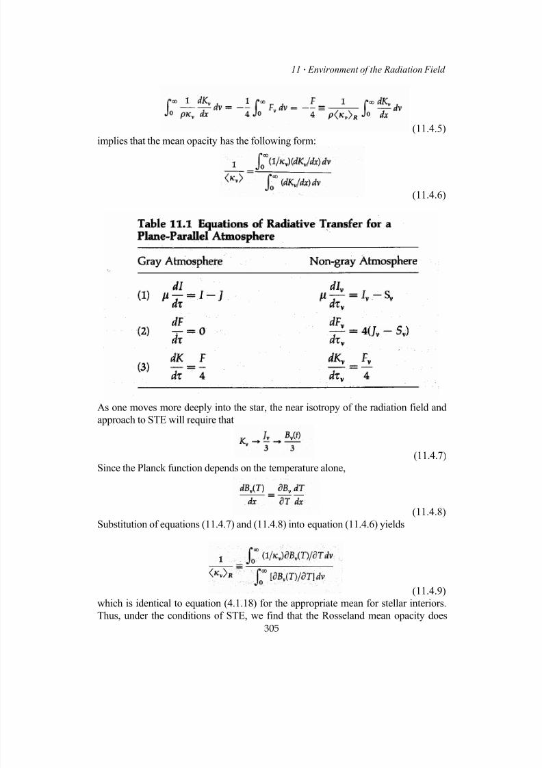
7/18/2019 The Fundamentals of Stellar Astrophysics - Collins G. W.
http://slidepdf.com/reader/full/the-fundamentals-of-stellar-astrophysics-collins-g-w 325/524
11 Environment of the Radiation Field
(11.4.5)implies that the mean opacity has the following form:
(11.4.6)
As one moves more deeply into the star, the near isotropy of the radiation field andapproach to STE will require that
(11.4.7)Since the Planck function depends on the temperature alone,
(11.4.8)Substitution of equations (11.4.7) and (11.4.8) into equation (11.4.6) yields
(11.4.9)
305
which is identical to equation (4.1.18) for the appropriate mean for stellar interiors.Thus, under the conditions of STE, we find that the Rosseland mean opacity does

7/18/2019 The Fundamentals of Stellar Astrophysics - Collins G. W.
http://slidepdf.com/reader/full/the-fundamentals-of-stellar-astrophysics-collins-g-w 326/524
II Stellar Atmospheres
indeed remove the frequency dependence from the radiative transfer problem.However, in the stellar atmosphere the conditions required by equation (11.4.7) donot apply, so that the Rosseland mean will not fulfill the same function for the theoryof stellar atmospheres as it does in the theory of stellar interiors.
c Planck Mean Opacity
Finally, let us consider a mean opacity that will yield a correct valuefor the thermal emission. Thus,
(11.4.10)To appreciate the utility of this mean, we develop the condition of radiativeequilibrium for the nongray case and see how that approaches the gray result. Let ussee what condition would be placed on a mean opacity in order to bring radiativeequilibrium in line with the gray case. Consider a mean opacity such that
(11.4.11)This is just a condition that expresses the difference between the nongray conditionfor radiative equilibrium and the gray condition, both of which should be zero. Nowfrom equation (10.1.13), we can write Jν as
(11.4.12)Under the condition that S ν(t)=Bν[T (t)], we can expand the source function inequation (11.4.12) in a Taylor series about τν and integrate term by term, to obtain
(11.4.13)Thus, near the surface of the atmosphere
(11.4.14)Substitution of equation (11.4.14) into equation (11.4.11) yields
(11.4.15)Thus, the Planck mean opacity is the most physically relevant mean for satisfyingradiative equilibrium near the surface of the atmosphere.
306

7/18/2019 The Fundamentals of Stellar Astrophysics - Collins G. W.
http://slidepdf.com/reader/full/the-fundamentals-of-stellar-astrophysics-collins-g-w 327/524
11 Environment of the Radiation Field
These various means all have their regions of validity and utility, but nonecan fulfill the promise of reducing the nongray atmosphere problem to that of a grayatmosphere. Indeed, clearly such a mean does not exist. Three separate momentequations are listed in table 11.1 and a mean opacity represents only one parameteravailable to bring them all into conformity with their gray analogs. For an arbitrary behavior for κν, this is impossible. Thus, we must be content with solving thenongray radiative transfer problem at all frequencies for which a significant amountof flux flows through the atmosphere.
11.5 Hydrostatic Equilibrium and the Stellar Atmosphere
Any discussion of the environment of the radiation field would be incompletewithout some mention of the motions to be expected within the atmosphere.Recently, considerable effort has been expended in describing radiation-driven winds
that originate in the outer reaches of the atmospheres of hot stars. This moreadvanced topic is well beyond the scope of our interest at this point. Instead, we takeadvantage of the fact that radiation is the primary mode of energy transport throughthe stellar atmosphere, and we assume that the atmosphere is in hydrostaticequilibrium. While turbulent convection is present in many stars, the motions implied by the observed velocities are likely to cause problems only for the stars with thelowest surface gravities. For stars on the main sequence, hydrostatic equilibrium isan excellent assumption.
The notion of hydrostatic equilibrium has been mentioned repeatedlythroughout this book from the general concept obtained from the Boltzmann
transport equation in Chapter 1, through the explicit formulation for spherical starsgiven by equation (2.1.6) to the representation for plane-parallel atmospheres foundin equation (9.1.1). However, the introduction of the concept of optical depth allowsfor a further refinement. Since the logical depth variable for radiative transfer is theoptical depth variable τν, it makes some sense to reformulate the other structureequations that explicitly involve the depth coordinate to reflect the use of the opticaldepth and the independent variable of the structure. Some atmosphere modelingcodes use a variant of equation (9.1.1),
(11.5.1)
so that the quantity ρdx is the depth variable. A more common formulation takesadvantage of the definition of the optical depth
(11.5.2)which yields the condition for hydrostatic equilibrium in terms of the opticaldepth. Thus,
307

7/18/2019 The Fundamentals of Stellar Astrophysics - Collins G. W.
http://slidepdf.com/reader/full/the-fundamentals-of-stellar-astrophysics-collins-g-w 328/524
II Stellar Atmospheres
(11.5.3)
Having described the environment of the radiation field in terms of thestate variables P, T, and ρ, we can now proceed to the actual construction of amodel atmosphere.
Problems
1. Find the ratio of ionized to neutral hydrogen at τλ (λ = 5000Å) = 1 in(a) the sun, (b) Sirius, and (c) Rigel.
2. Find the ratio of SiI to SiII to SiIII in η Ursa Majoris.
3. Consider an atmosphere made up of pure hydrogen that is almost all in aneutral state. The radiation pressure is negligible, and the opacity is due tothe H-minus ion.
(a) Determine how the pressure at a given optical depth depends onthe surface gravity (i.e., how it would change if g werechanged).
(b) Express the pressure as a function of the temperature. Leave theanswer in integral form.
(c) How can one find the pressure as a function of physical depth?Display explicitly all equations.
(d) Suppose that the effective temperature is T e and that one wants tofind the pressure at the point in the atmosphere corresponding tothat temperature. Further, suppose that the surface temperature isin error by 10 percent. Estimate the resultant error in P(T e).
4 Use a model atmosphere code to construct a model as described inProblem 3 (try T e = 6000 K and log g = 3 and log g = 4). Compare yourresults with those of Problem 3.
5. Consider a gas composed of 60 percent hydrogen and 40 percent helium at10,000 K in a gravity field where log g = 4.5.(a) Find the ratio of neutral to ionized hydrogen and the ratio of the
three states of ionization for helium.(b) Find the ratio of the level populations for the first four levels of
excitation in neutral hydrogen.
308
7/18/2019 The Fundamentals of Stellar Astrophysics - Collins G. W.
http://slidepdf.com/reader/full/the-fundamentals-of-stellar-astrophysics-collins-g-w 329/524
11 Environment of the Radiation Field
309
6. Use a model atmosphere code to find how the state of ionization ofhydrogen varies with physical depth in a star with T e = 10,000 K andLog g = 4.0. Repeat the calculation for a star with T e= 7000 K and
Log g = 1.5. Compare the two cases.
References
1. For additional reading on the subject of stellar atmospheric opacities,consult:
Aller, L. H.: The Atmospheres of the Sun and Stars, 2d ed., Ronald Press, New York, 1963, chap.4, pp.141 - 199.
Mihalas, D.: Stellar Atmospheres, W.H.Freeman, San Francisco, 1970,
chap.4, pp.81 - 128.
Mihalas, D.: Stellar Atmospheres, 2d ed., W.H.Freeman, San Francisco,1978, chap.4, pp.77 - 107.
Mihalas, D.: Methods in Computational Physics, (Eds. B. Alder,S.Fernbach, M. Rotenberg), Academic, New York, 1967, pp.19 - 23.
2. Ueno, S., Saito, S., and Jugaku, K. Continuous Absorption Coefficients of
the Model Stellar Atmosphere,Cont. Inst. Ap. Univ. of Kyoto, no. 43,1954, pp.1 - 28.
3. Stewart, A. and Webb, T. Photo-ionization of Helium and Ionized
Lithium, Proc. Phys. Soc. (London) 82, 1963, pp.532 - 536.
4. Mihalas, D. Stellar Atmospheres, W.H.Freeman, San Francisco, 1970,chap. 2, pp. 37 - 41.
7/18/2019 The Fundamentals of Stellar Astrophysics - Collins G. W.
http://slidepdf.com/reader/full/the-fundamentals-of-stellar-astrophysics-collins-g-w 330/524
II Stellar Atmospheres
Copyright (2003) George W. Collins, II
12
The Construction of a
Model Stellar Atmosphere
. . .
12.1 Statement of the Basic Problem
We have now acquired all the material necessary to construct a model of the
atmosphere of a star. This material includes not only the dependence of the state
variables P, T and ρ with depth in the atmosphere but also an approximation to the
emergent spectrum. That predicted spectrum will not contain the details of the stellar
absorption lines, but will show the departures from the Planck function of a radiation
field in thermodynamic equilibrium. The major departures are caused by the
absorption edges corresponding to the ionization limits for the elements included in
the calculation. Even if there were no such discontinuities in the frequency
dependence of the absorption coefficient, the emergent spectra would still differ from
those of a blackbody. Since the photons emerge from different depths in theatmosphere, having different temperatures, even a gray atmosphere spectrum will
depart from the Planck function. The more sophisticated spectrum results from the
solution of the equation of radiative transfer, the calculation of which represents a
major part of the construction of a model atmosphere.
310

7/18/2019 The Fundamentals of Stellar Astrophysics - Collins G. W.
http://slidepdf.com/reader/full/the-fundamentals-of-stellar-astrophysics-collins-g-w 331/524
12 Construction of a Model Stellar Atmosphere⋅ In developing this material, we have used the same conservation laws that
yielded the equations of structure for the stellar interior. However, the resulting
formulation is somewhat different. The conservation of momentum yielded the
expression for hydrostatic equilibrium, as it did in the stellar interior. However, the
assumption of a plane-parallel structure for the atmosphere and the use of a different
depth coordinate have caused the expression of hydrostatic equilibrium to take a
somewhat different form than for the stellar interior. The conservation of energy is at
the root of radiative equilibrium. This condition is imposed on the Boltzmann
transport equation itself which was used to produce the equation of radiative transfer.
However, because of the departure of the radiation field from STE, the flow of
radiation was described by an integral equation, implying that the solution at any
point depends on the solution at all points. As a result, we no longer have the simple
differential equation for the radiative gradient that was appropriate for the stellar
interior. Even the equation of state, which results from saying that the local velocity
field of the particles is largely isotropic and dominates any macroscopic flowvelocity, is present in basically the form used in the stellar interior. Although the
calculation of the mass absorption coefficient appears to present a greater problem
for stellar atmospheres, this is largely an illusion. The construction of an accurate
model interior requires careful calculation of the frequency-dependent absorption
coefficient, and the range of atomic phenomena that must be included is actually
greater than that of an atmosphere because of the greater range of possible ionization
states. However, in the stellar atmosphere, the frequency dependence of the
absorption coefficient enters far more directly into the solution and plays a greater
role. The use of the Rosseland Mean opacity for stellar interiors tends to average out
the "mistakes" in the opacity calculations whereas those mistakes in a stellar
atmosphere are directly visible in the emergent spectrum. The presence of moleculesis an added complication for the theory of stellar atmospheres that does not plague
the theory of stellar interiors.
Much has been concealed by writing the opacity as a function of the state
variables. But while the details are messy and LTE has been assumed, the process is
straightforward. The major difference between the calculation of a stellar interior and
the construction of a model stellar atmosphere can be seen in the last of equations
(12.1.1). No longer do we have a situation that can be mathematically described as a
linear two-point boundary value problem. Because of the assumption of plane
parallelism the "eigenvalues" of the problem have been reduced to two, T e and g . In
addition, the four nonlinear differential equations of the interior structure have beenreplaced by one first order differential equation and an integral equation for the
source function from which all physically relevant moments of the radiation field can
be calculated. The global nature of this integral equation forces a rather different
approach to the construction of a model stellar atmosphere from that adopted for the
stellar interior.
311
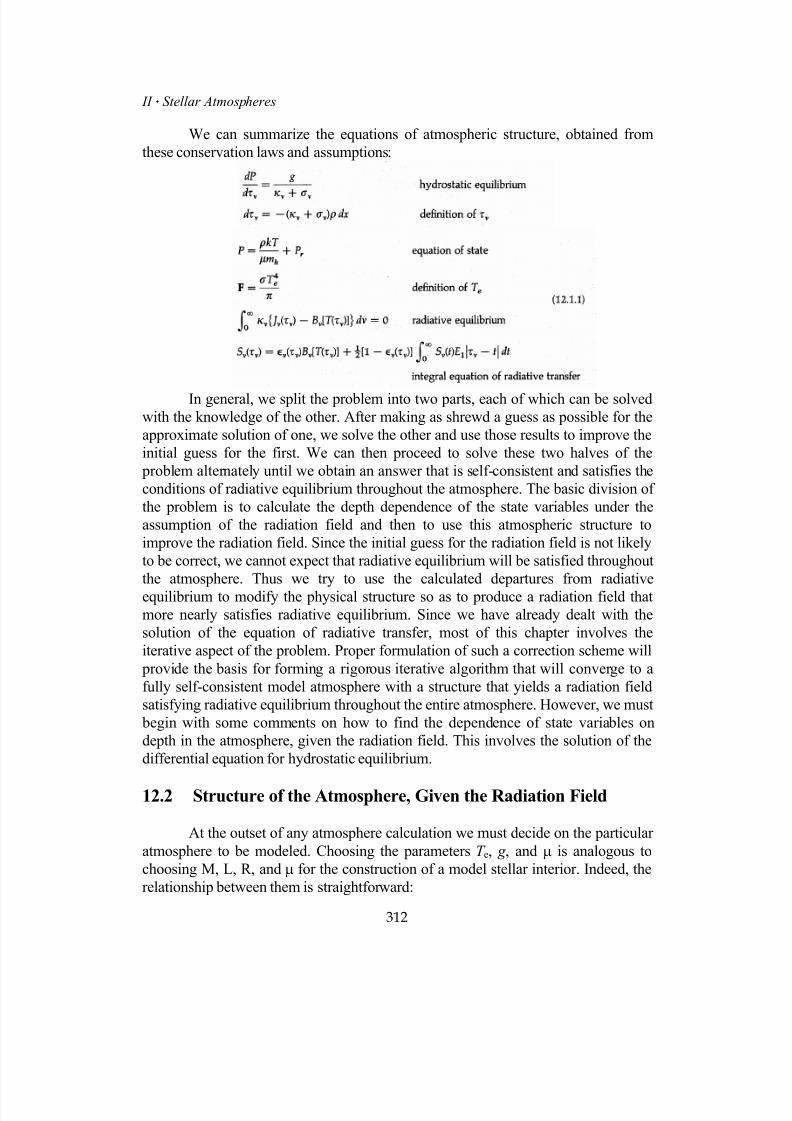
7/18/2019 The Fundamentals of Stellar Astrophysics - Collins G. W.
http://slidepdf.com/reader/full/the-fundamentals-of-stellar-astrophysics-collins-g-w 332/524
II Stellar Atmospheres
We can summarize the equations of atmospheric structure, obtained from
these conservation laws and assumptions:
In general, we split the problem into two parts, each of which can be solved
with the knowledge of the other. After making as shrewd a guess as possible for the
approximate solution of one, we solve the other and use those results to improve the
initial guess for the first. We can then proceed to solve these two halves of the
problem alternately until we obtain an answer that is self-consistent and satisfies the
conditions of radiative equilibrium throughout the atmosphere. The basic division of
the problem is to calculate the depth dependence of the state variables under the
assumption of the radiation field and then to use this atmospheric structure to
improve the radiation field. Since the initial guess for the radiation field is not likely
to be correct, we cannot expect that radiative equilibrium will be satisfied throughout
the atmosphere. Thus we try to use the calculated departures from radiative
equilibrium to modify the physical structure so as to produce a radiation field that
more nearly satisfies radiative equilibrium. Since we have already dealt with the
solution of the equation of radiative transfer, most of this chapter involves the
iterative aspect of the problem. Proper formulation of such a correction scheme will
provide the basis for forming a rigorous iterative algorithm that will converge to a
fully self-consistent model atmosphere with a structure that yields a radiation field
satisfying radiative equilibrium throughout the entire atmosphere. However, we must
begin with some comments on how to find the dependence of state variables on
depth in the atmosphere, given the radiation field. This involves the solution of the
differential equation for hydrostatic equilibrium.
12.2 Structure of the Atmosphere, Given the Radiation Field
At the outset of any atmosphere calculation we must decide on the particular
atmosphere to be modeled. Choosing the parameters T e, g , and µ is analogous to
choosing M, L, R, and µ for the construction of a model stellar interior. Indeed, the
relationship between them is straightforward:
312
7/18/2019 The Fundamentals of Stellar Astrophysics - Collins G. W.
http://slidepdf.com/reader/full/the-fundamentals-of-stellar-astrophysics-collins-g-w 333/524
12 Construction of a Model Stellar Atmosphere⋅
(12.2.1)
a Choice of the Independent Variable of Atmospheric Depth
Before beginning the model calculation itself, we must choose a
depth parameter to serve as an independent variable. While the traditional choice has
always been the optical depth, some more modern atmosphere codes use a "density
depth" like
(12.2.2)
as the independent depth variable. As we see, this greatly simplifies the calculation
of hydrostatic equilibrium, but introduces some difficulties in the solution of the
equation of transfer. For the most part, we use the traditional optical depth as our
independent depth variable.
Which optical depth should we use? Early investigators would pick one of
the mean opacities to generate a mean optical depth, and this dimensionless,
frequency-independent variable would provide an excellent parameter for describing
the atmospheric structure. Unfortunately, the calculation of the mean opacity at
numerous depths in the atmosphere is a nontrivial undertaking and is completely
avoidable. Since there is no particular significance for any of the mean opacities, no
optical depth scale is to be preferred over any other on the basis of the physical
information contained there. Therefore, it makes good sense to pick a
monochromatic optical depth at some frequency τ(ν0) (or simply τ0) as the depth
parameter, thereby avoiding the tedious calculation of the mean opacity and the
associated mean optical depths. However, since the radiative transfer equation must
be solved at each frequency, it will be necessary to interpolate the solution to the
reference optical depth τ0. So it would be wise to choose a frequency in the general
vicinity of the maximum energy flow through the atmosphere and in a part of the
spectrum where the opacity does not vary rapidly with frequency. This will tend to
minimize interpolation errors when the solutions are transferred to the reference
optical depth. For the majority of the development in this chapter, this is the choice
that we make. The relevant optical depths are then given by
(12.2.3)
The parameter κν is just a normalized opacity which relates the differential
monochromatic optical depth to its counterpart on the reference depth scale.
313
7/18/2019 The Fundamentals of Stellar Astrophysics - Collins G. W.
http://slidepdf.com/reader/full/the-fundamentals-of-stellar-astrophysics-collins-g-w 334/524
II Stellar Atmospheres
b Assumption of Temperature Dependence with Depth
Having specified the nature of the atmosphere and chosen the depth
parameter, we can begin the calculation of the atmospheric structure with depth. We
have indicated that we will split the process of making the model into two parts by
assuming the results of the radiative transfer solution in order to calculate the
atmospheric structure. The form that this assumption takes is the dependence of the
temperature with depth. That is, the end result for the solution of the radiative
transfer calculation will be to generate the dependence of the temperature with depth
in a manner that is consistent with radiative equilibrium. Thus, to begin our
calculation, we must assume the existence of this temperature distribution. We may
obtain this information either as a result of an earlier model calculation or from an
initial approximation.
In Section 10.2, we spent considerable effort in solving the equation of
transfer for the gray atmosphere. One of the results of this effort was the temperature
distribution in the Eddington approximation [equation (10.2.16)]. Remembering that
for a gray atmosphere in radiative equilibrium
(12.2.4)
we can write the more general result
(12.2.5)
where q(τ) is the Hopf function specified in equation (10.2.34). Although the gray
atmosphere does not specify a unique physical atmospheric structure, it does provide
a temperature distribution that scales with the effective temperature and is consistent
with radiative equilibrium. In addition, the opacity in a wide variety of stars is
relatively independent of frequency over a large part of the spectrum, so that the gray
atmosphere temperature distribution provides a good first approximation to the actual
temperature distribution. However, the accuracy of this assumption does depend on
the choice of reference optical depth being representative of the atmosphere as a
whole, so we can only expect it to form an approximate first guess.
c Solution of the Equation of Hydrostatic Equilibrium
The equation of hydrostatic equilibrium is a deceptively simple
looking first-order differential equation. There are many sophisticated methods for
obtaining the numerical solution to such an equation, but all such methods involve
knowing at least one value (and usually several values) for the solution at and near
314
7/18/2019 The Fundamentals of Stellar Astrophysics - Collins G. W.
http://slidepdf.com/reader/full/the-fundamentals-of-stellar-astrophysics-collins-g-w 335/524
12 Construction of a Model Stellar Atmosphere⋅ the boundary. This poses both philosophical and practical problems. The boundary of
a plane-parallel atmosphere, while well located in optical depth, is poorly placed in
physical depth since it formally occurs where the density vanishes. In principle, this
occurs at an infinite distance from the star where the plane-parallel approximation
itself would no longer be valid. However, in practice, a small but finite optical depth
is reasonably located with respect to the photosphere (i.e., near optical depth τ.2/3)
so that boundary conditions can be specified there without jeopardizing the accuracy
of the solution. Since we have assumed a distribution of temperature with optical
depth, there is no problem in determining the boundary temperature.
In Section 4.1a we discussed how to relate the mass fractions of hydrogen,
helium, and "metals" to the mean molecular weight and thereby provide a connection
between the number and mass density. The Saha equations for each element
[equation (11.1.16)] provide a relationship between the relative ionization fraction,
the temperature, and the electron pressure. By remembering that the sum of all thevarious states of ionization for a particular element is simply equal to the number
abundance for the element, it is possible to parameterize the opacity in terms of the
gas pressure, temperature, and electron pressure. Thus, we may write the total
pressure at any optical depth as
(12.2.6)
In a similar manner it is possible to integrate the equation of hydrostatic equilibrium
[as stated in equation (11.5.3)] so that
(12.2.7)
We may look for a value of P e that makes equations (12.2.6) and (12.2.7)
self-consistent. Numerically this can be accomplished by creating tables of κ0 and σ0
as functions of P e so that the integral in equation (12.2.7) can be done directly by any
efficient quadrature scheme and then a solution found by iteration with equation
(12.2.6). Details of this procedure are given by Mihalas1. In carrying out this
procedure, one keeps the value of the optical depth τi sufficiently small that
T (0) . T (τi). When one has found a self-consistent value of P e(τi) (and hence all the
state variables), values of the state variables may be interpolated for all intermediate
optical depths between 0 and τi. This technique will provide all the required values ofthe pressure to initiate a general numerical integration procedure for the differential
equation for hydrostatic equilibrium. Since all the other state variables are given in
terms of algebraic expressions, the entire atmospheric structure may be obtained as a
function of τ0.
A note of caution should be interjected at this point concerning the numerical
315
7/18/2019 The Fundamentals of Stellar Astrophysics - Collins G. W.
http://slidepdf.com/reader/full/the-fundamentals-of-stellar-astrophysics-collins-g-w 336/524
II Stellar Atmospheres
solution described by this procedure. The range in pressures to be expected from the
solution is several powers of 10. For this reason, logarithmic variables are often used
to improve the stability of the numerical solution. In any case, the method used to
solve the equation of hydrostatic equilibrium should be reasonably sophisticated
since the rapid initial growth of the pressure, if not carefully dealt with, can produce
systematic errors that destroy the accuracy of the entire atmosphere as the integration
proceeds. Several investigators have found it necessary to employ up to a seven-
point predictor-corrector integration scheme to achieve the accuracy required. In
addition, although the remaining equations are indeed algebraic, the Saha equations
for the various elements and states of ionization represent a system of coupled
nonlinear algebraic equations and must be solved by iteration. Furthermore, the
equations for the opacity due to the different elements in their various states of
ionization and excitation represent a significant amount of calculation. Thus, the
calculation of κν(τ0) can be quite time-consuming and represents a significant time
burden for the calculation of the model structure. This is particularly evident whenone remembers that a multipoint numerical integration scheme requires multiple
evaluations of the function g/κν to carry out one step in the integration. The situation
is further exacerbated by the realization that a rapidly varying numerical solution to a
differential equation usually requires that the solution proceed with very small steps,
and the range required for the independent variable will be of the order of 2 powers
of 10. This is the reason that some modern atmosphere codes utilize a density depth
as given in equation (12.2.2) as the independent depth variable. With this choice, the
calculation of the opacity is entirely avoided. However, as we see, this choice of an
independent variable is not without its own set of problems.
The solution of the equation of hydrostatic equilibrium also provides us withthe dependence on depth of all the state variables and the various states of ionization
and excitation of the elements. With this information, it is possible to calculate the
opacity and hence the radiation field at all points in the atmosphere.
12.3 Calculation of the Radiation Field of the Atmosphere
All Chapter 10 was devoted to solving the equation of radiative transfer, so there is
no need to repeat the specifics here. However, some numerical aspects of those
solutions require comment. As even the casual reader of Chapter 10 will notice, the
general solution of the equation of radiative transfer is fraught with some formidable
numerical difficulties. Not the least of these is ensuring the numerical accuracy of theresults. Whether one chooses to solve the integrodifferential equation for the specific
intensity or the integral equation for the source function of the radiation field, the
spacing of the optical depth points at which the solution is to be obtained is crucial
for determining the accuracy of that solution.
However, to obtain the radiative flux and source function at a sufficient
316
7/18/2019 The Fundamentals of Stellar Astrophysics - Collins G. W.
http://slidepdf.com/reader/full/the-fundamentals-of-stellar-astrophysics-collins-g-w 337/524

7/18/2019 The Fundamentals of Stellar Astrophysics - Collins G. W.
http://slidepdf.com/reader/full/the-fundamentals-of-stellar-astrophysics-collins-g-w 338/524
II Stellar Atmospheres
which the atmosphere is relatively optically thick, and for which the interpolation
errors of the mapping can be expected to be the greatest, will make a
correspondingly smaller contribution to the total flux and to the conditions of
radiative equilibrium. However, one must be careful that, at the frequencies for
which the atmosphere is most transparent, a sufficient number of optical depth points
are chosen to ensure that the maximum optical depth is optically remote from the
surface. In practice, this generally means that τν >> 10.
12.4 Correction of the Temperature Distribution and Radiative
Equilibrium
Having created an accurate representation of the radiation field from the previously
obtained physical structure, we must see how well the solution conforms to the
condition of radiative equilibrium. Departures of the radiation field from that
required to satisfy radiative equilibrium will form the basis for correcting thetemperature distribution throughout the atmosphere. We have developed the concept
of radiative equilibrium several times in this book and most recently in Chapter 10
[equations (10.4.4) and (10.4.5)] as
(12.4.1)
Even though these two conditions are logically equivalent, their utilization for
generating a temperature correction scheme will be quite different. Although asubstantial number of temperature correction schemes have been developed during
the last 40 years, we describe only two. The first is chosen for its simplicity and
historical interest while the second represents the most widely used method in
contemporary use.
a Lambda Iteration Scheme
The first of equations (12.4.1) is obtained by setting the total flux
derivative to zero. In general, the radiation field obtained from our approximate
structure will not satisfy this expression. If we assume that the reason for this is that
the temperature used to evaluate the local Planck function is incorrect, we canreplace the temperature with a first-order Taylor series expansion about the current
temperature. Thus,
318
7/18/2019 The Fundamentals of Stellar Astrophysics - Collins G. W.
http://slidepdf.com/reader/full/the-fundamentals-of-stellar-astrophysics-collins-g-w 339/524
12 Construction of a Model Stellar Atmosphere⋅
(12.4.2)
or solving for the temperature correction we have
(12.4.3)
This is known as the Λ iteration scheme since Jn(t0) = Λ[ Bν(τ0)] [see equation
(10.1.16)]. The method yields suitable corrections to the temperature distribution as
long as the opacity κν is decidedly nongray. However, as one moves deeper and
deeper in the atmosphere, Jν → Bν and the integrand vanishes for all frequencies.
Thus, this method relies on the departure of the source function from the value itwould have in statistical equilibrium to provide corrections to the local temperature.
So while the method may produce a useful temperature correction near the surface,
the correction will become smaller and smaller as one descends into the atmosphere.
This fact will be reflected in the rate at which the atmosphere converges to a self-
consistent value. Indeed, it may become difficult to even know when meaningful
convergence has been achieved. To make matters worse, equation (12.4.3)
guarantees − in principle − that a self-consistent atmosphere with zero total flux
derivative can be calculated. However, it may not have the desired flux, σT e4/π.
Thus, we should look for a method for correcting the temperature that employs the
second of equations (12.4.1) as well as the first. Such a scheme is due to E. Avrett
and M. Krook 3 although it is more lucidly described by D. Mihalas1 (pp. 35 - 39).
b Avrett-Krook Temperature Correction Scheme
Since the temperature correction scheme is to form the basis for an
iteration algorithm, it is not essential that it produce the correct temperature the first
time it is applied. However, repeated application should produce a series of
temperature distributions which approach the one that is correct for radiative
equilibrium. Thus, all temperature corrections must vanish asymptotically as the
sequence approaches radiative equilibrium. This is the only essential criterion for an
iteration scheme. Therefore, it is not necessary to justify all assumptions made in
establishing the iterative equations as long as the final result converges to a
temperature distribution that is consistent with radiative equilibrium.
319
The beauty of the Avrett-Krook scheme is that it simultaneously uses both
expressions of radiative equilibrium as given in equations 12.4.1. There are two ways
of correcting the temperature distribution. The first is the obvious one of simply
changing the value of the temperature at some given value of the independent
7/18/2019 The Fundamentals of Stellar Astrophysics - Collins G. W.
http://slidepdf.com/reader/full/the-fundamentals-of-stellar-astrophysics-collins-g-w 340/524
II Stellar Atmospheres
variable τ0. This is the approach taken by the Λ-iteration scheme. A second way to
find an improved temperature distribution is to find the value of the independent
variable, in this case the reference optical depth, for which the given temperature is
the correct temperature. This approach amounts to inverting the problem and treating
the temperature as the independent variable and perturbing τ0.
The Avrett-Krook scheme does both, using one statement of radiative
equilibrium to calculate a temperature correction and the other condition of radiative
equilibrium to find a new value of the optical depth at which the corrected
temperature is to be applied. Thus, both temperature and optical depth become
independent variables in the perturbation calculation. The perturbation equations for
the temperature are very similar to the Λ-iteration equations and therefore provide
good corrections near the surface. The perturbation equations for the optical depth
yield small corrections near the surface, but become significant at larger optical
depths where the Λ-iteration scheme is ineffective. Thus, the combination yields atemperature correction scheme which converges fairly quickly throughout the entire
atmosphere. Unfortunately, the resulting temperature distribution will not directly
give the corrected temperatures at the reference optical depths. However, the
appropriate temperatures at the reference optical depths can be obtained from the
new temperature distribution by interpolation.
The basic approach is to express both the correct temperature and the optical
depth in terms of the given values and a first order correction to them, namely,
(12.4.4)The parameter λ simply measures the order of significance for the particular term
and will eventually be set to unity. Substitution of these expressions into the equation
of transfer will produce similar corrections in the parameters that describe the
radiation field so that
(12.4.5)
We can expand the normalized opacity [equation (12.2.3)] and the Planck function in
a Taylor Series in t and T , respectively, and get
(12.4.6)
For simplicity, from now on we denote differentiation with respect to optical depth
320
7/18/2019 The Fundamentals of Stellar Astrophysics - Collins G. W.
http://slidepdf.com/reader/full/the-fundamentals-of-stellar-astrophysics-collins-g-w 341/524
12 Construction of a Model Stellar Atmosphere⋅ and temperature by
(12.4.7)In addition, for clarity we ignore scattering and treat the problem of pure absorption
only. Later we give the perturbation equations appropriate for a source function that
includes scattering, justifying the results on physical grounds alone.
Perturbed Equation of Radiative Transfer The general nongray equation of
transfer for a plane-parallel atmosphere for the case of pure absorption is
(12.4.8)
If we insert the expansions given by equations (12.4.4) and (12.4.5) into this equationand ignore all second order terms (i.e., terms involving λ2), we get
(12.4.9)
Since this equation must hold for any value of λ, we can separate the zeroth- and
first-order terms. The zeroth-order equation is then
(12.4.10)
We can use this result to eliminate dIν(0)
/dt from the first-order equation so that it
becomes
(12.4.11)
This equation can be solved by using the Eddington approximation to moments of
the equation in a manner that should be familiar by now.
Forming the first two moments of equation (12.4.11) (i.e., just integratingover all µ to obtain the first and multiplying by µ and integrating to get the second),
we obtain
321
(12.4.12)
7/18/2019 The Fundamentals of Stellar Astrophysics - Collins G. W.
http://slidepdf.com/reader/full/the-fundamentals-of-stellar-astrophysics-collins-g-w 342/524
II Stellar Atmospheres
In the second equation, we have already assumed that the Eddington approximation
can be applied to the first-order perturbations as it is to the entire radiation field.
Tau Perturbation Equation Now we integrate the second of equations
(12.4.12) over all frequencies and get
(12.4.13)
Requiring that
(12.4.14)guarantees that the left-hand side of equation (12.4.13) will vanish. The assumption
stated by equation (12.4.14) is justified by expediency alone. However, it is an
assumption concerning the perturbation only and therefore can affect only the rate of
convergence. There may be some instances where this approximation should be
replaced. However, to do so, we must know something additional about the problem.
The first term on the right-hand side of equation (12.4.13) is just the
integrated flux error so that
(12.4.15)where
(12.4.16)
With this, we can rewrite equation (12.4.12) as a first-order linear differential
equation for the perturbed optical depth
(12.4.17)
All that remains is to specify a boundary condition for the solution of the equation.An appropriate condition is
(12.4.18)
While this condition appears to be arbitrary, it anticipates the result for the T
perturbation which will provide the majority of the correction at the surface. The
322
7/18/2019 The Fundamentals of Stellar Astrophysics - Collins G. W.
http://slidepdf.com/reader/full/the-fundamentals-of-stellar-astrophysics-collins-g-w 343/524
12 Construction of a Model Stellar Atmosphere⋅ boundary condition given in equation (12.4.18) will ensure that the tau corrections
are small near the surface and thus will not compete heavily with the T corrections.
Temperature Perturbation Equation To obtain the T perturbation equation,we begin with the first of equations (12.4.12). Since we required that the derivative
of the perturbed mean intensity Jν(1)
be zero at all frequencies and depths [equation
(12.4.14)], we may get the last term on the right-hand side of the first of equations
(12.4.12) from the second equation, so that
(12.4.19)
That same assumption on the derivative of the perturbed mean intensity will require
that
(12.4.20)
The last term implies the Eddington approximation; so that a is usually taken to be
½. However, some authors use somewhat different values for a based on empirical
work. As with any iteration scheme, one that works is a good one. Remembering that
we have assumed a boundary condition on the τ(1)
- equation of τ(1)
= 0, we see that
equations (12.4.17) and (12.4.19) give
(12.4.21)
Thus, we may obtain the perturbed value for J as
(12.4.22)
Inserting this result and equation (12.4.19) into the first of equations (12.4.12) we get
(12.4.23)
From the definition of F’ν(1)
we know that
(12.4.24)
Incorporating this into equation (12.4.23), integrating over all frequencies, and
remembering that the condition of radiative equilibrium applies to the zeroth-order
equations, we finally get the perturbation equation for the temperature as
323
7/18/2019 The Fundamentals of Stellar Astrophysics - Collins G. W.
http://slidepdf.com/reader/full/the-fundamentals-of-stellar-astrophysics-collins-g-w 344/524
II Stellar Atmospheres
(12.4.25)We now have expressions for the temperature corrections T
(1)(t ) and the
corrected values of the optical depth t + τ(1)
, to which they are to apply. Interpolation
of this temperature distribution back onto the original optical depth scale completes
the temperature correction procedure. A comparison of equations (12.4.25) and
(12.4.3) shows that the Avrett-Krook temperature correction equation is indeed very
close to the Λ-iteration equation. However, an additive constant appears in the
Avrett-Krook equation which ensures that the corrections will converge to the
correct flux F.
Perturbation Equations Including Scattering The inclusion of
scattering significantly complicates the algebra of deriving the perturbationequations, but not the concept. However, the essence of the problem can be seen
without suffering through the algebra of the derivation. Consider a very general
source function such as that given in equation (10.1.7). The parameter εν is a
measure of the fraction of photon interactions that can be viewed as pure absorptions.
Thus, 1-εν is the relative fraction of scatterings. Since at the microscopic level
scattering is a fully conservative process, we should expect it to have no influence on
the physical structure of the atmosphere. Scattering decouples the radiation field
from the physical domain of the gas. Thus, any temperature correction procedure will
become less well defined for an atmosphere where the opacity becomes more nearly
gray.
To carry out the perturbation analysis, we must add a perturbation equation
for εν(τ0) similar to equations (12.4.6). It could take the form
(12.4.26)
As with the opacity, an assumption is made that the derivatives with respect to
optical depth are more important than the derivatives with respect to temperature.
The appropriate equation of radiative transfer analogous to equation (12.4.8) is then
(12.4.27)
where κν is now defined by
(12.4.28)
324

7/18/2019 The Fundamentals of Stellar Astrophysics - Collins G. W.
http://slidepdf.com/reader/full/the-fundamentals-of-stellar-astrophysics-collins-g-w 345/524
12 Construction of a Model Stellar Atmosphere⋅ Development of the two moment equations analogous to equations (12.4.12) will
show that the second is unchanged by the presence of scattering. This leads to the
happy result that the tau perturbation equation is also unchanged, so that equation
(12.4.17) and its solution are correct for the more general case including scattering.
The presence of scattering does modify the first moment equation of
equations (12.4.12). This yields a somewhat different temperature perturbation
equation from equation (12.4.25). With scattering, it takes the form
(12.4.29)
In the limit of pure absorption where εν → 1, we recover immediately equation
(12.4.25). As we approach the limit of a pure scattering atmosphere εν → 0. All
terms in the numerator of equation (12.4.29) clearly vanish. Unfortunately so does
the denominator, leaving the asymptotic behavior of T(1)
in doubt. An application of
L'Hospital's rule shows that the temperature correction terms indeed formally go to
zero for the case of pure scattering. However, many of the terms of equation
(12.4.29) are difficult to calculate numerically so that the practical result of increased
scattering will be to at first slow the rate of convergence of the iteration procedure.
The iteration procedure will become unstable as the amount of scattering becomes
very large. This is not surprising since the instability merely reflects the decoupling
of the radiation field from the physical structure of the atmosphere.
Equations (12.4.17) and (12.4.29) provide the mechanism by which
departures from radiative equilibrium can be translated to an improved temperature
distribution. With this temperature distribution, we may return to the beginning of
this chapter and re-compute the structure and improved radiation field of the
atmosphere. The entire process can be iterated until radiative equilibrium is satisfied
at the appropriate level.
12.5 Recapitulation
Building on the results of the previous three chapters, We present in this chapter the
basic approach to the construction of a model stellar atmosphere. The process isessentially an iterative one where an initial guess of the temperature distribution
throughout the atmosphere yields the atmosphere's physical structure. To obtain this
structure, one needs a lot of information about the dependence of the opacity on the
state variables of the gas. One generally assumes that the Saha ionization and
Boltzmann excitation formulas hold so that one can relatively easily calculate the
abundance of each type of absorber in the atmosphere. This, then, allows for the
325

7/18/2019 The Fundamentals of Stellar Astrophysics - Collins G. W.
http://slidepdf.com/reader/full/the-fundamentals-of-stellar-astrophysics-collins-g-w 346/524
II Stellar Atmospheres
solution of the equation of hydrostatic equilibrium and the calculation of the
radiation field at all points in the atmosphere. Application of the condition of
radiative equilibrium and a temperature correction procedure allow for the entire
process to be iterated until a self-consistent model of the atmosphere is obtained.
What constitutes a converged, self-consistent atmosphere is not at all obvious
and may depend on which properties of the model are of particular interest to the
investigator. For example, it makes little sense to require 0.1 percent constancy in the
radiative flux at optical depth 100 if one is interested in only the emergent flux.
Conversely, if the atmosphere is to form the boundary layer for the calculation of a
model stellar interior, then some care should be taken with the deep solution. If one
is concerned about strong spectral lines, then considerable care should be taken with
the surface solution. Since it is still relatively difficult to construct a model stellar
atmosphere that exhibits both a constant flux and a zero flux derivative throughout
the atmosphere at an arbitrary level of accuracy, such considerations regarding theuse of the model should be weighed.
We have now completed the fundamental physics concerning the
construction of models for both the inside and surface layers of a star. For normal
stars, these models would give a reasonably accurate picture of the structure of these
stars and the processes that take place within them. We have even included the
departure of the radiation field from strict thermodynamic equilibrium that results
from the escape of photons that are near the surface into free space. To the extent that
the continuous opacity dominates the total stellar opacity, this will even yield a
reasonably correct picture of the grosser aspects of the star's spectrum. However, as
anyone who has looked at a stellar spectrum knows, the most salient feature of such aspectrum is the dark lines that cover it. These lines provide most of the information
that we have about stars, from their composition to their motions. No description of
stellar structure can hope to be taken seriously unless it provides some explanation of
the occurrence of these lines. Therefore, for the majority of the rest of this book, we
discuss the fundamentals of the formation of spectral absorption lines and the physics
that yields their characteristic shape.
Problems
1. Assume that all particles in a normal GV star at optical depth τ(λ5000) = 1
have the same speed. Estimate the time required for LTE to be established.
2. Starting with the gray atmosphere temperature distribution, find the rate of
convergence toward radiative equilibrium as a function of the Rosseland
optical depth for a standard atmosphere (i.e., T e=10,000 K, Log g = 4.0, and
the chemical composition m equals that of the sun). Explicitly define what
you mean by the "rate of convergence".
326

7/18/2019 The Fundamentals of Stellar Astrophysics - Collins G. W.
http://slidepdf.com/reader/full/the-fundamentals-of-stellar-astrophysics-collins-g-w 347/524
12 Construction of a Model Stellar Atmosphere⋅ 3. As one moves deeper into a stellar atmosphere, the dependence of the source
function becomes more linear with optical depth. Is this a result of the
opacity becoming more gray (i.e., independent of wavelength), or does the
result follow from the directional randomization of the radiation field? Give
explicit evidence to support your conclusion.
4. Compute Fλ/Fλ(λ5560) for a nongray atmosphere where
(a) σλ = 0, and κλ = a + bλ and the effective temperature
T e = 5000 K, and
(b) same as in (a) but with κλ=a.
Assume that the Eddington approximation is sufficiently accurate to solve
the equation of radiative transfer.
(c) how do Fλ(l2000) and Fλ(l5560) vary with the optical depth.
327
7/18/2019 The Fundamentals of Stellar Astrophysics - Collins G. W.
http://slidepdf.com/reader/full/the-fundamentals-of-stellar-astrophysics-collins-g-w 348/524
II Stellar Atmospheres
References and Supplemental Reading
1. Mihalas, D. Methods in Computational Physics, (Eds: B. Alder, S. Fernbach,
and M.Rotenberg), Vol. 7 Academic, New York, 1967, pp.24 - 27.
2.. Kurucz, R.L. ATLAS: A Computer Program for Calculating Model Stellar
Atmospheres, SAO Special Report 309, 1970.
4. Avrett,E.H., and Krook,M. The Temperature Distribution in a
StellarAtmosphere, Ap.J.137, 1963, pp.874 - 880.
For further insight into temperature correction procedures, the student should read
Mihalas, D.: Stellar Atmospheres, W.H.Freeman, San Francisco, 1970
pp.169 - 186.
Additional Reading on the Subject of Stellar Atmospheres
Often some of the oldest references remain the most illuminating in any
subject. This is particularly true of stellar atmospheres. The computer has made it to
easy to avoid thinking about the interaction of the physical processes going on in the
atmosphere and to rely instead on the output of the machine. Those references that
predate the computer often focus on this physics, for the authors had no other option.Since knowledge and understanding of these interactions are central to the
understanding of stellar atmospheres, We strongly recommend that the serious
student make some effort to at least peruse some of these references:
Aller, L.: The Atmospheres of the Sun and Stars, 2d ed.,Ronald, New York, 1963.
Ambartsumyan, V. A. Theoretical Astrophysics, (Trans.: J. B. Sykes), Pergamon,
New York, 1959, pp.1 - 106.
Barbier, D. "Theorie Generale des Atmospheres Stellaire", Handbuch der Physik ,
vol. 51, Springer-Verlag, Berlin, 1958, pp. 274 - 397.
Chandrasekhar,S. Radiative Transfer , Dover, New York, 1960.
Greenstein,J.L.: Stars and Stellar Systems, vol. 6, “Stellar Atmospheres”, (Ed.: J. L.
Greenstein), University of Chicago Press, Chicago, 1960,(particularly the articles by
G. Münch and A. D. Code) pp.1 - 86.
328

7/18/2019 The Fundamentals of Stellar Astrophysics - Collins G. W.
http://slidepdf.com/reader/full/the-fundamentals-of-stellar-astrophysics-collins-g-w 349/524
12 Construction of a Model Stellar Atmosphere⋅
329
Kourganoff, V.: Basic Methods in Transfer Problems, Dover, New York, 1963.
Menzel, D. H.: Selected Papers on the Transfer of Radiation, Dover, New York,1966.
Pagel, B. E. J.: The Surface of a Star , Quart. J. R. astr. Soc., 1, 1960, pp. 66 - 72.
Sobolev, V. V.: A Treatise on Radiative Transfer , (Trans.: S. I. Gaposchkin), Van
Nostrand, Princeton, N.J., 1963.
Underhill, A. B.: Some Methods for Computing Model Stellar Atmospheres, Quart.
J. R. astr. Soc. vol. 3, 1963, pp. 7 - 24.
Unsöld, A.: Physik der Sternatmosphα
ren, 2d ed. Springer-Verlag, Berlin, 1955.
Waldmier, M.: Einführung in die Astrophysik , Birkhαuser Verlag, Basel,
Switzerland, 1948.
Wooly, R. v. d. R., and Stibbs, D. W. N.: The Outer Layers of a Star , Oxford
University Press, London, 1953.

7/18/2019 The Fundamentals of Stellar Astrophysics - Collins G. W.
http://slidepdf.com/reader/full/the-fundamentals-of-stellar-astrophysics-collins-g-w 350/524
II Stellar Atmospheres Copyright (2003) George W. Collins, II
13
Formation of Spectral Lines
. . .
Certainly the existence of such striking features as the dark spectral lines that breakup the spectra of stars implies the presence of absorption processes that operate in ahighly selective manner. The most obvious candidates for this selective absorptionare the bound-bound atomic transitions occurring in the abundant species of commonelements. Although we saw in Chapter 11 that bound-bound atomic transitions could,when they occur in very large numbers, depress large regions of the spectrum, sometransitions will produce lines that dominate the nearby spectrum in a very singularmanner. The contrast between these lines and the neighboring spectrum is often somarked that the investigator tends to make a distinction between a specific line andthe neighboring spectrum by denoting the spectrum at nearby wavelengths as the"continuum" spectrum.
330

7/18/2019 The Fundamentals of Stellar Astrophysics - Collins G. W.
http://slidepdf.com/reader/full/the-fundamentals-of-stellar-astrophysics-collins-g-w 351/524
13 Formation of Spectral Lines This choice often causes some grief, for there is rarely a sharp transition
between where the line absorption dominates the continuum absorption and viceversa. Indeed, the neighboring absorption of the continuum is often not evendominated by continuum processes, but represents an unresolved blend of discreteand continuous sources. Thus, the assumed location and the subsequentinterpretation of the continuum are one of the largest sources of error in quantitiesresulting from the study of spectral lines. This problem, and the advent of relativelyfast computing machines, has led modern analysis away from the discussion ofsingle spectral lines to a synthesis of the entire spectrum by including all the relevantopacity sources. Although this approach undoubtedly yields more accurate results, itis difficult to appreciate the relative contribution of the various constituents of theatmosphere to the resultant spectrum.
Therefore, we follow the traditional development and assume that a clear
distinction can be made between the processes that produce a specific atomic spectralline and the absorption processes that control the spectrum at adjacent frequencies.
13.1 Terms and Definitions Relating to Spectral Lines
a Residual Intensity, Residual Flux, and Equivalent Width
Now that the notion of a continuum has been established, we can useit to provide a normalization of the spectrum so that the resulting line strength ismeasured in units of the continuum (see Figure 13.1). Some authors call this
normalized flux as the residual intensity; however, all that can be observed fromstars (other than the sun) is the flux of radiation emitted from all points on the stellarsurface in the direction of the observer. Only for the sun can the specific intensity ofa particular part of the stellar disk be directly observed. For that reason, we reservethe term residual intensity for the normalized intensity spectra obtainable from thesun, and we use the term residual flux to describe the normalized spectra from stars.Thus, in terms of the emergent intensity and flux of the line and continuum, we have
(13.1.1)After the wavelength of the center of the line, probably the most common quantityused to describe a spectral line is the equivalent width. For absorption lines, this isthe width of a rectangular shaped "line", completely black at the center, that absorbsthe same number of photons as the spectral line of interest (see Figure 13.2).
331
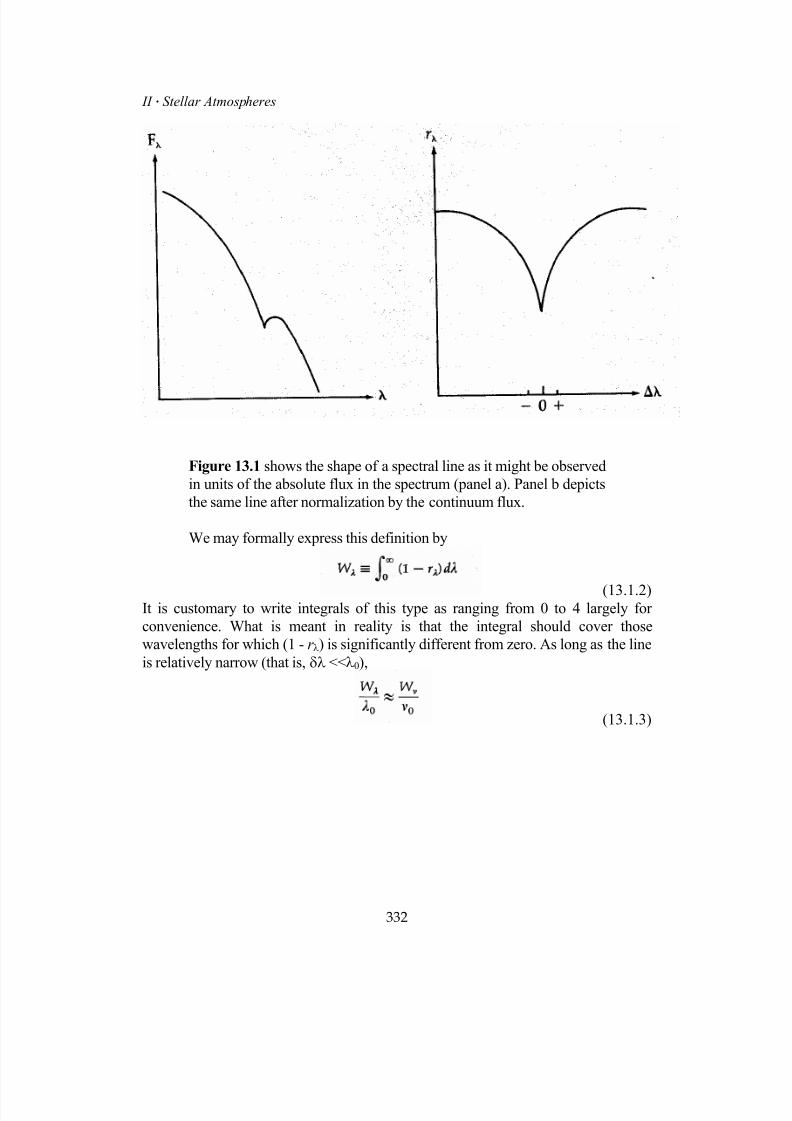
7/18/2019 The Fundamentals of Stellar Astrophysics - Collins G. W.
http://slidepdf.com/reader/full/the-fundamentals-of-stellar-astrophysics-collins-g-w 352/524
II Stellar Atmospheres
Figure 13.1 shows the shape of a spectral line as it might be observedin units of the absolute flux in the spectrum (panel a). Panel b depictsthe same line after normalization by the continuum flux.
We may formally express this definition by
(13.1.2)It is customary to write integrals of this type as ranging from 0 to 4 largely forconvenience. What is meant in reality is that the integral should cover thosewavelengths for which (1 - r λ) is significantly different from zero. As long as the lineis relatively narrow (that is, δλ <<λ0),
(13.1.3)
332

7/18/2019 The Fundamentals of Stellar Astrophysics - Collins G. W.
http://slidepdf.com/reader/full/the-fundamentals-of-stellar-astrophysics-collins-g-w 353/524
13 Formation of Spectral Lines
Figure 13.2 shows the equivalent 'black' line profile (double cross-hatched area) appropriate for a specific spectral line (single cross-hatched area). The areas of the two profiles are equal and so the
rectangular one can be characterized by its width alone. Suchequivalent widths are usually measured in Ångstroms.
b Selective (True) Absorption and Resonance Scattering
It is useful to divide the processes by which a photon interacts withan atom into two idealized cases. The first is called true, or pure absorption. In thisinstance, the emission of photons is completely uncorrelated to the previousabsorption of photons. In a sense, any photon that is emitted has "lost all memory ofwhat it was". Such a process is called a true absorption process, and it can occur instellar atmospheres when an atom suffers numerous collisions between the time that
the photon is absorbed and reemitted. These collisions can de-excite or further excitethe atom, and with the assumption of LTE, these collisions will be randomlydistributed so that any subsequently emitted photon is, indeed, totally uncorrelatedwith the one that was absorbed. Spectral lines formed in this manner are known as pure absorption lines. They exist in stellar spectra since the enhanced opacity provided by the line implies that the line will become optically thick higher in theatmosphere where it is generally cooler. Since it is cooler, then the source function is
333

7/18/2019 The Fundamentals of Stellar Astrophysics - Collins G. W.
http://slidepdf.com/reader/full/the-fundamentals-of-stellar-astrophysics-collins-g-w 354/524
II Stellar Atmospheres smaller and the emergent intensity is less than that of the neighboring continuum.
The second type of process is called resonance scattering and it results in theloss of photons in a specialized and indirect manner. Here the photon has a "perfectmemory" of its origin. The emitted photon is completely correlated in frequency withthe absorbed photon. In Chapter 9, we described such a process as a coherentscattering and lines for which this is true are known as scattering lines. In contrast tothe case of pure absorption, a scattering line is formed when the emitted photon iscreated so soon after the prior absorption that there is no time for the atom to be perturbed by collisions, and the probability of a transition to the prior state is verygreat. Such cases occur from those states that have very short lifetimes and only onelower level to which the electron can jump. The resonance line transitions meet allthese conditions, and hence any resonance line is likely to be a strong scattering line.However, it is possible for any strong line to behave as a scattering line if the
probability of returning to the previous state is very large. The same photon that wasabsorbed is then reemitted, with no net energy exchange with the atom. This isessentially the condition for an interaction to be termed a scattering. The scattering process does not directly result in any loss of energy from the radiation field, but bychanging the direction of the photon the process lengthens the stay of the photon inthe atmosphere making it subject to destruction by continuum absorption processes.
Thus, we can divide spectral lines into two types; the pure absorption lines,where the absorbed energy of the photon is fully shared with the gas, and theresonance scattering lines where it is not. In Chapter 9 we showed that nature isreally more complicated than this and in reality most lines can be viewed as a
mixture of these two extreme states. However, the radiative transfer of these twokinds of lines is quite different, and understanding the behavior of these two limitingcases will provide a comprehensive basis for understanding the behavior of spectrallines in general. The different behavior of these two processes is clearly seen bynoting that the energy of a pure absorption process is shared immediately with thegas while that of a resonance scattering processes is not. Scattering is a fullyconservative process and therefore cannot, by itself, result in the destruction of photons. However, scattering does change the direction of a photon, therebyincreasing the distance that the photon must travel through the atmosphere beforeescaping into interstellar space. Any process that lengthens the path of a photonthrough the atmosphere also enhances the probability that the photon will be
absorbed by some other process such as continuum absorption. Thus, the redirectionof line photons that results from resonant scattering also produces a net loss of these photons relative to those in the neighboring continuum. This, then, is the origin of theresonance scattering lines in stellar spectra.
334

7/18/2019 The Fundamentals of Stellar Astrophysics - Collins G. W.
http://slidepdf.com/reader/full/the-fundamentals-of-stellar-astrophysics-collins-g-w 355/524
13 Formation of Spectral Lines c Equation of Radiative Transfer for Spectral Line Radiation
It is customary to denote the part of the mass extinction coefficientthat results from pure absorption processes by the letter κ, while the part that resultsfrom scattering is represented by the Greek letter σ. Those photon interactions thatoccur as a result of absorptions within the line are subscripted by the letter ν. Sincethe continuum processes generally vary quite slowly across a spectral line, we omitthe subscript ν entirely. Thus,
(13.1.4)Since the origin of the equation of radiative transfer was dealt with
extensively in Section 9.2, we provide only a brief derivation here. Basically we balance the energy passing in and out of a differential volume along a specific paththrough the atmosphere. If we do this for a plane-parallel atmosphere where we keepthe line and continuum processes separate, we get
(13.1.5)where the first term on the right-hand side represents the energy lost from the beam.The second and third terms on the right-hand side denote the contributions to the beam within the differential volume. The first of these is just due to thermalemission, while the second results from scattering by both line and continuum processes. By making the usual identification between the Planck function and the processes of thermal emission and absorption, the equation of radiative transfer forline radiation becomes
(13.1.6)where the optical depth in the line τν is given by
(13.1.7)
335
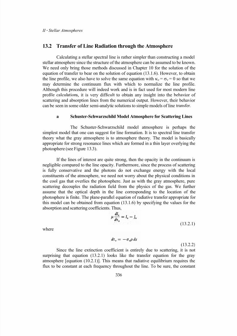
7/18/2019 The Fundamentals of Stellar Astrophysics - Collins G. W.
http://slidepdf.com/reader/full/the-fundamentals-of-stellar-astrophysics-collins-g-w 356/524
II Stellar Atmospheres
13.2 Transfer of Line Radiation through the Atmosphere
Calculating a stellar spectral line is rather simpler than constructing a modelstellar atmosphere since the structure of the atmosphere can be assumed to be known.We need only bring those methods discussed in Chapter 10 for the solution of theequation of transfer to bear on the solution of equation (13.1.6). However, to obtainthe line profile, we also have to solve the same equation with κν = σν = 0 so that wemay determine the continuum flux with which to normalize the line profile.Although this procedure will indeed work and is in fact used for most modern line profile calculations, it is very difficult to obtain any insight into the behavior ofscattering and absorption lines from the numerical output. However, their behaviorcan be seen in some older semi-analytic solutions to simple models of line transfer.
a Schuster-Schwarzschild Model Atmosphere for Scattering Lines
The Schuster-Schwarzschild model atmosphere is perhaps thesimplest model that one can suggest for line formation. It is to spectral line transfertheory what the gray atmosphere is to atmosphere theory. The model is basicallyappropriate for strong resonance lines which are formed in a thin layer overlying the photosphere (see Figure 13.3).
If the lines of interest are quite strong, then the opacity in the continuum isnegligible compared to the line opacity. Furthermore, since the process of scatteringis fully conservative and the photons do not exchange energy with the local
constituents of the atmosphere, we need not worry about the physical conditions inthe cool gas that overlies the photosphere. Just as with the gray atmosphere, purescattering decouples the radiation field from the physics of the gas. We furtherassume that the optical depth in the line corresponding to the location of the photosphere is finite. The plane-parallel equation of radiative transfer appropriate forthis model can be obtained from equation (13.1.6) by specifying the values for theabsorption and scattering coefficients. Thus,
(13.2.1)where
(13.2.2)Since the line extinction coefficient is entirely due to scattering, it is not
surprising that equation (13.2.1) looks like the transfer equation for the grayatmosphere [equation (10.2.1)]. This means that radiative equilibrium requires theflux to be constant at each frequency throughout the line. To be sure, the constant
336
7/18/2019 The Fundamentals of Stellar Astrophysics - Collins G. W.
http://slidepdf.com/reader/full/the-fundamentals-of-stellar-astrophysics-collins-g-w 357/524
13 Formation of Spectral Lines will be different for each frequency, but the flux at any particular frequency will notvary with the depth. The condition of monochromatic flux constancy can beexpressed as
(13.2.3)
Figure 13.3 shows a schematic representation of the Schuster-Schwarzschild Model Atmosphere for the formation of strongscattering lines.
Solution of the Radiative Transfer Equation for the Schuster-
Schwarzschild Model Since the equation of transfer for line radiation in this
model formally resembles the gray atmosphere equation; we may use the results ofChapter 10 to find the solution. Specifically, equation (10.2.31) gives a general resultfor the solution of the plane-parallel finite gray atmosphere. However, to keep thediscussion simple, we take n = 2. Then the appropriate zeros of the Legendre
polynomials require that3
1±=iµ and equation (10.2.31) becomes
(13.2.4)where the subscripts '+' and '-' refer to the outward- and inward-directed streams ofradiation, respectively. Applying the surface boundary condition that I_ (0) = 0 wefind
(13.2.5)and the complete solution becomes
337
7/18/2019 The Fundamentals of Stellar Astrophysics - Collins G. W.
http://slidepdf.com/reader/full/the-fundamentals-of-stellar-astrophysics-collins-g-w 358/524
II Stellar Atmospheres
(13.2.6)
This solution for the gray atmosphere is sometimes called the Chandrasekhartwo-stream approximation. It conceptually replaces the entire radiation field by twostreams of radiation directed along a line oriented about 54 degrees (
31±=i ) to
the normal of the atmosphere. The result is nearly identical to that obtained from theEddington approximation, only the angle is slightly different.
Residual Flux and Intensity for the Schuster-Schwarzschild Model
The ratio of the emergent flux in the line to that of the continuum can beobtained immediately by requiring that the line intensity incident on the base of thecool gas be the same as the emergent intensity in the neighboring continuum, so that
(13.2.7)Here τ0 is the optical depth at any frequency in the line measured at the base of theatmosphere. This value is zero for all frequencies corresponding to the continuum.The quantity Fc is just the continuum flux. Thus, the residual flux is
(13.2.8)However, to complete the description of the Schuster-Schwarzschild model,
we would like an expression for the residual intensity f ν. To obtain the angledependence of the intensity we have to appeal to the classical solution of the
equation of transfer for a finite atmosphere, so that the emergent intensity is
(13.2.9)The value for the mean intensity Jν(τν) can be obtained directly from the two-streamapproximation as
(13.2.10)Substitution of this into equation (13.2.9) and then into the definition for the residualintensity [equation (13.1.1)] yields
(13.2.11)Remember that t0 is a function of frequency, and so its behavior with frequency willdetermine the line shape or profile.
338

7/18/2019 The Fundamentals of Stellar Astrophysics - Collins G. W.
http://slidepdf.com/reader/full/the-fundamentals-of-stellar-astrophysics-collins-g-w 359/524
13 Formation of Spectral Lines To see how scattering lines will vary in strength across the surface of a stellar disk,consider some limiting cases.
(13.2.12)The first of equations (13.2.12) represents relatively weak spectral lines (or the wingsof strong lines). Here there is no angular dependence whatsoever except that dictated by the limb-darkening of the continuum. Thus, we can expect that even weakscattering lines will be visible at all points on the stellar disk with equal strength.While the strong lines described by the second of equations (13.2.12) do show some
limb-darkening through the dependence on µ, that dependence is not great. Therange in line strength to be expected for a strong scattering line between one formednear the center of the disk and one formed at the limb is about a factor of 2. As wesee, this contrasts greatly with the behavior of spectral lines formed by pureabsorption processes. However, a model that includes absorption processes mustinclude information about the atmospheric structure and so will be somewhat moresophisticated. One such model atmosphere is known as the Milne-Eddington model.
b Milne-Eddington Model Atmosphere for the Formation of
Spectral Lines
To appreciate the importance of pure absorption in the formation of aspectral line, we must acknowledge the fact that pure absorption processes imply aninteraction between the radiation field and the particles that make up the gas. Thus,we will have to specify something about the behavior of the opacity and sourcefunction with optical depth. The trick is to place as few limitations as possible so asto preserve generality and to make those limitations "reasonable" and yet specify thesituation sufficiently to guarantee a unique solution.
The Milne-Eddington model is considerably more sophisticated than theSchuster-Schwarzschild model and is correspondingly more complicated. It attemptsto simultaneously include the effects of absorption and scattering in the line
extinction coefficient (that is, κν+σν). Let us define the following parameters in termsof the absorption and scattering coefficients of the line and continuum:
339

7/18/2019 The Fundamentals of Stellar Astrophysics - Collins G. W.
http://slidepdf.com/reader/full/the-fundamentals-of-stellar-astrophysics-collins-g-w 360/524
II Stellar Atmospheres
(13.2.13)The parameter εν measures the relative importance of pure absorption to total
extinction for processes involving the spectral line, and ην is a measure of the linestrength, since it is a ratio of the total line extinction coefficient to that of thecontinuum. The Milne-Eddington model does make the somewhat restrictiveassumption that scattering processes are relatively unimportant for continuum photons. Hence,σ = 0. The parameter is clearly not linearly independent of εν andην, but is useful to introduce because it measures the relative importance of totalabsorption to total extinction for all processes of the line and continuum that operate
on the photons passing through the atmosphere.
By substituting these values into the equation for the transfer of line radiation[equation (13.1.6)], we have the appropriate equation of transfer for the Milne-Eddington model atmosphere
(13.2.14)A simpler equation of transfer for the continuum radiation can be obtained simply byletting κν and σν go to zero, so that
(13.2.15) Now if we relate the structure of the atmosphere to the source function in the linethrough its behavior in the continuum, we can write
(13.2.16)Here, we have made use of the Eddington approximation where the asymptotic behavior of the source function with optical depth is linear [see equation (10.2.32)].To find the behavior of the residual intensity and flux for the line, we follow
basically the same steps as for the Schuster-Schwarzschild model.
Solution of the Equation of Radiative Transfer for the Milne-Eddington
Model Atmosphere Before we can solve equations (13.2.14), we must makeone additional assumption regarding the behavior of the opacity coefficients withatmospheric depth. We assume that both εν and ην (and hence ν) are not functionsof depth in the atmosphere and can therefore be regarded as constants in the equation
340
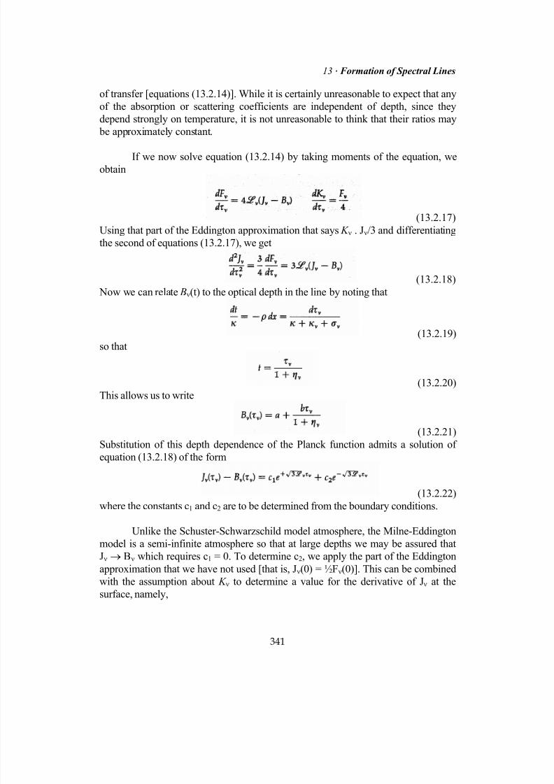
7/18/2019 The Fundamentals of Stellar Astrophysics - Collins G. W.
http://slidepdf.com/reader/full/the-fundamentals-of-stellar-astrophysics-collins-g-w 361/524
13 Formation of Spectral Lines of transfer [equations (13.2.14)]. While it is certainly unreasonable to expect that anyof the absorption or scattering coefficients are independent of depth, since theydepend strongly on temperature, it is not unreasonable to think that their ratios may be approximately constant.
If we now solve equation (13.2.14) by taking moments of the equation, weobtain
(13.2.17)Using that part of the Eddington approximation that says K ν . Jν/3 and differentiatingthe second of equations (13.2.17), we get
(13.2.18) Now we can relate Bν(t) to the optical depth in the line by noting that
(13.2.19)so that
(13.2.20)This allows us to write
(13.2.21)Substitution of this depth dependence of the Planck function admits a solution ofequation (13.2.18) of the form
(13.2.22)where the constants c1 and c2 are to be determined from the boundary conditions.
Unlike the Schuster-Schwarzschild model atmosphere, the Milne-Eddingtonmodel is a semi-infinite atmosphere so that at large depths we may be assured thatJν → Bν which requires c1 = 0. To determine c2, we apply the part of the Eddingtonapproximation that we have not used [that is, Jν(0) = ½Fν(0)]. This can be combinedwith the assumption about K ν to determine a value for the derivative of Jν at thesurface, namely,
341

7/18/2019 The Fundamentals of Stellar Astrophysics - Collins G. W.
http://slidepdf.com/reader/full/the-fundamentals-of-stellar-astrophysics-collins-g-w 362/524
II Stellar Atmospheres
(13.2.23)
The right-hand side of this result is obtained from the solution [equation (13.2.22)]itself. If we differentiate that solution and evaluate the result at the surface, we have
(13.2.24)which yields the following value of c2:
(13.2.25)Had we used the Chandrasekhar two-stream approximation to solve the equation oftransfer, we would have gotten
(13.2.26)This indicates that the solution is not too sensitive to the mode of solution of theequation of transfer.
Residual Flux and Intensity for the Milne-Eddington Model Theresidual flux can be obtained from its definition and the Eddington approximation sothat
(13.2.27)In the continuum, ην = 0 andℒν = 1 so that
(13.2.28)This leads to a residual flux given by
3.2.29)
To evaluate the residual intensity, we must again use the classical solution tothe equation of transfer. However, to do so, we must have expressions for the sourcefunction in the line and continuum. It is clear from the equation of transfer [equation(13.2.14)] that the line source function is
342
(13.2.30)

7/18/2019 The Fundamentals of Stellar Astrophysics - Collins G. W.
http://slidepdf.com/reader/full/the-fundamentals-of-stellar-astrophysics-collins-g-w 363/524
13 Formation of Spectral Lines Again, remembering that in the continuum ℒν = 1 , we see that the source functionfor the continuum is just
(13.2.31)Substitution of these two source functions into the classical solution for the equationof transfer, and some algebra, gives the residual intensity as
(13.2.32)
Some aspects of this solution should not surprise us. For example, the terma+bµ is simply 1/µ times the Laplace transform of the continuum source functiona+bt . Similarly, the numerator of the first term is the Laplace transform of the Planckfnction in the line, so that the lead term of equation (13.2.32) is just the ratio of theLaplace transforms of the absorption components of the line to the continuum sourcefunctions. This is to be expected from the result obtained for limb-darkening inChapter 10 [equations (10.1.19), and (10.1.20)]. Since the second term vanishes forthe case of pure absorption (that is, → 1), this term must represent thecontribution of scattering in the line to the residual intensity.
Asymptotic Behavior of the Residual Flux and Intensity Because of theincreased generality of the Milne-Eddington model over the Schuster-Schwarzschildmodel, we can investigate the asymptotic behavior of the line not only with strength but also as the line extinction coefficient ranges from pure absorption to purescattering. In the case of pure absorption ε
ν = 1, ℒ
ν = 1 and equations (13.2.29) and
(13.2.32) become
(13.2.33) Note that in an isothermal atmosphere (that is, b = 0) both the residual intensity andthe flux are asymptotic to unity and the line disappears. Thus, as one might expect, ifthere are no temperature gradients, there can be no spectral absorption lines. Theradiation field would then be in STE and the source function as well as the radiationfield would be given by the Planck function regardless of the dependence of theabsorption coefficient on frequency.
For stellar atmospheres, this has the more immediate implication that thestronger the source function gradient the stronger the line. This is the simpleexplanation of why the central depths of the lines in late-type stars are so muchdarker than those for the early-type stars. For the later type stars, the visible part ofthe spectrum tends to lie at wavelengths shorter than that of the stellar energymaximum. For these wavelengths, the source function varies as a large power of the
343
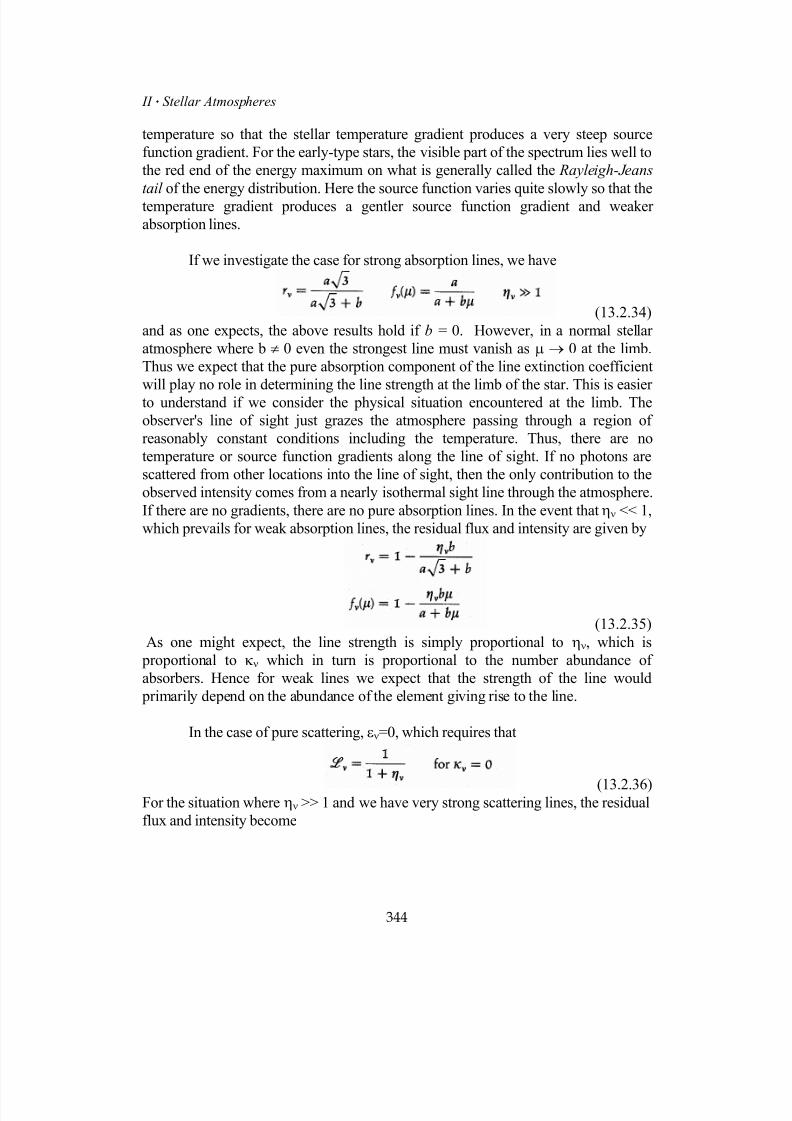
7/18/2019 The Fundamentals of Stellar Astrophysics - Collins G. W.
http://slidepdf.com/reader/full/the-fundamentals-of-stellar-astrophysics-collins-g-w 364/524
II Stellar Atmospheres temperature so that the stellar temperature gradient produces a very steep sourcefunction gradient. For the early-type stars, the visible part of the spectrum lies well tothe red end of the energy maximum on what is generally called the Rayleigh-Jeans
tail of the energy distribution. Here the source function varies quite slowly so that thetemperature gradient produces a gentler source function gradient and weakerabsorption lines.
If we investigate the case for strong absorption lines, we have
(13.2.34)and as one expects, the above results hold if b = 0. However, in a normal stellaratmosphere where b ≠ 0 even the strongest line must vanish as µ → 0 at the limb.Thus we expect that the pure absorption component of the line extinction coefficientwill play no role in determining the line strength at the limb of the star. This is easierto understand if we consider the physical situation encountered at the limb. Theobserver's line of sight just grazes the atmosphere passing through a region ofreasonably constant conditions including the temperature. Thus, there are notemperature or source function gradients along the line of sight. If no photons arescattered from other locations into the line of sight, then the only contribution to theobserved intensity comes from a nearly isothermal sight line through the atmosphere.If there are no gradients, there are no pure absorption lines. In the event that ην << 1,which prevails for weak absorption lines, the residual flux and intensity are given by
(13.2.35)As one might expect, the line strength is simply proportional to ην, which is
proportional to κν which in turn is proportional to the number abundance ofabsorbers. Hence for weak lines we expect that the strength of the line would primarily depend on the abundance of the element giving rise to the line.
In the case of pure scattering, εν=0, which requires that
(13.2.36)For the situation where ην >> 1 and we have very strong scattering lines, the residualflux and intensity become
344
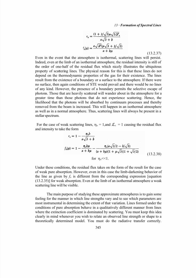
7/18/2019 The Fundamentals of Stellar Astrophysics - Collins G. W.
http://slidepdf.com/reader/full/the-fundamentals-of-stellar-astrophysics-collins-g-w 365/524
13 Formation of Spectral Lines
(13.2.37)Even in the event that the atmosphere is isothermal, scattering lines will persist.Indeed, even at the limb of an isothermal atmosphere, the residual intensity is still ofthe order of one-half of the residual flux which nicely illustrates the ubiquitous property of scattering lines. The physical reason for this is that these lines do notdepend on the thermodynamic properties of the gas for their existence. The linesresult from the existence of a boundary or a surface to the atmosphere. If there wereno surface, then again conditions of STE would prevail and there would be no linesof any kind. However, the presence of a boundary permits the selective escape of photons. Those that are heavily scattered will wander about in the atmosphere for a
greater time than those photons that do not experience scattering. Hence, thelikelihood that the photons will be absorbed by continuum processes and therebyremoved from the beam is increased. This will happen in an isothermal atmosphereas well as in a normal atmosphere. Thus, scattering lines will always be present in astellar spectrum.
For the case of weak scattering lines, ην = 1,and ℒν = 1 causing the residual fluxand intensity to take the form
(13.2.38)for ην<<1.
Under these conditions, the residual flux takes on the form of the result for the caseof weak pure absorption. However, even in this case the limb-darkening behavior ofthe line as given by f ν is different from the corresponding expression [equation(13.2.35)] for weak absorption. Even at the limb of an isothermal atmosphere a weakscattering line will be visible.
The main purpose of studying these approximate atmospheres is to gain somefeeling for the manner in which line strengths vary and to see which parameters aremost instrumental in determining the extent of that variation. Lines formed under theconditions of pure absorption behave in a qualitatively different manner from lineswhere the extinction coefficient is dominated by scattering. You must keep this ideaclearly in mind whenever you wish to relate an observed line strength or shape to atheoretically determined model. You must do the radiative transfer correctly.
345

7/18/2019 The Fundamentals of Stellar Astrophysics - Collins G. W.
http://slidepdf.com/reader/full/the-fundamentals-of-stellar-astrophysics-collins-g-w 366/524
II Stellar Atmospheres Knowledge of the behavior of spectral lines also will serve you well when you try tounderstand the results of a complex model atmosphere computer code. If the linedoes not behave in a manner described by these simple models, then there must be agood and compelling reason that should be understood by the investigator.
Although the 1940s and 1050s generated additional approaches to the problem of radiative transfer of line radiation, most of that work has been superceded by the advent of high-speed computers and large complex atmosphere codes. Thecontemporary approach basically treats the line absorption coefficient as anadditional opacity source that has a strongly variable frequency dependence. Thus,no special distinction is made between opacity due to lines and that of the continuum.The problem of locating the continuum for the purposes of generating a line profile isthen about the same for the model maker as for the observer. The many complex physical processes that contribute to the shape of the line, and whose importance
varies with position in the atmosphere, are automatically included in the calculations.However, for obtaining insight into the processes of line formation, these simplemodels remain most useful.
Problems
1. Find equivalent expressions for the asymptotic behavior of the residualintensity and flux as given by equations (13.2.33) through (13.2.37) for thecase where the radiative transfer equation is solved by the Chandrasekhartwo-stream approximation.
2. Find expressions for the residual intensity and flux of a Schuster-Schwarzschild atmosphere if the equation of transfer is to be solved by usingthe Chandrasekhar nth-order approximation.
3. Show that the expression for f ν can be used to obtain the expression for r ν forthe Milne-Eddington atmosphere.
4. Find an expression for r ν in a Milne-Eddington atmosphere where the sourcefunction in the continuum is given by
5. Derive expressions for a Milne-Eddington type of model atmosphere of finiteoptical depth τ0 for f ν(µ) and r ν. Assume the atmosphere is illuminated from
below by a uniform isotropic intensity I0.
346
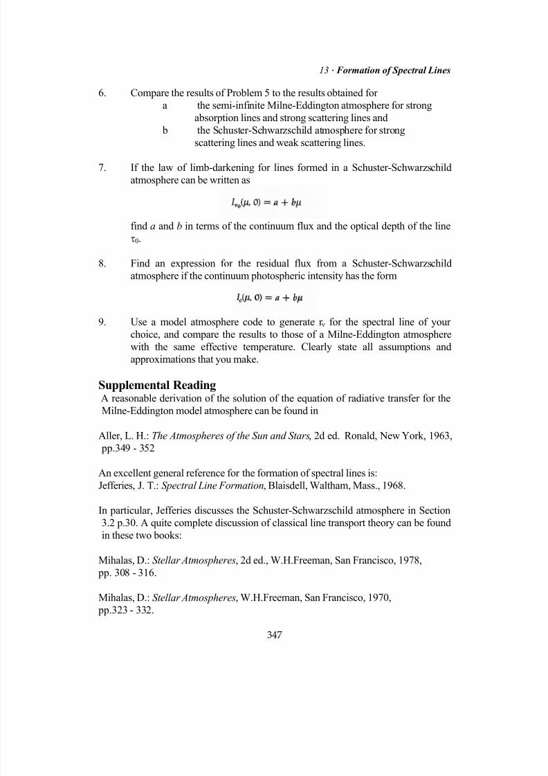
7/18/2019 The Fundamentals of Stellar Astrophysics - Collins G. W.
http://slidepdf.com/reader/full/the-fundamentals-of-stellar-astrophysics-collins-g-w 367/524
13 Formation of Spectral Lines
347
6. Compare the results of Problem 5 to the results obtained fora the semi-infinite Milne-Eddington atmosphere for strong
absorption lines and strong scattering lines and b the Schuster-Schwarzschild atmosphere for strong
scattering lines and weak scattering lines.
7. If the law of limb-darkening for lines formed in a Schuster-Schwarzschildatmosphere can be written as
find a and b in terms of the continuum flux and the optical depth of the lineτ0.
8. Find an expression for the residual flux from a Schuster-Schwarzschild
atmosphere if the continuum photospheric intensity has the form
9. Use a model atmosphere code to generate r ν for the spectral line of yourchoice, and compare the results to those of a Milne-Eddington atmospherewith the same effective temperature. Clearly state all assumptions andapproximations that you make.
Supplemental Reading A reasonable derivation of the solution of the equation of radiative transfer for the
Milne-Eddington model atmosphere can be found in
Aller, L. H.: The Atmospheres of the Sun and Stars, 2d ed. Ronald, New York, 1963, pp.349 - 352
An excellent general reference for the formation of spectral lines is:Jefferies, J. T.: Spectral Line Formation, Blaisdell, Waltham, Mass., 1968.
In particular, Jefferies discusses the Schuster-Schwarzschild atmosphere in Section3.2 p.30. A quite complete discussion of classical line transport theory can be foundin these two books:
Mihalas, D.: Stellar Atmospheres, 2d ed., W.H.Freeman, San Francisco, 1978, pp. 308 - 316.
Mihalas, D.: Stellar Atmospheres, W.H.Freeman, San Francisco, 1970, pp.323 - 332.
7/18/2019 The Fundamentals of Stellar Astrophysics - Collins G. W.
http://slidepdf.com/reader/full/the-fundamentals-of-stellar-astrophysics-collins-g-w 368/524
II Stellar Atmospheres
Copyright (2003) George W. Collins, II
14
Shape of Spectral Lines
. . .
If we take the classical picture of the atom as the definitive view of the formation ofspectral lines, we would conclude that these lines should be delta functions offrequency and appear as infinitely sharp black lines on the stellar spectra. However,many processes tend to broaden these lines so that the lines develop a characteristicshape or profile. Some of these effects originate in the quantum mechanicaldescription of the atom itself. Others result from perturbations introduced by the
neighboring particles in the gas. Still others are generated by the motions of theatoms giving rise to the line. These motions consist of the random thermal motion ofthe atoms themselves which are superimposed on whatever large scale motions may be present. The macroscopic motions may be highly ordered, as in the case of stellarrotation, or show a high degree of randomness such as is characteristic of turbulentflow.
348

7/18/2019 The Fundamentals of Stellar Astrophysics - Collins G. W.
http://slidepdf.com/reader/full/the-fundamentals-of-stellar-astrophysics-collins-g-w 369/524
14 Shape of Spectral Lines
In practice, all these effects are present and give the line its characteristicshape. The correct representation of these effects allows for the calculation of theobserved line profile and in the process reveals a great deal about the conditions inthe star that give rise to the spectrum. Of course the photons that give rise to theabsorption lines in the stellar spectrum have their origins at different locations in theatmosphere. So the conditions giving rise to a spectral line are really an average of arange of conditions. Thus, when we talk of the excitation temperature or the kinetictemperature appropriate for a specific spectral line, it must be clear that we arereferring to some sort of average temperature appropriate for that portion of theatmosphere in which most of the line photons originate. For strong lines with opticaldepths much greater than the optical depth of the adjacent continuum, the physicaldepth of the line-forming region is quite small, and the approximation of the physicalconditions by their average value is a good one. Unfortunately, for very strong lines,
the optical depths can range to such large values that the line-forming region islocated in the chromosphere, where most of the assumptions that we have madeconcerning the structure of the stellar atmosphere break down. A discussion of suchlines will have to wait until we are ready to relax the condition of LTE.
In describing the shape or profile of a spectral line, we introduce the notionof the atomic line absorption coefficient. This is a probability density function thatdescribes the probability that a given atom in a particular state of ionization andexcitation will absorb a photon of frequency ν in the interval between ν and ν + dν.We then assume that an ensemble of atoms will follow the probability distributionfunction of the single atom and produce the line. In order to make the connection
between the behavior of a single atom and that of a collection of atoms, we shallmake use of the Einstein coefficients that were introduced in Section 11.3.
14.1 Relation between the Einstein, Mass Absorption, and Atomic
Absorption Coefficients
Since the Einstein coefficient Bik is basically the probability that an atom will make atransition from the ith state to the kth state in a given time interval, the relationship tothe mass absorption coefficient can be found by relating all upward transitions to thetotal absorption of photons that must take place. From the definition of the Einsteincoefficient of absorption, the total number of transitions that take place per unit time
is Ni6k = niBik Iνdt
(14.1.1)where ni is the number density of atoms in the ith state. Since the number of photonsavailable for absorption at a particular frequency is (Iν/hν)dν, the total number ofupward transitions is also
349

7/18/2019 The Fundamentals of Stellar Astrophysics - Collins G. W.
http://slidepdf.com/reader/full/the-fundamentals-of-stellar-astrophysics-collins-g-w 370/524
II Stellar Atmospheres
(14.1.2)If we assume that the radiation field seen by the atom is relatively independent offrequency throughout the spectral line, then the integral of the mass absorptioncoefficient over the line is
(14.1.3)where ν0 is the frequency of the center of the line.
For the remainder of this chapter, we will be concerned with thedetermination of the frequency dependence of the line absorption coefficient. Thus,we will be calculating the absorption coefficient of a single atom at variousfrequencies. We will call this absorption coefficient the atomic line absorptioncoefficient , which is related to the mass absorption coefficient by
(14.1.4) Note that we will occasionally use the circular frequency ω instead of the frequencyν, where ω = 2πν.
14.2 Natural or Radiation Broadening
Of all the physical processes that can contribute to the frequency dependence of the
atomic line absorption coefficient, some are intrinsic to the atom itself. Since theatom must emit or absorb a photon in a finite time, that photon cannot be represented by an infinite sine wave. If the photon wave train is of finite length, it must berepresented by waves of frequencies other than the fundamental frequency of the linecenter ν0. This means that any photon can be viewed in terms of a "packet" offrequencies ranging around the fundamental frequency. So the photon will consist ofenergy occupying a range of wavelengths about the line center. The extent of thisrange will depend on the length of the photon wave train. The longer the wave-train,the narrower will be the range of frequencies or wavelengths required to represent it.
Since the length of the wave train will be proportional to the time required to
emit or absorb it, the characteristic width of the range will be proportional to thetransition probability (i.e., the inverse of the transition time) of the atomic transition.This will be a property of the atom alone and is known as the natural width of thetransition. It is always present and cannot be removed. Its existence depends only onthe finite length of the wave train and so is not just the result of the quantum natureof the physical world. Indeed, there are two effects to estimate: the classical effectrelying on the finite nature of the wave train, and the quantum mechanical effect that
350
7/18/2019 The Fundamentals of Stellar Astrophysics - Collins G. W.
http://slidepdf.com/reader/full/the-fundamentals-of-stellar-astrophysics-collins-g-w 371/524
14 Shape of Spectral Lines
can be obtained for a specific atom's propensity to emit photons. The former will beindependent of the type of atom, while the latter will yield a larger broadening thatdepends specifically on the type of atom and its specific state.
a Classical Radiation Damping
The classical approach to the problem of absorption relies on a picture of the atom in which the electron is seen to oscillate in response to the electricfield of the passing photon. There is a strong analogy here between the behavior ofthe electrons in the atom and the free electrons in an antenna. The energy of the passing wave is converted to oscillatory motion of the electron(s), which in theantenna produce a current that is subsequently amplified to signal the presence of the photon. It then makes sense to use classical electromagnetic theory to estimate thiseffect for the single optical electron of an atom. The oscillation of this electron can
then be viewed as a classical oscillating dipole.
Since an oscillating electron represents a continuously accelerating charge,the electron will radiate or absorb energy. In the classical picture, the processes ofemission and absorption are interchangeable. The emission simply requires the presence of a driving force, which is the ultimate source of the energy that is emitted,while the energy source for the absorption processes is the passing photon itself. Ifwe let W represent the energy gained or lost over one cycle of the oscillating dipole,then any good book on classical electromagnetism (i.e., W. Panofsky and M.Phillips1 or J. Slater and N. Frank 2) will show that
(14.2.1)where d2x/dt2 is the acceleration of the oscillating charge. Now if we assume that theoscillator is freely oscillating, then the instantaneous acceleration is simply
(14.2.2)This is a good assumption as long as the energy is to be absorbed on a time scale thatis long compared to the period of oscillation. Since the driving frequency of theoscillator is that of the line center, this is equivalent to saying that the spread or rangeof absorbed frequencies is small compared to the frequency of the line center.
Equation (14.2.2) can be used to replace the mean square acceleration ofequation (14.2.1) to get
(14.2.3)
The mean position of the oscillator can, in turn, be replaced with the mean total
351

7/18/2019 The Fundamentals of Stellar Astrophysics - Collins G. W.
http://slidepdf.com/reader/full/the-fundamentals-of-stellar-astrophysics-collins-g-w 372/524
II Stellar Atmospheres
energy of the oscillator from
(14.2.4)so that the differential equation for the absorption or emission of radiation from aclassical oscillating dipole is
(14.2.5)The quantity γ is known as the classical damping constant and is
(14.2.6)The solution of equation (14.2.5) shows that the absorption of the energy of the
passing photon will be
(14.2.7)where I0 is the presumably sinusoidally varying energy field of the passing photon.The result is that energy of the absorbed or emitted photon resembles a damped sinewave (see Figure 14.1).
But, we are interested in the behavior of the absorption with wavelength orfrequency, for that is what yields the line profile. Since we are interested in the behavior of an uncorrelated collection of atoms, their combined effect will be
proportional to the combined effect of the squares of the electric fields of theiremitted photons. Thus, we must calculate the Fourier transform of the time-dependent behavior of the electric field of the photon so that
(14.2.8)
If we assume that the photon encounters the atom at t = 0 so that E(t) = 0 fort < 0, and that it has a sinusoidal behavior for t ≥ 0, then the
frequency dependence of the photon's electric field will be
t ie 0
0EE(t) ω −=
(14.2.9)Thus the power spectrum of the energy absorbed or emitted by this classicaloscillator will be
352
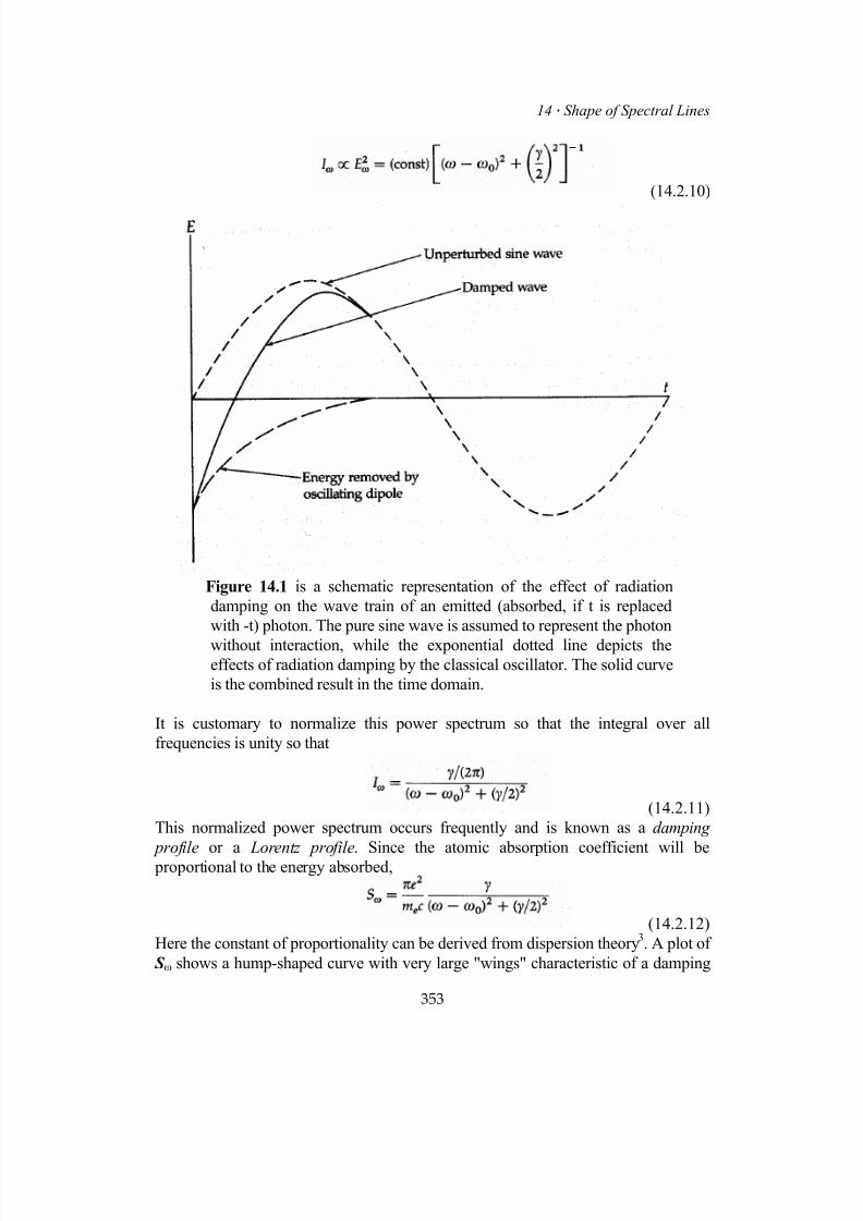
7/18/2019 The Fundamentals of Stellar Astrophysics - Collins G. W.
http://slidepdf.com/reader/full/the-fundamentals-of-stellar-astrophysics-collins-g-w 373/524
14 Shape of Spectral Lines
(14.2.10)
Figure 14.1 is a schematic representation of the effect of radiationdamping on the wave train of an emitted (absorbed, if t is replacedwith -t) photon. The pure sine wave is assumed to represent the photon
without interaction, while the exponential dotted line depicts theeffects of radiation damping by the classical oscillator. The solid curveis the combined result in the time domain.
It is customary to normalize this power spectrum so that the integral over allfrequencies is unity so that
(14.2.11)This normalized power spectrum occurs frequently and is known as a damping
profile or a Lorentz profile. Since the atomic absorption coefficient will be proportional to the energy absorbed,
(14.2.12)Here the constant of proportionality can be derived from dispersion theory3. A plot of S ω shows a hump-shaped curve with very large "wings" characteristic of a damping
353

7/18/2019 The Fundamentals of Stellar Astrophysics - Collins G. W.
http://slidepdf.com/reader/full/the-fundamentals-of-stellar-astrophysics-collins-g-w 374/524
II Stellar Atmospheres
profile (see Figure 14.2). At some point in the profile, the absorption coefficientdrops to one-half of its peak value. If we denote the full width at this half-power point by ∆λc, then
(14.2.13)This is known as the classical damping width of a spectral line and is independent ofthe atom or line. It is also very much smaller than the narrowest lines seen in thelaboratory, and to see why, we must turn to a quantum mechanical representation ofradiation damping.
Figure 14.2 shows the variation of the classical damping coefficientwith wavelength. The damping coefficient drops to half of its peakvalue for wavelength shifts equal to ∆λc/2 on either side of the centralwavelength. The overall shape is known as the Lorentz profile.
b Quantum Mechanical Description of Radiation Damping
The quantum mechanical view of the emission or absorption of a photon israther different from the classical view since it is intimately connected with thenature of the atom in question. The basic approach involves the Heisenberguncertainty principle as the basis of the broadening. If we consider an atom to be in a
certain state, then the length of time that it can remain in that state is related to theuncertainty of the energy of that state by
(14.2.14)
354
7/18/2019 The Fundamentals of Stellar Astrophysics - Collins G. W.
http://slidepdf.com/reader/full/the-fundamentals-of-stellar-astrophysics-collins-g-w 375/524
14 Shape of Spectral Lines
If there are a large number of states to which the atom can make a transition, then the probability of it doing so is great, ∆t is small, and the uncertainty of the energy levelis large. A large uncertainty in the energy of a specific state means that a wide rangeof frequencies can be involved in the transition into or out of that state. Thus any lineresulting from such a transition will be unusually broad. Thus any strong lineresulting from frequent transitions will also be quite broad.
This view of absorption and emission was quantified by Victor Weisskopfand Eugene Wigner 4,5in 1930. They noted that the probability of finding an atomwith a wave function j in an excited state j after a transition from a state i is
(14.2.15)where Γ is the Einstein coefficient of spontaneous emission A ji. The exponential behavior of P
j(t ) ensures that the power spectrum of emission will have the same
form as the classical result, namely,
(14.2.16)If the transition takes place between two excited levels, which can be labeled u and l ,the broadening of which can be characterized by transitions from those levels, thenthe value of gamma for each level will have the form
(14.2.17)The power spectrum of the transition between them will then have the form ofequation (14.2.16), but with the value of gamma determined by the width of the twolevels so that
(14.2.18)
c Ladenburg f-value
Since the power spectrum from the quantum mechanical view ofabsorption has the same form as that of the classical oscillator, it is common to writethe form of the atomic absorption coefficient as similar to equation (14.2.12) so that
(14.2.19)The quantity f ik is then the equivalent number of classical oscillators that thetransition from i → k can be viewed as representing. If you like, it is the number that brings the quantum mechanical calculation into line with the classical representation
355
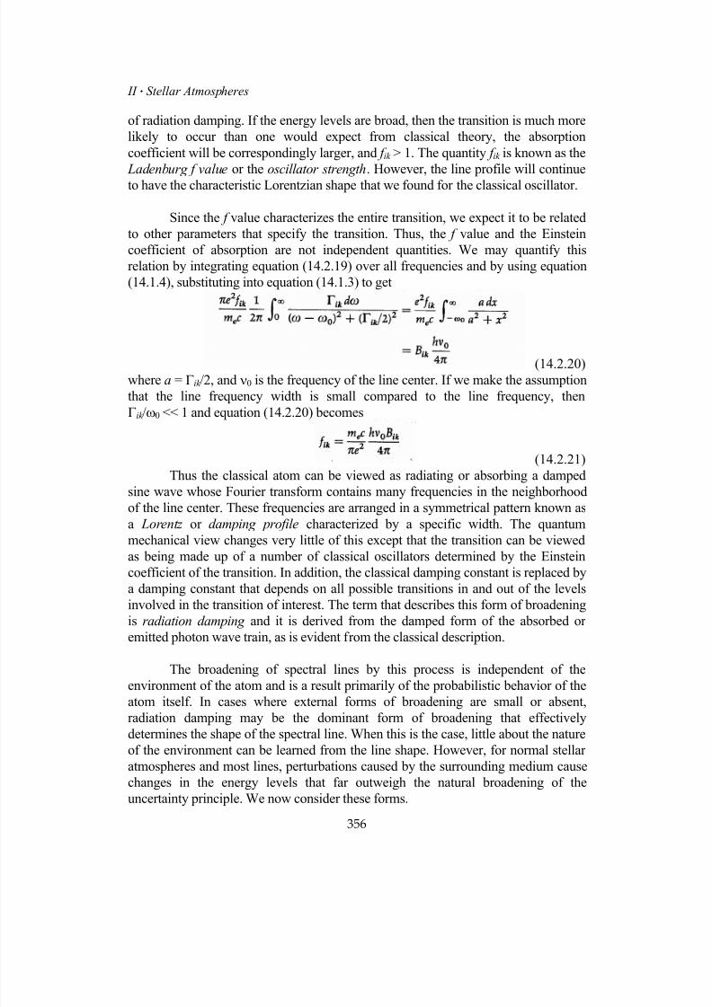
7/18/2019 The Fundamentals of Stellar Astrophysics - Collins G. W.
http://slidepdf.com/reader/full/the-fundamentals-of-stellar-astrophysics-collins-g-w 376/524
II Stellar Atmospheres
of radiation damping. If the energy levels are broad, then the transition is much morelikely to occur than one would expect from classical theory, the absorptioncoefficient will be correspondingly larger, and f ik > 1. The quantity f ik is known as the
Ladenburg f value or the
oscillator strength. However, the line profile will continue
to have the characteristic Lorentzian shape that we found for the classical oscillator.
Since the f value characterizes the entire transition, we expect it to be relatedto other parameters that specify the transition. Thus, the f value and the Einsteincoefficient of absorption are not independent quantities. We may quantify thisrelation by integrating equation (14.2.19) over all frequencies and by using equation(14.1.4), substituting into equation (14.1.3) to get
(14.2.20)where a = Γik /2, and ν0 is the frequency of the line center. If we make the assumptionthat the line frequency width is small compared to the line frequency, thenΓik /ω0 << 1 and equation (14.2.20) becomes
(14.2.21)Thus the classical atom can be viewed as radiating or absorbing a damped
sine wave whose Fourier transform contains many frequencies in the neighborhoodof the line center. These frequencies are arranged in a symmetrical pattern known as
a Lorentz or damping profile characterized by a specific width. The quantummechanical view changes very little of this except that the transition can be viewedas being made up of a number of classical oscillators determined by the Einsteincoefficient of the transition. In addition, the classical damping constant is replaced bya damping constant that depends on all possible transitions in and out of the levelsinvolved in the transition of interest. The term that describes this form of broadeningis radiation damping and it is derived from the damped form of the absorbed oremitted photon wave train, as is evident from the classical description.
The broadening of spectral lines by this process is independent of theenvironment of the atom and is a result primarily of the probabilistic behavior of the
atom itself. In cases where external forms of broadening are small or absent,radiation damping may be the dominant form of broadening that effectivelydetermines the shape of the spectral line. When this is the case, little about the natureof the environment can be learned from the line shape. However, for normal stellaratmospheres and most lines, perturbations caused by the surrounding medium causechanges in the energy levels that far outweigh the natural broadening of theuncertainty principle. We now consider these forms.
356
7/18/2019 The Fundamentals of Stellar Astrophysics - Collins G. W.
http://slidepdf.com/reader/full/the-fundamentals-of-stellar-astrophysics-collins-g-w 377/524
14 Shape of Spectral Lines
14.3 Doppler Broadening of Spectral Lines
The atoms that make up the gas of the stellar atmosphere are constantly in motion,and this motion shifts the wavelengths, seen by an observer, at which the atoms canabsorb radiation. This motion may be only the thermal motion of the gas, or it mayinclude the larger-scale motions of turbulence or rotation. Whatever the combination,the shifting of the rest wavelengths by varying amounts for different populations ofatoms will usually result in the observed line's being broadened by an amountsignificantly greater than the natural width determined by atomic properties.
The shifting of the rest wavelength caused by the motion of the atoms notonly produces a change as seen by the observer, but also may expose the atom to asomewhat different radiation field. This will be true if the motion is locally random
so that the motion of each atom is uncorrelated with that of its neighbors. However,should the motions be large-scale, then entire collections of atoms will have their restwavelengths shifted by the same amount with respect to the observer and the star. Ifthese collections of atoms constitute an optically thick ensemble, then the radiationfield of the ensemble will be shifted along with the rest wavelength. To atoms withinsuch a "cloud" there will be no effect of the motion on the atoms themselves. It will be as if a "mini-atmosphere" was moving, and no additional photons will beabsorbed as a result of the motion. Such motions will not affect the equivalent widthsof lines but may change the profiles considerably.
Contrast this with the situation resulting from an atom whose motion is
uncorrelated with that of its neighbors. Imagine a line with an arbitrarily sharpatomic absorption coefficient [that is, S ν = δ(ν-ν0)]. If there were no motion in theatmosphere, the lowest-lying atoms would absorb all the photons at frequency ν0,leaving none to be absorbed by the overlying atoms. Such a line is said to besaturated because the addition of absorbing material will make no change in the line profile or equivalent width. But, allow some motion, and the rest frequency of theseatoms is changed slightly from ν0. Now these atoms will be capable of absorbing photons at the neighboring frequencies, and the line will appear wider and stronger.Its equivalent width will be increased simply as a result of the Doppler shiftsexperienced by some atoms. Thus, if the motion consists of collections of atoms thatare optically thin, we can expect changes in the line strengths as well as in the
profiles. However, if those collections of atoms are large enough to be opticallythick, then no change in the equivalent width will occur in spite of marked changesin the line profile. We refer to the motions of the first case as microscopic motions soas to contrast them with the second case of macroscopic motion.
357
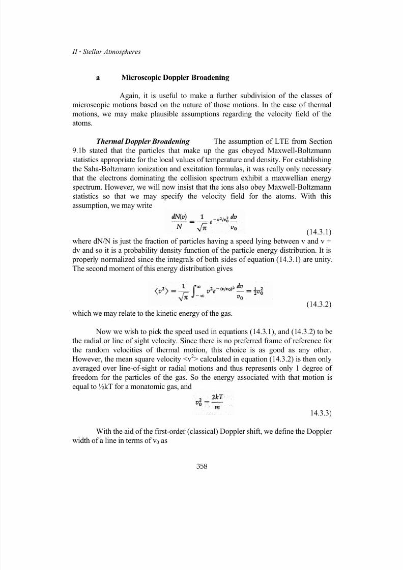
7/18/2019 The Fundamentals of Stellar Astrophysics - Collins G. W.
http://slidepdf.com/reader/full/the-fundamentals-of-stellar-astrophysics-collins-g-w 378/524
II Stellar Atmospheres
a Microscopic Doppler Broadening
Again, it is useful to make a further subdivision of the classes ofmicroscopic motions based on the nature of those motions. In the case of thermalmotions, we may make plausible assumptions regarding the velocity field of theatoms.
Thermal Doppler Broadening The assumption of LTE from Section9.1b stated that the particles that make up the gas obeyed Maxwell-Boltzmannstatistics appropriate for the local values of temperature and density. For establishingthe Saha-Boltzmann ionization and excitation formulas, it was really only necessarythat the electrons dominating the collision spectrum exhibit a maxwellian energyspectrum. However, we will now insist that the ions also obey Maxwell-Boltzmann
statistics so that we may specify the velocity field for the atoms. With thisassumption, we may write
(14.3.1)where dN/N is just the fraction of particles having a speed lying between v and v +dv and so it is a probability density function of the particle energy distribution. It is properly normalized since the integrals of both sides of equation (14.3.1) are unity.The second moment of this energy distribution gives
(14.3.2)which we may relate to the kinetic energy of the gas.
Now we wish to pick the speed used in equations (14.3.1), and (14.3.2) to bethe radial or line of sight velocity. Since there is no preferred frame of reference forthe random velocities of thermal motion, this choice is as good as any other.However, the mean square velocity <v2> calculated in equation (14.3.2) is then onlyaveraged over line-of-sight or radial motions and thus represents only 1 degree offreedom for the particles of the gas. So the energy associated with that motion isequal to ½kT for a monatomic gas, and
14.3.3)
With the aid of the first-order (classical) Doppler shift, we define the Dopplerwidth of a line in terms of v0 as
358

7/18/2019 The Fundamentals of Stellar Astrophysics - Collins G. W.
http://slidepdf.com/reader/full/the-fundamentals-of-stellar-astrophysics-collins-g-w 379/524
14 Shape of Spectral Lines
(14.3.4)Using equation (14.3.4), we may rewrite the particle distribution function forvelocity as one for the fraction of atoms capable of absorbing at a frequency shift ∆ν (or wavelength shift ∆λ).
(14.3.5)Since the atomic line absorption coefficient is basically the probability of an atom'sabsorbing a photon at a given frequency, that probability should be proportional tothe number of atoms capable of absorbing at that frequency. Thus,
(14.3.6)where A is simply a constant of proportionality. This constant can be related to theEinstein coefficient by equations (14.1.3), and (14.1.4), with the result that
(14.3.7)
To get the result on the far right-hand side, we used the relationship betweenthe f value for a particular transition and the Einstein coefficient given by equation(14.2.21). This is the expression for the atomic line absorption coefficient for thermalDoppler broadening. It differs significantly from the Lorentz profile of radiationdamping by exhibiting much stronger frequency dependence. A spectral line where
both broadening mechanisms are present will possess a line core that is dominated byDoppler broadening while the far wings of the line will be dominated by the damping profile as the gaussian profile of the Doppler core rapidly goes to zero.
Microturbulent Broadening In addition to the thermal velocity field, theatoms in the atmospheres of many stars experience motion due to turbulence.Unfortunately, the theory of turbulent flow is insufficiently developed to enable us tomake specific predictions concerning the velocity distribution function of theturbulent elements. So, for simplicity, we assume that they also exhibit a maxwellianvelocity distribution, but one having a characteristic velocity different from thethermal velocity. Thus, the form of the probability density distribution function forturbulent elements is the same as equation (14.3.1) except that the velocity is theradial velocity of the turbulent cell:
(14.3.8)
359
If there were no other processes to consider, the atomic absorption coefficient for aturbulently broadened line would have the same form as one that is thermally
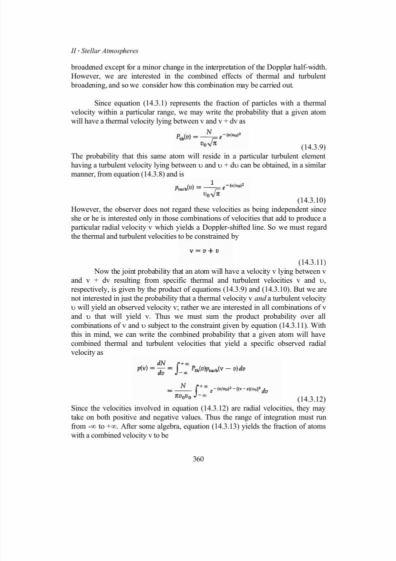
7/18/2019 The Fundamentals of Stellar Astrophysics - Collins G. W.
http://slidepdf.com/reader/full/the-fundamentals-of-stellar-astrophysics-collins-g-w 380/524
II Stellar Atmospheres
broadened except for a minor change in the interpretation of the Doppler half-width.However, we are interested in the combined effects of thermal and turbulent broadening, and so we consider how this combination may be carried out.
Since equation (14.3.1) represents the fraction of particles with a thermalvelocity within a particular range, we may write the probability that a given atomwill have a thermal velocity lying between v and v + dv as
(14.3.9)The probability that this same atom will reside in a particular turbulent elementhaving a turbulent velocity lying between υ and υ + dυ can be obtained, in a similarmanner, from equation (14.3.8) and is
(14.3.10)However, the observer does not regard these velocities as being independent sinceshe or he is interested only in those combinations of velocities that add to produce a particular radial velocity v which yields a Doppler-shifted line. So we must regardthe thermal and turbulent velocities to be constrained by
(14.3.11) Now the joint probability that an atom will have a velocity v lying between v
and v + dv resulting from specific thermal and turbulent velocities v and υ,respectively, is given by the product of equations (14.3.9) and (14.3.10). But we arenot interested in just the probability that a thermal velocity v and a turbulent velocityυ will yield an observed velocity v; rather we are interested in all combinations of vand υ that will yield v. Thus we must sum the product probability over allcombinations of v and υ subject to the constraint given by equation (14.3.11). Withthis in mind, we can write the combined probability that a given atom will havecombined thermal and turbulent velocities that yield a specific observed radialvelocity as
(14.3.12)Since the velocities involved in equation (14.3.12) are radial velocities, they maytake on both positive and negative values. Thus the range of integration must runfrom -∞ to +∞. After some algebra, equation (14.3.13) yields the fraction of atomswith a combined velocity v to be
360
7/18/2019 The Fundamentals of Stellar Astrophysics - Collins G. W.
http://slidepdf.com/reader/full/the-fundamentals-of-stellar-astrophysics-collins-g-w 381/524
14 Shape of Spectral Lines
(14.3.13)
where
(14.3.14)
The similarity of the form of equation (14.3.13) to that of equations(14.3.1), and (14.3.8) is no accident. The integral in equation (14.3.12) is knownas a convolution integral . The combined probability of p(a) and p(b) involvestaking the product p(a) × p(b). If, in addition, one has a constraint q(c) = q(a,b), then he must consider all combinations of a and b that yield c and sum over them.That is, one wants the probability of (a1,b1) or (a2,b2) etc. that yields c.
Combining probabilities of A or B involves summing those probabilities. So, ingeneral, if one wishes to find the combined probability of two processes subject toan additional constraint, one "convolves" the two probabilities. It is a general property of convolution integrals where the probability distributions have thesame form that the resultant probability will also have the same form with avariance that is just the sum of the variances of the two initial probabilitydistribution functions. Thus the convolution of any two Gaussian distributionfunctions will itself be a Gaussian distribution function having a variance that is just the sum of the two initial variances. This explains the form of equation(14.3.14). As a result, we may immediately write the atomic absorptioncoefficient for the combined effects of thermal and turbulent Doppler broadening
as
(14.3.15)where
(14.3.16)and
(14.3.17)
It is now clear why we assumed the turbulent broadening to have aMaxwellian velocity distribution. If this were not the case, the convolution integralwould be more complicated. If the turbulent velocity distribution function had theform
361

7/18/2019 The Fundamentals of Stellar Astrophysics - Collins G. W.
http://slidepdf.com/reader/full/the-fundamentals-of-stellar-astrophysics-collins-g-w 382/524
II Stellar Atmospheres
(14.3.18)then the convolution integral with thermal broadening would become
(14.3.19)If the function Φ( x) is sufficiently simple, the integral may be expressed in terms ofanalytic functions. If not, then the integral must be evaluated numerically as part ofthe larger calculation for finding the line profile.
Combination of Doppler Broadening and Radiation Damping Anyspectral line will be subject to the effects of radiation damping or some other intrinsic broadening mechanism as well as the broadening introduced by Doppler motions. Soto get a reasonably complete description of the atomic absorption coefficient, wehave to convolve the Doppler profile with the classical damping profile given byequation (14.2.19). However, since the atomic absorption coefficient is expressed interms of frequency, the constraint on the independent variables of velocity andfrequency must contain the Doppler effect of that velocity on the observedfrequency. Thus the frequency ν' at which the atom will absorb in terms of the restfrequency ν0 is
(14.3.20)For an atom moving with a line-of-sight velocity v, the atomic absorption forradiation damping is
(14.3.21)This atomic absorption coefficient is essentially the probability that an atom havingvelocity v will absorb a photon at frequency ν. To get the total absorption coefficient,we must multiply by the probability that the atom will have the velocity v [equation(14.3.13)] and sum all possible velocities that can result in an absorption at ν. Thus,
(14.3.22)
The convolution integral represented by equation (14.3.22) is clearly not asimple one. When one is faced with a difficult integral, it is advisable to changevariables so that the integrand is made up of dimensionless quantities. This fact willremove all the physical parameters to the front of the integral, clarifying their role inthe result, and reduce the integral to a dimensionless weighting factor. This also
362
7/18/2019 The Fundamentals of Stellar Astrophysics - Collins G. W.
http://slidepdf.com/reader/full/the-fundamentals-of-stellar-astrophysics-collins-g-w 383/524
14 Shape of Spectral Lines
facilitates the numerical evaluation of the integral since the relative values of all the parameters of the integrand are clear. With this in mind we introduce the followingtraditional dimensionless variables:
(14.3.23)Substituting these into equation (14.3.22), we get
(14.3.24)It is common to absorb all the physical parameters on the right-hand side of equation(14.3.24) into a single constant that has the units of an absorption coefficient so that
(14.3.25)The remaining dimensionless function can be written as
(14.3.26)This is known as the Voigt function, and it allows us to write the atomic absorption
coefficient in the following simple way:
(14.3.27)For small values of the damping constant (a < 0.2), the Voigt function is near unity atthe line center (that is, u = 0) and falls off rapidly for increasing values of u. Forvalues of u near zero the Voigt function is dominated by the exponential thatcorresponds to the Doppler core of the line. However, at larger values of u, thedenominator dominates the value of the integral. This corresponds to the dampingwings of the line profile.
Considerable effort has gone into the evaluation of the Voigt function because it plays a central role in the calculation of the atomic line absorptioncoefficient. One of the earliest attempts involved expressing the Voigt function as
(14.3.28)
363
where the functions Hi(u) are known as the Harris functions6. More commonly one
7/18/2019 The Fundamentals of Stellar Astrophysics - Collins G. W.
http://slidepdf.com/reader/full/the-fundamentals-of-stellar-astrophysics-collins-g-w 384/524
II Stellar Atmospheres
finds the alternative function
(14.3.29)whose integral over all u is unity. This function is known as the normalized Voigt function. Extensive tables of this function were calculated by D.Hummer 7 and areasonably efficient computing scheme has been given by G.Finn andD.Mugglestone8. However, with the advent of fast computers emphasis has been puton finding a fast and accurate computational algorithm for the Voigt function. The best to date is that given by J.Humíek 9. This has been expanded by McKenna10 toinclude functions closely related to the Voigt function. All this effort has made it possible to obtain accurate values for the Voigt function with great speed, making theinclusion of this function in computer codes little more difficult than includingtrigonometric functions.
b Macroscopic Doppler Broadening
The fact that each atom was subject to all the broadening mechanismsdescribed above caused most of the problems in calculating the atomic absorptioncoefficient through the introduction of a convolution integral. This approachassumed that each atom could "see" other atoms subject to the different velocitysources. However, if the turbulent elements were sufficiently large that theythemselves were optically thick, then each element would optically behaveindependently of the others. The line profiles of each would be similar, but shiftedrelative to the others by an amount determined by the turbulent velocity of the
element. Indeed, this would be the case if any motions involving optically thicksections of the atmosphere were present.
The proper approach to this problem involves finding the locally emittedspecific intensity, convolving it with the velocity distribution function andintegrating the result over the visible surface of the star to obtain the integrated flux.This flux can then be normalized to produce the traditional line profile. However,since the macroscopic motions can affect the structure of the atmosphere, the problem can become exceedingly difficult and solvable only with the aid of largecomputers. In spite of this, much can be learned about the qualitative behavior ofthese broadening mechanisms from considering some greatly simplified examples.
We discuss just two, the first involves motions of large sections of the atmosphere ina presumably uncorrelated fashion, and the second involves the correlated motion ofthe entire star.
Broadening by Macroturbulence It would be a mistake to assume thatturbulent elements only come in sizes that are either optically thick or thin. However,to gain some insight into the degree to which turbulence can affect a line profile, we
364
7/18/2019 The Fundamentals of Stellar Astrophysics - Collins G. W.
http://slidepdf.com/reader/full/the-fundamentals-of-stellar-astrophysics-collins-g-w 385/524
14 Shape of Spectral Lines
divide the phenomena into these two cases. We have already discussed the effectsthat small turbulent elements have on the resulting atomic line absorption coefficient(i.e., microturbulence), and we have seen that they lead to an increase in value of that parameter for all frequencies. Such is not the case for macroturbulence. The motionof optically thick elements cannot change the value of the atomic line absorptioncoefficient because the environment of a particular atom concealed within theturbulent element is unaffected by the motion of that element. Thus, each element behaves as a separate "atmosphere", producing its own line profile, which contributesto the stellar profile by an amount proportional to the ratio of the visible area of theelement to that of the apparent disk of the star. Thus, the combining (or convolution)of line profiles occurs not on the atomic level as with microturbulent Doppler broadening, but after the radiative transfer has been locally solved to yield a localline profile. This requires that we make assumptions that apply globally to the entirestar in order to relate one turbulent element to another.
To demonstrate the nature of this effect, we consider a particularly simplesituation where there is no limb-darkening in or out of the line. In addition, weassume that the local line profile is given by a Dirac delta function of frequency andthat the macroturbulent motion is purely radial with a velocity ∀vm. Under theseconditions, zones of constant radial velocity will appear as concentric circles on theapparent disk (see Figure 14.3).
Since the intrinsic line profile is a delta function of frequency, the line profileoriginating at a ring of constant radial velocity located at an angle θ measured fromthe center of the disk will be Doppler shifted by an amount
(14.3.30)where, as usual,
(14.3.31)
The amount of energy removed from the total continuum flux by the local lineabsorption will simply be proportional to the area of the differential annulus locatedat the particular value of µ corresponding to ∆ν. Thus,
(14.3.32)Therefore, the line profile would be given by
365
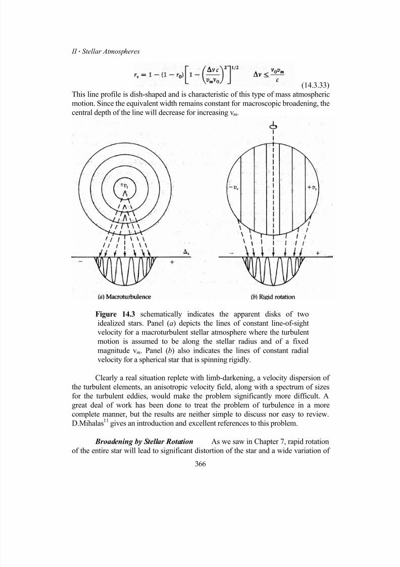
7/18/2019 The Fundamentals of Stellar Astrophysics - Collins G. W.
http://slidepdf.com/reader/full/the-fundamentals-of-stellar-astrophysics-collins-g-w 386/524
II Stellar Atmospheres
(14.3.33)This line profile is dish-shaped and is characteristic of this type of mass atmosphericmotion. Since the equivalent width remains constant for macroscopic broadening, thecentral depth of the line will decrease for increasing vm.
Figure 14.3 schematically indicates the apparent disks of twoidealized stars. Panel (a) depicts the lines of constant line-of-sightvelocity for a macroturbulent stellar atmosphere where the turbulentmotion is assumed to be along the stellar radius and of a fixedmagnitude vm. Panel (b) also indicates the lines of constant radialvelocity for a spherical star that is spinning rigidly.
Clearly a real situation replete with limb-darkening, a velocity dispersion ofthe turbulent elements, an anisotropic velocity field, along with a spectrum of sizes
for the turbulent eddies, would make the problem significantly more difficult. Agreat deal of work has been done to treat the problem of turbulence in a morecomplete manner, but the results are neither simple to discuss nor easy to review.D.Mihalas11 gives an introduction and excellent references to this problem.
Broadening by Stellar Rotation As we saw in Chapter 7, rapid rotationof the entire star will lead to significant distortion of the star and a wide variation of
366
7/18/2019 The Fundamentals of Stellar Astrophysics - Collins G. W.
http://slidepdf.com/reader/full/the-fundamentals-of-stellar-astrophysics-collins-g-w 387/524
14 Shape of Spectral Lines
the parameters that define a stellar atmosphere over its surface. In such a situation,most of the assumptions we have made for the purpose of modeling the atmosphereno longer apply and recourse must be made to a more numerical approach (seeG.Collins12 and J.Cassinelli13). However, as with macroturbulence, some insight may be gained by considering the effects of rotation on the line profile of a slowlyrotating star. Such a model is originally due to G.Shajn and O.Struve13 and is nowcommonly referred to as the Struve model.
Consider a uniformly bright spherical star which is rotating as a solid body.Except for the rotation, this is essentially the same model as that used for thediscussion of macroturbulence (see Figure 14.3). If we defineθ and φ , respectively, to be the polar and azimuthal angles of a spherical coordinate system with its polar axisaligned with the rotation axis of the star, then the velocity toward the observer's lineof sight is
(14.3.34)where veq is the equatorial velocity of the star and i is the angle between the line-of-sight and the rotation axis, called the inclination. An inspection of Figure 14.3 andsome geometry leads one to the conclusion that for spherical stars the product sinì sinφ is constant on the stellar surface along any plane parallel to the meridian plane.Thus, any chord on the apparent disk that is parallel to the central meridian is a locusof constant radial velocity (see Figure 14.3). Any profile formed along this cord will be displaced in frequency by an amount
(14.3.35)
For a sphere of unit radius, the length of the chord is 2µ. If we make thesame assumptions about the intrinsic line profile as were made for the case ofmacroturbulence (i.e., it can be locally represented by a delta function), then theamount of flux removed from the continuum intensity by any profile located on oneof these chords will just be proportional to the length of the chord. Therefore,
(14.3.36)
which leads to a profile of the form
(14.3.37)Except for the replacement of the turbulent velocity by the equatorial velocity, therotational profile has the same form as the profile for macroturbulence [equation
367

7/18/2019 The Fundamentals of Stellar Astrophysics - Collins G. W.
http://slidepdf.com/reader/full/the-fundamentals-of-stellar-astrophysics-collins-g-w 388/524
II Stellar Atmospheres
(14.3.33)]. This points out a fundamental problem of Doppler broadening by massmotions. In general, it is not possible to infer the velocity field from the line profilealone. To be sure, the presence of limb-darkening would affect these two casesdifferently, as would the introduction of gravity darkening for the case of rotation.But the non-uniqueness remains for the general case, and any determination of thevelocity field from the analysis of line profiles is strongly model-dependent andusually relies on some assumed symmetry.
Many of the simplifying assumptions of these models for macroturbulenceand rotation can be removed for a modest increase in complexity. In the case ofrotation, if the local line profile were not given by a delta function but had anintrinsic shape r'( x) where
(14.3.38)then the observed line profile would be given by the convolution integral
(14.3.39)Here Q( y) is known as the rotational broadening function which, if limb-darkeningis included, is given by A.Unsöld15 as
(14.3.40)
The parameter β is the first-order limb-darkening coefficient. Consider the case for β = 0 and that the intrinsic line profile is a delta function. It is clear that equations(14.3.39) and (14.3.40) will yield equation (14.3.37) as long as the integral of Q( y) isnormalized to unity. Integration of equation (14.3.40) will satisfy the skeptic that thisis indeed the case. It is also clear that the general effects of rotation are notqualitatively very different from those implied by equation (14.3.37). Whilequantitative comparison with observation will clearly be affected by such things asthe intrinsic line profile and limb-darkening, a truly useful comparison will have togo even further and include the effects of the variation of the atmospheric structureover the surface on the line profile.
While macroturbulence and rotation constitute the most important forms ofmacroscopic broadening, there are others. The presence of magnetic fields can splitatomic lines through the Zeeman effect. In some instances, this can lead toanomalously broad spectral lines and subsequent errors in the abundances derivedfrom these lines. In some instances, the broadening is sufficiently large to allow theestimation of the magnetic field itself. Fortunately, strong magnetic fields appear to be sufficiently rare among normal stellar atmospheres to allow us to ignore their
368

7/18/2019 The Fundamentals of Stellar Astrophysics - Collins G. W.
http://slidepdf.com/reader/full/the-fundamentals-of-stellar-astrophysics-collins-g-w 389/524
14 Shape of Spectral Lines
effects most of the time. However, we should be ever mindful of the possibility oftheir existence and of the effects that they can introduce in the shaping of spectrallines.
14.4 Collisional Broadening
To this point, we have described the broadening of spectral lines arising fromintrinsic properties of the atom and the collective effects of the motion of theseatoms. However, in all but the most extreme cases of macroscopic broadening, themost prominent source of broadening of spectral lines results from the interaction ofthe absorbing atom with neighboring particles of the gas. Since these particles areoften charged (even the neutral atoms possess the potential field of an electricdipole), their potential will interact with that of the atomic nucleus which binds theorbiting electrons. This interaction will perturb the energy levels of the atom in a
time-dependent fashion. The collective action of these perturbations on an ensembleof absorbing atoms is to broaden the spectral line. The details of this broadeningdepend on the nature of the atom and energy level being perturbed and the propertiesof the dominant perturber. All phenomena that fall into this general class of broadening mechanisms are usually gathered under the generic term collisionalbroadening . However, some authors refer to this concept or a subset of it as pressurebroadening , on the grounds that there can be no collisions unless the gas has some pressure. The use of the different terms is usually not of fundamental importance,and the basic notion of what is behind them should always be kept in mind.
There is some confusion in the literature (and much more among students)
regarding the terminology for describing these processes. Some of this results from agenuine confusion among the authors, but most derives from an unfortunate choiceof terms to describe some aspects of the problem. You should keep clearly in mindwhat is being described during any discussion of this topic - the broadening ofatomic energy levels resulting from the perturbations of neighboring particles. Weadopt a variety of theoretical approaches to this problem, each of which has its ownname. Care must be taken lest the name of the theoretical approach be confused witha qualitatively different type of broadening. We discuss perturbations introduced bydifferent types of perturbers, each of which will produce a characteristic line profilefor the absorbing gas. Each of these profiles has its own name so as to delineate thetype of perturbation. However, they are all just perturbations of the energy levels.
Each type will generally be discussed in a "vacuum", in that we assume that it is theonly form of perturbation that exists, when in reality virtually all types of perturbations are present at all times and affect the energy levels. Fortunately, one ofthem usually does dominate the level broadening.
There are two main theoretical approaches to collisional broadening. Onedeals with the weak, but numerous, perturbations that cause small amounts of
369

7/18/2019 The Fundamentals of Stellar Astrophysics - Collins G. W.
http://slidepdf.com/reader/full/the-fundamentals-of-stellar-astrophysics-collins-g-w 390/524
II Stellar Atmospheres
broadening. The other is concerned with the large, but infrequent, perturbations thatdetermine the shape of the wings of the line. It as somewhat unfortunate that theformer theoretical approach is known as impact phase-shift theory, while the latter iscalled the
statistical or
static broadening theory. The word impact conjures up
visions of violence, yet the theoretical approach labeled by this word is concernedonly with the weakest and least violent of the interactions. Similarly, the term static implies calm, but this approach deals with the most violent perturbations. So be it.We try to justify this apparent anomaly during the specific discussions of theseapproaches. In addition, we clearly label the myriad terms as they are introduced sothat those which are synonymous are clearly separated from those which have uniquemeanings.
To estimate the perturbation to the atom that changes the energy of thetransition and thereby broadens the line, we must characterize the nature of the
collision. The two theoretical approaches to collisional broadening differ in thisdescription. Both approaches are largely classical in form so that whatever is true forabsorption is also true for emission. So we often deal with the effects of a collisionon a radiating atom with the full intention of applying the results to absorption.
a Impact Phase-Shift Theory
The approach of impact phase-shift theory assumes that the collisionis of a very short duration compared to the span of time during which the atom isactually radiating (or absorbing) the photon. Thus,
(14.4.1)It is the short duration of the collision that is responsible for the name impact for thetheoretical approach.
Determination of the Atomic Line Absorption Coefficient Suppose thatthe atom radiates in an undisturbed manner between collisions with a frequency ω0.The electric field of the emitted photon will vary as
(14.4.2)where T is the time between collisions. Further assume that the radiation of the photon does not continue before or after the collision, so that
(14.4.3)
370

7/18/2019 The Fundamentals of Stellar Astrophysics - Collins G. W.
http://slidepdf.com/reader/full/the-fundamentals-of-stellar-astrophysics-collins-g-w 391/524
14 Shape of Spectral Lines
It is this interruption in the emission of the photon, or at least a complete anddiscontinuous change in the phase of the emitted photon that terminates the wavetrain and provides the motivation for the second half of the name for this approach.Since a sine wave of finite length must contain wave components of higherfrequency introduced by the discontinuity of the wave train, the emitted photon willhave more components than the fundamental frequency and thus the line will appearto be broadened. To find this distribution in frequencies, we must take the Fouriertransform of the temporal description of the electric field of the photon. So
(14.4.4)
or
(14.4.5)Since the power spectrum of the emitted photon will depend on the square of theelectric field,
(14.4.6)Here we have assumed that we will be dealing with emissions and absorptions thatare totally uncorrelated, which for random collisions occurring in a sea of unrelated
atoms is a perfectly reasonable assumption.
Now to determine the effects of multiple collisions (or numerous atoms), wemust combine the effects of these collisions, which means that we must have someestimate of the time between them T . Let P (t ) be the probability that a collision hasnot occurred in a time t measured from the last collision. Now if the collisions areindeed random, the differential probability dp that a collision will occur in a timeinterval dt is
(14.4.7)
where T 0 is the average time between collisions. Thus, the differential change in the probability P (t ) is
371
(14.4.8)
7/18/2019 The Fundamentals of Stellar Astrophysics - Collins G. W.
http://slidepdf.com/reader/full/the-fundamentals-of-stellar-astrophysics-collins-g-w 392/524
II Stellar Atmospheres
or
(14.4.9)Since a collision must occur at some time, we can determine the constant in equation(14.4.9) by normalizing that expression to unity and integrating over all time. Thuswe see that the collision frequency distribution is a Poisson distribution of the form
(14.4.10)and the constant of proportionality in equation (14.4.6) is 1/T 0.
To obtain the total energy distribution or power spectrum resulting from amultitude of collisions, we must sum the power spectra of the individual collisions
multiplied by the probability of their occurrence. Thus,
(14.4.11)We can use the same normalization process implied by equations (14.1.3), (14.1.4),and (14.2.21) to write the atomic absorption coefficient as
(14.4.12)In going from equation (14.4.11) to (14.4.12), we have changed from circular
frequency w to frequency n so that the appropriate factors of 2π must be introduced.The quantity 2/T 0 is usually called the collisional damping constant so that
(14.4.13)Since the form of equation (14.4.12) is identical to that of equation (14.3.21), we canimmediately obtain the convolution of the collisional damping absorption coefficientwith that for radiation damping by simply adding the respective damping constants:
(14.4.14)The combined absorption coefficient could then be convolved with that appropriatefor microturbulent Doppler broadening producing a total line profile that is still aVoigt profile but with
372
7/18/2019 The Fundamentals of Stellar Astrophysics - Collins G. W.
http://slidepdf.com/reader/full/the-fundamentals-of-stellar-astrophysics-collins-g-w 393/524
14 Shape of Spectral Lines
(14.4.15)where Γ is the combined damping constant for radiation and collisional damping.However, before this result can be of any practical use, we must have an estimateof the collisional damping constant in terms of the state variables of theatmosphere.
Determination of the Collisional Damping Constant Determining the collisional damping constant is equivalent to determining theaverage time between collisions T 0. To do this, it is necessary to be quite specificabout exactly what constitutes a collision. We follow a method originally due toVictor Weisskopf 16 and described by many authors17-19. Consider that the perturbation of an energy level ∆ E caused by a passing perturber has the distancedependence
(14.4.16)which will produce a change in the frequency of the emitted photon of
(14.4.17)
The constant C n is known as the interaction constant , and it must bedetermined empirically from laboratory experiments involving the kinds of particlesfound in the collisions. Since all these collisions are mediated by the electromagneticforce, the typical interaction can be viewed as a "long range" one so that the shortcollisions [see equation (14.4.1)] refer to distant collisions where the colliding particle is located near its point of closest approach. This distance is commonlyreferred to as the impact distance, or impact parameter . Since the collision is shortand the interaction weak, we can assume that the perturbing particle is largelyunaffected by the encounter, and its path can be viewed as a straight line (see Figure14.4). This assumption is usually referred to as the classical path approximation andit appears in one form or another in all theories of collisional broadening.
We wish to calculate the entire frequency shift caused by the collision because when the accumulated phase shift becomes large enough, it is reasonable tosay that the wave train has been interrupted and a collision has occurred.
373

7/18/2019 The Fundamentals of Stellar Astrophysics - Collins G. W.
http://slidepdf.com/reader/full/the-fundamentals-of-stellar-astrophysics-collins-g-w 394/524
II Stellar Atmospheres
Figure 14.4 shows the "classical path" taken by a perturbing particleunder the Weisskopf approximation. The point of closest approach ρ iscalled the impact parameter.
To estimate this total phase shift, it is necessary to describe the path taken by the particle, so we use of the classical path approximation. It is clear from Figure 14.4that
(14.4.18)This enables the total phase shift η caused by the encounter to be calculated from
(14.4.19)where
(14.4.20)
Here Γ( x) is the gamma function, and it should not be confused with thesymbol for the damping constant. Before using this for the determination of theaverage time between collisions, we must decide what constitutes an interruption inthe wave train. Weisskopf took this value of η to be 1 radian. The smaller the valuefor the phase shift, the larger the value of the impact parameter may be that will
produce that phase shift. The value of the impact parameter ρ0 that produces theminimum phase shift η which constitutes an interruption in the wave train is knownas the Weisskopf radius:
374
(14.4.21)

7/18/2019 The Fundamentals of Stellar Astrophysics - Collins G. W.
http://slidepdf.com/reader/full/the-fundamentals-of-stellar-astrophysics-collins-g-w 395/524
14 Shape of Spectral Lines
Since the Weisskopf radius defines the distance inside of which anyencounters will produce a large enough phase shift to be considered a collision, itmay be used to calculate a collision cross section σ = πρ
0
2 and an average time between collisions T 0. The collision frequency is
(14.4.22)where N is the number density of the perturbing particles, l is the mean free path between collisions, and <v>rel is the relative velocity between the perturber and the perturbed atom. That relative velocity is
(14.4.23)
where Ai is the atomic weight of the constituents of the collision in units of the massof the hydrogen atom. Thus, we can write the collisional damping constant as
(14.4.24)where N is the number density of perturbers and
(14.4.25)All that remains is to specify the power law that describes the perturbing
force and the interaction constant C n. Since the force that mediates the collision is
electromagnetic, the exponent of the perturbing field is determined by the electricfield of the perturber. A simple way of understanding this is to view the passage ofthe perturber as interposing a "screening" potential energy between an opticalelectron and the nucleus. The screening potential energy will depend on the locallyinterposed energy density of the perturber's electric field which is proportional to E2 so that for a perturbing ion or electron, n = 4. This is called the quadratic Stark effect because it depends quadratically on the perturber's electric field. If the perturber is aneutral atom, it still possesses a dipole moment that produces a measurable field nearthe particle. However, this field varies as r -3 so that the perturbing energy densityvaries as r -6 and n = 6. Broadening of this type is called van der Waal's broadeningand it will to play a role in relatively cool gases where there are few ions.
If the atomic energy level of interest is degenerate, the interposition of anexternal electric field will result in the removal of the degeneracy and a splitting ofthe energy level into a set of discrete energy levels. The amount of the splitting is proportional to the electric field. Since a time-dependent splitting is equivalent to a broadening brought about by a shift of the energy level itself, the broadening ofdegenerate levels will occur, but their broadening will be directly proportional to the
375

7/18/2019 The Fundamentals of Stellar Astrophysics - Collins G. W.
http://slidepdf.com/reader/full/the-fundamentals-of-stellar-astrophysics-collins-g-w 396/524
II Stellar Atmospheres
electric field of the perturber rather than to its square. Thus the broadening of adegenerate level by ions or electrons will produce n = 2. This form of broadening isknown as the linear Stark effect . This form of broadening creates an interesting problem for the impact phase-shift theory since the integral for the minimum phaseshift [equation (14.4.19)] will not converge for n = 2 and the theory is not applicable.Since the energy levels of hydrogen are degenerate, and the hydrogen lines areamong the most prominent in stellar spectra, we are left with the somewhatembarrassing result that these lines can not be dealt with by the impact phase-shifttheory and we have to resort to some other description of collisional broadening toobtain line profiles for hydrogen. The problem basically arises from the 1/r 2 nature ofthe perturbing field and is not restricted to the theory of line broadening. Since thenumber of perturbers increases as r 2 while the perturbation from any one of themdeclines as r 2, the contribution to the total perturbation from particles at a givendistance is independent of distance. Thus some cutoff of the distances to be
considered must be invoked. This problem arises frequently in gravitation theorywhere there can be no screening of the potential field and the fundamental force isalso long-range. In our case, the Heisenberg uncertainty principle sets a limit on thesmallest perturbation that can matter and hence an upper limit on the volume ofspace to be considered.
The case of the broadening of degenerate levels by neutral atoms does present a situation that can be dealt with by the impact phase-shift theory. Here theelectric field near the perturber varies as r -3, so that the proper value of n is n = 3. Inthe special case where the broadening is by atoms of the same species as the atom being perturbed a significant enhancement of the broadening occurs. Indeed, for
astrophysical cases, the broadening of spectral lines arising from degenerate levels by neutral particles is of interest only when the broadening occurs from collisionswith atoms of the same species. For that reason, this kind of broadening is known as self-broadening . These considerations are summarized in table 14.1.
An important improvement was made by Lindholm20 and Foley21 whichincluded the effects of multiple collisions on the line. Although the multiplecollisions are weak, they are frequent. The result of their work is that the secondarycollisions introduce a slight shift in the line center of the atomic absorptioncoefficient so that
(14.4.26)where
(14.4.27)
376

7/18/2019 The Fundamentals of Stellar Astrophysics - Collins G. W.
http://slidepdf.com/reader/full/the-fundamentals-of-stellar-astrophysics-collins-g-w 397/524
14 Shape of Spectral Lines
Limits of Validity for Impact Phase-Shift Theory In developing theimpact phase-shift theory, we tacitly assumed that the collisions were adiabatic. Bythat we mean that all the perturbing energy was contained in the perturbation andnone was lost to other processes. There were no collisional transitions within theenergy level or between the split levels of the degenerate cases. This will be areasonable approximation as long as the splitting of the degenerate levels or thewidth of the perturbed level is greater than the uncertainty of energy of the perturberdue to the Heisenberg uncertainty principle.
Since the duration of the collision is of the order of ρ/v, the uncertainty of thecolliding particle's energy is of the order
(14.4.28)In equation (14.4.16) we estimated the energy of the perturbation itself so that
(14.4.29)which requires that
(14.4.30)So it appears that only collisions that occur inside the Weisskopf radius will beadiabatic, and all the energy of the collision goes into perturbing the energy level.
377
However, if the impact parameter is too small, the classical pathapproximation will be violated and the duration of the collision will exceed theradiation time [equation (14.4.1)]. The extent of this constraint can be estimated by
7/18/2019 The Fundamentals of Stellar Astrophysics - Collins G. W.
http://slidepdf.com/reader/full/the-fundamentals-of-stellar-astrophysics-collins-g-w 398/524
II Stellar Atmospheres
noting that the duration of the collision is of the order of ρ/v. The radiation time is ofthe order of 1/∆ω, so that
(14.4.31)if the classical path approximation is to be valid. However, equation (14.4.29) placesa constraint of the impact parameter ρ that must be met if the collisions are to beadiabatic. Using equation (14.4.29) to eliminate ρ/v from equation (14.4.31) we get
(14.4.32)Obviously the impact phase-shift theory will be valid only for the inner part of theline. For the outer part we must turn to another description of collisional broadening.
b Static (Statistical) Broadening Theory
In some real sense, the impact phase-shift theory follows the lifehistory of a single radiating (or absorbing) atom which is subject to numerous weakcollisions of short duration. The atomic absorption coefficient is then represented bythe average of many atoms in various phases of that temporal history. In static broadening theory, the atomic absorption coefficient is constructed from the averageof many atoms that are subject to the electric field of perturbers scattered randomlyabout. The opposite assumption is made concerning the duration of the collisioncompared to the radiation time. That is, the collision time is much longer than theradiation time, so that
(14.4.33)
It is as if we took a picture of the perturbed atom with a shutter duration ofthe radiation time for the photon. In the impact phase-shift theory, we would see a blur of colliding tracks of the perturbers, while in the case of statistical broadeningthe picture would show individual perturbers fixed in space and some might be quiteclose to the atom in question. We are most interested in these near perturbers, forthey are responsible for the largest perturbations to the atomic energy levels which inturn generate the broadest part of the line. This is precisely the part of the line forwhich the impact phase-shift theory fails.
.
378

7/18/2019 The Fundamentals of Stellar Astrophysics - Collins G. W.
http://slidepdf.com/reader/full/the-fundamentals-of-stellar-astrophysics-collins-g-w 399/524
7/18/2019 The Fundamentals of Stellar Astrophysics - Collins G. W.
http://slidepdf.com/reader/full/the-fundamentals-of-stellar-astrophysics-collins-g-w 400/524
II Stellar Atmospheres
equivalent to the classical path approximation of the impact phase-shift theory in thatthe position and momentum of the perturber are specified throughout the interactiontime and are such that they are unaffected by the interaction.
To these complementary assumptions we add one more. Let us assume thatthe perturbative electric field can be represented by the electric field of the perturberclosest to the atom and by that perturber alone. This is known as the nearest-neighbor approximation. Our task, then, is to find the probability distributionfunction for the perturber lying within a specified distance and thereby producing a perturbing electric field of a particular strength. Consider a spherical shell ofthickness dr located a distance r from the perturbed atom (see Figure 14.5), and letthe probability that the nearest neighbor is located within that shell be P(r)dr . Then
the probability that the nearest neighbor lies within a sphere of radius r is .
Since the universe is not empty, there must be a nearest neighbor somewhere, so thatthe probability that the nearest neighbor does not lie within that sphere is
(1 ). Now if the region around the perturbed atom is of uniform density,
the probability of finding any perturber within the spherical shell of thickness dr located at r is 4π r
∫r
dr r P 0
)(
∫−r
dr r P 0
)(
2ndr , where n is the perturber density. Thus, the probability that the particle in that shell is the nearest neighbor is just the probability that there is a particle there multiplied by the probability that there is no particle nearer to the perturbed atom. So
(14.4.34)This is an integral equation for the distribution function of nearest neighbors
P(r). We can solve it most easily by differentiating with respect to r and forming adifferential equation for, P(r)/4π r 2n. The solution to this equation is
(14.4.35)However, we need the probability distribution of perturbing electric fields, so weassume that the perturber has a field that behaves as
(14.4.36)
Then, by substituting this dependence of the electric field on r into equation(14.4.35), the probability that an atom will see a perturbing electric field of strengthE is
(14.4.37)where
380
7/18/2019 The Fundamentals of Stellar Astrophysics - Collins G. W.
http://slidepdf.com/reader/full/the-fundamentals-of-stellar-astrophysics-collins-g-w 401/524
14 Shape of Spectral Lines
(14.4.38)and it is sometimes called the normalizing field strength. If we further define thedimensionless quantity
(14.4.39)we can write the probability distribution for this dimensionless field strength as
(14.4.40)
Finally, if we consider the case for broadening by ions or electrons, then m = 2 and we have
(14.4.41)which is usually called the Holtsmark distribution function. As can be seen fromFigure 14.6, the probability of finding a weak field due to the nearest neighbor isvery small simply because it is unlikely that the nearest neighbor can be so far awayand still be the nearest neighbor. As the field strength rises, so does the probability ofit being the perturbing field, peaking between 1 and 2 times the normalized fieldstrength. Stronger fields become less likely because the volume of space surroundingthe atom within which the perturber would have to exist becomes just too small.
Behavior of the Atomic Line Absorption Coefficient If we assume that the perturbative change in the atomic energy level is proportional to the electric field tosome power, then we can write
(14.4.42)We can then use the nearest-neighbor distribution function to generate a probabilitydensity distribution function for the absorption of photons at a particular frequencyshift ∆ν as
(14.4.43)For large frequency or wavelength shifts, the argument of the exponential approacheszero, so the wavelength-dependent probability of absorption becomes
(14.4.44)
381
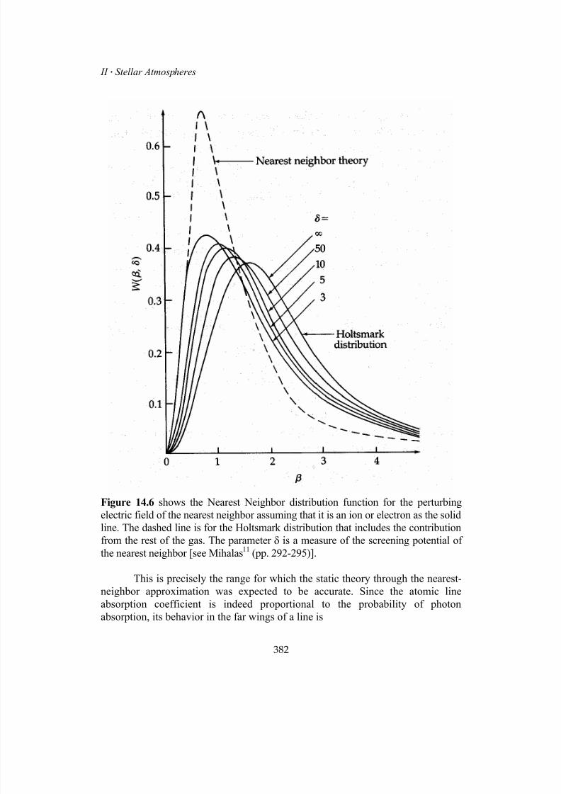
7/18/2019 The Fundamentals of Stellar Astrophysics - Collins G. W.
http://slidepdf.com/reader/full/the-fundamentals-of-stellar-astrophysics-collins-g-w 402/524
II Stellar Atmospheres
Figure 14.6 shows the Nearest Neighbor distribution function for the perturbingelectric field of the nearest neighbor assuming that it is an ion or electron as the solidline. The dashed line is for the Holtsmark distribution that includes the contributionfrom the rest of the gas. The parameter δ is a measure of the screening potential of
the nearest neighbor [see Mihalas11
(pp. 292-295)].
This is precisely the range for which the static theory through the nearest-neighbor approximation was expected to be accurate. Since the atomic lineabsorption coefficient is indeed proportional to the probability of photonabsorption, its behavior in the far wings of a line is
382

7/18/2019 The Fundamentals of Stellar Astrophysics - Collins G. W.
http://slidepdf.com/reader/full/the-fundamentals-of-stellar-astrophysics-collins-g-w 403/524
14 Shape of Spectral Lines
(14.4.45)Table 14.2 provides a brief summary of the asymptotic dependence of theabsorption coefficient in the wings of the line for the various types of interactionsdiscussed.
Finally, we may find the constant of proportionality for the atomic lineabsorption coefficient in terms of the interaction constant for the force law C l .This is analogous to the constant C n that appears in equation (14.4.17) and isusually determined empirically. In terms of this constant, the atomic lineabsorption coefficient becomes
(14.4.46)where am is given by equation (14.4.20), and
(14.4.47)In the broadening of degenerate levels, the splitting of the energy levels is so
large that the line should be considered to consist of individual linear Starkcomponents, each of which is quadratically Stark broadened. Under these conditions,the atomic line absorption coefficient for the combined Stark components becomes
(14.4.48)
If one were to improve on the static theory, the most obvious place would beto relax the nearest-neighbor approximation. The problem of including an ensembleof perturbers, all with their electric fields adding vectorially, was considered byJ.Holtsmark 22 and solved by S. Chandrasekhar 23, who also provides tables of theresults. As one might expect, the resultant form is similar to that of the nearest-
383
7/18/2019 The Fundamentals of Stellar Astrophysics - Collins G. W.
http://slidepdf.com/reader/full/the-fundamentals-of-stellar-astrophysics-collins-g-w 404/524
II Stellar Atmospheres
neighbor distribution in shape but somewhat more spread out (see Figure 14.6).Unfortunately the result takes the form of an integral so a complete description must be obtained numerically. However, for β in the vicinity of 1 we get the followingasymptotic formula for
W (β
):
(14.4.49)As we might expect, the lead term of this series is just that of the nearest-neighborapproximation [see equation (14.4.41).]
Limits of Validity and Further Improvements for the Static Theory
Since the assumption relating the collision time to the radiation time led to alimit on the range of validity for the impact phase-shift theory [equation (14.4.32)],we should not be surprised if the same were true for the static theory. This is indeedthe case and the result is known as the Holstein relation, can be deduced fromequation (14.4.32) almost by inspection:
(14.4.50)So, as we hoped at the outset of the development of the static theory, it will be validfor precisely those regions of the line profile for which the impact phase-shift theoryfails.
Of course, any microscopic inspection of a problem usually finds phenomenathat provide additional complications for the solution. For example, we haveassumed that the perturbers interact with the atom in question but do not interactamong themselves. In reality an ion will attract electrons so as to create a neutral plasma on as small a scale as possible. In effect, then, the plasma will try to shieldthe ions from even more distant perturbers. This phenomenon is known as Debye shielding and is discussed in some detail by Mihalas11 (pp. 292-295). The basic effectis density dependent and tends to flatten the Holtsmark distribution still further,thereby broadening the line even more. Fortunately, for normal stellar atmospheresthe densities are not large enough to make Debye shielding a major effect until onereaches optical depths in the line that are quite remote from the boundary.
The treatment of collisional line broadening described so far has been basedon purely classical considerations and has now been largely replaced by quantum
mechanical calculations of the atomic line absorption coefficient for the moreimportant stellar spectral lines. However, the quantum mechanical treatment isconsiderably less transparent than the classical one, so we give only the basic form.The power spectrum for the line is given by
(14.4.51)
384
7/18/2019 The Fundamentals of Stellar Astrophysics - Collins G. W.
http://slidepdf.com/reader/full/the-fundamentals-of-stellar-astrophysics-collins-g-w 405/524
14 Shape of Spectral Lines
where P is the probability density matrix for the atomic states involved in theformation of the spectral line, and Q is the matrix of dipole moments with elements
(14.4.52)The wave functions i must include the effects of the perturbers as well as theatomic states of interest. A very complete discussion of the quantum theory ofspectral line formation is given by Hans Griem24.
For simple lines the classical theories of collisional broadening produce line profiles that agree well with observation. However, for the stronger lines of hydrogenand helium, any serious model should involve an atomic absorption coefficient basedon the quantum mechanical description. While tables of these coefficients exist formany important lines (see Griem24 and references there), much remains to be done to produce accurate values for many lines of astrophysical interest.
14.5 Curve of Growth of the Equivalent Width
While we have discussed the most important aspects of the formation ofspectral lines, we have said little about the most important contributor to theappearance of the line in the spectrum - the abundance of the atomic species givingrise to the line. Obviously the more absorbers present in the atmosphere, the strongerthe associated spectral line will appear. However, the quantitative relationship between the abundance and the equivalent width is not simple and is worthy of somediscussion. Although most contemporary determinations of elemental abundances
rely on detailed atmospheric modeling with the abundance as a parameter to bedetermined from comparison with observation, the classical picture of the relation between the equivalent width and the abundance is quite revealing about what toexpect from such models. That classical quantitative relationship is known as thecurve of growth. Some students have wondered what is growing in the curve ofgrowth. The answer is that the equivalent width increases or "grows" with increasingabundance.
a Schuster-Schwarzschild Curve of Growth
To create a curve of growth, we must relate the equivalent width to
the atomic abundance. This requires some model of the atmosphere in which theatoms reside. For purposes of illustration, we take the simplest model possible. InChapter 13 we set up the equation of radiative transfer for line radiation [equation(13.1.6)], and we solved it for some special cases. For the Schuster-Schwarzschildatmosphere, this led to a line profile given by equation (13.2.8):
385

7/18/2019 The Fundamentals of Stellar Astrophysics - Collins G. W.
http://slidepdf.com/reader/full/the-fundamentals-of-stellar-astrophysics-collins-g-w 406/524
II Stellar Atmospheres
(14.5.1)The definition of τ0 allows us to write
(14.5.2)where Ni is the column density of the atom giving rise to the line and < S ν> is the lineabsorption coefficient averaged over depth. Since for this simple model theatmospheric conditions are considered constant throughout the cool gas, we drop theaverage-value symbols for the remainder of this section. We have already seen[equation (14.3.27)] that for many atomic lines the atomic line absorption coefficient,including the effects of radiation damping, collisional damping, and Doppler broadening, can be written as
(14.5.3)where H(a,u) can be either the Voigt or normalized Voigt function depending onwhat constants have been absorbed into S 0. Thus the line profile for the Schuster-Schwarzschild atmosphere is
(14.5.4)To relate this to the equivalent width, equation (14.5.4) must be integrated
over the frequencies contained the line so that
(14.5.5)It is convenient to express the frequency-dependent optical depth in the line in termsof the optical depth at the line center χ0 so that
(14.5.6)From equations (14.5.2), and (14.5.3)
(14.5.7)
386
Consider the case where the damping constant is small compared to Doppler broadening so that a < 0.2. Then the Doppler core will dominate the line profile, and
7/18/2019 The Fundamentals of Stellar Astrophysics - Collins G. W.
http://slidepdf.com/reader/full/the-fundamentals-of-stellar-astrophysics-collins-g-w 407/524
14 Shape of Spectral Lines
we can write the optical depth in the line as
(14.5.8)where ξ ≡ ∆λ/∆λd. Substitution into equation (14.5.5) yields
(14.5.9)The integral can be expanded in a series so that
(14.5.10)But
(14.5.11)Thus, we can write the equivalent width in the line as
(14.5.12)This, then, represents the first part of the curve of growth, and the equivalent width is
indeed directly proportional to χ0 and hence the abundance Ni. This is acommonsense result that simply says that the number of photons removed from the beam is proportional to the number of atoms doing the absorbing, so that section ofthe curve of growth is known as the linear section.
However, the seeds of difficulties are apparent in the higher-order terms inequation (14.5.12). As the number of absorbers increases, we would expect that someatoms high in the atmosphere to be "shadowed" by atoms lower in the atmosphere.When all the photons at a given frequency have been absorbed, then the furtheraddition of atoms that can absorb at those frequencies will make no change in theequivalent width. When this happens, the line is said to be saturated. As the optical
depth in the line center χ0 increases, the term in brackets will fall below unity and thecurve of growth will increase more slowly than the linear growth. For 0 ≤ χ0 ≤ 0.5,the series may be terminated after the first term. However, for larger values of χ0, asomewhat different expression of the integral on the left hand side of equation(14.5.10) is in order. If we make the transformation
387
7/18/2019 The Fundamentals of Stellar Astrophysics - Collins G. W.
http://slidepdf.com/reader/full/the-fundamentals-of-stellar-astrophysics-collins-g-w 408/524
II Stellar Atmospheres
(14.5.13)the equivalent width becomes
(14.5.14)If χ0 > 55, all but the lead term of the approximation may be ignored. However, inthe region where 0.5 < χ0 < 55, the series given by either equation (14.5.12) orequation (14.5.14) must be used. From the lead term of equation (14.5.14) it is clearthat as the Doppler core saturates, the equivalent width grows very slowly as
(14.5.15)This is known as the "flat" part of the curve of growth.
As the abundance increases still further, a significant number of atoms willexist that can absorb in the damping wings of the line and the equivalent width willagain begin to increase, but at a rate that will depend on the damping constantappropriate for the line (see Figure 14.7).
Once more we will need a different representation of the optical depth that isappropriate for the damping wings of the line. From the definition of thedimensionless variables of the Voigt function [see equation (14.3.23)]
(14.5.16)so that we can rewrite equation (14.5.5) with the aid of equation (14.5.6) to obtain
(14.5.17)The Voigt function as given in equation (14.3.26) can be approximated for large u as
(14.5.18)For modest values of the damping parameter a, H (a,0) is near unity so that
(14.5.19)So for large abundances the curve of growth will again increase in a manner thatdepends on the square root of the damping constant as well as the square root of the
388

7/18/2019 The Fundamentals of Stellar Astrophysics - Collins G. W.
http://slidepdf.com/reader/full/the-fundamentals-of-stellar-astrophysics-collins-g-w 409/524
14 Shape of Spectral Lines
abundance. Except for the separation brought about by the growth of the dampingwings of the line, the curve of growth is a single-valued function of Wλ/∆λd versusthe optical depth at the line center χ0. Both these parameters are dimensionless, so forthis model a single curve satisfies all problems. However, it is worth rememberingthat the Schuster-Schwarzschild model is correct for scattering lines only, and veryfew spectral lines that go into abundance calculations are scattering lines. Thus, theclassical curve of growth can give only very approximate results even if it iscalculated exactly.
Figure 14.7 shows the curve of growth for the classical Schuster-Schwarzschild model atmosphere.
b More Advanced Models for the Curve of Growth
There are several ways to improve the accuracy of the curve ofgrowth. First, we could use a more accurate solution to the equation of radiative
transfer such as the Chandrasekhar discrete ordinate method. The use of theequations of condition on the boundary values [equation (10.2.31)] enables us toobtain a profile of the form
389
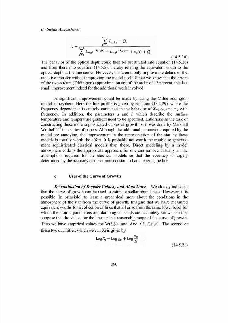
7/18/2019 The Fundamentals of Stellar Astrophysics - Collins G. W.
http://slidepdf.com/reader/full/the-fundamentals-of-stellar-astrophysics-collins-g-w 410/524
II Stellar Atmospheres
(14.5.20)The behavior of the optical depth could then be substituted into equation (14.5.20)and from there into equation (14.5.5), thereby relating the equivalent width to theoptical depth at the line center. However, this would only improve the details of theradiative transfer without improving the model itself. Since we know that the errorsof the two-stream (Eddington) approximation are of the order of 12 percent, this is asmall improvement indeed for the additional work involved.
A significant improvement could be made by using the Milne-Eddingtonmodel atmosphere. Here the line profile is given by equation (13.2.29), where thefrequency dependence is entirely contained in the behavior of ℒν, εν, and ην with
frequency. In addition, the parameters a and b which describe the surfacetemperature and temperature gradient need to be specified. Laborious as the task ofconstructing these more sophisticated curves of growth is, it was done by MarshallWrubel25-27 in a series of papers. Although the additional parameters required by themodel are annoying, the improvement in the representation of the star by thesemodels is usually worth the effort. It is probably not worth the trouble to generatemore sophisticated classical models than these. Direct modeling by a modelatmosphere code is the appropriate approach, for one can remove virtually all theassumptions required for the classical models so that the accuracy is largelydetermined by the accuracy of the atomic constants characterizing the line.
c Uses of the Curve of Growth
Determination of Doppler Velocity and Abundance We already indicatedthat the curve of growth can be used to estimate stellar abundances. However, it is possible (in principle) to learn a great deal more about the conditions in theatmosphere of the star from the curve of growth. Imagine that we have measuredequivalent widths for a collection of lines that all arise from the same lower level forwhich the atomic parameters and damping constants are accurately known. Furthersuppose that the values for the lines span a reasonable range of the curve of growth.
Thus we have empirical values for W(λi)/λ
i and )/(2 cm f e
eiiλπ . The second of
these two quantities, which we call Χi is given by
(14.5.21)
390
7/18/2019 The Fundamentals of Stellar Astrophysics - Collins G. W.
http://slidepdf.com/reader/full/the-fundamentals-of-stellar-astrophysics-collins-g-w 411/524
14 Shape of Spectral Lines
Thus, a plot of Log Xi versus. Log[W(λi)/λi] will yield an empirical curve of growththat differs from the theoretical curve given in Figure 14.7 by a shift in both theordinate and the abscissa. Since the lines all arise from the same lower level, N is thesame for all points. The horizontal shift then specifies Log(v
0/N), while the vertical
shift specifies Log(c/v0). Thus both the abundance and the Doppler velocity aredetermined independently. To the extent that the kinetic temperature is known, weknow the microturbulent velocity. If the span of the curve of growth is large enoughto determine a, an average value of c may also be found.
Determination of the Excitation Temperature Consider the situationwhere, in addition to the information given above, we know the equivalent widths fora number of lines arising from different states of excitation. Further assume that LTEholds so that the populations of those excited states are given by the Boltzmannformula. Then
(14.5.22)We have already determined v0, so we may correct the observed equivalent widths sothat the observed values are brought into correspondence with the theoreticalordinate of the curve of growth Wλ/∆λd. The horizontal points will now miss thetheoretical curve of growth by an amount
(14.5.23)or
(14.5.24)Since everything about the lines in equation (14.5.24) is known, only the constantand the temperature are unknowns, and they can be determined by least squares.
Important parameters concerning the structure of a stellar atmosphere can beestimated from the classical curve of growth. Not only can the abundance of theelements that make up the atmosphere be measured, but also the turbulent velocityand excitation temperature can be roughly determined. However, to use the classicalcurve of growth is to make some very restrictive assumptions. The assumption that
the parameters determining the lines are independent of optical depth is a poorassumption and is usually the reason that the excitation temperature does not agreewith the effective temperature. In addition, the thickness of the atmosphere is probably not the same for all the lines used. Finally, the lines are usually notscattering lines. Nevertheless, the method should be used prior to undertaking anydetailed analysis in order to set the ranges for the expected solution. Anysophisticated analysis that produces answers wildly different from those of the curve
391
7/18/2019 The Fundamentals of Stellar Astrophysics - Collins G. W.
http://slidepdf.com/reader/full/the-fundamentals-of-stellar-astrophysics-collins-g-w 412/524
II Stellar Atmospheres
of growth should be regarded with suspicion.
Finally, sooner or later, we must be wary of the assumption of LTE. In theupper layers of the atmosphere, the density will become low enough that collisionswill no longer occur frequently enough to overcome the nonequilibrium effects of theradiation field, and the level populations of the various atomic states will depart fromthat given by the Saha-Boltzmann ionization-excitation formula. This will particularly affect the strong spectral lines that are formed very high up in theatmosphere. In the next chapter, we survey what is to be done when LTE fails.
Problems
1. Imagine a line whose intensity profile is
Calculate the observed line profile for a radially expanding atmospherewhich exhibits a velocity gradient
State any assumptions that you make in solving the problem.
2. Consider a line generated by atoms constrained to move perpendicular to aradius vector from the center of the star. Find an expression for the atomicabsorption coefficient due to Doppler broadening alone.
3. Find the natural width fora Hβ b Mg II (λ4481)c FeI (λ3720) .
4. Estimate the transition times from the natural widths of the lines in Problem3, and compare them with a crude estimate of the collision rates for atoms inthese states. State clearly any assumptions you make. In what kind of starwould you expect to find these spectral lines?
5. If both the atoms of a radiating gas and the particles perturbing them are instatistical equilibrium, show that the average relative velocity between themis given by
392
7/18/2019 The Fundamentals of Stellar Astrophysics - Collins G. W.
http://slidepdf.com/reader/full/the-fundamentals-of-stellar-astrophysics-collins-g-w 413/524
14 Shape of Spectral Lines
where µh = the mass of a unit atomic weight and A1 and A2 are the atomicweight of the atom and perturber respectively.
6. Find the far-wing dependence of the line absorption coefficient of an atomhaving nondegenerate energy levels which are broadened by perturbershaving only octopole moments of their charge configurations.
7. Compute a line profile for Si II(λλ6347.10) for an A0V star. Use a modelatmosphere code if possible.
8. Show that Wλ/λ = Wν/ν
9. Use a model atmosphere code such as ATLAS to generate "curves of
growth" for Fe I(λλ4476), Mg II(λλ4481), and Si II(λλ4130). Include amicroturbulent velocity of 2 km/s. Consider the reference atmosphere to beone with T e = 104K, Log g = 4.0, and solar abundance (except for Fe, Mg,and Si). Compare your results with the classical curve of growth for aSchuster-Schwarzschild model atmosphere and obtain values for ∆λd, thekinetic temperature, microturbulent velocity, and Γ for each line. Compareyour results with the values used to generate the line profiles and discussany differences.
10. Consider the following situation: A 1-mm beam of neutral hydrogen gas withan internal kinetic temperature of 104 K is accelerated to an energy of 10-3eV
per atom. The beam enters a 10-m vacuum chamber and is directed toward a1-cm bar located in the center of the chamber and oriented at right angles tothe beam. The bar has been charged to 107v. The beam passes through a 1-mm hole in the bar and proceeds out the opposite side of the chamber. Aspectrograph is placed so that it "looks" along the beam and sees the beamagainst a 2 ×10⁴ K continuum blackbody source located near where the beamenters the chamber. Assuming that the beam density is sufficiently low toensure that it is optically thin, but high enough to establish LTE, find the line profile for Hβ. Further assume that the central depth of the line is 0.6. Findthe equivalent width of Hβ and the density of hydrogen. On the basis of yourresults, discuss the validity of the assumptions you used.
11. Consider a Schuster-Schwarzschild model atmosphere populated withseveral types of atoms having different atomic absorption coefficients. Findthe theoretical curves of growth for each of these atoms.
393
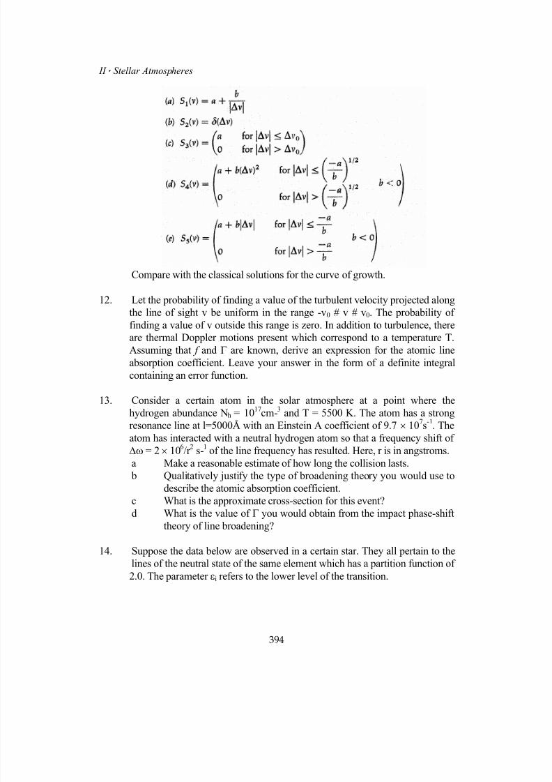
7/18/2019 The Fundamentals of Stellar Astrophysics - Collins G. W.
http://slidepdf.com/reader/full/the-fundamentals-of-stellar-astrophysics-collins-g-w 414/524
II Stellar Atmospheres
Compare with the classical solutions for the curve of growth.
12. Let the probability of finding a value of the turbulent velocity projected alongthe line of sight v be uniform in the range -v0 # v # v0. The probability offinding a value of v outside this range is zero. In addition to turbulence, thereare thermal Doppler motions present which correspond to a temperature T.Assuming that f and Γ are known, derive an expression for the atomic lineabsorption coefficient. Leave your answer in the form of a definite integralcontaining an error function.
13. Consider a certain atom in the solar atmosphere at a point where the
hydrogen abundance Nh = 1017cm-3 and T = 5500 K. The atom has a strongresonance line at l=5000Å with an Einstein A coefficient of 9.7 × 10⁷s-1. Theatom has interacted with a neutral hydrogen atom so that a frequency shift of∆ω = 2 × 10⁶/r 2 s-1 of the line frequency has resulted. Here, r is in angstroms.a Make a reasonable estimate of how long the collision lasts. b Qualitatively justify the type of broadening theory you would use to
describe the atomic absorption coefficient.c What is the approximate cross-section for this event?d What is the value of Γ you would obtain from the impact phase-shift
theory of line broadening?
14. Suppose the data below are observed in a certain star. They all pertain to thelines of the neutral state of the same element which has a partition function of2.0. The parameter εi refers to the lower level of the transition.
394
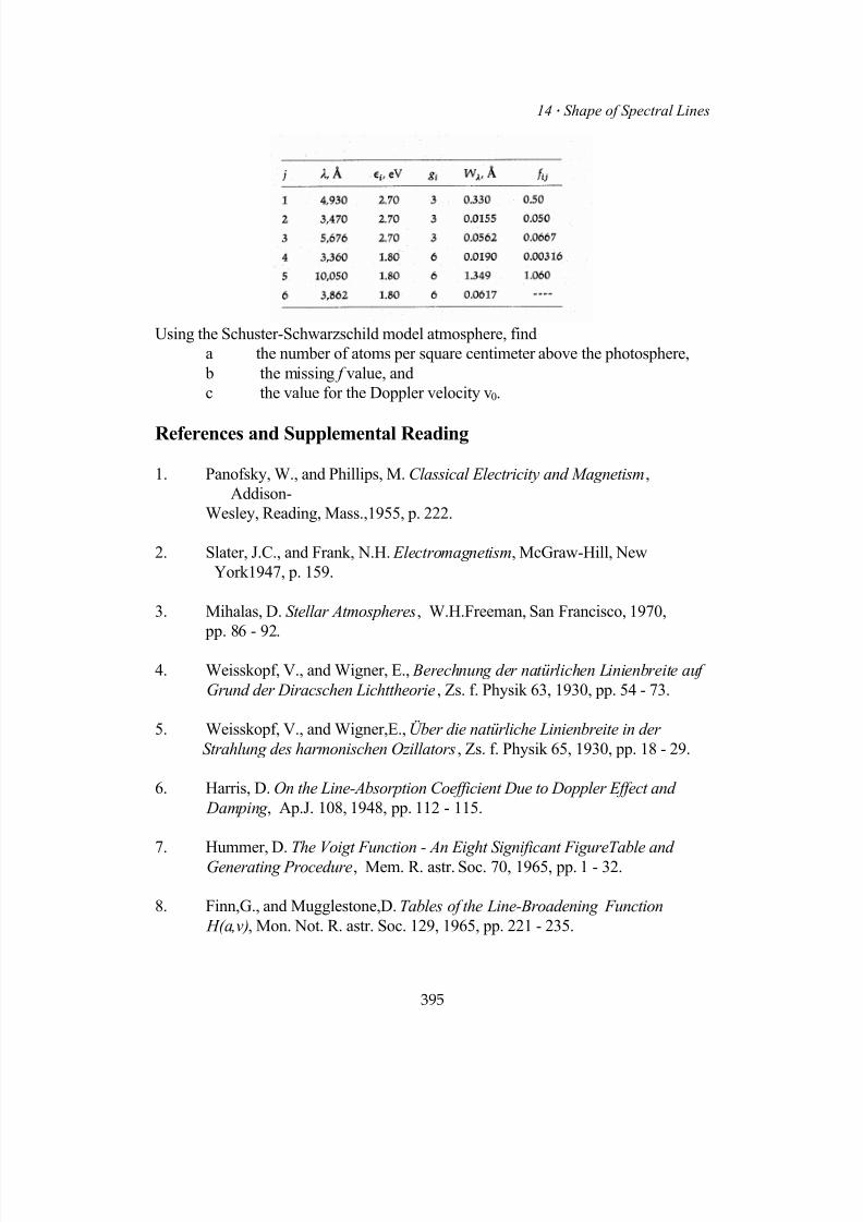
7/18/2019 The Fundamentals of Stellar Astrophysics - Collins G. W.
http://slidepdf.com/reader/full/the-fundamentals-of-stellar-astrophysics-collins-g-w 415/524
14 Shape of Spectral Lines
Using the Schuster-Schwarzschild model atmosphere, finda the number of atoms per square centimeter above the photosphere, b the missing f value, andc the value for the Doppler velocity v0.
References and Supplemental Reading
1. Panofsky, W., and Phillips, M. Classical Electricity and Magnetism,Addison-
Wesley, Reading, Mass.,1955, p. 222.
2. Slater, J.C., and Frank, N.H. Electromagnetism, McGraw-Hill, NewYork1947, p. 159.
3. Mihalas, D. Stellar Atmospheres, W.H.Freeman, San Francisco, 1970, pp. 86 - 92.
4. Weisskopf, V., and Wigner, E., Berechnung der natürlichen Linienbreite aufGrund der Diracschen Lichttheorie, Zs. f. Physik 63, 1930, pp. 54 - 73.
5. Weisskopf, V., and Wigner,E., Über die natürliche Linienbreite in derStrahlung des harmonischen Ozillators, Zs. f. Physik 65, 1930, pp. 18 - 29.
6. Harris, D. On the Line-Absorption Coefficient Due to Doppler Effect and Damping , Ap.J. 108, 1948, pp. 112 - 115.
7. Hummer, D. The Voigt Function - An Eight Significant FigureTable andGenerating Procedure, Mem. R. astr. Soc. 70, 1965, pp. 1 - 32.
8. Finn,G., and Mugglestone,D. Tables of the Line-Broadening Function H(a,v), Mon. Not. R. astr. Soc. 129, 1965, pp. 221 - 235.
395

7/18/2019 The Fundamentals of Stellar Astrophysics - Collins G. W.
http://slidepdf.com/reader/full/the-fundamentals-of-stellar-astrophysics-collins-g-w 416/524
II Stellar Atmospheres
9. Humíček, J. "An Efficient Method for Evaluation of the Complex Probability
Function: The Voigt Function and Its Derivatives", J. Quant. Spectrosc. &Rad. Trans. 21, 1979, pp. 309 - 313.
10. McKenna, S. A Method of Computing the Complex Probability Function andOther Related Functions over the Whole Complex Plane, Astrophy. & Sp.Sci. 107, 1984, pp. 71 - 83.
11. Mihalas, D. Stellar Atmospheres, 2d ed., W.H. Freeman, San Francisco,1978, pp. 463 - 471.
12. Collins II, G.W., "The Effects of Rotation on the Atmospheres of Early-
Type Main Sequence Stars", Stellar Rotation, (ed.: A. Slettebak), Reidel,Dordrecht, Holland, 1970, pp. 85 - 109.
13. Cassenilli, J.P. "Rotating Stellar Atmospheres", The Physics of Be Stars,(eds.: A.Slettebak and T. Snow), Cambridge University Press, Cambridge,1987, pp. 106 - 122.
14. Shajn,G., and Struve,O. On the Rotation of Stars, Mon. Not. R. astr. Soc. 89,1929, pp. 222 - 239.
15. Unsöld, A. Physik der Sternatmospharen, 2d Ed.,Springer-Verlag, Berlin,
1955, pp. 508 - 518.
16. Weisskopf, V. Zur Theorie der Kopplungsbreite und der Stossdampfung ,Zs. f. Physik 75, 1932, pp. 287 - 301.
17. Aller, L. H. The Atmospheres of the Sun and Stars, 2d ed., Ronald, NewYork, 1963, p. 317.
18. Unsöld, A. Physik der Sternatmospharen, 2d ed., Springer-Verlag, Berlin,1955, p.302.
19. Mihalas, D. Stellar Atmospheres, 2d ed., W.H.Freeman, San Francisco,1978, pp.281-284.
20. Lindholm, E. Zur Theorie der Verbreiterung von Spektrallinien, Arkiv. F.Math. Astron. och Fysik 28B (no. 3), 1942, pp. 1 - 11.
396

7/18/2019 The Fundamentals of Stellar Astrophysics - Collins G. W.
http://slidepdf.com/reader/full/the-fundamentals-of-stellar-astrophysics-collins-g-w 417/524
14 Shape of Spectral Lines
397
21. Foley, H. The Pressure Broadening of Spectral Lines, Phys. Rev. 69, 1946, pp. 616 - 628.
22. Holtsmark, J. Über die Verbreiterung von Spektrallinien, Ann.der Physik58, 1919, pp. 577 - 630.
23. Chandrasekhar, S. Stochastic Problems in Physics and Astronomy, Rev.Mod. Phy. 15, 1943, pp. 1 - 89.
24. Griem, H. Spectral Line Broadening by Plasmas, Academic, New York,1974.
25. Wrubel, M. Exact Curves of Growth for the Formation of Absorption Lines
According to the Milne-Eddington Model I. Total Flux, Ap.J. 109, 1949, pp.66 - 75.
26. Wrubel, M. Exact Curves of Growth for the Formation of Absorption Lines According to the Milne-Eddington Model II. Center of the Disk , Ap.J. 111,
1950, pp. 157 - 164.
27. Wrubel, M. Exact Curves of Growth. III. The Schuster- Schwarzschild Model , Ap.J. 119, 1954, pp. 51 - 57.
In addition to the references listed above, an excellent overall reference to
line broadening theory can be found in:
Böhm, K.-H.: "Basic Theory of Line Formation", Stellar Atmospheres, (ed.:J.Greenstein), Stars and Stellar Systems: Compendium of Astronomy and Astrophysics Vol VI , University of Chicago Press, Chicago, 1960, pp. 88 - 155.
For a somewhat different approach to the problem of line broadening, the interestedstudent should consult
Jefferies, J.T.:Spectral Line Formation, Blaisdell, New York, 1968, pp. 46 - 91.
A more complete treatment than we have given here can be found in
Mihalas, D.: Stellar Atmospheres, 2d ed., W.H.Freeman, San Francisco, 1978, pp.273 - 331.
Griem, H.R.: Plasma Spectroscopy, McGraw-Hill, New York, 1964.

7/18/2019 The Fundamentals of Stellar Astrophysics - Collins G. W.
http://slidepdf.com/reader/full/the-fundamentals-of-stellar-astrophysics-collins-g-w 418/524
II Stellar Atmospheres
Copyright (2003) George W. Collins, II
15
Breakdown of LocalThermodynamic
Equilibrium
. . .
Thus far we have made considerable use of the concepts of equilibrium. In
the stellar interior, the departures from a steady equilibrium distribution for the
photons and gas particles were so small that it was safe to assume that all the
constituents of the gas behaved as if they were in STE. However, near the surface of
the star, photons escape in such a manner that their energy distribution departs from
that expected for thermodynamic equilibrium, producing all the complexities that are
seen in stellar spectra. However, the mean free path for collisions between the
particles that make up the gas remained short compared to that of the photons, and so
the collisions could be regarded as random. More importantly, the majority of the
collisions between photons and the gas particles could be viewed as occurring
between particles in thermodynamic equilibrium. Therefore, while the radiation field
departs from that of a black body, the interactions determining the state of the gas
continue to lead to the establishment of an energy distribution for the gas particles
characteristic of thermodynamic equilibrium. This happy state allowed the complex
properties of the gas to be determined by the local temperature alone and is known as
LTE.
398

7/18/2019 The Fundamentals of Stellar Astrophysics - Collins G. W.
http://slidepdf.com/reader/full/the-fundamentals-of-stellar-astrophysics-collins-g-w 419/524
15 Breakdown of Local Thermodynamic Equilibrium
However, in the upper reaches of the atmosphere, the density declines to such
a point that collisions between gas particles and the remaining "equilibrium" photons
will be insufficient for the establishment of LTE. When this occurs, the energy level populations of the excited atoms are no longer governed by the Saha-Boltzmann
ionization-excitation formula, but are specified by the specific properties of the
atoms and their interactions.
Although the state of the gas is still given by a time-independent distribution
function and can be said to be in steady or statistical equilibrium, that equilibrium
distribution is no longer the maximal one determined by random collisions. We have
seen that the duration of an atom in any given state of excitation is determined by the
properties of that atomic state. Thus, any collection of similar atoms will attempt to
rearrange their states of excitation in accordance with the atomic properties of their
species. Only when the interactions with randomly moving particles are sufficient tooverwhelm this tendency will the conditions of LTE prevail. When these interactions
fail to dominate, a new equilibrium condition will be established that is different
from LTE. Unfortunately, to find this distribution, we have to calculate the rates at
which excitation and de-excitation occur for each atomic level in each species and to
determine the population levels that are stationary in time. We must include
collisions that take place with other constituents of the gas as well as with the
radiation field while including the propensity of atoms to spontaneously change their
state of excitation. To do this completely and correctly for all atoms is a task of
monumental proportions and currently is beyond the capability of even the fastest
computers. Thus we will have to make some approximations. In order for the
approximations to be appropriate, we first consider the state of the gas that prevailswhen LTE first begins to fail.
A vast volume of literature exists relating to the failure of LTE and it would
be impossible to cover it all. Although the absorption of some photon produced by
bound-bound transitions occurs in that part of the spectrum through which the
majority of the stellar flux flows, only occasionally is the absorption by specific lines
large enough to actually influence the structure of the atmosphere itself. However, in
these instances, departures from LTE can affect changes in the atmosphere's structure
as well as in the line itself. In the case of hydrogen, departures in the population of
the excited levels will also change the "continuous" opacity coefficient and produce
further changes in the upper atmosphere structure. To a lesser extent, this may also be true of helium. Therefore, any careful modeling of a stellar atmosphere must
include these effects at a very basic level. However, the understanding of the physics
of non-LTE is most easily obtained through its effects on specific atomic transitions.
In addition, since departures from LTE primarily occur in the upper layers of the
atmosphere and therefore affect the formation of the stellar spectra, we concentrate
on this aspect of the subject.
399
7/18/2019 The Fundamentals of Stellar Astrophysics - Collins G. W.
http://slidepdf.com/reader/full/the-fundamentals-of-stellar-astrophysics-collins-g-w 420/524
II Stellar Atmospheres
15.1 Phenomena Which Produce Departures from Local
Thermodynamic Equilibrium
a Principle of Detailed Balancing
Under the assumption of LTE, the material particles of the gas are
assumed to be in a state that can be characterized by a single parameter known as the
temperature. Under these conditions, the populations of the various energy levels of
the atoms of the gas will be given by Maxwell-Boltzmann statistics regardless of the
atomic parameters that dictate the likelihood that an electron will make a specific
transition. Clearly the level populations are constant in time. Thus the flow into any
energy level must be balanced by the flow out of that level. This condition must hold
in any time-independent state. However, in thermodynamic equilibrium, not onlymust the net flow be zero, so must the net flows that arise from individual levels.
That is, every absorption must be balanced by an emission. Every process must be
matched by its inverse. This concept is known as the principle of detailed balancing .
Consider what would transpire if this were not so. Assume that the values of
the atomic parameters governing a specific set of transitions are such that absorptions
from level 1 to level 3 of a hypothetical atom having only three levels are vastly
more likely than absorptions to level 2 (see figure 15.1). Then a time-independent
equilibrium could only be established by transitions from level 1 to level 3 followed
by transitions from level 3 to level 2 and then to level 1. There would basically be a
cyclical flow of electrons from levels 1 → 3 → 2 → 1. The energy to supply theabsorptions would come from either the radiation field or collisions with other
particles. To understand the relation of this example to LTE, consider a radiation-less
gas where all excitations and de-excitations result from collisions. Then such a
cyclical flow would result in energy corresponding to the 1 → 3 transition being
systematically transferred to the energy ranges corresponding to the transitions 3 →
2 and 2 → 1. This would lead to a departure of the energy momentum distribution
from that required by Maxwell-Boltzmann statistics and hence a departure from
LTE. But since we have assumed LTE, this process cannot happen and the upward
transitions must balance the downward transitions. Any process that tends to drive
the populations away from the values they would have under the principle of detailed
balancing will generate a departure from LTE. In the example, we considered thecase of a radiationless gas so that the departures had to arise in the velocity
distributions of the colliding particles. In the upper reaches of the atmosphere, a
larger and larger fraction of the atomic collisions are occurring with photons that are
departing further and further from the Planck function representing their
thermodynamic equilibrium distribution. These interactions will force the level
populations to depart from the values they would have under LTE.
400
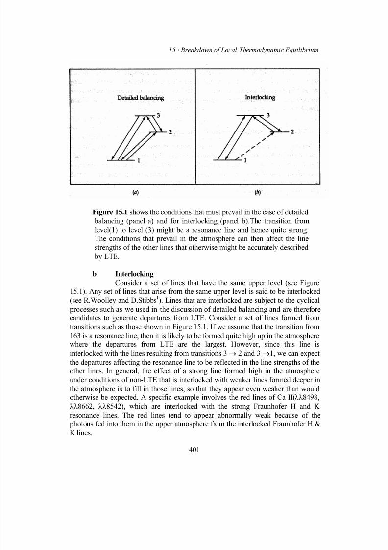
7/18/2019 The Fundamentals of Stellar Astrophysics - Collins G. W.
http://slidepdf.com/reader/full/the-fundamentals-of-stellar-astrophysics-collins-g-w 421/524
15 Breakdown of Local Thermodynamic Equilibrium
Figure 15.1 shows the conditions that must prevail in the case of detailed
balancing (panel a) and for interlocking (panel b).The transition from
level(1) to level (3) might be a resonance line and hence quite strong.
The conditions that prevail in the atmosphere can then affect the line
strengths of the other lines that otherwise might be accurately described
by LTE.
b Interlocking
Consider a set of lines that have the same upper level (see Figure
15.1). Any set of lines that arise from the same upper level is said to be interlocked(see R.Woolley and D.Stibbs
1). Lines that are interlocked are subject to the cyclical
processes such as we used in the discussion of detailed balancing and are therefore
candidates to generate departures from LTE. Consider a set of lines formed from
transitions such as those shown in Figure 15.1. If we assume that the transition from
163 is a resonance line, then it is likely to be formed quite high up in the atmosphere
where the departures from LTE are the largest. However, since this line is
interlocked with the lines resulting from transitions 3 → 2 and 3 →1, we can expect
the departures affecting the resonance line to be reflected in the line strengths of the
other lines. In general, the effect of a strong line formed high in the atmosphere
under conditions of non-LTE that is interlocked with weaker lines formed deeper in
the atmosphere is to fill in those lines, so that they appear even weaker than would
otherwise be expected. A specific example involves the red lines of Ca II(λλ8498,
λλ8662, λλ8542), which are interlocked with the strong Fraunhofer H and K
resonance lines. The red lines tend to appear abnormally weak because of the
photons fed into them in the upper atmosphere from the interlocked Fraunhofer H &
K lines.
401
7/18/2019 The Fundamentals of Stellar Astrophysics - Collins G. W.
http://slidepdf.com/reader/full/the-fundamentals-of-stellar-astrophysics-collins-g-w 422/524
II Stellar Atmospheres
c Collisional versus Photoionization
We have suggested that it is the relative dominance of the interaction
of photons over particles that leads to departures from LTE that are manifest in the
lines. Consider how this notion can be quantified. The number of photoionizations
from a particular state of excitation that takes place in a given volume per second
will depend on the number of available atoms and the number of ionizing photons.
We can express this condition as
(15.1.1)
The frequency ν0 corresponds to the energy required to ionize the atomic state under
consideration. The integral on the far right-hand side is essentially the number of
ionizing photons (modulo 4π), so that this expression really serves as a definition of
R ik as the rate coefficient for photoionizations from the ith state to the continuum. In
a similar manner, we may describe the number of collisional ionizations by
(15.1.2)
Here, C ik is the rate at which atoms in the ith state are ionized by collisions with
particles in the gas. The quantity σ(v) is the collision cross section of the particular
atomic state, and it must be determined either empirically or by means of a lengthy
quantum mechanical calculation; and f (v) is the velocity distribution function of the
particles.
In the upper reaches of the atmosphere, the energy distribution functions of
the constituents of the gas depart from their thermodynamic equilibrium values. The
electrons are among the last particles to undergo this departure because their mean
free path is always less than that for photons and because the electrons suffer many
more collisions per unit time than the ions. Under conditions of thermodynamic
equilibrium, the speeds of the electrons will be higher than those of the ions by (m h
A/me)½ as a result of the equipartition of energy. Thus we may generally ignore
collisions of ions of atomic weight A with anything other than electrons. Since the
electrons are among the last particles to depart from thermodynamic equilibrium, we
can assume that the velocity distribution f (v) is given by Maxwell-Boltzmann
statistics. Under this assumptionΩ
ik will depend on atomic properties and thetemperature alone. If we replace Jν with Bν(T), then we can estimate the ratio of
photoionizations to collisional ionizations R ik /Cik under conditions that prevail in the
atmospheres of normal stars. Karl Heintz Böhm2 has used this procedure along with
the semi-classical Thomson cross section for the ion to estimate this ratio. Böhm
finds that only for the upper-lying energy levels and at high temperatures and
densities will collisional ionizations dominate over photoionizations. Thus, for most
402
7/18/2019 The Fundamentals of Stellar Astrophysics - Collins G. W.
http://slidepdf.com/reader/full/the-fundamentals-of-stellar-astrophysics-collins-g-w 423/524
15 Breakdown of Local Thermodynamic Equilibrium
lines in most stars we cannot expect electronic collisions to maintain the atomic-level
populations that would be expected from LTE. So we are left with little choice but to
develop expressions for the energy-level populations based on the notion that the
sum of all transitions into and out of a level must be zero. This is the weakest
condition that will yield an atmosphere that is time-independent.
15.2 Rate Equations for Statistical Equilibrium
The condition that the sum of all transitions into and out of any specific level must be
zero implies that there is no net change of any level populations. This means that we
can write an expression that describes the flow into and out of each level,
incorporating the detailed physics that governs the flow from one level to another.
These expressions are known as the rate equations for statistical equilibrium. The
unknowns are the level populations for each energy level which will appear in every
expression for which a transition between the respective states is allowed. Thus we
have a system of n simultaneous equations for the level populations of n states.Unfortunately, as we saw in estimating the rates of collisional ionization and
photoionization, it is necessary to know the radiation field to determine the
coefficients in the rate equations. Thus any solution will require self-consistency
between the radiative transfer solution and the statistical equilibrium solution.
Fortunately, a method for the solution of the radiative transfer and statistical
equilibrium equations can be integrated easily in the iterative algorithm used to
model the atmosphere (see Chapter 12). All that is required is to determine the source
function in the line appropriate for the non-LTE state.
Since an atom has an infinite number of allowed states as well as an infinite
number of continuum states that must be considered, some practical limit will haveto be found. For the purpose of showing how the rate equations can be developed, we
consider two simple cases.
a Two-Level Atom
It is possible to describe the transitions between two bound states we
did for photo- and collisional ionization. Indeed, for the radiative processes, basically
we have already done so in (Section 11.3) through the use of the Einstein
coefficients. However, since we are dealing with only two levels, we must be careful
to describe exactly what happens to a photon that is absorbed by the transition from
level 1 to level 2. Since the level is not arbitrarily sharp, there may be someredistribution of energy within the level. Now since the effects of non-LTE will
affect the level populations at various depths within the atmosphere, we expect these
effects will affect the line profile as well as the line strength. Thus, we must be clear
as to what other effects might change the line profile. For that reason, we assume
complete redistribution of the line radiation. This is not an essential assumption, but
rather a convenient one.
403
7/18/2019 The Fundamentals of Stellar Astrophysics - Collins G. W.
http://slidepdf.com/reader/full/the-fundamentals-of-stellar-astrophysics-collins-g-w 424/524
II Stellar Atmospheres
If we define the probability of the absorption of a photon at frequency
ν' by
(15.2.1)
and the probability of reemission of a photon at frequency ν as
(15.2.2)
then the concept of the redistribution function describes to what extent these photons
are correlated in frequency. In Chapter 9, we introduced a fairly general notion of
complete redistribution by stating that ν' and ν would not be correlated. Thus,
(15.2.3)
Under the assumption of complete redistribution, we need only count radiative
transitions by assuming that specific emissions are unrelated to particular
absorptions. However, since the upward radiative transitions in the atom will depend
on the availability of photons, we will have to develop an equation of radiative
transfer for the two-level atom.
Equation of Radiative Transfer for the Two-Level Atom In Chapter 11
[equations (11.3.6) and (11.3.7)] we described the emission and absorption
coefficients, jν and κν, respectively, in terms of the Einstein coefficients. Using these
expressions, or alternatively just balancing the radiative absorptions and emissions,
we can write an equation of radiative transfer as
(15.2.4)
This process of balancing the transitions into and out of levels is common to any
order of approximation in dealing with statistical equilibrium. As long as all the
processes are taken into account, we will obtain an expression like equation (15.2.4)
for the transfer equation for multilevel atoms [see equation (15.2.25)]. Equation
(15.2.4) can take on a somewhat more familiar form if we define
(15.2.5)
Then the equation of transfer becomes
404
7/18/2019 The Fundamentals of Stellar Astrophysics - Collins G. W.
http://slidepdf.com/reader/full/the-fundamentals-of-stellar-astrophysics-collins-g-w 425/524
15 Breakdown of Local Thermodynamic Equilibrium
(15.2.6)
where
(15.2.7)
Making use of the relationships between the Einstein coefficients determined in
Chapter 11 [equation (11.3.5)], we can further write
(15.2.8)
Under conditions of LTE
(15.2.9)
so that we recover the expected result for the source function, namely
(15.2.10)
Two-Level-Atom Statistical Equilibrium Equations The solution to
equation (15.2.6) will provide us with a value of the radiation field required to
determine the number of radiative transitions. Thus the total number of upward
transitions in the two-level atom is
(15.2.11)
Similarly, the number of downward transitions is
(15.2.12)
The requirement that the level populations be stationary means that
(15.2.13)
so that the ratio of level populations is
(15.2.14)
405
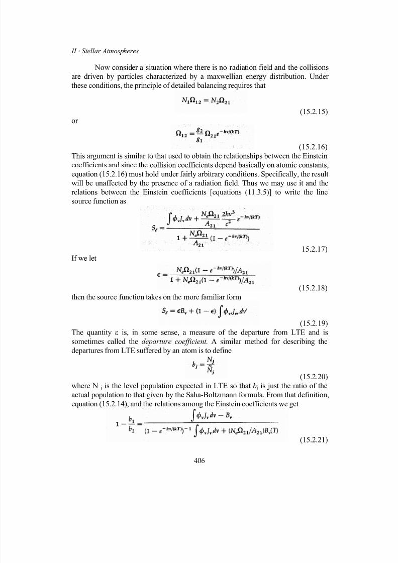
7/18/2019 The Fundamentals of Stellar Astrophysics - Collins G. W.
http://slidepdf.com/reader/full/the-fundamentals-of-stellar-astrophysics-collins-g-w 426/524
II Stellar Atmospheres
Now consider a situation where there is no radiation field and the collisions
are driven by particles characterized by a maxwellian energy distribution. Under
these conditions, the principle of detailed balancing requires that
(15.2.15)
or
(15.2.16)
This argument is similar to that used to obtain the relationships between the Einstein
coefficients and since the collision coefficients depend basically on atomic constants,
equation (15.2.16) must hold under fairly arbitrary conditions. Specifically, the result
will be unaffected by the presence of a radiation field. Thus we may use it and the
relations between the Einstein coefficients [equations (11.3.5)] to write the line
source function as
15.2.17)
If we let
(15.2.18)
then the source function takes on the more familiar form
(15.2.19)
The quantity ε is, in some sense, a measure of the departure from LTE and is
sometimes called the departure coefficient . A similar method for describing the
departures from LTE suffered by an atom is to define
(15.2.20)
where N j is the level population expected in LTE so that b j is just the ratio of the
actual population to that given by the Saha-Boltzmann formula. From that definition,equation (15.2.14), and the relations among the Einstein coefficients we get
(15.2.21)
406
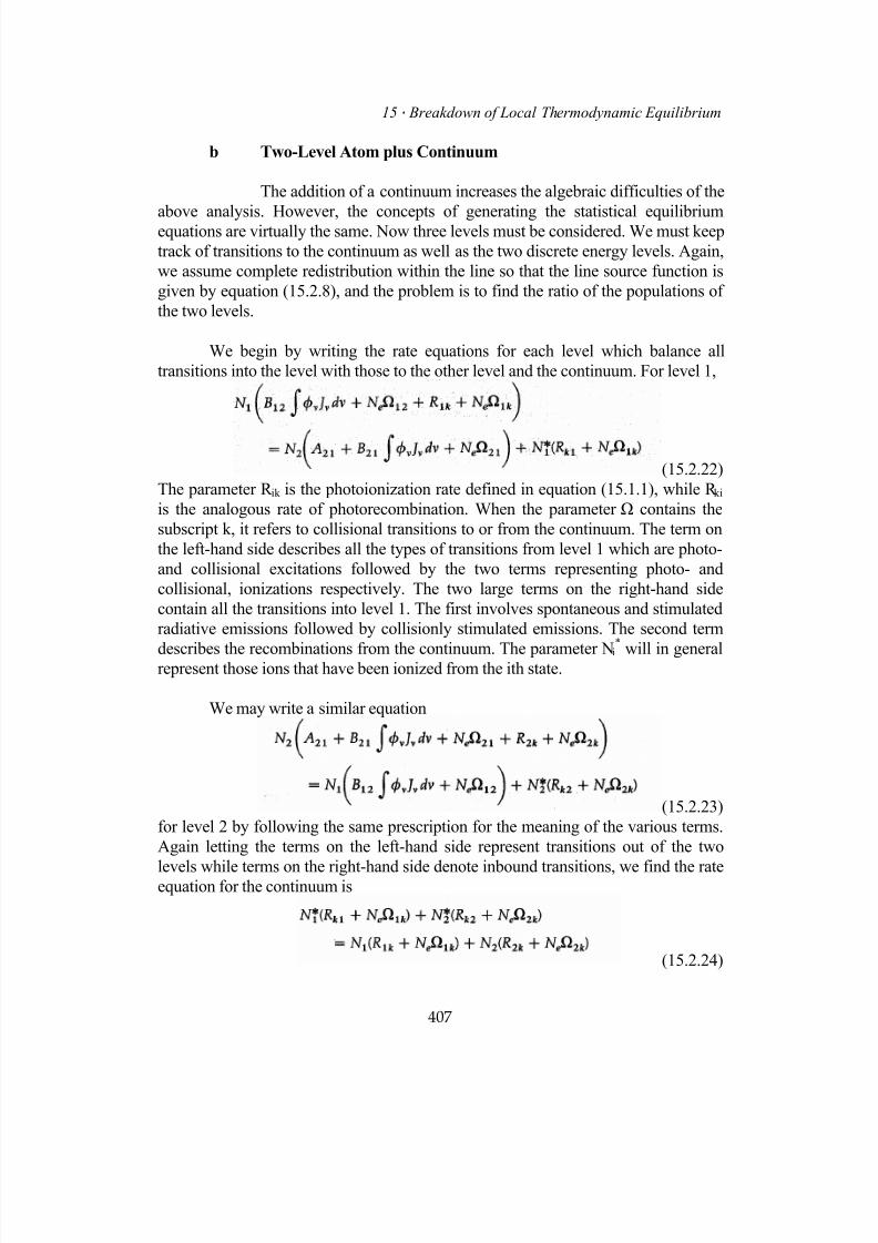
7/18/2019 The Fundamentals of Stellar Astrophysics - Collins G. W.
http://slidepdf.com/reader/full/the-fundamentals-of-stellar-astrophysics-collins-g-w 427/524
15 Breakdown of Local Thermodynamic Equilibrium
b Two-Level Atom plus Continuum
The addition of a continuum increases the algebraic difficulties of the
above analysis. However, the concepts of generating the statistical equilibriumequations are virtually the same. Now three levels must be considered. We must keep
track of transitions to the continuum as well as the two discrete energy levels. Again,
we assume complete redistribution within the line so that the line source function is
given by equation (15.2.8), and the problem is to find the ratio of the populations of
the two levels.
We begin by writing the rate equations for each level which balance all
transitions into the level with those to the other level and the continuum. For level 1,
(15.2.22)
The parameter R ik is the photoionization rate defined in equation (15.1.1), while R ki
is the analogous rate of photorecombination. When the parameter Ω contains the
subscript k, it refers to collisional transitions to or from the continuum. The term on
the left-hand side describes all the types of transitions from level 1 which are photo-
and collisional excitations followed by the two terms representing photo- and
collisional, ionizations respectively. The two large terms on the right-hand side
contain all the transitions into level 1. The first involves spontaneous and stimulated
radiative emissions followed by collisionly stimulated emissions. The second term
describes the recombinations from the continuum. The parameter Ni
*
will in generalrepresent those ions that have been ionized from the ith state.
We may write a similar equation
(15.2.23)
for level 2 by following the same prescription for the meaning of the various terms.
Again letting the terms on the left-hand side represent transitions out of the two
levels while terms on the right-hand side denote inbound transitions, we find the rateequation for the continuum is
(15.2.24)
407
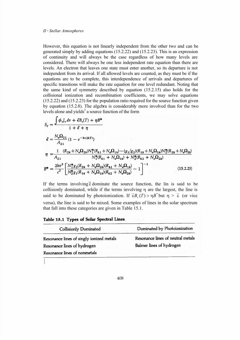
7/18/2019 The Fundamentals of Stellar Astrophysics - Collins G. W.
http://slidepdf.com/reader/full/the-fundamentals-of-stellar-astrophysics-collins-g-w 428/524
II Stellar Atmospheres
However, this equation is not linearly independent from the other two and can be
generated simply by adding equations (15.2.22) and (15.2.23). This is an expression
of continuity and will always be the case regardless of how many levels are
considered. There will always be one less independent rate equation than there are
levels. An electron that leaves one state must enter another, so its departure is not
independent from its arrival. If all allowed levels are counted, as they must be if the
equations are to be complete, this interdependence of arrivals and departures of
specific transitions will make the rate equation for one level redundant. Noting that
the same kind of symmetry described by equation (15.2.15) also holds for the
collisional ionization and recombination coefficients, we may solve equations
(15.2.22) and (15.2.23) for the population ratio required for the source function given
by equation (15.2.8). The algebra is considerably more involved than for the two
levels alone and yields3 a source function of the form
If the terms involving ε dominate the source function, the lin is said to be
collisionly dominated, while if the terms involving η are the largest, the line is
said to be dominated by photoionization. If *)( BT B η>ε ν but η > ε (or vice
versa), the line is said to be mixed. Some examples of lines in the solar spectrum
that fall into these categories are given in Table 15.1.
408
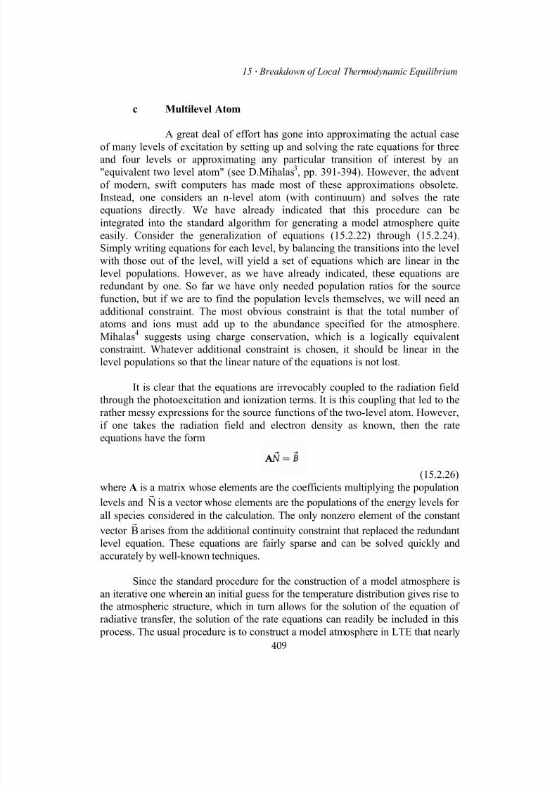
7/18/2019 The Fundamentals of Stellar Astrophysics - Collins G. W.
http://slidepdf.com/reader/full/the-fundamentals-of-stellar-astrophysics-collins-g-w 429/524
15 Breakdown of Local Thermodynamic Equilibrium
c Multilevel Atom
A great deal of effort has gone into approximating the actual caseof many levels of excitation by setting up and solving the rate equations for three
and four levels or approximating any particular transition of interest by an
"equivalent two level atom" (see D.Mihalas3, pp. 391-394). However, the advent
of modern, swift computers has made most of these approximations obsolete.
Instead, one considers an n-level atom (with continuum) and solves the rate
equations directly. We have already indicated that this procedure can be
integrated into the standard algorithm for generating a model atmosphere quite
easily. Consider the generalization of equations (15.2.22) through (15.2.24).
Simply writing equations for each level, by balancing the transitions into the level
with those out of the level, will yield a set of equations which are linear in the
level populations. However, as we have already indicated, these equations areredundant by one. So far we have only needed population ratios for the source
function, but if we are to find the population levels themselves, we will need an
additional constraint. The most obvious constraint is that the total number of
atoms and ions must add up to the abundance specified for the atmosphere.
Mihalas4 suggests using charge conservation, which is a logically equivalent
constraint. Whatever additional constraint is chosen, it should be linear in the
level populations so that the linear nature of the equations is not lost.
It is clear that the equations are irrevocably coupled to the radiation field
through the photoexcitation and ionization terms. It is this coupling that led to the
rather messy expressions for the source functions of the two-level atom. However,if one takes the radiation field and electron density as known, then the rate
equations have the form
(15.2.26)
where A is a matrix whose elements are the coefficients multiplying the population
levels andr
is a vector whose elements are the populations of the energy levels for
all species considered in the calculation. The only nonzero element of the constant
vector
N
Br
arises from the additional continuity constraint that replaced the redundant
level equation. These equations are fairly sparse and can be solved quickly and
accurately by well-known techniques.
409
Since the standard procedure for the construction of a model atmosphere is
an iterative one wherein an initial guess for the temperature distribution gives rise to
the atmospheric structure, which in turn allows for the solution of the equation of
radiative transfer, the solution of the rate equations can readily be included in this
process. The usual procedure is to construct a model atmosphere in LTE that nearly

7/18/2019 The Fundamentals of Stellar Astrophysics - Collins G. W.
http://slidepdf.com/reader/full/the-fundamentals-of-stellar-astrophysics-collins-g-w 430/524
II Stellar Atmospheres
satisfies radiative equilibrium. At some predetermined level of accuracy, the rate
equations are substituted for the Saha-Boltzmann excitation and ionization equations
by using the existing structure (electron density and temperature distribution) and
radiation field. The resulting population levels are then used to calculate opacities
and the atmospheric structure for the next iteration. One may even chose to use an
iterative algorithm for the solution of the linear equations, for an initial guess of the
LTE populations will probably be quite close to the correct populations for many of
the levels that are included. The number of levels of excitation that should be
included is somewhat dictated by the problem of interest. Depending on the state of
ionization, four levels are usually enough to provide sufficient accuracy. However,
some codes routinely employ as many as eight. One criterion of use is to include as
many levels as is necessary to reach those whose level populations are adequately
given by the Saha-Boltzmann ionization-excitation formula.
Many authors consider the model to be a non-LTE model if hydrogen alonehas been treated by means of rate equations while everything else is obtained from
the Saha-Boltzmann formula. For the structure of normal stellar atmospheres, this is
usually sufficient. However, should specific spectral lines be of interest, one should
consider whether the level populations of the element in question should also be
determined from a non-LTE calculation. This decision will largely be determined by
the conditions under which the line is formed. As a rule of thumb, if the line occurs
in the red or infra-red spectral region, consideration should be given to a non-LTE
calculation. The hotter the star, the more this consideration becomes imperative.
d Thermalization Length
Before we turn to the solution of the equation of radiative transfer for
lines affected by non-LTE effects, we should an additional concept which helps
characterize the physical processes that lead to departures from LTE. It is known as
the thermalization length. In LTE all the properties of the gas are determined by the
local values of the state variables. However, as soon as radiative processes become
important in establishing the populations of the energy levels of the gas, the problem
becomes global. Let l be the mean free path of a photon between absorptions or
scatterings and ℒ be the mean free path between collisional destructions. If
scatterings dominate over collisions, then ℒ will not be a "straight line" distance
through the atmosphere. Indeed, ℒ >> l if Aij >> Cij. That is, if the probability of
radiative de-excitation is very much greater than the probability of collisional de-excitation, then an average photon will have to travel much farther to be destroyed by
a collision than by a radiative interaction. However, ℒ >> l if Cij >> Aij. In this
instance, all photons that interact radiatively will be destroyed by collisions.
410
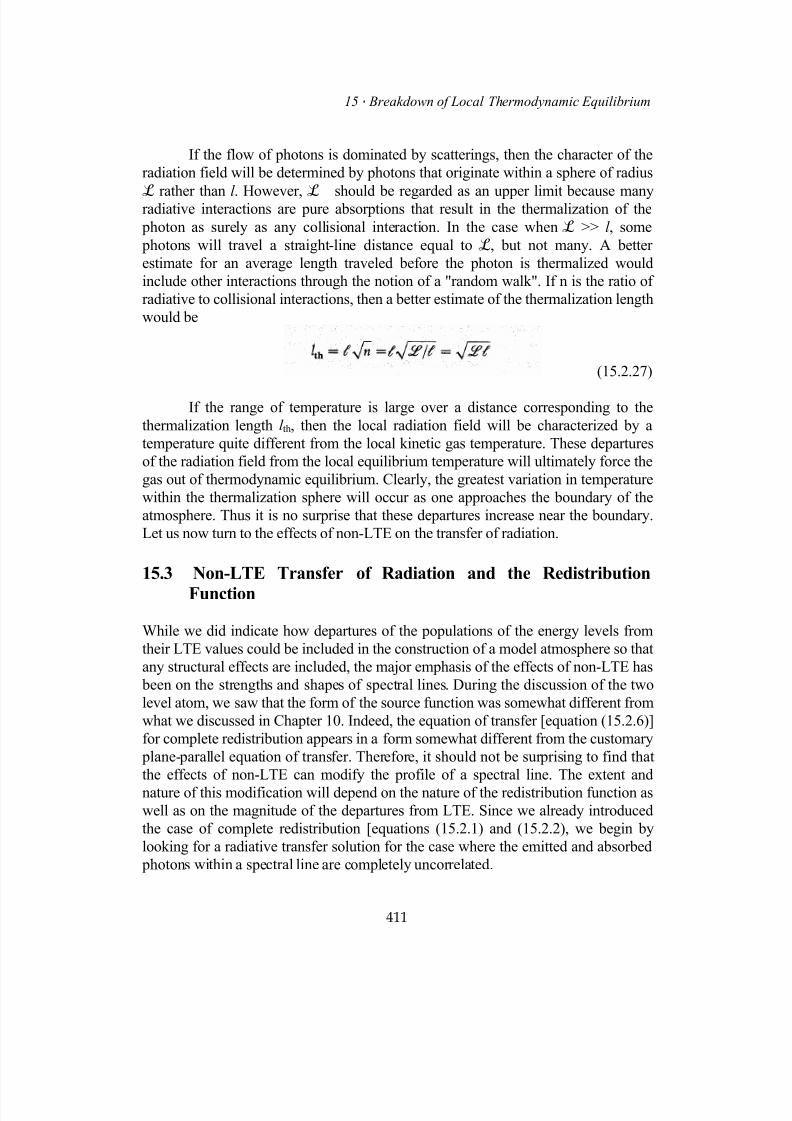
7/18/2019 The Fundamentals of Stellar Astrophysics - Collins G. W.
http://slidepdf.com/reader/full/the-fundamentals-of-stellar-astrophysics-collins-g-w 431/524
15 Breakdown of Local Thermodynamic Equilibrium
If the flow of photons is dominated by scatterings, then the character of the
radiation field will be determined by photons that originate within a sphere of radius
ℒ rather than l . However,
ℒ should be regarded as an upper limit because manyradiative interactions are pure absorptions that result in the thermalization of the
photon as surely as any collisional interaction. In the case when ℒ >> l , some
photons will travel a straight-line distance equal to ℒ, but not many. A better
estimate for an average length traveled before the photon is thermalized would
include other interactions through the notion of a "random walk". If n is the ratio of
radiative to collisional interactions, then a better estimate of the thermalization length
would be
(15.2.27)
If the range of temperature is large over a distance corresponding to the
thermalization length l th, then the local radiation field will be characterized by a
temperature quite different from the local kinetic gas temperature. These departures
of the radiation field from the local equilibrium temperature will ultimately force the
gas out of thermodynamic equilibrium. Clearly, the greatest variation in temperature
within the thermalization sphere will occur as one approaches the boundary of the
atmosphere. Thus it is no surprise that these departures increase near the boundary.
Let us now turn to the effects of non-LTE on the transfer of radiation.
15.3 Non-LTE Transfer of Radiation and the Redistribution
Function
While we did indicate how departures of the populations of the energy levels from
their LTE values could be included in the construction of a model atmosphere so that
any structural effects are included, the major emphasis of the effects of non-LTE has
been on the strengths and shapes of spectral lines. During the discussion of the two
level atom, we saw that the form of the source function was somewhat different from
what we discussed in Chapter 10. Indeed, the equation of transfer [equation (15.2.6)]
for complete redistribution appears in a form somewhat different from the customary
plane-parallel equation of transfer. Therefore, it should not be surprising to find that
the effects of non-LTE can modify the profile of a spectral line. The extent and
nature of this modification will depend on the nature of the redistribution function as
well as on the magnitude of the departures from LTE. Since we already introduced
the case of complete redistribution [equations (15.2.1) and (15.2.2), we begin by
looking for a radiative transfer solution for the case where the emitted and absorbed
photons within a spectral line are completely uncorrelated.
411
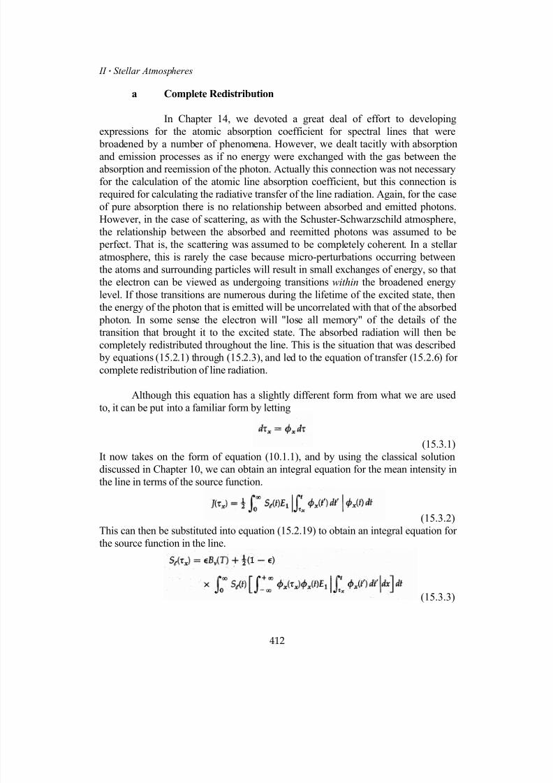
7/18/2019 The Fundamentals of Stellar Astrophysics - Collins G. W.
http://slidepdf.com/reader/full/the-fundamentals-of-stellar-astrophysics-collins-g-w 432/524
II Stellar Atmospheres
a Complete Redistribution
In Chapter 14, we devoted a great deal of effort to developing
expressions for the atomic absorption coefficient for spectral lines that were
broadened by a number of phenomena. However, we dealt tacitly with absorption
and emission processes as if no energy were exchanged with the gas between the
absorption and reemission of the photon. Actually this connection was not necessary
for the calculation of the atomic line absorption coefficient, but this connection is
required for calculating the radiative transfer of the line radiation. Again, for the case
of pure absorption there is no relationship between absorbed and emitted photons.
However, in the case of scattering, as with the Schuster-Schwarzschild atmosphere,
the relationship between the absorbed and reemitted photons was assumed to be
perfect. That is, the scattering was assumed to be completely coherent. In a stellar
atmosphere, this is rarely the case because micro-perturbations occurring between
the atoms and surrounding particles will result in small exchanges of energy, so thatthe electron can be viewed as undergoing transitions within the broadened energy
level. If those transitions are numerous during the lifetime of the excited state, then
the energy of the photon that is emitted will be uncorrelated with that of the absorbed
photon. In some sense the electron will "lose all memory" of the details of the
transition that brought it to the excited state. The absorbed radiation will then be
completely redistributed throughout the line. This is the situation that was described
by equations (15.2.1) through (15.2.3), and led to the equation of transfer (15.2.6) for
complete redistribution of line radiation.
Although this equation has a slightly different form from what we are used
to, it can be put into a familiar form by letting
(15.3.1)
It now takes on the form of equation (10.1.1), and by using the classical solution
discussed in Chapter 10, we can obtain an integral equation for the mean intensity in
the line in terms of the source function.
(15.3.2)
This can then be substituted into equation (15.2.19) to obtain an integral equation for
the source function in the line.
(15.3.3)
412

7/18/2019 The Fundamentals of Stellar Astrophysics - Collins G. W.
http://slidepdf.com/reader/full/the-fundamentals-of-stellar-astrophysics-collins-g-w 433/524
15 Breakdown of Local Thermodynamic Equilibrium
The integral over x results from the integral of the mean intensity over all
frequencies in the line [see equation (15.2.19)]. Note the similarity between this
result and the integral equation for the source function in the case of coherent
scattering [equation (9.1.14)]. Only the kernel of the integral has been modified bywhat is essentially a moment in frequency space weighted by the line profile function
φ x(t). This is clearly seen if we write the kernel as
(15.3.4)
so that the source function equation becomes a Schwarzschild-Milne equation of the
form
(15.3.5)
Since
(15.3.6)
the kernel is symmetric in τx and t, so that K (τx,t) = K (t,τx). This is the same
symmetry property as the exponential integral E1τ-t in equation 10.1.14.
Unfortunately, for an arbitrary depth dependence of φ x(t), equations (15.3.4) and
(15.3.5) must be solved numerically. Fortunately, all the methods for the solution of
Schwarzschild-Milne equations discussed in Chapter 10 are applicable to the
solution of this integral equation.
While it is possible to obtain some insight into the behavior of the solutionfor the case where φ x(t) ≠ f (t) (see Mihalas
3, pp.366-369), the insight is of dubious
value because it is the solution for a special case of a special case. However, a
property of such solutions, and of noncoherent scattering in general, is that the core
of the line profile is somewhat filled in at the expense of the wings. As we saw for
the two-level atom with continuum, the source function takes on a more complicated
form. Thus we turn to the more general situation involving partial redistribution.
b Hummer Redistribution Functions
The advent of swift computers has made it practical to model the
more complete description of the redistribution of photons in spectral lines.However, the attempts to describe this phenomenon quantitatively go back to
L.Henyey5 who carried out detailed balancing within an energy level to describe the
way in which photons are actually redistributed across a spectral line. Unfortunately,
the computing power of the time was not up to the task, and this approach to the
problem has gone virtually unnoticed. More recently, D.Hummer 6 has classified the
problem of redistribution into four main categories which are widely used today. For
413
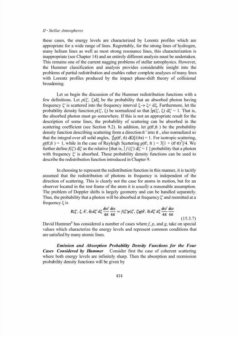
7/18/2019 The Fundamentals of Stellar Astrophysics - Collins G. W.
http://slidepdf.com/reader/full/the-fundamentals-of-stellar-astrophysics-collins-g-w 434/524
II Stellar Atmospheres
these cases, the energy levels are characterized by Lorentz profiles which are
appropriate for a wide range of lines. Regrettably, for the strong lines of hydrogen,
many helium lines as well as most strong resonance lines, this characterization is
inappropriate (see Chapter 14) and an entirely different analysis must be undertaken.
This remains one of the current nagging problems of stellar astrophysics. However,
the Hummer classification and analysis provides considerable insight into the
problems of partial redistribution and enables rather complete analyses of many lines
with Lorentz profiles produced by the impact phase-shift theory of collisional
broadening.
Let us begin the discussion of the Hummer redistribution functions with a
few definitions. Let p(ξ', ξ)dξ be the probability that an absorbed photon having
frequency ξ' is scattered into the frequency interval ξ→ ξ+ dξ. Furthermore, let the
probability density function p(ξ', ξ) be normalized so that ∫ p(ξ', ξ) dξ' = 1. That is,
the absorbed photon must go somewhere. If this is not an appropriate result for thedescription of some lines, the probability of scattering can be absorbed in the
scattering coefficient (see Section 9.2). In addition, let g (n',n ) be the probability
density function describing scattering from a direction n ' into n , also normalized so
that the integral over all solid angles, [∫ g (n', n) dΩ]/(4π) = 1. For isotropic scattering,
g (n',n ) = 1, while in the case of Rayleigh Scattering g (n', n ) = 3[1 + (n'⋅n)2]/4. We
further define f (ξ') dξ' as the relative [that is, ∫ f (ξ') dξ' = 1 ] probability that a photon
with frequency ξ' is absorbed. These probability density functions can be used to
describe the redistribution function introduced in Chapter 9.
In choosing to represent the redistribution function in this manner, it is tacitly
assumed that the redistribution of photons in frequency is independent of thedirection of scattering. This is clearly not the case for atoms in motion, but for an
observer located in the rest frame of the atom it is usually a reasonable assumption.
The problem of Doppler shifts is largely geometry and can be handled separately.
Thus, the probability that a photon will be absorbed at frequency ξ' and reemitted at a
frequency ξ is
(15.3.7)
David Hummer 6 has considered a number of cases where f , p, and g , take on special
values which characterize the energy levels and represent common conditions that
are satisfied by many atomic lines.
Emission and Absorption Probability Density Functions for the Four
Cases Considered by Hummer Consider first the case of coherent scattering
where both energy levels are infinitely sharp. Then the absorption and reemission
probability density functions will be given by
414

7/18/2019 The Fundamentals of Stellar Astrophysics - Collins G. W.
http://slidepdf.com/reader/full/the-fundamentals-of-stellar-astrophysics-collins-g-w 435/524
15 Breakdown of Local Thermodynamic Equilibrium
(15.3.8)
If the lower level is broadened by collisional radiation damping but the upper level
remains sharp, then the absorption probability density function is a Lorentz profile
while the reemission probability density function remains a delta function, so that
15.3.9)
If the lower level is sharp but the upper level is broadened by collisional radiation
damping, then both probability density functions are given Lorentz profiles since the
transitions into and out of the upper level are from a broadened state. Thus,
(15.3.10)
Since ξ' and ξ are uncorrelated, this case represents a case of complete
redistribution of noncoherent scattering. Hummer gives the joint probability of
transitions from a broadened lower level to a broadened upper level and back again
as
(15.3.11)
This probability must be calculated as a unit since ξ' is the same for both f and p.
Unfortunately a careful analysis of this function shows that the lower level is
considered to be sharp for the reemitted photon and therefore is inconsistent with the
assumption made about the absorption. Therefore, it will not satisfy detailed
balancing in an environment that presupposes LTE. A correct quantum mechanical
analysis7 gives
415
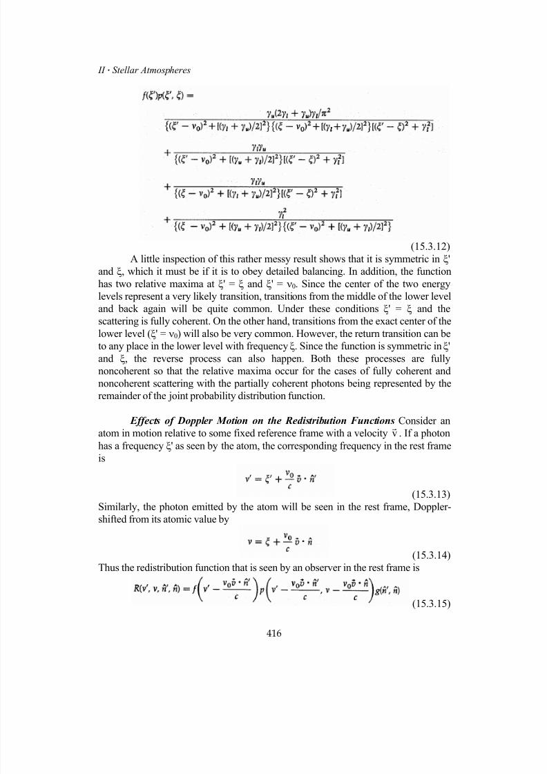
7/18/2019 The Fundamentals of Stellar Astrophysics - Collins G. W.
http://slidepdf.com/reader/full/the-fundamentals-of-stellar-astrophysics-collins-g-w 436/524
II Stellar Atmospheres
(15.3.12)
A little inspection of this rather messy result shows that it is symmetric in ξ'
and ξ, which it must be if it is to obey detailed balancing. In addition, the functionhas two relative maxima at ξ' = ξ and ξ' = ν0. Since the center of the two energy
levels represent a very likely transition, transitions from the middle of the lower level
and back again will be quite common. Under these conditions ξ' = ξ and the
scattering is fully coherent. On the other hand, transitions from the exact center of the
lower level (ξ' = ν0) will also be very common. However, the return transition can be
to any place in the lower level with frequency ξ. Since the function is symmetric in ξ'
and ξ, the reverse process can also happen. Both these processes are fully
noncoherent so that the relative maxima occur for the cases of fully coherent and
noncoherent scattering with the partially coherent photons being represented by the
remainder of the joint probability distribution function.
Effects of Doppler Motion on the Redistribution Functions Consider an
atom in motion relative to some fixed reference frame with a velocityr
. If a photon
has a frequency ξ' as seen by the atom, the corresponding frequency in the rest frame
is
v
(15.3.13)
Similarly, the photon emitted by the atom will be seen in the rest frame, Doppler-
shifted from its atomic value by
(15.3.14)
Thus the redistribution function that is seen by an observer in the rest frame is
(15.3.15)
416

7/18/2019 The Fundamentals of Stellar Astrophysics - Collins G. W.
http://slidepdf.com/reader/full/the-fundamentals-of-stellar-astrophysics-collins-g-w 437/524
15 Breakdown of Local Thermodynamic Equilibrium
We need now to relate the scattering angle determined from to the
angle between the atomic velocity and the directions of the incoming and outgoing
scattered photon. Consider a coordinate frame chosen so that the x-y plane is thescattering plane and the x axis lies in the scattering plane midway between the
incoming and outgoing photon (see Figure 15.2). In this coordinate frame, the
directional unit vectors n and n ' have Cartesian components given by
nn •′
(15.3.16)
Figure 15.2 displays a Cartesian coordinate frame where the x-axis
bisects the angle between the incoming and outgoing photon and the
x-y plane is the scattering plane.
417
7/18/2019 The Fundamentals of Stellar Astrophysics - Collins G. W.
http://slidepdf.com/reader/full/the-fundamentals-of-stellar-astrophysics-collins-g-w 438/524
II Stellar Atmospheres
Now if we assume that the atoms have a maxwellian velocity distribution
(15.3.17)
we can obtain the behavior of an ensemble of atoms by averaging equation (15.3.15)
over all velocity. First it is convenient to make the variable transformations
(15.3.18)
so that the components of the particle's velocity projected along the directions of the
photon's path become
(15.3.19)
and the velocity distribution is
(15.3.20)The symbol means duudr
xduyduz.
We define the ensemble average over the velocity of the redistribution
function as
(15.3.21)
or
(15.3.22)
A coordinate rotation by y/2 about the y axis so that n ' is aligned with x (see Figure
15.2) leads to the equivalent, but useful, form
418
7/18/2019 The Fundamentals of Stellar Astrophysics - Collins G. W.
http://slidepdf.com/reader/full/the-fundamentals-of-stellar-astrophysics-collins-g-w 439/524
15 Breakdown of Local Thermodynamic Equilibrium
(15.3.23)
We are now in a position to evaluate the effects of thermal Doppler motion
on the four cases given by Hummer 6, represented by equations (15.3.8) through
(15.3.12). The substitution of these forms of f(ξ') and p(ξ', ξ) into equation (15.3.22)
or equation (15.3.23) will yield the desired result. The frequencies ξ' and ξ must be
Doppler shifted according to equations (15.3.13) and (15.3.14) and some difficulty
may be encountered for the case of direct forward or back scattering (that is, β = 0)
and when one of the distribution functions is a delta function (i.e., for a sharp energy
level). The fact that β = 0 for these cases should be invoked before any variable
transformations are made for the purposes of evaluating the integrals.
Making a final transformation to a set of dimensionless frequencies
(15.3.24)
we can obtain the following result for Hummer's case I:
(15.3.25)
Consider what the emitted radiation would look like for an ensemble ofatoms illuminated by an isotropic uniform radiation field I0. Substitution of such a
radiation field into equation (9.2.29) would yield
(15.3.26)
which after some algebra gives
(15.3.27)
This implies that the emission of the radiation would have exactly the same form as
the absorption profile. But this was our definition of complete redistribution [seeequation (15.2.3)]. Thus, although a single atom behaves coherently, an ensemble of
thermally moving atoms will produce a line profile that is equivalent to one suffering
complete redistribution of the radiation over the Doppler core. Perhaps this is not too
surprising since the motion of the atoms is totally uncorrelated so that the Doppler
shifts produced by the various motions will mimic complete redistribution.
419
7/18/2019 The Fundamentals of Stellar Astrophysics - Collins G. W.
http://slidepdf.com/reader/full/the-fundamentals-of-stellar-astrophysics-collins-g-w 440/524
II Stellar Atmospheres
As one proceeds with the progressively more complicated cases, the results
become correspondingly more complicated to derive and express. Hummer's cases II
and III yield
(15.3.28)
and
(15.3.29)respectively. There is little point in giving the result for case IV as given by equation
(15.3.11). But the result for the correct case IV (sometimes called case V) that is
obtained from equation (15.3.12) is of some interest and is given by McKenna8 as
(15.3.30)
where
(15.3.31)and the function K(a,x), which is known as the shifted Voigt function is defined by
(15.3.32)
420

7/18/2019 The Fundamentals of Stellar Astrophysics - Collins G. W.
http://slidepdf.com/reader/full/the-fundamentals-of-stellar-astrophysics-collins-g-w 441/524
15 Breakdown of Local Thermodynamic Equilibrium
Unfortunately, all these redistribution functions contain the scattering angle
ψ explicitly and so by themselves are difficult to use for the calculation of line
profiles. Not only does the scattering angle appear in the part of the redistributionfunction resulting from the effects of the Doppler motion, but also the scattering
angle is contained in the phase function g (n', ). Thus, the Doppler motion can be
viewed as merely complicating the phase function. While there are methods for
dealing with the angle dependence of the redistribution function (see McKenna
n
9),
they are difficult and beyond the present scope of this discussion. They are, however,
of considerable importance to those interested in the state of polarization of the line
radiation. For most cases, the phase function is assumed to be isotropic, and we may
remove the angle dependence introduced by the Doppler motion by averaging the
redistribution function over all angles, as we did with velocity. These averaged forms
for the redistribution functions can then be inserted directly into the equation of
radiative transfer. As long as the radiation field is nearly isotropic and the angularscattering dependence (phase function) is also isotropic, this approximation is quite
accurate. However, always remember that it is indeed an approximation.
Angle-Averaged Redistribution Functions We should remember from
Chapter 13 [equation (13.2.14)], and the meaning of the redistribution function [see
equation (9.2.29)], that the equation of transfer for line radiation can be written as
(15.3.33)
Here the parameter ℒν is not to be considered constant with depth as it was for the
Milne-Eddington atmosphere. If we assume that the radiation field is nearly
isotropic, then we can integrate the equation of radiative transfer over µ and write
(15.3.34)
If we define the angle-averaged redistribution function as
(15.3.35)
then in terms of the absorption and reemission probabilities f(ξ') and p(ξ', ξ) it
becomes
(15.3.36)
421

7/18/2019 The Fundamentals of Stellar Astrophysics - Collins G. W.
http://slidepdf.com/reader/full/the-fundamentals-of-stellar-astrophysics-collins-g-w 442/524
II Stellar Atmospheres
The phase function g (n', n ) must be expressed in the coordinate frame of the
observer, that is, in terms of the incoming and outgoing angles that the photon makes
with the line of sight (see Figure 15.3).
Figure 15.3 describes the scattering event as seen in the coordinate
frame of the observer. The k - axis points along the normal to the
atmosphere or the observer's line-of-sight. The angle θ is the angle between the scattered photon and the observer's line-of-sight, while
the angle θ' is the corresponding angle of the incoming photon. The
quantities µ and µ' are just the cosines of these respective angles.
ˆ
422
7/18/2019 The Fundamentals of Stellar Astrophysics - Collins G. W.
http://slidepdf.com/reader/full/the-fundamentals-of-stellar-astrophysics-collins-g-w 443/524
15 Breakdown of Local Thermodynamic Equilibrium
We may write the phase function g (n', n ) as
(15.3.37)so that the angle-averaged redistribution function becomes
(15.3.38)
The two most common types of phase functions are isotropic scattering and
Rayleigh scattering. Although the latter occurs more frequently in nature, the former
is used more often because of its simplicity. Evaluating these phase functions in
terms of the observer's coordinate frame yields
(15.3.39)
In general, the appropriate procedure for calculating the angle-averaged
redistribution functions involves carrying out the integrals in equation (15.3.38) and
then applying the effects of Doppler broadening so as to obtain a redistribution
function for the four cases described by Hummer. For the first two cases, the delta
function representing the upper and lower levels requires that some care be used in
the evaluation of the integrals (see Mihalas4, pp. 422-433). In terms of the
normalized frequency x, the results of all that algebra are, for case I
(15.3.40)
For case II the result is somewhat more complicated where
(15.3.41)
while for case III it is more complex still:
(15.3.42)
Note that for all these cases the redistribution function is symmetric in x and
x'. From equations (15.2.1) through (15.2.3), it is clear that the angle-averaged
423
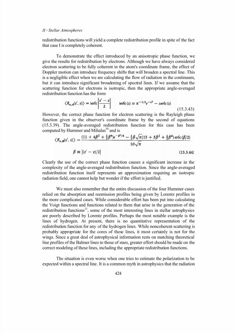
7/18/2019 The Fundamentals of Stellar Astrophysics - Collins G. W.
http://slidepdf.com/reader/full/the-fundamentals-of-stellar-astrophysics-collins-g-w 444/524
II Stellar Atmospheres
redistribution functions will yield a complete redistribution profile in spite of the fact
that case I is completely coherent.
To demonstrate the effect introduced by an anisotropic phase function, we
give the results for redistribution by electrons. Although we have always considered
electron scattering to be fully coherent in the atom's coordinate frame, the effect of
Doppler motion can introduce frequency shifts that will broaden a spectral line. This
is a negligible effect when we are calculating the flow of radiation in the continuum,
but it can introduce significant broadening of spectral lines. If we assume that the
scattering function for electrons is isotropic, then the appropriate angle-averaged
redistribution function has the form
(15.3.43)
However, the correct phase function for electron scattering is the Rayleigh phase
function given in the observer's coordinate frame by the second of equations
(15.3.39). The angle-averaged redistribution function for this case has been
computed by Hummer and Mihalas10
and is
Clearly the use of the correct phase function causes a significant increase in the
complexity of the angle-averaged redistribution function. Since the angle-averaged
redistribution function itself represents an approximation requiring an isotropic
radiation field, one cannot help but wonder if the effort is justified.
We must also remember that the entire discussion of the four Hummer cases
relied on the absorption and reemission profiles being given by Lorentz profiles in
the more complicated cases. While considerable effort has been put into calculating
the Voigt functions and functions related to them that arise in the generation of the
redistribution functions11
, some of the most interesting lines in stellar astrophysics
are poorly described by Lorentz profiles. Perhaps the most notable example is the
lines of hydrogen. At present, there is no quantitative representation of the
redistribution function for any of the hydrogen lines. While noncoherent scattering is
probably appropriate for the cores of these lines, it most certainly is not for thewings. Since a great deal of astrophysical information rests on matching theoretical
line profiles of the Balmer lines to those of stars, greater effort should be made on the
correct modeling of these lines, including the appropriate redistribution functions.
The situation is even worse when one tries to estimate the polarization to be
expected within a spectral line. It is a common myth in astrophysics that the radiation
424

7/18/2019 The Fundamentals of Stellar Astrophysics - Collins G. W.
http://slidepdf.com/reader/full/the-fundamentals-of-stellar-astrophysics-collins-g-w 445/524
15 Breakdown of Local Thermodynamic Equilibrium
in a spectral line should be locally unpolarized. Hence, the global observation of
spectral lines should show no net polarization. While this is true for simple lines that
result only from pure absorption, it is not true for lines that result from resonant
scattering. The phase function for a line undergoing resonant scattering is essentially
the same as that for electron scattering - the Rayleigh phase function. Whilenoncoherent scattering processes will tend to destroy the polarization information,
those parts of the line not subject to complete redistribution will produce strong local
polarization. If the source of the radiation does not exhibit symmetry about the line
of sight, then the sum of the local net polarization will not average to zero as seen by
the observer. Thus there should be a very strong wavelength polarization through
such a line which, while difficult to model, has the potential of placing very tight
constraints on the nature of the source. Recently McKenna12
has shown that this
polarization, known to exist in the specific intensity profiles of the sun, can be
successfully modeled by proper treatment of the redistribution function and a careful
analysis of the transfer of polarized radiation. So it is clear that the opportunity is
there remaining to be exploited. The existence of modern computers now makes thisfeasible.
15.4 Line Blanketing and Its Inclusion in the Construction of
Model Stellar Atmospheres and Its Inclusion in the
Construction of Model Stellar Atmospheres
In Chapter 10, we indicated that the presence of myriads of weak spectral lines could
add significantly to the total opacity in certain parts of the spectrum and virtually
blanket the emerging flux forcing it to appear in other less opaque regions of the
spectrum. This is particularly true for the early-type stars for which the major
contribution from these lines occurs in the ultraviolet part of the spectrum, wheremost of the radiative flux flows from the atmosphere. Although it is not strictly a
non-LTE effect, the existence of these lines generally formed high in the atmosphere
can result in structural changes to the atmosphere not unlike those of non-LTE. The
addition of opacity high up in the atmosphere tends to heat the layers immediately
below and is sometimes called backwarming .
425
Because of their sheer number, the inclusion of these lines in the calculation
of the opacity coefficient poses some significant problems. The simple approach of
including sufficient frequency points to represent the presence of all these lines
would simply make the computational problem unmanageable with even the largest
of computing machines that exist or can be imagined. Since the early attempts of
Chandrasekhar 13
, many efforts have been made to include these effects in the
modeling of stellar atmospheres. These early efforts incorporated approximating the
lines by a series of frequency "pickets". That is, the frequency dependence would be
represented by a discontinuous series of opaque regions that alternate with
transparent regions. One could then average over larger sections of the spectrum to
obtain a mean line opacity for the entire region. However, this did not represent the

7/18/2019 The Fundamentals of Stellar Astrophysics - Collins G. W.
http://slidepdf.com/reader/full/the-fundamentals-of-stellar-astrophysics-collins-g-w 446/524
II Stellar Atmospheres
effect on the photon flow through the alternatingly opaque and relatively transparent
regions with any great accuracy. Others tried using harmonic mean line opacities to
reduce this problem. Of these attempts, two have survived and are worthy of
consideration.
a Opacity Sampling
This conceptually simple method of including line blanketing takes
advantage of the extremely large number of spectral lines. The basic approach is to
represent the frequency-dependent opacity of all the lines as completely as possible.
This requires tabulating a list of all the likely lines and their relative strengths. For an
element like iron, this could mean the systematic listing of several million lines. In
addition, the line shape for each line must be known. This is usually taken to be a
Voigt function for it represents an excellent approximation for the vast majority of
weak lines. However, its use requires that some estimate of the appropriate dampingconstant be obtained for each line. In many cases, the Voigt function has been
approximated by the Doppler broadening function on the assumption that the
damping wings of the line are relatively unimportant. At any frequency the total line
absorption coefficient is simply the sum of the significant contributions of lines that
contribute to the opacity at that frequency, weighted by the relative abundance of the
absorbing species. These abundances are usually obtained by assuming that LTE
prevails and so the Saha-Boltzmann ionization-excitation equation can be used.
If one were to pick a very large number of frequencies, this procedure would
yield an accurate representation of the effects of metallic line blanketing. However, it
would also require prodigious quantities of computing time for modeling theatmosphere. Sneden et al.14
have shown that sufficient accuracy can be obtained by
choosing far fewer frequency points than would be required to represent each line
accurately. Although the choice of randomly distributed frequency points which
represent large chunks of the frequency domain means that the opacity will be
seriously overestimated in some regions and underestimated in others, it is possible
to obtain accurate structural results for the atmosphere if a large enough sample of
frequency points is chosen. This sample need not be anywhere near as large as that
required to represent the individual lines, for what is important for the structure is
only the net flow of photons. Thus, if the frequency sampling is sufficiently large to
describe the photon flow over reasonably large parts of the spectrum, the resulting
structure and the contribution of millions of lines will be accurately represented. This procedure will begin to fail in the higher regions of the atmosphere where the lines
become very sharp and non-LTE effects become increasingly important. In practice,
this procedure may require the use of several thousand frequency points whereas the
correct representation of several million spectral lines would require tens of millions
of frequency points. For this reason (and others), this approach has been extremely
successful as applied to the structure of late-type model atmospheres where the
426
7/18/2019 The Fundamentals of Stellar Astrophysics - Collins G. W.
http://slidepdf.com/reader/full/the-fundamentals-of-stellar-astrophysics-collins-g-w 447/524
15 Breakdown of Local Thermodynamic Equilibrium
opacity is dominated by the literally millions of bound-bound transitions occurring in
molecules. The larger the number of weak lines and the more uniform their
distribution, the more accurate this procedure becomes. However, the longer the lists
of spectral lines, the more computer time will be required to carry out the calculation.
This entire procedure is generally known as opacity sampling and it possesses a greatdegree of flexibility in that all aspects of the stellar model that may affect the line
broadening can be included ab initio for each model. This is not the case with the
competing approach to line blanketing.
b Opacity Distribution Functions
This approach to describing the absorption by large numbers of lines
also involves a form of statistical sampling. However, here the statistical
representation is carried out over even larger regions of the spectra than was the case
for the opacity sampling scheme. This approach has its origins in the mean opacity
concept alluded to earlier. However, instead of replacing the complicated variation ofthe line opacity over some region of the spectrum with its mean, consider the fraction
of the spectral range that has a line opacity less than or equal to some given value.
For small intervals of the range, this may be a fairly large number since small
intervals correspond to the presence of line cores. If one considers larger fractions of
the interval, the total opacity per unit frequency interval of this larger region will
decrease, because the spaces between the lines will be included. Thus, an opacity
distribution function represents the probability that a randomly chosen point in the
interval will have an opacity less than or equal to the given value (see Figure 15.4).
The proper name for this function should be the inverse cumulative opacity
probability distribution function, but in astronomy it is usually referred to as just the
opacity distribution function or (ODF). Carpenter 15
gives a very complete descriptionof the details of computing these functions while a somewhat less complete picture is
given by Kurucz and Pettymann16
and by Mihalas4(pp. 167-169).
The ODF gives the probability that the opacity is a particular fraction of a
known value for any range of the frequency interval, and the ODF may be obtained
from a graph that is fairly simple to characterize by simple functions. This approach
allows the contribution to the total opacity due to spectral lines appropriate for that
range of the interval to be calculated. Unfortunately, the magnitude of that given
value will depend on the chemical composition and the details of the individual line-
broadening mechanisms. Thus, any change in the chemical composition, turbulent
broadening, etc., will require a recalculation of the ODF.
427

7/18/2019 The Fundamentals of Stellar Astrophysics - Collins G. W.
http://slidepdf.com/reader/full/the-fundamentals-of-stellar-astrophysics-collins-g-w 448/524
II Stellar Atmospheres
Figure 15.4 schematically shows the opacity of a region of the spectrumrepresented in terms of the actual line opacity (panel a) and the opacity
distribution function (panel b).
In addition, ODFs must be calculated as a function of temperature and pressure (or
alternatively, electron density), and so their tabular representation can be extremely
large. Their calculation also represents a significant computational effort. However,
once ODF's exist, their inclusion in a stellar atmosphere code is fairly simple and the
additional computational load for the construction of a model atmosphere is not
great, particularly compared to the opacity sampling technique. This constitutes the
primary advantage of this approach for the generation of model stellar atmospheres.
For stars where the abundances and kinematics of the atmospheres are well known,ODF's provide by far the most efficient means of including the effects of line
blanketing. This will become increasingly true as the number of spectral lines for
which atomic parameters are known grows; although the task of calculating the
opacity distribution functions will also increase.
Considerations such as these will enable the investigator to include the
effects of line blanketing and thereby to create reasonably accurate models of the
stellar atmosphere which will represent the structure correctly through the line
forming region of a normal star. These, when combined with the model interiors
discussed in the first six chapters of the book, will allow for the description of normal
stars from the center to the surface. While this was the goal of the book, We cannotresist the temptation to demonstrate to the conservative student that the concepts
developed so far will allow the models to be extended into the region above stars and
to determine some properties of the stellar radiation field that go beyond what is
usually considered to be part of the normal stellar model. So in the last chapter we
will consider a few extensions of the ideas that have already been developed
428
7/18/2019 The Fundamentals of Stellar Astrophysics - Collins G. W.
http://slidepdf.com/reader/full/the-fundamentals-of-stellar-astrophysics-collins-g-w 449/524
15 Breakdown of Local Thermodynamic Equilibrium
Problems
1. Estimate the ratio of collisional ionization to photoionization for hydrogen
from the ground state, and compare it to the ratio from the second level.
Assume the pressure is 300 bars. Obtain the physical constants you may needfrom the literature, but give the appropriate references.
2. Calculate the Doppler-broadened angle-averaged redistribution function for
Hummer's case I, but assuming a Rayleigh phase function [i.e., find
<R(x,x')>I,B] and compare it to <R(x,x')>I,A and the result for electron
scattering.
3. Show that
is indeed a solution to
and obtain an integral equation for S l .
4. Describe the mechanisms which determine the Lyα profile in the sun. Be
specific about the relative importance of these mechanisms and the parts of
the profile that they affect.
5. Given a line profile of the form
find S l . Assume complete redistribution of the line radiation. State what
further assumptions you may need; indicate your method of solution and
your reasons for choosing it.
6. Show explicitly how equation (15.2.21) is obtained.
7. Show how equation (15.3.25) is implied by equation (15.3.15).
8. How does equation (15.3.27) follow from equation (15.3.26).
9. Derive equations (15.3.28) and (15.3.29).
10. Use equation (15.3.30) to obtain the angle-averaged form of <R IV,A(x',x)>.
11. Show explicitly how equations (15.3.40) and (15.3.41) are obtained.
429
7/18/2019 The Fundamentals of Stellar Astrophysics - Collins G. W.
http://slidepdf.com/reader/full/the-fundamentals-of-stellar-astrophysics-collins-g-w 450/524
II Stellar Atmospheres
References and Supplemental Reading
1. Woolley, R.v.d.R., and Stibbs, D.W.N. The Outer Layers of a Star , OxfordUniversity Press, London, 1953, p. 152.
2. Böhm, K.-H. "Basic Theory of Line Formation", Stellar Atmospheres, (Ed.:
J. Greenstein), Stars and Stellar Systems: Compendium of Astronomy and
Astrophysics, Vol.6, University of Chicago Press, 1960, pp. 88 - 155.
3. Mihalas, D. Stellar Atmospheres, W.H. Freeman, San Francisco, 1970,
pp. 337 - 378.
4. Mihalas, D. Stellar Atmospheres, 2d ed., W.H. Freeman, San Francisco,
1978, pp. 138.
5. Henyey, L. Near Thermodynamic Radiative Equilibrium, Ap.J. 103, 1946,
pp. 332 - 350.
6. Hummer, D.G. Non-Coherent Scattering , Mon. Not. R. astr. Soc. 125, 1962,
pp. 21 - 37.
7. Omont, A., Smith, E.R., and Cooper, J. Redistribution of Resonance
Radiation I. The Effect of Collisions, Ap.J. 175, 1972, pp. 185 - 199.
8. McKenna,S. A Reinvestigation of Redistribution Functions R III and R IV , Ap.J. 175, 1980, pp. 283 - 293.
9. McKenna, S. The Transfer of Polarized Radiation in Spectral
Lines:Formalism and Solutions in Simple Cases, Astrophy. & Sp. Sci., 108,
1985, pp. 31 - 66.
10. Hummer, D.G., and Mihalas, D. Line Formation with Non-Coherent
Electron Scattering in O and B Stars, Ap.J. Lett. 150, 1967, pp. 57 - 59.
11. McKenna, S. A Method of Computing the Complex Probability Functionand
Other Related Functions over the Whole Complex Plane, Astrophy. & Sp.Sci. 107, 1984, pp. 71 - 83.
12. McKenna, S. The Transfer of Polarized Radiation in Spectral Lines: Solar-
Type Stellar Atmospheres, Astrophy. & Sp. Sci., 106, 1984, pp. 283 - 297.
430
7/18/2019 The Fundamentals of Stellar Astrophysics - Collins G. W.
http://slidepdf.com/reader/full/the-fundamentals-of-stellar-astrophysics-collins-g-w 451/524
15 Breakdown of Local Thermodynamic Equilibrium
431
13. Chandrasekhar,S. The Radiative Equilibrium of the Outer Layers of a Star
with Special Reference to the Blanketing Effect of the Reversing Layer , Mon.
Not. R. astr. Soc. 96, 1936, pp. 21 - 42.
14. Sneden, C., Johnson, H.R., and Krupp, B.M. A Statistical Method forTreating Molecular Line Opacities, Ap. J. 204, 1976, pp. 281 - 289.
15. Carpenter,K.G. A Study of Magnetic, Line-Blanketed Model Atmospheres,
doctoral dissertation: The Ohio State University, Columbus, 1983.
16. Kurucz, R., and Peytremann, E. A Table of Semiemperical gf Values Part 3,
SAO Special Report #362, 1975.
Although they have been cited frequently, the serious student of departures
from LTE should read both these:
Mihalas, D.: Stellar Atmospheres, W.H.Freeman, San Francisco, 1970,
chaps. 7-10, 12, 13.
and
Mihalas, D.: Stellar Atmospheres, 2d ed., W.H.Freeman, San Francisco,
1978, chaps. 11-13.
A somewhat different perspective on the two-level and multilevel atom can be found
in:
Jefferies, J.T.: Spectral Line Formation, Blaisdell, New York, 1968,
chaps. 7, 8.
Although the reference is somewhat old, the physical content is such that I would
still recommend reading the entire chapter:
Böhm, K.-H.: "Basic Theory of Line Formation", Stellar Atmospheres, (Ed.:
J.Greenstein), Stars and Stellar Systems: Compendium of Astronomy and
Astrophysics, Vol.6, University of Chicago Press, Chicago, 1960, chap. 3.
7/18/2019 The Fundamentals of Stellar Astrophysics - Collins G. W.
http://slidepdf.com/reader/full/the-fundamentals-of-stellar-astrophysics-collins-g-w 452/524
II Stellar Atmospheres
Copyright (2003) George W. Collins, II
16
Beyond the Normal Stellar Atmosphere
. . .
With the exception of a few subjects in Chapter 7, we have dealt exclusively
with spherical stars throughout this book. In addition, these stars have been "normal"
stars; that is, they are stars without strange peculiarities or large time-dependent
effects in their spectra. These are stars, for the most part, with interiors evolving on a
nuclear time scale and atmospheres which can largely be said to be in LTE. The
prototypical star that fits this description is a main sequence star, and for such stars
the theoretical framework laid down in this book will serve quite well as a basis for
understanding their structure and spectra. However, the notion of a spectral
peculiarity is somewhat "in the eye of the beholder". Someone who looks closely at
any star will find grounds for calling it peculiar or atypical. This is true of even the
main sequence stars, and we would delude ourselves if we believed that all aspects of
any star are completely understood.
432

7/18/2019 The Fundamentals of Stellar Astrophysics - Collins G. W.
http://slidepdf.com/reader/full/the-fundamentals-of-stellar-astrophysics-collins-g-w 453/524
16 Beyond the Normal Stellar Atmosphere
Phenomena are known to exist in the atmospheres of stars that we have not
included in the basic theory. For example, convection does exist in the upper layers
of late-type stars and contributes to the transport of energy. However, the efficiency
of this transport is vastly inferior to that which occurs in the stellar interior, because
the mean free path for a convective element is of the order of that for a photon.
Nevertheless, in the lower sections of the atmosphere, convection may carry a
significant fraction of the total energy. Unfortunately, the crude mixing length theory
of convective transport that was effective for the stellar interior is insufficient for an
accurate description of atmospheric convection.
The turbulent motion exhibited by the atmospheres of many giant stars also
represents the transport of energy and momentum in a manner similar to convection.
Just the kinetic energy of the turbulent elements themselves should contribute
significantly to the pressure equilibrium in the upper atmosphere. However, if onenaively assigned a turbulent pressure of ρv2 to the elements, the measured turbulent
velocities would imply a pressure greater than the total pressure of the gas and the
atmosphere would be unstable. Clearly a better theory of turbulence is required
before any significant progress can be made in this area.
In the last 20 years, it has become clear that the atmospheres of many stars
are indeed unstable. Ultraviolet observations of the spectra of early-type stars suggest
that they all possess a stellar wind of out-flowing matter of significant proportions.
As one moves upward in the atmosphere of a star, departures from LTE increase to
such a point that they dominate the atmospheric structure. In addition, energy sources
such as magnetic fields, atmospheric mass motions, and possibly acoustic wavesassociated with convection or turbulence may contribute significantly to the higher
level structure. While these energy contributions are tiny when compared to the
energy densities in the photosphere, the contributions may supply the majority of the
interaction energy between the star and its outermost layers which are basically
transparent to photons.
In the hottest stars, the pressure of radiation, transmitted to the rarefied upper
layers of the atmosphere through absorption by the resonance lines of metals, will
cause this low-density region to become unstable, expand, and eventually be driven
away. This is undoubtedly the source of the stellar winds for stars on the upper main
sequence and in the early-type giants and supergiants. The extended atmospheres ofthese stars pose an entirely new set of problems for the theory of stellar atmospheres.
Many stars exist in close binary systems so that the atmosphere of each is
exposed to the radiation from the other. In some instances, the illuminating radiant
flux from the companion may exceed that of the star. Under these conditions we can
expect the local atmospheric structure to be dominated by the external source of
433

7/18/2019 The Fundamentals of Stellar Astrophysics - Collins G. W.
http://slidepdf.com/reader/full/the-fundamentals-of-stellar-astrophysics-collins-g-w 454/524
II Stellar Atmospheres
radiation. In addition, such stars are liable to be severely distorted from the spherical
shape of a normal star. This implies that the defining parameters of the stellar
atmosphere (µ, g , and T e) will vary across the surface. Even in the absence of a
companion, rapid rotation of the entire star can provide a similar distortion with the
accompanying variation of atmospheric parameters over the surface.
These are some of the areas of contemporary research and to even recount
the present state of progress in them would require another book. Instead of
skimming them all, in this last chapter, we consider one or two of them in the hopes
of pricking the reader's interest to find out more and perhaps contribute to the
solution of some of these problems.
16.1 Illuminated Stellar Atmospheres
Although the majority of stars exist in binary systems, and many of them are close binary systems, little attention has been paid to the effects on a stellar atmosphere, by
the illuminating radiation of the companion. The general impact of this illumination
on the light curve of an eclipsing binary system has usually been lumped under the
generic term "reflection effect". This is a complete misnomer, for most of any
incident energy is absorbed by the atmosphere and then reradiated. Only that fraction
which is scattered could, in any sense, be considered to be reflected and then only
that fraction that is scattered in the direction of the observer.
a Effects of Incident Radiation on the Atmospheric Structure
The presence of incident radiation introduces an entirely new set of parameters into the problem of modeling a stellar atmosphere. Basically the incident
radiation will be absorbed in the atmosphere, causing local heating. The amount of
this heating will depend on the intensity, direction, and frequency of the incident
radiation as well as the fraction of the visible sky covered by the source. This local
heating can totally alter the atmospheric structure causing the appearance of the
illuminated star to change greatly. However, if radiative equilibrium is to apply, all
the radiation that falls on the star must eventually emerge. The interaction of the
incident radiation with the atmosphere will cause its spectral energy distribution to
be significantly altered. In any event, the total emergent flux must simply be the sum
of the incident flux and that which would be present in the unilluminated star. In
addition to this being the common sense result, it is a consequence of the linearity ofthe equation of radiative transfer.
Before we can even formulate an equation of radiative transfer appropriate
for an illuminated atmosphere, we must know the angular distribution of the incident
energy. For simplicity, let us assume that the incident radiation comes from some
known direction (θ0, φ0) in the form of a plane wave (see Figure 16.1).
434
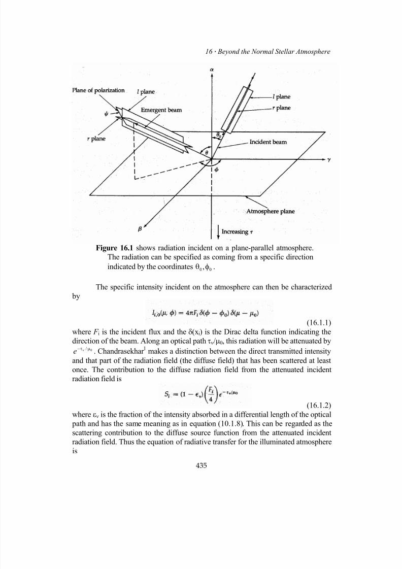
7/18/2019 The Fundamentals of Stellar Astrophysics - Collins G. W.
http://slidepdf.com/reader/full/the-fundamentals-of-stellar-astrophysics-collins-g-w 455/524
16 Beyond the Normal Stellar Atmosphere
Figure 16.1 shows radiation incident on a plane-parallel atmosphere.
The radiation can be specified as coming from a specific direction
indicated by the coordinates 00 ,φθ .
The specific intensity incident on the atmosphere can then be characterized
by
(16.1.1)
where F i is the incident flux and the δ(xi) is the Dirac delta function indicating the
direction of the beam. Along an optical path τν/µ0, this radiation will be attenuated by
. Chandrasekhar 0/µτ− νe1 makes a distinction between the direct transmitted intensity
and that part of the radiation field (the diffuse field) that has been scattered at least
once. The contribution to the diffuse radiation field from the attenuated incident
radiation field is
(16.1.2)
where εν is the fraction of the intensity absorbed in a differential length of the optical
path and has the same meaning as in equation (10.1.8). This can be regarded as the
scattering contribution to the diffuse source function from the attenuated incident
radiation field. Thus the equation of radiative transfer for the illuminated atmosphere
is
435
7/18/2019 The Fundamentals of Stellar Astrophysics - Collins G. W.
http://slidepdf.com/reader/full/the-fundamentals-of-stellar-astrophysics-collins-g-w 456/524
II Stellar Atmospheres
(16.1.3)
By applying the classical solution to the equation of transfer, we can generate an
integral equation for the diffuse field source function, as we did in (Section 10.1) so
that
(16.1.4)
This is a Schwarzschild-Milne integral equation of the same type as we
considered in Chapter 10 it and can be solved in the same manner. The only
difference is that the term that makes the equation inhomogeneous has been
augmented by the last term on the right in equation (16.1.4). Thus the presence of
incident radiation will even make a pure scattering atmosphere inhomogeneousand subject to a unique solution.
Modification of the Avrett-Krook Iteration Scheme for Incident
Radiation. Buerger 2 has solved this equation, using the ATLAS
atmosphere program for a variety of cases. He found that the standard Avrett-
Krook iteration scheme described in Section 11.4 would no longer lead to a
converged atmosphere. This is not surprising since the Eddington approximation
was used to obtain the specific perturbation formulas (see equations (12.4.17),
(12.4.25), and (12.4.29), and the approximation J(0) = ½F(0) will no longer be
correct. Buerger therefore adopted a modification of the Avrett-Krook scheme
due to Karp3
which replaces the ad hoc assumption of equations (12.4.14) and(12.4.20) with
(16.1.5)
which implies that
(16.1.6)
He continues by making the plausible assumption that perturbed flux variations have
the same frequency dependence as the zeroth-order flux variations so that
(16.1.7)
Following the same procedure as Karp, Buerger 2 finds the perturbation formulas for
τ(1) and T
(1) analogous to equations (12.4.21) and (12.4.29), respectively, to be
436
7/18/2019 The Fundamentals of Stellar Astrophysics - Collins G. W.
http://slidepdf.com/reader/full/the-fundamentals-of-stellar-astrophysics-collins-g-w 457/524
16 Beyond the Normal Stellar Atmosphere
(16.1.8)
where
(16.1.9)
While these equations do provide a convergent iteration algorithm, the rate of
convergence can be quite slow if the amount of incident radiation is large and differs
greatly from that which the illuminated star would have in the absence of incident
radiation.
If event that the incident flux has an energy distribution significantly
different from that of the illuminated star and large compared to the stellar flux, the
Eddington approximation will fail rather badly at some frequencies and in that part of
the atmosphere where the majority of the incident flux is absorbed. Under these
conditions, the Avrett-Krook iteration scheme will fail badly. Steps must be taken todirectly estimate those parameters obtained from the Eddington approximation. In
some instances it is possible to use results from a previous iteration.
Initial Temperature Distribution As with any iteration process, the closer
the initial guess, the faster a correct answer will be found. In Chapter 12, we
suggested that the model-making process could be initiated with the unilluminated
gray atmosphere temperature distribution in the absence of anything better. In the
case of incident radiation, such a choice will yield an initial temperature distribution
that departs rather badly from the correct one. It is tempting to suggest that a suitable
first guess could be obtained by merely scaling up the gray atmosphere temperature
distribution so as to include the incident flux in the definition of the effectivetemperature. Thus,
(16.1.10)
where T e(0) is the effective temperature and the temperature distribution is
437
7/18/2019 The Fundamentals of Stellar Astrophysics - Collins G. W.
http://slidepdf.com/reader/full/the-fundamentals-of-stellar-astrophysics-collins-g-w 458/524
II Stellar Atmospheres
(16.1.11)
Here q(τ) is the Hopf function defined in Chapter 10 [equation (10.2.33)]. For theEddington approximation,
(16.1.12)
However, there are two effects that make this a poor choice. First, if the sky of the
illuminated star is partially filled with the illuminating star, then much of the incident
radiation will enter at a grazing angle and preferentially heat the upper atmosphere.
This will raise the surface temperature over what would normally be expected from a
gray atmosphere and will flatten the temperature gradient. The more radiation that
enters from grazing angles, the greater this effect will be. This effect may also be
understood by considering how radiation can ultimately escape from the atmosphere.If the source of radiation is a close companion filling much of the sky, then a smaller
and smaller fraction of the sky is "black" representing directions of possible escape.
As the possible escape routes for photons diminish, the atmosphere will heat up since
the photons have nowhere to go. Anderson and Shu4 suggest that this may be
compensated for by
(16.1.13)
where Ω0 is the solid angle subtended by the source of radiation in the sky. As Ω0
→ 0, we recover the Eddington approximation's value for Q0. As Ω0 increases, so
does the value of Q0 implying that the surface temperature will rise relative to the
effective temperature. In the limit, the atmosphere will approach being isothermal.
The second aspect of incident radiation that can markedly affect the
temperature distribution is the frequency distribution. If the source of the incident
radiation contains a large quantity of ionizing radiation and is incident on a relatively
cool star, then almost all the radiation will be absorbed by the neutral hydrogen of
the upper reaches of the atmosphere, raising the local temperature significantly.
Similarly, if the incident radiation is highly penetrating radiation, such as x-rays, the
heating may occur much lower in the atmosphere. Since this energy must be
reradiated, this will result in a general elevation of the entire atmospheric
temperature distribution. This dependence of the atmosphere's temperature gradient
on the frequency distribution makes predicting the outcome extremely difficult since
the process is highly nonlinear. That is, the local heating may change the opacity,
which will in turn change the heating.
438

7/18/2019 The Fundamentals of Stellar Astrophysics - Collins G. W.
http://slidepdf.com/reader/full/the-fundamentals-of-stellar-astrophysics-collins-g-w 459/524
16 Beyond the Normal Stellar Atmosphere
In general, incident radiation will preferentially heat the surface layers and a
modification like that suggested by Anderson and Shu4 should be used for the initial
guess. An additional approach that some investigators have found useful is to slowly
increase the amount of incident radiation during the iteration processes from an
initially low value until the desired level is reached. The rate at which this can be
done depends on the spectral energy distribution of the incident radiation and always
tends to lengthen the convergence process.
b Effects of Incident Radiation on the Stellar Spectra
If the amount of this illuminating radiation is large, then the heating
of the upper atmosphere will cause a decrease in the temperature gradient. As we
have seen in Chapter 13, the strength of a pure absorption line will depend strongly
on the temperature gradient in the atmosphere. Thus, aside from changes in theenvironment of the radiation field caused by the external heating, we should expect
spectral lines to appear weaker simply because of the change in the source function
gradient. The change in line strength may cause an attendant change in the spectral
type. Although such changes should be phase dependent in a binary system, as
different aspects of the illuminated surface are presented to the observer, such
changes can be confused with the contribution to the light by the companion.
Although Milne5 first laid the foundations for estimating these effects in
1930, very little has been done in the intervening half-century to quantify them. The
atmospheres investigated by Buerger 2 did indeed show the general decrease in the
equivalent widths of the lines investigated due to heating of the higher levels of theatmosphere. However, his investigation was restricted to point-source illumination
which tends to minimize the upper-level heating of the atmosphere. A more realistic
modeling of the atmosphere of an early-type binary system by Kuzma6 showed that
the effects can be quite pronounced. Local changes of the atmospheric structure can
produce spectral changes of several spectral subtypes with the integrated effect being
as large as several tenths of a subtype with phase.
The effects of the incident radiation on the spectra become deeply
intertwined with the structure. The inclusion of metallic line blanketing brought
about a reversal of the effects of non-LTE on the hydrogen lines in that, in the upper
levels of the atmosphere, the departure coefficients for the first two levels ofhydrogen (b1 and b2) went from about 0.6 to 1.5 when the effects of line blanketing
were included. Similar anomalies occurred for the departure coefficients for the
higher levels as well. This fact largely serves to show the interconnectedness of the
phenomena which earlier we were able to consider separately. This results primarily
from the dominance of the interactions of the gas with the radiation field over
interactions with itself. That is, the radiation field and its departures from statistical
439
7/18/2019 The Fundamentals of Stellar Astrophysics - Collins G. W.
http://slidepdf.com/reader/full/the-fundamentals-of-stellar-astrophysics-collins-g-w 460/524
II Stellar Atmospheres
equilibrium begin to determine completely the statistical equilibrium of the gas. The
illuminating radiation has a spectral energy distribution significantly different from
that of the illuminating star, the departures from LTE may be very large indeed.
16.2 Transfer of Polarized Radiation
Even before the advent of classical electromagnetism in 1864 by James Clerk
Maxwell, it was generally accepted that light propagated by means of a transverse
wave. Any such wave would have a preferred plane of vibration as seen by an
observer, and any collection of such beams that exhibited such a preferred plane was
said to be polarized. In 1852, George Stokes7 showed that such a collection of light
beams could be characterized by four parameters that now bear his name. Normally a
heterogeneous collection of light beams will have planes of oscillation that are
randomly oriented as seen by an observer and will be called unpolarized. However,
should a light beam exhibit some degree of polarization, a measure of that polarization potentially contains a significant amount of information about the nature
of the source.
This property of light has been largely ignored in stellar astrophysics until
relatively recently. The probable reason can be found in the assumption that all stars
are spherical. Any such object would be completely symmetric about the line of sight
from the observer to the center of the apparent disk so if even local regions on the
surface emitted 100 percent polarized light, the symmetric orientation of their planes
of polarization would yield no net polarization to an observer viewing the integrated
light of the disk. However, many astrophysical processes produce polarized light,
and numerous stars are not spherical. In particular, eclipsing binary systems present asource of integrated light which is not symmetric about the line of sight. Early work
by Chandrasekhar 8,9
and Code10
implied that there might be measurable polarization
that would place significant constraints on the nature of the source. However, only
after the development of very sensitive detectors and the discovery of intrinsic
circular polarization in white dwarfs did intrinsic stellar polarization attract any great
interest. In the hope that this interest will continue to grow, we will discuss some of
the theoretical approaches to the problems posed by the transfer of polarized light.
a Representation of a Beam of Polarized Light and the Stokes
Parameters
Imagine a collection of largely uncorrelated electromagnetic waves
propagating in the same direction through space. The combined effect of these beams
can be obtained by adding the squares of the amplitudes of their oscillating electric
and magnetic vectors. If the waves were completely correlated as are those from a
laser, the amplitudes themselves would vectorially add directly. Indeed, the
representation of the addition of the squares of the amplitudes can be taken as a
440
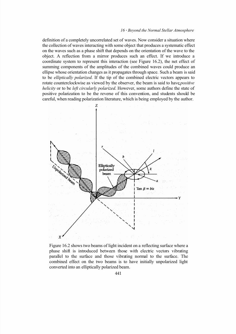
7/18/2019 The Fundamentals of Stellar Astrophysics - Collins G. W.
http://slidepdf.com/reader/full/the-fundamentals-of-stellar-astrophysics-collins-g-w 461/524
16 Beyond the Normal Stellar Atmosphere
definition of a completely uncorrelated set of waves. Now consider a situation where
the collection of waves interacting with some object that produces a systematic effect
on the waves such as a phase shift that depends on the orientation of the wave to the
object. A reflection from a mirror produces such an effect. If we introduce a
coordinate system to represent this interaction (see Figure 16.2), the net effect of
summing components of the amplitudes of the combined waves could produce an
ellipse whose orientation changes as it propagates through space. Such a beam is said
to be elliptically polarized . If the tip of the combined electric vectors appears to
rotate counterclockwise as viewed by the observer, the beam is said to have positive
helicity or to be left circularly polarized . However, some authors define the state of
positive polarization to be the reverse of this convention, and students should be
careful, when reading polarization literature, which is being employed by the author.
Figure 16.2 shows two beams of light incident on a reflecting surface where a
phase shift is introduced between those with electric vectors vibrating
parallel to the surface and those vibrating normal to the surface. The
combined effect on the two beams is to have initially unpolarized light
converted into an elliptically polarized beam.
441
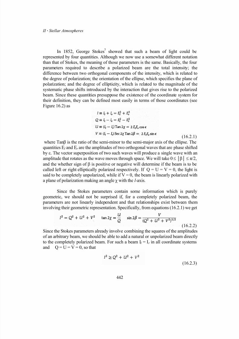
7/18/2019 The Fundamentals of Stellar Astrophysics - Collins G. W.
http://slidepdf.com/reader/full/the-fundamentals-of-stellar-astrophysics-collins-g-w 462/524
II Stellar Atmospheres
In 1852, George Stokes7 showed that such a beam of light could be
represented by four quantities. Although we now use a somewhat different notation
than that of Stokes, the meaning of those parameters is the same. Basically, the four
parameters required to describe a polarized beam are the total intensity; the
difference between two orthogonal components of the intensity, which is related to
the degree of polarization; the orientation of the ellipse, which specifies the plane of
polarization; and the degree of ellipticity, which is related to the magnitude of the
systematic phase shifts introduced by the interaction that gives rise to the polarized
beam. Since these quantities presuppose the existence of the coordinate system for
their definition, they can be defined most easily in terms of those coordinates (see
Figure 16.2) as
(16.2.1)
where Tanβ is the ratio of the semi-minor to the semi-major axis of the ellipse. The
quantities El and Er are the amplitudes of two orthogonal waves that are phase shifted
by ε. The vector superposition of two such waves will produce a single wave with an
amplitude that rotates as the wave moves through space. We will take 0 ≤ β ≤ π/2,
and the whether sign of β is positive or negative will determine if the beam is to be
called left or right elliptically polarized respectively. If Q = U = V = 0, the light is
said to be completely unpolarized, while if V = 0, the beam is linearly polarized with
a plane of polarization making an angle χ with the l-axis.
Since the Stokes parameters contain some information which is purely
geometric, we should not be surprised if, for a completely polarized beam, the
parameters are not linearly independent and that relationships exist between them
involving their geometric representation. Specifically, from equations (16.2.1) we get
(16.2.2)
Since the Stokes parameters already involve combining the squares of the amplitudes
of an arbitrary beam, we should be able to add a natural or unpolarized beam directlyto the completely polarized beam. For such a beam I l = Ir in all coordinate systems
and Q = U = V = 0, so that
(16.2.3)
442

7/18/2019 The Fundamentals of Stellar Astrophysics - Collins G. W.
http://slidepdf.com/reader/full/the-fundamentals-of-stellar-astrophysics-collins-g-w 463/524
16 Beyond the Normal Stellar Atmosphere
Thus for a collection of light beams, some of which may be polarized, all four Stokes
parameters are indeed linearly independent and must be specified to completely
characterize the beam.
It is clear from the definitions of the Stokes parameters that I and V are
invariant to a coordinate rotation about the axis of propagation while Q and U are
not. If we rotate the l-r coordinate frame through an angle φ in a counterclockwise
direction (see Figure 16.2), then
(16.2.4)
Since I and V are invariant to rotational transformations, we can write the general
rotation for the Stokes parameters in matrix-vector notation. If we define an intensity
vector to have components Ir
[I,Q,U,V] so that
(16.2.5)
then we can call the matrix the rotation matrix for the Stokes parameters. If we
choose a coordinate system so that Il is a maximum, then the degree of linear
polarization P is a useful parameter defined by
(16.2.6)where, since the l-r coordinate frame has been chosen so that the l -axis lies along this
direction of maximum intensity, U = 0.
It is also useful to linearly decompose the Stokes parameters I and Q into Il
and Ir so that
(16.2.7)
However, neither of these parameters is invariant to a coordinate rotation so that if
we denote a vector Ir
(Il ,Ir ,U,V) whose components are this different set of Stokes
parameters, then
(16.2.8)
where the rotation matrix for these Stokes parameters is
443

7/18/2019 The Fundamentals of Stellar Astrophysics - Collins G. W.
http://slidepdf.com/reader/full/the-fundamentals-of-stellar-astrophysics-collins-g-w 464/524
II Stellar Atmospheres
(16.2.9)
The rotation matrix L(φ ) can be obtained from equation (16.2.5) by
employing the definitions of I and Q in terms of I l and Ir in equation (16.2.7). Here
the angle φ is taken positively increasing for counterclockwise rotations. While this
definition is the opposite of that used by Chandrasekhar 1 (p. 26), it is the more
common notation for a rotational angle. The form of this rotation matrix is a little
different from that used to transform vectors because the quantities being
transformed are the squares of vector components rather than the components and
their composition law is different from that for vectors alone. However, the
transformation matrix does share the common group identities of the normal rotation
matrices so that
(16.2.10)
Finally, there is an additional way to conceptualize the Stokes parameters
that many have found useful. In general, a polarized beam of light can be imagined
as being composed of two orthogonally oscillating electric vectors bearing a relative
phase shift e with respect to one another. The vector sum of these two amplitudes
will be a vector whose tip traces out an elliptically helical spiral as the vector
propagates through space. We have defined the Stokes parameters in terms of the
projection of that spiral onto a plane normal to the direction of propagation.
However, we can also view them in terms of the motion of the vector through space.
The fact that the vector rotates results from the phase difference between the two
waves. If the phase difference were an odd multiple of π/2, then the wave would
spiral through space and would be said to contain a significant amount of circular
polarization. However, if the phase difference e were zero or a multiple of π, the tip
of the vector would merely oscillate in a plane whose orientation is determined by
the ratio of the amplitudes of the electric vectors in the original orthogonal
coordinate frame defining the beam, and the beam would be said to be linearly
polarized.
Since the Stokes parameters are intensity-like (i.e. they have they units of the
square of the electric field), one way to identify them is to take the outer (tensor)
product of the electric vector with itself. Such an electric vector will have
components El and Er so that the outer product will be
(16.2.11)
444

7/18/2019 The Fundamentals of Stellar Astrophysics - Collins G. W.
http://slidepdf.com/reader/full/the-fundamentals-of-stellar-astrophysics-collins-g-w 465/524
16 Beyond the Normal Stellar Atmosphere
Only three of these components are linearly independent, but the component Er itself
is made up of two linearly independent components Er cosε and Er sinε. Thus the
expansion of the term El Er leaves us with four intensity-like components which we
can identify with the Stokes parameters so that formally
(16.2.12)
Thus taking the outer product of a general electric vector provides an excellent
formalism for generating the Stokes parameters for that beam.
b Equations of Transfer for the Stokes Parameters
The intensity-like nature of the Stokes parameters that describe anarbitrarily polarized beam makes them additive. This and the linear nature of the
equation of radiative transfer ensures that we can write equations of transfer for each
of them. Thus, if the components of Ir
are the Stokes parameters, we can express this
result as a vector equation of radiative transfer that has the familiar form
(16.2.13)
As usual, all the problems in the equations of transfer are contained in the source
function. If we choose the intensity vector to have components Ir
[Il ,Ir ,U,V], then the
source function can be written as a vector whose components are S l , Sr , SU, and SV.Again, as we did with incident radiation, it is convenient to break up the radiation
field into the "diffuse" field consisting of photons that have interacted at least once
and the direct transmitted field that could originate from any incident radiation. We
concentrate initially on the diffuse field since, in the absence of incident radiation, it
exhibits axial symmetry about the normal to the atmosphere.
Nature of the Source Function for Polarized Radiation The source
function that appears in equation (16.2.13) is a vector quantity that must account for
all contributions to the four Stokes parameters from thermal and scattering processes.
Since thermal emission is by nature a random equilibrium process, we expect it to
make no contribution to the Stokes parameters U and V for these measure thedeparture of the radiation field from isotropy but now carry energy. In short, thermal
radiation is completely unpolarized. For the same reasons, the thermal radiation will
make an equal contribution to both Il and Ir . Therefore the thermal contribution to the
vector source function in equation (16.2.13) will have components
445
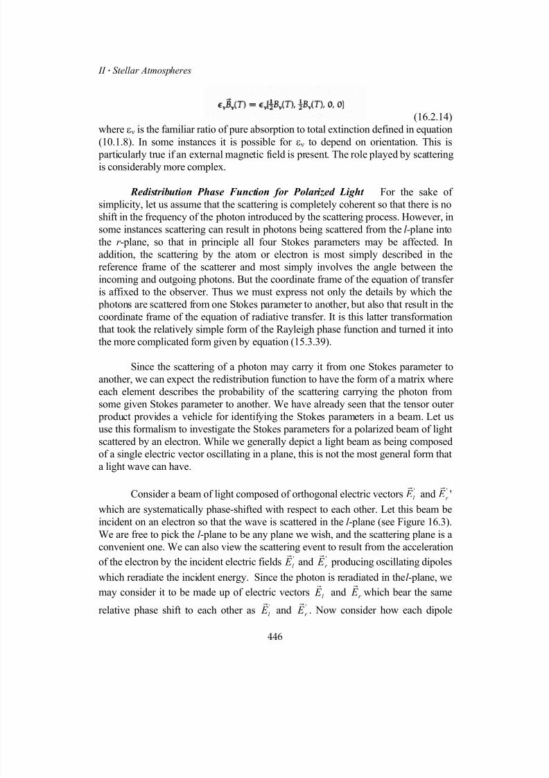
7/18/2019 The Fundamentals of Stellar Astrophysics - Collins G. W.
http://slidepdf.com/reader/full/the-fundamentals-of-stellar-astrophysics-collins-g-w 466/524
II Stellar Atmospheres
(16.2.14)
where εν is the familiar ratio of pure absorption to total extinction defined in equation
(10.1.8). In some instances it is possible for εν to depend on orientation. This is
particularly true if an external magnetic field is present. The role played by scattering
is considerably more complex.
Redistribution Phase Function for Polarized Light For the sake of
simplicity, let us assume that the scattering is completely coherent so that there is no
shift in the frequency of the photon introduced by the scattering process. However, in
some instances scattering can result in photons being scattered from the l- plane into
the r -plane, so that in principle all four Stokes parameters may be affected. In
addition, the scattering by the atom or electron is most simply described in the
reference frame of the scatterer and most simply involves the angle between the
incoming and outgoing photons. But the coordinate frame of the equation of transfer
is affixed to the observer. Thus we must express not only the details by which the
photons are scattered from one Stokes parameter to another, but also that result in the
coordinate frame of the equation of radiative transfer. It is this latter transformation
that took the relatively simple form of the Rayleigh phase function and turned it into
the more complicated form given by equation (15.3.39).
Since the scattering of a photon may carry it from one Stokes parameter to
another, we can expect the redistribution function to have the form of a matrix where
each element describes the probability of the scattering carrying the photon from
some given Stokes parameter to another. We have already seen that the tensor outer product provides a vehicle for identifying the Stokes parameters in a beam. Let us
use this formalism to investigate the Stokes parameters for a polarized beam of light
scattered by an electron. While we generally depict a light beam as being composed
of a single electric vector oscillating in a plane, this is not the most general form that
a light wave can have.
Consider a beam of light composed of orthogonal electric vectors and'
l E r
'
r E r
'
which are systematically phase-shifted with respect to each other. Let this beam be
incident on an electron so that the wave is scattered in the l -plane (see Figure 16.3).
We are free to pick the l -plane to be any plane we wish, and the scattering plane is a
convenient one. We can also view the scattering event to result from the acceleration
of the electron by the incident electric fields '
l E r
and '
r E r
producing oscillating dipoles
which reradiate the incident energy. Since the photon is reradiated in the l -plane, we
may consider it to be made up of electric vectors l E r
and r E r
which bear the same
relative phase shift to each other as '
l E r
and '
r E r
. Now consider how each dipole
446
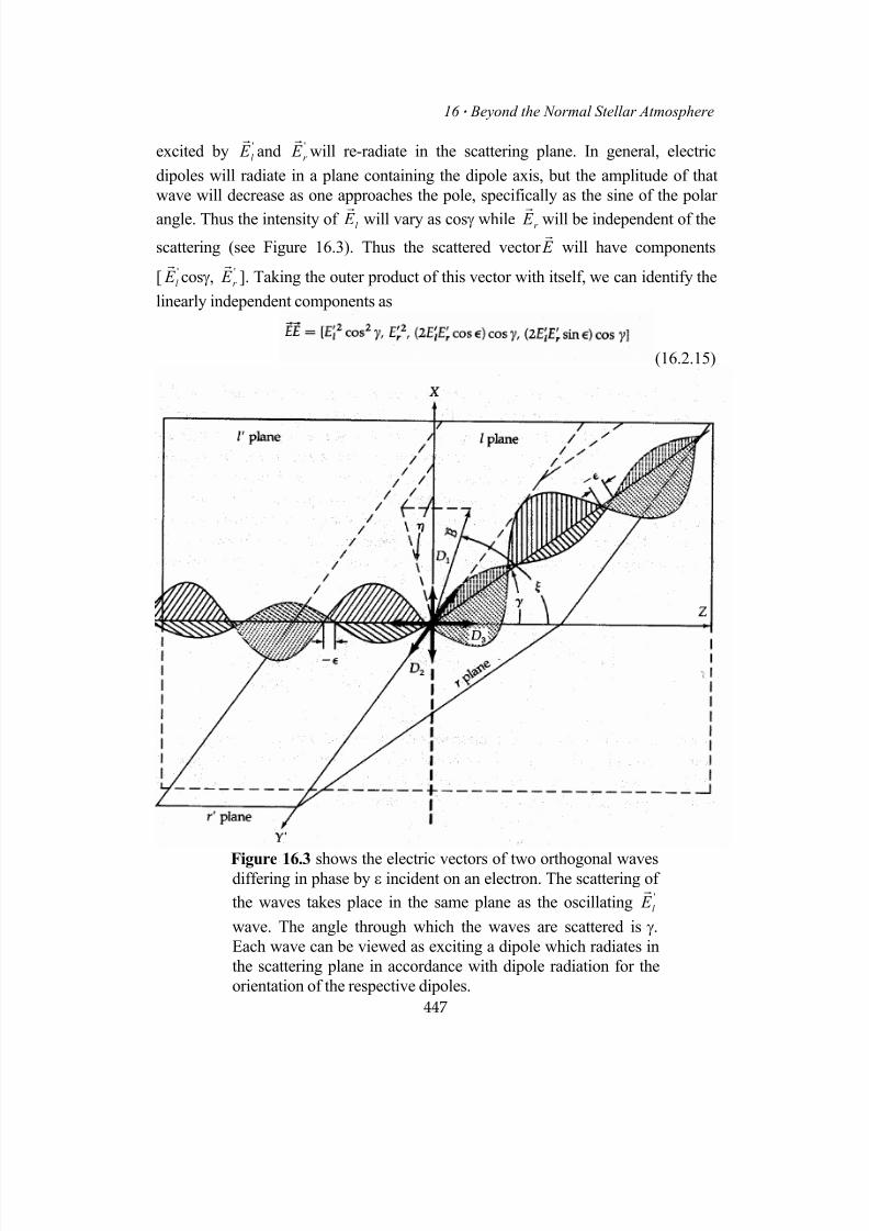
7/18/2019 The Fundamentals of Stellar Astrophysics - Collins G. W.
http://slidepdf.com/reader/full/the-fundamentals-of-stellar-astrophysics-collins-g-w 467/524
16 Beyond the Normal Stellar Atmosphere
excited by and'
l E r
'
r E r
will re-radiate in the scattering plane. In general, electric
dipoles will radiate in a plane containing the dipole axis, but the amplitude of that
wave will decrease as one approaches the pole, specifically as the sine of the polar
angle. Thus the intensity ofr
will vary as cosγ whilel E r E r
will be independent of the
scattering (see Figure 16.3). Thus the scattered vector E r
will have components
[ cosγ, ]. Taking the outer product of this vector with itself, we can identify the
linearly independent components as
'
l E r
'
r E r
(16.2.15)
447
Figure 16.3 shows the electric vectors of two orthogonal wavesdiffering in phase by ε incident on an electron. The scattering of
the waves takes place in the same plane as the oscillatingr
wave. The angle through which the waves are scattered is γ.
Each wave can be viewed as exciting a dipole which radiates in
the scattering plane in accordance with dipole radiation for the
orientation of the respective dipoles.
'
l E
7/18/2019 The Fundamentals of Stellar Astrophysics - Collins G. W.
http://slidepdf.com/reader/full/the-fundamentals-of-stellar-astrophysics-collins-g-w 468/524
II Stellar Atmospheres
Since the dipoles excited by the incident radiation do not reradiate in a plane
orthogonal to the exciting radiation, there can be no mixing of energy from the r -
plane to the l -plane or vice versa. Thus, in any scattering matrix for Stokes parameters, the four independent components of the beam given by equation
(16.2.15) must appear on the diagonal. In addition, one would expect a constant of
proportionality determined by the conservation of energy. Specifically, the total
energy of the incident beam must equal the total energy of radiation scattered
through all allowed scattering angles. Thus, factoring out the definitions of the
Stokes parameters from the components given in equation (16.2.15), we can write
(16.2.16)
where A0 is the constant of proportionality described above. By applying the
conservation of energy, A0 can be found to be 3/2. Thus the matrix in equation
(16.2.16) represents the transformation of Ir
[I'l , I' , U',V'] into Ir
[Il , Ir , U,V]. This
matrix is generally called the Rayleigh phase matrix and is
(16.2.17)
Here γ is the scattering angle between the incoming and outgoing photons.
The Stokes parameters in the scattering coordinate system will be given by the vector
components of the intensityr
[II l , Ir , U, V] where Il and Ir lie in the scattering plane
and perpendicular to it in a plane containing the outgoing photon (see Figure 16.3
and Figure 16.4). The equivalent matrix for scattering of the more common Stokes
vectorr
'[I', Q', U', V'] tor
[I, Q, U, V] can be obtained by transforming equation
(16.2.17) in accordance with the definitions given in equation (16.2.7) so that
I I
(16.2.18)
To be useful for radiative transfer, these matrices must now expressed in the
observer's coordinate frame by multiplying them by the appropriate rotation matrix
as given in equation (16.2.9) or (16.2.5).
448

7/18/2019 The Fundamentals of Stellar Astrophysics - Collins G. W.
http://slidepdf.com/reader/full/the-fundamentals-of-stellar-astrophysics-collins-g-w 469/524
16 Beyond the Normal Stellar Atmosphere
Figure 16.4 shows the coordinate frame for a single scattering event
and the orientation of the polarized components.
The final transformation to the coordinate system of the equation of transfer
is moderately complicated (see Chandrasekhar 1, pp.37- 41) and I will simply quote
the result for equation (16.2.17), using his notation.
(16.2.19)
where
449
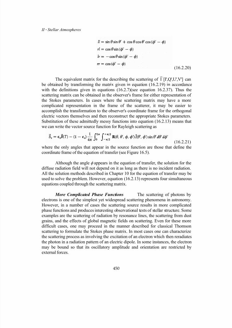
7/18/2019 The Fundamentals of Stellar Astrophysics - Collins G. W.
http://slidepdf.com/reader/full/the-fundamentals-of-stellar-astrophysics-collins-g-w 470/524
II Stellar Atmospheres
(16.2.20)
The equivalent matrix for the describing the scattering of 'Ir
[I',Q',U',V'] can
be obtained by transforming the matrix given in equation (16.2.19) in accordance
with the definitions given in equations (16.2.7)(see equation 16.2.37). Thus the
scattering matrix can be obtained in the observer's frame for either representation of
the Stokes parameters. In cases where the scattering matrix may have a more
complicated representation in the frame of the scatterer, it may be easier to
accomplish the transformation to the observer's coordinate frame for the orthogonal
electric vectors themselves and then reconstruct the appropriate Stokes parameters.Substitution of these admittedly messy functions into equation (16.2.13) means that
we can write the vector source function for Rayleigh scattering as
(16.2.21)
where the only angles that appear in the source function are those that define the
coordinate frame of the equation of transfer (see Figure 16.5).
Although the angle φ appears in the equation of transfer, the solution for the
diffuse radiation field will not depend on it as long as there is no incident radiation.
All the solution methods described in Chapter 10 for the equation of transfer may beused to solve the problem. However, equation (16.2.13) represents four simultaneous
equations coupled through the scattering matrix.
More Complicated Phase Functions The scattering of photons by
electrons is one of the simplest yet widespread scattering phenomena in astronomy.
However, in a number of cases the scattering source results in more complicated
phase functions and produces interesting observational tests of stellar structure. Some
examples are the scattering of radiation by resonance lines, the scattering from dust
grains, and the effects of global magnetic fields on scattering. Even for these more
difficult cases, one may proceed in the manner described for classical Thomson
scattering to formulate the Stokes phase matrix. In most cases one can characterizethe scattering process as involving the excitation of an electron which then reradiates
the photon in a radiation pattern of an electric dipole. In some instances, the electron
may be bound so that its oscillatory amplitude and orientation are restricted by
external forces.
450

7/18/2019 The Fundamentals of Stellar Astrophysics - Collins G. W.
http://slidepdf.com/reader/full/the-fundamentals-of-stellar-astrophysics-collins-g-w 471/524
16 Beyond the Normal Stellar Atmosphere
Figure 16.5 shows the scattering of a photon in the 'observer's'
coordinate frame. The Z-axis points in the direction of the
normal to the atmosphere and cosθ = µ. The angle φ is the
azimuthal angle and now is a parameter of the problem.
As long as the physics of this restriction is understood, the re-radiation can be
characterized and the nature of the scattered wave described. The tensor outer
product of that wave will then describe the scattering behavior of the Stokes
parameters of the incident wave. As long as one is careful to keep track of the plane
of origin of the various scattered electric vector amplitudes as well as the planes in
which they are radiated, the contribution of the elements of the tensor outer product
of the scattered beam with itself to the Stokes parameters of the scattered beam is
unique.
For example, consider the case of Thomson scattering by an electron in amacroscopic magnetic field. The motion of the electron produced by the incident
electric fields will subject the electron to Lorentz forces orthogonal to both the
magnetic field and the induced velocity. This will cause the electron to oscillate and
generate a second "electric dipole" whose radiation is added to that of the first. This
allows energy to be transferred from one plane of polarization to another by an
amount that depends on the magnetic field strength and orientation. This will have a
451
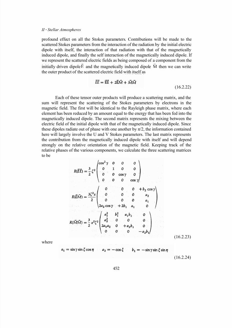
7/18/2019 The Fundamentals of Stellar Astrophysics - Collins G. W.
http://slidepdf.com/reader/full/the-fundamentals-of-stellar-astrophysics-collins-g-w 472/524
II Stellar Atmospheres
profound effect on all the Stokes parameters. Contributions will be made to the
scattered Stokes parameters from the interaction of the radiation by the initial electric
dipole with itself, the interaction of that radiation with that of the magnetically
induced dipole, and finally the self interaction of the magnetically induced dipole. If
we represent the scattered electric fields as being composed of a component from the
initially driven dipoleEr
and the magnetically induced dipole Mr
then we can write
the outer product of the scattered electric field with itself as
(16.2.22)
Each of these tensor outer products will produce a scattering matrix, and the
sum will represent the scattering of the Stokes parameters by electrons in the
magnetic field. The first will be identical to the Rayleigh phase matrix, where each
element has been reduced by an amount equal to the energy that has been fed into themagnetically induced dipole. The second matrix represents the mixing between the
electric field of the initial dipole with that of the magnetically induced dipole. Since
these dipoles radiate out of phase with one another by π/2, the information contained
here will largely involve the U and V Stokes parameters. The last matrix represents
the contribution from the magnetically induced dipole with itself and will depend
strongly on the relative orientation of the magnetic field. Keeping track of the
relative phases of the various components, we calculate the three scattering matrices
to be
(16.2.23)
where
(16.2.24)
452

7/18/2019 The Fundamentals of Stellar Astrophysics - Collins G. W.
http://slidepdf.com/reader/full/the-fundamentals-of-stellar-astrophysics-collins-g-w 473/524
16 Beyond the Normal Stellar Atmosphere
The coordinates of the magnetic field with respect to the scattering plane of the
incident photon are given by η and the polar angle ξ, respectively. The strength of
the magnetic field is contained in the parameter x so that
(16.2.25)
If we require that the scattering be conservative, then since energy is required to
generate those oscillations, the amplitude of the incident electric vector will be
reduced in order to supply the energy to excite them. However, the energy that
excites the dipoles must be equal to the energy of the incident beam so that
(16.2.26)
where ξ is the angle between the electric vector and the magnetic field. If we
assume that the magnitude of the electric vector is reduced by ζ, then
(16.2.27)
where
(16.2.28)r
If we assume that x<<1, then Er
will remain nearly parallel to E ' and we may expand
equations (16.2.27), and (16.2.28) to give
(16.2.29)
and we may write
(16.2.30)
For zero magnetic field, one recovers the Rayleigh phase matrix. As the
strength of the field increases, the contribution of the second two matrices
increases and normal electron scattering decreases. As the gyro-frequency ωc is
reached, the motion of the electron becomes circular and significant circular
polarization is introduced to the beam along the direction of the magnetic field.Since we have ignored the resonance that occurs at the gyro-frequency (that is,
x=1), these results are only approximate. For the scattering of natural light,r
[½I,½I,0,0], the strength of the components from the Rayleigh matrix are
reduced while the R( Mrr
) contributes solely to the V stokes parameter, indicating
that the beam will be circularly polarized when scattered along the magnetic field.
I
E
453
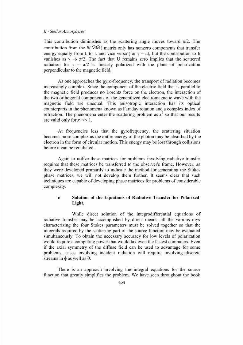
7/18/2019 The Fundamentals of Stellar Astrophysics - Collins G. W.
http://slidepdf.com/reader/full/the-fundamentals-of-stellar-astrophysics-collins-g-w 474/524
II Stellar Atmospheres
This contribution diminishes as the scattering angle moves toward π/2. The
contribution from the R( Mrr
) matrix only has nonzero components that transfer
energy equally from I
M
l to Ir and vice versa (for γ = π), but the contribution to Il
vanishes as γ → π/2. The fact that U remains zero implies that the scatteredradiation for γ = π/2 is linearly polarized with the plane of polarization
perpendicular to the magnetic field.
As one approaches the gyro-frequency, the transport of radiation becomes
increasingly complex. Since the component of the electric field that is parallel to
the magnetic field produces no Lorentz force on the electron, the interaction of
the two orthogonal components of the generalized electromagnetic wave with the
magnetic field are unequal. This anisotropic interaction has its optical
counterparts in the phenomena known as Faraday rotation and a complex index of
refraction. The phenomena enter the scattering problem as x2 so that our results
are valid only for x << 1.
At frequencies less that the gyrofrequency, the scattering situation
becomes more complex as the entire energy of the photon may be absorbed by the
electron in the form of circular motion. This energy may be lost through collisions
before it can be reradiated.
Again to utilize these matrices for problems involving radiative transfer
requires that these matrices be transferred to the observer's frame. However, as
they were developed primarily to indicate the method for generating the Stokes
phase matrices, we will not develop them further. It seems clear that such
techniques are capable of developing phase matrices for problems of considerablecomplexity.
c Solution of the Equations of Radiative Transfer for Polarized
Light.
While direct solution of the integrodifferential equations of
radiative transfer may be accomplished by direct means, all the various rays
characterizing the four Stokes parameters must be solved together so that the
integrals required by the scattering part of the source function may be evaluated
simultaneously. To obtain the necessary accuracy for low levels of polarization
would require a computing power that would tax even the fastest computers. Evenif the axial symmetry of the diffuse field can be used to advantage for some
problems, cases involving incident radiation will require involving discrete
streams in φ as well as θ.
There is an approach involving the integral equations for the source
function that greatly simplifies the problem. We have seen throughout the book
454
7/18/2019 The Fundamentals of Stellar Astrophysics - Collins G. W.
http://slidepdf.com/reader/full/the-fundamentals-of-stellar-astrophysics-collins-g-w 475/524
16 Beyond the Normal Stellar Atmosphere
that the development of Schwarzschild-Milne equations for the source function
always produced equations that involved moments of the radiation field, usually
the mean intensity J. As long as the redistribution function can be expressed as a
finite series involving tesseral harmonics of θ and φ , the source function can be
expressed in terms of simple functions of θ and φ which multiply various
moments of the radiation field that depend on depth only. As we did in Chapter 9,
it will then be possible to generate Schwarzschild-Milne-like equations for these
moments that depend on depth only. Indeed, since a moment of a radiation field
cannot depend on angle, by definition, this effectively separates the angular
dependence of the radiation field from the depth dependence. This is true even for
the case of incident radiation. The solution of these equations will then yield the
source function at all depths which, together with the classical solution for the
equation of transfer, will provide a complete description of the radiation field in
all four Stokes parameters. This conceptually simple approach becomes rather
algebraically complicated in practice, even for the relatively simple case ofRayleigh scattering.
The general case of this problem has been worked out by Collins11
and
more succinctly by Collins and Buerger 12
and we will only quote the results. The
source functions for nongray Rayleigh scattering can be written as
(16.2.31)
where the moments of the radiation field X(τ), Y(τ), Z(τ), M(τ), P(τ), and W(τ)
depend on depth alone and satisfy these integral equations:
455
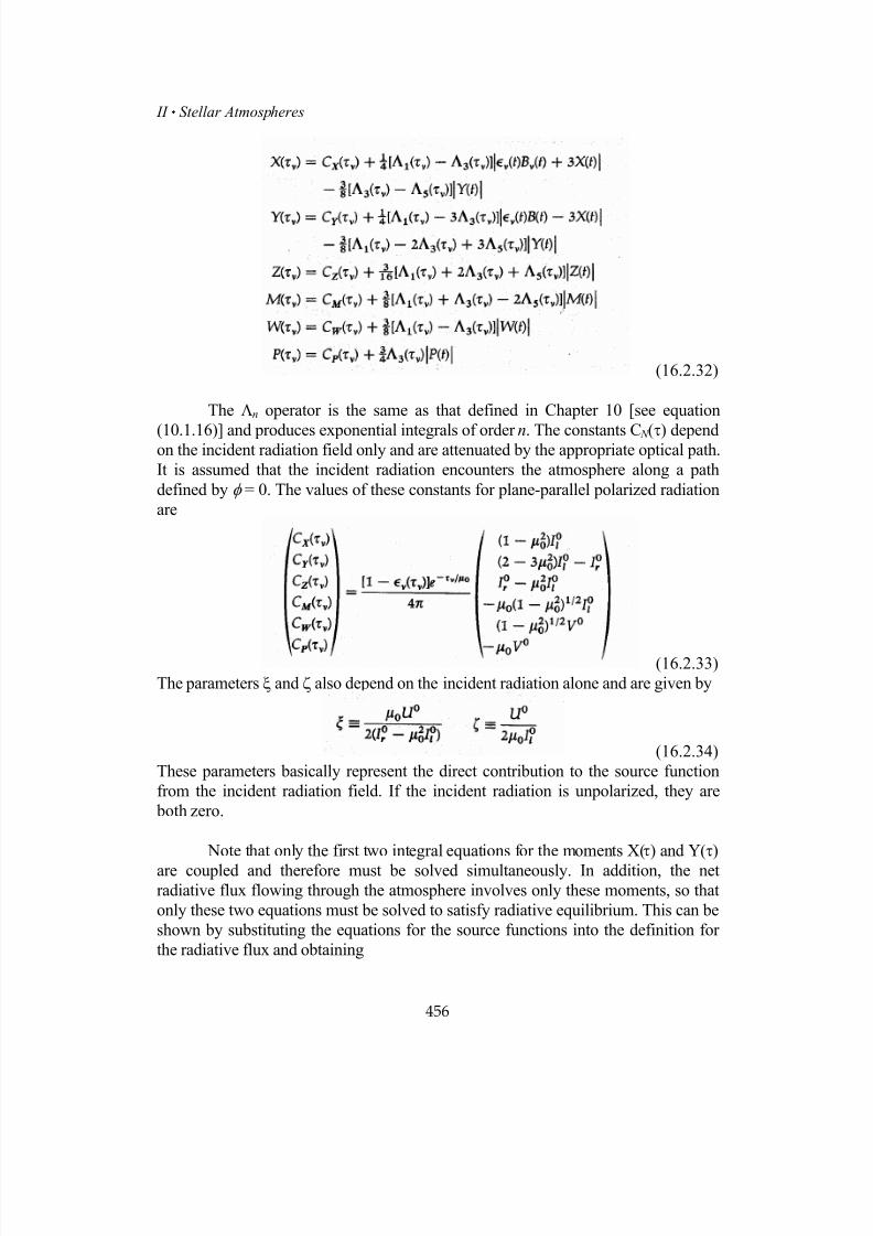
7/18/2019 The Fundamentals of Stellar Astrophysics - Collins G. W.
http://slidepdf.com/reader/full/the-fundamentals-of-stellar-astrophysics-collins-g-w 476/524
II Stellar Atmospheres
(16.2.32)
The Λn operator is the same as that defined in Chapter 10 [see equation
(10.1.16)] and produces exponential integrals of order n. The constants C N (τ) dependon the incident radiation field only and are attenuated by the appropriate optical path.
It is assumed that the incident radiation encounters the atmosphere along a path
defined by φ = 0. The values of these constants for plane-parallel polarized radiation
are
(16.2.33)
The parameters ξ and ζ also depend on the incident radiation alone and are given by
(16.2.34)
These parameters basically represent the direct contribution to the source function
from the incident radiation field. If the incident radiation is unpolarized, they are
both zero.
Note that only the first two integral equations for the moments X(τ) and Y(τ)
are coupled and therefore must be solved simultaneously. In addition, the netradiative flux flowing through the atmosphere involves only these moments, so that
only these two equations must be solved to satisfy radiative equilibrium. This can be
shown by substituting the equations for the source functions into the definition for
the radiative flux and obtaining
456
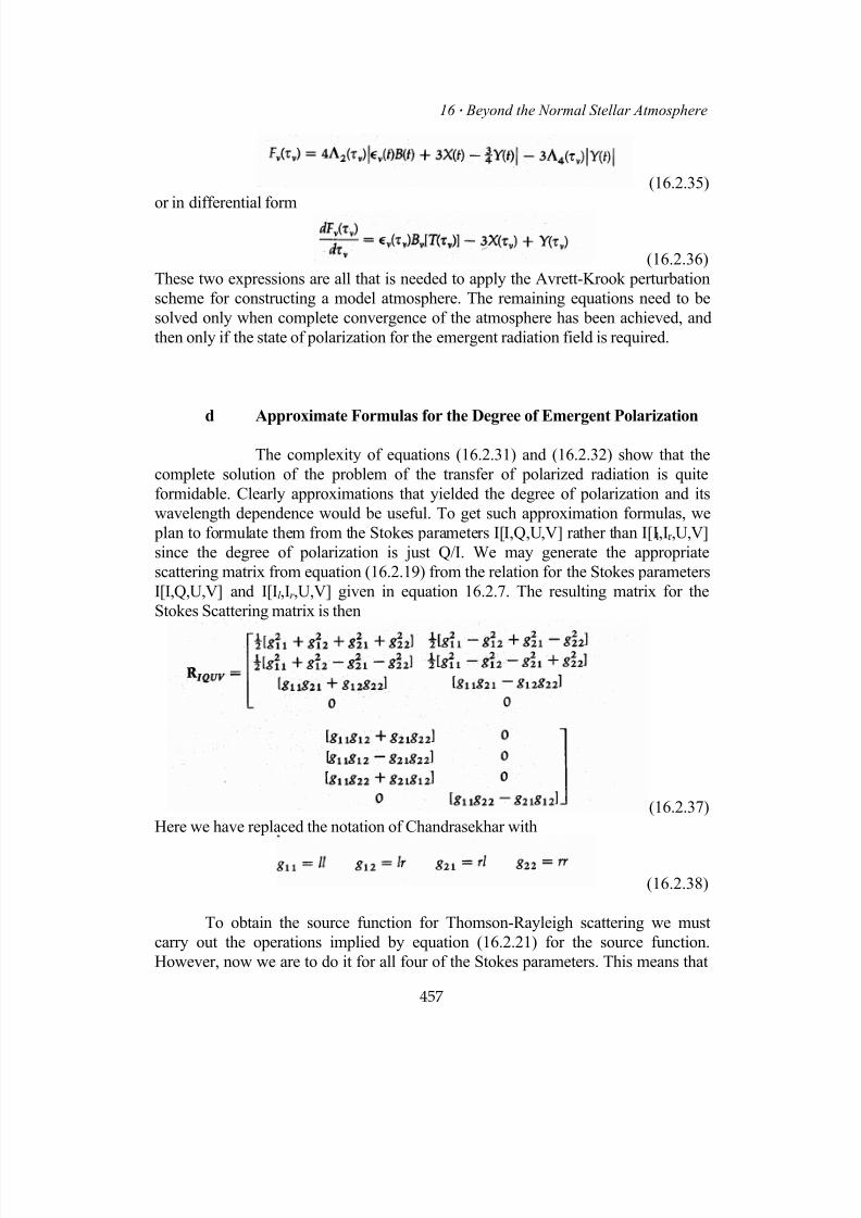
7/18/2019 The Fundamentals of Stellar Astrophysics - Collins G. W.
http://slidepdf.com/reader/full/the-fundamentals-of-stellar-astrophysics-collins-g-w 477/524
16 Beyond the Normal Stellar Atmosphere
(16.2.35)
or in differential form
(16.2.36)
These two expressions are all that is needed to apply the Avrett-Krook perturbation
scheme for constructing a model atmosphere. The remaining equations need to be
solved only when complete convergence of the atmosphere has been achieved, and
then only if the state of polarization for the emergent radiation field is required.
d Approximate Formulas for the Degree of Emergent Polarization
The complexity of equations (16.2.31) and (16.2.32) show that the
complete solution of the problem of the transfer of polarized radiation is quite
formidable. Clearly approximations that yielded the degree of polarization and its
wavelength dependence would be useful. To get such approximation formulas, we
plan to formulate them from the Stokes parameters I[I,Q,U,V] rather than I[Il,Ir ,U,V]
since the degree of polarization is just Q/I. We may generate the appropriate
scattering matrix from equation (16.2.19) from the relation for the Stokes parameters
I[I,Q,U,V] and I[Il ,Ir ,U,V] given in equation 16.2.7. The resulting matrix for the
Stokes Scattering matrix is then
(16.2.37)
Here we have replaced the notation of Chandrasekhar with
(16.2.38)
To obtain the source function for Thomson-Rayleigh scattering we must
carry out the operations implied by equation (16.2.21) for the source function.
However, now we are to do it for all four of the Stokes parameters. This means that
457

7/18/2019 The Fundamentals of Stellar Astrophysics - Collins G. W.
http://slidepdf.com/reader/full/the-fundamentals-of-stellar-astrophysics-collins-g-w 478/524
II Stellar Atmospheres
we shall integrate all elements of the scattering matrix over φ ' and θ'. However, we
know that the geometry of the plane parallel atmosphere means that the solution can
have no φ -dependence so that all odd functions of φ ' must vanish as well as sin2φ '.
Similarly the resulting source function can have no explicit φ -dependence. Also theelements of R [I,Q,U,V] contain a limited number of squares and products of the g ijs.
If we simply average these quantities over φ ' we get
(16.2.39)
Integration of these terms over θ' will then yield familiar moments of the Stokes parameters such as J and K (Section 9.3). If we let the subscript P stand for the
different Stokes parameters, then expressing the product of the g ijs in equation
(16.2.39) and the Stokes vector in terms of the moments of the Stokes parameters
yields
(16.2.40)
Substituting these average values into the respective elements of equation (16.2.19)
we can calculate the scattering fraction of the source functions for the Stokes
parameters. Adding the contribution to the I-source function from thermal emission
we can then write the source functions for all the Stokes parameters as
458

7/18/2019 The Fundamentals of Stellar Astrophysics - Collins G. W.
http://slidepdf.com/reader/full/the-fundamentals-of-stellar-astrophysics-collins-g-w 479/524
16 Beyond the Normal Stellar Atmosphere
(16.2.41)
where as before
(16.2.42)For an isotropic radiation field such as one could expect deep in the star that
JI = 3K I and JQ = K Q = 0 since there is no preferred plane in which to measure Q.
Under these conditions all fluxes vanish and the source functions become
(16.2.43)
which is the expected result for isotropic scattering and is consistent with an isotropic
radiation field.
For anisotropic scattering the source function is no longer independent of θ.
However, the θ-dependent terms depend on a collection of moments that measure thedeparture of the radiation field from isotropy. For a one dimensional beam JQ = K Q,
while for an isotropic radiation field JI = 3K I. This is true for both SI and SQ. Indeed,
the coefficient of the angular term is the same for both source functions. The fact that
SU is zero means that U is zero throughout the atmosphere. This result is not
surprising as for U to be non-zero would imply that polarization would have to have
a maximum in some plane other than that containing the normal to the atmosphere
and the observer (or one perpendicular to it). From symmetry, there can be no such
plane and hence U must be zero everywhere. We are now in a position to generate
integral equations for quantities that will explicitly determine the variation of the
source functions with depth.
Approximation of S Q in the Upper Atmosphere To begin our analysis of
the polarization to be expected from a stellar atmosphere, let us consider the
complete source functions for such an atmosphere. These can be written as
459
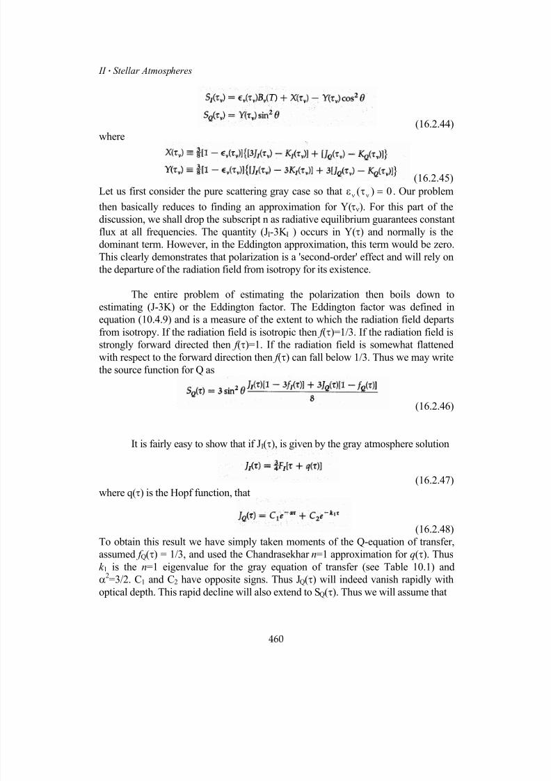
7/18/2019 The Fundamentals of Stellar Astrophysics - Collins G. W.
http://slidepdf.com/reader/full/the-fundamentals-of-stellar-astrophysics-collins-g-w 480/524
II Stellar Atmospheres
(16.2.44)
where
(16.2.45)
Let us first consider the pure scattering gray case so that 0)( =τε νν . Our problem
then basically reduces to finding an approximation for Y(τν). For this part of the
discussion, we shall drop the subscript n as radiative equilibrium guarantees constant
flux at all frequencies. The quantity (JI-3K I ) occurs in Y(τ) and normally is the
dominant term. However, in the Eddington approximation, this term would be zero.
This clearly demonstrates that polarization is a 'second-order' effect and will rely on
the departure of the radiation field from isotropy for its existence.
The entire problem of estimating the polarization then boils down to
estimating (J-3K) or the Eddington factor. The Eddington factor was defined in
equation (10.4.9) and is a measure of the extent to which the radiation field departs
from isotropy. If the radiation field is isotropic then f (τ)=1/3. If the radiation field is
strongly forward directed then f (τ)=1. If the radiation field is somewhat flattened
with respect to the forward direction then f (τ) can fall below 1/3. Thus we may write
the source function for Q as
(16.2.46)
It is fairly easy to show that if JI(τ), is given by the gray atmosphere solution
(16.2.47)
where q(τ) is the Hopf function, that
(16.2.48)
To obtain this result we have simply taken moments of the Q-equation of transfer,
assumed f Q(τ) = 1/3, and used the Chandrasekhar n=1 approximation for q(τ). Thus
k 1 is the n=1 eigenvalue for the gray equation of transfer (see Table 10.1) and
α2=3/2. C1 and C2 have opposite signs. Thus JQ(τ) will indeed vanish rapidly with
optical depth. This rapid decline will also extend to SQ(τ). Thus we will assume that
460
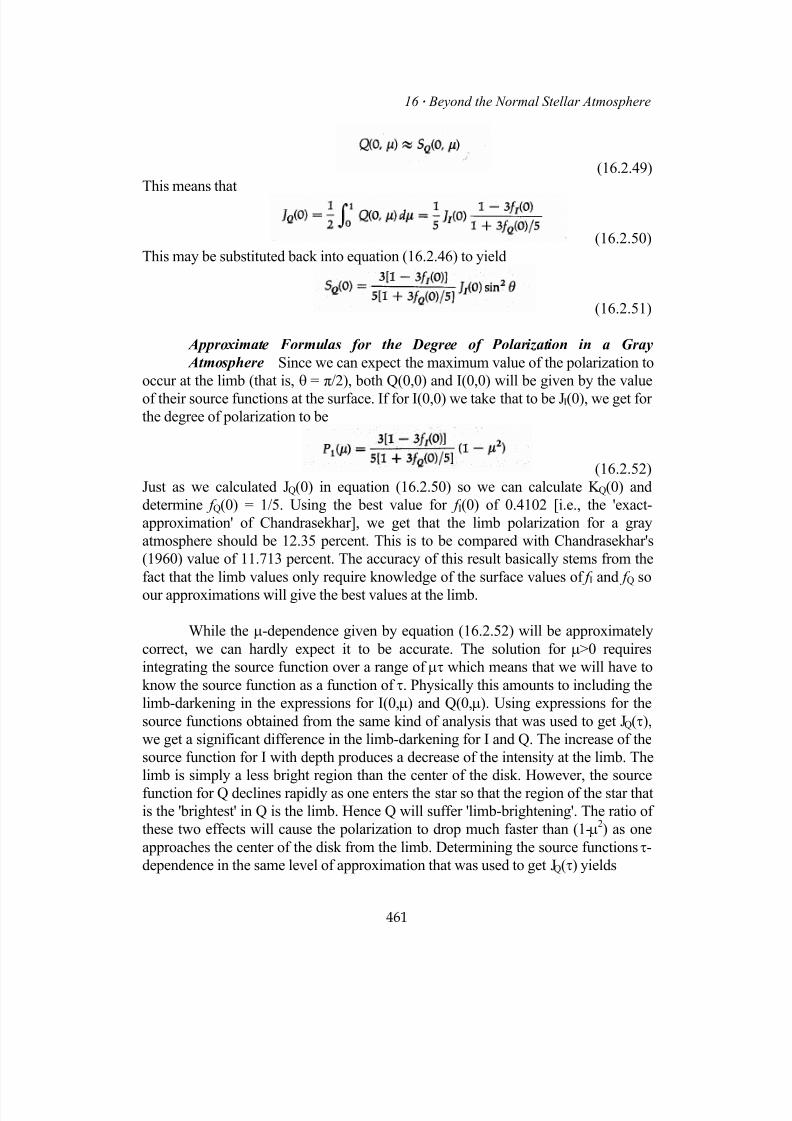
7/18/2019 The Fundamentals of Stellar Astrophysics - Collins G. W.
http://slidepdf.com/reader/full/the-fundamentals-of-stellar-astrophysics-collins-g-w 481/524
16 Beyond the Normal Stellar Atmosphere
(16.2.49)
This means that
(16.2.50)
This may be substituted back into equation (16.2.46) to yield
(16.2.51)
Approximate Formulas for the Degree of Polarization in a Gray
Atmosphere Since we can expect the maximum value of the polarization to
occur at the limb (that is, θ = π/2), both Q(0,0) and I(0,0) will be given by the value
of their source functions at the surface. If for I(0,0) we take that to be JI(0), we get for
the degree of polarization to be
(16.2.52)
Just as we calculated JQ(0) in equation (16.2.50) so we can calculate K Q(0) and
determine f Q(0) = 1/5. Using the best value for f I(0) of 0.4102 [i.e., the 'exact-
approximation' of Chandrasekhar], we get that the limb polarization for a gray
atmosphere should be 12.35 percent. This is to be compared with Chandrasekhar's
(1960) value of 11.713 percent. The accuracy of this result basically stems from the
fact that the limb values only require knowledge of the surface values of f I and f Q so
our approximations will give the best values at the limb.
While the µ-dependence given by equation (16.2.52) will be approximately
correct, we can hardly expect it to be accurate. The solution for µ>0 requires
integrating the source function over a range of µτ which means that we will have to
know the source function as a function of τ. Physically this amounts to including the
limb-darkening in the expressions for I(0,µ) and Q(0,µ). Using expressions for the
source functions obtained from the same kind of analysis that was used to get JQ(τ),
we get a significant difference in the limb-darkening for I and Q. The increase of the
source function for I with depth produces a decrease of the intensity at the limb. The
limb is simply a less bright region than the center of the disk. However, the source
function for Q declines rapidly as one enters the star so that the region of the star that
is the 'brightest' in Q is the limb. Hence Q will suffer 'limb-brightening'. The ratio of
these two effects will cause the polarization to drop much faster than (1-µ2) as one
approaches the center of the disk from the limb. Determining the source functions τ-
dependence in the same level of approximation that was used to get JQ(τ) yields
461
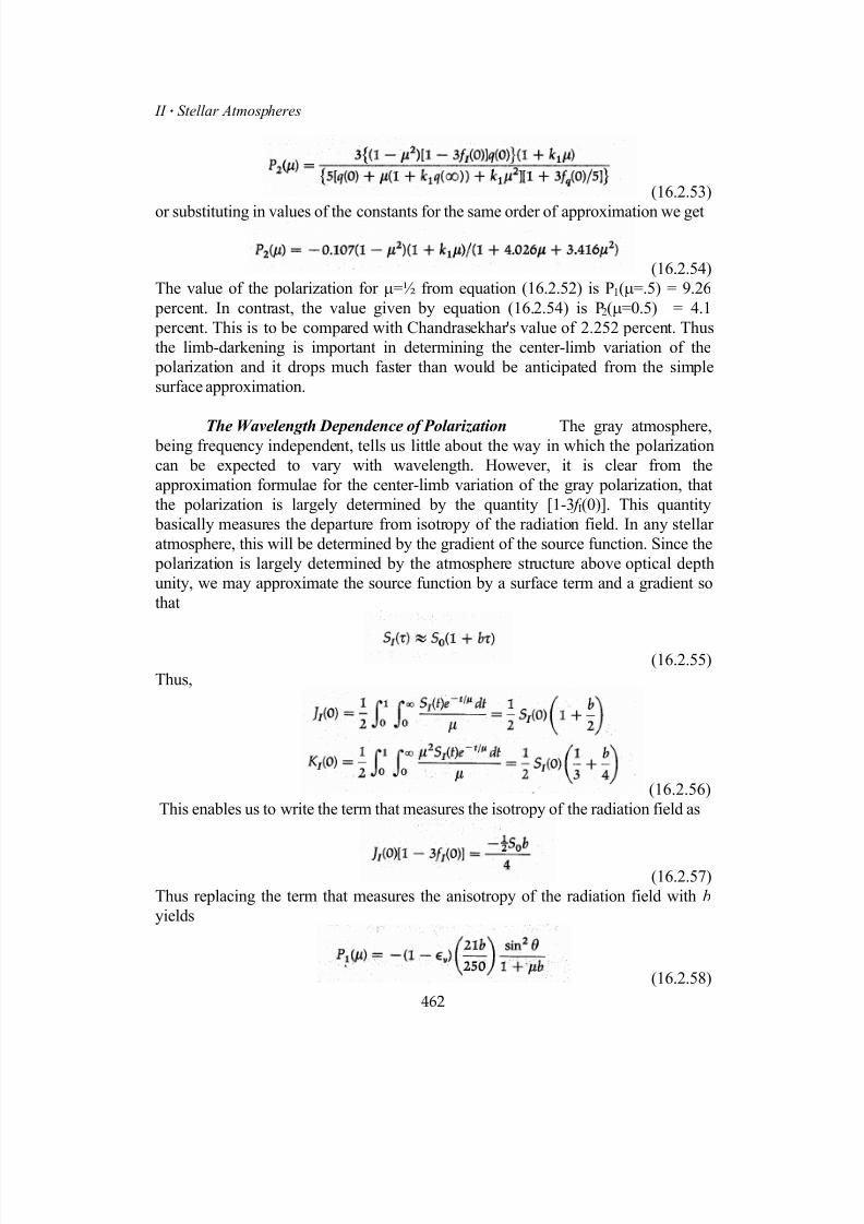
7/18/2019 The Fundamentals of Stellar Astrophysics - Collins G. W.
http://slidepdf.com/reader/full/the-fundamentals-of-stellar-astrophysics-collins-g-w 482/524
II Stellar Atmospheres
(16.2.53)
or substituting in values of the constants for the same order of approximation we get
(16.2.54)
The value of the polarization for µ=½ from equation (16.2.52) is P1(µ=.5) = 9.26
percent. In contrast, the value given by equation (16.2.54) is P2(µ=0.5) = 4.1
percent. This is to be compared with Chandrasekhar's value of 2.252 percent. Thus
the limb-darkening is important in determining the center-limb variation of the
polarization and it drops much faster than would be anticipated from the simple
surface approximation.
The Wavelength Dependence of Polarization The gray atmosphere, being frequency independent, tells us little about the way in which the polarization
can be expected to vary with wavelength. However, it is clear from the
approximation formulae for the center-limb variation of the gray polarization, that
the polarization is largely determined by the quantity [1-3 f I(0)]. This quantity
basically measures the departure from isotropy of the radiation field. In any stellar
atmosphere, this will be determined by the gradient of the source function. Since the
polarization is largely determined by the atmosphere structure above optical depth
unity, we may approximate the source function by a surface term and a gradient so
that
(16.2.55)
Thus,
(16.2.56)
This enables us to write the term that measures the isotropy of the radiation field as
(16.2.57)
Thus replacing the term that measures the anisotropy of the radiation field with b
yields
(16.2.58)
462
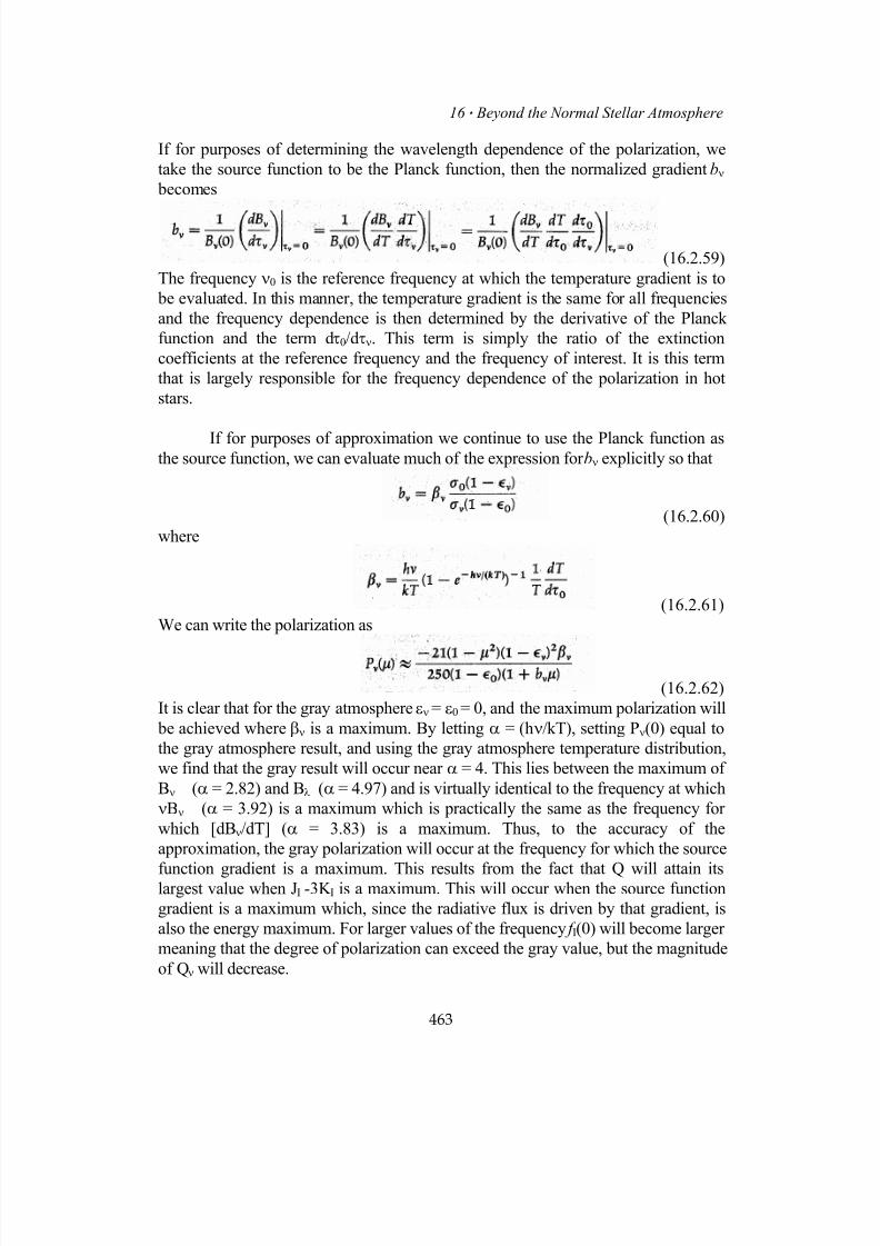
7/18/2019 The Fundamentals of Stellar Astrophysics - Collins G. W.
http://slidepdf.com/reader/full/the-fundamentals-of-stellar-astrophysics-collins-g-w 483/524
16 Beyond the Normal Stellar Atmosphere
If for purposes of determining the wavelength dependence of the polarization, we
take the source function to be the Planck function, then the normalized gradient bν
becomes
(16.2.59)
The frequency ν0 is the reference frequency at which the temperature gradient is to
be evaluated. In this manner, the temperature gradient is the same for all frequencies
and the frequency dependence is then determined by the derivative of the Planck
function and the term dτ0/dτν. This term is simply the ratio of the extinction
coefficients at the reference frequency and the frequency of interest. It is this term
that is largely responsible for the frequency dependence of the polarization in hot
stars.
If for purposes of approximation we continue to use the Planck function asthe source function, we can evaluate much of the expression for bν explicitly so that
(16.2.60)
where
(16.2.61)
We can write the polarization as
(16.2.62)
It is clear that for the gray atmosphere εν = ε0 = 0, and the maximum polarization will
be achieved where βν is a maximum. By letting α = (hν/kT), setting Pν(0) equal to
the gray atmosphere result, and using the gray atmosphere temperature distribution,
we find that the gray result will occur near α = 4. This lies between the maximum of
Bν (α = 2.82) and Bλ (α = 4.97) and is virtually identical to the frequency at which
νBν (α = 3.92) is a maximum which is practically the same as the frequency for
which [dBν/dT] (α = 3.83) is a maximum. Thus, to the accuracy of the
approximation, the gray polarization will occur at the frequency for which the source
function gradient is a maximum. This results from the fact that Q will attain itslargest value when JI -3K I is a maximum. This will occur when the source function
gradient is a maximum which, since the radiative flux is driven by that gradient, is
also the energy maximum. For larger values of the frequency f I(0) will become larger
meaning that the degree of polarization can exceed the gray value, but the magnitude
of Qν will decrease.
463

7/18/2019 The Fundamentals of Stellar Astrophysics - Collins G. W.
http://slidepdf.com/reader/full/the-fundamentals-of-stellar-astrophysics-collins-g-w 484/524
II Stellar Atmospheres
In the non-gray case, the situation is somewhat more complicated. Here, in
addition to the frequency dependence of the source function gradient, the variation of
the opacity with frequency strongly influences the value of the polarization. If we
assume that the gray result is actually realized for hot stars in the vicinity of the
energy maximum, then the polarization in the visible will be roughly given by
(16.2.63)
That is, it will drop quadratically with (1-εν) as one moves into the visible. The
change in εν with frequency will be largely by the change in κν. To the extent that
this is largely due to Hydrogen, we can expect the opacity to vary as ν-3. Thus, in
stars where the dominant extinction is from absorption by hydrogen and the energy
maximum is in the far ultraviolet, we can expect the polarization to drop by several
powers of ten from its maximum value. In stars where electron scattering is thedominant opacity source, a significant decrease in the degree of polarization will still
in the visible as a result of the increase in the pure absorption component of the
extinction.
In the limit of α = (hν/kT) << 1, the source function asymptotically
approaches a constant given by the temperature gradient, and the wavelength
dependence of the polarization depends only on the opacity effects. In the case where
α>>1, β is proportional to α times the normalized temperature gradient and the
polarization will continue to rise into the ultraviolet until there is a change in the
opacity. Thus we should expect the early type stars to show significant polarization
approaching or exceeding the gray value in the vicinity of the Lyman Jump. Little polarization will be in evidence in the Lyman continuum as a result of the marked
increase in the absorptive opacity. The polarization will also decline as one moves
into the optical part of the spectrum to values typically of the order of 0.01 percent at
the limb and will slowly decline throughout the Paschen continuum.
Everything done so far has presupposed that the dependence of the source
function near the surface can be expressed in terms of a first-order Taylor series. In
many stars, this is not adequate as there is a very steep plunge in the temperature near
the surface. This will require a substantial second derivative of opposite sign from
the first derivative to adequately describe the surface behavior of the source function.
It is clear from equations (16.2.55) and (16.2.56) that the presence of such a term willincrease the value of (JI -3K I) and could in principle reverse its sign resulting in a
positive degree of polarization (i.e., polarization with the maximum electric vector
aligned with the atmospheric normal). Detailed models of gray atmospheres indeed
show this and it can be expected any time the second order limb-darkening
coefficient to positive and greater than half the magnitude of the first order limb-
darkening coefficient.
464

7/18/2019 The Fundamentals of Stellar Astrophysics - Collins G. W.
http://slidepdf.com/reader/full/the-fundamentals-of-stellar-astrophysics-collins-g-w 485/524
16 Beyond the Normal Stellar Atmosphere
e Implications of the Transfer of Polarization for Stellar
Atmospheres.
It is clear from equations (16.2.33) that in the absence of illumination
on the atmosphere, all the C N 's in the integral equations for the moments [equations
(16.2.32)] vanish and all but the first two integral equations become homogeneous.
The last two of equations (16.2.18) deal with the propagation of the ellipticity of the
polarization, and they make it clear that in the absence of incident elliptically
polarized light and sources of such light in the atmosphere, Rayleigh scattering will
make no contribution to the Stokes parameter V. The trivial solution V = 0 will
prevail throughout the atmosphere, and no amount of circularly polarized light is to
be expected. In the absence of incident radiation, the resulting homogeneity of the
integral equations for Z(τ) and M(τ) simply means that it is always possible to
choose a coordinate system aligned with the plane of the resulting linear polarizationso that U = 0 is also true throughout the atmosphere. The only parameter that
prevents the integral equations for X(τ) and Y(τ) from becoming homogeneous is the
presence of the Planck function tying the radiation field of the gas to the thermal
field of the particles.
Interpretation of the Polarization Moments of Radiation Field From the
behavior of the integral equations (16.2.32), it is possible to understand the properties
of the Stokes parameters that they represent. For numerical reasons, the scattering
fraction 1-ε(τ) has been absorbed into the definition of the moments. Clearly W(τ)
and P(τ) describe the propagation of the Stokes parameter V throughout the
atmosphere. Since both U and V are basically geometric, two equations are requiredto determine the magnitude and quadrant of the angular parameters which they
contain. Since the scattering matrix [equation (16.2.19)] is reducible with respect to
V (i.e., only the diagonal element describing scatterings from V' into V is nonzero), it
is not surprising that these two equations stand alone and can generally be ignored.
The two equations for Z(τ) and M(τ) describe the orientation of the plane of linear
polarization throughout the atmosphere. Since the orientation of the plane of
polarization is also a geometric quantity, no energy is involved in the propagation of
Z(τ) and M(τ) so their absence in the equations for radiative equilibrium is
explained. The moments X(τ) and Y(τ) describe the actual flow of the energy field
associated with the photons. An inspection of the X(τ) equation of equations
(16.2.32) shows that X(τ) is very like the mean intensity J. The moment Y(τ)measures the difference between Il and Ir and therefore describes the propagation of
the degree of linear polarization in the atmosphere. Since both these moments appear
in the flux equations, the amount of linear polarization does affect the condition of
radiative equilibrium and hence the atmospheric structure. However, in the stellar
atmosphere, the effect is not large.
465
7/18/2019 The Fundamentals of Stellar Astrophysics - Collins G. W.
http://slidepdf.com/reader/full/the-fundamentals-of-stellar-astrophysics-collins-g-w 486/524
II Stellar Atmospheres
The reason that there should be any effect at all can be found in the
explanation for the existence of scattering lines in stars. Anisotropic scattering
redirects the flow of photons from that which would be expected for isotropic
scattering. This redirection increases the distance that a photon must travel to escape
the atmosphere, thereby increasing the probability that the photon will be absorbed.
This effectively increases the extinction coefficient and the opacity of the gas. While
the effect is small for Rayleigh scattering, it has been found to play a significant role
in the stellar interior when electron scattering is a major source of the opacity. In the
stellar atmosphere, the effect on the stellar structure is small because the photon
mean free path is comparable to the dimensions of the atmosphere (by definition), so
that there is simply not enough space for anisotropic scattering to significantly affect
the photon flow.
However, Rayleigh scattering will always produce linear polarization of the
emergent radiation field. Since the Rayleigh phase function correctly describeselectron scattering as resonance scattering, we can expect that polarization will be
ubiquitous in stellar spectra, even in the absence of incident radiation.
Effects on the Continuum The early work by Chandrasekhar 8,9
on the
gray atmosphere showed that one might expect up to 11 percent linear polarization at
the limb of a star with a pure scattering atmosphere. As was pointed out earlier, even
this rather large polarization would average to zero for observers viewing spherical
stars. Hence, Chandrasekhar suggested that the effect be searched for in eclipsing
binary systems. Such search led Hiltner 13
and Hall14
to independently discover the
interstellar polarization. It was not until 1984 that Kemp and colleagues15
verified the
existence of the effect in binary systems. However, the measured result wassignificantly smaller than that anticipated by the gray atmosphere study.
The reason can be found by considering the effects that tend to destroy
intrinsic stellar polarization. The most significant is the near-axial symmetry about
the line of sight of most stars. This tends to average any locally generated
polarization to much lower values. The second reason results from the sources of the
polarization itself. It is obvious that to generate polarization locally on the surface of
a star, it is necessary to have opacity sources that produce polarization. In the hot
early-type stars (earlier than B3), electron scattering is the dominant source of
opacity, while in the late-type stars Rayleigh scattering from molecules is a major
source of continuous opacity. Unfortunately, the spectra of these stars are so blanketed by atomic and molecular lines that it is difficult to find a region of the
spectrum dominated by the continuous opacity alone. For stars of spectral type
between late B and early K, there is a general lack of anisotropic scatterers making a
major contribution to the total opacity, so that polarization is generally absent even
locally.
466

7/18/2019 The Fundamentals of Stellar Astrophysics - Collins G. W.
http://slidepdf.com/reader/full/the-fundamentals-of-stellar-astrophysics-collins-g-w 487/524
16 Beyond the Normal Stellar Atmosphere
In the early-type stars where anisotropic scattering electrons are abundant,
the third reason comes into play and is basically a radiative transfer effect. To
understand this rather more subtle effect, consider the following extreme and
admittedly contrived examples. Remember that an electron acting as an oscillating
dipole will scatter photons which are polarized in a plane perpendicular to the
scattering plane. Consider a region of the atmosphere so that the observer sees the
last scattering and is therefore in the scattering plane. The distribution of polarized
photons that the observer sees will then reflect the distribution of the photons
incident on the electrons. Further consider a point near the limb so that photons
emerging from deep in the atmosphere will be scattered through 90 degrees and be
100 percent linearly polarized. If the source function gradient is steep, most of the
photons scattered toward the observer will indeed come from deep in the atmosphere
and exhibit such polarization and the observer will see a beam of light, strongly
polarized in a plane tangent to the limb. However, if the source function gradient is
shallow or nearly nonexistent, the majority of last scattered photons will originate notfrom deep within the star, but from positions near the limb. There will then be a
surplus of scattered photons, with their scattering plane parallel to the limb and
therefore polarized at right angles to the limb. Somewhere between these two
extremes there exists a source function gradient which will produce zero net
polarization locally at the limb. This argument can be generalized for any point on
the surface of the star. Unfortunately, in the early-type stars that abound with
anisotropically scattering electrons, the energy maximum lies far in the ultraviolet
part of the spectrum. Thus the source function in the optical part of the spectrum is
weakly dependent on the temperature and hence has a rather flat gradient. So these
stars may exhibit little more than one percent or so of linear polarization in the
optical part of the spectrum, even at the limb. The integrated effect, even from ahighly distorted star, is minuscule. Such would not be the case for the late-type stars
where the energy maximum lies to longer wavelengths than the visible light. These
stars have very strong source function gradients in the visible part of the spectrum
and should produce large amounts of polarization of the local continuum flux.
There remains a class of stars for which significant amounts of polarization
may be found in the integrated light. These are the close binaries. Here the source of
the polarization is not the star itself, but the scattered light of the companion.
Although little has been done in a rigorous fashion to investigate these cases,
Kuzma16
has found that measurable polarization should be detected in at least some
of these stars. Study of these stars offers the significant advantage that the polarization will be phase dependent and so the effects of interstellar polarization
may be removed in an unambiguous manner. Much work remains to be done in this
area, but it must be done very carefully. All the effects that determine the degree of
polarization of the emergent light depend critically on the temperature distribution of
the upper atmosphere. Thus, such studies must include nongray and non-LTE effects.
Kuzma16
also included the effect that the incident radiation comes not from a point
467

7/18/2019 The Fundamentals of Stellar Astrophysics - Collins G. W.
http://slidepdf.com/reader/full/the-fundamentals-of-stellar-astrophysics-collins-g-w 488/524
II Stellar Atmospheres
source, but from a finite solid angle and found that this significantly affected the
result. While the task of modeling these stars is formidable, the return for
determining the structure of the upper layers of the atmosphere will be great.
Effects of Polarization on Spectral Lines While that a line formed in
pure absorption will be completely unpolarized except for contributions from
electron scattering, this is not the case for scattering lines. For resonance lines where
an upward transition must be followed quickly by a downward transition, the
reemission of the photon is not isotropic, but follows a phase function not unlike the
Rayleigh phase function. The scattering process can change the state of polarization
in much the same fashion as electron scattering does. Thus, these lines can behave in
much the same way as electrons in introducing or modifying the polarization of a
beam of light. Since any absorption has a finite probability of being followed
immediately by the reemission of a similar photon, any spectral line has the
possibility of introducing some polarization into the beam. For example, undernormal atmospheric conditions, the formation of Hβ results in a scattered photon
about 25 percent of the time. For Hα the fraction can approach 50 percent. In other
strong lines such as the Fraunhofer H and K lines of calcium, the fraction is much
larger. Thus one should not be surprised if large amounts of local polarization are
present in such lines. Unfortunately, the effect will be wavelength dependent.
The majority of the wavelength dependence arises from the redistribution
function by linking one frequency within the line to another. The introduction of a
frequency-dependent redistribution function greatly complicates the problem. To
handle this problem, it is necessary to express the redistribution function in some
analytic form such as those of Hummer (see Section 15.3). Furthermore, one cannotuse the angle-averaged forms because the angle dependence is crucial to the transfer
of polarized radiation. McKenna17
has developed the formalism from the standpoint
of integral equations for the moments of the radiation field for a fairly general class
of spectral lines. In the case of coherent scattering, these equations reduce to those
presented here. For a general redistribution function, the equations are much more
complicated.
Using the corrected Hummer R IV for the case of the sun, McKenna18
found
that weak resonance lines showed a slowly decreasing degree of polarization from
the core to the wings. The structure of the line as well as the state of polarization
agreed well with observation and reproduced the center-limb variation observed forsuch lines. For strong resonance lines, a sharp spike in the polarization at the line
core was found that rapidly diminished as one moved away from the line core before
rising again and then diminishing into the wings as, in the case of the weak lines.
Again, this effect is seen in the sun and provides a useful diagnostic tool for the
upper atmosphere structure.
468
7/18/2019 The Fundamentals of Stellar Astrophysics - Collins G. W.
http://slidepdf.com/reader/full/the-fundamentals-of-stellar-astrophysics-collins-g-w 489/524
16 Beyond the Normal Stellar Atmosphere
In most stars, except those distorted by rotation, binary systems, and
nonradially pulsating stars, symmetry will tend to destroy these effects. But for these
other classes of stars, line polarization may provide a useful constraint on their shape
and structure. Unfortunately, the correct redistribution function for hydrogen has yet
to be worked out. Since the hydrogen lines are readily observed and are often found
in situations where the geometry would indicate little symmetry, an analysis of this
type extended to these lines would provide an interesting constraint on the physical
nature of the system.
16.3 Extended Atmospheres and the Formation of Stellar Winds
So far we have limited the subject of this book to the interiors and atmospheres of
normal stars. However, we cannot leave the subject of stellar astrophysics without
offering some comments about the transition between the outer layers of the stars and
the interstellar medium that surrounds the stars. This is the domain where all of thesimplifying assumptions, which made the description the inner regions of the star
possible, fail. As one moves outward from the photosphere, through the
chromosphere and beyond, he or she will encounter regions that involve some of the
most difficult physics in astrophysics. Here the regions become sufficiently large that
the plane-parallel assumption which so simplified radiative transfer is no longer
valid, for the transition region may extend for many stellar radii. The density of
matter is so low that LTE can no longer be applied to any elements of the gas.
Because of the low density, the radiative interactions, while remaining crucial to the
understanding of the structure of the medium, receive competition from previously
neglected modes of energy transport. From observation, we know that turbulence is
present in most stars. In some instances, the mechanical energy of the turbulentmotion can be systematically transmitted to the outer layers of the star in amounts
that compete with the energy from the radiation field. For some stars, the coupling of
the magnetic field of the underlying star may provide a mechanism for the
transmission of the rotational energy and momentum of the star to the surrounding
low-density plasma.
The influx of energy from all sources seems to be sufficient to cause much of
the surrounding plasma to be driven into the interstellar medium. Thus, we must deal
with a medium in which hydrostatic equilibrium no longer applies. Continuous
absorption is no longer of great significance so that the primary coupling of the
radiation field to the gas is through the bound-bound transitions that produce the linespectra of stars. However, as we have seen, the frequency dependence of the line
absorption coefficient is quite large, so Doppler shifts supplied by the mass motions
of the gas will yield an absorption coefficient that is strongly dependent on the
location of the gas. Thus the coupling of the radiation field is further complicated.
469
7/18/2019 The Fundamentals of Stellar Astrophysics - Collins G. W.
http://slidepdf.com/reader/full/the-fundamentals-of-stellar-astrophysics-collins-g-w 490/524
II Stellar Atmospheres
The region surrounding the star where these processes take place is generally
known as the extended atmosphere of the star while the material that is driven away
is referred to as the stellar wind . It is likely that all stars possess such winds, but the
magnitude of the mass loss produced by them may vary by 8 powers of 10 or more.The primary processes responsible for their origin differ greatly with the type of star.
For example, the wind from the sun originates from the inability of the hot corona to
come into equilibrium with the interstellar medium, so that the outer layers "boil"
away. The details of the solar wind are complicated by coupling of the rotational
energy of the sun to the corona through the solar magnetic field. Thus the outer
regions of the solar atmosphere are accelerated outward at an average mass loss rate
of the order of 10-14
M⊙ per year. The heating of the corona is likely to result from
coupling with the convective envelope of the sun. Thus corona-like winds are
unlikely to originate in the early-type stars that have radiative envelopes. For the
hotter stars on the left-hand side of the H-R diagram, the acceleration mechanism is
most likely radiative in origin. The coupling of the turbulent motions of the photosphere to the outer regions of the atmosphere is so poorly understood that its
role is not at all clear. However, in the case of some giants and supergiants, this
coupling may well be the dominant source of energy driving the stellar wind.
In the face of these added difficulties, it would be both beyond the scope of
this book and presumptuous to attempt a thorough discussion of this region. For that
the reader is directed to the supplemental reading at the end of the chapter. We will
merely outline some approaches to some aspects of these problems that have yielded
a small measure of understanding of this transition region between the star and the
surrounding interstellar space.
a Interaction of the Radiation Field with the Stellar Wind
For those stars where the stellar wind results from the star's own
radiation, not only is the wind driven by the radiation, but also the motion of the
material influences the radiative transport. Thus one has a highly nonlinear problem
involving the formidable physics of hydrodynamics and radiative transfer. This
interplay between the two is the source of the major problems in the theory of
radiatively driven stellar winds.
Since it is clear that we must abandon most of the assumptions in describing
this region, we will have to replace them with others. Thus I shall assume that these
outer regions are spherically symmetric. Although this is clearly not the case for
many stars, an understanding of the problems posed by a spherically symmetric star
will serve as a foundation for dealing with the more difficult problems of distorted
stars. Since we have already dealt with the problems of spherical radiative transport
(see Section 10.4) and departures from LTE (see Chapter 15), we concentrate on the
470

7/18/2019 The Fundamentals of Stellar Astrophysics - Collins G. W.
http://slidepdf.com/reader/full/the-fundamentals-of-stellar-astrophysics-collins-g-w 491/524
16 Beyond the Normal Stellar Atmosphere
difficulties introduced by the velocity field of the outer atmosphere and wind.
One of the earliest indications that some stars were undergoing mass loss
came from the observation of the line profiles of the star P-Cygni. The Balmer lines
(and others) in the spectrum of this star showed strong emission shifted slightly to the
red of the stellar rest wavelength and modest absorption centered slightly to the blue
side of the rest wavelength. This was recognized as the composite line profile arising
from an expanding envelope with the emission being formed in a relatively
transparent out- flowing spherical envelope. The "blue" absorption arose from that
material that was moving, more or less, toward the observer and was seen silhouetted
against the hotter underlying star (see Figure 16.6). Such line profiles are generally
known as P-Cygni profiles and are seen during novae outbursts and in many other
types of stars.
To understand the formation of such profiles, one must deal with theradiative transport of spectral line radiation in a moving medium. If the envelope
surrounding the star cannot be assumed to be optically thin to line radiation, then one
is faced with a formidable radiative transfer problem. In 1958, V. V. Sobolev21
realized that the velocity gradient in such an expanding envelope could actually
simplify the problem. If the gradient is sufficiently large, then the relative Doppler
shifts implied by that gradient could effectively decouple line interaction in one part
of the envelope from that in another part. Since the outflow velocities often reach
several thousand kilometers per second, the region of the envelope where photons
are not Doppler-shifted by more than the line width can actually be quite thin. The
contribution to the observed line profile at any given frequency therefore arises from
emission (or absorption) occurring on surfaces of constant radial (i.e., line-of-sight)velocity. The extent of that contribution will then depend on the probability that a
photon emitted on one of these surfaces can escape to the observer.
471
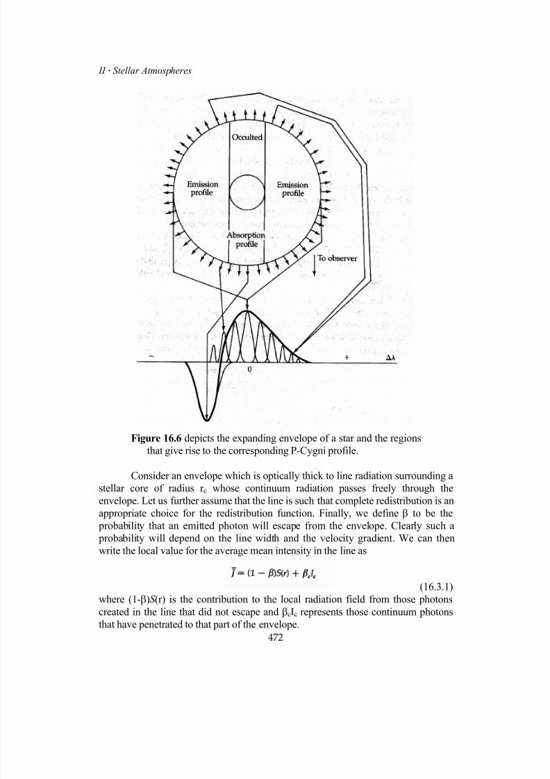
7/18/2019 The Fundamentals of Stellar Astrophysics - Collins G. W.
http://slidepdf.com/reader/full/the-fundamentals-of-stellar-astrophysics-collins-g-w 492/524
II Stellar Atmospheres
Figure 16.6 depicts the expanding envelope of a star and the regions
that give rise to the corresponding P-Cygni profile.
Consider an envelope which is optically thick to line radiation surrounding a
stellar core of radius r c whose continuum radiation passes freely through the
envelope. Let us further assume that the line is such that complete redistribution is an
appropriate choice for the redistribution function. Finally, we define β to be the
probability that an emitted photon will escape from the envelope. Clearly such a
probability will depend on the line width and the velocity gradient. We can then
write the local value for the average mean intensity in the line as
(16.3.1)
472
where (1-β)S (r) is the contribution to the local radiation field from those photons
created in the line that did not escape and βcIc represents those continuum photons
that have penetrated to that part of the envelope.

7/18/2019 The Fundamentals of Stellar Astrophysics - Collins G. W.
http://slidepdf.com/reader/full/the-fundamentals-of-stellar-astrophysics-collins-g-w 493/524
16 Beyond the Normal Stellar Atmosphere
An estimate of β and βc will then provide us with a relationship between
J and S which we can substitute into equations for the non-LTE source function
developed in Chapter 15 [see equations (15.2.19) and (15.2.25)]. The mean escape probabilities β and βc will depend on local conditions only if the velocity gradient is
sufficiently large that the conditions determining the probabilities can be represented
by the local values of temperature and density.
Castor 20
has developed this formalism for a two-level atom and it is nicely
described in Mihalas21
. Basically, the problem becomes one of geometry.
Contributions to the local mean intensity will come largely from surfaces within the
envelope which exhibit a relative Doppler shift that is less than the Doppler width of
the line. Castor finds this to be
(16.3.2)
where
(16.3.3)
is simply the velocity measured in units of the thermal velocity characterizing the
line width and
(16.3.4)
which occurs from expanding the effective optical path in a power series of thevelocity field and retaining only the first-order term. The parameter τ0 is effectively
the optical depth in the line along a radius from the star and is defined by
(16.3.5)
This quantity is essentially the line extinction coefficient multiplied by some
effective length that is obtained by dividing by the dimensionless velocity gradient.
We may approximate βc by the following argument. Since βc is essentially an
escape probability of a continuum photon leaving the envelope by traveling in any
direction, it is essentially the same as β except for the probability of the photon'shitting the stellar core. That probability is given simply by the fraction of 4π
occupied by the core itself and is commonly called the dilution factor since it is the
amount by which the local radiation density is diluted as one recedes from the star.
The dilution factor W is therefore
473

7/18/2019 The Fundamentals of Stellar Astrophysics - Collins G. W.
http://slidepdf.com/reader/full/the-fundamentals-of-stellar-astrophysics-collins-g-w 494/524
II Stellar Atmospheres
(16.3.6)
so that
(16.3.7)
We now have β and βc defined in terms of the velocity field, position, and
parameters of the gaseous envelope that determine the local effective optical depth in
the line τ0. Remembering that
(16.3.8)
we may substitute into either of the non-LTE source functions given by equation(15.2.19) or (15.2.25) and obtain the source function for the line. Once the line
source function is known, the solution for the equation of transfer (see Section 10.4
for spherical geometry) can be solved and the line profile obtained.
Solution of this problem also yields the radiant energy deposited in the
envelope as a result of the line interactions. By doing this for a number of lines, the
local effects of radiation on the envelope can be determined. This is one of the
primary factors in determining the dynamics of the envelope.
b Flow of Radiation and the Stellar Wind
Most progress in understanding stellar winds has been made with the
radiation-driven winds of the early-type stars. While coronal winds of the later-type
stars are important, particularly for slowing down the rotational velocity of these
stars by magnetic breaking, the uncertainties concerning the formation of their
coronal source force us to leave their discussion another to elucidate. What is
presently known about them is nicely summarized by Mihalas21
(pp.521-540) and
Cassinelli22
. Instead, we concentrate on some aspects of the large winds encountered
in the early-type stars.
In Chapter 6 [equation (6.5.2)] we showed that if the radiation pressure
became sufficiently high, a star would become unstable. While many stars on theupper main sequence approach this limit, they still fall short. Yet these same stars
exhibit significant mass loss in the form of a substantial stellar wind. In 1970, Leon
Lucy and Philip Solomon23
showed that, under certain circumstances, the coupling of
the radiation field to the matter in the upper atmosphere through the strong resonance
lines of certain elements could provide sufficient momentum transport to the
envelope to drive it away from the star. This idea was developed more fully by
474
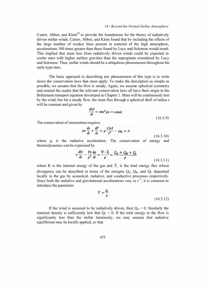
7/18/2019 The Fundamentals of Stellar Astrophysics - Collins G. W.
http://slidepdf.com/reader/full/the-fundamentals-of-stellar-astrophysics-collins-g-w 495/524
16 Beyond the Normal Stellar Atmosphere
Castor, Abbot, and Klein24
to provide the foundations for the theory of radiatively
driven stellar winds. Castor, Abbot, and Klein found that by including the effects of
the large number of weaker lines present in material of the high atmosphere,
accelerations 100 times greater than those found by Lucy and Solomon would result.
This implied that mass loss from radiatively driven winds could be expected in
cooler stars with higher surface gravities than the supergiants considered by Lucy
and Solomon. Thus, stellar winds should be a ubiquitous phenomenon throughout the
early-type stars.
The basic approach to describing any phenomenon of this type is to write
down the conservation laws that must apply. To make the description as simple as
possible, we assume that the flow is steady. Again, we assume spherical symmetry
and remind the reader that the relevant conservation laws all have their origin in the
Boltzmann transport equation developed in Chapter 1. Mass will be continuously lost
by the wind, but for a steady flow, the mass flux through a spherical shell of radius rwill be constant and given by
(16.3.9)
The conservation of momentum requires
(16.3.10)
where g r is the radiative acceleration. The conservation of energy and
thermodynamics can be expressed by
(16.3.11)r
where U is the internal energy of the gas and tF is the total energy flux whose
divergence can be described in terms of the energies QA, QR , and QC deposited
locally in the gas by acoustical, radiative, and conductive processes respectively.
Since both the radiative and gravitational accelerations vary as r -2
, it is common to
introduce the parameter
(16.3.12)
If the wind is assumed to be radiatively driven, then QA = 0. Similarly the
material density is sufficiently low that QC = 0. If the total energy in the flow is
significantly less than the stellar luminosity, we may assume that radiative
equilibrium may be locally applied, so that
475
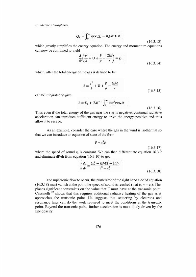
7/18/2019 The Fundamentals of Stellar Astrophysics - Collins G. W.
http://slidepdf.com/reader/full/the-fundamentals-of-stellar-astrophysics-collins-g-w 496/524
II Stellar Atmospheres
(16.3.13)
which greatly simplifies the energy equation. The energy and momentum equations
can now be combined to yield
(16.3.14)
which, after the total energy of the gas is defined to be
(16.3.15)
can be integrated to give
(16.3.16)
Thus even if the total energy of the gas near the star is negative, continual radiative
acceleration can introduce sufficient energy to drive the energy positive and thus
allow it to escape.
As an example, consider the case where the gas in the wind is isothermal so
that we can introduce an equation of state of the form
(16.3.17)
where the speed of sound cs is constant. We can then differentiate equation 16.3.9
and eliminate dP/dr from equation (16.3.10) to get
(16.3.18)
For supersonic flow to occur, the numerator of the right hand side of equation
(16.3.18) must vanish at the point the speed of sound is reached (that is, v = c s). This
places significant constraints on the value that Γ must have at the transonic point.
Cassinelli22
shows that this requires additional radiative heating of the gas as itapproaches the transonic point. He suggests that scattering by electrons and
resonance lines can do the work required to meet the conditions at the transonic
point. Beyond the transonic point, further acceleration is most likely driven by the
line opacity.
476
7/18/2019 The Fundamentals of Stellar Astrophysics - Collins G. W.
http://slidepdf.com/reader/full/the-fundamentals-of-stellar-astrophysics-collins-g-w 497/524
16 Beyond the Normal Stellar Atmosphere
Since it has been shown that it is possible to drive stellar winds radiatively
for stars whose luminosity is well below the Eddington luminosity, it remains for a
complete and fully consistent model to be made. The problem here is largely
numerical for the basic physical constraints are understood. To be sure these
problems are formidable. Correct representation of the radiative acceleration requires
calculation of the effects due to the myriads of weak spectral lines that populate the
ultraviolet region of the spectrum where these stars radiate most of their energy. The
energy balance equations must be solved to properly incorporate the effects of
heating near the transonic point and to determine the temperature structure of the
flow. Then the hydrodynamic flow equations will have to be solved numerically,
incorporating an appropriate equation of state. Of course, all this must be done in
non-LTE so that the proper ionization and excitation structure can be obtained.
Undoubtedly the Castor, Abbot, and Klein models have pointed the correct way to
understanding radiatively driven winds, but much remains to be done before themodels can be used as a probe of the physics of the outer layers of stars.
This brief look at the problems of extended atmospheres and radiatively
driven winds points out that the transition region between the normal stellar
atmosphere and the interstellar medium is a difficult region to understand. A closer
look at the chromospheres and coronas of other stars would have shown the same, or
possibly more difficult, problems. Certainly the description of the transition zone for
nonspherical stars will include more difficulties and require greater cleverness on the
part of astrophysicists to understand them. Certainly this will be necessary if we are
to understand the evolution of close binary stars in sufficient detail to understand
their ultimate fate and the manner in which they influence the interstellar medium.Without that understanding, the evolution of the galaxy will be difficult, if not
impossible, to understand. And without a reliable knowledge of galactic evolution
can we ever hope to delineate the evolution, of the universe as a whole?
Problems
1. Show that equation (16.1.4) is indeed an equation for the diffuse field source
function for an illuminated atmosphere.
2. Show that equations (16.1.8), and (16.1.9) do give the correct form of theAvrett-Krook perturbation scheme for an illuminated stellar atmosphere.
3 Find an integral expression for the radiative flux transmitted horizontally
through a plane-parallel stellar atmosphere that is illuminated by a point
source located at [µ0=cos θ0, φ0=0].
477
7/18/2019 The Fundamentals of Stellar Astrophysics - Collins G. W.
http://slidepdf.com/reader/full/the-fundamentals-of-stellar-astrophysics-collins-g-w 498/524
7/18/2019 The Fundamentals of Stellar Astrophysics - Collins G. W.
http://slidepdf.com/reader/full/the-fundamentals-of-stellar-astrophysics-collins-g-w 499/524
16 Beyond the Normal Stellar Atmosphere
10. Code, A.: Radiative Equilibrium in an Atmosphere in which Pure Scattering
and Pure Absorption Play a Role, Ap.J. 112, 1950, pp. 22 - 47.
11. Collins, G.W.,II: Transfer of Polarized Radiation, Ap.J. 175, 1972,
pp. 147 - 156.
12. Collins, G.W.,II, and Buerger, P.F. "Polarization from Illuminated
Non-Gray Stellar Atmospheres", Planets, Stars, and Nebulae Studied with
Photopolarimetry, (Ed: T. Geherels), University of Arizona Press, Tucson,
1974, pp. 663 - 675.
13. Hiltner, W.A.: Polarization of the Light from Distant Stars by Interstellar
Medium, Science 109, 1949, p.165.
14. Hall, J.S.: Observations of the Polarized Light from Stars, Science 109,
1949, pp. 166 - 167.
15. Kemp, J.C., Henson, G.D., Barbour, M.S., Krause, D.J., and Collins, G.W.,II
Discovery of Eclipse Polarization in Algol , Ap.J., 273, 1982, pp. L85 - L88.
16. Kuzma, T.J.: On Some Aspects of the Radiative Interaction in a Close Binary
System, doctoral thesis, The Ohio State University, Columbus, 1981, p. 135.
17. Mc Kenna, S. The Transfer of Polarized Radiation in Spectral Lines:
Formalism and Solutions in Simple Cases, Astrophy. & Sp. Sci. 108, 1985, pp. 31 - 66.
18. McKenna, S. The Transfer of Polarized Radiation in Spectral Lines:
Solar-Type Stellar Atmospheres, Astrophy. & Sp. Sci. 106, 1984,
pp. 283 - 297.
19. Sobolev, V.V.: The Formation of Emission Lines, Theoretical Astrophysics,
(Ed: V.A. Ambartsumyan, Trans. J.B.Sykes), Pergammon, New York, 1958,
pp. 478 - 497.
20. Castor, J.I.: Spectral Line Formation in Wolf-Rayet Envelopes, Mon. Not.R. astr. Soc. 149, 1970, pp. 111 - 127.
21. Mihalas, D.: Stellar Atmospheres, 2d ed., W. H. Freeman, San Francisco,
1978, pp. 478 - 485.
479

7/18/2019 The Fundamentals of Stellar Astrophysics - Collins G. W.
http://slidepdf.com/reader/full/the-fundamentals-of-stellar-astrophysics-collins-g-w 500/524
II Stellar Atmospheres
22. Cassinelli, J.P. "Stellar Winds", Annual Reviews of Astronomy and
Astrophysics, (Ed.: G.Burbidge), vol. 17, Annual Reviews, Palo Alto, Calif.,
1979, pp. 300 - 306.
23. Lucy, L.B., and Solomon, P.M. Mass Loss by Hot Stars , Ap.J. 159, 1970,
pp. 879 - 893.
24. Castor, J.I., Abbot, D.C., and Klein, R.I. Radiation Driven Winds in
Of Stars, Ap. J. 195, 1975, pp. 157 - 174.
For general review on the subject of stellar winds one should read
Cassinelli22
pp. 275-308.
Epilogue
. . .Those who have labored through this entire book will have noticed that the
first half appears to form a more cohesive and understandable unit than the secondhalf. The pedagogy seems more complete for the theory of stellar interiors than for
stellar atmospheres. I believe this to be an intrinsic property of the material rather
than a reflection of the my ability. More effort and minds have been involved in the
formulation of the theory of stellar interiors and evolution than in the development of
the theory of stellar atmospheres. More importantly, more time has elapsed during
which the central ideas, important concepts, and their interrelationships can become
apparent. This distillation process requires time as well as good minds to produce the
final product.
The reason this is not simply a temporal accident, but has its origin in the
relative difficulty of the formulation of the subjects themselves. I have emphasizedthroughout this book the steady removal of simplifying assumptions as the
description of stellar structure moves progressively out from the center of the star to
the surface and beyond. This loss of assumptions that make the physical description
of the star easier to effect also sets the time scale for the development of the subject
itself, for people generally try to solve the simple problems first. So the effort to
understand the stellar interior began in earnest as soon as nuclear physics delineated
480

7/18/2019 The Fundamentals of Stellar Astrophysics - Collins G. W.
http://slidepdf.com/reader/full/the-fundamentals-of-stellar-astrophysics-collins-g-w 501/524
16 Beyond the Normal Stellar Atmosphere
the source of the energy in stars. This is not to belittle the elegant work with
polytropes that began at the end of the nineteenth century. But it is clear that fully
credible models of stellar interiors, suitable for the description of stellar evolution,
could not be made without certain knowledge of the origin of a star's source of
energy. After the elucidation by Hans Bethe of the probable energy sources for the
sun, the theory of stellar structure and evolution developed with remarkable speed. In
a mere two decades, one of which was dominated by world war II, the basic
framework of the theory of stellar evolution was in place.
Although the origin of stellar atmospheres can be traced back nearly as far as
that of stellar interiors, its development has been slower. It is tempting to suggest that
the theory required the existence of good stellar interior models before it could be
developed, but that would be false. The defining parameters for the stellar
atmosphere are known sufficiently well from direct observation to permit the
development of a full-blown theory of atmospheric structure. The retardeddevelopment of stellar atmospheres as compared to stellar interiors can be attributed
entirely to the loss of the assumption of STE. All the complications introduced by the
myriad complexities of atomic structure now become entwined with the description
of the atmospheric structure through the radiative opacity. While this fact was
realized early in the century, little could be done about it until the numerical and
computational capabilities required to include these complexities developed after
World War II. The computational requirements of the theory of stellar atmospheres
exceed those stellar interiors, so that it was logical that the theory of stellar structure
and evolution should develop earlier. This, plus the "sifting and winnowing" of ideas
of central importance from those of necessary detail by people like Martin
Schwarzschild and others, has provided that more lucid pedagogy of stellar interiorsand evolution. It is the task of our generation and the next to bring the same level of
conceptual understanding to the theory of stellar atmospheres.
While the business of model making, in both stellar interiors and stellar
atmospheres, has become almost routine, one must remain wary lest the work of
large computers beguile the investigator into believing that the process is simple. It is
tempting to think that in the future computer codes will yield all aspects of the
structure of a star as easily as one obtains values for trigonometric functions at
present. To believe this is to miss a central difference between physical science and
mathematics. Mathematics is a logical construct of the human mind, resting on a set
of axioms within the framework of which the majority of statements can be adjudgedtrue or false. (The exceptions implied by Gödel's incompleteness theorem are duely
noted.) Thus, one can have complete confidence that a competently written computer
code designed to calculate trigonometric functions will always deliver the correct
answer within some known tolerance. While physical science aspires to the status of
an axiomatic discipline, it is far from reaching that goal. Even if such a goal is
reached, the complexities of the universe require us continue to make simplifying
481
7/18/2019 The Fundamentals of Stellar Astrophysics - Collins G. W.
http://slidepdf.com/reader/full/the-fundamentals-of-stellar-astrophysics-collins-g-w 502/524
II Stellar Atmospheres
482
assumptions to describe the physical world. These assumptions cannot be deemed
either true or false for they will only yield a correct description of the phenomena of
interest within some generally unknown tolerance. The interplay of the tolerances
associated with the assumptions and those of numerical and computational
approximation is so complex as to always raise some doubt about the model's level
of accuracy. Only the naive would ascribe the same level of confidence to the results
of such a model description as to the calculation of a trigonometric function.
Nevertheless, we may expect to see a rapid growth in the art of modeling the
physical world by computer. However, we must always be alert to the simplicity
engendered by the speed and accuracy of digital computers lest we credit greater
accuracy to their results than is warranted. We must also eschew the false
understanding of the results of those models encompassed by the explanation that the
universe is the way it is "because the computer tells me so". Such is no
understanding at all. Instead we must continually struggle to understand thefundamental laws at work in framing the universe and the manner by which they
relate to one another. It is the interrelationships among those laws describing the
physical world that provide the insight necessary to advance our understanding, and
they must be seen as concepts, not merely numbers.
The remaining problems to be solved in stellar astrophysics are legion. But
the tools to solve them remain the same: the conservation laws of physics, the
fundamental properties of matter, and the mathematical language to relate the two.
To contribute to our understanding of the universe, the student must master them all.
7/18/2019 The Fundamentals of Stellar Astrophysics - Collins G. W.
http://slidepdf.com/reader/full/the-fundamentals-of-stellar-astrophysics-collins-g-w 503/524
Index
Copyright (2003) George W. Collins, II
Index
. . .
The pages listed here correspond roughly to those of the book. However, since the
chapter pagination of this edition corresponds to that of the book, the agreement,
while not perfect is likely to be within a page or two.
483

7/18/2019 The Fundamentals of Stellar Astrophysics - Collins G. W.
http://slidepdf.com/reader/full/the-fundamentals-of-stellar-astrophysics-collins-g-w 504/524
Index
484

7/18/2019 The Fundamentals of Stellar Astrophysics - Collins G. W.
http://slidepdf.com/reader/full/the-fundamentals-of-stellar-astrophysics-collins-g-w 505/524

7/18/2019 The Fundamentals of Stellar Astrophysics - Collins G. W.
http://slidepdf.com/reader/full/the-fundamentals-of-stellar-astrophysics-collins-g-w 506/524
Index
486

7/18/2019 The Fundamentals of Stellar Astrophysics - Collins G. W.
http://slidepdf.com/reader/full/the-fundamentals-of-stellar-astrophysics-collins-g-w 507/524
Index
487
7/18/2019 The Fundamentals of Stellar Astrophysics - Collins G. W.
http://slidepdf.com/reader/full/the-fundamentals-of-stellar-astrophysics-collins-g-w 508/524
Index
488
7/18/2019 The Fundamentals of Stellar Astrophysics - Collins G. W.
http://slidepdf.com/reader/full/the-fundamentals-of-stellar-astrophysics-collins-g-w 509/524
Index
489

7/18/2019 The Fundamentals of Stellar Astrophysics - Collins G. W.
http://slidepdf.com/reader/full/the-fundamentals-of-stellar-astrophysics-collins-g-w 510/524
Index
490
7/18/2019 The Fundamentals of Stellar Astrophysics - Collins G. W.
http://slidepdf.com/reader/full/the-fundamentals-of-stellar-astrophysics-collins-g-w 511/524
Index
491
7/18/2019 The Fundamentals of Stellar Astrophysics - Collins G. W.
http://slidepdf.com/reader/full/the-fundamentals-of-stellar-astrophysics-collins-g-w 512/524
Index
492
7/18/2019 The Fundamentals of Stellar Astrophysics - Collins G. W.
http://slidepdf.com/reader/full/the-fundamentals-of-stellar-astrophysics-collins-g-w 513/524
Index
493

7/18/2019 The Fundamentals of Stellar Astrophysics - Collins G. W.
http://slidepdf.com/reader/full/the-fundamentals-of-stellar-astrophysics-collins-g-w 514/524
Index
494
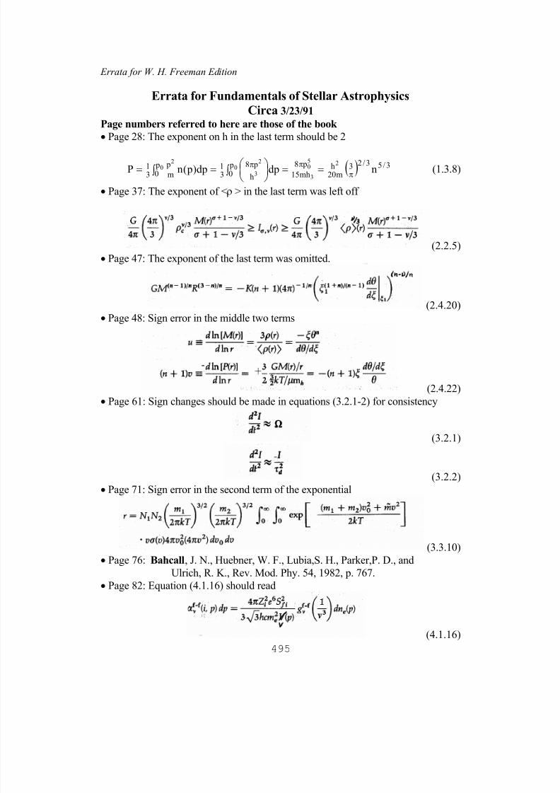
7/18/2019 The Fundamentals of Stellar Astrophysics - Collins G. W.
http://slidepdf.com/reader/full/the-fundamentals-of-stellar-astrophysics-collins-g-w 515/524
Errata for W. H. Freeman Edition
Errata for Fundamentals of Stellar Astrophysics
Circa 3/23/91
Page numbers referred to here are those of the book
• Page 28: The exponent on h in the last term should be 2
( )∫ ∫ ==
== π
ππ0 02
3
50
3
22 p0
p0
3/53/23m20
hmh15
p8
h
p8
31
m
p
31 ndpdp) p(nP (1.3.8)
• Page 37: The exponent of <ρ > in the last term was left off
(2.2.5)
• Page 47: The exponent of the last term was omitted.
(2.4.20)
• Page 48: Sign error in the middle two terms
(2.4.22)
• Page 61: Sign changes should be made in equations (3.2.1-2) for consistency
(3.2.1)
(3.2.2)
• Page 71: Sign error in the second term of the exponential
(3.3.10)
• Page 76: Bahcall, J. N., Huebner, W. F., Lubia,S. H., Parker,P. D., and
Ulrich, R. K., Rev. Mod. Phy. 54, 1982, p. 767.
• Page 82: Equation (4.1.16) should read
495
(4.1.16)

7/18/2019 The Fundamentals of Stellar Astrophysics - Collins G. W.
http://slidepdf.com/reader/full/the-fundamentals-of-stellar-astrophysics-collins-g-w 516/524
Errata for W.H. Freeman Edition
• Page 101: The last two of equations 4.6.1 should read
(4.6.1)
• Page 103: Equation 4.7.3 (d) should read
(4.7.3)
• Page 107: Quantity left out of (b) and an improvement made to (d)
(4.7.10)
• Page 108: Runge-Kutta is mispelled in line 10 of ¶2.
496

7/18/2019 The Fundamentals of Stellar Astrophysics - Collins G. W.
http://slidepdf.com/reader/full/the-fundamentals-of-stellar-astrophysics-collins-g-w 517/524
Errata for W. H. Freeman Edition
• Page 131: Lead coefficient is wrong, should be
(5.4.5)• Pages 140-143: Equations (5.4.9) - (5.4.14) should be renumbered to agree with
the new section 5.5 that was introduced
• Page 142: (Equation 5.5.1 needs an integral of ε over volume to get the entire
contribution of energy to the star to match the losses through L.)
• Page 142: Last paragraph line two, replace potential energy with internal energy.
(5.5.1)
• Page 145: problem 5 should read5. Choose a representative set of models from the evolutionary
calculations in Problem 4, (a) Calculate the moment of inertia,
gravitational and internal energies of the core and envelope, and the
total energy of the star (b) Determine the extent to which the
conditions in Section 5.5a are met during the evolution of the star.
• The discussion of Neutron Star Structure on pp 158-160 should be expanded
to include the work by Keith Olive (1991 Sci. 251, pp.1197-1198) on the
Quark-Hadron phase transition. Nothing here is wrong; it could just be
made more complete.
• Page 163: The ε on the right hand side was left out.
(6.4.8)
• Page 168: Capriotti14
has evaluated the luminosity integral and gets
• Page 168: last paragraph
c Limiting Masses for Supermassive Stars
Let us add equations (6.4.19) and (6.4.20) and, taking care toexpress the relativistic integrals as dimensionless integrals by making use of the
homology relations for pressure and density, get for the total energy:
497

7/18/2019 The Fundamentals of Stellar Astrophysics - Collins G. W.
http://slidepdf.com/reader/full/the-fundamentals-of-stellar-astrophysics-collins-g-w 518/524
Errata for W.H. Freeman Edition
(6.5.5)
• Page 169: The exponent on M⊙ in the last term should be 3
(6.5.6)
• Page 170: last paragraph - However, the only energy transportable by
convection is the kinetic energy of the gas, which is an insignificant fraction
of the internal energy. Therefore, unlike normal main sequence stars,
although it is present, convection will be a very inefficient vehicle for the
transport of energy. This is
• Page 173: Capriotti is spelled wrong
• Page 179: Sign should be changed for consistencyr
Λ∇= -D (7.1.9)
• Page 180: We may remove the unit vector from the s-component
sD,0DD 2
sz ω=== φ (7.1.12)
• Page 183: sign error in second term of first eq.
θ∂
θ∂=
θ∂
θ∂ψπρ=
θ+=θ
∂ψ∂
ψ+ψ
πρ=
−θ
−
)Cos(P)r (C
~)Cos(P
r
)r ()c4((D
)Cos(P)r (B~
)r (A
~
Sinr )r (r
)r (
)c4(D
22
21
2
22
1
r
(7.1.31)
• Page 186: The last term should have a (1/r) in it
r /)r (C)r ()r ()r ()r (P
)r (B)r (r
)r ()r (
r
)r ()r (
r
)r (P
)r (A)r (r
)r (
r
)r (P
0202
00
22
02
00
00
ρ+Ωρ−=
ρ+∂
Ω∂ρ+
∂Ω∂
ρ−=∂
∂
ρ+∂
Ω∂ρ−=
∂
∂
(7.2.5)
• Page 191: last two lines - In the equilibrium model, there are no mass motions,
the velocity in equation (7.2.6) is already a first-order term and so to
estimate its value we need only .....
498
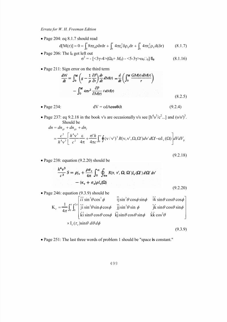
7/18/2019 The Fundamentals of Stellar Astrophysics - Collins G. W.
http://slidepdf.com/reader/full/the-fundamentals-of-stellar-astrophysics-collins-g-w 519/524
Errata for W. H. Freeman Edition
• Page 204: eq 8.1.7 should read
∫ ∫ ∫ δρπ+δρπ+ρδπ==r
0
r
0
r
00
2
00
2
00 )r (dr 4dr r 4rdr r 80)]r (M[d (8.1.7)
• Page 206: The I0 got left out
σ2 = - [<3γ-4>(Ω0+ M 0) - <5-3γ>ω00]/I0 (8.1.16)
• Page 211: Sign error on the third term
(8.2.5)
• Page 234: dV = cdAcosθdt (9.2.4)
• Page 237: eq 9.2.18 in the book v's are occasionally υ's see [h4 υ
3/c
2...] and ( υ/ υ')
3.
Should be
p0
3
2
34
34
2
)(I'')',,',()'/(4
'
4 dVdV d d R
c
h
c
h
h
c
dndndndn l gs gt
Ωα−ΩνΩΩνννν
πσ
+πεν
ν=
++=
∫ ∫∞
ν
(9.2.18)
• Page 238: equation (9.2.20) should be
(9.2.20)
• Page 246: equation (9.3.9) should be
φ θ θ τ
θ φ θ θ φ θ θ
φ θ θ φ θ φ φ θ
φ θ θ φ φ θ φ θ
π
ν ν
π π
ν
d d
ii
sin)(I
cosk ˆk ˆ sincossin jk ˆ coscossinik ˆ
sincossink ˆ j sinsin j j cossinsini j
coscossink ˆi sincossin ji cossinˆˆ
4
1K
0
2
0
2
22
222
×
= ∫ ∫
(9.3.9)
• Page 251: The last three words of problem 1 should be "space is constant."
499
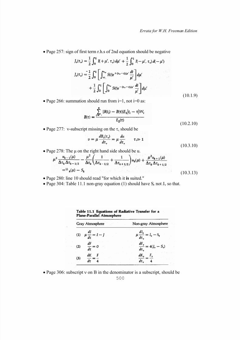
7/18/2019 The Fundamentals of Stellar Astrophysics - Collins G. W.
http://slidepdf.com/reader/full/the-fundamentals-of-stellar-astrophysics-collins-g-w 520/524
Errata for W.H. Freeman Edition
• Page 257: sign of first term r.h.s of 2nd equation should be negative
(10.1.9)
• Page 266: summation should run from i=1, not i=0 as:
(10.2.10)
• Page 277: ν-subscript missing on the τ, should be
(10.3.10)
• Page 278: The µ on the right hand side should be u.
(10.3.13)
• Page 280: line 10 should read "for which it is suited."• Page 304: Table 11.1 non-gray equation (1) should have Sν not Jν so that.
500
• Page 306: subscript ν on B in the denominator is a subscript, should be
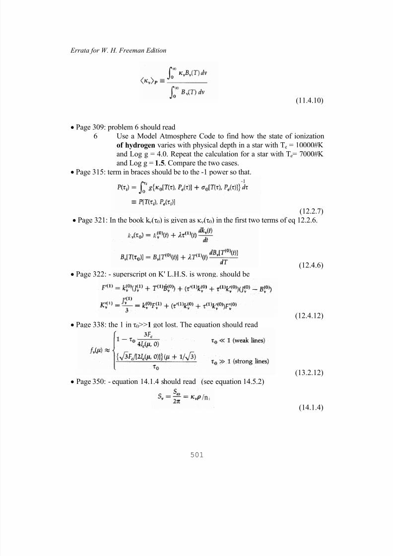
7/18/2019 The Fundamentals of Stellar Astrophysics - Collins G. W.
http://slidepdf.com/reader/full/the-fundamentals-of-stellar-astrophysics-collins-g-w 521/524
Errata for W. H. Freeman Edition
(11.4.10)
• Page 309: problem 6 should read
6 Use a Model Atmosphere Code to find how the state of ionization
of hydrogen varies with physical depth in a star with Te = 10000#K
and Log g = 4.0. Repeat the calculation for a star with Te= 7000#K
and Log g = 1.5. Compare the two cases.
• Page 315: term in braces should be to the -1 power so that.
(12.2.7)
• Page 321: In the book k ν(τ0) is given as κ ν(τ0) in the first two terms of eq 12.2.6.
(12.4.6)
• Page 322: - superscript on K' L.H.S. is wrong. should be
(12.4.12)
• Page 338: the 1 in τ0>>1 got lost. The equation should read
(13.2.12)
• Page 350: - equation 14.1.4 should read (see equation 14.5.2)
(14.1.4)
501
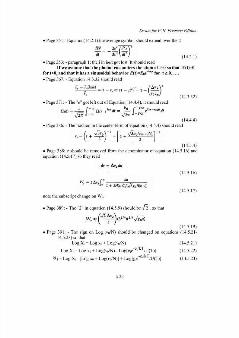
7/18/2019 The Fundamentals of Stellar Astrophysics - Collins G. W.
http://slidepdf.com/reader/full/the-fundamentals-of-stellar-astrophysics-collins-g-w 522/524
Errata for W.H. Freeman Edition
• Page 351:- Equation(14.2.1) the average symbol should extend over the 2
(14.2.1)
• Page 353: - paragraph 1: the i in iω0t got lost. It should read
If we assume that the photon encounters the atom at t=0 so that E(t)=0
for t<0, and that it has a sinusoidal behavior E (t)= E 0e-iω0t
for t ≥ 0, ….
• Page 367: - Equation 14.3.32 should read
(14.3.32)
• Page 371: - The "e" got left out of Equation (14.4.4), it should read
(14.4.4)• Page 386: - The fraction in the center term of equation (14.5.4) should read
(14.5.4)
• Page 388: c should be removed from the denominator of equation (14.5.16) and
equation (14.5.17) so they read
(14.5.16)
(14.5.17)
note the subscript change on Wν.
• Page 389: - The "2" in equation (14.5.9) should be 2 , so that
(14.5.19)
• Page 391: - The sign on Log (ν0/N) should be changed on equations (14.5.21-
14.5.23) so thatLog Xi = Log x0 + Log(v0/N) (14.5.21)
Log Xi = Log x0 + Log(v0/N) - Log[gie-ei/kT
/U(T)] (14.5.22)
i = Log Xi - [Log x0 + Log(v0/N)] + Log[gie-ei/kT
/U(T)] (14.5.23)
502
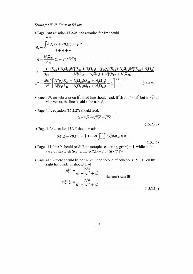
7/18/2019 The Fundamentals of Stellar Astrophysics - Collins G. W.
http://slidepdf.com/reader/full/the-fundamentals-of-stellar-astrophysics-collins-g-w 523/524
Errata for W. H. Freeman Edition
• Page 408: equation 15.2.25, the equation for B* should
read
• Page 409: no subscript on B*, third line should read: If ~εBν(T) > ηB* but η > ε~ (orvice versa), the line is said to be mixed.
• Page 411: equation (15.2.27) should read:
(15.2.27)
• Page 413: equation 15.3.5 should read:
(15.3.5)• Page 414: line 9 should read: For isotropic scattering, g(n',n) = 1, while in the
case of Rayleigh Scattering g(n',n) = 3[1+(n'•n)2]/4.
• Page 415: - there should be no ' on ξ' in the second of equations 15.3.10 on the
right hand side. It should read
(15.3.10)
503
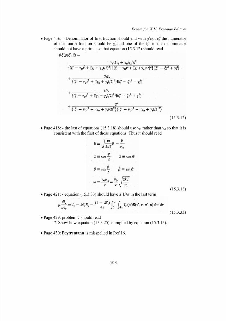
7/18/2019 The Fundamentals of Stellar Astrophysics - Collins G. W.
http://slidepdf.com/reader/full/the-fundamentals-of-stellar-astrophysics-collins-g-w 524/524
Errata for W.H. Freeman Edition
• Page 416: - Denominator of first fraction should end with γ2
l not η2
l, the numerator
of the fourth fraction should be γ2
l, and one of the ξ's in the denominator
should not have a prime, so that equation (15.3.12) should read
Related Documents