Modules for Experiments in Stellar Astrophysics (MESA) Bill Paxton and Lars Bildsten Kavli Institute for Theoretical Physics and Department of Physics, Kohn Hall, University of California, Santa Barbara, CA 93106 USA Aaron Dotter 1 and Falk Herwig Department of Physics and Astronomy, University of Victoria, PO Box 3055, STN CSC, Victoria, BC, V8W 3P6 Canada Pierre Lesaffre LERMA-LRA, CNRS UMR8112, Observatoire de Paris and Ecole Normale Superieure, 24 Rue Lhomond, 75231 Paris cedex 05, France Frank Timmes School of Earth and Space Exploration, Arizona State University, PO Box 871404, Tempe, AZ, 85287-1404 USA ABSTRACT Stellar physics and evolution calculations enable a broad range of research in astrophysics. Modules for Experiments in Stellar Astrophysics (MESA) is a suite of open source, robust, efficient, thread-safe libraries for a wide range of ap- plications in computational stellar astrophysics. A 1-D stellar evolution module, MESA star, combines many of the numerical and physics modules for simulations of a wide range of stellar evolution scenarios ranging from very-low mass to mas- sive stars, including advanced evolutionary phases. MESA star solves the fully coupled structure and composition equations simultaneously. It uses adaptive mesh refinement and sophisticated timestep controls, and supports shared mem- ory parallelism based on OpenMP. State-of-the-art modules provide equation of state, opacity, nuclear reaction rates, element diffusion data, and atmosphere boundary conditions. Each module is constructed as a separate Fortran 95 li- brary with its own explicitly defined public interface to facilitate independent development. Several detailed examples indicate the extensive verification and 1 Current address: Space Telescope Science Institute, 3700 San Martin Drive, Baltimore, MD, 21218, USA arXiv:1009.1622v1 [astro-ph.SR] 8 Sep 2010

Welcome message from author
This document is posted to help you gain knowledge. Please leave a comment to let me know what you think about it! Share it to your friends and learn new things together.
Transcript

Modules for Experiments in Stellar Astrophysics (MESA)
Bill Paxton and Lars Bildsten
Kavli Institute for Theoretical Physics and Department of Physics, Kohn Hall, University
of California, Santa Barbara, CA 93106 USA
Aaron Dotter1 and Falk Herwig
Department of Physics and Astronomy, University of Victoria, PO Box 3055, STN CSC,
Victoria, BC, V8W 3P6 Canada
Pierre Lesaffre
LERMA-LRA, CNRS UMR8112, Observatoire de Paris and Ecole Normale Superieure, 24
Rue Lhomond, 75231 Paris cedex 05, France
Frank Timmes
School of Earth and Space Exploration, Arizona State University, PO Box 871404, Tempe,
AZ, 85287-1404 USA
ABSTRACT
Stellar physics and evolution calculations enable a broad range of research
in astrophysics. Modules for Experiments in Stellar Astrophysics (MESA) is a
suite of open source, robust, efficient, thread-safe libraries for a wide range of ap-
plications in computational stellar astrophysics. A 1-D stellar evolution module,
MESA star, combines many of the numerical and physics modules for simulations
of a wide range of stellar evolution scenarios ranging from very-low mass to mas-
sive stars, including advanced evolutionary phases. MESA star solves the fully
coupled structure and composition equations simultaneously. It uses adaptive
mesh refinement and sophisticated timestep controls, and supports shared mem-
ory parallelism based on OpenMP. State-of-the-art modules provide equation of
state, opacity, nuclear reaction rates, element diffusion data, and atmosphere
boundary conditions. Each module is constructed as a separate Fortran 95 li-
brary with its own explicitly defined public interface to facilitate independent
development. Several detailed examples indicate the extensive verification and
1Current address: Space Telescope Science Institute, 3700 San Martin Drive, Baltimore, MD, 21218, USA
arX
iv:1
009.
1622
v1 [
astr
o-ph
.SR
] 8
Sep
201
0

– 2 –
testing that is continuously performed, and demonstrate the wide range of capa-
bilities that MESA possesses. These examples include evolutionary tracks of very
low mass stars, brown dwarfs, and gas giant planets to very old ages; the complete
evolutionary track of a 1M� star from the pre-main sequence to a cooling white
dwarf; the Solar sound speed profile; the evolution of intermediate mass stars
through the He-core burning phase and thermal pulses on the He-shell burning
AGB phase; the interior structure of slowly pulsating B Stars and Beta Cepheids;
the complete evolutionary tracks of massive stars from the pre-main sequence to
the onset of core collapse; mass transfer from stars undergoing Roche lobe over-
flow; and the evolution of helium accretion onto a neutron star. MESA can be
downloaded from the project web site.1
Subject headings: stars: general — stars: evolution — methods: numerical
Contents
1 Introduction 4
2 Module design and implementation 9
3 Numerical methods 9
4 Microphysics 12
4.1 Mathematical constants, physical and astronomical data . . . . . . . . . . . 12
4.2 Equation of state . . . . . . . . . . . . . . . . . . . . . . . . . . . . . . . . . 12
4.3 Opacities . . . . . . . . . . . . . . . . . . . . . . . . . . . . . . . . . . . . . 17
4.4 Thermonuclear and weak reactions . . . . . . . . . . . . . . . . . . . . . . . 22
4.5 Nuclear reaction networks . . . . . . . . . . . . . . . . . . . . . . . . . . . . 23
5 Macrophysics 26
5.1 The mixing length theory of convection . . . . . . . . . . . . . . . . . . . . 26
1http://mesa.sourceforge.net/
– 3 –
5.2 Convective overshoot mixing . . . . . . . . . . . . . . . . . . . . . . . . . . 29
5.3 Atmosphere boundary conditions . . . . . . . . . . . . . . . . . . . . . . . . 29
5.4 Diffusion and gravitational settling . . . . . . . . . . . . . . . . . . . . . . . 32
5.5 Testing MESA modules in an existing stellar evolution code . . . . . . . . . . 34
6 Stellar structure and evolution 36
6.1 Starting models and basic input/output . . . . . . . . . . . . . . . . . . . . 37
6.2 Structure and composition equations . . . . . . . . . . . . . . . . . . . . . . 38
6.3 Convergence to a solution . . . . . . . . . . . . . . . . . . . . . . . . . . . . 42
6.4 Timestep selection . . . . . . . . . . . . . . . . . . . . . . . . . . . . . . . . 43
6.5 Mesh adjustment . . . . . . . . . . . . . . . . . . . . . . . . . . . . . . . . . 44
6.6 Mass loss and accretion . . . . . . . . . . . . . . . . . . . . . . . . . . . . . . 45
6.7 Resolution sensitivity . . . . . . . . . . . . . . . . . . . . . . . . . . . . . . . 46
6.8 Multithreading . . . . . . . . . . . . . . . . . . . . . . . . . . . . . . . . . . 53
6.9 Visualization with PGstar . . . . . . . . . . . . . . . . . . . . . . . . . . . . 53
7 MESA star results: comparisons and capabilities 53
7.1 Low mass stellar structure and evolution . . . . . . . . . . . . . . . . . . . . 55
7.1.1 Low mass pre-main sequence stars, contracting brown dwarfs and giant
planets . . . . . . . . . . . . . . . . . . . . . . . . . . . . . . . . . . . 58
7.1.2 Code comparisons of 0.8M� and 1M� models . . . . . . . . . . . . . 63
7.1.3 The MESA star Solar model . . . . . . . . . . . . . . . . . . . . . . 64
7.2 Intermediate Mass Structure and Evolution . . . . . . . . . . . . . . . . . . . 65
7.2.1 Comparison of EVOL and MESA star . . . . . . . . . . . . . . . . . 68
7.2.2 Interior structure of Slowly Pulsating B Stars and Beta Cepheids . . 75
7.3 High Mass Stellar Structure and Evolution . . . . . . . . . . . . . . . . . . . 77
7.3.1 25M� Model Comparisons . . . . . . . . . . . . . . . . . . . . . . . . 79

– 4 –
7.3.2 Comparison of 15, 20, and 25M� Models . . . . . . . . . . . . . . . . 83
7.3.3 1000M� metal-free star capabilities . . . . . . . . . . . . . . . . . . . 84
7.4 Stellar Evolution with Mass Transfer . . . . . . . . . . . . . . . . . . . . . . 88
7.4.1 Mass Transfer in a Binary . . . . . . . . . . . . . . . . . . . . . . . . 89
7.4.2 Rapid Helium Accretion onto a Neutron Star . . . . . . . . . . . . . . 92
8 Summary and conclusion 97
A Manifesto 98
A.1 Motivation for a new tool . . . . . . . . . . . . . . . . . . . . . . . . . . . . 98
A.2 MESA philosophy . . . . . . . . . . . . . . . . . . . . . . . . . . . . . . . . . 99
A.3 Establishment of the MESA council . . . . . . . . . . . . . . . . . . . . . . . 100
B Code testing and verification 101
1. Introduction
Much of the information that astronomers use to study the universe comes from starlight.
Interpretation of that starlight requires a detailed understanding of stellar astrophysics,
especially as it relates to stellar atmospheres, structure, and evolution. Stellar structure and
evolution models underpin much of modern astrophysics as they are used to analyze: the Sun
through helioseismology (e.g., Bahcall et al. 1998), the pulsational properties of many nearby
stars with asteroseismic data from, e.g., Corot (Degroote et al. 2009) and Kepler (Gilliland et
al. 2010), the color-magnitude diagrams of resolved stellar and sub-stellar populations in the
Milky Way and nearby galaxies (e.g., VandenBerg 2000; Dotter et al. 2010), the integrated
light of distant galaxies and star clusters via population synthesis techniques (e.g., Worthey
1994; Coelho et al. 2007), stellar yields and galactic chemical evolution (e.g., Timmes et
al. 1995), physics of the first stars (Fujimoto et al. 2000), and a variety of aspects in time
domain astrophysics (e.g., LSST2).
Stellar evolution is broadly recognized as the first key problem in computational as-
2http://www.lsst.org/lsst/scibook
– 5 –
trophysics. The introduction of electronic computers enabled the solution of the highly
non-linear, coupled differential equations of stellar structure and evolution, and the first
detailed reports of computer programs for stellar evolution soon appeared (Iben & Ehrman
1962; Henyey et al. 1964; Hofmeister et al. 1964; Kippenhahn et al. 1967). Implicit in
the development of these codes was a sufficiently mature theoretical understanding of stars
(Chandrasekhar 1938; Schwarzschild 1958, see as well the compilation of references later
in this section), development of a concise yet sufficiently accurate treatment of convection
(Bohm-Vitense 1958), as well as a better understanding of the properties of stellar matter,
including nucleosynthesis (Burbridge et al. 1957; Cameron 1957). Further improvements and
alternative implementations became available addressing, for example, the numerical stabil-
ity of computations (Sugimoto 1970), more efficient methods for following shell burning in
low mass stars (Eggleton 1971), and the hydrodynamics of advanced burning in massive stars
(Weaver et al. 1978). Progress continues on stellar evolution codes, with code developments
and comparisons often facilitated by the opening of new observational windows. For example,
the participants (Christensen-Dalsgaard 2008; Degl’Innocenti et al. 2008; Demarque et al.
2008; Eggenberger et al. 2008; Hui-Bon-Hoa 2008; Morel & Lebreton 2008; Roxburgh 2008;
Scuflaire et al. 2008; Ventura et al. 2008; Weiss & Schlattl 2008) in the CoRoT Evolution
and Seismic Tools Activity (Lebreton et al. 2008) are a representative sample of the active
community.
Modules for Experiments in Stellar Astrophysics (MESA) began as an effort to improve
upon the EZ stellar evolution code (Eggleton 1971; Paxton 2004). It employs modern soft-
ware engineering tools and techniques to target modern computer architectures that are
significantly different from those available to the pioneers half a century ago. As the pieces
of the new system started to emerge, it became clear that the parts would be of greater
value than the whole if they were carefully structured for independent use. MESA includes a
new 1-D stellar evolution code, MESA star, but is designed to be useful for a wide range of
stellar physics applications. The physical inputs to stellar evolution models, like the equation
of state, opacities, and nuclear reaction networks, have a broader application than stellar
evolution calculations alone. MESA is designed so that each of the individual components is
usable on its own, with the intention of facilitating verification test suites amongst different
codes and encouraging new computational experiments in stellar astrophysics.
MESA star approaches stellar physics, structure, and evolution with modern, sophisti-
cated numerical methods and updated physics that give it a very wide range of applicability.
The numerical and computational methods employed allow MESA star to consistently evolve
stellar models through challenging phases, e.g., the He core flash in low mass stars and ad-
vanced nuclear burning in massive stars, that have posed substantial challenges for stellar
evolution codes in the past.

– 6 –
MESA is open source: anyone can download the source code, compile it, and run it for
their own research or education purposes. It is meant to engage the broader community of
astrophysicists in related fields and encourage contributions in the form of testing, finding
and fixing bugs, adding new capabilities, and, generally, sharing experience with the MESA
community. The philosophy and guidelines of MESA are described in more detail in the MESA
manifesto (see Appendix A).
This paper serves as an introduction to MESA and demonstrates its current capabili-
ties. We assume that the reader is familiar with the basic stellar physics and numerical
methods, both of which are essential to arrive at meaningful solutions when using MESA.
For background material we refer the reader to Eddington (1926), Chandrasekhar (1939),
Schwarzschild (1958), Cox & Giuli (1968), Clayton (1984), Iben (1991), Hansen & Kawaler
(1995), Arnett (1996), and Kippenhahn & Weigert (1996).
The MESA codebase is in constant development, and future capabilities and applications
will be detailed in subsequent papers. The paper is outlined as follows: §2 explains the
design and implementation of MESA modules; §3-5 describe the numerical, microphysics, and
macrophysical modules; §6 describes the stellar evolution module MESA star; §7 presents a
series of tests and code comparisons that serve as rudimentary verification and demonstrates
the broader capabilities of of MESA star; and §8 summarizes the material presented.

– 7 –
Table 1. Variable Index
Name Description First appears
A atomic mass number §4.4
a acceleration at the cell face §6.2
α order of convergence §6.7
αMLT mixing length parameter §5.1
C “spacetime” parameter for convergence study §6.7
CP specific heat at constant pressure §4.2
CV specific heat at constant volume §4.2
cs sound speed §7.2.2
χρ ≡ dlnP/dlnρ|T §4.2
χT ≡ dlnP/dlnT |ρ §4.2
D Eulerian diffusion coefficient §5.2
DOV overshoot diffusion coefficient §5.2
∆ grid difference §6.5
δ time difference §6.5
dm mass of a cell §6.2
dPs P difference between surface and center of first cell §6.2
dTs T difference in between surface and center of first cell §6.2
δt timestep §6.4
E energy §4.2
enuc nuclear energy generation in ergs/g §4.5
ε power per unit mass (nuclear, thermal neutrino, gravity) §6.2
εF Fermi energy §7.1
F mass flow rate §6.2
f overshoot mixing parameter §5.2
g local gravity §5.1
Γ1 ≡ dlnP/dlnρ|S §4.2
Γ Coulomb coupling parameter §4.2
Γ3 ≡ dlnT/dlnρ|S + 1 §4.2
∇ad adiabatic temperature gradient §4.2
∇rad radiative temperature gradient §5.1
∇T actual temperature gradient §5.1
κs opacity at the surface of the outermost cell §5.3
L total luminosity §5.1
Lconv convective luminosity §5.1
Λ mixing length (αMLTλP ) §5.1
λP pressure scale height §5.1
m mass interior to cell §6.2
Mc inner mass (not modeled) for central BC §6.6
Mm modeled mass §6.6
µ mean molecular weight per gas particle §4.2
µe mean molecular weight per electron §4.2
N Brunt-Vaisala frequency §7.2.2
η dimensionless electron degeneracy parameter §6.5
P total pressure §4.2
Pgas gas pressure §4.2
Ps pressure at surface of outermost cell §5.3

– 8 –
Table 1—Continued
Name Description First appears
q relative mass coordinate §6.6
ρ density §4.2
R total radius §5.1
RCZ radius of the base of the solar convective zone §7.1
r radius at the cell face §6.2
S entropy §4.2
σ Lagrangian diffusion coefficient §5.1
T temperature §4.2
Ts temperature at surface of outermost cell §5.3
Teff effective temperature §5.3
τs optical depth at the surface of the outermost cell §5.3
τ optical depth §5.3
v velocity at the cell face §6.2
vc timestep control target §6.4
vconv convective velocity §5.1
vt timestep control variable §6.4
w diffusion velocity §5.4
X H mass fraction §4.2
Xi mass fraction of the ith isotope §6.2
ξ relative difference in convergence study §6.7
Y He mass fraction §4.3
Ye electrons per baryon (Z/A) §7.3
Z metals mass fraction (1−X − Y ) §4.2
Z atomic number §5.4
z distance from convective boundary §5.2

– 9 –
2. Module design and implementation
Each MESA module is responsible for a different aspect of numerics or physics required
to construct computational models for stellar astrophysics. Each has a similar organization:
a public interface, a private implementation, a makefile to create a library, and a test suite
for verification. Each module includes an installation script that builds the library, tests it,
and, if the test succeeds, exports it to the MESA libraries directory. Comparisons between
local and expected results are carried out with the open source ndiff utility.3 There is a
global install script for MESA that performs the installation of each of the modules in the
required order to satisfy dependencies. The installation on UNIX-like systems, including
Linux and Mac OS X requires a modern, up-to-date Fortran compiler.4 A template module,
package template, exists for initiation of new modules by the community. All current MESA
modules are listed in Table 2, along with the function they perform and the section in this
paper where the description resides.
The MESA modules are “thread-safe”—meaning that more than one process can execute
the module routines at the same time—allowing applications to utilize multicore processors.
A module is thread-safe if all of its shared data is read-only after initialization. This prohibits
the use of common blocks and “SAVE” statements. Working memory must be allocated
as local variables of routines or allocated dynamically. To take full advantage of shared
memory on multicores, an operation that is performed in parallel needs to fit in the processor
cache. Evaluations of local microphysics, such as the equation of state, opacity, and nuclear
reaction networks can be carried out in parallel using the OpenMP application programming
interface.5 The capability of MESA star to take advantage of multithreading is discussed in
§6.8.
3. Numerical methods
MESA includes several modules that provide numerical methods. The following briefly
describes each one presently available and references the relevant literature (or web-based
resource) where the full description resides.
3See http://www.math.utah.edu/~beebe/software/ndiff/. MESA installs its own copy of ndiff the
first time the main installation process is performed.
4Information about supported compilers and installation is provided on the MESA project website.
5http://openmp.org

– 10 –
Table 2. MESA Module Definitions and Purposes
Name Type Purpose Section
alert utility error handling 3
atm microphysics grey and non-grey atmospheres; tables and integration 5.3
const utility numerical and physical constants 4.1
chem microphysics properties of elements and isotopes 4.1
diffusion macrophysics gravitational settling and chemical and thermal diffusion 5.4
eos microphysics equation of state 4.2
interp 1d numerics 1-D interpolation routines 3
interp 2d numerics 2-D interpolation routines 3
ionization microphysics average ionic charges for diffusion 5.4
jina macrophysics large nuclear reaction nets using reaclib 4.5
kap microphysics opacities 4.3
karo microphysics alternative low-T opacities for C and N enhanced material 4.3
mlt macrophysics mixing length theory 5.1
mtx numerics linear algebra matrix solvers 3
net macrophysics small nuclear reaction nets optimized for performance 4.5
neu microphysics thermal neutrino rates 4.5
num numerics solvers for ordinary differential and differential-algebraic equations 3
package template utility template for creating a new MESA module 2
rates microphysics nuclear reaction rates 4.4
screen microphysics nuclear reaction screening 4.5
star evolution 1-D stellar evolution 6
utils utility miscellaneous utilities 3
weaklib microphysics rates for weak nuclear reactions 4.5
– 11 –
The mtx module provides an interface to linear algebra routines for matrix manipulation.
A large set of BLAS and LAPACK routines are included, but the mtx module can easily be
modified to accept these routines from other linear algebra packages, e.g. GotoBLAS6 or
the Intel Math Kernel Library7 (MKL). Sparse matrix operations are supported, including a
subset of the SPARSKIT sparse matrix iterative solver8 and an interface to the Intel version
of the PARDISO sparse matrix direct solver. The routines in num make use of these matrix
routines.
Modules interp 1d and interp 2d deal with 1-D and 2-D interpolation, respectively.
One dimensional interpolation is carried out using either a piecewise monotonic cubic method
(Huynh 1993; Suresh & Huynh 1997) or a monotonicity-preserving method (Steffen 1990).
Compared to the piecewise monotonic method, the monotonicity-preserving method is stricter
and does not allow an interpolated value to range outside of the given values (Steffen 1990).
Module interp 2d includes parts of the PSPLINE package9 and routines by both Akima
(1996) and Renka (1999) for bivariate interpolation and surface fitting on a grid or with a
scattered set of data points. Both single- and double-precision versions of the 2-D interpo-
lation routines are provided.
Module num provides a variety of solvers for stiff and non-stiff systems of ordinary
differential equations (ODEs) and a Newton-Raphson solver for multidimensional, nonlinear
root-finding. The family of ODE solvers is derived from the routines of Hairer & Wanner
(1996). The non-stiff ODE class are explicit Runge-Kutta integrators of orders 5 and 8
with dense output, automatic stepsize control, and optional monitoring for stiffness. The
stiff ODE solvers are linearly implicit Runge-Kutta, with 2nd, 3rd, and 4th order versions
and two implicit extrapolation integrators of variable order: either midpoint or Euler. All
integrators support dense, banded, or sparse matrix routines, analytic or numerical difference
Jacobians, explicit or implicit ODE systems, dense output, and automatic stepsize control.
The Newton-Raphson solver for multidimensional, nonlinear root-finding supports square,
banded, and sparse matrices and analytic or automatic numerical differencing for the Ja-
cobians. It has the ability to reuse Jacobians and employs a line search method to give
improved convergence. The multidimensional Newton-Raphson solver is used by MESA star
to solve highly non-linear systems of differential-algebraic equations with tens of thousands
6http://www.tacc.utexas.edu/resources/software
7http://software.intel.com/en-us/intel-mkl/
8http://www-users.cs.umn.edu/saad/software/SPARSKIT/sparskit.html
9http://w3.pppl.gov/NTCC/PSPLINE
– 12 –
of variables (see §6). The structure of the Newton-Raphson solver is derived from Lesaffre’s
version of the Eggleton stellar evolution code (Eggleton 1971; Pols et al. 1995; Lesaffre et al.
2006) and some details of the implementation will be described in §6.
The alert module provides a framework for reporting messages, including errors, to
the terminal. The utils module provides a number of functions for checking if a variable
has been assigned a bad value (e.g., NaN or Infinity) and tracking Fortran I/O unit numbers
in use. It also provides subroutines for basic file I/O and for allocating arrays of different
types and dimensions, including a Fortran implementation of a hash tree that is used by the
stellar evolution module to update the model mesh. Programs and scripts that are used for
testing that each module has compiled correctly are stored in utils.
4. Microphysics
The MESA microphysics modules provide the physical properties of stellar matter, with
each module focusing on a separate aspect of the physics.
4.1. Mathematical constants, physical and astronomical data
The MESA module const contains mathematical, physical, and astronomical constants
relevant to stellar astrophysics in cgs units. The primary source for physical constants is the
CODATA Recommended Values of the Fundamental Physical Constants (Mohr et al. 2008).
Values for the Solar age, mass, radius, and luminosity are taken from Bahcall et al. (2005).
The MESA module chem is a collection of data, functions, and subroutines to manage
the chemical elements and their isotopes. It contains basic information about the chemi-
cal elements and their isotopes from Hydrogen through Uranium. It includes routines for
translating between atomic weights and numbers and isotope names. It contains full list-
ings of Solar abundances on several scales (Anders & Grevesse 1989; Grevesse & Noels 1993;
Grevesse & Sauval 1998; Lodders 2003; Asplund et al. 2004). Module chem contains a frame-
work for the user to provide an arbitrary set of species in a text file.
4.2. Equation of state
The equation of state (EOS) is delivered by the eos module. It works with density, ρ, and
temperature, T , as independent variables. These are the natural variables in a Helmholtz

– 13 –
free energy formulation of the thermodynamics. However, as some calculations are more
naturally performed using pressure, P , and T (as in a Gibbs free energy formulation), a
simple root find can provide ρ given the desired Pgas = P−aT 4/3 and T . While conceptually
simple, this can impose a substantial computational overhead if done for each eos call. To
alleviate this computational burden, the root finds are pre-processed, creating a set of tables
indexed by Pgas and T . As a result, the runtime cost of evaluating eos using Pgas and T is
the same as for using ρ and T , as long as the Pgas− T requests are within the pre-computed
ranges. When outside those ranges, the root find is performed during runtime, slowing the
computations.
The MESA ρ− T tables are based on the 2005 update of the OPAL EOS tables (Rogers
& Nayfonov 2002). To extend to lower temperatures and densities, we use the SCVH ta-
bles (Saumon et al. 1995), and construct a smooth transition between these tables in the
overlapping region that we define (shown by the blue dotted lines in Figure 1). The lim-
ited thermodynamic information available from these EOSs restricts our blending to the
output quantities listed in Table 3. The resulting MESA tables are more finely gridded than
the original tables (so that no information is lost) and are provided at six X and three Z
values: X = (0.0, 0.2, 0.4, 0.6, 0.8, 1.0) and Z = (0.0, 0.02, 0.04) in keeping with the OPAL
tables, allowing for Helium rich compositions. In order to save space, the MESA tables are
not rectangular in the independent variables. Instead, the region occupied by usual stel-
lar models is roughly rectangular in the stellar modeling motivated variables, log T and
logQ = log ρ − 2 log T + 12. The range in log T is from 2.1 to 8.2 in steps of 0.02 and the
range in logQ is from -10.0 to 5.69 in steps of 0.03. Partials with log T and logQ are derived
from the interpolating polynomials, while partials with respect to log ρ then follow. The
resulting region of these MESA tables is that inside of the dashed black lines of Figure 1. The
MESA Pgas − T tables are rectangular in log T and logW = logPgas − 4 log T over a range
−17.2 ≤ logW ≤ −2.9, and 2.1 ≤ log T ≤ 8.2.
Outside the region covered by the MESA tables, the HELM (Timmes & Swesty 2000) and
PC (Potekhin & Chabrier 2010) EOSs are employed. Both HELM and PC assume complete
ionization and were explicitly constructed from a free energy approach, guaranteeing thermo-
dynamic consistency. In nearly all cases, the full ionization assumption is appropriate since
the OPAL and SCVH tables are used at those cooler temperatures where partial ionization
is significant.10 Since the MESA tables are only constructed for Z ≤ 0.04, eos uses HELM
and PC for Z > 0.04 in the whole ρ− T plane.
10We discuss the ionization states of trace heavy elements in §5.4.
– 14 –
log Density (g cm−3)
log
Tem
pera
ture
(K)
OPAL
SCVH
PC
HELM
HELM
e−e+
oxygenΓ=
175
0.001M�
0.8M� WD1.0M�25M�
−10 −8 −6 −4 −2 0 2 4 6 8
2
3
4
5
6
7
8
9
10
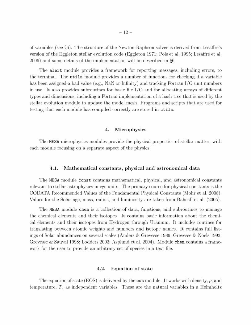
Fig. 1.— The ρ−T coverage of the equations of state used by the eos module for Z ≤ 0.04.
Inside the region bounded by the black dashed lines we use MESA EOS tables that were
constructed from the OPAL and SCVH tables. The OPAL and SCVH tables were blended
in the region shown by the blue dotted lines, as described in the text. Regions outside of
the black dashed lines utilize the HELM and PC EOSs, which, respectively, incorporate
electron-positron pairs at high temperatures and crystallization at low temperatures. The
blending of the MESA table and the HELM/PC results occurs between the black dashed lines
and is described in the text. The dotted red line shows where the number of electrons per
baryon has doubled due to pair production, and the region to the left of the dashed red line
has Γ1 < 4/3. The very low density cold region in the leftmost part of the figure is treated
as an ideal, neutral gas. The region below the black dashed line labeled as Γ = 175 would
be in a crystalline state for a plasma of pure oxygen and is fully handled by the PC EOS.
The red dot-dashed line shows where MESA blends the PC and HELM EOSs. The green
lines show stellar profiles for a main sequence star (M = 1.0M�), a contracting object of
M = 0.001M� and a cooling white dwarf of M = 0.8M�. The heavy dark line is an evolved
25M� star that has a maximum infalling speed of 1000 km s−1. The jagged behavior reflects
the distinct burning shells.

– 15 –
Table 3. eos output quantities and units
Output Definition Units
Pgas gas pressure ergs cm−3
E internal energy ergs g−1
S entropy per gram ergs g−1 K−1
dE/dρ|T ergs cm3 g−2
CV specific heat at constant V ≡ 1/ρ ergs g−1 K−1
dS/dρ|T ergs cm3 g−2 K−1
dS/dT |ρ ergs g−1 K−2
χρ ≡ dlnP/dlnρ|T none
χT ≡ dlnP/dlnT |ρ none
CP specific heat at constant pressure ergs g−1 K−1
∇ad adiabatic T gradient with pressure none
Γ1 ≡ dlnP/dlnρ|S none
Γ3 ≡ dlnT/dlnρ|S + 1 none
η ratio of electron chemical potential to kBT none
µ mean molecular weight per gas particle none
1/µe mean number of free electrons per nucleon none

– 16 –
HELM was constructed for high temperatures (up to log T = 13) and densities (up
to log ρ = 15), and accounts for the onset of electron-positron pair production at high
temperatures. The dotted red line in Figure 1 shows where the number of electrons per
baryon has doubled due to pair production. The domination of pairs in the plasma creates
a region where Γ1 < 4/3 (to the left of the dashed red line). The blending region to HELM
(from the MESA tables) is shown by the black dashed lines in Figure 1, and can by modified
by the user. In this transition region, the blend of the two EOSs is performed in a way that
preserves thermodynamic consistency. Therefore, if each separate EOS satisfies Maxwell’s
relations, the blend will also satisfy them. To accomplish this, we linearly sum the EOS
quantities Qi (i.e. P,E, S and their partial derivatives with respect to ρ and T ) needed to
satisfy Maxwell’s relations (Timmes & Swesty 2000).11 The blend is calculated by defining
the boundary limits, inside of which we define a fractional “distance”, F , from the boundary.
As F varies from zero to one, we use the smoothing function S = (1 − cos(Fπ))/2 and for
each of the nine quantities we construct Qi = SQAi + (1− S)QB
i , where QAi and QB
i are the
outputs from the two EOSs. We then use these to rederive the thermodynamic quantities
(χρ, χT , CP ,∇ad,Γ3,Γ1) delivered by the eos routine.
In late stages of the cooling of white dwarfs, the ions in the core will crystallize. For pure
oxygen, the crystallization limit corresponds to a value of the Coulomb coupling parameter,
Γ ≈ 175, shown by the black dashed line in Figure 1. In this region, we use the PC EOS,
which accounts for the modified thermodynamics of a crystal, as well as carefully handling
mixtures (e.g. carbon and oxygen). The blend between PC and HELM (as shown by the
dot-dashed red lines in Figure 1) is performed in the same manner as described above. In
the dense liquid realm, the blending region is defined by the Coulomb coupling parameter,
Γ = Z2e2/aikBT , where ai is the mean ion spacing, and Z is the average ion charge. The
default choice is PC for Γ > 80 and HELM for Γ < 40. The PC EOS is not constructed
for arbitrarily low densities, forcing a transition to HELM at log ρ < 2.8, with the blend
beginning at log ρ = 3.7. These boundaries may be re-defined by the user if needed.
In addition to the two independent variables, the eos module requires as input X,Z,
A (the mass-averaged atomic weight of metals), and Z (the mass-averaged atomic charge
of metals). When operating in the regime where the PC EOS is implemented, the mass
fractions for all isotopes with mass fractions above a specified minimum are needed (default
is 0.01), allowing PC to correctly handle isotope mixtures. It returns a total of sixteen quan-
tities (listed in Table 3) as well as the partial derivatives of each quantity with respect to the
independent variables. The tables are interpolated in the independent variables using bicu-
11The more conventional forms of these nine thermodynamic quantities are displayed in the first nine rows
in Table 3.

– 17 –
bic splines from interp 2d with partial derivatives determined from the splines. Separate
quadratic interpolations are performed in X and Z.
The construction of eos tables as outlined above is the default option for MESA but the
eos module has the flexibility to accept tables from any source so long as the tables conform
to the MESA standard format. For example, the comparison with the Stellar Code Calibration
project (Weiss et al. 2007) described in §7.1.2 utilizes tables constructed using FreeEOS.12
The FreeEOS code does not cover the same range of ρ and T as SCVH+OPAL+HELM but
the eos module is designed with this flexibility in mind: the table dimensions are specified
in the table headers and the module dynamically allocates arrays of the appropriate size to
hold them when the tables are read in.
Since not all EOS sources may be in the tabular form desired by eos, we have created
a module, other eos, that provides the user an opportunity to incorporate their own EOS
and use it with the stellar evolution module MESA star.
4.3. Opacities
The pre-processor make kap resides within the kap module and constructs the MESA
opacity tables by combining radiative opacities with the electron conduction opacities from
Cassisi et al. (2007). In the rare circumstances where ρ or T are outside the region covered
by Cassisi et al. (2007) (−6 ≤ log ρ ≤ 9.75 and 3 ≤ log T ≤ 9), the Iben (1975) fit to
the Hubbard & Lampe (1969) electron conduction opacity is used for non-degenerate cases
while the Yakovlev & Urpin (1980) fits are used for degenerate cases. Radiative opacities
are taken from Ferguson et al. (2005) for 2.7 ≤ log T ≤ 4.5 and OPAL (Iglesias & Rogers
1993, 1996) for 3.75 ≤ log T ≤ 8.7. The low T opacities of Ferguson et al. (2005) include
the effects of molecules and grains on the radiative opacity. Tables from OP (Seaton et al.
2005) can be used in place of OPAL as the table format is identical. The radiative opacity
is dominated by Compton scattering for log T > 8.7 and is calculated using the equations of
Buchler & Yueh (1976) up to a density of 106 g cm−3. We use the HELM EOS to calculate
the increasing number of electrons and positrons per baryon when pair production becomes
prevalent, an important opacity enhancement.
The OPAL tables with fixed metal distributions are called Type 1 (Iglesias & Rogers
1993, 1996) and cover the region 0.0 ≤ X ≤ 1−Z and 0.0 ≤ Z ≤ 0.1. Additionally, there is
support for the OPAL Type 2 (Iglesias & Rogers 1996) tables that allow for varying amounts
12http://freeeos.sourceforge.net

– 18 –
of C and O beyond that accounted for by Z; these are needed during helium burning and
beyond. These have a range 0.0 ≤ X ≤ 0.7, 0.0 ≤ Z ≤ 0.1.
The resulting kap tables cover the large range 2.7 ≤ log T ≤ 10.3 and −8 ≤ logR ≤ 8
(R = ρ/T 36 , so logR = log ρ − 3 log T + 18), as shown by the heavy orange and black lines
in Figure 2. The MESA release includes MESA opacity tables derived from Type 1 and 2
OPAL tables, tables from OP, and Ferguson et al. (2005). The heavy orange lines delineate
the boundaries where we use existing tables to make the MESA opacity table. The blended
regions in Figure 2 are where two distinct sources of radiative opacities exist for the same
parameters, requiring a smoothing function that blends them in a manner adequate for
derivatives. The blend is calculated at a fixed logR by defining the upper (log TU) and
lower (log TL) boundaries of the blending region in log T space, where κU (κL) is the opacity
source above (below) the blend. We perform the interpolation by defining F = (log T −log TL)/(log TU − log TL), and using a smooth function S = (1− cos(Fπ))/2 for
log κ = S log κU(R, T ) + (1− S) log κL(R, T ). (1)
At high temperatures, the blend from Compton to OPAL (or OP) has log TU = 8.7 and
log TL = 8.2. At low temperatures, the blend between Ferguson et al. (2005) and OPAL has
log TU = 4.5 and log TL = 3.75.
The absence of tabulated radiative opacities for logR > 1 and log T < 8.2 (the region
below the heavy dashed line in Figure 2) leads us to use the radiative opacity at logR = 1
(for a specific log T ) when combining with the electron conduction opacities. This introduces
errors in the MESA opacity table between logR = 1 and the region to the right of the dashed
blue line in Figure 2 where conductive opacities become dominant. However, as we show in
Figure 3, main sequence stars are always efficiently convective in this region of parameter
space, alleviating the issue.
The module kap gives the user the resulting opacities by interpolating in log T and
logR with bicubic splines from interp 2d. The user has the option of either linear or cubic
interpolation in X and Z and can specify whether to use the fixed metal (Type 1) tables or
the varying C and O (Type 2) tables. In the latter case, the user must specify the reference
C and O mass fractions, usually corresponding to the C and O in the initial composition.
– 19 –
log ρ (g cm−3)
log
T(K
)
FERG
OPAL/OP
COMPTONBLEND
e+e−
BLEND
logR
=-8
logR
=1
logR
=80.01
0.11.0
100
−10 −5 0 5 10
34
56
78
910
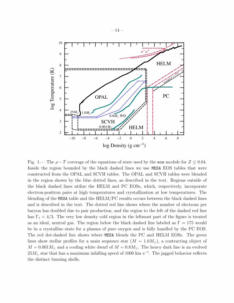
Fig. 2.— The sources of the standard MESA opacity tables. Construction of opacity tables
requires incorporating different sources, denoted by the labels. The heavy orange lines
denote regions where input tables exist for radiative opacities, whereas the heavy black
lines extend into regions where we use algorithms to derive the total opacities, described
in the text. Above the dashed red line, the number of electrons and positrons from pair
production exceeds the number of electrons from ionization, and is accounted for in the
opacity table. The opacity in the region to the right of the dashed blue line is dominated
by electron conduction. Also shown are stellar profiles for stars on main sequence (M =
0.1, 1.0, & 100M�) or just below (a contracting M = 0.01M� brown dwarf).
– 20 –
For requests outside the log T and logR boundaries, the following is done. The region
to the left of logR = −8 and below log T = 8.7 is electron scattering dominated, so the
cross-section per electron is density independent. However, the increasing importance of
the Compton effect as the temperature increases (which is incorporated in the OPAL/OP
tabulated opacities) must be included, so we use the opacity from the table at logR = −8
at the appropriate value of log T . For higher temperatures (log T > 8.7) electron-positron
pairs become prevalent, as exhibited by the red dashed line that shows where the number of
positrons and electrons from pair production exceeds the number of electrons from ionization.
MESA incorporates the enhancement to the opacity from these increasing numbers of leptons
per baryon.
At the end of a star’s life, low enough entropies can be reached that an opacity for
logR > 8 is needed. When kap is called in this region, we simply use the value at logR = 8
for the same log T . For regions where Z > 0.1, the table at Z = 0.1 is used.
The resulting opacities for Z = 0.019 and Y = 0.275 are shown in Figure 3, both
as a color code, and as contours relative to the electron scattering opacity, κ0 = 0.2(1 +
X) cm2 g−1. The orange lines show (top to bottom) where logR = −8, logR = 1 and
logR = 8. We show a few stellar profiles for main sequence stars as marked. The green
parts of the line are where heat transfer is dominated by heat transport, requiring an opacity,
whereas the light blue parts of the line are where the model is convective. As is evident,
nearly all of the stellar cases of interest (shown by the green-blue lines) are safely within the
boundaries or the MESA tables. The lack of radiative opacities in the higher density region to
the right of logR = 1 implies opacity uncertainties until the dark blue line is reached (where
the conductive opacity takes over). However, the stellar models are convectively efficient in
this region, so that the poor value for κ does not impact the result as long as the convective
zone’s existence is independent of the opacity (the typical case for these stars, where the
ionization zone causes the convection).

– 21 –
log ρ (g cm−3)
logT
(K)
Z=0.019, Y=0.275
κ0
10κ0
102κ0
103κ0
104κ0
105κ0
conduction bydegenerate electrons
0.10.3
1.03
100
−6 −4 −2 0 2 4
45
67
8
logop
acity(cm
2g−1)
−6
−4
−2
02
46
Fig. 3.— The resulting MESA opacities for Z = 0.019, Y = 0.275. The underlying shades
show the value of κ, whereas the contours are in units of the electron scattering opacity,
κ0 = 0.2(1 + X) cm2 g−1. The orange lines show (top to bottom) where logR = −8,
logR = 1 and logR = 8. Stellar interior profiles for main sequence stars of mass M =
0.1, 0.3, 1.0, 3.0 & 100M� are shown by the green(radiative regions )-light blue(convective
regions) lines. Electron conduction dominates the opacity to the right of the dark blue line
(which is where the radiative opacity equals the conductive opacity).
It is also possible to generate a new set of kap readable opacity tables using the make kap
pre-processor. The requirements are high-temperature radiative opacities in the standard
OPAL format and low-temperature radiative opacities in the number and format provided

– 22 –
by Ferguson et al. (2005).13 Specific high-temperature radiative opacities can be made by
using the OPAL site14 or the Opacity Project site15.
Since not all opacity sources can be placed in the tabular form desired by kap, we have
created a module, other kap, that provides the user an opportunity to incorporate their own
opacity source. A simple flag tells MESA star to call other kap rather than kap, allowing
for experiments with new opacity schemes and physics updates. The first example of such
an implementation that has now become a MESA module is karo. It was developed to study
the stellar evolution effects of dust-driven winds in Carbon-rich stars, using the Rosseland
opacities of Lederer & Aringer (2009) and the hydro-dynamical wind models of Mattsson et
al. (2010).
4.4. Thermonuclear and weak reactions
The rates module contains thermonuclear reaction rates from Caughlan & Fowler (1988,
CF88) and Angulo et al. (1999, NACRE), with preference given to the NACRE rate when
available. The reaction rate library includes more than 300 rates for elements up to Nickel,
and includes the weak reactions needed for Hydrogen burning (e.g. positron emissions,
electron captures), as well as neutron-proton conversions and a few other electron and neu-
tron capture reactions. Significant updates to the NACRE rates have been included for14N(p,γ)15O (Imbriani et al. 2004), triple-α (Fynbo et al. 2005), 14N(α, γ)18F (Gorres et al.
2000) and 12C(α, γ)16O (Kunz et al. 2002). In these special cases, the rate can be selected
from CF88, NACRE, or the newer reference by the user at run time.
The weaklib module calculates lepton captures and β-decay rates for the high densities
and temperatures encountered in late stages of stellar evolution. The rates are based on
the tabulations of Fuller et al. (1985), Oda et al. (1994), and Langanke & Martınez-Pinedo
(2000) for isotopes with 45 < A < 65. The most recent tabulations of Langanke & Martınez-
Pinedo (2000) take precedence, followed by Oda et al. (1994), then Fuller et al. (1985). The
user can override this to create tables using any combination of these or other sources.
The screen module calculates electron screening factors for thermonuclear reactions in
both the weak and strong regimes. The treatment has two options. One is based on Dewitt
13http://webs.wichita.edu/physics/opacity
14http://opalopacity.llnl.gov/new.html
15http://cdsweb.u-strasbg.fr/topbase/op.html

– 23 –
et al. (1973) and Graboske et al. (1973). The other16 combines Graboske et al. (1973) in
the weak regime and Alastuey & Jancovici (1978) with plasma parameters from Itoh et al.
(1979) in the strong regime.
The neu module calculates energy loss rates and their derivatives from neutrinos gen-
erated by a range of processes including plasmon decay, pair annihilation, Bremsstrahlung,
recombination and photo-neutrinos (i.e. neutrino pair production in Compton scattering). It
is based on the publicly available routine (see footnote 16) derived from the fitting formulas
of Itoh et al. (1996).
4.5. Nuclear reaction networks
The net module implements nuclear reaction networks and is derived from publicly
available code (see footnote 16). It includes a “basic” network of 8 isotopes: 1H, 3He,4He, 12C, 14N, 16O, 20Ne, and 24Mg, and extended networks for more detailed calculations
including coverage of hot CNO reactions, α-capture chains, (α,p)+(p,γ) reactions, and heavy-
ion reactions (Timmes 1999). In addition to using existing networks, the user can create
a new network by listing the desired isotopes and reactions in a data file that is read at
run time. The amount of heat deposited in the plasma by reactions is derived from the
nuclear masses in chem, taken from the JINA Reaclib database (Rauscher & Thielemann
2000; Sakharuk et al. 2006; Cyburt et al. 2010), and accounts for positron annihilations
and energy lost to weak neutrinos, using Bahcall (1997, 2002) for the hydrogen burning
reactions. The list of approximately 350 reactions is stored in a data file that catalogs the
reaction name, the input and output species, and their heat release.
The jina module is an alternative nuclear network module that specializes in large
networks. It is based on the ‘netjina’ package by Ed Brown and uses the JINA Reaclib
16http://cococubed.asu.edu/code_pages/codes.shtml
Table 4. Comparison of 1-zone Solar burn results at 10 Gyr
Network log10 enuc log10 X(1H) log10 X(4He) log10 X(12C) log10 X(14N) log10 X(16O)
jina 25 18.63757961 -3.87550319 -0.008144854 -4.40235799 -1.9195882 -3.07400339
net 25 18.63685339 -3.87550517 -0.008145036 -4.40235799 -1.9195882 -3.07400333
net 8 18.63675658 -3.93650004 -0.008137607 -4.39650625 -1.9135911 -3.04585377

– 24 –
log age (years)
log
mas
sfr
acti
on
jina 25net 25net 8
1H
3He
4He
12C
13C
14N
15N
16O
17O
18O
X = 0.706, Y = 0.275log ρ = 2.00 (g cm−3), log T = 7.28 (K)
6 7 8 9 10
−8
−6
−4
−2
0
log
tota
ler
gsg−
1
enuc
6 7 8 9 1017
.017
.518
.018
.519
.0
Fig. 4.— A 1-zone hydrogen burn at constant T = 19× 106 K and ρ = 100 g cm−3 by three
different networks. The number following net or jina indicates the number of isotopes
considered in that network. The 25 isotope networks expand on the 8 isotope network by
including minor contributors to the pp and CNO cycles. The plot shows the evolution of the
mass fraction abundances of the 10 most abundant isotopes and net energy generation per
unit mass, enuc (ergs g−1), as a function of time. The left-hand axis shows the mass fraction
while the right-hand axis shows the net energy generation per unit mass.

– 25 –
Table 5. Comparison of 1-zone He-burn results at 10 Gyr
Network log10 enuc log10 X(12C) log10 X(16O) log10 X(22Ne) log10 X(26Mg)
jina 200 17.9085633 -0.721578469 -0.108630252 -1.50380756 -4.01520633
net 11 17.9086380 -0.721576540 -0.108630957 -1.50385214 -3.99780015
net 8 17.9083877 -0.718866029 -0.107692784 · · · · · ·
log age (years)
log
mas
sfr
acti
on
jina 200net 11net 8
4He
4He
12C
14N
16O
18O
22Ne
26Mg
4He = 0.98, 14N = 0.02
log ρ = 4.0 (g cm−3)
log T = 8.1 (K)
1 2 3 4 5 6 7 8 9 10
−5
−4
−3
−2
−1
0
log
tota
ler
gsg−
1
enuc
1 2 3 4 5 6 7 8 9 10
17.0
17.2
17.4
17.6
17.8
18.0
Fig. 5.— Equivalent to Figure 4 but now showing a 1-zone helium burn at constant log T =
8.1, log ρ = 4.0. The “net 11” network adds 18O, 22Ne, and 26Mg to the 8 isotope network;
“jina 200” includes about 200 isotopes up to 71Ge.
– 26 –
database for thermonuclear reaction rates (Rauscher & Thielemann 2000; Sakharuk et al.
2006),17 the rates and weaklib modules for weak interactions, and screen for electron
screening. Most importantly, it allows the user to create large nuclear networks by specifying
the list of isotopes to consider. All nuclear reactions (both strong and weak) linking the
isotopes in the set are automatically included in the network. In all, jina covers more than
76,000 nuclear reactions involving more than 4,500 isotopes. The jina module is slower
than net for small networks but the flexibility and capacity to handle large networks make
it advantageous in some cases.
Both net and jina include one-zone burn routines that operate on a user-defined initial
composition, nuclear network, and a trajectory comprising density and temperature as a
function of time. The one-zone burn routines interface with mtx and num, enabling the
use of the sparse matrix solver, which substantially improves performance compared to the
dense matrix solver for networks of more than a few hundred isotopes. Figures 4 and 5
demonstrate these one-zone routines operating on conditions appropriate for the Sun on the
main sequence and for a core He-burning star, respectively. Both examples were evolved at
fixed density and temperature for 10 Gyr. Each figure compares three networks of varying
size in terms of the mass fractions and net energy generation per unit mass, enuc (ergs g−1),
produced. Tables 4 and 5 complement Figures 4 and 5, respectively, by listing the final values
from each of the one-zone burn simulations. These comparisons indicate that the 8 isotope
network produces results that agree with larger networks to 4-5 significant figures in net
energy generation per unit mass and generally 2-3 significant figures in the mass fractions of
various isotopes. Hence, the 8 isotope network is sufficiently accurate to describe the energy
generation for hydrogen and helium burning.
5. Macrophysics
5.1. The mixing length theory of convection
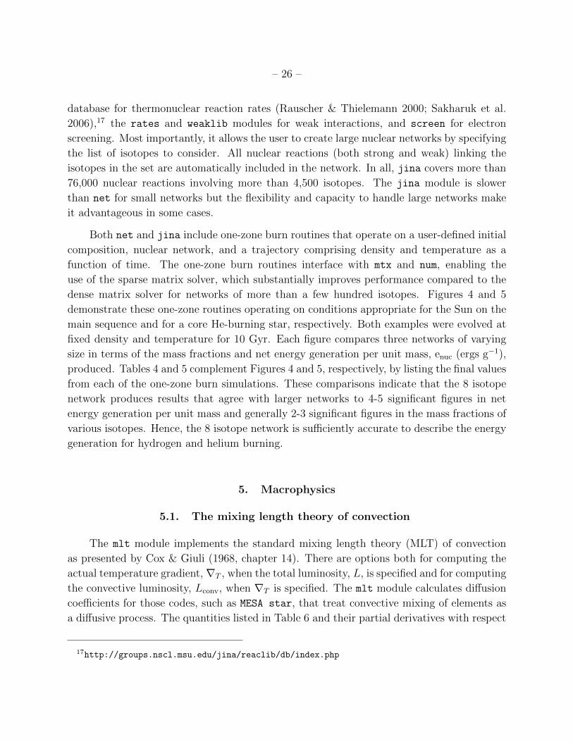
The mlt module implements the standard mixing length theory (MLT) of convection
as presented by Cox & Giuli (1968, chapter 14). There are options both for computing the
actual temperature gradient, ∇T , when the total luminosity, L, is specified and for computing
the convective luminosity, Lconv, when ∇T is specified. The mlt module calculates diffusion
coefficients for those codes, such as MESA star, that treat convective mixing of elements as
a diffusive process. The quantities listed in Table 6 and their partial derivatives with respect
17http://groups.nscl.msu.edu/jina/reaclib/db/index.php
– 27 –
to several physical variables are returned by the mlt module.
In addition to the standard MLT of Cox & Giuli, the mlt module includes the option
to use the modified MLT of Henyey et al. (1965). Whereas the standard MLT assumes
high optical depths and no radiative losses, the Henyey et al. (1965) variation allows the
convective efficiency to vary with the opaqueness of the convective element, an important
effect for convective zones near the outer layers of stars. If the Henyey et al. (1965) option
is used, the parameter ν (a mixing length velocity multiplier) and y (a parameter that sets
the temperature gradient in a rising bubble) may be set by the user. They default to the
recommended values of y = 1/3 and ν = 8.
Towards the center of a star, the commonly used definition of the pressure scale height,
λP = P/gρ, diverges as g → 0. Therefore, we provide the option of using the alternate
definition of Eggleton (1971), λ′P = (P/Gρ2)1/2, when λ′P < λP . At the center of the star,
λ′P ∼ R.

– 28 –
Table 6. MESA mlt output quantities and units
Output Definition Units
∇T actual temperature gradienta Dimensionless
∇rad radiative temperature gradienta Dimensionless
Lconv convective luminosityb ergs s−1
L total luminosityc ergs s−1
λP pressure scale height cm
Λ mixing length (≡ αMLTλP ) cm
vconv convective velocity cm s−1
D Eulerian diffusion coefficient cm2 s−1
σ Lagrangian diffusion coefficient (≡ D(4πr2ρ)2) g2 s−1
aOnly when L is specified.
bOnly when ∇T is specified.
cOnly when ∇T is specified and Lconv > 0.
– 29 –
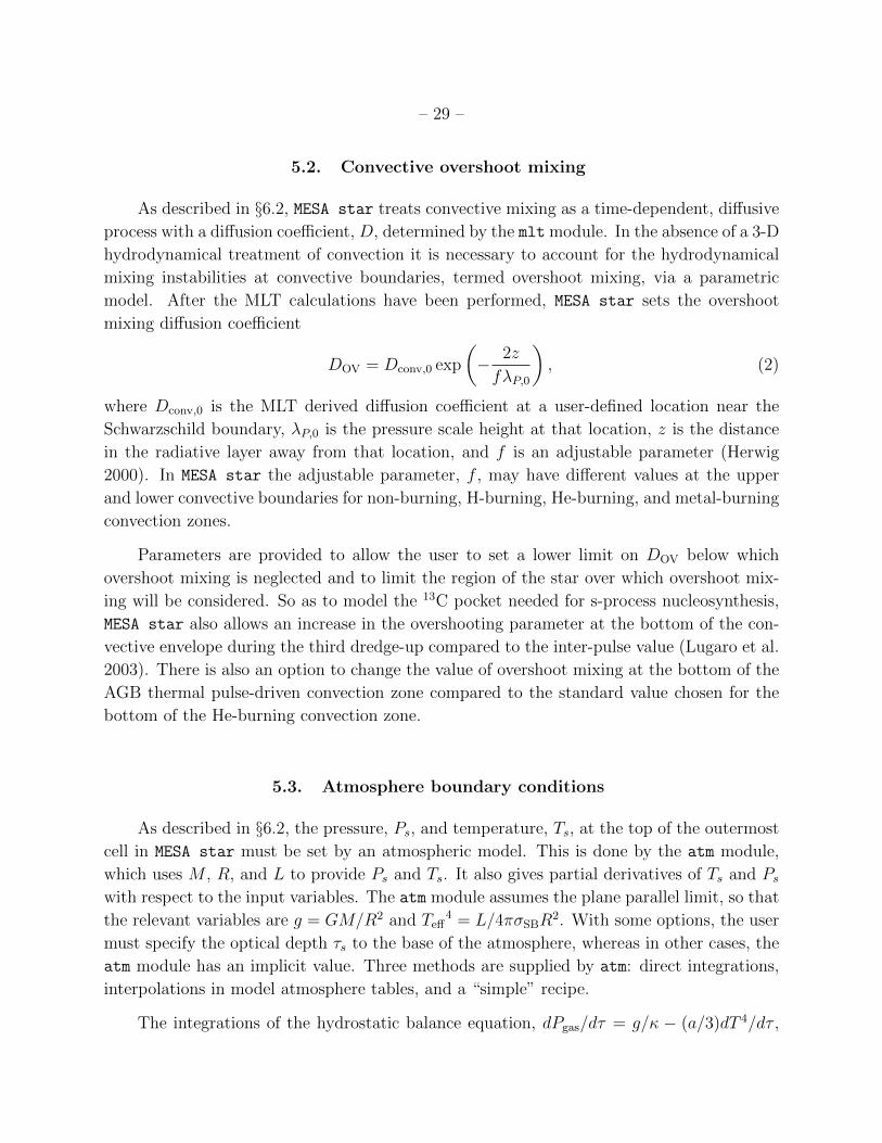
5.2. Convective overshoot mixing
As described in §6.2, MESA star treats convective mixing as a time-dependent, diffusive
process with a diffusion coefficient, D, determined by the mlt module. In the absence of a 3-D
hydrodynamical treatment of convection it is necessary to account for the hydrodynamical
mixing instabilities at convective boundaries, termed overshoot mixing, via a parametric
model. After the MLT calculations have been performed, MESA star sets the overshoot
mixing diffusion coefficient
DOV = Dconv,0 exp
(− 2z
fλP,0
), (2)
where Dconv,0 is the MLT derived diffusion coefficient at a user-defined location near the
Schwarzschild boundary, λP,0 is the pressure scale height at that location, z is the distance
in the radiative layer away from that location, and f is an adjustable parameter (Herwig
2000). In MESA star the adjustable parameter, f , may have different values at the upper
and lower convective boundaries for non-burning, H-burning, He-burning, and metal-burning
convection zones.
Parameters are provided to allow the user to set a lower limit on DOV below which
overshoot mixing is neglected and to limit the region of the star over which overshoot mix-
ing will be considered. So as to model the 13C pocket needed for s-process nucleosynthesis,
MESA star also allows an increase in the overshooting parameter at the bottom of the con-
vective envelope during the third dredge-up compared to the inter-pulse value (Lugaro et al.
2003). There is also an option to change the value of overshoot mixing at the bottom of the
AGB thermal pulse-driven convection zone compared to the standard value chosen for the
bottom of the He-burning convection zone.
5.3. Atmosphere boundary conditions
As described in §6.2, the pressure, Ps, and temperature, Ts, at the top of the outermost
cell in MESA star must be set by an atmospheric model. This is done by the atm module,
which uses M , R, and L to provide Ps and Ts. It also gives partial derivatives of Ts and Pswith respect to the input variables. The atm module assumes the plane parallel limit, so that
the relevant variables are g = GM/R2 and Teff4 = L/4πσSBR
2. With some options, the user
must specify the optical depth τs to the base of the atmosphere, whereas in other cases, the
atm module has an implicit value. Three methods are supplied by atm: direct integrations,
interpolations in model atmosphere tables, and a “simple” recipe.
The integrations of the hydrostatic balance equation, dPgas/dτ = g/κ − (a/3)dT 4/dτ ,

– 30 –
with dτ = −κρdr are performed using either the relation T 4(τ) = 3T 4eff(τ+2/3)/4 (Eddington
1926), or the specific T − τ relation of Krishna Swamy (1966). These integrations start at
τ = 10−5 and end at a user specified stopping point, τs, which defaults to τs = 2/3 (0.312)
for Eddington (Krishna Swamy).18 The routine integrates the gas pressure and then adds
the radiation pressure at the stopping point to get Ps.
The MESA model atmosphere tables come in two forms. The MESA photospheric tables
(which return Ts ≡ Teff and assume that τs ≈ 1) cover logZ/Z� = −4 to +0.5 assuming
the Grevesse & Noels (1993) Solar abundance mixture. They span log(g) = −0.5 to 5.5
at 0.5 dex intervals and Teff =2,000-50,000K at 250K intervals. They are constructed, in
precedence order, with, first, the PHOENIX (Hauschildt et al. 1999a,b) model atmospheres
(which span log(g) = −0.5 to 5.5 and Teff = 2, 000 to 10, 000 K); and second, the Castelli
& Kurucz (2003) model atmospheres (which span log(g) = 0 to 5 and Teff = 3500 to 50, 000
K). In regions where neither table is available, we generate the MESA table entry using the
integrations described above with the Eddington T-τ relation. The second MESA table is
for Solar metallicity and gives Ps and Ts at τs = 100. It is primarily for the evolution of
low mass stars, brown dwarfs, and giant planets. It is constructed from Castelli & Kurucz
(2003), and for Teff < 3000K, the COND model atmospheres (Allard et al. 2001) which
assume gravitational settling of those elements that form dust, depleting those elements
from the photosphere. Figure 6 shows the regions where the different sources are used, and
in those regions where there are no published results, we use the integration of the Eddington
T-τ relation.
18If the first attempt to integrate fails, the code makes two further attempts, each time increasing the
initial τ by a factor of 10. The integration is carried out with the Dormand-Price integrator from the num
module.

– 31 –
Teff (K)
log
g(c
mse
c−2)
0.001M�
0.005M�
0.01M�
0.05M�0.09M�
1.0M�
2.3M�
COND
CK
Eddington T (τ)
0200040006000800010000
0.0
0.5
1.0
1.5
2.0
2.5
3.0
3.5
4.0
4.5
5.0
5.5
6.0
Fig. 6.— The range of Teff and log(g) covered by the MESA atm tables for τs = 100 and Solar
metallicity. The CK region uses the tables of Castelli & Kurucz (2003), whereas the COND
region uses Allard et al. (2001). At lower log(g) and cold regions, we use direct integrations
of the Eddington T − τ relation. The green lines show evolutionary tracks of stars, brown
dwarfs and giant planets of the noted masses.
Finally, there is a simple option where the user specifies τs and we use the constant

– 32 –
opacity, κs, solution of radiative diffusion,
Ps =τsg
κs
[1 + 1.6× 10⁻⁴κs
(L/L�M/M�
)], (3)
where the factor in square brackets accounts for the nonzero radiation pressure (see, e.g.,
Cox & Giuli 1968, Section 20.1). The temperature is simply given by the Eddington relation.
The user can either specify κs or it will be calculated in an iterative manner using the initial
value of Ps from an initial guess at κs (usually given by MESA star as the value in the
outermost cell; see §6.2). In addition, the atm module has the option to revert to Equation
(3) if a model wanders outside the range of the currently used model atmosphere tables or
if the atmosphere integration fails for any reason.
5.4. Diffusion and gravitational settling
MESA diffusion calculates particle diffusion and gravitational settling by solving Burger’s
equations using the method and diffusion coefficients of Thoul et al. (1994). The transport
of material is computed using the semi-implicit, finite difference scheme described by Iben &
MacDonald (1985). Radiative levitation is not presently included. The diffusion module
treats the elements present in the stellar model as belonging to “classes” defined by the
user in terms of ranges of atomic masses. For each class, the user specifies a representative
isotope, and all members of that class are treated identically with their diffusion velocities
determined by the representative isotope, and the diffusion equation solved with the mass
fraction in that class. The caller can either specify the ionic charge for each class at each
cell in the model or have the charge calculated by the ionization module, which estimates
the typical ionic charge as a function of T , ρ, and free electrons per nucleon from Paquette
et al. (1986).
– 33 –
● ●●
●
●
●
●
●
●
●
●
●
●
●
●
●
●
●
r (R�)
|w|(R�/τθ)
HOFe (Z=21)FeHe
0.1 0.2 0.3 0.4 0.5 0.6
050
100
150
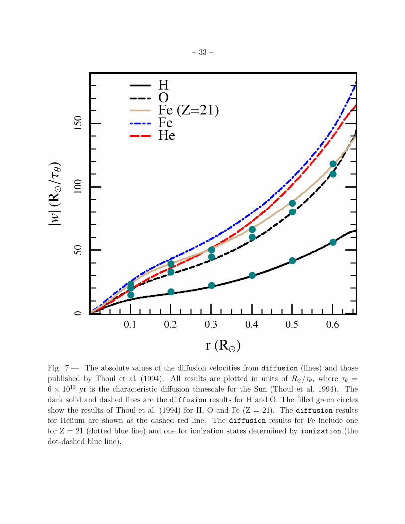
Fig. 7.— The absolute values of the diffusion velocities from diffusion (lines) and those
published by Thoul et al. (1994). All results are plotted in units of R�/τθ, where τθ =
6 × 10¹³ yr is the characteristic diffusion timescale for the Sun (Thoul et al. 1994). The
dark solid and dashed lines are the diffusion results for H and O. The filled green circles
show the results of Thoul et al. (1994) for H, O and Fe (Z = 21). The diffusion results
for Helium are shown as the dashed red line. The diffusion results for Fe include one
for Z = 21 (dotted blue line) and one for ionization states determined by ionization (the
dot-dashed blue line).

– 34 –
The lines in Figure 7 plot four classes (H, He, O, and Fe) with a solar model from
MESA star and compares where possible to the results from Figure 9 of Thoul et al. (1994),
shown by the filled green circles. The agreement is excellent for H, O and Fe (when we fix Fe
to have the Z = 21 ionization state chosen by Thoul et al. (1994)). Thoul et al. (1994) did
not exhibit the He velocity, so we have no comparison. For Fe, we also show the diffusion
velocity when ionization finds a changing ionization state in the Z = 16, 17, 18 region
(shown by the upper dot-dashed blue line), highlighting the need to better determine the Fe
ionization state (Gorshkov & Baturin 2008). We also compared the diffusion output to
the recent calculations of Gorshkov & Baturin (2008), finding agreement at better than 5%
for the Fe case at Z = 26 and for O.
The diffusion calculation can be restricted to areas where the temperature is above some
minimum value, or where the mass fraction of a diffusing element is above some minimum
value, aiding the convergence of solutions in a variety of environments. The physics imple-
mentation is presently limited to regions where the Coulomb coupling parameter, Γ, is less
than unity. At present, this inhibits an accurate calculation for segregation and settling of
the remaining envelope H and He envelope on a cooling white dwarf.
5.5. Testing MESA modules in an existing stellar evolution code
The complex, nonlinear behavior of stellar structure and evolution models makes it
difficult to disentangle the effects of model components (e.g., EOS, opacities, boundary
conditions, etc.) when comparing results of separate codes. By design, the modularity of
MESA allows individual physics modules to be incorporated into an existing stellar evolution
code, tested, and then compared against the prior implementation of comparable physics in
the same code.
During the development of MESA, several MESA modules were integrated into the Dart-
mouth Stellar Evolution Program (DSEP, Dotter et al. 2007). This section reports the results
of using four MESA modules, eos, kap, atm, and mlt, in DSEP to compute the evolution of
a 1.0M� star with initial values of X = 0.70 and Z = 0.02. The star was evolved from the
fully convective pre-main sequence to the onset of the core He flash. This was done six times:
once, as the control case, using only DSEP routines and no MESA modules; next, using each
of four MESA modules individually; and, finally, using the four MESA modules at the same
time in DSEP.
DSEP employs a ρ(P, T ) EOS and so the MESA Pgas − T tables were used during the
eos test. Though DSEP and kap use the same sources for radiative opacities, they differ

– 35 –
in interpolation methods and the treatment of electron conduction opacities (see Bjork &
Chaboyer 2006, for a thorough list of the physics in DSEP). When atm was tested, we used
the Eddington grey atmosphere model integrated to τ = 2/3. DSEP uses the Henyey et al.
(1965) modification of the mixing length theory, which is available in mlt, and assumes that
convective regions are instantaneously mixed to a uniform composition.
log Teff
log
L/L�
M = 1.0 M�Z = 0.02X = 0.70
3.53.63.7
01
23 DSEP
DSEP+MESA
log ρc (g cm−3)
log
Tc(
K)
2 3 4 5 6
7.2
7.4
7.6
7.8
log Tc(K)
log
L/L�
7.2 7.4 7.6 7.8
01
23
Age (Gyr)
log
L/L�
8 9 10 11 12
01
23
Fig. 8.— Comparison of DSEP tracks using built-in physics modules and MESA modules
for opacities, EOS, mixing length theory, and the atmospheric boundary condition. These
tracks are for a 1.0M� star with initial X = 0.70 and Z = 0.02 evolved from the fully
convective pre-main sequence to the onset of the He core flash. Only the H-R diagram shows
the full evolutionary track. The Tc panels omit the pre-main sequence in order to highlight
the regions where the differences are most pronounced; the lifetime panel focuses on the end
of the main sequence and red giant phase for the same reason.
DSEP tracks employing either the atm or the mlt modules produce results that agree
with the DSEP-only track to about 1 part in 104. DSEP tracks employing the kap and eos
modules exhibit some difference when compared to the DSEP-only track but, even in these
– 36 –
cases, the main sequence lifetime differs by less than 0.3% and Teff differs by less than 10K
along the main sequence. As shown in Figure 8, the largest discrepancy between the DSEP-
only track and the one that employs all four MESA modules appears in the Tc − ρc diagram
when ρc > 3× 10⁴g cm−3, corresponding to the growing helium core in the center of the red
giant. Above log ρc = 4, the track employing MESA modules is hotter than the DSEP-only
track by ∼ 0.02 in log Tc at constant log ρc. The center of the model has entered the region
of electron degeneracy and electron conduction has become an important source of opacity.
The majority of the difference is due to the EOS whereas the opacity difference amounts to
about −0.005 in log Tc, in the opposite direction to the EOS. The hotter conditions produced
by the eos module is likely the cause for the slightly shorter RGB lifetime that can be seen
in Figure 8.
6. Stellar structure and evolution
MESA star is a full-featured stellar structure and evolution library that utilizes the nu-
merics and physics modules described in §’s 3-5. It provides a clean-sheet implementation
of a Henyey style code (Henyey et al. 1959) with automatic mesh refinement, analytic Ja-
cobians, and coupled solution of the structure and composition equations. The design and
implementation of MESA star was influenced by a number stellar evolution and hydrody-
namic codes that were made available to us: EV (Eggleton 1971), EVOL (Herwig 2004),
EZ (Paxton 2004), FLASH-the-tortoise (Lesaffre et al. 2006), GARSTEC (Weiss & Schlattl
2008), NOVA (Starrfield et al. 2000), TITAN (Gehmeyr & Mihalas 1994), and TYCHO
(Young & Arnett 2005).
We now briefly describe the primary components of MESA star. MESA star first reads
the input files and initializes the physics modules (see §6.1) to create a nuclear reaction
network and access the EOS and opacity data. The specified starting model or pre-main
sequence model is then loaded into memory (see §6.1), and the evolution loop is entered.
The procedure for one timestep has four basic elements. First, it prepares to take a new
timestep by remeshing the model if necessary (§6.5 and 6.4). Second, it adjusts the model
to reflect mass loss by winds or mass gain from accretion (§6.6) , adjusts abundances for
element diffusion (§5.4), determines the convective diffusion coefficients (§5.1 and 5.2), and
solves for the new structure and composition (§6.2 and 6.3) using the Newton-Raphson solver
(§3). Third, the next timestep is estimated (§6.4). Fourth, output files are generated (§6.1).
– 37 –
6.1. Starting models and basic input/output
MESA star receives basic input from two Fortran namelist files. One file specifies the
type of evolutionary calculation to be performed, the type of input model to use, the source of
EOS and opacity data, the chemical composition and nuclear network, and other properties
of the input model. The second file specifies the controls and options to be applied during
the evolution.
There are two ways to start a new evolutionary sequence with MESA star. The first
is to use a saved model from a previous run. A variety of saved models are distributed
with MESA as a convenience. These saved models fall into three general categories: (1) Zero
Age Main Sequence (ZAMS) models for Z = 0.02 with 32 masses between 0.08 and 100M�(MESA star will automatically interpolate any mass within this range); (2) very low mass,
pre-main sequence models for Z = 0.02 and masses from 0.001 to 0.025M�; and (3) white
dwarf models for Z = 0.02 with He cores of 0.15− 0.45M�, C/O cores of 0.496− 1.025M�,
and O/Ne cores of 1.259 − 1.376M�. The user can also create saved models for essentially
any purpose through available controls.
The second way to start a new evolution is to create a pre-main sequence (PMS) model
by specifying the mass, M , a uniform composition, a luminosity, and a central temperature,
Tc low enough that nuclear burning is inconsequential (Tc = 9×10⁵ K by default). For a fixed
Tc and composition, the total mass depends only on the central density, ρc. An initial guess
for ρc is made by using the n = 1.5 polytrope, which is appropriate for a fully convective
star, but we do not assume the star is fully convective during the subsequent search for
a converged PMS model. Instead, MESA star uses the mlt, eos, and Newton solver from
num to search for a ρc that gives a model of the desired mass. The PMS routine presently
creates starting models for 0.02 ≤ M/M� ≤ 50. Beyond these limits we find challenges
converging the generated PMS model within the MESA star evolutionary loop. For such
cases it is currently better to generate a starting model within the acceptable mass range,
save it, relax it to a new mass with a specified mass gain or loss (see §6.6), and save that
model.
MESA star has the ability to create a binary file of its complete current state, called a
photo, at user-specified timestep intervals. Restarting from a photo ensures no differences
in the ensuing evolution. When restarting from a photo, many controls and options can
be changed. A photo is different than a saved model in that a saved model is a text file
containing a minimal description of the structure and composition but does not have enough
information to allow a perfect restart. However, saved models are not tied to a particular
version of the code and therefore are suitable for long term use or sharing with other users.

– 38 –
There are two additional types of output files, logs and profiles. A log records evolu-
tionary properties over time such as stellar age, current mass, and a wide array of other
quantities. A profile records model properties at a specified timestep at each zone from sur-
face to center. MESA star can also output models in the FGONG format19 for use with stellar
pulsation codes and se output for nucleosynthesis post-processing with NuGrid codes.20 Fi-
nally, a few simple lines of user-supplied code allows for saving variables or combinations of
variables that are not in the list of predefined options.
6.2. Structure and composition equations
MESA star builds 1-D, spherically-symmetric models by dividing the structure into cells,
anywhere from hundreds to thousands depending on the complexity of nuclear burning, gra-
dients of state variables, composition, and various tolerances. Cells are numbered starting
with one at the surface and increasing inward. MESA star does not require the structure
equations to be solved separately from the composition equations (operator splitting). In-
stead, it simultaneously solves the full set of coupled equations for all cells from the surface
to the center. The solution of the equations is done by the Newton solver from num using
either banded or sparse matrix routines from mtx. The partial derivatives for use by the
solver are calculated analytically using the partials returned by modules such as eos, kap,
and net.
19 http://owww.phys.au.dk/~jcd/solar_models/
20http://forum.astro.keele.ac.uk:8080/nugrid

– 39 –
toward surface
toward center
mk−1, rk−1, Lk−1, vk−1, ...face k-1
mk, rk, Lk, vk, σ
σ
k,
, ,
Fi,k ,dmk Pk, T k, ∇T, kface k
mk+1, rk+1, Lk+1, vk+1, k+1, Fi,k+1, ...face k+1
dmk−1 ρk−1, Tk−1, Xi,k−1, Pk−1, ...cell k-1
dmk ρk, Tk, Xi,k, Pk, ∇ad,k εnuc,k εgrav,kcell k
Fig. 9.— Schematic of some cell and face variables for MESA star.
Each cell has some variables that are mass-averaged and others that are defined at
the outer face, as shown in Figure 9. This way of defining the variables is a consequence
of the finite volume, flux conservation formulation of the equations and improves stability
and efficiency (Sugimoto et al. 1981). The inner boundary of the innermost cell is usually
the center of the star and, therefore, has radius, luminosity, and velocity equal to zero.
Nonzero center values can be used for applications that remove the underlying star (e.g., the
envelope of a neutron star), in which case the user must define the values of Mc and Lc at
the inner radius Rc. The cell mass-averaged variables are density ρk, temperature Tk, and
mass fraction vector Xi,k. The boundary variables are mass interior to the face mk, radius
rk, luminosity Lk, and velocity vk. In addition to these basic variables, composite variables
are calculated for every cell and face, such as εnuc, κ, σk, and Fk (see Table 1 for variable
definitions). All variables are evaluated at time t+ δ t unless otherwise specified.
– 40 –
The density evolution of cell k is determined by a finite volume form of the mass con-
servation equation
ρk =dmk
(4/3)π(r3k − r3
k+1). (4)
For the innermost cell, rk+1 is replaced by the inner boundary condition which is typically
zero but can be nonzero for some applications. We reformulate many of our equations to
improve numerical stability of the linear algebra and minimize round-off errors. We thus
rewrite equation (4) as
log rk =1
3log
[r3k+1 +
3
4π
dmk
ρk
]. (5)
The velocity of face k is zero unless the hydrodynamics option is activated, in which
case
vk = rkd(log rk)
dt, (6)
is the Lagrangian time derivative of the radius at face k. For enhanced numerical stability,
we rescale this equation by dividing by the local sound speed.
The pressure Pk is set by momentum conservation at interior cell boundaries,
Pk−1 − Pk = dmk
[(dP
dm
)hydrostatic
+
(dP
dm
)hydrodynamic
]
= dmk
[−Gmk
4πr4k
− ak4πr2
k
], (7)
where dmk = 0.5(dmk−1 + dmk), and ak is the Lagrangian acceleration at face k, evaluated
by the change in vk over the timestep δt. The acceleration is set to zero if the hydrodynamic
option is not used. Similarly, the temperature of interior cells Tk is set by energy transport
across interior cell boundaries,
Tk−1 − Tk = dmk
[∇T,k
(dP
dm
)hydrostatic
T k
P k
], (8)
where∇T,k = d log T/d logP at face k from the MESA module mlt (see §5.1), T k = (Tk−1dmk+
Tkdmk−1)/(dmk + dmk−1) is the temperature interpolated by mass at face k, and P k =
(Pk−1dmk + Pkdmk−1)/(dmk + dmk−1) is the pressure interpolated by mass at face k. For
enhanced numerical stability, we rescale equation (7) by dividing by P k and equation (8) by
dividing by T k.
The pressure and temperature boundary conditions are constructed by using Ps and Tsfrom the MESA module atm (see §5.3). The difference in pressure and temperature from the

– 41 –
surface to the center of the first cell is found from hydrostatic equilibrium and ∇T by
dPs =Gm1dm1/2
4πr41
dTs = dPs∇T,1T1
P1
. (9)
The boundary conditions are then
log T1 = log(Ts + dTs)
logP1 = log(Ps + dPs) . (10)
These implicit equations for P1 and T1 are solved together with the regular structure and
composition equations.
Our finite volume form of energy conservation for cell k is
Lk − Lk+1 = dmk(εnuc − εν,thermal + εgrav) , (11)
where εnuc (from module net or jina) is the total nuclear reaction specific energy generation
rate minus the nuclear reaction neutrino loss rate, and εν,thermal (from module neu) is the
specific thermal neutrino loss rate. The εgrav term is the specific rate of change of gravitational
energy due to contraction or expansion,
εgrav = −T dsdt
= −TCP
[(1−∇adχT )
d log T
dt−∇adχρ
d log ρ
dt
], (12)
where d log T/dt and d log ρ/dt are Lagrangian time derivatives at cell center by mass, and
the other symbols are defined in Tables 3 and 6. For the innermost cell, Lk+1 is replaced
by the inner boundary condition which is typically zero but can be nonzero, Lc, in specific
applications. For additional numerical stability, we rescale equation (11) by dividing by a
scale factor that is typically the surface luminosity of the previous model.
The equation for mass fraction Xi,k of species i in cell k is
Xi,k(t+ δt)−Xi,k(t) = dXburn + dXmix
=dXi,k
dtδt+ (Fi,k+1 − Fi,k)
δt
dmk
, (13)
where dXi,k/dt is the rate of change from nuclear reactions reported by net or jina, Fi,k is
the mass of species i flowing across face k
Fi,k = (Xi,k −Xi,k−1)σk
dmk
, (14)

– 42 –
where σk is the Lagrangian diffusion coefficient from the combined effects of convection
(§5.1) and overshoot mixing (§5.2). For numerical stability, σk is calculated at the beginning
of the timestep and held constant during the implicit solver iterations. This assumption
accommodates the non-local overshooting algorithm and significantly improves the numer-
ical convergence. It leads to a small inconsistency between the mixing boundary and the
convection boundary as calculated at the end of the timestep.
Equations (5), (7), (8), (11), (14), and, optionally equation (6), are by default solved
fully coupled and simultaneously with a 1st order backwards differencing time integration.
6.3. Convergence to a solution
The generalized Newton-Raphson scheme is represented by
0 = ~F (~y) = ~F (~yi + δ~yi) = ~F (~yi) +
[d~F
d~y
]i
δ~yi +O(δ~y 2i ) (15)
where yi is a trial solution, ~F (~yi) is the residual, δ~yi is the correction, and [d~F/d~y]i is the
Jacobian matrix.
MESA star uses the previous model, modified by remeshing, mass change, and element
diffusion, as the initial trial solution for the Newton-Raphson solver. This is generally suc-
cessful because we use analytic Jacobians and have sophisticated timestep controls (see §6.4).
The use of analytic Jacobians in MESA star requires that each of the MESA modules provides
not just the required output quantities but also quality, preferentially analytic, partial deriva-
tives with respect to the input quantities. At each timestep, MESA star converges on a final
solution by iteratively improving upon the trial solution. We calculate the residuals, con-
struct a Jacobian matrix, and solve the resulting system of linear equations with the solvers
in mtx to find the corrections to the variables.
The trial solution is accepted when the corrections and residuals meet a specifiable set
of comprehensive convergence criteria. In most cases, the solver is able to satisfy these limits
in 2 or 3 iterations. However, under difficult circumstances like the He core flash or advanced
nuclear burning in massive stars, MESA star can automatically adjust the convergence cri-
teria. The corrections to the variables will, generally, not produce zero residuals because the
system of equations is nonlinear. In some cases, the corrections might make the residuals
larger rather than smaller. In such cases, the length of the correction vector is reduced by a

– 43 –
line search scheme21 until they improve the residuals. In principle, the residuals can be made
arbitrarily small, but this may take a prohibitively large number of iterations. In practice,
the use of the line search scheme helps the convergence rate in many cases, but cannot ensure
convergence in all cases.
If convergence cannot be achieved with the current timestep, then MESA star will first
try again with a reduced timestep (a “retry”) anticipating that a smaller timestep will reduce
the non-linearity. If the retry fails, MESA star will return to the previous model and with
a smaller timestep than it used to get to the current model (a “backup”). If the backup
fails, MESA star will continue to reduce the timestep until either the model converges or
the timestep reaches some pre-defined minimum, in which case the evolutionary sequence is
terminated.
6.4. Timestep selection
Timestep selection is a crucial part of stellar evolution. The timesteps should be small
enough to allow convergence in relatively few iterations, but large enough to allow efficient
evolutions. Changes to the timestep should also provide for rapid responses to varying struc-
ture or composition conditions, but need to be carefully controlled to avoid over-corrections
that can reduce the convergence rate.
MESA star does timestep selection as a two stage process. The first stage proposes
a new timestep using a scheme based on digital control theory (Soderlind & Wang 2006).
The second stage implements a wide range of tests that can reduce the proposed timestep
if certain selected properties of the model are changing faster than specified. For the first
stage, we use a low-pass filter. The control variable vc is the unweighted average over all cells
of the relative changes in log ρ, log T , and logR. The target value vt is 10−4 by default. For
improved stability and response, the low-pass filter method uses the previous two results.
Let δti−1, δti, and δti+1 be the previous, current, and next timestep, respectively, while vc,i−1
and vc,i are the previous and current values of vc. The timestep for model i + 1 is then
determined by
δti+1 = δtif
[f(vt/vc,i)f(vt/vc,i−1)
f(dti/dti−1)
]1/4
, (16)
where f(x) = 1 + 2 tan−1[0.5(x − 1)]. The control scheme implemented by equation (16)
allows rapid changes in timestep without undesirable fluctuations.
21This is a globally convergent method and is similar to what is described in §9.7 of Press et al. (1992).

– 44 –
The timestep proposed by this low-pass filtering scheme can be reduced according to a
variety of special tests that have hard and soft limits. If a change exceeds its specified hard
limit, the current solution is rejected, and the code is forced to do a retry or a backup. If a
change exceeds its specified soft limit, the next timestep is reduced proportionally. Examples
of special tests include limits on the maximum absolute or relative changes in mesh structure,
composition variables, nuclear burning rate, Teff , L, M , Tc, ρc, and integrated luminosity
from various types of nuclear burning.
6.5. Mesh adjustment
MESA star checks the structure and composition profiles of the model at the beginning of
each timestep and, if necessary, adjusts the mesh. Cells may be split into two or more pieces,
or they may be made larger by merging two or more adjacent cells. The overall remeshing
algorithm is designed such that most cells are not changed during a typical remesh. This
minimizes numerical diffusion and tends to help convergence. Remeshing is divided into a
planning stage and an adjustment stage.
The planning stage determines which cells to split or merge based on allowed changes
between adjacent cells. Mesh revisions minimize the number of splits and maximize the
number of merges while ensuring that the magnitudes, ∆, of differences between any two
adjacent cells are below specific thresholds: ∆ logP < θP , ∆ log T < θT , and ∆ log[X(4He)+
X(4He0)] < θHe where X(4He) is the helium mass fraction and X(4He0) sets an effective lower
lower limit on the sensitivity to the helium abundance. The default thresholds are θP = 1/30,
θT = 1/80, θHe = 1/20, and X(4He0) = 0.01. Options are available for specifying allowed
changes between cells for other mass fractions, ∆∇ad and ∆ log(T/(T + T0)) for arbitrary
T0.
Local reductions in the magnitude of allowed changes will place higher resolution in
desired regions of the star. For example, the default is to increase resolution in regions of
nuclear burning having ∆ log εnuc large compared to ∆ logP . This increase takes effect at a
minimum log εnuc = −2 and increases to a maximum factor of 4 in resolution for log εnuc ≥ 4.
The size and range of enhancement can also be set for various specific types of burning.
Similarly, it is possible to increase resolution near the boundaries of convection zones over a
distance measured in units of the pressure scale height. Different enhancements and distances
can be specified for above and below the upper and lower boundaries of zones with or without
burning. There are also options to increase spatial resolution in regions having ∆ logXi large
compared to ∆ logP , or near locations where there are spatial gradients in the most abundant
species. Finally, further splitting is done as necessary to limit the relative sizes of adjacent

– 45 –
cells.
The adjustment stage executes the remesh plan. Cells to be split are constructed by first
performing a monotonicity preserving cubic interpolation (Steffen 1990) in mass to obtain
the luminosities and enclosed volumes at the new cell boundaries. The new densities are
then calculated from the new cell masses and volumes, as shown in equation (4). Next, new
composition mass fraction vectors are calculated. For cells being merged, this is straightfor-
ward. For cells being split, neighboring cells are used to form a linear approximation of mass
fraction for each species as a function of mass coordinate within the cell. The slopes are
adjusted so that the mass fractions sum to one everywhere, and the functions are integrated
over the new cell mass to determine the abundances.
Finally, the method for calculating the new temperature varies according to electron
degeneracy. As the electrons become degenerate (i.e. η > 0), split cells simply inherit their
temperature while merged cells take on the mass-average of their constituent temperatures.
If the electrons are not degenerate (i.e. η < 0), then a reconstruction parabola is created
for the specific internal energy profile of the parent and its neighbor cells (Stiriba 2003).
The parabola is integrated over the new cell to find its total internal energy. The new cell
temperature is determined by repeatedly calling the eos module using the new composition
and density with trial temperatures until the desired internal energy is found.
6.6. Mass loss and accretion
Mass adjustment for mass loss or accretion is done at each timestep before solving the
equations for stellar structure and composition. MESA star offers a variety of ways to set
the rate of mass change M . A constant mass accretion or mass loss rate may be specified in
the input files (see §6.1). Implementations of Reimers (1975) for red giants, Blocker (1995)
for AGB stars, de Jager et al. (1988) for a range of stars in the H-R diagram, mass loss for
massive stars by (Glebbeek et al. 2009; Vink, de Koter & Lamers 2001; Nugis & Lamers
2009; Nieuwenhuijzen & de Jager 1990), supersonic mass loss inspired by Prialnik & Kovetz
(1995), and super-Eddington mass loss (Paczynski & Proszynski 1986) are available options.
An arbitrary mass accretion or mass loss scheme may be implemented by writing a new
module. An example of such a routine provided with MESA star is Mattsson et al. (2010)
mass loss for carbon stars. Finally, one may write a wrapper program that calculates M for
each timestep and then calls the MESA star module.
Since MESA star allows for simulations with a fixed (and unmodeled) inner mass, Mc,
the total mass is M = Mc + Mm, where Mm is the modeled mass. For cell k, MESA star
– 46 –
stores the relative cell mass dqk = dmk/Mm and the relative mass interior to a cell face
qk = mk/Mm = 1 −∑i=k−1i=1 dqi (see Figure 9). Rather than evaluate dqk as qk − qk+1, it is
essential to define q in terms of dq to maintain accuracy (Lesaffre et al. 2006). For example,
in the outer envelope of a star where the qk approach 1, the dqk can be 10−12 or smaller.
Subtraction of two adjacent qk to find a dqk leads to a intolerable loss of precision.
After a change in mass, δM , has been determined, the mass structure of the stellar
model is modified. This procedure changes the mass location of some cells and revises the
composition of those cells to match their new location. It does not add or remove cells,
nor does it change the initial trial solution for the structure variables such as ρ, T , r, or
L. The mass structure is divided into an inner (usually the central regions of the star), an
intermediate, and an outer region (usually the stellar envelope). The boundaries of the inner
and outer regions are initially set according to temperature, with defaults of log T = 6 for the
inner boundary and log T = 5 for the outer boundary. This range is automatically expanded,
for enhanced numerical stability, if the mass in the intermediate region is not significantly
larger than δM . The range is first enlarged by moving the outer boundary to the surface. If
the enclosed mass in the intermediate region is still too small, then the inner boundary can
be moved inward subject to certain limits. One limit is that the inner boundary does not
cross a region of the model where the composition changes rapidly. Another limit is that the
fractional mass of the intermediate region cannot change by more than a factor of two from
its previous value nor exceed 10% of the total mass.
Once the regions have been defined, the dqk are updated. In the inner region the dqkare rescaled by M/(M+δM). Thus, dmk, mk, and Xk have the sames value before and after
a change in mass to eliminate the possibility of unwanted numerical mixing in the center.
In the outer region, cells retain the same value of dqk to improve convergence in the high
entropy regions of the star (Sugimoto et al. 1981). The dqk in the intermediate region are
scaled so that∑dqk = 1. The composition of cells in the intermediate and outer regions are
then updated. In the case of mass accretion, the composition of the outermost cells whose
enclosed mass totals δM is set to match the specified accretion abundances. Cells that were
part of the old structure have their compositions set to match the previous composition.
6.7. Resolution sensitivity
We examined the resolution convergence properties of a 1M� model by varying the
parameters for mesh refinement and timestepping. The mesh refinement parameter multi-
plies the limits for variable changes across mesh cells and is closely correlated with the cell
size. The timestepping parameter controls the tolerance of the cell average of the relative

– 47 –
changes between time steps in log ρ, log T , and logR (see §6.4) and is closely correlated
with the timestep. We varied the mesh refinement and timestepping controls in tandem
through a parameter C, which is a multiplicative factor on their default values of 1 and 10−4,
respectively. Therefore, C is anti-correlated with the time and space resolution.
Table 7 and Figure 10 detail the convergence properties with C of a solar metallicity,
1.0 M� model with an ηR=0.5 Reimers mass loss model (Reimers 1975, see §6.6). These
calculations begin at the ZAMS and are terminated at 11.0 Gyr, when the model stars
are turning off the main sequence. As a measure of convergence, we use the difference, ξ,
between a quantity at a given resolution and the quantity at the highest resolution considered
(C=1/16). In order to determine how convergence depends on resolution (|ξ| ∝ Cα), we
determine the order of convergence, α, for increasingly resolved pairs in Table 7:
α = log
(ξfine
ξcoarse
)/log
(Cfine
Ccoarse
). (17)
The convergence orders show that all values converge linearly at large values of C and
display super-linear convergence (α ∼ 1.6) at smaller values of C. These convergence orders
are plausible given that we use a first order time integration scheme and a finite volume
differencing scheme that is second order accurate on uniform grids.
Table 8 and Figure 11 detail the same stellar models as a function of C except the
calculations are stopped at L = 100L�, when the stars are on the RGB. Table 8 suggests
the age of the star converges linearly at larger values of C and super-linearly (α ∼ 1.5) at
smaller values of C. However, Teff , Tc, ρc, M , and MHe all display oscillatory behavior about
the C=1/16 solution, suggesting factors other than spacetime resolution are dominating the
error at this stage of the evolution. Such factors could be limits in the precision attained
by interpolation in the various tables (e.g., 4 significant figures for opacities, ∼ 6 significant
figures for the OPAL and SCVH EOS), or small changes in boundary conditions.
The lower panel of Figure 12 shows the sound speed profile for the 100L� model with
C=1/16, our highest resolution case. The helium core and convective zone boundaries are
labeled. The mass interior to the convective zone boundary is 0.95 M�. The upper panel of
Figure 12 shows the convergence properties of the sound speed profile with resolution in the
hydrogen layer. Both the C=1 and C=1/2 profiles have sound speeds that are smaller than
the C=1/16 profile, while the C=1/4 and C=1/8 profiles have larger sound speeds. Note
that the difference between the various profiles becomes less as the parameter C is made
smaller, indicating that the convergence rate is becoming smaller. This suggests factors
other than spacetime resolution are dominating the convergence rates at this stage of the
evolution. Again, this could be due to the precision attained by table interpolations, small
changes in boundary conditions, or differencing errors.

– 48 –
Table 7. 1M� Model Convergence Properties at 11.00 Gyr
Control parameter C 2 1 1/2 1/4 1/8 1/16
Number of cells 457 732 1385 2740 5426 10777
Number of timesteps 93 135 225 418 813 1608
L (L�) 2.06094 2.04251 2.03241 2.02678 2.023737 2.02217
ξ (×10−3) 19.17 10.06 5.06 2.28 0.775 0.0
α 0.93 0.99 1.15 1.56
Teff (K) 5543.195 5573.935 5587.434 5593.334 5596.064 5597.361
ξ (×10−3) -9.68 -4.19 -1.77 -0.72 -0.232 0.0
α 1.21 1.24 1.30 1.63
Log Tc 7.301645 7.298305 7.296797 7.296052 7.295676 7.295486
ξ (×10−3) 0.8442 0.3864 0.1797 0.0776 0.0260 0.0
α 1.13 1.10 1.21 1.57
Log ρc 3.393658 3.348505 3.32615 3.314372 3.308441 3.305552
ξ (×10−3) 26.65 12.99 6.23 2.69 0.874 0.0
α 1.04 1.06 1.22 1.61
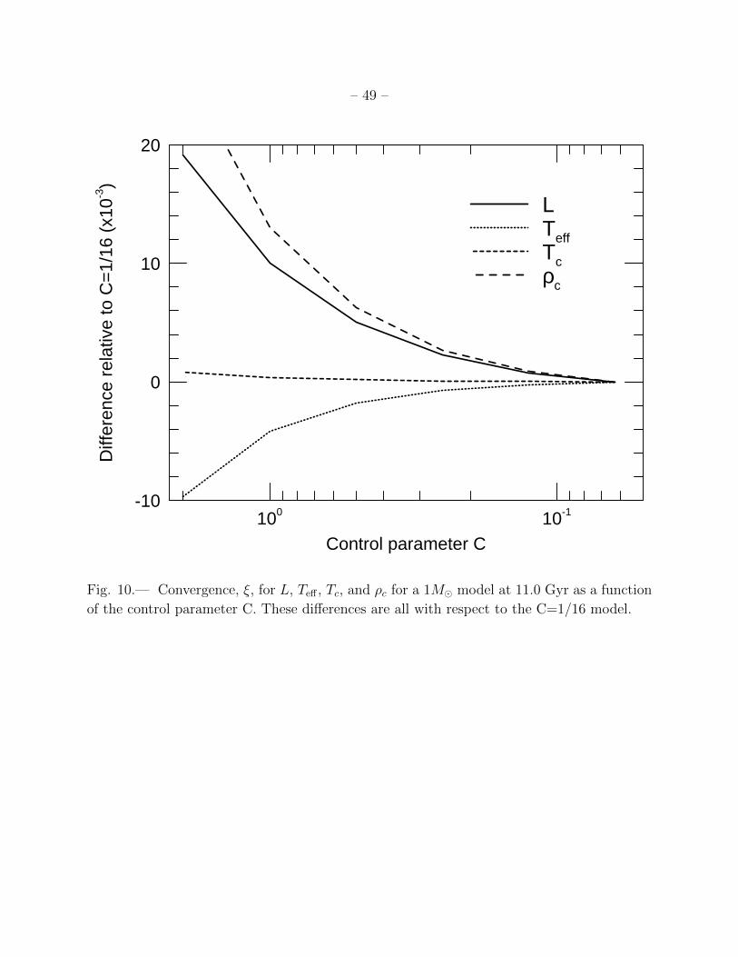
– 49 –
100 10-1-10
0
10
20
Diff
eren
ce r
elat
ive
to C
=1/
16 (
x10-3
)
Control parameter C
LTeffTcρc
Fig. 10.— Convergence, ξ, for L, Teff , Tc, and ρc for a 1M� model at 11.0 Gyr as a function
of the control parameter C. These differences are all with respect to the C=1/16 model.
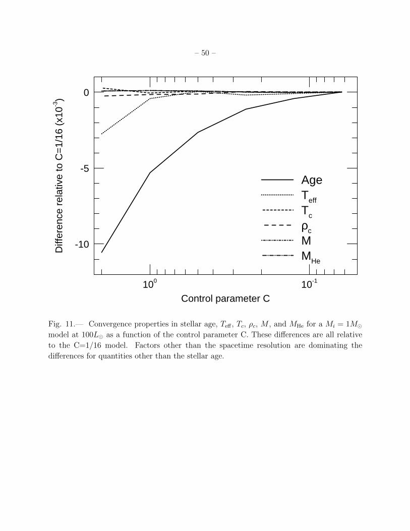
– 50 –
100 10-1
-10
-5
0
Diff
eren
ce r
elat
ive
to C
=1/
16 (
x10-3
)
Control parameter C
AgeTeff
Tc
ρc
MMHe
Fig. 11.— Convergence properties in stellar age, Teff , Tc, ρc, M , and MHe for a Mi = 1M�model at 100L� as a function of the control parameter C. These differences are all relative
to the C=1/16 model. Factors other than the spacetime resolution are dominating the
differences for quantities other than the stellar age.
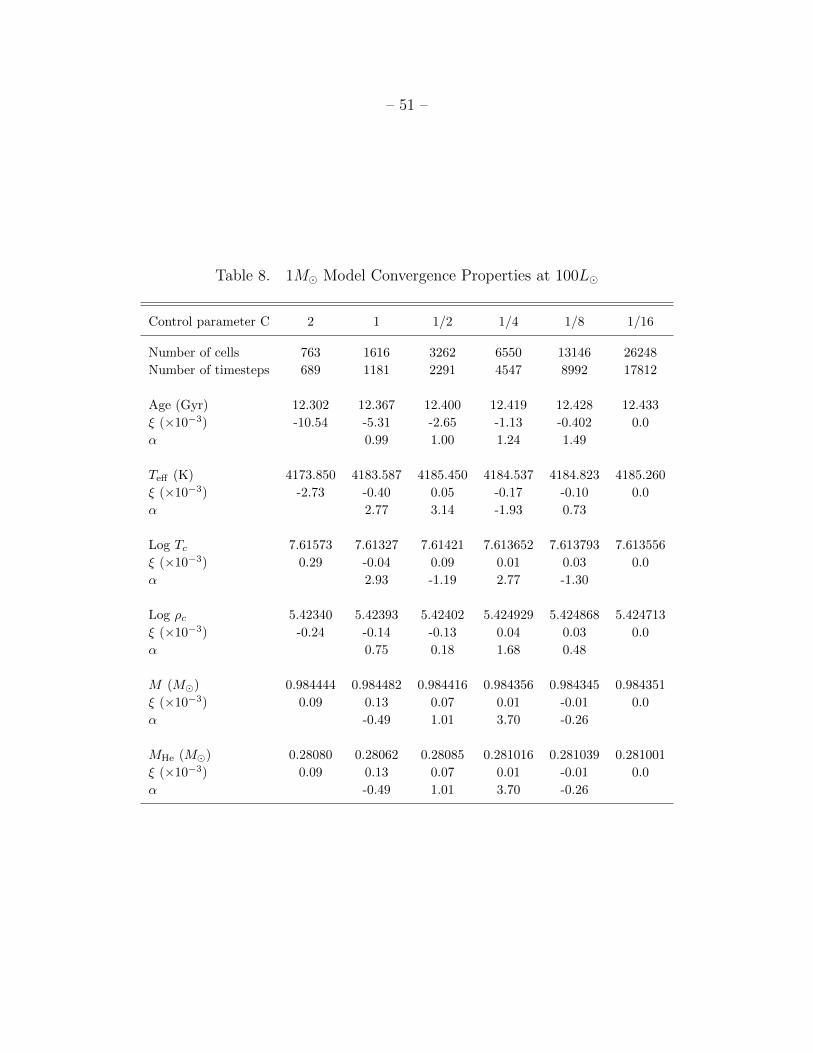
– 51 –
Table 8. 1M� Model Convergence Properties at 100L�
Control parameter C 2 1 1/2 1/4 1/8 1/16
Number of cells 763 1616 3262 6550 13146 26248
Number of timesteps 689 1181 2291 4547 8992 17812
Age (Gyr) 12.302 12.367 12.400 12.419 12.428 12.433
ξ (×10−3) -10.54 -5.31 -2.65 -1.13 -0.402 0.0
α 0.99 1.00 1.24 1.49
Teff (K) 4173.850 4183.587 4185.450 4184.537 4184.823 4185.260
ξ (×10−3) -2.73 -0.40 0.05 -0.17 -0.10 0.0
α 2.77 3.14 -1.93 0.73
Log Tc 7.61573 7.61327 7.61421 7.613652 7.613793 7.613556
ξ (×10−3) 0.29 -0.04 0.09 0.01 0.03 0.0
α 2.93 -1.19 2.77 -1.30
Log ρc 5.42340 5.42393 5.42402 5.424929 5.424868 5.424713
ξ (×10−3) -0.24 -0.14 -0.13 0.04 0.03 0.0
α 0.75 0.18 1.68 0.48
M (M�) 0.984444 0.984482 0.984416 0.984356 0.984345 0.984351
ξ (×10−3) 0.09 0.13 0.07 0.01 -0.01 0.0
α -0.49 1.01 3.70 -0.26
MHe (M�) 0.28080 0.28062 0.28085 0.281016 0.281039 0.281001
ξ (×10−3) 0.09 0.13 0.07 0.01 -0.01 0.0
α -0.49 1.01 3.70 -0.26

– 52 –
104×
(Cs−
Cs,
ref)/C
s,re
f
C=1/8
C=1/4
C=1/2
C=1
CZB
0.95 M/M�
He core
−4
−2
02
Radius (R�)
Cs,
ref
(km
s−1 )
M = 1.0M�L = 100L�X = 0.68Z = 0.02
0.0 0.2 0.4 0.6 0.8 1.0 1.2
200
400
Fig. 12.— Sound speed profile (lower panel) and convergence properties (upper panel) for
the 1M� model at 100L� with respect to the reference case, C=1/16. The helium core
boundary and convective zone boundary are labeled.

– 53 –
6.8. Multithreading
MESA modules are designed to be thread-safe (see §2), thereby enabling parallel execu-
tion. Table 9 lists the execution times in seconds of several specific tasks from 4 identical
evolutionary calculations, each with a different number of threads (one thread per core). The
essential difference between modules that scale as the inverse of the number of threads (eos
and net) and those that don’t (e.g., kap and neu) is the ratio of the overhead associated
with parallel execution to the actual time required for each module to perform its calculation.
The time required to complete serial tasks sets a lower limit on the total execution time of
MESA star.
6.9. Visualization with PGstar
By default, MESA star provides alpha-numeric output at regular intervals. In addition,
it provides the option for concurrent graphical output. PGstar uses the PGPLOT22 library
to create on-screen plots or images in PNG format that can be post-processed into anima-
tions of an evolutionary sequence. A wide variety of visualization options are provided and
these are all configurable through the PGstar inlist. For example, the PGstar window can
simultaneously hold: an H-R diagram, a Tc − ρc diagram, and interior profiles of physical
variables, such as nuclear energy generation, and composition. Animation is very useful for
visualizing complex, time dependent processes. For example, view the short selection from
the MESA website that shows the He core flash in a 1M� star.23
7. MESA star results: comparisons and capabilities
As with any modeling approach, MESA star must be verified (“Is it solving the equations
correctly?” Roache 1998) and validated (“Does it solve the right equations?”) to demonstrate
its accuracy and predictive credibility (e.g., Oberkampf 2004). V&V is a maturing discipline
(e.g., Roache 1998; Calder et al. 2004), with the goal of assessing the error and uncertainty in
a numerical simulation, which also includes addressing sources of error in theory, experiment,
observation, and computation (Calder et al. 2004). The results of V&V testing are historical
statements of reproducible evidence that a simulation demonstrates a quantified level of
22We thank Philip Pinto for initiating this MESA capability, see http://www.astro.caltech.edu/~tjp/
pgplot/.
23 http://mesa.sourceforge.net/pdfs/1MHeflash.mov

– 54 –
Table 9. Execution times (s) with multiple threads
Number of Threads
1 2 4 8
totala 12.2146 8.0099 5.8963 5.0634
ratio · · · 1.53 1.36 1.16
Threaded tasks
net 6.2602 3.1721 1.6047 0.8182
eos 1.7185 0.8897 0.4539 0.2399
mlt 0.2479 0.1384 0.0704 0.0357
kap 0.2285 0.1386 0.1044 0.0875
neu 0.0240 0.0209 0.0139 0.0098
subtotal 8.4791 4.3597 2.2473 1.1911
ratio · · · 1.95 1.94 1.89
fraction of total 0.69 0.54 0.38 0.24
Serial tasks
file output 1.1848 1.0301 1.0036 1.1679
matrix linear algebra 0.6569 0.7654 0.7885 0.7926
miscellaneous 1.8938 1.8547 1.8569 1.9118
subtotal 3.7355 3.6502 3.6490 3.8723
fraction of total 0.31 0.46 0.62 0.76
aThese numbers do not include initialization, e.g., loading
of data tables.
– 55 –
accuracy in the solution of a specific problem.
V&V is an ongoing activity for MESA via the MESA test suite (see Appendix B), where
code modules are tested individually, and, where possible, the integrated code MESA star
is verified and validated. Verification for MESA includes a systematic study of the effect of
mesh and time-step refinement on simulation accuracy (§6.7), specific module comparisons
(§5.5), and stellar evolution code comparisons presented in this section.
This section shows MESA star evolution calculations of single stellar and substellar
objects with 10−3M� < M < 1000M� (in §§7.1, 7.2, 7.3) as well as verification results
(§§7.1.1, 7.1.2, 7.2.1, 7.2.2, 7.3.1, and 7.3.2). In §7.1.3 we compare the MESA star Solar
model with helioseismic data. As examples of the many other experiments that are possible
with MESA, we model prolonged accretion of He onto a neutron star and a mass-transfer
scenario relevant to cataclysmic variables in §7.4.
7.1. Low mass stellar structure and evolution
MESA star has sufficiently broad input physics to compute the evolution of low mass
stars and substellar objects down to Jupiter’s mass (≈ 10−3M�), as well as complete evolu-
tionary sequences of low mass stars (M . 2M�) from the PMS to the white dwarf cooling
curve without any intervention. Figure 13 shows evolutionary tracks in the H-R diagram
for 1 and 1.25M� models with Z = 0.01.24 The 1.25M� model exhibits a late He-shell flash
during the pre-white dwarf phase.
Figure 14 provides further examples, spanning 0.9-2M� at Z = 0.02; for clarity, the
pre-main sequence portion of the tracks were removed and the runs were terminated after
the models left the thermally-pulsating asymptotic giant branch (TP-AGB). The bottom
panel shows the evolution in the Tc−ρc plane, exhibiting the convergence of the 0.9, 1.2 and
1.5 M� models to nearly identical, degenerate, Helium cores when on the RGB. The 2M�model ignites He at a lower level of degeneracy.
24Each calculation takes a few hours on a laptop computer.

– 56 –
Mi = 1.00M�Mi = 1.25M�
Z = 0.01
log Teff (K)
log
L(L�)
3.54.04.55.0
01
23
4
Fig. 13.— The MESA star evolution of a 1M� and a 1.25M�, Z = 0.01 star from the
pre-main sequence to cooling white dwarfs.

– 57 –
●
●
●
●
●
●
●●
●
ZAMS
log Teff (K)
log
L/L�
0.9
Y = 0.28Z = 0.02
1.2
1.5
2.0
3.53.63.73.83.9
01
23
4
εF/kT=4εF/kT=20
log P=20.25
log ρc (g cm−3)
log
Tc(
K)
0.91.2
1.52.0
1 2 3 4 5 6
7.0
7.5
8.0
Fig. 14.— Evolution from MESA star of 0.9, 1.2, 1.5, and 2 M� stars with Z = 0.02 up to
the end of the TP-AGB. The top panel shows their evolution in the H-R diagram, where the
solid red point is the ZAMS. The bottom panel shows the evolution in the Tc − ρc plane,
exhibiting the He core flash and later evolution of the C/O core during the thermal pulses.
The dashed blue (heavy grey) line shows a constant electron degeneracy of εF/kBT = 20(4).
The dashed red line is for a constant pressure of logP = 20.25; relevant to the He core flash.
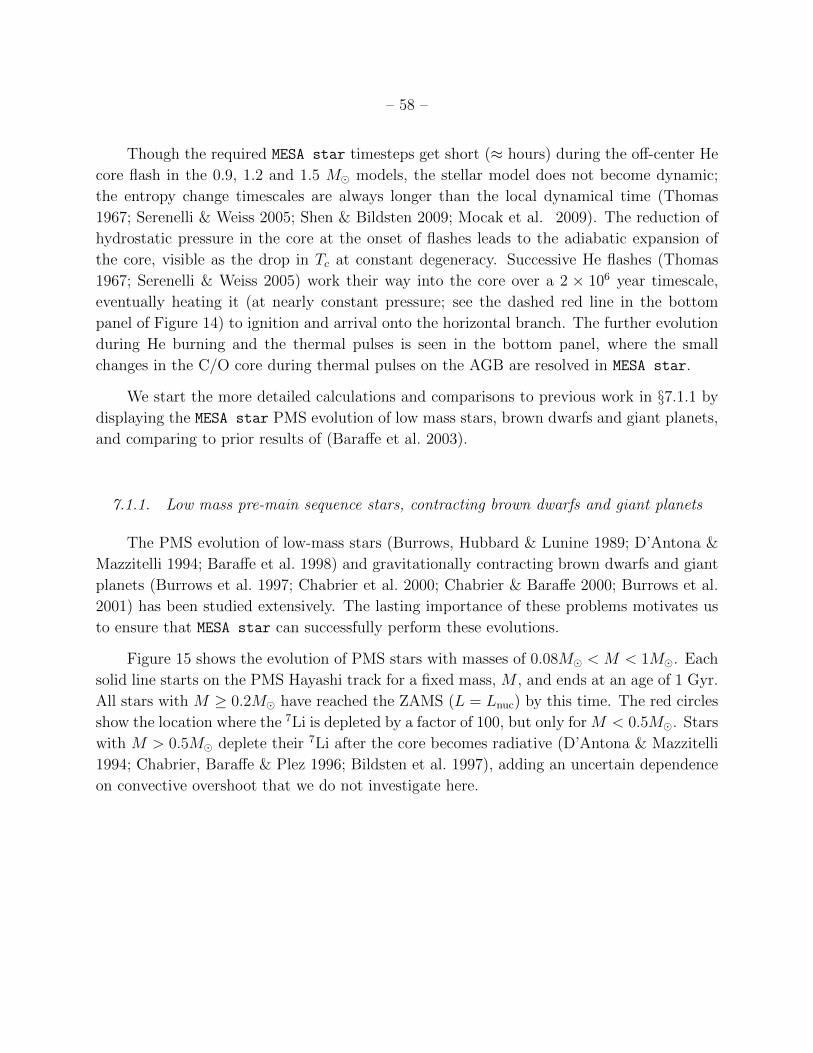
– 58 –
Though the required MESA star timesteps get short (≈ hours) during the off-center He
core flash in the 0.9, 1.2 and 1.5 M� models, the stellar model does not become dynamic;
the entropy change timescales are always longer than the local dynamical time (Thomas
1967; Serenelli & Weiss 2005; Shen & Bildsten 2009; Mocak et al. 2009). The reduction of
hydrostatic pressure in the core at the onset of flashes leads to the adiabatic expansion of
the core, visible as the drop in Tc at constant degeneracy. Successive He flashes (Thomas
1967; Serenelli & Weiss 2005) work their way into the core over a 2 × 10⁶ year timescale,
eventually heating it (at nearly constant pressure; see the dashed red line in the bottom
panel of Figure 14) to ignition and arrival onto the horizontal branch. The further evolution
during He burning and the thermal pulses is seen in the bottom panel, where the small
changes in the C/O core during thermal pulses on the AGB are resolved in MESA star.
We start the more detailed calculations and comparisons to previous work in §7.1.1 by
displaying the MESA star PMS evolution of low mass stars, brown dwarfs and giant planets,
and comparing to prior results of (Baraffe et al. 2003).
7.1.1. Low mass pre-main sequence stars, contracting brown dwarfs and giant planets
The PMS evolution of low-mass stars (Burrows, Hubbard & Lunine 1989; D’Antona &
Mazzitelli 1994; Baraffe et al. 1998) and gravitationally contracting brown dwarfs and giant
planets (Burrows et al. 1997; Chabrier et al. 2000; Chabrier & Baraffe 2000; Burrows et al.
2001) has been studied extensively. The lasting importance of these problems motivates us
to ensure that MESA star can successfully perform these evolutions.
Figure 15 shows the evolution of PMS stars with masses of 0.08M� < M < 1M�. Each
solid line starts on the PMS Hayashi track for a fixed mass, M , and ends at an age of 1 Gyr.
All stars with M ≥ 0.2M� have reached the ZAMS (L = Lnuc) by this time. The red circles
show the location where the 7Li is depleted by a factor of 100, but only for M < 0.5M�. Stars
with M > 0.5M� deplete their 7Li after the core becomes radiative (D’Antona & Mazzitelli
1994; Chabrier, Baraffe & Plez 1996; Bildsten et al. 1997), adding an uncertain dependence
on convective overshoot that we do not investigate here.
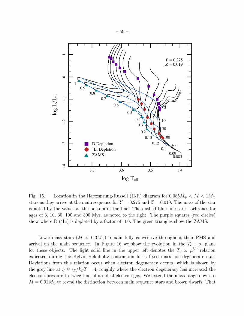
– 59 –
■●▲
■
●
■
●
■
●
■
●
■
●
■
●
▲
■
●
▲
■
●
▲
■
●
▲
■
▲
■
▲
■
▲
■
▲
■
▲
D Depletion7Li DepletionZAMS
Y = 0.275Z = 0.019
3
10
30
100
300
log Teff
log
L/L�
0.0850.09
0.10.12
0.150.2
0.30.4
0.5
0.6
0.70.8
0.91
3.43.53.63.7
−4
−3
−2
−1
01
Fig. 15.— Location in the Hertzsprung-Russell (H-R) diagram for 0.085M� < M < 1M�stars as they arrive at the main sequence for Y = 0.275 and Z = 0.019. The mass of the star
is noted by the values at the bottom of the line. The dashed blue lines are isochrones for
ages of 3, 10, 30, 100 and 300 Myr, as noted to the right. The purple squares (red circles)
show where D (7Li) is depleted by a factor of 100. The green triangles show the ZAMS.
Lower-mass stars (M < 0.3M�) remain fully convective throughout their PMS and
arrival on the main sequence. In Figure 16 we show the evolution in the Tc − ρc plane
for these objects. The light solid line in the upper left denotes the Tc ∝ ρ1/3c relation
expected during the Kelvin-Helmholtz contraction for a fixed mass non-degenerate star.
Deviations from this relation occur when electron degeneracy occurs, which is shown by
the grey line at η ≈ εF/kBT = 4, roughly where the electron degeneracy has increased the
electron pressure to twice that of an ideal electron gas. We extend the mass range down to
M = 0.01M� to reveal the distinction between main sequence stars and brown dwarfs. That

– 60 –
distinction becomes clearer in Figure 17 which shows the L evolution for a range of stars with
M < 0.3M�. Only the M > 0.08M� stars asymptote at late times to a constant L, whereas
the others continue to fade. We also exhibit the expected scaling for a contracting fully
convective star with a constant Teff , L ∝ t−2/3. At the D mass fraction of this calculation,
XD = 3 × 10⁻⁵, the onset of D burning provides some luminosity for a finite time, causing
the evident kink at early times.
■●▲
■
●
▲
■
●
▲
■
●
▲
■
●
▲
■
●
▲
■
●
▲
■
●
■
●
■
●
■
●
■
●
■■ ■■■ ■ ■
■■
■
εF/kT=4Tc ∝ ρ
1/3c
10 301003001000
D Depletion7Li DepletionZAMS
Y = 0.275Z = 0.019
log ρc (g cm−3)
log
Tc(
K)
0.30.2
0.150.12
0.10.09
0.080.075
0.070.065
0.060.055
0.050.045
0.04
0.035
0.03
0.025
0.02
0.017
0.0140.012
0.0110.01
0 1 2 3
5.5
6.0
6.5
7.0
Fig. 16.— Trajectories of central conditions for fully convective M < 0.3M� stars as they
approach the main sequence (M > 0.08M�) or become brown dwarfs for Y = 0.275 and
Z = 0.019. Each solid line shows Tc and ρc for a fixed mass, M , noted at the end of the line
(when the age is 3 Gyr). The dashed blue lines are isochrones for ages of 10, 30,100, 300
Myr and 1 Gyr. The purple squares and red circles show where D and 7Li is depleted by a
factor of 100. The green triangles show the ZAMS.

– 61 –
●
●
■
●
■
●
■
●
■
●
■
■
■
■
■
■
●
log
L(L�)
log age (years)
0.3
0.2
0.15
0.15
0.1
0.1
0.08
0.08
0.07
0.07
0.050.04
0.03
0.02
0.015
0.01
0.005
0.0030.002
0.001
D Depletion
7Li Depletion
L ∝ t−2/3
6 7 8 9
−7
−6
−5
−4
−3
−2
−1
Fig. 17.— Luminosity evolution for fully convective M < 0.3M� stars as they approach the
main sequence (M > 0.08M�) or become brown dwarfs for Y = 0.275 and Z = 0.019. From
top to bottom, the lines are for M = 0.3, 0.2, 0.15, 0.1, 0.08, 0.07, 0.05, 0.04, 0.03, 0.02,
0.015, 0.010, 0.005, 0.003, 0.002, & 0.001M�. The purple squares (red circles) denote where
D (7Li) is depleted by a factor of 100.
MESA star models evolved from the PMS Hayashi line to an age of 10 Gyr with masses
ranging from 0.09 to 0.001M� are compared with the models of Baraffe et al. (2003, BCBAH)
in Figure 18. Ages in increasing powers of 10 are marked by filled circles along each track
from 1 Myr to 10 Gyr. For comparison, separate points from the BCBAH evolutionary
models are plotted as plus symbols (“+”). So as to match the choice of BCBAH, we set

– 62 –
the D mass fraction at XD = 2 × 10⁻⁵ (Chabrier et al. 2000). Evolution at the youngest
ages is uncertain due to different assumptions regarding D burning but beyond 10 Myr the
MESA star and the BCBAH models overlap at almost every point. Note that the BCBAH
models were only evolved to 5 Gyr for the two lowest masses shown in Figure 18.
●✚
●
●●
●●
✚
✚✚
✚✚✚
✚✚
✚✚✚
✚✚
✚
✚
✚
✚
✚✚✚
✚✚✚✚✚✚
✚
✚
✚
✚
✚
✚
✚✚✚✚✚✚✚
✚
✚
✚
✚
✚
✚
✚
✚✚
✚✚✚✚
✚
✚
✚
✚
✚
✚
✚✚
✚
✚✚
●
●●
●●
✚
✚✚
✚✚✚
✚✚
✚✚✚
✚✚
✚
✚
✚
✚
✚✚✚
✚✚✚✚✚✚
✚
✚
✚
✚
✚
✚
✚✚✚✚✚✚✚
✚
✚
✚
✚
✚
✚
✚
✚✚
✚✚✚✚
✚
✚
✚
✚
✚
✚
✚✚
✚
✚✚
●
●●
● ●
✚
✚✚
✚✚✚
✚✚
✚✚✚
✚✚
✚
✚
✚
✚
✚✚✚
✚✚✚✚✚✚
✚
✚
✚
✚
✚
✚
✚✚✚✚✚✚✚
✚
✚
✚
✚
✚
✚
✚
✚✚
✚✚✚✚
✚
✚
✚
✚
✚
✚
✚✚
✚
✚✚
●
●
●●
●
✚
✚✚
✚✚✚
✚✚
✚✚✚
✚✚
✚
✚
✚
✚
✚✚✚
✚✚✚✚✚✚
✚
✚
✚
✚
✚
✚
✚✚✚✚✚✚✚
✚
✚
✚
✚
✚
✚
✚
✚✚
✚✚✚✚
✚
✚
✚
✚
✚
✚
✚✚
✚
✚✚
●
●
●●
●
✚
✚✚
✚✚✚
✚✚
✚✚✚
✚✚
✚
✚
✚
✚
✚✚✚
✚✚✚✚✚✚
✚
✚
✚
✚
✚
✚
✚✚✚✚✚✚✚
✚
✚
✚
✚
✚
✚
✚
✚✚
✚✚✚✚
✚
✚
✚
✚
✚
✚
✚✚
✚
✚✚
●
●
●
●●
✚
✚✚
✚✚✚
✚✚
✚✚✚
✚✚
✚
✚
✚
✚
✚✚✚
✚✚✚✚✚✚
✚
✚
✚
✚
✚
✚
✚✚✚✚✚✚✚
✚
✚
✚
✚
✚
✚
✚
✚✚
✚✚✚✚
✚
✚
✚
✚
✚
✚
✚✚
✚
✚✚
●
●
●
●●
✚
✚✚
✚✚✚
✚✚
✚✚✚
✚✚
✚
✚
✚
✚
✚✚✚
✚✚✚✚✚✚
✚
✚
✚
✚
✚
✚
✚✚✚✚✚✚✚
✚
✚
✚
✚
✚
✚
✚
✚✚
✚✚✚✚
✚
✚
✚
✚
✚
✚
✚✚
✚
✚✚
●
●
●
●●
✚
✚✚
✚✚✚
✚✚
✚✚✚
✚✚
✚
✚
✚
✚
✚✚✚
✚✚✚✚✚✚
✚
✚
✚
✚
✚
✚
✚✚✚✚✚✚✚
✚
✚
✚
✚
✚
✚
✚
✚✚
✚✚✚✚
✚
✚
✚
✚
✚
✚
✚✚
✚
✚✚
●
●
●
●
●
✚
✚✚
✚✚✚
✚✚
✚✚✚
✚✚
✚
✚
✚
✚
✚✚✚
✚✚✚✚✚✚
✚
✚
✚
✚
✚
✚
✚✚✚✚✚✚✚
✚
✚
✚
✚
✚
✚
✚
✚✚
✚✚✚✚
✚
✚
✚
✚
✚
✚
✚✚
✚
✚✚
●
●
●
●
●
✚
✚✚
✚✚✚
✚✚
✚✚✚
✚✚
✚
✚
✚
✚
✚✚✚
✚✚✚✚✚✚
✚
✚
✚
✚
✚
✚
✚✚✚✚✚✚✚
✚
✚
✚
✚
✚
✚
✚
✚✚
✚✚✚✚
✚
✚
✚
✚
✚
✚
✚✚
✚
✚✚
●
●
●
●
●
✚
✚✚
✚✚✚
✚✚
✚✚✚
✚✚
✚
✚
✚
✚
✚✚✚
✚✚✚✚✚✚
✚
✚
✚
✚
✚
✚
✚✚✚✚✚✚✚
✚
✚
✚
✚
✚
✚
✚
✚✚
✚✚✚✚
✚
✚
✚
✚
✚
✚
✚✚
✚
✚✚
●
●
●
●●
✚
✚✚
✚✚✚
✚✚
✚✚✚
✚✚
✚
✚
✚
✚
✚✚✚
✚✚✚✚✚✚
✚
✚
✚
✚
✚
✚
✚✚✚✚✚✚✚
✚
✚
✚
✚
✚
✚
✚
✚✚
✚✚✚✚
✚
✚
✚
✚
✚
✚
✚✚
✚
✚✚
●
●
●
●●
✚
✚✚
✚✚✚
✚✚
✚✚✚
✚✚
✚
✚
✚
✚
✚✚✚
✚✚✚✚✚✚
✚
✚
✚
✚
✚
✚
✚✚✚✚✚✚✚
✚
✚
✚
✚
✚
✚
✚
✚✚
✚✚✚✚
✚
✚
✚
✚
✚
✚
✚✚
✚
✚✚
MESABCBAH03
1 Myr
10 Myr
100 Myr1 Gyr 10 Gyr
Teff (K)
log
g(c
ms−
2 )
0.001
0.002
0.003
0.005
0.01
0.02
0.03
0.040.05
0.060.070.08
0.09
050010001500200025003000
3.0
3.5
4.0
4.5
5.0
5.5
Fig. 18.— Evolution of very low mass stars and substellar objects from 0.09 to 0.001 M� for
Z = 0.02, Y = 0.28 in the log(g)-Teff plane. The solid lines are the MESA star tracks, with
labeled masses (in M�) at the bottom of each. The filled circles denote the location of each
track at a given age. The plus symbols (+) mark the locations of the BCBAH tracks for the
same masses and ages. The two lowest mass tracks from BCBAH do not extend to 10 Gyr.

– 63 –
7.1.2. Code comparisons of 0.8M� and 1M� models
The Stellar Code Calibration Project (Weiss et al. 2007) was created to provide in-
sight into the consistency of results obtained from different state-of-the-art stellar evo-
lution codes. The contributors performed a series of stellar evolution calculations with
the physics choices held constant to the greatest extent possible. This section compares
MESA star models with published results from that project for two specific cases. The com-
parison codes are BaSTI/FRANEC (Pietrinferni et al. 2004), DSEP (Dotter et al. 2007),
and GARSTEC (Weiss & Schlattl 2008). MESA star models lie within the range exhibited
by BaSTI/FRANEC, DSEP, and GARSTEC in these comparisons.
Two examples are shown here, a 0.8M�, Z = 10−4 star and a 1M�, Z = 0.02, both
modeled from the pre-MS to the onset of the He core flash. The models assume, as much
as possible, the same nuclear reaction rates (NACRE), opacities (OPAL and Alexander &
Ferguson 1994), equation of state (FreeEOS), and mixing length (αMLT = 1.6). These tests
do not represent the best models for the various codes. Instead, the goal of the comparisons
was to see how consistent the codes would be when using simple assumptions and comparable
input physics (Weiss et al. 2007). While the agreement is good in most respects, in temporal
resolution there is a discrepancy.
log Teff
log
L(L�)
M=0.8 M�, Y0 = 0.25, Z0 = 0.0001
3.653.703.753.803.85
01
23
MESADSEPGARSTECBASTI
log ρc (g cm−3)
log
Tc(K
)
εF /kT=4
−2 0 2 4 6
6.0
6.5
7.0
7.5
8.0
log Tc
log
L(L�)
6.0 6.5 7.0 7.5 8.0
01
23
Age (Gyr)
log
L(L�)
8 9 10 11 12
01
23
log Teff
log
L(L�)
M=1.0 M�, Y0 = 0.28, Z0 = 0.02
3.53.63.7
01
23
MESADSEPGARSTECBASTI
log ρc (g cm−3)
log
Tc(K
)
εF /kT=4
−2 0 2 4 6
6.0
6.5
7.0
7.5
8.0
log Tc(K)
log
L(L�)
6.0 6.5 7.0 7.5 8.0
01
23
Age (Gyr)
log
L(L�)
8 9 10 11 12
01
23
Fig. 19.— Stellar Code Calibration project models for the 0.8M�, Z = 10−4 (left) and
the 1M�, Z = 0.02 (right) cases. The upper-left panels show the H-R diagram; upper-
right panels show luminosity versus central temperature; lower-left panels show central T-ρ;
lower-right shows luminosity versus age.
The H-R diagram of the 0.8M�, Z = 10−4 case is nearly identical for all four tracks
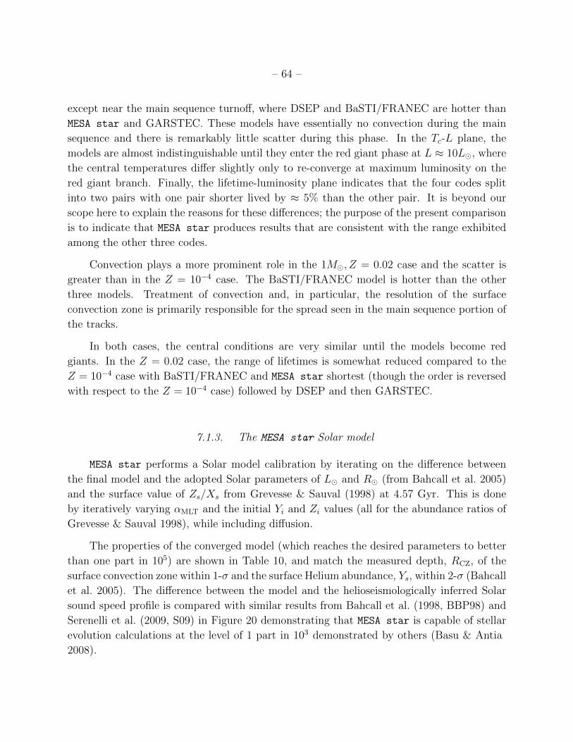
– 64 –
except near the main sequence turnoff, where DSEP and BaSTI/FRANEC are hotter than
MESA star and GARSTEC. These models have essentially no convection during the main
sequence and there is remarkably little scatter during this phase. In the Tc-L plane, the
models are almost indistinguishable until they enter the red giant phase at L ≈ 10L�, where
the central temperatures differ slightly only to re-converge at maximum luminosity on the
red giant branch. Finally, the lifetime-luminosity plane indicates that the four codes split
into two pairs with one pair shorter lived by ≈ 5% than the other pair. It is beyond our
scope here to explain the reasons for these differences; the purpose of the present comparison
is to indicate that MESA star produces results that are consistent with the range exhibited
among the other three codes.
Convection plays a more prominent role in the 1M�, Z = 0.02 case and the scatter is
greater than in the Z = 10−4 case. The BaSTI/FRANEC model is hotter than the other
three models. Treatment of convection and, in particular, the resolution of the surface
convection zone is primarily responsible for the spread seen in the main sequence portion of
the tracks.
In both cases, the central conditions are very similar until the models become red
giants. In the Z = 0.02 case, the range of lifetimes is somewhat reduced compared to the
Z = 10−4 case with BaSTI/FRANEC and MESA star shortest (though the order is reversed
with respect to the Z = 10−4 case) followed by DSEP and then GARSTEC.
7.1.3. The MESA star Solar model
MESA star performs a Solar model calibration by iterating on the difference between
the final model and the adopted Solar parameters of L� and R� (from Bahcall et al. 2005)
and the surface value of Zs/Xs from Grevesse & Sauval (1998) at 4.57 Gyr. This is done
by iteratively varying αMLT and the initial Yi and Zi values (all for the abundance ratios of
Grevesse & Sauval 1998), while including diffusion.
The properties of the converged model (which reaches the desired parameters to better
than one part in 105) are shown in Table 10, and match the measured depth, RCZ, of the
surface convection zone within 1-σ and the surface Helium abundance, Ys, within 2-σ (Bahcall
et al. 2005). The difference between the model and the helioseismologically inferred Solar
sound speed profile is compared with similar results from Bahcall et al. (1998, BBP98) and
Serenelli et al. (2009, S09) in Figure 20 demonstrating that MESA star is capable of stellar
evolution calculations at the level of 1 part in 103 demonstrated by others (Basu & Antia
2008).
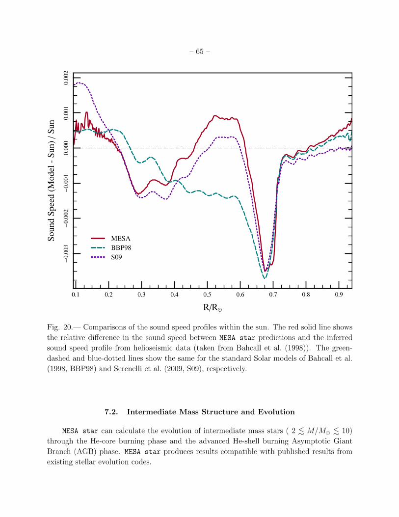
– 65 –
R/R�
Soun
dSp
eed
(Mod
el-S
un)/
Sun
0.1 0.2 0.3 0.4 0.5 0.6 0.7 0.8 0.9
−0.
003
−0.
002
−0.
001
0.00
00.
001
0.00
2
MESABBP98S09
Fig. 20.— Comparisons of the sound speed profiles within the sun. The red solid line shows
the relative difference in the sound speed between MESA star predictions and the inferred
sound speed profile from helioseismic data (taken from Bahcall et al. (1998)). The green-
dashed and blue-dotted lines show the same for the standard Solar models of Bahcall et al.
(1998, BBP98) and Serenelli et al. (2009, S09), respectively.
7.2. Intermediate Mass Structure and Evolution
MESA star can calculate the evolution of intermediate mass stars ( 2 . M/M� . 10)
through the He-core burning phase and the advanced He-shell burning Asymptotic Giant
Branch (AGB) phase. MESA star produces results compatible with published results from
existing stellar evolution codes.
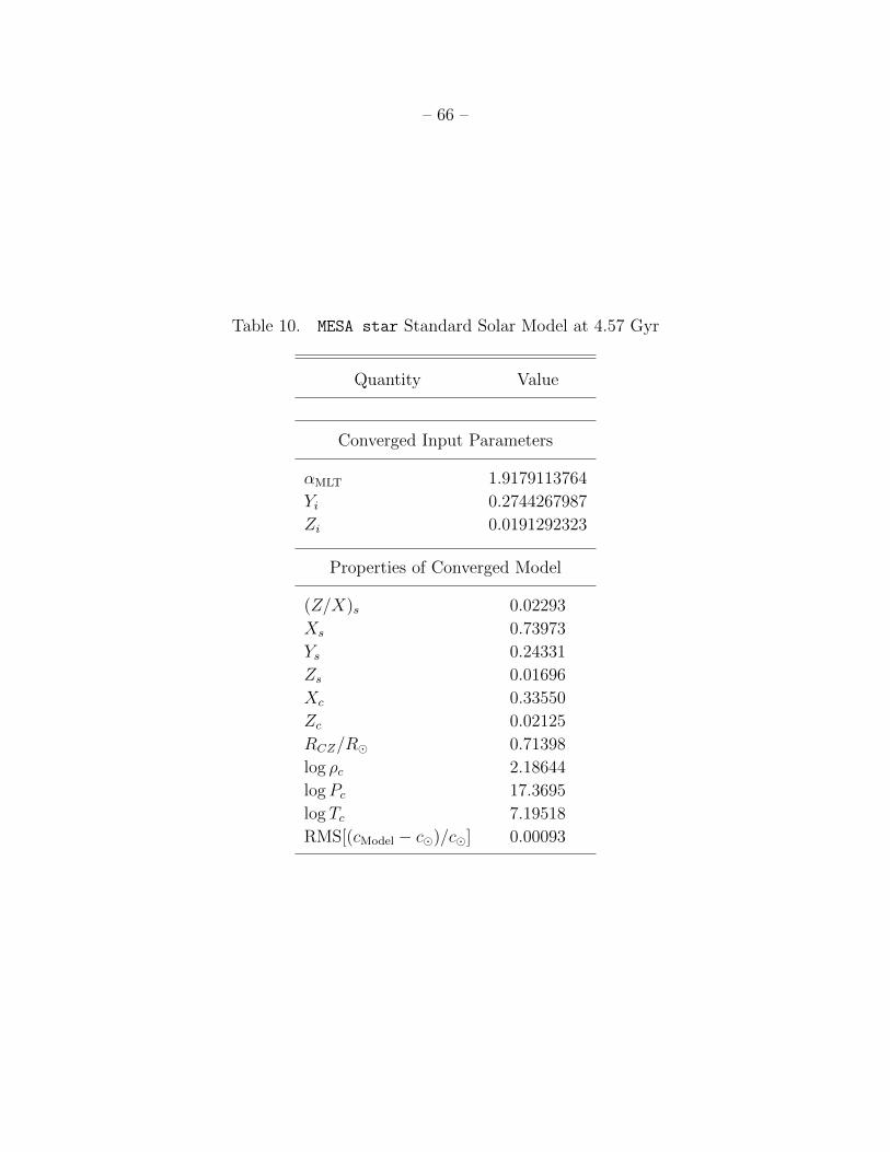
– 66 –
Table 10. MESA star Standard Solar Model at 4.57 Gyr
Quantity Value
Converged Input Parameters
αMLT 1.9179113764
Yi 0.2744267987
Zi 0.0191292323
Properties of Converged Model
(Z/X)s 0.02293
Xs 0.73973
Ys 0.24331
Zs 0.01696
Xc 0.33550
Zc 0.02125
RCZ/R� 0.71398
log ρc 2.18644
logPc 17.3695
log Tc 7.19518
RMS[(cModel − c�)/c�] 0.00093

– 67 –
● ●
●
●
●
●
●●
●
●●●●●●●●
ZAMS
log Teff (K)
log
L(L�)
2
3
4
5
67
810
3.63.84.04.24.4
12
34
εF/kT=4
Y = 0.28Z = 0.02
log ρc (g cm−3)
log
Tc(
K)
2
2
3
3
4
4
5
5
6
6
7
7
8
8
10
10
0 1 2 3 4 5 6 7
7.0
7.5
8.0
8.5
9.0
Fig. 21.— Top: MESA star H-R diagram for 2-10 M� models from the pre-main sequence
to the end of the thermally pulsating AGB. Bottom: trajectories of the central conditions.
The filled red points show the ZAMS.
We start by showing in Figure 21 a grid of MESA star evolutionary tracks with masses
ranging from 2 to 10M� with Z = 0.02. The top panel shows the evolution in the H-R
diagram while the bottom panel shows the evolution in the Tc − ρc diagram. The 8 and
10M� models start to ignite carbon burning off center, whereas the 2−7M� models produce
C/O white dwarfs. The lack of a complete treatment in MESA star of liquid diffusion inhibits
our ability to verify the resulting white dwarf cooling sequences from MESA star at this time.
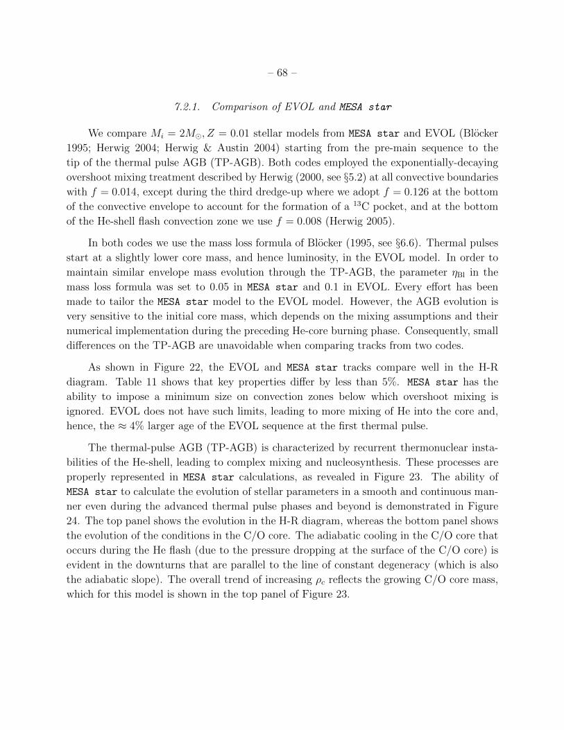
– 68 –
7.2.1. Comparison of EVOL and MESA star
We compare Mi = 2M�, Z = 0.01 stellar models from MESA star and EVOL (Blocker
1995; Herwig 2004; Herwig & Austin 2004) starting from the pre-main sequence to the
tip of the thermal pulse AGB (TP-AGB). Both codes employed the exponentially-decaying
overshoot mixing treatment described by Herwig (2000, see §5.2) at all convective boundaries
with f = 0.014, except during the third dredge-up where we adopt f = 0.126 at the bottom
of the convective envelope to account for the formation of a 13C pocket, and at the bottom
of the He-shell flash convection zone we use f = 0.008 (Herwig 2005).
In both codes we use the mass loss formula of Blocker (1995, see §6.6). Thermal pulses
start at a slightly lower core mass, and hence luminosity, in the EVOL model. In order to
maintain similar envelope mass evolution through the TP-AGB, the parameter ηBl in the
mass loss formula was set to 0.05 in MESA star and 0.1 in EVOL. Every effort has been
made to tailor the MESA star model to the EVOL model. However, the AGB evolution is
very sensitive to the initial core mass, which depends on the mixing assumptions and their
numerical implementation during the preceding He-core burning phase. Consequently, small
differences on the TP-AGB are unavoidable when comparing tracks from two codes.
As shown in Figure 22, the EVOL and MESA star tracks compare well in the H-R
diagram. Table 11 shows that key properties differ by less than 5%. MESA star has the
ability to impose a minimum size on convection zones below which overshoot mixing is
ignored. EVOL does not have such limits, leading to more mixing of He into the core and,
hence, the ≈ 4% larger age of the EVOL sequence at the first thermal pulse.
The thermal-pulse AGB (TP-AGB) is characterized by recurrent thermonuclear insta-
bilities of the He-shell, leading to complex mixing and nucleosynthesis. These processes are
properly represented in MESA star calculations, as revealed in Figure 23. The ability of
MESA star to calculate the evolution of stellar parameters in a smooth and continuous man-
ner even during the advanced thermal pulse phases and beyond is demonstrated in Figure
24. The top panel shows the evolution in the H-R diagram, whereas the bottom panel shows
the evolution of the conditions in the C/O core. The adiabatic cooling in the C/O core that
occurs during the He flash (due to the pressure dropping at the surface of the C/O core) is
evident in the downturns that are parallel to the line of constant degeneracy (which is also
the adiabatic slope). The overall trend of increasing ρc reflects the growing C/O core mass,
which for this model is shown in the top panel of Figure 23.
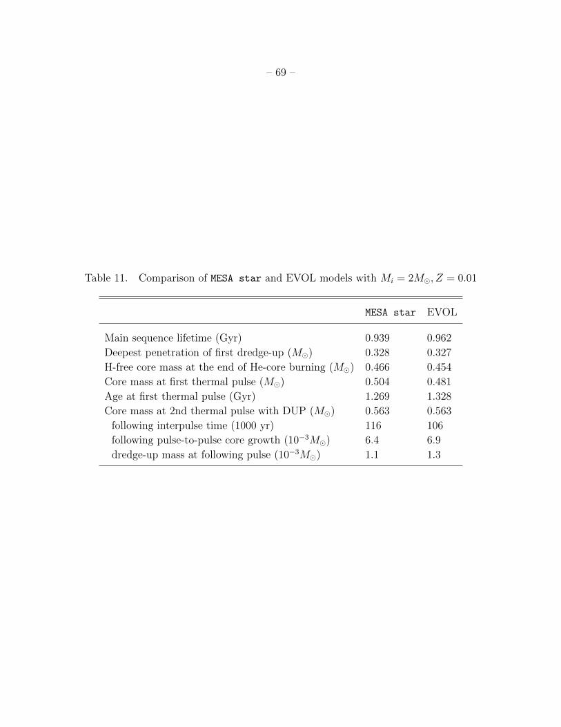
– 69 –
Table 11. Comparison of MESA star and EVOL models with Mi = 2M�, Z = 0.01
MESA star EVOL
Main sequence lifetime (Gyr) 0.939 0.962
Deepest penetration of first dredge-up (M�) 0.328 0.327
H-free core mass at the end of He-core burning (M�) 0.466 0.454
Core mass at first thermal pulse (M�) 0.504 0.481
Age at first thermal pulse (Gyr) 1.269 1.328
Core mass at 2nd thermal pulse with DUP (M�) 0.563 0.563
following interpulse time (1000 yr) 116 106
following pulse-to-pulse core growth (10−3M�) 6.4 6.9
dredge-up mass at following pulse (10−3M�) 1.1 1.3

– 70 –
log Teff
log
L/L�
MESAEVOL
M = 2.00 M�Z = 0.01
3.53.63.73.83.94.0
12
34
Fig. 22.— The 2M�, Z = 0.01 tracks up to the first thermal pulse from EVOL (solid black
line) and MESA star (thick grey line) in the H-R diagram.

– 71 –B
ound
ary
(M�) H-free core
He-free core
0.54
0.57
0.60
log
L(L�)
Hydrogen burningHelium burning
04
8
Mi = 2.0M�Zi = 0.01Yi = 0.26
Time (Myr)
log
Tc(
K)
0.0 0.2 0.4 0.6 0.8 1.0 1.2
7.86
7.88
7.90
Fig. 23.— Properties of a Mi = 2M� star from MESA star as it approaches the end of the
AGB. Top: the boundaries of the C/O core and the He layer. Middle: luminosities from
hydrogen and helium burning. Bottom: central temperature evolution.
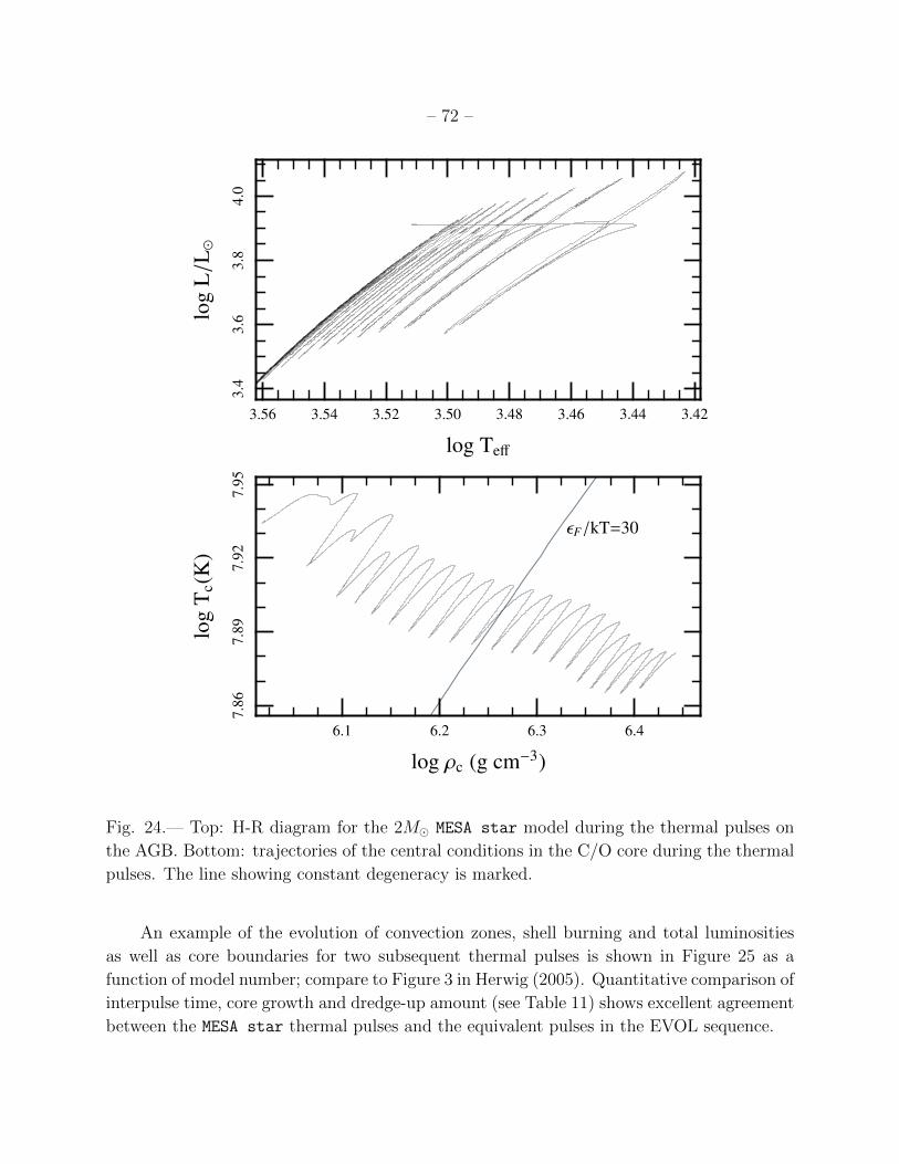
– 72 –
log Teff
log
L/L�
3.423.443.463.483.503.523.543.56
3.4
3.6
3.8
4.0
εF/kT=30
log ρc (g cm−3)
log
Tc(
K)
6.1 6.2 6.3 6.4
7.86
7.89
7.92
7.95
Fig. 24.— Top: H-R diagram for the 2M� MESA star model during the thermal pulses on
the AGB. Bottom: trajectories of the central conditions in the C/O core during the thermal
pulses. The line showing constant degeneracy is marked.
An example of the evolution of convection zones, shell burning and total luminosities
as well as core boundaries for two subsequent thermal pulses is shown in Figure 25 as a
function of model number; compare to Figure 3 in Herwig (2005). Quantitative comparison of
interpulse time, core growth and dredge-up amount (see Table 11) shows excellent agreement
between the MESA star thermal pulses and the equivalent pulses in the EVOL sequence.
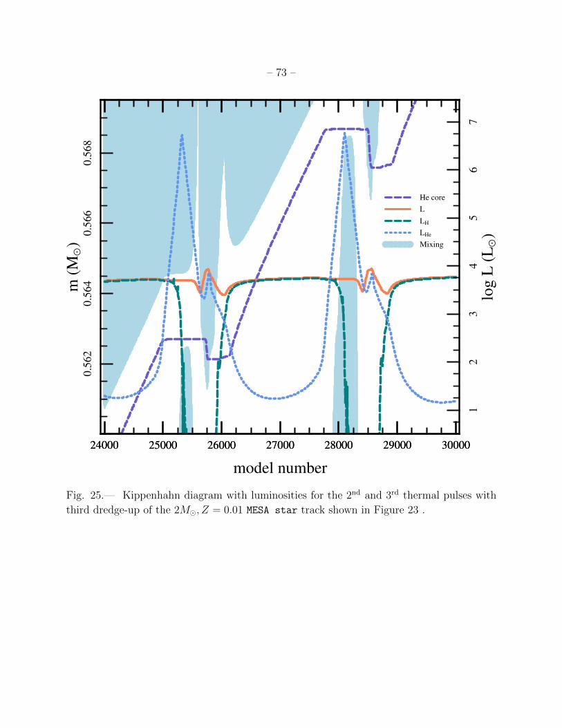
– 73 –
model number
m(M!)
24000 25000 26000 27000 28000 29000 30000
0.56
20.
564
0.56
60.
568
log
L(L!)
24000 25000 26000 27000 28000 29000 30000
12
34
56
7
He coreLLH
LHe
Mixing
Fig. 25.— Kippenhahn diagram with luminosities for the 2nd and 3rd thermal pulses with
third dredge-up of the 2M�, Z = 0.01 MESA star track shown in Figure 23 .

– 74 –Su
rfac
eC/O
Num
berR
atio
MESAEVOL
Mi = 2.00M�Zi = 0.01
0.5
1.0
1.5
2.0
Time (Myr)
M(M�)
0.0 0.2 0.4 0.6 0.8 1.0 1.2
1.0
1.5
2.0
Fig. 26.— The C/O number ratio (top panel) and stellar mass, M (bottom panel) as a
function of time from EVOL (solid black line) and MESA star (thick grey line). Time has
been set to zero for both tracks at the onset of the third dredge-up.
Another important property of the He-shell flashes is the intershell abundance as a result
of the convective mixing and burning. Again, the comparison of results from both codes
shows good agreement, which is expected since they both implement the same overshooting
– 75 –
mixing assumptions for the He-shell flash convection zone. A consequence of the third dredge-
up is the gradual increase of the envelope C/O ratio as thermal pulses repeatedly occur.
Since the 2M� models do not experience hot-bottom burning, the evolution of this ratio is
an effective probe of the cumulative efficiency of the third dredge-up in these simulations.25
The top panel of Figure 26 shows the surface C/O ratio evolution according to EVOL
(dashed-red line) and MESA star (solid black line). They are in good agreement, e.g. in
terms of the time period over which the third dredge-up occurs and the amount by which
C/O increases. The mass loss history over the same time period, shown in the bottom panel
of Figure 26, is similar by design.
7.2.2. Interior structure of Slowly Pulsating B Stars and Beta Cepheids
The advent of space-based asteroseismology for main sequence B stars with the Corot
(Degroote et al. 2009) and Kepler (Gilliland et al. 2010) satellites is probing the slowly
pulsating B stars (SPBs, M ≈ 3−8M�) and the more massive (M ≈ 7−20M�) β Cepheids
(Degroote et al. 2009, 2010). These stars are all undergoing main sequence H burning
and are unstably pulsating due to the κ mechanism from the Fe-group opacity bump at
T ≈ 2 × 10⁵ K (Dziembowski et al. 1993). The observed modes have finite amplitudes
deep in the stellar core, demanding a full interior model for mode frequency (and stability)
prediction (Dziembowski et al. 1993; Pamyatnykh et al. 2004).
25For massive AGB stars MESA star shows the expected hot-bottom burning behavior, including, for
example, the avoidance of the C-star phase for a 5M�, Z = 0.01 stellar model track despite efficient third
dredge-up.
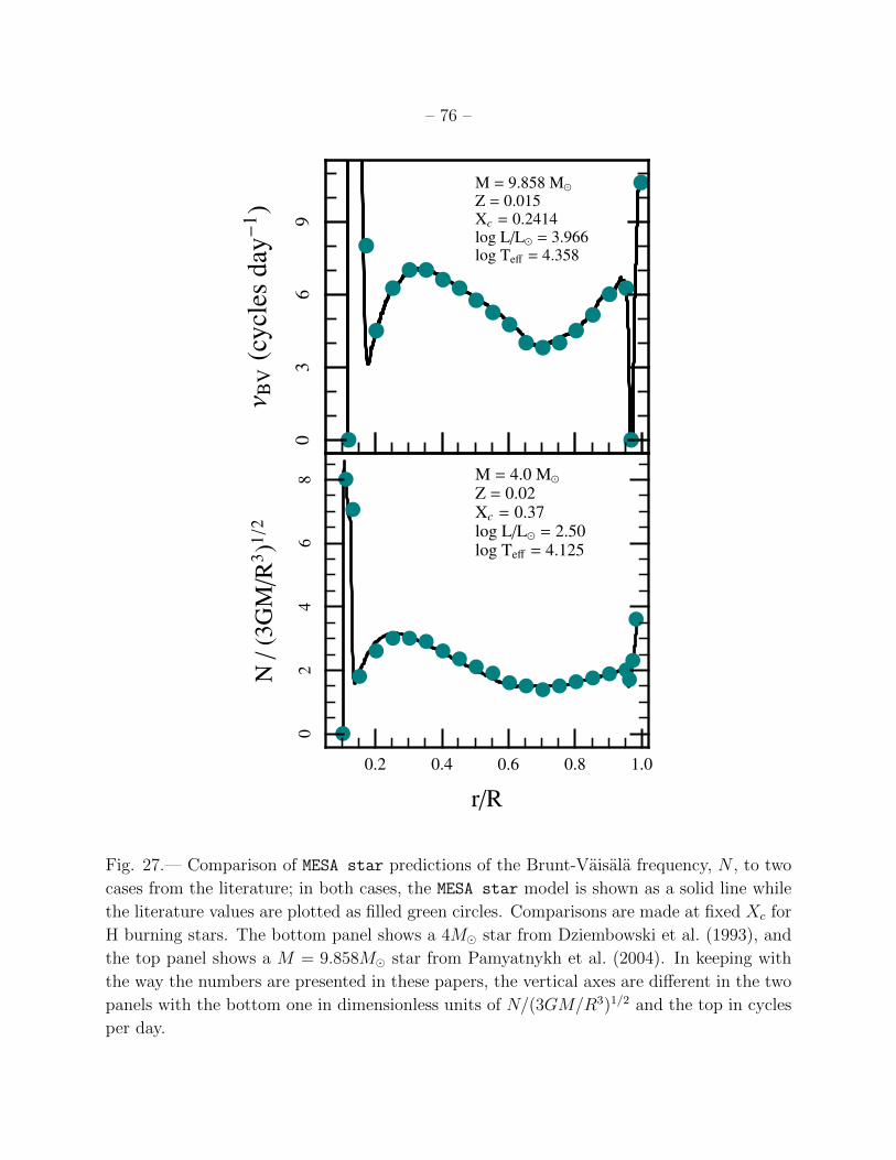
– 76 –
●
●
●
●●●
●●●
●●
●●●●
●●●
●
●
●
●
●
●
●●●●
●●●●●●●●●●●●
●●
●
ν BV
(cyc
les
day−
1 )
M = 9.858 M�Z = 0.015Xc = 0.2414log L/L� = 3.966log Teff = 4.358
03
69
r/R
N/
(3G
M/R
3 )1/2
M = 4.0 M�Z = 0.02Xc = 0.37log L/L� = 2.50log Teff = 4.125
0.2 0.4 0.6 0.8 1.0
02
46
8
Fig. 27.— Comparison of MESA star predictions of the Brunt-Vaisala frequency, N , to two
cases from the literature; in both cases, the MESA star model is shown as a solid line while
the literature values are plotted as filled green circles. Comparisons are made at fixed Xc for
H burning stars. The bottom panel shows a 4M� star from Dziembowski et al. (1993), and
the top panel shows a M = 9.858M� star from Pamyatnykh et al. (2004). In keeping with
the way the numbers are presented in these papers, the vertical axes are different in the two
panels with the bottom one in dimensionless units of N/(3GM/R3)1/2 and the top in cycles
per day.

– 77 –
These papers provide a few specific models that allow a direct comparison to the
MESA star prediction of the Brunt-Vaisala frequency
N2 = g
(1
Γ1
d lnP
dr− d ln ρ
dr
)= g
(− gc2s
− d ln ρ
dr
), (18)
where c2s = Γ1P/ρ is the adiabatic sound speed, and we used hydrostatic balance, dP/dr =
−ρg. Numerically, these are obtained by interpolating the sound speed at the cell boundary,
whereas d ln ρ/dr is estimated by numerical differencing and then smoothed. This method
naturally captures the extra restoring force from composition gradients, especially relevant
in these evolving stars that leave a He rich radiative region above the retreating convective
core during the main sequence.
Our first comparison is to Dziembowski et al. (1993)’s M = 4M� main sequence star
with Z = 0.02 at a time when the hydrogen abundance in the convective core is Xc = 0.37.
With no overshoot from the convective core, Dziembowski et al. (1993) found logL/L� =
2.51 and log Teff = 4.142 whereas MESA star gives logL/L� = 2.50 and log Teff = 4.125.
The top panel in Figure 27 compares the MESA star results (solid line) to the values (green
circles) from Figure 3 of Dziembowski et al. (1993). The agreement is remarkable as an
integral test of MESA star. The bottom panel of Figure 27 is a comparison to the more
massive M = 9.858M� main sequence star with Z = 0.015 from Figure 5 of Pamyatnykh
et al. (2004) at an age (15.7 Myr) when Xc = 0.2414 with logL/L� = 3.969 and log Teff =
4.3553. MESA star gave logL/L� = 3.966, log Teff = 4.358 and an age of 16.4 Myr at the
same value of Xc. These comparisons highlight the readiness of MESA star for adiabatic
asteroseismological studies of main sequence stars.
7.3. High Mass Stellar Structure and Evolution
To explore MESA star’s results in this mass range, models of 15M�, 20M�, and 25M�of solar metallicity and 1000M� of zero metallicity were evolved from the Hayashi track to
the onset of core-collapse. Nuclear reactions are treated with the 21 isotope reaction net-
work, inspired by the 19 isotope network in Weaver et al. (1978), that is capable of efficiently
generating accurate nuclear energy generation rates from hydrogen burning through silicon
burning (see §4.5). This network includes linkages for PP-I, steady-state CNO cycles, a
standard α-chain, heavy ion reactions, and aspects of photodisintegration into 54Fe. Atmo-
spheres are treated as a τ=2/3 Eddington gray surface as described in §5.3. Mass loss for the
solar metallicity stars uses the combined results of Glebbeek et al. (2009); Vink, de Koter &
Lamers (2001); Nugis & Lamers (2009); Nieuwenhuijzen & de Jager (1990), as described in
§6.6. These massive star models are non-rotating, use no semi-convection, employ a mixing

– 78 –
length parameter of αMLT = 1.6, and adopt f=0.01 for exponential diffusive overshoot (see
§5.2) for convective regions that are either burning hydrogen or are not burning.
Most of this section consists of comparisons to results from other stellar evolution codes.
However, for consistency (and completeness), we show in Figure 28 the H-R diagram and cen-
tral condition evolution of 10−100M� stars from the PMS to the end of core Helium-burning.
Though these are stars with Z = 0.02, we turned off mass loss during this calculation so that
the plot would be easier to read and of some pedagogical use. The tendency of Tc to scale
with ρ1/3c (also a constant radiation entropy) during these stages of evolution is expected
from hydrostatic balance with only a mildly changing mean molecular weight. The rest of
the calculations in this section included mass-loss as described above.
●
●
●
●
●
●
●
●
●
●
●●●●●●●●●
log Teff (K)
log
L(L�)
10
13
16
2025
35
50
70
100
3.63.84.04.24.44.6
45
6
Y = 0.28Z = 0.02
log ρc (g cm−3)
log
Tc(
K)
10
Tc ∝ ρ1/3cTc ∝ ρ1/3c
16
Tc ∝ ρ1/3cTc ∝ ρ1/3c
25
Tc ∝ ρ1/3cTc ∝ ρ1/3c
50
Tc ∝ ρ1/3cTc ∝ ρ1/3c
100
Tc ∝ ρ1/3c
0 1 2 3 4
7.2
7.5
7.8
8.1
8.4
Fig. 28.— Top: H-R diagram for 10 − 100M� models from the PMS to the end of core
Helium burning for Z = 0.02 but with zero mass loss. Bottom: trajectories of the central
conditions in the T − ρ plane over this same evolutionary period.
– 79 –
7.3.1. 25M� Model Comparisons
Figure 29 shows the Tc − ρc evolution in Mi = 25M� solar metallicity models from
MESA star, Kepler (private communication - Alex Heger), Hirschi et al. (2004), and FRANEC
(Limongi & Chieffi 2006) from helium burning until iron-core collapse. The curves fall below
the Tc ∝ ρ1/3c scaling relation as the mean molecular weight increases due to the subsequent
burning stages. The curves are also punctuated with non-monotonic behavior when nuclear
fuels are first ignited in shells. Figure 29 shows that MESA star produces core evolutionary
tracks consistent with other pre-supernova efforts. The bump in the MESA star curve around
carbon burning is due to the development of central convection whereas the other codes do
not (although see Figure 2 of Limongi et al. 2000). The development of a convective core
during carbon burning depends on the carbon abundance left over from core helium burning
(Limongi et al. 2000).
The mass fraction profiles of the inner 2.5M� of this Mi = 25M� model are shown
in Figure 30 at the onset of core collapse. At the time of these plots, the infall speed has
reached ≈ 1000 km s−1 just inside the iron core (at m = 1.5M�) and the electron fraction,
Ye, has dropped below ≈ 0.48. The oxygen shell lies at 1.88 ≤ m/M� ≤ 2.5, the silicon
shell between 1.61 ≤ m/M� ≤ 1.88, and the iron core at m ≤ 1.61M�. Figure 31 shows T ,
ρ, S, the radial velocity, the infall timescale, and Ye of this inner 2.5M�. Note the entropy
decrements at the oxygen, silicon and iron core boundaries.
Figure 32 summarizes the history of the inner 7M� of this Mi = 25M� model as a
function of interior mass (left y-axis). Evolution is measured by the logarithm of time (in
years) remaining until the death of the star as a supernova (x-axis), which reveals the late
burning stages. Levels of red and blue shading indicate the magnitude of the net energy
generation (nuclear energy generation minus neutrino losses), with red reflecting positive
values and blue indicating negative ones. The vertical lines indicate regions that are fully
convective. Note the appearance of a convective envelope characteristic of a red supergiant
late during helium burning. Abundance profiles of key isotopes during the major burning
stages are shown (right y-axis). The hydrogen core shrinks towards the end of hydrogen
burning, and the helium core grows as helium is depleted. The total mass shrinks to about
M = 12M� due to mass loss.

– 80 –
Tc ∝ ρ1/3c
MESAKEPLERHMMLC06
Mi = 25M�Zi = 0.02
He burn
C burn
Ne burn
O burn
Si burn
log ρc (g cm−3)
log
Tc(
K)
3 4 5 6 7 8 9
8.5
9.0
9.5
10.0
Fig. 29.— Evolution of the central temperature and central density in solar metallicity
Mi = 25M� models from different stellar evolution codes. The locations of core helium,
carbon, neon, oxygen, and silicon burning are labeled, as is the relation Tc ∝ ρ1/3c .

– 81 –
m (M�)
log
mas
sfr
actio
n
4He 4He
4He
4He
4He
12C
16O
16O16O
20Ne
20Ne
24Mg
24Mg
28Si
28Si28Si
28Si
28Si
28Si
32S
32S
32S
32S
32S
36Ar36Ar
36Ar
40Ca40Ca
40Ca
54Fe54Fe
54Fe
54Fe54Fe
56Fe56Fe 56Fe
56Fe 56Fe
56Fe 56Fe
56Ni56Ni
“56Cr”“56Cr”
“56Cr”
“56Cr”
“56Cr”
neutneut
M0 = 25M�Z0 = 0.02
0.5 1.0 1.5 2.0 2.5
−3
−2
−1
0
Fig. 30.— Mass fraction profiles of the inner 2.5M� of the solar metallicity Mi = 25M�model at the onset of core collapse. The reaction network includes links between 54Fe, 56Cr,
neutrons, and protons to model aspects of photodisintegration and neutronization.

– 82 –lo
gT
(K)
9.2
9.6
10.0
logρ
(gcm−
3 )
68
10
m (M�)
s(k
Bm−
1P
)
0.0 0.5 1.0 1.5 2.0 2.5
24
6
v(k
ms−
1 )
−80
0−
400
0
r/|v|(s
)
36
m (M�)
Ye
0.5 1.0 1.5 2.0 2.5
0.45
0.48
Fig. 31.— Profiles of T (top left), ρ (middle left), dimensionless entropy (bottom left),
material speed (top right), infall timescale (middle right), and electron fraction Ye = Z/A
(bottom right) over the inner 2.5M� of the Mi = 25M� star at the end of the pre-supernova
evolution.

– 83 –
log(years before end of run)
m(M�)
−4−20246
01
23
45
67
Cen
tral
mas
sfr
actio
n
H
4He
4He
12C
12C
12C
16O16O
16O
16O
20Ne20Ne
20Ne20Ne
28Si
28Si
32S
32S
54Fe
56Fe“56Cr”
−4−20246
0.0
0.1
0.2
0.3
0.4
0.5
0.6
0.7
0.8
0.9
1.0
sign
(εnu
c)lo
g(m
ax(1,|ε n
uc|))
−15
−10
−5
05
1015
Fig. 32.— Kippenhahn diagram showing the full time evolution of the inner 7 M� of the
Mi = 25M� evolutionary sequence from the main sequence to the onset of core collapse. Mass
coordinate and abundance mass fraction are labeled on the left and right y-axes, respectively.
The shaded bar on the right indicates the net energy generation: red for positive values and
blue for negative values. The vertical lines indicate convection.
7.3.2. Comparison of 15, 20, and 25M� Models
Now that we have shown that the Mi = 25M� MESA star models compare well to
previous efforts at the qualitative level, we will make more detailed comparisons to other
available results. Table 12 compares the core burning lifetimes of solar metallicity stars
with Mi = 15, 20 and 25M�, from MESA star, Hirschi et al. (2004), Woosley et al. (2002),
and Limongi et al. (2000). We define a core burning lifetime to begin when the central mass
fraction of fuel has dropped by 0.003 from its maximum value (or onset of central convection)

– 84 –
and to terminate when the central mass fraction has dropped below 10−4 (or the end of central
convection). Different authors adopt different lifetime definitions, which likely contribute to
some of the scatter. The hydrogen burning lifetimes for the 15M�, 20M�, and 25M� models
from the different authors are within 10% percent of each other, with the Limongi et al.
(2000) models generally having the shortest lifetimes and the Woosley et al. (2002) models
having the longest lifetimes. There is more spread in the helium burning lifetimes, with
MESA star models showing shorter lifetimes and Woosley et al. (2002) models having the
longest lifetimes. The carbon burning lifetimes show agreement within 20% for the 15M�model, but differ by factors of ∼3 for the 20M� and 25M� models. The neon, oxygen, and
silicon burning lifetimes show agreement within 20% between some models, but factor of
∼5 differences in others. It is beyond the scope of this paper to put the different lifetime
definitions on the same footing, and explore the reasons for these differences. Nevertheless,
Table 12 suggests MESA star produces lifetimes consistent with the range of lifetimes from
other works.
Table 13 compares pre-supernova core masses of solar metallicity stars with Mi = 15, 20
and 25M� models from MESA star, Hirschi et al. (2004), Rauscher et al. (2002), Heger et al.
(2000), and Limongi et al. (2000). MESA star core masses are defined as the mass interior to
the location where the element mass fraction is 0.5. The definitions used by various authors
may differ, contributing to scatter in the results. However, most of the scatter is probably
due to the different mass loss prescriptions used by different authors, resulting in different
total masses. The helium yields differ by about 10%, with the Heger et al. (2000) models
producing less helium. There is more diversity in the C+O+Ne bulk yields, up to a factor
of 2 for the 25M� model, with the Rauscher et al. (2002) models producing the most and
the Heger et al. (2000) models producing the least. Strikingly, the Fe core masses show
less variations, with the Hirschi et al. (2004) models producing the heaviest cores. Table 13
suggests MESA star produces bulk yields compatible with previous efforts.
7.3.3. 1000M� metal-free star capabilities
We close this section with a demonstration of MESA star’s capabilities by describing the
unlikely scenario of a purely metal-free stellar evolution of a Mi = 1000M� star. The Tc−ρctrajectory for a 1000M�, zero metallicity, zero mass loss model is shown in the left panel
of Figure 33. The starting time point is in the lower left corner and the final model, at the
onset of core-collapse, is in the upper right at very high values of Tc and ρc. Fluid elements
in the region to the left of the red-dashed line have Γ1 < 4/3. When the center enters this
region, the central portions of the star become dynamically unstable and begin to contract.
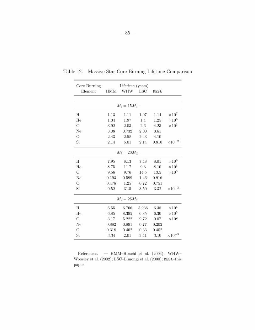
– 85 –
Table 12. Massive Star Core Burning Lifetime Comparison
Core Burning Lifetime (years)
Element HMM WHW LSC MESA
Mi = 15M�
H 1.13 1.11 1.07 1.14 ×10⁷
He 1.34 1.97 1.4 1.25 ×10⁶
C 3.92 2.03 2.6 4.23 ×10³
Ne 3.08 0.732 2.00 3.61
O 2.43 2.58 2.43 4.10
Si 2.14 5.01 2.14 0.810 ×10⁻²
Mi = 20M�
H 7.95 8.13 7.48 8.01 ×10⁶
He 8.75 11.7 9.3 8.10 ×10⁵
C 9.56 9.76 14.5 13.5 ×10³
Ne 0.193 0.599 1.46 0.916
O 0.476 1.25 0.72 0.751
Si 9.52 31.5 3.50 3.32 ×10⁻³
Mi = 25M�
H 6.55 6.706 5.936 6.38 ×10⁶
He 6.85 8.395 6.85 6.30 ×10⁵
C 3.17 5.222 9.72 9.07 ×10²
Ne 0.882 0.891 0.77 0.202
O 0.318 0.402 0.33 0.402
Si 3.34 2.01 3.41 3.10 ×10⁻³
References. — HMM–Hirschi et al. (2004); WHW–
Woosley et al. (2002); LSC–Limongi et al. (2000); MESA–this
paper

– 86 –
Table 13. Pre-Supernovae Core Mass Comparisons
Mass (M�) HMM RHW HLW LSC MESA
Mi = 15M�
Total 13.232 12.612 13.55 15 12.81
He 4.168 4.163 3.82 4.10 4.37
C+O+Ne 2.302 2.819 1.77 2.39 2.27
“Fe” 1.514 1.452 1.33 1.429 1.510
Mi = 20M�
Total 15.69 14.74 16.31 20 15.50
He 6.21 6.13 5.68 5.94 6.33
C+O+Ne 3.84 4.51 2.31 3.44 3.77
“Fe” 1.75 1.46 1.64 1.52 1.58
Mi = 25M�
Total 16.002 13.079 18.72 25 15.28
He 8.434 8.317 7.86 8.01 8.41
C+O+Ne 5.834 6.498 3.11 4.90 5.49
“Fe” 1.985 1.619 1.36 1.527 1.62
References. — HMM–Hirschi et al. (2004); RHW–
Rauscher et al. (2002); HLW–Heger et al. (2000);
LSC–Limongi et al. (2000); MESA–this paper
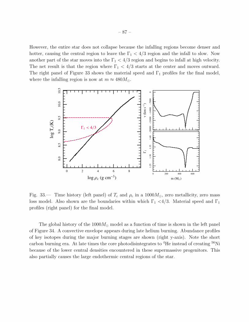
– 87 –
However, the entire star does not collapse because the infalling regions become denser and
hotter, causing the central region to leave the Γ1 < 4/3 region and the infall to slow. Now
another part of the star moves into the Γ1 < 4/3 region and begins to infall at high velocity.
The net result is that the region where Γ1 < 4/3 starts at the center and moves outward.
The right panel of Figure 33 shows the material speed and Γ1 profiles for the final model,
where the infalling region is now at m ≈ 480M�.
log ρc (g cm−3)
log
Tc(
K)
Γ1 < 4/3
0 2 4 6 8
8.0
8.5
9.0
9.5
10.0
10.5
v(k
ms−
1 )
−28
000−
2100
0−
1400
0−
7000
0
m (M�)
Γ1
0 200 400 600
1.25
1.30
1.35
1.40
Fig. 33.— Time history (left panel) of Tc and ρc in a 1000M�, zero metallicity, zero mass
loss model. Also shown are the boundaries within which Γ1 <4/3. Material speed and Γ1
profiles (right panel) for the final model.
The global history of the 1000M� model as a function of time is shown in the left panel
of Figure 34. A convective envelope appears during late helium burning. Abundance profiles
of key isotopes during the major burning stages are shown (right y-axis). Note the short
carbon burning era. At late times the core photodisintegrates to 4He instead of creating 56Ni
because of the lower central densities encountered in these supermassive progenitors. This
also partially causes the large endothermic central regions of the star.
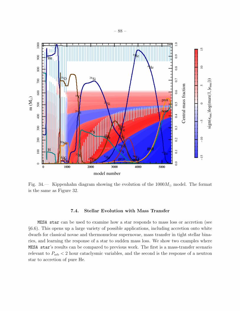
– 88 –
model number
m(M�)
0 1000 2000 3000 4000 5000
010
020
030
040
050
060
070
080
090
010
00
Cen
tral
mas
sfr
actio
n
H4He
4He
4He
4He
4He4He
4He
12C
16O
16O
20Ne
28Si
28Si
28Si
28Si
32S
32S32S
32S
54Fe
54Fe
54Fe56Fe
56Fe
neut
neut
neut
prot
prot
protprot
0 1000 2000 3000 4000 5000
0.0
0.1
0.2
0.3
0.4
0.5
0.6
0.7
0.8
0.9
1.0
sign
(εnu
c)lo
g(m
ax(1,|ε n
uc|))
−15
−10
−5
05
1015
Fig. 34.— Kippenhahn diagram showing the evolution of the 1000M� model. The format
is the same as Figure 32.
7.4. Stellar Evolution with Mass Transfer
MESA star can be used to examine how a star responds to mass loss or accretion (see
§6.6). This opens up a large variety of possible applications, including accretion onto white
dwarfs for classical novae and thermonuclear supernovae, mass transfer in tight stellar bina-
ries, and learning the response of a star to sudden mass loss. We show two examples where
MESA star’s results can be compared to previous work. The first is a mass-transfer scenario
relevant to Porb < 2 hour cataclysmic variables, and the second is the response of a neutron
star to accretion of pure He.
– 89 –
7.4.1. Mass Transfer in a Binary
To illustrate MESA star’s ability to calculate the impact of mass loss on a star, we
model the evolution of a compact binary consisting of a Roche Lobe filling low-mass ZAMS
(M < 0.2M�) model and an accreting white dwarf with MWD = 0.6M�. These short orbital
period (Porb < 2 hr) cataclysmic variables are the end points of these mass transferring
systems (Patterson 1998; Kolb & Baraffe 1999) and are now being discovered in large numbers
in the SDSS database (more than 100 studied by Gansicke et al. 2009).
We model the parameters of the binary system and the Roche lobe overflow triggered
mass transfer rate M as in Madhusudhan et al (2006). So as to compare to the previous
work of Kolb & Baraffe (1999), we presume angular momentum losses from gravitational
wave emission and keep the accreting WD mass fixed at its initial value, MWD = 0.6M�.
The evolution of the donor star is carried out by MESA star, using the τ = 100 atmosphere
tables from atm. The evolution shown in Figure 35 is followed for over 6 Gyr until the
donor has been reduced to a brown dwarf remnant of M ≈ 0.03M� (see Table 14). During
that time, the binary period drops to a minimum value of 67.4 minutes and then increases,
independent of the initial donor mass. This plot is very similar to Figure 1 of Kolb & Baraffe
(1999). We also show in Table 14 the evolution in time of the main properties of the donor
star and mass transfer rate of the Mi = 0.21M� model. Again, this agrees with the results
in Table 2 of Kolb & Baraffe (1999). The prime differences can be attributed to a slightly
different R(M) relation.

– 90 –
MWD = 0.6M�
Porb(hr)
log
M(M�
yr−
1 )
Mi = 0.10M� donor
Mi = 0.13M� donor
Mi = 0.21M� donor
1.2 1.4 1.6 1.8 2.0 2.2
−11.5
−11.0
−10.5
Fig. 35.— Mass transfer rate for cataclysmic variables with low mass main sequence donor
stars of varying initial masses Mi. Each line shows the M history for different initial mass
donors, all accreting onto a MWD = 0.6M� white dwarf. After a period of initial adjustment
to the mass transfer, each track tends to the same trajectory, showing the orbital period
minimum at Porb = 67.4 minutes.

– 91 –
Table 14. Mass Transfer History for Mi = 0.21M� and MWD = 0.6M�
Time (Gyr) Porb(hr) M/M� Teff (K) log(L/L�) R/R� log M
0.00 2.1319 0.2100 3278 -2.2688 0.2279 -10.24
0.25 2.0962 0.1987 3262 -2.3041 0.2209 -10.39
0.50 2.0367 0.1887 3242 -2.3467 0.2129 -10.40
0.75 1.9770 0.1787 3217 -2.3939 0.2049 -10.41
1.00 1.9181 0.1693 3191 -2.4414 0.1971 -10.42
1.25 1.8560 0.1599 3167 -2.4904 0.1891 -10.44
1.50 1.7938 0.1510 3142 -2.5404 0.1814 -10.45
1.75 1.7299 0.1421 3113 -2.5952 0.1735 -10.46
2.00 1.6684 0.1336 3074 -2.6563 0.1659 -10.47
2.25 1.6097 0.1252 3018 -2.7277 0.1585 -10.48
2.50 1.5475 0.1170 2965 -2.8004 0.1510 -10.50
2.75 1.4829 0.1093 2916 -2.8737 0.1435 -10.51
3.00 1.4151 0.1016 2854 -2.9590 0.1358 -10.52
3.25 1.3484 0.0942 2774 -3.0577 0.1283 -10.53
3.50 1.2804 0.0868 2666 -3.1796 0.1207 -10.54
3.75 1.2172 0.0796 2525 -3.3273 0.1135 -10.54
4.00 1.1663 0.0726 2355 -3.4987 0.1071 -10.55
4.25 1.1345 0.0659 2161 -3.6915 0.1019 -10.58
4.50 1.1227 0.0596 1963 -3.8930 0.0980 -10.63
4.75 1.1291 0.0541 1771 -4.0949 0.0953 -10.70
5.00 1.1487 0.0495 1595 -4.2924 0.0937 -10.78
5.25 1.1752 0.0457 1445 -4.4725 0.0927 -10.86
5.50 1.2051 0.0426 1314 -4.6436 0.0922 -10.94
5.75 1.2379 0.0399 1201 -4.8016 0.0919 -11.02
6.00 1.2706 0.0377 1110 -4.9398 0.0918 -11.09
6.25 1.3035 0.0358 1028 -5.0720 0.0918 -11.16
6.50 1.3343 0.0343 969 -5.1749 0.0919 -11.22
6.75 1.3636 0.0328 921 -5.2630 0.0920 -11.29
7.00 1.3902 0.0316 879 -5.3425 0.0921 -11.34

– 92 –
7.4.2. Rapid Helium Accretion onto a Neutron Star
The outer envelope of an accreting neutron star is modeled in MESA star by using non-
zero boundary conditions Mc and Lc (see discussion in §6.2) at a finite radius Rc. This
allows for a time dependent calculation of the thermonuclear instability that yields Type I
X-ray bursts (Strohmayer & Bildsten 2006) for those accretion rates where the burning is
thermally unstable (M ≤ 10−8M� yr−1). Such calculations have been performed with the
KEPLER code (Woosley et al. 2004; Cyburt et al. 2010) and prove very valuable in direct
comparisons to observed Type I X-ray burst recurrence times and light curves, especially for
the H-rich accreting “clocked burster” GS 1826-24 (Heger et al. 2007). We focus here on
pure He accretion, relevant to neutron stars in ultra-compact binaries, such as 4U 1820-30
(Cumming 2003).
For these simulations we set Mc = 1.4M�, Rc = 10 km, Lc = 3.6 × 1034 ergs s−1,
and g = 2.39 × 1014 cm s−2 (correcting for the gravitational redshift). The initial model
consisted of 3 × 1025g of pure 56Fe and accreted pure He at M = 3 × 10⁻⁹M� yr−1. We
require a slightly higher value of core luminosity Lc/M ≈ 0.19 keV nucleon−1 to reach the
same ignition column depth (5×10⁸ g cm−2) as Weinberg et al. (2006). We used 31 species in
the nuclear reaction network, including the 12C bypass reaction chain 12C(p,γ)13N(α,p)16O
and elements (23Na, 27Al, 31P, 35Cl, and 39K) that can appear as intermediates in (α, p)(p, γ)
reactions and serve as the proton source for the 12C bypass (Weinberg et al. 2006).
Figure 36 shows a snapshot of the time history of the helium burning luminosity, LHe,
which is periodic at the Type I burst recurrence time of 9.56 hours. This luminosity, as well
as L, very quickly exceeds LEdd, in which case we allow for mass loss via a wind (Paczynski
& Proszynski 1986). We arbitrarily set our time coordinate to zero at the time of maximum
luminosity, L, in the second burst after the start of accretion. The peak for LHe is at
t = −0.0269 s, and L > LEdd for the time interval −0.0047 < t < 1.2169 seconds..26
Figure 37 shows the evolving temperature profile during the convective burning runaway,
where time increases upwards. Though not for the same ignition depth, this plot is very
similar to Figure 2 of Weinberg et al. (2006), including the evolution of the location of the
top of the convective zone (open squares). Weinberg et al. (2006) discussed in detail the
onset of heat transport in the outer, thin, radiative layer that allows for the retreat of the
top of the convective zone. This MESA star result is the first numerical confirmation of this
transition for a pure helium accretor and demonstrates our ability to obtain excellent time
26A movie of this flash (made with PGstar, see §6.9) is at http://mesa.sourceforge.net/pdfs/nshe.
mov.

– 93 –
and mass resolution as shown in Figure 38. By using nonzero center boundary conditions so
that the dq variables (see §6.6) cover only the relatively small envelope mass, we reach a mass
resolution of ≈ 1.5×10⁻²⁰M�. The timestep adjustment algorithms (§6.4) provide a smooth
change from timesteps of almost an hour between bursts down to millisecond steps at peak
luminosity (see middle panel in Figure 38). The secular increase in the number of cells is to
track the accumulation of the pile of ashes from each burst. The evolution of abundances
at the base of the convective zone is shown in Figure 39 and exhibits the presence of the
isotopes 35Cl and 39K.
log
LH
e(L�)
hours
−10 0 10 20
−4
−2
02
46
8
Fig. 36.— The helium-burning luminosity, LHe, as a function of time for a neutron star of
mass Mc = 1.4M� and radius Rc = 10 km accreting pure helium at M = 3× 10⁻⁹M� yr−1.
The Type I X-ray bursts occur every 9.56 hours.

– 94 –
■
■
■
■
■
■
■
■
■
log column depth (g cm−2)
log
T(K
)
4 5 6 7 8 9
7.5
8.0
8.5
9.0
7.5
8.0
8.5
9.0
Fig. 37.— The evolving temperature profile during the convective burning phase of a Type
I burst, as a function of column depth, P/g. Starting from the bottom, each successive solid
line is the temperature profile at a later time. The open squares marks the location of the
top of the convective zone. The top curve is at t = −0.00716.

– 95 –
log
LH
e(L�)
−4
04
8
log
times
tep
(s)
−3
03
num
bero
fcel
ls
model number
400 600 800 1000
1000
1200
Fig. 38.— The He burning luminosity, timestep, and number of cells as a function of model
number for the MESA star simulation of an accreting neutron star. The timestep ranges
from a millisecond to an hour, whereas the number of cells only grows by ≈ 25% during the
burst and shows a secular trend upward as partially burned material accumulates.

– 96 –
Time since Peak Luminosity (s)
log
mas
sfr
actio
n 4He
4He
12C
12C
27Al
28Si
31P
32S
35Cl36Ar
39K
40Ca
44Ti
−0.2 0.0 0.2 0.4 0.6 0.8 1.0
−3
−2
−1
0
Fig. 39.— Abundances of the dominant isotopes at the base of the convective zone as a
function of time during the Type I burst. The temperature at the base of the convective
zone at t = 1 second is log T = 9.15.
We have performed simulations at lower accretion rates but these become dynami-
cal events where the temperature rises on a local dynamical timescale and are beyond the
present scope of MESA star. While multi-dimensional hydrodynamical codes (e.g., Zingale
et al. 2009) may be needed to follow the details of such an event, MESA star can be used for
studying the longer timescale, hydrostatic evolution leading up to the point where hydrody-
namic effects become dominant.
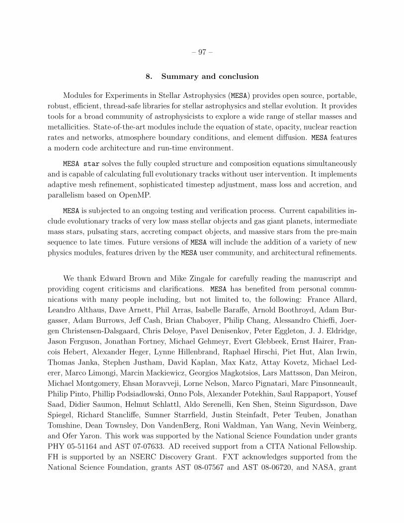
– 97 –
8. Summary and conclusion
Modules for Experiments in Stellar Astrophysics (MESA) provides open source, portable,
robust, efficient, thread-safe libraries for stellar astrophysics and stellar evolution. It provides
tools for a broad community of astrophysicists to explore a wide range of stellar masses and
metallicities. State-of-the-art modules include the equation of state, opacity, nuclear reaction
rates and networks, atmosphere boundary conditions, and element diffusion. MESA features
a modern code architecture and run-time environment.
MESA star solves the fully coupled structure and composition equations simultaneously
and is capable of calculating full evolutionary tracks without user intervention. It implements
adaptive mesh refinement, sophisticated timestep adjustment, mass loss and accretion, and
parallelism based on OpenMP.
MESA is subjected to an ongoing testing and verification process. Current capabilities in-
clude evolutionary tracks of very low mass stellar objects and gas giant planets, intermediate
mass stars, pulsating stars, accreting compact objects, and massive stars from the pre-main
sequence to late times. Future versions of MESA will include the addition of a variety of new
physics modules, features driven by the MESA user community, and architectural refinements.
We thank Edward Brown and Mike Zingale for carefully reading the manuscript and
providing cogent criticisms and clarifications. MESA has benefited from personal commu-
nications with many people including, but not limited to, the following: France Allard,
Leandro Althaus, Dave Arnett, Phil Arras, Isabelle Baraffe, Arnold Boothroyd, Adam Bur-
gasser, Adam Burrows, Jeff Cash, Brian Chaboyer, Philip Chang, Alessandro Chieffi, Joer-
gen Christensen-Dalsgaard, Chris Deloye, Pavel Denisenkov, Peter Eggleton, J. J. Eldridge,
Jason Ferguson, Jonathan Fortney, Michael Gehmeyr, Evert Glebbeek, Ernst Hairer, Fran-
cois Hebert, Alexander Heger, Lynne Hillenbrand, Raphael Hirschi, Piet Hut, Alan Irwin,
Thomas Janka, Stephen Justham, David Kaplan, Max Katz, Attay Kovetz, Michael Led-
erer, Marco Limongi, Marcin Mackiewicz, Georgios Magkotsios, Lars Mattsson, Dan Meiron,
Michael Montgomery, Ehsan Moravveji, Lorne Nelson, Marco Pignatari, Marc Pinsonneault,
Philip Pinto, Phillip Podsiadlowski, Onno Pols, Alexander Potekhin, Saul Rappaport, Yousef
Saad, Didier Saumon, Helmut Schlattl, Aldo Serenelli, Ken Shen, Steinn Sigurdsson, Dave
Spiegel, Richard Stancliffe, Sumner Starrfield, Justin Steinfadt, Peter Teuben, Jonathan
Tomshine, Dean Townsley, Don VandenBerg, Roni Waldman, Yan Wang, Nevin Weinberg,
and Ofer Yaron. This work was supported by the National Science Foundation under grants
PHY 05-51164 and AST 07-07633. AD received support from a CITA National Fellowship.
FH is supported by an NSERC Discovery Grant. FXT acknowledges supported from the
National Science Foundation, grants AST 08-07567 and AST 08-06720, and NASA, grant

– 98 –
NNX09AD106.
A. Manifesto
MESA was developed through the concerted efforts of the lead author over a six year
period with the engagement and deep involvement of many theoretical and computational
astrophysicists. The public availability of MESA will serve education, scientific research, and
outreach. This appendix describes the scientific motivation for MESA, the philosophy and rules
of use for MESA, and the path forward on stewardship of MESA and advanced development
of future research and education tools. We make MESA openly available with the hope that
it will grow into a community resource. We therefore consider it important to explain the
guiding principles for using and contributing to MESA. Our goal is to assure the greatest
usefulness for the largest number of research and educational projects.
A.1. Motivation for a new tool
Stellar evolution calculations (i.e. stellar evolution tracks and detailed information about
the evolution of internal and global properties) are a basic tool that enable a broad range
of research in astrophysics. Areas that critically depend on high-fidelity and modern stel-
lar evolution include asteroseismology, nuclear astrophysics, galactic chemical evolution and
population synthesis, compact objects, supernovae, stellar populations, stellar hydrodynam-
ics, and stellar activity. New observational capabilities are emerging in these fields that place
a high demand on exploration of stellar dependencies on metallicity and age. So, even though
one dimensional stellar evolution is a mature discipline, we continue to ask new questions
of stars. The emergence of demand requires the construction of a general, modern stellar
evolution code that combines the following advantages:
• Openess: should be open to any researcher, both to advance the pace of scientific
discovery, but also to share the load of updating physics, fine-tuning, and further
development.
• Modularity: should provide independent, reusable modules.
• Wide Applicability: should be capable of calculating the evolution of stars in a
wide range of environments, including low- and massive stars, binaries, accreting, mass-
losing stars, early and advanced phases of evolution etc. This will enable multi-problem,
multi-object physics validation.
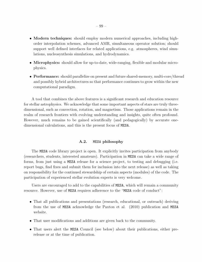
– 99 –
• Modern techniques: should employ modern numerical approaches, including high-
order interpolation schemes, advanced AMR, simultaneous operator solution; should
support well defined interfaces for related applications, e.g. atmospheres, wind simu-
lations, nucleosynthesis simulations, and hydrodynamics.
• Microphysics: should allow for up-to-date, wide-ranging, flexible and modular micro-
physics.
• Performance: should parallelize on present and future shared-memory, multi-core/thread
and possibly hybrid architectures so that performance continues to grow within the new
computational paradigm.
A tool that combines the above features is a significant research and education resource
for stellar astrophysics. We acknowledge that some important aspects of stars are truly three-
dimensional, such as convection, rotation, and magnetism. Those applications remain in the
realm of research frontiers with evolving understanding and insights, quite often profound.
However, much remains to be gained scientifically (and pedagogically) by accurate one-
dimensional calculations, and this is the present focus of MESA.
A.2. MESA philosophy
The MESA code library project is open. It explicitly invites participation from anybody
(researchers, students, interested amateurs). Participation in MESA can take a wide range of
forms, from just using a MESA release for a science project, to testing and debugging (i.e.
report bugs, find fixes and submit them for inclusion into the next release) as well as taking
on responsibility for the continued stewardship of certain aspects (modules) of the code. The
participation of experienced stellar evolution experts is very welcome.
Users are encouraged to add to the capabilities of MESA, which will remain a community
resource. However, use of MESA requires adherence to the “MESA code of conduct”:
• That all publications and presentations (research, educational, or outreach) deriving
from the use of MESA acknowledge the Paxton et al. (2010) publication and MESA
website.
• That user modifications and additions are given back to the community.
• That users alert the MESA Council (see below) about their publications, either pre-
release or at the time of publication.
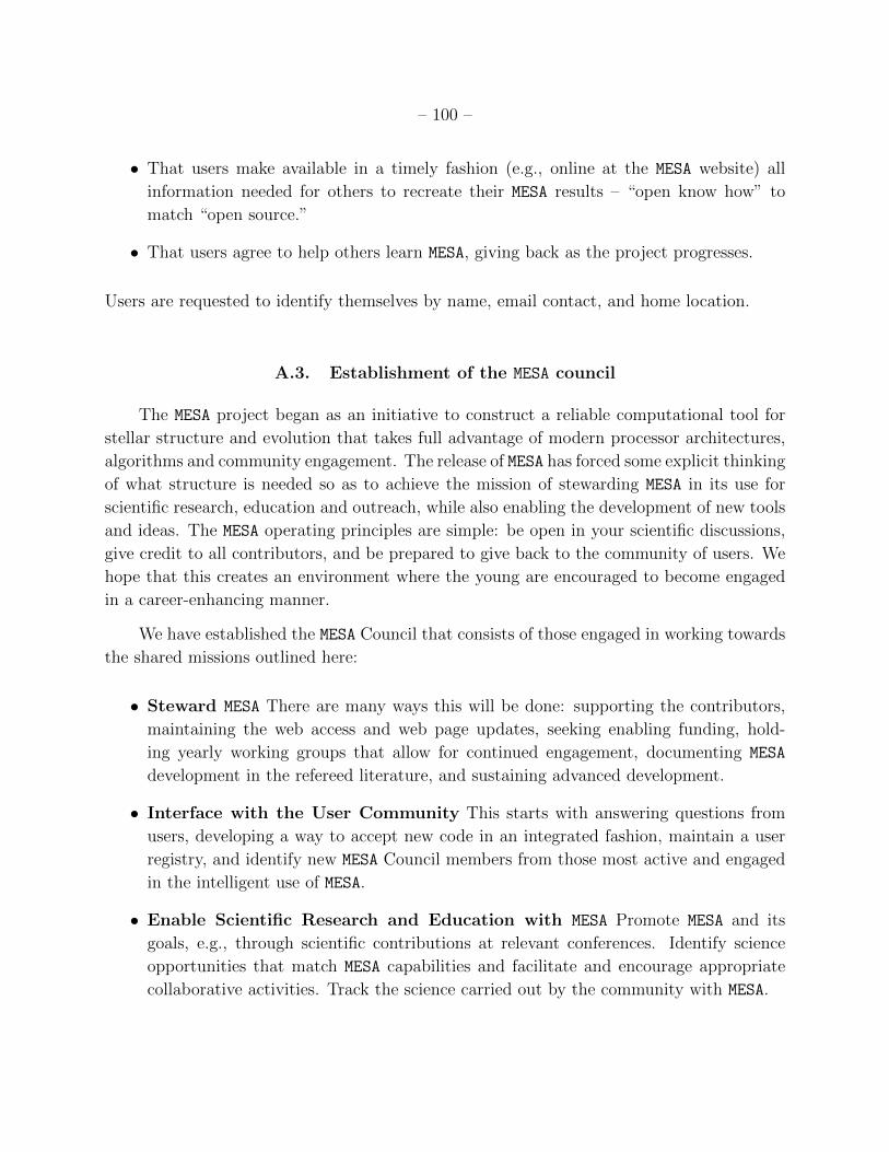
– 100 –
• That users make available in a timely fashion (e.g., online at the MESA website) all
information needed for others to recreate their MESA results – “open know how” to
match “open source.”
• That users agree to help others learn MESA, giving back as the project progresses.
Users are requested to identify themselves by name, email contact, and home location.
A.3. Establishment of the MESA council
The MESA project began as an initiative to construct a reliable computational tool for
stellar structure and evolution that takes full advantage of modern processor architectures,
algorithms and community engagement. The release of MESA has forced some explicit thinking
of what structure is needed so as to achieve the mission of stewarding MESA in its use for
scientific research, education and outreach, while also enabling the development of new tools
and ideas. The MESA operating principles are simple: be open in your scientific discussions,
give credit to all contributors, and be prepared to give back to the community of users. We
hope that this creates an environment where the young are encouraged to become engaged
in a career-enhancing manner.
We have established the MESA Council that consists of those engaged in working towards
the shared missions outlined here:
• Steward MESA There are many ways this will be done: supporting the contributors,
maintaining the web access and web page updates, seeking enabling funding, hold-
ing yearly working groups that allow for continued engagement, documenting MESA
development in the refereed literature, and sustaining advanced development.
• Interface with the User Community This starts with answering questions from
users, developing a way to accept new code in an integrated fashion, maintain a user
registry, and identify new MESA Council members from those most active and engaged
in the intelligent use of MESA.
• Enable Scientific Research and Education with MESA Promote MESA and its
goals, e.g., through scientific contributions at relevant conferences. Identify science
opportunities that match MESA capabilities and facilitate and encourage appropriate
collaborative activities. Track the science carried out by the community with MESA.

– 101 –
B. Code testing and verification
An important part of the ongoing development of a large, complex software project, such
as MESA, is regular, systematic testing. Testing is necessary to ensure that MESA continues
to function as expected and that the addition of new features does not have unintended
consequences for existing features.
MESA is tested at the module level each time it is compiled from the install scripts. These
tests check that each module produces results that are consistent with expectations. The
next level is the MESA star test suite, which consists of various evolutionary cases that are
intended to cover a broad range of applications, including Roche lobe overflow, the He core
flash in a low mass star, the evolution of sub-stellar mass objects, advanced nuclear burning
in massive stars, accreting white dwarfs and neutron star envelopes, and more are being
added all the time. The test cases come in both short and long varieties. Run in serial,
the full set of short tests completes in less than one hour on modern hardware. The long
tests might each take one or several hours to complete. Many of the evolutionary sequences
presented in §7 are included in the test suite. Short tests include the very low mass models
evolved to 10 Gyr (Figure 18) and the 0.8M�, Z = 10−4 track (Figure 19) while longer tests
include the Solar model calibration (Figure 20), the “hands off” 1M� pre-main sequence to
white dwarf calculation (Figure 13), and Si-burning in a 15M�, Z = 0.02 model (Tables 12
and 13).
The test suite is readily extended in order to ensure regular testing of certain aspects
of MESA that are not covered by the existing set but are important for a particular avenue of
research. A template is provided to encourage the creation of new test cases.
REFERENCES
Akima, Hiroshi, 1996, ACM Algorithm 760., ACM Trans. Math. Software, 22, 357
Alastuey, A., & Jancovici, B. 1978, ApJ, 226, 1034
Alexander, D. R. & Ferguson, J. W., 1994, ApJ, 437, 879
Allard, F., Hauschildt, P. H., Alexander, D. R., Tamanai, A. & Schweitzer, A. 2001, 556,
357
Anders, E. & Grevesse, N., 1989, Geochimica et Cosmochimica Acta, 53, 197
Angulo, C., Arnould, M., Rayet, M., et al. 1999, Nucl. Phys. A, 656, 3
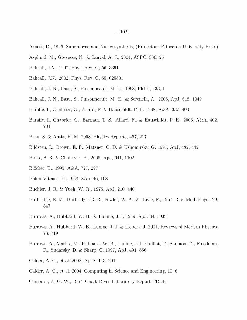
– 102 –
Arnett, D., 1996, Supernovae and Nucleosynthesis, (Princeton: Princeton University Press)
Asplund, M., Grevesse, N., & Sauval, A. J., 2004, ASPC, 336, 25
Bahcall, J.N., 1997, Phys. Rev. C, 56, 3391
Bahcall, J.N., 2002, Phys. Rev. C, 65, 025801
Bahcall, J. N., Basu, S., Pinsonneault, M. H., 1998, PhLB, 433, 1
Bahcall, J. N., Basu, S., Pinsonneault, M. H., & Serenelli, A., 2005, ApJ, 618, 1049
Baraffe, I., Chabrier, G., Allard, F. & Hauschildt, P. H. 1998, A&A, 337, 403
Baraffe, I., Chabrier, G., Barman, T. S., Allard, F., & Hauschildt, P. H., 2003, A&A, 402,
701
Basu, S. & Antia, H. M. 2008, Physics Reports, 457, 217
Bildsten, L., Brown, E. F., Matzner, C. D. & Ushomirsky, G. 1997, ApJ, 482, 442
Bjork, S. R. & Chaboyer, B., 2006, ApJ, 641, 1102
Blocker, T., 1995, A&A, 727, 297
Bohm-Vitense, E., 1958, ZAp, 46, 108
Buchler, J. R. & Yueh, W. R., 1976, ApJ, 210, 440
Burbridge, E. M., Burbridge, G. R., Fowler, W. A., & Hoyle, F., 1957, Rev. Mod. Phys., 29,
547
Burrows, A., Hubbard, W. B., & Lunine, J. I. 1989, ApJ, 345, 939
Burrows, A., Hubbard, W. B., Lunine, J. I. & Liebert, J. 2001, Reviews of Modern Physics,
73, 719
Burrows, A., Marley, M., Hubbard, W. B., Lunine, J. I., Guillot, T., Saumon, D., Freedman,
R., Sudarsky, D. & Sharp, C. 1997, ApJ, 491, 856
Calder, A. C., et al. 2002, ApJS, 143, 201
Calder, A. C., et al. 2004, Computing in Science and Engineering, 10, 6
Cameron, A. G. W., 1957, Chalk River Laboratory Report CRL41

– 103 –
Cassisi, S., Potekhin, A. Y., Pietrinferni, A., Catelan, M., & Salaris, M. 2007, ApJ, 661,
1094
Castelli, F., & Kurucz, R. L. 2003, IAU Symp. 210, ed. N. Piskunov, W. W. Weiss, & D. F.
Gray San Francisco: ASP
Caughlan, G. R., Fowler, W. A., 1988, At. Data Nuc. Data Tab., 40, 283
Chabrier, G. & Baraffe, I. 2000, Annual Reviews of Astronomy and Astrophysics, 38, 337
Chabrier, G., Baraffe, I., Allard, F., & Hauschildt, P. 2000, ApJ, 542, L119
Chabrier, G., Baraffe, I. & Plez, B. 1996, ApJ, 459, L91
Chandrasekhar, S., 1938, Stellar Structure (Chicago: University of Chicago Press)
Chandrasekhar S., 1939, An Introduction to the Study of Stellar Structure, (New York:
Dover)
Christensen-Dalsgaard, J., 2008, Ap&SS, 316, 13
Clayton, D.D., 1984, Principles of Stellar Evolution and Nucleosynthesis, (Chicago: Univer-
sity of Chicago Press)
Coelho, P., Bruzual, G., Charlot, S., Weiss, A., Barbuy, B., Ferguson, J. W., 2007, MNRAS,
382, 498
Cox, J. P. & Giuli, R. T., 1968, Principles of Stellar Structure, (New York: Gordon &
Breach)
Cumming, A., 2003, ApJ, 595, 1077
Cyburt, R. H. et al. 2010, ApJS, 189, 240
D’Antona, F. & Mazzitelli, I. 1994, ApJS, 90, 467
Degl’Innocenti, S., Prada Moroni, P. G., Marconi, M., & Ruoppo, A., 2008, Ap&SS, 316, 25
Degroote, P. et al. 2009, A&A, 506, 471
Degroote, P. et al. 2010, Nature, 464, 259
de Jager, C., Nieuwenhuijzen, H., & van der Hucht, K. A. 1988, A&AS, 72, 259
Demarque, P, Guenther, D. B., Li, L. H., Mazumdar, A., Straka, C. W., 2008, Ap&SS, 316,
31
– 104 –
Dewitt, H.E., Graboske, H.C., & Cooper, M.S., 1973, ApJ, 181, 439
Dotter, A., Chaboyer, B., Jevremovic, D., Baron, E., Ferguson, J. W., Sarajedini, A., &
Anderson, J., 2007, AJ, 2007, 134, 376
Dotter, A., Sarajedini, A., Anderson, J., Aparicio, A., Bedin, L. R., Chaboyer, B., Majewski,
S., Marın-Franch, A., Milone, A., Paust, N., Piotto, G., Reid, I. N., Rosenberg, A.,
Siegel, M., 2010, ApJ, 708, 698
Dziembowski, W. A., Moskalik, P. & Pamyatnykh, A. A. 1993, MNRAS, 265, 588
Eddington, A.S. 1926, Internal Constitution of the Stars, (Cambridge:Cambridge University
Press)
Eggenberger, P., Meynet, G., Maeder, A., Hirschi, R., Charbonnel, C. Talon, S., & Ekstrom,
S., 2008, Ap&SS, 316, 43
Eggleton, P.P., 1971, MNRAS, 151, 351
Ferguson, J. W., Alexander, D. R., Allard, F., Barman, T., Bodnarik, J. G., Hauschildt, P.
H., Heffner-Wong, A., & Tamanai, A., 2005, ApJ, 623, 585
Fujimoto, M. Y., Ikeda, Y., & Iben, I., Jr., 2000, ApJ, 529, L25
Fuller, G.M., Fowler, W.A., & Newman, M.J., 1985, ApJ, 293, 1
Fynbo, H. O. U. et al., 2005, Nature, 433, 136
Gallino, R., Arlandini, M., Busso, M., Lugaro, M., Travaglio, C., Straniero, O., Chieffi, A.,
& Limongi, M., 1998, ApJ, 497, 388
Gansicke, B. T. et al, 2009, MNRAS, 397, 2170
Gehmeyr, M. & Mihalas, D., 1994, Physica D, 77, 320
Gilliland, R. L. et al. 2010, PASP, 122, 131
Glebbeek, E., et al. 2002, A&A, 497, 255
Gorres, J., Arlandini, C., Giesen, U., Heil, M., Kappeler, F., Leiste, H., Stech, E., & Wi-
escher, M. 2000, Phys. Rev. C, 62, 055801
Gorshkov, A. B. & Baturin, V. A. 2008, Astronomy Reports, 52 760
Graboske, H.C., Dewitt, H.E., Grossman, A.S., & Cooper, M.S., 1973, ApJ, 181, 457

– 105 –
Grevesse, N. & Noels, A., 1993, Phys. Scr. T, 47, 133
Grevesse, N. & Sauval, A. J., 1998, SSRv, 85, 161
Hairer, E. & Wanner, G., Solving Ordinary Differential Equations II. Stiff and Differential-
Algebraic Problems. Springer Series in Comput. Math., vol. 14
Hansen, C.J., & Kawaler, S.D., 1995, Stellar Interiors: Physical Principles, Structure, and
Evolution, (New York: Springer-Verlag)
Hauschildt, P. H., Allard, F., & Baron, E., 1999a, ApJ, 512, 377
Hauschildt, P. H., Allard, F., Ferguson, J., Baron, E., & Alexander, D., 1999b, ApJ, 525,
871
Heger, A., Cumming, A., Galloway, D. K., & Woosley, S. E., 2007, ApJ, 671, L141
Heger, A., Langer, N., Woosley, S. E. 2000, ApJ, 528, 368 (HLW)
Henyey, L. G., Forbes, J. E., & Gould, N. L., 1964, ApJ, 139, 306
Henyey, L. G., Vardya, M. S., & Bodenheimer, P., 1965, ApJ, 142, 841
Henyey, L. G., Wilets, L., Bohm, K.H., LeLevier, R., & Levee, R.D., 1959, ApJ, 129, 628
Herwig, F., 2000, A&A, 360, 952
Herwig, F., 2004, ApJ, 605, 425
Herwig, F., 2005, ARA&A, 43, 435
Herwig, F. & Austin, S. M., 2004, ApJ, 613, 73
Hirschi, R., Meynet, G., & Maeder, A., A&A, 425, 649 (HMM)
Hofmeister, E., Kippenhahn, R., & Weigart, A., 1964, ZAp, 59, 215
Hubbard, W. B., & Lampe, M. 1969, ApJS, 18, 297
Hui-Bon-Hoa, A., 2008, Ap&SS, 316, 55
Huynh, H.T., 1993, SIAM J Numer. Anal. 30, 57
Iben, I., 1975, ApJ, 196, 525
Iben, I., 1991, ApJS, 76, 55
– 106 –
Iben, I. & Ehrman, J. R., 1962, ApJ, 135, 770
Iben, I. & MacDonald, J. 1985, ApJ, 296, 540
Iglesias, C. A., & Rogers, F. J. 1993, ApJ, 412, 752
Iglesias, C. A., & Rogers, F. J. 1996, ApJ, 464, 943
Iliadis, C. 2007, Nuclear Physics of Stars
Imbriani, G. et al., 2005, European Physics Journal A, 25, 455
Itoh, N., Hayashi, H., Nishikawa, A., and Kohyama, Y. 1996, ApJS, 102, 411
Itoh, N., Totsuji, H., Ichimaru, S., & Dewitt, H. E. 1979, ApJ, 234, 1079
Kippenhahn, R., Ruschenplatt, G., & Thomas, H.-C. 1980, A&A, 91, 175
Kippenhahn, R., & Weigert, A., 1996, Stellar Evolution and Nucleosynthesis, (New York:
Springer-Verlag)
Kippenhahn, R., Weigert, A., & Hofmeister, E., 1967, in Methods in Computational Physics
Vol. 7 (Ed. Alder, B., Fernbach, S., and Rotenberg, M., Academic Press)
Kolb, U. & Baraffe, I. 1999, MNRAS, 309, 1034
Krishna Swamy, K.S., 1966, ApJ, 145, 174
Kunz, R., Fey, M., Jaeger, M., Mayer, A., Hammer, J. W., Staudt, G., Harissopulos, S., &
Paradellis, T., 2002, ApJ, 567, 643
Langanke, K & Martınez-Pinedo, 2000, Nucl. Phys. A, 673, 481
Lebreton, Y. et al., 2008, Ap&SS, 316, 1
Lederer, M.T. & Aringer, B., 2009, A&A, 494, 403
Lesaffre, P, Han, Z., Tout, C. A., Podsiadlowski, Ph., & Martin, R. G., 2006, MNRAS, 368,
187
Limongi, M., & Chieffi, A., 2006, ApJ, 647, 483
Limongi, M., Straniero, O., Chieffi, A., 2000, ApJS, 129, 625 (LSC)
Lodders, K., 2003, ApJ, 591, 1220
– 107 –
Lugaro, M., Herwig, F., Lattanzio, J. C., Gallino, R., Straniero, O., 2003, ApJ, 586, 1305
Madhusudhan, N., Justham, S., Nelson, L., Paxton, B., Pfahl, E., Posdsiadlowski, P. &
Rappaport, S. 2006, ApJ, 640, 918
Mattsson, L.; Wahlin, R.; Hfner, S., 2010 A&A, 509, 14M
Mocak, M., Muller, E., Weiss, A. & Kifonidis, K. 2009, A&A, 501, 659
Mohr, P. J., Taylor, B. N., & Newell, D. B., 2008, Rev. Mod. Phys., 80, 633
Morel, P, & Lebreton, Y., 2008, Ap&SS, 316, 61
Nieuwenhuijzen, H., & de Jager, C. 1990, A&A, 231, 134
Nugis, T., & Lamers, H.J.G.L.M., 2000, A&A, 360, 227
Oberkampf, W. L., 1998, Bibliography for Verification and Validation in Computational
Simulation, tech. report SAND98-2041, Sandia National Laboratories
Oda, T., Hino, M., Muto, K., Takahara, M., & Sato, K., 1994, Atomic Data and Nuclear
Data Tables, 56, 231
Oke, J. B. & Schwarzschild, M., 1952, ApJ, 116, 317
Paczynski, B. & Proszynski, M. 1986, ApJ, 302, 519
Pamyatnykh, A. A., Handler, G. & Dziembowski, W. A. 2004, MNRAS, 350, 1022
Paquette, C., Pelletier, C., Fontaine, G., Michaud, G., 1986, ApJS, 61, 197
Patterson, J. 1998, PASP, 110, 1132
Paxton, B., 2004, PASP, 116, 699
Pietrinferni, A., Cassisi, S., Salaris, M., Castelli, F., 2004, ApJ, 612, 168
Pols, O. R., Tout, C. A., Eggleton, P. P. & Han, Zh. 1995, MNRAS, 274, 964
Potekhin, A.Y. & Chabrier, G., 2010, Contrib. Plasma Phys., 50, 82
Press, W. H., Teukolsky, S. A., Vetterling, W. T., & Flannery, B. P., 1992 Numerical Recipes
in C, (Cambridge Univ. Press: London)
Prialnik, D. & Kovetz, A., 1995, ApJ, 445, 789
– 108 –
Rauscher, T. & Thielemann, F.-K., 2000, At. Data Nucl. Data Tables, 75, 1
Rauscher, T., Heger, A., Hoffman, R. D., Woosley, S. E., 2002, ApJ, 576, 323
Reimers, D. 1975, Mem. Soc. R. Sci Liege, 8, 369
Renka, Robert J., 1999, ACM Algorithm 790., ACM Trans. Math. Software, 25, 70
Roache, P.J., 1998, Verification and Validation in Computational Science and Engineering,
Hermosa
Rogers, F. J., & Nayfonov, A., 2002, ApJ, 576, 1064
Roxburgh, I. W., 2008, Ap&SS, 316, 75
Sakharuk, A., Elliot, T., Fisker, J. L., Hemingray, S., Kruizenga, A., Rauscher, T., Schatz,
H., Smith, K., Thielemann, F.-K., & Wiescher, M., 2006, CAPTURE GAMMA-RAY
SPECTROSCOPY AND RELATED TOPICS: 12th International Symposium, Eds.
A. Woehr & A. Aprahamian, 819, 118
Saumon, D., Chabrier, G., & van Horn, H. M., 1995, ApJS, 99, 713
Schwarzschild, M., 1958, Structure and Evolution of the Stars, (Princeton: Princeton Uni-
versity Press)
Scuflaire, R., Theado, S., Montalban, J., Miglio, A., Bourge, P.-O., Godart, M., Thoul, A.,
& Noels, A., 2008, Ap&SS, 316, 83
Seaton, M. J., 2005, MNRAS, 362, 1
Serenelli, A. M., Basu, S., Ferguson, J. W., & Asplund, M., 2009, ApJ, 705, 123
Serenelli, A. & Weiss, A. 2005, A&A, 442, 1041
Shen, K. J. & Bildsten, L., 2009, ApJ, 699, 1373
Shen, K. J., Idan, I. & Bildsten, L., 2009, ApJ, 705, 693
Soderlind, G. & Wang, L., 2006, Journal of Computational and Applied Mathematics, 225,
243
Starrfield, S., Sparks, W. M., Truran, J. W., & Wiescher, M. C. 2000, ApJS, 127, 485
Steffen, M., A&A, 1990, 239, 443

– 109 –
Stiriba, Y., 2003, Appl. Numer. Math., 45, 499
Strohmayer, T. & Bildsten, L. 2006, in Compact Stellar X-Ray Sources, ed. W. H. G. Lewin
& M. van der Klis (Cambridge: Cambridge Univ. Press), p. 113
Sugimoto, D., 1970, ApJ, 159, 619
Sugimoto, D., Nomoto, K., & Eriguchi, Y., 1981, Progress of Theoretical Physics Supple-
ment, 70, 115
Suresh, A., & Huynh, H.T., 1997, J. Computational Physics, 136, 83
Thomas, H.-C. 1967, Z. Astrophys., 67, 420
Thoul, A. A., Bahcall, J. N., & Loeb, A. 1994, ApJ, 421, 828
Timmes, F. X. 1999, ApJS, 124, 241
Timmes, F. X. & Swesty, F. D., 2000, ApJS, 126, 501
Timmes, F. X., Woosley, S. E., & Weaver, T. A., 1995, ApJS, 98, 617
VandenBerg, D. A. 2000, ApJS, 129, 315
Ventura, P., D’Antona, F., Mazzitelli, I., 2008, Ap&SS, 316, 93
Vink, J.S., de Koter, A., & Lamers, H.J.G.L.M., 2001, A&A, 369, 574.
Weaver, T. A., Zimmerman, G. B., & Woosley, S. E., 1978, ApJ, 225, 1021
Weinberg, N. N., Bildsten, L. & Schatz, H. 2006, ApJ, 639, 1018
Weiss, A., Cassisi, S., Dotter, A., Han, Z., & Lebreton, Y., 2007, IAUS, 241, 28
Weiss, A. & Schlattl, H., 2008, Ap&SS, 2008, 316, 99
Woosley, S. E. et al. 2004, ApJS, 151, 75
Woosley, S. E., Heger, A., & Weaver, T. A., 2002, Rev. Mod. Phys., 74, 1015 (WHW)
Worthey, G., 1994, ApJS, 95, 107
Yakovlev, D. G, & Urpin, V. A., 1980, Soviet Astronomy, 24, 303
Young, P. A., & Arnett, D., 2005, ApJ, 618, 908
Zingale, M., Almgren, A. S., Bell, J. B., Nonaka, A. & Woosley, S. E. 2009, ApJ, 704, 196

– 110 –
This preprint was prepared with the AAS LATEX macros v5.2.
Related Documents