The Extended Chandra Deep Field-South Survey: X-Ray Point-Source Catalog

arX

iv:a

stro

-ph/

0506

551v

2 3

0 Ja

n 20

06

Submitted to AJ

The Extended Chandra Deep Field-South Survey: X-ray

Point-Source Catalog

Shanil N. Virani, Ezequiel Treister1,2, C. Megan Urry1, and Eric Gawiser1,3

Department of Astronomy, Yale University, P.O. Box 208101, New Haven, CT 06520

[email protected]

ABSTRACT

The Extended Chandra Deep Field-South (ECDFS) survey consists of 4

Chandra ACIS-I pointings and covers ≈ 1100 square arcminutes (≈ 0.3 deg2)

centered on the original CDF-S field to a depth of approximately 228 ks. This is

the largest Chandra survey ever conducted at such depth, and only one XMM-

Newton survey reaches a lower flux limit in the hard 2.0–8.0 keV band. We detect

651 unique sources — 587 using a conservative source detection threshold and

64 using a lower source detection threshold. These are presented as two separate

catalogs. Of the 651 total sources, 561 are detected in the full 0.5–8.0 keV band,

529 in the soft 0.5–2.0 keV band, and 335 in the hard 2.0–8.0 keV band. For

point sources near the aim point, the limiting fluxes are approximately 1.7×10−16

erg cm−2 s−1 and 3.9 × 10−16 erg cm−2 s−1 in the 0.5–2.0 keV and 2.0–8.0 keV

bands, respectively. Using simulations, we determine the catalog completeness as

a function of flux and assess uncertainties in the derived fluxes due to incomplete

spectral information. We present the differential and cumulative flux distribu-

tions, which are in good agreement with the number counts from previous deep

X-ray surveys and with the predictions from an AGN population synthesis model

that can explain the X-ray background. In general, fainter sources have harder

X-ray spectra, consistent with the hypothesis that these sources are mainly ob-

scured AGN.

Subject headings: diffuse radiation — surveys — cosmology: observations —

galaxies: active — X-rays: galaxies — X-rays: general.

1Yale Center for Astronomy and Astrophysics, Yale University, P.O. Box 208121, New Haven, CT 06520

2Departamento de Astronomia, Universidad de Chile, Casilla 36-D, Santiago, Chile.

3NSF Astronomy and Astrophysics Postdoctoral Fellow

– 2 –

1. Introduction

Wide-area X-ray surveys have played a fundamental role in understanding the nature of

the sources that populate the X-ray universe. Early surveys like the Einstein Medium Sen-

sitivity Survey (Gioia et al. 1990), the ROSAT International X-ray/Optical Survey (Ciliegi

et al. 1997), and the ASCA Large Sky Survey (Akiyama et al. 2000) showed that the vast

majority of the bright X-ray sources are active galactic nuclei (AGNs). More specifically,

shallow wide-area surveys in the soft (0.5–2.0 keV) X-ray band yield mostly unobscured,

broad-line AGNs, which are characterized by a soft X-ray spectrum with a photon index of

Γ ≃ 1.9 (Nandra & Pounds 1994). In contrast, deep X-ray surveys — particularly surveys

that make use of the unprecedented, sub-arsecond spatial resolution of the Chandra X-ray

Observatory — find AGN with harder X-ray spectra (Γ ∼ 1.4) at fainter fluxes, more like

the hard spectrum of the X-ray background.

Deep Chandra surveys have thus opened a new vista on resolving the X-ray background

and identifying the role and evolution of accretion power in all galaxies. The cosmic X-

ray background is now almost completely resolved (∼ 70–90%) into discrete sources in the

deep, pencil beam surveys like the Chandra Deep Fields (CDF-N, Brandt et al. 2001; CDF-

S, Giacconi et al. 2002). To understand the composition of the sources that make up the

X-ray background, population synthesis models have been constructed (Madau et al. 1994;

Comastri et al. 1995; Gilli et al. 1999; Gilli et al. 2001; Treister & Urry 2005) which typically

require approximately 3 times as many obscured AGN as traditional Type 1 (unobscured)

AGN.

While the deep fields provide the deepest view of the X-ray universe and have generated

plentiful AGN samples at lower luminosities, the small area covered by pencil-beam surveys

means luminous sources are poorly sampled. In an attempt to determine the luminosity

function of X-ray emitting AGN up to z ∼ 5, as well as to leverage existing deep multiwave-

length data in the extended 30′×30′ field centered on the CDF-S, the region surrounding the

CDF-S was recently observed by Chandra. Covering ≈ 1100 square arcminutes (≈ 0.3 deg2),

the Extended Chandra Deep Field-South (ECDFS) survey is the largest Chandra survey field

at this depth (≈ 230 ks), and is the second deepest and widest survey ever conducted in the

X-rays (the XMM-Newton survey of the Lockman Hole is deeper in the hard band and has

∼ 30% more area; Hasinger 2004).

In this paper, we present the X-ray catalog for the ECDFS and the number counts in

two energy bands. In subsequent papers, we will present the optical and near-IR properties

of these X-ray sources, including first results from our deep optical spectroscopy campaign

obtained as part of the one-square-degree MUltiwavelength Survey by Yale/Chile (MUSYC)

(Gawiser et al. 2005).

– 3 –

In Section 2, we describe our data reduction procedure. In Section 3, we describe the

point source detection and astrometry. The X-ray source catalog and basic survey results

are presented in Section 4 and the conclusions are given in Section 5. The average Galactic

column density along this line of sight for the four pointings is 9.0× 1019 cm−2 (Stark et al.

1992). H0 = 70 km s−1 Mpc−1, ΩM = 0.3, and ΩΛ = 0.7 are adopted throughout this paper

which is consistent with the cosmological parameters reported by Spergel et al. (2003). All

coordinates throughout this paper are J2000.

2. Observations and Data Reduction

2.1. Instrumentation and Diary of Observations

All nine observations of the ECDFS survey field were conducted with the Advanced

CCD Imaging Spectrometer (ACIS) on-board the Chandra X-ray Observatory1 as part of

the approved guest observer program in Cycle 5 (proposal number 05900218 – PI Niel Brandt;

Lehmer et al. 2005). ACIS consists of 10 CCDs, distributed in a 2×2 array (ACIS-I) and a

1×6 array (ACIS-S). All 4 of the ACIS-I CCDs are front-illuminated (FI) CCDs; 2 of the 6

ACIS-S CCDs are back-illuminated CCDs (S1 and S3). Of these 10 CCDs, at most 6 can

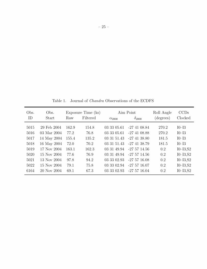
be operated at any one time. Table 1 presents a journal of the Chandra observations of

the ECDFS. All nine observations were conducted in VERY FAINT mode (See the Chandra

Proposers’ Guide, pg. 95) so that the pixel values of the 5 × 5 event island are telemetered

rather than just the 3 × 3 event island as in FAINT mode. This telemetry format offers

the advantage of further reducing the instrument background after ground processing (see

Section 2.2). Observation ids (ObsIds) 5019–5022 and 6164 also had the ACIS-S2 CCD

powered on (see Table 1). However, due to the large off-axis angle of the S2 CCD during

these observations, it has a much broader point spread function (PSF) and hence lower

sensitivity so we exclude data from this CCD and focus only on data collected from the

ACIS-I CCDs. The on-axis CCD for each ACIS-I observation is I3 and the ACIS-I field of

view is 16.′9 × 16.′9.

1For additional information on the ACIS and Chandra see the Chandra Proposers’ Guide at

http://cxc.harvard.edu/proposer/POG/html.

– 4 –

2.2. Data Reduction

All data were re-processed using the latest version of the Chandra Interactive Analysis of

Observations2 (CIAO; Version 3.2.1; released 10 February 2005) software as well as version

3.0.0 of the calibration database (CALDB; released 12 December 2004). We chose to re-

reduce all nine datasets rather than simply use the standard data processing (SDP) level 2

event files because we wanted the datasets to be reduced in a consistent manner, and more

importantly, we wanted to take advantage of better Chandra X-ray Center (CXC) algorithms

to reduce the ACIS particle background by using the information located in the outer 16

pixels of the 5×5 event island3, as well as executing a new script that is much more efficient

at identifying ACIS “hot pixels” and cosmic ray afterglow events4. This new hot pixel and

cosmic ray afterglow tool is now implemented in the standard data processing pipeline at

the CXC but was not applied in the SDP pipeline of the present observations.

The following procedure was used to arrive at a new level 2 event file. Before applying

the new CIAO tool to identify ACIS hot pixels and cosmic ray afterglow events, the pixels

identified in the CXC-provided level 1 event file as being due to a cosmic ray afterglow

event were reset. An afterglow is the residual charge from the interaction of a cosmic ray

in a front-side illuminated CCD frame. Some of the excess charge is captured by charge

traps created by the radiation damage suffered early in the mission (see Townsley et al.

2000 and references therein) and released over the next few to a few dozen frames. If these

afterglow events are not removed from the data, they can result in the spurious detection of

faint sources. To better account for such events, a new, more precise method for identifying

afterglow events was developed by the CXC and has now been introduced into the standard

data processing pipeline. This CIAO tool, “acis run hotpix,” was then run on the reset level

1 event file to identify and flag hot pixels and afterglow events in all 9 ACIS observations

of the ECDFS. The last step in producing the new level 2 event file was to run the CIAO

tool “acis process events.” In addition to applying the newest gain map supplied in the

latest release of the CALDB, this tool also applies the pixel randomization and the ACIS

charge transfer inefficiency (CTI) correction. The latter corrects the data for radiation

damage sustained by the CCDs early in the mission. All of these corrections are part of the

standard data processing and are on by default in acis process events. The time-dependent

gain correction is also applied to the event list to correct the pulse-invariant (PI) energy

2See http://cxc.harvard.edu/ciao/.

3See “Reducing ACIS Quiescent Background Using Very Faint Mode”,

http://cxc.harvard.edu/cal/Acis/Cal prods/vfbkgrnd/index.html.

4See http://cxc.harvard.edu/ciao/threads/acishotpixels/.

– 5 –

channel for the secular drift in the average pulse-height amplitude (PHA) values. This drift

is caused primarily by gradual degradation of the CTI of the ACIS CCDs (e.g., Schwartz &

Virani 2004). Finally, the observation-specific bad pixel map created by “acis run hotpix”

was supplied, and the option to clean the ACIS particle background by making use of the

additional pixels telemetered in VERY FAINT mode was turned on.

Once a new level 2 event file was produced, we applied the standard grade filtering to

each observation, choosing only event grades 0, 2, 3, 4, and 6 (the standard ASCA grade

set), and the standard Good Time Intervals supplied by the SDP pipeline. We also restrict

the energy range to 0.5–8.0 keV, as the background rises steeply below and above those

limits5. Lastly, we examined the background light curves for all 9 observations as the ACIS

background is known to vary significantly. For example, Plucinsky & Virani (2000) found

that the front-illuminated CCDs can show typical increases of 1 - 5 cts s−1 above the quiescent

level, while the back-illuminated CCDs can show large excursions — as high as 100 cts s−1

above the quiescent level — during background flares. The durations of these intervals of

enhanced background are highly variable, ranging from 500 s to 104 s. The cause of these

background flares is currently not known (see Grant, Bautz, & Virani 2002); however, they

may be caused by low-energy protons (<100 keV; e.g., Plucinsky & Virani 2000; Struder et

al. 2001). The time periods corresponding to these background flares are generally excised

from the data before proceeding with further analysis although not always (see Brandt et al.

2001; Nandra et al. 2005). In fact, Kim et al. (2004) find that the source detection probability

depends strongly on the background rate. To examine our observations for such periods, we

used the CIAO script ANALYSE LTCRV.SL which identifies periods where the background

is ±3σ above the mean. All 9 observations were filtered according to this prescription (see

Table 1 for a comparison of raw exposure time vs. filtered exposure time), resulting in only

∼40.6 ks (∼4%) being lost due to background flares (954.2 ks vs. 913.6 ks). Of this, 20.3 ks

were excluded from the end of ObsID 5017 due to a flare in which the count rate increased

by a factor of ∼2. Table 2 lists the net exposure time for each of the 4 pointings used to

image the ECDFS region. The net exposure time for each of the 4 pointings varies from a

low of 205 ks to a high of 239 ks, with the mean net exposure time for the entire survey field

of 228 ks. These extra steps in processing help remove spurious sources and result in fewer

catalog sources than if the standard processing or pipeline products were used.

5See http://cxc.harvard.edu/contrib/maxim/stowed/.

– 6 –

3. Data Analysis

In this paper, we report on the sources detected in three standard X-ray bands (see

Table 3): 0.5–8.0 keV (full band), 0.5–2.0 keV (soft band), and 2.0–8.0 keV (hard band).

The raw ACIS resolution is 0.492 arcsec pixel−1, however, source detection and flux deter-

minations were performed on the block 4 images, i.e., 1.964 arcsec pixel−1, as the source

detect tool and exposure map generation require significant computer resources for full size

images; for greater accuracy, source positions were determined from the block 1 images.

3.1. Image and Exposure Map Creation

Observations at each of the four pointings were combined via the CIAO script “merge all.”

This script was executed using CIAO version 2.3 because of a known bug in the “asphist”

tool under CIAO version 3.2.1; this bug results in incorrect exposure maps for the merged

image6. At each pointing, the observation with the longest integration time was used for

co-ordinate registration. For example, when merging ObsIds 5015 and 5016, the merged

event list was registered to ObsId 5015 as it has approximately twice the integration time as

5016. Table 2 lists the ObsIds for each pointing, as well as the raw and the net integration

time. For each pointing, we constructed images in the three standard bands: 0.5–8.0 keV

(full band), 0.5–2.0 keV (soft band), and 2.0–8.0 keV (hard band); see Table 3. The full

band exposure-corrected image for the entire survey field7 is presented in Figure 1.

We constructed exposure maps in these three energy bands for each pointing and for

the entire survey field8. These exposure maps were created in the standard way and are

normalized to the effective exposure of a source location at the aim point. The procedure

used to create these exposure maps accounts for the effects of vignetting, gaps between

the CCDs, bad column filtering, and bad pixel filtering. However, it should be noted that

charge blooms caused by cosmic rays can reduce the detector efficiency by as much as few

percent9. There is currently no way to account for such charge cascades; however, when a

tool becomes available, we will correct for this effect as necessary and make the new exposure

6See the usage warning at http://cxc.harvard.edu/ciao/threads/merge all/.

7Raw and smoothed ASCA -grade images for all three standard bands (See Table 3) are available from

http://www.astro.yale.edu/svirani/ecdfs/.

8Exposure maps for all three standard bands (see Table 3) are available from

http://www.astro.yale.edu/svirani/ecdfs/.

9See http://cxc.harvard.edu/ciao/caveats/acis caveats 050620.html.

– 7 –

maps publicly available at the World Wide site listed in Footnote 7. The exposure maps

were binned by 4 so that they were congruent to the final reduced images. A photon index

of Γ = 1.4, the slope of the X-ray background in the 0.5–8.0 keV band (e.g. Marshall et al.

1980; Gendreau et al. 1995; Kushino et al. 2002) was used in creating these exposure maps.

In order to calculate the survey area as a function of the X-ray flux in the soft and hard

bands, we used the exposure maps generated for each band and assumed a fixed detection

threshold of 5 counts in the soft band and 2.5 in the hard band (∼2σ). Dividing these

counts by the exposure map, we obtain the flux limit at each pixel for each band. The pixel

area is then converted into a solid angle and the cumulative histogram of the flux limit is

constructed (Figure 2). The total survey area is ≈ 1100 arcmin2 (≈ 0.3 deg2). A more

precise method of determining the survey area as a function of the X-ray flux is described

by Kenter & Murray (2003); however, this would affect only the faint tail of the sample and

would not significantly alter the present results. Therefore, a more sophisticated treatment

is deferred to a later paper.

3.2. Point Source Detection

To perform X-ray source detection, we applied the CIAO wavelet detection algorithm

wavdetect (Freeman et al. 2002). Although several other methods have been used in other

survey fields to find sources in Chandra observations (e.g., Giacconi et al. 2002; Nandra et

al. 2005), we chose wavdetect to allow a straightforward comparison between sources found

in our catalog with those found in the CDF-S (Giacconi et al. 2002; Alexander et al. 2003).

Moreover, wavdetect is more robust in detecting individual sources in crowded fields and

in identifying extended sources than the other CIAO detection algorithm, celldetect. Point-

source detection was performed in each standard band (see Table 3) using a “√

2 sequence”

of wavelet scales; scales of 1,√

2, 2, 2√

2, 4, 4√

2, and 8 pixels were used. Brandt et al.

(2001), for example, showed that using larger scales can detect a few additional sources at

large off-axis angles but found that this “√

2 sequence” gave the best overall performance

across the CDF-N field. Moreover, as Alexander et al. (2003) point out, sources found with

larger scales tend to have source properties and positions too poorly defined to give useful

results.

Our criterion for source detection is that a source must be found with a false-positive

probability threshold (pthresh) of 1 × 10−7 in at least one of the three standard bands. This

false-positive probability threshold is typical for point-source catalogs (e.g., Alexander et

al. 2003; Wang et al. 2004), although Kim et al. (2004) found that a significance threshold

parameter of 1×10−6 gave the most efficient results in the Chandra Multiwavelength Project

– 8 –

(ChaMP) survey. We ran wavdetect using both probability thresholds and found that using

the lower significance threshold (i.e., 1 × 10−6) results in only an additional 64 unique

sources. Visual inspection of each of these sources suggest they are bona fide X-ray sources.

However, because these are sources found with the lower significance threshold, we present

them in a separate table (the secondary catalog; Table 5). The primary catalog (Table 4)

is a compilation of 587 unique sources found using the higher significance threshold in at

least one of the three energy bands. For the remaining source detection parameters, we used

the default values specified in CIAO which included requiring that a minimum of 10% of

the on-axis exposure was needed in a pixel before proceeding to analyze it. We also applied

the exposure maps generated for each pointing (see Section 3.1) to mitigate finding spurious

sources which are most often located at the edge of the field of view.

The number of spurious sources per pointing is approximately pthresh×Npix, where Npix

is the total number of pixels in the image, according to the wavdetect documentation. Since

there are approximately 2 × 106 pixels in each image for each pointing, we expect ∼0.2

spurious sources per pointing per band for a probability threshold of 1 × 10−7. Therefore,

treating the 12 images searched as independent, we expect ∼ 2-3 false sources in our primary

catalog (Table 4) for the case of a uniform background. Of course the background is neither

perfectly uniform nor static as the level decreases in the gaps between the CCDs and increases

slightly near bright point sources. As mentioned by Brandt et al. (2001) and Alexander et

al. (2003), one might expect the number of false sources to be increased by a factor of ∼2–3 due to the large variation in effective exposure time across the field and the increase

in background near bright sources due to the point-spread function (PSF) wings. But our

false-source estimate is likely to be conservative by a similar factor since wavdetect suppresses

fluctuations on scales smaller than the PSF. That is, a single pixel is unlikely to be considered

a source detection cell — particularly at large off-axis angles (Alexander et al. 2003).

The source lists generated by the procedure above for each of the standard bands in each

of the pointings of the ECDFS were merged to create the point-source catalogs presented

in Tables 4 and 5. The source positions listed in each catalog are the full band wavdetect-

determined positions except when the source was detected only in the soft or hard bands. To

identify the same source in the different energy bands, a matching radius of 2.′′5 or twice the

PSF size of each detect cell, whichever was the largest, was used. For comparison, Alexander

et al. (2003) and Nandra et al. (2005) used a matching radius of 2.′′5 for sources within 6′ of

the aimpoint, and 4.′′0 for sources with larger off-axis angles. With our method, 9 and 3 soft-

and hard-band sources, respectively, have more than 1 counterpart, so we took the closest

one. Note that both Tables 4 and 5 excludes sources found by wavdetect in which one

or both of the axes of the “source ellipse” collapsed to zero. Over the survey field, 70 such

sources are found; in general, these are unusual sources and although the formal probability

– 9 –

of being spurious is low, there may be problems with these detections. Hornschemeier et al.

(2001) found that using the wavdetect-determined counts for such objects as we do results

in a gross underestimate of the number of counts even though the source was detected with

a probability threshold of 1 × 10−7. Since these sources would appear in catalogs that do

circular aperture photometry instead, we present this list in a separate catalog (Table 6) for

completeness.

Below we define the columns in Tables 4 and 5, our primary and secondary source

catalogs for the ECDFS survey.

• Column 1 gives the ID number of the source in our catalog.

• Column 2 indicates the International Astronomical Union approved names for the

sources in this catalog. All sources begin with the acronym “CXOYECDF” (for “Yale

E-CDF”)10.

• Columns 3 and 4 give the right ascension and declination, respectively. These are

wavdetect-determined positions for the unbinned images. If a source is detected in

multiple bands, then we quote the position determined in the full band; when a source

is not detected in the full band, we quote the soft-band position or the hard-band

position.

• Column 5 gives the PSF cell size, in units of arcseconds, as determined by wavdetect.

The farther off-axis a source lies, the larger the PSF size.

• Columns 6, 7, and 8 give the count rates (in units of cts s−1) in the full band and

the corresponding upper and lower errors estimated according to the prescription of

Gehrels (1986). If a source is undetected in this band, no count rate is tabulated.

• Columns 9, 10, and 11 give the count rates (in units of cts s−1) in the soft band and

the corresponding upper and lower errors estimated according to the prescription of

Gehrels (1986). If a source is undetected in this band, no count rate is tabulated.

• Columns 12, 13, and 14 give the count rates (in units of cts s−1) in the hard band and

the corresponding upper and lower errors estimated according to the prescription of

Gehrels (1986). If a source is undetected in this band, no count rate is tabulated.

• Column 15 lists the full band flux (in units of erg cm−2 s−1) calculated using a photon

slope of Γ =1.4 and corrected for Galactic absorption. If a source was undetected in

10Name registration submitted to http://cdsweb.u-strasbg.fr/viz-bin/DicForm.

– 10 –

the full band but was detected in the hard or soft band, the hard- or soft- band flux

(in that order of priority) was used to extrapolate to the full band assuming a photon

slope of 1.4.

• Column 16 lists the soft band flux (in units of erg cm−2 s−1) calculated using a photon

slope of Γ =1.4 and corrected for Galactic absorption. If a source was undetected in

the soft band but was detected in the full or hard band, the full- or hard- band flux

(in that order of priority) was used to extrapolate to the soft band assuming a photon

slope of 1.4.

• Column 17 lists the hard band flux (in units of erg cm−2 s−1) calculated using a photon

slope of Γ =1.4 and corrected for Galactic absorption. If a source was undetected in

the hard band but was detected in the full or soft band, the full- or soft- band flux (in

that order of priority) was used to extrapolate to the hard band assuming a photon

slope of 1.4.

• Column 18 provides individual notes for each source. Examples include the catalog ID

(c#) if detected in the CDF-S by Alexander et al. (2003), or if the source was selected

from a band other the full band (’h’ or ’s’) or only detected in the full band (’f’).

To determine source counts for each of our sources, we extracted counts in the standard

bands from each of the images using the geometry of the wavdetect source cell and the

wavdetect-determined source position. For example, to determine the counts in the soft

band, we used the position and geometry determined by wavdetect in the soft band image

to extract soft band counts. Some studies use circular aperature photometry to extract

sources counts. However, as both Hornschemeier et al. (2001) and Yang et al. (2004; see

their Figure 5) demonstrate, both techniques generally return the same result. Net count

rates were then calculated using the effective exposure (which includes vignetting) for each

pointing (exposure maps generated as described in Section 3.1). Errors were derived following

Gehrels (1986), assuming an 84% confidence level. Note that the exposure maps do account

for the degradation of the soft X-ray response of ACIS due to the build-up of a contamination

layer on the ACIS optical blocking filter (Marshall et al. 2004; see Section 3.4). Therefore,

the count rates reported in Table 4 are exposure- and contamination-corrected.

In Table 7 we summarize the source detections in the three standard bands, and in

Table 8 we summarize the number of sources detected in one band but not in another. To

convert the count rates to flux, we determined the conversion factor for each band assuming

a photon slope of Γ = 1.4 and the mean Galactic NH absorption along the line-of-sight for

each of the 4 pointings (NH = 9 × 1019 cm−2; Stark et al. 1992).

– 11 –

Our faintest soft-band sources have ≈ 4 counts (about one every 1.5 days), and our

faintest hard-band sources have ≈ 6 counts; these sources are detected near the aim point.

The corresponding 0.5–2.0 keV and 2–8 keV flux limits, corrected for the Galactic column

density, are ≈ 1.7 × 10−16 erg cm−2 s−1 and ≈ 3.9 × 10−16 erg cm−2 s−1, respectively. Of

course, these flux limits vary and generally increase across the field of view.

Undoubtedly, there are some sources in Table 4 that are extended sources (i.e., resolved

by Chandra). Giacconi et al. (2002) find 18 extended sources in their 1 Ms catalog of

the CDF-S out of 346 unique sources. The ECDFS survey has approximately 25% the

integration time of the CDF-S but is approximately 3 times larger in area. Therefore, we

expect roughly the same fraction of our sources reported in Table 4 are likely to be extended.

The identification, X-ray, and optical properties of these sources will be presented in a later

paper.

3.3. Astrometry

Given the superb Chandra spatial resolution, the on-axis positional accuracy is often

quoted as being accurate to within 1′′ (e.g., Kim et al. 2004); in fact, the overall 90%

uncertainty circle of a Chandra X-ray absolute position has a radius of 0.6 arcsec, and the

99% limit on positional accuracy is 0.8 arcsec11. Nevertheless, as the off-axis angle increases,

the PSF broadens and becomes circularly asymmetric (see Chandra Proposer’s Guide; URL

listed in Footnote 1). Therefore, source positions for faint sources at large off-axis angles

may not be accurate. In order to test the astrometry of the wavdetect-determined positions,

we have matched our full-band X-ray positions provided in Table 4 against deep BV R-band

imaging produced by the MUltiwavelength Survey by Yale/Chile (MUSYC12; Gawiser et

al. 2005). The 5σ depth of the MUSYC optical imaging of this field is 27.1 AB mag with

approximately 0.′′85 seeing. Correlating the X-ray positions reported in Tables 4 and 5

with the optical positions found for sources in the ECDFS field, we find that approximately

72% of the sources reported in Table 4 and 41% of the sources reported in Table 5 have an

optical counterpart within 1.′′5 of the X-ray position. Furthermore, comparing the X-ray

positions with the optical positions for these matched sources, we find a mean offset of -0.′′08

in RA and +0.′′28 in Dec. (We do not correct the X-ray positions for these offsets.) The

optical properties of these X-ray sources will be presented in a forthcoming paper (Virani et

al. 2005b, in prep.).

11See http://cxc.harvard.edu/cal/ASPECT/celmon/.

12For more information: http://www.astro.yale.edu/musyc/.

– 12 –

3.4. Accuracy of Source Detections and Fluxes

Approximately one third of the ECDFS field overlaps with the 1 Ms Chandra Deep

Field South (see Figure 1 for the field layout). This is very useful as it allows us to compare

our results with the properties of the overlapping sources already published. In particular,

we used the catalog of Alexander et al. (2003), who re-analyzed the original CDF-S data.

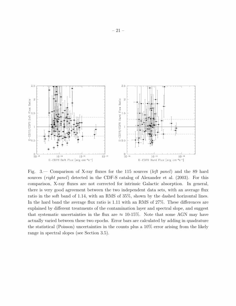
In Figure 3 we show the ratio of our fluxes to those reported by Alexander et al. (2003) for

the overlapping sources. For this comparison, neither the CDF-S nor the ECDFS sources

were corrected for intrinsic Galactic absorption. (This correction is ≃4% in the soft band

and is negligible in the hard band.) Error bars are calculated by adding in quadrature the

statistical (Poisson) uncertainties in the counts plus a 10% error arising from the likely range

in spectral slopes (see Section 3.5).

Sources were matched using the closest CDF-S counterpart to each ECDFS source, us-

ing a maximum search radius of ∼ 2′′. To compare the fluxes of matched sources in the two

data sets, we excluded the most discrepant top and bottom 15% of the flux ratios, and found

our fluxes are ∼14% higher in the soft band and ∼11% higher in the hard band. In the first

case, the difference can be explained by the different treatment of the contamination layer,

which is particularly important in the soft band. The Alexander et al. (2003) catalog used

ACISABS13 to correct their fluxes for the presence of a contamination layer in the ACIS

instrument. This tool assumes a spatially-uniform contamination layer composed of hydro-

gen, carbon, nitrogen, and oxygen. However, recent analysis of grating data (Marshall et al.

2004) shows that the amount of contamination correction depends on the spatial position

on the instrument, and that the actual composition of the contamination is hydrogen, car-

bon, oxygen, and fluorine (P. Plucinsky, priv. comm.). These two new discoveries may have

caused Alexander et al. (2003) to underestimate the contamination correction, thus making

their fluxes lower in the soft band. In the hard band, the discrepancy can be explained by

our assumed value of Γ = 1.4 for the spectral slope to calculate fluxes, while Alexander et al.

(2003) used individual spectral fits for most of these overlapping sources. We conclude that

the fluxes are broadly consistent and that systematic uncertainties in their average values

are ∼ 15%, although individual fluxes have larger uncertainties (and some AGN may have

actually varied).

13Available at http://www.astro.psu.edu/users/chartas/xcontdir/xcont.html

– 13 –

3.5. Simulations

We performed extensive XSPEC and MARX simulations to investigate the statistical

properties of the catalog, its completeness, and its flux limits. First, in order to investigate

the effect of a fixed photon slope on the true flux of sources found in the ECDFS, we

simulated 2000 sources with extreme photon spectral slopes, Γ=1 and Γ=2, and with fluxes

distributed smoothly from the minimum to the maximum in our sample. We then computed

their count rates in a typical ECDFS pointing (∼ 230 ks). Using a fixed photon slope of

Γ=1.4 to compute fluxes then results in systematic flux errors of ∼ 10% in both the hard

and soft bands.

To investigate the completeness of our catalog, we used MARX to simulate X-ray images

of sources with known properties, including the range of count rates from just below our

threshold to just above our highest count rate, and a generous range of spectral slopes (1 ≤Γ ≤ 2) drawn from the observed Γ distribution observed in the 1 Ms CDFS survey (Alexander

et al. 2003). We positioned 1000 sources of known fluxes (consistent with an exposure time of

∼ 230 ks) randomly within the ECDFS survey field, so the background and noise properties

of the data are real. We then analyzed these simulated data with the same procedures used

on the real ECDFS data; that is, we performed source detection on the resulting event list via

wavdetect. This resulted in ∼90% of the sources being recovered overall, with incompleteness

becoming important below ∼2×10−16 erg cm−2 s−1 and ∼2×10−15 erg cm−2 s−1, in the soft

and hard bands, respectively.

4. Results and Discussion

We found 651 unique sources in the Extended Chandra Deep Field-South survey field,

which spans ≈ 0.3 deg2 on the sky. Of these, 561 were detected in the 0.5–8.0 keV full

band, 529 in the 0.5–2.0 keV soft band, and 335 in the 2.0–8.0 keV hard band. There are 9

hard-band sources that are not detected in either the soft or full bands, 81 soft-band sources

are not detected in either the hard or full bands, and 56 full-band sources are not detected

in either the soft or hard bands (see Table 8). Of the 335 hard-band sources, 83 were not

detected in the soft band (∼20%); these are candidates for highly absorbed sources. Of

the 529 and 335 sources detected in the soft and hard bands, respectively, 118 and 73 are

detected in the CDF-S itself. Over this 0.11 deg2 area, with an exposure time of ∼ 1 Ms,

Giacconi et al. (2002) found 346 unique sources, of which 307 were detected in the 0.5–2.0

keV band and 251 in the 2–10 keV band. In the CDF-N, with an area similar to the CDF-S

but with twice the exposure, Alexander et al. (2003) found 503 X-ray sources in the 2 Ms

exposure. The number of sources found in the ECDFS is consistent with these two pencil

– 14 –

beam surveys, given an approximate slope of unity for the X-ray counts in this flux range.

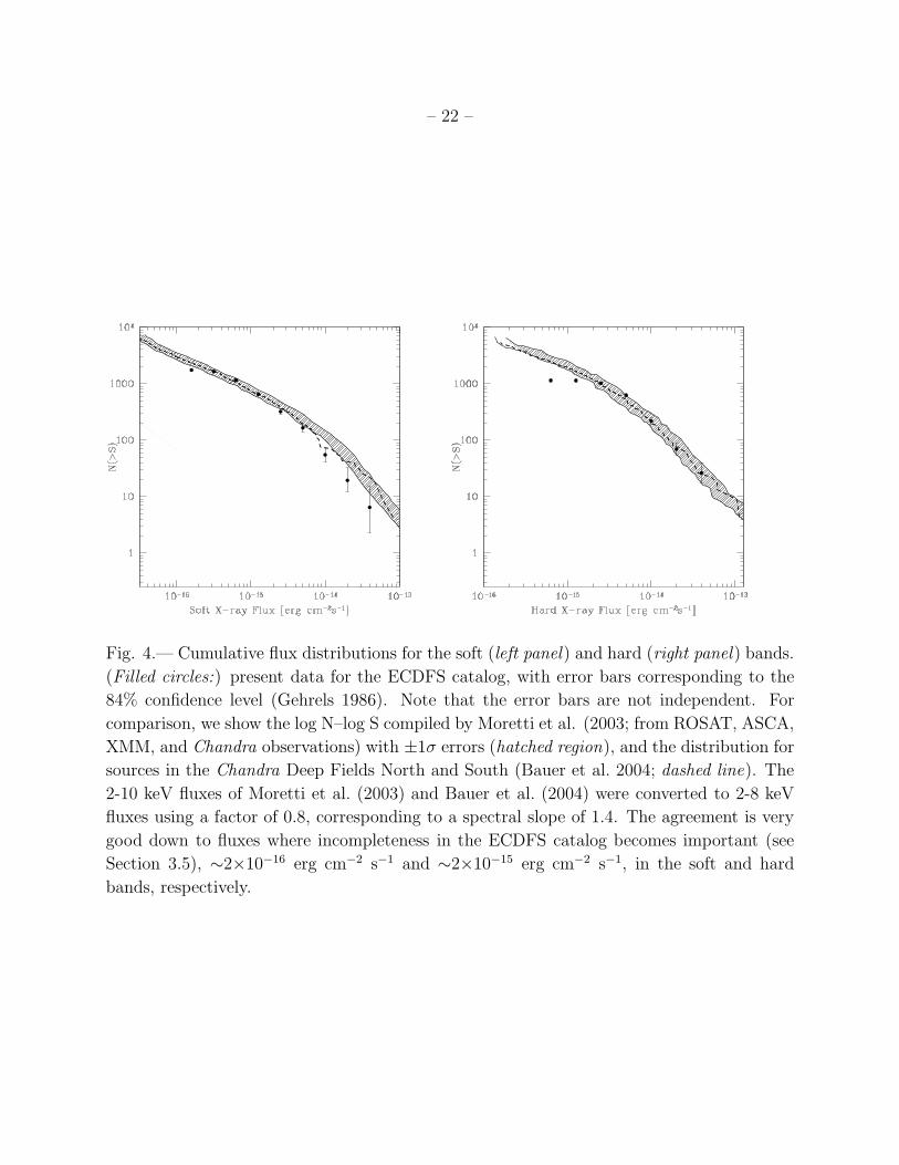
The cumulative distribution of sources for the soft and hard bands is shown in Figure 4.

Error bars for a given bin were calculated by adding in quadrature the error bars from

the previous bin to the 84% confidence error bars appropriate to the additional number

of sources in the present bin, following the procedure described in Gehrels (1986). The

observed distribution is compared to the compilation of Moretti et al. (2003) and to the

log N–log S for the Chandra deep fields reported by Bauer et al. (2004). In the soft band

there is very good agreement with the comparison sample in the flux range from ∼ 4 ×10−14 to 2 × 10−16 erg cm−2 s−1. At the bright end, the discrepancy is not statistically

significant, ∼1σ, because there are few bright X-ray sources in our field. At fluxes below

∼2×10−16 erg cm−2 s−1, the observed log N–log S in the ECDFS flattens relative to the

comparison samples because of incompleteness near the flux limit. Sources with soft fluxes

of ≤2×10−16 erg cm−2 s−1 are only detected at the ≤ 2σ level, and thus not all sources will

be recovered.

The log N–log S relation for the hard band is shown in the right panel of Figure 4 and

is compared again with the distributions of Moretti et al. (2003) and Bauer et al. (2004).

Moretti et al. (2003) used 2-10 keV instead of 2-8 keV for the hard band. To convert 2-10 keV

fluxes to the 2-8 keV band, we used a factor of 0.8, corresponding to the flux conversion

assuming a Γ=1.4 spectral slope. Bauer et al. (2004) quote 2-8 keV but appear to have

used 2-10 keV, so we also converted their fluxes by the same factor (which reproduces their

curve in Figure 4 of their paper). As in the soft band, very good agreement with previously

reported log N–log S relations is seen for the 4×10−14 to 2×10−15 erg cm−2 s−1 range, and

again, incompleteness at the faint end explains the observed discrepancy.

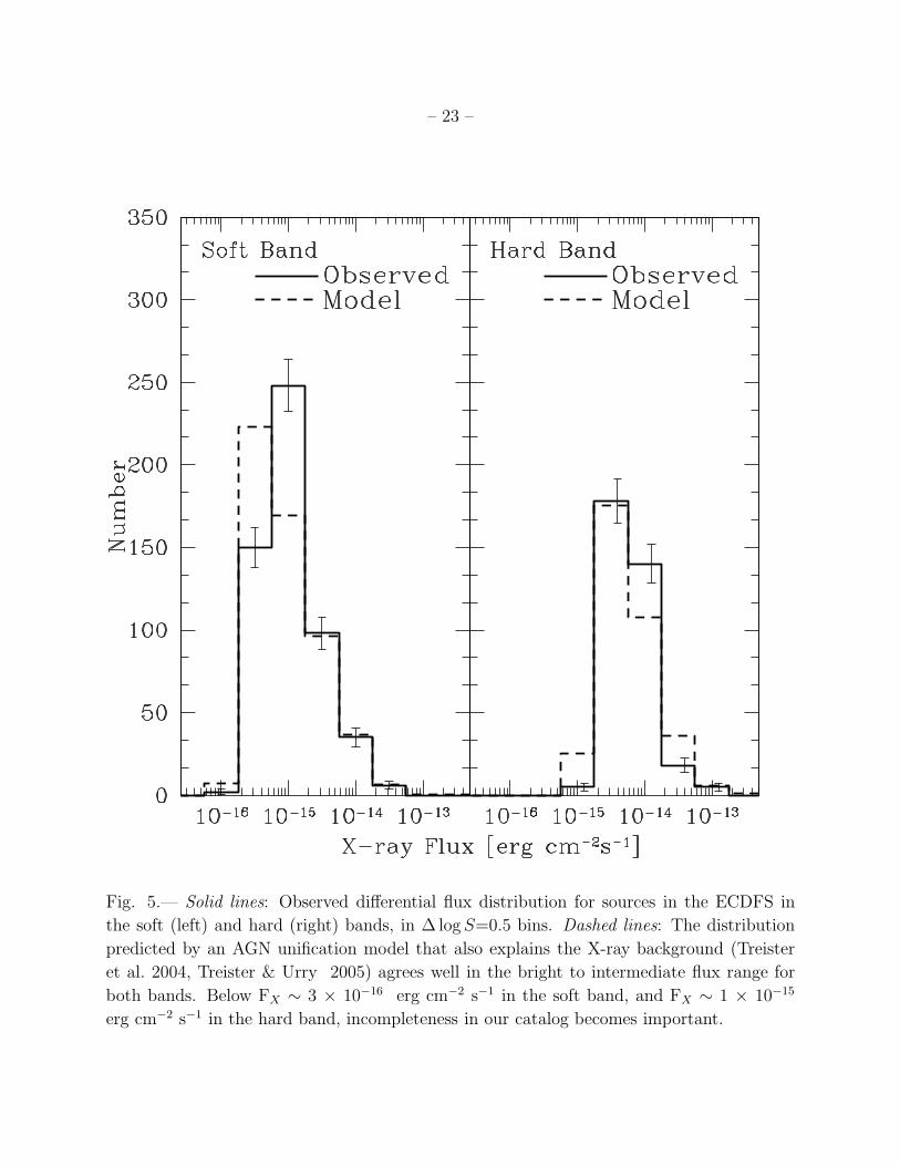
The differential log N–log S for both the soft and hard bands is shown in Figure 5. These

observed distributions are compared to the predictions of the AGN population synthesis

model of Treister & Urry (2005) which explains the X-ray background as a superposition

of mostly obscured AGN. This model also explains the multiwavelength number counts of

AGN in the Chandra Deep Fields (Treister et al. 2004). Given that these models match very

well to the observed cumulative flux distributions from existing surveys, it is not surprising

that this model also successfully explains the log N–log S distributions in the ECDFS field.

Discrepancies can be found only at the fainter end, where incompleteness causes the number

of observed sources to fall below the model prediction.

One of the early Chandra results was the finding that fainter X-ray sources have in

general harder spectra (Giacconi et al. 2001), represented by higher values of the hardness

ratio. Figure 6 shows that this effect is also observed in the ECDFS field, for a much larger

number of sources. This trend is explained by obscuration since the soft band count rate

– 15 –

is relatively more affected than the hard band, creating a harder observed X-ray spectrum

while at the same time reducing the observed soft flux. This is in accordance with the

general picture of AGN unification, although the precise geometry is not constrained, and it

is as expected from population synthesis models (e.g., Treister & Urry 2005 and references

therein) which require a large number of obscured AGN at moderate redshift to explain the

spectral shape of the X-ray background.

5. Conclusions

We present here the X-ray properties of sources detected in deep Chandra observations

of the ECDFS field, the largest Chandra survey ever performed in terms of both area and

depth. This survey covers a total of 0.3 square degrees, roughly 3 times the area of each very

deep Chandra Deep Field. A total of 651 unique sources were detected in the four ACIS-I

pointings in this field; 81 sources were detected in the soft but not in the full band, while

9 were detected only in the hard band. Roughly 15% of these 651 unique sources — 118

sources in the soft band and 73 in the hard band — were previously detected in the CDF-S.

The fluxes derived for these sources agree well with the fluxes obtained from the CDF-S

observations.

The X-ray log N–log S in the soft and hard bands agree well with those derived from

other X-ray surveys and with predictions of the most recent AGN population synthesis

models for the X-ray background.

As first discovered in early deep Chandra observations, we find in this sample that faint

X-ray sources have in general harder spectra, indicating that these sources are likely obscured

AGN at moderate redshifts. This is predicted by AGN unification models that explain the

properties of the X-ray background. A future paper will discuss the optical and near-IR

properties of these objects. This field was observed with the Spitzer Space Telescope by

the MIPS GTO team and will also be observed by Spitzer as part of an approved program

related to the MUSYC survey (PI: P. van Dokkum).

The source catalogs and images presented in this paper are available in electronic format

on the World Wide Web (http://www.astro.yale.edu/svirani/ecdfs). We will continue to

improve the source catalog as better calibration information, analysis methods, and software

become available. For example, we plan to optimize the searching for variable sources and

to study the multiwavelength properties of these X-ray sources.

Note: After this paper was submitted, another catalog paper by Lehmer et al. (2005)

appeared on astro-ph. Our catalogs are similar but the analysis assumptions are different

– 16 –

and therefore the source catalogs differ, as do the papers. We expect the comparison to be

useful.

We thank the referee for helpful comments that improved the manuscript and are grate-

ful to Samantha Stevenson of the CXC Help Desk for her help and patience in answering

our many questions regarding CIAO-related tools. We also acknowledge the help of Jeffrey

Van Duyne in cross-correlating the X-ray and optical positions. This work was supported in

part by NASA grant HST-GO-09425.13-A. ET would like to thank the support of Fundacion

Andes, Centro de Astrofısica FONDAP and the Sigma-Xi foundation through a Grant in-aid

of Research. EG acknowledges support by the National Science Foundation under Grant No.

AST-0201667, an NSF Astronomy and Astrophysics Postdoctoral Fellowship (AAPF).

REFERENCES

Akiyama, M., et al. 2000, ApJ, 532, 700

Alexander, D. M., et al. 2003, AJ, 126, 539

Barger, A. J., et al. 2003, AJ, 126, 632

Bauer, F. E., Alexander, D. M., Brandt, W. N., Schneider, D. P., Treister, E., Hornschemeier,

A. E., & Garmire, G. P. 2004, AJ, 128, 2048

Brandt, W. N., et al. 2001, AJ, 122, 2810

Ciliegi, P., Elvis, M., Wilkes, B. J., Boyle, B. J., & McMahon, R. G. 1997, MNRAS, 284,

401

Comastri, A., Setti, G., Zamorani, G., & Hasinger, G. 1995, A&A, 296,1

Freeman, P. E., Kashyap, V., Rosner, R., & Lamb, D. Q. 2002, ApJS, 138 185

Gawiser, E., et al. 2005, ApJS, in press, astro-ph/0509202

Gendreau, K. C., et al. 1995, PASJ, 47, L5

Gehrels, N., 1986, ApJ, 303, 336

Giacconi, R., et al. 2001, ApJ, 551, 624

Giacconi, R., et al. 2002, ApJS, 139, 369

– 17 –

Gilli, R., Risaliti, G., & Salvati, M. 1999, A&A, 347, 424

Gilli, R., Salvati, M., & Hasinger, G. 2001, A&A, 366, 407

Gioia, I. M., Maccacaro, T., Schild, R. E., Wolter, A., Stocke, J. T., Morris, S. L., & Henry,

J. P. 1990, ApJS, 72, 567

Grant, C. E., Bautz, M. W., & Virani, S. N. 2002, ASP Conf. Ser. 262, The High Energy

Universe at Sharp Focus: Chandra Science, ed. E. M. Schlegel & S. D. Vrtilek (San

Francisco: ASP), 401.

Hasinger, G. 2004, Nuc. Phys. B (Proc. Supp.), 132, 86

Hornschemeier, A. E., et al. 2001, ApJ, 554, 742

Kim, D.-W., et al. 2004, ApJS, 150, 19

Kushino, A., et al. 2002, PASJ, 54, 237

Kenter, A. T., $ Murray, S. S. 2003, ApJ, 584, 1016

Lehmer, B., et al. 2005, ApJS, 161, 21

Madau, P., Ghisellini, G., & Fabian, A. C. 1994, MNRAS, 270, L17

Marshall, F. E., et al. 1980, ApJ, 235 4

Marshall, H. E., et al. 2004, SPIE, 5165, 497

Moretti, A., Campana, S., Lazzati, D., & Tagliaferri, G. 2003, ApJ, 588, 696

Nandra, K., & Pounds, K. A. 1994, MNRAS, 268, 405

Nandra, K., et al. 2005, MNRAS, 356, 568

Plucinsky, P. P. & Virani, S. N. 2000, SPIE, 4012, 681

Schwartz, D. A., & Virani, S. N. 2004, ApJ, 615, L21

Spergel, D. N., et al. 2003, ApJS, 148, 175

Stark, A. A., Gammie, C. F., Wilson, R. W., Bally, J., Linke, R. A., Heiles, C., & Hurwitz,

M. 1992, ApJS, 79, 77

Struder, L., et al. 2001, A&A, 365, 18

– 18 –

Szokoly, G. P., et al. 2004, ApJS, 155, 271

Townsley, L. K., Broos, P. S., Garmire, G. P., & Nousek, J. A. 2000,ApJ, 534, L139

Treister, E., et al. 2004, ApJ, 616, 123

Treister, E., & Urry, C. M. 2005, ApJ, in press, astro-ph/0505300

Wang, J. X., et al. 2004, ApJ, 608, 21

Yang, Y., Mushotzky, R. F., Steffen, A. T., Barger, A. J., & Cowie, L. L. 2004, AJ, 128,

1501

This preprint was prepared with the AAS LATEX macros v5.2.

– 19 –

Fig. 1.— Exposure-corrected full band (0.5–8.0 keV) image of the ECDFS. This image has

been binned by a factor of four in both RA and Dec, and has been made using the standard

ASCA grade set. The black square superimposed on the raw image is the approximate

footprint (most of the exposure lies within this region) of the CDF-S proper (Giacconi et al.

2002).

– 20 –

Fig. 2.— The survey area vs. limiting flux for the two bands for which we have calculated

the log N–log S function: soft band (thin line) and the hard band (thick line). The total

area of the survey is ≈ 1100 arcmin2 (∼0.3 deg2).

– 21 –

Fig. 3.— Comparison of X-ray fluxes for the 115 sources (left panel) and the 89 hard

sources (right panel) detected in the CDF-S catalog of Alexander et al. (2003). For this

comparison, X-ray fluxes are not corrected for intrinsic Galactic absorption. In general,

there is very good agreement between the two independent data sets, with an average flux

ratio in the soft band of 1.14, with an RMS of 35%, shown by the dashed horizontal lines.

In the hard band the average flux ratio is 1.11 with an RMS of 27%. These differences are

explained by different treatments of the contamination layer and spectral slope, and suggest

that systematic uncertainties in the flux are ≈ 10-15%. Note that some AGN may have

actually varied between these two epochs. Error bars are calculated by adding in quadrature

the statistical (Poisson) uncertainties in the counts plus a 10% error arising from the likely

range in spectral slopes (see Section 3.5).

– 22 –

Fig. 4.— Cumulative flux distributions for the soft (left panel) and hard (right panel) bands.

(Filled circles:) present data for the ECDFS catalog, with error bars corresponding to the

84% confidence level (Gehrels 1986). Note that the error bars are not independent. For

comparison, we show the log N–log S compiled by Moretti et al. (2003; from ROSAT, ASCA,

XMM, and Chandra observations) with ±1σ errors (hatched region), and the distribution for

sources in the Chandra Deep Fields North and South (Bauer et al. 2004; dashed line). The

2-10 keV fluxes of Moretti et al. (2003) and Bauer et al. (2004) were converted to 2-8 keV

fluxes using a factor of 0.8, corresponding to a spectral slope of 1.4. The agreement is very

good down to fluxes where incompleteness in the ECDFS catalog becomes important (see

Section 3.5), ∼2×10−16 erg cm−2 s−1 and ∼2×10−15 erg cm−2 s−1, in the soft and hard

bands, respectively.

– 23 –

Fig. 5.— Solid lines: Observed differential flux distribution for sources in the ECDFS in

the soft (left) and hard (right) bands, in ∆ log S=0.5 bins. Dashed lines: The distribution

predicted by an AGN unification model that also explains the X-ray background (Treister

et al. 2004, Treister & Urry 2005) agrees well in the bright to intermediate flux range for

both bands. Below FX ∼ 3 × 10−16 erg cm−2 s−1 in the soft band, and FX ∼ 1 × 10−15

erg cm−2 s−1 in the hard band, incompleteness in our catalog becomes important.

– 24 –

Fig. 6.— Hardness ratio (defined as the ratio of hard minus soft counts to the summed

counts) versus soft X-ray count rate for sources in the ECDFS. Error bars correspond to

84% confidence level on the count rates (Gehrels 1986). For sources not detected in the soft

band (i.e., HR=+1), the hard count rate was used instead. Fainter sources in the soft band

have harder X-ray spectra, supporting the hypothesis that these sources are mainly obscured

AGN, as required by population synthesis models for the X-ray background.

– 25 –

Table 1. Journal of Chandra Observations of the ECDFS

Obs. Obs. Exposure Time (ks) Aim Point Roll Angle CCDs

ID Start Raw Filtered α2000 δ2000 (degrees) Clocked

5015 29 Feb 2004 162.9 154.8 03 33 05.61 -27 41 08.84 270.2 I0–I3

5016 03 Mar 2004 77.2 76.8 03 33 05.61 -27 41 08.88 270.2 I0–I3

5017 14 May 2004 155.4 135.2 03 31 51.43 -27 41 38.80 181.5 I0–I3

5018 16 May 2004 72.0 70.2 03 31 51.43 -27 41 38.79 181.5 I0–I3

5019 17 Nov 2004 163.1 162.3 03 31 49.94 -27 57 14.56 0.2 I0–I3,S2

5020 15 Nov 2004 77.6 76.9 03 31 49.94 -27 57 14.56 0.2 I0–I3,S2

5021 13 Nov 2004 97.8 94.2 03 33 02.93 -27 57 16.08 0.2 I0–I3,S2

5022 15 Nov 2004 79.1 75.8 03 33 02.94 -27 57 16.07 0.2 I0–I3,S2

6164 20 Nov 2004 69.1 67.3 03 33 02.93 -27 57 16.04 0.2 I0–I3,S2

– 26 –

Table 2. Exposure Time Per Pointing

Pointing Obsids Raw Exposure Net Exposure

(ks) (ks)

Northeast 5015, 5016 240.1 231.6

Northwest 5017, 5018 227.4 205.4

Southeast 5021, 5022, 6164 240.7 237.4

Southwest 5019, 5020 246.0 239.2

Mean 238.6 228.4

– 27 –

Table 3. Definition of Energy Bands and Hardness Ratio

Name Definition

Full Band (F) 0.5–8.0 keV

Soft Band (S) 0.5–2.0 keV

Hard Band (H) 2.0–8.0 keV

Hardness Ratio (HR) (H − S)/(H + S)

–28

–

Table 4. Primary Catalog of X-ray sources in the ECDFS field (pthresh = 1 × 10−7).

ID Name RA Dec PSF Count Rate: Full Band Count Rate: Soft Band Count Rate: Hard Band FB Fluxa SB Fluxa HB Fluxa Notes

CXOYECDF J2000 ′′ value upper lower value upper lower value upper lower erg cm−2s−1

1 J033335.6-273935 03 33 35.56 -27 39 35.3 1.75 7.64e-04 8.26e-04 7.07e-04 5.05e-04 5.56e-04 4.59e-04 ——– ——– ——– 9.16e-15 2.95e-15 6.44e-15

2 J033334.9-274209 03 33 34.93 -27 42 08.5 1.64 9.00e-03 9.20e-03 8.80e-03 ——– ——– ——– 2.88e-03 3.00e-03 2.77e-03 1.08e-13 3.30e-14 6.38e-14

3 J033332.9-274011 03 33 32.92 -27 40 11.2 1.45 2.16e-04 2.51e-04 1.85e-04 1.94e-04 2.28e-04 1.65e-04 ——– ——– ——– 2.59e-15 1.14e-15 1.82e-15

4 J033332.8-274908 03 33 32.79 -27 49 08.0 4.05 1.81e-03 1.91e-03 1.73e-03 1.06e-03 1.13e-03 9.95e-04 4.45e-04 4.93e-04 4.01e-04 2.17e-14 6.21e-15 9.83e-15

5 J033329.8-274009 03 33 29.84 -27 40 09.1 1.17 3.45e-04 3.89e-04 3.07e-04 1.81e-04 2.14e-04 1.54e-04 ——– ——– ——– 4.14e-15 1.06e-15 2.91e-15

Note. — This table is published in its entirety in the electronic edition of the Journal. A portion is shown here for guidance regarding its form and content.

aFlux: Corrected for Galactic absorption with NH = 9 × 1019 cm−2 assuming Γ = 1.4.

–29

–

Table 5. Secondary Catalog of X-ray sources in the ECDFS field (pthresh = 1 × 10−6).

ID Name RA Dec PSF Count Rate: Full Band Count Rate: Soft Band Count Rate: Hard Band FB Fluxa SB Fluxa HB Fluxa Notes

CXOYECDF J2000 ′′ value upper lower value upper lower value upper lower erg cm−2s−1

1 J033331.7-273850 03 33 31.70 -27 38 50.3 0.75 1.34e-04 1.63e-04 1.10e-04 ——– ——– ——– ——– ——– ——– 1.61e-15 4.91e-16 1.13e-15 f

2 J033329.0-274558 03 33 28.97 -27 45 58.1 0.93 2.38e-04 2.74e-04 2.06e-04 ——– ——– ——– ——– ——– ——– 2.85e-15 8.70e-16 2.00e-15 f

3 J033326.4-273522 03 33 26.36 -27 35 22.4 1.06 1.43e-04 1.72e-04 1.18e-04 ——– ——– ——– ——– ——– ——– 1.71e-15 5.22e-16 1.20e-15

4 J033323.9-273828 03 33 23.91 -27 38 27.8 0.47 1.30e-04 1.58e-04 1.06e-04 ——– ——– ——– ——– ——– ——– 1.55e-15 4.75e-16 1.09e-15 f

5 J033231.2-273919 03 32 31.18 -27 39 18.5 1.23 3.37e-04 3.79e-04 2.99e-04 6.48e-05 8.62e-05 4.83e-05 ——– ——– ——– 4.04e-15 3.78e-16 2.84e-15

Note. — This table is published in its entirety in the electronic edition of the Journal. A portion is shown here for guidance regarding its form and content.

aFlux: Corrected for Galactic absorption with NH = 9 × 1019 cm−2 assuming Γ = 1.4.

– 30 –

Table 6. Catalog of Collapsed wavdetect X-ray sources in the ECDFS Survey

ID Name RA Dec Notes

CXOYECDF J2000

1 J033208.9-275910 03 32 08.87 -27 59 10.10 full

2 J033203.3-280128 03 32 03.33 -28 01 27.90 full, hard

3 J033201.5-280004 03 32 01.50 -28 00 03.94 full

4 J033151.8-280035 03 31 51.79 -28 00 34.80 full

5 J033150.9-280154 03 31 50.87 -28 01 53.85 full

Note. — This table is published in its entirety in the electronic edition

of the Journal. A portion is shown here for guidance regarding its form

and content.

– 31 –

Table 7. Summary of Chandra Source Detections

Energy Number of Detected Counts Per Source

Band Sourcesa Maximum Minimum Median Mean

Full Band 561 2403.0 2.9 55.4 127.6

Soft Band 529 1643.5 4.4 32.4 89.9

Hard Band 335 757.4 3.3 42.7 75.2

aThere are 651 independent X-ray sources detected with either a false-

positive probability threshold of 1×10−7 (Table 4) or 1×10−6 (Table 5).

– 32 –

Table 8. Sources Detected in One Band But Not Another (Primary and Seconday Tables

Combined)

Detection Non-Detection Energy Band

Energy Band Full Soft Hard Neither

Full 0 113 235 56

Soft 81 0 260 81

Hard 9 65 0 9

Note. — For example, there were 113 sources

out of 651 that are detected in the full band but

not in the soft band.