RHEOLOGICAL STUDY OF KAOLIN CLAY SLURRIES A Thesis Submitted to the College of Graduate studies and Research in Partial Fulfilment of the Requirements for a Degree of Masters of Science in the Department of Chemical Engineering University of Saskatchewan Saskatoon © Copyright Chad Gordon Litzenberger April 2003. All rights reserved. The University of Saskatchewan claims copyright in conjunction with the author. Use shall not be made of the material contained herein without proper acknowledgement.

Welcome message from author
This document is posted to help you gain knowledge. Please leave a comment to let me know what you think about it! Share it to your friends and learn new things together.
Transcript

RHEOLOGICAL STUDY OF KAOLIN CLAY SLURRIES
A Thesis Submitted to the College of
Graduate studies and Research
in Partial Fulfilment of the Requirements
for a Degree of Masters of Science
in the Department of Chemical Engineering
University of Saskatchewan
Saskatoon
© Copyright Chad Gordon Litzenberger April 2003. All rights reserved.
The University of Saskatchewan claims copyright in conjunction with the author.
Use shall not be made of the material contained herein without proper
acknowledgement.

PERMISSION TO USE
In presenting this thesis in partial fulfilment of the requirements for a
Postgraduate degree from the University of Saskatchewan, I agree that the Libraries
of this University may make it freely available for inspection. I further agree that
permission for copying of this thesis in any manner, in whole or in part, for scholarly
purposes may be granted by the professor or professors who supervised my thesis
work or, in their absence, by the Head of the Department or the Dean of the College
in which my thesis work was done. It is understood that any copying or publication or
use of this thesis or parts thereof for financial gain shall not be allowed without my
written permission. It is also understood that due recognition shall be given to me and
to the University of Saskatchewan in any scholarly use which may be made of any
material in my thesis.
Requests for permission to copy or to make other use of material in this thesis
in whole or part should be addressed to:
Head of the Department of Chemical Engineering
University of Saskatchewan
Saskatoon, Saskatchewan S7N 5A9
i

ABSTRACT
Concentrated kaolin clay slurries are found in a number of industrial
operations including mine tailings surface disposal, underground paste backfill, and
riverbed dredging. An understanding of the impact of solids concentration and
addition of chemical species on slurry rheology is of importance to designers of
pipeline transport and waste disposal systems. A project to determine the rheology of
an idealized industrial kaolin clay slurry using a concentric cylinder viscometer and
an experimental pipeline loop was undertaken. Additional laboratory test work
including particle size analysis, slurry pH, calcium ion concentration in the slurry
supernatant and particle electrophoretic mobility measurements were completed to
aid in the understanding of their effects on the slurry rheology.
The slurries were prepared in varying kaolin clay solids concentrations with
reverse osmosis water. A flocculant, dihydrated calcium chloride (CaCl2 • 2H2O),
was added to the reverse osmosis water in concentrations equivalent to those found in
typical industrial hard water supply. A dispersant, tetra-sodium pyrophosphate
(TSPP, Na4P2O7) was used to disperse the clay particles for selected slurries.
It was found that the kaolin clay slurries, in the absence of TSPP, exhibited
yield stresses and could be characterized with either the two-parameter Bingham or
Casson continuum flow models. Increasing the clay concentration in the slurry, while
keeping the mass ratio of flocculant to kaolin constant, increased both the yield and
plastic viscosity parameters. There was generally good agreement between the
rheological parameters obtained in the Couette flow viscometer and that in the
pipeline loop.
ii

In slurries for which it was possible to obtain turbulent flow, the transition to
turbulent flow was predicted accurately by the Wilson & Thomas method for both
Bingham and Casson models.
It was possible to eliminate the yield stress of a slurry with the addition of the
dispersing agent TSPP. The calcium ion content of the supernatant extracted from the
slurries proved to be a indicator of the degree of flocculation.
When exposed to extended periods of high shear conditions in the pipeline
loop, slurries with clay concentrations of 17% by volume solids or greater exhibited
an irreversible increase in apparent viscosity with time. An attempt was made to
investigate this irreversible thickening characteristic. Laboratory tests did not reveal
any appreciable differences in particle size, electrophoretic mobility, calcium ion
concentration or pH with this irreversible change. The shear duration test shows the
importance of using the appropriate shear environment when testing high solids
concentration kaolin clay slurries.
iii

ACKNOWLEDGMENTS
I wish to express my sincere gratitude and appreciation to Dr. R. J. Sumner,
my supervisor, for introducing me to the field of research. Without his guidance this
thesis could not have been completed. I would also like to express my appreciation to
Dr. C. A. Shook and Dr. R. S. Sanders for their assistance in the final preparation of
my thesis.
Thanks to the Saskatchewan Research Councils Pipe Flow Technology Centre
for the use of their research facility. I wish to express my deepest gratitude to the
staff for their contributions in developing and sustaining a research division that is
recognized around the world. I consider myself lucky to have been able to discuss
ideas with more experienced researchers especially Dr. R.G. Gillies, Dr. M.J.
McKibben, Mr. R. Sun, and Mr. J.J. Schaan.
I would like to acknowledge the work of the late Miss E. Reichert who helped
me interpret a difficult scientific paper. A special thanks to the students that have
contributed to this research program. Specifically, Mr. T. Barnstable and Mr. R.
Spelay with whom I conducted the experimental test work and benefited from their
assistance and invaluable input.
Finally, I thank my parents and family for instilling in me confidence and a
drive for pursuing my education and for the support that they have provided me
through my entire life.
iv

DEDICATION
To my wife, Krista, without her love and support I doubt that the completion
of this thesis would have ever been possible.
v

TABLE OF CONTENTS Page
PERMISSION TO USE …………………………………………………...…….i ABSTRACT ……………………………………………………………....…….......ii ACKNOWLEDGMENTS ………………………………………..………......…..iv DEDICATION …………………………………………………………...........v TABLE OF CONTENTS ……………………………………………….........….vi LIST OF TABLES …………………………………………………………........viii LIST OF FIGURES ………………………………………………………..………ix LIST OF SYMBOLS …………………………………………………………...….xiii 1. INTRODUCTION …………………………………………………..……..1 2. LITERATURE REVIEW …………………………………………....……5
2.1. Determination of Flow Properties …………………..…………..…5 2.2. Principles of Pipeline Flow ……………………………..………..…8 2.3. Principles of Couette Flow ………………………………………..12 2.4. Wilson & Thomas Turbulent Flow Prediction ……………..…17 2.5. Factors Affecting Clay Rheology ………………………………..18
2.5.1. Structure of Kaolin Clay and Associated Surface Charges ..19 2.5.2. Charged Atmosphere Surrounding a Particle ……………..…22 2.5.3. Factors Affecting Flocculation ……………………..…27 2.5.4. Factors Affecting Deflocculation ……………………..…30
2.6. Clay Rheology Present Work ……………………………………..…31 2.7. Key Elements of This Investigation ....................................................36
3. MATERIALS APPARATUS AND PROCEDURE …………………..……37 3.1. Materials ……………………………...……………………..….37 3.2. Particle Properties ……………………………………………..…38
3.2.1. Particle Size Analysis ………………………………………..38 3.2.2. Particle Density ……………………………..…………47
3.3. Electrophoretic Mobility ………………………………..………48 3.4. Supernatant Chemical Analysis ………………………..………50 3.5. Pipe loop Operation ………………………………………..………51 3.6. Couette Viscometer Operation ……………………..…………56
4. RESULTS AND DISCUSSION ………………………………..………58
4.1. Introduction ………………………………………………..………58 4.2. Particle Characterization ………………………………..………63 4.3. Rheological Characterization ………………………………..………67 4.4. Pipeline and Viscometer Agreement ………………………..………70 4.5. Pipeline Turbulent Flow Predictions ………………………..………80 4.6. Effects of Dispersant Addition ………………………..………83 4.7. Calcium Ion Supernatant Analysis ………………………..………85 4.8. Irreversible Increase in Apparent Viscosity ………………..………90
vi

5. CONCLUSIONS AND RECOMMENDATIONS ………………...……...98 6. REFERENCES …………………………………………………..…..101 APPENDICIES
A. Pipeline and Viscometer Flow Data …………….………...103 B. Slurry Supernatant Calcium Ion Analysis ………………...……….129 C. Turbulent Pipeline Flow Loop Experimental Data .…….………..132 D. Particle Diameter Derivation For Centrifugal Andreason ...….....140 E. Instrument Calibrations ...………………………………….…147
vii
LIST OF TABLES Page
3.1 IDC standard particle electrophoretic mobility measurements .......…...50
4.1 Summary of slurry flow tests and inferred rheological parameters ..........…60
4.2 Summary of slurry flow tests and inferred rheological parameters ….........61
4.3 Summary of slurry flow tests and inferred rheological parameters ..............62 4.4 Particle Size Distribution Dry Branch Kaolin Clay Andreason
Pipette Gravity Sedimentation Trial 1 ........…………………………..65
4.5 Particle Size Distribution Dry Branch Kaolin Clay Andreason Pipette Gravity Sedimentation Trial 2 ………....……………………..65
4.6 Particle Size Distribution Dry Branch Kaolin Clay Andreason
Pipette Centrifugal Sedimentation ..........…………………………………66 4.7 Experimental Particle Density Data. Dry Branch Kaolin Clay ......…....66 4.8 Average difference between experimental and predicted data
sets for each non-Newtonian slurry run …………………......…………68 4.9 Calcium ion analysis for supernatant ......……………………………89
4.10 Experimental results of shear duration tests of 19 by volume solids kaolin clay slurry containing 0.10% flocculant / clay mass ratio ........…..94
4.11 Replicate experimental results of 4 hour shear duration tests of
19 by volume solids kaolin clay slurry containing 0.10% flocculant / clay mass ratio .............……………………………….96
Appendix B: B.1 Kaolin Clay Slurry Cv = 0.19 Calcium ion supernatant data .……...130 B.2 Kaolin Clay Slurry Cv = 17% by volume solids Calcium ion
supernatant data ....………………………………………………..…..130 B.3 Kaolin Clay Slurry Cv = 0.14 Calcium ion supernatant data .............……...130 B.4 Kaolin Clay Slurry Cv = 0.10 Calcium ion supernatant data .............……...131 B.5 Kaolin Clay Slurry Cv = 10% by volume solids total ion
mass spectrometer supernatant data (mg of analyte/ L of solution) .............131
viii

LIST OF FIGURES Page
2.1 Rheograms of various continuum fluid models .…….…………..………5 2.2 Flow in a vertical pipeline .............…………………………….….....…… 8
2.3 Concentric cylinder viscometer .…………………………………….…13
2.4 Taylor Vortices, a secondary flow pattern at high rotation rates in a concentric cylinder viscometer ...………………………………….…..16
2.5 Atomic Structure of Kaolin Clay ...……………………………….……..20 2.6 Van Olphen idealized kaolin clay particle charge distribution ….…….21 2.7 Carty idealized kaolin particle charge distribution ......………………....…21
2.8 Electron micrograph of a kaolinite and gold sol ..……………………....22
2.9 The electric double layer used to visualize the ionic environment surrounding a charged particle ...……………………………………...23
2.10 The electrical potential in the atmosphere surrounding a negative
surface of a particle ......……………………………………………….…...24 2.11 Net Energy Interaction Curve .…………………...……………….….27
2.12 Modes of particle association .....………………………………….…29 2.13 Chemisorption of tetrasodium pyrophosphate on a positively
charged edge surface of a clay particle …………………………….….30 2.14 Effect of counter ions on the viscosity of porcelain batch
suspensions .....………………………………………………………….…34 3.1 Electron scanning microscope image of well crystallized
Georgia kaolin ..………………………………………………………38 3.2 Illustration of an Andreasen pipette used in for gravity
sedimentation .……………………………………………………….42
3.3 Picture of Modified Andreasen Sedimentation Pipette used in centrifuge sedimentation …..……………………………………………45
3.4 Rank Brothers micro electrophoresis apparatus Mk II with
rectangular cell set-up …...…………………………………………...48
ix

3.5 SRC’s 25.8 mm vertical pipeline flow loop ........……………….………….52
3.6 Haake Rotovisco 3 viscometer with interchangeable measuring head sensor system ......……………………………………………………56
4.1 Dry Branch Pioneer kaolin clay particle size distribution as
determined by Andreason pipette experimental procedures .........………….64 4.2 Predicted laminar flow pressure gradient using Bingham and
Casson inferred model parameters for run G2000206, Cv = 0.17 Dry Branch kaolin clay slurry with no TSPP added ..………69
4.3 Predicted laminar flow viscometer torque per spindle length using
Bingham and Casson inferred model parameters for run G2000206, Cv = 0.17 Dry Branch kaolin clay slurry with no TSPP added ..………69
4.4 Effect of clay concentration and tetrasodium pyrophosphate
addition on Bingham model inferred yield stress for Dry Branch kaolin clay slurries ......……………………………………………………72
4.5 Effect of clay concentration and tetrasodium pyrophosphate
addition on Casson model inferred yield stress for Dry Branch kaolin clay slurries ......……………………………………………………73
4.6 Effect of clay concentration and tetrasodium pyrophosphate
addition on Bingham model inferred plastic viscosities for Dry Branch kaolin clay slurries ......……………………………………………………75
4.7 Effect of clay concentration and tetrasodium pyrophosphate
addition on Casson model inferred plastic viscosities for Dry Branch kaolin clay slurries ......……………………………………………………75
4.8 Predicted laminar flow wall shear stresses using pipeline and
viscometer inferred model parameters for run G2000206, Cv = 0.17 Dry Branch kaolin clay slurry with no TSPP added ..………77
4.9 Predicted laminar flow wall shear stresses using pipeline and
viscometer inferred model parameters for run G2000209, Cv = 17% Dry Branch kaolin clay slurry with 0.13% mass TSPP per mass clay added ....……………………………………..78
x

4.10 Predicted pressure gradient using pipeline and viscometer inferred model parameters for Cv = 17% Dry Branch kaolin clay slurry with 0.27% mass TSPP per mass clay added ....……..78
4.11 Effect of concentration and tetrasodium pyrophosphate addition
on Bingham model inferred effective viscosities for Dry Branch kaolin clay slurries ......……………………………………………………80
4.12 Bingham and Casson turbulent flow model comparison for run
G2000106 Cv=10% kaolin with no TSPP added .....…………………….82 4.13 Bingham and Casson turbulent flow model comparison for run
G2000214 Cv=14% Kaolin with mass ratio of TSPP/Clay = 0.13% added .......…………………………………………...82
4.14 Comparison of experimental pressure gradients for all slurries
having a TSPP to clay mass ratio of 0.27% to Newtonian pipe flow model ..……………………………………………………....84
4.15 Effect of adding TSPP to Dry Branch Pioneer kaolin clay slurry
19% by volume with a measured Bingham yield stress of 128 Pa .......…...85 4.16 Comparison of inferred Bingham yield stress and associated
supernatant calcium ion concentrations obtained for 14% by volume solids slurries …………………………………..……86
4.17 Comparison of inferred Bingham yield stress and associated
supernatant calcium ion concentrations obtained for 17% by volume solids slurries ……………………………………..…87
4.18 Experimental pressure gradient data for increasing amounts of
flocculant added to a 17% by volume solids kaolin clay slurry ...…..….88 4.19 Pressure gradient versus velocity data collected for run
G2000201/202 showing an increase in apparent viscosity with duration of shear ..……………………………..….…….92
Appendix D: D.1 Comparison of the experimental frictional head loss with Bingham
and Casson fluid model predictions for Cv = 0.10 Kaolin Clay Slurry in 25.8 mm vertical pipeline loop .....…………………….………..……133
D.2 Comparison of the experimental frictional head loss with Bingham
and Casson fluid model predictions for Cv = 0.10 Kaolin Clay Slurry in 25.8 mm vertical pipeline loop .....……………………….……..……134
xi

D.3 Comparison of the experimental frictional head loss with Bingham and Casson fluid model predictions for Cv = 0.14 Kaolin Clay Slurry
in 25.8 mm vertical pipeline loop ....……………………………………135 D.4 Comparison of the experimental frictional head loss with Bingham and Casson fluid model predictions for Cv = 0.14 Kaolin Clay Slurry
in 25.8 mm vertical pipeline loop ....……………………………………136 D.5 Comparison of the experimental frictional head loss with Bingham and Casson fluid model predictions for Cv = 0.14 Kaolin Clay Slurry in 25.8 mm vertical pipeline loop ………………………………………137 D.6 Comparison of the experimental frictional head loss with Bingham and Casson fluid model predictions for Cv = 0.14 Kaolin Clay Slurry in 25.8 mm vertical pipeline loop ………………………………………138 D.7 Comparison of the experimental frictional head loss with Bingham and Casson fluid model predictions for Cv = 0.14 Kaolin Clay Slurry
in 25.8 mm vertical pipeline loop ………………………………………139
xii

LIST OF SYMBOLS
A Cross-section area
A Constant, Eq 2.9
B Constant, Eq 2.10
Cv Concentration of solids by volume
D Pipe internal diameter
Dp Diameter of spherical particle
E Applied field strength
f Fanning friction factor
g Acceleration due to gravity
h Height
k Pipe wall equivalent roughness
L Length of pipe section
P Pressure
Q Volumetric flow rate
r Radial coordinate position
R Radius of particle of cylinder
R1 Inner cylinder radius (concentric cylinder viscometer)
R2 Outer cylinder radius (concentric cylinder viscometer)
Re Reynolds number for pipe flow
Rω Taylor vortices transition criterion (concentric cylinder viscometer)
S Separation distance
T Torque
xiii

t time
tRD Time of centrifuge deceleration, Eq. 3.2
tRU Time of centrifuge acceleration, Eq. 3.2
tRUN Time of centrifuge operation, Eq. 3.2
u* Friction velocity
v Local velocity
V Bulk velocity of pipe flow
VN Newtonian fluid velocity at specified condition, Eq. 2.29, 2.30
y Cartesian coordinate position
z Cartesian coordinate position
GREEK SYMBOLS
γ Shear strain
γ& Time rate of shear strain
µ Viscosity
µapp Apparent viscosity
µp Bingham Plastic Viscosity
µ∞ Casson Viscosity
ν Particle velocity, Eq. 2.33
θ Angular coordinate position
ρ Density
ρ1 Density of particles, Eq. 3.1
xiv

xv
ρ2 Density of suspending medium, Eq. 3.1
τ Shear stress
τc Yield stress (Casson Fluid Model)
τy Yield stress (Bingham Fluid Model)
υ Electrophoretic mobility
ωc Angular velocity of the centrifuge, Eq. 3.2
ω Angular Velocity
ξ Stress ratio

1. INTRODUCTION
The study of pipeline transportation of solid-liquid mixtures has undergone
considerable advances in the past half century. However, there is still an incomplete
understanding of some aspects governing the flow characteristics of these systems.
Proper slurry pipeline design and operation requires an understanding of the frictional
pressure loss caused by delivering a specific solids concentration under laminar or
turbulent flow conditions. This information is used to select the optimum pipeline
diameter and pump horsepower required to provide the flow rate and discharge
pressure necessary to avoid particle deposition and overcome the frictional resistance
of the pipeline.
Two simplistic categories have been used to classify solid-liquid mixtures:
settling and non-settling slurries (Shook et al., 2002). Settling slurries contain larger
particles which have high settling velocities. A stationary bed will develop at low
velocities and to avoid particle deposition, pipeline operation usually occurs under
turbulent flow conditions. Non-settling slurries are composed of fine particles which,
when flowing, have a uniform distribution across the pipeline cross section and
produce a symmetrical velocity distribution. In fact it could be said that the term non-
settling is not strictly accurate since many industrial slurries exhibit characteristics of
both categories (Shook et al., 2002).
It is the focus of this thesis to further investigate factors affecting the
rheological nature of an idealized kaolin clay industrial non-settling slurry. Non-
settling slurries often exhibit non-Newtonian behaviour due to particle-particle
- 1 -

interactions. It is difficult to define a particle size at which the transition between the
settling and non-settling slurry classifications occurs.
It is important to predict flow regime transition from laminar to turbulent flow
of a non-settling slurry. Laminar flow pressure drops can be predicted for a variety of
non-Newtonian model slurries. Wilson & Thomas (1985, 1987) have proposed a
method for turbulent flows that is based on a model for the flow in the viscous
sublayer. This method has produced accurate predictions.
In many industrial slurries it is clay particles that makes the most significant
solids component of the non-settling carrier fluid. The rheological behaviour of
slurries containing clay particles is important to industries as diverse as paint
manufacturing, petroleum drilling, and mining waste disposal.
The mining industry is investigating alternative methods to dispose of mine
wastes which contain a significant fraction of clays. By increasing the solids content
of the slurry through the removal of water, mining companies are able to achieve two
benefits. The footprint or area required to deposit the mine waste is significantly
reduced from a large tailings pond to small land based deposit. There is also a
reduction in demand for fresh water resulting from recycling of the process water,
making this approach environmentally attractive.
A fine kaolin clay slurry may be described as a colloidal system in which the
solids are dispersed through the liquid. Because of the high surface charge to mass
ratio of clays, van der Waals attractive forces and electrostatic repulsive forces
dominate particle interactions. It is the sum of these two forces between particles that
determine the nature of the slurry rheology.
- 2 -

The net particle interactions can be strongly repulsive, where the particles
remain dispersed, so that the fluid exhibits Newtonian characteristics. Alternatively,
the net interaction between particles can be strongly attractive so that a floc structure
is created. Flocs can form networks which cause the slurry to exhibit non-Newtonian
characteristics. This structure can resist shear distortion giving the fluid a yield
stress. Two non-Newtonian models which use a yield stress term are the Bingham
and Casson models.
The rheological characteristics of fine particle clay slurries can be
manipulated by altering the concentration of solids and by controlling the electrostatic
repulsive forces between particles. The electrostatic repulsive forces can be increased
or decreased by manipulating the pH and the ionic content in the suspending medium.
Increasing the repulsive forces with the addition of a dispersing agent may break
down the structure and reduce or eliminate non-Newtonian behaviour. Conversely by
decreasing the repulsive forces and allowing the net interaction of particles to be
dominated by attractive forces, the non-Newtonian behaviour can be increased.
To extend the current state of knowledge of fine particle clay slurries, the
effects of solids concentration and chemical addition on the rheology of kaolin clay
slurries have been studied. The rheology of kaolin clay slurries has been studied
using a vertical pipe flow loop and a Couette viscometer. The experimental data have
been interpreted using the Bingham and Casson models. All slurries were prepared
with a constant mass ratio of calcium ion to clay to represent the ion content in a
typical industrial fresh water supply. To understand the effects of chemical species in
the suspending medium on the rheology of these fine particle slurries, the viscosity
- 3 -

was modified with the addition of tetra sodium pyrophosphate (TSPP) and the
calcium ion content in the resulting supernatant was monitored.
To further understand the nature of viscosity modification additional
experiments were conducted. For selected slurries the pH, particle size,
electrophoretic mobility, and calcium ion content were monitored before and after the
slurries had been exposed to a high shear environment.
- 4 -

2. LITERATURE REVIEW
2.1. Determination of Flow Properties
Rheology is the study of deformation of matter. When a shear stress (τ) is
applied to a fluid it causes successive layers of that fluid to be displaced by different
amounts. The displacement (S) of two parallel layers relative to each other divided by
their separation distance (y) is the shear strain (γ = S/y). For liquids, the time derivative
of the relative displacement yields the velocity component and if this displacement is
divided by the separation distance one obtains the time rate of shear strain (γ ). This
quantity is also known as the shear rate. Viscosity is a measure of the ability of a fluid
to resist flow by means of internal friction. The magnitude of the shear stress that is
developed during flow depends on the product of viscosity and the rate of
deformation. The graphical representation of the shear stress versus the shear rate is
known as a rheogram. Figure 2.1 details the shear stress as a function of shear rate
for various fluids.
1. Newtonian
2. Dilatant (Shear Thickening)
3. Pseudoplastic (Shear Thinning)
4. Hershel-Bulkley 5. Bingham 6. Casson
Figure 2.1: Rheograms of various continuum fluid models.
- 5 -

If the shear stress is linear with respect to shear rate and the rheogram passes
through the origin, the fluid is considered to be Newtonian. The slope of the
rheogram is the viscosity as shown in Equation 2.0.
τ = -µ γ (2.0)
Although fine particle slurries are composed of two distinct phases, when
flowing they are usually dispersed homogeneously so that the flow can be analysed
with a continuum model. The Bingham and Casson fluid models are time-
independent, two parameter rheological models. They are often used to characterize
non-settling fine particle slurries. These slurries are considered to be viscoplastic,
which means that they behave like solids below a critical stress (the yield stress).
These slurries exhibit fluid behaviour when the applied shear stress exceeds the yield
stress. This is illustrated by the curves in Figure 2.1 which represent the various fluid
models.
There are other non-Newtonian rheological models which incorporate a yield
stress term, but the Bingham and Casson models have been chosen to analyze the
experimental data in this program because of their robust two parameter functional
relationship. The Bingham model is presented in Equation 2.1 where τy is the
Bingham model yield parameter and µp is the Bingham viscosity term. The Casson
model is presented in Equation 2.2 where τc is the Casson yield parameter and µ∞ is
the Casson viscosity.
τ = - µpγ +τy (2.1)
τ1/2 = - (µ∞γ )1/2 + τc1/2 (2.2)
- 6 -

In 1957 Casson arrived at this equation theoretically by considering the
magnitude of interparticle forces such as those found in pigment-oil suspensions of
the printing ink type.
The total resistance to shear for a two parameter model may be expressed
using an apparent viscosity. For any fluid one can draw a secant line from the origin
of Figure 2.1, as shown for the curve of a Bingham fluid by the dashed line, to a
particular shear stress. The slope that this line reveals is the apparent Newtonian
viscosity at that shear rate. The Bingham and Casson apparent viscosities are shown
in Equations 2.3 and 2.4.
papp
y1
µµ =
τ−
τ
(2.3)
app 2
c1
∞µµ =
τ− τ
(2.4)
These equations illustrate that the yield stress of the fluid will dominate the
fluid behaviour if a shear stress slightly greater than the yield stress is applied. In this
situation a high apparent viscosity is observed. As the shear rate increases, the
apparent viscosity term approaches the Bingham or Casson viscosity.
In concentrated clay slurries, particle interactions produce a structure with
some rigidity which is the source of the yield stress. If a shear stress is applied below
the yield stress this network or structure prevents flow. At high particle
concentrations, this structure would be present throughout the suspending water
medium. For shear stresses above the critical yield stress flow causes the structure to
break up into smaller and smaller elements composed of flocculated particles
- 7 -

(Michaels and Bolger 1962). The apparent viscosity may also decreases with
increasing shear rate as particle or aggregate orientation becomes more ordered
(Carty, 2001).
Rheological parameters for non-Newtonian slurries are determined
experimentally using a viscometer. In the present study a pipeline loop (tube
viscometer) and a concentric cylinder viscometer have been employed.
2.2. Principles of Pipeline Flow
For the specific case of steady state operation of a vertical pipeline of constant
cross-section, transporting a constant density fluid, a force balance over a pipe
element, shown in Figure 2.2, provides the following relationship between pressure
gradient and wall shear stress:
w4 dP dhgD dz dτ
= − − ρz
(2.5)
Figure 2.2: Flow in a vertical pipeline.
- 8 -

The left hand side of Equation 2.5 is the frictional resistance to flow where τw
is the wall shear stress and D the diameter of the pipe. For a horizontally orientated
pipe (dh/dz = 0), Equation 2.5 shows that τw can be obtained experimentally by
measuring the difference in the static pressures between planes 1 and 2 and dividing
by the length (L) of the pipeline section.
For a vertical pipeline loop with upward and downward flow test sections the
average pressure gradient between the sections can be used to calculate the wall shear
stress because the gravitational term in Equation 2.5 is eliminated.
For a Newtonian fluid it is possible to express the frictional energy loss in
terms of the Fanning friction factor f defined in Equation 2.6:
w2
2fVτ
=ρ
(2.6)
The friction factor for a Newtonian fluid can be estimated using Churchill’s
equation (Churchill, 1977) using the bulk velocity (V), viscosity (µ), and density (ρ)
of the fluid, in a pipeline of known diameter and wall roughness (k).
( )1
12 121.58f 2 A B
Re− = + +
(2.7)
160.97 0.27kA 2.457 ln
Re D
= − +
(2.8)
- 9 -

1637530BRe
=
(2.9)
DVRe ρ=
µ (2.10)
To obtain the fluid viscosity from pipe flow data, it is necessary to integrate
the relationship between shear stress and shear rate as a function of radial position.
The shear stresses for steady laminar pipe flow of Newtonian, Bingham, and Casson
fluids are shown in Equations (2.11 to 2.13)
xrx
dvdr
τ = −µ (2.11)
xrx p y
dvdr
τ = −µ + τ (2.12)
xrx c
dvdr∞τ = −µ + τ (2.13)
The shear stress decay law provides a relationship for the radial variation of
shear stress with respect to the wall shear stress.
rx
w
2rD
τ=
τ (2.14)
Combining the shear stress decay law with the pipe flow rheological
equations of state (Equations 2.11, 2.12, or 2.13) and integrating, the velocity profile
can be obtained by assuming a “no slip” condition at the pipe wall (vx = 0 at r = ½ D).
The velocity profile for a Newtonian fluid in laminar flow is given in Equation 2.15.
- 10 -

2w
z 2
D 4ru 14 D
τ= −µ
(2.15)
A second integration over the pipe cross-section provides a relationship
between bulk velocity and wall shear stress in pipe flow. These laminar pipe flow
equations for Newtonian, Bingham, and Casson fluids are shown in Equations 2.16,
2.17 and 2.18.
Laminar Pipe Flow of Newtonian fluid (Poiseuille flow):
w8VD
τ=
µ (2.16)
Bingham fluid (Buckingham equation): 4
y yw4
p w
48V 1D 3
w3 τ ττ
= − + µ τ τ (2.17)
Casson Fluid: 1 42
w c c
w w
8V 16 4 11D 7 3 21∞
τ τ τ = − + − µ τ τ
c
w
ττ
(2.18)
The left hand sides of these equations can be determined experimentally by
dividing the measured volumetric flow rate by the cross sectional area to obtain the
bulk velocity.
V = Q/A (2.19)
- 11 -

Experimental measurement of pressure drop (P1-P2) over a pipe section of
length L provides a direct measure of wall shear stress τw as shown in Equation 2.5.
Results obtained from laminar flow experiments are plotted to show the
variation of wall shear stress with bulk velocity. The “best fit” model parameters
may be obtained using an iterative computer program. The slope and intercept of the
pressure gradient versus velocity experimental data are calculated. Velocities are
calculated using the laminar pipe flow Equations (2.16, 2.17, or 2.18) for the set of
experimental pressure gradient data given an initially low guess of yield stress and
viscosity. The slope and intercept of this modelled data is compared to the
experimental slope and intercept. A bisection method is used to converge on a yield
stress and plastic viscosity which satisfies the condition that the slope and intercept
differences are less then a specified value.
2.3. Principles of Couette Flow
It is possible to measure the rheology of a fluid by shearing the fluid in the
annular space between two concentric cylinders. This type of viscometer is
advantageous compared to a pipeline loop in that it only requires a small sample.
However, because of the differing geometries, the shear stress distribution is different
for a pipe and concentric cylinder viscometer. When comparing test results for these
two types of flow it is important to ensure that the shear rates are similar. (Hill and
Shook 1998).
- 12 -

In a Couette viscometer, fluid is placed in the annular space between the outer
cylinder and the inner cylinder and sheared by rotating the outer or inner cylinder and
keeping the other stationary. The device used during this experimental program
measured the torque required to rotate the inner cylinder of radius R1 and height L at
an angular velocity ω while the outer cylinder remained stationary as illustrated in
Figure 2.3.
Figure 2.3: Concentric cylinder viscometer
Once again, the constitutive equation for each fluid model can be written for
this particular geometry. The shearing process for Couette flow of a Newtonian,
Bingham, and Casson fluid is described by Equation 2.20, 2.21, or 2.22.
( )r
d v / rr
drθ
θ
τ = −µ
(2.20)
( )r p
d v / rr
drθ
θ
τ = −µ + τ
y (2.21)
- 13 -

( )r
d v / rr
drθ
θ ∞
τ = −µ + τ
c
) r
(2.22)
In these equations the subscript θ represents the tangential direction. We assume that
the only velocity component is tangential.
The relationship between the shear stress and measured torque is obtained by
performing a force balance on a cylindrical shaped elemental volume of length L and
thickness dr for any surface of a fluid between the cup (R2) and spindle (R1) at radius
r and the torque:
( rT 2 Lr θ= π τ (2.23)
The boundary condition at r=R1 is given by Equation 2.24.
vθ (r=R1) = R1ω (2.24)
One can determine the relationship between the torque T applied to the
spindle and the angular velocity ω by substituting Equation 2.23 into the Newtonian,
Bingham, or Casson Couette flow expressions Equations (2.20, 2.21, or 2.22) and
then integrating. The corresponding relationships for these fluids are presented as
Equations 2.25, 2.26 and 2.27.
Newtonian:
2 21 2
T 1 14 R R
− πµ
ω = (2.25)
- 14 -

Bingham:
y 22 2
p 1 2 p 1
T 1 1 Rln4 R R R
τ ω = − − πµ µ
(2.26)
Casson:
11 22
22c c2 2 2
1 2 1 2 1
T 1 1 T 1 1 R4 l2 R R 2 R R R ∞
ω= − − τ − +τ µ π π
n / 2 (2.27)
Using the dimensions of the cup and spindle one can obtain model parameters
by “fitting” the appropriate equations to a set of (T,ω) data. The Bingham Couette
flow Equation 2.26 is linear with respect to T,ω so that one can calculate the plastic
viscosity and yield stress directly from the slope and intercept of the (T,ω) data.
However, the Casson Couette flow Equation 2.27 is non linear with respect to torque
therefore an iterative method must be used. The method used is analogous to that
used in obtaining model parameters from pipe flow data.
In steady flow the torque is constant with radial position within the annular
gap for concentric radial surfaces and the quantity r2τrθ in Equation 2.23 is constant.
Therefore, the shear stress decreases with increasing radial distance from the spindle
with this viscometer. In fluids with yield stresses it is important to ensure that the
shear stress in the gap between the spindle and cup does not fall below the yield stress
of the fluid.
It is also important to ensure that data are obtained in a region where only the
tangential velocity component contributes to flow. Instability occurs when a velocity
component other than vθ contributes to the shear stress. At higher angular velocities,
- 15 -

the fluid experiences a significant centrifugal force and Taylor vortices may be
generated as shown in Figure 2.4. At the onset of Taylor vortices the flow is no
longer one dimensional and the relationship between torque and angular velocity
becomes non-linear, curving upward. Data obtained with angular velocities above
the onset of Taylor vortices must be rejected.
For a rotating spindle, Shook and Roco (1991) suggest that vortices occur at:
( )
12
m
2 1
RR 45 R - Rω
≤
(2.28)
where
( )m 2 1R R RRω
ω −=
µρ
; ( )m 21 R2
= + 1R R
Figure 2.4: Taylor Vortices, a secondary flow pattern at high rotation rates in a concentric cylinder viscometer.
Once model parameters have been determined from laminar pipeline tube or
viscometer Couette flow, turbulent flow predictions of wall shear stress and the
laminar-turbulent transition velocity can be made.
- 16 -

2.4. Wilson & Thomas Turbulent Flow Prediction
The Wilson & Thomas model (1985, 1987) has often been employed for
turbulent flow predictions of fine particle slurries which exhibit yield stresses.
Turbulent flow of a Newtonian fluid in a pipeline has been separated conceptually
into two flow regions. In the thin sub-layer near the wall of the pipeline, viscous
effects dominate and in the turbulent core momentum transfer occurs by inertial
turbulent mixing. The Wilson & Thomas model proposes that for a non-Newtonian
fluid the thickness of the viscous sub-layer increases. When their model is applied to
a fluid with a yield stress there is also a flattening of the velocity profile near the
centre of the pipeline where the shear stress is less than the yield stress.
For Bingham and Casson fluids the Wilson & Thomas model for bulk velocity
V is written in terms of the friction velocity u* = (τw/ρ)1/2 as shown in Equations 2.29
and 2.30.
Bingham:
(*N
1V V 2.5 u ln 14.1 1.251
− ξ= + + ξ + ξ + ξ
) ; ξ=τy/τw (2.29)
Casson:
*N 1/ 2
1V V 2.5u ln21
3 3
− ξ
= + ξ ξ + +
( )*u 2.5 1.25 11.6 23
1/ 2 ξ+ ξ + ξ + ξ +
; ξ=τc/τw (2.30)
Equation 2.30 is given by Shook et al. (2002). In these equations VN is the
bulk velocity calculated using the Newtonian frictional energy loss approach of
- 17 -

Equation 2.7. In the evaluation of the friction factor the apparent viscosity and
mixture density are used to calculate the Reynolds number:
Bingham:
( )N m
p
DV 1Re
ρ − ξ=
µ (2.31)
Casson:
( )21/ 2N mDV 1
Re∞
ρ − ξ=
µ (2.32)
Iteration is necessary when the velocity is calculated using Equation 2.31 or 2.32.
The transition from laminar to turbulent flow for a fluid with a yield stress is
defined by the intersection of the laminar wall shear stress locus with the turbulent
wall shear stress locus.
2.5. Factors Affecting Clay Rheology
Fine clay particle slurries may be described as colloidal systems in which the
solids are dispersed through the liquid. In these systems the clay particle-particle
interactions strongly affect slurry rheology. Particles falling into the colloidal size
range have a high surface area to mass ratio. This high surface to mass ratio allows
van der Waals attractive forces and electrostatic repulsive forces to dominate particle-
particle interactions. The rheological characteristics of fine particle slurries can be
manipulated by altering the ionic content in the suspending medium through addition
of flocculating and dispersing agents.
Clay particles carry a net negative charge and when placed in water, inter-
particle attractive and repulsive forces become evident. The interaction forces can be
- 18 -

strongly attractive so that the particles form a coherent structure in the suspending
medium. Alternatively, if the forces are strongly repulsive the particles remain
isolated and dispersed. Strong attraction and strong repulsion forces between
particles represent the extreme forms of clay slurry particle interactions and the
typical situation lies between these limits.
A highly concentrated kaolin clay slurry exhibits non-Newtonian rheological
characteristics if particle attraction forces are significant. In order for flow to occur a
critical stress must be overcome and above this yield stress the slurry will deform
continuously. The relationship between shear stress and shear rate for these slurries
can be characterized with the two parameter Bingham and Casson rheological models
as described in Equations 2.1 and 2.2. If the particle-particle interactions are highly
repulsive such that no structure forms, the resulting slurry often exhibits Newtonian
behaviour.
To understand how clay particle-particle interactions affect slurry rheological
characteristics it is necessary to understand particle repulsion and attraction. The
subsequent sections are devoted to a review of clay particle charge mechanisms and
the influence of particle charge and particle-particle interactions on clay slurry
rheology.
2.5.1. Structure of Kaolin Clay and Associated Surface Charges
Kaolin clay is composed of two layer-lattice sheets making up a platelet or
unit layer. Unit layers stack face to face to form a crystal lattice. Approximately 100
unit layers make up one kaolin clay particle. The unit layer is composed of
dioctahedral and tetrahedral sheets. In the dioctahedral sheet oxygen atoms and
- 19 -

hydroxyl groups are arranged octahedrally around a central aluminium atom. In the
tetrahedral sheet the oxygen atoms surround a primary silicon atom. These sheets are
covalently bonded by sharing common oxygen atoms as shown in Figure 2.5. The
unit layers are held together by fundamental attractive forces between molecules
known as van der Waals attractive forces.
Figure 2.5: Atomic Structure of Kaolin Clay, Holtz and Kovacs (1981)
Kaolin clay minerals are plate-like in structure and carry a net negative
potential. Van Olphen (1977) suggested that both basal surfaces carry a negative
charge because of isomorphous substitutions of central atoms in the mineral structure
by atoms of a lower valence (i.e. Al3+ for Si4+, or Mg2+ for Al3+). The atoms which
are substituted in the crystal structure are not exactly the same size however they are
called isomorphous because they do not disrupt the mineral structure. This creates
negative basal surfaces on the clay particle as illustrated in Figure 2.6.
- 20 -

Figure 2.6: Van Olphen idealized kaolin clay particle charge distribution. (Carty 2002)
More recently Carty (1999) has suggested that the basal surfaces of kaolin
clay are of opposite charge in a fluid having a pH ranging from 3.0 - 8.5. The pH at
which the particle exhibits a reversal of charge is known as the isoelectric point
(i.e.p.). Carty states that alumina sols (dilute slurries) have an i.e.p. at a pH of
approximately 2.0 - 3.0 whereas the silica sols have an i.e.p. at a pH of 8.5 - 10.0.
This indicates that kaolin particles in a slurry having a pH between 3.0 - 8.5 should
have oppositely charged basal surfaces with the tetrahedral silica-like sheet carrying a
positive potential and the dioctahedral alumina-like sheet carrying a negative
potential as illustrated in Figure 2.7.
Figure 2.7: Carty idealized kaolin particle charge distribution. (Carty 2002).
- 21 -

The clay particle cannot extend in the lateral direction indefinitely. The
interruption of the crystal structure results in exposed atoms with positive valences so
that at these edges a slight positive charge is apparent. Thiessen (1942) mixed kaolin
sols (dilute slurries) and negatively charged gold sols and prepared electron-
microscopic pictures of the suspensions. Van Olphen (1977) interpreted Thiessen’s
photograph, shown in Figure 2.8, as a mutual attraction of the negatively charged
gold particles (which appear as the fine black dots) to the kaolin. This suggests that
the kaolin has positively charged edges.
Figure 2.8: Electron micrograph of a kaolinite and gold sol. Van Olphen (1977).
2.5.2. Charged Atmosphere Surrounding a Particle
It is possible to manipulate clay particle-particle interactions by altering the
ionic environment of the suspending liquid which can alter the rheological properties
of the slurry significantly. Manipulating the chemical species in the suspending fluid
affects the balance of electrostatic repulsion and van der Waals attraction forces
between particles. When a charged particle is suspended in liquid, the ionic
- 22 -

environment surrounding the particle develops in such a way to balance the charge
difference between the particle and the bulk liquid medium. This charged
atmosphere is known as the electrical double layer and is illustrated in Figure 2.9 for
an idealized sphere having a negative charge.
Figure 2.9: The electric double layer used to visualize the ionic environment surrounding a charged particle.
Clay particles which have two oppositely charged surfaces develop two
separate electrical double layers. The negatively charged basal surface of a clay
particle is balanced by positive cations in solution creating one double layer.
Conversely the positively charged edge surface is balanced by anions in solution
creating a double layer of opposite charge. These charge balancing ions are
considered exchangeable because they can be readily substituted by other ions in
solution.
- 23 -

In the double layer model, the layer of ions adsorbing around the surface of
the clay particle is termed the Stern layer. Additional positive ions in solution are
now repelled by the positive ions in the attached Stern layer and create a dynamic
equilibrium of ions between this layer and the bulk fluid. This secondary ion layer
called the diffuse layer. The Stern and diffuse layers make up the double layer.
Figure 2.10 illustrates the electrical potential surrounding a negatively charged
particle where a maximum electrical potential exists at the surface of the clay and
decreases to zero in the bulk solution. The thickness of the electric double layer is
referred to as the Debye length (κ-1). For a clay particle suspended in water
containing ions the Debye length is a function of the particle charge, the valence of
the ions in solution, and the ionic concentration in the bulk solution.
When a dilute clay slurry is subjected to an electric field, particles and
adsorbed ions in the Stern layer (electro-kinetic unit) will move in the direction of the
oppositely charged electrode through the solution. The movement of particles under
the action of an electromotive force is called electrophoresis. Drag forces acting upon
the moving electro-kinetic unit oppose the motion induced by the electromotive
attractive force. The particles reach a constant velocity when the forces are balanced.
The potential at the surface of shear, as illustrated in Figure 2.10, is known as the zeta
potential and can be determined by measuring the electrophoretic mobility (υ) of the
particles.
/ Eυ = ν 2.33
where ν is the particle velocity and E is the applied field strength (V/L) where V is
the voltage and L is the effective inter-electrode distance. Changes in mobility or
- 24 -

zeta potential represent changes in electrical repulsive forces between particles.
Monitoring the electrophoretic mobility aids in understanding the effect of chemical
species on particle-particle interactions
Figure 2.10: The electrical potential in the atmosphere surrounding a negative surface of a particle. (adapted from Masliyah, 1994)
If the electrophoretic mobility of a particle in the suspending medium is
known, the particle zeta potential can be determined by evaluating the forces acting
on the particle. After an electric field is supplied and the particle has reached a
constant velocity there is an electrical force on the charged particle which is balanced
by the hydrodynamic frictional forces on the particle by the liquid. There are
additional forces caused by the movement of water and counter ions which move in
the opposite direction of the particle. When calculating the zeta potential for clays
complications arise due to their nonspherical geometry and the presence of two
different double layers. Van Olphen (1977) suggests that it is advisable to report
- 25 -

electrophoretic mobility results (i.e. in cm/s per volt/cm) instead of zeta potential as
calculated from simpler formulas.
The net interaction of particles results from the balance of opposing repulsion
and attraction forces. The Derjaguin, Landau, Verwey and Overbeek (DLVO) theory
explains why some particles will flocculate while others remain dispersed.
Electrostatic repulsion occurs between the electric double layers of charged particles
when they have the same charge. As the particles approach, and double layers begin
to overlap, the level of energy required to overcome this repulsion increases. There is
also an attraction between the particles. The intermolecular van der Waals attractive
forces become large with particles in colloidal systems as the distance between the
particles decreases.
The net interaction energy can be illustrated on a graph with attractive or
repulsive energy on the ordinate and the distance between colloid surfaces on the
abscissa as shown in Figure 2.11. This diagram shows the net interaction of two
charged particles. The solid line N1 on Figure 2.11 shows the net energy of
interaction for a given system by summing the van der Waals attraction energy curve
and the electrical repulsion curve R1. The peak of curve N1 represents an energy
barrier between particles and indicates how resistant the system is to flocculation.
- 26 -

Figure 2.11: Net Energy Interaction Curve (adapted from Masliyah, 1994)
Flocculation can occur if the particles have sufficient kinetic energy to
overcome the energy barrier and come into close enough contact that van der Waals
forces will dominate. By manipulating the ionic content in the suspending medium
the thickness of the electric double layer can be reduced. A lower energy barrier is
then produced and flocculation can occur.
2.5.3. Factors Affecting Flocculation
As mentioned earlier clay particles carry a net negative charge. As a result of
their like charge, clay particles suspended in deionized water (free from ions) will
remain dispersed and will not flocculate. These particles have a large diffuse layer
and the electrical repulsion energy remains large as illustrated by the R1 curve in
Figure 2.11. However, if the charge on the particle is balanced with the addition of
- 27 -

counterions (ions of opposite charge to the clay surface) such as Ca2+ a reduction of
the electric double layer thickness occurs. Figure 2.11 illustrates an electric repulsion
energy decrease between particles associated with a double layer reduction (curves
R2 and R3). The net interaction energy, curves N2 and N3, will fall into a region
where particle association is dominated by van der Waals forces and flocculation will
occur.
The concentration of ions at which flocculation occurs is known as the
flocculation value. This value is dependent upon a combination of the clay mineral
being flocculated and the ion used to flocculate. There is a difference in flocculation
value between ions. In 1882 Schulze studied the effects of cation valence on the
flocculation of negative sols. At the same time Hardy was studying the effects of
anion valence on the flocculation of positive sols. In 1900 the Schulze-Hardy rule
was formulated. “The coagulative power of a salt is determined by the valency of one
of its ions. This proponent ion is either the negative or the positive ion, according to
whether the colloidal particles move down or up the potential gradient. The
coagulating ion is always of the opposite electrical sign to the particle.” Van Olphen
(1977). For cations this flocculation power is shown below. This series is known as
the Hofmeister series.
H+ > Ba2+ > Sr2+ > Ca2+ >Cs+ >Rb+ >NH4+>K+ > Na+ > Li+
Note that hydrogen is strongly adsorbed, so that pH has a large influence on particle-
particle interactions. It is possible to achieve a particle with zero charge by reducing
- 28 -

the pH. Remembering that the source of the negative basal charge on the clay is due
to isomorphous substitutions i.e. (Al3+ for Si4+), the added H+ ions can combine with
the oxygen atoms on the tetrahedral surface to form hydroxyl groups (Masliyah
1994).
Clay particles may orient themselves in a flocculated structure in different
ways. The mode of particle association is governed by the interaction of the two
double layers on each clay particle. The flat plate like structure can lead to edge-to-
edge (EE), edge-to-face (EF), and face-to-face (FF) particle associations as illustrated
in Figure 2.12 (Van Olphen 1977).
Figure 2.12: Modes of particle association. (A) Dispersed, (B) Face-to-Face, (C) Edge to Face, (D) Edge to Edge.
A flocculated structure is created by EE and EF particle associations. These
associations immobilize free water and strongly affect the nature of the suspensions
created by these associations. The FF associations create an effectively thicker
particle with a minimal immobilization of water. When the concentration of the clay
in the suspending fluid is high enough and the ionic environment promotes
flocculation, a continuous structure known as a gel will form. If fluid ionic
conditions favour charged particles having negative basal surfaces and positive edges
there will preferentially be edge to face particle associations in the flocculated gel.
- 29 -

The EF orientations of particles are sometimes referred to as the “card house”
structure.
2.5.4. Factors Affecting Deflocculation
With the addition of small amounts of specific chemicals it is possible to
manipulate particle-particle interactions between clay particles in a slurry. Variations
in flow behaviour including elimination of yield stress are associated with these
changes. Flocculation of clay particles may be prevented or reversed by manipulating
the ionic environment surrounding the clay particles. It can also be prevented by
changing the surface charge of the particle causing electrostatic repulsive forces to
dominate over attractive van der Waals. Tetrasodium pyrophosphate (TSPP), which
was used in this experimental program, can complex with metal ions such as
aluminium, magnesium, and calcium. Complexing with calcium in solution will shift
the ionic equilibrium between the clay surface and the bulk solution thereby
increasing the electrical repulsion energy between particles. There is also strong
evidence to indicate that chemisorption of the phosphate group occurs on the edge
surfaces of the clay particle as shown in Figure 2.13 (Van Olphen 1977).
Figure 2.13: Chemisorption of tetrasodium pyrophosphate on a positively charged edge surface of a clay particle. (adapted from Van Olphen, 1977).
- 30 -

Tetrasodium pyrophosphate is known to form insoluble salts, or complexes,
with aluminium, whose atoms are exposed at the edge of the clay particle indicating
chemisorption. Dissociation of the sodium ions will produce a negative edge surface
and one double layer will surround the charged particle. As a result, electrostatic
repulsive forces dominate between clay particles and the EE and EF associations will
be reduced or eliminated. The floc structure will weaken and the yield stress of the
slurry may be also reduced or eliminated. A reduction in apparent viscosity will be
associated with this dispersed slurry. Higher concentrations of multivalent cations
will now be required to reduce repulsive forces and reverse this affect. In other
words, adding a small amount of TSPP to a clay slurry increases its flocculation
value.
2.6. Clay Rheology
Many researchers have investigated the rheological behaviour of kaolin clay
slurries. In a classical study Michaels and Bolger (1962) investigated the flow
behaviour of kaolin suspensions. They proposed a physical model of the floc
structure which produced the yield stress in clay slurries. The floc was considered to
be the basic flow unit of a small cluster of particles plus the immobilized water that
they contained. These units could grow by collision or would be broken down by
shear forces. They could also extend into networks giving the slurry a yield stress. In
1963 D. G. Thomas published a study of factors affecting Bingham rheological
parameters of fine particle slurries. He reported that in the case where slurry particles
- 31 -

approach colloidal size, such as kaolin clay in water, the yield stress and plastic
viscosity vary with concentration. He found that the plastic viscosity varied
exponentially with volumetric concentration and the yield stress varied with
volumetric solids concentration to the third power.
Xu et al. (1993) reported the experimental results of laminar and turbulent
flow of kaolin clay slurries. The slurries characterized with the Bingham model
showed good agreement between yield stress values obtained from laminar pipe flow
experiments and concentric cylinder viscometry. However, the plastic viscosities
obtained from pipe flow measurements were found to be approximately 50% higher
than those obtained with concentric cylinder viscometry.
Xu et al. also found that the transition velocity from laminar to turbulent flow
as predicted by the intersection of the pressure gradient predicted by the Buckingham
Equation (2.17) and that predicted for turbulent flow by the Wilson & Thomas
Equation (2.29) agreed well with experimental observation. However the theoretical
pressure gradient calculated for a Bingham fluid, using Equation (2.29), was found to
over predict that found experimentally. It was suggested that the deflocculation
mechanism proposed by D. G. Thomas (1964) caused lower experimental frictional
resistance which is not considered in the Wilson & Thomas model. D.G. Thomas
stated that the break up of the floc is promoted by an increase in the energy
dissipation per unit mass of the fluid. Because this energy dissipation is a maximum
near the pipe wall, the floc size is at a minimum in this region.
The effect of modifying clay particle-particle interaction, and consequently
the slurry rheology, by manipulation of continuous phase ion composition has been
- 32 -

experimentally studied by researchers in the ceramic industry. O’Connor and Carty
(1998) evaluated viscosity modification of clay systems by adding six salts (NaCl,
Na2SO4, CaCl2, CaSO4, MgCl2 and MgSO4) over a broad concentration range for a
slurry composed of 30% solids by volume porcelain batch clay in distilled water. The
batch composition of their typical whiteware suspension consisted of kaolin 29%, ball
clay 7%, alumina 12.5%, quartz 29.5% and Nepheline syenite 22.0% all based on dry
weight percent of solids.
The dispersant sodium polyacrylic acid (Na-PAA) was added and it was found
that an increased amount of salt was necessary to induce flocculation. Figure 2.14
illustrates that the flocculation value for Ca2+ and Mg2+ are almost identical where as
it is necessary to add approximately eight times the amount of the monovalent Na+
ion to achieve flocculation with the associated dramatic increase in apparent
viscosity.
O’Connor and Carty found that once enough counter-ion (Na+, Ca2+, Mg2+)
was added to reach the flocculation value of the clay the apparent viscosity of the
suspension increased dramatically. It was also evident that above a certain ionic
concentration the apparent viscosity reached a stable plateau where any further
addition of counter-ion did not increase the apparent viscosity. These results are
shown in Figure 2.14.
- 33 -

Figure 2.14: Effect of counter ions on the viscosity of porcelain batch suspensions (O’Connor and Carty 1998).
Rossington et al. (1999) studied the effects of six dispersants commonly used
in the ceramics industry on the rheological properties of highly concentrated (Cv ≈
30% solids) kaolin clay slurries. The slurries were prepared with distilled water in
the absence of dispersant. Stepwise dispersant additions were used to create a
dispersion demand curve. Sodium hexametaphosphate (Na-HMP), which has an
identical dispersing mechanism to TSPP, was one of the dispersants tested. The
apparent viscosity at a time rate of shear strain = 1.0 s-1 and the pH were reported for
all the dispersed slurries. Effectiveness was measured by the amount of phosphate
- 34 -

group needed to reduce the apparent viscosity. Na-HMP was found to reduce the
apparent viscosity of the slurries by a factor of 1000. The concentrations of
dispersant addition are reported in mass of dispersant per surface area of clay particle
(mg/m2). The pH value remained relatively constant (7.3-7.8) when compared to the
slurries prepared without the phosphate group.
Carty (2001) also states that thixotropy has been observed in which the
viscosity decreases with time at a constant shear rate and, when the shear is removed,
the viscosity increases slowly with time. When shear is removed the particles begin
to slowly rearrange by Brownian motion to develop a structure similar to that which
was present prior to shearing. The time required to return to the pre-sheared viscosity
may be several days.
Work performed by P. Larsen et al. (1994) reported rheopectic behaviour in
kaolin clay suspensions at a concentration of 32% by volume. Rheopexy is observed
when the viscosity increases with time at a constant shear rate. Like thixotropic
behaviour when shear is removed the particles will rearrange to develop a structure
similar to the one present prior to shear. They found that at low clay concentrations
or if the shear rate was lower than a threshold value, the shear stress did not increase.
Larsen proposed that an explanation of the phenomenon could be that “a considerable
part of the flat clay particles overlapped each other in the suspensions, they were
separated by the high shear rate, and therefore, more and thinner particles built
stronger flocculant structure.” The kaolin clay slurry initially exhibited a yield stress
of 30 Pa but after being exposed to a high shear rate the yield stress increased to 300
Pa.
- 35 -

2.7. Key Elements of This Investigation
The present work investigated vertical pipe flow and Couette viscometer flow
of kaolin clay slurries. The intent of the work was to advance the present state of
knowledge regarding factors affecting fine particle slurry rheology. Specifically, the
study investigates which constitutive model describes fine kaolin clay particle
rheology, and to determine if the rheological parameters inferred from pipe flow and
Couette viscometry agree. The experimental matrix was designed to examine the
nature of the effects of clay concentration and chemical species on the rheology of
kaolin clay slurries. The dispersant TSPP was added to various concentrated kaolin
clay slurries containing calcium ions in the suspending water medium. The calcium
ion concentration was monitored in an attempt to understand particle-particle
interactions and their effect on slurry rheology.
- 36 -

3. MATERIALS APPARATUS AND PROCEDURE
3.1. Materials
The Pioneer clay used in this experimental program was obtained from Dry
Branch Kaolin Clay Company, located in Dry Branch, GA, USA. Mr. B. Blossom
(2002) of IMERYS research laboratory located in Roswell, GA, revealed that this
clay originated from the in-situ degradation of igneous rock. The clay ore body is
mined and sent through a primary crushing mill and then to a secondary roller mill to
achieve a specific bulk density. In this dry air separation process there is no chance
for ions to be exchanged from the surface of the kaolin. Exchangeable ions such as
Ca2+, Mg2+ and Na+ may be present on the surface of the clay because the kaolin
deposit may have undergone a weathering process in which the minerals came into
contact with a hard water supply.
Calcium ions may also be present in small amounts from residual calcite
(calcium carbonate) or dolomite (calcium magnesium carbonate) that remains with
the clay even after beneficiation. It is therefore necessary to determine the prevalent
ion on the surface of the clay by washing with pure water. The results of a mass
spectrometer analysis of supernatant obtained from a 14 volume percent solids slurry
prepared with Pioneer clay and reverse osmosis (R/O) water are presented in
Appendix B, Table B.5. The most concentrated ions found in the supernatant are
calcium (24 ppm) and sodium (5ppm). A microphotograph of a sample of Georgia
kaolin is illustrated in Figure 3.1.
- 37 -

Figure 3.1: Electron scanning microscope image of well crystallized Georgia kaolin. (Carty 2002)
3.2. Particle Properties
3.2.1. Particle Size Analysis
The method with which particle size is analysed is dependent on the size of
the particles. For coarse granular particles sieve analysis may be performed in which
a sample is shaken mechanically through a series of wire mesh sieves with
successively smaller openings. Sub-sieve size particles are considered to be fine
grained. The particle size of fines can be determined using sedimentation of the
particles in a viscous fluid. Gravity sedimentation with an Andreasen pipette may be
used for particles in this sub sieve size range down to 0.6 µm. Below 0.6 µm
gravitational techniques (Andreasen pipette) are inappropriate because settling rates
start to become affected significantly by Brownian motion.
- 38 -

Brownian motion is the diffusional broadening of the path of a settling particle
and is a topic of much debate Allen (1997). By diffusion, it is meant that the particles
no longer travel only in the settling direction (downward for gravity or outward for
centrifuges) but have a velocity component in a random direction determined by the
molecules of the carrier fluid. This diffusional phenomenon is due to bombardment
of the solid fine particles by the fluid molecules. This causes the particles to move
about in a random matter rather than solely in a settling manner.
Loomis (1938) has shown that a centrifuge can be used to increase the
sedimentation rate particles below 0.6 µm. A centrifuge employs a spinning
apparatus and a centrifugal driving force rather than a gravitational driving force.
This speeds up sedimentation rates significantly and allows for the determination of
the particle size distribution at the fine end. It is for this reason that centrifugal
sedimentation is known as a sub-micron technique. In this experiment the particle
size distribution for particles below 0.6 µm were obtained using centrifugal
sedimentation.
The equivalent spherical diameter of a particle settling in Stokes
Region under gravity sedimentation can be found using Equation 3.1.
( )p1 2
18hD2 g
µ=
ρ − ρ t 3.1
where Dp = diameter of spherical particle
µ = viscosity of suspending medium
h = distance between liquid surface and pipette tip when sample is drawn
- 39 -

ρ1 = specific gravity of particles
ρ2 = specific gravity of suspending medium
g = gravitational acceleration
t = time from start of test
It is assumed that the particles are so fine that they immediately reach their
terminal settling velocity. The concentration of particles is also assumed to be low so
that there is no hindered settling. Particle-wall effects are also assumed to be
negligible because the settling vessel diameter is several orders of magnitude larger
than the particle diameter. The assumption of a single particle settling at infinite
dilution is used in Stokes’ Law and is assumed to apply to both sedimentation
techniques but it may not be applicable if the system contains flocculated particles.
Bolger and Michaels (1962) have shown that significant variations in the settling rate
and the rheological behaviour can occur when particles are flocculated. To eliminate
flocs, the dispersant tetrasodium pyrophosphate (TSPP) is added to the slurry. As
well, low concentration slurries are used to limit the interparticle interactions as much
as possible.
The centrifugal sedimentation method was used to achieve separation of
particles below 0.6 µm in diameter. By using a centrifuge, the driving force for
sedimentation of the particles can be increased from gravity (1.0 g) to much higher
centrifugal forces (g-forces) which arise through the angular velocity of the particle in
the centrifuge. The g force is ω2r where ω is the angular velocity in rad/s and r is the
radial distance of the particle from the axis of rotation. One can see that if angular
- 40 -

velocities of 2000 rpm (209 rad/s) are used at a radial distance of 10 cm the angular
acceleration is 4386 m/s2, or 447 g.
When working with a centrifuge the desired angular velocity is not achieved
instantaneously but rather it takes a finite period of time to be reached. This is also
true when the centrifuge decelerates. These acceleration and de-acceleration times
must be accounted for in the derivation of the particle sedimentation under centrifugal
forces.
The equivalent spherical diameter of a particle settling during centrifugal
forced sedimentation including ramping (accelerating and decelerating) times can be
found using Equations 3.2. The derivation can be found in the Appendix D.
12
P2 RU RUN RD
C s f
RlnSD
t t t( )54 18 54
µ = ω ρ − ρ + +
3.2
where
R = the final radial displacement of a particle with DP
S = the initial radial displacement of a particle with DP
ωc = the angular velocity of the centrifuge
ρs = density of the solid
ρf = density of the fluid
tRUN = time of centrifuge operation at specified angular velocity
tRU = time required to accelerate centrifuge to specified angular velocity
tRD = time required to decelerate centrifuge to specified angular velocity
µ = viscosity of the fluid
Dp = equivalent spherical particle diameter
- 41 -

In both Andreasen sedimentation pipette tests (gravity and centrifugal), once
the samples have been dried and weighed and the particle diameters have been
calculated for the various samples, one must associate a fraction of the total weight
percent of the sample with them. This is commonly expressed as a “percent finer
than” term. If samples are drawn at both the initial state and at some later time it can
be assumed that the larger particles have been allowed to settle to the bottom of the
sampling zone. In this way the fraction or percentage of particles finer than the given
particle size can be calculated.
Andreasen Sedimentation Pipette (Gravity Settling)
The Andreasen sedimentation pipette was used to determine the particle size
distribution of kaolin clay having particles larger than 0.6 µm. An illustration of the
pipette is detailed in Figure 3.2. The stem of the pipette is inserted into a glass
cylinder with a capacity of 550 ml. The bottom of the stem extends 20 cm below the
surface of the fluid and is elevated ≈ 4 cm off the bottom of the cylinder. At the top
of the pipette there is a three way stopcock and spout for drainage of an aspirated
sample into a weighed evaporation dish.
Figure 3.2: Illustration of an Andreasen pipette used in for gravity sedimentation.
- 42 -

The following procedure is a replication of work by Loomis (1938) for
determining grain sizes of white ware clays.
Procedure:
1. Weigh out sufficient solid material (clay) so that upon dilution a 1% by volume
solid slurry will exist. One must make sure that a representative sample of clay is
obtained from the source so that an accurate particle size distribution can be
obtained.
2. For a separate sample, determine the moisture content to determine the true
powder mass percent.
3. Prepare the suspension so that a high degree of dispersion is obtained. In all cases
Na4P2O7 was added at 0.002 g-mol/L and RO water was used as the medium
(Loomis, 1938).
4. Transfer the dispersed sample to the Andreasen Pipette and add RO water up to
the 20 cm mark.
5. Insert a stopper in the pipette and shake the apparatus vigorously until the slurry is
well mixed. Allow the temperature of the apparatus to come to equilibrium with
the room.
6. Once equilibrium is obtained with the room, the apparatus should once again be
shaken for approximately 2 minutes.
7. Note the exact time when the shaking is stopped.
8. Take the first sample from the apparatus with the pipette bulb immediately by
drawing 10 mL of slurry into the pipette. A reasonable sampling time would be
20 seconds. If the sample is drawn too fast one might create a disturbance within
- 43 -

the apparatus and thus the quiescent fluid assumption will not be valid. All
results obtained after this sample will therefore be biased by the first sample.
9. Drain the sample into a pre-weighed crucible (weighing vessel) and immediately
weigh the sample. Then place the sample in an oven and dry it until all moisture
is eliminated from the slurry. Once again weigh the sample. One can now
calculate the mass percent of solids in the slurry.
10. Withdraw samples from the Andreasen pipette at the appropriate intervals so that
the desired particle sizes may be obtained as done in step (8).
11. Weigh and dry all samples.
Modified Andreasen Sedimentation Pipette (Centrifugal Settling)
Figure 3.3 shows the centrifuge tube and the associated syringe, which was
used to draw the fluid samples during the modified Andreasen Centrifugal settling
tests. This apparatus was used for the sub-micron particle size distributions in the
centrifuge. It was designed and constructed for the specific centrifuge and the
particular clay used in this experimental work. Only one sample may be withdrawn
from this centrifuge tube therefore a predetermined time must be calculated to obtain
a data point for a target particle diameter.
- 44 -

Figure 3.3. Picture of Modified Andreasen Sedimentation Pipette used in centrifuge sedimentation. Procedure:
1. Turn on the centrifuge and turn dial on side to desired setting to warm up.
This will minimize any fluctuation in set rotational velocity. Switch the
cooling compressor motor on to maintain a constant temperature in the
centrifuge. Once the centrifuge motor has been operated for 10 min shut
down to load samples.
2. Preparation of the sample suspension is identical to that previously
discussed for the gravity sedimentation trials.
3. Draw 10 mL of original sample with syringe and place in crucible.
4. Weigh the sample and record the mass.
5. Dry the sample and re-weigh to find the original powder weight.
6. Fill the centrifuge bottles with the sample. Put lids on the bottles and
swirl vigorously.
- 45 -

7. Place samples in the centrifuge and set rotational velocity to desired value.
Once complete start the timer.
8. Record the time (tRU) at which the centrifuge reaches steady state
operation.
9. Continue to time the run. Monitor the RPM value periodically to verify it
is holding constant.
10. Record both the set point temperature and room temperature.
11. At the end of the run when the desired time is reached, switch the
centrifuge motor off. Let the centrifuge come to a stop and record the
time the centrifuge took to decelerate tRD.
12. Draw out 10 cc samples from each bottle using the corresponding syringe.
Each draw should take approximately 30 seconds. Ensure that the bottle is
vertical when performing the withdrawal.
13. Place each withdrawn sample into a pre-weighed crucible and weigh
quickly. The mass will begin to change immediately because of
evaporation. Record the mass of the (slurry + crucible).
14. Place the crucibles in the oven to dry.
15. Weigh again after the samples are dried in the oven. Put samples back in
the oven and allow them to dry for a few more hours (2 or 3). Continue to
repeat this procedure until the mass of the dry clay and crucible are
constant.
- 46 -

3.2.2. Particle Density
The density of the Dry Branch Pioneer kaolin clay used in these experiments
was determined experimentally by the Saskatchewan Research Council.
Approximately 100 ml of premixed 40 wt% slurry of clay and water was placed in a
200 ml volumetric flask. The flask was then connected to a vacuum pump for 20 min
to remove any air that may have been attached to the clay particles. After aspiration
of the air was completed the resulting slurry volume was made up to the 200 ml mark
on the flask and weighed. The slurry was then oven-dried and the mass of solids was
recorded. This procedure was repeated four times by two different operators. The
clay particle density could then be determined from the weight of solids wS, the
weight and density of liquid, wL, and ρL, and the volume of the flask:
S LFlask
S L
w wV = +ρ ρ
3.4
From this information an average density of 2693 kg/m3 was determined for the
Pioneer kaolin clay. The experimental data can be found in Table 4.7. This is within
the acceptable limits of typical Georgia kaolin clay.
- 47 -

3.3. Electrophoretic Mobility
A Rank Brothers Ltd. Microeletrophoresis apparatus (MKII) was used to
obtain electrophoretic mobility of various clay particles from previously characterized
slurries. This information is used in the understanding of associated electrical
repulsive forces between particles in those slurries. An illustration of the apparatus is
shown in Figure 3.4. The unit consists of a microscope, lamp, collimator tube,
cylindrical sample cell containing electrodes, and a water bath.
Figure 3.4: Rank Brothers micro electrophoresis apparatus Mk II with rectangular cell set-up (adapted from Rank Brothers operating instructions)
A dilute clay sample is placed in the sample cell and positioned under the
microscope. An electric field is applied across the sample chamber. This causes
- 48 -

charged particles to move towards the oppositely charged electrode. The terminal
velocity of the particle is measured by timing the motion of the particle across a grid
in the microscopic eyepiece. The velocity and direction under the applied voltage are
used in the calculation of electrophoretic mobility of the particle and adsorbed ions in
the Stern layer.
To ensure that the Rank Brothers instrument was working properly styrene
particles purchased from Interfacial Dynamics Corp. (IDC) of known electrophoretic
mobility were tested. The particles are spherical and have a diameter of 0.83 µm.
When place in a 25.0°C 0.01 M NaCl aqueous solution the particles should have a
mobility of 3.00x10⁻⁸ m2/sec/volt. The average of 15 trial runs confirmed the IDC
stated mobility of the standard particles to be 2.96x10⁻⁸ m2/sec/volt with a standard
deviation of 1.07x10⁻⁹ m2/sec/volt resulting in an error of 1.31%. The results are
shown in Table 3.1.
- 49 -

Table 3.1 IDC standard particle electrophoretic mobility measurements.
Trial Voltage (volts)
DivisionsTraveled
Distance (µm)
Time (sec)
Velocity (µm/s)
Field Strength (volts/m)
Mobility (m2/volt sec)
1 60.1 8 248 10.27 24.1 847 2.85E-08 2 -60.2 8 248 10.34 24.0 -848 2.83E-08 3 60.1 8 248 9.76 25.4 847 3.00E-08 4 -60.2 8 248 9.48 26.2 -848 3.08E-08 5 60.1 8 248 9.40 26.4 847 3.12E-08 6 -60.2 8 248 9.89 25.1 -848 2.96E-08 7 60.1 8 248 10.23 24.2 847 2.86E-08 8 -60.2 8 248 10.36 23.9 -848 2.82E-08 9 60.1 8 248 9.94 24.9 847 2.95E-08
10 -60.2 8 248 9.98 24.8 -848 2.93E-08 11 60.1 8 248 9.49 26.1 847 3.09E-08 12 -60.2 9 279 10.75 26.0 -848 3.06E-08 13 60.1 8 248 9.57 25.9 847 3.06E-08 14 -60.2 9 279 10.99 25.4 -848 2.99E-08 15 60.1 7 217 9.12 23.8 847 2.81E-08
The study of concentrated or flocculated clay samples in the cylindrical
electrophoretic sample cell is not recommended (Goodwin, 2001). Flocs may fall out
of the field of view not allowing the operator to get an accurate measurement of
distance travelled. Goodwin suggested a procedure to minimize flocculated
structures in the sample. A sample was prepared and the flocculated structures where
allowed to settle. Once settled, a sample was drawn from the interface of clear
supernatant and settled solids. This procedure was adopted for the clay experimental
test work.
3.4. Supernatant Chemical Analysis
After samples had been withdrawn from the pipeline loop and rheological
characterization had been completed using Couette viscometry, the solid particles
were allowed to settle in the sample container to provide a volume of clear
- 50 -

supernatant. If the samples contained dispersant tetrasodium pyrophosphate, the clay
remained dispersed and the sample remained cloudy. These cloudy samples were
centrifuged at 2000 rpm for 20 min to obtain a clear supernatant. Approximately 30
ml of clear supernatant was then decanted from samples and analysed for calcium ion
content using a Perkin Elmer Atomic Absorption Spectrophotometer. The
spectrophotometer, located in the environmental engineering labs at the University of
Saskatchewan, was calibrated with calcium ion standards and operated by Mr. D.
Fisher.
Phosphate groups are known to form non-volatile complexes with calcium in
the flame of an atomic absorption spectrophotometer. It is therefore necessary to add
an ion which will preferentially complex with any phosphate present. Lanthanum,
which has a higher positive valence, is preferentially complexed with TSPP over the
lower valence calcium ion. The supernatants decanted from clay slurry samples
containing TSPP were treated with a 10% by volume Lanthanum nitrate solution. To
verify that calcium ion concentration data obtained with the atomic absorption
spectrophotometer were not altered by phosphate interference, selected samples were
analysed with a mass spectrometer. The mass spectrometer technique provides an
accurate measurement of ion concentration and is not subject to complexing
interference.
3.5. Pipeline Loop Operation
A vertical pipeline loop (I.D. = 25.8 mm) was used to collect experimental
data. The loop is illustrated in Figure 3.5. The loop, which has a volume of 11.95
litres, consists of two vertical pipeline test sections, a progressive cavity pump
- 51 -

controlled by a variable speed drive, and a stand tank for loading the experimental
slurry. The loop operates as a closed system whereby the slurry delivered at the
pump outlet is fed through the pipeline test sections returning to the inlet of the pump.
Figure 3.5: SRC’s 25.8 mm vertical pipeline flow loop.
A progressive cavity pump (3 stage, L frame, Moyno, Inc.) was used to re-
circulate slurry through the pipe loop. The stand tank and return line delivered slurry
to a 75 mm suction port. The slurry was discharged through a 64 mm discharge port.
- 52 -

The pump shaft was coupled to a 1725 rpm 60 Hz Baldor 7.5 kW electric motor. The
pulley ratio of the motor and pump shaft was set to achieve a maximum pump shaft
rotational velocity of 550 rpm. The rotational velocity of the pump was varied using
a Baldor variable frequency drive. A bucket and stopwatch water calibration was
used to obtain the volumetric flow rate versus rotational velocity indicator voltage
output relationship for the pump. Water was discharged into a bucket over a recorded
time interval and its mass and temperature were recorded. The volumetric flow rate
was then calculated. This calibration can be found in Appendix E.
The pressure gradient versus velocity data sets to characterize the fluids were
recorded under isothermal operation of the pipe loop. The temperature was
controlled to within ± 1°C of 20°C with the use of two double pipe heat exchangers.
An ethylene glycol water mixture was recirculated counter currently through the heat
exchangers to a refrigeration system which removed thermal energy created by
pipeline friction energy losses.
Pressure gradient measurements were recorded with the use of Validyne
Engineering variable reluctance differential pressure transducers which were
calibrated against U-tube manometers. This calibration can be found in Appendix E.
The pressure gradient is (∆P) / L where the pressure difference between the pressure
taps of a known length L (1.83m). Pressure gradients were recorded for both
upstream and downstream vertical test sections. A 3.3 m (L/D = 127) approach of
straight run pipeline, free of disturbances, was used upstream of the pressure gradient
test sections to ensure fully developed flow. The test section diameters were
determined to be 0.0258m by filling the section lengths with a known volume of
- 53 -

deaerated water. Stainless steel polished tubing was used for the test sections. A
water run was completed prior to experimental slurry data collection to verify
equipment calibration and to determine the pipe wall roughness. A physically
reasonable wall roughness value of 2.5 µm was obtained.
Measurement outputs of rotational velocity, pressure, and temperature were
electronically stored using a computerized data acquisition system which consisted of
a Keithley Metrabyte Das-20 (Keithley Instruments, Inc.) analogue to digital
converter installed in a Dell computer. Acquisition code for this system was
developed by Dr. Randall Gillies of the Saskatchewan Research Council’s Pipe Flow
Technology Centre.
Each test consisted of the following steps:
1. 30 Litres of clay slurry, which represented approximately 3 pipe loop
volumes, were prepared in a separate mixing vessel. The mixing vessel was
placed on a Toledo scale, tarred, and appropriate amounts of dry clay were
added. The required amount of reverse osmosis (R/O) water to achieve the
experimental concentration of interest was then added to the dry clay, and the
weight recorded. A pre-determined amount of calcium chloride CaCl2•2H2O
crystalline powder was added to the unmixed slurry. The slurry was then
blended with a Lightnin ¼ HP mixer with a maximum rated RPM of 1800.
The mixing speed was increased to a maximum provided that air entrainment
did not occur. If the experimental plan required, tetrasodium pyrophosphate
- 54 -

Na4P2O7 was added during the first few minutes of mixing. Mixing continued
for approximately 60 minutes to ensure that all of the clay had been
homogeneously dispersed and ionic equilibrium had been developed.
2. The vertical pipe loop was filled with water and purged of all air. The water
level in the stand tank was lowered to the valve at the base of the tank and the
pipe loop recirculation was stopped. Pressure transducer lines were purged of
air, isolated from the pipe loop, and zeroed. The valve was closed to avoid
mixing prepared clay slurry with water in the line.
3. The slurry was loaded to the stand tank. The pump was started and valves
were manipulated so that the contents of the stand tank were injected into the
pipe loop. Water and some slurry were discharged during the recirculation to
drain.
4. Recirculation was maintained at 1.0 m/s until a temperature of 20°C had been
achieved. Steady state pressure gradient versus bulk velocity data were then
collected. After the pump rotational speed had been manipulated to achieve a
pre-determined low initial bulk velocity, one minute time-averaged
measurements of pressure gradient were recorded. The velocity was then
increased stepwise to the maximum pump speed and then decreased to the
initial velocity.
5. 1.0 litre samples were collected prior to loading and after pipeline discharge to
analyze density, supernatant water chemical properties, particle size
distribution, electrophoretic mobility, and rheological viscometric properties.
- 55 -

These procedures can be assumed to apply to the results reported herein unless
otherwise indicated.
3.6. Couette Viscometer Operation
A Haake Rotovisco 3 Concentric Cylinder Viscometer was used to determine
the torque versus angular velocity relationship of each sample withdrawn during pipe
loop operation. The complete viscometer system consisted of a drive, measuring
head, sensor system, control console and a strip chart recorder. A cup of radius 21.00
mm and a spindle of radius 20.04 mm were attached to an interchangeable measuring
head sensor system as shown in Figure 3.6.
Figure 3.6: Haake Rotovisco 3 viscometer with interchangeable measuring head sensor system (adapted from Haake operating instructions).
- 56 -

A viscosity standard fluid, Cannon S200, was used to verify the MK50 and
MK500 viscometer measuring heads operation. The data can be found in Appendix
E. The viscosities obtained from the torque / length versus angular velocity data for
both measuring heads were within one percent of the Cannon certified standard fluid.
Immediately after samples had been withdrawn from the pipe loop they were
tested with viscometer using the appropriate measuring head. Rheological properties
for the fluid were assessed by analysing the torque required to rotate the inner
cylinder for a range of rotational speeds. For fluids displaying a yield stress it is
possible that shear between the cup and spindle may fall below this yield stress,
leaving a region of unsheared fluid. Data points were rejected if a measured torque
value fell below the minimum torque as calculated with Equation 2.23 with τrθ
replaced by the model τy. Iteration was used since the yield stress is obtained
implicitly within the calculation. Data points were also rejected if the flow was
affected by the presence of Taylor vortices.
- 57 -

4. RESULTS AND DISCUSSION
4.1. Introduction
Satisfactory fine particle slurry pipeline design and operation requires a
thorough understanding of the rheological nature of the slurry being transported. For
these flows, experimental testing is necessary because of an incomplete
understanding of some aspects governing the flow characteristics of these systems.
Rheological characterization can be accomplished with a viscometer or pipeline loop
to model the flow behaviour. The Bingham and Casson rheological models have
been used in this research program to describe the behaviour of the slurries tested.
Both models use two parameters, a yield term and a viscosity term, to characterize the
non-Newtonian behaviour.
An experimental research program was conducted at the Saskatchewan
Research Council Pipe Flow Technology Centre to determine the nature of the effects
of solids concentration and chemical species on the rheology of kaolin clay slurries.
Kaolin clay slurries were prepared in varying volumetric concentrations with reverse
osmosis water and a constant mass ratio of calcium chloride dihydrate (CaCl2
• 2H2O) to mass clay. The mass ratio of calcium chloride dihydrate was chosen to
represent a typical industrial hard water source. Varying mass ratios of tetrasodium
pyrophosphate (Na4P2O7), a particle dispersant, to clay mass were added to selected
slurries. A 25.8 mm vertical pipeline flow loop and a Haake Couette viscometer were
used to determine the rheological characteristics of these slurries.
- 58 -

A summary of the operating conditions for each test can be found in Tables
4.1, 4.2, and 4.3. Tests were also conducted with the department of environmental
engineering’s atomic absorption spectrophotometer to determine the ionic
concentration of calcium in the clay suspending medium of water. This analysis was
performed to aid in the understanding of the nature of the kaolin clay particle-particle
interactions and their effect on the slurries rheology.
The experimental frictional head loss data and associated Couette viscometer
frictional resistance data can be found in tabular form in Appendix A. The calcium
ion analysis performed on the slurry supernatant for each operating condition can be
found in Appendix B. Appendix C presents the data obtained with pipe flow in
graphical form. Curves representing the best fit Buckingham equation (laminar flow)
and Wilson & Thomas equation (turbulent flow) have been included in these figures.
- 59 -

Table 4.1: Summary of slurry flow tests and inferred rheological parameters.
Run # Cv Mass Ratios Pipe Line Loop Inferred Parameters Couette Viscometry Inferred Bingham Casson Bingham Casson2 2CaCl 2H O
Clayi 4 2 7Na P O
Clay τy (Pa) µp (Pa.s) τc (Pa) µ∞ (Pa.s)
τy (Pa) µp (Pa.s) τc (Pa) µ∞ (Pa.s)
G2000106 0.10 0.10 -- 2.6 0.0051 1.9 0.0016 3.3 0.0052 2.3 0.0018G2000208 0.10
0.10 -- 2.6 0.0055 1.9 0.0015 3.2 0.0048 2.3 0.0016
G2000212 0.10 0.10 0.27 -- 0.0022* -- 0.0022* -- 0.0033* -- 0.0033*
G2000205 0.14 0.10 -- 14.3 0.0057 12.0 0.0010 11.3 0.0094 9.2 0.0022G2000105 0.14
0.10 0.10 5.9 0.0078 4.4 0.0021 7.1 0.0084 5.2 0.0025G2000214 0.14 0.10 0.13 6.7 0.0072 5.2 0.0018 6.2 0.0077 4.5 0.0023G2000215 0.14 0.10 0.27 -- 0.0035* -- 0.0035* -- 0.0040 -- 0.0040
G2000217 0.14 0.10 0.27 -- 0.0032* -- 0.0032* -- 0.0043* -- 0.0043*G2000217 0.14 0.10 + 5grams 0.27 -- 0.0034* -- 0.0034* -- 0.0049* -- 0.0049* G2000217c 0.14 0.10 +10grams 0.27 7.9 0.0092 6.1 0.0023 8.2 0.0097 6.0 0.0028G2000217 0.14 0.10 + 15grams 0.27 15.9 0.0096 12.9 0.0020 15.6 0.0119 12.5 0.0025
*Viscosity values presented in table did not exhibit a yield stress and were inferred with a Newtonian fluid model.
- 60 -

Table 4.2: Summary of slurry flow tests and inferred rheological parameters.
Run # Shear Cv Mass Ratios Pipe Line Loop Inferred Parameters Couette Viscometry Inferred Duration Bingham Casson Bingham Casson (Hr:min)
2 2CaCl 2H OClayi 4 2 7Na P O
Clay τy (Pa) µp (Pa.s) τc (Pa) µ∞ (Pa.s) τy (Pa) µp (Pa.s) τc (Pa) µ∞ (Pa.s)
SLURRY G2000206 EXHIBITED AN IRREVERSIBLE INCREASE IN APPARENT VISCOSITY WITH DURATION OF SHEAR.
G2000206 Before 0.17 0.10 -- -- -- -- -- 24.8 0.0139 20.6 0.0025Day 1 2:20
0.17 0.10 -- 57.2 0.0134 49.1 0.0021 -- -- -- -- Day 2 8:40 0.17 0.10 -- 93.9 0.0210 80.5 0.0033 -- -- -- --Day 3 9:00 0.17 0.10 -- 100.0 0.0222 86.3 0.0034 -- -- -- --
After 0.17 0.10 -- -- -- -- -- 104.8 0.0335 93.3 0.0039SLURRY G2000210 EXHIBITED AN IRREVERSIBLE INCREASE IN APPARENT VISCOSITY WITH DURATION OF SHEAR.
G2000210 Before 0.17 0.10 0.07 -- -- -- -- 19.4 0.0133 15.8 0.0027Day 1 3:25
0.17 0.10 0.07 40.8 0.0149 33.8 0.0029 -- -- -- -- Day2 10:45 0.17 0.10 0.07 71.1 0.0192 60.2 0.0033 -- -- -- --Day3 17:00 0.17 0.10 0.07 93.8 0.0243 80.1 0.0040 -- -- -- --
After 0.17 0.10 0.07 -- -- -- -- 98.1 0.0345 86.3 0.0044
G2000209
--
0.17 0.10 0.13 12.0 0.0090 9.6 0.0020 11.1 0.0117 8.3
0.0032-- 0.17 0.10 0.27 -- 0.0047* -- 0.0047* -- 0.0047 -- 0.0047
*Viscosity values presented in table did not exhibit a yield stress and were inferred with a Newtonian fluid model.
- 61 -

Table 4.3: Summary of slurry flow tests and inferred rheological parameters.
Run # Shear Cv Mass Ratios Pipe Line Loop Inferred Parameters Couette Viscometry Inferred Duration Bingham Casson Bingham Casson (Hr:min)
2 2CaCl 2H OClayi 4 2 7Na P O
Clay τy (Pa) µp (Pa.s) τc (Pa) µ∞ (Pa.s) τy (Pa) µp (Pa.s) τc (Pa) µ∞ (Pa.s)
SLURRY G2000201/G2000202 EXHIBITED AN IRREVERSIBLE INCREASE IN APPARENT VISCOSITY WITH DURATION OF SHEAR.
G2000201 Before 0.19 0.10 -- -- -- -- -- 51.9 0.0255 44.0 0.0042Day 1 0:10
0.19 0.10 -- 51.7 0.0108 44.0 0.0018 -- -- -- -- -- 1:30 0.19 0.10 -- 86.7 0.0198 74.5 0.0031 -- -- -- --
Day 2 1:40 0.19 0.10 -- 90.4 0.0215 77.8 0.0034 -- -- -- ---- 4:00 0.19 0.10 -- 126.3 0.0268 108.3 0.0042 -- -- -- ---- 5:45 0.19 0.10 -- 147.8
0.0321
128.0
0.0048
-- -- -- --
After 0.19 0.10 -- -- -- -- -- 158.4 0.0353 138.9 0.0046SLURRY G2000204 EXHIBITED AN IRREVERSIBLE INCREASE IN APPARENT VISCOSITY WITH DURATION OF SHEAR.
G2000204 Before 0.19 0.10 0.13 -- -- -- -- 31.0 0.0207 25.2 0.0041Day 1 3:00 0.19
0.10 0.13 40.9 0.0205 32.5 0.0047 -- -- -- -- Day2 3:30 0.19 0.10 0.13 46.8 0.0266 37.2 0.0062 -- -- -- --
After 0.19 0.10 0.13 -- -- -- -- 51.4 0.0355 41.5 0.0073SLURRY G2000203 EXHIBITED AN IRREVERSIBLE INCREASE IN APPARENT VISCOSITY WITH DURATION OF SHEAR.
G2000203 Before 0.19 0.10 0.27 -- -- -- -- 0.56 0.0065 0.13 0.0052Day 1 3:00 0.19
0.10 0.27 -- 0.0058* -- 0.058* -- -- -- -- Day2 3:30 0.19 0.10 0.27 0.52 0.0070 0.21 0.0042 -- -- -- --
After 0.19 0.10 0.27 -- -- -- -- 1.05 0.0087 0.3 0.0064*Viscosity values presented in table did not exhibit a yield stress and were inferred with a Newtonian fluid model.
- 62 -

4.2. Particle Characterization
The Dry Branch Pioneer kaolin clay used in this experimental program is fine
grained and therefore the particle size determination required the use of methods
other than mechanical sieving. The particle size distribution of the fine clay particles
was determined using sedimentation analysis. Gravity sedimentation with an
Andreasen pipette was used for particles in the sub-sieve size range larger than 0.6
µm. Below 0.6 µm gravitational techniques are inappropriate due to Brownian
motion. In this investigation the particle size distribution for particles below 0.6 µm
was obtained using centrifugal sedimentation. The centrifuge accelerates the
sedimentation rates and allows the determination of the finer particle sizes.
Figure 4.1 shows the particle size distribution for the kaolin clay as
determined by gravitational and centrifugal Andreasen pipette sedimentation. This
figure indicates that approximately 50% of the particles have an equivalent spherical
diameter of less than 0.6 µm. The two gravity sedimentation trials show good
agreement. The mass of the particles obtained at the lower end of the accepted
particle size range for this method deviates from those obtained for the top of the
centrifugal sedimentation curve. This may indicate that particles having a diameter of
0.6 microns were influenced by Brownian motion in gravity sedimentation. This
discontinuity in the particle size distribution was not expected and thought to be a
result of experimental error.
The density of the Dry Branch Pioneer kaolin clay was determined to be 2693
kg/m3. The methods used to determine the density can be found in section 3.2.2. The
experimental data can be found in Table 4.7. Electrophoretic mobility, supernatant
- 63 -

ionic composition, and pH analysis were completed for selected slurry samples and
will be discussed in later sections.
0
10
20
30
40
50
60
70
80
90
100
0.00.11.010.0100.0Equivalent Spherical Diameter (µm)
Perc
ent F
iner
Tha
n (%
)Gravity Sedimentation, Trial 1
Gravity Sedimentation, Trial 2
Centrifuge Sedimentation
Figure 4.1: Dry Branch Pioneer kaolin clay particle size distribution as determined by Andreasen pipette experimental procedures.
- 64 -

Table 4.4: Particle Size Distribution Dry Branch Kaolin Clay Andreasen Pipette Gravity Sedimentation Trial 1
Sample
Total Time (s)
Target Particle Size (µm)
Wt% Kaolin Clay Sampled
Percent Finer Than
Initial 0 -- 2.41 100.00 1 953 14.4 2.34 96.96 2 2104 9.6 2.29 94.91 3 3226 7.7 2.24 92.88 4 5625 5.8 2.18 90.24 5 12408 3.8 2.11 87.58 6 67808 1.6 1.86 77.29 7 156330 1.1 1.71 70.89 8 177795 1.0 1.74 72.29 9 498730 0.58 1.52 63.04 10 760800 0.47 1.35 56.13
Table 4.5: Particle Size Distribution Dry Branch Kaolin Clay Andreasen Pipette Gravity Sedimentation Trial 2
Sample
Total Time (s)
Target Particle Size (µm)
Wt% Kaolin Clay Sampled
Percent Finer Than
Initial -- -- 2.46 100.00 1 236 30.0 2.41 98.10 2 521 20.0 2.39 97.31 3 980 14.4 2.33 94.50 4 1590 11.2 2.32 94.19 5 3075 8.0 2.25 91.36 6 5575 5.9 2.19 89.12 7 14101 3.7 2.11 85.73 8 86130 1.5 1.85 75.10 9 107610 1.30 1.84 74.78 10 428600 0.64 1.51 61.22 11 690540 0.5 1.38 56.25
- 65 -

Table 4.6: Particle Size Distribution Dry Branch Kaolin Clay Andreasen Pipette Centrifugal Sedimentation Sample Total
Time (s)
Centrifuge
ω (RPM)
Target
Particle
Size (µm)
Wt%
Kaolin
Clay
Initial
Wt%
Kaolin
Clay
Sampled
Percent
Finer
Than
1 1659 872 0.51 0.0252 0.0069 27.23 2 1528 652 0.71 0.0250 0.0101 40.30 3 2476 988 0.35 0.0255 0.0048 18.67 4 2810 1231 0.27 0.0256 0.0030 11.60 5 3719 1475 0.19 0.0255 0.0009 3.50
Table 4.7: Experimental Particle Density Data. Dry Branch Kaolin Clay.
Trial Clay Volume (ml) Clay Mass (g) Clay Density
(Kg/m3)
1 15.47 42.26 2731
2 18.43 49.39 2680
3 19.37 52.05 2687
4 20.65 54.84 2655
5 16.03 44.17 2755
6 16.60 44.54 2682
7 16.89 45.34 2684
8 17.17 45.78 2667
Average -- -- 2693
- 66 -

4.3. Rheological Characterization
Those kaolin clay slurries which exhibited a yield stress were fitted to either
the non-Newtonian Bingham or Casson rheological models. Above the yield stress,
the slurry will continually deform and behave as a fluid. Below the yield stress,
particle-particle interactions are strong enough to provide a structure able to resist
shear distortion and the slurry will behave as a solid.
With the addition of tetrasodium pyrophosphate it was possible to create
kaolin clay slurries in which the particle-particle interactions were highly repulsive.
The clay particles remained dispersed and the slurry could be characterized with the
Newtonian fluid model.
Both a 25.8 mm vertical pipeline loop and a Haake Couette viscometer were
used to characterize the clay slurries. Figures 4.2 and 4.3 show typical experimental
data sets collected with the pipeline and viscometer and the associated agreement
between the data and inferred Bingham and Casson rheological models. Figure 4.2
shows that for a given pipeline experimental set of pressure gradient and velocities,
each model predicts a velocity for the experimental pressure gradient. As a measure
of goodness of fit, the average percent difference between each experimental and
predicted velocity data points have been calculated. The results are presented in
Table 4.8. An example of this analysis, shown in Figure 4.2, indicates that for the
experimental data of run G2000206 the Casson model analysis is marginally better
than Bingham with an average percent difference between experimental and predicted
velocities of 2.4% compared to 5%.
- 67 -

Figure 4.3 illustrates the corresponding analysis for data obtained with the
viscometer by comparing experimental torque per length versus angular velocity data.
The average percent difference between experimental and predicted angular velocities
for the Casson and Bingham models was 5.0% and 9.3%. The Casson model’s ability
to predict the experimental time rate of shear strain was slightly better in almost all
cases because of the model’s non-linear relationship at low shear rates. However for
practical purposes both models do a good job of predicting the laminar flow
behaviour of kaolin clay slurries with yield stresses.
Table 4.8: Average difference between experimental and predicted data sets for each non-Newtonian slurry run. Run # Cv Pipeline Data Analysis Viscometer Data Analysis
Average velocity difference (Vfitted-Vexp)/ Vfitted x 100%
Average angular velocity difference (ωfitted-ωexp)/ ωfitted x 100%
Bingham Casson Bingham Casson
G2000106 10% 3.6% 4.7% 15.3% 3.6% G2000208 10% 1.5% 3.5% 11.1% 1.5% G2000205 14% 4.1% 1.5% 13.2% 4.1% G2000214 14% 4.3% 2.6% 12.2% 4.3% G2000206 17% 5.0% 2.4% 9.3% 5.0% G2000210 17% 5.1% 1.0% 17.1% 5.1% G2000209 17% 2.8% 3.4% 10.3% 2.8% G2000202 19% 5.6% 2.2% 6.2% 5.6% G2000204 19% 9.4% 3.2% 11.8% 9.4%
- 68 -

0
5
10
15
20
25
0.0 0.5 1.0 1.5 2.0 2.5 3.0 3.5Bulk Velocity, V (m/s)
Pres
sure
Gra
dien
t, -d
P/z
(KPa
/m)
Experimental DataCassonBingham
τy = 100 Pa µp = 0.0222 Pa.s τc = 86 Pa µ∞ = 0.0039 Pa.s
Figure 4.2: Predicted laminar flow pressure gradient using Bingham and Casson inferred model parameters for run G2000206, Cv = 0.17 Dry Branch kaolin clay slurry with no TSPP added.
0.00
0.05
0.10
0.15
0.20
0.25
0.30
0.35
0.40
0 10 20 30 4Angular Velocity, ω (rad/s)
Torq
ue/L
engt
h (N
.m/m
)
0
Experimental Data Increasing Angular VelocityExperimental Data Decreasing Angular VelocityCasson PredictionBingham Prediction
τy = 105 Pa µp = 0.0335 Pa.s τc = 93 Pa µ∞ = 0.0034 Pa.s
Figure 4.3: Predicted laminar flow viscometer torque per spindle length using Bingham and Casson inferred model parameters for run G2000206, Cv = 0.17 Dry Branch kaolin clay slurry with no TSPP added.
- 69 -

4.4. Pipeline and Viscometer Agreement
Pipeline loop and Couette viscometry testing has been used to describe the
behaviour of kaolin clay slurries in this research program. It is advantageous to use a
viscometer because of the relatively small sample needed to characterize the slurry
behaviour and its simple flow geometry. However when using data inferred from
Couette viscometry to design a pipeline it is important to ensure that the shear stresses
in the viscometer are similar to those which will be encountered in the pipeline. In
this research study both the Bingham and Casson model results obtained from
pipeline flow and Couette viscometry experiments have been compared.
There are various methods of comparing different model parameters obtained
from Couette and pipeline flow regimes. For a given model, one can compare the
yield stress and viscosity parameters obtained from pipeline and Couette viscometer
measurements. It is also possible to calculate an apparent viscosity term at a given
shear rate using both parameters to aid in the comparison of pipeline tube and Couette
viscometry data. Yet another method is to plot predicted pipeline pressure gradients
with model parameters obtained from Couette viscometry and compare the predicted
data set to the experimental pipeline pressure gradients. All of the above methods
have been employed in the comparison of pipeline and Couette flow experimental
data collected.
Figures 4.4 and 4.5 show the effects of clay concentration and TSPP on the
Bingham and Casson model yield stresses that were inferred from pipeline and
- 70 -

viscometer methods. Figures 4.6 and 4.7 show the analogous plastic viscosity model
parameters inferred for the same clay slurries.
It is apparent from these figures that there is good agreement between the
yield stresses inferred from the vertical pipeline tube and concentric cylinder
viscometer measurements. The Bingham yield parameters inferred from the pipeline
and viscometer at the highest concentration, 19% solids by volume, with no TSPP
added were 148 Pa and 158 Pa respectively. The viscometer results are 6% higher
than that of the pipeline. The Casson yield parameters inferred for the same slurry
were 128 Pa for the pipeline and 139 Pa for the Couette viscometer.
The Casson model yield stresses are consistently lower than those obtained
with the Bingham model. The Casson model’s non-linear function used to describe
rheological behaviour of slurries may describe the true yield stress better. However
pipeline designers are usually concerned with the prediction of wall shear stresses at
velocities much greater than just above the true yield stress. At higher shear stresses,
both the Bingham and Casson models provide satisfactory predictions as a function of
bulk velocity.
Figures 4.4 to 4.7 also illustrate the dependence of yield stress on
concentration and TSPP addition for both the pipeline and Couette viscometer data.
As the concentration of clay was increased the yield stress also increased. Although
the yield stress was observed to increase with increasing clay concentration, the yield
stress did not vary with concentration to the third power as was predicted by Thomas
(1963). However in this investigation it was found that there was a threshold
concentration of approximately 14% above which the yield stress increased rapidly
- 71 -

because of an irreversible increase in apparent viscosity with elapsed time of shear.
The nature of these behaviours will be discussed in detail in Section 4.7. It is also
possible to reduce or eliminate the yield stress with the addition of TSPP. As the
concentration of TSPP was increased the yield stress decreased and in all slurry
concentration prepared it was possible to eliminate the yield stress.
0
20
40
60
80
100
120
140
160
180
0.00 0.05 0.10 0.15 0.20 0.25Concentration
Bin
gham
Yie
ld S
tres
s (P
a)
Pipeline, TSPP = 0.0Pipeline TSPP, = 0.13% Viscometer, TSPP = 0.0Viscometer TSPP, = 0.13%Power (Pipeline, TSPP = 0.0)
τy = 4E+06 Cv 6.2
Figure 4.4: Effect of clay concentration and tetrasodium pyrophosphate addition on Bingham model inferred yield stress for Dry Branch kaolin clay slurries.
- 72 -

0
20
40
60
80
100
120
140
160
180
0.00 0.05 0.10 0.15 0.20 0.25Concentration
Cas
son
Yiel
d St
ress
(Pa)
Pipeline, TSPP = 0.0Pipeline TSPP, = 0.13% Viscometer, TSPP = 0.0Viscometer TSPP, = 0.13%
Figure 4.5: Effect of clay concentration and tetrasodium pyrophosphate addition on Casson model inferred yield stress for Dry Branch kaolin clay slurries.
The agreement between plastic viscosities inferred from pipeline and
viscometer data is not as good as the agreement observed for yield stress values.
Figures 4.6 and 4.7 illustrate the Bingham and Casson plastic viscosities inferred
from the pipeline loop and the Couette viscometer. In some instances, there is good
agreement; in others, there is a wide discrepancy between the results obtained using
the two methods.
The deviation between plastic viscosity parameters inferred by the pipeline
and those obtained from concentric cylinder viscometer tests could be caused by a
number of factors. The sample withdrawn from the pipeline to be characterized in the
viscometer represents only a small portion of the total pipeline volume and may not
have been representative. The different geometries between pipeline tube and
- 73 -

Couette viscometer flow also contribute to different shear conditions. Also, the range
of shear stresses that the viscometer can impose on the slurry sample is relatively
narrow when compared to those associated with pipeline tests.
Figures 4.6 and 4.7 also illustrate the dependence of plastic viscosity on
concentration and TSPP addition. Although Figure 4.6 indicates that the Bingham
plastic viscosity increases with increasing clay concentration and decreasing addition
of TSPP, the plastic viscosity did not vary with concentration as predicted by Thomas
(1963). Thomas’ suggestion that plastic viscosity increases exponentially with
increasing volumetric concentration did not hold true in this experimental research
program. Some of this was due to the irreversible increase in apparent viscosity with
elapsed time of shear.
Figure 4.7 shows the Casson plastic viscosity dependence on concentration of
solids and TSPP addition. The same trend is observed with increasing concentration
but not with increasing TSPP addition. As the concentration of TSPP is increased the
electrostatic repulsive forces between particles is also increased. This results in a
decrease in apparent viscosity. One would think that this should also result in a
decrease in the Bingham or Casson viscosity. The Bingham model’s ability to
describe the systematic relationship between increasing dispersant concentration and
the resulting viscosity parameter gives it an advantage over the Casson model.
- 74 -

0.000
0.005
0.010
0.015
0.020
0.025
0.030
0.035
0.040
0.00 0.05 0.10 0.15 0.20 0.25Concentration
Bin
gham
Pla
stic
Vis
cosi
ty (P
a.s)
Pipeline, TSPP = 0.0Pipeline TSPP, = 0.13% Pipeline, TSPP = 0.27%Viscometer, TSPP = 0.0Viscometer TSPP, = 0.13%Viscometer TSPP, = 0.27%
Figure 4.6: Effect of clay concentration and tetrasodium pyrophosphate addition on Bingham model inferred plastic viscosities for Dry Branch kaolin clay slurries.
0.000
0.001
0.002
0.003
0.004
0.005
0.006
0.007
0.008
0.00 0.05 0.10 0.15 0.20 0.25Concentration
Cas
son
Plas
tic V
isco
sity
(Pa.
s)
Pipeline, TSPP = 0.0Pipeline TSPP, = 0.13% Pipeline, TSPP = 0.27%Viscometer, TSPP = 0.0Viscometer TSPP, = 0.13%Viscometer, TSPP = 0.27%
Figure 4.7: Effect of clay concentration and tetrasodium pyrophosphate addition on Casson model inferred plastic viscosities for Dry Branch kaolin clay slurries.
- 75 -

Hill (1996) showed that if concentric cylinder viscometer data are to be used
to predict pipeline wall shear stresses the shear stresses in the viscometer must be
similar to those that will be encountered in the pipeline. The same type of analysis
has been used in Figures 4.8 and 4.9. The model parameters obtained with Couette
viscometer data have been used to predict the laminar regime wall shear stresses
observed in the 25.8 mm pipeline.
Figures 4.8, 4.9, and 4.10 show the experimental and viscometer predicted
wall shear stresses for the kaolin clay slurries containing 17% by volume solids.
Figure 4.8 shows that for both the Bingham and Casson models, the parameters
obtained with Couette viscometer over predict the wall shear stresses by
approximately 10% throughout the velocity test range although the inferred plastic
viscosities from the pipeline and viscometer differ by more than 30%. It is interesting
to note that the shear stress range that was used to obtain model parameters with the
viscometer (105 Pa - 124 Pa) only covered the lower end of the range encountered in
the pipeline loop (112 Pa – 143 Pa).
Figure 4.9 shows that, although the plastic viscosities obtained with the
pipeline and viscometer differ by more than 20%, the model parameters obtained with
the viscometer predicts the wall shear stresses more accurately. The shear stress
range that was used in the Couette viscometer were 11 Pa -19 Pa which more
accurately covers the wall shear stress encountered in the pipeline loop of 14 Pa – 21
Pa. This analysis shows the importance of using the appropriate shear environment
when obtaining model parameters. These figures also show that the wall shear stress
- 76 -

predictions may be more sensitive to the yield stress parameter and less sensitive to
the viscosity parameter obtained by the viscometer.
For the specific case where the yield stress has been eliminated using TSPP,
Figure 4.10 shows that the Newtonian viscosity predicted by the viscometer was
identical to that found in the pipeline loop. This analysis shows the importance of
using both parameters to ascertain whether the agreement between pipeline and
viscometer data is acceptable.
0
20
40
60
80
100
120
140
160
180
0.0 1.0 2.0 3.0 4.0Bulk Velocity, V (m/s)
Wal
l She
ar S
tres
s τ
w (P
a)
Yield Stress ViscosityPipeline Bingham 100 Pa 0.0222 Pa.sViscometer Bingham 105 Pa 0.0335 Pa.sPipeline Casson 86 Pa 0.0039 Pa.sViscometer Casson 93 Pa 0.0034 Pa.sExperimental Data
`
Viscometer Shear Stress Range
Figure 4.8: Predicted laminar flow wall shear stresses using pipeline and viscometer inferred model parameters for run G2000206, Cv = 0.17 Dry Branch kaolin clay slurry with no TSPP added.
- 77 -

0
5
10
15
20
25
0.0 0.5 1.0 1.5 2.0 2.5Bulk Velocity, V (m/s)
Wal
l She
ar S
tres
s τ
w (P
a)
Yield Stress ViscosityPipeline Bingham 12.0 Pa 0.0090 Pa.sViscometer Bingham 11.0 Pa 0.0117 Pa.sPipeline Casson 9.7 Pa 0.0020 Pa.sViscometer Casson 8.3 Pa 0.0032 Pa.sExperimental Data
`
Viscometer Shear Stress Range
Figure 4.9: Predicted laminar flow wall shear stresses using pipeline and viscometer inferred model parameters for run G2000209 Cv = 17% Dry Branch kaolin clay slurry with 0.13% mass TSPP per mass clay added.
0
5
10
15
20
25
30
35
40
45
0.0 0.5 1.0 1.5 2.0 2.5 3.0 3.5Bulk Velocity, V (m/s)
Wal
l She
ar S
tres
s τ
w (P
a)
Newtonian Model, Pipeline and ViscometerViscosity = 0.0047 Pa.sExperimental Data
Figure 4.10: Predicted pressure gradient using pipeline and viscometer inferred model parameters for Cv = 17% Dry Branch kaolin clay slurry with 0.27% mass TSPP per mass clay added.
- 78 -

An alternative method used to study this agreement is to compare the apparent
viscosity each model predicts at a given shear rate of interest. By using an apparent
viscosity both the yield stress and viscosity parameters describe the relationship
between shear stress and shear rate. This analysis shows the weight of importance
that each model parameter has when comparing pipeline and Couette viscometry
results. Recall that the apparent viscosity equation for the Bingham and Casson
models are given by Equations 2.3 and 2.4, respectively.
Figure 4.11 shows the agreement between Bingham model apparent
viscosities calculated at a shear rate of 300 s-1. The shear rate value of 300 s-1 was
chosen for analysis because it corresponds to a shear rate at the pipe wall for a
Newtonian fluid at a bulk velocity of 1.0 m/s. The quantity 8V/D for Newtonian flow
is called the shear rate at the pipe wall. One can see why when comparing Equations
2.11 to 2.16. The analysis was conducted for a bulk velocity of 1.0 m/s because all
slurries which exhibited a yield stress would be in laminar flow condition at this
velocity.
Figure 4.11 shows clearly the ability of the viscometer to describe the flow
behaviour of these kaolin clay slurries accurately. The trend of these results is similar
to those observed in Figures 4.4 and 4.5. This shows the importance that the yield
stress value has in modelling flow behaviour of these kaolin clay slurries. The
Casson models results are similar.
- 79 -

0.00
0.10
0.20
0.30
0.40
0.50
0.60
0.00 0.05 0.10 0.15 0.20 0.25Concentration
Bin
gham
App
aren
t Vis
cosi
ty (P
a.s) Pipeline, TSPP = 0.0
Pipeline TSPP, = 0.13% Pipeline, TSPP = 0.27%Viscometer, TSPP = 0.0Viscometer TSPP, = 0.13%Viscometer TSPP, = 0.27%
Figure 4.11: Effect of concentration and tetrasodium pyrophosphate addition on Bingham model inferred apparent viscosities for Dry Branch kaolin clay slurries.
4.5. Pipeline Turbulent Flow Predictions
The Wilson & Thomas model (1985, 1987) was used to predict turbulent flow
pressure gradients for slurry runs in which a laminar to turbulent flow transition was
observed. The model, described in Section 2.4, uses the yield stress and viscosity
parameters inferred from the laminar flow data to predict turbulent flow pressure
gradients. The transition from laminar to turbulent flow is given by the intersection
between the laminar flow model prediction and the Wilson-Thomas turbulent flow
prediction.
In this research program it was not possible to achieve turbulent flow for all
slurries because of velocity limitations. The maximum flow rate the progressive
- 80 -

cavity pump delivered was 1.7 L/s. At the highest velocity attained in the pipeline
loop, the transition from laminar to turbulent flow occurred only when the yield stress
of the slurry was below approximately 20 Pa. Figures 4.12 and 4.13 show that it was
possible to predict turbulent flow pressure gradients using both the Bingham and
Casson models. The Wilson & Thomas turbulent flow pressure gradient prediction
using Bingham model parameters is consistently higher than those predicted with
Casson model parameters.
The author could not find a systematic reason, with the limited amount of data
produced, why each model was successful in modelling some flow behaviour and
provided poor predictions in others. However, in all turbulent flow situations both
models were satisfactory at predicting the transition between laminar and turbulent
flow regimes as shown in appendix C.
Further work could be undertaken to test the Bingham and Casson fluid
turbulent flow predictions by investigating turbulent flow pressure gradients of
slurries possessing higher yield stresses.
- 81 -

0
1
2
3
4
5
6
0.0 0.5 1.0 1.5 2.0 2.5 3.0 3.5Bulk Velocity, V (m/s)
Pres
sure
Gra
dien
t -dP
/dz
(KPa
/m) Laminar Bingham Model
Turbulent Bingham ModelLaminar Casson ModelTurbulent Casson ModelExperimental Data
τy = 2.6 Pa µp = 0.0051 Pa.s τc = 1.9 Pa µ∞ = 0.0016 Pa.s
Figure 4.12: Bingham and Casson turbulent flow model comparison for run G2000106 Cv=10% kaolin with no TSPP added.
0
1
2
3
4
5
6
7
0.0 1.0 2.0 3.0 4Bulk Velocity, V (m/s)
Pres
sure
Gra
dien
t -dP
/dz
(KPa
/m)
.0
Laminar Bingham ModelTurbulent Bingham ModelLaminar Casson ModelTurbulent Casson ModelExperimental Data
τy = 6.7 Pa µp = 0.0072 Pa.s τc = 5.2 Pa µ∞ = 0.0018 Pa.s
Figure 4.13: Bingham and Casson turbulent flow model comparison for run G2000214 Cv=14% Kaolin with mass ratio of TSPP/Clay = 0.13% added.
- 82 -

4.6. Effects of Dispersant Addition
All slurries were prepared initially with RO water and a constant mass ratio of
dihydrated calcium chloride to mass of kaolin clay of 0.10% to model an industrial
hard water. As discussed previously, positive ions such as calcium balance the
negative charge of the particle and reduce the electric double layer thickness in an
aqueous solution. The net interaction energy between particles falls into a region
where particle association is dominated by van der Waals attraction and flocculation
occurs. The structure created by flocculation of particles may cause the fluid to
exhibit non-Newtonian yield stress characteristics. The concentration of ions at
which this net particle attraction occurs is known as the flocculation value of the
slurry.
TSPP, a known particle dispersant, can alter particle interactions either by
chemisorption on the edge surfaces of a clay particle, producing a negative surface, or
by sequestering calcium ions in solution. As a result, electrostatic repulsive forces
between clay particles dominate and edge to edge and edge to face associations are
weakened or eliminated. The flocculated structure in the slurry is weakened and the
water originally bound in the flocculated structure is freed. The rheology of the clay
slurry will thus undergo a reduction in apparent viscosity. Higher concentrations of
positive ions will now be required to permit van der Waals forces to produce an
increase in apparent viscosity.
In this experimental program it was possible, with the addition of small
amounts of TSPP, to manipulate interactions between clay particles to target a
particular slurry yield stress as shown in Figures 4.4 and 4.5. It was also possible to
- 83 -

eliminate non-Newtonian behaviour totally at all concentrations as illustrated in
Figure 4.14. This figure also shows the increased energy losses with increasing solids
concentration for the dispersed slurries.
0
1
2
3
4
5
6
7
8
0 1 2 3 4Bulk Velocity (m/s)
Pres
sure
Gra
dien
t (-d
P/dz
) kPa
/m
Cv, 19% Clay 0.0058 Pa.sCv, 17% Clay 0.0047 Pa.sCv, 14% Clay 0.0036 Pa.sCv, 10% Clay 0.0022 Pa.sWater @ 20°C 0.0010 Pa.s
Concentration Newtonian Viscosity
Figure 4.14: Comparison of experimental pressure gradients for all slurries having a TSPP to clay mass ratio of 0.27% to Newtonian pipe flow model.
- 84 -

The first photograph shown in Figure 4.15 depicts a 19% by volume solids
slurry prepared with reverse osmosis water and mass ratio of dihydrated calcium
chloride to clay of 0.10%. The Bingham yield stress of this slurry was measured to
be 128 Pa. The second photo shows that it is possible to eliminate this yield stress by
increasing the dispersant concentration of TSPP to a mass ratio of 0.27%. This
caused this slurry to flow and take on the shape of its container.
Figure 4.15: Effect of adding TSPP to Dry Branch Pioneer kaolin clay slurry 19% by volume with a measured Bingham yield stress of 128 Pa.
4.7. Calcium Ion Supernatant Analysis
In an attempt to understand the nature of the effects of TSPP on the rheology
of clay slurries, supernatants from samples withdrawn from the pipeline loop were
tested for calcium ion concentration using an atomic absorption spectrophotometer.
These results can be found in Appendix B Tables B.1 to B.4. To verify that calcium
ion concentration data obtained with the atomic absorption spectrophotometer was
- 85 -

not altered by phosphate interference, selected samples were analysed with a mass
spectrometer. These results can be found in Appendix B in Table B.5.
For samples that contained a sufficient concentration of TSPP to eliminate
non-Newtonian behaviour, the calcium ion concentration was always less than 25
parts per million (ppm). Examples of the relationship between calcium ion
concentration in the slurry supernatant and yield stress are shown in Figures 4.16 and
4.17. Figure 4.16 illustrates the effect of calcium concentration on yield stress for a
slurry containing 14% by volume clay. Figure 4.17 shows a similar relationship for a
solids concentration of 17% by volume. In all cases the yield stress increases with
increasing calcium ion concentration.
0
2
4
6
8
10
12
14
16
18
20
0.00% 0.05% 0.10% 0.15% 0.20% 0.25% 0.30%Mass of TSPP (g) / Mass of Kaolin Clay (g)
Bin
gham
Yie
ld S
tres
s (P
a)
0
20
40
60
80
100
120
140
Con
cent
ratio
n (p
pm)
Pipeline Yield Stress
Calcium Ion Concentration inSupernatant
Figure 4.16: Comparison of inferred Bingham yield stress and associated supernatant calcium ion concentrations obtained for 14% by volume solids slurries.
- 86 -

0
20
40
60
80
100
120
0.00% 0.05% 0.10% 0.15% 0.20% 0.25% 0.30%Mass of TSPP (g) / Mass of Kaolin Clay (g)
Bin
gham
Yie
ld S
tres
s (P
a)
0
20
40
60
80
100
120
140
160
180
Con
cent
ratio
n (p
pm)
Pipeline Yield Stress
Calcium Ion Concentration inSupernatant
Figure 4.17: Comparison of inferred Bingham yield stress and associated supernatant calcium ion concentrations obtained for 17% by volume solids slurries.
The amount of flocculating agent needed to cause attractive particle
associations increases with the addition of a dispersant i.e. the flocculation value of
the slurry will increase. To verify this, an experimental slurry was prepared with 14%
by volume solids and a TSPP to clay mass ratio of 0.27% to eliminate any non-
Newtonian behaviour. After recording the initial pressure gradient versus velocity
data set for the dispersed slurry, additional amounts of flocculant (CaCl2·H2O) were
added. After each 5 grams of flocculant were added, samples were withdrawn and
characterized with Couette viscometry. The data can be found in Appendix A.
Figure 4.18 shows the effects of adding 5, 10, and 15 grams of flocculant to
previously dispersed slurry. This slurry had a Newtonian viscosity of 0.0032 Pa.s.
After the first 5 gram addition of flocculant, there was no noticeable increase in the
- 87 -

viscous nature of the slurry. However, after 10 grams of flocculant was added, non-
Newtonian behaviour was evident. A Bingham yield stress of 7.9 Pa and a plastic
viscosity of 0.0092 Pa.s were inferred for this data set. After a total of 15 grams of
flocculant had been added the non-Newtonian viscous nature of the slurry continued
to rise. The yield stress and plastic viscosity increased to 15.9 Pa and 0.0096 Pa.s
respectively.
0
1
2
3
4
5
6
7
0 1 2 3 4Bulk Velocity, V (m/s)
Pres
sure
Gra
dien
t, -d
P/dz
(KPa
/m)
Yield Stress ViscosityDispersed -- 0.0032 (Pa.s) 5 g -- 0.0034 (Pa.s)10 g 7.9 (Pa) 0.0092 (Pa.s) 15 g 15.9 (Pa) 0.0096 (Pa.s)
Figure 4.18: Experimental pressure gradient data for increasing amounts of flocculant added to a 17% by volume solids kaolin clay slurry.
- 88 -

The calcium ion concentration in the supernatant was monitored for the
initially dispersed slurry and after subsequent additions of 10 and 15 grams of
flocculant. Table 4.9 shows that the measured calcium ion content in the supernatant
is much lower than would be expected if no dispersant had been used to alter the
nature of the slurry. This also shows that TSPP is very effective at increasing the
flocculation value of the slurries.
It is interesting to note that the rheological characteristics and the supernatant
calcium ion concentration of runs G2000217c and G2000214 are very similar
although different quantities of dispersing and flocculating agents were used. The
Bingham yield stresses inferred for each data set are 7.9 Pa and 6.7 Pa and the
corresponding Ca ions measured in the supernatant were 47 and 42 mg/L. Although
the quantities of calcium and phosphate used in run G2000217c are higher than in
G2000214 both slurries were composed of 14% by volume solids. This shows the
importance of the slurry ionic environment in manipulating the nature of clay slurries
and that it is the calcium ion concentration which is the dominant factor.
Table 4.9: Calcium ion analysis for supernatant
Run # Mass of CaCl2·2H2O added to stand tank
(grams)
CaCl2·2H2O / Kaolin Clay Mass Ratio
Ca ion calculated (ppm)
Ca ion measured by AASP (ppm)
G2000217a -- 0.10% 113 15 G2000217b 5 0.16% 182 Not Taken G2000217c 10 0.22% 252 47 G2000217d 15 0.28% 322 110
- 89 -

4.8. Irreversible Increase in Apparent Viscosity
At volumetric concentrations of 17% and 19% solids by volume, instances of
irreversible time dependent behaviour were observed. Figure 4.18 shows the
behaviour of the highest concentration slurry tested, 19% by volume, in the absence
of dispersant. To describe this behaviour it is necessary to explain how operations
were carried out.
Slurry was initially loaded to the pipeline loop and recirculated for
approximately 10 minutes at the highest bulk velocity attainable (3.2 m/s). A
pressure gradient versus velocity data set was recorded starting at a high velocity. It
was observed that as the velocity was decreased from 3.2 m/s to 3.0 m/s the
corresponding 60 second time averaged pressure gradient actually increased from
11.1 kPa/m to 11.3 kPa/m. The nature of the slurry had evidently undergone an
increase in apparent viscosity with elapsed time of shear. The stand tank was sealed,
to ensure that these rheological increases were not due to increasing solids
concentrations through evaporation. Isothermal operation of the pipeline was
maintained throughout the experiment ensuring that changes in the viscosity were not
due to temperature fluctuations.
Once the full pressure gradient versus velocity data set had been recorded the
pump speed was increased to achieve a bulk velocity of 3.2 m/s. After approximately
one hour of shear at this velocity, another pressure gradient scan was recorded. After
these data had been gathered the pump was shut down and operations ceased until the
next morning. When operations resumed, identical operating procedures were used in
which the pump was operated at its maximum speed between successive data sets.
- 90 -

The experiment was eventually terminated due to excessive pump discharge
pressures.
The data collected during the first day of operation are illustrated in Figure
4.19 (open symbols). The Bingham model parameters inferred from the first data set
were τy = 51.7 Pa and µp = 0.0108 Pa.s. Over the next hour the yield stress increased
to 86.7 Pa with a µp of 0.0198 Pa.s. The next morning, when operations resumed, it
was noted that the apparent viscosity did not revert to its original value at the start of
the run. In fact the apparent viscosity remained close to its value when the run had
been stopped on the previous day. A continuous increase in apparent viscosity was
observed throughout the day.
This behaviour was not rheopectic time dependence. Rheopexy occurs when
the viscosity increases with time at a constant shear rate and when the shear is
removed, the viscosity will gradually decrease with time to its original viscous state.
When the run was concluded the yield stress had increases to approximately 3 times
its initial value. Various samples withdrawn from the pipeline were also tested a
week after storage and no change in the nature of the slurry was observed.
Table 4.1 shows a summary of slurry flow tests completed during this
experimental program. Slurry runs which exhibited an irreversible increase in
apparent viscosity have been marked as such. The non-Newtonian model parameters
listed in this table are shown with the associated duration of shear which the slurry
had undergone before characterization. Irreversible apparent viscosity increases
occurred only in slurries having concentrations of 17 and 19% by volume solids. It
- 91 -

should again be noted that the data presented in Figures 4.4 to 4.11 illustrate the
highest Bingham model parameters obtained.
0
5
10
15
20
25
30
35
0.0 1.0 2.0 3.0Bulk Velocity (m/s)
Pres
sure
Gra
dien
t, -d
P/dz
(KPa
/m)
Elapsed Time, Yield Stress, Viscosity 0:10 51.7 0.0108 1:30 86.7 0.0198 1:40 90.4 0.0215 4:00 126.3 0.0268 5:45 147.8 0.0321
Day 1 Day 2
Figure 4.19: Pressure gradient versus velocity data collected for run G2000201 / 202 showing an increase in apparent viscosity with duration of shear. Slurry composition: 19% by volume kaolin slurry with no phosphate present.
- 92 -

It was possible to eliminate this time dependent behaviour in the 17% by
volume solids slurry with the addition of TSPP, using a dispersant to clay mass ratio
of 0.27%. For the 19% by volume solids slurry, an increase in apparent viscosity was
observed for every run regardless of TSPP addition. However, the magnitude of the
increase was reduced with the addition of TSPP. In the absence of TSPP the yield
stress increased from an initial value of 51.7 Pa to 126.3 Pa after 4 hours of shear
whereas in the presence of 0.13% mass ratio TSPP/Clay the yield stress increased
from an initial value of 31 Pa to 46.8 Pa after similar shear duration. Likewise the
slurry run containing the highest mass ratio of TSPP / Clay (0.27%) began with no
yield stress and only developed a yield stress of 0.5 Pa after 3 hours and 30 minutes.
An experimental program was conducted to further investigate the nature of
these irreversible increases in apparent viscosity with time. Five 0.6 litre samples of
slurries containing 19% by volume kaolin clay were prepared with RO water and a
constant dihydrated calcium chloride to clay mass ratio of 0.10%. The samples were
mixed initially in a low shear environment with a spatula to create a homogeneous
slurry. The mixtures were then sheared with a Servodyne mixer at a rotation speed
which would not entrain air. The slurries were mixed for various durations: (0, 1, 2,
4, and 8 hours) to examine any changes taking place in the slurry. 400 ml of sample
were withdrawn to examine any change in viscosity, particle size, electrophoretic
mobility, slurry pH, and the calcium ion content in the supernatant. The results are
summarized in Table 4.10.
- 93 -

Table 4.10 Experimental results of shear duration tests of 19 by volume solids kaolin clay slurry containing 0.10% flocculant / clay mass ratio. Run Number Shear
Duration (hours)
Couette Viscometry (Bingham)
τy (Pa) µp (Pa.s)
Particles wt% finer than 0.50
micron
ElectrophoreticMobility
(m2/volt sec) x10-8
Calcium Ion
Analysis (ppm)
pH
P00140 0 24.5 0.0226 19.9 -- 202.1 6.60
P01140 1 28.4 0.0245 14.7 1.41 202.1 6.49
P02140 2 36.5 0.0256 16.7 1.40 202.9 6.59
P04140 4 47.0 0.0241 15.8 1.37 180.5 6.60
P08140 8 49.8 0.0200 19.7 1.41 199.7 6.58
- 94 -

Table 4.10 shows the associated increase in viscosity with duration of shear.
After 8 hours of shear duration with the mixer, the yield stress of the 19 percent
volume by solids slurry was measured to be 50 Pa. The highest yield stress measured
for the same slurry makeup in the vertical pipeline loop as measured by the same
viscometer was 158 Pa. If this slurry had been characterized with only the viscometer
and had been prepared in a low shear environment a yield stress of 24.5 Pa would
have been obtained.
This shear duration test shows the importance of using the appropriate shear
environment when testing high concentration solids kaolin clay slurries. It is
advisable to use similar industrial mixing procedures in the experimental test work
when characterizing the slurry. It is also advisable to test the slurry using a pipeline
with similar diameter and velocity at or below the design velocity when
characterizing high concentration fine particle slurries in which increases in apparent
viscosity are observed.
No change was noted with respect to the properties of particle size, pH,
calcium ion concentration, and electrophoretic mobility. The mobility and pH results
show no appreciable variation for the five samples created (duration of shear at times
0, 1, 2 ,4 ,and 8 hours). The particle size analysis results do not trend with the
witnessed increase in yield stress. The results for the sample sheared with the spatula
(duration of shear 0) indicate a yield stress of 24.5 Pa and a corresponding weight
percent of particles finer than 0.50 microns of 19.9%. The yield stress for the sample
shear for the longest duration of 8 hours increased to 49.8 Pa. However the
- 95 -

corresponding weight percent of particle finer than 0.50 microns remained relatively
unchanged at 19.7%.
The analysis of calcium ions in the supernatant showed very little change from
the spatula sheared mixture to those exposed to 1,2, and 8 hours of intense shear with
the mixer. At a shear duration of 4 hours there is change from the time zero sample
of 202.1 ppm of calcium ions to 180.5 ppm of calcium ions. To verify this result two
additional calcium ion concentration 4 hour shear duration tests were completed.
These results are summarized in Table 4.11.
Table 4.11 Replicate experimental results of 4 hour shear duration tests of 19 by volume solids kaolin clay slurry containing 0.10% flocculant / clay mass ratio.
Time of Shear (hour)
Calcium ion in supernatant
(mg/L)
pH
0 166 6.86 4 164 6.89 0 170 6.23 4 173 6.28
The results found in Table 4.11 indicate that there is little variation in calcium
ion concentration with elapsed time of shear. The variation in calcium ion
concentration in the original test may have been due to experimental error.
A possible explanation for the observed increase in apparent viscosity was
proposed by Larsen (1994). Kaolin particle agglomerates, which are initially
orientated in a face to face structure, are reoriented under high shear conditions into a
card house structure. The card house structure both immobilizes a finite fraction of
the aqueous phase and also forms a stronger particle network. The net result is that
- 96 -

additional energy is required to transport the mixture and the apparent viscosity
increases. It is important to note that Larsen proposed this mechanism to describe
rheopectic behaviour. Rheopectic time dependence was not observed in this study
since the slurries did not revert back to their original rheological behaviour after a
period of time. On the other hand, the explanation of a shift from face to face to a
face to edge structure is consistent with the results presented in Table 4.10
To further understand the irreversible increase in apparent viscosity in
concentrated kaolin clay slurries, work could be done to interpret the change in
structure that the clay slurry undergoes. It may be possible in further studies to look
at this changing structure in its natural environment without altering the slurry using
specialized microscopic techniques.
- 97 -

5. CONCLUSIONS AND RECOMMENDATIONS
An experimental research program was conducted at the Saskatchewan
Research Council Pipe Flow Technology Centre to determine the nature of the effects
of solids concentration and chemical species on the rheology of kaolin clay slurries.
Specifically, the effect of adding a flocculant, dihydrated calcium chloride,
(CaCl2•2H2O) and a dispersing agent tetrasodium pyrophosphate (TSPP, Na4P2O7), to
the rheology of kaolin clay slurries.
To characterise these slurries, a 25.8 mm vertical pipe loop was used to gather
pressure gradient measurements as a function of bulk velocity. These experimental
pressure gradients were then compared to the integrated Bingham and Casson model
equations to obtain yield stress and viscosity parameters. Concentric cylinder
viscometry was also used to obtain torque measurements as a function of angular
velocity to obtain model parameters. The calcium ion concentration in the slurry
supernatant was monitored to understand its effect on clay rheology. Electrophoretic
mobility, particle size, and pH measurements were also made to understand the effect
of chemical species on the charged atmosphere surrounding the clay particles.
• The kaolin clay slurries exhibited yield stresses and could be characterised with
either the two-parameter Bingham or Casson continuum flow models. Increasing
the clay concentration in the slurry, while keeping the mass ratio of flocculant to
kaolin constant, increased both the yield and viscosity parameters.
• There was generally good agreement between the rheological parameters obtained
in the Couette flow viscometer and that in the pipeline loop.
- 98 -

• In slurries for which it was possible to obtain turbulent flow, the transition to
turbulent flow was predicted accurately by the Wilson & Thomas method for both
Bingham and Casson models. However, the author could not find a systematic
reason why the pressure gradient predictions were modelled more accurately with
the Bingham model in some instances and the Casson in others.
• It was possible to reduce or eliminate the yield stress of a slurry which has
significant amount of calcium ion present with the addition of the dispersing agent
TSPP.
• The calcium ion content of the supernatant extracted from the slurries proved to
be an indicator of the degree of flocculation. If the Calcium ion remained below
25 mg / litre of supernatant, the particle-particle repulsion forces were dominant
and the slurry exhibited Newtonian characteristics.
• When exposed to extended periods of high shear conditions in the pipeline loop,
slurries with clay concentrations of 17% by volume solids or greater exhibited an
irreversible increase in apparent viscosity with time.
• An attempt was made to understand this irreversible thickening characteristic.
Four identical 19% by volume solids clay slurries were exposed to varying
amounts of shear (0, 2, 4 and 8 hours of vigorous mixing). The rheological
parameters where then determined using a Couette viscometry. All displayed an
increase in yield stress with time of shear mixing. Laboratory tests did not reveal
any appreciable differences in particle size, electrophoretic mobility, calcium ion
concentration or pH with this irreversible change.
- 99 -

• It is recommended that further work be undertaken to understand the irreversible
increase in apparent viscosity in concentrated kaolin clay slurries.
• It is recommended that when characterizing kaolin clay particle slurries the
appropriate shear environment be used.
• It is recommended that further work be undertaken to extend the current body of
knowledge regarding the Wilson & Thomas turbulent flow pressure gradient
predictions for the Bingham and Casson models. Such an investigation should
allow designers to determine which of the two models is more appropriate for a
given slurry.
- 100 -

6. REFERENCES
Allen, T.A., “Particle Size Measurement – Powder Sampling and Particle Size Measurement”, Chapman & Hall, Fifth Edition, New York, NY, 228-235, 296-275, 1997
Blossem, B., Personal communication, IMERYS Worldwide Paper Division, Rosswell, GA, December 2000.
Carty W.M., “Rheology and Plasticity for Ceramic Processing,” Ceramic Transactions (Fundamentals of Refractory Technology), American Ceramic Society, Westerville, OH, 29-52, 2001 Carty W.M., “Rheology of Aqueous Clay Suspensions” Available at: http://www.conrad.ab.ca/yildirim/seminars/process_water/21_WCarty_Rheolgy_aqueous_clay_suspensions.pdf May 2001 Carty, W.M., “The Colloidal Nature of Kaolinite”, The American Ceramic Society Bulletin, 78, No. 8, August 1999.
Casson, N., “A Flow Equation For Pigment-Oil Suspensions of The Printing Ink Type”, Rheology of Disperse Systems, University College of Swansea, Sept. 1957, 84-105
Goodwin, J., Personal communication, Interfacial Dynamics Corporation, Portland, OR, July 2001
Hill, K.B., “Pipeline Flow of Particles in Fluids With Yield Stresses”, Ph.D. Thesis in Chemical Engineering, University of Saskatchewan, Saskatoon, SK, 1996 Hill, K.B., and Shook. C.A., “Pipeline Transport of Coarse Particles by Water and by Fluids with Yield Stresses”, Particulate Science and Technology, 16, 163-183, 1998 Holtz R.D., and W.D. Kovacs, “An introduction to Geotechnical Engineering”, Prentice Hall, New Jersey, 84, 1981. Larsen P., Wang, Z., and Xiang, W., “Rheological properties of sediment suspensions and their implications” Journal of Hydraulic Research, 32, 495-516, 1994 Loomis, G.A., “Grain Size of Whiteware Clays as Determined by the Andreasen Pipette”, Journal of the American Ceramic Society, 21, 393-399, 1938
- 101 -

Masliyah, J., “Electrokinetic transport phenomenon”, Alberta Oil Sands Technology and Research Authority, Edmonton, AB, 35, 1994. Michaels, A.S., and Bolger, J.C., “The Plastic Flow Behaviour of Flocculated Kaolin Suspensions”, I & EC Fundamentals, 1, No. 3, 153-162, August 1962
O’Connor and W.M. Carty, “The Effect of Ionic Concentration on the Viscosity of Clay-Based Systems”, Ceramic Engineering and Science Proceedings, 19[2], 65-76, 1998 Rossington K.R., Y. Senapati, and Carty, W.M., “A Critical Evaluation of Dispersants: Part 2, Effects on Rheology, pH, and Specific Adsorption," Ceram. Eng. Sci. Proc., 20 [2], 119-132, 1999 Shook, C.A. and Gillies, R.G., and Sanders, R. S., “Pipeline Hydrotransport with Applications in the Oil Sand Industry”, Saskatchewan Research Council, Saskatoon, SK, Publication No. 11508-1E02, 3-1 - 3-5, 2002 Shook, C.A. and Roco, M.C., “Slurry Flow: Principles and Practice”, Butterworth-Heinemann, Boston, 1-154, 1991. Thiessen, P. A., “Wechselseitige Adsorbtion von Kolloiden”, Z. Elektrochem., 48, 675-681, 1942 Thomas, D.G., “Transport Characteristics of Suspensions - VII Relation of Hindered Settling Floc Characteristics to Rheological Parameters”, American Institute of Chemical Engineering Journal, 9, No. 3, 310-316, May 1963 Van Olphen, H., “An introduction to Clay Colloid Chemistry” Second Edition, Wiley, New York, 1977. Wilson, K.C. and Thomas, A.D., “A New Analysis of Non-Newtonian Fluids”, Can. J. Chem. Eng., 63, 539-546, 1985 Xu, J., Gillies, R.G., Small, M.H., and Shook, C.A., “Laminar and Turbulent Flow of Kaolin Slurries”, Proc. Hydrotransport 12, BHR Group, Cranfield, U. K., 595-613, 1993
- 102 -

APPENDIX A
PIPELINE AND VISCOMETER FLOW DATA
- 103 -

Pipeline Flow Data for Clear Water Run Number: G2000100 Date: 07/00 Pipe Diameter (m): 0.025825 Wall Roughness (µm): 2.51 Velocity Pressure Gradient Temperature (m/s) (kPa/m) (°C)
3.20 3.719 23.9 2.80 2.932 24.9 2.42 2.229 25.5 2.00 1.603 26.0 1.60 1.078 26.3 1.22 0.652 26.6 0.82 0.326 26.7
- 104 -

Pipeline and Viscometer Flow Data for Cv = 0.10 Kaolin Clay Slurries Run Number: G2000208 Date: 08/00 Temperature (°C): 20 Slurry Density (kg/m3): 1161 Pipeline Diameter (m): 0.025825 Wall Roughness (µm): 2.51 Mass of CaCl2·2H2O added / Mass Clay: 0.10% Mass of TSPP added / Mass Clay: No TSPP Added
Velocity Pressure Gradient (m/s) (kPa/m) Inferred Bingham Parameters: 3.19 5.182
2.86 4.229 2.35 2.947 1.75 1.735 1.60 1.454 1.46 1.071 1.30 0.859 1.15 0.794 1.00 0.754 0.84 0.716 0.70 0.681 0.55 0.641 0.40 0.597 0.29 0.562
Yield Stress τy (Pa): 2.6 Plastic Viscosity µp (Pa.s): 0.0055 Inferred Casson Parameters: Yield Stress τc (Pa): 1.9 Plastic Viscosity µ∞ (Pa.s): 0.0015 Viscometer: Haake RV 3 Length of Spindle (m): 0.60 Radius of Spindle (m): 0.2001 Radius of Cup (m): 0.2004 ω (rad/s) T/L (N.m/m) Inferred Bingham Parameters: 3.35 9.25E-03
4.73 9.68E-03 6.70 1.05E-02 9.48 1.15E-02
13.40 1.23E-02 18.95 1.38E-02 26.81 1.58E-02 37.91 1.86E-02 26.81 1.58E-02 18.95 1.38E-02 13.40 1.23E-02 9.48 1.14E-02 6.70 1.02E-02 4.73 9.60E-03 3.35 9.10E-03
Yield Stress τy (Pa): 3.2 Plastic Viscosity µp (Pa.s): 0.0048 Inferred Casson Parameters: Yield Stress τc (Pa): 2.3 Plastic Viscosity µ∞ (Pa.s): 0.0016
- 105 -

Pipeline and Viscometer Flow Data for Cv = 0.10 Kaolin Clay Slurries Run Number: G2000106 Date: 07/00 Temperature (°C): 20 Slurry Density (kg/m3): 1161 Pipeline Diameter (m): 0.025825 Wall Roughness (µm): 2.51 Mass of CaCl2·2H2O added / Mass Clay: 0.10% Mass of TSPP added / Mass Clay: No TSPP Added Velocity Pressure Gradient (m/s) (kPa/m)
Inferred Bingham Parameters: 3.19 5.333 3.00 4.512 2.50 3.218 2.00 2.131 1.60 1.370 1.40 0.936 1.20 0.825 1.00 0.766 0.90 0.741 0.80 0.717 0.70 0.690 0.60 0.662 0.48 0.621
Yield Stress τy (Pa): 2.6 Plastic Viscosity µp (Pa.s): 0.0051 Inferred Casson Parameters: Yield Stress τc (Pa): 1.9 Plastic Viscosity µ∞ (Pa.s): 0.0016 Viscometer: Haake RV 3 Length of Spindle (m): 0.60 Radius of Spindle (m): 0.2001 Radius of Cup (m): 0.2004 ω (rad/s) T/L (N.m/m) Inferred Bingham Parameters: 3.35 9.25E-03
4.73 9.89E-03 6.70 1.08E-02 9.48 1.18E-02
13.40 1.29E-02 18.95 1.44E-02 26.81 1.64E-02 37.91 1.95E-02 26.81 1.66E-02 18.95 1.47E-02 13.40 1.30E-02 9.48 1.18E-02 6.70 1.08E-02 4.73 9.96E-03 3.35 9.32E-03
Yield Stress τy (Pa): 3.3 Plastic Viscosity µp (Pa.s): 0.0052 Inferred Casson Parameters: Yield Stress τc (Pa): 2.3 Plastic Viscosity µ∞ (Pa.s): 0.0018
- 106 -

Pipeline and Viscometer Flow Data for Cv = 0.10 Kaolin Clay Slurries Run Number: G2000212 Date: 08/00
3
Pipeline Diameter (m): 0.025825 Wall Roughness (µm): 2.51
Mass of CaCl ·2H O added / Mass Clay: 0.10% 2Mass of TSPP added / Mass Clay: 0.27%
Temperature (°C): 20 Slurry Density (kg/m ): 1161
2
Velocity Pressure Gradient (m/s) (kPa/m)
3.18 5.019 2.80 4.013 2.50 3.263 2.00 2.210 1.75 1.756 1.50 1.341 1.25 0.975 1.00 0.667 0.75 0.403 0.60 0.274 0.50 0.204 0.40 0.140 0.29 0.082
Viscometer: Haake RV 3 Length of Spindle (m): 0.60 Radius of Spindle (m): 0.2001 Radius of Cup (m): 0.2004 ω (rad/s) T/L (N.m/m)
18.95 2.37E-03 26.81 4.59E-03
8.17E-03 26.81 5.02E-03 18.95 2.72E-03
37.91
Inferred Newtonian Viscosity: Viscosity µ (Pa.s): 0.0022* *Turbulent Flow Data Inferred Newtonian Viscosity: Viscosity µ (Pa.s): 0.0033
- 107 -

Pipeline and Viscometer Flow Data for Cv = 0.14 Kaolin Clay Slurries Run Number: G2000205 Date: 07/00 Temperature (°C): 20 Slurry Density (kg/m3): 1228 Pipeline Diameter (m): 0.025825 Wall Roughness (µm): 2.51 Mass of CaCl2·2H2O added / Mass Clay: 0.10% Mass of TSPP added / Mass Clay: No TSPP Added Velocity Pressure Gradient (m/s) (kPa/m)
3.20 5.457 3.00 4.829 2.80 3.829 2.60 3.483 2.40 3.402 2.20 3.336 2.00 3.278 1.60 3.156 1.00 2.925 0.70 2.771 0.50 2.650
Viscometer: Haake RV 3 Length of Spindle (m): 0.60 Radius of Spindle (m): 0.2001 Radius of Cup (m): 0.2004 ω (rad/s) T/L (N.m/m)
4.73 3.14E-02 6.70 3.29E-02 9.48 3.50E-02
13.40 3.75E-02 18.95 4.05E-02 26.81 4.41E-02 37.91 4.90E-02 26.81 4.45E-02 18.95 4.09E-02 13.40 3.79E-02 9.48 3.55E-02 6.70 3.35E-02 4.73 3.18E-02
Inferred Bingham Parameters: Yield Stress τy (Pa): 14.3 Plastic Viscosity µp (Pa.s): 0.0057 Inferred Casson Parameters: Yield Stress τc (Pa): 12.0 Plastic Viscosity µ∞ (Pa.s): 0.0010 Inferred Bingham Parameters: Yield Stress τy (Pa): 11.3 Plastic Viscosity µp (Pa.s): 0.0094 Inferred Casson Parameters: Yield Stress τc (Pa): 9.2 Plastic Viscosity µ∞ (Pa.s): 0.0022
- 108 -

Pipeline and Viscometer Flow Data for Cv = 0.14 Kaolin Clay Slurries Run Number: G2000105 Date: 07/00 Temperature (°C): 20 Slurry Density (kg/m3): 1228 Pipeline Diameter (m): 0.025825 Wall Roughness (µm): 2.51 Mass of CaCl2·2H2O added / Mass Clay: 0.10% Mass of TSPP added / Mass Clay: 0.10% Velocity Pressure Gradient (m/s) (kPa/m)
3.23 5.845 3.00 5.144 2.50 3.562 2.00 2.123 1.60 1.790 1.40 1.677 1.19 1.582 1.00 1.504 0.90 1.467 0.80 1.422 0.70 1.402 0.60 1.346 0.45 1.281
Viscometer: Haake RV 3 Length of Spindle (m): 0.60 Radius of Spindle (m): 0.2001 Radius of Cup (m): 0.2004 ω (rad/s) T/L (N.m/m)
4.73 2.02E-02 6.70 2.17E-02 9.48 2.36E-02
13.40 2.57E-02 18.95 2.82E-02 26.81 3.15E-02 37.91 3.58E-02 26.81 3.16E-02 18.95 2.82E-02 13.40 2.55E-02 9.48 2.33E-02 6.70 2.16E-02 4.73 2.01E-02
Inferred Bingham Parameters: Yield Stress τy (Pa): 5.9 Plastic Viscosity µp (Pa.s): 0.0078 Inferred Casson Parameters: Yield Stress τc (Pa): 4.4 Plastic Viscosity µ∞ (Pa.s): 0.0021 Inferred Bingham Parameters: Yield Stress τy (Pa): 7.1 Plastic Viscosity µp (Pa.s): 0.0084 Inferred Casson Parameters: Yield Stress τc (Pa): 5.2 Plastic Viscosity µ∞ (Pa.s): 0.0025
- 109 -

Pipeline and Viscometer Flow Data for Cv = 14% Kaolin Clay Slurries Run Number: G2000214 Date: 07/00 Temperature (°C): 20 Slurry Density (kg/m3): 1228 Pipeline Diameter (m): 0.025825 Wall Roughness (µm): 2.51 Mass of CaCl2·2H2O added / Mass Clay: 0.10% Mass of TSPP added / Mass Clay: 0.13% Velocity Pressure Gradient (m/s) (kPa/m)
3.19 6.075 2.80 4.856 2.40 3.739 2.00 2.350 1.70 1.909 1.40 1.779 1.10 1.666 0.91 1.606 0.75 1.549 0.60 1.471 0.45 1.389 0.31 1.287
Viscometer: Haake RV 3 Length of Spindle (m): 0.60 Radius of Spindle (m): 0.2001 Radius of Cup (m): 0.2004 ω (rad/s) T/L (N.m/m)
4.73 1.78E-02 6.70 1.89E-02 9.48 2.04E-02
13.40 2.24E-02 18.95 2.50E-02 26.81 2.80E-02 37.91 3.20E-02 26.81 2.84E-02 18.95 2.52E-02 13.40 2.29E-02 9.48 2.08E-02 6.70 1.94E-02 4.73 1.83E-02 3.35 1.72E-02
Inferred Bingham Parameters: Yield Stress τy (Pa): 6.7 Plastic Viscosity µp (Pa.s): 0.0072 Inferred Casson Parameters: Yield Stress τc (Pa): 5.2 Plastic Viscosity µ∞ (Pa.s): 0.0018 Inferred Bingham Parameters: Yield Stress τy (Pa): 6.2 Plastic Viscosity µp (Pa.s): 0.0077 Inferred Casson Parameters: Yield Stress τc (Pa): 4.5 Plastic Viscosity µ∞ (Pa.s): 0.0023
- 110 -

Pipeline and Viscometer Flow Data for Cv = 14% Kaolin Clay Slurries Run Number: G2000215 Date: 07/00 Temperature (°C): 20 Slurry Density (kg/m3): 1228 Pipeline Diameter (m): 0.025825 Wall Roughness (µm): 2.51 Mass of CaCl2·2H2O added / Mass Clay: 0.10% Mass of TSPP added / Mass Clay: 0.27% Velocity Pressure Gradient (m/s) (kPa/m)
3.18 5.774 2.80 4.588 2.40 3.493 2.00 2.537 1.60 1.702 1.20 1.029 0.90 0.615 0.75 0.442 0.60 0.294 0.45 0.170 0.30 0.053
Viscometer: Haake RV 3 Length of Spindle (m): 0.60 Radius of Spindle (m): 0.2001 Radius of Cup (m): 0.2004 ω (rad/s) T/L (N.m/m)
13.40 2.29E-03 18.95 3.51E-03 26.81 5.52E-03 37.91 9.96E-03 26.81 5.59E-03 18.95 3.37E-03 13.40 2.22E-03
Inferred Newtonian Viscosity: Viscosity µ (Pa.s): 0.0035* *Turbulent Flow Data Inferred Newtonian Viscosity: Viscosity µ (Pa.s): 0.0040
- 111 -

Pipeline and Viscometer Flow Data for Cv = 14% Kaolin Clay Slurries Run Number: G2000217 Date: 07/00 Temperature (°C): 20 Slurry Density (kg/m3): 1228 Pipeline Diameter (m): 0.025825 Wall Roughness (µm): 2.51 Mass of CaCl2·2H2O added / Mass Clay: 0.10% Mass of TSPP added / Mass Clay: 0.27% Velocity Pressure Gradient (m/s) (kPa/m)
3.19 5.671 2.80 4.496 2.40 3.429 2.00 2.495 1.60 1.710 1.20 1.026 0.80 0.519 0.50 0.240 0.29 0.093
Viscometer: Haake RV 3 Length of Spindle (m): 0.60 Radius of Spindle (m): 0.2001 Radius of Cup (m): 0.2004 ω (rad/s) T/L (N.m/m)
13.40 2.94E-03 18.95 4.30E-03 26.81 6.24E-03 37.91 1.02E-02 26.81 6.09E-03 18.95 4.30E-03 13.40 3.01E-03
Inferred Newtonian Viscosity: Viscosity µ (Pa.s): 0.0032* *Turbulent Flow Data Inferred Newtonian Viscosity: Viscosity µ (Pa.s): 0.0043
- 112 -

Pipeline Flow Data for CaCl2·2H2O Recirculation Addition to Cv = 0.14 Kaolin Clay Slurry Run G2000217 Cumulative mass of CaCl2·2H2O added to recirculation stream: 5.0 grams Velocity Pressure Gradient (m/s) (kPa/m)
3.18 5.723 2.80 4.554 2.40 3.481 2.00 2.528 1.60 1.707 1.20 1.032 0.80 0.499 0.50 0.203 0.30 0.064
Cumulative mass of CaCl2·2H2O added to recirculation stream: 10.0 grams Velocity Pressure Gradient (m/s) (kPa/m)
3.18 5.972 2.80 4.759 2.40 3.169 2.00 2.509 1.60 2.231 0.90 1.928 0.60 1.778 0.30 1.575
Cumulative mass of CaCl2·2H2O added to recirculation stream: 15.0 grams Velocity Pressure Gradient (m/s) (kPa/m)
3.18 5.200 2.80 4.487 2.50 4.295 2.00 3.999 1.50 3.744 1.05 3.501 0.75 3.302 0.30 2.880
Inferred Newtonian Viscosity: Viscosity µ (Pa.s): 0.0034* *Turbulent Flow Data Inferred Bingham Parameters: Yield Stress τy (Pa): 7.9 Plastic Viscosity µp (Pa.s): 0.0092 Inferred Casson Parameters: Yield Stress τc (Pa): 6.1 Plastic Viscosity µ∞ (Pa.s): 0.0023
Inferred Bingham Parameters: Yield Stress τy (Pa): 15.9 Plastic Viscosity µp (Pa.s): 0.0096 Inferred Casson Parameters: Yield Stress τc (Pa): 12.9 Plastic Viscosity µ∞ (Pa.s): 0.0020
- 113 -

Viscometer Flow Data for CaCl2·2H2O Recirculation Addition to Cv=14% Kaolin Clay Slurry Run G2000217 Cumulative mass of CaCl2·2H2O added to recirculation stream: 5.0 grams Viscometer: Haake RV 3 Length of Spindle (m): 0.60 Radius of Spindle (m): 0.2001 Radius of Cup (m): 0.2004 ω (rad/s) T/L (N.m/m)
13.40 3.66E-03 18.95 5.09E-03 26.81 7.67E-03 37.91 1.04E-02 26.81 7.24E-03 18.95 5.16E-03 13.40 3.87E-03
Cumulative mass of CaCl2·2H2O added to recirculation stream: 10.0 grams Viscometer: Haake RV 3 Length of Spindle (m): 0.60 Radius of Spindle (m): 0.2001 Radius of Cup (m): 0.2004 ω (rad/s) T/L (N.m/m)
4.73 2.34E-02 6.70 2.51E-02 9.48 2.71E-02
13.40 2.94E-02 18.95 3.25E-02 26.81 3.65E-02 37.91 4.14E-02 26.81 3.66E-02 18.95 3.26E-02 13.40 2.94E-02 9.48 2.71E-02 6.70 2.51E-02 4.73 2.33E-02
Inferred Newtonian Viscosity: Viscosity µ (Pa.s): 0.0049 Inferred Bingham Parameters: Yield Stress τy (Pa): 8.2 Plastic Viscosity µp (Pa.s): 0.0097 Inferred Casson Parameters: Yield Stress τc (Pa): 6.0 Plastic Viscosity µ∞ (Pa.s): 0.0028
- 114 -

Cumulative mass of CaCl2·2H2O added to recirculation stream: 15.0 grams Viscometer: Haake RV 3 Length of Spindle (m): 0.60 Radius of Spindle (m): 0.2001 Radius of Cup (m): 0.2004 ω (rad/s) T/L (N.m/m)
3.18 5.200 2.80 4.487 2.50 4.295 2.00 3.999 1.50 3.744 1.05 3.501 0.75 3.302 0.30 2.880
Inferred Bingham Parameters: Yield Stress τy (Pa): 15.6 Plastic Viscosity µp (Pa.s): 0.0119 Inferred Casson Parameters: Yield Stress τc (Pa): 12.5 Plastic Viscosity µ∞ (Pa.s): 0.0025
- 115 -
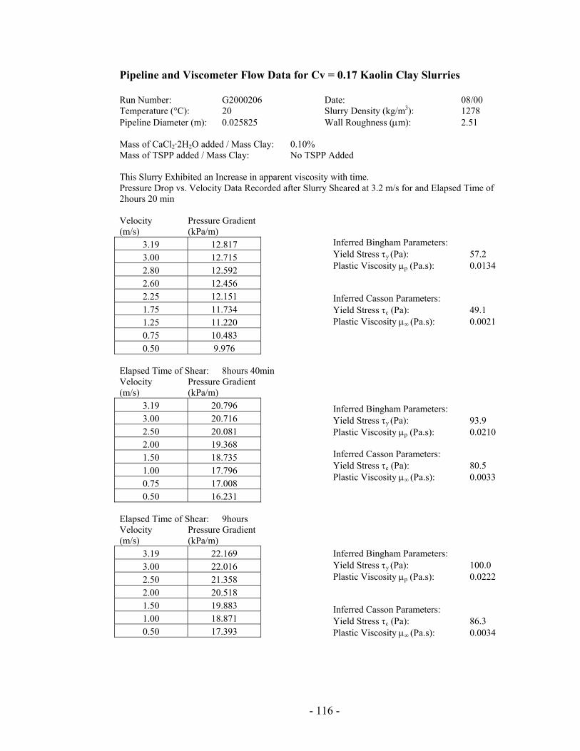
Pipeline and Viscometer Flow Data for Cv = 0.17 Kaolin Clay Slurries Run Number: G2000206 Date: 08/00 Temperature (°C): 20 Slurry Density (kg/m3): 1278 Pipeline Diameter (m): 0.025825 Wall Roughness (µm): 2.51 Mass of CaCl2·2H2O added / Mass Clay: 0.10% Mass of TSPP added / Mass Clay: No TSPP Added This Slurry Exhibited an Increase in apparent viscosity with time. Pressure Drop vs. Velocity Data Recorded after Slurry Sheared at 3.2 m/s for and Elapsed Time of 2hours 20 min Velocity Pressure Gradient (m/s) (kPa/m)
3.19 12.817 3.00 12.715 2.80 12.592 2.60 12.456 2.25 12.151 1.75 11.734 1.25 11.220 0.75 10.483 0.50 9.976
Elapsed Time of Shear: 8hours 40min Velocity Pressure Gradient (m/s) (kPa/m)
3.19 20.796 3.00 20.716 2.50 20.081 2.00 19.368 1.50 18.735 1.00 17.796 0.75 17.008 0.50 16.231
Elapsed Time of Shear: 9hours Velocity Pressure Gradient (m/s) (kPa/m)
3.19 22.169 3.00 22.016 2.50 21.358 2.00 20.518 1.50 19.883 1.00 18.871 0.50 17.393
Inferred Bingham Parameters: Yield Stress τy (Pa): 57.2 Plastic Viscosity µp (Pa.s): 0.0134 Inferred Casson Parameters: Yield Stress τc (Pa): 49.1 Plastic Viscosity µ∞ (Pa.s): 0.0021 Inferred Bingham Parameters: Yield Stress τy (Pa): 93.9 Plastic Viscosity µp (Pa.s): 0.0210 Inferred Casson Parameters: Yield Stress τc (Pa): 80.5 Plastic Viscosity µ∞ (Pa.s): 0.0033 Inferred Bingham Parameters: Yield Stress τy (Pa): 100.0 Plastic Viscosity µp (Pa.s): 0.0222 Inferred Casson Parameters: Yield Stress τc (Pa): 86.3 Plastic Viscosity µ∞ (Pa.s): 0.0034
- 116 -

Viscometry performed on slurry before loading pipeline loop and after discharge. Viscometer: Haake RV 3 Length of Spindle (m): 0.60 Radius of Spindle (m): 0.2001 Radius of Cup (m): 0.2004 Before Loading Pipeline Loop ω (rad/s) T/L (N.m/m)
9.48 6.98E-02 13.40 7.51E-02 18.95 7.82E-02 26.81 8.59E-02 37.91 9.28E-02 26.81 9.05E-02 18.95 8.36E-02 13.40 7.82E-02 9.48 7.44E-02
After Discharging Pipeline Loop ω (rad/s) T/L (N.m/m)
9.48 2.91E-01 13.40 3.02E-01 18.95 3.14E-01 26.81 3.30E-01 37.91 3.44E-01 26.81 3.30E-01 18.95 3.16E-01 13.40 3.05E-01 9.48 2.92E-01
Inferred Bingham Parameters: Yield Stress τy (Pa): 24.8 Plastic Viscosity µp (Pa.s): 0.0139 Inferred Casson Parameters: Yield Stress τc (Pa): 20.6 Plastic Viscosity µ∞ (Pa.s): 0.0025 Inferred Bingham Parameters: Yield Stress τy (Pa): 104.8 Plastic Viscosity µp (Pa.s): 0.0335 Inferred Casson Parameters: Yield Stress τc (Pa): 93.3 Plastic Viscosity µ∞ (Pa.s): 0.0039
- 117 -

Pipeline and Viscometer Flow Data for Cv = 0.17 Kaolin Clay Slurries Run Number: G2000210 Date: 08/00 Temperature (°C): 20 Slurry Density (kg/m3): 1278 Pipeline Diameter (m): 0.025825 Wall Roughness (µm): 2.51 Mass of CaCl2·2H2O added / Mass Clay: 0.10% Mass of TSPP added / Mass Clay: 0.07% This Slurry Exhibited an Increase in apparent viscosity with time. Pressure Drop vs. Velocity Data Recorded after Slurry Sheared at 3.2 m/s for and Elapsed Time of: 3hours 25 min Velocity Pressure Gradient (m/s) (kPa/m)
3.19 10.099 3.00 10.001 2.80 9.871 2.25 9.465 1.75 9.042 1.25 8.540 0.60 7.610 0.30 6.959
Elapsed Time of Shear: 10hours 45min Velocity Pressure Gradient (m/s) (kPa/m)
3.19 16.253 2.99 16.220 2.50 15.810 2.00 15.230 1.50 14.602 1.20 14.134 0.90 13.527 0.60 12.795 0.29 11.824
Elapsed Time of Shear: 17hours Velocity Pressure Gradient (m/s) (kPa/m)
3.19 21.395 3.00 21.147 2.50 20.657 2.00 19.948 1.50 19.129 1.00 18.127 0.60 16.819 0.30 15.831
Inferred Bingham Parameters: Yield Stress τy (Pa): 40.8 Plastic Viscosity µp (Pa.s): 0.0149 Inferred Casson Parameters: Yield Stress τc (Pa): 33.8 Plastic Viscosity µ∞ (Pa.s): 0.0029 Inferred Bingham Parameters: Yield Stress τy (Pa): 71.1 Plastic Viscosity µp (Pa.s): 0.0192 Inferred Casson Parameters: Yield Stress τc (Pa): 60.2 Plastic Viscosity µ∞ (Pa.s): 0.0033 Inferred Bingham Parameters: Yield Stress τy (Pa): 93.8 Plastic Viscosity µp (Pa.s): 0.0243 Inferred Casson Parameters: Yield Stress τc (Pa): 80.1 Plastic Viscosity µ∞ (Pa.s): 0.0040
- 118 -

Viscometry performed on slurry before loading pipeline loop and after discharge. Viscometer: Haake RV 3 Length of Spindle (m): 0.60 Radius of Spindle (m): 0.2001 Radius of Cup (m): 0.2004 Before Loading Pipeline Loop ω (rad/s) T/L (N.m/m)
9.48 5.44E-02 13.40 5.98E-02 18.95 6.52E-02 26.81 7.13E-02 37.91 7.74E-02 26.81 7.36E-02 18.95 6.90E-02 13.40 6.36E-02 9.48 6.06E-02 6.70 5.52E-02 9.48 5.44E-02
After Discharging Pipeline Loop ω (rad/s) T/L (N.m/m)
9.48 2.72E-01 13.40 2.84E-01 18.95 2.97E-01 26.81 3.12E-01 37.91 3.29E-01 26.81 3.14E-01 18.95 3.01E-01 13.40 2.89E-01 9.48 2.76E-01
Inferred Bingham Parameters: Yield Stress τy (Pa): 19.4 Plastic Viscosity µp (Pa.s): 0.0133 Inferred Casson Parameters: Yield Stress τc (Pa): 15.8 Plastic Viscosity µ∞ (Pa.s): 0.0027 Inferred Bingham Parameters: Yield Stress τy (Pa): 98.1 Plastic Viscosity µp (Pa.s): 0.0345 Inferred Casson Parameters: Yield Stress τc (Pa): 86.3 Plastic Viscosity µ∞ (Pa.s): 0.0044
- 119 -

Pipeline and Viscometer Flow Data for Cv = 0.17 Kaolin Clay Slurries Run Number: G2000209 Date: 08/00 Temperature (°C): 20 Slurry Density (kg/m3): 1278 Pipeline Diameter (m): 0.025825 Wall Roughness (µm): 2.51 Mass of CaCl2·2H2O added / Mass Clay: 0.10% Mass of TSPP added / Mass Clay: 0.13% Velocity Pressure Gradient (m/s) (kPa/m)
3.20 6.545 2.75 4.349 2.51 3.894 2.25 3.386 2.00 3.225 1.61 3.003 1.20 2.824 0.90 2.674 0.60 2.489 0.30 2.250
Viscometer: Haake RV 3 Length of Spindle (m): 0.60 Radius of Spindle (m): 0.2001 Radius of Cup (m): 0.2004 ω (rad/s) T/L (N.m/m)
4.73 3.15E-02 6.70 3.32E-02 9.48 3.58E-02
13.40 3.88E-02 18.95 4.25E-02 26.81 4.72E-02 37.91 5.30E-02 26.81 4.72E-02 18.95 4.24E-02 13.40 3.87E-02 9.48 3.58E-02 6.70 3.33E-02 4.73 3.16E-02
Inferred Bingham Parameters: Yield Stress τy (Pa): 12.0 Plastic Viscosity µp (Pa.s): 0.0090 Inferred Casson Parameters: Yield Stress τc (Pa): 9.6 Plastic Viscosity µ∞ (Pa.s): 0.0020 Inferred Bingham Parameters: Yield Stress τy (Pa): 11.1 Plastic Viscosity µp (Pa.s): 0.0117 Inferred Casson Parameters: Yield Stress τc (Pa): 8.3 Plastic Viscosity µ∞ (Pa.s): 0.0032
- 120 -

Pipeline and Viscometer Flow Data for Cv = 0.17 Kaolin Clay Slurries Run Number: G2000207 Date: 07/00 Temperature (°C): 20 Slurry Density (kg/m3): 1278 Pipeline Diameter (m): 0.025825 Wall Roughness (µm): 2.51 Mass of CaCl2·2H2O added / Mass Clay: 0.10% Mass of TSPP added / Mass Clay: 0.27% Velocity Pressure Gradient (m/s) (kPa/m)
3.00 5.722 2.90 5.359 2.80 5.031 2.70 4.710 2.51 4.107 2.25 3.406 2.00 2.764 1.75 2.197 1.50 1.684 1.25 1.229 1.00 0.833 0.80 0.568 0.60 0.345 0.50 0.251 0.35 0.106
Viscometer: Haake RV 3 Length of Spindle (m): 0.60 Radius of Spindle (m): 0.2001 Radius of Cup (m): 0.2004 ω (rad/s) T/L (N.m/m)
13.40 3.23E-03 18.95 4.66E-03 26.81 6.59E-03 37.91 1.08E-02 26.81 6.67E-03 18.95 4.87E-03 13.40 3.23E-03
Inferred Newtonian Viscosity: Viscosity µ (Pa.s): 0.0047* *Turbulent Flow Data Inferred Newtonian Viscosity: Viscosity µ (Pa.s): 0.0047
- 121 -

Pipeline and Viscometer Flow Data for Cv = 0.19 Kaolin Clay Slurries Run Number: G2000201 / G2000202 Date: 07/00 Temperature (°C): 20 Slurry Density (kg/m3): 1321 Pipeline Diameter (m): 0.025825 Wall Roughness (µm): 2.51 Mass of CaCl2·2H2O added / Mass Clay: 0.10% Mass of TSPP added / Mass Clay: No TSPP added This Slurry Exhibited an Increase in apparent viscosity with time. Pressure Drop vs. Velocity Data Recorded after Slurry Sheared at 3.2 m/s for and Elapsed Time of: 0hours 10 min Velocity Pressure Gradient (m/s) (kPa/m)
3.19 11.112 3.00 11.301 2.50 11.114 2.00 10.796 1.50 10.322 1.00 9.707 0.70 9.209 0.50 8.793
Elapsed Time of Shear: 1hour 30 min Velocity Pressure Gradient (m/s) (kPa/m)
3.18 19.363 2.50 18.598 2.00 18.036 1.50 17.332 1.00 16.451 0.50 15.099
Day 2 Elapsed Time of Shear: 1hours 40 min Velocity Pressure Gradient (m/s) (kPa/m)
3.18 20.133 2.50 19.701 2.00 19.081 1.50 18.322 1.00 17.330 0.65 16.388 0.50 15.874 0.35 15.250
Inferred Bingham Parameters: Yield Stress τy (Pa): 51.7 Plastic Viscosity µp (Pa.s): 0.0108 Inferred Casson Parameters: Yield Stress τc (Pa): 44.0 Plastic Viscosity µ∞ (Pa.s): 0.0018 Inferred Bingham Parameters: Yield Stress τy (Pa): 86.7 Plastic Viscosity µp (Pa.s): 0.0198 Inferred Casson Parameters: Yield Stress τc (Pa): 75.5 Plastic Viscosity µ∞ (Pa.s): 0.0031 Inferred Bingham Parameters: Yield Stress τy (Pa): 90.4 Plastic Viscosity µp (Pa.s): 0.0215 Inferred Casson Parameters: Yield Stress τc (Pa): 77.8 Plastic Viscosity µ∞ (Pa.s): 0.0034
- 122 -

Elapsed Time of Shear: 4hours Velocity Pressure Gradient (m/s) (kPa/m)
3.18 27.693 3.00 27.522 2.75 27.223 2.50 26.814 2.25 26.434 2.00 25.993 1.75 25.500 1.50 24.965 1.25 24.321 1.00 23.611 0.51 21.791
Elapsed Time of Shear: 5hours 45min Velocity Pressure Gradient (m/s) (kPa/m)
3.17 32.518 2.90 32.251 2.60 31.581 2.30 31.201 2.00 30.517 1.70 29.845 1.40 29.030 1.10 28.128 0.90 27.436 0.70 26.690 0.50 25.742
Inferred Bingham Parameters: Yield Stress τy (Pa): 126.3 Plastic Viscosity µp (Pa.s): 0.0268 Inferred Casson Parameters: Yield Stress τc (Pa): 108.3 Plastic Viscosity µ∞ (Pa.s): 0.0042 Inferred Bingham Parameters: Yield Stress τy (Pa): 147.8 Plastic Viscosity µp (Pa.s): 0.0321 Inferred Casson Parameters: Yield Stress τc (Pa): 128.0 Plastic Viscosity µ∞ (Pa.s): 0.0048
- 123 -

Viscometry performed on slurry before loading pipeline loop and after discharge. Viscometer: Haake RV 3 Length of Spindle (m): 0.60 Radius of Spindle (m): 0.2001 Radius of Cup (m): 0.2004 Before Loading Pipeline Loop ω (rad/s) T/L (N.m/m)
9.48 1.46E-01 13.40 1.55E-01 18.95 1.64E-01 26.81 1.76E-01 37.91 1.89E-01 26.81 1.78E-01 18.95 1.69E-01 13.40 1.59E-01 9.48 1.53E-01
After Discharging Pipeline Loop ω (rad/s) T/L (N.m/m)
13.40 4.42E-01 18.95 4.58E-01 26.81 4.76E-01 37.91 4.98E-01 53.62 5.23E-01 53.62 5.23E-01 37.91 4.98E-01 26.81 4.72E-01 18.95 4.52E-01 13.40 4.42E-01
Inferred Bingham Parameters: Yield Stress τy (Pa): 51.9 Plastic Viscosity µp (Pa.s): 0.0255 Inferred Casson Parameters: Yield Stress τc (Pa): 44.0 Plastic Viscosity µ∞ (Pa.s): 0.0042 Inferred Bingham Parameters: Yield Stress τy (Pa): 158.4 Plastic Viscosity µp (Pa.s): 0.0353 Inferred Casson Parameters: Yield Stress τc (Pa): 138.9 Plastic Viscosity µ∞ (Pa.s): 0.0046
- 124 -
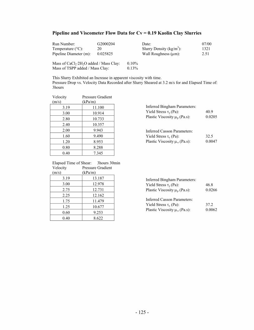
Pipeline and Viscometer Flow Data for Cv = 0.19 Kaolin Clay Slurries Run Number: G2000204 Date: 07/00 Temperature (°C): 20 Slurry Density (kg/m3): 1321 Pipeline Diameter (m): 0.025825 Wall Roughness (µm): 2.51 Mass of CaCl2·2H2O added / Mass Clay: 0.10% Mass of TSPP added / Mass Clay: 0.13% This Slurry Exhibited an Increase in apparent viscosity with time. Pressure Drop vs. Velocity Data Recorded after Slurry Sheared at 3.2 m/s for and Elapsed Time of: 3hours Velocity Pressure Gradient (m/s) (kPa/m)
3.19 11.100 3.00 10.914 2.80 10.733 2.40 10.357 2.00 9.943 1.60 9.490 1.20 8.953 0.80 8.288 0.40 7.345
Elapsed Time of Shear: 3hours 30min Velocity Pressure Gradient (m/s) (kPa/m)
3.19 13.187 3.00 12.978 2.75 12.731 2.25 12.162 1.75 11.479 1.25 10.677 0.60 9.253 0.40 8.622
Inferred Bingham Parameters: Yield Stress τy (Pa): 40.9 Plastic Viscosity µp (Pa.s): 0.0205 Inferred Casson Parameters: Yield Stress τ (Pa): 32.5 c
Yield Stress τ (Pa): 46.8 y
Plastic Viscosity µ (Pa.s): 0.0047 ∞
Inferred Bingham Parameters:
Plastic Viscosity µ (Pa.s): 0.0266 p Inferred Casson Parameters: Yield Stress τ (Pa): 37.2 c
Plastic Viscosity µ (Pa.s): 0.0062 ∞
- 125 -

Viscometry performed on slurry before loading pipeline loop and after discharge. Viscometer: Haake RV 3 Length of Spindle (m): 0.60 Radius of Spindle (m): 0.2001 Radius of Cup (m): 0.2004 Before Loading Pipeline Loop ω (rad/s) T/L (N.m/m)
6.70 8.66E-02 9.48 9.12E-02
13.40 9.74E-02 18.95 1.04E-01 26.81 1.14E-01 37.91 1.23E-01 26.81 1.15E-01 18.95 1.07E-01 13.40 9.97E-02 9.48 9.28E-02 6.70 8.97E-02
After Discharging Pipeline Loop ω (rad/s) T/L (N.m/m)
6.70 1.45E-01 9.48 1.54E-01
13.40 1.65E-01 18.95 1.76E-01 26.81 1.90E-01 37.91 2.07E-01 26.81 1.91E-01 18.95 1.77E-01 13.40 1.66E-01 9.48 1.55E-01 6.70 1.46E-01
Inferred Bingham Parameters: Yield Stress τy (Pa): 31.0 Plastic Viscosity µp (Pa.s): 0.0207 Inferred Casson Parameters: Yield Stress τc (Pa): 25.2 Plastic Viscosity µ∞ (Pa.s): 0.0041 Inferred Bingham Parameters: Yield Stress τy (Pa): 51.4 Plastic Viscosity µp (Pa.s): 0.0355 Inferred Casson Parameters: Yield Stress τc (Pa): 41.5 Plastic Viscosity µ∞ (Pa.s): 0.0073
- 126 -

Pipeline and Viscometer Flow Data for Cv = 0.19 Kaolin Clay Slurries Run Number: G2000203 Date: 08/00 Temperature (°C): 20 Slurry Density (kg/m3): 1321 Pipeline Diameter (m): 0.025825 Wall Roughness (µm): 2.51 Mass of CaCl2·2H2O added / Mass Clay: 0.10% Mass of TSPP added / Mass Clay: 0.27% This Slurry Exhibited an Increase in apparent viscosity with time. Pressure Drop vs. Velocity Data Recorded after Slurry Sheared at 3.2 m/s for and Elapsed Time of: 0 min Velocity Pressure Gradient (m/s) (kPa/m)
3.19 6.917 3.00 6.161 2.50 4.453 2.00 3.035 1.50 1.850 1.25 1.335 1.00 0.906 0.80 0.611 0.60 0.275 0.40 0.202
Elapsed Time of Shear: 30min Velocity Pressure Gradient (m/s) (kPa/m)
3.19 6.914 3.00 6.130 2.50 4.453 2.00 3.021 1.75 2.377 1.25 1.323 0.80 0.634 0.75 0.474 0.70 0.398 0.65 0.326 0.60 0.308 0.55 0.297 0.50 0.274 0.45 0.253 0.40 0.242 0.35 0.227
Inferred Newtonian Viscosity: Viscosity µ (Pa.s): 0.0058 Inferred Bingham Parameters: Yield Stress τy (Pa): 0.52 Plastic Viscosity µp (Pa.s): 0.0070 Inferred Casson Parameters: Yield Stress τc (Pa): 0.21 Plastic Viscosity µ∞ (Pa.s): 0.0042
- 127 -

Viscometry performed on slurry before loading pipeline loop and after discharge. Viscometer: Haake RV 3 Length of Spindle (m): 0.60 Radius of Spindle (m): 0.2001 Radius of Cup (m): 0.2004 Before Loading Pipeline Loop ω (rad/s) T/L (N.m/m)
26.81 1.13E-02 18.95 8.53E-03 13.40 6.38E-03 9.48 5.09E-03 6.70 3.80E-03
After Discharging Pipeline Loop ω (rad/s) T/L (N.m/m)
26.81 1.58E-02 18.95 1.23E-02 13.40 9.46E-03 9.48 7.53E-03 6.70 5.88E-03
Inferred Bingham Parameters: Yield Stress τy (Pa): 0.56 Plastic Viscosity µp (Pa.s): 0.0065 Inferred Casson Parameters: Yield Stress τc (Pa): 0.13 Plastic Viscosity µ∞ (Pa.s): 0.0052 Inferred Bingham Parameters: Yield Stress τy (Pa): 1.05 Plastic Viscosity µp (Pa.s): 0.0087 Inferred Casson Parameters: Yield Stress τc (Pa): 0.30 Plastic Viscosity µ∞ (Pa.s): 0.0064
- 128 -

APPENDIX B
SLURRY SUPERNATANT CALCIUM ION ANALYSIS
WITH AN ATOMIC ABSORPTION SPECTROPHOTOMETER
- 129 -

Table B.1 Kaolin Clay Slurry Cv = 0.19 Calcium ion supernatant data. Run # Mass of TSPP /
Mass Clay Mass of CaCl2·2H2O / Mass Clay
Ca++ ion calculated (ppm)
Ca++ ion measured by AASP (ppm)
G2000201/2 0.00% 0.10% 168 198 G2000204 0.13% 0.10% 168 57 G2000203 0.27% 0.10% 168 21
Table B.2 Kaolin Clay Slurry Cv = 17% by volume solids Calcium ion supernatant data. Run # Mass of TSPP / Mass
Clay Mass of CaCl2·2H2O / Mass Clay
Ca++ ion calculated (ppm)
Ca++ ion measured by AASP (ppm)
G2000206 0.00% 0.10% 142 136 G2000210 0.07% 0.10% 142 Not Taken G2000209 0.13% 0.10% 142 40 G2000207 0.27% 0.10% 142 4
Table B.3 Kaolin Clay Slurry Cv = 0.14 Calcium ion supernatant data. Run # Mass of TSPP / Mass
Clay Mass of CaCl2·2H2O / Mass Clay
Ca++ ion calculated (ppm)
Ca++ ion measured by AASP (ppm)
G2000205 0.00% 0.10% 113 124 G2000214 0.13% 0.10% 113 42 G2000217a 0.27% 0.10% 113 15 G2000217b 0.27% 0.16% 182 Not Taken G2000217c 0.27% 0.22% 252 47 G2000217d 0.27% 0.28% 322 110 G2000215 0.27% 0.10% 113 14
* CaCl2·2H2O was added stepwise during run G2000217 through recirculation into the stand tank in an attempt to increase the viscosity of this slurry. G2000217b,c,d each underwent 5 gram additions of CaCl2·2H2O for a total of 15 additional grams added.
- 130 -

Table B.4 Kaolin Clay Slurry Cv = 0.10 Calcium ion supernatant data. Run # Mass of TSPP / Mass
Clay Mass of CaCl2·2H2O / Mass Clay
Ca++ ion calculated (ppm)
Ca++ ion measured by AASP (ppm)
G2000106a -- 0.10% 76 79 G2000208 -- 0.10% 77 82 G2000212 0.27% 0.10% 76 14
Table B.5 Kaolin Clay Slurry Cv = 10% by volume solids total ion mass spectrometer supernatant data (mg of analyte/ L of solution). Sample Description: Analogous Pipeline Run: 1564: R/O Water 1565: Clay Slurry Cv: 13%, (No Chemicals Added) 1566: Clay Slurry Cv: 13%, Flocculant Mass Ratio: 0.10%, Deflocculant Mass Ratio: N/A 1567: Clay Slurry Cv: 13%, Flocculant Mass Ratio: 0.10%, Deflocculant Mass Ratio: 0.13% 1568: Clay Slurry Cv: 13%, Flocculant Mass Ratio: 0.10%, Deflocculant Mass Ratio: 0.27% 1569*: Clay Slurry Cv: 13%, Flocculant Mass Ratio: 0.10%, Deflocculant Mass Ratio: 0.27% *Supernatant filtered with 0.22 mm filter paper Analyte 1564 1565 1566 1567 1568 1569 Aluminum 0.14 0.12 0.11 0.09 4.1 2.9 Barium 0.004 0.01 0.039 0.005 0.021 0.006 Beryllium <0.001 <0.001 <0.001 <0.001 <0.001 <0.001 Boron 0.007 0.02 0.02 0.021 0.033 0.042 Cadmium <0.001 <0.001 <0.001 <0.001 <0.001 <0.001 Calcium 1.4 24 130 27 15 12 Chromium <0.001 0.002 0.002 0.003 0.006 0.006 Cobalt <0.001 <0.001 <0.001 <0.001 <0.001 <0.001 Copper <0.001 0.004 0.003 0.005 0.012 0.011 Iron 0.005 0.014 0.01 0.004 0.37 0.29 Lead <0.002 <0.002 <0.002 <0.002 0.007 0.009 Magnesium <0.1 0.6 2 0.7 1.3 1.4 Manganese <0.001 <0.001 <0.001 <0.001 0.053 0.1 Molybdenum <0.001 <0.001 <0.001 0.002 0.004 0.003 Nickel <0.001 <0.001 <0.001 <0.001 0.003 0.002 Phosphorus <0.01 0.02 0.01 5.4 16 17 Potassium <0.2 0.8 1.7 1.5 1.3 1.4 Silicon, Soluble 0.93 11 11 15 15 14 Silver <0.001 <0.001 <0.001 <0.001 <0.001 <0.001 Sodium 3.9 5.2 7.4 86 150 160 Strontium 0.007 0.089 0.34 0.065 0.038 0.022 Titanium <0.001 <0.001 <0.001 <0.001 0.01 0.008 Vanadium <0.001 0.003 0.001 0.032 0.068 0.07 Zinc <0.005 <0.005 <0.005 <0.005 0.055 0.046 Zirconium <0.001 <0.001 <0.001 <0.001 0.007 0.005
- 131 -

APPENDIX C
TURBULENT PIPELINE FLOW LOOP EXPERIMENTAL DATA WITH
WILSON & THOMAS TURBULENT FLOW PREDICTIONS
- 132 -

Run#: G2000106 Cv: 0.10 Mass CaCl2·H2O / Mass Clay: 0.10% Mass TSPP / Mass Clay: 0.00% Inferred Parameters from Laminar Flow Experimental Data Bingham: τy (Pa): 2.6 µp (Pa.s): 0.0051 Casson: τc (Pa): 1.9 µ∞ (Pa.s): 0.0016
0.0
1.0
2.0
3.0
4.0
5.0
6.0
0.0 0.5 1.0 1.5 2.0 2.5 3.0 3.5Bulk Velocity, V (m/s)
Pres
sure
Gra
dien
t -dP
/dz
(KPa
/m)
Laminar Bingham ModelTurbulent Bingham ModelLaminar Casson ModelTurbulent Casson ModelExperimental Data
Figure D.1: Comparison of the experimental frictional head loss with Bingham and Casson fluid model predictions for Cv = 0.10 Kaolin Clay Slurry in 25.8 mm vertical pipeline loop. The model parameters were chosen to fit the laminar flow data.
- 133 -

Run#: G2000208 Cv: 0.10 Mass CaCl2·H2O / Mass Clay: 0.10% Mass TSPP / Mass Clay: 0.00% Inferred Parameters from Laminar Flow Experimental Data Bingham: τy (Pa): 2.6 µp (Pa.s): 0.0051 Casson: τc (Pa): 1.9 µ∞ (Pa.s): 0.0015
0.0
1.0
2.0
3.0
4.0
5.0
6.0
0.0 1.0 2.0 3.0 4.0Bulk Velocity, V (m/s)
Pres
sure
Gra
dien
t -dP
/dz
(kPa
/m)
Laminar Bingham ModelTurbulent Bingham ModelLaminar Casson ModelTurbulent Casson ModelExperimental Data
Figure D.2: Comparison of the experimental frictional head loss with Bingham and Casson fluid model predictions for Cv = 0.10 Kaolin Clay Slurry in 25.8 mm vertical pipeline loop. The model parameters were chosen to fit the laminar flow data.
- 134 -

Run#: G2000205 Cv: 0.14 Mass CaCl2·H2O / Mass Clay: 0.10% Mass TSPP / Mass Clay: 0.00% Inferred Parameters from Laminar Flow Experimental Data Bingham: τy (Pa): 14.3 µp (Pa.s): 0.0057 Casson: τc (Pa): 12.0 µ∞ (Pa.s): 0.0010
0.0
1.0
2.0
3.0
4.0
5.0
6.0
0.0 1.0 2.0 3.0 4.0 5.0Bulk Velocity, V (m/s)
Pres
sure
Gra
dien
t -dP
/dz
(kPa
/m)
Laminar Bingham ModelTurbulent Bingham ModelLaminar Casson ModelTurbulent Casson ModelExperimental Data
Figure D.3: Comparison of the experimental frictional head loss with Bingham and Casson fluid model predictions for Cv = 0.14 Kaolin Clay Slurry in 25.8 mm vertical pipeline loop. The model parameters were chosen to fit the laminar flow data.
- 135 -

Run#: G2000105 Cv: 0.14 Mass CaCl2·H2O / Mass Clay: 0.10% Mass TSPP / Mass Clay: 0.10% Inferred Parameters from Laminar Flow Experimental Data Bingham: τy (Pa): 5.9 µp (Pa.s): 0.0078 Casson: τc (Pa): 4.4 µ∞ (Pa.s): 0.0021
0.0
1.0
2.0
3.0
4.0
5.0
6.0
7.0
0.0 1.0 2.0 3.0 4.0Bulk Velocity, V (m/s)
Pres
sure
Gra
dien
t -dP
/dz
(kPa
/m)
Laminar Bingham ModelTurbulent Bingham ModelLaminar Casson ModelTurbulent Casson ModelExperimental Data
Figure D.4: Comparison of the experimental frictional head loss with Bingham and Casson fluid model predictions for Cv = 0.14 Kaolin Clay Slurry in 25.8 mm vertical pipeline loop. The model parameters were chosen to fit the laminar flow data.
- 136 -

Run#: G2000217 Cv: 0.14 Mass CaCl2·H2O / Mass Clay: 0.10% Mass TSPP / Mass Clay: 0.13% 10 grams of CaCl2·H2O has been re-circulated into the system to increase the inter particle attraction. Inferred Parameters from Laminar Flow Experimental Data Bingham: τy (Pa): 7.9 µp (Pa.s): 0.0092 Casson: τc (Pa): 6.1 µ∞ (Pa.s): 0.0023
0.0
1.0
2.0
3.0
4.0
5.0
6.0
7.0
0.0 1.0 2.0 3.0 4.0Bulk Velocity, V (m/s)
Pres
sure
Gra
dien
t -dP
/dz
(kPa
/m)
Laminar Bingham ModelTurbulent Bingham ModelLaminar Casson ModelTurbulent Casson ModelExperimental Data
Figure D.5: Comparison of the experimental frictional head loss with Bingham and Casson fluid model predictions for Cv = 0.14 Kaolin Clay Slurry in 25.8 mm vertical pipeline loop. The model parameters were chosen to fit the laminar flow data.
- 137 -

Run#: G2000214 Cv: 0.14 Mass CaCl2·H2O / Mass Clay: 0.10% Mass TSPP / Mass Clay: 0.13% Inferred Parameters from Laminar Flow Experimental Data Bingham: τy (Pa): 6.7 µp (Pa.s): 0.0072 Casson: τc (Pa): 5.2 µ∞ (Pa.s): 0.0018
0.0
1.0
2.0
3.0
4.0
5.0
6.0
7.0
0.0 1.0 2.0 3.0 4.0Bulk Velocity, V (m/s)
Pres
sure
Gra
dien
t -dP
/dz
(kPa
/m)
Laminar Bingham ModelTurbulent Bingham ModelLaminar Casson ModelTurbulent Casson ModelExperimental Data
Figure D.6: Comparison of the experimental frictional head loss with Bingham and Casson fluid model predictions for Cv = 0.14 Kaolin Clay Slurry in 25.8 mm vertical pipeline loop. The model parameters were chosen to fit the laminar flow data.
- 138 -

Run#: G2000209 Cv: 0.17 Mass CaCl2·H2O / Mass Clay: 0.10% Mass TSPP / Mass Clay: 0.13% Inferred Parameters from Laminar Flow Experimental Data Bingham: τy (Pa): 12.0 µp (Pa.s): 0.0090 Casson: τc (Pa): 9.7 µ∞ (Pa.s): 0.0020
0.0
1.0
2.0
3.0
4.0
5.0
6.0
7.0
8.0
0.0 1.0 2.0 3.0 4.0 5.0Bulk Velocity, V (m/s)
Pres
sure
Gra
dien
t -dP
/dz
(kPa
/m)
Laminar Bingham ModelLaminar Casson Model Turbulent Bingham ModelTurbulent Casson ModelExperimental Data
Figure D.7: Comparison of the experimental frictional head loss with Bingham and Casson fluid model predictions for Cv = 0.14 Kaolin Clay Slurry in 25.8 mm vertical pipeline loop. The model parameters were chosen to fit the laminar flow data.
- 139 -

APPENDIX D
Particle Diameter Derivation From Centrifugal Andreasen Pipette Methods
Ryan Spelay 2000
- 140 -

In order to determine the settling velocity of a particle one must perform a force balance on a single particle settling in infinite dilution. In this derivation it is assumed that the particle reaches terminal settling velocity immediately. The gravitational term can also be neglected since it was previously shown that the centrifugal force is so much greater than the gravitational force. Therefore, accounting for the centrifugal, buoyancy and drag forces on the settling particle it is known that at the terminal velocity:
( ) rVAVC
FFF
PfspsfD
lcentrifugadrag
particle
22
2
0
ωρρρ
−=
=
=∑
Where: CD = Coefficient of drag {Dimensionless} Ap = Projected area of a settling particle {m2} VP = Volume of a particle {m3} In order for Stokes Law to be applicable for a centrifuging situation many simplifying assumptions have to be made. One such assumption is that the particles are perfectly rigid, smooth and spherical. Another assumption is that the flow is in the Stokes region. This means that the Reynolds Number must be less than 0.1. The Reynolds Number for a settling particle is a dimensionless quantity defined as:
f
sPf VDN
µρ
=Re
Where: NRe = the Reynolds Number {dimensionless} ρf = the density of the fluid {kg/m3} Dp = particle diameter {m} Vs = particle settling velocity {m/s} µf = fluid viscosity {Pa.s} In the Stokes region of settling for a spherical rigid particle the coefficient of drag can be related to the Reynolds number by the equation:
sPf
fD VDNC
ρµ2424
Re
==
Substitution of this equation into the force balance along with the formulas for the projected area and volume of a sphere yields:
( ) rDDDV
PfsPP
sf 232
6412
ωπρρπµ
−=
- 141 -

- 142 -
Upon further simplification, Stokes Law for gravitational sedimentation can be rewritten for a particle travelling in a circular path as:
Where: vsettle = the particles settling velocity {m/s} ω = the angular velocity of the centrifuge {rad/s} r = the radial position in the centrifuge {m} ρs = the density of the solid particles {kg/m3} ρf = the density of the fluid {kg/m3} Dp = the spherical diameter of the settling particle {m} µ = the viscosity of the fluid {Pa.s} One can see by Stokes Law that the settling velocity is not only dependent on many of the same factors as in gravitational sedimentation but it is also dependent on radial position. This radial dependence makes a straightforward solution impossible and thus a more involved approach must be taken. This involved approach treats each individual particle as rigid body. It is also assumed that after dispersion and mixing, each of the particles has an initial velocity of zero but attains its terminal velocity instantly. It is also assumed that particle flow is only in the radial direction of the centrifuge (azimuthal/axial direction of the pipette) and that the wall and interparticle effects are negligible. From the basic kinematic equations it is known that for a rigid body travelling at a constant velocity:
Where: v = terminal velocity of particle {m/s} r = radial displacement of the particle {m} t = time of displacement {s} It should be noted that in the Stokes equation the terminal velocity is a function of radial distance and it is not constant but rather it changes instantaneously with increasing radial displacement. However, if the particle’s motion is only in the radial direction the differential term of the above equation can be equated to the Stokes terminal settling velocity by:
( )µρρω
18
22Pfs
settle
Drv
−=
dtdrv =

- 143 -
Manipulating the above equation into a solvable form and applying the boundary conditions yields:
Where: R = the final radial displacement of a particle with DP {m} S = the initial radial displacement of a particle with DP {m} Solving the above integral and noting that all of the terms on the right hand side are independent of time yields:
Solving for DP, the particles equivalent spherical diameter, yields:
µρρ
18)( 22
Pfssettle
Drwdtdrv
−==
∫∫−
=t
PfsR
S
dtDw
rdr
0
22
18)(
µρρ
tDw
SR Pfs
µρρ
18)(
ln22 −
=
21
2 ln)(
18
−=
SR
twD
fsP ρρ
µ

- 144 -
When working with a centrifuge the desired angular velocity is not achieved instantaneously but rather it takes a finite period of time to be reached. This is also true for the stopping of the centrifuge in that it also takes a finite period of time for the centrifuge to come to rest. These acceleration and de-acceleration times are not accounted for in the original derivation and thus if they become significant compared to the actual run time, a sizeable error will be incorporated into the particle sizes calculated. To overcome the possibility of introducing this error, a derivation incorporating ramp times has been created. In this derivation linear ramping functions are assumed for the acceleration and de-acceleration periods of the centrifuge. A schematic graph of angular velocity versus time is shown below. Figure D.1: Idealized plot of centrifuge angular velocities in the ramping regions From the plot above it can be seen that:
The angular velocity can also be expressed as a function of t for the 3 time regions:
t t2 t3 t10
ωC
ω(t)
tRU tRUN tRD
Acceleration Constant De-
23
12
1
tttttt
tt
RD
RUN
RU
−=−=
=
( ) 3223
21
11
tt t; 3)(
tt t; )(
tt0 ; )(
<<−−
=
<<=
<<=
tttt
t
t
tt
t
C
C
C
ωω
ωω
ωω

- 145 -
Therefore if one follows the same derivation that was performed when the ramping times were ignored the following equations are obtained for each of the three time regions. For (0 < t < t1):
For (t1 < t < t2):
RUt
µP
)Df
ρs
(ρCw
S
R
tµ
P)Df
ρs
(ρCw
S
R
tdtt
µt
P)Df
ρs
(ρCwR
S rdr
tdt
µP
)Df
ρs
(ρwR
S rdr
54
221ln
154
221ln
1
0
221
18
221
1
0 18
221
−=
−=
∫−
=∫
∫−
=∫
( )
RUNPfsC
PfsC
t
t
PfsCR
R
t
t
PfsR
R
tDw
RR
ttDw
RR
dtDw
rdr
dtDw
rdr
µρρ
µρρ
µρρ
µρρ
18)(
ln
18)(
ln
18)(
18)(
22
1
2
12
22
1
2
22
22
2
1
2
1
2
1
2
1
−=
−−
=
−=
−=
∫∫
∫∫

- 146 -
For (t2 < t < t3):
Summing the resulting equations for each of the three time periods yields:
Now particle diameters can be calculated based on not only the constant run time of the centrifuge but also on the ramping times. However, it should be noted that in this derivation it is assumed that the tubes are always oriented horizontally and in the radial direction. In some centrifuges when the acceleration and de-acceleration phases are occurring, the tube may be oriented at some angle to the horizontal. This may introduce some error (be it small), to the final particle diameter calculated. However, the error resulting from the tubes not being horizontal is smaller than the error resulting from ignoring the ramping times completely.
( )( )
( )
RDPfsC
PfsC
t
t
PfsCR
R
t
t
PfsR
R
tDw
RR
ttDw
RR
dtttttDw
rdr
dtDw
rdr
µρρ
µρρ
µ
ρρ
µρρ
54)(
ln
54)(
ln
18)(
18)(
22
2
23
22
2
232
23
22
22
3
22
3
22
−=
−−
=
−−
−=
−=
∫∫
∫∫
21
2
22
541854)(
ln
541854)(
ln
++−
=
++
−=
RDRUNRUfsC
P
RDRUNRUPfsC
tttw
SR
D
tttDwSR
ρρ
µ
µρρ

APPENDIX E
Instrument Calibrations
- 147 -

- 148 -
Pressure Transducer (Upstream Pressure Gradient Test Section) Validyne differential pressure transducer calibrated against pressure measured by a manometer containing merium fluid with a density of 2.950 kg/m3
High Side Low Side Reading Pressure
(cm) (cm) (volts) (kPa) 189.9 16.1 2.503 50.25 179.9 25.9 2.225 44.52 170.2 35.9 1.942 38.83 159.7 46.6 1.636 32.70 149.6 56.7 1.356 26.86 139.3 67.0 1.049 20.90 129.1 77.2 0.754 15.00 119.3 86.9 0.473 9.37 103.0 103.0 0.006 0.00
Slope (kPa/volt) 20.094 Zero (volts) 0.0085 Correlation coefficient 0.99999
0
10
20
30
40
50
60
0.0 1.0 2.0 3.0Voltage
Pres
sure
(kPa
)

- 149 -
Pressure Transducer (Downstream Pressure Gradient Test Section) Validyne differential pressure transducer calibrated against pressure measured by a manometer containing merium fluid with a density of 2.950 kg/m3
High Side Low Side Reading Pressure
(cm) (cm) (volts) (kPa) 189.5 16.4 2.495 50.04 175.4 30.7 2.086 41.83 160.8 45.3 1.666 33.39 144.8 61.2 1.208 24.17 130.0 76.0 0.782 15.61 119.7 86.2 0.487 9.68 111.1 94.8 0.240 4.71 102.9 102.9 0.006 0.00
Slope (kPa/volt) 20.109 Zero (volts) 0.0058 Correlation coefficient 1.0000
0
10
20
30
40
50
60
0.0 1.0 2.0 3.0Voltage
Pres
sure
(kPa
)

- 150 -
Bucket and Stopwatch Flow Calibration for 3L6 progressive cavity pump
Elapsed Weight Density Reading Flow Rate Time (s) (kg) (kg/m3) (volts) (L/s)
0.00 0.00 997.3 0.989 0.000 41.34 19.50 998.5 1.621 0.472 23.40 18.12 998.4 2.007 0.776 16.06 18.78 998.4 2.542 1.171 11.97 18.14 998.3 2.975 1.518
Slope (L/s/volt) 0.763 Zero (volts) 0.995 Correlation coefficient 0.99992
0.0
0.5
1.0
1.5
2.0
0.0 1.0 2.0 3.0Voltage
Flow
Rat
e (L
/s)

- 151 -
Viscometer Calibration (Measuring Head MK500) Viscosity Standard Cannon S200 oil Temperature (°C) 25 Standard Viscosity (Pa.s) 0.4078 Spindle MV1 R1 (m) 0.02004 R2 (m) 0.02100 L (m) 0.0600 Full Scale T. (N.m) 0.045 Slope (T/L vs. w) 0.0231 Viscosity 0.4089 Percent Error 0.26% Experimental Data
RPM TORQUE (% OF FS) ω (rad/s) T/L (N.m/m) 32.0 10.6 3.35 0.080 64.0 21.0 6.70 0.158 90.5 29.6 9.48 0.222 128.0 41.6 13.40 0.312 181.0 58.5 18.95 0.439 256.0 81.6 26.81 0.612 181.0 58.7 18.95 0.440 128.0 41.2 13.40 0.309 90.5 28.9 9.48 0.217 64.0 21.1 6.70 0.158 45.2 15.3 4.73 0.115 32.0 10.8 3.35 0.081 22.6 7.8 2.37 0.059
0.00.10.20.30.40.50.60.7
0 10 20 3ω (rad/s)
T/L
(N.m
/m)
0

- 152 -
Viscometer Calibration (Measuring Head MK50) Viscosity Standard Cannon S200 oil Temperature (°C) 25 Standard Viscosity (Pa.s) 0.4078 Spindle MV1 R1 (m) 0.02004 R2 (m) 0.02100 L (m) 0.0600 Full Scale T. (N.m) 0.0043 Slope (T/L vs. w) 0.0228 Viscosity 0.4035 Percent Error 1.05%
0.000.010.020.030.040.050.06
0 1 2 3ω (rad/s)
T/L
(N.m
/m)
Experimental Data
RPM TORQUE (% OF FS) ω (rad/s) T/L (N.m/m) 4.0 12.7 0.42 0.0092 8.0 25.8 0.84 0.0187 16.0 52.7 1.68 0.0382 22.6 75.3 2.37 0.0545 22.6 75.2 2.37 0.0544 16.0 52.7 1.68 0.0382 11.3 36.6 1.18 0.0265 8.0 25.4 0.84 0.0184 5.7 17.8 0.59 0.0129 4.0 12.3 0.42 0.0089 2.0 6.0 0.21 0.0043
Related Documents


