> The Ecological Scarcity Method Eco-Factors 2006 A method for impact assessment in LCA > Life Cycle Assessments > Environmental studies 06 09

Welcome message from author
This document is posted to help you gain knowledge. Please leave a comment to let me know what you think about it! Share it to your friends and learn new things together.
Transcript

> The Ecological Scarcity Method Eco-Factors 2006
A method for impact assessment in LCA
> Life Cycle Assessments> Environmental studies
0609


> The Ecological Scarcity Method Eco-Factors 2006
A method for impact assessment in LCA
The eco-factors were determined on the basis of the latest data available in 2006 on ambient loads and levels in Switzerland, and in accordance with the environmental quality targets
and limit values established in Swiss law at that time.
>> Environmental studies Life Cycle Assessments
Issued by Federal Office for the Environment FOEN
öbu – works für sustainabilityBern, 2009

Impressum Issued by Federal Office for the Environment (FOEN) FOEN is an office of the Federal Department of Environment, Transport, Energy and Communications (DETEC).
Authors of the study Rolf Frischknecht, Roland Steiner, Niels Jungbluth (ESU-services GmbH)
Authors of the synoptic overview Markus Ahmadi, ideja – Agentur für Kommunikation
Project coordinators Arthur Braunschweig, E2 Management Consulting AG Norbert Egli, FOEN Gabi Hildesheimer, Öbu
FOEN consultants Patrik Burri, Credit Suisse Group Fernand Hochenauer, CTW-Strassenbaustoffe Roland Högger, Geberit International AG Rudolf Sollberger, Basler Versicherungen Adnan Ucar, Coop Patrick Walser, Migros Genossenschafts-Bund
FOEN acknowledgements For ideas, suggestions, groundwork and field tests: Fredy Dinkel, Gabor Doka, Stefanie Hellweg, Harald Jenk, KBOB, Andreas Liechti, Nobuyuki Miyazaki, Ruedi Müller-Wenk, Claude Siegenthaler For reviews, suggestions and funding: Basler Versicherungen, Coop, Credit Suisse, CTW-Strassenbaustoffe AG, Geberit International, Migros Genossenschafts-Bund Suggested form of citation Frischknecht Rolf, Steiner Roland, Jungbluth Niels 2009: The Ecological Scarcity Method – Eco-Factors 2006. A method for impact assessment in LCA. Environmental studies no. 0906. Federal Office for the Environment, Bern: 188 pp.
Translation Christopher Hay, Translation Bureau for Environmental Sciences
Design Ursula Nöthiger-Koch, Uerkheim
Cover picture Heiner H. Schmitt, Basel (based on an idea of FOEN). The scales were provided by Agnès and Antoine Harnist, vegetable producers in Village-Neuf (Alsace, France); the picture was processed in accordance with FOEN’s stipulations.
Downloadable PDF file www.environment-switzerland.ch/uw-0906-e (no printed version available) Code: UW-0906-E
This publication is also available in German (UW-0906-D).
© FOEN 2009

> Table of contents 3
> Table of contents
Abstracts 5 Foreword 7 Zusammenfassung 9 Résumé 9 Summary 17 Synoptic overview 21
1 Introduction 42 1.1 Position of the ecological scarcity method in
relation to life cycle assessment (LCA) 42 1.2 Terminology 42 1.3 Structure of the report 42
2 Methodological fundamentals 44 2.1 The ecological scarcity method 44 2.2 Principles governing the derivation of eco-factors 52 2.3 Principles governing the application of eco-factors 56 2.4 Data quality 58 2.5 Characterization 59
3 Emissions to air 60 3.1 Introduction 60 3.2 CO2 and further greenhouse gases 62 3.3 Ozone-depleting substances 67 3.4 NMVOCs and further substances with
photochemical ozone creation potential 75 3.5 Nitrogen oxides (NOx) 77 3.6 Ammonia (NH3) 79 3.7 SO2 and further acidifying substances 81 3.8 Particulate matter (I): PM10, PM2.5 + PM2.5–10 84 3.9 Particulate matter (II): Diesel soot 88 3.10 Carbon monoxide (CO) 90 3.11 Benzene 91 3.12 Dioxins and furans (PCDD/PCDF) 93 3.13 Lead (Pb) 95 3.14 Cadmium (Cd) 96 3.15 Mercury (Hg) 98 3.16 Zinc (Zn) 99
4 Emissions to surface waters 101 4.1 Introduction 101 4.2 Nitrogen 103 4.3 Phosphorus 104 4.4 Organic matter (BOD, COD, DOC, TOC) 108 4.5 Heavy metals and arsenic 111 4.6 Radioactive emissions to seas 114 4.7 AOX 119 4.8 Chloroform 121 4.9 PAHs (polycyclic aromatic hydrocarbons) 122 4.10 Benzo(a)pyrene 124 4.11 Endocrine disruptors 125
5 Emissions to groundwater 130 5.1 Introduction 130 5.2 Nitrate in groundwater 130
6 Emissions to soil 132 6.1 Introduction 132 6.2 Heavy metals in soils 134 6.3 Plant protection products (PPPs) 138
7 Resources 142 7.1 Overview 142 7.2 Energy resources 142 7.3 Land use 148 7.4 Gravel extraction 153 7.5 Freshwater consumption 154
8 Wastes 160 8.1 Introduction 160 8.2 Carbon in material consigned to bioreactive
landfills 160 8.3 Hazardous wastes in underground repositories 162 8.4 Radioactive wastes in final repositories 163
9 Not assessed: Noise 167

The Ecological Scarcity Method – Eco-Factors 2006 FOEN 2009 4
Annex 168 A1 Conversion factors for emissions 168 A2 Eco-factors for greenhouse gases and ozone-
depleting substances 169 A3 PAHs (polycyclic aromatic hydrocarbons) 172 A4 Plant protection products 173 A5 Eco-factors for land use 177 A6 Eco-factors for freshwater consumption in the OECD
states 179
Index 180 Abbreviations 180 Figures 181 Tables 181 Bibliography 184

> Abstracts 5
> Abstracts
Applied within the context of a life cycle assessment (LCA), the ecological scarcity method allows for the assessment of the impacts generated by the releases of pollutantsand extraction of resources identified in a life cycle inventory analysis. Eco-factors, expressed as eco-points per unit of pollutant emission or resource extraction, are the key parameter used by the method. The publication sets out how the eco-factors are determined, reflecting, on the one hand, the current emission situation, and, on theother hand, Swiss national policy targets as well as international targets supported by Switzerland. New statutory and political settings, new findings and experience, and thechanging emission situation make it essential to adapt the eco-factors regularly. The present edition adjusts the eco-factor formula to the structure of the relevant ISO standard, updates the figures on which existing eco-factors are based, and takes account of new substances and resources.
Keywords: LCA eco-factors assessment of impacts life cycle inventory eco-points
Die Methode der ökologischen Knappheit ermöglicht im Rahmen einer Ökobilanzie-rung die Wirkungsabschätzung von Sachbilanzen. Zentrale Grösse der Methode sinddie Ökofaktoren, welche die Umweltbelastung einer Schadstoffemission resp. Ressour-cenentnahme in der Einheit Umweltbelastungspunkte pro Mengeneinheit angeben. Die Publikation beschreibt die Herleitung der Ökofaktoren, die einerseits die aktuelleEmissionssituation und anderseits die schweizerischen oder von der Schweiz mitgetra-genen internationalen Emissionsziele widerspiegeln. Aufgrund neuer gesetzlicher und politischer Rahmenbedingungen, neuer Erkenntnisse und Praxiserfahrungen sowie dersich ändernden Emissionssituation ist eine regelmässige Anpassung der Ökofaktoren nötig. Mit der vorliegenden Ausgabe wurden die Ökofaktorformel an die Struktur der ISO-Norm angepasst, die Datengrundlagen der bestehenden Ökofaktoren aktualisiert sowie neue Stoffe und Ressourcen berücksichtigt.
Stichwörter: Ökobilanzierung Ökofaktoren Wirkungsabschätzung Sachbilanzen Umweltbelastungspunkte
La méthode de la saturation écologique permet d’évaluer l’impact des inventaires de cycle de vie lors d’un écobilan. Les écofacteurs constituent les variables centrales de laméthode: ils représentent la charge environnementale due à l’émission d’un polluant ou à la consommation d’une ressource, exprimée en unités de charge écologique (ouécopoints) par quantité de matière. La présente publication décrit comment les écofac-teurs ont été obtenus, reflétant à la fois le niveau des émissions actuelles et les objectifsde la Suisse en la matière, qu’ils soient nationaux ou qu’ils découlent d’accords inter-nationaux auxquels notre pays a adhéré. Les écofacteurs doivent régulièrement être misà jour, pour tenir compte de la mutation du contexte légal et politique, des nouvellesconnaissances et de l’expérience pratique accumulées, ainsi que de l’évolution desémissions elles-mêmes. La réédition actuelle a permis d’adapter la formule de l’éco-facteur à la structure de la norme ISO 14040, de mettre à jour la base de données pourles écofacteurs existants et de prendre en compte de nouvelles substances et ressources.
Mots-clés: écobilan écofacteurs impact des inventaires écopoints

The Ecological Scarcity Method – Eco-Factors 2006 FOEN 2009 6
Nel quadro di un ecobilancio, il metodo della saturazione ecologica permette di valuta-re l’impatto degli inventari del ciclo di vita dei prodotti. Gli ecofattori costituiscono lavariabile centrale di tale metodo: indicano l’impatto ambientale dovuto all’emissione diinquinanti o al consumo di risorse, che viene espresso in unità di impatto ambientale (oecopunti) per quantità di materia. La presente pubblicazione illustra le modalità dicalcolo degli ecofattori, le quali rispecchiano contemporaneamente il livello attualedelle emissioni e gli obiettivi della Svizzera in materia, siano essi nazionali o sostenuti dalla Svizzera nell’ambito di convenzioni internazionali. Gli ecofattori devono essereaggiornati periodicamente in seguito ai cambiamenti del contesto legale e politico, alleacquisizioni di nuove conoscenze, all’esperienza pratica accumulata e all’evoluzione delle emissioni. In questa nuova edizione, le formule degli ecofattori sono state adegua-te alla struttura prevista dalla norma ISO 14040, i dati di basi degli ecofattori esistentisono stati attualizzati e, infine, sono state incluse nuove sostanze e risorse.
Parole chiave: ecobilancio ecofattori impatto ambientale ecopunti

> Foreword 7
> Foreword
Upon the entry into force on 1 July 2008 of the amended legislation governing mineral oil taxation (comprising the Mineral Oil Tax Act and the Mineral Oil Tax Ordinance), Switzerland became the first country to introduce binding minimum environmental and social standards for the promotion of fuels produced from renewable feedstocks. Promotion takes the form of a reduction in mineral oil tax. Under the new legislation, fuels from renewable feedstocks are only eligible for such tax relief if proof of their positive aggregate environmental impact has been furnished and they were produced under socially acceptable conditions. The Ordinance on Proof of the Positive Aggre-gate Environmental Impact of Fuels from Renewable Feedstocks (Biofuels Life Cycle Assessment Ordinance, BLCAO) sets out how such proof is to be furnished and as-sessed. As a part of its assessment process, the Swiss Federal Office for the Environ-ment (FOEN) performs an environmental life cycle assessment (LCA). The LCA is based on the ecological scarcity method, which rates environmental impacts using an “eco-points” (EP) metric. As a result, this LCA method is attracting widespread inter-est.
The ecological scarcity method was originally developed upon a private initiative in 1990, and has been updated once in the intervening period. FOEN recognizes the method and has been instrumental in its methodological refinement, providing data on the state of the environment and information on the applicable environmental targets enshrined in statute.
In view of the growing relevance of LCA, and especially of the eco-points method, as a decision support tool for policymaking, it is important that this method is not only available to expert circles, but is also made accessible to a wider public. This is why FOEN has supplemented the report on the ecological scarcity method – already pub-lished by Öbu, providing updated and partly new ecofactors for the 2006 reference year – with a detailed “synoptic overview”. In order that the method is more readily com-prehensible abroad as well, from where such fuels may be imported, this expanded report is now also published in English.
The version last published by FOEN as No. 297 in its “Schriftenreihe Umwelt” publi-cation series under the German title “Bewertung in Ökobilanzen mit der Methode der ökologischen Knappheit, Ökofaktoren 1997” was no longer up to date. In the mean-time, the political and statutory setting had changed, as had emissions situations. Measures taken since then have delivered emissions reductions; new environmental targets have been adopted. An overhaul of the method was due.
This latest revision integrates expertise from three realms: policy knowledge about environmental targets and present environmental situations from FOEN, the experience and needs of users of LCA studies from the Öbu network and further companies and, finally, expertise in LCA performance from specialized consultancies. Numerous

The Ecological Scarcity Method – Eco-Factors 2006 FOEN 2009 8
individuals supported the project team by contributing their knowledge and providing data. Several organizations and firms conducted extensive practical tests, contributed LCA user feedback and provided significant financial support. FOEN extends its warmest thanks to all these partners and to the project team.
Gérard Poffet Vice Director Federal Office for the Environment (FOEN)
> Zusammenfassung 9
> Zusammenfassung
Ökobilanzen von Produkten, Prozessen oder Unternehmen bestehen gemäss der Norm ISO 14040 aus den vier Phasen
> Festlegung des Ziels und des Untersuchungsrahmens, > Sachbilanz (Ökoinventar), > Wirkungsabschätzung und > Interpretation (Auswertung).
Bei der Methode der ökologischen Knappheit erfolgt die Wirkungsabschätzung von Sachbilanzen (Life Cycle Inventories) nach dem «Distance-to-target»-Prinzip. Zentrale Grösse der Methode sind die Ökofaktoren, welche die Umweltbelastung einer Schadstoffemission resp. Ressourcenentnahme in der Einheit Umweltbelastungspunkte pro Mengeneinheit angeben. Bei der Bestimmung der Ökofaktoren spielen einerseits die aktuelle Emissionssituation und andererseits die schweizerischen oder die von der Schweiz mitgetragenen internationalen Ziele die wesentliche Rolle. Diese Methode wurde erstmals 1990 publiziert.
Die in der ersten Aktualisierung (Brand et al. 1998) für verschiedene Umwelt-einwirkungen vorgeschlagenen Ökofaktoren werden von einem breiten Kreis angewen-det. Neue wissenschaftliche Erkenntnisse, neue gesetzliche und politische Grundlagen, neue internationale Abkommen, Entwicklungen im Rahmen der Internationalen Nor-mierung sowie die Erfahrungen aus der Praxis haben die nun vorliegende Überarbei-tung nötig gemacht. Im Rahmen dieser Überarbeitung wurde die Ökofaktor-Formel an die Struktur der ISO-Norm angepasst (Elemente Charakterisierung, Normierung, Gewichtung). Die Auswahl der bewerteten Stoffe wurde nochmals erweitert. Die Daten- und Informationsgrundlagen der bestehenden Ökofaktoren wurden überprüft und aktualisiert. Nachfolgend werden die wichtigsten Änderungen zusammengefasst:
> In der Ökofaktor-Formel wird durch eine leicht veränderte mathematische Dar-stellung der Charakterisierungsschritt neu explizit aufgeführt, und für die Normie-rung werden neu wie heute üblich die aktuellen Emissionen herangezogen. Dadurch wird der Gewichtungsfaktor (Verhältnis von aktuellem Fluss zu kritischem Fluss) quadratisch dargestellt. Im Ergebnis sind die alte und neue Formeldarstellung bei gleicher Datengrundlage identisch.
> Bei CO2 und Energie wird das Fernziel des Bundes (1 Tonne CO2 beziehungsweise 2000 W pro Kopf) auf einen in der Gesetzgebung üblichen Zeithorizont von 2030 interpoliert.
> Bei den Luftschadstoffen werden zusätzlich Ökofaktoren für Benzol, Dioxin und Dieselruss unter Anwendung des im Umweltschutzgesetz verankerten Vorsorge-prinzips bereitgestellt.
> Bei den Schwermetallemissionen (sowohl in die Luft als auch in den Boden) wird neu die langfristige Erhaltung der Bodenfruchtbarkeit als Ziel verwendet.

The Ecological Scarcity Method – Eco-Factors 2006 FOEN 2009 10
> Die Ökofaktoren können bei Bedarf und Datenverfügbarkeit neu auf der Basis von regionalen Knappheiten ermittelt werden. Dieses Prinzip wird für Phosphor in schweizerischen Oberflächengewässern angewendet.
> Aktuelle Forschungsresultate erlauben das Bereitstellen eines Ökofaktors (inkl. Cha-rakterisierung) für hormonaktive Substanzen (östrogene Aktivität) in Gewässer. Damit wird erstmals dem zunehmend wichtigen Bereich der Mikroverunreinigungen in Gewässern Rechnung getragen.
> Auf der Basis internationaler Abkommen zum Schutze der Nordsee können neu auch Ökofaktoren für die Einleitung radioaktiver Isotope in die Meere bereit gestellt werden (ebenfalls mit Charakterisierung).
> In manchen Gegenden der Welt ist Süsswasser eine knappe Ressource. Deshalb werden neu Ökofaktoren eingeführt, die sich an der regionalen Knappheit dieser Ressource orientieren.
> In der Schweiz werden die abbaubaren Kiesreserven (auf Grund der zulässigen Landnutzung) zunehmend knapp. Darum wurde neu ein Ökofaktor für Kies einge-führt.
> Neu werden Ökofaktoren für die Landbeanspruchung ausgewiesen. Die Charak-terisierung erfolgt auf der Basis der Auswirkungen von Landnutzungen auf die Pflanzenbiodiversität.
> Neu wird der in Reaktordeponien einzulagernde Abfall über den im Abfall enthal-tenen Kohlenstoff bewertet. Das bisher bei allen Deponietypen verwendete Prinzip der Bewertung des Deponievolumens wird fallen gelassen. Das Deponievolumen wird lediglich verwendet zur Bewertung der Endlagerung von radioaktiven Abfällen und der Untertagedeponie von Sonderabfällen.
Übersicht Ökofaktoren 2006
Die folgende Tabelle zeigt die Ökofaktoren gemäss der Schweizer Situation. Faktoren für weitere Substanzen, die mittels Charakterisierung bestimmt wurden, sind in den Anhängen aufgeführt (Anh. A2 bis A5). Die Spalte «Normierungsfluss» stellt die heutige Emissionssituation (gemäss den 2006 verfügbaren Daten) dar. Die Spalte «Aktueller Fluss» stellt die Referenzgrösse dar. Sie ist meist identisch mit dem Norm-ierungsfluss. Die Spalte «Kritischer Fluss» repräsentiert das politisch gesetzte Ziel. Ist der kritische Fluss grösser als der aktuelle Fluss, unterschreitet die aktuelle Situation das Ziel.

> Zusammenfassung 11
Tab. A > Übersicht Ökofaktoren 2006 Normierungsfluss Aktueller Fluss Kritischer Fluss Ökofaktor 2006 UBP pro
Emissionen in die Luft
CO2 53 034 000 t CO2-eq 45 436 000 11 183 000 ¹ t CO2 0.31 g CO2-eq Ozonschichtabbauende Substanzen 391 t R11-eq 391 188 t R11-eq 11 000 g R11-eq NMVOC 116 000 t 116 000 81 000 t 18 g NOx 91 000 t 91 000 45 000 t 45 g NH3 (als N) 44 000 t 44 000 25 000 t 70 g N SO2 19 000 t SO2-eq 19 000 25 000 t 30 g SO2-eq PM2.5–10 22 000 t 9 255 5 048 ² t 150 g PM2.5 22 000 t 12 745 6 952 ² t 150 g Dieselruss 3 400 t 3 400 450 t 17 000 g Benzol 1 055 t 1 055 525 t 3 800 g Dioxine und Furane 67.5 g 67.5 34.5 g 5.7E+10 g Blei 91 t 91 58 ³ t 27 000 g Cadmium 2.00 t 2.00 2.08 ³ t 460 000 g Quecksilber 1.02 t 1.02 2.22 t 210 000 g Zink 560 t 560 359 ³ t 4 400 g
Emissionen in Oberflächengewässer
Stickstoff (als N) 31 360 t 24 827 17 510 t 64 g N Phosphor (als P) 1 694 t 28.6 20 mg/m³ 1 200 g P CSB 47 700 t 47 700 144 000 t 2.3 g Arsen 8.6 t 10.5 40 mg/kg 8 000 g Blei 32 t 38 100 mg/kg 4 400 g Cadmium 0.61 t 0.42 1.0 mg/kg 290 000 g Chrom 25 t 44 100 mg/kg 7 600 g Kupfer 74 t 51 50 mg/kg 14 000 g Nickel 84 t 38 50 mg/kg 6 800 g Quecksilber 0.20 t 0.21 0.50 mg/kg 880 000 g Zink 167 t 182 200 mg/kg 5 000 g Radioaktive Emissionen 2 000 GBq C14-eq 96 64.1 TBq 1 100 kBq C14-eq AOX (als Cl-) 288 t 288 1 200 t 200 g Cl Chloroform 1.5 t 0.04 0.60 mg/m³ 1 500 g PAK 0.144 t 0.004 0.1 mg/m³ 11 000 g Benzo(a)pyren (BaP) 0.048 t 0.001 0.01 mg/m³ 210 000 g Hormonaktive Stoffe 5.0 kg E2-eq 5.0 24.0 kg E2-eq 8 700 000 g E2-eq
Emissionen in Grundwasser
Stickstoff (als N) 34 000 t 34 000 17 000 t 120 g N

The Ecological Scarcity Method – Eco-Factors 2006 FOEN 2009 12
Normierungsfluss Aktueller Fluss Kritischer Fluss Ökofaktor 2006 UBP pro
Emissionen in den Boden
Blei 79.9 t 30.3 19.4 g/ha.a 31 000 g Cadmium 2.98 t 1.25 1.30 g/ha.a 310 000 g Kupfer 120 t 73.4 58.0 g/ha.a 13 000 g Zink 870 t 473 303 g/ha.a 2 800 g Pflanzenschutzmittel (PSM) 1 507 t PSM-eq 1 577 1 500 t 730 g PSM-eq
Ressourcen
Primärenergieträger 1 030 PJ-eq 1 169 636 1 PJ 3.3 MJ-eq Landnutzung, Siedlungsfläche 3 378 km².a-eq 2 791 3 224 km².a 220 m²a-eq Süsswasser Schweiz 2.57 km³ 2.57 10.7 km³ 22 m³ Süsswasser OECD 2.57 km³ 1 020 2 040 km³ 97 m³ Kies 34 000 000 t 34 000 000 34 000 000 t 0.029 g
Abfälle
C in Reaktordeponie 97 410 t 97 410 79 420 t 15 g C Sonderabfälle in Untertagedeponien 36 900 t 36 900 36 900 t 27 g hochradioaktive Abfälle 218 m³ 218 109 m³ 18 000 cm³ Schwach-/mittelradioaktive Abfälle 1 230 m³ 1 230 615 m³ 3 300 cm³ 1 Wert emittelt durch Interpolation zwischen Zielsetzung 2010 und 2050 2 Wert abgeleitet aus kritischem Fluss PM10 und Anteil PM2.5 3 Wert ermittelt auf Basis Verhältnis aktueller zu kritischer Fluss der Emissionen in Boden Zeitlicher Bezugsrahmen: es liegen die im Jahr 2006 verfügbaren aktuellsten Daten zu Grunde. Genauigkeit: Die Flüsse sind für eine optimale Rückverfolgbarkeit nicht gerundet, sondern wie iDie Knappheitsfaktoren sind auf zwei signifikante Stellen gerundet.
n den verwendeten Quellen angegeben.
> Résumé 13
> Résumé
Selon la norme ISO 14040, l’analyse du cycle de vie de produits, de processus ou d’entreprise est structurée en 4 phases:
> détermination des buts et des cadres de recherche, > analyse de l’inventaire, > évaluation de l’impact > interprétation.
La méthode de la saturation écologique permet d’évaluer l’impact des inventaires de cycle de vie, selon le principe de leur distance à la cible (en anglais, “distance to tar-get”). Les écofacteurs constituent les variables centrales de la méthode: ils représentent la charge environnementale due à l’émission d’un polluant ou à la consommation d’une ressource, exprimée en unités de charge écologique (ou écopoints) par quantité de matière. Leur calcul se base principalement sur le niveau actuel des émissions ainsi que sur les objectifs environnementaux de la Suisse, qu’ils soient nationaux ou qu’ils découlent d’accords internationaux auxquels notre pays a adhéré.
Les écofacteurs proposés selon la première actualisation pour les différents impacts environnementaux (Brand et al. 1998) sont de plus en plus employés. L’actualisation présente est devenue nécessaire suite aux nouveaux résultats scientifiques, aux nou-veaux fondements légaux et politiques, aux nouveaux accords internationaux, aux expériences pratiques et aux développements des normes internationales. La formule de l’écofacteur a été structurellement adaptée et inclue les éléments: charactérisation, normalisation et pondération. Le choix des matières analysées a été élargi et les bases de données et d’informations des facteurs existants ont été verifiées et actualisées. Voici un bref résumé des changements les plus importants qui ont eu lieu:
> La formule de l’écofacteur a été légèrement remaniée au niveau de sa représentation mathématique. La charactérisation a été introduite et la normalisation se base sur les émissions actuelles. Le facteur de pondération (ratio des flux actuels versus des flux critiques) est élevé au carré. En employant la nouvelle formule ou l’ancienne avec une même base de données, les écofacteurs restent identiques.
> Pour le CO2 et l’énergie, les buts (1 tonne de CO2 ou de 2000 W par habitant) à long terme de la confédération ont été interpolés à 2030 selon l’horizon prévu par la légi-slation.
> En ce qui concerne les polluants atmosphériques, des écofacteurs supplémentaires ont été établis pour le benzène, la dioxine et les particules de diesel. Ceux-ci se ba-sent sur le principe de précaution dicté dans la loi sur la protection de l’environne-ment.
> Pour les émissions atmosphériques et terrestres des métaux lourds, les buts ont été alignés à ceux utilisés pour la conservation à long terme de la fertilité des sols.

The Ecological Scarcity Method – Eco-Factors 2006 FOEN 2009 14
> Les écofacteurs peuvent, si le besoin se fait ressentir et si les données sont disponi-bles, être établis selon les spécificités régionales. Ce principe est appliqué au phos-phor présent dans les eaux de surface en Suisse.
> Les résultats scientifiques actuels ont permis l’établissement d’un écofacteur sur les micro-polluants (mesurant l’activité oestrogénique) introduits dans les eaux. Ainsi, pour la première fois, les calculs portent aussi sur les micro-polluants qui deviennent de plus en plus importants.
> Sur la base des accords internationaux pour la protection de la mer du Nord, de nouveaux écofacteurs ont été créés pour l’introduction des isotopes radioactifs en mer (la charactérisation y est inclue).
> Dans certaines régions du monde, les eaux douces sont une ressource limitée. Pour cette raison, un écofacteur portant sur ces limites régionales a été introduit.
> Les réserves de gravier en Suisse diminuent (selon les zones autorisées) de plus en plus et un nouvel écofacteur lui a été alloué.
> Nouvellement des écofacteurs sont déterminés pour l’utilisation du sol. La caractéri-sation se fait sur la base des impacts de l’utilisation des sols sur la biodiversité des plantes.
> Les déchets bioactives sont dorénavant évalués selon leur teneur carbonique. Jus-qu’à présent seul le volume de tous les déchets déchargés était pris en compte. Le volume de stockage reste uniquement employé pour le stockage souterrain des dé-chets radioactifs et des déchets spéciaux.
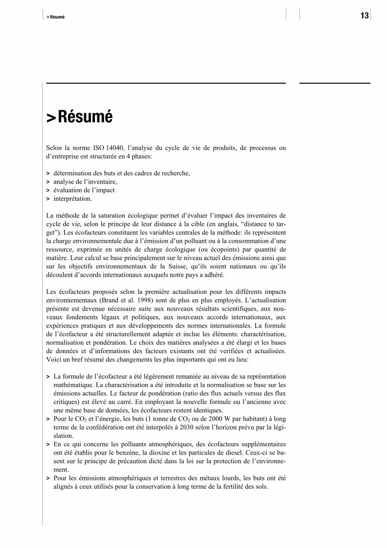
Aperçu des écofacteurs 2006
Le tableau suivant montre les écofacteurs selon la situation suisse. Des écofacteurs supplémentaires, définis par la normalisation, se trouvent dans les annexes de 2 à 5. La colonne «flux de normalisation» présente la situation actuelle des émissions. La colon-ne «flux actuel» sert de référence et est la plupart du temps égale au flux de normali-sation. La colonne des «flux critiques» représente les buts politiques. Si le flux critique est supérieur au flux actuel, la situation actuelle correspond au but politique.
> Résumé 15
Tab. A > Aperçu des écofacteurs 2006
Flux de normalisation Flux actuel Flux critique Ecofacteur 2006 UBP par
Emissions dans l’air
CO2 53 034 000 t CO2-eq 45 436 000 11 183 000 ¹ t CO2 0.31 g CO2-eq Substances appauvrissant la couche d’ozone
391 t R11-eq 391 188 t R11-eq 11 000 g R11-eq
NMVOC 116 000 t 116 000 81 000 t 18 g NOx 91 000 t 91 000 45 000 t 45 g NH3 (en N) 44 000 t 44 000 25 000 t 70 g N SO2 19 000 t SO2-eq 19 000 25 000 t 30 g SO2-eq PM2.5–10 22 000 t 9 255 5 048 ² t 150 g PM2.5 22 000 t 12 745 6 952 ² t 150 g Particules de diesel 3 400 t 3 400 450 t 17 000 g Benzène 1 055 t 1 055 525 t 3 800 g Dioxines et Furanes 67.5 g 67.5 34.5 g 5.7E+10 g Plomb 91 t 91 58 ³ t 27 000 g Cadmium 2.00 t 2.00 2.08 ³ t 460 000 g Mercure 1.02 t 1.02 2.22 t 210 000 g Zinc 560 t 560 359 ³ t 4 400 g
Emissions dans les eaux de surface
Azote (comme N) 31 360 t 24 827 17 510 t 64 g N Phosphore (en P) 1 694 t 28.6 20 mg/m³ 1 200 g P DCO 47 700 t 47 700 144 000 t 2.3 g Arsenic 8.6 t 10.5 40 mg/kg 8 000 g Plomb 32 t 38 100 mg/kg 4 400 g Cadmium 0.61 t 0.42 1.0 mg/kg 290 000 g Chrome 25 t 44 100 mg/kg 7 600 g Cuivre 74 t 51 50 mg/kg 14 000 g Nickel 84 t 38 50 mg/kg 6 800 g Mercure 0.20 t 0.21 0.50 mg/kg 880 000 g Zinc 167 t 182 200 mg/kg 5 000 g Emissions radioactives 2 000 GBq C14-eq 96 64.1 TBq 1 100 kBq C14-eq AOX (en Cl-) 288 t 288 1 200 t 200 g Cl Chloroforme 1.5 t 0.04 0.60 mg/m³ 1 500 g HAP 0.144 t 0.004 0.1 mg/m³ 11 000 g benzo[a]pyrène 0.048 t 0.001 0.01 mg/m³ 210 000 g Perturbateurs endocriniens 5.0 kg E2-eq 5.0 24.0 kg E2-eq 8 700 000 g E2-eq
Emissions dans les eaux souterraines
Azote (en N) 34 000 t 34 000 17 000 t 120 g N

The Ecological Scarcity Method – Eco-Factors 2006 FOEN 2009 16
Flux de normalisation Flux actuel Flux critique Ecofacteur 2006 UBP par
Emissions dans le sol
Plomb 79.9 t 30.3 19.4 g/ha.a 31 000 g Cadmium 2.98 t 1.25 1.30 g/ha.a 310 000 g Cuivre 120 t 73.4 58.0 g/ha.a 13 000 g Zinc 870 t 473 303 g/ha.a 2 800 g Pesticides 1 507 t PSM-eq 1 577 1 500 t 730 g PSM-eq
Ressources
Source d’énergie primaire 1 030 PJ-eq 1 169 636 ¹ PJ 3.3 MJ-eq Affectation des sols, agglomération 3 378 km².a-eq 2 791 3 224 km².a 220 m²a-eq Eaux douces suisses 2.57 km³ 2.57 10.7 km³ 22 m³ Eaux douces OCDE 2.57 km³ 1 020 2 040 km³ 97 m³ Gravier 34 000 000 t 34 000 000 34 000 000 t 0.029 g
Déchets
C dans les décharges 97 410 t 97 410 79 420 t 15 g C Déchets spéciaux dans les déchar-ges souterraines
36 900 t 36 900 36 900 t 27 g
Déchets fortement radioactifs 218 m³ 218 109 m³ 18 000 cm³ Déchets faiblement et moyennement radioactif
1 230 m³ 1 230 615 m³ 3 300 cm³
¹ Valeur calculée par interpolation entre les buts pour 2010 et 2050 ² Valeur deduite du flux critique PM10 et en partie de PM2.5 ³ Valeur calculée de la relation entre flux actuel et flux critique des émissions dans le sol. Cadre temporel: les chiffres sont basées sur les données disponibles en 2006. Précision des données: Les flux ne sont pas arrondis, pour faciliter leurs traçabilité dans les publications sources. Les facteurs de pondération, par contre, sont arrondis à deux chiffres significatifs.

> Summary 17
> Summary
According to ISO Standard 14040, the life cycle assessment (LCA) of products, processes or companies comprises four phases:
> Goal and scope definition > Inventory analysis > Impact assessment and > Interpretation.
The “ecological scarcity” method permits impact assessment of life cycle inventories according to the “distance to target” principle. Eco-factors, expressed as eco-points per unit of pollutant emission or resource extraction, are the key parameter used by the method. With that method, eco-factors are determined by the current emissions situa-tion and, secondly, by the political targets set by Switzerland or by international policy and supported by Switzerland. The method was first published in 1990.
The eco-factors proposed for various environmental impacts in the first update of the method (Brand et al. 1998) are used widely. The fresh update presented here became necessary to reflect new scientific findings, new statutory and political targets, new international agreements, developments in international standarization and experience gathered in practice. As a part of this revision, the eco-factor formula has been adjusted to the structure of the ISO standard (with its elements of charactization, normalization and weighting). The set of substances assessed has been further enlarged. The data and information on which the existing eco-factors were based was checked and updated. The key changes made are as follows:
> The mathematical representation of the ecofactor formula has been slightly modi-fied. The characterization step is now made explicit. In addition, normalization is now based on current emissions, as has become common practice. As a consequence the weighting factor (ratio of current to critical flow) is squared. With both the old and new formula representation, the resulting eco-factors remain identical if the data is the same.
> With regard to CO2 and energy, the long-term target of the Swiss confederation (1 tonne CO2 or 2000 W per capita) was interpolated for the year 2030, which is a common time horizon of Swiss legislation.
> With regard to air pollutants, new eco-factors were determined for benzene, dioxin and diesel soot, based on the precautionary principle enshrined in the Swiss Environmental Protection Act.
> For heavy metal emissions (both to air and to soil), the long-term maintenance of soil fertility is now used as the new target.
> Eco-factors can now be defined according to regional scarcities, if needed and if regional data are available. This principle is applied to phosphorus and emissions to Swiss surface waters.

The Ecological Scarcity Method – Eco-Factors 2006 FOEN 2009 18
> Recent reesearch findings allow the establishment of an eco-factor (incl. characteri-zation) for endocrine disruptors (measured as oestrogen activity) in waters. Account is thus taken for the first time of micropollutants in waters, an issue that is gaining importance.
> A further new feature is that eco-factors can be established for discharges of radioactive isotopes to the seas (again including characterization); this is based on international agreements for the protection of the North Sea.
> In some parts of the world freshwater is a scarce resource. Therefore new eco-factors have been introduced that are oriented to the regional scarcity of this resource.
> In Switzerland, extractable gravel reserves are becoming decreasing scarce (due to permissible land uses). A new eco-factor for gravel was therefore introduced.
> New eco-factors were introduced for land use. Characterization is based on the impacts of land uses upon plant biodiversity.
> A new feature concerning the assessment of bioreactive landfills is that the wastes consigned to them are assessed on the basis of their carbon content. Previously, landfill types were assessed on the basis of landfill volume; this practice has been discontinued. Landfill volume is now only used to assess the final storage of radioactive wastes and underground disposal of hazardous wastes.
Overview of eco-factors for 2006
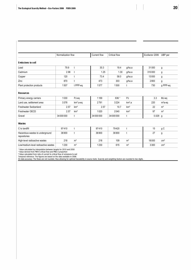
The following table lists the eco-factors according to the Swiss situation. Annexes A2 to A5 present the factors for further substances determined by characterization. The “normalization flow” column states today’s emission situation (in accordance with the data available in 2006). The “current flow” column presents the reference quan-tity, which in most cases is identical to the normalization flow. The “critical flow” column represents the political target. If the critical flow is larger than the current flow, then today’s situation is in accordance with the target.

> Summary 19
Tab. A > Overview of eco-factors for 2006 Normalization flow Current flow Critical flow Ecofactor 2006 UBP per
Emissions to air
CO2 53 034 000 t CO2-eq 45 436 000 11 183 000 ¹ t CO2 0.31 g CO2-eq Ozone-depleting substances 391 t R11-eq 391 188 t R11-eq 11 000 g R11-eq NMVOC 116 000 t 116 000 81 000 t 18 g NOx 91 000 t 91 000 45 000 t 45 g NH3 (as N) 44 000 t 44 000 25 000 t 70 g N SO2 19 000 t SO2-eq 19 000 25 000 t 30 g SO2-eq PM2.5–10 22 000 t 9 255 5 048 ² t 150 g PM2.5 22 000 t 12 745 6 952 ² t 150 g Diesel soot 3 400 t 3 400 450 t 17 000 g Benzene 1 055 t 1 055 525 t 3 800 g Dioxins and Furans 67.5 g 67.5 34.5 g 5.7E+10 g Lead 91 t 91 58 ³ t 27 000 g Cadmium 2.00 t 2.00 2.08 ³ t 460 000 g Mercury 1.02 t 1.02 2.22 t 210 000 g Zinc 560 t 560 359 ³ t 4 400 g
Emissions to surface waters
Nitrogen (as N) 31 360 t 24 827 17 510 t 64 g N Phosphorus (as P) 1 694 t 28.6 20 mg/m³ 1 200 g P COD 47 700 t 47 700 144 000 t 2.3 g Arsenic 8.6 t 10.5 40 mg/kg 8 000 g Lead 32 t 38 100 mg/kg 4 400 g Cadmium 0.61 t 0.42 1.0 mg/kg 290 000 g Chromium 25 t 44 100 mg/kg 7 600 g Copper 74 t 51 50 mg/kg 14 000 g Nickel 84 t 38 50 mg/kg 6 800 g Mercury 0.20 t 0.21 0.50 mg/kg 880 000 g Zinc 167 t 182 200 mg/kg 5 000 g Radioactive emissions 2 000 GBq C14-eq 96 64.1 TBq 1 100 kBq C14-eq AOX (as Cl-) 288 t 288 1 200 t 200 g Cl Chloroform 1.5 t 0.04 0.60 mg/m³ 1 500 g PAHs 0.144 t 0.004 0.1 mg/m³ 11 000 g Benzo(a)pyrene 0.048 t 0.001 0.01 mg/m³ 210 000 g Endocrine disruptors 5.0 kg E2-eq 5.0 24.0 kg E2-eq 8 700 000 g E2-eq
Emissions to groundwater
Nitrogen (as N) 34 000 t 34 000 17 000 t 120 g N
The Ecological Scarcity Method – Eco-Factors 2006 FOEN 2009 20
Normalization flow Current flow Critical flow Ecofactor 2006 UBP per
Emissions to soil
Lead 79.9 t 30.3 19.4 g/ha.a 31 000 g Cadmium 2.98 t 1.25 1.30 g/ha.a 310 000 g Copper 120 t 73.4 58.0 g/ha.a 13 000 g Zinc 870 t 473 303 g/ha.a 2 800 g Plant protection products 1 507 t PPP-eq 1 577 1 500 t 730 g PPP-eq
Resources
Primary energy carriers 1 030 PJ-eq 1 169 636 ¹ PJ 3.3 MJ-eq Land use, settlement area 3 378 km².a-eq 2 791 3 224 km².a 220 m²a-eq Freshwater Switzerland 2.57 km³ 2.57 10.7 km³ 22 m³ Freshwater OECD 2.57 km³ 1 020 2 040 km³ 97 m³ Gravel 34 000 000 t 34 000 000 34 000 000 t 0.029 g
Wastes
C to landfill 97 410 t 97 410 79 420 t 15 g C Hazardous wastes to underground repositories
36 900 t 36 900 36 900 t 27 g
High-level radioactive wastes 218 m³ 218 109 m³ 18 000 cm³ Low/medium-level radioactive wastes 1 230 m³ 1 230 615 m³ 3 300 cm³ ¹ Value calculated by interpolation between targets for 2010 and 2050 ² Value derived from PM10 critical flow and PM2.5 proportion ³ Value calculated from ratio of current to critical flow of emissions to soil Temporal reference: The figures are based on the data available in 2006. On data accuracy: The flows are not rounded, thus allowing for optimal traceability in source texts. Scarcity and weighting factors are rounded to two digits.

> Synoptic overview 21
> Synoptic overview
Introduction
The Swiss Mineral Oil Tax Ordinance1 amended as per 1 July 2008 states: “For tax relief to apply to fuels from renewable resources, proof must be furnished that these fuels meet the minimum criteria for positive aggregate environmental impact.” This is the first time that life cycle assessment (LCA) of a product – in this case of “biogenic” fuels – is required explicitly at the level of a statutory ordinance. As it can be expected that the growing importance of LCA will generate greater interest in the underlying methodology beyond expert circles, the Swiss Federal Office for the Environment (FOEN) has produced this synoptic overview in order to make accessible to an inter-ested public the content of the technical publication “Life Cycle Assessment: The Ecological Scarcity Method – Eco-Factors 2006” (“Ökobilanzen: Methode der ökolo-gischen Knappheit – Ökofaktoren 2006” (Öbu SR 28/2008)). The first part of this abridged version presents the life cycle assessment method, while the second part explains the general procedure by which eco-factors are derived. The third and largest part discusses the individual pollutants and resources rated with an eco-factor.
Life cycle assessment
Life cycle assessment (LCA) is a decision-support tool for companies, organizations and public authorities wishing to analyse the environmental aspects of processes, products, sites or entire companies. LCA studies can be used to identify the environ-mental relevance of processes and the potential to optimize them, deliver the funda-mentals for decisions on which options to choose, furnish evidence of environmental performance, and raise awareness of environmental issues among participants and stakeholders. An LCA records and assesses the environmental impacts arising through-out the life cycle of a product. The life cycle encompasses the extraction of resources, their processing to semi-finished goods, the manufacture of products, their use across their service life, and the final disposal or recycling processes. Transports required between the individual life cycle stages are also taken into account. LCA studies are preformed in the following four steps:
1. Definition of the goal and scope of the study The goal of the study is defined, for instance to produce a comparison of returnable and non-returnable mineral water packaging. The definition of the functional unit and the question of system boundaries are essential when defining the scope of the study: What is an appropriate and fair basis for the comparison? How far does the study of the subject go? Are, for instance, the construction of the factory and the manufacture of the machinery taken into account? How is the recycling of packag-
1 Mineralölsteuerverordnung (MinöStV) of 20 November 1996 (amended as per 1 July 2008). The details of the criteria are regulated in the
DETEC Ordinance on Proof of the Positive Aggregate Environmental Impact of Fuels from Renewable Feedstocks – Biofuels Life Cycle Assessment Ordinance, BLCAO (Verordnung des UVEK über den Nachweis der positiven ökologischen Gesamtbilanz von Treibstoffen aus erneuerbaren Rohstoffen – Treibstoff-Ökobilanzverordnung, TrÖbiV).
The Ecological Scarcity Method – Eco-Factors 2006 FOEN 2009 22
ing materials modelled? Which impact assessment methods are chosen to quantify the environmental impacts related to returnable and non-returnable packaging sys-tems? The assumptions made and constraints imposed upon the study are made ex-plicit in this step.
2. Generation of a life cycle inventory Inventory analysis records the quantities of resources, semi-finished products, en-ergy carriers and services required and the pollutants released by each individual process required to manufacture a product. The outcome of this analysis could for instance be that the manufacture of the product under review releases, among other things, 130 kg carbon dioxide (CO2), 3 kg methane (CH4) and 45 grams of nitrogen oxides (NOx) across the entire life cycle. To produce an inventory analysis it is nec-essary to collect detailed environmental and product data, which are often listed in datasets of life cycle inventory databases.
3. Assessment of impacts In the impact assessment step, the findings of the inventory analysis are assessed with regard to their environmental and health impacts. This is done in several sub-steps. The resource consumption and pollutant emissions identified in the inventory analysis can be aggregated to a single or several indicators by means of assessment factors applying classification, characterisation, normalisation and weighting or just classification and characterisation. In the first substep, classification, resources ex-tracted and pollutants emitted are classified according to the environmental impacts caused. For instance, carbon dioxide and methane are grouped in the “climate change” category. In the second substep, characterisation, the relative contribution of the substances grouped in one class is quantified relative to a reference substance. For instance, the relative global warming potential of the different greenhouse gases (carbon dioxide and methane in the above example) is determined and added on the basis of a uniform metric (CO2-equivalents in the present case). In our example, the climate change impact is 199 kg CO2-equivalents (applying the following charac-terisation factors: 1 kg CO2-equivalents per kg CO2 and 23 kg CO2-equivalents per kg methane). In a third step, normalisation, characterised environmental impacts caused by a product are put in relation to the total impacts occurring worldwide, in a region (Europe) or a nation (Switzerland). These impacts may be expressed as annual totals or on an annual per capita basis (resulting in 0.02 person years, applying 10 tons CO2-equivalents per year and person). Finally, the normalised impacts caused by a product are further aggregated using weighting factors.
4. Interpretation and recommendation for action Indicators and aggregate environmental impacts quantified using a common metric can be compared to alternative products or processes, or to company LCAs per-formed previously. The results can be used to derive a recommendation in line with the targets set (e.g. for a decision on which option to choose, or for a process opti-mization), or to provide evidence of environmental performance (e.g. reduction of greenhouse gas emissions). Sensitivity analyses are carried out to test the robustness of the results, and contribution analyses help to identify environmental hot spots.

> Synoptic overview 23
Eco-factors
The ecological scarcity method weights environmental impacts – pollutant emissions and resource consumption – by applying “eco-factors”. The eco-factor of a substance is derived from environmental law or corresponding political targets. The more the current level of emissions or consumption of resources exceeds the environmental protection target set, the greater the eco-factor becomes, expressed in eco-points (EP). An eco-factor is essentially derived from three elements (in accordance with ISO Standard 14044): characterization, normalization and weighting.
Characterization captures the relative harmfulness of a pollutant emission or resource extraction vis-à-vis a reference substance within a given impact category (global warming potential, acidification potential, radioactivity etc.). The factors are based upon scientific findings. For instance, the radiative forcing (global warming potential) of methane (CH4) is 23 times higher than that of carbon dioxide (CO2). Sulphur hexafluoride (SF6), which is used to insulate electric components, even has a global warming potential 22 000 times that of CO2. It is common practice to express the characterized quantity in equivalents of the reference substance. In the case of green-house gases, these are CO2-equivalents (CO2-eq). Methane has a characterization factor of 23 kg CO2-eq, meaning that 1 kg methane has the same impact as 23 kg CO2, and accordingly the eco-factor is 23 times that of CO2.
Normalization quantifies the contribution of a unit of pollutant or resource use to the total current load/pressure in a region (in this case the whole of Switzerland) per year. If, for instance, 100 000 tonnes of a substance are released annually, then the contribu-tion of 10 grams is small. If, in contrast, only 70 grams are released in total, then the same contribution of 10 grams is very large. The smaller the normalization flow, the larger the eco-factor will tend to be.
Weighting expresses the relationship between the current pollutant emission or re-source consumption (current flow) and the politically determined emission or con-sumption targets (critical flow). The more the overall load of a substance exceeds the politically determined critical flow, i.e. the environmental protection target, the more eco-points are assigned per unit (e.g. gram) to a substance. Any growth of the current flow leads to exponential growth of the weighting factor, as does any reduction in the critical flow (tightening of legal/political targets). Any reduction in the current flow or any increase in the critical flow (due to a relaxation of environmental targets) leads to an exponential reduction of the weighting factor.
The following formula governs calculation of the eco-factor:
{ {Constant
Weighting
2
k
ionNormalizat
n(optional)
zationCharacteric
FF
FEP1K factor-coE ⋅⎟⎟
⎠
⎞⎜⎜⎝
⎛⋅
⋅⋅=
321321
Eco-factor

The Ecological Scarcity Method – Eco-Factors 2006 FOEN 2009 24
K = Characterization factor of a pollutant or of a resource Fn = Normalization flow: Current annual flow, with Switzerland as
system boundary F = Current flow: Current annual flow in the reference area Fk = Critical flow: Critical annual flow in the reference area c = Constant (1012/a): Serves to obtain readily presentable
numerical quantities EP = Eco-point: The unit of environmental impact assessed
“Flow” refers to the load of a pollutant, the quantity of a resource consumed, or the level of an environmental impact characterized.
If the eco-factors are applied to production processes abroad, it needs to be taken into account that the given eco-factors weight every emission as if it were taking place in Switzerland. Thus, the actual level of emissions remaining constant, shifting a process to another country does not affect the impact assessment result. Where required and where data availability permits, eco-factors can be regionalized. For instance, an agricultural product produced in North Africa is then assessed with a regional weight-ing term (current flow in region over critical flow for region, e.g. freshwater consump-tion) and a normalization to Swiss conditions (normalization flow for Switzerland). This makes it possible to conduct an assessment of the regional scarcity situation in a manner permitting comparison with the Swiss eco-factors. The present publication contains the data for assessing water use abroad. For certain pollutants whose loads vary greatly from site to site, such as phosphorus emitted to surface waters, a regional differentiation can be performed within Switzerland in the same manner.
One and the same pollutant can generate different environmental impacts. It follows that different eco-factors based upon different political targets could be assigned to that pollutant. For instance, ammonia emissions to air could be assessed on the basis of an explicit reduction target for nitrogen or, alternatively, on the basis of their acidification potential. In such cases the principle applied is that assessment is based on the strict-est political target and thus the highest eco-factor is used.
Depending upon whether a certain pollutant is emitted to water, air or soil, different eco-factors may result depending upon the specific political and statutory emission targets. Hence in some cases the same pollutant is addressed in several contexts in the following; this applies notably to the heavy metals.
A principle in preparing LCA studies is that every emission only scores once. This takes place when a substance first crosses the boundary from the anthropo-technosphere to the natural environment (or vice versa in the case of resource extrac-tion). Further substance and material flows within the natural environment – including substances that originated in the anthroposphere – are not taken into account, as other-wise these would be counted double.
A characterization is acceptable under the terms of this methodology if it is in line with the intention of the legislator. Moreover, the characterization should be scientifi-

> Synoptic overview 25
cally recognized and it should be possible to derive it from political targets. In the case of greenhouse gases, only the CO2 reduction target is enshrined in law, but the inten-tion of the legislator is to contribute to limiting global climate change. It is therefore appropriate in this case to differentiate according to global warming potential and to assign a characterization factor to each individual substance. In the case of volatile organic compounds (NMVOCs), in contrast, characterization is not appropriate, be-cause the legislator has imposed a uniform levy upon all pollutants in this category (the Swiss VOC levy).
Assessing emissions and resources
The following sections briefly set out the environmental and health impacts of the pollutant emissions and resource extractions assessed. They further present emission sources, the derivation of critical flows from statutory texts, emission and consumption trends, and differences to earlier assessments. The synoptic table contained in the “Summary” section of the full publication provides a reference listing the figures for current and critical flows and the eco-factors. Reference is made to the corresponding sections of the full publication for more detailed data.
The selection of substances is guided by their environmental and political relevance. As environmental policy has by no means set targets for all substances, the selection of environmental impacts assessed is limited. Hence no assessment is provided of emis-sions that have little environmental relevance in Switzerland and Europe (e.g. sulphate in waters) or for which not enough knowledge is available (e.g. noise).
Substances are classified according to the environmental compartment they enter when leaving the anthropo-technosphere. This synopsis of the publication presents emissions to air, waters and soil, then assesses resource extractions and, finally, the landfilling and underground storage of wastes.
Emissions to air
The airborne pollutants assessed with an eco-factor were selected according to their environmental relevance for the whole of Switzerland. Air pollution control measures have led to a drop in emissions in recent years. Thus in some cases impacts within Switzerland are of subordinate importance. It needs to be taken into account, however, that the eco-factors are applied not only to Swiss processes, but also to processes taking place abroad. An eco-factor is therefore retained for substances which may be unprob-lematic in Switzerland, but have the potential to continue to be environmentally rele-vant abroad.
Modelling shows that the global mean temperature can be expected to rise by 1.4 to 5.8 °C between 1990 and 2100, and the sea level can be expected to rise by 10 to 90 cm. Moreover, more extreme weather events are anticipated, and more precipitation or greater aridity depending upon region. This is caused by the human-induced ampli-fication of the greenhouse effect. Reducing greenhouse gas emissions is therefore a priority target of Swiss environmental policy. 86 % of the impact of greenhouse gas
CO2 and further greenhouse gases

The Ecological Scarcity Method – Eco-Factors 2006 FOEN 2009 26
emissions is attributable to carbon dioxide (CO2), around 7 % to methane (CH4) and some 6 % to nitrous oxide (N2O). Although the global warming potential of chlorinated and fluorinated hydrocarbons and of sulphur hexafluoride (SF6) can, as such, be several thousand times greater than that of CO2, in Switzerland their contribution to the im-pacts is small (slightly above 1 %) – their current flow is relatively small.
The Swiss CO2 Act stipulates a reduction by 10 % from the 1990 level for fuels. This would result in a critical flow of 36.96 million t CO2 per year. The Swiss Federal Council (Bundesrat) envisages the “2000 watt society” as a long-term target, which implies a maximum emission of 1 t CO2 per person and year. The resulting target would be 8.06 million t CO2 for the year 2050, given the anticipated population at that time. To calculate the critical flow, these two emission targets are interpolated to a time horizon to 2030. This results in an eco-factor that is higher by half than that determined in 1997.
CO2-equivalents (abbreviated to CO2-eq) are used as the metric for all climate-relevant emissions. The global warming potential of the other greenhouse gases can be deter-mined via characterization factors (see Table 8, Section 3.2.6).
The ozone layer is located in the stratosphere, at an altitude between 15 and 50 km. This layer protects life on Earth from a part of the ultraviolet radiation of the sun. Volatile substances containing chlorine and/or bromine atoms cause depletion of the ozone layer. The resultant elevated UV radiation causes an increase in skin cancers and eye diseases in humans, and is mutagenic in all organisms.
The most important ozone-depleting substances are CFCs (chlorofluorocarbons), halons and carbon tetrachloride (CCl4). HCFCs (partially halogenated CFCs) have the same effect, but in a significantly weaker form. At the same time, CFCs and HCFCs are contributors to human-induced climate change. If a substance is both a greenhouse gas and an ozone-depleting substance, then the higher of the two eco-factors is used.
A substance labelled internationally as R11 provides the reference. The eco-factors of the other ozone-depleting substances can be determined by means of characterization factors (see Section 3.3.6, Table 14) and are expressed as R11-equivalents (R11-eq).
The new eco-factor is substantially larger than that of 1997. This is partly because measured data have now replaced earlier estimates. A further reason is that an absolute ban on ozone-depleting substances will enter into force in the foreseeable future, leading to a smaller critical flow.
Non-methane volatile organic compounds (NMVOCs) comprise volatile organic compounds (VOCs) with the exception of the greenhouse gas methane. VOCs include largely harmless as well as highly toxic and carcinogenic compounds. NMVOCs are important precursors to ground-level ozone (also known as summer smog), which can harm human health and plants. Some individual VOCs – such as benzene and dioxins – receive their own specific eco-factors because of their great harmfulness to human health.
Ozone-depleting substances
Volatile organic compounds (NMVOCs)

> Synoptic overview 27
The introduction of the Swiss VOC levy in 2000, together with increasingly strict emission rules for vehicles, has contributed to a steep reduction in emissions. As the current flow has been reduced and the critical flow has remained unchanged, the eco-factor is significantly below that of 1997. The trend towards lower emissions is ex-pected to continue.
Nitrogen oxides are formed above all when fossil energy carriers are burnt. Transport is the main source, accounting for 58 % of emissions in 2000. Further sources of nitro-gen oxides include construction machines and agricultural and silvicultural machines (12 %), combustion facilities/furnaces (6 %) and commercial and industrial processes (24 %). Nitrogen loads cause soils and waters to acidify. This severely endangers sensitive ecosystems. Moreover, it promotes nitrophilous plants, which can lead to a reduction of plant diversity and to the loss of ecologically valuable ecosystems such as oligotrophic grassland and open submerged swards.
Nitrogen dioxide (NO2) and the secondary particles formed from nitrogen oxides are particularly harmful to human health. They can cause respiratory tract diseases or cardiac arrhythmia, and can reduce life expectancy. Nitrogen oxides are important precursors in the formation of ground-level ozone, which in turn impairs health.
Measures adopted since 1985 have succeeded in reducing NOx emissions significantly. However, to comply with limit values emissions still need to be reduced by some 60 %. The planned tightening of rules will then lead to a further drop. The eco-factor is one-third lower than in 1997, as the current flow has dropped while the critical flow has remained the same.
Ammonia is formed in livestock management and when mineral nitrogen fertilizers are applied. Agriculture is the main generator of emissions, accounting for 93 %. Because of its nitrogen content, ammonia contributes to the acidification and over-fertilization of soils and waters. Its mode of effect is similar to that of nitrogen oxides (see above).
The critical flow corresponds to the target set in 2005 by the Swiss Federal Commis-sion for Air Hygiene, which in turn corresponds to the lower value of the range of targets set in 1999 by the Swiss Federal Council (Bundesrat). The critical flow is thus set slightly lower than in 1997, while the current flow has dropped significantly. A slightly smaller eco-factor results.
Sulphur dioxide leads to respiratory tract diseases. Through its acidifying effect it also damages plants, sensitive ecosystems and built structures. Moreover, SO2 is an impor-tant precursor of acid precipitation and of aerosols.
Determination of the critical flow is based on the international Sulphur Protocol, which has been ratified by Switzerland. The protocol sets an emissions target which corre-sponds to a reduction of 78 % from the 1980 baseline. The eco-factor for SO2 is sig-nificantly smaller than in 1997, which is attributable to the reduction in current SO2 emissions with the critical flow remaining constant.
Nitrogen oxides (NOX)
Ammonia (NH3)
Sulphur dioxide (SO2) and further acidifying substances
The Ecological Scarcity Method – Eco-Factors 2006 FOEN 2009 28
Sulphur dioxide makes by far the largest contribution to acidification. Specific eco-factors can be determined by means of characterization factors for further acidifying substances such as hydrogen fluoride, phosphoric acid and hydrogen sulphide (see Section 3.7.6, Table 20).
PM10 is a mixture of soot, resuspended road dust, particles from the abrasion of pav-ings and tyres and substances attached to these (sulphate, nitrate, ammonium, organic carbon). PM is the abbreviation of “particulate matter”, while the number gives the size of the particles (in micrometres). PM10 means that the particle size is below 10 mi-crometres. PM10 can enter the lung because of the small size of the particles. Numer-ous studies prove the correlation between PM10 levels in ambient air and complaints and diseases of the respiratory tract.
The harmfulness of the particles depends upon their size and composition. PM2.5–10 (size between 2.5 and 10 micrometres) can cause coughing, asthma attacks and other diseases of the respiratory tract. PM2.5 (size < 2.5 micrometres) remains in the lung much longer and accumulates there, as it is not readily coughed up. It can cause cardiac arrhythmia and cardiovascular diseases. Diesel soot particles, which count among the ultrafine particles (PM0.1), can enter the bloodstream and the lymphatic system via the lung. They are considered carcinogenic and are thus particularly hazardous to human health.
Although it must be assumed that PM2.5 is more harmful than PM2.5–10, the legisla-tor has not distinguished between the two. A distinction is made, in contrast, between PM10 and diesel soot. Accordingly, in addition to the previous eco-factor for PM10, a new one for diesel soot has been introduced. The critical flow for PM10 was deter-mined on the basis of the limit values established by the Swiss Federal Ordinance on Air Pollution Control (Luftreinhalteverordnung). While PM10 emissions have dropped since 1997, the eco-factor is nonetheless higher because of the lower critical flow. No threshold value has been established for diesel soot, but the Ordinance on Air Pollution Control requires that as much is done to reduce emissions of carcinogenic substances as technology and operating conditions will allow, providing this is economically acceptable (precautionary principle). The introduction of stricter standards and the possibility of using particle filters results in the critical flow stated in the table. Because of the major human health impact of diesel soot particles, the eco-factor for diesel soot is 100 times higher than that for PM10.
Benzene enters the atmosphere when mineral oil products are burnt. Small quantities of the substance are already contained in crude oil, and further benzene is formed during refining. Motorized transport is the source of three-quarters of all benzene emissions in Switzerland.
Benzene is taken into the body via the respiratory tract, and is stored in fatty tissue. As women have a higher body fat ratio than men, the impacts of this pollutant are greater for women. There is unequivocal evidence that benzene harms blood formation and that long-term exposure can lead to leukaemia. Furthermore, it must be assumed that benzene is mutagenic.
PM10 and diesel soot
Benzene

> Synoptic overview 29
Even small quantities of benzene are harmful to human health. According to FOEN benzene emissions would need to be brought down to 100 t per year if the acceptable risk is not to be exceeded. This reduction target is not achievable today by measures that are economically acceptable and feasible in terms of technology and operating conditions. Reduction targets for specific emission sources for the years 2010 and 2030 are therefore used to determine the critical flow. The new eco-factor is 100 times higher than in the earlier assessment, when benzene was classed as an NMVOC; this is justified in view of its carcinogenic effect.
Polychlorinated dibenzodioxins and dibenzofurans (PCDD and PCDF, usually simply termed dioxins and furans) are chlorinated aromatic hydrocarbons. There are in total 76 polychlorinated dioxins and 135 polychlorinated furans. The substances differ in their numbers and positions of chlorine atoms. They are formed in technological but also in natural combustion processes in the presence of chlorine. They accumulate in the food chain and some are highly toxic to humans and animals. Dioxins impair embryonal development in several ways. In particular, they appear to give rise to miscarriage, deformity of (genital) organs, and intellectual deficits.
As a result of continuous improvements in flue gas purification in industry, the burning of wastes and treated wood in private households will become the main source of emissions in the near future in relative terms. Applying the precautionary principle – under which the measures that are technologically and operationally feasible and economically acceptable are the standard – it is possible to halve the current flow. The critical flow was set accordingly. The eco-factor for dioxins and furans is very high. This is an expression of the low emission quantities in the order of several grams per year, and further reflects the great harmfulness of these substances and the available reduction options.
Lead emissions damage animals and plants. Lead harms soil fertility and accumulates in food chains. In humans it can impair blood formation and can cause developmental disorders in children.
Because lead was blended into petrol from the 1950s onwards, lead emissions rose sharply. This trend has reversed thanks to the emergence of unleaded petrol from 1970 onwards. Further uses of lead include batteries, paints and lead for bullets. The pres-ently remaining emissions are caused largely by waste incineration plants and the steel industry.
A new feature of the present eco-factor is that it is derived from soil protection targets – this approach is based on statements made in the Swiss Federal Ordinance on Air Pollution Control. Heavy metal emissions to air that are finally deposited and enter the soil are weighted in the same way as direct lead emissions to soil. This new derivation results in an eco-factor that is around ten times higher than the previous one.
Dioxins and furans
Lead
The Ecological Scarcity Method – Eco-Factors 2006 FOEN 2009 30
Cadmium is taken in mainly via the respiratory tract. Even small quantities are toxic to humans and animals if exposure is chronic. The heavy metal accumulates in the body, where it can cause cancer and disturbs storage of other, vital metals. The consequences of chronic cadmium exposure can include diseases of the respiratory tract, kidney damage, and anaemia due to iron deficiency. Moreover, cadmium is toxic to plants and microorganisms and impairs soil fertility.
As a result of measures implemented in waste incineration and in the metal industry to reduce airborne emissions, cadmium emissions have dropped significantly since 1980. The main applications of cadmium were alloys and the production of dry batteries and colouring pigments. Today, the use of cadmium is banned for many applications.
No critical flow can be derived from the ambient limit values set by the Swiss Federal Ordinance on Air Pollution Control. Therefore, as in the case of lead, a critical flow is derived from soil protection targets. Despite a trend towards lower emissions, the new derivation results in an eco-factor that is about four times higher than the 1997 eco-factor.
Mercury is highly toxic to humans and animals. It is taken in via the respiratory tract and accumulates in various organs. It is also toxic to plants and microorganisms and impairs soil fertility. Industry and commerce are the principal generators of mercury emissions. Emissions have dropped steadily in recent years; no further reduction is expected.
The strictest target of the Swiss Federal Council is to reduce emissions to the level of 1950. This value is taken as the critical flow. The eco-factor has almost doubled from 1997.
Zinc exposure impairs plant growth. While emissions from industry and commerce are dropping, those from road transport are rising. Tyre and road wear is the main source of emissions, presently accounting for two-thirds. If the trend towards increasing zinc emissions from transport persists, it is to be expected that overall emissions will rise again.
No critical flow can be derived from the ambient limit values of the Air Pollution Control Ordinance. Therefore, as in the case of lead, a critical flow is derived from soil protection targets. The new derivation results in an eco-factor that is more than eight times higher compared to the previous eco-factor.
Emissions to surface waters
The eco-factors used to weight emissions to surface waters are based on loads that apply to the whole of Switzerland, and thus reflect an average situation. To perform an exact appraisal, it is necessary to take account of regional circumstances, notably the size of water bodies affected, which in view of the volume of work involved has only been performed for phosphorus. Separate eco-factors have been determined for emis-sions to groundwater.
Cadmium
Mercury
Zinc
> Synoptic overview 31
Effluent treatment measures have led to a drop in emissions in the last decades. Thus in some cases impacts within Switzerland are of lesser importance. It needs to be taken into account, however, that the eco-factors are applied not only to Swiss processes, but also to processes taking place abroad. An eco-factor is therefore retained for substances which may be unproblematic in Switzerland, but have the potential to continue to be environmentally relevant abroad. This is the case if pollutant emissions are regulated by the international agreements on the protection of the Rhine or of the North Sea to which Switzerland is a signatory.
The sources of nitrogen emissions to waters are fertilizers from agriculture and efflu-ents from industry, commerce and households. More than 90 % of anthropogenic total nitrogen inputs to surface waters consist of nitrate and ammonium or ammonia. Nitro-gen loading is not a general problem anymore in Switzerland in ecological terms. It remains a concern in the North Sea, however, where its consequences – elevated algal growth and fish mortality (see phosphorus) – are issues.
Although the contribution of Switzerland to overall pollution of the Rhine is small, Switzerland has signed the declaration of intent of North Sea states. This envisages halving phosphorus and nitrogen inputs from the 1985 baseline. The target envisaged for 1995 has not yet been achieved to this day for nitrogen. The reduction achieved by 2003 was 29 %. The target is taken as the basis for setting the critical flow for total nitrogen. The eco-factor for nitrogen has dropped slightly, as nitrogen loading has been reduced substantially since 1997.
Elevated phosphorus loads lead to elevated algal growth in lakes and seas. Decomposi-tion of dead algae in the deep water layers requires oxygen, which is then not available to other organisms. Oxygen deficiency and fish mortality result. Phosphorus (or phos-phate) enters waters mainly through erosion and runoff from arable land. As a result, lakes in areas where agriculture is intensive are affected most severely.
The above-mentioned target of halving inputs to the North Sea has been achieved for phosphorus, but the protection target for Swiss lakes, in contrast, has not yet been achieved throughout the country. The loads of individual lakes vary widely, so that a regional differentiation was performed (see Table 33, Section 4.3.4).
The connection of households and commercial enterprises to sewage treatment plants and the ban on phosphates in textile detergents have succeeded in greatly reducing phosphorus loading over the last two decades. In agriculture, too, the situation has improved slightly, as in integrated agricultural production only the amount of phospho-rus can be applied that is taken up by the crops. As a result, phosphorus concentrations have dropped even in the most severely polluted lakes. This relaxation of the phospho-rus problem results in a substantially lower eco-factor.
In principle, all organic substances exert pressure on waters by requiring oxygen for their decomposition which is then no longer available to the fauna. A part of the or-ganic matter comes from natural sources, and another from effluents. The principle is established in law that the organic matter arising in effluent must be reduced to the
Nitrogen (N)
Phosphorus (P)
Organic matter (COD)

The Ecological Scarcity Method – Eco-Factors 2006 FOEN 2009 32
extent that no ecological detriment results for waters. In view of the available oxygen levels in waters, the residual load coming from effluent treatment facilities is non-critical in most cases. The toxicity of many organic substances is therefore of greater ecological relevance; this, however, is not taken into account here.
The critical flow can be derived from the Swiss Water Protection Ordinance, which requires that the organic matter arising in effluent is reduced to a level at which no ecological detriment results for waters. From an ecological perspective, downstream from the points of discharge of effluents organic matter should consume a maximum of 30 % of the average quantity of oxygen dissolved in water. The critical flow can thus be calculated on the basis of total runoff. Chemical oxygen demand (COD) is generally taken as the metric for the concentration of organic matter in waters. Other measures can be converted into COD values (see Table 35, Section 4.4.4).
Broad-scale effluent treatment, in combination with provisions governing effluent discharges, have led to a reduction of organic matter in waters. As a result of the lower current flow, the eco-factor is lower than in 1997.
Heavy metals and arsenic damage the aquatic ecosystem by accumulating in organ-isms, where they can cause growth impairments and metabolic disturbances. They propagate through the food chain. In Switzerland these substances are not a serious problem in the concentrations observed. If arsenic is ingested over long periods through drinking water, it can promote cancers of the skin and of the urinary bladder, but also other forms of cancer.
The Water Protection Ordinance sets limit values for seven environmentally relevant heavy metals: lead (Pb), cadmium (Cd), chromium (Cr), copper (Cu), nickel (Ni), mercury (Hg) and zinc (Zn). The Convention on the Protection of the Rhine, to which Switzerland is a signatory, sets stricter standards for heavy metals, so that these are taken as the basis for calculating the critical flow. The resultant eco-factors are sub-stantially higher than those of 1997.
One possible effect of radioactive radiation is to disturb or destroy the cell functions of organisms (somatic effects), which can cause cancer. Another potential effect is to change the genes of the cells (mutagenic effects). The eco-factor takes account of these two effects. It does not take account of the effects of radioactive radiation upon ecosys-tems, nor of the potential impacts of accident-related releases of large quantities of radioactive substances.
The emissions of Swiss nuclear power plants are well below the limit values. The eco-factor set out here refers only to the discharge of radioactivity to seawater by the reprocessing plants at La Hague (F) and Sellafield (GB), where fuel elements from Swiss nuclear power plants were reprocessed until July 2006. This eco-factor is defined for the first time here, as the reduction targets for the protection of the North Sea supported by Switzerland were only defined in recent years. Table 41 (Section 4.6.7) lists eco-factors for inputs of selected isotopes to the sea.
Arsenic and heavy metals
Radioactive emissions
> Synoptic overview 33
AOXs are a sum parameter of adsorbable organic halogenated substances that can be of both human and natural origin. They include substances such as chlorinated non-aromatic hydrocarbons (e.g. chloroform), chlorinated aromatic hydrocarbons, poly-chlorinated biphenyls (PCBs) and certain pesticides. Pulp production is a major source of AOX emissions. Overall, AOX contamination of surface waters in Switzerland has declined substantially in recent years.
The environmental impact of the compounds grouped as AOXs varies widely. How-ever, subdividing AOXs into distinct, homogeneous substance classes or even individ-ual substances would only be practicable to a limited extent. A single eco-factor for all AOXs is therefore a necessary compromise. As AOXs now only play a minor role in water resources protection, a more exact determination is not of prime concern. A separate eco-factor is only derived for chloroform.
An important criterion of toxicity is the propensity of a substance to accumulate in organisms. The more highly chlorinated a substance is, the more toxic it is. The eco-factor is therefore defined in relation to chlorine, i.e. it rises in step with the number of chlorine atoms.
The international association of waterworks in the Rhine catchment area IAWR has set a non-legally-binding emissions target for AOXs, which corresponds to the standards required for potable water supply. This provides a basis for calculating the critical flow. As the current flow has dropped while the critical flow has remained the same, the eco-factor is lower than in 1997.
Chloroform is a substance within the AOX group that was formerly in widespread use. It was used as a dry-cleaning agent, and as a solvent and disinfectant. Chloroform is considered potentially carcinogenic and is banned today, with very few exemptions. As a result, loads have dropped substantially. The weighting factor is determined from the measured current concentration and the critical concentration. The critical concentra-tion results from the target value established by the Convention on the Protection of the Rhine. The resulting new eco-factor for chloroform is several times higher than that for the other AOXs.
PAH emissions are the result of combustion processes and of abrasion particles being washed from roads. Some PAHs are highly toxic and carcinogenic. As they occur exclusively in suspended matter, their distribution depends upon the concentration of suspended solids in waters. The most frequent PAHs are compiled in Annex 3.
Previously there was no eco-factor for PAHs as the available data did not suffice. The weighting factor is calculated from the measured current concentration and the critical concentration in accordance with the target value established by the agreement on the protection of the Rhine. The eco-factor reflects the harmfulness of certain PAHs and the small quantities discharged to waters.
Adsorbable organic halogens (AOXs)
Chloroform
Polycyclic aromatic hydrocarbons (PAHs)

The Ecological Scarcity Method – Eco-Factors 2006 FOEN 2009 34
A separate eco-factor is established for benzo(a)pyrene. All other PAHs are assessed using a generic PAH eco-factor, as the available data does not suffice to conduct a further characterization of individual substances.
BaP is a PAH (see above). It is formed in the incomplete combustion of organic mate-rial, e.g. in furnaces and engines, but also in cigarettes. BaP pollution in waters stems largely from wood preservatives containing creosote, for instance from railway sleep-ers. Today, the use of creosote is only permitted – with restrictions – for commercial applications. BaP is certainly carcinogenic in animals, and probably in humans. The procedure for deriving the eco-factor is analogous to that for the other PAHs. Its eco-factor is about twice that of the other PAHs; this is justified because BaP is highly toxic and carcinogenic.
Hormones are chemical messengers between tissues and cells that regulate processes in the body. Endocrine disruptors are hormonally active exogenous substances with the capacity to disrupt the hormone system (also termed endocrine system). They are already effective in small quantities. As hormonal processes are similar in many organ-isms, a single endocrine disruptor can impact upon very many different organisms. Fertility disturbances have been proven in numerous aquatic and terrestrial animal species. Concentrations of endocrine disruptors that cause feminization effects in male fishes have been found close to the discharge points of sewage treatment plants. This disrupts via the food chain the reproductive capacity of, for instance, the otter Lutra lutra, which has led to the species becoming severely endangered in Switzerland. In humans, substances that disrupt the reproductive endocrine system are considered responsible for developmental abnormalities of embryos, reduced fertility, and breast, testicular and prostate cancer. Intake of the substances can be via the digestive system, the skin or the lungs.
A hormonally active effect is attributed to a broad range of chemicals. It has been proven for the following substances: natural and artificial oestrogens, various pesti-cides containing organochlorine compounds, certain industrial chemicals used in plastics, various dioxins and furans, organotin compounds from anti-fouling ship paints among other sources, and certain UV filter substances contained in sun lotions. It must be expected that many substances have not yet been identified as endocrine disruptors, as many of the chemicals presently on the market have not yet been tested for their hormonally active effect.
As no statutory limit values have yet been established for endocrine disruptors, calcula-tion of the eco-factor uses a target value below which expert judgement holds that no chronic effects should occur. Assessment of endocrine disruptors takes the oestrogen potential of E2 (17-oestradiol) as reference. The eco-factors of further endocrine disruptors can be determined by means of characterisation factors shown in Table 50 (Section 4.11.6.).
Benzo(a)pyrene (BaP)
Endocrine disruptors

> Synoptic overview 35
Emissions to groundwater
Strict quality standards apply to Swiss groundwater, as 80 % of drinking water comes from this source. The eco-factors only assess nitrate because this is the only substance for which quantifiable data is presently available. In addition, however, plant protec-tion products and volatile halogenated hydrocarbons are relevant groundwater con-taminants to which quantified standards apply (plant protection products exceed the standards set by the Swiss Water Protection Ordinance at some 10 % of the monitoring wells operated by the Swiss groundwater monitoring system; the standards for volatile halogenated hydrocarbons are exceeded at around 7 % of the wells).
The main source of nitrate pollution is nitrogen fertilizer applied to fields, which is readily washed out from the soil into groundwater. In areas where farming practices are intensive, nitrate concentrations in groundwater are measured that exceed the 25 mg/l limit set by the Swiss Water Protection Ordinance, and in some cases even exceed the 40 mg/l tolerance value for drinking water. FOEN calls for the nitrate flow of 1990 to be halved; this delivers the critical flow. In contrast to nitrate in surface waters, nitrate in groundwater continues to be problematic; the eco-factor is thus higher than the eco-factor for nitrogen loading of surface waters, but has not changed from 1997.
Emissions to soil
The aim of the various statutes adopted at national level is to maintain soil fertility over the long term. In addition to the pollutant loads addressed in this section, soil fertility is also endangered by the paving-over of soils, by erosion, and by compaction due to machine use. These factors are assessed partly via the “land use” eco-factor.
The quality of soils in Switzerland is impaired by various substance-related impacts. These include acidification, overfertilization and loading with heavy metals and or-ganic pollutants. Soils are polluted on the one hand directly by substance inputs from plant protection and fertilization activities, but also indirectly through the deposition of airborne pollutants (heavy metals, nitrogen). Non-point airborne inputs to soils are assessed at the point of their emission to air.
Substance loads generated by agriculture are inventoried at the point where they no longer contribute to agricultural use of soils. For nitrate this is when it is washed into the groundwater, for phosphate when eroded or washed into surface waters, and for ammonia and nitrous oxide when emitted to air. These substances are therefore treated in the corresponding sections. As a result, the present section only addresses heavy metals and plant protection products, as these are already pollutants when they enter the soil.
Nitrogen (nitrate)

The Ecological Scarcity Method – Eco-Factors 2006 FOEN 2009 36
Heavy metals impair plant growth and disturb soil fertility. Because plants can build available heavy metals into their biomass, these accumulate in food chains. If heavy metals are ingested at high doses and over longer periods, this can lead to chronic poisoning. Cleaning up soils contaminated with heavy metals requires major resource inputs.
In order to maintain soil fertility over the long term, the article specifying the purpose of the Swiss Soil Pollution Ordinance states that no accumulation of heavy metals in soils must occur, meaning that inputs can at most be equal to outputs from soil. The calculation of current loads was based on spot-check measurements. This new manner of derivation leads to substantially higher eco-factors for the above-mentioned heavy metals, as the eco-factor now only applies for non-settlement areas. The increase is most striking for lead, which is due to the rather generous ambient limit values previ-ously set. Copper and zinc have an almost identical eco-factor. For cadmium – the current flow is smaller than the critical flow – the increase in the eco-factor compared to 1997 is minor.
Plant protection products include crop protectants and plant growth regulators, as well as postharvest protection products. These can be substances, preparations, organisms or other agents. The eco-factor assessment only addresses chemical-synthetic plant pro-tection products. These are applied above all in open arable farming, and in fruit grow-ing and viticulture.
The associated environmental problems are a function of the primary effects, the quantities and rates of degradation of the active agents, and the types and behaviour of degradation products and residues. They can have unintended adverse effects upon biodiversity in the areas on which they are applied, also affecting spiders, myriapoda and birds. Because plant protection products are dispersed directly or with the wind by being attached to soil particles, they are also detectable in mountain lakes and in rain-fall. Human health impacts arise notably in drinking water use.
The Swiss Federal Office for Agriculture had set itself the target of reducing the appli-cation of plant protection products by 30 % by the year 2005 from the 1990/1992 baseline. The use of novel plant protection products that are effective in small quanti-ties, in combination with extensification programmes and the expansion of organic farming practices, has led to a marked drop in consumption, resulting in a slightly lower eco-factor. That trend will continue.
Characterization is performed with reference to the standard dose of an average plant protection product (PPP) applied in Switzerland, the PPP-equivalent (PPP-eq). The 20 active agents most sold in Switzerland and the approximately 80 pesticides listed in the ecoinvent v1.2 life cycle inventory database are characterized (see the full list in Annex 4).
Heavy metals (lead, cadmium, copper, zinc)
Plant protection products

> Synoptic overview 37
Resources
In the past, the ecological scarcity approach only took account of the consumption of energy resources. Now, for the first time, it embraces further resources – namely freshwater, gravel and land use – as these are increasingly considered ecologically scarce. In addition, a further new feature is that a distinction is made in the energy resource category between renewable (limited rate of replenishment) and non-renewable (limited stock) energies. An eco-factor is assigned to renewable energies as it must be assumed that for them, too, there is an upper limit to use.
The long-term target of becoming a “2000 watt society”, as envisaged by the Swiss Federal Council, calls not only for a reduction in energy consumption, but also for an increase in the contribution made by renewable energy sources: Of the 2000 watts per person, 1500 are to come from renewable sources. As a consequence renewable ener-gies need to supply three times more energy than the non-renewable sources. It follows from this political evaluation that 3 MJ of energy from renewable sources are rated with the same weight as 1 MJ from non-renewable sources. The weight assigned to non-renewable energies is appreciably higher than in the past, while renewable ener-gies retain practically the same value. The eco-factor for renewable energy, which was previously only applied to hydropower, now also applies to all other types of energy production. In a manner similar to the approach taken for greenhouse gases, an interim target is interpolated for the year 2030 on the basis of the long-term target to be achieved by 2050.
The overview table states the average eco-factor for non-renewable energy resources in EP/MJ-eq, while Table 65 (Section 7.2.7) lists in detail the individual primary energy carriers. The eco-factor for energy consumption only assesses the scarcity of the energy resource. The other environmental impacts generated by the emissions from energy use are captured by means of the eco-factors for emissions to air, water and soil.
Land-use statistics break down the area of Switzerland, which totals 41 286 km², into the following types of use: settlement and urban areas (buildings, transportation areas, recreational and open green spaces, landfills, building sites), agriculturally utilized areas (grassland, arable land, orchards), wooded areas (forest, shrub forest, woods), unproductive areas (rock, ice, lakes, rivers, glaciers).
The overall settlement area is growing at a rate of around one square metre per second, mostly at the expense of agricultural land in the Swiss plateau (the Mittelland region of Switzerland). This is driven by a growing population, in combination with growing levels of land take per person. The target of the Swiss government set out in the 2002 strategy for a sustainable Switzerland is to meet further demand wherever possible by means of inward development, i.e. improved utilization of existing settlement areas. Sparing use should be made of soils, and action should be taken to counter urban sprawl. Specifically, for a future population of 8.06 million, settlement area is to be stabilized over the longer term at a level of 400 m² per inhabitant. This delivers the critical flow.
Energy resources
Land use

The Ecological Scarcity Method – Eco-Factors 2006 FOEN 2009 38
Land use is characterized in terms of the plant diversity of a land-use type. The “set-tlement area” land-use type taken as basis for characterization is a mixture of highly disparate types of area, ranging from urban green spaces to industrial estates. The metric is the settlement area utilized during a year (settlement-area-and-year equiva-lent, SA*a-eq). Land-use forms exhibiting great plant diversity, such as agricultural fallows or forest margins, are assigned a negative impact factor in view of their posi-tive environmental effect. Table 67 (Section 7.3.6) states the eco-factors of selected individual land-use types, while Annex 5 provides the full list.
Gravel in mineral deposits is an important material for the formation and protection of groundwater. Gravel extracted from deposits is used mainly in the construction indus-try, especially as a concrete aggregate and in road and railway subgrades. Gravel resources are replenished very slowly: Only around 1 % of Switzerland’s annual gravel consumption is formed anew in rivers in the same period. Moreover, the quality of gravel deposits differs widely, and the extractable quantity is much smaller than the resource. Hence an eco-factor was newly introduced.
As the quantity extracted annually ranges between 30 and 40 million tonnes, the gravel reserves designated for extraction in Switzerland suffice for 15 to 20 years. Although the resource is finite, the current quantity extracted is tolerated by the responsible cantonal spatial planning authorities. The critical flow thus corresponds to the current flow. The eco-factor for gravel, now set for the first time, captures a special case in the realm of land-use concerns: the level of gravel extraction that is legally and environ-mentally acceptable.
Switzerland is in the fortunate position of commanding over more than enough clean water. Nonetheless, in its 2002 strategy for a sustainable Switzerland, the Swiss Fed-eral Council, noting the global freshwater problems, calls for sparing use of this re-source, too, for Switzerland.
Freshwater is scarce in some regions of the world, while in others there is a surplus. Eco-factors are determined on the one hand for specific countries (for Switzerland and further OECD states), and on the other hand for six different scarcity situations (low, moderate, medium, high, very high and extreme). This permits – depending upon the life cycle inventory available from case to case – a highly differentiated analysis. It is thus possible for the first time – for instance in life cycle assessments of foods – to take account of the actually observed water scarcity in a region of origin. When required to explore specific issues, users of the method can themselves derive regional or local eco-factors. If, in contrast, water consumption data is not available with a sufficient degree of differentiation, the average for OECD countries, which is also calculated here, can be used as a first approximation.
In accordance with the OECD procedure, the scarcity of freshwater resources is meas-ured as the share of gross consumption in the available renewable water resource. Gross consumption comprises drinking water requirements and water extractions for agricultural irrigation and industrial processes. The available renewable resource is calculated from annual precipitation on the area of the state, plus inflows from
Gravel
Freshwater

> Synoptic overview 39
neighbouring states, minus evaporation. The OECD considers a moderate to medium pressure on water resources to be tolerable. On that basis, the critical flow is set as being a gross water consumption that amounts to 20 % of the available renewable freshwater resource.
The annual available water resource in Switzerland is 53.5 km³. The tolerable pressure on Swiss water resources is 20 % of the available resource, which amounts to 10.7 km³ per year. Gross consumption in Switzerland is 2.57 km³ per year (around 350 m³ per capita and year or 1000 litres per capita and day), which corresponds to just below 5 % of the available renewable water resource. Although there is thus no water scarcity in Switzerland, local water shortages can arise in summer. The eco-factor stated here does not capture such temporarily and spatially limited situations.
The available renewable resources of all OECD states total 10 300 km³ per year. The tolerable pressure on water resources is 2050 km³ per year. Gross consumption is 1020 km³, which is just below 10 % of the available renewable resource. While in general this translates into a “low” level of water scarcity, the eco-factor for the aver-age of all OECD states is nonetheless higher than that for Switzerland by a factor of 5. Annex 6 lists the data and eco-factors for the individual OECD states.
Numerous other countries have “low” to “medium” water scarcity, corresponding to eco-factors spanning a factor of around 40. In contrast, there is almost a factor of 1000 between the eco-factors in the “low” and “extreme” categories. This reflects the severe over-exploitation in arid regions such as Saudi-Arabia, where more freshwater (espe-cially groundwater) is utilized than is available from precipitation and inflows. Table 72 (Section 7.5.5) lists the eco-factors for the categories of the scarcity scale, while Table 74 (Section 7.5.7) classes a representative selection of states on that scale.
Wastes
In the following, we discuss the eco-factor for substances in aboveground bioreactive landfills, for hazardous wastes stored underground, and for radioactive wastes.
The Environmental Protection Act stipulates that wastes with a potential to cause long-term problems must not be stored in landfills in Switzerland. The indicator for the reaction potential of waste is its carbon (C) content, which should be kept as low as possible. Wastes deposited in aboveground landfills are therefore assessed on the basis of their carbon content. Slags contain an estimated 4 % C, while the average for other wastes consigned to bioreactive landfills is 15 %. 661 500 tonnes of slags are consigned annually to such landfills, plus 473 000 tonnes of other wastes. The current C flow can be calculated from these figures.
According to FOEN, the target for the C content in bioreactive landfill wastes is 7 %, from which the critical flow can be determined. The eco-factor is listed here for the first time. Wastes consigned to landfills for inert materials or to landfills for stabilized residues contain practically no reactive organic material, and are not taken into account in the annual flows on which the eco-factor is based.
Carbon in bioreactive landfills

The Ecological Scarcity Method – Eco-Factors 2006 FOEN 2009 40
There are no underground landfills in Switzerland. Of the 1.1 million tonnes of hazard-ous wastes arising annually, 90 % are treated within the country. Around one-third is incinerated. The remainder is either recycled, consigned to physical-chemical treatment or stored in a landfill for stabilized residues.
The remaining 10 % of hazardous wastes are exported. Of this, in turn, one-third is made up of the filter dusts from municipal solid waste incineration plants, which are stored in underground landfills. As these wastes cannot be stored expediently within Switzerland, the current flow is tolerated and is equated with the critical flow for weighting purposes. The present eco-factor, which is slightly higher than that of 1997, relates exclusively to these stored hazardous wastes.
Electricity produced by nuclear power plants generates radioactive wastes that must eventually be consigned to final storage. The hazardousness of radioactive wastes depends upon their persistence (half-life), and on the type and intensity of their radia-tion. The Swiss strategy for a final repository classes radioactive wastes in two catego-ries:
1. Short-lived low-level and medium-level wastes present a low degree of hazard after a relatively short period. A necessary shut-in time of 500 years is anticipated.
2. Long-lived medium-level wastes (LMLW), high-level wastes (HLW) and spent fuel elements must be stored safely for at least 100 000 years.
The Swiss Nuclear Power Act establishes that radioactive wastes arising in Switzerland must be disposed of within the country. No decision on a site for the required final repository is to be expected in the near future.
Including the encasement materials and assuming that the service lives of nuclear power plants are extended from 40 to 60 years, around 8300 m³ spent fuel elements, around 1000 m³ HLW from reprocessing and 3460–7260 m³ LMLW will arise in Switzerland. Overall, therefore, the deep repository will need to accept around 16 000 m³ long-lived high-level and medium-level radioactive wastes. Storage volume in the order of 115 000 m³ is envisaged for the final storage of short-lived low-level and medium-level wastes, the bulk of which also comes from the operation and decommis-sioning of nuclear power plants.
There is no political consensus on the tolerable quantity of radioactive wastes. There would be an argument for setting the tolerable level at the level of the current flow, but also for setting it at zero. For the purposes of determining the eco-factor, the critical flow is set at half the current flow as a first approximation. This reflects the current situation, in which efforts are under way with regard to a final repository, but no specific construction project is in progress. The eco-factor has not changed from 1997 for short-lived low-level and medium-level wastes. For fuel elements, LMLW and HLW it has been re-assessed at 40 % of the previous value due to the larger expected volume of wastes as a result of the extension of the service lives of nuclear power plants by 50 %.
Hazardous wastes in underground landfills
Radioactive wastes in final repositories

> Synoptic overview 41
Noise
Noise pollution is an ubiquitous problem that severely affects the cities in particular. The main sources are road and rail vehicles, agricultural and silvicultural machines, aircraft, motorboats, building sites, shooting ranges and sports facilities. The Swiss Noise Abatement Ordinance defines the noise target that is to be achieved – in analogy to the precautionary principle – as what technology and operating conditions will allow providing this is economically acceptable. A further goal is that there should be no severe nuisance to the affected public.
The basic problem in assessing noise is that, in contrast to substance emissions, sound quickly dissipates and is therefore always locally contained. A further problem is that assessment can only be performed on the basis of the ambient situation, which, more-over, is conditioned by subjective perceptions. An assessment method has albeit been developed within the context of the ecological scarcity methodology for road traffic noise; this, however, is not readily transferable to noise from other sources and would, in its original form, lead to a one-sided assessment of road traffic. As there is thus no generally recognized method for assessing noise in life cycle assessments, no eco-factor was derived for the present.

The Ecological Scarcity Method – Eco-Factors 2006 FOEN 2009 42
1 > Introduction
1.1 Position of the ecological scarcity method in relation to life cycle assessment (LCA)
The ecological scarcity method makes it possible to weight environmental impacts within the context of a life cycle assessment of products, processes or entire organiza-tions (production sites, companies, etc.).
The method requires as input parameters the outcomes of a life cycle inventory analy-sis. The result is a weighting of these inventory analysis results, expressed as “eco-points” (EP). In other words, the inventory analysis parameters (e.g. CO2 emissions) are multiplied by the respective eco-factor (310 EP/kg CO2 in this case) in order to receive the eco-points of the parameters in question. These eco-points can then be added up to deliver an aggregate score.
For a company or other stakeholders, it can be highly informative to assess the envi-ronmental impacts of products or of a company in this manner, as the eco-points reflect the priorities of public environmental policy. The results of such an assessment can support decision-making in product development, and in management, procurement and consultancy.
1.2 Terminology
The method presented in this report is known under various names, including “ecologi-cal scarcity method”, “ecoscarcity method” and “eco-points method” (or, in German: Methode der ökologischen Knappheit, Methode BUWAL 133, Stoffflussmethode, Ökopunktmethode, UBP-Methode and others). In this publication, “ecological scarcity method” is used to designate the method. The established name for the measure of ecological scarcity is “eco-points” (EP; in German: Umweltbelastungspunkte, UBP).
1.3 Structure of the report
The report commences with a presentation of the fundamentals of the ecological scar-city method in Chapter 2. The formula used to calculate the eco-factors is explained, and further specified in sections on derivation rules (Section 2.2), on application (Sec-tion 2.3) and on data quality (Section 2.4). The derivations of the specific eco-factors are presented in Chapter 3 onwards, whereby the characterizations used are explained separately in the preceding Section 2.5.

1 > Introduction 43
The structure of the methodology chapter, and that of the sections on the individual eco-factors, is organized around the basic elements of the formula representation or calculation sequence. This results in the following structure:
1. Ecological relevance (only in the chapters on the individual eco-factors) 2. Characterization (insofar as applied) 3. Normalization 4. Weighting (with sections presenting the current and critical flows) 5. Eco-factor 6. Application guidance (where necessary)

The Ecological Scarcity Method – Eco-Factors 2006 FOEN 2009 44
2 > Methodological fundamentals
2.1 The ecological scarcity method
2.1.1 The basic principle
The ecological scarcity method is a “distance-to-target” method as defined by SETAC (Udo de Haes 1996). The method delivers standardized, generic weights.
Weighting is based primarily on environmental protection targets set at national level and, in some cases, international level. Such targets are
> ideally adopted in legally binding form or at least defined as targets by competent authorities,
> formulated by a democratically elected or legitimated body, > and oriented to sustainability as far as possible.
Weighting is conducted on the basis of the goals set by Swiss environmental policy; here – as in the determination of target values – local and global impact categories are converted to the Swiss level. The method can also be applied to other regions. Thus, for instance, eco-factors have already been developed for Holland, Norway, Sweden (Nordic Council of Ministers 1995, Table A22 / A23), Belgium (SGP 1994) and Japan (Miyazaki et al. 2004).
Through the manner in which the eco-factor is calculated, the ecological scarcity method permits optimization within the framework set by environmental policy targets.
The method converts the various environmental impacts into points, so that these values can be added and compared. The eco-factors thus have the formal nature of a utility value analysis, whereby they can be determined from the current environmental situation (current flow), the target situation aimed at by environmental policy (critical flow) and the calculation algorithm (see Section 2.1.3).

2 > Methodological fundamentals 45
2.1.2 Previous formula and derivation of the new formula representation
The ecological scarcity method was introduced by Müller-Wenk (1978) and refined for the first time by Braunschweig (1982). It was then further developed a second time in the context of the interpretation of the LCAs for packaging materials published by BUWAL, the precursor agency from which BAFU/FOEN emerged, in 1984 (Ahbe et al. 1990).
Ahbe et al. (1990) discussed various formulae that can be used to calculate eco-factors. The logistic function proposed by Braunschweig (1982) was replaced by a function in which the eco-factor (as a percentage of the critical flow) is proportionate to the ratio of the current to the critical flow. From this, the authors derived the following formula:
cFF
FEP 1factorEco
kk
⋅⋅=− (1)
F = Current flow: current annual pollutant load or resource extraction, in Switzerland
Fk = Critical flow: critical annual pollutant load or resource extraction, in Switzerland
c = 1012/a EP = Eco-point (the unit of the evaluated result)
In the update performed by Brand et al. (1998) the formula was retained unchanged. The following reasons have now prompted a mathematical reformulation and careful modernization of this formula:
> The international LCA Standard ISO 14042 prescribes the basic structure of impact assessment. As set out in Section 2.1.3, the aim is to largely comply with these pre-scriptions.
> Environmental concerns can vary greatly in time and place. This is, for instance, the case for the freshwater resource, which is very scarce in some regions of the world, but available in surplus in others. As there is no water scarcity in Switzerland, there was until now no eco-factor for the freshwater resource. As a result, these aspects, which may be of environmental relevance, could not yet be taken into account in LCA studies of foods and resources from arid regions (e.g. tomatoes from southern Spain, or cotton from India). The new formula permits both regional and temporal differentiation.
As the new representation is based on a mathematical reformulation, great continuity is ensured, whereby
> if the critical and current flows of a pollutant are unchanged, then the same eco-factor results from the revised formula as it did from the original formula,
> the linear dependence of the eco-factor (as a percentage of the critical flow) upon the ratio of the current to the critical flow remains,
Eco-factor
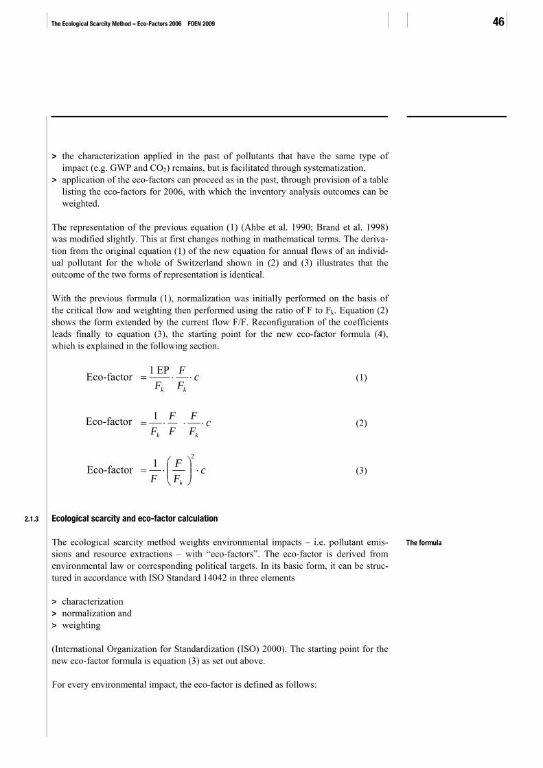
The Ecological Scarcity Method – Eco-Factors 2006 FOEN 2009 46
> the characterization applied in the past of pollutants that have the same type of impact (e.g. GWP and CO2) remains, but is facilitated through systematization,
> application of the eco-factors can proceed as in the past, through provision of a table listing the eco-factors for 2006, with which the inventory analysis outcomes can be weighted.
The representation of the previous equation (1) (Ahbe et al. 1990; Brand et al. 1998) was modified slightly. This at first changes nothing in mathematical terms. The deriva-tion from the original equation (1) of the new equation for annual flows of an individ-ual pollutant for the whole of Switzerland shown in (2) and (3) illustrates that the outcome of the two forms of representation is identical.
With the previous formula (1), normalization was initially performed on the basis of the critical flow and weighting then performed using the ratio of F to Fk. Equation (2) shows the form extended by the current flow F/F. Reconfiguration of the coefficients leads finally to equation (3), the starting point for the new eco-factor formula (4), which is explained in the following section.
cFF
F
kk
⋅⋅=EP1factor -Eco (1)
cFF
FF
F kk
⋅⋅⋅=1factor -Eco (2)
cFF
F k
⋅⎟⎟⎠
⎞⎜⎜⎝
⎛⋅=
21factor -Eco (3)
2.1.3 Ecological scarcity and eco-factor calculation
The ecological scarcity method weights environmental impacts – i.e. pollutant emis-sions and resource extractions – with “eco-factors”. The eco-factor is derived from environmental law or corresponding political targets. In its basic form, it can be struc-tured in accordance with ISO Standard 14042 in three elements
> characterization > normalization and > weighting
(International Organization for Standardization (ISO) 2000). The starting point for the new eco-factor formula is equation (3) as set out above.
For every environmental impact, the eco-factor is defined as follows:
The formula
Eco-factor
Eco-factor
Eco-factor
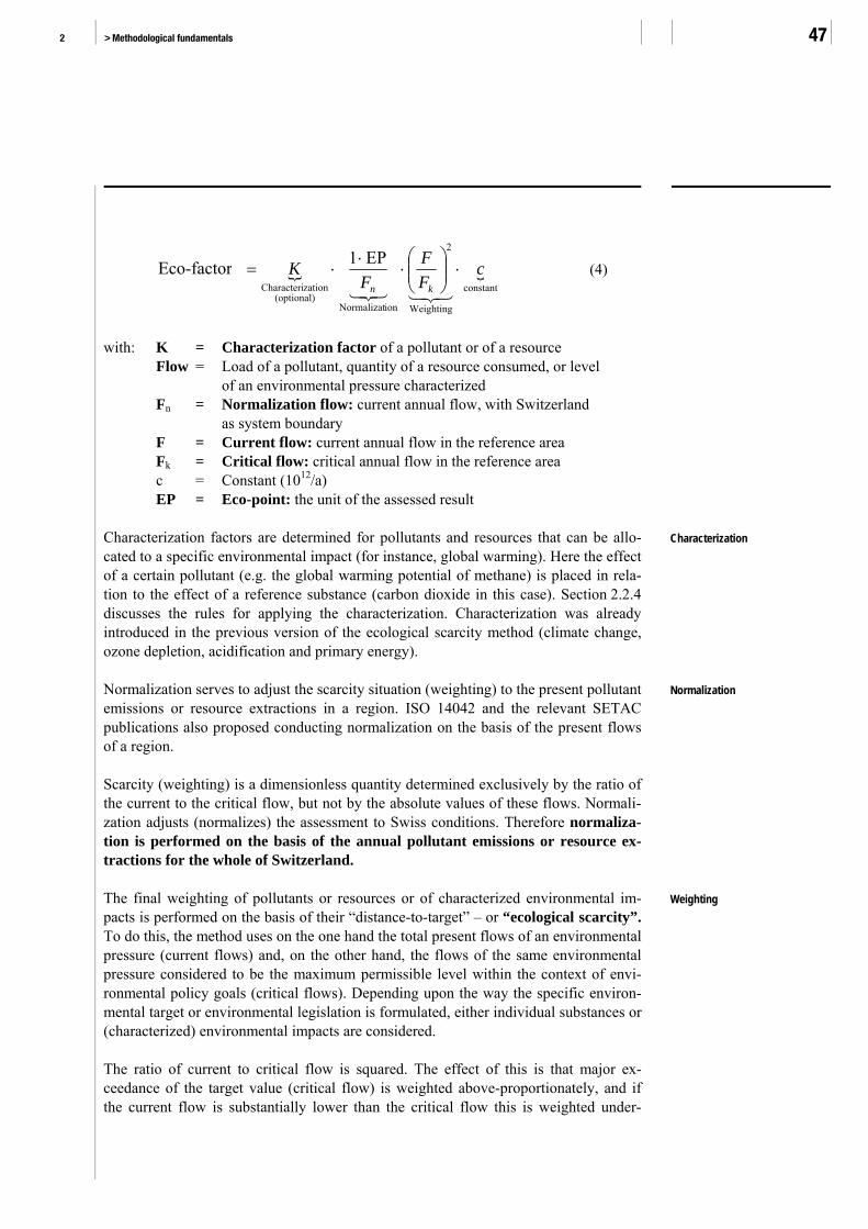
2 > Methodological fundamentals 47
{ {constant
Weighting
2
ionNormalizat(optional)
zationCharacteri
EP1factor -Eco cFF
FK
kn
⋅⎟⎟⎠
⎞⎜⎜⎝
⎛⋅
⋅⋅=
321321
(4)
with: K = Characterization factor of a pollutant or of a resource Flow = Load of a pollutant, quantity of a resource consumed, or level
of an environmental pressure characterized Fn = Normalization flow: current annual flow, with Switzerland
as system boundary F = Current flow: current annual flow in the reference area Fk = Critical flow: critical annual flow in the reference area c = Constant (1012/a) EP = Eco-point: the unit of the assessed result Characterization factors are determined for pollutants and resources that can be allo-cated to a specific environmental impact (for instance, global warming). Here the effect of a certain pollutant (e.g. the global warming potential of methane) is placed in rela-tion to the effect of a reference substance (carbon dioxide in this case). Section 2.2.4 discusses the rules for applying the characterization. Characterization was already introduced in the previous version of the ecological scarcity method (climate change, ozone depletion, acidification and primary energy).
Normalization serves to adjust the scarcity situation (weighting) to the present pollutant emissions or resource extractions in a region. ISO 14042 and the relevant SETAC publications also proposed conducting normalization on the basis of the present flows of a region.
Scarcity (weighting) is a dimensionless quantity determined exclusively by the ratio of the current to the critical flow, but not by the absolute values of these flows. Normali-zation adjusts (normalizes) the assessment to Swiss conditions. Therefore normaliza-tion is performed on the basis of the annual pollutant emissions or resource ex-tractions for the whole of Switzerland.
The final weighting of pollutants or resources or of characterized environmental im-pacts is performed on the basis of their “distance-to-target” – or “ecological scarcity”. To do this, the method uses on the one hand the total present flows of an environmental pressure (current flows) and, on the other hand, the flows of the same environmental pressure considered to be the maximum permissible level within the context of envi-ronmental policy goals (critical flows). Depending upon the way the specific environ-mental target or environmental legislation is formulated, either individual substances or (characterized) environmental impacts are considered.
The ratio of current to critical flow is squared. The effect of this is that major ex-ceedance of the target value (critical flow) is weighted above-proportionately, and if the current flow is substantially lower than the critical flow this is weighted under-
Characterization
Normalization
Weighting
Eco-factor

The Ecological Scarcity Method – Eco-Factors 2006 FOEN 2009 48
proportionately. This means that the higher the current impact already is, the more strongly every additional emission is weighted.
Weighting is a dimensionless quantity determined exclusively by the ratio of the current to critical flow. The absolute level of the flows has no influence whatsoever upon the weighting. Thus, regardless of whether, for instance, there is a current flow of 2000 t/a and a critical flow of 1000 t/a or of 6 and 3 kg/a respectively, an identical weighting factor will result. In both cases the ratio of the flows is 2:1, and the weight-ing factor is 4.
The factor c is identical for all eco-factors and serves to make the factor easier to present; it delivers more practicable orders of magnitude and takes account of the temporal dimension that remains from the quantitative units.
The unit in which the eco-factor is expressed is “eco-point (EP) per unit of environ-mental pressure”, e.g. “30 EP per gram SO2”, or “eco-points (EP) per unit of environ-mental impact”, e.g. “0.31 EP per gram CO2-equivalent”.
The new representation of the formula now makes it possible to determine eco-factors that are differentiated temporarily and spatially, and to determine eco-factors for sub-groups of certain pollutants – all of which are fully compatible with the basic scheme and with the annual eco-factors for Switzerland and can thus be combined seamlessly. The following sections present the options for differentiation.
2.1.4 Regionalization of eco-factors
The breakdown of the eco-factor into characterization, normalization and weighting terms now permits conversion from and to different regions. The weighting factor is calculated on the basis of the current and critical flows of a certain area. Normalization is performed on the basis of the current flow of the region to which the eco-factor is to apply, which, in our case, is Switzerland (see equation (5)). Equation (5) corresponds to equation (1) if Region 1 is identical to Switzerland.
cFF
FEPKfactorEco Region 1
k
Region 1
CHn
1 Region ⋅⎟⎟⎠
⎞⎜⎜⎝
⎛⋅
⋅⋅=−
21
(5)
with: K = Characterization factor of a pollutant or of a resource Fn
CH = Normalization flow: current annual load of a pollutant, quantity of a resource consumed or level of an environmental pressure characterized, with Switzerland as system boundary
F Region 1 = Current flow: current annual load of a pollutant, quantity of a resource consumed or level of an environmental pressure characterized, with Region 1 as system boundary
The constant
The eco-factor
Eco-factor

2 > Methodological fundamentals 49
FkRegion 1 = Critical flow: critical annual load of a pollutant, quantity
of a resource consumed or level of an environmental pressure characterized, with Region 1 as system boundary
c = 1012/a EP = Eco-point (the unit of the assessed result)
There are three ways in which this regionalized eco-factor calculation can be applied:
1. A weighting factor determined for a certain region can be normalized to Switzerland and thus integrated in the assessment. For instance, a regional weighting factor can be calculated for freshwater consumption in North Africa on the basis of the current and critical flows there. Account can thus be taken of the much greater scarcity of freshwater in North Africa compared to Switzerland. Normalization to the current Swiss flow results in an eco-factor compatible with Swiss eco-factors which repre-sents the scarcity situation in North Africa. Using this eco-factor, water consumption taking place in North Africa can now be assessed from a Swiss perspective.
2. Where environmental policy sets targets that vary greatly in terms of their spatial reference, eco-factors can be determined for smaller areas (e.g. regional or even site-specific factors) if substantially more critical situations arise that are not or insuffi-ciently captured with an average factor for the whole of Switzerland. For instance, the state of Swiss waters varies greatly. Lakes in the central plateau (Mittelland), such as the Greifensee or the Hallwilersee, have greater phosphorus pollution levels than, for instance, the Brienzersee or Lake Constance. Measures taken to improve the situation in lakes where pollution levels are previously higher lead to a greater reduction of environmental impacts.
3. In cases where Swiss environmental policy is guided by binding international objec-tives, weighting factors can be calculated for regions larger than Switzerland on the basis of these goals. Such weighting factors applying to, for instance, the European level, are then normalized to the Swiss situation. Thus, for instance, Switzerland has agreed with the North Sea states that nitrogen discharges to the North Sea be re-duced by half from 1985 levels.
If regionally specific eco-factors have been determined within Switzerland, then these should be used to calculate the average Swiss eco-factor. The weighted sum of the regional eco-factors is then formed. Equation (6) shows an example with two regions:
Eco-factorCH = Eco-factorRegion 1 * r1 + Eco-factorRegion 2 * r2. (6)
with: r1 = Share of the current flow of Region 1 in the current flow of the whole of Switzerland
r2 = Share of the current flow of Region 2 in the current flow of the whole of Switzerland
Through the quadratic function of the weighting factor, an eco-factor differentiated in this manner will tend to carry greater weight than the corresponding, uniform eco-factor. Spatial differentiation is thus not mathematically neutral, but gives greater weight to regions where environmental pressure is higher.

The Ecological Scarcity Method – Eco-Factors 2006 FOEN 2009 50
2.1.5 Temporal differentiation of eco-factors
In a similar fashion, the new formula representation permits temporal differentiation of weighting and thus of the eco-factor. For instance, a future assessment of noise could distinguish between different times of day. In the same vein, for certain airborne pollutants a distinction could be made for the current and critical flows in specific periods, such as the summer and winter halves of the year (cf. equation (7)).
cFF
FEPKfactorEco Period 1
k
Period 1
Yearn
1 Period ⋅⎟⎟⎠
⎞⎜⎜⎝
⎛⋅
⋅⋅=−
21
(7)
with: K = Characterization factor of a pollutant or of a resource Fn
Year = Normalization flow: current annual load of a pollutant, quantity of a resource consumed or level of an environmental pressure characterized, with Switzerland as system boundary
F Period 1 = Current flow: current load of a pollutant, quantity of a resource consumed or level of an environmental pressure characterized, during Period 1 (e.g. in daytime or in summer half of year), with Switzerland as system boundary
FkPeriod 1 = Critical flow: critical load of a pollutant, quantity of a resource
consumed or level of an environmental pressure characterized, during Period 1 (e.g. in daytime or in summer half of year), with Switzerland as system boundary
c = 1012/a EP = Eco-points (the unit of the assessed result)
The resulting eco-factors can then in turn be weighted, and aggregated to form a daily or annual average. This is illustrated for the example of two periods:
Eco-factorYear = Eco-factorPeriod 1 * p1 +Eco-factorPeriod 2 * p2 (8)
with: p1 = Share of the current flow of Period 1 in the annual current flow p2 = Share of the current flow of Period 2 in the annual current flow
The formula can be used for every kind of temporal differentiation; a breakdown into any number of periods would also be conceivable, such as four periods in accordance with the four seasons of the year.
Here again, as in regional differentiation, situations in which the current flow is sub-stantially above the critical flow are weighted over-proportionately stronger due to the squared weighting factor. Therefore an annual eco-factor calculated on the basis of temporally differentiated eco-factors is not the same as an eco-factor determined on the basis of annual loads.
Eco-factor
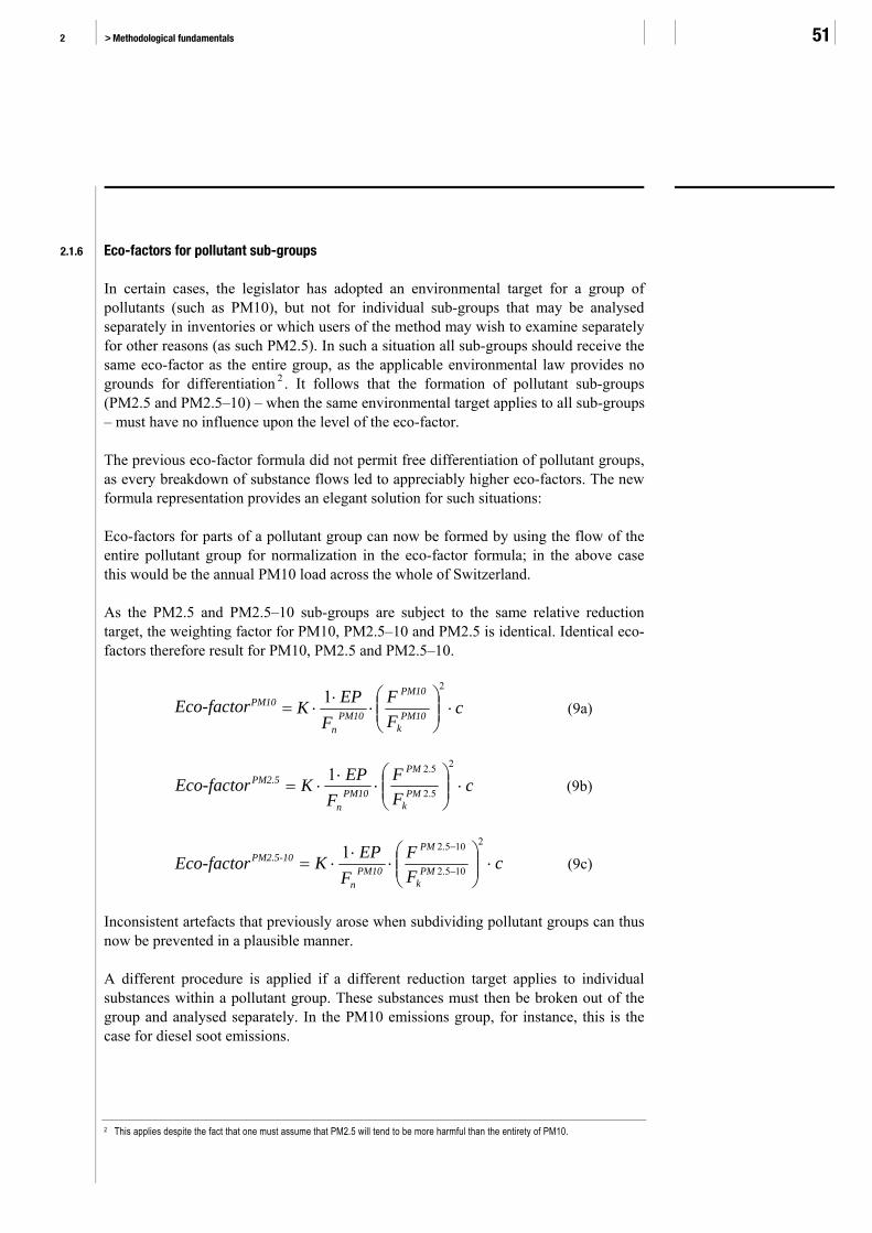
2 > Methodological fundamentals 51
2.1.6 Eco-factors for pollutant sub-groups
In certain cases, the legislator has adopted an environmental target for a group of pollutants (such as PM10), but not for individual sub-groups that may be analysed separately in inventories or which users of the method may wish to examine separately for other reasons (as such PM2.5). In such a situation all sub-groups should receive the same eco-factor as the entire group, as the applicable environmental law provides no grounds for differentiation 2 . It follows that the formation of pollutant sub-groups (PM2.5 and PM2.5–10) – when the same environmental target applies to all sub-groups – must have no influence upon the level of the eco-factor.
The previous eco-factor formula did not permit free differentiation of pollutant groups, as every breakdown of substance flows led to appreciably higher eco-factors. The new formula representation provides an elegant solution for such situations:
Eco-factors for parts of a pollutant group can now be formed by using the flow of the entire pollutant group for normalization in the eco-factor formula; in the above case this would be the annual PM10 load across the whole of Switzerland.
As the PM2.5 and PM2.5–10 sub-groups are subject to the same relative reduction target, the weighting factor for PM10, PM2.5–10 and PM2.5 is identical. Identical eco-factors therefore result for PM10, PM2.5 and PM2.5–10.
cFF
FEPKfactorEco PM10
k
PM10
PM10n
PM10 ⋅⎟⎟⎠
⎞⎜⎜⎝
⎛⋅
⋅⋅=−
21
(9a)
cFF
FEPKfactorEco PM
k
PM
PM10n
PM2.5 ⋅⎟⎟⎠
⎞⎜⎜⎝
⎛⋅
⋅⋅=−
2
5.2
5.21 (9b)
cFF
FEPKfactorEco PM
k
PM
PM10n
10-PM2.5 ⋅⎟⎟⎠
⎞⎜⎜⎝
⎛⋅
⋅⋅=− −
− 2
105.2
105.21 (9c)
Inconsistent artefacts that previously arose when subdividing pollutant groups can thus now be prevented in a plausible manner.
A different procedure is applied if a different reduction target applies to individual substances within a pollutant group. These substances must then be broken out of the group and analysed separately. In the PM10 emissions group, for instance, this is the case for diesel soot emissions.
2 This applies despite the fact that one must assume that PM2.5 will tend to be more harmful than the entirety of PM10.
Eco-factor
Eco-factor
Eco-factor

The Ecological Scarcity Method – Eco-Factors 2006 FOEN 2009 52
2.2 Principles governing the derivation of eco-factors
2.2.1 Taking account of natural background levels
Wherever possible, only anthropogenic flows are considered for the calculation of eco-factors (for instance, nitrogen in waters). Natural background pollution is outside of the system boundary.
2.2.2 Aggregate parameters
Parameters that aggregate several substances (e.g. NMVOC, total nitrogen) are used if the environmental policy targets are only formulated for the aggregate parameter or if the ecological effect of the individual substances is similar. If an aggregate parameter is in widespread use in life cycle inventories, an eco-factor can be calculated for that parameter as a proxy.
Using aggregate parameters presents a risk of double counting if substances that are already contained in an aggregate parameter are designated separately in addition in life cycle inventory databases and are thus assessed twice. Therefore assessment should proceed at the level of the individual active substances wherever possible.
2.2.3 Precautionary principle
The precautionary principle is defined and handled in slightly different ways depending upon the source, the country and the issue at hand. What is common to all definitions, however, is that the principle applies when there is no conclusive scientific evidence of cause-effect mechanisms but there are indications that make a threat to human or animal health or to the environment appear probable (BAG et al. 2003).
The article setting out the aim of the Swiss Environmental Protection Act (EPA) makes explicit mention of the precautionary principle: “Early preventive measures must be taken in order to limit effects which could become harmful or a nuisance.” The right or obligation to take precautionary action can be derived from the precautionary principle (BAG et al. 2003, p. 4f.)
Even in cases where a threshold can be defined at which there is no harm, adverse effects continue to be possible for certain persons or certain environmental compart-ments. For example, individual sensitivity to exposure to ozone or other airborne pollutants varies widely. Nonetheless, effects below the threshold of no harm or for which no such threshold has been defined must only be reduced to the extent that this is operationally (technically) feasible and economically viable. The situation is differ-ent if the threshold of no harm is exceeded – that restriction then does not apply and mitigation action must be taken. Federal Swiss agencies other than FOEN can have slightly different definitions (BAG et al. 2003, pp. 8ff). Their specifications, however, have little relevance to the derivation of eco-factors.
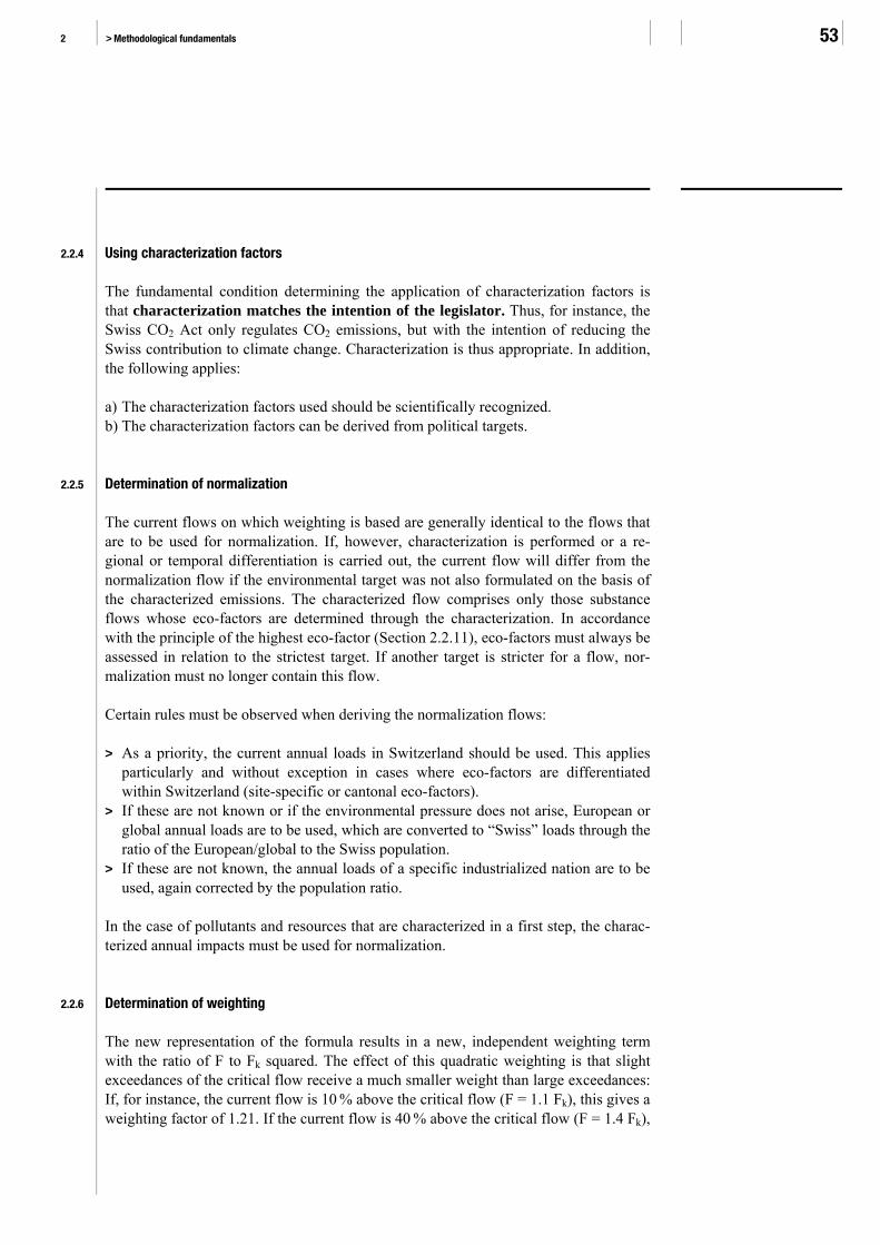
2 > Methodological fundamentals 53
2.2.4 Using characterization factors
The fundamental condition determining the application of characterization factors is that characterization matches the intention of the legislator. Thus, for instance, the Swiss CO2 Act only regulates CO2 emissions, but with the intention of reducing the Swiss contribution to climate change. Characterization is thus appropriate. In addition, the following applies:
a) The characterization factors used should be scientifically recognized. b) The characterization factors can be derived from political targets.
2.2.5 Determination of normalization
The current flows on which weighting is based are generally identical to the flows that are to be used for normalization. If, however, characterization is performed or a re-gional or temporal differentiation is carried out, the current flow will differ from the normalization flow if the environmental target was not also formulated on the basis of the characterized emissions. The characterized flow comprises only those substance flows whose eco-factors are determined through the characterization. In accordance with the principle of the highest eco-factor (Section 2.2.11), eco-factors must always be assessed in relation to the strictest target. If another target is stricter for a flow, nor-malization must no longer contain this flow.
Certain rules must be observed when deriving the normalization flows:
> As a priority, the current annual loads in Switzerland should be used. This applies particularly and without exception in cases where eco-factors are differentiated within Switzerland (site-specific or cantonal eco-factors).
> If these are not known or if the environmental pressure does not arise, European or global annual loads are to be used, which are converted to “Swiss” loads through the ratio of the European/global to the Swiss population.
> If these are not known, the annual loads of a specific industrialized nation are to be used, again corrected by the population ratio.
In the case of pollutants and resources that are characterized in a first step, the charac-terized annual impacts must be used for normalization.
2.2.6 Determination of weighting
The new representation of the formula results in a new, independent weighting term with the ratio of F to Fk squared. The effect of this quadratic weighting is that slight exceedances of the critical flow receive a much smaller weight than large exceedances: If, for instance, the current flow is 10 % above the critical flow (F = 1.1 Fk), this gives a weighting factor of 1.21. If the current flow is 40 % above the critical flow (F = 1.4 Fk),

The Ecological Scarcity Method – Eco-Factors 2006 FOEN 2009 54
this gives a weighting factor around 2, and if exceedance of the critical flow is 100 % (F = 2 Fk) the weighting factor is 4.
National annual flows are generally used for weighting. Depending upon the issue at hand, site-specific, cantonal, national, regional, continental or global, as well as sea-sonal or annual current and critical flows can be used for certain environmental con-cerns. In accordance with the environmental targets and in a manner matching the normalization, the flows are quantified either as individual substances or as environ-mental pressures.
The weighting term is unitless. The current and critical flows must therefore be ex-pressed in the same units.
The weighting function remains quadratic when eco-factors are differentiated spatially or temporarily. This differs from the proposal made by Dinkel et al. (2004), where the weighting factor is linear for regionalized eco-factors.
Current flows are always to be determined with regard to the reduction target. The reference for the current and critical flows should be the same. For instance, the Swiss CO2 Act only refers to CO2 emissions from certain sources, whereas the Kyoto Proto-col embraces all greenhouse gases. The current flow must be calculated in accordance with the target or the critical flow. In most cases the current flow is identical to the normalization flow.
Critical flows are generally based upon binding political targets (which in turn can be based on scientific findings). These are primarily protection targets established by law (annual loads, ambient levels). Where no statutory provisions exist, critical flows are based upon political statements of intent with as binding a nature as possible (for instance, the stated intent to limit settlement area, which provides a basis for assessing land use).
2.2.7 Determination of the eco-factor
Through characterization, normalization and weighting, the eco-factors capture politi-cal and statutory evaluations of the ecological relevance of pollutants. For instance, the emissions of various heavy metals to air, soil and water are assessed with specific eco-factors, which (ideally) are calculated from the specific current and critical flows. This normally leads to different eco-factors for the emission of one and the same pollutant to water, air or soil. These differences reflect the different statutory requirements and current pressures.
Current flow
Critical flow

2 > Methodological fundamentals 55
2.2.8 Temporal aspects of eco-factor determination
Stipulations enshrined in statutes, such as ambient limit values for airborne pollutants, generally do not set any explicit time horizon apart from transitional provisions. Their provisions apply from their entry into force onwards. When political goals are set, in contrast, specific targets can be defined for certain points in time. With its report on sustainable development in Switzerland (Schweizerischer Bundesrat 2002a), the Swiss Federal Council underscores that it aims for a long-term perspective, as already stipu-lated in the Federal Constitution of the Swiss Confederation (Art. 73). Moreover, the preamble to the Federal Constitution notes responsibility towards future generations.
In cases where there are several political targets with (very) different time horizons for the determination of an eco-factor, then, on the basis of an appraisal of the current political situation, either one of the points in time should be selected or an interpolation performed to an intermediate point in time (cf. determination of the eco-factor for CO2, Section 3.2).
2.2.9 Time lag between current flows and future impacts
The ecological scarcity method proceeds from the present situation when determining eco-factors. But how are pressures listed in inventories to be handled that already arose long ago or will only arise in the distant future?
Pressures listed in inventories that arose long ago can be taken into account or not, depending upon the issue analysed. In general, no special adjustment is necessary.
The situation is somewhat different for pressures that are generated by processes today but will only arise in the very distant future. The long-term emissions from landfills (modelled in the ecoinvent data to 60 000 years in the future) generated by today’s wastes are such an example.
Such emissions in the distant future should not simply be assessed with an eco-factor of zero and thus neglected. On the other hand, these pressures may possibly never arise. With sufficient engineering effort, landfills can be cleaned up at practically any time. It is therefore acceptable to either only partly take account of such emissions in the very distant future, or to determine a specific eco-factor for them. The ecological scarcity method is guided in principle by present political goals and the targets estab-lished in environmental law. A deviating assessment of long-term emissions is there-fore conceivable in principle, as both these goals and targets and also the exposure situation at the point in time of occurrence of the long-term emissions can differ sub-stantially from the present situation.
It needs to be checked carefully in each case how long-term emissions are treated in life cycle inventory data. It depends upon this whether a more differentiated analysis and assessment of long-term emissions is required.

The Ecological Scarcity Method – Eco-Factors 2006 FOEN 2009 56
2.2.10 Spatial aspects
Political and statutory goals are sometimes spatially differentiated. This is for instance the case for limit values governing pollutants in surface waters and groundwater. In most cases, however, provisions apply uniformly across the whole of Switzerland. If a relevant distinction is made, this should be captured with corresponding eco-factors.
Where there is a uniform limit value across Switzerland for pollutants but the pollution situation varies greatly from region to region, it is appropriate to perform a differentia-tion. For airborne pollutants, the differences are usually too small or cannot be quanti-fied. For water pollutants, in contrast, relevant and quantifiable differences in levels of pollution can arise (e.g. phosphorus in lakes, see Section 4.3). In such cases, regional-ized eco-factors should be applied as a basis for determining the eco-factor for the whole of Switzerland (see also Section 2.1.4).
2.2.11 Eco-factor selection when several derivations are possible (principle of highest eco-factor)
There are several possible ways of deriving some eco-factors. For instance, specific ammonia emissions to air can be assessed on the basis of the political target for nitro-gen, but also on the basis of their acidification potential. The principle governing the ecological scarcity method is that the highest resulting eco-factor in each instance is used. Weighting is thus performed on the basis of the dominant assessable environ-mental pressures.
2.3 Principles governing the application of eco-factors
2.3.1 Selection of substances
The selection of substances is guided by their ecological and political relevance. This limits the list of environmental pressures that can be weighted. For environmental policy by no means set targets for all substances, especially not for those that have little environmental relevance in Switzerland and Europe (such as sulphate emissions to waters) or for which knowledge is lacking (such as noise). Nonetheless, through more rigorous use of characterization, the substance list has been extended substantially compared to that presented by Brand et al. (1998).
Most of the eco-factors given in the previous report (Brand et al. 1998) continue to be determined, but some are now derived differently. For instance, wastes in surface landfills are no longer assessed on the basis of a special volume eco-factor. A new feature is the assessment of the carbon content of wastes consigned to bioreactive landfills.

2 > Methodological fundamentals 57
Substances are inventoried at the point of passage from the technosphere to the eco-sphere. This boundary is not always clearly defined – especially that between soil and groundwater. A more detailed discussion of this boundary is provided in Section 6.1.2 in the chapter on soil. Tab. 1 provides a schematic overview showing the points at which environmental pressures are assessed with eco-factors (fields shaded grey). Each emission should only be assessed once – at its first passage from the technosphere to the ecosphere. Further substance flows within the ecosphere, including those of sub-stances that originally came from the anthropo-technosphere, are not taken into ac-count, as otherwise double counting would occur.
Fig. 1 > Overview of system boundaries
The environmental pressures assessed by eco-factors are shaded grey.
Ressourcen (Primärenergie und Süsswasser)
NOx , SO2, NMVOC, NH3, PM10, Dieselruss, FCKW,
usw.
NO3, NO2, PO4, Schwermetalle, PSM, usw.
Surface waters
Air
Land use
Resources (primary energy and freshwater)
Product
Process
Company
NOX, SO2, NMVOCs, NH3, PM10, diesel soot, CFCs, etc.
COD, NO3, PO4, AOX, heavy metals, etc.
Resource consumption Emissions Ambient loads/levels
NH4+, SO42-, particulates, heavy metals
NO3-, PO43-, plant protection products, heavy metals
NO3+, SO42-,particulates, heavy metals
Soil and groundwater
NO3, NO2, PO4, heavy meals, plant pro-
tection products, etc.
2.3.2 Spatial and temporal validity of the eco-factors
Life cycle inventories of product systems generally comprise globally distributed emissions and consumption. Care must therefore be taken when applying the eco-factors that each emission is weighted as if it were taking place in Switzerland (with the exception of freshwater insofar as the life cycle inventory is differentiated accord-ingly, and of radioactive emissions to the North Sea). Through this approach, the shift of a process to another country does not affect the outcome of an LCA, if the absolute emission level is the same. When environmental impacts have a globally uniform effect, such as greenhouse gas emissions, the eco-factors for all emissions are globally applicable. In other cases, the environmental impacts of a pollutant emission or re-source extraction can differ from region to region (e.g. water pollutant emissions). The regionalization of eco-factors presented above makes it possible to take account of such differences.

The Ecological Scarcity Method – Eco-Factors 2006 FOEN 2009 58
In practice, however, taking systematic account of specific regional circumstances for a product LCA generally entails major effort, due to a lack of information on the specific environmental situation and the environmental policy goals applying there. This would require an independent and systematic definition of eco-factors for that region. It is indeed conceivable that an eco-factor which is of particular relevance to an LCA is adjusted to the specific regional scarcities in a manner similar to a sensitivity analysis (e.g. specific pollutant emissions to water in a region in which pollution levels are very high or very low). Such “private” or scientifically based eco-factors must, however, be interpreted with great caution.
Such an approach can also be taken when interpreting a site audit as a part of the environmental management activities of a company, or when assessing the on-site impacts of a locally defined project (such as a major road or railway construction project).
As the eco-factors reflect present environmental targets, their informative value de-clines with time. On the other hand, a comparison of the 1997 eco-factors to those of 2006 shows that most of the political targets, i.e. the critical flows, have changed little.
Time elapses until an environmental issue is reflected in political targets. Target values therefore rarely encapsulate the most recent scientific findings. In the same vein, the current flows are often based on extrapolation of past values. The eco-factors must therefore continue to be updated in future at regular intervals. Online updating, e.g. on the Internet, does not however appear expedient, as a “daily quotation” of eco-factors would presumably engender more uncertainty than accuracy.
2.4 Data quality
The stated data quality grades relate to the underlying data. For the current flows, they represent the accuracy of the available data. For the critical flows, the assignment of different quality grades reflects the binding nature of the underlying statutory provi-sions or political statements.
The quality or binding nature of the data is graded in the explanatory part of the report in accordance with the following table:
Tab. 1 > Indicators of the quality or binding nature of data Quality indicator Uncertainty attaching
to the current flow Indicator of binding nature Derivation of the critical flow
A <20 % a Calculation or derivation from statutory emission/ambient targets and/or from political statements of intent
B 20 to 40 % b Expert recommendation or expert estimate C >40 % c Modelling assumption of advisory group

2 > Methodological fundamentals 59
2.5 Characterization
Characterization factors capture the relative environmental impact of substances com-pared to a reference substance. The characterized quantity is normally expressed in reference substance equivalents. In the case of greenhouse gases, carbon dioxide is the reference substance and CO2-equivalent (CO2-eq.) is the unit of the quantity character-ized.
The characterization factors are based on scientific knowledge of the relative effect in terms of the environmental impact characterized. In the case of greenhouse gases, for instance, the characterization value of 296 kg CO2-eq./kg N2O for nitrous oxide (N2O) means that 1 kg N2O has the same global warming impact as 296 kg CO2.
In the ecological scarcity method, applying characterization is permissible if the corre-sponding environmental impact played a key role when the target was set. In the case of greenhouse gases, for instance, only a CO2 reduction target is enshrined in statute. As, however, the intention of the legislator is to thereby contribute to limiting global climate change, applying global warming potential values is possible and appropriate.
Characterization is not, however, appropriate in every theoretically conceivable case. It should not be applied in cases where the environmental impact of the characterization does not match the intention of the legislator with regard to the way the reduction target (or the limit or target value) was set. For instance, the Swiss legislator has adopted a uniform VOC levy. Characterizing individual NMVOCs according to their photochemical oxidation potential (POCP) is therefore not appropriate.
The new formula representation introduces an explicit characterization term (K). Characterization had partly already been used in previous reports on eco-points (Brand et al. 1998), but had not been introduced formally in the EP formula. Tab. 2 lists the characterizations used in the present report and compares them to those of EP97.
Tab. 2 > Characterization methods used in EP97 and EP06
Implementation Abbr. Reference unit EP97 EP06 Source 2006
Global warming potential GWP CO2-eq. Yes Sec. 3.2 IPCC 2001 Ozone depletion potential ODP R11-eq. Yes Sec. 3.3 UNEP 2000 Acidification potential AP SO2-eq. Partly Sec. 3.7 Guinée et al. 2001 Characterization of radioactive emissions C-14-eq. No Sec. 4.6 Frischknecht et al. 2000 Characterization of endocrine disruptors E2-eq. No Sec. 4.11 Rutishauser et al. 2004 Characterization of plant protection products PPP PPP-eq. No Sec. 6.3 based on the Danish indicator in OECD 2001Characterization of primary energy resources MJ-eq. No Sec. 7.2 Schweizerischer Bundesrat 2002b Ecosystem damage potential through land use EDP Settlement area eq. No Sec. 7.3 Köllner 2001 The sources cited relate to EP06

The Ecological Scarcity Method – Eco-Factors 2006 FOEN 2009 60
3 > Emissions to air
3.1 Introduction
3.1.1 Selection of substances
The report on “Human-induced air pollutant emissions in Switzerland from 1900 to 2010” (BUWAL 1995) quantifies the emissions of 17 different pollutants and allocates them to four source groups: transport, industry and commerce, agriculture and forestry, and households. Air pollutants are selected on the basis of their ecological relevance for the whole of Switzerland. In addition, eco-factors are calculated for greenhouse gases and ozone-depleting substances by means of characterization.
A range of measures has succeeded in reducing remissions to air in recent years, in some cases substantially. Some of the remaining emissions and their impacts in Swit-zerland are therefore of subordinate importance. It needs to be taken into account, however, that the eco-factors are applied not only to Swiss processes, but also to processes taking place abroad. An eco-factor is therefore retained for substances which may be unproblematic in Switzerland, but have the potential to continue to be envi-ronmentally relevant abroad.
Tab. 3 compiles the air pollutants assessed with an eco-factor. It further states, in broad categories, which impacts the pollutants have and which of these are significant in determining the eco-factor.

3 > Emissions to air 61
Tab. 3 > Impact mechanisms of the air pollutants assessed
Environmental Human Gl
obal
warm
ing p
oten
tial (
GWP)
Ozon
e de
pletio
n po
tent
ial (O
DP)
Ozon
e pr
ecur
sor p
oten
tial (
POCP
)
Eutro
phica
tion
Acidi
ficat
ion
Dam
age
to flo
ra
Impa
irmen
t of s
oil fe
rtility
Dama
ge to
buil
t stru
cture
s
Resp
irato
ry d
iseas
es
Carc
inoge
nicity
Mut
agen
esis
Embr
yona
l dam
age
Othe
r / fu
rther
type
s of d
amag
e
Char
acte
rizat
ion
Notes
CO2 and further greenhouse gases # x x GWP Ozone-depleting substances x # x ODP NMVOCs # x x x x x POCP Nitrogen oxides (NOX) * * * x x - Targets are designed to protect human
health, fauna and flora Ammonia (NH3) * * x - Targets are designed to protect ecosystems
Alternative assessment via AP SO2 and further acidifying substances # x x x AP Particulates (excl. diesel soot) # x x - Derivation from Swiss Air Pollution Control
Ordinance Diesel soot x x # - Application of precautionary principle Benzene x # (x) x - Application of precautionary principle Dioxins/furans # x x (I-TEQ) Application of precautionary principle Lead (Pb) x # x - Emissions to air are assessed using the
weighting factor for soil, as the greatest scarcity prevails there
Cadmium (Cd) # x x (x) x - dito Zinc (Zn) x # x - dito x Impact or link proven (x) Impact or link presumed # Principal impact for determining the eco-factor * Several significant impacts
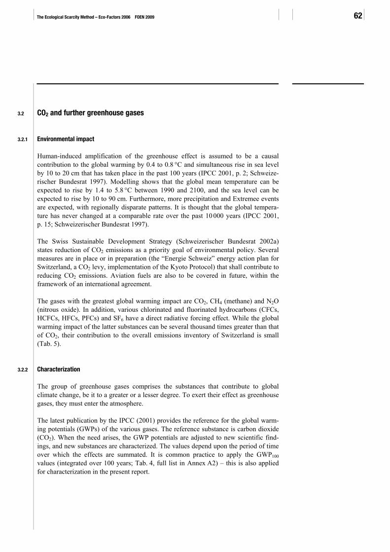
The Ecological Scarcity Method – Eco-Factors 2006 FOEN 2009 62
3.2 CO2 and further greenhouse gases
3.2.1 Environmental impact
Human-induced amplification of the greenhouse effect is assumed to be a causal contribution to the global warming by 0.4 to 0.8 °C and simultaneous rise in sea level by 10 to 20 cm that has taken place in the past 100 years (IPCC 2001, p. 2; Schweize-rischer Bundesrat 1997). Modelling shows that the global mean temperature can be expected to rise by 1.4 to 5.8 °C between 1990 and 2100, and the sea level can be expected to rise by 10 to 90 cm. Furthermore, more precipitation and Extremee events are expected, with regionally disparate patterns. It is thought that the global tempera-ture has never changed at a comparable rate over the past 10 000 years (IPCC 2001, p. 15; Schweizerischer Bundesrat 1997).
The Swiss Sustainable Development Strategy (Schweizerischer Bundesrat 2002a) states reduction of CO2 emissions as a priority goal of environmental policy. Several measures are in place or in preparation (the “Energie Schweiz” energy action plan for Switzerland, a CO2 levy, implementation of the Kyoto Protocol) that shall contribute to reducing CO2 emissions. Aviation fuels are also to be covered in future, within the framework of an international agreement.
The gases with the greatest global warming impact are CO2, CH4 (methane) and N2O (nitrous oxide). In addition, various chlorinated and fluorinated hydrocarbons (CFCs, HCFCs, HFCs, PFCs) and SF6 have a direct radiative forcing effect. While the global warming impact of the latter substances can be several thousand times greater than that of CO2, their contribution to the overall emissions inventory of Switzerland is small (Tab. 5).
3.2.2 Characterization
The group of greenhouse gases comprises the substances that contribute to global climate change, be it to a greater or a lesser degree. To exert their effect as greenhouse gases, they must enter the atmosphere.
The latest publication by the IPCC (2001) provides the reference for the global warm-ing potentials (GWPs) of the various gases. The reference substance is carbon dioxide (CO2). When the need arises, the GWP potentials are adjusted to new scientific find-ings, and new substances are characterized. The values depend upon the period of time over which the effects are summated. It is common practice to apply the GWP100 values (integrated over 100 years; Tab. 4, full list in Annex A2) – this is also applied for characterization in the present report.

3 > Emissions to air 63
Tab. 4 > Global warming potential of the substances regulated under the Kyoto and Montreal Protocols
GWP100 Used in this report
(IPCC 2001)(CO2-eq.)
Used in the Kyoto Protocol (Houghton et al. 1996)
(CO2-eq.) Carbon dioxide CO2 1 1 Methane CH4 23 21 Nitrous oxide N2O 296 310 Chlorofluorocarbons CFCs/HCFCs 120–14 000 90–8 100 Partially halogenated fluorocarbons HFCs 12–12 000 140–11 700 Perfluorinated hydrocarbons PFCs 5 700–11 900 6 500–9 200 Sulphur hexafluoride SF6 22 200 23 900
The current IPCC report (IPCC 2001) rates the relative radiative forcing of individual gases in most cases higher than was the case in the Second Assessment Report of 1996 (Houghton et al. 1996). It is the GWP values of the latter on which national greenhouse gas emissions inventories are based. The changes in the GWPs are due above all to advances in the radiative forcing model.
Some greenhouse gases also damage the ozone layer. Their ozone depletion potential is therefore also assessed. The higher of the resultant eco-factors is then applied. Other environmental impacts of greenhouse gases (such as the herbicidal effect of the de-composition products of fluorocarbons) are not taken into account here.
3.2.3 Normalization
By signing the Kyoto Protocol, Switzerland has committed to reducing its greenhouse gas emissions. Although the reduction target established by the Swiss CO2 Act exclu-sively refers to carbon dioxide, the Swiss Federal Council makes it clear in its memo-randum on the CO2 Act (Schweizerischer Bundesrat 1997) and in its Sustainable Development Strategy (Schweizerischer Bundesrat 2002a) that the goal of Swiss climate policy is to reduce the emissions of all greenhouse gases.
As characterization is performed using the current GWPs (IPCC 2001), normalization is also performed with the overall flow of greenhouse gases calculated with these GWPs. This leads to a normalization flow of 53 034 million t CO2-eq/a (see Tab. 5).

The Ecological Scarcity Method – Eco-Factors 2006 FOEN 2009 64
Tab. 5 > Greenhouse gas emissions in Switzerland
according to FOEN (2006), weighted with the GWP 100 values according to IPCC (2001) GWP100 (IPCC 2001)
(CO2-eq.)
Emissions in 2004 (1000 t CO2-eq)
Share in overall greenhouse gas emissions
CO2 1 45 436 86 % CH4 23 3 661 6.9 % N2O 296 3 075 5.8 % HFCs 12–12 000 618 1.2 % PFCs 5 700–11 900 67 0.1 % SF6 22 200 176 0.3 % Total 53 034 100 %
3.2.4 Weighting
There are two political targets for CO2 or greenhouse gases in Switzerland: One is based on the Kyoto Protocol, which is operationalized in the shape of the Swiss CO2 Act and aims at reducing CO2 emissions by 10 % by the year 2010 from the 1990 baseline. The other follows from the mention made in the memorandum to the CO2 Act (Schweizerischer Bundesrat 1997) that the 10 % reduction will not suffice to stabilize CO2 concentrations in the atmosphere, and that a long-term reduction of 70–80 % is in fact necessary.
There is a certain incongruence between these two very different targets, which apply to quite different target times. As both targets are positioned on the same reduction path but apply to different points in time, it is not possible here to apply the principle that where there are several reduction targets the largest resulting eco-factor is used. Moreover, using a target that is in the distant future would greatly over-stress the severity and urgency compared to other environmental problems. On the other hand, the first target has by now become very short-term (4 years) and also does not suffi-ciently reflect the severity of global warming. An appropriate eco-factor must therefore be situated between these two endpoints.
The draft Swiss Electricity Supply Act states the year 2030 as target date for the share of renewable energies in Swiss electricity generation. This can be interpreted as the present time horizon with which policymakers operate in relation to climate and energy issues.
Current and critical flow for the 2010 time horizon (CO2 Act)
The reduction target established by the CO2 Act relates exclusively to the carbon dio-xide emissions of fuels used to produce energy. The Act does not cover other sources. The baseline year is 1990. The current flow is thus smaller than that listed in Tab. 5. It figures 41.1 million t CO2/a (BUWAL 2005b, Table 2).

3 > Emissions to air 65
The CO2 Act defines a reduction for fuels of 10 % from the 1990 baseline. This results in a critical flow of 37.0 million t CO2/a (BUWAL 2005b).
Current and critical flow for the 2050 time horizon (Sustainable Development Strategy)
As the critical flow relates to CO2 emissions (and not to the CO2-equivalents of all Kyoto greenhouse gases) the current flow must also be determined on the basis of CO2 emissions only. This comprises all sources, but not the land-use change and forestry sector (e.g. forest sinks). It follows from the national greenhouse gas emissions inven-tory (FOEN 2006) that the current flow of carbon dioxide in 2004 in Switzerland is 45 436 million t CO2 (Tab. 5).
The 1 t CO2 target is a part of the vision of a 2000 watt society, and is also stated in the Swiss Sustainable Development Strategy (Schweizerischer Bundesrat 2002a). Different points in time for attaining that goal are stated in various studies: 2050, 2100 or 2150 (Koschenz & Pfeiffer 2005; Spreng & Semadeni 2001; Würsten 2003). The most stringent variant is used here, i.e. the year 2050.
A resident Swiss population of 8.06 million is assumed for the year 2050 (intermediate scenario of the BFS (2006). This results in a critical flow of 8.06 million t CO2/a for 2050.
3.2.5 Eco-factor for CO2
Tab. 6 > Calculation of the CO2 eco-factors for the two endpoints – 2010 and 2050 Target 2010
Q Target 2050 Q Notes
Normalization (1000 t CO2-eq./a) 53 034 A 53 034 A Emissions according to FOEN (2006), but with GWPs in accordance with IPCC (2001)
Current flow (1000 t CO2/a) 41 130* A 45 436 A (BUWAL 2005b; FOEN 2006) Critical flow (1000 t CO2/a) 36 960* a 8 060 b see text Weighting (-) 1.24 31.8 Eco-factor (EP/g CO2-eq.) 0.023 0.60 Basis for interpolation Q=data quality; for explanation see Section 2.4 * only carbon dioxide from fuels used to produce energy
The calculation of the eco-factors for 2010 and 2050 shows that they differ by a factor of around 25. These two endpoint eco-factors are interpolated to the year 2030 in a next step. The two targets are thus adjusted to the time horizon commonly applied by the Swiss legislator.
Eco-factors of the endpoints

The Ecological Scarcity Method – Eco-Factors 2006 FOEN 2009 66
Tab. 7 > Eco-factor for CO2 and further greenhouse gases in EP/g CO2-equivalents3
The eco-factor has risen by around 50 % from 1997. Situation 2006
Q Notes Situation 1997
Normalization (1000 t CO2-eq./a) 53 034 A Emissions according to FOEN (2006), but with GWPs in accordance with IPCC (2001)
-
Current flow (1000 t CO2/a) - 44 200 Critical flow (1000 t CO2/a) - 15 000 Weighting (-) 16.5 Calculated from interpolated eco-factor
and normalization -
Eco-factor (EP/g CO2-eq.) 0.31 Interpolated eco-factor 0.2 Q=data quality; for explanation see Section 2.4
3.2.6 Eco-factors for further greenhouse gases
Taken together, the further greenhouse gases contribute around 15 % of the global warming impact attributable to Switzerland (Tab. 5). Their eco-factors are determined via characterization using GWP100 values (IPCC 2001; cf. Tab. 8 and the detailed list in A2).
In cases where substances contribute both to global warming and ozone depletion, both eco-factors are calculated and the higher of the two is used.
Tab. 8 > Eco-factors for several greenhouse gases, calculated from the weighting factor for CO2 Formula GWP Eco-factor 2006
(EP/g)Basis in 2006
Eco-factor 1997 (EP/g)
Basis in 1997
Carbon dioxide CO2 1 0.31 GWP 0.2 GWP Methane CH4 23 7.1 GWP 4.2 GWP Nitrous oxide N2O 296 92 GWP 62 GWP HCFC -22 CHClF2 1 700 610 ODP* 300 GWP HCFC -142b CH3CF2Cl 2 400 740 GWP* 360 GWP HFC -125 CHF2CF3 3 400 1 100 GWP 560 GWP HFC -134a CH2FCF3 1 300 400 GWP 260 GWP Sulphur hexafluoride SF6 22 200 6 900 GWP 4 800 GWP The detailed list is in A2. * The eco-factor can be determined both on the basis of the GWP and the ODP; the higher of the two is used and listed here.
3 Interpolation to 2030
Interpolated eco-factor
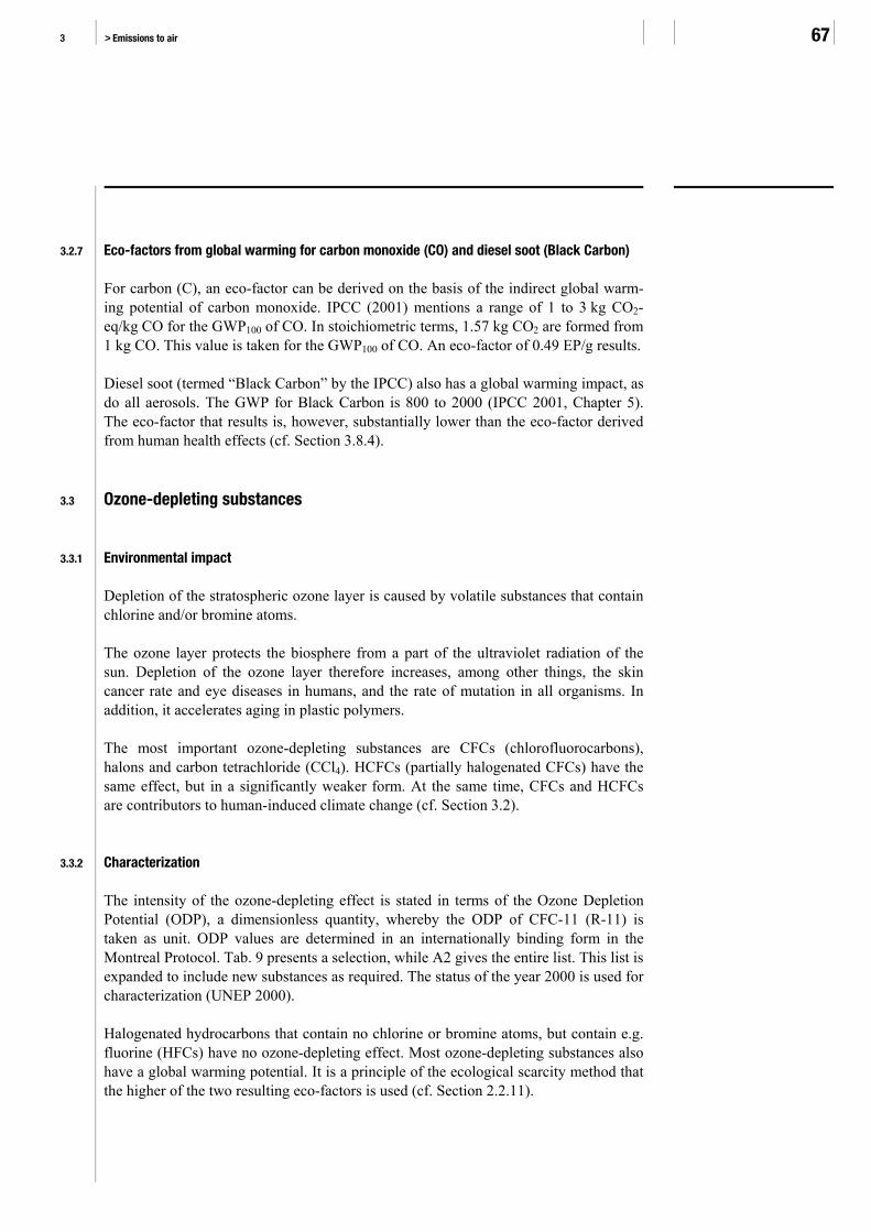
3 > Emissions to air 67
3.2.7 Eco-factors from global warming for carbon monoxide (CO) and diesel soot (Black Carbon)
For carbon (C), an eco-factor can be derived on the basis of the indirect global warm-ing potential of carbon monoxide. IPCC (2001) mentions a range of 1 to 3 kg CO2-eq/kg CO for the GWP100 of CO. In stoichiometric terms, 1.57 kg CO2 are formed from 1 kg CO. This value is taken for the GWP100 of CO. An eco-factor of 0.49 EP/g results.
Diesel soot (termed “Black Carbon” by the IPCC) also has a global warming impact, as do all aerosols. The GWP for Black Carbon is 800 to 2000 (IPCC 2001, Chapter 5). The eco-factor that results is, however, substantially lower than the eco-factor derived from human health effects (cf. Section 3.8.4).
3.3 Ozone-depleting substances
3.3.1 Environmental impact
Depletion of the stratospheric ozone layer is caused by volatile substances that contain chlorine and/or bromine atoms.
The ozone layer protects the biosphere from a part of the ultraviolet radiation of the sun. Depletion of the ozone layer therefore increases, among other things, the skin cancer rate and eye diseases in humans, and the rate of mutation in all organisms. In addition, it accelerates aging in plastic polymers.
The most important ozone-depleting substances are CFCs (chlorofluorocarbons), halons and carbon tetrachloride (CCl4). HCFCs (partially halogenated CFCs) have the same effect, but in a significantly weaker form. At the same time, CFCs and HCFCs are contributors to human-induced climate change (cf. Section 3.2).
3.3.2 Characterization
The intensity of the ozone-depleting effect is stated in terms of the Ozone Depletion Potential (ODP), a dimensionless quantity, whereby the ODP of CFC-11 (R-11) is taken as unit. ODP values are determined in an internationally binding form in the Montreal Protocol. Tab. 9 presents a selection, while A2 gives the entire list. This list is expanded to include new substances as required. The status of the year 2000 is used for characterization (UNEP 2000).
Halogenated hydrocarbons that contain no chlorine or bromine atoms, but contain e.g. fluorine (HFCs) have no ozone-depleting effect. Most ozone-depleting substances also have a global warming potential. It is a principle of the ecological scarcity method that the higher of the two resulting eco-factors is used (cf. Section 2.2.11).
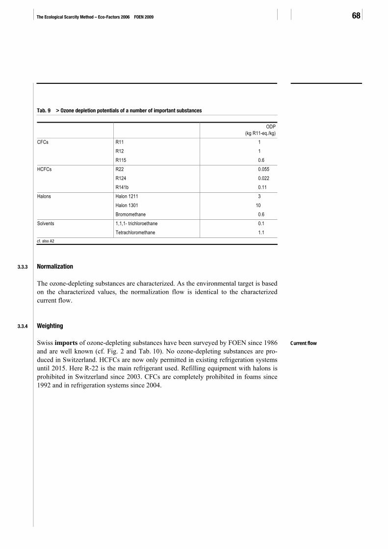
The Ecological Scarcity Method – Eco-Factors 2006 FOEN 2009 68
Tab. 9 > Ozone depletion potentials of a number of important substances ODP
(kg R11-eq./kg) R11 1 R12 1
CFCs
R115 0.6 R22 0.055 R124 0.022
HCFCs
R141b 0.11 Halon 1211 3 Halon 1301 10
Halons
Bromomethane 0.6 1,1,1- trichloroethane 0.1 Solvents
Tetrachloromethane 1.1 cf. also A2
3.3.3 Normalization
The ozone-depleting substances are characterized. As the environmental target is based on the characterized values, the normalization flow is identical to the characterized current flow.
3.3.4 Weighting
Swiss imports of ozone-depleting substances have been surveyed by FOEN since 1986 and are well known (cf. Fig. 2 and Tab. 10). No ozone-depleting substances are pro-duced in Switzerland. HCFCs are now only permitted in existing refrigeration systems until 2015. Here R-22 is the main refrigerant used. Refilling equipment with halons is prohibited in Switzerland since 2003. CFCs are completely prohibited in foams since 1992 and in refrigeration systems since 2004.
Current flow

3 > Emissions to air 69
Fig. 2 > Development of Swiss imports of ozone-depleting substances from 1989 to 2003, measured in R11-eq.
0
1000
2000
3000
4000
5000
6000
1989 1990 1991 1992 1993 1994 1995 1996 1997 1998 1999 2000 2001 2002 2003
t R11-eq./a
CFCs (refrigeration, air-conditioning) CFCs (solvents) CFCs (foams) CFCs (aerosols)Halons (fire control) HCFC (refrigeration, air-conditioning) HCFC (foams) 1,1,1-trichloroethaneCarbon tetrachloride Bromomethane (pesticide)
source: FOEN
Due to the formation of stocks in the past, current emissions of ozone-depleting sub-stances are substantially greater than the present quantities imported. Emissions can be classed in four source groups:
4. Diffuse emissions from foam insulation materials containing CFCs and HCFCs that are already in place in buildings and in refrigeration systems.
5. Losses of CFCs and HCFCs as refrigerants in refrigeration and air-conditioning systems and in heat pumps.
6. Releases from the disposal of insulation material, equipment and systems that contain CFCs, halons or HCFCs (e.g. refrigeration equipment, refrigerators).
7. Halon emissions resulting from the use of fire control equipment and systems.

The Ecological Scarcity Method – Eco-Factors 2006 FOEN 2009 70
Tab. 10 > Average imports of ozone-depleting substances in tonnes and in tonnes R11-equivalent over the period from 2001 to 2003
Imports to Switzerland: average over 2001–2003 period (t/a) (t R11-eq./a)
CFCs
Refrigerants 27 27 Solvents 1.3 1.3 Foaming agents (insulation) 0 0 Aerosol propellants 0 0
HCFCs
Refrigerants (mainly R22) 229 13 Foaming agents (insulation) 32 2.9
Further substances
Halons (for fire control) 0 0 Trichloroethane (as solvent) 1.0 0.1 Tetrachloromethane (in laboratories) 2.2 2.4 Bromomethane (as pesticide) 17 10 Total 310 57 source: FOEN
Empa has been conducting a measurement programme for halogenated gases in the atmosphere since 2000 on the Jungfraujoch mountain. Empa has found that emissions of the main ozone-depleting substances are dropping (Reimann et al. 2004). The calcu-lation of the current flow (Tab. 11) uses the average value of these measurements over the period from 2001 to 2003, and the HCFC-22 and tetrachloromethane import data from the import statistics gathered by FOEN; these figures cover more than 90 % of the overall ozone-depleting impact4, 5.
The national halon register6 reports a stock of around 200 tonnes in 2005 for the halon 1301 (this is estimated to be 80 % of the real stock). Emissions through triggering fire extinguishers are on the scale of 0.2 % to 0.6 % of the stock, which would amount to a figure of between 500 and 1500 kg emissions to air. The difference to the measure-ments performed by Empa (see Tab. 11) can probably be explained by unrecorded stocks. The figures provided by the Empa measurements (Reimann et al. 2004) are used here.
4 The appraisal is based on the global production volume of halogenated hydrocarbons (AFEAS 2004, AFEAS (2004) Annual Global
Fluorocarbon Production (Excel Sheet), retrieved 6.6.2005 from http://www.afeas.org/., where the contribution of CFC-113 and CFC-114, which are not taken into account in the present report, is around 12 %. As these substances have been banned in Switzerland for some time, it can be assumed that their contributions are substantially smaller. The contribution of other CFCs and HCFCs not taken into account is well below 1 %.
5 As HCFC-22 can now only be used to refill existing equipment, the imported quantity corresponds roughly to the emitted quantity. Tetrachloromethane is mostly used in small quantities in laboratories, and has little relevance to the emissions balance.
6 Personal communication by B. Horisberger (FOEN) of 15.8.2006

3 > Emissions to air 71
Tab. 11 > Swiss emissions of the most important ozone-depleting substances in t/a and as R11-eq./a
Stock reduction for the year 2005 Total as emissions to air through disposal
(t/a) (t R11-eq./a) (t/a) (t R11-eq./a) (t/a) (t R11-eq./a)
CFCs
CFC -11 CCl3F 278 278 167 167 111 111 CFC -12 CCl2F2 167 167 100 100 67 67 CFC -115 CF3CClF2 6.1 3.7 3.7 2.2 2.4 1.5
HCFCs
HCFC -22 CHClF2 280 15 229 13 51 2.8 HCFC -124 CHFClCF
3 6.5 0.1 5.3 0.1 1.2 0.03
HCFC -141b CH3CFCl2 156 17 74 8 82 9.0
Halons
Halon 1211 CBrClF2 20 61 6.7 20 14 41 Halon 1301 CBrF3 19 192 6.3 63 13 129 Methane, bromo- CH3Br 31 19 19 11 12 7.5
Solvents
Ethane, 1,1,1-trichloro- CH3CCl3 47 5 39 3.9 8.6 0.86 Methane, tetrachloro – * CCl4 2.7 2.9 2.2 2.4 0.5 0.53 Total 1 015 761 652 391 363 370 * HCFC-22 and tetrachloromethane emissions are not measured. The FOEN import statistics provide approximate values (Tab. 10)
The current flow of 391 t R11-eq. per year is therefore a good approximation for the Swiss emissions to air of ozone-depleting substances.
The Swiss Chemicals Risk Reduction Ordinance (Chemikalien-Risikoreduktions-Verordnung, ChemRRV) prohibits the production, importation and use of ozone-depleting substances. Exemptions regarding importation and use are presently only in place for the maintenance of existing HCFC refrigeration equipment and for the recy-cling of HCFC refrigerants (transitional period until 2015).
The provisions of the ChemRRV have led to a sharp reduction in emissions of ozone-depleting substances (Fig. 2). However, the stocks formed mainly in building insula-tion materials (CFC-11, HCFCs) will release considerable amounts in the coming decades. Emissions will therefore only drop slowly.
The ChemRRV thus regulates the use of ozone-depleting substances, but not their emission. No critical flow can therefore be derived directly from the wide-ranging ban on the consumption of ozone-depleting substances.
Critical flow

The Ecological Scarcity Method – Eco-Factors 2006 FOEN 2009 72
The tolerated emissions are taken as a basis for determining the critical flow. As these decline gradually, choice of the reference year is decisive. The transitional provisions (i.e. the exemptions for HCFC use in existing refrigeration equipment) terminate in 2015.
Hence in the following an estimation is performed of the emissions of ozone-depleting substances that are to be anticipated in 2015. This proceeds from the current flows listed in Tab. 11, whereby the following assumptions are made for the derivation of the reduction:
> CFC-12 and CFC-115 were used mainly in refrigeration equipment. The last transi-tional period for these two substances ends in 2008. Therefore zero emissions of these substances are expected for 2015.
> Emissions from insulating material amount to around 1 % of the stock. For refrigera-tion systems, a leakage rate of around 10 % is expected.7
> CFCs and HCFCs in insulating material are consigned to disposal in the course of building and equipment refurbishment. It is assumed that the stock (and thus also the emissions to air) are thus reduced by 0.8 % (CFCs) and 1.4 % (HCFCs) annually (these assumptions are identical to those made in the previous report (Brand et al. 1998)).
> An annual reduction rate of around 7 % to 9 % can be concluded for halon 1211 and halon 1301 from the figures of the national halon register on disposal quantities (there is a ban on refilling) and the emissions to air derived from the Empa meas-urements on the Jungfraujoch (Reimann et al. 2004). The mean of these two values is used, i.e. 8 %.
> Building on the assumptions made, an annual reduction in emissions by 1.8 % (CFCs) and 2.4 % (HCFCs) is anticipated for the substances that are in the meantime only present in insulating material. These two values are applied to the emissions of CFC-11 and HCFC-141b.
> For the other HCFCs, the annual reduction is determined from the mean of the reduction of emissions to air (5.5 %) and the annual percentage disposed (1.4 %). This results in an annual emissions reduction of 6.9 %.
> From 2006 onwards, bromomethane is only used in chemical synthesis processes. Only a slow reduction and small quantities emitted can therefore be expected. As a first approximation, the rate of reduction of CFC-11 is used here.
> For solvents, the rate of reduction of HCFC-22 is applied. This is purposeful as the solvents listed and HCFC-22 can at present still be used under certain conditions.
Tab. 12 presents in detail the derivation of the critical flow. It follows that the emis-sions to be expected in 2015, i.e. the critical flow, figure 188 t R11-eq.
It is further apparent that the assumptions made on HCFCs and on solvents have minor relevance to the assessment of the critical flow. Their ozone depletion potential (see Tab. 9) is substantially smaller, while their emission quantities are on the same scale (cf. also Tab. 11). 7 Personal communication by B. Horisberger (FOEN) of 10.8.2006

3 > Emissions to air 73
Tab. 12 > Assessment of Swiss emissions of the main ozone-depleting substances in 2015, in t/a and as R11-eq./a
Stock reduction for the year 2015 Reduction rate of the stock Total as emissions to air through disposal
per year (t/a) (t R11-eq./a) (t/a) (t R11-eq./a) (t/a) (t R11-eq./a)
CFCs
CFCs -11 1.8 % 224 224 134 134 90 90 CFCs -12 - 0 0 0 0 0 0 CFC-115 - 0 0 0 0 0 0
HCFCs
HCFC-22* 6.9 % 119 7 97 5 22 1.2 HCFC-124 6.9 % 2.8 0.1 2.3 0.05 0.5 0.01 HCFC-141b 2.4 % 117 13 56 6 61 6.8
Halons
Halon 1211 8.0 % 7.4 22 2.5 7 5.0 15 Halon 1301 8.0 % 7.1 71 2.3 23 4.7 47 Methane, bromo- 1.8 % 25 15 15 9 10 6.0
Solvents
Ethane, 1,1,1-trichloro- 6.9 % 20 2.0 16 1.6 3.7 0.4 Methane, tetrachloro- * 6.9 % 1.1 1.2 0.92 1.0 0.2 0.2 Total 523 354 326 188 197 166 * The figures for HCFC-22 and tetrachloromethane are based on data in the import statistics maintained by FOEN.
3.3.5 Eco-factor for ozone-depleting substances
Tab. 13 > Eco-factor for R11-equivalents in EP/g R11-eq Situation 2006
Q Notes Situation 1997
Normalization (t R11-eq./a) 391 Current flow (t R11-eq./a) 391 B Based on data in Reimann et al. (2004) 1 470 Critical flow (t R 11-eq./a) 188 b Assessed on basis of tolerated emissions as
set out in text 850
Weighting (-) 4.33 Eco-factor (EP/g R11-eq./a) 11 000 2 000 Q = data quality; for explanation cf. Section 2.4
The new factor is substantially higher than that of 1997, which is partly attributable to the new method of determining emission loads. This is now based on real measured data. Rough estimates of the stocks of ozone-depleting substances are no longer neces-

The Ecological Scarcity Method – Eco-Factors 2006 FOEN 2009 74
sary. On the one hand, the consumption of ozone-depleting substances has dropped sharply, while, on the other hand, the absolute ban will enter into force in the foresee-able future. A substantially higher eco-factor is therefore plausible.
3.3.6 Eco-factor for further ozone-depleting substances
The eco-factor for further ozone-depleting substances can be derived from the charac-terization values for the ozone depletion potential (ODP) and the eco-factor for R11-equivalents derived in Section 3.3.5.
Many ozone-depleting substances also contribute to global warming. For these, both the eco-factor resulting from global warming and that resulting from their ozone-depleting effect was calculated. A2 lists all substances and the dominant impact.
No separate eco-factors are calculated for refrigerant blends. The values for blends can be calculated from the eco-factors of the individual components, weighted according to their respective share in mass.
Tab. 14 > Eco-factors for ozone-depleting substances, stated in EP/g of substance Formula ODP
(kg R11-eq/kg) Eco-factor 2006
(EP/g)Basis in
2006Eco-factor 1997
(EP/g)Basis in
1997 CFC-11 CCl3F 1 11 000 ODP* 2 000 ODP CFC-12 CCl2F2 1 11 000 ODP* 2 000 ODP CFC-111 C2Cl5F 1 11 000 ODP 2 000 ODP HCFC-123 CHCl2CF3 0.02 220 ODP* 40 ODP HCFC-142b CH3CF2Cl 0.065 740 GWP* 360 GWP HCFC-225ca CF3CF2CHCl2 0.025 280 ODP* - Halon 1211 CBrClF2 3 33 000 ODP* 6 000 ODP Halon 1301 CBrF3 10 110 000 ODP* 20 000 ODP Methane, bromo- CH3Br 0.6 6 600 ODP* 1 400 ODP * Data available for both GWP and ODP, the higher value is used
3.3.7 Implementation in the ecoinvent v2.0 dataset
The substance “halogenated solvents, chlorinated” is assessed with the eco-factor of R22.
3 > Emissions to air 75
3.4 NMVOCs and further substances with photochemical ozone creation potential
3.4.1 Environmental impact
Volatile organic compounds (VOCs) are a group comprising a range of non-toxic to highly toxic and carcinogenic compounds. The Swiss VOC Ordinance (VOC Ver-ordnung, VOCV) defines VOCs as “organic compounds with a vapour pressure of at least 0.1 mbar at 20 °C or with a boiling point of at most 240 °C at 1013.25 mbar”. NMVOCs (non-methane volatile organic compounds) are VOCs excluding the gas methane.
Together with nitrogen oxides, NMVOCs are important precursors for photochemical oxidants (giving rise to tropospheric ozone or “summer smog”) which can harm human health and flora. In addition, many VOCs lead to further undesirable impacts upon humans and flora and fauna. These further effects are not, however, taken into account in the eco-factor calculation, which is why individual VOCs (benzene and dioxins) are weighted with separate eco-factors.
3.4.2 Characterization
Photochemical ozone creation potential (POCP) is a measure of the contribution of a molecule to ozone formation and could provide a starting point for characterization. However, as the Swiss VOC Ordinance intentionally makes no distinction between different NMVOC substances, characterization is not appropriate.
3.4.3 Normalization
The current flow already relates to the whole of Switzerland. Normalization is there-fore identical to the current flow.
3.4.4 Weighting
Annual NMVOC emissions in Switzerland rose from 70 000 to 324 000 tonnes over the period from 1950 to 1985. Emissions have been dropping since 1985. In 1995 they figured 211 000 tonnes (BUWAL 1991, p. 74). The introduction of the VOC levy in 2000, in combination with increasingly stricter emission rules for vehicles, has contrib-uted to a further halving of emissions to a current level of just under 116 000 t/a (BU-WAL 2003f; BUWAL 2005a).
Current flow

The Ecological Scarcity Method – Eco-Factors 2006 FOEN 2009 76
The Swiss Federal Air Pollution Control Ordinance sets ambient limit values for ozone (O3). These are presently often exceeded, especially in conurbations and in rural areas (BUWAL 1997b, p. 20).
In order to comply with the ambient limit values, and specifically to reduce the maxi-mum 1-hour mean value for O3 to the range of the limit values, BUWAL (1989, p. 247) states that NMVOC emissions need to be reduced by more than 75 % from their peak level reached in the 1980s. This results in a critical flow for NMVOCs of 81 000 t/a.
The Swiss air pollution control strategy stipulates as a minimum target for NMVOCs a reduction to the level of 1960 (145 000 t/a; (BUWAL 1991, p. 75; BUWAL 1996a)). In addition, the environment ministers of Germany, Liechtenstein, Switzerland and Aus-tria adopted on 23 August 1993 in Graz a declaration setting the target of reducing NMVOC emissions by 70–80 % from the level of the 1980s (Graz 1993, p. 2). This results in a maximum emission level of 64 800 to 97 200 t/a (BUWAL 1996a, p. 33). The mean value of this target range corresponds to the critical flow derived above.
3.4.5 Eco-factor for NMVOCs
Tab. 15 > Eco-factor for volatile organic compounds (excl. methane and CFCs) in EP/g NMVOC Situation 2006
Q Notes Situation 1997
Normalization (t NMVOC/a) 116 000 B Current flow (t NMVOC/a) 116 000 A (BUWAL 2005a) 211 000 Critical flow (t NMVOC/a) 81 000 a (Künzler 2004, BUWAL 2005d) 81 000 Weighting (-) 2.05 Eco-factor (EP/g NMVOC) 18 32 Q = data quality; for explanations see Section 2.4
The eco-factor has dropped substantially from 1997, as the current flow has been reduced while the critical flow has remained unchanged. It can be assumed that emis-sions will continue to drop in future.
Critical flow

3 > Emissions to air 77
3.5 Nitrogen oxides (NOx)
3.5.1 Environmental impact
Nitrogen oxide loads cause many forms of pressure and damage. As a result of their acidifying effect, sensitive ecosystems are severely endangered. Moreover, nitrophilous plants are promoted, which can lead to a reduction of plant diversity and to the loss of ecologically valuable terrestrial and aquatic ecosystems (e.g. oligotrophic grassland and open submerged swards).
Nitrogen dioxide (NO2) and the secondary particles formed from nitrogen oxides are particularly harmful to human health. Respiratory tract diseases and cardiac disrhyth-mia are direct effects. Over the longer term, this reduces life expectancy. NO attaches to haemoglobin and thus reduces oxygen transport capacity in blood. Moreover, nitro-gen oxides are major precursors in the formation of ground-level ozone, which in turn impairs health.
NOx appears to at least promote damage to built structures caused by biological proc-esses (dissolution of carbonate materials by nitrifying microflora) (BUWAL 1996c; BUWAL 2005c).
3.5.2 Normalization
The given target is to reduce the quantity of NOx emitted (stated as NO2), and no characterization is performed. The normalization flow is therefore identical to the current flow.
3.5.3 Weighting
Nitrogen oxides are formed above all when fossil energy carriers are burnt. Transport is the main source, accounting for 58 % of emissions in 2000. Further anthropogenic sources of nitrogen oxides include construction machines and agricultural and silvicul-tural machines (12 %), combustion facilities/furnaces (6 %) and certain commercial and industrial processes (24 %) (BUWAL 2005c).
Annual NOx emissions in Switzerland (measured as NO2) rose from 31 300 t to 179 000 t over the period from 1950 to 1985. Emissions have been declining since 1985 (BUWAL 1991, p. 72). Thanks to the measures taken, NOx emissions have dropped substantially. The current flow in 2005 is just under 91 000 t/a (BUWAL 2005a).
The Swiss Air Pollution Control Ordinance stipulates ambient limit values for nitrogen dioxide (NO2) and ozone (O3). These were set such that, if complied with, no danger
Current flow
Critical flow

The Ecological Scarcity Method – Eco-Factors 2006 FOEN 2009 78
arises to humans, animals, plants, their biotic communities or their habitats. At present, the limit values for nitrogen dioxide are exceeded everywhere in urban centres, in some cases substantially, while in rural areas they are generally complied with. The ambient limit values for ozone, in contrast, are frequently exceeded above all in rural areas and in conurbations (BUWAL 1997b, p. 20).
Substantial emissions reductions are therefore essential in order to comply with the ambient limit values. A report produced by the Swiss Federal Commission for Air Hygiene (BUWAL 2005c) states that NOx emissions would need to be reduced by around 40 % (from their 2000 level) in order for the ambient limit value for NO2 to be complied with. Compliance with the ambient limit value for O3 requires a reduction by around 60 %. The latter target is used to determine the critical flow, as it is stricter. This reduction also has the effect of reducing the contribution to over-fertilization to a level acceptable over the longer term (BUWAL 1996c). In (BUWAL 2005a) the O3 target is taken as a basis for defining the NOx target value. The critical flow corre-sponds to this BUWAL target.
3.5.4 Eco-factor for NOx
Tab. 16 > Eco-factor for nitrogen oxides in EP/g NOX as NO2 Situation 2006 Q Notes Situation 1997
Normalization (t NOx as NO2/a) 91 000 A Current flow (t NOx as NO2/a) 91 000 A (BUWAL 2005a) 136 000 Critical flow (t NOx as NO2/a) 45 000 a (BUWAL 2005a) 45 000 Weighting (-) 4.09 Eco-factor (EP/g NOx as NO2) 45 67 Q = data quality; for explanation see Section 2.4
The eco-factor is one-third lower than in 1997, as the current flow has dropped while the critical flow has remained the same. The planned further tightening of emission standards in the transport sector can be expected to deliver a further drop.

3 > Emissions to air 79
3.6 Ammonia (NH3)
3.6.1 Sources and environmental impact
Agriculture is the main source of ammonia, accounting for 93 %. Ammonia forms on the one hand in livestock management (animal housing, farmyard manure storage and field application) and, on the other hand, is emitted when mineral nitrogen fertilizers are applied (BUWAL 2005c).
Ammonia contributes to the acidification and over-fertilization of aquatic and terres-trial ecosystems, leading to longer-term direct and indirect changes to ecosystems. Because of the complexity of the processes, the effects of elevated nitrogen loading are difficult to predict. They include increased sprout growth and greater susceptibility to parasites, and the promotion of nitrophilous plants, thus displacing endemic plant species. Ecosystems recover only very slowly from over-fertilization, if at all (BU-WAL 1996c; BUWAL 2005c).
Ammonia also contributes to the formation of secondary particles, which causes human health impacts. Moreover, ammonia in air promotes the formation of sulphuric acid (H2SO4) from sulphur dioxide (SO2) (BUWAL 1996c; BUWAL 2005c).
3.6.2 Normalization
The reduction target relates to the over-fertilizing impact and to the acidifying impact of ammonia. No characterization is performed. The normalization flow is therefore identical to the current flow.
3.6.3 Weighting
Ammonia emissions rose gradually from the early 20th century onwards, peaking in 1980. Since then, emissions have dropped. In 2005 they totalled 44 000 t NH3-N/a (corresponding to 53 400 t NH3/a) (BUWAL 2004b; BUWAL 2005d).
According to BUWAL (1996c, p. 34), ecological considerations would require a long-term reduction of the mean overall deposition of nitrogen compounds to 10 kg N/(ha*a). Proceeding from this deposition target for total nitrogen and from the goal for nitrogen oxides, and taking account of the input-output inventories of the various N compounds, an ecologically based goal for ammonia emissions of 25 000 to 30 000 t NH3-N is derived in (BUWAL 1996c, p. 34). The Swiss Federal Council (Schweizerischer Bundesrat) affirmed this goal in 1999 in its report on air hygiene measures (Schweizerischer Bundesrat 1999).8 The Swiss Federal Commission for Air Hygiene states a reduction target of 25 000 t NH3-N (i.e. 30 400 t NH3) (BUWAL 2005c, p. 129). This value is used for the critical flow.
8 Reduction of ammonia emissions by 40–50 % from 1995 (60,200 t NH3).
Current flow
Critical flow

The Ecological Scarcity Method – Eco-Factors 2006 FOEN 2009 80
3.6.4 Eco-factor for NH3
Tab. 17 > Eco-factor for ammonia in EP/g NH3-N and in EP/g NH3 Situation 2006 Q Notes Situation 1997
Normalization (t NH3-N/a) 44 000 B Current flow (t NH3-N/a) 44 000 B (BUWAL 2005d) 70 700 Critical flow (t NH3-N/a) 25 000 a (BUWAL 2005c) 33 400 Weighting (-) 3.098 Eco-factor (EP/g NH3-N) 70 63 Eco-factor (EP/g NH3) 57.65 Q = data quality; for explanation see Section 2.4
The eco-factor has dropped slightly as the current flow has already dropped apprecia-bly while the critical flow is set only slightly lower.
A further way to derive an eco-factor for ammonia would be characterization via the acidification potential (Section 3.7.6). The eco-factor derived here using the direct reduction target is, however, higher and is therefore applied.
Thanks to reductions already achieved in ammonia emissions, the current flow is dropping slightly from its previous value. A major reduction potential is available in, among other fields, agriculture through low-emission animal housing and slurry stor-age as well as optimized slurry application to fields. If this and other technical options are exploited, it is possible to reduce emissions by 30–40 % (BUWAL 2004b).

3 > Emissions to air 81
3.7 SO2 and further acidifying substances
3.7.1 Environmental impact
Sulphur dioxide (SO2) leads to respiratory tract diseases. Through its acidifying effect it also damages plants, sensitive ecosystems and built structures. Moreover, SO2 is an important precursor of acid precipitation and of aerosols (BUWAL 1995, Table 2.1).
3.7.2 Characterization
Sulphur dioxide (SO2), nitrogen oxides (NOx) and ammonia (NH3) are the most impor-tant acidifying air pollutants. The acidification potential (AP) is defined with sulphur dioxide as reference substance, and is stated as SO2-equivalents. The “generic AP” given by Guinée et al. (2001, as per April 2004) were adopted as characterization factors.
Tab. 18 > Characterization factors for the acidification potential in accordance with Guinée et al. (2001, as per April 2004, “generic AP”) in relation to SO2 Acidification potential
(SO2-eq.) Ammonia NH3 1.88 Hydrogen fluoride HF 1.6 Phosphoric acid H3O4P 0.98 Nitric acid HNO3 0.51 Hydrochloric acid HCl 0.88 Sulphur dioxide SO2 1 Sulphuric acid H2SO4 0.65 Hydrogen sulphide H2S 1.88 Nitrogen oxides NOx (as NO2) 0.7
3.7.3 Normalization
The target for sulphur dioxide is based on its acidifying effect. The other acidifying substances (cf. Tab. 20 in 3.7.6) would also need to be taken into account for the normalization flow. Separate targets have been established for NOx and NH3, which is why these two substances are not included in the normalization. Due to a lack of data, however, the other acidifying substances could not be taken into account for the calcu-lation of the normalization flow. It can, however, be assumed that sulphur dioxide makes by far the largest contribution and that the stated normalization flow of around 19 000 t SO2-eq./a only slightly underestimates the real situation (see Tab. 20).
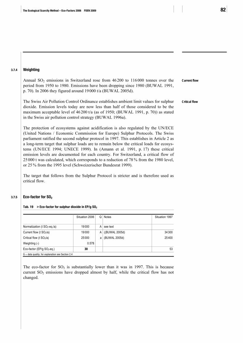
The Ecological Scarcity Method – Eco-Factors 2006 FOEN 2009 82
3.7.4 Weighting
Annual SO2 emissions in Switzerland rose from 46 200 to 116 000 tonnes over the period from 1950 to 1980. Emissions have been dropping since 1980 (BUWAL 1991, p. 70). In 2006 they figured around 19 000 t/a (BUWAL 2005d).
The Swiss Air Pollution Control Ordinance establishes ambient limit values for sulphur dioxide. Emission levels today are now less than half of those considered to be the maximum acceptable level of 46 200 t/a (as of 1950; (BUWAL 1991, p. 70)) as stated in the Swiss air pollution control strategy (BUWAL 1996a).
The protection of ecosystems against acidification is also regulated by the UN/ECE (United Nations / Economic Commission for Europe) Sulphur Protocols. The Swiss parliament ratified the second sulphur protocol in 1997. This establishes in Article 2 as a long-term target that sulphur loads are to remain below the critical loads for ecosys-tems (UN/ECE 1994; UNECE 1999). In (Amann et al. 1991, p. 17) these critical emission levels are documented for each country. For Switzerland, a critical flow of 25 000 t was calculated, which corresponds to a reduction of 78 % from the 1980 level, or 25 % from the 1995 level (Schweizerischer Bundesrat 1999).
The target that follows from the Sulphur Protocol is stricter and is therefore used as critical flow.
3.7.5 Eco-factor for SO2
Tab. 19 > Eco-factor for sulphur dioxide in EP/g SO2 Situation 2006
Q Notes Situation 1997
Normalization (t SO2-eq./a) 19 000 A see text Current flow (t SO2/a) 19 000 A ((BUWAL 2005d) 34 300 Critical flow (t SO2/a) 25 000 a (BUWAL 2005d) 25 400 Weighting (-) 0.578 Eco-factor (EP/g SO2-eq.) 30 53 Q = data quality; for explanation see Section 2.4
The eco-factor for SO2 is substantially lower than it was in 1997. This is because current SO2 emissions have dropped almost by half, while the critical flow has not changed.
Current flow
Critical flow

3 > Emissions to air 83
3.7.6 Eco-factors for further acids
Further substances are responsible for the acidification of ecosystems in addition to sulphur dioxide. An eco-factor can be derived for further substances by using the acidification potential, which characterizes the relative acidification attributable to a substance in relation to SO2 (see Section 3.7.2).
The eco-factors only assess the acidifying effect, as they are linked to SO2 via the characterization. No account is taken of the further effects of individual acids. Ammo-nia and nitrogen oxide are weighted more strongly by their specific reduction targets (cf. Sections 3.5 and 3.6), so that the eco-factor established there applies.
Tab. 20 > Eco-factors for substances with acidifying potential in EP/g acid, characterized with reference to sulphur dioxide
Acidification potential (kg SO2-eq./kg)
Eco-factor 2006 (EP/g)
Notes Eco-factor 1997 (EP/g)
Ammonia NH3 1.88 The eco-factor from direct derivation is higher (cf. Section 3.6)
63
Hydrogen fluoride HF 1.6 48 85 Phosphoric acid H3O4P 0.98 29 - Nitric acid HNO3 0.51 15 - Hydrochloric acid HCl 0.88 26 47 Sulphuric acid H2SO4 0.65 20 - Hydrogen sulphide H2S 1.88 56 - Nitrogen oxides NOx 0.7 The eco-factor from direct
derivation is higher (cf. Section 3.5)
67
for weighting and normalization see Tab. 19

The Ecological Scarcity Method – Eco-Factors 2006 FOEN 2009 84
3.8 Particulate matter (I): PM10, PM2.5 and PM2.5–10
3.8.1 Environmental impact
Particulate matter (PM) is a mixture that is complex in both physical and chemical terms. It comprises, among other things, soot, geological material, heavy metals, abrasion particles, biological material (e.g. spores) and particles formed in secondary processes in the air (sulphate, nitrate, ammonium, organic carbon) (BUWAL 2001c).
An eco-factor for PM10 has been established in the past (Brand et al. 1998). The harmfulness of particles depends on the one hand upon their size and on the other upon their composition. Account is taken of size by determining additional eco-factors for PM2.5 and PM2.5–10. The legislator, however, has not yet introduced this differentia-tion. The derivation of the new eco-factor for diesel soot, in contrast, is determined primarily by the composition – which means the carcinogenicity – of the particles. Furthermore, it is thought that in the case of diesel soot in particular toxicity correlates more closely with particle number than with absolute mass.
Fig. 3 > Schematic of particle sizes and their relationships
TSP
PM>10
PM10
PM2.5–10
PM2.5
Diesel soot
TSP: Total Suspended Particles
Epidemiological studies have shown that the particles with a diameter of less than 10 micrometres (PM10) correlate closely with the observed human health impacts of air pollution. PM10 comprises those particles which can move beyond the larynx and enter the lung. PM10 is a mixture of primary emissions (particles from combustion proc-esses, resuspended road dust and particles from the abrasion of pavings and tyres) and aerosols formed in secondary processes (BUWAL 1996b, p. 9). For instance, it has been shown in the National Research Programme 26 (People, Health, Environment) that if the long-term exposure increases by 10 micrograms PM10 per m³ the risk of various diseases of the respiratory tract rises by 30 to 60 %.

3 > Emissions to air 85
Recent scientific findings show that the risk presented by different aerosols varies in magnitude. Diesel soot emissions – defined as elemental carbon (EC)9 (Jenk 2005) – are presently considered carcinogenic and particularly hazardous to health. Diesel soot particles consist of tiny spherical tar particles. Typical diesel soot particles have a diameter of 0.1–0.2 μm, but can also be larger. Further carcinogenic organic substances adsorb on the particle surface, but their carcinogenicity is negligible compared to that of the particles (Yetergil 1997, pp. 38ff). It is assumed that in the case of diesel engines without particle filters and in the case of furnaces / combustion processes, elemental carbon accounts for approx. 90 % of the total mass of particle emissions, while in the case of internal combustion engines the proportion is approx. 3 % (Jenk 2005). Soot particles also have a global warming impact (termed Black Carbon in IPCC (2001)), which this is small compared to the hazard to health (see Section 3.2.7).
The “coarse” fraction of suspended particulate matter (PM2.5–10) is associated more closely with coughing, asthma attacks and other diseases of the respiratory tract. These larger aerosols can be coughed out of the lung. The fine fraction (PM2.5) correlates more with cardiac disrhythmia and an increased incidence of cardiovascular diseases. These fine particles remain much longer in the lung and accumulate there, as they are not readily coughed up. Ultrafine particles (PM0.1) – diesel soot particles are on this scale – can enter the bloodstream and the lymphatic system via the lung. Over time they are decomposed by the immune system and excreted (BUWAL 2001c).
Building upon these more recent findings, more detailed eco-factors are derived in the following for particles of different sizes and properties. It is tolerated here that the “total particulate” emissions listed in some inventory analyses cannot be converted directly into the new categories.
At present there are two reduction targets for particles: 1) for PM10 and 2) for diesel soot. Although it is to be assumed that the health impacts of PM2.5 are more severe than those of PM10, no corresponding differentiation has yet been performed at politi-cal or statutory level.
9 According to the new SUVA definition, soot only comprises elemental carbon (EC), while the earlier definition also included organic
carbon (OC). The present report only considers EC as soot.
The Ecological Scarcity Method – Eco-Factors 2006 FOEN 2009 86
3.8.2 Normalization
Due to a lack of robust data, no characterization is performed. PM2.5–10 and PM2.5 are subgroups to which the same environmental policy target applies. Therefore the normalization flow for the entire PM10 group and for the PM2.5–10 and PM2.5 sub-groups is identical to the current flow for PM10.
3.8.3 Weighting
The data situation for PM10 loads has been substantially improved vis-à-vis Brand et al. (1998). The current flow of 22 000 t/a is based on the BUWAL report SRU 379 (BUWAL 2005d). PM10 emissions from abrasion and resuspension are difficult to quantify. Ongoing research projects are designed to improve the assessment basis in this regard over the medium term. It must be assumed that, with the exception of road and rail transport, the present emission estimates of PM10 from abrasion and resuspen-sion are systematically too high. As the update is based on estimated values, a degree of uncertainty remains in this regard.
Scarcely any emission inventories are available for primary PM2.5. BUWAL UM 169 (BUWAL 2003d, Table 13) contains emission estimates for 2000 (13 332 t) and 2010 (12 158 t, with “business as usual” scenario); this is based upon ambient measurements. The mean – 12 745 t for primary PM2.5 – is adopted as the current flow for 2005.
The current flow for PM2.5–10 results from the difference of the annual loads for PM2.5 and 10, and figures 9255 t.
The Swiss Air Pollution Control Ordinance (Luftreinhalteverordnung, LRV) stipulates ambient limit values for PM10 (annual mean 20 µg/m³; 24-h mean 50 µg/m³) since 1 March 1998. These were adopted in response to a recommendation by the Swiss Federal Commission for Air Hygiene in view of the health impacts of fine particulate exposure (BUWAL 1996b). According to BUWAL (2005d) the emission target is approx. 12 000 tonnes PM10 per year.
There is no limit value for PM2.5 in Switzerland. However, as it is a subgroup of PM10, the same target can be applied, i.e. the critical flow is 6952 t/a.
The reduction target for PM10 is also taken for the PM2.5–10 fraction, i.e. the critical flow is 5048 t/a.
Current flow
Critical flow

3 > Emissions to air 87
3.8.4 Eco-factors for PM10, PM2.5 and PM2.5–10
Tab. 21 > Eco-factor for PM10 in EP/g PM10 Situation 2006 Q Notes Situation 1997
Normalization (t PM10/a) 22 000 B Current flow (t PM10/a) 22 000 B PM10 emissions with diesel soot 36 000 Critical flow (t PM10/a) 12 000 a (BUWAL 2005d) 18 000 Weighting (-) 3.36 Eco-factor (EP/g PM10) 150 110 Q = Data quality; for explanation see Section 2.4
Tab. 22 > Eco-factors for PM2.5 in EP/g PM2.5 Situation 2006 Q Notes Situation 1997
Normalization (t PM2.5/a) 22 000 B Applying target for PM10 Current flow (t PM2.5/a) 12 745 B (BUWAL 2003d),
PM2.5 emissions incl. diesel soot -
Critical flow (t PM2.5/a) 6 952 a - Weighting (-) 3.36 Eco-factor (EP/g PM2.5) 150 110 Q = Data quality; for explanation see Section 2.4
Tab. 23 > Eco-factor for PM2.5–10 in EP/g PM2.5–10 Situation 2006 Q Notes Situation 1997
Normalization (t PM2.5–10/a) 22 000 B Applying target for PM10 Current flow (t PM2.5–10/a) 9 255 B Difference between PM2.5 and PM10,
emissions incl. diesel soot -
Critical flow (t PM2.5–10/a) 5 048 a - Weighting (-) 3.36 Eco-factor (EP/g PM2.5–10) 150 110 Q = Data quality; for explanation see Section 2.4
Although PM10 emissions have dropped since 1997, the eco-factor is higher as a stricter reduction target is now applied. The eco-factors for PM2.5 and PM2.5–10 are identical to those for PM10, as the same reduction target is applied in each case.
3.8.5 Instruction for implementation
If the eco-factor for diesel soot is also used, care must be taken that no double weight-ing of particles is performed (see Section 3.9.4), as the particle groups overlap (Fig. 3).

The Ecological Scarcity Method – Eco-Factors 2006 FOEN 2009 88
3.9 Particulate matter (II): Diesel soot
3.9.1 Introduction
The sources and impacts of diesel soot are described in Section 3.8.1.
There is considerable debate on diesel soot at present. This has to do on the one hand with the precise definition (as “elemental carbon” in the present report), and on the other hand with its toxic effects. There are indications that the toxic effect of elemental carbon particles correlates more closely with particle number than with mass. If that is the case, the eco-factor would need to relate to the particle number. The requisite measurement technology, however, is not yet mature and derivation based on particle number is therefore not (yet) possible.
3.9.2 Normalization
The normalization flow is identical to the current flow, as no characterization is applied and the target directly concerns diesel soot.
3.9.3 Weighting
The calculation of the current flow for diesel soot is based primarily on the data given in the BUWAL report UM-136 (BUWAL 2001b), whereby certain updates were performed for road transport, construction machines and aviation. The Swiss Air Pollution Control Ordinance LRV uses the term “diesel soot”. In addition to diesel engines, further sources are taken into account in the calculations whose soot emissions scarcely differ from diesel soot. Following the rules established by SUVA for diesel engines in underground mining, diesel soot is measured as elemental carbon. The emissions of the following processes are taken into account:
> Diesel and internal combustion engines in vehicles (automobiles, buses, utility vehicles, aircraft, ships, locomotives, agricultural vehicles, military vehicles and construction machines)
> Oil and gas firings > Diesel aggregates > Gas turbines
Soot emissions from the combustion of wood, coal and wastes are not taken into account. A total current flow of 3400 t/a results.
There is no threshold value for the carcinogenic effect of diesel soot. Therefore, apply-ing the minimization rule for the emissions of carcinogenic substances (LRV, Annex 1 (82) para 1), the standard to be applied is that as much is done to reduce emissions as
Current flow
Critical flow

3 > Emissions to air 89
technology and operating conditions will allow, providing this is economically viable, i.e. the precautionary principle is to be applied (Section 2.2.3).
It follows from earlier publications and more recent findings that it should be possible to reduce diesel soot emissions in Switzerland, while applying the precautionary prin-ciple, to less than 500 t/a; this can be achieved above all by fitting particle filters to diesel engines.10 The precautionary principle is considered to be observed under the following assumptions:
1. EURO5/6 for road vehicle (truck, automobile, bus) emissions in accordance with the “Future Diesel” proposal by UBA, or elimination of diesel soot emissions from road transport by means of particle filters
2. Equipment of 40 %11 of construction machines with particle filters in accordance with the requirements established by the FOEN construction directive
3. Reduction of diesel soot emissions from construction machines, agriculture, forestry and industrial machinery in accordance with EU Directive 2004/26/EC (EU3B)
4. Particle filters are only used in specific cases in agriculture, forestry and industrial machinery, as the emissions standard for particles can also be achieved without us-ing such filters.
As the EU directive makes strict stipulations with its EU3B standard, diesel soot emissions from agriculture and forestry are dropping rapidly even without particle filters being mandatory. For larger machines in particular (>56 kW), a reduction of particle emissions by a factor of 50 from present levels is prescribed. In the other emission sectors, particle filters eliminate 99 % and more of diesel soot emissions. This results in the achievable critical flow of 450 t/a.
3.9.4 Eco-factor for diesel soot (elemental carbon, EC)
Tab. 24 > Eco-factor for diesel soot in EP/g diesel soot
To be applied when the life cycle inventory contains correspondingly adjusted PM10 and PM2.5 data. Situation 2006
Q Notes Situation 1997
Normalization (t diesel soot/a) 3 400 B Current flow (t diesel soot/a) 3 400 B Derived from BUWAL (2001b) and updated t - Critical flow (t diesel soot/a) 450 a Precautionary principle - Weighting (-) 57.1 Eco-factor (EP/g diesel soot) 17 000 - Q = Data quality; for explanation see Section 2.4
10 Personal communication, H. Jenk, FOEN, 22 February 2005 11 Proportion of construction sites in Switzerland for which particle filters are mandatory

The Ecological Scarcity Method – Eco-Factors 2006 FOEN 2009 90
This newly introduced eco-factor for diesel soot (elemental carbon, EC) is higher by a factor of 100 than that for PM10 or PM2.5. This reflects the fact that diesel soot parti-cles have a far more harmful impact upon human health than other particles. Particle filters effectively eliminate soot particles. A considerable reduction of other air pollut-ants has already been achieved by deploying catalytic converters. Current assessments of transport and combustion processes therefore depend greatly upon diesel soot emis-sions.
Diesel soot also has a global warming impact (see Section 3.2.7). The eco-factor calculated for that impact, however, is much lower than the eco-factor derived here for the human health impact.
3.10 Carbon monoxide (CO)
Carbon monoxide is an air pollutant that is formed in incomplete combustion proc-esses. CO emissions can also arise naturally from the chemical transformation proc-esses of mircoorganisms (e.g. oxidation of methane). Motor vehicle traffic generates around a half of all anthropogenic emissions (BUWAL 1995, p. 77).
CO is a colourless, odourless and tasteless gas. It is toxic when inhaled; low concentra-tions in the inhaled air already significantly reduce the oxygen transport capacity in the human body (BUWAL 1995).
In Switzerland there are statutory provisions governing maximum permissible concen-trations, but not for loads. The carbon monoxide eco-factor is therefore derived on the basis of its global warming potential (Section 3.2.7).

3 > Emissions to air 91
3.11 Benzene
3.11.1 Sources and environmental impact
Small quantities of benzene are already present in crude oil. Further quantities are formed when mineral oil is refined and when organic matter is burnt incompletely (e.g. in forest fires). Emissions of benzene to the atmosphere result primarily from combus-tion processes. In Switzerland, motorized transport is the source of three-quarters of all benzene emissions. The remainder is attributable to wood- and oil-fired heating sys-tems, and to losses in fuel handling and storage (BUWAL 2003b).
Inhalation is the main exposure route for benzene. Benzene is soluble in fat and is therefore stored in the fatty tissue of the body. As women have a higher body fat ratio than men, the impacts of this pollutant are greater for women. Individuals living or working near to highly frequented roads or petrol stations are also more greatly ex-posed. Uptake via the skin is only relevant where benzene is handled directly (BU-WAL 2003b).
Benzene is toxic to blood formation and chronic exposure can lead to leukaemia. There is unequivocal evidence that benzene is carcinogenic, and strong indications that it is mutagenic. There is no threshold below which exposure to benzene presents no hazard to human health (BUWAL 2003b).
3.11.2 Normalization
As the reduction target relates solely to benzene and no characterization is performed, the normalization flow is identical to the current flow.
3.11.3 Weighting
Emissions in 2000 figured approx. 1370–1430 t/a. A reduction to half this level (680–740 t/a) by 2010 is expected, primarily in the transport sector due to tightened exhaust standards (BUWAL 2003b). The mean value of the years 2000 and 2010 is used here as the current flow for 2005, i.e. 1055 t/a.
There is no threshold value for the carcinogenic effect of benzene. In accordance with the principle that emissions of carcinogenic substances must be minimized (LRV, Annex 1 (82), para 1) the precautionary principle should be applied (Section 2.2.3). This means that all measures must be taken that technology and operating conditions will allow and that are economically viable.
Engines in line with the EURO4 standard are the state of the art in road transport. No further tightening of hydrocarbon limit values is currently under debate. It is assumed
Current flow
Critical flow

The Ecological Scarcity Method – Eco-Factors 2006 FOEN 2009 92
for boat motors and small equipment that benzene emissions are halved by 2010 (more 4-stroke engines, more alkylated petrol). For the handling and storage of fuels and for firings, the figures anticipated by BUWAL (2003b) in 2010 are used here. Benzene emissions are assumed to drop by 2030 to a level of 316 t/a in road transport, 77.5 t/a in the fields of boat motors and small equipment, and 130 t/a in the field of handling / storage / firings, which results in a total critical flow of 525 t/a.
According to the report on “Benzene in Switzerland” (BUWAL 2003b) benzene emis-sions would need to be reduced to 100 t per year if an acceptable risk is not to be exceeded. Such a target, however, would go substantially beyond what technology and operating conditions and economic viability would allow today.
3.11.4 Eco-factor for benzene
Tab. 25 > Eco-factor for benzene in EP/g benzene Situation 2006
Q Notes Situation 1997
Normalization (t benzene/a) 1 055 A Current flow (t benzene/a) 1 055 A (BUWAL 2003b) - Critical flow (t benzene/a) 525 a Precautionary principle - Weighting (-) 4.04 Eco-factor (EP/g benzene) 3 800 32* Q = Data quality; for explanation see Section 2.4 * NMVOC eco-factor based on situation in 1997
Benzene was not previously assessed as an individual substance, but as a part of the NMVOC group. The new form of assessment, based on carcinogenicity, leads to an eco-factor that is approximately 100 times greater; this is appropriate considering the severity of the problems presented by this substance compared to average NMVOCs.

3 > Emissions to air 93
3.12 Dioxins and furans (PCDD/PCDF)
3.12.1 Environmental impact
Dioxins and furans (PCDD and PCDF) are chlorinated aromatic hydrocarbons, some of which are highly toxic to humans and animals. There are in total 76 dioxins and 135 furans. They are formed in technological but also in natural combustion processes in the presence of chlorine. These processes always generate a mixture of various indi-vidual substances, expressed as a “dioxins and furans” aggregate parameter (PCDD/F) in international toxicity equivalents (I-TEQ).12 They accumulate in the food chain and are also embryotoxic. Dioxins impair embryonal development in several ways. In particular, they appear to give rise to miscarriage, deformity of (genital) organs, and intellectual deficits (BUWAL 1995; Lippmann 2000).
Dioxins and furans are scarcely volatile; their dispersal is mainly through attachment to particles. The main exposure route is via the ingestion of foods containing fat. In 1990, the WHO set the limit value for the acceptable daily intake (ADI) by humans at 10 pg 2,3,7,8-TCDD-eq per kg body weight. Based on more recent findings, the Dutch health ministry has proposed reducing the ADI limit value to 1 pg I-TEQ/kg body weight. The daily dioxin and furan intake of individuals in Western Europe is between 0.3 and 2 pg I-TEQ per kg body weight. Thanks to the drop in emissions, a reduction of the daily dioxin and furan intake can be expected (BUWAL 1997a).
The guideline value for dioxins and furans in soil, which is 5 ng I-TEQ/kg, is not exceeded in Switzerland, except in soils subject to major anthropogenic impact.
3.12.2 Normalization
Dioxins and furans are practically always stated in life cycle inventories as character-ized quantities in I-TEQ. The reduction target therefore also applies to this character-ized quantity, and thus the normalization flow is identical to the (already characterized) current flow.
3.12.3 Weighting
Before 1955, dioxin and furan emissions were below 40 g I-TEQ/a. They rose between 1955 and 1980 to a level of 485 g I-TEQ/a. Since then they have been dropping thanks to improved exhaust purification technology, as today all municipal waste incineration plants are fitted with a flue gas purification system (BUWAL 2003a). In 2000 they amounted to 70 g I-TEQ/a, whereby now almost half of the emissions (30 g I-TEQ/a) are generated by households (BUWAL 1997a). 12 I-TEQ: International toxicity equivalent is a weighting factor that aggregates the various dioxins and furans in accordance with their
respective toxicities. The factor 1 is assigned to the Seveso dioxin 2,3,7,8-TCDD.
Current flow

The Ecological Scarcity Method – Eco-Factors 2006 FOEN 2009 94
For the period to 2010, it is anticipated on the one hand that overall emissions will drop slightly to 65 g I-TEQ/a due to improvements in municipal waste incineration plants and in industrial processes. On the other hand, it must be expected that the introduction or increase of waste collection charges will cause more household wastes and treated wood to be burnt in open fires (including cheminées). Private households will then be responsible for more than half of total emissions (37 g I-TEQ/a out of a total of 65 g I-TEQ/a) (BUWAL 1997a). The current flow is taken as the mean of the emissions in 2000 and those in 2010, i.e. 67.5 g I-TEQ/a.
As dioxins and furans accumulate in the food chain, their formation needs to be pre-vented wherever possible. In line with the precautionary principle (Section 2.2.3), the calculation of the critical flow is based on the state of the art in dioxin and furan emis-sions reduction. Flue gas purification systems such as those installed in municipal waste incineration plants achieve 99 % reduction of dioxins and furans in the exhaust.13 The provisions of the Swiss Air Pollution Control Ordinance on nitrogen oxide emis-sions also have an indirect limiting effect on dioxin and furan emissions. As a result, it can be assumed that there is a minor potential for further reductions in combustion facilities in industry and commerce. There is significant potential in private house-holds, whose emissions could be reduced by 99 % if only untreated wood and no wastes at all were burnt. This means that household emissions could be reduced from 33.5 g I-TEQ to 0.33 g I-TEQ, which translates into roughly halving the current flow to 34.5 g I-TEQ/a. This quantity is taken as the critical flow.
3.12.4 Eco-factor for dioxins and furans
Tab. 26 > Eco-factors for dioxins and furans in EP/g I-TEQ Situation 2006
Q Notes Situation 1997
Normalization (g I-TEQ/a) 67.5 B Current flow (g I-TEQ/a) 67.5 B (BUWAL 1997a) - Critical flow (g I-TEQ/a) 34.5 b Precautionary principle - Weighting (-) 3.83 Eco-factor (EP/g I-TEQ) 5.7 * 1010 - Q = Data quality; for explanation see Section 2.4
The eco-factor for dioxins and furans is very high. This is an expression of the low emission quantities in the order of several grams per year, and further reflects the great harmfulness of these substances and the available reduction options.
13 According to the personal communication by Beat Müller, FOEN, of 17.2.2005 a reduction by a factor of 100 to 1000 is to be expected,
and a reduction by 99 % is thus a reasonable assumption.
Critical flow

3 > Emissions to air 95
3.13 Lead (Pb)
Lead exposure damages animals and plants, and impairs soil fertility. Lead accumu-lates in food chains. It can impair blood formation and can cause developmental disor-ders in children (BUWAL 1991, p. 29).
3.13.1 Normalization
As the various lead compounds are not characterized, the normalization flow is the quantity emitted to air across the whole of Switzerland.
3.13.2 Weighting
Because lead was blended into petrol, lead emissions rose sharply from the 1950s onwards. They peaked at 2160 t/a in 1970. Thanks to the introduction of unleaded petrol, emissions have dropped again since then. Further uses of lead include batteries, paints and lead for bullets. Total emissions figured 226 t/a in 1995 and were estimated at 91 t/a for 2005 (BUWAL 1995, p. 86). These 91 tonnes are generated mainly by waste incineration plants and the steel industry.
The Swiss Air Pollution Control Ordinance (Luftreinhalteverordnung, LRV) stipulates ambient limit values (annual mean values) for lead in dust deposition. However, no critical flow can be derived from this. A theoretical critical flow can, however, be derived from the weighting factor for soil, as set out in the following.
The purpose o the LRV is to “[…] protect humans, animals, plants, their biotic com-munities and habitats as well as soil from air pollution that is harmful or noxious” (LRV, Art. 1). Soil protection is thus a stated goal of the LRV. It is therefore possible to apply targets established for soils to air emissions, i.e. to make use of the weighting factors for emissions to soils. If soil is taken to be a target of protection in its own right, the ratio of current to critical flow for heavy metal emissions to air that finally enter the soil via deposition must be the same as that for direct emissions to soil. The weighting factor for lead to soil, as determined in Section 6.2, is therefore used.
Current flow
Critical flow
Weighting factor

The Ecological Scarcity Method – Eco-Factors 2006 FOEN 2009 96
3.13.3 Eco-factor for lead
Tab. 27 > Eco-factor for lead emissions to air in EP/g lead Situation 2006 Q Notes Situation 1997
Normalization (t Pb/a) 91 B Current flow (t Pb/a) 91 B Value for 2005 in accordance with BUWAL
(1995, p. 86) 226
Critical flow (t Pb/a) (58) Theoretical value calculated from weighting 280 Weighting (-) 2.44 Corresponds to weighting factor for lead loading of soil Eco-factor (EP/g Pb) 27 000 2 900 Q = Data quality; for explanation see Section 2.4
Due to the new derivation methodology, the new eco-factor is substantially higher than the previous one, although emissions have already dropped significantly. The increase by almost a factor of 10 is possibly due to the circumstance that the ambient limit value (the previous basis) tends to be set more generously than is the case for other heavy metals, because of the emissions from the transport sector. This has led until now to a relatively less strict assessment.
3.14 Cadmium (Cd)
3.14.1 Environmental impact
Even small quantities of cadmium are toxic to humans and animals if exposure is chronic. Attached to aerosols, cadmium is resorbed particularly readily in the lungs. It is bioaccumulative, and, moreover, disturbs storage of vital metals in the body. Cad-mium is also carcinogenic. The consequences of chronic cadmium exposure can in-clude diseases of the respiratory tract, kidney damage, and anaemia due to iron defi-ciency. Moreover, it is toxic to plants and microorganisms and impairs soil fertility (BUWAL 1991, p. 30).
3.14.2 Normalization
As the various cadmium compounds are not characterized, the normalization flow is the quantity emitted to air across the whole of Switzerland.

3 > Emissions to air 97
3.14.3 Weighting
Cadmium emissions peaked at 7 t/a around 1970. As a result of measures taken in waste incineration and in the metal industry, they have dropped substantially since 1980. The main applications of cadmium are alloys and the production of dry batteries and colouring pigments. In 1995 emissions amounted to approx. 2.5 t/a. Emissions are estimated at 2 t/a for 2005 (BUWAL 1995, p. 90).
The Swiss Air Pollution Control Ordinance (Luftreinhalteverordnung, LRV) stipulates ambient limit values (annual mean values) for cadmium in dust deposition. However, no critical flow can be derived from this. A theoretical critical flow can, however, be derived from the weighting factor for soil, as set out in the following.
The purpose o the LRV is to “[…] protect humans, animals, plants, their biotic com-munities and habitats as well as soil from air pollution that is harmful or noxious” (LRV, Art. 1). Soil protection is thus a stated goal of the LRV. It is therefore possible to apply targets established for soils to air emissions, i.e. to make use of the weighting factors for emissions to soils. If soil is taken to be a target of protection in its own right, the ratio of current to critical flow for heavy metal emissions to air that finally enter the soil via deposition must be the same as that for direct emissions to soil. The weighting factor for cadmium to soil, as determined in Section 6.2, is therefore used.
3.14.4 Eco-factor for cadmium
Tab. 28 > Eco-factor for cadmium emissions to air in EP/g cadmium Situation 2006
Q Notes Situation 1997
Normalization (t Cd/a) 2.00 B Current flow (t Cd/a) 2.00 B Value for 2005 in accordance with BUWAL (1995, p. 90) 2.5 Critical flow (t Cd/a) (2.08) Theoretical value calculated from weighting 4.5 Weighting (-) 0.925 Corresponds to weighting factor for cadmium loading of
soil
Eco-factor (EP/g Cd) 460 000 120 000 Q = Data quality; for explanation see Section 2.4
The current flow of cadmium has dropped in recent years and is now slightly below the critical flow. Due to the ban on accumulators containing cadmium and their resulting replacement by more modern, cadmium-free products, a further drop can be expected in future.
Current flow
Critical flow
Weighting factor
The Ecological Scarcity Method – Eco-Factors 2006 FOEN 2009 98
3.15 Mercury (Hg)
3.15.1 Environmental impact
Mercury is highly toxic to humans and animals. It is taken in via the respiratory tract and accumulates in various organs. It is also toxic to plants and microorganisms and impairs soil fertility (BUWAL 1995).
3.15.2 Normalization
The normalization flow is identical to the current flow.
3.15.3 Weighting
Industry and commerce are the principal generators of mercury emissions. In the past, municipal waste incineration plants were a further important source, but their emis-sions have been reduced substantially through improved flue gas purification. Switzer-land reported annual emissions of 1020 kg Hg to the United Nations for 2004.14.
As mercury is not addressed by the study on heavy metal inventories (Keller et al. 2005b), no eco-factor can be derived for mercury from the rate of accumulation in soil. Mercury is, however, addressed by the NABO standard measurement programme. This has found major dynamics with regard to mercury concentration changes. The guide-line value of 0.5 mg/kg was, however, only exceeded at 3 of 102 sites (BUWAL 2000b).
The strictest target of the Swiss air pollution control strategy is to reduce emissions to the level of 1950 (Schweizerischer Bundesrat 1999). In the case of mercury, emissions in 1950 amounted to 2220 kg Hg. This value is taken as the critical flow.
14 Personal communication by N. Egli, FOEN, 3 November 2006
Current flow
Critical flow

3 > Emissions to air 99
3.15.4 Eco-factor for mercury
Tab. 29 > Eco-factor for mercury emissions to air in EP/g mercury Situation 2006
Q Notes Situation 1997
Normalization (kg Hg/a) 1 020 B Current flow (kg Hg/a) 1 020 B 3.3 Critical flow (kg Hg/a) 2 220 b Weighting (-) 0.21 Eco-factor (EP/g Hg) 210 000 120 000* Q = Data quality; for explanation see Section 2.4 * In the absence of a defined critical flow, the eco-factor for cadmium was also applied for mercury in Brand et al. (1998)
The current flow of mercury has dropped steadily in recent years. No further reduction is expected.
3.16 Zinc (Zn)
3.16.1 Environmental impact
Zinc loads impair plant growth (BUWAL 1991, p. 29).
3.16.2 Normalization
As the various zinc compounds are not characterized, the normalization flow is the quantity emitted to air across the whole of Switzerland.

The Ecological Scarcity Method – Eco-Factors 2006 FOEN 2009 100
3.16.3 Weighting
Until the 1970s, zinc emissions came mainly from steelworks and from the unfiltered burning of wastes. Total emissions peaked in 1970 at 1750 t/a. In 1995, approx. 630 t were still emitted, whereby dropping emissions in industry and commerce were partly compensated by rising zinc emissions from road traffic (tyre and road abrasion). A further drop to 560 t/a is taken as the figure for 2005, whereby the transport sector is now the main source, accounting for two-thirds (BUWAL 1995, p. 88). If the trend towards increasing zinc emissions from transport persists, it must be expected that overall zinc emissions rise again, as no further significant reductions are to be expected in industry.
The Swiss Air Pollution Control Ordinance (Luftreinhalteverordnung, LRV) stipulates ambient limit values (annual mean values) for zinc in dust deposition. However, no critical flow can be derived from this. A theoretical critical flow can, however, be derived from the weighting factor for soil, as set out in the following.
The purpose o the LRV is to “[…] protect humans, animals, plants, their biotic com-munities and habitats as well as soil from air pollution that is harmful or noxious” (LRV, Art. 1). Soil protection is thus a stated goal of the LRV. It is therefore possible to apply targets established for soils to air emissions, i.e. to make use of the weighting factors for emissions to soils. If soil is taken to be a target of protection in its own right, the ratio of current to critical flow for heavy metal emissions to air that finally enter the soil via deposition must be the same as that for direct emissions to soil. The weighting factor for zinc to soil, as determined in Section 6.2, is therefore used.
3.16.4 Eco-factor for zinc
Tab. 30 > Eco-factor for zinc emissions to air in EP/g zinc Situation 2006 Q Notes Situation 1997
Normalization (t Zn/a) 560 B Current flow (t Zn/a) 560 B Value for 2005 in accordance with BUWAL
(1995, p. 88) 630
Critical flow (t Zn/a) (359) Theoretical value calculated from weighting 1 100 Weighting (-) 2.44 Corresponds to weighting factor for zinc loading of soil Eco-factor (EP/g Zn) 4 400 520 Q = Data quality; for explanation see Section 2.4
The current flow of zinc has dropped slightly compared to 1997. However, due to the new derivation methodology, the critical flow has dropped much more strongly, lead-ing to an eco-factor that is now higher.
Current flow
Critical flow
Weighting factor

4 > Emissions to surface waters 101
4 > Emissions to surface waters
4.1 Introduction
4.1.1 Preliminary remarks
The eco-factors for the weighting of emissions to waters are based on the loads for the whole of Switzerland and therefore apply to the “average” situation in the country. Regional conditions are only taken into account in the case of phosphorus. Thus, for example, substances which pose a problem in individual small water bodies neverthe-less present levels in the Rhine below the required concentration limit for waters, owing to dilution. Ideally graded eco-factors should be made available to reflect the situation in different water bodies. This has not been done on economic grounds, but if need be it could be undertaken at any time, as set out in the chapter on methodology (Chapter 2).
The derivation of eco-factors for emissions into waters is based on simplifications which do not entirely take the ecological conditions into account. The aim of determin-ing eco-factors is not to be able to make an ecological assessment of individual pollut-ant emissions but to produce a comparative weighting across all environmental media as part of life cycle assessments.
As explained in the chapter on groundwater (see Section 5.1) , the eco-factors for surface waters should not be applied to pollutants emitted into groundwater.
4.1.2 Selection of substances
Owing to effluent purification measures taken, it has been possible to reduce signifi-cantly the emission of a number of substances into surface waters, with any emissions remaining being of subordinate importance for the ecology of Swiss waters. The question arises as to what extent eco-factors should be assigned to such substances. On the other hand, it should be borne in mind that eco-factors are applied not only to emissions within Switzerland, but also outside the country. Where possible an eco-factor is assigned to substances that may well pose no problem within Switzerland but may be environmentally significant elsewhere.
Since the entry into force of the Swiss Water Protection Ordinance (WPO; Gewässer-schutzverordnung, GSchV) in the autumn of 1997 water quality requirements are only specified for substances which are still relevant to the quality of watercourses today. The list in the WPO represents a starting point for the selection of eco-factors for substances polluting waters. Additions to the list include phosphorus on account of its significant impact on water quality in lakes, the aggregate parameter AOX (adsorbable organic halogens in waters), endocrine disruptors and radioactive emissions (from reprocessing spent fuel elements).
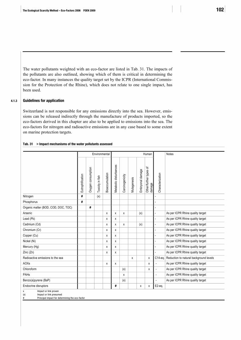
The Ecological Scarcity Method – Eco-Factors 2006 FOEN 2009 102
The water pollutants weighted with an eco-factor are listed in Tab. 31. The impacts of the pollutants are also outlined, showing which of them is critical in determining the eco-factor. In many instances the quality target set by the ICPR (International Commis-sion for the Protection of the Rhine), which does not relate to one single impact, has been used.
4.1.3 Guidelines for application
Switzerland is not responsible for any emissions directly into the sea. However, emis-sions can be released indirectly through the manufacture of products imported, so the eco-factors derived in this chapter are also to be applied to emissions into the sea. The eco-factors for nitrogen and radioactive emissions are in any case based to some extent on marine protection targets.
Tab. 31 > Impact mechanisms of the water pollutants assessed
Environmental Human
Eutro
phific
ation
Oxyg
en co
nsum
ption
Toxic
ity in
fish
Bioa
ccum
ulatio
n
Met
aboli
c dist
urba
nces
Carc
inoge
nicity
Mut
agen
esis
Embr
yona
l dam
age
Othe
r/fur
ther
type
s of
dama
ge
Char
acte
rizat
ion
Notes
Nitrogen # (x) - Phosphorus # - Organic matter (BOD, COD, DOC, TOC) # - Arsenic x x x (x) - As per ICPR Rhine quality target Lead (Pb) x x - As per ICPR Rhine quality target Cadmium (Cd) x x x (x) - As per ICPR Rhine quality target Chromium (Cr) x x - As per ICPR Rhine quality target Copper (Cu) x x - As per ICPR Rhine quality target Nickel (Ni) x x - As per ICPR Rhine quality target Mercury (Hg) x x - As per ICPR Rhine quality target Zinc (Zn) x x - As per ICPR Rhine quality target Radioactive emissions to the sea x x C14-eq. Reduction to natural background levels AOXs x x x - As per ICPR Rhine quality target Chloroform (x) x - As per ICPR Rhine quality target PAHs x - As per ICPR Rhine quality target Benzo(a)pyrene (BaP) (x) - As per ICPR Rhine quality target Endocrine disruptors # x x E2-eq. x Impact or link proven (x) Impact or link presumed # Principal impact for determining the eco-factor
4 > Emissions to surface waters 103
4.2 Nitrogen
4.2.1 Environmental impact
Over 90 % of anthropogenic total nitrogen in surface waters consists of nitrate and ammonium or ammonia. Sources of nitrogen in waters are agricultural fertilizers and industrial, commercial and household effluents. The eco-factors in this chapter only evaluate the the nitrogen loads in surface waters. Nitrogen compounds (notably nitrate) which are first released into groundwater and enter surface waters from there are assessed separately in the chapter on groundwater (see Section 5.2).
In present quantities nitrate no longer represents a general problem for the ecology of surface waters in Switzerland, although a few local problems may persist. However, the nitrogen load in the North Sea and other shallow seas is of great importance with regard to eutrophification. The aim, therefore, is to achieve a marked reduction in the nitrogen discharged into the North Sea, including by reducing loads in the Rhine (BUWAL 1996c).
4.2.2 Normalization
The assessment of the normalization flow is based on the nitrogen discharge into the Rhine catchment according the model developed by Prashun et al. (2005) extrapolated to the whole of Switzerland using the ratio of Rhine catchment runoff to total Swiss runoff.
The nitrogen load for the Rhine catchment amounts to 30 556 t N/a. Runoff via the Rhine amounts to a long-term average of around 38 bn. m³/a, and the total for Switzer-land to 48 bn. m³/a. This produces an extrapolated load of 38 597 t N/a for the whole of Switzerland.
4.2.3 Weighting
Since the reduction target refers only to emissions in the Rhine catchment within Switzerland (see next paragraph on critical flows), the current flow must cover the same area. According to the OSPAR Commission (2006) the current flow amounts to 24 827 t N/a.
In 1987, as a result of the over-use of fertilizers which became evident in the course of the 1980s, the countries bordering the North Sea issued a declaration of intent.15 The aim of this was to reduce loads of phosphorus and nitrogen to 50 % of 1985 levels by 1995. Although it is responsible for only a small amount of the total discharge into the Rhine, Switzerland has contributed to these efforts (BUWAL 1996c, p. 36). In the case of nitrogen the target has still not been reached, with the reduction amounting to 29 % by 2003 (OSPAR Commission 2006).
15 Second International Conference on the Protection of the North Sea, London, 24–25 November 1987
Current flow
Critical flow

The Ecological Scarcity Method – Eco-Factors 2006 FOEN 2009 104
This target is used as a basis for establishing the critical flow for total nitrogen emis-sions (Ntot). In 1985 the nitrogen load in the Rhine catchment was 35 020 t N/a (OSPAR Commission 2006), producing a critical flow of 17 510 t N/a. The derivation of the critical flow from the Swiss Water Protection Ordinance would result in a sig-nificantly higher critical flow16, so for that reason it is not used.
4.2.4 Eco-factor for nitrogen in surface waters
Tab. 32 > Eco-factor for nitrogen and nitrogen compounds in surface waters in EP/g N Situation 2006 Q Remarks Situation 1997
Normalization flow (t N/a) 31 360 B Extrapolated to the whole of Switzerland using NADUF runoff data
Current flow (t N/a) 24 827 A Rhine catchment only (OSPAR Commission 2006) 40 000 Critical flow (t N/a) 17 510 a 50 % reduction target in Rhine catchment
(OSPAR Commission 2006) 24 000
Weighting factor (-) 2.01 Eco-factor (EP/g N) 64 69 Q = Data quality; for explanation see Section 2.4
The eco-factor for nitrogen has fallen slightly compared with the previous situation, as the nitrogen load has been significantly reduced from the 1997 level.
4.3 Phosphorus
4.3.1 Environmental impact
The phosphorus load is more critical for lakes (and seas) than for rivers, as in standing waters it is mostly the amount of phosphorus available which represents the limiting factor for algal growth. Algal growth elevated by phosphorus causes sedimentation and the increased aerobic decomposition of this biomass, leading to oxygen deficiency and fish mortality in the deep water of lakes (BLW & BUWAL 1998).
The phosphorus load in lakes varies enormously according to location. Alpine lakes (e.g. Lake Lucerne, Lake Thun) exhibit very low concentrations, whereas lakes in areas of intensive farming can still be severely polluted by the phosphorus that is applied to the fields in manure and synthetic fertilizers. The connection of households and busi-nesses to sewage treatment works and the ban on phosphates in textile detergents has led to a marked drop in the phosphorus load over the last two decades (BLW & BU-WAL 1998; BUWAL 2004a).
16 Assuming a mean runoff via the Rhine of 1000 m³/s and taking the required value of 5.6 mg NO3-N/l, a critical flow of 176,600 t NO3-N/a
would result for the Rhine catchment.

4 > Emissions to surface waters 105
Phosphorus is released into waters as particle-bound phosphate, mainly through erosion and leaching from cropland. The still substantial contribution of agriculture to the loads is also a consequence of liberal use of fertilizers in the past. Thus agricultural land in Switzerland registers a phosphorus content far in excess of the plants’ annual require-ments. In integrated production systems it is now only permitted to use as much phos-phorus as the crops can take up, which has improved the situation somewhat (BUWAL 2004a). The ChemRRV (Chemical Risk Reduction Ordinance) also contains regula-tions on permitted applications of compost, fermented material and silage effluent, which should result in further improvement.
4.3.2 Normalization
The amount of phosphorus discharged into surface waters in the whole of Switzerland can only be estimated, as the runoff from agricultural land, which accounts for a sig-nificant proportion, is impossible to measure. Phosphorus entering the waters is ab-sorbed by aquatic plants and eventually deposited through sedimentation of the bio-mass.
Assessment of the normalization flow is based on the phosphorus entering the Rhine catchment according to the model developed by Prashun et al. (2005) and extrapolated to the whole of Switzerland using the ratio of Rhine catchment runoff to total Swiss runoff. The most recent figures (2003) are published in OSPAR Commission (2006).
The phosphorus load for the Rhine catchment amounts to 1341 t P/a. Runoff via the Rhine itself amounts to a long-term average of around 38 bn. m³/a and that from the whole of Switzerland to 48 bn. m³/a. This produces a phosphorus load of 1694 t P/a for the country as a whole.
4.3.3 Weighting: Protecting the North Sea
The current flow differs from the normalization flow, as the reduction target only applies to the Rhine catchment. According to the OSPAR Commission (2006) the phosphorus load amounts to 1341 t P/a.
The states bordering the North Sea have issued a ministerial declaration, which Swit-zerland has also signed, agreeing to reduce phosphorus and nitrogen loads to 50 % of the 1985 level. The phosphorus target has already been achieved. At 1434 t P/a the critical flow is slightly higher than the current flow (OSPAR Commission 2006).
4.3.4 Weighting: Phosphorus content of Swiss lakes
Alternatively, the weighting factor (and consequently the eco-factor) for phosphorus can also be calculated separately for every lake in Switzerland by using the target value for the phosphorus concentration in lake water (Tab. 33). The target value is set at
Current flow
Critical flow

The Ecological Scarcity Method – Eco-Factors 2006 FOEN 2009 106
20 mg P/m³ of well-mixed open water (BLW & BUWAL 1998, p. 6). Some lakes have a measured value well below this target (Walensee), while others exceed it quite con-siderably (Lake Zug and the north basin of Lake Lugano). The ecological scarcity of the large Swiss lakes is thus Extremeely varied.
To determine an average ecological scarcity for Switzerland both the current individual phosphorus concentrations and the volume of water in the lakes are relevant. The capacity of the lakes to absorb phosphorus is dependent on these two parameters. As the weighting factor has the effect of squaring the ratio of the current to the target concentration, the average weighting factor is determined on the basis of the sum of the weighting factors of each lake, weighted with their respective volumes (see Tab. 33).
Tab. 33 > Calculation of the weighting factor for Swiss lakes based on the current and target concentrations
Only lakes with reliable values for 2004, or if necessary 2005, have been included Volume of lake
m³ (millions) Total concentra-
tion of phosphorusmg/m³
Year recorded
Target valuemg/m³
Weighting factor (-)
Lake Geneva 89 900 29.5 2004 20 2.18 Lake Constance 48 000 9 2004 20 0.20 Lake Neuchâtel 14 170 7 2004 20 0.12 Lake Maggiore 37 100 10 2004 20 0.25 Lake Lucerne 11 800 5 2004 20 0.06 Lake Zurich 3 900 24.6 2004 20 1.51 Lake Lugano, north basin 4 690 110 2005 20 30.25 Lake Lugano, south basin 1 140 45 2005 20 5.06 Lake Thun 6 500 4 2004 20 0.04 Lake Biel 1 240 18 2004 20 0.81 Lake Zug 3 210 108 2005 20 29.16 Lake Brienz 5 170 4 2004 20 0.04 Walensee 2 490 3 2004 20 0.02 Lake Murten 600 11 2004 20 0.30 Lake Sempach 660 29 2004 20 2.10 Lake Hallwil 215 49 2004 20 6.00 Greifensee 161 67 2004 20 11.22 Lake Baldegg 178 43 2004 20 4.62 Pfäffikersee 58 22 2004 20 1.21 Weighting factor for Switzerland 2.04 Source: phosphor_dans_les_lacs.xls17
17 Data on phosphorus in lakes, transmitted by Dr. P. Liechti (FOEN/BAFU) on 5 April 2006. The data were collected by international
commissions (CIPEL, CIPAIS, IGKB), cantonal authorities, Eawag and Wasserversorgung Zürich (WVZ, the Zurich water utility; for Lake Zurich and the Walensee).

4 > Emissions to surface waters 107
4.3.5 Eco-factor for phosphorus
In Sections 4.3.3 and 4.3.4, the weighting has been derived by two different methods: in one instance from the 50 % reduction target for emissions into the North Sea and in the second from the protection target for Swiss lakes. The latter produces a larger eco-factor, so the one derived from the 50 % reduction target will not be included in Tab. 34.
Tab. 34 > Eco-factor for phosphorus in EP/g P Situation 2006
Q Remarks Situation 1997
Normalization flow (t P/a) 1 694 B Extrapolated using NADUF runoff data from the loads for the Rhine catchment accord-ing to the OSPAR Commission (2006)
Current flow (t P/a) - 2 900 Critical flow (t P/a) - 1 200 Weighting factor (-) 2.04 Calculated from the lake protection target Eco-factor (EP/g P) 1 200 2 000 Q = Data quality; for explanation see Section 2.4
The smaller eco-factor reflects the easing of the phosphorus problem and the effect of the measures undertaken. As shown in Tab. 33, some lakes are still subject to severe pollution, although concentrations have fallen compared with previous years.

The Ecological Scarcity Method – Eco-Factors 2006 FOEN 2009 108
4.4 Organic matter (BOD, COD, DOC, TOC)
4.4.1 Environmental impact
BOD (biochemical oxygen demand), COD (chemical oxygen demand), DOC (dis-solved organic carbon) and TOC (total organic carbon) are parameters for the concen-tration of organic matter in waters. These organic substances originate in part from natural sources and in part from waste water. In essence all organic substances pollute waters in that they consume oxygen, thus restricting the habitat of the fauna that de-pends on it. In addition to this, many substances (such as chlorinated organic com-pounds or endocrine substances) can have specific toxic impacts which should be recorded separately (Kummert & Stumm 1989; Sigg & Stumm 1989).
The pollution of Swiss waters has fallen in recent decades, owing to measures to improve effluent treatment. Moreover, the legislation (WPO) requires implementation of measures to reduce organic endocrine substances in effluent to a level at which there is no ecological detriment to waters. In most cases the residual load from effluent treatment works is non-critical in terms of the total oxygen available. Of foremost environmental importance, therefore, are persistent, bioaccumulative and toxic organic substances. However, the specific impacts of the substances encompassed by the aggregate parameter “organic matter” cannot be considered here.
The concentration of organic matter in waters can be recorded using the parameters COD, DOC and, where necessary, TOC.
BOD (biochemical oxygen demand) BODx expresses the amount of oxygen consumed by biological activity in water in x days. Incubation takes place in the dark, at 20 °C and normally over a period of 5 days (BOD5). The proportion of hydrocarbons which break down readily, particularly through microbial degradation, is determined from this. The BOD value is always lower than that for COD. Usually BOD5 is determined.
COD (chemical oxygen demand) COD expresses the amount of oxygen required to oxidize organic compounds. In Switzerland COD is used principally to determine the quality of the discharge from water treatment works (effluent parameter). In most other countries pollution of waters with organic substances is assessed in terms of COD. Many life cycle inventories contain figures for COD emissions.
DOC (dissolved organic carbon) DOC measures the bound organic carbon content of dissolved organic compounds. This measurement produces more exact results than the COD test when dealing with small concentrations such as those in Swiss watercourses (clean water parameter).

4 > Emissions to surface waters 109
TOC (total organic carbon) TOC is a measure of the total carbon bound in organic molecules. It is made up of dissolved organic carbon and particle-bound organic carbon.
Since many life cycle inventories state COD values, an eco-factor has been derived for it. If necessary DOC can be converted into COD using the estimation factor COD (in g) ≈ 3 DOC (in g). A lower estimate for COD can also be derived from BOD, with COD (in g) = BOD (in g). If only the TOC value has been measured, this can be re-garded as equivalent to DOC for the purpose of a rough approximation, hence COD can be estimated with COD (in g) ≈ 3 TOC (in g) (Brand et al. 1998).
4.4.2 Normalization
The total load cannot be extrapolated from the COD concentrations at the places where the large rivers flow out of Switzerland, as firstly some of the organic substances are of natural origin and secondly organic substances degrade to some extent relatively quickly in watercourses and do not reach the measuring stations at these runoff points.
The loads from sewage treatment works and agriculture have been determined for the canton of Berne. Dinkel et al. (2004) have extrapolated the total Swiss flow of 47 700 t COD/a from this data.
4.4.3 Weighting
The current flow is identical to the normalization flow, since the reduction target is also based on the total load for Switzerland.
In the project group Nitrogen Balance Switzerland (Stickstoffhaushalt Schweiz, 1996, p. 16–17) the critical flow is assessed on the basis of ecological criteria: from an envi-ronmental perspective a maximum of 30 % of the oxygen dissolved in water should be consumed downstream from the discharge points. The average oxygen content of river water is estimated at 10 g/m³, which produces a maximum permissible consumption of 3 g O2/m³ together with a maximum permissible load of 3 g COD/m³ (Projektgruppe Stickstoffhaushalt Schweiz 1996, p. 16–17).
The maximum anthropogenically generated COD load can be extrapolated from the quantity of runoff from Switzerland (48 bn. m³) and is put at 144 000 tonnes per year.
4.4.4 Eco-factors for BOD, COD, DOC and TOC
As all these factors measure the same thing – organic carbon – care must be taken not to count them twice. It is preferably only to assess COD, for which the eco-factor has been derived directly from the current and critical flows. In inventory analyses missing
Current flow
Critical flow

The Ecological Scarcity Method – Eco-Factors 2006 FOEN 2009 110
COD values can then be derived from the other values using the rule of thumb in Section 4.4.1.
Tab. 35 > co-factor for COD (chemical oxygen demand) in EP/g COD
The eco-factors for BOD, DOC and TOC can be calculated using the rough rules of thumb BOD ≈ COD, COD ≈ 3 DOC and DOC ≈ TOC, if no inventory analysis data is available for COD – see also the text regarding counting twice. Situation 2006
Q Notes Situation 1997
Normalization flow (t COD/a) 47 700 B Current flow (t COD/a) 47 700 B (Dinkel & Stettler 2004) 115 000 Critical flow (t COD/a) 144 000 b Derived from the project group Nitrogen
Balance Switzerland (1996, p. 16–17) 140 000
Weighting factor (-) 0.11 Eco-factor (EP/g COD) 2.30 5.9 Eco-factor (EP/g BOD) 2.30 Rough approximation: BOD ≈ COD 5.9 Eco-factor (EP/g DOC) 6.90 Derived from the eco-factor for COD with
COD ≈ 3 DOC 18
Eco-factor (EP/g TOC) 6.90 Rough approximation: COD ≈ 3 DOC ≈ 3 TOC
18
Q = Data quality; for explanation see Section 2.4
The eco-factor is smaller than in 1997 as a result of the reduction in emissions. Waste water purification throughout Switzerland and the regulations governing the discharge of effluent into waters have led to a drop in organic matter there.
The weighting of specific impacts of persistent bioaccumulative substances is not possible with the eco-factor for COD.

4 > Emissions to surface waters 111
4.5 Heavy metals and arsenic
4.5.1 Environmental impact
Heavy metals and arsenic damage the aquatic ecosystem by accumulating in organ-isms, where they can cause growth impairments and metabolic disturbances. They are able to propagate through the food chain. However, these substances do not represent a major problem in Switzerland.
Zinc and copper come from roof runoff and the use of pipes made of these metals to carry the drinking water supply. In addition zinc is released through tyre wear and enters waters via road runoff. Copper is also used as a fungicide in vineyards and as a food supplement in pig rearing.
Cadmium is an ingredient of phosphorus fertilizers and pesticides, meaning that agri-culture is another source of heavy metals. Chromium arises mainly from the corrosion of chromium steel products. Since the use of leaded petrol has declined and industrial effluent discharges have been cleaned up these have now become the predominant sources of heavy metals (BUWAL et al. 2000).
Arsenic is carcinogenic to humans (IARC group 1). It causes skin and bladder cancer in particular, but other types of cancers as well, through chronic exposure via drinking water (IARC 1987). Arsenic arises as a by-product of metal extraction, but is also used in industrial processes such as glass production and as gallium arsenide in electronic equipment. In some countries (for example, Bangladesh and Vietnam) even natural sources can lead to concentrations in drinking water that are harmful to health (Lippmann 2000).
4.5.2 Normalization
The total load of heavy metals entering surface waters in Switzerland can be extrapo-lated from the concentration values measured in the Rhine.
In Weil am Rhein heavy metal concentrations in the water are determined in accor-dance with NADUF (Swiss National River Monitoring and Survey Programme) regula-tions (BUWAL et al. 2000), and the heavy metal content of suspended matter is meas-ured according to the International Commission for the Protection of the Rhine (IKSR 2004). To determine the normalization the NADUF values have been used, as these include dissolved heavy metals. In order to compensate for the occasional wide varia-tions in concentration from one year to another and obtain more representative values, the average for the years 2001 to 2004 has been used in each case (Tab. 36).
The following factors could account for any difference between the actual situation and the extrapolated flow:

The Ecological Scarcity Method – Eco-Factors 2006 FOEN 2009 112
> the total concentration of heavy metals rises with the concentration of suspended matter, since the metals accumulate there. In the Rhone, which registers compara-tively high particle concentrations, concentrations of heavy metals may therefore exceed those in the Rhine.
> the Rhine may exhibit above average mercury loads on account of the structure of industry in the catchment.
> between entering the water and being measured in Basel the heavy metals undergo some degree of exchange with the sediment. Depending on the concentration ratios in the river and the sediment net heavy metals are either dissolved or deposited.
Tab. 36 > Calculation of the normalization flow for heavy metals based on NADUF concentration figures (mean value for the years 2001 to 2004) at Weil am Rhein monitoring station. Average concentration in the Rhine
g/sNormalization
t/a Arsenic (As) 0.188* 8.6* Lead (Pb) 0.704 32 Cadmium (Cd) 0.0134 0.61 Chromium (Cr) 0.555 25 Copper (Cu) 1.61 74 Nickel (Ni) 1.84 84 Mercury (Hg) 0.0044 0.20 Zinc (Zn) 3.65 167 * Arsenic values calculated from ICPR (2004) concentration figures and the assumption of 17.9 kg of suspended solids/s (mean value for the years 2001 to 2004 based on NADUF)
4.5.3 Weighting
Seven heavy metals with implications for the environment are listed in the Swiss Water Protection Ordinance (WPO). They are mercury (Hg), cadmium (Cd), lead (Pb), chro-mium (Cr), copper (Cu), zinc (Zn) and nickel (Ni). The WPO sets out quality require-ments both for watercourses in the form of required and guideline values and for the discharge of effluent into sewers and waters. The limits for the latter are more rigor-ously defined (BUWAL et al. 2000).
In addition, in 2003 the Convention on the Protection of the Rhine (IKSR 1999), which was renewed in 1999 and to which Switzerland is also a signatory, entered into force. The ICPR (International Commission for the Protection of the Rhine), like the WPO, sets water quality targets in the form of concentration limits – including for heavy metals. The ICPR targets for heavy metals bound in the suspended solids phase are roughly similar to the WPO concentration limits for effluent discharges (working on the basis of an average suspended matter content of 16 mg/l).
The ratio of the heavy metal content of suspended solids to their ICPR (2004) target levels is significantly higher than the ratio of the total concentration of heavy metals in water to the limits set by the WPO. Therefore for weighting purposes the more strin-
Weighting factor

4 > Emissions to surface waters 113
gent targets, and thus higher eco-factors based on ICPR data, are used. To produce the weighting factor the concentrations in the suspended solids (rather than the rivers) are compared directly with each other (Tab. 37). The data on current concentrations is taken from the annual report from the Rhine monitoring station at Weil am Rhein (AUE 2005), which gives the most recent figures.
Tab. 37 > Weighting factors for heavy metals calculated from current and critical concentrations
Current concentration (measured value)
Critical concentration (target value)
Weighting
mg/kg suspended matter mg/kg suspended matter (-) Arsenic (As) 10.5 40 0.07 Lead (Pb) 38 100 0.14 Cadmium (Cd) 0.42 1.00 0.18 Chromium (Cr) 44 100 0.19 Copper (Cu) 51 50 1.04 Nickel (Ni) 38 50 0.57 Mercury (Hg) 0.21 0.50 0.18 Zinc (Zn) 182 200 0.83 Quelle: (AUE 2005) (IKSR 2004)
4.5.4 Eco-factors for heavy metals and arsenic in surface waters
Tab. 38 > Eco-factors for heavy metals in surface waters in EP/g of each heavy metal
Normali-zation
Q Current con-
centration
Q Critical con-
centration
Q Weighting Eco-factor 2006
Eco-factor 1997
t/a mg/kg mg/kg (-) EP/g EP/g Arsenic (As) 8.6 B 10.5 A 40 a 0.069 8 000 - Lead (Pb) 32 B 38 A 100 a 0.14 4 400 190 Cadmium (Cd) 0.61 B 0.42 A 1.00 a 0.18 290 000 11 000 Chromium (Cr) 25 B 44 A 100 a 0.19 7 600 660 Copper (Cu) 74 B 51 A 50 a 1.04 14 000 1 200 Nickel (Ni) 84 B 38 A 50 a 0.57 6 800 190 Mercury (Hg) 0.20 B 0.21 A 0.50 a 0.18 880 000 240 000 Zinc (Zn) 167 B 182 A 200 a 0.83 5 000 210 Q = Data quality; for explanation see Section 2.4
The values required by the WPO have not altered since being used in Brand et al. (1998), which would have resulted in the eco-factors staying more or less the same. By using the more stringent targets from the ICPR account has been taken of political developments which have not yet found expression in the Water Protection Ordinance. The resulting eco-factors are significantly higher than those from 1997.

The Ecological Scarcity Method – Eco-Factors 2006 FOEN 2009 114
4.6 Radioactive emissions to seas
4.6.1 Introduction
Until now radioactive emissions have been excluded from assessments using the ecological scarcity method. The quantity of emissions from nuclear power plants in Switzerland is well below statutory limits. No other substantial sources of emissions have been identified in the country.
The reason why radioactive emissions to seas are now being assessed lies in the OSPAR Conventions for the protection of the North Sea. The OSPAR member states have agreed to reduce substantially the loads of radioactive substances from reprocess-ing plants into the Irish and North Seas.
Because of that an eco-factor is derived on the basis of emissions occurring outside Switzerland. The reduction targets are based on international agreements which Swit-zerland supports. (A similar procedure is applied in relation to fresh water use in arid countries, see Section 7.5 )
The moratorium on reprocessing spent fuel elements, which came into effect on July 1 2006, has no influence on the scarcity formula produced here. It is an exceptional situation, and of limited duration. The cessation of reprocessing and its associated emissions of radioactive elements to the seas will nonetheless have an impact on future inventory analyses of electricity generation at Swiss nuclear power plants, although those of, for example, French nuclear energy and France’s strategy for disposing of spent fuel elements remain unaffected. Emissions generated by French nuclear energy are still relevant to Switzerland because of the electricity imported from there.
4.6.2 Environmental impact
Exposure to radiation transfers energy into human tissue and in doing so can interfere with the molecular structure. This can disturb or destroy cell functions in living organ-isms (somatic effects, i.e. fatal or non-fatal cancer), or it can alter the genetic code of the cells (mutagenic effects).
The characterization factors take both these effects into account. The impact of radia-tion on ecosystems is not considered here, nor are the potential impacts of accident-related releases of large quantities of radioactive substances.
4.6.3 Characterization
The environmental impact of the emission of radioactive elements is characterized according to its carcinogenic impact on humans. Impacts on ecosystems are not con-
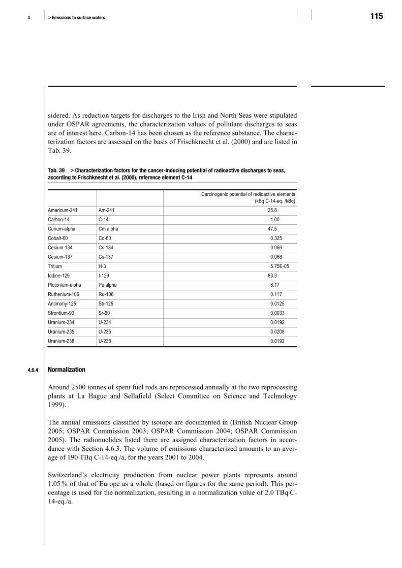
4 > Emissions to surface waters 115
sidered. As reduction targets for discharges to the Irish and North Seas were stipulated under OSPAR agreements, the characterization values of pollutant discharges to seas are of interest here. Carbon-14 has been chosen as the reference substance. The charac-terization factors are assessed on the basis of Frischknecht et al. (2000) and are listed in Tab. 39.
Tab. 39 > Characterization factors for the cancer-inducing potential of radioactive discharges to seas, according to Frischknecht et al. (2000), reference element C-14 Carcinogenic potential of radioactive elements
(kBq C-14-eq. /kBq) Americum-241 Am-241 25.8 Carbon-14 C-14 1.00 Curium-alpha Cm alpha 47.5 Cobalt-60 Co-60 0.325 Cesium-134 Cs-134 0.066 Cesium-137 Cs-137 0.066 Tritium H-3 5.75E-05 Iodine-129 I-129 83.3 Plutonium-alpha Pu alpha 6.17 Ruthenium-106 Ru-106 0.117 Antimony-125 Sb-125 0.0125 Strontium-90 Sr-90 0.0033 Uranium-234 U-234 0.0192 Uranium-235 U-235 0.0208 Uranium-238 U-238 0.0192
4.6.4 Normalization
Around 2500 tonnes of spent fuel rods are reprocessed annually at the two reprocessing plants at La Hague and Sellafield (Select Committee on Science and Technology 1999).
The annual emissions classified by isotope are documented in (British Nuclear Group 2005; OSPAR Commission 2003; OSPAR Commission 2004; OSPAR Commission 2005). The radionuclides listed there are assigned characterization factors in accor-dance with Section 4.6.3. The volume of emissions characterized amounts to an aver-age of 190 TBq C-14-eq./a, for the years 2001 to 2004.
Switzerland’s electricity production from nuclear power plants represents around 1.05 % of that of Europe as a whole (based on figures for the same period). This per-centage is used for the normalization, resulting in a normalization value of 2.0 TBq C-14-eq./a.

The Ecological Scarcity Method – Eco-Factors 2006 FOEN 2009 116
4.6.5 Weighting
OSPAR targets are defined separately for alpha and beta emitters (see next paragraph). These two separate targets have been amalgamated here to a single goal by means of characterization. As the French reprocessing plant at La Hague does not set any quanti-tative targets it is assumed that the Sellafield target is also applicable there. Having made this assumption, it is sufficient to look at the emissions from the Sellafield re-processing plant to determine the weighting factor.
The emissions from the Sellafield plant fluctuate from year to year with no obvious trend (see British Nuclear Group 2005; OSPAR Commission 2003; OSPAR Commis-sion 2004; OSPAR Commission 2005). For this reason a sliding average over four years (2001–2004)is used. This four-year average value of the current emissions from Sellafield amounts to 96.0 TBq C14-eq (3.2 TBq C14-eq alpha and 92.8 TBq C14-eq beta emitters).
The OSPAR Decision 2000 aims to prevent pollution of the North Sea by ionising radiation through substantial reductions in the disposal, emission and loss of radioac-tive substances. The goal is to reduce the concentrations of natural isotopes in the seas to background pollution levels and of synthetic isotopes to practically zero (OSPAR Convention 2000).
This general demand was put in more concrete terms in the Progress Report (OSPAR Convention 2003, p. 15). Whereas no specific targets have been set for France the emission targets for the British plant have been concisely defined. By 2020 the emis-sions from alpha emitters are to fall to 0.2 TBq per year, and those from beta emitters to 65 TBq per year. This corresponds to a characterized volume of emissions totalling 64.1 TBq C14-eq (2.0 TBq C14-eq alpha and 62.1 TBq C14-eq beta emitters).
Current flow
Critical flow

4 > Emissions to surface waters 117
4.6.6 Eco-factor for radioactive emissions to seas
Current and critical flows are based on characterized values. The ratio of current to critical flow is 2.24. The normalization flow is based on Switzerland’s contribution to the characterized volume of all alpha and beta emitters discharged annually into the North Sea from La Hague and Sellafield.
Tab. 40 > Eco-factor for radioactive emissions to seas in EP/kBq C14-eq Situation 2006 Q Notes Situation 1997
Normalization flow (TBq C14-eq/a) 2.00 C Current flow (TBq C14-eq/a) 96.0 B Characterized four-year average
(2001–04) of emissions from the Sellafield plant
Critical flow (TBq C14-eq/a) 64.1 b Characterized emissions target for the Sellafield plant 2020
Weighting factor (-) 2.24 Eco-factor (EP/kBq C14-eq) 1 100 Q = Data quality; for explanation see Section 2.4
The eco-factor is assigned for the first time here, as the reduction targets for the protec-tion of the North Sea, which Switzerland supports, have only been stipulated in recent years.
4.6.7 Eco-factors for individual isotopes
Using the characterization described in Section 4.6.3 it is possible to calculate eco-factors for selected isotopes. These are listed in Tab. 41. They apply to the discharge of these substances to seas. Because of the way these eco-factors have been derived they should not be used for discharges to other waters.
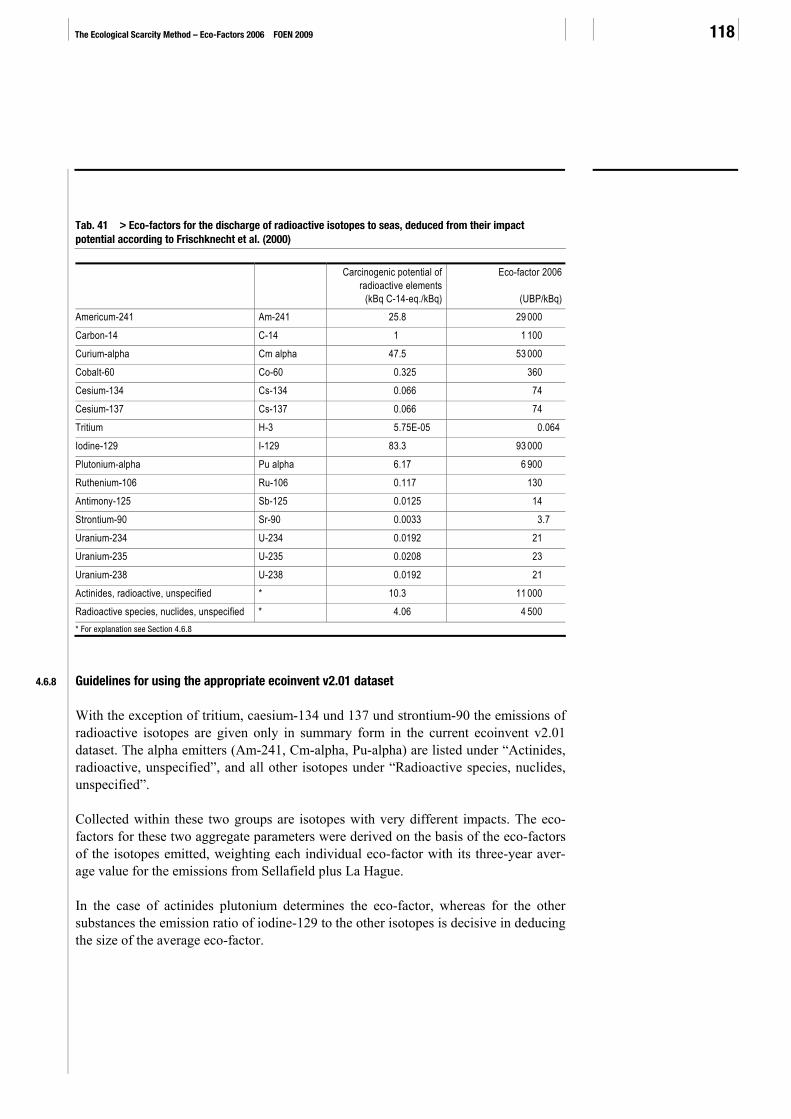
The Ecological Scarcity Method – Eco-Factors 2006 FOEN 2009 118
Tab. 41 > Eco-factors for the discharge of radioactive isotopes to seas, deduced from their impact potential according to Frischknecht et al. (2000) Carcinogenic potential of
radioactive elements (kBq C-14-eq./kBq)
Eco-factor 2006
(UBP/kBq) Americum-241 Am-241 25.8 29 000 Carbon-14 C-14 1 1 100 Curium-alpha Cm alpha 47.5 53 000 Cobalt-60 Co-60 0.325 360 Cesium-134 Cs-134 0.066 74 Cesium-137 Cs-137 0.066 74 Tritium H-3 5.75E-05 0.064 Iodine-129 I-129 83.3 93 000 Plutonium-alpha Pu alpha 6.17 6 900 Ruthenium-106 Ru-106 0.117 130 Antimony-125 Sb-125 0.0125 14 Strontium-90 Sr-90 0.0033 3.7 Uranium-234 U-234 0.0192 21 Uranium-235 U-235 0.0208 23 Uranium-238 U-238 0.0192 21 Actinides, radioactive, unspecified * 10.3 11 000 Radioactive species, nuclides, unspecified * 4.06 4 500 * For explanation see Section 4.6.8
4.6.8 Guidelines for using the appropriate ecoinvent v2.01 dataset
With the exception of tritium, caesium-134 und 137 und strontium-90 the emissions of radioactive isotopes are given only in summary form in the current ecoinvent v2.01 dataset. The alpha emitters (Am-241, Cm-alpha, Pu-alpha) are listed under “Actinides, radioactive, unspecified”, and all other isotopes under “Radioactive species, nuclides, unspecified”.
Collected within these two groups are isotopes with very different impacts. The eco-factors for these two aggregate parameters were derived on the basis of the eco-factors of the isotopes emitted, weighting each individual eco-factor with its three-year aver-age value for the emissions from Sellafield plus La Hague.
In the case of actinides plutonium determines the eco-factor, whereas for the other substances the emission ratio of iodine-129 to the other isotopes is decisive in deducing the size of the average eco-factor.

4 > Emissions to surface waters 119
4.7 AOX
4.7.1 Environmental impact
AOX (adsorbable organic halogenated compounds) is an aggregate parameter includ-ing halogenated (mostly chlorinated) organic substances. Materials of both anthropo-genic and natural origin, such as chlorinated non-aromatic hydrocarbons (e.g. chloro-form), chlorinated aromatic hydrocarbons, polychlorinated biphenyls (PCBs) and certain pesticides fall into this group.
The toxicity and environmental impact of the compounds in the AOX group varies widely. An important criterion for toxicity is the ability of the substance to accumulate in an organism. This is possible for fat-soluble substances. The greater the chlorination, the more toxic the substance, as they are fat-soluble and thus bioavailable. Because of this the eco-factor in the following is determined in relation to the chlorine, so that the eco-factor of a substance rises in proportion to the number of chlorine atoms.
Tab. 42 shows the rough classification of the AOXs according to their environmental impacts.
Tab. 42 > Rough classification of various AOXs according to their environmental impacts
Chlorinatedsolvents
Degradable,relatively non-toxic
Polychlorinatedphenols
Pesticides
Degradable,toxic in high doses
Polychlorinatedbiphenyls
Dioxinsand furans
Persistent,bioaccumulative, toxic
Increasingenvironmentalpollution
AOX pollution of surface waters in Switzerland has fallen significantly in recent years and has lost much of its importance regarding water protection. Furthermore, the creation of an eco-factor for AOXs is a compromise. The weighting of very different toxic substances with a common eco-factor can lead to inaccurate statements in respect of environmental pollution. Nevertheless an eco-factor is derived for AOXs, partly because life cycle inventories often still state this value and partly because subdividing AOXs into distinct, homogeneous substance classes or even individual substances is only practicable to a limited extent. A separate eco-factor is derived below for chloro-form alone (Section 4.8). In this case too there has been a marked fall in pollution in the intervening period, owing to a ban on its use.

The Ecological Scarcity Method – Eco-Factors 2006 FOEN 2009 120
4.7.2 Normalization
Measurements taken at the Rhine monitoring station at Weil am Rhein (AUE 2005) show AOX concentrations of between 3.2 and 8.5 μg Cl-/l with a mean value of 6.0 μg Cl-/l. The substances included in the AOX aggregate parameter degrade by very varying degrees. Extrapolating the concentrations measured to total Swiss loads 18 produces a lower limit of 288 t Cl-/a for the loads measured.
4.7.3 Weighting
The current flow corresponds to the normalization flow, as the reduction target also applies to the whole of Switzerland.
The Swiss Water Protection Ordinance (WPO) contains various regulations concerning AOXs. One of these stipulates that a limit of 10 μg/l applies in groundwater used for drinking water. In addition there are requirements regarding industry-specific produc-tion processes: no more than 0.5 kg of AOXs may be produced in the manufacture of 1 tonne of pulp, which is an important source of AOX pollution. Yet no quality target exists in Switzerland for the AOX concentration in surface waters.
However, the international association of waterworks in the Rhine catchment area (IAWR) has established just such a quality target at 25 μg/l (IAWR 2003), in line with the requirements for the drinking water supply, although this is a recommendation and is in no way legally binding. If this quality target is taken as the basis for a rough estimate of the critical flow for AOXs for Switzerland, it produces a resulting flow of around 1200 t Cl-/a; on account of degradability this is also a lower limit.
4.7.4 Eco-factor for AOXs
Tab. 43 > Eco-factor for AOXs in EP/g Cl Situation 2006
Q Notes Situation 1997
Normalization flow (t AOX as Cl-/a) 288 B Current flow (t AOX as Cl-/a) 288 B Calculated using concentration
readings (AUE 2005) 470
Critical flow (t AOX as Cl-/a) 1 200 a Quality target for surface waters (IAWR 2003)
1 200
Weighting factor (-) 0.058 Eco-factor (EP/g AOX as Cl-) 200 330 Q = Data quality; for explanation see Section 2.4
18 Assuming a runoff of 48 bn. m³/a for the whole of Switzerland
Current flow
Critical flow
4 > Emissions to surface waters 121
The AOX group is made up of various individual substances with widely differing environmental impacts. The eco-factor represents an average composition, and is therefore a rough estimate. Since AOXs are now only of minor importance in water protection, a more accurate determination of this aggregate parameter is not of prime concern. Where possible a specific eco-factor should be derived for environmentally significant substances which would fall into the AOX category.
4.8 Chloroform
4.8.1 Environmental impact
Chloroform is a substance in the AOX group (see Section 4.7), which was formerly in widespread use in dry cleaning, as a solvent, and as a disinfectant, amongst other things. ChemRRO19 prohibits both the distribution and use of chloroform. Exceptions to this include the use in closed industrial processes, such as in the manufacture of CFC-22. Chloroform is produced as a by-product of chlorination of, for example, drinking water (EPA 2000; IARC 1999; Lippmann 2000).
In animal experiments chloroform emerged as a carcinogen, although to date there is insufficient evidence of this effect in humans. The IARC classifies chloroform as Group 2B (possibly carcinogenic in humans) (IARC 1999).
4.8.2 Normalization
The total load for Switzerland is estimated from the total Swiss runoff (48 bn. m³) and the concentration readings at Weil am Rhein (0.04 μg/l) according to AUE (Amt für Umwelt und Energie, the Basel department for energy and the environment) (2005). Based on these values the load amounts to around 1.9 t chloroform/a.
4.8.3 Weighting
The weighting factor is derived from the measured (current) concentration and the ICPR target value (critical concentration) (2004). The former comes out at 0.04 μg/l, the latter at 0.6 μg/l.
19 Swiss Chemical Risk Reduction Ordinance (Chemikalien-Risikoreduktions-Verordnung, ChemRRV)
Weighting factor

The Ecological Scarcity Method – Eco-Factors 2006 FOEN 2009 122
4.8.4 Eco-factor für Chloroform
Tab. 44 > Eco-factor for chloroform (CHCl3) in EP/g CHCl3 Situation 2006
Q Notes Situation 1997
Normalization flow (t CHCl3/a) 1.5 B Current concentration (μg CHCl3/l) 0.04 B Concentration readings as per
AUE (2005)
Critical concentration (μg CHCl3/l) 0.60 b ICPR quality target for surface waters (IKSR 2004)
Weighting factor (-) 0.0028 Eco-factor (EP/g CHCl3) 1 500 Q = Data quality; for explanation see Section 2.4
The eco-factor for chloroform is several times higher than for AOXs. However, the situation with regard to pollution is similar and in general terms chloroform no longer presents a problem.
4.9 PAHs (polycyclic aromatic hydrocarbons)
4.9.1 Environmental impact
PAH is an aggregate parameter and stands for polycyclic aromatic hydrocarbons. PAHs have some carcinogenic effect in mammals. They occur exclusively in sus-pended matter, so the PAH concentration is dependent on the concentration of sus-pended solids in waters. They arise from combustion processes and runoff from roads. The most common PAHs (including CAS numbers and synonyms) are listed in A3.
4.9.2 Normalization
The calculation of Switzerland’s total discharge to waters is extrapolated from the concentration in the Rhine at Weil am Rhein monitoring station. The concentration for four PAHs20 measured gives a reading of <0.003 μg/l (this is excluding benzo(a)py-rene, as this is assessed separately in Section 4.10). The estimate is based on 0.003 μg/l, which, with the runoff of 48 bn. m³/a from Switzerland results in a load of 144 kg/a.
20 Benzo(b)fluoranthene, benzo(k)fluoranthene, benzo(ghi)perylene, indeno(1,2,3-cd)pyrene

4 > Emissions to surface waters 123
4.9.3 Weighting
The weighting factor is derived from the measured concentrations and the target val-ues, in exactly the same way as for heavy metals. The measured concentration for PAHs is <0.004 μg/l (0.001 μg/l benzo(a)pyrene content), so it is calculated on the basis of a concentration of 0.004 μg/l. The ICPR target (IKSR 2004) is set at 0.1 μg/l and therefore substantially higher.
4.9.4 Eco-factor for PAHs
Tab. 45 > Eco-factor for PAHs in EP/g PAH Situation 2006
Q Notes Situation 1997
Normalization flow (t PAH/a) 0.144 B Current concentration (μg PAH/l) 0.004 B Calculated from concentration
readings, AUE 2005
Critical concentration (μg PAH/l) 0.1 a Target for surface waters (IKSR 2004)
Weighting factor (-) 0.0016 Eco-factor (EP/g PAH) 11 000 Q = Data quality; for explanation see Section 2.4
There was previously no eco-factor for PAHs, as the available data did not suffice. The eco-factor now derived appears rather high, but compared with other substances certain PAHs are highly toxic and even carcinogenic. Furthermore, they are only emitted to waters in small quantities, so the eco-factor is appropriate to the situation.
The available data is insufficient for a characterization of individual PAHs, so they are assigned the same eco-factor. Only benzo(a)pyrene is allocated its own eco-factor in the section below. In A3 there is a list of some of the other PAH substances.
Weighting factor
The Ecological Scarcity Method – Eco-Factors 2006 FOEN 2009 124
4.10 Benzo(a)pyrene
4.10.1 Environmental impact
Benzo(a)pyrene (BaP) belongs to the PAH group (see Section 4.9). BaP is not pro-duced commercially, but is nevertheless widespread, as it is formed in the incomplete combustion of organic material, e.g. in furnaces and engines, but also in cigarettes. The carcenogenicity of BaP has long been proven in experiments on animals, and is prob-able in humans (IARC Group 2A) (EPA 2006; IARC 1983; UGZ 2003).
Sources relevant to water bodies are wood preservatives containing creosote, used for instance on railway sleepers. Creosote contains benzo(a)pyrene, which over time is washed out and enters waters. ChemRRO21 now prohibits the use of creosote in wood preservatives for domestic purposes, although it is permitted for commercial applica-tions, provided that the benzo(a)pyrene content is less than 50 mg/kg.
4.10.2 Normalization
The load in waters is estimated from concentration readings at Weil am Rhein. The average concentration measured is 0.001 μg/l (IKSR 2004), which with a runoff of 48 bn. m³ produces an estimated load of 48 kg/a.
4.10.3 Weighting
The weighting factor is derived from the concentrations in exactly the same way as for the PAHs. The measured concentration is 0.001 μg/l, with the target concentration slightly higher at 0.01 μg/l (IKSR 2004).
21 Ordinance on the reduction of risks in dealing with specific particularly hazardous substances, preparations and objects (Verordnung zur
Reduktion von Risiken beim Umgang mit bestimmten besonders gefährlichen Stoffen, Zubereitungen und Gegenständen)
Weighting factor
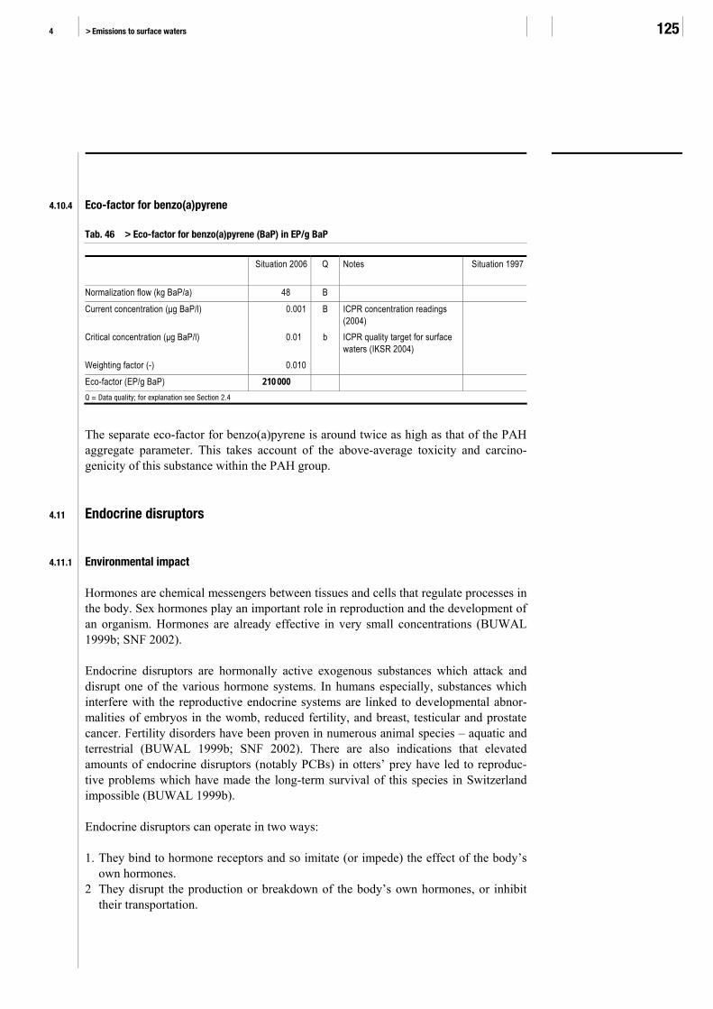
4 > Emissions to surface waters 125
4.10.4 Eco-factor for benzo(a)pyrene
Tab. 46 > Eco-factor for benzo(a)pyrene (BaP) in EP/g BaP Situation 2006 Q Notes Situation 1997
Normalization flow (kg BaP/a) 48 B Current concentration (μg BaP/l) 0.001 B ICPR concentration readings
(2004)
Critical concentration (μg BaP/l) 0.01 b ICPR quality target for surface waters (IKSR 2004)
Weighting factor (-) 0.010 Eco-factor (EP/g BaP) 210 000 Q = Data quality; for explanation see Section 2.4
The separate eco-factor for benzo(a)pyrene is around twice as high as that of the PAH aggregate parameter. This takes account of the above-average toxicity and carcino-genicity of this substance within the PAH group.
4.11 Endocrine disruptors
4.11.1 Environmental impact
Hormones are chemical messengers between tissues and cells that regulate processes in the body. Sex hormones play an important role in reproduction and the development of an organism. Hormones are already effective in very small concentrations (BUWAL 1999b; SNF 2002).
Endocrine disruptors are hormonally active exogenous substances which attack and disrupt one of the various hormone systems. In humans especially, substances which interfere with the reproductive endocrine systems are linked to developmental abnor-malities of embryos in the womb, reduced fertility, and breast, testicular and prostate cancer. Fertility disorders have been proven in numerous animal species – aquatic and terrestrial (BUWAL 1999b; SNF 2002). There are also indications that elevated amounts of endocrine disruptors (notably PCBs) in otters’ prey have led to reproduc-tive problems which have made the long-term survival of this species in Switzerland impossible (BUWAL 1999b).
Endocrine disruptors can operate in two ways:
1. They bind to hormone receptors and so imitate (or impede) the effect of the body’s own hormones.
2 They disrupt the production or breakdown of the body’s own hormones, or inhibit their transportation.

The Ecological Scarcity Method – Eco-Factors 2006 FOEN 2009 126
Substances which attack the reproductive endocrine system have the potential to cause oestrogenous effects (the same effect as the female sex hormone oestrogen) and andro-genous effects (the same effect as the male sex hormone androgen), as well as anti-oestrogenous and anti-androgenous effects (BUWAL 1999b).
In humans intake of endocrine disruptors is principally via the digestive tract, the skin or the lungs, while aquatic organisms absorb them mainly from the water. As certain types of hormone receptor occur throughout the animal kingdom, a very large number of species can be affected by a single endocrine disruptor (SNF 2002).
Concentrations of endocrine disruptors have been found which are sufficiently high to trigger oestrogenous (feminizing) effects in male fish (BUWAL 1999b), in particular close to the water discharge points of sewage treatment plants.
Hormonal effects have been proven in the case of the following substances and sub-stance groups (BUWAL 1999b; SNF 2002):
> natural (e.g. 17β-oestradiol, oestrone) and synthetic oestrogens (e.g. 17α-ethinylo-estradiol)
> phyto- und myco-oestrogens (e.g. isoflavones) > alkylphenol polyethoxylates (APEOs) and byproducts (e.g. nonylphenol, octylphe-
nol) > various organochlorate pesticides (e.g. DDT, methoxychlor, lindane und kepone) > certain industrial chemicals used in plastics (e.g. bisphenol A, PCBs and possibly
phthalate) > various polychlorinated dibenzo-p-dioxins and furans (PCDDs/PCDFs) > organotin compounds used among other things in antifouling ship paints (e.g. tribu-
tyltin (TBT) und triphenyltin (TPT)) > certain UV filter substances contained in sun lotions (presumed in the case of 4-
methylbenzylidene camphor)
It should be noted here that there are as yet no standardized and validated tests to identify a chemical as an endocrine disruptor. Many of the chemicals presently on the market have not been tested for effects of this type.
4.11.2 Characterization
Rutishauser et al. (2004) lists the oestrogenic potential (kg E2-eq./kg) of a number of endocrine disruptors. This figure describes the strength of the impact of an endocrine disruptor in relation to 17β-oestradiol (abbreviation E2). The equivalence factors were determined by using YES (yeast estrogen screening), as other methods can easily produce inaccurate factors. The YES procedure is well accepted in scientific circles.
The figures for oestrogenic potential in Tab. 47 can be used as characterizations for calculating the eco-factors of individual substances. To determine eco-factors for other endocrine substances their oestrogenic potential must be known. It should also be noted

4 > Emissions to surface waters 127
that, for reasons of comparability, the characterization factors should in each case be based on results from similar testing systems.
Tab. 47 > Characterization factors for some endocrine disruptors, based on their oestrogenic potential according to Rutishauser et al. (2004) Name of substance Abbreviation Oestrogenic potential
(kg E2-eq./kg) Oestrone E1 0.38 17β-oestradiol E2 1 Oestriol E3 2.40 * 10–3 17α-ethinyloestradiol EE2 1.19 Bisphenol A BPA 1.10 * 10–4 Nonylphenol NP 2.50 * 10–5 4-tert-octylphenol OP 7.80 * 10–6 Mestranol MES 0.013 β-oestradiol-17-valerate E2-Val 0.21
4.11.3 Normalization
The discharge of endocrine disruptors from anthropogenic sources to surface waters can be extrapolated from concentration measurements in the outfall from sewage treatment plants. Based on the estimated average concentration of endocrine disruptors in the runoff from treatment plants in Tab. 48 and the total runoff from all Swiss treatment plants of 1511 million m³/a (BUWAL 2000a) the load for Switzerland is calculated at 5.0 kg E2-eq./a.
Tab. 48 > Concentration data for the oestrogenic potential of three treatment plants and the weighted average from two of these
Oestrogenic potential Treatment plants Discharge from plants(m³/d) Minimum
(ng E2-eq./l)Maximum
(ng E2-eq/l)Mean*
(ng E2-eq./l) Rontal ** 8 200 0.4 (53) Glatt 45 000 2.4 5.5 3.95 Surental 15 000 0.5 2.2 1.35 Glatt & Surental 60 000 1.93 4.68 3.30 Source: Aerni et al. 2004 * own calculation from minimum and maximum values ** not used for the calculation, as the maximum value shown is an anomaly and would have skewed the result.
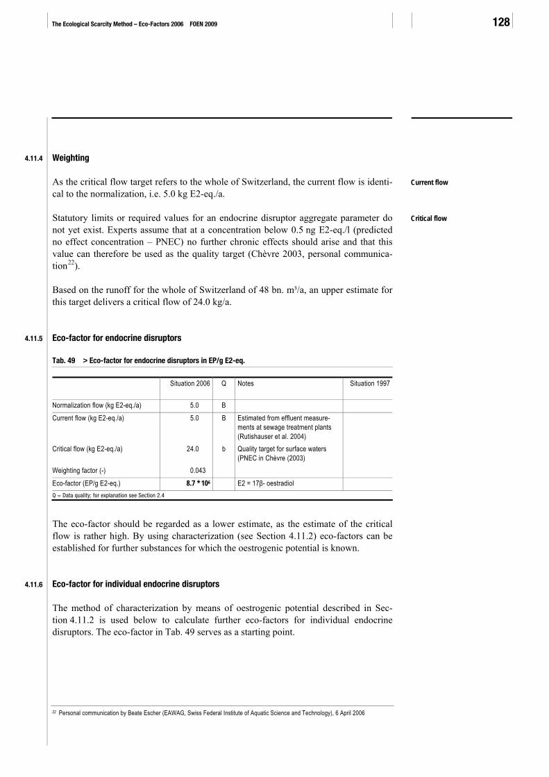
The Ecological Scarcity Method – Eco-Factors 2006 FOEN 2009 128
4.11.4 Weighting
As the critical flow target refers to the whole of Switzerland, the current flow is identi-cal to the normalization, i.e. 5.0 kg E2-eq./a.
Statutory limits or required values for an endocrine disruptor aggregate parameter do not yet exist. Experts assume that at a concentration below 0.5 ng E2-eq./l (predicted no effect concentration – PNEC) no further chronic effects should arise and that this value can therefore be used as the quality target (Chèvre 2003, personal communica-tion22).
Based on the runoff for the whole of Switzerland of 48 bn. m³/a, an upper estimate for this target delivers a critical flow of 24.0 kg/a.
4.11.5 Eco-factor for endocrine disruptors
Tab. 49 > Eco-factor for endocrine disruptors in EP/g E2-eq. Situation 2006
Q Notes Situation 1997
Normalization flow (kg E2-eq./a) 5.0 B Current flow (kg E2-eq./a) 5.0 B Estimated from effluent measure-
ments at sewage treatment plants (Rutishauser et al. 2004)
Critical flow (kg E2-eq./a) 24.0 b Quality target for surface waters (PNEC in Chèvre (2003)
Weighting factor (-) 0.043 Eco-factor (EP/g E2-eq.) 8.7 * 106 E2 = 17β- oestradiol Q = Data quality; for explanation see Section 2.4
The eco-factor should be regarded as a lower estimate, as the estimate of the critical flow is rather high. By using characterization (see Section 4.11.2) eco-factors can be established for further substances for which the oestrogenic potential is known.
4.11.6 Eco-factor for individual endocrine disruptors
The method of characterization by means of oestrogenic potential described in Sec-tion 4.11.2 is used below to calculate further eco-factors for individual endocrine disruptors. The eco-factor in Tab. 49 serves as a starting point.
22 Personal communication by Beate Escher (EAWAG, Swiss Federal Institute of Aquatic Science and Technology), 6 April 2006
Current flow
Critical flow

4 > Emissions to surface waters 129
Tab. 50 > Eco-factors of some endocrine disruptors in EP/g of the substance, calculated using oestrogenic potential as the characterization factor Name
Abbreviation Oestrogenic potential[kg E2-eq./kg]
Eco-factor 2006[EP/g]
Eco-factor 1997
Oestrone E1 0.38 3.3 * 106 - 17β- oestradiol E2 1 8.7 * 106 - Oestriol E3 2.40 * 10–3 2.1 * 104 - 17α- ethinyloestradiol EE2 1.19 1.0 * 107 - Bisphenol A BPA 1.10 * 10–4 9.6 * 102 - Nonylphenol NP 2.50 * 10–5 2.2 * 102 - 4-tert-octylphenol OP 7.80 * 10–6 6.8 * 101 - Mestranol MES 0.013 1.1 * 105 - β-oestradiol-17-valerate E2-Val 0.21 1.8 * 106 - Source: Rutishauser et al. 2004
The Ecological Scarcity Method – Eco-Factors 2006 FOEN 2009 130
5 > Emissions to groundwater
5.1 Introduction
More than 80 % (1 bn. m³/a) of Switzerland’s drinking water supply comes from groundwater (BUWAL 2003c). Groundwater is therefore particularly important and justifies quality requirements relating specifically to its use which are stricter than for surface water.
The boundaries between groundwater and surface water are very porous. Water which initially enters groundwater via precipitation and drainage will sooner or later reach surface waters, either through natural processes or via groundwater use.
Only nitrate is assessed, as this is the only substance for which relevant data is pres-ently available.
5.2 Nitrate in groundwater
5.2.1 Environmental impact
Especially in areas where farming practices are intensive nitrate concentrations in groundwater often exceed the required limits for groundwater that is used or reserved for use, and in some cases even exceed the tolerance value for drinking water. Nitrogen fertilizer applied to fields is readily washed from the soil into groundwater.

5 > Emissions to groundwater 131
5.2.2 Normalization
According to BUWAL (1996c) the nitrate discharged into groundwater amounts to 34 000 t N/a (1994 figure). As other nitrogen compounds are only present in small quantities, this normalization flow can be used not only for nitrate, but also for nitrogen loads in general.
According to FOEN experts the total load has scarcely altered, so the normalization flow remains at 34 000 t N/a.
5.2.3 Nitrate weighting
The current flow is identical to the normalization flow: 34 000 t N/a, as the reduction target for nitrate applies to the whole of Switzerland as well.
On the basis of the targets and limits for groundwater and thus also for drinking water, BUWAL (1996c, p. 37) calls for a target of halving the 1990 nitrate flow. This delivers a critical flow of 17 000 t NO3-N/a for nitrate discharges into groundwater.
5.2.4 Eco-factor for nitrate in groundwater
The eco-factor for nitrate in groundwater is practically unchanged from 1997, but it is higher than that for the load in surface waters. This is in line with the fact that nitrate continues to be problematic in groundwater – in contrast to surface waters – notably with regard to its use as drinking water.
Tab. 51 > Eco-factor for nitrate-N in groundwater in EP/g NO3--N and for nitrate in groundwater
in EP/g NO3-
Situation 2006
Q Notes Situation 1997
Normalization flow (t N/a) 34 000 B Current flow (t N/a) 34 000 B Assuming that the nitrogen load has
remained constant since 1996 34 000
Critical flow (t N/a) 17 000 a (BUWAL 1996c, S. 37) 17 000 Weighting factor (-) 4.0 Eco-factor (EP/g NO3-N) 120 Eco-factor for nitrate-N into groundwater (118) Eco-factor (EP/g NO3) 27.1 Eco-factor for nitrate into groundwater 27 Q = Data quality; for explanation see Section 2.4
Current flow
Critical flow
The Ecological Scarcity Method – Eco-Factors 2006 FOEN 2009 132
6 > Emissions to soil
6.1 Introduction
6.1.1 Background
The quality of soils in Switzerland is impaired by various substance-related impacts (acidification, overfertilization, contamination by heavy metals and organic pollutants). The contamination stems on one hand from the direct input of substances into the soil (plant protection products, fertilizer, waste landfilling), but also indirectly through the deposition of pollutants emitted to air.
The Swiss Ordinance on Soil Pollution (Verordnung über die Belastungen des Bodens, VBBo) is not applicable to all surfaces. Thus soils that are permanently paved over, sediment in waters and soils making up land whose designated use precludes soil protection (e.g. football pitches, motocross tracks, percolation facilities, roadside drainage strips) are not covered by the Ordinance. However, it does apply to rocky soils, provided that at least sparse vegetation grows or can grow on them (BUWAL 2001a, p.9). As a result soil protection is addressed not only in the Ordinance on Soil Protection, but also in other ordinances with indirect relevance to soils, such as the Swiss Federal Ordinance on Air Pollution Control or the Chemical Risk Reduction Ordinance (EPA, Art. 33, para. 1). In each of these the long-term maintenance of soil fertility must be taken into account (BUWAL 2001a).
Equally important for the long-term maintenance of soil fertility is the partial or total destruction of soils by paving over them, by erosion and by mechanical damage (soil compaction). These impacts can be assessed partly via land use and are treated sepa-rately in Section 7.3.
Assessment of the most important substance-related contaminations is discussed below.
6.1.2 Separating the soil and groundwater compartments
The ecological scarcity method assesses substance flows at their point of entry into the environment, i.e. when they leave the anthroposphere. Whereas with emissions to air and waters the boundary between anthroposphere and environment is relatively easy to define (“end of pipe” concept: the top of the chimney, the outfall from the sewage treatment plant), separating the systems is more difficult in the case of soil and groundwater. Thus the nutrients from fertilizers are available to agricultural crops and

6 > Emissions to soil 133
are taken up by them to some extent as long as they remain in the root zone of the soil. Hence nutrients taken up by plants do not leave the agricultural production system.
Heavy metals, on the other hand, which enter the topmost layers of soil and accumulate there, do not form part of the desired agricultural cycle. The guidelines for pollutant content of soil in the Ordinance on Soil Pollution refer to the top 20 cm of the soil. Therefore the Ordinance intends that, with regard to heavy metals, this soil layer belongs to the “environment”.
The boundary between the anthroposphere and the soil/groundwater compartment is therefore drawn at the point where substances no longer form part of agricultural use. Current and critical flows for nutrients are thus assessed when they leave the produc-tive agricultural system, therefore when washed into groundwater (nitrate), when entering surface waters through erosion or runoff (phosphate), or when emitted to the air (ammonia and nitrous oxide). Heavy metals, in contrast, are already pollutants when they enter the soil and are assessed at this point.
6.1.3 Selection of substances
In the case of substance-related soil contamination we should distinguish between different paths of entry:
> non-point inputs of nutrients, acidifiers, and heavy metals from the atmosphere > entry via fertilizers (can contain traces of harmful substances, such as heavy metals
and fluoride) > entry via plant protection products
The non-point input of pollutants occurs either in liquid form (wet deposition) or bound to dust particles (dry deposition).
The most important non-point source pollutants include:
> heavy metals: lead, cadmium, copper, mercury and zinc. > acidifiers: SO4
2-, NO3-, NH4+. With the exception of SO42- they also contribute to
overfertilization of ecosystems.
Non-point airborne inputs to soils (atmospheric deposition) are inventoried and as-sessed at the point of their emission to air (cf. Section 2.1). Separate eco-factors for non-point inputs to soils are therefore unnecessary. Therefore only the direct inputs to soils listed in Tab. 52 are assessed.

The Ecological Scarcity Method – Eco-Factors 2006 FOEN 2009 134
Tab. 52 > Impact mechanisms of the water pollutants assessed
Environment Human
Dam
age
to flo
ra
mpa
irmen
t of s
oil f
ertil
ity
Bioa
ccum
ulatio
n
Met
aboli
c dist
urba
nces
Carc
inoge
nicity
Mut
agen
esis
Em
bryo
nal d
amag
e
Oth
er/fu
rther
type
s of
dam
age
Char
acte
rizat
ion
Notes
Lead (Pb) x # x x - Cadmium (Cd) x # x x x (x) - Copper (Cu) x # x x - Zinc (Zn) x # x x - Plant protection products (PPPs)
x x x x x x x x PSM A single PPP normally only exhibits some of the impacts listed. Moreover, plant damage is an intentional effect of herbicides.
x Impact or link proven (x) Impact or link presumed # Principal impact for determining the eco-factor
6.2 Heavy metals in soils
6.2.1 Environmental impact
Heavy metals impair plant growth, disturb soil fertility and can accumulate in food chains. A high intake of a range of heavy metals with food (plants build available heavy metal into their biomass) over a long period can lead to chronic poisoning (BUWAL 1995). Moreover, major resource inputs are required to clean up soils con-taminated with heavy metals.
6.2.2 Normalization
The normalization flow is the current flow extrapolated to the surface area according to the Ordinance on Soil Pollution (Keller et al. 2005a). The surface area in the Ordinance has been determined from the categories wooded areas, agriculturally utilized areas and unproductive vegetation in the Swiss Land Use Statistics (BfS 2001) and covers 3.06 million hectares (around three quarters of Switzerland). It has also been taken into account that heavy metal inputs via pesticides, fertilizers and sewage sludge occur primarily on land used for agriculture (around 1.5 million hectares, over which loads

6 > Emissions to soil 135
may be subject to wide regional variations), whereas deposition from the atmosphere affects all types of land (Tab. 53).
Tab. 53 > Calculation of the normalization value for heavy metal input into soils based on the values for atmospheric deposition and on direct loading via pesticides, manure, mineral fertilizers and sewage sludge Deposition
(g/(ha*a))Direct input
(g/(ha*a))Normalization value
(t/a) Lead (Pb) 22 8.25 79.9 Cadmium (Cd) 0.7 0.55 2.98 Copper (Cu) 5.05 68.4 120 Zinc (Zn) 96.8 376 870
6.2.3 Weighting
The current flow of heavy metals to soils is made up of non-point input via the atmos-phere and direct input through fertilizers (especially compost) and plant protection products.
Eight heavy metals together with fluoride have been recorded at 105 different sites by the Swiss Soil Monitoring Network NABO. Of the heavy metals regulated by the Ordinance on Soil Protection (VBBo), only molybdenum is not measured by NABO. The measurements enable an inventory and evaluation of the current heavy metal load in soils to be performed (BUWAL 2000b).
In connection with the NABO monitoring programme Keller et al. (2005a) have estab-lished detailed substance inventories for lead, cadmium, copper and zinc on 48 selected representative areas of land. The median23 of these values has been used as the current flow for heavy metals. The values are listed in the corresponding tables of eco-factors (Tab. 54 to Tab. 57).
It is not possible to derive critical flows from the guideline values in the Ordinance on Soil Protection. However, the long-term maintenance of soil fertility is stated in Art. 1 as the purpose of this Ordinance (this applies only to soil types included in the Ordi-nance – see Section 6.1.1). To achieve this there should be no accumulation of heavy metals in the soil, i.e. the maximum input must be only as great as the output. Keller et al. (2005a) assess only the output via plants, and this is used as a first approximation for the critical flow. Transfer of heavy metals into groundwater or transport through erosion were not investigated. However, except for antimony and chromium (VI) this effect is of little relevance.
23 Using the median reduces the influence of individual extreme values (e.g. owing to the application of copper as a pesticide in vineyards)
on the calculation of the current flow, compared with the mean value.
Current flow
Critical flow

The Ecological Scarcity Method – Eco-Factors 2006 FOEN 2009 136
6.2.4 Eco-factor for lead
Tab. 54 > Eco-factor for lead in soils in EP/g lead Situation 2006
Q Notes Situation 1997
Normalization (t Pb/a) 79.9 B Extrapolation to surface area based on VBBo definition
Current flow (g Pb/(ha*a)) 30.3 B Calculated from data in Keller et al. (2005b) Critical flow (g Pb/(ha*a)) 19.4 b Calculated from data in Keller et al. (2005b) Weighting (-) 2.44 Eco-factor (EP/g Pb) 31 000 2 900 Q = Data quality; for explanation see Section 2.4
The new derivation method for heavy metal eco-factors produces an eco-factor for lead around 10 times higher than that derived by Brand et al. (1998). This is because 1) the eco-factor now only applies to areas without settlements, 2) the ambient limit value for lead was probably set at a rather generous level previously (owing to the substantial volume of emissions from transport) and 3) the existing ambient limit values are clearly inadequate for sustainable protection of the soil.
6.2.5 Eco-factor for cadmium
Tab. 55 > Eco-factor for cadmium in soils in EP/g cadmium Situation 2006
Q Notes Situation 1997
Normalization (t Cd/a) 2.98 B Extrapolation to surface area based on VBBo definition
Current flow (g Cd/(ha*a)) 1.25 B Calculated from data in Keller et al. (2005b) Critical flow (g Cd/(ha*a)) 1.30 b Calculated from data in Keller et al. (2005b) Weighting (-) 0.925 Eco-factor (EP/g Cd) 310 000 120 000 Q = Data quality; for explanation see Section 2.4
The eco-factor for cadmium is also somewhat higher than before, although less mark-edly so than for lead. It can be assumed that in future, as a result of the ban on cad-mium in accumulators and plastics, the problem and therefore the eco-factor, too, will reduce.
Cadmium is the only heavy metal for which the current flow is lower than the critical flow. Hence the rise in the eco-factor as against the former method is relatively small compared with the other eco-factors.
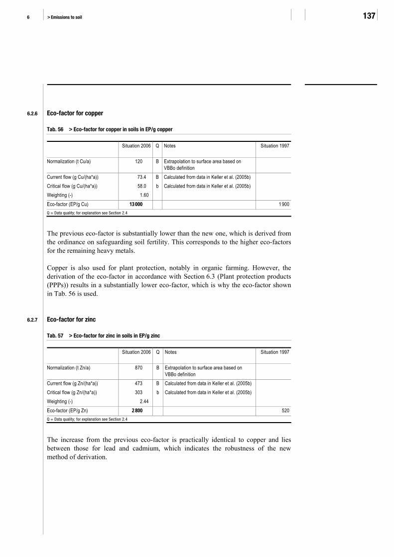
6 > Emissions to soil 137
6.2.6 Eco-factor for copper
Tab. 56 > Eco-factor for copper in soils in EP/g copper Situation 2006
Q Notes Situation 1997
Normalization (t Cu/a) 120 B Extrapolation to surface area based on VBBo definition
Current flow (g Cu/(ha*a)) 73.4 B Calculated from data in Keller et al. (2005b) Critical flow (g Cu/(ha*a)) 58.0 b Calculated from data in Keller et al. (2005b) Weighting (-) 1.60 Eco-factor (EP/g Cu) 13 000 1 900 Q = Data quality; for explanation see Section 2.4
The previous eco-factor is substantially lower than the new one, which is derived from the ordinance on safeguarding soil fertility. This corresponds to the higher eco-factors for the remaining heavy metals.
Copper is also used for plant protection, notably in organic farming. However, the derivation of the eco-factor in accordance with Section 6.3 (Plant protection products (PPPs)) results in a substantially lower eco-factor, which is why the eco-factor shown in Tab. 56 is used.
6.2.7 Eco-factor for zinc
Tab. 57 > Eco-factor for zinc in soils in EP/g zinc Situation 2006
Q Notes Situation 1997
Normalization (t Zn/a) 870 B Extrapolation to surface area based on VBBo definition
Current flow (g Zn/(ha*a)) 473 B Calculated from data in Keller et al. (2005b) Critical flow (g Zn/(ha*a)) 303 b Calculated from data in Keller et al. (2005b) Weighting (-) 2.44 Eco-factor (EP/g Zn) 2 800 520 Q = Data quality; for explanation see Section 2.4
The increase from the previous eco-factor is practically identical to copper and lies between those for lead and cadmium, which indicates the robustness of the new method of derivation.

The Ecological Scarcity Method – Eco-Factors 2006 FOEN 2009 138
6.3 Plant protection products (PPPs)
6.3.1 Environmental impact
According to the Ordinance on plant protection products (Pflanzenschutzmittelverord-nung, PSMV)24, such products include crop protectants, plant development regulators and post-harvest protection products. These can be substances, preparations, organisms or other agents. One of their purposes can be to destroy undesired plants or parts of plants. The eco-factor assessment mainly addresses chemical-synthetic plant protection products. The environmental problems associated with their use are a function of the primary effects, the quantities applied, the rates of degradation and dispersal behaviour (mobility) of the active agents, and the types and behaviour of degradation products and residues.
Plant protection products are applied above all in open arable farming, and in specialist fruit growing and viticulture. Their use on grassland is minimal (BLW 2000).
In a field trial in Denmark Esbjerg et al. (2002) demonstrated not only that the pesti-cide dose correlates with plant diversity (which is the desired effect, particularly in the case of herbicides), but also that it reduces the diversity of creatures outside the target group, such as spiders, myriapoda and birds.
The movement of soil particles in the wind and atmospheric transport of plant protec-tion products has also led meanwhile to the detection of active agents in mountain lakes and in rain. Human health impacts of these products arise notably from the use of groundwater as drinking water. Furthermore, two thirds of the active agents of plant protection products licensed in Switzerland cannot be routinely analysed (Angehrn 2001).
6.3.2 Characterization
The recommended dose for plant protection products (PPPs) – in terms of the quantity of the active agent – varies by approximately a factor of 1000 between traditional PPPs which are applied at the rate of several kilograms per hectare (e.g. atrazine, copper, sulphur) and modern PPPs, where in some cases a few grams per hectare suffice (e.g. triflusulfuron) (BUWAL 2003e).
It is assumed that the standard weighed dose (expressed in kg/ha) of a plant protection product represents as first approximation a measure of its effectiveness – the higher the permitted dose, the smaller the effect per unit measured. In the absence of better infor-mation about the environmental side effects of PPPs it is assumed that the specific effectiveness in relation to the intended effect and the side effects runs parallel. The
24 In older ordinances Pflanzenbehandlungsmittel (PBM) [plant treatment product] was used as the umbrella term, with Pflanzenschutzmit-
tel (PSM) [plant protection product] as a sub-category. PBM is now no longer in use and PSM has become the umbrella term.

6 > Emissions to soil 139
characterization factor is therefore set in inverse proportion to the standard weighed dose.
The standard dose of a plant protection product depends on the crop to be treated and sometimes also on the pest to be controlled. In order to obtain an average standard dose these values are weighted with the area of Switzerland under cultivation.
The data on the standard dose comes from the Swiss directory of plant protection products (FAW et al. 1999). For the small number of pesticides not listed in the direc-tory, e.g. because they are not licensed in Switzerland, data sheets from the products’ manufacturers have been used.
The standard dose of an average plant protection product used in Switzerland is 2.24 kg/ha. This amount is used as a reference unit to perform the characterization. The 20 active agents most sold in Switzerland and the approximately 80 pesticides listed in the ecoinvent v1.2 life cycle inventory dataset are characterized. Tab. 59 shows the standard doses and characterization factors for selected PPPs. The full list can be found in A4.
6.3.3 Normalization
As a characterization is performed, the normalization flow corresponds to the charac-terized quantities. The quantity of plant protection products used is not available classified by substance: detailed application rates are only available for 20 PPPs (von Arx 2005). However, these make up two thirds of the total quantity, so the character-ized normalization flow is estimated from these 20 substances and a linear extrapola-tion of the missing third. This delivers an annual flow of 1507 t PPP-eq.
6.3.4 Weighting
The increasing use of newer PPPs, some of which are effective with a dose of only a few grams per hectare, growing financial pressure, and direct payments for extensive farming programmes (without fungicide or insecticide) and organic farming have led to a substantial drop in the consumption of plant protection products from 2455 tonnes in 1988 to 1577 tonnes in 2000 (weight based on quantity of active agent). In 2000 this included 700 tonnes each of herbicide and fungicide (BUWAL 2002; BUWAL 2003e).
The Swiss Federal Office for Agriculture envisaged as a target a reduction of 30 % in the use of plant protection products from the1990/1992 level (mean value, 2100 t/a) by 2005 (BLW 2000). This corresponds to a critical flow of 1500 t PPP/a (rounded) (BLW 2000; BUWAL 2003e). A longer-term goal has not yet been stipulated. There is no information about the reduction of individual substances envisaged (for example, the current top 20 PPPs). Therefore the weighting factor is determined on the basis of the quantities of active agents which have not been characterized.
Current flow
Critical flow

The Ecological Scarcity Method – Eco-Factors 2006 FOEN 2009 140
6.3.5 Eco-factor für durchschnittliches Pflanzenschutzmittel
Tab. 58 > Eco-factor for the emission of plant protection products into soils in EP/g PPP active agents Situation 2006
Q Notes Situation 1997
Normalization (t PPP-eq/a) 1 507 A Current flow (t PPP/a) 1 577 A Quantity in 2000 according to BUWAL 2002 1 800 Critical flow (t PPP/a) 1 500 b Reduction of 30 % from 1990/92 BLW 2000 1 500 Weighting (-) 1.11 Eco-factor (EP/g PPP-eq.) 730 800 Q = Data quality; for explanation see Section 2.4
The eco-factor is slightly lower than in 1997,as a consequence of the characterization, which delivers a lower normalization value. However, this does not outweigh the reduction in the current flow. It can be assumed that the current flow will fall further in future as a result of the use of plant protection products which are effective in lower doses and the growing proportion of organic farming.
6.3.6 Eco-factor of other plant protection products
It is possible to calculate eco-factors for individual PPPs using the characterization based on the standard dose of PPPs described in Section 6.3.2. Tab. 59 provides an overview of selected characterization and eco-factors. The comprehensive list can be found in A4.
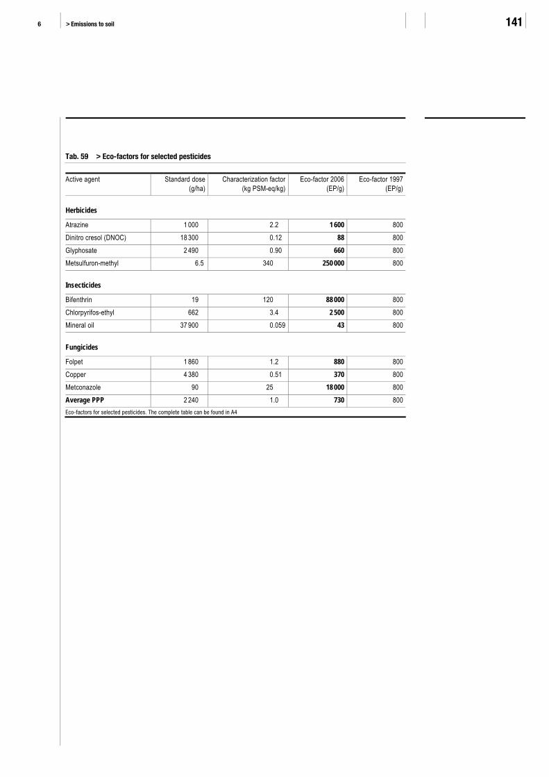
6 > Emissions to soil 141
Tab. 59 > Eco-factors for selected pesticides Active agent Standard dose
(g/ha) Characterization factor
(kg PSM-eq/kg)Eco-factor 2006
(EP/g)Eco-factor 1997
(EP/g)
Herbicides
Atrazine 1 000 2.2 1 600 800 Dinitro cresol (DNOC) 18 300 0.12 88 800 Glyphosate 2 490 0.90 660 800 Metsulfuron-methyl 6.5 340 250 000 800
Insecticides
Bifenthrin 19 120 88 000 800 Chlorpyrifos-ethyl 662 3.4 2 500 800 Mineral oil 37 900 0.059 43 800
Fungicides
Folpet 1 860 1.2 880 800 Copper 4 380 0.51 370 800 Metconazole 90 25 18 000 800 Average PPP 2 240 1.0 730 800 Eco-factors for selected pesticides. The complete table can be found in A4
The Ecological Scarcity Method – Eco-Factors 2006 FOEN 2009 142
7 > Resources
7.1 Overview
The extraction of certain resources from nature is also weighted with an eco-factor. Until now, only the consumption of energy resources has been weighted within the scope of the ecological scarcity method. The present review now integrates further types of resource consumption for the first time.
A new distinction in relation to energy resources (Section 7.2) is now made between an eco-factor for renewable (limited rate of replenishment) and non-renewable energies (limited stock). This takes account of the different sustainability aspects of these types of energy. Furthermore, new eco-factors are defined for land use (Section 7.3), for the extraction of natural gravel (Section 7.4) and for freshwater (Section 7.5), as these are increasingly considered to be ecologically scarce.
7.2 Energy resources
7.2.1 Environmental relevance
The Federal Constitution (Art. 89) states the goal of efficient and environmentally sound energy supply in the same sentence in which it calls for reliable and economical supply: “Within their powers, the Confederation and the Cantons shall strive to ensure a sufficient, diversified, reliable, and economical energy supply compatible with the protection of the environment, and the economical and efficient use of energy.”
Not only the available quantities of non-renewable energy carriers – such as oil, gas and uranium – are limited. The renewable resources are also limited. The sun, the driving force behind most renewable energies, only supplies a limited quantity of energy to the Earth per unit time. Moreover, a part of this energy is required to keep Ecosystem Earth running, e.g. for the biogenic production of oxygen, pollination and pollen dispersal by wind, maintenance of the hydrological cycle, provision of daylight, etc. Furthermore, when solar energy is converted into renewable energy carriers, the efficiency is often only a few percent. It is therefore not known which proportion of renewable energy can be utilized sustainably. It can at least be concluded that an upper utilization limit also applies to renewables. It is therefore purposeful to assign an eco-factor both to renewable and non-renewable energy carriers.
While technical efficiencies are often low when renewables are converted into final energy, especially when solar radiation is converted into biomass, due to the remaining

7 > Resources 143
ecological benefits the energy not utilized technically does not in fact dissipate use-lessly. This is why renewables are assessed not on the basis of primary energy content, but on the basis of final energy.
In contrast, where non-renewable energy carriers deliver no further ecological benefit, the entire energy contained in the resource should be utilized wherever possible, which is why the eco-factor is applied to the primary energy content.
For renewable and non-renewable energy resources alike, the assessed energy corre-sponds to the energy yield – the energy content of the biomass harvested, the rotation energy in the case of wind and hydropower generators, the electrical energy delivered to the inverter in photovoltaic installations, the thermal energy delivered to the heat storage system in the case of solar collectors, and the energy quantity extracted from the geosphere in the form of crude oil, raw hard coal, lignite, natural gas and fissile uranium.
The eco-factor for energy consumption assesses the scarcity of the energy resource; account is taken of the environmental impacts of energy uses caused by emissions through the corresponding eco-factors for air, water and soil pollution.
7.2.2 Characterization
Beside reducing energy consumption, a further goal of the 2000 watt society (cf. also 7.2.4) is to increase the proportion of renewable energies: of the 2000 watts per person, 1500 are to be produced from renewable sources (Schweizerischer Bundesrat 2002b). Conventional energy supply with non-renewable energy carriers is the reference (i.e. a characterization factor of 1 MJ-eq./MJ non-renewable energy). The goal is that renew-able sources are to supply three times more energy than non-renewable sources, which results in a politically established characterization factor of ⅓ MJ-eq./MJ (Tab. 60). In other words, 3 MJ energy from renewable sources is rated as being equivalent to 1 MJ from non-renewable sources.
Tab. 60 > Characterization factors for renewable and non-renewable energy carriers, based on Schweizerischer Bundesrat (2002a) Characterization factor
(MJ-eq./MJ) Non-renewable energy 1 Renewable energy ⅓

The Ecological Scarcity Method – Eco-Factors 2006 FOEN 2009 144
7.2.3 Normalization
Aggregate energy statistics (BFE 2004) present the energy balance of Switzerland according to energy carriers (Tab. 61). This encompasses domestic production as well as imports and exports. The normalization flow comprises the characterized flow. For this, renewable and non-renewable energy consumption is multiplied by the corre-sponding characterization factors (⅓ and 1). This results in a normalization flow of 1030 PJ-eq./a (Tab. 61).
7.2.4 Weighting
The current flow corresponds to the primary energy consumption of Switzerland and figures 1169 PJ/a (Tab. 61).
Tab. 61 > Primary energy consumption in Switzerland according to 2003 energy statistics (BFE 2004), and its conversion into characterized primary energy consumption Non-renewable
energy (PJ)
Renewable energy
(PJ)
Primary energy consumption
(PJ)
Primary energy consumption
(PJ-eq.) Mineral oil 537 100 % - 0 % 537 537 Nuclear fuels 283 100 % - 0 % 283 283 Hydropower - 0 % 164 100 % 164 55 Gas 110 100 % - 0 % 110 110 Coal 6 100 % - 0 % 6 5.9 Wood and charcoal 0 0 % 23 100 % 23 7.5 Municipal and industrial wastes 23 50 % 22 50 % 45 30 Solar, wind, biogas, ambient heat - 0 % 13 100 % 13 4.2 Electricity exports -148 91 % -16 9 % -164 -153 Electricity imports 150 98 % 3 2 % 152 150 Total 960 82 % 209 18 % 1 169 1 030
The goal of the 2000 watt society (Schweizerischer Bundesrat 2002b) is used to deter-mine the weighting factor. The 2000 watt society is a long-term goal without any specific target year for goal attainment: The various studies state 2050, 2100 or 2150 (Koschenz & Pfeiffer 2005; Spreng & Semadeni 2001; Würsten 2003). The goal is, however, definitely a long-term one. In order to define a medium-term goal, the same procedure is adopted as for greenhouse gas emissions. The long-term goal is taken to apply to 2050, and is then interpolated to the year 2030. 2030 can be interpreted as the most distant tangible time horizon of Swiss energy policy, as it is for the year 2030 that the draft of the Swiss Electricity Supply Act (as per 3 December 2004) sets a specific target for the proportion of renewable energies in Swiss electricity generation.
The critical flow is taken to be equal to the current flow for the short term, as no spe-cific short-term statutory or political reduction targets have been established at present.
Current flow
Critical flow

7 > Resources 145
The long-term reduction target is 2000 watts per person by the year 2050. The popula-tion figure is taken from the intermediate scenario of the BFS (2006), which anticipates a resident population of 8.06 million for the year 2050.
7.2.5 Eco-factors for energy
Tab. 62 > Eco-factors for primary energy consumption in accordance with the 2005 and 2050 endpoints, in EP/MJ-eq. 2006 target
Q 2006 target Q Notes
Normalization (PJ-eq./a) 1 030 A 1 030 A Characterized energy quantity Current flow (PJ/a) 1 169 A 1 169 A Critical flow (PJ/a) 1 169 b 508 b Weighting (-) 1.00 5.29 Eco-factor (EP/MJ-eq.) 0.97 5.14 Basis for interpolation Q = Data quality; for explanation see Section 2.4
The eco-factor varies by a factor of five depending upon whether the short-term or long-term target is selected (Tab. 62). The former would underestimate the situation, while the latter exaggerates the issue, as the target only needs to be achieved in a good 40 years. In the following, the eco-factor is interpolated to 2030, as explained above.
Tab. 63 > Eco-factor for the consumption of energy equivalents in EP/MJ-eq., calculated from the targets for 2005 and 2050 and interpolated to 2030 Situation 2006
Q Notes Situation 1997
Normalization (PJ-eq./a) 1 030 A Characterized energy quantity - Current flow (PJ/a) - 1 027 Critical flow (PJ/a) - 1 012 Weighting (-) 3.38 b Interpolated and calculated from eco-factor and
normalization -
Eco-factor (EP/MJ-eq.) 3.3 Energy eco-factor interpolated to 2030 1.0 Q = Data quality; for explanation see Section 2.4
Eco-factor of endpoints
Interpolated eco-factor

The Ecological Scarcity Method – Eco-Factors 2006 FOEN 2009 146
7.2.6 Eco-factors for renewable and non-renewable energy carriers
Tab. 64 > co-factors for renewable final energy and non-renewable primary energy in EP/MJ renewable and non-renewable energy Characterization
(PJ-eq./PJ) Normalization
(PJ-eq./a)Weighting
(-)Eco-factor 2006
(UBP/MJ-eq)Eco-factor 1997
(UBP/MJ-eq) Non-renewable primary energy 1 1030 3.38 3.3 1.0 Renewable final energy 0.33 1030 3.38 1.1 1.0* for the eco-factors for renewable primary energy see Tab. 65. * Hydropower was assessed with an eco-factor in EP97, but the other forms of renewable energy carriers were not.
As a result of characterizing forms of energy in accordance with the 2000 watt society goal, the eco-factor for non-renewable energy is appreciably higher than in the past, while the eco-factor for renewable energy retains practically the same value. This eco-factor for renewable energy, however, was previously only applied to hydropower, while now it applies to all forms of renewable energy.
The energy content of energy resources not used for energy production (feedstock energy content, for instance when hydrocarbons are used as refrigerants or wood is used in a building) is also assessed with a primary energy factor.
7.2.7 Guideline for application in relation to the ecoinvent v2.01 dataset
Tab. 65 presents the application of the two energy eco-factors to the energy resources listed in the ecoinvent dataset.
If a life cycle inventory is based on other assumptions concerning energy content and transformation ratio, the eco-factors can be adjusted to that specific situation following the same method.
Eco-factors of common energy carriers

7 > Resources 147
Tab. 65 > Eco-factors for the consumption of primary energy resources. Calculated using the eco-factors from Tab. 64 and the energy values in Frischknecht et al. (2007) Energy content Eco-factor, primary energy
Fossil energy
Crude oil (before refining) 45.8 MJ/kg 151 UBP/kg Natural gas (before refining) 40.3 MJ/Nm³ 133 UBP/Nm³ Mine gas 39.8 MJ/Nm³ 131 UBP/Nm³ Hard coal (in mine) 19.1 MJ/kg 63 UBP/kg Lignite (in mine) 9.9 MJ/kg 33 UBP/kg
Nuclear energy
Uranium (in ore) 560 000 MJ/kg 1 850 000 UBP/kg
Biomass
Energy in biomass 1 MJ/MJ 1.10 UBP/MJ Energy in biomass, primary forest clearcut 1 MJ/MJ 3.30 UBP/MJ Hardwood, standing a) 19.6 MJ/kg 21.57 UBP/kg Softwood, standing a) 20.4 MJ/kg 22.44 UBP/kg
Hydro
Potential energy of water in impoundment b) 0.95 MJe/MJ 1.05 UBP/MJ
Further renewables
Kinetic energy in wind b) 0.93 MJe/MJ 1.02 UBP/MJ Solar energy in solar radiation b) 0.91 MJe u. t/MJ 1.00 UBP/MJ Geothermal energy b) 1.00 MJt/MJ 1.10 UBP/MJ a) Wood may only be assessed here if it is not already taken account of as energy in biomass, as otherwise double counting would occur. b) According to the ecoinvent v2.01 dataset, the transformation ratio (ratio of final to primary energy) is: hydro = 0.95; wind = 0.93; solar = 0.91 (average of photovoltaics (0.935) and solar thermal (0.885)); geothermal = 1.00.

The Ecological Scarcity Method – Eco-Factors 2006 FOEN 2009 148
7.3 Land use
7.3.1 Introduction
The land-use statistics of 1992/97 (BfS 2001) break down the area of Switzerland, which totals 41 286 km², into four broad types of use:
1. 6.8 % settlement and urban areas (buildings, transportation areas, recreational and green urban areas, landfills, building sites)
2. 36.9 % agriculturally utilized areas (grassland, arable land, orchards) 3. 30.8 % wooded areas (forest, shrub forest, woods) 4. 25.5 % unproductive areas (rock, ice, lakes, rivers, glaciers)
The Swiss Spatial Planning Act (Raumplanungsgesetz) prescribes that soil resources should be used prudently and urban sprawl should be countered. Settlement area is expanding nonetheless. According to the Swiss land-use statistics of 92/97, the overall settlement area is growing at a rate of around one square metre per second, mostly at the expense of agricultural land in the Swiss plateau (the “Mittelland” region of Swit-zerland). In remote areas, agricultural land that is no longer managed is transformed again into wooded areas. While the unproductive areas are subject to constant change, their overall area remains roughly constant (BfS 2001).
According to the BfS (2001), the settlement area of Switzerland, which totals 2791 km², is composed as follows:
> 49.3 % building areas > 32.0 % transportation areas > 7.2 % industrial areas > 5.8 % special urban areas (utility facilities, quarries/mines and dumps, construction
sites) > 5.7 % recreational and green urban areas
Growth in settlement area is driven by a growing population, in combination with growing levels of land take per person. The target of the Swiss Federal Council set out in the 2002 strategy for a sustainable Switzerland is to meet further demand wherever possible by means of inward development, i.e. improved utilization of existing settle-ment areas (Schweizerischer Bundesrat 2002a).
7 > Resources 149
7.3.2 Characterization
The characterization of land use applies the method developed by Köllner (2001), which assesses the various types of land cover in accordance with their respective plant biodiversity. Building upon the Swiss biodiversity monitoring programme and other publications, Köllner (2001) derives EDP (Ecosystem Damage Potential) factors for various land-use types, which reflect the anticipated number of species and the actually encountered number of species for the specific type of land use. Positive EDP factors of a land use mean that plant biodiversity is below average, while negative EDP factors indicate a plant diversity that is above the average.
The non-linear EDP factors (EDPtotal-nonl-pla) were used to derive the characterization factors. “Settlement area” is taken as the reference type of land cover (see the full list in A5).
In order to reach a degree of detail that is suitable for life cycle assessments, the ex-tended CORINE nomenclature set out in Köllner (2007) was adopted. The EDP fac-tors, however, are not available in similar detail. Where items of data were absent, average values were used, or an estimate performed by means of equation with similar land-use types. The use of water surfaces and bare land (e.g. rock) can not be charac-terized at present. These types, however, are usually of minor importance for life cycle assessments, and hence neglecting them is unlikely to have any significant effect on the outcome.
For unknown uses, a category encountered occasionally in life cycle inventories, a suitable EDP factor was derived. In Switzerland, most land-use changes involve a transformation from agricultural area to settlement area. The weighted mean was taken from the EDP factors for these two area types – the resultant EDP factor for unknown use captures an average settlement/agriculture area in Switzerland.
7.3.3 Normalization
On the basis of the characterization, the normalization flow is also calculated as a characterized quantity. The surface areas of the land-use types, with their respective characterization factors, result in a normalization flow of 3378 km²-eq*a.
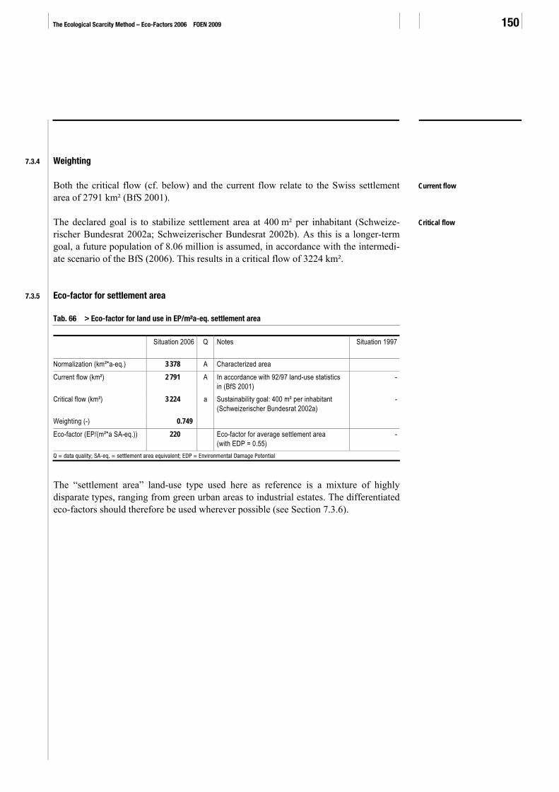
The Ecological Scarcity Method – Eco-Factors 2006 FOEN 2009 150
7.3.4 Weighting
Both the critical flow (cf. below) and the current flow relate to the Swiss settlement area of 2791 km² (BfS 2001).
The declared goal is to stabilize settlement area at 400 m² per inhabitant (Schweize-rischer Bundesrat 2002a; Schweizerischer Bundesrat 2002b). As this is a longer-term goal, a future population of 8.06 million is assumed, in accordance with the intermedi-ate scenario of the BfS (2006). This results in a critical flow of 3224 km².
7.3.5 Eco-factor for settlement area
Tab. 66 > Eco-factor for land use in EP/m²a-eq. settlement area Situation 2006
Q Notes Situation 1997
Normalization (km²*a-eq.) 3 378 A Characterized area Current flow (km²) 2 791 A In accordance with 92/97 land-use statistics
in (BfS 2001) -
Critical flow (km²) 3 224 a Sustainability goal: 400 m² per inhabitant (Schweizerischer Bundesrat 2002a)
-
Weighting (-) 0.749 Eco-factor (EP/(m²*a SA-eq.)) 220 Eco-factor for average settlement area
(with EDP = 0.55) -
Q = data quality; SA-eq. = settlement area equivalent; EDP = Environmental Damage Potential
The “settlement area” land-use type used here as reference is a mixture of highly disparate types, ranging from green urban areas to industrial estates. The differentiated eco-factors should therefore be used wherever possible (see Section 7.3.6).
Current flow
Critical flow

7 > Resources 151
7.3.6 Eco-factors (and characterization) for specific types of land use
Tab. 67 compiles the eco-factors and the characterization values of several frequent categories of land cover; A5 provides the full list.
Tab. 67 > Overview of the eco-factors for selected land-use types in EP/(m²a) of land covered CORINE+ Land use EDP Charact. factor
(m² SF-eq./m²)Eco-factor 2006
(UBP/m²a)
Settlement area
REF Settlement area (reference) 0.548 1.0 220 111 Urban fabric, continuous, >80 % sealed 0.68 1.2 260 112 Urban fabric, discontinuous, <80 % sealed 0.54 0.99 220 121 Industrial or commercial units 0.573 1.0 220 122 Road and rail networks and associated land 0.56 1.0 220
Agricultural areas
211b Arable land, non-irrigated, IP 0.32 0.58 130 211c Arable land, non-irrigated, organic 0.15 0.27 59 245 Agricultural fallow with hedgerows -0.12 -0.22 -48
Forests
311 Forest, broad-leaved 0.0378 0.069 15 313 Forest, mixed -0.020 -0.037 -8.1 314 Forest, forest edge -0.11 -0.20 -44
Other use
- Unknown use 0.403 0.74 160 A5 provides the complete list REF: Reference area (average of several CORINE land-cover types); SA-eq.: settlement area equivalents
A5 contains the full list of land-cover types. Section 7.3.7 gives recommendations on how to classify land-use types not contained in this list, such as FSC forest or green roofs.

The Ecological Scarcity Method – Eco-Factors 2006 FOEN 2009 152
7.3.7 Guidelines for application: Assessing special land-use types
There are two possible ways to handle land uses not covered by the extended CORINE nomenclature (cf. also Tab. 68):
1. Increasing the degree of detail: A land use can be broken down into defined types of use. The assessment problem can thus be transferred to the life cycle inventory level at which is it is more readily resolved (for instance, forests managed to FSC standards can be inventoried by assigning a part to managed forest and a part to natural forest).
2. Forming analogies: A land use is similar to a type of use for which there is an eco-factor (for instance, the eco-factor for green urban areas can be applied to green roofs).
Tab. 68 > Recommendation for the characterization of “FSC forest” and “green roof” Land-use type
Recommendation for classification Notes
Forest, managed to FSC standards
a) Depending upon the type of forest and management: 1) 311: Forest, broad-leaved 2) 312: Forest, coniferous 3) 313: Forest, mixed In the case of plantations, the subcatego-ries 311a, 312a and 313c are to be used
b) and, in accordance with the circumstances on the ground, proportions classified as semi-natural 1) 311b: Forest, broad-leaved, semi-natural 2) 312b: Forest, coniferous, semi-natural 3) 313: Forest, mixed
The Swiss FSC rules prescribe ecological management and designation of at least 5 % of the area as strict reserve (Natur-waldreservat) (BUWAL 1999a). The rules are specified at national level, and can therefore differ in other countries. The inventorization of FSC forest should be performed at the level of the life cycle inventory.
1) 113: Urban fallow Where plantings are ecologically valuable, e.g. oligotrophic grassland on a large flat roof
Green roof
2) 141: Green urban areas Where roof planting is simple Note: Areas are only counted once, either as normal settlement area or as green roof
7.3.8 Implementation in the ecoinvent v2.0 dataset
In the ecoinvent dataset, managed forests are classified as “forest, high-intensity”, being the average form of managed forest in Europe. This would correspond to planta-tion forests in the present categorization (cf. categories 311a, 312a and 313c in A5). This leads to an assessment that does not fully reflect circumstances in European forest management, especially not in Switzerland. For the assessment of products and fuels from Swiss timber, we therefore recommend using the (identical) eco-factors for “forest, broad-leaved” or “forest, coniferous” (see A5) in place of the ecoinvent cate-gory “forest, high-intensity”.

7 > Resources 153
7.4 Gravel extraction
7.4.1 Introduction
Gravel is a sui generis resource: On the one hand a construction material, and on the other hand a material important to the protection and formation of groundwater. Not all physical gravel occurrences are extractable – permissible land uses set limits. An eco-factor is therefore defined for gravel here for the first time.
Gravel is used mainly in the construction sector, notably as a concrete aggregate and in road and railway subgrades. The quality of gravel deposits can vary widely. High-grade alluvial gravels are found especially on valley floors, while morainic mounts often have a mixed composition, making gravel extraction more costly (Jäckli & Schindler 1986; Kündig et al. 1997).
Gravel resources replenish very slowly. Only around 1 % of Switzerland’s annual gravel consumption is formed anew in rivers in the same period. Moreover, the geo-logical gravel deposits are reduced by competing demands such as housing construc-tion, groundwater protection and, in some cases, forest protection. As a result, the extractable quantity is substantially smaller than the resource (Jäckli & Schindler 1986). In the canton of Zug, for instance, it is assumed that if extraction intensity remains at the same level the utilizable gravel reserves suffice for only 18 years (Raumplanungsamt Kt. Zug 2005).
7.4.2 Normalization
The normalization flow is identical to the current flow, as the latter relates to the whole of Switzerland.
7.4.3 Weighting
The gravel production of Swiss gravel works depends to some degree upon construc-tion sector activity, and has ranged between 30 and 40 million t over the past 20 years, with a maximum around 1990. In the year 2000, 34 million t were extracted (Rubli & Jungbluth 2004); this is taken as current flow.
The spatial planning authorities of the cantons are responsible for approving gravel extraction. Provisions governing extraction have therefore only been established, if at all, at cantonal level. It has been clear for some time that gravel reserves will be ex-hausted in the foreseeable future (see e.g. Kündig et al. 1997; Raumplanungsamt Kt. Zug 2005). Across the whole of Switzerland, the volume of gravel reserves designated for extraction has always been sufficient for the next 15 to 20 years. It follows that, although the resource is essentially finite, the present extraction situation is tolerated. The critical flow is therefore taken to be equal to the current flow.
Current flow
Critical flow

The Ecological Scarcity Method – Eco-Factors 2006 FOEN 2009 154
7.4.4 Eco-factor for gravel extraction
Tab. 69 > Eco-factor for gravel extraction in EP/g gravel Situation 2006
Q Notes Situation 1997
Normalization (million t gravel/a) 34 A Current flow ((million t gravel/a) 34 A Rubli et al. 2005 Critical flow ((million t gravel/a) 34 c Weighting (-) 1.00 Eco-factor (EP/g gravel) 0.029 Q = Data quality; for explanation see Section 2.4
The eco-factor for gravel is defined for the first time here. It reflects the presently tolerated extraction volume.
7.5 Freshwater consumption
7.5.1 Introduction
In some regions of the world freshwater is scarce, while in others there is a surplus. Switzerland is in the comfortable position of having access to more than enough clean water. Nonetheless, the Federal Council (Schweizerischer Bundesrat 2002a, p. 9) demands that “[…] natural resources be utilized with due regard to future genera-tions” and specifies this by demanding that, among other things, “[…] the consump-tion of renewable resources (e.g. farmed biomass, water) is kept below the level at which they can regenerate or below the natural level of availability”. The same docu-ment also notes the global freshwater problem, citing the OECD.
With this in mind, and because an eco-factor for freshwater is purposeful when consid-ering water-poor locations, three types of eco-factors are derived for freshwater:
1. Country-specific (for Switzerland and for further OECD states) 2. Average of OECD countries (as first approximation for cases in which a life cycle
inventory does not list water consumption levels in a differentiated manner) 3. For six different scarcity situations (low, Moderatee, medium, high, very high and
Extremee)
This now makes it possible for the first time to differentiate – for instance in life cycle assessments of foods or of other products requiring large amounts of water for their production – between origin from arid regions where water scarcity prevails and from regions with ample water resources, and to take account of the aspect of water scarcity in arid regions that can be relevant in some cases. Users of the method can also derive regional or local eco-factors themselves to address specific issues.
According to the OECD (2004, p. 24) the scarcity of freshwater resources can be expressed as the share of gross consumption in the available renewable water resource (precipitation, plus inflows from neighbouring states, minus evaporation).

7 > Resources 155
If the share of gross consumption in the available resource is 10–20 %, water stress is classed as Moderatee according to the OECD (2004), if the ratio is 20–40 % it is me-dium to high, and if it is above 40 %, it is high. The OECD considers a Moderatee to medium pressure on water resources to be tolerable. The critical flow is therefore set at 20 % of the available resource.
In accordance with the OECD (2004) and FAO (2005) we understand water consump-tion to mean all extractions of freshwater for production or consumption processes. Water consumption does not include water used by hydroelectric facilities to generate electricity (cf. also Section 2.1.4).
7.5.2 Normalization
The Swiss level of water consumption, which is 2.57 km³/a (around 350 m³ per capita and year or 1000 litres per capita and day) is used as normalization flow (FAO 2005). This value corresponds to the current flow when assessing the eco-factor for Switzer-land. When calculating country-specific eco-factors or assessing water scarcity catego-ries, their weighting factors must be converted to the Swiss situation, i.e. normalized. This normalization also applies to any other, regionalized freshwater eco-factors (cf. also Section 2.1.4).
7.5.3 Weighting
According to the FAO (2005), the current flow, i.e. the quantity of freshwater con-sumed annually in Switzerland, is 2.57 km³/a. This includes not only consumption for potable water, but also water extractions to irrigate agricultural areas and for use in industrial processes. According to the FAO (2005) the available annual resource in Switzerland is 53.5 km³.
According to the OECD (OECD 2004) a tolerable water stress is 20 % of the available resource. It follows that the critical quantity of freshwater use for Switzerland is 10.7 km³/a.
The water consumption of all OECD states (excluding the Slovak Republic, for lack of data) is 1020 km³/a (calculated from data in FAO (2005), A6 lists the data for the individual OECD states). The water consumption figure includes mine water and water extracted by irrigation measures. The extraction of water that was already used once and was returned to a body of surface water is also contained in the gross consumption figure. Water used in hydropower facilities is considered in-situ consumption and is therefore not included in the statistics. The current flow of all OECD states is 1020 km³/a (see A3 for detailed country data).
As noted above, a Moderatee to medium pressure on water resources is considered tolerable, and the critical flow is therefore set at 20 % of the available water resource. This means for the OECD states a critical flow of 2050 km³/a (the entire available renewable resource is 10 300 km³/a, see A6 for detailed country data).
Current and critical flow for Switzerland
Current and critical flow for the OECD states (average value)

The Ecological Scarcity Method – Eco-Factors 2006 FOEN 2009 156
It is assumed that water scarcity in the OECD states provides an expedient average value for weighting. This pragmatic assumption is supported by the broad range of countries represented – from very water-rich countries such is Ireland and Iceland, to those where there are greater levels of water scarcity, such as Spain. Moreover, reliable data are available for these countries.
The OECD defines four categories of water scarcity, whereby if the share of water consumption in the available resource exceeds 0.4 it is assumed that water scarcity is high (OECD 2004). For the purposes of a life cycle assessment, however, cases may also arise in which very high (up to a ratio of 1) and Extremeely high scarcity (water consumption exceeds the available resource) are relevant. The OECD categories are therefore complemented by two further categories: very high (0.6 to <1.0) and Extre-mee (≥1.0).
The weighting factor is given by the ratio of water consumption to available resource (without needing to know the absolute values) and the assumption that the critical flow is 20 % of the available resource as:
)12(%20
1resource Available
nconsumptioWater
)11(%) 20 · resource (Available
nconsumptioWater
)10(flow CriticalflowCurrent Weighting
2
2
ratioScarcity
2
2
⎟⎠⎞
⎜⎝⎛⋅
⎟⎟⎟⎟
⎠
⎞
⎜⎜⎜⎜
⎝
⎛
⎟⎠⎞
⎜⎝⎛=
⎟⎟⎠
⎞⎜⎜⎝
⎛=
⎟⎠⎞
⎜⎝⎛=
4444 34444 21
Tab. 70 > Calculation of weighting factors from the ratios of water consumption to available resource, for the different water scarcity categories Category Weighting Water scarcity ratio
⎟⎠⎞
⎜⎝⎛
resource Available consuptionWater
Ratio used for calculation Critical flow at x% of available resource
Weighting factor (-)
Low <0.1 0.05 20 % 0.0625 Moderate 0.1 to <0.2 0.15 20 % 0.563 Medium 0.2 to <0.4 0.3 20 % 2.25 High 0.4 to <0.6 0.5 20 % 6.25 Very high 0.6 to <1.0 0.8 20 % 16.0 Extreme ≥1 1.5 20 % 56.3
Weighting according to scarcity situation
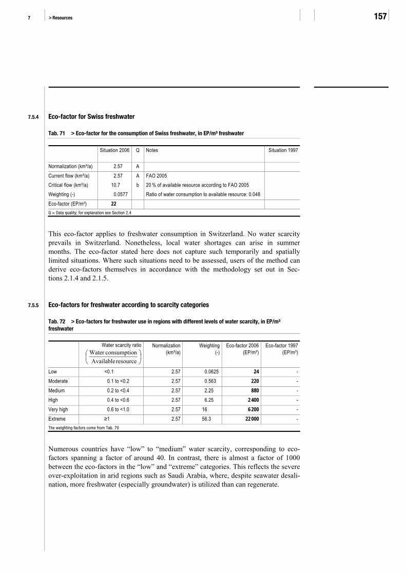
7 > Resources 157
7.5.4 Eco-factor for Swiss freshwater
Tab. 71 > Eco-factor for the consumption of Swiss freshwater, in EP/m³ freshwater Situation 2006
Q Notes Situation 1997
Normalization (km³/a) 2.57 A Current flow (km³/a) 2.57 A FAO 2005 Critical flow (km³/a) 10.7 b 20 % of available resource according to FAO 2005 Weighting (-) 0.0577 Ratio of water consumption to available resource: 0.048 Eco-factor (EP/m³) 22 Q = Data quality; for explanation see Section 2.4
This eco-factor applies to freshwater consumption in Switzerland. No water scarcity prevails in Switzerland. Nonetheless, local water shortages can arise in summer months. The eco-factor stated here does not capture such temporarily and spatially limited situations. Where such situations need to be assessed, users of the method can derive eco-factors themselves in accordance with the methodology set out in Sec-tions 2.1.4 and 2.1.5.
7.5.5 Eco-factors for freshwater according to scarcity categories
Tab. 72 > Eco-factors for freshwater use in regions with different levels of water scarcity, in EP/m³ freshwater Water scarcity ratio
⎟⎠⎞
⎜⎝⎛
resource Available nconsumptioWater
Normalization(km³/a)
Weighting(-)
Eco-factor 2006(EP/m³)
Eco-factor 1997 (EP/m³)
Low <0.1 2.57 0.0625 24 - Moderate 0.1 to <0.2 2.57 0.563 220 - Medium 0.2 to <0.4 2.57 2.25 880 - High 0.4 to <0.6 2.57 6.25 2 400 - Very high 0.6 to <1.0 2.57 16 6 200 - Extreme ≥1 2.57 56.3 22 000 - The weighting factors come from Tab. 70
Numerous countries have “low” to “medium” water scarcity, corresponding to eco-factors spanning a factor of around 40. In contrast, there is almost a factor of 1000 between the eco-factors in the “low” and “extreme” categories. This reflects the severe over-exploitation in arid regions such as Saudi Arabia, where, despite seawater desali-nation, more freshwater (especially groundwater) is utilized than can regenerate.

The Ecological Scarcity Method – Eco-Factors 2006 FOEN 2009 158
7.5.6 Eco-factors for freshwater in OECD states (average value)
Tab. 73 > Eco-factor for freshwater of unknown or undifferentiated origin, in EP/m³ freshwater – derived from the water scarcity in OECD countries Situation 2006 Q Notes Situation 1997
Normalization (km³/a) 2.57 A Water consumption in Switzerland (i.e. current flow in Switzerland)
Current flow (km³/a) 1 020 A FAO 2005 Critical flow (km³/a) 2 040 b 20 % of available resource according to FAO 2005 Weighting (-) 0.250 Corresponds to a ratio of water consumption to
available resource of 0.10
Eco-factor (EP/m³) 97 Q = Data quality; for explanation see Section 2.4
This average value should be applied when the water consumed is of unknown or undifferentiated origin. The eco-factor is positioned between the categories for low and moderate water scarcity (Tab. 72), which is considered plausible. Water scarcity is a particular problem in arid regions, where it can be further exacerbated by intensive agriculture. Water scarcities that are limited in space or time are not taken into account by this eco-factor.
Wherever possible, classification into one of the six water scarcity categories (Sec-tion 7.5.5) is preferable over use of this average eco-factor. A6 lists eco-factors for the individual OECD states.

7 > Resources 159
7.5.7 Guidelines for application
The eco-factors can be applied to all types of renewable water resources. Applications of water that neither pollute it chemically nor change its temperature or physical state, and do not remove it from the hydrological cycle for longer periods, are exempted from the assessment using the freshwater eco-factor. This exemption also applies to hydro-power facilities, as the water becomes available again after the turbine and its quality or physical parameters are not appreciably changed. Cases in which the freshwater eco-factor is to be applied include – the list is not conclusive:
> Drinking water use (incl. distribution losses) > Irrigation in agriculture (incl. losses) > Use for and in industrial processes, including use as cooling water (because of the
change in the physical state or temperature)
If the life cycle inventory contains no regional or scarcity-based differentiation, the average eco-factor as set out in Section 7.5.6 is to be used. When fossil (non-renewable) water is used, the eco-factor of the most severe scarcity category is to be applied.
These country eco-factors have already been calculated for the OECD countries, and are listed in A6. If corresponding data are available, eco-factors can be calculated for further countries or certain eco-regions. The procedure is analogous to that for calculat-ing the Swiss eco-factor. In all cases, the data sources, all assumptions made, and the calculation of any eco-factors derived by users must be stated in a reproducible man-ner.
Tab. 74 classes several typical countries in the six scarcity categories. This list provides orientation in order to be able to appraise, by analogy, the water scarcity category of other countries or regions without detailed data. These eco-factors do not, however, capture any regional scarcities within these countries.
Tab. 74 > Classification of several countries in the water scarcity categories Water scarcity ratio
⎟⎠⎞
⎜⎝⎛
resource Available nconsumptioWater
Typical countries
Low <0.1 Argentina, Austria, Estonia, Iceland, Ireland, Madagascar, Russia, Switzerland, Venezuela, Zambia
Moderate 0.1 to <0.2 Czech Republic, Greece, France, Mexico, Turkey, USA Medium 0.2 to <0.4 China, Cyprus, Germany, Italy, Japan, Spain, Thailand High 0.4 to <0.6 Algeria, Bulgaria, Morocco, Sudan, Tunisia Very high 0.6 to <1.0 Pakistan, Syria, Tadzhikistan, Turkmenistan Extreme ≥1 Israel, Kuwait, Oman, Qatar, Saudi Arabia, Yemen

The Ecological Scarcity Method – Eco-Factors 2006 FOEN 2009 160
8 > Wastes
8.1 Introduction
The following sections determine eco-factors for different types of wastes. Wastes in aboveground landfills are assessed on the basis of their carbon content. Certain hazard-ous wastes (Section 8.3) and radioactive wastes (Section 8.4) are stored underground.
8.2 Carbon in material consigned to bioreactive landfills
8.2.1 Environmental relevance
The Swiss Environmental Protection Act stipulates that no wastes that may cause long-term problems can be stored in landfills in Switzerland. The indicator for the reaction potential of waste is its carbon (C) content. The goal is to minimize the C flow to landfills. The experts at FOEN therefore consider this to be the key critical aspect when consigning material to bioreactive landfills.
8.2.2 Normalization
The normalization flow is identical to the current flow, as the current flow represents the C flow in landfills for the whole of Switzerland.
8.2.3 Weighting
The current flow comprises the quantity of carbon stored through the waste in bioreac-tive landfills and slag compartments. According to FOEN estimates, slags contain an estimated 4 % C, while the average for other wastes consigned to bioreactive landfills (excluding slags) is 15 %. 25 Wastes consigned to landfills for inert materials or to landfills for stabilized residues contain practically no reactive organic material. 661 500 t slags are consigned annually to bioreactive landfills, plus 473 000 t other wastes (figures for 2002: BUWAL 2003a). This yields the current flow of 97 410 t C/a.
The target for the C content in bioreactive landfill wastes is 7 %.26 With the quantity currently landfilled, this translates into a critical C flow of 79 420 t C/a.
25 Personal communication by M. Tellenbach, FOEN, 15 July 2006. 26 Personal communication by M. Tellenbach, FOEN, 15 July 2006.
Current flow
Critical flow

8 > Wastes 161
8.2.4 Eco-factors for carbon in bioreactive landfill wastes
Tab. 75 > Eco-factor for carbon in bioreactive landfill wastes, in EP/g C. The table also lists eco-factors for average slags and for other bioreactive landfill wastes Situation 2006 Q Notes Situation 1997
Normalization (t C/a) 97 410 B Current flow (t C/a) 97 410 B Critical flow (t C/a) 79 420 b Weighting (-) 1.50 Eco-factor (EP/g C) 15 Eco-factor (EP/g slags) 0.61 C content: 4 % Eco-factor (EP/g other bioreactive landfill wastes) 2.3 C content: 15 % Q = Data quality; for explanation see Section 2.4
The eco-factors for carbon in wastes consigned to landfill is presented here for the first time.
8.2.5 Guideline for application in relation to ecoinvent v2.01 dataset
It is not possible to apply this eco-factor directly in the ecoinvent database, as the C content of wastes consigned to landfill is not listed. Long-term TOC emissions are used instead as a proxy. In the ecoinvent database, these come exclusively from bioreactive landfills and landfills for stabilized residues. The transfer coefficient of bioreactive landfills for carbon in waste to carbon as long-term TOC is 0.244. The eco-factor to be applied in the ecoinvent database can thus be calculated. This figures 63 EP/g TOC.

The Ecological Scarcity Method – Eco-Factors 2006 FOEN 2009 162
8.3 Hazardous wastes in underground repositories
8.3.1 Background
The greater part of the hazardous wastes arising in Switzerland (around 1.1 million t per year) is treated within the country. Around one third can be incinerated, while the rest is, wherever possible, recycled, consigned to physical-chemical treatment or otherwise stored in a landfill for stabilized residues. Soil removed when cleaning up contaminated sites is the principal source of hazardous waste, accounting for around one quarter of the quantity (BUWAL 2003a, pp. 42–43).
Hazardous wastes are only exported in exceptional cases; this accounts for around 10 % of the total hazardous waste quantity. One third of the exported quantity is made up of the filter dusts of municipal waste incineration plants, which are stored in under-ground repositories. Their storage in underground repositories has been declining slightly since 1996, as the acid scrubbing process is increasingly being deployed. When this process is used, it is no longer necessary to store filter dust in underground reposi-tories (BUWAL 2003a, p. 44).
8.3.2 Normalization
No characterization is performed, and both the current and the critical flow comprise the entire quantity of hazardous wastes consigned to underground repositories. The normalization flow is therefore identical to the current flow.
8.3.3 Weighting
The Swiss waste statistics give the quantity of wastes stored in underground reposito-ries. This figures 36 900 t/a in 2002, and is exported in its entirety (BUWAL 2003a, p. 44). There are no underground repositories in Switzerland.
The Swiss Environmental Protection Act (Umweltschutzgesetz, USG, Art. 30 para 3) stipulates the principle that wastes “must be disposed of …, insofar as this possible and reasonable, within Switzerland.” It is assumed that the exported quantity cannot be consigned purposefully to final storage in Switzerland, and therefore the critical flow is equated with the current flow.27
27 According to personal communication by H.-P. Fahrni, FOEN, of 28 February 2005, this determination is expedient.
Current flow
Critical flow

8 > Wastes 163
8.3.4 Eco-factors for the consignment of hazardous wastes to repositories
Tab. 76 > Eco-factor for consigning hazardous wastes to underground repositories, in EP/g and EP/cm³ waste Situation 2006
Q Notes Situation 1997
Normalization (t Abfall/a) 36 900 A Current flow (t Abfall/a) 36 900 A 41 000 Critical flow (t Abfall/a) 36 900 c 41 000 Weighting (-) 1.00 Eco-factor (EP/g Abfall) 27 24 Eco-factor (EP/cm³ Abfall) 43 Density 1,600 kg/m³ in accordance with Doka 2003b,
Part III, p. 41
Q = Data quality; for explanation see Section 2.4
This eco-factor relates exclusively to hazardous wastes stored in underground reposito-ries. The final storage of wastes – including hazardous wastes – on normal above-ground landfills is assessed via the eco-factors for land use and for emissions to air, water and groundwater.
8.4 Radioactive wastes in final repositories
8.4.1 Preliminary note
The generation of electricity in nuclear power plants produces radioactive wastes that must eventually be consigned to final storage. No final repository could yet be con-structed in Switzerland. The Wellenberg site in the canton of Nidwalden was envisaged for low-level and medium-level wastes. In 2002 the construction of an exploratory shaft was rejected in a referendum, so that now a new site must be sought. Similarly, no decision has yet been taken on a final repository site for high-level and long-lived wastes, nor is this in prospect in the near future. As the unresolved issues have re-mained largely unchanged, the approach towards defining an eco-factor established by Brand et al. (1998) is adopted here for the assessment of radioactive wastes.
8.4.2 Background
The Swiss strategy for the disposal of radioactive wastes is to aim for the interim to reduce the quantities and harmfulness of residues and then to isolate these permanently through final storage. The Swiss Nuclear Energy Act (Kernenergiegesetz, Art. 30 para 2) requires for the radioactive wastes that arise that “The radioactive wastes arising in Switzerland must be disposed of within the country as a matter of principle”. In addi-

The Ecological Scarcity Method – Eco-Factors 2006 FOEN 2009 164
tion, the Act stipulates a moratorium on reprocessing spent fuel elements from July 2006 to 2016.28
Originally two final repositories were envisaged – one for spent fuel elements, high-level wastes (HLW) and long-lived medium-level wastes (LMLW), and a second for low-level and medium-level wastes. Following rejection of the Wellenberg as a site for low-level and medium-level wastes, the option of building one single deep repository is now also under review.
The planned capacities required for the repository are determined on the basis of the estimated quantities of radioactive wastes including their encasements. Improved reprocessing processes will tend to reduce the volumes. On the other hand, extending the service life of nuclear power plants from the original term of 40 to 60 years in-creases repository capacity requirements. NAGRA29 now also bases its calculations of required volumes on plant service lives of 60 years (192 GW scenario).
Based on this scenario, some 8300 m³ spent (and conditioned) fuel elements, some 1000 m³ HLW from reprocessing and 4360 m³ (cement waste option; 3460 m³ in the case of the vitrification option) LMLW arise. One option calculated assumes an addi-tional 2900 m³ LMLW. Overall, the deep repository thus needs to accept around 16 000 m³ long-lived high-level and medium-level wastes (volume incl. encasements) (NAGRA 2002).
According to the plans drawn up in 1996, the repository for short-lived low-level and medium level wastes is to have a capacity of 100 000 m³. Of this, 42 000 m³ are wastes from nuclear power plant decommissioning, 11 000 m³ from plant operation, 24 000 m³ from reprocessing and the remaining 23 000 m³ from research and medicine (of which 14 000 m³ from the decommissioning of the PSI proton accelerator). This volume was estimated on the basis of a 40-year service life of nuclear power plants and a 70-year collection period for wastes from medicine and research (Prêtre 1996). Extrapolation to a service life of 60 years implies a required storage volume of around 115 000 m³ (volume incl. encasements).
The hazardousness of radioactive wastes depends upon their persistence (half-life), and on the type and intensity of their radiation. The Swiss strategy for a final repository classes the various types of radioactive waste in two categories:
1. Short-lived low-level and medium-level wastes 2. Long-lived medium-level wastes (LMLW), high-level wastes (HLW) and spent fuel
elements
28 Nuclear Energy Act, Art. 106 para 4 “Spent fuel elements may not be exported for reprocessing for a period of ten years from 1 July
2006 onwards. During this period, they are to be disposed of as radioactive wastes.” 29 NAGRA is the national cooperative for radioactive waste storage (Nationale Genossenschaft für die Lagerung radioaktiver Abfälle) in
Switzerland

8 > Wastes 165
The former are relatively short-lived, and already present a minor hazard after a shorter period. A requisite shut-in time of around 500 years is assumed (KFW 2002; PSI 1996).
The shut-in time of long-lived wastes is much longer. It is assumed that these need to be stored safely for at least 100 000 years (EKRA 2000; PSI 1996).
8.4.3 Normalization
No characterization is performed. The normalization flow is thus identical to the current flow.
8.4.4 Weighting
The quantity of radioactive wastes (incl. encasements) currently arising is taken from the ecoinvent report on nuclear power (Dones 2003). The net capacity of Swiss nuclear power plants figured 2.96 GW in 2002 (Dones 2003, Table 9.1), which results in a current flow of 1230 m³/a for low-level and medium-level wastes, and 218 m³/a for high-level wastes (HLW).
When setting the critical flow, the following aspects need to be taken into account:
> In Switzerland there is presently no repository capacity – neither for low-level and medium-level nor for high-level and long-lived wastes. The repository envisaged in the Wellenberg has been rejected. At the present time, radioactive wastes therefore cannot be disposed of (as envisaged by the legislator) in an environmentally sound manner. It would follow from this consideration that the critical flow would need to be set at zero.
> Possible repositories that could accept the wastes arising in existing nuclear power plants are in a tangible planning stage. Although no statement can be made as to the point in time at which such a facility may commence operations nor at which site, it is possible that sufficient repository capacity will exist in future. This consideration would suggest that the current flow should be equated with the critical flow.
The Swiss strategic report on sustainability (Schweizerischer Bundesrat 2002a, p.9) postulates as a guideline that “Accident risks are only to be accepted to the extent that, even in the case of occurrence of the most severe event, no permanent damage that extends beyond one generation is caused.” The present interim storage of radioactive wastes in surface storage sites is a transitional solution.
The critical flow used to determine the eco-factor is therefore positioned between the current flow and zero. In a first, rough approximation, the critical flow is set at half of the current flow. This reflects the present situation, in which there are efforts to find a final repository, but no specific construction project is under way.
Current flow
Critical flow
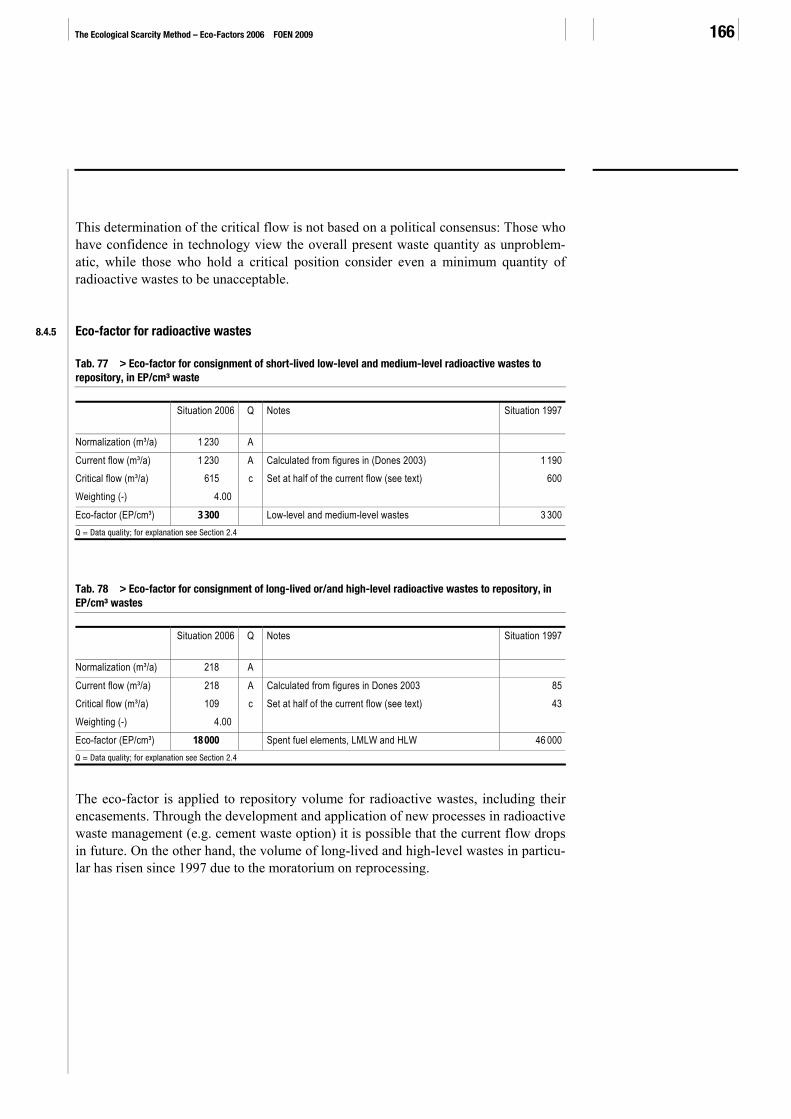
The Ecological Scarcity Method – Eco-Factors 2006 FOEN 2009 166
This determination of the critical flow is not based on a political consensus: Those who have confidence in technology view the overall present waste quantity as unproblem-atic, while those who hold a critical position consider even a minimum quantity of radioactive wastes to be unacceptable.
8.4.5 Eco-factor for radioactive wastes
Tab. 77 > Eco-factor for consignment of short-lived low-level and medium-level radioactive wastes to repository, in EP/cm³ waste Situation 2006 Q Notes Situation 1997
Normalization (m³/a) 1 230 A Current flow (m³/a) 1 230 A Calculated from figures in (Dones 2003) 1 190 Critical flow (m³/a) 615 c Set at half of the current flow (see text) 600 Weighting (-) 4.00 Eco-factor (EP/cm³) 3 300 Low-level and medium-level wastes 3 300 Q = Data quality; for explanation see Section 2.4
Tab. 78 > Eco-factor for consignment of long-lived or/and high-level radioactive wastes to repository, in EP/cm³ wastes Situation 2006 Q Notes Situation 1997
Normalization (m³/a) 218 A Current flow (m³/a) 218 A Calculated from figures in Dones 2003 85 Critical flow (m³/a) 109 c Set at half of the current flow (see text) 43 Weighting (-) 4.00 Eco-factor (EP/cm³) 18 000 Spent fuel elements, LMLW and HLW 46 000 Q = Data quality; for explanation see Section 2.4
The eco-factor is applied to repository volume for radioactive wastes, including their encasements. Through the development and application of new processes in radioactive waste management (e.g. cement waste option) it is possible that the current flow drops in future. On the other hand, the volume of long-lived and high-level wastes in particu-lar has risen since 1997 due to the moratorium on reprocessing.

9 > Not assessed: Noise 167
9 > Not assessed: Noise
ARE (2004, p.14) defines noise as a parameter determined by subjective factors: “Noise is a sound perceived to be unpleasant and disturbing. The actual level of im-pairment depends largely upon the subjective perception of the person affected.””
Noise pollution is an ubiquitous problem, especially in cities. The main sources are road and rail vehicles on the one hand, and the building sites on the other hand that are needed to maintain and extend settlement infrastructure. In rural areas agricultural and silvicultural machines cause noise, but also jingling cow bells can be perceived as noise by some. In the vicinity of airports, arriving and departing aircraft are a relevant source of noise. Persons living next to bodies of water can be affected by ambient noise caused by motorboats. Shooting ranges and sports facilities or similar installations are locally defined, stationary sources of noise.
The Swiss Noise Abatement Ordinance (Lärmschutzverordnung, LSV) defines the noise target that is to be achieved – in analogy to the precautionary principle (Sec-tion 2.2.3) – as what technology and operating conditions will allow providing this is economically acceptable. A further goal is that there should be no severe nuisance to the affected public. These goals apply to both mobile and stationary sources of sound.
The basic problem in assessing noise is that, in contrast to substance emissions, sound quickly dissipates and is therefore always locally contained. A further problem is that assessment can only be performed on the basis of the ambient situation, as it is only through the human perception of a sound that this can be considered to be noise. It is therefore essential when conducting an assessment to consider the emission situation in combination with the ambient situation. Sound emissions are locally bound, which makes it difficult to derive eco-factors. No generally recognized method for assessing noise in life cycle assessments is yet available.
Doka (2003a) has developed an option for integrating road traffic noise in the ecologi-cal scarcity method. The derivation is relatively complex and not immediately transfer-able to noise from other sources. In the present report, these factors, which only apply to road traffic, have not been adopted, as this would result in a one-sided attribution of impacts to road vehicles alone. These factors can continue to be highly useful when addressing specific issues in the road transport sector, but when studies address other issues they would produce an unfair assessment bias.

The Ecological Scarcity Method – Eco-Factors 2006 FOEN 2009 168
> Annex
A1 Conversion factors for emissions
Tab. 79 > Conversion factors for emissions of nitrogen and phosphorous compounds and for COD/DOC Mass, rounded
(g/mol)
NOx as NO2 46 1 g NO2 corresponds to 0.3 g NOx-N NH3 17 1 g NH3 corresponds to 0.82 g NH3-N NH4+ 18 1 g NH4+ corresponds to 0.78 g NH4+-N NO3
− 62 1 g NO3− corresponds to 0.23 g NO3
−-N N2O 44 1 g N2O corresponds to 0.64 g N2O-N PO43− 95 1 g PO43− corresponds to 0.33 g PO43−-P P2O5 142 1 g P2O5 corresponds to 0.44 g P2O5-P COD - 1 g COD corresponds to 0.3 g DOC (rough approximation)

> Annex 169
A2 Eco-factors for greenhouse gases and ozone-depleting substances
When substances have both a GWP and an ODP, the factor resulting in the higher eco-factor is used. The grey shading of values in the table indicates whether the GWP or the ODP was used for the calculation. The GWP values are in accordance with IPCC (2001), the ODP values are in accordance with UNEP (2000).
Tab. 80 > Eco-factors for greenhouse gases and ozone-depleting substances Formula CAS No. GWP
(CO2-eq.)ODP
(R11-eq.)Eco-factor 2006
(EP/g) Eco-factor 1997
(EP/g)Basis in 1997
Carbon dioxide CO2 124–38–9 1 - 0.31 0.2 GWP Carbon monoxide CO 630–08–0 1.57 - 0.49 0.2 GWP Methane CH4 74–82–8 23 - 7.1 4.2 GWP Nitrous oxide N2O 10024–97–2 296 - 92 62 GWP
Chlorofluorocarbons (CFCs)
CFC-11 CCl3F 75–69–4 4 600 1 11 000 2 000 ODP CFC-12 CCl2F2 75–71–8 10 600 1 11 000 2 000 ODP CFC-13 CClF3 75–72–9 14 000 1 11 000 2 000 ODP CFC-111 C2Cl5F 354–56–3 - 1 11 000 2 000 ODP CFC-112 C2Cl4F2 76–12–0 - 1 11 000 2 000 ODP CFC-113 CCl2FCClF2 76–13–1 6 000 0.8 8 800 1 600 ODP CFC-114 CClF2CClF2 76–14–2 9 800 1 11 000 2 000 ODP CFC-115 CF3CClF2 76–15–3 7 200 0.6 6 600 1 200 ODP CFC-211 C3Cl7F 422–78–6 - 1 11 000 2 000 ODP CFC-212 C3Cl6F2 3182–26–1 - 1 11 000 2 000 ODP CFC-213 C3Cl5F3 2354–06–5 - 1 11 000 2 000 ODP CFC-214 C3Cl4F4 29255–31–0 - 1 11 000 2 000 ODP CFC-215 C3Cl3F5 4259–43–2 - 1 11 000 2 000 ODP CFC-216 C3Cl2F6 661–97–2 - 1 11 000 2 000 ODP CFC-217 C3ClF7 422–86–6 - 1 11 000 2 000 ODP
Hydrofluorocarbons (HFCs)
HFC-23 CHF3 75–46–7 12 000 - 3 700 2 300 GWP HFC-32 CH2F2 75–10–5 550 - 170 130 GWP HFC-41 CH3F 593–53–3 97 - 30 30 GWP HFC-125 CHF2CF3 354–33–6 3 400 - 1 100 560 GWP HFC-134 CHF2CHF2 359–35–3 1 100 - 340 200 GWP HFC-134a CH2FCF3 811–97–2 1 300 - 400 260 GWP HFC-143 CHF2CH2F 430–66–0 330 - 100 60 GWP HFC-143a CF3CH3 420–46–2 4 300 - 1 300 760 GWP HFC-152 CH2FCH2F 624–72–6 43 - 13 - HFC-152a CH3CHF2 75–37–6 120 - 37 28 GWP HFC-161 CH3CH2F 353–36–6 12 - 3.7 -

The Ecological Scarcity Method – Eco-Factors 2006 FOEN 2009 170
Formula CAS No. GWP(CO2-eq.)
ODP(R11-eq.)
Eco-factor 2006 (EP/g)
Eco-factor 1997(EP/g)
Basis in 1997
HFC-227ea CF3CHFCF3 431–89–0 3 500 - 1 100 580 GWP HFC-236cb CH2FCF2CF3 677–56–5 1 300 - 400 - HFC-236ea CHF2CHFCF3 431–63–0 1 200 - 370 - HFC-236fa CF3CH2CF3 690–39–1 9 400 - 2 900 1 300 GWP HFC-245ca CH2FCF2CHF2 679–86–7 640 - 200 110 GWP HFC-245fa CHF2CH2CF3 460–73–1 950 - 290 - HFC-365mfc CF3CH2CF2CH3 406–58–6 890 - 280 - HFC-43–10mee CF3CHFCHFCF2CF3 138495–42–8 1 500 - 470 260 GWP
Partially halogenated chlorofluorocarbons (HCFCs)
HCFC-21 CHCl2F 75–43–4 210 0.04 440 - HCFC-22 CHClF2 75–45–6 1 700 0.055 610 300 GWP HCFC-31 CH2FCl 593–70–4 - 0.02 220 - HCFC-121 CHCl2CCl2F 354–14–3 - 0.04 440 - HCFC-122 CHCl2CClF2 354–21–2 - 0.08 880 - HCFC-123 CHCl2CF3 306–83–2 120 0.02 220 40 ODP HCFC-124 CHFClCF3 2837–89–0 620 0.022 240 94 GWP HCFC-131 CH2ClCCl2F 359–28–4 - 0.05 550 - HCFC-133a CH2ClCF3 75–88–7 - 0.06 660 - HCFC-141 CH2ClCHClF 430–57–9 - 0.07 770 - HCFC-141b CH3CFCl2 1717–00–6 700 0.11 1 200 220 ODP HCFC-142b CH3CF2Cl 75–68–3 2 400 0.065 740 360 GWP HCFC-225ca CF3CF2CHCl2 422–56–0 180 0.025 280 - HCFC-225cb CClF2CF2CHClF 507–55–1 620 0.033 360 - HCFC-253 C3H4F3Cl 460–35–5 - 0.03 330 - HCFC-261 CH3CClFCH2Cl 420–97–3 - 0.02 220 - HCFC-271 C3H6FCl 430–55–7 - 0.03 330 -
Perfluorocarbons (PFCs)
Methane, perfluoro- (HFC-14) CF4 75–73–0 5 700 - 1 800 1 300 GWP Ethane, perfluoro- (HFC-116) C2F6 76–16–4 11 900 - 3 700 1 800 GWP Propane, octafluoro- (HFC-218) C3F8 76–19–7 8 600 - 2 700 1 400 GWP Propane, hexafluorocyclo- c-C3F6 931–91–9 16 800 - 5 200 - Butane, decafluoro- C4F10 355–25–9 8 600 - 2 700 1 400 GWP Butane, octafluorocyclo- c-C4F8 115–25–3 10 000 - 3 100 1 700 GWP Pentane, dodecafluoro- C5F12 678–26–2 8 900 - 2 800 1 500 GWP Hexane, tetradecafluoro- C6F14 355–42–0 9 000 - 2 800 1 500 GWP
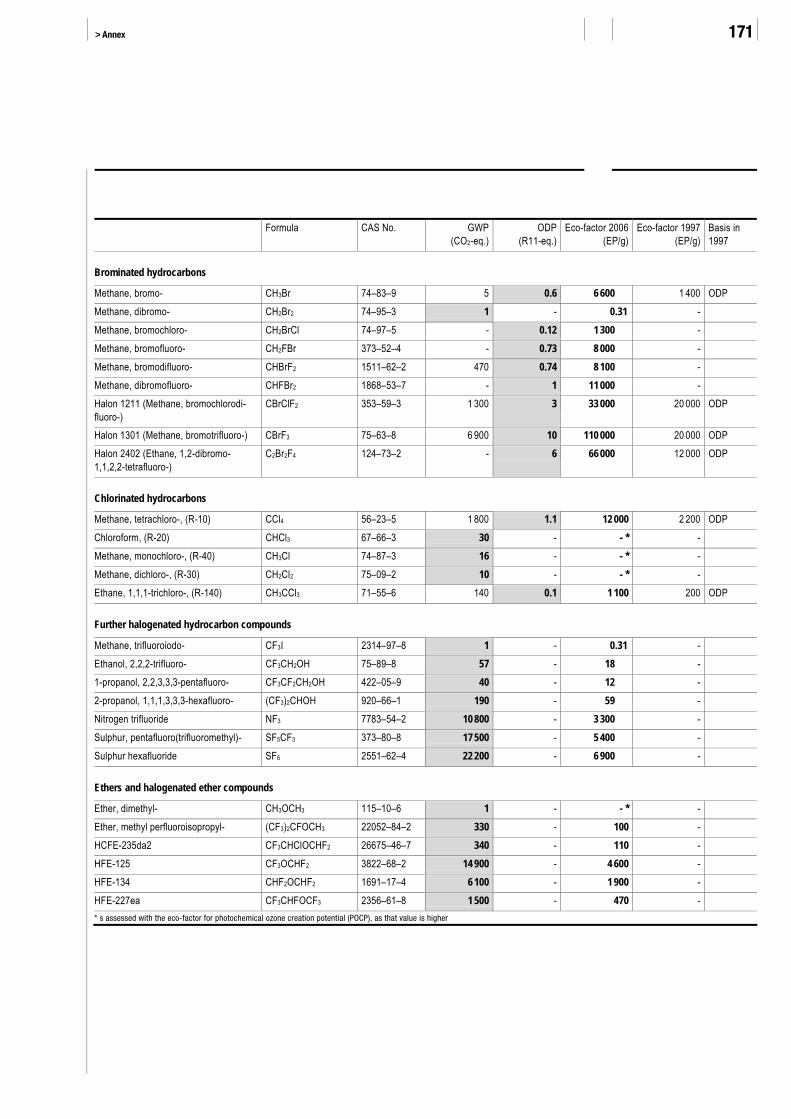
> Annex 171
Formula CAS No. GWP(CO2-eq.)
ODP(R11-eq.)
Eco-factor 2006 (EP/g)
Eco-factor 1997(EP/g)
Basis in 1997
Brominated hydrocarbons
Methane, bromo- CH3Br 74–83–9 5 0.6 6 600 1 400 ODP Methane, dibromo- CH2Br2 74–95–3 1 - 0.31 - Methane, bromochloro- CH2BrCl 74–97–5 - 0.12 1 300 - Methane, bromofluoro- CH2FBr 373–52–4 - 0.73 8 000 - Methane, bromodifluoro- CHBrF2 1511–62–2 470 0.74 8 100 - Methane, dibromofluoro- CHFBr2 1868–53–7 - 1 11 000 - Halon 1211 (Methane, bromochlorodi-fluoro-)
CBrClF2 353–59–3 1 300 3 33 000 20 000 ODP
Halon 1301 (Methane, bromotrifluoro-) CBrF3 75–63–8 6 900 10 110 000 20 000 ODP Halon 2402 (Ethane, 1,2-dibromo-1,1,2,2-tetrafluoro-)
C2Br2F4 124–73–2 - 6 66 000 12 000 ODP
Chlorinated hydrocarbons
Methane, tetrachloro-, (R-10) CCl4 56–23–5 1 800 1.1 12 000 2 200 ODP Chloroform, (R-20) CHCl3 67–66–3 30 - - * - Methane, monochloro-, (R-40) CH3Cl 74–87–3 16 - - * - Methane, dichloro-, (R-30) CH2Cl2 75–09–2 10 - - * - Ethane, 1,1,1-trichloro-, (R-140) CH3CCl3 71–55–6 140 0.1 1 100 200 ODP
Further halogenated hydrocarbon compounds
Methane, trifluoroiodo- CF3I 2314–97–8 1 - 0.31 - Ethanol, 2,2,2-trifluoro- CF3CH2OH 75–89–8 57 - 18 - 1-propanol, 2,2,3,3,3-pentafluoro- CF3CF2CH2OH 422–05–9 40 - 12 - 2-propanol, 1,1,1,3,3,3-hexafluoro- (CF3)2CHOH 920–66–1 190 - 59 - Nitrogen trifluoride NF3 7783–54–2 10 800 - 3 300 - Sulphur, pentafluoro(trifluoromethyl)- SF5CF3 373–80–8 17 500 - 5 400 - Sulphur hexafluoride SF6 2551–62–4 22 200 - 6 900 -
Ethers and halogenated ether compounds
Ether, dimethyl- CH3OCH3 115–10–6 1 - - * - Ether, methyl perfluoroisopropyl- (CF3)2CFOCH3 22052–84–2 330 - 100 - HCFE-235da2 CF3CHClOCHF2 26675–46–7 340 - 110 - HFE-125 CF3OCHF2 3822–68–2 14 900 - 4 600 - HFE-134 CHF2OCHF2 1691–17–4 6 100 - 1 900 - HFE-227ea CF3CHFOCF3 2356–61–8 1 500 - 470 - * s assessed with the eco-factor for photochemical ozone creation potential (POCP), as that value is higher

The Ecological Scarcity Method – Eco-Factors 2006 FOEN 2009 172
A3 PAHs (polycyclic aromatic hydrocarbons)
The following table contains a list of the most common PAHs. The list is not conclu-sive. The eco-factor to use can be found in Section 4.9.
Tab. 81 > PAHs (polycyclic aromatic hydrocarbons)
PAH No.
Name CAS No. Molecular weight
Synonyms
8 Acenaphthene 83–32–9 154 1,2-Dihydroacenaphthylene; 1,8-Ethylenenaphthalene 7 Acenaphthylene 208–96–8 152 Acenaphthalene
15 Anthracene 120–12–7 178 Anthracin 38 Benz(a)anthracene 56–55–3 228 1,2-Benzanthracene; 1,2-Benzanthrene; Benzo[b]phenanthrene; 2,3-Benzophenanthrene; Tetra-
phene; Naphthanthracene 74 Benzo(a)pyrene 50–32–8 252 Benzo[def]chrysene; 3,4-Benzopyrene; 6,7-Benzopyrene; 1,2-Benzpyrene; 4,5-Benzpyrene 69 Benzo(b)fluoranthene 205–99–2 252 3,4-Benz[e]acephenanthrylene; Benzo[b]fluoranthene; Benzo[e]fluoranthene; 2,3-Benzofluoranthene;
3,4-Benzofluoranthene; 120 Benzo(ghi)perylene 191–24–2 276 1,12-Benzoperylene
71 Benzo(k)fluoranthene 207–08–9 252 11,12-Benzofluoranthene; 8,9-Benzofluoranthene; 2,3:1’,8’-Binaphthylene; Dibenzo[b,jk]fluorene 39 Chrysene 218–01–9 228 Benzo[a]phenanthrene; 1,2-Benzophenanthrene
130 Dibenz(a,h)anthracene 53–70–3 278 1,2:5,6-Benz[a]anthracene; 1,2:5,6-Benzanthracene; 1,2,5,6-Dibenzoanthracene 18 Fluoranthene 206–44–0 202 Benzo[jk]fluorene; Idryl; 1,2-(1,8-Naphthalenediyl)benzene; Benz[a]acenaphthylene; 1,2-
Benzoacenaphthylene 11 Fluorene 86–73–7 166 o-Biphenylenemethane; Diphenylenemethane; 9H-Fluorene; 2,2’-Methylenebiphenyl; 2,3-Benzidene;
o-Biphenylmethane 113 Indeno(1,2,3-cd)pyrene 193–39–5 276 1,10-(1,2-Phenylene)pyrene; 1,10-(o-Phenylene)pyrene; o-Phenylenepyrene; 2,3-(o-
Phenylene)pyrene; 2,3-Phenylenepyrene 4 Naphthalene 91–20–3 128 Naphthalin
14 Phenanthrene 85–01–8 178 Phenanthrin 21 Pyrene 129–00–0 202 Benzo[def]phenanthrene; Pyren

> Annex 173
A4 Plant protection products
Tab. 82 > Plant protection products Standard dose (g/ha) Characterization factor (kg
PPP-eq/kg)Eco-factor
(EP/g)
Herbicides
2,4-D 951 2.4 1 800 Aclonifen 2 580 0.87 640 Alachlor 3 360 0.67 490 Amidosulfuron 36.2 62 45 000 Asulam 2 150 1 730 Atrazine 1 000 2.2 1 600 Benazolin 301 7.4 5 400 Bentazone 1 180 1.9 1 400 Bifenox 1 630 1.4 1 000 Bromoxynil 378 5.9 4 300 Carbetamide 2 780 0.81 590 Chloridazon 2 060 1.1 800 Chlorothalonil 1 500 1.5 1 100 Chlorotoluron 2 000 1.1 800 Cinidon-ethyl 50 45 33 000 Clethodim 173 13 9 500 Clodinafop-propargyl 86.1 26 19 000 Clomazone 99.3 23 17 000 Cloquintocet-mexyl 18 120 88 000 Desmedipham 98.7 23 17 000 Dicamba 234 9.6 7 000 Dichlobenil 294 7.6 5 500 Dichlorprop-P 630 3.6 2 600 Diflufenican 86.8 26 19 000 Diflufenzopyr-sodium 66.7 34 25 000 Dimefuron 545 4.1 3 000 Dimethachlor 656 3.4 2 500 Dimethenamid 1 260 1.8 1 300 Dinoseb 5 160 0.43 310 Diquat 1 580 1.4 1 000 DNOC 18 300 0.12 88 Ethofumesate 750 3 2 200 Fluazifop-p-butyl 276 8.1 5 900 Flumioxazin 450 5 3 700 Fluorochloridone 735 3 2 200 Fluoroglycofen-ethyl 30 75 55 000

The Ecological Scarcity Method – Eco-Factors 2006 FOEN 2009 174
Standard dose (g/ha) Characterization factor (kg PPP-eq/kg)
Eco-factor (EP/g)
Fluroxypyr 233 9.6 7 000 Foramsulfuron 90 25 18 000 Glufosinate 838 2.7 2 000 Glyphosate 2 490 0.9 660 Imazethapyr 89 25 18 000 Ioxynil 660 3.4 2 500 Isoproturon 1 250 1.8 1 300 Linuron 648 3.5 2 600 MCPA 1 070 2.1 1 500 MCPB 1 710 1.3 950 Mecoprop 770 2.9 2 100 Mecoprop-P 1 010 2.2 1 600 Metamitron 3 390 0.66 480 Metazachlor 1 000 2.2 1 600 Methabenzthiazuron 2 730 0.82 600 Methiocarb 119 19 14 000 Metolachlor 1 670 1.3 950 Metribuzin 546 4.1 3 000 Metsulfuron-methyl 6.5 340 250 000 Monolinuron 1 080 2.1 1 500 Nicosulfuron 50 45 33 000 Napropamide 1 310 1.7 1 200 Orbencarb 3 150 0.71 520 Oxadixyl 215 10 7 300 Oxydemeton-methyl 545 4.1 3 000 Paraquat 723 3.1 2 300 Pendimethalin 1 590 1.4 1 000 Phenmedipham 864 2.6 1 900 Propaquizafop 163 14 10 000 Prosulfocarb 3 540 0.63 460 Prosulfuron 13.5 170 120 000 Pyridate 735 3 2 200 Rimsulfuron 8.98 250 180 000 Simazine 992 2.3 1 700 Starane 208 11 8 000 Sulfosate 3 270 0.68 500 Tebutam 3 300 0.68 500 Teflubenzuron 55.4 40 29 000 Terbufos 206 11 8 000 Terbuthylazine 767 2.9 2 100 Thifensulfuron-methyl 17.5 130 95 000 Triasulfuron 7.5 300 220 000

> Annex 175
Standard dose (g/ha) Characterization factor (kg PPP-eq/kg)
Eco-factor (EP/g)
Tribenuron 30 75 55 000 Trifluralin 1 240 1.8 1 300 Triflusulfuron-methyl 12.5 180 130 000
Plant growth regulators
Chlormequat 690 3.2 2 300 Chlormequat Chloride 690 3.2 2 300 Ethephon 269 8.3 6 100 Mepiquat chloride 980 2.3 1 700 Trinexapac-ethyl 125 18 13 000
Seed dressings
Fenpiclonil 50.2 45 33 000 Fipronil 90 25 18 000 Metalaxyl 8 280 200 000
Insecticides
Bifenthrin 19 120 88 000 Carbofuran 2 500 0.9 660 Chlorpyrifos 662 3.4 2 500 Cyfluthrin 44.5 50 37 000 Cypermethrin 50 45 33 000 Deltamethrin 12.5 180 130 000 Diflubenzuron 120 19 14 000 Dimethoate 400 5.6 4 100 Endosulfan 945 2.4 1 800 Esfenvalerate 15.6 140 100 000 Lambda-cyhalothrin 7.58 300 220 000 Mineral oil 37 900 0.059 43 Parathion 1 000 2.2 1 600 Permethrin 2 000 1.1 800 Pirimicarb 76.1 29 21 000 Rapeseed oil 2 580 0.87 640 Tau-fluvalinate 50.3 44 32 000
Molluscicides
Metaldehyde 7 500 0.3 220
Fungicides
Captan 1 600 1.4 1 000 Carbendazim 274 8.2 6 000 Cymoxanil 120 19 14 000 Cyproconazole 70 32 23 000

The Ecological Scarcity Method – Eco-Factors 2006 FOEN 2009 176
Standard dose (g/ha) Characterization factor (kg PPP-eq/kg)
Eco-factor (EP/g)
Cyprodinil 600 3.7 2 700 Difenoconazole 125 18 13 000 Dimethomorph 150 15 11 000 Dithianon 600 3.7 2 700 Epoxiconazole 93.8 24 18 000 Fenbuconazole 100 22 16 000 Fenpropidin 300 7.5 5 500 Fenpropimorph 750 3 2 200 Fentin acetate 364 6.1 4 500 Fentin hydroxide 339 6.6 4 800 Fluazinam 250 9 6 600 Flusilazole 225 9.9 7 200 Folpet 1 860 1.2 880 Fosetyl-Al 2 400 0.93 680 Fluquinconazole 79.7 28 20 000 Hexaconazole 185 12 8 800 Imazamox 40 56 41 000 Iodosulfuron 4 560 410 000 Iprodione 550 4.1 3 000 Kresoxim-methyl 127 18 13 000 Copper 4 380 0.51 370 Lindane 1 500 1.5 1 100 Mancozeb 2 110 1.1 800 Maneb 2 250 1 730 Mesotrione 125 18 13 000 Metconazole 90 25 18 000 Prochloraz 450 5 3 700 Propamocarb HCl 758 3 2 200 Propiconazole 125 18 13 000 Sulphur 32 500 0.069 50 Spiroxamine 752 3 2 200 Tebuconazole 206 11 8 000 Thiophanate-methyl 934 2.4 1 800 Thiram 1 510 1.5 1 100 Triadimenol 40 56 41 000 Tridemorph 280 8 5 800 Vinclozolin 375 6 4 400

> Annex 177
A5 Eco-factors for land use
The EDP (Ecosystem Damage Potential) values are adopted or derived from Köllner (2001) (see notes at the end of the table). The characterization factors are calculated using the EDP of 0.55 for the reference land-cover type (settlement area – SA).
Tab. 83 > Eco-factors for land use CORINE+ Land use EDP Charact. factor
(m² SA-eq./m²) Eco-factor 2006
(EP/m²)
Settlement areas
REF Settlement area (reference) 0.55 1 220111 Urban fabric, continuous, >80 % sealed 0.68 a) 1.24 260112 Urban fabric, discontinuous, <80 % sealed 0.54 a) 0.986 220113 Urban fallow -0.08 a) -0.146 -33114 Rural settlement 0.48 a) 0.876 190121 Industrial or commercial units 0.573 b) 1.05 220121a Industrial area, built up part, >80 % sealed 0.68 c) 1.24 260121b Industrial area, part with vegetation, <80 % sealed 0.52 a) 0.949 210122 Road and rail networks and associated land 0.56 d) 1.02 220122a Road networks 0.56 d) 1.02 220122b Road embankments and associated land (min. 100 m width) 0.46 e) 0.84 180122c Rail networks 0.56 d) 1.02 220122d Rail embankments and associated land (min. 100 m width) 0.45 a) 0.821 180122e Rail fallow -0.01 a) -0.0183 -4125 Industrial fallow -0.09 a) -0.164 -35131 Mineral extraction sites 0.56 d) 1.02 220132 Dump sites 0.56 d) 1.02 220133 Construction sites 0.56 d) 1.02 220134 Mining fallow -0.08 a) -0.146 -3314 Artificial, non-agricultural areas with vegetation 0.56 b) 1.02 220141 Green urban areas 0.46 a) 0.84 180142 Sport and leisure facilities 0.66 a) 1.2 260
Agricultural areas
211 Arable land, non-irrigated 0.258 b) 0.472 100211a Arable land, non-irrigated, conventional 0.27 a) 0.493 110211b Arable land, non-irrigated, IP 0.32 a) 0.584 130211c Arable land, non-irrigated, organic 0.15 a) 0.274 59211d Arable land, non-irrigated, fibre/energy crops 0.28 a) 0.511 110211e Arable land, non-irrigated, fallow -0.1 a) -0.183 -40211f Arable land, non-irrigated, artificial meadow 0.24 f) 0.438 9722 Permanent crops 0.071 b) 0.13 29221 Permanent crops, vineyards 0.071 j) 0.13 29

The Ecological Scarcity Method – Eco-Factors 2006 FOEN 2009 178
CORINE+ Land use EDP Charact. factor (m² SA-eq./m²)
Eco-factor 2006 (EP/m²)
221a Permanent crops, vineyards, intensive 0.071 j) 0.13 29221b Permanent crops, vineyards, non-intensive 0.071 j) 0.13 29222 Permanent crops, fruit trees and berry plantations 0.032 b) 0.059 13222a Permanent crops, orchards, conventional 0.24 f) 0.438 97222b Permanent crops, orchards, organic -0.03 a) -0.0548 -12231 Pastures and meadows 0.145 b) 0.265 57231a Pastures and meadows, intensive 0.21 a) 0.383 84231b Pastures and meadows, less intensive 0 a) 0 0.0231c Pastures and meadows, organic -0.12 a) -0.219 -48245 Agricultural fallow with hedgerows -0.12 a) -0.219 -48
Forests and shrub
311 Forest, broad-leaved 0.038 b) 0.069 15311a Forest, broad-leaved, plantations 0.26 g) 0.475 100311b Forest, broad-leaved, semi-natural -0.02 a) -0.0365 -8.1312 Forest, coniferous 0.038 b) 0.069 15312a Forest, coniferous, plantations 0.26 g) 0.475 100312b Forest, coniferous, semi-natural -0.02 h) -0.0365 -8.1313 Forest, mixed -0.02 h) -0.0365 -8.1313a Forest, mixed broad-leaved -0.02 h) -0.0365 -8.1313b Forest, mixed coniferous -0.02 h) -0.0365 -8.1313c Forest, mixed, plantations 0.26 g) 0.475 100314 Forest, forest edge -0.11 a) -0.201 -44321 Shrub and/or herbaceous vegetation, grassland, semi-natural -0.09 a) -0.164 -35322 Shrub and/or herbaceous vegetation, moors and heathland 0.03 a) 0.0548 12323 Shrub and/or herbaceous vegetation, sclerophyllous vegetation -0.03 i) -0.0548 -12324 Shrub and/or herbaceous vegetation, transitional woodland/shrub -0.03 i) -0.0548 -12325 Shrub and/or herbaceous vegetation, hedgerows -0.1 a) -0.183 -40
Other uses
- Unknown use 0.403 b) 0.736 160SA: Settlement area
a) Derived from the values in Tab. App. 6a-1 in Köllner (2001)
b) Derived via weighted average of subcategories
c) Equated with factor for Corine 111
d) Derived using the “Artificial high-intensity” average factor in accordance with Köllner (2001)
e) Derived using the “Artificial low-intensity” average factor in accordance with Köllner (2001)
f) Derived using the “Agriculture high-intensity” average factor in accordance with Köllner (2001)
g) Derived using the “Forest high-intensity” average factor in accordance with Köllner (2001)
h) Derived using the “Forest low-intensity” average factor in accordance with Köllner (2001)
i) Derived using the “non use” average factor in accordance with Köllner (2001)
j) Equated with the factor for Corine 22

> Annex 179
A6 Eco-factors for freshwater consumption in the OECD states
The eco-factors listed in the following table are only to be used for specific or suffi-ciently detailed life cycle inventories. Normally the classification in scarcity categories as set out in Section 7.5.5 should be applied.
Tab. 84 > Eco-factors for freshwater consumption in the OECD states Scarcity ratio Normalization
(km³/a)Current flow
(km³/a)Critical flow
(km³/a) Weighting
(-)Eco-factor 2006
(EP/m³)Australia 0.049 2.57 23.9 98.4 0.0591 23 Austria 0.027 2.57 2.11 15.5 0.0184 7.2 Belgium-Luxembourg 0.42 2.57 8.98 4.28 4.4 1 700 Canada 0.016 2.57 46 580 0.00627 2.4 Czech Republic 0.2 2.57 2.58 2.63 0.962 370 Denmark 0.21 2.57 1.27 1.2 1.12 440 Finland 0.023 2.57 2.48 22 0.0127 4.9 France 0.2 2.57 40 40.7 0.962 370 Germany 0.31 2.57 47.1 30.8 2.33 910 Greece 0.1 2.57 7.77 14.9 0.274 110 Hungary 0.073 2.57 7.64 20.8 0.135 53 Iceland 0.00088 2.57 0.15 34 0.0000195 0.0076Ireland 0.022 2.57 1.13 10.4 0.0118 4.6 Italy 0.23 2.57 44.4 38.3 1.34 520 Japan 0.21 2.57 88.4 86 1.06 410 Korea 0.12 2.57 9.02 15.4 0.342 130 Luxembourg a) 2.57 a) a) a) a)Mexico 0.17 2.57 78.2 91.4 0.732 280 Netherlands 0.087 2.57 7.94 18.2 0.19 74 New Zealand 0.0065 2.57 2.11 65.4 0.00104 0.40 Norway 0.0057 2.57 2.19 76.4 0.000822 0.32 Poland 0.26 2.57 16.2 12.3 1.73 670 Portugal 0.16 2.57 11.3 13.7 0.672 260 Slovak Republic b) 2.57 b) b) - -Spain 0.32 2.57 35.6 22.3 2.55 990 Sweden 0.017 2.57 2.96 34.8 0.00723 2.8 Switzerland 0.048 2.57 2.57 10.7 0.0577 22 Turkey 0.18 2.57 37.5 42.7 0.772 300 UK (Great Britain & Northern Ireland) 0.065 2.57 9.54 29.4 0.105 41 USA 0.16 2.57 479 610 0.617 240 OECD 0.1 2.57 1 018 2 043 0.248 97 a) See Belgium (contained there) b) No data available Source: (FAO 2005)

The Ecological Scarcity Method – Eco-Factors 2006 FOEN 2009 180
> Index
Abbreviations
a Annum, year
AOXs Adsorbable organic halogen compounds (aggregate parameter expressing the quantity of halogenated substances in waters and in sewage sludge)
CFCs Chlorofluorocarbons
COD Chemical oxygen demand (measure of the quantity of oxygen needed to oxidate organic compounds in waters)
DOC Dissolved organic carbon (measure of the content of organically bound carbon from dissolved organic compounds)
Ecological scarcity Is determined as a function of the limited carrying capacity of the envi-ronment in relation to anthropogenic impacts (critical flow) and of the effective extent of these impacts (current flow) upon the environment. The greater the ratio of the current flow to the critical flow, the greater the ecological scarcity.
EP Eco-point (unit for the ecological scarcity assessment method)
eq. equivalent
F Current flow (emission load in an area over a year)
Feedstock Energy resource not used to produce energy
Fk Critical flow (critical emission load in an area over a year)
Fn Normalization flow (emission load of Switzerland, as characterized quantity where required)
GWP100 Global warming potential (of a substance relative to CO2; in the present report, all data relate to a time horizon of 100 years and are based on the latest IPCC figures (IPCC 2001))
HCFCs Partially halogenated CFCs
IAWR Internationale Arbeitsgemeinschaft der Wasserwerke im Rheineinzugs-gebiet (international association of waterworks in the Rhine catchment area)
Inventory Analysis of material and energy flows, or outcome of such an analysis
ISO International Organisation for Standardization (Geneva/CH)
MJ Megajoule (106 joules)
MJe
Megajoule electric (in the form of electric energy)
MJt
Megajoule thermal (in the form of thermal energy)
NMVOCs Non-methane volatile organic compounds (excl. methane, excl. CFCs), see also VOCs
ODP Ozone depletion potential (measure of the ozone-depleting effect of a substance relative to R11)
PAHs Polycyclic aromatic hydrocarbon compounds
PFCs Perfluorocarbons
PJ Petajoule (1015 joules)
PM10 Particle with a diameter of less than 10 micrometres
PM2.5 Particle with a diameter of less than 2.5 micrometres

> Index 181
PPP Plant protection product; comprises herbicides, plant growth regulators and products and items which protect plants and their propagative material against diseases and pests
SETAC Society for Environmental Toxicology and Chemistry (Brussels/B)
TJ Terajoule (1012 joules)
TOC Total Organic Carbon (carbon bound in organic molecules)
VOCs Volatile organic compounds (examples of VOCs are listed in the Swiss Air Pollution Control Ordinance of 16 December 1985 in Art. 72 (table of organic substances in gaseous, vapour or particle form))
Figures
Fig. 1 Overview of system boundaries 57
Fig. 2 Development of Swiss imports of ozone-depleting substances from 1989 to 2003, measured in R11-eq. 69
Fig. 3 Schematic of particle sizes and their relationships 84
Tables
Tab. A Übersicht Ökofaktoren 2006 11
Tab. A Aperçu des écofacteurs 2006 15
Tab. A Overview of eco-factors for 2006 19
Tab. 1 Indicators of the quality or binding nature of data 58
Tab. 2 Characterization methods used in EP97 and EP06 59
Tab. 3 Impact mechanisms of the air pollutants assessed 61
Tab. 4 Global warming potential of the substances regulated under the Kyoto and Montreal Protocols 63
Tab. 5 Greenhouse gas emissions in Switzerland 64
Tab. 6 Calculation of the CO2 eco-factors for the two endpoints – 2010 and 2050 65
Tab. 7 Eco-factor for CO2 and further greenhouse gases in EP/g CO2-equivalents 66
Tab. 8 Eco-factors for several greenhouse gases, calculated from the weighting factor for CO2 66
Tab. 9 Ozone depletion potentials of a number of important substances 68
Tab. 10 Average imports of ozone-depleting substances in tonnes and in tonnes R11-equivalent over the period from 2001 to 2003 70
Tab. 11 Swiss emissions of the most important ozone-depleting substances in t/a and as R11-eq./a 71
Tab. 12 Assessment of Swiss emissions of the main ozone-depleting substances in 2015, in t/a and as R11-eq./a 73
Tab. 13 Eco-factor for R11-equivalents in EP/g R11-eq 73
Tab. 14 Eco-factors for ozone-depleting substances, stated in EP/g of substance 74
Tab. 15 Eco-factor for volatile organic compounds (excl. methane and CFCs) in EP/g NMVOC 76
Tab. 16 Eco-factor for nitrogen oxides in EP/g NOX as NO2 78
Tab. 17 Eco-factor for ammonia in EP/g NH3-N and in EP/g NH3 80
Tab. 18 Characterization factors for the acidification potential in accordance with Guinée et al. (2001, as per April 2004, “generic AP”) in relation to SO2 81

The Ecological Scarcity Method – Eco-Factors 2006 FOEN 2009 182
Tab. 19 Eco-factor for sulphur dioxide in EP/g SO2 82
Tab. 20 Eco-factors for substances with acidifying potential in EP/g acid, characterized with reference to sulphur dioxide 83
Tab. 21 Eco-factor for PM10 in EP/g PM10 87
Tab. 22 Eco-factors for PM2.5 in EP/g PM2.5 87
Tab. 23 Eco-factor for PM2.5–10 in EP/g PM2.5–10 87
Tab. 24 Eco-factor for diesel soot in EP/g diesel soot 89
Tab. 25 Eco-factor for benzene in EP/g benzene 92
Tab. 26 Eco-factors for dioxins and furans in EP/g I-TEQ 94
Tab. 27 Eco-factor for lead emissions to air in EP/g lead 96
Tab. 28 Eco-factor for cadmium emissions to air in EP/g cadmium 97
Tab. 29 Eco-factor for mercury emissions to air in EP/g mercury 99
Tab. 30 Eco-factor for zinc emissions to air in EP/g zinc 100
Tab. 31 Impact mechanisms of the water pollutants assessed 102
Tab. 32 Eco-factor for nitrogen and nitrogen compounds in surface waters in EP/g N 104
Tab. 33 Calculation of the weighting factor for Swiss lakes based on the current and target concentrations 106
Tab. 34 Eco-factor for phosphorus in EP/g P 107
Tab. 35 co-factor for COD (chemical oxygen demand) in EP/g COD 110
Tab. 36 Calculation of the normalization flow for heavy metals based on NADUF concentration figures (mean value for the years 2001 to 2004) at Weil am Rhein monitoring station. 112
Tab. 37 Weighting factors for heavy metals calculated from current and critical concentrations 113
Tab. 38 Eco-factors for heavy metals in surface waters in EP/g of each heavy metal 113
Tab. 39 Characterization factors for the cancer-inducing potential of radioactive discharges to seas, according to Frischknecht et al. (2000), reference element C-14 115
Tab. 40 Eco-factor for radioactive emissions to seas in EP/kBq C14-eq 117
Tab. 41 Eco-factors for the discharge of radioactive isotopes to seas, deduced from their impact potential according to Frischknecht et al. (2000) 118
Tab. 42 Rough classification of various AOXs according to their environmental impacts 119
Tab. 43 Eco-factor for AOXs in EP/g Cl 120
Tab. 44 Eco-factor for chloroform (CHCl3) in EP/g CHCl3 122
Tab. 45 Eco-factor for PAHs in EP/g PAH 123
Tab. 46 Eco-factor for benzo(a)pyrene (BaP) in EP/g BaP 125
Tab. 47 Characterization factors for some endocrine disruptors, based on their oestrogenic potential according to Rutishauser et al. (2004) 127
Tab. 48 Concentration data for the oestrogenic potential of three treatment plants and the weighted average from two of these 127
Tab. 49 Eco-factor for endocrine disruptors in EP/g E2-eq. 128

> Index 183
Tab. 50 Eco-factors of some endocrine disruptors in EP/g of the substance, calculated using oestrogenic potential as the characterization factor 129
Tab. 51 Eco-factor for nitrate-N in groundwater in EP/g NO3
--N and for nitrate in groundwater in EP/g NO3
- 131
Tab. 52 Impact mechanisms of the water pollutants assessed 134
Tab. 53 Calculation of the normalization value for heavy metal input into soils based on the values for atmospheric deposition and on direct loading via pesticides, manure, mineral fertilizers and sewage sludge 135
Tab. 54 Eco-factor for lead in soils in EP/g lead 136
Tab. 55 Eco-factor for cadmium in soils in EP/g cadmium 136
Tab. 56 Eco-factor for copper in soils in EP/g copper 137
Tab. 57 Eco-factor for zinc in soils in EP/g zinc 137
Tab. 58 Eco-factor for the emission of plant protection products into soils in EP/g PPP active agents 140
Tab. 59 Eco-factors for selected pesticides 141
Tab. 60 Characterization factors for renewable and non-renewable energy carriers, based on Schweizerischer Bundesrat (2002a) 143
Tab. 61 Primary energy consumption in Switzerland according to 2003 energy statistics (BFE 2004), and its conversion into characterized primary energy consumption 144
Tab. 62 Eco-factors for primary energy consumption in accordance with the 2005 and 2050 endpoints, in EP/MJ-eq. 145
Tab. 63 Eco-factor for the consumption of energy equivalents in EP/MJ-eq., calculated from the targets for 2005 and 2050 and interpolated to 2030 145
Tab. 64 co-factors for renewable final energy and non-renewable primary energy in EP/MJ renewable and non-renewable energy 146
Tab. 65 Eco-factors for the consumption of primary energy resources. Calculated using the eco-factors from Tab. 64 and the energy values in Frischknecht et al. (2007) 147
Tab. 66 Eco-factor for land use in EP/m²a-eq. settlement area 150
Tab. 67 Overview of the eco-factors for selected land-use types in EP/(m²a) of land covered 151
Tab. 68 Recommendation for the characterization of “FSC forest” and “green roof” 152
Tab. 69 Eco-factor for gravel extraction in EP/g gravel 154
Tab. 70 Calculation of weighting factors from the ratios of water consumption to available resource, for the different water scarcity categories 156
Tab. 71 Eco-factor for the consumption of Swiss freshwater, in EP/m³ freshwater 157
Tab. 72 Eco-factors for freshwater use in regions with different levels of water scarcity, in EP/m³ freshwater 157
Tab. 73 Eco-factor for freshwater of unknown or undifferentiated origin, in EP/m³ freshwater – derived from the water scarcity in OECD countries 158
Tab. 74 Classification of several countries in the water scarcity categories 159
Tab. 75 Eco-factor for carbon in bioreactive landfill wastes, in EP/g C. The table also lists eco-factors for average slags and for other bioreactive landfill wastes 161
Tab. 76 Eco-factor for consigning hazardous wastes to underground repositories, in EP/g and EP/cm³ waste 163

The Ecological Scarcity Method – Eco-Factors 2006 FOEN 2009 184
Tab. 77 Eco-factor for consignment of short-lived low-level and medium-level radioactive wastes to repository, in EP/cm³ waste 166
Tab. 78 Eco-factor for consignment of long-lived or/and high-level radioactive wastes to repository, in EP/cm³ wastes 166
Tab. 79 Conversion factors for emissions of nitrogen and phosphorous compounds and for COD/DOC 168
Tab. 80 Eco-factors for greenhouse gases and ozone-depleting substances 169
Tab. 81 PAHs (polycyclic aromatic hydrocarbons) 172
Tab. 82 Plant protection products 173
Tab. 83 Eco-factors for land use 177
Tab. 84 Eco-factors for freshwater consumption in the OECD states 179
Bibliography
Aerni H.-R., Kobler B., Rutishauser B.V., Wettstein F.E., Fischer R., Giger W., Hungerbühler A., Marazuela M.D., Peter A., Schönenberger R., Vögeli A.C., Suter M.J.-F., Eggen R.I.L. 2004: Combined Biological and Chemical Assessment of Estrogenic Activities in Wastewater Treatment Plant Effluents. In: Anal. Bioanal. Chem., 378: pp. 688–696.
Ahbe S., Braunschweig A., Müller-Wenk R. 1990: Methodik für Ökobilanzen auf der Basis ökologischer Optimierung. 133. Bundesamt für Umwelt, Wald und Landschaft (BUWAL), Bern.
Amann M., Klaasen G., Schöpp W. 1991: UN/ECE Workshop on exploring European Sulfur Abatement Strategies – Background Paper. International Institute for Applied System Analysis (IIASA).
Angehrn D. 2001: Keine Pflanzenschutzmittel im Trinkwasser. In: Gas, Wasser, Abwasser, 81(12), pp. 3–8. http://www.bwg.admin.ch/themen/geologie/d/pdf/gwapsm.pdf.
ARE 2004: Externe Lärmkosten des Strassen- und Schienenverkehrs der Schweiz, Aktualisierung für das Jahr 2000. Bundesamt für Raumentwicklung, Bern.
AUE 2005: Rheinüberwachungsstation Weil am Rhein (RÜS): Jahresbericht 2004. Amt für Umwelt und Energie Basel-Stadt, from www.aue.bs.ch/rheinberichte.
BAG, BUWAL, BLW, BVET, seco and EDA 2003: Das Vorsorgeprinzip aus schweizerischer und internationaler Sicht: Synthesepapier der interdepartementalen Arbeitsgruppe “Vorsorgeprinzip”, August 2003. Bundesamt für Gesundheit (BAG), Bundesamt für Umwelt, Wald und Landschaft (BUWAL), Bundesamt für Landwirtschaft (BLW), Bundesamt für Veterinärwesen (BVET), Staatssekretariat für Wirtschaft (seco), Eidgenössisches Departement des Äussern (EDA).
BFE 2004: Schweizerische Gesamtenergiestatistik 2003. Bundesamt für Energie, Bern.
BfS 2001: Bodennutzung im Wandel, Arealstatistik Schweiz. Bundesamt für Statistik (BfS), Neuchâtel, from http://www.bfs.admin.ch/ bfs/portal/de/index/news/publikationen. Document.49861.pdf.
BFS 2006: Bevölkerungswachstum und demografische Alterung: ein Blick in die Zukunft. Hypothesen und Ergebnisse der Bevölkerungssze-narien für die Schweiz 2005–2050. Bundesamt für Statistik, Neuchâtel.
BLW 2000: Evaluation der Ökomassnahmen und Tierhaltungs-programme. Bundesamt für Landwirtschaft, Bern, retrieved Mai.
BLW, BUWAL 1998: Konzept zur Verminderung der Phosphorbelastung von oberirdischen Gewässern aus der landwirtschaftlichen Bewirtschaftung. Bundesamt für Landwirtschaft
Brand G., Scheidegger A., Schwank O., Braunschweig A. 1998: Bewertung in Ökobilanzen mit der Methode der ökologischen Knappheit – Ökofaktoren 1997. Schriftenreihe Umwelt 297. Bundesamt für Umwelt, Wald und Landschaft (BUWAL), Bern.
Braunschweig A. 1982: Ökologische Buchhaltung für eine Stadt. Rüegger Verlag, Chur.
British Nuclear Group 2005: Monitoring our Environment: Discharges and Monitoring in the UK Annual Report 2004, Sellafield, from http://www.britishnucleargroup.com/.
BUWAL 1989: Ozon in der Schweiz. 101. Bundesamt für Umwelt, Wald und Landschaft (BUWAL), Bern.
BUWAL 1991: Ökobilanz von Packstoffen Stand 1990: 132. Bundesamt für Umwelt, Wald und Landschaft (BUWAL), Bern.
BUWAL 1995: Vom Menschen verursachte Schadstoffemissionen 1900–2010: 256. Bundesamt für Umwelt, Wald und Landschaft (BUWAL), Bern, from http://www.bafu.admin.ch/publikationen/publikation/ 00384/index.html?lang=de.
BUWAL 1996a: Luftreinhaltekonzept des Bundesrates: Stand der Realisierung und Ausblick September 1996: 272.
> Index 185
BUWAL 1996b: Schwebestaub, Messung und gesundheitliche Bewer-tung. 270. Bundesamt für Umwelt, Wald und Landschaft (BUWAL), Bern.
BUWAL 1996c: Strategie zur Reduktion von Stickstoffemissionen. 273. Bundesamt für Umwelt, Wald und Landschaft, Bern.
BUWAL 1997a: Dioxine und Furane: Standortbestimmung, Beurteilungsgrundlagen, Massnahmen. 290. Bundesamt für Umwelt, Wald und Landschaft, Bern.
BUWAL 1997b: NABEL, Luftbelastung 1996. Messresultate des nationalen Beobachtungsnetzes für Luftfremdstoffe. 286. Bundesamt für Umwelt, Wald und Landschaft, Bern.
BUWAL 1999a: Nationale Standards für die Waldzertifizierung in der Schweiz. Bundesamt für Umwelt, Wald und Landschaft, Bern, retrieved Juni 1999.
BUWAL 1999b: Stoffe mit endokriner Wirkung in der Umwelt. 308. Bundesamt für Umwelt, Wald und Landschaft, Bern.
BUWAL 2000a: Daten der Erhebung für den Vollzug des Gewässerschutzgesetzes, Stand 1.1.2000. retrieved, retrieved Date from http://www.bafu.admin.ch/gewaesserschutz/01295/01296/01297/ index.html?lang=de.
BUWAL 2000b: NABO: Nationales Boden-Beobachtungsnetz Verände-rungen von Schadstoffgehalten nach 5 und 10 Jahren Messperioden 1985–1991 und 1992–1997: 320. Bundesamt für Umwelt Wald und Landschaft, Bern.
BUWAL 2001a: Erläuterungen zur Verordnung vom 1. Juli 1998 über Belastungen des Bodens (VBBo). Bundesamt für Umwelt, Wald und Landschaft, Bern.
BUWAL 2001b: Massnahmen zur Reduktion der PM10-Emissionen. Umwelt-Materialien Nr. 136. Bundesamt für Umwelt, Wald und Landschaft (BUWAL), Bern.
BUWAL 2001c: PM10: Fragen und Antworten zu Eigenschaften, Emissionen, Immissionen, Auswirkungen, und Massnahmen. Bundesamt für Umwelt, Wald und Landschaft; Abteilung Luftreinhaltung und NIS, Bern, retrieved 29. März 2001.
BUWAL 2002: Umwelt Schweiz 2002. Bundesamt für Umwelt Wald und Landschaft (BUWAL), Bern.
BUWAL 2003a: Abfallstatistik 2002: 186. Bundesamt für Umwelt, Wald und Landschaft, Bern.
BUWAL 2003b: Benzol in der Schweiz. 350. Bundesamt für Umwelt, Wald und Landschaft, Bern.
BUWAL 2003c: Grundwasser. Schweiz Bundesamt für Umwelt Wald und Landschaft, Bern.
BUWAL 2003d: Modelling of PM10 and PM2.5 ambient concentrations in Switzerland 2000 and 2010. Environmental Documentation No. 169. Bundesamt für Umwelt, Wald und Landschaft (BUWAL), Bern.
BUWAL 2003e: Reduktion der Umweltrisiken von Düngern und Pflan-zenschutzmitteln. Bundesamt für Umwelt, Wald und Landschaft, Bern.
BUWAL 2003f: VOC-Immissionsmessungen in der Schweiz 1991–2001: 163.
BUWAL 2004a: Phosphor in Böden: Standortbestimmung Schweiz. In: Schriftenreihe Umwelt, Vol. Nr. 368. Bundesamt für Umwelt Wald und Landschaft BUWAL, Bern.
BUWAL 2004b: Stickstoffhaltige Luftschadstoffe: Fragen und Antworten zu stickstoffhaltigen Luftschadstoffen aus Verkehr, Industrie/Gewerbe, Haushalten und Landwirtschaft. Bundesamt für Umwelt, Wald und Landschaft, retrieved 11.3.2004.
BUWAL 2005a: Emissionen gemäss Excel-File Tab. 256+ rev. NC4 Stand 9. August 2005. Andreas Liechti.
BUWAL 2005b: Emissionen nach CO2-Gesetz und Kyoto-Protokoll. Bundesamt für Umwelt, Wald und Landschaft, Bern, retrieved 25.05.2005 http://www.umwelt-schweiz.ch/imperia/md/content/ oekonomie/ klima/daten/CO2-statab8_04/1.pdf
BUWAL 2005c: Stickstoffhaltige Luftschadstoffe in der Schweiz: Status-Bericht der Eidg. Kommission für Lufthygiene. 384. Bundesamt für Umwelt, Wald und Landschaft, Bern.
BUWAL 2005d: Weiterentwicklung des Luftreinhaltekonzepts: Stand, Handlungsbedarf, mögliche Massnahmen. SRU 379. Bundesamt für Umwelt, Wald und Landschaft, Bern.
BUWAL, BWG 2004: NAQUA – Grundwasserqualität in der Schweiz 2002/2003. Bundesamt für Umwelt, Wald und Landschaft, Bern, from http://www.bafu.admin.ch/publikationen/publikation/00371/ index.html?lang=de.
BUWAL, BWG, EAWAG 2000: NADUF Messresultate 1977–1998 Nationales Porgramm für die analytische Daueruntersuchung der schweizerischen Fliessgewässer. 319, Bern.
Chèvre N. 2003: Synthese Ökotoxizität: Risikobewertung von sechs verschiedenen Substanzen, die in Schweizer Flüssen vorkommen. Fischnetz. EAWAG, Dübendorf.
Dinkel F., Stettler C. 2004: Aktualisierung und Erweiterung Methode UBP – Beurteilung ARA. Carbotech, Basel.
Doka G. 2003a: Ergänzung der Weightingsmethode für Ökobilanzen Umweltbelastungspunkte’97 zu Mobilitäts-UBP’97.
The Ecological Scarcity Method – Eco-Factors 2006 FOEN 2009 186
Doka G. 2003b: Life Cycle Inventories of Waste Treatment Services. Final report ecoinvent 2000 No. 13. EMPA St. Gallen, Swiss Centre for Life Cycle Inventories, Dübendorf, CH, from http://www.ecoinvent.ch.
Dones R. 2003: Kernenergie. In: Sachbilanzen von Energiesystemen: Grundlagen für den ökologischen Vergleich von Energiesystemen und den Einbezug von Energiesystemen in Ökobilanzen für die Schweiz (ed. Dones R.). Paul Scherrer Institut Villigen, Swiss Centre for Life Cycle Inventories, Dübendorf, CH, retrieved from http://www.ecoinvent.ch.
EKRA 2000: Entsorgungskonzept für radioaktive Abfälle. Expertengruppe Entsorgungskonzepte für radioaktive Abfälle, retrieved 10. August 2005 from http://www.entsorgungsnachweis.ch/pictures/dokumente/ ekra_schlussbericht.pdf.
EPA 2000: Chloroform. Environmental Protection Agency, from http://www.epa.gov/ttn/atw/hlthef/chlorofo.html.
EPA 2006: Consumer Factsheet on: Benzo(a)pyrene. Environmental Protection Agency, from http://www.epa.gov/safewater/contaminants/ dw_contamfs/benzopyr.html.
Esbjerg P., Petersen B.S. 2002: Effects of reduced pesticide use on flora and fauna in agricultural fields. 58, from http://www2.mst.dk/common/Udgivramme/Frame.asp?http://www2.mst.dk/Udgiv/publications/2002/87–7972–111–7/html/default_eng.htm.
FAO 2005: Aquastat: FAO’s Information System on Water and Agriculture. retrieved 24. August 2005 2005, retrieved Date from http://www.fao.org/ag/agl/aglw/aquastat/dbase/index.stm.
FAW, Eidg. Forschungsanstalt Wädenswil and Bundesamt für Land-wirtschaft 1999: Pflanzenbehandlungsmittel: Verzeichnis 1999. EDMZ, Bern, Wädenswil, retrieved 4. from http://www.acw.admin.ch/aktuell/.
FOEN 2006: Switzerland’s Greenhouse Gas Inventory 1990-2004, Na-tional Inventory Report and CRF tables 2006. Submission to the United Nations Framework Convention on Climate Change. Federal Office for the Environment, Bern, draft version, file INV04_4.xls, January 2006
Frischknecht R., Braunschweig A., Hofstetter P., Suter P. 2000: Human Health Damages due to Ionising Radiation in Life Cycle Impact Assess-ment. In: Review Environmental Impact Assessment, 20(2), pp. 159–189.
Frischknecht R., Jungbluth N., Althaus H.-J., Bauer C., Doka G., Dones R., Hellweg S., Hischier R., Humbert S., Margni M., Nemecek T. 2007: Implementation of Life Cycle Impact Assessment Methods. ecoinvent report No. 3, v2.0. Swiss Centre for Life Cycle Inventories, Dübendorf, CH, from http://www.ecoinvent.ch.
Graz 1993: Deklaration über die Reduktion von Emissionen der Ozonvorläufersubstanzen, Graz, retrieved 23. August 1993.
Guinée J.B., (final editor), Gorrée M., Heijungs R., Huppes G., Kleijn R., de Koning A., van Oers L., Wegener Sleeswijk A., Suh S., Udo de Haes H.A., de Bruijn H., van Duin R., Huijbregts M.A. J., Lindeijer E., Roorda A.A. H., Weidema B.P. 2001: Life cycle assessment; An operational guide to the ISO standards; Parts 1 and 2. Ministry of Housing, Spatial Planning and Environment (VROM) and Centre of Environmental Science (CML), Den Haag and Leiden, The Netherlands, from http://www.leidenuniv.nl/cml/ssp/projects/lca2/lca2.html.
Houghton J.T., Meira-Filho L.G., Callander B.A., Harris N., Kattenberg A., Maskell K. 1996: Climate Change 1995 – The Science of Climate Change., (ed. Lakeman J.A.). Intergovernmental Panel on Climate Change, Cambridge University Press.
IARC 1983: Polynuclear Aromatic Compounds, Part 1. Chemical, Environmental and Experimental Data. In: IARC Monographs on the Evaluation of Carcinogenic Risk of Chemicals to Humans, 32, pp. 211.
IARC 1987: Arsenic and Arsenic Compounds. In: IARC Monographs on the Evaluation of Carcinogenic Risk of Chemicals to Humans, Supplement 7, pp. 100, from http://monographs.iarc.fr/ENG/Monographs/suppl7/index.php.
IARC 1999: Chloroform. In: IARC Monographs on the Evaluation of Carcinogenic Risk of Chemicals to Humans, 73, pp. 131, from http://monographs.iarc.fr/ENG/Monographs/vol73/index.php.
IAWR 2003: Rhein-Memorandum 2003. Internationale Arbeits-gemeinschaft der Wasserwerke im Rheineinzugsgebiet, Nieuwegein.
IKSR 1999: Übereinkommen zum Schutz des Rheins. Internationale Kommission zum Schutz des Rheins, Bern, from http://www.iksr.org/.
IKSR 2004: Vergleich des Istzustandes des Rheins 1990 bis 2001 mit den Zielvorgaben. IKSR Nr. 143d. Internationale Kommission zum Schutz des Rheins, Bern, from http://www.iksr.org/.
International Organization for Standardization (ISO) 2000: Environmental management – Life cycle assessment – Life cycle impact assessment. European standard EN ISO 14042, Geneva.
IPCC 2001: Climate Change 2001: The Scientific Basis. In: Third Assess-ment Report of the Intergovernmental Panel on Climate Change (IPCC) (ed. Houghton J.T., Ding Y., Griggs D.J., Noguer M., van der Linden P.J., Xiaosu D.). IPCC, Intergovernmental Panel on Climate Change, Cam-bridge University Press, The Edinburgh Building Shaftesbury Road, Cambridge, UK, retrieved Date from http://www.grida.no/climate/ipcc_tar/wg1/.
Jäckli H., Schindler C. 1986: Möglichkeiten der Substitution Highwertiger Alluvialkiese durch mineralische Rohstoffe. Schweizerische Geotechnische Kommission (Hrsg.), Bern.
Jenk H. 2005: Bestimmung von Dieselrussemissionen (ed. Steiner R.).

> Index 187
Keller A., Rossier N., Desaules A. 2005a: Schwermetallbilanzen von Landwirtschaftsparzellen der Nationalen Bodenbeobachtung. 54. Agroscope FAL Reckenholz.
Keller A., Rossier N., Desaules A. 2005b: Schwermetallbilanzen von Landwirtschaftsparzellen der Nationalen Bodenbeobachtung (Anhang). 54. Agroscope FAL Reckenholz, from http://www.umwelt-schweiz.ch/ imperia/md/content/stobobio/boden/nabo/anhang_128_sr54.pdf.
KFW 2002: Bericht zur Standortwahl Wellenberg. Kantonale Fachgruppe Wellenberg, retrieved 10. August 2005 from http://www.uns.ethz.ch/ people/associated/thomasfl/publ/KFW_Standort.pdf.
Köllner T. 2001: Land Use in Product Life Cycles and its Consequences for Ecosystem Quality. Dissertation Nr. 2519. Universität St. Gallen, Hochschule für Wirtschafts-, Rechts- und Sozialwissenschaften (HSG), St. Gallen.
Köllner T., Scholz R. 2007: Assessment of land use impact on the natural environment: Part 1: An Analytical Framework for Pure Land Occupation and Land Use Change. In: Int J LCA, 12(1), pp. 16–23, from http://dx.doi.org/10.1065/lca2006.12.292.1.
Koschenz M., Pfeiffer A. 2005: Potenzial Wohngebäude Energie- und Gebäudetechnik für die 2000-Watt-Gesellschaft. Faktor, Zürich.
Kummert R., Stumm W. 1989: Gewässer als Ökosysteme, Grundlagen des Gewässerschutzes.
Kündig R., Mumenthaler T., Eckardt P., Keusen H.R., Schindler C., Hofmann F., Vogler R., Guntli P. 1997: Die mineralischen Rohstoffe der Schweiz. Schweizerische Geotechnische Kommission, Zürich.
Künzler 2004: Evaluation von Massnahmen zur Luftreinhaltung, Technischer Bericht. BUWAL, retrieved Juli 2004.
Lippmann M. (ed.) 2000: Environmental Toxicants (2nd edition). John Wiley, New York, retrieved Date from
Miyazaki N., Siegenthaler C., Schoenbaum T., Azuma K. 2004: Japan Environmental Policy Priorities Index (JEPIX) – Calculation of Ecofactors for Japan: Method for Environmental Accounting based on the EcoScarcity Principle. 7. International Christian University Social Science Research Institute, Tokyo.
Müller-Wenk R. 1978: Die ökologische Buchhaltung: Ein Informations- und Steuerungsinstrument für umweltkonforme Unternehmenspolitik. Campus Verlag Frankfurt.
NAGRA 2002: Projekt Opalinuston: Konzept für die Anlage und den Betrieb eines geologischen Tiefenlagers.
Nordic Council of Ministers 1995: LCA-NORDIC technical report no. 10 and special reports no. 1–2., Kopenhagen.
OECD 2001: OECD Survey of National Pesticide Risk Indicators, 1999–2000. Organisation for Economic Co-operation and Development, from http://www.oecd.org/dataoecd/20/43/1934154.pdf.
OECD 2004: Key environmental indicators. OECD Environment Directorate, Paris, retrieved 16.06.2005 from http://www.oecd.org/dataoecd/32/20/31558547.pdf.
OSPAR Commission 2003: Liquid discharges from nuclear installations in 2001. OSPAR Commission for the Protection of the Marine Environment of the North-East Atlantic, London, retrieved 10.03.2006 from http://www.ospar.org/v_publications/download.asp?v1=p00177.
OSPAR Commission 2004: Liquid discharges from nuclear installations in 2002: OSPAR Commission for the Protection of the Marine Environment of the North-East Atlantic, London, retrieved 10.03.2006 from http://www.ospar.org/v_publications/download.asp?v1=p00206.
OSPAR Commission 2005: Liquid discharges from nuclear installations in 2003. OSPAR Commission for the Protection of the Marine Environment of the North-East Atlantic, London, retrieved 10.03.2006 from http://www.ospar.org/v_publications/download.asp?v1=p00224.
OSPAR Commission 2006: Nutrients in the Convention Area: Assess-ment of Implementation of PARCOM Recommendations 88/2, 89/4 and 92/7.
OSPAR Convention 2000: OSPAR Decision 2000/1 on Substantial Reduc-tions and Elimination of Discharges, Emissions and Losses of Radioactive Substances, with Special Emphasis on Nuclear Reproces-sing. OSPAR Commission, Bremen, retrieved 12.11.2004 from http://www.ospar.org/v_measures/browse.asp?menu=00510416000000_000000_000000.
OSPAR Convention 2003: Progress Report on the More Detailed Implementation of the OSPAR Strategy with regard to Radioactive Substances. OSPAR Commission for the Protection of the Marine Environment of the North-East Atlantic, Bremen, retrieved 05.04.2006 http://www.iur-uir.org/en/projects/id-8-ospar-convention-for-the-protection-of-the-marine-environment-of-the-north-east-atlantic http://www.jncc.gov.uk/pdf/comm07N10.pdf
Prashun V., Sieber S. 2005: Changes in diffuse phosphorus and nitrogen inputs into surface waters in the Rhine watershed in Switzerland. In: Aquat. Sci., 67: pp. 363–371.
Prêtre S. 1996: Gutachten zum Besuch um Rahmenbewilligung für ein SMA Endlager am Wellenberg, Würenlingen, retrieved 31. Mai 1996.
Projektgruppe Stickstoffhaushalt Schweiz 1996: Festlegung der Ökofaktoren. Basis für die Kostenwirksamkeitsberechnungen in den Bereichen Landwirtschaft, Luftreinhaltung und Abwasserreinigung. INFRAS, Zürich.

The Ecological Scarcity Method – Eco-Factors 2006 FOEN 2009 188
PSI 1996: Gutachten zum Gesuch um Rahmenbewilligung für ein SMA-Endlager am Wellenberg. Paul Scherrer Institut, Villigen, retrieved 10. August 2005 from http://www.ensi.ch/fileadmin/deutsch/files/Wellenberg96.pdf.
Raumplanungsamt Kt. Zug 2005: Kiesabbau im Kanton Zug 2004, Zug.
Reimann S., Folini D., Stemmler K., Schaub D., Buchmann B. 2004 Kontinuierliche Messung von halogenierten Treibhausgasen auf dem Jungfraujoch (HALCLIM2): 1. Zwischenbericht. EMPA, Dübendorf.
Rubli S., Jungbluth N. 2004: Materialflussanalyse für die Schweiz (Machbarkeitsstudie). Wertstoff-Börse GmbH, ESU-services im Auftrag des Bundesamtes für Statistik, Uster.
Rubli S., Jungbluth N., Demarne A.-M.M. 2005: Materialflussrechnung für die Schweiz: Machbarkeitsstudie. Bestellnummer: 672-0500-05 / ISBN: 3-303-02089-2. Wertstoff-Börse GmbH, ESU-services im Auftrag des Bundesamtes für Statistik, Uster, from http://www.esu-services.ch/ cms/fileadmin/download/Ruebli-2005-Matflussrechn_CH.pdf.
Rutishauser B.V., Pesonen M., Escher B.I., Ackermann G.E., Aerni H.-R., Suter M.J.-F., Eggen R.I. L. 2004: Comparative Analysis of Estrogenic Activity in Sewage Treatment Plant Effluents Involving Three In Vitro Assays and Chemical Analysis of Steroids. In: Environ. Toxicol. Chem, 23, pp. 857–868.
Schweizerischer Bundesrat 1997: Botschaft zum Bundesgesetz über die Reduktion der CO2-Emissionen, Bern, retrieved 17.März 1997.
Schweizerischer Bundesrat 1999: Bericht über die lufthygienischen Massnahmen des Bundes und der Kantone. 99.077, retrieved 23.6.1999.
Schweizerischer Bundesrat 2002a: Strategie Nachhaltige Entwicklung 2002. IDARio, Bundesamt für Raumentwicklung, Bern.
Schweizerischer Bundesrat 2002b: Strategie Nachhaltige Entwicklung 2002; Technischer Teil: Massnahmenblätter. Bundesamt für Raumentwicklung, Bern.
Select Committee on Science and Technology 1999: Management of Nuclear Waste. The United Kingdom Parliament, London, retrieved 18.04.2006 from http://www.parliament.the-stationery-office.co.uk/pa/ld199899/ldselect/ldsctech/41/4102.htm.
SGP 1994: Etude relative à la normalisation écologique des emballages en Belgique, raport final au ministre belge de la santé publique, de l’intégration sociale et de l’environnement, Liège.
Sigg L., Stumm W. 1989: Eine Einführung in die Chemie wässriger Lösungen und in die Chemie natürlicher Gewässer. Verlag der Fachvereine, Zürich.
SNF 2002: Hormonaktive Stoffe: Bedeutung für Menschen, Tiere und Ökosysteme (Nationales Forschungsprogramm NFP50). Schweizerischer Nationalfonds, Bern.
Spreng D.T., Semadeni M. 2001: Energie, Umwelt und die 2000 Watt Gesellschaft. CEPE Centre for Energy Policy and Economics Swiss Federal Institute of Technology, Zürich, from http://e-collection.ethbib.ethz.ch/show?type=incoll&nr=420.
Udo de Haes H.A. (ed.) 1996: Towards a methodology for life cycle impact assessment. Society of Environmental Toxicology and Chemistry – Europe, Brussels, retrieved.
UGZ 2003: Kanzerogene Luftschadstoffe in der Stadt Zürich. Umwelt- und Gesundheitsschutz Zürich, Zürich, from http://www3.stzh.ch/internet/ugz/home/dokumente/berichte.html.
UNECE 1994: Protocol to the 1979 Convention on Long-range Transboundary Air Pollution on Further Reduction of Sulphur Emissions. United Nations Economic Commission for Europe, Genève.
UNECE 1999: The 1999 Gothenburg Protocol to Abate Acidification, Eutrophication and Ground-level Ozone. United Nations Economic Comission for Europe, Genève, retrieved 30. November 1999.
UNEP 2000: The Montreal Protocol on Substances that Deplete the Ozone Layer. United Nations Environment Programme.
von Arx R. 2005: Persönliche Mitteilung zu den zwanzig nach Tonnen meistverkauften Wirkstoffen 2002. BUWAL.
Würsten F. 2003: Der lange Weg zur 2000-Watt-Gesellschaft: Die Weichen werden schon heute gestellt. In: ETH Life, Zürich.
Yetergil D. 1997: Externe Kosten von Krebserkrankungen durch kanzerogene Luftschadstoffe: Eine Abschätzung für die Schweiz mit besonderer Berücksichtigung von Benzol, polyzyklischen aromatischen Kohlenwasserstoffen und Dieselrusspartikeln. VDI Verlag, Düsseldorf.
Related Documents