GENERAL MOTORS CORPORATION t1 THE DYNAMICS OF SIMPLE DEEP-SEA BUOY MOORINGS A Report Submitted to U.S. NAVY OFFICE OF NAVAL RESEARCH ~~ under ~MQ~i* ~1 1iIP4~ThCONTRACT Nonr-4558t00) PROJECT NR 083-196 GM DEFENS' RESEARCH LABORATORIES SEAA OPERATIONS DEPARTMENT TR65-79 NOVEMBER 1965

Welcome message from author
This document is posted to help you gain knowledge. Please leave a comment to let me know what you think about it! Share it to your friends and learn new things together.
Transcript

GENERAL MOTORS CORPORATION t1
THE DYNAMICS OFSIMPLE DEEP-SEA BUOY MOORINGS
A Report Submitted toU.S. NAVY OFFICE OF NAVAL RESEARCH
~~ under~MQ~i* ~1 1iIP4~ThCONTRACT Nonr-4558t00)
PROJECT NR 083-196
GM DEFENS' RESEARCH LABORATORIESSEAA OPERATIONS DEPARTMENT
TR65-79 NOVEMBER 1965

Copyet _9
GENERAL MOTORS CORPORATION
THE DYNAMICS OFSIMPLE DEEP-SEA BUOY MOORINGS
Robert G. Paquette
Bion E. Henderson
A Report Submitted to
U.S. NAVY OFFICE OF NAVAL RESEARCH
under
CON'TRACT Nonr-4558(00)
PROJECT NR 083-196
GM DEFENSE RESEARCH LABORATORIES
SANTA BARBARA, CALIFORNIA
SEA OPERATIONS DEFARTMENT
TR65-79 NOVEMBER 1965

GM DEFENSE RESEARCH LABORATORIES ) GENERAL MOTORS CORPORATION
I TR65-79
I ABSTRACT
The dynamics of buoy mooring ropes ander conditions typical of the open
f sea were simulated in an analog compL'ter. Motions sufficient to cause
significant errors in current meters were found in the ropes. Dynamic
tensions rising to dangerous values wert found in short, taut, steel
ropes. Lesser tensions were found in nylrn ropes. Rope shapes in ocean
currents varying with depth also were obt;. reed incidental to the principal
study.
I;
.4:
iii

GM DEFENSE RESEARCH LABORATORIES Z GENERAL MOTORS CORPORATION
TR65-79
CONTENTS
Section Page
Abstract iii
Illustrations vi
Tables viii
Definition of Symbols ix
Introduction 1Object 1Method IPrior Work 1The Present Study 2Variables Studied 3
11 Methods 5Introduction 5General Description 5Drag Coefficient 7Water and Wind Velocity 7Buoy Drag 9Simulation of Current Meters 13Water Depths 14Rope Diameters, Materials, and Tensions 14Rope Properties 16Elasticity of Synthetic Fibers 18Wave Excitaxinn 24Checking 27
III Results 29Static Solutions 29
Analog Computer Output 29Reduction of Analog Results 29
Dynamic Solutions 32Cases Studied 32Analog Computer Outputs 32Noise and Offsets 41
IV Discussion of Results 43Static Rope Shapes and Tensions 43
Accuracy 43Adequacy of Method 43Comparison of Rope Shapes 44
Dynamic Displacements and Tensions 47Accuracy 47Displacements of Nodes 52The Effect of Displacements on Current Meters 52
iv

I v 1 DEFENSE RESEARCH LABORATORIES ( GENERAL MOTORS CORPORATION
I TR65-'t9
I
CONTENTS (Continued)
SSecti on Page
V Conclusions 54
VI Data 55Cable Configurations and Tensions 56Tables of Dynamic Tensions 89Plots of Dynamic Tensions 93Motions of Nodes 106
Appendix Details of the Computer Study 131Introduction 131Solution of the Equilibrium Curve of a Mooring Rope 131
Method of Solution 131Derivation of Equations 134Computer Implementation 143
Perturbation Analysis of the Motion of a Buoy MooringRope 147Method of Solution 147Computer Implementation 162
Literature Cited 166
Iv
iII[!.[_
t
i.V

GM DEFENSE RESEARCH LA3ORATORIES (Z GE-11VAL MOTORS CORPORATION
TR65-79
ILLUSTRATIONS
Figure Title Page
I Lumped-Parameter Simulation of Mooring Line 6
2 Basic Current Profiles 8
3 Test Record of Dynamic Stress-Strain Relation in Half-InchNylon Rope 19
4 Dynamic Spring Constant of Half-Inch Nylon Rope 20
5 Tracing of Test Record Hysteresis and Dynamic Spring Constantof Half-Inch Nylon Rope as Function of Cyclic Amplitude 21
6 Dynamic Spring Constant of Half-Inch Nylon Rope as a Functionof Cyclic Amplitude (mean tension = 2, 000 lb) 22
7 Dynamic Spring Constant of Half-Inch Nylon Rope as aFunction of Mean Tension and Amplitude 23
8 Comparison of 4-Segment and 10-Segment Rope Shapes,Case D 28
9 Portions of Two Strip-Chart Records Showing Tensions 34
10 Motions of Nodes, Case A-I 35
11 Motions of Nodes, Case A-2 36
12 Motions of Nodes, Case G 37
13 Motions of Nodes, Case I-I 38
14 Motions of Nodes, Case 1-2
15 Motions of Nodes, Case 1-3 40
16 Rope Shapes Compared at T1 (18, 000 ft) 45
17 Rope Shapes Compared at T 1 (6, 000 ft) 46
18 Comparison of Tensions (15-ft waves) 48
19 Comparison of Tensions (5-ft waves) 49
20 Lumped Parameter Model of Mooring Rope 133
21 Detailed Representation of nth Node 135
22 Drag Forces on Rope Segments, sn and sn+1 138
23 Sketch Showing Method of Calculating Current Meter Drag 141
vi

GM DEFENSE RESEARC" LABORATOR!.S (t GENERAL MOTORS CORPORATION
f TR65-79
IILLUSTRATIONS (Continued)
IFigure Title Page
1 24 BlcIk Diagram Showing Implementation of Phase IEquations for n= 0 and n= 1 144
25 Forces Near the Buoy 145
26 Sketch Showing Method of Resolution of HydrodynamicReaction Forces 148
27 Configuration of n th Rope Segment Before and After aSmall Displacement 156
28 Representation of Rope for Purpose of Computing Drag Forces 158
1 29 Analog Computer Circuit Diagram Showing Implementation ofPerturbation Equations of nth Node 165
vI
I
I
I
I
Ii
S~vii

GM DEFENSE RESEARCH LABORATORIES Z GENERAL MOTORS CORPORATION
TR65-79
TABLES
Table Title Page
1 Definition of Current Profiles 9
2 Constants of Several Moored Buoys 11
3 Calculated Drags of Buoys 12
4 Summary of Static Mooring Line Calculations 15
5 Properties of Ropes of Half-Inch Diameter 17
6 Hysteresis in 1/2-inch Nylon Rope (mean tension 2,000 1b) 25
7 Sample Analog Computer Print-Out for Rope Shape andTension (Ref. p. 2) 30
8 Sample Analog Computer Print-Out for Rope Shape andTension (Ref. p. 22) 31
9 Summary of Dynamic Cases Studied 33
viii

GM DEFENSE RESEARCH LABORATORIES 2) GENERAL MOTORS CORPORATION
S~TR65-79I
DEFINITION OF SYMBOLS
A Effective cross-sectional area of the rope
a an bn ' cn (See Equation (72))
ann Acceleration at Node n normal to Segment sn+1
aN Acceleration at Node n normal to Segment sn
CD Normal drag coefficient
dCM Diameter of current meter
DB Horizontal drag force on the buoy
D Water drag normal to the rope on the entire ropesegment between Nodes n-1 and n
Dn Normal drag on Rope Segment if rope were vertical
[Dn] TOTAL Total normal drag, including current meters ascribedto Rope Segment sn
Dn]TOTAL Total normal drag, including current meters ascribedto Rope Segment sn when the rope is vertical
nOM Normal drag on lower half of current meter at Node n-1
DnCM Normal drag on upper half of current meter at Node nDnCMD cM A general expression for either D+ or DnCM nCM+ +
(DnCM) The equivalent of D+ if the current meter were vertical
DNn Water drag concentrated at Node n normal to the mean"Nn tangent to the rope at Node n
DTn Water drag concentrated at Node n tangential to themean rope direction at Node n
E Effective value of Young's Modulus for a rope, unitsof force/unit area
ix

GM DEFENSE RESEARCH LABORATORIES ( GSENERAL MOTORS CORFORATION
TR65-79
Qxn Component in the x-direction of water drag due to currentconcentrated at Node n
QX1 Cyclic portion of Qxn
Qyn Component in the y-direction of water drag due to currentconcentrated at Node n
sn Length of rope Segment between Nodes n-1 and n
sn Mean value of sn in the dynamic simulation (same as snin the static simulation)
Sno Unstretched reference length of Rope Segment snt Time
Tn Tension of the rope immediately above Node n
Tn Cyclic portion of Tn
T Mean value of Tn in the dynamic simulation (same as Tnnnin the static simulation)
U Vertical component of rope tension at the anchor
"Vc Water velocity
"Vc(n-l) Water velocity at Node n-1
"Vc(X) Water velocity varying as a function of x
"VNn Node velocity normal to the mean tangent of the ropeat Node n relative to the water
"VTn Node velocity tangential to the rope at Node n relativeto the water
wn Rope weight per unit length in water
Wn Weight forces in water assumed concentrated at Node n
W Weight in water of an object (current meter) attached tothe rope at Node n
x Vertical cartesian cooi dinate of Node n measured froman origin at the water surface vertically above the anchor
x

" GM DEFENSE RESEARCH LABORATORIES (t GENERAL MOTORS CORPORATION
A
TR65-79
II
F+ Reaction force at Node n, normal to Segment sNndue to entrained water about the half-segment n
of sn+1 nearest Node n
FNn Reaction force at Node n, normal to Segment snloSnnaetNddue to entrainled water about the half -segmentof s nearest Node n
n
J Fn Vertical component of FNn
F yHorizontal component of F Nn-] yn
J F F- + F+xn xn xn
e F_ F+1yn yn yn•-Fx Sum of all vertical external forces concentrated at Node n
Fn Aexcept hydrodynamic reaction forces
SEFY Sum of all horizontal external forces concentrated at Node nn except hydrodynamic reaction forces
jhn Preassigned depth of Node n
Ah X - Xn n-l n
IH Horizontal component of rope tension at the anchor
In, Jn, Kn Matrix quantities, see Equations (33), (34), (37)I,, J', yKfn n n
1 kNn See Equation (53)
KR An arbitrary rate damping constant multiplying the firstorder term in the typical differential equation for the
J static case
Length -, current meter
in Mass ascribed to Node n
mn lvVirtual mass of water entrained by upper half ofn 2 Segment Sn+1
S~Vinn l/2 Virtual mass of water entrained by lower half of
Segment sn
f n Number of Node counting downward frem zero at the buoy to10 (or 4) at the anchor
Xt: xi

GM DEFENSE RESEARCH LABORATORIES f) GENERAL MOTORS CORPOPATIOIJ
TR65-79
xn Cyclic portion of xn
R-n Mean value of xn in the dynamic simulation (same as xnin the static simulation)
v Horizontal nartesian coordinate of Node n measured from"an origin at the water surface vertically above the anchor
!Yn Cyclic portion of Yn
Yn Mean value of Yn in the dynamic simulation (same as Ynin the static simulation)
a n Drag normal to the rope on the upper half of Segment sn,divided by Dn
' Ratio of tangential drag coefficient to normal dragcoefficient for a rope
0 The angle measured clockwise from the vertical to thesection of rope above Node n
6n cyclic portion of On
9 Mean value of On in the dynamic simulation (same as Onin the static simulation)
. Dynamic spring constant of nylon rope in units of force!unit extension
p Water density
q~n Mean of n and On+l
Is approximately equal to
Is deflned as
xii

GM DEFENSE RESEARCH LABORATORIES X GENERAL MOTORS CORPORATION
TR65-79
I. INTRODUCTION
T OBJECT
This work had as its object the study of the dynamics of firmly anchored steel
T and nylon mooring lines attached to a buoy on a sea. surface disturbed by simple
"sinusoidal waves. Interest was especially directed to:
I . The motions of current meters attached to the mooring line and the
resultant spurious current indications
.• The dynamic component of mooring line tension
METHOD
I First an analog computer was used to determine rope shapes without wave
excitation in typical current profiles. After this the computer was rewired
j to simulate the dynamic situation as perturbations of typical static cases.
J PRIOR WORK
Wilson(1 , 2)* has recently studied mooring line shapes at some length in both
uniform and non-uniform currents. His calculations for non-uniform currents
were for 12, 000 feet of depth and currents typical of the Gulf Stream. Some of
Wilson's methods have been used here, but the necessity of including other
J depths and weaker currents typical of the greater parts of the ocean prevented
any direct use of his results except for checking ours.
Dynamic studies of mooring lines have been made by Whicker, 3) by Walton and
Polachek,( 4 ' 5 )and by Polachek, et al.(6) Whicker treats the longitudinal oscilla-
tions of a steel rope as though it were a straight-stretched, undamped elastic
cord, excited longitudinally by sinusoidal displacements; he demonstrates the
* Raised numbers in parentheses indicate references at the end of this report.
T1

GM DEFENSE RESEARCH LABORATORiES () GENERAL MOTORS CORPORATION
TR65-79
probable existence of standing-wave phenomena in long steel ropes. Walton and
Polachek made a mathematical analysis of the dynamics of a rope with curvature,
water drag, and water inertia, in which they permit components of motion normal
to the rope; but they consider the rope inextensible and present results for only
a few cases. (Assumption of an inextensible rope is obviously untenable for
synthetic fiber ropes and must yield tensions which are substantially too high
in long steel ropes at low frequencies.) Polacheck, et al., extended the computa-
tional method to provide for elasticity and reported the result of one practical
computation. We have made use of some of these authors' methods also.
The authors of References 1, 2, 4, 5, and 6 all used digital computers. (Whicker,
who makes no mention of a computer, may have used a desk calculator.) The
digital solution of Polachek, et al., was exceedingly time consuming, and
Walton(7) estimates 20 hours per case on the IBM 7090 - hence, the choice of
an analog computer for the present study.
THE PRESENT STUDY
This study treats curved elastic mooring lines in which all the fixed and oscillatory
forces and motions are in the same vertical plane and water and wind velocities
have the same direction. Transverse as well as longitudinal motions are permitted.
and account is taken of transverse and longitudinal rope drag and of the virtual
mass of entrained water. The mooring lines were approximated as a number of
unequal, straight spring segments with all the associatcd masses and forces con-
centrated at the junctions of the segments (nodes). 1Mass, weight, and drag, approxi-
mating a Richardson current meter,were inserted at each node, except at the buoy
and anchor. The buoy was assumed to have no dynamics of its own; the oscillatory
excitations were simple elliptical displacements of the top of the mooring line.
with the vertical axis of the ellipse four times as great as the horizontal.
The study of line-shape and tension under static conditions was done using a 10-
segment approximation. About half of the dynamic study was done with 10 segments
also. The complexity of the problem, however, nearly saturated the capabilities
of the analog computer, so that componz:nt breakdowns were difficult to find and
2

q GM DEFENSE RESEARCH LABORATORIES & GENERAL MOTORS CORPORATIO,
j TR65- 79
|the patch panel was so crowded with wires that scaling changes could be made
only with difficulty. Since it appeared economically unjust.fiab)e to proceed,
the computer was rewired for a four-segment simulation and the study completed.
VARIABLES STUDIED
One of the limiting factors in this study was the multiplicity of cases. Desirably,
j the problem should have been solved for several of each of the following:
rope diameter
I rope type
current velocity structure
J wind drag
water depth
scope (or tension) of mooring line
wave height
wave frequency
I current meter distribution
SIn addition, x and y displacements at, perhaps, 9 points and tensions at from
2 to 11 were required. If each tabulated variable had a multiplicity of, perhaps,
3, there would be 3 9, or 19,683 cases, each requiring roughly 10 minutes
I of computer time. Evidently a drastic limitation in multiplicity was necessary.
The static solution for rope shape and tensions, therefore, was carried out for
63 of the possible 144 cases derived from the following variables:
4 current-profile/surface-drag combinations
3 rope materials: steel, nylon, glass
2 rope diameters: 1/2 inch and 2 inches
3 depths: 1,800, 6,000, and 18,000 feet
1-4 rope tensions at the buoy, distributed between breaking strengthJ1 and a tension at which the rope approached bottom within 10 degrees of
horizontal (rescaling about the amplifier representing the length of thebottom rope segment would have been necessary to approach more closely)
1 current meter distribution: one meter at each node
h 3

GM DEFENSE RESEARCH LABORATORIES (V GENERAL MOTORS CORPORATION
"TR65-79
The dynamic solution was carried out for:
1 rope diameter: 1/2 inch
2 rope materials: steel and nylon
2 rope shapes at each depth: one resulting from high tension and onefrom low tension
3 depths: 1,800, 6,000, and 18, 000 feet
5 wave periods: 2, 4, 8, 16, and 32 seconds
3 wave heights: 5, 15, and 50 feet (with an occasional substitution of30 or 40 feet for 50 feet when amplifier limiting demanded)
Ten wave-period/wave-height combinations were used to give a total of 120
separate cases. Displacements of each node were recorded on an x-y recorder;
tensions at the top, middle, and bottom of the mooring rope were recorded on a
strip-chart recorder. The results were analyzed and are presented as tables
and graphs in Section VI. Details of the study are given in the following sections.
4

GM DEFENSE RESEARCH LABORATORIES (& GENERAL MOTORS COWPORATION
II. METHODS
INTRODUCTION
This section treats the general aspects of the computer solutions and details of
the philosophy used in setting up the problem and choosing the ranges of variables.
Mathematical details are reserved for the appendix.
GENERAL DESCRIPTION OF METHOD
In either a digital- or analog-computer simulation of a mooring rope, the rope is
5 represented as a series of straight segments joined at points called nodes. All
forces and masses associated with the rope are assumed to be concentrated at
I the nodes; sections of rope between nodes are considered to be straight springs
without mass. Figure 1 shows this simulation graphically. Any desired degree
of accuracy in simulation may be had by increasing the number of segments.
but at the cost of increasing the complexity of the problem. For a complete
description of its behavior, each node requires two second-order partial
differential equations. The resultant equations for the entire rope form a
simultaneous, set upon which is imposed the requirement that the tension at
each end of a between-node segment be the same.
The computer used to solve these equatio.ns was the Pace Model 231-R fitted
with 150 amplifiers, 40 integrators, 10 servo multipliers, and 4 servo resolvers,
plus diode squarers and other aalog components. In addition, at one stage a
I small special computer was brought into play.
As explained earlier, the problem had to be done in two stages, the first a
determination of static rope shapes and the second a dynamic simulation calcu-
lated as a perturbation of the static condition. This was necessary because the
dynamic range of the analog computer was not great enough to show accurately a
small perturbation on a background of an already large displacement. *
• Whereas a digital computer conceptually has sufficient dynamic range, the same
requirement is found in practice since the static case must be pre-calculated toserve as the initial condition for the dynamir solution.
1 5

GM DEFENSE RESEARCH LABORATORIES (8 GENERAL MOTORS CORPORATION
TR65-79
SURFACE - 0
NODES (all forces andmasses assumed to beconcentrated at nodes)
ANCHOR -J
Figure 1 Lumped-Parameter Simulation of Mooring Line

GM DEFENSE RESEARCH LABORATORIES V GENERAL MOTORS CORPORATION
TR65-79
In the static simulation, the nodes were all constrained to move at constant
depth, andthe rope was permitted to lengthen between nodes, as necessary.
Elasticity did not enter into this case. Reduction in rope diameter by stretching
was assumed to be negligible. Water drag was taken as proportional to the
square of the component of velocity perpendicular to the rope.
DRAG COEFFICIENT
The drag coefficient was taken to be 1. 8 (instead of the 1. 4 used by Wilson in
f Reference 1) to allow for the effects of rope flutter caused by vortex shedding.
This choice requires explanation.
1 All of the work upon which the frequently quoted values of drag coefficient are
based was done by towing lengths of rope so short as to be incapable of flutter.
The flutter which occurs in long ropes absorbs energy and increasas the drag.
The meager qdantitative information available on the subject follows.j 8
Johnson and Lampietti(8) report the calculations of Daniel Savitsky, who calcula-
ted theoretically for 11, 500 feet of 3/16-inch (diameter) wire rope at 0.3 knot
- a drag coefficient of 1. 9. Rather, et al. ,(9) report an experiment in which
0. 465-inch well-logging cable was towed at 4.0 knots, and the cable shape
f corresponded to a drag coefficient of 1. 9. As Rather, et al., suggest, some
decrease in drag coefficient may occur at lower velocities, but since Savitsky's
estimate at low velocity is also 1. 9, it seems safer to retain a high value
throughout the velocity range, compromising on a value of 1. 8.
The tangential drag coefficient for the rope was taken to be 0.02 of the norm;.
drag coefficient.r
WATER AND WIND VELOCITIES
Two basic water-velocity profiles were used, one slightly modified from Wilson's
Design Current B (in Ref. 2), the other a weak current of 0.5 knot lumped. for
convenience, in the upper 500 feet (Fig. 2). Wilson's represents a strong current,
such as the Gulf Stream; the other approximates a weak current, such as the
7
- 6

GM DEFENSE RESLARCH LABORtATORIES GENERAL MOTORS CORPORtATION
TR65-79
zz .4
3=z PROFIL B -----
7--j
Fiur 2 Bai=CrenTroie
- -- -- -- -

GM DEFENSE RESEARCH LABORATORIES (& GENERAL MOTORS CORPORATION
TR65-79I
California Current in mild weather conditions. Variations were assumed to be the
re•aiL of brief storms that would increase the speed of water near the surface. One
would ordinarily assume the increase in water velocity to be about 2 percent of
the wind velocity, depending upon which of several formulas in the literature was
used. The penetration of storm-driven current downward into the mixed layer
could not be estimated so simply, however. Thus, rather than enter the
complexities of modifying the water velocity profile below the surface, a con-
siderably higher value of water velocity was used, so that effects of storm-
driven current on the rope might be lumped as buoy drag. The velocities chosen
are admittedly somewhat subjective.
Five such current-wind conditions were assigned originally, though only four
were used. Called Current Profile 2 through 5, they are characterized in the
table below.
Table 1
DEFINITION OF CURRENT PROFILES
Current Profile 2 3 4 5
Wind (knots) 20 20 50 100
Basic Curr --nt Profile B A A A
Surface Skin Current (knots) 0.5 3.0 6.0 10.0
BUOY DRAG
The increasing multiplicity of variables did not permit a specification of several
independeat buoy drags. Instead, buoy drag was assumed to be proportional to
rope strength at each current-wind condition. To estimate the proportionality
constants, drag was calculated for several buoys* described in the literature:
t NOMAD(10, 1 1 ) the Woods Hole toroid,(1 2 ) the Isaacs-Schick catamaran,( 1 3 )
(14) ~and the Vinogradov spar. Since all the required data was not available from
the descriptions, it was sometimes necessary to scale photographs or make
estimates.
* The Convair discus was not included because a suitable mooring line bad not
yet been chosen•.
Ij,
GM DEFENSE RESEARCH LABORATORIES Z GENERAL MOTORS CORPORATION
TR65 -79
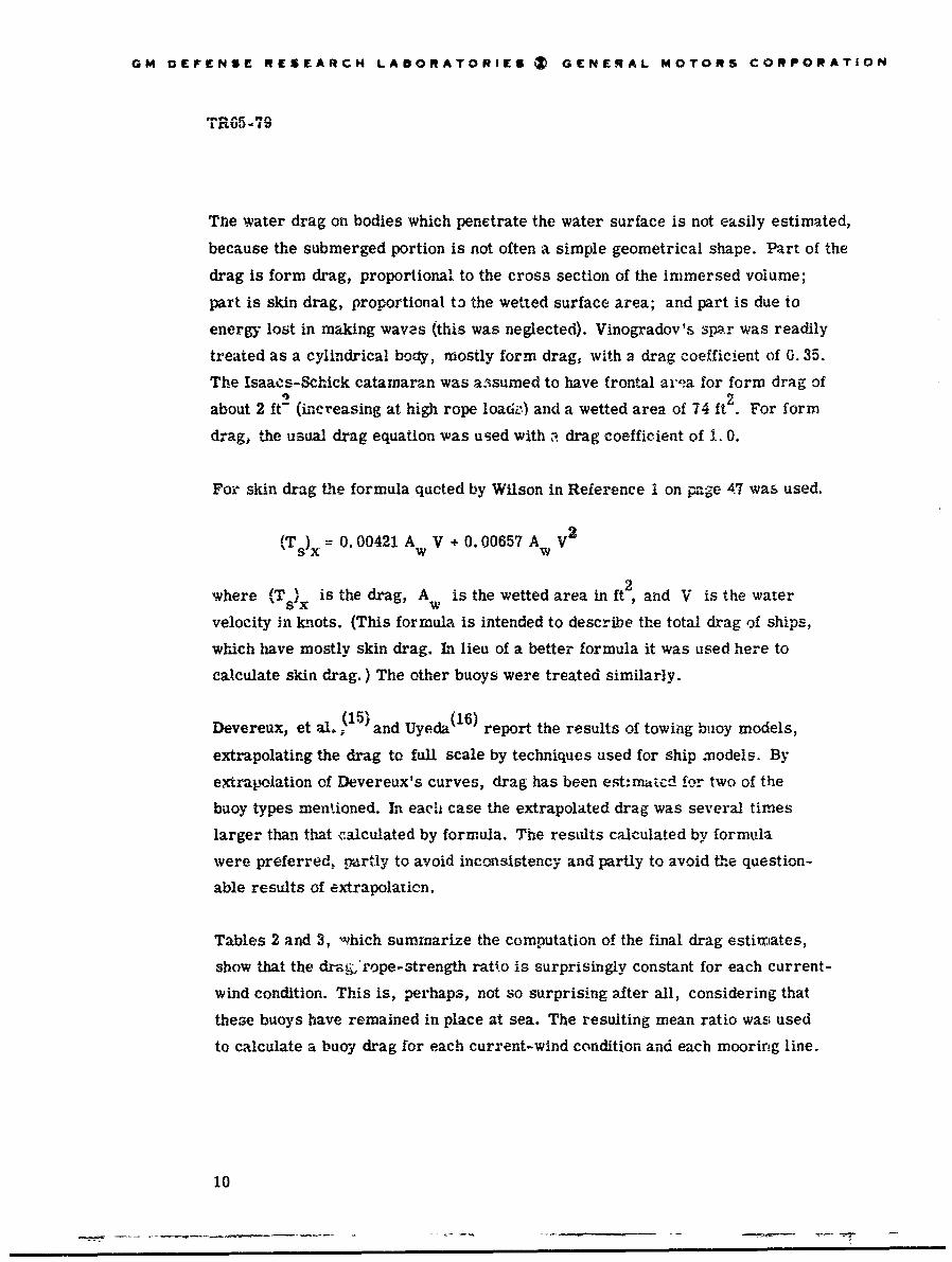
Tne water drag on bodies which penetrate the water surface is not easily estimated,
because the submerged portion is not often a simple geometrical shape. Part of the
drag is form drag, proportional to the cross section of the immersed volume;
part is skin drag, proportional to the wetted surface area; and part is due to
energy lost in making waves (this was neglected). Vinogradov's spar was readily
treated as a cylindrical body, mostly form drag, with a drag coefficient of 0. 35.
The Isaacs-Schick catamaran was a.sumed to have frontal ar,ýa for form drag of
about 2 ft (ihncreasing at high rope loade) and a wetted area of 74 ft2. For form
drag, the usual drag equation was used with :a drag coefficient of 1. 0.
For skin drag the formula qucted by Wilson in Reference i on page 47 was used.
(Ts)x= 0.00421 Aw V + 0.00657 AW V2
where T s)x is the drag, A is the wetted area in ft 2, and V is the watervelocity in knots. (This formula is intended to describe the total drag of ships,
which have mostly skin drag. hi lieu of a better formula it was used here to
calculate skin drag.) The other buoys were treated similarly.
Devereux, et aL$ 1 5 ) and Uyeda(16) report the results of towing buoy models,
extrapolating the drag to full scale by techniques used for ship models. By
extrapolation of Devereux's curves, drag has been esti.matzd for two of the
buoy types mentioned. In each case the extrapolated drag was several times
larger than that calculated by formula. The results calculated by formula
were preferred, prtly to avoid inconsistency and partly to avoid the question-
able results of extrapolation.
Tables 2 and 3, which summarize the computation of the final drag estinates,show that the dra.'rope-strength rat.o is surprisingly constant for each current-
wind condition. This is, perhaps, not so surprising after all, considering that
these buoys have remained in place at sea. The resulting mean ratio was; used
to calculate a buoy drag for each current-wind condition and each mooring line.
10

GM DEFENSE RESEARCHl LABORtATOHtitS GE~NERAL MOTOR!, LUHtU,4A;~
TR65-79
'4cv
C4.
0~
0 e
zz
0 o
444
eq co 9- n
0~ 0 -o>

GM ULF ENS.: RLSEARCH LABORATORIES GENERAL Mol ONb COHPQHA I L)
TR65-79
p09~ 0 4 4V4 t 0 0o 0-
o 9.4 "4 0 P-0
3miQ 000 ~0 0, C C4;0 £O
(121 -4L
>401
C-1 -41- 0Ln~ m 4-.
-4 -- -
-4 4MO~ PLMO cq - v 1 4 9
V-4-
Iei af0q, -0
uorpe
use) mi.oa* -*" *o A M" 4 000 V* t* r-
Pasituml-PaA m m co IV 14 C CIN C-
BT9w)~ lq.,u, Jo'~'u, c~s
'gong V QgQ
z 6
12
GM DEFENSE RESEARCH LABORATORIES ( GENERAL MOTORS CORPORATION
"rR65-79
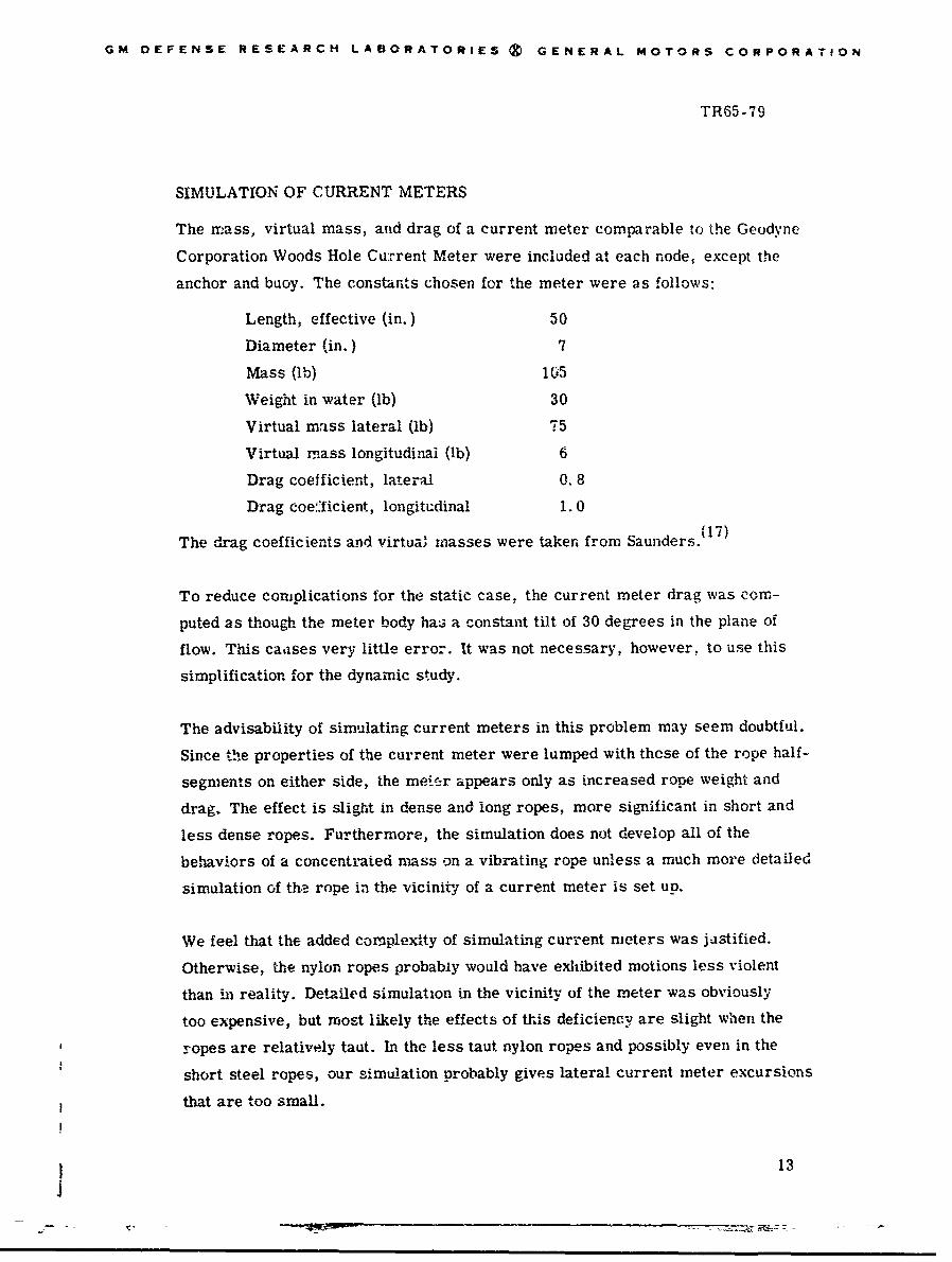
SIMULATION OF CURRENT METERS
The mass, virtual mass, and drag of a current meter comparable to the Geodyne
Corporation Woods Hole Current Meter were included at each node, except the
anchor and buoy. The constants chosen for the meter were as follows:
Length, effective (in.) 50
Diameter (in.) 7
Mass (lb) 1iG5
Weight in water (lb) 30
Virtual mass lateral (lb) 75
Virtual mass longitudinal (Ib) 6
Drag coefficient, lateral 0.8
Drag coeý:ficient, longitudinal 1. 0
The drag coefficients and virtual masses were taken from Saunders. 17 )
To reduce complications for the static case, the current meter drag was corn-
puted as though the meter body has a constant tilt of 30 degrees in the plane of
flow. This catises very little error. It was not necessary, however, to use this
simplification for the dynamic study.
The advisability of simulating current meters in this problem may seem doubtful.
Since the properties of the current meter were lumped with those of the rope half-
segments on either side, the mei-_r appears only as increased rope weight and
drag. The effect is slight in dense and long ropes, more significant in short and
less dense ropes. Furthermore, the simulation does not develop all of the
behaviors of a concentr-ated mass on a vibrating rope unless a much more detailed
simulation of the rope in the vicinity of a current meter is set up.
We feel that the added complexity of simulating current meters was justified.
Otherwise, the nylon ropes probably would have exhibited motions less violent
than in reality. Detailed simulation in the vicinity of the meter was obviously
too expensive, but most likely the effects of this deficiency are slight when the
ropes are relatively taut. In the less taut nylon ropes and possibly even in the
short steel ropes, our simulation probably gives lateral current meter excursions
that are too small.
13j

1M DEFENSE RESEARCH LABORATORIES (t GENERAL MOTORS CORPORATION
TR65-79
WATER DEPTHS
Depths of 18, 000, 6, 000, and 1, 800 feet were chosen as a reasonable bracketing
of practical conditions. We actually expected the dynamic conditions in 1, 800 feet
of water to demonstrate what an impractical depth this is for many purposes.
ROPE DIAMETERS, MATERIALS, AND TENSIONS
We had originally intended to study three synthetic fibers, plus fiberglass and
steel, in a number of rope diameters. But again the multiplicity of factors forced
a retrenchment. Only nylon, fiberglass, and steel were chosen, all with a
diameter of 1/2 inch except for five cases of 2-inch nylon in 18, 000 feet of
water. (The 67 static cases studied are summarized in Table 4.,) When the
dynamic problem was set up, it became necessary to eliminate both the fiber-
glass and th'e 2-inch nylon, so that finally the dynamic cases were limited to
1/'2-inch rope of either nylon or steel.
The manner of choosing tensions may be explained as follows: In the static cases,
once all the constants for current profile, rope and current meters, drag, depth,
etc., had been entered, the independent variable was the tension at Node 1 just
below the buoy. * The dependent variables calculated by the computer were the y
increments for each rope segment, the x and y components of tension at each
node, and the length of each segment. Thus, the choice of tension at Node 1
determined all the other variables.
The two extremes of tension are the breaking strength of the rope and the tensio'n
(if one exists) at which the anchored end of the rope sags enough to become tangent
to the sea bottom. In practice it was not possibie to reach the condition of tangency
on the computer, because it meant that the entire bottom segment of rope would
have to lie horizontally. Its length necessarily would be simulated as infinite,
and the corresponding amplifier would limit. Generally it was practicable to
approach the horizontal within 10 degrees; beyond this point tension settings
were very critical. (There are cases with high water velocities and low-density
* The tension at Node 1 was very nearly the same as at Node 0; for much of thisreport the difference between them is ignored.
14

4 t GM DEFENSE RESEARCH LABORATORIES Z GENERAL MOTOMR CORPORATION
TR65-79
iiTable 4
SUMMARY OF STATIC MOORING LINE CALCULATIONS
IIDeph ROPQ op Correcdt Temstomt Tesulo Rowe COffo Angle Angle Page
(i) t'2 131& ProIIue N4O" 1 %D~cbor '?Ygth Of &.5 07 Ancho.-fL,) (Ih,' (lb) r(t Ct)(4 )(06II
26,000 Ol 0.5 2 :0.000 2,573 1].030 830 1A4 6 I 32 7,34 274 13"510 2,271 1.5 67 5 43 20:000 12,530 26,34A 3,142 2.1 13 2 53 10,00 1,78 23,310 12.730 4,0 87 0 6
16,000 Gus$ 0.5 le.150 14,6"0 28,370 3,241 2 4 22 I13 8,07 6,648 19,200 on 34 4 7 24.3 23 4,843 3.401 23.050 14. 150 8 2 48 2 C '
-3 3. 10 2, SH 2 83* is, 508 10 2 "13 c 10
26.1150 14,6 0 11,710 5, 61l 9 0 17.9 1 14 6,073 a,437 21,610 1.530 17 7 39 6 124 6,400 5,052 35,2140 ?.5o0 23 1 52 6 134 3,444 4,081 31,440 25.520 26 0 66 5 14
IS 10.150 14.750 23.950 is t6 32 a 43 7 155 12. 20 1.5.0 21,140 23,920r 42 2 '7 8 IS
5 11.652 10.360 36,.I0 31.630 47 9 07 2 17
16,000 N71o. 0.5 2 3.00 WO 2.205 2.70 449 1 2 2 5 16S2,10D 1,770 18.0410 Im 1 6 4 5 is
2 720 34,• 16,400 3.319 5 2 23 . 2C2 400 13M 22.310 10.96 9 6 $3 2 223 7,200 6.702 19,060 4,537 3.6 21 S 225 3,600 3,15 23,430 14,600 7 2 4! I 231 2,0 1,S t0 38.430 33,7P0 It 3 TO 3 24
4 :,00 6-7"S 1 ",830 s,31 M 3 2e 7; ^5
3 ,000 3,346 6,.090 is 630 17.1 51 7 23S 2 .Zw•S7 24.350 17.3420 24 6 44 4 2
49.000 Nylon 1.0 3 53.000 50.10 1.6470 4,042 3.1 13 5 4a3 3.!i$60 22390 19260 3.272 . 1 22 9 443 0070, @00 2 .350 2 9 6 36 5 453 20,OM 17.03 21.610 12.24D0 2 . 37 4 3463 1i.000 No 13,m0 24,370 16.70 13 2 7 0 32
6,0OD Steel 0.5 2 10,0OC0 7.314 4,00 ow isi I t 1 3 33
2 4,000 3.352 .4505 22113 27.2 4 0 344 3,000 3.3 1,6W0 1.070 3 7 30 35 3'2 2,13 21.70 6,02 2.0 3 1 - 5 3f3 70 02 17,210 5 077 44 1-5 1 1 3-3 '0:000 7,3411 :.$u 1,9119 1 112 36
3 c.600 3,403 7,43 4 4.064 423 '.
3 1 .104 1.S 1,2V13 6.758 75 6 6 40S10,000 17,2t0 2.173 1.423 5 6 12 Q 49
4 10.00 2.680 104.00 3.359 13 3 36 S 424 2,6O6 2,687 ?,2,50 4,310 16 7 0. . 0 434 ,1W0 4,047 2,230 81,73 20 3 24 . 44
2,0 0 Glass 0.5 3 10.000 7.,3" 0.211 1.20 3 0 i21 . 4.3 slow0 4,373 7.034 3.010 5 ff If 5 44
.03 ,00 3,421 10,G30 6,865 9 a 4t? 41
3 2.104 294 2,63 178 3. 02 6I'M44 2.380 4.1 3.73 56 76I II
4 5.000 :,•438I t.450 B,1l .,7. 1 .7• •4 3,77/4 3,202 11,380 •S070 30• 7 3• •
,G. -0 Nylon 0 5 2t 3.tSO 3.204 4.033 344 1.1 2• C "2
A) 3. 70 2. TO 1.768 307 9 I2 I % '3
r50 )Am , :t25 Im A.1 19 r to kl43 3,4w ,3,1333 1 ,Sm 4,4U• 1 42 3
3 C. I O. ! 1•.o Its (%). e-e-8 orS 1t . p S1 1,80 2,?l17 13.,01 I.37 7.8 72 3 114 3. IN 3.344 4.$35 4,043 14 A " 6 .4 1,$*0 2,.m ;0,400 3,1tl 111 a w¢ *4 2,M0 2, ? 1,),380 6,3"4 18.0 60.6 60".•,4 2.131 1.r74 101n3o 14. 0*0 24.2 75 4 651
1.800 srtet! 0.5 3 10:. 0m0 .3ft 1.$|0 426 2I S 21.[ t -• 4
0 .000 3,431 2.00 "A1 4 0 47-4 6f•
-!3 4.,tsu 2,.t• -1K21s 1.504 5 0 so 2 11.
1.1100 Nylon 0.5 3 3.400 3.m1 11.0s1 U3 2 3 40 46 6:3 3.110 l,"i on Ji 1 7,1 3.6 41 ". 4I13 I. 4c• '1111 .312 3,T30 3 6 et u
ii12, Ow stNI 0.5 A (c) 11. 144 7.244 31,111 Is, im S45 "14 7
A (C) 7.073 3,3W 16. 7W 6.8M 12.01 ;
(a) A "Witim vth !mliumd l lktt OMUW
(c) Frrom W~lt, (3t). *1 fa ch"*U Puqm•
I15

GM DErENSE RESEARCH LABORATORIES (X GENERAL MOTORS CORlPORATION
TR65-79
ropes in which tangency at the bottom cannot occur at any rope length. There
also are cases in which tangency theoretically could have been attained but only
at rope lengths exceeding the dynamic range of the amplifiers.)
The upper limit of tension was usually half the breaking strength of the rope in
question. * Ln some cases, however, the full breaking strength was introduced
at Node 1. The problem is so nonlinear that it was not feasible to pre-select
intermediate points. Instead, they were chosen by trial, so that the rope shapes
interpolated reasonably well between the two extremes.
ROPE PROPERTIES
Table 5 summarizes the constants d, .criptive of the various ropes. For the
elasticity of steel rope the data in United States Steel Wire Rope Handbook,
Section 20, were used. All cases are for ropes with steel cores.** The Hand-
book apparently calculates the metallic area of the rope normal to the strand.
This is the area used in calculating the elasticity. The area given in the table
is the effective area normal to the rope, obtained by dividing linear rope density
by the bulk density of steel.
The properties of fiberglass rope were obtained by measuring a -ample of laid
fiberglass rope made by the Materials Section of the Sea Operations Department*
in mid-1964. (Newer constructions are stronger.) The sample was 0. 312 inches
in diameter; properties for the 1/2-inch diameter were calculated on the
assumption that strength and elasticity vary as the square of the diameter.
Properties of the synthetic-fiber ropes, except for elasticity, were taken from
standard tables and from the tables issued by Plymouth Cordage Co. for their
"Standard" rope constructions.
Breaking strengths for 1/2-inch ropes taken as: steel, 20, 000 ib: nylon,7,200 Ib. glass (GM DRL design), 32,300 lb.
•* Wilson(') apparently calculated for fiber-cored rope.
t GM Defense Research Laboratories, General Motors Corporation.
16

TR 65-7 ý
* 04
n qeAz" -4 -
000
cc c
4 4
ifl C'
100
Go I
'-17

GM DEFENSE RESEARCH LABORATORIES (9 GCNERAL MCTORS CORPORATION
TR65-7 9
ELASTICITY OF SYNTHETIC FIBERS
Elasticity in a synthetic fiber is a complex property which depends upon the unit
strain, the rate of stretching, the cyclic amplitude, the temperature, and perhaps
the pressure. Hysteresis is marked. Creep under moderate loads is considerable,
usually approaching a limit in several tens of minutes. Under high loadines the rope
may creep to destruction. Such behavior has been noted with polypropylene at
stresses above about half the breaking stress.
Since dynamic elasticities were not available, some studies were made with the
Tinius Olsen testing machine at GM DRL. Standard nylon rope, 1/2-inch in
diameter, was pulled to a series of mean tensions and finally to destruction. In
two cases, the rope was cycled ± 180 lb and ± 400 lb about each -mean tension
pulling at 1.2 inches/minute. In a third test the mean tension was maintained
at 2,000 lb, and the rope was cycled ± 140, ± 280, - 560, and - 1,120 lb at
pulling rates increasing with amplitude. In some other tests, run with 9/16-inch
plaited nylon rope, the results were in essential agreement.
Figure 3 is a reproduction of the test record in which the cyclic loading was
S180 lb. At each cycling point there is at first a fairly rapid creep which at
last becomes slow enough that the shape of the loop may be considered reasonably
well stabilized. The dynamic spring constant was determina.d by measuring the
slope between the extreme points of a stabilized hysteresis loop. The resulting
spring constants are shown in Figure 4. They are evidently much greater
(stiffer spring) than those for slow unidirectional pulling.
Figure 5 is a tracing of the record made at various cyclic amplitudes, and
Figure 6 shows the resulting spring constant as a function of cyclic amplitude.
It was then assumed that the semi-log plot of Figure 6 could be moved parallel
to itself to produce similar plots for different mean tensions. These curves
were located by the already-determined relation between spring constant and
mean tension. The resalting diagram, augmented by lines of equal strain
variation, is shown in Figure 7.
18

GM DEFENSE RELEAHCH LAB3UHAI OkiL'ý
TR65 -76
0
-u0
W
in
o acg o .. - to-0
(ql) ols~a

GM DEFENSE RES EARCH LABORATORIES GENERAL. MOTORS CORVI0RATION
TR65- 79
7--T
- X06,
tX
-±--.-.z~-
, 2
PULN RAE I in mi
I. .... .. ......
TENIO (lb.... x 1, 000Figure ~ 4 yni pigCntn fHl-nhNlnRp
-so -

TR65 -79
.s .. ......
Cd
-- Ns'
(10
212

GM OErlENSE RESEARCH LABORATORIES • GENERAL MOTORS CORPORATION
TR65-79
7 C)
• I ..... ~ * .. '' .1: . .. .
::::t t .
-J-
Or: rb Ar-
"" .4z:1"7' "-- q-*-~ :::: -÷
Funcion - . = 2022------I---.- - . - . •
1. .. I • 4 . . I . . .I . .
-• • ..- x- .
S..-j1 4 ,-__jI .t: I±' T-ENSI.N VARIATION i ...lb... .. .
Figure-- - .. 6 Dynami Spr--in Constat o.. Half-Inch. _ Nylon Rope as a . .. I..Function of Cyclic.Amplitude.(mean tension.2,000 Ib
22: -- : • - . -: : . : : .: : i : :

j GM DEFENSE RESEARCH LABORATORIES GENERAL MOTORS CORPORATION
I ' 6 6 -79
I ... , - -7 9
jf
I-I I -"• ,,o•S'I /- . . .i--- . .. .
0
O _ e "1,.. 1 I - __ _ __ _ _ __ _ _
| I !-'&-, i " I I '/ !
LI'I• , I I ! I, ! • i !! I
S i , I '- i" " i , ! -- '+I_ - -, - . -
T TENSION VARIATION (lb:) 'T,1
f Figure 7 Dynamic Spring Constant of Half-Inch Nylon Rope asFunction of Mean Tension and Amplitude
s 23
GM DEFENSE REfSEARCH LABORATORIftS Z GENCRAL. MOTORS CO*PONATION
TR65-79
To determine the spring constant for a particular set of conditions, the cyclic
strain variation throughout the rope was assumed to be both uniform and equal
to 7-1/2 feet divided by the length of the rope. Using the mean tension at the
top of the rope, a spring constant was picked from the graph and used for all
the wave amplitudes of that run. The errors due to this procedure are relatively
small.
The hysteresis of nylon rope also was measured, and one set of values is pre-
sented in Table 6. At the higher values of cyclic tension, the hysteresis certainly
is significant. It was not feasible to introduce hysteresis into the problem directly,
but part of its effect was included by using the experimentally measured dynamic
spring constant; thus we would expect to get approximately correct values for
the maximum cyclic tensions. However, phase shifts and energy losses in the
rope might result in damping some of the resonances observed in our results.
Insofar as resonances modified the tensions, it may be expected that a failure
to introduce hysteresis would cause some error, positive or negative.
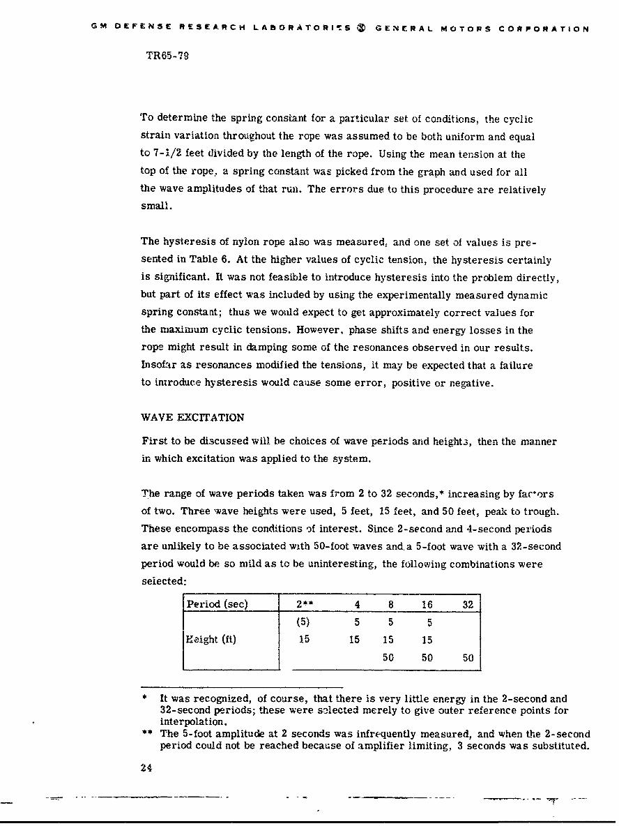
WAVE EXCITATION
First to be discussed will be choices of wave periods and height3, then the manner
in which excitation was applied to the system.
The range of wave periods taken was from 2 to 32 seconds,* increasing by fac~orsof two. Three wave heights were used, 5 feet, 15 feet, and 50 feet, peak to trough.
These encompass the conditions of interest. Since 2-second and 4-second periods
are unlikely to be associated with 50-foot waves and.a 5-foot wave with a 32-second
period would be so mild as to be uninteresting, the following combinations were
selected:
Period (sec) 2** 4 8 16 32
(5) 5 5 5H•ight (fi) 15 15 15 15
50 50 50
* It was recognized, of course, that there is very little energy in the 2-second and32-second periods; these were selected merely to give outer reference points forinterpolation.
** The 5-foot amplitude at 2 seconds was infrequently measured, and when the 2-secondperiod could not be reached because of amplifier limiting, 3 seconds was substituted.
24

GM DEFENSE RESEARCH4 LABORATORIES .Z GENERAL MOTORS CORPORATION
T TR65 -7
I
I Table 6
HYSTERESIS IN HALF-INCH NYLON ROPE(MEAN TENSION 2000 Ib)
Tension HysteresisVariation per cycle
(Ib) (ft - ib)ft length
14') 0.12
±280 0.52
-560 2.3
-1120 15.2
-1400 29.7
ii

GM DEFENSE RESEARCH LABORATORIES e GENERAL MOTORS CORPORATION
TRG5-79
This study was restricted to buoys with a large buoyancy coefficient, since they
could be expected to sink only slightly with the increases in rope tension. Thus
it was possible to ignore inertial effects in the buoy, assuming that in the vertical
it rose and fell with the waves.
The horizontal component of motion was not so easily established. In one extreme
the buoy might move vertically up and down; in the other it might respond com-
pletely to wave particle motion and move in a circle. Neither is correct. Although
we could have simulated the true motion on the computer, we were already at the
practical limits of complexity and felt it best to make a simplifying assumption.
Consequently, the excitation was introduced as an elliptical displacement with the
vertica2 a3xis four times as great as the horizontal.
We now believe that the horizontal component of motion had very little effect on
the system, since its effects could not be detected with any certainty, even at
the first node below the buoy.
DIFFERENCES BETWEEN TEN-SEGMENT AND FOUR-SEGMENTROPE SHAPES
There is a difference in rope shape which results from the 4-segment simula-
tion. To obtain the rope shape for the 4-segment cases, corresponding 10-
segment rope shapes were plotted on a large scale and divided into four equal
lengths. Secants were then drawn between the five resultant nodal positions.
A body equivalent to 2-1/2 current meters was simulated at each of the three
nodes in the rope span to retain similarity with the 10-segment simulations.
The length of the secant was taken to be equal to one-fourth of the total rope
length. This approximation is believed to be reasonably good in all cases in
which the rope has moderate curvature, a condition existing in all cases except
D and L . In Case D the secant nearest the bottom departed widely from the
10-segment curve. In Case L the departure was only about half as great as in
Case D, but it was at the top.
26

GM OEFENSE RESEARCH LABORATORIES Z GENERAL MOTORS CORPORATION
TR65-79
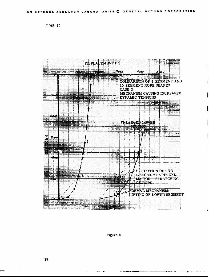
The situation for Case D, illustrated in Figure 8, is of particular interest because
dynamic tensions were determined for both the 4-segment and the 10-segment
simulations. The dynamic tensions for the 4-segment case are much higher than
for the 10-segment case, because in the latter with its highly curved lower section
the motion of the buoy was mostly expended in Lifting the bottom one or two segments
of rope, without much necessity for stretching the rope. In the 4-segment case, the
easily lifted arc of rope is absent, so that the concentrated lateral drag at Node 3
forces the rope to stretch, thereby developing high tensions. The discrepancy in
tension, a factor of 3 at the 50-ft wave height and 32-seconds period, decreases
with period and amplitude until there is scarcely any difference with 5-foot wave
heights.
Case L also would be expected to give dynamic tensions that are higher than they
would have been with the 10-segment rope shape. But the discrepancy should be
less by a factor of about 3, since the secant iv only half as far from the 10-segment
shape and the rope is nylon in which a larger fraction of the mechanism already is
one of stretching the rope.
CHECKING
The static simulation was checked by duplicating two of Wilson's cases, using
his current structure and rope constants. * The total rope lengths and maximum
horizontal coordinates checked within 0.5 percent and the tensions at the bottorr.
within 1. 3 percent, which was regarded as satisfactory.
To check Lne dynamic simulation, one of Whicker's cases(3) was computed, using
two arbitrary values of longitudinal drag. (Whicker himself used no drag. ) Our
results compared well with Whicker's in nonresonant conditions; but where
j Whicker had forces approaching infinity due to resonance, our forces were
finite and the resonant frequency decreased slightly with increasing damping,
j J as would be expected.
pp. 166 and 170 of Reference 2, Vol.2.
11 27
GM DEFENSE RESEARCH LABORATORIES (Z GENEftAL MOTORS COFIP02ATION
A 1v I U
... .. : .... A N D ...
S-... ...-.. :=H 10-SEGMENT ROPE SHAPES£. ~ --- --- --- CASE D
4.- ~::~IMECHANISM CAUSING V4CREASED
DYNAMIC TENSIONS -- i-
.t . 1...-......~
I~ ...........
.t .. .~ .
. . . .
-.------ TOTI
.. .. . ..... ... .
---------
GDOLOWER
Figure 8
28

GM DEFENSE RESEARCH LABORATORIES ( GENERAL MOTORS CORPORATION
TR65-79
II. RESULTS
STATIC SOLUTIONS
Analog Computer Output
Computer outputs in the static rope-shape simulation were read out automatically
on an electric typewriter. The first of two sample pages, shown as Tables 7 and 8,
is the simulation of one of Wilson's cases referred to in Section II. Column headings,
printed irn capitals because of machine limitations, have the following meanings:
I N is the number of the node, counting downward from zero at the buoy; YSU1B(N-1)-
YSUB(N) is the length of the projection on the y-axis of the rope segment between Nodes
n-1 and n; XSUB(N) is tihe vertical coordinate of Node n and S SUB(N) is the length
of the ro3e segment between Nodes n-1 and n; T SIN THETA and T COS THETA
are the l:orizontai and vertical components of the rope tension just above the
respective nodes. The nunibers in these columns are expressed as a four-digit
decimal followed by a scaling factor consisting of a multiplier and exponent of 10.
SThus 0. '2765/2E3 indicates that 0. 2765 must be multiplied by 2 x 10³ The numbers
1f67, 1a88, etc., which are the numbers of the amplifiers being read, may be
I ignored for the purposes of this report. The page number entered in the lower
right corner is for identification and reference.
Reduct ion of Analog Computer Results
All of the results from the original print-out were converted in the IBM 7040digital computer to obtain the x and y coordinates of nodes, the accumulated
rope length measured from the anchor, the tension just above each node, and
n %, 0hv angle from the vertical just above the node. These quantities are labelled
as barred or mean quantities in anticipation of their use later on as the rest
t states for the dynamic studies. Sixty-five cases (Reference Page Numbers 3-67)*
are presented in Secticn VI.
I* The first two are check cases, not shown.
I
• • • • • • • • • •29

GM DEFENSE RESEARCH LABORATORIES GENERAL MOTORS CORPORATION
TR65-79
I ~ q~
Cý~~ ~ ~ ~ ~ I' l 1 1'ýI amf 0 0D m~ C. m N 0% - 0
40 m NS In co~) 0 )
N ~U% N NN -w -ft
Iz ~ ~ ID e4 -
0~~~~~% r!.O t..-0~ ~ n. 0 ;C
0. . . . . . . . a . .N ~ ~ ~ ~ 2 N N N N N
N N NN N NN N NN Nm
o
qN V40 0 V % Ln 0% 0% 6-1
Z V vNN NN
59 In C, M~S In I % I
-C 00 00 0 0020000
fn V'4'. 1
00
.0 m-4 C4
300

TR65-79
40 ; C; 8 C; - ; C; C
o~~ ~ N 6n 6- 0 0 0 M
04
; 's V; 4ý C; ' 43 C; ; C; C;
1.3131.3.31*13 .3W 1.3*31314N. ~ r OD P- N .N N
N N N4N
40con 40 N i ~ 0 0 N *0o ccM 0 0 I N 0 0 4
4 m vn 44 , v "~NN N - .
NN
N N4 C
1-4 0 04 en C! Et V- 4 V 'V :4Z~~N N o o 0 o N N N o N N V
N4 NE 0 4 1 4 . .
14 C40. W E 40 in 40
*4 . .a4 - 4 ..4 .4 -"
enn
031

GM DEFENSE RESEARCH LABORATORIES (R) GENERAL MOTORS CORPORATION
TR 65-79
DYNAMIC SOLUTIONS
Cases Studied
The twelve cases studied are summarized in Table 9. Lettered A through L,
these are identified also by the reference page number of the static solution
used for the rest state of the system. Steel and nylon ropes of 1/2-in. diameter
were studied in two tension conditions (one-half breaking strength and a relatively
slack condition) and three water depths. The tauter rope conditions were all taken
from cases in Current Profile 3, as were Cases F and L; all but these two of the less
taut conditions were taken from cases in Current Profile 2. Six of the twelve
cases were done with the 10-segment simulation and six with the 4-segment
simulation. The 4-segment simulation was necessary for steel rope in the
6,000- and 1, 800-foot depths, and for nylon in the 1, 800-foot depth.
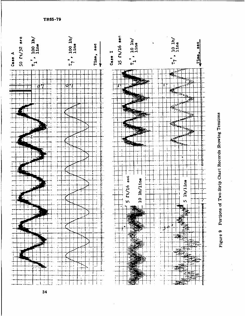
Analog Computer Outputs
The analog computer outputs were in two forms: a strip-chart aad an x-y plot.
Tensions T 1_ , Tt 0, and some of the x Xn-X and Ynil-y quantities
were read out on two eight-channel oscillographs, each channel - 20 millimeters
in width, full-scale. The portions oi two separate records shown in Figure 9
include one of the noisiest, purposely chosen to give a feeling for the worst
conditions encountered. Only a small proportion of the records were as noisy
as this, though it will be noted that even here the true signal may be extracted
from the noise by reading the middle of the densest portion of the trace.
The records of xn - Xn_1 ad y n-1- Yn served a diagnostic purpose, making it
easier to find the source of trouble in case of anomalous behavior of the computer.
Tensions were read visually from the strip charts. They are presented in Section VI.
where they also are plotted as a function of wave height on a log-log scale.
The cyclic motions of all nine active nodes, including the buoy, were plotted
successively by an 11 by 17-inch x-y plotter for each period/wave-height
combination of each case (Figs. 10-15 are examples). The plots were read
32

GM OEFENSE RESEARCH LABORATORIES (t GENERAL MOTORS CORPOIIATION
J Table 9
SUMMARY OF DYNAMIC CASES STUDIED
Case Page Material Depth I Segments Tension :Profile_(ft) __(lb)
A 6 Steel 18,000 10 10,000 3
B 4 Steel 18,000 10 P7,634 2
C 38 Steel 6,000 4 10,000 3
j D 36 Steel 6,000 4 2,838 2
E 65 Steei 1,800 4 10,000 3
F 67 Steel 1,800 4 4,858 3
G 23 Nylon I 18,000 10 3,600 3H 21 INylon 18,000 10 460 2
I I1 55 Nylon 6,000 10 3,600 3
54 Nylon 6, 000 10 720 2
K 62 Nylon 1,800 4 3,600 3
II. • , L 64 Nylon 1• 1800 4 1,440 3
3I!I.
TR65-79
0-4 0 F4Hr -4
0UN E-4 E- E-4 0E r-
.- 4r' p4E-
4)V
* '.4 -
* -- .i -n 1
Z. t
- r~ji..... 12.....4 - 4
CA
-1-T --
I- - - T
T '. ----
.. .j .....
34

GM DEFENSE RESEARCH LASORATORIES GENERAL MOTORS CORPORATioN
TR65 -79
.t............
-.. .. . ...... -
.. .. .......
.. .. ... .7
. . .. ....
. . . . .. . . . . . . . . .
*...........
0
*...... 04::::: :::;:i...
* -. 0. . - . ... . .... ......*** >:: ::
~.:7:
... .......

TR65 -79
.. ~ ~ ~ ~ ~ ....... ....
.. ~ . .
-. ....... - -.-
. .. . .... t:::. : .
7 7 - .... .
.~. 4 .-. ....
. . .. ... ..
.... .. .. .
._ .. .........
... ... .. ..
. . .. . . . . . . .
.* ..........
. . .... .
............ t i- -- :7
t .4 : , .. ....
36

TR65-79
+-
. . .. ....... ..... .. ..
... ...... I.'4
4~.2:1 .i.~ .U i... ... 2......::~ .: t ......1... L: .. ......... ;
. . .. . . . . . . . . . . . . . . T T E ....... .. .. .. ....
a~~~~.. .....: .:t.....
........ : .....
-... t. L
14
.~~~~ . ...
+37

TR65 -79
... ... ....
+ +
.4.-.. . . . . . . -. . - - . -.. -....
.. .. .. .. 4..... - - -*----.4- - -
. 4 . - . -. 4 . . .. . . . . . . . . .
. ........ ....... :.:..
.. . . . . . . . . . . ... . ......
: :: :- i* .......
.......................... .
.. .. .....
_____________.. . .... .. -. *- - - -.. --- -
.,.
....-. -. 1 >TI... .... *~+.. 7j. ,4
38____________________________________________.... ... ...*.**4 ~ .. , .: : : ~ '

I ~TR65 -79
3~~ ~ 4 4- 4--
+ +1
I7 .. 0hI2
I ....... . .. ._____
... .. . ... t
. ., , . . . ...
g
. .39 ....

GN DEFENSE RESEARCH LABCRATOMRIE (3 GENERAL MOTORS CORPORATION
TR65-79
+4 ++
......... ..... :Z
40n

GM DEFENSE RESEARCH LABORATORIES X GENERAL MOTORS CORPORATION
TR65-79
visually, and the results are tabulated in Section VI, Motions of Nodes. These
rables give the lengths of the major and minor axes of the quasi-elliptical motions
in feet. In addition, at each node they give the mean, rope angle k. and the angle
of the major axis of the loop, both measured from the vertical. Toward the bottom
of the mooring line where the loops sometimes were more nearly circular, the
choice of major axis direction was subjective.
Each loop of the x-y plot has two phase marks, sometimes difficalt to discern,
consisting of small perturbations deliberately introduced into the record when
the input ellipse was at its maximum at the top or its minimum at the bottom.
These marks, identified when necessary and marked as 00 and 1800 by referring
to the scale on the resolver generating the input, served as reference marks
to measure the phase of the major axis of the loop. Positive phase angle -was
indicated when the major axis occurred later in time than the zero-degree phase
mark. We discovered later that the phases had been read incorrectly, and since
they are of minor importance, they were omitted.
There are no data on motior s of nodes for the 10..segment simulation of Case D,
the case which prompted the decision to convert to a 4-segment simulation. The
dynamic tensions were recorded and tabulated, however, for both 10-segment
and 4-segment simulations.
Noise and Offsets
, Noise in the system most likely arose from the wiper contacts of the resolvers.
These small noise sources probably were exciting the individual vibrating
systems formed by current :neter masses and the connecting rope segments.
Although this noise was regarded as a nuisance in the idealized solution of the
problem, it possibly has some real significance. Noise sources equivalent to
"the wiper noise must exist in a real mooring and must excite similar real behaviors.
r
.141

GM DEFENSE RESEARCH LABORATORIES ( GENERAL MOTORS CORPORATION
TR65-79
An intei*,esting behavior in some of the dynamic records, both strip-charts and
x-y plots, was the development of an offset from the original mean value. This
was quite troublesome when the offset was too great to be overcome by the offset
controls on the recorders, making it necessary to record x-y plots in an unnatural
order or to reduce the gain on the strip-chart recorder with a consequent loss of
accuracy. This, too, is a phenomenon with probably some real basis, since the
mooring is a nonlinear system and some rectification of cyclic displacements
and tensions wouW be expected.
42

GM DEFENSE RESEARCH LABORATORIES () GENERAL MOTORS CORPORATION
TR65-79
IIV. DISCUSSION OF RESULTS1
STATIC ROPE SHAPES AND TENSIONS
Accuracy
i Neglecting, for the moment, the reduction of rope diameter with stretch, we
believe that the error in rope shape and tension is in the region of 2 pert At,
with the possibility of larger errors near the bottom where rope curvature is
occasionally quite sharp. This conclusion is prompted by the favorable compari-
l sons with Wilson's results.(2 ) Bear in mind that, except for the two check cases,
our ropes have current meters at the nodes and a simulated horizontal buoy
JIt drag - hence, they cannot be compared directly to ropes not containing these.
Like Wilson, we have neglected the reduction in rope diameter with tension.
S(Otherwise, each change of tension would have required a time-consuming
recomputation and change of Dotentiometer settings.) This amounts to only one
j or two percent in steel or glass rope but to much more in nylon. In nylon the
elongation at half the breaking strength is about 42 percent, resulting in a
reduction of rope diameter from 10 to 20 percent. (This is a behavior for which
I we have no experimental data.) Hence, at high tensions the water drag would be
correspondingly reduced so that the rope would be straighter than calculated.
I However, with a slightly larger rope that has been reduced to the nominal size
by stretching, the results would be directly applicable.
1' Adequacy of Method
Wilson's digital-computer solution(2) is relatilyely easy to carry out and probably
less expensive than the method used here. However, much of the thinking that
went into setting up the analog computer for the static case was introductory to
I the dynamic case and thus doubly useful. In any further studies we would probaoly
use digital methods to establish static rope shapes and tensions.
4
1 4
-nf - - - - -

GM DEFENSE RESEARCH LABORATORIES & GENERAL MOTORS CORPORATI-N
TR65-79
Comparison of Rope Shapes
To give some feeling for the peculiarities of different ropes, several rope shapes
in Current Profile 3 are presented in Figures 16 and 17 where ropes of different
materials and diameters are compared when the tension at the buoy is half the
breaking strength.
In 18, 000 feet of water the less dense ropes, nylon and glass, form relatively
straight lines and the 1/2-inch nylon is carried out to a horizontal displacement
that is 3.7 times as great as the 2-inch nylon. This results from the fact that
the drag/strength ratio in vertical ropes is inversely proportional to the rope
diameters. The relation between rope diameter and horizontal displacement is
complex and it may be only a coincidence that the observed 3.7 is so close to
4. 0. The obvious conclusion is that large buoys with mooring lines of large
diameter may be held closer to the anchor than small buoys.
The 1/2-inch steel rope, with its high density, shows a pronounced catenary and acorrespondingly substantial horizontal displacement comparable to that of the 1/2-
inch nylon. If steel were to be compared with nylon at the same strength, we would
expect relative drag to increase in the steel rope as diameter is reduced, with
consequent larger displacements.
Glass rope yields the least displacement of all because of its high strength and
low density. However, as will be apparent below, such short tethers with ropes
that have high spring constants will produce high transient tensions when the buoy
is lifted by waves.
In 6, 000 feet of water the 1/2-inch steel rope shows much less displacement than
the 1/2-inch nylon, because now it no longer contains. . the highly curved ,ower
catenary. Drawn as tautly as in Figure 17, the steel, like the glass, will show
high transient tensions in waves.
44

j GM DEFENSE RESEARCH LABORATORIES GIENERIAL MOTORS CORPORATION
TR65-7ý
RQRýZON4TAI 4 D1SVLAýEMENT (ft)
T I pt
- ---
II
PAGE 28: 2.05 in. NYELO, 53, 000 lb
I Figure 16
45

GM DEFENSE RE5KARCH LAN01tA1roREs aw-4rf AL MOTORS CORPORATION
THUD -'I'
tot
.p5 i-i p3
4v
ROPE SHAPES COMPARED AT Ti2. -'HALF OF BREAXIW3 STRENGTH -
'CURRENT PROFILE J
-PAC-E 55: 0. 5..ix. NYLON, 3600 lb:~PAGE 28: 0.5-in. STEEL, 10, 000 lb
Figure 17
46

V GM DEFENSE RESEARCH LABORATORIES (t GENERAL MOTORS- CO*PORATtON
TR65-79
t DYNAMIC DISPLACEMENTS AND TENSIONS
I Accuracy
The results contain three types of errors: those inherent in the simulation, those
I due to an incorrect choice of constants, and those caused by human error in read-
ing data from the charts.
I The principal errors in the dynamic simulation itself arise from:
i deficiencies of the 4-segment simulation, or the less serious deficiencies
I of the 10-segment simulation
* approximations made in solving the equations of motion
I * inability to provide for all the effects of hysteresis in nylon rope
* the necessity of choosing a fixed value of elasticity for nylon rope
Inadequacies of the 10-segment simulation are negligible compared to the other
errors.
We lack a good estimate of the error due to converting to the 4-segment simula-
tion; and the only comparison we have between the 4- and the 10-segment
simulations is for Case D, which unfortunately is the one in which there should
be by far the greatest error. In spite of the likelihood of concltsions that are too
pessimistic, we compare tensions in the two simulations, plotted as a function of
wave period (Figs. 18 and 19). The two compare well in some regions and poorly
I in others. The general tendency for this particular 4-segment simulation to show
higher tensions than the 10-segment simulation was accounted for in Section 11.
The two simulations should become more nearly the same at shorter wave periods.
because the resulting higher drag and inertia in the mooring would induce stretching
rather than lifting. The curves do agree, to some extent, at short periods; but
the tensions at Node 1 in the 4-segment case deviate sharply downward near the
3-seconds period. Since a bit of the same phenomenon shows in the 10-segmentr data, we suspect a mechanism that exaggerates the response at this period in
the simpler simulation.
44

GM DEKNOW RESEARCH LAUORATORIES 6 GIENERAL MOTORS CORPORATION
~-*±~ t ±Th COMPARISON OF TENSIONS :.- 4.
.4 ~ 4- ~ ~t~t N THE 4-SEGMENT AND ~::~~~:2'I~ ~ '~' 4Iý 1O-SEGMr.NT SIMULATIONS
W5AVES '4-i',4j~ 4;~ijj~j0 10-SEGME NTI, NODE 1I. T~~4~~4
~fli~4410-SEGMENT AT ANCHOR 9*.4
El-~ 4-SEGMENT., NODE 1 1-4:T H
9 .-~ 4 4-SEGM1ENT AT ANCHOR
Figur 16
48

GM DEFENSE RESEARCH LAGORAlORIKS GKN'CRAL MOTORS CORPORATION
I ~TR65 -79
J ~~~COMPARISON OF TENSIONS - * -
JN THE 4-SEGMENT AND -
10-SEGMENT SIMULATIONS -1 CASE D
-ft ___V
I ~, 0SGMNoND
4-SEMNT
I Figure 19
E-LN TND --

GM DEFENSE RESEARCH LABORATORIES OR GRNERAL MOTORS CORPORATION
The explanation is as follows: Pronounced near-resonance phenomena of whichthis must be an example, should occur only in ropes that are long enough or at
periods that are short enough to make the rope length nearly an integral number
of quarter-wavelengths for the travel of a longiludinal elastic wave through the
rope. In 1/2-inch steel rope, the velocity of an undamped longitudinal wave is
10, 350 ft/sec. When the rope length is 6,580 feet, as in Case D, the buoy would
first become a standing-wave node, with a consequent maximum decrease in
tension, at a period of (4)(6580)/10,350 = 2.54 sec. Because of damping, the
period is actually longer. ".ae conclusion must be that the four-segment rope
with its lesser curvature .; stretching more at short periods, as well as at long
periods - hence the exaggeration of phenomena associated with stretching. At
the anchor, where the phase difference is only about a quarter-wavelength,
the agreement at short periods is good.
We admit that as a measure of accuracy it would be more satisfying to bring
forward two cases which should act the same. But without any other duplications,
we must be satisfied with the argument given above. Although there is little
basis for a quantitative estimate of error, we suggest that the error due to using
a four-segment simulation is less than a factor of 1.3, or 1/1.3, in all instances
except Cases D and L.
As mentioned in the Appendix, the approximations made in simplifying the
perturbation equations produced significant error in two cases,* both steel
rope in 1,800 feet of water, at 50- and 25-foot wave heights. In these, the errors
in the matrix quantity Kn were a negative 34 and 24 percent. In all other cases
the errors in Kn were less than 20 percent. Tension error will not be so large,
since tension iu not directly proportional to Kn ; consequently, we may expect
the recorded tensions to be a little low in the more extreme cases (steel rope,
short length, large waves).
* Cases E and F.
50

GM DEFENSE RKSIA4CH LAVfWA .1RIES (1) GILNERAL MOTORS CORPORATION
TR65-79
The effects of neglecting hysteresis in nylon are difficult to estimate. As pointed
out, a dynamic spring constant that is different from the slope of the slowly
developed stress-strain curve is one of the effects of hysteresis. By using a
dynamic spring constant, we have partially provided for hysteresis. But the
I necessity of using a mean value of the constant has resulted in a spring that is
too resilient at the higher wave heights, so that the observed tensions in nylon
are too low at the 50-foot wave heights; and, conversely, they are too high at
the 5-foot wave heights.
The energy loss due to the hysteresis loop is a significant factor, one far
It greater than longitudinal drag near the bottom of the rope (where dynamic drag
effects are small). We would expect, therefore, that in nature there will be
more attenuation of the longitudinal elastic wave, lower tensions at the anchor,
I j and shifted and reduced resonance effects.
SI [The use of the nominal rope diameter instead of the stretched diameter fortunately
produced little -vrror. It was estimated earlier that at 3,600 lb mean tension the
diameter of the rope will decrease 10-20 percent. The assumption of a fixed
nominal diameter causes the rope to show, incorrectly, a larger lateral drag
which reduces the tendency of the rope to straighten out when pulled and forces
more motion into the stretching mode. However, since a substantial proportion
of the wave motion already is acting in the stretching mode (because lateral
I i drag is fairly high in nylon in comparison to the elastic forces) little error
need be expected. *
i •Human errors are confined mainly to reading charts. The probable errors from
misreading the strip charts are limited to + 15 percent. Dimensions of the nodalIi ellipses generally could be read to within one.4fourth of a small division, or
0.025 foot for 5-foot waves., 0.05 foot for 15-foot waves and 0.25 foot for 50-foot
Iii waves.
*It must be pointed out that since the static rope shapes are somewhat in error forthe same reason, the dynamic simiulation was applied to rope shapes that do notcorrespond exactly to the assumed current-wind conditions.
I5I1 5

GM OEFENSE RESZARCH LABORATORIES ( GENERAL MOTORS CORPORATION
2iu I'• -J;
Displacements of Nodes
The displacements of nodes are generally in quasi-elliptical loops, decreasing
in size from top to bottom. In taut ropes that are relatively straight, the motion
tends to be nearly longitudinal, along the rope, with very little lateral motion,
especially at the shorter periods. (As has been explained, more motion gnes into
ithe longitudinal stretching mode at short periods.) In the sharply curved catenaries,
the loops open up into almost rectangular shapes near the bottom of the rope
because of the large proportion of lifting and the change of curvature taking place
in this region. Because they are more curved than nylon ropes, steel ropes give
more open loops.
The Effect of Displacements on Current Meters
It is difficult to make a simple general statement about current meter errors from
these complex results. Let us exclude from consideration the steel ropes. which
have large curvatures ai. excessive nodal movement, and examine the nylon
moorings, which show the smallest motions.
As an average condition, consider ropes oscillating at a 16--second period in
15-fo•.L wa-aves. In Cases G, H, I, anld J, the length of the minor axis is relatively
constant at all depths, averaging slightly greater than 0.3 ft. (Cases K and L,
which show much more displacement, are left to be mentioned later.) We shall
ignore momentarily the effect of axial motion on the meter; and to come . little
closer to reality we shall change the period to cme more probable in the sea and
assume that these same displacements would occur at a 12-second period. Then,
in still water a current meter which cannot distinguish positive water motion from
negative would be exposed to cumulative apparent water motion of (0.3) (2)/ 12 or
0. 05 ft/sec. In moving water at speeds greater than 0. 05 ft/sec, the mean error
would disappear if the speed sensor werc ideal. However, it is well known that
rotors tend to over-register in fluctuating flow, so scme effect always would remain.
Tixu effect on current meter sensors of motion normal to the sensitive axis of the
speed sensor* is not well known. Gaul (19 showed that Savonius rotors ran
* We call this "axial motion" for want of a more rigorous terzi.,
52

i ¶ GM DEFENS1 RESEARCH LABORATORIrS (V GENERAL MOTORS CORPORATION
TR65-79
significantly slower when oscillated axially only one or two feet. Gaul ran no
tests in still water where it is likely that spurious rotor turns would have been
produced by the turbulence around the meter. Had he tested bucket wheels and
propellers, he would have found marked increases in apparent velocity (see
Paquette, Ref. 20).- I
Probably more important than pure axial motion is axial motion combined with
. a slight dynamic tilting of the current meter, a not improbable behavior of a
long massive body on a disturbed rope. This kind of behavior would cause
additional errors in apparent speed that would be largest near the surface.
Cases K and L have been ignored until now because our results indicate that
"simple moorings in such snauow water in the open sea are undesirable from the
point of view of both nodal motion and dynamic tensions. It is sufficient to note
that the lateral motion is nearly seven times greater than in moorings in deeper
water.
We believe that near wave frequency an erroneous apparent speed vector of
0. 05 ft/sec (1.5 cm/sec) is smaller than that observed in practice. We must,
therefore, conclude that axial motion comb;.ned with dynamic tilting of the
meter is responsible for as much or more error than that caused by lateral
motion.
We wish to avoid leaving the uninitiated with an impression that we have now
expressed the principal sources of current meter error. We have studied only
those errors which can be ascribed directly to the action of waves on a buoy at
"the surface. The sources of what has been called "mooring noise" are numerous
and serious. The simple fact that rope is flexible and that it may yield locally or
in toto to turbulent forces of all time scales and from any direction leads to a
spectrum of velocity errors that are beyond the scope of this report.
53

GM DEFENSE RESEARCH LABORATORIES () GENERAL MOTORS CORPORATION
± rXou-79
V. CONCLUSIONS
For a system consisting of a buoy excited by ocean waves and anchored to the
bottom by a simple mooring, we make the following conclusions:
1. All points in the mooring rope undergo quasi-elliptical moticn, with
the loops usually elongated approximately along the rope direction.
2. The motion is probably large enough to account for the errors
observed at wave frequency in moored current meters if motion
along the rope direction can be assumed to contribute some error.
3. Fairly taut, resilient ropes of low density, like nylon, produce the
least lateral motion and probably the smallest current meter errors
if depths significantly less than 6,000 feet are avoided.
4. Dynamic tensions are moderate in long ropes and those buffered by
resilience or ,i well developed catenary. In taut, only slightly
curved ropes eel, dynamic tensions can rise to dangerous values
in storms; this can happen even in moderate weather if the ropes
are as short as about 1,800 feet. Resilient, synthetic fiber ropes
develop much lower dynamic tensions, even when the ratio of dynamic
tension to breaking strength is considered.
5. Resonances develop in the ropes, but tensions due to them are small
compared to those generated by the more direct mechanisms. (Exceptions
occur in moderately short ropes, but only at the short resoiant periods
where there is little wave energy.)
54

3 GM DEFENSE RESEARCH LANORATORIES ) GENERAL MOTORS CORPORATION
a TR65-79
*1
VI. DATA
II
I
II
1 55

GM DETENSE RESEARCH LABORATORIES (t GENERAL MOTORS CORPORATION
CABLE CONFIGURATIO'IS AAD TENSIO0NS
CABLL MAr:RiAL STLCL CABLL bIAMLTE4 :.5 I'•CURRENT PROFILE ? KCEA D)F,1lt, I,0C•0 FEElT SUB(1) 10000 LS PAGE 3
X Sufi(N) y SUt(N) CABLE MLAN IHP:A SIM(N)BAR bAR LENGTti TEENSI ON 1ARFELT FEET FEET LBS DEGsECS
I (1 829 11033 00l052 1.?
1 30U 823 17734 9992 1.2
2 15CO 794 16533 9664 1.4
3 3000 756 15f38 9 0') 2 1.4
4 600% 679 12032 R163 1.1
5 900(1 568 9023 692b 2.0
5 12000 450 6015 i56Qi 2. o
S15000 269 2995 4465 3.3
3 16500 173 1511 3539 4.2
4 17700 41 302 29.1 5.r
I, I 8C*C -0 -c 2634 6.1
ANCHOR 2572 6.1
CABLE t¶ATERiAL STEEL CABLE I)IAMETER .. INCURRENT PROFILE 2 OCEAN frEPTti 18Cfl- FEETI SUO(1) 7634 LBS PAGE 4
X SUII(N) Y SUP (1) CARLE MEAN TI'FTA SU.•(N)BAR LIAR LENGTH 1 NS. rl N, PfAR
N FEET FEET FEET LBS nEGR, EFS
C 2210 145015 760P. 1.5
I l30 2263 18205 7628 1.5
2 1500 2223 17004 7?'97 1.
! 3090 -171 1 5, 11 6729 1.9
4 60,'0 2064 12502 5P, cO 2.2
5 9000 1893 9485 4566 3.C
6 I,:04',0 168A -466 3330 4.5
7 loi 1299 3417 20Q94 1.1
16500 1036 1919 1175 12.m
1700 552 629 631 21.1
13 I11000 -0 -0 (410 64.4
ANCHOR 274 s9.?56

IGI • DEFENSE RIESEARCH LABORATORIES 4| D ERAL MOTORS CORPORAT1Or
| i|CABLE CONFIGURATIOS AND TENSIONS
CABLE MATERIAL STEEL CABLE COIAMLTLR 0.5 IN~IICURRENT PROFILE 3 OCEAN DEPTH 18000 FEETT SUBMi 20000 LBS PAU ;F
IIX SUB(N) Y SULI(N) CABLE MEAN TH~ETA Sud(N)BAR BAR LENGTH TENSION BAR
N FEET FEET FEET LRS DEGREES
I 0 0 3142 18339 ?oL59 2.1
1 300 3131 18049 19984 2.0
2 2 1500 3310 16831 19630 5.8
3 3000 2788 15320 19063 8.4
1 4 6000 2323 12262 18134 9.1
5 9000 1808 9197 16991 9.6
S6 12000 !258 6128 15649 ll, C.5
7 15000 654 3049 14410 11.4
a 16500 344 1q37 13484 1e.2
9 17710 71 308 12916 12.3
II 10 18000 -0 -C 12589 13.1
II ANCHOR 12527 13.2
CABLE MATERIAL STEEL CABLE DIAMETER 0.5 INCURRENT PROFILE 3 OCEAN DEPTH 1.8006 FEETTI SUB(1 10000 LBS PAGE 6
X SUB(N) Y SUB(N) CABLE MEAN THETA S~ifiN)BAR BAR LENGTH TENSION bAR
N FEET FEET FEET LBS DEGREES
0 0 12732 23315 10210 4.0
II 1 300 12711 23013 10129 4.0
2 1500 12468 21789 9754 11.5
Ii 3 3000 12003 20215 9193 17.1
4 6000 10950 17052 8268 19.5
II 5 9000 9674 13797 7047 23.2
6 12000 8040 10387 5824 28.5
I 7 15000 5769 6624 4580 37.4
8 16500 4053 4364 3671 49.2
Ii9 171700 17 25 1745 3127 63.5
10 1800ra -0 -0 2823 79.9
IIANCHOR 2785 87.0 57

GM DEFENSE RRESARCH LABORATORIES 0 GENERAL MOTORS CORPORATION
CABLE CONFIGURATIONS AND IENSIONS
CABLE MATERIAL GLASS CABLE DIAMFTER 0.5 INCURRENT PROFILE 3 OCEAN OLPTH 18000 FEClT SUBIl) 1615U LBS PAGE 7
X SUS(N) Y SUb(N) CABLE MLAN THETA SU's(N)BAR BAR LENGTH TENSION BAR
N FEET FEET FEET LBS DEGREES
0 0 3240 18366 16174 2.4
1 300 3228 18066 IbIrl 2.1
2 1500 3078 16856 16043 7.0
3 3000 2815 15335 19927 9.9
4 6000 2282 12263 15790 10,4
5 9000 1733 9190 15518 1C.4
6 12000 1172 6118 15286 10.6
7 15000 599 3042 15054 10.7
8 16500 303 l;27 1487q 1ý.9
9 17700 60 305 14763 11.2
10 18000 -0 -1) 14677 11.2
ANCHOR 14666 l1.1
CABLE MATERIAL GLASS CABLE DIAMETER 0.5 INCURRENT PROFILE 3 OCEAN DEPTH 18000 FEETT SUU(l) t075 LBS PAGF 8
X SUB(N) Y SUBIN) CARLE MEAl THETA SUB(041BAR BAR LENGTH TEISI()N BAR
N FELT FEET FEET LBS DEGREES
0 0 6945 19288 8135 4.8
1 300 6919 18986 8104 S.C
2 1500 6620 17749 7972 13.9
3 3000 6077 16150 7861 19.8
4 6000 4967 12961 7691 20.7
5 9000 3802 9750 7467 21.4
6 12000 2587 6519 7247 22.2
7 15000 1326 3266 7009 72.-A
8 16500 663 1636 6435 23.6
9 17700 136 329 6711 23.9
10 18000 -0 -0 6645 24.4
58 ANCHOR 6627 2a.3

' M DCFENSC RESEARCH LABORATORIES Z GENERAL MOTORS CORPORATION
i CABLE OF|iGURAIXOuN AND !LNSIONS
CABLE MATERIAL GLASS CABLE f)IAMETFR 0.5 INCURRENT PROFILE 3 OCEAN DLPItI 18000 FEElT SUB(l) 4845 LBS PAGE 9
X SUB(N) Y SUB(N) CABLE MAN FHETA SUh(NIBAR BAR LENGTH TENSION BAR
N FEET FEET FEET LBS DEGREES
0 0 14147 23050 4897 8.2
1 300 14103 22747 4845 3.3
3 2 1500 13600 21447 4694 22.9
3 3000 12644 19676 4601 32.6
1 4 6000 10578 16054 4437 34.6
5 9000 8323 12302 4212 36.7
I 6 12000 5830 8381 399 8 39.4
7 15000 3100 4313 1774 42.3
B 16500 1596 2189 3623 45.0
9 17700 332 448 34V7 46.7
J10 18000 -0 -0 3433 48.2
ANCHOR 3400 48.1
1? CABLE MATERIAL GLASS CABLE OIAMtETER 0.5 I4CURRENT PROFILE 3 OCEAN DEPTH 18000 FEETT SUB(1} 3410 LBS PAGE IC
x SUs(N) Y SUo(N) CABLE MEAN IH-ETA SUB(N)BAR BAR LENGTH TENSION BRR
N FEET FEET FEET LBS DEGREES
0 0 22846 29616 3970 10.2
1. 300 22793 29312 3906 10.1
2 1500 22162 27957 3743 28.0
3 3000 20909 26025 3657 39.9
"4 6000 18149 21938 3495 42.9
IJ5 9000 14976 17584 3259 46.4
6 12000 11.315 12839 3057 51.1
.ii7 15000 6710 7352 2822 56.7
8 16500 3761 4042 2690 63.1
9 9 17700 854 904 2589 68.0
to 18000. -0 -0 2532 71.4
i ANCHOR 2506 72.0 59

GM DEFENSE RESEARCH LASORATORIES ;t GENERAL MOTORS CORPORATION
CABLE CONFIGURATIONS AND TFNSIUNS
CABLE MATERIAL GLASS CABLE DIAMETER ',.5 INCURRENT PROFILE 4 OCEAN DEP! 180OU FFETT SUM(1) 16150 LUS PAGE 11
X SUB(N) Y SUB(N) CABLE PEAN I HETA SUi(Ni)BAR BAR LENGTH TENSION [BAP
N FEET FEET FEEf LBS DEGREES
0 0 5365 18706 16206 8.1
1 300 5318 18403 16150 8.9
2 1500 5036 17170 16047 13.4
3 3000 4599 15606 15926 16.2
4 6000 3713 12484 15760 16.7
5 9000 2810 9361 15520 16.9
6 12000 1896 6239 15291 17.?
7 15000 965 3112 15C71 17.4
8 16500 485 1573 148P6 17.7
9 17700 97 315 14784 1f..
I0 18000 -0 -0 14698 .
ANCHOR 14679 11.9
CABLE MATERIAL GLASS CABLE PIAMETER 2.• 1'4CURRENT PROFILE 4 OCEAN DEP71i 1600C FFETT SUB(I) 8075 LBS PAGE 12
X Sul(N) Y SUB(N) CABLE MEAN THETA SUL(3J)BAR BAR LENGTH TENSION BAR
N FEET FEET FEET LBS DEGREES
S0 12532 21907 8161 17.7
1 300 12435 21592 8070 17.9
2 1500 11837 20256 7947 26.5
3 3000 10896 18493 7846 32.2
4 6000 8921 14935 7679 33.3
5 9000 6842 11308 7469 34.6
6 12000 4663 7611 7242 35.8
7 15000 2389 3845 7009 37.2
8 16500 1204 1923 6863 38.4
9 17700 248 391 6729 39.1
10 18000 -0 -0 6656 39.6
60 ANCHOR 6636 39.6

j GM DEFrtNSE RESEARCH LAMORATORIES (t GENERAL MOTORS CORPORATION
CAiLE CO)JFIGUPAT Ifl4S ANID IENSIOIJI
CAMIF MATLRIAL GLASS CABLE ,llintIf I 0.5 INCJRREII PROdFILE 4 uCrAN IdPMh 96,O.) FEETI SUtM(1) 6460 LUIS PAGE 13
SX SU,- () Y SUH1N) CARLF ME EAN IIoIA SUt(N)BA'•, bAR LENGTH TLNSI ON BAR
' F FElT FE C- I FEE r LBS "EK;PFFES
0 175157 2 5242 6561 27.1
1 3oc) 11462 24918 6456 22.5
S2 1500 16690 23492 6132 32.7
3 3f0lO 15454 21550 6230 39.6
[ 4 6000 12854 17555 6177 41.4
5 91'0.34 13437 5946 43. ?
16 12COC. 6963 9150 5623 45.3
7 15c000 3639 4679 5393 47.9
a 8 1650C 1P, 7 2399 5266 55 .
9 177,00 3pO 484 5134 51.5
19 18Cno' -3 -0 5066 52.5
A qCIlOR 5052 52.6
CABLE tlATFRIAL GLASS CAPLE 1I) 1,AMLT R 0.5 INCURUL4T PRtFILE 4 0CFAN 4 Ehi' IlOCO FEETT SUU(•) 5444 LBS PAGE 14
X Surl(N) Y SUB(.N) CABLE MEEAN THFTA SUjCt4)G LAR CAR LENGTH T FS'I S 1O)AR
N FEET FEET FFET LBS DLGREES
C 0 2552u 31439 5if55 26.0
11 300 25368 31104 5447 26.7
2 1500 24428 29580 5324 34.2
3 3000 22873 27430 5224 46.0
4 6000 19518 27945 5079 4..4
5 O000 15718 1812u 4840 51.3
6 12000 11474 12899 4637 55.0
1 7 15000 6470 7079 4403 59.1
B 15.0 3444 3742 4277 63.3
9 17730 731 795 4173 66.2
13 18000 -0 -0 4113 68.2
1 ANCHOR 4-n80 68.5 61

GM JEFENSE RESEARCH LABORATORIES (t GENERAL MOTORS CORPORATION
CABLE COnFIGUR4TIrlNS AND TENSIONS
CAHLC MAIERIAL GL4SS CABLE DI',-EMLE' . 1. '4CURRENT PROFILE 5 LOCEAN DEPrfi 1,t o FrETT StIdl) 1615C Lt6S PAGE 15
( SUB(J) Y SUB (,f) C VLE ME AN. TIIFTA SUj(i\'liar t!iA R L E~liý I f 'INS1 4 it Ap 0'A
" " FL'_T . E_.T F6ELI L65 1EF,:' E L
0 0 15686 23050 16292 32.u
I 3.00 15440 23S91 16 1r-S 33.1
2 1S1C. 1,4588 220-)1 16064 36.1)
3 1000 1 34d 2?)146 1 c;0; ,7 39 . 6
4 6000 1?819 16196 157(0 39. P
5 1400(1 12 16 127l 1 V-,. 4 ,
6 120 0 G r4A 81I0 1532H 41.6
7 19330 2v 14 4109 15228 42. Q
8 165-3 1424 2n69 I 5 59 43. c
9 17790 283 413 14778 43.?
10, 1000 -C -C 14776 43..R
ANCHOR 1479;0 4 1. 6
CAHLr MATERIAL GLASS CARLE DIAMETER --. 5 INCURRL:4f PRIUFILi: 5 OCEAN L-PTH tbCOd, jI-.TT SUt,(I) 1292C Le, S PAGE 16
X SUMIN) Y SUB(N) CARLL P.LAN ii|ZTA SIl.(fi)1 AR bAR LENGIH TENSION BAR
N FE- I FEET FFET LRS f E("R EGL
3 0 23921 29939 1301;I 42.3
1 300 23f43 29-29 12941 42.7
2 1500 22398 27171 12842 46.9
3 3LI00 20S81 29443 12744 5n.O
4 6000 16889 ?0683 12517
9 ?000 13004 19776 124C,6 52.5
6 12000 8925 10709 12155 53.7
7 15000 4606 5456 11959 55.2
8 16500 23"-6 2182 11700 r6.2
9 17700 473 160 1111 57.0
1f 18000 -0 -0 11'•96 57.7
ANCHOR 11579 57.,7

GM DKENSE RESEARCH LABORATORIES Z GENERAL MOTORS CORPONATION
CABLE CONFICURATIONS AND TENSIONS
CABLE MATERIAL GLASS CABLE DIAMLTER 0.5 INCURRENT PROFILE 5 OCEAN [)FPTIH 18(00 FEETT SUB(l) 11652 LBS PAGE 17
X SU3(N) Y SUB(N) CABLE MEAN ThETA SUm(N)BAR BAR LENGTH TFNSIOON BAR
N FEET FEET FEET LBS DEGRLR
0 0 31828 36r69 11779 48.C
1 300 31487 36119, 11674 48.5
2 1500 29902 34128 11583 52.8
3 3000 27683 31472 11486 56.0
4 6000 23032 25942 11362 57.5
5 9000 18014 20105 11149 59.?
6 12000 12611 13911 10919 61.1
7 15000 6667 7295 10669 63.2
8 16500 3431 3739 1055g 61.1
9 17700 702 763 I(-47r 66.4
10 18000 -c -0 10377 67.,1
ANCHOR 10356 67.2
CABLE MATERIAL NYLON CARLE DIAVETER 9.5 INCURRENT PROFILE 2 OCEAN DEPTh 18000 FEETT SUB(i) 3600 LbS PAGE 18
X SUB(N) Y SUB(N) CABLE MEAN THETA SU3(N)BAR BAR LENGTH TENSION BAR
N FEET FEET FEET LBS DEGREES
0 0 488 17992 '596 1.1
1- 300 482 17692 3;94 1.2
2 1500 456 16492 3563 1.4
3 3000 423 14998 3525 1.6
4 6000 353 11991 3477 1.6
5 9000 274 P984 3430 2.0
6 12000 188 5980 3382 2.0
J-7 15000 98 2971 3328 2.1
8 16500 50 1501 32850 2.4
9 17700 10 300 3243 2.5
.10 18000 -0 -0 3209 2.9
I ANCHOR 3204 2.5 63

GM DEFKNSE RESEARCH LABORATORIES ( GENt, RAL MOTORS CORPORATION
CAB".E CONFI(GURATIONS AND TFNSI!ONS
CABLE MATERIAl. NYLON CABLE DIAMETER 0.5 INCURRENJT PROFILE 2 OCEAN DEPTH 18000 FEETI SUBM() 2160 LaS PAGE 19
X SUO(N) Y SUB(N) CABLE MEAN THETA SUW(N)BAR BAR LENGTH TENSION BAR
N FEET FEET FEFT LBS DEGRELS
0 0 1018 18057 2161 1.8
1 300 1009 17757 2159 1.0
2 1500 956 16555 2125 2.9
3 3000 887 15058 2086 2.5
4 6000 734 12043 2040 2.8
5 9000 569 9027 1994 2.9
6 12000 390 6011 1943 3.5
7 15000 202 2991 1891 3.6
8 16500 102 1506 1835 4.4
9 17700 20 301 1809 4.4
10 18000 -0 -c 1773 4.5
ANCHOR 1769 4.5
CABLE MATERIAL NYLON CABLE DIAMETER 0.5 INCURRENT PROFILE 2 OCEAN DFPTH 18000 FEETT SU•I() 720 LbS PAGE 20
X 0UB(N) Y SUb(N) CABLE MEAN THETA Stlb(N)BAR BAR LENGTH TLNSION BAR
N FEET FEET FEET LBS DEGREES
0 0 3319 18401 723 5.2
1 300 3292 18099 721 5.4
2 1500 3168 16892 687 7.0
3 3000 2918 15377 650 8.1
4 6000 2491 12325 606 9.5
5 9000 2019 9266 560 10.3
6 12000 1489 6200 512 13.5
7 15000 918 312j 456 15.3
8 16500 498 1578 421 19.4
9 17700 93 314 377 18.5
10 18000" -0 -0 349 23.6
64 ANCHOR 348 23.3

I GM DEFENSE RESKANC:H LABORATORIIS 0 GENERAL MOTORS CORPORATION
I CABLE CONqFIGURATIONS AJfD TEISION,
CABLC MATERIAL NYL0N CABLL DIAMLT'E 0.5u INCURRENT PROFILE 2 OCEA DJ !PIit MO00 FEETI SUB(1) 460 LUS PAGE 21
x ( Ud(,4) Y SU3('J) CABLE VEA*4 IIIETA SUB(N)
-AR BIAR LENGTH TF"IScON BARN FEET FEET FFFT LBS O)EGREE!
0 0 0 10956 2230'j 461 8.7
1 300 lu91l ?2002 459 F.H
j2 150C 10617 20767 425 11.9
3 30l0 102R7 19232 389 13.7
4 60;)O 9715 16165 346 16.8
5 9000 8265 12834 299 19.5
6 12000 b711 9456 252 28.4
7 1500C 5317 6320 211 34.6
a8 16.500 3460 3863 185 48.9
9 17700 1736 1761 157 62.8
1ia, 13 &10))C -0 -c 142 79.5
ANCHOR 132 83.1
I CABLE MATERIAL NYLON CABLE DIAM.TER 0.5 INCURRENT PROFILE 3 OCEAN DEPTIi WO0O FEETIT SUB(M) 7200 LBS PAGE 22
X SUI3!N) Y SI1(N) CABLE MEAN THETA SUO(N)BAR BAR LENGTH rLNSION KAR
SN FEET FEET FEET LBS DEGREES
0 0 6537 19093 7230 3.6
11 300 6518 18792 7210 3.6
2 1500 6226 17557 7118 13.5
I3 3000 5683 15967 7094 19.9
4 6000 4573 12780 7058 20.4
5 9000 3446 9587 7016 20.7
6 12000 2304 6389 6962 20.9
7 15000 1150 3182 6906 21.0
8 16500 570 1601 6856 21.2
3 9 17700 117 322 6819 21.1
13 18000 -0 -0 6792 21.4
SANHOR 6792 21.5 65

OM DEPI[NSE RESEARCH LABORATORIES ( GENERAL MOTR1S COMPORAT!ON
CABLE CONFIGURATIONS AND TENSIONS
CABLE MATERIAL NYLON CABLE DIAMLTER 0.5 INCURRENT PROFILE 3 OCEAN DEPIii leOOO FEETT SUBt1) 3600 LBS PAGE 23
X SUB(N) Y SUB(N) CABLE PEA% THETA SU•(dj)BAR BAR LENGTH TENSION BARFEET FEET FEET LBS DEGREES
3 0 14t02 23432 3640 7.2
1 300 14764 23130 3602 7.2
2 1500 14191 21807 3500 27.0
3 3000 13003 19904 3466 38.4
4 60(0 10540 159Q9 3437 38.9
5 9000 7965 12043 3396 40.4
6 12000 5361 8052 3353 4&.5
7 15000 2701 4025 3315 41.1
a 16500 1349 2014 3?58 42.U
9 1770C 279 4C9 3230 42.4
10 1u000 -0 -0 3216 43.2
ANCHOR 3214 43.1
CABLE MATERIAL NYLON CABLE DIAMFTER 0.5 INCURRENT PROFILE 3 OCEAN DEPTH 1800C FEETT SUB(1) 2160 LBS PAGE 24
X SUB(N) Y SUB(N) CABLE MEAN THETA SUW(N)BAR BAR LENG TH TENSION BAR
N FEET FEET FEET LBS DESREES
0 0 33697 38433 2219 11.6
1 300 33634 38127 2158 11.4
2 1500 32617 36557 2016 40.3
3 3000 30300 33830 2027 57.2
4 6000 25277 27q88 2000 59.3
5 9000 19916 21840 1965 61.0
6 12000 13909 15130 1930 63.0
7 15000 7467 8023 1893 65.3
8 16500 3750 4030 184? 66.9
9 17700 810 863 1R64 68.9
10 18000 -0 -0 1829 ?0. I
SANCHOR 1840 70.2

GM DEFENSE RESEARCH LAEORATORIES 0 alNKRAL MOTORS CORPORATION
II| CAILC CONFIGURATIONS ANrD TL.'JSI,
CAR~LE MATERIAL N4YLfI.' CABLE ')[AMFTFý f). 5 1NCURVCNT PqOFIL: 4 {OCIAN OLPr'H 1G FLEET SUB(1) 720G LIKS PAGF 25
[ IX Sljji(N) Y SOJR(N) CABLE. PL'EAN I-'LTA Sti(N)
BAR bAt LENGTH I C'SI D'; YAkN FEET FEFT FEET LIAS PCGRErS
[10 0 8382 19428 7242 i
1 300' 8336 19c;25 7199EA0-
2 1500 7931 18265 711I; A~
3 3000 7234 16613 70f1 1 24.
Fr-4 6000 927 1330C 7047 2r.4
5 90'30 4403 9Q81 7007 25.7
6 12000 2965 6655 6948 2r. 8
7 1 000 1513 33?2 16903 ?2%. I
1 8 1650C 75? 14577 6841 2".?2
Q 17700 1'3 338 (.815 25..3
I-.L 10 18000 -;Q -- 0 )794 26.6
ANCHOR 6794 26.7
CABLE MATERIAL NYLON CABLE VIAMETER C.5 INCURRENI PROI-ILh 4 OCEAN CEPTH 18000 FEETT T SUBI0 ) 36CC, LBS PAGE 26
X SUK(N) Y SUIH(N) CABLE WEA, 1HETA SUI3(N)
P BAR BAR LENGTH lr':S InN BARN FFFT FELT FEET LBS FlEGOE2.,
0 0 19630 26,92 3678 17.1
1 1 300 19536 26378 3 $94 17.9
2 1500 18697 24916 3490 35.2
3 -4000 17147 22766 3486 46.1
4 6000 13923 18376 3457 47.3
[15 9000 10603 13909 3415 48F,. %-
6 12000 7181 9350 3373 4.8.8
7 1500c 3666 4730 333't 4o 9 .6
8 16500 1.25 2365 3323 50. 4
S19 17700 384 488 3267 51.01
13 18000 -0 -0 32';9 ;1 .a
¶1ANCHOR 3248 51.7 67

GM DEFENSE RESEARCH LA\BORATORIES V GENERAL MOTORS CORPORATION
CALLý COjrIbURA0IiflS AND TLNSIOW-
C4BLE MATERIAL %4YtOU CABLI CIIAtCTE', 0.5 I1JCURRE,0I PROFILE 5 tOCAN {C-Ptli tOOO FEETT Stirs(IJ 72PO L15S tAGF 27
X SU'j4({N) Y SUi1(N) C lis.E PLAN 1IIL A SOs(,i)I'A t 6AR I E'JGTH I F1 S I WI1j 1AN
N I, iT FELt f Frr LS DEp3Lt-S
0 16317 24315 7309 27.3
l 3,3C 161C9 /3977 7?2c, 27.71
2 15Ou 15292 22493 7143 36.2"
3 3O0:1 13;'57 20 490 71ii 41.
4 6000 11249 i6435 704f ?.?
5 90)C I502 8r"t h0 70r2 4? .7
6 12060 5719 8i655 6142 42.9
7 i5t000 2900 4149 (19rP, 4-1.2
8 16500 1445 2")84 69:?0) 43.5
9 17 100 216 4?2 68 0 43.8
10 ILo00) -0 C. 665 4e.. 1
ANCHOR sr 4'-.!
CABLL MATLRIAL NYLON CABLE fI:,MLTER 2.I IiCtJRRE4I PR0FILE 3 OCEAN nEVTh. lhoC0 FFETT SUI 8) 1 3 CT, L 1"S PAGE 2 h
X Sui(1,4) Y SUiB{N) CAFRLF VEA% IHETA SUd('\)PAR BAR L -AG Th TENSIN !;PR
N FEET FEET FFF I LBS F6 1C C-
0 C 4041 13469 53191 3. 7
i 300 4022 1816R 530P7 3,7
i iSOC 3833 16955 52865 9.1
3 . 090 34,98 15.2 0 52694 12.6
4 6000 2821 12332 524'CO 12. C
5 900C 2145 9243 5?049 12.9
6 12U)O 1456 6154 51685 13.2
7 150'0 762 3063 51237 13.3
8 165b0 387 1547 !1003 13.4
9 177,0 75 309 50724 i3.2
10 1800C -0 -0 50653 13.5
68 ANCHOR '30614 13.5

GM DEFENSr RSrEARCH LAUORATORIES 0 GENEWRAL MOTORS CORPORAT;ON
CABLE COIFIGURATIONS ANn TENSI{ItiS
CABLE MATERIAL NYLL)UA CABLE PIAM,[E• 2.0 INCURRENT PROFILE 3 OCEAN r'EPrti 18000 FEETr SUM1(I) lbOC LtBS PAGE 29
X SU63(N) Y SUO(N) CABLE MEAN IhFTA SiJb(N)tIAM bAR LENGTH TLNSION 1AR
N FEFT FEET FEFT 1.S% OEGREES
4 0 64 71 19277 31•c 03 6.1
1 30C 6939 18975 31R44I 6.2
ii 2 15)0 h623 17735 315r 3 15.0
3 3000 6G57 16129 31413 2C.7
II 4 60(0 00 4898 12923 31124 21.1
5 900C 37013 9704 3C733 21.4
ii6 12000, 2494 6474 30398 22.0
7 15030 12 2 3231 3C046 22.3
8 16500 635 1626 29658 22.6
9 17100 124 324 29529 22.7
1 13 18009 -0 -( 29400 02. p
ANCHOR 29378 22.9ICABLE MATERIAL NYLON CAL[ I)IA.;MTE 2." INCURRENT PROFILE 3 M'CEAN I)EPIH 18000 FEETT SUO{I) 20000 LUS PAGE 10
4 SU3'N) Y sUi3(N) CABLE MEAN ItiETA SUM(N)BAR BAR LENGTH TFNSTON KiAR
N FECT FEET FFET LBS 0EGRE'ra
0 i 11624 21346 20192 9.4
1 300 11574 21042 199117 9.5
2 1500 11066 19741 19593 22.9
1 3 3000 10141 17q85 19498 31.7
4 6030 8229 14456 19279 32.9
4 5 9000 6255 10901 18R30 33.2
6 12000 4226 7310 18526 34.1
1 7 15000 2136 3676 18137 34.8
B 150C 1078 1849 17879 35.5
1 9 17700 219 372 17780 36.3
13 lbOoo -0 -0 17624 3b.3
ANCHOR 17598 36.3 69

GM DEFENSE RESEARCH LASORATORIES () GENERAL MOTORS CORPORATION
CAbLE Cf)NFIGURATInOS AND TEN,1[ONS
CABLE PATERIAL IYLO1N CABLE I1AMcTEQ 2.r I'jCURRENT PROFILE 3 OCEAN I)LPit Ifocg rrEr
1 SUM(1) 200iM., L|.S PAGE 31
X SUUBIN) Y SUJH(V) MAILE l AN IF f1A SIJA(';)HAR (3AR I. .NGI H T LNS10 14 ,iR
A FEET FEET FlF.?T 1 S ()Ell Ft-',
0 0 11999 ?158J 20214
1 300 11947 21279 1"9f).
7 1500 11440 !9978 1963r) 23.1
S3000 10508 1 lc 9 19554 3f. 1
4 6000 1 1-646 19343 3. I
5 9000 6453 11340 1 F1959 3 .
6 120OO 4352 7iqG 18583 34.8P
7 15000 2?05 3724 1p139 3VicP
8 1650C 1140 1f886 17q61 36.2
9 177 01 216 371 177C4 36.F
13 18000 -0 -0 17697 37.6
A'4CHOR 17592 37.4
CABLL MAfERIAL 4YLON4 CABLE VIAM.TZr 2,,' -'CURRENT PROFILE 3 0CEAAN DE~fH 1800i FF-IT SU{I3) 15900 LBS PAGE 32
* SUIJ(,i) Y SUB(N) CA8LE A [A'4 TIETA SIJ-1U4)BAR BAR LENGTH TENSi0dI4 AR
N FtET FEET FEET LBS zEGREE,
3 . 16270 24174 16146 12.2
1 300 16204 24n67 158'Q2 i2.4
2 i500 15540 ?269b 154kQ 28.5
3 3000 14311 20760 15375 3Y).4
4 OO0o 11740 167?2 15C63 4C.6
5 9000 9038 12732 14617 41.9
6 12000 619, R606 14456 43.8
1 15000 3243 4414 144128 49.1
e lbO0 1674 2248 13IM2 46.2
t?77.%0 •26 444 13601 47.,
S 1800., -0 -0 134B0 47.9
70 ANCHOR 13438 49 . 0

GM DCFKNSE AESEARCH LANORATORIES I GENERAL MOTORS CORPORATION
3 CABLE CONFIGURAT104S AND TENSIONS
CABLE MATFRIAL STEFL CABLE D)IAMETER 2.0 INCURRENT PROFILE 2 OCEAN DFPTh 6000 FEETT SUHMI) 1000C LBS PAGE 33
X SUB(N) Y SUB(N) CABLE MEAN THFTA SUJt!N)BAR BAR LENGTH TENSION BARFEET FEET FEET LBS DEGRFES
0 0 156 6003 10009 1.1
1 100 154 5903 9991 1.1
f2 500 146 5503 9861 1.1
3 W000 134 5004 9652 1.3
4I ?000 lie 4C02 1318 1.4
5 3000 86 3nL00 8892 1.4
II 6 4000 60 1998 8460 1.5
7 5000 34 996 8035 1.6
98 5500 17 500 1705 1.6
0 5900 3 100 749118
S13 6000 -c -0 7361 1.9
ANCHOR 7337 1.8
CABLE MATERIAL STEEL CABLE DIAMLTER 0.; INCURRENT PROFILE 2 OCEAN DEPTH 6000 FEET3 T SUB(!) 6000 LBS PAGE 34
X SUB(N) Y SUB(N) CABLE MEAN THETA SUt3(N)
BAR BAR LENGTH TENSION BARN FEET FEET FEET LBS DEGREES
0 0 288 6014 6016 1.7
1 100 285 5914 5998 1.7
2 500 271 5514 5853 2.1
5 3 1000 252 5015 565q 2.1
4 2000 210 4012 5332 2.4
5 5 3000 159 3007 4900 2.6
6 4000 107 2002 4471 2.8
? 7 5000 54 997 4037 3.1
8 5500 27 501 3727 3.7
39 5900 5 too 3502 3.9
1.0 6000 -0-.. -0. 3370 4. 1.
SAMNCHOR 3352 4.0 71

GM DEFENSE RESEARCH LANORATORIES () GENETAL MOTORS CORPORATION
CABLE CONFIGURATIONS AVq 'ENSI,.S
CABLE MATERIAL STEEL CABLE DIAMETEO. 0.5 INCURRENT P•OFILE 2 OCrAN D)EPTHI 6000 FEETT SUB(l) 3000 LRS PAGF 35
X SUB(N) Y SUB{Nj) CABLE ME[AN THETA SIUBIN)BAR 3BAR LENGTH TFUNSION BAR
N FELT FtEr FEET LBS DE3SREES
0 0 1019 6150 1023 3.5
1 100 1013 6049 i0f 3 3.6
2 5)0 984 5648 2.373 4.1
3 1000 945 5148 2666 4.6
S2000 8.36 4135 2336 b.4
5 3000 726 3121 1912 6.4
6 4000 600 21,0 ? 1476 H.6
7 5000 399 1080 1n49 13.2
8 550c 253 566 722 17.7
9 5930 94 137 513 29.4
10 6000 -0 -0 400 36.9
ANCHUR 372 3R.5
CABLF MATERIAL STEEL CABLE DIAMETER 0.5 INCURR,-4T PROFILE 2 DCLA'J DEPTH 60C' FFETV SUB(l) 2838 LBS PAGF 36
X SUH(N) Y SUB(N! CABLE M.CA. THLTA SU(td)BAR BAR LENGTH TENSION BAR
N FELT FEET FEET LBS DEGREES
0 0 1629 6-8G 2861 3.7
1 I,')o 1622 6480 2841 3.7
2 500 1592 6079 2713 4.1
3 1000 1551 5r;78 2504 4.8
4 2000 1442 4565 2175 c. s
5 3000 1332 3552 1745 7.?
6 4000 1178 2533 1323 10.4
7 5000 949 1502 893 14.3
8 5500 776 979 964 22.9
9 5900 457 466 367 40.R
13 6000 -0 -0 246 77.3
72 ANCHOR 240 79.4
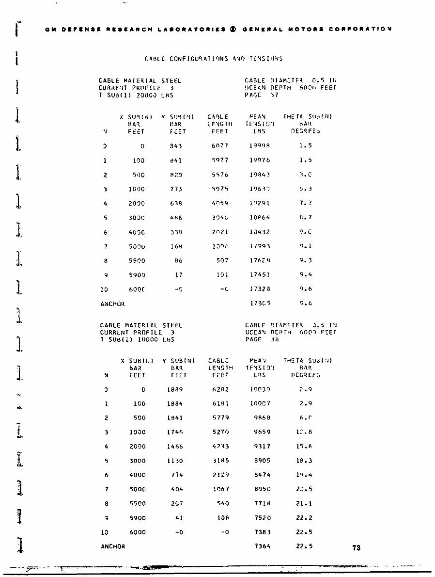
GM DEFENSE RESEARCH LAWORATORIES 0 GENERAL MOTORS CORPORATION
CABLE CONFIGURATIONS *nr) T[NSII1hNS
CABLE MATERIAL STEEtL CABLE DIAMETF4 0.5 INCURAE.JT PROFILE 3 !OCEkhN DEPTH 60%'(- FEETT SU8(1) 20000 LiS PAGE 37
;X SU10') Y SJB(NJ) C01L E? {AN THETA StlW-N)HAr? •AR LF%4G TH T EN S I 0,N1 HAR
N FEET FEET FEET L4S O)E3RFE-
3 0 ?43 6?7? 19998 1.5
1 1t3 dl 9977 199-6 1.5
2 500 820 5576 19843 3.c
3 1000 773 S079 1963') 5.3
4 2030 638 4n59 11)291 7.7
5 300C 486 3014U, 18P64 8.7
6 4030 330 2ri21 13432 9.C
7 50%L 16 . 1 19Q 3 9.1
] 8 5500 86 507 17628 9.3
9 5900 17 101 17451 9.4
10 600( -0 -C 217328 9.6
ANCHOR 173C.5 9.6
CABLE MATERIAL STEEL CARLF 9IAYETER ).5 IlJ
CURRLNT PROFILE 3 OCEAN flEprH 6001 FEETT SUBM1 10000 LbS PAGE 38
X SU8(D) Y SUB(N) CABLE VfAN T HETA SUdj(W)
9 AR BAR LENGTH TFNSI O' BARN FEET FEET FEET LBS DEGREES
I 0 1889 6282 1003f 2.9
411 100 1884 6181 10007 2.9
2 500 1841 5779 9868 6*c
3 1030 1746 5270 9659 IZ.8
4 2000 1466 4733 9317 IS.f.
5 3000 1130 3185 9905 13.3
6 4000 774 2129 8474 19.4
7 5000 404 1067 8050 2).5
8 5500 207 540 7718 21.1
9 5900 41 108 7520 22.2
10 6000 -0 -0 7383 22.5
SANCHOR 7364 22.5 73

GM DEFENSE RESEARCH LAMORATORIES Z GKNtRAL MOTORS CORPORATION
CAtbLF C''JFIGUJRATI,04S A4r0 1E'SItfl.
CABLE ý"AIERIAL SIEEL CAtoLF IIAML T 1 V.5 1*CJRýF4T PWWI- [-.E 3 )CEANj lEUTH, )C" IE II SUM( I ) 600L LIhS PA G; 3c
SSU'IN(N) Y SUIi(N) CARL[ PI:AN !hFIA Wulu,4)BAR 'AR ' EIGTH TF'S 0,, .AFLLT F Z L T F E L T 1. cis E1L.
L 406S5 7364. 601.c;4.
1 L 00 46.ý 72(3 6?0 4 .,Q
2 '0( ( Qc84 689 7 rq78 11. 1
3 1000 3b 1"- 6330 9(16 9 1-.. 1
4 2 33(7 5207 5329
5 W0'O0 2 6,Sd 0 1 49 1 32.1"
6 4U,)0 194i '-- '796 44PO J6. 1
7 5000 Ip74 1465 4 1)'4 4 .
8 9'-:to c.71 759 37%; 45. 1
4 9C 12? 158 ;534 4 .4
12 10)0 -3 -0 A432
ANCI;W)S 140) % . e
CABLE MAi=RI.PL STEEL CABLF .IMAVETE,1 P,CURAEWJT PROFILE 3 OCLAN ,,EPTH , rF .IT SUBL(} 5164 LbS PAGE 4"
X StJri(N) Y SJB(%,) CAftLE MEAN THETA SU;!U\)BAR OAR LE'IGIH T2NSIO'A bAP
N FECT FEET FFET LBS nEGRE•"
3 C 6754 9483 5205 -. 7
] 10c* 6744 9382 r,175 9.7
2 500 6660 8974 5019 11.1"
3 100( 6464 8437 482C 21. 3
4 20"10 5P,53 7771 4479 31.5
9 30'00 5C 3r 9974 40c2 3 F. %
6 4000 4052 4578 3617 44.7
7 50OC. 2726 2q18 3214 52.t:
8 5500 1786 1852 2903 61.8
9 "j9fl0, 566 S75 2701 I'.Z
10 6000 -0 -0 ?62? 79.6
74 ANCHOR 2'94 b,.2

j GM DEFENSE RESEARCH LABORATORIES V GEN9.4AL MOTORS COWSORATION
i CABLE CONF!GU.RATI0'NS ANn TENSI(JNS
CABLC MATERIAL STEEL CABLE DIAMETER 0.5 14CURRENT PROFILE 4 OCEAN DEPTH 6000 FEETT SUB{I} 20000 LBS PAGE 41
X SUB(N) Y SUBIN) CABLE MEAN THETA SUBfN)BAR BAR LENGTH TENSION BAR
N FEEl FEET FELT LBS DEG-ELS
0 0 1441 6172 20037 6.6
1 100 1430 6071 20007 6.6
1 2 500 1371 5668 19879 8.3
3 1000 1277 5159 19665 10.6
4 2000 1050 4130 19333 13.0
5 3000 797 3096 18901 14.0
f 6 4000 539 2063 18481 14.5
7 5000 275 1027 18029 14.7
f 8 5500 140 ,18 17684 14.9
9 5900 28 103 17490 15.2
10 6000 -0 -0 17373 15.4
ANCHOR 17352 15.4
CABLE MATERIAL STEEL CABLE DIAMETER 0.5 INCURRENT PROFILE 4 OCEAN DEPTH 6000 FEET
r T SUB(1) 10000 LBS PAGE 42
X SUBIN) Y SUBIN) CABLE MEAN THETA SUB(N)BAR BAR LENGTH TENSION BAR
N FEET FEET FEET LBS DEGREES
0 0 3358 6885 10027 13.3
jF 1 100 3335 6782 99&6 13.4
2 500 3216 6366 9849 16.5
3 1000 3022 5829 9641 21.3
4 2000 2535 4718 9288 26.1
i5- 3000 1970 3573 8887 29.4
6 4000 1366 2411 8470 31.1
7 5000 716 1229 8033 32.9
8 5500 369 622, 7683 34.2
19 _5900 74 124 7501 35. 5
10 6000 -0 -0 7389 36.3
ANCHOR 7368 36.5 75
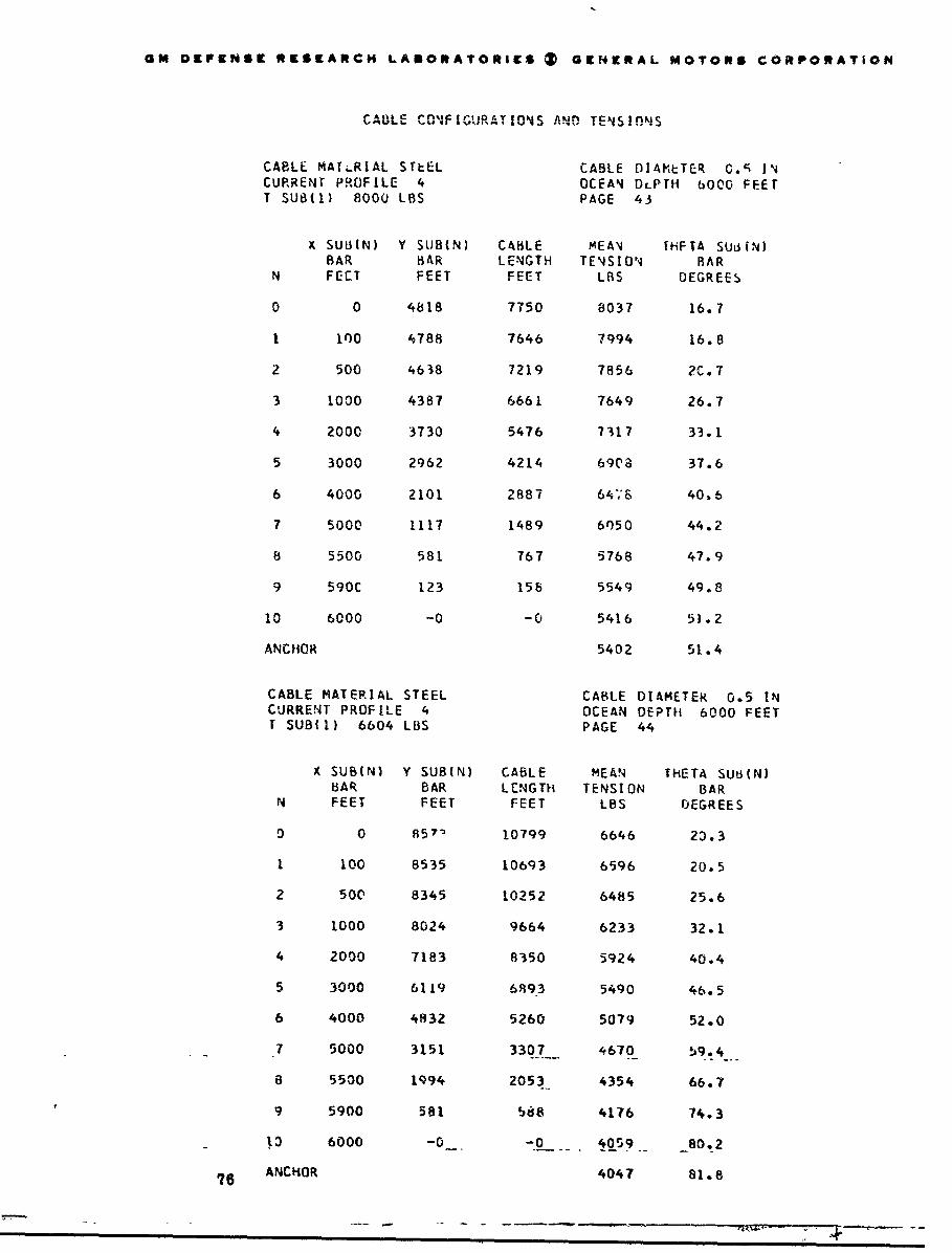
GM DEFENSE RESEARCH LABORATORIES 0 GENERAL MOTORS CORPORATiON
CA 0LE" CQnkFI~kjRATIOn4S AND TENSIONS
CABLE MATERIAL STtEL CABLE DIAMtTER C.S INCURRENT PROFILE 4 OCEAN DLPTH 6000 FEETT SUB(1) 8000 LBS PAGE 43
X SUB{N) Y SUB(N) CABLE MEANJ THFTA SUd.N)BAR BAR LENGTH TE4SION BAR
N FEET FEET FEET LBS DEGREES
0 0 4818 7750 8037 16.7
1 100 4788 7646 7994 16.8
2 500 4638 7219 7856 2C.7
3 1000 4387 6661 7649 26.7
4 2000 3730 5476 7317 33.1
5 3000 2962 4214 6908 37.6
6 4000 2101 2887 64,6 40.6
7 5000 1117 1489 6050 44.2
8 5500 581 767 5768 47.9
9 590C 123 158 5549 49.8
10 6000 -0 -0 5416 5).2
ANCHOR 5402 51.4
CABLE MATERIAL STEEL CABLE DIAMETER 0.5 INCURRENT PROFILE 4 OCEAN DEPTH 6000 FEETT SUB{I) 6604 LBS PAGE 44
X SUB(N) Y SUB(N) CABLE MEAN THETA SUu(N)BAR BAR LENGTH TENSION BAR
N FEET FEET FEET LBS DEGREES
0 0 85'. 10799 6646 23.3
1 100 8535 10693 6596 20.5
2 500 8345 10252 6485 25.6
3 1000 8024 9664 6233 32.1
4 2000 7183 8350 5924 40.4
5 3000 6119 6893 5490 46.5
6 4000 4832 5260 5079 52.0
7 5000 3151 3307 4670 !9.4
8 5500 1994 2053 4354 66.7
9 5900 581 b18 4176 74.3
p3 6000 -0- -.0 _ 40S9_ 80.2
76 ANCHOR 4047 81.8
==• •• mm• m- -am - -ra - -m - - -m ••m m m rm m

GM DEFENSE RESEARCH LASORAlORIES ft GENERAL MOTORS CORPORATIONf
CABLE CONFIGURATIONS AlIf TENSIONJS
'T CABLE MATERIAL GLASS CA 11LL I)1AF;,ýTE Eo INCURREIT PROFILE 3 OCEAN DEPrH 6000 F[ETT SUB(1) 10000 LBS PAGE :-
)x SUB(N) Y SUbi'j) CABLE mEA'j THETA SUr.,(')BAR 8,AR LENGTH TENSION .AR
N FU.ET FEFT FEE T LBS DEGREL S
3 C 1628 6210 loCi 5 4.0
1 100 1624 6110 1000 7 3.0
2 500 1582 5707 9954
3 1000 148d 5199 9891 IC.57
4 2000 1227 4164 98C4 14.P
5 30C0 928 3125 9721 16.7
6 4060 623 2084 962b 17.C
7 500C 312 1041 9550 17.4
8 5500 156 522 9458 11.5
9 590C 31 104 939") 17.6
10 6000 -0 - 0 934-7 11.6
ANCHOR 9344 17.6
-. CABLE MATERIAL GLASS CAFILF DIAMLTE4 0.5 V4CURRENT PROFILE 3 OEFAN DEPIH 6000 FEETT SUB(1) 5000 L1S PAGE 46
X SUB(N Y SUB(N) CABLE t"I N THETA SLW4I(BAR BAR LENGTH TENSION !AR
N FEET FEEA FFET LBS DEGREEj
0 0 36410 7023 5024 5.9
1 100 3609 6923 501046
2 500 35,e4 6514 4948 11.9
"" 3 1000 3332 5978 4887 21..9
4 2000 2777 4837 4R14 29.4
5 3000 2119 3652 4726 33.1
6 400C- 1439 2451 4639 34.1
7 5000 739 1?36 4536 34.7
8 5500 378 626 4483 35.8
I9 5900 74 124 4428 36.3
10 6000 -0 -0 4376 36.5
ANCHOR 4371 3f.5 77- U.

GM DEFENSE RESCARCH LAXORATORIES (t GENERAL MOTORS CORPORATION
CABLE CONFIGURATInNS AND TENSIUNS
CABLE MATERIAL GLASS CABLE DIAMETER 0.5 INCURRENT PROFILL 3 OCEAN DEPTH 6000 FEElT SUB(1) 3000 LBS PAGE 47
X SUB(N) Y SUB(N) CABLE MEAN THET"A SULS(N)BAR BAR LENGTH TENSION 6AR
N FEET FEET FEET LBS DEGREES
0 0 1858 10045 3020 9.8
1 100 7841 9944 300C 9.9
2 500 1697 9520 2932 19.8
3 1000 7359 8919 2879 34.0
4 2000 6295 7463 28C5 46.6
5 3000 4972 5806 2715 52.7
6 4000 3495 4020 2645 55.5
7 5000 1879 2126 2562 58.3
8 5500 985 1194 2482 60.5
9 5900 204 227 2451 62.8
13 6000 -0 -0 2422 64.2
ANCHr.R 2425 66.4
CABLE MATERIAL GLASS CABLE DIAMETE4 0.5 INCURRENT PROFILE 3 OCEAN DEPTH 6000 FEETT SUB(1) 2584 LBS PAGE 48
X SUB(N) Y SUB(N) CAqL[ MEAN THETA SUB(N)BAR BAR LENGTH TENSION BAR
N F-ZT FEET FEET LBS DESREES
0 0 12244 13968 2604 11.3
1 100 12224 13866 2583 11.4
2 500 12057 13433 2510 22.7
3 1000 11658 12795 2464 38.9
4 2000 10347 11146 2388 52.7
5 3000 8612 9142 2311 59.9
6 4000 6554 6850 2246 64.1
7 5000 4C04 4112 2168 68.6
8 5500 2313 2361 2089 73.2
9 5900 532 589 2070 77.3
10 6000 -0 -0 2050 80.1
78 ANCHOR 2048 80.7

I) GM OCEFENSE RESEARCH LABORATORIES 9 GENKRAL MOTO*S CORPORATI-ON
I ~ ~CABLE COW~IGURAT TONS A~ID TENS IONS
CABLE MArERIAL GLASS CABLE DIAMETER 0.5 INCURRENT PROFILE 4 OCEAN DLPrH 6000 FLETT SUBti) 10000 LBS PAGE 49
X SUM(N) Y SUB(N) CABLE MEAN THETA SUrI(N)BAR BAR LENGTH TENSION BAR
N FEET FEET FEF~ LBS DE'OREES
(0 0 2858 6638 10010 13.3
1 100 2834 61536 99F4 13.4
2 500 271.7 6119 9933 16.3
3 1000 2527 5ci84 9872 2C.,8
14. 2000 2063 4482 9777 24.8
5 3000 1561 3364 9706 26.8
IJ6 4000 1051 2242 9615 27.2
7 5000 535 1117 91525 27.6
1.8 5500 267 566 9423 27.6
9 5900 54 113 9405 2.
10 6000 -0 -0 9342 28.1
ANCHOR 9339 28.1
CABLE MATERIAL GLASS CABLE DIAMETER 0.5 INCURRENT PROFILE 4 OCEAN DEPTH 6000 FEET1' SUB(1 5000 LBS PAGE 50
X SUB(N) Y SUSIN) CABLE MEAN THETA SUHi(N)BAR BAR. LENGTH TENSION BAR
N FEET i~EET FEET LBS DEGREES
0 0 7236 9449 5044 27.1
]1- 100 '7184 9)337 5002 27.2
2 500 6927 8862 4953 32.8
13ý 1000 6500 8204 4899 40.5
--- 4 200 5410 -67-30- 4837 47.1
15 3000 4152 5124 4758 51.4
_6 4000 2838 3469 4674 52.7
17 5000 1465 _ 1773 4575 54.0
a 5500 742 894 4537 55.5
9 5900 153 183 4457 _ 56.1
6000 -0 -0 4441, -56.9
A14CHOR 4437 57.0 7

GM OEFENSE R Ce[ARCH LABOftATORIES QD GENERAL MOTORS COWPOPATiON
CA,,Lý C( O FIGIMAI,"NIS AN'JD IENSI.,?4C,
CARLE M, ERI•L GLASs CAR1.E I),I"lPT. .5 T"I
CIJRRE'jT PIR0FiLC- 4 0CFANI IO !.'Ift 6(,1;i [[L ,
T SUk.( M, 377/, LUS V'fGr c I
x SUJIN! Y 3U '") CA5LE &F' , ttTA N.$U.(r )FiA,, bAQ LCNGTH TFNS 1 ON•b i:,
N FF k!T ELI FE T. T ,S rE5" F
0 1)C65 1531 1 3.P1 36.7
I too I4489 16756 3774 ;1. ]
2 ,n 1) i46-) 1 15703 3721 1, 3. 6
3 100 1 19 P 14 q82 31,8C r,2. 7
4 2'.OC i2164 3129 322 $).- .7
5 30)C 0C66 l0418 354c A-. '.
6 40)C) 7441 7697 348'- 6P.'
7 5000 4173 44Y2 3424 72. !
8 55C10 24(19 24'Wi8 33,4 74. .'.
9 5910 571 594 32(yC 7. I
10 b 000 - -,.
A'JCHU4 3262
CABLE MATERIAL NYLOIN .ABLL I)IAsrTz T ., !CURRE'4T PR'IFII.E 2 OCFA'i PUP Il- H >'Z Fr1: TI Si,(1) 3600 LIhS PAGE 5?
X SUM(N) Y SUYM('4) ;CA.,LF hf:A'j fltL: TA .tl P0i)ti -A:ý hAR EGLE GTH TC"4S I ONJ k'P
N FI ET FEFT FFET t. 1 ,'FGR F"
U C. 143 600? 35c06 1.1
l 100 1.42 5')02 1596 1
2 2hC 114 5502 3562 1.2
3 i1uj0 124 5004 3525 I. 6
4 ,°.3 102 400 2 347 7 1 . t,
5 3030 7t 3000 34.?5 1. 7
6 4000 5? 1l99 3375 1.7
7 5030, 27 995 3331 1.7
8 5506 ;3 499 32P6 2. 1
9 59"00 2 99 12'1 1.8
10 6000 -0 -0 3206 2.1
80 ANCHOR 3204 2.0

GM DEFEKSK RESEARCH LABORATORIES (V GENERAL MOTORS CORPORAriON
CAHLFE CONFIGUPATOf'4S ANn 1F'IS
CABLF MATERIAL NYLON CABLE FlItý,E, "r. INCURREN4T PqOFILE 2 OCFAN DEPIh f,Or- rifcfT Sub(1) 2160 LtiS PAGZ r,
x SU(JHN) Y SUlB( N) CAI. F PFFAN ihFTASBAR 15AR L E,4f"H ILN %SII Iq -.,A.<
14 FrET FEýT FFET LBS ()Fý,kFrS
C0 336 6b15 25 1.
1 100 3C3• 5"41 15 57 1.,
2 500 287 55s15 ?119 2.2
3 10 Ž'0 264 5016 2of, ( P. 1,
S4 2000 215 4' 11 2042 ?
5 30 30 164 3(10 lq96 2. 9
5 4000 I11 ?n02 1946
7 3000 57 996 1P.C), 3.0
8 55C(0 8 901 1853 3.7
5900 5 100 1.(0u
6 1_ boorn -o -T32
ANCHOR 1?69 3.[CABLE MATERIAL NYLON CABLE P!A,-,LTEq V 4iCURRL•T PROFILE 2 EICEAN DEPTH (o,(C Ft-U
T T SUB(1) 720 LBS PAGF q4
X SUB(N) V SUBIN) CABLE MFA.% IETA SJ-,('•)BAR lIAR LENGTH TENSI eAN P,
N FECT FEET FEET Las nEGRECS
0 0 1055 6125 7?2.
1 100 1346 6024 721 5.3
2 500 ltOS 5622 68H 6.7
f 3 I000 '23 5116 650 6.i
4 2000 ?83 4096 60 5 9.5
1 5 3000 630 3179 560 , 13.3
6 4000 463 2059 5C9 11.3
S7 5000 2A7 1036 455 12.7
8 5500 156 522 420 13.8
a 9 5900 29 104 161 18.3
1- 6000 -0 -0 347 20.?
SANCHOR 342 1-).P fFi

GM DgI~N5I RCGRARCM LAUORATORiES ( GENERAL MOTORS CORPORATION
CABLE CONIGuaTLIONS AND iESIONS
"CABLE MATERIAL NYLON CABLE DIAME"TE4 0.5 INCJRRE'IT PROFILE 3 OCEAN DEPTH 6O"G FEETT SUB(O) 3600 LBS PAGE 55
X SUR(N) V SU6(N) CAPLL Mz' THE!A Su N1)BAR BAR LENGTH TENSION BAR
N FEtr FEET FEET LBS DEGREES
3 0 4491 7587 3617 4.1
1 100 4484 7487 3607 4.1
2 500 4400 7077 3559 12."
3 1000 4168 6527 3522 24,5
4 2000 3467 5312 3493 35.3
5 300C 2621 3996 3459 34.5
6 4000 1757 2667 3451 40.5
7 5000 880 1330 3397 40.P
8 5500 436 665 3367 41.2
9 5900 90 135 3349 41.5
6000 -0 -- 3337 42.2
ANCii,-1 3333 42.1
CABLE MATERIAL N4YLON C4BLE DIAMETER 0.5 INCURREAT PROFILE 3 OCEAN DFPTH 60C0 FEETT SUMi3) 2160 LBS PAGE 56
X S0H(N) Y SUa(,A) CABLE MEAN THETA SUti(N)BAR BAR LENGTH TENSION FiFEET FEET I:EET LBS DEGREES
3 V 9367 11270 2178 7.5
1 00 9355 11170 2162 6.5
2 500 9184 10749 2133 22.0
3 1000 876S 10111 2030 38.1
4 2000 739S 8417 2083 54.7
5 3000 5684 6432 2060 59.R
6 4000 3892 4376 2031 61.2
2 5000 2030 2264 1999 61.7
8 5500 1055 £172 1455 63.5
9 5900 206 228 099i 64.7
1- 6000 -0 -0 i957 6!.4
82ANCHOR 1954 65.5

GM DEFENSE RESEARCH LAlORArtORIES 0 GENERAL MOTORS CORPORATION
CABLE CONFIGURATIONS A'40 TEN$!IONS
CAtBLE MATERIAL NYLON CABLE bI'-'ýFTL4 3.; IiCURRENT PROFILE 3 OCEAN OEPTh 60C0 FEETT SU'b(; 1890 LAS PAGE 57
X SUi-iN) Y SUBMN CABLE tlEA'N THETA SIh6tN)[AAR BAR LENGTH TENSION PýAR
N FLI:T FEET FEET LBS DEGREEsý
' I0 0 3691-9 41734 1905 7f
1 100 36H77 41432 1891 7.8
2 500 36'175 40132 1829 23.2
3 1000 34940 38065 1917 43.,9
4 2C0, 29906 32213 1795 59.0
5 3000 23468 25105 1803 65.4
1 6 4.,Or0 16279 17304 1780 67.1
7 50O0 8722 9180 1762 68.5
1 8 5500 4716 4936 1706 6c).7
9 5900 935 1029 1714 70.9
1 110 6000 -0 -0 17G2 72.1
ANCHOR 171'_ 72.3
I CABLE MATERIAL NYLON CABLE DIAMETER 0.5 INCURRENT PROFILE 4 (,C&4N DEPTH 6000 FFETr I , SUB({) 3600 LBS PAGE '8
X SUB(N) Y SUB(N) CABLE MEAN rHETA SUz(N)
BAR bAik LENGTH Tc'jsION SARN FEET FEET FEEtU LBS DEGREES
O C 6043 8974 3621 14.4
J 100 6017 B471 35c18 14.5
2 500 98 0 8038 3t4Q 22.5
3 1000 5512 7437 3521 34.0
4 2000 4564 6060 3495 43.8
1 J5 3000 3462 4575 3461 47.7
6 41000 2331, 3063 3445 48.5
j j7 soco 1182 1540 3416 49.0
8 550C 591 774 342~? 5-0.0
1 19 590C 1-12 1-98 3368 50.0
10 . . 6000 -0 -0 3361 50.7
ANCHOR 3348 50.5 83

GM DEFSNSE RESEARCH LAIORATOR1IS a GN9NERAL MOTORS CORPORATION
CA:ILF CriNJFjCUkiTjfit4J AND 1lrNSI.JS
CABLE MATERIAL NYLOIN CAHLF DIIMFIEE4 0.5, I'CJRRENT PRiWFILE 4 O]CEAN DEPTH 600) FEEtT SUMI() 2680 LBS PAGF 59
x SU• ()I Y S'.1( ,) CABLE ME Al THETA Suu("I)11A. kbAR L FSIGTI$ TI ThSI U.'4 4AR
N FLLT FZLT FEE T LBS rJE';LL I
0 0 8384 10403 2904 1I. ("
1 ['00 83S6 I0298 287 1 V. 2
2 500 h143 :)A46 2829 2P. r
3 1 it70 4178 2805 41 .1
2000 ý415 7599C 27b 52.'
3uObi 4195 9731 27,2 5f.7
6 4UO0( ' 333 3P75 274C 51.9
7 5000 1708 1974 2721 *,•.. 9
8 S900 878 1010 271 9 5'J. 4
9 59)C 177 2; 3 76Q0- 2
1') 60~?C -0 ~ -0 ?662,?.(
ANCHCO 26 4 6.f4
CABLE PATERIAL NYLON CABLE DIAMLTER E j.5 INCURRENT PýQFIL. 4 OCILAN r.LII '50("n FLEFT SUt3{I) 2880 LbS PAGE 60
A SUi(N) Y SUB(N) CARLE PEAN TtiETA S1Js(N)6 AR bAR LF'NGT It "SIEI N 14
N FELT FEET FEET LBS ESR E E
3 0 8368 1)3,3 ?3290 1 .,, r
1 100 8331 10278 2874 le.2
2 510 8123 9RA?( 2830 28.
3 1000 7682 9158 28[,n 41.3
4 2000 6402 7935 2781 c2.3
9 3000 41'83 5717 279? 56.7
6 4000 1326 3865 2745 57. 7
7 5000 1707 1967 2705 58.2
8 5500 877 1009 2681 59.1
i 5900 17? 203 2696 63.2
101 6000 -0 -0 2662 60.6
84 ANCHOR 26S7 60.6

GM DEFENSE RESEARCH LABORATORIES ( GENERAL MOTORS CORPORATION
IA L -!F 14 nA 'rI n. A '4D T r-- c1 ' N
CABLE MATERIAL NYLON CABLE 0II'MLTER 0.5 INCURRENT PROFILE 4 OCEAN DEPTH 6000 FEETT SUB(1) 2140 LBS PAGE 61
X SUB(N Y SUB(N) CABLE MEAN THIFTA SUd(N)BAR BAR LENGTH TENSION BAR
N FEET FEET F[ T LBS DESREES
0 0 14922 16223 2174 24.2
1 100 14876 16113 2139 24.6
2 500 14576 15613 20Q0 36.8
3 1000 13925 14793 2068 52.i
4 2000 11864 12502 2065 64.2
5 3000 9298 9748 2036 68.9
6 4000 6447 6723 2018 70.3
7 5000 3452 3575 2042 71.7
8 5500 1770 1834 2022 73.6
9 i900 405 416 IQ74 74.2
10 6000 -0 -0 1984 75.4
ANCHOR 1Q73 75.4
CABLE MATERIAL NYLON CABLE DIAMETER 0.5 INCURRENT PROFILE 3 OCEAN DEPTH 1800 FEETT SUB{I) 3600 LBS PAGE 62
X SUB(N) Y SUB(N) CABLE MEAN [HETA SUB(N)BAR BAR LENGTH IENSION BAR
N FEET FEET FEET LBS DEGREES
0 0 921 2091 3600 2.3
1 30 920 2021 3598 2.3
2 150 909 1900 3571 5.3
3 300 880 1748 3555 10.8
4 600 781 1434 3498 18.0
5 900 636 1101 3472 26.0
6 1200 455 753 3454 31.8
7 1500 239 384 3418 35.8
8 1650 120 192 3393 38.2
9 1770 25 39 3378 39.7
_.___10 1800 _ -0 -0 3357 40.5
ANCHOR 3362 40.6 85

GM DEFENSE RESEARCH LADORATORIES 0 GI[NIrRAL MOTORS CORPORATION
e'* Atl 'Itk{.,,• I . ... I,,o T n , C•n T ,, n ,
CABLE MATERIAL NYLON CABLE D)Ji.METE, 0.5 I'CURRENT PROFILE 3 OCEAN DF:PTfH 1800 FEETT SUIBf() 2160 LBS PAGE 63
X SUB(N) Y SUB(N) CABLE MEAN IHETA SUS(N)BAR IRAR LENGTH TENSION 4AR
N FEET FLLr FEET LBS DEE=
0 0 1780 2621 216.6 3.8
1 30 1778 2591 2164 3.7
2 150 1760 2470 2137 f-.k
3 300 1715 2313 2104 16 . 4
4 600 1542 1968 2057 29.1
5 900 1283 1569 2039 41.1
6 1200 934 LU IGt 2325 49.5
7 1500 506 586 2003 55.0
H 1650 258 29h 1964 c:;. P.
9 1770 55 63 1977 6n.4
10 1800 -0 -0 1951 61.A
ANCHUR 1964 61.7
CABLE MATERIAL NYLON CABLE DIAMLTER 3.5 INCURRENT PROFILE 3 OCEAN DEPTH 1800 FEETT SUB(l) 144o LBS PAGE 64
X SUB(N) Y SUR(N) CABLE MEAl THETA S'tftN)BAil bAR LENGTH TENSION tAR
N FEET FEET FEET LBS DEGREI:S
0 0 3730 4312 1446 5.6,
1 30 3727 4282 1443 5.7
2 150 3699 4159 1410 13.1
3 300 3628 3993 1381 2.z2
4 600 3358 3588 1343 42.0
5 900 2877 3022 1312 97.2
6 1200 2225 2303 1331 66.4
7 1500 XL318 1348 1342 72.5
8 1650 700 714 1319 75.9
9 1770 173 175 1289 77.8
10 1800 -0 -0 1300 70o9
86 ANCHOR 1294 79.9

GM DCFKNS[ RESEARCH LASOOATORIES I GENERAL MOTORS CORPORATION
CCAOLE CONFIGUPATIONS Afn 7FNSIINSI
CABLE MATERIAL STEEL CABLE DIAPbTEI u.5 I1CURRENIT PROFILE 3 OCEAM DEPTH 1600 FEETT SUBII) 10000 LBS PAGE 65
x SUBMN) Y SudIN) CABLE '"CEA'% ItiETA SUti(N)BAR BAR LENGTH TNSIO;,N BAR
N FEET FEET FEET LBS DL:34tS
j0 0 429 1858 10023 2.5
1. 30 428 1828 10001 2.5
2 150 420 170 8 9873 3.6
3 300 406 1558 9663 5.5
, 4 600 360 1252 9329 8.6
5 900 295 943 8904 12.2
if6 1200 21? 632 8467 Ir. 3
T 1500 114 319 8050 18.1
a 1650 59 161 7706196
9 1770 11 32 7515 21.?
10 1800 -0 -0 7385 21.i
ANCHOR 7367 21.•
CABLE MATERIAL STLEL CABLE DIAMETER 0.5 INCURRENT PROFILE 3 OCEAN DEPTh IPCO FEETT SUU(1) 6000 LBS PAGE 66
X SUB(N) Y SUB(N) CABLE MEAN THETA SU3(N)BAR BAR LENGTH TENSION BAR
-N FEET FEET FEET LBS DE3REEý
3 0 888 2047 6034 4.0
1 30 886 2017 6013 4.1
2 150 873 1896 5884 6.0
3 300 848 1745 5674 9,3
4 600 770 1434 5343 15.0
5 900 650 1112 4919 21.7
6 1200 490 772 4497 28.4
7 1500 280 407 4068 35.1
8 1650 148 211 3774 41.1
t 9 177C 31 43 3562 44.6
lo- 1800 -0 -0 3448 47.0
ANCHOR 3430 47.4 87

GM DEFENSE RESEARCH LASORATORIES & GENERAL MOTORS CORPORATION
CABLE CONFIGURATIONS AND !F•4SINS
CABLE MATERIAL STEEL CABLE DIAMtTER 0.5 INCURRENT PROFILE 3 OCEAN DEPTH 1800 FEETT SUB{l) 4858 LSS PAGE 67
X SUBIN) Y SUM{N) CABLE MEAN IHErA SUB(N)BAR BAR LENGTH TENSION BAR
N FEET FEET FEET LBS DEGREES
0 0 1596 2564 4894 5.0
1 30 1593 2514 4873 5.1
2 150 1578 2413 4746 7.5
3 300 1547 2260 4539 11.6
4 600 1444 1945 4198 18.9
5 900 1285 1606 3770 28.2
6 1200 1050 1223 3351 37.9
7 1500 707 769 2921 48.9
a 1650 453 478 2636 59.9
9 1770 145 141 2433 69.6
i3 1800 -.0 -0 2352 77.9
ANCHOR 2323 80.2
88

GM DEFENSE IRESEARCH LABORATORIES Z GENERAL MOTORS CORPORATION
TR65-79
(
TABLES OF DYNAMIC TENSIONS
(3 pages)
8 I
89

GM OEFENS R•s RE SEARCH LA"ORATORIES G GENERAL MOTORS COR PORAT1ON i
TR65-79
if!Jill fit 21111 ! !1
!II Iu l mi 111 ;16 fl i !11!!! !t I HE 1 -9 R 51
III__ __ Is II
III I II- all
__ IN
!I- Iill III ...
!ti ~~~i Et iiii!!-;..
-------- -
--P -
_______ ____ I !t____
90
9O

GM DEFENSE RsCrANICH LAUORA7ORtS ? GENERAL MOTORS CORPORATION
TR65-79
J.1. !1 ,. .', l .S,,f•isll six
H I II Z.""" ''
fil fil I I fl
04n
i -#4. C",
11: Mo a•; 1 ao$Hi !lip ja! i RI
T
- , -, . .-----------
r . __ __ __ __
#4 i,
* I -

L L'ILh ~LL A RLH ,AUUkA H ILS L .N LRAL M T R S LOR PUR A T1N
TR65-79 I
lii A
__ __ __ __ __ .*zu. :: I••'002
-- ....-
Iii.- 1,1 1I -
S..... .n
I 0
a-. F' . • . Ca,•
a, '
f- ~ ~ a 1 ftO.-C-- niF) .i Vq .. t"Wl -MMWl .. 5 0%W P) V
_ad
92

GMl DEFENSE RESEARCH LAF5ORATORIES -Z GENERAL MOTORS CORPORATION
TR65-79
PLOTS OF DYNAMIC TENSIONS
S93

TR65 -79
""1 71 -1 7 1 TO -, t' ~ --
- I ~ . 0' I I1
.
-. - .1
H i .1 H ; %,II ,I I N
* ~ ~ ~ ~ ~ A --- 21 4
... .........
i N1I - , - t,.I
tit.
0 ~ 0 ..
... .. . ...
0~-4. op!; f* 1
">j7E 7 (7!) ...I~ ...
944

TR65-79
IN I
~~vi
- if~ ~io!
- * 1 ~ 77-.,;i
11ito~~ s+L
f!
Ns ý I i, I Q495

TR65-79
1.__ !;:T 7T ; I.I. - I
I I
.. . .. . m :
4i I-- r
Tg; + o .t H -1 ! 1 ! 1
'I" c.J .4:_%14_ ~~+
960

1' TR65-79
t ~ ~ ~N -~~ ~ tit
I ~ *~: 11 I7
a -.f .
444I~~~~~0 06',',,... ---
7* 1:. 14! i T A
IT'
1 . I? f.:~i0
,.44,
96.. o oo. :
(-4 - .
14 77

TR65 -79
::~ ~ - 4 :1 zE:Ki ~$I
;-T: I r
IL~~c - __
C13
0 0
-- E-
z 0 n
':l (U) aAVMi
98

TR65-79
ITT. if 1 T i !;i:................ 7 7_7
pt
... .... .tU ll:
....... .......
7Z
f!-4
t
tr
Z 64
UNIH
111111111INt w 1 No o T7A .u z 01. i. TZ 4:!04c Z
tj!
p ll :Ill !!tf "tmf:i;:Nff.00 ArZý 0 414
.... .... ... :4ý 4 It... .... O t iiiii ý 10 i ; .
; F,
... .... .... . IN i - I f , *11 : -;I
Htt_1 f I4
r It4- -- -, ýi 'ý ill it
41-4 1 T,t [tit
t U 1111 [if] H 74- 1 11- HLn 1-1 1- tý H .111 WHIM I I H I ýý 1! W!CD At , "i, i I
Ml I I I . i --'ill:'-*4 1.7C4 U f,
LAJ tzo
!I
4 ý4+ 4tiz co z 44 -1 M --ill"no w 11; 1:111 it 11 tit! H NOý'p 111 HH! I J- H, -WlI _71F
w + -1Pa It0 W 4.1i 'i: '0 E-4
U 04 U v 1z u E. o I rif ti Ot I HIH4.1 t 44
P TPT
_J_ j .0J) LHDIHH 3AVA&4% 49
99

TR65 -79
...... ... ..... -.. .. = H . - -. z-77 7. -4 -Z
Z. m 4-U1~~~ _ 0----F
j! ii I i 3-- --- -- 'I, ~ z ii04
1:::
C.L
wZ
:!~ *r'
ot100'JI

TR65 -79
EI Zi
I I Iw
.0- 04 u ,
tI ~~ P-4E4
* . .... P4 Z0jZr*
T.
+1+- - T
0 0 rt !. N,1,1 .i*~ c~~*j
'I 'il
.) 0 t. opif JT tt1 LOS ~ a! aV11
-Z 0. ~~iWLn
H -1h t ' * 4j I 1 I : I i V
(§) Vd V1 E-4 4 d : 1 ~ 1Ii4
j 101

TR65-79
-- S~~ . J ~J~jpp _ I
I .i. . . . .I_ _
ii; i; i1a0
-4 - - U .41
W, --- ___
",4'
4P.4
ZUE
...... ...... .. ..... .. ..Ti
10.2

I I THO5 -79
_ 1777_-7
I~ Ni
tt ti i~l _ _
I~i. a-ý iti'" TIf --
1~j I
rzco
z 4 .r t:- ___
0V o :v:s

TR65 -79
i wi
... ... ....
It
....... ......... ......
7117 Ar~t ~r.:f
- -- -- -Q.0
- -.. I.:;0. 0j:
- - -
Z z*f .0__
104-

TR65-79
q- Qp 'D vULL
pl
t I I :7r
4-141
4;tO
itit
fill
.*4 .... Ht
I i 11 WHIIIIHN, 111 1 -r 1-4 1HII H, Ili I i I i I I. I- -V 1, 1A I 1 -1 Mi f I I I f I 1 1. IN! 11HINN, till 1:171-N i I
H i It !H! HNItH M
A- 1- -- 0 : 11 1 t, i 111 IH 1 1111I -H f 1: H,
I jili t i 1 4! T41 -t
F-4it 115
i IIHU-1,; M 11
I 1 0 11
iý. INN' it ti!, i't to 'ý-t 4:47+
itit
i"T !i-l
4L +
+
1 11111
fill,It lit! I FRRI I UNIJO ft! J-6f-4. +
I ;
14 u
Ul
z 3ý,. .* I -
E-4 - -1 -4-1- -f IT-
E-4
co z Mill
Týz
-.1 fm-
> w PQ I11 N 1z z I+cn rn 0 =) W I-7ý: r Cý U E- IZ U E. 0 1 uf
.T. fild t
ti11M144
jf--VA 1 1-rT
OJ) JLHDIH HAVA&.... rt, b
105

GM DEFENSE RESEARCH LABOR ATORIES () GI NERAL MOTORS CORPORATION
TR65-79
I
I
MOTIONS OF NODES
IC6

GM DEFENSE RESEARCH LAUORATORIES ( GENERAL MOTORS CORPORATION
ST R •5 -7 9
tMOTIONS OF NODES
Rope Material = Steel Water Depth = 113, 000 ft Reference Page 6
Rope Diameter = 0. 5 in. T 1 = 10, 000 lb Case A
Major Major MinorWave Wave Rope Axis Axis Axis
Height Period n Angle Angle Length Length CW*(ft) (secl, 'deg) (deg) (f)(ft)
S50 32 1 7.8 0 50.0 3.22 14.3 3.5 47.0 10.03 18.3 17.5 43.2 9.44 21.4 19.0 37.6 7.35 25. 9 20.0 31.2 8.A6 32.9 22.5 25.0 10.07 43.3 6.0 19.0 10.6
8 56.4 -5.0 14.6 9.29 71.7 -1-.0 14.5 4.5
50 16 1 7.8 3.0 50.0 2.02 14.3 8.0 48.0 6.03 18.3 18.0 45.4 4.54 21.4 21.3 40.2 3.75 25.9 24.0 34.6 5.06 32.9 30.5 27.8 6.47 43,3 39.5 19.4 8.08 56.4 54.0 13.8 7.29 71.7 -10.5 8.2 5.0
50 8 1. 7.8 3.5 49.8 1.0[2 14.3 8.0 47.4 2.03 18.3 15.5 45.0 1.64 21.4 22.0 42.4 1.05 25.9 23.5 39.0 1.86 32.9 31.5 33.0 3.07 43.3 41.0 24.2 4.28 56.4 5.r.0 18.0 3.0
S9 71.7 52.0 7.4 5.0
AL
* Rotation of nodes counterclockwise except when X is3 shown in this column.
11 107

GM DEFENSE RESEARCH LABORATORIES ( GENERAL MOTORS CORPORATION
TR65-79
MOTIONS OF NODES
Rope Material = Steel Water Depth = 6, 000 ft Reference Page 6
Rope Diameter = 0.5 in. T1 = 10,000 lb Case A
Major Major MinorWave Wave Rope Axis Axis AxisHeight Period n Angle Angle Length Length CW(ft) (see) (deg) (deg) (ft) (4t)
15 16 1 7.8 4.0 15.0 0.62 14.3 5.5 14.6 3.03 18.3 19.0 13.7 2.44 21.4 22.0 12. 1 2.05 25.9 26.0 10.6 2.66 32.9 30.0 8.6 3.27 43.3 30.0 6.2 3.89 56.4 31.5 4.2 2.69 71.7 -9.0 3.4 1.6
15 8 1 7.82 14.3 6.0 15.4 0.23 18.3 16.5 15.0 0.84 21.4 21.5 14.8 0.45 25.9 25.5 12.8 1. 16 32.9 33.0 10.6 1.67 43.3 43.5 8.1 2.48 56.4 54.0 3.1 2.19 71.7 -8.5 2.6 2.1
15 4 1 7.8 5.0 14. 9 0.32 14.3 9.0 13.3 1.53 18.3 17.0 11.6 0.54 21.4 19.0 8.8 0.55 25.9 21.0 10.0 0.26 32.9 30.0 12.5 0.27 43.3 42.5 11.6 1.08 56.4 60.0 9.2 0.39 71.7 69.0 3.8 1.6
108

I GM DEFENSE RESEAPICH LABORATOR|1ES Z GENERAL MOTORS CORPORATION
I TR65-79
I
MOTIONS OF NODESURope Material = Steel Water Depth = 6, 000 ft Reference Page 6
Rope Diameter = 0.5 in. T =10,000 lb Case A
Major Major Minor
Wave Wave Rope Axis Axis AxisHeight Period n Angle Angle Length Length CW
(ft) (sec) (deg) (deg) (ft) (ft)
5 16 1 7.8 4.0 5.0 0.22 14.3 -3.0 5.0 1.13 18.3 18.5 4.3 1.64 21.4 21.5 4.0 1.05 25.9 25.0 3.5 1.46 32.9 33.0 2.9 1.87 43.3 -32.0 2.5 1.98 56.4 22.0 1.6 1.0I 9 71.7 -12.5 1.4 0A5
5 8 1 7.8 5.5 5.0 02 14.3 3.5 5.2 03 18.3 19.0 5.2 0.34 21.4 22.5 5.1 0.25 25.9 28.5 4.7 0.56 32.9 36.0 3.9 0.87 43.3 49.0 2.8 1.38 56.4 60.0 2.2 1. 19 71.7 -12.0 - 1 0.8
5 4 1 7.8 5.0 4.8 0.22 14.3 13.0 4.1 1.03 18.3 21.9 3.2 0.44 21.4 13.5 2.3 0.25 25.9 19.0 4.1 06 32.9 30.0 5.7 0.27 43.3 45.0 5.4 0 58 56.4 63.0 4.3 0.29 71.7 71.5 1.8 0.5
5 2 1 7.8 5.5 5.2 02 14.3 8.0 5.1 0.43 18.3 19.0 4.2 0.24 21.4 20.0 3.2 0. 15 25.9 27.0 4.7 0.16 32.9 34.0 2.9 0.4
7 43.3 35.5 3.5 08 56.4 51.5 4 2 0
9 71.7 72.0 1.9 0.4
Ij i09
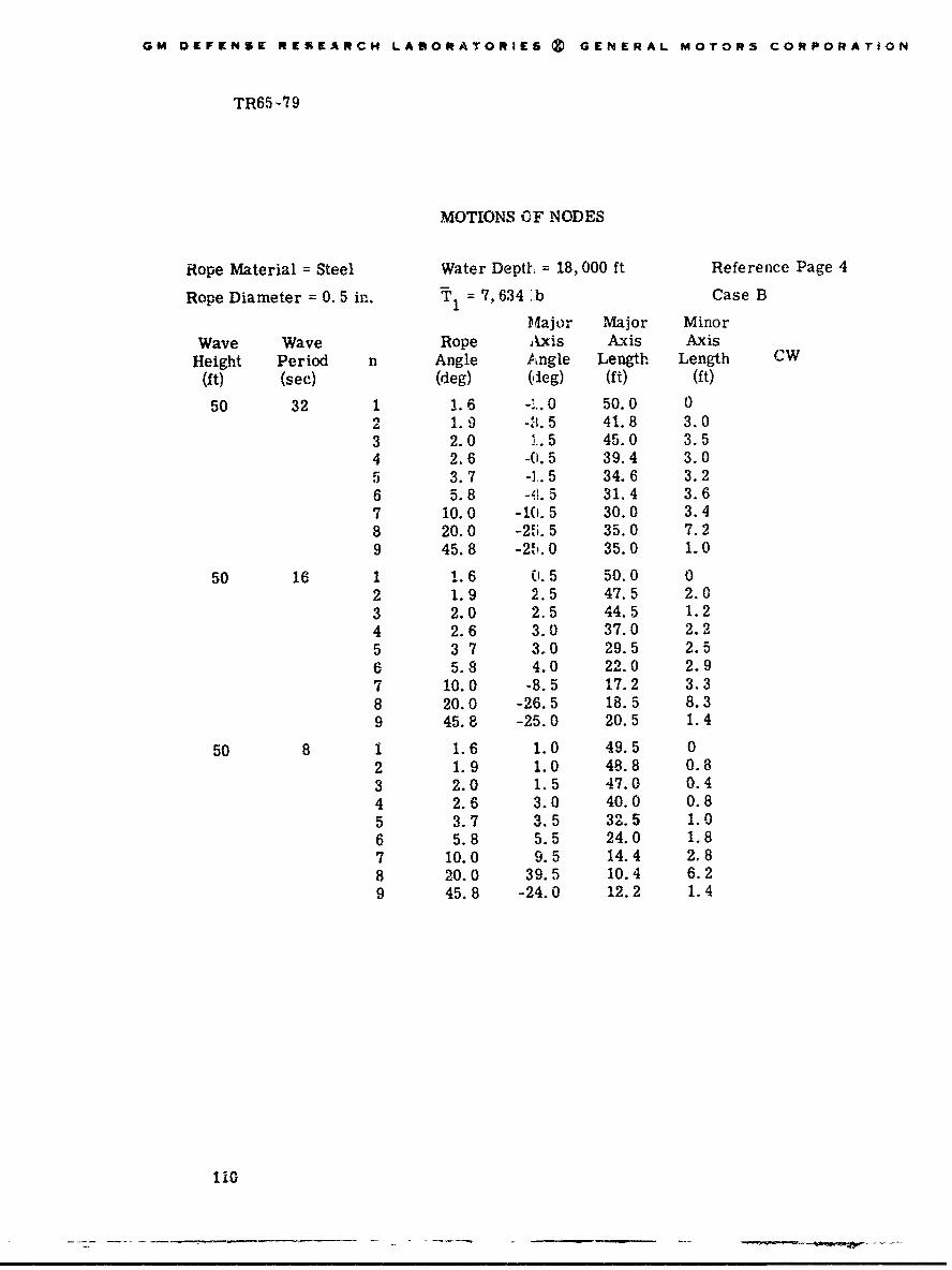
GM DEFENSE RESEARCH LABORATORIES (t GENERAL MOTORS CORPORATION
TR65-79
MOTIONS OF NODES
Rope Material = Steel Water Depti = 18, 000 ft Reference Page 4
Rope Diameter = 0.5 in. T 1 = 7,634 :b Case B
Major Major Minor
Wave Wave Rope JAxis Axis AxisHeight Period n Angle Angle Length Length CW
(ft) (see) (deg) (d4eg) (ft) (ft)
50 32 1 1.6 -,..0 50.0 01.9 -8.5 41.8 3.0
3 2.0 ;.5 45.0 3.54 2.6 -0.5 39.4 3.05 3.7 -4.5 34.6 3.26 5.8 -41.5 31.4 3.67 10.0 -10.5 30.0 3.48 20.0 -25.5 35.0 7.29 45.8 -21.0 35.0 1.0
50 16 1 1.6 (0.5 50.0 02 1.9 2.5 47.5 2.03 2.0 2.5 44.5 1.24 2.6 3.0 37.0 2.25 3 7 3.0 29.5 2.56 5.8 4.0 22.0 2.97 10.0 -8.5 17.2 3.38 20.0 -26.5 18.5 8.39 45.8 -25.0 20.5 1.4
50 8 1 1.6 1.0 49.5 02 1.9 1.0 48.8 0.83 2.0 1.5 47.0 0.44 2.6 3.0 40.0 0.85 3.7 3.5 32.5 1.06 5.8 5.5 24.0 1.87 10.0 9.5 14.4 2.88 20.0 39.5 10.4 6.29 45.8 -24.0 12.2 1.4
1iO

GM OEFENSI" RESEARCH LABORATORie (t GENERAL MOTORS CORPORATION
TR65-79I
MOTIONS OF NODES
Rope Material = Steel Water Depth = 18, 000 ft Reference Page 4
Rope Diameter = 0, 5 in. T 1 = 7,634 lb Case B
Maj or Major MinorWave Wave Rope Axis Axis AxisHeight Period n Angle Angle Length Length CW(ft) (sec) (deg) (deg) (ft) (ft)
15 16 1 1.6 0 15.0 02 1.9 -2.0 14.4 0.33 2.0 3.0 13.4 0.84 2.6 1.5 11.6 0.95 3.7 0 10.0 1.26 5.8 -2.5 8.7 1.47 10.0 -12.5 8.2 1.48 20.0 -26.5 9.4 2.4
j 9 45.8 -25.5 9.4 0.4
15 8 1 1.6 1.0 15.0 02 1.9 -0.5 14.8 0.43 2.0 2.5 13.9 0.24 2.6 4.0 12.0 0.35 3.7 3.5 10.0 0.66 5.8 4.0 7.6 1.07 10.0 -1.5 5.3 1.48 20.0 -25.0 4.6 3.09 45.8 -25.0 4.9 0.5
15 4 1 1.6 1.5 15.0 02 1.9 0 14.8 0.83 2.0 2.0 16.0 0.84 2.6 2.0 18.8 05 3.7 3.5 18.8 0.86 5.8 6.5 15.2 0.47 10.1'. 10.0 8.2 1.28 20. 0 50.0 4.9 0.49 45.8 -26.0 5.0 1.1
111

GM DEFENSE RESEARCH LABORATORIES (& GENERAL MOTORS CORPORATION
TR65-79
MOTIONS OF NODES
Rope Material = Steel Water Depth = 18,000 ft Reference Page 4Rope Diameter = 0. 5 in. T = 7,634 lb Case B
Major Major MinorWave Wave Rope Axis Axis AxisHeight Period V Angle Angle Length Length CW(ft) (see) (deg) (deg) (ft) (ft)
5 16 1 1.6 0 5.0 02 1.9 0 4.9 0.13 2.0 2.5 4.6 0.44 2.6 2.0 4.2 0.45 3.7 0 3.9 0.66 5.8 -5.0 3.8 0.87 10.0 -17.5 3.8 0.78 20.0 -26.5 4.3 0.79 45.8 -24.5 4.2 0.1
5 8 1 1.6 1.0 5.0 02 1.9 -4.0 5.0 03 2.0 4.0 4.6 0.14 2.6 3.0 4.0 0.15 3.7 4.5 3.5 0.36 5.8 3.0 2.9 0.57 10.0 -7.0 2.4 0.88 20.0 -33.0 2.7 1.19 45.8 -25.0 2.8 0.2
5 4 1 1.6 1.0 5.2 02 1.9 0.5 5.7 0.13 2.0 2.0 7.0 04 2.6 1.5 8.8 05 3.7 4.0 8.8 0.16 5.8 7.0 7.2 0.37 10.0 8,5 4.0 0.88 20.0 64.0 3.4 0.89 45.8 -26.5 3.2 0.6
5 2 1
3456789
* (x) and (y) sweeps not obtainable
112

GM DEFENSE RESEARCH LAIORATORIES ( GENERAL MOTORS CORPORATION
MOTIONS OF NODES
Rope Material = Steel Water Depth = 6, 000 ft Reference Page 38
Rope Diameter = 0. 5 in. = 10, 000 lb Case C
Major Major Minor
Wave Wave Rope Axis Axis Axis
Height Period n Angle Angle Length Length CW
(ft) (sec) (deg) (deg) (ft) (it)
50 32 1 12.9 8.5 37.5 17.02 18.8 18.0 25.0 18.03 20.6 -63.0 14.8 12.0
50 16 1 12.9 11.5 37.2 10.02 18.8 20.0 24.8 10.0
3 20.6 20.0 12.5 8.2
50 8 1 12.9 12.5 38.4 3.82 18.8 20.5 26.8 3.6
3 20.6 23.5 13 5 3.0
15 16 1 12.9 13.0 11.2 2.1
2 18.8 16.0 7.4 3.8
3 10.6 39.0 3.8 3.2
15 8 1 12.9 13.0 11.4 1.1
2 18.8 25.0 7.6 1.8
3 20.6 31.0 4.0 1.4
15 4 1 12.9 12.6 12.5 0.4
2 18.8 21.0 9.0 0.6
3 20.6 25.0 4.9 0.5
5 16 1 12.9 12.0 3.8 0.8
2 18.8 -10.0 2.4 2.43 20.6 -73.0 2.0 1.2
5 8 1 12.9 13.0 3.8 0.4
2 18.8 31.0 2.6 0.8
3 20.6 46.0 1.4 0.6
5 4 1 12.9 12.6 4.1 0.29 2 18.8 23.5 3.0 o.2
" 3 20.6 28.5 1.6 0.2
113

GM DEFENSE RESEARCH LABORATORIES (Z GENERAL MOTORS CORPORATION
TR65-79
MOTIONS OF NODES
Rope Material - Steel Water Depth = 6,000 ft Reference Page 36
Rope Diameter = 0. 5 in. = 2,838 lb Case D
Major Major Minor
Wave Wave Rope Axis Axis Axis
Height Period n Angle Angle Length Length CW
(It) (sec) (deg) (deg) (ft) (ft)
50 32 1 5.7 -6.5 42.5 9.0
2 8,8 -18.0 37.6 11.0
3 25.9 -48.0 57.5 10.0
50 16 1 5.7 1.5 39.0 7.0
2 8.8 -4.0 28.5 9.5
3 25.9 -50.0 34.0 11.6
50 8 1 5.7 6.0 39.0 3.6
2 8.8 7.0 27.0 5.2
3 25.9 -25.0 15.0 12.0
15 16 1 5..7 -3.5 12.4 3.0
2 8,8 -15.0 11.0 3.8
3 25.9 50.0 16.9 3.2
15 8 1 5.7 6.0 11.6 1.7
2 8.8 4.5 8.0 2.6
3 25.9 -54.0 7.8 4.0
15 4 1 5.7 6.0 12.4 0.6
2 8.8 9.0 9.1 1.2
3 5. 9 10.0 5.2 4.1
5 16 1 5.7 -7.5 4.6 1.0
2 8.8 -14.5 4.6 1.4
3 25.9 7.5 8.0 0.8
5 8 1 5.7 4.0 4.0 0.8
2 8.8 -2.0 3.1 1.3
3 25.9 -53.0 4.4 i. 3
5 4 1 5.7 5.5 4.1 0.22 8.8 10.0 2.9 0.53 25.9 -54.0 2.2 1.5
114

GM DEFENSE RESEARCH LABORATORIES Z GENERAL MOTORS CORPORATION
TR65-79
MOTIONS OF NODES
Rope Material = Steel Water Depth = 1, 800 ft Reference Page 65
Rope Diameter = 0.5 in. T! =10,000 Case E
Major Major MinorWave Wave Rope Axis Axis Axis
Height Period n Angle Angle Length Length CW
(ft) (sec) (deg) (deg) (ft) (ft)
25 32 1 8.6 -47.5 26.5 14.52 13.8 -66.0 31.2 11.03 18.2 -66.0 25.0 5.2
25 16 1 8.6 -11.5 19.6 12.02 13,8 -76.0 17.6 12.03 18.2 -73.0 14.8 6.0
25 8 1 8,6 5.0 19.0 6.02 13.8 6.0 12.5 8.03 18.2 -60.5 7.0 6.0
15 16 1 8.6 -11.0 11.6 7.0f 2 13.8 -55.0 9.6 7.2
3 18.2 -64.0 7.9 3.6
15 8 1 8.6 5.0 11.2 3,62 13.8 10.0 7.5 4.43 18.2 -40.0 4.0 3.7
15 4 1 8. 5 7.5 11.4 1.82 13.8 14.0 7.8 2.13 18.2 18.0 4.0 2.0
5 16 1 8.6 -10.0 3.9 2.32 13.8 -51.0 3.1 2.43 18.2 -64.0 2.6 1.2
5 8 1 8.6 5.5 3.7 1.22 13.8 14.0 2.5 1.43 18.2 -54.0 1 3 1.2
5 4 1 8. u 8.5 3.8 0.62 i3.8 14.0 2.6 0.73 18.2 19.0 1.3 0.7
5 2 1 8.6 9.0 4.0 0.3"2 13.8 15.5 2.8 0.43 18.2 22.0 1.5 0.4
115

GM DEFENSE RPSEARCH LAmORATORIKS • GENERAL MOTORS CORPORATION
[ TR65-7 9
MOTIONS OF NODES
Rope Material = Steel Water Depth = 1,800 ft Reference Page 67
Rope Diameter = 0. 5 in, T = 4,858 lb Case F
Major Major Minor
Wave Wave Rope Axis Axis Axis CWHeight Period Angle Angle Length Length
(ft) (sec) n (deg) (deg) (ft) (it)
50 3 1 23.8 -16.5 54.0 8.02 41.5 -19.5 55.0 8.53 59.3 -19.5 60.0 4.0
50 16 1 23.8 -16.0 49.5 16.02 41.5 -19.0 43.0 15.03 59.3 -21.0 42.5 8.5
50 8 123
15 16 1 23.8 -7.0 14.4 3.12 41.5 -14.5 15.0 3.43 59.3 -21.0 19.2 1.8
15 8 1 23.8 -1,5 12.6 4.42 41.5 -15.0 11.6 5.13 59.3 -22.0 12.8 3.0
15 4 1 23.8 -29.5 7.0 3.82 41.5 29.5 7.6 5.23 59.3 28.0 7.0 3.8
15 2 1 23.8 21.0 12.2 1.82 41.5 41.5 8.8 3.93 59.3 59.5 4.8 3.6
5 16 1 23.8 -5.0 4.9 0.82 41.5 -7.5 4.7 1.13 59.3 -20.5 7.5 0.5
5 8 1 23,8 1.0 4.3 1.12 41.5 -4.0 3.9 1.43 59.3 -21.5 6.0 0.9
5 4 1 23.8 13.0 3.9 1.12 41.5 8.0 2.8 1.63 59.3 -27.0 3.5 1.2
5 2 1 23.8 21.0 4.0 0.62 41.5 37.0 2.8 1.13 59.3 -46.0 2,0 1.4
* (x) and (y) sweeps not availabie
1
116

GM DErENSK R'Z$EAWCH LAI3ORATOIEZ 09 GINERAL MOTORS CORPORATION
TR65-19
MOTIONS OF NODES
Rope Material = Nylon Water Depth = 18,000 ft Reference Page 23
Rope Diameter = 0. 5 in. 3,600 lb Case G
Major Major MinorWave Wav. Rope Axis -Axis AxisHeight Period 11 Angle Angle Length Length CW
(fI) (sec) (deg) (deg) 00 (ft)
50 32 1 17.1 14.0 50.0 1.a
2 32.7 25.5 46.0 4.23 38.6 40.0 42.0 2.44 39.6 40.0 35.0 0.85 40.4 40.0 27. 0 06 0 40.8 40.0 19.0 1.87 41.6 40.0 10.0 0.4 x8 42.2 78.0 6.0 0.1 X
S9 42.8 37.0 1.0 0.4
50 16 1 17.1 15.5 50.0 1.02 32.7 24.5 43.5 2.23 38.6 39.0 38.0 1,04 39.6 39.0 31.5 0.45 40.4 41.0 24.0 06 40.8 43.5 18.5 1. 0I7 41.6 33.0 11.0 0.4
8 42.2 68.0 6.0 1.69 42.8 30.0 1.2 .2 X
150 8 1 17.1 15.0 48.0 i. 02 32.7 27.5 35.6 2.03 38.6 40.0 25.6 0
4 39.6 37.0 17.0 05 40.4 40.0 14.4 0
6 40.8 40.0 10.8 0.8
7 41.6 40.0 6.6 0.28 8 42.2 50.0 4.0 1.09 42.8 0 0 0
11
I1 117

"iGM- DEPENSE RESEARCH LADORATORIES 3) GEINERAL MOTORS COR.PORATOON
TIR65 79
MOTIONS OF NODES
Rope Material = Nylon Water Depth = 18,000 ft Reference Page 23Rope Diameter = 0. 5 in. 1 = 3,600 lb Case G
Major Major MinorvWave Wave Rope Axis Axis Axis
Height Period n Angle Angle Length Length CW(ft) (sec) (deg) (deg) (ft) (ft)
15 16 1 17.1 16.0 15.2 0.22 32.7 25.0 14.4 0.93 38.6 40.0 13.3 0.64 39.6 41.0 11.7 ?5 40.4 42.0 9.6 0.2 X6 40.8 43.5 6.8 0.57 41.6 40.0 3.7 08 42.2 70.0 2.2 0.6 X9 42.8 32.5 0.4 0 X
15 8 1 17.1 16.0 14.8 0.22 32.7 25.0 12.6 0. 13 38.6 41.0 10.8 0.14 39.6 39.5 9.6 0.16 40.4 41.5 9.0 06 40.8 41.5 4.0 0.27 41.6 ? 6.0 ?B 42.2 40.5 2.4 1.09 42.8 42.0 0.6 0
15 4 1 117.1 15.5 14.6 0.22 32.7 27.5 11.4 0.73 38.6 39.0 8.2 0.14 39.6 40.0 4.7 05 40.4 40.0 4.8 06 4. 3 46.0 3.3 0.27 41.6 42.0 3.4 08 42.2 42.0 2.2 0.49 42.8 43.0 0.4 0
* (x) and (y) sweeps not obtainabie
1
118

aGM DEFENSE RESEARCH LABORATORIES (t GOLNUAL. MOTCI•t CORPORATION
TR65-79
MOTIONS OF NODES
Rope Material = Nylon Water Depth = 18,000 ft Reference Page 23
3 Rope Diameter = 0. 5 in. = 3,600 lb Case G
Major Major MinorWave Wave Rope Axis Axis AxisHeight Period n Angle Angle Length Length CW
(ft) (sec) (deg) (deg) (ft) (ft)
5 10 1 17.1 15.0 5.1 0.12 32.7 20.5 5.0 0.73 38.6 41.5 4.4 0.44 39.6 40.5 3.9 05 40.4 43.0 3. ? ?6 40.8 44.0 2.2 0.37 41.6 43.0 1.2 0.1 X8 42.2 82.0 0.8 0.1 X
j9 42.8 37.0 0.2 0
6 8 1 17.1 15.5 5.0 02 32.7 23.0 4.7 0.43 38.6 41.0 4.7 0.14 39.6 40.0 5.4 0.15 40.4 40.6 5.2 0.1 X6 40.8 46.0 4.3 0.2 "7 41.6 41.5 2.6 0.18 42.2 56.5 1.5 0.7 X9
5 4 1 17.1 15.5 5.0 0
2 32.7 2L 0 4.7 0.43 38.6 39.0 3.8 0.1
4 39.6 38.0 2.8 05 40.4 40.0 2.4 0.16 40.8 46.5 2.2 0.17 41.6 41.5 2.5 08 42.2 40.0 1.8 0.4 X
9 42.8 41.0 0.3 0
I * (x) and (y) sweeps not obtainable
III3 119

GM "EFKHk6 RESEARCH LABORATORIES Z GENERAL MOTORS COftPORATION
TfR65-79
MOTIONS OF NODES
Rope Material = Nylon Water Depth = 18,000 ft Reference Page 21
Rope Diameter = 0. 5 in. = 460 lb Case H
Major Major Minor
Wave Wave Rope Axis Axis AxisHeight Period n Angle Angle Length Length CW
(ft) (sec) (deg) (deg) (ft) (ft)
50 32 1 10.4 11.0 48.0 0 X2 12.8 11.5 40.0 2.03 15.2 12.0 35.0 0.84 18.1 17.5 25.0 0.55 24.0 21.0 23.0 1.06 31.5 34.0 18.0 2.07 41.8 41.0 13.0 1.58 55.8 55.0 9.0 09 71.1 75.0 4.0 0.8
50 16 1 10.4 10.0 46.2 02 12.8 12.5 33.0 1.43 15.2 16.0 25.0 0.64 18.1 16.5 17.0 05 24.0 20.0 13.5 0.46 31.5 31.0 10.0 1.07 41.8 36.0 7.0 0.68 55,8 52.0 5.0 0.29 71.1 72.5 1.5 0
50 8 1 10.4 11.0 45.0 02 12.8 13.0 24.0 0.53 15.2 15.5 14.0 0.34 18.1 16.0 6.5 05 24.0 22.0 9.0 06 31.5 37.0 4.0 0.47 41.8 38.0 3.4 08 55.8 54.0 3.0 09 71.1 7C.0 0.4 0
120

LGM DEFENSE RESEARCH LARORATORIKs (V GENERAL MOTOR* CORPORATION
I TR65-79
iMOTIONS OF NODES
Rope Material = Nylon Water Depth = 18,000 ft Reference Page 21
i Rope Diameter = 0.5 in. T 460 lb Case H
Major Major MinorWave Wave Rope Axis Axis Axis
Height Period n Angle Angle Length Length CW
(ft) (sec) (deg) (deg) (ft) (ft)
15 16 1 10.4 10.0 14.4 02 12.8 13.0 12.0 0.23 15.2 13.0 10.6 0.44 18.1 17.0 9.0 0.25 24.0 21.5 7.9 0.26 31.5 31.0 6.4 0.67 41.8 41.0 4.8 0.48 55.8 55.0 3.2 0.2
I 9 71.1 71.5 1.2 0.1
15 8 1 10.4 10.0 14.2 02 1%.8 13.5 10.6 0.1I 3 15.2 15.0 7.5 0.24 18.1 18.0 4.2 05 24.0 23.0 5.4 0.10 31.5 36.0 3.1 0.38 41.8 37.0 2.8 0.1
•8 55.8 55.0 2.0 0
9 71.1 73.0 0.2
15 4 1 10.4 10.0 14.3 02 12.8 13.0 7.2 03 15.2 14.0 4.5 04 18.1 15.0 1.7 0.15 24.0 19.0 0.6 0.16 31.5 38.0 0.2 07 41.8 36.0 0.2 0
855.8 50.0 0.2 09 71.1 ? ? ?
I!I!1 121

77°
GM DEFENSE RESEARCH LABORATORIES ) GENERAL MOTORS CORPORATION
"TR65'-79
MOTIONS OF NODES
Rope Material = Nylon Water Depth = 18,000 ft Reference Page 21
Rope Diameter = 0. 5 in. 460 lb Cabe H
Major Major MinorWave Wave Rope Axis Axis AxisHeight Period n Angle Angle Length Length CW
(ft) (sec) (deg) (deg) (ft) (it)
5 16 1 10.4 11,0 4.9 02 12.8 12.5 4.6 03 15.2 12.5 4.3 0.24 18.1 17.0 4.4 0.25 24.0 23.0 4.4 0.16 31.5 31.5 3.9 0.47 41.8 41.0 3.0 0.48 55.8 46.0 2.1 0.39 71.1 ? ? ?
5 8 1 10.4 8.0 5.0 02 12.8 13.0 4.5 03 15.2 15.5 3.5 0.14 18.1 16.0 2.4 05 24.0 13.0 3.4 0.16 31.5 32.0 1.8 0.27 41.8 40.0 2.0 0.18 5P. 8 60.0 1.5 0.19 71.1 80.0 0.8
5 4
* (x) and (y) sweeps not obtainable
122

GM DEFENSE RESEARCH LABORATORIES t) GINERAL MOTORS CORPORATION
TR65-79
MOTIONS OF NODES
Rope Material = Nylon Water Depth = 6, 000 ft Reference Page 55
Rope Diameter = 0.5 in. T1 = 3,600 lb Case I
Major Major MinorWave Wave Rope Axis Axis AxisHeight Period n Angle Angle Length Length CW
(ft) (sec) (deg) (deg) (ft) (ft)
50 32 1 8.2 0 49.6 0.22 18.4 11.0 47.8 5.53 29.9 30.0 43.0 2.54 37.4 37.0 35.0 2.55 40.0 39.0 26.0 2.86 40.6 43.0 18.0 1.57 41.0 51.0 9.0 0.48 41.4 72.0 6.0 0.89 41.8 9.0 1.6 0.4
50 16 1 8.2 0 50.0 02 18.4 16.0 49.0 3.43 29.9 30.0 45.2 1.24 37.4 37.0 37.4 1.45 40.0 39.0 28.4 1.86 40.6 41.5 19.6 0.47 41.0 45.0 10.0 0.8 X8 41.4 73.0 6.0 0.29 41.8 6.5 2.0 0.1
1 50 8 1 8.2 0 50.0 0.82 18.4 17.0 49.0 1.43 29.9 29.0 45.0 0.64 37.4 36.0 39.0 0.65 40.0 40.0 31.2 0.86 40.6 41.0 23.0 0.27 41.0 38.0 12.0 0.48 41.4 68.0 7.0 1.69 41.8 10.0 1.4 0.2
1:1II'j 123

GM DEFENSE RESEARCH LABORATORIES ( G[EN"2AL MOTORS CORPORATION
TR65-79
MOTIONS OF NODES
Rope Material = Nylon Water Depth = 6,000 ft Reference Page 55
Rope Diameter = 0. 5 in. T= 3,600 lb Case I
Major Major MinorWave Wave Rope Axis Axis AxisHeight Period n Angle Angle Length Length CW
(ft) (sec) (deg) (deg) (ft) (ft)
15 16 1 8.2 1.0 15.0 02 18.4 18.0 14.7 1.03 29.9 30.0 13.8 0.44 37.4 37.0 11.2 0.45 40.0 39.0 8.6 0.86 40.6 43.0 6.0 0.27 41.0 50.0 3.4 0.2 X8 41.4 ? 2.0 ? X9 41.8 39.0 0.5 0.1
15 8 1 8.2 2.5 15.0 0.32 18.4 20.0 15.4 03 29.9 30.0 14.6 0.14 37.4 37.0 12.8 0.25 40.0 40.0 10.4 0.46 40.6 41.5 7.8 0.27 40.0 40.0 4.2 0.48 41.4 86.0 1.8 0.2 X9 41.8 31.0 5.4 0.2
15 4 1 8.2 4.0 14.9 0.42 18.4 18.0 14.7 0.13 29.9 29.5 14.0 04 37.4 37.0 13.4 05 40.0 40.5 13.0 0.16 40.6 41.0 10.0 07 41.0 39.0 5.6 0.28 41.4 62.0 3.4 1.8 X9 41.8 20.0 0.6 0
124

GM DEFENSE RESEARCH LABORATORIES ( GENERAL MOTORS CORPORATION
TR65 -79
"MOTIONS OF NODES
Rope Material = Nylon Water Depth = 6, 000 ft Reference Page 55
- Rope Diameter = 0. 5 in. T1 =3,600 lb Case I
Major Major MinorWave Wave Rope Axis Axis Axis: Height Period n Angle Angle Length Lenr.h CW(ft) (sec) (deg) (deg) (ft) (ft)
5 16 1 8.2 1.5 5.2 01 2 18.4 17.5 5.0 0 33 29.9 30.0 4.8 0.14 37.4 38.0 3.4 0.3"5 40.0 45.5 2.2 0.2I 6 40.6 38.0 4.2 0.17 41.0 52.0 1.6 0.28 41.4 ? 1.0 ?( 9 41.8 37.0 0.4 0
5 8 1 8.2 2.5 5.0 0.12 18.4 20.5 5.2 0.11 3 29.9 30.0 5.0 04 37.4 38.5 4.4 0.15 40.0 41.0 3.7 0.26 40.6 41.0 2.5 07 41.0 41.0 1.7 0.28 41.4 ? ? ?9 41.8 39.0 0.4 0
5 4 1 8.2 5.0 5.2 0.12 18.4 18.0 5.6 0.13 29.9 30.0 6.1 04 37.4 37.0 6.6 05 40.0 40.0 6.5 06 40.6 41.0 5.0 07 41.0 39.. 3.0 0.18 41.4 51.0 1.7 0.79 41.8 28.0 0.4 0
1
S~125

GM DEFENSl RESEARCH LAIORATORI$S (V GlENrRAL MOTORS CORPORATION
T1ER 65- 7 U
MOTIONS OF NODES
Rope Material = Nylon Water Depth 6, 000 ft Reference Page 54
Rope Diameter 0.5 in. T1 = 720 lb Case J
Major Major MinorRope Axis Axis Axis
Wave Wave Angle Angle Length Angle CWHeight Period n (deg) (deg) (ft) (ft)
(ft) (sec)
50 32 1 6.0 2.5 49.5 1.02 7.4 18.5 48.0 0.83 8.8 8.0 44.0 0.54 9.9 9.5 36.0 0.55 10.8 12.0 27.0 2.26 12.0 13.0 18.0 2.47 13.2 10.0 11.0 08 16.0 70.0 7.0 1.29 19.3 0 1.1 0
50 16 1 6.0 4.0 49.5 1.02 7.4 10.5 47.5 4.03 8.8 6.5 45,0 04 9.9 10.0 38.0 0.85 10.8 12.0 30.0 1.06 12.0 12.5 20.0 1.27 13.2 11.0 12.0 0.68 16.0 60.0 6.0 2.69 19.3 0 1.6 0
46 8 1 6.0 5.0 46.0 0.62 7.4 7.0 39.0 2.23 8.8 7.5 35.0 0.84 9.9 9.0 30.0 05 10.8 11,5 25.0 0.26 12.0 13.0 19.0 0.2
"13.2 14.0 11.0 0.2a 16.0 .2. 0 6.0 2.7 X9 19.11 -5.0 1.0 0
126

GM DEFENSE RESEARCH LASORATORIEM 0 GENERAL MOTORS CORPORATION
i ~TRt65-7/9
JMOTIONS OF NODES
| Rope Material = Nylon Water Depth 6, 000 ft Reference Page 54
1 Rope Diameter 0.5 in. T 1 = 720 lb Case J
Major Major MinorI Rope Axis Axis Axis
Wave Wave Angle Angle Length Length CW
Height Period n (deg) (deg) (ft) (it)
-1 (ft) (sec)
15 16 1 6.0 3.5 14.8 0.32 7.4 11.0 14.6 1.03 8.8 4.5 14.0 0.1i4 9.9 11.0 11.6 0.45 10.8 13.0 9.2 0.56 12.0 15.0 6.2 0.77 13.2 6.0 3.8 0.3,,8 16.0 55.0 2.6 0.8 X9 19.3 -62.0 1.0 0.3
II15 8 1 6.0 5.5 15.3 0.22 7.4 7.0 15.0 1.03 8.3 8.0 14.8 0.44 9.9 10.0 14.0 0
II
5 10.8 11.0 11.8 0.16 12.0 12.5 8.8 0.27 13.2 12.5 5.2 0.2II8 16.0 31.0 3.2 1.6 x9 19.3 -21.0 0.6 0.1
15 4 1 6.0 6.0 14.8 0.12 7.4 7.0 12.7 0.43 8.3 8.5 10.8 0.24 9.9 9.5 8.5 0(I5 10.8 10.0 8.4 06 12.0 12.0 7.8 07 13.2 13.5 5.2 08 16.0 13.0 3.0 0.9 X
[! 9 19.3 0 0.6 0
II 127

GM DEFKNSK RESEARCH LABORATORIES (V GENERAL MOTORS CORPORATION JTR65 -79 1'I
MOTIONS OF NODES
Rope Material Nylon Water Depth 6, 000 ft Reference Page 54
Rope Diameter = 0.5 in. T 1 = 720 lb Case J
Major Major MinorWave Wave Rope Axis Axis AxisHeight Period n Angle Angle Length Length CW I(ft) (sec) (deg) (deg) (ft) (ft)
5 16 1 6.0 4.5 5ý0 0.12 7.4 10.0 4.9 0.33 8.8 4.0 4.6 0.24 9.9 11.0 ? ?5 10.8 11.0 ?6 12.0 17.0 2.3 0.47 13.2 -1.0 1.4 08 16.0 64.0 1.0 0.39 19.3 -63.0 0.4 0.1
5 8 1 6.0 5.5 5.2 0.12 7.4 7.5 5.3 0.33 8.8 8.5 5.5 0.24 9.9 10.0 10.5 0.15 10.8 11.0 ? ?6 12.0 15.0 ? ?7 13.2 14.0 1.9 0.28 16.0 51.0 1.4 0.9 X9 19.3 34.0 0.4 0.1 X
5 4 1 6.0 5.5 5.1 02 7.4 7.0 4.5 0.1 X3 8.8 10.0 4.0 0.14 9.9 12.0 ?5 10.8 10.06 12.0 12.0 4.9 07 13.2 13.5 3.3 08 16.0 9.0 1.9 0.69 19.3 1.0 0.4 0 ]
128 r

GM DEFENSE RESEARC4 LAWORATORIES * GENERAL MOTORS CORPORATION
TR65-79
MOTIONS OF NODES
Rope Material = Nylon Water Depth = 1, 800 ft Reference Page 62
Rope Diameter = 0. 5 in. T1 = 3,600 lb Case K
Major Major MinorWave Wave Rope Axis Axis AxisHeight Period n Angle Angle Length Length CW(0t) (sec) (deg) (dog) (Wt) (ft)
50 32 1 18.6 15.0 37.4 5.82 29.2 29.0 25.0 5.53 35.6 33.0 12.5 3.8
50 16 1 18.6 17.0 . 7.5 3.12 29.2 29.0 25.0 2.93 35.6 35.0 12.5 2.0
50 8 1 18.6 17.5 39.2 1.42 29.2 29.0 27.3 1.33 35.6 36.0 14.2 1.1
15 16 1 18.6 17.0 56.0 5.02 29.2 28.0 37.8 5.03 35.6 36.5 18.7 2.4
15 8 1 18.6 17.5 58.0 2.52 29.2 29.0 40.5 2.63 35.6 36.0 20.0 1.2
15 4 1 18.6 17.5 66.0 1.02 29.2 29.0 49.0 1.33 35.6 37.0 26.0 0.8
5 16 1 18.6 16.5 37.0 4.3
2 29.2 29.0 25.0 3.93 35.6 34.5 12.5 2.8
5 8 1 18.6 18,0 38.4 2.12 29.2 29.0 26.0 2.03 35.6 38.0 13.0 1.3
5 4 1 18.6 18.5 42.0 0.92 29.2 28.5 30.0 1.03 35.6 35.5 15.5 1.0
5 2 1 18.6 18.0 62.0 02 29.2 28.5 59.0 0.63 .35.6 35.5 35.4 0.7
129

GM DEFENSE RESEARCH LABORATORIES ( GENERAL MOTORS COUPORATION
TR65-79
MOTIONS OF NODES
Rope Material = Nylon Water Depth = 1, 800 ft Reference Page 64
Rope Diameter 0.5 in. TI = 1, 440 lb Case L
Major Major MinorWave Wave Rope Axis Axis AxisHeight Period n Angle Angle Length Length CW
(ft) (sec) (deg) (deg) (ft) (ft)
50 32 1 52.6 51.0 30.0 3.02 68.8 67.5 19.5 2.23 75.1 75.5 10.0 1.7
50 16 1 52.6 51.5 30.0 1.82 68.8 68.5 19.8 1.53 75.1 75.0 10.0 1. 3
50 8 1 52.6 51.5 31.0 0.82 68.8 69.0 21.5 0.73 75.1 75.5 11.5 0.6
15 16 1 52.6 51.0 45.0 2.42 6-8.8 68.0 30.0 1.83 75.1 75.0 15.0 1.4
15 8 1 52.6 51.5 47.5 1.02 68.8 68.5 34.5 1.03 75.1 75.0 18.1 0.9
15 4 1 52.6 51.4 43.0 0.22 68.8 68.5 38.4 0.13 75.1 76.0 26.3 0.6
5 16 1 52.6 51.5 30.0 1.52 68.8 68.0 19.8 1.43 75.1 75.0 10.1 A1.0
5 8 1 52.6 52.0 31.7 0.72 68.8 68.5 22.0 0.73 75.1 75.0 12.0 0.5
5 4 1 52.6 52.0 31.5 02 68.8 68.5 28.0 0.43 75.1 75.0 18.5 0.3
5 2 1 52.6 51.5 26.6 02 68.8 67.0 12.5 03 75.1 75.5 15.8 0
130

GM DEFENSE RESEARCH LABORATORIES ( GENERAL MOTORS CORPORATION
TR65-79
APPENDIX
DETAILS OF THE COMPUTER STUDY
INTRODUCTION
This study was accomplished in two phases. Phase I consisted of finding the
static deflection curves of buoy mooring ropes for a wide range of combinations
of system parameters, including buoy drag, current profile, rope tension at
the surface, rope material, rope diameter, and water depth. Phase H consisted
of a perturbation analysis of rope motions resulting from time-varying buoy
displacements. The data required for Phase. 11 was obtained from the static
deflection curves of Phase I.
In both cases the mooring rope was represented by a lumped parameter model,
and a set of finite-difference differential equations was derived. These were
solved on an aralog computer. Both the static deflection and dynamic solutions
were checked by comparing results with those obtained by Wilson( 1 , 2) and
Whicker.(3)
SOLUTION OF THE EQUILIBRIUM CURVE OF
A BUOY MOORING ROPE
Method of Solution
The basic problem solved during Phase I may be stated as follows:
Find the equilibrium curve and tensions of a buoy mooring rope anchored
to the sea bed when given the following:
1. Rope weight per unit length in water
2. Rope diameter
3. Depth of water
4. Current velocity profile as a function of depth
5. Buoy drag
6. Rope tension at the surface
1
.j 131

GM DEFENSE RESEARCH LABORATORIES () GENERAL MOTORS CORPORATION
TR65-79
The principal advantage of this formulation of the problem is that the investigator
is free to choose in advance the tension in the rope at the surface as well as the
surface drag, both of which are important mooring design parameters. In contrast,
Wilson, 'whose approach to the problem involves a different method of computation,
specifies as input parameters two angles: the angle of the rope at the anchor and
the angle of the rope at the height above the sea bed where current velocity becomes
non-zero.
In this study the basic problem formulated above was solved by approximating
the distributed parameter system with a lumped parameter model, '.s shown in
Figure 20. Rope mass and external forces were assumed to be concentrated at
the indicated nodes, with each mass joined to the two adjacent ones by a laterally
rigid but longitudinally extensible member which was free to pivot about the
nodal points. The depth of each node was forced to remain constant, and the
vertical separation between nodes was made smaller at both ends of the rope,
where large curvature was anticipated, to obtain a better approximation of rope
shape in those regions.
The use of the lumped-p arameter-rope model facilitates the inclusion of loads
due to objects attached to the rope, such as current meters. Often it is desirable
to affix current meters to the mooring line in such a way that after the rope has
assumed its steady state configuration, the current meters are at predetermined
depths of particular interest. By using the method described in this report, the
effect on rope shape of current meters located at any discrete depth may be handled
by assigning a node to that depth. The drag and weight of the curren. meters can than
be combined with the forces on the rope when obtaining the static deflection curve.
Total weight at a node is obtained by adding the weights of the current meter and
the two adjacent half-lengths of rope. The method used to obtain current meter
drag is explained in Derivation of Equations.
Motion of the assumed lumped parameter model of the mooring rope can be
described by a set of differential equations in x and y, solvable by the method
of finite differences (Refs. 4, 5, and 6). In essence, the method used to find the
I
132
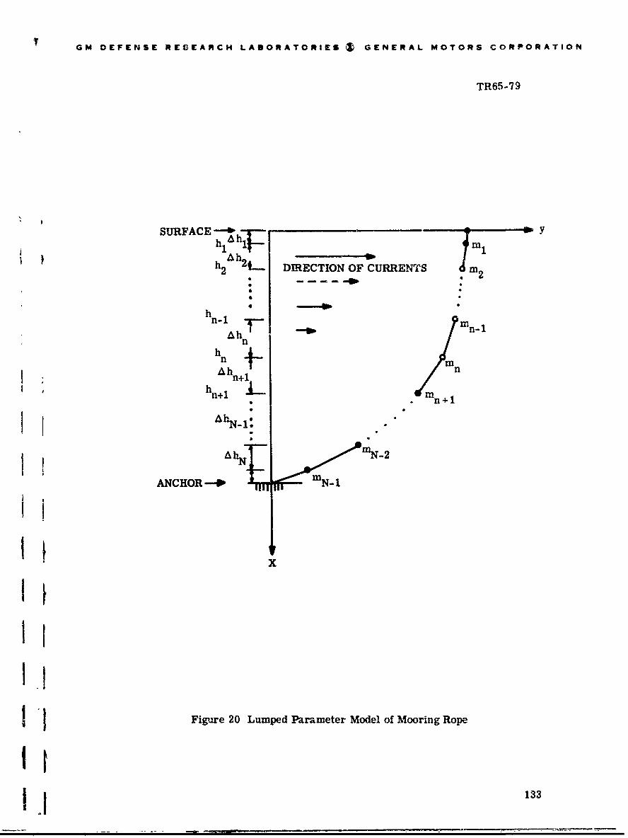
GM DEFENSE RESEARCH LABORATORIES I- GENERAL MOTORS CORPORATION
TR65-79
SURFACE Yhl1Ah F ml
h h2 2t-- DIRECTION OF CURRENTS I 2
h n -1 Ah- n-1-n
hn
n
h n ,+h mnAh n+1
hn+ /mn
11ANCHOR-W -*-
I IIx
I!
Figure 20 Lumped Parameter Model of Mooring Rope
I13

GM DEFENSK RESEAOCH LABORATORIE2 , GENERAL MOTORS CORPORATION
TR65-79
equilibrium curve of the rope is based on the solution of these equations of
motion. T: solve the equations, the forces acting on each nodal mass must
first be computed. If the summation of such forces is not zero, the resultant
force unbalance causes motion at the node until the rope assumes a shape i-
which the forces are balanced. The final configuration of the rope for which the
sum of the x and y forces on each nodal mass ft zero is, by definition, the
static deflection curve of the rope.
Since only the steady state solution is uf interest, the general equations of
motion can be greatly simplified because, under the final condition of equilibrium,
forces arising from accelerations and velocities vanish. Thus, such quantities as
added liquid mass and drag due to rope motion in the fluid medium may be ignored.
The forces considered to act on each nodal mass, including tension, weight, and
hydrodynamic drag due to currents, were confined to a vertical plane. The
positive buoyancy of the surface buoy was assumed to be equal at all times to
the vertical component Af line tension at the surface.
Derivation of Equations
The n th finite difference differentiaW equations for motion in the x and y
directions may be derived by consideration of Figure 21, which shows a more
detailed representation of the nth node. T hus,
2In n -= Tn sin 9 n - Tn+1 sin e n+l + Qyn (1)
dt
and.2
a xm n• -TncosOn+Tn cosen++Wn +Qmn= =_Tn cs8n +Tn41 o n+1 +Wn +Qxn (2)dt
where Qyn and Qxn are the horizontal and vertical drag forces at Node n,
Tn is the tension in the rope segment joining inn 1 and m n (i.e., S ); 8n
is the angle between the vertical and sn I and Wn is the weight concentrated
at Node n.
134

1 GM DEFENSE RESEARCH LABORATORIES 9 GENERAL MOTORS CORPORATION
I TR65-79
I
I yInI
1 n-
inn
xT
6
+1 mn
x
I.
[
Figure 21 Detailed Representation of Pth Node
135
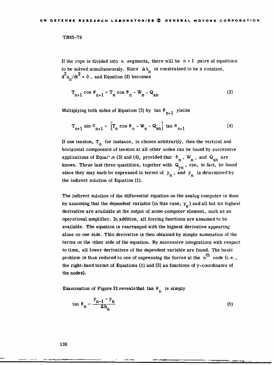
GM DEFENSE RESEARCH LABORATORIES (t GENERAL MOTORS CORPORATION
TR65-79
If the rope is divided into n segments, there will be n + 1 pairs of equations
to be solved simultaneously. Since Ahn is constrained to be a constant,
d 2X /dt2 = 0, and Equation (2) becomes
Tn+l cos en÷1 = Tn cos en - Wn - Q (3)
Multiplying both sides of Equation (3) by tan n+1 yields
r1Tn41 sin 0n+1= LVnCosen-Wn-Qxn1 tan 0n+1 (4)
If one tension, Tn for instance, is chosen arbitrarily, then the vertical and
horizontal components of tension at all other nodes can be found by successive
applications of Equa%' •n (3) and (4), provided that 6 n, W n, and Qxn are
known. These last three quantities, together with Qvn ' can, in fact, be found
since they may each be expressed in terms of yn , and y n is determined by
the indirect solution of Equation (1).
The indirect solution of the differential equation on the analog computer is done
by assuming that the dependent variable (in this case, yn ) and all but its highest
derivative are available at the output of some computer element, such as an
operational amplifier. In addition, all forcing functions are assumed to be
available. The equation is rearranged with the highest derivative appearing
alone on one side. This derivative is then obtained by simple summation of the
terms on the other side of the equation. By successive integrations with respect
to time, all lower derivatives of the dependent variable are found. The basic
problem is thus reduced to one of expressing the forces at the nth node (i. e.,
the right-hand terms of Equations (1) and (2) as functions of y-coordinates of
the nodes).
Examination of Figure 21 reveals that tan 6 n is simply
t an = - fl (5)n
136
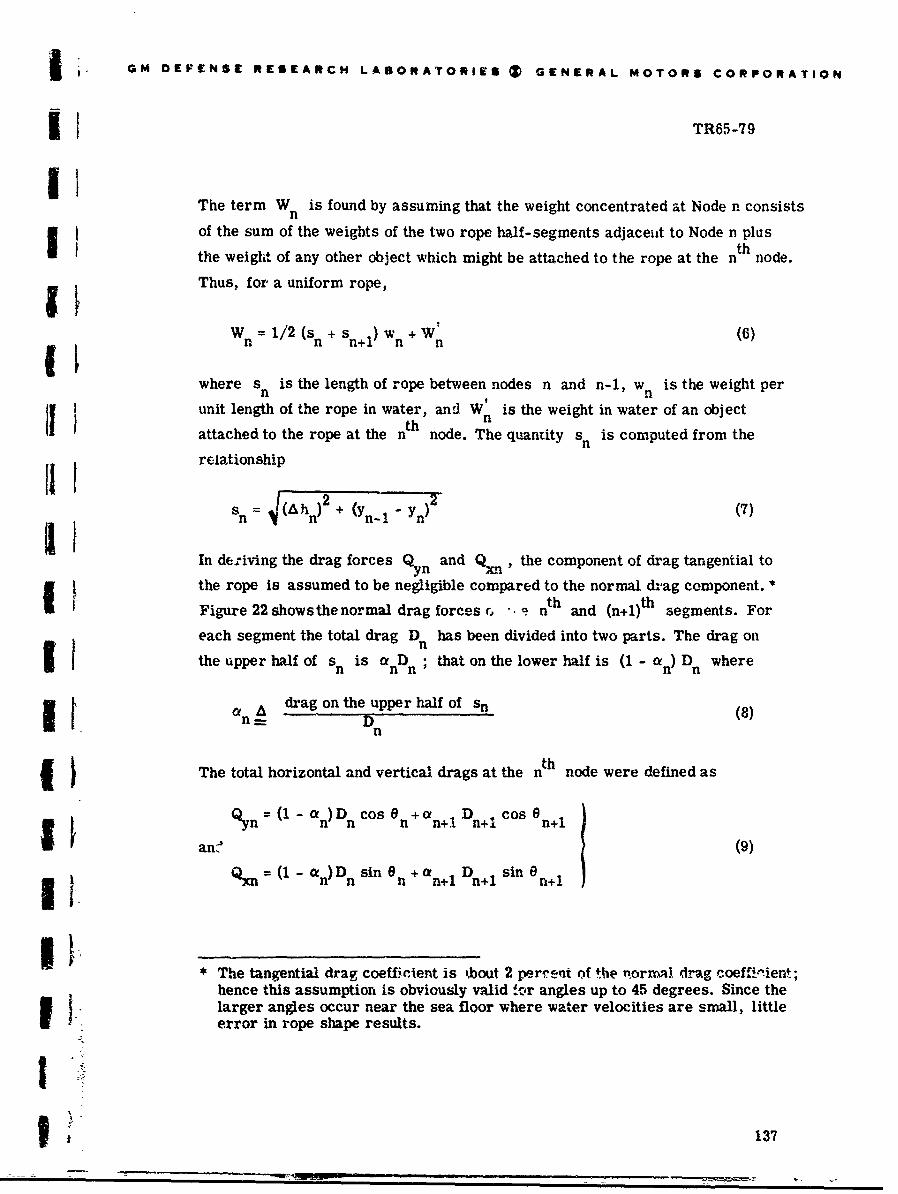
GM DEFE[NSE RESEARCH LABORATORIES 0 GENERAL MOTORS CORPORATION
ii TR65-79
The term Wn is found by assuming that the weight concentrated at Node n consists
of the sum of the weights of the two rope half-segments adjaceut to Node n plus
the weight of any other object which might be attached to the rope at the nth node.
Thus, for a uniform rope,
W =1/2 (s + si) w +Wn (6)
where sn is the length of rope between nodes n and n-i, wn is the weight per
unit length of the rope in water, ani Wn is the weight in water of an object
attached to the rope at the nth node. The quantity sn is computed from the
relationship
Sn n + (Yn( Ayn)h( (7)
In de.iving the drag forces Qyn and Qn ,' the component of drag tangential to
the rope is assumed to be negligible compared to the normal drag component. *Figure 22 showsthe normal drag forces r, -. . nth and (n+i)th segments. For
each segment the total drag Dn has been divided into two parts. The drag on
the upper half of sn is anDn ; that on the lower half is (1 - an) Dn where
an drag on the upper half of sn (8)
The total horizontal and vertical drags at the nth node were defined as
anc' Qn = (l - an) Dn cos On+ tn+1 Dn+1 cos n+l)
S=- (1 - cnD n sin en +an+, Dn+1 sin 9n+1
The tangential drag coefficient is ibout 2 rperrent of the liormal drg coefftr~ient;hence this assumption is obviously valid !vr '•angles up to 45 degrees. Since the
larger angles occur near the sea floor where water velocities are small, littleerror in rope shape results.
I 137

GM DEFENSE RESEARCH LABORATORIES ) GENERAL MOTORS CORPORATION
TR65-79 I
-41 y
hn -1
mn-1
I Vc W(x)
Ahn
hn n
s n+1 (1 -can) Dn
mn+l a rn+l D n+l
(I -an+1)Dn+l
Figure 22 Drag Forces on Rope Segments, sn and sn+1
138
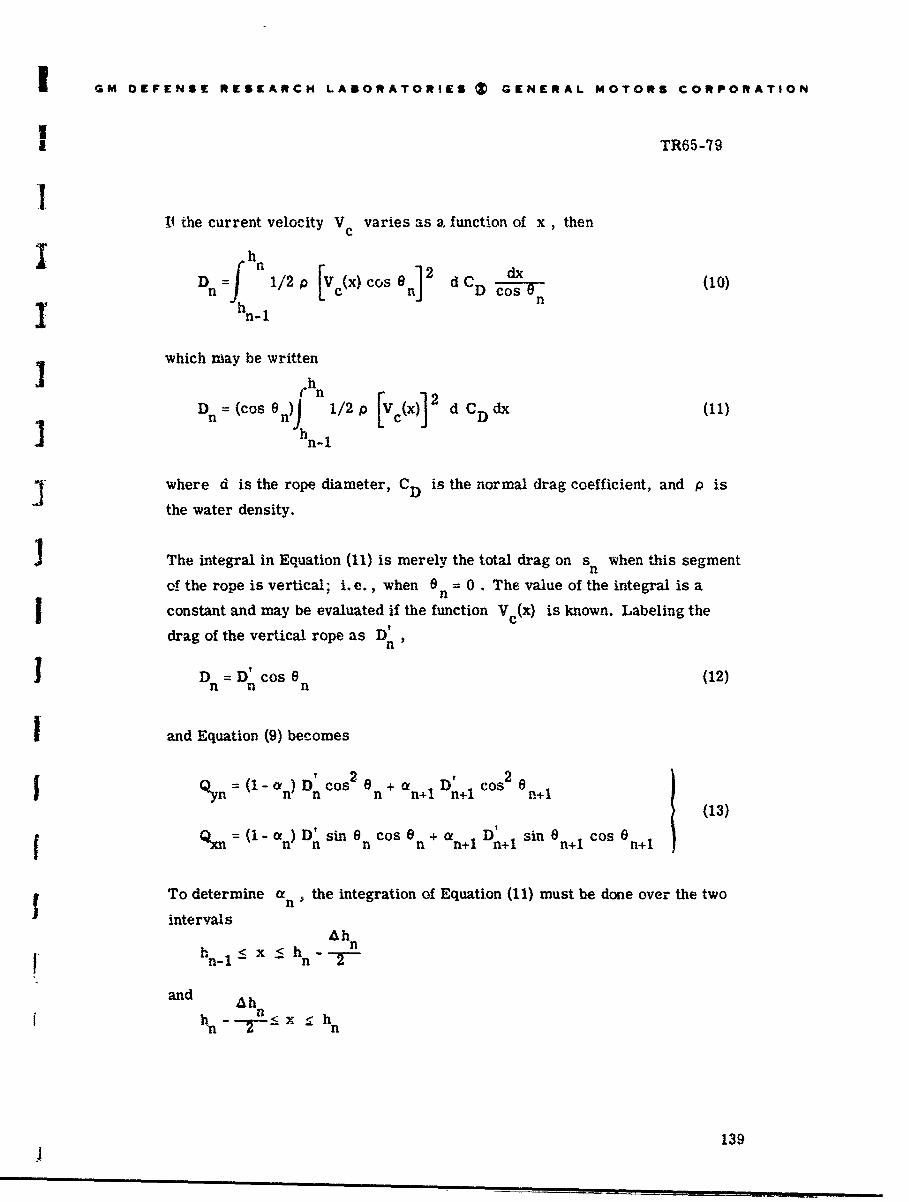
I GM DEFENSC RESEARCH LABORATORIES Z GENERAL MOTORS CORPORATION
II TR65-79
IV the current velocity V varies as a. function of x , then
D = h 1/2p [VX) cc's en2 d CD (10)n fI ] DCos " n10
I n_ 1
which way be written
n-Dn =(cosen)j n/2 [Vc(X)] 2 d CDdx (II)
where d is the rope diameter, CD is the normal drag coefficient, and p is
the water density.
I The integral in Equation (11) is merely the total drag on sn when this segment
of the rope is vertical; i.e., when 8 = 0. The value of the integral is an
constant and may be evaluated if the function Vc (x) is known. Labeling the
drag of the vertical rope as D'
D = D' cos 6 (12)n n n
I and Equation (9) becomes
(1-an)D'cos2 2e Dn Cos2 0Qyn= n nmn 4n 1 n+1 n+l( (13)D'sin cos 1 D'
=x n n n 0nCos en + n sin Cos +l
To determine a n, the integration of Equation (11) must be done over the two
intervalsAhh hn_l < : x <ý hn - n
and Ahhn n:5- x :ý h n
139.j

GM DEFENSE RESEARCH LASORATORIE5 Z GENERAL MOTORS CORPORATION
TR65-79
As a final step the sin 6 and cos & terms appearing in Equation (13) cann n
be expressed in terms of the nodal coordinates and the rope lengths, yielding
(Ah 2 " h 2)
Qyn(Icn)n n7;) +al1 n+l ksn+ 1 (14)
Q =(1-a)fl ,(Yn-1 Yn) &hn D (Yn- Yn+i)Ahn+1xn n n s2 +n1Dn+1 2
n Sn+l
If current meters are attached to the mooring rope, the resultant drag can be
calculated and comhined with that of the rope. It was assumed that half the drag
of a current meter was associated with the upper and lower ends of segment
s , as shown in Figure 23. From the figure,
D+CM = 1/2 p (Vc( )cos 9n)2 CD + d
and (15)
DnCM= 1/2 c (V cos 2 dCM
From the standpoint of computer implementation it is desirable to simplify
Equation (15) to the form of Equation (12); that is,
DL- = (constant) cos 8nCM n
The current meter drag can then be combined with cable drag to yield a new set
of equations of the form given by Equation (13). By approximating cos 2 0 asn(.866) cos 8n I Equation (15) may be written
DcM (D cos 6
DCM= (DC cos en
wbere(D:1/ M~=!P(866)VnC.) c2n- C1 dCM
140
... ...... ... .

GM DIFENSE RESEARCH LABORATORIES ) GENERAL MOTORS CORPORATION
I TR65-79
II
v N
//D
S/ sncn
/ n
V -mII
D(n+l)CM
-Ji+ i nC
x
3. 110
j Figure 23 Sketch Showing Method of Cýaculating Current Meter Drag
11 141
4 m m • •"-•

GM DEFENSE RESEARCH LASORATORIES ( GENERAL MOTORS CORPORATION
TRA5-79
and
(DnC4)=1/2 (.866) V2 CD J dncn D• CM
The magnitude of 30 degrees chosen for 6 is a compromise which gives an
fairly accurate value for the current meter drag at the top of the mooring line
where current meter drag may be significant compared to rope drag since the
lengths of the rope segments are snmall. For o s 8 < 400 the maximum error
in DnC or D due to the approximation above is 13%. For e > 400 , thenCM ' nCM
accuracy of the current meter approximation falls off; but when this happens
rope segments either have become longer, where the contribution of current
meter drag to total drag becomes less, or they are near bottom where the
current is weaker.
The total normal drag on sn may be written
nitotal I n C+D )' + (nCM) 1 c
= [DJ cos 0n total n
and Equation (13) becomes, when current meter drag is included,
-Of)D Cos2 En+ D' n [
Qyn (1- a) n +1 n+iJ to s n+1t.nltotal toa I~
r[1D sin n cos n +a n+ [Dn sin8 11+1tcos 8 niQ•._.= 1 an) n ntotal n. n J1 total ~
whereTh
h n-l+T2n.
f 1/2 p IV c(X)I d CD dx + LCDh n- 1
an = hSd CDx+ (D+ 1 + (D
4n-1
142

GM DEFENSE RESEARCH LABORATORIES (& GENERAL MOTORS CORPORATION
TR65-79
Computer Implementation
SDuring a computer run the accelerations a ocities of the nodes are unimportant
because these quantities vanish when steady sLate is achieved. However, it is
desirable to obtain a well-damped, rapidly converging solution. The damping
characteristic can be modified by the addition of a rate damping term in
Equation (1). Thus,
MY =T sin en- T sin 6 KR 'n
ni=T11 n n+1 n4.1 + QynIr,
I where K. can be adjusted until desired damping characteristics are obtained.
Rapidity of solution is determined by the choice of mn which can be interpreted
as a force scale factor. Although the value of nn has no effect on the final shape
of the mooring rope, this is not true of the term Wn in Equation (2) which must
be computed from Equation (6).
Figure 24 isablock diagram showing how the foregoing equations were implemented
on the analog computer for the upper two nodes (n = 0, and n = 1). As previously
stated, if one tension is known then all other tensions are determined from
Equations (3) and (4). The tension that was arbitrarily chosen for the Phase I
study was T 1 ' The angle e 1 was obtained with a servo resolver bý inverse
resolution of (y - Yl) and A h1, the two components of s1 . One cup of this
resolver was then used to multiply the selected T 1 by the sine and cosine of
a 1 . The extra drag force DB which acts on the surface node corresponds to
buoy drag.
The tension T 1 , chosen arbitrarily, does not represent the tension at the buoy
but rather the tension in the cable at the midpoint of cable segment s1 * To
f obtain a better approximation of tension magnitude and direction at the buoy, it
is necessary to consider the forces on the isolated system composed of the
upper half of s1 and the buoy (Fig. 25). The weight of the indicated section of
rope is Wo , the horizontal and vertical drag forces acting on the segment
are Qyo and Qxo , B is the buoyant force acting on the buoy, and DB is
I buoy drag. Since this system is in equilibrium, the summation of the vertical
forces and the summation of the horizontal forces are equal to zero. Thus,
I

GM DEFENSE RESEARCH LABORATORIES X~GENERAL MOTORS CORPORA! ION
TR65-79
0
4a
qE0
ba
1444

GM DEFENSE RESEARCH LABORATORIES ( GENERAL MOTORS CORPORATION
B
BUOY
SURFAC E ----- - -- -- -- 1 1)DB •
Syo
TI1 sinQ 1 Qxo +W Wo s
T11
(a) Upper Half-Segment of Cable and Buoy
B
Tosine 0 B D
TO T cos O 0
(b) Buoy
Figure 25 Forces Near the Buoy
145

GM DEFENSE RESEARCH LABORATORIES ( GENERAL MOTORS CORPORATION
T1 os +Qxo +Wo-B= 0w
and (16)
-T 1 sin 91 +Qyo +DB =0 )
Let us now isolate the buoy. labeling the magnitude of rope tension at the buoy
as T0 and the angle of the rope at the buoy as e (see Figure 5b). Since the0
buoy is in equilibrium,
-T sin e + DB = 0
and (17)
TO cos o - B = 0
Combining Equations (16) and (17) gives the following relationship:
TO sin 00 D DB = T1 sin 8 1 - Qyo )T cos 8o-B=T 1cos eI+Q xoW (18)e =tan-1 1B
0 a T1 cos l+QXo +W
from which T and 6 can be calculated.
o 0
In like manner it can be shown that the components of tension at the anchor are
"TA sin 8A =T. sin 6l0 + Q10"H (19)
andTAcos A =T10 Cos 10 - (Qxl+W )=U (20)
where H and U are the required holding power and negative buoyancy of the
anchor.
146

I GM DEFENSE RESEARCH LABORATORIES (3 GENERAL MOTORS CORPORATION
A
PERTURBATION ANALYSIS 07 THE MOTION OF
A BUOY MOORING ROPE
Method of Solution
Phase II consisted of a perturbation study of the motion of a buoy mooring rope
resulting from time-varying buoy displacements. The unperturbed rope shapes
were obtained from the Phase I data. The dynamic analysis was carried out on
an analog computer, using a lumped parameter model of the rope similar to that
of Phase I. For Phase 1I, however, both horizontal and vertical nodal motions
j were considered, and the rope was considered to be elastic.
Although developed independently, the equations used here are similar to those
of Walton and Polachek(4'5) and of Polachek, et al.(6) Our method, however,
contains additional simplifying assumptions necessary to adapt the equations to
an analog computer.
When writing the equations of motion of the rope, account must be taken (as was
done in Refs. 4 and 5) of the hydrodynamic reaction forces which occur when the
rope is accelerated laterally. The water entrained by the moving rope is moved
only by the normal component of motion. Hence, to handle the so-called virtual
mass, accelerations must be resolved both normal and tangential to the rope.
The resulting inertial forc2- must then be resolved again along the x and
y axes. The method of resolution of these forces is shown in Figure 26. Theth
acceleration at the n node normal to segment sn is
aNn = yn cos 6n +x 'n sin 6 n (21)
The reaction force is proportional to the normal acceleration; thus
Sv +FNn = 1/2 mn_1/2 aN (22)
where Fn represents the reaction force at node n due to lateral acceleration ofV
that half of segment sn adjacent to mn . The term mani 2 is the virtual mass
of .he fluid entrained by sn . Resolving FNn into its horizontal and vertical
components gives
147

GM DEKrNSE RESEARCH LABORATORIES Z GENERAL MOTORS CORPORATION
TR65-79
mn-I
ran+ n •On+!
x
Figure 26 Sketch Showing Method of Resolution of Hydrodynamic ReactionForces
148

j GM DEFENSE RESEARCH LABORATORIES (V GENERAL MOTORS CORPORATION
j TR65-79
F F - cos 0 (23)
3 and
F- F - F n sin 8 (24)Sxnn n
By combining Equations (21), (22), (23) and (24), we obtain the following equations:
F-= - 1/2 m' Cos2 o + 6 sin n coss 0 ) (25)yn1/n P, n (25
3 F - 1,2m (M' sin cos + sin2 0 ) (26)xn = - 1/2 .n n
3In a similar manner the x and y components of the reaction force at Node n
due to lateral acceleration of the adjacent half of segment sn+1 can be found.
J Thus,
Vn = r/ n l'2 Cos 0n + sin e1 cos (27)
F+ -l/2m" (yn sins cos 2 n (28)xn n+1/2 n n+l n+1 + n n+1
I The total horizontal and vertical components of reaction force are found by
combining the forces of Equations (25), (26), (27) and (28), giving!v
Fv = F- +F+ (29)and i xn
I a = F + F (30)
yt h
The equations of motion of the n mass may now be written as follows:
mynFFY+Fvn (31)
mn x= -v (32)
I1 149
• -••. •-•- .. • -

GM DEFENSE RESEARCH LASORATORIES ( GIENERAL MOTORS CORPORATION
TR65-79
where m is the mass concentrated at Node n, and E Fy and V FX representn n (-a n
the summation of all horizontal and vertical external forces other than the hydro-
dynamic reaction forces.
After combining Equations (25) through (32) and collecting terms, the equations of
motion can be written in matrix notation, yielding
K n . (33)U
where
=n mn + 1/n4 /2 sin 2n8 + 1/2 n / sin 2ne2 v 2
J=m -r 1/2 inv Cos 2 6 + 1/2 m v Cs2 8(34)
Jn mn -I1 / 2 n n+1/2 cos 6 n+1
Kn= 1/2 m n/2 sine cos 6 + 1/2 m sin v Cos 19nn12 n n rn+1 si n+1 co i•-I-
The term mn includes not oniy the average mass of the two adjacent rope segments,
but also the mass of any additional object, such as a current meter which may be
attached to the rope at the ith node. Furthermore, if such objects are symmetrical
with respect to the rope, their virtual mass can be included in the term m /
The -y and .FX forces correspond to the terms on the right-hand sides ofnn
Equatic..Ns (1) and (2) (see Fig. 2). Thus,
e = T sin en- T sin +Qn II n n-1- n+1 + yn
F"' =-Tncos8 T+T ,cose 8l W +QW
10n+ n+1 n xn
1501

L GM DEFENSE RESEARCH LAMORATORIIrS (V GENERAL MOTORS CORPORATION
j TRO5 -79
And Equation (33) may be rewritten
Sn KJn xYnJ Tn csn n -T Tn+l Cos 8 n+l+ - yn + .x
(35)
I To simplify scaling and, in particular, to obtain a higher degree of accuracy in
the calculation of tensions, recourse is now made to the perturbation technique.
5 If the amplitude of the surface buoy displacement is small compared to the length
of the rope, then the shape of the rope at any time will differ only slightly from
3 tOhat at static equilibrium and the resulting relative displacements of each node
will be small compared to the static displacements.
I Applying the perturbation technique, we define the variables xn and y n as fDoows:
(36)in = Yn+Yn
where xn and yn are the vertical and horizontal displacements at t = 0 (i. e.,
static equilibrium), and Xn and yn are the displacements resulting from buoymotion. Since Tn n ,Qxn yn I n , Jn , and Kn are functions of xn and
I n' these parameters must be similarly defined. Thus,
T =7F +T
n n n
e 4n=T + e x
n ýn n
in = In + In
J + J
n n nK=R +K'
n n n
5 151

GM DEFENSE RESEARCH LABORATORIES Z GENEPAL MOTORS CORPO,.ýATIOM
TR65-79
Substituting Equations (36) aad (37) into (35) gives
In the absence cf buoy motion, all the primed quantities are zero; in addition,
-T cos"n K T, cos+ W nn
n n n nl n+ n x
( (39)
nt-, Cos r1 Tn+1 n.
Tn sin -- sin +Q = s
si InT l n n+l+ yn-) l n+ y +Q
from the condition of static equilibrium.
The assumption is now made that n is a snfall angle, thusn
sin 8' a-8' and cos 8 a 1n n Ii
On thisbasisthe right-hand matrix of Equation (38) becomes
-T - -Tn sin'ýn- T' (cos-S - 9' sin' ) COs' - 8'T sin- +n co n n R n n n n n+1 n+l n-1 nA
-- ns in -n ' c o s - n + T n(E in -6 n e ' c s - )- T , 1 s in - - T 1 c o s -nl n 1 n n n n !!1 n. n-A n-A n-A
T- s 6 + ( os 4- QsxInTn. (c s "n~d- n-- si n "n-lA 4 W
T' (si3n + e' Cos - + Q+ , nn I en1-l n. y. --• _ +n
152
4

I GM DEFENSE RESEARCH LANORATOR*ES Z GENERAL MOTORS CORPORATION
TR65-79
"But the sum of the underlined terms is zero (Eq. 39) and, in general, the higher-
order products of the primed quantities can be neglected. Equation (38) may therefore
be simplified to
( nKn n" (40)
Sn r.) ,n
0' T si -6-T o 6 0 i ofn 1, n n n n-&1 n+- n+1 n+- Qxn
8' cos + T' sin- -T O' -Cn+l n+1
The y differential equation that was used for Node 1 differed from Equation (40);
thaL is, the higher-order term T1 S1 cos was retained, since in most cases
"was a small angle.
Expressions will now be developed for the quantities of Equation (40) in terms of
4 x and y"
Assuming Hooke's law for steel cables, we can express the tension in any segment1j as a function of the elongation of that segment. Thus,
J T s-s nn E n o
where A is the effective cross-sectional area; E is the effective value of
Young's Modulus, and sno is an unstretched reference length. Applying
I incremental substitution gives
1+ T =AE --- +n n( no o
153

GM DEFENSE RESEARCH LABORATORIES ( GENERAL MOTORS CORPORATION
The nominal equation is
T AE n no) (41)= Sno
and the perturbation equation isSs' n
T =AE-- (42)n s no
Solving Equation (41) for Sno gives
S
Sn (43)Sno
A E
For all steel ropes considered in this study
Tn << 1AE
Thus,
no p.
ands
T' A E--- (44)n
n
The nominal tension Tn is not, of course, obtained from Equation (41) but from
the Phase I data.
For nylon the function relating stress and strain is more complicated, so that aI
"dynamic spring constant," m was therefore determined experimentally.
In (45)
IT i inylon s n
154

GM DEFENSE RESEARCH LAIORATORIE$ Z GENERAL MOTOf•S CORPORATION
TR65-79
I As shown in Figure 7, the value of j is a function not only of T but also ofn
Sn/ISn , the variation of m with Sn/'sn becoming more pronounced at the higherI static tensions. To obtain an approximate solution to this problem, the value of
m chosen for each computer run was that one determined by the given static
~ I tension and the average value of the anticipated perturbation strain variation.
To find the changes in tension from Equations (42) and (45), the change in lengths must be determined. Consider Figure 27, which shows the configuration ofn th
the n rope segment before and after a small displacement. From the figure
' 2 -• ,)2 ,, 2
1n + sSn sin -n + Y 'n Y + cosn + X' X-
Solving for sn
2S I - n i y 1 -'sn' n -1y n n-l 11 XnXn-1) (6
n
I HIf we assume that
and (47)
I(x'-x <<2 cos~n n-i- n n
i I then the higher-order terms can be neglected and Equation (44) reduces to
S n (Y'- - 'sin +(X - cos -9 (48)n n n n
For n = 1 , the higher-order term (yn_1 - yn)/r S was retained, since it was' n
not obvious that the first inequality of Equation (47) would be valid because of
the smallness of in some cases.
L155 ------I ..... V W

GM OEFENSE RESEARCH LABORATORIES (t GENERAL MOTORS CORPORATION
TR65-79
-y
Yn-1
S?
n
/n
+
Y'nnnfn
0n
x
Figure 27 Configuration of nth Rope Segment Before andAfter a Small Displacement
156

3 GM DEFENSE RESEARCH LABORATORIES (t GENERAL MOTORS CORPORATION
l TR65-79
IThe final expression for Tn is obtained by combining either Equation (42) or
(45) with Equation (48); thus
(for steel)
n -AE y' ' ) sinn + (x' - x' cosn s n n Co~
i (for nylon)
T' = -_n 1n-1 - y') sin-n + (Xn -xl) cos5 n
The value of 0' can also be found by referring to Figure 27. From the figure,n
tantan(- 8")n= s n S n n-n n n n-i,
II Expanding the left side of the equaation by the formula for the tangent of the sum
of two angles and solving for 6n gives
tan 6' - 1(Yn- Y n) cos-n -(Xn - X 1 ) sin-n] n -n f ~
s n +S n
With the assumption that 0 is a small angle, and that s' << s the expression
n n nfor 0 becomesn
' ," (Yn 1 -Y- (X - xn) sin9 - - n (50)Sn Sn
By the use of Equations (49) and (50), the tension forces of Equation (40) can be
J computed.
The method of calculating the drag force of Equation (40) is based on the representa-I tion of the rope shown in Figure 28. Dragforces are computed in orthogonal-axis
systems, one axis of which is assumed to be tangent to the rope at Node n. The
angle with the vertical made by this axis is defined as 0 n where
L! 157
-**•i •a*.•a •.

GM DEFENSE RESEARCH tAMORATORIES (8) GENERAL MOTORS CORPORATION
TR65-79
m 1an -S
DNn
Vn DTN n VTnen m(+) 5n+l 1"~
/DTn+1
Nnn+l
Figure 28 Representation of Rope for Purpose of Computng DragForces
158

S GM DEFENSE RESEARCH LABORATORIES (t GENERAL MOTORS CORPORATION
ST R 65-7 9
+"n+l nn - ,i
I or -O
o n+n (51)
Because of the relatively small amplitudes of surface buoy displacement, the
Sangle 0 n was assumed to be constant.
A tangential drag and a normal drag are compute!d, and the forces so obtained aithen resolved back into the x-, y-axis system. Thus, if DTn and DNn are the
tangential and normal drag forces, then
Qxn = - DNn sin 0n + DTn cos In
I and (52)
Qyn =- DNn cos 0n- DTn sin 0n
The normal drag DNn is defined as
D Nn = Nn I VN (53n
13_ k~=l/2 PC d(S + n1)
~ where p is the fluid mass density, CD the dimensionless normal drag coefficient,
and d is r-ope diameter.
Equation (53) is a good approximation if 8n+1 - 9n is a small angle and
(i + ) >>s + S Similarly, D is defined asn n+) n n+1 . Tn1 .j
DTD = v1 k~n IVTn IVTn (54)
where , is the ratio of the dimensionless tangential drag coefficient to the
I I dimension ess normal drag coefficient. (A numerical value of. 02 was used
for v.)
11.5!!15

GM DEFENSE RESEARCH LABORATORIES 0 GENERAL MOTORS CORPORATION
TR65-79
The tangential and normal velocity components VTn and VNn are found by
resolving the x and y velocity components of mn with respect to the
surrounding fluid onto the tangential and normal axes. Thus,
VTn (Yn - V cn) sin 0n - xn cos 0n
(55)
VNn (in n x n + sin n
where V is the current velocity at the depth of Node n.cn
By the use of incremental substitution, the following nominal and perturbation
equations are obtained from Equation (55):
VTn Vcn sin nI .1(56)
VTn yn sin40n xn COs 0n
VNn -V cnCos n
V t is +(57)n n n n
In addition, Equation (52) can be written
Q% = - DNn sin i n + DTn cos 0n - 'xnt (58)
Qyn = -DNn Cosn-DTn sinkn - yn
Combining Equations (54) through (58) gives
Qxn = -kNn JVNn IVNn sini On + Y kNn 1nI~ V Tn o' n
+ kN IVNn IVNn sin On -"kNn flVTn IVTn cos On
sin On(59)-yn =kNnI IVNn INn co's O n n Ivn Ivn iv 1n(
+ kNn Nn IVN Cos cOn + Y k° n IVT IVTn sn
160
- . . . . . . . . . . . . . . . . . . . . . . . . . . . . . . . . . . . . ..- - - - - n n- n-mn u n u u i i i m m m
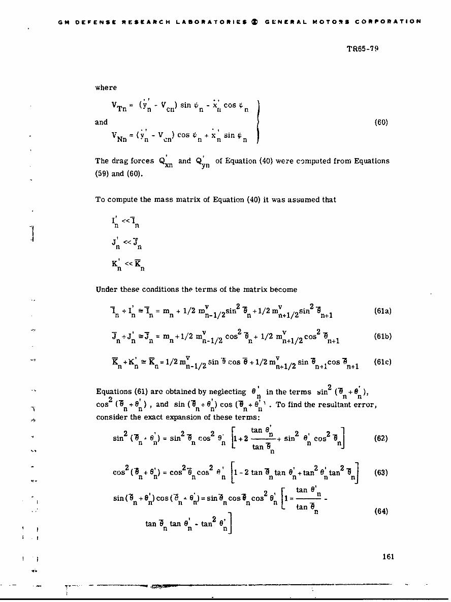
GM OEFENSE RESEARCH LABORATORIES (t GENERAL MOTO.5 CORPORATION
TR65-79
where
VTn: (Yn- Vcn) sinn C-XnCOSýn
and (60)
VNn= (v- Vn) Cos +xnsin nn en' n n n
The drag forces Qxn and Qy of Equation (40) were computed from Equationsyn
(59) and (60).
To compute the mass matrix of Equation (40) it was assumed that
I' «<'In n
j' << :Fn n
K' <<Kn n
Under these conditions the terms of the matrix become
I' = m +1/2 v . 2 /2mv 2"n n n n n-I/2 n n+1/2 "(n+lmn =lC2Sm "• +1/2 61a)
-i +J' a! J = m +1/2 mv co /2 mv Cs2(6bn n n n/n n- 1/ 2 (61b)
1/2 +.v" (611Kn nR n /mnn-2 sin "1/2cos6+1/2r+ sin -o Sn
Equations (61) are obtained by neglecting 8 in the terms sin2 (6+ +'2 n8n'cos (' n n) ' and sin (•n+ 8') cos (' + e'' . To find the resultant error,
An n n n n niconsider the exact expansion of these terms:
8 s2 2'n Cos 2 9' +2 +sin 2 e' 2 (62)
62 2 2tan tn co2 ta (63)n n n n ta n n n
sin('n +8')cos(-C eO) = sinn cosn cos2 [1tan "'n
" t " n (64)
tan tan - tan 2 (64
SIn n n

GM DEFENSE RESEARCH LABORATORIES (Z GENERAL MOTORS CORPORATION
TR65-79
For all cases examined, e' was sufficiently small to justify neglecting the lastn 2 1 1 1term in the brackets and approximating cos 6 by unity and tan e by en n nWith these approximations, Equations (62), (63), and (64) become
sipn2 +n) sin2 " + 2 n (65)n+6n n tan - Itan 6 Jn
Cos 2(0 + e -Cos2 6()2 n n [I-2(tan )8] (66
sin (-6 + 6 cos 0+ G') t sin -- cos + 2 -(tan -) en (67)n nn n n tan -n nn
If, in Equation (65), the second term in the bracket is not much less than unity,
then - must be a small angle. But if both 8' and -6 are small angles, thenn 2n n
1/2 mv sin + 8') is much less than m in Equation (61a) and neglectingn_-112 n n-n
6 ' does not lead to a significant overall percentage error in I . In a similarn nmanner it can be shown that neglecting 6' in Equ,.tion (66) results in no significantnoverall error in J . For the great majority of the cases examined, the last two
terms in the bracket of Equation (67) were sma.ll compared to unity; but for the
most violent excitation conditions (50-ft amplitude and 1, 800-ft depth), the
neglecting of e did lead to appreciable error in the value of Kn at the top of
the rope. In only two runs, however, did this error exceed 20 percent. These
were Case F (50-ft wave height, 16-sec period) and Case E (25-ft wave height,
32-sec period), which had maximum errors in Kn of 24 percent and 34 percent.
Computer Implementation
To simplify analog computer programing, the tension forces at Node n were
expressed as a function of y' and x' in pairs. From Equation (40) the x andn n
y tension forces on mn areT =0'T sin-9 -T cos- 0' T sin- 4T cos (68)
xn n n n n n n n+l n+l n+l n+l
and
T =T 0' cos6 +T' sin --T e' ":os'nO TnI sn9(yn nn n n n ni-il n+1 n+ln- ' sin i (69)
162

SGM DE•FENSE RESEARCH LABORATORIES (& GENERAL MOTORS CORPOnATION
TR65-79
Substitution of the values of T' and 8' from Equations (49) and (50) into (68)n n
and (69) gives the following equations:
I K. sin'9 cos~ -F ny sin-6rI cos-0n+T "n" s ) n(Y-l-Yn) - I(Tn+l- sSxn •n ( - n +l n
S(Yn-n-1i -s +COS (7 -n
n+1 sin2 + + A cos"nl (X 1 _ X) (70)
Sn+1 i
T n cos 2 -r,+ u sin2 "6n (Ynn-l - nYn1 .i+j
Tyn n J--In-- .nSn- i
(Yn! n+1 - s n _X+l X
kljsin sin+1 cos*• n
n _ 1 (xn - xn ) -1
Inn l
n sn6n+1 Cos (x n (71)]x n+1 i n)
•I And now the following "ter.sion coefficients" are defined:
T a n cos2 "6 + p sin2 "6
b =("_n) "il •On (72)n -
n
,I~ s.2 "• +M•cos 2 "d
n n nn = n
r
163

GM DEFENSE RESEARCH LABORATORIES a GENERAL MOTORS CORPORATION
TR65-79
For each given rope configuration, these coefficients are constants, L, terms of
the tension coefficients, Equations (70) and (71) become
T1xn =bn(Yn-1" Yn) -bn+l(Yn- Yn+) - c)n(xn - xn-I)+c n+1(xn+l- Xn) (73)
T a(Y- a +1 -y b-(x
n n+,Yn b n(xn- Xn_ 1 ) n+1 (xn+1- xn) (74)
Equations (73) and (74) were used to obtain the tensioa forces on the analog
coraputer.
A computer diagram showing the implementation of the nth nodal equations is
given in Figure 29.
164

TR65-7 9
" AV.
a *6 0
E
* 0
-* ...
* -
°..4
1 165
0 4.
* /Y
- - '-.
- *4AN6

GM DEFENSE RISEARCH LABORATORIES Z GENERAL MOTORS CORPORATION
TR65-79
LITER ATURE CITED
(1) Wilson, B. W., Characteristics of Anchor Cables in Uniform OceanCurrents, The A. and M. College of Texas Department of Oceanographyand Meterology Technical Report No. 204-1 (Apr 1960) 149 pp.
(2) Wilson, B. W., Characteristics of Deep-Sea Anchor Cables in StrongOcean Currents, The A. and M. College of Texas Technical ReportsNos. 204-3 and 204-34 (2 vols.), (Feb 1961 and Mar 1961, respectively)89 and 266 pp. (Note: 204-3 is ASTIA AD-259379)
(3) Whicker, L. F., Theoretical Analysis of the Effect of Ship Motion onMooring Cables in Deep Water, U. S. Navy David Taylor Model BasinReport 1221, (Mar 1958) 24 pp.
(4) Walton, T. S. and H. Polachek, Calculation of Non-Linear TransientMotions of Cables, U.S. Navy David Taylor Model Basin Report No. 1279(Jul 1959), 50 pp. (DDC No. AD418603)
(5) Walton, T. S. and H. Polachek, Calculation of Transient Motion ofSubmerged Cables, Mathematical Tables and Aids to Computation 14,27-46 (1960)
(6) Polachek, H. , T. S. Walton, R. Mejia, and C. Dawson, Transient Motionof an Elastic Cable Immersed in a Fluid, Mathematics of Computation,Jan 1963, pp. 60-63
(7) WaltonT. S., Personal communication to R. P. Brumbach, (Sept 1 S65)
(8) Johnson, H. and F. Lampietti,. in "Experimental Drilling in Deep Waterat La Jolla and Guadalupe Sites" AMSOC Committee Report, NationalAcademy of Sciences - National Research Council Pub. No. 914 (1961),p. 58
(9) Rather, R. L., Vil Goerland, J. B. Hersey, A. C. Vine, and F. Dakin,1965, Improved towline design for oceanography, Undersea Technology6 (5), 57-63(1965)
(10) Hakkarinen, W., The World of NOMAD-i, Buoy Technology, MarineTechnology Society, Trans. 1964 Buoy Technology Symposium 24-25 Mar1965, Washington, D.C., 1, 443-456
(11) Roberts, E. B., Roberts Radio Current Meter Mod II Operating Manual,U.S. Dept. Commerce, Coast and Geodetic Survey, Washington, D.C.,1952, 33 pp. (The NOMAD hull is almost identical to a scaled-up RobertsCurrent MeLer Buoy)
166

GM DEFENSE RESEARCH LABORATORIES Z .GENERAL MOTORS CORPORATION
I TR65-79
II LITERATURE CITED (Cont.)
I(12) Geodyne Corporation, Waltham, Mass., Bull. No. S-32 7/24/63 and
DWG A-92 of 3/7/63 describing Model A-92 Instrument Buoy
(13) Isaacs, J.D., J.L. Faughn, G.B. Schick, and M.C. Sargent, Deep-SeaMooring, Bull. Scripps Inst. Oceanography 8 (3), 271-312 (1963)
f (14) Vinogradov, V. V., Russian Naval Hidrographic Service Foam Buoy,Okeanologiya 2 (2), 346-352 (1962), transl. in Deep-Sea Research 11m•-37-141( 964)
J(15) Devereux, R., et al., Development of a Telemetering OceanographicBuoy, General Dynamics/Convair Progress Report GDC-63-060 underContract Nonr-3062(00) (Feb 1963'
(16) Uyeda, S. T., Buoy Configuration Resulting From Model Tests andComputer Study, Buoy Technology, Transactions of the 1964_ BuoyTechnology Symposium, Washington, D.C., 24-25 Mar 1564, Supplementpp. 31-42 (1964)
(17) Saunders, H. E., Hydrodynamics in Ship Design, New York, Society ofNaval Architects and Marine Engineers, 2 vols. (1957), vol 2, p. 291
I and pp. 418-423
(18) United States Steel Corporation, Columbia-Geneva Steel Division, WireRope Handbook, San Francisco, Calif. (1959) 194 pp.
(19) Gaul, R. D., Influence of Vertical Motion on the Savonius Rotor CurrentMeter, Agricultural and Mechanical College of Texas, Department ofOceanography and Meteorology, Tech. Rept. Ref. No. 63-4T, 1 Feb 1963,29 pp.
(20) Paquette, R.G., Pro rtical Problems in the Direct Measurement of OceanCurrents, Marine Aciences Instrumentation (Proceedings of the Symposiumon Transducers for Oceanic Research, San Diego, California, 8-9 November1962) New York, Plenum Press (1963), 195 pp., pp. 135-146
167
*i
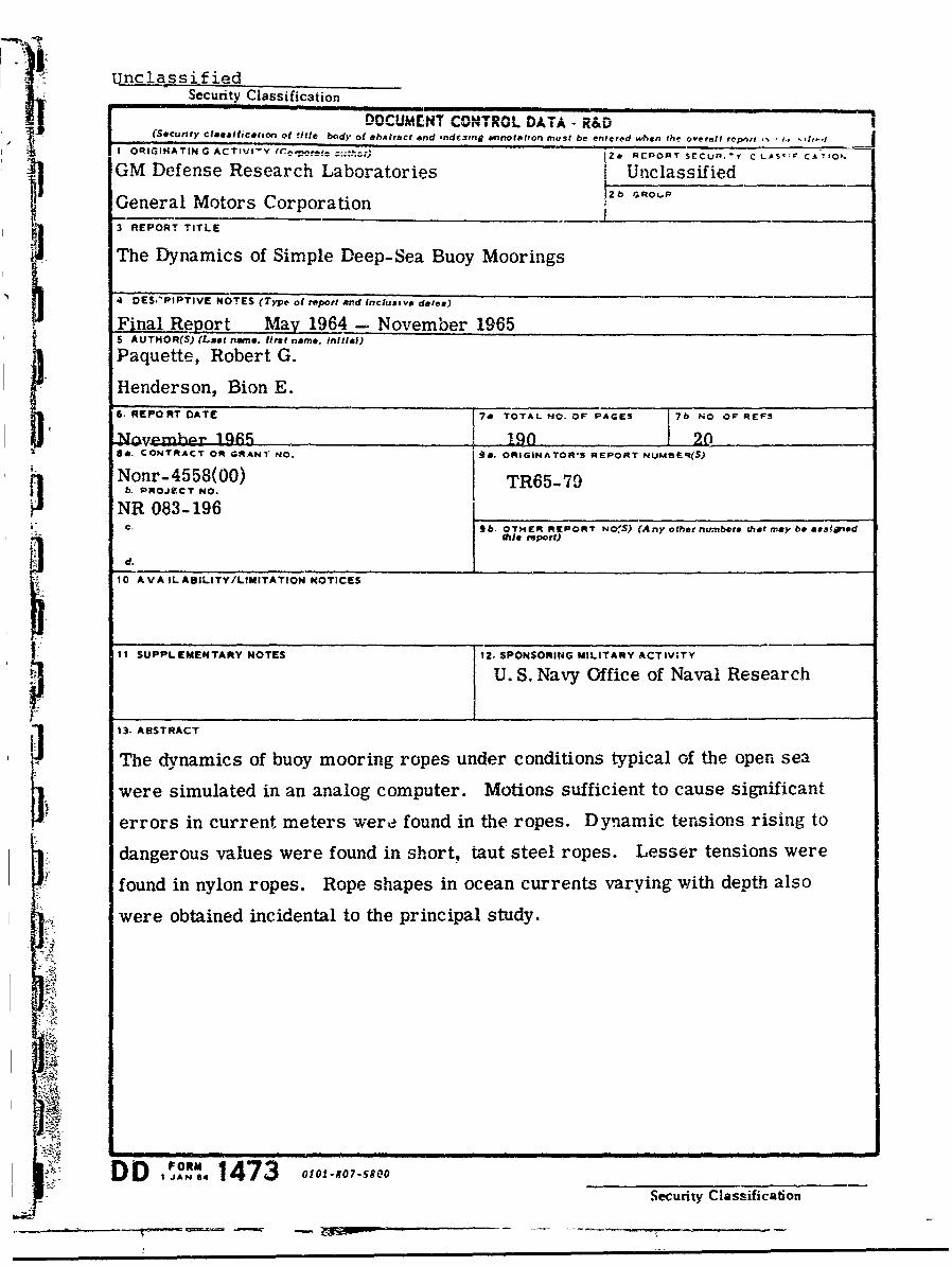
.- UTnclassifiedSecurity Classification[ DOCUMENT CONTROL DATA - R&D
• ~~(Security classifJicationl of Wite body of ahxtract and -ndcaitng annlotation mnast be entered when the overall report %, j ., %,thl
GM Defense Research Laboratories 1 Unclassified
General Motors Corporation F2 ýGRo-P
C3 REPORT TITLE
4 The Dynamics of Simple Deep-Sea Buoy Moorings
' 4 DES.PFPTIVE NOTES (Type of report And lnclusive dates)
Final Report May 1964 - November 1965S AUTHOR(S) (Last nane. first name, initial)
Paquette, Robert G.
Henderson, Bion E.6. REPORT DATE 7o TOTAL NO. OF PAGES 7b NO OF REFS-November 19_5_,_ , 190 20
as. CONTRACT OR GRANT NO. ta. ORIGINATOR'S REPORT NUM8Ef(S)
1Nonr-4558(00) TR65-79&. PROJECT No.
• NR 083-196VC. 9b. OT E R RIEPORT NO•,$) (Any oth~er numbers that may, be aas~sfid
"M- this port)
d.___________10 A VA IL AILITY/LIMITATION NOTICES
S11 SUPPLEMENTARY NOTES f 12. SPONSORING MILITARY ACTIV;TY
U. S. Navy Office of Naval Research
] 13- ABSTRACT
The dynamics of buoy mooring ropes under conditions typical of the open sea
were simulated in an analog computer. Motions sufficient to cause significant
errors in current meters were found in the ropes. Dynamic tensions rising to
dangerous values were found in short, taut steel ropes. Lesser tensions were
found in nylon ropes. Rope shapes in ocean currents varying with depth also
were obtained incidental to the principal study.
FORM
Security Classification

Security Classification14KYWRSLINK A LINK B T LINK C
RPOLE WT4 ROF __ ROLEi IBuoy Dynamics
Buoy Moorings
Anchoring
Mooring Dynamics
Ocean CurrentsI
Oceanography ,
Computers, Analog
.NtTRUCTIONS
t. ORIGINATING ACTIVITY: Enter the name and address imposed by security classification, using standard statementsof the contractor, subcontractor, grantee. Department of De- such as:fense activity or other organization (corpoiate author) issuing (1) "Qualified requesters -ay obtain copies of thisthe rr- report from DDC"2a. REPORT SECURTY CLASSIFICATION: Entertheo er- "Foreign announcement and dissemination of thisall security classification of the report. Indicate whetherb"Restricted Data" is included. Marking is to be in accord- e by DDC is not authorized."ance with appropriate security regulations. (3) "U. S. Government agencies may obtain copies of
this report directly from DDC. Other qualified DDC2b. GROUP: Automatic downgrading is specified in DoD Di- users shall request throughrective 5200. 10 and Armed Forces Industrial Manual. Entesthe group number. Also. when applicabie, show that optionalmarkings have been used for Group 3 and Group 4 as author- (4) "U. S. military agencies may obtain copies of thisized. report directly from DDC. Other qualified users
3. REPORT TITLE: Enter the complete report title in all shall request throughcapital letters. Titles in all cases should be untlassified. ,,If a n-,eaningful title cannot be selected without ( lassifica-tion, show title classification in all capitals in parenthesis (5) "All distribution of this report is controlled. Qual-immediately following the title. ified DDC users shall request through
4. DESCRIPTIVE NOTES. If appropriate, enter the type of ."report, e.g.. interim, progress, summary, annual, or final. If the report has been furnished to the Office of TechnicalGive the inclusive dates when a specific reporting period is Services, Department of Commerce, for sale to the public, indi-covered. cate this fact and enter the price. if known.
S. AUTHOR(S): Enter the name(s) of author(s) as -hown on IL SUPPLEMENTARY NOTES: Use for additional explana-or in the report. Entet last name, first name, middle initial. tory notes.If military, show rank and branch of service. The name of tthe principal author is an absolute minimum requirement. 12. SPONSORING MILITARY ACTIVITY: Enter the name of6. REPORT DATE: Enter the date of t1he report as day. the departmental project office or laboratory sponsoring (pay-mont. REPORT DArmonT. year. I e date appthearporta s daing for) the research and development. Include address.
on the report, use date of publication. 13. ABSTRACT: Enter an abstract giving a brief and factualOsummary of the document indicative of the report, even though
7a. TOTAL NUMBER OF PAGES: "'he total page count it may also appear elsewhere in the body of the technical re-should follow normal pagination procedures. i.e.. enter the port. If additional space is required, a continuation sheet shallnumber of pages containing information. be attached.7b. NUBROIEEECS ne h oa ubro
.NUMBER OF REFERENCES• Enter the total number of j It is highly desirable that the abstract of classified reportsreferences cited in the report. be unclassified. Each paragraph of the abstract shall end vwith
8a. CONTRACT OR GRANT NUMBER: If appropriate, enter an indication of the military security classification of the ;n-the applicable number of the contract or grant under which formation in the paragraph, represented as (TS) (S) (C, at (UIthe report was written. There is no limitation on the length of the abstract How-
8b, 8c, & 8d. PROJECT NUMBErC Enter the appropriate ever. the suggested length is from 150 ti 225 wordsmilitary department identification, such as project number, 14. KEY WORDS: Key words are techically meanigful termssubproject number, system numbe's, task number, etc.
or short phrases that characterize a report and may be used as9a. ORIGINATOR'S REP'RT NUMBER(S): Enter the offi- index entries for cataloging the report. Key words must becial report number by which the document will be identified selected so that no security class fication is required Identiand controlled by the originating activity. This number must fiers, such as equipment model designation, trade name. militarybe unique to this report. project code name, geographic location. may be used as key
9b. OTHER REPORT NUMBER(S): If the report has been words but will be followed by an indicati-on of technical con-assigned any other report numbers (either by the originator text. The assignment of links, roles, and weights is optional.or by the sponsor), also enter this number(s).
10. AVAILABILITY/LIMITATION NOTICES: Enter any lirn-itations on further dissemination of the report, other than thosel
Security Classification
7~~J
Related Documents