The Development Problem under Embodiment

THE DEVELOPMENT PROBLEM UNDER EMBODIMENT*

Raouf Boucekkine, Blanca Martínez and Cagri Saglam**

WP-AD 2003-08

Correspondence to: Blanca Martínez, Universidad de Alicante, Departamento de Fundamentos del Análisis Económico, Campus de San Vicente, 03071 Alicante (Spain). E-mail: [email protected]. Editor: Instituto Valenciano de Investigaciones Económicas, S.A. Primera Edición Febrero 2003 Depósito Legal: V-899-2003 IVIE working papers offer in advance the results of economic research under way in order to encourage a discussion process before sending them to scientific journals for their final publication.

* We are grateful to Omar Licandro, Ramon Marimon, Franck Portier and the participants at the 2002 Florence EuroMac conference for very useful comments. The financial support of the Belgian research programmes “Poles d'Attraction inter-universitaires”' PAI P5/21, and “Action de Recherches Concertée”' 99/04-235 are gratefully acknowledged. ** R. Boucekkine: IRES and CORE, Université catholique de Louvain. B. Martínez: Universidad de Alicante. C. Saglam: IRES, Université catholique de Louvain.

2

THE DEVELOPMENT PROBLEM UNDER EMBODIMENT

Raouf Boucekkine, Blanca Martinez and Cagri Saglam

ABSTRACT

We study technology adoption in an optimal growth model with embodied technical change. The economy consists of the final good sector, the capital sector, and the technology sector which role is the imitation of exogenous innovations. Labor resources are scarce. They are freely allocated to the technology and final good sectors. The final good is freely allocated to consumption and to the capital sector. We analytically characterize the optimal allocation decisions in the long run. Using a calibrated version of the model, we find that an acceleration in the rate of embodied technical change should not be responded by an immediate and strong adoption effort. Instead, adoption labor should decrease in the short run, and the optimal technological gap is shown to increase either in the short or in the long run. The state of the institutions and policies around the technology sector is key in the design of the optimal adoption timing. Keywords: Embodiment, Technology adoption, Technological gap, Transition dynamics. Journal of Economic Literature: E22, E32, O40.

1 Introduction

In the recent years, the North-South digital divide has been the main con-cern of many policy oriented studies and committees. Many bodies nowexist that all focus on the stakes involved by the digital divide. The G8 DotForce, established at the 2000 Okinawa G8 summit, was among the first.More recently, in 2002, the United Nations have launched their Informationand Communication Technologies (ICT) Task Force, and it is frequent toread in the official publications of many industrial countries some explicitstatements like the following: ”bridging the North-South digital divide is apriority for the foreign co-operation policy”.1

In this context, many developing countries have undertaken a significanteffort in ICT equipment investment, specially in Asia and Latin America.Figure 1 displays the patterns of ICT expenditures in six Latin Americancountries over the period 1992-2001. In Brazil, Chile and especially Colom-bia, this effort has been tremendous. The Brazilian ICT expenditures haveincreased from less than 4% of GDP in 1992 to more than 8% in 2001. Chilehas followed almost the same pattern. ICT expenditures have tripled inColombia over the same interval, reaching 12% in 2001! Overall there is aclear technology adoption effort in this part of the world, though it is un-evenly distributed across countries.

Beside the issue of the connectivity of the South, which is certainly veryimportant to address properly, one may question the relevance of the North-South digital divide problem as a key and urgent development issue, and thesubsequent technology adoption and transfer programs. After all, the ICTgrowth enhancing effect is still at the heart of a tough debate even on the USeconomy (see Gordon, 2000). Moreover, the existing (and very long) recordof technology transfers calls for much more caution in the assessment of thepotential ICT contribution to the economic development of the South. Inparticular, the two following lessons are worth pointing out.

(i) First, technology adoption programs are usually undermined by theinstitutional barriers inherent to developing countries. As reported by Niosi,Hanel and Fiset (1995) using a survey of the performances of some 50 majorinternational technology transfer projects, the costs associated with lack oftransferee expertise and poor training, and those induced by the administra-

1French inter-ministerial committee, July 10th, 2002.

3

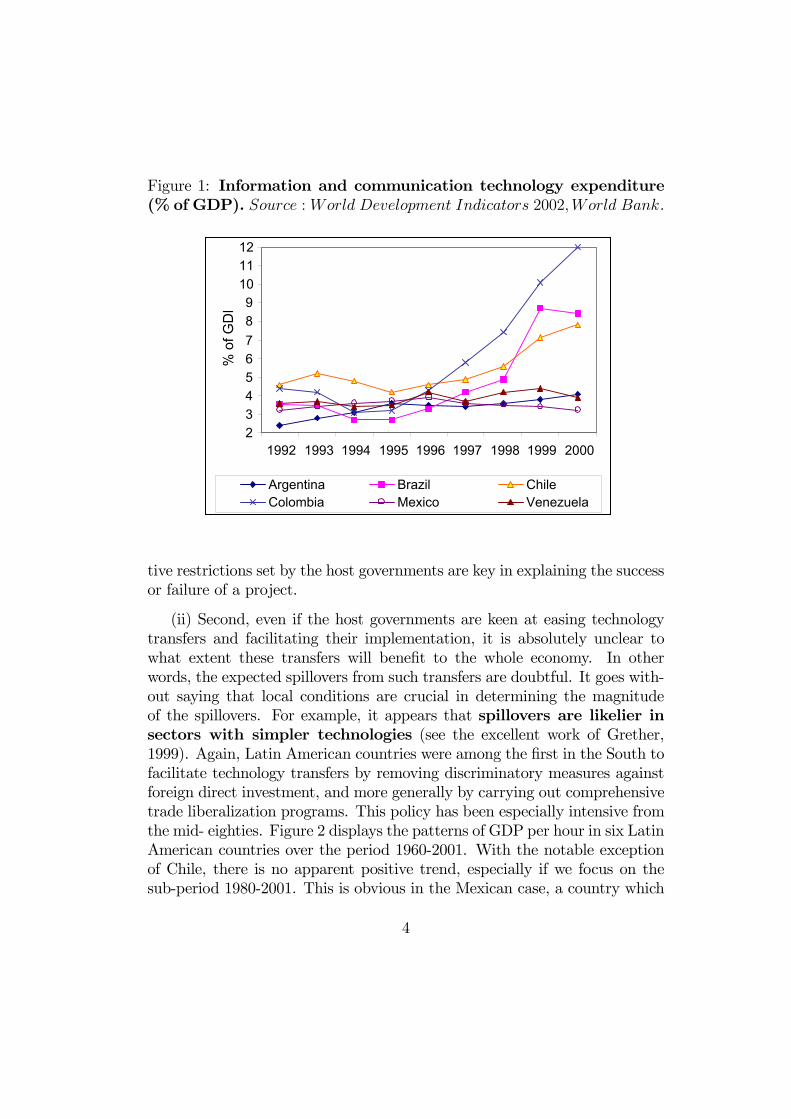
Figure 1: Information and communication technology expenditure(% of GDP). Source :World Development Indicators 2002,World Bank.

23456789

101112

1992 1993 1994 1995 1996 1997 1998 1999 2000

% o

f GD

P

Argentina Brazil ChileColombia Mexico Venezuela

tive restrictions set by the host governments are key in explaining the successor failure of a project.

(ii) Second, even if the host governments are keen at easing technologytransfers and facilitating their implementation, it is absolutely unclear towhat extent these transfers will benefit to the whole economy. In otherwords, the expected spillovers from such transfers are doubtful. It goes with-out saying that local conditions are crucial in determining the magnitudeof the spillovers. For example, it appears that spillovers are likelier insectors with simpler technologies (see the excellent work of Grether,1999). Again, Latin American countries were among the first in the South tofacilitate technology transfers by removing discriminatory measures againstforeign direct investment, and more generally by carrying out comprehensivetrade liberalization programs. This policy has been especially intensive fromthe mid- eighties. Figure 2 displays the patterns of GDP per hour in six LatinAmerican countries over the period 1960-2001. With the notable exceptionof Chile, there is no apparent positive trend, especially if we focus on thesub-period 1980-2001. This is obvious in the Mexican case, a country which

4

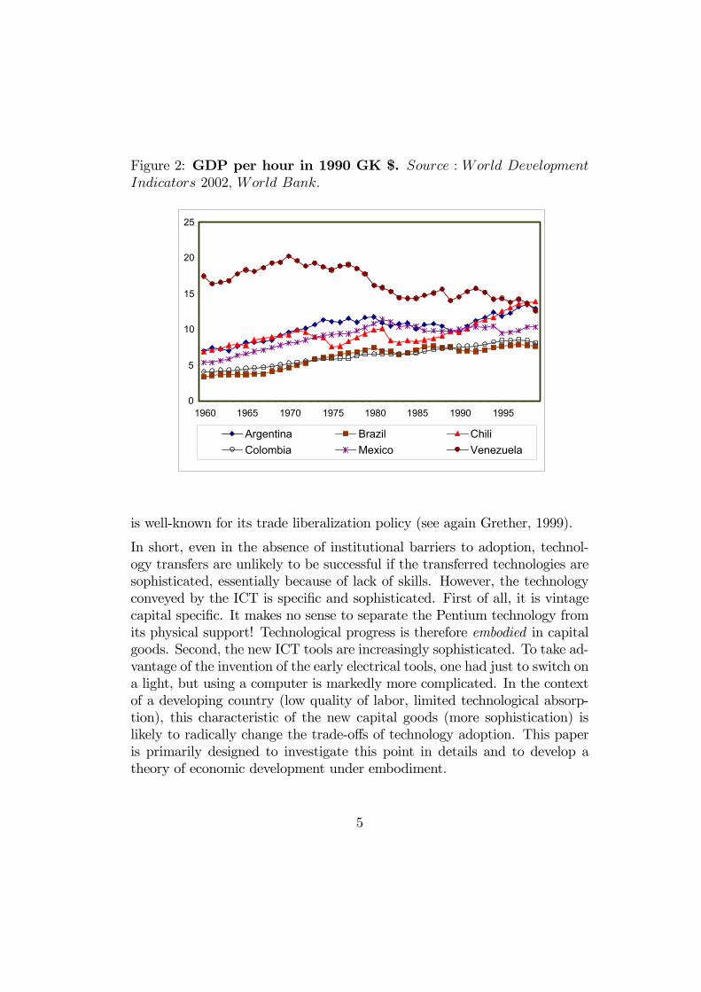
Figure 2: GDP per hour in 1990 GK $. Source : World DevelopmentIndicators 2002, World Bank.

0

5

10

15

20

25

1960 1965 1970 1975 1980 1985 1990 1995

Argentina Brazil ChiliColombia Mexico Venezuela

is well-known for its trade liberalization policy (see again Grether, 1999).

In short, even in the absence of institutional barriers to adoption, technol-ogy transfers are unlikely to be successful if the transferred technologies aresophisticated, essentially because of lack of skills. However, the technologyconveyed by the ICT is specific and sophisticated. First of all, it is vintagecapital specific. It makes no sense to separate the Pentium technology fromits physical support! Technological progress is therefore embodied in capitalgoods. Second, the new ICT tools are increasingly sophisticated. To take ad-vantage of the invention of the early electrical tools, one had just to switch ona light, but using a computer is markedly more complicated. In the contextof a developing country (low quality of labor, limited technological absorp-tion), this characteristic of the new capital goods (more sophistication) islikely to radically change the trade-offs of technology adoption. This paperis primarily designed to investigate this point in details and to develop atheory of economic development under embodiment.

5

The role of embodiment in the growth process of the industrialized countrieshas been intensively studied in the recent years, notably in the US economy.As documented in Greenwood and Yorukoglu (1997), two major stylized factsseriously undermine the neoclassical growth model: The steady decrease inthe relative price of equipment investment and the secular rise in the equip-ment investment to GDP ratio. Both are incompatible with the long termproperties of the neoclassical growth model. In contrast, these two facts canbe rationalized in a canonical two-sector growth model assuming that part oftechnological advances are specific to the capital goods sector (the so-calledembodiment hypothesis). Using this approach, Greenwood, Hercowitz andKrusell (1997) found that around 60% of post-war US productivity growthcan be attributed to embodied technological change. More theoretical stud-ies on the implications of the embodied nature of technical change for longterm growth can be found in Krusell (1998), Benhabib and Hobijn (2002),and Boucekkine, del Río and Licandro (2001, 2002).

Our objective is to study to which extent the embodiment characteristicmatters in the technology adoption decisions in the context of a developingcountry. The basic structure of the models we would like to analyze is thefollowing. The economy consists of three sectors: the sector producing thefinal good, the sector producing the capital goods, and the technology sector.Technological progress is embodied in capital goods. The technology sectordoes not conduct any R&D activity. Its unique role is the adoption (or im-itation) of the innovations coming from abroad. However, the technologicalabsorption is limited in that it is never feasible to close the technological gapwith respect to abroad as in Nelson and Phelps (1966). We consider optimalgrowth models in which a benevolent central planner enforces the social op-timum by choosing the best consumption, investment and adoption patternsfor the economy.2 To this end, he has to settle some resource allocationsproblems involved in the economy. For example, he has to ensure that the(scarce) skilled labor resources are optimally assigned to both the technologyand the final good sectors. What could an optimal adoption plan in such acontext? How should the economy react to a technological acceleration? Isan immediate and massive adoption effort optimal in this case?

To tackle these issues, we organize the paper as follows. The next sectiongives the analytical structure of the model. It also derives the corresponding

2Since the model does not rely on any externality, imperfect competition or incom-pleteness ingredient, the social optimum can be trivially decentralized.

6

balanced growth paths and some interesting comparative statics. Section 3is devoted to the analysis of the short term dynamics. Section 4 concludes.

2 The model

We start by giving the technology at work in each of the three sectors of theeconomy:

Yt = AtKαt L

1−αt (1)

Kt = qtIt + (1− δ)Kt−1 (2)

qt = qt−1 + dtuθt (q◦t − qt) (3)

Equation (1) gives the production function in the final good sector at anydate t. The final good (Yt) is produced with capital (Kt) and labor (Lt).At is technological progress in the final good sector. Note that this form oftechnological progress is independent of the pace of capital accumulation, itis therefore disembodied. The parameter α measures as usual the capitalshare.

Equation (2) is the production function in the capital sector. Capital is pro-duced according to a linear production function with a unique input, the finalgood. The amount of final good used to increase the capital stock and to re-place the depreciated fraction of it (namely δKt−1 where δ is the depreciationrate) is denoted It. qt is technological progress in the capital good sector.In contrast to At, qt is specific to capital goods: It is embodied in capitalgoods. Equation (2) is exactly the production function of equipment goodsconsidered by Greenwood, Hercowitz and Krusell (1997). However, in con-trast to these authors, we shall endogenize the embodied part of technologicalprogress, as measured by qt.

Precisely, we assume that there is a third sector, say an imitation sector,which production technology is given by equation (3). This sector ensuresan increasing pattern for the level of embodied technical progress, qt. q◦t isthe level of (embodied) technical progress abroad at date t. ut is the laborresources allocated to this sector, and dt is an exogenous variable represent-ing any potential shock to this sector. For example, dt may represent anexogenous improvement of the productivity of labor in the imitation sector(coming from an improvement in the quality of the skills) or a trade policy

7

reform easing technology transfers. It is readily checked that equation (3)implies that the level of embodied technological progress in the economy atdate t, qt, is a convex combination of the technological level abroad at datet, and of the technological level of the economy at t − 1, qt−1. In the caseof a developing country, we must assume: qt−1 < q◦t . It follows that qt < q

◦t ,

∀t. The technological absorption capacity of a developing country is limited,and the technological gap cannot be closed at any fixed date t. Indeed, thetechnological gap, TGt, at t , may be defined according to Nelson and Phelps(1966), as q

0t−qtqt, which by equation (3) implies:

TGt =1

dtuθt1− qt−1

qt. (4)

It follows that the technological gap can only vanish asymptotically. And itdoes so if and only if either the exogenous variable dt or the labor assignmentut goes to infinity when t tends to infinity. In this paper, we assume thatthe productivity variable dt has no (positive or negative) trend. We alsoassume that the (skilled) labor resources of this developing economy arelimited at any date. Either dt or the amount of skilled labor can increasepermanently following an exogenous shock but, since our goal is to modelunder-developed economies, we do not incorporate any internal or externalmechanism assuring a cumulative and balanced law of motion for these twomagnitudes. More precisely, the following resource constraints hold:

Lt + ut = 1 (5)

Yt = Ct + It (6)

Therefore, we assume that total (skilled) labor resources are constant overtime and we normalize them to 1. These resources have to be allocated to twosectors: the sector producing the final good and the imitation sector. Thefinal good is used for consumption, Ct, and as an input in the productionof capital goods, It. How should the economy choose the allocation of laborresources to the production of the final good Vs the imitation sector? Howshould the economy choose the allocation of the final good to consumptionVs the capital sector? We shall address these questions within an optimalgrowth set-up in the next section. A final comment before. We assume thatthere is no inter-action between the embodied and disembodied componentsof technological progress: qt is endogenous and At is not. According to

8

some New Economy enthusiasts (see Greenwood and Jovanovic, 1998, forexample), the productivity gains registered in the capital goods sectors (eg.hardware production) will eventually spillover to the rest of the economy,which is likely to lead to a permanent rise in aggregate productivity growth.That is qt growth will have an impact on At after a (long) adjustment period.

This view of embodiment is far from unanimously accepted (see Gordon,2000, again), and there is no unquestionable statistical evidence so far sup-porting it. Applied to under-developed countries, this spillover question ismuch simpler. As outlined in the introduction, most empirical studies tendto show that there is no spillover at all, especially when the technology im-ported is sophisticated. So, consistently with this overwhelming evidence andwith our assumptions on the capacity of technological absorption and humancapital endowment, we assume that there is no inter-action between qt andAt. The effects of an increasing level of disembodied technical progress willbe simply examined through permanent shocks exercises on At.

2.1 The central planner problem

We consider the following optimal growth problem:

Max{Ct,It,Kt, qt, ut, Lt}

∞

t=0

βtU(Ct)

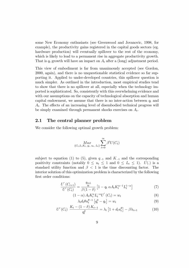
subject to equation (1) to (5), given q−1 and K−1 and the correspondingpositivity constraints (notably 0 ≤ ut ≤ 1 and 0 ≤ Lt ≤ 1). U(.) is astandard utility function and β < 1 is the time discounting factor. Theinterior solution of this optimization problem is characterized by the followingfirst order conditions:

U (Ct+1)

U (Ct)=

qt+1qt

β (1− δ)1− qt αAtKα−1

t L1−αt (7)

(1− α)AtKαt L

−αt U (Ct) = wt (8)

λtdtθuθ−1t q0t − qt = wt (9)

U (Ct)Kt − (1− δ)Kt−1

q2t= λt 1 + dtu

θt − βλt+1 (10)

9

where w and λ are the multipliers associated with the labor market clearingcondition (5) and with the imitation technology (3), respectively.3 Equation(7) gives the optimal intertemporal consumption (or saving) plan. It is a com-pletely standard Keynes-Ramsey rule if one abstracts from the presence of theq terms. In particular, it implies that the optimal growth rate of consump-tion is determined by the marginal productivity of capital α AtKα−1

t L1−αt ,the discount rate β, and the depreciation rate δ. For example, the higherthe marginal productivity of capital, the stronger the incentives to save andthe higher the expected growth rate of consumption. When we accountfor embodied technological progress, the Keynes-Ramsey rule is modified intwo aspects. Since the capital goods are increasingly efficient over time,the marginal productivity of capital should incorporate this efficiency. It isexpressed in efficiency units in equation (7), ie. it is multiplied by qt.

On the other hand, it should be noted that, consistently with Greenwood,Hercowitz and Krusell (1997), the price of the capital good in terms of theconsumption good is 1

qtin our model: For each unit of forgone consumption

at t, the economy can build up qt units of capital at t. Suppose that qt is in-creasing, then the relative price of capital is decreasing, and the consumptiongood is expected to be more expensive over time, and consumption is likelyto fall in the future. This effect is called obsolescence effect by Boucekkine,del Río and Licandro (2002); it is inherent to embodied technical change andit tends to lower the growth effects of the latter.

Equations (8) and (9) are the optimality conditions with respect to produc-tion labor and adoption labor respectively. In each equation, the marginalproductivity of labor is equal to the shadow wage. Since labor is homoge-nous, we have a unique shadow wage. Equation (10) is the optimal conditionwith respect to qt. The left hand side is the benefit from a marginal increasein qt: such an increase will allow to raise the capital stock by It in efficiencyunits, which is equal by equation (2) to Kt−(1−δ)Kt−1

qt, and by It

qtin physical

units (in terms of the consumption good), which in turn allows to raise utilityby U (Ct)

Itqt. The right hand side gives the cost of a marginal increase in qt.

Notice that λt is by definition, the shadow price of qt. The right hand side ofequation (10) is the marginal cost of qt: It includes the usual intertemporalterm λt − β λt+1, retrieving future value gains from the shadow price, plus

3plus the standard transversality conditions: limt→∞ λt qt = 0, and limt→∞ λt Kt =0, where λt is the multiplier associated with the production function of capital goods, (2).

10

the less usual term λt dtuθt . This term comes entirely from the specification of

the imitation technology (3): a marginal increase in qt costs indeed 1+ dtuθt ,to be multiplied by the shadow price to get eh welfare cost.

We now turn to the analysis of the steady state growth paths.

2.2 The balanced growth paths: existence and com-parative statics

>From now, we assume a logarithmic utility function. We define the steadystate growth paths as usual in exogenous growth theory: along the balancedgrowth path, ut and Lt are constant and the remaining variables grow atconstant rates. Denoting by gx the long-run growth factor of a variable Xtand

_

X its long-run level, we have the following simple properties:

Proposition 1 If q0t grows at rate γ > 1, then all the other variables growat strictly positive rates with

gq = γ

gK = γ1

1−α

gC = gI = gY = γα

1−α .

Not surprisingly, the growth rate of the capital stock is higher than the othervariables: the capital stock is expressed in efficiency units and as such, itsgrowth rate is the sum of the growth rates of q and I. The long term levelsare much harder to characterize. In order to simplify a little bit, we useequation (9) to eliminate the multiplier λ. The resulting eight restrictionsare as follows:

1− β (1− δ) γ−11−α = αqAKα−1L1−α

K 1− (1− δ) γ−11−α

q2C=

1 + duθ γ − β w

γdθuθ−1 (1− q)(1− α)AKαL−α = wC

1− qq

=(γ − 1)γduθ

11

K 1− (1− δ) γ−11−α = qI

Y = C + I

L+ u = 1

Y = AKαL1−α

The stationary long term system appears very messy. Nonetheless, we canprove that it has always a unique solution.

Proposition 2 If γ > 1, a unique stationary equilibrium exists for our econ-omy.

A detailed proof of this claim is reported in the Appendix. We can also proveanalytically the following comparative statics with respect to the technolog-ical parameters γ and d appearing in the imitation technology.

Proposition 3 Denote by s = IYthe long term investment ratio. The long-

run technological gap being TG = (γ−1)γduθ

, we have the following comparativestatics properties:

∂u

∂γ> 0,

∂TG

∂γ> 0,

∂s

∂γ> 0

∂u

∂d< 0,

∂TG

∂d< 0,

∂s

∂d= 0.

The proof is in the Appendix. A technological acceleration abroad inducea stronger adoption effort. However, this increment is not enough to lowerthe long term technological gap. This property comes from an importantarbitrage settlement in the model. When u goes up, the amount of labordevoted to production decreases, which in turn tends to decrease output andconsumption. Moreover, the consumption share in output goes down whenthe rate of embodied technological progress is raised. It is very importantto understand why this property holds. Recall that the growth rate of q isprecisely the rate of decline of the relative price of capital. Hence, when γincreases, this rate of decline decreases, inducing a typical substitution effectunfavorable to consumption. Overall, consumption tends to decrease for tworeasons when a technological acceleration occurs. A central planner whocares about consumption per capital should consequently try to alleviate theinduced fall in consumption by producing a moderate adoption effort. Social

12

welfare maximization is indeed incompatible with a sharp adoptioneffort in the long run.The same mechanisms are involved when the productivity d of the imitationsector goes up. This could be the result of a trade reform facilitating adoptionor a permanent improvement in the skills of the employees of the technologysector. In such a case, the fraction of labor devoted to adoption goes downbut the technological gap goes down too. Given the expression of the long runtechnological gap, this means that the product d uθ increases when d goes updespite the reduction in u. It is not hard to understand this result. Produc-tivity improvements in adoption allow to increase the level of technologicalprogress even though the labor contribution to this activity diminishes. Insuch a case, more labor is assigned to production, and the economy gainsa double advantage: More production (and so more consumption and morewelfare) and lower technological gap. In other words, the first best decisionsallow to reduce both the output and technological gaps. Finally in contrastto the shock on the rate of embodied technical change, a rising d does notalter the consumption and investment shares in output. Both investmentand consumption will rise, following the output increment, but they do so atthe same growth rate. There is fundamental reason for this. In contrast tothe shock on γ, a rising d does not alter the rate of decline of the relativeprice of capital (precisely equal to γ), which is the crucial determinant theoutput composition.

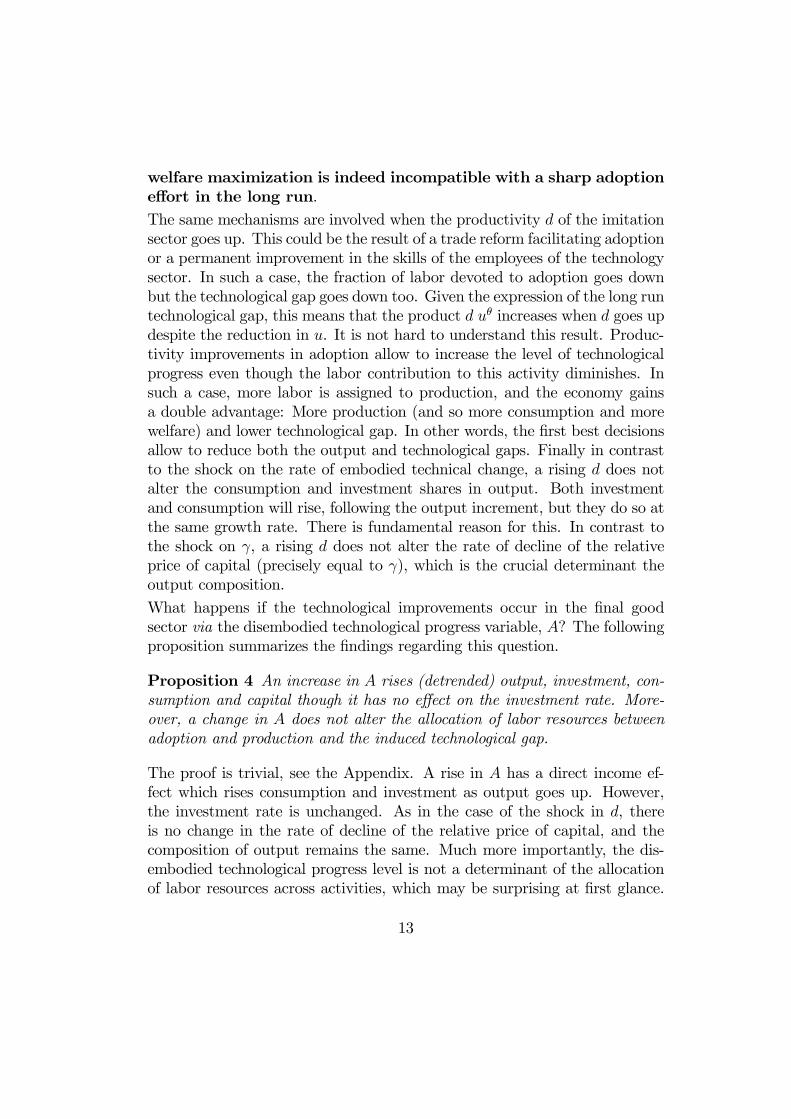
What happens if the technological improvements occur in the final goodsector via the disembodied technological progress variable, A? The followingproposition summarizes the findings regarding this question.

Proposition 4 An increase in A rises (detrended) output, investment, con-sumption and capital though it has no effect on the investment rate. More-over, a change in A does not alter the allocation of labor resources betweenadoption and production and the induced technological gap.

The proof is trivial, see the Appendix. A rise in A has a direct income ef-fect which rises consumption and investment as output goes up. However,the investment rate is unchanged. As in the case of the shock in d, thereis no change in the rate of decline of the relative price of capital, and thecomposition of output remains the same. Much more importantly, the dis-embodied technological progress level is not a determinant of the allocationof labor resources across activities, which may be surprising at first glance.

13

However, one should keep in mind that an increase in A raises the shadowwage (since labor marginal productivity is shifted upwards). Since labor ishomogenous and given the optimal labor decisions (8) and (9), the directwage impact of the shock in A is identical in the two sectors (final good andtechnology sectors), and there is no reason to alter the initial allocation oflabor resources across sectors. As a consequence, the technological gap isalso insensitive to the latter variable, since it entirely depends on the adop-tion of investment-specific technological progress. If the adoption effort isunaffected, the technological gap is.

3 Dynamics

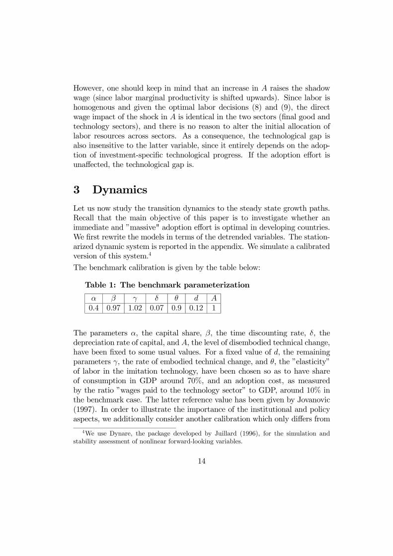
Let us now study the transition dynamics to the steady state growth paths.Recall that the main objective of this paper is to investigate whether animmediate and ”massive" adoption effort is optimal in developing countries.We first rewrite the models in terms of the detrended variables. The station-arized dynamic system is reported in the appendix. We simulate a calibratedversion of this system.4

The benchmark calibration is given by the table below:

Table 1: The benchmark parameterization

α β γ δ θ d A0.4 0.97 1.02 0.07 0.9 0.12 1

The parameters α, the capital share, β, the time discounting rate, δ, thedepreciation rate of capital, and A, the level of disembodied technical change,have been fixed to some usual values. For a fixed value of d, the remainingparameters γ, the rate of embodied technical change, and θ, the ”elasticity”of labor in the imitation technology, have been chosen so as to have shareof consumption in GDP around 70%, and an adoption cost, as measuredby the ratio ”wages paid to the technology sector” to GDP, around 10% inthe benchmark case. The latter reference value has been given by Jovanovic(1997). In order to illustrate the importance of the institutional and policyaspects, we additionally consider another calibration which only differs from

4We use Dynare, the package developed by Juillard (1996), for the simulation andstability assessment of nonlinear forward-looking variables.

14

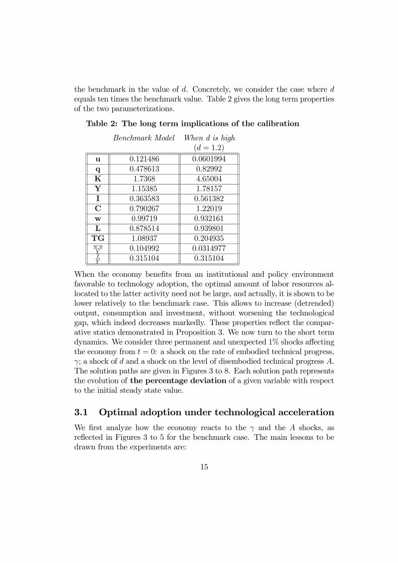
the benchmark in the value of d. Concretely, we consider the case where dequals ten times the benchmark value. Table 2 gives the long term propertiesof the two parameterizations.

Table 2: The long term implications of the calibration

Benchmark Model When d is high(d = 1.2)

u 0.121486 0.0601994q 0.478613 0.82992K 1.7368 4.65004Y 1.15385 1.78157I 0.363583 0.561382C 0.790267 1.22019w 0.99719 0.932161L 0.878514 0.939801TG 1.08937 0.204935w uY

0.104992 0.0314977IY

0.315104 0.315104

When the economy benefits from an institutional and policy environmentfavorable to technology adoption, the optimal amount of labor resources al-located to the latter activity need not be large, and actually, it is shown to belower relatively to the benchmark case. This allows to increase (detrended)output, consumption and investment, without worsening the technologicalgap, which indeed decreases markedly. These properties reflect the compar-ative statics demonstrated in Proposition 3. We now turn to the short termdynamics. We consider three permanent and unexpected 1% shocks affectingthe economy from t = 0: a shock on the rate of embodied technical progress,γ; a shock of d and a shock on the level of disembodied technical progress A.The solution paths are given in Figures 3 to 8. Each solution path representsthe evolution of the percentage deviation of a given variable with respectto the initial steady state value.

3.1 Optimal adoption under technological acceleration

We first analyze how the economy reacts to the γ and the A shocks, asreflected in Figures 3 to 5 for the benchmark case. The main lessons to bedrawn from the experiments are:

15

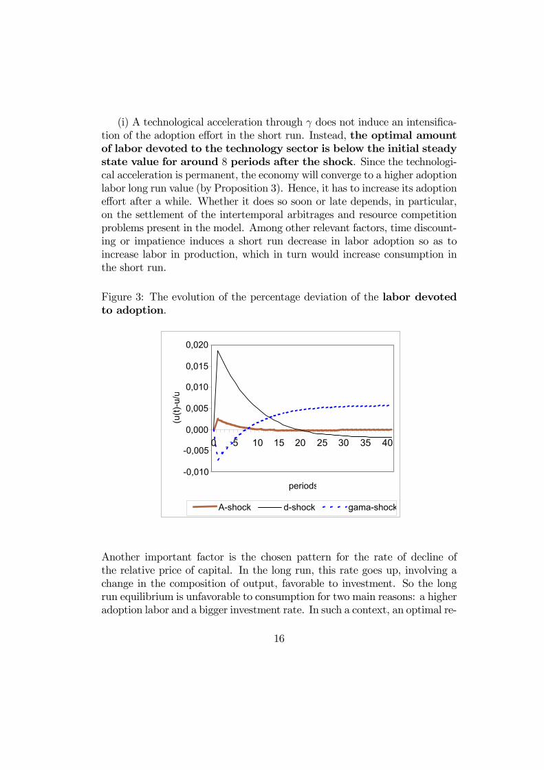
(i) A technological acceleration through γ does not induce an intensifica-tion of the adoption effort in the short run. Instead, the optimal amountof labor devoted to the technology sector is below the initial steadystate value for around 8 periods after the shock. Since the technologi-cal acceleration is permanent, the economy will converge to a higher adoptionlabor long run value (by Proposition 3). Hence, it has to increase its adoptioneffort after a while. Whether it does so soon or late depends, in particular,on the settlement of the intertemporal arbitrages and resource competitionproblems present in the model. Among other relevant factors, time discount-ing or impatience induces a short run decrease in labor adoption so as toincrease labor in production, which in turn would increase consumption inthe short run.

Figure 3: The evolution of the percentage deviation of the labor devotedto adoption.

-0,010

-0,005

0,000

0,005

0,010

0,015

0,020

0 5 10 15 20 25 30 35 40

periods

(u(t)

-u/u

A-shock d-shock gama-shock

Another important factor is the chosen pattern for the rate of decline ofthe relative price of capital. In the long run, this rate goes up, involving achange in the composition of output, favorable to investment. So the longrun equilibrium is unfavorable to consumption for two main reasons: a higheradoption labor and a bigger investment rate. In such a context, an optimal re-

16

action in the short run, given the discounted nature of the objective function,implies more production labor and/or a lower investment rate. In Figures 3and 5, we see that while the adoption labor goes clearly down in the shortrun, there is a very slight increase in the investment rate at t = 1, immedi-ately followed by a long transition below the initial steady state value. Bychoosing such a behavior, the economy lets the technological gap increasefrom t = 0 (to the new steady state value). Not surprisingly, welfare max-imization does not produce a decreasing pattern for the technological gap,neither in the long run (as proved in Proposition 3), nor in the short run.

Figure 4: The evolution of the percentage deviation of the technologicalgap.

-0,010

-0,006

-0,002

0,002

0,006

0 3 6 9 12151821 2427 30 3336 39

periods

(tg(t)

-tg/tg

A-shock d-shock gama-shock

(ii) The A shock produces much trickier outcomes. Figures 3 to 5 show aslight increase in the adoption effort, an almost immobile technological gapand a sharp rise in the investment rate, in the short run. It seems that theshock is almost entirely absorbed by the quantity variables, even in the shortrun! We know by Proposition 4 that only these variables are affected in thelong run. Whether the obtained short run dynamics are robust to changes inthe environment (notably to the value of d) is an interesting issue that willbe tackled in the next sub-section. Yet it is important to understand why a

17

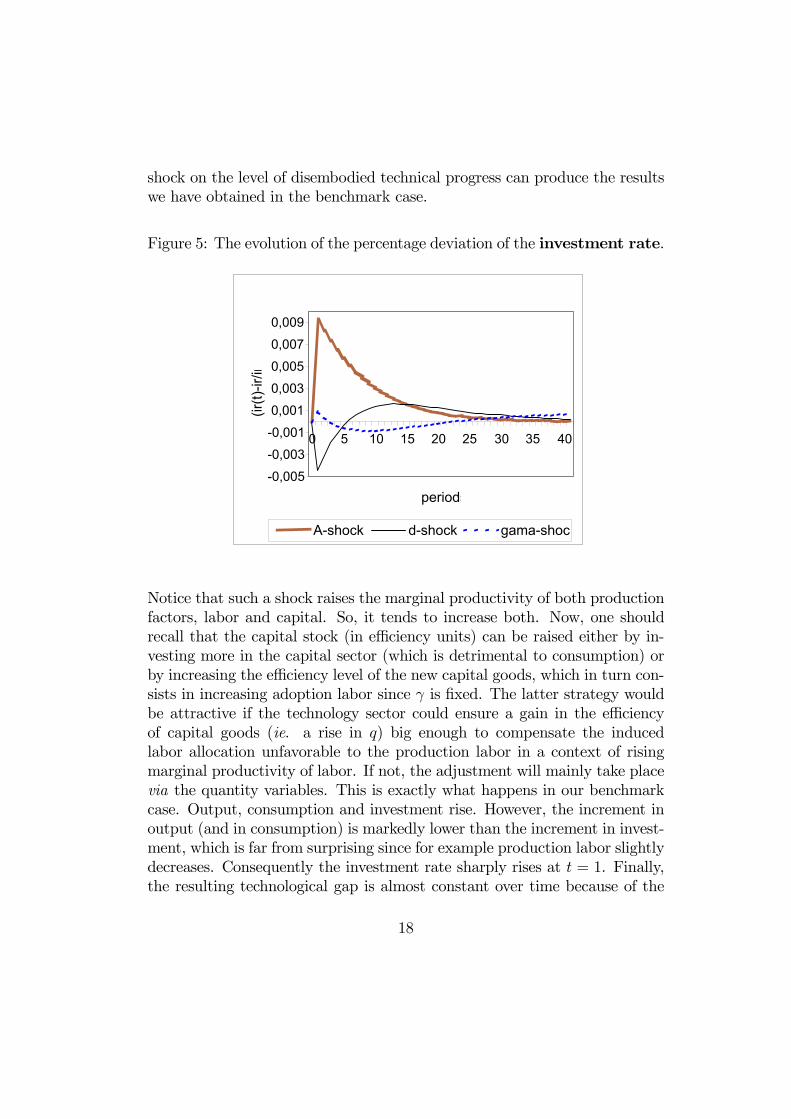
shock on the level of disembodied technical progress can produce the resultswe have obtained in the benchmark case.

Figure 5: The evolution of the percentage deviation of the investment rate.

-0,005

-0,003

-0,001

0,001

0,003

0,005

0,007

0,009

0 5 10 15 20 25 30 35 40

periods

(ir(t)

-ir/ir

A-shock d-shock gama-shoc

Notice that such a shock raises the marginal productivity of both productionfactors, labor and capital. So, it tends to increase both. Now, one shouldrecall that the capital stock (in efficiency units) can be raised either by in-vesting more in the capital sector (which is detrimental to consumption) orby increasing the efficiency level of the new capital goods, which in turn con-sists in increasing adoption labor since γ is fixed. The latter strategy wouldbe attractive if the technology sector could ensure a gain in the efficiencyof capital goods (ie. a rise in q) big enough to compensate the inducedlabor allocation unfavorable to the production labor in a context of risingmarginal productivity of labor. If not, the adjustment will mainly take placevia the quantity variables. This is exactly what happens in our benchmarkcase. Output, consumption and investment rise. However, the increment inoutput (and in consumption) is markedly lower than the increment in invest-ment, which is far from surprising since for example production labor slightlydecreases. Consequently the investment rate sharply rises at t = 1. Finally,the resulting technological gap is almost constant over time because of the

18

very limited scope of the reallocation of labor resources. Again, the techno-logical acceleration does not produce any short term intense adoption effort.However, in contrast to the acceleration in the rate of embodied technicalchange, the response of the economy is now characterized by an investmentboom in the short run.

3.2 Institutions, policy and optimal adoption

We now study the robustness of the results listed above to changes in thepolicy variable d. This is done in two steps.

(i) Figures 3 to 5 also report the results of a permanent shock on d forthe benchmark economy. From Proposition 3, we know that the economywill converge to a lower adoption labor but will achieve a smaller technolog-ical gap. So in the long run, labor allocation is favorable to the productionsector, and to consumption. In the short run, the economy takes advan-tage of the improvement in education and/or trade policy and institutionsby sharply raising adoption labor. So in contrast to the case of techno-logical accelerations, institutional and policy improvements in thetechnology sector can carry out a massive adoption effort in theshort run. Note however, that the subsequent decrease in production labordoes not lead to a drastic cut in the consumption level. Indeed, at the sametime, the optimal allocation of the final good is detrimental to the capitalsector (see Figure 5).

(ii) In a last experiment, we study the response of the economy to techno-logical accelerations for a value of d, ten times bigger than in the benchmarkcase. The results are reported in Figures 6 to 8. In the case of the γ shock,we get no massive and immediate adoption effort after the acceleration, ex-actly as in the benchmark case. There are however some clear quantitativedifferences. First of all, the initial drop in the adoption effort is less sharpand it takes only 4 periods to the economy to get above the initial steadystate value (it takes 8 periods in the benchmark case). Hence, under betterinstitutions and policy for monitoring technology adoption, the intense phaseof adoption starts much earlier, and it converges to a higher adoption laborvalue and to a lower technological gap (in percentage change with respect tothe steady state value).

In the case of the A shock, the differences with respect to the benchmarkcase are not only quantitative. Recall that such a shock induces an increase

19

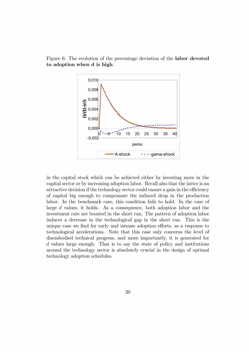
Figure 6: The evolution of the percentage deviation of the labor devotedto adoption when d is high.

-0,002

0,000

0,002

0,004

0,006

0,008

0,010

0 5 10 15 20 25 30 35 40

period

(ir(t)-ir/ir

A-shock gama-shock

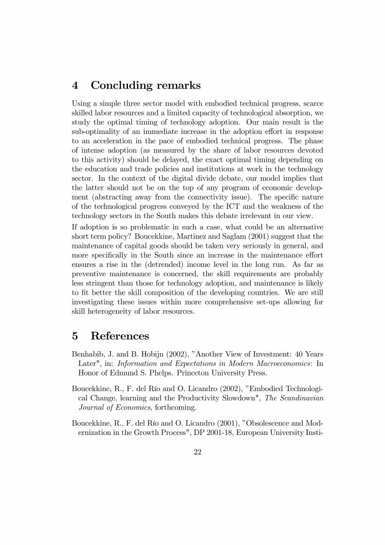
in the capital stock which can be achieved either by investing more in thecapital sector or by increasing adoption labor. Recall also that the latter is anattractive decision if the technology sector could ensure a gain in the efficiencyof capital big enough to compensate the induced drop in the productionlabor. In the benchmark case, this condition fails to hold. In the case oflarge d values, it holds. As a consequence, both adoption labor and theinvestment rate are boosted in the short run. The pattern of adoption laborinduces a decrease in the technological gap in the short run. This is theunique case we find for early and intense adoption efforts, as a response totechnological accelerations. Note that this case only concerns the level ofdisembodied technical progress, and more importantly, it is generated ford values large enough. That is to say the state of policy and institutionsaround the technology sector is absolutely crucial in the design of optimaltechnology adoption schedules.

20

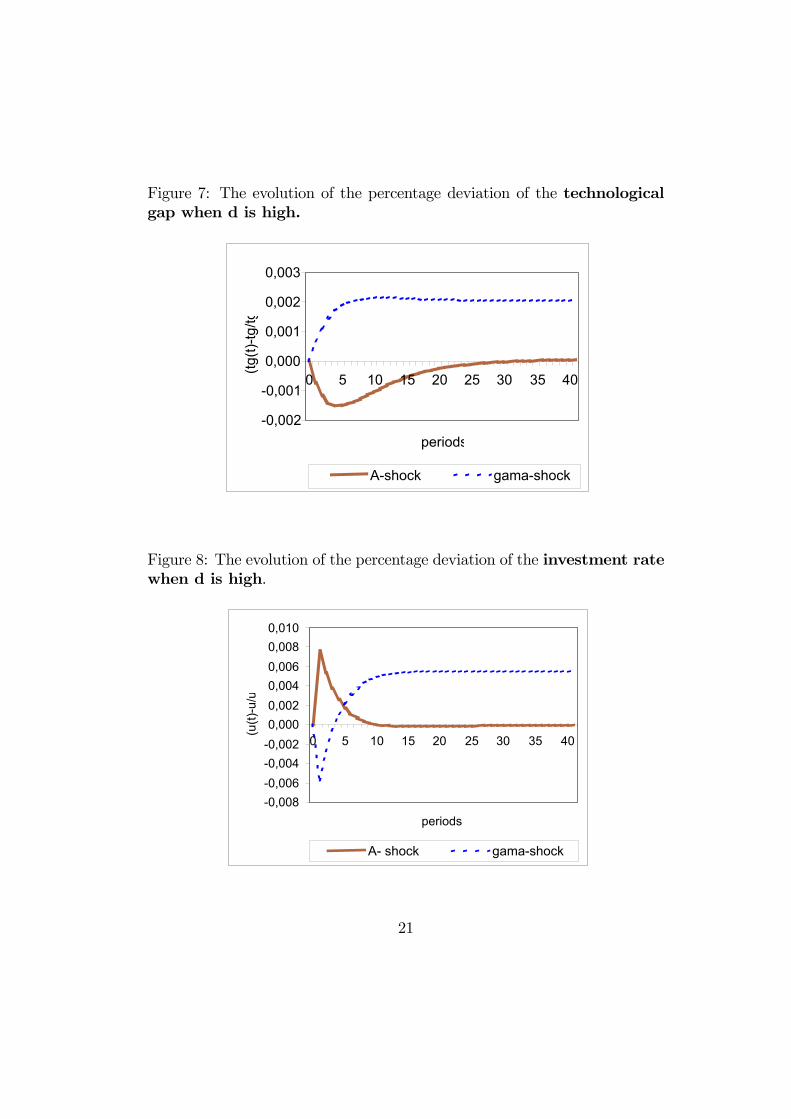
Figure 7: The evolution of the percentage deviation of the technologicalgap when d is high.

-0,002

-0,001

0,000

0,001

0,002

0,003

0 5 10 15 20 25 30 35 40

periods

(tg(t)

-tg/tg

A-shock gama-shock

Figure 8: The evolution of the percentage deviation of the investment ratewhen d is high.

-0,008-0,006-0,004-0,0020,0000,0020,0040,0060,0080,010

0 5 10 15 20 25 30 35 40

periods

(u(t)

-u/u

A- shock gama-shock

21

4 Concluding remarks

Using a simple three sector model with embodied technical progress, scarceskilled labor resources and a limited capacity of technological absorption, westudy the optimal timing of technology adoption. Our main result is thesub-optimality of an immediate increase in the adoption effort in responseto an acceleration in the pace of embodied technical progress. The phaseof intense adoption (as measured by the share of labor resources devotedto this activity) should be delayed, the exact optimal timing depending onthe education and trade policies and institutions at work in the technologysector. In the context of the digital divide debate, our model implies thatthe latter should not be on the top of any program of economic develop-ment (abstracting away from the connectivity issue). The specific natureof the technological progress conveyed by the ICT and the weakness of thetechnology sectors in the South makes this debate irrelevant in our view.

If adoption is so problematic in such a case, what could be an alternativeshort term policy? Boucekkine, Martinez and Saglam (2001) suggest that themaintenance of capital goods should be taken very seriously in general, andmore specifically in the South since an increase in the maintenance effortensures a rise in the (detrended) income level in the long run. As far aspreventive maintenance is concerned, the skill requirements are probablyless stringent than those for technology adoption, and maintenance is likelyto fit better the skill composition of the developing countries. We are stillinvestigating these issues within more comprehensive set-ups allowing forskill heterogeneity of labor resources.

5 References

Benhabib, J. and B. Hobijn (2002), ”Another View of Investment: 40 YearsLater", in: Information and Expectations in Modern Macroeconomics: InHonor of Edmund S. Phelps. Princeton University Press.

Boucekkine, R., F. del Río and O. Licandro (2002), ”Embodied Technologi-cal Change, learning and the Productivity Slowdown", The ScandinavianJournal of Economics, forthcoming.

Boucekkine, R., F. del Río and O. Licandro (2001), ”Obsolescence and Mod-ernization in the Growth Process", DP 2001-18, European University Insti-

22

tute (Florence), under revision in the Journal of Development Economics.

Boucekkine, R., B. Martinez and C. Saglam (2001), ”Technology Adoption,Capital Maintenance and the Technological Gap", Discussion Paper IRES2001-33.

Gordon, R. (2000), “Does the New Economy Measure up to the Great In-ventions of the Past?", Journal of Economic Perspectives 14, 49-74.

Greenwood, J. and B. Jovanovic (1998), “Accounting for growth", NBERWorking paper 6647.

Greenwood, J., Hercowitz, Z. and Krusell, P. (1997), Long-Run Implicationsof Investment-Specific Technological Change, American Economic Review87, 342-362.

Greenwood, J. and Yorukoglu, M. (1997), ”1974", Carnegie-Rochester Con-ference Series on Public Policy 46, 49-95.

Grether, JM. (1999), ”Determinants of Technological Diffusion in MexicanManufacturing: A Plant-Level Analysis", World Development 27, 1287-1298.

Jovanovic, B. (1997), “Learning and Growth", in D. Kreps and K. Wallis,eds., Advances in economics, Vol. 2 (Cambridge University Press, London):318-339.

Juillard, M. (1996), “DYNARE, a Program for the Resolution of NonlinearModels with Forward-Looking Variables. Release 2.1", CEPREMAP.

Krusell, P. (1998), Investment-Specific R & D and the Decline in the RelativePrice of Capital, Journal of Economic Growth 3, 131-141.

Nelson, R. and E. Phelps (1966), “Investment in Humans, Technology Dif-fusion and Economic Growth", American Economic review 56, 69-75.

Niosi, J., P. Hanel and L. Fiset (1995), Technology transfer to developingcountries through engineering firms: The Canadian Experience,World De-velopment 23, 1815-1824.

23

6 Appendix

1. Proof of Proposition 2 :

Proof. By means of successive substitutions, one can reduce the systemof eight equilibrium restrictions to a single implicit equation involving onlyu :

G (u) =1 + duθ γ − β u

(1− u) −αθ (γ − 1) γ

11−α − (1− δ)

(1− α) γ1

1−α − β (1− δ)= 0. (11)

It could be easily checked that G (u) is an increasing and convex functionwith

limu→0

G (u) = −αθ (γ − 1) γ

11−α − (1− δ)

(1− α) γ1

1−α − β (1− δ)< 0

limu→1

G (u) = +∞, as γ > 1, β < 1, d > 0.

Thus there exists a unique u∗ ∈ (0, 1) which satisfies G (u) = 0.

2. Proof of Proposition 3 :

Proof. The comparative statics are derived explicitly. For sake of sim-plicity, let’s denote by

R = γ1

1−α − β (1− δ) > 0,

Z = γ1

1−α − (1− δ) > 0, and

M =αθ (γ − 1) (1− δ) (1− β) γ

11−α

(α− 1)2 γR +αθZ

(1− α)R> 0.

We have:

∂u

∂γ=

(u− 1)2 u(1+duθ)1−u −M

[β − γ (1 + duθ (1 + (1− u) θ))] > 0

24

It is clear that the denominator is always negative for all values of u. The

sign of the expression depends onu(1+duθ)1−u −M . By means of the equi-

librium condition (11), one can conclude that, ∀u, such that G (u) = 0,u(1+duθ)1−u −M < 0. Thus, ∂u

∂γ> 0.

∂TG

∂γ=

1

duθγ2

1− (u− 1)2 (γ − 1) γθ u(1+duθ)

1−u −Mu [β − γ (1 + duθ (1 + (1− u) θ))]

> 0The sign of the expression depends on:

u β − γ 1 + duθ (1 + (1− u) θ) − (u− 1)2 (γ − 1) γθ u 1 + duθ

1− u −M .

For sake of simplicity, without loss of generality, let δ = 1. Then, we have:

−αθ (γ − 1)1− α

1− (1− u) γθ β − 1− duθ(1 + duθ) γ − β

− αθduθ+1 (1− u) < 0,

so that ∂TG∂γ

> 0.The rest of the comparative statics analysis is straightforward:

∂u

∂d=

(1− u)uθ+1γ[β − γ (1 + duθ (1 + (1− u) θ))] < 0

∂TG

∂d=

(γ − 1)u−θ γ 1 + duθ − β

γd2 [β − γ (1 + duθ (1 + (1− u) θ))] < 0.

Since s = IY= α γ

11−α−(1−δ)

γ1

1−α−β(1−δ), we get:

∂s

∂γ=

α (1− β) (1− δ) γα

1−α

(1− α) γ1

1−α − β (1− δ)2 > 0,

25

and

∂s

∂d= 0.

3. Proof of Proposition 4 :

Proof. The proof is trivial. Indeed: ∂x∂A= x

A11−α > 0, where x stands for

K, C, Y and I. Moreover, from the explicit expression of s given just above,∂s∂A= 0.

4. The stationarized dynamic system:

∼Ct∼Ct+1

=

∼qt+1γ

11−αt+1

∼qtβ (1− δ)

1− ∼qtα

∼At

∼K

α−1t

∼L1−αt

∼Kt − (1− δ)

∼Kt−1γ

−11−αt

∼q2

t

∼Ct

=1 +

∼dt∼uθ

t

∼wt

∼dtθ

∼uθ−1t 1− ∼

qt

− β∼wt+1

γt+1∼dt+1θ

∼uθ−1t+1 1− ∼

qt+1

(1− α)∼At

∼K

α

t

∼L−αt

∼Ct

=∼wt

∼qtγt =

∼qt−1 +

∼dt∼uθ

tγt 1−∼qt

∼Kt =

∼qt∼I t + (1− δ)

∼Kt−1γ

−11−αt

∼Y t =

∼At

∼K

α

t

∼L1−αt

∼Ct +

∼I t −

∼Y t = 0

∼Lt +

∼ut = 1

26