The Competitive Facility Location Problem Under Disruption …coral.ie.lehigh.edu/~ted/files/papers/CFLPD16.pdf · 2016-11-02 · The Competitive Facility Location Problem Under Disruption

The Competitive Facility Location Problem Under DisruptionRisks

Ying Zhang

Zhejiang Cainiao Supply Chain Management Co., Ltd., Hangzhou 310000, China

Lawrence V. Snyder and Ted K. Ralphs

Department of Industrial and Systems Engineering, Lehigh University, Bethlehem, PA, USA

Zhaojie Xue

Shenzhen University

COR@L Technical Report 16T-011-R2

The Competitive Facility Location Problem Under Disruption Risks

Ying Zhang∗1, Lawrence V. Snyder†2, Ted K. Ralphs‡2, and Zhaojie Xue3

1Zhejiang Cainiao Supply Chain Management Co., Ltd., Hangzhou 310000, China2Department of Industrial and Systems Engineering, Lehigh University, Bethlehem, PA, USA

3Shenzhen University

Original Publication: July 3, 2015

Last Revised: May 30, 2016

Abstract

Two players sequentially locate a fixed number of facilities, competing to capture market share. Facilitiesface disruption risks, and each customer patronizes the nearest operational facility, regardless of who operates it.The problem therefore combines competitive location and location with disruptions. This combination has beenabsent from the literature. We model the problem as a Stackelberg game in which the leader locates facilities first,followed by the follower, and formulate the leader’s decision problem as a bilevel optimization problem. A variableneighborhood decomposition search heuristic which includes variable fixing and cut generation is developed.Computational results suggest that high quality solutions can be found quickly. Interesting managerial insightsare drawn.

1 Introduction

This paper introduces the competitive facility location problem under disruption risks (CFLPD), a discrete facilitylocation model that, to the best of our knowledge, is the first to incorporate possible disruptions into a compet-itive facility location problem. In many industries, service competition is present among multiple firms such assupermarkets or gas stations. Customers may choose among competing facilities based on distance (as we assumein this paper), quality, brand loyalty, or other factors. In addition, facilities may face disruptions from time totime due to natural disasters, labor actions, or power outages. When a facility is disrupted, its customers mayseek service from another operational facility belonging to the same player; they may seek service from a facilitybelonging to a different player; or their sales may be lost entirely. In either of last two cases, the customer’s originalservice provider loses revenue, and in all three cases, the customers incur higher service costs. For express carrierssuch as FedEx and UPS, both service competition and delivery delays or labor disputes will influence their brandrecognition, service quality and market share. For example, a FedEx store may lose its customers if it deliverspackages late due to labor actions or other disruptions, or if a UPS store is nearby. This highlights the need foran optimal facility deployment that considers both service competition and probabilistic facility disruptions.

We consider a supplier–receiver network with multiple customers and two noncooperative firms (the playersof the Stackelberg game): the leader and the follower. The players make facility location decisions sequentially,

∗[email protected]†[email protected]‡[email protected]

2

with each aiming to maximize its own market share or revenue. This setup is well modeled as a Stackelberg game(Dempe 2002) in which each player has exactly one move. The leader will first open B facilities, anticipating thatthe follower will react rationally by optimally placing K facilities. Each customer has a demand and seeks thenearest operating facility for service. We assume a binary preference model in which each customer chooses onlya single operating facility for service at any one time.

In addition, the facilities opened are subject to disruptions. When a facility is disrupted, it cannot servecustomers. Following Snyder and Daskin (2005), we assume that customers of disrupted facilities are reassignedto another (functional) facility. In particular, we assign each customer to multiple facilities in a sequence ofassignment levels r = 1, 2, · · · .1 For each customer, the closest facility (r = 1), the so-called the primary facility,will serve it under normal circumstances. If the primary facility fails, the customer is served by its first backupfacility (r = 2). If that facility fails too, it is served by its level-3 facility, and so on. In general, a facility assignedto a customer at level r serves that customer if all r − 1 facilities at lower levels have failed. If a customer’sprimary facility fails and the nearest operating facility is owned by the other player, then the player that owns theprimary facility will lose that customer until the disruption ends. If all of the facilities assigned to the customerare disrupted, the customer is lost by both of the players.

We formulate the problem as a binary bilevel linear optimization problem (BBLP). The model determines theoptimal locations for the leader in order to maximize her market share, under the strongest possible response bythe follower. If the facilities are assumed to be always reliable, i.e., each customer can always be captured by thenearest facility, then we obtain as a special case the discrete (r|p)-centroid problem (RPCP) (Alekseeva et al. 2010)and the closely related competitive maximal covering location model (Serra and ReVelle 1994, Seyhan et al. 2015).(The competitive maximal covering model assumes that customers will only patronize facilities within a givencoverage radius, whereas the RPCP allows any assignment, regardless of distance; otherwise, the two problemsare identical.)

It has been shown that the discrete RPCP is NP-hard; in fact, it belongs to the class of∑P

2 -hard problems(Noltemeier et al. 2007). This means that to check whether a (leader’s) decision is feasible requires solving an NP-hard problem (to optimize the follower’s strategy). This study addresses this complicated but also realistic problem.Our main contributions are as follows: First, we construct a BBLP model for this new type of facility locationproblem. Second, we develop a matheuristic based on variable neighborhood decomposition search (VNDS) whichincludes variable fixing and cut generation interactively. We further show that this matheuristic can be extendedto a large class of BBLP directly. Third, extensive experiments and sensitive analysis demonstrate the effectivenessof our approach. Results on RPCP benchmarks show that the VNDS matheuristic is very promising comparedto the current best heuristics and exact approaches for this special case. Results on the more general CFLPDinstances draw many interesting managerial insights on the approximate facility deployment strategies and marketshare competition.

The remainder of this paper is organized as follows. We review the relevant literature in §2 and formulate theCFLPD as a BBLP in §3. A matheuristic using VNDS is provided in §4. The numerical experiment design andcomputational results are presented in §5. Finally, §6 concludes the paper and discusses future research.

2 Literature Review

Facility location problems have been extensively studied in the past few decades, due to the wide variety ofapplications that arise in placing distribution centers, warehouses, gas stations, and fire stations, as well asin constructing communication networks, and so on. Two of the most well-studied problems are the p-medianproblem and the maximal covering location problem. The p-median problem is to locate p facilities so that the totaldemand-weighted distance between each customer and the nearest facility is minimized. The maximal covering

1Note that we index the levels beginning at r = 1, whereas Snyder and Daskin (2005) and others index them beginning at r = 0.

3

location problem seeks to locate a fixed number (e.g., p) of facilities so that the number of covered demands ismaximized. For overviews of these two classical models, see, for example, Snyder (2010) or Daskin (2013).

Both the p-median problem and the maximal covering location problem ignore the effect of competition onthe location decision and assume that there is a single decision-maker. However, many firms face location-basedcompetition, and failing to account for this competition when choosing facility locations can result in lower thananticipated market share. Competitive facility location problems take this competition into account; most assumethere are two players who successively open their facilities, each aiming to capture customers and maximize revenue.For reviews of competitive location models, see Eiselt et al. (1993), Serra et al. (1994), Eiselt and Laporte (1997),Kress and Pesch (2012) and Farahani et al. (2014).

One competitive location problem, the RPCP, has attracted increased attention in the past five years. In thisproblem, the leader places p facilities on a graph knowing that the follower will react by placing r facilities.2.The goal of both the leader and the follower is to maximize its own market share (Alekseeva et al. 2010). Thisproblem is often formulated as a BBLP. Recent algorithms have been tested using instances with up to 100 cus-tomers, 100 potential facilities and p = r = 20 or 30 from the Discrete Location Problems benchmark library3.Exact approaches—including the iterative exact method by Alekseeva et al. (2010), the branch-and-cut (RP-B&C)method by Roboredo and Pessoa (2013) and the modified iterative exact method (MEM) by Alekseeva and Ko-chetov (2013)—guarantee global optimality but are very computationally intensive (e.g., more than 10 hours forp = r = 10; see Roboredo and Pessoa (2013)). The iterative exact method by Alekseeva et al. (2010) is basedon a single-level binary optimization problem with exponentially many constraints and variables. The model isrepeatedly solved, with new sets of follower locations added iteratively. The RP-B&C method by Roboredo andPessoa (2013) is similar but with only a polynomial number of variables, and the exponentially many constraintsare lifted into stronger inequalities. MEM (Alekseeva and Kochetov 2013) improves the iterative exact method byusing a model with only a polynomial number of variables and by using the strengthening inequalities introducedby Roboredo and Pessoa (2013). Heuristics based on operations (e.g., probabilistic swapping) for the p-medianproblem have shown high accuracy for a relatively small number of iterations. However, the complexity of eachiteration still remains rather high, because the follower’s problem has to be solved to evaluate the leader’s neigh-borhood solution. The most effective heuristic methods proposed to date are the hybrid memetic algorithm (HMA)by Alekseeva et al. (2009), the tabu search algorithm with Lagrangian relaxation (TSL) by Davydov (2012), thevariable neighborhood search (VNS) and stochastic tabu search (STS) by Davydov et al. (2014), and the hybridgenetic algorithm with solution archive (GA+solA) by Biesinger et al. (2015).

As noted above, the RPCP is closely related to the competitive maximal covering location problem, introducedby Serra and ReVelle (1994) and based on the classical maximal covering location problem (Church and Velle 1974).Most heuristics for this problem, including the heuristic by Serra and ReVelle (1994), involve iterating betweenthe leader’s and follower’s decisions, which will result in finding a Nash equilibrium (NE) but not necessarily theNE that is best for the leader. For the same problem and two variants, Plastria and Vanhaverbeke (2008) restrictthe follower to opening a single facility (K = 1), which allows them to reformulate the problem as a single-levelproblem. Seyhan et al. (2015) expand this idea to allow general K by assuming that the follower solves his problemusing a greedy algorithm; the greedy solution is captured by a polynomial number of constraints in the leader’ssingle-level problem.

The competitive location literature generally assumes that all facilities are completely reliable. In contrast,facility location models with disruptions have appeared only more recently. Snyder and Daskin (2005) introducethe reliable fixed-charge location problem (RFLP) and reliable p-median problem (RPMP), in which facilities aresubject to random disruptions with identical probability, to investigate the effect of probabilistic facility failureson the optimal facility deployment. Berman et al. (2007) consider a p-median problem under facility disruptionsand study its asymptotic properties. Cui et al. (2010) and Aboolian et al. (2012) generalize the work of Snyder

2When discussing the RPCP, we will use p and r to denote the number of facilities opened by the leader and the follower, respectively,instead of B and K as in our model, to remain consistent with the existing research.

3http://www.math.nsc.ru/AP/benchmarks/english.html

4

and Daskin (2005) by allowing site-dependent disruption probabilities. Zhang et al. (2016) allow site-dependentprobabilities and also incorporate inventory costs. Shen et al. (2011) formulate the RFLP as a nonlinear integeroptimization problem and propose a near-optimal heuristic for the special case with identical probabilities. SeeSnyder et al. (2015) for a recent review of the literature on facility location models with disruptions. Note,however, that all of the reliable location models we are aware of assume only a single firm, ignoring the potentialcompetition.

Another related body of literature is that on the network interdiction problem. As in the RPCP and CFLPD,this problem is usually modeled as a Stackelberg game between an intelligent attacker and a defender (Aksen et al.2014). The attacker’s (leader’s) objective is to cause the maximum (worst-case) disruption in an existing servicenetwork; the defender (follower) is responsible for locating/relocating facilities as well as protecting some of those toguarantee service. The majority of the research has its roots in military, homeland security applications or criticalinfrastructure planning (O’ Hanley and Church 2011, Liberatore et al. 2011, Losada et al. 2012, Gedik et al. 2014).Although they are similar in some respects to facility location problems, network interdiction problems are generallybeyond the scope of competitive location problems because only one player’s decision involves location/relocationactions.

Finding the optimal facility location design under service competition and disruption risks is extremely hard.Simultaneously using a bilevel optimization structure and a probabilistic facility disruption mechanism makes thisproblem very challenging to handle, especially for large instances. The bilevel structure introduces a nonconvexand combinatorial nature (Dempe 2002), while disruption risks give rise to a large number of probabilistic facilityfailure scenarios. To the best of our knowledge, only Wang and Ouyang (2013) simultaneously consider spatialcompetition and facility disruption risks in the context of facility location. They build a leader–follower Stackelbergcompetition model and design a continuous approximation scheme to find closed-form analytical solutions. In theirwork, location decisions are represented using continuous and differentiable density functions. Our paper, on theother hand, seeks to optimize facility locations on a discrete network. Our model is, to the best of our knowledge,the first to consider both service competition and disruptions in the context of a discrete facility location problem.

3 Model Formulation

In this section, we first introduce the notation that will be used throughout the paper. We then formulate theproblem as a BBLP. Finally, we will show how the proposed model can be simplified to suit the RPCP case, thusleading to some cutting planes which will be used in §4.

3.1 Notation

3.1.1 Parameters

Let I be a set of customer locations and J a set of potential facility locations. The parameter dij defines thedistance between customer i ∈ I and facility j ∈ J . Associated with each customer i is a demand (or purchasingpower) µi. Each facility in J can fail independently with an equal probability q. Each customer can be assignedto up to R facilities—one primary facility and R − 1 backup facilities—where R is a constant, 1 ≤ R ≤ B + K.To avoid ties in case of equal distances, we assume that two players cannot open the same site, and dij 6= dik,∀i ∈ I, j, k ∈ J, j 6= k. (If the true distances do have ties, the distances can be perturbed slightly to break themarbitrarily.) The goal of the leader is to choose B locations from J in order to maximize her market share underthe assumption that the follower in turn chooses K facilities to maximize his own market share.

To summarize, we have the following parameters:

• I = set of customers, indexed by i;

• J = set of potential facility locations, indexed by j;

5

• R = number of assignment levels;

• µi = demand of customer i ∈ I;

• q = (identical) failure probability of each facility;

• B,K = number of facilities that the leader, follower will open;

• dij = distance between customer i and facility j;

• aijk = 1 if dij < dik, for i ∈ I, j, k ∈ J , 0 otherwise.

Note that if the customers’ preferences are based on something other than distance, we can simply redefine dijas customer i’s “penalty” for using facility j, where smaller values indicate stronger preferences.

Realistically, facility failure probabilities may be heterogeneous and may depend, for example, on the facilities’geographical locations. Furthermore, a customer may be more willing to change to another facility if the openfacilities are closer, i.e., R could be increasing in K and B. Or, different customers may accept a different numberof facilities for service. However, for simplicity, in this paper, we assume that the failure probabilities are identicaland that R is constant, independent of K and B, among all customers. Furthermore, customers may use alternatedecision rules, such as the Huff rule (Ashtiani et al. 2013), which defines an attractiveness function on the facilities.However, the Huff rule would introduce nonlinearity, so we assume a binary preference for simplicity.

3.1.2 Decision Variables

We introduce the following binary decision variables:

xj =

{1, if facility j is opened by the leader

0, otherwise

yj =

{1, if facility j is opened by the follower

0, otherwise

zir =

{1, if customer i is assigned to a leader facility at level r

0, if customer i is assigned to a follower facility at level r

wijr =

{1, if customer i is assigned to facility j at level r

0, otherwise

3.2 Bilevel Formulation

Due to the independent-failure assumption, the probability that a customer receives service from its level-r facilityis (1− q)qr−1. The players want to maximize their own expected demand captured in the end of the game, takingall possible disruptions into account. The leader’s objective function is

max∑i∈I

R∑r=1

µizir(1− q)qr−1, (1)

while the follower’s objective function is

max∑i∈I

R∑r=1

µi(1− zir)(1− q)qr−1. (2)

6

Since this is a zero-sum game, (2) is equivalent to

min∑i∈I

R∑r=1

µizir(1− q)qr−1. (3)

Now the discrete CFLPD problem can be formulated as a BBLP model:

max∑i∈I

R∑r=1

µizir(1− q)qr−1 (4)

s.t. ∑j∈J

xj = B (5)

xj ∈ {0, 1} ∀j ∈ J (6)

where given the leader’s decision x, z is a component of the optimal solution to the follower’s problem:

min∑i∈I

R∑r=1

µizir(1− q)qr−1 (7)

s.t. ∑j∈J

yj = K (8)

xj + yj ≤ 1 ∀j ∈ J (9)

xj + 1 ≥ zir + wijr ∀i ∈ I, j ∈ J, 1 ≤ r ≤ R (10)

yj + zir ≥ wijr ∀i ∈ I, j ∈ J, 1 ≤ r ≤ R (11)∑k∈J

aikj(xk + yk)− (1− wijr)Mr ≤ r ∀i ∈ I, j ∈ J, 1 ≤ r ≤ R (12)∑j∈J

wijr = 1 ∀i ∈ I, 1 ≤ r ≤ R (13)

R∑r=1

wijr ≤ 1 ∀j ∈ J, i ∈ I (14)

yj , wijr ∈ {0, 1}, 0 ≤ zir ≤ 1 ∀i ∈ I, j ∈ J, 1 ≤ r ≤ R (15)

Constraints (9) prevent the players from opening facilities at the same site. Constraints (10) and (11) ensurethat if customer i is assigned to facility j at level r (i.e., wijr = 1), and if j is a leader facility (i.e., zir = 1), thenthe leader must open it (i.e., xj = 1); otherwise, if j is a follower facility (i.e., zir = 0), then the follower mustopen it (i.e., yj = 1). Summing (10) and (11) results in the following valid inequality4, which will tighten thelinear relaxation:

xj + yj + 1 ≥ 2wijr ∀i ∈ I, j ∈ J, 1 ≤ r ≤ R. (16)

Constraints (12) guarantee that customers are assigned to open facilities level by level in increasing order ofdistance. A customer i can’t be assigned to facility j at level r if there are more than r closer open facilities.

4We would like to express our gratitude to the referees for the introduction of this inequality.

7

The quantity∑

k∈J aikj(xk + yk) represents the number of open facilities that are closer than j for customer i.Mr = B +K − r is a large number.

Finally, constraints (13) say that each customer has to be assigned to a facility at each level (since we assumethat customer demands are lost only if all assigned facilities have been disrupted), and constraints (14) prohibita customer from being assigned to a given facility at more than one level. Constraints (6) and (15) are standardintegrality constraints. We can drop the integrality requirements on the z variables; in an optimal solution theywill equal 0 or 1.

From the leader’s perspective, (4)–(15) can be viewed as a mathematical optimization problem with a constraintregion that is implicitly defined by the follower’s subproblem (7)–(15). Once the vector x is chosen, though, thefollower simply faces a single-level optimization problem. The upper level (4)–(6) is called the leader’s problem;the lower level (7)–(15) is called the follower’s problem. Removing the lower-level optimality constraints yields thehigh point problem (Bialas and Karwan 1984): (4)–(6) and (8)–(15).

3.3 Remarks

The proposed CFLPD model reduces to the RPCP when q = 0 (so that R = 1). To formulate the leader’s problemin the RPCP, the subscript r could be removed from variables w and z, and constraints (14) can be removed sincethey would be redundant. Constraints (12) can be simplified to

wik ≤ 2− aijk − (xj + yj) ∀i ∈ I; k, j ∈ J. (17)

However, in this case, the follower’s problem has a tighter formulation. Given leader’s solution x, we can definethe set of facilities that allow the follower to capture customer i (Alekseeva and Kochetov 2013):

Ji(x) =

{j ∈ J

∣∣∣∣dij < minl∈J{dil|xl = 1}

}. (18)

Now the follower’s problem can be formulated as:

min∑i∈I

µizi (19)

s.t. ∑j∈J

yj = K (20)

1− zi ≤∑

j∈Ji(x)

yj ∀i ∈ I (21)

yj ∈ {0, 1}, 0 ≤ zi ≤ 1,∀i ∈ I, j ∈ J (22)

For the RPCP, formulation (19)–(22) has fewer variables and constraints than (7)–(15), which will reduce thecomputational burden when checking the feasibility of a given leader’s solution. For both the CFLPD and RPCP,in order to calculate the leader’s objective function, we need to solve the follower’s problem, which is NP-hardin the strong sense. Some bilevel methods which solve both the leader’s and the follower’s problems heuristicallyproduce only what are called semi-feasible solutions (Alekseeva and Kochetov 2013). However, the hybridizationof heuristics for the upper level with exact approaches for the lower level allows one to find optimal or near-optimalfeasible solutions. The method in §4 is based on this idea.

4 Variable Neighborhood Decomposition Search

Solving a bilevel optimization problem, even in its simplest form, is a difficult task. The vast majority of themethods proposed for bilevel problems have been restricted to special cases, such as using the KKT conditions to

8

transform linear bilevel optimization problems into equivalent single-level ones (e.g., Audet et al. (2007)). Thiscan be implemented by relaxing the integrality restrictions in the follower’s problem and taking the inner dual toconvert the bilevel problem into a single-level maximization problem. If the LP bound is tight, it is beneficial touse these bounds. However, our follower’s problem has the variable w, which makes the LP relaxation very weak:all customers will be assigned at all levels to the follower as long as K ≥ R.

Based on the analysis above, we solve the problem as a bilevel one. No practical methods are currently availablethat can consistently produce optimal solutions for general bilevel problems in reasonable computation time. Mooreand Bard (1990) and DeNegre and Ralphs (2009) propose a branch-and-bound algorithm and a branch-and-cutalgorithm for generalized BBLPs, respectively. According to DeNegre and Ralphs (2009), an integer point (x, y)is bilevel feasible if after fixing the leader’s solution x, solving the follower’s problem to optimality does result inthe follower’s decision y. With regards to a bilevel infeasible solution (x, y), Moore and Bard (1990) propose tobranch on the variable x (even if it is integer), while DeNegre and Ralphs (2009) propose to use valid inequalitiesto separate (x, y).

However, these methods may require substantial enumeration and also require repeated solution of binary mixedinteger optimization problems in checking bilevel feasibility of integer solutions. Therefore, direct application canbe time-consuming for large instances, so we now focus on a reduced solution space in this section, by fixing somevariables and by introducing new linear constraints.

In recent years, a growing literature has proposed heuristics for general MIPs, especially 0-1 MIPs, that combineaspects of local search with mathematical optimization techniques. Such heuristics are known as matheuristics andinclude the local branching paradigm (Fischetti and Lodi 2003), relaxation induced neighborhood search (Dannaet al. 2005), variable neighborhood search branching (Hansen et al. 2006) and variable neighborhood decompositionsearch (VNDS) (Lazic et al. 2010, Hanafi et al. 2014), among others. These papers demonstrate that combiningheuristic frameworks with the use of generic solvers can often give significant improvements in the resolution oflarge general MIPs. In this section, we propose a VNDS matheuristic to efficiently solve the CFLPD and show itsextendibility to general BBLPs. Some key procedures are elaborated first, followed by the main algorithm.

4.1 Algorithm Schematic

Once the facilities open by the players are given, the customer-assignment variables (w and z) can be determinedby the customers’ proximity to these open facilities. For the simplicity of notation, we will use X and Y torepresent the set of facilities opened by the leader and the follower, respectively. Recall that x and y are theincidence vectors in formulation (4)–(15). Then, X = {j|xj = 1}, Y = {j|yj = 1}. In addition, in the algorithmprocedures, (x0, y0) represents the incumbent solution whose neighborhood we are interested in, while (x∗, y∗)stores the current global best solution.

Assume that the total “available” demand is D =∑

i∈I∑R

r=1 µi(1− q)qr−1. Given the leader’s decision x′ andthe follower’s decision y′, function COST(x′, y′) will return the leader’s objective value (demand captured). Wewill use f(z) =

∑i∈I∑R

r=1 µizir(1− q)qr−1 to represent the objective function of the high point problem.In the sections that follow, given a leader’s solution x, any time we solve the follower’s problem exactly by

y = FOLLOWER-SOLVE(x), we will have a bilevel feasible solution (x, y). To avoid costly and unnecessaryre-evaluations and prevent the search from coming back to the previously visited solutions, we add the followingtabu cut,∑

j∈X

xj ≤ B − 1, (23)

where B is the cardinality of the binary support of the leader’s solution, to prohibit a revisit to x.The Local Search procedure proposed in §4.5 is developed to find the local optimum of the neighborhood

around (x, y). Once the local search is terminated and the solution (x, y) is recorded, it is valid to use (23) tocut off any solution (x, y). However, the bilevel feasible solution (x, y) is cut off as well. During the local search,

9

this may cause problems in practice when using a commercial framework, such as Gurobi or CPLEX, since it mayprevent the solution from being identified as feasible. Instead, we propose the following cut (24), which is satisfiedby (x, y), but not by the combination of x with a different follower’s solution.

Proposition 1 Given a bilevel feasible solution (x, y) to the high point problem (4)–(6), (8)–(15), let X0 = {j|xj =0},X1 = {j|xj = 1} and Y0 = {j|yj = 0},Y1 = {j|yj = 1}. The inequality

∑j∈Y0

yj +∑j∈Y1

(1− yj) ≤ K

∑j∈X0

xj +∑j∈X1

(1− xj)

(24)

is valid for (x, y), and is violated by every other integer solution (x, y).

Proof. Suppose x = x, y = y; then the left- and right-hand sides of (24) are both equal to 0, so the inequalityholds and is valid for (x, y).

On the other hand, suppose x = x, y = y 6= y; then the left-hand side of (24) is greater than or equal to 1,while the right-hand side equals 0, so the inequality is violated.

Fischetti and Lodi (2003) observe that the neighborhood of a feasible 0-1 MIP solution often contains bettersolutions. To reduce the neighborhood of (x, y), the following local branching cut is added to the high pointproblem,

∆(x, x) + ∆(y, y) =∑j∈X

(1− xj) +∑j∈Y

(1− yj) ≤ rhs, (25)

where rhs is the neighborhood size. Cut (25) is further equivalent to∑

j∈X xj +∑

j∈Y yj ≥ B + K − rhs. Asexplained by Fischetti and Lodi (2003), given the incumbent solution (x, y), the solution space associated withthe current branching node can be partitioned by means of the disjunction

∆(x, x) + ∆(y, y) ≤ rhs (left branch) or ∆(x, x) + ∆(y, y) ≥ rhs+ 1 (right branch).

Each left-branch subproblem constrained by ∆(x, x) + ∆(y, y) ≤ rhs (so-called soft variable fixing) will be easierto solve than the original problem; once it is solved to optimality or proved to contain no better solutions, theright-branch subproblem takes over and a new local branching cut is added.

Also note that in all pseudo-codes, right after an initial solution with objective value LB is obtained, anobjective cut

f(z) ≥ LB + ε (26)

is added to the high point problem; while each time the best lower bound LB is improved, the right hand side ofthe objective cut (26) should be set to the new value. ε > 0 is a small real number.

4.2 Intensification and Diversification

We first introduce the intensification and diversification procedure, which either intensifies or diversifies a givensolution depending on the input parameters. The procedure is presented in Algorithm 1.

As pointed out by Hansen et al. (2010), for many combinatorial optimization problems, local optima withrespect to one or several neighborhoods are located rather close to each other. This implies that a local optimumoften provides some information about the global optimum. Based on this fact, the search region may be reducedby using information about local optima that have already been found. Alekseeva and Kochetov (2013) show thatthe follower’s facilities are often in the immediate vicinity of the leader’s facilities. The follower attempts to “drag”

10

customers from the leader. Due to this property, and similar to the neighborhoods Fswap and Nswap designedby Davydov et al. (2014), Steps 2–8 in Algorithm 1 make an attempt to predict the follower’s behavior and findthe strongest preventive move for the leader. These steps attempt to find all solutions of the leader that resultfrom x0 by closing one facility j and opening another facility k. This new facility k should be either one from thefollower’s decision y0, or one located at no more than the 8th facility nearest to j. This replacement constitutes anew leader solution x1.

To evaluate x1, the corresponding follower’s subproblem has to be solved. Since x1 is just an intermediatesolution candidate, we are only interested in an approximate objective value for x1; the exact value will be too timeconsuming to solve since the follower’s problem is NP-hard. For the (r|p)-centroid problem, some papers (Biesingeret al. 2015, Davydov et al. 2014) solve the LP relaxation of the follower’s problem exactly. This approximationyields a lower bound on the true objective value of x1. However, the LP relaxation of our follower’s formulationis very weak, as explained in the front of §4. So instead, we adopt a greedy algorithm for solving the follower’sproblem, which yields an upper bound on the objective value of x1. Follower facilities are placed one after the otheraccording to the following greedy criterion: at each iteration, the facility that can capture the largest demand isopened. This process is repeated until K locations (y1) are chosen.

Steps 2–8 of Algorithm 1 will find the best 1-exchange neighborhood for the leader. Steps 9–15 will furtherrandomly choose a subset of B facilities from the union set X 0 ∪ Y0 that will induce the largest approximateobjective value for the leader if the follower uses the greedy method. Note that in Step 3 and Step 10, theleader’s new decision x1 should not have been tabu yet. Finally, as shown in Steps 18–20, if the input parameterisAlwaysUpdated = TRUE, this procedure will always update the incumbent (x0, y0) (thus a diversification); onthe other hand, if isAlwaysUpdated = FALSE, this procedure will update (x0, y0) only if the new solution (x′, y′)is better (thus an intensification).

Algorithm 1 (x′, y′) = Mutation(x0, y0, isAlwaysUpdated)

1. Set maxC = 0;2. for each facility j in X 0 do3. replace j with another facility k, resulting a new leader’s solution x1;4. use x1 as an input, solve the follower’s problem greedily, obtain the follower’s decision y1;5. if COST(x1, y1) > maxC then6. set x′ = x1,maxC = COST(x1, y1);7. end if8. end for9. for i = 0 to 10 do

10. randomly select B facilities from the set X 0 ∪ Y0 to constitute a new leader’s solution x1;11. use x1 as an input, solve the follower’s problem greedily, obtain the follower’s decision y1;12. if COST(x1, y1) > maxC then13. set x′ = x1,maxC = COST(x1, y1);14. end if15. end for16. use x′ as an input, solve the follower’s problem exactly, y′ =FOLLOWER-SOLVE(x′);17. add the tabu cut

∑j∈X ′ xj ≤ B − 1;

18. if isAlwaysUpdated = FALSE and COST(x′, y′) ≤ COST(x0, y0) then19. reset x′ = x0, y′ = y0;20. end if21. return (x′, y′)

11

4.3 Initialization

For the initial solution, we select an approximate solution of the p-median problem with a weighted distance

matrix (µidij). In this case, the leader ignores the follower but tries to place her facilities as close to customers

as possible. Alekseeva and Kochetov (2013) indicate that this approach yields a good approximate solution.

Then, as introduced in Section 4.1, we add the tabu cut with respect to x0 to avoid revisiting the same solution.

Simultaneously, we will search the neighborhood of the incumbent solution (x0, y0) to see whether it can be further

improved by the procedure “Mutation”. Finally, we add the objective cut to discard worse solutions in the future

search. The initialization procedure is illustrated in Algorithm 2.

Algorithm 2 (x0, y0) = Initialization()

1. solve the p-median problem, get the leader’s decision x0;2. use x0 as an input, solve the follower’s problem exactly, y0 =FOLLOWER-SOLVE(x0);3. add the tabu cut

∑j∈X 0 xj ≤ B − 1 to the high point problem;

4. intensify the initial solution by (x0, y0) = Mutation(x0, y0, FALSE);5. add the objective cut f(z) ≥ COST(x0, y0) +ε;6. return (x0, y0);

4.4 Variable Fixing

Danna et al. (2005) observe that in a general 0-1 MIP, some variables often take the same values in the optimal

solution and in the LP relaxation solution. Therefore, if a variable has the same value in the incumbent and the

LP relaxation solution, it is more likely that it will keep that value in the optimal solution. If such variables

are fixed, then one can get a much smaller problem. Based on this observation, Danna et al. (2005) propose a

relaxation induced neighborhood search (RINS) method. This variable fixing process is often called hard variable

fixing (Bixby et al. 2000). We extend this idea in our VNDS heuristic.

At each iteration, we fix B + K − l location variables to their values in the incumbent solution (x0, y0), i.e.,

the subsequent local search (Section 4.5) will be performed on the subspace of l variables. The decomposition

procedure is presented in Algorithm 3. After this process, the number of free variables in the current problem is

decreased.

Since the current leader’s solution x0 must have been tabu, the locations that are opened by the leader cannot

all be fixed. In other words, at least one facility that belongs to the set X 0 has to be released. So in the variable

fixing process, we first randomly choose one facility j from the leader’s decision X 0. Then the other l− 1 facilities

to be released are chosen from the set X 0∪Y0, according to their distance to the facility j. The remaining facilities

will be fixed in the local search phase. This procedure is similar to the decomposition scheme used by Hansen

12

et al. (2001) for the p-median problem.

Note that after fixing the location variables, the high point problem could be further reduced by fixing the

assignment variables w and z. For a problem with R ≥ 3, suppose the facilities that are fixed by the leader and

the follower are {j1, j2} and {j3, j4, j5}, respectively. For customer i, suppose the 3 closest facilities are j1, j2 and

j3. Then, as long as facilities j1, j2 and j3 are open (and this is always the case, since they are fixed), customer i

will surely be assigned to j1 at the first level, to j2 at the second level and to j3 at the third level. So we can fix

wij11 = 1, wij22 = 1, wij33 = 1 and zi1 = 1, zi2 = 1, zi3 = 0. Next, considering constraints (13), we can further set

wij1 = 0, ∀j ∈ J \ {j1}, wij2 = 0,∀j ∈ J \ {j2} and wij3 = 0, ∀j ∈ J \ {j3}; regarding constraints (14), we can set

wij1r = 0,∀r 6= 1, wij2r = 0, ∀r 6= 2 and wij3r = 0,∀r 6= 3. Finally, if the number of follower’s facilities that are

fixed is equal to K, e.g., K = 3 in this case, we can set yj = 0,∀j ∈ J \ {j3, j4, j5}.

After this variable fixing process, the scale of the problem will be decreased considerably, so that the solver

will solve the reduced problem quite efficiently in the local search phase.

Algorithm 3 P = Variable-Fixing(l, x0, y0)

1. choose at random one site j from leader’s facilities X 0;2. take j’s l − 1 closest facilities among those that belong to the set X 0 ∪ Y0;3. let J1 and J2 be the sets of leader’s and follower’s facilities, resp., chosen in the previous two steps;4. for problem P , fix the locations X 0 \ J1 and Y0 \ J2 for the leader and the follower, respectively;5. fix the corresponding values for variables w and z;6. return P ;

4.5 Local Search

Note that in our algorithm, we combine two approaches: hard variable fixing in the main scheme (Section 4.4) and

soft variable fixing in the local search. Soft variable fixing is implemented by adding local branching cuts. The

procedure of the local search phase is given in Algorithm 4.

At each iteration of the Local Search procedure, a local branching cut ∆(x, x0) + ∆(y, y0) ≤ rhs, with the

incumbent solution (x0, y0) and the current value of rhs, is added to the current problem (Step 3). Then the MIP

solver is called to solve the high point problem (Step 4) within given node time limit tmip and current best lower

bound LB. Thus, the search space for the solver is reduced, and a solution is expected to be found (or be proven

infeasible) in a much shorter time than the time needed for the original problem without the local branching cut

and without the variable fixing.

The subsequent steps depend on the status of the MIP solver. If the subproblem is solved to optimality (Step

6) or proved to be infeasible (including the case that the upper bound is lower than LB) (Step 12), we do not

need to consider the current neighborhood in further solution space exploration, so the current local branching

13

cut is reversed (Step 7 and Step 16). In case of infeasibility (Step 12), the neighborhood size is increased by one

(rhs = rhs + 1, Step 17); however, if rhs ≥ l, the next solving must be infeasible so the local search terminates

immediately (Step 14), since in the subproblem, the hard variable fixing requires that B+K− l location variables

are fixed to 1, while the soft variable fixing imposes B +K − rhs location variables to be 0. If a feasible solution

is found but has not been proven optimal (this new solution must be better than the incumbent (x0, y0), since we

update the objective cut once an improved lower bound is obtained), the last left branching is removed (Step 10),

and later will be replaced by the new branching cut (Step 3). Finally, if the solver fails to find a feasible solution

and also to prove the infeasibility of the current subproblem (Step 19), the local search phase is terminated.

We should emphasize that when the MIP solver is used to solve the problem, during the solving process, any

time the solver finds an integer solution (x1, y1), the follower problem is solved exactly to check whether (x1, y1)

is bilevel feasible or not. If it is bilevel feasible, now an improved solution is obtained; otherwise, if it is infeasible,

we will get another follower’s decision y1, and solution (x1, y1) is bilevel feasible. When the solver terminates, it

will return a set of bilevel feasible solutions, consisting of the set S, along with a set of checked leader’s solutions

x′ (Step 4). We can traverse the set S, and select the best one to update the incumbent solution (x0, y0) (if the

best one is better than the incumbent, Step 22). In addition, in order to avoid returning to the same solutions

(x′) again during the search process, we need to add a tabu cut for each checked leader’s solution (Step 25). Note

that all branching cuts are temporary, they need to be removed at the end of the local search phase (Step 28),

while all tabu cuts are static or permanent.

4.6 The VNDS Algorithm

Variable neighborhood search (VNS) (Hansen and Mladenovic 2001, Hansen et al. 2010) is a recent metaheuristic

that is based on the systematic change of neighborhoods, aiming for an ascent to local optimum and an escape

from local valleys. Variable Neighborhood Search Branching is a heuristic for solving MIPs, using a general-purpose

MIP solver as the black-box (Hansen et al. 2006). As in the local branching method, neighborhoods are defined

by adding constraints to the original problem, thus reducing the solution space and yielding an easier problem.

VNDS follows a general VNS scheme within a successive approximate decomposition method (Hansen et al. 2001).

Readers may refer to these literatures for details. The main scheme of the proposed VNDS algorithm is presented

in Algorithm 5, consisting of all the sub-procedures introduced in the above sections. The basic idea is to define

a variable fixing scheme for generating a sequence of smaller subproblems that are normally easier to solve than

the original problem.

The local branching heuristic (Fischetti and Lodi 2003) and the general VNS scheme (Hansen et al. 2010)

have many parameters. Here, we make our heuristic more user-friendly by reducing those parameters to only two,

14

Algorithm 4 (x′, y′) = Local-Search(x0, y0, LB, l, P )

1. set rhs = 1, isExit = FALSE, tmip = max{20, 10l};2. while isExit = FALSE do3. add the local branching cut ∆(x, x0) + ∆(y, y0) ≤ rhs to P ;4. solve P within node time limit tmip and best lower bound LB: (S, x′, solutionStatus) = LEADER-

SOLVE(tmip, LB, P );5. switch (solutionStatus)6. case “optSolFound”:7. reverse last local branching cut into ∆(x, x0) + ∆(y, y0) ≥ rhs+ 1;8. set rhs = 1;9. case “feasibleSolFound”:

10. remove the last left branching cut;11. set rhs = 1;12. case “provenInfeasible”:13. if rhs ≥ l then14. isExit = TRUE;15. else16. reverse last local branching cut into ∆(x, x0) + ∆(y, y0) ≥ rhs+ 1;17. set rhs = rhs+ 1;18. end if19. case “noFeasibleSolFound”:20. isExit = TRUE;21. end switch22. (x0, y0) = UpdateSolution(S);23. LB = max{LB,COST(x0, y0)};24. for all checked x′′ in x′ do25. add the tabu cut

∑j∈X ′′ xj ≤ B − 1;

26. end for27. end while28. remove all local branching cuts from P ;29. return (x0, y0)

i.e., the outer iterations outerIter and the inner iterations innerIter in the following way: (i) The number of

released variables l satisfies l ≤ min{B + K, innerIter} (Step 13 in Algorithm 5). If the value of l exceeds this

limit, we set l = 1, i.e., we continue the decomposition by solving smaller subproblems. We observe that solutions

can be improved quite fast in the early iterations of the algorithm even with small l. (ii) We allow an increase of

the neighborhood size rhs without limit (that is, we actually allow rhs < l in Step 13 in Algorithm 4). (iii) We

restrict the node time limit (in seconds) to solve the subproblem to be tmip = max{20, 10l} for a given l (Step 1 in

Algorithm 4). (iv) We do not restrict the overall time to perform one local search phase, since in fact one phase

can typically be completed quite quickly.

In Algorithm 5, at each iteration of the outer loop, the right-hand side of the objective cut should be set to

the current best lower bound LB (Step 22). After the local search phase, if an improved solution is obtained, we

15

will try to further intensify this solution (Step 7); while if parameter l exceeds the maximal value allowed, we will

diversify the best solution to find a new incumbent (Step 15).

Although Algorithm 5 is specifically designed to solve the CFLPD problem, it can be extended to other BBLPs,

since it is based on mathematical optimization techniques (known as matheuristics) and the use of generic solvers.

To solve general BBLPs, one only needs to reformulate the specific high point problem, and cut off bilevel infeasible

solutions using valid inequality (24) through the callback interface of the MIP solver; the bounding, fathoming

and branching procedures employed in a traditional LP-based branch-and-bound algorithm can be applied in a

straightforward way. Then the checked solutions are visited from outside of the local search phase. For general

problems, the hard variable fixing process is discussed by Danna et al. (2005), Lazic et al. (2010) and Hanafi et al.

(2014), i.e., variables which have smaller distances between the incumbent and the LP relaxation values are fixed

first. The other procedures remain the same. In Section 5.1, we test the performance of the proposed algorithm

on the (r|p)-centroid problem.

Algorithm 5 (x∗, y∗) = VNDS(outerIter, innerIter)

1. (x0, y0) = Initialization();2. set x∗ = x0, y∗ = y0, sameCnt = 0, l = 1, LB = COST(x∗, y∗);3. while sameCnt < outerIter do4. P = Varible-Fixing(l, x0, y0);5. (x0, y0) = Local-Search(x0, y0, LB, l, P );6. if COST(x0, y0) > COST(x∗, y∗) then7. (x0, y0) = Mutation(x0, y0,FALSE);8. update current best solution x∗ = x0, y∗ = y0;9. set l = 1, sameCnt = 0;

10. else11. set l = l + 1;12. end if13. if l > min{B +K, innerIter} then14. set l = 1, sameCnt = sameCnt+ 1;15. try to update current solution (x0, y0) = Mutation(x∗, y∗,TRUE);16. if COST(x0, y0) > COST(x∗, y∗) then17. update current best solution x∗ = x0, y∗ = y0;18. set sameCnt = 0;19. end if20. end if21. set current best lower bound LB = COST(x∗, y∗);22. update the right hand side of the objective cut to LB + ε;23. end while24. return (x∗, y∗)

16

5 Numerical Experiments

In this section, we present computational results of proposed VNDS. All experiments are carried out on an Intel

Core Dual PC, 2.53 GHz and 3GB RAM. We use Gurobi 6.0 as the optimization solver. In the algorithm, we

simply set outerIter = 5 and innerIter = 8. (These two parameters can take larger values to explore a wider

space, but we observed that this setting balances well between the scale and the desired quality of each subproblem

solved.)

We test our method on two different group of instances. The first group is composed of 80 instances from the

Discrete Location Problems benchmark library.5 This dataset is to test the performance of the proposed VNDS

on the RPCP compared with published best results. The second group is composed of extensive instances based

on U.S. census data.6 This dataset is to demonstrate the performance of proposed VNDS heuristic on the CFLPD

problem, and to draw some managerial insights. In all tables that follow, the column labeled “TTBS” reports the

“Time To Best Solution,” i.e., the moment that the best solution is obtained; and the “time” column reports the

total computational time when the algorithm terminates; all computational times are measured in seconds.

Note that in all data sets, no two facility–customer pairs have the same distance; that is, all data sets satisfy

the assumption made in Section 3.1.1.

5.1 Computational Results for the RPCP

In this section, we use the proposed VNDS heuristic to solve the RPCP (a special case of the CFLPD, as noted in

§ 1) and compare its performance with that of the best available exact methods—MEM (Kochetov et al. 2013) and

RP-B&C (Roboredo and Pessoa 2013)—as well as the best available heuristic methods—VNS and STS (Davydov

et al. 2014), TSL (Davydov 2012) and GA+solA (Biesinger et al. 2015).

For all instances in the first group, customers and facilities are located at the same sites (I = J), which are

chosen randomly on a Euclidean plane of size 7000× 7000. The distances dij are the Euclidean distances between

the sites i and j. With respect to the customers’ demand, there are two cases: µi ∼ U(1, 200), ∀i ∈ I and µi =

1, ∀i ∈ I. The number of sites is n = 100, and the number of facilities to be opened is p = r ∈ {5, 10, 15, 20, 25, 30}.

(In the more general CFLPD, p and r are called B and K, respectively.)

Tables 1–4 show experimental results for the proposed VNDS heuristic compared with the best published

approaches. In particular, the first two tables report the case µi ∼ U(1, 200), ∀i ∈ I, while the last two tables

report the case µi = 1, ∀i ∈ I. In all tests, p = r, so we only show the value of p in the tables. The GA+solA

solves each instance 30 times, and the average of 30 runs are recorded in the tables, while the other methods have

5The Discrete Location Problems dataset is available at http://math.nsc.ru/AP/benchmarks/english.html.6The U.S. census dataset is available at http://coral.ie.lehigh.edu/~larry/research/publications/

17

Table 1: Comparison of the results from Euclidean class with n = 100, p = r = 5, µi ∼ U(1, 200)

Inst p optimal MEM RP-B&C VNDS

LB time LB time LB TTBS

111 5 4139 4139 60 4139 1649.21 4139 53.66211 5 4822 4822 240 4822 9597.10 4822 62.13311 5 4215 4215 2280 4215 18823.93 4215 72.03411 5 4678 4678 4140 4678 4442.98 4678 6.12511 5 4599 4599 960 4599 28142.65 4599 25.89611 5 4483 4483 120 4483 1540.20 4483 70.12711 5 5153 5153 300 5153 7852.78 5153 18.56811 5 4404 4404 120 4404 11730.26 4404 62.50911 5 4700 4700 780 4700 17417.78 4700 22.12

1011 5 4923 4923 60 4923 1100.63 4923 25.43Avg. - 4611.6 4611.6 906 4611.6 10229.75 4611.6 41.86

Table 2: Comparison of the results from Euclidean class with n = 100, p = r ≥ 10, µi ∼ U(1, 200)

Inst p optimal STS TSL GA MEM RP-B&C VNDS

LB TTBS LB TTBS LB TTBS LB time LB time LB TTBS

111 10 4361 4361 63.7 4361 342 4361 11.2 4361 3600 4361 10217 4361 27.8211 10 5310 5310 23.5 5310 405 5310 8.1 5310 2520 5310 9488.8 5310 30.2311 10 4483 4483 33.8 4483 819 4483 8.2 4483 8760 4483 19071.3 4483 89.1411 10 4994 4994 19.3 4994 270 4994 8.0 4994 1980 4994 13743.9 4994 50.2511 10 4906 4906 27.2 4906 396 4906 11.4 4906 23940 4906 80413.8 4906 102.4611 10 4595 4595 44.5 4595 504 4595 21.6 4595 8580 4595 51583.2 4595 90.6711 10 5586 5586 101.0 5586 207 5586 9.2 5586 4380 5586 20352.7 5586 120.0811 10 4609 4609 88.3 4609 603 4609 18.8 4609 9120 4609 26808.0 4609 58.1911 10 5302 5302 19.2 5302 297 5302 7.5 5302 360 5302 2377.9 5302 50.3

1011 10 5005 5005 103.5 5005 333 5005 15.0 5005 5820 5005 33765.1 5005 21.2Avg. - 4915.1 4915.1 52.4 4915.1 418 4915.1 11.9 4915.1 6906 4915.1 26782.2 4915.1 64.0

111 15 4596 4596 173.3 4596 545 4596 16.3 4596 4320 4596 9752.0 4596 92.3211 15 5373 5373 88.9 5373 12021 5373 18.0 5373 230700 5373 80956.4 5373 46.1311 15 4800 4800 91.1 4800 3126 4800 18.9 4800 23700 4800 27707.3 4800 16.5411 15 5064 5064 121.3 5064 1442 5064 54.5 5064 73380 5064 84140.1 5064 103.2511 15 5131 5131 216.2 5123 1928 5123 58.2 5131 127200 5131 79099.6 5131 8.7611 15 4881 4881 114.8 4881 781 4881 17.2 4881 137580 4881 28342.7 4881 56.7711 15 5827 5827 210.9 5827 2043 5827 33.8 5827 79200 5827 48600.5 5827 25.2811 15 4675 4675 123.4 4675 1088 4675 52.1 4675 274200 4675 115183.5 4675 62.3911 15 5158 5158 157.8 5158 1322 5158 240.1 5158 >36000 5158 >36000 5157 33.2

1011 15 5195 5195 48.2 5195 2403 5195 28.2 5195 >36000 5195 72034.4 5195 56.1Avg. - 5070 5070 134.6 5069.2 2670 5069.2 53.7 5070 >102228 5070 >58181 5069.9 50.0

111 20 4512 4484 118.1 4512 6008 4512 159.4 4512 60 4512 >36000 4512 82.3211 20 5432 5432 289.2 5432 4922 5432 75.4 5432 11100 5432 >36000 5432 142.1311 20 4893 4893 211.3 4893 9365 4893 85.4 4893 14880 4893 >36000 4893 36.2411 20 5209 5209 288.9 5209 5165 5209 46.8 5209 300 5209 >36000 5209 70.1511 20 5334 5334 133.2 5334 7922 5334 60.9 5334 6600 5334 >36000 5334 82.1611 20 4952 4944 198.1 4952 13081 4952 58.1 4952 11400 4952 >36000 4952 54.9711 20 5893 5893 254.3 5893 6000 5893 21.5 5893 5820 5893 >36000 5893 44.2811 20 4858 4858 118.8 4858 8526 4858 22.9 4858 34200 4858 >36000 4858 66.3911 20 5459 5455 202.2 5459 1023 5459 146.2 5459 9900 5459 >36000 5459 32.6

1011 20 5399 5399 184.4 5399 2347 5399 28.0 5399 7800 5399 >36000 5399 75.2Avg. - 5194.1 5190.1 199.8 5194.1 6436 5194.1 70.5 5194.1 10206 5194.1 >36000 5194.1 68.6

single runs for each instance. All heuristic methods record the “TTBS”, i.e., the time needed for find the best

solution; all exact methods record the total computation “time”. The column “Inst” indicates the code name of

the test instance; the column “LB” indicates the best lower bound found by each method. For each instance, the

18

Table 3: Comparison of the results from Euclidean class with n = 100, p = r = 5 and 10, µi = 1

Inst p optimal MEM RP-B&C VNDS

LB CPU LB CPU LB TTBS

111 5 47 47 360 47 2653.16 47 24.10211 5 48 48 60 48 3523.85 48 38.12311 5 45 45 1560 45 12165.54 45 4.38411 5 47 47 120 47 3122.87 47 4.20511 5 47 47 60 47 2363.45 47 2.01611 5 47 47 180 47 3060.19 47 0.23711 5 47 47 240 47 3201.57 47 9.29811 5 48 48 60 48 2142.08 48 32.14911 5 47 47 120 47 2685.41 47 2.93

1011 5 47 47 120 47 3973.72 47 7.49Avg. - 47 47 288 47 3889.18 47 12.49

111 10 50 50 780 50 2283.22 50 21.18211 10 49 49 1200 49 4707.05 49 8.12311 10 48 48 11700 48 13366.85 48 56.19411 10 49 49 8100 49 11318.52 49 28.10511 10 48 48 16200 48 18923.81 48 1.98611 10 47 47 54000 47 22906.99 47 45.19711 10 51 51 720 51 2530.35 51 34.72811 10 48 48 8700 48 15593.08 47 6.97911 10 49 49 6120 49 11238.96 49 14.02

1011 10 49 49 10800 49 14228.92 49 38.01Avg. - 48.8 48.8 11832 48.8 11709.78 48.7 25.45

Table 4: Comparison of the results from Euclidean class with n = 100, p = r = 25 and 30, µi = 1

Inst p VNS STS VNDS

LB TTBS LB TTBS LB TTBS

111 25 53 33.14 53 56.88 53 82.13211 25 52 65.78 52 21.17 52 62.31311 25 57 80.48 57 12.16 57 55.19411 25 53 274.94 53 106.18 53 30.21511 25 53 18.84 53 37.14 53 102.87611 25 57 15.69 57 148.12 56 516.34711 25 54 18.71 54 8.14 54 332.09811 25 55 42.25 55 86.11 55 209.19911 25 58 46.18 58 89.17 58 18.02

1011 25 55 39.65 55 64.81 55 385.28Avg. - 54.7 63.57 54.7 62.99 54.6 179.36

111 30 58 155.74 58 84.16 58 268.19211 30 56 58.35 56 119.57 56 276.12311 30 58 34.30 58 56.61 58 129.02411 30 55 64.56 55 33.98 55 302.19511 30 58 48.02 58 45.18 58 128.01611 30 59 25.67 59 27.11 59 441.01711 30 58 31.92 58 18.67 58 5.83811 30 57 40.52 57 25.94 57 6.98911 30 59 15.71 59 35.85 59 11.92

1011 30 59 18.24 59 67.94 59 10.92Avg. - 57.7 49.30 57.7 51.50 57.7 158.02

19

column “optimal” contains the leader’s objective value for the optimal solution, if any. The “LB” found by each

method is marked with an underline if it is strictly less than the optimal value. The results for all methods other

than VNDS are taken directly from the sources cited above (not from our own independent tests). Not all papers

report results for all sets of instances, so some of the Tables 1–4 contain more columns than others.

We observe that the proposed VNDS heuristic is able to find optimal solutions for 77 of the 80 instances, and

the other 3 approximate solutions are very close to optimal. The performance of our heuristic is very similar to

that of the best heuristic to date—the recent GA+solA heuristic (Biesinger et al. 2015)—and is very competitive

in terms of CPU time with the other methods (exact and heuristic), though of course a head-to-head comparison of

CPU times is not possible due to differences in the platforms and environments in which the various methods were

implemented and tested. The exact approaches can guarantee optimality but are very computationally intensive.

The results shown in Table 4 are to study the algorithm’s behavior on the hardest values of parameters p and

r, i.e., p = r = 25, 30. Previously, only Davydov et al. (2014) have reported computational experiments for such

values, so we compare with them. In these cases, exact methods are already unable to find a solution for the

problem. Table 4 indicates that the proposed VNDS heuristic is able to find 19 of the same solutions as VNS and

STS out of 20 tests. It has been observed by Alekseeva et al. (2010) that under fixed values of |I| and |J |, the

problem becomes more difficult when p and r are greater than or equal to about a one-third of |J |. In this case,

considerable computational time is needed to solve the follower’s problem and check bilevel feasibility.

It is not an easy task to establish a fair comparison of the efficiency of various algorithms, since they are running

on different hardware platforms and use different MIP solvers. Nevertheless, our method is the first attempt to

use a general MIP matheuristic to this very challenging computational setting. Based on the analysis above, we

can conclude that VNDS is a good method for approximately solving RPCP since it is able to tackle instances

with up to 100 customers, 100 potential facilities and p = r = 30 in a reasonable time. In the next section, we are

interested in its performance on the CFLPD.

5.2 Computational Results for the CFLPD

In this section, we test the performance of the VNDS heuristic using the second group of instances. Numerical tests

are performed with different parameter settings on both the 49-node dataset and the 88-node dataset. Results are

shown in Tables 5–8 and Figures 1–3.

5.2.1 Performance of the VNDS method

First, we design two enumeration methods to verify the performance of the proposed VNDS heuristic based on

the 49-node dataset. Comparisons are shown in Table 5, in which |J | = 20 means that we take the first 20 cities

20

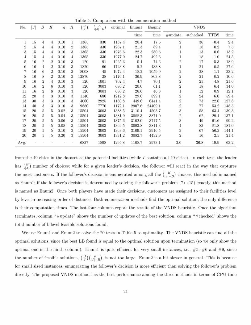
Table 5: Comparison with the enumeration method

No. |J | B K q R(B|J|) (

K|J|−B

)optimal Enum1 Enum2 VNDS

time time #update #checked TTBS time

1 15 4 4 0.10 1 1365 330 1137.4 20.4 17.6 2 36 0.4 2.42 15 4 4 0.10 2 1365 330 1267.1 21.3 89.4 1 18 0.2 7.53 15 4 4 0.10 3 1365 330 1276.6 22.3 280.6 1 13 0.6 13.24 15 4 4 0.10 4 1365 330 1277.9 24.7 492.6 1 18 1.0 24.55 16 2 2 0.10 3 120 91 1225.3 0.4 74.6 2 17 5.3 18.96 16 4 2 0.10 3 1820 66 1723.8 5.2 433.8 1 21 0.5 27.67 16 6 2 0.10 3 8008 45 1972.4 18.2 1059.9 2 28 1.1 33.28 16 8 2 0.10 3 12870 28 2176.1 36.9 803.8 2 21 0.2 10.69 16 2 4 0.10 3 120 1001 702.4 4.7 70.1 2 25 4.8 21.6

10 16 2 6 0.10 3 120 3003 680.2 20.0 61.1 2 18 6.4 34.011 16 2 8 0.10 3 120 3003 680.2 26.6 46.8 1 12 0.9 12.112 20 3 3 0.10 3 1140 680 1212.8 29.6 899.1 2 24 6.0 59.413 30 3 3 0.10 3 4060 2925 1180.8 449.6 6441.4 2 73 22.6 127.814 40 3 3 0.10 3 9880 7770 1172.1 2907.6 24409.1 2 77 53.2 148.515 20 5 5 0.02 3 15504 3003 1388.5 3110.4 4503.7 3 58 63.4 139.316 20 5 5 0.04 3 15504 3003 1381.9 3088.3 3871.0 2 62 29.4 137.117 20 5 5 0.06 3 15504 3003 1375.6 3102.0 3747.5 3 49 61.6 99.218 20 5 5 0.08 3 15504 3003 1369.5 3093.8 3811.3 4 83 81.8 181.019 20 5 5 0.10 3 15504 3003 1363.6 3109.1 3916.5 3 67 56.3 144.120 20 5 5 0.20 3 15504 3003 1331.2 3082.7 4432.9 2 16 2.5 21.4

Avg. - - - - - 6837 1898 1294.8 1108.7 2973.1 2.0 36.8 19.9 63.2

from the 49 cities in the dataset as the potential facilities (while I contains all 49 cities). In each test, the leader

has(B|J |)

number of choices; while for a given leader’s decision, the follower will react in the way that captures

the most customers. If the follower’s decision is enumerated among all the(

K|J |−B

)choices, this method is named

as Enum1; if the follower’s decision is determined by solving the follower’s problem (7)–(15) exactly, this method

is named as Enum2. Once both players have made their decisions, customers are assigned to their facilities level

by level in increasing order of distance. Both enumeration methods find the optimal solution; the only difference

is their computation times. The last four columns report the results of the VNDS heuristic. Once the algorithm

terminates, column “#update” shows the number of updates of the best solution, column “#checked” shows the

total number of bilevel feasible solutions found.

We use Enum1 and Enum2 to solve the 20 tests in Table 5 to optimality. The VNDS heuristic can find all the

optimal solutions, since the best LB found is equal to the optimal solution upon termination (so we only show the

optimal one in the ninth column). Enum1 is quite efficient for very small instances, i.e., #5, #6 and #9, since

the number of feasible solutions,(B|J |)(

K|J |−B

), is not too large. Enum2 is a bit slower in general. This is because

for small sized instances, enumerating the follower’s decision is more efficient than solving the follower’s problem

directly. The proposed VNDS method has the best performance among the three methods in terms of CPU time

21

(except for some very small instances). The best LB can be found even during the initialization process (Step 4 of

Algorithm 2), which is shown in the column “#update”. The total number of checked solutions is also very small,

as shown in the column “#checked”, indicating the intelligent direction guided by the local search mechanism.

Table 5 shows that the proposed VNDS method performs well on the CFLPD. Next, we use it to solve larger

instances. Tables 6 and 7 show the results for the 49-node dataset. In these two tables, the “LB” column means

the best lower bound found; the “share” column represents the leader’s market share (in %) in the best solution

obtained; the last two columns, for each test, show the facilities that are opened by the leader and the follower,

respectively. Furthermore, we select two parameters from B,K, q,R and |J |, while keeping the other parameters

unchanged, then show how these two parameters will affect the leader’s market share; these results are illustrated

in Figures 1, 2 and 3(a). The tests in Figure 3(a) and Figure 3(b) have the same parameter settings, except that

Figure 3(b) shows the changes in the leader’s objective value.

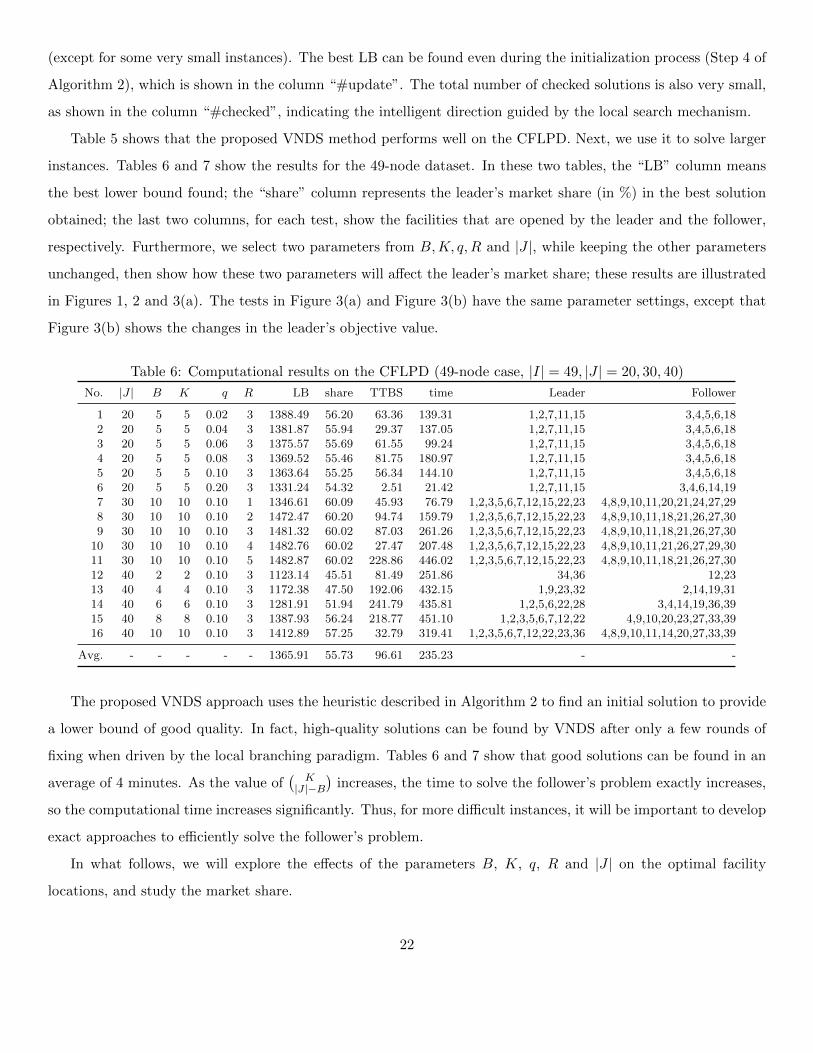
Table 6: Computational results on the CFLPD (49-node case, |I| = 49, |J | = 20, 30, 40)

No. |J | B K q R LB share TTBS time Leader Follower

1 20 5 5 0.02 3 1388.49 56.20 63.36 139.31 1,2,7,11,15 3,4,5,6,182 20 5 5 0.04 3 1381.87 55.94 29.37 137.05 1,2,7,11,15 3,4,5,6,183 20 5 5 0.06 3 1375.57 55.69 61.55 99.24 1,2,7,11,15 3,4,5,6,184 20 5 5 0.08 3 1369.52 55.46 81.75 180.97 1,2,7,11,15 3,4,5,6,185 20 5 5 0.10 3 1363.64 55.25 56.34 144.10 1,2,7,11,15 3,4,5,6,186 20 5 5 0.20 3 1331.24 54.32 2.51 21.42 1,2,7,11,15 3,4,6,14,197 30 10 10 0.10 1 1346.61 60.09 45.93 76.79 1,2,3,5,6,7,12,15,22,23 4,8,9,10,11,20,21,24,27,298 30 10 10 0.10 2 1472.47 60.20 94.74 159.79 1,2,3,5,6,7,12,15,22,23 4,8,9,10,11,18,21,26,27,309 30 10 10 0.10 3 1481.32 60.02 87.03 261.26 1,2,3,5,6,7,12,15,22,23 4,8,9,10,11,18,21,26,27,30

10 30 10 10 0.10 4 1482.76 60.02 27.47 207.48 1,2,3,5,6,7,12,15,22,23 4,8,9,10,11,21,26,27,29,3011 30 10 10 0.10 5 1482.87 60.02 228.86 446.02 1,2,3,5,6,7,12,15,22,23 4,8,9,10,11,18,21,26,27,3012 40 2 2 0.10 3 1123.14 45.51 81.49 251.86 34,36 12,2313 40 4 4 0.10 3 1172.38 47.50 192.06 432.15 1,9,23,32 2,14,19,3114 40 6 6 0.10 3 1281.91 51.94 241.79 435.81 1,2,5,6,22,28 3,4,14,19,36,3915 40 8 8 0.10 3 1387.93 56.24 218.77 451.10 1,2,3,5,6,7,12,22 4,9,10,20,23,27,33,3916 40 10 10 0.10 3 1412.89 57.25 32.79 319.41 1,2,3,5,6,7,12,22,23,36 4,8,9,10,11,14,20,27,33,39

Avg. - - - - - 1365.91 55.73 96.61 235.23 - -

The proposed VNDS approach uses the heuristic described in Algorithm 2 to find an initial solution to provide

a lower bound of good quality. In fact, high-quality solutions can be found by VNDS after only a few rounds of

fixing when driven by the local branching paradigm. Tables 6 and 7 show that good solutions can be found in an

average of 4 minutes. As the value of(

K|J |−B

)increases, the time to solve the follower’s problem exactly increases,

so the computational time increases significantly. Thus, for more difficult instances, it will be important to develop

exact approaches to efficiently solve the follower’s problem.

In what follows, we will explore the effects of the parameters B, K, q, R and |J | on the optimal facility

locations, and study the market share.

22

Table 7: Computational results on the CFLPD (49-node case, |I| = |J | = 49)

No. |J | B K q R LB share TTBS time Leader Follower

1 49 5 3 0.10 2 1554.70 63.57 359.20 571.93 1,9,11,14,32 37,40,472 49 5 4 0.10 2 1351.11 55.24 138.18 431.41 1,2,14,22,28 15,23,39,473 49 5 5 0.10 2 1207.16 49.36 84.47 401.85 1,2,14,22,28 4,7,15,39,474 49 5 6 0.10 2 1082.10 44.24 122.90 473.37 1,2,6,7,22 4,15,23,27,39,475 49 5 7 0.10 2 1001.92 40.96 39.26 419.95 1,2,6,7,22 4,14,15,19,20,27,396 49 3 5 0.05 2 706.68 28.68 199.00 419.59 1,2,6 12,15,23,27,397 49 4 5 0.05 2 995.71 40.40 64.16 370.94 1,2,6,22 12,15,23,27,398 49 5 5 0.05 2 1216.88 49.38 57.87 356.43 1,2,14,22,28 4,7,15,27,399 49 6 5 0.05 2 1422.81 57.74 29.73 271.41 1,2,6,7,22,28 3,4,15,19,39

10 49 7 5 0.05 2 1593.97 64.68 3.98 195.88 1,2,6,7,19,22,28 3,4,5,15,3911 49 4 4 0.02 3 1145.29 46.36 176.03 427.86 1,2,6,22 4,14,15,2712 49 4 4 0.04 3 1147.13 46.44 1068.65 1180.38 1,2,6,22 4,14,15,2713 49 4 4 0.06 3 1149.65 46.37 49.45 524.45 1,9,23,32 14,27,31,4714 49 4 4 0.08 3 1161.32 47.03 374.67 887.55 1,9,23,32 14,27,31,4715 49 4 4 0.10 3 1171.88 47.48 240.07 910.48 1,9,23,32 14,27,31,4716 49 4 4 0.20 3 1199.89 48.96 2716.07 3550.06 1,9,23,32 11,14,27,3717 49 4 4 0.05 1 1085.94 46.27 12.62 261.07 1,2,6,22 4,14,15,2718 49 4 4 0.05 2 1144.80 46.45 42.42 424.91 1,5,14,31 6,9,23,3319 49 4 4 0.05 3 1146.46 46.41 552.16 839.40 1,2,23,28 14,17,39,4720 49 4 4 0.05 4 1146.51 46.41 625.27 1069.01 1,2,23,28 5,14,17,3921 49 4 4 0.05 5 1146.51 46.39 171.75 747.84 1,2,23,28 5,14,17,39

Avg. - - - - - 1179.92 48.04 339.42 701.70 - -

5.2.2 Number of Located Facilities B and K

To investigate the influence of the parameters B and K, we first assume that B = K. In either Figure 1 or

Figure 3(a), the leader’s market share increases when B and K grow. The leader obtains half of the market for

B = K = 5. The case B = K = 4.4 is a demarcation point: If larger than that, the leader will dominate the

market; if smaller than that, the follower will dominate the market. Based on the assumption that two players

cannot operate at the same site, a large B favors the leader because the leader can choose all the “good” locations

first, and then dominates the market via these good locations. This is the first-mover advantage. This conclusion

is also demonstrated in tests #12–#16 from Table 6.

Then, we assume that B 6= K to study how the two players’ decisions influence each other. From tests #1–#10

in Table 7, we observe that the leader’s market share decreases when K increases and vice versa. If the players

open different numbers of facilities, then the one that opens more will attract more market share. In contrast, we

assume that both players open the same number of facilities, and this number is a constant. For #1–#11 in Table

6 and #11–#21 in Table 7, we observe that the facilities that the leader opens are basically the same, no matter

how the other parameters change. However, for the same leader’s solution, the follower may react with different

responses (e.g., #7 and #8 in Table 6).

23

4 6 8 10 12 1445

50

55

60

65

70

75

B = K

Lead

er’s

mar

ket s

hare

(%

)

q=0.01q=0.02q=0.05q=0.10q=0.15q=0.20

Figure 1: |J | = 30, R = 3

10 15 20 25 30 35 40 4545

50

55

60

65

70

75

Number of potential facilities |J|

Lead

er’s

mar

ket s

hare

(%

)

q=0.01q=0.02q=0.05q=0.10q=0.15q=0.20

Figure 2: B = K = 5, R = 3

Table 8: Computational results on the CFLPD (88-node case, |I| = 88)

No. |J | B K q R LB share TTBS time Leader Follower

1 30 5 5 0.01 3 2664.73 59.43 17.31 170.23 1,2,3,18,27 5,6,8,14,232 30 5 5 0.02 3 2656.96 59.25 21.42 229.88 1,2,3,18,27 5,6,8,14,233 30 5 5 0.05 3 2631.33 58.69 203.38 413.05 1,2,3,18,27 5,6,8,13,144 30 5 5 0.10 3 2586.55 57.74 60.44 391.85 1,2,3,8,19 5,14,18,23,285 30 5 5 0.20 3 2480.72 55.77 58.73 439.41 1,2,3,8,19 5,14,16,18,286 40 10 10 0.05 1 2681.14 62.94 32.24 357.79 1,2,3,4,8,19,23,33,36,39 5,7,9,11,14,17,18,27,29,327 40 10 10 0.05 2 2757.74 61.66 38.64 371.98 1,2,3,4,8,19,23,36,38,39 5,6,7,11,13,14,17,18,27,298 40 10 10 0.05 3 2763.51 61.64 87.07 439.60 1,2,3,4,8,19,23,33,36,39 5,7,9,11,14,17,18,27,29,329 40 10 10 0.05 4 2763.92 61.64 237.30 606.64 1,2,3,4,8,19,23,33,36,39 5,7,9,11,14,17,18,27,29,32

10 40 10 10 0.05 5 2763.93 61.64 306.52 740.60 1,2,3,4,8,19,23,33,36,39 5,7,9,11,14,17,18,27,29,3211 50 2 2 0.02 3 2135.96 47.63 238.33 789.96 19,29 12,2612 50 3 3 0.02 3 2329.09 51.94 347.82 880.05 1,2,3 5,13,4613 50 4 4 0.02 3 2511.32 56.01 230.43 531.86 1,2,3,8 4,5,44,4614 50 5 5 0.02 3 2541.31 56.67 124.42 603.75 1,2,3,18,27 5,8,32,44,4615 50 6 6 0.02 3 2603.80 58.07 101.32 595.68 1,2,3,18,19,27 4,8,23,32,37,4616 40 3 3 0.05 2 2333.43 52.17 87.70 279.70 1,2,3 5,13,3217 50 3 3 0.05 2 2313.95 51.73 125.79 459.06 1,2,3 5,13,4618 60 3 3 0.05 2 2311.94 51.69 80.98 428.62 1,2,3 5,44,5719 70 3 3 0.05 2 2311.94 51.69 202.98 614.34 1,2,3 5,44,5720 80 3 3 0.05 2 2311.94 51.69 244.87 783.35 1,2,3 5,44,5721 88 10 10 0.01 3 2702.37 60.27 288.11 711.40 1,2,3,7,9,27,39,50,59,82 4,5,8,14,23,32,36,38,58,8022 88 10 10 0.02 3 2693.75 60.07 922.28 1229.15 1,2,3,7,9,27,39,50,59,82 4,8,14,23,32,36,38,58,72,8023 88 10 10 0.05 3 2669.22 59.53 1057.83 1692.84 1,2,3,7,9,27,39,50,59,82 4,8,14,23,32,36,38,58,72,8024 88 10 10 0.10 3 2652.92 59.22 2760.29 3767.48 1,2,3,5,7,27,33,39,59,67 4,8,13,15,23,32,41,47,55,8325 88 10 10 0.20 3 2595.24 58.34 3154.47 4704.79 1,2,3,5,6,7,27,36,39,50 4,8,9,12,14,32,58,72,80,8426 88 8 8 0.05 3 2627.40 58.60 4041.99 5269.69 1,2,3,7,27,50,59,82 4,8,23,32,36,41,47,7227 88 9 9 0.05 3 2672.84 59.62 1049.10 2638.15 1,2,3,7,27,39,50,59,82 4,5,14,23,32,36,38,58,8028 88 10 10 0.05 3 2669.22 59.53 1082.72 2106.64 1,2,3,7,9,27,39,50,59,82 4,8,14,23,32,36,38,58,72,8029 88 11 11 0.05 3 2676.55 59.70 702.98 2588.02 1,2,3,4,7,8,33,36,39,67,82 5,9,11,14,18,23,27,32,50,58,7130 88 12 12 0.05 3 2726.64 60.81 1456.75 2798.57 1,2,3,4,5,7,8,38,39,44,67,71 6,11,13,14,23,27,36,50,57,66,70,83

Avg. - - - - - 2571.38 57.51 645.47 1254.47 - -

24

4 6 8 10 12 1445

50

55

60

65

70

75

B = K

Lead

er’s

mar

ket s

hare

(%

)

R=1R=2R=3R=4R=5

(a) leader’s market share

4 6 8 10 12 141000

1100

1200

1300

1400

1500

1600

1700

B = K

Lead

er’s

obj

ectiv

e va

lue

R=1R=2R=3R=4R=5

(b) leader’s objective value

Figure 3: |J | = 30, q = 0.1

5.2.3 Failure Probability q

We again assume that both players open the same number of facilities (B = K) and that this number is a constant.

An interesting observation is that when they both open 5 facilities (B = K = 5, #1–#6 in Table 6), the leader’s

market share will decrease as the failure probability q increases, whereas when both of them open 4 facilities

(B = K = 4, #11–#16 in Table 7), the leader’s market share will increase as q increases. This observation is

further demonstrated in Figure 1, where all six curves intersect at the same point (approximately B = K = 4.4).

So if both players open a large number of facilities (B = K ≥ 5), the leader will benefit from small q; in contrast,

if they open a small number of facilities (B = K ≤ 4), the leader will benefit from large q. This is because, when

q is large, the increased chance that customers will change their service location due to disruptions reduces the

first-mover advantage in the leader’s location selection. Therefore, the leader gains less benefit, even for large B.

5.2.4 Maximum Assignment Level R

The maximum assignment level R can be explained as the maximum number of facilities that the customer is

willing to seek for service. If all R facilities that are closest to the customer are disrupted, the customer’s demand

is lost, so both players will lose that customer. In that sense, our model and solution algorithms can also suit

the case in which each customer has a different tolerated number of facilities for service. Small R indicates that

the customers are conservative and can tolerate few backup service locations due to occasional disruptions, while

large R implies that the customers are flexible and can accept a large number of facilities for service.

25

As shown in Figure 3(a), if B = K ≥ 5, the leader will benefit more from a market with conservative customers;

while if B = K ≤ 4, the leader will benefit from flexible customers. This conclusion is related to consumer behavior

analysis. The same conclusions can be observed in #7–#11 in Table 6 and #17–#21 in Table 7. This is because,

when B is large, the leader is more likely to occupy all the good locations, better controlling the lower levels

(especially the primary level, r = 1); thus the leader favors conservative customers (R is small). Conversely,

when B is small, the leader favors flexible customers (R is large), who will change the firm they patronize due to

disruptions; thus the leader has more opportunity to serve them on the backup level (r ≥ 2). In addition, from

Table 6, we observe that the difference is not that significant between larger R (e.g., R = 4 and R = 5); this is

because of the scaling in the objective function (4), i.e., the demand captured decreases exponentially with r. The

leader’s objective value increases as the assignment level R increases (Figure 3(b)); this is because customers will

have more choice in case of disruptions and so less demand will be lost.

5.2.5 Number of Potential Facilities |J |

From Figure 2, we observe that if the area that is available for the players to locate facilities in is limited (|J |

is small), the leader will benefit more from the smaller-failure-probability case. And the smaller |J | is, the more

beneficial it will be for the leader to dominate the market. That is also because of the first-mover advantage: The

fewer potential facilities there are, the more possibility the leader will have to control the best locations.

The numerical results for the 88-node dataset are summarized in Table 8. The results remain consistent with

those from the 49-node dataset. Despite the increased problem sizes, the proposed solution approach can still

solve most of these instances efficiently, within 10 minutes.

5.3 Comparison of the Models: RPCP and CFLPD

We are also interested in comparing the solutions that result from considering disruptions (i.e., reliable solutions

(Snyder and Daskin 2005)) and from ignoring disruptions (i.e., non-reliable solutions), and the error that results

if one were to ignore disruptions as a heuristic to solve a problem in which disruptions actually exist. To this end,

we perform a series of numerical experiments and show the results in Table 9.

For each parameter setting in Table 7, we solve a RPCP (q = 0, R = 1); once the algorithm terminates,

the leader’s objective value is recorded in the “LB1” column; the leader’s and the follower’s decisions are shown

in the “Leader” column and the “Follower1” column, respectively; then, for the given leader’s decision, the

follower’s problem when considering disruptions is solved exactly, the associated follower’s decision is reported in

the “Follower” column, the leader’s true objective value under disruptions is shown in the “LB” column, and the

percentage difference compared with the reliable case is listed in the “error” column. As expected, if solving the

26

1

(a) non-reliable: RPCP (q = 0)

1

(b) reliable: #11 (q = 0.02), #12 (q = 0.04)

1

(c) reliable: #13 (q = 0.06), #14 (q = 0.08), #15 (q = 0.10)

1

(d) reliable: #16 (q = 0.20)

Figure 4: Comparison (|I| = |J | = 49, B = K = 4, R = 3; black circles: customers; red rectangles: leader’s

facilities; blue triangles: follower’s facilities)

RPCP happens to yield the same leader’s solution, then the leader’s objective value will be the same as the reliable

case considering disruptions. Tests #11–#21 from Table 9 show that an integer solution that is bilevel feasible in

the RPCP model is not necessarily feasible in the CFLPD model, and if parameters change, for a given leader’s

solution, the follower may have different optimal responses. From Table 9, we observe that for certain parameter

settings, the RPCP can be a good heuristic. However, this may not be a safe approach to use, in general, since

the RPCP model ignores possible disruptions. That is, except for some special cases, the RPCP solutions will not

be accurate for the CFLPD, and instead one should use the proposed methods to solve the general problem.

Figure 4 shows the approximate facility deployments and the corresponding (level-1) customer assignments for

different q (|I| = |J | = 49, B = K = 4, R = 3). In detail, Figure 4(a) shows the RPCP solution, as reported

in #11–#21 from Table 9; Figures 4(b)–4(d) show CFLPD solutions for various q as reported in #11–#16 from

Table 7. In the numerical analysis in §5.1, we find that several different deployments may yield the same leader’s

27

Table 9: Evaluation of RPCP solutions on CFLPD models (|I| = |J | = 49)

No. B K q R Reliable Non-reliable

LB LB1 time Leader Follower1 Follower LB error

1 5 3 0.10 2 1554.70 1574.64 35.12 1,7,9,11,32 19,37,42 19,23,37 1549.71 0.322 5 4 0.10 2 1351.11 1383.53 50.21 1,2,6,22,28 3,4,14,27 3,5,14,36 1338.34 0.953 5 5 0.10 2 1207.16 1220.62 52.32 1,2,6,22,28 3,4,14,27,36 3,12,14,27,36 1196.66 0.874 5 6 0.10 2 1082.10 1082.59 50.82 1,2,6,7,22 4,14,15,19,39,42 4,15,23,27,39,47 1082.10 0.005 5 7 0.10 2 1001.92 989.63 60.23 1,2,6,7,22 4,8,14,15,19,39,42 4,5,15,20,23,27,39 1001.92 0.006 3 5 0.05 2 706.68 690.11 42.37 1,2,6 14,15,39,42,45 12,15,23,27,39 706.68 0.007 4 5 0.05 2 995.71 982.04 41.49 1,2,6,22 4,15,23,27,39 12,15,23,27,39 995.71 0.008 5 5 0.05 2 1216.88 1220.62 67.34 1,2,6,22,28 3,4,14,27,36 3,12,23,27,36 1216.39 0.049 6 5 0.05 2 1422.81 1427.63 64.29 1,2,6,7,22,28 3,4,5,36,39 3,4,15,19,39 1422.81 0.00

10 7 5 0.05 2 1593.97 1616.33 75.97 1,2,6,7,19,22,28 3,4,5,36,39 3,4,5,15,39 1593.97 0.0011 4 4 0.02 3 1145.29 1143.09 54.95 1,2,6,22 4,15,23,27 4,14,15,27 1145.29 0.0012 4 4 0.04 3 1147.13 1143.09 54.95 1,2,6,22 4,15,23,27 4,15,23,27 1147.13 0.0013 4 4 0.06 3 1149.65 1143.09 54.95 1,2,6,22 4,15,23,27 12,15,23,27 1144.66 0.4314 4 4 0.08 3 1161.32 1143.09 54.95 1,2,6,22 4,15,23,27 12,15,23,27 1141.57 1.7015 4 4 0.10 3 1171.88 1143.09 54.95 1,2,6,22 4,15,23,27 12,15,23,27 1138.35 2.8616 4 4 0.20 3 1199.89 1143.09 54.95 1,2,6,22 4,15,23,27 15,23,39,47 1117.36 6.8817 4 4 0.05 1 1085.94 1143.09 54.95 1,2,6,22 4,15,23,27 4,14,15,27 1085.94 0.0018 4 4 0.05 2 1144.80 1143.09 54.95 1,2,6,22 4,15,23,27 12,14,15,27 1143.55 0.1119 4 4 0.05 3 1146.46 1143.09 54.95 1,2,6,22 4,15,23,27 12,15,23,27 1146.17 0.0320 4 4 0.05 4 1146.51 1143.09 54.95 1,2,6,22 4,15,23,27 12,15,23,27 1146.25 0.0221 4 4 0.05 5 1146.51 1143.09 54.95 1,2,6,22 4,15,23,27 12,15,23,27 1146.26 0.02

Avg. - - - - 1179.92 1179.13 54.51 - - - 1171.75 0.68

objective value. However, we can always choose one that is more reliable. This is demonstrated in the comparison

of Figure 4(a) and 4(b). One of the follower’s facilities, Frankfort, KY, in Figure 4(a) is replaced by another

facility, Indianapolis, IN, in Figure 4(b). The solutions in Figures 4(a) and 4(b) have the same leader’ objective

value, if evaluated under the RPCP model. But the solution in Figure 4(b) is more beneficial for the leader, since

she will serve more customers at the backup level, gaining a larger market share if disruptions occur. Next, we

observe that none of the customers are closest to the leader’s facility in Trenton, NJ, in Figure 4(c). But it is

still optimal for the leader to select this facility, since many customers are assigned to Trenton at level 2, if the

follower’s facilities in Hartford, CT and Washington, DC fail. Furthermore, we see that the optimal facilities tend

to be more dispersed as the failure probability q increases, as highlighted in the four figures in Figure 4 (as q varies

from 0 to 0.2). Intuitively, more dispersed facilities can provide better backups to each other in a competitive

environment.

6 Conclusions and Future Research

In this paper we investigate a new discrete competitive facility location problem by taking into account the

sequential game between two players and by considering facility disruption risks. The players successively place

their facilities to capture customers, in order to maximize their profit. Customers seek the nearest functional facility

for service. We formulate this problem as a binary bilevel linear optimization problem (BBLP) to determine the

28

locations for the leader to maximize her market share, under the strongest possible response by the follower.

We then discuss the challenges associated with solving this problem. To solve it, we design a VNDS heuristic.

The VNDS method combines, in a nested schema, hard variable fixing, soft variable fixing and linear constraints.

Numerical studies are conducted first on a special case of our problem, the RPCP. The results demonstrate that

the proposed VNDS method is very promising compared with the state-of-the-art heuristics and exact approaches

from the literature. Then, we test the algorithm on CFLPD instances. Managerial insights are obtained through

sensitivity analysis of the model and through several illustrative examples. For example, the player who locates

more facilities will control most of the market. In the case in which the follower will react by locating the same

number of facilities, the leader tends to dominate the market for large values of B and K. In addition, if B and K

are large (B = K ≥ 5), the leader will benefit from facilities that are more reliable (q is small) and conservative

customers who tolerate few backup locations (R is small); if B and K are small (B = K ≤ 4), the leader will

benefit from vulnerable facilities (q is large) and flexible customers that can accept a large number of facilities

for service (R is large). And the fewer the available potential locations are, the more beneficial it will be for the

leader to dominate the market.

We believe that the proposed mathematical model is an important generalization of the classical facility

location problem in terms of applications. This model has great potential for application where the decision

on the placement of facilities is taken by two or more parties, and the facilities may fail from time to time. The

VNDS matheuristic we design can be seen as a generalization of the familiar algorithm used for the solution

of standard MIPs. The primary advantage of this approach is the ability to exploit the vast array of existing

technology for solving MIPs techniques. All the usual rules of fathoming and branching are preserved. Our

computational analysis shows that it is possible, in principle, to generalize the MIP matheuristics to solve BBLPs,

a very challenging computational setting.

In the proposed CFLPD, we assume that the leader knows the exact number of facilities opened by the

follower. In reality, the number of facilities could be flexible and it mainly depends on capital constraints. One

future research topic is to develop stochastic or robust models to maximize the leader’s market share under a

range of scenarios specifying the number of follower’s facilities. In addition, from a practical perspective, it is also

important to generalize the assumption of uncapacitated facilities and identical failure probabilities. Furthermore,

future research can be focused on the development of improved bound to achieve global optimality, and the

development of more efficient computational methods.

29

Acknowledgments

This work was supported by the National Natural Science Foundation of China (71502112), and partly sponsored

by the State Scholarship Fund of China Scholarship Council. In addition, this research was supported in part by

NSF grant #CMMI-1541177 and will contribute to the PRAISys platform (www.praisys.org). This support is

gratefully acknowledged. We also wish to thank the anonymous referees for their helpful suggestions, which led to

improved clarity of the paper and improved computational performance of the algorithms.

References

Aboolian, Robert, Tingting Cui, Zuo-Jun Max Shen. 2012. An efficient approach for solving reliable facility location models.

INFORMS Journal on Computing 25(4) 720–729.

Aksen, Deniz, Sema Sengul Akca, Necati Aras. 2014. A bilevel partial interdiction problem with capacitated facilities and

demand outsourcing. Computers & Operations Research 41 346–358.

Alekseeva, E, N Kochetova, Yu Kochetov, A Plyasunov. 2009. A hybrid memetic algorithm for the competitive p-median

problem. Preprints of the 13th IFAC Symposium on Information Control Problems in Manufacturing, Moscow . 1516–

1520.

Alekseeva, Ekaterina, Yury Kochetov. 2013. Matheuristics and exact methods for the discrete (r|p)-centroid problem. Meta-

heuristics for Bi-Level Optimization. Springer, 189–219.

Alekseeva, Ekaterina, Nina Kochetova, Yury Kochetov, Alexandr Plyasunov. 2010. Heuristic and exact methods for the

discrete (r|p)-centroid problem. Evolutionary Computation in Combinatorial Optimization. Springer, 11–22.

Ashtiani, Milad Gorji, Ahmad Makui, Reza Ramezanian. 2013. Applied Mathematical Modelling 37 62 – 71. doi:http://dx.doi.

org/10.1016/j.apm.2011.12.013. URL http://www.sciencedirect.com/science/article/pii/S0307904X11007992.

Audet, Charles, Gilles Savard, Walid Zghal. 2007. New branch-and-cut algorithm for bilevel linear programming. Journal of

Optimization Theory and Applications 134(2) 353–370.

Berman, Oded, Dmitry Krass, Mozart BC Menezes. 2007. Facility reliability issues in network p-median problems: strategic

centralization and co-location effects. Operations Research 55(2) 332–350.

Bialas, Wayne F, Mark H Karwan. 1984. Two-level linear programming. Management Science 30(8) 1004–1020.

Biesinger, Benjamin, Bin Hu, Gunther Raidl. 2015. A hybrid genetic algorithm with solution archive for the discrete (r|p)-

centroid problem. Journal of Heuristics 21(3) 391–431.

Bixby, E Robert, Mary Fenelon, Zonghao Gu, Ed Rothberg, Roland Wunderling. 2000. System Modelling and Optimization.

Springer, 19–49.

Church, Richard, Charles R Velle. 1974. The maximal covering location problem. Papers in Regional Science 32(1) 101–118.

30

Cui, Tingting, Yanfeng Ouyang, Zuo-Jun Max Shen. 2010. Reliable facility location design under the risk of disruptions.

Operations Research 58(4-part-1) 998–1011.

Danna, Emilie, Edward Rothberg, Claude Le Pape. 2005. Exploring relaxation induced neighborhoods to improve mip

solutions. Mathematical Programming 102(1) 71–90.

Daskin, Mark S. 2013. Network and Discrete Location: Models, Algorithms, and Applications. 2nd ed. Wiley, New York.

Davydov, Ivan Aleksandrovich. 2012. Local tabu search for the discrete (r|p)-centroid problem. Diskret. Anal. Issled. Oper.

19(2) 19–40.

Davydov, Ivan Aleksandrovich, Yu A Kochetov, Nenad Mladenovic, D Urosevic. 2014. Fast metaheuristics for the discrete

(r|p)-centroid problem. Automation and Remote Control 75(4) 677–687.

Dempe, Stephan. 2002. Foundations of bilevel programming . Springer Science & Business Media.

DeNegre, ST, Ted K Ralphs. 2009. A branch-and-cut algorithm for integer bilevel linear programs. Operations Research and

Cyber-Infrastructure. Springer, 65–78.

Eiselt, Horst A, Gilbert Laporte. 1997. Sequential location problems. European Journal of Operational Research 96(2)

217–231.

Eiselt, Horst A, Gilbert Laporte, Jacques-Francois Thisse. 1993. Competitive location models: A framework and bibliography.

Transportation Science 27(1) 44–54.

Farahani, Reza Zanjirani, Shabnam Rezapour, Tammy Drezner, Samira Fallah. 2014. Competitive supply chain network

design: An overview of classifications, models, solution techniques and applications. Omega 45 92–118.

Fischetti, Matteo, Andrea Lodi. 2003. Local branching. Mathematical Programming 98(1-3) 23–47.

Gedik, Ridvan, Hugh Medal, Chase Rainwater, Ed A Pohl, Scott J Mason. 2014. Vulnerability assessment and re-routing of

freight trains under disruptions: A coal supply chain network application. Transportation Research Part E: Logistics

and Transportation Review 71 45–57.

Hanafi, Saıd, Jasmina Lazic, Nenad Mladenovic, Christophe Wilbaut, Igor Crevits. 2014. New variable neighbourhood search

based 0-1 mip heuristics. Yugoslav Journal of Operations Research (00) 14–14.

Hansen, Pierre, Nenad Mladenovic. 2001. Variable neighborhood search: Principles and applications. European Journal of

Operational Research 130(3) 449–467.

Hansen, Pierre, Nenad Mladenovic, Jose A Moreno Perez. 2010. Variable neighbourhood search: methods and applications.

Annals of Operations Research 175(1) 367–407.

Hansen, Pierre, Nenad Mladenovic, Dionisio Perez-Britos. 2001. Variable neighborhood decomposition search. Journal of

Heuristics 7(4) 335–350.

Hansen, Pierre, Nenad Mladenovic, Dragan Urosevic. 2006. Variable neighborhood search and local branching. Computers

& Operations Research 33(10) 3034–3045.

Kochetov, Yury, Nina Kochetova, Alexandr Plyasunov. 2013. A matheuristic for the leader-follower facility location and

design problem. Proceedings of the 10th Metaheuristics International Conference (MIC 2013). 32.

31

Kress, Dominik, Erwin Pesch. 2012. Sequential competitive location on networks. European Journal of Operational Research

217(3) 483–499.

Lazic, Jasmina, Saıd Hanafi, Nenad Mladenovic, Dragan Urosevic. 2010. Variable neighbourhood decomposition search for

0–1 mixed integer programs. Computers & Operations Research 37(6) 1055–1067.

Liberatore, Federico, Maria P Scaparra, Mark S Daskin. 2011. Analysis of facility protection strategies against an uncertain

number of attacks: the stochastic r-interdiction median problem with fortification. Computers & Operations Research

38(1) 357–366.

Losada, Chaya, M Paola Scaparra, Jesse R O’ Hanley. 2012. Optimizing system resilience: a facility protection model with

recovery time. European Journal of Operational Research 217(3) 519–530.

Moore, James T, Jonathan F Bard. 1990. The mixed integer linear bilevel programming problem. Operations Research 38(5)

911–921.

Noltemeier, Hartmut, Joachim Spoerhase, H-C Wirth. 2007. Multiple voting location and single voting location on trees.

European Journal of Operational Research 181(2) 654–667.

O’ Hanley, Jesse R, Richard L Church. 2011. Designing robust coverage networks to hedge against worst-case facility losses.

European Journal of Operational Research 209(1) 23–36.

Plastria, Frank, Lieselot Vanhaverbeke. 2008. Discrete models for competitive location with foresight. Computers & Opera-

tions Research 35(3) 683–700.

Roboredo, Marcos Costa, Artur Alves Pessoa. 2013. A branch-and-cut algorithm for the discrete (r|p)-centroid problem.

European Journal of Operational Research 224(1) 101–109.

Serra, Daniel, Charles ReVelle. 1994. Market capture by two competitors: The preemptive location problem. Journal of

Regional Science 34(4) 549–561.

Serra, Daniel, Charles ReVelle, et al. 1994. Competitive location in discrete space. Universitat Pompeu Fabra.

Seyhan, Tolga H., Lawrence V. Snyder, Ying Zhang. 2015. A new heuristic formulation for a competitive maximal covering

location problem .

Shen, Zuo-Jun Max, Roger Lezhou Zhan, Jiawei Zhang. 2011. The reliable facility location problem: Formulations, heuristics,

and approximation algorithms. INFORMS Journal on Computing 23(3) 470–482.

Snyder, Lawrence V. 2010. Introduction to facility location. Wiley Encyclopedia of Operations Research and Management

Science .

Snyder, Lawrence V, Zumbul Atan, Peng Peng, Ying Rong, Amanda J Schmitt, Burcu Sinsoysal. 2015. Or/ms models for

supply chain disruptions: A review. IIE Transactions 1–21.

Snyder, Lawrence V, Mark S Daskin. 2005. Reliability models for facility location: the expected failure cost case. Trans-

portation Science 39(3) 400–416.

Wang, Xin, Yanfeng Ouyang. 2013. A continuum approximation approach to competitive facility location design under

facility disruption risks. Transportation Research Part B: Methodological 50 90–103.

32

Zhang, Ying, Lawrence V Snyder, Mingyao Qi, Lixin Miao. 2016. A heterogeneous reliable location model with risk pooling

under supply disruptions. Transportation Research Part B: Methodological 83 151–178.

33