RESEARCH SEMINAR IN INTERNATIONAL ECONOMICS Gerald R. Ford School of Public Policy The University of Michigan Ann Arbor, Michigan 48109-3091 Discussion Paper No. 592 The Collapse of International Trade During the 2008-2009 Crisis: In Search of the Smoking Gun Andrei A. Levchenko University of Michigan Logan Lewis University of Michigan Linda L. Tesar University of Michigan & NBER October 14, 2009 Recent RSIE Discussion Papers are available on the World Wide Web at: http://www.fordschool.umich.edu/rsie/workingpapers/wp.html

Welcome message from author
This document is posted to help you gain knowledge. Please leave a comment to let me know what you think about it! Share it to your friends and learn new things together.
Transcript

RESEARCH SEMINAR IN INTERNATIONAL ECONOMICS
Gerald R. Ford School of Public Policy The University of Michigan
Ann Arbor, Michigan 48109-3091
Discussion Paper No. 592
The Collapse of International Trade During the 2008-2009 Crisis:
In Search of the Smoking Gun
Andrei A. Levchenko
University of Michigan
Logan Lewis University of Michigan
Linda L. Tesar
University of Michigan & NBER
October 14, 2009
Recent RSIE Discussion Papers are available on the World Wide Web at: http://www.fordschool.umich.edu/rsie/workingpapers/wp.html
The Collapse of International Trade During the 2008-2009 Crisis:
In Search of the Smoking Gun∗
Andrei A. LevchenkoUniversity of Michigan
Logan LewisUniversity of Michigan
Linda L. TesarUniversity of Michigan and NBER
October 14, 2009
Abstract
One of the most striking aspects of the recent recession is the collapse in international trade. Thispaper uses disaggregated quarterly and monthly data on U.S. imports and exports to shed lighton the anatomy of this collapse. We find that the recent reduction in trade relative to overalleconomic activity is far larger than in previous downturns. Information on quantities and pricesof both domestic absorption and imports reveals a more than 50% shortfall in imports, relativeto what would be predicted by a simple import demand relationship. In a sample of importsand exports disaggregated at the 6-digit NAICS level, we find that sectors used as intermediateinputs experienced significantly higher percentage reductions in both imports and exports. Wealso find support for compositional effects: sectors with larger reductions in domestic outputhad larger drops in trade. By contrast, we find no support for the hypothesis that trade creditplayed a role in the recent trade collapse.
JEL Classifications: F41, F42
Keywords: 2008-2009 Crisis, International Trade
∗We are grateful to David Weinstein and workshop participants at the University of Michigan for helpful sugges-tions. E-mail: [email protected], [email protected], [email protected].

1 Introduction
A remarkable feature of the recent crisis is the collapse in international trade. This collapse is
global in nature (WTO 2009), and dramatic in magnitude. To give one example, while the U.S.
GDP has so far declined by 3.9% from its peak, real U.S. imports fell by 18.6% and real exports
fell by 15.2% over the same period. Though protectionist pressures inevitably increased over the
course of the recent crisis, it is widely believed that the collapse is not due to newly erected trade
barriers (Baldwin and Evenett 2009).
While these broad facts are well known, we currently lack both a nuanced empirical under-
standing of the patterns and a successful economic explanation for them. This paper has three
main parts. In the first, we use high-frequency (quarterly and monthly) foreign trade data for the
United States to document the patterns of collapse at a disaggregated level. We focus on the U.S.
in part due to its central role in the global downturn and because it offers up-to-date, detailed
monthly data. We first use historical data to reveal whether the recent collapse in international
trade relative to the level of economic activity is exceptional by historical standards, or just an
amplified version of what has happened in earlier downturns. We then establish whether the re-
cent reduction in international trade is especially pronounced in certain sectors. For instance, are
intermediate inputs, investment, or consumption goods experiencing the largest drops? Durables
vs. nondurables? Goods or services? We also determine with which countries U.S. trade has fallen
the most. Is it with the closest trade partners, such as Canada and Mexico? With newly important
trade partners such as China, India, or Southeast Asian countries? With Europe, Latin America,
or Africa? Finally, we separate movements in prices and quantities, to examine whether the fall is
mainly real or nominal.
In the second part, use data on domestic absorption, sectoral price levels, as well as quantities
and prices of imports to perform a simple “trade wedge” exercise in the spirit of Cole and Oha-
nian (2002) and Chari, Kehoe and McGrattan (2007). A model that features CES aggregation
of domestic and foreign varieties in a particular sector – that is, virtually any model in interna-
tional macroeconomics – has implications for the joint behavior of domestic absorption, domestic
prices, and import prices and quantities. Using this simple optimality condition allows us to ex-
plore two questions: first, is the recent trade collapse truly a puzzle? That is, the wedge exercise
that accounts for both domestic and foreign prices and quantities is the appropriate benchmark to
evaluate whether the recent decrease in international trade is in any sense “extraordinary.” Second,
by pitting against the data conditions that would have to hold period-by-period in virtually any
quantitative model of international transmission, we can offer a preliminary view on whether – and
which – DSGE models can have some hope of matching the magnitude of the recent collapse in
international trade.
1

Finally, the third part uses monthly sector-level data to examine a range of potential explana-
tions for the trade collapse proposed in the policy literature. We record the percentage changes in
exports and imports during the recent crisis at the 6-digit NAICS level of disaggregation (about
450 distinct sectors). We then relate the variation in these changes to sectoral characteristics that
would proxy for the leading explanations. The first is that trade may be collapsing because of the
transmission of shocks through vertical production linkages. When there is a drop in final output,
the demand for intermediate inputs will suffer, leading to a more than proportional drop in trade
flows.1 To test for this possibility, we build several measures of intermediate input linkages at
the detailed sector level based on the U.S. Input-Output tables, as well as measures of production
sharing based on data on exports and imports within multinational firms. The second explanation
we evaluate is trade credit: if during the recent crisis, firms in the U.S. are less willing to extend
trade credit to partners abroad, trade may be disrupted.2 We therefore use U.S. firm-level data
to construct measures of the intensity of trade credit use in each sector. Finally, the collapse in
trade could be due to compositional effects. That is, if international trade happens disproportion-
ately in sectors whose domestic absorption (or production) collapsed the most, that would explain
why trade fell more than GDP. Two special cases of the compositional story are investment goods
(Boileau 1999, Erceg, Guerrieri and Gust 2008) and durable goods (Engel and Wang 2009). Since
investment and durables consumption are several times more volatile than GDP, trade in invest-
ment and durable goods would be expected to experience larger swings than GDP as well. Thus, we
collect measures of domestic output at the most disaggregated available level, and check whether
international trade fell systematically more in sectors that also experienced the greatest reductions
in domestic output. In addition, we build an indicator for whether a sector produces durable goods.
Our main findings can be summarized as follows. The recent collapse in international trade
is indeed exceptional by historical standards. Relative to economic activity, the drop in trade is
an order of magnitude larger than what was observed in the previous postwar recessions, with the
exception of 2001. The collapse appears to be broad-based across trading partners: trade with
virtually all parts of the world decreased by a similar order of magnitude. The sharpest percentage
drops in trade are in automobiles, durable industrial supplies and capital goods. Those categories
also account for most of the absolute decrease in trade as well.
Another way to assess whether the recent trade collapse is exceptional is to use information on
prices and examine the wedges. The time series behavior of the international trade wedge does1Hummels, Ishii and Yi (2001) and Yi (2003) document the dramatic growth in vertical trade in recent decades,
and di Giovanni and Levchenko (2009) demonstrate that greater sector-level vertical linkages play a role in thetransmission of shocks between countries.
2Raddatz (2009) shows that there is greater comovement between sectors that have stronger trade credit links,while Iacovone and Zavacka (2009) demonstrate that in countries experiencing banking crises, export fell systemati-cally more in financially dependent industries. Amiti and Weinstein (2009) show that exports by Japanese firms inthe 1990s declined when the bank commonly recognized as providing trade finance to the firm was in distress.
2

reveal a drastic deviation from the norm during the recent episode. In the recent episode, the overall
trade wedge has reached −54%, revealing a collapse in trade well in excess of what is predicted by
the pace of economic activity and prices. This is indeed exceptional: over the past 25 years the
mean value of the wedge is less than 9%, with a standard deviation of 8.7%. We conclude from
this exercise that the recent trade collapse does represent a puzzle, in the sense that any import
demand function derived from CES aggregation would predict a far smaller drop in imports given
observed overall economic activity and prices.3
Finally, using detailed trade data, we shed light on which explanations are consistent with
cross-sectoral variation in trade flow changes. We find some support for the vertical linkages view,
as well as for compositional effects. Sectors that are used intensively as intermediate inputs, and
those with greater reductions in domestic output experienced significantly greater reductions in
trade, after controlling for a variety of other sectoral characteristics. By contrast, trade credit does
not appear to play a significant role: more trade credit-intensive sectors did not experience greater
trade flow reductions.
The rest of this paper is organized as follows. Section 2 presents a set of stylized facts on the
recent trade collapse using detailed quarterly data on U.S. imports and exports. Section 3 describes
a framework to build the international trade wedges, and presents the behavior of those wedges
over time and in different sectors. Section 4 uses detailed data on sectoral characteristics to assess
whether the variation across sectors is consistent with the main explanations proposed in the policy
literature. Section 5 concludes.
2 Facts
This section uses disaggregated quarterly data on U.S. imports and exports to establish a number
of striking patterns in the data. We discuss three aspects of the recent episode: (i) its magnitude
relative to historical experience; (ii) the sector- and destination- level breakdown; and (iii) the
behavior of prices and quantities separately. The total imports, exports, and GDP data come from
the U.S. National Income and Product Accounts (NIPA). The trade flows and prices disaggregated
by sector are from the Bureau of Economic Analysis’ Trade in Goods and Services Database, while
trade flows disaggregated by partner are from the U.S. International Trade Commission’s Tariffs
and Trade Database.
Fact 1 As a share of economic activity, the collapse in U.S. exports and imports in the recent3Chinn (2009) estimates an econometric model of U.S. exports, and shows that the recent level of exports is
far below what would be predicted by the model. Freund (2009) analyzes the behavior of trade in previous globaldownturns, and shows that the elasticity of trade to GDP has increased in recent decades, predicting a reductionin global trade in the current downturn of about 15%. Our methodology looks at U.S. imports rather than U.S. orglobal exports, and takes explicit account of domestic and import prices at the quarterly frequency.
3

downturn is exceptional by historical standards. Only the 2001 recession is comparable.
Figure 1(a) plots quarterly values of imports and exports normalized by GDP over the past 62
years, along with the recession bars. Visually, the 2008-09 collapse appears larger than most
changes experienced in the past.4 It is also clear, however, that a similar drop occurred in 2001, a
fact that appears underappreciated. Table 1 reports the change in the ratios of imports and exports
to GDP during the 2008 and 2001 recessions, as well as the average changes in those variables during
the recessions that occurred between 1950 and 2000. For the 2008 and 2001 recessions, the total
declines are calculated both during the official NBER recession dates, and with respect to the peak
value of trade/GDP around the onset of the recession. It is apparent that both the imports and
exports to GDP decline by 14 to 30% during the last two recessions, depending on the measure.
By contrast, in all the pre-2000 recessions, the average decline in exports is less than 1 percentage
point, and the average change in imports is virtually nil. As an alternative way of presenting the
historical series, Figure 1(b) plots the deviations from trend in real imports, exports, and GDP
over the same period. To detrend the series, we use the Hodrick-Prescott filter with the standard
parameter of 1600. The recent period is characterized by large negative deviations from trend for
both imports and exports. We can see that these are greater in magnitude than the deviation from
trend in GDP.
Fact 2 For both U.S. exports and imports, the sharpest percentage drops are in the automotive
and industrial supplies sectors, with consumer goods trade experiencing a far smaller percentage
decrease. For imports, the decrease in petroleum category alone accounts for one third of the total
decline.
Panel A of Table 2 reports the reductions in exports and imports by sector for the recent trade
collapse. While the overall reduction in nominal exports is about 26%, exports in the automotive
sector (which comprises both vehicles and parts) drop by 47%, and in industrial supplies by 34%.
By contrast, exports of consumer goods (−12%), agricultural output (−19%), and capital goods
(−20%) experience less than average percentage reductions. The table also reports the share of
each of these sectors in total exports at the outset of the crisis, as well as the absolute reductions
in trade. It is clear that industrial supplies and automotive sectors accounted for almost 40% of all
U.S. goods exports, and their combined decrease accounts for more than half of the total collapse
of U.S. exports.
Total imports decline by 34%. The petroleum and products category has the largest percentage
decrease at −54%. It also accounts for some 20% of the pre-crisis imports, and about 1/3 of the4The concurrent change in the exchange rate is relatively subdued. Appendix Figure A1 plots the long-run path
of the nominal and real effective exchange rates for the United States. Over the period coinciding with the tradecollapse, the U.S. dollar appreciated slightly in real terms, but the change has been less than 10%.
4

total absolute decline. As with exports, the next largest percentage declines are in the automotive
(−49%) and industrial supplies (−47%) sectors. By contrast, consumer goods decrease by only
15%, and agricultural products by 9%.
Figures 2 and 3 illustrate the collapse in real trade over time. Figure 2 displays the trade in
real goods and services separately. We can see that goods trade is both larger in volume, and the
decrease is more pronounced than in services. Figure 3 breaks total goods trade into real durables
and non-durables, to highlight that the reduction in the trade categories considered durable is more
pronounced, for both imports and exports. These figures indicate that in order to understand the
collapse in real trade flows, it is reasonable to focus on goods trade and examine durable goods
more closely. We follow this strategy in Sections 3 and 4.
Fact 3 The recent collapse in U.S. foreign trade is roughly similar in magnitude across all major
U.S. trading partners.
Panel B of Table 2 reports the reduction, in absolute and percentage terms, of exports and imports
to and from the main regions of the world and the most important individual partners within those
regions. To be precise, the first three columns, under “Exports,” report the exports from the U.S.
to the various countries and regions. Correspondingly, the columns labeled “Imports” report the
imports to the U.S. from these countries. What is remarkable is how broad-based the collapse is.
With virtually every major partner, U.S. exports are dropping by more than 20% (with China and
India being the notable exceptions), while imports are dropping by 30% or more (with once again
China as the exception at −16%).
Fact 4 Both quantities and prices of exports and imports decreased, with changes in real quantities
explaining the majority of the nominal decrease in trade.
Figure 4 plots both nominal and real trade, each normalized to its 2005q1 value. While nominal
exports fall by 26% from its peak, the fall in real exports accounts for about three quarters of that
decline, 19%. For imports, the role of declining import prices is greater. In addition, the peak
in real imports occurred 3 quarters earlier than the peak of nominal imports, due largely to the
timing of the oil price collapse. Nonetheless, real quantities account for about 60% of the total
nominal decline in imports. Table 3 presents the nominal, real, and price level changes in each
export and import category. It is remarkable that in some important sectors, such as automotive,
capital goods, and consumer goods, the prices did not move much at all, and the entire decline in
nominal exports and imports is accounted for by real quantities. By contrast, prices moved the
most in industrial supplies, especially petroleum. Figure 5 presents the contrast between nominal
and real graphically. It plots the nominal declines in each sector against the real ones, along with
the 45-degree line. For points on the 45-degree line, all of the nominal decrease in trade is accounted
5

for by movements in real quantities, with no change in prices. For points farther from the line, price
changes account for more of the nominal change in trade. There are several things to take away
from this figure. First, we can see that some important sectors are at or very near the 45-degree
line: all of the change in nominal trade in those sectors comes from quantities. Second, petroleum
imports is by far the biggest exception, as the only sector in which most of the change comes from
prices. Finally, in most cases import and export prices experienced a drop – the bulk of the points
are below the 45-degree line. This implies that in the recent episode, trade prices and quantities
are moving in the same direction.
3 Wedges
The discussion of nominal and real quantities foreshadows the exercise in this section. In particular,
we ask, is there any way to assess whether the trade changes during the recent crisis are in some
sense “exceptional” or “abnormal”? That is, how would we expect trade flows to behave in the
recent recession? To provide a model-based benchmark for the behavior of trade flows, we follow
the “wedge” methodology of Cole and Ohanian (2002) and Chari et al. (2007). We set down an
import demand equation that would be true in virtually any International Real Business Cycle
(IRBC) model, and check how the deviation from this condition, which we call the “trade wedge”
behaves in the recent crisis relative to historical experience.
Let us begin with the simplest 2-good IRBC model of Backus, Kehoe and Kydland (1995).
There are two countries, Home and Foreign, and two intermediate goods, one produced in Home,
the other in Foreign. There is one final good, used for both consumption and investment. The
resource constraint of the Home country in each period is given by:
Ct + It =[ω
1ε
(yh
t
) ε−1ε + (1− ω)
1ε
(yf
t
) ε−1ε
] εε−1
, (1)
where Ct is Home consumption, It is Home investment, yht is the output of the Home intermediate
good that is used in Home production, and yft is the amount of the Foreign intermediate used in
Home production. In this standard formulation, consumption and investment are perfect substi-
tutes, and Home and Foreign goods are aggregated in a CES production function. The parameter
ω allows for a home bias in preferences.
The household (or, equivalently, a perfectly competitive final goods producer), chooses the mix
6

of Home and Foreign intermediates optimally:
minyht ,yft
{ph
t yht + pf
t yft
}s.t.
Ct + It ≤[ω
1ε
(yh
t
) ε−1ε + (1− ω)
1ε
(yf
t
) ε−1ε
] εε−1
where pht is the price of the domestically-produced good and pf
t is the price of the imported good,
both expressed in the home country’s currency. This yields the standard demand equations:
yht = ω
(Pt
pht
)ε
(Ct + It)
yft = (1− ω)
(Pt
pft
)ε
(Ct + It) ,
where Pt is the standard CES price level:
Pt =[ω(ph
t
)1−ε+ (1− ω)
(pf
t
)1−ε] 1
1−ε.
Log-linearizing these, we obtain the following relationship in log changes, denoted by a caret:
yf = ε(P − pf
)+ (C + I). (2)
This equation provides a benchmark for evaluating whether the recent trade collapse represents
a large deviation from business as usual. They will hold exactly in any model that features the
relationship of the type given by (1), a quite common one in the IRBC literature. Economically,
it ties real import demand to (i) overall real domestic absorption (C + I); (ii) the overall domestic
price level (P ); and (iii) import prices pf . Since all of these are observable, we proceed by using
equation (2) to compute the log deviation from it holding exactly, calling it the “trade wedge.”
On the left-hand side is the log change in real imports. The term (C + I) is captured by the log
change in the sum of real consumption and real investment in the national accounts data; P is
the change in the GDP deflator,5 and pf is the change in the import price deflator. We must also
choose a value of the elasticity of substitution ε. We report results for two values: ε = 1.5, which
is the “classic” IRBC value of the elasticity of substitution between domestic and foreign goods
(Backus et al. 1995); and ε = 6, which is a common value in the trade literature (Anderson and
van Wincoop 2004).6
5We also constructed a price index for just consumption and investment based on the consumption and investmentprices in the National Income and Product Accounts, and used that instead of the GDP deflator. The results werevirtually unchanged.
6Throughout this section, we assume that the taste parameter ω is not changing. If ω is thought of as a taste shock
7

We use quarterly data and compute year-to-year log changes in each variable. Column 1 in
Table 4 presents the current value of the year-to-year wedge (in this case, the wedge computed
2009q2 relative to 2008q2) for the two elasticities. The wedge is indeed quite large, at −54% for
the more conservative choice of ε. The negative value indicates, not surprisingly, that imports fell
by 54% more than overall U.S. domestic demand and price movements would predict. To get a
sense whether the current level of the wedge is out of the ordinary, Figure 6 plots the quarterly
values of the year-on-year wedge for the period 1968 to the present. The recent period is indeed
exceptional. Over the entire sample period going back to 1968, the long-run average of the wedge is
actually slightly positive, at 9.5%, with a standard deviation of 11.5%.7 After 1984 – a year widely
considered to be a structural break, also evident in Figure 6 – the average wedge is 8.5%, with a
standard deviation of 8.7%. Thus, the current value of the wedge is 7 standard deviations away
from the mean, and 6 standard deviations away from zero, when compared to the post-1984 period.
Note that a more muted instance of the “collapse in the wedge” occurred in the 2001 recession.
However, in that episode the wedge reached −20%, well short of the current value.8
We can also determine whether price or quantity movements make up the bulk of the current
wedge. Real imports (the left-hand side of equation 2) fell by 21%, while the total final demand(C + I) fell by 6.7%. This implies that in the absence of any relative price movements, the wedge
would have been about −14%. The price movements conditioned by the elasticity of substitution
make up the rest of the difference: the GDP deflator went up by 1.5%, while import prices actually
fell by 16%.
3.1 Durable Goods
Beyond the simple structure of the canonical IRBC model, this methodology can be applied to con-
struct a wedge for any sector that would be modeled as a CES aggregate of domestic and foreign
varieties. The key data limitation that prevents the construction of wedges for disaggregated indus-
in the demand for foreign goods, an alternative interpretation of the wedge would be that it reveals what this tasteshock must be in each period to satisfy the first-order condition for import demand perfectly. In the IRBC literature,the parameter ω is sometimes thought of as a trade cost, and its value calibrated to the observed share of importsto GDP. Under this interpretation, it may be that during this crisis trade costs went up, thereby lowering imports.While we do not have comprehensive data on total trade costs at high frequencies, anecdotal evidence suggests that ifanything shipping costs decreased dramatically in the course of the recent crisis, due in part to the oil price collapse(Economist 2009). Thus, taking explicit account of shipping costs would make the wedge even larger.
7We conjecture that the positive long-run average value over this period may reflect a secular reduction in tradecosts, which we do not incorporate explicitly into our exercise.
8In the baseline analysis we compute the wedges based on log changes over time – in our case, year-on-year changesin quarterly data. An alternative would be to compute them based on deviations from trend in each variable. To dothis, we HP-detrended each series, and built a wedge using equation (2) such that the caret means the log deviationfrom trend. This procedure yields qualitatively similar results. In 2009q2 the overall wedge stands at −24%. Thisis considerably smaller in magnitude than the baseline value we report. However, it is still quite exceptional byhistorical standards. In the post-1984 period, the standard deviation of the deviation-from-trend wedge is 4.3%, andits mean is zero. This implies that the value of 2009q2 wedge is 5.6 standard deviations away from the historicalaverage.
8

tries is the availability of domestic absorption and price levels at the detailed level. We can make
progress, however, for one important sector: durable goods. Engel and Wang (2009) demonstrate
that both imports and exports are about 3 times more volatile than GDP in OECD countries, and
propose a compositional explanation. It is well known that durable goods consumption is more
volatile than overall consumption, and that much of international trade is in durable goods. Putting
the two together provides a reason for why trade is more volatile than GDP: it is composed of the
more volatile durables. This hypothesis can be extended to apply to the recent crisis. It may be
that imports and exports fell so much relative to GDP because their composition is different from
the composition of GDP.
The wedges methodology can be used to shed light on the potential for this explanation to
work. If the reason for the fall in trade is compositional, then the wedges should disappear (or at
least get smaller) when we compute them on the durable goods separately. In particular, suppose
that durable goods consumption in the Home country, Dt, is an aggregate of Home and Foreign
durable varieties:
Dt =[ω
1ε dh
t
ε−1ε + (1− ω)
1ε df
t
ε−1ε
] εε−1
, (3)
where dht is the domestic durable variety consumed in Home, and df
t is the Foreign durable variety
consumed in Home. In other words, a “final durable goods” producer aggregates domestically-
produced durable intermediates with foreign-produced durable intermediates to create a durable
good that can be used either as purchases of new durable consumption goods or capital investment.9
By standard CES cost minimization, the “durable trade wedge” has the familiar form:
df = ε(PD − pf
D
)+ D,
where, as above, PD is the domestic price level of the durable spending, and pfD is the price of
the foreign durables. To construct the durable wedge, we use the BEA definition of durable goods
imports.10 Using sector-level price and quantity import data, we construct the log change in real
durable imports df and in the prices of durable imports pfD. To proxy for real durable demand D we
combine domestic spending on consumer durables and fixed investment, building the corresponding9This formulation may appear to sidestep the special feature of durable goods, namely that it is the stock of
durables that enters utility. In our formulation, equation (3) defines the flow of new durable goods, rather than thestock. Our assumption is then that the flow of new durable goods is a CES aggregate of the flows of foreign anddomestic durable purchases, dht and dft . We can then define the stock of durables by its evolutionDt = (1−δ)Dt−1+Dt,with the stock Dt entering the utility function. An alternative assumption would be that foreign and domestic durableshave separate stocks, and consumer utility depends on a CES aggregate of domestic and foreign durable stocks (thisis the assumption adopted by Engel and Wang 2009). A priori, we find no economic reason to favor one set ofassumptions over the other, while our formulation is much more amenable to analyzing prices and quantities jointly.This is because statistical agencies record quantities and prices of purchases, which are flows.
10This roughly corresponds to the sum of capital goods; automotive vehicles, engines, and parts; consumer durables;and durable industrial supplies and materials.
9

domestic durable price level.11
The second column of Table 4 reports the current (2009q2) value of the year-to-year wedge.
It is clear that the durable wedge is just as pronounced as the overall wedge: for ε = 1.5, it
stands at −57%. Thus, the trade collapse puzzle persists even when we consider the durable sector
exclusively, suggesting that the compositional explanation relying on durables trade is not likely to
fully account for the recent episode. Note that the level of the durable wedge is also exceptional
by historical standards, as Figure 6 demonstrates. The durable wedge actually tracks the overall
wedge quite closely, albeit with a slightly higher mean (12% post-1984), and standard deviation
(11.5%). The contribution of the real quantities to the current level of the wedge is also similar
to the overall wedge. Real durable imports fell by 34%, while the real durable domestic spending
fell by 18%. This implies that in the complete absence of relative price movements, the “quantity
wedge” would be about 16%. The rest of the wedge comes from relative prices.
3.2 Final Goods
We can make progress in shedding light on the compositional explanations in another way. It may
be that equation (1) is not a good description of the production structure of the economy. One
immediate possibility is that consumption and investment goods are very different. Indeed, Section
2 shows that consumption and capital goods experienced different price and quantity movements.
We can glean further where the data diverge from the model by positing a production structure in
which investment and consumption goods are different, but both are produced from domestic and
foreign varieties (see, e.g., Boileau 1999, Erceg et al. 2008):
Ct =[ω
1ε
(cdt
) ε−1ε + (1− ω)
1ε
(cft
) ε−1ε
] εε−1
,
It =[ζ
1σ
(idt
)σ−1σ + (1− ζ)
1σ
(ift
)σ−1σ
] σσ−1
.
In this formulation, domestic consumption goods cdt are different from domestic investment
goods idt , and the same holds for the foreign consumption and investment goods. Note that we
allow home bias and the elasticity of substitution to be different for the consumption and investment
sectors. Going through the same cost minimization calculation, we obtain the import demands for
consumption and investment goods expressed in log changes:
cf = ε(PC − pf
C
)+ C,
if = σ(PI − pf
I
)+ I .
11Our calculation includes in bD structures and residential investment in addition to machinery and equipment.This inclusion tends to make the durable wedge smaller, as real estate prices fell more than overall investment goodsprices, shrinking the price component of the durable wedge.
10

These equations now relate the real reduction in consumption goods imports to the overall domestic
real consumption, the consumption price index, and the price index of imported consumption goods,
and same for investment. Provided that we have data on all of these prices and quantities, we can
calculate the “consumption trade wedge” and the “investment trade wedge,” and determine which
one reveals greater deviations from the theoretical benchmark.
To construct these, we isolate imports of consumer goods (about 20% of total U.S. imports
at the outset of the crisis), and compute the real change in consumer goods imports cf , and the
corresponding import price change pfC . We then match these up to the change in real consumption
expenditures on goods C, and the domestic consumption price index. Column 3 of Table 4 reports
the results. The consumption wedge is much smaller, at −6.2%. Figure 7 displays the time path
of the year-on-year consumption wedge since 1968. It is clear that the recent episode is completely
unexceptional if we confine our attention to consumer goods trade. Historically, the consumption
wedge is closer to zero, with a post-1984 mean of 4.5% and a standard deviation of 5.5%.
To construct the investment trade wedge, we isolate imports of capital goods (also about 20% of
U.S. imports at the outset of the crisis), and match them up with investment data in the National
Accounts. Column 4 of Table 4 presents the results. The investment wedge is also quite small,
at −10%. As Figure 7 shows, it is unexceptional by historical standards: the mean investment
wedge post-1984 is 2%, with a standard deviation of 9.3%. This implies that the current level of
the investment wedge is about one standard deviation away from the historical mean, or from the
model implied value of zero.
These results tell us that the puzzle in the recent trade collapse is not in final goods, be it
consumption or investment. Instead, the discrepancy between the large overall wedge and the
small consumption and investment wedges appears to be in the intermediate goods sectors, and
these partially overlap with durable goods. This suggests that modeling exercises that focus on
movements in the final domestic demand are unlikely to match the data well. Instead, explanations
that focus on trade in intermediates appear potentially more fruitful.
4 Empirical Evidence
In this section, we investigate whether the patterns of trade collapse at the detailed industry level
are consistent with a variety of explanations proposed in the policy debate. In order to carry out
empirical analysis, we collect monthly nominal data for U.S. imports and exports vis-a-vis the rest
of the world at the NAICS 6-digit level of disaggregation from the USITC. This the most finely
disaggregated NAICS trade data available at the monthly frequency, yielding about 450 distinct
sectors. For each sector, we compute the percentage drop in trade flows over the course of a year
11

ending in June 2009 (most recent available data), and estimate the following specification:
γtradei = α0 + α1CHARi + β ×Xi + εi.
In this estimating equation i indexes sectors, γtradei is the percentage change in the trade flow, which
can be exports or imports, and CHARi is the sector-level variable meant to capture a particular
explanation proposed in the literature.12 We include a vector of controls Xi in each specification.
Our strategy is to exploit variation in sectoral characteristics to evaluate three main hypotheses:
vertical production linkages, trade credit, and compositional effects/durables demand. We now
describe each of them in turn.
The vertical linkages view, most often associated with Yi (2003), suggests that since much of
international trade is in intermediate inputs, and intermediates at different stages of processing
often cross borders multiple times, a drop in final consumption demand associated with the re-
cession will decrease cross-border trade in intermediate goods. This can matter for the business
cycle: di Giovanni and Levchenko (2009) show that trade in intermediate inputs leads to higher
comovement between countries, both at sectoral and aggregate levels. The simplest way to test
the vertical linkage hypothesis is to classify goods according to the intensity with which they are
used as intermediate inputs. We start with the 2002 benchmark version of the detailed U.S. Input-
Output matrix available from the Bureau of Economic Analysis, and construct our measures using
the Direct Requirements Table. The (i, j)th cell in the Direct Requirements Table records the
amount of a commodity in row i required to produce one dollar of final output in column j. By
construction, no cell in the Total Requirements Table can take on values greater than 1. To build
an indicator of “downstream vertical linkages,” we record the average use of a commodity in row
i in all downstream industries j: the average of the elements across all columns in row i. This
measure gives the average amount of good i required to produce one dollar worth of output across
all the possible final output sectors. In other words, it is the intensity with which good i is used as
an intermediate input by other sectors.
We build two additional indicators of downstream vertical linkages: the simple number of sectors
that use input i as an intermediate, and the Herfindahl index of downstream intermediate use. The
former is computed by simply counting the number of industries for which the use of intermediate
input i is positive. The latter is an index of diversity with which different sectors use good i: it
will take the maximum value of 1 when only one sector uses good i as an input, and will take the
minimum value when all sectors use input i with the same intensity.12The change in trade is computed using the total values of exports and imports in each sector, implying that it is a
nominal change. As an alternative, we used import price data from the BLS at the most disaggregated available levelto deflate the nominal flows. The shortcoming of this approach is that the import price indices are only available ata more coarse level of aggregation (about 4-digit NAICS). This implies that multiple 6-digit trade flows are deflatedusing the same price index, potentially introducing measurement error. Nonetheless, the main results were unchanged.
12

A related type of the vertical linkage story is the “disorganization” hypothesis (Kremer 1993,
Blanchard and Kremer 1997). In a production economy where intermediate inputs are essential,
following a disruption such as the financial crisis, shocks to even a small set of intermediate inputs
can create a large drop in output. For instance, Blanchard and Kremer (1997) document that
during the collapse of the Soviet Union, output in more complex industries – those that use a greater
number of intermediate inputs – fell by more than output in less complex ones. This view suggests
that we should construct measures of “upstream vertical linkages,” that would capture the intensity
and the pattern of intermediate good use by industry (in column) j. The three indices we construct
parallel the downstream measures described above. We record the intensity of intermediate good
use by industry j as total spending on intermediates per dollar of final output. We also measure
an industry’s complexity in two ways: by counting the total number of intermediate inputs used
by industry j, and by computing the Herfindahl index of intermediate use shares in industry j.13
Burstein, Kurz and Tesar (2008) propose another version of the vertical linkage hypothesis.
They argue that it is not trade in intermediate inputs per se, but how production is organized.
Under “production sharing,” inputs are customized and the factory in one country depends crucially
on output from a particular factory in another country. In effect, inputs produced on different sides
of the border become essential, and a shock to one severely reduces the output of the other. To
build indicators of production sharing, we follow Burstein et al. (2008) and use data on shipments
by multinationals from the BEA. In particular, we record imports from foreign affiliates by their
U.S. parent plus imports from a foreign parent company by its U.S. affiliate as a share of total U.S.
imports in a sector. Similarly, we record exports to the foreign affiliate from their U.S. parents
plus exports to a foreign parent from a U.S. affiliate as a share of total U.S. exports. In effect,
these measures of production sharing are measures of intra-firm trade relative to total trade in a
sector. We use the BEA multinational data at the finest level of disaggregation that is publicly
available, which is about 2 or 3 digit NAICS, and take the average over the period 2002-2006 (the
latest available years).
The second suggested explanation for the collapse in international trade is a contraction in
trade credit (see, e.g., Auboin 2009, IMF 2009). Under this view, international trade is being
disrupted because the domestic companies that are buying imports are no longer extending trade
credit to their foreign counterparties. Without trade credit, foreign firms are unable to produce and
imports do not take place. Indeed, there is some evidence that sectors more closely linked by trade
credit relationships experience greater comovement (Raddatz 2009). To test this hypothesis, we
used Compustat data to build standard measures of trade credit by industry. The first is accounts
payable/cost of goods sold. This variable records the amount of credit that is extended to the
firm by suppliers, relative to the cost of production. The second is accounts receivable/sales. This13For more on these product complexity measures, see Cowan and Neut (2007) and Levchenko (2007).
13

is a measure of how much the firm is extending credit to its customers. These are the two most
standard indices in the trade credit literature (see, e.g., Love, Preve and Sarria-Allende 2007). To
construct them, we obtain quarterly data on all firms in Compustat from 2000 to 2008, compute
these ratios for each firm in each quarter, and then take the median value for each firm across all
the quarters for which data are available. We then take the median of this value across firms in
each industry.14 Since coverage is uneven across sectors, we ensure that we have at least 10 firms
over which we calculate trade credit intensity. This implies that sometimes the level of variation
is at the 5-, 4-, and even 3-digit level, though the trade data are at the 6-digit NAICS level of
disaggregation.15
Finally, another explanation for the collapse of international trade has to do with composition. It
may be that trade fell by more than GDP simply because international trade occurs systematically
in sectors that fell more than overall GDP. A way to evaluate this explanation would be to control
for domestic absorption in each sector. While we do not have domestic absorption data, especially
at this level of aggregation, we instead proxy for it using industrial production indices. These
indices are compiled by the Federal Reserve, and are available monthly at about the 4-digit NAICS
level of disaggregation. They are not measured in the same units as import and export data,
since industrial production is an index number. Our dependent variables, however, are percentage
reductions in imports and exports, thus we can control for the percentage reduction in industrial
production to measure the compositional effect. Two special cases of the compositional channel are
due to Boileau (1999), Erceg et al. (2008), and Engel and Wang (2009). These authors point out
that a large share of U.S. trade is in investment and durable goods, which tend to be more volatile
than other components of GDP. In order to explore this possibility, we classify goods according to
whether they are durable or not, and examine whether durable exports indeed fell by more than
nondurable ones.16
We use several controls in the baseline estimation. To control for sector size, we include each
industry’s share in total imports (resp. exports) over the period 2002-2007, the elasticity of substi-
tution between varieties in a sector from Broda and Weinstein (2006), as well as labor intensity com-
puted from the U.S. Input-Output table. These are indicators available for both non-manufacturing
and manufacturing industries. To check robustness, we also control for skill and capital intensity14We take medians to reduce the impact of outliers, which tend to be large in firm-level data. Taking the means
instead leaves the results unchanged.15Amiti and Weinstein (2009) emphasize that trade credit in the accounting sense and trade finance are distinct.
Trade credit refers to payments owed to firms, while trade finance refers to short-term loans and guarantees used tocover international transactions. We are not aware of any reliable sector-level measures of trade finance used by U.S.firms engaged in international trade.
16We created a very rough classification of durables at the 3-digit NAICS level. Durable sectors include 23X(construction) and 325-339 (chemical, plastics, mineral, metal, machinery, computer/electronic, transportation, andmiscellaneous manufacturing). All other 1XX, 2XX, and 3XX NAICS categories are considered non-durable for thisexercise.
14

sourced from the NBER productivity database, and the level of inventories from the BEA, which
are unfortunately only available for manufacturing industries. Appendix Table A1 reports the
summary statistics for all the dependent and independent variables used in estimation.
4.1 Vertical Linkages
Table 5 describes the results of testing for the role of downstream vertical linkages in the reduction
in trade. In this and all other tables, the dependent variable is the percentage reduction in imports
(Panel A) or exports (Panel B) from June 2008 to June 2009.17 There is evidence that downstream
linkages play a role in the reduction in international trade, especially for imports into the United
States. Goods that are used intensely as intermediates (“Average Downstream Use”) experienced
larger percentage drops in imports and exports. In addition, other proxies such as the number of
sectors that use an industry as an intermediate input as well as the Herfindahl index of downstream
intermediate use, are significant for imports, though not for exports. On the other hand, there is
no evidence that measures of production sharing based on trade within the multinational firms are
significantly correlated with a drop in international trade. Table 6 examines instead the role of
upstream vertical linkages, with more mixed results. While some of the measures are significant for
either imports or exports, and all have the expected signs, there is no robust pattern of significance.
4.2 Trade Credit
Table 7 examines the hypothesis that trade credit played a role in the collapse of international trade.
In particular, it tests for whether imports and exports experienced greater percentage reductions
in industries that use trade credit intensively. As above, Panel A reports the results for imports,
and Panel B for exports. There appears to be no evidence that sectors that either use, or extend,
trade credit more intensively exhibited larger changes in trade flows.
We can also examine the time evolution of trade credit directly. The Compustat database con-
tains information on accounts payable up to and including the first quarter of 2009 for a substantial
number of firms. While there are between 7,000 and 8,000 firms per quarter with accounts payable
data in the Compustat database over the period 2007-2008, there are 6,250 firms for which this
variable is available for 2009q1. While this does represent a drop-off in coverage that may be non-
random, it is still informative to look at what happens to trade credit for those firms over time.
With this selection caveat in mind, we construct a panel of firms over 2000-2009q1 for which data
are available at the end of the period, and trace out the evolution of accounts payable as a share
of cost of goods sold. The median value of this variable across firms in each period is plotted in17The peak of both total nominal imports and total nominal exports in the recent crisis is August 2008. An
alternative dependent variable would be the percentage drop from the peak to the present. However, that measure ismore noisy because of seasonality. Therefore, we consider a year-on-year reduction, sidestepping seasonal adjustmentissues.
15

Figure 8(a). The dashed line represents the raw series. There is substantial seasonality in the raw
series, so the solid black line reports it after seasonal adjustment. The horizontal line plots the
mean value of this variable over the entire period.18 There is indeed a contraction in trade credit
during the recent crisis, but its magnitude is very small. The 2009q1 value of this variable is 55.2%,
just 1.3% below the period average of 56.5%, and only 3 percentage points below the most recent
peak of 58.1% in 2007q4. We conclude from this that the typical firm in Compustat experienced
at most a small contraction in trade credit it receives from other firms.19
Figure 8(b) presents the median of the other trade credit indicator, accounts receivable/sales
over the period 2004q1-2009q1. The coverage for this variable is not as good: there are very few
firms that report it before 2004, and there are only around 6,000 observations per quarter in 2007-
2008. In 2009q1, there are 4,967 firms that report this variable, and we use this sample of firms
to construct the time series for the median accounts receivable. Once again, the decrease during
the recent crisis is very small: the 2009q1 value of 56.3% is only 1 percentage point below the
period average of 57.3%, and just 2 percentage points below the 2007q4 peak of 58.5%. Indirectly,
accounts receivable may be a better measure of the trade credit conditions faced by the typical firm
in the economy, as it measures the credit extended by big Compustat firms to (presumably) smaller
counterparts. But the picture that emerges from looking at the two series is quite consistent: there
is at most a small reduction in trade credit during the recent downturn.
4.3 Composition
Finally, Table 8 tackles the issue of composition and durability. There appears to be robust evidence
that compositional effects play a role. Both exports and imports tend to collapse more in industries
where industrial production contracted more. In addition, the simple durable 0/1 dummy variable is
highly significant, implying that on average imports in durable sectors contracted by 7.2 percentage
points more than non-durable ones, and exports in durable sectors contracted by 5.5 percentage
points more.
There is an alternative way to examine how much composition matters. We can compare
the data on percentage reductions in exports and imports with data on industrial production at
sector level. According to the compositional explanation, imports and exports will drop relative to
the level of overall economic activity if international trade flows are systematically biased towards18It is suggestive from examining the raw data that there is no time trend in this variable. We confirm this by
regressing it on a time trend: the coefficient on the time trend turns out to be very close to zero, and not statisticallysignificant.
19It may be that while the impact on the median firm is small, there is still a large aggregate effect due to an unevendistribution of trade credit across firms. To check for this possibility, we built the aggregate accounts payable/costof goods sold series, by computing the ratio of total accounts payable for all the firms to the sum of all cost of goodssold for the same firms. The results from using this series are even more stark: it shows an increase during the crisis,and its 2009q1 value actually stands above its long-run average.
16

sectors in which domestic absorption fell the most. Composition will account for all of the reduction
in imports and exports relative to economic activity if at sector level, reductions in trade perfectly
matched reductions in domestic absorption, and all that was different between international trade
and economic activity was the shares going to each sector. By contrast, composition will account for
none of the reduction in trade relative to output if there are no systematic differences in the trade
shares relative to output shares, at least along the volatility dimension. Alternatively, composition
will not explain the drop in trade if imports and exports simply experienced larger drops within
each sector than did total absorption.
With this logic in mind, we construct a hypothetical reduction in total trade that is implied
purely by compositional effects:
γtrade =I∑
i=1
atradei γIP
i .
In this expression, i = 1, ..., I indexes sectors, atradei is the initial share of sector i in the total trade
flows, and γIPi is the percentage change in industrial production over the period of interest. That
is, γtrade is the percentage reduction in overall trade that would occur if in each sector, trade was
reduced by exactly as much as industrial production. Following the rest of the empirical exercise
in this section, we compute γIPi over the period from June 2008 to June 2009, and apply the trade
shares atradei as they were in June 2008.
Table 9 reports the results. For both imports and exports, the first column reports the percent-
age change in nominal trade, the second column the percentage change in real trade, and the third
column reports γtrade, the hypothetical reduction in trade that would occur if in each sector, trade
fell by exactly as much as industrial production. Because trade data are available for a greater
range of sectors than industrial production data, the last column reports the share of total U.S.
trade flows that can be matched to industrial production. We can see that we can match 88% of
exports and 94% of imports to sectors with IP data. Nonetheless, the fact that this table does not
capture all trade flows explains the difference between the values reported there and in Table 2. For
ease of comparison, the last line of the table reports the percentage change in the total industrial
production. By construction, the actual and implied values are identical.
We can see that industrial production fell by 13.4%, while the matching nominal imports and
exports fell by 33% and 35%, respectively. Comparing the actual changes in nominal trade to the
implied ones in column 3, we can see that composition explains about half: the implied reduction in
exports is 17.6%, and the implied reduction in imports 16.4%. As expected, both of these are larger
than the reduction in industrial production itself, so it is true that trade is systematically biased
towards sectors with larger reductions in domestic output. The real reductions in trade (column 2)
are smaller, as we saw above. Thus, the compositional effect accounts for about two-thirds of the
real reduction in exports, and almost the entire reduction in real imports.
17

We conclude from this exercise that compositional effects are an important part of the story:
depending on the measure used, they account for between 50% and almost 100% of the actual drop
in trade flows. Several caveats are of course in order to interpret the results. First and foremost,
this is an accounting exercise rather than an economic explanation. We do not know why trade
flows are systematically biased towards sectors that experienced larger output reductions, nor do
we have a good sense of why some sectors experienced larger output drops than others.20 It also
does not explain why the trade collapse during this recession is so different from most previous
recessions. And second, industrial production may not be an entirely appropriate benchmark,
since it captures domestic output, while a more conceptually correct measure would be domestic
absorption. Nonetheless, our exercise does provide suggestive evidence of compositional effects.
To combine the above results together, Table 10 reports specifications in which all the distinct
explanations are included together. The first column presents results for all sectors and the baseline
set of control variables. The second column reports the results for manufacturing sectors only,
which allows us to include additional controls such as capital and skill intensity. The bottom
line is essentially unchanged: both downstream linkages and compositional effects are significant
for imports, while upstream linkages and trade credit are not. For exports, compositional effects
continue to matter, while evidence on other channels is inconclusive.
In the subsample of the manufacturing sectors in columns 2 and 4, we also control for inventories.
We use monthly inventory data for 3-digit NAICS sectors from the BEA. Unfortunately, this coarse
level of aggregation implies that we only have 20 distinct sectors for which we can record inventory
levels. The particular variable we use is the ratio of inventories to imports (resp., exports) at the
beginning of the period, June 2008.21 The initial level of inventories is significant, but its inclusion
leaves the rest of the results unchanged. In addition, it appears to have the “wrong” sign: sectors
with larger initial inventories had smaller reductions in imports, all else equal. These estimates are
not supportive of the hypothesis that imports collapsed partly because agents decided to deplete
inventories as a substitute to buying more from abroad.
5 Conclusion
This paper uses highly disaggregated monthly data on U.S. imports and exports to examine the
anatomy of the recent collapse in international trade. We show that this collapse is exceptional in20Indeed, benchmarking the trade drop to the drop in industrial production leaves open the question of why the
reduction in industrial production itself is so much larger than in GDP: while total GDP contracted by 4% in therecent episode, industrial production fell by 13.4%.
21Alternatively, we used the average level of inventories to imports (resp., exports) over the longer period, 2001-2007,and the results were unchanged. We also used the percentage change in inventories that happened contemporaneouslywith the reduction in trade, and the coefficient was insignificant: it appears that there is no relationship betweenchanges in inventories and changes in trade flows over this period.
18

two ways: it is far larger relative to economic activity than what has been observed in previous
U.S. downturns; and it is far larger than what would be predicted by the evolution of domestic
absorption and prices over the same period. Clearly, the behavior of international trade over this
period is evidence of a widespread disruption. Cross-sectional patterns of declines are consistent
with vertical specialization and compositional effects as (at least partial) explanations for the
collapse. By contrast, we do not detect any impact of trade credit on the reduction in international
trade.
An important next step in this research agenda is to develop a theoretical framework that can
be quantitatively successful at replicating this collapse in trade. Doing so will enable us to use this
episode as a laboratory to distinguish between the different models of international transmission.
Our hope is that the empirical results in this paper can offer some guidance as to which channels
are likely to be most promising.
19

References
Amiti, Mary and David E. Weinstein, “Exports and Financial Shocks,” September 2009. mimeo,Federal Reserve Bank of New York and Columbia University.
Anderson, James and Eric van Wincoop, “Trade Costs,” Journal of Economic Literature, 2004,42 (3), 691–751.
Auboin, Marc, “Restoring Trade Finance: What the G20 Can Do,” in Richard Baldwin andSimon Evenett, eds., The Collapse of Global Trade, Murky Protectionism, and the Crisis:Recommendations for the G20, London: CEPR, 2009, chapter 15, pp. 75–80.
Backus, David K., Patrick J. Kehoe, and Finn E. Kydland, “International Business Cycles: The-ory and Evidence,” in Thomas Cooley, ed., Frontiers of business cycle research, Princeton:Princeton University Press, 1995, pp. 331–356.
Baldwin, Richard and Simon Evenett, “Introduction and Recommendations for the G20,” inRichard Baldwin and Simon Evenett, eds., The Collapse of Global Trade, Murky Protectionism,and the Crisis: Recommendations for the G20, London: CEPR, 2009, chapter 1, pp. 1–9.
Blanchard, Olivier and Michael Kremer, “Disorganization,” Quarterly Journal of Economics, 1997,112, 1091–1126.
Boileau, Martin, “Trade in capital goods and the volatility of net exports and the terms of trade,”Journal of International Economics, August 1999, 48 (2), 347–365.
Broda, Christian and David Weinstein, “Globalization and the Gains from Variety,” QuarterlyJournal of Economics, May 2006, 121 (2), 541–85.
Burstein, Ariel, Christopher Kurz, and Linda L. Tesar, “Trade, Production Sharing, and theInternational Transmission of Business Cycles,” Journal of Monetary Economics, 2008, 55,775–795.
Chari, V.V., Patrick J. Kehoe, and Ellen R. McGrattan, “Business Cycle Accounting,” Economet-rica, May 2007, 75 (3), 781–836.
Chinn, Menzie, “What Does the Collapse of US Imports and Exports Signify?,” June 23 2009.
Cole, Harold and Lee Ohanian, “The U.S. and U.K. Great Depressions through the Lens ofNeoclassical Growth Theory,” American Economic Review, P&P, May 2002, 92 (2), 28–32.
Cowan, Kevin and Alejandro Neut, “Intermediate Goods, Institutions, and Output Per Worker,”2007. Central Bank of Chile Working Paper No. 420.
di Giovanni, Julian and Andrei A. Levchenko, “Putting the Parts Together: Trade, VerticalLinkages, and Business Cycle Comovement,” July 2009. Forthcoming, American EconomicJournal: Macroeconomics.
Economist, “Shipping in the Downturn: Sea of Troubles,” June 30 2009.
Engel, Charles and Jian Wang, “International Trade in Durable Goods: Understanding Volatility,Cyclicality, and Elasticities,” July 2009. mimeo, University of Wisconsin and Federal ReserveBank of Dallas.
Erceg, Christopher J., Luca Guerrieri, and Christopher Gust, “Trade adjustment and the compo-sition of trade,” Journal of Economic Dynamics and Control, August 2008, 32 (8), 2622–2650.
Freund, Caroline, “The Trade Response to the Global Downturn: Historical Evidence,” August2009. World Bank Policy Research Working Paper 5015.
Hummels, David, Jun Ishii, and Kei-Mu Yi, “The Nature and Growth of Vertical Specializationin World Trade,” Journal of International Economics, June 2001, 54, 75–96.
20

Iacovone, Laonardo and Veronika Zavacka, “Banking Crises and Exports: Lessons from the Past,”May 2009. World Bank Policy Research Working Paper 5016.
IMF, “Survey of Private Sector Trade Credit Developments,” February 2009. memorandum.
Kremer, Michael, “The O-Ring Theory of Economic Development,” Quarterly Journal of Eco-nomics, August 1993, 108 (3), 551–75.
Levchenko, Andrei A., “Institutional Quality and International Trade,” Review of Economic Stud-ies, 2007, 74 (3), 791–819.
Love, Inessa, Lorenzo A. Preve, and Virginia Sarria-Allende, “Trade Cerdit and Bank Credit:Evidene from Recent Financial Crises,” Journal of Financial Economics, 2007, 83, 453–469.
Raddatz, Claudio, “Credit Chains and Sectoral Comovement: Does the Use of Trade CreditAmplify Sectoral Shocks?,” 2009. Forthcoming, Review of Economics and Statistics.
WTO, “World Trade Report,” July 2009.
Yi, Kei-Mu, “Can Vertical Specialization Explain the Growth of World Trade?,” Journal of PoliticalEconomy, February 2003, 111 (1), 52–102.
21
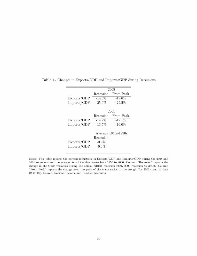
Table 1. Changes in Exports/GDP and Imports/GDP during Recessions
2008Recession From Peak
Exports/GDP -14.6% -19.6%Imports/GDP -25.0% -29.5%
2001Recession From Peak
Exports/GDP -14.2% -17.1%Imports/GDP -13.5% -16.0%
Average 1950s-1990sRecession
Exports/GDP -0.9%Imports/GDP -0.3%
Notes: This table reports the percent reductions in Exports/GDP and Imports/GDP during the 2008 and2001 recessions and the average for all the downturns from 1950 to 2000. Column “Recession” reports thechange in the trade variables during the official NBER recession (2007-2009 recession to date). Column“From Peak” reports the change from the peak of the trade ratios to the trough (for 2001), and to date(2008-09). Source: National Income and Product Accounts.
22

Tab
le2.
Dis
aggr
egat
edT
rade
Flo
ws,
Nom
inal
Expor
tsIm
por
tsSh
are
ofT
otal
Abs
olut
eC
hang
eP
erce
ntC
hang
eSh
are
ofT
otal
Abs
olut
eC
hang
eP
erce
ntC
hang
e
Tot
al1.
00-3
48.5
-26%
1.00
-766
.2-3
4%
Pan
elA
:B
ySe
ctor
Food
s,fe
eds,
and
beve
rage
s0.
09-2
1.5
-19%
0.04
-8.2
-9%
Indu
stri
alsu
pplie
san
dm
ater
ials
0.30
-135
.0-3
4%0.
15-1
55.2
-47%
Dur
able
good
s0.
10-5
0.3
-36%
0.08
-84.
5-5
0%N
ondu
rabl
ego
ods
0.20
-84.
6-3
3%0.
07-7
0.7
-44%
Pet
role
uman
dpr
oduc
ts0.
22-2
70.3
-54%
Cap
ital
good
s,ex
cept
auto
mot
ive
0.35
-94.
6-2
0%0.
21-1
23.8
-26%
Civ
ilian
airc
raft
,en
gine
s,an
dpa
rts
0.06
-3.7
-5%
0.02
-6.6
-17%
Com
pute
rs,
peri
pher
als,
and
part
s0.
04-1
1.0
-24%
0.05
-23.
7-2
2%O
ther
0.26
-79.
9-2
3%0.
15-9
3.5
-29%
Aut
omot
ive
vehi
cles
,en
gine
s,an
dpa
rts
0.09
-58.
1-4
7%0.
11-1
21.6
-49%
Con
sum
ergo
ods,
exce
ptau
tom
otiv
e0.
12-1
9.5
-12%
0.22
-75.
2-1
5%D
urab
lego
ods
0.07
-23.
0-2
4%0.
12-5
0.1
-18%
Non
dura
ble
good
s0.
053.
65%
0.10
-25.
1-1
1%O
ther
0.04
-19.
9-3
5%0.
04-1
1.8
-12%
Pan
elB
:B
yD
esti
nati
onC
anad
a0.
19-8
0.6
-33%
0.17
-157
.7-4
3%A
sia
0.25
-80.
2-2
6%0.
34-1
70.2
-24%
Chi
na0.
06-1
0.5
-15%
0.15
-51.
4-1
6%In
dia
0.01
-2.3
-13%
0.01
-5.1
-21%
Japa
n0.
05-2
0.3
-31%
0.07
-61.
2-4
2%T
aiw
an0.
02-1
0.9
-42%
0.02
-10.
0-2
8%E
U25
0.22
-68.
0-2
5%0.
18-1
20.1
-31%
Ger
man
y0.
04-1
6.2
-30%
0.05
-40.
5-3
9%U
nite
dK
ingd
om0.
04-1
3.8
-25%
0.03
-17.
1-2
8%E
aste
rnE
urop
e0.
01-4
.8-4
9%0.
01-3
.8-3
1%L
atin
Am
eric
a0.
21-7
6.8
-29%
0.18
-132
.6-3
3%B
razi
l0.
02-7
.8-2
8%0.
01-1
3.9
-43%
Mex
ico
0.11
-37.
6-2
8%0.
11-6
7.3
-29%
OP
EC
0.04
-9.9
-18%
0.10
-146
.5-6
0%A
ustr
alia
0.02
-5.5
-26%
0.00
-4.0
-35%
Note
s:T
his
table
rep
ort
sth
ep
erce
nta
ge
dec
rease
innom
inal
U.S
.ex
port
sand
imp
ort
sov
erth
ep
erio
d2008q2
to2009q2,
dis
aggre
gate
dby
sect
or
(Panel
A)
and
by
des
tinati
on
(Panel
B).
Sourc
e:N
ati
onal
Inco
me
and
Pro
duct
Acc
ounts
and
U.S
.In
tern
ati
onal
Tra
de
Com
mis
sion.
23

Tab
le3.
Nom
inal
Tra
deF
low
s,R
eal
Tra
deF
low
s,an
dP
rice
s
Expor
tsIm
por
tsN
omin
alR
eal
Pri
ceN
omin
alR
eal
Pri
ce
Tot
al-2
6.3%
-19.
0%-8
.9%
-34.
4%-2
1.4%
-16.
5%
Food
s,fe
eds,
and
beve
rage
s-1
8.5%
-6.8
%-1
2.7%
-9.1
%-4
.7%
-4.8
%In
dust
rial
supp
lies
and
mat
eria
ls-3
4.0%
-13.
9%-2
3.2%
-47.
1%-3
0.3%
-24.
1%D
urab
lego
ods
-36.
4%-2
0.3%
-20.
2%-5
0.4%
-35.
1%-2
3.4%
Non
dura
ble
good
s-3
2.6%
-10.
3%-2
4.8%
-43.
7%-2
5.5%
-24.
5%P
etro
leum
and
prod
ucts
-54.
3%-7
.2%
-50.
7%C
apit
algo
ods,
exce
ptau
tom
otiv
e-2
0.2%
-19.
2%-1
.2%
-26.
4%-2
5.3%
-1.4
%C
ivili
anai
rcra
ft,
engi
nes,
and
part
s-4
.8%
-9.4
%5.
0%-1
7.3%
-21.
6%5.
3%C
ompu
ters
,pe
riph
eral
s,an
dpa
rts
-23.
7%-1
6.8%
-8.2
%-2
1.9%
-16.
3%-6
.7%
Oth
er-2
3.2%
-22.
0%-1
.6%
-28.
9%-2
8.6%
-0.4
%A
utom
otiv
eve
hicl
es,
engi
nes,
and
part
s-4
6.6%
-46.
8%0.
6%-4
9.0%
-49.
2%0.
3%C
onsu
mer
good
s,ex
cept
auto
mot
ive
-11.
9%-1
1.4%
-0.6
%-1
5.1%
-14.
5%-0
.8%
Dur
able
good
s-2
4.5%
-25.
0%0.
6%-1
8.4%
-17.
0%-1
.6%
Non
dura
ble
good
s5.
2%7.
5%-2
.2%
-11.
2%-1
1.4%
0.2%
Oth
er-3
5.2%
-29.
2%-8
.7%
-12.
4%-1
1.4%
-1.2
%
Note
s:T
his
table
rep
ort
sth
ep
erce
nta
ge
dec
rease
innom
inal
U.S
.ex
port
sand
imp
ort
sov
erth
ep
erio
d2008q2
to2009q2,
the
per
centa
ge
change
inre
al
U.S
.ex
port
sand
imp
ort
s,and
the
per
centa
ge
change
inth
epri
ceof
exp
ort
sand
imp
ort
s,by
sect
or.
24

Table 4. Trade Wedges
ε Overall Durable Consumption Investment
1.5 -0.536 -0.5706 -0.062 -0.1026 -1.327 -0.710 0.075 -0.203
Notes: This table reports the wedges calculated for 2009q2 with respect to 2008q2 (year-on-year). Source:National Income and Product Accounts and authors’ calculations.
25

Tab
le5.
Tra
deC
hang
esan
dD
owns
trea
mP
rodu
ctio
nL
inka
ges
(1)
(2)
(3)
(4)
(5)
(6)
(7)
(8)
Pan
elA
:P
erce
ntag
eR
educ
tion
inIm
port
sP
anel
B:
Per
cent
age
Red
ucti
onin
Exp
orts
Ave
rage
Dow
nstr
eam
Use
-27.
463*
**-9
.835
**(5
.686
)(4
.916
)N
umbe
rof
Dow
nstr
eam
Indu
stri
es-0
.333
***
-0.0
76(0
.103
)(0
.101
)D
owns
trea
mH
erfin
dahl
0.13
7***
-0.0
26(0
.050
)(0
.056
)P
rodu
ctio
nSh
arin
g-0
.117
0.11
1(0
.080
)(0
.104
)Sh
are
inT
otal
-2.1
45*
-2.7
24**
*-3
.848
***
-3.0
74**
*-9
.598
***
-10.
288*
**-1
0.54
7***
-11.
671*
**(1
.145
)(0
.993
)(0
.994
)(1
.084
)(3
.099
)(2
.945
)(2
.792
)(2
.903
)E
last
icit
yof
Subs
titu
tion
-0.0
01-0
.001
-0.0
010.
000
-0.0
02-0
.002
-0.0
01-0
.001
(0.0
02)
(0.0
02)
(0.0
02)
(0.0
02)
(0.0
01)
(0.0
01)
(0.0
01)
(0.0
01)
Lab
orIn
tens
ity
-0.1
20**
-0.1
08*
-0.1
21*
-0.1
06*
-0.1
16**
-0.1
15**
-0.1
23**
-0.1
36**
(0.0
61)
(0.0
62)
(0.0
63)
(0.0
61)
(0.0
56)
(0.0
57)
(0.0
58)
(0.0
54)
Con
stan
t-0
.114
**-0
.120
**-0
.174
***
-0.1
41**
*-0
.079
**-0
.083
**-0
.080
*-0
.096
**(0
.047
)(0
.049
)(0
.050
)(0
.048
)(0
.040
)(0
.040
)(0
.046
)(0
.044
)O
bser
vati
ons
436
436
436
442
435
435
435
441
R-s
quar
ed0.
060.
040.
030.
020.
070.
060.
060.
07
Note
s:R
obust
standard
erro
rsin
pare
nth
eses
;*
signifi
cant
at
10%
;**
signifi
cant
at
5%
;***
signifi
cant
at
1%
.T
he
dep
enden
tva
riable
isth
ep
erce
nta
ge
reduct
ion
inU
.S.
Imp
ort
s(P
anel
A)
and
the
per
centa
ge
reduct
ion
inex
port
s(P
anel
B)
ina
6-d
igit
NA
ICS
cate
gory
from
2008m
6to
2009m
6(y
ear-
to-y
ear)
.A
vera
geD
ow
nst
rea
mU
seis
the
aver
age
usa
ge
outp
ut
ina
sect
or
as
an
inte
rmed
iate
input
inoth
erse
ctors
;N
um
ber
of
Do
wn
stre
am
Ind
ust
ries
isth
enum
ber
of
indust
ries
that
use
ase
ctor
as
an
inte
rmed
iate
;D
ow
nst
rea
mH
erfi
nd
ah
lis
the
Her
findahl
index
of
the
usa
ge
of
ase
ctor
as
an
inte
rmed
iate
inoth
erse
ctors
.T
hes
eth
ree
indic
ato
rsare
com
pute
dbase
don
the
U.S
.2002
Ben
chm
ark
Input-
Outp
ut
Table
.P
rod
uct
ion
Sh
ari
ng
isth
esh
are
of
intr
a-fi
rmim
port
sin
tota
lU
.S.
imp
ort
s(P
anel
A),
or
the
share
of
intr
a-fi
rmex
port
sin
tota
lU
.S.ex
port
s(P
anel
B),
com
pute
dfr
om
the
BE
Am
ult
inati
onals
data
,and
aver
aged
over
the
per
iod
2002-2
006.
Sh
are
inT
ota
lis
the
share
of
ase
ctor
into
tal
U.S
.im
port
s(P
anel
A),
or
exp
ort
s(P
anel
B).
Ela
stic
ity
of
Su
bsti
tuti
on
bet
wee
nva
riet
ies
ina
sect
or
isso
urc
edfr
om
Bro
da
and
Wei
nst
ein
(2006).
La
bor
Inte
nsi
tyis
the
com
pen
sati
on
of
emplo
yee
sas
ash
are
of
valu
eadded
,fr
om
the
U.S
.2002
Ben
chm
ark
Input-
Outp
ut
Table
.
26

Tab
le6.
Tra
deC
hang
esan
dU
pstr
eam
Pro
duct
ion
Lin
kage
s
(1)
(2)
(3)
(4)
(5)
(6)
Pan
elA
:P
erce
ntag
eR
educ
tion
inIm
port
sP
anel
B:
Per
cent
age
Red
ucti
onin
Exp
orts
Inte
rmed
iate
Use
Inte
nsit
y-0
.225
*-0
.071
(0.1
33)
(0.1
16)
Num
ber
ofIn
term
edia
tes
Use
d-0
.739
*-1
.198
**(0
.425
)(0
.470
)H
erfin
dahl
ofIn
term
edia
teU
se-0
.102
0.02
0(0
.171
)(0
.174
)Sh
are
inT
otal
-2.9
88**
*-2
.944
***
-3.2
65**
*-1
0.57
6***
-8.9
20**
*-1
0.82
4***
(1.0
80)
(1.0
36)
(1.0
79)
(2.8
52)
(3.0
23)
(2.8
57)
Ela
stic
ity
ofSu
bsti
tuti
on-0
.001
0.00
00.
000
-0.0
01-0
.002
-0.0
01(0
.002
)(0
.002
)(0
.002
)(0
.001
)(0
.001
)(0
.001
)L
abor
Inte
nsit
y-0
.075
-0.0
93-0
.125
**-0
.111
*-0
.083
-0.1
25**
(0.0
69)
(0.0
62)
(0.0
61)
(0.0
63)
(0.0
59)
(0.0
56)
Con
stan
t-0
.035
-0.0
83-0
.136
***
-0.0
480.
023
-0.0
86*
(0.0
77)
(0.0
64)
(0.0
50)
(0.0
66)
(0.0
56)
(0.0
44)
Obs
erva
tion
s44
244
244
244
144
144
1R
-squ
ared
0.03
0.02
0.02
0.06
0.08
0.06
Note
s:R
obust
standard
erro
rsin
pare
nth
eses
;*
signifi
cant
at
10%
;**
signifi
cant
at
5%
;***
signifi
cant
at
1%
.T
he
dep
enden
tva
riable
isth
ep
erce
nta
ge
reduct
ion
inU
.S.
Imp
ort
s(P
anel
A)
and
the
per
centa
ge
reduct
ion
inex
port
s(P
anel
B)
ina
6-d
igit
NA
ICS
cate
gory
from
2008m
6to
2009m
6(y
ear-
to-y
ear)
.In
term
edia
teU
seIn
ten
sity
issp
endin
gon
inte
rmed
iate
inputs
per
dollar
of
final
sale
s;N
um
ber
of
Inte
rmed
iate
sU
sed
isth
enum
ber
inte
rmed
iate
sa
sect
or
use
sin
pro
duct
ion;
Her
fin
da
hl
of
Inte
rmed
iate
Use
isth
eH
erfindahl
index
of
the
inte
rmed
iate
good
usa
ge
ina
sect
or.
Thes
eth
ree
indic
ato
rsare
com
pute
dbase
don
the
U.S
.2002
Ben
chm
ark
Input-
Outp
ut
Table
.S
ha
rein
To
tal
isth
esh
are
of
ase
ctor
into
tal
U.S
.im
port
s(P
anel
A),
or
exp
ort
s(P
anel
B).
Ela
stic
ity
of
Su
bsti
tuti
on
bet
wee
nva
riet
ies
ina
sect
or
isso
urc
edfr
om
Bro
da
and
Wei
nst
ein
(2006).
La
bor
Inte
nsi
tyis
the
com
pen
sati
on
of
emplo
yee
sas
ash
are
of
valu
eadded
,fr
om
the
U.S
.2002
Ben
chm
ark
Input-
Outp
ut
Table
.
27

Tab
le7.
Tra
deC
hang
esan
dT
rade
Cre
dit
Inte
nsit
y
(1)
(2)
(3)
(4)
Pan
elA
:P
erce
ntag
eR
educ
tion
inIm
port
sP
anel
B:
Per
cent
age
Red
ucti
onin
Exp
orts
Acc
ount
sP
ayab
le/C
ost
ofG
oods
Sold
-0.0
03-0
.119
(0.1
12)
(0.0
84)
Acc
ount
sR
ecei
vabl
e/Sa
les
-0.0
130.
041
(0.1
10)
(0.0
98)
Shar
ein
Tot
al-3
.830
***
-3.8
27**
*-1
0.31
3***
-10.
803*
**(1
.291
)(1
.031
)(2
.918
)(2
.824
)E
last
icit
yof
Subs
titu
tion
0.00
00.
000
-0.0
01-0
.001
(0.0
02)
(0.0
02)
(0.0
01)
(0.0
01)
Lab
orIn
tens
ity
-0.1
64**
-0.1
64**
-0.1
49**
*-0
.133
***
(0.0
64)
(0.0
66)
(0.0
53)
(0.0
51)
Con
stan
t-0
.114
-0.1
09-0
.016
-0.1
03(0
.074
)(0
.068
)(0
.062
)(0
.065
)O
bser
vati
ons
418
418
418
418
R-s
quar
ed0.
030.
030.
070.
07
Note
s:R
obust
standard
erro
rsin
pare
nth
eses
;*
signifi
cant
at
10%
;**
signifi
cant
at
5%
;***
signifi
cant
at
1%
.T
he
dep
enden
tva
riable
isth
ep
erce
nta
ge
reduct
ion
inU
.S.
Imp
ort
s(P
anel
A)
and
the
per
centa
ge
reduct
ion
inex
port
s(P
anel
B)
ina
6-d
igit
NA
ICS
cate
gory
from
2008m
6to
2009m
6(y
ear-
to-y
ear)
.A
cco
un
tsP
aya
ble/
Co
sto
fG
ood
sS
old
and
acc
ou
nts
rece
iva
ble/
sale
sare
mea
sure
sof
trade
cred
ituse
dand
exte
nded
,re
spec
tivel
y,co
mpute
dusi
ng
firm
-lev
elin
form
ati
on
from
the
Com
pust
at
data
base
.S
ha
rein
To
tal
isth
esh
are
of
ase
ctor
into
tal
U.S
.im
port
s(P
anel
A),
or
exp
ort
s(P
anel
B).
Ela
stic
ity
of
Su
bsti
tuti
on
bet
wee
nva
riet
ies
ina
sect
or
isso
urc
edfr
om
Bro
da
and
Wei
nst
ein
(2006).
La
bor
Inte
nsi
tyis
the
com
pen
sati
on
of
emplo
yee
sas
ash
are
of
valu
eadded
,fr
om
the
U.S
.2002
Ben
chm
ark
Input-
Outp
ut
Table
.
28

Tab
le8.
Tra
deC
hang
esan
dC
ompo
siti
onal
Effe
cts
(1)
(2)
(3)
(4)
Pan
elA
:P
erce
ntag
eR
educ
tion
inIm
port
sP
anel
B:
Per
cent
age
Red
ucti
onin
Exp
orts
Per
cent
age
Cha
nge
inIn
dust
rial
Pro
duct
ion
0.55
4***
0.46
9***
(0.0
92)
(0.0
95)
Dur
able
dum
my
-0.0
72**
*-0
.055
**(0
.025
)(0
.024
)Sh
are
inT
otal
-3.1
20**
-2.9
45**
*-1
0.65
5***
-9.6
35**
*(1
.529
)(1
.133
)(3
.185
)(2
.834
)E
last
icit
yof
Subs
titu
tion
0.00
0-0
.001
-0.0
01-0
.002
(0.0
02)
(0.0
02)
(0.0
01)
(0.0
01)
Lab
orIn
tens
ity
-0.0
98-0
.076
-0.0
56-0
.092
*(0
.062
)(0
.060
)(0
.058
)(0
.056
)C
onst
ant
-0.0
68-0
.134
***
-0.0
49-0
.074
*(0
.044
)(0
.048
)(0
.040
)(0
.041
)O
bser
vati
ons
394
442
395
441
R-s
quar
ed0.
10.
030.
120.
07
Note
s:R
obust
standard
erro
rsin
pare
nth
eses
;*
signifi
cant
at
10%
;**
signifi
cant
at
5%
;***
signifi
cant
at
1%
.T
he
dep
enden
tva
riable
isth
ep
erce
nta
ge
reduct
ion
inU
.S.
Imp
ort
s(P
anel
A)
and
the
per
centa
ge
reduct
ion
inex
port
s(P
anel
B)
ina
6-d
igit
NA
ICS
cate
gory
from
2008m
6to
2009m
6(y
ear-
to-y
ear)
.P
erce
nta
geC
ha
nge
inIn
du
stri
al
Pro
du
ctio
nis
the
dec
line
inth
ein
dex
of
indust
rial
pro
duct
ion
ina
sect
or;
Sh
are
inT
ota
lis
the
share
of
ase
ctor
into
tal
U.S
.im
port
s(P
anel
A),
or
exp
ort
s(P
anel
B).
Ela
stic
ity
of
Su
bsti
tuti
on
bet
wee
nva
riet
ies
ina
sect
or
isso
urc
edfr
om
Bro
da
and
Wei
nst
ein
(2006).
La
bor
Inte
nsi
tyis
the
com
pen
sati
on
of
emplo
yee
sas
ash
are
of
valu
eadded
,fr
om
the
U.S
.2002
Ben
chm
ark
Input-
Outp
ut
Table
.
29

Table 9. Compositional Effects: Change in Trade Flows as Implied by Industrial Production.
Nominal Real Implied by IP change Share of TradeChange Change
(γtrade
)Corresponding to IP
Exports -34.5% -24.7% -17.6% 0.88Imports -32.9% -17.6% -16.4% 0.94IP -13.4% -13.4% 1.00
Notes: Changes in nominal and real exports over 2008m6 to 2009m6 for NAICS sectors where industrialproduction (IP) data are available. Weights calculated from share of nominal trade and used to generatethe third column. The fourth column indicates the fraction of overall nominal trade that can be matchedto IP data.
30

Tab
le10
.T
rade
Cha
nges
and
and
All
Exp
lana
tory
Var
iabl
esT
oget
her
(1)
(2)
(3)
(4)
Pan
elA
:P
erce
ntag
eR
educ
tion
inIm
port
sP
anel
B:
Per
cent
age
Red
ucti
onin
Exp
orts
Ave
rage
Dow
nstr
eam
Use
-23.
842*
**-2
1.36
7***
-8.0
17-0
.112
(5.7
87)
(5.4
65)
(5.0
40)
(5.7
29)
Inte
rmed
iate
Use
Inte
nsit
y-0
.200
-0.2
15-0
.105
-0.1
46(0
.144
)(0
.222
)(0
.129
)(0
.186
)A
ccou
nts
Pay
able
/Cos
tof
Goo
dsSo
ld0.
061
0.38
7***
-(0.
082)
0.24
7(0
.133
)(0
.149
)(0
.097
)(0
.166
)D
urab
leD
umm
y-0
.089
***
-0.1
33**
*-0
.052
*-0
.138
***
(0.0
31)
(0.0
29)
(0.0
29)
(0.0
34)
Shar
ein
Tot
al-2
.109
0.32
5-2
.109
-10.
470*
**(1
.611
)(1
.698
)(1
.611
)(2
.995
)E
last
icit
yof
Subs
titu
tion
-0.0
01-0
.001
-0.0
01-0
.001
(0.0
02)
(0.0
02)
(0.0
02)
(0.0
01)
Lab
orIn
tens
ity
-0.0
65-0
.083
-0.0
93-0
.293
(0.0
74)
(0.2
49)
(0.0
67)
(0.3
17)
Cap
ital
Inte
nsit
y0.
179
0.20
4(0
.304
)(0
.322
)Sk
illIn
tens
ity
-0.0
620.
986
(0.6
17)
(1.1
76)
Inve
ntor
ies
0.00
9*0.
000
(0.0
05)
(0.0
02)
Con
stan
t0.
004
-0.2
30.
037
-0.1
11(0
.100
)(0
.306
)(0
.085
)(0
.308
)O
bser
vati
ons
414
350
414
351
R-s
quar
ed0.
090.
180.
090.
17
Note
s:R
obust
standard
erro
rsin
pare
nth
eses
;*
signifi
cant
at
10%
;**
signifi
cant
at
5%
;***
signifi
cant
at
1%
.T
he
dep
enden
tva
riable
isth
ep
erce
nta
ge
reduct
ion
inU
.S.
Imp
ort
s(P
anel
A)
and
the
per
centa
ge
reduct
ion
inex
port
s(P
anel
B)
ina
6-d
igit
NA
ICS
cate
gory
from
2008m
6to
2009m
6(y
ear-
to-y
ear)
.A
vera
geD
ow
nst
rea
mU
seis
the
aver
age
usa
ge
outp
ut
ina
sect
or
as
an
inte
rmed
iate
input
inoth
erse
ctors
;In
term
edia
teU
seIn
ten
sity
issp
endin
gon
inte
rmed
iate
inputs
per
dollar
of
final
sale
s;A
cco
un
tsP
aya
ble/
Co
sto
fG
ood
sS
old
isa
mea
sure
of
trade
cred
it;
Sh
are
inT
ota
lis
the
share
of
ase
ctor
into
tal
U.S
.im
port
s(P
anel
A),
or
exp
ort
s(P
anel
B).
Ela
stic
ity
of
Su
bsti
tuti
on
bet
wee
nva
riet
ies
ina
sect
or
isso
urc
edfr
om
Bro
da
and
Wei
nst
ein
(2006).
La
bor
Inte
nsi
tyis
the
com
pen
sati
on
of
emplo
yee
sas
ash
are
of
valu
eadded
,fr
om
the
U.S
.2002
Ben
chm
ark
Input-
Outp
ut
Table
.C
ap
ita
lIn
ten
sity
=1-(
tota
lco
mp
ensa
tion)/
(valu
eadded
);S
kill
Inte
nsi
ty=
[(nonpro
duct
ion
work
ers)
/(t
ota
lem
plo
ym
ent)
]*(1
-capit
al
inte
nsi
ty).
Thes
etw
oin
dic
ato
rsare
com
pute
dusi
ng
the
NB
ER
Pro
duct
ivit
yD
ata
base
.In
ven
tori
esis
the
beg
innin
g-o
f-p
erio
dle
vel
of
inven
tori
esre
lati
ve
toim
port
s(r
esp.,
exp
ort
s).
31

Figure 1. Historical Trends in Aggregate Trade, 1947-2009.
0.00
0.02
0.04
0.06
0.08
0.10
0.12
0.14
0.16
0.18
0.20
1947 1952 1957 1962 1967 1972 1977 1982 1987 1992 1997 2002 2007
Imports/GDP
Exports/GDP
(a) Imports/GDP and Exports/GDP
-0.25
-0.2
-0.15
-0.1
-0.05
0
0.05
0.1
0.15
0.2
1947 1952 1957 1962 1967 1972 1977 1982 1987 1992 1997 2002 2007
Imports
Exports GDP
(b) Imports, Exports, and GDP in Deviations from Trend
Notes: The top panel plots the ratios of imports/GDP and exports/GDP for the U.S., along with the NBERrecession bars. The bottom panel plots total imports, exports, and GDP in deviations from HP trend withparameter 1600. Source: National Income and Product Accounts.
32

Figure 2. Goods and Services Trade
0
200
400
600
800
1000
1200
1400
1600
1800
Billi
ons
2005
USD
2005 2006 2007 2008 2009
Goods
Services
-19%
-7%
(a) Exports
0
500
1000
1500
2000
2500
Billi
ons
2005
USD
2005 2006 2007 2008 2009
Goods
Services
-24%
-6%
(b) Imports
Notes: This Figure reports the total real exports (top panel) and real imports (bottom panel), of both goodsand services. Source: National Income and Product Accounts.
33

Figure 3. Durables and Non-Durables Trade
0
200
400
600
800
1000
1200
1400
Billi
ons
2005
USD
2005 2006 2007 2008 2009
Durable
Nondurable
-25%
-8%
(a) Exports
0
200
400
600
800
1000
1200
1400
1600
1800
2000
Billi
ons
2005
USD
2005 2006 2007 2008 2009
Durable
Nondurable
-30%
-15%
(b) Imports
Notes: This Figure reports the total real exports (top panel) and real imports (bottom panel), of bothdurable and non-durable goods. Source: National Income and Product Accounts.
34

Figure 4. Real and Nominal Trade
80
90
100
110
120
130
140
150
160
2005 2006 2007 2008 2009
Nominal exports
Real exports
(a) Exports
80
90
100
110
120
130
140
150
160
Real imports
Nominal imports
2005 2006 2007 2008 2009
(b) Imports
Notes: This Figure reports the evolution of nominal and real exports (top panel) and imports (bottompanel). Both the nominal and real series are normalized to 2005. Source: National Income and ProductAccounts.
35

Figure 5. Real and Nominal Changes in Trade, by Sector
Total
Dur. ind. supplies
Non-dur. C goods
Total
Petroleum
Autos
-60%
-50%
-40%
-30%
-20%
-10%
0%
10%
-60% -50% -40% -30% -20% -10% 0% 10%% change real trade
Exports Imports
% change nom
inal trade
Notes: This figure plots the percentage changes in real imports and exports against the percentage changesin nominal imports and exports, by EndUse sector, along with a 45-degree line. Source: National Incomeand Product Accounts.
36

Figure 6. Overall and Durable Wedges
-0.8
-0.6
-0.4
-0.2
0
0.2
0.4
0.6
0.8
1968 1973 1978 1983 1988 1993 1998 2003 2008
Simple wedge
Durable wedge
Notes: This figure plots the wedges for total imports and the durable imports. Source: National Incomeand Product Accounts and authors’ calculations.
Figure 7. Consumption and Investment Wedges
-0.8
-0.6
-0.4
-0.2
0
0.2
0.4
0.6
0.8
1968 1973 1978 1983 1988 1993 1998 2003 2008
Consumption wedge
Investment wedge
Notes: This figure plots the wedges for consumption imports and investment imports. Source: NationalIncome and Product Accounts and authors’ calculations.
37

Figure 8. The Evolution of Trade Credit
.5.5
2.5
4.5
6.5
8.6
Acco
unts
Pay
able
/Cos
t of G
oods
Sol
d
2000q1 2003q1 2006q1 2009q1
Non−Seas. Adj. Seas. Adj.Average, 2000−2009q1
(a) Accounts Payable/Cost of Goods Sold
.54
.56
.58
.6Ac
coun
ts R
ecei
vabl
e/Sa
les
2004q1 2005q1 2006q1 2007q1 2008q1 2009q1
Non−Seas. Adj. Seas. Adj.Average, 2004−2009q1
(b) Accounts Receivable/Sales
Notes: The top panel of this figure displays the median value of accounts payable/cost of goods sold acrossfirms in each period. The bottom panel reports the median value of accounts receivable/sales across firmsin each period. Source: Compustat.
38

Table A1. Summary Statistics
Mean Std. Dev. Min MaxIndependent Variables
Percentage Change in Imports -0.235 0.264 -1.000 0.995Percentage Change in Exports -0.199 0.238 -0.956 0.965
Downstream IndicatorsAverage Downstream Use 0.001 0.002 0.000 0.013Number of Downstream Industries 102 111 1 419Downstream Herfindahl 0.220 0.223 0.009 1.000Production Sharing (exports) 0.196 0.133 0.005 0.612Production Sharing (imports) 0.150 0.139 0.000 0.577
Upstream IndicatorsIntermediate Use Intensity 0.631 0.122 0.254 0.949Number of Intermediates Used 113 26 46 218Herfindahl of Intermediate Use 0.094 0.066 0.028 0.532
Trade Credit IndicatorsAccounts Payable/Cost of Goods Sold 0.469 0.141 0.194 1.733Accounts Receivable/Sales 0.532 0.131 0.156 0.817
Compositional IndicatorsPercentage Change in Industrial Production -0.180 0.119 -0.836 0.069Durable dummy 0.588 0.493 0 1
Control VariablesShare in Total Imports 0.002 0.007 0.000 0.088Share in Total Exports 0.002 0.005 0.000 0.045Elasticity of Substitution 6.8 10.7 1.2 103Labor Intensity 0.633 0.229 0.049 0.998
Notes: This table presents the summary statistics for the variables used in the estimation. Variable defini-tions and sources are described in detail in the text.
39

Figure A1. Nominal and Real Effective Exchange Rates for the U.S..
0
20
40
60
80
100
120
140
1975 1980 1985 1990 1995 2000 2005
REER
NEER
Notes: This figure displays the Nominal Effective Exchange Rate and the Real Effective Exchange Rate forthe United States. Source: IMF.
40
Related Documents